Beyond Ideal MHD

Nick Murphy

Harvard-Smithsonian Center for Astrophysics

Astronomy 253: Plasma Astrophysics

February 12, 2014

These lecture notes are largely based on Plasma Physics for Astrophysics by Russell Kulsrud, Lectures inMagnetohydrodynamics by Dalton Schnack, Ideal Magnetohydrodynamics by Jeffrey Freidberg, and The

Physics of Fully Ionized Gases by Lyman Spitzer.

The frozen-in condition doesn’t just apply to plasmas

I Ironically, few would call this weather ideal!

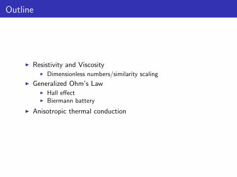
Outline

I Resistivity and ViscosityI Dimensionless numbers/similarity scaling

I Generalized Ohm’s LawI Hall effectI Biermann battery

I Anisotropic thermal conduction

How do we approach a problem when MHD is insufficient?

I Extended MHDI Keep the fluid approximationI Add terms including effects beyond MHDI Resistivity, viscosity, anisotropic thermal conduction, separate

ion and electron temperatures, neutrals, etc.

I Kinetic theory/particle-in-cell simulationsI Abandon the fluid approximationI Keep track of particles/distribution functions directly

I A hybrid approachI Keep some parts of the fluid approximationI Express other parts kinetically

Key Properties of Ideal MHD

I Frozen-in condition: if two parcels of plasma are attached bya field line at one time, they will continue to be attached by afield line at future times

I Magnetic topology is preserved

I Mass, momentum, and energy are convserved

I Helicity and cross-helicity are conserved

I Only adiabatic heating/cooling

I No dissipation!

I The equations of ideal MHD have no inherent scale(“scale-free”)

The ideal MHD Ohm’s law

I The ideal Ohm’s law is

E +V × B

c= 0 (1)

I By combining this equation with Faraday’s law, we arrive atthe induction equation for ideal MHD

∂B

∂t= ∇× (V × B) (2)

I When these conditions are met, the frozen-in condition isvalid.

The resistive MHD Ohm’s law

I The resistive Ohm’s law is1

E +V × B

c= ηJ (3)

I By combining this equation with Faraday’s law, we arrive atthe induction equation for resistive MHD

∂B

∂t= ∇× (V × B)− c∇× (ηJ) (4)

= ∇× (V × B)− c2

4π∇× (η∇× B) (5)

where we allow η to vary in space.

1Kulsrud’s definition of η differs by a factor of c.

The induction equation with constant resistivity

I If η is constant, then the induction equation becomes

∂B

∂t= ∇× (V × B)︸ ︷︷ ︸

advection

+ Dη∇2B︸ ︷︷ ︸diffusion

(6)

where the electrical diffusivity is defined to be

Dη ≡ηc2

4π(7)

and has units of a diffusivity: length2

time or cm2 s−1 in cgs

I Annoyingly, conventions for η vary. Sometimes Dη is called ηin Eq. 6. In SI units, typically Dη ≡ η

µ0.

Writing the induction equation as a diffusion equation

I If V = 0, the resistive induction equation becomes

∂B

∂t= Dη∇2B (8)

I The second order spatial derivative corresponds to diffusionI A fourth order spatial derivative corresponds to hyperdiffusivity

I This is a parabolic vector partial differential equation that isanalogous to the heat equation

I Let’s look at the x component of Eq. 8

∂Bx

∂t= Dη

(∂2Bx

∂x2+∂2Bx

∂y2+∂2Bx

∂z2

)(9)

This corresponds to the diffusion of Bx in the x , y , and zdirections

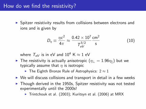
How do we find the resistivity?

I Spitzer resistivity results from collisions between electrons andions and is given by

Dη ≡ηc2

4π≈ 0.42× 107

T3/2eV

cm2

s(10)

where TeV is in eV and 104 K ≈ 1 eVI The resistivity is actually anisotropic (η⊥ = 1.96η‖) but we

typically assume that η is isotropicI The Eighth Bronze Rule of Astrophysics: 2 ≈ 1

I We will discuss collisions and transport in detail in a few weeksI Though derived in the 1950s, Spitzer resistivity was not tested

experimentally until the 2000s!I Trintchouk et al. (2003); Kuritsyn et al. (2006) at MRX

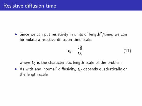
Resistive diffusion time

I Since we can put resistivity in units of length2/time, we canformulate a resistive diffusion time scale:

tη ≡L2

0

Dη(11)

where L0 is the characteristic length scale of the problem

I As with any ‘normal’ diffusivity, tD depends quadratically onthe length scale

Application: the physics of cooking!

I The cooking time for potato cubes depends quadratically onthe length of one side

I This is another example of

diffusion time =(length scale)2

diffusion coefficient(12)

Viscosity. . . it’s such a drag!

I Viscosity transports momentum between parts of the fluidthat are in relative motion

I Viscosity results from particle collisions

I The momentum equation with viscosity is given by

ρ

(∂

∂t+ V · ∇

)V =

J× B

c−∇p + ρν∇2V (13)

Here, ν is the kinematic viscosity

Putting the momentum equation in dimensionless form

I Define V ≡ V0V. . . where V0 is a characteristic value and V isdimensionless, and use V0 ≡ L0/t0

I Use these definitions in the momentum equation whileincluding only the viscosity term on the RHS

ρ∂V

∂t+ V · ∇V = ρν∇2V (14)

V0

t0

∂V

∂ t+

V 20

L0V · ∇V =

νV0

L20

∇2V

∂V

∂ t+ V · ∇V =

ν

V0L0∇2V (15)

where the Reynolds number is

Re ≡ V0L0

ν(16)

The Reynolds number gauges the importance of theadvective term compared to the viscous term

I We can rewrite the momentum equation with only viscosity as

∂V

∂ t+ V · ∇V︸ ︷︷ ︸

advection

=1

Re∇2V︸ ︷︷ ︸

viscous diffusion

(17)

I A necessary condition for turbulence to occur is if

Re� 1 (18)

so that the viscous term is negligible on scales ∼ L0.I In astrophysics, usually Re ≡ L0V0

ν ≫≫ 1

I The only scale in this equation is the viscous scale

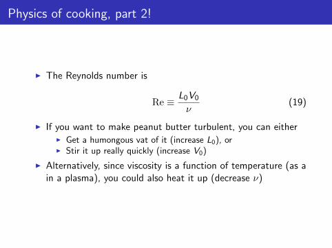
Physics of cooking, part 2!

I The Reynolds number is

Re ≡ L0V0

ν(19)

I If you want to make peanut butter turbulent, you can eitherI Get a humongous vat of it (increase L0), orI Stir it up really quickly (increase V0)

I Alternatively, since viscosity is a function of temperature (as ain a plasma), you could also heat it up (decrease ν)

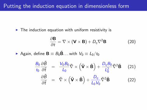
Putting the induction equation in dimensionless form

I The induction equation with uniform resistivity is

∂B

∂t= ∇× (V × B) + Dη∇2B (20)

I Again, define B ≡ B0B. . . with V0 ≡ L0/t0

B0

t0

∂B

∂ t=

V0B0

L0∇ ×

(V × B

)+

DηB0

L20

∇2B (21)

∂B

∂ t= ∇ ×

(V × B

)+

DηL0V0

∇2B (22)

Defining the magnetic Reynolds number and Lundquistnumber

I We define the magnetic Reynolds number as

Rm ≡ L0V0

Dη(23)

I The Alfven speed is

VA ≡B√4πρ

(24)

I We define the Lundquist number as

S ≡ L0VA

Dη(25)

where we use that the characteristic speed for MHD isV0 = VA

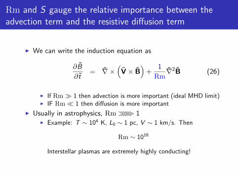
Rm and S gauge the relative importance between theadvection term and the resistive diffusion term

I We can write the induction equation as

∂B

∂ t= ∇ ×

(V × B

)+

1

Rm∇2B (26)

I If Rm� 1 then advection is more important (ideal MHD limit)I IF Rm� 1 then diffusion is more important

I Usually in astrophysics, Rm ≫≫ 1I Example: T ∼ 104 K, L0 ∼ 1 pc, V ∼ 1 km/s. Then

Rm ∼ 1016

Interstellar plasmas are extremely highly conducting!

Re, Rm, and S can also be expressed as the ratio oftimescales

I The Reynolds number is

Re ≡ L0V0

ν=

viscous timescale

advection timescale(27)

I The magnetic Reynolds number is

Rm ≡ L0V0

Dη=

resistive diffusion timescale

advection timescale(28)

I The Lundquist number is

S ≡ L0VA

Dη=

resistive diffusion timescale

Alfven wave crossing time(29)

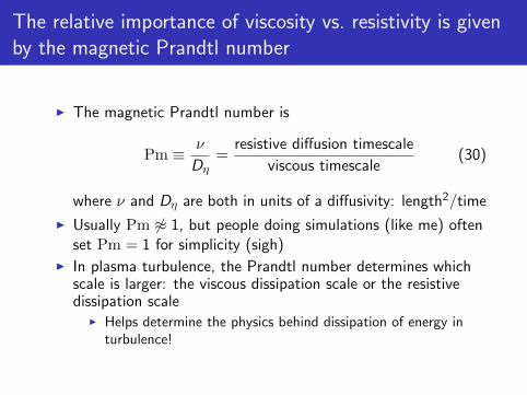
The relative importance of viscosity vs. resistivity is givenby the magnetic Prandtl number

I The magnetic Prandtl number is

Pm ≡ ν

Dη=

resistive diffusion timescale

viscous timescale(30)

where ν and Dη are both in units of a diffusivity: length2/time

I Usually Pm 6≈ 1, but people doing simulations (like me) oftenset Pm = 1 for simplicity (sigh)

I In plasma turbulence, the Prandtl number determines whichscale is larger: the viscous dissipation scale or the resistivedissipation scale

I Helps determine the physics behind dissipation of energy inturbulence!

Is there flux freezing in resistive MHD?

I Short answer: no!

I Long answer: let’s modify the frozen-flux derivation!

I The change of flux through a co-moving surface bounded by acontour C is

dΨ

dt= −c

∮C

(E +

V × B

c

)· dl (31)

I In ideal MHD, the integrand is identically zero.

I In resistive MHD, the integrand is ηJ!

I The change in flux becomes

dΨ

dt= −c

∮CηJ · dl (32)

This is generally 6= 0, so flux is not frozen-in.

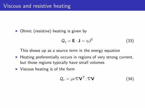
Viscous and resistive heating

I Ohmic (resistive) heating is given by

Qη = E · J = ηJ2 (33)

This shows up as a source term in the energy equation

I Heating preferentially occurs in regions of very strong current,but those regions typically have small volumes

I Viscous heating is of the form

Qν = ρν∇VT :∇V (34)

Key Properties of Resistive MHD

I Magnetic topology is not preserved

I Mass, momentum, and energy are conserved

I Helicity and cross-helicity are approximately conserved

I There is Ohmic (resistive) and viscous heating

I There’s dissipation!

I The scales in the problem are set by viscosity and resistivity

The resistive term allows magnetic reconnection to happen

I Magnetic reconnection is the breaking and rejoining of fieldlines in an otherwise highly conducting plasma

I Reconnection preferentially occurs in current sheets: regionswhere there are sharp changes in B

I Resistive diffusion is usually negligible outside of these regions

But there’s more!

I The resistive MHD Ohm’s law is

E +V × B

c= ηJ (35)

I However, there are additional terms that contribute to theelectric field!

I The generalized Ohm’s law is derived from the electronequation of motion

The electron equation of motion

I The electron equation of motion is

neme

(∂

∂t+ V · ∇

)Ve =

−ene(E +

Ve × B

c

)−∇ · Pe + pie (36)

whereI Pe is the electron pressure tensorI pie represents the exchange of momentum between ions and

electrons due to collisions (this leads to resistivity)

I To derive the generalized Ohm’s law, solve for E

The generalized Ohm’s law

I The generalized Ohm’s law is given by

E +V × B

c= ηJ +

J× B

enec︸ ︷︷ ︸Hall

− ∇ · Pe

neec︸ ︷︷ ︸elec. pressure

+me

nee2

dJ

dt︸ ︷︷ ︸elec. inertia

(37)

I The frozen-in condition can be broken byI The resistive termI The divergence of the electron pressure tensor termI Electron inertia

I These additional terms introduce new physics into the systemat short length scales

Each of the terms in the generalized Ohm’s law enters inat a different scale

I The Hall and electron pressure terms enter in at the ioninertial length,

di ≡c

ωpi=

√c2mi

4πniZ 2e2, (38)

which is the characteristic length scale for ions to beaccelerated by electromagnetic forces in a plasma

I The electron inertia term enters in at the electron inertiallength

de ≡c

ωpe=

√c2me

4πnee2. (39)

I The electron inertia term is usually negligible, so we cantypically assume massless electrons (since di ≈ 43de)

What are typical ion and electron inertial lengths inastrophysics?

I ISM: n ∼ 1 cm−3 ⇒ di ∼ 200 km, de ∼ 5 km

I Solar corona: n ∼ 109 cm−3 ⇒ di ∼ 7 m, de ∼ 20 cm

I Solar wind at 1 AU: n ∼ 10 cm−3 ⇒ di ∼ 70 km, de ∼ 2 kmI That’s ridiculous! These scales are tiny! Why should

astrophysicists care about them at all?I These are comparable to dissipation length scales in MHD

turbulence!I When current sheets thin down to these scales, reconnection

becomes explosive and fast!I The Hall effect can modify the magnetorotational instability in

protoplanetary/accretion disksI The Earth’s magnetosphere has ∼ISM/solar wind densities,

and 200 km is actually not ridiculously small!

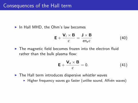
Consequences of the Hall term

I In Hall MHD, the Ohm’s law becomes

E +Vi × B

c=

J× B

enec(40)

I The magnetic field becomes frozen into the electron fluidrather than the bulk plasma flow:

E +Ve × B

c= 0. (41)

I The Hall term introduces dispersive whistler wavesI Higher frequency waves go faster (unlike sound, Alfven waves)

Situations where the Hall term may be important

I Planetary magnetospheres

I Dissipation scales in MHD turbulence

I Collisionless (fast) magnetic reconnection

I Accretion disks/protoplanetary disks

I Laboratory plasma experiments

I Hall thrusters (ion propulsion)

I Neutron star atmospheres/magnetospheres

I Our class’s final exam

How do you get off-diagonal terms in the electron pressuretensor?

I Rapid variation of E or other fields can lead to bunching ofelectrons in the phases of their gyration about magnetic fieldlines

I This results in more electrons around one particular phase intheir orbits than at other phases

I These agyrotropies are captured by off-diagonal terms in theelectron pressure tensor

How did the magnetic field arise in the early universe?

I Evolutionary models of magnetic fields in galaxies must beable to explain coherent ∼µG fields by z ∼ 2

I Dynamos require a seed field to exist before it can be amplifiedI The seed field can be small, but must have been above some

minimum valueI Estimates vary!

I Most terms in the generalized Ohm’s law rely on magneticfields already being present for stronger fields to be generated

I But not all!

Open questions about primordial magnetic fields2

I How did the first magnetic fields in the universe originate?

I Were they created during the Big Bang, or did they developafterward?

I How coherent were the first magnetic fields? Over whatlength scales?

I Are galactic magnetic fields top-down or bottom-upphenomena?

I Is there a connection between the creation of the first fieldsand the formation of large-scale structure?

I Did primordial magnetic fields affect galaxy formation?

I Did early fields play a role in magnetic braking/angularmomentum transport in Pop III stars?

2From Widrow (2002)

The Biermann battery is a promising mechanism forgenerating seed magnetic fields in the early universe

I If you assume a scalar electron pressure, your Ohm’s law willbe

E +V × B

c= −∇pe

ene. (42)

If you combine this with Faraday’s law, you will arrive at

∂B

∂t= ∇× (V × B)− c

∇ne ×∇pen2ee

(43)

I The Biermann battery term can generate magnetic fieldswhen none were present before!

How do we generate conditions under which the Biermannbattery can operate?

I The Biermann battery requires that ∇ne &∇pe not be parallel

I Vorticity (ω ≡ ∇× V) can generate such conditions

I Kulsrud’s example: a shock of limited extent propagates intoa cold medium

Cold, unshocked Cold, unshocked

Hot, denseshocked plasma

Less denseCold, unshocked

Shock front

∇ρ

∇T

How does the Biermann battery fit into the big picture?

I The Biermann battery can yield B ∼ 10−18 GI This is plus or minus a few orders of magnitude

I Galactic magnetic fields are ∼ 10−6 G

I Dynamo theory must be able to explain magnetic fieldamplification of ∼12 orders of magnitude within a few Gyr

I There are other candidate mechanisms for magnetic fieldformation (e.g., Naoz & Narayan 2013)

I Key difficulty: lack of observational constraints!

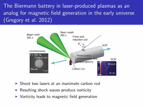
The Biermann battery in laser-produced plasmas as ananalog for magnetic field generation in the early universe(Gregory et al. 2012)

I Shoot two lasers at an inanimate carbon rod

I Resulting shock waves produce vorticity

I Vorticity leads to magnetic field generation

Anisotropic thermal conduction

I Ideal MHD assumes an adiabatic equation of stateI No additional heating/cooling or thermal diffusion

I In real plasmas, charged particles are much more free topropagate along field lines than across them

I There is fast thermal transport along field lines

I Thermal transport across field lines is suppressedI Confinement of fusion plasmas requires closed flux surfaces

I When the magnetic field becomes stochastic, heat is able torapidly escape to the wall

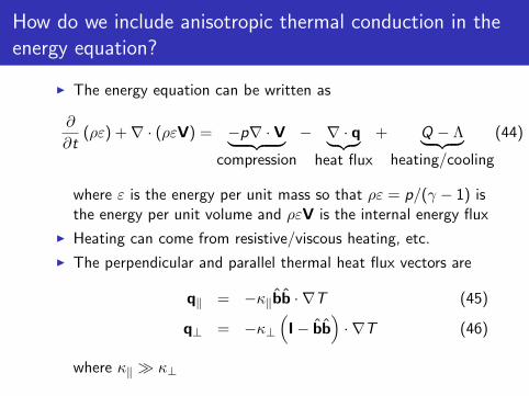
How do we include anisotropic thermal conduction in theenergy equation?

I The energy equation can be written as

∂

∂t(ρε) +∇ · (ρεV) = −p∇ · V︸ ︷︷ ︸

compression

− ∇ · q︸ ︷︷ ︸heat flux

+ Q − Λ︸ ︷︷ ︸heating/cooling

(44)

where ε is the energy per unit mass so that ρε = p/(γ − 1) isthe energy per unit volume and ρεV is the internal energy flux

I Heating can come from resistive/viscous heating, etc.

I The perpendicular and parallel thermal heat flux vectors are

q‖ = −κ‖bb · ∇T (45)

q⊥ = −κ⊥(I− bb

)· ∇T (46)

where κ‖ � κ⊥

How does stochasticity in the field modify thermalconduction?

I Electrons may jump from one field line to a neighboring one

I In a chaotic system, the field lines exponentially separate

I This results in a net effective thermal diffusion and may beimportant in galaxy clusters

Plasmas can have different ion and electron temperatures

I Some heating mechanisms primarily affect either ions orelectrons

I There will be separate energy equations for ions and electronsI Different heating terms, heat flux vectors, etc.

I Equilibration occurs through collisions

I Important in collisionless or marginally collisional plasmas likethe solar wind, supernova remnants, etc.

There are additional forms of viscosity that we have notcovered

I These can be included in the viscous stress tensor

ρ

(∂

∂t+ V · ∇

)V =

J× B

c−∇p +∇ ·Π (47)

I For example, gyroviscosity results from electron gyrationabout magnetic field lines

I These are fundamentally important for magnetically confinedfusion plasmas

I These viscosities are important on dissipation scales in plasmaturbulence in the solar wind, ISM, and elsewhere

Summary

I Resistivity leads to diffusion of B

I Viscosity leads to diffusion of V

I Re, Rm, S , and Pm are dimensionless numbers that gaugethe importance of viscosity and resistivity

I The generalized Ohm’s law includes the Hall effect, thedivergence of the electron pressure tensor, and electron inertia

I These additional terms become important on short lengthscales and introduce new waves into the system

I The Biermann battery may be the source of seed magneticfields in the early Universe

I Thermal conduction in plasmas is much faster along magneticfield lines than across them