Beyond Hard Shadows: Moment Shadow Maps for Single Scattering,Soft Shadows and Translucent Occluders

Christoph Peters∗ Cedrick Münstermann∗ Nico Wetzstein∗ Reinhard Klein∗

University of Bonn, Germany

Single scattering, 6 moments, 1.49 ms Moment soft shadow mapping, 2.22 ms Translucent occluders, 1.2 ms

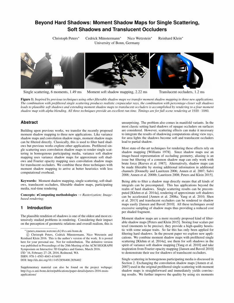
Figure 1: Inspired by previous techniques using other filterable shadow maps we transfer moment shadow mapping to three new applications.The combination with prefiltered single scattering produces realistic crepuscular rays, the combination with percentage-closer soft shadowsleads to plausible soft shadows and extending moment shadow maps to translucent occluders is accomplished by rendering to a four momentshadow map with alpha blending. All three techniques provide an excellent run time. Timings are for full scene rendering at 1920 · 1080.

Abstract

Building upon previous works, we transfer the recently proposedmoment shadow mapping to three new applications. Like varianceshadow maps and convolution shadow maps, moment shadow mapscan be filtered directly. Classically, this is used to filter hard shad-ows but previous works explore other applications. Prefiltered sin-gle scattering uses convolution shadow maps to render single scat-tering in homogenous participating media, variance soft shadowmapping uses variance shadow maps for approximate soft shad-ows and Fourier opacity mapping uses convolution shadow mapsfor translucent occluders. We combine these three techniques withmoment shadow mapping to arrive at better heuristics with lesscomputational overhead.

Keywords: Moment shadow mapping, single scattering, soft shad-ows, translucent occluders, filterable shadow maps, participatingmedia, real-time rendering

Concepts: •Computing methodologies→ Rasterization; Image-based rendering;

1 Introduction

The plausible rendition of shadows is one of the oldest and most ex-tensively studied problems in rendering. Considering their impacton the perception of geometric relations and overall realism, this is

∗{peters,muenste,wetzstei,rk}@cs.uni-bonn.dec© Christoph Peters, Cedrick Münstermann, Nico Wetzstein and

Reinhard Klein 2016. This is the author’s version of the work. It is postedhere for your personal use. Not for redistribution. The definitive versionwas published in Proceedings of the 20th Meeting of the ACM SIGGRAPHSymposium on Interactive 3D Graphics and Games, March 2016.I3D ’16, February 27–28, 2016, Redmond, WAISBN: 978-1-4503-4043-4/16/03DOI: http://dx.doi.org/10.1145/2856400.2856402

Supplementary material can also be found on the project webpage:http://cg.cs.uni-bonn.de/en/publications/paper-details/peters-2016-msm-applications/

unsurprising. The problem also comes in manifold variants. In themost classic setting hard shadows of opaque occluders on surfacesare considered. However, scattering effects can make it necessaryto integrate the results of shadowing computations along view rays,for area lights the shadows become soft and translucent occluderslead to partial shadow.

Most state-of-the-art techniques for rendering these effects rely onshadow mapping [Williams 1978]. Since shadow maps use animage-based representation of occluding geometry, aliasing is anissue but filtering of a common shadow map can only work withbrute force [Reeves et al. 1987]. Alternatively, shadow maps canbe made filterable by storing additional information in additionalchannels [Donnelly and Lauritzen 2006; Annen et al. 2007; Salvi2008; Annen et al. 2008b; Lauritzen 2008; Peters and Klein 2015].

Being able to filter a shadow map directly means that all kinds ofintegrals can be precomputed. This has applications beyond therealm of hard shadows. Single scattering results can be precom-puted [Klehm et al. 2014a], rendering of approximate soft shadowscan be accelerated [Annen et al. 2008a; Yang et al. 2010; Shenet al. 2013] and translucent occluders can be rendered to shadowmaps easily [Jansen and Bavoil 2010]. All these techniques avoidexcessive sampling of shadow maps thus providing a reduced costper shaded fragment.

Moment shadow maps are a more recently proposed kind of filter-able shadow maps [Peters and Klein 2015]. Storing four scalars pertexel (moments to be precise), they provide a high-quality heuris-tic with some unique traits. So far this has only been applied forfiltering hard shadows. In the present paper we explore new appli-cations. We combine moment shadow maps with prefiltered singlescattering [Klehm et al. 2014a], use them for soft shadows in thespirit of variance soft shadow mapping [Yang et al. 2010] and takeinspiration from Fourier opacity mapping [Jansen and Bavoil 2010]to demonstrate their use for shadows of translucent occluders.

Single scattering in homogenous participating media is discussed inSection 2. Exchanging the convolution shadow maps [Annen et al.2007] used in the original prefiltered single scattering with momentshadow maps is straightforward and immediately yields convinc-ing results. We further improve the quality by using six moments

stored with 10 bits per moment. Besides we introduce a method touse filtered samples from a moment shadow map during resamplingto diminish aliasing artifacts due to the rectification. The result isconvincing single scattering with little aliasing and a predictableand short run time. Bandwidth requirements of the original tech-nique are reduced heavily and ringing artifacts are eliminated.

Our soft shadow method, based on the framework of percentage-closer soft shadows [Fernando 2005], is introduced in Section 3.Like variance soft shadow mapping [Yang et al. 2010] it uses asummed-area table [Crow 1984] storing four moments in four 32-bit integers. Our heuristic blocker search robustly determines theaverage depth of occluding geometry from a single query to thesummed-area table. The filter size is adapted accordingly and an-other query to the summed-area table provides the information forfiltering. No further texture loads are needed.

Finally, we transfer the idea of Fourier opacity mapping [Jansenand Bavoil 2010] to moment shadow maps in Section 4. Renderingshadows for translucent occluders is as simple as rendering to themoment shadow map with alpha blending. Our evaluation showsthat this technique increases the risk of light leaking but providesan excellent solution for scenes with few translucent occluders atalmost no additional cost.

All proposed techniques work together naturally requiring nothingmore than a single moment shadow map as input. The techniquesare designed to be easy to implement and give robust results withoutcomplicated treatment of special cases.

1.1 Related Work

Before discussing the three major applications of this paper, wediscuss related work relevant for all of them. Related work that isspecific to the individual applications will be discussed in Sections2.1, 3.1 and 4.1. For now we focus on shadow mapping basics andthe various kinds of filterable shadow maps.

The major approaches for rendering shadows in real time areshadow mapping [Williams 1978] and shadow volumes [Crow1977]. In recent years there has been a clear trend to shadow map-ping because it scales better with scene complexity. A shadow mapis an image rendered from the point of view of a light source stor-ing depth values. Comparing the stored depth values to the depthof fragments allows for an efficient shadow test.

To avoid aliasing the sampling of the scene in the shadow mapshould closely resemble the sampling on screen and various tech-niques help to accomplish this [Martin and Tan 2004; Zhang et al.2006; Lauritzen et al. 2011]. Still filtering is needed to get accept-able results. Since direct filtering of shadow maps would be mean-ingless, percentage-closer filtering [Reeves et al. 1987] instead sam-ples the shadow map, turns each sample into a shadow intensity andfilters these. This works well but requires many samples. Besidesaliasing due to initial sampling of the shadow map remains.

Variance shadow mapping [Donnelly and Lauritzen 2006] takes adifferent approach by storing more information. A variance shadowmap has two channels storing depth and depth squared. Filteredsamples from such a shadow map provide two moments of the dis-tribution of depth values within the filter region which can be usedto evaluate a lower bound to the shadow intensity.

The idea of making shadow maps filterable has inspired further re-search. Convolution shadow maps [Annen et al. 2007] expand theshadow test function into a Fourier basis. This can yield an arbitrar-ily good approximation at the cost of high memory and bandwidthrequirements. Exponential shadow maps [Salvi 2008; Annen et al.2008b] approximate the shadow test function by an exponential that

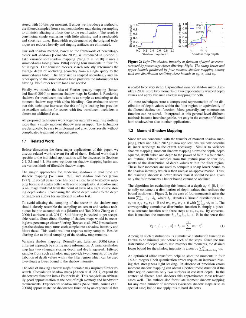
Figure 2: Left: The shadow intensity as function of depth as recon-structed by percentage closer filtering. Right: The sharp lower andupper bounds produced by four moment shadow mapping amongwith one distribution realizing these bounds at zf , z2 and z3.

is scaled to be very steep. Exponential variance shadow maps [Lau-ritzen 2008] store two moments of two exponentially warped depthvalues and apply variance shadow mapping for both.

All these techniques store a compressed representation of the dis-tribution of depth values within the filter region or equivalently ofthe filtered shadow test function. More generally, any monotonousfunction can be stored. Interpreted at this general level differentmethods become interchangeable, not only in the context of filteredhard shadows but also in other applications.

1.2 Moment Shadow Mapping

Since we are concerned with the transfer of moment shadow map-ping [Peters and Klein 2015] to new applications, we now describeits inner workings to the extent necessary. Similar to varianceshadow mapping, moment shadow mapping stores the depth, depthsquared, depth cubed and depth to the power of four in a four chan-nel texture. Filtered samples from this texture provide four mo-ments of the distribution of depth values within the filter region.These four moments are used to compute a sharp lower bound tothe shadow intensity which is then used as an approximation. Thus,the resulting shadow is never darker than it should be and givenonly the four moments a better bound cannot be obtained.

The algorithm for evaluating this bound at a depth zf ∈ [0, 1] in-ternally constructs a distribution of depth values that realizes thebound as shown in Figure 2. In the case of four moments it takes theform

∑3i=1 wi · δzi where δzi denotes a Dirac-δ distribution at zi,

z1 := zf , z2, z3 ∈ R andw1, w2, w3 > 0 with∑3

i=1 wi = 1. Thecorresponding cumulative distribution function is simply a piece-wise constant function with three steps at z1, z2, z3. By construc-tion it matches the moments b1, b2, b3, b4 ∈ R in the sense that

∀j ∈ {1, . . . , 4} : bj =

3∑i=1

wi · zji . (1)

Among all such distributions its cumulative distribution function isknown to be minimal just before each of the steps. Since the truedistribution of depth values also matches the moments, the desiredlower bound for the shadow intensity is given by

∑3i=2, zi<zf

wi.

An optimized affine transform helps to store the moments in four16-bit integers albeit quantization errors require an increased bias-ing that strengthens light leaking. In absence of precision errorsmoment shadow mapping can obtain a perfect reconstruction if thefilter region contains only two surfaces at constant depth. In thecontext of filtered hard shadows this approximates most relevantcases well. The authors also formulate moment shadow mappingfor any even number of moments (variance shadow maps arise asspecial case) but do not apply this to hard shadows.

2 Single Scattering

In rendering it is common to assume that all relevant light interac-tions happen at surfaces. This neglects volumetric scattering oc-curring in participating media such as smoke, dusty air, moist airand so forth. Light can be reflected towards the camera in midair.When this effect is coupled with proper computation of shadows itprovides great artistic value. Holes in geometry lead to shafts oflight known as crepuscular rays. These are perceived as aestheticand provide a great tool to direct attention of the viewer.

Unsurprisingly the creative industry likes to use this effect but itstill comes at a high cost. Scattering can occur anywhere withina volume. At the same time the visibility of the light source canchange arbitrarily along a view ray. This visibility term makes theintegration expensive. One way to evaluate it is based on classicshadow mapping coupled with ray marching but this leads to manyshadow map reads with poor cache coherence.

Prefiltered single scattering [Klehm et al. 2014a] accelerates thisprocedure by precomputing the relevant integrals into a convolu-tion shadow map. In the following we improve upon this idea byusing moment shadow maps with four (Section 2.4) or six moments(Section 2.5). Besides we demonstrate how to apply filtering duringthe necessary resampling step (Section 2.3).

2.1 Related Work

Just like surfaces participating media exhibits global illuminationeffects known as multiple scattering. In real-time rendering theseare commonly ignored to accommodate tight frame-time budgets.What remains is single scattering; light coming directly from a lightsource is scattered into the view ray. We focus on this effect.

Early works for rendering single scattering rely on shadow vol-umes [Max 1986] but more recent works employ shadow mapping.Dobashi et al. [2002] render translucent planes with shadow map-ping. This is equivalent to ray marching and on modern hardwaremore efficient implementations use programmable shaders with in-terleaved sampling [Tóth and Umenhoffer 2009]. For accelerationit has been proposed to use shadow volumes to identify regions con-taining shadows and to render single scattering at a lower resolutionfollowed by bilateral upscaling [Wyman and Ramsey 2008].

Engelhardt et al. [2010] apply more drastic subsampling in screenspace placing samples intelligently along few epipolar lines throughthe light source. Voxelized shadow volumes [Wyman 2011] pro-vide a more cache-friendly way to store shadow information forscattering. The results of 128 shadow tests along a view ray can bequeried at once. With proper parallelization this can be extended toarea lights [Wyman and Dai 2013].

Baran et al. [2010] exploit the simplicity of the shadow test functionto perform ray marching at amortized logarithmic time. Buildingupon this work Chen et al. [2011] propose use of a 1D min-max-mipmap to traverse ray segments that are fully lit or fully shadowedin a single step. Both techniques use epipolar coordinates and thelatter technique is easily mapped to graphics hardware.

Prefiltered single scattering [Klehm et al. 2014a; Klehm et al.2014b] introduces the concept of filterable shadow maps to sin-gle scattering. The authors generate a convolution shadow mapin a rectified coordinate system where rows correspond to epipo-lar planes containing the camera position while being parallel tothe directional light. Computing weighted prefix sums along rowseffectively precomputes the result of single scattering for the wholeepipolar slice at once. While this method works fast independentof scene complexity, the Fourier series used in convolution shadowmaps introduces ringing and memory requirements are high.

Lig

ht

dir

ect

ion

Light

dir

ect

ion

View

ray

View

ray

Up vectorUp vector

Lig

ht

ray

Light

ray

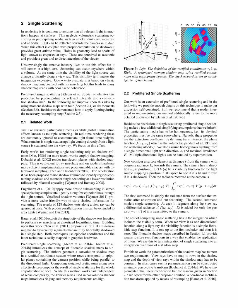
Figure 3: Left: The definition of the rectified coordinates r, θ, ϕ.Right: A resampled moment shadow map using rectified coordi-nates with appropriate bounds. The checkerboard serves to visual-ize the alpha channel.

2.2 Prefiltered Single Scattering

Our work is an extension of prefiltered single scattering and in thefollowing we provide enough details on this technique to make ourdiscussion self-contained. Still we recommend that a reader inter-ested in implementing our method additionally refers to the moredetailed discussion by Klehm et al. [2014b].

Besides the restriction to single scattering prefiltered single scatter-ing makes a few additional simplifying assumptions that we inherit.The participating media has to be homogenous, i.e. its physicalproperties must be the same everywhere. Namely, these propertiesare the extinction coefficient σt defining transmittance, the phasefunction f(ωl, ωp) which is the volumetric pendant of a BRDF andthe scattering albedo ρ. We also assume homogenous lighting froma single directional light with direction ωl and maximal irradianceEl. Multiple directional lights can be handled by superposition.

Now consider a surface element at distance s from the camera withoutgoing radiance Ls towards the camera. The camera lies in direc-tion ωp at position p. Let V (q) be a visibility function for the lightsource mapping a position in 3D-space to one if it is lit and to zeroif it is shadowed. Then the radiance received at the camera is

exp(−σt ·s)·Ls+f(ωl, ωp)·El ·∫ s

0

exp(−σt ·t)·V (p−t·ωp)dt.

The first summand is simply the radiance from the surface that re-mains after absorption and out-scattering. The second summandmodels single scattering. At each lit segment along the view raya differential radiance of f(ωl, ωp) · El is added but only the partexp(−σt · t) of it is transmitted to the camera.

The cost of computing single scattering lies in the integration whichincludes the visibility term. When we view it as one-dimensionalfunction along a light ray the visibility function is a simple Heav-iside step function. It is one up to the first occluder and then it iszero. The filterable shadow maps described in Section 1.1 providemeans to store such functions in a way that enables the applicationof filters. We use this to turn integration of single scattering into anintegration over rows of a shadow map.

For this to work the parametrization of the shadow map has to meettwo requirements. View rays have to map to rows in the shadowmap and the depth of view rays within the shadow map has to beconstant. In most cases such a parametrization can be constructedas simple perspective transform [Klehm et al. 2014a]. We have im-plemented this linear rectification but for reasons given in Section2.3 we opted for the other proposed solution; a non-linear rectifica-tion transform applied by means of resampling [Baran et al. 2010].

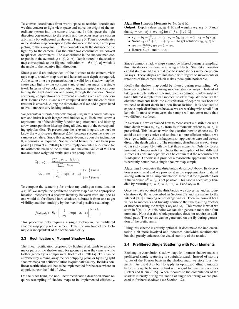
To convert coordinates from world space to rectified coordinateswe first convert to light view space and move the origin of the co-ordinate system into the camera location. In this space the lightdirection corresponds to the z-axis and the other axes are chosenarbitrarily but orthogonal as shown in Figure 3. Then u-coordinatesin the shadow map correspond to the distance to the origin after pro-jecting to the x-y-plane, r. This coincides with the distance of thelight ray to the camera. For the other two coordinates we convertto spherical coordinates. The v-coordinate in the shadow map cor-responds to the azimuth ϕ ∈ [0, 2 · π]. Depth stored in the shadowmap corresponds to the flipped inclination π − θ ∈ [0, π] which isthe angle to the negative light direction.

Since ϕ and θ are independent of the distance to the camera, viewrays map to shadow map rows and have constant depth as required.At the same time the parametrization is valid for a shadow map be-cause each light ray has constant r and ϕ and thus maps to a singletexel. In terms of epipolar geometry ϕ indexes epipolar slices con-taining the light direction and going through the camera. Singlescattering computations for different epipolar slices are indepen-dent. Bounds for r, ϕ and θ are computed such that the entire viewfrustum is covered. Along the dimension of θ we add a guard bandto avoid unnecessary leaking artifacts.

We generate a filterable shadow map b(u, v) in this coordinate sys-tem and index it with integer texel indices u, v. Each texel stores arepresentation of the visibility function (e.g. moments) and filteringa row corresponds to filtering along all view rays in the correspond-ing epipolar slice. To precompute the relevant integrals we need toknow the world-space distance ∆(v) between successive view raysamples per slice. Since this quantity depends upon the inclinationθ, a heuristic is required. Sophisticated heuristics have been pro-posed [Klehm et al. 2014b] but we simply compute the distance forthe arithmetic mean of the minimal and maximal values of θ. Thentransmittance weighted prefix sums are computed as

b(u, v) :=

∑ui=1 wi,v · b(i, v)∑u

i=1 wi,v,

wu,v :=

[− 1

σt· exp(−σt · t)

](u+ 12 )·∆(v)

(u− 12 )·∆(v)

.

To compute the scattering for a view ray ending at some locationq ∈ R3 we sample the prefiltered shadow map b at the appropriatelocation, reconstruct a shadow intensity between zero and one asone would do for filtered hard shadows, subtract it from one to getvisibility and then multiply by the maximal possible scattering

f(ωl, ωp) · El ·[− 1

σt· exp(−σt · t)

]‖q−p‖2

0

.

This procedure only requires a single lookup in the prefilteredshadow map per pixel on screen. Thus, the run time of the tech-nique is independent of the scene complexity.

2.3 Rectification of Moment Shadow Maps

The linear rectification proposed by Klehm et al. tends to allocatemajor parts of the shadow map for geometry near the camera whilefarther geometry is compressed [Klehm et al. 2014a]. This can bealleviated by moving away the near clipping plane or by using splitshadow maps but neither solution is quite satisfactory. Besides non-linear rectification still has to be implemented for the case where anepipole is near the field of view.

On the other hand, the non-linear rectification described above re-quires resampling of shadow maps to be implemented efficiently.

Algorithm 1 Input: Moments b1, b2, b3 ∈ R.Output: Depth values z2, z3 ∈ R and weights w2, w3 > 0 suchthat bj = w2 · zj2 + w3 · zj3 for all j ∈ {1, 2, 3}.• c2 := b2 − b21, c1 := b1 · b2 − b3, c0 := −b1 · c1 − b2 · c2.• Solve c2 · z2 + c1 · z + c0 = 0 to get solutions z2, z3 ∈ R.• w3 := b1−z2

z3−z2, w2 := 1− w3.

• Return z2, z3 and w2, w3.

Since common shadow maps cannot be filtered during resampling,this introduces considerable aliasing artifacts. Straight silhouettesexhibit staircase artifacts that lead to visible stripes in the crepuscu-lar rays. These stripes are not stable with regard to movements orrotations of the camera which makes them quite noticeable.

Ideally the shadow map could be filtered during resampling. Wehave accomplished this using moment shadow maps. Instead oftaking a sample without filtering from a common shadow map wetake a filtered sample from a moment shadow map. We then turn theobtained moments back into a distribution of depth values becausewe need to distort depth in a non-linear fashion. It is adequate toexpect simple distributions because we are working with small filterkernels. In most relevant cases the sample will not cover more thantwo different surfaces.

In Section 1.2 we explained how to reconstruct a distribution withthree depth values z1, z2, z3 from four moments where z1 = zf isprescribed. This leaves us with the question how to choose z1. Toavoid an arbitrary choice and to obtain a more efficient solution welet z1 go to infinity. As this happensw1 approaches zero and we candiscard the depth value z1. The remaining distributionw2·δz2+w3·δz3 is still compatible with the first three moments. Only the fourthmoment no longer matches. Under the assumption of two differentsurfaces at constant depth we can be certain that the reconstructionis adequate. Otherwise it provides a reasonable approximation thatis certainly better than a single shadow map sample.

Algorithm 1 computes the distribution described above. Its deriva-tion is non-trivial and we provide it in the supplementary materialamong with an HLSL implementation. Note that the algorithm failsif the variance σ2 = c2 is not positive. This case is adequately han-dled by returning z2 = z3 = b1, w2 = 1 and w3 = 0.

Once we have obtained the distribution we convert z2 and z3 to in-clinations θ2, θ3 as described in Section 2.2 and normalize to theinterval [0, 1] clamping out-of-range values. Then we convert bothvalues to moments and linearly combine the two resulting vectorsof moments using the weights w2 and w3. This vector is what westore in b(u, v). At this point we can also generate more than fourmoments. Note that this whole procedure does not require an addi-tional pass. The vectors can be generated on the fly during genera-tion of the prefix sums.

Using this scheme is entirely optional. It does make the implemen-tation a bit more involved and increases bandwidth requirementsbut also greatly enhances the visual stability of the results.

2.4 Prefiltered Single Scattering with Four Moments

Exchanging convolution shadow maps for moment shadow maps inprefiltered single scattering is straightforward. Instead of storingvalues of the Fourier basis in the shadow map, we store four mo-ments. As usual it is best to apply an optimized affine transformbefore storage to be more robust with regard to quantization errors[Peters and Klein 2015]. When it comes to the computation of theshadow intensity during evaluation of single scattering we can pro-ceed as for hard shadows (see Section 1.2).

However, some assumptions made for hard shadows are inadequatefor single scattering. For hard shadows we always underestimatethe shadow intensity to avoid surface acne. For single scattering thisis not necessary. We care more about small approximation error.Our solution is to take a weighted combination of a sharp lowerbound and a sharp upper bound. This only incurs a small additionalcost. If we have represented the moments as in Equation (1), thesharp upper bound is simply given by w1 +

∑3i=2, zi<zf

wi, i.e.the lower bound and the upper bound only differ by w1 (Figure 2).

To get the desired weighted combination we fix a weighting fac-tor β ∈ [0, 1] and compute β · w1 +

∑3i=2, zi<zf

wi. For β = 0

this yields the lower bound, i.e. single scattering is too bright. Forβ = 1 it yields the upper bound and single scattering is too dark.Intermediate values blend linearly. This is an intuitive parameterthat may be exposed to artists to control the effect of approximationerrors. For example large values seem preferable for indoor envi-ronments to avoid light leaking through walls. In our experimentswe always use β = 0.5 to achieve a minimal worst-case error.

2.5 Prefiltered Single Scattering with Six Moments

Moment shadow mapping with four moments is a particularly goodmatch for hard shadows because as long as filter kernels only con-tain two surfaces, the reconstruction can be nearly perfect. Forsingle scattering our kernels correspond to epipolar planes stretch-ing through the whole scene. Thus the case of two surfaces withinthe kernel is rarely present. Depth distributions generally exhibit agreater complexity and it is unrealistic to expect an adequate recon-struction from four moments in all cases.

Therefore we propose to use six moments. While the original al-gorithm is formulated for any even number of moments [Peters andKlein 2015], this has never been tried in a graphics context and theimplementation is challenging due to numerical issues. Here webriefly outline our solutions and provide all more technical detailsand HLSL implementations in the supplementary material.

To avoid loss of information during quantization we optimize anaffine transform as described by Peters and Klein [2015]. For sixmoments the found transform increases entropy per texel by 30.5bits. This is almost certainly not the global maximum but consid-erable computational resources were invested to get close. The al-gorithm requires solution of a symmetric and positive semi-definite4× 4 system of linear equations. As for four moments a Choleskydecomposition solves this robustly and efficiently. To solve the re-sulting cubic equation we use a closed-form solution followed byone iteration of Newton’s method to counteract instabilities.

This gives us the depth values z2, z3, z4 for the distribution. Forstability reasons we avoid computing the corresponding weightsw2, w3, w4 explicitly. Instead we immediately compute the rele-vant sum of weights by constructing a Newton polynomial. This isstable and works in quadratic time.

The resulting algorithm still requires considerable biasing (α =4 · 10−3). While this would be a serious problem for hard shadows,it does not prevent us from using the algorithm for single scattering.

2.6 Results and Discussion

Our implementation uses Direct3D 11 and applies all discussedsingle scattering techniques during a deferred rendering pass withthe depth buffer as input. Our method should be fast enough tobe applied during forward rendering to avoid problems with trans-parencies and multisampling but we have not tested this. Through-out the paper all our timings refer to an nVidia GeForce GTX 980

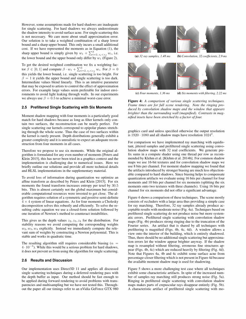
(a) 32 ray samples, 1.48 ms (b) Convolution, 32 coefficients, 2.9 ms

(c) Four moments, 1.36 ms (d) Six moments with filtering, 2.22 ms

Figure 4: A comparison of various single scattering techniques.Frame times are for full scene rendering. Note the ringing pro-duced by convolution shadow maps and the window that appearsbrighter than the surrounding wall (magnified). Contrasts in mag-nified insets have been stretched by a factor of four.

graphics card and unless specified otherwise the output resolutionis 1920 · 1080 and all shadow maps have resolution 10242.

For comparison we have implemented ray marching with equidis-tant, jittered samples and prefiltered single scattering using convo-lution shadow maps with 32 real coefficients. We generate pre-fix sums in a compute shader using one thread per row as recom-mended by Klehm et al. [Klehm et al. 2014b]. For common shadowmaps we use 16-bit textures and for convolution shadow maps weuse 8 bits per channel. For moment shadow mapping we found thatthe artifacts introduced by stronger biasing are much less objection-able compared to hard shadows. Since biasing helps to compensatequantization artifacts we evaluate using 16 bits per channel for fourmoments and 10 bits per channel for six moments (splitting the sixmoments onto two textures with three channels). Using 16 bits perchannel for six moments did not offer a significant advantage.

Figure 4 shows a comparison of these techniques. The scene mostlyconsists of occluders with a large area thus providing a simple casefor ray marching. Therefore, 32 ray samples already produce ac-ceptable results with moderate noise (Fig. 4a). Techniques based onprefiltered single scattering do not produce noise but more system-atic errors. Prefiltered single scattering with convolution shadowmaps (Fig. 4b) produces strong ringing due to the truncation of theFourier series. An artifact that is shared by all techniques withprefiltering is magnified (Figs. 4b, 4c, 4d). A window allows aview onto the interior of the building, which is entirely shadowed.Thus, there should be no additional single scattering but approxima-tion errors let the window appear brighter anyway. If the shadowmap is resampled without filtering, erroneous fine structures ap-pear (Figs. 4b, 4c) which are reduced heavily by filtering (Fig. 4d).Note that Figures 4a, 4b and 4c exhibit some surface acne frompercentage-closer filtering which is not present in Figure 4d becausethe available moment shadow map is used for shadowing.

Figure 5 shows a more challenging test case where all techniquesexhibit some characteristic artifacts. In spite of the increased num-ber of samples ray marching still produces strong noise (Fig. 5a).Ringing in prefiltered single scattering with convolution shadowmaps makes parts of crepuscular rays disappear entirely (Fig. 5b).A characteristic artifact of prefiltered single scattering with mo-

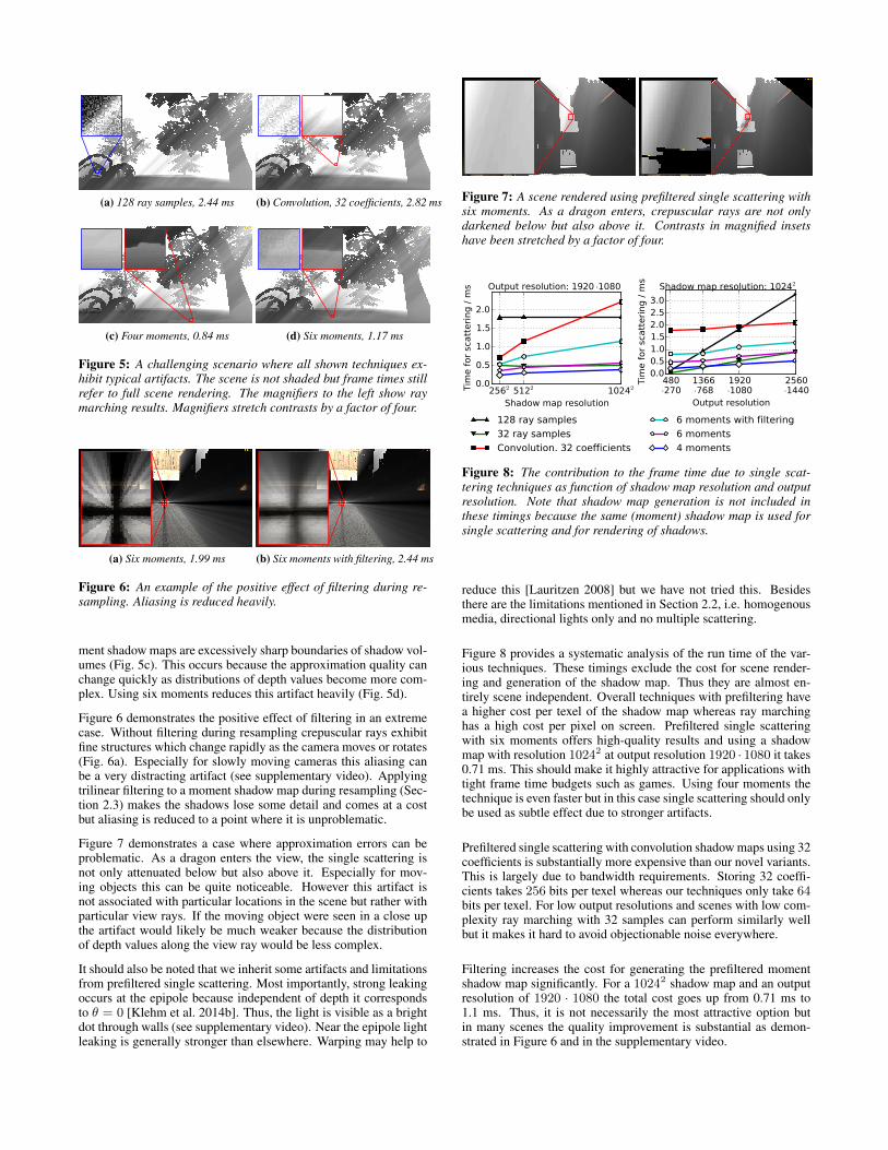
(a) 128 ray samples, 2.44 ms (b) Convolution, 32 coefficients, 2.82 ms

(c) Four moments, 0.84 ms (d) Six moments, 1.17 ms

Figure 5: A challenging scenario where all shown techniques ex-hibit typical artifacts. The scene is not shaded but frame times stillrefer to full scene rendering. The magnifiers to the left show raymarching results. Magnifiers stretch contrasts by a factor of four.

(a) Six moments, 1.99 ms (b) Six moments with filtering, 2.44 ms

Figure 6: An example of the positive effect of filtering during re-sampling. Aliasing is reduced heavily.

ment shadow maps are excessively sharp boundaries of shadow vol-umes (Fig. 5c). This occurs because the approximation quality canchange quickly as distributions of depth values become more com-plex. Using six moments reduces this artifact heavily (Fig. 5d).

Figure 6 demonstrates the positive effect of filtering in an extremecase. Without filtering during resampling crepuscular rays exhibitfine structures which change rapidly as the camera moves or rotates(Fig. 6a). Especially for slowly moving cameras this aliasing canbe a very distracting artifact (see supplementary video). Applyingtrilinear filtering to a moment shadow map during resampling (Sec-tion 2.3) makes the shadows lose some detail and comes at a costbut aliasing is reduced to a point where it is unproblematic.

Figure 7 demonstrates a case where approximation errors can beproblematic. As a dragon enters the view, the single scattering isnot only attenuated below but also above it. Especially for mov-ing objects this can be quite noticeable. However this artifact isnot associated with particular locations in the scene but rather withparticular view rays. If the moving object were seen in a close upthe artifact would likely be much weaker because the distributionof depth values along the view ray would be less complex.

It should also be noted that we inherit some artifacts and limitationsfrom prefiltered single scattering. Most importantly, strong leakingoccurs at the epipole because independent of depth it correspondsto θ = 0 [Klehm et al. 2014b]. Thus, the light is visible as a brightdot through walls (see supplementary video). Near the epipole lightleaking is generally stronger than elsewhere. Warping may help to

Figure 7: A scene rendered using prefiltered single scattering withsix moments. As a dragon enters, crepuscular rays are not onlydarkened below but also above it. Contrasts in magnified insetshave been stretched by a factor of four.

Figure 8: The contribution to the frame time due to single scat-tering techniques as function of shadow map resolution and outputresolution. Note that shadow map generation is not included inthese timings because the same (moment) shadow map is used forsingle scattering and for rendering of shadows.

reduce this [Lauritzen 2008] but we have not tried this. Besidesthere are the limitations mentioned in Section 2.2, i.e. homogenousmedia, directional lights only and no multiple scattering.

Figure 8 provides a systematic analysis of the run time of the var-ious techniques. These timings exclude the cost for scene render-ing and generation of the shadow map. Thus they are almost en-tirely scene independent. Overall techniques with prefiltering havea higher cost per texel of the shadow map whereas ray marchinghas a high cost per pixel on screen. Prefiltered single scatteringwith six moments offers high-quality results and using a shadowmap with resolution 10242 at output resolution 1920 · 1080 it takes0.71 ms. This should make it highly attractive for applications withtight frame time budgets such as games. Using four moments thetechnique is even faster but in this case single scattering should onlybe used as subtle effect due to stronger artifacts.

Prefiltered single scattering with convolution shadow maps using 32coefficients is substantially more expensive than our novel variants.This is largely due to bandwidth requirements. Storing 32 coeffi-cients takes 256 bits per texel whereas our techniques only take 64bits per texel. For low output resolutions and scenes with low com-plexity ray marching with 32 samples can perform similarly wellbut it makes it hard to avoid objectionable noise everywhere.

Filtering increases the cost for generating the prefiltered momentshadow map significantly. For a 10242 shadow map and an outputresolution of 1920 · 1080 the total cost goes up from 0.71 ms to1.1 ms. Thus, it is not necessarily the most attractive option butin many scenes the quality improvement is substantial as demon-strated in Figure 6 and in the supplementary video.

In conclusion the combination of prefiltered single scattering withmoment shadow maps appears to provide an attractive solution formany interactive applications. The run time is short compared toprevious techniques and the produced artifacts are perceptionallyunproblematic in most cases. Compared to convolution shadowmaps ringing is eliminated entirely and the technique is acceler-ated. The variant with six moments and without filtering providesan excellent trade-off between quality and run time. Filtering pro-vides a substantial quality improvement but comes at a cost. Fourmoments should only be used for subtle scattering.

3 Soft Shadows

Hard shadows assume an infinitesimally small light source that isoccluded either entirely or not at all. Obviously, this is an unrealis-tic assumption. Natural light sources always have some extent andcorrespondingly cast soft shadows with smooth penumbra regionswhere the light is partially occluded. Filtered hard shadows canhave a similar look but lack important characteristics. Most notablythey remain soft near the occluder.

The currently most practical approximation to soft shadows inperformance-sensitive real-time applications is to filter hard shad-ows with a filter size that depends linearly upon the distance be-tween occluder and receiver [Fernando 2005]. This yields convinc-ing results at the cost of excessive sampling of the shadow map.

In the following we demonstrate how to implement such an approx-imation using moment shadow maps. The technique is largely ana-log to variance soft shadow mapping [Yang et al. 2010] but behavesmuch more robustly thanks to the additional information in the mo-ment shadow map. Our technique is the first to provide robust ap-proximate soft shadows using only two queries to a four-channelsummed-area table.

3.1 Related Work

Various techniques attempt to compute physically based shadowsfrom shadow maps. Backprojection takes a single shadow map asdiscrete geometry representation and estimates the occluded area onthe light source [Guennebaud et al. 2006]. Stochastic soft shadowmapping transfers depth of field techniques using filterable shadowmaps [Liktor et al. 2015]. GEARS accelerates exact ray-triangleintersection tests using a shadow map [Wang et al. 2014]. Whilethese techniques can produce accurate soft shadows, they are toocostly for many interactive applications.

More practical methods (including ours) build upon percentage-closer soft shadows [Fernando 2005]. This technique can only getaccurate results under the assumption of a single planar occluderwhich is parallel to the planar light source. Per pixel it performs ablocker search sampling the shadow map to determine the averagedepth of occluding geometry. Then the adequate size of the penum-bra can be estimated by exploiting the planarity assumption. Fora directional light the penumbra size is simply proportional to thedistance between receiver and occluder. Finally percentage-closerfiltering with a corresponding filter size generates the penumbra.Percentage-closer soft shadows generates plausible results with fewnoticeable artifacts but the cost is high due to excessive sampling.Temporal coherency may be exploited to amortize this cost overmultiple frames [Schwärzler et al. 2013].

Summed-area variance shadow maps [Lauritzen 2007] try to avoidthis sampling using a summed-area table. A summed-area table[Crow 1984] is a prefiltered representation of a texture where eachtexel stores the integral over a rectangle from the left top to its lo-cation. By sampling a summed-area table at the four corners of an

arbitrary rectangle the integral over this rectangle can be queried(see Figure 9a). A summed-area table of a variance shadow mapenables filtering with an arbitrary filter size in constant time but theblocker search still requires sampling.

Variance soft shadow mapping [Yang et al. 2010] accelerates theblocker search using a heuristic based on a single query to asummed-area variance shadow map. To improve performance andquality a hierarchical shadow map identifies the umbra and fullylit regions early and where appropriate smaller kernels are used toavoid artifacts. In some cases a fallback to percentage-closer fil-tering is needed. Convolution soft shadow mapping [Annen et al.2008a] uses either a summed-area table or mipmaps to filter basedon convolution shadow maps. The blocker search uses a secondset of filterable textures. Exponential soft shadow mapping [Shenet al. 2013] uses summed-area tables over smaller regions of an ex-ponential shadow map to avoid catastrophic precision loss. Againadditional textures are needed for the blocker search. The authorsuse kernel subdivision to better approximate Gaussian filter kernels.

3.2 Summed Area Tables with Four Moments

Our technique follows the same basic steps as variance soft shadowmapping. We generate a summed-area table of a moment shadowmap, use it to estimate average blocker depth during the blockersearch, estimate the appropriate filter size and use the summed-areatable to perform the filtering. We first discuss generation of thesummed-area table.

This can be done in much the same way as generation of prefix sumsfor prefiltered single scattering (see Section 2.6). We use a computeshader with one thread per row to generate horizontal prefix sums.Then a second compute shader takes the result as input and gen-erates vertical prefix sums thus producing the final summed-areatable. As for single scattering we have not evaluated other schemes.

For small variance shadow maps the precision provided bysummed-area tables with single-precision floating point values canbe sufficient but for moment shadow maps it is generally insuffi-cient. We instead use 32-bit integers and modular arithmetic be-cause this allows us to exploit prior knowledge about maximal ker-nel sizes [Lauritzen 2007].

Suppose that the largest used kernel coversN ∈ N texels (e.g. N =256 for a 16 · 16 kernel). Moments b1, . . . , b4 initially lie in theinterval [0, 1]. If we multiply them by 232−1

Nand round to integers

afterwards, the sum of moments stored in the largest relevant kernelis known to lie in {0, . . . , 232 − 1}. Thus, this number can berepresented by a 32-bit unsigned integer. At the same time we stillhave a precision of log2

232−1N

which evaluates to 24 bits for theabove example. This is on par with with single precision floats.

To make use of this we generate such an integer moment shadowmap and generate an integer summed-area table for it. During thisstep overflows will occur frequently but they can be safely ignoredbecause they only subtract multiples of 232. When we query thesummed-area table in a kernel containingN texels or less, we knowthat the result has to lie in {0, . . . , 232 − 1} and thus computing itin integer arithmetic necessarily leads to the correct result.

In practice we initially create the moment shadow map with singleprecision floats. This way we do not need to implement a customresolve for multisample antialiasing. Conversion to integers hap-pens on the fly during creation of horizontal prefix sums.

3.3 Blocker Search

For the blocker search we perform a single look-up in the summed-area table to query four moments for the search region. We thenuse these moments and the biased fragment depth to reconstruct adistribution consisting of three depth values as described in Section1.2. The inherent assumption of our blocker search is that the re-sulting distribution

∑3i=1 wi · δzi is correct. If the filter kernel does

not contain more than two distinct surfaces, this assumption is well-justified. For three surfaces it is still justified as long as the blockersearch is performed for one of them.

Since this distribution is correct by assumption, we can derive av-erage blocker depth in analogy to percentage closer soft shadows:∑3

i=2, zi<zfwi · zi∑3

i=2, zi<zfwi

However, this formulation is not robust. The divisor is exactly theshadow intensity computed for the search region. It can be arbitrar-ily small or even exactly zero. In this case the expression becomesmeaningless. A small shadow intensity implies an unoccluded frag-ment. For such fragments the blocker search should return z1 = zfto indicate that a small filter kernel is to be used.

This requirement can be incorporated into the above formula ro-bustly by setting average blocker depth to

εz1 · z1 +∑3

i=2, zi<zfwi · zi

εz1 +∑3

i=2, zi<zfwi

where εz1 > 0 is a small constant. Greater values move averageblocker depth towards the receiver slightly thus making shadowsharder. The choice εz1 = 0.01 worked well in all experiments.

3.4 Filtering

Once average blocker depth is available the penumbra estimation[Fernando 2005] provides an adequate filter size. From this andthe texture coordinate of the fragment within the shadow map wecan compute the left top and right bottom texture coordinates of thefilter region. In general these will not lie in the center of texels.This necessitates interpolation for our integer summed-area tables.

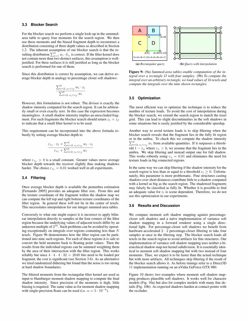
Conversely to what one might expect it is incorrect to apply bilin-ear interpolation directly to samples at the four corners of the filterregion because the underlying values of adjacent texels differ by anunknown multiple of 232. Such problems can be avoided by operat-ing exceptionally on integrals over regions containing less than Ntexels. Figure 9b demonstrates how the filter region can be parti-tioned into nine such regions. For each of these regions it is safe toconvert the held moments back to floating point values. Then theresults from the individual regions can be summed weighting themby the area of their intersection with the filter region. This worksreliably but since 4 · 4 · 4 · 32 = 2048 bits need to be loaded perfragment, the cost is significant (see Section 3.6). As an alternativewe tried randomized dithering but found that the noise is too strongat hard shadow boundaries.

The filtered moments from the rectangular filter kernel are used asinput to Hamburger moment shadow mapping to compute the finalshadow intensity. Since precision of the moments is high, littlebiasing is required. The same value as for moment shadow mappingwith single-precision floats can be used (i.e. α = 5 · 10−6).

BA

C D

A+B+C+DA+C

A+BA

D=(A+B+C+D)+A-(A+B)-(A+C)

(a) Rectangular query (b) Query with interpolation

Figure 9: (9a) Summed-area tables enable computation of the in-tegral over a rectangle D with four samples. (9b) To compute theintegral over an arbitrary rectangle, we load values of 16 texels andcompute the integrals over the nine shown rectangles.

3.5 Optimization

The most efficient way to optimize the technique is to reduce thenumber of texture loads. To avoid the cost of interpolation duringthe blocker search, we extend the search region to match the texelgrid. This can lead to slight discontinuities in the soft shadows insome situations but is easily justified by the considerable speedup.

Another way to avoid texture loads is to skip filtering when theblocker search reveals that the fragment lies in the fully lit regionor in the umbra. To check this we compute the shadow intensity∑3

i=2, zi<zfwi from available quantities. If it surpasses a thresh-

old 1 − εu where εu > 0, we assume that the fragment lies in theumbra. We skip filtering and instead output one for full shadow.This works robustly using εu = 0.01 and eliminates the need fortexture loads in big connected regions.

In the same way we can skip filtering if the shadow intensity for thesearch region is less than or equal to a threshold εl ≥ 0. Unfortu-nately, this parameter is more problematic. Fine structures castingshadows over short distances contribute little to a shadow computedwith a kernel as big as the search region. The shadowed fragmentsmay falsely be classified as fully lit. Whether it is possible to findan adequate value for εl is scene dependent. Therefore, we do notuse this optimization in our experiments.

3.6 Results and Discussion

We compare moment soft shadow mapping against percentage-closer soft shadows and a naïve implementation of variance softshadow mapping in a forward renderer using a single direc-tional light. For percentage-closer soft shadows we benefit fromhardware-accelerated 2 · 2 percentage-closer filtering to take foursamples at once in the filtering step. The blocker search loads alltexels in the search region to avoid artifacts for fine structures. Ourimplementation of variance soft shadow mapping uses neither a hi-erarchical shadow map nor kernel subdivision. It is essentially iden-tical to moment soft shadow mapping but with two instead of fourmoments. Thus, we expect it to be faster than the actual techniquebut with more artifacts. All techniques skip filtering if the result ofthe blocker search allows it. As before timings refer to a Direct3D11 implementation running on an nVidia GeForce GTX 980.

Figure 10 shows two examples where moment soft shadow map-ping produces plausible soft shadows. It works well for charactermodels (Fig. 10a) but also for complex models with many fine de-tails (Fig. 10b). As expected shadows harden at contact-points withthe occluder.

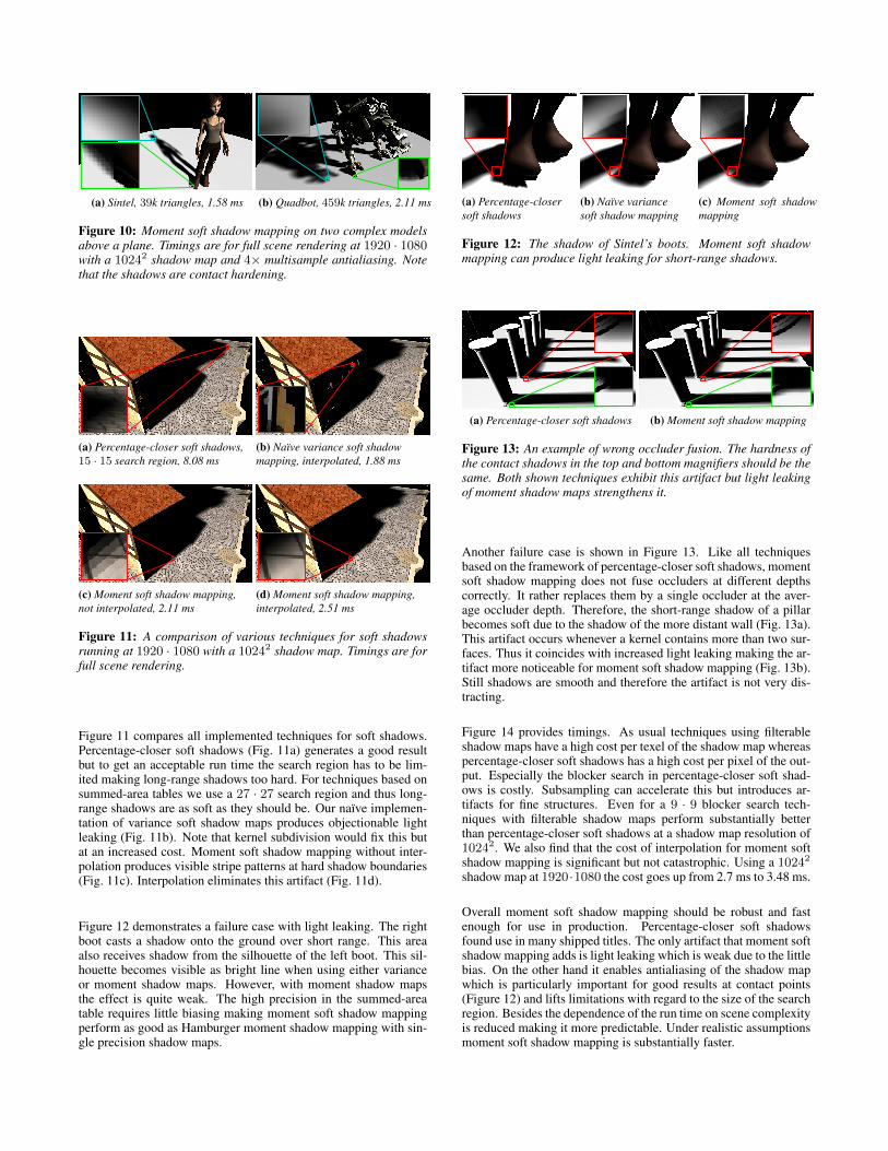
(a) Sintel, 39k triangles, 1.58 ms (b) Quadbot, 459k triangles, 2.11 ms

Figure 10: Moment soft shadow mapping on two complex modelsabove a plane. Timings are for full scene rendering at 1920 · 1080with a 10242 shadow map and 4× multisample antialiasing. Notethat the shadows are contact hardening.

(a) Percentage-closer soft shadows,15 · 15 search region, 8.08 ms

(b) Naïve variance soft shadowmapping, interpolated, 1.88 ms

(c) Moment soft shadow mapping,not interpolated, 2.11 ms

(d) Moment soft shadow mapping,interpolated, 2.51 ms

Figure 11: A comparison of various techniques for soft shadowsrunning at 1920 · 1080 with a 10242 shadow map. Timings are forfull scene rendering.

Figure 11 compares all implemented techniques for soft shadows.Percentage-closer soft shadows (Fig. 11a) generates a good resultbut to get an acceptable run time the search region has to be lim-ited making long-range shadows too hard. For techniques based onsummed-area tables we use a 27 · 27 search region and thus long-range shadows are as soft as they should be. Our naïve implemen-tation of variance soft shadow maps produces objectionable lightleaking (Fig. 11b). Note that kernel subdivision would fix this butat an increased cost. Moment soft shadow mapping without inter-polation produces visible stripe patterns at hard shadow boundaries(Fig. 11c). Interpolation eliminates this artifact (Fig. 11d).

Figure 12 demonstrates a failure case with light leaking. The rightboot casts a shadow onto the ground over short range. This areaalso receives shadow from the silhouette of the left boot. This sil-houette becomes visible as bright line when using either varianceor moment shadow maps. However, with moment shadow mapsthe effect is quite weak. The high precision in the summed-areatable requires little biasing making moment soft shadow mappingperform as good as Hamburger moment shadow mapping with sin-gle precision shadow maps.

(a) Percentage-closersoft shadows

(b) Naïve variancesoft shadow mapping

(c) Moment soft shadowmapping

Figure 12: The shadow of Sintel’s boots. Moment soft shadowmapping can produce light leaking for short-range shadows.

(a) Percentage-closer soft shadows (b) Moment soft shadow mapping

Figure 13: An example of wrong occluder fusion. The hardness ofthe contact shadows in the top and bottom magnifiers should be thesame. Both shown techniques exhibit this artifact but light leakingof moment shadow maps strengthens it.

Another failure case is shown in Figure 13. Like all techniquesbased on the framework of percentage-closer soft shadows, momentsoft shadow mapping does not fuse occluders at different depthscorrectly. It rather replaces them by a single occluder at the aver-age occluder depth. Therefore, the short-range shadow of a pillarbecomes soft due to the shadow of the more distant wall (Fig. 13a).This artifact occurs whenever a kernel contains more than two sur-faces. Thus it coincides with increased light leaking making the ar-tifact more noticeable for moment soft shadow mapping (Fig. 13b).Still shadows are smooth and therefore the artifact is not very dis-tracting.

Figure 14 provides timings. As usual techniques using filterableshadow maps have a high cost per texel of the shadow map whereaspercentage-closer soft shadows has a high cost per pixel of the out-put. Especially the blocker search in percentage-closer soft shad-ows is costly. Subsampling can accelerate this but introduces ar-tifacts for fine structures. Even for a 9 · 9 blocker search tech-niques with filterable shadow maps perform substantially betterthan percentage-closer soft shadows at a shadow map resolution of10242. We also find that the cost of interpolation for moment softshadow mapping is significant but not catastrophic. Using a 10242

shadow map at 1920·1080 the cost goes up from 2.7 ms to 3.48 ms.

Overall moment soft shadow mapping should be robust and fastenough for use in production. Percentage-closer soft shadowsfound use in many shipped titles. The only artifact that moment softshadow mapping adds is light leaking which is weak due to the littlebias. On the other hand it enables antialiasing of the shadow mapwhich is particularly important for good results at contact points(Figure 12) and lifts limitations with regard to the size of the searchregion. Besides the dependence of the run time on scene complexityis reduced making it more predictable. Under realistic assumptionsmoment soft shadow mapping is substantially faster.

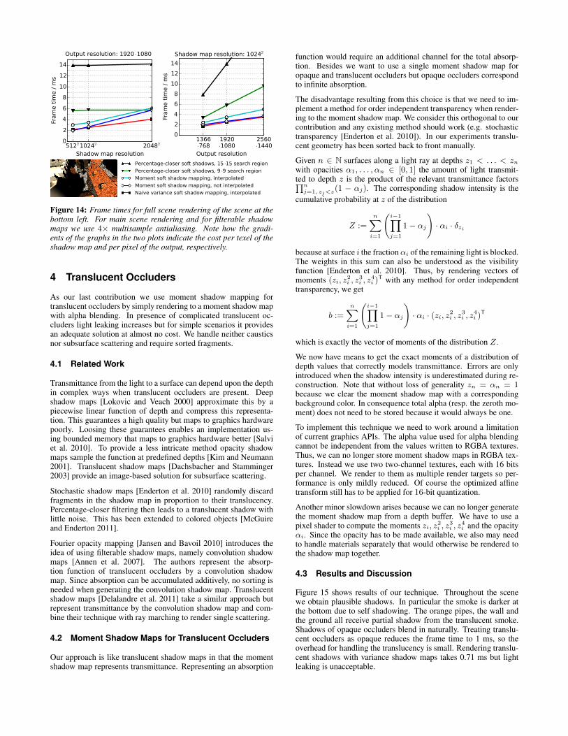
Figure 14: Frame times for full scene rendering of the scene at thebottom left. For main scene rendering and for filterable shadowmaps we use 4× multisample antialiasing. Note how the gradi-ents of the graphs in the two plots indicate the cost per texel of theshadow map and per pixel of the output, respectively.

4 Translucent Occluders

As our last contribution we use moment shadow mapping fortranslucent occluders by simply rendering to a moment shadow mapwith alpha blending. In presence of complicated translucent oc-cluders light leaking increases but for simple scenarios it providesan adequate solution at almost no cost. We handle neither causticsnor subsurface scattering and require sorted fragments.

4.1 Related Work

Transmittance from the light to a surface can depend upon the depthin complex ways when translucent occluders are present. Deepshadow maps [Lokovic and Veach 2000] approximate this by apiecewise linear function of depth and compress this representa-tion. This guarantees a high quality but maps to graphics hardwarepoorly. Loosing these guarantees enables an implementation us-ing bounded memory that maps to graphics hardware better [Salviet al. 2010]. To provide a less intricate method opacity shadowmaps sample the function at predefined depths [Kim and Neumann2001]. Translucent shadow maps [Dachsbacher and Stamminger2003] provide an image-based solution for subsurface scattering.

Stochastic shadow maps [Enderton et al. 2010] randomly discardfragments in the shadow map in proportion to their translucency.Percentage-closer filtering then leads to a translucent shadow withlittle noise. This has been extended to colored objects [McGuireand Enderton 2011].

Fourier opacity mapping [Jansen and Bavoil 2010] introduces theidea of using filterable shadow maps, namely convolution shadowmaps [Annen et al. 2007]. The authors represent the absorp-tion function of translucent occluders by a convolution shadowmap. Since absorption can be accumulated additively, no sorting isneeded when generating the convolution shadow map. Translucentshadow maps [Delalandre et al. 2011] take a similar approach butrepresent transmittance by the convolution shadow map and com-bine their technique with ray marching to render single scattering.

4.2 Moment Shadow Maps for Translucent Occluders

Our approach is like translucent shadow maps in that the momentshadow map represents transmittance. Representing an absorption

function would require an additional channel for the total absorp-tion. Besides we want to use a single moment shadow map foropaque and translucent occluders but opaque occluders correspondto infinite absorption.

The disadvantage resulting from this choice is that we need to im-plement a method for order independent transparency when render-ing to the moment shadow map. We consider this orthogonal to ourcontribution and any existing method should work (e.g. stochastictransparency [Enderton et al. 2010]). In our experiments translu-cent geometry has been sorted back to front manually.

Given n ∈ N surfaces along a light ray at depths z1 < . . . < znwith opacities α1, . . . , αn ∈ [0, 1] the amount of light transmit-ted to depth z is the product of the relevant transmittance factors∏n

j=1, zj<z(1 − αj). The corresponding shadow intensity is thecumulative probability at z of the distribution

Z :=

n∑i=1

(i−1∏j=1

1− αj

)· αi · δzi

because at surface i the fractionαi of the remaining light is blocked.The weights in this sum can also be understood as the visibilityfunction [Enderton et al. 2010]. Thus, by rendering vectors ofmoments (zi, z

2i , z

3i , z

4i )T with any method for order independent

transparency, we get

b :=

n∑i=1

(i−1∏j=1

1− αj

)· αi · (zi, z2

i , z3i , z

4i )T

which is exactly the vector of moments of the distribution Z.

We now have means to get the exact moments of a distribution ofdepth values that correctly models transmittance. Errors are onlyintroduced when the shadow intensity is underestimated during re-construction. Note that without loss of generality zn = αn = 1because we clear the moment shadow map with a correspondingbackground color. In consequence total alpha (resp. the zeroth mo-ment) does not need to be stored because it would always be one.

To implement this technique we need to work around a limitationof current graphics APIs. The alpha value used for alpha blendingcannot be independent from the values written to RGBA textures.Thus, we can no longer store moment shadow maps in RGBA tex-tures. Instead we use two two-channel textures, each with 16 bitsper channel. We render to them as multiple render targets so per-formance is only mildly reduced. Of course the optimized affinetransform still has to be applied for 16-bit quantization.

Another minor slowdown arises because we can no longer generatethe moment shadow map from a depth buffer. We have to use apixel shader to compute the moments zi, z2

i , z3i , z

4i and the opacity

αi. Since the opacity has to be made available, we also may needto handle materials separately that would otherwise be rendered tothe shadow map together.

4.3 Results and Discussion

Figure 15 shows results of our technique. Throughout the scenewe obtain plausible shadows. In particular the smoke is darker atthe bottom due to self shadowing. The orange pipes, the wall andthe ground all receive partial shadow from the translucent smoke.Shadows of opaque occluders blend in naturally. Treating translu-cent occluders as opaque reduces the frame time to 1 ms, so theoverhead for handling the translucency is small. Rendering translu-cent shadows with variance shadow maps takes 0.71 ms but lightleaking is unacceptable.

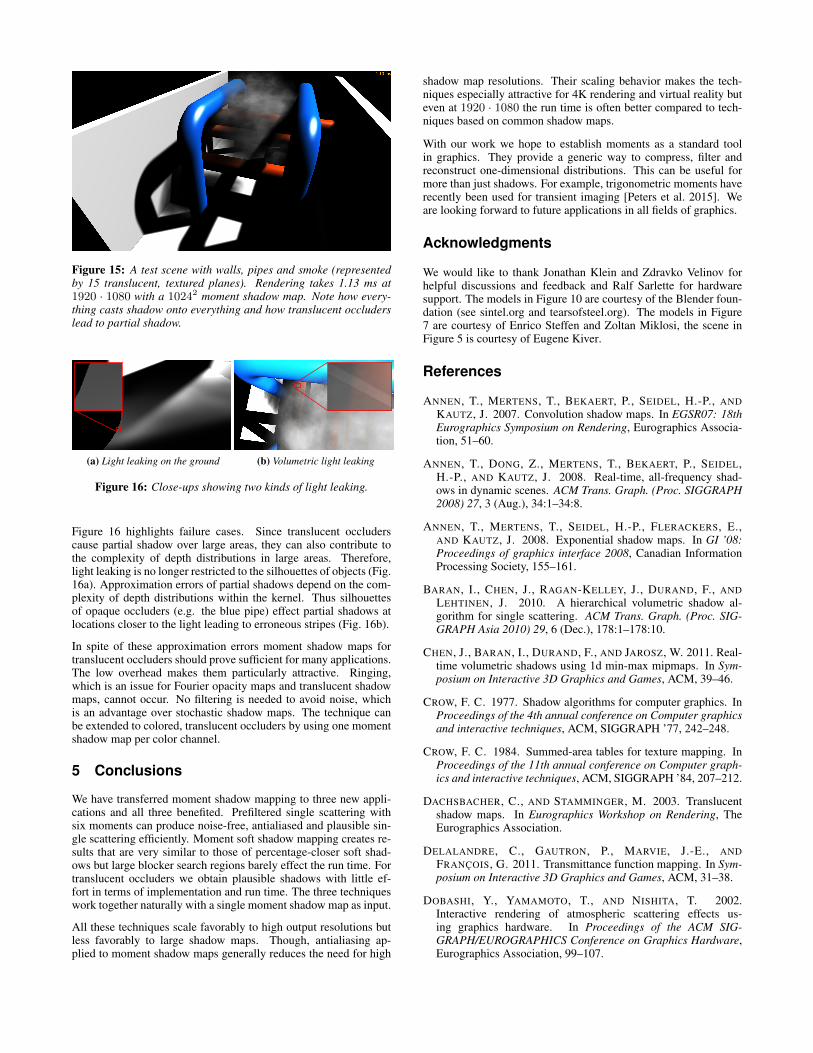
Figure 15: A test scene with walls, pipes and smoke (representedby 15 translucent, textured planes). Rendering takes 1.13 ms at1920 · 1080 with a 10242 moment shadow map. Note how every-thing casts shadow onto everything and how translucent occluderslead to partial shadow.

(a) Light leaking on the ground (b) Volumetric light leaking

Figure 16: Close-ups showing two kinds of light leaking.

Figure 16 highlights failure cases. Since translucent occluderscause partial shadow over large areas, they can also contribute tothe complexity of depth distributions in large areas. Therefore,light leaking is no longer restricted to the silhouettes of objects (Fig.16a). Approximation errors of partial shadows depend on the com-plexity of depth distributions within the kernel. Thus silhouettesof opaque occluders (e.g. the blue pipe) effect partial shadows atlocations closer to the light leading to erroneous stripes (Fig. 16b).

In spite of these approximation errors moment shadow maps fortranslucent occluders should prove sufficient for many applications.The low overhead makes them particularly attractive. Ringing,which is an issue for Fourier opacity maps and translucent shadowmaps, cannot occur. No filtering is needed to avoid noise, whichis an advantage over stochastic shadow maps. The technique canbe extended to colored, translucent occluders by using one momentshadow map per color channel.

5 Conclusions

We have transferred moment shadow mapping to three new appli-cations and all three benefited. Prefiltered single scattering withsix moments can produce noise-free, antialiased and plausible sin-gle scattering efficiently. Moment soft shadow mapping creates re-sults that are very similar to those of percentage-closer soft shad-ows but large blocker search regions barely effect the run time. Fortranslucent occluders we obtain plausible shadows with little ef-fort in terms of implementation and run time. The three techniqueswork together naturally with a single moment shadow map as input.

All these techniques scale favorably to high output resolutions butless favorably to large shadow maps. Though, antialiasing ap-plied to moment shadow maps generally reduces the need for high

shadow map resolutions. Their scaling behavior makes the tech-niques especially attractive for 4K rendering and virtual reality buteven at 1920 · 1080 the run time is often better compared to tech-niques based on common shadow maps.

With our work we hope to establish moments as a standard toolin graphics. They provide a generic way to compress, filter andreconstruct one-dimensional distributions. This can be useful formore than just shadows. For example, trigonometric moments haverecently been used for transient imaging [Peters et al. 2015]. Weare looking forward to future applications in all fields of graphics.

Acknowledgments

We would like to thank Jonathan Klein and Zdravko Velinov forhelpful discussions and feedback and Ralf Sarlette for hardwaresupport. The models in Figure 10 are courtesy of the Blender foun-dation (see sintel.org and tearsofsteel.org). The models in Figure7 are courtesy of Enrico Steffen and Zoltan Miklosi, the scene inFigure 5 is courtesy of Eugene Kiver.

References

ANNEN, T., MERTENS, T., BEKAERT, P., SEIDEL, H.-P., ANDKAUTZ, J. 2007. Convolution shadow maps. In EGSR07: 18thEurographics Symposium on Rendering, Eurographics Associa-tion, 51–60.

ANNEN, T., DONG, Z., MERTENS, T., BEKAERT, P., SEIDEL,H.-P., AND KAUTZ, J. 2008. Real-time, all-frequency shad-ows in dynamic scenes. ACM Trans. Graph. (Proc. SIGGRAPH2008) 27, 3 (Aug.), 34:1–34:8.

ANNEN, T., MERTENS, T., SEIDEL, H.-P., FLERACKERS, E.,AND KAUTZ, J. 2008. Exponential shadow maps. In GI ’08:Proceedings of graphics interface 2008, Canadian InformationProcessing Society, 155–161.

BARAN, I., CHEN, J., RAGAN-KELLEY, J., DURAND, F., ANDLEHTINEN, J. 2010. A hierarchical volumetric shadow al-gorithm for single scattering. ACM Trans. Graph. (Proc. SIG-GRAPH Asia 2010) 29, 6 (Dec.), 178:1–178:10.

CHEN, J., BARAN, I., DURAND, F., AND JAROSZ, W. 2011. Real-time volumetric shadows using 1d min-max mipmaps. In Sym-posium on Interactive 3D Graphics and Games, ACM, 39–46.

CROW, F. C. 1977. Shadow algorithms for computer graphics. InProceedings of the 4th annual conference on Computer graphicsand interactive techniques, ACM, SIGGRAPH ’77, 242–248.

CROW, F. C. 1984. Summed-area tables for texture mapping. InProceedings of the 11th annual conference on Computer graph-ics and interactive techniques, ACM, SIGGRAPH ’84, 207–212.

DACHSBACHER, C., AND STAMMINGER, M. 2003. Translucentshadow maps. In Eurographics Workshop on Rendering, TheEurographics Association.

DELALANDRE, C., GAUTRON, P., MARVIE, J.-E., ANDFRANÇOIS, G. 2011. Transmittance function mapping. In Sym-posium on Interactive 3D Graphics and Games, ACM, 31–38.

DOBASHI, Y., YAMAMOTO, T., AND NISHITA, T. 2002.Interactive rendering of atmospheric scattering effects us-ing graphics hardware. In Proceedings of the ACM SIG-GRAPH/EUROGRAPHICS Conference on Graphics Hardware,Eurographics Association, 99–107.

DONNELLY, W., AND LAURITZEN, A. 2006. Variance shadowmaps. In Proceedings of the 2006 Symposium on Interactive 3DGraphics and Games, ACM, 161–165.

ENDERTON, E., SINTORN, E., SHIRLEY, P., AND LUEBKE, D.2010. Stochastic transparency. In Proceedings of the 2010 ACMSIGGRAPH Symposium on Interactive 3D Graphics and Games,ACM, 157–164.

ENGELHARDT, T., AND DACHSBACHER, C. 2010. Epipolar sam-pling for shadows and crepuscular rays in participating mediawith single scattering. In Proceedings of the 2010 ACM SIG-GRAPH Symposium on Interactive 3D Graphics and Games,ACM, 119–125.

FERNANDO, R. 2005. Percentage-closer soft shadows. In ACMSIGGRAPH 2005 Sketches, ACM.

GUENNEBAUD, G., BARTHE, L., AND PAULIN, M. 2006. Real-time soft shadow mapping by backprojection. In EGSR06: 17thEurographics Symposium on Rendering, Eurographics Associa-tion, 227–234.

JANSEN, J., AND BAVOIL, L. 2010. Fourier opacity mapping. InProceedings of the 2010 ACM SIGGRAPH Symposium on Inter-active 3D Graphics and Games, ACM, 165–172.

KIM, T.-Y., AND NEUMANN, U. 2001. Opacity shadow maps. InEurographics Workshop on Rendering, The Eurographics Asso-ciation.

KLEHM, O., SEIDEL, H.-P., AND EISEMANN, E. 2014. Pre-filtered single scattering. In Proceedings of the 18th Meetingof the ACM SIGGRAPH Symposium on Interactive 3D Graphicsand Games, ACM, 71–78.

KLEHM, O., SEIDEL, H.-P., AND EISEMANN, E. 2014. Filter-based real-time single scattering using rectified shadow maps.Journal of Computer Graphics Techniques (JCGT) 3, 3, 7–34.

LAURITZEN, A., SALVI, M., AND LEFOHN, A. 2011. Sampledistribution shadow maps. In Proceedings of the 2011 ACMSIGGRAPH Symposium on Interactive 3D Graphics and Games,ACM, 97–102.

LAURITZEN, A. 2007. GPU Gems 3. Addison-Wesley,ch. Summed-Area Variance Shadow Maps, 157–182.

LAURITZEN, A. 2008. Rendering antialiased shadows usingwarped variance shadow maps. Master’s thesis, University ofWaterloo.

LIKTOR, G., SPASSOV, S., MÜCKL, G., AND DACHSBACHER,C. 2015. Stochastic soft shadow mapping. Computer GraphicsForum 34, 4, 1–11.

LOKOVIC, T., AND VEACH, E. 2000. Deep shadow maps. In Pro-ceedings of the 27th Annual Conference on Computer Graphicsand Interactive Techniques, ACM Press/Addison-Wesley Pub-lishing Co., SIGGRAPH ’00, 385–392.

MARTIN, T., AND TAN, T.-S. 2004. Anti-aliasing and continuitywith trapezoidal shadow maps. In EGSR04: 15th EurographicsSymposium on Rendering, Eurographics Association, 153–160.

MAX, N. L. 1986. Atmospheric illumination and shadows. In Pro-ceedings of the 13th Annual Conference on Computer Graphicsand Interactive Techniques, ACM, SIGGRAPH ’86, 117–124.

MCGUIRE, M., AND ENDERTON, E. 2011. Colored stochasticshadow maps. In Symposium on Interactive 3D Graphics andGames, ACM, 89–96.

PETERS, C., AND KLEIN, R. 2015. Moment shadow mapping. InProceedings of the 19th Symposium on Interactive 3D Graphicsand Games, ACM, 7–14.

PETERS, C., KLEIN, J., HULLIN, M. B., AND KLEIN, R. 2015.Solving trigonometric moment problems for fast transient imag-ing. ACM Trans. Graph. (Proc. SIGGRAPH Asia) 34, 6 (Nov.).

REEVES, W. T., SALESIN, D. H., AND COOK, R. L. 1987. Ren-dering antialiased shadows with depth maps. In Proceedings ofthe 14th annual conference on Computer graphics and interac-tive techniques, ACM, SIGGRAPH ’87, 283–291.

SALVI, M., VIDIMCE, K., LAURITZEN, A., AND LEFOHN, A.2010. Adaptive volumetric shadow maps. Computer GraphicsForum 29, 4, 1289–1296.

SALVI, M., 2008. Probabilistic approaches to shadow maps filter-ing, February. A talk in the tutorial "Core Techniques and Algo-rithms in Shader Programming" at Game Developers Conference2008.

SCHWÄRZLER, M., LUKSCH, C., SCHERZER, D., AND WIM-MER, M. 2013. Fast percentage closer soft shadows using tem-poral coherence. In Proceedings of the ACM SIGGRAPH Sym-posium on Interactive 3D Graphics and Games, ACM, 79–86.

SHEN, L., FENG, J., AND YANG, B. 2013. Exponential softshadow mapping. Computer Graphics Forum 32, 4.

TÓTH, B., AND UMENHOFFER, T. 2009. Real-time volumetriclighting in participating media. In Eurographics 2009 - ShortPapers, The Eurographics Association.

WANG, L., ZHOU, S., KE, W., AND POPESCU, V. 2014. GEARS:A general and efficient algorithm for rendering shadows. Com-puter Graphics Forum 33, 6, 264–275.

WILLIAMS, L. 1978. Casting curved shadows on curved surfaces.In Proceedings of the 5th annual conference on Computer graph-ics and interactive techniques, ACM, SIGGRAPH ’78, 270–274.

WYMAN, C., AND DAI, Z. 2013. Imperfect voxelized shadowvolumes. In Proceedings of the 5th High-Performance GraphicsConference, ACM, 45–52.

WYMAN, C., AND RAMSEY, S. 2008. Interactive volumetric shad-ows in participating media with single-scattering. In InteractiveRay Tracing, 2008. RT 2008. IEEE Symposium on, 87–92.

WYMAN, C. 2011. Voxelized shadow volumes. In Proceedings ofthe ACM SIGGRAPH Symposium on High Performance Graph-ics, ACM, 33–40.

YANG, B., DONG, Z., FENG, J., SEIDEL, H.-P., AND KAUTZ, J.2010. Variance soft shadow mapping. In Computer GraphicsForum, vol. 29, 2127–2134.

ZHANG, F., SUN, H., XU, L., AND LUN, L. K. 2006. Parallel-split shadow maps for large-scale virtual environments. In Pro-ceedings of the 2006 ACM international conference on Virtualreality continuum and its applications, ACM, 311–318.