AQR Capital Management, LLCTwo Greenwich PlazaGreenwich, CT 06830 p: +1.203.742.3600 | w: aqr.com

Better Diversification in the Low Expected Return World

SQA, New YorkJanuary 15, 2015

PrincipalAntti Ilmanen

For Investment Professional Use Only 1

Today’s Presenter

2

Antti Ilmanen,Principal, Portfolio Solutions Group

Antti Ilmanen, a Principal at AQR, manages the Portfolio Solutions Group, which advises institutional investors and sovereign wealth funds, and develops AQR’s broad investment ideas. Before AQR, Antti spent seven years as a senior portfolio manager at Brevan Howard, a macro hedge fund, and a decade in a variety of roles at Salomon Brothers/Citigroup. He began his career as a central bank portfolio manager in Finland. Antti earned a Ph.D. in finance from the University of Chicago and M.Sc. degrees in economics and law from the University of Helsinki. Over the years, he has advised many institutional investors, including Norway’s Government Pension Fund Global and the Government of Singapore Investment Corporation. Antti has published extensively in finance and investment journals and has received the Graham and Dodd award and the Bernstein Fabozzi/Jacobs Levy award for his articles. His book Expected Returns (Wiley, 2011) is a broad synthesis of the central issue in investing. Antti recently scored a rare double in winning the best-paper and runner-up award for best articles published in 2012 in the Journal of Portfolio Management (coauthored articles “The Death of Diversification Has Been Greatly Exaggerated” and “The Norway Model”).

Low Expected Return World

0%

2%

4%

6%

8%

10%

12%

1900 1910 1920 1930 1940 1950 1960 1970 1980 1990 2000 2010

60/40 Real Yield CPI + 5%

-2%

2%

6%

10%

14%

1900 1910 1920 1930 1940 1950 1960 1970 1980 1990 2000 2010

Equity Real Yield Bond Real Yield

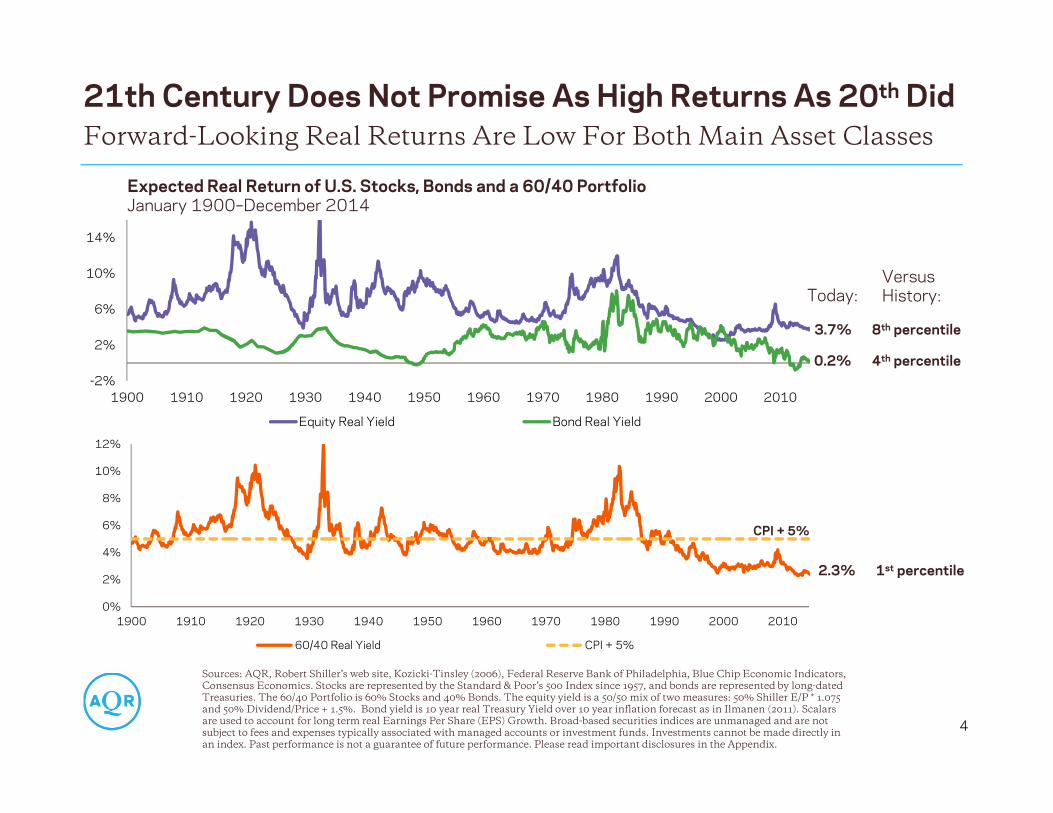
21th Century Does Not Promise As High Returns As 20th Did

4

Forward-Looking Real Returns Are Low For Both Main Asset Classes

Sources: AQR, Robert Shiller’s web site, Kozicki-Tinsley (2006), Federal Reserve Bank of Philadelphia, Blue Chip Economic Indicators, Consensus Economics. Stocks are represented by the Standard & Poor’s 500 Index since 1957, and bonds are represented by long-dated Treasuries. The 60/40 Portfolio is 60% Stocks and 40% Bonds. The equity yield is a 50/50 mix of two measures: 50% Shiller E/P * 1.075 and 50% Dividend/Price + 1.5%. Bond yield is 10 year real Treasury Yield over 10 year inflation forecast as in Ilmanen (2011). Scalars are used to account for long term real Earnings Per Share (EPS) Growth. Broad-based securities indices are unmanaged and are notsubject to fees and expenses typically associated with managed accounts or investment funds. Investments cannot be made directly in an index. Past performance is not a guarantee of future performance. Please read important disclosures in the Appendix.

Expected Real Return of U.S. Stocks, Bonds and a 60/40 PortfolioJanuary 1900–December 2014

CPI + 5%

VersusHistory:

8th percentile

4th percentile

Today:

3.7%

0.2%

1st percentile2.3%

-4%

-2%

0%

2%

4%

6%

8%

10%

12%

14%

1980 1985 1990 1995 2000 2005 2010 2015

U.S. Equity Real Yield Non-U.S. Equity Real Yield

U.S. 10Y Treasury Real Yield Non-U.S. 10Y Bond Real Yield

Cash (U.S. T-Bill)

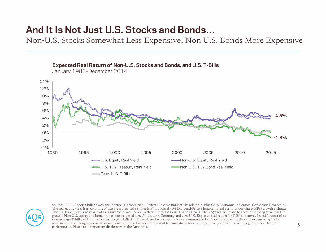
And It Is Not Just U.S. Stocks and Bonds…

5

Non-U.S. Stocks Somewhat Less Expensive, Non U.S. Bonds More Expensive

Expected Real Return of Non-U.S. Stocks and Bonds, and U.S. T-BillsJanuary 1980–December 2014

4.5%

-1.3%

Sources: AQR, Robert Shiller’s web site, Kozicki-Tinsley (2006), Federal Reserve Bank of Philadelphia, Blue Chip Economic Indicators, Consensus Economics. The real equity yield is a 50/50 mix of two measures: 50% Shiller E/P * 1.075 and 50% Dividend/Price + long-term real earnings-per-share (EPS) growth estimate. The real bond yield is 10-year real Treasury Yield over 10-year inflation forecast as in Ilmanen (2011). The 1.075 scalar is used to account for long term real EPS growth. Non-U.S. equity and bond proxies are weighted 40% Japan, 40% Germany and 20% U.K. Expected real return for T-Bills is survey-based forecast of 10-year average T-Bill yield minus forecast 10-year inflation. Broad-based securities indices are unmanaged and are not subject to fees and expenses typically associated with managed accounts or investment funds. Investments cannot be made directly in an index. Past performance is not a guarantee of future performance. Please read important disclosures in the Appendix.

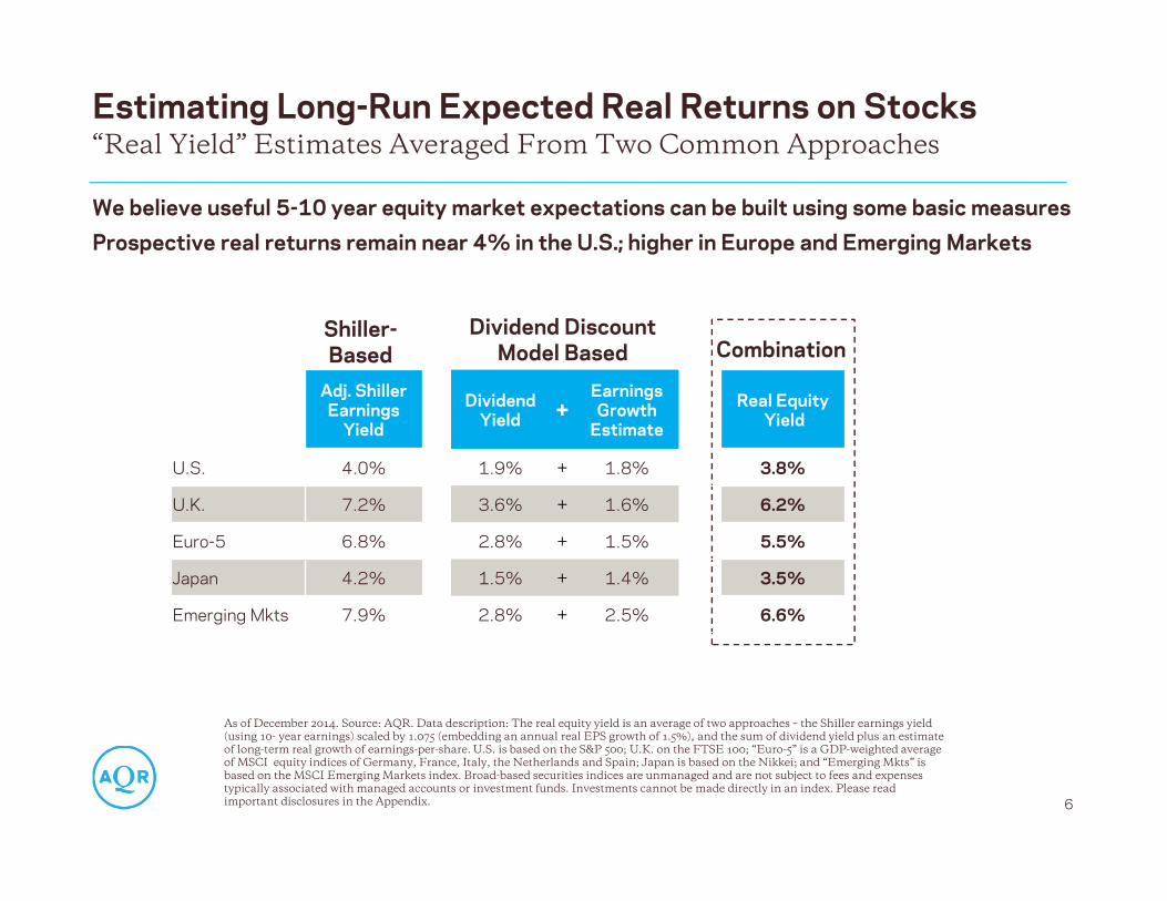
We believe useful 5-10 year equity market expectations can be built using some basic measuresProspective real returns remain near 4% in the U.S.; higher in Europe and Emerging Markets

Estimating Long-Run Expected Real Returns on Stocks

6

“Real Yield” Estimates Averaged From Two Common Approaches

As of December 2014. Source: AQR. Data description: The real equity yield is an average of two approaches – the Shiller earnings yield (using 10- year earnings) scaled by 1.075 (embedding an annual real EPS growth of 1.5%), and the sum of dividend yield plus an estimate of long-term real growth of earnings-per-share. U.S. is based on the S&P 500; U.K. on the FTSE 100; “Euro-5” is a GDP-weighted average of MSCI equity indices of Germany, France, Italy, the Netherlands and Spain; Japan is based on the Nikkei; and “Emerging Mkts” is based on the MSCI Emerging Markets index. Broad-based securities indices are unmanaged and are not subject to fees and expenses typically associated with managed accounts or investment funds. Investments cannot be made directly in an index. Please read important disclosures in the Appendix.

Shiller-Based

Dividend Discount Model Based Combination

Adj. Shiller Earnings

Yield

Dividend Yield +

Earnings Growth

Estimate

Real EquityYield

U.S. 4.0% 1.9% + 1.8% 3.8%

U.K. 7.2% 3.6% + 1.6% 6.2%

Euro-5 6.8% 2.8% + 1.5% 5.5%

Japan 4.2% 1.5% + 1.4% 3.5%

Emerging Mkts 7.9% 2.8% + 2.5% 6.6%

y = -0.45x + 0.00R² = 0.19

-6%

-4%

-2%

0%

2%

4%

6%

8%

-4.0% -2.0% 0.0% 2.0% 4.0% 6.0%

y = -0.48x - 0.01R² = 0.26

-8%

-6%

-4%

-2%

0%

2%

4%

6%

-4.0% -2.0% 0.0% 2.0% 4.0% 6.0%

Low Long-Run Expected Returns

*As of September 2014. Sources: AQR, Robert Shiller’s web site, Kozicki-Tinsley (2006), Federal Reserve Bank of Philadelphia, Blue Chip Economic Indicators, Consensus Economics. The Equity Real Yield is a 50/50 mix of two measures: 50% Shiller E/P * 1.075 and 50% Dividend/Price + 1.5%. Bond Real Yield is 10 year real Treasury Yield over 10 year inflation forecast as in Ilmanen (2011). Scalars are used to account for long term real Earnings Per Share (EPS) Growth. Broad-based securities indices are unmanaged and are not subject to fees and expenses typically associated with managed accounts or investment funds. Investments cannot be made directly in an index. Past performance is not a guarantee of future performance. Please read important disclosures in the Appendix.

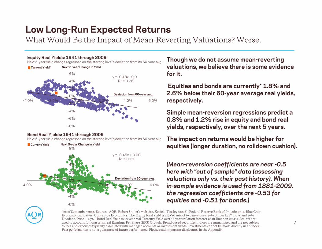
Equity Real Yields: 1941 through 2009Next 5-year yield change regressed on the starting level’s deviation from its 60-year avg.

Bond Real Yields: 1941 through 2009Next 5-year yield change regressed on the starting level’s deviation from its 60-year avg.

Though we do not assume mean-reverting valuations, we believe there is some evidence for it.

Equities and bonds are currently* 1.8% and 2.6% below their 60-year average real yields, respectively.

Simple mean-reversion regressions predict a 0.8% and 1.2% rise in equity and bond real yields, respectively, over the next 5 years.

The impact on returns would be higher for equities (longer duration, no rolldown cushion).

(Mean-reversion coefficients are near -0.5 here with “out of sample” data (assessing valuations only vs. their past history). When in-sample evidence is used from 1881-2009, the regression coefficients are -0.53 for equities and -0.51 for bonds.)

7

What Would Be the Impact of Mean-Reverting Valuations? Worse.

Current Yield*

Current Yield*

Deviation from 60-year avg.

Deviation from 60-year avg.

Next 5-year Change in Yield

Next 5-year Change in Yield

1

10

100

1,000

1900 1920 1940 1960 1980 2000

Cumulative Excess Return

Buy & Hold Value Timing Outperformance

‐5%

0%

5%

10%

15%

1(most

expensive)

2 3 4 5(cheapest)Eq

uity Excess R

eturn (Ann

ualized

)

Starting Shiller E/P Quintiles

Next Quarter Return Next 1Y Return Next 5Y Return

Promising Forecasting Ability; Timing is Difficult in Practice

8

Correlations May Not Translate to Profitable Signals

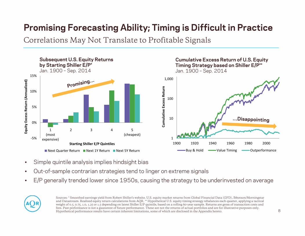
Subsequent U.S. Equity Returns by Starting Shiller E/P* Jan. 1900 – Sep. 2014

Sources: * Smoothed earnings yield from Robert Shiller’s website. U.S. equity market returns from Global Financial Data (GFD), Ibbotson/Morningstar and Datastream. Realized equity return calculations from AQR. ** Hypothetical U.S. equity timing strategy rebalances each quarter, applying a tactical weight of 0.5, 0.75, 1.0, 1.25 or 1.5 depending on latest Shiller E/P quintile, based on a rolling 60-year sample. Returns are gross of transaction costs and fees. Past performance is not a guarantee of future performance. These are not the returns of actual portfolios and are for illustrative purposes only. Hypothetical performance results have certain inherent limitations, some of which are disclosed in the Appendix hereto.

Cumulative Excess Return of U.S. Equity Timing Strategy based on Shiller E/P**Jan. 1900 – Sep. 2014

• Simple quintile analysis implies hindsight bias• Out-of-sample contrarian strategies tend to linger on extreme signals • E/P generally trended lower since 1950s, causing the strategy to be underinvested on average

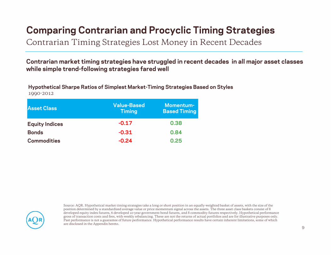
Contrarian market timing strategies have struggled in recent decades in all major asset classes while simple trend-following strategies fared well

Comparing Contrarian and Procyclic Timing Strategies

9

Source: AQR. Hypothetical market timing strategies take a long or short position in an equally-weighted basket of assets, with the size of the position determined by a standardized average value or price momentum signal across the assets. The three asset class baskets consist of 8 developed equity index futures, 6 developed 10-year government bond futures, and 8 commodity futures respectively. Hypothetical performance gross of transaction costs and fees, with weekly rebalancing. These are not the returns of actual portfolios and are for illustrative purposes only. Past performance is not a guarantee of future performance. Hypothetical performance results have certain inherent limitations, some of which are disclosed in the Appendix hereto.

Hypothetical Sharpe Ratios of Simplest Market-Timing Strategies Based on Styles 1990-2012

Asset Class Value-Based Timing

Momentum-Based Timing

Equity Indices -0.17 0.38

Bonds -0.31 0.84Commodities -0.24 0.25

Contrarian Timing Strategies Lost Money in Recent Decades

Focus on Better Diversification (& Be Humble on Forecasts)

Good and Bad News on ForecastingGood News: We can identify long-run return sources that may be useful strategic holdings(“Strategic Beats Tactical”)• Several alternative beta premia besides major market risk premiaBad News: Tactical (near-term) predictability is limited. Humility is needed.• Any timing efforts face a higher bar when we start with a well-diversified portfolio. Timing skills

must be exceptional to simply offset the foregone diversification in concentrated bets.

Good and Bad News on DiversificationGood News: Small forecasting edges can be magnified by diversification (“Many Beats Few”)• Diversification across lowly correlated investments may help to smooth portfolio returns and thus

boost Sharpe ratio (SR)• If we assume similar SRs for all building blocks (say, long-only asset class premia and long-short

style premia all have SRs of 0.2-0.3), a well-diversified long-only portfolio may not be able toreach SR > 0.5, while a well-diversified style premia portfolio could, thanks to its greater breadth

Bad News: Diversification requires meaningful shorting and leverage to be most effective• Long-only investors are often forced to risk concentration, with portfolios typically dominated by

equity market risk

10

We Believe Strategic Diversification Beats Tactical Concentration

Please read important disclosures in the Appendix. Diversification does not eliminate the risk of experiencing investment losses.

Better Diversification Is Bold

0.0

0.1

0.2

0.3

0.4

0.5

0.6

0.7

0.8

0.9

1.0

1992 1994 1995 1997 1998 2000 2001 2002 2004 2005 2007 2008 2009 2011

Global 60/40 Endowment Proxy Hedge Fund Index

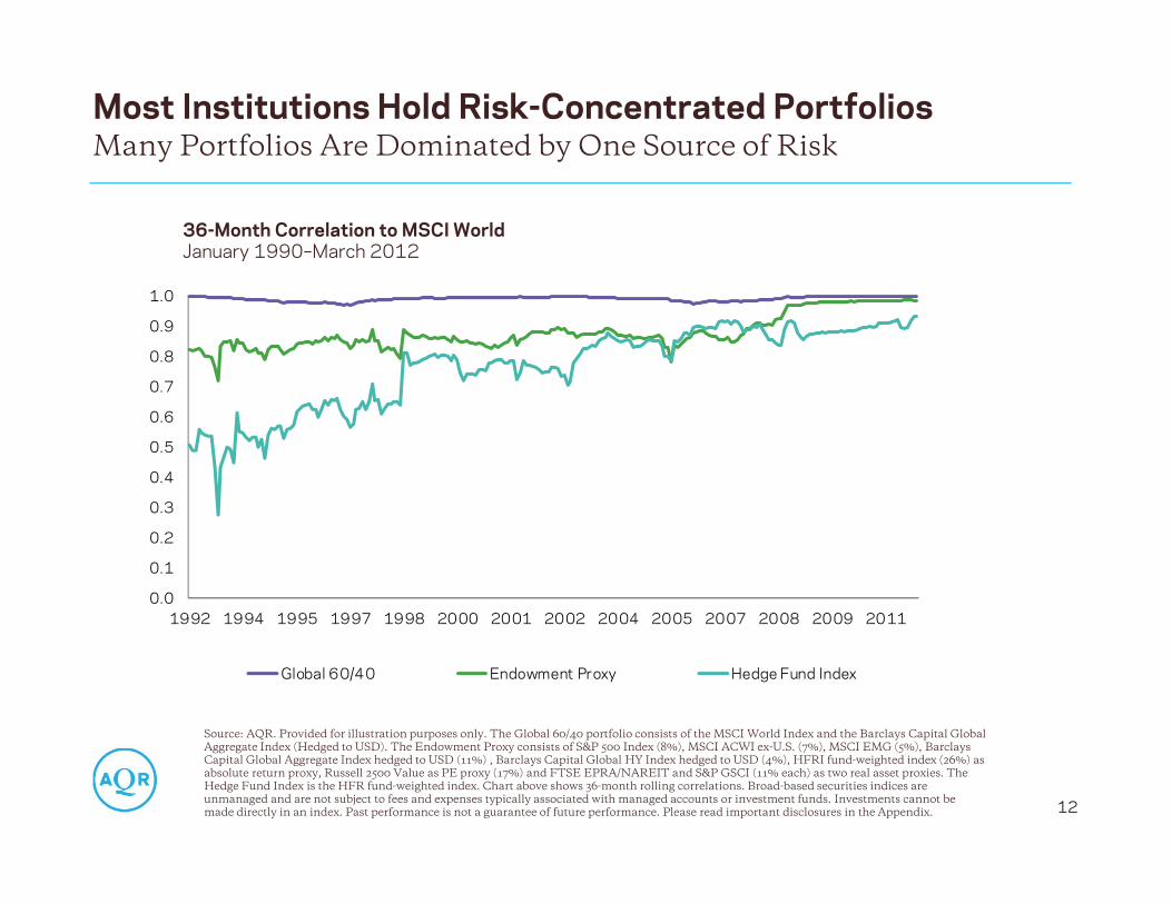
Most Institutions Hold Risk-Concentrated Portfolios

12

Many Portfolios Are Dominated by One Source of Risk

Source: AQR. Provided for illustration purposes only. The Global 60/40 portfolio consists of the MSCI World Index and the Barclays Capital Global Aggregate Index (Hedged to USD). The Endowment Proxy consists of S&P 500 Index (8%), MSCI ACWI ex-U.S. (7%), MSCI EMG (5%), Barclays Capital Global Aggregate Index hedged to USD (11%) , Barclays Capital Global HY Index hedged to USD (4%), HFRI fund-weighted index (26%) as absolute return proxy, Russell 2500 Value as PE proxy (17%) and FTSE EPRA/NAREIT and S&P GSCI (11% each) as two real asset proxies. The Hedge Fund Index is the HFR fund-weighted index. Chart above shows 36-month rolling correlations. Broad-based securities indices are unmanaged and are not subject to fees and expenses typically associated with managed accounts or investment funds. Investments cannot be made directly in an index. Past performance is not a guarantee of future performance. Please read important disclosures in the Appendix.

36-Month Correlation to MSCI WorldJanuary 1990–March 2012

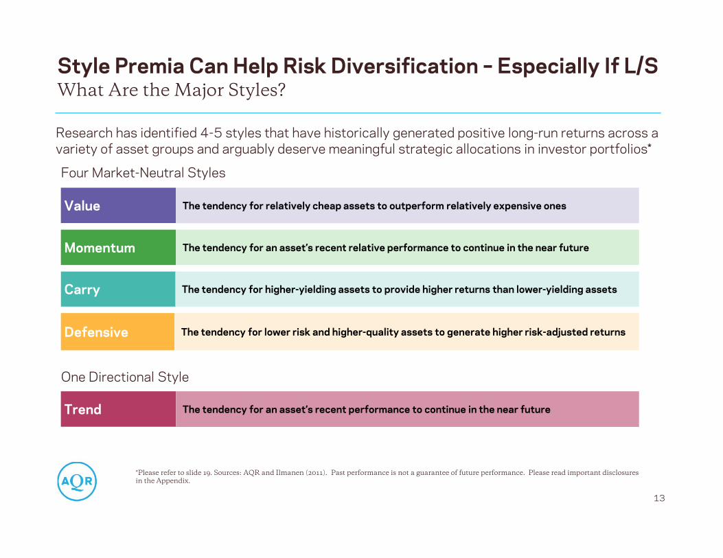
Style Premia Can Help Risk Diversification – Especially If L/S

13

Momentum The tendency for an asset’s recent relative performance to continue in the near future

Value The tendency for relatively cheap assets to outperform relatively expensive ones

Carry The tendency for higher-yielding assets to provide higher returns than lower-yielding assets

Defensive The tendency for lower risk and higher-quality assets to generate higher risk-adjusted returns

What Are the Major Styles?

Research has identified 4-5 styles that have historically generated positive long-run returns across a variety of asset groups and arguably deserve meaningful strategic allocations in investor portfolios*

Four Market-Neutral Styles

*Please refer to slide 19. Sources: AQR and Ilmanen (2011). Past performance is not a guarantee of future performance. Please read important disclosures in the Appendix.

One Directional Style

Trend The tendency for an asset’s recent performance to continue in the near future

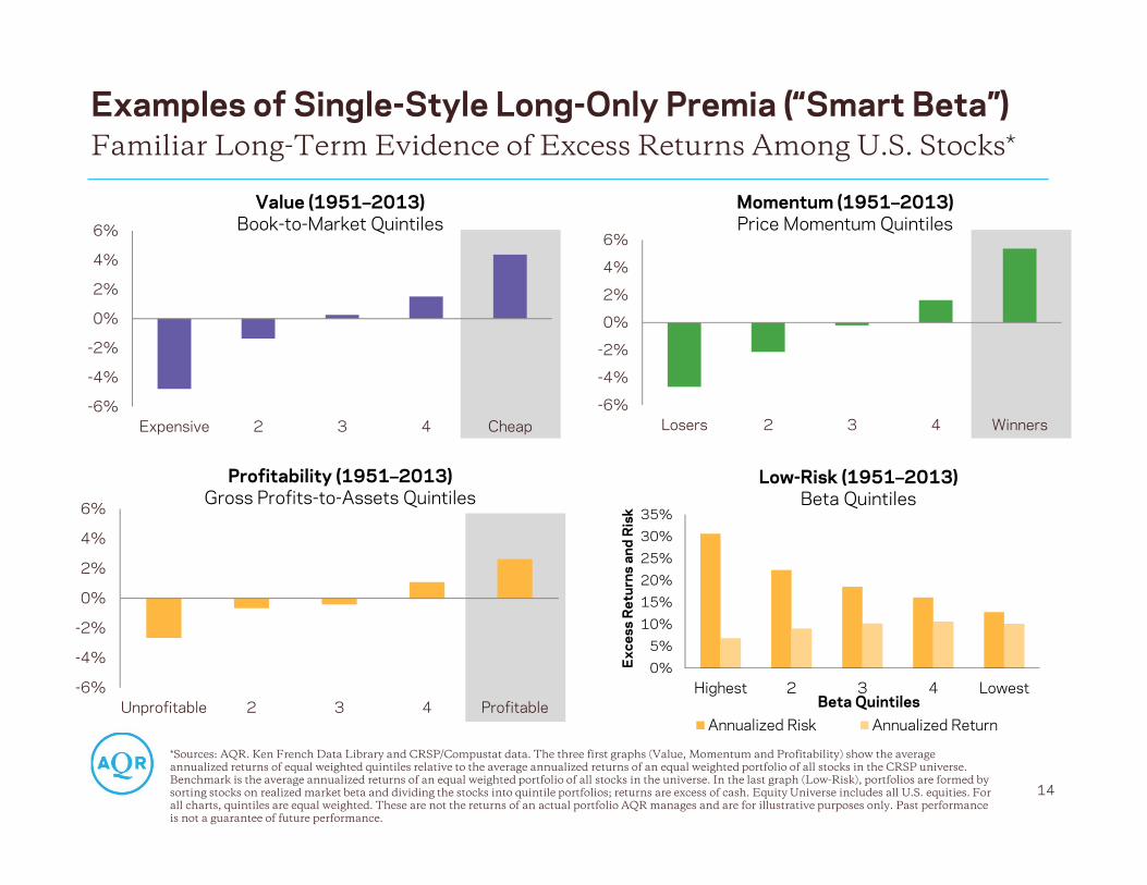
Examples of Single-Style Long-Only Premia (“Smart Beta”)

14

*Sources: AQR. Ken French Data Library and CRSP/Compustat data. The three first graphs (Value, Momentum and Profitability) show the average annualized returns of equal weighted quintiles relative to the average annualized returns of an equal weighted portfolio of all stocks in the CRSP universe.Benchmark is the average annualized returns of an equal weighted portfolio of all stocks in the universe. In the last graph (Low-Risk), portfolios are formed by sorting stocks on realized market beta and dividing the stocks into quintile portfolios; returns are excess of cash. Equity Universe includes all U.S. equities. For all charts, quintiles are equal weighted. These are not the returns of an actual portfolio AQR manages and are for illustrative purposes only. Past performance is not a guarantee of future performance.

Familiar Long-Term Evidence of Excess Returns Among U.S. Stocks*

Value (1951–2013)Book-to-Market Quintiles

Momentum (1951–2013)Price Momentum Quintiles

Profitability (1951–2013)Gross Profits-to-Assets Quintiles

-6%

-4%

-2%

0%

2%

4%

6%

Expensive 2 3 4 Cheap-6%

-4%

-2%

0%

2%

4%

6%

Losers 2 3 4 Winners

-6%

-4%

-2%

0%

2%

4%

6%

Unprofitable 2 3 4 Profitable

0%5%

10%15%20%25%30%35%

Highest 2 3 4 Lowest

Exc

ess

Ret

urns

and

Ris

k

Beta QuintilesAnnualized Risk Annualized Return

Low-Risk (1951–2013)Beta Quintiles

Smart Beta Is A Good First Step, Hardly The Last One

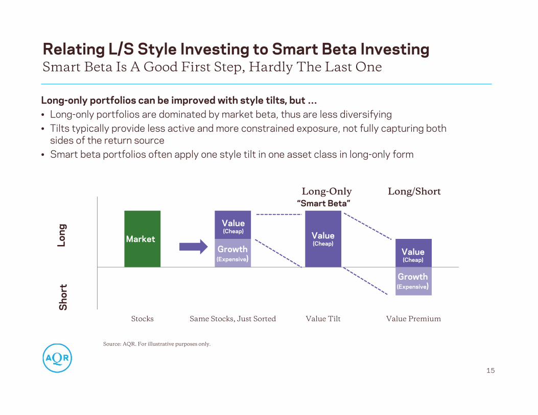
Source: AQR. For illustrative purposes only.

15

Long

“Smart Beta”

Sho

rt

Value(Cheap)

Market

Growth(Expensive)

Value(Cheap)

Value(Cheap)

-1.5

-1

-0.5

0

0.5

1

1.5

2

2.5

Stocks Same Stocks, Just Sorted Value Tilt Value Premium

Value(Cheap)

MarketGrowth(Expensive)

Value(Cheap)

Growth(Expensive)

Value(Cheap)

Long-Only Long/Short

Long-only portfolios can be improved with style tilts, but …• Long-only portfolios are dominated by market beta, thus are less diversifying• Tilts typically provide less active and more constrained exposure, not fully capturing both

sides of the return source• Smart beta portfolios often apply one style tilt in one asset class in long-only form

Relating L/S Style Investing to Smart Beta Investing

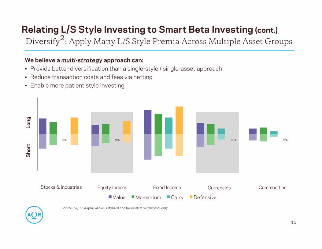
We believe a multi-strategy approach can: • Provide better diversification than a single-style / single-asset approach• Reduce transaction costs and fees via netting• Enable more patient style investing

Source: AQR. Graphic above is stylized and for illustrative purposes only.

16

N/A N/A N/A N/A

Value Momentum Carry Defensive

Stocks & Industries Equity Indices CommoditiesCurrencies Fixed Income

‐2.00

‐1.50

‐1.00

‐0.50

0.00

0.50

1.00

1.50

2.00

1 2 3 4 5 6 7 8 9 10 11 12 13 14 15 16 17 18 19 20 21 22 23 24

Long

Sho

rt

Diversify2: Apply Many L/S Style Premia Across Multiple Asset GroupsRelating L/S Style Investing to Smart Beta Investing (cont.)

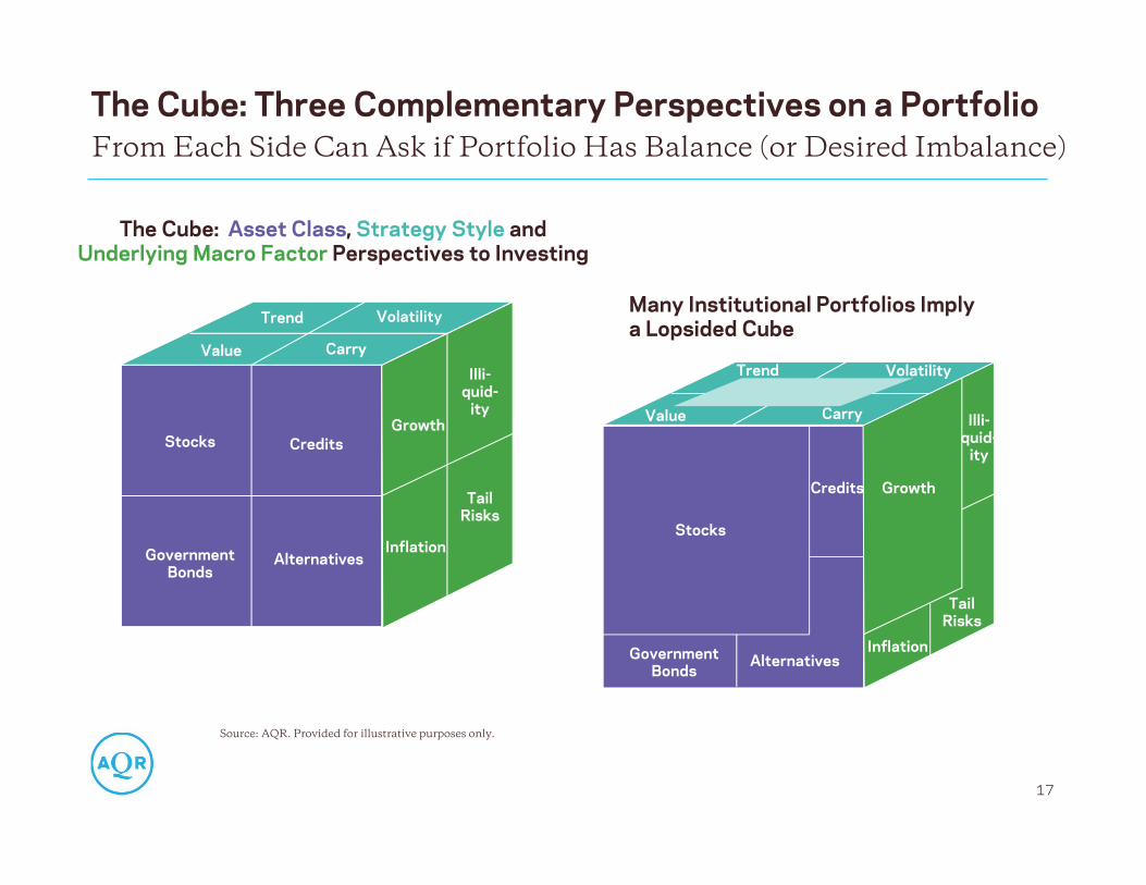
The Cube: Three Complementary Perspectives on a Portfolio

17

From Each Side Can Ask if Portfolio Has Balance (or Desired Imbalance)

Source: AQR. Provided for illustrative purposes only.

Value Carry

VolatilityTrend

Stocks

Credits

GovernmentBonds

Alternatives

Illi-quid-

ity

Inflation

TailRisks

Growth

Stocks Credits

GovernmentBonds

Alternatives

Growth

Illi-quid-

ity

TailRisks

Inflation

Trend

Value

Volatility

Carry

Many Institutional Portfolios Imply a Lopsided Cube

The Cube: Asset Class, Strategy Style andUnderlying Macro Factor Perspectives to Investing

0.0

0.1

0.2

0.3

0.4

0.5

Stocks Bonds Commodities Equal RiskWeight

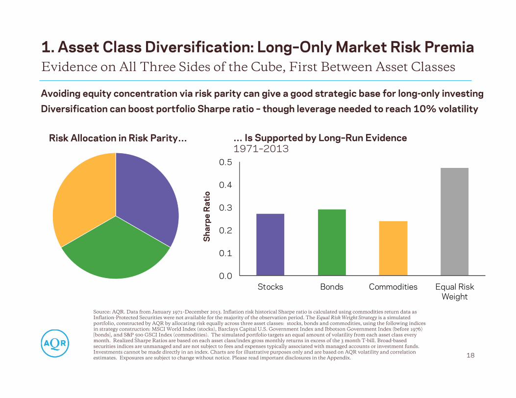
1. Asset Class Diversification: Long–Only Market Risk PremiaEvidence on All Three Sides of the Cube, First Between Asset Classes

Source: AQR. Data from January 1971–December 2013. Inflation risk historical Sharpe ratio is calculated using commodities return data as Inflation-Protected Securities were not available for the majority of the observation period. The Equal Risk Weight Strategy is a simulated portfolio, constructed by AQR by allocating risk equally across three asset classes: stocks, bonds and commodities, using the following indices in strategy construction: MSCI World Index (stocks), Barclays Capital U.S. Government Index and Ibbotson Government Index (before 1976) [bonds], and S&P 500 GSCI Index (commodities). The simulated portfolio targets an equal amount of volatility from each asset class everymonth. Realized Sharpe Ratios are based on each asset class/index gross monthly returns in excess of the 3 month T-bill. Broad-based securities indices are unmanaged and are not subject to fees and expenses typically associated with managed accounts or investment funds. Investments cannot be made directly in an index. Charts are for illustrative purposes only and are based on AQR volatility and correlation estimates. Exposures are subject to change without notice. Please read important disclosures in the Appendix.

Risk Allocation in Risk Parity… … Is Supported by Long–Run Evidence 1971–2013

18

Sha

rpe

Rat

io

Avoiding equity concentration via risk parity can give a good strategic base for long-only investingDiversification can boost portfolio Sharpe ratio – though leverage needed to reach 10% volatility

-0.2

0.0

0.2

0.4

0.6

0.8

1.0

1.2

1.4

1.6

1.8

Stocks & Industries Equity Indices Fixed Income Currencies Commodities Style PremiaComposites

IntegratedStrategy

Sha

rpe

Rat

io

Value Momentum Carry Defensive

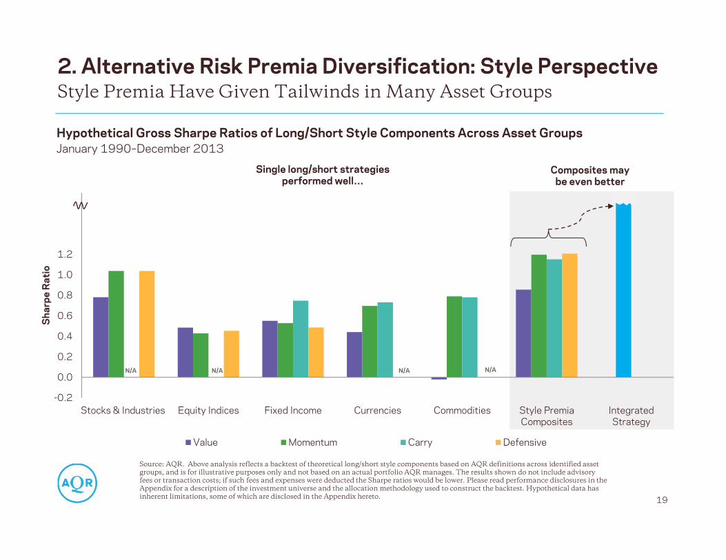
2. Alternative Risk Premia Diversification: Style Perspective

19

Style Premia Have Given Tailwinds in Many Asset Groups

Source: AQR. Above analysis reflects a backtest of theoretical long/short style components based on AQR definitions across identified asset groups, and is for illustrative purposes only and not based on an actual portfolio AQR manages. The results shown do not include advisory fees or transaction costs; if such fees and expenses were deducted the Sharpe ratios would be lower. Please read performance disclosures in the Appendix for a description of the investment universe and the allocation methodology used to construct the backtest. Hypothetical data has inherent limitations, some of which are disclosed in the Appendix hereto.

Hypothetical Gross Sharpe Ratios of Long/Short Style Components Across Asset GroupsJanuary 1990–December 2013

N/A N/A N/A N/A

Single long/short strategiesperformed well…

Composites may be even better

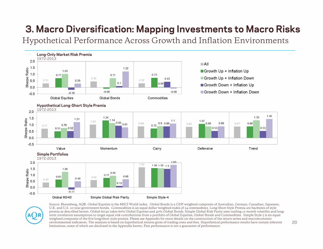
3. Macro Diversification: Mapping Investments to Macro Risks

20

Hypothetical Performance Across Growth and Inflation Environments

Source: Bloomberg, AQR. Global Equities is the MSCI World index. Global Bonds is a GDP weighted composite of Australian, German, Canadian, Japanese, U.K. and U.S. 10-year government bonds. Commodities is an equal dollar-weighted index of 24 commodities. Long-Short Style Premia are backtests of style premia as described herein. Global 60/40 takes 60% Global Equities and 40% Global Bonds. Simple Global Risk Parity uses trailing 12-month volatility and long-term correlation assumptions to target equal risk-contributions from a portfolio of Global Equities, Global Bonds and Commodities. Simple Style-5 is an equal weighted composite of the five long/short style premia. Please see Appendix for more details on the construction of the return series and macroeconomic environmental indicators. The analysis is based on hypothetical returns gross of trading costs and fees. Hypothetical performance results have certain inherent limitations, some of which are disclosed in the Appendix hereto. Past performance is not a guarantee of performance.

Long-Only Market Risk Premia1972-2013

Hypothetical Long-Short Style Premia1972-2013

Simple Portfolios 1972-2013

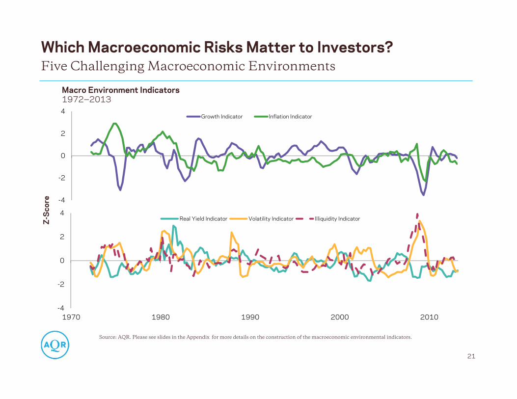
Which Macroeconomic Risks Matter to Investors?

21

Five Challenging Macroeconomic Environments

Source: AQR. Please see slides in the Appendix for more details on the construction of the macroeconomic environmental indicators.

Macro Environment Indicators1972‒2013

-4

-2

0

2

4

1970 1980 1990 2000 2010

Real Yield Indicator Volatility Indicator Illiquidity Indicator

-4

-2

0

2

4Growth Indicator Inflation Indicator

Z-S

core

0.40 0.49 0.34 0.08 0.96-0.01

0.89

-0.5

0.5

1.5

2.5

1.76 1.74 1.79 1.52 2.07 1.38 2.43

-0.5

0.5

1.5

2.5

Global 60/40

Simple Style-5

0.31 0.550.17

-0.01

0.85

-0.05

0.71

-0.50.00.51.01.5

0.32 0.38 0.27 0.200.55

0.30 0.45

-0.50.00.51.01.5

0.460.04

1.07 0.360.61 0.15 0.85

-0.50.00.51.01.5

Commodities

Global Bonds

Global Equities

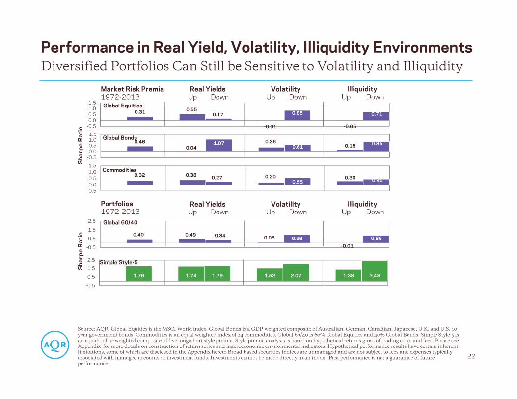
Performance in Real Yield, Volatility, Illiquidity EnvironmentsDiversified Portfolios Can Still be Sensitive to Volatility and Illiquidity

Source: AQR. Global Equities is the MSCI World index. Global Bonds is a GDP-weighted composite of Australian, German, Canadian, Japanese, U.K. and U.S. 10-year government bonds. Commodities is an equal weighted index of 24 commodities. Global 60/40 is 60% Global Equities and 40% Global Bonds. Simple Style-5 is an equal-dollar-weighted composite of five long/short style premia. Style premia analysis is based on hypothetical returns gross of trading costs and fees. Please see Appendix for more details on construction of return series and macroeconomic environmental indicators. Hypothetical performance results have certain inherent limitations, some of which are disclosed in the Appendix hereto Broad-based securities indices are unmanaged and are not subject to fees and expenses typically associated with managed accounts or investment funds. Investments cannot be made directly in an index. Past performance is not a guarantee of future performance.

Sha

rpe

Rat

io

22

Real YieldsUp Down

Market Risk Premia1972-2013

Portfolios 1972-2013

Sha

rpe

Rat

ioVolatility

Up DownIlliquidity

Up Down

Real YieldsUp Down

VolatilityUp Down

IlliquidityUp Down

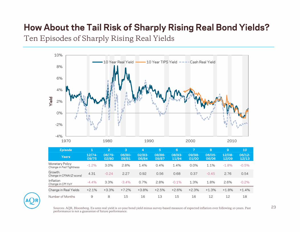
How About the Tail Risk of Sharply Rising Real Bond Yields?

23

Ten Episodes of Sharply Rising Real Yields

-4%

-2%

0%

2%

4%

6%

8%

10%

1970 1980 1990 2000 2010

10 Year Real Yield 10 Year TIPS Yield Cash Real Yield

Episode 1 2 3 4 5 6 7 8 9 10

Years 12/74-09/75

06/79-02/80

06/80-09/81

02/83-06/84

08/86-09/87

08/93-11/94

09/98-01/00

06/05-06/06

12/08-12/09

06/12-12/13

Monetary PolicyChange in Fed Tightness -1.2% 3.0% 2.8% 1.4% 0.4% 1.4% 0.0% 1.1% -1.8% -0.5%

Growth:Change in CFNAI (Z-score) 4.31 -0.24 2.27 0.92 0.56 0.68 0.37 -0.45 2.76 0.54

InflationChange in CPI YoY -4.4% 3.3% -3.4% 0.7% 2.8% -0.1% 1.3% 1.8% 2.6% -0.2%

Change in Real Yields +2.1% +3.3% +7.2% +3.8% +2.5% +2.6% +2.3% +1.3% +1.8% +1.4%

Number of Months 9 8 15 16 13 15 16 12 12 18

Sources: AQR, Bloomberg. Ex-ante real yield is 10-year bond yield minus survey-based measure of expected inflation over following 10 years. Past performance is not a guarantee of future performance.

Yie

ld

-40%

-30%

-20%

-10%

0%

10%

20%

30%

40%

Global Equities Global Bonds Commodities (Eq-wtd)

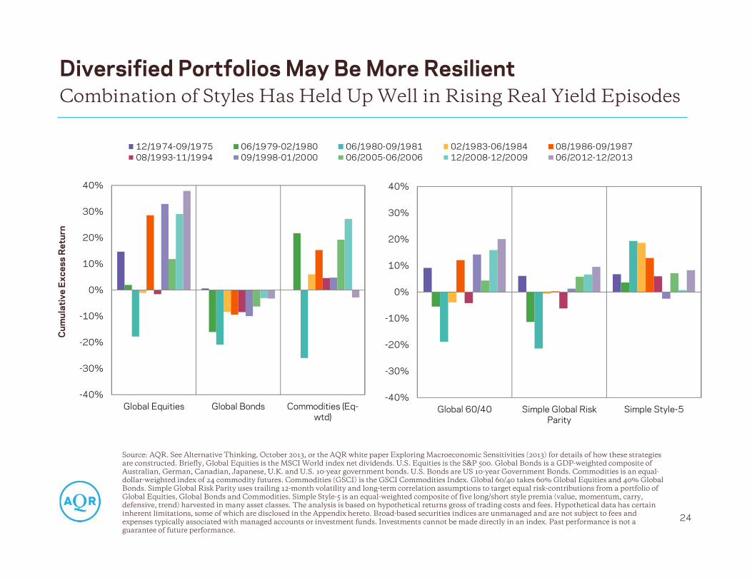
Diversified Portfolios May Be More Resilient

24

Combination of Styles Has Held Up Well in Rising Real Yield Episodes

Cum

ulat

ive

Exc

ess

Ret

urn

12/1974-09/1975 06/1979-02/1980 06/1980-09/1981 02/1983-06/1984 08/1986-09/198708/1993-11/1994 09/1998-01/2000 06/2005-06/2006 12/2008-12/2009 06/2012-12/2013

-40%

-30%

-20%

-10%

0%

10%

20%

30%

40%

Global 60/40 Simple Global RiskParity

Simple Style-5

Source: AQR. See Alternative Thinking, October 2013, or the AQR white paper Exploring Macroeconomic Sensitivities (2013) for details of how these strategies are constructed. Briefly, Global Equities is the MSCI World index net dividends. U.S. Equities is the S&P 500. Global Bonds is a GDP-weighted composite of Australian, German, Canadian, Japanese, U.K. and U.S. 10-year government bonds. U.S. Bonds are US 10-year Government Bonds. Commodities is an equal-dollar-weighted index of 24 commodity futures. Commodities (GSCI) is the GSCI Commodities Index. Global 60/40 takes 60% Global Equities and 40% Global Bonds. Simple Global Risk Parity uses trailing 12-month volatility and long-term correlation assumptions to target equal risk-contributions from a portfolio of Global Equities, Global Bonds and Commodities. Simple Style-5 is an equal-weighted composite of five long/short style premia (value, momentum, carry, defensive, trend) harvested in many asset classes. The analysis is based on hypothetical returns gross of trading costs and fees. Hypothetical data has certain inherent limitations, some of which are disclosed in the Appendix hereto. Broad-based securities indices are unmanaged and are not subject to fees and expenses typically associated with managed accounts or investment funds. Investments cannot be made directly in an index. Past performance is not a guarantee of future performance.

Practical Considerations

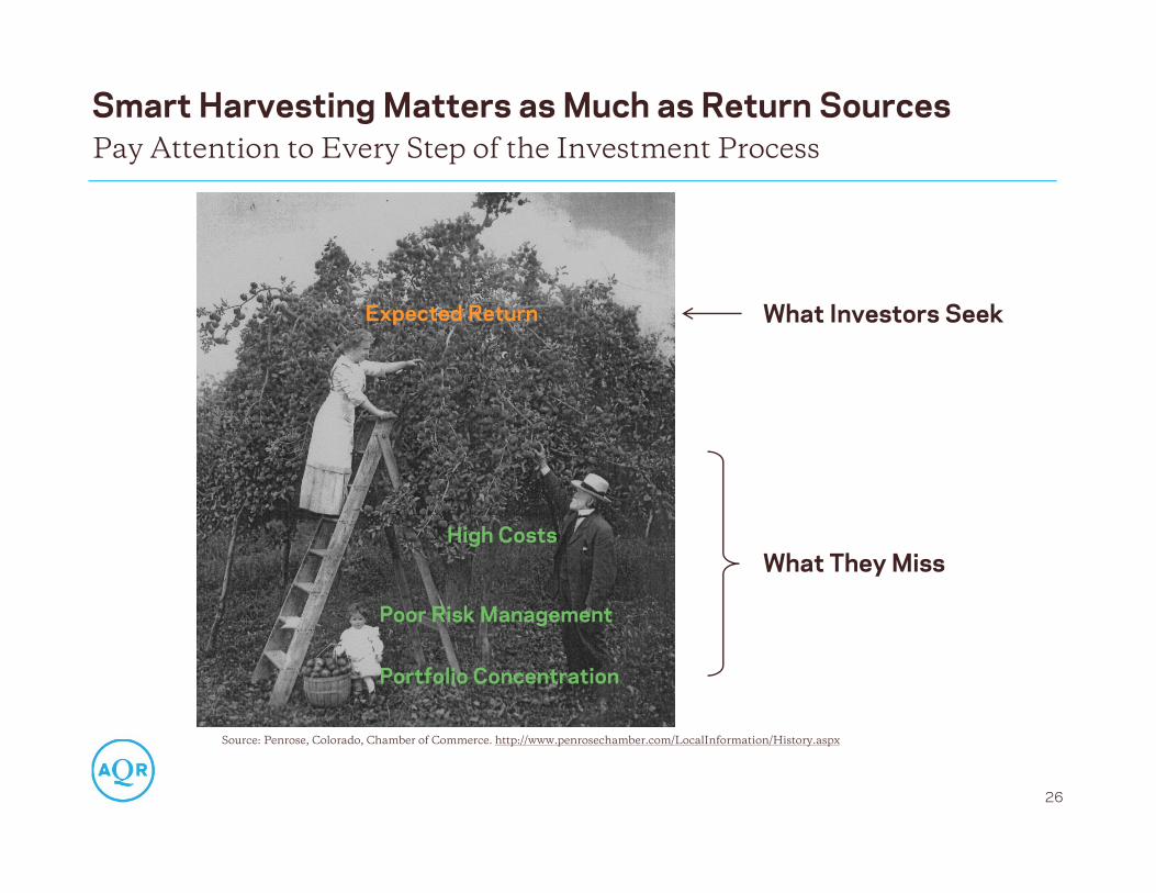
Smart Harvesting Matters as Much as Return SourcesPay Attention to Every Step of the Investment Process

Source: Penrose, Colorado, Chamber of Commerce. http://www.penrosechamber.com/LocalInformation/History.aspx

26

What Investors Seek

What They Miss

Portfolio Concentration

Expected Return

Poor Risk Management

High Costs

Why Do We Favor Strategic Over Tactical Allocations?

Tactical style timing/rotation is at least as difficult as market timing. Moreover, the hurdle on timingskills is higher due to greater “forgone diversification” (next slide).

We believe that strategic diversification across return sources we believe in beats tactical timing.• Boldly take advantage of that free lunch (if you can stomach the three dirty words…)• Most investors are arguably strategically underweight the major style premia. Increasing strategic

allocations is the first-order business• We do not know that risk balance between style premia is optimal but it is an excellent starting

point given our belief in diversification

Our research on tactical timing signals suggests they are not a Holy Grail.• We rarely find a major Sharpe ratio improvement versus stable style allocations, except when we

succumb to overfitting and hindsight biases• If anything, continuation/momentum signals offer more hope than contrarian/value signals• We keep researching but do not expect that tactical tilts deserve more than a supporting role in

style investing – partly due to the impact of forgone diversification

27

Tactical Predictions Are Imprecise And The Hurdle is High

Source: AQR. Please read important disclosures in the Appendix.

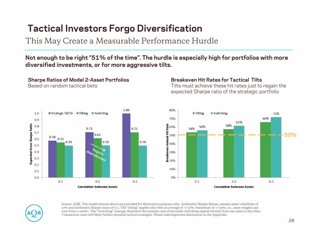
Tactical Investors Forgo Diversification

28

This May Create a Measurable Performance Hurdle

Source: AQR. The model returns above are provided for illustrative purposes only. Arithmetic Sharpe Ratios, assume asset volatilities of 10% and arithmetic Sharpe ratios of 0.5. The “tilting” applies tilts with an average of +/-25% (maximum of +/-50%, i.e., asset weights can vary from 0-100%). The “switching” strategy illustrates the extreme case of tactically switching capital entirely from one asset to the other. Transaction costs will likely further penalize tactical strategies. Please read important disclosures in the Appendix.

Sharpe Ratios of Model 2-Asset PortfoliosBased on random tactical bets

Breakeven Hit Rates for Tactical TiltsTilts must achieve these hit rates just to regain the expected Sharpe ratio of the strategic portfolio

Not enough to be right “51% of the time”. The hurdle is especially high for portfolios with more diversified investments, or for more aggressive tilts.

50%

Source: AQR. Analysis based on monthly returns of the CS Hedge Fund Index and publicly available index data. Note that the CS Equity Market Neutral Hedge Fund Index reflects Madoff-adjusted data. Style Risk Premia are represented by the hypothetical discounted excess returns, net of t-costs, gross of fees, of AQR proprietary strategies from January 1994–October 2013. Please read performance disclosures in the Appendix for a description of the investment universe and the allocation methodology used to construct the backtest. Hypothetical performance results have certain inherent limitations, some of which are disclosed in the Appendix hereto. Past performance is not a guarantee of performance. Broad-based securities indices are unmanaged and are not subject to fees and expenses typically associated with managed accounts or investment funds. Investments cannot be made directly in an index.

29

Demystifying Hedge Funds – Not Just Alpha

.

Relating Hedge Fund and Risk Premia Investing

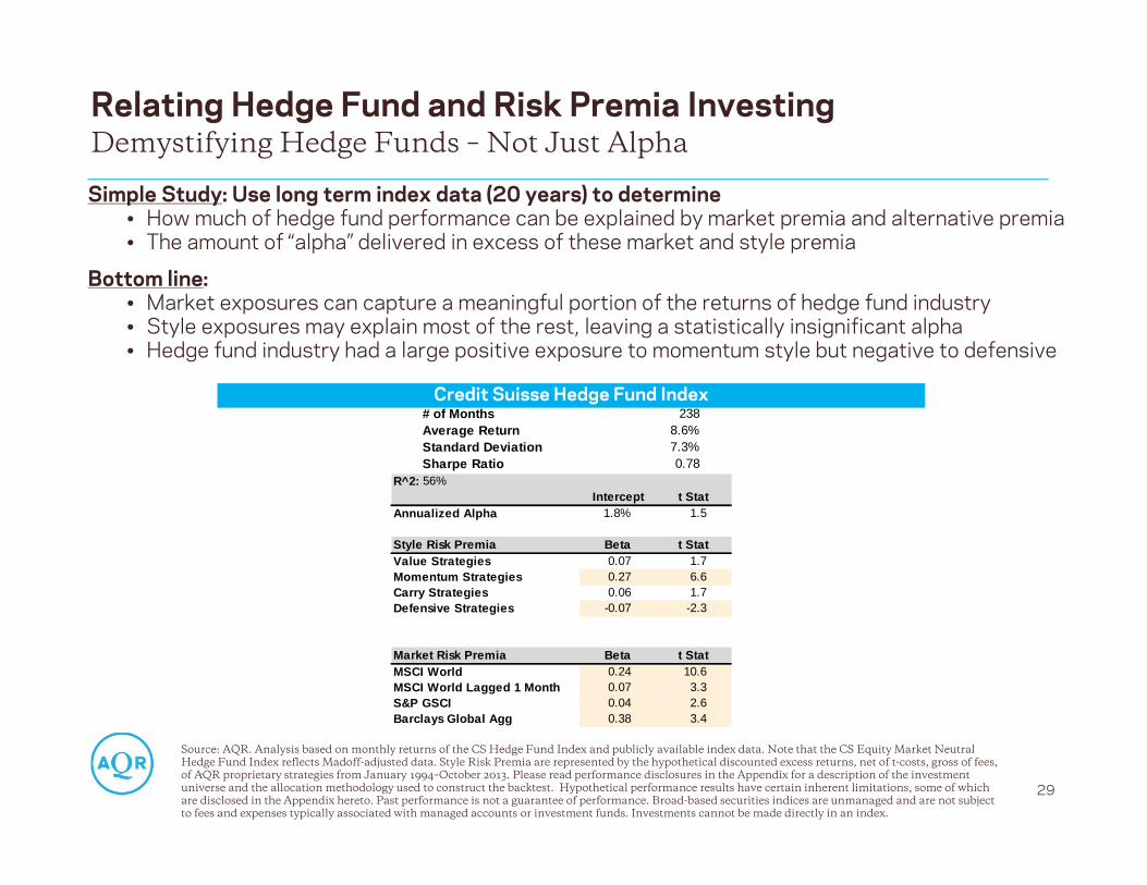
Simple Study: Use long term index data (20 years) to determine• How much of hedge fund performance can be explained by market premia and alternative premia• The amount of “alpha” delivered in excess of these market and style premia

Bottom line: • Market exposures can capture a meaningful portion of the returns of hedge fund industry• Style exposures may explain most of the rest, leaving a statistically insignificant alpha• Hedge fund industry had a large positive exposure to momentum style but negative to defensive

R^2: 56%Intercept t Stat

Annualized Alpha 1.8% 1.5 Style Risk Premia Beta t StatValue Strategies 0.07 1.7Momentum Strategies 0.27 6.6Carry Strategies 0.06 1.7Defensive Strategies -0.07 -2.3

Market Risk Premia Beta t StatMSCI World 0.24 10.6MSCI World Lagged 1 Month 0.07 3.3S&P GSCI 0.04 2.6Barclays Global Agg 0.38 3.4

# of Months 238Average Return 8.6%Standard Deviation 7.3%Sharpe Ratio 0.78

Credit Suisse Hedge Fund Index

What Is Realistic Future Expectation For Style Portfolios?

No matter how stringent our criteria, history may overstate future results• It is important to adjust historical backtest returns for costs and fees• Even though these styles have been known for a long time, there’s still some “data mining” in

everything, and estimates of costs may be too low• The magnitude of returns from style premia may well be smaller going forward; we assume half or less

of historical rewards

But diversification helps – consider the following for a portfolio that allocates equally across uncorrelated strategies• A portfolio of 4 strategies, each with a 0.4 Sharpe ratio, would have an expected 0.8 Sharpe ratio• A portfolio of 16 strategies, each with a 0.2 Sharpe ratio, would have an expected 0.8 Sharpe ratio

Thus a diversified portfolio of these strategies may be less reliant on the standalone efficacy of any one style in any one asset class – but very reliant on efficient execution as we magnify small edges

However, to convert the Sharpe ratio advantage into high returns, some leverage will be needed

30

Skepticism On Past Success Repeating…Is Warranted

Source: AQR. Please read important disclosures in the Appendix.

Why Do Many Investors Underutilize Style Premia?

Mean-variance analysis with even heavily discounted historical return inputs would likely point tolarge portfolio weights for alternative risk premia (compared with long-only asset classes)

Yet, many appealing and diversifying return sources are only modestly used. Why? “The 4Cs”:

• Conviction: investor uncertainty about the sustainability of non-equity premia

• Constraints: aversion to leverage, shorting and derivatives

• Conventionality: “better to fail conventionally” – Keynes

• Capacity: limitations may apply especially for very large investors

The 4Cs also help explain why investors “choose” equity risk concentration and why the diversifyingstyle premia are not likely to be “arbed away” soon

31

The 4 Cs Drive Real-World Investor Behaviour

Source: AQR. Please read important disclosures in the Appendix.

Disclosures

This document has been provided to you solely for information purposes and does not constitute an offer or solicitation of an offer or any advice or recommendation to purchase any securities or other financial instruments and may not be construed as such. The factual information set forth herein has been obtained or derived from sources believed to be reliable but it is not necessarily all-inclusive and is not guaranteed as to its accuracy and is not to be regarded as a representation or warranty, express or implied, as to the information’s accuracy or completeness, nor should the attached information serve as the basis of any investment decision. This document is intended exclusively for the use of the person to whom it has been delivered and it is not to be reproduced or redistributed to any other person. This document is subject to further review and revision.

This presentation is not research and should not be treated as research. This presentation does not represent valuation judgments with respect to any financial instrument, issuer, security or sector that may be described or referenced herein and does not represent a formal or official view of AQR.

The views expressed reflect the current views as of the date hereof and neither the speaker nor AQR undertakes to advise you of any changes in the views expressed herein. It should not be assumed that the speaker will make investment recommendations in the future that are consistent with the views expressed herein, or use any or all of the techniques or methods of analysis described herein in managing client accounts. AQR and its affiliates may have positions (long or short) or engage in securities transactions that are not consistent with the information and views expressed in this presentation.

The information contained herein is only as current as of the date indicated, and may be superseded by subsequent market events or for other reasons. Charts and graphs provided herein are for illustrative purposes only. The information in this presentation has been developed internally and/or obtained from sources believed to be reliable; however, neither AQR nor the speaker guarantees the accuracy, adequacy or completeness of such information. Nothing contained herein constitutes investment, legal, tax or other advice nor is it to be relied on in making an investment or other decision.

There can be no assurance that an investment strategy will be successful. Historic market trends are not reliable indicators of actual future market behavior or future performance of any particular investment which may differ materially, and should not be relied upon as such. Target allocations contained herein are subject to change. There is no assurance that the target allocations will be achieved, and actual allocations may be significantly different than that shown here. This presentation should not be viewed as a current or past recommendation or a solicitation of an offer to buy or sell any securities or to adopt any investment strategy.

The information in this presentation may contain projections or other forward‐looking statements regarding future events, targets, forecasts or expectations regarding the strategies described herein, and is only current as of the date indicated. There is no assurance that such events or targets will be achieved, and may be significantly different from that shown here. The information in this presentation, including statements concerning financial market trends, is based on current market conditions, which will fluctuate and may be superseded by subsequent market events or for other reasons. Performance of all cited indices is calculated on a total return basis with dividends reinvested.

The investment strategy and themes discussed herein may be unsuitable for investors depending on their specific investment objectives and financial situation. Please note that changes in the rate of exchange of a currency may affect the value, price or income of an investment adversely.

Neither AQR nor the speaker assumes any duty to, nor undertakes to update forward looking statements. No representation or warranty, express or implied, is made or given by or on behalf of AQR, the speaker or any other person as to the accuracy and completeness or fairness of the information contained in this presentation, and no responsibility or liability is accepted for any such information. By accepting this presentation in its entirety, the recipient acknowledges its understanding and acceptance of the foregoing statement.

There is no guarantee, express or implied, that long-term return and/or volatility targets will be achieved. Realized returns and/or volatility may come in higher or lower than expected. PAST PERFORMANCE IS NOT A GUARANTEE OF FUTURE PERFORMANCE. Diversification does not eliminate the risk of experiencing investment losses.

There is a risk of substantial loss associated with trading commodities, futures, options, derivatives and other financial instruments. Before trading, investors should carefully consider their financial position and risk tolerance to determine if the proposed trading style is appropriate. Investors should realize that when trading futures, commodities, options, derivatives and other financial instruments one could lose the full balance of their account. It is also possible to lose more than the initial deposit when trading derivatives or using leverage. All funds committed to such a trading strategy should be purely risk capital.

32

Disclosures

Hypothetical performance results (e.g., quantitative backtests) have many inherent limitations, some of which, but not all, are described herein. No representation is being made that any fund or account will or is likely to achieve profits or losses similar to those shown herein. In fact, there are frequently sharp differences between hypothetical performance results and the actual results subsequently realized by any particular trading program. One of the limitations of hypothetical performance results is that they are generally prepared with the benefit of hindsight. In addition, hypothetical trading does not involve financial risk, and no hypothetical trading record can completely account for the impact of financial risk in actual trading. For example, the ability to withstand losses or adhere to a particular trading program in spite of trading losses are material points which can adversely affect actual trading results. The hypothetical performance results contained herein represent the application of the quantitative models as currently in effect on the date first written above and there can be no assurance that the models will remain the same in the future or that an application of the current models in the future will produce similar results because the relevant market and economic conditions that prevailed during the hypothetical performance period will not necessarily recur. There are numerous other factors related to the markets in general or to the implementation of any specific trading program which cannot be fully accounted for in the preparation of hypothetical performance results, all of which can adversely affect actual trading results. Discounting factors may be applied to reduce suspected anomalies. This backtest’s return, for this period, may vary depending on the date it is run. Hypothetical performance results are presented for illustrative purposes only. n addition, our transaction cost assumptions utilized in backtests , where noted, are based on AQR's historical realized transaction costs and market data. Certain of the assumptions have been made for modeling purposes and are unlikely to be realized. No representation or warranty is made as to the reasonableness of the assumptions made or that all assumptions used in achieving the returns have been stated or fully considered. Changes in the assumptions may have a material impact on the hypothetical returns presented. Hypothetical performance is gross of advisory fees, net of transaction costs, and includes the reinvestment of dividends. If the expenses were reflected, the performance shown would be lower.

AQR monthly backtests of Value, Momentum, Carry and Defensive strategies are undiscounted, gross of fees and transaction costs, excess of a cash rate proxied by the Merrill Lynch 3-Month T-Bill Index, and scaled to 12% annualized volatility. Each strategy is designed to take long positions in the assets with the strongest style attributes and short positions in the assets with the weakest style attributes, while seeking to ensure the portfolio is market-neutral. The representative Style Premia Composite portfolio is based on the target asset group allocations as noted on page 14, roughly equally risk weighting styles within the asset group, resulting in a style allocation of approximately 32% to Value, 32% to Momentum, 22% to Defensive and 14% to Carry. Please see below for a description of the Universe selection.

Stock and Industry Selection: approximately 1,500 stocks across Europe, Japan, U.K. and U.S. Country Equity Indices: Developed Markets: Australia, Canada, Eurozone, Hong Kong, Japan, Sweden, Switzerland, U.K., U.S. Within Europe: Italy, France, Germany, Netherlands, Spain. Emerging Markets: Brazil, China, India, Russia, South Africa, South Korea, Taiwan. Bond Futures: Australia, Canada, Germany, Japan, U.K., U.S. Interest Rate Futures: Australia, Canada, Europe (Euribor), U.K. and U.S. Currencies: Developed Markets: Australia, Canada, Euro, Japan, New Zealand, Norway, Sweden, Switzerland, U.K., U.S. Emerging Markets: Brazil, India, Mexico, Poland, Russia, Singapore, South Korea, Taiwan, Turkey. Commodity Selection: Silver, Copper, Gold, Crude, Brent Oil, Natural Gas, Corn, Soybeans.

Broad-based securities indices are unmanaged and are not subject to fees and expenses typically associated with managed accounts or investment funds. Investments cannot be made directly in an index. The Morgan Stanley Capital International World Index is a market-capitalization-weighted index composed of company’s representative of the market structure of 23 developed market countries in North America, Europe and the Asia/Pacific Region. There are material differences between an index and the strategy. The Barclays Global Aggregate Index is a flagship measure of global investment grade debt from 23 different local currency markets. This multicurrency benchmark includes fixed-rate Treasury, government-related, corporate and securitized bonds from both developed and emerging markets issuers. There are material differences between an index and the strategy. One significant difference between the indices and the performance presented is that the index performance is weighted on the basis of capitalization whereas the strategy performance reflects a risk-weighted calculation. This difference may have a material affect on the comparison of the indices with the performance of the strategy. The S&P GSCI® is a composite index of commodity sector returns representing an unleveraged, long-only investment in commodity futures that is broadly diversified across the spectrum of commodities.

33

Building Macro Indicators / Investment Return Series

34

Macro IndicatorsOur first choice was to decide which macro dimensions are most relevant. We chose economic growth, inflation, real yields, volatility, and illiquidity. Monetary policy was another candidate; it is closely related to real yields. We choose to construct macro indicators, or risk factors, mainly based on fundamental economic data, and not based on asset market returns (which are “too close” to the patterns we try to explain). For example, potential market-based proxies of economic growth include equity market returns, the relative performance of cyclical industries, dividend swaps, and estimates from cross-sectional regressions of asset returns on growth surprises. This choice brings its own problems, notably timing challenges as macroeconomic data are backward-looking, published with lags and later revised, while asset prices are clearly forward-looking. The impact of publication lags and the mismatch between backward- and forward-looking perspectives can be mitigated by using longer windows. Thus, we use contemporaneous annual economic data and asset returns through our analysis (past-year data with quarterly overlapping observations). Arguably composite growth surprise indices are the best proxies of economic growth news, but such composites are available at best going back to 1990s. Forecast changes in economist surveys as well as business and consumer confidence surveys may be the next best choices because they are reasonably forward-looking and timely. In a globalized world, it is not clear whether we should focus only on domestic macro developments, but data constraints make us focus on U.S. data. Finally, it is not clear how real economic growth ties to expected corporate cash flow growth (e.g., earnings per share) that influence stock prices or to real yields that influence all asset prices but especially those of bonds.Each of our macro indicators combines two series, which are first normalized to Z-scores: that is, we subtract a historical mean from each observation and divide by a historical volatility. We use rolling 10-year windows for means and volatilities when normalizing the last three macro indicators. However, for growth and inflation indicators we use in-sample 1972-2013 means and volatilities because we do not have long histories of economist forecasts needed to construct the surprise series below. This choice does not seem to change any major results. When we classify our quarterly 12-month periods into, say, ‘growth up’ and ‘growth down’ periods, we compare actual observations to the median so as to have an equal number of up and down observations (because we are not trying to create an investable strategy where data should be available for investors in real time, we use the full sample median).The underlying series for our growth indicator are the Chicago Fed National Activity Index (CFNAI) and the “surprise” in industrial production growth over the past year. Since there is no uniquely correct proxy way to capture “growth”; averaging may make the results more robust and signals appropriate humility. CFNAI takes this averaging idea to extremes as it combines 85 monthly indicators of U.S. economic activity. The other series – the difference between actual annual growth in industrial production and the consensus economist forecast a year earlier – is narrower but more directly captures the surprise effect in economic developments. We use median forecasts from the Survey of Professional Forecasters data as published by the Philadelphia Fed. While data surprises a priori have a zero mean, this series has exhibited a downward trend in recent decades, reflecting the (partly unexpected) relative decline of the U.S. manufacturing sector. Our inflation indicator is also an average of two normalized series. One series measures the de-trended level of inflation (CPIYOY minus its mean, divided by volatility), while the other measures the surprise element in realized inflation (CPIYOY minus consensus economist forecast a year earlier).

Investment Return SeriesThe investment return series we study include both asset class premia and style premia. The former are long-only returns but expressed in excess returns over the Treasury bill rate. The latter are long-short returns and scaled to target or realize 10% annual volatility. We subtract no trading costs or fees, which makes a bigger difference for the long-short strategies.The main asset class premia we focus on are U.S. equities (proxied by the S&P500 index), U.S. Treasuries (proxied by the constant-maturity 10-year return), and commodities (proxied by the S&P GSCI index). For robustness, we also studied global equities (MSCI World), global bonds (GDP-weighted average of 10-year government bonds in six countries), and an equal-weighted composite of 24 commodity futures. In addition, we studied the credit excess returns of investment-grade corporates over duration-matched Treasuries (Barclays index data since 1973) and TIPS returns (using an in-house proxy for inflation-linked bond performance; the series begins already in 1980, well before the first TIPS were issued in 1997).Style premia series are more difficult to compile, especially because we apply these premia in numerous asset classes. To start histories back in 1972, we splice together different series. Since 1990, we use value, momentum, carry and defensive style premia as described in “Investing With Style” (AQR white paper, 2012) Available upon request. The intuition in the four styles is to buy assets that are cheap, or recently outperforming, or high-yielding, or boring (low risk) – while selling assets with opposite characteristics. We apply these styles in stock selection, industry allocation, country allocation in equity, fixed income and currency markets, as well as in commodities. Briefly, we construct market-neutral long-short portfolios in several asset classes (stocks, bonds, currencies, commodities) based on a few indicators in each style. Besides the broadest style composites, we also construct separate style premia for global stock selection (GSS) and global asset allocation (GAA). When we create the composite GAA style premia, we use the same relative risk weights for asset classes as “Investing With Style” (33% equity country allocation, 25% fixed income, 25% currencies, 17% commodities). However, for GSS we use 50/50 risk weights between stock selection within industries and across industries (to be in line with the common but arguably inefficient practice of letting across-industry positions matter as much as within-industry positions), and we also use 50/50 risk weights when we combine GSS and GAA style composites. For 1972-1989, we source value and momentum style returns from “Value and Momentum Everywhere” (Journal of Finance, 2013), defensive style returns from “Betting Against Beta” (forthcoming in Journal of Financial Economics, 2013), and GSS carry style premium from dividend yield strategy returns in Ken French’s data library. We construct the GAA carry style premia before 1990 as well as some early histories of GAA value, momentum and defensive styles with AQR in-house backtests.

In addition to the market-neutral “big four” style premia, we use market-directional premia. Trend style applies 12-month trend-following strategy in liquid investments in four major asset classes (GAA). While the style is nearly uncorrelated with equity markets in the long run, at any point in time it can be directionally long or short. We source trend style premia from “Time Series Momentum” (Journal of Financial Economics, 2012) and in-house data extension before 1985.

While the GSS style premia proxies we use since 1990 are market (beta) neutral, the value and momentum premia before 1990, and the carry premium throughout, are ‘only’ dollar-neutral and may contain moderate empirical beta exposures. The defensive style premia are beta-neutral through the whole sample (we buy larger amounts of low-risk investments than we sell high-risk investments), which means that they are actually not as defensive as the dollar-neutral quality style. (The general lesson is that we need to be precise in understanding strategy designs. Just as corporate bond positions will have very different market exposures depending on whether they are duration-hedged with Treasuries, market exposures of style premia will depend on the degree of hedging).