Best Practices in Managing Volunteers - James Madison University

EURASIP Journal on Applied Signal Processing 2004:18, 1–11c© 2004 Hindawi Publishing Corporation

Tracking of Multiple Moving Sources UsingRecursive EM Algorithm

Pei-Jung ChungDepartment of Electrical Engineering and Computer Science, University of Michigan, Ann Arbor, MI 48109-2122, USAEmail: peijung [email protected]

Johann F. BohmeSignal Theory Group, Department of Electrical Engineering and Information Science,Ruhr-University of Bochum, 44780 Bochum, GermanyEmail: [email protected]

Alfred O. Hero

Department of Electrical Engineering and Computer Science, University of Michigan, Ann Arbor, MI 48109-2122, USAEmail: [email protected]

Received 31 December 2003; Revised 17 June 2004

We deal with recursive direction-of-arrival (DOA) estimation of multiple moving sources. Based on the recursive EM algorithm,we develop two recursive procedures to estimate the time-varying DOA parameter for narrowband signals. The first procedurerequires no prior knowledge about the source movement. The second procedure assumes that the motion of moving sources isdescribed by a linear polynomial model. The proposed recursion updates the polynomial coefficients when a new data arrives.The suggested approaches have two major advantages: simple implementation and easy extension to wideband signals. Numericalexperiments show that both procedures provide excellent results in a slowly changing environment. When the DOA parameterchanges fast or two source directions cross with each other, the procedure designed for a linear polynomial model has a better

performance than the general procedure. Compared to the beamforming technique based on the same parameterization, our

approach is computationally favorable and has a wider range of applications.

Keywords and phrases: sensor array processing, recursive estimation, moving sources, tracking.

1. INTRODUCTION

The problem of estimating the direction of arrival (DOA) of1

2

3

plane waves impinging on a sensor array is of fundamental

4

importance in many applications such as radar, sonar, geo-physics, and wireless communication. The maximum like-lihood (ML) method is known to have excellent statisticalperformance and is robust against coherent signals and smallsample numbers [1]. However, the high computational costassociated with ML method makes it less attractive in prac-tice.

To improve the computational efficiency of the ML ap-proach, numerical methods such as the expectation andmaximization (EM) algorithm [2] were suggested in [3, 4, 5].Recursive procedures based on the recursive EM (REM) al-gorithm for estimating constant DOA parameters were dis-cussed in [6, 7]. Similar procedures for tracking multiplemoving sources were studied in [8, 9]. In [9], the authorsfocused on narrowband sources and assumed known signal

waveforms.The REM algorithm is a stochastic approximation pro-

cedure for finding ML estimates (MLEs). It was first sug-gested by Titterington [10] and extended to the multidimen-sional case in [6]. As it was pointed out by Titterington,REM can be seen as a sequential approximation of the EMalgorithm. The gain matrix of REM is the inversion of theaugmented data information matrix. Through proper designof the augmentation scheme, the augmented data and thecorresponding information matrixes usually have a simplestructure [2]. In this case, the REM algorithm is very easy to 5implement. For constant parameters , estimates generated

by REM are strongly consistent and asymptotically normallydistributed. For time-varying parameters , the tracking abil-

ity of a stochastic approximation procedure depends mainlyon the dynamics of the true parameter, gain matrix, and stepsize [11].

Based on REM, we will derive two recursive procedures

mailto:[email protected]



2 EURASIP Journal on Applied Signal Processing

for estimating time-varying DOA. The first procedure doesnot require any prior knowledge on the motion model. Theonly assumption is that the unknown parameter changesslowly with time. The second procedure assumes that thetime-varying DOA parameter θ(t) is described by a linearpolynomial of time. This model is important since a smoothfunction θ(t) can be approximated by a local linear polyno-mial in a short-time interval [12]. The procedure reported in[8] employs a decreasing step size to estimate the polynomialcoefficients. However, since the DOA parameter θ(t) and thelog-likelihood function change with time, a decreasing stepsize may not capture the nonstationary feature of the under-lying system over a long period. To overcome this problem,we suggest a constant step size to be used in the algorithm.It is noteworthy that both procedures are aimed at maximiz-ing the expected concentrated likelihood function [13]. In-troducing a linear polynomial model implies increasing thedimension of the parameter space. With the additional de-gree of freedom, the procedure designed for a linear polyno-mial model should perform better than the general one.

In contrast to methods based on subspace tracking [14]or two-dimensional beamforming [12], our approach can beeasily generalized to wideband cases including underwateracoustic signals. Unlike the Kalman-type algorithms [15], therecursive procedures considered here have a much simplerimplementation.

This paper is outlined as follows. We describe the sig-nal model and the REM algorithm briefly in Sections 2and 3. Section 4 presents two recursive procedures for lo-calizing moving sources. Simulation results are discussed inSection 5. We give concluding remarks in Section 6.

2. PROBLEM FORMULATION

Consider an array of N sensors receiving M far-fieldwaves from unknown time-varying directions θ(t) =[θ1(t) · · · θM(t)]. The array output x(t) ∈ CN×1 at time in-stant t is expressed as

x(t) = H(θ(t)

)s(t) + u(t), t = 1, 2, . . . , (1)

where the steering matrix

H(θ(t)

) = [d(θ1(t)) · · ·d(θM(t)

)] ∈ CN×M (2)

consists of M steering vectors d(θm(t)) ∈ CN×1 (m =1, . . . ,M). To avoid ambiguity, we assume that M < N . Thesignal waveform s(t) = [s1(t) · · · sM(t)]T ∈ CM×1 is con-sidered unknown and deterministic. (·)T denotes the trans-pose of a vector. Furthermore, the noise process u(t) ∈ CN×1

is independent identically complex and normally distributedwith zero mean and covariance matrix νI , where ν representsthe unknown noise spectral parameter and I is the identitymatrix.

In the following, we assume that the number of sourcesM is known. Standard procedures based on minimum de-6

7 scription length (MDL) criteria [16] or multiple hypoth-esis testing [7] can be used to determine M. The problem of

interest is to estimate the time-varying DOA parameter θ(t)recursively from the observation x(t). We assume that a goodinitial estimate θ0 is available at the beginning of the recur-sion.

3. RECURSIVE PARAMETER ESTIMATION USINGINCOMPLETE DATA

The REM algorithm suggested by Titterington is a stochasticapproximation procedure for finding MLEs. As pointed outin [10], there is a strong relationship between this procedureand the EM algorithm [2]. Using Taylor expansion, Tittering-ton showed that, approximately, REM maximizes EM’s aug-mented log likelihood sequentially. The unknown parame-ter is considered as constant in [10]. In the fixed parametercase, a properly chosen decreasing step size is necessary toensure strong consistency and asymptotic normality of thealgorithm [10, 17].

Suppose x(1), x(2), . . . are independent observations,each with underlying probability density function (pdf)f (x;ϑ), where ϑ denotes an unknown constant parameter.The augmented data associated with the EM y(1), y(2), . . . 8is characterized by the pdf f (y;ϑ). According to [2], the

augmented data y(t) is so specified that M(y(t)) = x(t) is amany-to-one mapping. Let ϑt denote the estimate after t ob-servations. The following procedure is aimed at finding thetrue parameter ϑ which may coincide with the MLE in theasymptotic sense [18]:

ϑt+1 = ϑt + εtIEM(ϑt)−1

γ(x(t),ϑt

), (3)

where εt is a decreasing step size and 9

IEM(ϑt) = E −∇ϑ∇T

ϑ log f (y;ϑ)|x(t),ϑ|ϑ=ϑt , (4)

γ(x(t),ϑt

) =∇ϑ log f(x(t);ϑ

)|ϑ=ϑt (5)

represent the augmented information matrix and gradientvector, respectively. ∇ϑ is a column gradient operator withrespect to ϑ. We assume that both (4) and (5) exist. Undermild conditions, the estimates generated by (3) are strongly

consistent, asymptotic, and normally distributed. In view 10of the well-known singularities and multiple maxima that areon likelihood surfaces, one could not of course expect con-sistency irrespective of the starting point [10].

The augmented data y usually has a simpler structurethan the observed data x. Therefore, the augmented datainformation matrix IEM(ϑt) is easier to compute and in-vert than the observed data information matrix I(ϑt) =E −∇ϑ∇T

ϑ log f (x;ϑ)|x(t),ϑ|ϑ=ϑt . Although REM does nothave the optimal convergence rate in the Cramer-Rao senseas the following procedure [10]:

ϑt+1 = ϑt + εtI(ϑt)−1

γ(x(t),ϑt

), (6)

it is much easier to implement than (6). Using IEM(ϑt)−1 asthe gain matrix is a trade-off between the convergence rateand computational cost.

Please provide a short running title 3

When the parameter of interest varies with time, a de-creasing step size such as εt = t−α, 1/2 < α ≤ 1, cannotcapture the nonstationary feature of the underlying system.A classical way to overcome this difficulty is to replace εt witha constant step size ε. In general, a large step size reduces thebias and increases the variance of the estimates [11]. A smallstep size has opposite effects. Since the time-varying param-eter ϑ(t) may follow a complicated dynamics, an exact inves-tigation of the convergence behavior of the algorithm

ϑt+1 = ϑt + εIEM(ϑt)−1

γ(x(t),ϑt

)(7)

is only possible when certain assumptions are made on theparameter model. More discussion about convergence prop-erties of a stochastic approximation procedure in a nonsta-tionary environment can be found in [11].

4. LOCALIZATION OF MOVING SOURCES

The REM algorithm with constant step size (7) is appliedto estimate the time-varying DOA parameter θ(t). We startwith a general case in which θ(t) changes slowly with timeand then consider a linear polynomial model.

4.1. General case

From the signal model in Section 2, we know that the arrayobservation x(t) is complex and normally distributed withthe log likelihood function

log f(x(t);ϑ

)= −

[N logπ + N log ν

+1ν

(x(t)−H

(θ(t)

)s(t)

)H(x(t)−H

(θ(t)

)s(t)

)],

(8)

where ϑ = [θ(t)Ts(t)Tν]T and (·)H denotes the Hermitiantranspose.

According to (7), all elements in ϑ should be updatedsimultaneously. Since we are mainly interested in the DOAparameter θ(t) and since including {s(t), ν} in the recursionwill complicate the gain matrix IEM(ϑt)−1, then the proce-dure (7) is only applied to θ(t). The estimate for signal wave-form and noise level, denoted by st = [st1 st2 · · · stM]T andνt, respectively, is updated by computing their MLEs once thecurrent DOA estimate is available. For simplicity, we use θinstead of θ(t) in the following discussion.

Taking the first derivative on the right-hand side of (8)with respect to θm, we obtain the mth element of the gradientvector γ(x(t),ϑt) [17]:

[γ(x(t),ϑt

)]m =

2νt

Re[(x(t)−H

(θt)st)H(

d′(θtm)stm)]

, (9)

where d′(θm) = ∂d(θm)/∂θm.The augmented data y(t) is obtained by decomposing the

array output into its signal and noise parts. Formally it is ex-pressed as

y(t) = [y1(t)T · · · ym(t)T · · · yM(t)T]T. (10)

The augmented data associated with the mth signal

ym(t) = d(θm)sm(t) + um(t) (11)

is complex and normally distributed with mean d(θm)sm(t)and covariance matrix νmI with the constraint

∑Mm=1 νm =

ν. A convenient choice is νm = ν/M. The corresponding loglikelihood is given by

log f(y(t);ϑ

)= −

M∑m=1

[N logπ + N log

(ν

M

)

+M

ν

(ym(t)− d

(θm)sm(t)

)H× (ym(t)− d

(θm)sm(t)

)].

(12)

Since the signals are decoupled through the augmentationscheme (10), IEM(ϑt) is an M ×M diagonal matrix when weonly consider the DOA parameter θ. By definition (4), themth diagonal element of IEM(ϑt) is the conditional expecta-tion of the second derivative of the augmented log likelihood

[IEM

(ϑt)]

mm = E − ∂2

∂θ2m

log f(y(t);ϑ

)∣∣x(t),ϑt , (13)

which is given by

[IEM(ϑt)

]mm =

2νt

Re[− (d′′(θtm)stm)H(x(t)−H

(θt)st)

+ M∥∥d′(θtm)stm∥∥2

],

(14)

where d′′(θm) = ∂2d(θm)/∂θ2m.

Once the estimate θt+1 is available, the signal and noiseparameters are obtained by computing their MLEs at currentθt+1 and x(t) as follows:

st+1 = H(θt+1)#

x(t),

νt+1 = 1N

tr[P(θt+1)⊥Cx(t)

],

(15)

where H(θt+1)# is the generalized left inverse of the matrixH(θt+1), P(θt+1)⊥ = I − P(θt+1) is the orthogonal comple-ment of the projection matrix P(θt+1) = H(θt+1)H(θt+1)#,and Cx(t) = x(t)x(t)H .

Given a constant step size ε, the number of sources M,and the current estimate θt, the (t + 1)st recursion of the al-gorithm proceeds as shown in Algorithm 1.

4.2. Linear polynomial model

We consider moving sources described by the linear polyno-mial model

θ = θ0 + tθ1, (16)


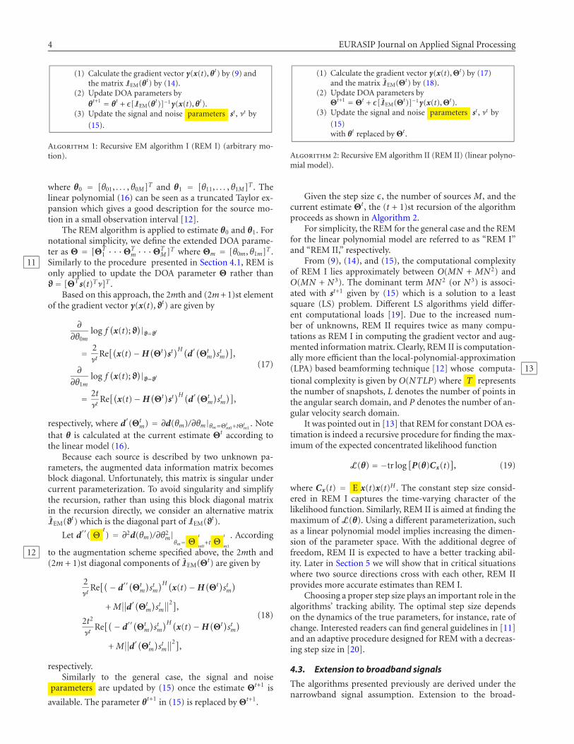
(1) Calculate the gradient vector γ(x(t), θt) by (9) andthe matrix IEM(θt) by (14).

(2) Update DOA parameters byθt+1 = θt + ε[IEM(θt)]−1γ(x(t), θt).

(3) Update the signal and noise parameters st , νt by

(15).

Algorithm 1: Recursive EM algorithm I (REM I) (arbitrary mo-tion).

where θ0 = [θ01, . . . , θ0M]T and θ1 = [θ11, . . . , θ1M]T . Thelinear polynomial (16) can be seen as a truncated Taylor ex-pansion which gives a good description for the source mo-tion in a small observation interval [12].

The REM algorithm is applied to estimate θ0 and θ1. Fornotational simplicity, we define the extended DOA parame-ter as Θ = [ΘT

1 · · ·ΘTm · · ·ΘT

M]T where Θm = [θ0m, θ1m]T .Similarly to the procedure presented in Section 4.1, REM is11only applied to update the DOA parameter Θ rather thanϑ = [ΘTs(t)Tν]T .

Based on this approach, the 2mth and (2m+ 1)st elementof the gradient vector γ(x(t),ϑt) are given by

∂

∂θ0mlog f

(x(t);ϑ

)|ϑ=ϑt= 2

νtRe[(x(t)−H

(Θt)st)H(d′(Θt

m

)stm)]

,

∂

∂θ1mlog f

(x(t);ϑ

)|ϑ=ϑt= 2t

νtRe[(x(t)−H

(Θt)st)H(d′(Θt

m

)stm)]

,

(17)

respectively, where d′(Θtm) = ∂d(θm)/∂θm|θm=Θt

m0+tΘtm1

. Notethat θ is calculated at the current estimate Θt according tothe linear model (16).

Because each source is described by two unknown pa-rameters, the augmented data information matrix becomesblock diagonal. Unfortunately, this matrix is singular undercurrent parameterization. To avoid singularity and simplifythe recursion, rather than using this block diagonal matrixin the recursion directly, we consider an alternative matrixIEM(ϑt) which is the diagonal part of IEM(ϑt).

Let d′′( Θt) = ∂2d(θm)/∂θ2

m|θm= Θ

t

m0+t Θ

t

m1

. According

to the augmentation scheme specified above, the 2mth and12(2m + 1)st diagonal components of IEM(Θt) are given by

2νt

Re[(− d′′

(Θt

m

)stm)H(

x(t)−H(Θt)stm)

+ M∥∥d′(Θt

m

)stm∥∥2]

,

2t2

νtRe[(− d′′

(Θt

m

)stm)H(

x(t)−H(Θt)stm)

+ M∥∥d′(Θt

m

)stm∥∥2]

,

(18)

respectively.Similarly to the general case, the signal and noise

parameters are updated by (15) once the estimate Θt+1 is

available. The parameter θt+1 in (15) is replaced by Θt+1.

(1) Calculate the gradient vector γ(x(t),Θt) by (17)and the matrix IEM(Θt) by (18).

(2) Update DOA parameters byΘt+1 = Θt + ε[IEM(Θt)]−1γ(x(t),Θt).

(3) Update the signal and noise parameters st , νt by

(15)with θt replaced by Θt .

Algorithm 2: Recursive EM algorithm II (REM II) (linear polyno-mial model).

Given the step size ε, the number of sources M, and thecurrent estimate Θt , the (t + 1)st recursion of the algorithmproceeds as shown in Algorithm 2.

For simplicity, the REM for the general case and the REMfor the linear polynomial model are referred to as “REM I”and “REM II,” respectively.

From (9), (14), and (15), the computational complexityof REM I lies approximately between O(MN + MN2) andO(MN + N3). The dominant term MN2 (or N3) is associ-ated with st+1 given by (15) which is a solution to a leastsquare (LS) problem. Different LS algorithms yield differ-ent computational loads [19]. Due to the increased num-ber of unknowns, REM II requires twice as many compu-tations as REM I in computing the gradient vector and aug-mented information matrix. Clearly, REM II is computation-ally more efficient than the local-polynomial-approximation(LPA) based beamforming technique [12] whose computa- 13tional complexity is given by O(NTLP) where T representsthe number of snapshots, L denotes the number of points inthe angular search domain, and P denotes the number of an-gular velocity search domain.

It was pointed out in [13] that REM for constant DOA es-timation is indeed a recursive procedure for finding the max-imum of the expected concentrated likelihood function

L(θ) = −tr log[P(θ)Cx(t)

], (19)

where Cx(t) = E x(t)x(t)H . The constant step size consid-ered in REM I captures the time-varying character of thelikelihood function. Similarly, REM II is aimed at finding themaximum of L(θ). Using a different parameterization, suchas a linear polynomial model implies increasing the dimen-sion of the parameter space. With the additional degree offreedom, REM II is expected to have a better tracking abil-ity. Later in Section 5 we will show that in critical situationswhere two source directions cross with each other, REM IIprovides more accurate estimates than REM I.

Choosing a proper step size plays an important role in thealgorithms’ tracking ability. The optimal step size dependson the dynamics of the true parameters, for instance, rate ofchange. Interested readers can find general guidelines in [11]and an adaptive procedure designed for REM with a decreas-ing step size in [20].

4.3. Extension to broadband signals

The algorithms presented previously are derived under thenarrowband signal assumption. Extension to the broad-


90

80

70

60

50

40

30

20

10

0

DO

A(d

egre

e)

5 10 15 20 25 30 35 40 45 50

Time index

True trajectoryEstimated trajectory

Figure 1: True trajectory and estimated trajectory by REM I for thenarrowband case. θ0 = [10◦, 60◦, 66◦], θ1 = [0.6◦,−1.0◦, 0.4◦]. SNR= 20 dB.

band case is straightforward. From the asymptotic theory ofFourier transform [21], we know that each frequency bin isasymptotically independent of the other [22]. The log likeli-hood function associated with the broadband signal is a sumof the log likelihoods of individual frequency bins. Corre-spondingly, the gradient vector and augmented informationmatrix can be easily obtained by adding up the gradient vec-tors and augmented data information matrices of relevantfrequency bins. Similarly to the narrowband case, the signaland noise parameters at each frequency are updated by calcu-lating their MLEs once the current DOA estimate is available.

5. SIMULATION

The proposed algorithms are tested by numerical experi-ments. In the first part, we consider REM algorithms’ appli-cation in narrowband and broadband cases. In the secondpart, we compare REM II with the LPA-based beamformingtechnique [12].

5.1. Recursive EM algorithms I and II

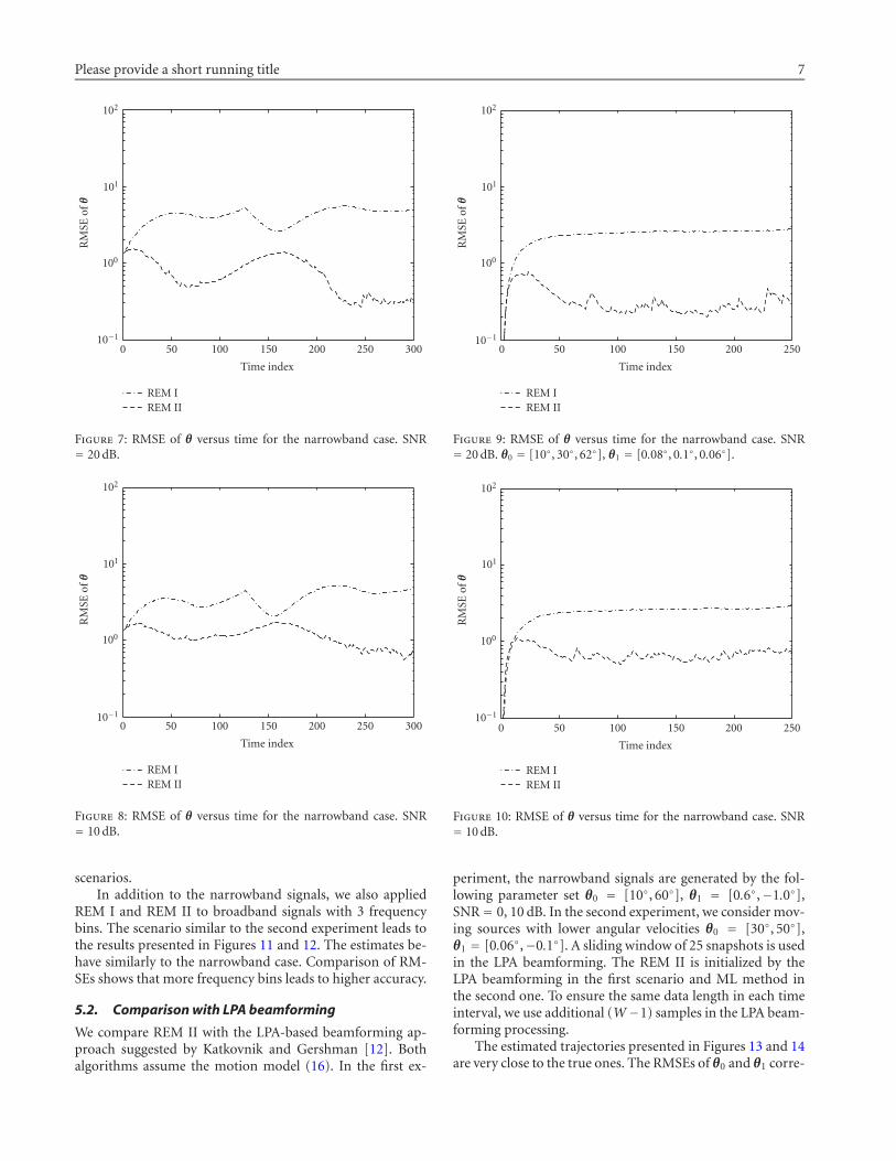
The narrowband signals generated by three sources of equalpower are received by a uniformly linear array of 15 sen-sors with interelement spacings of half a wavelength. Thesignal-to-noise ratio (SNR), defined as 10 log(sm(t)2/ν), m =1, 2, 3, is kept at 10, 20 dB. The motion of the moving14sources is described by the linear polynomial model (16).

15Three-different-parameter sets {θ0, θ1} are assumed in the

16 experiments. Each experiment performs 200 trials.

17 In the first experiment, we consider relatively fast mov-ing sources. The true parameters are given by θ0 =[10◦, 60◦, 66◦], θ1 = [0.6◦,−1.0◦, 0.4◦] where θ1 is measuredby degrees per time unit. In order to get a good insight into

90

80

70

60

50

40

30

20

10

0

DO

A(d

egre

e)

5 10 15 20 25 30 35 40 45 50

Time index


Figure 2: True trajectory and estimated trajectory by REM II forthe narrowband case. SNR = 20 dB.

the tracking behavior, the same initial values are used inall trials. We applied LPA-based beamforming to 20 snap-shots to obtain the initial estimates θ0

0 = [10.5◦, 59.5◦, 68.5◦],θ0

1 = [0.58◦,−0.99◦, 0.38◦]. The initial estimate for REM I isgiven by θ0

0. Both algorithms use a constant step size ε = 0.6.Figures 1 and 2 present the true values of θ and an example ofestimated trajectories. As shown in both figures, two sourcedirections cross with each other at t = 32. Obviously, the re-cursive procedure designed for the most general case cannotfollow fast moving sources at all. In contrast, the estimatedtrajectory obtained by REM II is very close to the true one.Figures 3 and 4 show the root mean square errors (RMSEs) of

the DOA estimates, defined as√‖θt − θ‖2 , averaged over 200

trials. Since REM I fails to track the moving sources, the cor-responding RMSE grows with increasing time. On the otherhand, the RMSE associated with REM II decreases slightlyat the beginning of the recursion and then remains almostconstant. Comparing Figures 3 and 4, one can observe thatSNR = 20 dB has a slightly lower RMSE than SNR = 10 dB.

The second experiment involves three slowly movingsources. The true parameter values are given by θ0 =[30◦, 50◦, 62◦], θ1 = [0.06◦,−0.1◦, 0.05◦]. Note that the an-gular velocity θ1 is approximately 1/10 of that considered inthe previous experiment. We applied the ML method to ob-tain the initial estimates θ0

0 = [30.1◦, 50.8◦, 60.9◦]. Becausethe angular velocity is very small compared to that in theprevious experiment, we take θ0

1 = [0◦, 0◦, 0◦] as the initialvalue for θ1. The initial estimate for REM I is given by θ0

0.Both algorithms use a constant step size ε = 0.6. Figures 5and 6 present the true and estimated trajectories obtainedby REM I and REM II. Similarly to the first experiment, twosource directions cross with each other at t = 126. The esti-mated trajectory by REM I is close to the true one when nocrossing happens. Between t = 100 and t = 230, where two


102

101

100

10−1

RM

SEof

θ

0 5 10 15 20 25 30 35 40 45 50

Time index

REM IREM II

Figure 3: RMSE of θ versus time for the narrowband case. SNR= 20 dB.

102

101

100

10−1

RM

SEof

θ

0 5 10 15 20 25 30 35 40 45 50

Time index

REM IREM II


source directions cross with each other, the estimated trajec-tories associated with the first two sources do not get close toeach other. Instead, they just depart in the vicinity of t = 126.For the same scenario, REM II provides a more accurate es-timate. Figure 6 shows that the crossing point causes a largerdeviation from the true trajectory. Due to a higher sensitivityto the variation of angular velocity at the crossing point, theestimated trajectory in Figure 6 is slightly worse than that inFigure 2. Comparison of Figures 7 and 8 with Figures 3 and4 shows an overall lower RMSE in this scenario. AlthoughREM I provides more reliable estimates than in the first ex-periment, REM II still outperforms REM I.

90

80

70

60

50

40

30

20

10

0

DO

A(d

egre

e)

50 100 150 200 250 300

Time index


Figure 5: True trajectory and estimated trajectory by REM I for thenarrowband case. θ0 = [30◦, 50◦, 62◦], θ1 = [0.06◦,−0.1◦, 0.05◦].SNR = 20 dB.

90

80

70

60

50

40

30

20

10

0

DO

A(d

egre

e)

50 100 150 200 250 300

Time index


Figure 6: True trajectory and estimated trajectory by REM II forthe narrowband case. SNR = 20 dB.

In the third experiment, three sources move slowlywith different speeds but do not cross with each other.The true parameters are given by θ0 = [10◦, 30◦, 62◦],θ1 = [0.08◦, 0.1◦, 0.06◦]. The initial estimates are θ0

0 =[10.04◦, 30.04◦, 62.05◦], θ0

1 = [0◦, 0◦, 0◦]. We use a constantstep size ε = 0.6. Both algorithms have good tracking abil-ity. Figures 9 and 10 show that RMSE is the lowest amongall three scenarios. REM II has a better performance thanREM I. While REM II has a better performance at higherSNR, REM I seems to be less sensitive to SNRs in all three


102

101

100

10−1

RM

SEof

θ

0 50 100 150 200 250 300

Time index

REM IREM II


102

101

100

10−1

RM

SEof

θ

0 50 100 150 200 250 300

Time index

REM IREM II


scenarios.In addition to the narrowband signals, we also applied

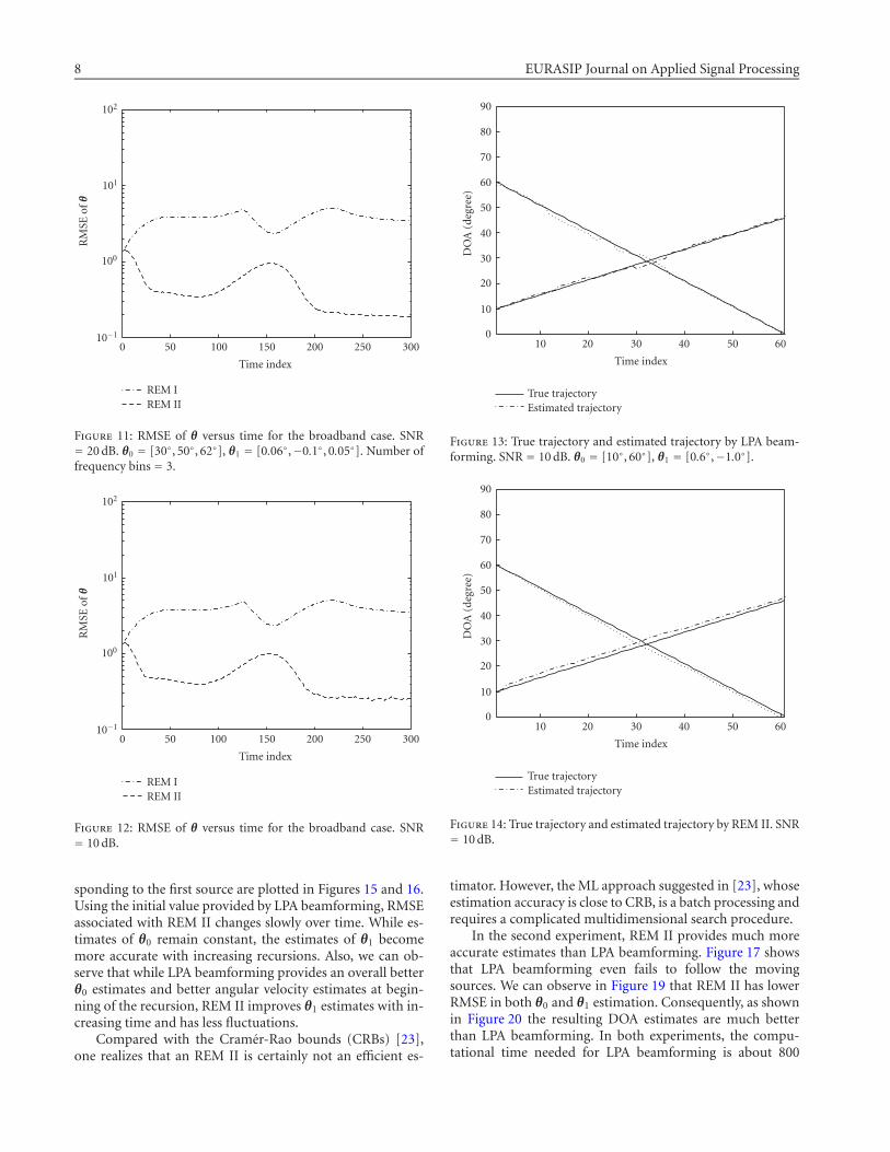
REM I and REM II to broadband signals with 3 frequencybins. The scenario similar to the second experiment leads tothe results presented in Figures 11 and 12. The estimates be-have similarly to the narrowband case. Comparison of RM-SEs shows that more frequency bins leads to higher accuracy.

5.2. Comparison with LPA beamforming

We compare REM II with the LPA-based beamforming ap-proach suggested by Katkovnik and Gershman [12]. Bothalgorithms assume the motion model (16). In the first ex-

102

101

100

10−1

RM

SEof

θ

0 50 100 150 200 250

Time index

REM IREM II

Figure 9: RMSE of θ versus time for the narrowband case. SNR= 20 dB. θ0 = [10◦, 30◦, 62◦], θ1 = [0.08◦, 0.1◦, 0.06◦].

102

101

100

10−1

RM

SEof

θ

0 50 100 150 200 250

Time index

REM IREM II


periment, the narrowband signals are generated by the fol-lowing parameter set θ0 = [10◦, 60◦], θ1 = [0.6◦,−1.0◦],SNR= 0, 10 dB. In the second experiment, we consider mov-ing sources with lower angular velocities θ0 = [30◦, 50◦],θ1 = [0.06◦,−0.1◦]. A sliding window of 25 snapshots is usedin the LPA beamforming. The REM II is initialized by theLPA beamforming in the first scenario and ML method inthe second one. To ensure the same data length in each timeinterval, we use additional (W−1) samples in the LPA beam-forming processing.

The estimated trajectories presented in Figures 13 and 14are very close to the true ones. The RMSEs of θ0 and θ1 corre-


102

101

100

10−1

RM

SEof

θ

0 50 100 150 200 250 300

Time index

REM IREM II

Figure 11: RMSE of θ versus time for the broadband case. SNR= 20 dB. θ0 = [30◦, 50◦, 62◦], θ1 = [0.06◦,−0.1◦, 0.05◦]. Number offrequency bins = 3.

102

101

100

10−1

RM

SEof

θ

0 50 100 150 200 250 300

Time index

REM IREM II

Figure 12: RMSE of θ versus time for the broadband case. SNR= 10 dB.

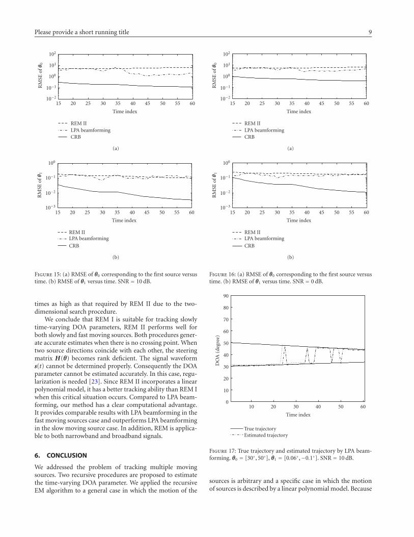
sponding to the first source are plotted in Figures 15 and 16.Using the initial value provided by LPA beamforming, RMSEassociated with REM II changes slowly over time. While es-timates of θ0 remain constant, the estimates of θ1 becomemore accurate with increasing recursions. Also, we can ob-serve that while LPA beamforming provides an overall betterθ0 estimates and better angular velocity estimates at begin-ning of the recursion, REM II improves θ1 estimates with in-creasing time and has less fluctuations.

Compared with the Cramer-Rao bounds (CRBs) [23],one realizes that an REM II is certainly not an efficient es-

90

80

70

60

50

40

30

20

10

0

DO

A(d

egre

e)

10 20 30 40 50 60

Time index


Figure 13: True trajectory and estimated trajectory by LPA beam-forming. SNR = 10 dB. θ0 = [10◦, 60◦], θ1 = [0.6◦,−1.0◦].

90

80

70

60

50

40

30

20

10

0

DO

A(d

egre

e)

10 20 30 40 50 60

Time index


Figure 14: True trajectory and estimated trajectory by REM II. SNR= 10 dB.

timator. However, the ML approach suggested in [23], whoseestimation accuracy is close to CRB, is a batch processing andrequires a complicated multidimensional search procedure.

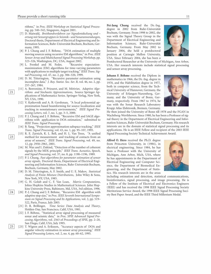
In the second experiment, REM II provides much moreaccurate estimates than LPA beamforming. Figure 17 showsthat LPA beamforming even fails to follow the movingsources. We can observe in Figure 19 that REM II has lowerRMSE in both θ0 and θ1 estimation. Consequently, as shownin Figure 20 the resulting DOA estimates are much betterthan LPA beamforming. In both experiments, the compu-tational time needed for LPA beamforming is about 800


102

101

100

10−1

10−2

RM

SEof

θ0

15 20 25 30 35 40 45 50 55 60

Time index

REM IILPA beamformingCRB

(a)

100

10−1

10−2

10−3

RM

SEof

θ1

15 20 25 30 35 40 45 50 55 60

Time index

REM IILPA beamforming

CRB

(b)

Figure 15: (a) RMSE of θ0 corresponding to the first source versustime. (b) RMSE of θ1 versus time. SNR = 10 dB.

times as high as that required by REM II due to the two-dimensional search procedure.

We conclude that REM I is suitable for tracking slowlytime-varying DOA parameters, REM II performs well forboth slowly and fast moving sources. Both procedures gener-ate accurate estimates when there is no crossing point. Whentwo source directions coincide with each other, the steeringmatrix H(θ) becomes rank deficient. The signal waveforms(t) cannot be determined properly. Consequently the DOAparameter cannot be estimated accurately. In this case, regu-larization is needed [23]. Since REM II incorporates a linearpolynomial model, it has a better tracking ability than REM Iwhen this critical situation occurs. Compared to LPA beam-forming, our method has a clear computational advantage.It provides comparable results with LPA beamforming in thefast moving sources case and outperforms LPA beamformingin the slow moving source case. In addition, REM is applica-ble to both narrowband and broadband signals.

6. CONCLUSION

We addressed the problem of tracking multiple movingsources. Two recursive procedures are proposed to estimatethe time-varying DOA parameter. We applied the recursiveEM algorithm to a general case in which the motion of the

102

101

100

10−1

10−2

RM

SEof

θ0

15 20 25 30 35 40 45 50 55 60

Time index


(a)

100

10−1

10−2

10−3

RM

SEof

θ1

15 20 25 30 35 40 45 50 55 60

Time index


CRB

(b)


90

80

70

60

50

40

30

20

10

0

DO

A(d

egre

e)

10 20 30 40 50 60

Time index


Figure 17: True trajectory and estimated trajectory by LPA beam-forming. θ0 = [30◦, 50◦], θ1 = [0.06◦,−0.1◦]. SNR = 10 dB.

sources is arbitrary and a specific case in which the motionof sources is described by a linear polynomial model. Because


90

80

70

60

50

40

30

20

10

0

DO

A(d

egre

e)

10 20 30 40 50 60

Time index


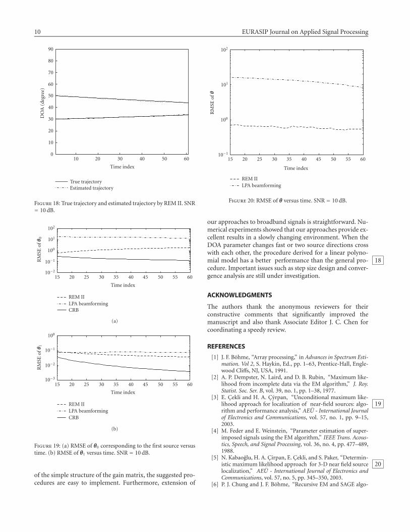
Figure 18: True trajectory and estimated trajectory by REM II. SNR= 10 dB.

102

101

100

10−1

10−2

RM

SEof

θ0

15 20 25 30 35 40 45 50 55 60

Time index


(a)

100

10−1

10−2

10−3

RM

SEof

θ1

15 20 25 30 35 40 45 50 55 60

Time index


(b)


of the simple structure of the gain matrix, the suggested pro-cedures are easy to implement. Furthermore, extension of

102

101

100

10−1

RM

SEof

θ

15 20 25 30 35 40 45 50 55 60

Time index


Figure 20: RMSE of θ versus time. SNR = 10 dB.

our approaches to broadband signals is straightforward. Nu-merical experiments showed that our approaches provide ex-cellent results in a slowly changing environment. When theDOA parameter changes fast or two source directions crosswith each other, the procedure derived for a linear polyno-mial model has a better performance than the general pro- 18cedure. Important issues such as step size design and conver-gence analysis are still under investigation.

ACKNOWLEDGMENTS

The authors thank the anonymous reviewers for theirconstructive comments that significantly improved themanuscript and also thank Associate Editor J. C. Chen forcoordinating a speedy review.

REFERENCES

[1] J. F. Bohme, “Array processing,” in Advances in Spectrum Esti-mation. Vol 2, S. Haykin, Ed., pp. 1–63, Prentice-Hall, Engle-wood Cliffs, NJ, USA, 1991.

[2] A. P. Dempster, N. Laird, and D. B. Rubin, “Maximum like-lihood from incomplete data via the EM algorithm,” J. Roy.Statist. Soc. Ser. B, vol. 39, no. 1, pp. 1–38, 1977.

[3] E. Cekli and H. A. Cyrpan, “Unconditional maximum like-lihood approach for localization of near-field sources: algo- 19rithm and performance analysis,” AEU - International Journalof Electronics and Communications, vol. 57, no. 1, pp. 9–15,2003.

[4] M. Feder and E. Weinstein, “Parameter estimation of super-imposed signals using the EM algorithm,” IEEE Trans. Acous-tics, Speech, and Signal Processing, vol. 36, no. 4, pp. 477–489,1988.

[5] N. Kabaoglu, H. A. Cirpan, E. Cekli, and S. Paker, “Determin-istic maximum likelihood approach for 3-D near field source 20localization,” AEU - International Journal of Electronics andCommunications, vol. 57, no. 5, pp. 345–350, 2003.

[6] P. J. Chung and J. F. Bohme, “Recursive EM and SAGE algo-


rithms,” in Proc. IEEE Workshop on Statistical Signal Process-ing, pp. 540–542, Singapore, August 2001.

[7] D. Maiwald, Breitbandverfahren zur Signalentdeckung und –ortung mit Sensorgruppen in Seismik– und Sonaranwendungen,Doctoral thesis, Department of Electrical Engineering and In-formation Sciences, Ruhr-Universitat Bochum, Bochum, Ger-many, 1995.

[8] P. J. Chung and J. F. Bohme, “DOA estimation of multiplemoving sources using recursive EM algorithms,” in Proc. IEEESensor Array and Multichannel Signal Processing Workshop, pp.323–326, Washington, DC, USA, August 2002.

[9] L. Frenkel and M. Feder, “Recursive expectation-maximization (EM) algorithms for time-varying parameterswith applications to multiple target tracking,” IEEE Trans. Sig-nal Processing, vol. 47, no. 2, pp. 306–320, 1999.

[10] D. M. Titterington, “Recursive parameter estimation usingincomplete data,” J. Roy. Statist. Soc. Ser. B, vol. 46, no. 2, pp.257–267, 1984.

[11] A. Benveniste, P. Priouret, and M. Metivier, Adaptive Algo-rithms and Stochastic Approximations, Source Springer Ap-21plications of Mathematics Series. Springer-Verlag, New York,NY, USA, 1990.

[12] V. Katkovnik and A. B. Gershman, “A local polynomial ap-proximation based beamforming for source localization andtracking in nonstationary environments,” IEEE Signal Pro-cessing Letters, vol. 7, no. 1, pp. 3–5, 2000.

[13] P. J. Chung and J. F. Bohme, “Recursive EM and SAGE algo-rithms with application to DOA estimation,” submitted to22IEEE Trans. Signal Processing.

[14] B. Yang, “Projection approximation subspace tracking,” IEEETrans. Signal Processing, vol. 43, no. 1, pp. 95–107, 1995.

[15] R. E. Zarnich, K. L. Bell, and H. L. Van Trees, “A unifiedmethod for measurement and tracking of contacts from an23array of sensors,” IEEE Trans. Signal Processing, vol. 49, no.12, pp. 2950–2961, 2001.

[16] M. Wax and I. Ziskind, “Detection of the number of coherentsignals by the MDL principle,” IEEE Trans. Acoustics, Speech,and Signal Processing, vol. 37, no. 8, pp. 1190–1196, 1989.

[17] P. J. Chung, Fast algorithms for parameter estimation of sensorarray signals, Doctoral thesis, Department of Electrical Engi-neering and Information Sciences, Ruhr-Universitat Bochum,Bochum, Germany, May 2002.

[18] D. M. Titterington, A. F. Smith, and U. E. Makov, StatisticalAnalysis of Finite Mixture Distributions, John Wiley & Sons,New York, NY, USA, 1985.

[19] G. H. Golub and C. F. Van Loan, Matrix Computations,Johns Hopkins Studies in Mathematical Sciences. John Hop-kins University Press, Baltimore, Md, USA, 3rd edition, 1996.

[20] P.-J. Chung and J. F. Bohme, “Recursive EM algorithm with24adaptive step size,” in Proc. IEEE Seventh International Sympo-sium on Signal Processing and Its Applications, vol. 2, pp. 519–522, Paris, France, July 2003.

[21] D. R. Brillinger, Time Series: Data Analysis and Theory,Holden-Day, San Francisco, Calif, USA, 1981.

[22] J. F. Bohme, “Statistical array signal processing of measuredsonar and seismic data,” in Proc. SPIE Advanced Signal Pro-cessing Algorithms, vol. 2563 of Proceedings of SPIE, pp. 2–20,San Diego, Calif, USA, July 1995.

[23] T. Wigren and A. Eriksson, “Accuracy aspects of DOA and25angular velocity estimation in sensor array processing,” IEEESignal Processing Letters, vol. 2, no. 4, pp. 60–62, 1995.

Pei-Jung Chung received the Dr.-Ing.degree in 2002 from Ruhr-UniversitatBochum, Germany. From 1998 to 2002, shewas with the Signal Theory Group in theDepartment of Electrical Engineering andInformation Sciences, Ruhr-UniversitatBochum, Germany. From May 2002 toJanuary 2004, she held a postdoctoralposition at Carnegie Mellon University,USA. Since February 2004, she has been aPostdoctoral Researcher at the University of Michigan, Ann Arbor,USA. Her research interests include statistical signal processingand sensor array processing.

Johann F. Bohme received the Diplom inmathematics in 1966, the Dr.-Ing. degree in1970, and the Habilitation degree in 1977,both in computer science, from the Tech-nical University of Hannover, Germany, theUniversity of Erlangen-Nuremberg, Ger-many, and the University of Bonn, Ger-many, respectively. From 1967 to 1974, hewas with the Sonar Research LaboratoryKrupp Atlas Elektronik, Bremen, Germany.He then joined the University of Bonn till 1978 and the FGAN inWachtberg-Werthhoven. Since 1980, he has been a Professor of sig-nal theory in the Department of Electrical Engineering and Infor-mation Sciences, Ruhr-Universitat Bochum, Germany. His researchinterests are in the domain of statistical signal processing and itsapplications. He is an IEEE Fellow and recipient of the 2003 IEEESignal Processing Society Technical Achievement Award.

Alfred O. Hero received the Ph.D. degreefrom Princeton University, in (1984), inelectrical engineering. Since 1984, he hasbeen a Professor with the University ofMichigan, Ann Arbor, Mich, USA, wherehe has appointments in the Department ofElectrical Engineering and Computer Sci-ence, the Department of Biomedical En-gineering, and the Department of Statis-tics. His research interests are in the areasincluding estimation and detection, statistical communications,bioinformatics, signal processing, and image processing. He isa Fellow of the Institute of Electrical and Electronics Engineers(IEEE) and has received the 1998 IEEE Signal Processing SocietyMeritorious Service Award, the 1998 IEEE Signal Processing Soci-ety Best Paper Award, and the IEEE Third Millenium Medal.


COMPOSITION COMMENTS

1 We changed the email addresses of the first and sec-ond authors and added the postal code of the first andthird authors addresses. Please check.

2 Please provide a short running title that should not ex-ceed 60 characters (including spaces).

3 Should we change “Alfred O. Hero” to “Alfred O. HeroIII” as in the biography? Please check.

4 We removed [12] after the highlighted word from theabstract as it should be citation-free. Please check.

5 We changed “parameter” to “parameters”. Please checkthroughout.

6 We added the spelled out form of “MDL”. Please check.

7 We changed “criterion” to “criteria”. Please check.

8 We changed “are” to “is” for consistency. Please check.

9 We changed “E (sans serif )” to “E (roman)” according tothe journal style. Please check throughout.

10 We moved the highlighted “and” to its current place.Please check.

11 We changed Tables 1 and 2 to Algorithms 1 and 2 and,thus, cited them in the text. Please check.

12 Should we change the highlighted occurrences of “Θ”to be bold? Please check.

13 Please choose another symbol instead of the high-lighted “T” to differentiate it from the “T” denoting trans-pose.

14 Please specify what other shapes of lines denote inFigures 1, 2, 5, 6, 13, 14, 17, and 18, for example, dottedlines and dashed lines.

15 We incorporated the illustrations above all figures intheir captions. Please check.

16 As the journal style does not allow the presence of re-peated equations we removed equation (23) in the originalmanuscript and replaced it by the citation of (16). Pleasecheck.

17 We changed “Three different parameter sets” to“Three-different-parameter sets”. Please check.

18 Please cite Figure 18 in the text.

19 We changed “AEU International” to “AEU - Interna-tional” in [3]. Please check.

20 We changed “near-field” to “near field” and “N.Kabaoglu, H. A. Cirpan, and E. Cekli,” to “N. Kabaoglu, H.A. Cirpan, and E. Cekli,” in [5]. Please check.

21 We changed the order of the authors in [11]. Pleasecheck.

22 Please update the information in [13] if possible.

23 We changed “mesurements” to “measurement” in[15]. Please check.

24 We changed “P. J. Chung” to “P.-J. Chung” in [20].Please check.

25 We changed “T. Wigern” to “T. Wigren” and “Eriksson”to “A. Eriksson” in [23]. Please check.

Documents

Best Practices in Managing Volunteers - James Madison University