Beräkningsmetoder för årsvärmefaktor för värmepumpsystem

Projekt 9

Beräkningsmetoder för årsvärmefaktor för värmepumpsystem för jämförelse, systemval och

dimensionering

Joachim Claesson, KTH‐Energiteknik

Per Lundqvist, KTH‐Energiteknik

Roger Nordman, SP‐Energiteknik

Kajsa Andersson, SP‐Energiteknik

Monica Axell, SP‐Energiteknik

Markus Lindahl, SP‐Energiteknik

2

Sammanfattning Föreliggande projekt har genomförts gemensamt av KTH‐Energiteknik och SP‐Energiteknik. Formell

projektledare har Prof. Per G. Lundqvist på KTH varit, biträdd av Dr. Monica Axell på SP‐Energiteknik.

Forskarutförande har i huvudsak varit Dr. Joachim Claesson, KTH‐Energiteknik, och Dr. Roger

Nordman, SP‐Energiteknik. Projektet har dels innehållit gemensamma delar, dels specifika för

respektive forskarutförare.

Projektet har syftat till att identifiera de behov för vidareutveckling och homogenisering av

beräkningsalgoritmer för att bestämma värmepumpsbaserade uppvärmningssystems effektivitet per

årsbasis (SPF = Seasonal Performance Factor) i småhus och flerfamiljshus.

Del I:

Inledande arbete inom IEA Annex angående rättvisande årsvärmefaktorer pågår löpande och

annexet är under uppstart. Detta arbete har precis startat och kommer att fortlöpa ett par år framåt.

Del II:

Fältmätningar är viktig del för att se om installerade system presterar enligt leverantörerna

utfästelser. En sammanställning av tidigare genomförda fältmätningar har gjorts, vilket visar att ett

omfattande antal fältmätningar finns rapporterade i litteraturen. Vidare har en genomgång och

sammanställning av standardiserade metoder att beräkna SPF baserat på mätningar av

värmepumpenheten utförts, vilket sedan jämförts mot mätningar. Även metoder för fältmätningar

har identifierats och redogörs för.

Del III:

Enkät har genomförts vilket visar att alla program inte kan hantera mer komplexa

uppvärmningssystem som t.ex. solfångare tillsammans med värmepump. Det är tydligt från enkäten

att inte alla programverktyg kan hantera olika kombinationssystem, inte heller finns alla

värmepumpsystem i alla program. En jämförelse ur användarsynpunkt av tre program har

genomförts som också pekar på skillnader på indata och möjligheter att använda olika

systmelösningar.

Del IV:

Ytterligare en enkät genomfördes som direkt jämförde resultaten mellan olika

dimensioneringsprogram. Skillnaden på årsvärmefaktorn (SPF) mellan de givna fiktiva fastigheterna

är inte speciellt besvärande, med beaktande att en leverantör räknade avfrostning dubbelt. Dock

pekar det på vikten av riktig och rak kommunikation kring den information som utbytes mellan kund

och säljare. Vidare har en metodik för beräkning av byggnaders energiprestanda tagits fram med

hänsyn tagen till de internationella och svenska standarder som finns. Strukturen hänvisar i stor

utsträckning till standarder där så tillämpligt och i vissa fall hänvisas till det arbete som genomfördes

av värmepumpbranschen i samband med effsys1 och programvaran PRESTIGE.

Till sist beskrivs de nu gällande rekommendationer från Boverket gällande miljöbedömning av

byggnaders energianvändning, där i huvudsak den kontrakterade energins belastning enligt uppgift

av leverantör rekommenderas användas. Detta är en skiljer sig från tidigare då framförallt el

räknades som marginal‐el, vilket nu längre inte är fallet.

3

Summary The present project has been a joint effort of KTH‐Energy Technology and SP‐Energy Technology. The

project responsible has been Prof. Per G. Lundqvist (KTH), assisted by Dr. Monica Axell (SP). The main

researchers have been Dr. Joachim Claesson (KTH) and Dr. Roger Nordman (SP). The project

consisted of common parts, as well several parts at only one of KTH or SP.

The aim of the project has been to identify the need for improvement, development, and

homogenization of Seasonal Performance Factors (SPF) of heat pump based heating systems in single

and multifamily dwellings.

Part I:

An IEA Annex concerning the same topic as the present project have been initiated and recently

launched, in which the project have participated actively. This work is just emerging, and will

continue for some years.

Part II:

Field measurement is an important aspect of heat pump installations as they serve to whether the

installation comply with the contracted performance. In the present project a summary of previously

conducted field measurement of heat pump installation is presented. A large number of studies are

available; however only a few have the necessary sufficient detailed level. The available standards for

calculating the SPF based on heat pump measurements has been summarized. These methods have

also been compared to field measurement.

Part III:

A survey have been sent out to the participant in the project investigating the limitations and

possibilities of the different calculation software’s. It is apparent that slightly more complex systems

is not able to calculated with these software´s.

Part IV:

A second survey was sent out in which the SPF of four buildings with four heat pumps were to be

evaluated in the software´s. The resulted SPF between the software´s is not very large, accounting

for typically 200 euros/year. This amount seems not large but could make an impact of the economy

of the installation.

A methodology for calculating SPF based on European standards has been developed.

3

Deltagande Parter Följande företag och parter har varit delaktiga i projektet:

Climacheck Klas Berglöf

ETM Kylteknik Kenneth Weber

EVI Heat Tommy Walfridson

IVT Jim Fredin

KTH ‐ Energiteknik Joachim Claesson

NIBE Ted Holmberg

SP ‐ Energiteknik Roger Nordman

SVEP Martin Forsén

Thermia Fredrik Karlsson

4

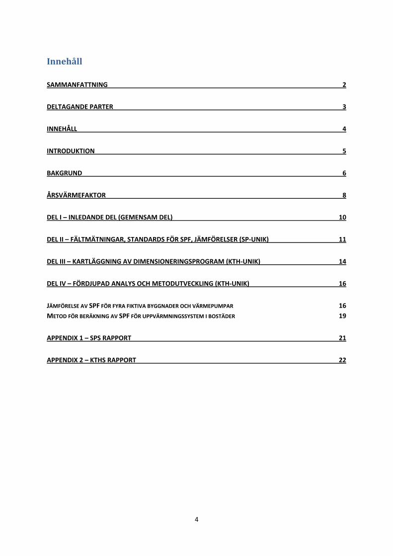
Innehåll

SAMMANFATTNING 2

DELTAGANDE PARTER 3

INNEHÅLL 4

INTRODUKTION 5

BAKGRUND 6

ÅRSVÄRMEFAKTOR 8

DEL I – INLEDANDE DEL (GEMENSAM DEL) 10

DEL II – FÄLTMÄTNINGAR, STANDARDS FÖR SPF, JÄMFÖRELSER (SP‐UNIK) 11

DEL III – KARTLÄGGNING AV DIMENSIONERINGSPROGRAM (KTH‐UNIK) 14

DEL IV – FÖRDJUPAD ANALYS OCH METODUTVECKLING (KTH‐UNIK) 16

JÄMFÖRELSE AV SPF FÖR FYRA FIKTIVA BYGGNADER OCH VÄRMEPUMPAR 16

METOD FÖR BERÄKNING AV SPF FÖR UPPVÄRMNINGSSYSTEM I BOSTÄDER 19

APPENDIX 1 – SPS RAPPORT 21

APPENDIX 2 – KTHS RAPPORT 22

5

Introduktion Föreliggande projekt har genomförts gemensamt av KTH‐Energiteknik och SP‐Energiteknik. Formell

projektledare har Prof. Per G. Lundqvist på KTH varit, biträdd av Monica Axell på SP‐Energiteknik.

Forskarutförande har i huvudsak varit Dr. Joachim Claesson, KTH‐Energiteknik, och Dr. Roger

Nordman, SP‐Energiteknik. Projektet har dels innehållit gemensamma delar, dels specifika för

respektive forskarutförare.

Projektet har syftat till att identifiera de behov för vidareutveckling och homogenisering av


årsbasis (SPF = Seasonal Performance Factor) i småhus och flerfamiljshus.

Rapporten är uppdelad enligt de projektdelar som angavs i ansökan. Detta motsvarar fyra delar.

Under varje projekdel redovisas kortfattat det arbete och resultat inom respektive del. Mer utförlig

redovisning av arbetet och resultaten inom respektive del går sedan att läsa i två appendix, en från

KTH och en från SP.

Under projektet har fyra projektmöten hållits, varav en var en workshop.

6

Bakgrund Det finns ett behov att dimensionering och energianvändning av energisystemen i byggnader

beräknas och hanteras på samma sätt. Detta är viktigt eftersom vid en tänkt installation jämförs

troligen olika leverantörer mot varandra, och om inte basen för deras beräkningar är gemensam går

det inte egentligen att utvärdera den ene leverantörens offert mot annan leverantör.

Det finns vidare behov av två typer av beräkningsprogram för värmepumpsystem, dels ett mer

detaljerat program för dimensionering av värmepumpsystem och dels en enklare transparent

beräkningsmetod som kan användas för jämförelse och kvalitetssäkring av värmepumpsystem.

Grundprincipen är att en enklare transparent programvara användas för initialt val av

värmepumpsystem (systemlösning, värmekälla etc.). Detta program skall även användas för

jämförelser nationellt och internationellt. När kunden/slutanvändaren sedan skall installera

värmepumpsystemet i sin egen fastighet är det viktigt att använda en mer detaljerad programvara så

att dimensioneringen blir korrekt. För dimensionering utvecklades beräkningsprogrammet ”Prestige”

inom ramen för effsys1. Detta och andra existerande dimensioneringsprogram behöver jämföras för

att undersöka om de behöver utvecklas för att svara upp mot dagens behov.

Befintliga beräkningsprogram för jämförelse och kvalitetssäkring behöver vidareutvecklas så att de

synliggör skillnaderna mellan olika typer av systemlösningar. Bland annat bör programmen utvecklas

så att de synliggör skillnad mellan on/off reglering och kapacitetsreglering samt andra typer av

teknikutveckling avseende kombinerad drift för värme och tappvarmvatten. Programvaran användas

som information till slutanvändaren då de skall välja typ av värmepumpsystem och för mellan olika

fabrikat. Det är viktigt att denna programvara då är transparent men ändå tillräckligt bra för att

synliggöra skillnaden i energibesparing och årsvärmefaktor (SPF) mellan de olika värme‐

pumpsystemen, inverkan av omgivningsklimatet samt distributionssystemet i fastigheten.

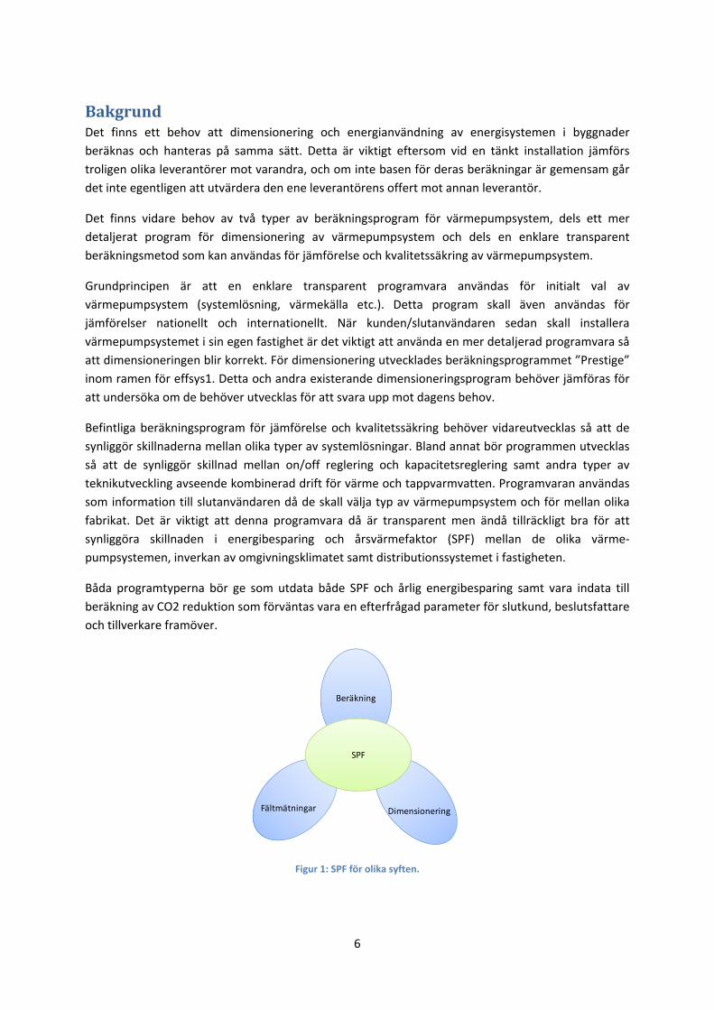
Båda programtyperna bör ge som utdata både SPF och årlig energibesparing samt vara indata till

beräkning av CO2 reduktion som förväntas vara en efterfrågad parameter för slutkund, beslutsfattare

och tillverkare framöver.

Figur 1: SPF för olika syften.

Beräkning

Fältmätningar Dimensionering

SPF

7

Båda programvarorna skall använda indata från gällande harmoniserade EU standarder. Ett väl

fungerande dimensioneringsprogram är viktigt för fortsatt tillväxt och acceptans för tekniken. Tillväxt

kräver nöjda kunder som får väl fungerande värmepumpsystem.

Ett program för jämförelse av olika värmepumpsystem är viktigt när slutkunden skall välja

systemlösning. Ur ett miljöperspektiv är det viktigt att slutkunden väljer bästa möjliga system på

marknaden. Ett värmepumpsystem har en livslängd på ca 20 år.

8

Årsvärmefaktor Det första fråga som inställer sig vid diskussion kring ett energisystems effektivitet är vilken

effektivitet som avses. Det mest naturliga ur konsumentsynpunkt är att effektivitet på ett

uppvärmningssystem är ett mått på hur mycket besparing (köpt energi, kr) som denna gör i sin

fastighet. Det är inte lika intressant för konsumenten att veta att värmepumpens effektivitet är

(COP1) t.ex. 4.2 vid en viss driftpunkt. Denna information kan visserligen vara intressant vid grov

utgallring av värmepumpar, då det kan tas för troligt att värmepumpens effektivitet vid en viss

driftpunk har viss bäring på hur effektiv den kommer att vara.

Bättre ändå är att få information kring hur effektiv värmepumpen är vid ”typisk” användning.

Problemet med värmepumpar i detta fall är att inga typiska generellt accepterade användning av

värmepumpen är identifierad av branschen. Detta spår har viss potential för bedömning av en

värmepumps prestanda, vilket är bättre än att sortera efter COP1. Metoden finns t.ex. omnämnd i

SS‐EN 15316‐4‐2, kap 5.2 (CEN SS‐EN 15316‐4‐2, 2008).

Metoden behöver som nämnts ovan definierade typiska användningar, dvs. typiska hus. Den

tilltänkte kunden kunde då i princip välja ett hus liknande sitt egna, välja klimat enligt ortens

placering samt jämföra olika leverantörers värmepumpsprestanda för detta väldefinierade huset

vilket ger mer information än enbart COP. Under projektets gång beslöts det dock i samråd med

företagsrepresentanter att detta inte skulle följas upp.

Vad avses med årsvärmefaktor? Under beaktande att kunden vill veta hur mycket energi som

kundens hus förväntas behöva köpa är en lämpligt definition av årsvärmefaktorn:

ä ö ä ä

ö ä

Använd energi avser alltså energi använd för uppvärmning eller kylning av byggnaden.

Det kan också vara av intresse att studera respektive värmegenererande enhets SPF. För en

värmepump blir då

å ä

ö ö ä

En värmepump med liten effekt i ett system med stort effektbehov kan ha högt SPFVP trots att

systemet är ineffektivt.

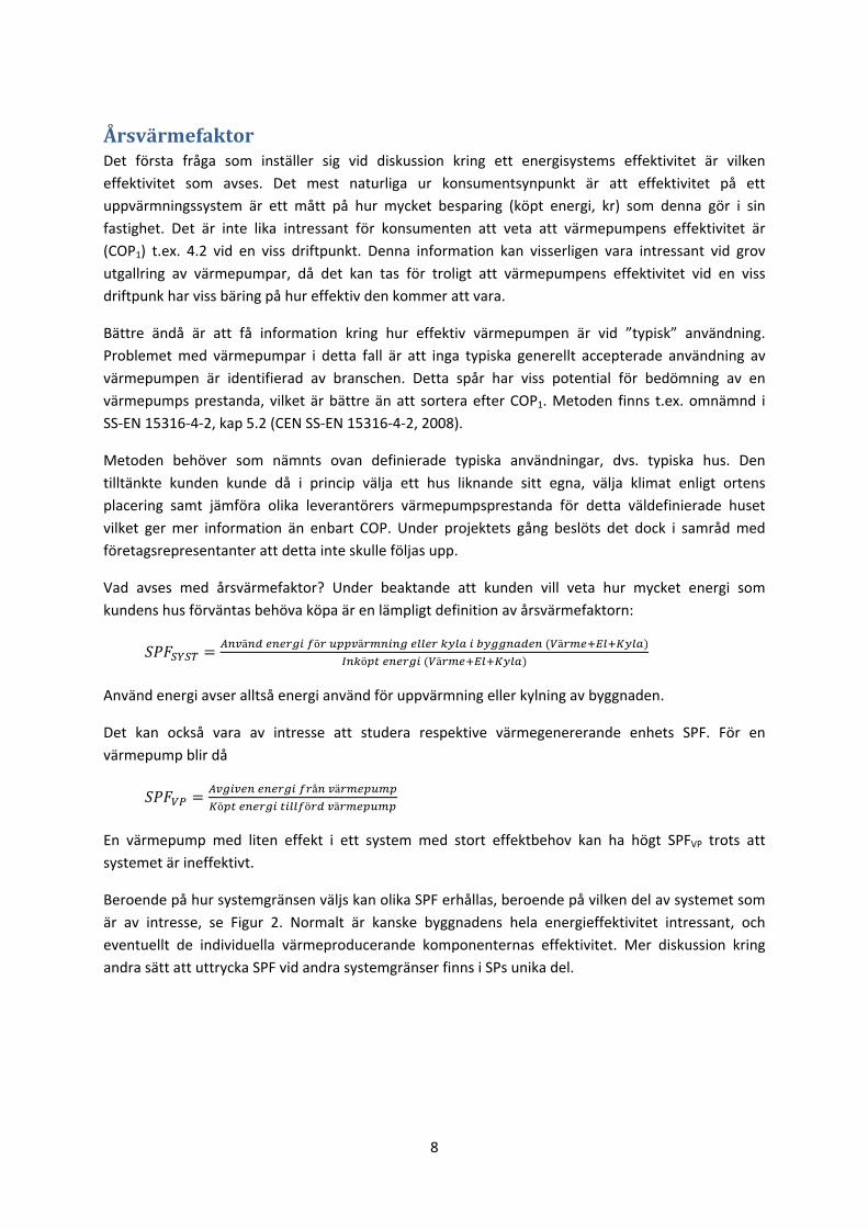
Beroende på hur systemgränsen väljs kan olika SPF erhållas, beroende på vilken del av systemet som

är av intresse, se Figur 2. Normalt är kanske byggnadens hela energieffektivitet intressant, och

eventuellt de individuella värmeproducerande komponenternas effektivitet. Mer diskussion kring

andra sätt att uttrycka SPF vid andra systemgränser finns i SPs unika del.

9

Figur 2: Olika ”SPF” beroende på var systemgränsen dras.

Mer generellt beskrivs energieffektiviteten i (CEN SS‐EN 15316‐1, 2007) där varje (del‐)system skall

beräknas enligt

, · , ,

· , · ,

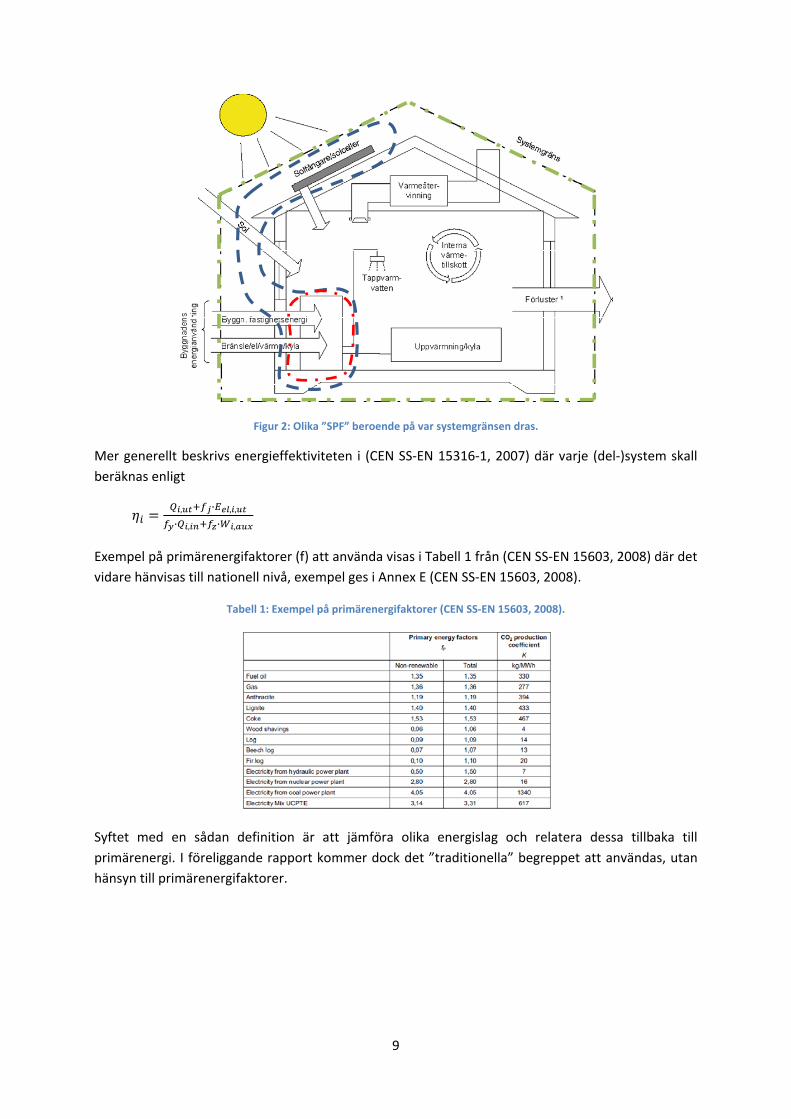
Exempel på primärenergifaktorer (f) att använda visas i Tabell 1 från (CEN SS‐EN 15603, 2008) där det

vidare hänvisas till nationell nivå, exempel ges i Annex E (CEN SS‐EN 15603, 2008).

Tabell 1: Exempel på primärenergifaktorer (CEN SS‐EN 15603, 2008).

Syftet med en sådan definition är att jämföra olika energislag och relatera dessa tillbaka till

primärenergi. I föreliggande rapport kommer dock det ”traditionella” begreppet att användas, utan

hänsyn till primärenergifaktorer.

10

Del I – Inledande del (Gemensam del)

Denna del är som rubriken antyder en inledande del som syftar till att dels initiera motsvarande

arbete internationellt. Vidare planerades under denna inledande del projektet tillsammans med

industrirepresentanterna. I samband med detta beslutades inom projektet att fokus i slutfasen av

projektet skulle vara på metodutveckling för beräkning av SPF och att det inte var realistiskt att göra

ett branschgemensamt beräkningsprogram.

Under detta möte beskrevs den volym av internationell och nationella ramar som finns att ta hänsyn

till, dels som regelverk, dels som standardiseringsarbete och produktmärkning.

Ett sådant direktiv som kan komma att påverka värmepumpar är Eu:s RES‐direktiv1, vilket bland

annat kommer att påverka hur miljömässiga olika uppvärmningssystem är. Syftet är att öka

användningen av förnybara energikällor, vilket är kopplat till EUs mål 20 % förnybara energikällor år

2020. Energibesparingar anses vara ett av de viktigaste sätten att minska energianvändningens

påverkan på globala miljön. Energi från värmepumpar kan delvis få räknas som förnybar energi enligt

direktivet, om värmepumpen är tillräckligt effektiv, dvs. har en SPF högre än 2.9. Det finns ingen

föreslagen metod att beräkna SPF, vilket gör att föreliggande projekt kan ligga som grund för ett

sådant arbete. Den förnybara andelen energi från en värmepump skall beräknas enligt

1

vilket torde motsvara upptagen energi från omgivningen (i förångaren). Från luftsvärmepump kan

inte tillgodogöra sig någon förnybar energi, då den inte tar sin energi från omgivningen. Det är

specificerat i RES‐direktivet vad som får räknas och vad som inte får räknas.

Inledande arbete inom ett IEA Annex pågår löpande och annexet är under uppstart. Detta arbete har

precis startat och kommer att fortlöpa ett par år framåt. Projektet och Sverige är aktiva i detta

arbete. Uppstartsmötet har precis varit (månadsskiftet juni/juli 2010).

1 EU, 2008/0016 (COD)

11

Del II – Fältmätningar, Standards för SPF, Jämförelser (SPunik)

Denna del av projektet är utförd av SP och mer information kan fås i ”Appendix 1 – SPs rapport”.

Rapporten beskriver först kortfattat aktuell status kring det internationella IEA Annex gällande

rättvisande årsvärmefaktorer som projektet aktivt deltagit i. Uppstartsmötet var nu i sommar.

Vidare presenteras redan genomförda fältmätningar där data är av god kvalité och tillräckligt

detaljerad för vidare analys. Bland en ganska omfattande volym av fältmätningar visade det sig att

endast tre stycket fältmätningar motsvarade dessa kriterier, två genomförda av SP, samt det sista

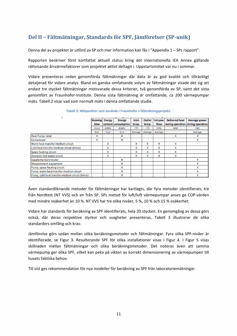
genomfört av Fraunhofer‐Institute. Denna sista fältmätning är omfattande, ca 200 värmepumpar

mäts. Tabell 2 visar vad som normalt mäts i denna omfattande studie.

Tabell 2: Mätpunkter som används i Fraunhofer´s fältmätningsprojekt.

Även standardliknande metoder för fältmätningar har kartlagts, där fyra metoder identifierats, tre

från Nordtest (NT VVS) och en från SP. SPs metod för luft/luft värmepumpar anses ge COP‐värden

med mindre osäkerhet än 10 %. NT VVS har tre olika nivåer, 5 %, 10 % och 15 % osäkerhet.

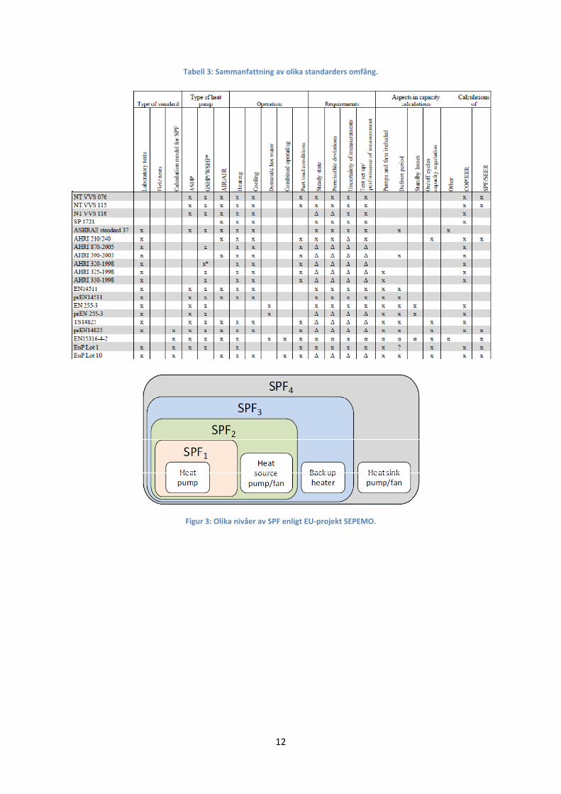
Vidare har standards för beräkning av SPF identifierats, hela 20 stycken. En genomgång av dessa görs

också, där deras respektive styrkor och svagheter presenteras. Tabell 3 illustrerar de olika

standarders omfång och krav.

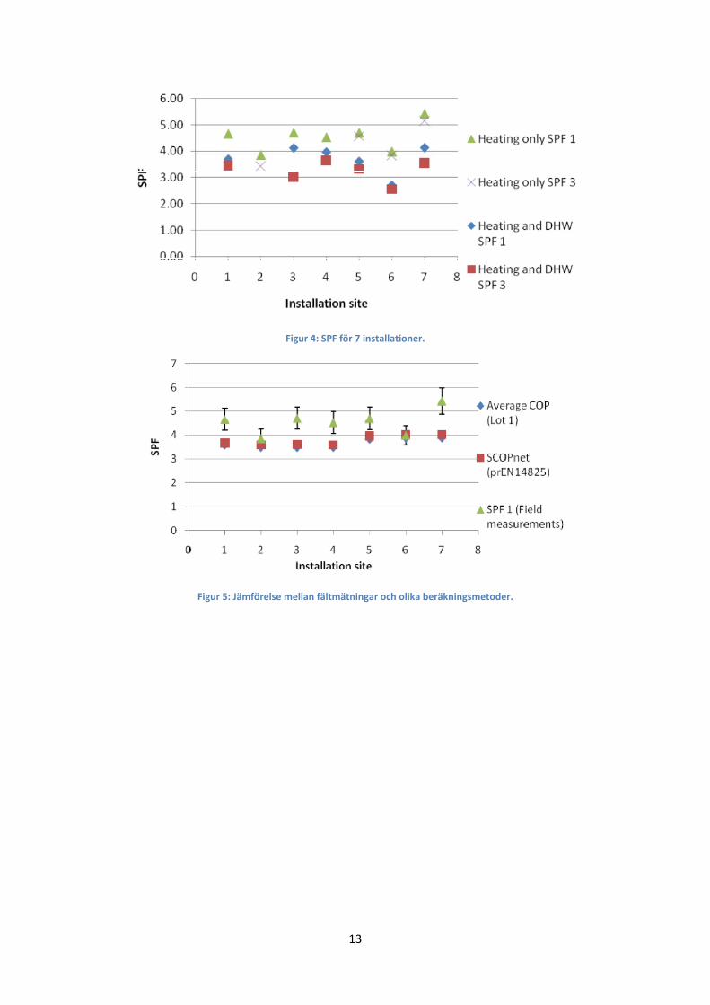
Jämförelse görs sedan mellan olika beräkningsmetoder och fältmätningar. Fyra olika SPF‐nivåer är

identifierade, se Figur 3. Resulterande SPF för olika installationer visas i Figur 4. I Figur 5 visas

skillnaden mellan fältmätningar och olika beräkningsmetoder. Det noteras även att samma

värmepump ger olika SPF, vilket kan peka på vikten av korrekt dimensionering av värmepumpen till

husets faktiska behov.

Till sist ges rekommendation för nya modeller för beräkning av SPF från laboratoriemätningar.

12

Tabell 3: Sammanfattning av olika standarders omfång.

Figur 3: Olika nivåer av SPF enligt EU‐projekt SEPEMO.

13

Figur 4: SPF för 7 installationer.

Figur 5: Jämförelse mellan fältmätningar och olika beräkningsmetoder.

14

Del III – Kartläggning av dimensioneringsprogram (KTHunik)

Denna del av projektet har utförts av KTH och mer finns att läsa i ”Appendix 2 – KTHs rapport”. Här

identifieras begränsningar och möjligheter i systemlösningar och metodik hos dimensionerings‐

program liknande PRESTIGE. En viktig del i arbetet var att kartlägga hur samtidig produktion av

tappvarmvatten och värme hanteras i programmen.

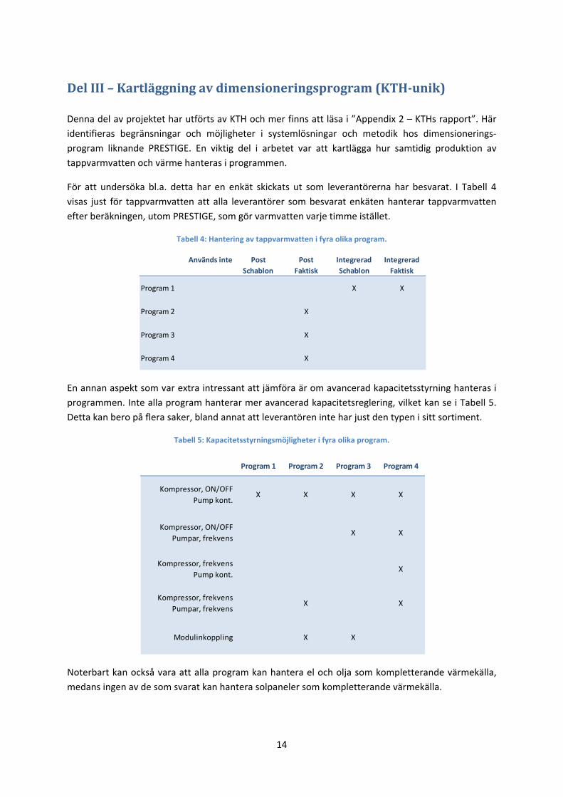
För att undersöka bl.a. detta har en enkät skickats ut som leverantörerna har besvarat. I Tabell 4

visas just för tappvarmvatten att alla leverantörer som besvarat enkäten hanterar tappvarmvatten

efter beräkningen, utom PRESTIGE, som gör varmvatten varje timme istället.

Tabell 4: Hantering av tappvarmvatten i fyra olika program.

En annan aspekt som var extra intressant att jämföra är om avancerad kapacitetsstyrning hanteras i

programmen. Inte alla program hanterar mer avancerad kapacitetsreglering, vilket kan se i Tabell 5.

Detta kan bero på flera saker, bland annat att leverantören inte har just den typen i sitt sortiment.

Tabell 5: Kapacitetsstyrningsmöjligheter i fyra olika program.

Noterbart kan också vara att alla program kan hantera el och olja som kompletterande värmekälla,

medans ingen av de som svarat kan hantera solpaneler som kompletterande värmekälla.

Används inte Post

Schablon

Post

Faktisk

Integrerad

Schablon

Integrerad

Faktisk

Program 1 X X

Program 2 X

Program 3 X

Program 4 X

Program 1 Program 2 Program 3 Program 4

Kompressor, ON/OFF

Pump kont.X X X X

Kompressor, ON/OFF

Pumpar, frekvensX X

Kompressor, frekvens

Pump kont.X

Kompressor, frekvens

Pumpar, frekvensX X

Modulinkoppling X X

15

Det kan konstateras att visst behov av utveckling är önskvärd kring möjligheterna att hantera

komplicerade systemlösningar, då denna möjlighet inte finns för kunder som t.ex. redan har

solpaneler installerade. Dessa kan i dagsläget inte få bra data kring eventuell besparing vid

installation av värmepump i sin byggnad.

Hela denna ovantstående enkät finns bifogad i KTHs delrapport (Appendix 2 – KTHs rapport).

Vidare i KTHs delrapport redovisas ett studentarbete som använt tre olika program och jämför deras

användbarhet och begränsningar.

16

Del IV – Fördjupad analys och metodutveckling (KTHunik)

Denna del av arbetet har utförts av KTH och finns att läsa mer utförligt i ”Appendix 2 – KTHs rapport”

Denna del innehåller arbete som inbegriper direkt jämförelse mellan olika leverantörers resultat när

det gäller en fiktiv värmepumps prestanda i form av SPF. Vidare har metodik utformats som kan

användas för bedömning av värmesystems prestanda i byggnader. Metodiken bygger till stor det på

befintliga standarder, där så varit möjligt.

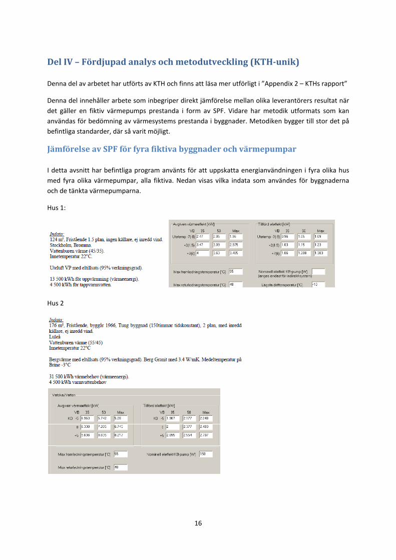
Jämförelse av SPF för fyra fiktiva byggnader och värmepumpar

I detta avsnitt har befintliga program använts för att uppskatta energianvändningen i fyra olika hus

med fyra olika värmepumpar, alla fiktiva. Nedan visas vilka indata som användes för byggnaderna

och de tänkta värmepumparna.

Hus 1:

Hus 2

17

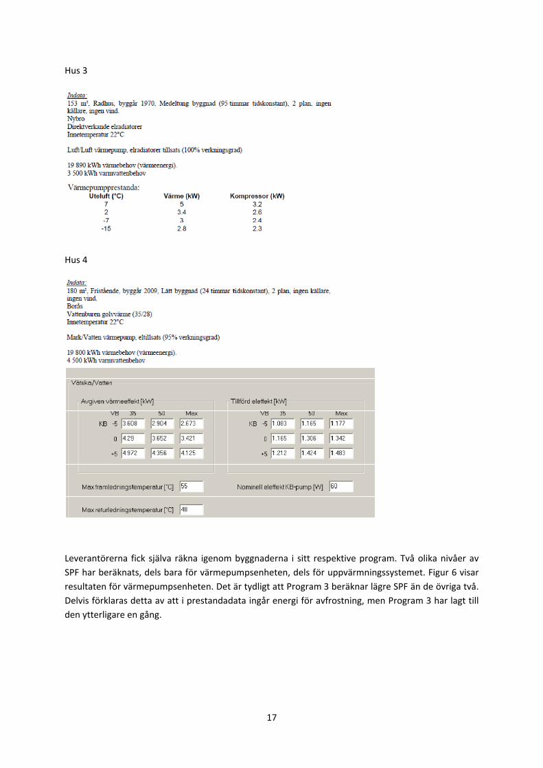
Hus 3

Hus 4

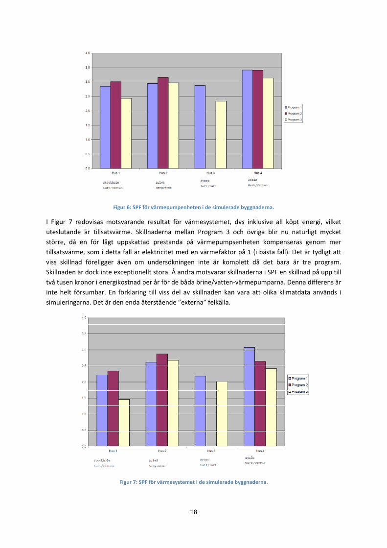
Leverantörerna fick själva räkna igenom byggnaderna i sitt respektive program. Två olika nivåer av

SPF har beräknats, dels bara för värmepumpsenheten, dels för uppvärmningssystemet. Figur 6 visar

resultaten för värmepumpsenheten. Det är tydligt att Program 3 beräknar lägre SPF än de övriga två.

Delvis förklaras detta av att i prestandadata ingår energi för avfrostning, men Program 3 har lagt till

den ytterligare en gång.

18

Figur 6: SPF för värmepumpenheten i de simulerade byggnaderna.

I Figur 7 redovisas motsvarande resultat för värmesystemet, dvs inklusive all köpt energi, vilket

uteslutande är tillsatsvärme. Skillnaderna mellan Program 3 och övriga blir nu naturligt mycket

större, då en för lågt uppskattad prestanda på värmepumpsenheten kompenseras genom mer

tillsatsvärme, som i detta fall är elektricitet med en värmefaktor på 1 (i bästa fall). Det är tydligt att

viss skillnad föreligger även om undersökningen inte är komplett då det bara är tre program.

Skillnaden är dock inte exceptionellt stora. Å andra motsvarar skillnaderna i SPF en skillnad på upp till

två tusen kronor i energikostnad per år för de båda brine/vatten‐värmepumparna. Denna differens är

inte helt försumbar. En förklaring till viss del av skillnaden kan vara att olika klimatdata används i

simuleringarna. Det är den enda återstående ”externa” felkälla.

Figur 7: SPF för värmesystemet i de simulerade byggnaderna.

19

Det kan alltså konstateras att det är viktigt att samma indata används för de olika programmen, att

modellerna är lika, så att ett rättvisande resultat kan erhållas.

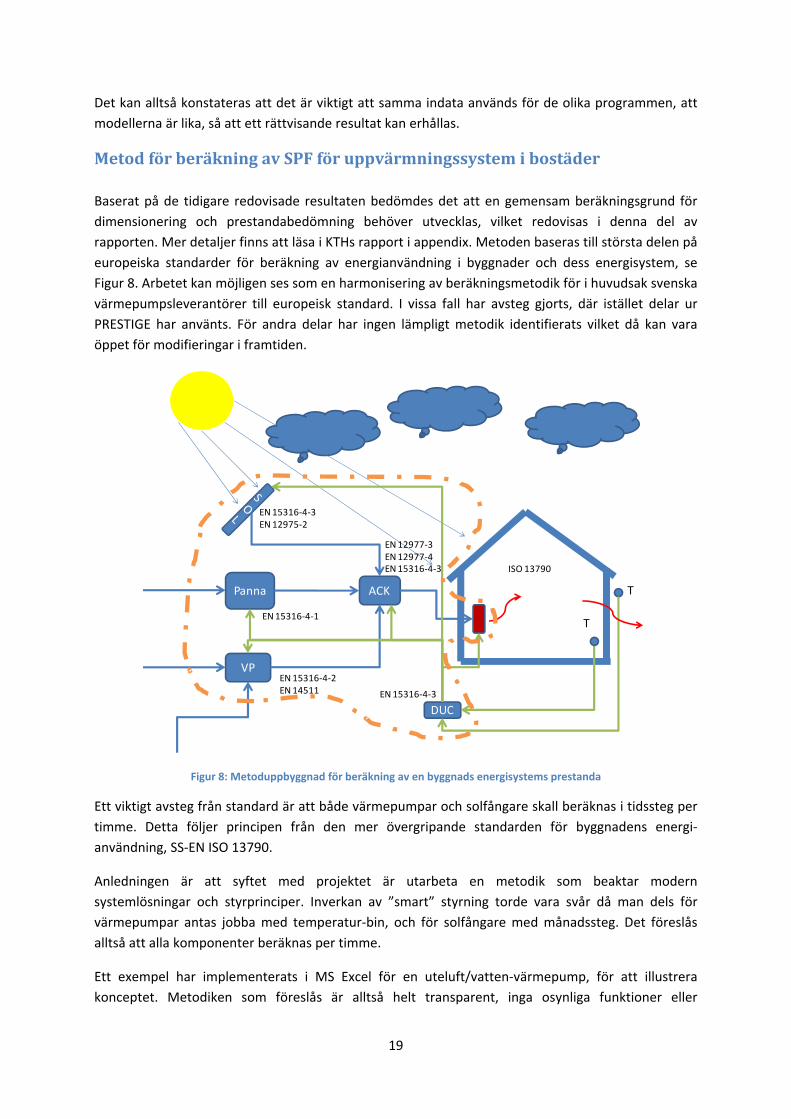
Metod för beräkning av SPF för uppvärmningssystem i bostäder

Baserat på de tidigare redovisade resultaten bedömdes det att en gemensam beräkningsgrund för

dimensionering och prestandabedömning behöver utvecklas, vilket redovisas i denna del av

rapporten. Mer detaljer finns att läsa i KTHs rapport i appendix. Metoden baseras till största delen på

europeiska standarder för beräkning av energianvändning i byggnader och dess energisystem, se

Figur 8. Arbetet kan möjligen ses som en harmonisering av beräkningsmetodik för i huvudsak svenska

värmepumpsleverantörer till europeisk standard. I vissa fall har avsteg gjorts, där istället delar ur

PRESTIGE har använts. För andra delar har ingen lämpligt metodik identifierats vilket då kan vara

öppet för modifieringar i framtiden.

Figur 8: Metoduppbyggnad för beräkning av en byggnads energisystems prestanda

Ett viktigt avsteg från standard är att både värmepumpar och solfångare skall beräknas i tidssteg per

timme. Detta följer principen från den mer övergripande standarden för byggnadens energi‐

användning, SS‐EN ISO 13790.

Anledningen är att syftet med projektet är utarbeta en metodik som beaktar modern

systemlösningar och styrprinciper. Inverkan av ”smart” styrning torde vara svår då man dels för

värmepumpar antas jobba med temperatur‐bin, och för solfångare med månadssteg. Det föreslås

alltså att alla komponenter beräknas per timme.

Ett exempel har implementerats i MS Excel för en uteluft/vatten‐värmepump, för att illustrera

konceptet. Metodiken som föreslås är alltså helt transparent, inga osynliga funktioner eller

VP

Panna ACK

DUC

T

T

ISO 13790

EN 15316‐4‐3EN 12975‐2

EN 15316‐4‐1

EN 15316‐4‐2EN 14511

EN 12977‐3EN 12977‐4EN 15316‐4‐3

EN 15316‐4‐3

20

algoritmer finns. Excelmodellen är lite långsam och syftet är inte att alla ska använda denna, utan att

den kan användas som referens.

Ytterligare versioner av värmepumpar får implementeras vid ett senare tillfälle. Avsikten då är att

implementera de värmepumpsmodeller som finns i PRESTIGE. För närvarande saknas då i huvudsak

markvärmepump och bergvärmepump.

21

Appendix 1 – SPs rapport

Calculation methods for SPF for heat pump systems for comparison, system choice and

dimensioning

Roger Nordman, Kajsa Andersson, Monica Axell, Markus Lindahl

Energy Technology

SP Report 2010:49

SP

Technic

al R

ese

arc

h I

nstitu

te o

f S

weden

Calculation methods for SPF for heat pump systems for comparison, system

choice and dimensioning

Roger Nordman, Kajsa Andersson, Monica Axell, Markus Lindahl

SP

Technic

al R

ese

arc

h I

nstitu

te o

f S

weden

3

Abstract In this project, results from field measurements of heat pumps have been collected and summarised.

Also existing calculation methods have been compared and summarised. Analyses have been made on

how the field measurements compare to existing calculation models for heat pumps Seasonal

Performance Factor (SPF), and what deviations may depend on. Recommendations for new

calculation models are proposed, which include combined systems (e.g. solar – HP), capacity

controlled heat pumps and combined DHW and heating operation.

Key words: Heat pump, SPF, calculation model, field measurements

SP Sveriges Tekniska Forskningsinstitut

SP Technical Research Institute of Sweden

SP Report 2010:49

ISBN 978-91-86319-86-1

ISSN 0284-5172

Borås 2010

4

Contents

Contents 4

Preface 6

Sammanfattning 7

1 Introduction 9

2 Preparing an IEA HPP Annex on SPF 10

3 Summary of already performed field measurements. 11 3.1 Description of evaluated field measurements 11 3.1.1 Fraunhofer 11 3.1.1.1 Measured parameters 11 3.1.1.2 System boundaries 12 3.1.1.3 Sampling interval 13 3.1.1.4 Measurement equipment 13 3.1.1.5 Measurement uncertainty 13 3.2 Measurement of ground source heat pumps 13 3.2.1 Measured parameters 13 3.2.1.1 Sampling interval 14 3.2.1.2 Measurement equipment 14 3.2.1.3 Measurement uncertainty 14 3.3 Field measurement of air-to-air heat pumps 14 3.3.1.1 Measured parameters 15 3.3.1.2 Sampling interval 16 3.3.1.3 Measurement equipment 16 3.3.1.4 Measurement uncertainty 16

4 Minimum required measured parameters in field measurements

17 4.1 Minimum results for the different SPF levels 18 4.2 Additional measurements 19 4.3 Data acquisition system 19

5 Studied methods for field measurement 20 5.1 NT VVS methods 20 5.2 SP method nr 1721 21

6 Studied methods for calculation of SPF 23 6.1 Other methods including calculation models 25 6.2 EN 15316-4-2:2008 26 6.3 Ecodesign LOT 10 28 6.4 PrEN14825 30 6.5 EuP LOT 1 - Boiler testing and calculation method 32 6.6 SP-method A3 528 34

7 Strengths and weaknesses with current methods 35 7.1 prEN14825 35 7.2 EN 15316-4-2 36 7.3 EuP LOT 1 36 7.4 EuP LOT 10 37

5

8 Comparison of existing calculation methods and results from field

measurements 39 8.1 Heat (and cooling-) demand of the house 39 8.2 Indoor climate 39 8.3 Outdoor climate 39 8.4 Definition of SPF field measurement system boundaries 39 8.5 Calculation of SPF 40 8.6 Analysis of the results 44 8.7 Conclusions from comparisons 47

9 Requirements for a new calculation model to evaluate SPF from lab

measurements 48

10 Conclusions 50

11 Further work 51

12 Publications from this project 52

13 References 53

Appendix 1. References for field measurements, presented in RIS-format.

54

6

Preface

This report summarize the findings from SP Technical Research Institute of Sweden in the joint KTH-

SP project “Calculation methods for SPF for heat pump systems for comparison, system choice

and dimensioning”, project P9 in the Effsys-2 research programme, financed by the Swedish Energy

Administration and participating companies and organizations.

The project was set up so that SP and KTH performed separate parts of the projects, but with

discussions and meetings in between.

The project parts are reported according to the parts stipulated in the application.

7

Sammanfattning

I denna rapport redovisas de delar av projektet ”Beräkningsmetoder för årsvärmefaktor för

värmepumpsystem för jämförelse, systemval och dimensionering” som SP Sveriges tekniska

forskningsinstitut svarat för. Projektet har genomförts av SP och KTH. KTH:s del av projektet

redovisas i en separat rapportdel.

I en inledande del av projektet har förberedelser för ett IEA samarbete, samt gemensam

övergripande projektplanering tillsammans med industriparterna utförts. IEA-projektet har

godkänts att starta av styrelsen för IEA Heat Pump Programme, och ett första inledande möte har

hållits.

SP har koordinerat samt sammanställt resultat av fältmätningar. Väl genomförda fältmätningar är

en förutsättning för validering av olika beräkningsalgoritmer. Sammanställningen visar att det

finns ett flertal utförda fältmätningar i Sverige under de senaste 20 åren, men få har gjorts med

SPF som fokus, utan ofta har mätningarna gjorts med syfte att studera en viss teknikförändring,

eller andra faktorer. Det har inte under de senaste 10 åren utförts någon stor mätning på

värmepumpar liknande de välkända Fraunhofermätningarna eller FAVA-studien i Schweiz. Den

enda studie som syftat till att mäta SPF är den som SP utfört. Detta kan ses som en brist i ett land

där värmepumpar har ett så stort genomslag för uppvärmningen av bostäder.

En kravspecifikation för mätdata som behövs för att användas för validering har tagits fram.

En sammanställning av befintliga standardliknande beräkningsmetoder (existerande algoritmer)

för SPF har gjorts. Syftet med analysen har varit att beskriva existerande algoritmer (modeller)

samt kartlägga om nuvarande program (Annex 28, SP´s beräkningsprogram mm) innefattar alla

typer av värmepumpsystem som finns på marknaden idag. En viktig del är att undersöka hur

kombinerad drift dvs. tappvarmvatten och värme behandlas i modellerna. En annan fråga är

huruvida olika typer av kapacitetsreglering behandlas. Sammanställningen har visat att det finns

en stor brist bland förekommande program och metoder vad gäller att ta hänsyn till :

Kombisystem, såsom sol-vp

Kapacitetsreglerade system

System med kombinerad varmvattentillverkning och uppvärmning

Existerande algoritmer har jämförts med resultat från fältmätningar. Från existerande

fältmätningar har data tagits för att jämföra resultaten med befintliga metoder för att beräkna SPF.

En analys av hur väl dessa metoder förmådde beräkna SPF för de studerade systemen har gjorts.

Denna analys visar att resultaten från fältmätningarna ofta visar på högre SPF än vad som

beräkningsmodellerna ger. Det finns flera orsaker till detta, bland annat att modellerna använder

sig av konstant marktemperatur (som i förekommande fall är lägre än verklig marktemperatur), att

modellerna använder en bivalent punkt som aldrig uppträtt i de verkliga mätningarna mm. Den

gjorda jämförelsen visar på ett antal viktiga faktorer att studera vidare.

För att utveckla ett enkelt program för jämförelse av värmepumpsystem är det viktigt att begränsa

beräkningarna till ett antal klimatzoner och ett antal typhus. Målet är att beräkningsmetoden skall

kunna användas både nationellt och internationellt. I ett dimensioneringsprogram skall däremot

stor frihet ges att definiera det specifika huset för att utförligt kunna studera de behov som finns

för de specifika installationerna.

En ny beräkningsmetodik för SPF och årsenergibesparing baserad på, eller som ersättning för

existerande algoritmer som input för nytt Annex inom IEA HPP och Europastandard (CEN) har

diskuterats. Det gemensamma beräkningsprogrammet skall baseras på indata från gällande

8

Europeiska standarder (EN 14511) för kombinerad drift med värme och tappvarmvatten. Det skall

även till fullo implementera rutiner för drift med kapacitetsreglerade värmepumpar (kompressorer

och pumpar/fläktar).

Förslag till vad som bör ingå i ett nytt transparent gemensamt beräkningsprogram som kan

användas för jämförelse och certifiering har getts. Industrigruppen menade tidigt att det viktiga i

denna del är att ta fram de samband som bör implementeras i ett beräkningsprogram, men att de

själva oftast skriver in-house kod som de kan implementera dessa samband i. Detta gör att

förutsättningarna blir likartade, men att tillverkarna fortfarande kan ha sina specifika (ofta

hemliga) indata själva.

9

1 Introduction

The existing calculation tools for 1) design and 2) comparison need to be further developed to show

the potential with new technology such as capacity controlled systems and more efficient system for

combined operation with space heating and domestic hot water production. The overall aim is to

develop existing tools for future needs. The outcome from the calculation tools should be useable for

calculation of environmental impact. The purpose is to compare existing tools for calculation of

seasonal performance factor and annual energy savings in order to propose needs for further

development. For validation of the calculation tools existing data from laboratory and field

measurements will be used.

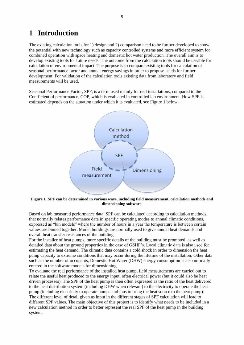
Seasonal Performance Factor, SPF, is a term used mainly for real installations, compared to the

Coefficient of performance, COP, which is evaluated in controlled lab environment. How SPF is

estimated depends on the situation under which it is evaluated, see Figure 1 below.

Figure 1. SPF can be determined in various ways, including field measurement, calculation methods and

dimensioning software.

Based on lab measured performance data, SPF can be calculated according to calculation methods,

that normally relates performance data in specific operating modes to annual climatic conditions,

expressed as “bin models” where the number of hours in a year the temperature is between certain

values are binned together. Model buildings are normally used to give annual heat demands and

overall heat transfer resistances of the building.

For the installer of heat pumps, more specific details of the building must be prompted, as well as

detailed data about the ground properties in the case of GSHP’s. Local climatic data is also used for

estimating the heat demand. The climatic data contains a cold shock in order to dimension the heat

pump capacity to extreme conditions that may occur during the lifetime of the installation. Other data

such as the number of occupants, Domestic Hot Water (DHW) energy consumption is also normally

entered in the software models for dimensioning.

To evaluate the real performance of the installed heat pump, field measurements are carried out to

relate the useful heat produced to the energy input, often electrical power (but it could also be heat

driven processes). The SPF of the heat pump is then often expressed as the ratio of the heat delivered

to the heat distribution system (including DHW when relevant) to the electricity to operate the heat

pump (including electricity to operate pumps and fans to bring the heat source to the heat pump).

The different level of detail given as input in the different stages of SPF calculation will lead to

different SPF values. The main objective of this project is to identify what needs to be included in a

new calculation method in order to better represent the real SPF of the heat pump in the building

system.

10

2 Preparing an IEA HPP Annex on SPF

Preparations for an IEA annex on SPF have included preparatory meetings, and communication with

research communities involved in the IEA HPP sphere. Meetings include a meeting during the

ASHRAE winter Conference 2009 [1.1.1.1.11], NT meeting in Borås, September 2009 , and a

Meeting in Paris march 5th, 2010 [2].

A draft legal text was prepared and circulated among interested parties and the executive committee in

HPP. The draft legal text was discussed in the ExCo meetings in Rome, November 2009 and in

Helsinki June 2010. In the Helsinki meeting it was suggested that the annex proposal for “Dynamic

testing of heat pumps” should be integrated with the SPF annex. The kick-off meeting for the SPF

Annex in June 30th- July 1

st 2010 will discuss the possibility for this integration. The legal was just

recently approved by the ExCo [3].

The preparation and starting up of the international Annex has taken much more time than expected,

mainly due to constraints in timing and funding. However, on June 30 –July 1st, the kick-off meeting

for the new annex is held in Albuquerque, New Mexico.

11

3 Summary of already performed field measurements.

In order to evaluate already made field measurements in Sweden, or made by Swedish manufacturers,

meetings in the project discussed earlier made field measurements. The result is that there has been a

large number of field measurements made during the last decades, see Appendix 1 and references [4-

6], but few studies have had the specific goal to examine the SPF.

In order to make detailed analyses of the performance, also detailed data from the measurements are

needed, and this was only available in two studies, the SP study ”Erfarenheter från fältutvärdering av

fem bergvärmepumpar i Sjuhärad” and the Fraunhofer study “Heat Pump Efficiency” where a number

of Swedish heat pump manufacturers participated with heat pump units. For Air-air heat pumps, only

one study has been found [7]. These three studies are describes more in detail below.

3.1 Description of evaluated field measurements

3.1.1 Fraunhofer

The Fraunhofer-Institute for Solar Energy Systems ISE is running two large field monitoring project

including approximately 200 heat pumps in total. The heat pump efficiency project includes

approximately 110 installed heat pumps with a heating capacity of 5-10 kW. In the Replacement of

Central Oil boilers with Heat Pumps in Existing Building Project 75 heat pumps are included. The

heat pump types included are air to water, ground source and water to water heat pumps. In this study

two heat pump producers, IVT and Nibe, have provided the project with data based on the field

measurements in the Fraunhofer study.

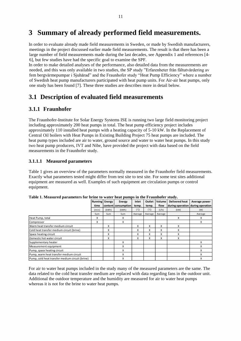
3.1.1.1 Measured parameters

Table 1 gives an overview of the parameters normally measured in the Fraunhofer field measurements.

Exactly what parameters tested might differ from test site to test site. For some test sites additional

equipment are measured as well. Examples of such equipment are circulation pumps or control

equipment.

Table 1. Measured parameters for brine to water heat pumps in the Fraunhofer study.

Running

time

Energy

content

Energy

consumption

Inlet

temp.

Outlet

temp.

Volume

flow

Delivered heat

during operation

Average power

during operation

(min) (kWh) (kWh) (˚C) (˚C) (l /h) (kW) (W)

Sum Sum Sum Average Average Average Average

Heat Pump, total X X X X

Compressor X X X

Warm heat transfer medium circuit X X X X X

Cold heat transfer medium circuit (brine) X X X X X

Space heating circuit X X X X X

Domestic hot water circuit X X X X X

Supplementary heater X X

Measurement equipment X X

Pump, space heating circuit X X

Pump, warm heat transfer medium circuit X X

Pump, cold heat transfer medium circuit (brine) X X

For air to water heat pumps included in the study many of the measured parameters are the same. The

data related to the cold heat transfer medium are replaced with data regarding fans in the outdoor unit.

Additional the outdoor temperature and the humidity are measured for air to water heat pumps

whereas it is not for the brine to water heat pumps.

12

Table 2. Measured parameters for air to water heat pumps in the Fraunhofer study. Running

time

Energy

content

Energy

consumption

Inlet

temp.

Outlet

temp.

Volume

flow

Delivered heat

during operation

Average power

during operation

(min) (kWh) (kWh) (˚C) (˚C) (l /h) (kW) (W)

Sum Sum Sum Average Average Average Average

Heat Pump, total X X X X

Compressor X X X

Warm heat transfer medium circuit X X X X X

Space heating circuit X X X X X

Domestic hot water circuit X X X X X

Supplementary heater X X

Measurement equipment X X

Pump, space heating circuit X X

Pump, warm heat transfer medium circuit X X

Fan X X

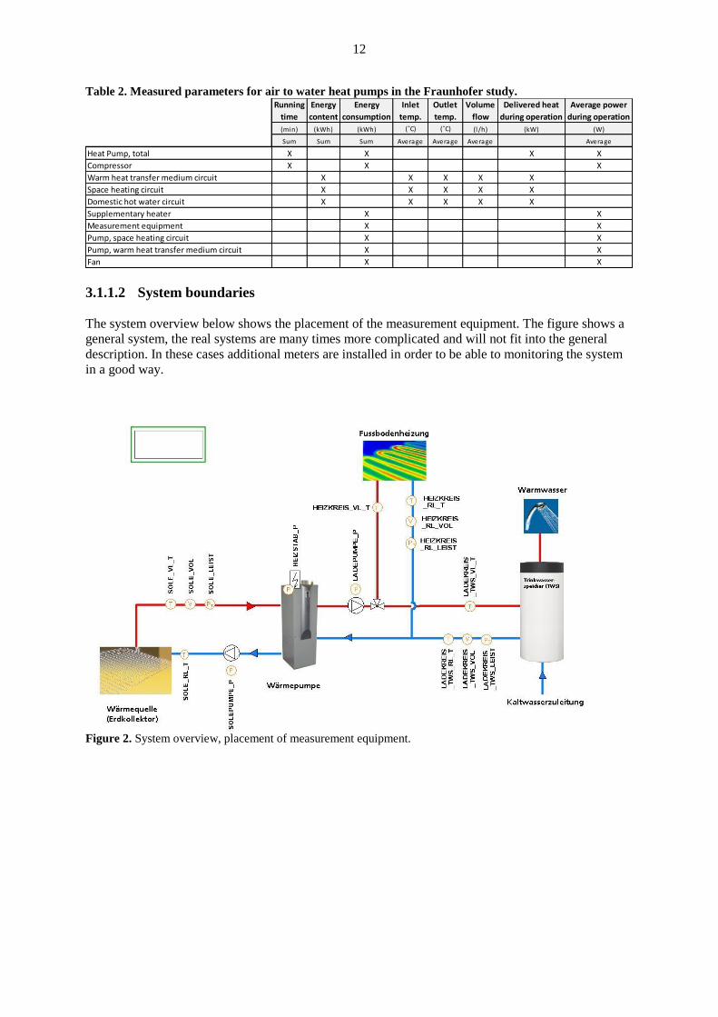
3.1.1.2 System boundaries

The system overview below shows the placement of the measurement equipment. The figure shows a

general system, the real systems are many times more complicated and will not fit into the general

description. In these cases additional meters are installed in order to be able to monitoring the system

in a good way.

Figure 2. System overview, placement of measurement equipment.

13

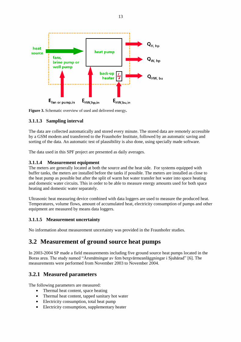
Figure 3. Schematic overview of used and delivered energy.

3.1.1.3 Sampling interval

The data are collected automatically and stored every minute. The stored data are remotely accessible

by a GSM modem and transferred to the Fraunhofer Institute, followed by an automatic saving and

sorting of the data. An automatic test of plausibility is also done, using specially made software.

The data used in this SPF project are presented as daily averages.

3.1.1.4 Measurement equipment The meters are generally located at both the source and the heat side. For systems equipped with

buffer tanks, the meters are installed before the tanks if possible. The meters are installed as close to

the heat pump as possible but after the split of warm hot water transfer hot water into space heating

and domestic water circuits. This in order to be able to measure energy amounts used for both space

heating and domestic water separately.

Ultrasonic heat measuring device combined with data loggers are used to measure the produced heat.

Temperatures, volume flows, amount of accumulated heat, electricity consumption of pumps and other

equipment are measured by means data loggers.

3.1.1.5 Measurement uncertainty

No information about measurement uncertainty was provided in the Fraunhofer studies.

3.2 Measurement of ground source heat pumps

In 2003-2004 SP made a field measurements including five ground source heat pumps located in the

Boras area. The study named “Årsmätningar av fem bergvärmeanläggningar i Sjuhärad” [6]. The

measurements were performed from November 2003 to November 2004.

3.2.1 Measured parameters

The following parameters are measured:

Thermal heat content, space heating

Thermal heat content, tapped sanitary hot water

Electricity consumption, total heat pump

Electricity consumption, supplementary heater

14

Indoor temperature

Outdoor temperature

Brine temperature, inlet (3 of 5 units)

Brine temperature, outlet (3 of 5 units)

Compressor, running time

Heat meters were installed between the space heating system and the heat pump, the same was done

for the tapped sanitary hot water. Thereby internal heat losses were not measured. The meters was

installed as close to the heat pump as possible in order to minimize the influence of these losses.

The electricity consumption of the supplementary heater was measured indirectly by measuring the

running time and the instantaneous power for each efficiency step.

The indoor and outdoor temperatures were logged continuously. The indoor meter was placed

centrally in the building with no influence of sunshine or other sources of interference. The outdoor

meter was placed on the north or northeast façade.

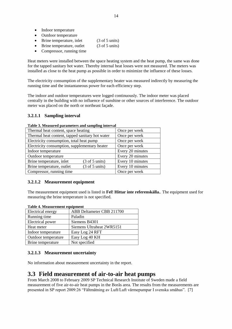
3.2.1.1 Sampling interval Table 3. Measured parameters and sampling interval

Thermal heat content, space heating Once per week

Thermal heat content, tapped sanitary hot water Once per week

Electricity consumption, total heat pump Once per week

Electricity consumption, supplementary heater Once per week

Indoor temperature Every 20 minutes

Outdoor temperature Every 20 minutes

Brine temperature, inlet (3 of 5 units) Every 10 minutes

Brine temperature, outlet (3 of 5 units) Every 10 minutes

Compressor, running time Once per week

3.2.1.2 Measurement equipment

The measurement equipment used is listed in Fel! Hittar inte referenskälla.. The equipment used for

measuring the brine temperature is not specified.

Table 4. Measurement equipment

Electrical energy ABB Deltameter CBB 211700

Running time Paladin

Electrical power Siemens B4301

Heat meter Siemens Ultraheat 2WR5151

Indoor temperature Easy Log 24 RFT

Outdoor temperature Easy Log 40 KH

Brine temperature Not specified


No information about measurement uncertainty in the report.

3.3 Field measurement of air-to-air heat pumps From March 2008 to February 2009 SP Technical Research Institute of Sweden made a field

measurement of five air-to-air heat pumps in the Borås area. The results from the measurements are

presented in SP report 2009:26 “Fältmätning av Luft/Luft värmepumpar I svenska småhus”. [7]

15

Electricity consumption and temperatures was logged continually and five performance tests were

made during the year. The performance tests were planned to be made at different outdoor

temperatures. Two test during spring and autumn and one during the winter. But due to the mild

winter and divergence between the weather forecast and the actual weather conditions at the test site

the planed dissemination was not reached. The performance test follows SP method no. 1721 [11].

3.3.1.1 Measured parameters

The following parameters are measured and logged continually:

Electricity consumption, total to the building

Electricity consumption, heat pump

Electricity consumption, supplementary heat

Indoor temperatures in tree rooms

Outdoor temperatures

Outdoor humidity

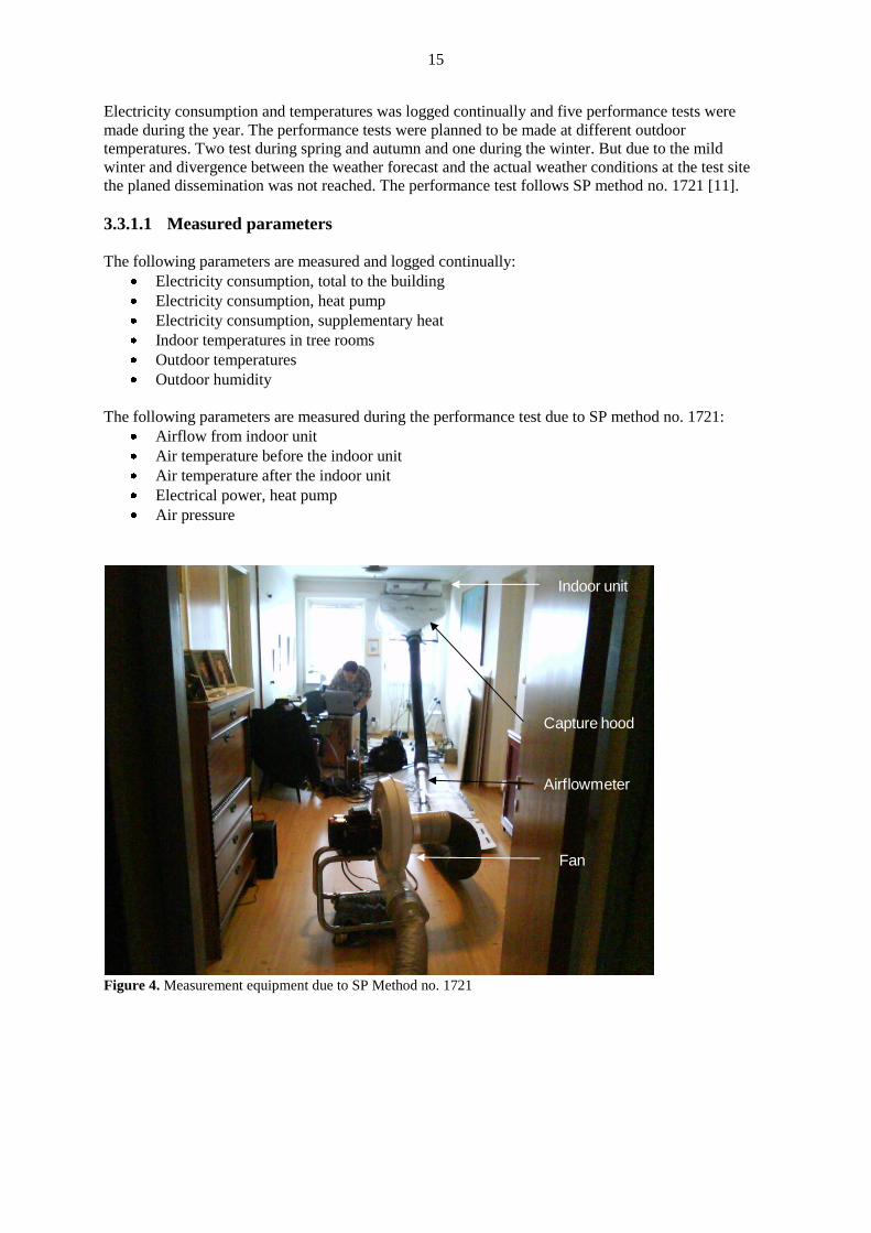
The following parameters are measured during the performance test due to SP method no. 1721:

Airflow from indoor unit

Air temperature before the indoor unit

Air temperature after the indoor unit

Electrical power, heat pump

Air pressure

Indoor unit

Airflowmeter

Fan

Capture hood

Figure 4. Measurement equipment due to SP Method no. 1721

16

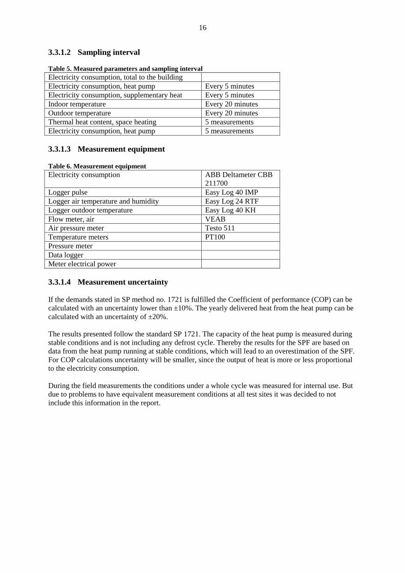
3.3.1.2 Sampling interval

Table 5. Measured parameters and sampling interval

Electricity consumption, total to the building

Electricity consumption, heat pump Every 5 minutes

Electricity consumption, supplementary heat Every 5 minutes

Indoor temperature Every 20 minutes

Outdoor temperature Every 20 minutes

Thermal heat content, space heating 5 measurements

Electricity consumption, heat pump 5 measurements

3.3.1.3 Measurement equipment Table 6. Measurement equipment

Electricity consumption ABB Deltameter CBB

211700

Logger pulse Easy Log 40 IMP

Logger air temperature and humidity Easy Log 24 RTF

Logger outdoor temperature Easy Log 40 KH

Flow meter, air VEAB

Air pressure meter Testo 511

Temperature meters PT100

Pressure meter

Data logger

Meter electrical power


If the demands stated in SP method no. 1721 is fulfilled the Coefficient of performance (COP) can be

calculated with an uncertainty lower than ±10%. The yearly delivered heat from the heat pump can be

calculated with an uncertainty of ±20%.

The results presented follow the standard SP 1721. The capacity of the heat pump is measured during

stable conditions and is not including any defrost cycle. Thereby the results for the SPF are based on

data from the heat pump running at stable conditions, which will lead to an overestimation of the SPF.

For COP calculations uncertainty will be smaller, since the output of heat is more or less proportional

to the electricity consumption.

During the field measurements the conditions under a whole cycle was measured for internal use. But

due to problems to have equivalent measurement conditions at all test sites it was decided to not

include this information in the report.

17

4 Minimum required measured parameters in field

measurements

The SPF-value can be calculated for different levels of the heating system. The level is described

by defined system boundaries. This project relates to four different system boundaries

developed in the SEPEMO EU project. The system boundaries are more detailed described in

section 8.4.

The system boundaries are named SPF1-SPF4, each number describing its own system boundary.

Different system boundaries mean different requirements of data to be measured. Before performing

field measurements it must be clear what SPF level that is to be measured.

The figure below shows the different system boundaries developed in SEPEMO. SPF1 includes SPF

for the heat pump itself only. SPF2 also includes heat source pumps and fans, the equipment to make

the heat source available for the heat pump. SPF3 also includes auxiliary heating, back up heating.

SPF4 includes heat sink equipment like fans or liquid pumps, to make the heat available in the house.

heat pump

heat

source

fan or pump

Back-up

heater

bu

ildin

g fa

ns o

r p

um

ps

SPFH1

SPFH2

SPFH3

SPFH4

QH_hp

QW_hp

QHW_bu

EB_fan/pumpEHW_buEbt_pumpEHW_hpES_fan/pump

The required measurements differ between different types of heat pumps. The required measurements

related to each type of heat pump is shown in Table 7.

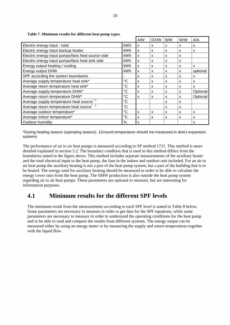
18

Table 7. Minimum results for different heat pump types.

A/W DX/W B/W W/W A/A

Electric energy input - total kWh x x x x x

Electric energy input backup heater kWh x x x x x

Electric energy input pumps/fans heat source side kWh x x x x

Electric energy input pumps/fans heat sink side kWh x x x x

Energy output heating / cooling kWh x x x x x

Energy output DHW kWh x x x x optional

SPF according the system boundaries - x x x x x

Average supply temperature heat sink* °C x x x x x

Average return temperature heat sink* °C x x x x x

Average supply temperature DHW* °C x x x x Optional

Average return temperature DHW* °C x x x x Optional

Average supply temperature heat source*, 1

°C x x

Average return temperature heat source* , 1

°C x x

Average outdoor temperature* °C x x x x x

Average indoor temperature* °C x x x x x

Outdoor humidity % x x

*During heating season (operating season). 1Ground temperature should me measured in direct expansion systems

The performance of air to air heat pumps is measured according to SP method 1721. This method is more

detailed explained in section 5.2. The boundary condition that is used in this method differs from the

boundaries stated in the figure above. This method includes separate measurements of the auxiliary heater

and the total electrical input to the heat pump, the fans in the indoor and outdoor unit included. For an air to

air heat pump the auxiliary heating is not a part of the heat pump system, but a part of the building that is to

be heated. The energy used for auxiliary heating should be measured in order to be able to calculate the

energy cover ratio from the heat pump. The DHW production is also outside the heat pump system

regarding air to air heat pumps. These parameters are optional to measure, but are interesting for

information purposes.

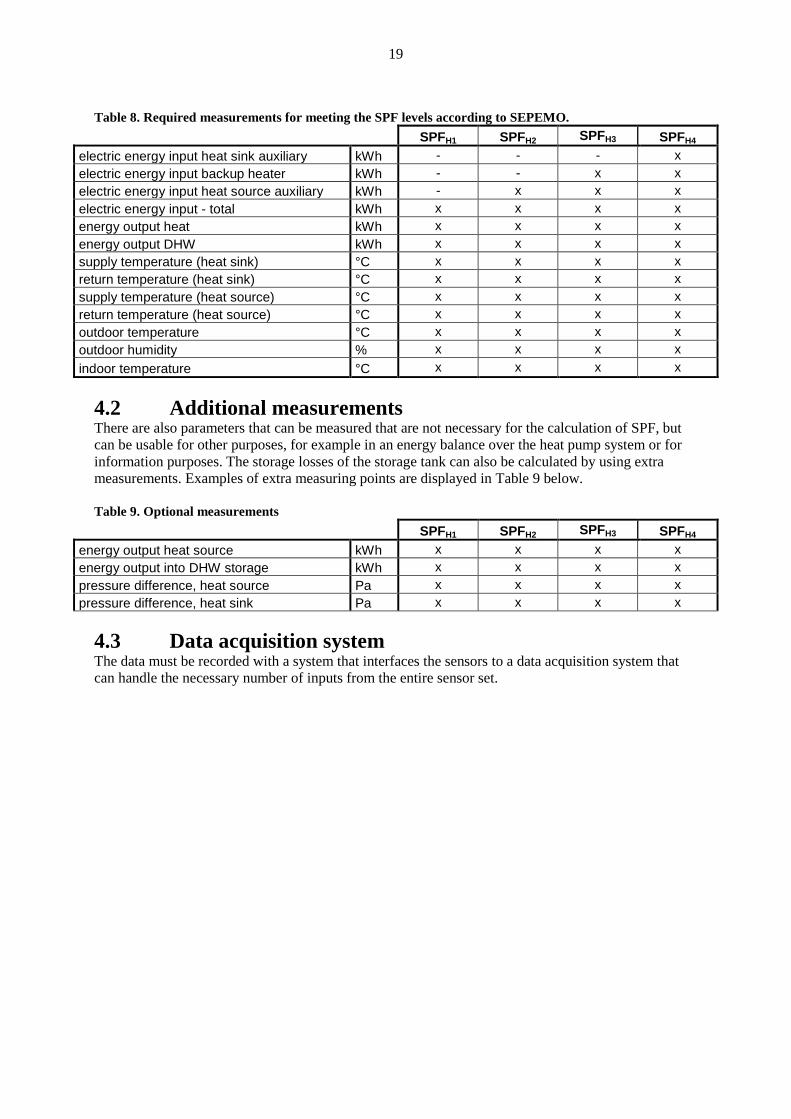
4.1 Minimum results for the different SPF levels

The minimum result from the measurements according to each SPF level is stated in Table 8 below.

Some parameters are necessary to measure in order to get data for the SPF equations, while some

parameters are necessary to measure in order to understand the operating conditions for the heat pump

and to be able to read and compare the results from different systems. The energy output can be

measured either by using an energy meter or by measuring the supply and return temperatures together

with the liquid flow.

19

Table 8. Required measurements for meeting the SPF levels according to SEPEMO.

SPFH1 SPFH2 SPFH3 SPFH4

electric energy input heat sink auxiliary kWh - - - x

electric energy input backup heater kWh - - x x

electric energy input heat source auxiliary kWh - x x x

electric energy input - total kWh x x x x

energy output heat kWh x x x x

energy output DHW kWh x x x x

supply temperature (heat sink) °C x x x x

return temperature (heat sink) °C x x x x

supply temperature (heat source) °C x x x x

return temperature (heat source) °C x x x x

outdoor temperature °C x x x x

outdoor humidity % x x x x

indoor temperature °C x x x x

4.2 Additional measurements There are also parameters that can be measured that are not necessary for the calculation of SPF, but

can be usable for other purposes, for example in an energy balance over the heat pump system or for

information purposes. The storage losses of the storage tank can also be calculated by using extra

measurements. Examples of extra measuring points are displayed in Table 9 below.

Table 9. Optional measurements

SPFH1 SPFH2 SPFH3 SPFH4

energy output heat source kWh x x x x

energy output into DHW storage kWh x x x x

pressure difference, heat source Pa x x x x

pressure difference, heat sink Pa x x x x

4.3 Data acquisition system The data must be recorded with a system that interfaces the sensors to a data acquisition system that

can handle the necessary number of inputs from the entire sensor set.

20

5 Studied methods for field measurement

The relevant methods for field measurements that are studied in this project are three Nordtest

methods (NT VVS) and one SP method:

Large heat pumps - Field testing and presentation of performance (NT-VVS076)

Refrigeration and heat pump equipment - General conditions regarding field testing and

presentation of performance (NT-VVS115)

Refrigeration and heat pump equipment - Check-ups and performance data inferred from

measurements in the refrigerant system (NT-VVS116)

Prestandaprovning av luft/luft värmepumpar i fält (SP metod nr 1721)

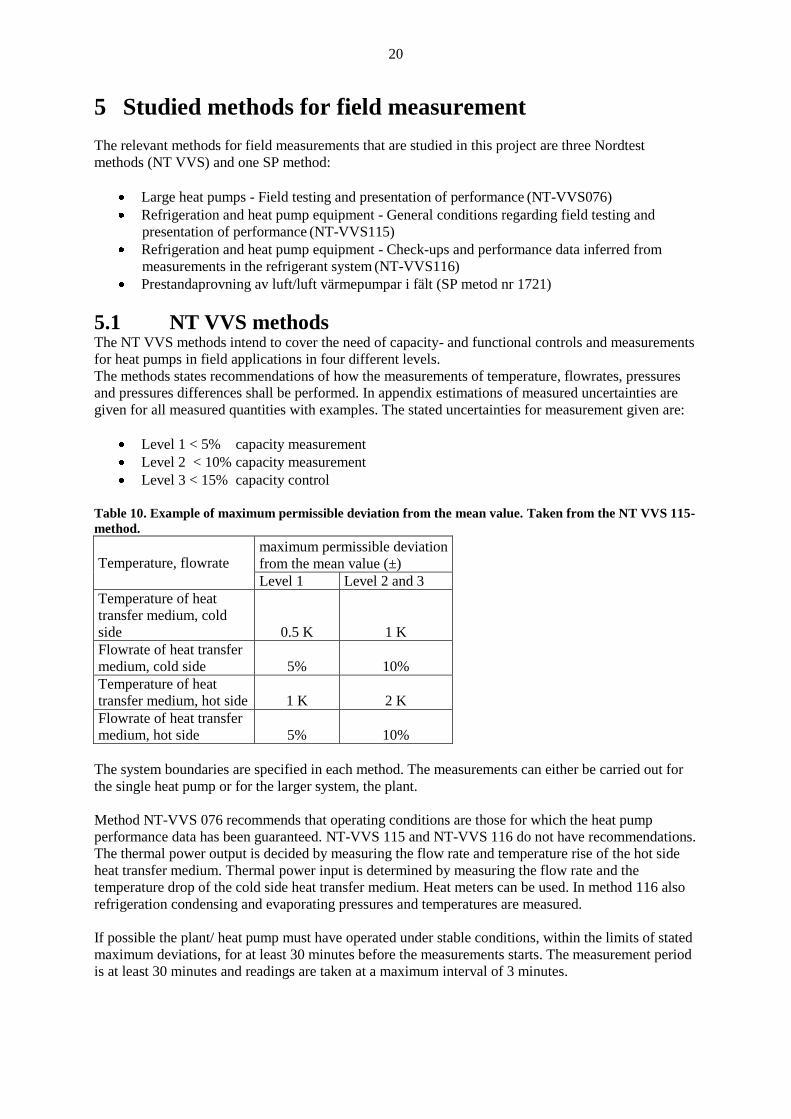
5.1 NT VVS methods The NT VVS methods intend to cover the need of capacity- and functional controls and measurements

for heat pumps in field applications in four different levels.

The methods states recommendations of how the measurements of temperature, flowrates, pressures

and pressures differences shall be performed. In appendix estimations of measured uncertainties are

given for all measured quantities with examples. The stated uncertainties for measurement given are:

Level 1 < 5% capacity measurement

Level 2 < 10% capacity measurement

Level 3 < 15% capacity control

Table 10. Example of maximum permissible deviation from the mean value. Taken from the NT VVS 115-

method.

Temperature, flowrate maximum permissible deviation

from the mean value (±)

Level 1 Level 2 and 3

Temperature of heat

transfer medium, cold

side 0.5 K 1 K

Flowrate of heat transfer

medium, cold side 5% 10%

Temperature of heat

transfer medium, hot side 1 K 2 K

Flowrate of heat transfer

medium, hot side 5% 10%

The system boundaries are specified in each method. The measurements can either be carried out for

the single heat pump or for the larger system, the plant.

Method NT-VVS 076 recommends that operating conditions are those for which the heat pump

performance data has been guaranteed. NT-VVS 115 and NT-VVS 116 do not have recommendations.

The thermal power output is decided by measuring the flow rate and temperature rise of the hot side

heat transfer medium. Thermal power input is determined by measuring the flow rate and the

temperature drop of the cold side heat transfer medium. Heat meters can be used. In method 116 also

refrigeration condensing and evaporating pressures and temperatures are measured.

If possible the plant/ heat pump must have operated under stable conditions, within the limits of stated

maximum deviations, for at least 30 minutes before the measurements starts. The measurement period

is at least 30 minutes and readings are taken at a maximum interval of 3 minutes.

21

If the heat pump operates during defrost conditions the measurements shall be carried out with

defrosted heat exchanger surfaces, during the most stable 30 minute period possible. The performance

test in NT-VVS 115 and NT-VVS 116 is carried out when the heat pump has attained regular frosting-

defrosting sequence starting at least 10 minutes after a terminated defrost cycle. In method NT-VVS

076, the defrosting function is checked concerning its influence on heat pump performance during one

complete frosting- and defrosting cycle.

Measuring instruments must have a certificate of calibration traceable to a national or international

primary standard that is not older than 1 year at the moment of testing.

Equations for calculating COP and SPF are given. The SPF equations include also any supplementary

heating and states that standby losses must be concerned.

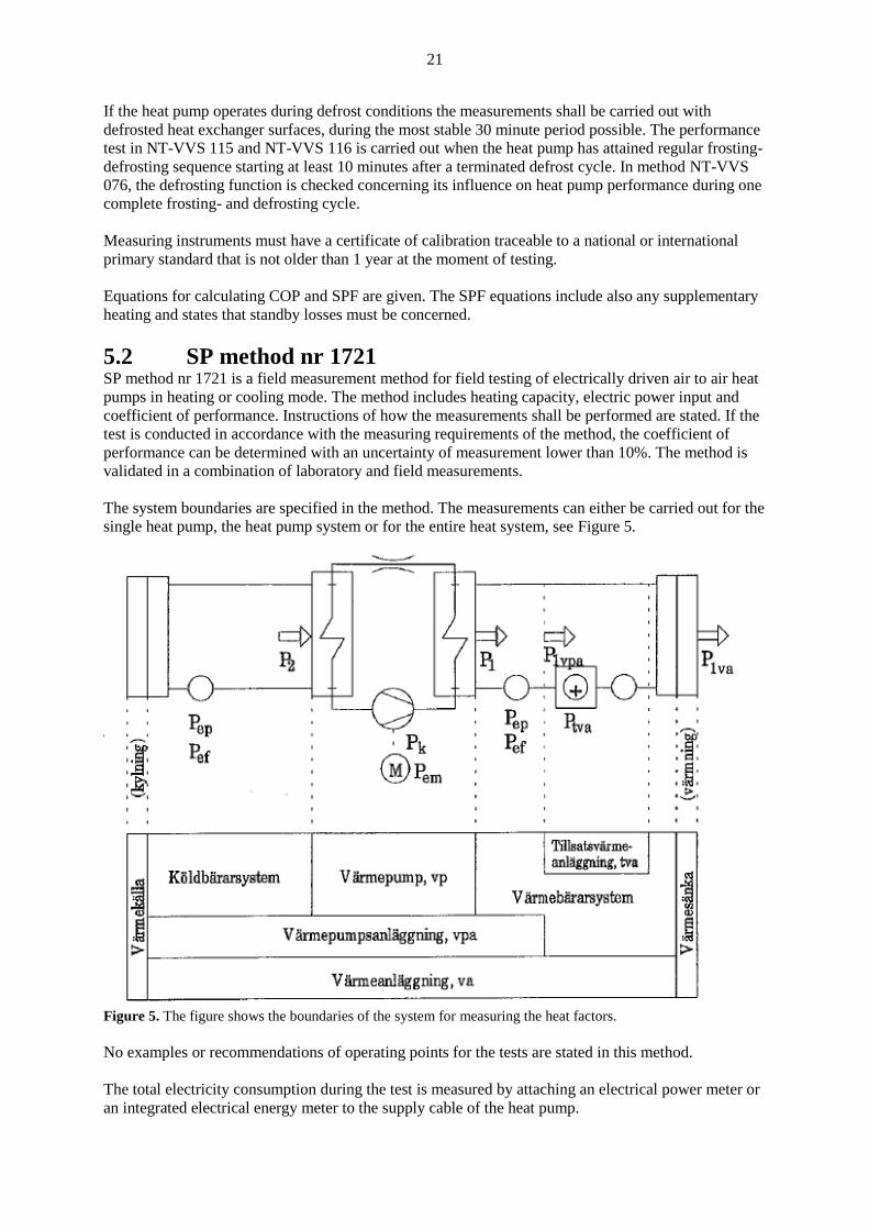
5.2 SP method nr 1721 SP method nr 1721 is a field measurement method for field testing of electrically driven air to air heat

pumps in heating or cooling mode. The method includes heating capacity, electric power input and

coefficient of performance. Instructions of how the measurements shall be performed are stated. If the

test is conducted in accordance with the measuring requirements of the method, the coefficient of

performance can be determined with an uncertainty of measurement lower than 10%. The method is

validated in a combination of laboratory and field measurements.

The system boundaries are specified in the method. The measurements can either be carried out for the

single heat pump, the heat pump system or for the entire heat system, see Figure 5.

Figure 5. The figure shows the boundaries of the system for measuring the heat factors.

No examples or recommendations of operating points for the tests are stated in this method.

The total electricity consumption during the test is measured by attaching an electrical power meter or

an integrated electrical energy meter to the supply cable of the heat pump.

22

The emitted heat effect is decided by measurements in the circulation flow. A volume- or a mass flow

meter (installed according to the manufacturer’s instructions) is used to measure the air flows in the

heat transfer medium circuit. To minimize effects at the air flow, the meter is not allowed to affect the

static pressure at the outflow of the heat pump more than ±3Pa. Therefore it is often necessary to

include an extra fan.

The temperatures that shall be measured are: incoming cooling medium temperature, incoming heating

medium and leaving heat transfer medium temperature. The temperature of the incoming cooling

medium is measured by one sensor placed in the centre of the air intake. The temperature of the

incoming heating medium is measured by at least four temperature sensors evenly spread over the air

intake. The variation between the highest and lowest temperature indication shall be lower than 1 K.

The temperature of the leaving heat transfer medium circuit is measured by at least four sensors evenly

spread out at a point where the air is mixed. The mixing device is not allowed to affect the static

pressure of the outflow of the heat pump more than ±3Pa, whereupon it is often necessary to include

an extra fan. Heat exchange between the mixing device and the surroundings shall be taken into

account. The variation between the highest and lowest temperature indication shall be lower than 1 K.

The data collection starts when “the plant” has operated at least five minutes at steady state conditions,

within the required permissible deviations, see Table 11. The stability is controlled by continuous

measuring at intervals shorter than 1/5 of the stability period, maximum one minute interval.

Table 11. Required permissible deviations for data collection in SP Method 1721.

Temperature, flow Maximum permissible deviations from mean

value

tvbin ± 1K

tvbut ± 1 K

qvvb, qmvb ± 5%

The sampling period shall be at least 10 minutes and the collection of data shall be either continuous

register or measuring by intervals more frequent than 1/5 of the measuring period (<2min). The

operation shall be stable also during the measurement period.

When the heat pump operates during conditions where frosting occurs, the capacity test is performed

after a defrost period at the most stable 10-minutes period possible (at least five minutes after the

defrost period).

23

6 Studied methods for calculation of SPF

The matrix below (Table 12) is a summary of the most important standards studied in the project. It is

divided into different categories trying to sort out the content of the different standards. All AHRI

standards mentioned above refers to ASHRAE standard 37 for the description the test method and

requirements for testing. The purpose of the AHRI standards is to provide test and rating requirements,

requirements for operating and the like for different kinds of heat pumps. The standards EN 255-3,

prEN 255-3, TS14825 and prEN14825 all refers to the standard EN 14511 for requirements to fulfil

the test method. For data input to the calculations of the calculation method EuP Lot 10 and to some

extent EuP Lot 1 and EN15316-4-2, one is referred to the test results from standard EN 14511.

The first category “type of standard” shows whether the standard describes a test method for

laboratory tests, for field tests and if it includes a calculation model for the calculation of seasonal

performance factor.

The second category “type of heat pump” describes what kind of heat pumps that is included in the

standard or test method.

The third category “Operation” describes the type of operation that is treated by the standard. The

different types of operation can be heating mode, cooling mode or production of domestic hot water.

The column called “combined operating” refers to the simultaneous production of heating and/or

cooling and the production of domestic hot water. The last column within this category “part load

conditions” shows if the standard includes the operation of the heat pump in part load.

The intention of the fourth category “requirements” is to show whether the standard has any

requirements of testing to reach accurate test results. Typical requirements could be that steady state

has to be reached before the measurements are performed, requirements of maximum deviations from

the stated measurements and a largest permissible uncertainty of measurements of the tests. The last

column within this category shows whether the standard gives any recommendations of how the

measurements shall be performed, such as the placement of sensors.

24

Table 12. Matrix of existing methods for testing and measurement and evaluation of SPF for heat pumps.

Type of standard

Type of heat

pump Operation Requirements

Aspects in capacity

calculations

Calculations

of

Lab

ora

tory

tes

ts

Fie

ld t

ests

Cal

cula

tion m

odel

for

SP

F

AS

HP

GS

HP

/WS

HP

*

AIR

/AIR

Hea

ting

Cooli

ng

Dom

esti

c hot

wat

er

Com

bin

ed o

per

atin

g

Par

t lo

ad c

ondit

ions

Ste

ady s

tate

Per

mis

sible

dev

iati

ons

Unce

rtai

nty

of

mea

sure

men

ts

Tes

t se

t up/

per

form

ance

of

mea

sure

men

t

Pum

ps

and f

ans

incl

uded

Def

rost

per

iod

Sta

ndby l

oss

es

On/o

ff c

ycl

es

capac

ity r

egula

tion

Oth

er

CO

P/E

ER

SP

F/S

EE

R

NT VVS 076

x x x x x

x x x x x

x x

NT VVS 115

x x x x x

x x x x x

x x

NT VVS 116

x x x x x

Δ Δ x x

x

SP 1721

x x x

x x x x

x

ASHRAE standard 37 x

x x x x x

x x x x

x

x

AHRI 210/240 x

x x x

x x x Δ x

x

x x

AHRI 870-2005 x

x

x x

x Δ Δ Δ Δ

x

AHRI 390-2003 x

x x x

x Δ Δ Δ Δ

x

x

AHRI 320-1998 x

x*

x x

x Δ Δ Δ Δ

x

AHRI 325-1998 x

x

x x

x Δ Δ Δ Δ x

x

AHRI 330-1998 x

x

x x

x Δ Δ Δ Δ x

x

EN14511 x

x x x x x

x x x x x x

prEN14511 x

x x x x x

x x x x x x

EN 255-3 x

x x

x

x x x x x x x

x

prEN 255-3 x

x x

x

Δ Δ Δ Δ x x x

x

TS14825 x

x x x x x

x Δ Δ Δ Δ x x

x

x

prEN14825 x

x x x x x x

x Δ Δ Δ Δ x x

x

x x

EN15316-4-2

x x x x x

x x x α α α α α α α x α

x

EuP Lot 1 x

x x x

x

x x x x x x ?

x

x x

EuP Lot 10 x

x

x x x

x x Δ Δ Δ Δ x x

x

x x

25

The sign “Δ” means that the standard refers to another standard where the requirements

are fulfilled.

The sign “α“ means that the method is a calculation method that does not include

requirements from a specified test method.

The fifth category “Aspects in capacity calculations” describes aspects that are taken into

account in the capacity calculations. It describes whether liquid pumps and fans are

included in the effective power absorbed by the unit. The “Defrost period” column

describes whether the defrost periods are taken into account when measuring and

calculating the capacity of the heat pump. The “standby losses” column means that

standby losses are measured and taken into account when calculating the capacity of the

heat pump. The NT-VVS 076 and NT-VVS 115 both mention that it is necessary to take

standby losses into account when calculating the SPF, but there is no method of how to

measure the losses. Both the standards for measuring the production of domestic hot

water EN 255-3 and prEN 255-3 states methods of how to measure the standby losses,

but the way of taking the standby losses into account when calculating the COP differs a

lot between the standards. “On/off cycles and capacity regulation” shows whether the

standard treats what kind of capacity regulation that is used by the heat pump. The last

column “other” shows whether there are other important aspects apart from the earlier

mentioned ones, which are taken into account in the capacity calculations. It shows that

for some of the methods mentioned in the standard ASHRAE 37 adjustments of the line

loss capacity and duct losses are made.

The last category “calculations of” describes the calculated outcome of the standard. The

NT VVS standards provide simple equations of how to calculate SPF without a

calculation model.

6.1 Other methods including calculation models Besides the models mentioned above there are several other standards and models that

can be used in order to find an appropriate model to calculate a seasonal performance

factor. The ones studied in this project are shortly summarized in this chapter.

EN 15316-2-3 Heating systems in buildings – Method for calculation of system energy

requirement and system efficiencies – Part 2-3: Space heating distribution systems

This method calculates the system thermal losses and the auxiliary energy demand of

water based distribution system for heating circuits (primary and secondary), as well as

the recoverable system thermal losses and the recoverable auxiliary energy. The

calculations are related to a design effect and design heat load of the accounted zone (EN

12831). Correction factors are provided for a number of different conditions, these

conditions can for example be corrections for the size of the building, for systems without

outdoor temperature compensation, efficiency and part load. The method can be applied

for any time step (hour, day, month or year).

EN 13790:2008, Energy performance of buildings – Calculation of energy use for space

heating and cooling (ISO 13790:2008)

This standard provides a calculation method for the assessment of the annual energy use

of buildings. Factors that are taken into account are for example the heat transfer by

transmission and ventilation of the building when heated or cooled to constant internal

temperature, contribution of internal and solar heat gains to the building energy balance

and the annual energy use for heating and cooling.

There are two different main methods that are used by the standard, one where the heat

balance is calculated during a sufficiently long time (one month or a season) and dynamic

effects of the building are taken into account by an empirically determined gain and/or

26

loss utilization factor and one method where the heat balance is calculated over small

time steps (typically one hour) and the heat stored in, and released from, the mass of the

building is taken into account.

EN 12831 Heating systems in buildings – Method for calculation of the design heat load

This standard is used to calculate the design heat losses of a heated space; the result is

then used to determine the design heat load at standard design conditions. The

temperature distribution (air and design temperature) is assumed to be uniform. The

climatic data that is used for the calculations are the external design temperature and the

annual mean external temperature.

Factors taken into account are for example size of the building, type of building, activities

inside the building, type of room, interior, building envelope and ventilation.

A number of standards/methods for the calculation of seasonal performance factor are

investigated. Some of the methods only contain a calculation model while some of them

also contain instructions of how to test the heat pumps. The calculation models that are

studied in this project are prEN14825:2009 draft Nov 09, EN 15316-4-2:2008, EUP LOT

1 and EUP Lot 10.

6.2 EN 15316-4-2:2008 Heating systems in buildings – method for calculation of system energy requirements and

system efficiencies – Part 4-2: space heating generation systems, heat pump systems

15316-4-2 is a calculation model for the calculation of system energy requirements and

system efficiencies. Input product data for the calculations, like heating capacity and COP

are determined according to European or national test standards. The method treats

calculations for space heating, production of sanitary hot water and combined operation

of space heating and sanitary hot water production in either simultaneous or alternating

operation. Presently there is no European standard for testing DHW production and space

heating simultaneously; therefore a national standard shall be used instead. As an

example in this standard calculations based on testing of a DHW cycle performed

according to EN 255-3 during heating operation are done, see Annex D in EN 15316-4-

2:2008.

System boundaries

The method takes into account different physical factors that can have impact on the SPF

and required energy input. For example type of generator, type of heat pump, variation of

heat source and sink temperature, effects of compressor working in part load (on-off,

stepwise, variable speed units), and system thermal losses.

Losses due to ON/OFF cycling are considered small and negligible unless part load

testing data or national values are available. If part load data is not available the stand-by

auxiliary energy is considered enough for the degradation of COP in part load operation.

27

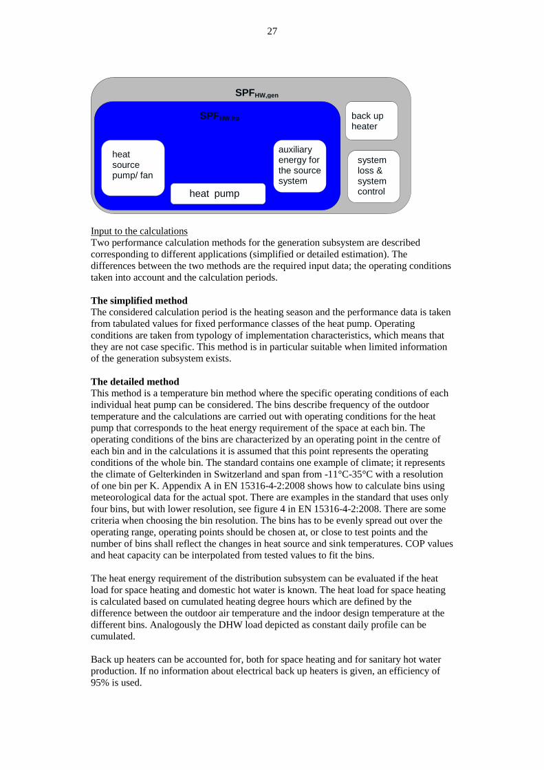
Input to the calculations

Two performance calculation methods for the generation subsystem are described

corresponding to different applications (simplified or detailed estimation). The

differences between the two methods are the required input data; the operating conditions

taken into account and the calculation periods.

The simplified method

The considered calculation period is the heating season and the performance data is taken

from tabulated values for fixed performance classes of the heat pump. Operating

conditions are taken from typology of implementation characteristics, which means that

they are not case specific. This method is in particular suitable when limited information

of the generation subsystem exists.

The detailed method

This method is a temperature bin method where the specific operating conditions of each

individual heat pump can be considered. The bins describe frequency of the outdoor

temperature and the calculations are carried out with operating conditions for the heat

pump that corresponds to the heat energy requirement of the space at each bin. The

operating conditions of the bins are characterized by an operating point in the centre of

each bin and in the calculations it is assumed that this point represents the operating

conditions of the whole bin. The standard contains one example of climate; it represents

the climate of Gelterkinden in Switzerland and span from -11°C-35°C with a resolution

of one bin per K. Appendix A in EN 15316-4-2:2008 shows how to calculate bins using

meteorological data for the actual spot. There are examples in the standard that uses only

four bins, but with lower resolution, see figure 4 in EN 15316-4-2:2008. There are some

criteria when choosing the bin resolution. The bins has to be evenly spread out over the

operating range, operating points should be chosen at, or close to test points and the

number of bins shall reflect the changes in heat source and sink temperatures. COP values

and heat capacity can be interpolated from tested values to fit the bins.

The heat energy requirement of the distribution subsystem can be evaluated if the heat

load for space heating and domestic hot water is known. The heat load for space heating

is calculated based on cumulated heating degree hours which are defined by the

difference between the outdoor air temperature and the indoor design temperature at the

different bins. Analogously the DHW load depicted as constant daily profile can be

cumulated.

Back up heaters can be accounted for, both for space heating and for sanitary hot water

production. If no information about electrical back up heaters is given, an efficiency of

95% is used.

SPFHW,gen

system loss & system control

SPFHW,hp back up heater

heat pump

heat source pump/ fan

auxiliary energy for the source system

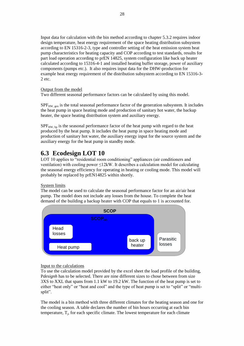
28

Input data for calculation with the bin method according to chapter 5.3.2 requires indoor

design temperature, heat energy requirement of the space heating distribution subsystem

according to EN 15316-2-3, type and controller setting of the heat emission system heat

pump characteristics for heating capacity and COP according to test standards, results for

part load operation according to prEN 14825, system configuration like back up heater

calculated according to 15316-4-1 and installed heating buffer storage, power of auxiliary

components (pumps etc.). It also requires input data for the DHW-production for

example heat energy requirement of the distribution subsystem according to EN 15316-3-

2 etc.

Output from the model

Two different seasonal performance factors can be calculated by using this model.

SPFHW, gen is the total seasonal performance factor of the generation subsystem. It includes

the heat pump in space heating mode and production of sanitary hot water, the backup

heater, the space heating distribution system and auxiliary energy.

SPFHW, hp is the seasonal performance factor of the heat pump with regard to the heat

produced by the heat pump. It includes the heat pump in space heating mode and

production of sanitary hot water, the auxiliary energy input for the source system and the

auxiliary energy for the heat pump in standby mode.

6.3 Ecodesign LOT 10 LOT 10 applies to “residential room conditioning” appliances (air conditioners and

ventilation) with cooling power ≤12kW. It describes a calculation model for calculating

the seasonal energy efficiency for operating in heating or cooling mode. This model will

probably be replaced by prEN14825 within shortly.

System limits

The model can be used to calculate the seasonal performance factor for an air/air heat

pump. The model does not include any losses from the house. To complete the heat

demand of the building a backup heater with COP that equals to 1 is accounted for.


To use the calculation model provided by the excel sheet the load profile of the building,

Pdesignh has to be selected. There are nine different sizes to chose between from size

3XS to XXL that spans from 1.1 kW to 19.2 kW. The function of the heat pump is set to

either “heat only” or “heat and cool” and the type of heat pump is set to “split” or “multi-

split”.

The model is a bin method with three different climates for the heating season and one for

the cooling season. A table declares the number of bin hours occurring at each bin

temperature, Tj, for each specific climate. The lowest temperature for each climate

SCOP

Parasitic losses

SCOPon

back up heater Heat pump

Head losses

29

respectively is declared the design temperature, Tdesign. The part load ratio (of the

building), plj, is calculated from the equation below:

The reference annual heating demand, QHE is decided in kWh for each climate as a

product of Pdesignh and the number of full load heating hours that corresponds to each

climate.

Load fractions fracA, fracC and fracW indicate the fraction of the total heating demand

(load) occurring in a specific bin at a specific climate. The fractions are given by:

Input to the calculations is the COP and capacity of the heat pump at four-five different

temperature levels +12°C, +7°C, +2°C, -7°C and -15°C(-15°C is only required for the

colder climate). The heat pump should be tested at part load to deliver the required heat

load of the building at each temperature level. At this point the paper version is not

consistent. In one way it says that the capacity of the heat pump at each bin shall

complete the energy demand of the building at the part load declared by the product of

the annual reference heating demand, QHe, and fracj, but in one way it says that the energy

demand is declared by the product of the part load ratio, Plj, and Pdesign. However the

excel sheet uses the first alternative and therefore care should be taken when deciding the

operating points (the required effect at each temperature bin) for testing the heat pump.

This alternative does not provide any effect balances. Since one house is chosen for the

calculations the required effect at each outdoor temperature should be the same among

the climates, but this is not the case.

In cases where the heating power supplied by the heat pump is not enough to cover the

energy demand of the building in a specific bin, the difference is filled up by a backup

heater with a declared capacity of COP=1. Deciding the part load from the product of

QHe, and fracj, might result in an underestimated effect demand and therefore

underestimate the required backup heating.

Instructions of how the heat pump shall be tested are given in the method for each type of

operation respectively; fixed capacity units, staged capacity units and variable speed

capacity units.

A degradation factor Cd, which is the efficiency loss per kW of output power when

cycling the heat pump, is decided from a specific cycling test.

The energy consumption for the heat pump when operating in thermostat off mode, off

mode and crankcase heater mode is decided in tests, but is only required for the

calculation of SCOP.

The turndown ratio for heating, which is the lowest steady state over the maximum power

and the binlimit, which is the lowest operating temperature of the heat pump, is used as

input to both of the SCOP calculations.


This model is used to calculate two different seasonal performance factors:

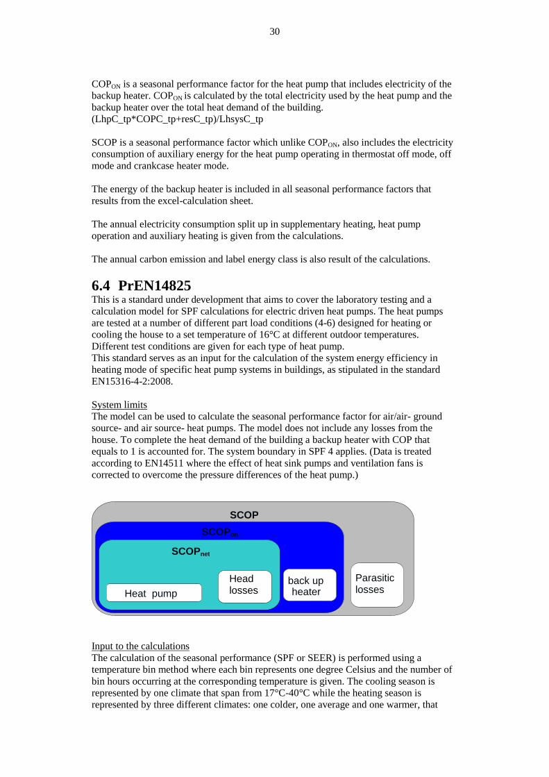
30

COPON is a seasonal performance factor for the heat pump that includes electricity of the

backup heater. COPON is calculated by the total electricity used by the heat pump and the

backup heater over the total heat demand of the building.

(LhpC_tp*COPC_tp+resC_tp)/LhsysC_tp

SCOP is a seasonal performance factor which unlike COPON, also includes the electricity

consumption of auxiliary energy for the heat pump operating in thermostat off mode, off

mode and crankcase heater mode.

The energy of the backup heater is included in all seasonal performance factors that

results from the excel-calculation sheet.

The annual electricity consumption split up in supplementary heating, heat pump

operation and auxiliary heating is given from the calculations.

The annual carbon emission and label energy class is also result of the calculations.

6.4 PrEN14825 This is a standard under development that aims to cover the laboratory testing and a

calculation model for SPF calculations for electric driven heat pumps. The heat pumps

are tested at a number of different part load conditions (4-6) designed for heating or

cooling the house to a set temperature of 16°C at different outdoor temperatures.

Different test conditions are given for each type of heat pump.

This standard serves as an input for the calculation of the system energy efficiency in

heating mode of specific heat pump systems in buildings, as stipulated in the standard

EN15316-4-2:2008.

System limits

The model can be used to calculate the seasonal performance factor for air/air- ground

source- and air source- heat pumps. The model does not include any losses from the

house. To complete the heat demand of the building a backup heater with COP that

equals to 1 is accounted for. The system boundary in SPF 4 applies. (Data is treated

according to EN14511 where the effect of heat sink pumps and ventilation fans is

corrected to overcome the pressure differences of the heat pump.)


The calculation of the seasonal performance (SPF or SEER) is performed using a

temperature bin method where each bin represents one degree Celsius and the number of

bin hours occurring at the corresponding temperature is given. The cooling season is

represented by one climate that span from 17°C-40°C while the heating season is

represented by three different climates: one colder, one average and one warmer, that

SCOP

Parasitic losses

SCOPon

back up heater

SCOPnet

Heat pump

Head losses

31

span from -30°C-15°C, see Table 29 and 30 in prEN 14825:2009 draft Nov 09. Each

climate corresponds to one design temperature and one design heat load of the building.

The heating/cooling demand and the number of bin hours for the different climates are

determined as templates, taking different aspects into account; the climate, type of

building and building characteristics, set point and set back settings and internal gains.

Those aspects also decide the number of hours in which the heat pump works in active

mode, thermostat off mode, standby mode, crankcase heater mode or off mode. The

electricity consumptions at the different modes are determined from tests. These effects

are called the parasitic losses.

Input to the calculations is the COP and capacity of the heat pump tested at four-five

different temperature levels +12°C, +7°C, +2°C, -7°C and -15°C (-15°C is only required

for the colder climate). The heat pump shall be tested in equivalence with standard EN

14511:2007, with the same test methods, test set up, uncertainty of measurements and the

way of evaluating data. The heat pump shall be tested at part load to deliver the required

heat load of the building at each temperature level. Instructions of how the heat pump

shall be tested by means of part load and type of operation; fixed capacity units, staged

capacity units and variable speed capacity units, are given in this method.

The required part load for the building at the test points are given by:

Where Tj is the outdoor (bin) temperature and Tdesign is the lower temperature limit of the

selected climate.

If the declared capacities of a unit matching with the required heating/ cooling demand

the corresponding COP/EER value is to be used. This may occur with staged capacity or

variable speed capacity units. If the declared capacity is higher than the heating/cooling

loads, the unit has to cycle on/off. Then a degradation factor (Cd (air/air or Water/air) or

Cc (others)) has to be used to calculate the corresponding COP/EER values. Cd and Cc

can be determined by testing; else a default value of 0.25 and 0.9 respectively is used.

The bivalent temperature, which is the lowest temperature when the heat pump can

deliver 100% of the heat demand of the building, is necessary to use the excel sheet. The

design heat demand of the building is a consequence of the stated bivalent temperature.

The reference annual heating demand, kWh/a, is given by the product of the full load in

heating Pdesign and the equivalent number of heating hours.

The operation limit of the heat pump is set to the lower temperature limit for which the

heat pump can operate.


With above input the excel sheet gives two different SCOP: SCOPNET and SCOPON.

SCOPNET is the seasonal performance factor for the heat pump, while SCOPON also

includes the electricity and heat delivered to the building from a backup heater.

The paper version of the standard also calculates a seasonal performance factor, SCOP

that includes the parasitic losses of the heat pump. The effect from each operational mode

is tested according to the standard while the corresponding operational hours for each

mode respectively are found in a reference table.

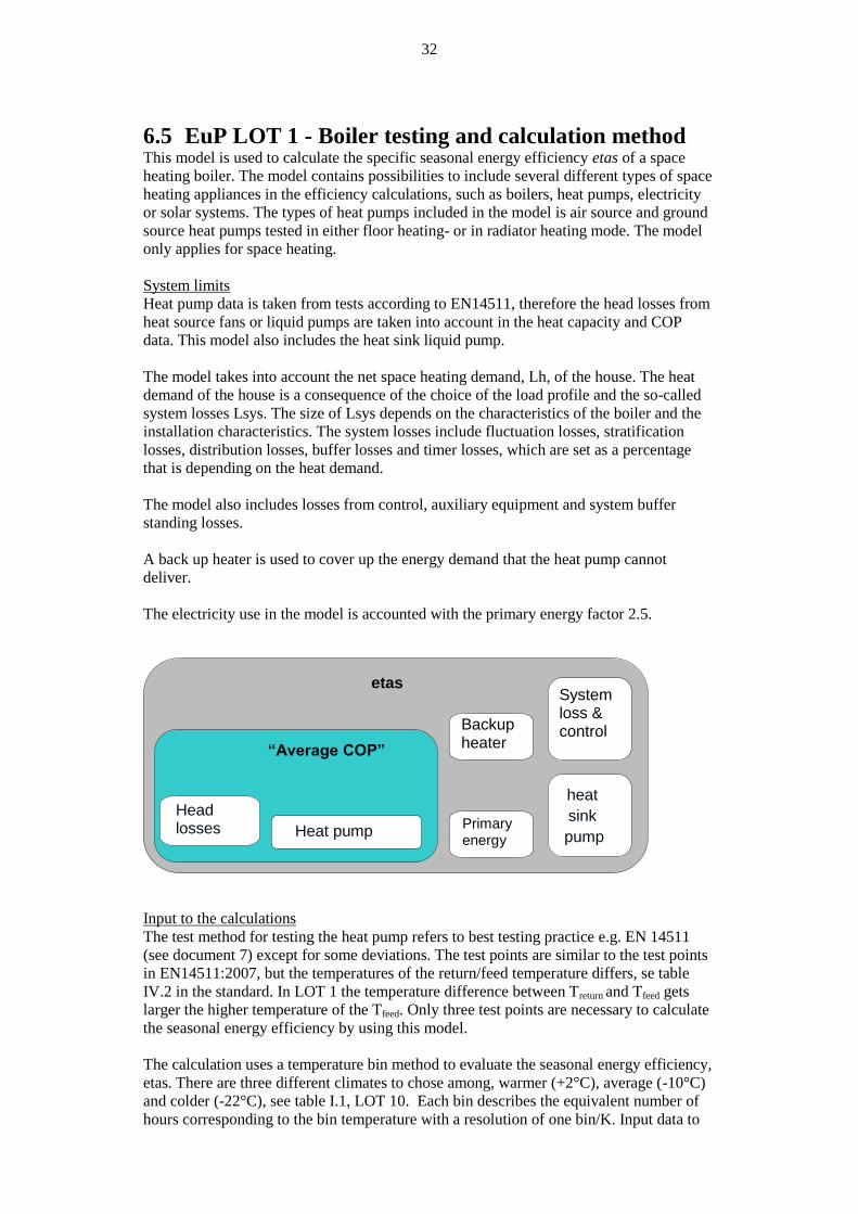
32

6.5 EuP LOT 1 - Boiler testing and calculation method This model is used to calculate the specific seasonal energy efficiency etas of a space

heating boiler. The model contains possibilities to include several different types of space

heating appliances in the efficiency calculations, such as boilers, heat pumps, electricity

or solar systems. The types of heat pumps included in the model is air source and ground

source heat pumps tested in either floor heating- or in radiator heating mode. The model

only applies for space heating.

System limits

Heat pump data is taken from tests according to EN14511, therefore the head losses from

heat source fans or liquid pumps are taken into account in the heat capacity and COP

data. This model also includes the heat sink liquid pump.

The model takes into account the net space heating demand, Lh, of the house. The heat

demand of the house is a consequence of the choice of the load profile and the so-called

system losses Lsys. The size of Lsys depends on the characteristics of the boiler and the

installation characteristics. The system losses include fluctuation losses, stratification

losses, distribution losses, buffer losses and timer losses, which are set as a percentage

that is depending on the heat demand.

The model also includes losses from control, auxiliary equipment and system buffer

standing losses.

A back up heater is used to cover up the energy demand that the heat pump cannot

deliver.

The electricity use in the model is accounted with the primary energy factor 2.5.


The test method for testing the heat pump refers to best testing practice e.g. EN 14511

(see document 7) except for some deviations. The test points are similar to the test points

in EN14511:2007, but the temperatures of the return/feed temperature differs, se table

IV.2 in the standard. In LOT 1 the temperature difference between Treturn and Tfeed gets

larger the higher temperature of the Tfeed. Only three test points are necessary to calculate

the seasonal energy efficiency by using this model.

The calculation uses a temperature bin method to evaluate the seasonal energy efficiency,

etas. There are three different climates to chose among, warmer (+2°C), average (-10°C)

and colder (-22°C), see table I.1, LOT 10. Each bin describes the equivalent number of

hours corresponding to the bin temperature with a resolution of one bin/K. Input data to

etas

heat

sink

pump

“Average COP”

Heat pump

Head losses

Backup heater

System loss & control

Primary energy

33

the calculations can be either the test points given in this method or test points given in

EN 14511.

The maximum heating capacity, Pmax, at the different climates is calculated from the

heating capacity data obtained in the test. It is not possible to choose the size of the

required heat load for the building, but is given by the model for each bin level based on

the capacity of the heat pump. To meet the lower heat load requirements at the different

bin levels, the heat pump is assumed to work in part load condition. The heat pump does

not have to be tested in part load operation; instead the model uses a degradation factor,

Cd, to calculate the COP when working in part load condition. Cd can either be obtained

from tests or a default value, Cd=0.15, can be used.

For fixed capacity units the default is COPmin= 0.89*COP at power output

Phpmin=0.5*Php.

For staged capacity units the default is COPmin= 0.975*COP at power output

Phpmin=0.5*Php.

For variable capacity units the default is COPmin= COP at power output

Phpmin=0.4*Php.

It is optional to choose whether the heat pump operates with night set back or not. The

bin assumes constant night temperatures during night set back to +1°C, +6°C and 0°C for

each climate respectively.

Other inputs to the calculations is type of heat pump, type of operation of the heat pump,

type of control of the heat pump, type of heating (floor heating or radiator heating),

minimum source operating temperature, the effect of auxiliary equipment and backup

electricity heater.

Other possible energy sources can also be chosen, but this chapter only treats the heat

pumps.

Output from the calculations

The model calculates the energy use and losses based upon constant fractions. The

fraction of the energy use and the different losses is displayed by the model. A diagram

shows the energy supply per temperature bin and how it is covered from different energy

sources. The seasonal energy efficiency, etas, is calculated.

Etas = Lh/Qtot+cctrl where Qtot=Lh + Lsys + Qgen + Qel

etas is the net space heating demand of the house over the sum of the generated heat of

the system. Qtot is the sum of the space heating demand (Lh), the losses from the heating

system (Lsys), the primary energy losses of the energy input to the system (Qgen) and the

energy needed by the auxiliary equipment such as control and heat sink pumps (Qel).

All electricity used by the heat pump and the backup heater is multiplied by a primary

energy factor of 2.5. The model is not transparent. It is tricky to follow the outputs of the

model since it consists from several excel-sheets and the information turns up all over. It

is also difficult to understand all steps of the calculations. To be able to compare the

results with field measurements and prEN14825 a value of SPF, the so called “average

COP” (see the system boundaries) is calculated without the system losses. Average COP

corresponds to SCOPnet in prEN14825.

34

6.6 SP-method A3 528 SPA3 528 is a calculation program that is used to calculate the seasonal performance

factor and energy saving over the year for houses having a defined heating requirement. It

can be used for air/air heat pumps, air source heat pumps and ground source heat pumps.

The heat loss from the house is defined in the program and given as the total loss factor,

k-value, of the house [W/K]. The method can be used to calculate the energy requirement

of a building with a k-value of either 109 W/K or 199W/K. A duration diagram of the

outdoor temperature can be calculated from the mean annual temperature and together

with the loss factor, the area under the duration curve gives the actual power requirement.

The heat pump is tested in accordance to EN 14511 at outdoor temperatures of -15°C, -

7°C, +2°C and +7°C with an indoor temperature of +20°C. The heat pump is also tested

in part load conditions according to CEN/TS 14825 at +7°C (75% and 50%) and at +2°C

(50%). The lowest ambient temperature is assumed to be -15 °C and no heating is

assumed to be required for ambient temperatures above +17 °C. The output data from the

tests, thermal heat capacity and electrical input power, is used as input to the calculations.

35

7 Strengths and weaknesses with current methods

7.1 prEN14825 Strenghts

A strength of standard prEN14825 is that it includes all kinds of heat pumps (except

exhaust air heat pumps). The model treats heat pumps both in heating and cooling

operation. The fact that the heat pump is tested in exactly part load should result in more

sufficient results compared to degradation coefficient etc. The model is foreseeable and

quite easy to follow.

Weakness

The model is not completely clear with its definitions of part loads. The part load ratio for

which the heat pump is to be tested is the part load energy demand of the building at the

corresponding temperature bin. To perform the SPF calculations according to prEN14825

the heat pump is tested at a certain climate (A,W or C) and a certain heat load profile for

the building. This means that the test data might not be suitable for another climate or

another heat load.

It is also not completely transparent since it describes (ANNEX C) the reference

heating/cooling demand and the number of hours in each operational mode (active mode,

thermostat off mode, standby and crankcase heater mode) is decided from weighted

climate, type of building, internal gains, set back setting and so on, but there is no

reference that describes the calculations. Therefore it is not possible to recalculate the

hours to fit specific needs. The climate hours that describes the temperature bins does not

seem to be adjusted in any ways since it is the same hours that is used in Ecodesign

LOT 1.

Another weakness is that the model does not include domestic hot water.

Possibility

The model could be developed so that it would be possible to decide the energy demand

of the house. It could also be a possibility to fit the model to your own climate. Maybe the

ground water temperature and thereby the bore hole temperature could be climate

depending.

It should be obvious how interpolations or extrapolations of capacity and/or COP should

be performed to avoid differences between users.

Risk

The performance of water/water heat pumps can be overestimated, especially at the cold

climate, since they are only tested at +10°C at the cold side (in reality the ground water

temperature can be lower than this). This can also be the case for other ground source

heat pumps.

The degradation coefficient Cc might be a disadvantage for a ground source heat pump

when default values are used. Cc =0.9 is a larger degradation of GSHP’s than what is

shown in reality. There is a risk that the requirement of having heat pumps tested in part

load might lead to extensive laboratory tests, which is costly. It is also difficult to get

sufficient data from existing laboratory tests, since few heat pumps are tested in part

loads.

36

7.2 EN 15316-4-2 Strength

This model is very wide and thorough in its content. It treats both room heating and tap

water production. The model is adaptable to different climates and the resolution of the

temperature bins can be chosen.

The model specifies the requirements and losses of the certain house and defines

recoverable respectively unrecoverable energy.

It is not necessary to test the heat pump at the part loads, since there are default values

that can be used.

The model can be used to calculate the SPF for the entire system with the building

included or only for the heat pump.

Weakness

The strengths of this model could also turn out to be its weaknesses. The wideness of the

model makes it complicated and twisty. There are too many aspects that are taken into

account in the calculations. The standard refers to several other standards for calculations

of losses and needs. The model requires large knowledge of the house.

The fact that default values can be used to calculate the operation in part load for the heat

pumps can result in lower accurateness of the model.

The model does not treat operation in cooling mode.

Possibility

The model can be studied and give input to a new easier model.

Risk

There is a present danger of doing mistakes when using the model. The large amount of

data that is taken into account will probably result in much estimation that will differ

from case to case and will therefore result in incomparable outcome of the model. Also

the same heat pump installation can probably give different results depending on the way

it is calculated, (choosing method, input, accuracy and test points).

7.3 EuP LOT 1 In general, the Energy Using Products (EuP) Directive have broadened to include also

Energy Related Products (ErP), but for the treatment in this report, we choose to use the

term EuP, since heat pumps are energy using.

Strength

Test data from EN 14511 can be used in the calculations. The model provides default

values to recalculate the test points to fit the part load of the heat pump for the different

kinds of heat pumps (fixed capacity, staged capacity och variable capacity). The capacity

and corresponding COP values are then interpolated between the temperature bins.

However, the accurateness of the recalculation is unknown.

The model itself has suggested test points with a radiator curve (supply temperature) that

is adjusted to the outdoor temperature. At colder outdoor temperatures the supply

temperature is higher and at warmer outdoor temperatures the supply temperatures are

lower.

37

The model can be used to calculate how to cover the energy need of the house by using

different techniques, for example solar cells, heat pumps and fossil fuel. This is a good

thought, but might not be interesting in this project (?).

Weakness

Unfortunately the model still contains bugs and technical mistakes in the equations and

the way of thinking. It seems to be adjusted to boilers and bio boilers instead of heat

pumps.

The model does not include a power balance, but is doing a temperature balance instead.

This makes the distribution of the energy need and the required amounts of backup heat

differ from the theoretical needed.

The model includes a decided fraction of heat loss that cannot be escaped from. For

example if the heat pump does not use night set back a default penalty loss of 12% from

the total delivered energy is subtracted. The losses from the apparatus and system

operation are also decided in percentages.

At part load operation there is no change in the system flows. This does not seem right

with controlled radiators. (Should the radiators be controlled or is it enough with a

displacement/adjustment of the radiator curve?)

The night set back function uses the same night temperature all year around, which is not

the case in reality.

It is not possible to choose the energy requirement of the house; instead the energy

demand is an outcome of the capacity of the heat pump. If the heat pump is not

monovalent also the fraction of backup heat is needed to decide the energy demand of the

house.

GSHP’s are treated unfairly when recalculating the operation data to part load operation.

The ground source heat pumps are degraded by a factor 0.89 at 50 % of the delivered

capacity. (The Cd factor, i.e. the on/off control, is overestimated for water borne systems)

Even though the program is transparent in the sense that all equations are reported in the

model, it is very hard to understand and follow the calculations, and the program cannot

be said to be transparent in the general sense. The interface of the program is not very

friendly and can easily confuse the user. The model does not include tap water.

Possibility

Making the ground water and borehole temperature climate dependent might lead to

results more sufficient to its actual installation spot.

Risk

The model is not adjusted to fit heat pumps and is disadvantaging heat pumps. Despite

this the COP and capacity of water to water heat pumps can be overestimated since they

are tested at +10°C at the cold side (this can also happen to ground source heat pumps,

but probably not to the same extent).

7.4 EuP LOT 10 Strength

This model can be used both in heating and cooling mode and it has three different

climates both for the cooling season and the heating season. The model has reference

heating/cooling demands to choose between.

38

Weakness

The model takes only air to air heat pumps into account. In accordance to prEN14825 the

test points for the heat pump has to be chosen specifically to fit the chosen climate and

heat profile of the house.

In accordance to LOT 1 the model does not include an effect balance at each temperature

bin. This results in that the heat demand of a house at a specific temperature bin is

different at different climates and that the heat requirement of a backup heater is

misleading.

The model does not seem to be entirely consistent, partly it is contradicting itself.

Possibility

To make the model usable at other spots it would be better to make it possible to use

other climates. Now the model only provides a number of specified heat loads of the

house. It would be useful to be able to freely choose the heat demand of the house. There

is a risk though, that since the heat pump has to be tested in part load, it has to be tested at

each specific heat requirement.

Other types of heat pumps could be included in the model. The model only provides the

SPF (SCOP) with the backup heater included. For comparable reasons, it would be useful

to include a SPF with backup heater excluded.

Risk

It is not obvious whether the excel model is compatible with the standard. There are also

some calculations in the standard that seems to be incorrect.

39

8 Comparison of existing calculation methods and

results from field measurements

8.1 Heat (and cooling-) demand of the house

This study is focused on heat pumps for indoor heating. The study is made in houses with

different heat demand. The ground source heat pumps in this study are considered

monovalent, but it is difficult to determine the actual energy demand of the house. When

using the calculation models the required heat load of the house is decided by the capacity

of the heat pump.

The studied air to air heat pump is not monovalent. The energy demand of the house with

the heat pump installation was estimated in the field study. When using the calculation

models the energy demand of the house were tried to be the same as in the field study.

8.2 Indoor climate

The indoor climate is expected to reach 20°C for all models. In the calculation models the

heat pump is used to reach a temperature of 16°C. Internal gains are expected to

contribute to the last temperature increase.

The actual indoor temperature has not been measured in the Fraunhofer field

measurements. Thereby it is not possible to compare the real indoor temperatures with the

temperatures estimated in the calculation models.

8.3 Outdoor climate

The outdoor climate follows the climate of the year. The calculation models use the same

temperature climate when calculating SPF for the ground source heat pumps. The climate

corresponds to a European average climate, Strasbourg, with the coldest temperature of -

10°C.

The field measurements of the ground source heat pumps are carried out in Germany. The

heat pumps installations used for the SPF calculations are spread over the country, from

the Hamburg area in the north to Stuttgart in the south. In the calculation models the

average climate is chosen as the climate mostly corresponding to the German.

The air to air heat pump installation is made in a climate that is similar to the “colder”

climate. Therefore the colder climate is used in the calculation models when calculating

SPF for the air to air heat pump.

8.4 Definition of SPF field measurement system

boundaries

In the ongoing EU project “SEPEMO-Build (SEPEMO short)” four SPF’s with different

system boundaries are defined. The definitions from the SEPEMO project have been used

for calculating the SPF for the field measurements. The four defined SPF’s are:

SPF1 includes only the heat pump unit itself. Thereby SPF1 is identical to the average

COP for the measured period.

40

hpHW

hpWhpH

HE

QQSPF

_

__

1

SPF2 consist of the heat pump unit and the equipment needed to make the heat source

available the heat pump.

hpHWpumpfanS

hpWhpH

HEE

QQSPF

_/_

__

2

SPF3 represents the heat pump system SPF. SPF3 includes the heat pump and the heat

source pump as in SPF2, but also the back up heater.

buHWhpHWpumpfanS

buHWhpWhpH

HEEE

QQQSPF

__/_

___

3

SPF4 includes all parts relates to SPF3, additionally SPF4 also includes the distribution of

the heat.

pumpfanBbuHWpumpbthpHWpumpfanS

buDHWbuHWhpWhpH

HEEEEE

QQQQSPF

/____/_

____

4

SPF4

SPF3

SPF2

Back up heater

Heat source

pump/fan

SPF1

Heat pump

Heat sink pump/fan

Figure 6 System boundaries for calculations of SPF

SPF1 is normally measured on the brine/water sides of the evaporator/condenser, but it

could also be measured directly in the refrigeration loop with e.g. the Climacheck

equipment [10]. This requires measurement of the pressure and temperature of the

refrigerant. This methodology is very efficient if the status/condition or diagnosis of the

heat pump is to be evaluated, but generally in domestic heat pumps, the measurement is

not easy to carry out since measurement sockets are not generally installed.

8.5 Calculation of SPF

In this study SPF is calculated for three of the four different system boundaries and

categories by using data from the field measurements. The system boundaries used are

SPF2, SPF3 and SPF4 and are described in section 8.4. The categories are “heating only”,

“heating and domestic hot water production” and “domestic hot water production”.

41

For facilities where the installed heat pump also is tested in a laboratory, the laboratory

test results are used to calculate SPF by using the calculation models. This is the case for

seven different ground source heat pumps and one air to air heat pump.

This chapter will explain how the calculations are performed and what assumptions are

made for the different models.

Field measurements

Ground source heat pumps

All analyzed heat pump systems are installed in German single family houses with floor

heating. The heat pump is more or less monovalent, only a very small amount of backup

heat has been used during the year of measurements. The heat pumps in the study were all

installed in new built houses during the years 2004-2008. The data used for the SPF

calculations are based on field measurements carried out during one year, with one

exception the SPF for site no. 1 is based on data measured from January to August.

The calculations of SPF’s are based on the field measurements data from the Fraunhofer

study. In the data we have received from the Fraunhofer study the total energy

consumption for the heat pump system and its components is presented as well as the

energy consumption divided into energy used for space heating and energy used for

production of domestic hot water.

In this project we have not been able to evaluate exactly how these allocations have been

made. For some of the studied installation sites a part (up to 20%) of the total electricity

consumption has been allocated neither to space heating nor to the domestic hot water

production. This is mainly the case for the electricity consumption. For the heat produced

no energy gap is seen between the total energy production and the energy divided into

space heating and domestic hot water.

The calculated SPF’s in the study are based on the energy allocated to the space heating

only, this in order to make the results comparable to the results from the calculation

models in prEN14825 and Lot 1, which not include the production of domestic hot water.

Air to air heat pumps

The field measurement of the air to air heat pumps is carried out in single family houses

located in the Borås area of Sweden. All houses in the study have electricity driven

radiators for back up heating. The field measurements are based on SP method 1721.

From the field measurements SPF2 and SPF3 has been calculated as described below.

The electricity consumed by the heat pump, WHP, is measured continually while the

produced space heating is measured at five “performance tests” done at different outdoor

temperatures. During the performance tests the heating capacity of the heat pump is

measured during stable conditions and is thereby not including any defrost period.

Therefore the calculated COP for each test point is based on data from only a part of the

operating cycle.

The total amount of heat produced during the total measuring period needs to be

calculated based on the five performance tests. The calculations are made as follows:

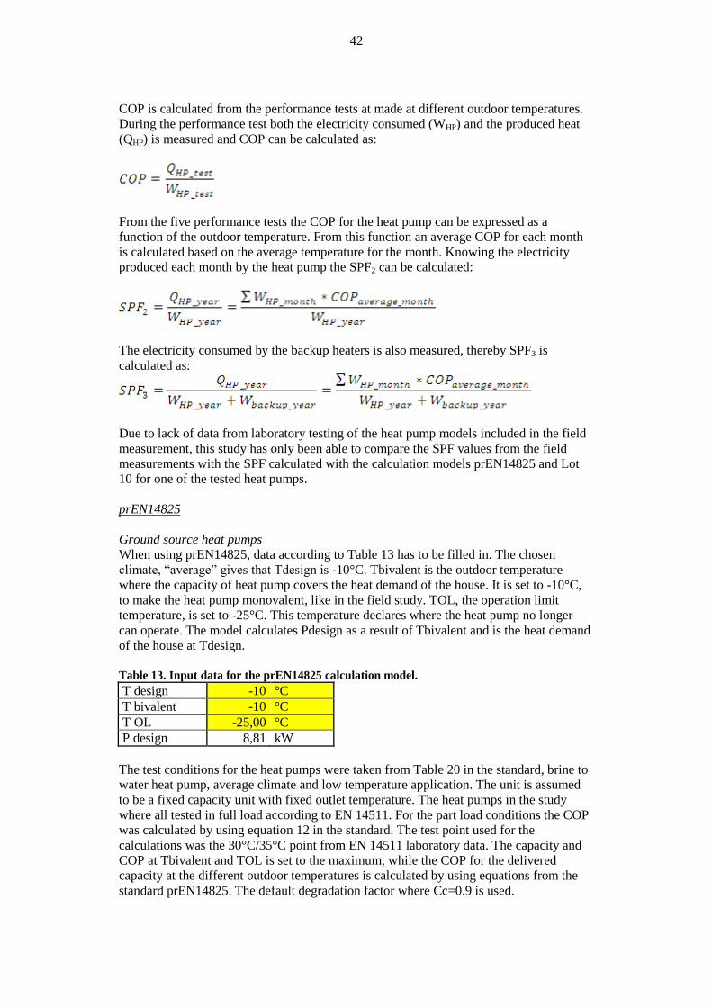
42

COP is calculated from the performance tests at made at different outdoor temperatures.

During the performance test both the electricity consumed (WHP) and the produced heat

(QHP) is measured and COP can be calculated as:

From the five performance tests the COP for the heat pump can be expressed as a

function of the outdoor temperature. From this function an average COP for each month

is calculated based on the average temperature for the month. Knowing the electricity

produced each month by the heat pump the SPF2 can be calculated:

The electricity consumed by the backup heaters is also measured, thereby SPF3 is

calculated as:

Due to lack of data from laboratory testing of the heat pump models included in the field

measurement, this study has only been able to compare the SPF values from the field

measurements with the SPF calculated with the calculation models prEN14825 and Lot

10 for one of the tested heat pumps.

prEN14825


When using prEN14825, data according to Table 13 has to be filled in. The chosen

climate, “average” gives that Tdesign is -10°C. Tbivalent is the outdoor temperature

where the capacity of heat pump covers the heat demand of the house. It is set to -10°C,

to make the heat pump monovalent, like in the field study. TOL, the operation limit

temperature, is set to -25°C. This temperature declares where the heat pump no longer

can operate. The model calculates Pdesign as a result of Tbivalent and is the heat demand

of the house at Tdesign.

Table 13. Input data for the prEN14825 calculation model.

T design -10 °C

T bivalent -10 °C

T OL -25,00 °C

P design 8,81 kW

The test conditions for the heat pumps were taken from Table 20 in the standard, brine to

water heat pump, average climate and low temperature application. The unit is assumed

to be a fixed capacity unit with fixed outlet temperature. The heat pumps in the study

where all tested in full load according to EN 14511. For the part load conditions the COP

was calculated by using equation 12 in the standard. The test point used for the

calculations was the 30°C/35°C point from EN 14511 laboratory data. The capacity and

COP at Tbivalent and TOL is set to the maximum, while the COP for the delivered

capacity at the different outdoor temperatures is calculated by using equations from the

standard prEN14825. The default degradation factor where Cc=0.9 is used.

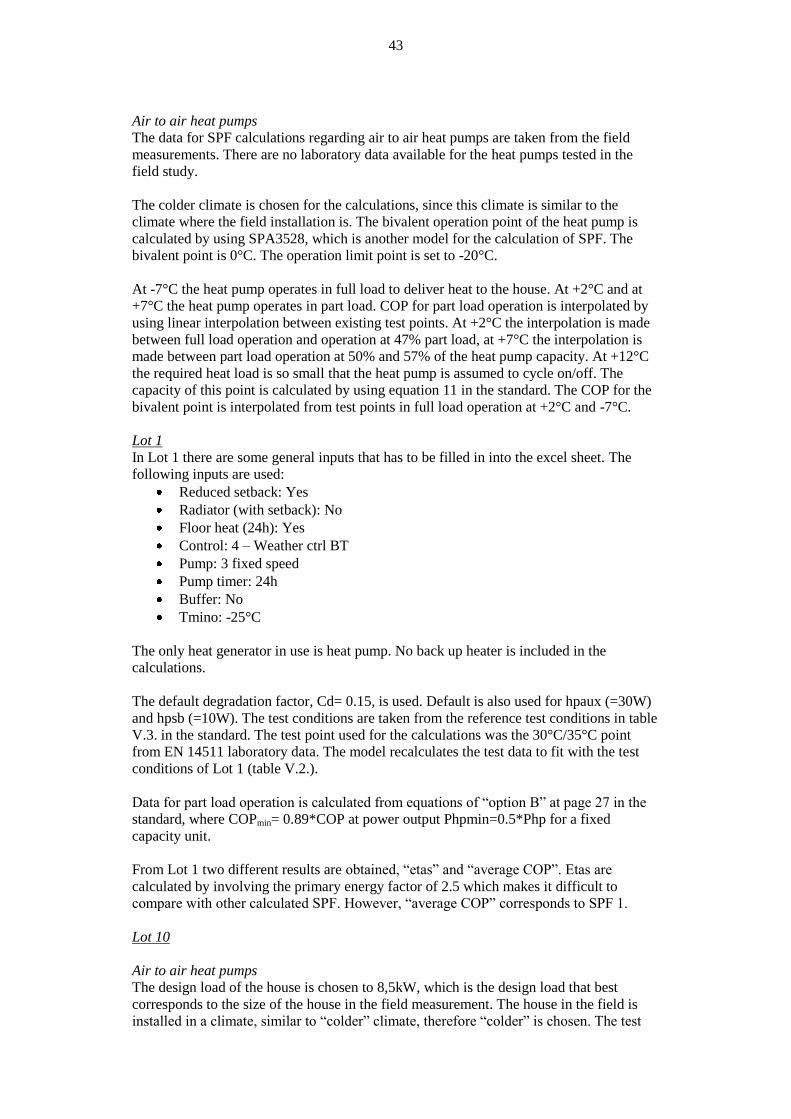
43


The data for SPF calculations regarding air to air heat pumps are taken from the field

measurements. There are no laboratory data available for the heat pumps tested in the

field study.

The colder climate is chosen for the calculations, since this climate is similar to the

climate where the field installation is. The bivalent operation point of the heat pump is

calculated by using SPA3528, which is another model for the calculation of SPF. The

bivalent point is 0°C. The operation limit point is set to -20°C.

At -7°C the heat pump operates in full load to deliver heat to the house. At +2°C and at

+7°C the heat pump operates in part load. COP for part load operation is interpolated by

using linear interpolation between existing test points. At +2°C the interpolation is made

between full load operation and operation at 47% part load, at +7°C the interpolation is

made between part load operation at 50% and 57% of the heat pump capacity. At +12°C

the required heat load is so small that the heat pump is assumed to cycle on/off. The

capacity of this point is calculated by using equation 11 in the standard. The COP for the

bivalent point is interpolated from test points in full load operation at +2°C and -7°C.

Lot 1

In Lot 1 there are some general inputs that has to be filled in into the excel sheet. The

following inputs are used:

Reduced setback: Yes

Radiator (with setback): No

Floor heat (24h): Yes

Control: 4 – Weather ctrl BT

Pump: 3 fixed speed

Pump timer: 24h

Buffer: No

Tmino: -25°C

The only heat generator in use is heat pump. No back up heater is included in the

calculations.

The default degradation factor, Cd= 0.15, is used. Default is also used for hpaux (=30W)

and hpsb (=10W). The test conditions are taken from the reference test conditions in table

V.3. in the standard. The test point used for the calculations was the 30°C/35°C point

from EN 14511 laboratory data. The model recalculates the test data to fit with the test

conditions of Lot 1 (table V.2.).

Data for part load operation is calculated from equations of “option B” at page 27 in the

standard, where COPmin= 0.89*COP at power output Phpmin=0.5*Php for a fixed

capacity unit.

From Lot 1 two different results are obtained, “etas” and “average COP”. Etas are

calculated by involving the primary energy factor of 2.5 which makes it difficult to

compare with other calculated SPF. However, “average COP” corresponds to SPF 1.

Lot 10


The design load of the house is chosen to 8,5kW, which is the design load that best

corresponds to the size of the house in the field measurement. The house in the field is

installed in a climate, similar to “colder” climate, therefore “colder” is chosen. The test

44

points for the calculation are given in a table at page 24 in LOT 10 Annex II. The heat

pump is tested according to EN 14511 and CEN/TS 14825 for part load conditions.

The heat pump is a variable capacity heat pump, but since the heat pump is not tested at

exactly the required heat effect (within ±3%), the calculations of COP has to be

performed in accordance with a staged capacity unit.

At -15°C and -7°C the delivered capacity from the heat pump is lower than the house

requires; capacity and COP data are taken from operation in full load at these outdoor

temperatures. An exception from the standard is made, since the standard proposes a

recalculation of the COP at those points. The recalculation does not seem to make sense

and is therefore ignored.

At +2°C and +7°C the heat delivered from the heat pump exceeds the required heat from

the house and is therefore operated in part load. COP for part load operation is

interpolated by using the equation for staged capacity units at page 26 in the standard. At

+2°C the interpolation is made between full load operation and operation at 47% part

load, at +7°C the interpolation is made between part load operation at 57% and 44% of

the heat pump capacity.

The heat pump is not tested at +12°C. Full load operation at +12°C is extrapolated from

test data at +7°C and +2°C. 50% part load is extrapolated from 50% part load operation at

+7°C and +2°C. COP for the required effect is extrapolated by using this data. Each

extrapolated COP value is corrected with a degradation factor of 0.975.

Default values are used for the degradation factor (Cd=0.1), turndown ratio heating

(=25%), thermostat off mode (50W), crankcase heater mode (=10W) and off mode

(=10W). The bin limit is set to -20°C.

8.6 Analysis of the results

The results from the SPF calculations of the different heat pump installations in field is

compared with the results obtained from the laboratory data used in calculation models.


Most of the heat pumps installed in field operates both in floor heating mode and

produces domestic hot water. The measurements include both kind of operations and the

results are presented in Table 14and Figure 7 below. SPF for domestic hot water

production is always lower compared to operation in heating mode. The energy balances

is not 100% complete for the field measurement, which is quite common in field

measurements, since heat losses are present, but cannot be measured directly as they can

be in the laboratory.

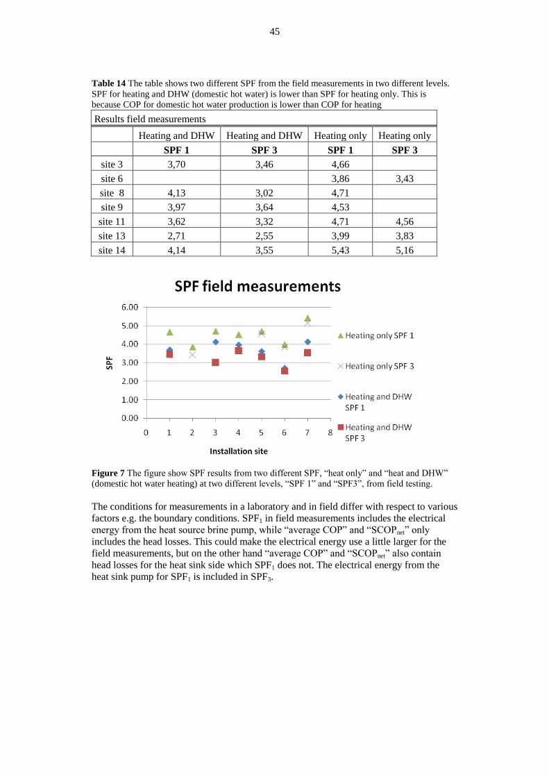
45

Table 14 The table shows two different SPF from the field measurements in two different levels.

SPF for heating and DHW (domestic hot water) is lower than SPF for heating only. This is

because COP for domestic hot water production is lower than COP for heating

Results field measurements

Heating and DHW Heating and DHW Heating only Heating only

SPF 1 SPF 3 SPF 1 SPF 3

site 3 3,70 3,46 4,66

site 6

3,86 3,43

site 8 4,13 3,02 4,71

site 9 3,97 3,64 4,53

site 11 3,62 3,32 4,71 4,56

site 13 2,71 2,55 3,99 3,83

site 14 4,14 3,55 5,43 5,16

Figure 7 The figure show SPF results from two different SPF, “heat only” and “heat and DHW”

(domestic hot water heating) at two different levels, “SPF 1” and “SPF3”, from field testing.

The conditions for measurements in a laboratory and in field differ with respect to various

factors e.g. the boundary conditions. SPF1 in field measurements includes the electrical

energy from the heat source brine pump, while “average COP” and “SCOPnet” only

includes the head losses. This could make the electrical energy use a little larger for the

field measurements, but on the other hand “average COP” and “SCOPnet” also contain

head losses for the heat sink side which SPF1 does not. The electrical energy from the

heat sink pump for SPF1 is included in SPF3.

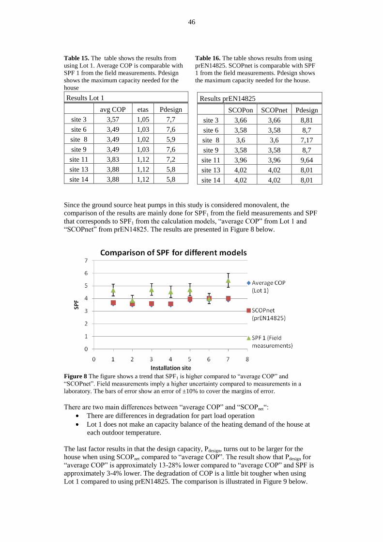
46

Table 15. The table shows the results from

using Lot 1. Average COP is comparable with

SPF 1 from the field measurements. Pdesign

shows the maximum capacity needed for the

house

Results Lot 1

avg COP etas Pdesign

site 3 3,57 1,05 7,7

site 6 3,49 1,03 7,6

site 8 3,49 1,02 5,9

site 9 3,49 1,03 7,6

site 11 3,83 1,12 7,2

site 13 3,88 1,12 5,8

site 14 3,88 1,12 5,8

Table 16. The table shows results from using

prEN14825. SCOPnet is comparable with SPF

1 from the field measurements. Pdesign shows

the maximum capacity needed for the house.

Results prEN14825

SCOPon SCOPnet Pdesign

site 3 3,66 3,66 8,81

site 6 3,58 3,58 8,7

site 8 3,6 3,6 7,17

site 9 3,58 3,58 8,7

site 11 3,96 3,96 9,64

site 13 4,02 4,02 8,01

site 14 4,02 4,02 8,01

Since the ground source heat pumps in this study is considered monovalent, the

comparison of the results are mainly done for SPF1 from the field measurements and SPF

that corresponds to SPF1 from the calculation models, “average COP” from Lot 1 and

“SCOPnet” from prEN14825. The results are presented in Figure 8 below.

Figure 8 The figure shows a trend that SPF1 is higher compared to “average COP” and

“SCOPnet”. Field measurements imply a higher uncertainty compared to measurements in a

laboratory. The bars of error show an error of ±10% to cover the margins of error.

There are two main differences between “average COP” and “SCOPnet“:

There are differences in degradation for part load operation

Lot 1 does not make an capacity balance of the heating demand of the house at

each outdoor temperature.

The last factor results in that the design capacity, Pdesign, turns out to be larger for the

house when using SCOPnet compared to “average COP”. The result show that Pdesign for

“average COP” is approximately 13-28% lower compared to “average COP” and SPF is

approximately 3-4% lower. The degradation of COP is a little bit tougher when using

Lot 1 compared to using prEN14825. The comparison is illustrated in Figure 9 below.

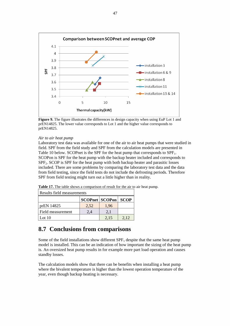
47

Figure 9. The figure illustrates the differences in design capacity when using EuP Lot 1 and

prEN14825. The lower value corresponds to Lot 1 and the higher value corresponds to

prEN14825.

Air to air heat pump

Laboratory test data was available for one of the air to air heat pumps that were studied in

field. SPF from the field study and SPF from the calculation models are presented in

Table 10 below. SCOPnet is the SPF for the heat pump that corresponds to SPF1.

SCOPon is SPF for the heat pump with the backup heater included and corresponds to

SPF2. SCOP is SPF for the heat pump with both backup heater and parasitic losses

included. There are some problems by comparing the laboratory test data and the data

from field testing, since the field tests do not include the defrosting periods. Therefore

SPF from field testing might turn out a little higher than in reality.

Table 17. The table shows a comparison of result for the air to air heat pump.

Results field measurements

SCOPnet SCOPon SCOP

prEN 14825 2,52 1,96

Field measurement 2,4 2,1

Lot 10

2,15 2,12

8.7 Conclusions from comparisons

Some of the field installations show different SPF1 despite that the same heat pump

model is installed. This can be an indication of how important the sizing of the heat pump

is. An oversized heat pump results in for example more part load operation and causes

standby losses.

The calculation models show that there can be benefits when installing a heat pump

where the bivalent temperature is higher than the lowest operation temperature of the

year, even though backup heating is necessary.

48

9 Requirements for a new calculation model to

evaluate SPF from lab measurements The requirements on a new calculation model differs defpending on the aim of the model.

In general, three different uses can be identified:

Based on lab data understand the consequences of technology choice in comparison with

competing heating technologies

To understand the consequences of correct sizing of the heat pump

To make a correct dimensioning of the heat pump in a specific house

It should also be possible to study three modes of operation, DHW production, heating or

combined DHW production and heating.

Based on the models, it should be possible to make comparisons of e.g. LCC and

environmental performance of different systems

What should be included/ not included in the model?

It should be possible to decide the energy demand of the house in the model,

either by given reference loads, or by choosing a specific energy demand of the

house. This should be separated into space heating and domestic hot water.

When the model itself calculates the losses of the house it can be misleading and

not sufficient for the actual house. This can be one boundary of the project.

Alternatively, typical houses are used in typical climates, both preset in the

model.

To take into account for the climate at the installation, generally accepted spot

climate data, for example Meteonorm data [9], Should be a part of the model.

The dynamics of the house can be a part of the model. The perceived temperature

of the house is not fully consistent with the actual outdoor temperature. At colder

temperature dips of for example -15°C, the house will not experience the real

outdoor temperature, but experiences a temperature of -12°C instead (due to

internal heat gains). Even the irradiance of the sun differs between the seasons

(and different spots). The energy demand of the house is affected from those

variances over the year, why it might be an idea to calculate the SPF over

monthly periods. Also the use of a fictive outdoor temperature would be an

alternative. The climate data can be adjusted (flattened out) depending on a

number of inputs, but a temperature dip is still needed in order to make a proper

effect dimensioning (this is dimensioning the entire system such as deep wells

etc.).

In a serious effort to evaluate dynamics, other factors have to e incorporated in a

model, such as form factor, impact of building weight, window area compared to

wall area, placement of windows, etc., which make such a model very complex.

For ground source heat pumps, the temperature of the ground is varying during

the year. The model should include a correction for this. This could be expressed

as a function where the ground source temperature is a function of the outdoor

temperature over the year.

The model should contain a radiator heat curve where requisite supply

temperature is calculated, an example of this can be found in the thesis of Fredrik

49

Karlsson [8]. At a colder outdoor temperature, the supply temperature should

peak; this makes the test scheme tables in EN 14511 deficient. Also other heat

distribution systems, such as under floor heating, and mixed systems should be

included in the model.

Part load performance of the heat pump must be properly taken into account, and

be based on relevant testing standards.

Night set back is a choice in some calculation models; this is not relevant for heat pumps

and should not be a part in a new calculation model.

Back up heaters is sometimes necessary to complete the energy demand of the

house. Back up heaters should be included in the calculation model.

Supplementary heating should be possible to choose between different sources of

supplementary heat, e.g. electricity, solar or biomass heating.

The possibility to include the production of domestic hot water to the SPF

calculations is also a necessity in future calculation models. It should also be

described how this shall be measured in tests alternatively, how the amount of

produced domestic hot water shall be estimated. Today there are two main ways

how to do the measurements, including the losses or not (one can measure the

amount of energy that is obtained by tappings or the amount of tap water the heat

pump is producing). A lot of work has already been done in this respect in the

IEA HPP Annex 28 [13]. Also, there is a CEN standard on the way on how to

treat DHW production. This standard however does not take into consideration

combined heating and DHW production.

Accumulators should be possible to include in the model.

A model must contain clear system boundaries for what is to be included in the

calculations and how measurements are performed. As a basis, the system

boundaries presented in the SEPEMO project [12] is recommended.

The model must be transparent so it is possible to follow and understand the

calculations. The studied models all contain parts that are more or less

transparent. For example how the estimation of the number of equivalent heating

hours is performed is not shown in any method.

An outcome of the results should be to see that a properly sized heat pump is the best

alternative to install. An oversized heat pump will result in unnecessary on/off cycling

losses and an undersized heat pump will result in unnecessary high back-up heating.

For the calculation, either BIN methods or hour by hour calculations could be used. The

existing calculation models based on heat pump performance testing according to

standards are all using BIN models. Therefore, to keep a clear connection to existing test

standards, it is the easiest to base a new model on BIN models. A hybrid model using

chronological BIN’s could also be an interesting option to look into.

The drawback with this approach might be that dynamic effects, especially in cases with

large or well stratified accumulators are not treated in a way that the full potential of these

units are revealed.

In the proposed IEA Annex, a thorough investigation of the positive and negative effects

of these approaches should be performed.

50

10 Conclusions

For a new calculation method to better represent real SPF values there is a need to rely on

consistent sets of performance data acquired from lab testing. These lab testings

guarantee consistency, repeatability and reliability.

If the objective is to give better values for individual houses, more details on the building

envelope, climate data etc. must be provided for the specific setup.

If the objective is to give reliable values for typical conditions, type houses in type

climates should be used, but with better details than currently used in existing models.

A new model should include combined DHW and heating to the full extent.

Other key numbers, such as energy performance, energy savings, environmental

performance and life cycle cost should be developed in a harmonized way. These key

numbers act as a complement to SPF values.

System boundaries should be transparent and comparable with other heating technologies.

The use of more than one system boundary allows analyzing parasitic losses from pumps,

fans and piping work. The use of different system boundaries also allows to communicate

what parts of a heat pump system that working properly or not satisfying in the final

installation.

It is important to not only act as a national project in the case of SPF, since much of the

activities are on an European or even global level, so the results from this project will be

very valuable input to the international work within IEA.

51

11 Further work

The results from this project will be fed into the IEA Annex on SPF, and further

development of a calculation method can be proposed to relevant stakeholders from that

Annex.

52

12 Publications from this project

Within this project, SP have presented results in the form of an article to the Swdish

magazine KYLA., “Jämförelse av metoder och fältmätningar för utvärdering av

årsvärmefaktor ( SPF) “. The article was planned to be published in issue 3, 2010.

An abstract has been submitted to the forthcoming IEA heat pump conference in 2011.

53

13 References

1. Meeting notes SPF Annex Chicago 2009-01-27

2. Meeting notes Paris: HPP SPF Annex 2010-03-05

3. A common method for testing and rating of residential HP and

AC seasonal performance, draft legal text IEA HPP Annex

4. Ekonomisk och driftserfarenhetsmässig utvärdering av

bergvärmepumpar, Utarbetad av Per Levin, Projektengagemang

Energi och klimatanalys Danderyd, februari, 2008

5. Two large field-teste of new heat pumps in Germany, Miara, M.

9th IEA heat pump conference, Zyrich, 2008

6. Årsmätning på fem bergvärmeanläggningar i Sjuhärad,

Energimyndigheten, 2005

7. Fältmätning på Luft/Luft värmepumpar i svenska enfamiljshus,

SP, 2009, to be published

8. Capacity Control of Residential Heat Pump Heating Systems,

Fredrik Karlsson, Building Services Engineering, Department of

Energy and Environment, Chalmers University of Technology,

Göteborg, Sweden 2007

9. Meteonorm, Global Meteorological Database for Engineers,

Planners and Education,

http://www.meteonorm.com/pages/en/meteonorm.php

10. Climacheck website, accessed 2010-04-21,

http://www.climacheck.com/

11. Prestandaprovning av luft/luft Värmepumpar i fält, SP metod nr

1721, Fahlén, P., Kjellgren, C., SP AP 1994:51, Energiteknik,

Borås 1994

12. Seasonal Performance factor and Monitoring for heat pump

systems in the building sector (SEPEMO-Build),

IEE/08/776/SI2.529222, http://www.sepemo.eu/

13. Final Report IEA HPP Annex 28, Test procedure and seasonal

performance calculation for residential heat pumps with

combined space and domestic hot water heating, HPP-AN28-1,

ISBN: 91-85533-30-0

http://www.meteonorm.com/pages/en/meteonorm.php

http://www.climacheck.com/

http://www.sepemo.eu/

54

Appendix 1. References for field measurements,

presented in RIS-format. TY - BOOK

A1 - Abrahamsson, Thore

T1 - Skövdebadet - solenergiuppvärmning? : alternativstudie

avseende uppvärmning genom värmepump, solfångare och

värmelager i utebassäng

AU - Jonson, Sten

AU - Norin, Fredrik

Y1 - 1979

CY - Stockholm

PB - Statens råd för byggnadsforskning :

T3 - Rapport / Byggforskningen, 0346-5616 ; 1979:71

SN - 91-540-3035-8

ER -

TY - BOOK

A1 - Andersson, Per-Åke

T1 - SIMSYS : simuleringsprogram för värmecentraler med ny

energiteknik

AU - Askling, Åke

AU - Dalenbäck, Jan-Olof

Y1 - 1986

CY - Göteborg

T3 - Intern skrift / Chalmers tekniska högskola, Avdelningen

för installationsteknik, 99-0354505-3 ; 24

T3 - Rapport / Chalmers tekniska högskola, Avdelningen för

installationsteknik, 0280-2899 ; 1986:2

ER -

TY - BOOK

A1 - Backman, Anders

T1 - Värmeåtervinning ur avloppsvatten med värmepump för 400

lägenheter i Falun : projektering

Y1 - 1983

CY - Stockholm


T3 - Rapport / Byggforskningsrådet, 0349-3296 ; 1983:103

SN - 91-540-3991-6

ER -

TY - BOOK

A1 - Björk, Erik

T1 - Praktisk provning av vattenburet värmesystem med

värmepump och konvektorer/radiatorer

AU - Wiklund, Sören

Y1 - 1980

CY - Stockholm



SN - 91-540-3356-X

ER -

TY - BOOK

A1 - Bokalders, Varis

55

T1 - Energisnåla hus : [30 hus med energisnåla lösningar:

solfångare, värmeåtervinning, växthus, braskamin, värmepump,

passiva solhus, värmelager]

Y1 - 1981

KW - Uppvärmning (byggnader)

KW - Energieffektiva byggnader

CY - Västerås

PB - Ica bokförl.

SN - 91-534-0568-4

ER -

TY - BOOK

A1 - Boklund, Tord

T1 - Värmepump för luft-vattensystem med mekanisk vinds- och

krypgrundsventilation som värmekälla : enplansbyggnad

Y1 - 1983

CY - Stockholm



SN - 91-540-3940-1

ER -

TY - BOOK

A1 - Buresten, Rune

T1 - Solvärme med värmepump som komplement till en oljeeldad

värmecentral i Göteborg

AU - Gunnarsson, Ingemar

Y1 - 1983

CY - Stockholm



SN - 91-540-3891-X

ER -

TY - BOOK

A1 - Claesson, Staffan

T1 - Lågenergihus i Högås : hydrologiska förutsättningar för

värmepump med en mindre tjärn som värmemagasin

AU - Sandén, Kent

Y1 - 1976

N1 - Examensarbete

T3 - Examensarbete / Institutionen för vattenbyggnad,

Chalmers tekniska högskola, 99-0211330-3 ; 1976:4

ER -

TY - BOOK

T1 - Energi ur grundvatten : inventering av stora

grundvattenmagasin för energiutvinning med värmepump :

slutrapport mars 1980

Y1 - 1980

ER -

TY - BOOK

A1 - Eriksson, Sven-Olof

T1 - Stockholmsprojektet : energibehov i flerbostadshus med

solvägg, tung stomme och värmepump : kv Konsolen

Y1 - 1993

KW - Flerbostadshus

56

KW - Energieffektiva byggnader

CY - Stockholm :

PB - Statens råd för byggnadsforskning ;

T3 - R / Byggforskningsrådet, 1103-6346 ; 1993:44

SN - 91-540-5590-3

ER -

TY - BOOK

A1 - Eriksson, Sven-Olof

T1 - Stockholmsprojektet, kv Konsolen : energiteknisk

utvärdering av flerbostadshus med solvägg, tung stomme och

värmepump

Y1 - 1993

N1 - Lic.-avh. Stockholm : Tekn. högsk.

CY - [Stockholm]

T3 - Arbetsrapport / Institutionen för byggnadsteknik,

Kungliga Tekniska högskolan, 0349-6562 ; 1993:1

ER -

TY - BOOK

A1 - Faarinen, Jukka

T1 - PoD anläggning av öppet absorptionssystem.

Y1 - 1993

N1 - Examensarbete

CY - Luleå

T3 - Examensarbete / Tekniska högskolan i Luleå,

Ingenjörslinjen 80 poäng, 1102-4070 ; 1993:22I

ER -

TY - BOOK

A1 - Hammarsten, Patrik

T1 - Experimentell studie av R22/R142b som arbetsmedium i en

värmepump.

Y1 - 1992

N1 - Examensarbete

CY - Göteborg

ER -

TY - BOOK

A1 - Hill, Anders

T1 - Återvinning av värme med värmepump från lokaler där

spillvärme alstras

AU - Matsson, Lars Olof

AU - Ryberg, Anders

Y1 - 1981

CY - Stockholm



SN - 91-540-3628-3

ER -

TY - BOOK

A1 - Holmgren, Mats

T1 - Användning av värmepump för återvinning av värme vid

godssvalning

AU - Stigmarker, Håkan

Y1 - 1984

CY - Jönköping

57

PB - Svenska gjuteriföreningen

ER -

TY - BOOK

A1 - Hult, Johan

T1 - Jämförelse mellan konventionell gaspanna och värmepump

med inbyggd gaspanna

AU - Jonasson, Jens

Y1 - 2000

CY - Malmö

PB - SGC

T3 - Rapport SGC, 1102-7371 ; 113

ER -

TY - BOOK

A1 - Jeal, David

T1 - Erfarenheter av luft-vatten värmepump med djurvärme som

energikälla : uppvärmning av personalutrymme vid Ökna

lantbruksskola

AU - Norrfors, Mats

Y1 - 1981

CY - Stockholm



SN - 91-540-3612-7

ER -

TY - BOOK

A1 - Jelbring, Hans

T1 - Prov med värmepump och sjöförlagd värmeväxlare vid

Kungliga slottet

Y1 - 1981

CY - Stockholm



SN - 91-540-3498-1

ER -

TY - BOOK

A1 - Jensen, Lars

T1 - Uteluft och mark som värmekälla för värmepump i kv

Bobinen i Malmö : utvärdering

AU - Wetterstad, Lennart

Y1 - 1985

CY - Stockholm



SN - 91-540-4430-8

ER -

TY - BOOK

A1 - Johansson, Lars

T1 - Energibehov vid torkning : jämförelse mellan mekanisk

värmepump och öppet absorptionssystem för torkskåp inom

hushåll : CFD-analys avabsorbator

Y1 - 1998

CY - Luleå

58

T3 - Examensarbete / Luleå tekniska universitet,

Civilingenjörsprogrammet, 1402-1617 ; 1998:020

ER -

TY - BOOK

A1 - Johansson, Mats

T1 - Datorprogram för studium av temperatur- och

frysningsförlopp i mark kring kylrör till värmepump

AU - Westman, Kristina

Y1 - 1979

CY - Lund

T3 - Rapport BKL, 0281-6318 ; 1979:9

ER -

TY - BOOK

A1 - Kahsay, Samson

T1 - Processintegration av en kompressions-/absorptions-

värmepump (KAVP) vid Värö bruk

AU - Wikensten, Bo

Y1 - 1999

N1 - Examensarbete

T3 - Examensarbete / Chalmers tekniska högskola,

Institutionen för värmeteknik och maskinlära, 99-1473418-9 ;

99:4

ER -

TY - BOOK

A1 - Karlsson, Hanna

T1 - Utredning om ökade fjärrleveranser från Shell

Raffinaderi AB genom installation av värmepump

Y1 - 2002

CY - Göteborg

PB - Chalmers tekniska högsk.

T3 - Examensarbete (Institutionen för kemiteknik och

miljövetenskap/Värmeteknik och maskinlära, Chalmers tekniska

högskola); 02:12

ER -

TY - BOOK

A1 - Lagerkvist, Knut-Olof

T1 - Mätning och utvärdering av värmepump med avloppsvatten

som värmekälla i Falun

Y1 - 1987

CY - Stockholm



SN - 91-540-4726-9

ER -

TY - BOOK

A1 - Landé, Johan

T1 - Praktiska prov med olika köldmedier [i] brine-vatten

värmepump

Y1 - 1992

CY - Stockholm

PB - Institutionen för mekanisk värmeteori och kylteknik, KTH

T3 - Trita-REFR, 1102-0245 ; 92:8

ER -

59

TY - BOOK

A1 - Ljungqvist, Jarl

T1 - Värmepump med frånluft som värmekälla för tappvatten i

befintligt flerbostadshus i Göteborg

AU - Ohlsson, Kjell

Y1 - 1982

CY - Stockholm



SN - 91-540-3818-9

ER -

TY - BOOK

A1 - Mogensen, Palne

T1 - Fullskaleförsök med berg som värmekälla för värmepump i

Järfälla : mätning och utvärdering

Y1 - 1985

CY - Stockholm



SN - 91-540-4470-7

ER -

TY - BOOK

A1 - Mårtensson, Alf-Göran Mårtensson

T1 - Redovisning av försök beträffande värmeåtervinning från

djurstall med värmepump placerad i bostadshuset samt

nedsmutsningens inverkan på lamellbatteriers funktion.

Y1 - 1983

CY - Lund

T3 - Intern stencil / Sveriges lantbruksuniversitet,

Institutionen för lantbrukets byggnadsteknik (LBT) och

konsulentavdelningen/teknik, 99-0412863-4 ; 6

ER -

TY - BOOK

A1 - Nilsson, Christer

T1 - Torkning av spannmål med hjälp av värmepump och balktork

Y1 - 1990

CY - Lund

PB - LBT

T3 - Sammanställt / Sveriges lantbruksuniversitet,

Institutionen för lantbrukets byggnadsteknik (LBT), 1101-5845

; 3

ER -

TY - BOOK

A1 - Nordström, Hans

T1 - Mätning, modellbygge, simulering och reglering tillämpat

på en anläggning med värmepump

AU - Svensson, Lennart

Y1 - 1977

CY - Lund

ER -

TY - BOOK

A1 - Nordström, Hans

60

T1 - Mätning, modellbygge, simulering och reglering tillämpat

på en anläggning med värmepump

AU - Svensson, Lennart

Y1 - 1977

CY - Lund

T3 - Rapport BKL, 0281-6318 ; 1977:9

ER -

TY - BOOK

A1 - Norén, Bjarne

T1 - Studie av kombinationen gasturbin med värmeväxlare och

värmepump

Y1 - 1981

CY - Lund

T3 - Technical report from the Division of Heat and Power

Engineering, 0280-9931 ; 5106

ER -

TY - CHAP

A1 - Norgren, Mårten

T1 - Värmepump i Bodens reningsverk betalar sig på tre år

Y1 - 1982

JF - Kommun-aktuellt

VL - 1982: nr 8, s. 15

PB - Kommun-aktuellt

SN - 0347-5484

KW - Uppvärmning (byggnader)-- Sverige -- Norrbotten

KW - Värmepumpar-- Sverige -- Norrbotten

KW - Boden

ER -

TY - BOOK

A1 - Nyman, Bertil

T1 - Värmebalans i småhus med kombinerat uppvärmningssystem -

solfångare, värmepump, värmeväxlare samt tidsstyrd värme och

ventilation : [licentiatavhandling]

Y1 - 1982

CY - Stockholm

PB - KTH

ER -

TY - BOOK

T1 - Oskadliggörande av läckande CFC-köldmedier från

värmepump- och kylanläggningar : förstudie

AU - Jacobson, Sten Olle

AU - Keck, Karl-Erik

AU - Jacobson, Lars

Y1 - 1988

CY - Stockholm



SN - 91-540-4932-6

ER -

TY - BOOK

A1 - Persson, Sven-Erik

T1 - Värmepump med ismaskin för 43 lägenheter i Sälen :

förstudie

61

Y1 - 1981

CY - Stockholm



SN - 91-540-3479-5

ER -

TY - BOOK

A1 - Sjöbris, Karin

T1 - Värmeåtervinnings- och rökgasreningsanläggning :

kondensation av rökgaser i kombination med värmepump :

förstudie

Y1 - 1987

CY - Stockholm



SN - 91-540-4836-2

ER -

TY - BOOK

A1 - Stock, Christina

T1 - Kriterier för dimensionering av bergborrande brunnar för

energiuttag med värmepump.

Y1 - 1984

T3 - Examensarbete / Institutionen för vattenbyggnad, Kungl.

Tekniska högskolan, 99-0535463-8 ; 291

ER -

TY - BOOK

T1 - Stora värmepumpsboken : nyttig kunskap, vägledning och

inspiration när du funderar på att köpa värmepump

Y1 - 2009

CY - Arvika

PB - Thermia Värme AB

SN - 91-631-7643-2

ER -

TY - BOOK

A1 - Svensson, Torbjörn

T1 - Värmeåtervinning ur avloppsvatten med värmepump för

fjärrvärmeanslutning i Enköping : förstudie

AU - Wahlberg, Herje

AU - Wahlberg, Olof

Y1 - 1983

CY - Stockholm



SN - 91-540-3913-4

ER -

TY - BOOK

A1 - Svärd, Ann-Christine

T1 - Bestämning av värmefaktorn för en värmepump vid Östra

Sjukhuset, Göteborg

Y1 - 1979

N1 - Examensarbete

CY - Göteborg

62

T3 - Examensarbete / Chalmers tekniska högskola, Avdelningen

för installationsteknik, 99-0354504-5 ; 4

ER -

TY - BOOK

A1 - Tengblad, Niklas

T1 - Resultat från prov med liten luft-luft värmepump med

propan/gasol som köldmedium

Y1 - 1993

CY - Stockholm

PB - Avdelningen för tillämpad termodynamik och kylteknik,

Institutionen för energiteknik, Kungliga Tekniska högskolan

T3 - Trita-REFR, 1102-0245 ; 93:12

ER -

TY - BOOK

A1 - Jagenäs, Arne

T1 - Mätning av ljudnivå från värmepump.

Y1 - 1981

T3 - Rapport / Chalmers tekniska högskola, Avdelningen för

byggnadsakustik. S, 0282-3446 ; 81:03

ER -

TY - BOOK

A1 - Jansson, Lennart

T1 - Värmepump med uteluft som värmekälla : projektering av

värmepumpsystem för befintligt flerbostadshus i Söderköping

AU - Strindehag, Ove

Y1 - 1982

CY - Stockholm



SN - 91-540-3814-6

ER -

TY - BOOK

A1 - Jilar, Torbjörn

T1 - Fjärås centrum - solvärmesystem med värmepump :

utvärderingsresultat

Y1 - 1987

CY - Stockholm



SN - 91-540-4692-0

ER -

TY - BOOK

A1 - Jilar, Torbjörn

T1 - Solvärmeteknik i stor skala : Ingelstad - en

värmecentral utan värmepump

Y1 - 1984

CY - Stockholm



SN - 91-540-4171-6

ER -

TY - BOOK

63

A1 - Johansson, Jan

T1 - Naturvärmesystem för biltestningsanläggning i Slagnäs :

ground heat storage sytem for the car test plant at Slagnäs

AU - Josephsson, Börje

Y1 - 1995

N1 - Examensarbete

CY - Luleå

T3 - Examensarbete / Tekniska högskolan i Luleå, 0349-6023 ;

1995:139E

ER -

TY - BOOK

A1 - Jonsson, Eric

T1 - Fullskaleprov med solfångare i kombination med

ytjordvärmesystem för uppvärmning av småhus : [ett energisnålt

alternativ för uppvärmning av småhus] : [beskrivning av ett

kombinationssystem] : [utvärdering och rapport]

Y1 - 1983

CY - [Eskilstuna]

PB - [Eskilstuna kommun]

ER -

TY - BOOK

A1 - Jönsson, Sven-Erik

T1 - Värmepump för spillvärme till fjärrvärmenät : teknisk

och ekonomisk utredning gällande spillvärme från Domsjö

sulfitfabrik till Örnsköldsviks fjärrvärmenät : förstudie

AU - Sandberg, Edvard

Y1 - 1980

CY - Stockholm



SN - 91-540-3278-4

ER -

TY - BOOK

A1 - Kangro, Andrus

T1 - Värmeåtervinning med värmepump i djurstallar : mätning

och utvärdering av anläggning i Klovarp

Y1 - 1982

CY - Lund

T3 - Specialmeddelande / Sveriges lantbruksuniversitet,


; 115

SN - 91-576-1167-X

ER -

TY - BOOK

A1 - Larsen, Johan

T1 - Uppvärmningsalternativ med värmepump för industri

AU - Usinovski, Dime

Y1 - 2003

CY - Göteborg

PB - Chalmers Lindholmen högsk.

ER -

TY - BOOK

A1 - Lemmeke, Leif

64

T1 - Renvatten som värmekälla till värmepump : en studie i

Åkarp

AU - Persson, Ulf

AU - Luterkort, Staffan

Y1 - 1984

CY - Stockholm



SN - 91-540-4125-2

ER -

TY - BOOK

A1 - Lindahl, Anders

T1 - Värmepump för utvinning av havsvattenvärme : förstudie

beträffande havsvattenvärmeväxlare

AU - Stenström, Börje

AU - Öst, Staffan

Y1 - 1980

CY - Stockholm



SN - 91-540-3337-3

ER -

TY - BOOK

A1 - Nilsson, Emma

T1 - Småhus med solceller och värmepump : utvärdering av

Ekosolkonceptet

Y1 - 2008

CY - Göteborg

PB - Chalmers tekniska högskola

ER -

TY - BOOK

A1 - Stråhlin, Fredrik

T1 - Optimering av värmeoproduktion : en studie vid Birka

Energi AB

Y1 - 1999

N1 - Examensarbete

CY - Luleå

T3 - Examensarbete / Luleå tekniska universitet,

Civilingenjörsprogrammet, 1402-1617 ; 1999:281

UR - http://epubl.luth.se/1402-1617/1999/281

ER -

TY - BOOK

A1 - Westerlund, Lars

T1 - Öppna absorptionssystem : absorbatorers egenskaper

Y1 - 1989

N1 - Examensarbete

CY - Luleå

T3 - Teknisk rapport / Tekniska högskolan i Luleå, 0349-3571

; 1989:17T

ER -

TY - BOOK

T1 - Årsmötet 1975. D. 2, Krångede och Gammelänge

kraftstationer - ökning av turbineffekten

65

Y1 - 1975

CY - Stockholm

PB - Svenska kraftverksfören.

ER -

TY - BOOK

A1 - Collin, Mats

T1 - Ångmotordriven värmepumpsprocess för bostadsbebyggelse :

förstudie och jämförelse med dieselmotordriven värmepump

AU - Palmgren, Mikael

Y1 - 1981

CY - Stockholm



SN - 91-540-3604-6

ER -

TY - BOOK

A1 - Dahlberg, Marcus

T1 - Marknadspotential för en kemisk kyl/värmepump

Y1 - 2002

CY - Stockholm

T3 - Trita-IEO. EX, 1403-7777 ; 2002:26

ER -

TY - BOOK

A1 - Franck, Per-Åke

T1 - Värmepump med vertikalt jordvärmesystem och

vindkonvektorer

AU - Modin, Björn

Y1 - 1981

CY - Göteborg

T3 - Rapport / Jordvärmegruppen, Chalmers tekniska högskola,

0349-9723 ; 2

ER -

TY - BOOK

A1 - Luterkort, Staffan

T1 - Gasmotordriven värmepump för fjärrvärmenätet i Oxie :

förstudie

AU - Lemmeke, Leif

AU - Torisson, Tord

Y1 - 1984

CY - Stockholm



SN - 91-540-4237-2

ER -

TY - BOOK

A1 - Mårtensson, Alf-Göran

T1 - Energibesparing med värmepump - stalluft som värmekälla

Y1 - 1978

KW - Värmepumpar

KW - Stallbyggnader

KW - Energisparande

CY - Uppsala

PB - Sveriges lantbruksuniv.

66

SN - 91-7088-931-7

ER -

TY - BOOK

A1 - Saue, Olav Jarle S.

T1 - Solinfångande bassäng, pulserande värmelager och

värmepump : diskussion av driftstrategier

Y1 - 1982

CY - Lund


Engineering, 0280-9931 ; 5118

ER -

TY - BOOK

T1 - Skarpnäcks trädgårdsstadsförening 80 år : från kakelugn

till värmepump : 1927-2007

AU - Barkman, Clas

KW - Skarpnäcks trädgårdsstadsförening

KW - Stockholm-- historia -- Skarpnäck -- 1900-talet --

sekelskiftet 2000

CY - Johannneshov

PB - Skarpnäcks trädgårdsstadsförening

ER -

TY - BOOK

A1 - Sönsteröd, Gunnar

T1 - Värmepump och oljepanna i bivalent drift : fältmätningar

på typfall

Y1 - 1988

CY - Stockholm



SN - 91-540-4846-X

ER -

TY - BOOK

A1 - Agerstrand, Torgny

T1 - Projekt Bergvärme : energiuttag med värmepump ur

bergborrade hål : förstudie

AU - Ericsson, Lars O.

Y1 - 1980

CY - Stockholm



SN - 91-540-3418-3

ER -

TY - BOOK

A1 - Backman, Lennart

T1 - Spillvärme från mejeri till fjärrvärmenät via värmepump

: alternativprojektering i Östersund

Y1 - 1980

CY - Stockholm



SN - 91-540-3228-8

ER -

67

TY - BOOK

A1 - Berntsson, John

T1 - Konstruktion av slavenhet för styrning av värmepump

AU - Bäckhage, Eric

Y1 - 2006

N1 - Examensarbete

CY - Göteborg

PB - Chalmers tekniska högskola

ER -

TY - BOOK

A1 - Bärring, Mats

T1 - Återvinning av värmeförluster i fjärrvärmekulvertar med

värmepump : kulverttyper och systemoptimering

AU - Rosenberg, Mats

Y1 - 1986

CY - Stockholm



SN - 91-540-4571-1

ER -

TY - BOOK

A1 - Cedheim, Lars

T1 - Nedbrytning av glykoler i värmepump och solvärmesystem :

förstudie

Y1 - 1986

CY - Stockholm



SN - 91-540-4506-1

ER -

TY - BOOK

A1 - Cedheim, Lars

T1 - Nedbrytning av glykoler i värmepump och solvärmesystem :

laboratorieundersökning

AU - Blume, Ulla

AU - Lundgren, Björn

Y1 - 1988

CY - Stockholm :



SN - 91-540-4980-6

ER -

TY - BOOK

A1 - Elmroth, Arne

T1 - SPARSAM : fem energisnåla småhus med glasveranda och

värmepump

AU - Granberg, Gunnar

Y1 - 1987

CY - Stockholm



SN - 91-540-4736-6

ER -

68

TY - BOOK

A1 - Grafström, Hans

T1 - Värmepump vid friluftsbad med havsvatten som värmekälla

: projektering, uppföljning och utvärdering

AU - Lagergren, Staffan

Y1 - 1982

CY - Stockholm



SN - 91-540-3692-5

ER -

TY - BOOK

A1 - Hammerbo, Erik

T1 - En femte värmepump vid Rya värmepumpverk, Göteborg

AU - Johansson, Björn

Y1 - 1994

N1 - Examensarbete

T3 - Examensarbete / Chalmers tekniska högskola,

Institutionen för installationsteknik, 1400-9552 ; 104

ER -

TY - BOOK

A1 - Hultmark, Göran

T1 - Grundvattenvärme med värmepump vid strandbadet i

Karlskoga : utvärdering

Y1 - 1985

CY - Stockholm



SN - 91-540-4479-0

ER -

TY - BOOK

A1 - Jacobsson, Carl

T1 - Värmeutvinning ur havsvik med värmepump för

villauppvärmning

AU - Jönsson, Sven

Y1 - 1981

N1 - Examensarbete

CY - Göteborg

T3 - Examensarbete / Institutionen för vattenbyggnad,

Chalmers tekniska högskola, 99-0211330-3 ; 1981:2

ER -

TY - BOOK

A1 - Johansson, Anders

T1 - Förvärmning av uteluft till värmepump med markkollektor

: datormodell

Y1 - 1990

CY - Stockholm :



SN - 91-540-5246-7

ER -

TY - BOOK

A1 - Lindvall, Anna

69

T1 - Strategier vid val av värmepump till småhus : en

energijämförelse mellan varvtalsreglerade och on-/offreglerade

värmepumpar

Y1 - 2007

CY - Helsingborg

PB - LTH Ingenjörshögskolan vid Campus Helsingborg, Lunds

universitet

T3 - Examensarbete (LTH Ingenjörshögskolan vid Campus

Helsingborg), 1651-2197 ; THID-07/5069

ER -

TY - BOOK

A1 - Margen, Peter H.

T1 - Optimering av solvärmecentraler med respektive utan

värmepump : VVS 78

Y1 - 1978

CY - Nyköping

PB - Studsvik energiteknik

ER -

TY - BOOK

A1 - Olsson, Ulf

T1 - Dieselmotordriven värmepump för gruppbebyggelse och

större fastigheter : förstudie i Fisksätra

Y1 - 1980

CY - Stockholm



SN - 91-540-3226-1

ER -

TY - BOOK

A1 - Rosengren, Bengt

T1 - Förvärmning med värmepump av dricksvatten till mjölkkor

: Preheating of drinking water to dairy cows by means of heat

pump

Y1 - 1991

CY - Lund

T3 - Specialmeddelande / Sveriges lantbruksuniversitet,


; 179

ER -

TY - BOOK

A1 - Schroeder, Kjell

T1 - Sjövärmeprojekt Motala Väster : utvärdering och analys

av värmekälla och värmepump

AU - Svensson, Torbjörn

Y1 - 1989

CY - Stockholm :



SN - 91-540-5019-7

ER -

TY - BOOK

T1 - Solenergi och värmepump värmer kontor och

industrilokaler.

70

Y1 - 1983

T3 - SV-rapport, 99-0308735-7 ; 1983:1

ER -

TY - BOOK

A1 - Stillesjö, Staffan

T1 - Värmepump eller direktel för lågenergihus i grupp :

förstudie

Y1 - 1984

CY - Stockholm



SN - 91-540-4281-X

ER -

TY - BOOK

T1 - Termokemisk lagring i kombination med dieseldriven

värmepump : fullskaleprov i Televerkets arbetslokal i

Jakobsberg

AU - Bakken, Kjell

Y1 - 1982

CY - Stockholm



SN - 91-540-3782-4

ER -

TY - BOOK

T1 - Värmeåtervinning med värmepump från Scaniarinken i

Södertälje

AU - Hagstedt, Bertil

Y1 - 1982

CY - Stockholm



SN - 91-540-3812-X

ER -

TY - BOOK

A1 - Wilén, Peter

T1 - Grundvatten som värmekälla för husuppvärmning med

värmepump : litteraturstudie, system och ekonomi

Y1 - 1981

CY - Göteborg

T3 - Rapport / Jordvärmegruppen, Chalmers tekniska högskola,

0349-9723 ; 1

ER -

TY - BOOK

T1 - Energi ur grundvatten : inventering av stora

grundvattenmagasin för energiutvinning med värmepump.

Kartbilaga till slutrapport : länsvis redovisning av

tätorternas och tätortsregionernas energiresurser i stora

grundvattenmagasin

Y1 - 1980

ER -

TY - BOOK

71

A1 - Jacobson, Lars

T1 - Jordvärmesystem med värmepump i befintlig och ny

bebyggelse : förprojektering av sju objekt i Västsverige

Y1 - 1982

KW - Geotermisk energi

KW - Värmepumpar

CY - Stockholm



SN - 91-540-3793-X

ER -

TY - BOOK

A1 - Larsson, Lars I.

T1 - Kraftvärmeverk och värmepump för utnyttjning av

rökgasens kondensationsvärme

Y1 - 1980

CY - Lund


Engineering, 0280-9931 ; 5101

ER -

TY - BOOK

A1 - Löving, Ronald

T1 - Elmotordriven värmepump för luft/vatten i Backatorp,

Göteborg

AU - Bäckström, Bernt

Y1 - 1983

CY - Stockholm



SN - 91-540-3988-6

ER -

TY - BOOK

A1 - Möller, Kjell

T1 - Gastät lagring och torkning av spannmål med värmepump :

Airtight storage and drying of grain using a heat pump

AU - Nilsson, Christer

Y1 - 1988

CY - Lund

PB - LBT

SN - 91-576-3577-3

ER -

TY - BOOK

A1 - Andersson, Frank

T1 - Fjärås centrum : projektering av solvärmesystem med

värmepump

AU - Länsberg, Mats

Y1 - 1980

CY - Stockholm



SN - 91-540-3170-2

ER -

TY - BOOK

72

A1 - Areskoug, Mats

T1 - Miljöfysik

Y1 - 1997

N1 - Prel.uppl.

KW - Miljöfysik

CY - Malmö

PB - Lärarhögskolan

ER -

TY - BOOK

A1 - Areskoug, Mats

T1 - Miljöfysik

Y1 - 1998

CY - Malmö

PB - Malmö högskola, Lärarutbildningen

ER -

TY - BOOK

A1 - Axby, Fredrik

T1 - Rökgaskondensering med värmepump = Flue gas condensing

with heat pump

AU - Pettersson, Camilla

Y1 - 2004

KW - Fjärrvärme

KW - Värmeteknik

CY - Stockholm

PB - Värmeforsk

T3 - Värmeforsk, 0282-3772 ; 891

ER -

TY - BOOK

A1 - Backman, Anders

T1 - Värmeåtervinning ur avloppsvatten via värmepump :

förstudie i Gävle

AU - Hallenberg, Jonas

AU - Bustad, Tohmmy

Y1 - 1983

CY - Stockholm



SN - 91-540-3922-3

ER -

TY - BOOK

A1 - Berendson, Jaak

T1 - Värmepump Motala Väster : korrosionsuppföljning

Y1 - 1991

CY - Stockholm :



SN - 91-540-5374-9

ER -

TY - BOOK

A1 - Bergström, Ulf

T1 - Direktverkande värmepump för småhus : utvärdering av

funktion och energibesparing genom fältmätningar

AU - Fehrm, Mats

73

AU - Mattsson, Per Olof

Y1 - 1981

CY - Stockholm



SN - 91-540-3641-0

ER -

TY - BOOK

A1 - Bovin, Jan

T1 - Stirlingmotordriven värmepump : förstudie avseende

planerat experimentbygge i Kågeröd

Y1 - 1990

CY - Stockholm :



SN - 91-540-5180-0

ER -

TY - BOOK

A1 - Bäckström, Bernt

T1 - Värmepump med energistapel : förprojektering av

befintligt mindre flerbostadshus i Göteborg

AU - Hallén, Tomas

AU - Samuelsson, Torbjörn

Y1 - 1981

CY - Stockholm



SN - 91-540-3618-6

ER -

TY - BOOK

A1 - Carlsson, Jan

T1 - Värmepump typ Stirling : examensarbete

AU - Åkersten, Lars-Erik

Y1 - 1981

CY - Göteborg

T3 - Rapport / Institutionen för energiteknik, Ångteknik med

reaktorteknologi, Chalmers tekniska högskola. T, 0280-9249 ;

93

ER -

TY - BOOK

A1 - Edman, Jan

T1 - Isbana som värmekälla för värmepump : förstudie i Hörby

Y1 - 1980

CY - Stockholm



SN - 91-540-3389-6

ER -

TY - BOOK

T1 - Energiutvinning ur ytvatten via värmepump :

förprojektering i Borlänge

AU - Backman, Anders

Y1 - 1980

74

CY - Stockholm



SN - 91-540-3326-8

ER -

TY - BOOK

A1 - Enström, Henrik

T1 - Louddens värmepump : utvärdering av

avloppsvatten/fjärrvärme-värmepump

AU - Solin, Lars

Y1 - 1987

CY - Stockholm



SN - 91-540-4679-3

ER -

TY - BOOK


T1 - Uppsala värmepump : utvärdering av

avloppsvatten/fjärrvärme, värmepump

AU - Solin, Lars

Y1 - 1988

CY - Stockholm



SN - 91-540-4960-1

ER -

TY - BOOK


T1 - Visby värmepump : utvärdering

AU - Nilsson, Madelaine

Y1 - 1989

CY - Stockholm :



SN - 91-540-5020-0

ER -

TY - BOOK

A1 - Fransson, Kenneth

T1 - Energiåtervinning i animalieproduktionen med värmepump :

värmekälla mjölk och stalluft

Y1 - 1982

N1 - Examensarbete

CY - Uppsala

T3 - Rapport / Sveriges lantbruksuniversitet, Institutionen

för arbetsmetodik och teknik, 0347-9773 ; 77

SN - 91-576-1314-1

ER -

TY - BOOK

T1 - Från kakelugn till värmepump : en presentation av

värmepumpinstallationerna i Forsmarks bruk

Y1 - 1987

CY - Vällingby

75

PB - Vattenfall

ER -

TY - BOOK

T1 - Från S- till F-system med värmepump : ombyggnad av

självdragssystem till mekanisk frånluftsventilation med

värmepump : ett praktikfall

AU - Erikson, Bengt E.

Y1 - 1985

CY - Gävle

PB - Statens inst. för byggnadsforskning

T3 - Meddelande / Statens institut för byggnadsforskning,

0347-4348 ; 85:1

SN - 91-540-9219-1

ER -

TY - BOOK

A1 - Grafström, Hans

T1 - Värmepump för uppvärmning av friluftsbad : förstudie i

Sölvesborg

AU - Lagergren, Staffan

Y1 - 1980

CY - Stockholm



SN - 91-540-3224-5

ER -

TY - BOOK

A1 - Gustafsson, Gösta

T1 - Avfuktning med värmepump i växthus : Dehumidification

with heat pump in greenhouses

AU - Nimmermark, Sven

Y1 - 1991

CY - Lund

T3 - Rapport / Sveriges lantbruksuniversitet, Institutionen

för lantbrukets byggnadsteknik (LBT), 0348-0259 ; 74

ER -

TY - BOOK

T1 - Gårdsvärme : ved, halm, torv, värmepump

AU - Liedholm, Hans

AU - Leuchovius, Torbjörn

Y1 - 1983

CY - Stockholm

PB - LT

SN - 91-36-02108-3

ER -

TY - BOOK

A1 - Hallén, Tomas

T1 - Västra klinikerna i Jönköping : grundvatten som

värmekälla för värmepump

AU - Edberg, Bo

Y1 - 1985

CY - Stockholm



76

SN - 91-540-4428-6

ER -

TY - BOOK

A1 - Hallenberg, Jonas

T1 - Avloppsvatten som värmekälla till värmepump :

utvärdering av installation i Boden

AU - Wahlberg, Herje

Y1 - 1982

CY - Stockholm



SN - 91-540-3816-2

ER -

TY - BOOK

A1 - Hallenberg, Jonas

T1 - Sjövatten som värmekälla till värmepump : erfarenheter

från uppvärmning av två småhus i Falun

AU - Norbäck, Kjell

Y1 - 1982

CY - Stockholm



SN - 91-540-3694-1

ER -

TY - BOOK

A1 - Henningsson, Lars

T1 - Värmepump : installationsförslag och

marknadsundersökning

Y1 - 1982

CY - Luleå

T3 - Examensarbete / Tekniska högskolan i Luleå, 0349-6023 ;

1982:067E

ER -

TY - BOOK

A1 - Henriksson, Jan

T1 - Bygg din egen värmepump

AU - Nilsson, Hans

Y1 - 1983

CY - Ljungby

PB - Colego

ER -

TY - BOOK

A1 - Hill, Anders

T1 - Ammoniak som köldmedie i värmepump

Y1 - 1989

CY - Stockholm :



SN - 91-540-5120-7

ER -

TY - BOOK

A1 - Hirschfeldt, Claes-Henrik

77

T1 - Utvärdering av en öppen kemisk värmepump

AU - Olofsson, Richard

Y1 - 1995

CY - Luleå

T3 - Examensarbete / Tekniska högskolan i Luleå,

Ingenjörslinjen 80 poäng, 1102-4070 ; 1995:44I

ER -

TY - BOOK

A1 - Härröd, Peter

T1 - Energibesparing med värmepump i banddiskmaskin

AU - Jorlöv, Andreas

Y1 - 2000

N1 - Examensarbete

CY - Göteborg

PB - Chalmers Lindholmen högsk., Chalmers tekniska högsk.

ER -

TY - BOOK

A1 - Högström, Carina

T1 - Värmepump med propan som köldmedium

Y1 - 1999

N1 - Lic.-avh. Stockholm : Tekn. högsk.

CY - Stockholm

T3 - Trita-REFR, 1102-0245 ; 99:26

ER -

TY - BOOK

A1 - Karlsson, Erik

T1 - Värmepump 1, Findus i Bjuv

AU - Taberman, Marie

Y1 - 2003

CY - Göteborg

PB - Chalmers Lindholmen högsk., Chalmers tekniska högsk.

ER -

TY - BOOK

A1 - Lemmeke, Leif

T1 - Storskalig värmeförsörjning med värmepump :

principförslag med kombinerat utnyttjande av yt- och

grundvatten som värmekälla

Y1 - 1981

CY - Stockholm



SN - 91-540-3597-X

ER -

TY - BOOK

A1 - Lindelöf, Jan

T1 - Effektiv effektivare värmepump : idéhandbok om

värmepumpar

AU - Sandström, Bengt

AU - Sandquist, Hans

Y1 - 1995

CY - Stockholm

PB - Stockholm energi

SN - 91-630-3394-1

78

ER -

TY - BOOK

A1 - Lundén, Roger

T1 - Värmepump med effektutjämningssystem : en studie av ett

system där värmepump kombineras med värmeackumulering i jord

Y1 - 1977

CY - Stockholm


T3 - Rapport / Byggforskningen, 0346-5616 ; 1977:85

SN - 91-540-2784-5

ER -

TY - BOOK

A1 - Lundqvist, Per G.

T1 - Stirling värmepump : konstruktion, byggande och

prestandaprovning : slutrapport

Y1 - 1996

CY - Stockholm

PB - KTH, Inst för energiteknik

T3 - Trita-REFR, 1102-0245 ; 96:20

ER -

TY - BOOK

A1 - Mårtensson, Hans

T1 - Värmepump i villan

Y1 - 2007

KW - Värmepumpar

CY - Västerås

PB - Ica

SN - 978-91-534-2873-2 (inb.)

ER -

TY - BOOK

T1 - Oljebrännare vs värmepump

AU - Andersson, Ola

Y1 - 1997

N1 - Examensarbete

CY - Göteborg

PB - Ingenjörs- och sjöbefälsskolan vid Chalmers tekniska

högsk.

ER -

TY - BOOK

A1 - Persson, Lars

T1 - Pelletseldning eller värmepump? : historik, nutid,

framtid

Y1 - 2005

CY - Delsbo

PB - GDE-Net

ER -

TY - BOOK

T1 - Processmodell för värmepump

AU - Abrahamsson, Lars

Y1 - 1986

CY - Luleå

79

T3 - Teknisk rapport / Tekniska högskolan i Luleå, 0349-3571

; 1986:012T

ER -

TY - BOOK

A1 - Ransmark, Sven-Erik

T1 - Värmepump med Lorenzprocess

Y1 - 1985

T3 - Institutionen för värme- och kraftteknik, Tekniska

högskolan i Lund, 0282-1990 ; 3128

ER -

TY - BOOK

A1 - Renntun, Mats

T1 - Värmepump och värmelagring

Y1 - 1978

CY - Lund


Engineering, 0280-9931 ; 5078

ER -

TY - BOOK

A1 - Rönnelid, Mats

T1 - Solfångare och värmepump : utvärdering av ett

värmesystem i Uppsala

AU - Tepe, Rainer

Y1 - 2004

KW - Solfångare

KW - Solenergi



CY - Borlänge

PB - EKOS, Högskolan i Dalarna

ER -

TY - BOOK

A1 - Saros, Georg

T1 - Att välja värmepump : handledning för att välja

värmepump och att räkna på ekonomin

AU - Pettersson, Anders

Y1 - 1998

CY - Stockholm

PB - Konsumentverket :

SN - 91-7398-636-4

ER -

TY - BOOK

A1 - Tepe, Rainer

T1 - Solfångare och värmepump : marknadsöversikt och resultat

av en preliminär simuleringsstudie av värmesystem med

solfångare och bergvärmepump

AU - Rönnelid, Mats

Y1 - 2002

KW - Solfångare

KW - Solenergi

KW - Solenergi

CY - Borlänge

PB - SERC, Högskolan i Dalarna

80

T3 - Centrum för solenergiforskning, Högskolan Dalarna, 1401-

7555 ; 75

ER -

TY - BOOK

A1 - Tepe, Rainer

T1 - Solfångare och värmepump : marknadsöversikt och resultat

av en preliminär simuleringsstudie av värmesystem med

solfångare och bergvärmepump

AU - Rönnelid, Mats

Y1 - 2002

KW - Solfångare

KW - Solenergi



CY - Borlänge

PB - EKOS, Högskolan i Dalarna

T3 - EKOS publikation, 1650-1497 ; 2002:2

ER -

TY - BOOK

T1 - Värmepump : ett tekniskt system i utveckling

Y1 - 1988

CY - Stockholm

PB - Styr. för teknisk utveckling

T3 - STU-information, 0347-8645 ; 671

SN - 91-7850-243-8

ER -

TY - BOOK

T1 - Värmepump för avloppsvatten i Sala.

Y1 - 1982

CY - Vällingby

T3 - SV-rapport, 99-0308735-7 ; 1982:3

ER -

TY - BOOK

T1 - Värmepump för avloppsvatten i Sundsvall.

Y1 - 1982

CY - Vällingby

T3 - SV-rapport, 99-0308735-7 ; 1982:4

ER -

TY - CHAP

A1 - Waldenstad, Bengt

T1 - Testas i Härnösand : Stirlingmotor driver värmepump

AU - Österberg, Roine

Y1 - 1985

JF - VVS & energi

VL - 1985:5, s. 35-36

PB - VVS & energi

SN - 0280-9524

KW - Stirlingmotorer-- Sverige -- Ångermanland

KW - Värmepumpar-- Sverige -- Ångermanland

KW - Härnösand

ER -

TY - BOOK

81

A1 - Wirén, Mikael

T1 - Avancerad värmepump för enbostadshus :

marknadsförutsättningar i Sverige, Norge, USA och Kanada

Y1 - 1988

CY - Stockholm



SN - 91-540-4891-5

ER -


Box 857, SE-501 15 BORÅS, SWEDEN

Telephone: +46 10 516 50 00, Telefax: +46 33 13 55 02

E-mail: [email protected], Internet: www.sp.se

www.sp.se

Energy Technology

SP Report 2010:49

ISBN 978-91-86319-86-1

ISSN 0284-5172

More information about publications published by SP: www.sp.se/publ

SP Sveriges Tekniska Forskningsinstitut

Vi arbetar med innovation och värdeskapande teknikutveckling. Genom att vi har

Sveriges bredaste och mest kvalificerade resurser för teknisk utvärdering, mätteknik,

forskning och utveckling har vi stor betydelse för näringslivets konkurrenskraft och

hållbara utveckling. Vår forskning sker i nära samarbete med universitet och

högskolor och bland våra cirka 9000 kunder finns allt från nytänkande småföretag till

internationella koncerner.


Our work is concentrated on innovation and the development of value-adding technology.

Using Sweden's most extensive and advanced resources for technical evaluation,

measurement technology, research and development, we make an important contribution to

the competitiveness and sustainable development of industry. Research is carried out in close

conjunction with universities and institutes of technology, to the benefit of a customer base of

about 9000 organisations, ranging from start-up companies developing new technologies or

new ideas to international groups.

22

Appendix 2 – KTHs rapport

Effsys2‐Projekt 9

KTH‐unik del:

Metod för beräkning av SPF för värmepumpsbaserade kombisystem

uppvärmningssystem

Joachim Claesson, KTH‐Energiteknik

2

Sammanfattning Projektet har syftat till att identifiera de behov för vidareutveckling och homogenisering av


årsbasis i småhus och flerfamiljshus. Enkät har genomförts vilket visar att alla program inte kan

hantera mer komplexa uppvärmningssystem som t.ex. solfångare tillsammans med värmepump.

Skillnaden på årsvärmefaktorn mellan de fiktiva fastigheterna är inte speciellt besvärande, med

beaktande att en leverantör räknade avfrostning dubbelt. Dock pekar det på vikten av riktig och rak

kommunikation kring den information som utbytes mellan kund och säljare.

Som andra del i projektet har metodik för beräkning av byggnaders energiprestanda tagits fram med

beaktande på de internationella och svenska standarder som finns. Strukturen hänvisar i stor




byggnaders energianvändning, där i huvudsak kontrakterad energis belastning enligt uppgift av

leverantör rekommenderas användas. Detta är en viss skillnad från tidigare då framförallt el räknades

som marginal‐el, vilket nu längre inte är fallet.

3

Innehåll

SAMMANFATTNING 2

INNEHÅLL 3

BERÄKNINGSPROGRAM 5

ENKÄT 1, BEGRÄNSNINGAR HOS PROGRAMMEN 5

ENKÄT 2, JÄMFÖRELSE AV BERÄKNAD SPF 5

DISKUSSION 7

BYGGNADENS ENERGIANVÄNDNING 8

SS‐EN ISO 13790:2008 9

STANDARDER FÖR UTVÄRDERING AV KOMPONENTERS PRESTANDA 11

METODUPPBYGGNAD 14

KLIMAT 15

BYGGNADENS EFFEKTBEHOV OCH ENERGIBEHOV 16

PERSONVÄRME 18

TAPPVARMVATTEN 19

HUSHÅLLSEL 21

VÄRMESYSTEMET 21

ACKUMULATORTANK OCH STYRSYSTEM 26

VÄRMEPANNOR 29

VÄRMEPUMPAR 31

VARMVATTENPRODUKTION 38

ENERGIKÄLLA FÖR VÄRMEPUMPEN 38

SOLFÅNGARSYSTEM 39

CO2‐BELASTNING AV VÄRMESYSTEMET 40

SLUTSATSER 41

REFERENSER 42

APPENDIX 1 – ENKÄT 1 45

HUSET 46

4

VÄRMEGENERERANDE KOMPONENTER 52

VÄRMESYSTEMET 57

KLIMAT 61

RESULTATHANTERING 62

APPENDIX 2 – ENKÄT 2 63

APPENDIX 3 ‐ STUDENTARBETEN 69

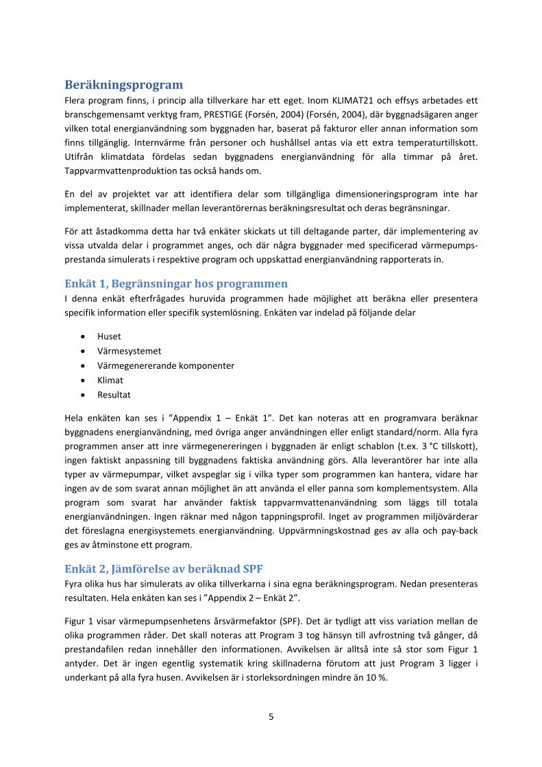
5

Beräkningsprogram Flera program finns, i princip alla tillverkare har ett eget. Inom KLIMAT21 och effsys arbetades ett

branschgemensamt verktyg fram, PRESTIGE (Forsén, 2004) (Forsén, 2004), där byggnadsägaren anger

vilken total energianvändning som byggnaden har, baserat på fakturor eller annan information som

finns tillgänglig. Internvärme från personer och hushållsel antas via ett extra temperaturtillskott.

Utifrån klimatdata fördelas sedan byggnadens energianvändning för alla timmar på året.

Tappvarmvattenproduktion tas också hands om.

En del av projektet var att identifiera delar som tillgängliga dimensioneringsprogram inte har

implementerat, skillnader mellan leverantörernas beräkningsresultat och deras begränsningar.

För att åstadkomma detta har två enkäter skickats ut till deltagande parter, där implementering av

vissa utvalda delar i programmet anges, och där några byggnader med specificerad värmepumps‐

prestanda simulerats i respektive program och uppskattad energianvändning rapporterats in.

Enkät 1, Begränsningar hos programmen I denna enkät efterfrågades huruvida programmen hade möjlighet att beräkna eller presentera

specifik information eller specifik systemlösning. Enkäten var indelad på följande delar

Huset

Värmesystemet

Värmegenererande komponenter

Klimat

Resultat

Hela enkäten kan ses i ”Appendix 1 – Enkät 1”. Det kan noteras att en programvara beräknar

byggnadens energianvändning, med övriga anger användningen eller enligt standard/norm. Alla fyra

programmen anser att inre värmegenereringen i byggnaden är enligt schablon (t.ex. 3 °C tillskott),

ingen faktiskt anpassning till byggnadens faktiska användning görs. Alla leverantörer har inte alla

typer av värmepumpar, vilket avspeglar sig i vilka typer som programmen kan hantera, vidare har

ingen av de som svarat annan möjlighet än att använda el eller panna som komplementsystem. Alla

program som svarat har använder faktisk tappvarmvattenanvändning som läggs till totala

energianvändningen. Ingen räknar med någon tappningsprofil. Inget av programmen miljövärderar

det föreslagna energisystemets energianvändning. Uppvärmningskostnad ges av alla och pay‐back

ges av åtminstone ett program.

Enkät 2, Jämförelse av beräknad SPF Fyra olika hus har simulerats av olika tillverkarna i sina egna beräkningsprogram. Nedan presenteras

resultaten. Hela enkäten kan ses i ”Appendix 2 – Enkät 2”.

Figur 1 visar värmepumpsenhetens årsvärmefaktor (SPF). Det är tydligt att viss variation mellan de

olika programmen råder. Det skall noteras att Program 3 tog hänsyn till avfrostning två gånger, då

prestandafilen redan innehåller den informationen. Avvikelsen är alltså inte så stor som Figur 1

antyder. Det är ingen egentlig systematik kring skillnaderna förutom att just Program 3 ligger i

underkant på alla fyra husen. Avvikelsen är i storleksordningen mindre än 10 %.

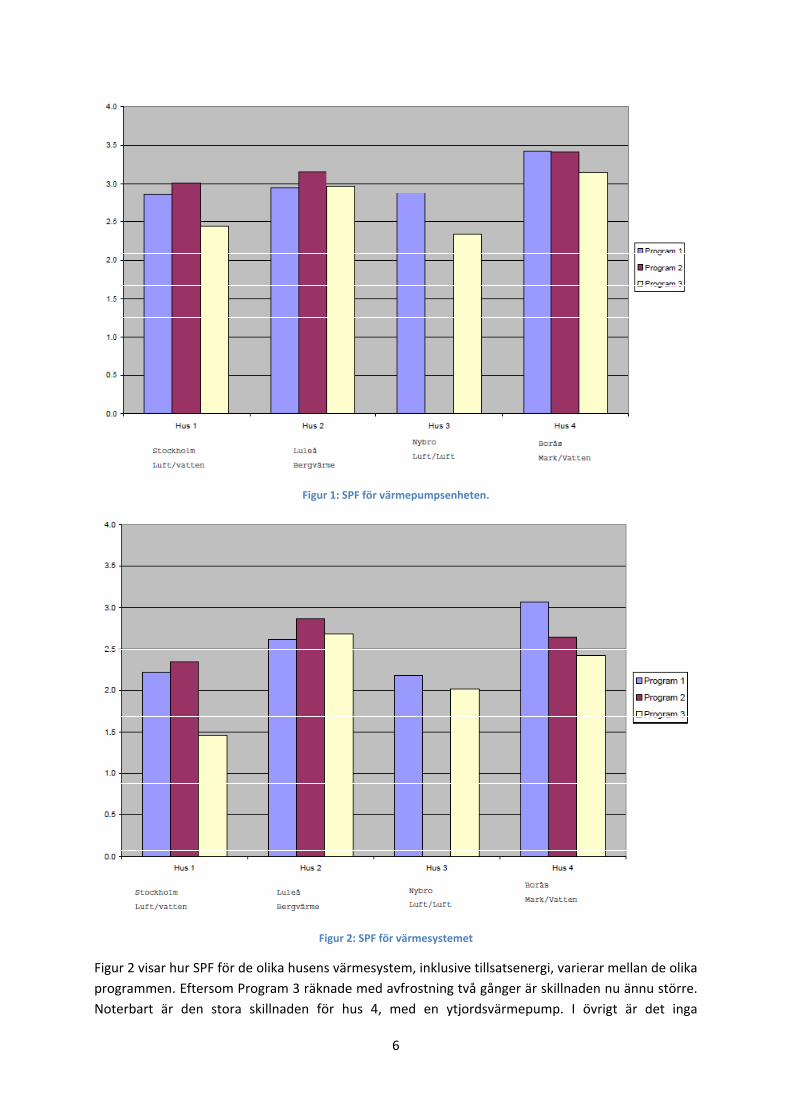
6

Figur 1: SPF för värmepumpsenheten.

Figur 2: SPF för värmesystemet

Figur 2 visar hur SPF för de olika husens värmesystem, inklusive tillsatsenergi, varierar mellan de olika

programmen. Eftersom Program 3 räknade med avfrostning två gånger är skillnaden nu ännu större.

Noterbart är den stora skillnaden för hus 4, med en ytjordsvärmepump. I övrigt är det inga

7

signifikanta skillnader. Motsvarande information syns i Figur 30, men i form av köpt energi.

Skillnaden är upp till cirka två tusen kronor, så skillnaden kan ha betydelse för utfallet av en

installation.

Diskussion Det förekommer skillnader, både i hur indata hanteras, vilka uppvärmningssystem, samt hur data

presenteras mellan programmen. Det är kanske naturligt att saluförs inte en viss typ av värmepump

hanterar inte programmet detta. Klart är att egentligen inget av programmen kan hantera mer

komplicerande sammansatta system. Det finns leverantörer som kombinerar värmepump med

solpaneler, vilka kan hantera just denna systemlösning. Men överlag så har leverantörerna fokuserat

på det produktutbud som de erbjuder.

När det gäller skillnader i SPF mellan programmen är det inte stor skillnad. Det ska sägas att det

statistiska underlaget är väl tunt för att dra några generella slutsatser. Det finns uppenbarligen ett

behov att kanske inte tvinga alla tillverkare att använda samma kod, men det kan finnas behovs att

presentera ett ramverk för hur prestandan av energisystem i byggnader kan uppskattas, då det inte

finns en sådan i dagsläget. Ett sådant presenteras i efterföljande kapitel.

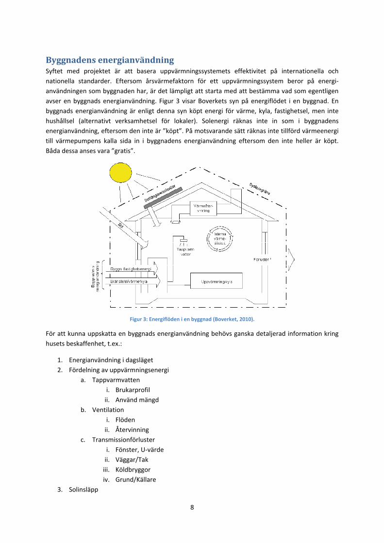
8

Byggnadens energianvändning Syftet med projektet är att basera uppvärmningssystemets effektivitet på internationella och

nationella standarder. Eftersom årsvärmefaktorn för ett uppvärmningssystem beror på energi‐

användningen som byggnaden har, är det lämpligt att starta med att bestämma vad som egentligen

avser en byggnads energianvändning. Figur 3 visar Boverkets syn på energiflödet i en byggnad. En

byggnads energianvändning är enligt denna syn köpt energi för värme, kyla, fastighetsel, men inte

hushållsel (alternativt verksamhetsel för lokaler). Solenergi räknas inte in som i byggnadens

energianvändning, eftersom den inte är ”köpt”. På motsvarande sätt räknas inte tillförd värmeenergi

till värmepumpens kalla sida in i byggnadens energianvändning eftersom den inte heller är köpt.

Båda dessa anses vara ”gratis”.

Figur 3: Energiflöden i en byggnad (Boverket, 2010).

För att kunna uppskatta en byggnads energianvändning behövs ganska detaljerad information kring

husets beskaffenhet, t.ex.:

1. Energianvändning i dagsläget

2. Fördelning av uppvärmningsenergi

a. Tappvarmvatten

i. Brukarprofil

ii. Använd mängd

b. Ventilation

i. Flöden

ii. Återvinning

c. Transmissionförluster

i. Fönster, U‐värde

ii. Väggar/Tak

iii. Köldbryggor

iv. Grund/Källare

3. Solinsläpp

9

a. Orientering av byggnad

b. Placering och storlek av fönster

c. Fönster, SHGC‐värde

d. Solavskärmning

4. Hushållsel

5. Fastighetsel

6. Personvärme

7. Klimat

8. Värmedistributionssystem

a. Typ

b. Temperaturnivåer

Utan detaljerad information kring dessa delar kan egentligen ingen tillförlitlig förutsägelse ges kring

vilken effektivitet ett nytt värmesystem kommer att få. Det är inte troligt att den typiske villaägaren

har sådan detaljerad kunskap om sin byggnad.

Viss hjälp finns/kommer att finnas genom energideklarationen av byggnaden, då en energiexpert har

bedömt delar av dessa i byggnaderna. Denna är dock av varierande kvalité, men troligt är ändå att

experten är mer skickad att göra denna bedömning än gängse villaägare.

SSEN ISO 13790:2008 Hur energianvändningen skall bedömas finns beskrivet i (CEN SS‐EN ISO 13790, 2008), se Figur 4 för

en schematisk bild över beräkningsstegen. Som kan ses i figuren tillåts tre olika tidsupplösningar,

timvis enkel, dynamisk, samt månatligt/säsong.

För ett energisystem som består av flera värmeproducerande komponenter, där även styrsystemet

väljer mellan hur och i vilken ordning värmegeneratorerna (pannor, värmepumpar, solfångare) skall

användas, är inte månatliga eller årsviktade beräkningsstrukturer tillräckligt för att bedöma

systemets effektivitet. Det är därför rekommenderat att beräkningsstrukturen sker med timsteg. Det

är inte rimligt att komplexa system skall handräknas utan beräknas på dator, vilket då innebär att

skälet till att använda månatliga fördelningsprocedurer inte längre är viktig.

Figur 4 visar också hur den förhåller sig till andra standards. Av primärt intresse är att bedöma hur

värmeproducerande komponenterna interagerar med varandra och med byggnaden. Utvärdering av

de flesta tänkbara värmeavgivande komponenter finns beskrivna i standarder, främst av intresse är

SS‐EN 15316.

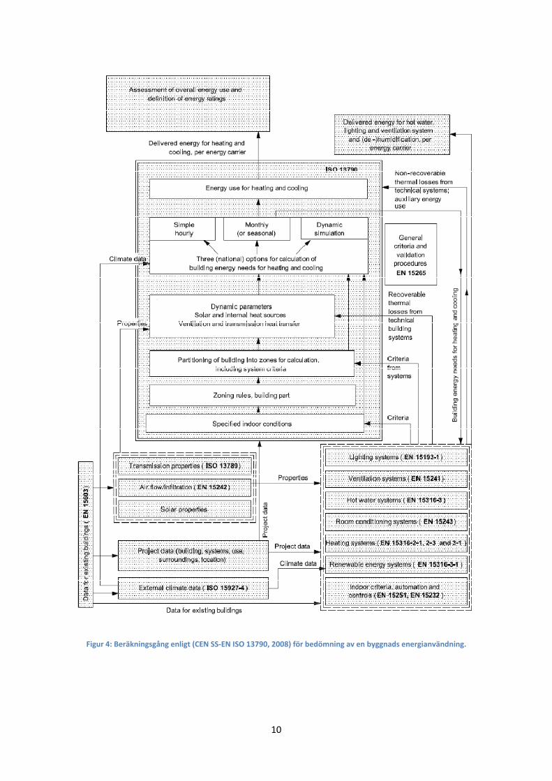
10

Figur 4: Beräkningsgång enligt (CEN SS‐EN ISO 13790, 2008) för bedömning av en byggnads energianvändning.

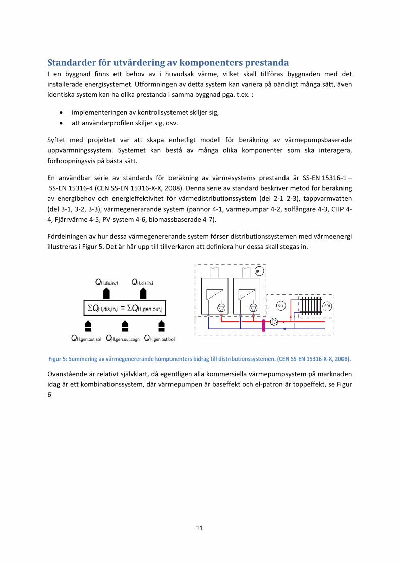
11

Standarder för utvärdering av komponenters prestanda I en byggnad finns ett behov av i huvudsak värme, vilket skall tillföras byggnaden med det

installerade energisystemet. Utformningen av detta system kan variera på oändligt många sätt, även

identiska system kan ha olika prestanda i samma byggnad pga. t.ex. :

implementeringen av kontrollsystemet skiljer sig,

att användarprofilen skiljer sig, osv.

Syftet med projektet var att skapa enhetligt modell för beräkning av värmepumpsbaserade

uppvärmningssystem. Systemet kan bestå av många olika komponenter som ska interagera,

förhoppningsvis på bästa sätt.

En användbar serie av standards för beräkning av värmesystems prestanda är SS‐EN 15316‐1 –

SS‐EN 15316‐4 (CEN SS‐EN 15316‐X‐X, 2008). Denna serie av standard beskriver metod för beräkning

av energibehov och energieffektivitet för värmedistributionssystem (del 2‐1 2‐3), tappvarmvatten

(del 3‐1, 3‐2, 3‐3), värmegenerarande system (pannor 4‐1, värmepumpar 4‐2, solfångare 4‐3, CHP 4‐

4, Fjärrvärme 4‐5, PV‐system 4‐6, biomassbaserade 4‐7).

Fördelningen av hur dessa värmegenererande system förser distributionssystemen med värmeenergi

illustreras i Figur 5. Det är här upp till tillverkaren att definiera hur dessa skall stegas in.

Figur 5: Summering av värmegenererande komponenters bidrag till distributionssystemen. (CEN SS‐EN 15316‐X‐X, 2008).

Ovanstående är relativt självklart, då egentligen alla kommersiella värmepumpsystem på marknaden

idag är ett kombinationssystem, där värmepumpen är baseffekt och el‐patron är toppeffekt, se Figur

6

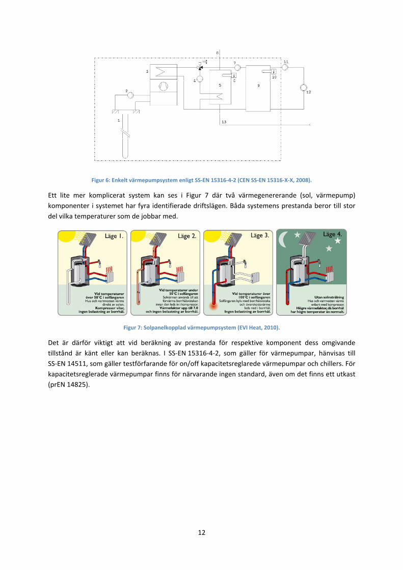
12

Figur 6: Enkelt värmepumpsystem enligt SS‐EN 15316‐4‐2 (CEN SS‐EN 15316‐X‐X, 2008).

Ett lite mer komplicerat system kan ses i Figur 7 där två värmegenererande (sol, värmepump)

komponenter i systemet har fyra identifierade driftslägen. Båda systemens prestanda beror till stor

del vilka temperaturer som de jobbar med.

Figur 7: Solpanelkopplad värmepumpsystem (EVI Heat, 2010).

Det är därför viktigt att vid beräkning av prestanda för respektive komponent dess omgivande

tillstånd är känt eller kan beräknas. I SS‐EN 15316‐4‐2, som gäller för värmepumpar, hänvisas till

SS‐EN 14511, som gäller testförfarande för on/off kapacitetsreglarede värmepumpar och chillers. För

kapacitetsreglerade värmepumpar finns för närvarande ingen standard, även om det finns ett utkast

(prEN 14825).

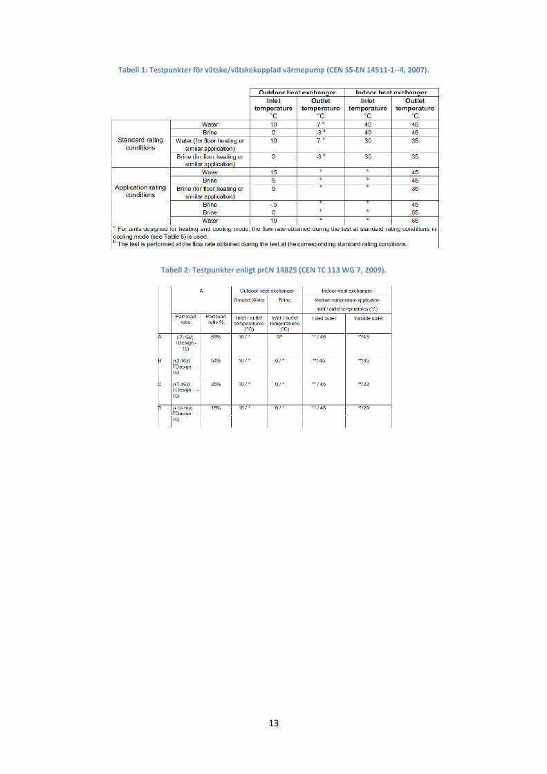
13

Tabell 1: Testpunkter för vätske/vätskekopplad värmepump (CEN SS‐EN 14511‐1‐‐4, 2007).

Tabell 2: Testpunkter enligt prEN 14825 (CEN TC 113 WG 7, 2009).

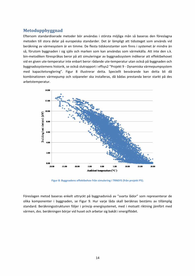
14

Metoduppbyggnad Eftersom standardiserade metoder bör användas i största möjliga mån så baseras den föreslagna

metoden till stora delar på europeiska standarder. Det är lämpligt att tidssteget som används vid

beräkning av värmesystem är en timme. De flesta tidskonstanter som finns i systemet är mindre än

så, förutom byggnaden i sig själv och marken som kan användas som värmekälla. Att inte den s.k.

bin‐metodiken förespråkas beror på att simuleringar av byggnadssystem indikerar att effektbehovet

vid en given ute‐temperatur inte enbart beror rådande ute‐temperatur utan också på byggnaden och

byggnadssystemens historik, se också slutrapport i effsys2 ”Projekt 9 ‐ Dynamiska värmepumpsystem

med kapacitetsreglering”. Figur 8 illustrerar detta. Speciellt besvärande kan detta bli då

kombinationen värmepump och solpaneler ska installeras, då bådas prestanda beror starkt på des

arbetstemperatur.

Figur 8: Byggnadens effektbehov från simulering i TRNSYS (från projekt P5).

Föreslagen metod baseras enkelt uttryckt på byggnadsnivå av ”svarta lådor” som representerar de

olika komponenter i byggnaden, se Figur 9. Hur varje låda skall beräknas bestäms av tillämplig

standard. Beräkningsstrukturen följer i princip energisystemet, med i motsatt riktning jämfört med

värmen, dvs. beräkningen börjar vid huset och arbetar sig bakåt i energiflödet.

15

Figur 9: Metoduppbyggnad för beräkning av en byggnads energisystems prestanda.

Genom att studera Figur 9 identifieras de komponenter eller indata som behövs för att kvantifiera

systemets prestanda:

1. Klimat

a. Temperatur

b. Relativ fuktighet

c. Solstrålning, direkt

d. Solstrålning, diffus

e. Solstrålning, reflekterat

2. Byggnadens effektbehov

3. Värmekällan (jord, berg, sjö, osv.)

4. Ackumulatortank

5. Solfångare

6. Värmepump

7. Panna

8. Kontrollenheten

9. Driftscenarior

Klimat I PRESTIGE (Forsén, 2004) används klimat från år 1996. Dessa klimatdata har branschen en gång

enats om att de är rimliga att använda för beräkning av värmepumpsystem. Det kan nämnas att

extremår för intervallet 1990 till 2000 enligt METEONORM ger god överreststämmelse för

åtminstone Stockholm, övriga orter återstår att validera. I de klimatfiler som PRESTIGE använder

ingår dock inte solstrålning eller relativ fuktighet, vilket innebär att dessa data behöver kompletteras.

VP

Panna ACK

DUC

T

T

ISO 13790

EN 15316‐4‐3EN 12975‐2

EN 15316‐4‐1

EN 15316‐4‐2EN 14511

EN 12977‐3EN 12977‐4EN 15316‐4‐3

EN 15316‐4‐3

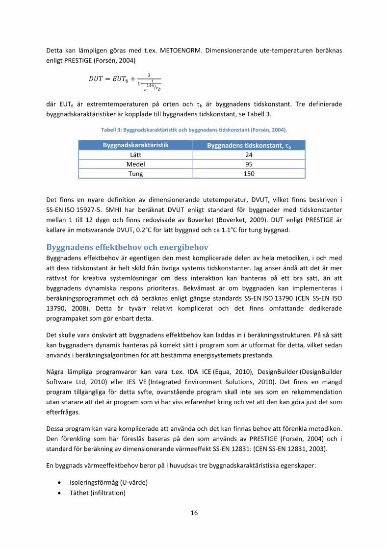
16

Detta kan lämpligen göras med t.ex. METOENORM. Dimensionerande ute‐temperaturen beräknas

enligt PRESTIGE (Forsén, 2004)

där EUT6 är extremtemperaturen på orten och b är byggnadens tidskonstant. Tre definierade byggnadskaraktäristiker är kopplade till byggnadens tidskonstant, se Tabell 3.

Tabell 3: Byggnadskaraktäristik och byggnadens tidskonstant (Forsén, 2004).

Byggnadskaraktäristik Byggnadens tidskonstant, b Lätt 24

Medel 95

Tung 150

Det finns en nyare definition av dimensionerande utetemperatur, DVUT, vilket finns beskriven i

SS‐EN ISO 15927‐5. SMHI har beräknat DVUT enligt standard för byggnader med tidskonstanter

mellan 1 till 12 dygn och finns redovisade av Boverket (Boverket, 2009). DUT enligt PRESTIGE är

kallare än motsvarande DVUT, 0.2°C för lätt byggnad och ca 1.1°C för tung byggnad.

Byggnadens effektbehov och energibehov Byggnadens effektbehov är egentligen den mest komplicerade delen av hela metodiken, i och med

att dess tidskonstant är helt skild från övriga systems tidskonstanter. Jag anser ändå att det är mer

rättvist för kreativa systemlösningar om dess interaktion kan hanteras på ett bra sätt, än att

byggnadens dynamiska respons prioriteras. Bekvämast är om byggnaden kan implementeras i

beräkningsprogrammet och då beräknas enligt gängse standards SS‐EN ISO 13790 (CEN SS‐EN ISO

13790, 2008). Detta är tyvärr relativt komplicerat och det finns omfattande dedikerade

programpaket som gör enbart detta.

Det skulle vara önskvärt att byggnadens effektbehov kan laddas in i beräkningsstrukturen. På så sätt

kan byggnadens dynamik hanteras på korrekt sätt i program som är utformat för detta, vilket sedan

används i beräkningsalgoritmen för att bestämma energisystemets prestanda.

Några lämpliga programvaror kan vara t.ex. IDA ICE (Equa, 2010), DesignBuilder (DesignBuilder

Software Ltd, 2010) eller IES VE (Integrated Environment Solutions, 2010). Det finns en mängd

program tillgängliga för detta syfte, ovanstående program skall inte ses som en rekommendation

utan snarare att det är program som vi har viss erfarenhet kring och vet att den kan göra just det som

efterfrågas.

Dessa program kan vara komplicerade att använda och det kan finnas behov att förenkla metodiken.

Den förenkling som här föreslås baseras på den som används av PRESTIGE (Forsén, 2004) och i

standard för beräkning av dimensionerande värmeeffekt SS‐EN 12831: (CEN SS‐EN 12831, 2003).

En byggnads värmeeffektbehov beror på i huvudsak tre byggnadskaraktäristiska egenskaper:

Isoleringsförmåg (U‐värde)

Täthet (infiltration)

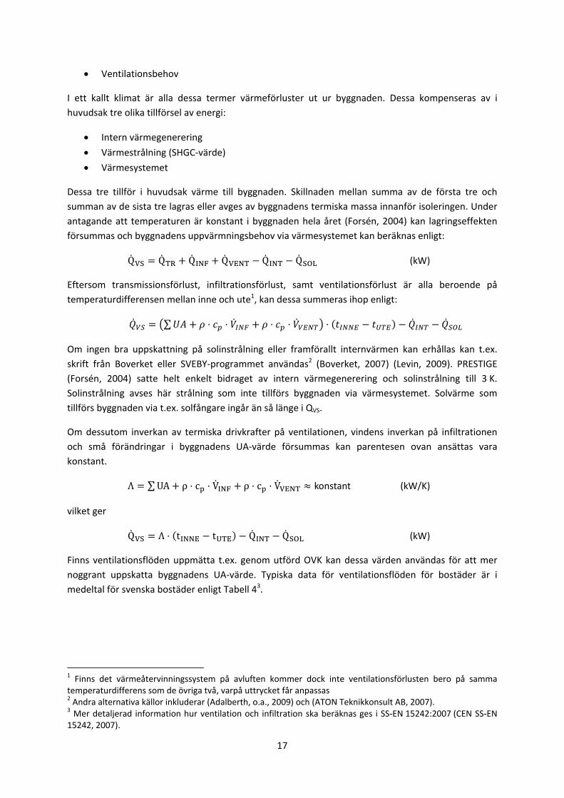
17

Ventilationsbehov

I ett kallt klimat är alla dessa termer värmeförluster ut ur byggnaden. Dessa kompenseras av i

huvudsak tre olika tillförsel av energi:

Intern värmegenerering

Värmestrålning (SHGC‐värde)

Värmesystemet

Dessa tre tillför i huvudsak värme till byggnaden. Skillnaden mellan summa av de första tre och

summan av de sista tre lagras eller avges av byggnadens termiska massa innanför isoleringen. Under

antagande att temperaturen är konstant i byggnaden hela året (Forsén, 2004) kan lagringseffekten

försummas och byggnadens uppvärmningsbehov via värmesystemet kan beräknas enligt:

QVS QTR QINF QVENT QINT QSOL (kW)

Eftersom transmissionsförlust, infiltrationsförlust, samt ventilationsförlust är alla beroende på

temperaturdifferensen mellan inne och ute1, kan dessa summeras ihop enligt:

∑

Om ingen bra uppskattning på solinstrålning eller framförallt internvärmen kan erhållas kan t.ex.

skrift från Boverket eller SVEBY‐programmet användas2 (Boverket, 2007) (Levin, 2009). PRESTIGE

(Forsén, 2004) satte helt enkelt bidraget av intern värmegenerering och solinstrålning till 3 K.

Solinstrålning avses här strålning som inte tillförs byggnaden via värmesystemet. Solvärme som

tillförs byggnaden via t.ex. solfångare ingår än så länge i QVS.

Om dessutom inverkan av termiska drivkrafter på ventilationen, vindens inverkan på infiltrationen

och små förändringar i byggnadens UA‐värde försummas kan parentesen ovan ansättas vara

konstant.

Λ ∑UA ρ c VINF ρ c VVENT konstant (kW/K)

vilket ger

QVS Λ tINNE tUTE QINT QSOL (kW)

Finns ventilationsflöden uppmätta t.ex. genom utförd OVK kan dessa värden användas för att mer

noggrant uppskatta byggnadens UA‐värde. Typiska data för ventilationsflöden för bostäder är i

medeltal för svenska bostäder enligt Tabell 43.

1 Finns det värmeåtervinningssystem på avluften kommer dock inte ventilationsförlusten bero på samma temperaturdifferens som de övriga två, varpå uttrycket får anpassas 2 Andra alternativa källor inkluderar (Adalberth, o.a., 2009) och (ATON Teknikkonsult AB, 2007). 3 Mer detaljerad information hur ventilation och infiltration ska beräknas ges i SS‐EN 15242:2007 (CEN SS‐EN 15242, 2007).

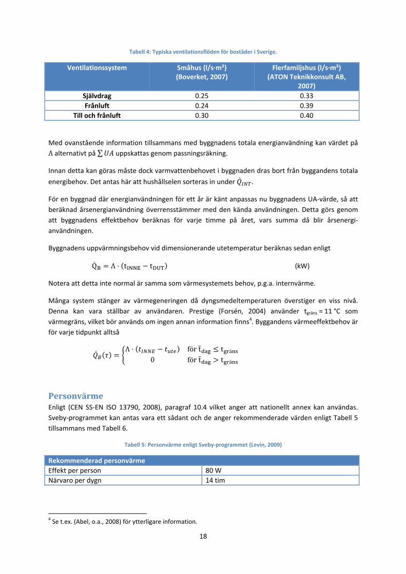
18

Tabell 4: Typiska ventilationsflöden för bostäder i Sverige.

Ventilationssystem Småhus (l/s∙m²) (Boverket, 2007)

Flerfamiljshus (l/s∙m²) (ATON Teknikkonsult AB,

2007)

Självdrag 0.25 0.33

Frånluft 0.24 0.39

Till och frånluft 0.30 0.40

Med ovanstående information tillsammans med byggnadens totala energianvändning kan värdet på

Λ alternativt på ∑ uppskattas genom passningsräkning.

Innan detta kan göras måste dock varmvattenbehovet i byggnaden dras bort från byggandens totala

energibehov. Det antas här att hushållselen sorteras in under .

För en byggnad där energianvändningen för ett år är känt anpassas nu byggnadens UA‐värde, så att

beräknad årsenergianvändning överrensstämmer med den kända användningen. Detta görs genom

att byggnadens effektbehov beräknas för varje timme på året, vars summa då blir årsenergi‐

användningen.

Byggnadens uppvärmningsbehov vid dimensionerande utetemperatur beräknas sedan enligt

QB Λ tINNE tDUT (kW)

Notera att detta inte normal är samma som värmesystemets behov, p.g.a. internvärme.

Många system stänger av värmegeneringen då dyngsmedeltemperaturen överstiger en viss nivå.

Denna kan vara ställbar av användaren. Prestige (Forsén, 2004) använder tgräns = 11 °C som

värmegräns, vilket bör används om ingen annan information finns4. Byggandens värmeeffektbehov är

för varje tidpunkt alltså

Λ för t t ä

0 för t t ä

Personvärme Enligt (CEN SS‐EN ISO 13790, 2008), paragraf 10.4 vilket anger att nationellt annex kan användas.

Sveby‐programmet kan antas vara ett sådant och de anger rekommenderade värden enligt Tabell 5

tillsammans med Tabell 6.

Tabell 5: Personvärme enligt Sveby‐programmet (Levin, 2009)

Rekommenderad personvärme

Effekt per person 80 W

Närvaro per dygn 14 tim

4 Se t.ex. (Abel, o.a., 2008) för ytterligare information.

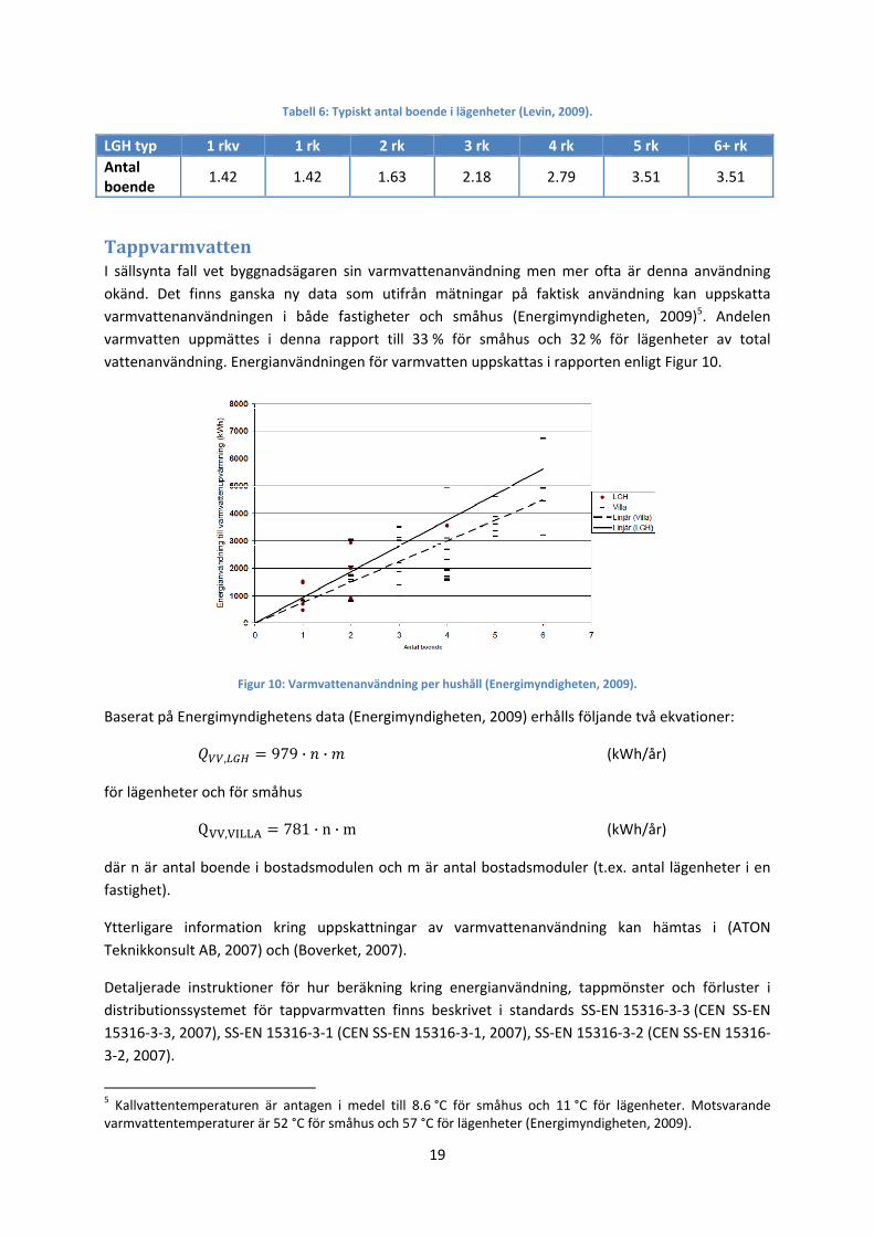
19

Tabell 6: Typiskt antal boende i lägenheter (Levin, 2009).

LGH typ 1 rkv 1 rk 2 rk 3 rk 4 rk 5 rk 6+ rk

Antal boende

1.42 1.42 1.63 2.18 2.79 3.51 3.51

Tappvarmvatten I sällsynta fall vet byggnadsägaren sin varmvattenanvändning men mer ofta är denna användning

okänd. Det finns ganska ny data som utifrån mätningar på faktisk användning kan uppskatta

varmvattenanvändningen i både fastigheter och småhus (Energimyndigheten, 2009)5. Andelen

varmvatten uppmättes i denna rapport till 33 % för småhus och 32 % för lägenheter av total

vattenanvändning. Energianvändningen för varmvatten uppskattas i rapporten enligt Figur 10.

Figur 10: Varmvattenanvändning per hushåll (Energimyndigheten, 2009).

Baserat på Energimyndighetens data (Energimyndigheten, 2009) erhålls följande två ekvationer:

, 979 · · (kWh/år)

för lägenheter och för småhus

QVV,VILLA 781 · n · m (kWh/år)

där n är antal boende i bostadsmodulen och m är antal bostadsmoduler (t.ex. antal lägenheter i en

fastighet).

Ytterligare information kring uppskattningar av varmvattenanvändning kan hämtas i (ATON

Teknikkonsult AB, 2007) och (Boverket, 2007).

Detaljerade instruktioner för hur beräkning kring energianvändning, tappmönster och förluster i

distributionssystemet för tappvarmvatten finns beskrivet i standards SS‐EN 15316‐3‐3 (CEN SS‐EN

15316‐3‐3, 2007), SS‐EN 15316‐3‐1 (CEN SS‐EN 15316‐3‐1, 2007), SS‐EN 15316‐3‐2 (CEN SS‐EN 15316‐

3‐2, 2007).

5 Kallvattentemperaturen är antagen i medel till 8.6 °C för småhus och 11 °C för lägenheter. Motsvarande varmvattentemperaturer är 52 °C för småhus och 57 °C för lägenheter (Energimyndigheten, 2009).

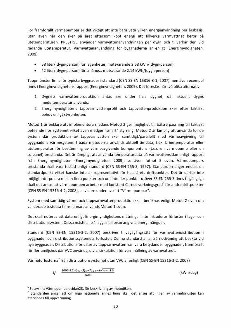
20

För framförallt värmepumpar är det viktigt att inte bara veta vilken energianvändning per årsbasis,

utan även när den sker på året eftersom köpt energi att tillverka varmvattnet beror på

utetemperaturen. PRESTIGE använder varmvattenanvändningen per dygn och tillverkar den vid

rådande utetemperatur. Varmvattenanvändning för byggnaderna är enligt (Energimyndigheten,

2009):

58 liter/(dygn∙person) för lägenheter, motsvarande 2.68 kWh/(dygn∙person)

42 liter/(dygn∙person) för småhus., motsvarande 2.14 kWh/(dygn∙person)

Tappmönster finns för typiska byggnader i standard (CEN SS‐EN 15316‐3‐1, 2007) men även exempel

finns i Energimyndighetens rapport (Energimyndigheten, 2009). Det föreslås här två olika alternativ:

1. Dygnets varmvattenproduktion antas ske under hela dygnet, där aktuellt dygns

medeltemperatur används.

2. Energimyndighetens tappvarmvattenprofil och tappvattenproduktion sker efter faktiskt

behov enligt styrenheten.

Metod 1 är enklare att implementera medans Metod 2 ger möjlighet till bättre passning till faktiskt

beteende hos systemet vilket även medger ”smart” styrning. Metod 2 är lämplig att använda för de

system där produktion av tappvarmvatten sker samtidigt/parallellt med värmeavgivning till

byggnadens värmesystem. I båda metoderna används aktuell timdata, t.ex. brinetemperatur eller

utetemperatur för bestämning av värmeavgivande komponentens (t.ex. en värmepump eller en

solpanel) prestanda. Det är lämpligt att använda temperaturdata på varmvattensidan enligt rapport

från Energimyndigheten (Energimyndigheten, 2009), se även fotnot 5 ovan. Värmepumpars

prestanda skall vara testad enligt standard (CEN SS‐EN 255‐3, 1997). Standarden anger endast en

standardpunkt vilket kanske inte är representativt för hela årets driftpunkter. Det är därför inte

möjligt interpolera mellan flera punkter och om inte fler punkter utöver SS‐EN 255‐3 finns tillgängliga

skall det antas att värmepumpen arbetar med konstant Carnot‐verkningsgrad6 för andra driftpunkter

(CEN SS‐EN 15316‐4‐2, 2008), se vidare under avsnitt ”Värmepumpar”.

System med samtidig värme och tappvarmvattenproduktion skall beräknas enligt Metod 2 ovan om

validerade testdata finns, annars används Metod 1 ovan.

Det skall noteras att data enligt Energimyndighetens mätningar inte inkluderar förluster i lager och

distributionssystem. Dessa måste alltså läggas till ovan angivna energimängder.

Standard (CEN SS‐EN 15316‐3‐2, 2007) beskriver tillvägagångssätt för varmvattendistribution i

byggnader och distributionssystemets förluster. Denna standard är alltså nödvändig att beakta vid

nya byggnader. Distributionsförluster av tappvarmvatten kan vara betydande i byggnader, framförallt

för flerfamiljshus där VVC används, d.v.s. cirkulation för varmhållning av varmvattnet.

Värmeförlusterna7 från distributionssystemet utan VVC är enligt (CEN SS‐EN 15316‐3‐2, 2007)

· . · ö · ·√ · ·

(kWh/dag)

6 Se avsnitt Värmepumpar, sidan28, för beskrivning av metodiken. 7 Standarden anger att om inga nationella annex finns skall det anses att ingen av värmeförlusten kan återvinnas till uppvärmning.

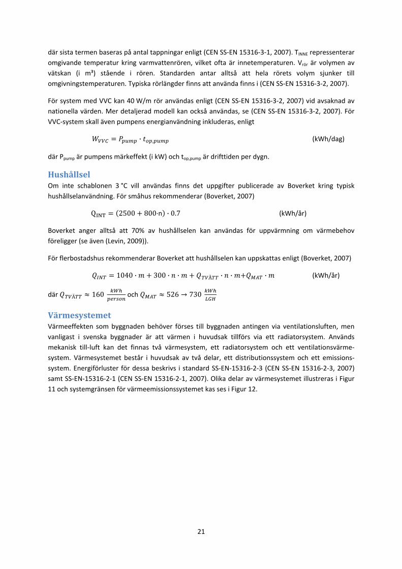
21

där sista termen baseras på antal tappningar enligt (CEN SS‐EN 15316‐3‐1, 2007). TINNE repressenterar

omgivande temperatur kring varmvattenrören, vilket ofta är innetemperaturen. Vrör är volymen av

vätskan (i m³) stående i rören. Standarden antar alltså att hela rörets volym sjunker till

omgivningstemperaturen. Typiska rörlängder finns att använda finns i (CEN SS‐EN 15316‐3‐2, 2007).

För system med VVC kan 40 W/m rör användas enligt (CEN SS‐EN 15316‐3‐2, 2007) vid avsaknad av

nationella värden. Mer detaljerad modell kan också användas, se (CEN SS‐EN 15316‐3‐2, 2007). För

VVC‐system skall även pumpens energianvändning inkluderas, enligt

· , (kWh/dag)

där Ppump är pumpens märkeffekt (i kW) och top,pump är drifttiden per dygn.

Hushållsel Om inte schablonen 3 °C vill användas finns det uppgifter publicerade av Boverket kring typisk

hushållselanvändning. För småhus rekommenderar (Boverket, 2007)

QINT 2500 800∙n · 0.7 (kWh/år)

Boverket anger alltså att 70% av hushållselen kan användas för uppvärmning om värmebehov

föreligger (se även (Levin, 2009)).

För flerbostadshus rekommenderar Boverket att hushållselen kan uppskattas enligt (Boverket, 2007)

1040 · 300 · · Ä · · · (kWh/år)

där Ä 160 och 526 730

Värmesystemet Värmeeffekten som byggnaden behöver förses till byggnaden antingen via ventilationsluften, men

vanligast i svenska byggnader är att värmen i huvudsak tillförs via ett radiatorsystem. Används

mekanisk till‐luft kan det finnas två värmesystem, ett radiatorsystem och ett ventilationsvärme‐

system. Värmesystemet består i huvudsak av två delar, ett distributionssystem och ett emissions‐

system. Energiförluster för dessa beskrivs i standard SS‐EN‐15316‐2‐3 (CEN SS‐EN 15316‐2‐3, 2007)

samt SS‐EN‐15316‐2‐1 (CEN SS‐EN 15316‐2‐1, 2007). Olika delar av värmesystemet illustreras i Figur

11 och systemgränsen för värmeemissionssystemet kas ses i Figur 12.

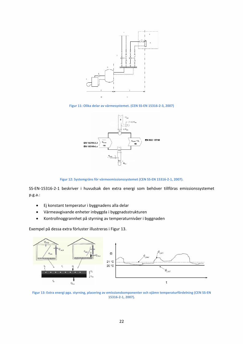
22

Figur 11: Olika delar av värmesystemet. (CEN SS‐EN 15316‐2‐3, 2007)

Figur 12: Systemgräns för värmeemissionssystemet (CEN SS‐EN 15316‐2‐1, 2007).

SS‐EN‐15316‐2‐1 beskriver i huvudsak den extra energi som behöver tillföras emissionssystemet

p.g.a.:

Ej konstant temperatur i byggnadens alla delar

Värmeavgivande enheter inbyggda i byggnadsstrukturen

Kontrollnoggrannhet på styrning av temperaturnivåer i byggnaden

Exempel på dessa extra förluster illustreras i Figur 13.

Figur 13: Extra energi pga. styrning, placering av emissionskomponenter och ojämn temperaturfördelning (CEN SS‐EN 15316‐2‐1, 2007).

23

Dessa förluster är redan inbakade i den angivna energianvändningen som byggnadsägaren anger,

men föreslås ändå inkluderas i beräkning av det nya energisystemets energiprestanda främst ur

konservativt perspektiv, alternativt görs beräkningen iterativt med befintligt värmesystem först.

Byggnadens värmebehov fås genom att jämföra befintligt systems simulerade energianvändning med

känd användning. Genom att inkludera denna del kommer det troliga utfallet vara i överkant (utan

iteration) mot verkligt utfall. Energi per tidsenhet (timme) beräknas enligt (CEN SS‐EN 15316‐2‐1,

2007)

QVS,IN QVS k · WVS QVSLOSS (kWh)

Den totala energi som behöver tillföras värmesystemet ( , ) är högre än husets energianvändning

( , på grund av avvikelser från idealt värmesystem. Viss del av pumparbete och fläktarbete i

värmesystemet kan återvinnas ( · ) enligt SS‐EN‐15316‐2‐1. Ingen vägledning av storleken på

återvinningsgraden (k) ges i standarden och sättes därför till noll (k=0), dvs ingen återvinning av

denna energi antas. Förlusterna som beror på avvikelser från idealt ( ) värmesystem beräknas

enligt (CEN SS‐EN 15316‐2‐1, 2007)

QVSLOSS.

1 · QVS (kWh)

där

vilket tar hänsyn till stratifiering av temperaturen inne, inbyggda värmeelement i

byggnadsstrukturen, samt p.g.a. reglerutrustning. Inverkan av kontrollenheten för

rumstemperaturen, föreslås enligt Tabell 7 för ej inbyggda radiatorer:

Tabell 7: Effektivitet av rumstemperaturreglering (CEN SS‐EN 15316‐2‐1, 2007), ej inbyggda radiatorer.

Typ av reglering

Framledningsreglering 0.80

En central rumskontroll 0.88

P‐reglering (2K) 0.93

P‐reglering (1K) 0.95

PI‐reglering 0.97

State‐of‐art 0.99

Approximativa värden för övertemperaturer föreslås enligt

. . ·∆

men mer information kan fås i (CEN SS‐EN 15316‐2‐1, 2007). · ∆ representerar

medelövertemperaturen på radiatorsystemet i förhållande till rumstemperaturen8.

För golvvärmesystem eller andra inbyggda system hänvisas till (CEN SS‐EN 15316‐2‐1, 2007).

8 Om t.ex. radiatortemperaturen är vid en given tidpunkt 33 och 41, är ∆ 17°C.

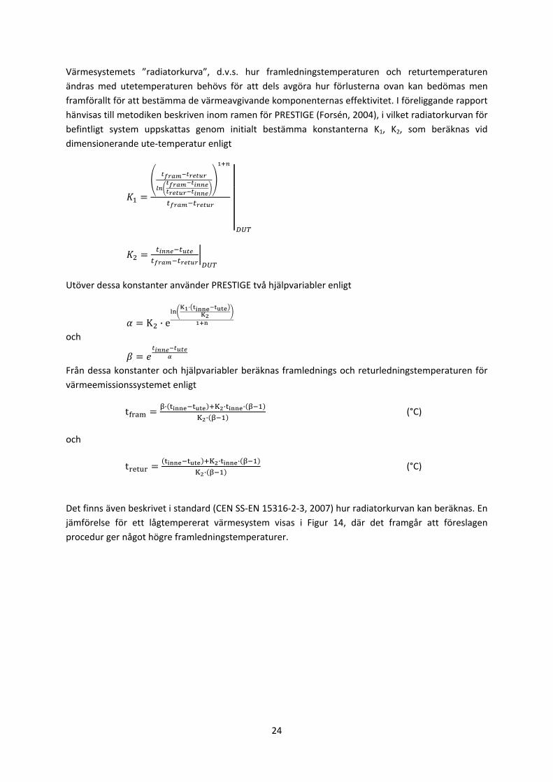
24

Värmesystemets ”radiatorkurva”, d.v.s. hur framledningstemperaturen och returtemperaturen

ändras med utetemperaturen behövs för att dels avgöra hur förlusterna ovan kan bedömas men

framförallt för att bestämma de värmeavgivande komponenternas effektivitet. I föreliggande rapport

hänvisas till metodiken beskriven inom ramen för PRESTIGE (Forsén, 2004), i vilket radiatorkurvan för

befintligt system uppskattas genom initialt bestämma konstanterna K1, K2, som beräknas vid

dimensionerande ute‐temperatur enligt

Utöver dessa konstanter använder PRESTIGE två hjälpvariabler enligt

K · e

K ·K

och

Från dessa konstanter och hjälpvariabler beräknas framlednings och returledningstemperaturen för

värmeemissionssystemet enligt

t· K · ·

K · (°C)

och

tK · ·

K · (°C)

Det finns även beskrivet i standard (CEN SS‐EN 15316‐2‐3, 2007) hur radiatorkurvan kan beräknas. En

jämförelse för ett lågtempererat värmesystem visas i Figur 14, där det framgår att föreslagen

procedur ger något högre framledningstemperaturer.

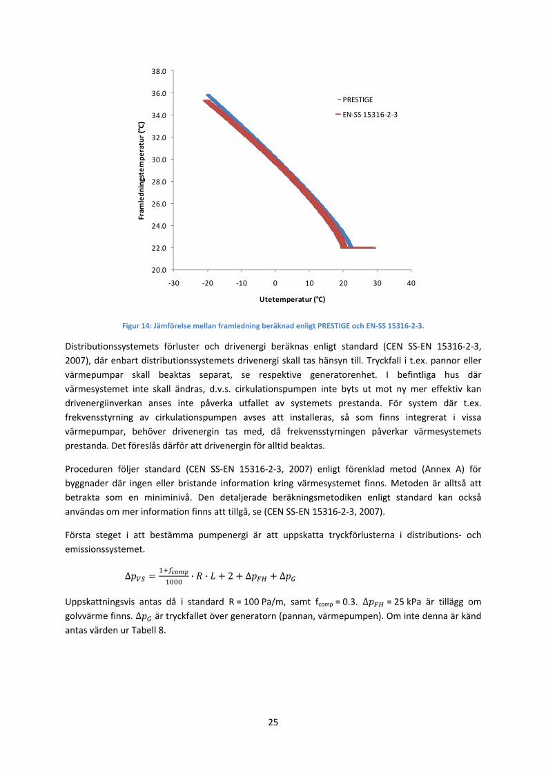
25

Figur 14: Jämförelse mellan framledning beräknad enligt PRESTIGE och EN‐SS 15316‐2‐3.

Distributionssystemets förluster och drivenergi beräknas enligt standard (CEN SS‐EN 15316‐2‐3,

2007), där enbart distributionssystemets drivenergi skall tas hänsyn till. Tryckfall i t.ex. pannor eller

värmepumpar skall beaktas separat, se respektive generatorenhet. I befintliga hus där

värmesystemet inte skall ändras, d.v.s. cirkulationspumpen inte byts ut mot ny mer effektiv kan

drivenergiinverkan anses inte påverka utfallet av systemets prestanda. För system där t.ex.

frekvensstyrning av cirkulationspumpen avses att installeras, så som finns integrerat i vissa

värmepumpar, behöver drivenergin tas med, då frekvensstyrningen påverkar värmesystemets

prestanda. Det föreslås därför att drivenergin för alltid beaktas.

Proceduren följer standard (CEN SS‐EN 15316‐2‐3, 2007) enligt förenklad metod (Annex A) för

byggnader där ingen eller bristande information kring värmesystemet finns. Metoden är alltså att

betrakta som en miniminivå. Den detaljerade beräkningsmetodiken enligt standard kan också

användas om mer information finns att tillgå, se (CEN SS‐EN 15316‐2‐3, 2007).

Första steget i att bestämma pumpenergi är att uppskatta tryckförlusterna i distributions‐ och

emissionssystemet.

∆ · · 2 ∆ ∆

Uppskattningsvis antas då i standard R = 100 Pa/m, samt fcomp = 0.3. ∆ = 25 kPa är tillägg om

golvvärme finns. ∆ är tryckfallet över generatorn (pannan, värmepumpen). Om inte denna är känd

antas värden ur Tabell 8.

20.0

22.0

24.0

26.0

28.0

30.0

32.0

34.0

36.0

38.0

‐30 ‐20 ‐10 0 10 20 30 40

Fram

ledningstemperatur (°C)

Utetemperatur (°C)

PRESTIGE

EN‐SS 15316‐2‐3

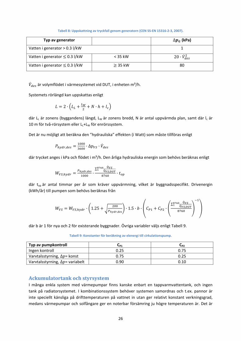
26

Tabell 8: Uppskattning av tryckfall genom generatorn (CEN SS‐EN 15316‐2‐3, 2007).

Typ av generator ∆ (kPa)

Vatten i generator > 0.3 l/kW 1

Vatten i generator 0.3 l/kW < 35 kW 20 ·

Vatten i generator 0.3 l/kW 35 kW 80

är volymflödet i värmesystemet vid DUT, i enheten m³/h.

Systemets rörlängd kan uppskattas enligt

2 · ·

där LL är zonens (byggandens) längd, LW är zonens bredd, N är antal uppvärmda plan, samt där lc är

10 m för två‐rörsystem eller LL+LW för enrörssystem.

Det är nu möjligt att beräkna den ”hydrauliska” effekten (i Watt) som måste tillföras enligt

, · ∆ ·

där trycket anges i kPa och flödet i m³/h. Den årliga hydrauliska energin som behövs beräknas enligt

,, ·

∑, ·

där top är antal timmar per år som kräver uppvärmning, vilket är byggnadsspecifikt. Drivenergin

(kWh/år) till pumpen som behövs beräknas från

, · 1.25,

· 1.5 · · ·∑

,

där b är 1 för nya och 2 för existerande byggnader. Övriga variabler väljs enligt Tabell 9.

Tabell 9: Konstanter för beräkning av elenergi till cirkulationspump.

Typ av pumpkontroll CP1 CP2

Ingen kontroll 0.25 0.75

Varvtalsstyrning, ∆ = konst 0.75 0.25

Varvtalsstyrning, ∆ = variabelt 0.90 0.10

Ackumulatortank och styrsystem I många enkla system med värmepumpar finns kanske enbart en tappvarmvattentank, och ingen

tank på radiatorsystemet. I kombinationssystem behöver systemen samordnas och t.ex. pannor är

inte speciellt känsliga på drifttemperaturen på vattnet in utan ger relativt konstant verkningsgrad,

medans värmepumpar och solfångare ger en noterbar försämring ju högre temperaturen är. Det är

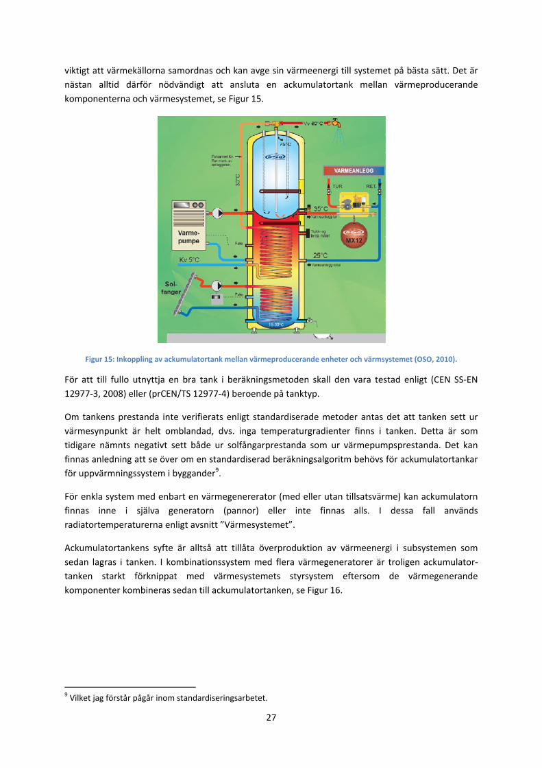
27

viktigt att värmekällorna samordnas och kan avge sin värmeenergi till systemet på bästa sätt. Det är

nästan alltid därför nödvändigt att ansluta en ackumulatortank mellan värmeproducerande

komponenterna och värmesystemet, se Figur 15.

Figur 15: Inkoppling av ackumulatortank mellan värmeproducerande enheter och värmsystemet (OSO, 2010).

För att till fullo utnyttja en bra tank i beräkningsmetoden skall den vara testad enligt (CEN SS‐EN

12977‐3, 2008) eller (prCEN/TS 12977‐4) beroende på tanktyp.

Om tankens prestanda inte verifierats enligt standardiserade metoder antas det att tanken sett ur

värmesynpunkt är helt omblandad, dvs. inga temperaturgradienter finns i tanken. Detta är som

tidigare nämnts negativt sett både ur solfångarprestanda som ur värmepumpsprestanda. Det kan

finnas anledning att se över om en standardiserad beräkningsalgoritm behövs för ackumulatortankar

för uppvärmningssystem i byggander9.

För enkla system med enbart en värmegenererator (med eller utan tillsatsvärme) kan ackumulatorn

finnas inne i själva generatorn (pannor) eller inte finnas alls. I dessa fall används

radiatortemperaturerna enligt avsnitt ”Värmesystemet”.

Ackumulatortankens syfte är alltså att tillåta överproduktion av värmeenergi i subsystemen som

sedan lagras i tanken. I kombinationssystem med flera värmegeneratorer är troligen ackumulator‐

tanken starkt förknippat med värmesystemets styrsystem eftersom de värmegenerande

komponenter kombineras sedan till ackumulatortanken, se Figur 16.

9 Vilket jag förstår pågår inom standardiseringsarbetet.

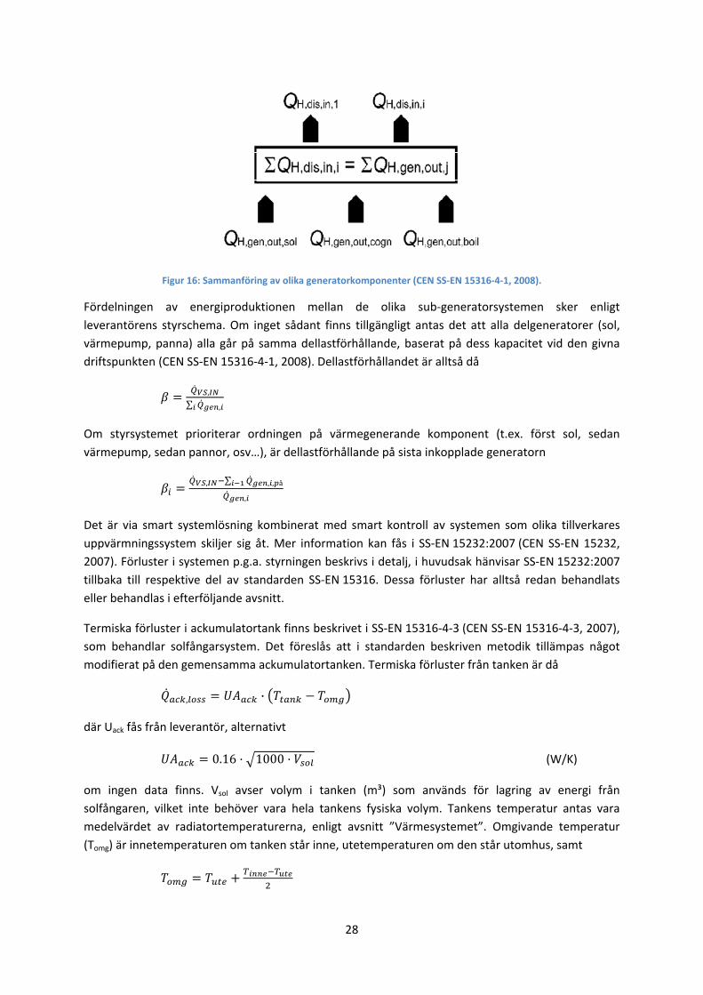
28

Figur 16: Sammanföring av olika generatorkomponenter (CEN SS‐EN 15316‐4‐1, 2008).

Fördelningen av energiproduktionen mellan de olika sub‐generatorsystemen sker enligt

leverantörens styrschema. Om inget sådant finns tillgängligt antas det att alla delgeneratorer (sol,

värmepump, panna) alla går på samma dellastförhållande, baserat på dess kapacitet vid den givna

driftspunkten (CEN SS‐EN 15316‐4‐1, 2008). Dellastförhållandet är alltså då

,

∑ ,

Om styrsystemet prioriterar ordningen på värmegenerande komponent (t.ex. först sol, sedan

värmepump, sedan pannor, osv…), är dellastförhållande på sista inkopplade generatorn

, ∑ , , å

,

Det är via smart systemlösning kombinerat med smart kontroll av systemen som olika tillverkares

uppvärmningssystem skiljer sig åt. Mer information kan fås i SS‐EN 15232:2007 (CEN SS‐EN 15232,

2007). Förluster i systemen p.g.a. styrningen beskrivs i detalj, i huvudsak hänvisar SS‐EN 15232:2007

tillbaka till respektive del av standarden SS‐EN 15316. Dessa förluster har alltså redan behandlats

eller behandlas i efterföljande avsnitt.

Termiska förluster i ackumulatortank finns beskrivet i SS‐EN 15316‐4‐3 (CEN SS‐EN 15316‐4‐3, 2007),

som behandlar solfångarsystem. Det föreslås att i standarden beskriven metodik tillämpas något

modifierat på den gemensamma ackumulatortanken. Termiska förluster från tanken är då

, ·

där Uack fås från leverantör, alternativt

0.16 1000 (W/K)

om ingen data finns. Vsol avser volym i tanken (m³) som används för lagring av energi från

solfångaren, vilket inte behöver vara hela tankens fysiska volym. Tankens temperatur antas vara

medelvärdet av radiatortemperaturerna, enligt avsnitt ”Värmesystemet”. Omgivande temperatur

(Tomg) är innetemperaturen om tanken står inne, utetemperaturen om den står utomhus, samt

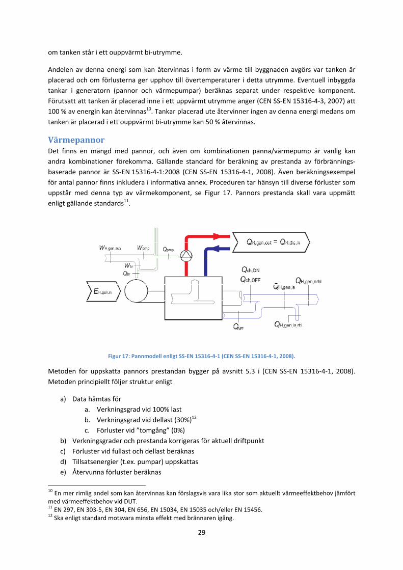
29

om tanken står i ett ouppvärmt bi‐utrymme.

Andelen av denna energi som kan återvinnas i form av värme till byggnaden avgörs var tanken är

placerad och om förlusterna ger upphov till övertemperaturer i detta utrymme. Eventuell inbyggda

tankar i generatorn (pannor och värmepumpar) beräknas separat under respektive komponent.

Förutsatt att tanken är placerad inne i ett uppvärmt utrymme anger (CEN SS‐EN 15316‐4‐3, 2007) att

100 % av energin kan återvinnas10. Tankar placerad ute återvinner ingen av denna energi medans om

tanken är placerad i ett ouppvärmt bi‐utrymme kan 50 % återvinnas.

Värmepannor Det finns en mängd med pannor, och även om kombinationen panna/värmepump är vanlig kan

andra kombinationer förekomma. Gällande standard för beräkning av prestanda av förbrännings‐

baserade pannor är SS‐EN 15316‐4‐1:2008 (CEN SS‐EN 15316‐4‐1, 2008). Även beräkningsexempel

för antal pannor finns inkludera i informativa annex. Proceduren tar hänsyn till diverse förluster som

uppstår med denna typ av värmekomponent, se Figur 17. Pannors prestanda skall vara uppmätt

enligt gällande standards11.

Figur 17: Pannmodell enligt SS‐EN 15316‐4‐1 (CEN SS‐EN 15316‐4‐1, 2008).

Metoden för uppskatta pannors prestandan bygger på avsnitt 5.3 i (CEN SS‐EN 15316‐4‐1, 2008).

Metoden principiellt följer struktur enligt

a) Data hämtas för

a. Verkningsgrad vid 100% last

b. Verkningsgrad vid dellast (30%)12

c. Förluster vid ”tomgång” (0%)

b) Verkningsgrader och prestanda korrigeras för aktuell driftpunkt

c) Förluster vid fullast och dellast beräknas

d) Tillsatsenergier (t.ex. pumpar) uppskattas

e) Återvunna förluster beräknas

10 En mer rimlig andel som kan återvinnas kan förslagsvis vara lika stor som aktuellt värmeeffektbehov jämfört med värmeeffektbehov vid DUT. 11 EN 297, EN 303‐5, EN 304, EN 656, EN 15034, EN 15035 och/eller EN 15456. 12 Ska enligt standard motsvara minsta effekt med brännaren igång.

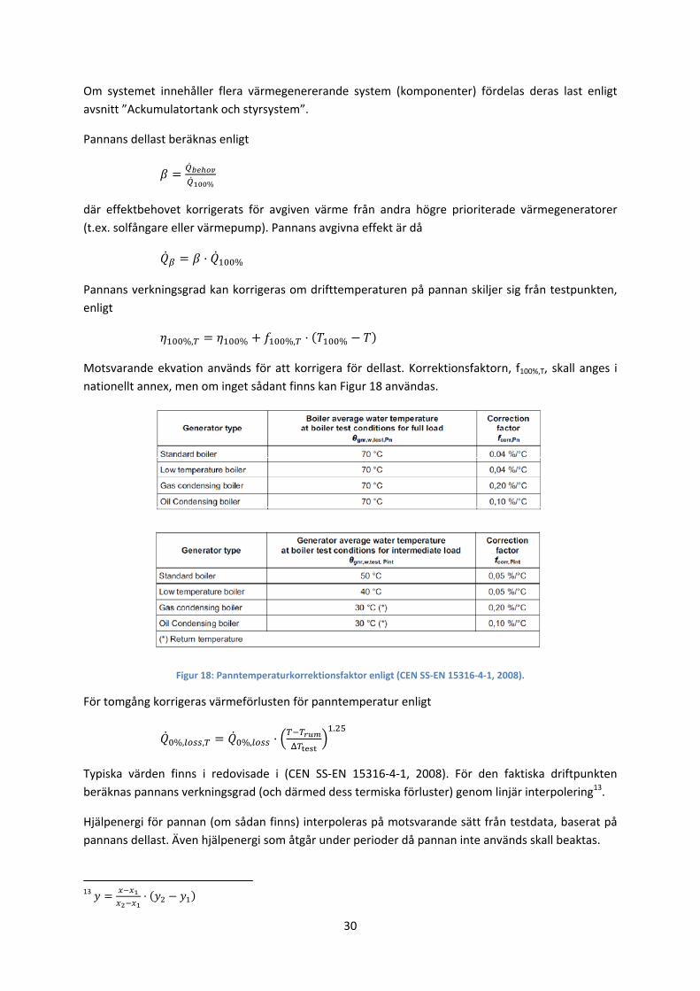
30

Om systemet innehåller flera värmegenererande system (komponenter) fördelas deras last enligt

avsnitt ”Ackumulatortank och styrsystem”.

Pannans dellast beräknas enligt

%

där effektbehovet korrigerats för avgiven värme från andra högre prioriterade värmegeneratorer

(t.ex. solfångare eller värmepump). Pannans avgivna effekt är då

%

Pannans verkningsgrad kan korrigeras om drifttemperaturen på pannan skiljer sig från testpunkten,

enligt

%, % %, %

Motsvarande ekvation används för att korrigera för dellast. Korrektionsfaktorn, f100%,T, skall anges i

nationellt annex, men om inget sådant finns kan Figur 18 användas.

Figur 18: Panntemperaturkorrektionsfaktor enligt (CEN SS‐EN 15316‐4‐1, 2008).

För tomgång korrigeras värmeförlusten för panntemperatur enligt

%, , %,

.

Typiska värden finns i redovisade i (CEN SS‐EN 15316‐4‐1, 2008). För den faktiska driftpunkten

beräknas pannans verkningsgrad (och därmed dess termiska förluster) genom linjär interpolering13.

Hjälpenergi för pannan (om sådan finns) interpoleras på motsvarande sätt från testdata, baserat på

pannans dellast. Även hjälpenergi som åtgår under perioder då pannan inte används skall beaktas.

13

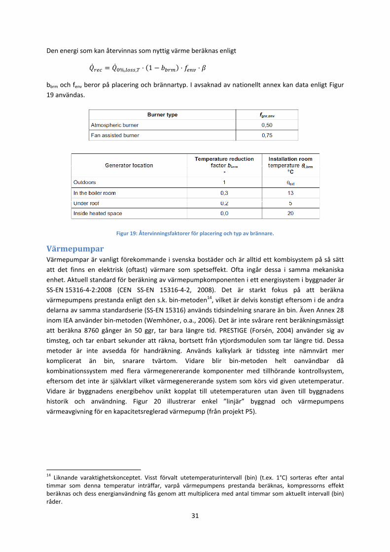
31

Den energi som kan återvinnas som nyttig värme beräknas enligt

%, , 1

bbrm och fenv beror på placering och brännartyp. I avsaknad av nationellt annex kan data enligt Figur

19 användas.

Figur 19: Återvinningsfaktorer för placering och typ av brännare.

Värmepumpar Värmepumpar är vanligt förekommande i svenska bostäder och är alltid ett kombisystem på så sätt

att det finns en elektrisk (oftast) värmare som spetseffekt. Ofta ingår dessa i samma mekaniska

enhet. Aktuell standard för beräkning av värmepumpkomponenten i ett energisystem i byggnader är

SS‐EN 15316‐4‐2:2008 (CEN SS‐EN 15316‐4‐2, 2008). Det är starkt fokus på att beräkna

värmepumpens prestanda enligt den s.k. bin‐metoden14, vilket är delvis konstigt eftersom i de andra

delarna av samma standardserie (SS‐EN 15316) används tidsindelning snarare än bin. Även Annex 28

inom IEA använder bin‐metoden (Wemhöner, o.a., 2006). Det är inte svårare rent beräkningsmässigt

att beräkna 8760 gånger än 50 ggr, tar bara längre tid. PRESTIGE (Forsén, 2004) använder sig av

timsteg, och tar enbart sekunder att räkna, bortsett från ytjordsmodulen som tar längre tid. Dessa

metoder är inte avsedda för handräkning. Används kalkylark är tidssteg inte nämnvärt mer

komplicerat än bin, snarare tvärtom. Vidare blir bin‐metoden helt oanvändbar då

kombinationssystem med flera värmegenererande komponenter med tillhörande kontrollsystem,

eftersom det inte är självklart vilket värmegenererande system som körs vid given utetemperatur.

Vidare är byggnadens energibehov unikt kopplat till utetemperaturen utan även till byggnadens

historik och användning. Figur 20 illustrerar enkel ”linjär” byggnad och värmepumpens

värmeavgivning för en kapacitetsreglerad värmepump (från projekt P5).

14 Liknande varaktighetskonceptet. Visst förvalt utetemperaturintervall (bin) (t.ex. 1°C) sorteras efter antal timmar som denna temperatur inträffar, varpå värmepumpens prestanda beräknas, kompressorns effekt beräknas och dess energianvändning fås genom att multiplicera med antal timmar som aktuellt intervall (bin) råder.

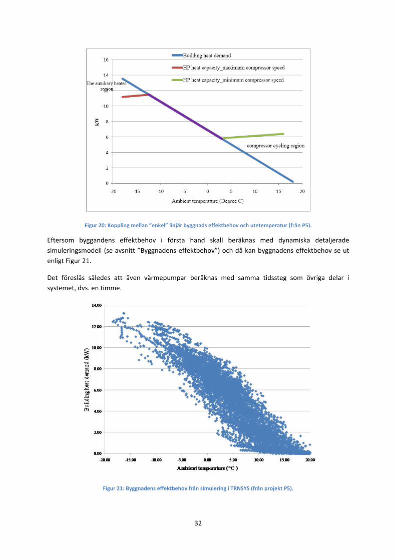
32

Figur 20: Koppling mellan ”enkel” linjär byggnads effektbehov och utetemperatur (från P5).

Eftersom byggandens effektbehov i första hand skall beräknas med dynamiska detaljerade

simuleringsmodell (se avsnitt ”Byggnadens effektbehov”) och då kan byggnadens effektbehov se ut

enligt Figur 21.

Det föreslås således att även värmepumpar beräknas med samma tidssteg som övriga delar i

systemet, dvs. en timme.

Figur 21: Byggnadens effektbehov från simulering i TRNSYS (från projekt P5).

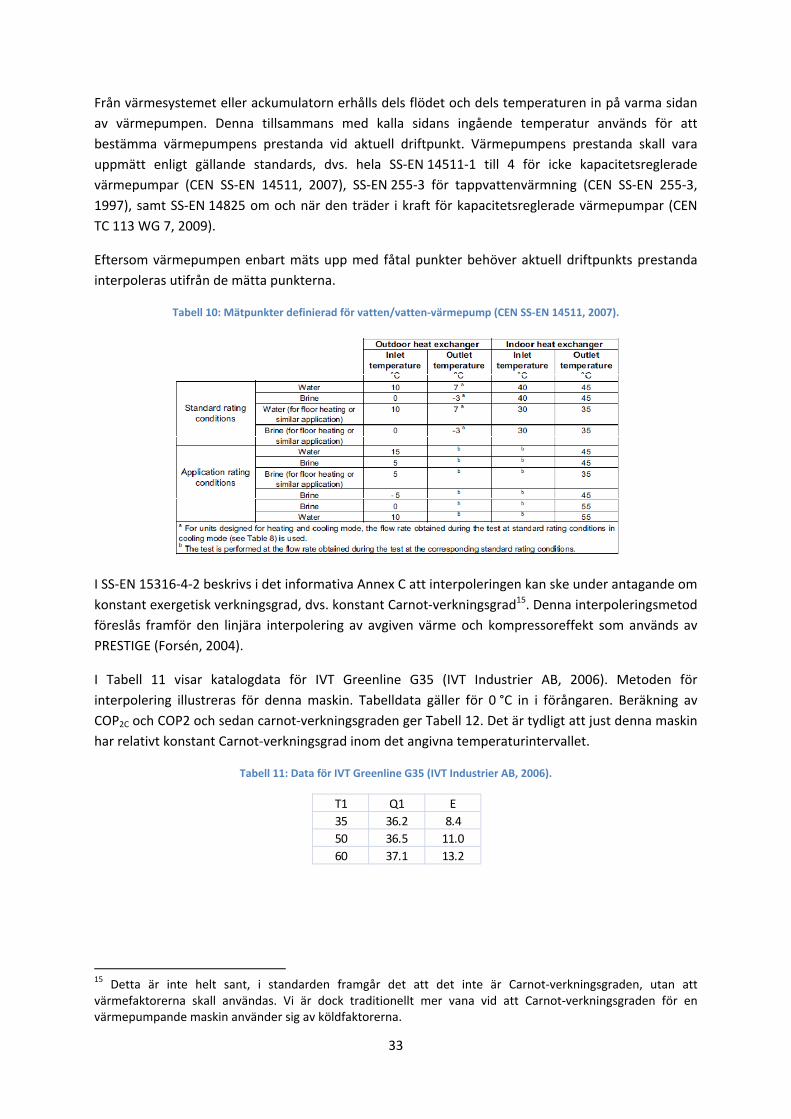
33

Från värmesystemet eller ackumulatorn erhålls dels flödet och dels temperaturen in på varma sidan

av värmepumpen. Denna tillsammans med kalla sidans ingående temperatur används för att

bestämma värmepumpens prestanda vid aktuell driftpunkt. Värmepumpens prestanda skall vara

uppmätt enligt gällande standards, dvs. hela SS‐EN 14511‐1 till 4 för icke kapacitetsreglerade

värmepumpar (CEN SS‐EN 14511, 2007), SS‐EN 255‐3 för tappvattenvärmning (CEN SS‐EN 255‐3,

1997), samt SS‐EN 14825 om och när den träder i kraft för kapacitetsreglerade värmepumpar (CEN

TC 113 WG 7, 2009).

Eftersom värmepumpen enbart mäts upp med fåtal punkter behöver aktuell driftpunkts prestanda

interpoleras utifrån de mätta punkterna.

Tabell 10: Mätpunkter definierad för vatten/vatten‐värmepump (CEN SS‐EN 14511, 2007).

I SS‐EN 15316‐4‐2 beskrivs i det informativa Annex C att interpoleringen kan ske under antagande om

konstant exergetisk verkningsgrad, dvs. konstant Carnot‐verkningsgrad15. Denna interpoleringsmetod

föreslås framför den linjära interpolering av avgiven värme och kompressoreffekt som används av

PRESTIGE (Forsén, 2004).

I Tabell 11 visar katalogdata för IVT Greenline G35 (IVT Industrier AB, 2006). Metoden för

interpolering illustreras för denna maskin. Tabelldata gäller för 0 °C in i förångaren. Beräkning av

COP2C och COP2 och sedan carnot‐verkningsgraden ger Tabell 12. Det är tydligt att just denna maskin

har relativt konstant Carnot‐verkningsgrad inom det angivna temperaturintervallet.

Tabell 11: Data för IVT Greenline G35 (IVT Industrier AB, 2006).

15 Detta är inte helt sant, i standarden framgår det att det inte är Carnot‐verkningsgraden, utan att värmefaktorerna skall användas. Vi är dock traditionellt mer vana vid att Carnot‐verkningsgraden för en värmepumpande maskin använder sig av köldfaktorerna.

T1 Q1 E

35 36.2 8.4

50 36.5 11.0

60 37.1 13.2

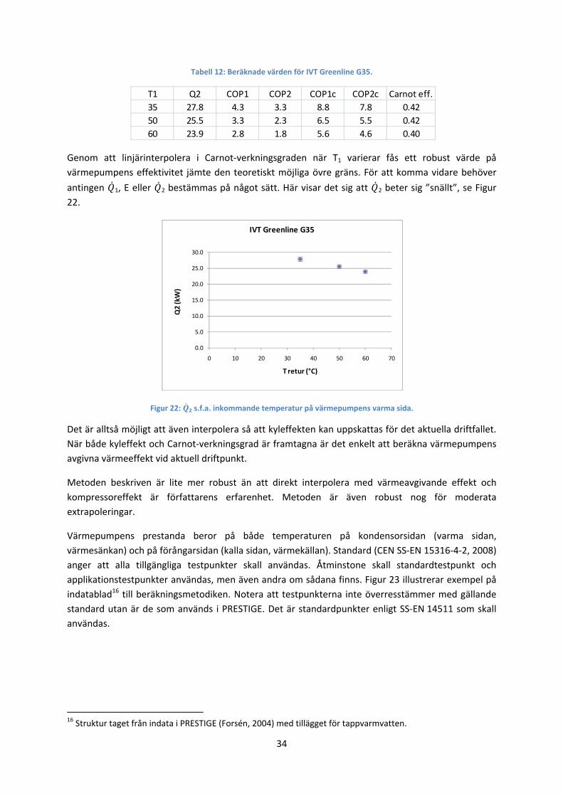
34

Tabell 12: Beräknade värden för IVT Greenline G35.

Genom att linjärinterpolera i Carnot‐verkningsgraden när T1 varierar fås ett robust värde på

värmepumpens effektivitet jämte den teoretiskt möjliga övre gräns. För att komma vidare behöver

antingen 1, E eller 2 bestämmas på något sätt. Här visar det sig att 2 beter sig ”snällt”, se Figur

22.

Figur 22: 2 s.f.a. inkommande temperatur på värmepumpens varma sida.

Det är alltså möjligt att även interpolera så att kyleffekten kan uppskattas för det aktuella driftfallet.

När både kyleffekt och Carnot‐verkningsgrad är framtagna är det enkelt att beräkna värmepumpens

avgivna värmeeffekt vid aktuell driftpunkt.

Metoden beskriven är lite mer robust än att direkt interpolera med värmeavgivande effekt och

kompressoreffekt är författarens erfarenhet. Metoden är även robust nog för moderata

extrapoleringar.

Värmepumpens prestanda beror på både temperaturen på kondensorsidan (varma sidan,

värmesänkan) och på förångarsidan (kalla sidan, värmekällan). Standard (CEN SS‐EN 15316‐4‐2, 2008)

anger att alla tillgängliga testpunkter skall användas. Åtminstone skall standardtestpunkt och

applikationstestpunkter användas, men även andra om sådana finns. Figur 23 illustrerar exempel på

indatablad16 till beräkningsmetodiken. Notera att testpunkterna inte överresstämmer med gällande

standard utan är de som används i PRESTIGE. Det är standardpunkter enligt SS‐EN 14511 som skall

användas.

16 Struktur taget från indata i PRESTIGE (Forsén, 2004) med tillägget för tappvarmvatten.

T1 Q2 COP1 COP2 COP1c COP2c Carnot eff.

35 27.8 4.3 3.3 8.8 7.8 0.42

50 25.5 3.3 2.3 6.5 5.5 0.42

60 23.9 2.8 1.8 5.6 4.6 0.40

0.0

5.0

10.0

15.0

20.0

25.0

30.0

0 10 20 30 40 50 60 70

Q2 (kW)

T retur (°C)

IVT Greenline G35

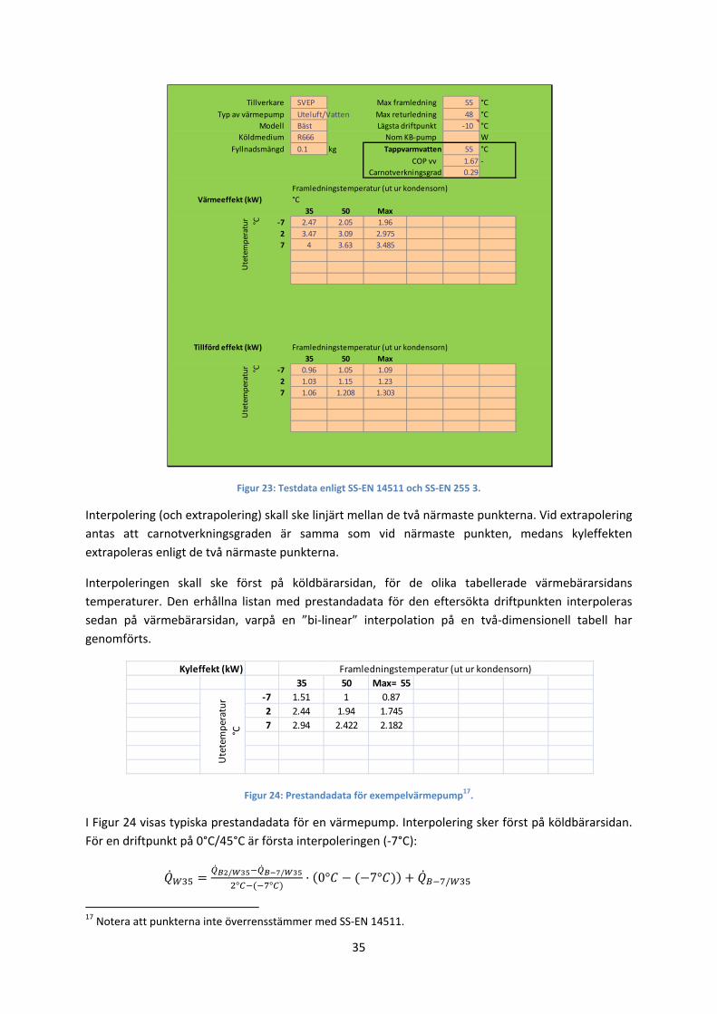
35

Figur 23: Testdata enligt SS‐EN 14511 och SS‐EN 255 3.

Interpolering (och extrapolering) skall ske linjärt mellan de två närmaste punkterna. Vid extrapolering

antas att carnotverkningsgraden är samma som vid närmaste punkten, medans kyleffekten

extrapoleras enligt de två närmaste punkterna.

Interpoleringen skall ske först på köldbärarsidan, för de olika tabellerade värmebärarsidans

temperaturer. Den erhållna listan med prestandadata för den eftersökta driftpunkten interpoleras

sedan på värmebärarsidan, varpå en ”bi‐linear” interpolation på en två‐dimensionell tabell har

genomförts.

Figur 24: Prestandadata för exempelvärmepump17.

I Figur 24 visas typiska prestandadata för en värmepump. Interpolering sker först på köldbärarsidan.

För en driftpunkt på 0°C/45°C är första interpoleringen (‐7°C):

/ /

° °0° 7° /

17 Notera att punkterna inte överrensstämmer med SS‐EN 14511.

Tillverkare SVEP Max framledning 55 °C

Typ av värmepump Uteluft/Vatten Max returledning 48 °C

Modell Bäst Lägsta driftpunkt ‐10 °C

Köldmedium R666 Nom KB‐pump W

Fyllnadsmängd 0.1 kg Tappvarmvatten 55 °C

COP vv 1.67 ‐

Carnotverkningsgrad 0.29

Värmeeffekt (kW)

35 50 Max

‐7 2.47 2.05 1.96

2 3.47 3.09 2.975

7 4 3.63 3.485

Tillförd effekt (kW)

35 50 Max

‐7 0.96 1.05 1.09

2 1.03 1.15 1.23

7 1.06 1.208 1.303

Framledningstemperatur (ut ur kondensorn)

°C

Utetemperatur °C


Utetemperatur °C

Kyleffekt (kW)

35 50 Max= 55

‐7 1.51 1 0.87

2 2.44 1.94 1.745

7 2.94 2.422 2.182


Utetemperatur

°C

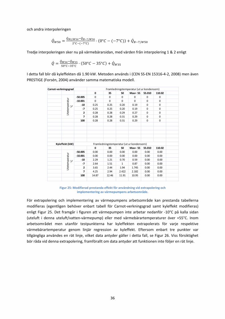
36

och andra interpoleringen

/ /

° °0° 7° /

Tredje interpoleringen sker nu på värmebärarsidan, med värden från interpolering 1 & 2 enligt

° °

50° 35°

I detta fall blir då kyleffekten då 1.90 kW. Metoden används i (CEN SS‐EN 15316‐4‐2, 2008) men även

PRESTIGE (Forsén, 2004) använder samma matematiska modell.

Figur 25: Modifierad prestanda effekt för användning vid extrapolering och implementering av värmepumpens arbetsområde.

För extrapolering och implementering av värmepumpens arbetsområde kan prestanda tabellerna

modifieras (egentligen behöver enbart tabell för Carnot‐verkningsgrad samt kyleffekt modifieras)

enligt Figur 25. Det framgår i figuren att värmepumpen inte arbetar nedanför ‐10°C på kalla sidan

(uteluft i denna uteluft/vatten‐värmepump) eller med värmebärartemperaturer över +55°C. Inom

arbetsområdet men utanför testpunkterna har kyleffekten extrapolerats för varje respektive

värmebärartemperatur genom linjär regression av kyleffekt. Eftersom enbart tre punkter var

tillgängliga användes en rät linje, vilket data antyder gäller i detta fall, se Figur 26. Viss försiktighet

bör råda vid denna extrapolering, framförallt om data antyder att funktionen inte följer en rät linje.

Carnot‐verkningsgrad

0 35 50 Max= 55 55.010 110.02

‐50.005 0 0 0 0 0 0

‐10.001 0 0 0 0 0 0

‐10 0.25 0.25 0.20 0.19 0 0

‐7 0.25 0.25 0.20 0.19 0 0

2 0.28 0.28 0.29 0.27 0 0

7 0.28 0.28 0.31 0.29 0 0

100 0.28 0.28 0.31 0.29 0 0

Kyleffekt (kW)

0 35 50 Max= 55 55.010 110.02

‐50.005 0.00 0.00 0.00 0.00 0.00 0.00

‐10.001 0.00 0.00 0.00 0.00 0.00 0.00

‐10 2.29 1.21 0.70 0.59 0.00 0.00

‐7 2.64 1.51 1 0.87 0.00 0.00

2 3.65 2.44 1.94 1.745 0.00 0.00

7 4.25 2.94 2.422 2.182 0.00 0.00

100 14.87 12.46 11.91 10.95 0.00 0.00


Utetemperatur

°C


Utetemperatur

°C

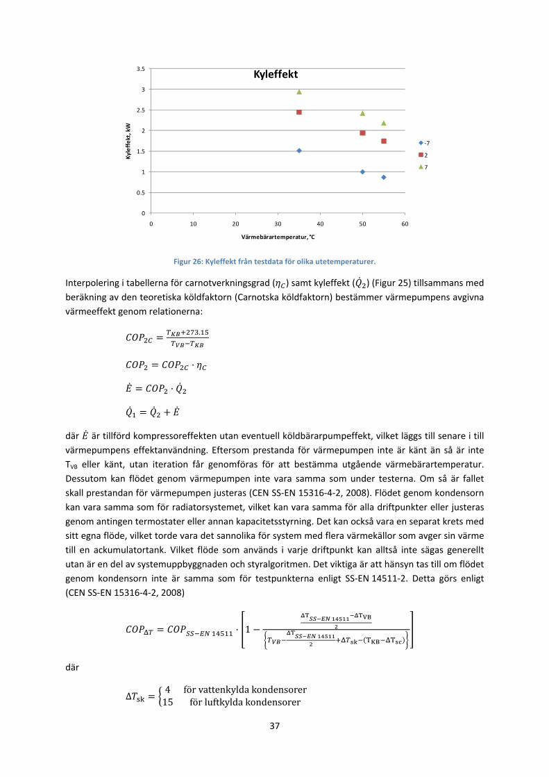
37

Figur 26: Kyleffekt från testdata för olika utetemperaturer.

Interpolering i tabellerna för carnotverkningsgrad ( ) samt kyleffekt ( ) (Figur 25) tillsammans med

beräkning av den teoretiska köldfaktorn (Carnotska köldfaktorn) bestämmer värmepumpens avgivna

värmeeffekt genom relationerna:

.

där är tillförd kompressoreffekten utan eventuell köldbärarpumpeffekt, vilket läggs till senare i till

värmepumpens effektanvändning. Eftersom prestanda för värmepumpen inte är känt än så är inte

TVB eller känt, utan iteration får genomföras för att bestämma utgående värmebärartemperatur.

Dessutom kan flödet genom värmepumpen inte vara samma som under testerna. Om så är fallet

skall prestandan för värmepumpen justeras (CEN SS‐EN 15316‐4‐2, 2008). Flödet genom kondensorn

kan vara samma som för radiatorsystemet, vilket kan vara samma för alla driftpunkter eller justeras

genom antingen termostater eller annan kapacitetsstyrning. Det kan också vara en separat krets med

sitt egna flöde, vilket torde vara det sannolika för system med flera värmekällor som avger sin värme

till en ackumulatortank. Vilket flöde som används i varje driftpunkt kan alltså inte sägas generellt

utan är en del av systemuppbyggnaden och styralgoritmen. Det viktiga är att hänsyn tas till om flödet

genom kondensorn inte är samma som för testpunkterna enligt SS‐EN 14511‐2. Detta görs enligt

(CEN SS‐EN 15316‐4‐2, 2008)

1

T TVB

T TKB T

där

Δ4 för vattenkylda kondensorer15 för luftkylda kondensorer

0

0.5

1

1.5

2

2.5

3

3.5

0 10 20 30 40 50 60

Kyleffekt, kW

Värmebärartemperatur, °C

Kyleffekt

‐7

2

7

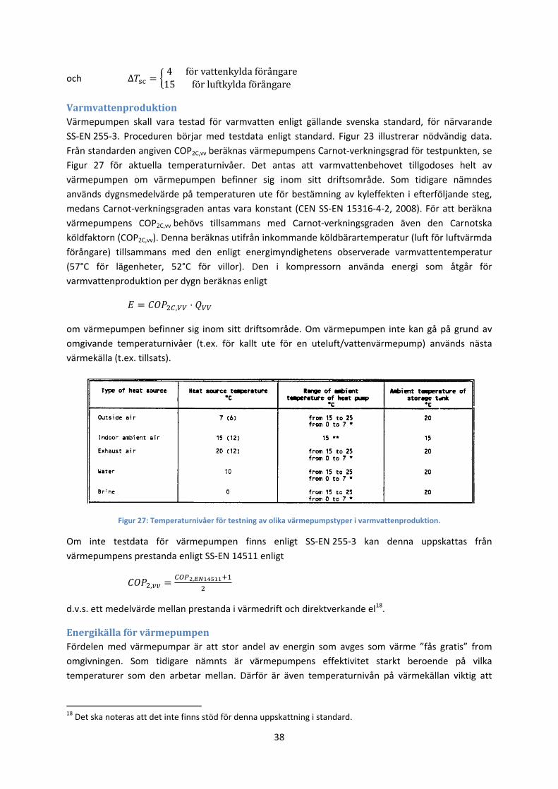
38

och Δ4 för vattenkylda förångare15 för luftkylda förångare

Varmvattenproduktion Värmepumpen skall vara testad för varmvatten enligt gällande svenska standard, för närvarande

SS‐EN 255‐3. Proceduren börjar med testdata enligt standard. Figur 23 illustrerar nödvändig data.

Från standarden angiven COP2C,vv beräknas värmepumpens Carnot‐verkningsgrad för testpunkten, se

Figur 27 för aktuella temperaturnivåer. Det antas att varmvattenbehovet tillgodoses helt av

värmepumpen om värmepumpen befinner sig inom sitt driftsområde. Som tidigare nämndes

används dygnsmedelvärde på temperaturen ute för bestämning av kyleffekten i efterföljande steg,

medans Carnot‐verkningsgraden antas vara konstant (CEN SS‐EN 15316‐4‐2, 2008). För att beräkna

värmepumpens COP2C,vv behövs tillsammans med Carnot‐verkningsgraden även den Carnotska

köldfaktorn (COP2C,vv). Denna beräknas utifrån inkommande köldbärartemperatur (luft för luftvärmda

förångare) tillsammans med den enligt energimyndighetens observerade varmvattentemperatur

(57°C för lägenheter, 52°C för villor). Den i kompressorn använda energi som åtgår för

varmvattenproduktion per dygn beräknas enligt

,

om värmepumpen befinner sig inom sitt driftsområde. Om värmepumpen inte kan gå på grund av

omgivande temperaturnivåer (t.ex. för kallt ute för en uteluft/vattenvärmepump) används nästa

värmekälla (t.ex. tillsats).

Figur 27: Temperaturnivåer för testning av olika värmepumpstyper i varmvattenproduktion.

Om inte testdata för värmepumpen finns enligt SS‐EN 255‐3 kan denna uppskattas från

värmepumpens prestanda enligt SS‐EN 14511 enligt

,,

d.v.s. ett medelvärde mellan prestanda i värmedrift och direktverkande el18.

Energikälla för värmepumpen Fördelen med värmepumpar är att stor andel av energin som avges som värme ”fås gratis” from

omgivningen. Som tidigare nämnts är värmepumpens effektivitet starkt beroende på vilka

temperaturer som den arbetar mellan. Därför är även temperaturnivån på värmekällan viktig att

18 Det ska noteras att det inte finns stöd för denna uppskattning i standard.

39

bestämma korrekt. Ingen standard har identifierats som anger hur temperaturnivån explicit skall

bestämmas. Det står i SS‐EN 15316‐4‐2 att:

För uteluftvärmepump skall uteluftens temperatur användas

För frånluftsvärmepump utan värmeåtervinning skall innetemperaturen användas.

För frånluftsvärmepump med värmeåtervinning skall återvinningsvärmeväxlaren och

värmepumpens prestanda mätas tillsammans eller så skall temperaturen beräknas efter

återvinningen genom värmeväxlarens temperaturverkningsgrad.

För mark‐, berg‐, eller sjövärmepumpar hänvisas till nationellt annex. Om inget sådant finns

kan Error! Reference source not found. användas för markvärmepump eller 0°C för

grundvattenvärmepump. (CEN SS‐EN 15316‐4‐2, 2008).

Det finns något som skulle kunna kallas nationellt annex, dvs. det arbete som utfördes under första

effsys‐programmet inom ramen för PRESTIGE (Forsén, 2004). Där beskrivs modell för både

markvärme och bergvärme. Eventuellt kanske en mer noggrann modell kan ersätta

bergvärmemodellen i PRESTIGE, då arbete fortgår (Javed, 2010) att utveckla en mer detaljerad och

noggrann, men till dess användes modeller enligt PRESTIGE (Forsén, 2004).

Solfångarsystem Solenergi som används i en byggnad anses precis som en värmepumps energiupptag from

omgivningen som ”gratis”. Solfångarsystem beräknas enligt standard SS‐EN 15316‐4‐3:2007 (CEN SS‐

EN 15316‐4‐3, 2007). Solfångarsystem kräver som indata solstrålning, så de klimatfiler som används i

t.ex. PRESTIGE behöver kompletteras med soldata. Typiska samhöriga data för utetemperatur och

solinstrålning måste bestämmas.

Enligt standard skall solfångarsystem beräknas per månad, två olika metoder för detta finns att tillgå.

Detta är inte tillräckligt små tidssteg då kombisystem skall utvärderas där prioritetsordningen på

systemen har stor inverkan. Istället föreslås att även solfångarsystem beräknas per timme.

En solfångares verkningsgrad kan skrivas som (Solar Energy Laboratory, 2006) (Duffie, o.a., 1991)

där , och är konstanter som bestäms experimentellt enligt standard SS‐EN 12975‐2.

Solfångarens effekt fås alltså sedan som

Solfångaren antas alltid leverera positiv effekt, d.v.s.

, max 0,

Om det i solfångarloopen även sitter en värmeväxlare mellan tank och solfångare skall dess negativa

inverkan på solfångarens effektivitet tas hänsyn till (Duffie, o.a., 1991). Även förlusterna i anslutande

rör samt solfångarens IAM som påverkar solfångarens prestanda skall inkluderas (Solar Energy

Laboratory, 2006) (Duffie, o.a., 1991).

40

CO2belastning av värmesystemet Avsikten med projektet var också att värmesystemets miljöbelastning kunde bedömas, vilket i

huvudsak inbegriper mängden CO2 som systemet orsakar. Boverket (Boverket, 2010) har gett

rekommendationer i sina anvisningar till energiexperter som utför energideklarationer hur dessa kan

uppskattas. Det är därför lämpligt att även värmepumpsbaserade system använder samma

bedömningsgrund.

För bränslen (fasta, flytande, gasformiga) som används i värmesystemet hänvisar Boverket till

Naturvårdsverket (Naturvårdsverket, 2010) som anger omräkningsfaktorer för olika bränslen och

dess miljöpåverkan. För fjärrvärme hänvisar Boverket till fjärrvärmedistributören eller energibolaget

(Boverket, 2010). För el som är kanske mest relevant för värmepumpsbaserade uppvärmningssystem

hänvisar Boverket till att en individuell bedömning av CO2‐belastningen genom att beakta byggnads‐

ägarens elavtal och elleverantörens uppgifter kring utsläpp för det aktuella avtalet. I praktiken

innebär detta väl att väljs ett elavtal som innebär vindel, vattenkraft eller kärnkraft påverkar

värmepumpen inte miljön via ökade utsläpp.

Detta har sedan länge varit ett omdiskuterat område hur el skall miljöbedömas, länge har det ansetts

att eftersom värmepumpen använder el ”på marginalen” skall också ”marginal‐el” användas för

miljöbedömningen, vilket för värmepumpar varit ofördelaktigt. Boverkets synvinkel synes vara mer

pragmatisk.

41

Slutsatser Projektet har syftat till att identifiera de behov för vidareutveckling och homogenisering av


årsbasis i småhus och flerfamiljshus. Enkät har genomförts vilket visar att alla program inte kan

hantera mer komplexa uppvärmningssystem som t.ex. solfångare tillsammans med värmepump.

Skillnaden på årsvärmefaktorn mellan de fiktiva fastigheterna är inte speciellt besvärande, med

beaktande att en leverantör räknade avfrostning dubbelt. Dock pekar det på vikten av riktig och rak

kommunikation kring den information som utbytes mellan kund och säljare.

Som andra del i projektet har metodik för beräkning av byggnaders energiprestanda tagits fram med

beaktande på de internationella och svenska standarder som finns. Strukturen hänvisar i stor




byggnaders energianvändning, där i huvudsak kontrakterad energis belastning enligt uppgift av

leverantör rekommenderas användas. Detta är en viss skillnad från tidigare då framförallt el räknades

som marginal‐el, vilket nu längre inte är fallet.

42

Referenser Adalberth Karin och Wahlström Åsa Energibesiktning av byggnader ‐ Flerbostadshus och lokaler

[Bok]. ‐ Stockholm : SIS Förlag AB, 2009.

ATON Teknikkonsult AB Energideklarering av bostadsbyggnader ‐ Metoder för besiktning och

beräkning, version 2 [Rapport]. ‐ Stockholm : ATON Teknikkonsult AB, 2007.

Boverket BFS 2007:4 BED 1: Boverkets föreskrifter och allmänna råd om energideklaration för

byggnader [Rapport]. ‐ Karlskrona : Anders Larsson, 2007. ‐ BFS 2007:4 BED 1.

Boverket Dimensionerande vinterutetemperatur, DVUT [Online] // Dimensionerande

vinterutetemperatur, DVUT. ‐ Boverket, den 16 November 2009. ‐ 2010. ‐

http://www.boverket.se/Global/Bygga_o_forvalta/Dokument/Bygg‐

%20och%20konstruktionsregler/BBR_avsnitt_9/dvut_2009%201_4_dagar.pdf.

Boverket Indata för energiberäkningar i kontor och småhus ‐ En sammanställning av brukarrelaterad

indata för elanvändning, personvärme och tappvarmvatten [Rapport]. ‐ Karlskrona : Boverket, 2007. ‐

ISBN: 978‐91‐85751‐65‐5.

Boverket Regelsamling för energideklaration med kommentarer [Rapport]. ‐ Karlskrona : Boverket,

2010. ‐ ISBN: 978‐91‐86342‐59‐3.

Boverket Regelsamling för energideklaration med kommentarer [Rapport]. ‐ Karlskrona : [u.n.],

2010. ‐ ISBN: 978‐91‐86342‐59‐3.

CEN SS‐EN 12831 SS‐EN 12831: Värmesystem i byggnader ‐ Metod för beräkning av dimensionerande

värmebehov [Bok]. ‐ Stockholm : SIS Förlag AB, 2003. ‐ SS‐EN 12831:2003.

CEN SS‐EN 14511 SS‐EN 14511, Luftkonditioneringsaggregat, vätskekylare och värmepumpar, med

elmotordrivna kompressorer, för rumsuppvärmning, Del 1, 2, 3, 4 [Rapport]. ‐ Stockholm : SIS Förlag

AB, 2007. ‐ SS‐EN 14511:1‐4.

CEN SS‐EN 14511‐1‐‐4 Luftkonditioneringsaggregat, vätskekylare och värmepumpar,med

elmotordrivna kompressorer, för rumsuppvärmning och ‐kylning – [Bok]. ‐ Stockholm : SIS Förlag AB,

2007. ‐ SS‐EN 14511‐1‐‐4.

CEN SS‐EN 15232 SS‐EN 15232:2007, Byggnaders energiprestanda ‐ Inverkan av

byggnadsautomation, styrning och teknisk byggnadsdrift [Rapport]. ‐ Stockholm : SIS Förlag AB,

2007. ‐ SS‐EN 15232:2007.

CEN SS‐EN 15242 Luftbehandling – Beräkningsmetoder för bestämning av luftflöden i byggnader

inklusive infiltration [Rapport]. ‐ Stockholm : SIS Förlag AB, 2007. ‐ SS‐EN 15242:2007.

CEN SS‐EN 15316‐2‐1 SS‐EN 15316‐2‐1 Värmesystem i byggnader ‐ Metod för beräkning av

energibehov och systemeffektivitet, Del 2.1 Värmeemmisionssystem för rumsuppvärmning

[Rapport]. ‐ Stockholm : SIS Förlag AB, 2007. ‐ SS‐EN 15316‐2‐1.

43


energibehov och systemeffektivitet, Del 2.3 Värmedistributionssystem för rumsuppvärmning

[Rapport]. ‐ Stockholm : SIS Förlag AB, 2007. ‐ SS‐EN 15316‐2‐3:2007.


energibehov och systemeffektivitet, Del 3.1 Krav på tappvarmvattensystem [Rapport]. ‐ Brussels :

CEN, 2007. ‐ SS‐EN 15316‐3‐1:2007.


energibehov och systemeffektivitet, Del 3.2 Tappvarmvattendistribution i bostadshus [Rapport]. ‐

Brussels : CEN, 2007. ‐ SS‐EN 15316‐3‐2:2007.


energibehov och systemeffektivitet, Del 3.3 Varmvattenberedning i bostadshus [Rapport]. ‐ Brussels :

CEN, 2007. ‐ SS‐EN 15316‐3‐3:2007.

CEN SS‐EN 15316‐4‐1 SS‐EN 15316‐4‐1:2008 Värmesystem i byggnader ‐ Metod för beräkning av

energibehov och systemeffektivitet. Del 4‐1: Värmegenerande system, förbränningsbaserade system

(pannor) [Bok]. ‐ Stocholm : SIS Förlag AB, 2008. ‐ SS‐EN 15316‐4‐1:2008.


energibehov och systemeffektivitet. Del 4‐2: Värmegenerande system, värmepumpsbaserade system



energibehov och systemeffektivitet. Del 4‐3: Värmegenerande system, termiska solvärmesystem


CEN SS‐EN 15316‐X‐X Värmesystem i byggnader – Metod för beräkning av energibehov och

systemeffektivitet [Bok]. ‐ Stockholm : SIS Förlag AB, 2008. ‐ SS‐EN 15316‐X‐X.

CEN SS‐EN 255‐3 SS‐EN 255‐3, Luftkonditioneringsaggregat, vätskekylare och värmepumpar med

eldriven kompressor ‐ Värmedrift ‐ Del 3: Provning och krav för märkning av aggregat för

tappvattenvärmning [Rapport]. ‐ Stockholm : SIS Förlag AB, 1997. ‐ SS‐EN 255‐3.

CEN SS‐EN ISO 13790 SS‐EN ISO 13790:2008, Byggnaders energiprestanda – Beräkning av

energianvändning för uppvärmning och kylning (ISO 13790:2008) [Bok]. ‐ Stockholm : SIS Förlag AB,

2008. ‐ SS‐EN ISO 13790:2008.

CEN TC 113 WG 7 Air conditioners, liquid chilling packages and heat pumps, with electrically

compressors, for space heating and cooling‐ Testing and rating at part load conditions and calculation

of seasonal performance [Bok]. ‐ Brussel : CEN TC 113 WG 7, 2009.

DesignBuilder Software Ltd DesignBuilder ‐ Building design, simulation and visualisation ‐ Building

Simulation... Made Easy [Online] // DesignBuilder ‐ Building design, simulation and visualisation ‐

Building Simulation... Made Easy. ‐ 2010. ‐ 2010. ‐ http://www.designbuilder.co.uk/.

Energimyndigheten Mätning av kall‐ och varmvattenanvändning i 44 hushåll [Rapport]. ‐ Eskilstuna :

Statens energimyndighet, 2009. ‐ ER 2009:26.

44

Equa www.equa.se [Online]. ‐ 2010. ‐ den 22 06 2010. ‐ www.equa.se.

EVI Heat Solvärmepumpen ‐en genialisk lösning [Online] // www.eviheat.se. ‐ 2010. ‐ 2010. ‐

http://www.eviheat.se/pages.aspx?r_id=44255.

Forsén Martin Prestige. ‐ [u.o.] : KTH ‐ Energiteknik, 2004.

Forsén Martin Simulering av värmepumpssystem [Rapport]. ‐ Stockholm : effsys, 2004.

Integrated Environment Solutions IES Virtual Environment [Online]. ‐ 2010. ‐ 2010. ‐

http://www.iesve.com/UK‐ROI.

IVT Industrier AB IVT Greenline G, modell 35‐45 kW. ‐ Tranås : [u.n.], den 05 Januari 2006.

Javed Saqib Design of ground source heat pump systems ‐ Thermal modelling and evaluation of

boreholes [Rapport]. ‐ Göteborg : Chalmers Tekniska Universitet, 2010. ‐ ISSN 1652‐6007, Technical

Report D2010:02.

Levin Per Brukarindata för energiberäkningar i bostäder [Rapport]. ‐ Stockholm : SVEBY‐programmet,

2009. ‐ 2009‐04‐14.

Naturvårdsverket Beräkna utsläpp av växthusgaser [Online] // www.naturvardsverket.se. ‐ 2010. ‐

2010. ‐ http://www.naturvardsverket.se/sv/Klimat‐i‐forandring/Minska‐utslappen/Verktygslada‐for‐

kommuner‐och‐foretag/Berakna‐utslapp‐av‐vaxthusgaser/.

OSO OSO Hotwater Norge [Online] // Optima EP2 300 & 400. ‐ OSO Hotwater, 2010. ‐ 2010. ‐

www.oso.no.

Solar Energy Laboratory TRNSYS 16 ‐ a TRaNsient SYstem Simulation program ‐ Volume 5,

Mathematical Reference [Bok]. ‐ [u.o.] : Solar Energy Laboratory, University of Wisconsin‐Madison,

2006.

Wemhöner Carsten och Afjei Thomas IEA Heat pump programme Annex 28, Test procedure and

seasonal performance calculation for residential heat pumps with combined space and domestic hot

water heating [Rapport]. ‐ Borås : IEA Heat Pump programme, 2006. ‐ HPP‐AN28‐1; ISBN 91‐85533‐

30‐0.

45

Appendix 1 – Enkät 1 I denna enkät efterfrågades huruvida programmen hade möjlighet att beräkna eller presentera

specifik information eller specifik systemlösning. Enkäten var indelad på följande delar

Huset

Värmesystemet


Klimat

Resultat

Nedan kommer varje fråga för sig att presenteras, först själva enkätfrågan, sedan svaren.

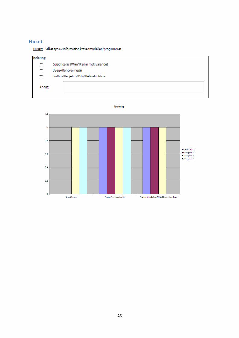
46

Huset

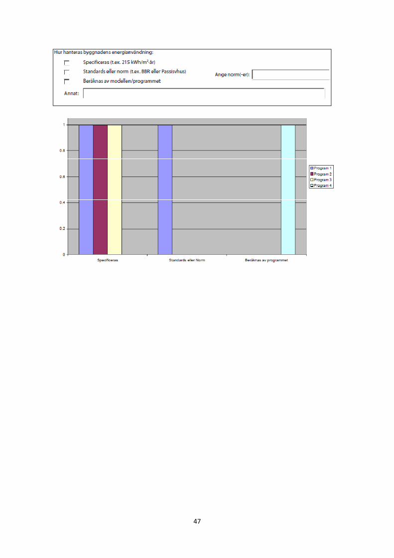
47

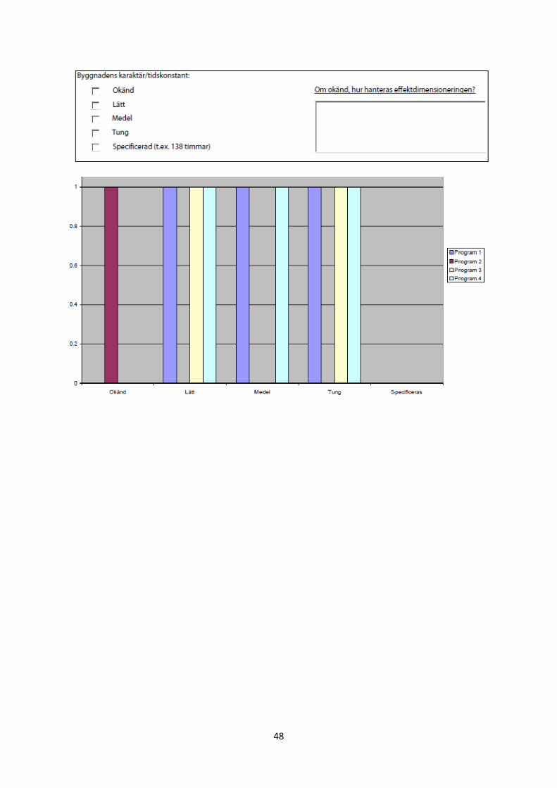
48

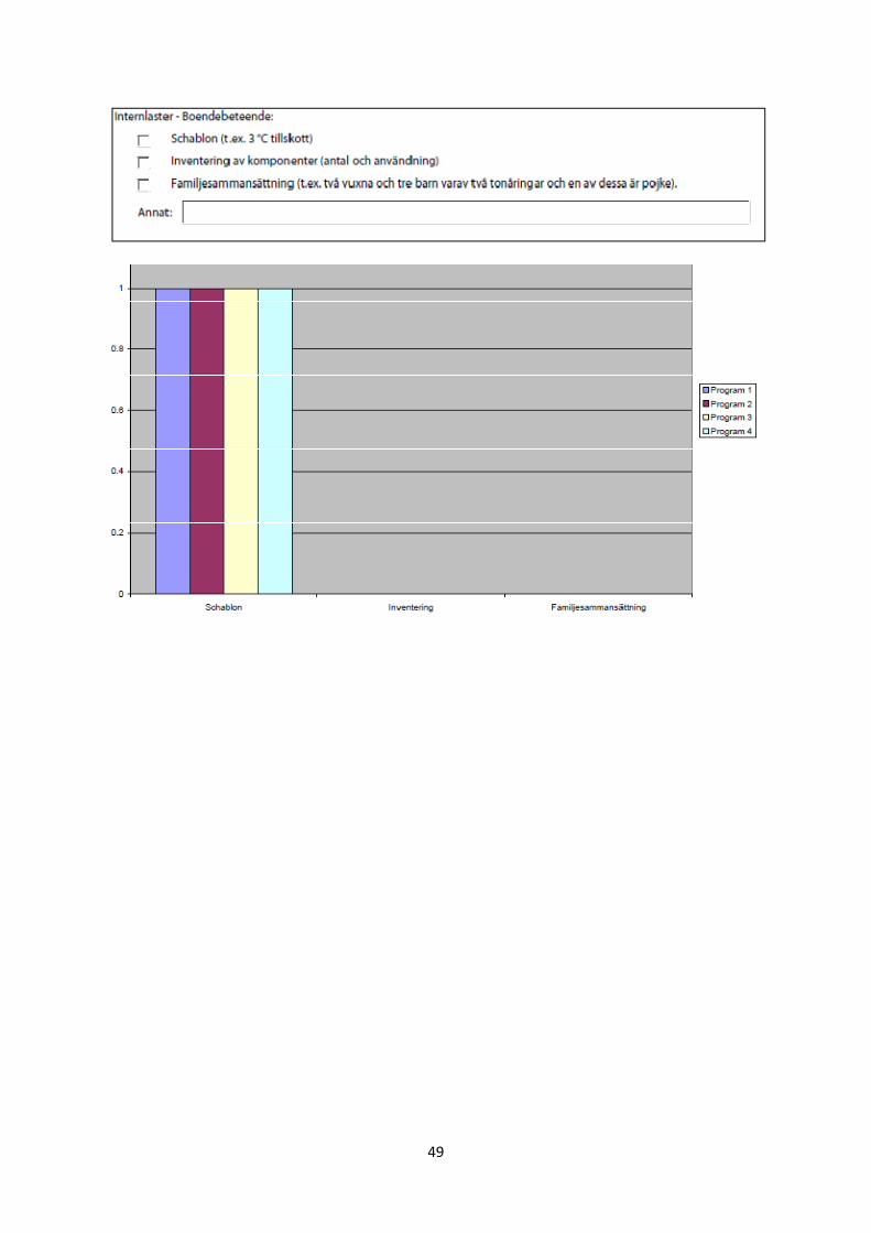
49

50

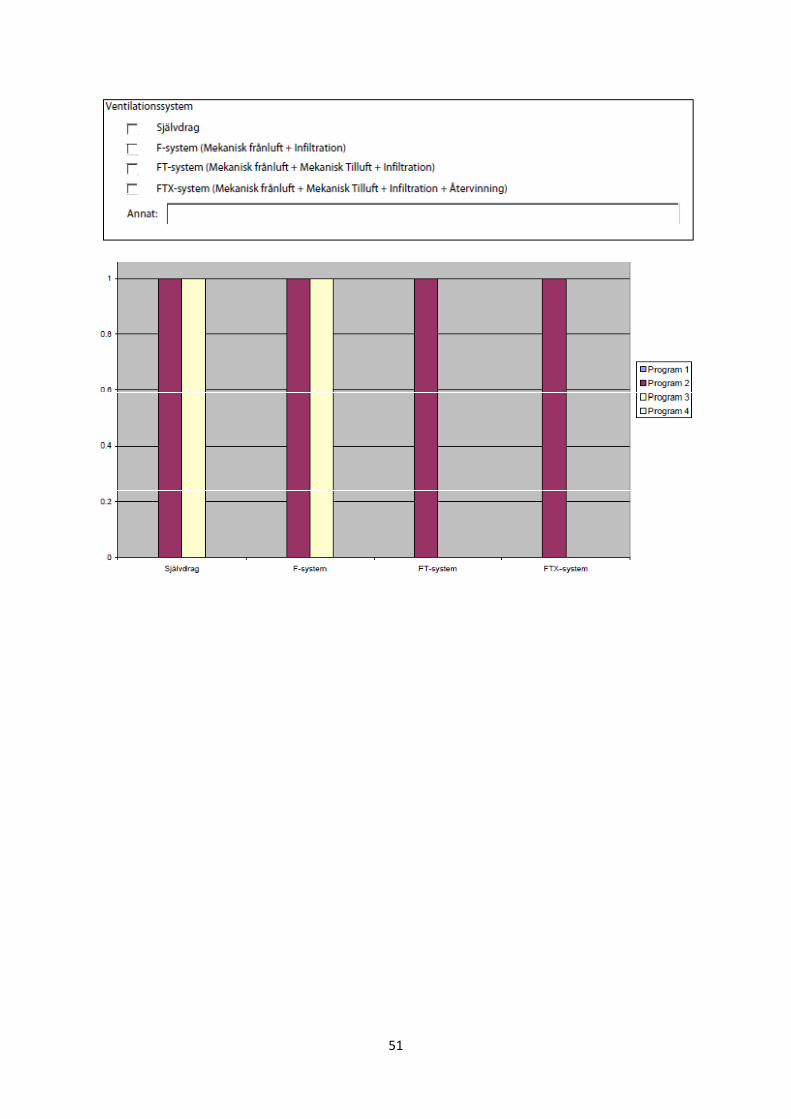
51

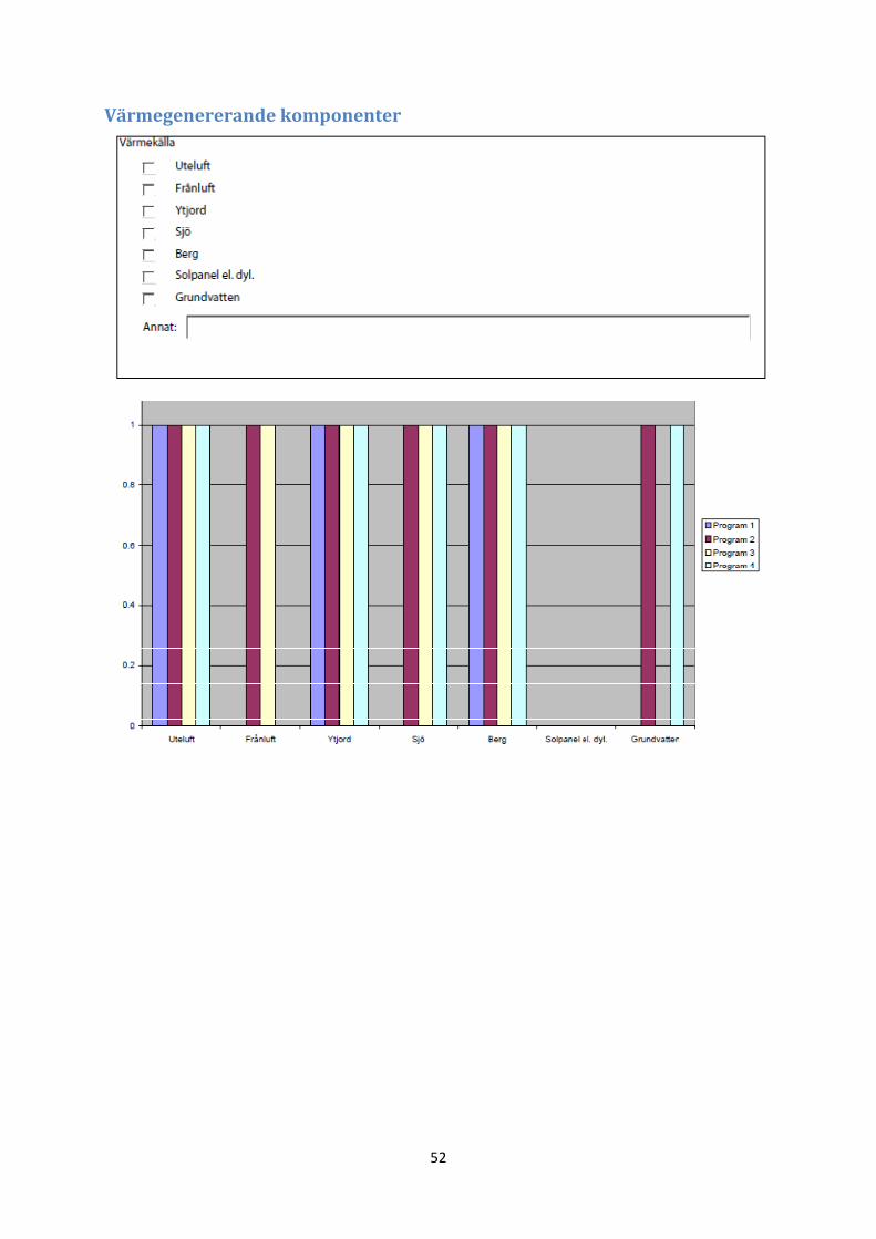
52


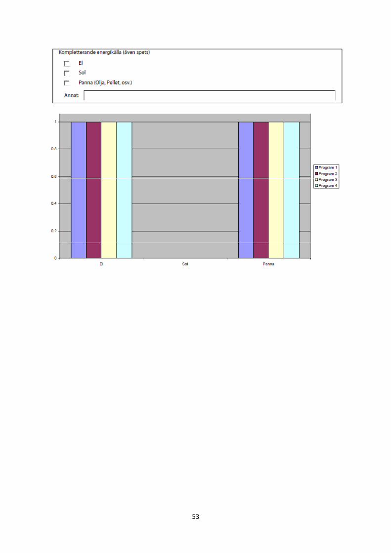
53

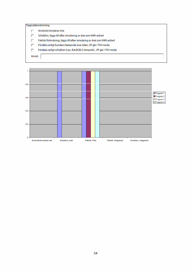
54

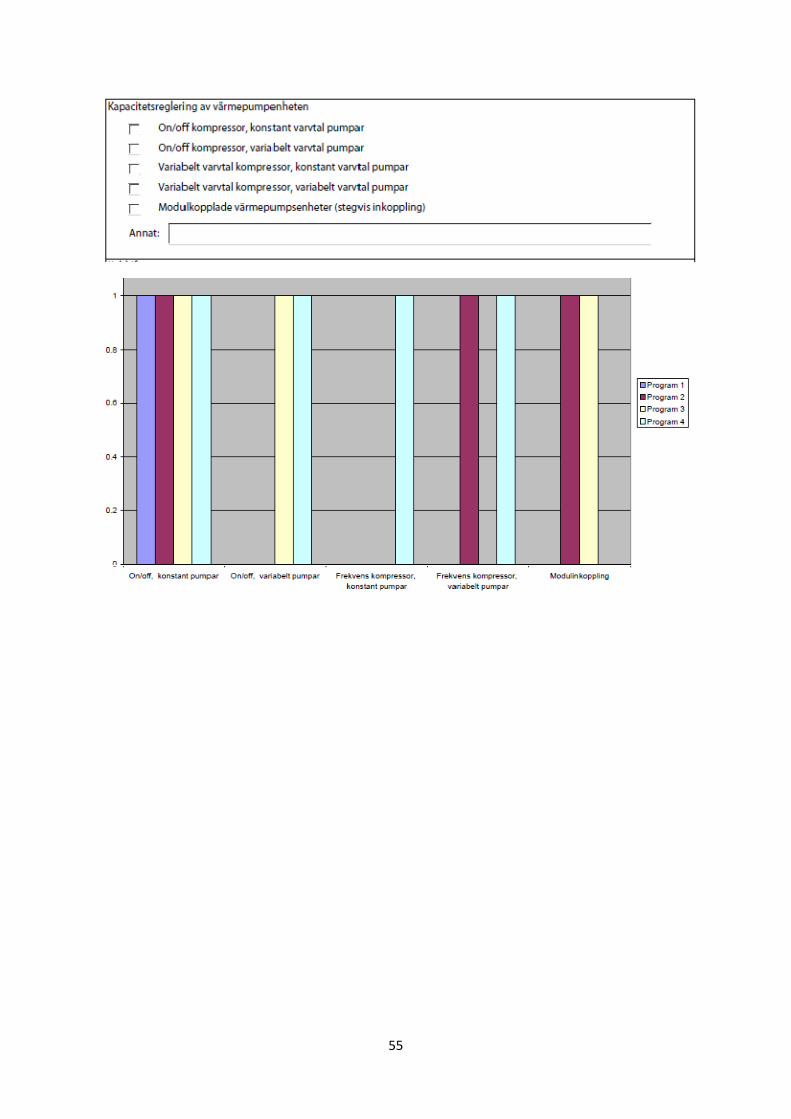
55

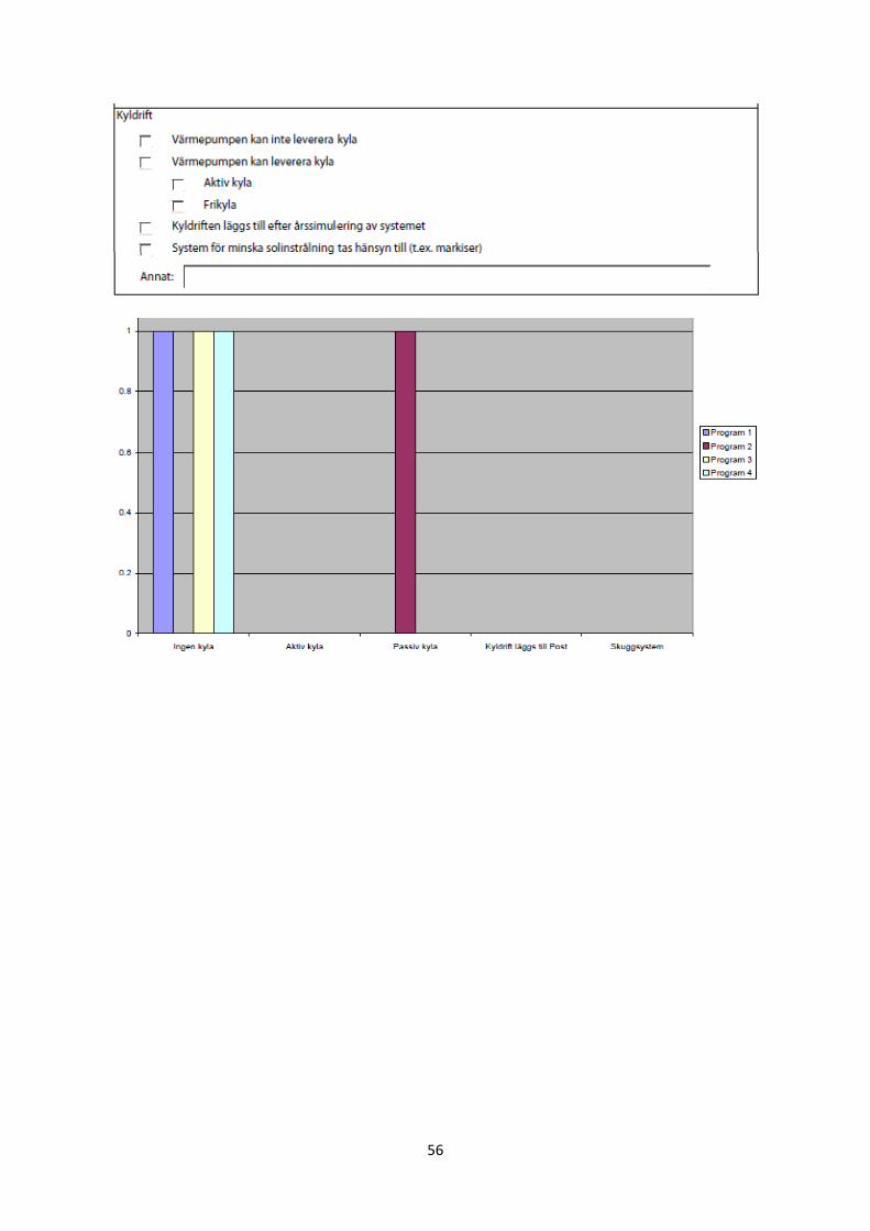
56

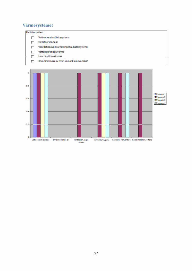
57

Värmesystemet

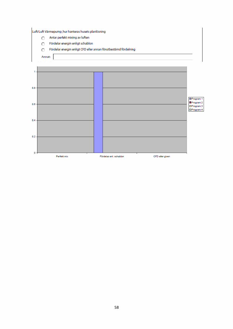
58

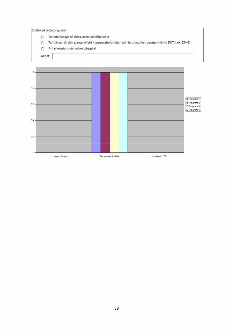
59

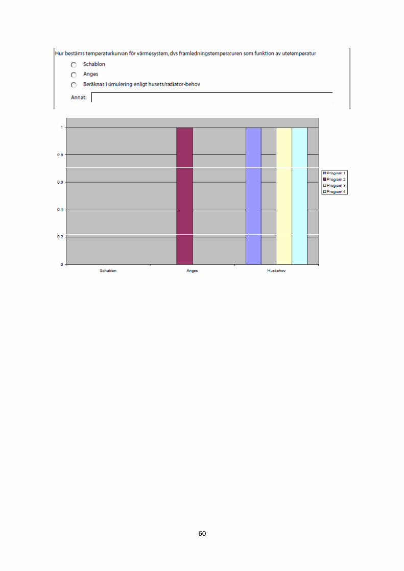
60

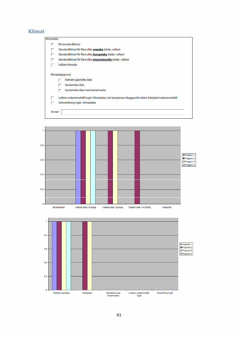
61

Klimat

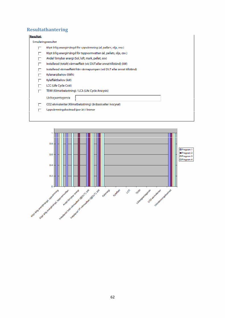
62

Resultathantering

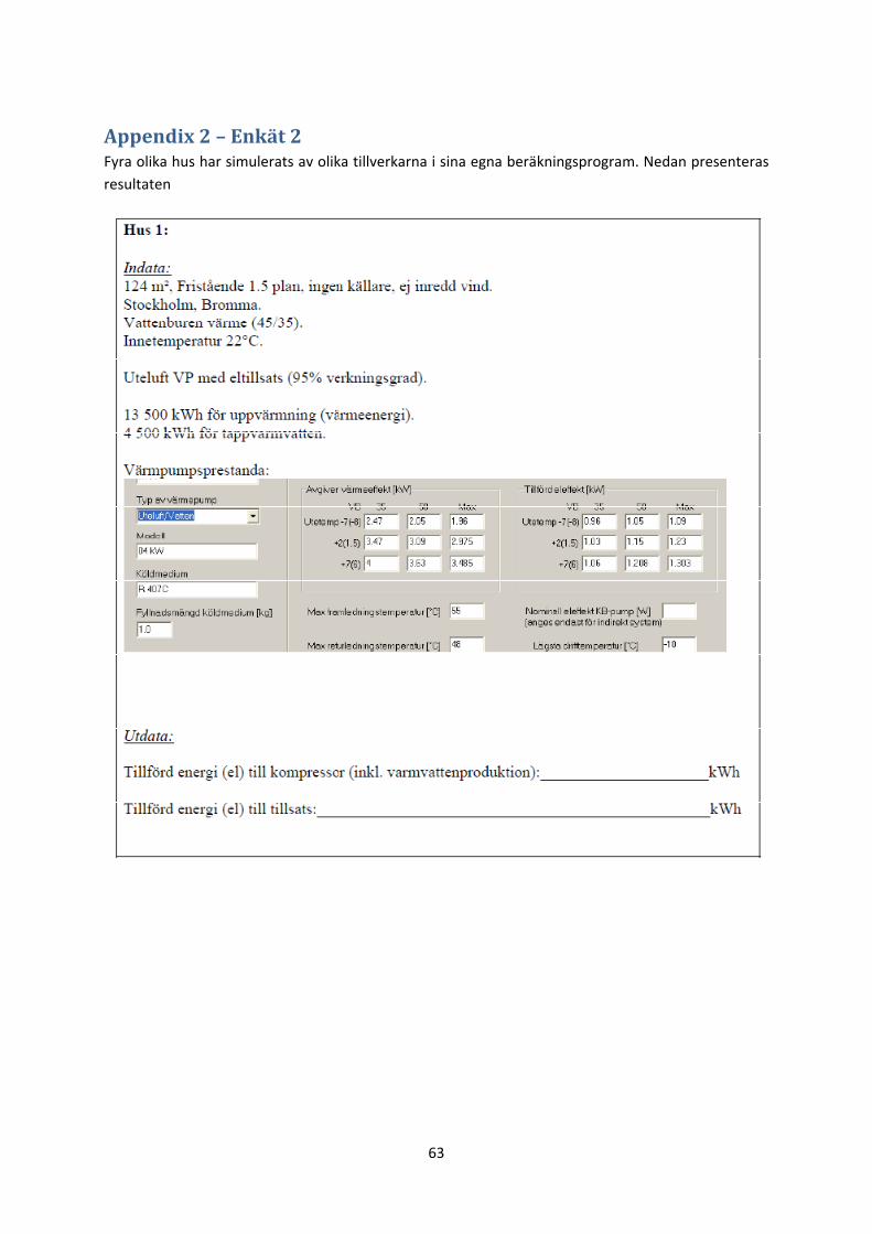
63

Appendix 2 – Enkät 2 Fyra olika hus har simulerats av olika tillverkarna i sina egna beräkningsprogram. Nedan presenteras

resultaten

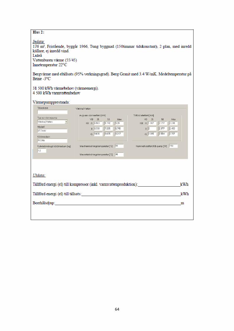
64

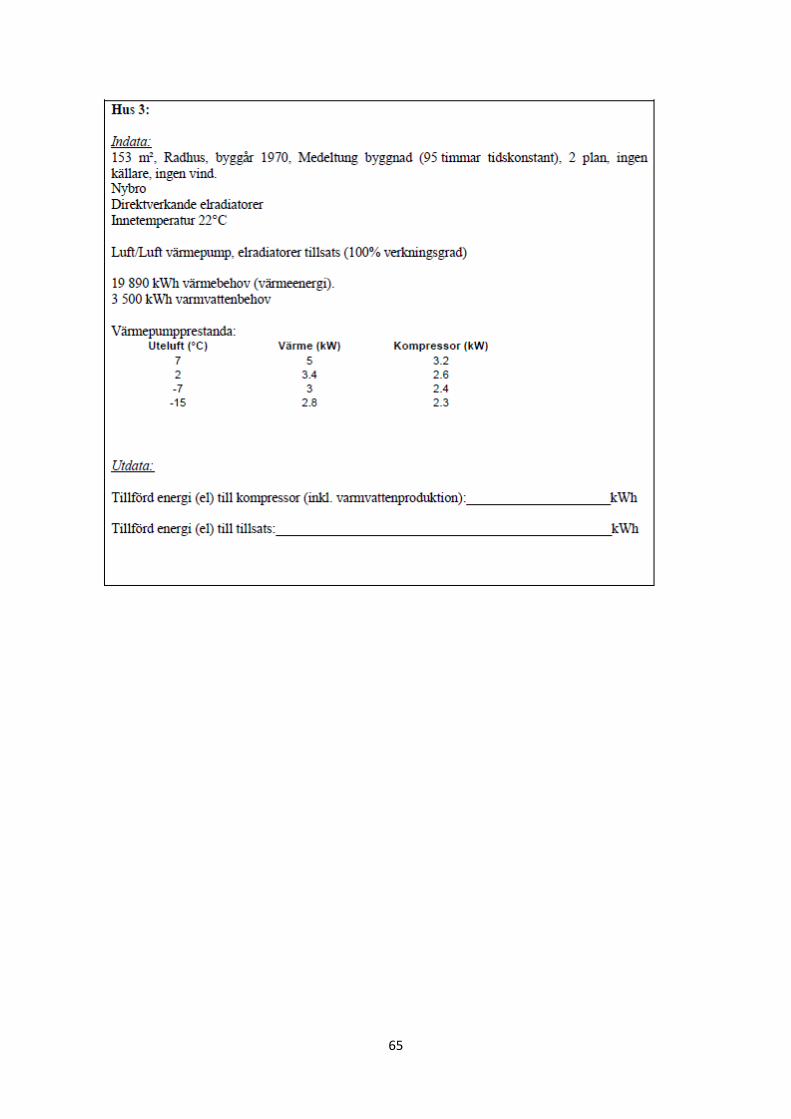
65

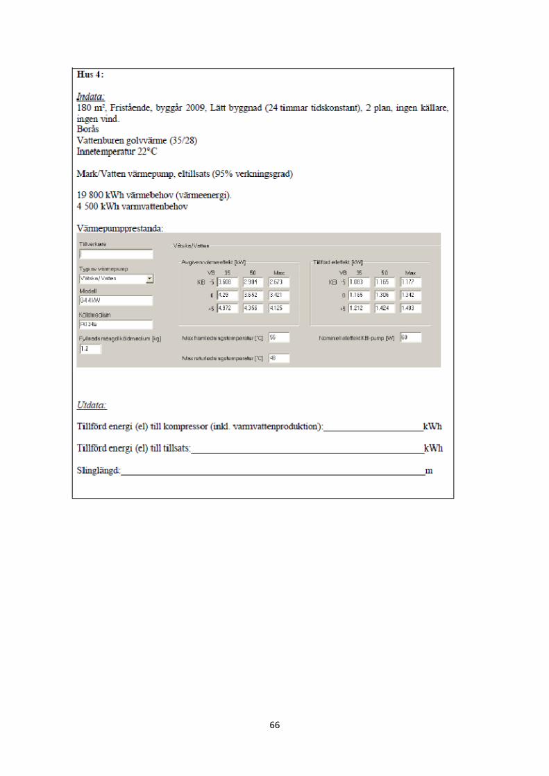
66

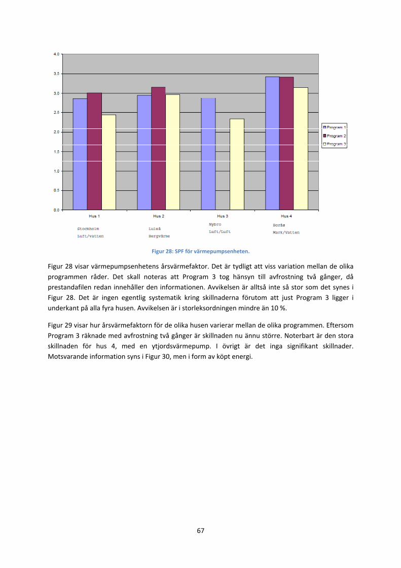
67

Figur 28: SPF för värmepumpsenheten.

Figur 28 visar värmepumpsenhetens årsvärmefaktor. Det är tydligt att viss variation mellan de olika

programmen råder. Det skall noteras att Program 3 tog hänsyn till avfrostning två gånger, då

prestandafilen redan innehåller den informationen. Avvikelsen är alltså inte så stor som det synes i

Figur 28. Det är ingen egentlig systematik kring skillnaderna förutom att just Program 3 ligger i

underkant på alla fyra husen. Avvikelsen är i storleksordningen mindre än 10 %.

Figur 29 visar hur årsvärmefaktorn för de olika husen varierar mellan de olika programmen. Eftersom

Program 3 räknade med avfrostning två gånger är skillnaden nu ännu större. Noterbart är den stora

skillnaden för hus 4, med en ytjordsvärmepump. I övrigt är det inga signifikant skillnader.

Motsvarande information syns i Figur 30, men i form av köpt energi.

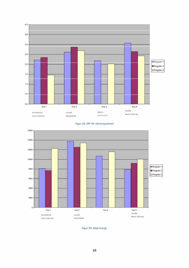
68

Figur 29: SPF för värmesystemet

Figur 30: Köpt energi.

69

Appendix 3 Studentarbeten På efterföljande sidor bifogas två stycken studentarbeten som utförts vid KTH – Energiteknik.

Comparison between three different heat pump sizing comptuter program concerning SPF and usability

Navid Ahmadi

Alessandro Pensini

Behzad A. Monfared

MJ2409 Applied Energy Technology PROJECT course

Department of Energy Technology Royal Institute of Technology

Stockholm, Sweden

TABLE OF CONTENTS

TABLE OF CONTENTS 1

1 OBJECTIVES 3

2 SCOPE 3

2.1 AVAILABLE TOOLS 3

2.2 APPROACH 3

2.3 OUTCOMES 4

3 INTRODUCTION 4

3.1 DEFINITIONS 4

3.1.1 GENERAL INTRODUCTION 4

3.1.2 SEASONAL PERFORMANCE FACTOR 6

3.2 PROBLEM FORMULATION 9

3.3 MAIN CHARACTERISTICS OF THE ASSESSED SOFTWARE TOOLS 12

4 ANALYSIS 13

4.1 PRESTIGE 2.0 13

4.1.1 WEATHER DATA 13

4.1.2 BUILDING CHARACTERISTICS 13

4.1.3 TEMPERATURES 13

4.1.4 ANNUAL ENERGY REQUIREMENT 13

4.1.5 CHOOSING HEAT PUMP 14

4.1.6 HEAT PUMP CALCULATIONS 14

4.1.7 ECONOMIC CALCULATIONS 16

4.2 VITOCALC 16





4.2.5 CHOOSING HEAT PUMP AND HEAT SOURCE 18



4.3 VPW 2100 21





4.3.5 CHOOSING HEAT PUMP AND HEAT SOURCE 23



5 DISCUSSION 29

5.1 COMPARISON 29

5.2 SUGGESTIONS 31

6 ACKNOWLEDGMENTS 32

7 REFERENCES 32

1 OBJECTIVES When installing a heat pump heating system, it is often of interest to know the amount of

energy saving that will be achieved. The SPF (seasonal performance factor) is an index that

gives information about the behaviour of a particular heat pump installed into a particular

building in terms of energy consumption during a full season, say a year. Such an index can

be used to compare different available solutions both for energetic and economic purposes.

Heat pump manufacturers basically follow the same frame for the SPF calculation procedure;

however there are some differences in their approach, which are the target points of our

assessment. Each manufacture has developed its own software tool in order to get the SPF

value of a system based on the heat pump, the building and the weather conditions

prevailing where the system is located.

In this project, an effort has been made to systematically compare the tools used by some

heat pump manufacturers for calculation of SPF.

The outcome of this project would be a comparison between three software packages in

terms of the features that characterize each program. Based on qualitative comparison of

different SPF calculation tools, conclusions will be presented at the end in order to propose

needs for further development.

2 SCOPE

2.1 AVAILABLE TOOLS

The programs we got access to are VITOCALC, PRESTIGE and VPW2100. In order to get these

software packages we have directly contacted several manufacturers and institutions and

we have included into our assessment the ones we got allowance to use. We did not get

access to tools developed by other manufactures mainly because of the distribution remains

internal among the technicians of the manufacturers. All the software packages we use are

covered by Copyright..

2.2 APPROACH

A quantitative approach would be achievable under different conditions of homogeneity.

A first difficulty in starting a quantitative comparison is the fact that the applications have

already built‐in characteristics for the heat pumps available for choosing. Another limitation

we have to deal with is that the software source codes are not available and the time the

group members can spend discussing with the developers of the software program or

specialists is limited. This fact often results in difficulties to understand the assumptions

behind the calculations performed by the programs. Thus, even if the same heat pump, in

term of performance characteristic, would be available to choose, the results of the energy

calculations given by different programs would be different.

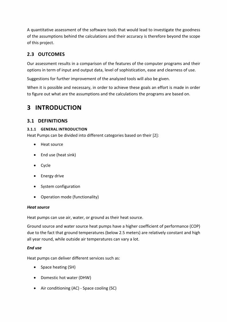
A quantitative assessment of the software tools that would lead to investigate the goodness

of the assumptions behind the calculations and their accuracy is therefore beyond the scope

of this project.

2.3 OUTCOMES

Our assessment results in a comparison of the features of the computer programs and their

options in term of input and output data, level of sophistication, ease and clearness of use.

Suggestions for further improvement of the analyzed tools will also be given.

When it is possible and necessary, in order to achieve these goals an effort is made in order

to figure out what are the assumptions and the calculations the programs are based on.

3 INTRODUCTION

3.1 DEFINITIONS

3.1.1 GENERAL INTRODUCTION

Heat Pumps can be divided into different categories based on their [2]:

• Heat source

• End use (heat sink)

• Cycle

• Energy drive

• System configuration

• Operation mode (functionality)

Heat source

Heat pumps can use air, water, or ground as their heat source.

Ground source and water source heat pumps have a higher coefficient of performance (COP)

due to the fact that ground temperatures (below 2.5 meters) are relatively constant and high

all year round, while outside air temperatures can vary a lot.

End use

Heat pumps can deliver different services such as:

• Space heating (SH)

• Domestic hot water (DHW)

• Air conditioning (AC) ‐ Space cooling (SC)

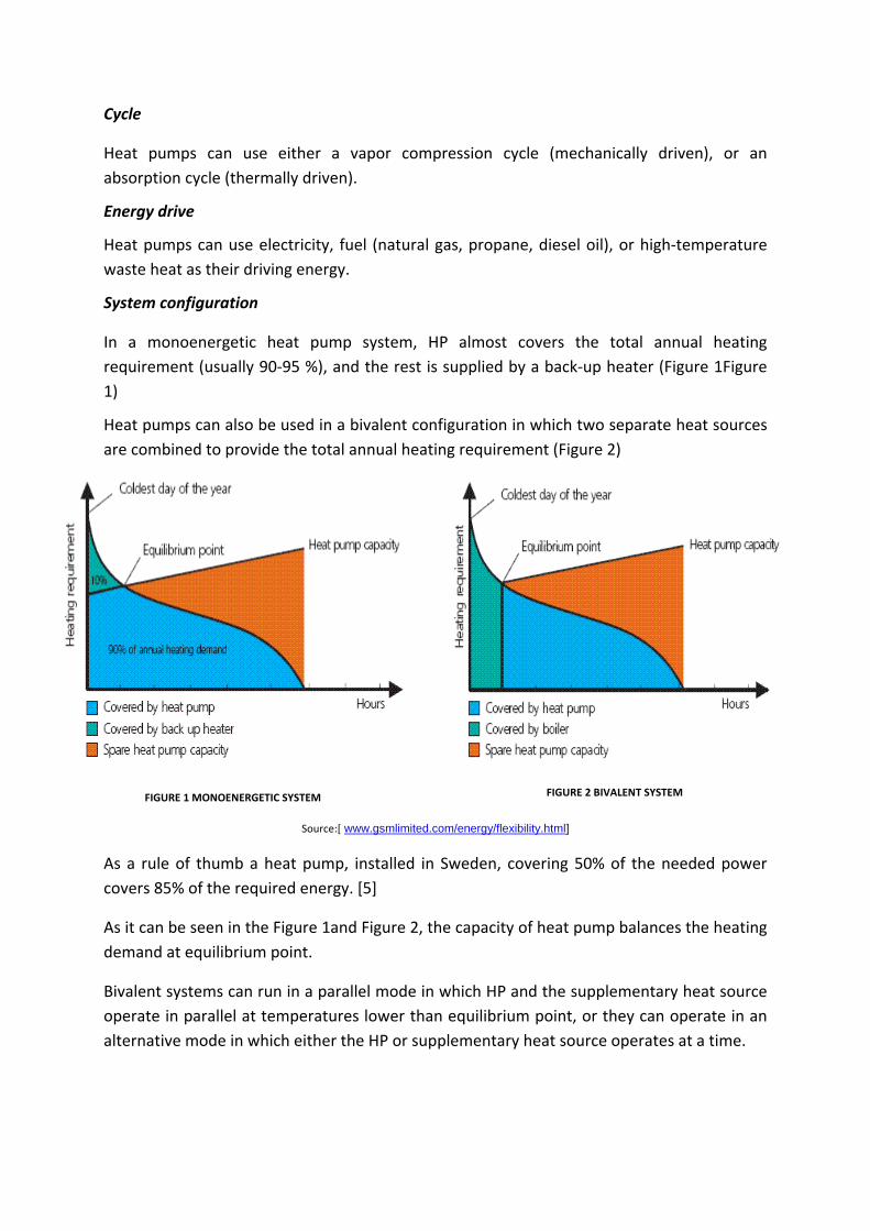
Cycle

Heat pumps can use either a vapor compression cycle (mechanically driven), or an

absorption cycle (thermally driven).

Energy drive

Heat pumps can use electricity, fuel (natural gas, propane, diesel oil), or high‐temperature

waste heat as their driving energy.

System configuration

In a monoenergetic heat pump system, HP almost covers the total annual heating

requirement (usually 90‐95 %), and the rest is supplied by a back‐up heater (Figure 1Figure

1)

Heat pumps can also be used in a bivalent configuration in which two separate heat sources

are combined to provide the total annual heating requirement (Figure 2)

FIGURE 1 MONOENERGETIC SYSTEM

FIGURE 2 BIVALENT SYSTEM

Source:[ www.gsmlimited.com/energy/flexibility.html]

As a rule of thumb a heat pump, installed in Sweden, covering 50% of the needed power

covers 85% of the required energy. [5]

As it can be seen in the Figure 1and Figure 2, the capacity of heat pump balances the heating

demand at equilibrium point.

Bivalent systems can run in a parallel mode in which HP and the supplementary heat source

operate in parallel at temperatures lower than equilibrium point, or they can operate in an

alternative mode in which either the HP or supplementary heat source operates at a time.

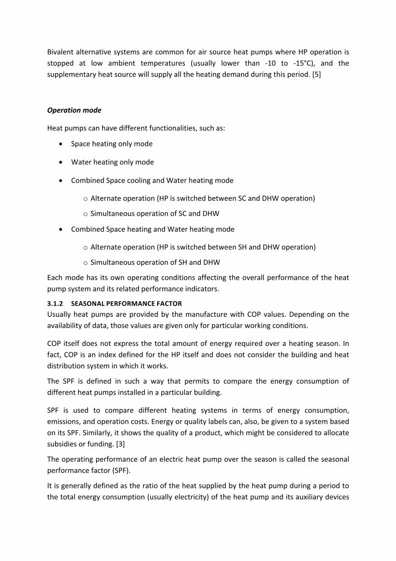
http://www.gsmlimited.com/energy/flexibility.html

Bivalent alternative systems are common for air source heat pumps where HP operation is

stopped at low ambient temperatures (usually lower than ‐10 to ‐15°C), and the

supplementary heat source will supply all the heating demand during this period. [5]

Operation mode

Heat pumps can have different functionalities, such as:

• Space heating only mode

• Water heating only mode

• Combined Space cooling and Water heating mode

o Alternate operation (HP is switched between SC and DHW operation)

o Simultaneous operation of SC and DHW

• Combined Space heating and Water heating mode

o Alternate operation (HP is switched between SH and DHW operation)

o Simultaneous operation of SH and DHW

Each mode has its own operating conditions affecting the overall performance of the heat

pump system and its related performance indicators.

3.1.2 SEASONAL PERFORMANCE FACTOR

Usually heat pumps are provided by the manufacture with COP values. Depending on the

availability of data, those values are given only for particular working conditions.

COP itself does not express the total amount of energy required over a heating season. In

fact, COP is an index defined for the HP itself and does not consider the building and heat

distribution system in which it works.

The SPF is defined in such a way that permits to compare the energy consumption of

different heat pumps installed in a particular building.

SPF is used to compare different heating systems in terms of energy consumption,

emissions, and operation costs. Energy or quality labels can, also, be given to a system based

on its SPF. Similarly, it shows the quality of a product, which might be considered to allocate

subsidies or funding. [3]

The operating performance of an electric heat pump over the season is called the seasonal

performance factor (SPF).

It is generally defined as the ratio of the heat supplied by the heat pump during a period to

the total energy consumption (usually electricity) of the heat pump and its auxiliary devices

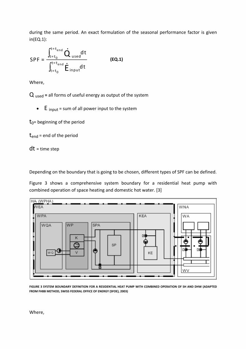
during the same period. An exact formulation of the seasonal performance factor is given

in(EQ.1):

∫

∫

end

0

end

0

t= t

usedt= t

t= t

inputt= t

dtSPF =

dt

Q

E (EQ.1)

Where,

Q used = all forms of useful energy as output of the system

• E input = sum of all power input to the system

t0= beginning of the period

tend = end of the period

dt = time step

Depending on the boundary that is going to be chosen, different types of SPF can be defined.

Figure 3 shows a comprehensive system boundary for a residential heat pump with

combined operation of space heating and domestic hot water. [3]

FIGURE 3 SYSTEM BOUNDARY DEFINITION FOR A RESIDENTIAL HEAT PUMP WITH COMBINED OPERATION OF SH AND DHW (ADAPTED

FROM FHBB METHOD, SWISS FEDERAL OFFICE OF ENERGY (SFOE), 2003)

Where,

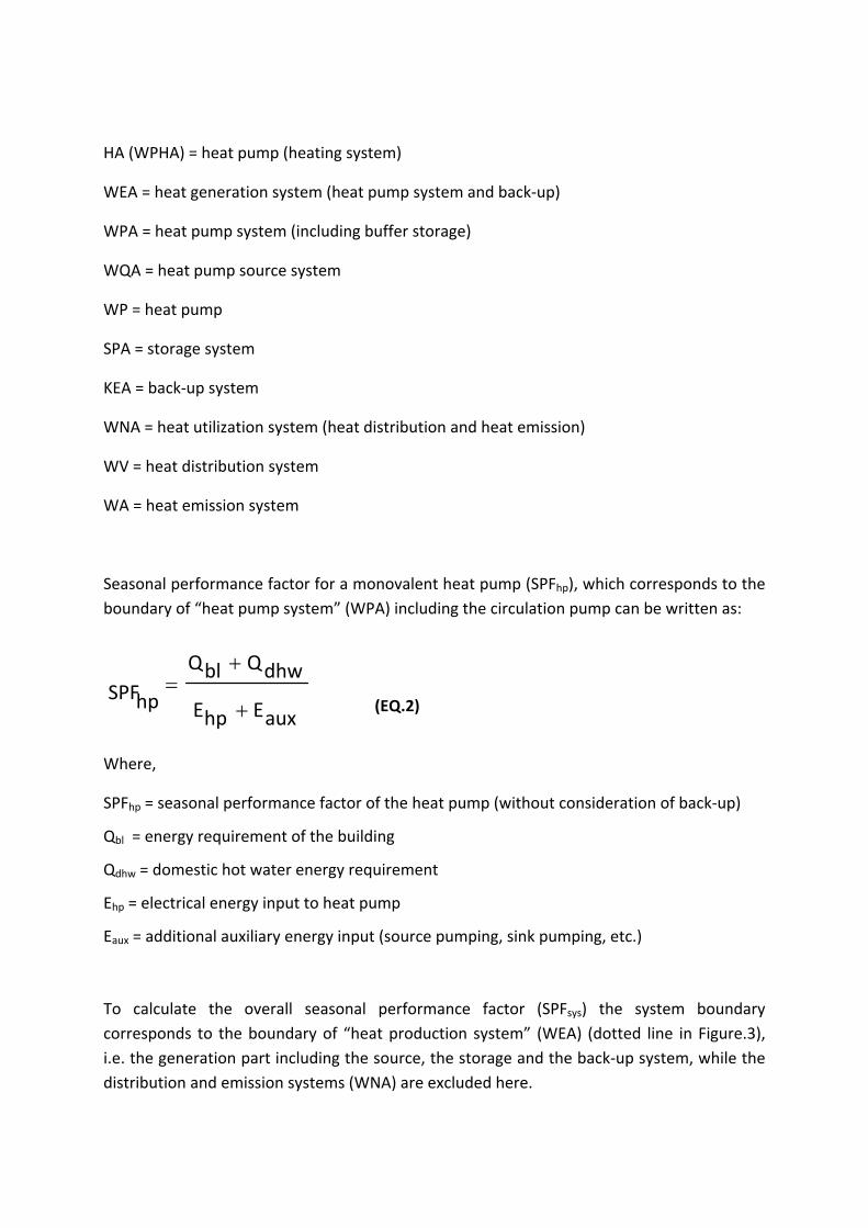
HA (WPHA) = heat pump (heating system)

WEA = heat generation system (heat pump system and back‐up)

WPA = heat pump system (including buffer storage)

WQA = heat pump source system

WP = heat pump

SPA = storage system

KEA = back‐up system

WNA = heat utilization system (heat distribution and heat emission)

WV = heat distribution system

WA = heat emission system

Seasonal performance factor for a monovalent heat pump (SPFhp), which corresponds to the

boundary of “heat pump system” (WPA) including the circulation pump can be written as:

auxEhpE

dhwQblQ

hpSPF+

+=

(EQ.2)

Where,

SPFhp = seasonal performance factor of the heat pump (without consideration of back‐up)

Qbl = energy requirement of the building

Qdhw = domestic hot water energy requirement

Ehp = electrical energy input to heat pump

Eaux = additional auxiliary energy input (source pumping, sink pumping, etc.)

To calculate the overall seasonal performance factor (SPFsys) the system boundary

corresponds to the boundary of “heat production system” (WEA) (dotted line in Figure.3),

i.e. the generation part including the source, the storage and the back‐up system, while the

distribution and emission systems (WNA) are excluded here.

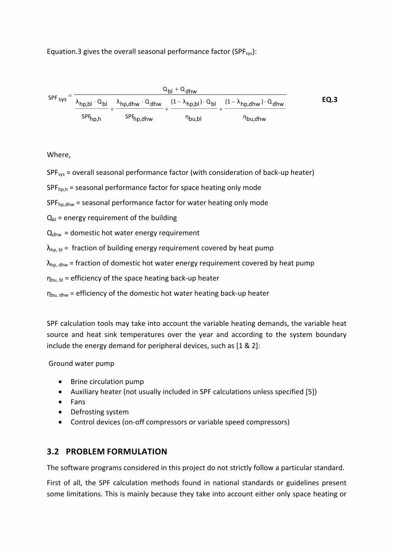
Equation.3 gives the overall seasonal performance factor (SPFsys):

dhwbu,η

dhwQ)dhwhp,λ(1

blbu,η

blQ)blhp,λ(1

dhwhp,SPF

dhwQdhwhp,λ

hhp,SPF

blQblhp,λ

dhwQblQ

sys SPF ⋅−+

⋅−+

⋅+

⋅

+=

EQ.3

Where,

SPFsys = overall seasonal performance factor (with consideration of back‐up heater)

SPFhp,h = seasonal performance factor for space heating only mode

SPFhp,dhw = seasonal performance factor for water heating only mode

Qbl = energy requirement of the building

Qdhw = domestic hot water energy requirement

λhp, bl = fraction of building energy requirement covered by heat pump

λhp, dhw = fraction of domestic hot water energy requirement covered by heat pump

ηbu, bl = efficiency of the space heating back‐up heater

ηbu, dhw = efficiency of the domestic hot water heating back‐up heater

SPF calculation tools may take into account the variable heating demands, the variable heat

source and heat sink temperatures over the year and according to the system boundary

include the energy demand for peripheral devices, such as [1 & 2]:

Ground water pump

• Brine circulation pump

• Auxiliary heater (not usually included in SPF calculations unless specified [5])

• Fans

• Defrosting system

• Control devices (on‐off compressors or variable speed compressors)

3.2 PROBLEM FORMULATION

The software programs considered in this project do not strictly follow a particular standard.

First of all, the SPF calculation methods found in national standards or guidelines present

some limitations. This is mainly because they take into account either only space heating or

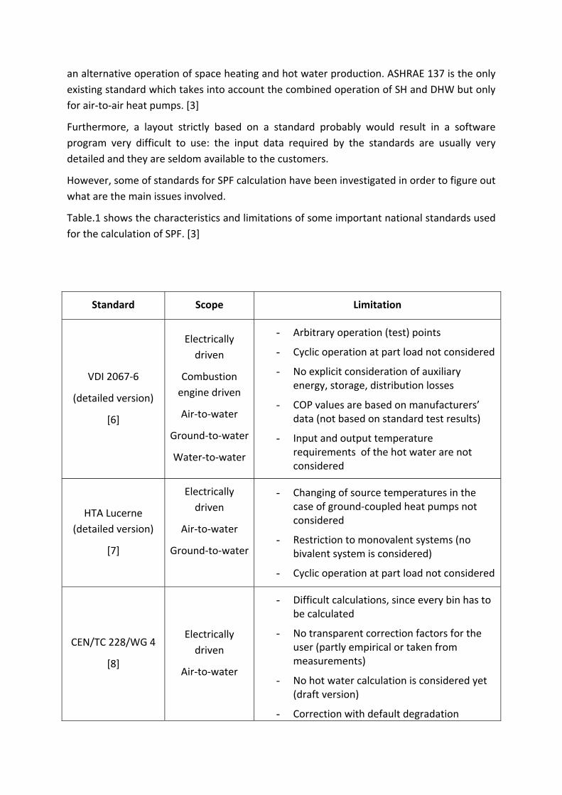
an alternative operation of space heating and hot water production. ASHRAE 137 is the only

existing standard which takes into account the combined operation of SH and DHW but only

for air‐to‐air heat pumps. [3]

Furthermore, a layout strictly based on a standard probably would result in a software

program very difficult to use: the input data required by the standards are usually very

detailed and they are seldom available to the customers.

However, some of standards for SPF calculation have been investigated in order to figure out

what are the main issues involved.

Table.1 shows the characteristics and limitations of some important national standards used

for the calculation of SPF. [3]

Standard Scope Limitation

VDI 2067‐6

(detailed version)

[6]

Electrically

driven

Combustion

engine driven

Air‐to‐water

Ground‐to‐water

Water‐to‐water

- Arbitrary operation (test) points

- Cyclic operation at part load not considered

- No explicit consideration of auxiliary energy, storage, distribution losses

- COP values are based on manufacturers’ data (not based on standard test results)

- Input and output temperature requirements of the hot water are not considered

HTA Lucerne

(detailed version)

[7]

Electrically

driven

Air‐to‐water

Ground‐to‐water

- Changing of source temperatures in the case of ground‐coupled heat pumps not considered

- Restriction to monovalent systems (no bivalent system is considered)

- Cyclic operation at part load not considered

CEN/TC 228/WG 4

[8]

Electrically

driven

Air‐to‐water

- Difficult calculations, since every bin has to be calculated

- No transparent correction factors for the user (partly empirical or taken from measurements)

- No hot water calculation is considered yet (draft version)

- Correction with default degradation

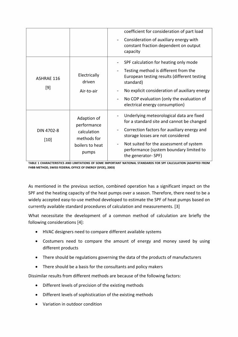
coefficient for consideration of part load

- Consideration of auxiliary energy with constant fraction dependent on output capacity

ASHRAE 116

[9]

Electrically

driven

Air‐to‐air

- SPF calculation for heating only mode

- Testing method is different from the European testing results (different testing standard)

- No explicit consideration of auxiliary energy

- No COP evaluation (only the evaluation of electrical energy consumption)

DIN 4702‐8

[10]

Adaption of

performance

calculation

methods for

boilers to heat

pumps

- Underlying meteorological data are fixed for a standard site and cannot be changed

- Correction factors for auxiliary energy and storage losses are not considered

- Not suited for the assessment of system performance (system boundary limited to the generator‐ SPF)

TABLE 1 CHARACTERISTICS AND LIMITATIONS OF SOME IMPORTANT NATIONAL STANDARDS FOR SPF CALCULATION (ADAPTED FROM

FHBB METHOD, SWISS FEDERAL OFFICE OF ENERGY (SFOE), 2003)

As mentioned in the previous section, combined operation has a significant impact on the

SPF and the heating capacity of the heat pumps over a season. Therefore, there need to be a

widely accepted easy‐to‐use method developed to estimate the SPF of heat pumps based on

currently available standard procedures of calculation and measurements. [3]

What necessitate the development of a common method of calculation are briefly the

following considerations [4]:

• HVAC designers need to compare different available systems

• Costumers need to compare the amount of energy and money saved by using

different products

• There should be regulations governing the data of the products of manufacturers

• There should be a basis for the consultants and policy makers

Dissimilar results from different methods are because of the following factors:

• Different levels of precision of the existing methods

• Different levels of sophistication of the existing methods

• Variation in outdoor condition

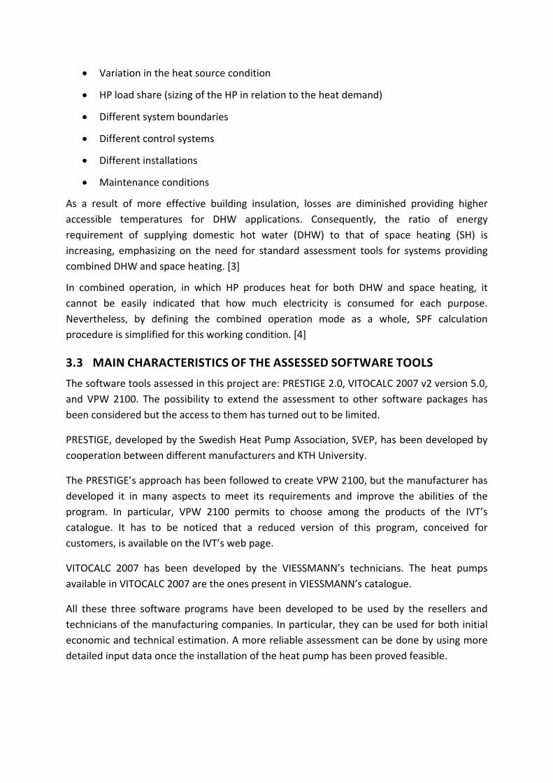
• Variation in the heat source condition

• HP load share (sizing of the HP in relation to the heat demand)

• Different system boundaries

• Different control systems

• Different installations

• Maintenance conditions

As a result of more effective building insulation, losses are diminished providing higher

accessible temperatures for DHW applications. Consequently, the ratio of energy

requirement of supplying domestic hot water (DHW) to that of space heating (SH) is

increasing, emphasizing on the need for standard assessment tools for systems providing

combined DHW and space heating. [3]

In combined operation, in which HP produces heat for both DHW and space heating, it

cannot be easily indicated that how much electricity is consumed for each purpose.

Nevertheless, by defining the combined operation mode as a whole, SPF calculation

procedure is simplified for this working condition. [4]

3.3 MAIN CHARACTERISTICS OF THE ASSESSED SOFTWARE TOOLS

The software tools assessed in this project are: PRESTIGE 2.0, VITOCALC 2007 v2 version 5.0,

and VPW 2100. The possibility to extend the assessment to other software packages has

been considered but the access to them has turned out to be limited.

PRESTIGE, developed by the Swedish Heat Pump Association, SVEP, has been developed by

cooperation between different manufacturers and KTH University.

The PRESTIGE’s approach has been followed to create VPW 2100, but the manufacturer has

developed it in many aspects to meet its requirements and improve the abilities of the

program. In particular, VPW 2100 permits to choose among the products of the IVT’s

catalogue. It has to be noticed that a reduced version of this program, conceived for

customers, is available on the IVT’s web page.

VITOCALC 2007 has been developed by the VIESSMANN’s technicians. The heat pumps

available in VITOCALC 2007 are the ones present in VIESSMANN’s catalogue.

All these three software programs have been developed to be used by the resellers and

technicians of the manufacturing companies. In particular, they can be used for both initial

economic and technical estimation. A more reliable assessment can be done by using more

detailed input data once the installation of the heat pump has been proved feasible.

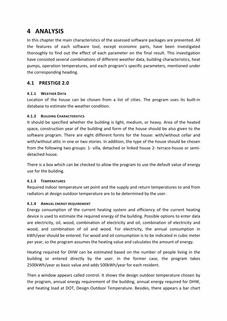
4 ANALYSIS In this chapter the main characteristics of the assessed software packages are presented. All

the features of each software tool, except economic parts, have been investigated

thoroughly to find out the effect of each parameter on the final result. This investigation

have consisted several combinations of different weather data, building characteristics, heat

pumps, operation temperatures, and each program’s specific parameters, mentioned under

the corresponding heading.

4.1 PRESTIGE 2.0

4.1.1 WEATHER DATA

Location of the house can be chosen from a list of cities. The program uses its built‐in

database to estimate the weather condition.

4.1.2 BUILDING CHARACTERISTICS

It should be specified whether the building is light, medium, or heavy. Area of the heated

space, construction year of the building and form of the house should be also given to the

software program. There are eight different forms for the house: with/without cellar and

with/without attic in one or two stories. In addition, the type of the house should be chosen

from the following two groups: 1‐ villa, detached or linked house 2‐ terrace‐house or semi‐

detached house.

There is a box which can be checked to allow the program to use the default value of energy

use for the building.

4.1.3 TEMPERATURES

Required indoor temperature set point and the supply and return temperatures to and from

radiators at design outdoor temperature are to be determined by the user.

4.1.4 ANNUAL ENERGY REQUIREMENT

Energy consumption of the current heating system and efficiency of the current heating

device is used to estimate the required energy of the building. Possible options to enter data

are electricity, oil, wood, combination of electricity and oil, combination of electricity and

wood, and combination of oil and wood. For electricity, the annual consumption in

kWh/year should be entered. For wood and oil consumption is to be indicated in cubic meter

per year, so the program assumes the heating value and calculates the amount of energy.

Heating required for DHW can be estimated based on the number of people living in the

building or entered directly by the user. In the former case, the program takes

2500kWh/year as basic value and adds 500kWh/year for each resident.

Then a window appears called control. It shows the design outdoor temperature chosen by

the program, annual energy requirement of the building, annual energy required for DHW,

and heating load at DOT, Design Outdoor Temperature. Besides, there appears a bar chart

comparing the current annual energy consumption of the building per square meter,

calculated by dividing the value entered by the user by the area of the building, and average

value.

4.1.5 CHOOSING HEAT PUMP

There are four types of heat pump to choose based on the heat source: rock, soil, outdoor

air, and air/air.

The two latter ones do not work in the coldest days of the year normally; an auxiliary heating

system is necessary, then.

If rock is the heat source, only two types of granite can be chosen and the average

temperature of the rock should be given to the software. The rest of the parameters needed

for calculations are assumed by the software.

If soil is the heat source, its type should be specified by good, mediocre, and bad. It is, also,

required to enter the mean temperature of the soil.

There is a drop‐down menu to choose the manufacturer, but there is only one option,

standard, to select. Then the capacity of the heat pump can be chosen from another drop‐

down menu.

User should choose the auxiliary system, which can be built‐in electrical cartridge, electricity,

oil, or wood, and its efficiency.

4.1.6 HEAT PUMP CALCULATIONS

Result of the calculations are categorized as energy saving, energy utilization, and also a

summary of given data in a window similar to Figure 4.

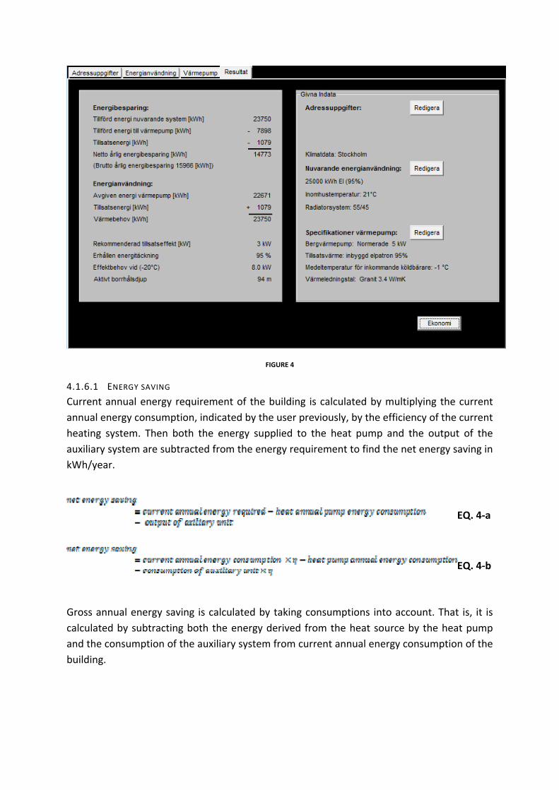
FIGURE 4

4.1.6.1 ENERGY SAVING

Current annual energy requirement of the building is calculated by multiplying the current

annual energy consumption, indicated by the user previously, by the efficiency of the current

heating system. Then both the energy supplied to the heat pump and the output of the

auxiliary system are subtracted from the energy requirement to find the net energy saving in

kWh/year.

EQ. 4‐a

EQ. 4‐b

Gross annual energy saving is calculated by taking consumptions into account. That is, it is

calculated by subtracting both the energy derived from the heat source by the heat pump

and the consumption of the auxiliary system from current annual energy consumption of the

building.

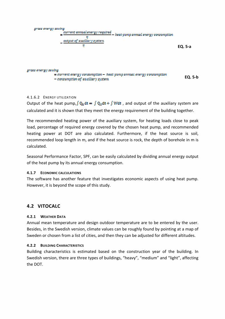
EQ. 5‐a

EQ. 5‐b

4.1.6.2 ENERGY UTILIZATION

Output of the heat pump, , and output of the auxiliary system are

calculated and it is shown that they meet the energy requirement of the building together.

The recommended heating power of the auxiliary system, for heating loads close to peak

load, percentage of required energy covered by the chosen heat pump, and recommended

heating power at DOT are also calculated. Furthermore, if the heat source is soil,

recommended loop length in m, and if the heat source is rock, the depth of borehole in m is

calculated.

Seasonal Performance Factor, SPF, can be easily calculated by dividing annual energy output

of the heat pump by its annual energy consumption.

4.1.7 ECONOMIC CALCULATIONS

The software has another feature that investigates economic aspects of using heat pump.

However, it is beyond the scope of this study.

4.2 VITOCALC

4.2.1 WEATHER DATA

Annual mean temperature and design outdoor temperature are to be entered by the user.

Besides, in the Swedish version, climate values can be roughly found by pointing at a map of

Sweden or chosen from a list of cities, and then they can be adjusted for different altitudes.


Building characteristics is estimated based on the construction year of the building. In

Swedish version, there are three types of buildings, “heavy”, “medium” and “light”, affecting

the DOT.

4.2.3 TEMPERATURES

Required indoor temperature set point is to be determined by the user.

The supply and return temperatures to and from radiators at design outdoor temperature

are presumed to be known, there is also an option to choose between floating condensing

and fixed condensing when the supply and return temperatures are fixed by the user. If

these two temperatures are not known to the user, they can be estimated based on the

current outdoor temperature and measured supply and return temperatures.


Required energy for space heating can be estimated in three ways:

4.2.4.1 “ESTIMATE (POWER)”

Present energy source (oil, electricity, gas, wood, or district heating) and the efficiency of the

heating device, except in case of district heating, and the power demand in kW is taken as

input. Type of present energy source does not change the estimated annual energy demand.

It, still, is important in economic considerations. Number of flats and the amount of energy

required to supply DHW is also entered as input. Multiplication of number of flats and DHW

energy demand gives the total energy demand for supplying DHW. That is, number of flats

does not change the space heating energy requirement.

The energy annually required for space heating is calculated based on the weather data,

building characteristics, indoor temperature set point, power demand, and number of flats.

Then the “net energy use” is calculated by adding the calculated annual energy required for

space heating to the DHW energy demand.

4.2.4.2 “PRESENT”

Current energy source (oil, electricity, gas, wood, district heating, or combined boiler) is

determined by the user.

In case oil, gas, or wood is currently used, number of consumed cubic meters per year is to

be determined in addition to the boiler efficiency. Based on these data and the heating

values taken from the built‐in database of the program, “net energy use”, which includes

annual energy required for both space heating and DHW, is calculated in kWh/year. User

may change the calculated value of net energy use manually, but the program does not use

the manually entered value in further calculations. Displaying the calculated net energy use

value in an inactive box could prevent confusion of the user. Then the share of DHW is to be

determined by the user in kWh/year.

In case that electricity is the current energy source of the building, the current annual

energy consumption of the building is taken as an input and multiplied by the efficiency of

the heating device, entered by the user, to find the “net energy use”, which includes annual

energy required for both space heating and DHW, in kWh/year. Then the share of DHW is to

be determined by the user in kWh/year.

Since in some houses there is only one measuring device for electricity consumption, the

value read on the meter includes consumption of all of the electrical appliances normally

used. It would be convenient to have the possibility to set the number of typical energy‐

consuming appliances (fridges, washing machines…) for estimating the Space heating and

DHW consumption, which may not be known to the user.

If the building presently uses district heating, the current annual energy consumption of the

building entered by the user, since no efficiency is applied, is used directly as the “net energy

use”, which includes annual energy required for both space heating and DHW, in kWh/year.

Then the share of DHW is to be determined by the user in kWh/year.

In case more than one (up to three) energy sources are used, their share and efficiencies of

the heating devices, if applicable, can be entered under combined boiler option.

4.2.4.3 “ESTIMATE (AREA)”

The user indicates whether the building is presently heated by using oil, electricity, gas,

wood, or district heating. Although it does not change the estimated annual energy demand,

it influences economic calculations, which lies beyond the scope of this project. The

efficiency of the heating device, except for district heating, and the area of the heated space

are to be entered, as well.

In addition, the use of the building should be chosen between the following options:

house/housing in combination with work rooms, Caretaking, hotels and restaurants, school,

offices, sports, food shop, other stores, and remaining.

Based on the annual mean temperature, building characteristics, currently used fuel, area,

and the use of the building, “net energy use”, including annual energy required for both

space heating and DHW, is calculated in kWh/year. Although the user may want to change

the indoor temperature manually here, it does not influence the calculations since indoor

temperature for each building use is a fixed value derived from statistical data. The share of

DHW is determined by the program in kWh/year according to the building use, weather

data, and area. It would be convenient if there was an option to enter the share of DHW

manually when the exact value is known.

4.2.5 CHOOSING HEAT PUMP AND HEAT SOURCE

There are three types of heat pump to choose: air/water, brine/water, and water/water. For

each type there are different product models available to choose from a drop‐down menu.

Once a particular model of heat pump is chosen, the program calculates the percentages of

power and energy demand covered by the heat pump using the built‐in database of the

products of the manufacturer.

4.2.5.1 AIR/WATER

The only heat source for air/water heat pump is outdoor air.

4.2.5.2 BRINE/WATER

For brine/water heat pumps rock, surface soil, lake, and exhaust air can be chosen as heat

source.

In any case, the average temperature of the incoming brine and should be specified,

whereas the power of the circulation pump varies by the model of the heat pump

automatically.

4.2.5.2.1 ROCK

22 different type of rock can be chosen from a drop‐down menu. The default value for the

thermal conductivity of the rock can be changed manually. Brine temperature change should

be entered by the user. There is a setting menu in which borehole diameter, hose outside

diameter, hose inside diameter, CC between hoses, thermal conductivity of hose, thermal

conductivity of brine, thermal conductivity of ice, kinematic viscosity of brine, thermal

capacity of brine, density of brine, and thermal capacity of water can be specified.

4.2.5.2.2 SURFACE SOIL

Under the setting menu five different soil types can be chosen, each of which has more

details to be specified such as water content, consistency and quartz content of the soil.

Thermal conductivity and latent heat of the soil for each type of soil has its own default

value, which can be changed manually. Brine temperature change and under setting menu

depth in soil and CC between hoses can be specified.

4.2.5.2.3 LAKE

Thermal conductivity of the lake bed, brine temperature change, and lake mean

temperature should be entered by the user.

4.2.5.2.4 EXHAUST AIR

Incoming and outgoing air temperature and relative humidity and volume flow rate of air

either given directly by the user or calculated according to ACH and volume of the room are

used to calculate available heat in the exhaust air and amount of condensed water.

4.2.5.3 WATER/WATER

Water/water heat pumps can only have ground water as the heat source. Incoming ground

water temperature and brine temperature change are the parameters should be given to the

program, whereas the power of the circulation pump varies by the model of the heat pump

automatically.


It should be entered that how many percent of the DHW is supplied by the heat pump.

Based on the all information given to the program a diagram showing heating power

demand in kW versus hours in a year is generated. In the diagram it can be graphically seen

that how much of the demand is covered by the supplementary heating device, how much

the energy saving is, and how much the energy consumption is. Percentage of energy

demand coverage and percentage of power demand coverage by the heat pump is

calculated, as well. Supplementary heating device can be selected between oil, electricity,

gas, wood, or district heating; the efficiency also should be provided for the program. At this

point, a printable summary, similar to figure5, of the given data and the results including

amount of energy saving, share of energy consumption and supplying of the heat pump and

the supplementary system, recommended power of the supplementary device, capacity of

the heat pump at DOT, and SPF, annual heating factor, is generated.


VITOCALC has another feature that investigates economic aspects of using heat pump.


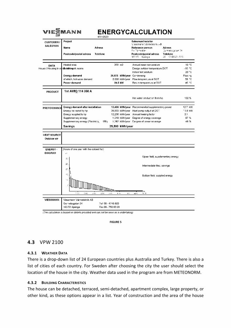
FIGURE 5

4.3 VPW 2100

4.3.1 WEATHER DATA

There is a drop‐down list of 24 European countries plus Australia and Turkey. There is also a

list of cities of each country. For Sweden after choosing the city the user should select the

location of the house in the city. Weather data used in the program are from METEONORM.


The house can be detached, terraced, semi‐detached, apartment complex, large property, or

other kind, as these options appear in a list. Year of construction and the area of the house

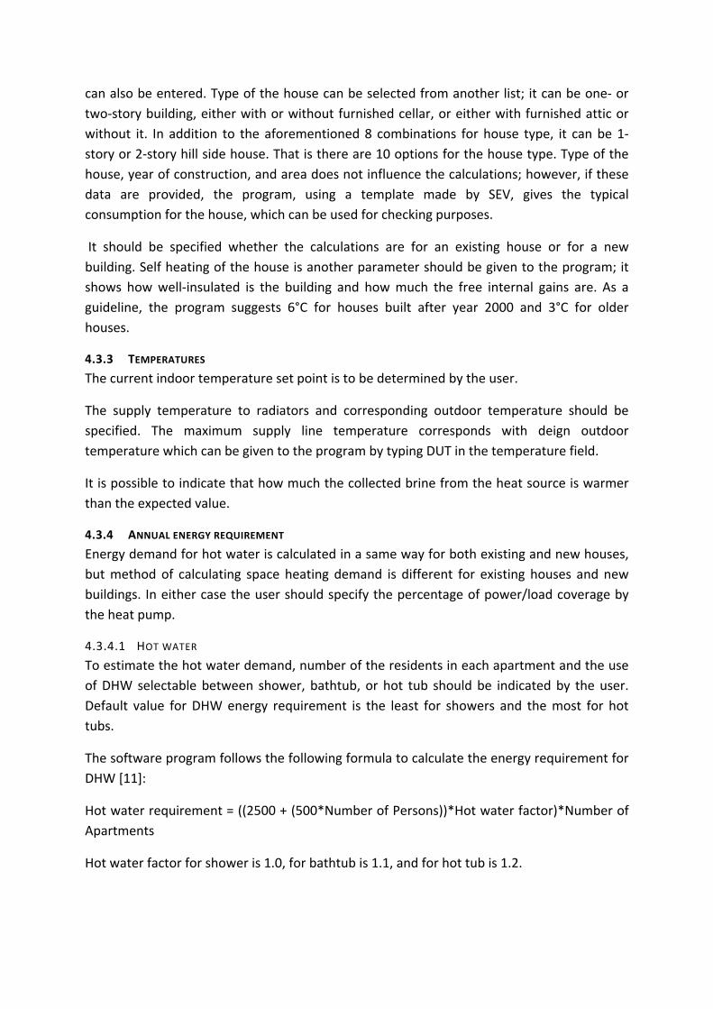
can also be entered. Type of the house can be selected from another list; it can be one‐ or

two‐story building, either with or without furnished cellar, or either with furnished attic or

without it. In addition to the aforementioned 8 combinations for house type, it can be 1‐

story or 2‐story hill side house. That is there are 10 options for the house type. Type of the

house, year of construction, and area does not influence the calculations; however, if these

data are provided, the program, using a template made by SEV, gives the typical

consumption for the house, which can be used for checking purposes.

It should be specified whether the calculations are for an existing house or for a new

building. Self heating of the house is another parameter should be given to the program; it

shows how well‐insulated is the building and how much the free internal gains are. As a

guideline, the program suggests 6°C for houses built after year 2000 and 3°C for older

houses.

4.3.3 TEMPERATURES

The current indoor temperature set point is to be determined by the user.

The supply temperature to radiators and corresponding outdoor temperature should be

specified. The maximum supply line temperature corresponds with deign outdoor

temperature which can be given to the program by typing DUT in the temperature field.

It is possible to indicate that how much the collected brine from the heat source is warmer

than the expected value.


Energy demand for hot water is calculated in a same way for both existing and new houses,

but method of calculating space heating demand is different for existing houses and new

buildings. In either case the user should specify the percentage of power/load coverage by

the heat pump.

4.3.4.1 HOT WATER

To estimate the hot water demand, number of the residents in each apartment and the use

of DHW selectable between shower, bathtub, or hot tub should be indicated by the user.

Default value for DHW energy requirement is the least for showers and the most for hot

tubs.

The software program follows the following formula to calculate the energy requirement for

DHW [11]:

Hot water requirement = ((2500 + (500*Number of Persons))*Hot water factor)*Number of

Apartments

Hot water factor for shower is 1.0, for bathtub is 1.1, and for hot tub is 1.2.

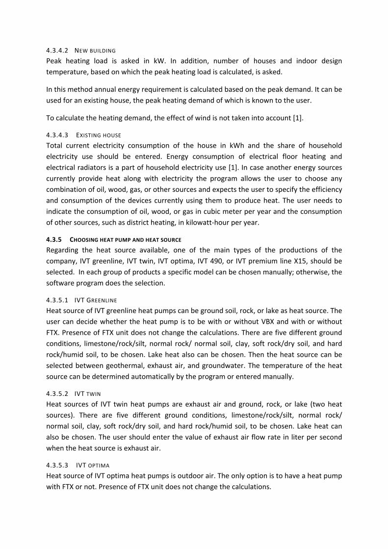
4.3.4.2 NEW BUILDING

Peak heating load is asked in kW. In addition, number of houses and indoor design

temperature, based on which the peak heating load is calculated, is asked.

In this method annual energy requirement is calculated based on the peak demand. It can be

used for an existing house, the peak heating demand of which is known to the user.

To calculate the heating demand, the effect of wind is not taken into account [1].

4.3.4.3 EXISTING HOUSE

Total current electricity consumption of the house in kWh and the share of household

electricity use should be entered. Energy consumption of electrical floor heating and

electrical radiators is a part of household electricity use [1]. In case another energy sources

currently provide heat along with electricity the program allows the user to choose any

combination of oil, wood, gas, or other sources and expects the user to specify the efficiency

and consumption of the devices currently using them to produce heat. The user needs to

indicate the consumption of oil, wood, or gas in cubic meter per year and the consumption

of other sources, such as district heating, in kilowatt‐hour per year.

4.3.5 CHOOSING HEAT PUMP AND HEAT SOURCE

Regarding the heat source available, one of the main types of the productions of the

company, IVT greenline, IVT twin, IVT optima, IVT 490, or IVT premium line X15, should be

selected. In each group of products a specific model can be chosen manually; otherwise, the

software program does the selection.

4.3.5.1 IVT GREENLINE

Heat source of IVT greenline heat pumps can be ground soil, rock, or lake as heat source. The

user can decide whether the heat pump is to be with or without VBX and with or without

FTX. Presence of FTX unit does not change the calculations. There are five different ground

conditions, limestone/rock/silt, normal rock/ normal soil, clay, soft rock/dry soil, and hard

rock/humid soil, to be chosen. Lake heat also can be chosen. Then the heat source can be

selected between geothermal, exhaust air, and groundwater. The temperature of the heat

source can be determined automatically by the program or entered manually.

4.3.5.2 IVT TWIN

Heat sources of IVT twin heat pumps are exhaust air and ground, rock, or lake (two heat

sources). There are five different ground conditions, limestone/rock/silt, normal rock/

normal soil, clay, soft rock/dry soil, and hard rock/humid soil, to be chosen. Lake heat can

also be chosen. The user should enter the value of exhaust air flow rate in liter per second

when the heat source is exhaust air.

4.3.5.3 IVT OPTIMA

Heat source of IVT optima heat pumps is outdoor air. The only option is to have a heat pump

with FTX or not. Presence of FTX unit does not change the calculations.

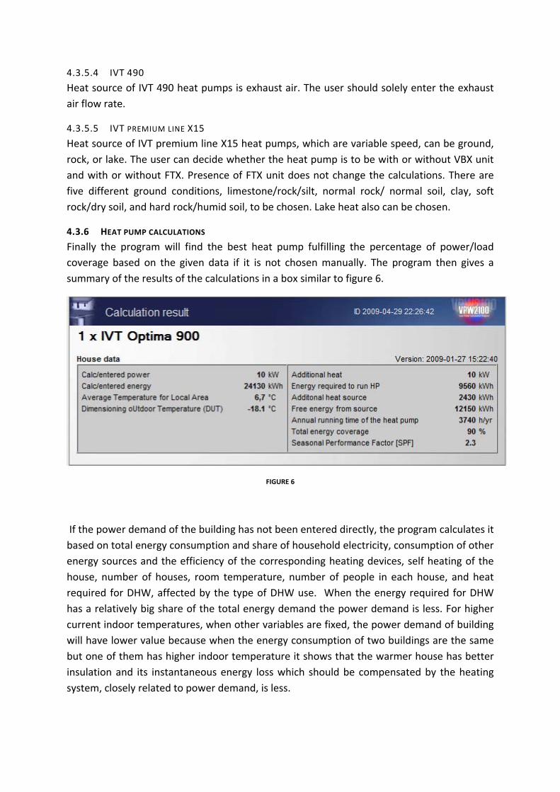
4.3.5.4 IVT 490

Heat source of IVT 490 heat pumps is exhaust air. The user should solely enter the exhaust

air flow rate.

4.3.5.5 IVT PREMIUM LINE X15

Heat source of IVT premium line X15 heat pumps, which are variable speed, can be ground,

rock, or lake. The user can decide whether the heat pump is to be with or without VBX unit

and with or without FTX. Presence of FTX unit does not change the calculations. There are

five different ground conditions, limestone/rock/silt, normal rock/ normal soil, clay, soft

rock/dry soil, and hard rock/humid soil, to be chosen. Lake heat also can be chosen.


Finally the program will find the best heat pump fulfilling the percentage of power/load

coverage based on the given data if it is not chosen manually. The program then gives a

summary of the results of the calculations in a box similar to figure 6.

FIGURE 6

If the power demand of the building has not been entered directly, the program calculates it

based on total energy consumption and share of household electricity, consumption of other

energy sources and the efficiency of the corresponding heating devices, self heating of the

house, number of houses, room temperature, number of people in each house, and heat

required for DHW, affected by the type of DHW use. When the energy required for DHW

has a relatively big share of the total energy demand the power demand is less. For higher

current indoor temperatures, when other variables are fixed, the power demand of building

will have lower value because when the energy consumption of two buildings are the same

but one of them has higher indoor temperature it shows that the warmer house has better

insulation and its instantaneous energy loss which should be compensated by the heating

system, closely related to power demand, is less.

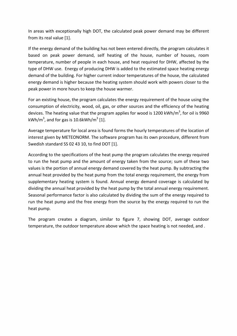
In areas with exceptionally high DOT, the calculated peak power demand may be different

from its real value [1].

If the energy demand of the building has not been entered directly, the program calculates it

based on peak power demand, self heating of the house, number of houses, room

temperature, number of people in each house, and heat required for DHW, affected by the

type of DHW use. Energy of producing DHW is added to the estimated space heating energy

demand of the building. For higher current indoor temperatures of the house, the calculated

energy demand is higher because the heating system should work with powers closer to the

peak power in more hours to keep the house warmer.

For an existing house, the program calculates the energy requirement of the house using the

consumption of electricity, wood, oil, gas, or other sources and the efficiency of the heating

devices. The heating value that the program applies for wood is 1200 kWh/m3, for oil is 9960

kWh/m3, and for gas is 10.6kWh/m3 [1].

Average temperature for local area is found forms the hourly temperatures of the location of

interest given by METEONORM. The software program has its own procedure, different from

Swedish standard SS 02 43 10, to find DOT [1].

According to the specifications of the heat pump the program calculates the energy required

to run the heat pump and the amount of energy taken from the source; sum of these two

values is the portion of annual energy demand covered by the heat pump. By subtracting the

annual heat provided by the heat pump from the total energy requirement, the energy from

supplementary heating system is found. Annual energy demand coverage is calculated by

dividing the annual heat provided by the heat pump by the total annual energy requirement.

Seasonal performance factor is also calculated by dividing the sum of the energy required to

run the heat pump and the free energy from the source by the energy required to run the

heat pump.

The program creates a diagram, similar to figure 7, showing DOT, average outdoor

temperature, the outdoor temperature above which the space heating is not needed, and .

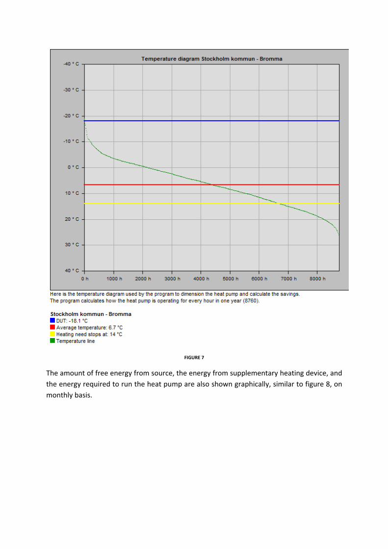
FIGURE 7

The amount of free energy from source, the energy from supplementary heating device, and

the energy required to run the heat pump are also shown graphically, similar to figure 8, on

monthly basis.

FIGURE 8

For an existing house, calculations made by the program are summarized in another box,

similar to figure 9, to calculate net and gross saving.

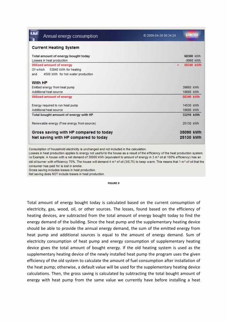
FIGURE 9

Total amount of energy bought today is calculated based on the current consumption of

electricity, gas, wood, oil, or other sources. The losses, found based on the efficiency of

heating devices, are subtracted from the total amount of energy bought today to find the

energy demand of the building. Since the heat pump and the supplementary heating device

should be able to provide the annual energy demand, the sum of the emitted energy from

heat pump and additional sources is equal to the amount of energy demand. Sum of

electricity consumption of heat pump and energy consumption of supplementary heating

device gives the total amount of bought energy. If the old heating system is used as the

supplementary heating device of the newly installed heat pump the program uses the given

efficiency of the old system to calculate the amount of fuel consumption after installation of

the heat pump; otherwise, a default value will be used for the supplementary heating device

calculations. Then, the gross saving is calculated by subtracting the total bought amount of

energy with heat pump from the same value we currently have before installing a heat

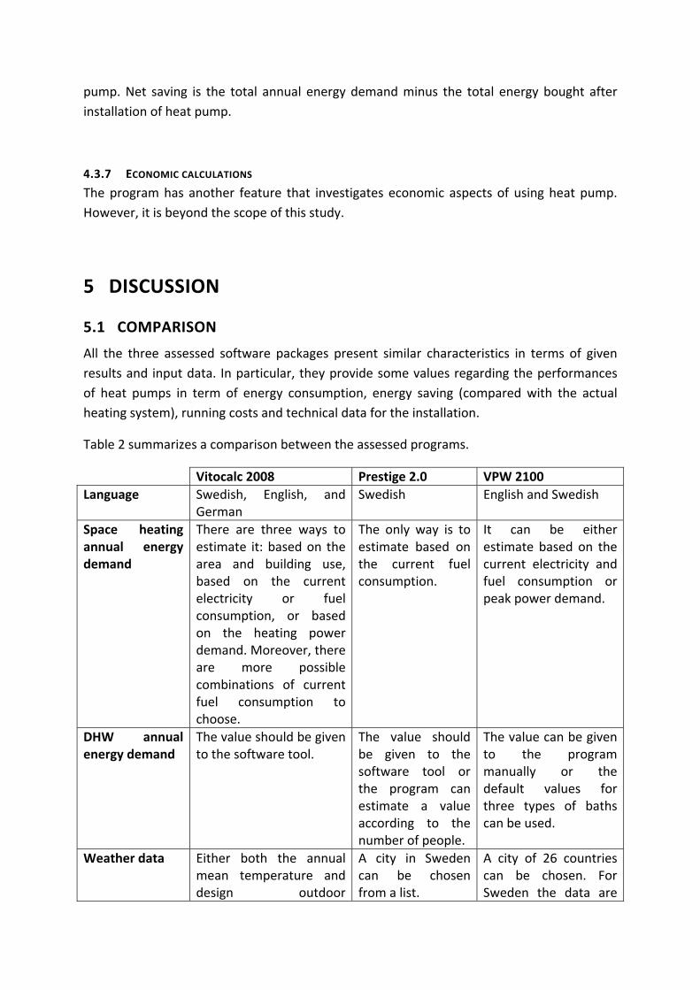
pump. Net saving is the total annual energy demand minus the total energy bought after

installation of heat pump.


The program has another feature that investigates economic aspects of using heat pump.


5 DISCUSSION

5.1 COMPARISON

All the three assessed software packages present similar characteristics in terms of given

results and input data. In particular, they provide some values regarding the performances

of heat pumps in term of energy consumption, energy saving (compared with the actual

heating system), running costs and technical data for the installation.

Table 2 summarizes a comparison between the assessed programs.

Vitocalc 2008 Prestige 2.0 VPW 2100

Language Swedish, English, and German

Swedish English and Swedish

Space heating annual energy demand

There are three ways to estimate it: based on the area and building use, based on the current electricity or fuel consumption, or based on the heating power demand. Moreover, there are more possible combinations of current fuel consumption to choose.

The only way is to estimate based on the current fuel consumption.

It can be either estimate based on the current electricity and fuel consumption or peak power demand.

DHW annual energy demand

The value should be given to the software tool.

The value should be given to the software tool or the program can estimate a value according to the number of people.

The value can be given to the program manually or the default values for three types of baths can be used.

Weather data Either both the annual mean temperature and design outdoor

A city in Sweden can be chosen from a list.

A city of 26 countries can be chosen. For Sweden the data are

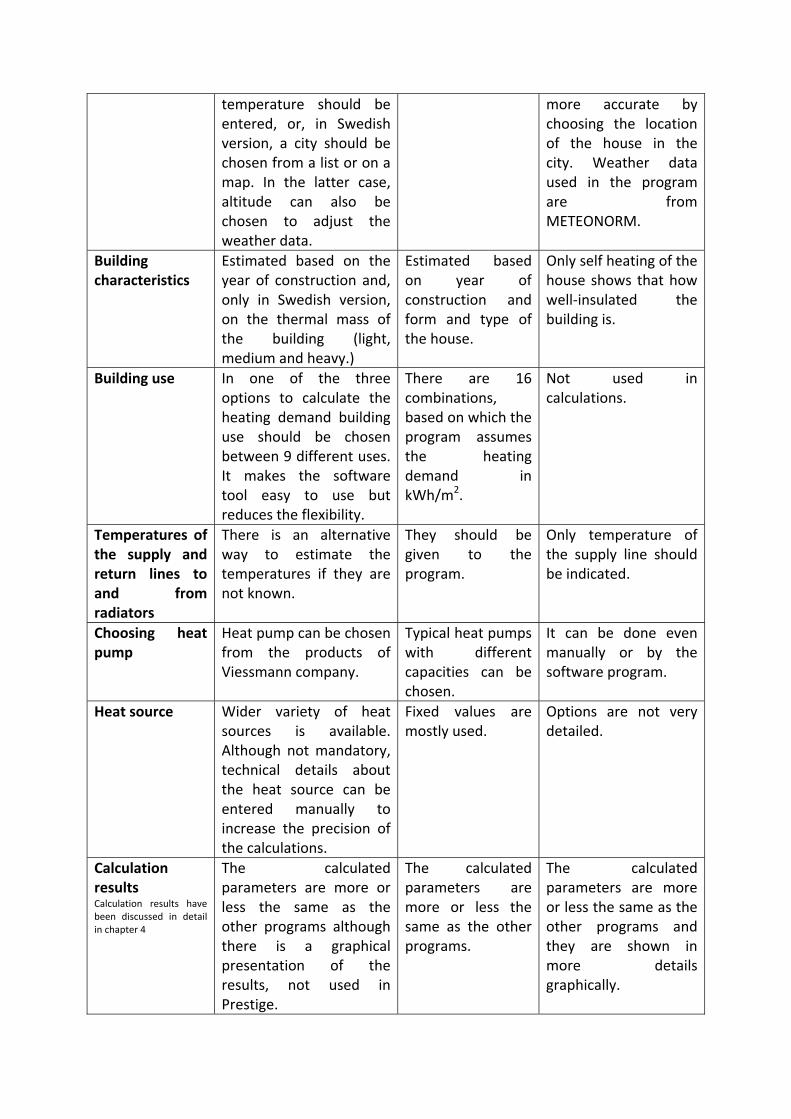
temperature should be entered, or, in Swedish version, a city should be chosen from a list or on a map. In the latter case, altitude can also be chosen to adjust the weather data.

more accurate by choosing the location of the house in the city. Weather data used in the program are from METEONORM.

Building characteristics

Estimated based on the year of construction and, only in Swedish version, on the thermal mass of the building (light, medium and heavy.)

Estimated based on year of construction and form and type of the house.

Only self heating of the house shows that how well‐insulated the building is.

Building use In one of the three options to calculate the heating demand building use should be chosen between 9 different uses. It makes the software tool easy to use but reduces the flexibility.

There are 16 combinations, based on which the program assumes the heating demand in kWh/m2.

Not used in calculations.

Temperatures of the supply and return lines to and from radiators

There is an alternative way to estimate the temperatures if they are not known.

They should be given to the program.

Only temperature of the supply line should be indicated.

Choosing heat pump

Heat pump can be chosen from the products of Viessmann company.

Typical heat pumps with different capacities can be chosen.

It can be done even manually or by the software program.

Heat source Wider variety of heat sources is available. Although not mandatory, technical details about the heat source can be entered manually to increase the precision of the calculations.

Fixed values are mostly used.

Options are not very detailed.

Calculation results Calculation results have been discussed in detail in chapter 4

The calculated parameters are more or less the same as the other programs although there is a graphical presentation of the results, not used in Prestige.

The calculated parameters are more or less the same as the other programs.

The calculated parameters are more or less the same as the other programs and they are shown in more details graphically.

TABLE 2 COMPARISON TABLE

5.2 SUGGESTIONS

In this chapter some observations and suggestions that have been arisen from the

assessment of the software packages are presented.

First of all, it is not possible to compare heat pumps of different manufactures in a very

suitable way. In fact, the built‐in characteristics of the heat pumps are taken from the

catalogue of the manufacture that developed the assessment program. Therefore, a

customer that would compare heat pumps of different manufactures should use the

different software tools in order to get the performances of these units. However, the

assumptions, the calculations and the input data are different for each program. Thus, the

results are not comparable in the sense that they are not obtained in the same way.

A limitation common among all the assessed programs seems to be related to the prediction

of the percentage of the total energy requirement covered by the heat pump. Although it is

not possible to access to the source code, it is still possible to deduce this fact by analyzing

the input data. Under particular severe weather conditions, the space heating demand

results are high. If, at the same time, there is a high requirement of domestic hot water, the

heat pump could not be sufficient and the backup heater could be utilized. These situations

are quite frequent especially in wintertime, early morning, when outside air is cold and

people tend to shower (e.g. in Sweden). Since a time schedule for domestic hot water

consumption is not required as input data by any of the assessed programs, it can be

deduced that a large tank is assumed, with enough capacity for storing a large amount of

heat. In reality, tanks are usually not large enough, resulting in a need of using backup

heating. Accordingly, the calculated percentage of the total energy covered by the heat

pump is higher than the real one, meaning higher performance than the actual one is

expected.

Notwithstanding reversible heat pumps are becoming popular, none of the assessed tools

present the possibility of modelling cooling demand. Thus, it is not possible to estimate the

actual electricity consumption of the reversible heat pump over the year but only over the

heating season. Furthermore, a customer may think that the bought heat pump has not the

expected performance if not well informed by the reseller.

Some bugs of minor importance have been detected especially when entering data. In

particular, we experienced that these problems appear if data are changed without

refreshing the input data windows .However, it seems that these problem can be easily

fixed.

Finally, sometimes the user friendliness could be improved. It has to be noted that

instructions and guidelines are available in Swedish language for PRESTIGE 2.0 and VITOCALC

2007 v2 while IVT provides a quite clear and detailed instruction file available on the website

of the manufacture.

6 ACKNOWLEDGMENTS We would like to express our gratitude to Mr. Jan‐Erik Nowacki and Mr. Martin Forsen for

the time they have spent to help us in this project.

7 REFERENCES

[1] European Heat Pump Statistics, EHPA, Outlook 2008.

[2] IEA Heat Pump Programme’s Information Centre (HPC), available at

http://www.heatpumpcentre.org , last modified 30.6.2008, as accessed 9.4.2009

[3] Swiss Federal Office of Energy (SFOE), Seasonal performance calculation for residential

heat pumps with combined space heating and hot water production (FHBB Method)– Final

report, C. Wemhöner, Prof. Dr. Th. Afjei, October 2003

[4] IEA HPP Annex 28 – standardized testing and seasonal performance calculation for

multifunctional heat pump systems, Carsten Wemhoener *, Thomas Afjei, Ralf Dott, Applied

Thermal Engineering 28 (2008) 2062–2069

[5] Eric Granryd (2005), ”Refrigerating Engineering” , Department of Energy Technology,

Division of Applied Thermodynamics and Refrigeration, Royal Institute of Technology,

Stockholm, Sweden.

[6] VDI Richtlinie 2067, Kostenberechnung fur Heizanlagen, Blatt 6, Warmepumpen,

Kurzverfahren, VDI‐Verlag, Dusseldorf, 1989

[7] Th. Afjei, G. Zwifel, M. Wetter, et al Kostengunstige Niedertemperaturheizung mit

Warmepumpe, Technisches Handbuch, darin: Handrechenmethode zur bestimung der

Jahresarbeitszahl von Warmepumpenanlagen fur Heiz und Wrmwasserbetrieb SFOE

research program heat pumping technologies, cogeneration, refrigeration, 1997 (available at

www.waermepumpe.ch/fe/projekte/nth)

[8] C. Feldmann: Methods for calculation of system energy requirement and system

efficiency, Working Paper N 259 of CEN/TC 228/WG 4, 2002

[9] ANSI/ASHRAE Standard 116‐ 1995: Methods of testing for rating seasonal efficiency of

unitary air‐conditioners and heat pumps, American Society of Heating, Refrigeration, and Air

Conditioning Engineers, inc., Atlanta 1995

http://www.heatpumpcentre.org/

http://www.waermepumpe.ch/fe/projekte/nth

[10] DIN 4702, Teil 8, Heizkessel, Ermittlung des Normnutzungsgrades und der

Normemissionsfaktoren , Beuth Verlag, Marz 1990

[11] Manual VPW2100, <http://www.vpw2100.com/af/vpw2100_manual.asp?lngLangID=5>,

as accessed 4/30/2009

http://www.vpw2100.com/af/vpw2100_manual.asp?lngLangID=5

Combined solar collectors and heat pump systems for single

family dwellings situated in Sweden

Sebastian Lembke 850830

André Szeles 871016

MJ2409 Applied Energy Technology PROJECT course

Department of Energy Technology

Royal Institute of Technology

Stockholm, Sweden

1

Abstract The objective of this report is to explain and evaluate different kind of heating systems for a

single-family house situated in Sweden.

The heating systems that are treated involve solar collectors in combination with a heat pump.

First the techniques of both solar collectors and heat pump systems are described in detail,

this is to provide an understanding of which, in order for the reader to understand how the

systems can be combined. Combined systems are also described and examples of a few

typologies are presented.

A model of one system has been created, in which the performance of a combined system is

calculated and analysed. The model provided a number of outputs that explains when and how

much the heat pump has to perform in order to complement the solar collectors.

In the analysis of the model-outputs it was found that it is crucial that the system contains a

heat storage tank in order for the system to be beneficial. Because the heat provided by the

solar collectors has to be available even when the sun is not shining, on cloudy days or during

the night a storage tank is needed. If there is no storage tank, the heat pump always has to be

running even if the heat provided by the solar collectors is sufficient.

Another interesting subject found during the analysis is that even if the heat energy is

sufficient from the solar collectors, the temperatures out of the collector vary a lot. These

temperatures are divided into three levels: 1) Over 55 °C and sufficient for both domestic hot

water and for space heating, 2) between 30 °C and 55 °C and sufficient only for the space

heating and 3) between 5 °C and 30 °C and not sufficient for heating. Where the solar

collectors are not sufficient enough the heat pump starts running. In temperature level 3

above, the heat could be used to either rise the evaporation temperature and/or to recharge the

borehole.

In conclusion it was found that the best alternative for a combined system, for a house situated

in Sweden, is: solar collectors in combination with a heat pump and a ground source heat

exchanger as the heat source. Also a storage tank should be installed and the solar collectors

should be connected to the evaporator side and the borehole for the heat pump.

2

Innehållsförteckning Abstract ................................................................................................................................................... 1

Index of figures ........................................................................................................................................ 4

Index of tables ......................................................................................................................................... 5

Nomenclature .......................................................................................................................................... 6

1. Introduction ......................................................................................................................................... 9

1.1 Background .................................................................................................................................... 9

1.2 Objectives .................................................................................................................................... 10

1.3 Limitations ................................................................................................................................... 10

1.4 Method ........................................................................................................................................ 10

2. Solar collector systems ...................................................................................................................... 11

2.1 Solar irradiance ...................................................................................................................... 11

2.2 Solar collectors ............................................................................................................................ 15

2.3 Heat storage/heat exchange ....................................................................................................... 17

2.4 Heat transfer fluid ....................................................................................................................... 19

2.5 Pump/piping ................................................................................................................................ 19

2.6 Control system............................................................................................................................. 20

2.7 System design .............................................................................................................................. 21

3. Heat pumps ....................................................................................................................................... 22

3.1 Heat pump systems ..................................................................................................................... 22

3.2 Heat exchangers and heat sources ............................................................................................. 22

3.3 Heat pump function and configuration ........................................................................................ 26

4. Combined solar and heat pump systems .......................................................................................... 33

4.1 Energy utilization ......................................................................................................................... 33

4.2 Heat transfer liquid...................................................................................................................... 33

4.3 Recharging ................................................................................................................................... 34

4.4 Increasing the temperature of the evaporator side .................................................................... 35

4.5 Increasing the temperature of the incoming brine to the condenser ........................................ 36

4.6 System solutions .......................................................................................................................... 38

4.7 On market solutions .............................................................................................................. 44

5. Modeling/Simulations ....................................................................................................................... 46

5.1 Purpose: ....................................................................................................................................... 46

5.2 The model .................................................................................................................................... 46

5.3 Subsystems .................................................................................................................................. 47

3

6. Analysis/Discussion ........................................................................................................................... 67

7. Conclusions ........................................................................................................................................ 70

References ............................................................................................................................................. 71

4

Index of figures Figure 1: Solar angles (Williams 1983) ................................................................................................. 12

Figure 2: Solar radiation on a tilted surface (Williams, 1983) ............................................................. 13

Figure 3: Relation between radiation on horizontal and tilted surface ................................................. 14

Figure 4: Energy flow in a water storage tank ...................................................................................... 18

Figure 5: A combined system where the solar collector are used to recharge the heat source ............ 39

Figure 6: A combined system where the solar collector are used to recharge the heat source or boost

the evaporator side of the heat pump .................................................................................................... 40

Figure 7: A combined system where the solar collector are used for domestic hot water .................... 41

Figure 8: A combined system where the solar collector are used for domestic hot water and for the

radiator system ...................................................................................................................................... 42

Figure 9: A combined system where the solar collector can be used for domestic hot water, radiator

system, recharging the heat source and/or boosting the evaporator or the condenser side of the heat

pump ...................................................................................................................................................... 43

Figure 10: Schematic of the model ........................................................................................................ 46

Figure 11: Direct, Diffuse and reflective solar irradiation on a tilted surface of 45 ......................... 48

Figure 12: Direct solar radiation as a function of the tilt of the solar collector ................................... 49

Figure 13: Solar radiation as a function of different tilt of the solar collector ..................................... 50

Figure 14: Yearly variation of output temperature between 10 and 30 C from the solar collectors ... 53

Figure 15: Yearly variation of output temperature over 55 from the solar collectors......................... 54

Figure 16: Output energy from the solar collector when the outlet temperature is under 30C. .......... 55

Figure 17: Output energy from the solar collector when the outlet temperature is over 30C ............. 56

Figure 18: Energy from the solar collectors when the outlet temperature is larger than 55C ........... 57

Figure 19: Domestic hot water demand for 24 hours ............................................................................ 58

Figure 20: Space heating demand for one year ..................................................................................... 59

Figure 21: Compressor work during one year ...................................................................................... 60

Figure 22: Excessive solar energy during one year .............................................................................. 61

Figure 23: Temperature and energy out of the solar collector and total load for one week in January64

Figure 24: Temperature and energy out of the solar collector and total load for one week in April .... 64

Figure 25: Compressor power vs. Total load for a year. ...................................................................... 65

Figure 26: Energy from solar collector vs. total load ........................................................................... 66

5

Index of tables Table 1: Properties of different heat transfer fluids (Kjellsson, 2004).................................................. 34

Table 2: Coefficient of heating performance for an ideal cycle at different condensing temperatures 37

Table 3: Outlet temperature from the solar collector for different solar collector tilts [Percentage of

hours in a year with corresponding temperature outlet]. ..................................................................... 51

Table 4: Total solar energy for a year, solar efficiency and outlet temperature from the solar collector

for a year for different solar collector inlet temperatures [Percentage of hours in a year with

corresponding temperature outlet]........................................................................................................ 52

Table 5: Total solar energy and solar energy for a year when the temperature is above and below 30

C, with different inlet temperatures to the solar collector. [Wh/year] ................................................ 52

Table 6: Compressor work and excessive solar for one year vs. tilt of the solar collector with a solar

collector area of 10m2 [Wh] .................................................................................................................. 62

Table 7: Compressor work and excessive solar for one year vs. tilt of the solar collector with a solar

collector area of 20m2 [Wh] .................................................................................................................. 62

Table 8: Compressor work and excessive solar for one year vs. tilt of the solar collector. .................. 63

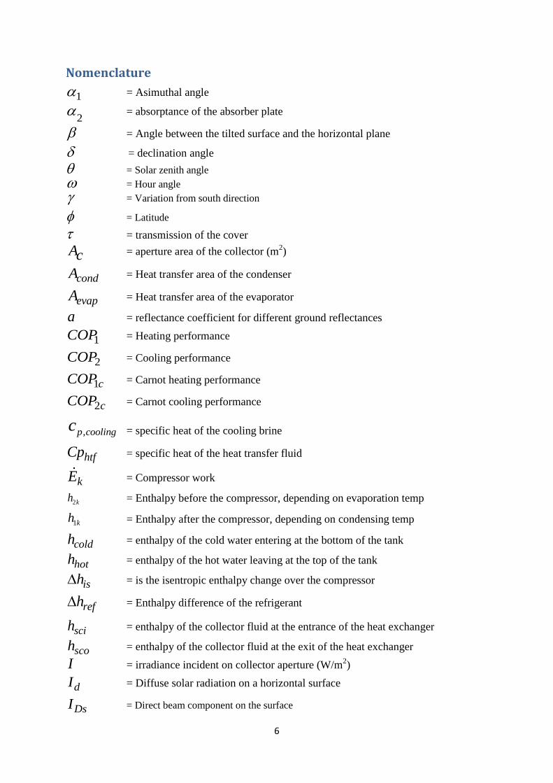
6

Nomenclature

1 = Asimuthal angle

2 = absorptance of the absorber plate

= Angle between the tilted surface and the horizontal plane

= declination angle

= Solar zenith angle

= Hour angle

= Variation from south direction

= Latitude

= transmission of the cover

Ac = aperture area of the collector (m2)

condA = Heat transfer area of the condenser

evapA = Heat transfer area of the evaporator

a = reflectance coefficient for different ground reflectances

1COP = Heating performance

2COP = Cooling performance

1cCOP = Carnot heating performance

2cCOP = Carnot cooling performance

,p coolingc = specific heat of the cooling brine

htfCp = specific heat of the heat transfer fluid

kE = Compressor work

2kh = Enthalpy before the compressor, depending on evaporation temp

1kh = Enthalpy after the compressor, depending on condensing temp

coldh = enthalpy of the cold water entering at the bottom of the tank

hoth = enthalpy of the hot water leaving at the top of the tank

ish = is the isentropic enthalpy change over the compressor

refh = Enthalpy difference of the refrigerant

scih = enthalpy of the collector fluid at the entrance of the heat exchanger

scoh = enthalpy of the collector fluid at the exit of the heat exchanger

I = irradiance incident on collector aperture (W/m2)

dI = Diffuse solar radiation on a horizontal surface

DsI = Direct beam component on the surface

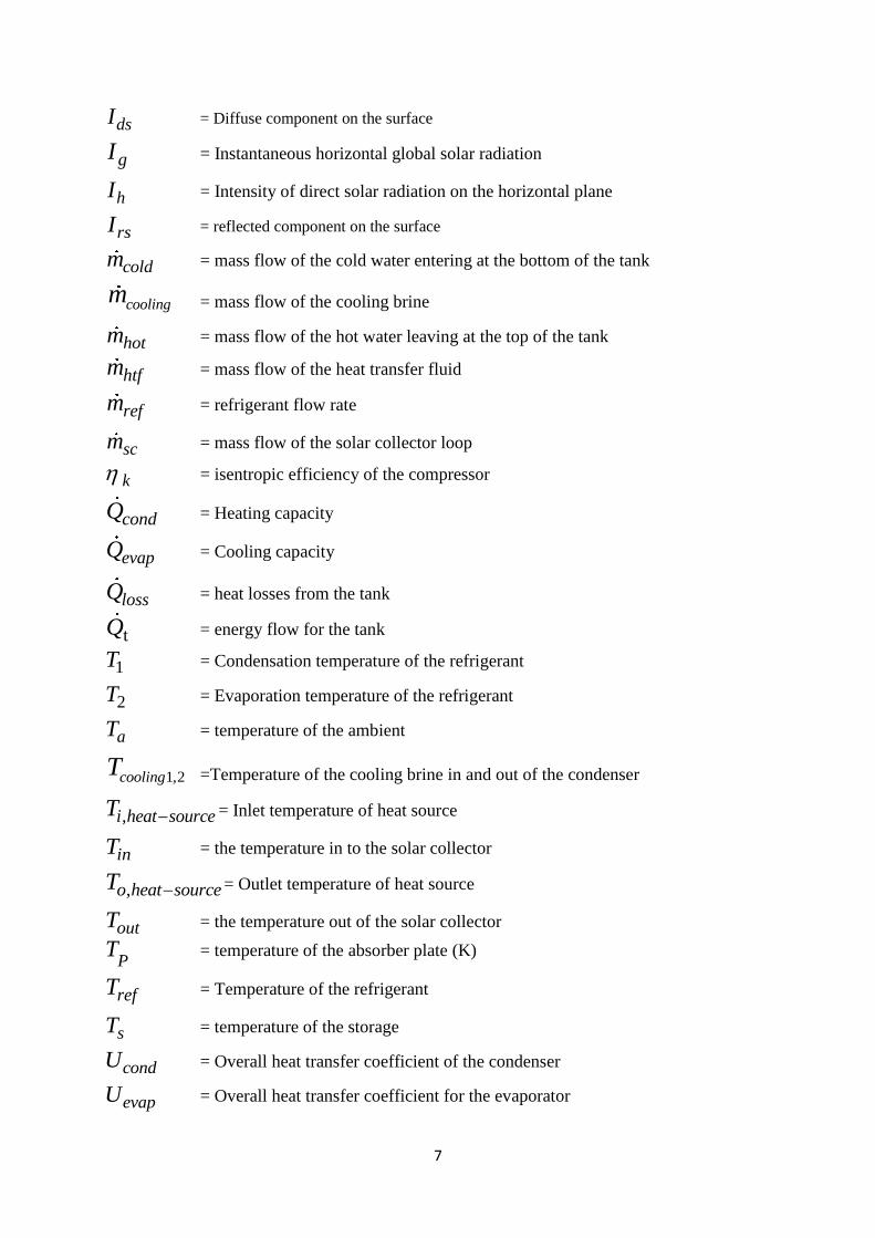
7

dsI = Diffuse component on the surface

gI = Instantaneous horizontal global solar radiation

hI = Intensity of direct solar radiation on the horizontal plane

rsI = reflected component on the surface

coldm = mass flow of the cold water entering at the bottom of the tank

coolingm = mass flow of the cooling brine

hotm = mass flow of the hot water leaving at the top of the tank

htfm = mass flow of the heat transfer fluid

refm = refrigerant flow rate

scm = mass flow of the solar collector loop

k = isentropic efficiency of the compressor

condQ = Heating capacity

evapQ = Cooling capacity

lossQ = heat losses from the tank

tQ = energy flow for the tank

1T = Condensation temperature of the refrigerant

2T = Evaporation temperature of the refrigerant

aT = temperature of the ambient

1,2coolingT =Temperature of the cooling brine in and out of the condenser

,i heat sourceT = Inlet temperature of heat source

inT = the temperature in to the solar collector

,o heat sourceT = Outlet temperature of heat source

outT = the temperature out of the solar collector

PT = temperature of the absorber plate (K)

refT = Temperature of the refrigerant

sT = temperature of the storage

condU = Overall heat transfer coefficient of the condenser

evapU = Overall heat transfer coefficient for the evaporator

8

LU = Overall heat loss coefficient (W / (m

2, K))

1LU = component of temperature independent heat loss

2LU = component of temperature dependent heat loss

9

1. Introduction This project is a part of an advanced master course at the Institution of Energy Technology at

KTH, Stockholm, Sweden.

This report is put together by two students in the master field of Sustainable energy utilization

and is treating the subject of a solar collector in combination with a heat pump, for single

family houses in Sweden.

The report is describing in detail:

Function of the solar collector systems and how to calculate the energy output. Also

how to design the systems and what parts that is crucial for its functionality.

Heat pump systems and its function. Also the calculation process for heating and

cooling capacity is described.

Different heat sources for the heat pump are described, also their limitations and

advantages against each other.

Some different combination methods for the solar collector and the heat pump, and

what the disadvantages and advantages are for these.

A model of a combined system has also been developed in order to simulate and evaluate the

performance. This has further been analyzed in order to present the advantages of such a

system and what needs to be done in the future.

The report also describes a number of on market solutions that can be delivered by different

companies over the world.

1.1 Background

As energy prices constantly are increasing and extreme weather conditions are relatively

common, a higher demand for cheaper solutions to high indoor thermal comfort is seen.

In Sweden, the temperature in the winter time is very low, causing a heating demand during

this period. The most common heat pump solution for heating today is a heat pump with

ground rock/ground water as the heat source. The compressor in the heat pump is electrically

driven, which means that, when the heating demand is at its maximum i.e. during the winter,

this will cost a lot of money. Especially as the prices for electrical power is higher during this

period. So therefore some alternative cheaper solutions are investigated and evaluated in order

to meet the demands.

Some solutions are:

Passive buildings

Heat recovery systems

Better heat pumps and components

This report will treat the aspect of a solar collector in combination with a heat pump.

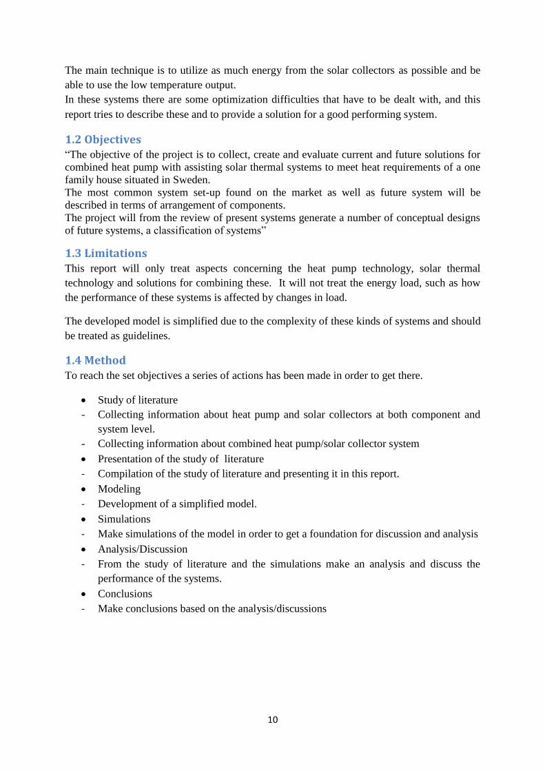
10

The main technique is to utilize as much energy from the solar collectors as possible and be

able to use the low temperature output.

In these systems there are some optimization difficulties that have to be dealt with, and this

report tries to describe these and to provide a solution for a good performing system.

1.2 Objectives “The objective of the project is to collect, create and evaluate current and future solutions for

combined heat pump with assisting solar thermal systems to meet heat requirements of a one

family house situated in Sweden.

The most common system set-up found on the market as well as future system will be

described in terms of arrangement of components.

The project will from the review of present systems generate a number of conceptual designs

of future systems, a classification of systems”

1.3 Limitations This report will only treat aspects concerning the heat pump technology, solar thermal

technology and solutions for combining these. It will not treat the energy load, such as how

the performance of these systems is affected by changes in load.

The developed model is simplified due to the complexity of these kinds of systems and should

be treated as guidelines.

1.4 Method To reach the set objectives a series of actions has been made in order to get there.

Study of literature

- Collecting information about heat pump and solar collectors at both component and

system level.

- Collecting information about combined heat pump/solar collector system

Presentation of the study of literature

- Compilation of the study of literature and presenting it in this report.

Modeling

- Development of a simplified model.

Simulations

- Make simulations of the model in order to get a foundation for discussion and analysis

Analysis/Discussion

- From the study of literature and the simulations make an analysis and discuss the

performance of the systems.

Conclusions

- Make conclusions based on the analysis/discussions

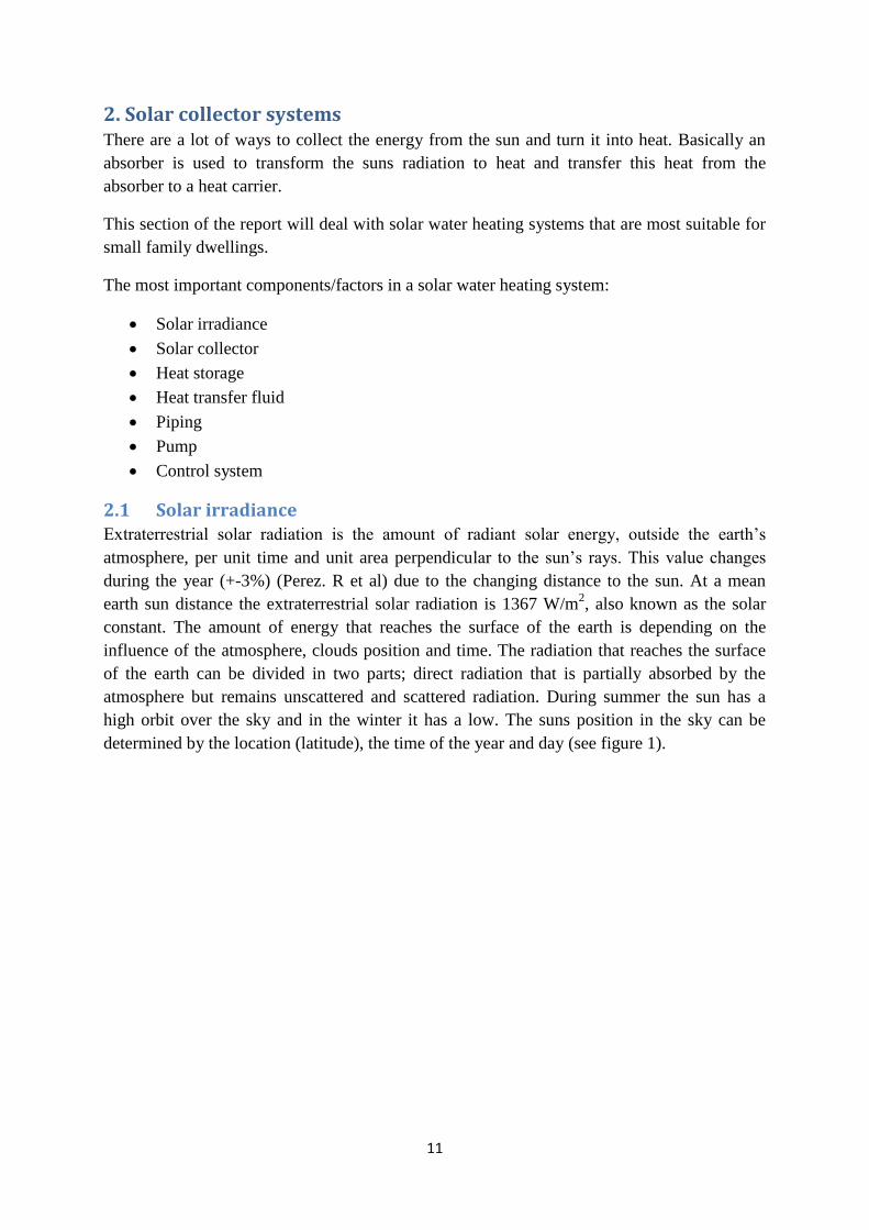
11

2. Solar collector systems There are a lot of ways to collect the energy from the sun and turn it into heat. Basically an

absorber is used to transform the suns radiation to heat and transfer this heat from the

absorber to a heat carrier.

This section of the report will deal with solar water heating systems that are most suitable for

small family dwellings.

The most important components/factors in a solar water heating system:

Solar irradiance

Solar collector

Heat storage

Heat transfer fluid

Piping

Pump

Control system

2.1 Solar irradiance Extraterrestrial solar radiation is the amount of radiant solar energy, outside the earth’s

atmosphere, per unit time and unit area perpendicular to the sun’s rays. This value changes

during the year (+-3%) (Perez. R et al) due to the changing distance to the sun. At a mean

earth sun distance the extraterrestrial solar radiation is 1367 W/m2, also known as the solar

constant. The amount of energy that reaches the surface of the earth is depending on the

influence of the atmosphere, clouds position and time. The radiation that reaches the surface

of the earth can be divided in two parts; direct radiation that is partially absorbed by the

atmosphere but remains unscattered and scattered radiation. During summer the sun has a

high orbit over the sky and in the winter it has a low. The suns position in the sky can be

determined by the location (latitude), the time of the year and day (see figure 1).

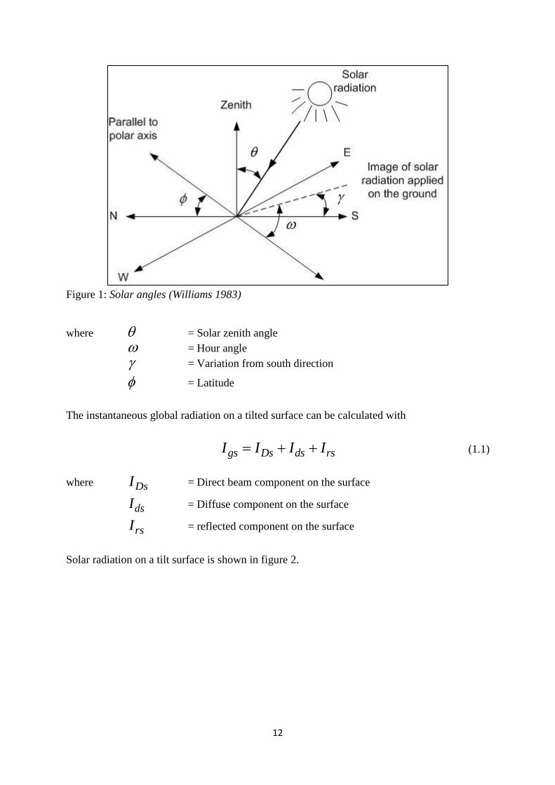
12

Figure 1: Solar angles (Williams 1983)

where = Solar zenith angle

= Hour angle

= Variation from south direction

= Latitude

The instantaneous global radiation on a tilted surface can be calculated with

gs Ds ds rsI I I I (1.1)

where DsI = Direct beam component on the surface

dsI = Diffuse component on the surface

rsI = reflected component on the surface

Solar radiation on a tilt surface is shown in figure 2.

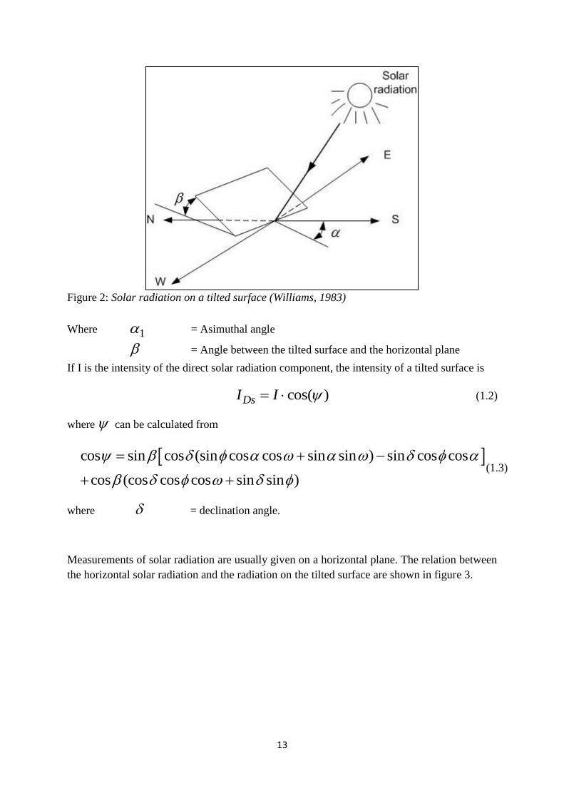
13

Figure 2: Solar radiation on a tilted surface (Williams, 1983)

Where 1 = Asimuthal angle

= Angle between the tilted surface and the horizontal plane

If I is the intensity of the direct solar radiation component, the intensity of a tilted surface is

cos( )DsI I (1.2)

where can be calculated from

cos sin cos (sin cos cos sin sin ) sin cos cos

cos (cos cos cos sin sin )

(1.3)

where = declination angle.

Measurements of solar radiation are usually given on a horizontal plane. The relation between

the horizontal solar radiation and the radiation on the tilted surface are shown in figure 3.

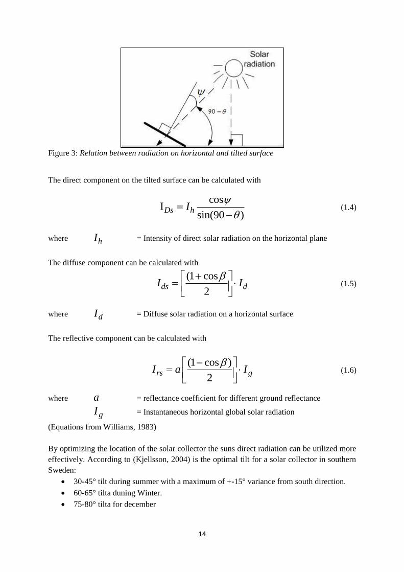
14

Figure 3: Relation between radiation on horizontal and tilted surface

The direct component on the tilted surface can be calculated with

cos

Isin(90 )

Ds hI

(1.4)

where hI = Intensity of direct solar radiation on the horizontal plane

The diffuse component can be calculated with

(1 cos

2ds dI I

(1.5)

where dI = Diffuse solar radiation on a horizontal surface

The reflective component can be calculated with

(1 cos )

2rs gI a I

(1.6)

where a = reflectance coefficient for different ground reflectance

gI = Instantaneous horizontal global solar radiation

(Equations from Williams, 1983)

By optimizing the location of the solar collector the suns direct radiation can be utilized more

effectively. According to (Kjellsson, 2004) is the optimal tilt for a solar collector in southern

Sweden:

30-45° tilt during summer with a maximum of +-15° variance from south direction.

60-65° tilta duning Winter.

75-80° tilta for december

15

This implies that depending on the application of the collector system, and when the energy is

needed, different tilts can be used.

2.2 Solar collectors

2.2.1 Flat plate solar collector

A flat plate solar collector absorb the energy from the sun light both through direct and

diffuse parts of the sun radiation and transfer this heat to a heat transfer fluid that runs through

the collector. The absorber plates should have a high thermal conductivity and have good

corrosion resistance. Usually some kind of metal or thermoplastics is used. To improve the

absorption the plate has a coating with high absorbance and low remittance, e.g. black

metallic oxide painter on a metal surface. This kind of coating is called a selective coating.

(G.L Morrison, 2001)

A cover glass is used to prevent heat losses from the collector. This cover is usually

toughened low iron glass, due to its high transmittance, its relatively good insulation

properties and its high resistance to thermal cycles. Anti-reflecting coatings are used to

increase the transmittance of the glass. To improve insulation a second layer of glass can be

added to the casing and is mostly used in high temperature applications.

Material properties of the back insulation of the casing are important to consider in order to

avoid out-gazing when the casing are exposed to elevated temperatures. It is important that

the insulation is kept dry or it will lose some of its insulation properties, this can be avoided

by sealing and desiccants.

2.2.2 Evacuated solar collector

Consists of an absorption surface inside a vacuum which reduces the heat transfer because

convection in eliminated. Some different designs for evacuated collectors are: metal fin

attached to a U-tube that removes the heat from the absorber, it can also be attached to a once

through pipe, although this design requires bellows to compensate for the expansion of the

metal tubes and the cold glass. When using a heat pipe system bellows are not required. The

evacuated collectors are more efficient than flat plate collectors but because material stresses

due to pressure, the manufacturing of evacuated collectors are more expensive.

2.2.3 Unglazed solar collector

This kind of collectors have no cover glass over the absorber, because of this there is no

transmission losses due to a cover, but the significant increase of heat loss to the surroundings

makes this kind of solar collector very inefficient at higher temperatures. It can efficiently be

used in low temperature applications such as swimming pool heating.

16

2.2.4 Output and efficiency of flat plate solar collector

For steady state conditions the useful heat output for a flat plate solar collector is given by

[ ( )]L P a

Q A I U T Tcout (1.7)

where = transmission of the cover

2

= absorptance of the absorber plate

Ac = aperture area of the collector (m2)

I = irradiance incident on collector aperture (W/m2)

LU = Overall heat loss coefficient (W / (m

2, K))

PT = temperature of the absorber plate (K)

aT = temperature of the ambient (K)

During operation of the collector system it is difficult to determine the temperature of the

absorber. Due to this the temperature of the absorber plate is usually replaced with the

average fluid temperature of the collector;

2

T Tout inT

m

. (1.8)

The temperature dependent form of L

U is

1 2( )L L L m aU U U T T (1.9)

where 1LU = component of temperature independent heat loss

2LU = component of temperature dependent heat loss

Equation (1.1) then becomes

1 2 [ ( ( ))( )]L L m a m aQ A I U U T T T Tout c (1.10)

The thermal efficiency of the collector can be expressed as

out

c

Q

A I (1.11)

or

17

21 2[ ( ) ( ) ]L m a L m aU T T U T T

I

(1.12)

Equations from (Morrison, 2001)

LU depends on heat losses from the top through the cover and from heat losses through the

insulation at the bottom and the sides of the collector. The main heat loss from a flat plate

solar collector is by convection and radiation through the cover.

The heat removal factor, RF , is defined as the actual useful energy collected divided by the

useful energy collected if the entire collector absorber surface were at the temperature of the

fluid entering the collector. Introducing this gives:

[ ( )]R L i aQ A F I U T Tout c (1.13)

Equation (1.12) shows that unglazed solar collectors are very efficient ( =1) when the mean

temperature of the fluid in the collectors is close to the surrounding temperature. When this

temperature difference grows bigger the efficiency rapidly decreases. This implies, as

discussed in section 1.1.3, that unglazed solar collectors are most efficient used in low

temperature applications.

2.3 Heat storage/heat exchange

To be able to use the heat given by the collectors even when the weather conditions are

unfavorable a heat storage tank is needed. A heat exchanger is needed to transfer the heat

from a closed collector system to the storage. This can be done by an internal heat exchanger

within the storage tank (e.g. coil) which has the inlet at a high level and the outlet at a lower

level. External heat exchanger can also be used and because of natural circulation no

additional pump is needed. Another option can be a mantle heat exchanger. To minimize heat

losses from the tank, it is desirable that thermal bridges such as piping are situated at the

bottom of the tank where the temperature is low.

When using the same tank for solar heated water and auxiliary heating problems could arise

with interactions between the solar heated part and the auxiliary part. Mixing and conduction

through the fluid and the tank walls could result in preheating of the water in the bottom of

the tank which affects the temperature of the inflow and outflow of the solar collectors. Two

tanks can be used to eliminate this problem or auxiliary boosting can take place outside the

tank.

It is important to maximize stratification within the tank. One reason for this is to get lower

temperature at the bottom of the tank where the collector water outlet is, this implies lower

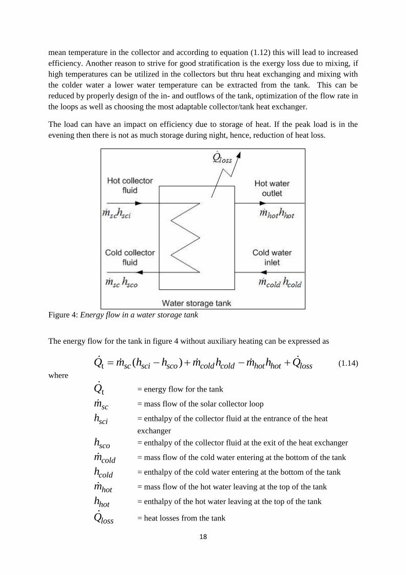
18

mean temperature in the collector and according to equation (1.12) this will lead to increased

efficiency. Another reason to strive for good stratification is the exergy loss due to mixing, if

high temperatures can be utilized in the collectors but thru heat exchanging and mixing with

the colder water a lower water temperature can be extracted from the tank. This can be

reduced by properly design of the in- and outflows of the tank, optimization of the flow rate in

the loops as well as choosing the most adaptable collector/tank heat exchanger.

The load can have an impact on efficiency due to storage of heat. If the peak load is in the

evening then there is not as much storage during night, hence, reduction of heat loss.

Figure 4: Energy flow in a water storage tank

The energy flow for the tank in figure 4 without auxiliary heating can be expressed as

t ( )sc sci sco cold cold hot hot lossQ m h h m h m h Q (1.14)

where

tQ = energy flow for the tank

scm = mass flow of the solar collector loop

scih = enthalpy of the collector fluid at the entrance of the heat

exchanger

scoh = enthalpy of the collector fluid at the exit of the heat exchanger

coldm = mass flow of the cold water entering at the bottom of the tank

coldh = enthalpy of the cold water entering at the bottom of the tank

hotm = mass flow of the hot water leaving at the top of the tank

hoth = enthalpy of the hot water leaving at the top of the tank

lossQ = heat losses from the tank

19

and

( )loss s aQ U A T T (1.15)

where

sT = temperature of the storage

aT = temperature of the ambient

2.4 Heat transfer fluid When choosing the heat transfer liquid in the solar collector system it’s important to consider

thermal expansion, viscosity, thermal capacity, freezing- boiling- and flash point. If freezing

can occur, an ethylene or propylene glycol-water mixture is often used. Since ethylene is very

toxic it is nowadays more common to use propylene due to environmental constrains. To

obtain a secure freezing protection recurrent supervision of the properties of the fluid must be

carried out and appropriate adjustments be made. If leakage exists in the system and

additional water is added it is important to ensure that the fraction of freezing protection is

high enough. (Energysavers, 2009)

With higher fraction of anti freezing in the brine the freezing protection gets better, although

this is a trade of against higher viscosity, lower thermal conductivity and lower specific heat.

(Williams, 1983)

2.5 Pump/piping Passive or thermosyphon systems uses natural circulation to circulate the water in the system,

this implies that the water tank is situated at a higher level than the solar collectors in order

for the solar heated water to rise up in the tank. The problem with these systems is the

location of the tank and the size of the system. The most common location for solar collectors

in small dwellings is the roof and if a passive system is used, the tank must be at a higher

level than the collectors. In smaller systems this can be done but in larger systems the

problems get bigger due to the weight of the tank. There can also be problems in colder

climates if the tank cannot be located inside the house as heat losses will increase because of

high temperature differences.

Active systems use a pump to circulate the water through the collectors. The use of a pump

makes these systems less efficient than passive ones. There are two kinds of ways to control

the speed of the pump, manually or automatic. The automatic ones is usually pressure

dependent and most often this kind of pumps are more efficient then the manually regulated.

In a test done by Energimyndigheten, 13 different circulations pumps where tested, this test

showed that the efficiency of different pumps can differ as much as 18 percent and that the

difference between new pumps can be large. (Energimyndigheten 2009a)

20

In locations where freezing will occur during wintertime a closed loop system is more often

used. In a closed loop system the fluid pumped through the collectors transfer the heat to the

water storage tank through a heat exchanger. This enables usage of an anti-freezing fluid in

the solar collectors. High flow through the collectors results in higher heat transfer to the heat

transfer fluid; hence more energy can be extracted from the system. If performance of the

total system is considered a low flow system is to prefer. The decrease in output is

compensated by lower pumping power in the collector loop, better stratification in the heat

storage tank and due to low flow (laminar), the heat transfer is independent of the diameter of

the tube and therefore smaller pipes can be used and installation cost is reduced. (Duff, 1996)

It is important for low flow systems that (Duff, 1996):

The flow in the collector loop should be about 2 to 4 grams/sec-m2.

The flow into the heat storage should give optimal stratification in the tank.

Total flow volume through the collector for an average day should be matched to

the volume supplied to the load for an average day.

The collector and load flow rates should be optimally matched.

When using two or more collectors together some different connections can be made. The

most common are series or parallel. Series coupled collectors are mostly used in high

temperature applications and they are less efficient then parallel coupled due to higher

average temperature in the collectors and higher pressure drop. Another drawback is that the

series of collector can be taken out of operation due to damage in just one collector. With a

parallel system it is important with balanced flows out of each collector.

2.6 Control system

The control system of a solar heating system should consist of sensors, differential

thermostats and valves.

For the collector system to be useful there has to be a temperature difference between the

outlet of the collectors and the bottom of the tank. The collector loop pump starts when a

differential thermostat, connected to sensors at the outlet of the collectors and at the bottom of

the tank, reaches a preset value. At this value the pump starts working and a check valve

opens (check valves is used to ensure that the no backflow occur when the pump is off). If

temperature difference drop while operation the shut down temperature should be lower than

the start temperature in order to avoid cycling of the pump.

To determine if the collectors is transferring sufficient heat to the storage tank two other

sensors, one at the inlet of the collector/storage heat exchanger and one at the outlet should be

mounted. If the temperature difference of these two values becomes too small it is not

profitable to run the system anymore and the pump should be shut off.

A tempering valve (mixes hot and cold water) must be used in order to insure that the

domestic hot water temperature does not exceed the highest allowed temperature. In some

systems a overheat protection is used to avoid stagnation temperatures in the collectors which

can decrease the life span of pipes, insulation and brine. Stagnation temperatures can be

21

reached for instance in case of a power outage or if the pump stops due to low temperature

difference between the bottom of the tank and the collector. To avoid this heat dumping can

be necessary in order to lower the temperature at the bottom of the tank.

In indirect systems an expansion tank is needed to compensate for expansions as the

temperature gets higher.

(Williams, 1983)

2.7 System design

To build an optimized solar heating system many factors must be considered.

To what is the system going to be used?

- E.g. heating and DHW or only DHW

What is the optimal size for the system considering the investment and the desired

degree of coverage?

- E.g. take in different offers

What kind of auxiliary energy source is going to be used?

- E.g. district heating, wood, electricity, heat pump

When these questions are answered the optimization of the components can begin and

depending on the answers different components is used to build the optimal system.

Some main principles when sizing a collector system are according to Energimyndigheten

2009c;

5 m2 solar collector area for DHW for a family dwelling

10-15 m2 solar collector area for heating and DHW

22

3. Heat pumps According to the International Energy Agency (IEA), there are two main types of heat pump

systems in use today, where one is based on a vapour compression cycle and the other on an

absorption cycle. (International Energy Agency 2009)

This report will be focused on the vapour compression cycle type. This system includes four

steps: evaporation, compression, condensation and expansion. Evaporation and condensation

are two types of heat exchangers where the working fluids of the cycle exchange thermal

energy.

The compression is done by a compressor where a (often electrical) motor is the source for

the incoming work. (International Energy Agency 2009)

3.1 Heat pump systems

When choosing a suitable heat pump system, there are many factors to be considered, as the

incoming heat for the cycle can be obtained in a few different ways. Some of the most

commonly used heat sources are; ambient air, ground water, lake/river/sea water, rock,

ground and waste water. (International Energy Agency 2009)

It is important that the heat source is stable and at relatively high temperature during the

heating season, therefore this is a key factor when deciding for a system. Other important

factors are; availability for utilization, thermophysical properties of the heat source and

investment costs for the utilization. (International Energy Agency 2009)

Considering above mentioned factors it is also important that the heat source will meet the

requirements of the building, such as heat load etc. therefore it would be a good idea to

calculate and evaluate the performance of the building before deciding for a heat pump

system. (Caneta Research inc. 1995)

3.2 Heat exchangers and heat sources

After deciding which heat pump system to be used the next step is to choose for, and size the

heat exchanger that is collecting the heat.

3.2.1 Ground heat exchanger systems

Depending on a few different factors, there are two types of ground heat exchangers,

horizontal bore field and vertical field, that can be implemented, both in different variants.

Factors to take under consideration are:

Land area that can be exploited, a horizontal field require a larger area.

Height of the building (especially when deciding for a high rise multi flat building),

the pressure head cannot get exceeded. This is crucial when considering a vertical bore

field.

23

Location of the horizontal heat exchanger field, different surface materials such as

asphalt or grass etc. can give different working temperature for the heat pump because

of the annual temperature variations and the absorptivity of the surface.

Installation cost is the key factor for deciding heat exchanger type, but only if both of

the alternatives performances are comparable.

(Caneta Research inc. 1995)

Ground source vertical heat exchanger

There are a few alternatives of vertical heat exchangers available. The basic technique is to let

a u-tube circulate a fluid in a borehole in order to heat exchange with ground heat. Low

temperature water (with 30% anti freeze liquid, ethanol) is heated in the borehole to a

required temperature, to heat exchange again in the evaporator of the heat pump.


As mentioned above, there are different types of vertical heat exchangers, some examples are:

One borehole per flow circuit and one u-tube per borehole, this is a common technique for

regular family residents in Sweden. (Svenska Värmepumpsföreningen 2010a)

One borehole per circuit and a pair of u-tubes per borehole.

Multi boreholes per circuit and one u-tube per borehole.

The economic perspective of these techniques is that with multiple u-tubes in each borehole

the total price of the pipes can get high, but this cost can on the other hand abolish the cost for

drilling. Local prices and conditions decide for which technique to be used.


The size of the heat exchanger is decided upon the loads of the building, which is a function

of; building type, size, location, internal heating, infiltration, solar gain, envelope conduction

and ventilation losses. Other design parameters are mean ground temperature, type of rock

(conduction), efficiency of the actual heat pump and size of the pipe.

Advantages with this system:

In Sweden, this is the most common type and therefore it is a large market.

A secure system with relatively long life length.

Disadvantages:

High costs for drilling and installation.

(Svenska Värmepumpsföreningen 2010a)

Ground source horizontal heat exchanger

The technique here is the same as for vertical heat exchangers, except for that the u-tube

circuit is placed in a horizontal plane, approximately 90 – 150 cm under the surface,

depending on the location and mean temperature. So in this system the sun has a sufficient

influence.

There are different alternatives for this type as well, where the installed system could use:

A two-pipe alternative with either side-by-side or over-under configuration.

A four-pipe arrangement, also side-by-side or over-under, or even a combination.

A six-pipe configuration.

24

The sizing principle for the horizontal heat exchanger is in general the same as for the vertical

type. The difference is that it is more sensible to annual temperature variations and also what

kind top layer there is.

This kind of system requires a much larger surface area and can be difficult to implement,

especially in locations where the buildings are tight situated. Nowadays there are techniques

though, where the pipes are in spirals and therefore the surface area can be reduced.


Advantages with this system:

Same as for vertical systems.

Disadvantages:

Could make a large impact on the garden.

Not suitable in areas where the buildings are situated tight.

Larger temperature fluctuations than for the vertical case

(Svenska Värmepumpsföreningen 2010a)

3.2.2 Groundwater heat exchanger system

This type uses the groundwater as a heat source for the heat pump. The groundwater

temperature is usually around 4-8 °C annually and is therefore stable as a heat source. There

are two ways of collecting this heat:

(Svenska Värmepumpföreningen, 2010b)

Closed loop system

A closed loop groundwater system uses the same technique as for the other ground source

system, except for that the heat source is from the groundwater instead of the rock.

The system collects groundwater with a professionally designed well, often combined with

pumps, and circulates it in a loop where it heat exchange with the internal loop of the building

and then get recharged to the ground, either just on the surface or injected in to the ground.

The latter one is more expensive, but often this is a regulatory demand. The heat exchange to

the internal loop is done with a regular plate and frame heat exchanger, where a metal sheet is

used to transfer heat between two fluids.

There are several alternatives for a closed loop system; one is the regular where the source is

connected to a heat pump, and another use a boiler before the heat pump. This could be an

alternative if the heat collecting area is limited.

There are some design parameters when deciding for a suitable well, which should be done by

a professional hydro geologist. After investigating for heat loads, ground water availability

etc. the hydro geologist will decide for number of wells, spacing and size, for both the supply

and recharge wells. Other factors that the hydro geologist have to take into account are the

temperature change, pressure- drop/rise, PH-levels, gas concentration etc. for the engineer to

design the system.


25

Open loop system

In an open loop system, the groundwater is directly supplied to the heat pumps with no heat

exchange in between. Because of this, there are several requirements that have to be taken

into account. There should be plenty of ground water available, it should be of high quality, it

should be a low-rise building (in order to have low pump power) and the static water level

should be high. It is also important to identify if there is any corrosion species in the water to

be able to choose pipes, heat exchanger etc.

Usually there are separate supply and discharge lines, where the supply is pressurized with the

well pump, and the expansion valve keeps the required pressure head constant.


Advantages with ground water heat pump systems:

High and stable supply temperature.

Can be used when high power requirements.

Long life length.

Disadvantages:

For an open loop there could be pollutions in the ground water from discharge water.

The supply water have to be of high quality.

Expensive drilling.

Insecure knowledge of water availability before drilling.


3.2.3 Sea/lake water heat exchanger systems

The sea/lake water is a good heat source because of that the water temperature are at

approximately 4°C at its minimum, and does therefore provide a stable supply for the heat

pump.

The technique is to place a collector-tube at the bottom of the sea/lake where the water

temperature is constant during most of the year, deeper the better, also because of the lower

risk for damages. This type is common for buildings with high heat consumption. The heat

pump in the system is the same as for ground heat exchanger systems, so the sizing and

design factors are the same.

Advantages with sea/lake water systems:

Cheap to place a collector-tube in the water.

Same heat pump as in ground source heat exchanger, and therefore a lot of

alternatives on the market.

Long life length.

Disadvantages:

An even sea/lake bottom is preferred when placing the tubes.

Have to keep the collector on the bottom prevent damages etc. which could be a

problematic task.


26

3.3 Heat pump function and configuration

A heat pump works in four steps:

1. Evaporation: In this step, the working fluid is kept colder than the supply temperature,

causing a heat flow from the heat source to the working fluid, which will evaporate.

2. Compression: Now when the fluid is in vapour phase, it is easier to compress. The

compressor is driven by a motor (often electrical) and is increasing the pressure of the

working fluid. This will cause a temperature rise.

3. Condensation: After leaving the compressor, the working fluid is entering the

condenser, still in high-pressure vapour phase, where it condensates and distribute heat

to the building.

4. Expansions: The last step in the cycle is an expansion where the pressure of the

working fluid is decreased. This will cause a temperature decrease as well, that will

enter the evaporator.

(International Energy Agency 2009)

3.3.1 Evaporators

The evaporator design is different depending on what applications it should be used for. So

there are different design parameters for this. There are different types depending on what

heat source the use; gas (air cooler), liquid (liquid cooler) or solid. This report will consider

indirect systems, where the evaporator itself is a liquid cooler but the heat is transferred from

the source via a brine (liquid) to the evaporator.

The refrigerant that flows in the heat pump is evaporated here, with the heat source, e.g.

ground heat, as the driving force. The temperature of the refrigerant is constant during the

evaporation, but is often superheated before the compressor. Before the evaporation there is,

as mentioned above, an expansion valve which lower the pressure of the refrigerant and

thereby also the temperature. This is a crucial step for making the evaporation possible.

There are two possible ways to force the refrigerant to evaporate:

Dry expansion: Here the refrigerant is forced through the evaporator and then on to the

compressor. In this case a superheating has to be made after the evaporation to prevent

that liquid reaches the compressor.

Flooded evaporation: Here the refrigerant is collected in a low-pressure receiver,

where the vapour and liquid are being separated.

There are two main types of liquid coolers, both shell and tube evaporators. One where the

refrigerant flows inside the tubes and another with the flow outside the tubes. Advantages

with inside flow are that there is no risk for oil accumulation inside, as the refrigerant will

transport it to the exit, another is that the refrigerant charge will be smaller. An advantage

with outside flow is that the brine side will be easier to clean. This could be a good alternative

when using sewage water as a heat source.

The performance of an evaporator is dependent on both the mass flow of the refrigerant and

the temperature difference from the inlet and the outlet.

The cooling capacity of an evaporator can be calculated with:

evap evap mQ UA (1.16)

27

where evapU = Overall heat transfer coefficient for the evaporator

evapA = Heat transfer area of the evaporator

and

ln( )

i om

i

o

(1.17)

where

,i i heat source refT T (1.18)

,o o heat source refT T (1.19)

where ,i heat sourceT = Inlet temperature of heat source

,o heat sourceT = Outlet temperature of heat source

refT = Temperature of the refrigerant

Desired mass flow rate of the refrigerant can then be calculated as:

evap

refref

Qm

h

(1.20)

where refh = Enthalpy difference of the refrigerant

refm = refrigerant flow rate

(Department of Energy Technology, KTH, 2009)

3.3.2 Compressors

A compressor is a device that compresses any compressible fluid or gas. It could be of several

types, such as reciprocating, rotary, scroll, screw or centrifugal. In a heat pump the

compressor should extract the vapour from the evaporator and force it into the condenser.


There are two different compression methods, one is referred to as intermittent and the other

to continuous. The intermittent method is a cyclic compression where a specific amount of

gas is taken in to the process, compressed, and discharged before the next cycle starts. In a

continuous compression, the fluid flow is constant through the compressor, which means that

there are no interruptions.

28

There are several types of compressors that can be placed under these above-mentioned

methods.

Intermittent:

Reciprocating: There are two types of reciprocating compressors, piston compressor

and diaphragm compressor. The piston compressor is one of the most used

compressors, and it works with a displacing action where a piston compresses the

media inside a cylinder, from a mechanical shaft work, together with the inlet valves.

The outlet valves in the discharge line prevent a backflow to the compression cylinder

as the next cycle starts. The piston compressor is well suited for high-pressure

applications and is one of the most efficient at a pressure ratio over 1.5. The

diaphragm compressor has the same layout as the piston compressor, but it works with

oil rather than with gas and is suitable for small flow applications.

Rotary: The rotary compressors have three things in common; (1) the gas is

compressed by rotating elements, (2) the compression is intermittent and (3) there are

no inlet or outlet valves.

They use either helical or spiral lobes to compress the gas between them and the rotary

chamber. In the spiral case, the compression starts as the spiral moving over the inlet

and bring a specific amount of gas. As the spiral screws inward through the rotary

chamber, gas is being compressed as the volume is decreasing. The gas is then

discharged in a nozzle at the end of the compression. This type is used only for lower

pressure applications.

The helical type (screw) compressor is either dry or flooded, where the flooded use a

liquid to prevent the rotors from touching and the dry uses gears for the same reason.

The technique is similar but it is more applicable to higher-pressure applications. The

compression state is at the discharge port where the backflow is the driving force for

the compression.

(Brown, R.N. 2005)

Scroll compressor: In a scroll compressor the compression takes place between two

spiral shaped chambers. One of these spirals is fixed with the other one orbiting in a

fixed pattern (orbiting motion) inside it. As gas entering in the outer periphery the

inner spiral will do one orbit and the size of the “gas pocket” will decrease and also

compress the gas. Continuing the process, this pocket will move closer to the center,

where the discharge is. Since there are two identical scrolls, one continuously orbiting,

there will be a new pocket directly after the discharge pocket, and therefore the

process is almost continuous and sometimes it is.

A scroll compressor is suitable where there is a need for low sound and low vibration.

It has relatively high volumetric efficiency and it is not very sensitive to pressure ratio

compared to a reciprocating compressor.

But, because of the high precision of the manufacturing of the scrolls, the development has

been a little bit constrained. (Department of Energy Technology, KTH, 2009)

Continuous:

Dynamic: These compressors use a different technique than the above-mentioned. As

they are continuous, the compressing never gets interrupted and are suitable for large

29

volumes with a limited compression ratio. They can be either radial or axial, with the

flow in that direction respectively. The radial alternative is often called centrifugal and

uses an impeller to force the flow in radial direction, from the area near the shaft to the

discharge, called a diffuser.

The axial alternative uses rotor blades as the energy converter. There are several of

these blades, and before and after every rotor are a stationary blade. So the flow is

forced through these stationary blades with the rotor blades, and the fluid is

compressed.

(Brown, R.N. 2005)

In order to calculate the work needed for the compression there are several parameters to take

into account. First one needs to specify the pressure rise/temperature rise in order to determine

the enthalpy change over the compressor itself. Then the compressor work can be calculated

as:

1

k ref isk

E m h

(1.21)

where kE = Compressor work

ish = is the isentropic enthalpy change over the compressor

k = isentropic efficiency of the compressor

Now it is possible to introduce the cooling performance of the cycle, which means the cooling

capacity divided by the compressor work needed:

2evap

k

QCOP

E (1.22)

Where 2COP = Cooling performance

evapQ = Cooling capacity


3.3.3 Condenser

At this side of the heat pump, the heat will be distributed to the buildings heating system.

The refrigerant entering the condenser is superheated vapour from the compressor and will

leave in a subcooled state.

The size of the condenser and its working temperature depend on the compressor type and its

size. This has to do with the required COP for the heat pump, which is a relation between the

30

compressor work and the amount of media that should be heated by the condenser. So if the

compressor is poor there is a need for a large condenser.

Air-cooled condenser: This type uses air as coolant where the heat exchange is due to

convection, either forced or natural. Natural convection types are commonly used in

refrigerators in regular family houses (domestic).

Water-cooled condenser: This type use water as coolant and the heat exchangers that are

mostly used are brazed plate-type, tube in tube-type or tube in shell-type. The shell in tube

condensers are used in larger plants, where the refrigerant condenses on the outside of the

tubes and the water flows inside these tubes.

Depending on the desired indoor temperature and the heat transfer area of the radiators

different water temperature must be obtained. In older systems with small heat transfer areas

supply temperatures about 80 C and return temperatures of 60 C is common. For newer

systems temperatures around 55 in supply and 45 in return is common. When using floor

heating these temperature are even lower. (Seminar, Claesson 2009)

Evaporative condensers: In this type, the refrigerant passes through the condenser inside

coils, which are wetted on the outside by water. This water will then condense and forced to

evaporate by air flowing over the coils. This evaporation removes heat from the evaporation.

In order to calculate the heating capacity of the condensers the following expression can be

used:

cond cond mQ UA (1.23)

where condQ = Heating capacity

condU = Overall heat transfer coefficient of the condenser

condA = Heat transfer area of the condenser

and

ln( )

i om

i

o

(1.24)

where

,i ref cooler inT T (1.25)

,o ref cooler outT T (1.26)

which is the same approach as for the evaporators (see eq. 1.16) except for that the refrigerant

temperature in the condenser is higher than the cooling media.

31

The heating capacity does also have relation to the mass flow rate of the refrigerant, by the

following equations:

cond ref refQ m h (1.27)

Now it is possible to calculate the heating performance of the cycle, which is interesting in

this project

1cond

k

QCOP

E (1.28)

where 1COP = Heating performance

which also can be written as, for an ideal cycle:

1 2 1COP COP (1.29)

Equation 1.28 is only true if all the heat rejected is useful, in other words:

1 2 kQ Q E (1.30)

where 1Q = condQ

2Q = evapQ


2.3.4 Expansion device

The expansion phase of the heat pump has the main purpose of keeping the wanted pressure

difference between the high and low-pressure side. Another purpose is to regulate the mass

flow of the refrigerant in order to have the correct heat exchange in both the evaporator and

condenser.

There are a few types of devices to consider:

The hand expansion valve:

This type is a hand-operated valve. The flow rate through the valve is dependent on the

pressure differential across the orifice and how large the hand-operated valve opening is.

There are some disadvantages for this type, for example if the load changes on the evaporator

side, then the valve has to be operated manually, which could be difficult or not preferable at

least.

The capillary tube:

The technique for this type is that the capillary tube, which has a small diameter relative to the

other tube, is placed between the condenser and the evaporator. When the refrigerant reaches

the capillary tube, the pressure drops because of the smaller diameter and the friction factor.

This type is often used in domestic refrigerators and smaller heat pumps.

32

The automatic expansion valve:

This valve is used when the evaporator temperature is wanted to be constant, so therefore also

the pressure the valve is wanted to be constant. The mechanism is automatic and therefore

adjust the pressure difference by itself.

The thermostatic expansion valve:

These expansion types’ main tasks are to maintain a constant superheating before the

compressor. The thermostatic expansion valve consists of a metal membrane, a bulb and a

spring. The bulb is filled with a refrigerant gas and is connected to the superheated vapour

temperature before the compressor, which will give a force working against the pressure on

the membrane. In order for the valve to open, the pressure above the membrane must be larger

than the pressure on the bulb and the spring below the membrane. So as the load on the

evaporator changes, the spring can be regulated in order to keep the same conditions.

The electronic expansion valve:

This type is a motor driven expansion valve, which is regulated by signals from a regulator.

The regulator send signals as it sense both pressure and temperature differences.

33

4. Combined solar and heat pump systems The reason for combining solar collector is to increase the overall efficiency of the system.

The advantages with these kind of systems are many and various and depends a lot on heat

loads, system design and control optimization. There are a lot of possibilities with different

system designs and this chapter brings up and discusses some of them and the problems that

can occur. Some on market solutions will be discussed as well.

4.1 Energy utilization There are basically two main reasons to combine solar collectors with heat pumps

1. Low temperatures from the solar collectors can be utilized

2. Lower usage of heat pump

To utilize the energy in the solar collectors when the temperature is insufficient for direct

heating or DHW this energy can be used to boost the temperature in the evaporator or

condensor side of the heat pump. This way the efficiency of the heat pump goes up. Another

way to use this low temperature energy could be to recharge the heat source of the heat pump.

This requires that the heat source is able to absorb and store the energy that it’s given so it can

be used later. (Kjellsson 2009, 2004)

4.2 Heat transfer liquid The heat transfer liquid in the heat pump loop has to be able to handle temperature down to

about -10 °C (Kjellsson, 2004) without freezing. It should have high specific heat and thermal

conductivity. Environmental aspects are also important due to the risk of leakage in case of

damage to the pipe. As said in section 2.4 propylene glycol- water solutions are common in

solar collector systems but due to environmental issues this solution is not to prefer in ground

loops. Ethanol solutions are the most common solution in ground loops (see section 3.2.2) but

it is not suitable for solar collectors due to explosion risk at stagnation temperatures. When

combining the two systems there is a need for a solution that are applicable both to the solar

collectors and the ground loop in order to avoid investments in a heat exchanger between the

two systems. A rapeseed oil derivative can be used and the difference in performance from

propylene glycol and ethanol solutions are visualized in table 1.

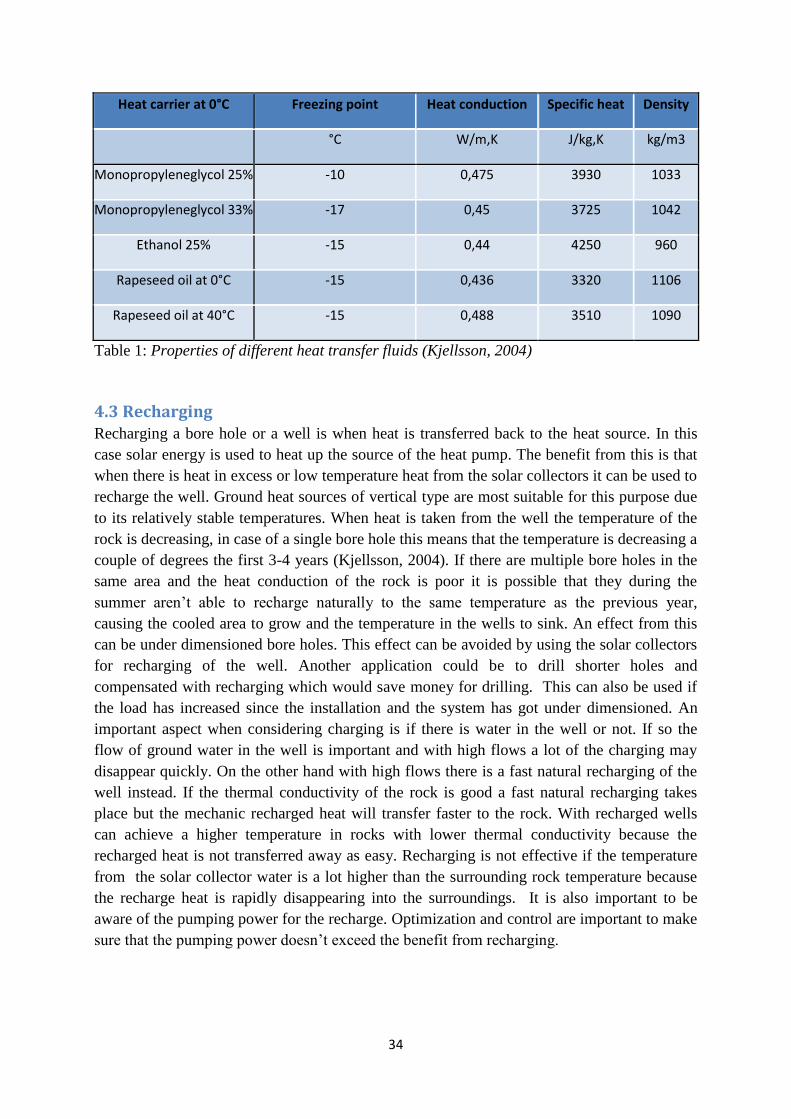
34

Heat carrier at 0°C Freezing point Heat conduction Specific heat Density

°C W/m,K J/kg,K kg/m3

Monopropyleneglycol 25% -10 0,475 3930 1033

Monopropyleneglycol 33% -17 0,45 3725 1042

Ethanol 25% -15 0,44 4250 960

Rapeseed oil at 0°C -15 0,436 3320 1106

Rapeseed oil at 40°C -15 0,488 3510 1090

Table 1: Properties of different heat transfer fluids (Kjellsson, 2004)

4.3 Recharging Recharging a bore hole or a well is when heat is transferred back to the heat source. In this

case solar energy is used to heat up the source of the heat pump. The benefit from this is that

when there is heat in excess or low temperature heat from the solar collectors it can be used to

recharge the well. Ground heat sources of vertical type are most suitable for this purpose due

to its relatively stable temperatures. When heat is taken from the well the temperature of the

rock is decreasing, in case of a single bore hole this means that the temperature is decreasing a

couple of degrees the first 3-4 years (Kjellsson, 2004). If there are multiple bore holes in the

same area and the heat conduction of the rock is poor it is possible that they during the

summer aren’t able to recharge naturally to the same temperature as the previous year,

causing the cooled area to grow and the temperature in the wells to sink. An effect from this

can be under dimensioned bore holes. This effect can be avoided by using the solar collectors

for recharging of the well. Another application could be to drill shorter holes and

compensated with recharging which would save money for drilling. This can also be used if

the load has increased since the installation and the system has got under dimensioned. An

important aspect when considering charging is if there is water in the well or not. If so the

flow of ground water in the well is important and with high flows a lot of the charging may

disappear quickly. On the other hand with high flows there is a fast natural recharging of the

well instead. If the thermal conductivity of the rock is good a fast natural recharging takes

place but the mechanic recharged heat will transfer faster to the rock. With recharged wells

can achieve a higher temperature in rocks with lower thermal conductivity because the

recharged heat is not transferred away as easy. Recharging is not effective if the temperature

from the solar collector water is a lot higher than the surrounding rock temperature because

the recharge heat is rapidly disappearing into the surroundings. It is also important to be

aware of the pumping power for the recharge. Optimization and control are important to make

sure that the pumping power doesn’t exceed the benefit from recharging.

35

4.4 Increasing the temperature of the evaporator side When looking in to an ideal vapor compression cycle, a so-called Carnot cycle, it is easier to

understand the relations between the evaporation and condensation. By assuming a Carnot

cycle the following equations for the coefficient of performance can be stated:

Cooling performance:

2

21 2

c

TCOP

T T

(1.31)

and heating performance:

1

11 2

c

TCOP

T T

(1.32)

where 2T = Evaporation temperature of the refrigerant

1T = Condensation temperature of the refrigerant

1cCOP = Carnot heating performance

2cCOP = Carnot cooling performance

When combining these two the following expression is derived:

1 2 1c cCOP COP (1.33)

In heat pump systems, a high value for COP1c is desired. This can be achieved by trying to

increase the COP2c value. As seen from equation 1.31 above, this can be done by increasing

the evaporation temperature, T2. This will also give another positive effect, where the COP1c

itself will increase with T2.

It is the expansion valve that performs the increasing of T2, where the pressure drop from the

condenser to the evaporator can be decreased and the evaporation temperature will then rise.

However, this puts a demand on the incoming temperature from the heat source in order to

still provide enough heat for the cooling capacity. This can be understood by looking at the

following equations:

evap evap mQ UA (1.34)

where

ln( )

i om

i

o

(1.35)

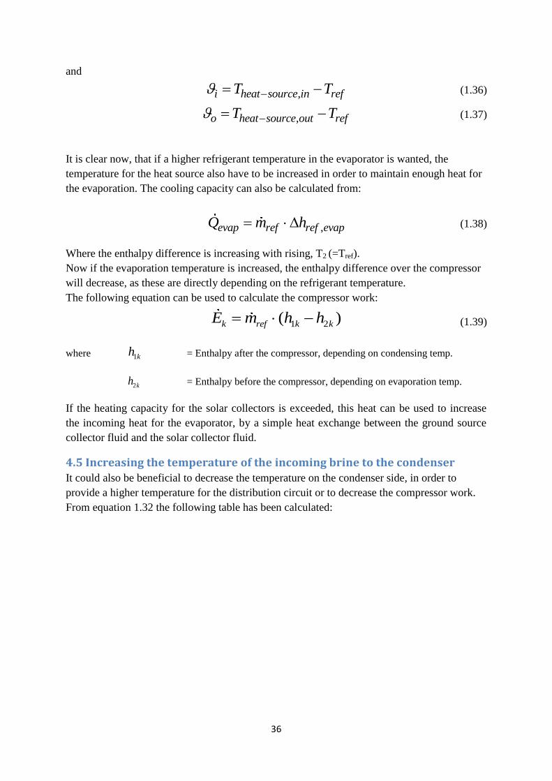
36

and

,i heat source in refT T (1.36)

,o heat source out refT T (1.37)

It is clear now, that if a higher refrigerant temperature in the evaporator is wanted, the

temperature for the heat source also have to be increased in order to maintain enough heat for

the evaporation. The cooling capacity can also be calculated from:

,evap ref ref evapQ m h (1.38)

Where the enthalpy difference is increasing with rising, T2 (=Tref).

Now if the evaporation temperature is increased, the enthalpy difference over the compressor

will decrease, as these are directly depending on the refrigerant temperature.

The following equation can be used to calculate the compressor work:

1 2( )k ref k kE m h h (1.39)

where 1kh = Enthalpy after the compressor, depending on condensing temp.

2kh = Enthalpy before the compressor, depending on evaporation temp.

If the heating capacity for the solar collectors is exceeded, this heat can be used to increase

the incoming heat for the evaporator, by a simple heat exchange between the ground source

collector fluid and the solar collector fluid.

4.5 Increasing the temperature of the incoming brine to the condenser It could also be beneficial to decrease the temperature on the condenser side, in order to

provide a higher temperature for the distribution circuit or to decrease the compressor work.

From equation 1.32 the following table has been calculated:

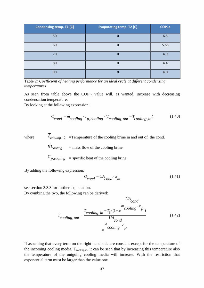
37

Condensing temp. T1 [C] Evaporating temp. T2 [C] COP1c

50 0 6.5

60 0 5.55

70 0 4.9

80 0 4.4

90 0 4.0

Table 2: Coefficient of heating performance for an ideal cycle at different condensing

temperatures

As seen from table above the COP1c value will, as wanted, increase with decreasing

condensation temperature.

By looking at the following expression:

( ), , ,

Q m c T Tcond cooling p cooling cooling out cooling in

(1.40)

where 1,2coolingT =Temperature of the cooling brine in and out of the cond.

coolingm = mass flow of the cooling brine

,p coolingc = specific heat of the cooling brine

By adding the following expression:

Q UAcond cond m

(1.41)

see section 3.3.3 for further explanation.

By combing the two, the following can be derived:

(1 ), 1

,

UAcond

m ccooling p

T T ecooling in

Tcooling out UA

cond

m ccooling p

e

(1.42)

If assuming that every term on the right hand side are constant except for the temperature of

the incoming cooling media, Tcooling,in, it can be seen that by increasing this temperature also

the temperature of the outgoing cooling media will increase. With the restriction that

exponential term must be larger than the value one.

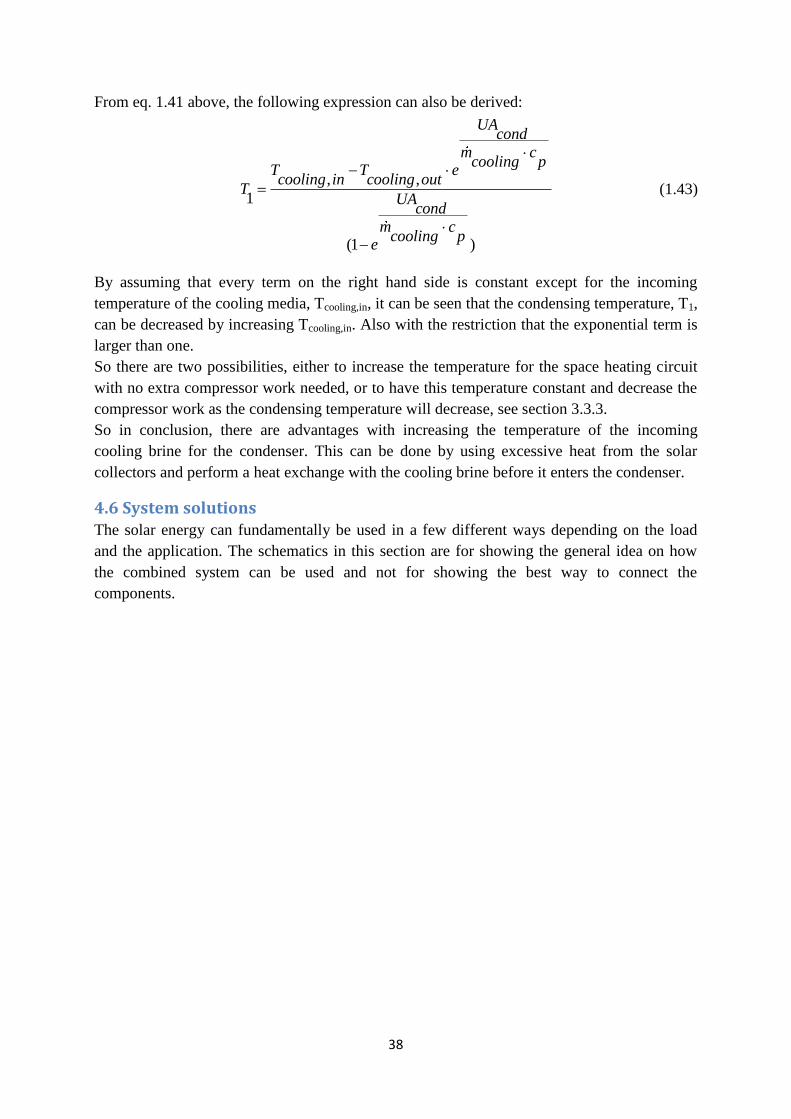
38

From eq. 1.41 above, the following expression can also be derived:

, ,

1

(1 )

UAcond

m ccooling p

T T ecooling in cooling out

TUA

cond

m ccooling p

e

(1.43)

By assuming that every term on the right hand side is constant except for the incoming

temperature of the cooling media, Tcooling,in, it can be seen that the condensing temperature, T1,

can be decreased by increasing Tcooling,in. Also with the restriction that the exponential term is

larger than one.

So there are two possibilities, either to increase the temperature for the space heating circuit

with no extra compressor work needed, or to have this temperature constant and decrease the

compressor work as the condensing temperature will decrease, see section 3.3.3.

So in conclusion, there are advantages with increasing the temperature of the incoming

cooling brine for the condenser. This can be done by using excessive heat from the solar

collectors and perform a heat exchange with the cooling brine before it enters the condenser.

4.6 System solutions The solar energy can fundamentally be used in a few different ways depending on the load

and the application. The schematics in this section are for showing the general idea on how

the combined system can be used and not for showing the best way to connect the

components.

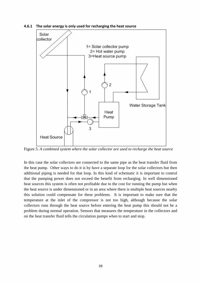
39

4.6.1 The solar energy is only used for recharging the heat source

Figure 5: A combined system where the solar collector are used to recharge the heat source

In this case the solar collectors are connected to the same pipe as the heat transfer fluid from

the heat pump. Other ways to do it is by have a separate loop for the solar collectors but then

additional piping is needed for that loop. In this kind of schematic it is important to control

that the pumping power does not exceed the benefit from recharging. In well dimensioned

heat sources this system is often not profitable due to the cost for running the pump but when

the heat source is under dimensioned or in an area where there is multiple heat sources nearby

this solution could compensate for these problems. It is important to make sure that the

temperature at the inlet of the compressor is not too high, although because the solar

collectors runs through the heat source before entering the heat pump this should not be a

problem during normal operation. Sensors that measures the temperature in the collectors and

on the heat transfer fluid tells the circulation pumps when to start and stop.

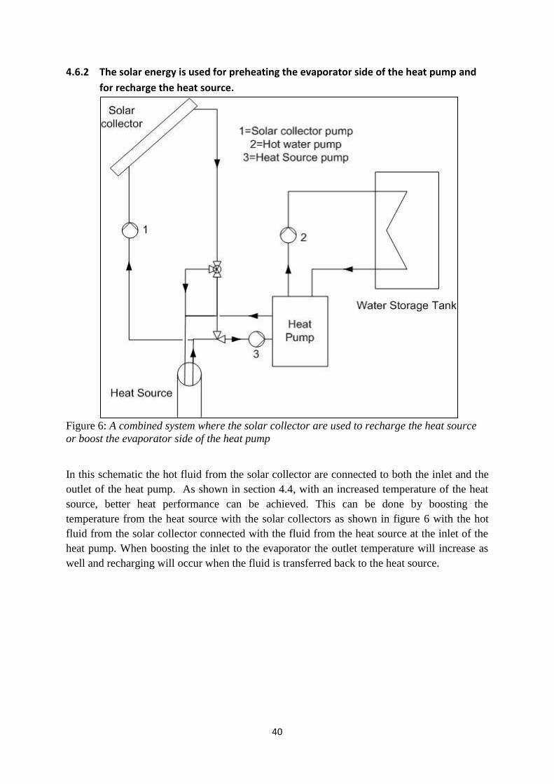
40

4.6.2 The solar energy is used for preheating the evaporator side of the heat pump and

for recharge the heat source.

Figure 6: A combined system where the solar collector are used to recharge the heat source

or boost the evaporator side of the heat pump

In this schematic the hot fluid from the solar collector are connected to both the inlet and the

outlet of the heat pump. As shown in section 4.4, with an increased temperature of the heat

source, better heat performance can be achieved. This can be done by boosting the

temperature from the heat source with the solar collectors as shown in figure 6 with the hot

fluid from the solar collector connected with the fluid from the heat source at the inlet of the

heat pump. When boosting the inlet to the evaporator the outlet temperature will increase as

well and recharging will occur when the fluid is transferred back to the heat source.

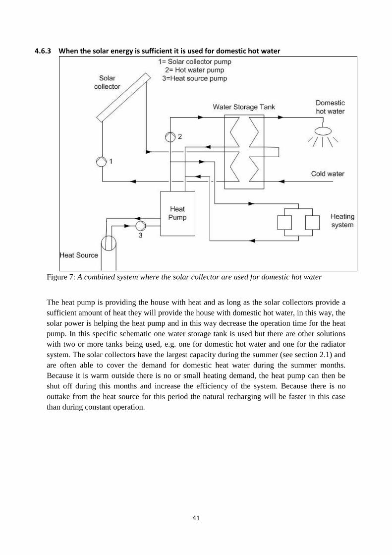
41

4.6.3 When the solar energy is sufficient it is used for domestic hot water

Figure 7: A combined system where the solar collector are used for domestic hot water

The heat pump is providing the house with heat and as long as the solar collectors provide a

sufficient amount of heat they will provide the house with domestic hot water, in this way, the

solar power is helping the heat pump and in this way decrease the operation time for the heat

pump. In this specific schematic one water storage tank is used but there are other solutions

with two or more tanks being used, e.g. one for domestic hot water and one for the radiator

system. The solar collectors have the largest capacity during the summer (see section 2.1) and

are often able to cover the demand for domestic heat water during the summer months.

Because it is warm outside there is no or small heating demand, the heat pump can then be

shut off during this months and increase the efficiency of the system. Because there is no

outtake from the heat source for this period the natural recharging will be faster in this case

than during constant operation.

42

4.6.4 When the solar energy is sufficient it is used for both domestic hot water and

heating

Figure 8: A combined system where the solar collector are used for domestic hot water and

for the radiator system

This system is almost as system nr 3 except that the solar collectors can be used for heating as

well. The connection circuit can be made in various ways in these kinds of system, for

example with multiple tanks and/or an external heat exchanger for the solar collector loop.

This kind of system implies for a larger solar collector system but can unburden the heat

pump in larger extent.

As seen in section (3.3.3) the outtake temperature of the domestic hot water and the water for

the radiator system are in the same range.

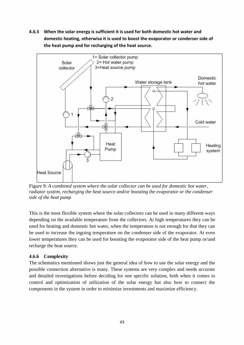
43

4.6.5 When the solar energy is sufficient it is used for both domestic hot water and

domestic heating, otherwise it is used to boost the evaporator or conderser side of

the heat pump and for recharging of the heat source.

Figure 9: A combined system where the solar collector can be used for domestic hot water,

radiator system, recharging the heat source and/or boosting the evaporator or the condenser

side of the heat pump

This is the most flexible system where the solar collectors can be used in many different ways

depending on the available temperature from the collectors. At high temperatures they can be

used for heating and domestic hot water, when the temperature is not enough for that they can

be used to increase the ingoing temperature on the condenser side of the evaporator. At even

lower temperatures they can be used for boosting the evaporator side of the heat pump or/and

recharge the heat source.

4.6.6 Complexity

The schematics mentioned shows just the general idea of how to use the solar energy and the

possible connection alternative is many. These systems are very complex and needs accurate

and detailed investigations before deciding for one specific solution, both when it comes to

control and optimization of utilization of the solar energy but also how to connect the

components in the system in order to minimize investments and maximize efficiency.

44

4.7 On market solutions

There is some companies that offers combined system solutions for single family dwellings.

This section mentions some solutions that different companies offers on the market.

4.7.1 Eviheat

A Swedish company that offers a solar heat pump, a combination solution between solar

collectors and heat pump. The solar collectors can be used in multiple ways, if the

temperature of the collector water is over 50 C it can be used to heat the house and for

domestic heat water. If the water gets colder it can first be heat exchanged to preheat the fluid

from the heat source (and therefore decrease the energy usage) and thereafter sent down to

recharge the drilled well.

When the temperature in the collectors gets to high during summer heat can be “dumped” in

the drilled well causing recharge of the well and cooling of the collectors.

When there is no sun insulation the heat pump is working on its own but since the well is

charged with heat the heat capacity increases.

(Eviheat, 2010)

4.7.2 Sol & Energiteknik

Another company that offers a lot of different connections in combined solar and heat pump

systems.

Some of their system is:

1. Solar collector system is used separately in a closed loop to be heat exchanged in a

storage tank. Heat is used from the collectors for domestic hot water whenever there is

sufficient heat from the collectors and a ground source heat pump provides the heating

of the house and domestic hot water when the collector temperature are insufficient.

2. Same as 1. except that the collectors are used for both heating and domestic hot water

by mixing solar heated water and heat pump water to get the desired temperature for

heating.

3. Same as 2. except that excess heat is used to charging the heat source.

4. Same as 1. except that excess heat is used to charging the heat source.

5. Solar collector system is used for domestic heat water whenever possible but also to

increase the temperature of the heat source fluid.

They have also some specific applications, e.g. swimming pool heating.

(Solenergiteknik, 2010)

4.7.3 Grup Romet

Grup Romet is a Romanian company that offers a solution where the solar collectors are

directly coupled to the domestic water heat exchanger. The remaining heat energy is then

exchanged with the space heating system that is coupled to buffer tank. To this buffer tank an

external heat source is connected. This company offers a solution with an air-water heat pump

45

but also have a suggestion with a gas burner. In the description it also states that an outside

temperature of -20 °C would be sufficient to heat a house with this technique.

(Grup Romet, 2010)

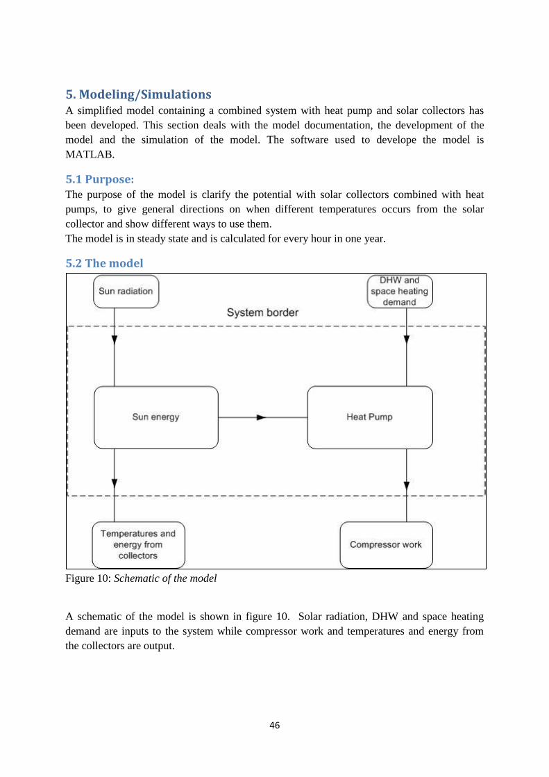
46

5. Modeling/Simulations A simplified model containing a combined system with heat pump and solar collectors has

been developed. This section deals with the model documentation, the development of the

model and the simulation of the model. The software used to develope the model is

MATLAB.

5.1 Purpose: The purpose of the model is clarify the potential with solar collectors combined with heat

pumps, to give general directions on when different temperatures occurs from the solar

collector and show different ways to use them.

The model is in steady state and is calculated for every hour in one year.

5.2 The model

Figure 10: Schematic of the model

A schematic of the model is shown in figure 10. Solar radiation, DHW and space heating

demand are inputs to the system while compressor work and temperatures and energy from

the collectors are output.

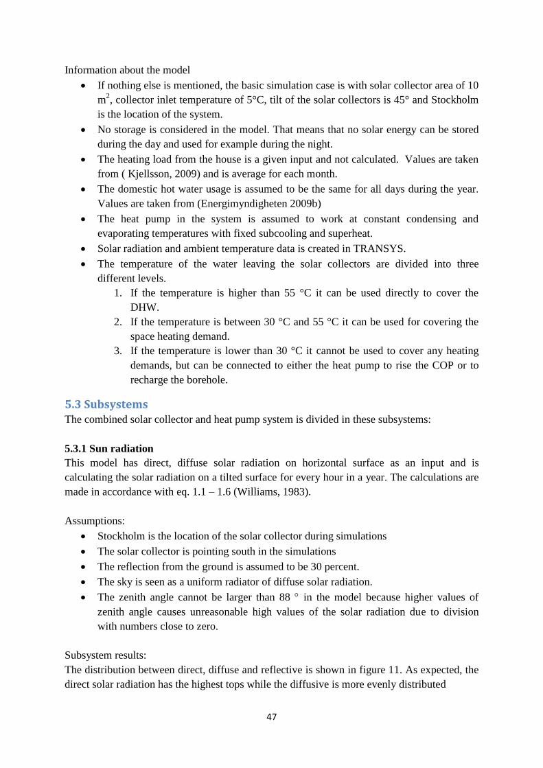
47

Information about the model

If nothing else is mentioned, the basic simulation case is with solar collector area of 10

m2, collector inlet temperature of 5°C, tilt of the solar collectors is 45° and Stockholm

is the location of the system.

No storage is considered in the model. That means that no solar energy can be stored

during the day and used for example during the night.

The heating load from the house is a given input and not calculated. Values are taken

from ( Kjellsson, 2009) and is average for each month.

The domestic hot water usage is assumed to be the same for all days during the year.

Values are taken from (Energimyndigheten 2009b)

The heat pump in the system is assumed to work at constant condensing and

evaporating temperatures with fixed subcooling and superheat.

Solar radiation and ambient temperature data is created in TRANSYS.

The temperature of the water leaving the solar collectors are divided into three

different levels.

1. If the temperature is higher than 55 °C it can be used directly to cover the

DHW.

2. If the temperature is between 30 °C and 55 °C it can be used for covering the

space heating demand.

3. If the temperature is lower than 30 °C it cannot be used to cover any heating

demands, but can be connected to either the heat pump to rise the COP or to

recharge the borehole.

5.3 Subsystems The combined solar collector and heat pump system is divided in these subsystems:

5.3.1 Sun radiation

This model has direct, diffuse solar radiation on horizontal surface as an input and is

calculating the solar radiation on a tilted surface for every hour in a year. The calculations are

made in accordance with eq. 1.1 – 1.6 (Williams, 1983).

Assumptions:

Stockholm is the location of the solar collector during simulations

The solar collector is pointing south in the simulations

The reflection from the ground is assumed to be 30 percent.

The sky is seen as a uniform radiator of diffuse solar radiation.

The zenith angle cannot be larger than 88 in the model because higher values of

zenith angle causes unreasonable high values of the solar radiation due to division

with numbers close to zero.

Subsystem results:

The distribution between direct, diffuse and reflective is shown in figure 11. As expected, the

direct solar radiation has the highest tops while the diffusive is more evenly distributed

48

The tilt of solar collector makes it possible to collect more energy from the sun and

Figure 11: Direct, Diffuse and reflective solar irradiation on a tilted surface of 45

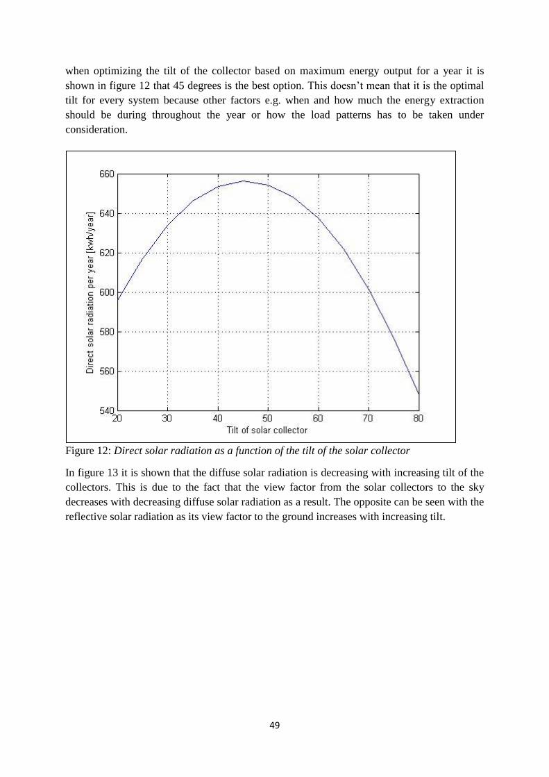
49

when optimizing the tilt of the collector based on maximum energy output for a year it is

shown in figure 12 that 45 degrees is the best option. This doesn’t mean that it is the optimal

tilt for every system because other factors e.g. when and how much the energy extraction

should be during throughout the year or how the load patterns has to be taken under

consideration.

Figure 12: Direct solar radiation as a function of the tilt of the solar collector

In figure 13 it is shown that the diffuse solar radiation is decreasing with increasing tilt of the

collectors. This is due to the fact that the view factor from the solar collectors to the sky

decreases with decreasing diffuse solar radiation as a result. The opposite can be seen with the

reflective solar radiation as its view factor to the ground increases with increasing tilt.

50

Figure 13: Solar radiation as a function of different tilt of the solar collector

5.3.2 Sun Energy

Input to this model is the solar radiation that is calculated in the sun radiation model and also

outside temperature data. The outputs are the temperature and energy from the solar collector

for every hour.

The heat transfer fluid is assumed to be rapeseed oil with properties from table 1. It is

assumed that it has constant specific heat and this gives:

( )out htf htf out inQ m Cp T T (1.44)

where htfm = mass flow of the heat transfer fluid

htfCp = specific heat of the heat transfer fluid

outT = the temperature out of the solar collector

inT = the temperature in to the solar collector

This equation together with equation 1.13 makes it possible to calculate the temperature out of

the solar collector and the useful energy output.

A solar collector is chosen from literature (Williams, 1983) but values can be changed in the

model.

Assumptions:

A low flow system with a mass flow of 3 g/(s m2) is chosen. The mass flow in fixed

during one simulation (one year).

0

200000

400000

600000

800000

1000000

1200000

20 30 40 50 60 70 80

Sola

r ra

dia

tio

n W

h/(

m2

,yea

r)

Tilt of solar collector

Solar radiation for different tilts

Direct solar radiation

Diffuse solar radiation

Reflective solar radiation

Total solar radiation

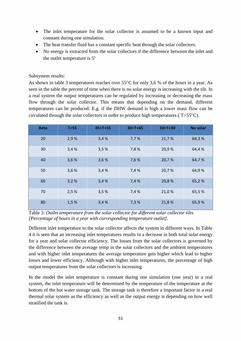
51

The inlet temperature for the solar collector is assumed to be a known input and

constant during one simulation.

The heat transfer fluid has a constant specific heat through the solar collectors.

No energy is extracted from the solar collectors if the difference between the inlet and

the outlet temperature is 5

Subsystem results:

As shown in table 3 temperatures reaches over 55C for only 3,6 % of the hours in a year. As

seen in the table the percent of time when there is no solar energy is increasing with the tilt. In

a real system the output temperatures can be regulated by increasing or decreasing the mass

flow through the solar collector. This means that depending on the demand, different

temperatures can be produced. E.g. if the DHW demand is high a lower mass flow can be

circulated through the solar collectors in order to produce high temperatures ( T>55C).

Beta T>55 45<T<55 30<T<45 10<T<30 No solar

20 2,9 % 3,4 % 7,7 % 21,7 % 64,3 %

30 3,4 % 3,5 % 7,8 % 20,9 % 64,4 %

40 3,6 % 3,6 % 7,6 % 20,7 % 64,7 %

50 3,6 % 3,4 % 7,4 % 20,7 % 64,9 %

60 3,2 % 3,4 % 7,4 % 20,8 % 65,2 %

70 2,5 % 3,5 % 7,4 % 21,0 % 65,5 %

80 1,5 % 3,4 % 7,3 % 21,8 % 65,9 %

Table 3: Outlet temperature from the solar collector for different solar collector tilts

[Percentage of hours in a year with corresponding temperature outlet].

Different inlet temperature to the solar collector affects the system in different ways. In Table

4 it is seen that an increasing inlet temperatures results in a decrease in both total solar energy

for a year and solar collector efficiency. The losses from the solar collectors is governed by

the difference between the average temp in the solar collectors and the ambient temperatures

and with higher inlet temperatures the average temperature gets higher which lead to higher

losses and lower efficiency. Although with higher inlet temperatures, the percentage of high

output temperatures from the solar collectors is increasing.

In the model the inlet temperature is constant during one simulation (one year) in a real

system, the inlet temperature will be determined by the temperature of the temperature at the

bottom of the hot water storage tank. The storage tank is therefore a important factor in a real

thermal solar system as the efficiency as well as the output energy is depending on how well

stratified the tank is.

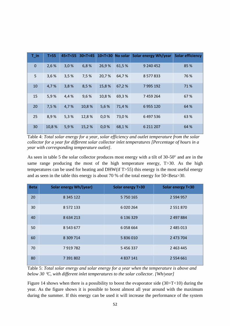
52

T_in T>55 45<T<55 30<T<45 10<T<30 No solar Solar energy Wh/year Solar efficiency

0 2,6 % 3,0 % 6,8 % 26,9 % 61,5 % 9 240 452 85 %

5 3,6 % 3,5 % 7,5 % 20,7 % 64,7 % 8 577 833 76 %

10 4,7 % 3,8 % 8,5 % 15,8 % 67,2 % 7 995 192 71 %

15 5,9 % 4,4 % 9,6 % 10,8 % 69,3 % 7 459 264 67 %

20 7,5 % 4,7 % 10,8 % 5,6 % 71,4 % 6 955 120 64 %

25 8,9 % 5,3 % 12,8 % 0,0 % 73,0 % 6 497 536 63 %

30 10,8 % 5,9 % 15,2 % 0,0 % 68,1 % 6 211 207 64 %

Table 4: Total solar energy for a year, solar efficiency and outlet temperature from the solar

collector for a year for different solar collector inlet temperatures [Percentage of hours in a

year with corresponding temperature outlet].

As seen in table 5 the solar collector produces most energy with a tilt of 30-50 and are in the

same range producing the most of the high temperature energy, T>30. As the high

temperatures can be used for heating and DHW(if T>55) this energy is the most useful energy

and as seen in the table this energy is about 70 % of the total energy for 50<Beta>30.

Beta Solar energy Wh/(year) Solar energy T>30 Solar energy T<30

20 8 345 122 5 750 165 2 594 957

30 8 572 133 6 020 264 2 551 870

40 8 634 213 6 136 329 2 497 884

50 8 543 677 6 058 664 2 485 013

60 8 309 714 5 836 010 2 473 704

70 7 919 782 5 456 337 2 463 445

80 7 391 802 4 837 141 2 554 661

Table 5: Total solar energy and solar energy for a year when the temperature is above and

below 30 C, with different inlet temperatures to the solar collector. [Wh/year]

Figure 14 shows when there is a possibility to boost the evaporator side (30>T<10) during the

year. As the figure shows it is possible to boost almost all year around with the maximum

during the summer. If this energy can be used it will increase the performance of the system

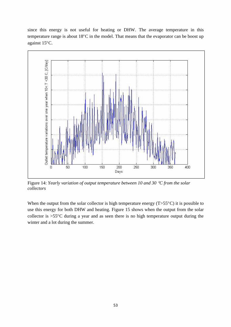
53

since this energy is not useful for heating or DHW. The average temperature in this

temperature range is about 18C in the model. That means that the evaporator can be boost up

against 15C.

Figure 14: Yearly variation of output temperature between 10 and 30 C from the solar

collectors

When the output from the solar collector is high temperature energy (T>55C) it is possible to

use this energy for both DHW and heating. Figure 15 shows when the output from the solar

collector is >55C during a year and as seen there is no high temperature output during the

winter and a lot during the summer.

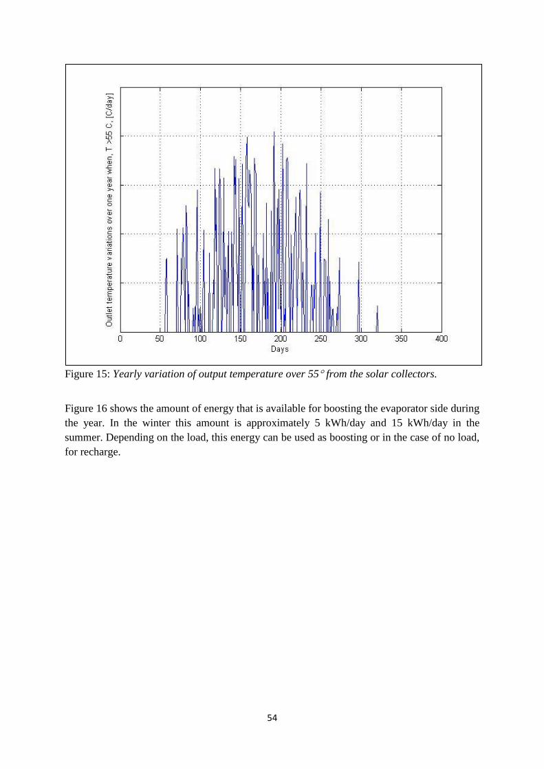
54

Figure 15: Yearly variation of output temperature over 55 from the solar collectors.

Figure 16 shows the amount of energy that is available for boosting the evaporator side during

the year. In the winter this amount is approximately 5 kWh/day and 15 kWh/day in the

summer. Depending on the load, this energy can be used as boosting or in the case of no load,

for recharge.

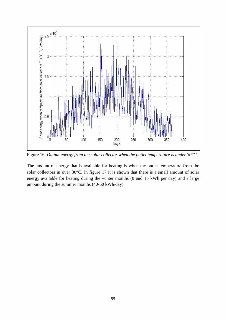
55

Figure 16: Output energy from the solar collector when the outlet temperature is under 30C.

The amount of energy that is available for heating is when the outlet temperature from the

solar collectors in over 30C. In figure 17 it is shown that there is a small amount of solar

energy available for heating during the winter months (0 and 15 kWh per day) and a large

amount during the summer months (40-60 kWh/day)

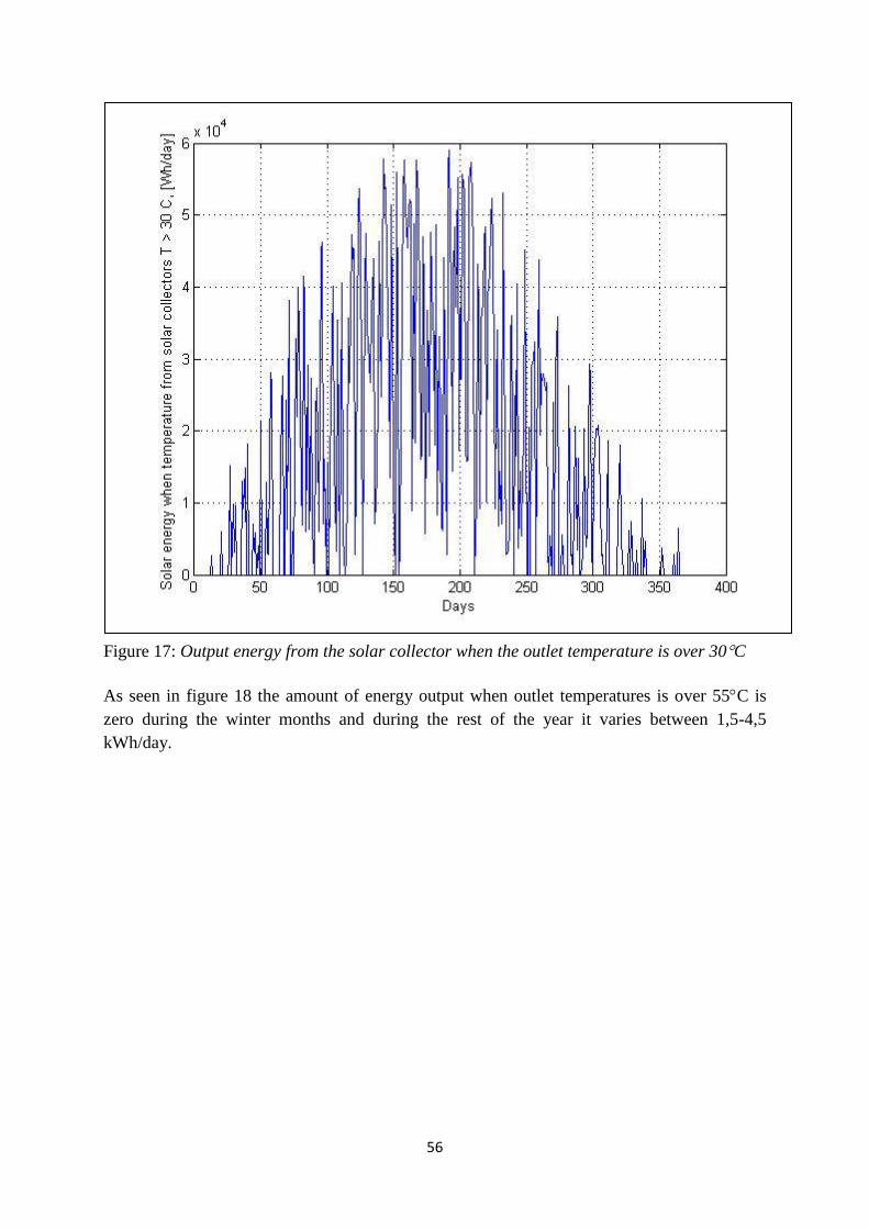
56

Figure 17: Output energy from the solar collector when the outlet temperature is over 30C

As seen in figure 18 the amount of energy output when outlet temperatures is over 55C is

zero during the winter months and during the rest of the year it varies between 1,5-4,5

kWh/day.

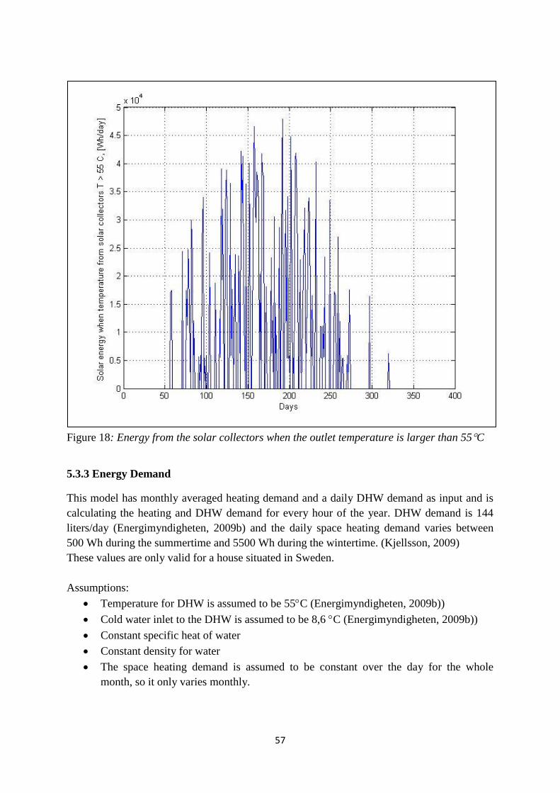
57

Figure 18: Energy from the solar collectors when the outlet temperature is larger than 55C

5.3.3 Energy Demand

This model has monthly averaged heating demand and a daily DHW demand as input and is

calculating the heating and DHW demand for every hour of the year. DHW demand is 144

liters/day (Energimyndigheten, 2009b) and the daily space heating demand varies between

500 Wh during the summertime and 5500 Wh during the wintertime. (Kjellsson, 2009)

These values are only valid for a house situated in Sweden.

Assumptions:

Temperature for DHW is assumed to be 55C (Energimyndigheten, 2009b))

Cold water inlet to the DHW is assumed to be 8,6 C (Energimyndigheten, 2009b))

Constant specific heat of water

Constant density for water

The space heating demand is assumed to be constant over the day for the whole

month, so it only varies monthly.

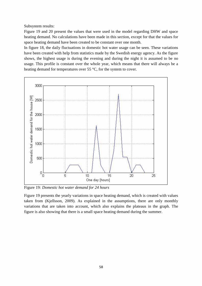
58

Subsystem results:

Figure 19 and 20 present the values that were used in the model regarding DHW and space

heating demand. No calculations have been made in this section, except for that the values for

space heating demand have been created to be constant over one month.

In figure 18, the daily fluctuations in domestic hot water usage can be seen. These variations

have been created with help from statistics made by the Swedish energy agency. As the figure

shows, the highest usage is during the evening and during the night it is assumed to be no

usage. This profile is constant over the whole year, which means that there will always be a

heating demand for temperatures over 55 °C, for the system to cover.

Figure 19: Domestic hot water demand for 24 hours

Figure 19 presents the yearly variations in space heating demand, which is created with values

taken from (Kjellsson, 2009). As explained in the assumptions, there are only monthly

variations that are taken into account, which also explains the plateaus in the graph. The

figure is also showing that there is a small space heating demand during the summer.

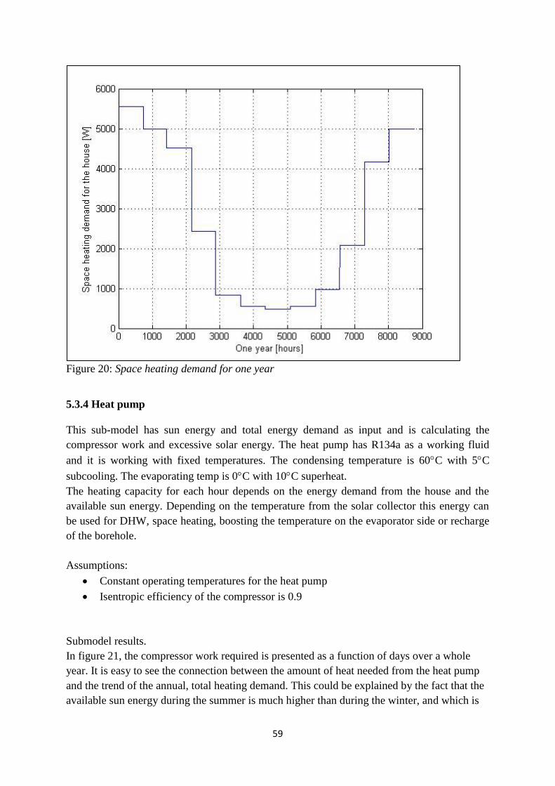
59

Figure 20: Space heating demand for one year

5.3.4 Heat pump

This sub-model has sun energy and total energy demand as input and is calculating the

compressor work and excessive solar energy. The heat pump has R134a as a working fluid

and it is working with fixed temperatures. The condensing temperature is 60C with 5C

subcooling. The evaporating temp is 0C with 10C superheat.

The heating capacity for each hour depends on the energy demand from the house and the

available sun energy. Depending on the temperature from the solar collector this energy can

be used for DHW, space heating, boosting the temperature on the evaporator side or recharge

of the borehole.

Assumptions:

Constant operating temperatures for the heat pump

Isentropic efficiency of the compressor is 0.9

Submodel results.

In figure 21, the compressor work required is presented as a function of days over a whole

year. It is easy to see the connection between the amount of heat needed from the heat pump

and the trend of the annual, total heating demand. This could be explained by the fact that the

available sun energy during the summer is much higher than during the winter, and which is

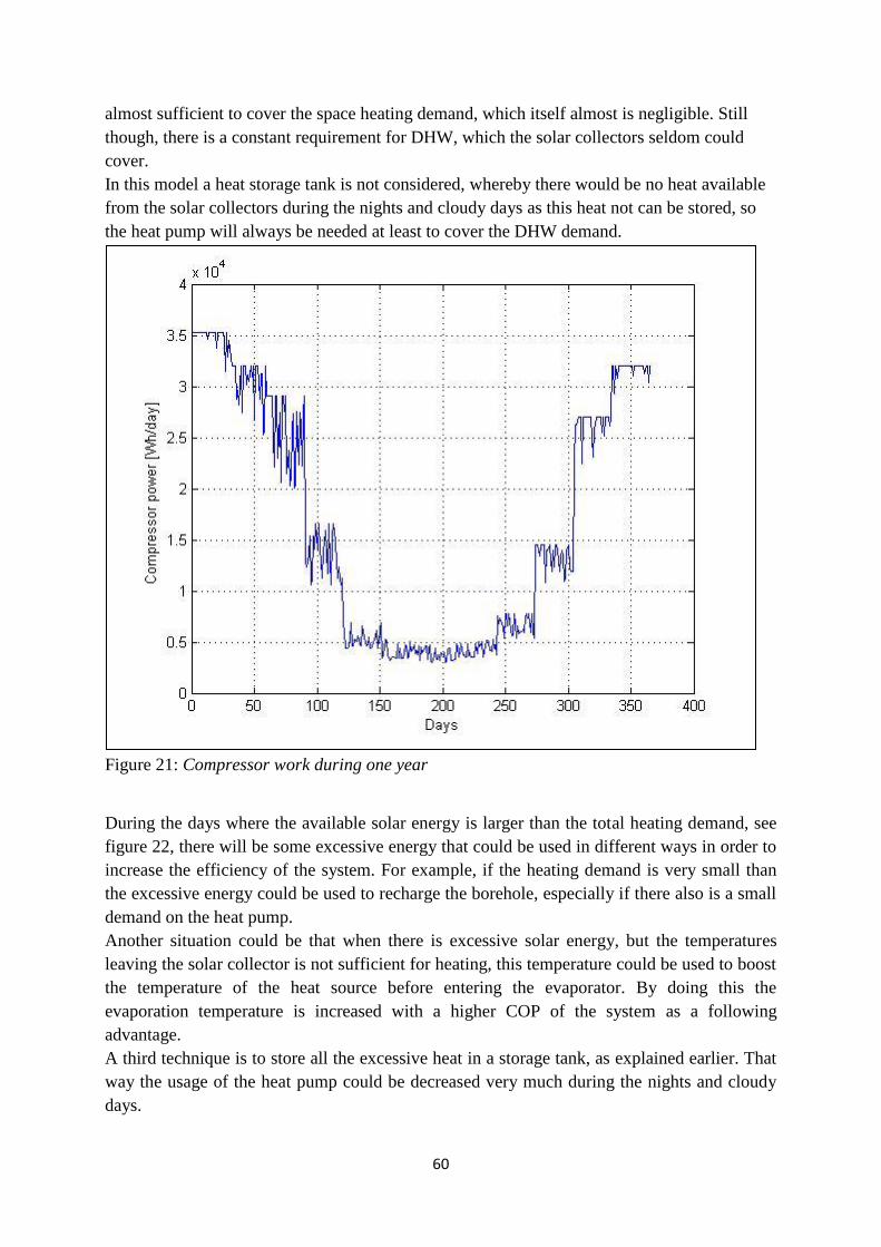
60

almost sufficient to cover the space heating demand, which itself almost is negligible. Still

though, there is a constant requirement for DHW, which the solar collectors seldom could

cover.

In this model a heat storage tank is not considered, whereby there would be no heat available

from the solar collectors during the nights and cloudy days as this heat not can be stored, so

the heat pump will always be needed at least to cover the DHW demand.

Figure 21: Compressor work during one year

During the days where the available solar energy is larger than the total heating demand, see

figure 22, there will be some excessive energy that could be used in different ways in order to

increase the efficiency of the system. For example, if the heating demand is very small than

the excessive energy could be used to recharge the borehole, especially if there also is a small

demand on the heat pump.

Another situation could be that when there is excessive solar energy, but the temperatures

leaving the solar collector is not sufficient for heating, this temperature could be used to boost

the temperature of the heat source before entering the evaporator. By doing this the

evaporation temperature is increased with a higher COP of the system as a following

advantage.

A third technique is to store all the excessive heat in a storage tank, as explained earlier. That

way the usage of the heat pump could be decreased very much during the nights and cloudy

days.

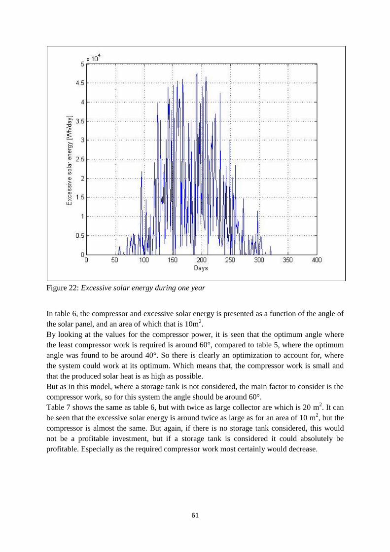
61

Figure 22: Excessive solar energy during one year

In table 6, the compressor and excessive solar energy is presented as a function of the angle of

the solar panel, and an area of which that is 10m2.

By looking at the values for the compressor power, it is seen that the optimum angle where

the least compressor work is required is around 60°, compared to table 5, where the optimum

angle was found to be around 40°. So there is clearly an optimization to account for, where

the system could work at its optimum. Which means that, the compressor work is small and

that the produced solar heat is as high as possible.

But as in this model, where a storage tank is not considered, the main factor to consider is the

compressor work, so for this system the angle should be around 60°.

Table 7 shows the same as table 6, but with twice as large collector are which is 20 m2. It can

be seen that the excessive solar energy is around twice as large as for an area of 10 m2, but the

compressor is almost the same. But again, if there is no storage tank considered, this would

not be a profitable investment, but if a storage tank is considered it could absolutely be

profitable. Especially as the required compressor work most certainly would decrease.

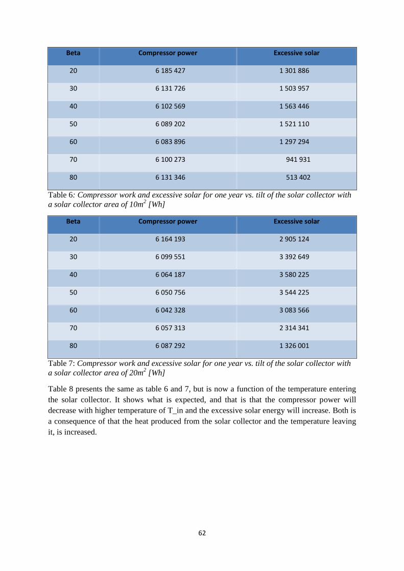
62

Beta Compressor power Excessive solar

20 6 185 427 1 301 886

30 6 131 726 1 503 957

40 6 102 569 1 563 446

50 6 089 202 1 521 110

60 6 083 896 1 297 294

70 6 100 273 941 931

80 6 131 346 513 402

Table 6: Compressor work and excessive solar for one year vs. tilt of the solar collector with

a solar collector area of 10m2 [Wh]

Beta Compressor power Excessive solar

20 6 164 193 2 905 124

30 6 099 551 3 392 649

40 6 064 187 3 580 225

50 6 050 756 3 544 225

60 6 042 328 3 083 566

70 6 057 313 2 314 341

80 6 087 292 1 326 001

Table 7: Compressor work and excessive solar for one year vs. tilt of the solar collector with

a solar collector area of 20m2 [Wh]

Table 8 presents the same as table 6 and 7, but is now a function of the temperature entering

the solar collector. It shows what is expected, and that is that the compressor power will

decrease with higher temperature of T_in and the excessive solar energy will increase. Both is

a consequence of that the heat produced from the solar collector and the temperature leaving

it, is increased.

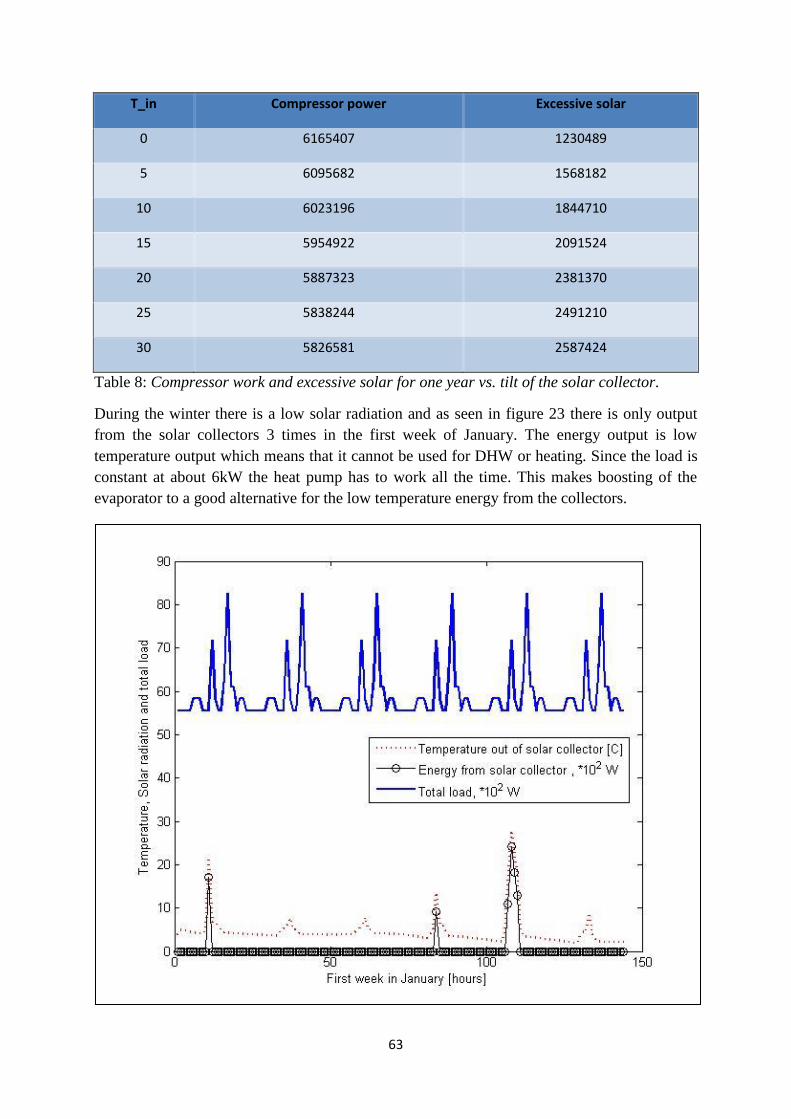
63

T_in Compressor power Excessive solar

0 6165407 1230489

5 6095682 1568182

10 6023196 1844710

15 5954922 2091524

20 5887323 2381370

25 5838244 2491210

30 5826581 2587424

Table 8: Compressor work and excessive solar for one year vs. tilt of the solar collector.

During the winter there is a low solar radiation and as seen in figure 23 there is only output

from the solar collectors 3 times in the first week of January. The energy output is low

temperature output which means that it cannot be used for DHW or heating. Since the load is

constant at about 6kW the heat pump has to work all the time. This makes boosting of the

evaporator to a good alternative for the low temperature energy from the collectors.

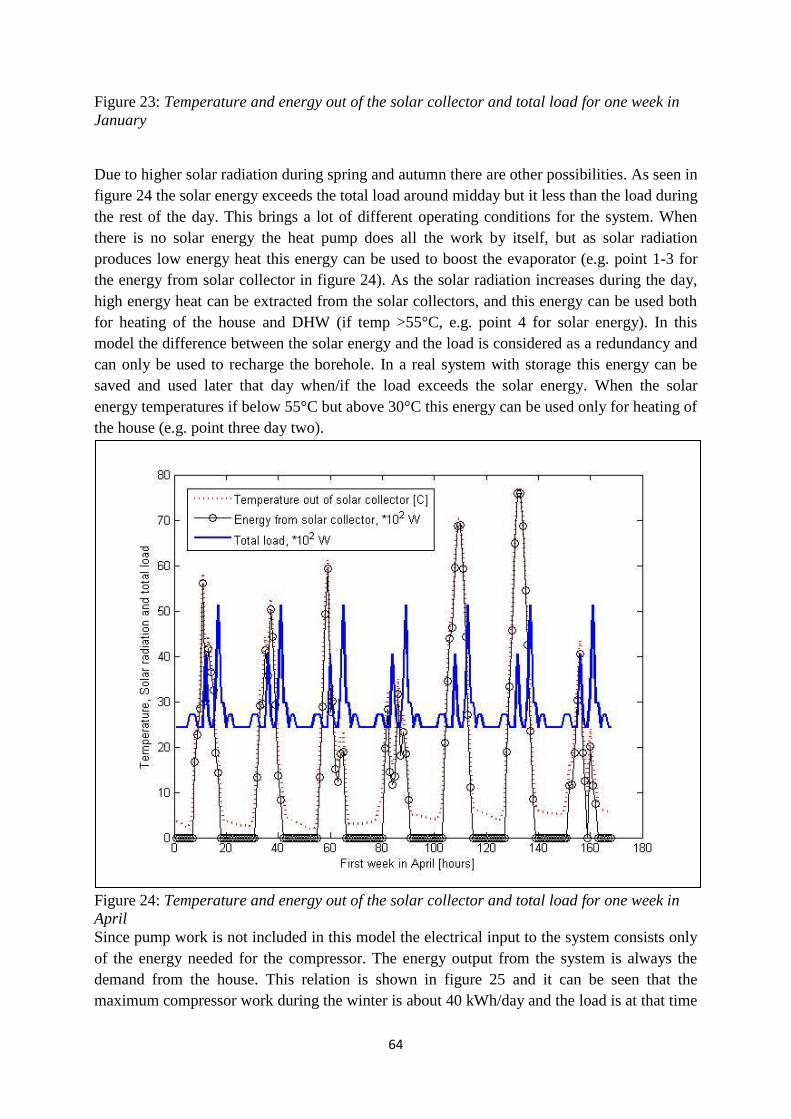
64

Figure 23: Temperature and energy out of the solar collector and total load for one week in

January

Due to higher solar radiation during spring and autumn there are other possibilities. As seen in

figure 24 the solar energy exceeds the total load around midday but it less than the load during

the rest of the day. This brings a lot of different operating conditions for the system. When

there is no solar energy the heat pump does all the work by itself, but as solar radiation

produces low energy heat this energy can be used to boost the evaporator (e.g. point 1-3 for

the energy from solar collector in figure 24). As the solar radiation increases during the day,

high energy heat can be extracted from the solar collectors, and this energy can be used both

for heating of the house and DHW (if temp >55°C, e.g. point 4 for solar energy). In this

model the difference between the solar energy and the load is considered as a redundancy and

can only be used to recharge the borehole. In a real system with storage this energy can be

saved and used later that day when/if the load exceeds the solar energy. When the solar

energy temperatures if below 55°C but above 30°C this energy can be used only for heating of

the house (e.g. point three day two).

Figure 24: Temperature and energy out of the solar collector and total load for one week in

April

Since pump work is not included in this model the electrical input to the system consists only

of the energy needed for the compressor. The energy output from the system is always the

demand from the house. This relation is shown in figure 25 and it can be seen that the

maximum compressor work during the winter is about 40 kWh/day and the load is at that time

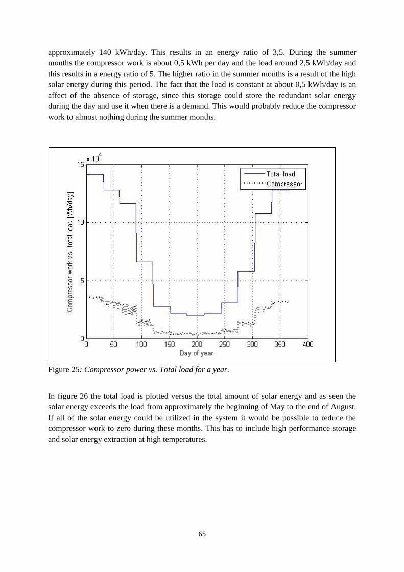
65

approximately 140 kWh/day. This results in an energy ratio of 3,5. During the summer

months the compressor work is about 0,5 kWh per day and the load around 2,5 kWh/day and

this results in a energy ratio of 5. The higher ratio in the summer months is a result of the high

solar energy during this period. The fact that the load is constant at about 0,5 kWh/day is an

affect of the absence of storage, since this storage could store the redundant solar energy

during the day and use it when there is a demand. This would probably reduce the compressor

work to almost nothing during the summer months.

Figure 25: Compressor power vs. Total load for a year.

In figure 26 the total load is plotted versus the total amount of solar energy and as seen the

solar energy exceeds the load from approximately the beginning of May to the end of August.

If all of the solar energy could be utilized in the system it would be possible to reduce the

compressor work to zero during these months. This has to include high performance storage

and solar energy extraction at high temperatures.

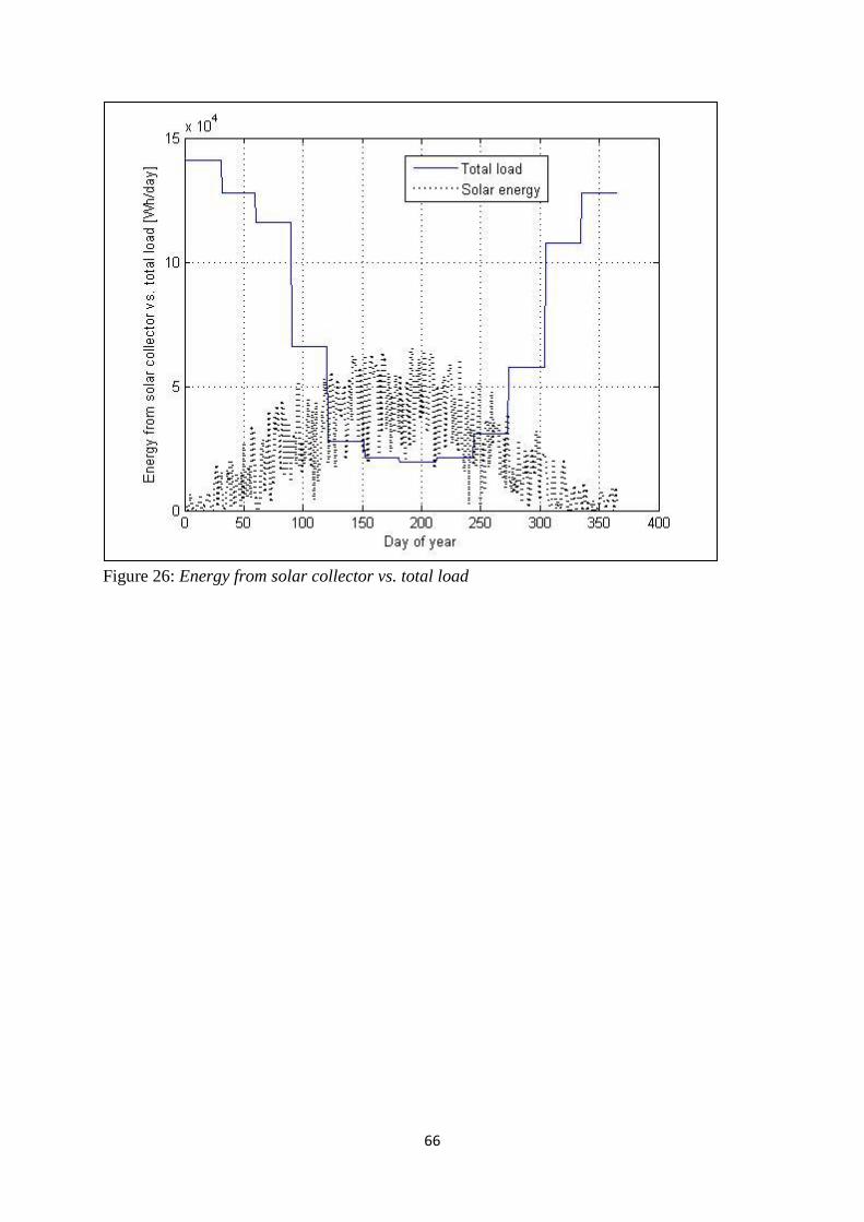
66

Figure 26: Energy from solar collector vs. total load

67

6. Analysis/Discussion This section deals with the discussion and analysis of the literature study and the model.

From the literature study we found that a heat pump system with a vertical ground source heat

exchanger is the best alternative for a combined system. This is because of the relative stable

temperatures from the heat source throughout the year and stable temperature is desired to the

evaporator side of the heat pump. In warmer climate than Sweden other sorts of heat pump

might be the best option although when it comes to recharge the vertical ground source is the

best. The stable temperature of the heat source is also positive when it comes to recharging

because the heat losses to the environment is lower in the rock than in for example a

horizontal ground heat source.

Another reason for choosing vertical ground source heat pump system is that it is a common

solution on the Swedish market and there is a high level of knowledge about these systems.

For the solar collectors it is important to point out that the solar radiation varies from year to

year and it is not certain that the system delivers exact the amount of energy as expected. To

get as much energy as possible from the solar collector, a sun tracking solar collector would

be the optimal. The investment for these solar collectors is large and they are seldom used in

small scale thermal solar solutions. The optimal tilt for the collectors is depending on the

amount of solar energy, the load and when the system should produce solar energy. During

winter time a high tilt is wanted because the sun is low on the sky and this is also the time

during the year when solar energy is needed the most for space heating. If a high energy

output is wanted during the winter a large tilt is the best option, although the sun radiation is a

lot smaller in the winter time compared to summer time and in this way a lower percentage of

solar radiation is absorbed through one year.

When combining these systems it is important to consider what kind of solar collector that is

best for the system. If, for example a heat pump is installed for a house and later on it appears

that the bore hole is under dimensioned. A simple solution can be to just to buy a simple and

inexpensive solar collector that can recharge the bore hole during the year. Also depending on

the purpose of the system and the desired temperature level different solar collectors can give

the optimal solution. For example, vacuum solar collectors can give very high temperatures

and are preferred in high temperature applications.

From the study of literature and the model we found that good heat storage is of outmost

importance. It is necessary to store the heat given from the collectors and the size of the

storage must be optimized for the load and amount of solar energy for the specific system

considered. It is possible to have two or more separate tanks in the system, this can increase

the efficiency of the system but it has to be optimizing for specific conditions. Stratification in

the tanks is an important factor because a low temperature is desired in the bottom of the tank

where the temperature to the solar collectors in determined but also because the outtake for

heating the house and DHW is made at the top of the tank. If the stratification is good the

exergy losses due to mixing will be lower and the solar energy can be utilized in a better way.

68

Recharge can be used when the energy from the solar collectors exceeds the load or if the

temperature of the energy is too low to be used elsewhere. In this case the energy can be heat

transferred with the ground source heat carrier at the inlet of the heat pump and the heat

carrier will go through the heat pump and transport this energy to the ground source. In this

solution the only additional pump power is for transporting the solar collector fluid to the

ground source.

How efficient the recharge is are depending on the properties of the rock. When the rock has a

high thermal conductivity there will be large heat losses if the heat from the solar collectors

has high temperature. The most efficient way to recharge is to use low temperatures from the

solar collectors and increase the temperature of the rock to that extent that it has equal or a

few degrees higher temperature than the surroundings. If the rock is heated further, this heat

will be lost to the surrounding. On the other hand, if the rock has a high thermal conductivity

it will have a high natural recharging from the surrounding rock. If the rock has low thermal

conductivity it has a low natural recharge and are more likely to need recharge. The

recharging will also be more efficient due to decreasing heat losses. It is hard to say if

recharging is profitable in a well dimensioned system but in the case of under dimensioned

bore holes recharging can be a good way to keep the temperature in the bore holes at a

constant level. It might also be used to create under dimensioned system by purpose and

therefore get lower costs for drilling.

When considering recharging it is important to be aware of the pump power needed to

transport the fluid. If the pump power exceeds the effect from recharging it is unnecessary to

do it. To be able to predict if recharging is beneficial for the system a good knowledge about

the rock is needed, a well design control system that controls when recharging should takes

place is also desired.

The bore hole can also be used as a heat sink. During the summer when the heating load is

low and there is a lot of solar radiation problems can arise when there is nowhere to cool the

fluid from the solar collectors. One way to avoid stagnation temperatures in the solar collector

can be to use the bore hole as a heat sink and cool the fluid by pumping it through the ground

loop.

Boosting of the condenser side is in the author’s opinion unnecessary. This is because

boosting can only take place in the temperature range between the inlet and the outlet of the

cooling fluid on the condenser side. The outgoing temperature in the model is 55C and the

inlet temperature is 45C. This means that it is only possible to boost when the temperature

from the solar collector is higher than 45 and lower than 55.

Boosting on the evaporator side can be beneficial because of the utilization of the low

temperature energy from the solar collector. These low temperatures can be extracted all year

around and improve the efficiency for the system. In the model was the average temperature

available for boosting about 18 C, assuming a boost at the inlet of the evaporator from 0C to

15 C this would make a 30 % decrease of the compressor work.

69

The complexity of these systems is very high and to optimize them a lot of information and

calculations is needed. When designing a combined system it is really important to know right

from the start what the system should perform, what it should be used for and when it is going

to be used. Information about the rock and solar radiation is necessary to be able to optimize

the system.

The model:

Many of the sub models in the model have a lot of simplifications and therefore the results

from the model has are valid only with the properties of this specific system. The simulation

gives general directions on how much solar energy that can be extracted from the solar

collectors. Heat storage was not included in the model and this is because it is a complex

component and there was not enough time to develop a good storage model. With that in mind

we decided to neglect storage in the model because a model with storage would have given to

insecure results.

Further work with the model is to:

Be able to vary the inlet temperature to the solar collector, this can be done by

implementing a storage tank with solar collector outlet at the bottom.

The mass flow in the solar collector system should not be constant but change

depending on the desired temperature out from the collectors.

The U-value for the solar collector should be divided in a temperature dependent part

and a temperature independent part.

The specific for the heat transfer fluid should vary with the temperature.

Develop the heat pump model so that the operating conditions for the heat pump can

change depending on evaporator temperature.

70

7. Conclusions Before considering a combination system, it is of great importance that is known how much

the system actually should perform. Because there are a number of system solutions on the

market, each providing different amount of heat and the cost of which wary a lot.

For a system that should work ideally, the best alternative for a system of a solar collector in

combination with a heat pump contains a vertical ground source heat exchanger. The solar

collector type should be decided carefully in order to get the desired temperature from the

collectors, depending on these temperatures the solar energy can be used for different

purposes and this depends on what the system are suppose to perform.

A combined system would only be beneficial if there is a storage tank installed in the system,

where the exceeded heat from the solar collectors could be stored and used during cloudy

days and during nighttime. Otherwise the compressor would need to be running in times when

the heat pump actually could be switched off. So if there is no storage tank installed all the

heat from the solar collectors would not be used and therefore the efficiency of the system

would go down significantly and that is a huge disadvantage in an economic point of view.

In order to further increase the efficiency of the system it should be possible to perform a heat

exchange between the heat from the solar collectors and the heat source entering the

evaporator of the heat pump. This is preferable in order for the system to both boost the

evaporating temperature and, when it is possible and if the pump power for the circulation is

not too large, recharge the borehole.

It seems that the potential for such a combination system is large but there is a complexity

factor that needs to be taken care of. In order for the system to work ideal, the connection

between the solar collector and the heat pump should be carefully controlled in order to get

the most out of it. If it would be possible to create a computer based system that is measuring

the temperature levels in the solar collectors, knows the heating demand of the house and

telling the heat pump exactly when to kick in, the potential would be high. If this control

system also could decide when the boosting is necessary and when there is a recharging

possibility the potential would be even higher. Then the economic savings could be large for a

family house in Sweden.

71

References

Literature: Brown, R.N. 2005. Compressors, Selection and Sizing. ISBN: 0-7506-7545-4

Department of Energy Technology, KTH, 2009. Refrigeration Engineering. Division of Applied

Thermodynamics and Refrigeration, Royal Institute of Technology, KTH, Stockholm.

Duff, W.S. 1996. Advanced solar domestic hot water systems. International Energy Agency, Task 14

final report

Morrison G.L 2001. Solar Collectors. Chapter 4 in ISES 2001. Solar energy: The state of the art.

ISBN: 1-902-91623-9.

Williams, R.J 1983. Design and installation of solar heating and solar water systems. ISBN: 0-250-

40593-8.

Manuals Caneta Research inc. 1995. Commercial/Institutional Ground-Source heat pumps. Engineering

Manual. ISBN: 1-883413-21-4

Reports ISES 2001. Solar energy: The state of the art. ISBN: 1-902-91623-9.

Energimyndigheten 2009b. Mätning av kall- och varmvattenanvändning i 44 hushåll. ID-nr: ER

2009:26

Energimyndigheten 2009c. Solklart Solvärme. ID-nr: ET 2009:17

Kjellsson, Elisabeth 2004. Solvärme i bostäder med analys av kombinationen solfångare och

bergvärmepump. Report TVBH-3047 Lund 2004. Building Physics LTH.

Kjellsson, Elisabeth 2009, Solar Collectors Combined with Ground-Source Heat Pumps in Dwellings

Analyses of System Performance. Report TVBH-1018 Lund 2009. Building Physics LTH

Internet: Energysavers 2009. Heat-Transfer Fluids for Solar Water Heating Systems

http://www.energysavers.gov/your_home/water_heating/index.cfm/mytopic=12940 ( 2010-02-15,

13:00)

Energimyndigheten 2009a. Cirkulationspumpar

http://www.energimyndigheten.se/sv/Hushall/Tester/Testresultat/Cirkulationspumpar/ (2010-02-17,

15:00)

Eviheat 2010

http://www.eviheat.se/ (2010-03-01,12:00)

http://www.energysavers.gov/your_home/water_heating/index.cfm/mytopic=12940

http://www.energimyndigheten.se/sv/Hushall/Tester/Testresultat/Cirkulationspumpar/

http://www.eviheat.se/

72

Grup Romet, 2010

http://www.grupromet.ro/Engleza/Panouri%20Solare/Sisteme%20combinate/Sisteme%20com

binate.html (2010-02-19, 16:00)

International Energy Agency 2009. About heat pumps

http://www.heatpumpcentre.org/ (2010-02-17, 16:00)

Solenergiteknik, 2010

http://www.solenergiteknik.se/ (2010-03-18, 16:00)

Svenska Värmepumpsföreningen 2010a. Värmepumpar-Berg

http://www.svepinfo.se/varmepumpar/berg/ (2010-02-18, 15:00)

Svenska Värmepumpföreningen, 2010b. Värmepumpar-Vatten

http://www.svepinfo.se/varmepumpar/vatten/#Grundvatten (2010-02-18, 16:00)

Seminars: KTH, Lecture, 2009,Liquid Heating/Cooling Distribution Systems Part 1

Joachim Claesson,(Prepared by Hans Jonsson)

http://www.grupromet.ro/Engleza/Panouri%20Solare/Sisteme%20combinate/Sisteme%20combinate.html

http://www.grupromet.ro/Engleza/Panouri%20Solare/Sisteme%20combinate/Sisteme%20combinate.html

http://www.heatpumpcentre.org/

http://www.solenergiteknik.se/

http://www.svepinfo.se/varmepumpar/berg/

http://www.svepinfo.se/varmepumpar/vatten/#Grundvatten

Documents

Beräkningsmetoder för årsvärmefaktor för värmepumpsystem