Benthic Recovery Project SARF030 - SARF - about · Benthic Recovery Project SARF030 Kenny Black, Scottish Association for Marine Science A REPORT COMMISSIONED BY SARF AND PREPARED

Benthic Recovery Project

SARF030

Kenny Black, Scottish Association for Marine Science

A REPORT COMMISSIONED BY SARF AND PREPARED BY

Published by the: Scottish Aquaculture Research Forum (SARF) This report is available at: http://www.sarf.org.uk Dissemination Statement This publication may be re-used free of charge in any format or medium. It may only be reused accurately and not in a misleading context. For material must be acknowledged as SARF copyright and use of it must give the title of the source publication. Where third party copyright material has been identified, further use of that material requires permission from the copyright holders concerned. Disclaimer The opinions expressed in this report do not necessarily reflect the views of SARF and SARF is not liable for the accuracy of the information provided or responsible for any use of the content. Suggested Citation Title: Benthic Recovery Project ISBN: 978-1-907266-42-3 First published: January 2012 © SARF 2010

SARF030 Final Report: Benthic Recovery Project

Kenny Black1

Chris Cromey

Thom Nickell1

1Scottish Association for Marine Science

Scottish Marine Institute

Oban, Argyll PA37 1QA

Scotland, UK

June 2011

1

1 Executive Summary

Our aspiration in this project was to provide a computer model able to predict the time of

benthic recovery for a fish farm on the basis of field information and modelling of organic

matter (OM) deposition on the seabed from the farming activity.

To better understand how recovery can be measured, we undertook a field campaign at 5

salmon farm sites on the west coast of Scotland. At these sites we sampled the benthos at a

known interval after the cessation of fish farming. For each of the sites we had access to the

benthic data that were collected by the farmers as part of their monitoring programme and to

husbandry data. We evaluated a standard suite of benthic indices to assess the recovery status

of each of the sites and also developed 2 new indices to aid this analysis: the Brooks

Recovery Index (BRI) and the Infaunal Trophic Recovery Index (IRI).

From our results we concluded that:

The studied sites fell into 2 categories: those that had high initial impacts but recovered

substantially within one year and those that had lower initial impacts but were further from

recovery after 2 years.

These results confirmed earlier work that showed that recovery processes have a site specific

component.

For modelling purposes, we based our approach on DEPOMOD. This model accommodates

the physical environment of the farm (depth, currents, resuspension) from observations and

uses an empirical relationship to predict characteristics (indices) of the benthic community

that would be expected based on the flux of material from the farm at around peak biomass.

The degradation rate of OM from fish farming has not hitherto received much attention. The

need to better understand this topic stimulated a separate degradation project at SAMS. This

work attempts to determine the rate constants for the degradation of fish feed and fish faeces.

This work has led to experimentally derived rate constants and an evaluation of the most

labile fractions of the OM in fish feed and faeces which have been used in the model.

Knowing something about the rate of decay of the OM that accumulates on the seabed, as

predicted by DEPOMOD, we can predict the oxygen demand from the sediment and

2

estimated estimate oxygen supply from the water column using a relationship based on near-

bed current speed from the literature. It is at times where demand exceeds the supply of

oxygen that we might expect the greatest stress on the macrobenthic community. We have

developed an index based on the work of Findlay and Watling (1997) in order to consider the

evolution of the ratio of oxygen demand to supply (Findlay Watling Index, FWI). Although

the FWI was a good predictor of impact during the operational phase of the study sites,

evaluation of this simple implementation of the FWI has not yielded good relationships

between observations and predictions of recovery order at the 5 study sites.

We subsequently developed a separate box model (named the RQ model) which attempts to

account for the role of sulphide formed through anaerobic degradation of OM in fish farm

sediments by including a first order equation for reoxidation of reduced chemical species

together with diffusive losses and burial of metal sulphides. The key hypothesis for this

model arose from the observed differences in the organic matter contents of sediments in the

mid-field i.e at around 50 m from the fish farms. We used this to scale the input of site

specific background OM. The resulting model proved able to account for the main features of

the observed order of recovery of the studied fish farms sites. It is suggested that background

levels of OM in marine sediments may be a good indicator of a site‟s potential to recover after

the cessation of fish farming. Further work will be required to test the validity of this

approach with field data and to refine the model parameterisation.

3

Table of Contents

1 Executive Summary........................................................................................................... 1

2 Introduction ....................................................................................................................... 5

2.1 Recovery of perturbed marine benthic systems ......................................................... 5

2.2 Recovery of benthic impacts from fish farming ........................................................ 7

3 Approach ......................................................................................................................... 12

4 Materials and Methods .................................................................................................... 15

4.1 Recovery study site characteristics .......................................................................... 15

4.2 Biological sampling method .................................................................................... 17

4.3 Chemical parameters ............................................................................................... 17

5 Results ............................................................................................................................. 18

5.1 Emamectin benzoate in sediment ............................................................................ 18

5.2 Organic matter ......................................................................................................... 19

5.3 Metals ...................................................................................................................... 20

6 Benthic biology ............................................................................................................... 22

6.1 Recovery .................................................................................................................. 22

6.2 Changes in benthic function .................................................................................... 28

6.3 Discussion of the benthic data ................................................................................. 33

7 Modelling approach 1 –the Findlay-Watling approach. .................................................. 35

7.1 Modelling approach ................................................................................................. 35

7.2 Method ..................................................................................................................... 36

7.3 Calculation of FWI using the method in Findlay and Watling (1997) and

comparison with observed ITI ............................................................................................. 42

7.3.1 Method ............................................................................................................. 42

7.3.2 Statistical testing of model performance ......................................................... 43

7.3.3 Results ............................................................................................................. 44

7.4 Hydrographic data summary ................................................................................... 44

7.5 Model validation ...................................................................................................... 45

7.5.1 (i) AutoDEPOMOD benthic module – ITI predictions and observations at time

of monitoring survey ....................................................................................................... 45

7.5.2 (ii) Findlay-Watling index (FWI) – suitability as indicator of impact and site

recovery 46

7.5.3 Dynamics of the FWI at the study sites ........................................................... 49

7.6 Discussion of modelling .......................................................................................... 51

8 Modelling approach 2 – the RQ model ........................................................................... 55

8.1 Introduction ............................................................................................................. 55

8.2 RQ model description .............................................................................................. 57

4

8.3 Model processes and parameters ............................................................................. 59

8.4 Results ..................................................................................................................... 66

8.5 Discussion and conclusions ..................................................................................... 73

9 Acknowledgements ......................................................................................................... 74

10 References ................................................................................................................... 75

11 Appendix 1: Summary diversity indices from peak biomass and recovery surveys at

studied sites. ............................................................................................................................ 79

5

2 Introduction

2.1 Recovery of perturbed marine benthic systems

While studies of the impacts of perturbations on marine benthic ecosystems are relatively

common, there has been much less work on processes that occur after the cessation of

perturbation. Such processes may affect the rate at which an impacted benthic habitat moves

towards conditions that are typical of ambient, un-impacted conditions. This process may be

called recovery, but it is important to appreciate that recovery to ambient un-impacted

conditions may not necessarily mean return to pre-impact conditions, as other factors, such as

perturbations caused by other anthropogenic or natural conditions or events, may mean that

such conditions no longer apply. Moreover, given the temporal dynamism and spatial

heterogeneity (or patchiness) of marine benthic ecosystems, which may be caused by natural

stochastic processes (e.g. changes in inter-annual recruitment success which may have

complex effects across food webs affecting community composition and structure) or more

systematic changes such as alterations to climatic regimes, the concept of recovery needs

careful consideration in order to avoid mistaking the consequences of unrelated processes for

the continuing effects of the original perturbation.

Studies on benthic ecosystems that have received attention with respect to recovery, rather

than simply impact, are shown in Table 1 sorted by perturbation type. There are a few lessons

that can be gleaned from this literature. Recovery is relatively fast when the benthic

community already contains species that are adapted to perturbation. For example, although

iceberg scouring can virtually wipe out a benthic assemblage, substantial recovery can take

place in as little as 12 months where the community is frequently assaulted by such

perturbations (Smale et al., 2008). This emphasises that the definition of local recovery may

be problematic where benthic communities face a high degree of natural or other

disturbances. Trawling impacts are likely to be the greatest global source of anthropogenic

disturbance to coastal seabed habitats and impacts may be severe and prolonged for slow

growing species such as sponges and soft corals (Kaiser et al., 2006). Again, the problem in

heavily trawled areas is to determine appropriate reference conditions. Tuck et al. (1998)

overcame this problem by considering impacts of trawling on a fjordic system that had been

un-fished for the previous 25 years. During experimental trawling, benthic biomass and

numbers of species increased but measures of diversity and evenness decreased. Eighteen

months after disturbance, it was still possible to distinguish benthic communities at trawled

and reference sites.

6

The recovery time of a perturbed benthic community depends on the nature, extent and

perhaps the timing of the impact, but some generic environmental and ecological factors are

likely to be play a role in most scenarios. These include: the habitat‟s history of previous

disturbance, the supply of organic matter and oxygen to the sediments, the biogeochemical

status of sediments, any changes caused to the substratum or any biogenic habitat feature, the

presence of any ecotoxic contaminants, the ambient hydrodynamics, and the timing and

availability of invertebrate larval supply. This great range contributes to the uncertainty of

predicting the time to recovery of benthic habitats and presents difficulties in determining the

most important causal factors that drive recovery, as these may vary during the recovery

process.

7

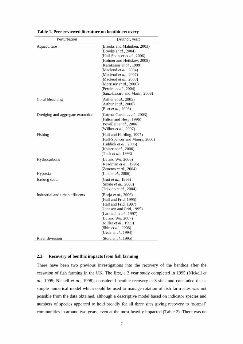
Table 1. Peer reviewed literature on benthic recovery

Perturbation (Author, year)

Aquaculture (Brooks and Mahnken, 2003)

(Brooks et al., 2004)

(Hall-Spencer et al., 2006)

(Holmer and Heilskov, 2008)

(Karakassis et al., 1999)

(Macleod et al., 2004)



(Morrisey et al., 2000)

(Pereira et al., 2004)

(Sanz-Lazaro and Marin, 2006)

Coral bleaching (Arthur et al., 2005)

(Arthur et al., 2006)

(Burt et al., 2008)

Dredging and aggregate extraction (Guerra-Garcia et al., 2003)

(Hilton and Hesp, 1996)

(Powilleit et al., 2006)

(Wilber et al., 2007)

Fishing (Hall and Harding, 1997)

(Hall-Spencer and Moore, 2000)

(Hiddink et al., 2006)

(Kaiser et al., 2006)

(Tuck et al., 1998)

Hydrocarbons (Lu and Wu, 2006)

(Readman et al., 1996)

(Zenetos et al., 2004)

Hypoxia (Lim et al., 2006)

Iceberg scour (Gutt et al., 1996)

(Smale et al., 2008)

(Teixido et al., 2004)

Industrial and urban effluents (Borja et al., 2006)

(Hall and Frid, 1995)

(Hall and Frid, 1997)

(Johnson and Frid, 1995)

(Lardicci et al., 1997)

(Lu and Wu, 2007)

(Miller et al., 1999)

(Shin et al., 2008)

(Ueda et al., 1994)

River diversion (Stora et al., 1995)

2.2 Recovery of benthic impacts from fish farming

There have been two previous investigations into the recovery of the benthos after the

cessation of fish farming in the UK. The first, a 3 year study completed in 1995 (Nickell et

al., 1995; Nickell et al., 1998), considered benthic recovery at 3 sites and concluded that a

simple numerical model which could be used to manage rotation of fish farm sites was not

possible from the data obtained, although a descriptive model based on indicator species and

numbers of species appeared to hold broadly for all three sites giving recovery to „normal‟

communities in around two years, even at the most heavily impacted (Table 2). There was no

8

obvious relationship between recovery times and ambient hydrography, and it appeared that

recovery was a complex process which had several drivers that might predominate at different

sites and seasons.

The second study (Pereira et al., 2004) of benthic recovery at a Scottish salmon farm was of a

shorter duration (15 months) and, at the most impacted station, recovery had not been

completed in that time. In contrast to the previous study, organic carbon was not found to be a

significant indicator of recovery, with different environmental variables of varying

importance at different stages in the process. The authors identified sedimentary oxygen

demand as the primary factor determining macrofaunal recolonisation.

Brooks and co-workers in Canada have probably made the most comprehensive series of

studies and observed a very wide range of recovery rates from a few weeks to 6+ years

(Brooks and Mahnken, 2003; Brooks et al., 2004). They proposed two very useful definitions

of recovery:

chemical – “defined as the reduction of accumulated organic matter with a

concomitant decrease in free sediment sulfide and an increase in sediment redox

potential under and adjacent to salmon farms to levels at which more than half the

reference area taxa can recruit and survive (free sulfides < 960 µM)”, and

biological – “defined as the restructuring of the infaunal community to include those

taxa whose individual abundance equals or exceeds 1% of the total invertebrate

abundance at a local reference station. Recruitment of rare species representing < 1%

of the reference abundance was not considered necessary for biological remediation

to be considered complete. As an example, if the mean reference station total

abundance was 8000 macrofauna m-2

, then all of those taxa with a mean abundance of

≥ 80 animals m-2

would be considered necessary for biological remediation to be

considered complete.”

Macleod and co-workers have studied recovery processes at salmon farms in Tasmania over

several years and reached some interesting conclusions:

1) macrobenthic recovery was slower than chemical recovery, so chemical methods

were not sufficient to define ecological recovery (Macleod et al., 2004)

9

2) recovery of macrobenthic community function (from analysis of life history

attributes of dominant fauna) is more rapid than return to community equivalence,

and may be a more useful measure of benthic recovery (Macleod et al., 2008)

3) macrobenthic recovery was faster at a more quiescent site than a more exposed site

attributed to the greater resilience of the species typically found at such sites and

differences in larval supply (Macleod et al., 2007).

In terms of the benthic community both Brook‟s definition of biological recovery and

Macleod and co-workers‟ idea of functional recovery appear attractive avenues for further

research.

10

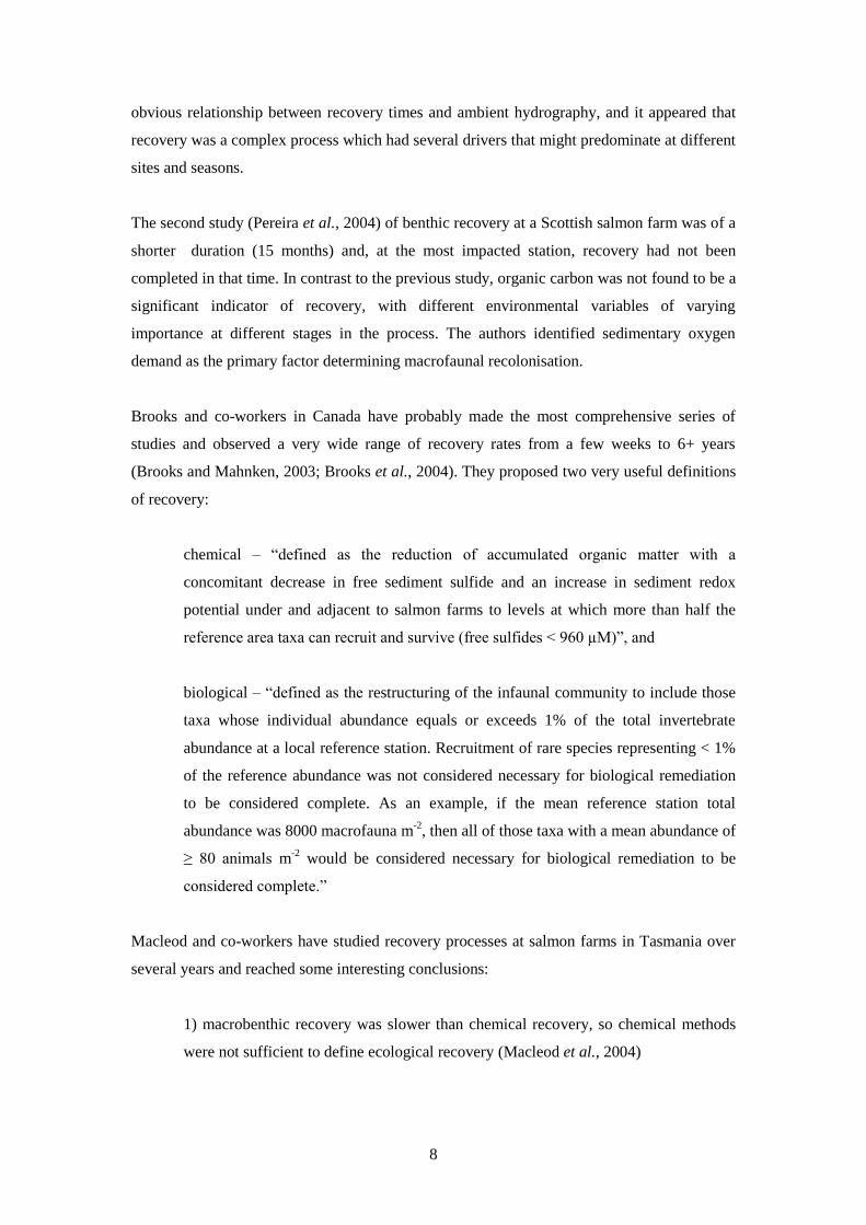
Table 2. Descriptive model of benthic faunal succession during sedimentary recovery from loading with fish farm wastes (Pearson and Black, 2001).

Degree of Enrichment Highly Enriched Moderately Enriched Lightly Enriched Normal Community

Characteristic Species Capitella capitata Apistobranchus tullbergi Scoloplos sp. Glycera alba

Malacoceros fuliginosus Spio decorata Thyasira ferruginea Mugga wahbergi

Nematoda Mediomastus fuliginosus Diplocirrus glaucus Ophelina sp.

Ophryotrocha sp. Protodorvillea kefersteini Sphaerosyllis tetralix Perugia caeca

Pseudoploydora paucibranchiata Microspio sp. Leptognathia brevirostris Synelmis klatti

Prionospio fallax Abra alba Owenia fusiformis

Scalibregma inflatum Glycera alba Magelona sp.

Chaetozone setosa Amphiura filiformis

Caulleriella sp. Polycirrus plumosus

Cossura sp. Eumida sp.

Melinna palmata Ophelina sp.

Pholoe inornata Lanice conchilega

Cirratulidae

Abra alba

Expected Number 5-10 25-40 40-45 30-35

Of Species Present

Approximate Time 0 9 18 21-24

Between Stages (months)

11

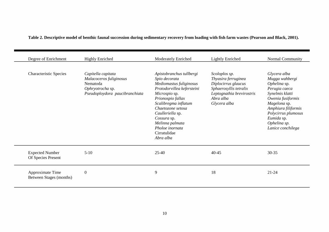
Karrakassis and co-workers, studying a farm in Greece (Karakassis et al., 1999) demonstrated

that recovery processess do not necessarily follow the linear model proposed in Table 2 as

seasonal effects can result in reversals owing to increased primary production stimulated by

sediment nutrient release. This non-linear pattern of recovery was also noted by Pereira et al.

(2004) (Figure 1).

Figure 1. Multi-dimensional scaling (MDS) plot of square-root transformed species-

abundance mean data at 3 recovering fish farm stations (A – least impacted, B, C – most

impacted) with respect to months post-cessation of farming (1, 2, 8, 14 and 15 months),

showing non-linearity of benthic community response (Pereira et al., 2004).

Since the earlier Scottish studies, salmon aquaculture in Scotland has changed significantly:

cages are bigger, average farm size has increased, more exposed sites have been developed

and the in-feed medicine Slice (active ingredient emamectin benzoate) has become widely

used. Although a recent study did not find a relationship between Slice in sediments and

community changes at active sites (Black et al., 2005) its potential to retard recovery has not

been studied. Copper is also widely used as an antifoulant and has been detected at very high

concentrations in fish farm sediments in Loch Craignish (Dean et al., 2007). Brooks and co-

workers argue that copper in enriched sediments is likely to be bound as sulphides and

therefore not bioavailable (Brooks and Mahnken, 2003; Brooks et al., 2004) but it has not

been shown whether recovering sediments (experiencing increased oxidation state) release

this copper back into pore waters with the potential to affect recolonisation.

More recent approaches to modelling inputs to the sea bed from cage farming have yielded an

improved understanding of effects on the macrofaunal community. The DEPOMOD model

has a benthic component (Cromey et al., 2002a; Cromey et al., 2002b) which at present

predicts likely benthic impact from modelled carbon flux to the sea bed. Morrisey et al.

12

(2000) had some success in predicting remineralisation of carbon/recovery rates in New

Zealand when using the Findlay-Watling oxygen supply model (Findlay and Watling, 1997);

they also noted the potential for increased recovery times due to the presence of heavy metals

in the sediment. Findlay and Watling‟s oxygen supply and demand model (Findlay and

Watling, 1997) was implimented in a non-dynamical mode with calculations of oxygen

supply based on short current records where the only data required are those relating to the 2-

hour period with minimum flow. Their hypothesis was that the benthic community is

structured by the balance between oxygen supply and demand at times of minimum oxygen

supply only. This is intuitively an attractive proposition, but their study had a number of

issues: 1) measurements of low-flow are highly sensitive to the threshold of the current meter

in very low flows; 2) their measurements of oxygen demand from the sediment were based on

measurments of organic matter flux using sediment traps, a technique prone to error owing to

the very steep contours of organic matter flux density around fish cages; 3) they did not take

into account resuspension processes that may remove carbon deposited on the bed before it

has time to cause an oxygen demand; and 4) they had only one study site (data point) at the

high end of the range of impacts typical of salmon farms. However, both the simplicity of

their model and the subsequent work by Morrisey et al. (2000) give strong grounds for

pursuing their approach as a basis for attempting to interpret and model benthic recovery

process around salmon farms.

3 Approach

Our aspiration in this project is to provide a computer model able to predict the time of

recovery for a site on the basis of information on how much organic material had

accumulated on the seabed from the farming activity and from simple environmental

conditions e.g. depth and current regime.

To better understand how recovery can be measured, we undertook a field campaign at 5

salmon farm sites on the west coast of Scotland (Section 5). At these sites we sampled the

benthos at a known interval after the cessation of fish farming. We sampled each site in the

autumn in order to reduce the variability in the results that might be associated with seasonal

effects, for instance caused by temperature, availability of larvae or timing of organic inputs

from natural primary production. For each of the sites we had access to the benthic data that

were collected by the farmers as part of their monitoring programme (Section 6). In all cases

this was collected in the second year of the farming cycle near peak biomass. In addition we

had access to the quantities of feed used by the farmers throughout the production cycle.

13

For modelling purposes, we based our approach on DEPOMOD. This model accommodates

the physical environment of the farm (depth, currents, resuspension) from observations and

uses an empirical relationship to predict characteristics (indices) of the benthic community

that would be expected based on the flux of material from the farm at around peak biomass.

However, the DEPOMOD programme has no validated temporal component. The link

between accumulation of organic matter (carbon in reduced form) to the bed and the benthos

is purely empirical with no consideration of the biogeochemical processes that underlie this

link (Section 8). These processes depend on the degradation of organic matter facilitated by

microbes which consumes oxygen and, when anaerobic, sulphate ion. Both the consumption

of oxygen and the generation of hydrogen sulphide from sulphate reduction generate

conditions that become increasingly hostile to benthic life forms. The rates at which oxygen is

consumed and sulphide is produced are dependent on several factors, but the dominant

processes are the degradation rate of organic mater under both aerobic and anaerobic

conditions (releasing sulphide) and the supply of oxygen from the water column (which itself

may be influenced by the irrigation of the sediments through animal burrows if these have not

been excluded).

For most organic matter, the rate at which it is oxidised does not depend strongly on whether

this takes place in the presence of oxygen or not although rate constants for aerobic oxidation

are generally higher than for anaerobic oxidation. However, for the organic matter that is very

recalcitrant, degradation is extremely slowly without oxygen (e.g. woody material is very

difficult for microbes to degrade without oxygen). Thus, only the least degradable carbon gets

permanently buried in anaerobic marine sediments, with the majority being degraded before it

can be buried.

The degradation rate of organic material from fish farming has not hitherto received much

attention. The need to better understand this topic has stimulated a separate degradation

project supervised by Prof. Ronnie Glud and Dr Henrick Stahl at SAMS and conducted by

Karl Attard, a student at SAMS (presented as an Annex to the present report, available from

SAMS on request). This work attempts to determine the rate constants for the degradation of

fish feed and fish faeces. In order to do this, we recognise that organic matter is a broad term

covering a wide range of organic components each of which will have distinct degradation

rates and be present in distinct amounts. By experimentally monitoring decay processes, we

have determined the rate constants and the amounts of different classes of material that can

used to approximate the decay characteristics of these materials in the marine system and use

this information in our models.

14

We followed 2 modelling approaches. The first used information on the rate of decay of the

material that accumulates on the seabed, as predicted by DEPOMOD, to predict the oxygen

demand from the sediment. But in order to be able to predict the impact of this oxygen

demand, we also estimated oxygen supply from the water column (Section 8). It is at times

where demand exceeds the supply of oxygen that we might expect the greatest stress on the

macrobenthic community. We have used the work of others in estimating the supply of

oxygen as a function of current speed at the farms. Very low near-bed currents will reduce the

supply of oxygen to the benthic boundary layer where transfer of oxygen becomes dependent

on molecular rather than turbulent processes. This approach did not produce a satisfactory

outcome for reasons that will be explained later.

The second approach involved the construction of a model in which the process of

reoxidation of sulphides produced during anaerobic oxidation of organic matter was included,

together with information on likely background levels of organic matter supply and this

approach provided some greater insights into factors that may be important in recovery rates.

Our first target was to determine whether we can correctly predict the order of recovery at the

sites sampled and the second target was to be able to predict the absolute time that a site night

take to reach recovery, using the study sites for calibrating the model.

15

4 Materials and Methods

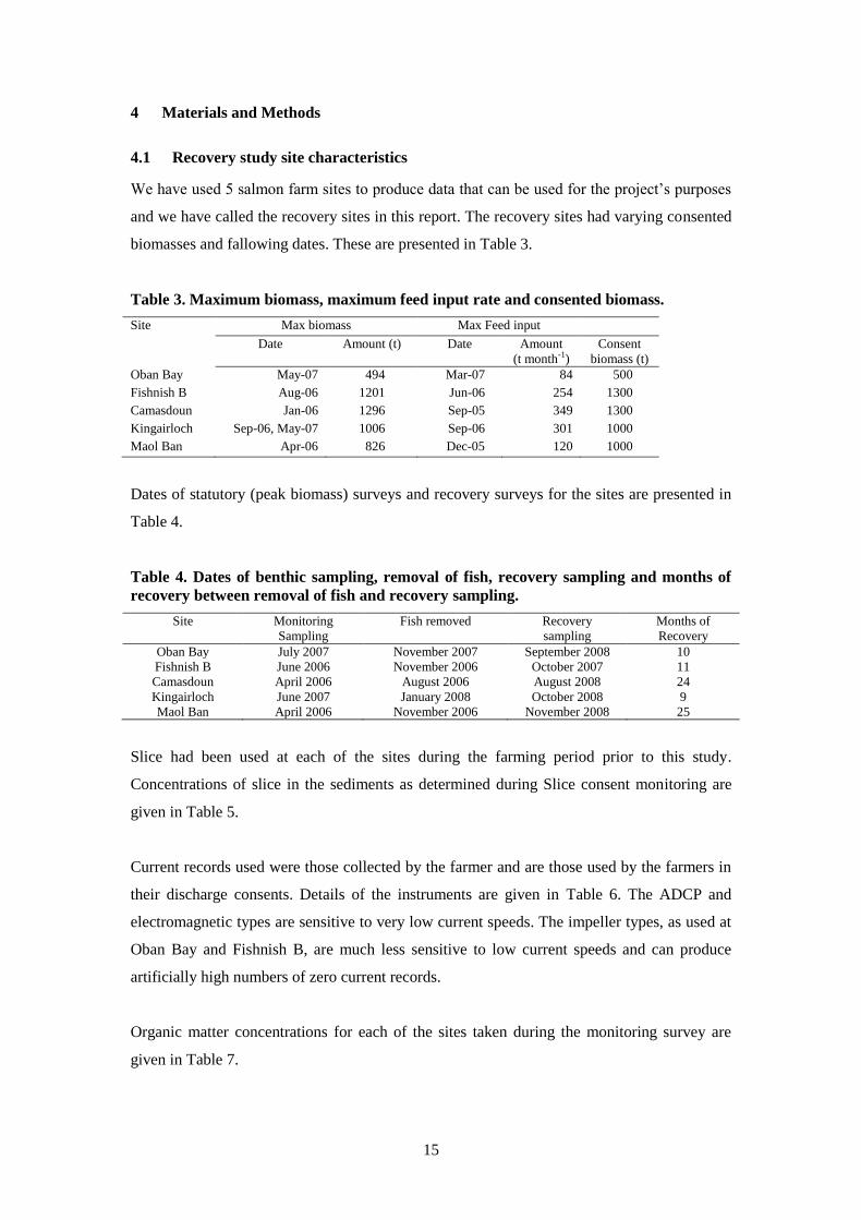
4.1 Recovery study site characteristics

We have used 5 salmon farm sites to produce data that can be used for the project‟s purposes

and we have called the recovery sites in this report. The recovery sites had varying consented

biomasses and fallowing dates. These are presented in Table 3.

Table 3. Maximum biomass, maximum feed input rate and consented biomass.

Site Max biomass Max Feed input

Date Amount (t) Date Amount

(t month-1)

Consent

biomass (t)

Oban Bay May-07 494 Mar-07 84 500

Fishnish B Aug-06 1201 Jun-06 254 1300

Camasdoun Jan-06 1296 Sep-05 349 1300

Kingairloch Sep-06, May-07 1006 Sep-06 301 1000

Maol Ban Apr-06 826 Dec-05 120 1000

Dates of statutory (peak biomass) surveys and recovery surveys for the sites are presented in

Table 4.

Table 4. Dates of benthic sampling, removal of fish, recovery sampling and months of

recovery between removal of fish and recovery sampling.

Site Monitoring

Sampling

Fish removed Recovery

sampling

Months of

Recovery

Oban Bay July 2007 November 2007 September 2008 10

Fishnish B June 2006 November 2006 October 2007 11

Camasdoun April 2006 August 2006 August 2008 24

Kingairloch June 2007 January 2008 October 2008 9

Maol Ban April 2006 November 2006 November 2008 25

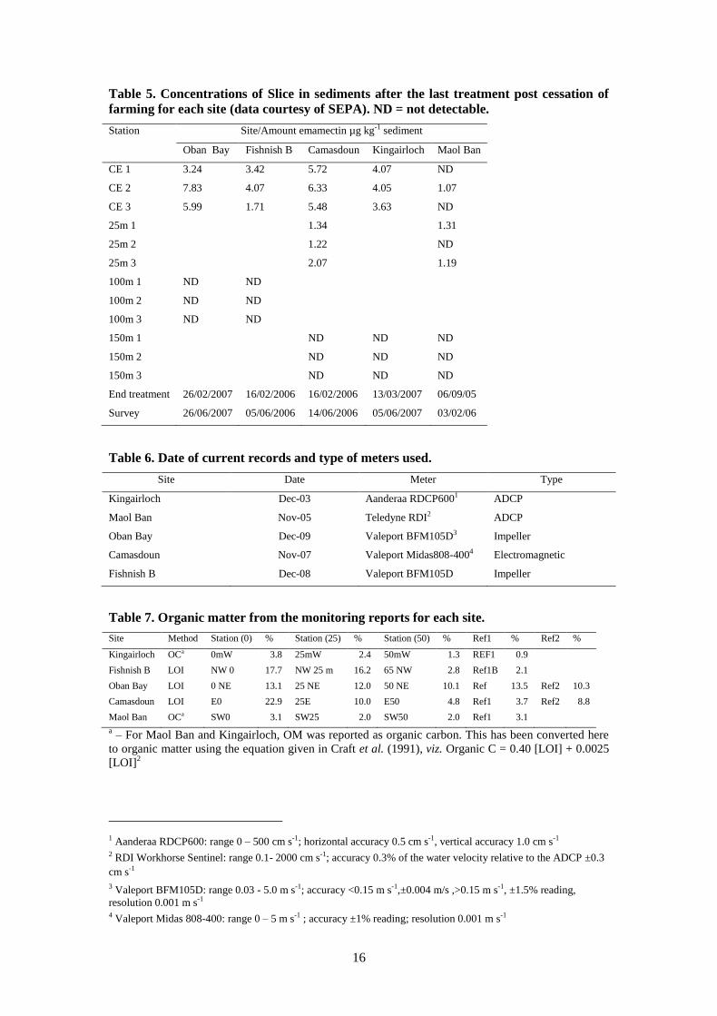
Slice had been used at each of the sites during the farming period prior to this study.

Concentrations of slice in the sediments as determined during Slice consent monitoring are

given in Table 5.

Current records used were those collected by the farmer and are those used by the farmers in

their discharge consents. Details of the instruments are given in Table 6. The ADCP and

electromagnetic types are sensitive to very low current speeds. The impeller types, as used at

Oban Bay and Fishnish B, are much less sensitive to low current speeds and can produce

artificially high numbers of zero current records.

Organic matter concentrations for each of the sites taken during the monitoring survey are

given in Table 7.

16

Table 5. Concentrations of Slice in sediments after the last treatment post cessation of

farming for each site (data courtesy of SEPA). ND = not detectable.

Station Site/Amount emamectin µg kg-1 sediment

Oban Bay Fishnish B Camasdoun Kingairloch Maol Ban

CE 1 3.24 3.42 5.72 4.07 ND

CE 2 7.83 4.07 6.33 4.05 1.07

CE 3 5.99 1.71 5.48 3.63 ND

25m 1 1.34 1.31

25m 2 1.22 ND

25m 3 2.07 1.19

100m 1 ND ND

100m 2 ND ND

100m 3 ND ND

150m 1 ND ND ND

150m 2 ND ND ND

150m 3 ND ND ND

End treatment 26/02/2007 16/02/2006 16/02/2006 13/03/2007 06/09/05

Survey 26/06/2007 05/06/2006 14/06/2006 05/06/2007 03/02/06

Table 6. Date of current records and type of meters used.

Site Date Meter Type

Kingairloch Dec-03 Aanderaa RDCP6001 ADCP

Maol Ban Nov-05 Teledyne RDI2 ADCP

Oban Bay Dec-09 Valeport BFM105D3 Impeller

Camasdoun Nov-07 Valeport Midas808-4004 Electromagnetic

Fishnish B Dec-08 Valeport BFM105D Impeller

Table 7. Organic matter from the monitoring reports for each site.

Site Method Station (0) % Station (25) % Station (50) % Ref1 % Ref2 %

Kingairloch OCa 0mW 3.8 25mW 2.4 50mW 1.3 REF1 0.9

Fishnish B LOI NW 0 17.7 NW 25 m 16.2 65 NW 2.8 Ref1B 2.1

Oban Bay LOI 0 NE 13.1 25 NE 12.0 50 NE 10.1 Ref 13.5 Ref2 10.3

Camasdoun LOI E0 22.9 25E 10.0 E50 4.8 Ref1 3.7 Ref2 8.8

Maol Ban OCa SW0 3.1 SW25 2.0 SW50 2.0 Ref1 3.1

a – For Maol Ban and Kingairloch, OM was reported as organic carbon. This has been converted here

to organic matter using the equation given in Craft et al. (1991), viz. Organic C = 0.40 [LOI] + 0.0025

[LOI]2

1 Aanderaa RDCP600: range 0 – 500 cm s-1; horizontal accuracy 0.5 cm s-1, vertical accuracy 1.0 cm s-1 2 RDI Workhorse Sentinel: range 0.1- 2000 cm s-1; accuracy 0.3% of the water velocity relative to the ADCP ±0.3

cm s-1

3 Valeport BFM105D: range 0.03 - 5.0 m s-1; accuracy <0.15 m s-1,±0.004 m/s ,>0.15 m s-1, ±1.5% reading,

resolution 0.001 m s-1 4 Valeport Midas 808-400: range 0 – 5 m s-1 ; accuracy ±1% reading; resolution 0.001 m s-1

17

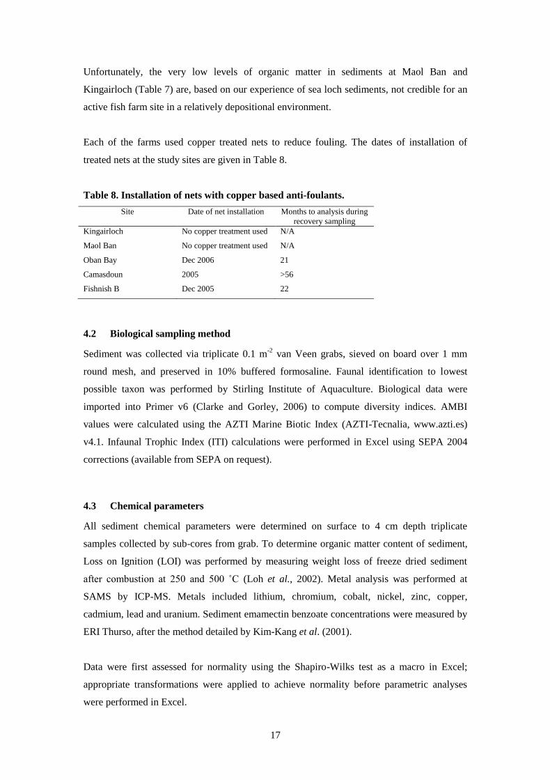
Unfortunately, the very low levels of organic matter in sediments at Maol Ban and

Kingairloch (Table 7) are, based on our experience of sea loch sediments, not credible for an

active fish farm site in a relatively depositional environment.

Each of the farms used copper treated nets to reduce fouling. The dates of installation of

treated nets at the study sites are given in Table 8.

Table 8. Installation of nets with copper based anti-foulants.

Site Date of net installation Months to analysis during

recovery sampling

Kingairloch No copper treatment used N/A

Maol Ban No copper treatment used N/A

Oban Bay Dec 2006 21

Camasdoun 2005 >56

Fishnish B Dec 2005 22

4.2 Biological sampling method

Sediment was collected via triplicate 0.1 m-2

van Veen grabs, sieved on board over 1 mm

round mesh, and preserved in 10% buffered formosaline. Faunal identification to lowest

possible taxon was performed by Stirling Institute of Aquaculture. Biological data were

imported into Primer v6 (Clarke and Gorley, 2006) to compute diversity indices. AMBI

values were calculated using the AZTI Marine Biotic Index (AZTI-Tecnalia, www.azti.es)

v4.1. Infaunal Trophic Index (ITI) calculations were performed in Excel using SEPA 2004

corrections (available from SEPA on request).

4.3 Chemical parameters

All sediment chemical parameters were determined on surface to 4 cm depth triplicate

samples collected by sub-cores from grab. To determine organic matter content of sediment,

Loss on Ignition (LOI) was performed by measuring weight loss of freeze dried sediment

after combustion at 250 and 500 ˚C (Loh et al., 2002). Metal analysis was performed at

SAMS by ICP-MS. Metals included lithium, chromium, cobalt, nickel, zinc, copper,

cadmium, lead and uranium. Sediment emamectin benzoate concentrations were measured by

ERI Thurso, after the method detailed by Kim-Kang et al. (2001).

Data were first assessed for normality using the Shapiro-Wilks test as a macro in Excel;

appropriate transformations were applied to achieve normality before parametric analyses

were performed in Excel.

18

5 Results

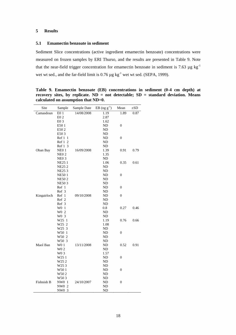
5.1 Emamectin benzoate in sediment

Sediment Slice concentrations (active ingredient emamectin benzoate) concentrations were

measured on frozen samples by ERI Thurso, and the results are presented in Table 9. Note

that the near-field trigger concentration for emamectin benzoate in sediment is 7.63 µg kg-1

wet wt sed., and the far-field limit is 0.76 µg kg-1

wet wt sed. (SEPA, 1999).

Table 9. Emamectin benzoate (EB) concentrations in sediment (0-4 cm depth) at

recovery sites, by replicate. ND = not detectable; SD = standard deviation. Means

calculated on assumption that ND=0.

Site Sample Sample Date EB (ng g-1) Mean ±SD

Camasdoun E0 1 14/08/2008 1.19 1.89 0.87

E0 2 2.87

E0 3 1.62

E50 1 ND 0

E50 2 ND

E50 3 ND

Ref 1 1 ND 0

Ref 1 2 ND

Ref 1 3 ND

Oban Bay NE0 1 16/09/2008 1.39 0.91 0.79

NE0 2 1.35

NE0 3 ND

NE25 1 1.06 0.35 0.61

NE25 2 ND

NE25 3 ND

NE50 1 ND 0

NE50 2 ND

NE50 3 ND

Ref 1 ND 0

Ref 3 ND

Kingairloch Ref 1 09/10/2008 ND 0

Ref 2 ND

Ref 3 ND

W0 1 0.8 0.27 0.46

W0 2 ND

W0 3 ND

W25 1 1.19 0.76 0.66

W25 2 1.08

W25 3 ND

W50 1 ND 0

W50 2 ND

W50 3 ND

Maol Ban W0 1 13/11/2008 ND 0.52 0.91

W0 2 ND

W0 3 1.57

W25 1 ND 0

W25 2 ND

W25 3 ND

W50 1 ND 0

W50 2 ND

W50 3 ND

Fishnish B NW0 1 24/10/2007 ND 0

NW0 2 ND

NW0 3 ND

19

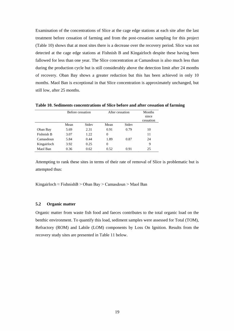
Examination of the concentrations of Slice at the cage edge stations at each site after the last

treatment before cessation of farming and from the post-cessation sampling for this project

(Table 10) shows that at most sites there is a decrease over the recovery period. Slice was not

detected at the cage edge stations at Fishnish B and Kingairloch despite these having been

fallowed for less than one year. The Slice concentration at Camasdoun is also much less than

during the production cycle but is still considerably above the detection limit after 24 months

of recovery. Oban Bay shows a greater reduction but this has been achieved in only 10

months. Maol Ban is exceptional in that Slice concentration is approximately unchanged, but

still low, after 25 months.

Table 10. Sediments concentrations of Slice before and after cessation of farming

Before cessation After cessation Months

since

cessation

Mean Stdev Mean Stdev

Oban Bay 5.69 2.31 0.91 0.79 10

Fishnish B 3.07 1.22 0 11

Camasdoun 5.84 0.44 1.89 0.87 24

Kingairloch 3.92 0.25 0 9

Maol Ban 0.36 0.62 0.52 0.91 25

Attempting to rank these sites in terms of their rate of removal of Slice is problematic but is

attempted thus:

Kingairloch ≈ FishnishB > Oban Bay > Camasdoun > Maol Ban

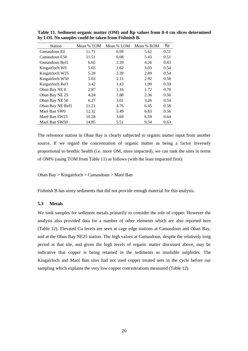
5.2 Organic matter

Organic matter from waste fish food and faeces contributes to the total organic load on the

benthic environment. To quantify this load, sediment samples were assessed for Total (TOM),

Refractory (ROM) and Labile (LOM) components by Loss On Ignition. Results from the

recovery study sites are presented in Table 11 below.

20

Table 11. Sediment organic matter (OM) and Rp values from 0-4 cm slices determined

by LOI. No samples could be taken from Fishnish B.

Station Mean % TOM Mean % LOM Mean % ROM Rp

Camasdoun E0 11.71 6.09 5.62 0.51

Camasdoun E50 11.51 6.08 5.43 0.51

Camasdoun Ref1 6.65 2.39 4.26 0.63

Kingairloch W0 5.65 2.62 3.03 0.54

Kingairloch W25 5.28 2.39 2.89 0.54

Kingairloch W50 5.03 2.11 2.92 0.58

Kingairloch Ref1 3.42 1.43 1.99 0.59

Oban Bay NE 0 2.87 1.16 1.72 0.70

Oban Bay NE 25 4.24 1.88 2.36 0.56

Oban Bay NE 50 6.27 3.01 3.26 0.54

Oban Bay NE Ref1 11.21 4.76 6.45 0.58

Maol Ban SW0 12.32 5.49 6.83 0.56

Maol Ban SW25 10.28 3.69 6.59 0.64

Maol Ban SW50 14.85 5.51 9.34 0.63

The reference station in Oban Bay is clearly subjected to organic matter input from another

source. If we regard the concentration of organic matter as being a factor inversely

proportional to benthic health (i.e. more OM, more impacted), we can rank the sites in terms

of OM% (using TOM from Table 11) as follows (with the least impacted first):

Oban Bay > Kingairloch > Camasdoun > Maol Ban

Fishnish B has stony sediments that did not provide enough material for this analysis.

5.3 Metals

We took samples for sediment metals primarily to consider the role of copper. However the

analysis also provided data for a number of other elements which are also reported here

(Table 12). Elevated Cu levels are seen at cage edge stations at Camasdoun and Oban Bay,

and at the Oban Bay NE25 station. The high values at Camasdoun, despite the relatively long

period at that site, and given the high levels of organic matter discussed above, may be

indicative that copper is being retained in the sediments as insoluble sulphides. The

Kingairloch and Maol Ban sites had not used copper treated nets in the cycle before our

sampling which explains the very low copper concentrations measured (Table 12).

21

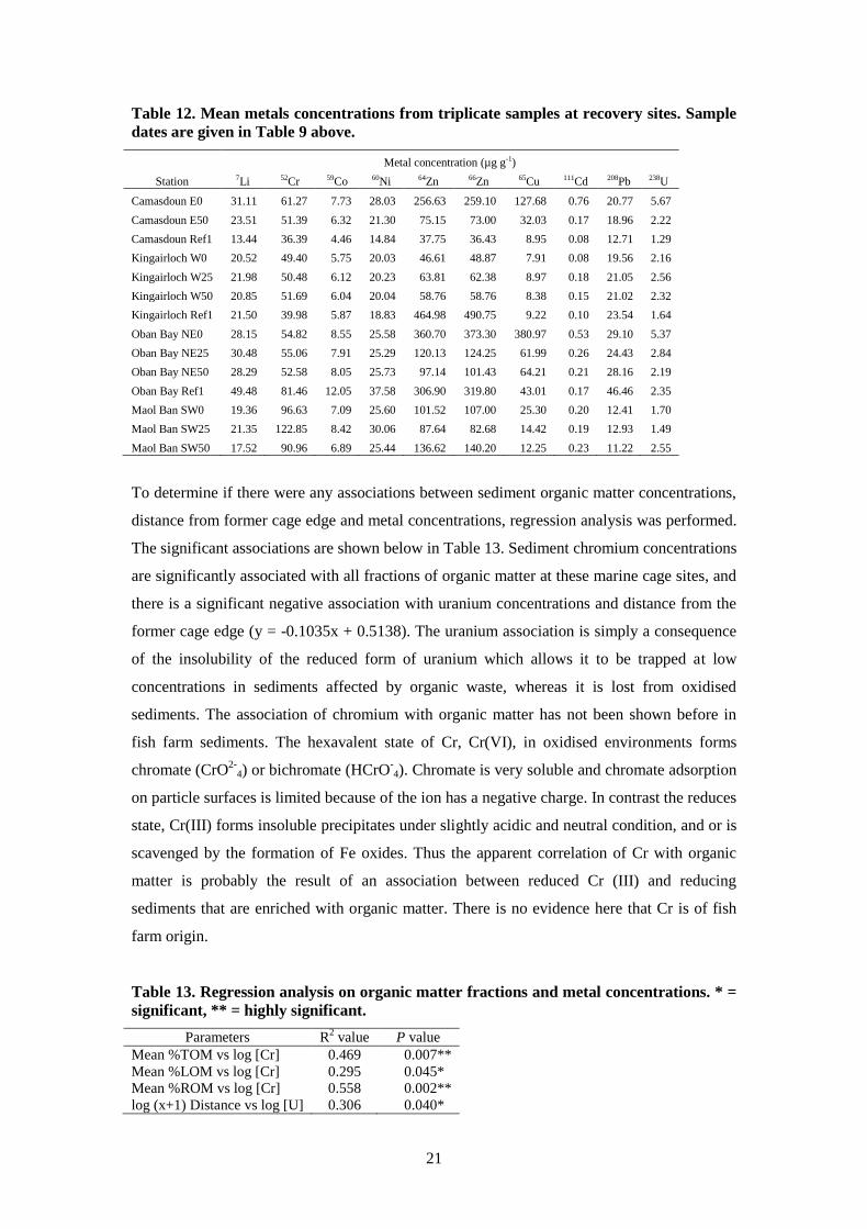
Table 12. Mean metals concentrations from triplicate samples at recovery sites. Sample

dates are given in Table 9 above.

Metal concentration (µg g-1)

Station 7Li 52Cr 59Co 60Ni 64Zn 66Zn 65Cu 111Cd 208Pb 238U

Camasdoun E0 31.11 61.27 7.73 28.03 256.63 259.10 127.68 0.76 20.77 5.67

Camasdoun E50 23.51 51.39 6.32 21.30 75.15 73.00 32.03 0.17 18.96 2.22

Camasdoun Ref1 13.44 36.39 4.46 14.84 37.75 36.43 8.95 0.08 12.71 1.29

Kingairloch W0 20.52 49.40 5.75 20.03 46.61 48.87 7.91 0.08 19.56 2.16

Kingairloch W25 21.98 50.48 6.12 20.23 63.81 62.38 8.97 0.18 21.05 2.56

Kingairloch W50 20.85 51.69 6.04 20.04 58.76 58.76 8.38 0.15 21.02 2.32

Kingairloch Ref1 21.50 39.98 5.87 18.83 464.98 490.75 9.22 0.10 23.54 1.64

Oban Bay NE0 28.15 54.82 8.55 25.58 360.70 373.30 380.97 0.53 29.10 5.37

Oban Bay NE25 30.48 55.06 7.91 25.29 120.13 124.25 61.99 0.26 24.43 2.84

Oban Bay NE50 28.29 52.58 8.05 25.73 97.14 101.43 64.21 0.21 28.16 2.19

Oban Bay Ref1 49.48 81.46 12.05 37.58 306.90 319.80 43.01 0.17 46.46 2.35

Maol Ban SW0 19.36 96.63 7.09 25.60 101.52 107.00 25.30 0.20 12.41 1.70

Maol Ban SW25 21.35 122.85 8.42 30.06 87.64 82.68 14.42 0.19 12.93 1.49

Maol Ban SW50 17.52 90.96 6.89 25.44 136.62 140.20 12.25 0.23 11.22 2.55

To determine if there were any associations between sediment organic matter concentrations,

distance from former cage edge and metal concentrations, regression analysis was performed.

The significant associations are shown below in Table 13. Sediment chromium concentrations

are significantly associated with all fractions of organic matter at these marine cage sites, and

there is a significant negative association with uranium concentrations and distance from the

former cage edge (y = -0.1035x + 0.5138). The uranium association is simply a consequence

of the insolubility of the reduced form of uranium which allows it to be trapped at low

concentrations in sediments affected by organic waste, whereas it is lost from oxidised

sediments. The association of chromium with organic matter has not been shown before in

fish farm sediments. The hexavalent state of Cr, Cr(VI), in oxidised environments forms

chromate (CrO2-

4) or bichromate (HCrO-4). Chromate is very soluble and chromate adsorption

on particle surfaces is limited because of the ion has a negative charge. In contrast the reduces

state, Cr(III) forms insoluble precipitates under slightly acidic and neutral condition, and or is

scavenged by the formation of Fe oxides. Thus the apparent correlation of Cr with organic

matter is probably the result of an association between reduced Cr (III) and reducing

sediments that are enriched with organic matter. There is no evidence here that Cr is of fish

farm origin.

Table 13. Regression analysis on organic matter fractions and metal concentrations. * =

significant, ** = highly significant.

Parameters R2 value P value

Mean %TOM vs log [Cr] 0.469 0.007**

Mean %LOM vs log [Cr] 0.295 0.045*

Mean %ROM vs log [Cr] 0.558 0.002**

log (x+1) Distance vs log [U] 0.306 0.040*

22

6 Benthic biology

6.1 Recovery

Several approaches were adopted to determine to what extent recovery had occurred at the

sites studied. A number of standard diversity indices for the benthic community at each

station were calculated, and the ratio of these indices to those at the reference station at each

site calculated. It was postulated that as the diversity index under consideration approached

the value of that at the reference station, the further advanced recovery would be, such that

the ratio of “diversity index at station x” : “diversity index at reference” would approach

unity.

The definition of recovery by Brooks and co-workers (Brooks and Mahnken, 2003; Brooks et

al., 2004) described previously (Section 2.2) was also emplyed, i.e. the taxa at the reference

station that contributed to 1% of the mean total abundance at that station were calculated.

For recovery to have occurred at a particular station, those same taxa must be present at that

station (but not necessarily in the same numbers as at the reference station). We have

developed this idea by taking the number of these “Brooks taxa” present at a particular station

and dividing this by the number of these taxa at the reference station to arrive at a ratio of

recovery, hereafter termed the Brooks Recovery Index (BRI) (Eq. 1).

mean total1%referenceat taxa

ref matchingstation at taxa(BRI)Index Recovery Brooks

(Eq. 1)

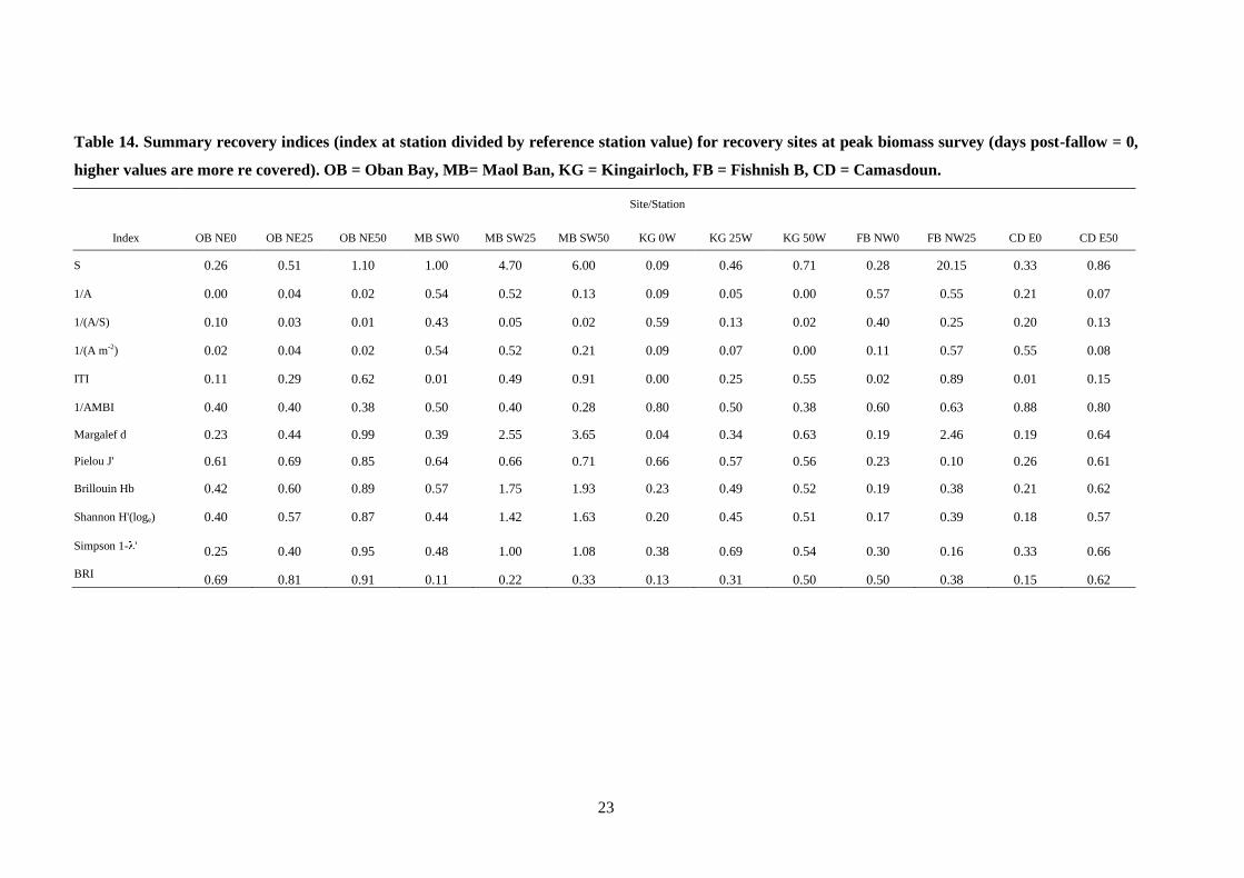
A summary of all the indices examined at each of the recovery stations is presented in Table

14 (peak biomass survey) and Table 15 (recovery survey). Increases in some indices will of

course indicate different things. For example, an increase in individual abundance relative to

the reference station is not necessarily indicative of improving (recovery) conditions, as

individual abundance generally reaches a maximum at an optimal enrichment level (the “peak

of opportunists” of Pearson and Rosenberg (Pearson and Rosenberg, 1978)). Likewise, an

increase in the AMBI index is indicative of impacted conditions, thus an increase in the

AMBI value at a particular station relative to the reference station value would also indicate

deteriorating or delayed recovery conditions. For these reasons the indices Abundance (A),

Abundance/Species (A/S), Abundance m-2

(A m-2

) and AMBI are presented as the inverse, i.e.

1

x, so that an increase in this inverse ratio is seen as an improvement in conditions (recovery)

relative to the reference station.

23

Table 14. Summary recovery indices (index at station divided by reference station value) for recovery sites at peak biomass survey (days post-fallow = 0,

higher values are more re covered). OB = Oban Bay, MB= Maol Ban, KG = Kingairloch, FB = Fishnish B, CD = Camasdoun.

Site/Station

Index OB NE0 OB NE25 OB NE50 MB SW0 MB SW25 MB SW50 KG 0W KG 25W KG 50W FB NW0 FB NW25 CD E0 CD E50

S 0.26 0.51 1.10 1.00 4.70 6.00 0.09 0.46 0.71 0.28 20.15 0.33 0.86

1/A 0.00 0.04 0.02 0.54 0.52 0.13 0.09 0.05 0.00 0.57 0.55 0.21 0.07

1/(A/S) 0.10 0.03 0.01 0.43 0.05 0.02 0.59 0.13 0.02 0.40 0.25 0.20 0.13

1/(A m-2) 0.02 0.04 0.02 0.54 0.52 0.21 0.09 0.07 0.00 0.11 0.57 0.55 0.08

ITI 0.11 0.29 0.62 0.01 0.49 0.91 0.00 0.25 0.55 0.02 0.89 0.01 0.15

1/AMBI 0.40 0.40 0.38 0.50 0.40 0.28 0.80 0.50 0.38 0.60 0.63 0.88 0.80

Margalef d 0.23 0.44 0.99 0.39 2.55 3.65 0.04 0.34 0.63 0.19 2.46 0.19 0.64

Pielou J' 0.61 0.69 0.85 0.64 0.66 0.71 0.66 0.57 0.56 0.23 0.10 0.26 0.61

Brillouin Hb 0.42 0.60 0.89 0.57 1.75 1.93 0.23 0.49 0.52 0.19 0.38 0.21 0.62

Shannon H'(loge) 0.40 0.57 0.87 0.44 1.42 1.63 0.20 0.45 0.51 0.17 0.39 0.18 0.57

Simpson 1- ' 0.25 0.40 0.95 0.48 1.00 1.08 0.38 0.69 0.54 0.30 0.16 0.33 0.66

BRI 0.69 0.81 0.91 0.11 0.22 0.33 0.13 0.31 0.50 0.50 0.38 0.15 0.62

24

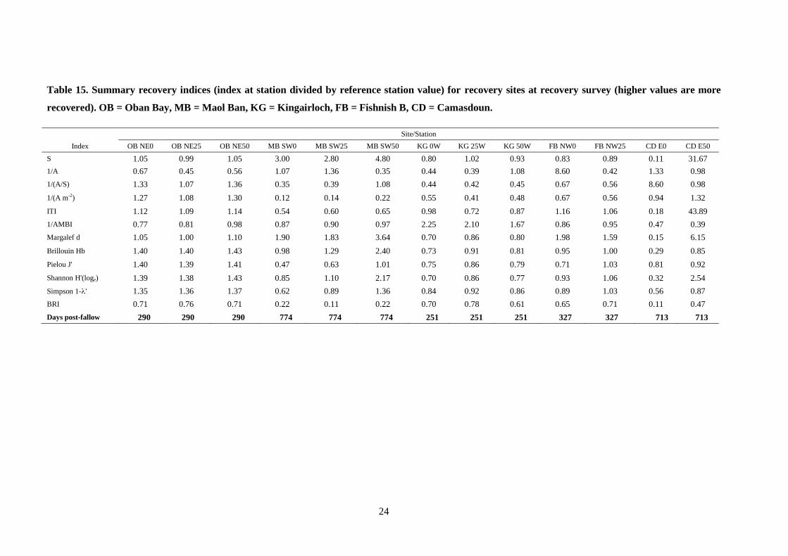
Table 15. Summary recovery indices (index at station divided by reference station value) for recovery sites at recovery survey (higher values are more

recovered). OB = Oban Bay, MB = Maol Ban, KG = Kingairloch, FB = Fishnish B, CD = Camasdoun.

Site/Station

Index OB NE0 OB NE25 OB NE50 MB SW0 MB SW25 MB SW50 KG 0W KG 25W KG 50W FB NW0 FB NW25 CD E0 CD E50

S 1.05 0.99 1.05 3.00 2.80 4.80 0.80 1.02 0.93 0.83 0.89 0.11 31.67

1/A 0.67 0.45 0.56 1.07 1.36 0.35 0.44 0.39 1.08 8.60 0.42 1.33 0.98

1/(A/S) 1.33 1.07 1.36 0.35 0.39 1.08 0.44 0.42 0.45 0.67 0.56 8.60 0.98

1/(A m-2) 1.27 1.08 1.30 0.12 0.14 0.22 0.55 0.41 0.48 0.67 0.56 0.94 1.32

ITI 1.12 1.09 1.14 0.54 0.60 0.65 0.98 0.72 0.87 1.16 1.06 0.18 43.89

1/AMBI 0.77 0.81 0.98 0.87 0.90 0.97 2.25 2.10 1.67 0.86 0.95 0.47 0.39

Margalef d 1.05 1.00 1.10 1.90 1.83 3.64 0.70 0.86 0.80 1.98 1.59 0.15 6.15

Brillouin Hb 1.40 1.40 1.43 0.98 1.29 2.40 0.73 0.91 0.81 0.95 1.00 0.29 0.85

Pielou J' 1.40 1.39 1.41 0.47 0.63 1.01 0.75 0.86 0.79 0.71 1.03 0.81 0.92

Shannon H'(loge) 1.39 1.38 1.43 0.85 1.10 2.17 0.70 0.86 0.77 0.93 1.06 0.32 2.54

Simpson 1- ' 1.35 1.36 1.37 0.62 0.89 1.36 0.84 0.92 0.86 0.89 1.03 0.56 0.87

BRI 0.71 0.76 0.71 0.22 0.11 0.22 0.70 0.78 0.61 0.65 0.71 0.11 0.47

Days post-fallow 290 290 290 774 774 774 251 251 251 327 327 713 713

25

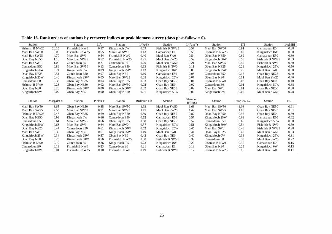
Table 16. Rank orders of stations by recovery indices at peak biomass survey (days post-fallow = 0).

Station S Station 1/A Station 1/(A/S) Station 1/(A m-2) Station ITI Station 1/AMBI

Fishnish B NW25 20.15 Fishnish B NW0 0.57 Kingairloch 0W 0.59 Fishnish B NW25 0.57 Maol Ban SW50 0.91 Camasdoun E0 0.88

Maol Ban SW50 6.00 Fishnish B NW25 0.55 Maol Ban SW0 0.43 Camasdoun E0 0.55 Fishnish B NW25 0.89 Kingairloch 0W 0.80

Maol Ban SW25 4.70 Maol Ban SW0 0.54 Fishnish B NW0 0.40 Maol Ban SW0 0.54 Oban Bay NE50 0.62 Camasdoun E50 0.80 Oban Bay NE50 1.10 Maol Ban SW25 0.52 Fishnish B NW25 0.25 Maol Ban SW25 0.52 Kingairloch 50W 0.55 Fishnish B NW25 0.63

Maol Ban SW0 1.00 Camasdoun E0 0.21 Camasdoun E0 0.20 Maol Ban SW50 0.21 Maol Ban SW25 0.49 Fishnish B NW0 0.60

Camasdoun E50 0.86 Maol Ban SW50 0.13 Camasdoun E50 0.13 Fishnish B NW0 0.11 Oban Bay NE25 0.29 Kingairloch 25W 0.50 Kingairloch 50W 0.71 Kingairloch 0W 0.09 Kingairloch 25W 0.13 Kingairloch 0W 0.09 Kingairloch 25W 0.25 Maol Ban SW0 0.50

Oban Bay NE25 0.51 Camasdoun E50 0.07 Oban Bay NE0 0.10 Camasdoun E50 0.08 Camasdoun E50 0.15 Oban Bay NE25 0.40

Kingairloch 25W 0.46 Kingairloch 25W 0.05 Maol Ban SW25 0.05 Kingairloch 25W 0.07 Oban Bay NE0 0.11 Maol Ban SW25 0.40 Camasdoun E0 0.33 Oban Bay NE25 0.04 Oban Bay NE25 0.03 Oban Bay NE25 0.04 Fishnish B NW0 0.02 Oban Bay NE0 0.40

Fishnish B NW0 0.28 Oban Bay NE50 0.02 Maol Ban SW50 0.02 Oban Bay NE0 0.02 Camasdoun E0 0.01 Kingairloch 50W 0.38

Oban Bay NE0 0.26 Kingairloch 50W 0.00 Kingairloch 50W 0.02 Oban Bay NE50 0.02 Maol Ban SW0 0.01 Oban Bay NE50 0.38 Kingairloch 0W 0.09 Oban Bay NE0 0.00 Oban Bay NE50 0.01 Kingairloch 50W 0.00 Kingairloch 0W 0.00 Maol Ban SW50 0.28

Station Margalef d Station Pielou J' Station Brillouin Hb Station Shannon H'(loge)

Station Simpson 1- ' Station BRI

Maol Ban SW50 3.65 Oban Bay NE50 0.85 Maol Ban SW50 1.93 Maol Ban SW50 1.63 Maol Ban SW50 1.08 Oban Bay NE50 0.91

Maol Ban SW25 2.55 Maol Ban SW50 0.71 Maol Ban SW25 1.75 Maol Ban SW25 1.42 Maol Ban SW25 1.00 Oban Bay NE25 0.81 Fishnish B NW25 2.46 Oban Bay NE25 0.69 Oban Bay NE50 0.89 Oban Bay NE50 0.87 Oban Bay NE50 0.95 Oban Bay NE0 0.69

Oban Bay NE50 0.99 Kingairloch 0W 0.66 Camasdoun E50 0.62 Camasdoun E50 0.57 Kingairloch 25W 0.69 Camasdoun E50 0.62

Camasdoun E50 0.64 Maol Ban SW25 0.66 Oban Bay NE25 0.60 Oban Bay NE25 0.57 Camasdoun E50 0.66 Kingairloch 50W 0.50 Kingairloch 50W 0.63 Maol Ban SW0 0.64 Maol Ban SW0 0.57 Kingairloch 50W 0.51 Kingairloch 50W 0.54 Fishnish B NW0 0.50

Oban Bay NE25 0.44 Camasdoun E50 0.61 Kingairloch 50W 0.52 Kingairloch 25W 0.45 Maol Ban SW0 0.48 Fishnish B NW25 0.38

Maol Ban SW0 0.39 Oban Bay NE0 0.61 Kingairloch 25W 0.49 Maol Ban SW0 0.44 Oban Bay NE25 0.40 Maol Ban SW50 0.33 Kingairloch 25W 0.34 Kingairloch 25W 0.57 Oban Bay NE0 0.42 Oban Bay NE0 0.40 Kingairloch 0W 0.38 Kingairloch 25W 0.31

Oban Bay NE0 0.23 Kingairloch 50W 0.56 Fishnish B NW25 0.38 Fishnish B NW25 0.39 Camasdoun E0 0.33 Maol Ban SW25 0.22

Fishnish B NW0 0.19 Camasdoun E0 0.26 Kingairloch 0W 0.23 Kingairloch 0W 0.20 Fishnish B NW0 0.30 Camasdoun E0 0.15 Camasdoun E0 0.19 Fishnish B NW0 0.23 Camasdoun E0 0.21 Camasdoun E0 0.18 Oban Bay NE0 0.25 Kingairloch 0W 0.13

Kingairloch 0W 0.04 Fishnish B NW25 0.10 Fishnish B NW0 0.19 Fishnish B NW0 0.17 Fishnish B NW25 0.16 Maol Ban SW0 0.11

26

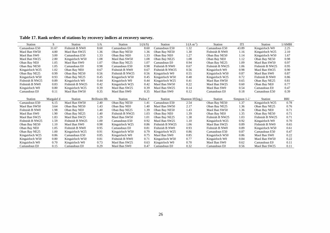
Table 17. Rank orders of stations by recovery indices at recovery survey.

Station S Station 1/A Station 1/(A/S) Station 1/(A m-2) Station ITI Station 1/AMBI

Camasdoun E50 31.67 Fishnish B NW0 8.60 Camasdoun E0 8.60 Camasdoun E50 1.32 Camasdoun E50 43.89 Kingairloch W0 2.25

Maol Ban SW50 4.80 Maol Ban SW25 1.36 Oban Bay NE50 1.36 Oban Bay NE50 1.30 Fishnish B NW0 1.16 Kingairloch W25 2.10

Maol Ban SW0 3.00 Camasdoun E50 1.33 Oban Bay NE0 1.33 Oban Bay NE0 1.27 Oban Bay NE50 1.14 Kingairloch W50 1.67 Maol Ban SW25 2.80 Kingairloch W50 1.08 Maol Ban SW50 1.08 Oban Bay NE25 1.08 Oban Bay NE0 1.12 Oban Bay NE50 0.98

Oban Bay NE0 1.05 Maol Ban SW0 1.07 Oban Bay NE25 1.07 Camasdoun E0 0.94 Oban Bay NE25 1.09 Maol Ban SW50 0.97

Oban Bay NE50 1.05 Camasdoun E0 0.98 Camasdoun E50 0.98 Fishnish B NW0 0.67 Fishnish B NW25 1.06 Fishnish B NW25 0.95 Kingairloch W25 1.02 Oban Bay NE0 0.67 Fishnish B NW0 0.67 Fishnish B NW25 0.56 Kingairloch W0 0.98 Maol Ban SW25 0.90

Oban Bay NE25 0.99 Oban Bay NE50 0.56 Fishnish B NW25 0.56 Kingairloch W0 0.55 Kingairloch W50 0.87 Maol Ban SW0 0.87

Kingairloch W50 0.93 Oban Bay NE25 0.45 Kingairloch W50 0.45 Kingairloch W50 0.48 Kingairloch W25 0.72 Fishnish B NW0 0.86 Fishnish B NW25 0.89 Kingairloch W0 0.44 Kingairloch W0 0.44 Kingairloch W25 0.41 Maol Ban SW50 0.65 Oban Bay NE25 0.81

Fishnish B NW0 0.83 Fishnish B NW25 0.42 Kingairloch W25 0.42 Maol Ban SW50 0.22 Maol Ban SW25 0.60 Oban Bay NE0 0.77

Kingairloch W0 0.80 Kingairloch W25 0.39 Maol Ban SW25 0.39 Maol Ban SW25 0.14 Maol Ban SW0 0.54 Camasdoun E0 0.47 Camasdoun E0 0.11 Maol Ban SW50 0.35 Maol Ban SW0 0.35 Maol Ban SW0 0.12 Camasdoun E0 0.18 Camasdoun E50 0.39

Station Margalef d Station Brillouin Hb Station Pielou J' Station Shannon H'(loge) Station Simpson 1- ' Station BRI

Camasdoun E50 6.15 Maol Ban SW50 2.40 Oban Bay NE50 1.41 Camasdoun E50 2.54 Oban Bay NE50 1.37 Kingairloch W25 0.78

Maol Ban SW50 3.64 Oban Bay NE50 1.43 Oban Bay NE0 1.40 Maol Ban SW50 2.17 Oban Bay NE25 1.36 Oban Bay NE25 0.76

Fishnish B NW0 1.98 Oban Bay NE0 1.40 Oban Bay NE25 1.39 Oban Bay NE50 1.43 Maol Ban SW50 1.36 Oban Bay NE0 0.71 Maol Ban SW0 1.90 Oban Bay NE25 1.40 Fishnish B NW25 1.03 Oban Bay NE0 1.39 Oban Bay NE0 1.35 Oban Bay NE50 0.71

Maol Ban SW25 1.83 Maol Ban SW25 1.29 Maol Ban SW50 1.01 Oban Bay NE25 1.38 Fishnish B NW25 1.03 Fishnish B NW25 0.71

Fishnish B NW25 1.59 Fishnish B NW25 1.00 Camasdoun E50 0.92 Maol Ban SW25 1.10 Kingairloch W25 0.92 Kingairloch W0 0.70 Oban Bay NE50 1.10 Maol Ban SW0 0.98 Kingairloch W25 0.86 Fishnish B NW25 1.06 Maol Ban SW25 0.89 Fishnish B NW0 0.65

Oban Bay NE0 1.05 Fishnish B NW0 0.95 Camasdoun E0 0.81 Fishnish B NW0 0.93 Fishnish B NW0 0.89 Kingairloch W50 0.61

Oban Bay NE25 1.00 Kingairloch W25 0.91 Kingairloch W50 0.79 Kingairloch W25 0.86 Camasdoun E50 0.87 Camasdoun E50 0.47 Kingairloch W25 0.86 Camasdoun E50 0.85 Kingairloch W0 0.75 Maol Ban SW0 0.85 Kingairloch W50 0.86 Maol Ban SW0 0.22

Kingairloch W50 0.80 Kingairloch W50 0.81 Fishnish B NW0 0.71 Kingairloch W50 0.77 Kingairloch W0 0.84 Maol Ban SW50 0.22

Kingairloch W0 0.70 Kingairloch W0 0.73 Maol Ban SW25 0.63 Kingairloch W0 0.70 Maol Ban SW0 0.62 Camasdoun E0 0.11 Camasdoun E0 0.15 Camasdoun E0 0.29 Maol Ban SW0 0.47 Camasdoun E0 0.32 Camasdoun E0 0.56 Maol Ban SW25 0.11

27

To appreciate how mixed the picture of recovery at each site is, the recovery indices at Oban

Bay may be examined. At the Oban Bay cage edge station, the recovery indices S, 1/(A/S),

1/(A m-2

), ITI, Margalef d, Brillouin Hb, Pielou J', Shannon H'(loge) and Simpson 1- ' all

yielded values higher than unity, suggesting that recovery had taken place 290 days post-

fallow (Table 15). In contrast the indices 1/A, 1/AMBI and the BRI all show values below

unity, indicating that recovery was not complete. This situation is repeated across all stations

and sites studied; wherever other recovery indices exceed unity and suggest recovery has

occurred, the BRI in all cases remains below unity.

To estimate the relative recovery status of the sites across all indices tested, the data were

ranked by each index and tabulated (Table 17). Taking the cage edge stations only into

account, these ranks were compared and the stations with the most top ranks tabulated (Table

18). This would suggest that the Oban Bay site had recovered the furthest taking all diversity

recovery indices into account, even though it had the second shortest recovery time since

fallowing. Furthermore, Camasdoun had the most bottom ranks despite having one of the

longest recovery times.

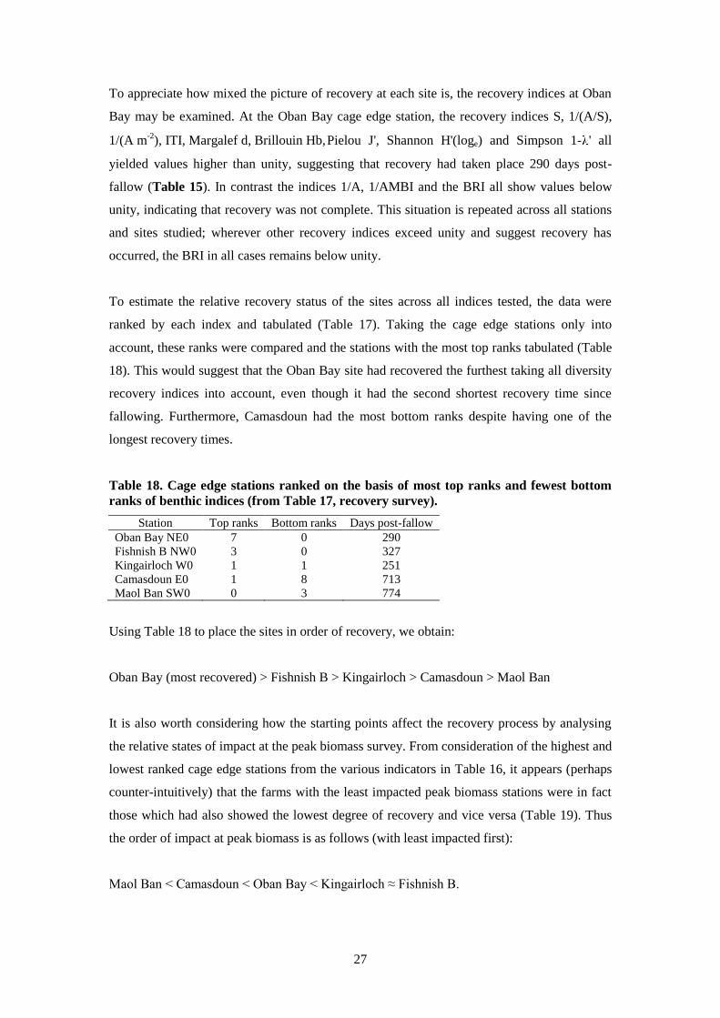
Table 18. Cage edge stations ranked on the basis of most top ranks and fewest bottom

ranks of benthic indices (from Table 17, recovery survey).

Station Top ranks Bottom ranks Days post-fallow

Oban Bay NE0 7 0 290

Fishnish B NW0 3 0 327

Kingairloch W0 1 1 251

Camasdoun E0 1 8 713

Maol Ban SW0 0 3 774

Using Table 18 to place the sites in order of recovery, we obtain:

Oban Bay (most recovered) > Fishnish B > Kingairloch > Camasdoun > Maol Ban

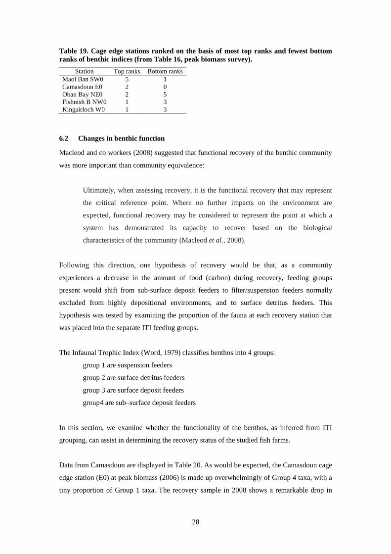
It is also worth considering how the starting points affect the recovery process by analysing

the relative states of impact at the peak biomass survey. From consideration of the highest and

lowest ranked cage edge stations from the various indicators in Table 16, it appears (perhaps

counter-intuitively) that the farms with the least impacted peak biomass stations were in fact

those which had also showed the lowest degree of recovery and vice versa (Table 19). Thus

the order of impact at peak biomass is as follows (with least impacted first):

Maol Ban < Camasdoun < Oban Bay < Kingairloch ≈ Fishnish B.

28

Table 19. Cage edge stations ranked on the basis of most top ranks and fewest bottom

ranks of benthic indices (from Table 16, peak biomass survey).

Station Top ranks Bottom ranks

Maol Ban SW0 5 1

Camasdoun E0 2 0

Oban Bay NE0 2 5

Fishnish B NW0 1 3

Kingairloch W0 1 3

6.2 Changes in benthic function

Macleod and co workers (2008) suggested that functional recovery of the benthic community

was more important than community equivalence:

Ultimately, when assessing recovery, it is the functional recovery that may represent

the critical reference point. Where no further impacts on the environment are

expected, functional recovery may be considered to represent the point at which a

system has demonstrated its capacity to recover based on the biological

characteristics of the community (Macleod et al., 2008).

Following this direction, one hypothesis of recovery would be that, as a community

experiences a decrease in the amount of food (carbon) during recovery, feeding groups

present would shift from sub-surface deposit feeders to filter/suspension feeders normally

excluded from highly depositional environments, and to surface detritus feeders. This

hypothesis was tested by examining the proportion of the fauna at each recovery station that

was placed into the separate ITI feeding groups.

The Infaunal Trophic Index (Word, 1979) classifies benthos into 4 groups:

group 1 are suspension feeders

group 2 are surface detritus feeders

group 3 are surface deposit feeders

group4 are sub–surface deposit feeders

In this section, we examine whether the functionality of the benthos, as inferred from ITI

grouping, can assist in determining the recovery status of the studied fish farms.

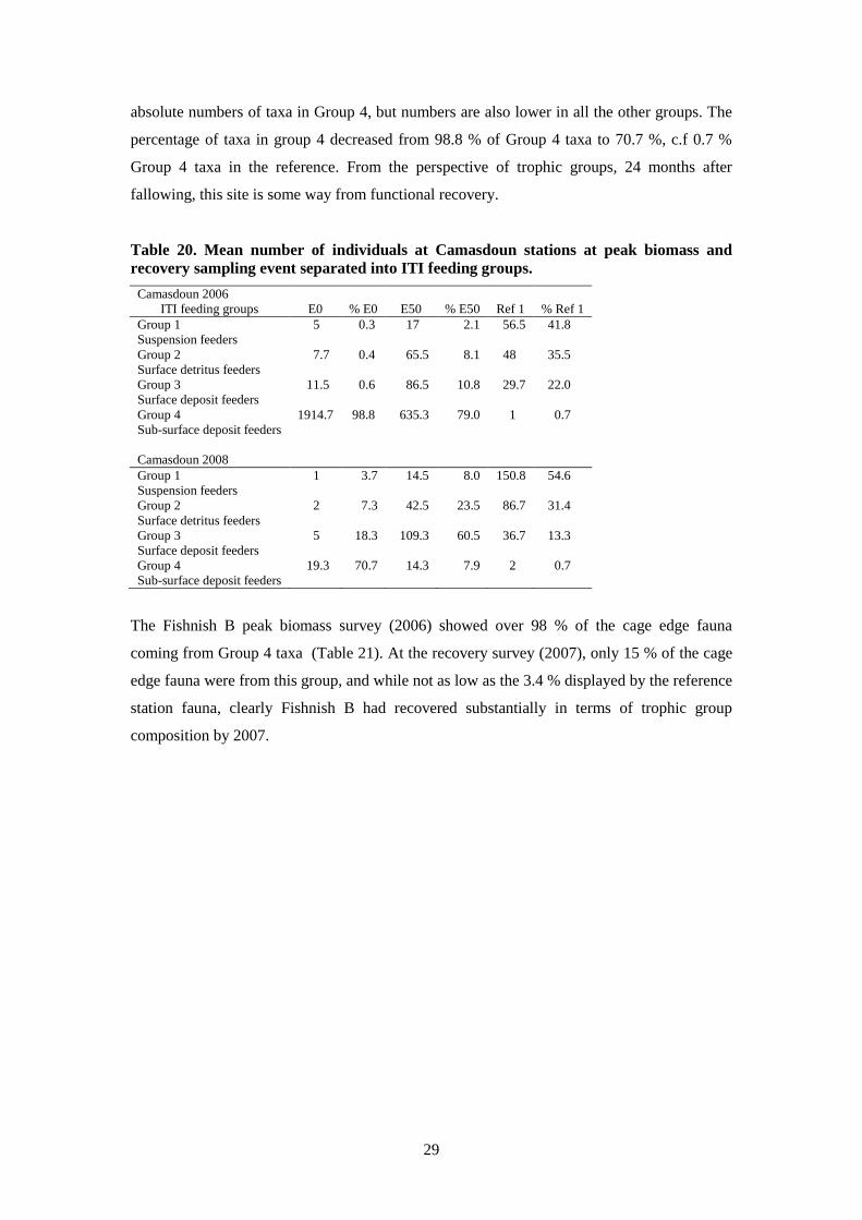
Data from Camasdoun are displayed in Table 20. As would be expected, the Camasdoun cage

edge station (E0) at peak biomass (2006) is made up overwhelmingly of Group 4 taxa, with a

tiny proportion of Group 1 taxa. The recovery sample in 2008 shows a remarkable drop in

29

absolute numbers of taxa in Group 4, but numbers are also lower in all the other groups. The

percentage of taxa in group 4 decreased from 98.8 % of Group 4 taxa to 70.7 %, c.f 0.7 %

Group 4 taxa in the reference. From the perspective of trophic groups, 24 months after

fallowing, this site is some way from functional recovery.

Table 20. Mean number of individuals at Camasdoun stations at peak biomass and

recovery sampling event separated into ITI feeding groups.

Camasdoun 2006

ITI feeding groups E0 % E0 E50 % E50 Ref 1 % Ref 1

Group 1 5 0.3 17 2.1 56.5 41.8

Suspension feeders

Group 2 7.7 0.4 65.5 8.1 48 35.5

Surface detritus feeders

Group 3 11.5 0.6 86.5 10.8 29.7 22.0

Surface deposit feeders

Group 4 1914.7 98.8 635.3 79.0 1 0.7

Sub-surface deposit feeders

Camasdoun 2008

Group 1 1 3.7 14.5 8.0 150.8 54.6

Suspension feeders

Group 2 2 7.3 42.5 23.5 86.7 31.4


Group 3 5 18.3 109.3 60.5 36.7 13.3


Group 4 19.3 70.7 14.3 7.9 2 0.7


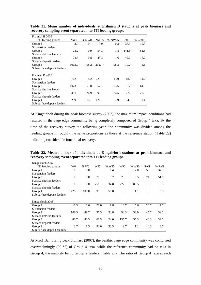
The Fishnish B peak biomass survey (2006) showed over 98 % of the cage edge fauna

coming from Group 4 taxa (Table 21). At the recovery survey (2007), only 15 % of the cage

edge fauna were from this group, and while not as low as the 3.4 % displayed by the reference

station fauna, clearly Fishnish B had recovered substantially in terms of trophic group

composition by 2007.

30

Table 21. Mean number of individuals at Fishnish B stations at peak biomass and


Fishnish B 2006

ITI feeding groups NW0 % NW0 NW25 % NW25 Ref1B % Ref1B

Group 1 3.0 0.1 9.0 0.3 36.5 15.8

Suspension feeders

Group 2 28.2 0.9 54.3 1.8 141.5 61.3


Group 3 24.3 0.8 48.3 1.6 42.0 18.2


Group 4 3013.0 98.2 2927.7 96.3 10.7 4.6


Fishnish B 2007

Group 1 162 8.2 221 13.9 187 14.2

Suspension feeders

Group 2 1023 51.8 852 53.6 812 61.8


Group 3 491 24.9 390 24.5 270 20.5


Group 4 299 15.1 126 7.9 45 3.4


At Kingairloch during the peak biomass survey (2007), the maximum impact conditions had

resulted in the cage edge community being completely composed of Group 4 taxa. By the

time of the recovery survey the following year, the community was divided among the

feeding groups in roughly the same proportions as those at the reference station (Table 22)

indicating considerable functional recovery.

Table 22. Mean number of individuals at Kingairloch stations at peak biomass and


Kingairloch 2007

ITI feeding groups W0 % W0 W25 % W25 W50 % W50 Ref1 % Ref1

Group 1 0 0.0 3 0.4 19 7.0 55 37.9

Suspension feeders

Group 2 0 0.0 70 9.7 23 8.5 74 51.0


Group 3 0 0.0 250 34.8 227 83.5 8 5.5


Group 4 1725 100.0 395 55.0 3 1.1 8 5.5


Kingairloch 2008

Group 1 18.3 8.6 28.0 9.8 13.7 5.6 20.7 17.7

Suspension feeders

Group 2 106.3 49.7 96.3 33.8 93.3 38.0 45.7 39.1


Group 3 86.7 40.5 68.3 24.0 135.7 55.3 46.3 39.6


Group 4 2.7 1.3 92.0 32.3 2.7 1.1 4.3 3.7


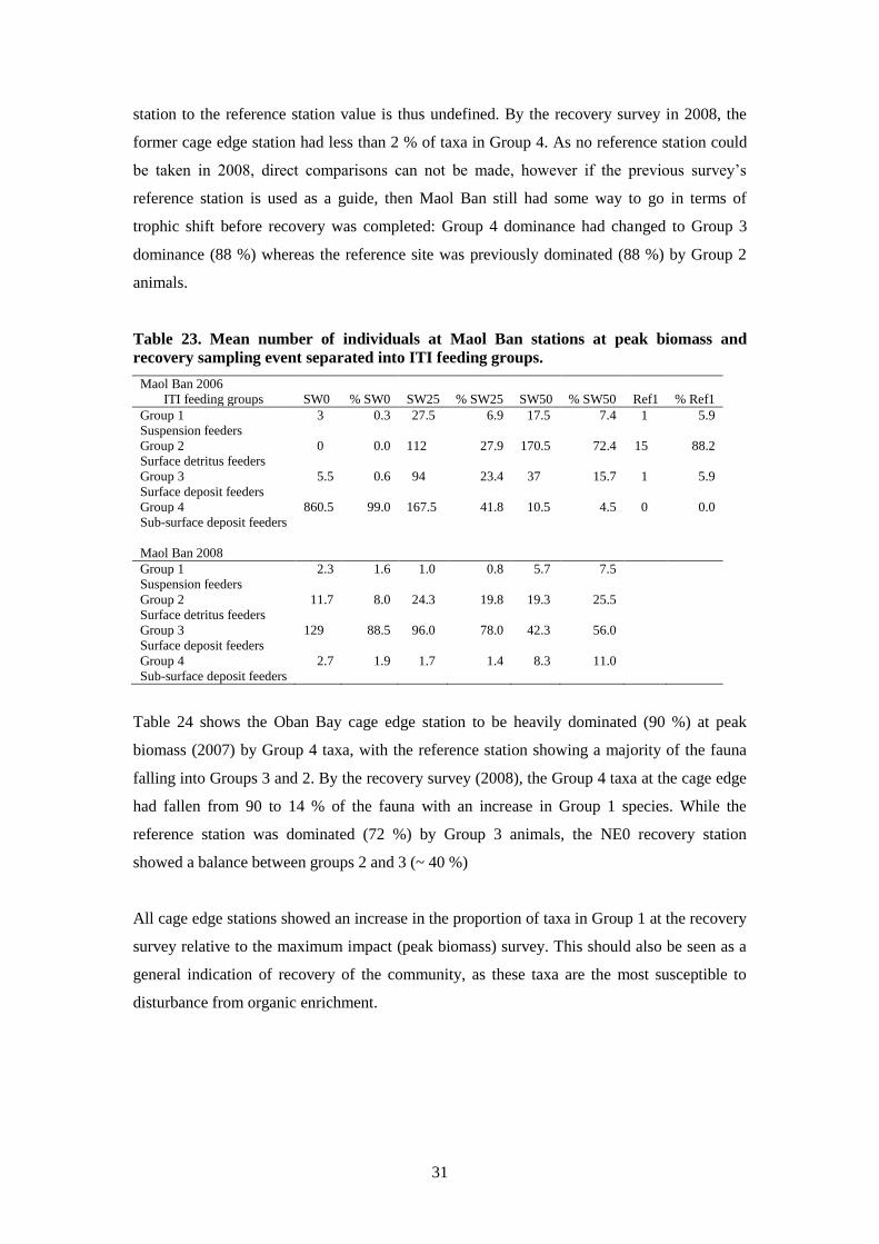
At Maol Ban during peak biomass (2007), the benthic cage edge community was comprised

overwhelmingly (99 %) of Group 4 taxa, while the reference community had no taxa in

Group 4, the majority being Group 2 feeders (Table 23). The ratio of Group 4 taxa at each

31

station to the reference station value is thus undefined. By the recovery survey in 2008, the

former cage edge station had less than 2 % of taxa in Group 4. As no reference station could

be taken in 2008, direct comparisons can not be made, however if the previous survey‟s

reference station is used as a guide, then Maol Ban still had some way to go in terms of

trophic shift before recovery was completed: Group 4 dominance had changed to Group 3

dominance (88 %) whereas the reference site was previously dominated (88 %) by Group 2

animals.

Table 23. Mean number of individuals at Maol Ban stations at peak biomass and


Maol Ban 2006

ITI feeding groups SW0 % SW0 SW25 % SW25 SW50 % SW50 Ref1 % Ref1

Group 1 3 0.3 27.5 6.9 17.5 7.4 1 5.9

Suspension feeders

Group 2 0 0.0 112 27.9 170.5 72.4 15 88.2


Group 3 5.5 0.6 94 23.4 37 15.7 1 5.9


Group 4 860.5 99.0 167.5 41.8 10.5 4.5 0 0.0


Maol Ban 2008

Group 1 2.3 1.6 1.0 0.8 5.7 7.5

Suspension feeders

Group 2 11.7 8.0 24.3 19.8 19.3 25.5


Group 3 129 88.5 96.0 78.0 42.3 56.0


Group 4 2.7 1.9 1.7 1.4 8.3 11.0


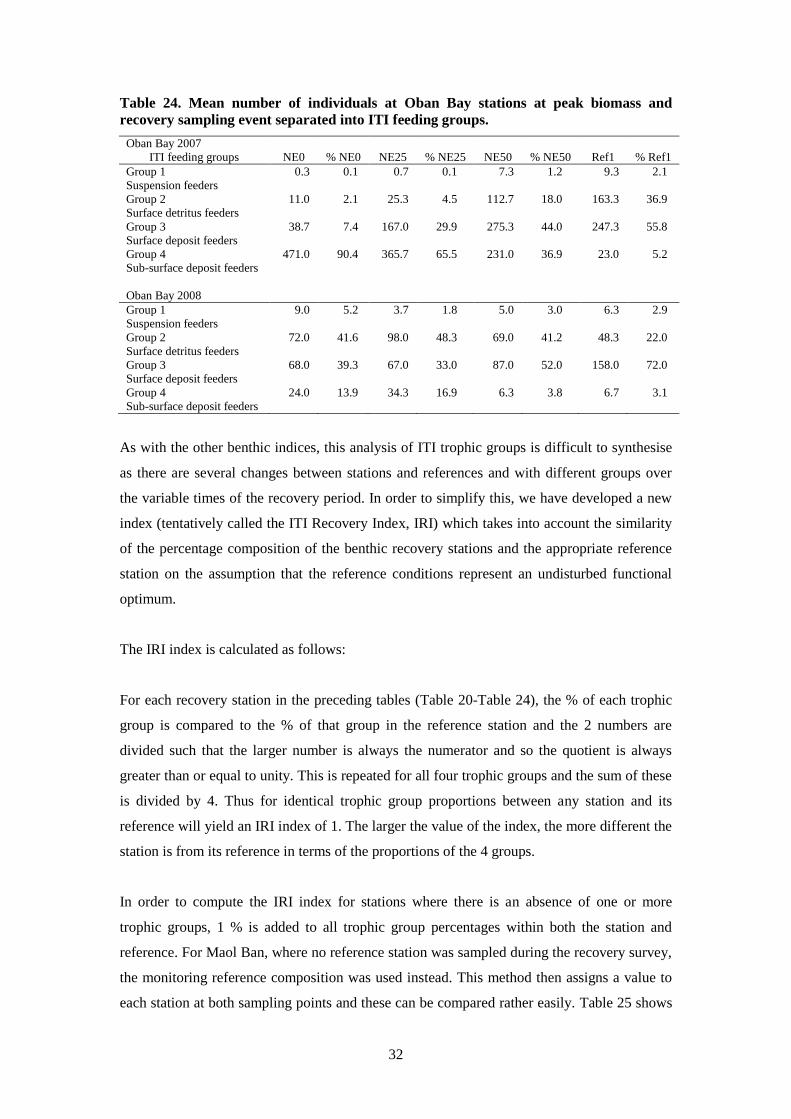
Table 24 shows the Oban Bay cage edge station to be heavily dominated (90 %) at peak

biomass (2007) by Group 4 taxa, with the reference station showing a majority of the fauna

falling into Groups 3 and 2. By the recovery survey (2008), the Group 4 taxa at the cage edge

had fallen from 90 to 14 % of the fauna with an increase in Group 1 species. While the

reference station was dominated (72 %) by Group 3 animals, the NE0 recovery station

showed a balance between groups 2 and 3 (~ 40 %)

All cage edge stations showed an increase in the proportion of taxa in Group 1 at the recovery

survey relative to the maximum impact (peak biomass) survey. This should also be seen as a

general indication of recovery of the community, as these taxa are the most susceptible to

disturbance from organic enrichment.

32

Table 24. Mean number of individuals at Oban Bay stations at peak biomass and


Oban Bay 2007

ITI feeding groups NE0 % NE0 NE25 % NE25 NE50 % NE50 Ref1 % Ref1

Group 1 0.3 0.1 0.7 0.1 7.3 1.2 9.3 2.1

Suspension feeders

Group 2 11.0 2.1 25.3 4.5 112.7 18.0 163.3 36.9


Group 3 38.7 7.4 167.0 29.9 275.3 44.0 247.3 55.8


Group 4 471.0 90.4 365.7 65.5 231.0 36.9 23.0 5.2


Oban Bay 2008

Group 1 9.0 5.2 3.7 1.8 5.0 3.0 6.3 2.9

Suspension feeders

Group 2 72.0 41.6 98.0 48.3 69.0 41.2 48.3 22.0


Group 3 68.0 39.3 67.0 33.0 87.0 52.0 158.0 72.0


Group 4 24.0 13.9 34.3 16.9 6.3 3.8 6.7 3.1


As with the other benthic indices, this analysis of ITI trophic groups is difficult to synthesise

as there are several changes between stations and references and with different groups over

the variable times of the recovery period. In order to simplify this, we have developed a new

index (tentatively called the ITI Recovery Index, IRI) which takes into account the similarity

of the percentage composition of the benthic recovery stations and the appropriate reference

station on the assumption that the reference conditions represent an undisturbed functional

optimum.

The IRI index is calculated as follows:

For each recovery station in the preceding tables (Table 20-Table 24), the % of each trophic

group is compared to the % of that group in the reference station and the 2 numbers are

divided such that the larger number is always the numerator and so the quotient is always

greater than or equal to unity. This is repeated for all four trophic groups and the sum of these

is divided by 4. Thus for identical trophic group proportions between any station and its

reference will yield an IRI index of 1. The larger the value of the index, the more different the

station is from its reference in terms of the proportions of the 4 groups.

In order to compute the IRI index for stations where there is an absence of one or more

trophic groups, 1 % is added to all trophic group percentages within both the station and

reference. For Maol Ban, where no reference station was sampled during the recovery survey,

the monitoring reference composition was used instead. This method then assigns a value to

each station at both sampling points and these can be compared rather easily. Table 25 shows

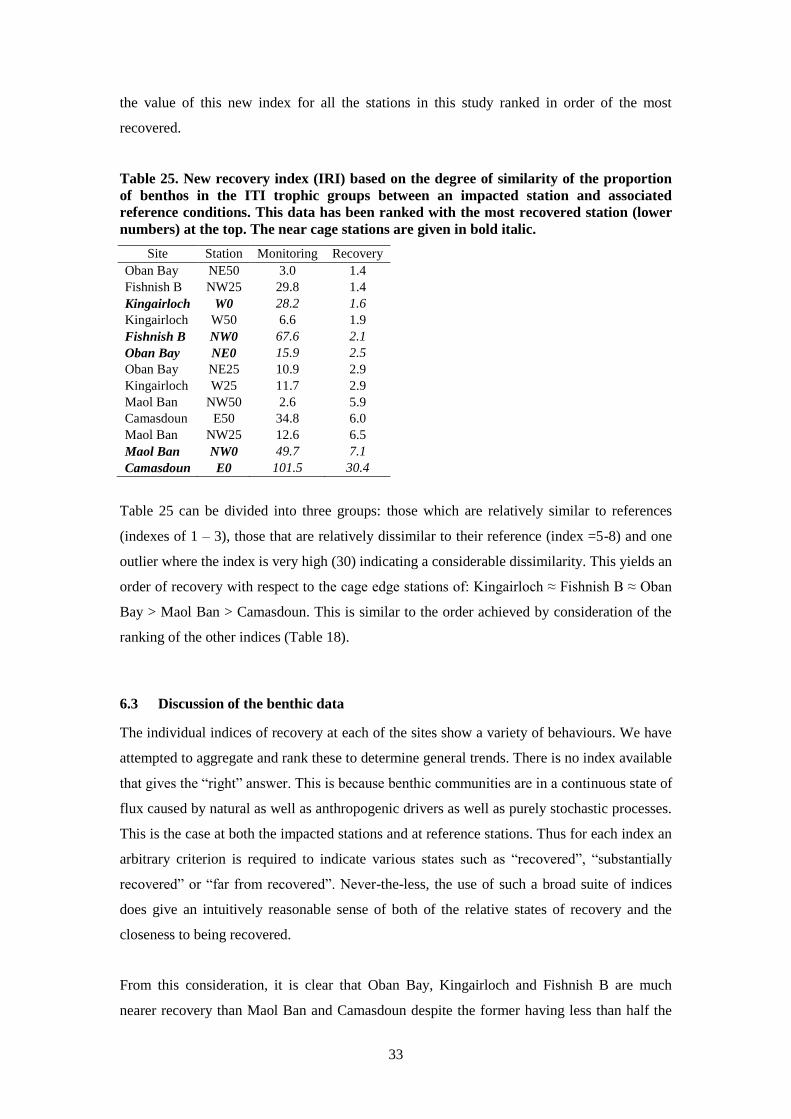
33

the value of this new index for all the stations in this study ranked in order of the most

recovered.

Table 25. New recovery index (IRI) based on the degree of similarity of the proportion

of benthos in the ITI trophic groups between an impacted station and associated

reference conditions. This data has been ranked with the most recovered station (lower

numbers) at the top. The near cage stations are given in bold italic.

Site Station Monitoring Recovery

Oban Bay NE50 3.0 1.4

Fishnish B NW25 29.8 1.4

Kingairloch W0 28.2 1.6


Fishnish B NW0 67.6 2.1




Maol Ban NW50 2.6 5.9

Camasdoun E50 34.8 6.0



Camasdoun E0 101.5 30.4

Table 25 can be divided into three groups: those which are relatively similar to references

(indexes of 1 – 3), those that are relatively dissimilar to their reference (index =5-8) and one

outlier where the index is very high (30) indicating a considerable dissimilarity. This yields an

order of recovery with respect to the cage edge stations of: Kingairloch ≈ Fishnish B ≈ Oban

Bay > Maol Ban > Camasdoun. This is similar to the order achieved by consideration of the

ranking of the other indices (Table 18).

6.3 Discussion of the benthic data

The individual indices of recovery at each of the sites show a variety of behaviours. We have

attempted to aggregate and rank these to determine general trends. There is no index available

that gives the “right” answer. This is because benthic communities are in a continuous state of

flux caused by natural as well as anthropogenic drivers as well as purely stochastic processes.

This is the case at both the impacted stations and at reference stations. Thus for each index an

arbitrary criterion is required to indicate various states such as “recovered”, “substantially

recovered” or “far from recovered”. Never-the-less, the use of such a broad suite of indices

does give an intuitively reasonable sense of both of the relative states of recovery and the

closeness to being recovered.

From this consideration, it is clear that Oban Bay, Kingairloch and Fishnish B are much

nearer recovery than Maol Ban and Camasdoun despite the former having less than half the

34

recovery period than the latter. Most interestingly, when we rank the sites by the values of the

indices at the peak biomass survey, to test the hypothesis that sites with a higher impact take

longer to recover (and vice versa) we find that the opposite appears to be the case.

Thus we have two seemingly counter-intuitive conclusions from analysis of these data:

1. site recovery seemed to be less complete at sites which were sampled ca. 2 years after

cessation of farming compared to sites sampled after only one year.

2. site recovery appears greater at the sites with highest monitoring survey benthic impacts

and lower at those sites where the monitoring survey benthic impacts were lower.

As these two conclusions refer to the same sites a composite can be made:

3. The studied sites fell into 2 categories: those that had high initial impacts but recovered


recovery after 2 years.

The sediment copper levels encountered in the present study (381 µg g-1

at Oban Bay; 128 µg

g-1

at Camasdoun) compare with the maximum of 805 µg g-1

found by Dean et al. (2007) in

their study of a Scottish fish farm site. These authors attributed the high concentrations to the

use of copper-based antifoulants and possibly from feed; Brooks and co-workers (Brooks and

Mahnken, 2003; Brooks et al., 2004) observed these metal concentrations decline to reference

values during recovery in their studies of Canadian Pacific salmon farming. Background

values of copper were calculated by Taylor (1964) at 55 µg g-1

; this compares with the 44 µg

g-1

found by Nickell and Anderson (1997) in their study of distillery effluent in Loch

Harport.

Finally, and this will be important in the second modelling approach, concentrations of

organic matter were much higher in sediments at Camasdoun and Maol Ban cage edge

stations than at the other 3 sites.

35

7 Modelling approach 1 –the Findlay-Watling approach.

7.1 Modelling approach

To determine performance of the existing DEPOMOD model for each of the study sites, the

model was used to predict flux and Infaunal Trophic Index (ITI) at each station at the time of

the monitoring survey for each of the five study sites. This allowed verification of benthic

impact predictions for each site by comparing predicted with observed ITI for each station.

The Findlay-Watling Index (Findlay and Watling, 1997; Morrisey et al., 2000) (denoted FWI

hereafter) was then developed in the model and FWI predictions obtained throughout most of

the production cycle and recovery period. The FWI is the ratio between oxygen supply to the

sediments from near bottom waters and oxygen demand arising from degradation of fish farm

wastes in the sediments. Where oxygen supply is less than demand, FWI is less than 1 and

this causes an oxygen stress on the benthic community and high impact. A FWI of around 1

was found to indicate moderate impact. Oxygen demand was determined from a relationship

between observed carbon flux to the sediments and associated oxygen demand (Findlay and

Watling, 1997; Morrisey et al., 2000). Both of these studies determined oxygen supply from

Fickian diffusion associated with current velocity, temperature and oxygen concentration in

near-bed flow. From current velocity data, the minimum 2 hour average was used as exposure

to reduced oxygen and elevated hydrogen sulphide over 2 hours was hypothesised to results

in permanent damage to gill tissue and thus significant changes to the benthic community.

Thus, Findlay and Watling (1997) and Morrissey et al. (2000) determined only 1 value of the

FWI for each station, based on maximum carbon flux and the minimum 2 hour average of

near bed current.

In our study, we modified the method for calculating oxygen demand and supply, but retained

the principle of the FWI as the ratio of oxygen supply to demand. Oxygen demand was

determined using a relationship between oxygen and carbon degradation, determined using

the first order G-model within DEPOMOD (Westrich and Berner, 1984). Recently measured

fractions and decay rates of salmonid feed and faeces were used (Attard, 2010). In our initial

modelling, we found the minimum 2 hour average to be inappropriate for estimating oxygen

supply, as this statistic is dependent on the details of the current meter deployment

(instrument type (accuracy and minimum threshold), sampling frequency and height above

the bed of deployment). In our initial modelling, we found the minimum 2 hour average to be

inappropriate for estimating oxygen supply, as this statistic is dependent on the details of the

current meter deployment (instrument type - accuracy and minimum threshold, sampling

36

frequency and height above the bed of deployment). In particular, this statistic is influenced

by the high incidence of zeros in a current record obtained with a high threshold current

meter. We overcame this by developing a method which used hourly current data for

calculcation of oxygen supply, rather than a single statistic which was biased by a high

number of zeros in the record. Oxygen supply is calculated from near bed current speed

(Findlay and Watling, 1997), but current is usually measured at different heights above the

bed between sites. Thus, we fitted a logarithmic profile to the measured near-bed current to

determine velocity at 1 cm above the bed, before using the relationships described in Findlay

and Watling (1997). These improvements over the Findlay and Watling method helped to

overcome the sensitivity of the calculation of oxygen supply to instrument type and height

above the bed of deployment. A further improvement we made was to determine the FWI for

each hour throughout most of the production cycle and post fallow period, so that trends in

the FWI could be correlated with benthic impact at the time of monitoring survey, and rate of

recovery for each site.

Thus, the objectives of the modelling were to:

1. verify predictions of benthic impact with observations using ITI - the standard data set of

information collected for each site as part of the regulatory process was used

2. determine whether predictions of FWI correlate with observed benthic impact measured at

the time of the monitoring survey

3. determine if trends in the FWI during both the production cycle and the fallow period

correlate with the rate of benthic recovery of sites after cessation of farming.

We undertook modifications to the DEPOMOD code, included new model parameters in the

G-model and used benthic faunal data from the project surveys. However, to assist with

further application of the model, we largely used site-specific data and model parameters used

in the regulatory process. Revised resuspension model parameters were used (vr ≈ 15 cm s-1

),

primarily influencing predictions at the dispersive site Fishnish B.

7.2 Method

Site specific model input data

Information supplied by the operators for each study was mostly in the form of pre-prepared

data sets used in consent modelling. e.g. current meter data (surface, mid-water and near-bed),

37

bathymetry and cage layouts. For each site, operators supplied monthly biomass and feed

input data for the duration of the production cycle of interest.

Default model input data

Mainly the standard set of model parameters used in regulatory modelling was used as

described in SEPA (2005). The exceptions were the resuspension model settings and water

content of the feed (this was set to 4 % when the G-model was in use following the

experiments of Attard (2010)). All model runs were undertaken with resuspension model

switched on and the revised set of resuspension model parameters (vr ≈ 15 cm s-1

). This

threshold for erosion is higher than the threshold currently used in regulatory modelling, and

this primarily affected Fishnish B (Table 30) by eroding less from the deposition footprint.

Model validation

(i) AutoDEPOMOD benthic module – ITI predictions and observations at time of monitoring

survey

To predict impact at the time of the monitoring survey, benthic fauna monitoring reports

submitted to SEPA were used to determine actual cage layouts and sampling station positions

which were input to AutoDEPOMOD. Three month average feed input was specified by

switching AutoDistribute off and adjusting SFR appropriately. Perform Single Run function

was used so that a single run was undertaken using the feed input at the time of monitoring

survey. No empty cages were modelled.

Predictions of flux and ITI were obtained from the AutoDEPOMOD mapping module

function for the actual sampling station positions at the time of monitoring survey.

Comparisons were then made with observations of ITI taken from benthic fauna monitoring

reports using an average ITI of duplicates where appropriate.

(ii) Findlay-Watling index (FWI) – suitability as indicator of impact and site recovery

To determine whether a relationship existed between FWI and observed benthic impact

and/or rate of recovery, DEPOMOD was set up to undertake lengthy runs for the production

cycle and fallow period. For the month of the monitoring survey, a monthly average for FWI

was determined for each station and compared with observed ITI. Thus, in the model, the

value of FWI would be influenced by the quantity and lability of waste material on the bed

and associated oxygen demand, and so was expected to be a useful indicator of impact.

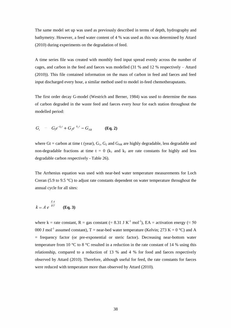
38

The same model set up was used as previously described in terms of depth, hydrography and

bathymetry. However, a feed water content of 4 % was used as this was determined by Attard

(2010) during experiments on the degradation of feed.

A time series file was created with monthly feed input spread evenly across the number of

cages, and carbon in the feed and faeces was modelled (31 % and 12 % respectively – Attard

(2010)). This file contained information on the mass of carbon in feed and faeces and feed

input discharged every hour, a similar method used to model in-feed chemotheraputants.

The first order decay G-model (Westrich and Berner, 1984) was used to determine the mass

of carbon degraded in the waste feed and faeces every hour for each station throughout the

modelled period:

Gt G1ek1t G2e

k2 tGNR (Eq. 2)

where Gt = carbon at time t (year), G1, G2 and GNR are highly degradable, less degradable and

non-degradable fractions at time t = 0 (k1 and k2 are rate constants for highly and less

degradable carbon respectively - Table 26).

The Arrhenius equation was used with near-bed water temperature measurements for Loch

Creran (5.9 to 9.5 °C) to adjust rate constants dependent on water temperature throughout the

annual cycle for all sites:

k A e

E A

RT (Eq. 3)

where k = rate constant, R = gas constant (= 8.31 J K-1

mol-1

), EA = activation energy (≈ 50

000 J mol-1

assumed constant), T = near-bed water temperature (Kelvin; 273 K = 0 °C) and A

= frequency factor (or pre-exponential or steric factor). Decreasing near-bottom water

temperature from 10 °C to 8 °C resulted in a reduction in the rate constant of 14 % using this

relationship, compared to a reduction of 13 % and 4 % for food and faeces respectively

observed by Attard (2010). Therefore, although useful for feed, the rate constants for faeces

were reduced with temperature more than observed by Attard (2010).

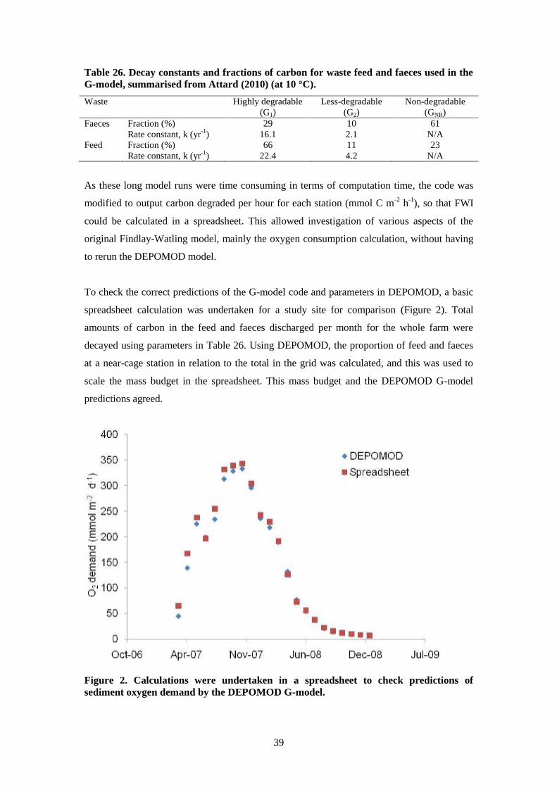
39

Table 26. Decay constants and fractions of carbon for waste feed and faeces used in the

G-model, summarised from Attard (2010) (at 10 °C).

Waste Highly degradable

(G1)

Less-degradable

(G2)

Non-degradable

(GNR)

Faeces

Fraction (%)

Rate constant, k (yr-1

)

29

16.1

10

2.1

61

N/A

Feed

Fraction (%)

Rate constant, k (yr-1

)

66

22.4

11

4.2

23

N/A

As these long model runs were time consuming in terms of computation time, the code was

modified to output carbon degraded per hour for each station (mmol C m-2

h-1

), so that FWI

could be calculated in a spreadsheet. This allowed investigation of various aspects of the

original Findlay-Watling model, mainly the oxygen consumption calculation, without having

to rerun the DEPOMOD model.

To check the correct predictions of the G-model code and parameters in DEPOMOD, a basic

spreadsheet calculation was undertaken for a study site for comparison (Figure 2). Total

amounts of carbon in the feed and faeces discharged per month for the whole farm were

decayed using parameters in Table 26. Using DEPOMOD, the proportion of feed and faeces

at a near-cage station in relation to the total in the grid was calculated, and this was used to

scale the mass budget in the spreadsheet. This mass budget and the DEPOMOD G-model

predictions agreed.

Figure 2. Calculations were undertaken in a spreadsheet to check predictions of

sediment oxygen demand by the DEPOMOD G-model.

40

To calculate sediment oxygen demand resulting from the decay of carbon in the waste feed

and faeces on the bed, 1 mmol C m-2

h-1

requires 1 mmol O2 m-2

h-1

. This was adjusted using a

respiratory quotient of 0.9, so that 0.9 mmol C m-2

h-1

required 1 mmol O2 m-2

h-1

. The was

based on consideration of Hansen and Blackburn (1992) (but see concluding comments on

proposed further work). Findlay and Watling (1997) calculated oxygen differently, using an

empirical relationship between oxygen demand and carbon flux to the sediments measured

with sediment traps. Our method makes use of recently determined decay constants (Attard,

2010) as well as predicting FWI throughout the production cycle and recovery period. Findlay

and Watling (1997) determine one value of the index only, using measured carbon flux at the

time of maximum biomass. Although we did not validate the sediment oxygen demand

predictions for each site, the predictions at the time of benthic monitoring survey were found

to agree with literature studies for near-cage stations at finfish farms (Figure 3).

Figure 3. Predicted sediment oxygen demand for the study sites compared with

measured rates in the literature.

We determined oxygen supply using an empirical relationship (Findlay and Watling, 1997;

Morrisey et al., 2000) which they had derived from Jørgensen and Des Marais (1990):

Oxygen Supply (mmol m 2 h 1) (736.3 672.6 log(u)) /24 (Eq. 4)

41

where u is near-bed current velocity. However, we standardised near-bed current by fitting a

logarithmic profile and calculating near bed velocity at a height of 0.01 m, as this height was

consistent with the data presented in the experiments by Jørgensen and Des Marais (1990) on

which Findlay and Watling (1997) depended:5

U *u(z,t)

ln (z zo) (Eq. 5)

where U* = shear velocity, u(z,t) = current velocity at height above the bed z and time t, κ =

von Kàrmàn constant (= 0.4) and zo is bed roughness (= 0.0002 m (Soulsby, 1983)). Using

this equation, u* was calculated for each hour and then u (z=0.01 m, t) was calculated by

rearranging Equation 5. Thus, a time series of near-bed current velocity at z = 0.01 m for each

site was used to calculate oxygen supply for each hour. Bed roughness was not varied

between sites.

Thus, using predictions of oxygen demand and supply the Findlay-Watling index was

calculated on an hourly basis:

FWIOxygen supply

Oxygen demand (Eq. 6)

Our method predicted oxygen supply and demand for each hour, resulting in an hourly value

of FWI throughout the modelled period. Although we do not expect the model to predict

accurately the balance between oxygen supply and demand on such a high temporal scale, it

does allow averaging of FWI for a particular month. This approach is in contrast to Findlay

and Watling‟s (1997) study, where a minimum 2 hour average current velocity is used to

determine oxygen supply resulting in one value of FWI only for each site.

To validate predictions of FWI as an indicator of impact, FWI was calculated for the month of

the benthic monitoring survey for each station and compared with observed ITI. To

investigate FWI as an indicator of potential for recovery the following were investigated for

cage-edge stations:

5 It appears that Findlay and Watling (and therefore subsequently Morrisey et al. (2000)) used current speeds at 1

m above the bed while using a relationship given by Jørgensen and Des Marais (1990) that had measured diffusive

oxygen fluxes in the mm scale diffusive boundary layer using currents measured at 1 cm above the bed. In the

present study we have driven the oxygen supply model using the relationships given in the Jørgensen and Des

Marais (1990) study.

42

(i) monthly averages of FWI throughout the production cycle and fallow period, as this may

indicate the general balance of demand and supply for a site.

(ii) the number of consecutive 2 hour periods where FWI was less than 1, as this may also

indicate prolonged periods of oxygen stress and may be related to potential for recovery.

(iii) the rate at which the FWI increases after cessation of farming. i.e. if FWI increases

rapidly then this indicates that oxygen supply far exceeds demand and may be a contributing

factor to the potential for a site to recover.

7.3 Calculation of FWI using the method in Findlay and Watling (1997) and

comparison with observed ITI

7.3.1 Method

Morrisey et al. (2000) stated a limitation of FWI as calculated in Findlay and Watling (1997)

to be over reliance on a single value of the minimum 2 hour average near-bed current velocity

calculated for each site. We also note, that the relationship between oxygen demand and

carbon flux results in zero oxygen demand for low carbon flux (< 130 g C m-2

yr-1

; < 800 g

solid m-2

yr-1

). This means that using the method in Findlay and Watling (1997) would result

in zero oxygen demand at some of our intermediate stations. In addition, for two of our sites

the minimum 2 hour average is less than 0.1 cm s-1

, resulting in zero oxygen supply from the

Findlay and Watling (1997) relationship. Therefore, to test these limitations, we predicted

FWI using the method of Findlay and Watling (1997) to determine if the index correlated

with observed ITI at the time of monitoring survey.

Predictions of solids flux at each station were taken from AutoDEPOMOD as previously

described. As AutoDEPOMOD predicts solids and not carbon, to calculate carbon flux from

solids flux a factor of 0.152 was applied. This takes account of the expected proportions of

feed and faeces at each station, and also the carbon fractions of feed and faeces. This

approach however, does not vary proportions of feed and faeces between near-cage and far-

field stations.

Carbon flux was converted to mmol m-2

d-1

and oxygen demand calculated from Findlay and

Watling (1997) (oxygen demand = 1.1*carbon flux – 32.6). FWI was calculated as previously

described and compared with observed ITI for each station at the time of monitoring survey.

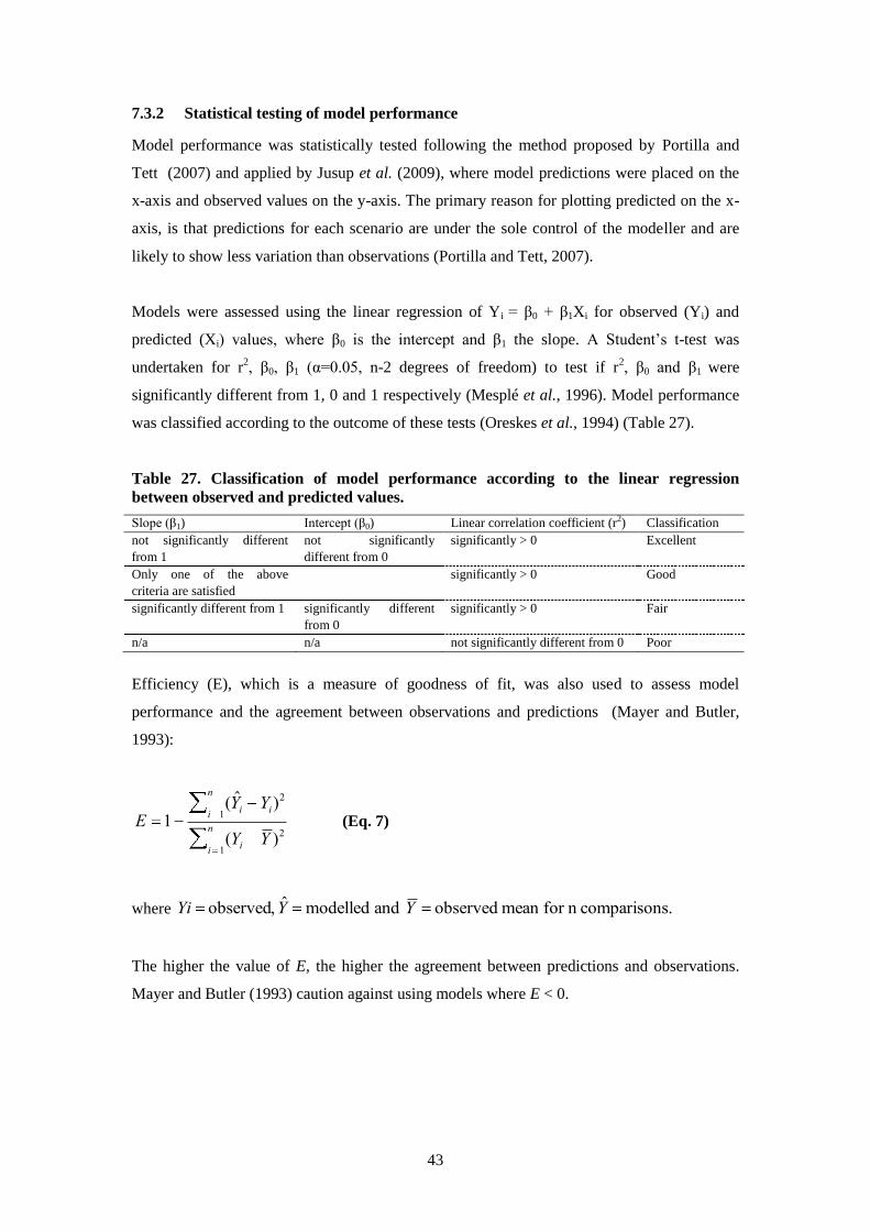
43

7.3.2 Statistical testing of model performance

Model performance was statistically tested following the method proposed by Portilla and

Tett (2007) and applied by Jusup et al. (2009), where model predictions were placed on the

x-axis and observed values on the y-axis. The primary reason for plotting predicted on the x-

axis, is that predictions for each scenario are under the sole control of the modeller and are

likely to show less variation than observations (Portilla and Tett, 2007).

Models were assessed using the linear regression of Yi = β0 + β1Xi for observed (Yi) and

predicted (Xi) values, where β0 is the intercept and β1 the slope. A Student‟s t-test was

undertaken for r2, β0, β1 (α=0.05, n-2 degrees of freedom) to test if r

2, β0 and β1 were

significantly different from 1, 0 and 1 respectively (Mesplé et al., 1996). Model performance

was classified according to the outcome of these tests (Oreskes et al., 1994) (Table 27).

Table 27. Classification of model performance according to the linear regression

between observed and predicted values.

Slope (β1) Intercept (β0) Linear correlation coefficient (r2) Classification

not significantly different

from 1

not significantly

different from 0

significantly > 0 Excellent

Only one of the above

criteria are satisfied

significantly > 0 Good

significantly different from 1 significantly different

from 0

significantly > 0 Fair

n/a n/a not significantly different from 0 Poor

Efficiency (E), which is a measure of goodness of fit, was also used to assess model

performance and the agreement between observations and predictions (Mayer and Butler,

1993):

E 1( ˆ Y i Yi)

2

i 1

n

(Yi Y )2

i 1

n (Eq. 7)

where Yi observed, ˆ Y modelled and Y observed mean for n comparisons.

The higher the value of E, the higher the agreement between predictions and observations.

Mayer and Butler (1993) caution against using models where E < 0.

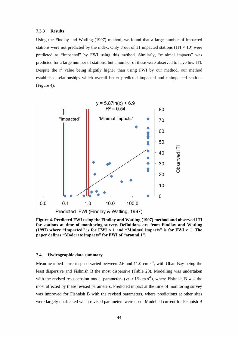
44

7.3.3 Results

Using the Findlay and Watling (1997) method, we found that a large number of impacted

stations were not predicted by the index. Only 3 out of 11 impacted stations (ITI ≤ 10) were

predicted as “impacted” by FWI using this method. Similarly, “minimal impacts” was

predicted for a large number of stations, but a number of these were observed to have low ITI.

Despite the r2 value being slightly higher than using FWI by our method, our method

established relationships which overall better predicted impacted and unimpacted stations

(Figure 4).

Figure 4. Predicted FWI using the Findlay and Watling (1997) method and observed ITI

for stations at time of monitoring survey. Definitions are from Findlay and Watling

(1997) where “Impacted” is for FWI < 1 and “Minimal impacts” is for FWI > 1. The

paper defines “Moderate impacts” for FWI of “around 1”.

7.4 Hydrographic data summary

Mean near-bed current speed varied between 2.6 and 11.0 cm s-1

, with Oban Bay being the

least dispersive and Fishnish B the most dispersive (Table 28). Modelling was undertaken

with the revised resuspension model parameters (vr ≈ 15 cm s-1

), where Fishnish B was the

most affected by these revised parameters. Predicted impact at the time of monitoring survey

was improved for Fishnish B with the revised parameters, where predictions at other sites

were largely unaffected when revised parameters were used. Modelled current for Fishnish B

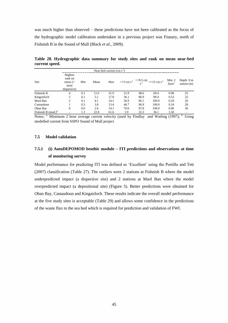
45

was much higher than observed – these predictions have not been calibrated as the focus of

the hydrographic model calibration undertaken in a previous project was Fiunary, north of

Fishnish B in the Sound of Mull (Black et al., 2009).

Table 28. Hydrographic data summary for study sites and rank on mean near-bed

current speed.

Near-bed current (cm s-1)

Site

Highest

rank on

mean (= most

dispersive)

Min Mean Max <=3 cm s-1 <=9.5 cm

s-1 <=15 cm s-1

Min. 2

houra

Depth 0 m

station (m)

Fishnish B 4 0.1 11.0 31.9 21.9 48.6 69.4 0.08 25

Kingairloch 3 0.1 5.1 17.8 36.1 86.9 99.4 0.53 22

Maol Ban 2 0.1 4.1 14.1 36.9 96.1 100.0 0.29 26

Camasdoun 1 0.3 3.8 13.4 46.7 96.9 100.0 0.24 28

Oban Bay 0 0.0 2.6 14.1 70.6 97.8 100.0 0.00 30

Fishnish B (mod.)b - 1.3 22.8 61.6 1.9 22.2 36.1 3.30 -

Notes: a. Minimum 2 hour average current velocity (used by Findlay and Watling (1997);

b. Using

modelled current from SSPO Sound of Mull project

7.5 Model validation

7.5.1 (i) AutoDEPOMOD benthic module – ITI predictions and observations at time

of monitoring survey

Model performance for predicting ITI was defined as „Excellent‟ using the Portilla and Tett

(2007) classification (Table 27). The outliers were 2 stations at Fishnish B where the model

underpredicted impact (a dispersive site) and 2 stations at Maol Ban where the model

overpredicted impact (a depositional site) (Figure 5). Better predictions were obtained for

Oban Bay, Camasdoun and Kingairloch. These results indicate the overall model performance

at the five study sites is acceptable (Table 29) and allows some confidence in the predictions

of the waste flux to the sea bed which is required for prediction and validation of FWI.

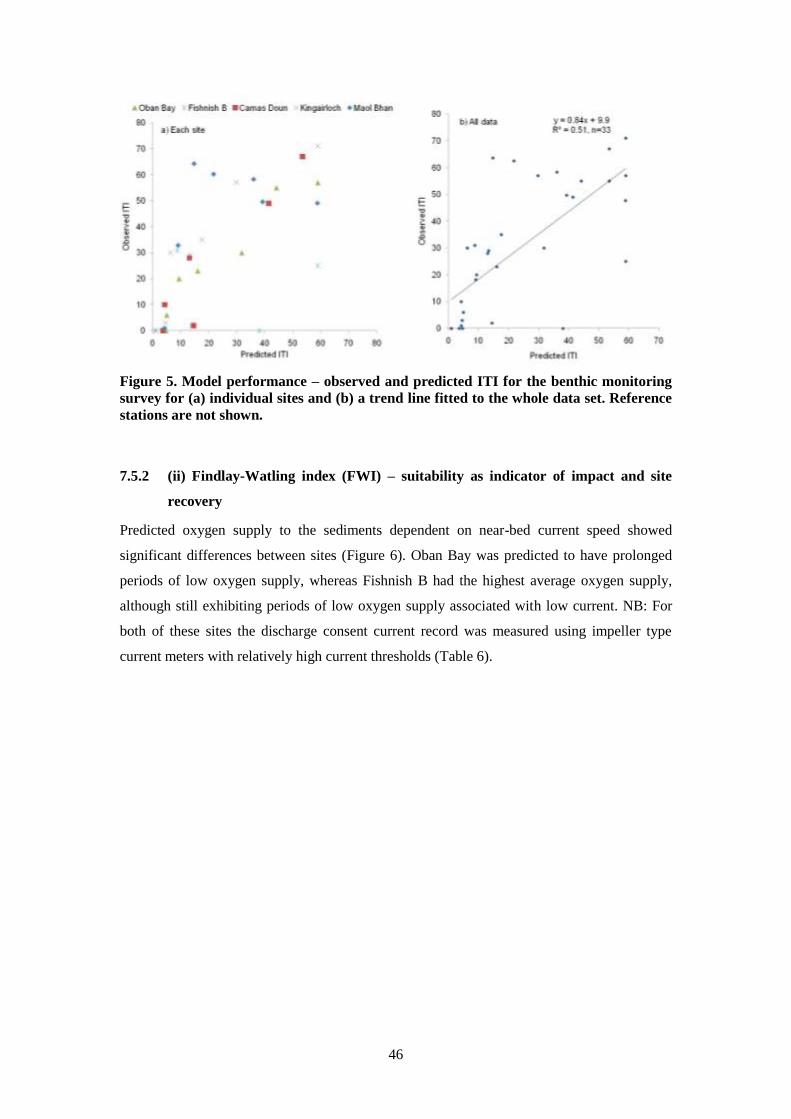
46

Figure 5. Model performance – observed and predicted ITI for the benthic monitoring

survey for (a) individual sites and (b) a trend line fitted to the whole data set. Reference

stations are not shown.

7.5.2 (ii) Findlay-Watling index (FWI) – suitability as indicator of impact and site

recovery

Predicted oxygen supply to the sediments dependent on near-bed current speed showed

significant differences between sites (Figure 6). Oban Bay was predicted to have prolonged

periods of low oxygen supply, whereas Fishnish B had the highest average oxygen supply,

although still exhibiting periods of low oxygen supply associated with low current. NB: For

both of these sites the discharge consent current record was measured using impeller type

current meters with relatively high current thresholds (Table 6).

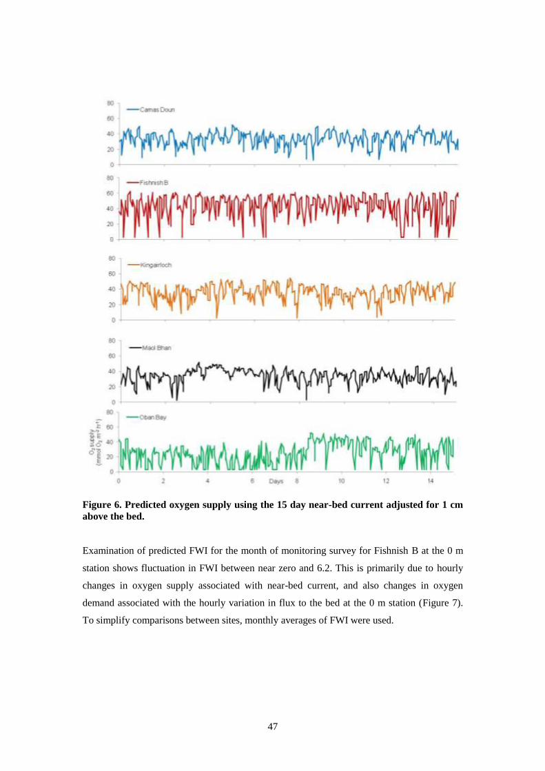
47

Figure 6. Predicted oxygen supply using the 15 day near-bed current adjusted for 1 cm

above the bed.

Examination of predicted FWI for the month of monitoring survey for Fishnish B at the 0 m

station shows fluctuation in FWI between near zero and 6.2. This is primarily due to hourly

changes in oxygen supply associated with near-bed current, and also changes in oxygen

demand associated with the hourly variation in flux to the bed at the 0 m station (Figure 7).

To simplify comparisons between sites, monthly averages of FWI were used.

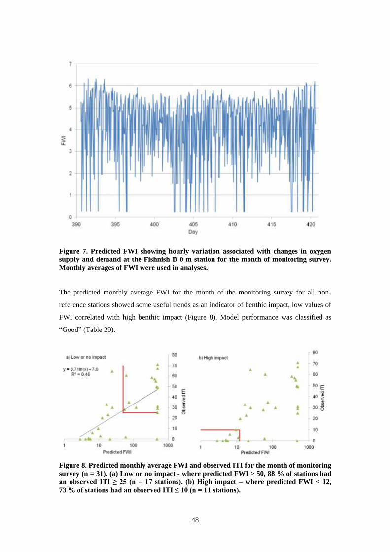
48

Figure 7. Predicted FWI showing hourly variation associated with changes in oxygen

supply and demand at the Fishnish B 0 m station for the month of monitoring survey.

Monthly averages of FWI were used in analyses.

The predicted monthly average FWI for the month of the monitoring survey for all non-

reference stations showed some useful trends as an indicator of benthic impact, low values of

FWI correlated with high benthic impact (Figure 8). Model performance was classified as

“Good” (Table 29).

Figure 8. Predicted monthly average FWI and observed ITI for the month of monitoring

survey (n = 31). (a) Low or no impact - where predicted FWI > 50, 88 % of stations had

an observed ITI ≥ 25 (n = 17 stations). (b) High impact – where predicted FWI < 12,

73 % of stations had an observed ITI ≤ 10 (n = 11 stations).

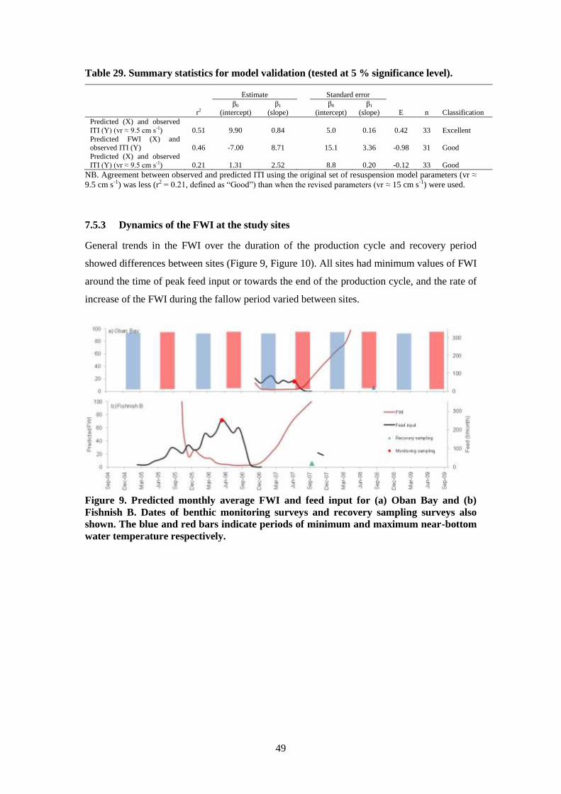
49

Table 29. Summary statistics for model validation (tested at 5 % significance level).

Estimate

Standard error

r2 β0

(intercept) β1

(slope) β0

(intercept) β1

(slope) E n Classification

Predicted (X) and observed

ITI (Y) (vr ≈ 9.5 cm s-1) 0.51 9.90 0.84

5.0 0.16 0.42 33 Excellent

Predicted FWI (X) and observed ITI (Y) 0.46 -7.00 8.71

15.1 3.36 -0.98 31 Good

Predicted (X) and observed

ITI (Y) (vr ≈ 9.5 cm s-1) 0.21 1.31 2.52

8.8 0.20 -0.12 33 Good

NB. Agreement between observed and predicted ITI using the original set of resuspension model parameters (vr ≈

9.5 cm s-1) was less (r2 = 0.21, defined as “Good”) than when the revised parameters (vr ≈ 15 cm s-1) were used.

7.5.3 Dynamics of the FWI at the study sites

General trends in the FWI over the duration of the production cycle and recovery period

showed differences between sites (Figure 9, Figure 10). All sites had minimum values of FWI

around the time of peak feed input or towards the end of the production cycle, and the rate of

increase of the FWI during the fallow period varied between sites.

Figure 9. Predicted monthly average FWI and feed input for (a) Oban Bay and (b)

Fishnish B. Dates of benthic monitoring surveys and recovery sampling surveys also

shown. The blue and red bars indicate periods of minimum and maximum near-bottom

water temperature respectively.

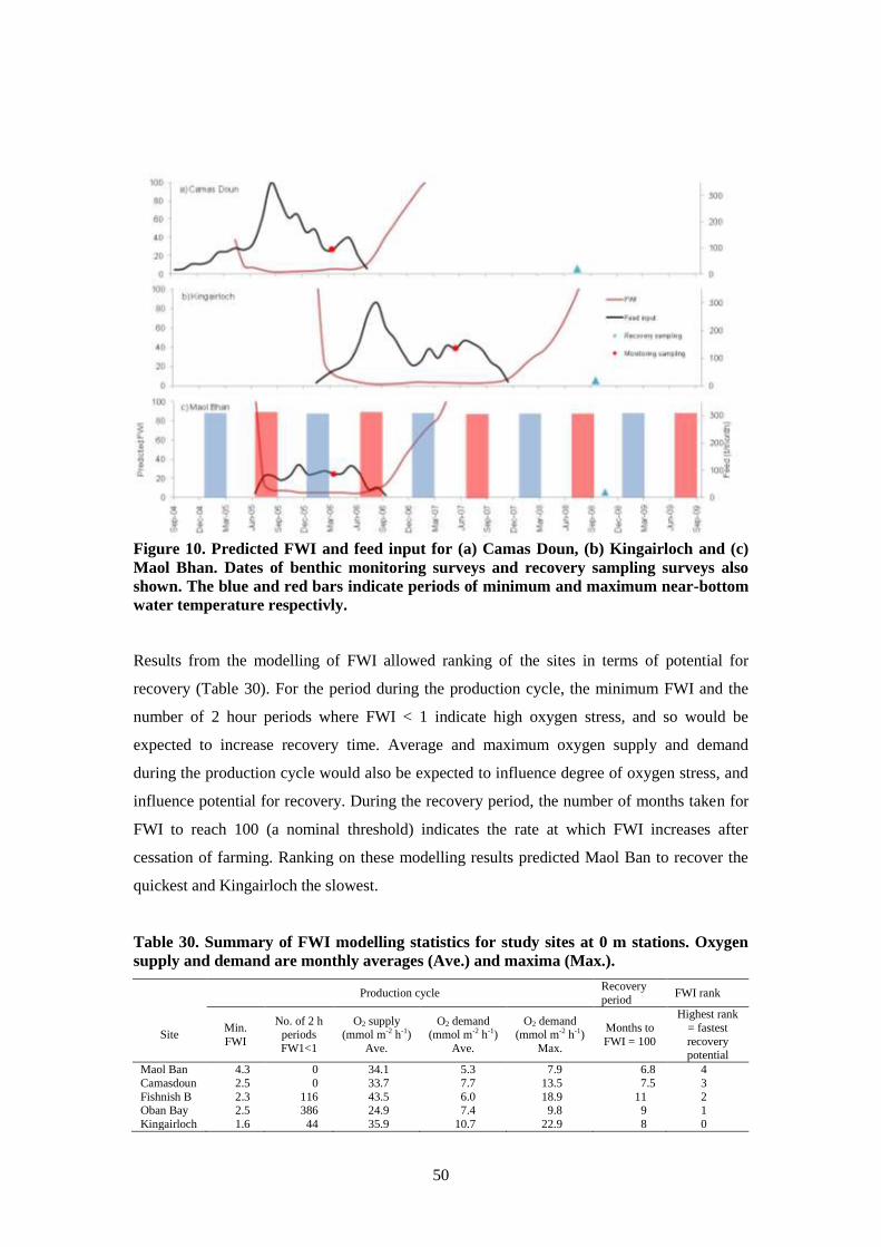
50

Figure 10. Predicted FWI and feed input for (a) Camas Doun, (b) Kingairloch and (c)

Maol Bhan. Dates of benthic monitoring surveys and recovery sampling surveys also

shown. The blue and red bars indicate periods of minimum and maximum near-bottom

water temperature respectivly.

Results from the modelling of FWI allowed ranking of the sites in terms of potential for

recovery (Table 30). For the period during the production cycle, the minimum FWI and the

number of 2 hour periods where FWI < 1 indicate high oxygen stress, and so would be

expected to increase recovery time. Average and maximum oxygen supply and demand

during the production cycle would also be expected to influence degree of oxygen stress, and

influence potential for recovery. During the recovery period, the number of months taken for

FWI to reach 100 (a nominal threshold) indicates the rate at which FWI increases after

cessation of farming. Ranking on these modelling results predicted Maol Ban to recover the

quickest and Kingairloch the slowest.

Table 30. Summary of FWI modelling statistics for study sites at 0 m stations. Oxygen

supply and demand are monthly averages (Ave.) and maxima (Max.).

Production cycle Recovery

period FWI rank

Site Min.

FWI

No. of 2 h periods

FW1<1

O2 supply (mmol m-2 h-1)

Ave.

O2 demand (mmol m-2 h-1)

Ave.

O2 demand (mmol m-2 h-1)

Max.

Months to

FWI = 100

Highest rank

= fastest

recovery potential

Maol Ban 4.3 0 34.1 5.3 7.9 6.8 4

Camasdoun 2.5 0 33.7 7.7 13.5 7.5 3

Fishnish B 2.3 116 43.5 6.0 18.9 11 2 Oban Bay 2.5 386 24.9 7.4 9.8 9 1

Kingairloch 1.6 44 35.9 10.7 22.9 8 0

51

Examination of husbandry and hydrographic data statistics resulted in a different ranking in

terms of recovery (Table 31). The amount of feed used in the production cycle, and the

months between peak feed input and harvest month might be expected to influence recovery

rates (i.e. high feed input just before harvest and cessation of farming might result in slower

recovery). Rank on mean SFR might indicate optimal use of feed during production cycle.

Although Maol Ban was predicted to recover the quickest as with the FWI modelling, a

different rank was achieved by this method with Camasdoun predicted as the slowest to

recover.

Table 31. Husbandry and hydrographic data summary for study sites, ranked in terms

of fastest recovery potential. Feed (tonnes) and mean SFR are for the whole production

cycle.

Mean near-bed

current (cm s-1) Feed (t)

Mean SFR

(% biomass

per day)

Months between

peak feed input

and harvest

month

Husbandry and hydrographic

data rank

Highest = fastest recovery

potential

Maol Ban 4.1 1160 0.54 11 4

Kingairloch 5.1 2769 0.67 16 3

Fishnish B 11.0 2282 1.10 6 2

Oban Bay 2.6 500 0.57 6 2

Camasdoun 3.8 2808 1.30 12 0

By modelling FWI during the production cycle and recovery period and ranking in terms of

potential for recovery it is clear that very different rankings are predicted than those derived

from the benthic data. (Table 32). The FWI ranks with fallowing time, with the longest

fallowing time (Table 4) showing the greatest recovery. Using husbandry and hydrographic

data rankings was only a little closer to the observed recovery rank.

Table 32. Predicted and observed recovery for study sites, based on predictions from the

modelling and husbandry and hydrographic data.

Predicted Observed

Recovery FWI rank Husbandry and

hydrographic data rank

Benthic data from recovery

surveys

Fastest Maol Ban Maol Ban Oban Bay

Camasdoun Kingairloch Fishnish B

Fishnish B Fishnish B Kingairloch

Oban Bay Oban Bay Maol Ban

Slowest Kingairloch Camasdoun Camasdoun

7.6 Discussion of modelling

The model predicted ITI at stations for the time of the monitoring survey satisfactorily.

Prediction of the balance between oxygen supply and demand (the FWI) at the time of

52

monitoring survey for each of the stations also correlated with observed ITI, indicating the

FWI has some potential for prediction of impact during the farming period. In particular,

some general relationships were established for low FWI (high impact) and ITI. In addition,

the predicted sediment oxygen demand for 0 m stations was similar to literature values

obtained from field measurements at active fish farms. These findings indicate that prediction

of FWI for a particular time in the production cycle is useful for predicting impact and

provided better predictive capability than using a single value of FWI based on minimum 2

hour current value (as undertaken by Findlay and Watling (1997)).

However, FWI was unable to predict the potential for recovery of sites. Use of husbandry and

hydrographic data statistics was also not useful in ranking the sites.

Apart from the sensitivity of predictions of dispersion to hydrographic data used for each site,

modelling of oxygen supply was highly sensitive to hydrographic data. In particular, where

low current was measured by current meters this results in very low predictions of oxygen

supply and associated low values of FWI. This influences results significantly, as prolonged

periods of low oxygen supply are predicted, when in fact, these may be an artefact of the

senstitivity of the current meter in use i.e. a high threshold current meter may record zero

current for quiescent periods. The Findlay and Watling (1997) oxygen supply equation is

sensitive to low current values and therefore instrument type influences this type of modelling

significantly. By standardising the measured current to a height of 1 cm above the bed, we

minimised the influence of measurements at different heights above the bed to some extent.

However, we could not completely overcome the influence of current meter type – this is

likely to be a factor in the poor performance of the FWI rankings.

Modelling of Fishnish B using modelled current from a hydrodynamic model resulted in

predictions of very high values of FWI > 100 throughout the production cycle (minimal

oxygen stress). This was due to the predictions of high oxygen supply associated with the

high near-bed currents (mean of 22.8 cm s-1

as opposed to 11.0 cm s-1

for observed), as well

as dispersion of the wastes. These modelled currents were not calibrated for Fishnish B, but

they indicate the influence of near bed current on this type of modelling.

As the model could not predict the differences between sites in terms of speed of recovery, it

could also not predict the time required for recovery. To investigate oxygen demand in the

recovery period, decay constants were reduced by 20% and the model run for Fishnish B,

keeping relative fractions of the labile and refractory components constant. Where lower

decay constants were used, a lower oxygen demand was predicted during the production cycle

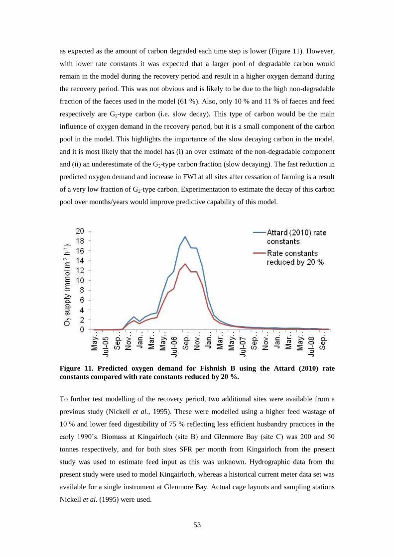
53

as expected as the amount of carbon degraded each time step is lower (Figure 11). However,

with lower rate constants it was expected that a larger pool of degradable carbon would

remain in the model during the recovery period and result in a higher oxygen demand during

the recovery period. This was not obvious and is likely to be due to the high non-degradable

fraction of the faeces used in the model (61 %). Also, only 10 % and 11 % of faeces and feed

respectively are G2-type carbon (i.e. slow decay). This type of carbon would be the main

influence of oxygen demand in the recovery period, but it is a small component of the carbon

pool in the model. This highlights the importance of the slow decaying carbon in the model,

and it is most likely that the model has (i) an over estimate of the non-degradable component

and (ii) an underestimate of the G2-type carbon fraction (slow decaying). The fast reduction in

predicted oxygen demand and increase in FWI at all sites after cessation of farming is a result

of a very low fraction of G2-type carbon. Experimentation to estimate the decay of this carbon

pool over months/years would improve predictive capability of this model.

Figure 11. Predicted oxygen demand for Fishnish B using the Attard (2010) rate

constants compared with rate constants reduced by 20 %.

To further test modelling of the recovery period, two additional sites were available from a

previous study (Nickell et al., 1995). These were modelled using a higher feed wastage of

10 % and lower feed digestibility of 75 % reflecting less efficient husbandry practices in the

early 1990‟s. Biomass at Kingairloch (site B) and Glenmore Bay (site C) was 200 and 50

tonnes respectively, and for both sites SFR per month from Kingairloch from the present

study was used to estimate feed input as this was unknown. Hydrographic data from the

present study were used to model Kingairloch, whereas a historical current meter data set was

available for a single instrument at Glenmore Bay. Actual cage layouts and sampling stations

Nickell et al. (1995) were used.

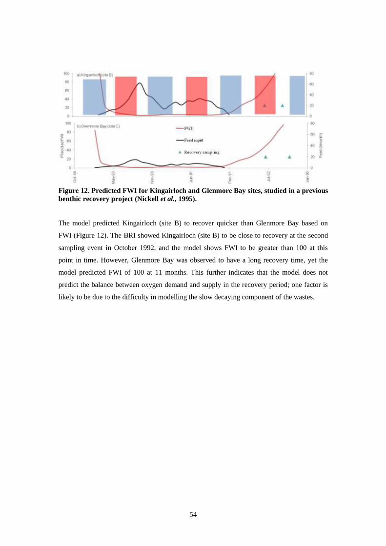
54

Figure 12. Predicted FWI for Kingairloch and Glenmore Bay sites, studied in a previous

benthic recovery project (Nickell et al., 1995).

The model predicted Kingairloch (site B) to recover quicker than Glenmore Bay based on

FWI (Figure 12). The BRI showed Kingairloch (site B) to be close to recovery at the second

sampling event in October 1992, and the model shows FWI to be greater than 100 at this

point in time. However, Glenmore Bay was observed to have a long recovery time, yet the

model predicted FWI of 100 at 11 months. This further indicates that the model does not

predict the balance between oxygen demand and supply in the recovery period; one factor is

likely to be due to the difficulty in modelling the slow decaying component of the wastes.

55

8 Modelling approach 2 – the RQ model

8.1 Introduction

The ultimate objective is to produce a model that includes only the first order processes that

are sufficient to make useful predictions. It is not intended to produce a biogeochemical

model that attempts a full description of all relevant processes - such a model would be

complex, data intensive, computing power intensive and ultimately unfit for use by industry

or regulatory agents.

The benthic results of this project are at first sight counter intuitive (Section 6.3) and reveal

that recovery is a complex process that is not simply a function of the degree of impact at the

end of the farming period and that the rate of recovery varies considerably between sites. This

is in a sense confirmed by the modelling carried out (section 7), as this has been built on the

assumption that the Findlay-Watling index (FWI) on its own would correlate with recovery

time, which it clearly does not. The FWI worked well in published studies at active sites

(Findlay and Watling, 1997; Morrisey et al., 2000) and also in this study during the period of

maximum biomass (Section 7.5). What is clear from our work is that these simple

assumptions are insufficient during the recovery process and that further work is necessary to

incorporate more complex processes.

In order to address the issue of the present model‟s inadequacies, our first thoughts were that

we need to look again at the currents - especially for the 2 sites that used impeller current

meters. DEPOMOD is very sensitive to the accuracy of hydrodynamical parameters, and this

is likely to be especially important when considering oxygen supply. For this reason these

new measurements are justified but this is most likely to be a second order improvement and

unlikely to make a large qualitative difference to the present results.

Our next thought was that the problem lay in the rate constants/carbon proportions for

degradation so we have explored whether revised parameters would under any likely

circumstances be able to change the predicted order of recovery between the sites. We

concluded that this is not likely to make a qualitative difference but think that this should be

done to provide greater confidence in the quantitative aspects. However, we would wish to do

this using a sediment system rather than a pure carbon system used in the present associated

study (Attard, 2010). This would allow study of the storage of reduced products during the

production phase for re-oxidation during the recovery phase, more of which later.

56

Our further thinking has come from an analysis of the key benthic conclusion:



recovery after 2 years."

Considering the LOI results it is clear that the sites that take longest to recover have much

higher levels of organic matter (OM) both at impacted and control stations compared to the

three sites which recovered most quickly. This leads us back to consideration of Macleod et

al.‟s paper (2007) on the differences of recovery rate between sites and their dependence on

the ambient environment. The following is a quotation form the abstract of this paper:

At the Stringers Cove site the primary ecological functions of the background community

were restored, but this was not the case at Creeses Mistake. These differences in recovery

response were a direct reflection of background environmental conditions. Stringers Cove

sediments had naturally high organic carbon content and as a result there was greater

similarity in the ecological function of the unimpacted and impacted conditions at this

location than at Creeses Mistake, where, under unimpacted conditions, the sediments had a

very low organic content.

The paper goes on to hypothesise that sites that have high organic carbon content might be

expected to recover more quickly than sites with low organic carbon content but, as that study

considered only short term process (3 months), and the proposed mechanisms for this

hypothesis related to larval supply for re-colonising sediments - rather than relating to the

biogeochemical status of the sediments, this mechanism is probably not the most important on

the timescales of most interest to the present project (1-3 years).

The model described above (section 7) takes local chemical and biological aspects into

account through the consideration of recovery (biologically) with respect to local controls

rather than through any direct measurement of the carbon richness of the system. What if sites

with high background levels of OM from natural sources have a) a greater resilience to further

OM input (say from a fish farm) and b) a longer recovery time from the same level of

additional OM input than a site that has a lower background OM supply?

Can we test this hypothesis by adapting the model? Essentially we need an input for OM

background at the beginning of the process. We then need to generate an additional base level

OM demand based on some function of background status using information from the

57

literature on the degradation rate of marine primary production as well as information on the

degradation rates of terrestrial detritus and some estimates of OM supply.

But to allow the maintenance of an impact that extends well beyond the farming period (as

observed) we need to generate a greater oxygen demand from our model than is taking place

currently. We can hypothesise that our original assumption that oxygen demand can be

estimated from carbon degradation was not supported by the model outcomes. Thus we need

to include processes where sulphide concentration increases in sediment and its subsequent

re-oxidation to sulphate causes an oxygen demand long after the original organic material has

been degraded.

8.2 RQ model description

This model was originally constructed in MS Excel and was later developed as stand-alone

computer software written in Delphi. At the outset it was called the RQ model – for

Respiratory Quotient6– as initial work used the RQ as an important model parameter.

The concept of the model is visualised in figure 13 although all of the compartments and

processes described are not modelled (but could be in a future version if thought necessary).

The model is constructed as a simple box model as a first approximation but could later be

elaborated into a more dynamical model with feedbacks between processes. Our initial

assumption is that while these feedbacks are likely to be very important in obtaining good

numerical fits between predictions and observations, they may be less important in estimating

the rank of sites in terms of recovery, given the scale of the OM input from fish farms

compared to most natural systems.

This model is not designed as a comprehensive biogeochemical model as we believe that at

present this would not be a practical option as a regulatory tool. However, we also hypothesis

that the fish farm sedimentary system may be so extreme (in terms of OM flux and

6 RQ = CO2 produced/ O2 consumed. Metabolism of different types of organic matter yield different values of RQ

as a consequence of their stoichiometry. In the context of marine sediments, where the production of carbon

dioxide (dissolved inorganic carbon) and the demand for oxygen may be decoupled for long periods through the

production of sulphide intermediates, the apparent RQ of the sediment system may vary in time where organic

matter supply is non-steady state. For example, we would expect RQ to be greater than unity under high OM

fluxes as much of the oxidising power comes from sulphate and the sulphides are to some extent stored in

sediments, whereas under later low OM fluxes (e.g. during recovery) we might expect an RQ of less than unity as

respiration is diminished but oxygen demand is still caused by the later oxidation of reduced intermediates like

sulphide.

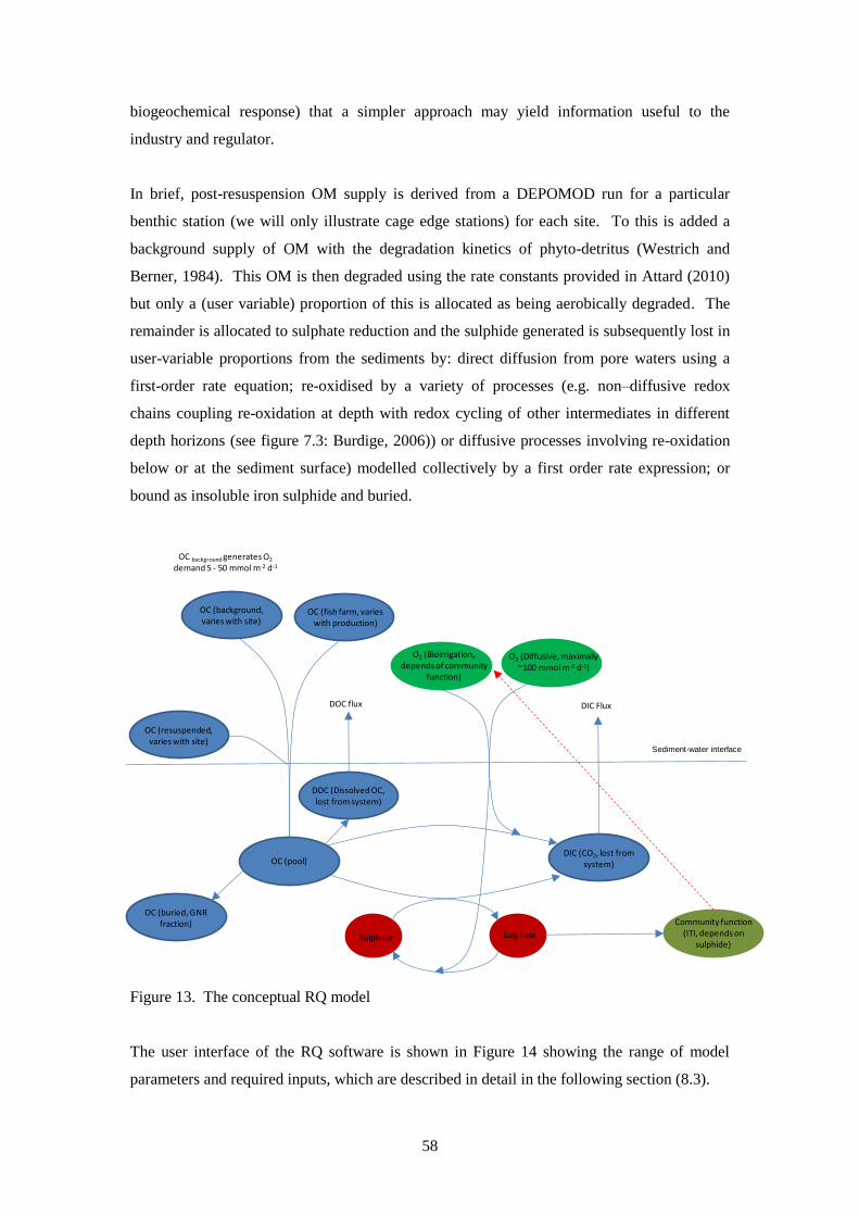
58

biogeochemical response) that a simpler approach may yield information useful to the

industry and regulator.

In brief, post-resuspension OM supply is derived from a DEPOMOD run for a particular

benthic station (we will only illustrate cage edge stations) for each site. To this is added a

background supply of OM with the degradation kinetics of phyto-detritus (Westrich and

Berner, 1984). This OM is then degraded using the rate constants provided in Attard (2010)

but only a (user variable) proportion of this is allocated as being aerobically degraded. The

remainder is allocated to sulphate reduction and the sulphide generated is subsequently lost in

user-variable proportions from the sediments by: direct diffusion from pore waters using a

first-order rate equation; re-oxidised by a variety of processes (e.g. non–diffusive redox

chains coupling re-oxidation at depth with redox cycling of other intermediates in different

depth horizons (see figure 7.3: Burdige, 2006)) or diffusive processes involving re-oxidation

below or at the sediment surface) modelled collectively by a first order rate expression; or

bound as insoluble iron sulphide and buried.

Sediment-water interface

OC (background, varies with site)

OC (fish farm, varies with production)

OC (pool)

OC (buried, GNR fraction)

OC (resuspended, varies with site)

DIC (CO2, lost from system)

O2 (Diffusive, maximally ~100 mmol m-2 d-1)

O2 (Bioirrigation, depends of community

function)

DOC (Dissolved OC, lost from system)

DOC flux

Sulphate Sulphide

DIC Flux

OC background generates O2

demand 5 - 50 mmol m-2 d-1

Community function (ITI, depends on

sulphide)

Figure 13. The conceptual RQ model

The user interface of the RQ software is shown in Figure 14 showing the range of model

parameters and required inputs, which are described in detail in the following section (8.3).

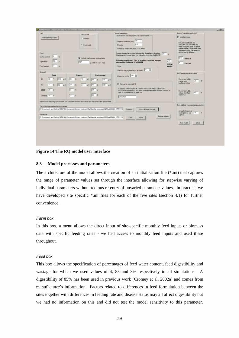
59

Figure 14 The RQ model user interface

8.3 Model processes and parameters

The architecture of the model allows the creation of an initialisation file (*.ini) that captures

the range of parameter values set through the interface allowing for stepwise varying of

individual parameters without tedious re-entry of unvaried parameter values. In practice, we

have developed site specific *.ini files for each of the five sites (section 4.1) for further

convenience.

Farm box

In this box, a menu allows the direct input of site-specific monthly feed inputs or biomass

data with specific feeding rates - we had access to monthly feed inputs and used these

throughout.

Feed box

This box allows the specification of percentages of feed water content, feed digestibility and

wastage for which we used values of 4, 85 and 3% respectively in all simulations. A

digestibility of 85% has been used in previous work (Cromey et al, 2002a) and comes from

manufacturer‟s information. Factors related to differences in feed formulation between the

sites together with differences in feeding rate and disease status may all affect digestibility but

we had no information on this and did not test the model sensitivity to this parameter.

60

Similarly the proportion of waste feed likely varies between sites and seasons but is very

difficult to estimate and so a constant value was chosen – the authors accept that this value is

likely to be important, as feed contains more reactive organic matter than faeces, but there is

presently no good method to estimate this over a farm cycle unless farms are using

sophisticated feeders with waste feed trapping and recycling. In the present comparative

exercise, the difference in impact between farms is more important than the absolute values

obtained and thus differences in feed wastage rates between farms is more important than the

absolute value (3%) chosen to represent an average. The water content was measured from

feed samples (Attard, 2010).

Background sedimentation

As mentioned above, background sedimentation may influence the recovery rate of sites.

Also, where background rates are high, the natural benthic assemblage may be more tolerant

of organic enrichment from the farm. In addition, measures of recovery which compare

reference values with impact stations, i.e. relative indices, may yield lower impact values that

would be obtained from consideration of impacted stations in isolation. Natural organic

matter accumulation rates (i.e. sedimentation minus resuspension) are hard to measure and

relatively few measurements have been made in Scottish fjordic systems. We attempted to

rank the sites in terms of sediment accumulation by using organic matter values for stations

close to the farms which were unlikely to experience a large farm input i.e. the 50m stations

(65m in the case of Fishnish B, Table 7). We did not use the reference values as these were

clearly unrepresentative of the farm location in at least one site (Oban Bay). There are few

published data on primary production in Scottish sea lochs. A study in Loch Linnhe has

shown annually integrated carbon fixation rates of between 78 and 199 g m-2

yr-1

(Rees et al.,

1995) which, assuming a carbon content of around 25% (Platt and Irwin, 1973) yields an OM

flux rate of 312 to 796 g m-2

yr-1

. Accordingly, we used a value of 800 g m-2

yr-1

as an

estimate of the supply rate of background OM to the site with the most OM rich 50 m station

and scaled the other sites linearly (Table 33). As the % OM in sediments reflects both the

total carbon supply rate and the non-reactive carbon content, this method of estimation of

relative supply depends on the quality of supply being approximately equal between sites, on

which we have no information, although it is probably that sites near river inputs have

considerable contributions of terrestrial as well as marine OM. At present there is no option to

vary background OM by month although some data exist that would enable this refinement to

be implemented (Rees et al., 1995).

61

Table 33 Estimation of relative background organic matter accumulation rate by

assigning Camasdoun with a rate of 800 g m-2

yr-1

and scaling other sites from organic

matter in sediments at stations 50m from the cage edge. (CD = Camasdoun, MB = Maol

Bhan, KG -= Kingairloch, OB = Oban Bay and FB = Fishnish B).

CD MB KG OB FB

%OM @ 50 m stations 11.51 10.28 5.03 4.24 2.80

Relative background OM

accumulation rate g m-2

yr-1

800 715 350 295 195

G- Model box

Here we parameterise the G-model (Eqn. 2, section 7.2). In this box we enter the fractions and

rate constants of three types of carbon for feed, faeces (from aerobic respiration of feed and

faeces - Attard, 2010: Table 26) and background sedimentation (from the experiments on

anaerobic degradation of phytodetritus by Westrich and Berner, 1984). The values presented

by Westrich and Berner (1994) for anaerobic respiration are given for 20-22 °C only and are

here reduced by factors of 0.56 and 0.85 respectively for use at 10 °C based on the

temperature dependencies observed by Attard (2010). The aerobic values given by Attard are

reduced by factors of 0.36 and 0.6 for k1 and k2 respectively to approximate anaerobic values

based on the ratios of the respective anaerobic and aerobic rate constants given by Westrich

and Berner (1984). These values, used as defaults in all model runs reported here, are given in

Table 34. These values require verification by experiment but are likely to be of the correct

order of magnitude and, therefore, sufficient for the present purpose.

Table 34 Proportions of carbon types (G1, G2, GNR), their associated anaerobic

degradation rate constants at 10 °C and total carbon content used as default model

parameters (see text for sources)

Feed Faeces Background

G1 % 66 29 50

k1 yr-1

8.1 5.8 2.0

G2% 11 10 16

k2 yr-1

2.5 1.3 0.4

GNR% 23 61 34

C% 31 12 25

No attempt has been made to simulate seasonal temperature variations and their effects on

rate constants although this could be implemented in future

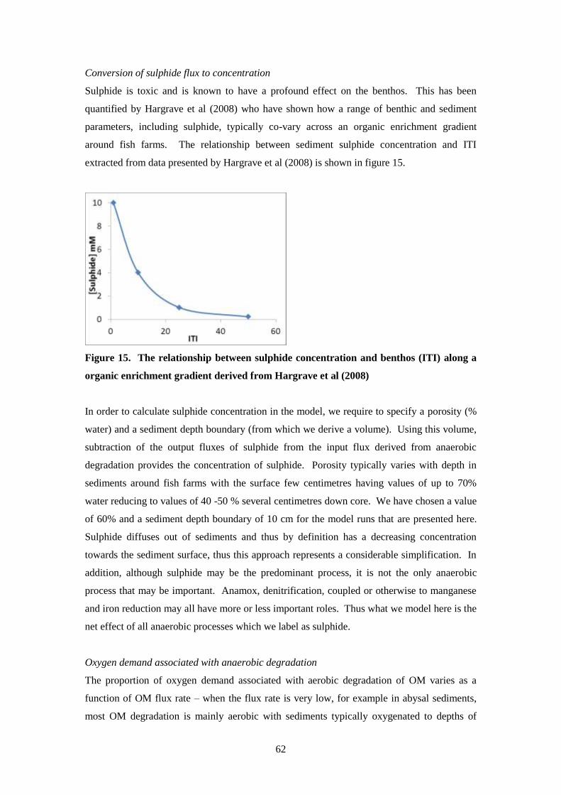
62

Conversion of sulphide flux to concentration

Sulphide is toxic and is known to have a profound effect on the benthos. This has been

quantified by Hargrave et al (2008) who have shown how a range of benthic and sediment

parameters, including sulphide, typically co-vary across an organic enrichment gradient

around fish farms. The relationship between sediment sulphide concentration and ITI

extracted from data presented by Hargrave et al (2008) is shown in figure 15.

Figure 15. The relationship between sulphide concentration and benthos (ITI) along a

organic enrichment gradient derived from Hargrave et al (2008)

In order to calculate sulphide concentration in the model, we require to specify a porosity (%

water) and a sediment depth boundary (from which we derive a volume). Using this volume,

subtraction of the output fluxes of sulphide from the input flux derived from anaerobic

degradation provides the concentration of sulphide. Porosity typically varies with depth in

sediments around fish farms with the surface few centimetres having values of up to 70%

water reducing to values of 40 -50 % several centimetres down core. We have chosen a value

of 60% and a sediment depth boundary of 10 cm for the model runs that are presented here.

Sulphide diffuses out of sediments and thus by definition has a decreasing concentration

towards the sediment surface, thus this approach represents a considerable simplification. In

addition, although sulphide may be the predominant process, it is not the only anaerobic

process that may be important. Anamox, denitrification, coupled or otherwise to manganese

and iron reduction may all have more or less important roles. Thus what we model here is the

net effect of all anaerobic processes which we label as sulphide.

Oxygen demand associated with anaerobic degradation

The proportion of oxygen demand associated with aerobic degradation of OM varies as a

function of OM flux rate – when the flux rate is very low, for example in abysal sediments,

most OM degradation is mainly aerobic with sediments typically oxygenated to depths of

63

several centimetres. In contrast, in coastal system with higher flux rates of OM, a large

proportion of the OM is metabolised anaerobically of which the majority is by sulphate

reduction (Holmer and Kristensen, 1992; Jorgensen, 1977). However, as we are dealing

primarily with highly reducing fish farm sediments, we have decided to simply allocate a

small proportion (10%) of the OM flux to aerobic degradation. This allows computational

simplicity but a more dynamic approach could be implemented in the future if warranted,

where the proportion of the OM oxidised by oxygen is dependent on the oxygen demand

caused by both aerobic and anaerobic processes. This would allow the balance between

aerobic and anaerobic processes to vary according to the changing state of the seabed during

the farming and recovery cycle.

The proportion allocated to aerobic oxidation is degraded over time using the multi-G model

with the parameterisation described earlier. At present, the model does not allow for different

rate constants between the aerobic fraction and the anaerobic fraction but this could be added

in a later version. The consequence of this is likely to be relatively minor as the proportion of

the carbon that is degraded aerobically is small and the difference in rate constants is only a

factor of 2-3. The aerobically degraded fraction causes an appropriate oxygen demand. The

larger anaerobic fraction is degraded using the same rate constants to produce a sulphide pool

which is then reoxidised according to the first order rate constant referred to as the diffusion

coefficient as it is likely to correspond to the net effect of several diffusion limited processes.

We have used a value of 2.8 month-1

in the results given here as this yielded plausible oxygen

demand and sulphide concentration results. This constant should be evaluated in a future

study.

Time

The time input box allows variation of the time (month) where feeding is started in the model

and the total duration of the model run. In order to display the information with respect to

recovery time, we adjusted the feeding start month for each farm so that they all ceased

feeding on the same month. We set this feeding end time at 80 months as this provided

sufficient time for the model to evolve to a steady state before feed input comenced and we

typically allowed the model to run for a total of 180 months (15 years).

Convert to mmol/m2/d

The model works on a whole farm scale. However, results for particular stations allow

comparison with benthic and sediment field data and the check box instructs this. At an early

stage in the modelling process we decided that to include the RQ model within DEPOMOD

for all grid points would result in enormous computational times that would both hamper

64

development and make the model practically unusable. We solve this by selecting stations for

which we have information from DEPOMOD and run the RQ model in stand-alone mode

(run times < 1s).

By calculating a station specific factor, we can estimate the flux at the near cage station each

month using the husbandry data specified. The factor can be calculated from DEPOMOD

predictions as follows:

Factor = Cflux (g C m-2

month-1

) / Cdischarged (g C month-1

)

where Cflux is the DEPOMOD prediction of flux at a station and Cdischarged is the amount

of carbon (waste feed and faeces) discharged from the farm each month calculated in a

spreadsheet. As Cflux is directly proportional to Cdischarged, Factor is a constant. Factor is

different for each station, as Cflux varies between stations. We have concentrated our effort

on cage edge stations for each of the five study sites (Table 5).

Table 35 Factors used to convert whole grid calculations to cage edge stations in mmol

m-2

d-1

Site Factor

Oban Bay 0.000120

Camasdoun 0.000029

Fishnish B 0.000024

Kingairloch 0.00053

Maol Bhan 0.000050

Loss of sulphide by diffusion

Sulphide is lost from sediments by diffusion. However, a considerable proportion of this may

be reoxidised at the sediment surface (creating an oxygen demand) and recycled as sulphate

back into the sediments. In this box we allow a first order loss of sulphide from the system

which does not contribute to oxygen demand. Similar to the issues relating to the balance

between aerobic and anaerobic metabolism discussed earlier, the amount of sulphide lost from

the system is a function of the sediment sulphide concentration as when the concentration is

small most sulphide is likely to be deoxidised at the sediment surface and recycled, but when

the it high the flux rate will become higher than the rate of reoxidation at the surface and

more of it will be able to escape to the water column. However, determining and modelling

this function is beyond the scope of this project and so the present approach is recognised as a

potentially large compromise which is likely to be more important during the recovery phase

65

when sulphide concentrations decrease. This may cause an underestimate of the oxygen

demand from sulphide reoxidation during this phase. The model is parameterised as a simple

first order rate equation with a rate constant and a reaction constant. At –present we have left

the reaction constant as unity in all runs but have changed the rate constant – on which we

presently have no information – in various model runs. Increasing the rate constant

effectively reduces the amount of sulphide available for re-oxidation and therefore the

modelled sediment sulphide concentration and consequently also reduces the oxygen demand

from the sediment. We have used a rate constant of 0.14 month-1

for the results presented in

this report.

DOC production from sediment

Under conditions of high OM flux, dissolved organic carbon builds up in sediments as the

products of initial degradation reactions on larger molecules at a rate faster than the rate at

which they are further degraded in subsequent degradation steps, leading to a flux of DOC

from the sediments. Similar to the argument above for sulphide diffusion, the rate of this

process is likely to be lower during low flux periods during the recovery phase. A recent

Faroes study (A Nordi et al., In press) has shown that over a period of several months

approximately 14% of the carbon flux from a fish farm was lost from the sediments as DOC.

We have used this figure for waste from the farm but have used a figure of 0% for the

background carbon supply on the basis that this is likely to make an important contribution to

the model outputs only when the total carbon flux is small and when DOC losses are likely to

be proportionally small.

Iron sulphide from sulphide

The sulphur cycle in sediments ultimately leads to the burial of metal sulphides, particularly

of iron (FeS2, pyrite). The sulphur cycle is complex with intermediate species such as FeS

which can either further react to pyrite or be reoxidised. According to Jorgensen (1977) about

11% of the total sulphate reduction can be “lost” to FeS and FeS2 and we have used this figure

in the model. However, Jorgensen was working in coastal sediments rather than under a fish

farm and it is most likely that this is not a good estimate. Iron sulphide formation may in

some circumstances be limited by the availability of highly reactive iron in the sediment and

these may apply in a fish farm sediments where sulphide is being cycled very rapidly. Until

further observational information is available we assume an 11% loss of sulphur to iron

sulphides and do not allow these to be reoxidised.

Operating the model

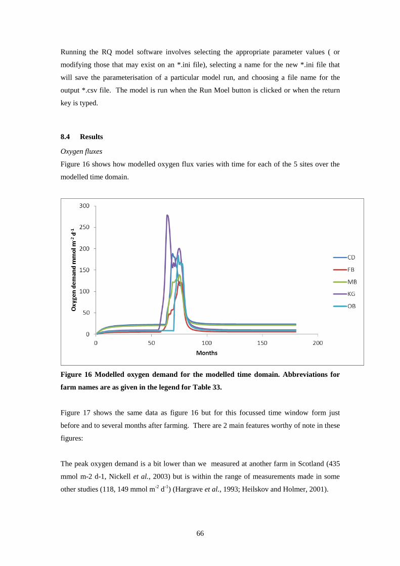
66

Running the RQ model software involves selecting the appropriate parameter values ( or

modifying those that may exist on an *.ini file), selecting a name for the new *.ini file that

will save the parameterisation of a particular model run, and choosing a file name for the

output *.csv file. The model is run when the Run Moel button is clicked or when the return

key is typed.

8.4 Results

Oxygen fluxes

Figure 16 shows how modelled oxygen flux varies with time for each of the 5 sites over the

modelled time domain.

Figure 16 Modelled oxygen demand for the modelled time domain. Abbreviations for

farm names are as given in the legend for Table 33.

Figure 17 shows the same data as figure 16 but for this focussed time window form just

before and to several months after farming. There are 2 main features worthy of note in these

figures:

The peak oxygen demand is a bit lower than we measured at another farm in Scotland (435

mmol m-2 d-1, Nickell et al., 2003) but is within the range of measurements made in some

other studies (118, 149 mmol m-2

d-1

) (Hargrave et al., 1993; Heilskov and Holmer, 2001).

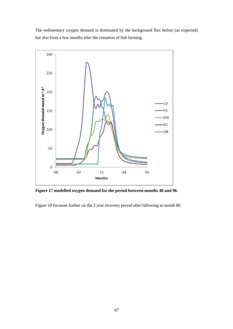
67

The sedimentary oxygen demand is dominated by the background flux before (as expected)

but also from a few months after the cessation of fish farming.

Figure 17 modelled oxygen demand for the period between months 48 and 96.

Figure 18 focusses further on the 2 year recovery period after fallowing at month 80.

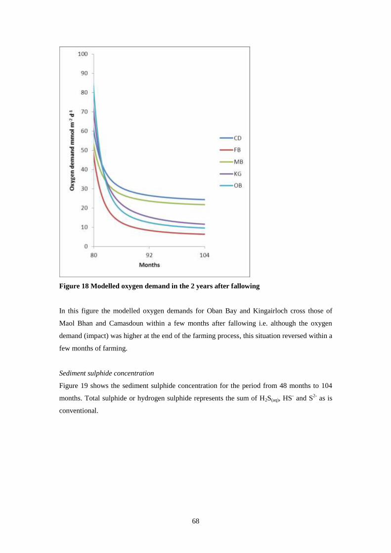
68

Figure 18 Modelled oxygen demand in the 2 years after fallowing

In this figure the modelled oxygen demands for Oban Bay and Kingairloch cross those of

Maol Bhan and Camasdoun within a few months after fallowing i.e. although the oxygen

demand (impact) was higher at the end of the farming process, this situation reversed within a

few months of farming.

Sediment sulphide concentration

Figure 19 shows the sediment sulphide concentration for the period from 48 months to 104

months. Total sulphide or hydrogen sulphide represents the sum of H2S(aq), HS- and S

2- as is

conventional.

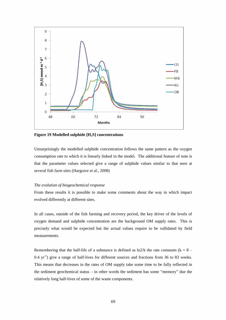
69

Figure 19 Modelled sulphide [H2S] concentrations

Unsurprisingly the modelled sulphide concentration follows the same pattern as the oxygen

consumption rate to which it is linearly linked in the model. The additional feature of note is

that the parameter values selected give a range of sulphide values similar to that seen at

several fish farm sites (Hargrave et al., 2008)

The evolution of biogeochemical response

From these results it is possible to make some comments about the way in which impact

evolved differently at different sites.

In all cases, outside of the fish farming and recovery period, the key driver of the levels of

oxygen demand and sulphide concentration are the background OM supply rates. This is

precisely what would be expected but the actual values require to be vallidated by field

measurements.

Remembering that the half-life of a substance is defined as ln2/k the rate constants (k = 8 –

0.4 yr-1

) give a range of half-lives for different sources and fractions from 36 to 83 weeks.

This means that decreases in the rates of OM supply take some time to be fully reflected in

the sediment geochemical status – in other words the sediment has some “memory” due the

relatively long half-lives of some of the waste components.

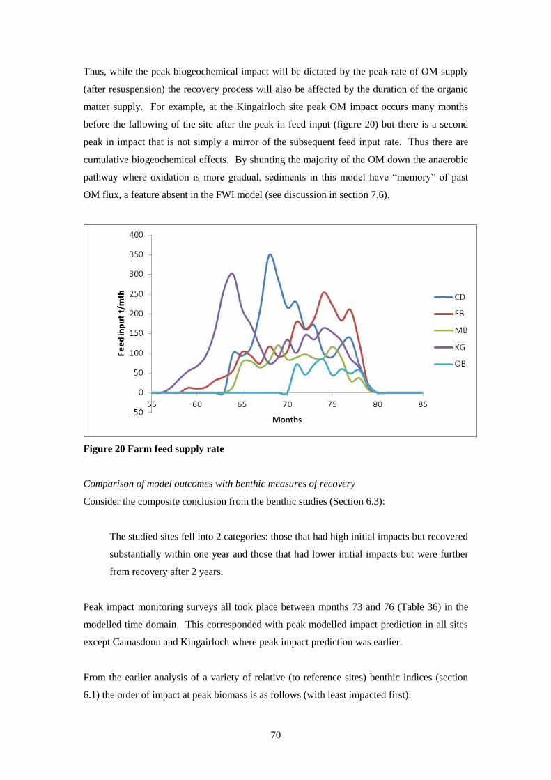
70

Thus, while the peak biogeochemical impact will be dictated by the peak rate of OM supply

(after resuspension) the recovery process will also be affected by the duration of the organic

matter supply. For example, at the Kingairloch site peak OM impact occurs many months

before the fallowing of the site after the peak in feed input (figure 20) but there is a second

peak in impact that is not simply a mirror of the subsequent feed input rate. Thus there are

cumulative biogeochemical effects. By shunting the majority of the OM down the anaerobic

pathway where oxidation is more gradual, sediments in this model have “memory” of past

OM flux, a feature absent in the FWI model (see discussion in section 7.6).

Figure 20 Farm feed supply rate

Comparison of model outcomes with benthic measures of recovery

Consider the composite conclusion from the benthic studies (Section 6.3):


substantially within one year and those that had lower initial impacts but were further

from recovery after 2 years.

Peak impact monitoring surveys all took place between months 73 and 76 (Table 36) in the

modelled time domain. This corresponded with peak modelled impact prediction in all sites

except Camasdoun and Kingairloch where peak impact prediction was earlier.

From the earlier analysis of a variety of relative (to reference sites) benthic indices (section

6.1) the order of impact at peak biomass is as follows (with least impacted first):

71

Maol Ban < Camasdoun < Oban Bay < Kingairloch ≈ Fishnish B

Consideration of the sediment oxygen demand and sulphide concentrations at the time of the

peak biomass survey (table 36) yields the following prediction of order (least impacted first):

Camasdoun < Oban Bay < Maol Ban ~ Fishnish B < Kingairloch

The main difference between the observed and predicted orders is that the model appears to

under predict the peak impact at the Maol Ban site.

Table 36 Month of peak biomass monitoring survey, modelled oxygen demand (SOD,

mmol m-2

d-1

) and sulphide concentration ([H2S], mM) together with ITI.

Site Month SOD [H2S] ITI

CD 76 114.0 3.22 0.73

FB 75 122.6 3.47 0.98

MB 73 126.6 3.58 0.42

OB 76 168.4 4.76 5.18

KG 73 179.4 5.07 0.01

However, the above measures of impact were all relative to the reference site station. When

we consider the absolute measure of ITI it is apparent (table 36) that there is very little

difference between the sites in terms of order – all are highly impacted, perhaps beyond the

ability of these indicators to provide useful information.

Table 37 shows similar information as table 36 but for the time of the recovery sampling

Table 37 Month of recovery survey, modelled oxygen demand (SOD, mmol m-2

d-1

) and

sulphide concentration ([H2S], mM) together with ITI.

Site Month SOD [H2S] ITI

FB 91 8.8 0.25 52.84

OB 90 13.67 0.39 47.02

KG 89 17.7 0.5 55.5

MB 105 22.04 0.61 36.24

CD 104 24.42 0.69 14.64

From the earlier analysis of a variety of relative (to reference sites) benthic indices (section

6.1) the order of impact at recovery survey is as follows (with least impacted first):

Oban Bay (most recovered) > Fishnish B > Kingairloch > Camasdoun > Maol Ban

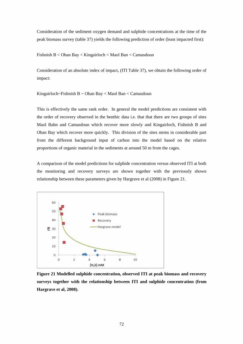
72

Consideration of the sediment oxygen demand and sulphide concentrations at the time of the

peak biomass survey (table 37) yields the following prediction of order (least impacted first):

Fishnish B < Oban Bay < Kingairloch < Maol Ban < Camasdoun

Consideration of an absolute index of impact, (ITI Table 37), we obtain the following order of

impact:

Kingairloch~Fishnish B ~ Oban Bay < Maol Ban < Camasdoun

This is effectively the same rank order. In general the model predictions are consistent with

the order of recovery observed in the benthic data i.e. that that there are two groups of sites

Maol Bahn and Camasdoun which recover more slowly and Kingairloch, Fishnish B and

Oban Bay which recover more quickly. This division of the sites stems in considerable part

from the different background input of carbon into the model based on the relative

proportions of organic material in the sediments at around 50 m from the cages.

A comparison of the model predictions for sulphide concentration versus observed ITI at both

the monitoring and recovery surveys are shown together with the previously shown

relationship between these parameters given by Hargrave et al (2008) in Figure 21.

Figure 21 Modelled sulphide concentration, observed ITI at peak biomass and recovery

surveys together with the relationship between ITI and sulphide concentration (from

Hargrave et al, 2008).

73

This presents a reasonable fit between the model predictions and the Hargrave model. It may

be possible to improve this fit by varying model parameters but it would be best to first have

access to the data that Hargrave used to produce this relationship or to collect new data before

optimising the parameterisation.

8.5 Discussion and conclusions

We have produced a simple box model (RQ) that can account for the major features of the

benthic data obtained at the five study site. This model is more appropriate for considering

recovery processes than the FWI approach attempted earlier (section 7). This is because

outside of the period of high oxygen demand when farm biomass is high, oxygen supply

issues are unlikely to be the factor which determines community structure. In considering

future work aimed at trying to improve our understanding of the processes that operate

throughout the faming cycle, it may be useful to combine the Findlay-Watling approach with

the RQ model.

The RQ model could be made more sophisticated and take into account seasonal effects by

including the facility to vary the input of OM by month and to introduce temperature

dependency in the rate constants. In addition we could allow different rate constants for

aerobic and anaerobic degradation. In addition, the degradation rate of so called non-reactive

components should be further investigated.

The RQ model should be tested with other datasets. It is possible that some of the

assumptions made are too drastic and a more sophisticated numerical approach is required.

Further work on the sulphur cycle would be extremely useful as this undoubtedly is a key

process during recovery.

In terms of practical application, the main conclusion from this work is that the background

input of organic carbon is a site specific factor important to recovery processes. We have

used the amount of organic material in sediments as a proxy for the background supply rate.

This has some merit as the organic content is likely to be largely made up of unreactive

carbon fractions but the accumulation of these unreactive fractions is a function of

background OM supply but further validation is required.

In simple terms this work supports the idea that recovery rate will be strongly influenced by

background OM supply, and that the higher the level of natural OM in sediments the longer

the likely recovery time.

74

9 Acknowledgements

We are very grateful to Sally Davies of Scottish Seafarms and to Chris Read of Marine

Harvest for supporting this project with data from the farms studied and for facilitating access

to the sites. We are very grateful to the fish farmers on the 5 sites studied for accommodating

our fieldwork and providing sampling vessels and other logistical support. We also gratefully

acknowledge the contributions of our sub-contractors, Dr Kenneth Boyd at ERI, North

Highland College, Thurso and Dr Richard Corner at the University of Stirling.

75

10 References

A Nordi, G., Glud, R.N., Gaard, E. and Simonsen, K. In press. Environmental impacts of coastal fish

farming: carbon and nitrogen budgets for trout farming in Kaldbaksfjørður (Faroe Islands).

Marine Ecology Progress Series.

Arthur, R., Done, T.J. and Marsh, H. 2005. Benthic recovery four years after an El Nino-induced coral

mass mortality in the Lakshadweep atolls. Current Science. 89. 694-699.

Arthur, R., Done, T.J., Marsh, H. and Harriott, V. 2006. Local processes strongly influence post-

bleaching benthic recovery in the Lakshadweep Islands. Coral Reefs. 25. 427-440.

Attard, K.M., 2010. The degradation kinetics of organic materials in the marine environment - A case

study using materials associated with sites of finfish aquaculture,The degradation kinetics of

organic materials in the marine environment - A case study using materials associated with

sites of finfish aquaculture. UHI Millenium Institute, Scottish Association for Marine Science,

pp. 30.

Black, K.D., Cromey, C.J., Dale, A. and Nickell, T.D., 2009 Modelling benthic effects of large salmon

cage farms in Scotland. Report to the Scottish Salmon Producers Organisation. 97 pp.

Black, K.D., Blackstock, J., Cromey, C.J., Duncan, J., Gee, M., Gillibrand, P., Needham, H., Nickell,

T.D., Pearson, T.H., Powell, H., Sammes, P., Somerfield, P., Walsham, P., Webster, L. and

Willis, K., 2005 The ecological effects of sea lice treatment agents. 286 pp.

http://www.sams.ac.uk/research/departments/ecology/past-projects/researchproject.2007-03-

09.9693635791/

Borja, A., Muxika, I. and Franco, J. 2006. Long-term recovery of soft-bottom benthos following urban

and industrial sewage treatment in the Nervion estuary - (southern Bay of Biscay). Marine

Ecology Progress Series. 313. 43-55.

Brooks, K.M. and Mahnken, C.V.W. 2003. Interactions of Atlantic salmon in the Pacific northwest

environment II. Organic wastes. Fisheries Research. 62. 255-293.

Brooks, K.M., Stierns, A.R. and Backman, C. 2004. Seven year remediation study at the Carrie Bay

Atlantic salmon (Salmo salar) farm in the Broughton Archipelago, British Columbia, Canada.

Aquaculture. 239. 81-123.

Burdige, D.J., 2006. Geochemistry of marine sediments. Princeton University Press, Woodstock, 609

pages pp.

Burt, J., Bartholomew, A. and Usseglio, P. 2008. Recovery of corals a decade after a bleaching event in

Dubai, United Arab Emirates. Marine Biology. 154. 27-36.

Clarke, K.R. and Gorley, R.N., 2006. PRIMER v6: User manual/tutorial. PRIMER-E, Plymouth, 192

pp.

Craft, C.B., Seneca, E.D. and Broome, S.W. 1991. LOSS ON IGNITION AND KJELDAHL

DIGESTION FOR ESTIMATING ORGANIC-CARBON AND TOTAL NITROGEN IN

ESTUARINE MARSH SOILS - CALIBRATION WITH DRY COMBUSTION. Estuaries.

14. 175-179.

Cromey, C.J., Nickell, T.D. and Black, K.D. 2002a. DEPOMOD - modelling the deposition and

biological effects of waste solids from marine cage farms. Aquaculture. 214. 211-239.

Cromey, C.J., Nickell, T.D., Black, K.D., Provost, P.G. and Griffiths, C.R. 2002b. Validation of a fish

farm waste resuspension model by use of a particulate tracer discharged from a point source in

a coastal environment. Estuaries. 25. 916-929.

Dean, R.J., Shimmield, T.M. and Black, K.D. 2007. Copper, zinc and cadmium in marine cage fish

farm sediments: an extensive survey. Environmental Pollution. 145. 84-95.

Findlay, R.H. and Watling, L. 1997. Prediction of benthic impact for salmon net-pens based on the

balance of benthic oxygen supply and demand. Marine Ecology Progress Series. 155. 147-

157.

Guerra-Garcia, J.M., Corzo, J. and Garcia-Gomez, J.C. 2003. Short-term benthic recolonization after

dredging in the harbour of Ceuta, North Africa. Marine Ecology-Pubblicazioni Della Stazione

Zoologica Di Napoli I. 24. 217-229.

Gutt, J., Starmans, A. and Dieckmann, G. 1996. Impact of iceberg scouring on polar benthic habitats.

Marine Ecology Progress Series. 137. 311-316.

Hall-Spencer, J., White, N., Gillespie, E., Gillham, K. and Foggo, A. 2006. Impact of fish farms on

maerl beds in strongly tidal areas. Marine Ecology Progress Series. 326. 1-9.

Hall-Spencer, J.M. and Moore, P.G. 2000. Scallop dredging has profound, long-term impacts on maerl

habitats. ICES Journal of Marine Science. 57. 1407-1415.

Hall, J.A. and Frid, C.L.J. 1995. Responses of estuarine benthic macrofauna in copper-contaminated

sediments to remediation of sediment quality. Marine Pollution Bulletin. 30. 694-700.

http://www.sams.ac.uk/research/departments/ecology/past-projects/researchproject.2007-03-09.9693635791/

http://www.sams.ac.uk/research/departments/ecology/past-projects/researchproject.2007-03-09.9693635791/

76

Hall, J.A. and Frid, C.L.J. 1997. Estuarine sediment remediation: Effects on benthic biodiversity.

Estuarine, Coastal and Shelf Science. 44. 55-61.

Hall, S.J. and Harding, M.J.C. 1997. Physical disturbance and marine benthic communities: The effects

of mechanical harvesting of cockles on non-target benthic infauna. Journal of Applied

Ecology. 34. 497-517.

Hansen, L.S. and Blackburn, T.H. 1992. EFFECT OF ALGAL BLOOM DEPOSITION ON

SEDIMENT RESPIRATION AND FLUXES. Marine Biology. 112. 147-152.

Hargrave, B.T., Holmer, M. and Newcombe, C.P. 2008. Towards a classification of organic enrichment

in marine sediments based on biogeochemical indicators. Marine Pollution Bulletin. 56. 810-

824.

Hargrave, B.T., Duplisea, D.E., Pfeiffer, E. and Wildish, D.J. 1993. Seasonal-changes in benthic fluxes

of dissolved-oxygen and ammonium associated with marine cultured Atlantic salmon. Marine

Ecology Progress Series. 96. 249-257.

Heilskov, A.C. and Holmer, M. 2001. Effects of benthic fauna on organic matter mineralization in fish-

farm sediments: importance of size and abundance. ICES Journal of Marine Science. 58. 427-

434.

Hiddink, J.G., Jennings, S. and Kaiser, M.J. 2006. Indicators of the ecological impact of bottom-trawl

disturbance on seabed communities. Ecosystems. 9. 1190-1199.

Hilton, M.J. and Hesp, P. 1996. Determining the Limits of Beach-Nearshore Sand Systems and the

Impact of Offshore Coastal Sand Mining. Journal of Coastal Research. 12. 496-519.

Holmer, M. and Kristensen, E. 1992. Impact of marine fish cage farming on metabolism and sulphate

reduction of underlying sediments. Marine Ecology Progress Series. 80. 191-201.

Holmer, M. and Heilskov, A.C. 2008. Distribution and bioturbation effects of the tropical alpheid

shrimp Alpheus macellarius in sediments impacted by milkfish farming. Estuarine, Coastal

and Shelf Science. 76. 657-667.

Johnson, L.J. and Frid, C.L.J. 1995. The recovery of benthic communities along the County Durham

coast after cessation of colliery spoil dumping. Marine Pollution Bulletin. 30. 215-220.

Jorgensen, B.B. 1977. Sulfur cycle of a coastal marine sediment (Limfjorden, Denmark). Limnology

and Oceanography. 22. 814-832.

Jørgensen, B.B. and Des Marais, D.J. 1990. The diffusive boundary layer of sediments: oxygen

microgradients over a microbial mat. Limnology and Oceanography. 35. 1343-1355.

Jusup, M., Klanjscek, J., Petricioli, D. and Legovic, T. 2009. Predicting aquaculture-derived benthic

organic enrichment: Model validation. Ecological Modelling. 220. 2407-2414.

Kaiser, M.J., Clarke, K.R., Hinz, H., Austen, M.C.V., Somerfield, P.J. and Karakassis, I. 2006. Global

analysis of response and recovery of benthic biota to fishing. Marine Ecology Progress Series.

311. 1-14.

Karakassis, I., Hatziyanni, E., Tsapakis, M. and Plaiti, W. 1999. Benthic recovery following cessation

of fish farming: a series of successes and catastrophes. Marine Ecology Progress Series. 184.

205-218.

Kim-Kang, H., Crouch, L.S., Bova, A., Robinson, R.A. and Wu, J. 2001. Determination of emamectin

residues in the tissues of Atlantic salmon (Salmo salar L.) using HPLC with fluorescence

detection. Journal of Agricultural and Food Chemistry. 49. 5294-5302.

Lardicci, C., Rossi, F. and Castelli, A. 1997. Analysis of macrozoobenthic community structure after

severe dystrophic crises in a Mediterranean coastal lagoon. Marine Pollution Bulletin. 34.

536-547.

Lim, H.S., Diaz, R.J., Hong, J.S. and Schaffner, L.C. 2006. Hypoxia and benthic community recovery

in Korean coastal waters. Marine Pollution Bulletin. 52. 1517-1526.

Loh, P.S., Reeves, A.D., Overnell, J., Harvey, S.M. and Miller, A.E.J. 2002. Assessment of terrigenous

organic carbon input to the total organic carbon in sediments from Scottish transitional waters

(sea lochs): methodology and preliminary results. Hydrology and Earth System Sciences. 6.

959-970.

Lu, L. and Wu, R.S.S. 2006. A field experimental study on recolonization and succession of

macrobenthic infauna in defaunated sediment contaminated with petroleum hydrocarbons.

Estuarine, Coastal and Shelf Science. 68. 627-634.

Lu, L. and Wu, R.S.S. 2007. A field experimental study on recolonization and succession of subtidal

macrobenthic community in sediment contaminated with industrial wastes. Marine Pollution

Bulletin. 54. 195-205.

Macleod, C.K., Crawford, C.M. and Moltschaniwskyj, N.A. 2004. Assessment of long term change in

sediment condition after organic enrichment: defining recovery. Marine Pollution Bulletin. 49.

79-88.

77

Macleod, C.K., Moltschaniwskyj, N.A. and Crawford, C.M. 2008. Ecological and functional changes

associated with long-term recovery from organic enrichment. Marine Ecology Progress Series.

365. 17-24.

Macleod, C.K., Moltschaniwskyj, N.A., Crawford, C.M. and Forbes, S.E. 2007. Biological recovery

from organic enrichment: some systems cope better than others. Marine Ecology Progress

Series. 342. 41-53.

Mayer, D.G. and Butler, D.G. 1993. Statistical validation. Ecological Modelling. 68. 21-32.

Mesplé, F., Troussellier, M., Casellas, C. and Legendre, P. 1996. Evaluation of simple statistical

criteria to qualify a simulation. Ecological Modelling. 88. 9-18.

Miller, K.L., Fernandes, T.F. and Read, P.A. 1999. The recovery of populations of dogwhelks suffering

from imposex in the Firth of Forth 1987-1997/98. Environmental Pollution. 106. 183-192.

Morrisey, D.J., Gibbs, M.M., Pickmere, S.E. and Cole, R.G. 2000. Predicting impacts and recovery of

marine-farm sites in Stewart Island, New Zealand, from the Findlay-Watling model.

Aquaculture. 185. 257-271.

Nickell, L.A., Black, K.D., Hughes, D.J., Overnell, J., Brand, T., Nickell, T.D., Breuer, E. and Harvey,

S.M. 2003. Bioturbation, sediment fluxes and benthic community structure around a salmon

cage farm in Loch Creran, Scotland. Journal of Experimental Marine Biology and Ecology.

285. 221-233.

Nickell, T.D. and Anderson, S.J., 1997 Environmental assessment of Loch Harport. Report prepared

for United Distillers. SAMS Internal Report No. 228. 49 pp.

Nickell, T.D., Black, K.D., Provost, P.G., Davies, I.M. and Pearson, T.H., 1995 Final report to the

Department of Trade and Industry/Scottish Salmon Growers Association on the Benthic

Recovery Programme, Progress Report No. 7. 73 pp.

Nickell, T.D., Black, K.D., Provost, P.G., Davies, I.M. and Pearson, T.H. 1998. The recovery of the

sea-bed after the cessation of fish farming: benthos and biogeochemistry. ICES CM. 1998

V:1.

Oreskes, N., Shrader-Frechette, K. and Belitz, K. 1994. Verification, validation, and confirmation of

numerical models in the earth sciences. Science. 263. 641-646.

Pearson, T.H. and Rosenberg, R. 1978. Macrobenthic succession in relation to organic enrichment and

pollution of the marine environment. Oceanography and Marine Biology Annual Review. 16.

229-311.

Pearson, T.H. and Black, K.D., 2001. The environmental impact of marine fish cage culture. In: Black,

K.D. (Ed.), Environmental Impacts of Aquaculture. Sheffield Academic Press, Sheffield, pp.

1-31.

Pereira, P.M.F., Black, K.D., McLusky, D.S. and Nickell, T.D. 2004. Recovery of sediments after

cessation of marine fish farm production. Aquaculture. 235. 315-330.

Platt, T. and Irwin, B. 1973. CALORIC CONTENT OF PHYTOPLANKTON. Limnology and

Oceanography. 18. 306-310.

Portilla, E. and Tett, P., 2007. Assessing goodness of fit for ECASA models (ECASA internal

paper),Assessing goodness of fit for ECASA models (ECASA internal paper). Napier

University, Edinburgh.

Powilleit, M., Kleine, J. and Leuchs, H. 2006. Impacts of experimental dredged material disposal on a

shallow, sublittoral macrofauna community in Mecklenburg Bay (western Baltic Sea). Marine

Pollution Bulletin. 52. 386-396.

Readman, J.W., Bartocci, J., Tolosa, I., Fowler, S.W., Oregioni, B. and Abdulraheem, M.Y. 1996.

Recovery of the coastal marine environment in the Gulf following the 1991 war-related oil

spills. Marine Pollution Bulletin. 32. 493-498.

Rees, A.P., Owens, N.J.P., Heath, M.R., Plummer, D.H. and Bellerby, R.S. 1995. Seasonal nitrogen

assimilation and carbon fixation in a fjordic sea loch. Journal of Plankton Research. 17. 1307-

1324.

Sanz-Lazaro, C. and Marin, A. 2006. Benthic recovery during open sea fish farming abatement in

Western Mediterranean, Spain. Marine Environmental Research. 62. 374-387.

SEPA, 1999. Emamectin benzoate use in marine fish farms: An environmental risk assessment. SEPA

Board Paper 65/99,Emamectin benzoate use in marine fish farms: An environmental risk

assessment. SEPA Board Paper 65/99, Stirling.

SEPA, 2005. Regulation and monitoring of marine cage fish farming in Scotland. Annex H. Methods

for modelling in-feed anti-parasitics and benthic effects,Regulation and monitoring of marine

cage fish farming in Scotland. Annex H. Methods for modelling in-feed anti-parasitics and

benthic effects Issue No. 2.3, 18 May 2005.

78

Shin, P.K.S., Lam, N.W.Y., Wu, R.S.S., Qian, P.Y. and Cheung, S.G. 2008. Spatio-temporal changes

of marine macrobenthic community in sub-tropical waters upon recovery from eutrophication.

I. Sediment quality and community structure. Marine Pollution Bulletin. 56. 282-296.

Smale, D.A., Barnes, D.K.A., Fraser, K.P.P. and Peck, L.S. 2008. Benthic community response to

iceberg scouring at an intensely disturbed shallow water site at Adelaide Island, Antarctica.

Marine Ecology Progress Series. 355. 85-94.

Soulsby, R.L., 1983. The bottom boundary layer of shelf seas. In: Johns, B. (Ed.), Physical

oceanography of coastal and shelf seas. Elsevier, London, pp. 189–266.

Stora, G., Arnoux, A. and Galas, M. 1995. Time and spatial dynamics of Mediterranean lagoon

macrobenthos during an exceptionally prolonged interruption of freshwater inputs.

Hydrobiologia. 301. 123-132.

Taylor, S.R. 1964. Abundance of chemical elements in the continental crust: a new table. Geochimica

et Cosmochimica Acta. 28. 1273-1285.

Teixido, N., Garrabou, J., Gutt, J. and Arntz, W.E. 2004. Recovery in Antarctic benthos after iceberg

disturbance: trends in benthic composition, abundance and growth forms. Marine Ecology

Progress Series. 278. 1-16.

Tuck, I.D., Hall, S.J., Robertson, M.R., Armstrong, E. and Basford, D.J. 1998. Effects of physical

trawling disturbance in a previously unfished sheltered Scottish sea loch. Marine Ecology

Progress Series. 162. 227-242.

Ueda, N., Tsutsumi, H., Yamada, M., Takeuchi, R. and Kido, K. 1994. Recovery of the marine bottom

environment of a Japanese bay. Marine Pollution Bulletin. 28. 676-682.

Westrich, J.T. and Berner, R.A. 1984. The role of sedimentary organic matter in bacterial sulphate

reduction: The G model tested. Limnology and Oceanography. 29. 236-249.

Wilber, D.H., Clarke, D.G. and Rees, S.I. 2007. Responses of benthic macroinvertebrates to thin-layer

disposal of dredged material in Mississippi Sound, USA. Marine Pollution Bulletin. 54. 42-52.

Word, J.Q., 1979 The Infaunal Trophic Index. Annual Report 1978. 19-39 pp.

Zenetos, A., Hatzianestis, J., Lantzouni, M., Simboura, M., Sklivagou, E. and Arvanitakis, G. 2004.

The Eurobulker oil spill: mid-term changes of some ecosystem indicators. Marine Pollution

Bulletin. 48. 122-131.

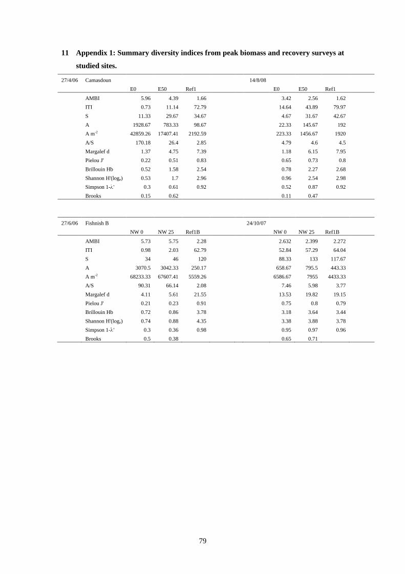
79

11 Appendix 1: Summary diversity indices from peak biomass and recovery surveys at

studied sites.

27/4/06 Camasdoun 14/8/08

E0 E50 Ref1 E0 E50 Ref1

AMBI 5.96 4.39 1.66 3.42 2.56 1.62

ITI 0.73 11.14 72.79 14.64 43.89 79.97

S 11.33 29.67 34.67 4.67 31.67 42.67

A 1928.67 783.33 98.67 22.33 145.67 192

A m-2 42859.26 17407.41 2192.59 223.33 1456.67 1920

A/S 170.18 26.4 2.85 4.79 4.6 4.5

Margalef d 1.37 4.75 7.39 1.18 6.15 7.95

Pielou J' 0.22 0.51 0.83 0.65 0.73 0.8

Brillouin Hb 0.52 1.58 2.54 0.78 2.27 2.68

Shannon H'(loge) 0.53 1.7 2.96 0.96 2.54 2.98

Simpson 1- ' 0.3 0.61 0.92 0.52 0.87 0.92

Brooks 0.15 0.62 0.11 0.47

27/6/06 Fishnish B 24/10/07

NW 0 NW 25 Ref1B NW 0 NW 25 Ref1B

AMBI 5.73 5.75 2.28 2.632 2.399 2.272

ITI 0.98 2.03 62.79 52.84 57.29 64.04

S 34 46 120 88.33 133 117.67

A 3070.5 3042.33 250.17 658.67 795.5 443.33

A m-2 68233.33 67607.41 5559.26 6586.67 7955 4433.33

A/S 90.31 66.14 2.08 7.46 5.98 3.77

Margalef d 4.11 5.61 21.55 13.53 19.82 19.15

Pielou J' 0.21 0.23 0.91 0.75 0.8 0.79

Brillouin Hb 0.72 0.86 3.78 3.18 3.64 3.44

Shannon H'(loge) 0.74 0.88 4.35 3.38 3.88 3.78

Simpson 1- ' 0.3 0.36 0.98 0.95 0.97 0.96

Brooks 0.5 0.38 0.65 0.71

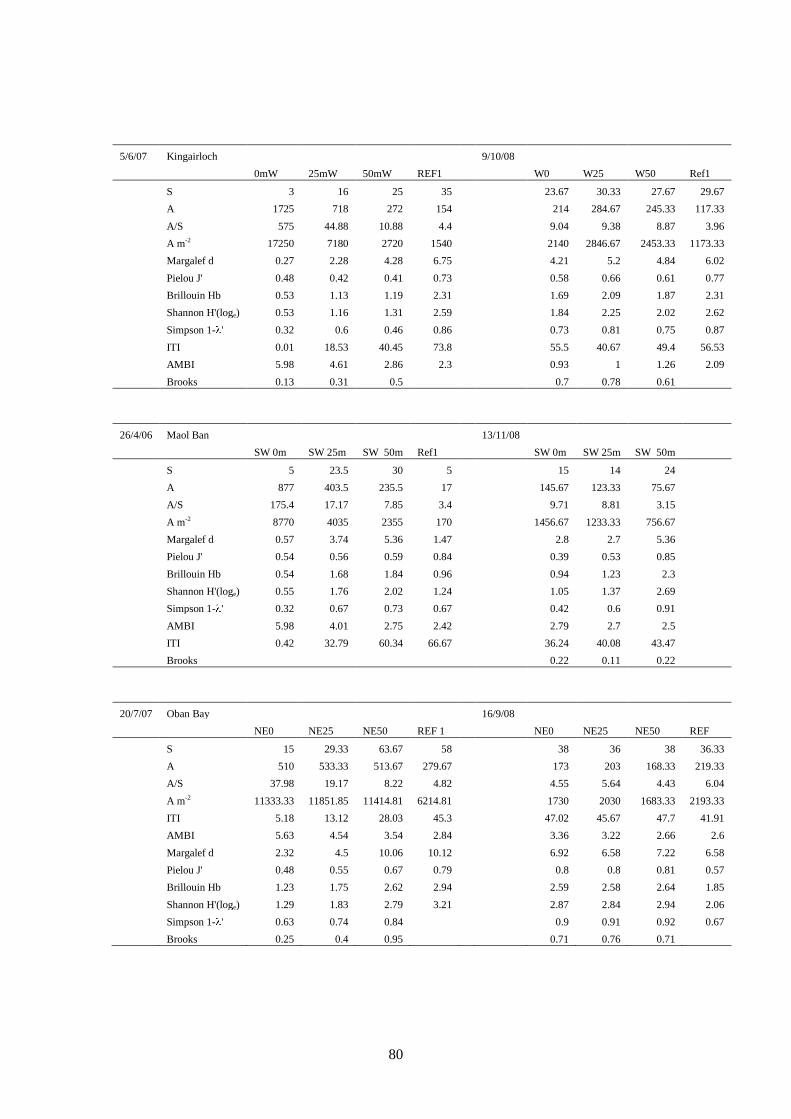
80

5/6/07 Kingairloch 9/10/08

0mW 25mW 50mW REF1 W0 W25 W50 Ref1

S 3 16 25 35 23.67 30.33 27.67 29.67

A 1725 718 272 154 214 284.67 245.33 117.33

A/S 575 44.88 10.88 4.4 9.04 9.38 8.87 3.96

A m-2 17250 7180 2720 1540 2140 2846.67 2453.33 1173.33

Margalef d 0.27 2.28 4.28 6.75 4.21 5.2 4.84 6.02

Pielou J' 0.48 0.42 0.41 0.73 0.58 0.66 0.61 0.77

Brillouin Hb 0.53 1.13 1.19 2.31 1.69 2.09 1.87 2.31

Shannon H'(loge) 0.53 1.16 1.31 2.59 1.84 2.25 2.02 2.62

Simpson 1- ' 0.32 0.6 0.46 0.86 0.73 0.81 0.75 0.87

ITI 0.01 18.53 40.45 73.8 55.5 40.67 49.4 56.53

AMBI 5.98 4.61 2.86 2.3 0.93 1 1.26 2.09

Brooks 0.13 0.31 0.5 0.7 0.78 0.61

26/4/06 Maol Ban 13/11/08

SW 0m SW 25m SW 50m Ref1 SW 0m SW 25m SW 50m

S 5 23.5 30 5 15 14 24

A 877 403.5 235.5 17 145.67 123.33 75.67

A/S 175.4 17.17 7.85 3.4 9.71 8.81 3.15

A m-2 8770 4035 2355 170 1456.67 1233.33 756.67

Margalef d 0.57 3.74 5.36 1.47 2.8 2.7 5.36

Pielou J' 0.54 0.56 0.59 0.84 0.39 0.53 0.85

Brillouin Hb 0.54 1.68 1.84 0.96 0.94 1.23 2.3

Shannon H'(loge) 0.55 1.76 2.02 1.24 1.05 1.37 2.69

Simpson 1- ' 0.32 0.67 0.73 0.67 0.42 0.6 0.91

AMBI 5.98 4.01 2.75 2.42 2.79 2.7 2.5

ITI 0.42 32.79 60.34 66.67 36.24 40.08 43.47

Brooks 0.22 0.11 0.22

20/7/07 Oban Bay 16/9/08

NE0 NE25 NE50 REF 1 NE0 NE25 NE50 REF

S 15 29.33 63.67 58 38 36 38 36.33

A 510 533.33 513.67 279.67 173 203 168.33 219.33

A/S 37.98 19.17 8.22 4.82 4.55 5.64 4.43 6.04

A m-2 11333.33 11851.85 11414.81 6214.81 1730 2030 1683.33 2193.33

ITI 5.18 13.12 28.03 45.3 47.02 45.67 47.7 41.91

AMBI 5.63 4.54 3.54 2.84 3.36 3.22 2.66 2.6

Margalef d 2.32 4.5 10.06 10.12 6.92 6.58 7.22 6.58

Pielou J' 0.48 0.55 0.67 0.79 0.8 0.8 0.81 0.57

Brillouin Hb 1.23 1.75 2.62 2.94 2.59 2.58 2.64 1.85

Shannon H'(loge) 1.29 1.83 2.79 3.21 2.87 2.84 2.94 2.06

Simpson 1- ' 0.63 0.74 0.84 0.9 0.91 0.92 0.67

Brooks 0.25 0.4 0.95 0.71 0.76 0.71

Documents

Benthic Recovery Project SARF030 - SARF - about · Benthic Recovery Project SARF030 Kenny Black, Scottish Association for Marine Science A REPORT COMMISSIONED BY SARF AND PREPARED