BEM: Opening the New Frontiers in the Industrial Products Design€¦ · BEM: Opening the New Frontiers in the Industrial Products Design Zoran Andjeli´c ABB Corporate Research [email protected]

BEM: Opening the New Frontiers in theIndustrial Products Design

Zoran Andjelic

ABB Corporate [email protected]

Summary. Thanks to the advances in numerical analysis achieved in the last sev-eral years, BEM became a powerful numerical technique for the industrial productsdesign. Until recent time this technique has been recognized in a praxis as a techniqueoffering from one side some excellent features (2D instead of 3D discretization, treat-ment of the open-boundary problems, etc.), but from the other side having some se-rious practical limitations, mostly related to the full-populated, often ill-conditionedmatrices. The new, emerging numerical techniques like MBIT (Multipole-Based In-tegral Technique), ACA (Adaptive Cross-Approximations), DDT (Domain-Decom-position Technique) seems to bridge some of these known bottlenecks, promotingthose the BEM in a high-level tool for even daily-design process of 3D real-worldproblems.

The aim of this contribution is to illustrate the application of BEM in the designprocess of the complex industrial products like power transformers or switchgears.We shall discuss some numerical aspects of both single-physics problems appearingin the Dielectric Design (Electrostatics) and multi-physics problems characteris-tic for Thermal Design (coupling of Electromagnetic - Heat transfer) and Electro-Mechanical Design (coupling of Electromagnetic - Structural mechanics).

Nomenclature

• x - source point• y - integration point• Γ := ∂Ω - surface around the body• σe - electric surface charge density [As/m2]• ρe - electric volume charge density [As/m3]• σm - magnetic surface charge density [V s/m2]• ρm - magnetic volume charge density [V s/m3]• q - charge [As]• ε - dielectric constant (permittivity, absolute) [F/m = As/V m]• ε0 - dielectric constant of free space (permittivity)=1/µ0c

20 ≈ 0.885419e−11

• c0 - speed of electromagnetic waves (light) in vacuum= 2.2997925e8 [m/s]• εr - relative dielectric constant

4 Z. Andjelic

• µ - magnetic permeability (absolute) [H/m]• µ0 - magnetic permeability of the free space [H/m] = 4π/107

• µr - relative magnetic permeability• σ - electrical conductivity [Sm/mm2]• E - electrical field strength [V/m]• D - electrical flux (displacement) density [As/m2]• ϕ - electrical potential [V ]• I - electrical current [A]• U - electrical voltage [V ]• ϕext(I) - potential of the external electrostatic field [V]• H - magnetic field strength [A/m]• B - magnetic flux density [T ]• F - force [N ]• fv - volume force density [N/m3]• fm - magnetic force density [N/m3]• fs

m - “strain” magnetic force density [N/m3]• J - current density [A/m2]• J0 - exciting current density [A/m2]• S - Poynting vector• f - time-average force density [N/m3] (volume) or [N/m2] (surface)• Θ - solid angle• j - current density (complex vector) [A/m2]• ω - angular velocity [rad/s]• f - frequency [Hz]• T - temperature [oC] or [K]• α - heat transfer coefficient [W/m2K]

1 Introduction

One of key challenges in a booming industrial market is to achieve a bettertime2market performance. This marketing syntagma one could translate as:“To be better (best) in a competition race, bring the product to the market in thefastest way (read cheapest way), simultaneously preserving / improving its func-tionality and reliability”. One of the nowadays unavoidable ways to achieve thistarget is to replace partially (or completely) the traditional Experimentally-Based Design (EBD) with the Simulation-Based Design (SBD) of industrialproducts. Usage of SBD contributes in:

• Acceleration of the design process (avoiding prototyping),• Better design through better understanding of the physical phenomena,• Recognizability of the product’s weak points already at the design stage.

Introduction of the SBD in the design process requires accurate, robust andfast numerical technologies for:

BEM: Opening the New Frontiers in the Industrial Products Design 5

• 3D real-world problems analysis, preserving the necessary structuraland physical complexity,

• ... but using the numerical technologies enough user-friendly to be ac-cepted by the designers,

• ... and using the numerical technologies suitable for the daily designprocess.

All these three items present quite tough requirements when speaking aboutthe industrial products that are usually featured by huge dimensions, huge as-pect ratio in model dimensions, complex physics, complex materials. For theclass of the problems we are discussing here, there are basically two candidatesamong many numerical methods that could potentially be used: FEM (FiniteElement Method) and BEM (Boundary Element Method). Our experienceshows that for the electromagnetic and electromagnetically-coupled problemsBEM has certain advantages when dealing with complex engineering design.

Without going into details, let us list some of the main BEM characteris-tics:

• Probably the most important feature of BEM is that for linear classes ofproblems the discretization needs to be performed only over the interfacesbetween different media. This excellent characteristic of BEM makes thediscretisation/meshing of complex 3D problems more straightforward andusable for simulations in a daily design process.

• Also, this feature is of utmost importance when dealing with the simulationof moving boundary problems. Thanks to the fact that the space betweenthe moving objects does not need to be meshed, BEM offers an excellentplatform for the simulation of dynamics, especially in 3D geometry.

• Furthermore, the open boundary problem is treated easily with BEM, with-out need to take into account any additionally boundary condition. Whenusing tools based on the differential approach (FEM, FDM), the openboundary problem requires an additional bounding box around the objectof interest, which has a negative impact on both mesh size and computa-tion error.

• Another important feature of BEM is its accuracy. Contrary to differentialmethods, where adaptive mesh refinement is almost imperative to achievethe required accuracy, with BEM it is frequently possible to obtain goodresults even with a relatively rough mesh. But, at this point we also donot want to say that “adaptivity” could not make life easier even whenusing BEM.

In spite of the above mentioned excellent features of BEM, this method haduntil recent time some serious limitations with respect to the practical design,mostly related to the:

• full populated matrix,• huge memory requirements,

6 Z. Andjelic

• bad matrix conditioning.

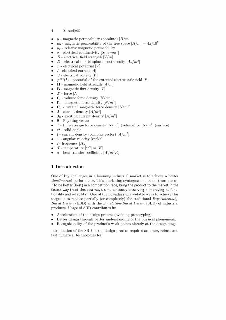
Fig. 1. Paradigm change in BEM development

Thanks to the real breakthroughs happening in the last decade in BEM-relatedapplied mathematics, most of these bottlenecks have been removed. To au-thor’s opinion the work done by Greengard and Rochlin, Greengard [10], isprobably one of the crucial ignitions contributing to this paradigm change,Figure 1. Today we can say that this work, together with a number of cap-ital contributions of other groups working with BEM, has lunched really anew dimension in the simulation of the complex real-world problems. In thefollowing we shall try to illustrate it on some practical examples like:

• Dielectric design of circuit breakers,• Electro-mechanical design of circuit breakers,• Thermal design for power transformers.

2 Dielectric Design of Circuit Breakers

Under Dielectric Design we usually understand the Simulation-Based De-sign (SBD) of configurations consisting of one or more electrodes loaded witheither fixed or floating potential and being in contact with one or more dielec-tric media. From the physics point of view, here we deal with a single-physicsproblem, which can be described either by a Laplace or Poisson equation.

2.1 Briefly About Formulation

For 3D BEM analysis of electrostatic problems, the equations satisfying thefield due to stationary charge distribution can be derived directly form theMaxwell equations, assuming that all time derivatives are equal to zero. Theformulation can be reduced to the usage of I and II Fredholm integral equa-tions1:1 The complete formulation derivation can be found in Tozoni [19], Koleciskij [15]


ϕ(x) = ϕext(x) +1

4πε0

M∑

m=1

∫

Γm

σe(y)K1dΓm(y) (1)

σe(x) =λ

2π

M∑

m=1

∫

Γm

σe(y)r · nr3

dΓm(y) (2)

where ε = ε0 · εr is absolute permittivity with ε0 = 8.85 · 10−12F/m thepermittivity of the free space and εr the relative permittivity or dielectricconstant, K1 = 1

r = 1|x−y| is a weakly singular kernel, r is a distance between

the calculation point x and integration point y, n is a unit normal vector inpoint x directed into the surrounding medium, and λ = εi−εe

εi+εe.

The equation (1) is usually applied for the points laying on the electrodes, andthe equation (2) is applied for the points positioned on the interface betweendifferent dielectrics. Then the electrostatic field strength at any point in thespace can be determined as:

E(x) = −∇ϕ(x) = − 1

4πε0

M∑

m=1

∫

Γm

σe(y) · ∇K1dΓm(y) (3)

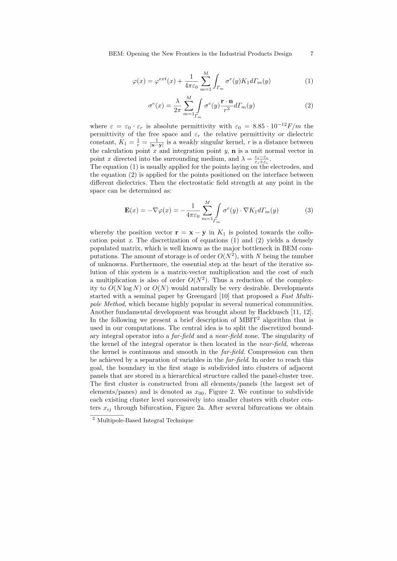
whereby the position vector r = x − y in K1 is pointed towards the collo-cation point x. The discretization of equations (1) and (2) yields a denselypopulated matrix, which is well known as the major bottleneck in BEM com-putations. The amount of storage is of order O(N2), with N being the numberof unknowns. Furthermore, the essential step at the heart of the iterative so-lution of this system is a matrix-vector multiplication and the cost of sucha multiplication is also of order O(N2). Thus a reduction of the complex-ity to O(N logN) or O(N) would naturally be very desirable. Developmentsstarted with a seminal paper by Greengard [10] that proposed a Fast Multi-pole Method, which became highly popular in several numerical communities.Another fundamental development was brought about by Hackbusch [11, 12].In the following we present a brief description of MBIT2 algorithm that isused in our computations. The central idea is to split the discretized bound-ary integral operator into a far-field and a near-field zone. The singularity ofthe kernel of the integral operator is then located in the near-field, whereasthe kernel is continuous and smooth in the far-field. Compression can thenbe achieved by a separation of variables in the far-field. In order to reach thisgoal, the boundary in the first stage is subdivided into clusters of adjacentpanels that are stored in a hierarchical structure called the panel-cluster tree.The first cluster is constructed from all elements/panels (the largest set ofelements/panes) and is denoted as x00, Figure 2. We continue to subdivideeach existing cluster level successively into smaller clusters with cluster cen-ters xij through bifurcation, Figure 2a. After several bifurcations we obtain

2 Multipole-Based Integral Technique

8 Z. Andjelic

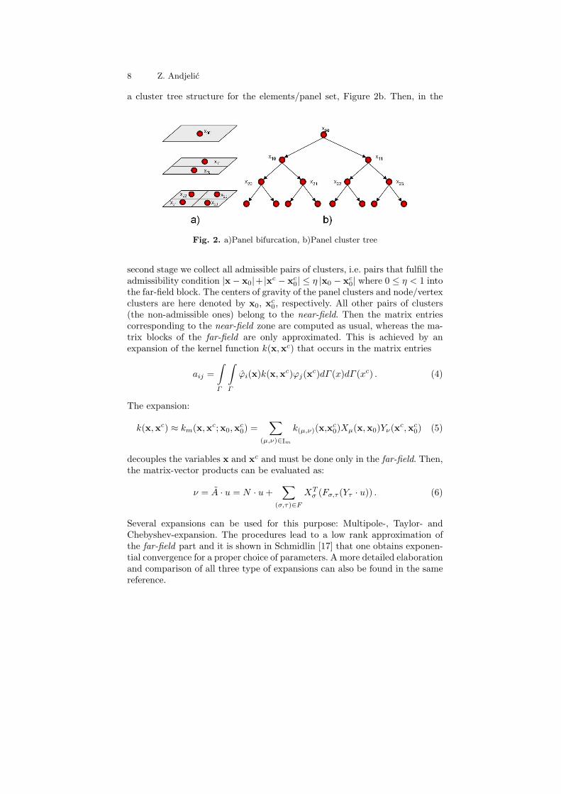
a cluster tree structure for the elements/panel set, Figure 2b. Then, in the

Fig. 2. a)Panel bifurcation, b)Panel cluster tree

second stage we collect all admissible pairs of clusters, i.e. pairs that fulfill theadmissibility condition |x − x0|+ |xc − xc

0| ≤ η |x0 − xc0| where 0 ≤ η < 1 into

the far-field block. The centers of gravity of the panel clusters and node/vertexclusters are here denoted by x0, xc

0, respectively. All other pairs of clusters(the non-admissible ones) belong to the near-field. Then the matrix entriescorresponding to the near-field zone are computed as usual, whereas the ma-trix blocks of the far-field are only approximated. This is achieved by anexpansion of the kernel function k(x,xc) that occurs in the matrix entries

aij =

∫

Γ

∫

Γ

ϕi(x)k(x,xc)ϕj(xc)dΓ (x)dΓ (xc) . (4)

The expansion:

k(x,xc) ≈ km(x,xc;x0,xc0) =

∑

(µ,ν)∈Im

k(µ,ν)(x,xc0)Xµ(x,x0)Yν(xc,xc

0) (5)

decouples the variables x and xc and must be done only in the far-field. Then,the matrix-vector products can be evaluated as:

ν = A · u = N · u+∑

(σ,τ)∈F

XTσ (Fσ,τ (Yτ · u)) . (6)

Several expansions can be used for this purpose: Multipole-, Taylor- andChebyshev-expansion. The procedures lead to a low rank approximation ofthe far-field part and it is shown in Schmidlin [17] that one obtains exponen-tial convergence for a proper choice of parameters. A more detailed elaborationand comparison of all three type of expansions can also be found in the samereference.


Example 1: SBD for a Generator Circuit-Breaker Design

In this example it is briefly shown how Simulation-Based Design of the Gen-erator Circuit-Breaker (GCB) is performed using a BEM3 module for electro-static field computation.

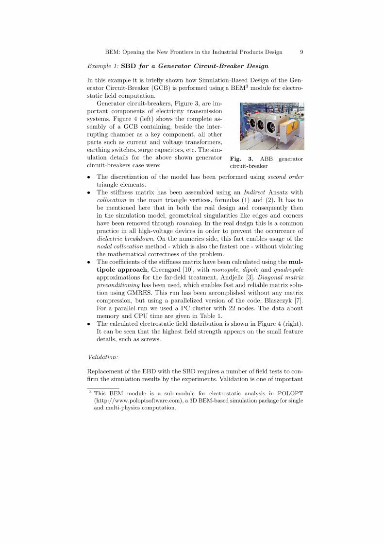
Generator circuit-breakers, Figure 3, are im-

Fig. 3. ABB generatorcircuit-breaker

portant components of electricity transmissionsystems. Figure 4 (left) shows the complete as-sembly of a GCB containing, beside the inter-rupting chamber as a key component, all otherparts such as current and voltage transformers,earthing switches, surge capacitors, etc. The sim-ulation details for the above shown generatorcircuit-breakers case were:

• The discretization of the model has been performed using second ordertriangle elements.

• The stiffness matrix has been assembled using an Indirect Ansatz withcollocation in the main triangle vertices, formulas (1) and (2). It has tobe mentioned here that in both the real design and consequently thenin the simulation model, geometrical singularities like edges and cornershave been removed through rounding. In the real design this is a commonpractice in all high-voltage devices in order to prevent the occurrence ofdielectric breakdown. On the numerics side, this fact enables usage of thenodal collocation method - which is also the fastest one - without violatingthe mathematical correctness of the problem.

• The coefficients of the stiffness matrix have been calculated using the mul-tipole approach, Greengard [10], with monopole, dipole and quadropoleapproximations for the far-field treatment, Andjelic [3]. Diagonal matrixpreconditioning has been used, which enables fast and reliable matrix solu-tion using GMRES. This run has been accomplished without any matrixcompression, but using a parallelized version of the code, Blaszczyk [7].For a parallel run we used a PC cluster with 22 nodes. The data aboutmemory and CPU time are given in Table 1.

• The calculated electrostatic field distribution is shown in Figure 4 (right).It can be seen that the highest field strength appears on the small featuredetails, such as screws.

Validation:

Replacement of the EBD with the SBD requires a number of field tests to con-firm the simulation results by the experiments. Validation is one of important

3 This BEM module is a sub-module for electrostatic analysis in POLOPT(http://www.poloptsoftware.com), a 3D BEM-based simulation package for singleand multi-physics computation.

10 Z. Andjelic

Fig. 4. GCB assembly (left). ABB Generator Circuit-Breaker: Electrostatic fielddistribution, E[V/m] (right)

Table 1. The analysis data for GCB example.

Elements Nodes Main vertices Memory CPU

145782 291584 80230 42GByte 2h20’

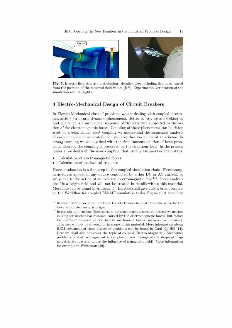
steps to gain the confidence in the simulation tools. Figure 5 (right) shows theexperimental verification of the results obtained by the simulation of the GCB.

Note 1:Calculated field distribution is just a “primary” information for the designers.For complete judgment about the products behavior, it is usually necessary togo one step forward, i.e. to evaluate the design criteria. Very often such criteriaare based on the analysis of the field lines, Figure 5 (left), that enables furtherthe conclusion about the breakdown probability in the inspected devices.


Fig. 5. Electric field strength distribution - detailed view including field lines tracedfrom the position of the maximal field values (left). Experimental verification of thesimulation results (right)

3 Electro-Mechanical Design of Circuit Breakers

In Electro-Mechanical class of problems we are dealing with coupled electro-magnetic / structural-dynamic phenomena. Better to say, we are seeking tofind out what is a mechanical response of the structure subjected to the ac-tion of the electromagnetic forces. Coupling of these phenomena can be eitherweak or strong. Under weak coupling we understand the sequential analysisof each phenomena separately, coupled together via an iterative scheme. Instrong coupling we usually deal with the simultaneous solution of both prob-lems, whereby the coupling is preserved on the equations level. In the presentmaterial we deal with the weak coupling, that usually assumes two main steps:

• Calculation of electromagnetic forces• Calculation of mechanical response

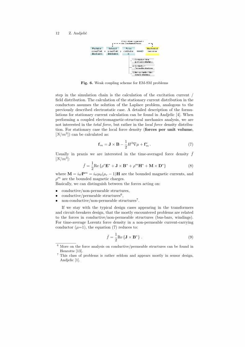
Forces evaluation is a first step in this coupled simulation chain. Electromag-netic forces appear in any device conducted by either DC or AC current, orsubjected to the action of an external electromagnetic field4,5. Force analysisitself is a bright field and will not be treated in details within this material.More info can be found in Andjelic [4]. Here we shall give only a brief overviewon the Workflow for coupled EM-ME simulation tasks, Figure 6. A very first

4 In this material we shall not treat the electro-mechanical problems whereby theforce are of electrostatic origin.

5 In certain applications (force sensors, pressure sensors, accelerometers) we are notlooking for mechanical response caused by the electromagnetic forces, but ratherfor electrical response caused by the mechanical forces (piezoelectric problem).This case will not be covered in the scope of this material. More information aboutBEM treatment of these classes of problems can be found in Gaul [9], Hill [14].Here we shall also not cover the topic of coupled Electro-Magnetic / Mechanicsproblems related to magnetostriction phenomena (change of the shape of mag-netostrictive material under the influence of a magnetic field). More informationfor example in Whiteman [20].

12 Z. Andjelic

Fig. 6. Weak coupling scheme for EM-SM problems

step in the simulation chain is the calculation of the excitation current /field distribution. The calculation of the stationary current distribution in theconductors assumes the solution of the Laplace problem, analogous to thepreviously described electrostatic case. A detailed description of the formu-lations for stationary current calculation can be found in Andjelic [4]. Whenperforming a coupled electromagnetic-structural mechanics analysis, we arenot interested in the total force, but rather in the local force density distribu-tion. For stationary case the local force density (forces per unit volume,[N/m3]) can be calculated as:

fm = J × B − 1

2H2∇µ+ fs

m . (7)

Usually in praxis we are interested in the time-averaged force density f[N/m3]:

f =1

2Re ρeE∗ + J × B∗ + ρmH∗ + M × D∗ (8)

where M = iωPm = iωµ0(µr − 1)H are the bounded magnetic currents, andρm are the bounded magnetic charges.Basically, we can distinguish between the forces acting on:

• conductive/non-permeable structures,• conductive/permeable structures6,• non-conductive/non-permeable structures7.

If we stay with the typical design cases appearing in the transformersand circuit-breakers design, that the mostly encountered problems are relatedto the forces in conductive/non-permeable structures (bus-bars, windings).For time-average Lorentz force density in a non-permeable current-carryingconductor (µ=1), the equation (7) reduces to:

f =1

2Re J × B∗ . (9)

6 More on the force analysis on conductive/permeable structures can be found inHenrotte [13].

7 This class of problems is rather seldom and appears mostly in sensor design,Andjelic [1].


These local forces are then further passed as an external load for the analysisof the mechanical quantities, last module in Figure 6. BEM formulations usedin our module for linear elasticity problems is described in more details inAndjelic [4].

Example 2: Electro-mechanical Design of Generator Circuit-Breaker

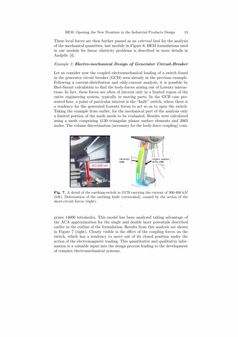
Let us consider now the coupled electromechanical loading of a switch foundin the generator circuit breaker (GCB) seen already in the previous example.Following a current-distribution and eddy-current analysis, it is possible byBiot-Savart calculation to find the body-forces arising out of Lorentz interac-tions. In fact, these forces are often of interest only in a limited region of theentire engineering system, typically in moving parts. In the GCB case pre-sented here, a point of particular interest is the “knife” switch, where there isa tendency for the generated Lorentz forces to act so as to open the switch.Taking the example from earlier, for the mechanical part of the analysis onlya limited portion of the mesh needs to be evaluated. Results were calculatedusing a mesh comprising 4130 triangular planar surface elements and 2063nodes. The volume discretization (necessary for the body-force coupling) com-

Fig. 7. A detail of the earthing-switch in GCB carrying the current of 300-400 kA!(left). Deformation of the earthing knife (overscaled), caused by the action of theshort-circuit forces (right).

.

prises 14000 tetrahedra. This model has been analyzed taking advantage ofthe ACA approximation for the single and double layer potentials describedearlier in the outline of the formulation. Results from this analysis are shownin Figure 7 (right). Clearly visible is the effect of the coupling forces on theswitch, which has a tendency to move out of its closed position under theaction of the electromagnetic loading. This quantitative and qualitative infor-mation is a valuable input into the design process leading to the developmentof complex electromechanical systems.

14 Z. Andjelic

4 Thermal Design for Power Transformers

When speaking about the Thermal Design we are usually looking for thermalresponse of the structures caused by the electromagnetic losses. In reality,the physics describing this problem is rather complex. There are three majorphysical phenomena that should be taken into account simultaneously: theelectromagnetic part responsible for the losses generation, a fluid part respon-sible for the cooling effects and thermal part responsible for the heat trans-fer. Simulation of such problems, taking into account both complex physicsand complex 3D structures found in the real-world apparatus is still a chal-lenge, especially with respect to the requirements mentioned at the beginning:accuracy-robustness-speed. A common practice to avoid a complex analysis ofthe cooling effects by a fluid-dynamics simulation is to introduce the Heat-Transfer Coefficients (HTC) obtained either by simple analytical formulae,(see for example Boehme [8]) or based on experimental observations. For thistype of analysis the link between the electromagnetic solver and heat-transfersolver is throughout the losses calculated on the electromagnetic side andpassed further as external loads to the heat-transfer module.

4.1 Workflow

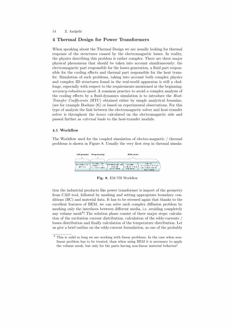
The Workflow used for the coupled simulation of electro-magnetic / thermalproblems is shown in Figure 8. Usually the very first step in thermal simula-

Fig. 8. EM-TH Workflow

tion the industrial products like power transformer is import of the geometryfrom CAD tool, followed by meshing and setting appropriate boundary con-ditions (BC) and material data. It has to be stressed again that thanks to theexcellent features of BEM, we can solve such complex diffusion problem bymeshing only the interfaces between different media, i.e. avoiding completelyany volume mesh8! The solution phase consist of three major steps: calcula-tion of the excitation current distribution, calculation of the eddy-currents /losses distribution and finally calculation of the temperature distribution. Letus give a brief outline on the eddy-current formulation, as one of the probably

8 This is valid so long we are working with linear problems. In the case when non-linear problem has to be treated, than when using BEM it is necessary to applythe volume mesh, but only for the parts having non-linear material behavior!


most complicated problems in the computational electromagnetics. More infoon the formulations of excitation current as well as thermal calculation canbe found in Andjelic [4].

4.2 Eddy-current Analysis

There are a number of possible formulation that can be used for BEM-basedanalysis of eddy-current problems. A useful overview of the available eddy-current formulations can be found in Kost [16]. Here we follow the H − ϕformulation, whereby for the treatment of the skin-effect problems an modifiedversion of this formulation is used, Andjelic [2]. TheH−ϕ formulation is basedon the indirect Ansatz, leading thus to the minimal number of 4 degrees offreedom (DoF) per node9. This nice feature makes this formulation suitablefor the eddy-current analysis of complex, real-world problems. The H − ϕformulation need to be used with a care in cases where the problem is multi-valued, i.e. when the model belongs to the class multi-connected problems,Tozoni [19]. The following integral representation is used10:

12 j(x) + 1

4π

∮Γ

n(x) ×(j(y) ×∇ e−(1+i)k·r

r

)dΓ (y)−

14π

∮Γ

σm(y)(n(x) ×∇ 1rdΓ (y)

= −n(x) × H0(x)

(10)

12σ

m(x) + 14π

∮Γ

σm(y) · n(x) · ∇( 1r )dΓ (y)+

µ4πµ0

∮Γ

n(x)(j(y) ×∇ e−(1+i)k·r

r

)dΓ (y)

= −n(x) · H0(x) .

(11)

This boundary integral equation system can be written in operator form:

[A1 B1

B2 A2

](jσm

)=

(−2n × H0

−2n · H0

). (12)

For more details on a numerical side of this approach the reader is referredto Schmidlin [18]. Solution of the equation system (12) gives the virtual mag-netic charges σm and virtual current density j. Then, the magnetic field inconductive materials can be expressed as:

H+(x) =1

4π

∮

Γ

∇× [j(y)K(x, y)] dΓ (y); x ∈ Ω+; y ∈ Ω+ (13)

9 With H−ϕ formulation it is possible to work even with only 3 DoF/node, wherebythe eddy-currents on the surfaces are described in a surface coordinate systeminstead of Cartesian, Yuan [21].

10 For complete derivation of the above formulations, please look in Kost [16], To-zoni [19], Andjelic [2]

16 Z. Andjelic

and

H−(x) = Ho(x) − 1

4π

∮

Γ

σm(y)∇xG(x, y)dΓ (y) x ∈ Ω−; y ∈ Ω− (14)

in the non-conductive materials. H0 is the primary magnetic field producedby the exciting current J0 and K = e−(1+i)k·r/r, G = 1/r .

Fast BEM for Eddy-current Analysis

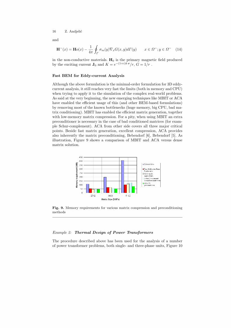
Although the above formulation is the minimal-order formulation for 3D eddy-current analysis, it still reaches very fast the limits (both in memory and CPU)when trying to apply it to the simulation of the complex real-world problems.As said at the very beginning, the new emerging techniques like MBIT or ACAhave enabled the efficient usage of this (and other BEM-based formulations)by removing most of the known bottlenecks (huge memory, big CPU, bad ma-trix conditioning). MBIT has enabled the efficient matrix generation, togetherwith low-memory matrix compression. For a pity, when using MBIT an extrapreconditioner is necessary in the case of bad conditioned matrices (for exam-ple Schur-complement). ACA from other side covers all three major criticalpoints. Beside fast matrix generation, excellent compression, ACA providesalso inherently the matrix preconditioning, Bebendorf [6], Bebendorf [5]. Asillustration, Figure 9 shows a comparison of MBIT and ACA versus densematrix solution.

Fig. 9. Memory requirements for various matrix compression and preconditioningmethods

Example 2: Thermal Design of Power Transformers

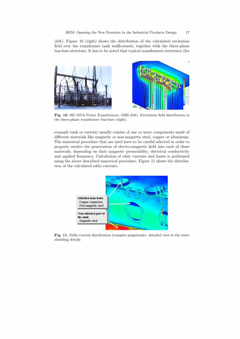
The procedure described above has been used for the analysis of a numberof power transformer problems, both single- and three-phase units, Figure 10


(left). Figure 10 (right) shows the distribution of the calculated excitationfield over the transformer tank wallfootnote, together with the three-phasebus-bars structure. It has to be noted that typical transformers structures (for

Fig. 10. 985 MVA Power Transformers, ABB (left). Excitation field distribution inthe three-phase transformer bus-bars (right)

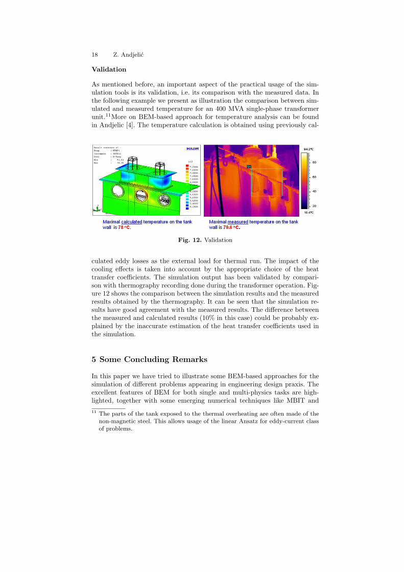
example tank or turrets) usually consist of one or more components made ofdifferent materials like magnetic or non-magnetic steel, copper or aluminum.The numerical procedure that are used have to be careful selected in order toproperly resolve the penetration of electro-magnetic field into each of thesematerials, depending on their magnetic permeability, electrical conductivityand applied frequency. Calculation of eddy currents and losses is performedusing the above described numerical procedure. Figure 11 shows the distribu-tion of the calculated eddy-currents.

Fig. 11. Eddy current distribution (complex magnitude)- detailed view to the innershielding details

18 Z. Andjelic

Validation

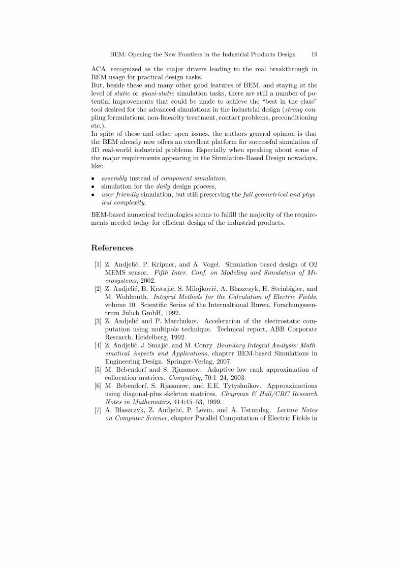
As mentioned before, an important aspect of the practical usage of the sim-ulation tools is its validation, i.e. its comparison with the measured data. Inthe following example we present as illustration the comparison between sim-ulated and measured temperature for an 400 MVA single-phase transformerunit.11More on BEM-based approach for temperature analysis can be foundin Andjelic [4]. The temperature calculation is obtained using previously cal-

Fig. 12. Validation

culated eddy losses as the external load for thermal run. The impact of thecooling effects is taken into account by the appropriate choice of the heattransfer coefficients. The simulation output has been validated by compari-son with thermography recording done during the transformer operation. Fig-ure 12 shows the comparison between the simulation results and the measuredresults obtained by the thermography. It can be seen that the simulation re-sults have good agreement with the measured results. The difference betweenthe measured and calculated results (10% in this case) could be probably ex-plained by the inaccurate estimation of the heat transfer coefficients used inthe simulation.

5 Some Concluding Remarks

In this paper we have tried to illustrate some BEM-based approaches for thesimulation of different problems appearing in engineering design praxis. Theexcellent features of BEM for both single and multi-physics tasks are high-lighted, together with some emerging numerical techniques like MBIT and

11 The parts of the tank exposed to the thermal overheating are often made of thenon-magnetic steel. This allows usage of the linear Ansatz for eddy-current classof problems.


ACA, recognized as the major drivers leading to the real breakthrough inBEM usage for practical design tasks.But, beside these and many other good features of BEM, and staying at thelevel of static or quasi-static simulation tasks, there are still a number of po-tential improvements that could be made to achieve the “best in the class”tool desired for the advanced simulations in the industrial design (strong cou-pling formulations, non-linearity treatment, contact problems, preconditioningetc.).In spite of these and other open issues, the authors general opinion is thatthe BEM already now offers an excellent platform for successful simulation of3D real-world industrial problems. Especially when speaking about some ofthe major requirements appearing in the Simulation-Based Design nowadays,like:

• assembly instead of component simulation,• simulation for the daily design process,• user-friendly simulation, but still preserving the full geometrical and phys-

ical complexity,

BEM-based numerical technologies seems to fulfill the majority of the require-ments needed today for efficient design of the industrial products.

References

[1] Z. Andjelic, P. Kripner, and A. Vogel. Simulation based design of O2MEMS sensor. Fifth Inter. Conf. on Modeling and Simulation of Mi-crosystems, 2002.

[2] Z. Andjelic, B. Krstajic, S. Milojkovic, A. Blaszczyk, H. Steinbigler, andM. Wohlmuth. Integral Methods for the Calculation of Electric Fields,volume 10. Scientific Series of the Internaltional Bureu, Forschungszen-trum Julich GmbH, 1992.

[3] Z. Andjelic and P. Marchukov. Acceleration of the electrostatic com-putation using multipole technique. Technical report, ABB CorporateResearch, Heidelberg, 1992.

[4] Z. Andjelic, J. Smajic, and M. Conry. Boundary Integral Analysis: Math-ematical Aspects and Applications, chapter BEM-based Simulations inEngineering Design. Springer-Verlag, 2007.

[5] M. Bebendorf and S. Rjasanow. Adaptive low rank approximation ofcollocation matrices. Computing, 70:1–24, 2003.

[6] M. Bebendorf, S. Rjasanow, and E.E. Tytyshnikov. Approaximationsusing diagonal-plus skeleton matrices. Chapman & Hall/CRC ResearchNotes in Mathematics, 414:45–53, 1999.

[7] A. Blaszczyk, Z. Andjelic, P. Levin, and A. Ustundag. Lecture Noteson Computer Science, chapter Parallel Computation of Electric Fields in

20 Z. Andjelic

a Heterogeneous Workstation Cluster, pages 606–611. Springer VerlagBerlin Heidelberg, hpcn europe 95 edition, 1995.

[8] H. Boehme. Mittelspannungstechnik. Verlag Technik GmbH Berlin-Munchen, 1972.

[9] L. Gaul, M. Kogl, and M. Wagner. Boundary Element Methods for En-gineers and Scientists. Springer-Verlag Berlin, 2003.

[10] L. Greengard and V. Rokhlin. A fast algorithm for particle simulations.J. Comput. Phys., 73:325–348, 1987.

[11] W. Hackbusch. The panel clustering technique for the boundary elementmethod. 9th Int. Conf. on BEM, pages 463–473, 1987.

[12] W. Hackbusch and Z.P. Nowak. On the fast matrix multiplication in theboundary element method by panel clustering. Numer. Math., 54:463–491, 1989.

[13] F. Henrotte and K. Hameyer. Computation of electromagnetic forcedensities: Maxwell stress tensor vs. virtual work principle. J. Comput.Appl. Math., 168(1-2):235–243, 2004.

[14] L.R. Hill and T.N. Farris. Three-dimensional piezoelectric boundary el-ement method. AIAA Journal, 36(1), January 1998.

[15] E.C. Koleciskij. Rascet eletriceskih poljei ustroistv visokog naprezenija.Energoatomizdat, 1983.

[16] A. Kost. Numerische Methoden in der Berechnung ElektromagnetischerFelder. Springer Verlag, 1994.

[17] G. Schmidlin. Fast Solution Algorithms for Integral Equations in R3.Master’s thesis, ETH Zurich, 2003.

[18] G. Schmidlin, U. Fischer, Z. Andjelic, and C. Schwab. Precondition-ing of the second-kind boundary integral equations for 3D eddy currentproblems. Internat. J. Numer. Methods Engrg., 51:1009–1031, 2001.

[19] O.B. Tozoni and I.D. Maergoiz. Rascet Trehmernih ElektromagnetnihPolei. Tehnika, Kiev, 1974.

[20] J.R. Whiteman and L. Demkowicz (eds.). Proceedings of the EleventhConference on The Mathematics of Finite Elements and Applications.Comput. Methods Appl. Mech. Engrg., 194(2-5), 2005.

[21] J. Yuan and A. Kost. A three-component boundary element algorithmfor three-dimensional eddy current calculation. IEEE Tran. on Mag.,30(5), September 1994.

Documents

BEM: Opening the New Frontiers in the Industrial Products Design€¦ · BEM: Opening the New Frontiers in the Industrial Products Design Zoran Andjeli´c ABB Corporate Research [email protected]