Bell’s dilemma resolved, nonlocality negated, QM demystified, etc.

Gordon Watson

1

Abstract: Eschewing naive realism, we define true (classical/quantum) realism:= some existents (ie,some Bell-beables) may change interactively. We then show that Bell’s mathematical ideas re localcausality—from his 1964:(1)-(2) to his 1990a:(6.9.3)—are valid under true realism. But we refuteBell’s analyses (and his local realism), as we resolve his consequent ‘action-at-a-distance’ dilemmain favor of true locality:= no influence propagates superluminally. In short: defining beables byproperties and values—and allowing that locally-causal interactions may yield new beables—we predictthe probabilities of such interaction outcomes via equivalence-classes that are weaker (hence moregeneral) than the corresponding classes in EPR/Bell. In this way delivering the same results asquantum theory and experiment—using EPRB, CHSH, GHZ and 3-space—we also advance QM’sreconstruction in spacetime with a new vector-product for geometric algebra. True local realism thussupports local causality, resolves Bell’s dilemma, negates nonlocality, demystifies QM, rejects naiverealism, eliminates the quantum/classical divide (since observables are clearly beables; being or notbeing, prior to an interaction, but certainly existing thereafter), etc: all at the level of undergraduatemath and logic, and all contra the analyses and impossibility-claims of Bell and many others. We alsoshow that Bayes’ Law and Malus’ Law hold, undiminished, under true local realism and the quantum.

Keywords: Bell’s theorem, causality, completeness, equivalence, GA, GHZ, true locality, true realism

Preamble: 0.1. (i) This draft replaces most of my earlier essays. (ii) Paragraphs, equations, figures,etc, are numbered to aid discussion, improvement, correction. (iii) Key texts are freely availableonline (see References). (iv) The term particle is used in accord with quantum conventions: a pristine

particle here is in its initial ex-source/pretest state; spin is intrinsic angular momentum. (v) It isoften di�cult to understand what is meant by the generic term realism; eg, see Norsen (2006). Here,true realism is well-defined and experimentally supported. (vi) Taking math to be the best logic, itmay flow for several lines before we comment. (vii) The resultant probabilities predict the outcomesof experiments in full accord with quantum theory and experiment. (viii) In this way advancing theideas of EPR and Bell (but not Bell’s conclusions), we demystify QM and refute claims like these:

(ix) Bell (1964:199), “In a theory in which parameters are added [to QM] to determinethe results of individual measurements, without changing the statistical predictions, theremust be a mechanism whereby the setting of one measuring device can influence [via aninstantaneous signal] the reading of another instrument, however remote.” Bell (1972: 880),“The nonlocal nature of quantum mechanics ... .” Aspect (2004:9), ‘Bell discovered that thesearch for [local-realistic] models is hopeless.’ Wiseman (2005:1), ‘Bell (1964) strengthenedEinstein’s theorem (but showed the futility of [Einstein’s] quest) by demonstrating thateither reality or locality is a falsehood.’ Goldstein et al (2011:1), “In light of Bell’s theorem,[many] experiments ... establish that our world is non-local.” Maudlin (2014:25), “Non-locality is here to stay ... the world we live in is non-local.” Gisin (2014:4), “For a realistictheory to predict the violation of some Bell inequalities, the theory must incorporate someform of nonlocality.” Brunner et al (2014:1), “Bell’s 1964 theorem [a profound development]... states that the predictions of quantum theory cannot be accounted for by any localtheory.” Norsen (2015:1), “In 1964 Bell demonstrated the need for non-locality in anytheory able to reproduce the standard quantum predictions.” Bricmont (2016:112), ‘Thereare nonlocal physical e�ects in Nature.’ Annals of Physics Editors (2016:67; unanimously),in the context of Bell’s theorem ‘it’s a proven scientific fact that a violation of local realismhas been demonstrated theoretically and experimentally.’

1eprb@me.com [Ex: BTRv1. 20170725] Ref: BTR23v2. Date: 20171031.

1

1 INTRODUCTION

0.2. For us (using Bell’s handy term for existents), true realism in physics: (i) a�rms the existence ofobjective (ie, mind-and-theory-independent) properties and values for well-defined beables; (ii) allowsthat such beables may change interactively (such changes long clear to us from Malus’ optics c1810and Bohr’s ‘disturbance’ insight); (iii) rejects as naive any brand of realism that negates/neglects (ii).

0.3. Thus, given Malus/Bohr, we show that naive realism (as in EPR) is no longer tenable: for ‘theresults of observation are not always given prior to and independent of observation,’ after Zeilinger(2011:56). So we reject the following realisms: Bell (2004:89) calls Einstein’s ‘deep commitment torealism and locality’ the ‘EPR axioms’. Clauser & Shimony (1978) unclearly, ‘Realism is a philosophicalview, according to which external reality is assumed to exist and have definite properties, whether ornot they are observed by someone.’ Miller (1996:35) helpfully, ‘The usual criterion for realism’ is EPR(1935). Janotta & Hinrichsen (2014:31) obscurely, ‘A theory obeys realism if measurement outcomescan be interpreted as revealing a property of the system that exists independent of the measurement.’

0.4. Thus, under true local realism: True realism allows that beables may change during interactions.True locality allows that the ‘direct causes (and e�ects) of events are nearby, and even the indirectcauses (and e�ects) are no further away than permitted by the velocity of light,’ Bell (1990a:105).

1 Introduction

1.0. (i) ‘This action-at-a-distance business will pass. If we’re lucky it will be to some bignew development like the theory of relativity. Maybe someone will just point out thatwe were being rather silly. But anyway, I believe the questions will be resolved,’ afterBell (1990:9). (ii) ‘Nobody knows where the boundary between the classical and quantumdomain is situated. More plausible is that we’ll find that there is no boundary,’ afterBell (2004:29-30). [Under the theory here, Wholistic Mechanics (WM)—the name for ourtheory (with its basis in true local realism) since 1989—we agree and deliver.]

1.1. Studying EPR (1935) in the context of EPRB—the EPR-based experiment in Bohm & Aharonov(1957)—Bell (1964:199) claims that EPR’s program requires a grossly non-local mechanism. However,instead of correcting EPR’s error—as we do at ¶1.5—Bell creates a personal dilemma [see ¶1.6(i)]:not seeing that a theory of the type that he (and we and EPR) favored could succeed. Thus, after

Bertlmann (2017:40): “Bell wondered, ‘Where does the quantum world stop and the classi-

cal world begin?’ He wanted to get rid of that division. [Agreeing, that’s what we do.] Forhim it was true that hidden variable theories [HVTs], where quantum particles do have defi-nite properties governed by hidden variables, would be appropriate to reformulate quantumtheory: ‘Everything has definite properties,’ Bell said.” Thus (see ¶2.8) Bell (1980:7) en-dorses d’Espagnat’s inferences to preexisting properties. So—contrary to QM orthodoxy,Bohr’s insight at ¶2.9, and our theory—Bell’s HVT seems bound by Bertlmann’s (ibid)generalization that “HVTs [not orthodox QM] postulate that the properties of individualsystems—[like the orientation of a particle’s spin]—do have preexisting values revealed bythe act of measurement”. Care is needed here, however: ‘Predetermined is Bell’s originalphrasing. If there is for Bell an identity between predetermined and preexisting I cannotsay ad hoc, but for a realist—as Bell was—there is clearly a close connection between bothphrasings,’ after R. Bertlmann (pers. comm., 14 June 2017). [See determinism at ¶2.13.]

1.1a. nb: for us, a revealed property (eg, charge) may preexist, a revealed spin-orientation may not.So—under Bertlmann’s generalization (ibid)—ours in not an HVT. Instead, we allow an observableto be made from beables whose (preexisting) pretest values may be forever hidden under interac-tions/transitions/transformations. Then, to advance our understanding, we encode the consequentincomplete—but adequate—information in conservation laws and probability relations. Thus:

2

1 INTRODUCTION

1.2. Cautiously seeking consensus, we begin by accepting d’Espagnat’s (1979:158) Bell-endorsed prin-ciples of local realism: (i) realism (regularities in observed phenomena are caused by some physicalreality whose existence is independent of human observers); (ii) locality (no influence of any kind canpropagate superluminally); (iii) induction (legitimate conclusions can be drawn from consistent ob-servations). So this is not a dispute about di�ering principles. Rather—merging our hopes with thoseof EPR and Bell; and given ¶1.0—we simply reject inferences that are false in quantum settings. Wethus show that Bell and d’Espagnat fail under (iii): ie, ignoring consistent observations re the validityof QM—and Bohr’s insight—they draw conclusions that are false under both QM and experiment (eg,see Aspect 2004). Indeed, for us—readily accepting the commonsense in d’Espagnat’s (i)-(iii) above;and succeeding with it (as we’ll show)—QM seems to be better-founded than Bell imagined; eg, here’sBertlmann (2017:54) on Bell (with Bellian naivety, puzzlement and doubts that we do not share):

“John was totally convinced that realism is the right position of a scientist. He believedthat experimental results are predetermined and not just induced by the measurementprocess. Even more, in John’s EPR analysis reality is not assumed but inferred! Otherwise(without realism), he said, ‘It’s a mystery if looking at one sock makes the sock pink and

the other one not-pink at the same time.’ So he did hold on [to] the hidden variableprogram continuously, and was not discouraged by the outcome of EPR-Bell experimentsbut rather puzzled. For him: ‘The situation was very intriguing that at the foundation of

all that impressive success [of QM] there are these great doubts,’ as he once remarked.”

1.3. In this way identifying the source of Bell’s dilemma—¶1.6(i)—let’s be clear about our ownposition: our core quantum-compatible principle is true local realism (TLR), the union of true lo-cality (no influence propagates superluminally, after Einstein) and true realism (some beables changeinteractively, after Bohr). TLR is therefore consistent with most interpretations of QM—and with con-textuality; thus bypassing the Kochen-Specker theorem—since interactions need not reveal preexistingproperties. We then advance EPR’s program by including every relevant beable in our EPRB analysis(see ¶2.1)—validating EPR’s belief (see next)—but rejecting their famous criterion (see ¶¶1.4-1.5):

“In a complete theory there is an element corresponding to each element of reality,” EPR(1935:777). “While we have thus shown that the wavefunction does not provide a completedescription of the physical reality, we left open the question of whether or not such adescription exists. We believe, however, that such a theory is possible,” EPR (1935:780).[Using every relevant EPRB beable at ¶2.1, we show that a more complete descriptionis possible. Further (¶3.7), we show that hidden dynamics can be adequately treated byencoding incomplete information in probabilistic relations; eg, via Bayes’ Law: P (XY |Z) = P (X | Z)P (Y | ZX). Given our focus on truth, our consequent expectations arevalidated by QM and experimental facts.]

1.4. So, using vector-products and physical operators in 3-space (not wavefunctions, etc, in Hilbertspace), we study the interaction of beables (particles) with other beables (polarizers). That is, tak-ing particles and polarizers to be sensitive contributors to the veiled reality (d’Espagnat 1983:94) ofour world, we allow: (i) any interactant may be transformed under TLR; (ii) any transformationmay be subject to an uncertainty induced by Planck’s action-constant; (iii) every less-than-certainprobability distribution represents a veiled reality. (iv) Then, identifying every relevant beable un-der EPRB—¶¶2.1-2.7—we provide a ‘complete description’ of what can be inferred from incompleteinformation. (v) We also address Bell’s dilemma—¶1.6(i)—by endorsing EPR’s next two sentences;marked [i], [ii]: but amending—at ¶1.5—the famous [naive] EPR criterion [iii] that follows [ii] here:

“[i] The elements of physical reality ... must be found by an appeal to the results ofexperiments and measurements. [ii] A comprehensive definition of reality is, however,unnecessary for our purpose. [iii] We [ie, EPR, but not us] shall be satisfied with thefollowing criterion, which we regard as reasonable. If, without any way disturbing a system,

3

1 INTRODUCTION

we can predict with certainty [P = 1] the value of a physical quantity, then there exists an

element of physical reality corresponding to this physical quantity,” EPR (1935:777).

1.5. Departing subtly from EPR—but wholly compatible with EPRB, QM, the Bell/d’Espagnat ‘local-realism’ of ¶1.2, and TLR at ¶1.3—here’s our su�cient condition for an element of physical reality(a beable), presented in the context of (8)-(9) below to be clear: ‘If, without in any way disturbing asystem q(µ

i

), we can predict with adequate accuracy the result B

i

= ≠1 of the interaction ”

±a

q(µi

)—ie,an interaction that may disturb q(µ

i

)—then local beables q(µi

), ”

±a

[and the consequent interaction-output q(a≠)] will mediate this result; ie, B

i

will be a local function of q(a≠) and [a · ú],’ after Watson(1998:417). [As to su�ciency: this condition delivers Bell’s hope (2004:167) for ‘a simple constructivemodel’ of EPRB; see ¶2.15. As to our view of adequacy: here’s Aspect’s (2004:24) example against ourpredictions (when we too depart from idealization): S

WM

= S

QM

= 2.70±0.05; S

Exp

= 2.697±0.015.]

1.6. All of which brings us to: (i) Bell’s dilemma re action-at-a-distance (AAD hereafter); (ii) aclarifying expansion about the motivation we share with Bell (and with EPR) from ¶1.0:

(i) ‘I cannot say that AAD is required in physics. I can say that you cannot get away with

no AAD. You cannot separate o� what happens in one place and what happens in another.Somehow they have to be described and explained jointly. That’s the fact of the situation;Einstein’s program fails ... Maybe we have to learn to accept not so much AAD, but the

inadequacy of no AAD. ... That’s the dilemma. We are led by analyzing this situationto admit that, somehow, distant things are connected, or at least not disconnected. ...I don’t know any conception of locality that works with QM. So I think we’re stuck with

nonlocality ... I step back from asserting that there is AAD and I say only that you cannot

get away with locality. You cannot explain things by events in their neighbourhood. But,I am careful not to assert that there is AAD,’ after Bell (1990:5-13); emphasis added.(ii) “Now nobody knows just where the boundary between the classical and quantumdomain is situated. ... More plausible to me is that we will find that there is no boundary.It is hard for me to envisage intelligible discourse about a world with no classical part—nobase of given events, be they only mental events in a single consciousness, to be correlated.On the other hand, it is easy to imagine that the classical domain could be extended tocover the whole. The wavefunctions—[not beables in our terms; in agreement with Bell(2004:53)]—would prove to be a provisional or incomplete description of the quantum-mechanical part, of which an objective account would become possible. It is this possibility,of a homogeneous account of the world, which is for me the chief motivation of the study ofthe so-called ‘hidden variable’ possibility,” Bell (2004:29-30). We agree and deliver. But.

1.7. Sharing this motivation, we deliver di�erently: for we prefer short-form expectations—like LHS(67) at ¶5.7—that at-once bypass the limitations in Bell’s analyses. However, for now, to match thestyle of typical Bellian essays, we defer our use of short-forms until we’ve established their validity.Thus, using our notation per ¶2.1, we come to what we call (for convenience; it matters not), Bell’sdefinition of true local realism: ie, we come to Bell’s view (1990a:109) re ‘locally explicable’ correlationswhere factorizability is not taken to be the starting point of the analysis—nor the formulation of ‘localcausality’—but a consequence thereof. Thus, with past causes included in — (which defines EPRB):

P (AB |—, a, b, ⁄) = P (A |—, a, ⁄)P (B |—, b, ⁄) after Bell 1975a:(4)-(6), 1990a:(6.9.3); with (1)

P (AB |—, a, b, q(⁄), q(µ)) = P (A |—, a, q(⁄))P (B |—, b, q(µ)), which is (1) amended prudently: (2)

because (for us, under TLR) it’s clearer to allow particle-variables ⁄ and µ to be di�erent—see¶2.1—correlated via (6). Thus, using Bell’s widely-accepted idea, (1), we move to show—via adequateand relevant classes of local beables—that our world is truly local and truly realistic.

4

2 ANALYSIS

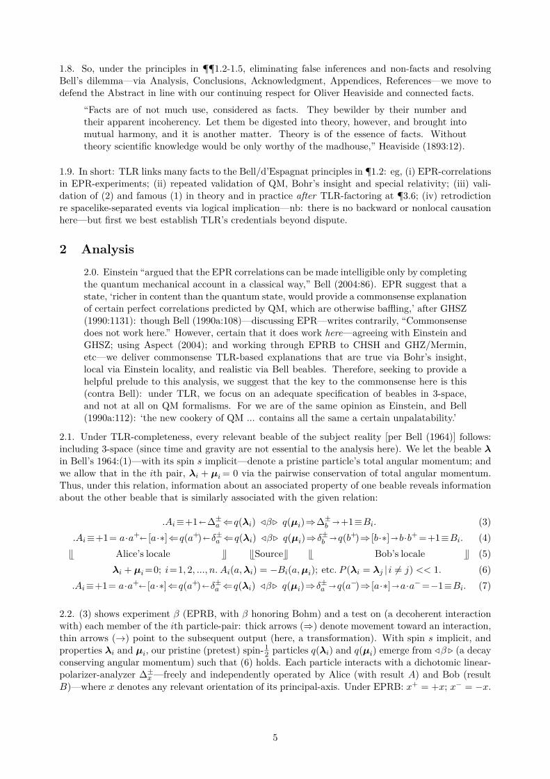
1.8. So, under the principles in ¶¶1.2-1.5, eliminating false inferences and non-facts and resolvingBell’s dilemma—via Analysis, Conclusions, Acknowledgment, Appendices, References—we move todefend the Abstract in line with our continuing respect for Oliver Heaviside and connected facts.

“Facts are of not much use, considered as facts. They bewilder by their number andtheir apparent incoherency. Let them be digested into theory, however, and brought intomutual harmony, and it is another matter. Theory is of the essence of facts. Withouttheory scientific knowledge would be only worthy of the madhouse,” Heaviside (1893:12).

1.9. In short: TLR links many facts to the Bell/d’Espagnat principles in ¶1.2: eg, (i) EPR-correlationsin EPR-experiments; (ii) repeated validation of QM, Bohr’s insight and special relativity; (iii) vali-dation of (2) and famous (1) in theory and in practice after TLR-factoring at ¶3.6; (iv) retrodictionre spacelike-separated events via logical implication—nb: there is no backward or nonlocal causationhere—but first we best establish TLR’s credentials beyond dispute.

2 Analysis

2.0. Einstein “argued that the EPR correlations can be made intelligible only by completingthe quantum mechanical account in a classical way,” Bell (2004:86). EPR suggest that astate, ‘richer in content than the quantum state, would provide a commonsense explanationof certain perfect correlations predicted by QM, which are otherwise ba�ing,’ after GHSZ(1990:1131): though Bell (1990a:108)—discussing EPR—writes contrarily, “Commonsensedoes not work here.” However, certain that it does work here—agreeing with Einstein andGHSZ; using Aspect (2004); and working through EPRB to CHSH and GHZ/Mermin,etc—we deliver commonsense TLR-based explanations that are true via Bohr’s insight,local via Einstein locality, and realistic via Bell beables. Therefore, seeking to provide ahelpful prelude to this analysis, we suggest that the key to the commonsense here is this(contra Bell): under TLR, we focus on an adequate specification of beables in 3-space,and not at all on QM formalisms. For we are of the same opinion as Einstein, and Bell(1990a:112): ‘the new cookery of QM ... contains all the same a certain unpalatability.’

2.1. Under TLR-completeness, every relevant beable of the subject reality [per Bell (1964)] follows:including 3-space (since time and gravity are not essential to the analysis here). We let the beable ⁄in Bell’s 1964:(1)—with its spin s implicit—denote a pristine particle’s total angular momentum; andwe allow that in the ith pair, ⁄

i

+ µi

= 0 via the pairwise conservation of total angular momentum.Thus, under this relation, information about an associated property of one beable reveals informationabout the other beable that is similarly associated with the given relation:

.A

i

©+1��±a

≈q(⁄i

) Ù—Û q(µi

)∆�±b

�+1©B

i

. (3).A

i

©+1= a·a+� [a·ú]≈q(a+)�”

±a

≈q(⁄i

) Ù—Û q(µi

)∆”

±b

�q(b+)∆ [b·ú]�b·b+ =+1©B

i

. (4)T Alice’s locale U TSourceU T Bob’s locale U (5)

⁄i

+ µi

=0; i=1, 2, ..., n. A

i

(a, ⁄i

) = ≠B

i

(a, µi

); etc. P (⁄i

= ⁄j

| i ”= j) << 1. (6).A

i

©+1= a·a+� [a·ú]≈q(a+)�”

±a

≈q(⁄i

) Ù—Û q(µi

)∆”

±a

�q(a≠)∆ [a·ú]�a·a≠ =≠1©B

i

. (7)

2.2. (3) shows experiment — (EPRB, with — honoring Bohm) and a test on (a decoherent interactionwith) each member of the ith particle-pair: thick arrows (∆) denote movement toward an interaction,thin arrows (æ) point to the subsequent output (here, a transformation). With spin s implicit, andproperties ⁄

i

and µi

, our pristine (pretest) spin-1

2

particles q(⁄i

) and q(µi

) emerge from Ù— Û (a decayconserving angular momentum) such that (6) holds. Each particle interacts with a dichotomic linear-polarizer-analyzer �±

x

—freely and independently operated by Alice (with result A) and Bob (resultB)—where x denotes any relevant orientation of its principal-axis. Under EPRB: x

+ = +x; x

≠ = ≠x.

5

2 ANALYSIS

2.2a. Given that A and B are discrete (±1), and seeking generality, we employ variables like ⁄i

, µi

(ordinary vectors with lengths in units of ~2

) so that our EPRB results are associated with ~2

. In this waylinking to vector-magnitudes—eg, ⁄

i

= |⁄i

|⁄̂i

, with |⁄i

| in units of ~2

, and ⁄̂i

the direction-vector—ourvariables may be continuous or discrete. This choice accords with the generality of our approach: andwith Bell’s (1964:195) indi�erence to whether such variables are discrete or continuous. [Then, in thatwe seek equivalence relations under orientations—taking Bell’s (1964) a and b to be principal-axisdirection-vectors—~

2

is suppressed in (3)-(7). The more complete story under EPRB—eg, ”

±a

q(⁄i

) æq(~

2

a

±), with allied relations under magnitudes—is developed at ¶5.3.]

2.3. Identifier i is used generically: but each particle may be tested once only in (what we call) itspristine state, and thereafter until absorbed in an analyzer; nb, under TLR, we generally favor theterm test over the term measurement. Then, since the tests are locally-causal and spacelike-separated,we hold fast to Einstein’s principle of local causality: the real factual situation of q(µ

i

) is independentof what is done with q(⁄

i

) which is spatially separated from q(µi

)—and vice-versa—per Bell (1964:endnote 2; citing Einstein). Consistent with this principle, paired test outcomes are correlated via (6).

2.4. (4) expands on (3) to show that each polarizer-analyzer �±x

is built from a polarizer ”

±x

and aremovable analyzer [x · ú] that responds to the polarization-vector (ú) of each post-polarizer particleq(ú) upon receipt. We thus assign the correct polarization x

± to q(ú) by observing the ±1 output of therelated analyzer; or by understanding the nature of particle/polarizer interactions. So experiment — isEPRB—per Bell (1964)—with this benign finesse: to facilitate additional analysis and experimentalconfirmations, we can employ additional polarizers (”±

y

) to test q(x±), etc; and y may equal x.nb: as in (3)-(4), with q(⁄

i

) ∆ ”

±a

leading to ”

±a

q(⁄i

) æ q(a±)—never requiring thatq(⁄

i

) = q(a±) prior to the interaction ”

±a

q(⁄i

)—we take interaction and transformation tobe concepts more fundamental than measurement: “Doesn’t any analysis of measurementrequire concepts more fundamental than measurement? And should not the fundamentaltheory be about these more fundamental concepts?” Bell (2004:118). We agree and deliver.

2.5. (5), with no symmetry requirements, shows the locales in (3)-(4) and (7) arbitrarily spacelike-separated from each other and from the source. Given that (3)-(7) hold over any spacelike separation, itfollows that the relevant (pretest) particle properties are stable between emission and interaction witha polarizer. Further, our theory is locally-causal and Lorentz-invariant because A

i

and B

i

are locally-caused by precedent local events ”

±a

q(⁄i

) and ”

±b

q(µi

) respectively, which are spacelike-separated.

2.6. (6) shows ⁄i

and µi

pairwise correlated via the conservation of total angular momentum; ouruse of ordinary vectors being prompted by Dirac (1982:149, eqn (48)) and geometric algebra as weseek a realistic replacement for Pauli’s vector-of-matrices. (Note: via Fröhner (1998), we reject notools of the quantum trade.) Motivated by Bell, these TLR-based variables provide a more completespecification of particle-pairs under —. Thus, for now, we allow these pristine spin-related variables tobe ordinary vectors for which all magnitudes and orientations are equally probable. (New conventionsbegin when we integrate our approach with geometric algebra at ¶5.2-5.4.) Then, under our doctrineof cautious conservatism—and though particle responses to interactions may be similar—(6) allows itto be far less than certain that two pristine (ie, pretest) particle-pairs are physically the same.

2.7. (7) shows experiment — with Alice and Bob having the same polarizer setting a. (Per ¶2.2a, ~2

is suppressed here.) Thus, as an idealized example—ie, by observing one result, we may predict theother (spacelike-separated) result with certainty—here’s how Alice predicts Bob’s result after observingA

i

= +1; and vice-versa, with Bob observing B

i

= ≠1 here:

A

i

= +1 * q(⁄i

)∆”

±a

æq(a+)∆ [a·ú] æ [a·a+] = +1. ⇧ ≠ using (6) ≠ (8)

q(µi

) = q(≠⁄i

)∆”

±a

æ q(a≠) ∆ [a·ú] æ [a·a≠] = ≠1 = B

i

. QED. ⌅ And vice-versa. (9)

6

2 ANALYSIS

2.8. This is consistent with our su�cient condition for a beable [¶1.5]. For, without in any waydisturbing q(µ

i

), Alice can predict with certainty that Bob’s result will be B

i

= ≠1 when he testsq(µ

i

) with ”

±a

(which may be a disturber). So beables q(µi

), ”

±a

and q(a≠) mediate Bob’s result; ie,the interaction ”

±a

q(µi

) will yield q(a≠) and the interaction [a · a

≠] will yield B

i

= ≠1. Thus theparticle corresponding to Bob’s B

i

= ≠1 result will be q(a≠); a TLR outcome acceptable to EPR, butan important departure from Bell’s position. For Bell endorses d’Espagnat’s (1979:166) inference thatthe input to the polarizer equals the output from the polarizer—ie, q(µ

i

) = q(a≠)—but we do not.

We thus come to the issue of Bell’s likely predilection for preexisting properties and the pos-sibility of clarifying ¶1.1. Now the use of induction—drawing legitimate conclusions fromconsistent observations—was foreshadowed at ¶1.2. But we will next see that d’Espagnat(and thus, seemingly, Bell) ignore a long history of consistent observations/facts thatsupport the validity of QM and Bohr’s insight. This failing would be OK if Bell andd’Espagnat were merely out to rebut EPR—and thus (maybe) endorse our amendment at¶1.5—but here, as in science generally: facts and subtle distinctions matter more thandi�ering theorems based on di�erent assumptions. And one fact is this: with Bell’s(1980:7) endorsement, d’Espagnat (1979:166) uses the phrase ‘definite spin components

at all times’—‘definite at all times’—ie, preexisting. So the d’Espagnat/Bell approachhere (unlike ours) is an HVT per ¶1.1; with related absurdities, see (28), (32), (40).Here’s Bell’s (1980:7): “To explain this dénouement [of his (1964) theorem, say] withoutmathematics I cannot do better than follow d’Espagnat (1979; 1979a).”Here’s d’Espagnat (1979:166), recast for EPRB (and our —) in our notation, with added

emphasis: ‘A physicist can infer that in every pair, one particle has the property a

+ [apositive spin-component along axis a] and the other has the property a

≠. Similarly, hecan conclude that in every pair one particle has the property b

+ and one b

≠, and one hasproperty c

+ and one c

≠. These conclusions require a subtle but important extension of

the meaning assigned to our notation a

+. Whereas previously a

+ was merely one possibleoutcome of a measurement made on a particle, it is converted by this argument into anattribute of the particle itself. To be explicit, if some unmeasured particle has the propertythat a measurement along the axis a would give the definite result a

+, then that particleis said to have the property a

+. In other words, the physicist has been led to the conclusion

that both particles in each pair have definite spin components at all times. ... This view iscontrary to the conventional interpretation of QM, but it is not contradicted by any factthat has yet been introduced.’ [nb: definite spin components at all times = preexisting.]

2.9. However, to the contrary under TLR, as we’ll show: (i) d’Espagnat’s inferences are false; (ii)weaker, more-general, inferences are available; (iii) there’s no need to contravene known facts re QM;(iv) and no need to negate Bohr’s insight: which—supported by Bell hereunder—bolsters our caseagainst d’Espagnat’s ‘Bell-endorsed’ inferences. [See also Kochen (2015:5): in QM, physicists ‘do notbelieve that the value of the spin component (S

z

) exists’ prior to the (polarizer) interaction.]

Here’s Bell (2004: xi-xii): It’s “Bohr’s insight that the result of a ‘measurement’ does not ingeneral reveal some preexisting property of the ‘system’, but is a product of both ‘system’and ‘apparatus’. It seems [to Bell] that full appreciation of [Bohr’s insight] would haveaborted most of the ‘impossibility proofs’ [like Bell’s impossibility theorem, as we’ll see],and most of ‘quantum logic’.” We agree, for in this way we reject the quantum/classicaldivide. Under true realism [¶1.3]—some beables change interactively—we do not assumethat all ‘measured’ properties already exist prior to ‘measurement’ interactions. Thus,under TLR—and given our view that Malus’ experiments involve disturbing interactionsbetween polarizers and light-beams—we negate and reject the following assumption: “Inclassical physics, we assume that the measured properties of the system already exist prior

7

2 ANALYSIS

to the measurement. ... The basic [classical] assumption is that systems have intrinsicproperties and the experiment measures the value of them,” Kochen (2015:5); see ¶2.19a.

2.10. Thus, to be clear and consistent with Bohr’s insight, TLR goes beyond the Bell-d’Espagnatinferences wherein the ‘measured’ property is equated to a pristine property. That is—going beyondd’Espagnat’s subtle extension cited in ¶2.8—we instead infer here to equivalence under a ‘polarizing’

operator . For equivalence—a relation without which science would hardly be possible; a weaker, moregeneral relation than equality—is here compatible with QM, Bohr’s view, and the consequent need torecognize the e�ect of ‘the means of observation’ on EPRB inputs:

“... the unavoidable interaction between the objects and the measuring instruments setsan absolute limit to the possibility of speaking of a behaviour of atomic objects which isindependent of the means of observation,” Bohr (1958:25).

2.11. So now, under TLR—via the known e�ect of linear-polarizer ”

±x

on polarized particles q(x+)—wecan match interactions like ”

±x

q(⁄i

) � q(x+) with ancillary interactions like ”

±x

q(x+) � q(x+). Then,since ”

±x

is a dichotomic operator that dyadically partitions its binary domain, we let ≥ here denotethe equivalence relation has the same output under the same operator. Thus, in the context of EPRB:

If ”

±a

q(⁄i

)�q(a+) then q(⁄i

)≥q(a+) * ”

±a

q(a+)�q(a+) only. ⇧ q(µi

)≥q(a≠) via q(≠⁄i

)≥q(a≠). (10)

If ”

±b

q(µi

)�q(b+) then q(µi

)≥q(b+) * ”

±b

q(b+)�q(b+) only. ⇧ q(⁄i

)≥q(b≠) via q(≠µi

)≥q(b≠). (11)

2.12. That is, in (10)—consistent with Alice’s frame of reference wherein Alice observes A

i

= +1, perq(a+)—we confirm ≥ under ”

±a

as follows: (i) polarizing-operators ”

±a

deliver q(⁄i

) and q(a+) to thesame output; (ii) it is impossible (under idealization) that an interaction with a ”

±a

might to deliverq(⁄

i

) and q(a+) to two di�erent outputs; (iii) an equivalence relation ≥ therefore holds between q(⁄i

)and q(a+) under ”

±a

. (11) similarly, via Bob’s frame of reference, wherein Bob observes B

i

= +1:the equivalence relation ≥ now holding between q(µ

i

) and q(b+) under ”

±b

. [nb: further, at (20)-(21)and ¶¶2.17-2.19 below, we find that particles equivalent under ”

±a

are also equivalent under ”

±b

inprobability functions; an important result because it licenses Malus’ Law under TLR.]

2.13. Re our equivalence relations ≥ (using the format ”

±x≥ to include the operator when clarity requires):

Q © {q(⁄i

), q(µi

); q(a±) |—, ”

±a

, ⁄i

+ µi

=0, i = 1, 2, ..., n}, given (7); (12)

[q(a+)] © {q(•i

) œ Q | —, q(•i

) ”

±a≥ q(a+)}; [q(a≠)] © {q(•

i

) œ Q | —, q(•i

) ”

±a≥ q(a≠)}; (13)

Q/≥ = {[q(a+)], [q(a≠)]}; (14)

where Q is the set of n particle-pairs under — and ”

±a

: ie, 2n input particles q(•i

) and 2n outputparticles q(a±) via ”

±a

q(•i

) æ q(a±). In (13), equivalence classes [q(a+)] and [q(a≠)] show Q partitioneddyadically under the mapping ”

±a

q(•i

) æ q(a±). So, on the elements of ”

±a

’s domain, ≥ denotes: has the

same output under ”

±a

. (”±b

similarly.) So the quotient set Q/≥ in (14)—the set of all equivalence classesunder ≥ —is a set of two diametrically-opposed extremes: a maximal antipodean discrimination; apowerful deterministic push-pull dynamic; a sound basis for determinism; see ¶¶2.16, 5.3.

2.13a. Consequently, in our terms: under —, the deterministic classes [q(a+)] and [q(a≠)] in (13)-(14) are adequately concrete—ie, adequately informative—to adequately fulfill ‘the more completespecification’ that Bell (1964:195) wanted ‘to be e�ected by means of ⁄. It is a matter of indi�erencein the following whether ⁄ denotes a single variable or a set ... .’ And testing new pairs of particles(say j = n + i) under — and ”

±b

yields a similar deterministic dichotomy; eg, see ¶2.25 and ...

8

2 ANALYSIS

2.14. ... this. We now combine (3), (4), (10), (11) into a single test on the ith particle-pair from twoperspectives: (15), which Alice reads from left-to-right; (16), which Bob reads from right-to-left:

A

i

©+1··· q(a+)��±a

≈q(⁄i

) Ù—Û q(µi

)=q(≠⁄i

)≥q(a≠) ∆”

±b

∆q(b+)� [b·ú]�b·b+ =+1©B

i

; (15)

A

i

©+1= a·a+ � [a·ú]≈q(a+)�”

±a

≈q(b≠)≥q(≠µi

)=q(⁄i

) Ù—Û q(µi

)∆�±b

�q(b+) ···+1©B

i

: (16)

Thus, in line with Bell’s (1964:196) specification for his ⁄: (i) seeking a physical theoryof the type envisioned by Einstein/EPR, our variables have dynamical significance andlaws of motion; (ii) our pristine ⁄ and µ—correlated under (6)—are the initial pretestvalues of such variables at some suitable instant; (iii) since di�erent tests produce di�erentdisturbances, di�erent properties may be pairwise revealed under ≥ without contradiction:ie, finding q(⁄

i

≥a

+) experimentally, we learn q(µi

≥a

≠) relationally via (6); etc. QED.⌅

2.15. So, from (6) and (10)-(16), with A

± (B±) denoting Alice’s (Bob’s) results (±1), we can nowprovide (under — per Bell 1964): (i) functions that satisfy Bell 1964:(1); (ii) valid correlated EPRBprobabilities and expectations; (iii) our rejection of the generality of Bell’s 1964 theorem; (iv) the wholefollowed by explanatory comments. [nb: here we use Malus’ classical Law at (20-(21) and Bayes’ Lawat (22). At (52)-(54) and (78)-(80) we use Malus’ Law to deliver Bayes’ Law. We thus show (contra theviews of many) that both laws—one from classical physics; one from classical logic—are valid underTLR. To be clear: there are many logical implications here, but no backward or nonlocal causation.]

�±a

q(⁄)æA(a, ⁄)=cos(a, ⁄ |q(⁄)≥q(a±))= ±1©A

±; ÈA |—Í=0 * P (A+ |—)≠P (A≠ |—)=0. (17)

�±b

q(µ)æB(b, µ)=cos(b, µ |q(µ)≥q(b±))= ±1©B

±; ÈB |—Í=0 * P (B+ |—)≠P (B≠ |—)=0. (18)P (A+ |—) = P (A≠ |—) = P (B+ |—) = P (B≠ |—) = 1

2

* ⁄ and µ are random variables here. (19)P (A+ |—B

+)=P (q(⁄≥a

+) |—, q(µ≥b

+))=P (”±a

q(b≠)�q(a+) |—)=cos2

s (a+

, b

≠)=sin2

1

2

(a, b). (20)P (B+ |—A

+)=P (q(µ≥b

+) |—, q(⁄≥a

+))=P (”±b

q(a≠)�q(b+) |—)=cos2

s (a≠, b

+)=sin2

1

2

(a, b). (21)⇧ P (A+

B

+ |—) = P (A+ |—)P (B+ |—A

+) = P (B+ |—)P (A+ |—B

+) = 1

2

sin2

1

2

(a, b). QED. ⌅ (22)

⇧eA

+

B

+ |—f

=+A

≠B

≠ |—,

= 1

2

sin2

1

2

(a, b);eA

+

B

≠ |—f

=eA

≠B

+ |—f

= ≠1

2

cos2

1

2

(a, b). (23)

⇧ ÈAB |—Í ©eA

+

B

+ |—f

+eA

+

B

≠ |—f

+eA

≠B

+ |—f

++A

≠B

≠ |—,

= ≠a·b. QED. ⌅ (24)

2.16. That is. Given (15), the cosine function in (17) reads: with q(⁄) equivalent to q(a+) under ≥,cos(a, ⁄ | q(⁄) ≥ q(a+)) denotes the cosine of the angle

!a, a

+

": ie—under the deterministic push-pull

dynamic identified in ¶2.13; with q(⁄) ≥ q(a+)—the outcome is +1 = A

+ here. (18) similarly, given(16); etc. Thus, under ≥, we could embrace Bell-d’Espagnat inferences [¶2.8] to equality, but: (i) theprobability that such inferences are valid is negligible; (ii) their theory does not embrace ours; (iii)under our safe conservatism—allowing P (⁄

i

= ⁄j

|—, i ”= j) << 1, per (6)—we get the right results.

2.17. Next in the logic-flow, (19) is self-explanatory. Then, re (20)—and (21) similarly—via stan-dard probability theory and Bayes’ Law ¶1.3: (i) the correlation of A

± and B

± via (6) induces theprobability relation at LHS (20); (ii) such correlation is recognized by Bell (in our favor) as follows:

Recasting Bell (2004:208) in line with EPRB: “There are no ‘messages’ in one system fromthe other. The inexplicable [sic] correlations of quantum mechanics do not give rise tosignalling between noninteracting systems. Of course, however, there may be correlations(eg, those of EPRB) and if something about the second system is given (eg, that it is theother side of an EPRB setup) and something about the overall state (eg, that it is theEPRB singlet state) then inferences from events in one system [eg, from Alice’s A

+] toevents in the other [eg, to Bob’s B

+] are possible.” [All consistent with our use of Bayes’Law in (22). The use of Malus’ Law in (20)-(21) is discussed next.]

9

2 ANALYSIS

2.18. Continuing the logic flow: in (20) under ≥, the LHS probability relation is—from the middleterm in (20)—equivalent to a test on spin-1

2

particles of known polarization. So we derive RHS (20) byextending Malus’ cos2

s (a+

, b

≠) Law (c.1808)—re the relative intensity of beams of polarized photons(s = 1)—to spin-1

2

particles (s = 1

2

). (21) similarly. Then, since our equivalence relations holdunder probability functions P , P is well-defined under ≥ and is that same law—Malus’ Law—nowTLR-compatible by extension; validated under s = 1

2

in (20)-(21), under s = 1 in Aspect (2004).

Thus: re Aspect’s (2004:5-7) ‘concerned’ discussion of Malus’ Law, our trigonometric argu-ments represent clear law-based dynamical processes under (10)-(11) and ¶¶2.3, 2.13: eg,(q(⁄

i

) ≥ q(a+)) © (”±a

q(⁄i

) æ q(a+)); the a in ”

±a

denotes the orientation of a non-uniformfield with which q(⁄

i

) interacts; superscript ± denotes two output ports. A wire-gridmicrowave-polarizer provides a macroscopic analogy. With its conducting wires representedby a direction-vector in 3-space, an impinging unpolarized beam of microwaves drives elec-trons within the wires, thereby generating an alternating current (Hecht 1975:104). Sothe wires become polarizing-operators (in our terms), for the transmitted beam is stronglylinearly polarized. (Polaroidr-sheet is a molecular equivalent for photons.) This suggests(see ¶5.3), that the micro-dynamics of particle/polarizer interactions may be representedby a suitable vector-product with two boundary-conditions: (i) the remnant angular mo-mentum finally aligned (±) with the field is typically the spin s~; (ii) each pairwise EPRB

correlation arises from the pairwise-dynamics associated with the conservation of totalangular momentum in (6).

2.19. Thus, from (21), P (B+ | —A

+) under ≥ is given by Malus’ Law under TLR. And Malus’ Lawapplies to the properties of beables—ie, the polarization of a Malusian light-beam or an equivalencerelation related to the angular momentum of an EPRB particle—defined to the point of adequacy, asat ¶3.6. So, using (10), (21) expands to:

P (B+ |—A

+) © P (”±b

q(µ) � q(b+) |—, ”

±a

q(⁄) � q(a+)) = P (”±b

q(µ) � q(b+) | —, q(⁄)≥q(a+))

=P (”±b

q(µ)�q(b+) |—, q(≠µ)≥ q(a+))=P (”±b

q(µ≥a

≠)�q(b+) |—)=cos2

s (a≠, b

+)=sin2

1

2

(a, b). (25)

⇧ [using LHS (65)]: ÈAB |—Í = 2P (B+ |—A

+) ≠ 1 = 2 sin2

1

2

(a, b) ≠ 1 = ≠a·b. QED. ⌅ (26)

2.19a. Given (25)-(26), we’re in good company: “Nobody knows just where the boundary between theclassical and quantum domain is situated. ... More plausible to me is that we will find that there is noboundary,” Bell (2004:29-30). QM ‘can be understood as a powerful extension of ordinary probabilitytheory,’ Fröhner (1998:652). “The major transformation from classical to quantum physics lies not inmodifying the basic classical concepts ... but rather in the shift from intrinsic to extrinsic properties,”Kochen (2015:26). But our strategy di�ers. Under TLR, we adequately predict the probabilities ofinteraction outcomes (including internal interactions in composite systems), via relevant classes ofbeables. Thus, from (25), interactions ”

±b

q(µ≥a

≠)�q(b±) proceed probabilistically to a cos2 Malusiandistribution: q(b+) proportional to q(b≠) as cos2

1

2

(a≠, b

+) is to cos2

1

2

(a≠, b

≠).

2.20. That is—allowing that every relevant beable here can be classified under an equivalence rela-tion—Malus’ Law applies generally. To put it another way, in Malus’ 19th-century context, considertwo photons: (i) under the format in (4), (”±

x

q(⁄j

)�q(x+)) © q(⁄j

”

±x≥ x

+) is a defining relation in ourterms; (ii) (”±

x

q(⁄k

= x

+)�q(x+)) is our notation for ”

±x

interacting with an x

+-polarized photon ina Malusian x

+-polarized beam . We then say that (x+) is a defining property under ≥. For—with P

well-defined under ≥ from ¶2.17—they yield identical/valid results; ie, with s = 1 here:

P (”±a

q(⁄j

”

±x≥ x

+) æ q(a+)) = P (”±a

q(⁄k

= x

+) æ q(a+)) = cos2

s(a+

, x

+) = cos2(a, x). (27)

10

2 ANALYSIS

“It is not easy [maybe] to identify precisely which physical processes are to be given thestatus of ‘observations’ and which are to be relegated to the limbo between one observationand another. So it could be hoped that some increase in precision [as is our aim here] mightbe possible by concentration on the beables, which can be described ‘in classical terms’,because they are there [like our q(⁄

j

), with q(⁄j

≥ x

+) under ”

±x

; and q(⁄k

= x

+)]. ...‘Observables’ [like A

j

and A

k

in our notation] must be made, somehow, out of beables [asour results are; eg, in (27)]. The theory of local beables should contain, and give precisephysical meaning to, the algebra of local observables [as TLR does],” Bell (2004:52).

2.21. Returning to the logic-flow in (17)-(24): (22) follows from (19)-(21) via Bayes’ Law; which is ap-plicable here—and thus applicable to EPR studies generally—since A

± and B

± are correlated via (6).The expectations in (23) follow from (22) via the definition of an expectation. Then, with (24) from(23) via the definition of the overall expectation, we have the expectation ÈAB |—Í. Thus—despiteBell’s claim in the line below his 1964:(3) that (24) is impossible—the generality of Bell’s theorem is

constrained by the limited generality of his inferences. [See Appendix B for a consequential refutationof Bell’s 1964 impossibility claim.] With N denoting absurdity, the source of that ‘impossibility theo-rem’—ie, the mathematical consequence of Bell’s EPR-inspired false inference [¶¶2.8-2.9]—follows:

2.22. Under ‘Contradiction: The main result will now be proved’, Bell (1964:197) takes us via his1964:(14), direction-vector c, and three unnumbered equations—say, (14a)-(14c)—to his 1964:(15); ie:

|ÈAB |—Í ≠ ÈAC |—Í | Æ 1 + ÈBC |—Í ; ie, using our (24): |(a·c) ≠ (a·b) | Æ 1 ≠ (b·c); N (28)

ie, Bell 1964:(15) is absurd under TLR, mathematics and QM * |(a·c) ≠ (a·b) | Æ 3

2

≠ (b·c). (29)2.23. To pinpoint the source of this absurdity (and avoid any defective intermediaries), we now linkLHS Bell 1964:(14a) directly to LHS Bell 1964:(15). Using illustrative angles, Bell’s 1964:(15) allows:

0 Æ ÈAB |—Í ≠ ÈAC |—Í Æ 1 + ÈBC |—Í ; (30)

ie, using our (24), 0 Æ (a·c) ≠ (a·b) Æ 1 ≠ (b·c); (31)so, if (a, b) = fi

4

and (a, c) = (c, b) = fi

8

, then 0 Æ 0.217 Æ 0.076 (conservatively); N (32)ie, Bell 1964:(14a) ”= Bell 1964:(14b) = Bell 1964:(14c) = Bell 1964:(15). QED. ⌅ (33)

2.24. Thus, under EPRB and TLR: Bell’s theorem (and related inequalities) stem from the ”= in (33);ie, they begin with Bell’s move from his valid (14a) to his invalid (14b). Now, via Bell’s note at1964:(14b), we find that Bell moves from (14a) to (14b) via the generalization (A(b, ⁄))2 = 1. But ifi ”= j, A(b, ⁄

i

)A(b, ⁄j

) = ±1; ie, the product of uncorrelated scalars—[each of which may take the value±1]—is ±1. So, as we’ll show, Bell’s generalization—ie, his set here of ⁄ that allows (A(b, ⁄))2 = 1 togo through—is invalid under EPRB, with the following consequences: (i) absurdities—like (28), (32),(40)—flow from the likes of Bell’s limiting generalization (A(b, ⁄))2 = 1; (ii) Bell’s theorem is limitedto systems for which his limited generalization holds; (iii) EPRB-based settings are not such systems;(iv) Bell’s generalization has nothing to do with local causality; (v) based on such a constrained‘realism’, Bell’s ambit claims are misleading. So let’s find the source of his problem:

2.25. Under TLR we distinguish between relevant classes of beables. Using our (3)-(7) and a particle-by-particle analysis of —: let 3n random particle-pairs be equally distributed over three randomizedpolarizer-pairings (a, b), (b, c), (c, a). We allow each particle-pair to be unique, and thus uniquelyindexed [i = 1, 2, ..., 3n] for identification purposes. [This conservative unrestricted generalizationunder TLR is consistent with our incomplete knowledge in (6).] Let n be such that (for conveniencein presentation and to an adequate accuracy hereafter):

Bell 1964:(14a) = ÈAB |—Í ≠ ÈAC |—Í = ≠ 1n

nÿ

i=1

[A(a, ⁄i

)A(b, ⁄i

) ≠ A(a, ⁄n+i

)A(c, ⁄n+i

)] (34)

11

2 ANALYSIS

= 1n

nÿ

i=1

A(a, ⁄i

)A(b, ⁄i

)[A(a, ⁄i

)A(b, ⁄i

)A(a, ⁄n+i

)A(c, ⁄n+i

) ≠ 1] (35)

= 1n

nÿ

i=1

A(a, ⁄i

)A(b, ⁄i

)[A(b, ⁄i

)A(c, ⁄i

)≠1] (after using ⁄i

= ⁄n+i

[sic])=Bell 1964:(14b) : N (36)

absurd, for under —, and TLR per (6) : P (⁄i

=⁄n+i

|—) << 1. So (36) joins (28) under N. (37)

2.26. Thus, via (A(b, ⁄))2 = 1 at ¶2.24, Bell makes a quantum-incompatible move akin to using anordered sample of n objects subject to repetitive non-destructive testing, with ⁄

i

© ⁄n+i

per (36).Allowing that adequate concreteness will eliminate such absurdities, we now derive the consequences.Since the average of |A(a, ⁄

i

)A(b, ⁄i

) | is Æ 1, valid (35) reduces to valid (38):

Bell 1964:(14a) = |ÈAB |—Í ≠ ÈAC |—Í| Æ 1 ≠ 1n

nÿ

i=1

A(a, ⁄i

)A(b, ⁄i

)A(a, ⁄n+i

)A(c, ⁄n+i

). (38)

2.27. Now, under TLR: (i) the independent and uncorrelated random variables ⁄i

and ⁄n+i

generateindependent and uncorrelated random variables (ie, the binary outputs ± 1), per (6); (ii) the expec-tation over the product of two independent and uncorrelated random variables is the product of theirindividual expectations; (iii) so valid (38) reduces to valid (39), a mathematical fact:

Bell 1964:(14a) = |ÈAB |—Í ≠ ÈAC |—Í | Æ 1 ≠ ÈAB |—ÍÈAC |—Í ”= Bell 1964:(14b); (39)

ie, |(a · b) ≠ (a · c) | Æ 1 ≠ (a · b)(a · c) ”= RHS Bell 1964:(15) unless a = b ‚ c, which is absurd.N (40)

2.28. In short: since LHS (40) is a mathematical fact, Bell’s 1964:(15) is absurd and false. In passing,the CHSH (1969) inequality—eg, Peres (1995:164)—falls to a similar mathematical fact. To wit:

|(a·b) + (b·c) + (c·d) ≠ (d·a) | Æ 2Ô

2. ⇧ |(a·b) + (b·c) + (c·d) ≠ (d·a) | Æ 2 is absurd. N (41)

2.29. Finally, furthering our analysis, we consider experiment “, Mermin’s (1990) 3-particle variant ofGHZ (1989); often regarded as the best variant of Bell’s theorem. Respectively, hereafter : three spin-1

2

particles with properties ⁄, µ, ‹ emerge from an angular-momentum conserving decay such that

⁄ + µ + ‹ = fi. ⇧ ‹ = fi ≠ ⁄ ≠ µ (for convenience; the choice matters not). (42)

2.30. The particles separate in the y-z plane and interact with spin-1

2

polarizers that are orthogonalto the related line of flight. Let a, b, c here [nb: elsewhere, they are direction-vectors] be the angleof each polarizer’s principal-axis relative to the positive x-axis; and let the equivalence relations for⁄, µ, ‹ be expressed in similar terms. Finally, let the test results be A, B, C. Then, based on LHS(17)-(18) in short-form—ie, A

+ = cos(a, ⁄ |q(⁄)≥q(a+)) = cos(a≠⁄ |⁄≥a

+) = 1; etc—let

A

+ = cos(a≠⁄ |⁄≥a) = 1; B

+ = cos(b≠µ |µ≥b) = 1; C

+ = cos(c≠‹ |‹ ≥c) = 1. (43)

2.31. Via the principles in (3)-(24)—and nothing more—we now derive ÈABC |“Í, the expectation forthe Mermin/GHZ experiment “. (Explanatory notes follow the derivation.)

eA

+

B

+

C

+ |“f

©

P (⁄≥a |“) cos(a≠⁄ |⁄≥a)·P (µ≥b |“) cos(b≠µ |µ≥b)·P (‹ ≥c |“, ⁄≥a, µ≥b) cos(c≠‹ |‹ ≥c) (44)

= 1

2

· 1

2

· P (‹ ≥c |“, ⁄≥a, µ≥b) = 1

4

P ((fi ≠ ⁄ ≠ µ)≥c |“, ⁄≥a, µ≥b) (45)

= 1

4

P ((fi ≠a ≠ b)≥c |“) = 1

4

cos2

1

2

(fi ≠a ≠ b≠c) = 1

4

sin2

1

2

(a + b + c). (46)

Similarly:eA

+

B

≠C

≠ |“f

=eA

≠B

+

C

≠ |“f

=eA

≠B

≠C

+ |“f

= 1

4

sin2

1

2

(a + b + c), and (47)

12

3 CONCLUSIONS

eA

+

B

+

C

≠ |“f

=eA

+

B

≠C

+ |“f

=eA

≠B

+

C

+ |“f

=+A

≠B

≠C

≠ |“,

= ≠1

4

cos2

1

2

(a + b + c). (48)

⇧ ÈABC |“Í © �+A

±B

±C

± |“,

= sin2

1

2

(a+b+c)≠cos2

1

2

(a+b+c) = ≠ cos(a+b+c). QED.⌅ (49)

2.32. Here’s the logic-flow: (44) defines the required expectation. (45) follows (44) by reductionusing (17)-(19). (46) follows from (45) by allocating the equivalence relations in the conditioningspace to the related variables. Thus, in words, LHS (46) is one-quarter the probability that ‹ — ie,‹ ≥ (fi ≠ a

+ ≠ b

+) — will be equivalent to c

+ under ”

±c

. In other words: LHS (46) = 1

4

P (”±c

q(‹ ≥fi ≠a

+ ≠ b

+) æ q(c+) |“) = RHS (46) via Malus’ Law. So (46) is the three-particle variant of (23) inthe two-particle EPRB experiment sketched in (3)-(6). (47)-(49) then follow naturally.

2.33. Thus, delivering Mermin’s (1990:11) crucial minus sign, (49) is the correct result for “: for when(a+b+c) = 0, ÈABC |“Í = ≠1. So—using TLR and our rules for physical operators and EPRB-basedinteractions in 3-space—we again deliver intelligible EPR/QM correlations. [nb: our use of a, b, c asthe angle of a polarizer’s principal-axis relative to the positive x-axis ends here.]

2.34. Via TLR’s valid results for EPRB at (24), CHSH at (41), Mermin/GHZ at (49), Aspect (2004)at (68)—and such results so clearly in conflict with Bellian conclusions—we rest our case. With TLR’scredentials established—contra Bell—ours is a valid general theory; eg, see how we factor (1) at ¶3.6.

3 Conclusions

3.0. TLR resolves Bell’s dilemma re AAD and fulfills his hope: ‘Let us hope that theseanalyses [local-causality ‘impossibility’ proofs] also may one day be illuminated, perhapsharshly, by a simple constructive model. However long that may be, long may Louis deBroglie continue to inspire those who suspect that what is proved by impossibility proofsis lack of imagination,’ Bell (2004:167). For Bellian di�culties arise from inadequatelyimagining the nature of micro-reality: ie, missing true (classical/quantum) realism at ¶0.2,they champion nonlocality at ¶0.1(ix) against true (relativistic) locality [¶0.4)], ¶0.1(viii)notwithstanding.

3.1. To be clear: via the Bell-endorsed d’Espagnat-principles at ¶1.2—deriving the correct resultsfor EPRB at (24), CHSH at (41), Mermin (1990) at (49), Aspect (2004) at (68); GHSZ and GHZsimilarly—TLR resolves Bell’s AAD/locality dilemma in line with his hope for a simple constructivemodel of EPRB. And though we reject and amend EPR’s ‘realism’ at ¶1.5, we still justify their beliefthat additional variables would bring locality and causality to QM. We conclude that we rightly reject‘nonlocal’ claims—like those at ¶0.1(ix)—for, as demonstrated via our simple constructive models:the world (with no quantum/classical divide) is governed by true local realism, etc.

3.2. Further, under true realism: against false Bell/d’Espagnat inferences to equality—¶¶2.8-2.10—ourweaker more-general equivalence relations (≥) in (10)-(11) correctly relate beables like q(⁄) to morefamiliar beables like q(a±); etc. So Bellian absurdities arise under equality relations while (as inTLR), science is hardly possible without equivalence relations under operators. Nevertheless, in andfrom Bellian studies—and honoring Bohr; though we learnt it from Malus’s work—we conclude thatBohr’s oft-neglected insight into true realism should henceforth rank equally with Einstein’s well-known insight into true locality. The more so since it is this neglect that leads to the naivety of Bell’srealism—¶1.1—and the rejection of locality in many Bellian studies. Here’s a wiser Bell in 1989:

“When it is said that something is ‘measured’ it is di�cult not to think of the result asreferring to some pre-existing property of the object in question. This is to disregard Bohr’sinsistence that in quantum phenomena the apparatus as well as the system is essentiallyinvolved. If it were not so, how could we understand, for example, that ‘measurement’

13

3 CONCLUSIONS

of a component of ‘angular momentum’ – in an arbitrarily chosen direction – yields oneof a discrete set of values? When one forgets the role of the apparatus, as the word‘measurement’ makes all too likely, one despairs of ordinary logic – hence ‘quantum logic’.When one remembers the role of the apparatus, ordinary logic is just fine,” Bell (2004:216).

3.3. Bringing logic to Bell’s equation at (1), TLR: (i) amends EPR’s su�cient condition for a beable;(ii) corrects Bell/d’Espagnat inferences; (iii) negates the quantum/classical divide; (iv) distinguishesour approach to realism—with no hint of, nor need for, nonlocal or backwards causation.

3.4. Thus, under causal and logical independence—given the outputs A and B in (1)—we should findÈAB |—Í= ÈA |—ÍÈB |—Í = 0. However,

from (17)-(18), ÈA |—Í= ÈB |—Í= 0; but from (24), ÈAB |—Í ”= 0: (50)

so, with A and B causally independent (via true locality) but correlated, we conclude that our simpledeparture from Bell’s naive position—via logical implication—makes all the di�erence.

3.5. For—(i) replacing Bell’s (1990a:106) “full specification of all local beables in a given space-timeregion” (our emphasis) with TLR’s adequate specification of local micro-beables, foreshadowed at ¶1.7;(ii) given Bell’s (1990a:109) reference to logically independent correlations which permit symmetricfactorizations as locally explicable; (iii) taking such factorizations to be a consequence of local causalityand not a formulation thereof; (iv) and using (6) and (19)—we conclude that TLR’s adequacy goesbeyond Bell to deliver a rudimentary factorization of (1); like this [but also see what follows at ¶3.6]:

P (A+

B

+ |—, a, q(⁄≥a

+), b, q(µ≥b

+))=P (A+ |—, a, q(⁄≥a

+))P (B+ |—, b, q(µ≥b

+))=1. (51)

3.6. We therefore conclude that Bell’s focus on (an improbable) full specification (¶3.5)—in typicalunrealistic HVT fashion—prevents him from deriving the result that follows next via TLR’s adequate

specification. For, more prudent and conservative, TLR allows us to complete (1)—which is oftencalled Bell’s locality hypothesis—via (2) like this [with · denoting and; using (19)-(22) at the end]:

P (A+

B

+ |—, a, q(⁄), b, q(µ)) = P (A+ |—, a, q(⁄))P (B+ |—, b, q(µ)) (52)

= P (q(⁄) ”

±a≥ q(a+) |—)P (q(µ)

”

±b≥ q(b+) |—) = 1

2

P (q(a≠)”

±b≥ q(b+) |—) · 1

2

P (q(b≠) ”

±a≥ q(a+) |—) (53)

= 1

2

sin2

1

2

(a, b) = P (A+|—)P (B+|—A

+) · P (B+|—)P (A+|—B

+) = P (A+

B

+ |—). QED. ⌅ (54)

3.7. (51)-(54) shows that logical independence at the micro-level—in (51), with 1x1 = 1; or in(52)—may lead to Malus’ Law at the macro-level, per (54); and vice-versa. Moreover, against Aspect(2004:9 with that hopeless search) and Bell generally, our TLR factorings under Bayes’ Law are licensedby the experimentally-verified generality of Malus’ Law; and vice-versa: note the link between (53)and (54) under our equivalence relations. (Moreover, contra Bell and his dilemma at ¶1.6(i), TLRexplains events via local interactions.) In passing: the symmetry associated with · in (53)-(54) showsthat Alice’s factoring is—of course—similar to Bob’s. Importantly, wrt Bayes’ Law at ¶1.3: validequivalence relations allow us the encode better information about random beables and their hidden

dynamics in our probability relations; thus (52) leads to RHS (54), and vice-versa.

3.8. Per du Sautoy (2016:170), “Bell’s theorem is as mathematically robust as they come.” But Bell’suse of [A(b, ⁄)]2 = 1 (see ¶2.24), renders his theorem unphysical under EPRB, physically false at (24),absurd at (28) and (32), refuted at (80), etc. For, per ¶2.25, [A(b, ⁄)]2 = 1 is invalid under EPRB dueto matching problems; ie, under i ”= j, the product of uncorrelated outcomes is: A(b, ⁄

i

)A(b, ⁄j

) = ±1.[nb: macro-pairing (eg, B

± with A

+ and A

≠ via Malus’ Law) yields valid results; see (54).] We con-clude: Bayes’ Law is never false here (neither mathematically nor experimentally). We thus confirm

14

5 APPENDIX A: A NEW VECTOR PRODUCT FOR GEOMETRIC ALGEBRA (GA)

Bell’s (1990a:106) utmost suspicion: he did throw the baby—baby Bayes—out with the ‘macro’ bath-water. For, since A and B are ‘macro’ and independent—but correlated per ¶3.4 and (50)—Bayes’ Law(and thus Malus’ Law), is central to a commonsense understanding of EPRB. And that understandingleads back from RHS (54) to (52): delivering the local explicitness that Bell sought.

3.9. Re ¶¶2.19 -20, we conclude that opportunities for a wholesale reconstruction of QM remain:‘collapse’ as the Bayesian updating of an equivalence class via prior correlations; ‘states’ as statesof information about multivectors; ‘measurements’ as the outcomes of interactions involving physicaloperators; more physically-significant TLR-style approaches, like that at (56) re Pauli’s vector-of-matrices. For: (i) our Lorentz-invariant analysis resolves Bell’s AAD/locality dilemma; (ii) we dispensewith AAD; (iii) we validate Einstein’s program; (iv) we do get away with locality; (v) we thus justifyBell’s motivation and validate our common enterprise; based on ¶¶1.0, 1.6-1.7.

3.10. Finally, re our position at ¶1.2—concerned re the meaning of generic realism; taking QM to be

better-founded than Bell imagined; correcting Bellian naiveties, puzzlements and doubts that we do not

share—we’ve justified our concern re the content of Bell’s remarks (in Bertlmann 2017:54) at ¶1.2.

3.11. In sum, consistent with Einstein’s locally-causal Lorentz-invariant worldview: (i) Bell’s theoremis bypassed; (ii) its unphysical restriction—via (36)—leads to its consequent lack of generality; (iii)Bell’s dilemma at ¶1.6(i) is resolved; (v) Bell’s chief motivation via ¶1.6(ii) is justified; (vi) his locality-causality at ¶1.7 is developed; (vii) his questions answered via (22), (24), (33), (49), (51)-(54), etc. Wethus conclude that—at peace with QM and relativity—a truly realistic account of the world beckons:TLR—true local realism—via interactions/transitions/transformations per (52)-(54), etc.

TLR: true via Bohr’s insight, local via Einstein’s locality, realistic via Bell’s beables.

4 Acknowledgment

4.1. It’s a pleasure to acknowledge many helpful interactions with Lazar Mayants (Amherst), OlivierCosta de Beauregard (Paris), Fritz Fröhner (Karlsruhe), Michel Fodje (Saskatoon), Roger Mc Murtrie(Canberra), Gerard ’t Hooft (Utrecht), Reinhold Bertlmann (Vienna); with special thanks to PhilipGibbs (Basildon) for www.viXra.org.

5 Appendix A: A new vector product for Geometric Algebra (GA)

5.1. Our TLR analysis—via equivalence relations under orientations; consistent with EPRB, QM andexperiment—resolves the Bellian dilemma defined at ¶1.6(i). So, from ¶2.2a and ¶2.6, we now showTLR’s accord with QM via relations under magnitudes. To this end: (i) from Bell 1964:(1) and ¶2.1,we let the beable ⁄ denote a pristine particle’s total angular momentum; (ii) from ¶2.15 we have therelationships missing from Bell 1964:(1); (iii) from ¶2.34, and the likes of Aspect’s experiments, suchrelationships are experimentally-validated; (iv) new relationships may be validated similarly.

5.2. The link between TLR and GA) follows: (i) let a

1

, a

2

, a

3

be a right-handed set of orthonormalbasis vectors; (ii) let our a © a

3

; (iii) let a be our preferred term. As the original identifier ofthe principal axis of Alice’s polarizer (from ¶2.1), a is the unit-vector denoting the key variableof polarizing-operator ”

±a

with respect to spin-1

2

particles q(⁄) under EPRB. Then, in conventionalshort-form notation under GA—eg, Chappell et al (2011:3)—with ‘

ijk

the Levi-Civita symbol:

a

i

a

j

= a

i

·aj

+ a

i

· a

j

= ”

ij

+ ı‘

ijk

a

k

; ı © a

i

a

j

a

k

; ı

2 = (ai

a

j

a

k

)2 = ≠1; a

1

a

2

= a

1

· a

2

= ıa

3

. (55)

So our real vectors satisfy the defining relation of the Pauli matrices: ‡

i

‡

j

= ”

ij

+ ı‘

ijk

‡

k.

(56)

15

5 APPENDIX A: A NEW VECTOR PRODUCT FOR GEOMETRIC ALGEBRA (GA)

The equiprobable spin-bivectors under the interaction ”

±a

q(⁄) are then: ±|s |a1

a2

= ±|s | ıa3

; (57)

where the spin-vector is: s = ±~2

a

3

= ±~2

a; where + denotes spin-up wrt a; etc. (58)

5.3. Based on ¶2.18, we now represent particle/polarizer interactions by a new vector-product. Sym-metrically, under the deterministic push-pull dynamics of ¶2.13, let a≠ be appropriately orthogonalto a

+ as determined by the relevant spin; see (59). Then—with h denoting equiprobability; ü © xor;a

≠ antiparallel to a

+; a

‹ perpendicular to a

+—we define the spin-product a{s~}⁄, a fair-coin:

a{s~}⁄ h s~a

+

≠: if s = 1

2

, a

+

≠ h a

+ü a

≠; if s = 1, a

+

≠ h a

+ü a

‹. (59)

5.4. For digital outputs, eg Bell 1964:(1), here’s the reduced spin-product a{s}⁄, another fair-coin:

a{s}⁄ h cos 2s(a, a

+

≠) = ±1 = A

±; with a

+

≠ defined in (59). (60)

5.5. Thus, using (4) to create two examples, we have for Alice under — (where s = 1

2

):

(�±a

q(⁄i

)æA(a, ⁄i

) |—)=+1 © A

+ = cos 2s(a, ⁄i

|q(⁄i

)≥q(a+)) © a{s}⁄i

= a·a+ = +1; (61)

(�±a

q(⁄j

)æA(a, ⁄j

) |—)= ≠1 © A

≠ = cos 2s(a, ⁄j

|q(⁄j

)≥q(a≠)) © a{s}⁄j

= a·a≠ = ≠1. (62)

5.6. Then, given (60), Bob’s corresponding results B

± are correlated with Alice’s A

± via (6). So,using the most basic (ie, a probability-based) definition of an expectation—eg, Whittle (1976:20)—wetake the expectation ÈX |—Í to be the conventional arithmetic mean of X under the conditional —:

⇧ ÈX |—Í ©nÿ

i=1

P

i

x

i

: given P

i

© P (X = x

i

|—);nÿ

i=1

P

i

= 1. (63)

⇧ ÈAB |—Í = P (AB = +1 |—) ≠ P (AB = ≠1 |—) = 2P (AB = 1 |—) ≠ 1 = 4P (A+

B

+ |—) ≠ 1 (64)

= 2P (B+ |—A

+) ≠ 1 = 2P (b{s}µ = 1 |—, a{s}⁄ = 1) ≠ 1, using Bayes’ Law and (60), (65)

= 2 sin2

1

2

(a, b) ≠ 1 = ≠a·b, using Malus’ Law as in (20). QED. ⌅ (66)

5.7. Note that the short-form representation of the expectation on LHS (65) is our preferred format.[Earlier (per ¶1.7), to be more in line with typical Bell essays, we refrained from using it.] By way ofexperimental confirmation—using –—the experiment in Aspect (2004) with photons (s = 1):

ÈAB |–Í = 2P (B+ |–A

+) ≠ 1 = 2P (b{s}µ = 1 |–, a{s}⁄ = 1) ≠ 1, using (65), (67)

= 2 cos2(a, b) ≠ 1 = cos 2(a, b), using Malus’ Law as in (27). QED. ⌅ (68)

5.8. Thus, with Bayes’ Law and Malus’ Law to the fore here in our short-form expressions, and inthe light of TLR, we now analyze Fröhner 1998:(75). There we see the inner products of the polarizerdirection-vectors a and b with ‘the spin ‡

1

= ≠‡2

taken to be an ordinary vector for which allorientations are equally probable’. Fröhner is thus able to ‘equal the QM result’ (in his terms):

Fröhner 1998:(75): È(a·‡1

)(‡2

· b)Í = ≠ È(a·‡1

)(‡1

· b)Í = ≠ȇ

21Í

3

(a·b). (69)

5.9. Thus, in our terms, and to match Bell 1964:(1), (69) needs to be solved for:

(a·‡1

) = ±1; (‡2

· b) = ±1; ȇ

21Í

3

= 1. (70)

5.10. Fröhner 1998:(70)-(73) does this by describing the spin-coordinates via Pauli matrices and usingEPR’s criterion at ¶1.4 [that we reject and amend at ¶1.5]. In that our method is coordinate-free,we now show our resolution of (69)-(70). Under TLR—using the statistical terms variance (var),covariance (cov) and statistical-correlation (cor); with ÈA |—Í = ÈB |—Í = 0 from (17)-(18)—we have:

cov (A, B |—) © È(A ≠ ÈAÍ)(B ≠ ÈBÍ) |—Í = (AB |—) = ≠a·b : from (24) or (66); (71)

16

6 APPENDIX B: BELL’S (1964) IMPOSSIBILITY CLAIM REFUTED

var (A |—) ©e(A ≠ ÈAÍ)2 |—

f=

eA

2 |—f

= 1; (72)

var (B |—) ©e(B ≠ ÈBÍ)2 |—

f=

eB

2 |—f

= 1. (73)

⇧ cor (A, B |—) © cov (A, B |—)

var (A |—)

var (B |—)= ÈAB |—Í = ≠a·b. QED. ⌅ (74)

5.11. Thus, independent of (71)-(74): our spin-products in (59)-(60), with their fair-coin outputs,deliver the correct (ie, QM/TLR-compatible) results.

5.12. In relation to EPRB and Bell (1964)—more particularly to EPR-completeness at ¶1.3 and ourEPR-amendment at ¶1.5—TLR leads us to conclude that ⁄ represents the total angular momentumof a particle in units of s~; ie, in units of spin (the intrinsic angular momentum). It follows that ourspin-product [¶5.3] represents the reduction of ⁄ and the collateral rotation of the remnant angularmomentum—ie, per ¶2.18, the rotation of the irreducible spin s~—onto a relevant axis via eachparticle/polarizer interaction. With µ similarly, under its pairwise correlation with ⁄ at (6): ie, viathe centrality and validated generality of Bayes’ Law and Malus’ Law to EPRB, Aspect (2004), etc.

6 Appendix B: Bell’s (1964) impossibility claim refuted

6.1. In our terms, Bell’s (1964) impossibility claim—stated in the line below his 1964:(3)—is:

A(a, ⁄)= ±1=cos(a, ⁄ |q(⁄)≥q(a±)); B(b, µ)= ±1=cos(b, µ |q(µ)≥q(b±)); (75)

⁄ + µ = 0; 0 Æ fl(⁄); Úd⁄ fl(⁄)=1: ÈAB |—Í = Úd⁄ fl(⁄)A(a, ⁄)B(b, µ) ”= ≠a·b. (76)

6.2. (i) (75) follows from Bell 1964:(1) and its completion via the functions that we introduced in (17)-(18); (ii) LHS (76) follows from our specification of EPRB (—)—(3)-(6)—and Bell (1964) generally;(iii) RHS (76) is our representation of Bell’s claim. Our refutation of Bell’s claim follows:

.A

i

©+1= a·a+� [a·ú]≈q(a+)�”

±a

≈q(⁄i

) Ù—Û q(µi

)∆”

±b

�q(b+)∆ [b·ú]�b·b+ =+1©B

i

. (77)

ÈAB |—Í = Úd⁄ fl(⁄)A(a, ⁄)B(b, µ) = Úd⁄ fl(⁄) cos(a, ⁄ |q(⁄)≥q(a±) cos(b, µ |q(µ)≥q(b±)) (78)

= 1

2

(1)[P (q(µ)≥q(b+) | —, q(⁄)≥q(a+)) ≠ P (q(µ)≥q(b≠) | —, q(⁄)≥q(a+))

≠ 1

2

(1)[P (q(µ)≥q(b+) | —, q(⁄)≥q(a≠)) ≠ P (q(µ)≥q(b≠) | —, q(⁄)≥q(a≠)) (79)

= 1

2

[sin2

1

2

(b+

, a

+) ≠ cos2

1

2

(b≠, a

+) ≠ cos2

1

2

(b+

, a

≠) + sin2

1

2

(b≠, a

≠)] = ≠a·b. QED : ⌅ (80)

6.3. Bell’s claim, RHS (76), is refuted. In the context of our (4)—for the i≠th particle-pair; reproducedhere as (77)—and via (78), a progressive denouement from Alice’s point-of-view follows: (i) integratingover the space of ⁄, particles from the equivalence classes [q(a+)] and [q(a≠)] in (13) interact withAlice’s polarizer ”

±a

equiprobably; (ii) via the corresponding Malusian distribution (21)—see ¶¶2.16-2.17—each clearly-separated twin [a member of the opposite class] interacts with Bob’s polarizer ”

±b

.(iii) (79) shows the related outcomes (±1) and probabilities delivering the QM expectation. (iv)Importantly, (78)-(80) is consistent with the most basic definition of an expectation; see ¶5.6. (v)(80) follows similarly, from Bob’s point-of-view, via (20) and the particle classes [q(b+)], [q(b≠)].

6.4. We conclude: Bell’s defective analyses start where our valid analyses begin—Bell 1964:(14a)”= Bell 1964:(14b)—see ¶¶2.26-2.28 and (40). And we stress: under TLR, experimentally-confirmedlogical implications give no license to nonlocal or backwards causation.

17

7 REFERENCES [DA = DATE ACCESSED]

7 References [DA = date accessed]

1. Annals of Physics Editors. (2016). “Annals of Physics 373: October 2016, 67–79.”http://www.sciencedirect.com/science/article/pii/S0003491616300975 [DA20170328]

2. Aspect, A. (2004). “Bell’s theorem: The naive view of an experimentalist.”http://arxiv.org/pdf/quant-ph/0402001v1.pdf [DA20170328]

3. Bell, J. S. (1964). “On the Einstein Podolsky Rosen paradox.” Physics 1, 195-200.http://cds.cern.ch/record/111654/files/vol1p195-200_001.pdf [DA20170328]

4. Bell, J. S. (1972). “Quantum mechanical ideas.” Science 177 (4052): 880-881.http://science.sciencemag.org/content/177/4052/880/tab-pdf [DA20170328]

5. Bell, J. S. (1975a). “The theory of local beables.” Geneva, CERN: TH. 2053, 0-13.http://cds.cern.ch/record/980036/files/197508125.pdf [DA20170328]

6. Bell, J. S. (1980). “Bertlmann’s socks and the nature of reality.” Geneva, CERN: TH.2926, 0-25.http://cds.cern.ch/record/142461/files/198009299.pdf [DA20170328]

7. Bell, J. S. (1982). “On the impossible pilot wave.” Foundations of Physics. 12: 989-999 (1982). In: Bell(2004: 159-168).

8. Bell, J. S. (1990). “Indeterminism and nonlocality.” Transcript of 22 January 1990, CERN Geneva.Driessen, A. & A. Suarez (1997). Mathematical Undecidability, Quantum Nonlocality and the Questionof the Existence of God. A. 83-100.http://www.quantumphil.org./Bell-indeterminism-and-nonlocality.pdf [DA20170328]

9. Bell, J. S. (1990a). “La nouvelle cuisine.” In Between Science and Technology, A. Sarlemijn & P. Kroes(eds). Amsterdam, North-Holland: 97–115. In Bell (2004:232-248).

10. Bell, J. S. (2004). Speakable and Unspeakable in Quantum Mechanics. Cambridge, Cambridge University.

11. Bertlmann, R. (2017). “Bell’s universe: a personal recollection.” In Bertlmann & Zeilinger (2017).

12. Bertlmann, R. & A. Zeilinger (eds.) (2017). Quantum [Un]Speakables II: Half a Century of Bell’sTheorem. Cham, Springer.

13. Bohm, D. & Y. Aharonov (1957). “Discussion of experimental proof for the paradox of Einstein, Rosen,and Podolsky.” Physical Review 108 (4): 1070-1076.

14. Bohr, N. (1958). Atomic Physics and Human Knowledge. New York, John Wiley.

15. Bricmont, J. (2016). Making Sense of Quantum Mechanics. Cham, Springer International.

16. Brunner, N. et al (2014). “Bell nonlocality.” Reviews of Modern Physics 86 (April-June): 419-478.http://arxiv.org/pdf/1303.2849.pdf [DA20170704]

17. Chappell, J. M. et al (2011). “Analyzing three-player quantum games in an EPR type setup.”https://arxiv.org/pdf/1008.4689.pdf [DA20170630]

18. CHSH (1969). “Proposed experiment to test local hidden-variable theories.” Physical Review Letters 23(15): 880-884. http://users.unimi.it/aqm/wp-content/uploads/CHSH.pdf [DA20170328]

19. Clauser, J. F. & A. Shimony (1978). “Bell’s theorem: experimental tests and implications.” Reports onProgress in Physics 41: 1881-1927.

20. d’Espagnat, B. (1979). “The quantum theory and reality.” Scientific American 241 (5): 158-181.http://www.scientificamerican.com/media/pdf/197911_0158.pdf [DA20170627]

21. d’Espagnat, B. (1979a). A la Recherche du Réel. Paris, Gauthier-Villars.

22. d’Espagnat, B. (1983). In Search of Reality. New York, Springer-Verlag.

18

7 REFERENCES [DA = DATE ACCESSED]

23. Dirac, P. (1982). The Principles of Quantum Mechanics (4th ed., rev.). Oxford, Clarendon.

24. du Sautoy, M. (2016). What We Cannot Know. London, 4th Estate.

25. EPR (1935). “Can quantum-mechanical description of physical reality be considered complete?” PhysicalReview 47 (15 May): 777-780. http://journals.aps.org/pr/pdf/10.1103/PhysRev.47.777 [DA20170328]

26. Fröhner, F. H. (1998). “Missing link between probability theory and quantum mechanics: the Riesz-Fejértheorem.” Z. Naturforsch. 53a, 637-654.http://zfn.mpdl.mpg.de/data/Reihe_A/53/ZNA-1998-53a-0637.pdf [DA20170328]

27. GHSZ (1990). “Bell’s theorem without inequalities.” American Journal of Physics 58(12): 1131-1143.http://www.physik.uni-bielefeld.de/%7Eyorks/qm12/ghsz.pdf [DA20170328]

28. GHZ (1989). “Going beyond Bell’s theorem.” in Bell’s Theorem, Quantum Theory and Conceptions ofthe Universe. M. Kafatos. Dordrecht, Kluwer Academic: 69-72.http://arxiv.org/pdf/0712.0921v1.pdf [DA20170328]

29. Gisin, N. (2014). "A possible definition of a realistic physics theory."http://arxiv.org/pdf/1401.0419.pdf [DA20170328]

30. Goldstein, S., et al (2011). “Bell’s theorem.” Scholarpedia, 6(10): 8378, revision #91049.http://www.scholarpedia.org/article/Bell%27s_theorem [DA20170328]

31. Gri�ths, R.G. (2006). “Quantum mechanics without measurements.”https://arxiv.org/pdf/quant-ph/0612065.pdf [DA20170912]

32. Heaviside, O. (1893). “Electromagnetic Theory, Volume 1.” New York, Van Nostrand.https://archive.org/details/electromagnetic00heavgoog [DA20170328]

33. Hecht, E. (1975). Schaum’s Outline of Theory and Problems of Optics. New York, McGraw-Hill.

34. Janotta, P. & H. Hinrichsen. (2014). “Generalized probability theories.”https://arxiv.org/pdf/1402.6562.pdf [DA20170912]

35. Kochen, S. (2015). “A reconstruction of quantum mechanics.” Foundations of Physics 45(5): 557-590.https://arxiv.org/pdf/1306.3951.pdf [DA20170328]

36. Maudlin, T. (2014). “What Bell did.” http://arxiv.org/pdf/1408.1826.pdf [DA20170328]

37. Mermin, N. D. (1990). “What’s wrong with these elements of reality?” Physics Today 43(June): 9, 11.http://www.phy.pku.edu.cn/~qiongyihe/content/download/3-2.pdf [DA20170328]

38. Mermin, N. D. (2007). Quantum Computer Science: an introduction. Cambridge, CUP.

39. Miller, D. J. (1996). "Realism and time symmetry in quantum mechanics." Physics Letters A 222 (21October): 31-36.

40. Norsen, T. (2006). “Against ‘realism’.”https://arxiv.org/pdf/quant-ph/0607057.pdf [DA20170705]

41. Norsen, T. (2015). “Are there really two di�erent Bell’s theorems?”https://arxiv.org/pdf/1503.05017.pdf [DA20170328]

42. Peres, A. (1995). Quantum Theory: Concepts and Methods. Dordrecht, Kluwer.

43. Schlosshauer, M., Ed. (2011). Elegance and Enigma: The Quantum Interviews. Heidelberg, Springer.

44. Watson, G. (1998). “Bell’s theorem refuted: Real physics and philosophy for quantum mechanics.”Physics Essays 11(3): 413-421. ... (1999). “Erratum for typesetting errors.” Physics Essays 12(1): 191.

45. Whittle, P. (1976). Probability. London, John Wiley.

46. Wiseman, H. M. (2005). “From Einstein’s theorem to Bell’s theorem: A history of quantum nonlocality.”http://www98.gri�th.edu.au/dspace/bitstream/handle/10072/14374/40703_1.pdf [DA20170328]

47. Zeilinger, A. (2011). In Schlosshauer (2011).

19