Behavioral Economics and Public Policy: A Pragmatic Perspective Raj Chetty

Behavioral Economics and Public Policy: A Pragmatic Perspective∗

Raj ChettyHarvard University and NBER

January 2015

Abstract

The debate about behavioral economics – the incorporation of insights from psychology into eco-nomics – is often framed as a question about the foundational assumptions of economic models.This paper presents a more pragmatic perspective on behavioral economics that focuses on itsvalue for improving empirical predictions and policy decisions. I discuss three ways in whichbehavioral economics can contribute to public policy: by offering new policy tools, improvingpredictions about the effects of existing policies, and generating new welfare implications. Iillustrate these contributions using applications to retirement savings, labor supply, and neigh-borhood choice. Behavioral models provide new tools to change behaviors such as savings ratesand new counterfactuals to estimate the effects of policies such as income taxation. Behav-ioral models also provide new prescriptions for optimal policy that can be characterized in anon-paternalistic manner using methods analogous to those in neoclassical models. Model un-certainty does not justify using the neoclassical model; instead, it can provide a new rationalefor using behavioral nudges. I conclude that incorporating behavioral features to the extentthey help answer core economic questions may be more productive than viewing behavioraleconomics as a separate subfield that challenges the assumptions of neoclassical models.

∗Prepared for the Richard T. Ely Lecture, American Economic Association, January 3, 2015. A video of the lectureis available here. I thank Saurabh Bhargava, Stefano DellaVigna, Nathaniel Hendren, Emir Kamenica, LawrenceKatz, David Laibson, Benjamin Lockwood, Sendhil Mullainathan, Ariel Pakes, James Poterba, Matthew Rabin, JoshSchwartzstein, Andrei Shleifer, and Dmitry Taubinsky for helpful comments and discussions. I am very grateful to mycollaborators John Friedman, Nathaniel Hendren, Lawrence Katz, Patrick Kline, Kory Kroft, Soren Leth-Petersen,Adam Looney, Torben Nielsen, Tore Olsen, and Emmanuel Saez for their contributions to the studies discussed inthis paper. Augustin Bergeron, Jamie Fogel, Michael George, Nikolaus Hildebrand, and Benjamin Scuderi providedoutstanding research assistance. This research was funded by the National Science Foundation.

Starting with Simon (1955), Kahneman and Tversky (1979), and Thaler (1980), a large body

of research has incorporated insights from psychology – such as loss aversion, present bias, and

inattention – into economic models.1 Although this subfield of “behavioral economics” has grown

very rapidly, the neoclassical model remains the benchmark for most economic applications, and

the validity of behavioral economics as an alternative paradigm continues to be debated.

The debate about behavioral economics is often framed as a question about the foundational

assumptions of neoclassical economics. Are individuals rational? Do they optimize in market

settings? This debate has proved to be contentious, with compelling arguments in favor of each

viewpoint in different settings (e.g., List 2004, Levitt and List 2007, DellaVigna 2009).

In this paper, I approach the debate on behavioral economics from a more pragmatic, policy-

oriented perspective. Instead of posing the central research question as “are the assumptions of the

neoclassical economic model valid?”, the pragmatic approach starts from a policy question – for

example, “how can we increase savings rates?” – and incorporates behavioral factors to the extent

that they improve empirical predictions and policy decisions.2 This approach follows the widely

applied methodology of positive economics advocated by Milton Friedman (1953), who argued that

it is more useful to evaluate economic models on the accuracy of their empirical predictions than on

their assumptions.3 While Friedman used this reasoning to argue in favor of neoclassical models,

I argue that modern evidence calls for incorporating behavioral economics into the analysis of

important economic questions.

I classify the implications of behavioral economics for public policy into three domains. Each

of these domains has a long intellectual tradition in economics, showing that from a pragmatic

perspective, behavioral economics represents a natural progression of (rather than a challenge to)

neoclassical economic methods.

First, behavioral economics offers new policy tools that can be used to influence behavior.

Insights from psychology offer new tools – such as changing default options or framing incentives as

losses instead of gains – that expand the set of outcomes that can be achieved through policy. This

expansion of the policy set parallels the transition in the public finance literature from studying

1Although the implications of psychology for economics have been formalized using mathematical models only inrecent decades, some of these ideas were discussed qualitatively by the founders of classical economics themselves,including Adam Smith (Ashraf, Camerer and Loewenstein 2005).

2I focus on factors that can be changed through policy, but much of the analysis in this paper also applies topredicting the effects of changes in other exogenous factors, such as technology.

3In a widely cited example, Friedman points out that the behavior of an expert billiards player may be accuratelymodeled using complex mathematical formulas even though the assumption that the player himself knows and appliesthese formulas is likely to be incorrect.

1

linear commodity taxes (Ramsey 1927) to a much richer set of non-linear tax policies (Mirrlees

1971).

Second, behavioral economics can yield better predictions about the effects of existing policies.

Incorporating behavioral features such as inertia into neoclassical models can yield better predic-

tions about the effects of economic incentives such as retirement savings subsidies or income tax

policies. Moreover, these behavioral features can help econometricians develop new counterfactuals

(control groups) to identify policy impacts.

Third, behavioral economics generates new welfare implications. Behavioral biases (such as

inattention or myopia) often generate differences between welfare from a policy maker’s perspective,

which depends on an agent’s experienced utility (his actual well-being), and the agent’s decision

utility (the objective the agent maximizes when making choices). Accounting for these differences

between decision and experienced utilities improves predictions about the welfare consequences

of policies. The difference between the policy maker’s and agent’s objectives in behavioral models

parallels non-welfarist approaches to optimal policy (Sen 1985, Kanbur, Pirttila and Tuomala 2006)

and the techniques used to identify agents’ experienced utilities resemble those used in the long

literature on externalities (Pigou 1920).

I illustrate these implications of behavioral economics for public policy using a set of applications

drawn from recent research. The applications focus on three major decisions people make over the

course of their lives: how much to save, how much to work, and where to live. Each application

is motivated by a policy question that has been studied extensively using neoclassical models. My

objective here is to illustrate how incorporating insights from behavioral economics can yield better

answers to these longstanding policy questions.

In the first application, I show how behavioral economics offers new policy tools to increase

retirement saving. The U.S. federal government currently spends approximately $100 billion per

year to subsidize retirement saving in 401(k) and IRA accounts (Joint Committee on Taxation

2012). I summarize recent evidence showing that such subsidies have much smaller effects on

savings rates than “nudges” (Thaler and Sunstein 2008) such as defaults and automatic enrollment

plans that are motivated by behavioral models of passive choice. These new policy tools allow us

to achieve savings rates that may have been unattainable with the tools suggested by neoclassical

model. These empirical findings are very valuable irrespective of the underlying behavioral model,

although theory remains essential for extrapolation (e.g., predicting behavior in other settings) and

for welfare analysis (e.g., determining whether policy makers should be trying to increase savings

2

rates to begin with).

The second application illustrates that behavioral models can be useful in predicting the impacts

of existing policies even if they do not produce new policy tools. Here, I focus on the effects of

the Earned Income Tax Credit (EITC) – the largest means-tested cash transfer program in the

United States – on households’ labor supply decisions. The EITC provides subsidies that are

intended to encourage low-wage individuals to work more. I discuss recent evidence showing that

individuals living in areas with a high density of EITC claimants have greater knowledge about

the parameters of the EITC schedule and, accordingly, are more responsive to program. These

differences in knowledge across areas provide new counterfactuals to identify the impacts of the

EITC on labor supply decisions and reveal that the program has been quite successful in increasing

earnings among low-wage individuals. These results demonstrate that even if one cannot directly

manipulate perceptions of the EITC, accounting for the differences in knowledge across areas is

useful in understanding the effects of the existing incentives.

The first two applications focus on the positive implications of behavioral economics, i.e. pre-

dicting the effects of policies on behavior. The third application shows how behavioral models

also provide new insights into the welfare consequences and optimal design of policies. I illustrate

these normative implications by considering policies such as housing voucher subsidies whose goal

is to change low-income families’ choice of neighborhoods. Recent empirical studies have shown

that some neighborhoods generate significantly better outcomes for children yet do not have higher

housing costs. Both neoclassical models and models featuring behavioral biases (e.g., present-bias

or imperfect information) can explain why families do not move to such neighborhoods, but these

models generate very different policy prescriptions. The neoclassical model says that there is no

reason to intervene except for externalities. Behavioral models call for policies that encourage fam-

ilies to move to areas that will improve their children’s outcomes, such as housing voucher subsidies

or assistance in finding a new apartment.

The optimal policy in this setting depends on agents’ experienced utilities – their willingness

to pay for a better neighborhood in the absence of behavioral biases. Many economists hesitate

to follow the policy recommendations of behavioral models because of concerns about paternal-

ism, i.e. giving policy makers’ perceptions of an individual’s experienced utility precedence over

the individual’s own choices. I discuss three non-paternalistic methods of identifying experienced

utilities that have been developed in recent research: (1) directly measuring experienced utility

based on self-reported happiness, (2) using revealed preference in an environment where agents

3

are known to make choices that maximize their experienced utilities, and (3) building a structural

model of the difference between decision and experienced utilities. These methods can provide more

accurate and robust prescriptions for optimal policy than those obtained from neoclassical models,

ultimately increasing social welfare if individuals suffer from behavioral biases.

In some situations – including the neighborhood choice application – one may have to make

judgments about optimal policy without being certain about whether the currently available data

are generated by a neoclassical or behavioral model. Economists are inclined to use the neoclassical

model as the default option when faced with such model uncertainty. A more principled approach is

to explicitly account for model uncertainty when solving for the optimal policy, as in the literature

on robust control (Hansen and Sargent 2007). Using some simple examples, I show that model

uncertainty does not necessarily justify using the neoclassical model for welfare analysis. On the

contrary, the optimal policy in the presence of model uncertainty may be to use behavioral nudges

(such as changes in defaults or framing), because such nudges can change behavior and increase

welfare if agents suffer from behavioral biases without distorting behavior if agents optimize. Model

uncertainty can thus provide a new argument for the use of behavioral nudges that is distinct from

the common rationale of “libertarian paternalism” (Thaler and Sunstein 2003).

Together, the three applications illustrate that incorporating behavioral features into economic

models can have substantial practical value in answering certain policy questions. Of course, behav-

ioral factors may not be important in all applications. The decision about whether to incorporate

behavioral features into a model should be treated like other standard modeling decisions, such as

assumptions about time-separable utility or price-taking behavior by firms. In some applications, a

simpler model may yield sufficiently accurate predictions; in others, it may be useful to incorporate

behavioral factors, just like it may be useful to allow for time non-separable utility functions. This

pragmatic, application-specific approach to behavioral economics may ultimately be more produc-

tive than attempting to resolve whether the assumptions of neoclassical or behavioral models are

correct at a general level.4

This paper builds on several related literatures. The applications discussed here are a small

4The relevance of behavioral economics is application-specific because deviations from rationality vary widelyacross settings. In some markets, behavioral phenomena can be diminished by experience effects, arbitrage, oraggregation that cancels out idiosyncratic mistakes (see e.g., List (2004), Farber 2014). But the rarity of importantdecisions (e.g., buying a house or choosing where to go to college), limits to arbitrage (Shleifer and Vishny 1997), andthe lack of returns to debiasing consumers (Gabaix and Laibson 2006) may lead behavioral anomalies to persist inother settings. This context-dependence makes it difficult to answer the question of whether individuals are “rational”or not at a general level. The pragmatic approach discussed here deals with these issues of external validity andgeneralizability by directly focusing on the relevance of behavioral economics for the question of interest.

4

subset of a much broader literature that takes a pragmatic approach to behavioral economics and

public policy. Thaler and Sunstein (2008), Congdon, Kling and Mullainathan (2011), Keller-Allen

and Li (2013), and Madrian (2014) provide examples of the new policy tools and predictions gen-

erated by behavioral economics. Bernheim (2009) and Mullainathan, Schwartzstein and Congdon

(2012) provide further discussion of normative issues in behavioral models. All of these applica-

tions of behavioral economics build directly on prior research translating lessons from psychology

to economics and documenting empirical evidence of deviations from neoclassical models. Conlisk

(1996), Rabin (1998), and DellaVigna (2009) provide an excellent overview of this earlier body of

work.

Finally, the empirical applications discussed in this article are all examples of recent studies

in applied microeconomics that use administrative datasets with millions of observations. This

“big data” approach often leads researchers to identify empirical regularities that are unrelated

to their initial hypotheses and sometimes do not match neoclassical predictions, making it useful

to draw on insights from behavioral economics. As economics becomes an increasingly empirical

science, economic theories will be shaped more directly by evidence, and the pragmatic approach

to behavioral economics described here may become even more prevalent and useful.5

The paper is organized as follows. Section I formalizes the three pragmatic implications of

behavioral economics for public policy using a stylized model. Section II discusses the new policy

tools offered by behavioral economics, focusing on retirement savings. Section III illustrates how

behavioral models can help us better predict the effects of income taxes and labor supply. Section

IV discusses the welfare implications of behavioral economics in the context of neighborhood choice.

Each section also briefly reviews other applications that illustrate the implications of behavioral

models for other questions. I conclude in Section V by discussing some lessons for future research.

I Conceptual Framework

This section formalizes the implications of behavioral economics for public policy using a simple

representative-agent model. Let c denote a vector of choices made by the agent. In canonical

examples, c represents a set of different consumption goods or consumption at different times,

but one can also interpret c as including other choices such as labor supply or neighborhood

characteristics. Let p denote the pre-tax price vector for the c goods and Z the individual’s wealth.

5Daniel Hamermesh (2013) documents the increasing influence of empirical evidence in economics by studyingpublication patterns. He reports that the fraction of empirical articles published in general interest economicsjournals increased from 38% to 72% between 1980 and 2010.

5

Following Kahneman, Wakker and Sarin (1997), let u(c) denote the agent’s experienced utility

– his actual well-being as a function of choices – and v(c) his decision utility – the objective he

seeks to maximize when choosing c. As discussed by DellaVigna (2009), in a setting without

uncertainty, the agent’s decision utility can differ from neoclassical specifications either because

he has non-standard preferences – e.g., a utility function that exhibits reference dependence – or

because he is influenced by ancillary conditions (Bernheim and Rangel, 2009), such as the way in

which choices are framed. The ancillary conditions do not enter the agent’s experienced utility and

budget set, and hence have no effect on behavior in a neoclassical model. It is useful to divide

the ancillary conditions into two groups: those that can be manipulated by policy makers (such

as defaults), which I label “nudges” n following Thaler and Sunstein (2008), and a set of other

ancillary conditions d that may affect agent behavior but cannot be manipulated through policy,

such as perceptions or overconfidence.

The planner’s objective is to choose a set of tax rates t and nudges n that maximize the agent’s

experienced utility u(c) subject to a revenue requirement R and a standard incentive-compatibility

condition for the agent:6

maxt,nu(c) s.t. (1)

t · c = R (2)

c = argmaxc{v(c|n, d) s.t. (p+ t) · c = Z} (3)

Neoclassical economics solves a special case of this general optimal policy problem, which typically

imposes the following additional constraints on (1).7

Assumption 1 [Neoclassical restrictions] The planner does not have any policy nudges n, the

agent’s decision utility is a smooth, increasing, and concave function of consumption choices, and

6The assumption that policy makers should maximize individuals’ experienced utilities has been a standard bench-mark in normative economics since Bentham’s formulation of utilitarianism, but many other objectives have also beenproposed (e.g., Sen 1985). See Kahneman and Sugden (2005) for a discussion of whether maximizing experiencedutility is a reasonable criterion in behavioral models.

7The definition of a “neoclassical” model varies across papers. A minimal requirement is that choices satisfyconsistency and transitivity, but most applied economists impose stronger additional assumptions, such as smoothnessof utility and concavity (which rule out phenomena such as reference points) or exponential discounting (to rule outtime inconsistent choices). The precise delineation between “neoclassical” and “behavioral” models is a matter ofterminology and is not central for the main arguments in this paper, which focus on the implications of relaxing therestrictions made in existing models.

6

experienced utility equals decision utility:

n = /O (4)

d = /O, v(c) smooth, increasing, and concave (5)

u = v (6)

Behavioral economics can be interpreted as relaxing the constraints in (4), (5), and (6). There is a

long methodological tradition of relaxing such constraints in economics, and in this sense behavioral

economics represents a natural progression of widely accepted methods in the economics literature.

I consider the implications of relaxing each of the three constraints in turn.8

Relaxing (4) yields new policy tools. For example, policy makers may be able to influence the

agent’s choice of c by making certain features of the choice set more salient or changing default

options. Expanding the policy set broadens the set of feasible allocations that can be achieved,

which could ultimately increase welfare u(c). This expansion of the policy set parallels the shift

from studying linear taxes on commodities (Ramsey 1927) to a mechanism design approach that

permits general, non-linear taxes (Mirrlees 1971).9 Ruling out the use of defaults or changes in

information provision is as ad hoc an assumption as restricting attention to linear taxes or limiting

attention to taxes on a subset of goods in the economy. Although any of these assumptions may

be useful simplifications to make progress in a given application, there is no deep justification for

giving priority to models that restrict the policy set. For example, consider the well-known result

that linear consumption taxes become superfluous once one permits non-linear income taxation

under fairly general conditions (Atkinson and Stiglitz 1976). This result prompted researchers

to re-evaluate the rationale for taxes on capital income and commodities in Mirrlees’s framework

rather than continue to work in Ramsey’s framework. Similarly, if one were to find that changes

in default provisions in retirement savings plans obviate the need for tax subsidies, it would be

difficult to justify retaining the assumption in (4) when studying optimal savings policies.

Relaxing (5) yields better predictions about the effects of existing policies. A model of decision

utility that incorporates non-standard preferences and ancillary conditions can be helpful in pre-

8Assumption (6) subsumes assumption (4); hence, dropping (4) requires dropping (6) as well. If decision utilitycoincides with experienced utility, policy nudges (which by definition do not enter experienced utility) cannot affectbehavior. I write (4) as a separate assumption to distinguish violations of (6) that yield new policy tools n fromthose that do not.

9Ramsey (1927) solved (1) subject to (2)-(6) as well as the additional condition that not all goods can be taxed.If all goods can be taxed, the problem is trivial: the optimal policy is to impose what is effectively a lump-sumtax by taxing all goods at the same rate to meet the revenue requirement, since this leaves behavior undistorted.Mirrlees (1971) expanded the set of policy tools under consideration by allowing for non-linear taxes on income, andsubsequent work in the mechanism design literature allows for a general set of taxes on consumption and income.

7

dicting the effects of taxes (dcj/dti) regardless of whether it offers new tools to manipulate behavior

(n = /O). Building models of behavior whose predictions more accurately match data is a core fo-

cus of positive economics. As one example, consider recent evidence that the drop in expenditure

around retirement may be better explained by a model that features complementarities between

consumption and labor in the utility function (Aguiar and Hurst 2005). Few would insist on re-

taining the assumption of separable utility when studying consumption patterns around retirement

in light of such evidence. Similarly, if one can better explain the data in a relevant application

by incorporating features such as inattention or reference dependence into the model of individual

decisions v(c|n, d), there would be little justification for excluding these factors. Importantly, these

modeling decisions are application-specific: for some applications (e.g., understanding the effects of

income taxes on labor supply), a model featuring separable utility might yield perfectly reasonable

predictions, and most economists would not insist on allowing for complementarity between con-

sumption and labor in such cases. Applying the same approach to behavioral economics would call

for incorporating only the behavioral elements that are essential for obtaining accurate predictions

for the application at hand.

Thus far, I have focused on the positive implications of behavioral economics, as in Friedman

(1953). Relaxing (4)-(6) also yields new welfare implications. If agents have non-standard experi-

enced utilities, such as reference-dependent preferences, then the welfare consequences of policies

naturally differ from the predictions one would obtain from a neoclassical model. However, as long

as the decision and experienced utility are identical (i.e., (6) holds), one can still conduct welfare

analysis using revealed preference methods analogous to those in the neoclassical model because

an agent’s observed choices reveal his experienced utility u(c).

Welfare analysis in behavioral models becomes more challenging when experienced and decision

utilities differ, as is the case when agents suffer from behavioral biases such as inattention or present

bias. Since the planner’s objective is no longer directly related to the agent’s decision utility, one

cannot use the agent’s observed choices to recover the welfare function u(c). As discussed by Kan-

bur, Pirttila and Tuomala (2006), this problem is formally analogous to non-welfarist approaches to

optimal policy, in which the planner’s objective differs from maximizing the agent’s private utility.

For example, Sen (1985) discusses social welfare functions that incorporate notions of individuals’

capabilities and freedoms in addition to their hedonic utilities, while Besley and Coate (1992) model

the planner’s objective as a function of income levels rather than utility.

The problem of measuring social welfare when experienced and decision utilities differ bears

8

many similarities to the classic problem of measuring social welfare in the presence of externalities

(Pigou 1920). This can be easily seen by writing the planner’s objective in (1) as v(c)+ e(c) where

e(c) = u(c)−v(c) measures the “externality” that the agent imposes on himself by making subopti-

mal choices. The term e(c) is frequently labeled an “internality” in the behavioral public economics

literature for this reason (e.g., Mullainathan, Schwartzstein and Congdon 2012). Measuring the

internality e(c) requires identifying the impact of an agent’s choice on his own experienced utility,

much as measuring a traditional externality requires identifying the impact of an agent’s choices

on other agents’ experienced utilities.10 Correspondingly, recent research has developed various

methods of estimating internalities e(c) that resemble those used in the literature on externalities,

which are discussed in Section IV below.

The pragmatic value of behavioral economics – new policy tools, better predictions of the effects

of existing policies, and new welfare implications – can ultimately be evaluated only in the context of

real-world applications. The next three sections of the paper illustrate these ideas more concretely

in the context of such applications.

II New Policy Tools: Increasing Retirement Savings

In this section, I illustrate the ways in which behavioral economics can expand the set of policy tools

available to policy makers. The central application that I focus on is increasing retirement savings,

an area where behavioral economics has already had a significant impact on policy (Madrian,

2014). I begin by summarizing recent evidence on the impacts of neoclassical tools (t) – namely,

tax subsidies for retirement saving – and then discuss new policy tools (n) – defaults and automatic

enrollment plans – that emerge from behavioral models. In the final subsection, I briefly review

other examples of policy tools that have emerged from behavioral models, such as information

provision to increase college enrollment rates and loss framing to increase the impacts of incentive

pay for teachers.

II.A Neoclassical Tools: Subsidies for Retirement Saving

There is growing concern that many people may not be saving adequately for retirement (e.g.,

Poterba 2014), and policy makers have expressed interest in increasing household savings rates.

10One conceptual difference between externalities and internalities is that other agents’ utilities are exogenouslyaffected by the actions of a given agent in the case of externalities. With internalities, the agent makes the choicein question herself, and hence the planner arguably needs a stronger rationale to intervene and overrule the agent’sendogenous decision. That is, the very fact that an agent herself made a choice c increases the probability that thechoice might have been optimal and thus raises the bar for policies that seek to change c.

9

What is the best way to achieve this goal?

The traditional approach to increasing retirement savings is to subsidize saving in retirement

accounts (changing t in the model in Section I). The United States federal government spends

more than $100 billion per year on subsidies for retirement savings accounts such as 401(k)’s and

IRA’s by granting saving in these accounts favorable tax treatment (Joint Committee on Taxation

2012). A large empirical literature has evaluated the effects of these subsidies on savings rates by

testing predictions derived from neoclassical lifecycle models. This work has obtained mixed results

(Poterba, Venti and Wise (1996), Engen, Gale and Scholz (1996)) because of limitations in data

availability and because the neoclassical model does not predict observed savings patterns well, as

I discuss below.

In a recent study, Chetty et al. (2014a) use 41 million observations on the savings of all Danish

citizens from 1995-2009 to present new evidence on the effects of subsidies on savings behavior. I

focus on this study here because it illustrates the value of incorporating behavioral economics into

the analysis of canonical policy questions.

The Danish pension system is similar to that in the U.S., except that Denmark has two types

of tax-deferred savings accounts: capital pensions that are paid out as a lump sum upon retirement

and annuity pensions that are paid out as annuities. In 1999, the Danish government reduced the

tax deduction for contributing to capital pension accounts from 59 cents per Danish Kroner (DKr)

to 45 cents per DKr for individuals in the top income tax bracket. The cutoff for the top tax bracket

was DKr 251,200 (US $38,600) in 1998, roughly the 80th percentile of the income distribution. The

deduction was unchanged for those in lower tax brackets, and the tax treatment of annuity pension

contributions was also unchanged.

Chetty et al. begin by analyzing the impacts of this reform on mean capital pension contri-

butions. The results of this analysis are shown in Figure 1a, which plots mean capital pension

contributions vs. taxable income. The figure is constructed by grouping individuals into DKr 5,000

income bins based on their current taxable income relative to the top tax cutoff, demarcated by

the dashed vertical line. It then plots the mean capital pension contribution in each bin in each

year from 1996 to 2001 vs. income. The relationship between income and capital pension contribu-

tions is stable from 1996 to 1998, the years before the reform. In 1999, the marginal propensity to

save in capital pension accounts falls sharply for those in the top bracket: each DKr of additional

income leads to a smaller increase in capital pension contributions. The changes are substantial:

mean capital pension contributions fell by nearly 50% for individuals with income between 25,000

10

to 75,000 DKr above the top income tax cutoff.

The aggregate patterns in Figure 1a appear to support the predictions of neoclassical lifecy-

cle models of savings behavior: reducing the subsidy for saving in a particular account reduces

contributions to that account. However, the individual-level responses underlying these aggregate

patterns point in a different direction. Figure 1b plots the distribution of changes to individual

capital pension contributions (as a fraction of lagged contributions) for individuals who were con-

tributing to capital pensions in the prior year. The sample in this figure consists of individuals

whose incomes place them 25,000 to 75,000 above the top tax cutoff, the “treatment” group affected

by the subsidy reduction.11 The figure plots the distribution of changes in contributions for this

group from 1998 to 1999 (the year of the treatment) and from 1997 to 1998 as a counterfactual.

Figure 1b shows that many the individuals in the top tax bracket leave their capital pension

contributions literally unchanged in 1999 despite the fact that the capital pension subsidy was

reduced. Since any optimizing agent at an interior optimum should change capital pension con-

tributions by some non-zero amount when the subsidy is reduced, this fact immediately implies

that the neoclassical model does not describe the behavior of all the individuals in the economy.12

Moreover, a large fraction of individuals stop contributing to capital pensions entirely, as shown

by the spike in the distribution at -100% in 1999. Chetty et al. show that the entire aggregate

reduction in capital pension contributions shown in Figure 1a is driven by the additional 19.3% of

individuals who stopped contributing to capital pensions when the subsidy was reduced in 1999.

The remaining 80.7% of the population appears to have made no change in their savings plans in

response to the change in subsidies, again contradicting the predictions of the neoclassical model.

Hence, 80.7% of individuals are “passive savers” who are unresponsive to changes in marginal

incentives, while 19.3% are “active savers” who behave as the neoclassical model would predict.

Next, Chetty et al. assess whether the 19.3% of individuals who stopped contributing to capital

pension accounts reduced their total amount of saving or shifted this money to other accounts.

They find that roughly half of the reduction in capital pension contributions was offset by increased

contributions to annuity pension accounts and the rest was almost entirely offset by increased saving

in taxable accounts (e.g., bank and brokerage accounts). Based on this analysis, they conclude

11The treatment group is defined starting with individuals DKr 25,000 above the top tax cutoff (rather than exactlyat the top tax cutoff itself) because individuals face uncertainty in their taxable income when making retirementaccount contributions during the year. Since individuals close to the cutoff might not have expected to be in the topbracket at the end of the year, including them could understate the true response to the subsidy change.

12A neoclassical lifecycle model can generate zero response if wealth and price effects happen to offset each otherexactly. However, this is a knife-edge (measure zero) case.

11

that each $1 of tax expenditure on retirement savings subsidies increases retirement saving by

approximately 1 cent, with an upper bound on the 95% confidence interval of 10 cents.

There are two lessons of this analysis from the perspective of behavioral public economics. First,

responses that appear to be consistent with optimization in the aggregate may mask significant

deviations from optimization at the individual level. Second, the standard tools suggested by

neoclassical models are not very successful (at least in some settings) in increasing savings rates

because they appear to induce only a small group of financially sophisticated individuals to respond,

and these individuals simply shift assets between accounts. These results naturally lead to the

question of whether other policy tools – perhaps those that directly target passive savers – can be

more effective in increasing saving.

II.B New Policy Tools: Defaults and Automatic Enrollment

A large body of research over the past decade has found that employer defaults have a large impact

on contributions to retirement accounts despite leaving individual’s incentives unchanged. In an

influential paper, Madrian and Shea (2001) show that an opt-out system – in which employees are

automatically enrolled into their company’s 401(k) plan but are given the option to stop contribut-

ing – increases participation rates in 401(k) plans from 20% to 80% at the point of hire. This result

has since been replicated in numerous other settings (e.g., Choi et al. 2002). Similarly, Benartzi

and Thaler (2004) show that individuals who enroll in plans to escalate retirement contributions

over time rarely opt out of these arrangements in subsequent years.

While defaults clearly have substantial effects on contributions to retirement accounts, it is

critical to determine whether these larger retirement contributions come at the expense of less

saving in non-retirement accounts or actually induce individuals to consume less (as required to

raise total savings rates). Most studies to date have not been able to estimate such crowd-out effects

because they do not have data on individuals’ full portfolios. Chetty et al. (2014a) are able to resolve

this problem because the Danish data they use contain information on savings in all accounts. They

study the impacts of defaults on total savings by exploiting variation in employers’ contributions

to retirement accounts across firms. In Denmark, employers and individuals contribute to the same

accounts, so changes in employer contributions are analogous to changes in defaults. Consider an

individual who is contributing DKr 2000 to his retirement account. Suppose his employer decides to

take DKr 1000 out of his pay check and contribute it to his retirement account, so the individual’s

total compensation stays fixed. Since the individual could fully offset this change by reducing his

12

personal contribution to DKr 1000, the employer contribution effectively changes the “default”

contribution rate without changing the individual’s budget set. Indeed, the neoclassical lifecycle

model predicts that individuals should fully offset changes in employer contributions in this manner.

Chetty et al. test this prediction and estimate the causal effect of employer pension contributions

on savings rates using an event-study research design, tracking individuals who switch firms. This

design is illustrated in Figure 2, which plots the savings rates of individuals who move to a firm

that contributes at least 3 percentage points more of labor income to their retirement accounts

than their previous firm. Let year 0 denote the year in which an individual switches firms and

define event time relative to that year (e.g., if the individual switches firms in 2001, year 1998

is -3 and year 2003 is +2). The sample consists of individuals who are observed for at least 4

years both before and after the year of the firm switch (to obtain a balanced panel) and who make

positive individual pension contributions in the year before they switch firms (to limit the sample

to individuals who are able to offset the increase in employer contributions).

The series in squares in Figure 2 plots total employer contributions (to capital and annuity

accounts). By construction, employer contributions jump in year 0, by an average of 5.64% of labor

income for individuals in this sample. The series in triangles plots the individual’s own pension

contributions. Individual pension contributions fall by 0.56% of income from year -1 to year 0,

far less than the increase in employer contributions. Finally, the series in circles in Figure 2 plots

savings in all other taxable accounts. Savings in taxable accounts are essentially unchanged around

the point of the firm switch. These findings show that increases in employer pension contributions

are not offset significantly by less saving in other accounts – that is, employer defaults effectively

increase total saving. Building on event studies of this form, Chetty et al. estimate that a $1

increase in employer retirement account contributions coupled with a $1 reduction in salary (so

that total compensation is unchanged) increases individuals’ net savings rate by approximately 85

cents. These savings increases persist for more than a decade and lead to greater wealth balances

at retirement, showing that employer defaults have long-lasting effects on savings behavior.

Since the neoclassical model predicts full offset of changes in employer defaults, the fact that a

$1 increase in defaults raises total savings by 85 cents implies that 85% of individuals are “passive

savers” who are inattentive to their retirement plans and simply follow the default option.13 This

13Crowdout could be less than 100% even in the neoclassical model if individuals hit the corner of 0 individualpension contributions. Chetty et al. show that this effect accounts for very little of the imperfect crowdout thatis observed because even individuals who are well within the interior do not offset most of the changes in employercontributions.

13

estimate is consistent with the finding discussed above that roughly 80 percent of agents respond

passively to changes in subsidies. The 15-20 percent of individuals who respond actively to price

incentives are also much more likely to offset employer pension contributions by reducing saving in

other accounts. These active savers tend to be more financially sophisticated (e.g., they rebalance

their portfolios more frequently), have higher levels of wealth, and are more likely to have taken

finance courses in college. Hence, defaults not only have a larger impact on aggregate saving,

but also target those who are saving the least for retirement more effectively than existing price

subsidies.

The broader lesson of this work is that defaults make it feasible to achieve outcomes that

cannot be achieved with subsidies. Given an exogenous policy objective of increasing saving,

this empirical finding has practical value even if the underlying behavioral assumptions remain

debated.14 Indeed, in light of the work by Madrian and Shea (2001) and Benartzi and Thaler

(2004), defaults have already started to be systematically applied to increase retirement savings by

both private companies and governments.

Although the empirical findings on defaults have great value, understanding the theory that

explains savings behavior remains useful for two reasons. The first is extrapolation: predicting the

impacts of defaults in other contexts – e.g., larger changes in default rates – requires a theory of

saving that explains why defaults matter, such as the model of procrastination proposed by Carroll

et al. (2009). Second, welfare analysis requires a model of savings behavior. Should we be trying

to increase the amount people save for retirement? If so, what is the optimal default savings rate?

These optimal policy questions cannot be answered without specifying the underlying behavioral

model. I return to these normative questions in Section IV.

From a methodological perspective, the research on retirement savings over the past decade

captures the essence of the pragmatic approach to behavioral economics. Much of the research in

this literature has been motivated by finding the most effective way to increase savings rates rather

than testing the assumptions of neoclassical models. For example, Chetty et al. did not set out

to test whether agents optimize in making savings decisions; instead, the goal of the study was to

evaluate the effectiveness of alternative policies to raise retirement saving, with an initial focus on

tax subsidies (t). In the process of studying the data, it became evident that individuals’ behavior

14For example, the evidence on defaults could be explained by a model with inattentive agents or a signaling modelin which individuals who are uncertain about how much they should save treat the default as an informative signalabout the correct savings rate. Distinguishing between these “behavioral” and “rational” models is only useful ifthe two models generate different predictions in some domains; from a pragmatic perspective, there is no inherentadvantage to the “rational” signalling model if it does not provide better predictions.

14

was better explained by behavioral models that generate passive choice. This naturally led to the

exploration of new policy tools (n) such as employer defaults. Although one could have approached

this policy question from a strictly neoclassical perspective – focusing exclusively on the impacts

of price subsidies – the analysis of new policy tools motivated by behavioral models yields richer

insights and ultimately better methods of increasing retirement saving.

II.C Other Applications

In this section, I briefly summarize four other applications in which insights from behavioral eco-

nomics have been used to develop new policy tools.15

Simplification and Choice of Health Plans. Bhargava, Loewenstein and Sydnor (2014) study a

large U.S. firm where employees choose from a menu of health insurance plans that vary in several

dimensions (e.g., deductibles, copay rates, out-of-pocket maximums, etc.). They show that many

individuals choose strictly dominated health insurance plans, i.e. plans that reduce their payoffs in

all states of the world. Their findings imply that simplifying the set of options given to individuals

can potentially improve their decisions. Interestingly, Bhargava, Loewenstein, and Sydnor find

that suboptimal choices are particularly common among low-income households, suggesting that

complexity may have negative distributional consequences in addition to reducing average welfare.

Application Assistance and College Attendance. Bettinger et al. (2012) show that offering infor-

mation and assistance in completing the Free Application for Federal Student Aid (FAFSA) form

to low-income families significantly increases the probability that their children attend college.

Similarly, Hoxby and Turner (2014) show that providing high-achieving students from low-income

families with simple information about the college application process and colleges’ net costs given

their families’ particular financial situation increases the probability that children apply to and

attend more selective colleges. The interventions implemented in both of these studies are in-

expensive; for instance, the intervention implemented by Hoxby and Turner cost $6 per student.

Information and application assistance thus provide new tools to raise college attendance rates that

may be much more cost-effective at the margin than existing policy tools, such as grants or loans.

Loss-Framing and Teacher Performance. Fryer, Levitt and Sadoff (2012) show that framing

teacher incentives as losses relative to a higher salary rather than bonuses given for good perfor-

mance increases the impact of these incentives on student performance. In particular, teachers who

15Perhaps the most concrete evidence that behavioral economics has expanded the set of policy tools available topolicymakers is the creation of “nudge units” in the United States and United Kingdom governments that are taskedwith formulating and testing new policies that do not involve direct changes in financial incentives, such as defaults,framing, and social persuasion.

15

are given bonuses in advance and told that the money will be taken back if their students do not

improve sufficiently generate significantly higher student test scores than those paid a conventional

performance bonus. Such loss-framing has no additional fiscal cost to the government and thus

provides an attractive new policy tool to improve students’ outcomes.

Social Comparisons and Energy Conservation. Allcott (2011) shows that sending households

a letter informing them about their energy usage relative to that of their neighbors reduces mean

energy consumption. This finding is consistent with models of social comparisons in which in-

dividuals are concerned about how their behavior compares with others’ behavior. Such social

comparisons are now commonly used by utility companies alongside conventional policy tools such

as price increases.

All of these studies exemplify the pragmatic approach to behavioral economics: their goal

is to evaluate the efficacy of new policy tools suggested by behavioral models rather than test

specific assumptions of neoclassical or behavioral models. In some cases, it is not even fully clear

exactly what the underlying behavioral model is. For instance, application assistance could matter

because individuals exhibit inertia, lack information, or procrastinate in filling out forms. Similarly,

there are various potential theories – “rational” models based on signaling effects and “behavioral”

models based on relative comparison utilities – that could explain tastes for conformity in electricity

consumption. Despite this uncertainty about the underlying assumptions, the new policy tools

identified as a result of incorporating behavioral considerations have pragmatic value in expanding

the set of outcomes that policy makers can achieve.16

III Better Predictions: Effects of Income Taxes on Labor Supply

Even if they do not generate new policy tools, behavioral models can still be useful in predicting

the impacts of existing policies. This section demonstrates this point by showing that the effects of

the Earned Income Tax Credit (EITC) on labor supply decisions are better predicted by a model

that allows for imperfect knowledge of the tax code, an ancillary condition (d) that plays no role

in neoclassical models of labor supply. I begin by discussing recent evidence which shows how

differences in knowledge about the EITC across areas lead to spatial variation in its impacts on

reported taxable income. I then turn to the program’s impacts on real labor supply decisions. In

16As noted above, understanding the underlying theory is still valuable for making extrapolations and for welfareanalysis. For example, Allcott (2014) shows that the efficacy of the social comparison intervention is highly heteroge-neous across cities. If one had a precise theory of why social comparisons matter, one might be able to better predictwhich places would benefit most from this new policy tool.

16

the final subsection, I discuss experiments that evaluate whether information provision can be used

as a new policy tool to increase the impacts of the EITC.

III.A Effects of the Earned Income Tax Credit on Reported Income

The EITC is the largest means-tested cash transfer program in the U.S. In 2012, 27.8 million tax

filers received over $63 billion in federal EITC payments (Internal Revenue Service 2012, Table 2.5).

The federal EITC was expanded to its current form in 1996, and remained essentially unchanged

over the next 15 years aside from inflation indexation.

EITC amounts depend upon a tax filer’s taxable income, marital status, and number of children.

Figure 3a plots EITC amounts as a function of taxable income for single tax filers with one vs.

two or more children, expressed in real 2010 dollars. EITC refund amounts first increase linearly

with earnings (the “phase-in” region), then are constant over a short income range (the “plateau”),

and are then reduced linearly (the “phase-out” region). The phase-in subsidy rate is 34 percent

for taxpayers with one child and 40 percent for those with two or more children; the corresponding

phase-out tax rates are 16 percent and 21 percent. Because individuals face payroll and other taxes,

they obtain the largest tax refund when their taxable income exactly equals the first kink of the

EITC schedule, which is $8,970 for filers with one child and $12,590 for those with two or more

children.17

One of the primary goals of the EITC is to increase the labor supply of low-wage workers by

increasing their effective wage rates. A large literature has evaluated whether the EITC is effective

in achieving this goal by estimating labor supply elasticities in neoclassical models of labor supply.

This work has found clear evidence that the EITC increases labor force participation, but mixed

evidence on the effects of the EITC on hours of work and earnings conditional on working (Eissa

and Hoynes 2006, Meyer 2010).

Chetty, Friedman and Saez (2013) [hereafter CFS] study the impacts of the EITC using new

data from de-identified federal income tax returns covering the U.S. population from 1996-2009.

These administrative data permit a much more precise analysis of the EITC’s impacts because they

are several orders of magnitude larger than the survey datasets used in prior research. CFS’s core

analysis sample includes 78 million taxpayers and 1.1 billion observations on income.

CFS’s initial research plan – which had no connection to behavioral models – was to exploit

state-level differences in EITC “top up” policies to identify the effects of the EITC. For example,

17Tax filers with no dependents are eligible for a very small EITC, with a maximum refund of $457 in 2010.

17

Kansas has a state EITC program that provides a 17% match on top of the federal EITC amount,

whereas Texas has no state EITC program. Figure 3b plots the distribution of taxable income for

EITC claimants with children in Kansas and Texas. The x axis of Figure 3b is taxable income

minus the income threshold for first kink of the EITC schedule shown in Figure 3a (the refund-

maximizing kink). The figure plots the percentage of tax filers in $1,000 bins centered around the

refund-maximizing kink.

In Texas, EITC claimants have a substantial excess propensity to “bunch” at the refund-

maximizing kink, a result first documented at the national level by Saez (2010). More than 5%

of EITC claimants report income within $500 of this kink in Texas, much higher than the density

at surrounding income levels. This is precisely the behavioral response that one would expect in

a neoclassical model with a non-linear budget set: since the effective wage rate falls by 40% once

one crosses the kink, many optimizing individuals should choose to report income exactly at the

refund-maximizing kink.

The degree of sharp bunching is much lower in Kansas than in Texas. In Kansas, the fraction

of individuals at the refund-maximizing kink is only slightly higher than at other nearby income

levels. This lower degree of responsiveness to the EITC is not what one would have predicted from

a neoclassical model, as Kansas offers its residents a larger EITC than Texas.

To understand what drives this heterogeneity in EITC response across areas, CFS estimate the

degree of sharp bunching at the refund-maximizing kink across all the 3-digit ZIP codes (ZIP-3’s)

in the United States. CFS define the degree of sharp bunching in a ZIP-3 c in year t bct as the

percentage of EITC claimants with children who report total earnings within $500 of the first EITC

kink and have non-zero self-employment income. CFS focus on self-employment income to define

sharp bunching because the excess mass at the refund-maximizing kink is driven entirely by self-

employed individuals. The distribution for wage earners exhibits no spike in its density at the kink

(see Figure 6a below). Sharp bunching is driven purely by the self-employed because self-employed

individuals directly report their income to the IRS, making it easier for them to manipulate their

reported income to exactly match the amount needed to obtain the largest refund.18

Figure 4 presents heat maps of the amount of self-employed sharp bunching across ZIP-3s in the

U.S. in 1996, 1999, 2002, 2005, and 2008. This figure is constructed by dividing the estimates of bct

into 10 deciles, pooling all of the years of the sample so that the decile cut points remain fixed across

18Wage earners have much less scope to manipulate their reported income, as it is reported directly to the IRS byemployers. I discuss the effects of the EITC on wage earners in the next subsection.

18

years. Deciles with higher levels of sharp bunching bct are represented with darker shades on the

map. In 1996, shortly after the EITC expanded to its current form, sharp bunching was prevalent

in very few areas (southern Texas, New York City, and Miami). Bunching then spread gradually

from these areas to other parts of the country over time. Much of the variation in these maps is

within states, again suggesting that differences in state EITC policies are not the key determinant

of variation in behavioral responses to the program.

In light of this evidence, CFS set out to determine why behavioral responses to the EITC vary

so much across areas of the U.S. Given the spatial diffusion pattern in Figure 4, one plausible model

is that the variation stems from differences in knowledge about the EITC’s incentive structure and

learning over time. While the neoclassical model typically assumes that all individuals are fully

informed about the tax code, in practice many families seem to have little understanding of the

marginal incentives created by the EITC (e.g., Smeeding, Ross-Phillips and O’Connor 2002).

To test whether differences in knowledge explain the spatial variation, CFS consider individuals

who move across ZIP-3’s. The knowledge model predicts that moving to a higher-bunching area –

e.g., from Kansas to Texas – should increase responsiveness to the EITC. But moving to a lower-

bunching area – e.g., from Texas to Kansas – should not affect responsiveness to the EITC, as

individuals should not forget what they have already learned. Figure 5 shows that this is precisely

what one finds in the data. This figure is a binned scatter plot of changes in EITC refund amounts

from the year after the move relative to the year before the move vs. the change in sharp bunching

rates among prior residents in the destination and origin ZIP-3’s. The EITC refund amount is

a simple summary measure of the concentration of the income distribution around the refund-

maximizing kink. The figure is constructed by binning the x-axis variable Δbct into intervals

of width 0.05 percent and plotting the means of the change in EITC refund within each bin.

Individuals to the right of the dashed line are moving to higher-bunching areas, while those to the

left are moving to lower-bunching areas. There is a sharp break in the slope at 0: increases in bct

raise EITC refunds, but reductions in bct leave EITC refunds unaffected.

CFS go on to show that areas with a larger density of EITC claimants tend to have much

higher levels of sharp bunching bct, consistent with a model in which knowledge diffuses through

local networks. In sum, a model that accounts for differences in knowledge and learning – i.e., a

model where decision utility v(c|d) depends upon information d – makes much better predictions

about the effects of the EITC than a model which assumes that all agents are fully informed about

19

the tax code.19

III.B Earnings Responses: Using Behavioral Models to Generate Counter-factuals

As discussed above, the sharp bunching response to the EITC is driven entirely by self-employed

individuals. Audit data reveal that most of this sharp bunching is driven by misreporting of self-

employment income rather than real changes in work patterns (Chetty, Friedman and Saez 2013).

While understanding the effects of the EITC on reported income is useful, the objective of the EITC

is to change the amount that people actually work and contribute to the economy, not just the

income they report to the IRS. To study the impacts of the EITC on labor supply decisions, CFS

characterize the program’s effects on the distribution of wage earnings, excluding self-employment

income. Because wage earnings are directly reported by employers to the IRS on W-2 forms,

individuals have little scope to misreport wage earnings. Misreporting rates for wage earnings are

below 2 percent (Internal Revenue Service 1996, Table 3). Hence, changes in wage earnings can be

interpreted as changes in real labor supply behavior rather than just reported income.

Figure 6a plots the distribution of wage earnings (using data from W-2 forms) in the U.S. as

a whole for EITC claimants with one child. Unlike with the self-employed, there is no sharp spike

in the density around the refund-maximizing kink. This is because wage earners face frictions

in choosing their labor supply. For example, workers typically cannot choose choose their hours

flexibly within a given job (Altonji and Paxson 1992), making it difficult for them to target a

specific level of earnings precisely. Because of these frictions, any effects of the EITC on real wage

earnings are too diffuse to detect without a counterfactual – i.e., an understanding of what the

earnings distribution in Figure 6a would look like in the absence of the EITC. This problem lies

at the root of why estimating the effects of the EITC has been challenging, as there are few good

counterfactuals for programs that are implemented primarily at the national level and are changed

relatively infrequently.

The spatial variation in knowledge about the EITC proves to be very useful in obtaining such

a counterfactual and identifying the impacts of the EITC on wage earnings. The idea is straight-

forward: areas with no information about the EITC can be used as a counterfactual for behavior

in the absence of the marginal incentives created by the program. Intuitively, individuals who do

19One may argue that models of imperfect knowledge and learning are not “behavioral” because they can poten-tially be explained by a neoclassical model with search costs for acquiring information. The key point here is thatincorporating such features into the analysis of taxes and labor supply is useful. Whether a model is labeled as“neoclassical” or “behavioral” is inconsequential; what matters is whether that model accurately predicts behavior.

20

not know about a program cannot respond to its marginal incentives.

To implement this strategy, CFS proxy for the level of information about the EITC in each ZIP-

3 using the level of sharp bunching among the self-employed, bct. Figure 6b plots the distribution of

wage earnings for individuals with one child living in ZIP-3’s in the highest decile of sharp bunching

(such as Southern Texas) vs. those living in the lowest decile of sharp bunching (such as Kansas).

There is significantly more mass in the plateau region of the EITC – between the income levels of

approximately $9,000 and $16,000 – in high-information (high self-employed sharp bunching) areas

than low-information areas. This suggests that the EITC induces individuals to take jobs that

generate earnings that are roughly in the range that yields the largest EITC refunds, even if they

cannot perfectly target the refund-maximizing kink itself.

The comparisons across areas in Figure 6b could be biased by omitted variables; for instance,

the industrial structure in Southern Texas is different from that in Kansas, which could lead to

differences in the distribution of wage earnings for reasons unrelated to the incentive structure

of the EITC. To address this concern, CFS study changes in wage earnings around childbirth.

Individuals without children are essentially ineligible for the EITC, and hence the birth of a first

child generates sharp variation in marginal incentives. Figure 7a plots the distribution of wage

earnings for individuals in the highest- and lowest-information deciles in the year before their first

child is born. Figure 7b replicates Figure 7a using data from the year in which the first child is

born. There are no differences in the distribution of wage earnings prior to childbirth across areas,

but as soon as the first child is born, the number of individuals in the EITC refund-maximizing

plateau region rises in high-information areas relative to low-information areas. Apparently, people

are more likely to continue to work and maintain earnings between $9,000 to $16,000 after they

have a child in areas with better knowledge about the EITC’s incentive structure.

Building on this approach, CFS show that the EITC primarily induces increases in earnings in

the phase-in region rather than reductions in the phase-out region. They therefore conclude that

the EITC is quite effective in increasing labor supply, as intended. The responses to the EITC are

largest in areas with dense EITC populations, where knowledge is more likely to spread.

In addition to explaining the spatial variation in the effects of the EITC, information diffusion

can also explain findings from the prior literature on the EITC. Most studies of the EITC focus on

short-run changes in behavior around policy reforms. These studies may have detected extensive-

margin (participation) responses because knowledge about the higher return to working diffused

more quickly than knowledge about how to optimize on the intensive margin. Indeed, surveys show

21

that the knowledge that working can yield a large tax refund – which is all one needs to know to

respond along the extensive margin – is much more widespread than knowledge about the non-

linear marginal incentives created by the EITC (e.g., Liebman 1998, Romich and Weisner 2002).

This pattern of knowledge diffusion is consistent with a model of rational information acquisition,

as re-optimizing in response to a tax reform on the extensive margin has first-order (large) benefits,

whereas reoptimizing on the intensive margin has second-order (small) benefits (Chetty 2012).

CFS’s analysis illustrates two lessons regarding the pragmatic value of behavioral economics for

public policy that can be translated to other applications. First, incorporating behavioral features

into the model (in this case, differences in knowledge) helps us better predict the impacts of existing

policies (in this case, the effects of the EITC on income reporting behavior). Second, behavioral

models can be used to generate new counterfactuals to estimate policy impacts that would otherwise

be difficult to identify, such as the effect of the EITC on wage earnings. Similar approaches can

be applied to identify reduced-form treatment effects in many other contexts. For example, recent

studies have shown that individuals exhibit inertia in choosing health insurance plans (Handel

2013, Ericson 2014). Such inertia creates differences in the health insurance plans that individuals

have depending upon what plans were offered when they joined their current company. Under

the plausible (and potentially testable) assumption that individuals’ underlying health does not

vary at a high frequency across entry cohorts within a company, one could exploit the cross-cohort

variation arising from differences in plan availability to identify the impacts of insurance plans on

health care spending and health outcomes. As another example, Gallagher and Muehlegger (2014)

show that tax rebates to buy energy-efficient hybrid cars have much larger effects on hybrid car

sales if they are framed as sales tax rebates given at the point of purchase rather than income tax

rebates paid when individuals file their income tax returns. By comparing the subsequent behavior

of individuals who get tax rebates framed in different ways, one may be able to evaluate the causal

effects of owning a hybrid car on driving behavior. The general point is that behavioral models

offer new insights into selection models, and can therefore be used to construct new comparison

groups to identify treatment effects.

III.C Providing Information About the EITC

Given the preceding evidence, a natural question is whether we can increase the impacts of the

EITC by providing more information about the program. That is, can one use the insight that

knowledge mediates the effects of the EITC to develop new policy tools n (as in Section II) rather

22

than just predict the effects of the existing policies more precisely?

Recent studies have investigated this question using experiments that provide information about

the EITC. Chetty and Saez (2013) report results of an experiment with 43,000 EITC clients of

H&R Block, in which half the tax filers were randomly selected to receive information from their

tax preparer about the marginal incentive structure of the EITC. Chetty and Saez find that this

intervention had no effect on earnings in the subsequent year on average.20 This finding suggests

that it is difficult to manipulate information about marginal incentives through policy even though

knowledge about the EITC affects behavioral responses to the program. This could be because in-

formation from tax preparers has much smaller effects on individuals’ perceptions than information

provided on a more regular basis by trusted friends. Given the apparent challenge in informing

individuals about the EITC, an alternative approach is to include the EITC directly in individuals’

paychecks as an automatic wage subsidy. For instance, if individuals were quoted an hourly wage

rate of $14 per hour instead of $10 per hour by their employers, they would not have to think about

the EITC when making labor supply decisions at all, and might respond more to the higher wage

rate.21

Bhargava and Manoli (2014) conduct an experiment involving 35,000 individuals who were

eligible for the EITC but did not file the tax forms needed to claim it. Approximately 25% of

EITC-eligible individuals do not file the paperwork needed to take up the credit. Bhargava and

Manoli find that mailing eligible individuals simplified information about the EITC raises EITC

takeup rates significantly. One potential explanation for why providing information increases EITC

takeup rates but appears to have little mean impact on earnings responses is that takeup generates

larger net utility gains than changing labor supply. Individuals may rationally pay more attention

to information that they have left money on the table (which can be claimed at little or no cost)

relative to information that their marginal wage differs from what they thought (which requires

real work to generate gains, and thus yields second-order benefits). Testing this explanation and

developing new models of when and how knowledge can be manipulated through policy would be

a very useful direction for future research.

In determining whether it is desirable to provide more information about the EITC, it is also

important to consider general equilibrium effects, as in neoclassical models. Leigh (2010) and Roth-

20Chetty and Saez find evidence of heterogeneity in treatment effects across tax preparers, with some tax preparersinducing larger earnings responses than others. They interpret this finding as evidence that persuasion by taxpreparers may matter more than raw information about the EITC’s parameters.

21A practical complication in implementing this proposal is that EITC amounts are currently based on annualhousehold income, and hence the marginal subsidy is not known until a household’s annual income is fully determined.

23

stein (2010) present evidence that part of the benefits of the EITC accrue to employers, who reduce

wage rates in equilibrium given the outward shift in the labor supply curve induced by the EITC.

Making the EITC more salient – especially by including it in individuals’ paychecks as discussed

above – could potentially further reduce wage rates in equilibrium, reducing the redistributive value

of the program. Hence, there may be a tradeoff between increasing labor supply and providing re-

distribution in choosing how to inform individuals about the program’s incentives. More generally,

incorporating firm responses and equilibrium effects when predicting the effects of policy changes

in behavioral models is an important area for further research.22

IV Welfare Analysis: Neighborhood Choice

Thus far, we have focused on the positive implications of behavioral economics, i.e. predicting the

effects of policies on behavior. Though such predictions are a key input into economic analysis,

understanding the effects of policies on social welfare is equally important. This section turns to

the welfare implications of behavioral models. I illustrate these implications using an application

to neighborhood effects and housing voucher policies. I begin by summarizing a set of empirical

results on neighborhood effects and then discuss neoclassical and behavioral models that fit these

facts. I then discuss optimal policy in neoclassical vs. behavioral models, focusing on recent work

that develops non-paternalistic methods of welfare analysis in behavioral models. Finally, I consider

implications for optimal policy when we are uncertain about whether the underlying positive model

is neoclassical or behavioral.

IV.A Three Facts about Neighborhood Effects

One of the most important decisions families make is where to live. A large body of research in

sociology and economics has investigated the consequences of neighborhood environmental condi-

tions on children’s and adults’ outcomes (e.g., Jencks and Mayer 1990, Cutler and Glaeser 1997,

Sampson, Morenoff and Gannon-Rowley 2002). Recent work has used newly available administra-

tive data to identify three empirical results about the causal effects of neighborhoods that motivate

the analysis in this section.

First, children’s long-term outcomes vary significantly across neighborhoods conditional on par-

ent income. Using data from population tax records covering all children born in the U.S. between

22See DellaVigna and Malmendier (2004), Gabaix and Laibson (2006), and Koszegi (2014) for some examples ofresearch in this vein.

24

1980-85, Chetty et al. (2014b) study how children’s prospects of moving up in the income distri-

bution relative to their parents vary across areas of the U.S. Chetty et al. divide the U.S. into 741

commuting zones (CZs), geographic units that are analogous to metro areas but provide a com-

plete partition of the U.S. based on commuting patterns, including rural areas. Figure 8 presents

a heat map of a simple measure of upward mobility by CZ: the probability that a child born to

parents in the bottom quintile of the U.S. income distribution reaches the top quintile of the U.S.

income distribution. The map is constructed by dividing commuting zones into deciles based on

this probability, with lighter colored areas representing areas with higher levels of upward mobil-

ity.23 Children’s chances of realizing the “American Dream” vary substantially across areas. In

some areas, such as Atlanta or Indianapolis, less than 5% of children born to parents in the bottom

quintile reach the top quintile. In others, such as Salt Lake City and San Jose, the rate of upward

mobility is nearly 13%, almost three times larger.24

Most of the geographic variation in outcomes in Figure 8 appears to be driven by causal effects

of place rather than differences in the type of people living in different places. Chetty and Hendren

(2015) study eight million families who move across areas and use quasi-experimental methods

– sibling comparisons, exogenous displacement shocks, and a set of placebo tests – to show that

neighborhoods have causal effects on children’s outcomes. In particular, they find that spending

more of one’s childhood in an area with higher rates of upward mobility (i.e., a lighter-colored

area in Figure 8) leads to higher earnings in adulthood. Chetty, Hendren and Katz (2015) revisit

the Moving to Opportunity (MTO) experiment, which offered families living in housing projects

subsidized housing vouchers to move to lower-poverty neighborhoods via a randomized lottery.

They find that moving to a lower poverty neighborhood significantly improves college attendance

rates and earnings for children who were young (below age 13) when their families moved, consistent

with the quasi-experimental results of Chetty and Hendren. The treatment effects of moving are

substantial: children whose families take up an experimental voucher to move to a lower-poverty

area when they are less than 13 years old have an annual income that is 31% higher relative to the

23Children are assigned to commuting zones based on the location of their parents (when the child was claimed asa dependent), irrespective of where they live as adults. The income quintiles for children are based on their householdincome in 2011-12, when they are around age 30, while parents’ incomes are based on mean household income between1996-2000. Children are ranked relative to other children in their birth cohort and parents are ranked relative to otherparents when constructing income quintiles. The quintiles are defined based on the national income distribution andhence do not vary across areas. See Chetty et al. (2014b) for further details on how income and other variables aremeasured.

24In a society where parent income has no influence at all on children’s outcomes, we would expect 20% of childrengrowing up in families in the bottom quintile to reach the top quintile. The variation in rates of upward mobilityacross areas is quite substantial given that the largest plausible value of the statistic is 20%.

25

control group in their mid-twenties. Importantly, the moves induced by the MTO experiment are

across short distances, often less than 10 miles. The MTO evidence therefore shows that there is

substantial variation in neighborhoods’ causal effects on children’s long-term outcomes even at fine

geographies (e.g., Census tracts), not just at the broad commuting zone level shown in Figure 8.

The second fact about neighborhood effects that emerges from recent work is that moving to

a lower-poverty neighborhood has little or no impact on adults’ earnings. In particular, the MTO

experiment had little effect on the earnings or employment rates of adults (Sanbonmatsu et al.

2011, Chetty, Hendren and Katz 2015). Hence, parents do not incur a personal cost in terms of

lost earnings when moving to an area where their children do better.

Third, many low-income families live near areas that would offer better outcomes for their

children without significantly higher house prices or rents than their current neighborhood. In

particular, Chetty and Hendren (2015) show that the correlation between the causal effect of a

county on children’s outcomes and local rents or house prices is less than 0.2 within commuting

zones.

Together, these three facts raise a simple question: why don’t parents move to affordable

neighborhoods where their children would do better? The next subsection discusses a set of models

that can answer this question.

IV.B Neoclassical vs. Behavioral Models of Neighborhood Choice

Neoclassical models of neighborhood choice posit that families choose to live in the area that

maximizes their utility (e.g., Tiebout 1956, Epple and Sieg 1999, Bayer, Ferreira and McMillan

2007). Such models offer two explanations for why families do not move to areas where their

children do better. First, families’ current neighborhoods may have advantages such as lower

commuting costs or proximity to friends that offset the gains from moving. Second, parents may

have high discount rates or place low weight on children’s long-term outcomes. Hence, it is perfectly

plausible that low-income families rationally choose to stay in high-poverty environments, and that

doing so maximizes their experienced utility.

Theories from behavioral economics suggest several different explanations for why families stay

in areas that ultimately harm their children. I consider four such explanations here. First, models

of present bias (e.g., Laibson 1997) suggest that parents may not move because the long-term gains

for children are realized only 10 or 20 years after the point of the move, but the costs of moving

26

must be paid up front.25 Such present bias may be a particularly strong deterrent to moving

because the marginal loss from delaying a move at any given time is small, as children’s outcomes

improve smoothly in proportion to their exposure to a better environment (Chetty and Hendren

2015). Since there is no discrete deadline by which one has to move in order to reap the gains

from a better neighborhood, even small fixed costs of moving can lead a present-biased agent to

procrastinate in moving despite the large potential gains from doing so (Carroll et al. 2009).

Second, low-income parents may lack information about neighborhoods’ causal effects on chil-

dren. Consistent with this view, Hastings and Weinstein (2008) present evidence that low-income

parents are less likely to choose good schools (as measured by students’ test scores) than high

income parents when they are offered a choice between schools in their area. Hastings and Wein-

stein show that providing simplified information about the relative quality of schools substantially

changes the choices made by low-income parents, suggesting that they choose worse schools not

because of intrinsic preferences but rather because of a lack of information.

Third, models of projection bias suggest that individuals may not accurately predict how their

tastes will evolve when they move to a new neighborhood (Loewenstein, O’Donoghue and Rabin

2003). For instance, individuals might overweight the lost utility from moving away from nearby

friends, not fully recognizing that they may make new friends in their new neighborhoods.

Finally, recent models of scarcity in cognitive capacity suggest that poverty can amplify indi-

viduals’ focus on immediate needs (Shah, Mullainathan and Shafir 2012). At a physiological level,

the stress induced by living in poverty has been shown to elevate cortisol levels, which in turn raises

individuals’ discount rates and amplifies present bias (Haushofer and Fehr 2014). More generally,

individuals have limited bandwidth to make complex decisions, and living in extreme poverty may

focus attention on immediate-term needs – such as having enough food to last through the end

of the month (Shapiro 2005) – rather than searching for information and making the longer-term

plans needed to find an apartment in a better neighborhood.

Note that all of these behavioral models are consistent with the fact that moving to a different

neighborhood has large causal effects on children’s long-term outcomes but not adults’ current

incomes. A higher level of current income has an immediate payoff, eliminating discounting and

projection biases. Moreover, individuals are presumably more likely to know about available jobs in

nearby areas than the causal effects of an area on their child’s outcomes several years later. Hence,

25Present bias differs from a neoclassical model with high discount rates because present-biased agents place lowweight on the future in their decision utility but not their experienced utility, whereas neoclassical agents with highdiscount rates place low weight on the future in their experienced utility.

27

individuals who could immediately obtain a higher salary by moving to a nearby neighborhood

would presumably have already done so even in the absence of a housing voucher encouraging them

to make such a move.

In summary, the three facts on neighborhood effects discussed in Section IV.A are consistent

with both neoclassical models and a variety of behavioral models. Testing between these alternative

explanations by examining new predictions would be a very useful direction for future work because

the neoclassical and behavioral models have quite different implications for optimal policy, which I

discuss in the next subsection.

IV.C Welfare Analysis in Behavioral Models

I now turn to the normative implications of the models of neighborhood choice discussed above,

focusing on whether policy makers should seek to influence where low-income families live.26 For

example, the U.S. federal government currently provides subsidized (Section 8) housing vouchers to

2.2 million low-income families at a cost of approximately $20 billion (Government Printing Office

2014). Are such policies desirable?

The neoclassical model says that policy interventions that alter neighborhood choices decrease

social welfare unless neighborhood choices have externalities that families do not take into account

when choosing where to live. Such externalities include the benefits to other citizens from having

better outcomes for children – such as reduced rates of crime – as well as fiscal externalities such

as the increased tax revenue obtained from children who earn more as adults. They could also

include intergenerational externalities that arise if parents underinvest in children relative to the

weight the social planner places on children’s utilities (Lazear 1983). As we shall see below, the

welfare implications of intergenerational externalities are very similar to those that emerge from

behavioral models.

In contrast with the neoclassical model, the behavioral models described above all imply that

encouraging families to move to areas where children do better (e.g., lower-poverty areas) will

increase their own private welfare and hence is desirable even ignoring any externalities. Behavioral

models thus call for using either traditional policy tools (e.g., subsidies) or nudges (e.g., counseling

26Like much of the existing literature in behavioral welfare economics, this application focuses on a case whereagents’ decision utilities differ from their experienced utilities because of behavioral biases. As discussed in SectionII, behavioral models can generate new welfare implications even when agents maximize their experienced utilityif they have non-standard preferences. For example, Rabin (1993) discusses welfare implications in a model whereagents have tastes for fairness. The implications of such non-standard preferences for optimal policy deserve furtherexploration.

28

and assistance in finding a new apartment) to influence neighborhood choice to some degree.

To formalize and quantify the implications of the two types of models for optimal policy, consider

a special case of the framework in Section I in which individuals make two choices: where to live

and how much to spend on other consumption goods (y). To eliminate the complexities that arise

from discrete choice of neighborhoods, assume that there is a continuum of neighborhoods that

differ in their impacts on children’s long-term outcomes, which I refer to as neighborhood “quality”

q. For example, one may think of q as measuring the local poverty rate or school expenditures in

an area. Let p denote the price of one unit of neighborhood quality and normalize the price of y to

1. Letting Z denote the consumer’s wealth, we can write y = Z − pq. Assume for simplicity that

utility is linear in y. The individual’s experienced utility as a function of neighborhood quality is

u(q) + Z − pq

and his decision utility is

v(q) + Z − pq,

where u(q) and v(q) are smooth, concave functions. The agent chooses q to maximize his decision

utility, setting v′(q) = p.27

This simple framework nests the neoclassical and behavioral models described above. In the

neoclassical model, u(q) = v(q). In all of the behavioral models described above, individuals

underestimate the benefits of neighborhood quality relative to their true willingness to pay when

deciding where to live: v(q) < u(q). As a result, their observed demand for neighborhood quality

qD(p) = v′−1(p) lies below their true willingness to pay u′(q), as shown in Figure 9. Given a price of

p0, the individual chooses q0 units of neighborhood quality, below the utility-maximizing choice of

q∗ where the marginal experienced utility of additional neighborhood quality equals the price. The

lost surplus from under-consumption – shown by the shaded triangle in Figure 9 – is analogous to

the deadweight loss that arises from a positive consumption externality (such as an intergenerational

externality) in the neoclassical model, where u′(q) would be social marginal welfare, i.e. private

marginal utility v′(q) plus the externality benefit of consumption u′(q) − v′(q). As in the case of

Pigouvian taxes to correct externalities, the optimal policy to correct the “internality” depicted in

Figure 9 depends upon the difference u′(q∗)−v′(q∗).27I do not restrict u′(q)> 0 or v′(q) > 0. Living in an area that is better for children might have costs such as

lower amenities for parents that drives the marginal utility of moving to an area that is better for children below 0beyond some level of q. This case may be empirically relevant because as noted above, in some areas, living in aneighborhood that produces better outcomes for children does not appear to have a significant monetary cost, i.e.p = 0. The only way to explain why demand for q remains finite when p = 0 is if v′(q) < 0 for some q.

29

Identifying the optimal policy – e.g., the optimal size of housing voucher subsidies – requires

an assessment of how individuals’ experienced utilities u′(q) differ from their decisions qD(p) =

v′(q). This issue lies at the heart of the common concern that behavioral economics can lead to

paternalism, as policy makers’ perceptions of individuals’ experienced utility u′(q) could be given

priority over individuals’ own choices qD(p).28 Why do policy makers necessarily have a better

sense of where families should live than they themselves do?

The pragmatic approach to addressing these concerns about paternalism is to measure u′(q) em-

pirically without leaving it as a free parameter at the discretion of policy makers. Recent research

has developed three non-paternalistic methods of identifying experienced utility in behavioral mod-

els that resemble methods used to identify the magnitude of externalities in neoclassical models.

Each of these approaches has certain advantages and drawbacks, which I describe in turn.

Method 1: Subjective Well-Being. The first approach is to measure experienced utility directly

using data on self-reported happiness (Diener, Luca and Oishi 2000, Kahneman and Sugden 2005).

This approach – which is analogous to the use of contingent valuation methods to assess externalities

(Diamond and Hausman 1994) – is attractive in its simplicity and versatility, as individuals can

be surveyed about their hypothetical happiness in many settings. Indeed, in the context of the

Moving to Opportunity experiment, adults who received an experimental voucher to move to a

lower-poverty area report significantly higher subjective well-being after moving (Ludwig et al.

2012). This finding suggests that experienced utility increased after individuals moved, consistent

with the presence of behavioral biases in neighborhood choice.

The subjective well-being approach suffers from shortcomings analogous to those faced in the

contingent valuation literature on externalities, which are discussed at length by Diamond and

Hausman (1994). Self-reported measures of happiness can be systematically distorted by tran-

sient contextual factors, are affected by selective memory and projection bias, and do not have a

clear cardinal interpretation. These problems are not necessarily insurmountable. For example,

researchers have made progress on recall bias by eliciting measures of well-being in real-time (Stone,

Shiffman and DeVries 1999) and by having individuals reconstruct their daily activities and recall

their feelings during each episode (Kahneman et al. 2004). More recently, Bernheim et al. (2013)

propose a method of combining choice data with subjective preferences to form predictions about

28This problem does not arise in the neoclassical model, where v(q) = u(q), because qD(p) coincides with theschedule of marginal utilities by assumption and hence willingness to pay can be recovered directly from the observeddemand curve. This revealed preference approach no longer works when decision utility differs from experiencedutility.

30

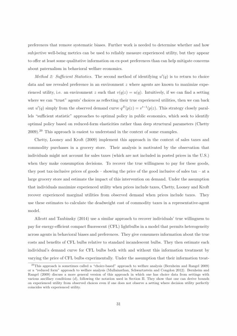
preferences that remove systematic biases. Further work is needed to determine whether and how

subjective well-being metrics can be used to reliably measure experienced utility, but they appear

to offer at least some qualitative information on ex-post preferences than can help mitigate concerns

about paternalism in behavioral welfare economics.

Method 2: Sufficient Statistics. The second method of identifying u′(q) is to return to choice

data and use revealed preference in an environment z where agents are known to maximize expe-

rienced utility, i.e. an environment z such that v(q|z) = u(q). Intuitively, if we can find a setting

where we can “trust” agents’ choices as reflecting their true experienced utilities, then we can back

out u′(q) simply from the observed demand curve qD(p|z) = v′−1(p|z). This strategy closely paral-

lels “sufficient statistic” approaches to optimal policy in public economics, which seek to identify

optimal policy based on reduced-form elasticities rather than deep structural parameters (Chetty

2009).29 This approach is easiest to understand in the context of some examples.

Chetty, Looney and Kroft (2009) implement this approach in the context of sales taxes and

commodity purchases in a grocery store. Their analysis is motivated by the observation that

individuals might not account for sales taxes (which are not included in posted prices in the U.S.)

when they make consumption decisions. To recover the true willingness to pay for these goods,

they post tax-inclusive prices of goods – showing the price of the good inclusive of sales tax – at a

large grocery store and estimate the impact of this intervention on demand. Under the assumption

that individuals maximize experienced utility when prices include taxes, Chetty, Looney and Kroft

recover experienced marginal utilities from observed demand when prices include taxes. They

use these estimates to calculate the deadweight cost of commodity taxes in a representative-agent

model.

Allcott and Taubinsky (2014) use a similar approach to recover individuals’ true willingness to

pay for energy-efficient compact fluorescent (CFL) lightbulbs in a model that permits heterogeneity

across agents in behavioral biases and preferences. They give consumers information about the true

costs and benefits of CFL bulbs relative to standard incandescent bulbs. They then estimate each

individual’s demand curve for CFL bulbs both with and without this information treatment by

varying the price of CFL bulbs experimentally. Under the assumption that their information treat-

29This approach is sometimes called a “choice-based” approach to welfare analysis (Bernheim and Rangel 2009)or a “reduced form” approach to welfare analysis (Mullainathan, Schwartzstein and Congdon 2012). Bernheim andRangel (2009) discuss a more general version of this approach in which one has choice data from settings withvarious ancillary conditions (d), following the notation used in Section II. They show that one can derive boundson experienced utility from observed choices even if one does not observe a setting where decision utility perfectlycoincides with experienced utility.

31

ment eliminates all behavioral biases, the demand curve post-information coincides with marginal

experienced utilities, u′(q) in Figure 9. They use these estimates to derive the optimal subsidy for

compact fluorescent lightbulbs and the welfare gain from correcting the internality.

Like the subjective well-being methodology, the sufficient statistic approach does not require

specifying the exact behavioral model that describes agents’ choices. This is attractive because

there are many behavioral models which could generate differences between decision utility and

experienced utility, as illustrated by the neighborhood choice application. A common criticism of

behavioral economics is that it does not offer a single unified framework as an alternative to the

neoclassical model. The sufficient statistic approach provides a method of handling this problem in

the context of normative analysis: if one can find a domain where agents optimize, one can make

robust statements about optimal policy that are valid irrespective of the underlying behavioral

model. For example, in the context of neighborhood effects, if the predominant source of bias

is that individuals are uninformed about the benefits of living in better areas for their children,

one could identify experienced utility by estimating demand after providing complete information

about the consequences of growing up in different neighborhoods.30

The drawback of the sufficient statistic approach is that one may not always be able to find

an environment z where behavioral biases do in fact vanish. For example, Bordalo, Gennaioli

and Shleifer (2014) propose a model of salience effects in which a surprise display of tax-inclusive

prices as in Chetty, Looney, and Kroft’s (2009) application causes consumers to overreact to taxes,

thereby leading to mis-estimation of experienced utility. Similarly, in Alcott and Taubinsky’s

application, one may be concerned that consumers did not fully understand and pay attention to

the information they were provided on different light bulbs and hence were not fully “debiased”

even after the information treatment. More generally, if there are many behavioral factors at play

– not just inattention but also present bias, cognitive limitations, etc. – it may be very difficult to

identify settings where all biases are removed.

Method 3: Structural Modeling. The third approach to welfare analysis is to specify and estimate

the structural parameters of a behavioral model. The logic here is to identify how demand varies

as a function of the degree of behavioral bias and then extrapolate to the case with no bias to

infer experienced utility. This approach is analogous to estimating the structural parameters of the

30As this example illustrates, one typically needs to place some structure on the behavioral model to understandwhat conditions will produce unbiased choices. However, one may not need to fully specify and parametrize thepositive model. For instance, one does not need to specify exactly why individuals are uninformed about neighborhoodeffects in order to recover experienced utility when they are given full information.

32

production function for externalities.

Perhaps the most well-known application of the structural approach in behavioral models is

Laibson’s (1997) quasi-hyperbolic discounting formulation of present-bias. In Laibson’s lifecycle

model, individuals making decisions at time t = 0 maximize u(c0) + β∑

t δtu(ct), where ct denotes

consumption in period t, u(ct) is the flow utility from consumption in period t, δ denotes the agent’s

discount factor, and β < 1 represents the underweighting of future utility relative to current

utility because of present-bias. Laibson (1997) assumes that individuals discount future payoffs

exponentially in their experienced utility (i.e., β = 1). If this is the true model of behavior, one

can identify experienced utility in two steps. First, one estimates the structural parameters (β

and δ) using variation in the stream of payoffs over time. Then one simply sets β = 1 to identify

experienced utility and derive welfare implications. For example, Angeletos et al. (2001) calibrate

Laibson’s β−δ model using consumption data and show that individuals exhibit substantial present-

bias when making savings decisions, calling for policies to increase savings rates such as those

discussed in Section II. Similarly, Paserman (2008) estimates a model of job search with hyperbolic

discounting and uses it to predict the effects of unemployment benefit policies.

Other behavioral models can be estimated using a similar structural approach. DellaVigna

et al. (2014) estimate a model of job search with reference-dependent preferences and use it to

make predictions about the optimal time path of unemployment benefits. A similar structural

approach could be used in the context of neighborhood choice by picking one or more of the

behavioral biases discussed above – e.g., present bias or cognitive limitations – and estimating the

parameters of such a model using the techniques applied by Bayer, Ferreira and McMillan (2007)

in neoclassical models.

The strength of the structural approach is that it allows us to infer experienced utility from

choice data even if we cannot find domains where all behavioral biases vanish. The drawback – like

structural estimation in neoclassical economics – is that it relies on strong modeling assumptions.31

This is well illustrated by Paserman (2008) and DellaVigna et al.’s (2014) work on unemployment

benefit policy in behavioral models. Paserman (2008) allows for present bias but rules out other be-

havioral features that appear to affect job search behavior, such as reference dependence and biased

31In the working paper version of their paper on tax salience, Chetty, Looney and Kroft (2007) take a structuralapproach to welfare analysis by developing a bounded rationality model of inattention to taxes. The formulas forthe efficiency costs of taxation obtained from this approach illustrate the tradeoffs between sufficient statistic andstructural approaches to welfare analysis. The sufficient-statistic formulas are more general, but the structuralformulas can be estimated even without data from an environment where agents maximize experience utility andyield additional predictions about the determinants of the welfare costs of taxation.

33

beliefs (Spinnewijn 2015). DellaVigna et al. (2014) permit present bias and reference dependence,

but do not allow for biased beliefs. Moreover, they require the reference point to be determined

by past unemployment benefit levels rather than past consumption or expectations of future con-

sumption, which would be an equally plausible specification (Koszegi and Rabin 2006). Ideally one

would use more flexible specifications in each of these models, but this is often theoretically and

empirically intractable.32

Although much remains to be learned about normative analysis in behavioral models, the three

approaches discussed above demonstrate one can make progress on characterizing experienced util-

ity and optimal policy in a disciplined, non-paternalistic manner. Importantly, the welfare impli-

cations obtained from neoclassical models will generally be incorrect if agents’ experienced utility

differs from their decision utility. Hence, the challenges in identifying experienced utility do not

provide a rationale for adhering to the neoclassical model. Further research on welfare analysis

in behavioral models is particularly critical because many policy debates are already motivated

by presumed behavioral biases. For example, policy proposals such as mandated retirement and

unemployment savings accounts (e.g., Feldstein 1998, Feldstein and Altman 2007) or consumer pro-

tection regulations that limit consumers’ choice sets are typically justified by behavioral arguments.

If economists do not contribute to these debates by analyzing the welfare consequences of these

policies in behavioral models, such policies may be implemented based on paternalistic assumptions

rather than empirical evidence.

IV.D Model Uncertainty and Optimal Policy

In many situations, one may have to make policy decisions without full information about the

underlying positive model. For instance, as discussed in Section IV.B, both neoclassical and be-

havioral models can fit available evidence about neighborhood effects.33 While future research

will hopefully shed light on the degree of behavioral biases in this application – i.e., the difference

between qD(p) and u′(q) in Figure 9 – what is the optimal policy given the available data?

32The challenges in identifying experienced utility grow larger when one allows for heterogeneity across individualsin preferences and the degree of behavioral biases. Each of the approaches described above can accommodateheterogeneity, but the data requirements grow much larger. See Allcott and Taubinsky (2014) and Goldin andReck (2014) for methods of identifying the distribution of preferences using a sufficient statistic approach and Carrollet al. (2009) for an analysis of optimal default policy using a structural model of present bias and procrastinationwith heterogeneous agents.

33Behavioral and neoclassical models can produce different normative implications even though they produce similarpositive predictions within a given domain. Of course, there will always be further tests one could run to discriminatebetween the two models; if there is no domain in which the two models generate different behavior, then they wouldeffectively imply the same underlying decision model.

34

When faced with uncertainty about the true model, economists are naturally inclined to use the

neoclassical model as the default. A more principled approach is to explicitly account for model

uncertainty when determining the optimal policy. This approach once again follows naturally

from established methodological traditions in neoclassical economics, such as the literature on

robust control (Hansen and Sargent 2007). Although a full treatment of optimal policy with model

uncertainty is outside the scope of this paper, some simple examples show that the neoclassical

model should not necessarily be given priority in the presence of model uncertainty.

Nudges with Model Uncertainty. Consider a model with two states of the world. Families either

optimize as in the neoclassical model when choosing neighborhoods or are biased toward staying

in worse areas because of the behavioral biases described in Section IV.B. Suppose optimizers

are insensitive to nudges such as counseling on the relative benefits of different neighborhoods.

However, behavioral agents are influenced by the way in which different neighborhoods are framed.

The intuition underlying this assumption is that behavioral biases are positively correlated. If

agents optimize perfectly in choosing neighborhoods, then they are also likely to be insensitive

to framing. If they suffer from behavioral biases when choosing where to live, then they may be

influenced by how choices are framed as well.

In this environment, the optimal policy is to follow the prescriptions of the behavioral model and

nudge agents toward moving to better (e.g., lower-poverty) areas for children. Nudging is optimal

irrespective of one’s prior beliefs on the two models because it is a weakly dominant policy. If fam-

ilies turn out to be optimizers, there is no loss from nudging families toward certain neighborhoods

because the nudges will be ignored.34 But if families turn out to have behavioral biases, then policy

makers increase welfare by nudging families to neighborhoods where their children will do better.

The result that one should exactly follow the prescriptions of the behavioral model rests on

the strong assumption that the nudge has literally no cost if agents optimize.35 But this simple

example illustrates that the neoclassical model should not necessarily be given priority when we

are uncertain about the true model. Indeed, there may be good reasons to prioritize behavioral

models instead.

Subsidies with Model Uncertainty. Now consider an alternative policy tool in the same two-state

example above: subsidized housing vouchers that are financed through a lump-sum tax. Housing

34This assumes that the marginal costs of the nudge (e.g., counseling) are negligible.35Moreover, this simple analysis ignores the equilibrium effects of nudges, which could have important welfare

consequences. For instance, Handel (2013) shows that nudges that improve individuals’ choices in health insurancemarkets could reduce social welfare by exacerbating adverse selection.

35

vouchers affect the behavior of both optimizing and behavioral agents. If families optimize, the

optimal subsidy is zero (ignoring externalities), as any subsidy distorts families’ choices relative to

their true preferences. If families underestimate the benefits of neighborhood quality, the optimal

subsidy is positive. If the policy maker seeks to maximize expected utility given uncertainty about

the true model, the optimal housing voucher subsidy is strictly positive, a result that follows from

O’Donoghue and Rabin’s (2006) analysis of optimal sin taxes. The reason is that introducing a

small subsidy has a second-order cost for optimizing agents (because they are already at their

optima to begin with) but yields a first-order gain for behavioral agents (since they under-invest

in neighborhood quality in the absence of the subsidy by assumption). Hence, once again the

optimal policy is not to strictly follow the prescriptions of the neoclassical model but rather to put

some weight on the possibility of behavioral biases. However, unlike with nudges, it is not optimal

to put full weight on the behavioral model, because the subsidy imposes a distortionary cost on

neoclassical agents.

An interesting implication of these examples is that model uncertainty can provide a new

justification for using nudges instead of conventional policy tools such as subsidies. Nudges are

typically justified based on the principle of “libertarian paternalism,” as they influence choice

without limiting any individual’s options (Thaler and Sunstein 2003). The examples above suggest

an alternative rationale for nudges: they maximize expected welfare in the presence of model

uncertainty. Nudges work when agents make behavioral mistakes, but have no impact when they

do not, thus providing a more robust way to correct internalities than tax incentives.36 Studying the

optimal combination of nudges and price incentives in a more general setting with model uncertainty

would be a fruitful direction for future research in behavioral welfare economics.

V Conclusion

The central message of this paper is that the decision to include behavioral factors in economic

models should be viewed as a pragmatic rather than philosophical choice. In some applications,

insights from psychology or other social sciences can help us develop better answers by identifying

new policy tools, offering better predictions of the effects of existing policies, or producing new

welfare implications. In other applications, one may be able to safely ignore behavioral factors and

use neoclassical economic models. Decisions about whether to include behavioral factors in a model

36Moreover, as illustrated by the results on retirement saving in Section II.A, subsidies may be ignored by agentswho suffer from behavioral biases such as inattention, which may make them particularly ill-suited for correctinginternalities.

36

should be treated like other standard modeling decisions, such as whether to assume quasi-linear or

time separable utility. These assumptions are convenient analytical simplifications in some cases; in

others, relaxing these assumptions is essential to capture key features of the problem. In this sense,

behavioral economics is better viewed as a part of all economists’ toolkit (like other tools in applied

theory) rather than as a separate subfield. Dividing our field into “behavioral” and “neoclassical”

economics is akin to distinguishing “time separable” economists from others.

Although this article has focused on applications of behavioral economics, this pragmatic per-

spective also has lessons for researchers who develop and test new behavioral theories. Behavioral

economists sometimes focus on the goal of rejecting the assumptions of neoclassical models by

searching for applications to demonstrate behavioral anomalies. At this point, it may be more pro-

ductive to instead ask how behavioral models can contribute to answering core economic questions.

In this vein, it would be useful for experts in psychology and economics to distill the list of behav-

ioral anomalies into those that are most relevant in common applications. One of the challenges

practitioners face in incorporating behavioral insights is that there are myriad factors to consider,

with little guidance about which factors are most important. The same problem arises in the neo-

classical model, but economists have developed a set of conventions that streamline applications.

For instance, economists have learned that Giffen goods (goods whose demand increases with price)

are a theoretical possibility but are not relevant in most real-world applications. Identifying which

behavioral anomalies are like Giffen goods would simplify the models under consideration and may

ultimately increase the application of behavioral economics.

Why should economists adopt the pragmatic approach to behavioral economics advocated here?

One argument is that it follows naturally from widely accepted methodological traditions in our

profession. From a positive perspective, the applications reviewed in this paper show that an

updated reading of the “as if” approach to economic modeling advocated by Friedman (1953) –

traditionally one of the main arguments used to defend neoclassical models – calls for incorporating

behavioral economics into the analysis of important economic questions. From a normative per-

spective, behavioral economics can offer more accurate and robust prescriptions for optimal policy,

again building on familiar methods used to recover individuals’ preferences dating to work on exter-

nalities by Pigou (1920). Beyond these methodological justifications, perhaps the most important

argument for such a pragmatic perspective is that it can help us answer some of the critical policy

questions of our time, from childhood to retirement.

37

References

Aguiar, Mark, and Erik Hurst. 2005. “Consumption versus Expenditure.” Journal of Political

Economy, 113(5): 919–948.

Allcott, Hunt. 2011. “Social Norms and Energy Conservation.” Journal of Public Economics,

95(9-10): 1082–1095.

Allcott, Hunt. 2014. “Site Selection Bias in Program Evaluation.” Unpublished Working Paper.

Allcott, Hunt, and Dmitry Taubinsky. 2014. “The Lightbulb Paradox: Evidence from Two

Randomized Experiments.” Unpublished Working Paper.

Altonji, Joseph G., and Christina H. Paxson. 1992. “Labor Supply, Hours Constraints and

Job Mobility.” Journal of Human Resources, 27(2): 256–278.

Angeletos, George-Marios, David Laibson, Andrea Repetto, Jeremy Tobacman, and

Stephen Weinberg. 2001. “The Hyperbolic Consumption Model: Calibration, Simulation, and

Empirical Evaluation.” Journal of Economic Perspectives, 15(3): 47–68.

Ashraf, Nava, Colin F. Camerer, and George Loewenstein. 2005. “Adam Smith, Behavioral

Economist.” Journal of Economic Perspectives, 19(3): 131–145.

Atkinson, Anthony B., and Joseph E. Stiglitz. 1976. “The Design of Tax Structure: Direct

Versus Indirect Taxation.” Journal of Public Economics, 6: 55–75.

Bayer, Patrick, Fernanado Ferreira, and Robert McMillan. 2007. “A Unified Frame-

work for Measuring Preferences for Schools and Neighborhoods.” Journal of Political Economy,

115(4): 588–638.

Benartzi, Shlomo, and Richard H. Thaler. 2004. “Save More Tomorrow: Using Behavioral

Economics to Increase Employee Saving.” Journal of Political Economy, 112(1): 164–187.

Bernheim, Douglas. 2009. “Behavioral Welfare Economics.” Journal of the European Economic

Association, 7(2-3): 267–319.

Bernheim, Douglas, and Antonio Rangel. 2009. “Beyond Revealed Preference: Choice The-

oretic Foundations for Behavioral Welfare Economics.” The Quarterly Journal of Economics,

124(1): 51–104.

38

Bernheim, Douglas, Daniel Bjorkegren, Jeffrey Naecker, and Antonio Rangel. 2013. “Do

Hypothetical Choices and Non-Choice Ratings Reveal Preferences ?” NBER Working Paper No.

19269.

Besley, Timothy, and Stephen Coate. 1992. “Workfare versus Welfare: Incentive Arguments

for Work Requirements in Poverty-Alleviation Programs.” The American Economic Review,

82(1): 249–261.

Bettinger, Eric. P., Bridget Terry Long, Philip Oreopoulos, and Lisa Sanbonmatsu.

2012. “The Role of Application Assistance and Information in College Decisions: Results from

the H&R Block Fafsa Experiment.” The Quarterly Journal of Economics, 127(3): 1205–1242.

Bhargava, Saurabh, and Dayanand Manoli. 2014. “Why are Benefits Left on the Table?

Assessing the Role of Information, Complexity, and Stigma on take-up with and IRS Field

Experiment.” Unpublished Working Paper.

Bhargava, Saurabh, George Loewenstein, and Justin Sydnor. 2014. “Health Insurance and

Sub-Optimal Choice.” Unpublished Working Paper.

Bordalo, Pedro, Nicola Gennaioli, and Andrei Shleifer. 2014. “Memory, Attention and

Surprises.” Unpublished Working Paper.

Carroll, Gabriel D., David Laibson, Brigitte C. Madrian, and Andrew Metrick. 2009.

“Optimal Defaults and Active Decisions.” Quarterly Journal of Economics, 124(4): 1639–74.

Chetty, Raj. 2009. “Sufficient Statistics for Welfare Analysis: A Bridge Between Structural and

Reduced-Form Methods.” Annual Review of Economics, 1: 451–488.

Chetty, Raj. 2012. “Bounds on Elasticities with Optimization Frictions: A Synthesis of Micro

and Macro Evidence on Labor Supply.” Econometrica, 80(3): 969–1018.

Chetty, Raj, Adam Looney, and Kory Kroft. 2007. “Salience and Taxation: Theory and

Evidence.” NBER Working Paper No. 13330.

Chetty, Raj, Adam Looney, and Kory Kroft. 2009. “Salience and Taxation: Theory and

Evidence.” American Economic Review, 99(4): 1145–1177.

39

Chetty, Raj, and Emmanuel Saez. 2013. “Teaching the Tax Code: Earnings Responses to an

Experiment with EITC Recipients.” American Economic Journal: Applied Economics, 5(1): 1–

31.

Chetty, Raj, and Nathan Hendren. 2015. “The Effects of Neighborhoods on Children’s Long-

Term Outcomes: Quasi-Experimental Estimates for the United States.” Unpublished Working

Paper.

Chetty, Raj, John Friedman, and Emmanuel Saez. 2013. “Using Differences in Knowledge

Across Neighborhoods to Uncover the Impacts of the EITC on Earnings.” American Economic

Review, 103(7): 2683–2721.

Chetty, Raj, John N. Friedman, Soren Leth-Peterson, Torben Heien Nielsen, and Tore

Olsen. 2014a. “Active vs. Passive Decisions and Crowd-out in Retirement Savings Accounts:

Evidence from Denmark.” Quarterly Journal of Economics, 129(3): 1141–1219.

Chetty, Raj, Nathan Hendren, and Larry Katz. 2015. “The Effects of Exposure to Bet-

ter Neighborhoods on Children: New Evidence from the Moving to Opportunity Experiment.”

Unpublished Working Paper.

Chetty, Raj, Nathaniel Hendren, Patrick Kline, and Emmanuel Saez. 2014b. “Where is

the Land of Opportunity? The Geography of Intergenerational Mobility in the United States.”

Quarterly Journal of Economics, 129(4): 1553–1623.

Choi, James J., David Laibson, Brigitte C. Madrian, and Andrew Metrick. 2002. “De-

fined Contribution Pensions: Plan Rules, Participant Decisions, and the Path of Least Resis-

tance.” Tax Policy and the Economy,, 16.

Congdon, William J., Jeffrey R. Kling, and Sendhil Mullainathan. 2011. “Policy

and Choice: Public Finance through the Lens of Behavioral Economics.” Washington, D.C.:

Brookings Institution Press.

Conlisk, John. 1996. “Why Bounded Rationality?” Journal of Economic Literature, 34(2): 669–

700.

Cutler, David M., and Edward L. Glaeser. 1997. “Are Ghettos Good or Bad?” The Quarterly

Journal of Economics, 112(3): 827–72.

40

DellaVigna, Stefano. 2009. “Psychology and Economics: Evidence from the Field.” Journal of

Economic Literature, 47(2): 315–72.

DellaVigna, Stefano, and Ulrike Malmendier. 2004. “Contract Design and Self-Control: The-

ory and Evidence.” The Quarterly Journal of Economics, 64(2): 353–402.

DellaVigna, Stefano, Attila Lindner, Balazs Reizer, and Johannes F. Schmieder. 2014.

“Reference-Dependent Job Search: Evidence from Hungary.” Unpublished Working Paper.

Diamond, Peter A., and Jerry A. Hausman. 1994. “Contingent Valuation: Is Some Number

better than No Number?” The Journal of Economic Perspectives, 8(4): 45–64.

Diener, Ed, Richard E. Luca, and Shigehiro Oishi. 2000. “Subjective Well-Being: The

Science of Happiness and a Proposal for a National Index.” American Psychologist, 55(1): 34–43.

Eissa, Nada, and Hilary Hoynes. 2006. “Behavioral Responses to Taxes: Lessons from the

EITC and Labor Supply.” Tax Policy and the Economy, 20.

Engen, Eric M., William G. Gale, and John Karl Scholz. 1996. “The Illusory Effects of

Saving Incentives on Saving.” Journal of Economic Perspectives, 10(4): 113–38.

Epple, Dennis, and Holger Sieg. 1999. “Estimating Equilibrium Models of Local Jurisdiction.”

Journal of Political Economy, 107(4): 645–681.

Ericson, Keith M. 2014. “Consumer Inertia and Firm Pricing in the Medicare Part D Prescription

Drug Insurance Exchange.” American Economic Journal: Economic Policy, 6(1): 38–64.

Farber, Henry S. 2014. “Why You Can’t Find a Taxi in the Rain and Other Labor Supply

Lessons from Cab Drivers.” NBER Working Paper No. 20604.

Feldstein, Martin, and Dan Altman. 2007. “Unemployment Insurance Savings Accounts.” Tax

Policy and the Economy, 21.

Feldstein, Martin S., ed. 1998. Privatizing Social Security. University of Chicago Press.

Friedman, Milton. 1953. “Essays in Positive Economics.” University of Chicago Press.

Fryer, Roland G., Steven D. Levitt, and Sally Sadoff. 2012. “Enhancing the Efficacy of

Teacher Incentives through Loss Aversion: A Field Experiment.” NBER Working Paper No.

18237.

41

Gabaix, Xavier, and David Laibson. 2006. “Shrouded Attributes, Consumer Myopia, and Infor-

mation Suppression in Competitive Markets.” The Quarterly Journal of Economics, 121(5): 505–

540.

Gallagher, Kelly Sims, and Erich Muehlegger. 2014. “Giving Green to Get Green? Incentives

and Consumer Adoption of Hybrid Vehicle Technology.” Journal of Environmental Economics

and Management, 61(1): 1–15.

Goldin, Jacob, and Daniel H. Reck. 2014. “Preference Identification Under Inconsistent

Choice: A Reduced-Form Approach.” Unpublished Working Paper.

Government Printing Office. 2014. “Budget of the United States Government.” Chapter De-

partment of Housing and Urban Development, 91–94.

Hamermesh, Daniel S. 2013. “Six Decades of Top Economics Publishing: Who and How?”

Journal of Economic Literature, 51(1): 162–72.

Handel, Benjamin. 2013. “Adverse Selection and Inertia in Health Insurance Markets: When

Nudging Hurts.” American Economic Review, 103(7): 2643–82.

Hansen, Lars Peter, and Thomas J. Sargent. 2007. “Robustness.” Princeton University Press.

Hastings, Justine S., and Jeffrey M. Weinstein. 2008. “Information, School Choice, and

Academic Achievement: Evidence from Two Experiments.” Quarterly Journal of Economics,

123(4): 1373–1414.

Haushofer, Johnanes, and Ernst Fehr. 2014. “On the Psychology of Poverty.” Science,

344(6186): 862–867.

Hoxby, Caroline, and Sarah Turner. 2014. “Expanding College Opportunities for High-

Achieving, Low Income Students.” Stanford Institute for Economic Policy Research.

Internal Revenue Service. 1996. “Federal Tax Compliance Research: Individual Income Tax

Gap Estimates for 1985, 1988, and 1992.” Government Printing Press.

Internal Revenue Service. 2012. “Statistics of Income: Individual Income Tax Returns, 2012

Publication 1304.” Government Printing Press.

42

Jencks, Christopher, and Susan E. Mayer. 1990. “The social consequences of growing up in

a poor neighborhood.” Inner-city poverty in the United States, 111: 186.

Joint Committee on Taxation. 2012. “Estimates of Federal Tax Expenditures for Fiscal Years

2011-2015.” Government Printing Press.

Kahneman, Daniel, Alan B. Krueger, David A. Schkade, Norbert Schwarz, and

Arthur A. Stone. 2004. “A Survey Method for Characterizing Daily Life Experience: the

Day Reconstruction Method.” Science, 306(5702): 1776–1780.

Kahneman, Daniel, and Amos Tversky. 1979. “Prospect Theory: An Analysis of Decision

under Risk.” Econometrica, 47(2): 263–292.

Kahneman, Daniel, and Robert Sugden. 2005. “Experienced Utility as a Standard of Policy

Evaluation.” Environmental & Resource Economics, 32: 161–181.

Kahneman, Daniel, Peter P. Wakker, and Rakesh Sarin. 1997. “Back to Bentham? Explo-

rations of Experienced Utility.” The Quarterly Journal of Economics, 112(2): 375–405.

Kanbur, Ravi, Jukka Pirttila, and Matti Tuomala. 2006. “Non-Welfarist Optimal Taxation

and Behavioural Public Economics.” Journal of Economic Surveys, 20(5): 849–868.

Keller-Allen, Chandra, and Rose Maria Li. 2013. “Psychological Science and Behavioral

Economics in the Service of Public Policy.” Meeting Summary, National Institute of Health,

National Institute on aging, Washington, D.C.

Koszegi, Botond, and Matthew Rabin. 2006. “A Model of Reference-Dependent Preferences.”

The Quarterly Journal of Economics, 121(4): 1133–1165.

Koszegi, Botond. 2014. “Behavioral Contract Theory.” Journal of Economic Literature,

52(4): 1075–1118.

Laibson, David. 1997. “Golden Eggs and Hyperbolic Discounting.” Quarterly Journal of

Economics, 112(2): 443–477.

Lazear, Edward. 1983. “Intergenerational Externalities.” Canadian Journal of Economics,

16(2): 212–28.

43

Leigh, Andrew. 2010. “Who benefits from the Earned Income Tax Credit? Incidence among

Recipients, Coworkers and Firms.” The B. E. Journal of Economic Analysis and Policy, 10(1).

Levitt, Steven D., and John A. List. 2007. “What do Laboratory Experiments Measuring

Social Preferences Reveal About the Real World?” Journal of Economic Perspectives, 21(2): 153–

174.

Liebman, Jeffrey. 1998. “The Impact of the Earned Income Tax Credit on incentives and the

Income Distribution.” Tax Policy and the Economy, 12.

List, John A. 2004. “Neoclassical Theory Versus Prospect Theory: Evidence from the Market-

place.” Econometrica, 72(2): 615–625.

Loewenstein, George, Ted O’Donoghue, and Matthew Rabin. 2003. “Projection Bias in

Predicting Future Utility.” Quarterly Journal of Economics, 118(4): 1209–1248.

Ludwig, Jen, Greg J. Duncan, Lisa A. Gennetian, Lawrence F. Katz, Ronald C.

Kessler, Jeffrey R. Kling, and Lisa Sanbonmatsu. 2012. “Neighborhood Effects on the

Long-Term Well-Being of Low-Income Adults.” Science, 337(6101): 1505–1510.

Madrian, Brigitte C. 2014. “Applying Insights from Behavioral Economics to Policy Design.”

Annual Review of Economics, 6(1): 663–688.

Madrian, Brigitte C., and Dennis F. Shea. 2001. “The Power of Suggestion: Inertia in 401(k)

Participation and Savings Behavior.” The Quarterly Journal of Economics, 116(4): 1149–1187.

Meyer, Bruce. 2010. “The Effects of the Earned Income Tax Credit and Recent Reforms.” Tax

Policy and the Economy, 24.

Mirrlees, James A. 1971. “An Exploration in the Theory of Optimum Income Taxation.” The

Review of Economic Studies, 38(2): 175–208.

Mullainathan, Sendhil, Joshua Schwartzstein, and William J. Congdon. 2012. “A

Reduced-Form Approach to Behavioral Public Finance.” The Annual Review of Economics,

4(17): 1–30.

O’Donoghue, Ted, and Matthew Rabin. 2006. “Optimal Sin Taxes.” Journal of Public

Economics, 90(10-11): 1825–1829.

44

Paserman, Daniele M. 2008. “Job Search and Hyperbolic Discounting: Structural Estimation

and Policy Evaluation.” The Economic Journal, 118(531): 1418–1452.

Pigou, Arthur C. 1920. The Economics of Welfare. London: Macmillan.

Poterba, James M. 2014. “Retirement Security in an Aging Population.” American Economic

Association, 104(5): 1–30.

Poterba, James M., Steven F. Venti, and David A. Wise. 1996. “How Retirement Saving

Programs Increase Saving.” Journal of Economic Perspectives, 10(4): 91–112.

Rabin, Matthew. 1993. “Incorporating Fairness into Game Theory and Economics.” The

American Economic Review, 83(5): 1281–1302.

Rabin, Matthew. 1998. “Psychology and Economics.” Journal of Economic Literature, 36(1): 11–

46.

Ramsey, Frank P. 1927. “A Contribution to the Theory of Taxation.” Economic Journal,

37(145): 47–61.

Romich, Jennifer L., and Thomas S. Weisner. 2002. “Making Work Pay.” , ed. Bruce Meyer

and Douglas Holtz-Eakin, Chapter How Families View and Use the Earned Income Tax Credit:

Advance Payment Versus Lump-Sum Delivery. Russell Sage Foundation.

Rothstein, Jesse. 2010. “Is the EITC as Good as an NIT? Conditional Cash Transfers and Tax

Incidence.” American Economic Journal: Economic Policy, 2(1): 177–208.

Saez, Emmanuel. 2010. “Do Taxpayers Bunch at Kink Points?” American Economic Journal:

Economic Policy, 2(3): 180–212.

Sampson, Robert J., Jeffrey D. Morenoff, and Thomas Gannon-Rowley. 2002. “Assessing

Neighborhood Effects: Social Processes and New Directions in Research.” Annual Review of

Sociology, 28(1): 443–478.

Sanbonmatsu, Lisa, Jens Ludwig, Lawrence F. Katz, Lisa A. Gennetian, Greg J. Dun-

can, Ronald C. Kessler, Emma Adam, Thomas W. McDade, and Stacy Tessler Lin-

dau. 2011. “Moving to Opportunity for Fair Housing Demonstration Program: Final Impacts

Evaluation.”

45

Sen, Amartya. 1985. “Commodities and Capabilities.” Amsterdam: North-Holland.

Shah, Anuj K., Sendhil A. Mullainathan, and Eldar Shafir. 2012. “Some Consequences of

Having Too Little.” Science, 338(6107): 682–685.

Shapiro, Jesse M. 2005. “Is there a Daily Discount Rate? Evidence from the Food Stamp

Nutrition Cycle.” Journal of Public Economics, 89(2-3): 303–325.

Shleifer, Andrei, and Robert W. Vishny. 1997. “The Limits of Arbitrage.” The Journal of

Finance, 52(1): 35–55.

Simon, Herbert A. 1955. “A Behavioral Model of Rational Choice.” The Quarterly Journal of

Economics, 69(1): 99–118.

Smeeding, Timothy M., Katherin Ross-Phillips, and Michael A. O’Connor. 2002. “The

Earned Income Tax Credit: Expectation, Knowledge, Use, and Economic and Social Mobility.”

National Tax Journal, 53(4): 1187–1209.

Spinnewijn, Johannes. 2015. “Unemployed but Optimistic: Optimal Insurance Design with

Biased Beliefs.” Journal of the European Economic Association, 13(1): 130–167.

Stone, Arthur A., Saul S. Shiffman, and Marten W. DeVries. 1999. “Ecological Momentary

Assessment.” In Daniel Kahneman, Edward Diener, and Norbert Schwarz (eds.) Well-Being: The

foundations of hedonic Psychology. New York: Russell-Sage.

Thaler, Richard. 1980. “Toward a Positive Theory of Consumer Choice.” Journal of Economic

Behavior and Organization, 1: 39–60.

Thaler, Richard H., and Cass R. Sunstein. 2003. “Libertarian Paternalism.” The American

Economic Review, 93(2): 175–179.

Thaler, Richard H., and Cass R. Sunstein. 2008. “Nudge: Improving Decisions About Health,

Wealth and Happiness.” Penguin Books.

Tiebout, Charles M. 1956. “A Pure Theory of Local Expenditures.” The Journal of Political

Economy, 64(5): 416–424.

46

FIGURE 1: Effects of Reduction in Subsidy for Retirement Savings Accounts in Denmark

A. Mean Retirement Account Contributions

B. Distribution of Changes in Retirement Account Contributions

Notes: This figure reproduces Figure Va and VIb in Chetty, Friedman, Leth-Petersen, Nielsen, and Olsen (2014). PanelA plots mean total (individual plus employer) capital pension contributions for individuals with income in each DKr 5,000income bin within DKr 75,000 of the top income tax threshold, in each year from 1996-2001. Panel B plots the distribution ofchanges to individual capital pension contributions, as a percentage of lagged individual pension contributions, for individualswho are DKr 25-75K above the top tax cutoff in 1998 and 1999 (the treatment group affected by the subsidy reduction). PanelB restricts the sample to individuals who were contributing to capital pension accounts in the previous year.

FIGURE 2: Effects of Employer Contributions to Retirement Accounts

Notes: This figure reproduces Figure Ib in Chetty, Friedman, Leth-Petersen, Nielsen, and Olsen (2014). The figure analyzesa set of workers who switched to a new firm whose employer pension contribution rate was at least 3 percentage points oflabor income higher than their previous firm. The x axis of the figure is the calendar year relative to the year the workerswitched firms, so that year 0 represents the first year the worker is employed at the new firm. The figure plots meanemployer and individual retirement account contributions as well as individuals’ taxable savings in each year, all measured asa percentage of current labor income. The sample consists of workers for whom data is available for event years [−4, +4], sothat the number of observations is constant through the figure. The sample also includes only workers with positive individualpension contributions prior to the switch, i.e. those who are able to reduce individual pension contributions when employercontributions rise. The figure lists the change in each form of savings (as a percentage of labor income) from year -1 to year 0.

FIGURE 3: Effects of the EITC on Reported Taxable Income

A. Federal EITC Schedule for Single Filers with Children in 2008

B. Taxable Income Distributions for EITC Claimants in Kansas and Texas

Notes: Panel A shows the EITC schedule for single filers with children in 2008 as a function of their reported taxable income.The vertical lines denote the refund-maximizing kink for each group. Panel B reproduces Figure 1a in Chetty, Friedman, andSaez (2013) using data for EITC claimants with children in Texas and Kansas. These distributions are histograms with $1,000bins centered around the first kink of the EITC schedule. Taxable income is the total amount of earnings used to calculate theEITC, and is equivalent to the sum of wage earnings and self-employment income reported on Form 1040 for most tax filers.

FIGURE 4: Geographical Variation in EITC Sharp Bunching by Year

A. Sharp Bunching in 1996 B. Sharp Bunching in 1999

C. Sharp Bunching in 2002 D. Sharp Bunching in 2005

E. Sharp Bunching in 2008

Notes: This figure reproduces Appendix Figure 3 in Chetty, Friedman and Saez (2013). It plots self-employed sharp bunchingrates by 3 digit ZIP code (ZIP-3) in 1996, 1999, 2002, 2005, 2008. Self-employed sharp bunching is defined as the fraction ofEITC-eligible households with children whose total income falls within $500 of the first kink point of the EITC schedule andwho have non-zero self-employment income. The observations are divided into deciles pooling all years so that the decile cutpoints are fixed across years. Each decile is assigned a different color on the maps, with darker shades representing higherlevels of sharp bunching.

FIGURE 5: Effects of Moving to Areas with Higher vs. Lower Sharp Bunching on EITC Refunds

Notes: This figure reproduces Figure 3b in Chetty, Friedman and Saez (2013). The sample in this figure consists of taxpayerswho move across 3-digit ZIP codes. The figure plots changes in EITC refund amounts from the year before the move to theyear after the move vs. differences in prior residents’ sharp bunching rates in the new and old ZIP-3’s. The figure groupsindividuals into bins of width 0.05 based on their change in sharp bunching and plots the mean change in EITC refund amountswithin each bin. The solid lines show linear regressions estimated on the individual-level data separately for the observationsabove and below 0. The estimated slopes are reported next to each line along with standard errors clustered by bin.

5

FIGURE 6: Effects of the EITC on Wage Earnings

A. U.S. Population

B. Highest Sharp Bunching Decile vs. Lowest Sharp Bunching Decile

Notes: This figure reproduces Figure 5a in Chetty, Friedman and Saez (2013). Panel A plots W-2 wage earnings distributionsfor single wage earners with one child, pooling data from 1999-2009 in the U.S. as a whole. Panel B focus on the subset ofindividuals living in the highest and lowest self-employment sharp bunching deciles, i.e. areas with the highest and lowest levelsof information about the EITC. Self-employed sharp bunching is defined as the percentage of EITC claimants with childrenin the ZIP-3-by-year cell who report total earnings within $500 of the first EITC kink and have non-zero self-employmentincome. The series in triangles includes individuals in ZIP-3-by-year cells in the highest self-employed sharp bunching decile,while the series in circles includes individuals in the lowest sharp bunching decile. Each distribution is a histogram showingthe percentage of observations in $1000 bins. The EITC schedule is shown on the right y axis, and the dashed vertical linesdepict the plateau region of the EITC schedule where individuals obtain the largest EITC refund amounts.

FIGURE 7: EITC and Wage Earnings Distributions: Changes Around Childbirth

A. Wage Earnings Distributions in the Year Before First Child Birth

B. Wage Earnings Distributions in the Year of First Child Birth

Notes: This figure reproduces Figure 6 in Chetty, Friedman and Saez (2013). The sample includes wage earners living in thehighest and lowest self-employment sharp bunching deciles, i.e. areas with the highest and lowest levels of information aboutthe EITC. Self-employed sharp bunching is defined as the percentage of EITC claimants with children in the ZIP-3-by-year cellwho report total earnings within $500 of the first EITC kink and have non-zero self-employment income. Panel A plots W-2wage earnings distributions in the year before child birth. Panel B replicates these distributions for the year of child birth.Each distribution is a histogram showing the percentage of observations in $1000 bins. The dashed vertical lines depict theplateau region of the EITC schedule for single individuals with one child, where individuals obtain the largest EITC refundamounts.

FIGURE 8: The Geography of Upward Income Mobility in the United States

Notes: This figure reproduces Appendix Figure VIb in Chetty, Hendren, Kline and Saez (2014). It presents a heat map ofupward income mobility based on de-identified federal income tax records for all children in the 1980-85 birth cohorts in theU.S. The map is divided into 741 commuting zones. In each commuting zone, upward income mobility is measured by theprobability that a child reaches the top quintile of the national income distribution (for his birth cohort) conditional on havingparents in the bottom quintile of the national income distribution. Children are assigned to commuting zones based on wherethey grew up (i.e., where they were first claimed as a dependent on a tax return), irrespective of where they live as adults.The commuting zones are divided into deciles based on their rate of upward mobility, with lighter colored areas representingareas with higher rates of upward mobility.

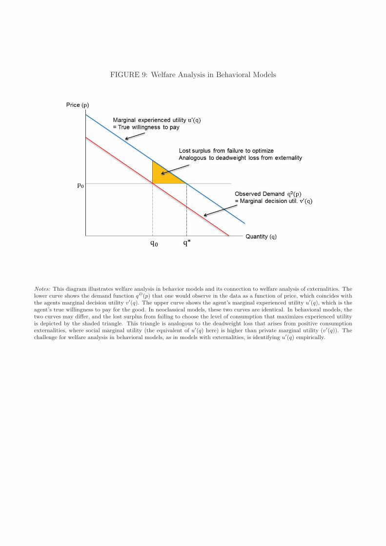
FIGURE 9: Welfare Analysis in Behavioral Models

Notes: This diagram illustrates welfare analysis in behavior models and its connection to welfare analysis of externalities. Thelower curve shows the demand function qD(p) that one would observe in the data as a function of price, which coincides withthe agents marginal decision utility v′(q). The upper curve shows the agent’s marginal experienced utility u′(q), which is theagent’s true willingness to pay for the good. In neoclassical models, these two curves are identical. In behavioral models, thetwo curves may differ, and the lost surplus from failing to choose the level of consumption that maximizes experienced utilityis depicted by the shaded triangle. This triangle is analogous to the deadweight loss that arises from positive consumptionexternalities, where social marginal utility (the equivalent of u′(q) here) is higher than private marginal utility (v′(q)). Thechallenge for welfare analysis in behavioral models, as in models with externalities, is identifying u′(q) empirically.