BEHAVIORALIZE THIS!

International Evidence on Autocorrelation Patterns of

Stock Index and Futures Returns

Dong-Hyun Ahna, Jacob Boudoukhb, Matthew Richardsonc, and Robert F. Whitelawd *

July 1999

*aKenan-Flagler Business School, University of North Carolina, Chapel Hill; bStern School of Business,New York University and NBER; cStern School of Business, New York University and NBER; and dSternSchool of Business, New York University. Thanks to Eli Ofek and seminar participants at the FederalReserve, Washington, D.C. for helpful comments.

Abstract

This paper investigates the relation between returns on stock indices and their corre-

sponding futures contracts in order to evaluate potential explanations for the pervasive yet

anomalous evidence of positive, short-horizon portfolio autocorrelations. Using a simple

theoretical framework, we generate empirical implications for both microstructure and be-

havioral models. These implications are then tested using futures data on 24 contracts

across 15 countries. The major �ndings are (i) return autocorrelations of indices tend to

be positive even though their corresponding futures contracts have autocorrelations close to

zero, (ii) these autocorrelation di�erences between spot and futures markets are maintained

even under conditions favorable for spot-futures arbitrage, and (iii) these autocorrelation

di�erences are most prevalent during low volume periods. These results point us towards a

market microstructure-based explanation for short-horizon autocorrelations and away from

explanations based on current popular behavioral models.

1 Introduction

Arguably, one of the most striking asset pricing anomalies is the evidence of large, positive,

short-horizon autocorrelations for returns on stock portfolios, �rst described in Hawawini

(1980), Conrad and Kaul (1988,1989,1998) and Lo and MacKinlay (1988,1990a). The ev-

idence is pervasive both across sample periods and across countries, and has been linked

to, among other �nancial variables, �rm size (Lo and MacKinlay (1988)), volume (Chordia

and Swaminathan (1998)), analyst coverage (Brennan, Jegadeesh and Swaminathan (1993)),

institutional ownership (Badrinath, Kale and Noe (1995) and Sias and Starks (1997)), and

unexpected cross-sectional return dispersion (Connolly and Stivers (1998)).1 The above

results are puzzling to �nancial economists precisely because time-variation in expected re-

turns is not a high-frequency phenomenon; asset pricing models link expected returns with

changing investment opportunities, which, by their nature, are low frequency events.

As a result, most explanations of the evidence have centered around the so-called lagged

adjustment model in which one group of stocks reacts more slowly to aggregate information

than another group of stocks. Because the autocovariance of a well-diversi�ed portfolio is

just the average cross-autocovariance of the stocks that make up the portfolio, positive auto-

correlations result. While �nancial economists have put forth a variety of economic theories

to explain this lagged adjustment, all of them impose some sort of underlying behavioral

model, i.e., irrationality, on the part of some agents, that matters for pricing. (See, for

example, Holden and Subrahmanyam (1992), Brennan, Jegadeesh and Swaminathan (1993),

Jones and Slezak (1998), and Daniel, Hirshleifer and Subrahmanyam (1998).) Alternative,

and seemingly less popular, explanations focus on typical microstructure biases (Boudoukh,

Richardson and Whitelaw (1994)) or transactions costs which prevent these autocorrela-

tion patterns from disappearing in �nancial markets (Mech (1993)). The latter explanation,

however, does not explain why these patterns exist in the �rst place.

This paper draws testable implications from the various theories by exploiting the relation

between the spot and futures market.2 Speci�cally, while much of the existing focus in the

1Another powerful and related result is the short-term continuation of returns, the momentum e�ect,

documented by Jegadeesh and Titman (1993). While this evidence tends to be �rm-speci�c, it also produces

positive autocorrelation in short-horizon stock returns (see Grinblatt and Moskowitz (1998) as recent exam-

ples). Moreover, this evidence holds across countries (e.g., Rouwenhorst (1998)) and across time periods.2Miller, Muthuswamy and Whaley (1994) and Boudoukh, Richardson and Whitelaw (1994) also argue

that the properties of spot index and futures returns should be di�erent. Miller, Muthuswamy and Whaley

(1994) look at mean-reversion in the spot-futures basis in terms of nontrading in S&P 500 stocks, while

1

literature has been on the statistical properties of arti�cially constructed portfolios (such as

size quartiles), there are numerous stock indices worldwide which exhibit similar properties.

Moreover, many of these indices have corresponding futures contracts. Since there is a direct

link between the stock index and its futures contract via a no arbitrage relation, it is possible

to show that, under the aforementioned economic theories, the futures contract should take

on the properties of the underlying index. In contrast, why might the properties of the

returns on the index and its futures contract diverge? If the index, or for that matter,

the futures prices are constructed based on mismeasured prices (e.g., stale prices, bid or

ask prices), then the link between the two is broken. Alternatively, if transaction costs on

the individual stocks comprising the index are large enough, then the arbitrage cannot be

implemented successfully. This paper looks at all of these possibilities in a simple theoretical

framework and tests their implications by looking at spot and futures data on 24 stock

indices across 15 countries.

The results are quite remarkable. In particular,

� The return autocorrelations of indices with less liquid stocks (such as the Russell 2000

in the U.S., the TOPIX in Japan, and the FTSE 250 in the U.K.) tend to be positive

even though their corresponding futures contracts have autocorrelations close to zero.

For example, the Russell 2000's daily autocorrelation is 22%, while that of its respective

futures contract is 6%. The di�erences between these autocorrelation levels are both

economically and statistically signi�cant.

� Transactions costs cannot explain the magnitude of these autocorrelation di�erences

as the magnitude changes very little even when adjusting for periods favorable for

spot-futures arbitrage. We view this as strong evidence against the type of irrational

models put forth in the literature.

� Several additional empirical facts point to microstructure-type biases, such as staleness

of pricing, as the most probable source of the di�erence between the autocorrelations of

the spot and futures contracts. For example, in periods of generally high volume, the

Boudoukh, Richardson and Whitelaw (1994) look at combinations of stock indices, like the S&P 500 and

NYSE, in order to isolate portfolios with small stock characteristics. While the conclusions in those papers

are consistent with this paper, those papers provide only heuristic arguments and focus on limited indices

over a short time span. This paper develops di�erent implications from various theories and tests them

across independent, international data series.

2

return autocorrelation of the spot indices drops dramatically. The futures contract's

properties change very little, irrespective of the volume in the market.

� All of these results hold domestically, as well as internationally. This is especially

interesting given that the cross-correlation across international markets is fairly low,

thus providing independent evidence in favor of our �ndings.

The paper is organized as follows. In Section 2, we provide an analysis of the relation

between stock indices and their corresponding futures contracts under various assumptions,

including the random walk model, a nontrading model, and a behavioral model. Of special

interest, we draw implications for the univariate properties of these series with and without

transactions costs. Section 3 describes the data on the various stock index and futures

contracts worldwide, while Section 4 provides the main empirical results of the paper. In

Section 5, we make some concluding remarks.

2 Models of the Spot-Futures Relation

There is a large literature in �nance on the relation between the cash market and the stock

index futures market, and, in particular, on their lead-lag properties. For example, MacKin-

lay and Ramaswamy (1988), Stoll and Whaley (1990), and Chan (1992), among others, all

look at how quickly the cash market responds to market-wide information that has already

been transmitted into futures prices. While this literature shows that the cash and futures

market have di�erent statistical properties, there are several reasons why additional analysis

is needed. First, while there is strong evidence that the futures market leads the cash mar-

ket, this happens fairly quickly. Second, most of the analysis is for indices with very active

stocks, such as the S&P 500 or the MMI, which possess very little autocorrelation in their

return series. Third, these examinations have been at the intraday level and not concerned

with longer horizons that are more relevant for behavioral-based models.

In this section, we provide a thorough look at implications for the univariate statistical

properties of the cash and futures markets under various theoretical assumptions about

market behavior with and without transactions costs. In order to generate these implications,

we make the following assumptions:

� The index, S, is an equally-weighted portfolio of N assets with corresponding futures

3

contract, F .3

� To the extent possible (i.e., transactions costs aside), there is contemporaneous arbi-

trage between S and F . That is, the market is rational with respect to index arbitrage.

� Prices of individual securities, Si; i = 1; :::; N , follow a random walk in the absence

of irrational behavior. This assumption basically precludes any \equilibrium" time-

variation in expected returns at high frequencies. All lagged adjustment e�ects, there-

fore, are described in terms of irrational behavior on the part of some agents, i.e., some

form of market ine�ciency.

� The dividend processes for each asset, di, and the interest rate, r, are independent of

the index price, S. Violations of this assumption are investigated in Section 4 and

evaluated for their e�ect on the relation between the cash and futures market

Under these assumptions, we consider three models. The �rst is the standard model with

no market microstructure e�ects or irrational behavior. The implications of this model are

well known, and are provided purely as a benchmark case. The second model imposes a

typical market structure bias, namely nontrading on a subset of the stocks in the index. The

third model imposes a lagged adjustment process for some of the stocks in the index. In

particular, we assume that some stocks react to market-wide information more slowly due to

the reasons espoused in the literature. Transaction costs are then placed on the individual

stocks in the index, as well as on the futures contract, to better understand the relation

between the cash and futures markets.

2.1 Case I: The Random Walk Model

Applying the cost of carry model and using standard arbitrage arguments, the futures price

is simply the current spot price times the compounded rate of interest (adjusted for paid

dividends):4

Ft;T = Ste(i�d)(T�t)

3The assumption of equal weights is used for simplicity.4See, for example, MacKinlay and Ramaswamy (1988). Note that, for the moment, we assume that

interest rates and dividend yields are constant. In practice, this assumption is fairly robust due to the fact

that these �nancial variables are signi�cantly less variable than the index itself. Violations of this assumption

are explored in Section 4.

4

where Ft;T is the futures price of the index, maturing in T-t periods,

St is the current level of the index,

i is the continuously compounded rate of interest,

d is the continuously compounded rate of dividends paid, and

T is the maturity date of the futures contract.

Thus, under the cost of carry model, we can write the return on the futures as

rF = rS; (1)

where rF is the continuously compounded return on the futures and rS is the excess return of

the underlying spot index (i.e., in excess of the risk-free interest rates). Note that the change

in the continuously compounded interest rate (adjusted for the dividend rate), �(i � d),

drops out due to the assumption of constant interest rates and dividend yields. For the more

realistic assumption that these variables are stochastic (yet perhaps independent) of stock

returns, �(i� d) would represent an additional term in equation (1).

Several observations are in order. First, under the random walk model, and assuming

that �(i�d) has either low volatility or little autocovariance, the autocorrelation of futures'

returns will mimic that of the spot market, i.e., it will be approximately zero. Second, the

variance of futures' returns should exceed that of the spot market by the variance of �(i�d),

assuming no correlation between the index returns and either dividend changes or interest

rate changes. Third, even in the presence of transaction costs, these results should hold as

the futures price should still take on the properties of the expected future stock index price,

which is the current value of the index in an e�cient market.

2.2 Case II: A Nontrading Model

The market microstructure literature presents numerous examples of market structures which

can induce non-random walk behavior in security prices. Rather than provide an exhaustive

analysis of each of these structures, we focus on one particular characteristic of the data

that has received considerable attention in the literature, namely nonsynchronous trading.

Nontrading refers to the fact that stock prices are assumed to be recorded at a particular

point in time from period to period when in fact they are recorded at irregular points in time

during these periods. For example, stock indices are recorded at the end of trading using

the last transaction price of each stock in the index. If those stocks (i) did not trade at the

5

same time, and (ii) did not trade exactly at the close, then the index would be subject to

nontrading-induced biases in describing its characteristics. The best known characteristic, of

course, is the spurious positive autocorrelation of index returns, as well as the lower variance

of measured returns on the index.

Models of nontrading, and corresponding results, have appeared throughout the �nance

literature, including, among others, Fisher (1966), Scholes and Williams (1977), Cohen,

Maier, Schwartz and Whitcomb (1978), Dimson (1979), Atchison, Butler and Simonds

(1987), Lo and MacKinlay (1990b), and Boudoukh, Richardson and Whitelaw (1994). In

this paper, we choose the simple model of Lo and MacKinlay (1990b) to illustrate the re-

lation between the spot and futures markets. In their model, in any given period, there

is an exogenous probability �i that stock Si does not trade. Furthermore, each security's

return, ri, is described by one zero-mean, i.i.d. factor, M , with loading, �i. Lo and MacKin-

lay (1990b) show that the measured excess returns on an equally-weighted portfolio of N

securities, denoted rS, can be written as

rS;t = �S � i+ (1� �S)�S1Xk=0

�kSMt�k;

where �S and �S are the average mean and average beta of the portfolio of the N stocks,

and �S is the probability of nontrading assuming equal nontrading probabilities across the

stocks. Of course, the true excess returns are simply described by

rS;t = �S � i+ �SMt;

where any idiosyncratic risk has been diversi�ed away.

In a no arbitrage world, the price of the futures contract will re ect the present value of

the stock index at maturity. That is,

Ft;T = PV(ST )e(i�d�)(T�t); (2)

where d� is the previous dividend rate, d, adjusted for the fact that some stocks in the index

don't trade. Note that, due to nontrading, the present value of the index is no longer its

true value, but instead a value that partly depends on the current level of nontrading. This

is because the futures price is based on the measured value of the index at maturity, which

includes stale prices. Within the Lo and MacKinlay (1990b) model, nontrading today has

some, albeit small, information about the staleness of prices in the distant future. However,

6

as long as the contract is not close to expiration, the e�ect, which is of order �T�t, is

miniscule. In particular, it is possible to show that the corresponding futures return is:

rFt;T = (1� �T�t)rS;t: (3)

Not surprisingly, in contrast to the measured index returns, futures returns will not be

autocorrelated due to the e�ciency of the market and the no arbitrage condition between

the cash and futures market. However, the futures return will di�er from the true excess spot

return because it is priced o� the measured value of the spot at maturity. This di�erence

leads to a lower volatility of the futures return than the true spot return, though by a small

factor for long-maturity contracts. Speci�cally, within the framework of this model, the

variance ratio between futures returns and true spot returns is (1��T�t)2, whereas the ratio

between measured index returns and true returns is (1��)2

1��2. Except for very short maturity

contracts, futures returns volatility will be greater than that of the measured index return.5

2.3 Case III: The Partial-Adjustment Model

As an alternative to market microstructure-based models, the �nance literature has devel-

oped so-called partial adjustment models. Through either information transmission, noise

trading or some other mechanism, these models imply that some subset of securities partially

adjust, or adjust more slowly, to market-wide information. While there is some debate about

whether these models can be generated in both a reasonable and rational framework, all the

models impose some restrictions on trading so that the partial adjustment e�ects cannot get

arbitraged away. There are a number of models that produce these types of partial adjust-

ment e�ects (e.g., see Holden and Subrahmanyam (1992), Foster and Viswanathan (1993),

Badrinath, Kale and Noe (1995), Chordia and Swaminathan (1998) and Llorente, Michaely,

Saar and Wang (1998)).

Here, we choose one particular model, which coincides well with Section 2.2 above, namely

Brennan, Jegadeesh and Swaminathan (1993). We assume that the index is made up of two

5It can be shown that futures returns volatility will be greater than that of the measure index return if

(T � t) >

ln�1�

q1��1+�

�ln�

�

r1

1� �2:

Even when � is 50%, which is a unrealistically large number, the volatility ratio will be greater than one if

the maturity of the futures contract is greater than 1.25 days.

7

equally-weighted portfolios of stocks, SF and SP , which for better terminology stand for full

(i.e., F ) and partial (i.e., P ) response stocks. (Brennan, Jegadeesh and Swaminathan (1993)

consider stocks followed by many analysts versus those followed by only a few analysts.)

Assume that the returns on these two portfolios can be written as

RF;t = �F + �FMt

RP;t = �P + �PMt + PMt�1:

Thus, for whatever reason, the return on the partial response stocks is a�ected by last period's

realization of the factor. One o�ered explanation is that market-wide information is only

slowly incorporated into certain stock prices, yielding a time-varying expected return that

depends on that information. Note that similar to Lo and MacKinlay (1990b) and Section

2.2 above, we have also assumed that these two portfolios are su�ciently well-diversi�ed that

there is no remaining idiosyncratic risk.

Assume that the index contains ! of the fully adjusting stock portfolio and 1 � ! of

the partially adjusting portfolio. Under the assumption of no transactions costs and no

arbitrage, it is possible to show that the excess returns on the index and its corresponding

futures contract can be written as:

rS;t = �S � i+ �SMt + SMt�1 (4)

rF;t = rS;t

where �S = !�F + (1� !)�P

�S = !�F + (1� !)�P

S = (1� !) P :

The returns on both the stock index and its futures contract coincide, and therefore pick up

similar autocorrelation properties. In fact, their autocorrelations can be solved for

[!�F + (1� !)�P ](1� !) P[!�F + (1� !)�P ]2 + [(1� !) P ]2

:

For indices with relatively few partial-adjustment stocks (i.e., high !) or low lagged response

coe�cients (i.e., small P ), the autocorrelation reduces to approximately :

(1� !) P!�F + (1� !)�P

:

With the additional assumption that the beta of the index to the factor is approximately

one, an estimate of the autocorrelation is (1 � !) P . That is, the autocorrelation depends

8

on the proportion of partially adjusting stocks in the index and on how slowly these stocks

respond. These results should not seem surprising. With the no arbitrage condition between

the cash and futures market, the price of the futures equals the present value of the future

spot index, which is just the current value of the index. That is, though the spot price at

maturity includes lagged e�ects, the discount rate does also, leading to the desired result.

With nontrading, because the lagged e�ects are spurious, discounting is done at �S, which

leads to zero autocorrelation of futures returns.

In response, a behavioralist might argue that the futures return does not pick up the

properties of the cash market due to the inability of investors to actually conduct arbitrage

between the markets. Of course, the most likely reason for the lack of arbitrage is the

presence of transactions costs, that is, commissions and bid-ask spreads paid on the stocks

in the index and the futures contract. The level of these transactions costs depend primarily

on costs borne by the institutional index arbitrageurs in these markets. Abstracting from

any discussion of basis risk and the price of that risk, we assume here that arbitrageurs buy

or sell all the stocks in the index, at a multiplicative cost of �. Thus, round-trip transactions

costs per arbitrage trade are equal to 2�. In this environment, it is possible to show that, in

the absence of arbitrage, the futures price must satisfy the following constraints:

�(2� + �i) � Ft;T � Ste(i�d)(T�t) � (2� + �i): (5)

In other words, the futures price is bounded by its no arbitrage value plus/minus round-trip

transactions costs.

What statistical properties do futures returns have within the bounds? There is no

obvious answer to this question found in the behavioral literature. If the futures is priced o�

the current value of the spot index, then, as described above, futures returns will inherit the

autocorrelation properties of the index return. Alternatively, suppose investors in futures

markets are more sophisticated, or at least respond to information in M fully. That is, they

price futures o� the future value of the spot index, discounted at the rate �S. In this case,

the futures returns will not be autocorrelated, and expected returns on futures will just equal

�S + E[�(i� d)].

Of course, if the futures-spot parity lies outside the bound, then arbitrage is possible,

and futures prices will move until the bound is reached. It is possible to show that futures

prices at time t will lie outside the bound (in the absence of arbitrage) under the following

condition:

jMtj �2� + �i

(1� !) P: (6)

9

That is, three factors increase the possibility of lying outside the bound: (i) large recent

movement in the stock index (i.e., jMtj), (ii) low transactions costs (i.e., �), (iii) large auto-

correlation in the index (i.e., (1 � !) P ). If condition (6) is met, then, even in the case of

sophisticated futures traders, expected returns on futures will not be a constant, but instead

capture some of the irrationality of the index. Speci�cally, if (6) is true, then

Et[rF;t] = (1� !) PMt � (2� + �i): (7)

Figure 1 illustrates the pattern in expected futures returns under this model. Within the

bounds, expected futures returns are at. Outside the bound, futures begin to take on the

properties of the underlying stock index, and futures returns are positively autocorrelated for

more extreme past movements. Figure 1 provides the basis for an analysis of the implications

of futures markets in the presence of index return autocorrelation.

Similarly, we can calculate the volatility of the returns on the index and the volatility of

the returns on its corresponding futures contract. Within the bound, using equation (4), it

is possible to show that the return variances are:

�2rS = (�2S + 2S)�

2M

�2rF = (�S + S)2�2M :

In other words, as long as S is positive (which is the prevailing view), the volatility of

futures returns will be higher than the volatility of the spot index excess returns. However,

volatility of interest rate changes aside (i.e., �2�(i�d)), the volatility of the spot and futures

returns will start to converge when condition (6) is realized. This is because the futures

return takes on the properties of the index return as index arbitrage forces convergence of

the two.

2.4 Implications

The above models for index and corresponding futures prices are clearly stylized and very

simple. For example, the Lo and MacKinlay (1988) model of nontrading has been general-

ized to heterogeneous nontrading and heterogeneous risks of stocks within a portfolio which

provides more realistic autocorrelation predictions (see, for example, Boudoukh, Richardson

and Whitelaw (1994)). Which model is best, however, is besides the point for this paper.

The purpose of the models is to present, in a completely transparent setting, di�erent impli-

cations of two opposing schools of thought. The �rst school believes that the time-varying

10

patterns in index returns are not tradeable, and in fact may actually be completely spurious,

i.e., an artifact of the way we measure returns. The second school believes that these pat-

terns are real and represent actual prices, resulting from some sort of ine�cient information

transmission in the market. The implications we draw from these models are quite general

and robust to more elaborate speci�cations of nontrading or agent's ability to incorporate

information quickly.

In particular, according to the models described in Sections 2.2 and 2.3, it is possible

to make several observations about the relative statistical properties of index and futures

returns:

� Under a market microstructure setting, the index returns will be positively autocor-

related while the futures returns will not be autocorrelated (bid-ask bounce aside).

Moreover, the magnitude of these di�erences will be related to the level of microstruc-

ture biases. In contrast, the behavioral model predicts spot index and futures returns

will inherit the same autocorrelation properties.

� Similar implications occur for the volatility of the index and futures returns. Behavioral

models predict spot and futures returns will have approximately the same volatility

(interest rate volatility aside), while market microstructure models imply di�erent

volatilities. Again, the di�erence in volatilities will be related to the magnitude of the

microstructure biases.

� In the presence of transactions costs, behavioral models can potentially form a wedge

between the statistical properties of spot index and futures returns. However, this

wedge leads to particular implications, namely that the spot index and futures returns

will behave similarly in periods of big stock price movements and possibly quite dif-

ferently in periods of small movements. For example, the autocorrelation of futures

returns should be zero for small movements, and positive for large movements. Like-

wise, the relative volatility between the futures and spot market should be higher in

the futures market for small past movements versus large past movements.

� Finally, a nontrading-based explanation of the patterns in spot index and futures re-

turns implies the following characteristic of the data. As the nontrading probability �

goes down, i.e., higher volume, the spot index return's properties, such as its autocor-

relation, should look like the true return process. Moreover, while the properties of the

11

index return change with volume, the properties of the futures return should remain

the same for long maturity contracts.

These observations are the basis for an empirical comparison of spot index and corresponding

futures returns. To build up as much independent evidence as possible, this analysis is

performed on over 24 indices across 15 countries. Because the daily index returns across

these countries are not highly correlated, the results here will have considerably more power

to di�erentiate between the implications of the two schools.

3 The Data

All the data are collected from Datastream; speci�cally, price levels of each stock index and

corresponding futures contract at the close of trade every day, daily volume on the overall

stock market in a given country, daily open interest and volume for each futures contract,

short-term interest rates and dividend yields. The data are collected to coincide with the

length of the available futures contract. For example, if the futures contract starts on June

1, 1982 (as did the S&P 500), all data associated with this contract start from that date.

The futures data are constructed according to usual conventions. In particular, a single

time series of futures prices is spliced together from individual futures contracts prices. For

liquidity, the nearest contract's prices are used until the �rst day of the expiration month,

then the next nearest is used, and so on. For a futures contract to be used, we require

at least four years of data (or roughly 1000 observations) to lower the standard errors of

the estimators. This leads us to drop a number of countries such as the Eastern European

block, emerging countries in Asia like Thailand, Korea and Malaysia, as well as some small

stock based indices like the MDAX in Germany. Given this criteria, we are left with 24

futures contracts on stock indices covering 15 countries. Table 1 gives a brief description

of each contract, the exchange it is traded on, its country a�liation, its starting date, as

well as some summary statistics on the futures' returns, open interest and trading volume.

Summary statistics on the underlying index returns are also provided.

Some observations are in order. First, given the wide breadth of countries used in this

analysis as seen in Table 1, and the fact that daily returns across countries have relatively

small contemporaneous correlations (e.g, with a mean of .39 and a median of .32), the data

in this study provide considerable independent information about the economic implications

described in Section 2. Second, while the unconditional means of the index returns and

12

corresponding futures returns are basically the same for all contracts, their volatilities are

substantially di�erent. While part of these di�erences can be explained by interest rate

volatility, the majority of the di�erences come from some other source (see Section 4). As

shown in Section 2, these types of di�erences are more commonly associated with market

microstructure biases since behavioral models imply the volatility will be picked up in both

markets. Third, the futures contracts have considerable open interest and daily volume in

terms of the number of contracts. Table 1 provides the mean for these contracts, and, for

less liquid ones such as the Russell 2000 and Value Line, these means are still high relative

to less liquid stocks, e.g., 455 and 197 contracts per day respectively. The fact that these

contracts are liquid allows us to focus primarily on market microstructure biases related to

the stocks in the underlying index. Section 4 of the paper addresses any potential biases

related to the futures contracts.

4 Empirical Results

In this section, we focus on providing evidence for or against the implications derived from

the models of Section 2. In particular, we investigate (i) the autocorrelation properties of

the spot index and corresponding futures returns, (ii) the relative time-varying properties of

spot index and future returns conditional on recent small and large movements in returns,

and (iii) the relation between these time-varying properties and underlying stock market

volume.

4.1 Autocorrelations

Table 2 presents the evidence for daily autocorrelations of spot indices and their corre-

sponding futures returns across 24 contracts. The most startling evidence is that, for every

contract, the spot index autocorrelation exceeds that of the futures. This cannot be ex-

plained by common sampling error as many of the contracts are barely correlated given

the 15 country cross-section. Figure 2 presents a scatter plot of the autocorrelations of the

futures and spot indices, i.e., a graphical representation of these results. On the 45 degree

line, the spot and futures autocorrelations coincide; however, as the graph shows, all the

points lie to the right of this line. Thus, all the spot autocorrelations are higher than their

corresponding futures.

Moreover, other than the Nikkei 225 contracts (which have marginally negative values),

13

all of the spot index returns are positively autocorrelated. Some of these indices, such as

the Russell 2000 (small �rm US), ValueLine (equal-weighted US), FTSE 250 (medium-�rm

UK), TOPIX (all �rms Japan), OMX (all �rms Sweden) and Australian All-Share index,

have fairly large autocorrelations | .22, .19, .21, .10, .12 and .10, respectively. Interestingly,

these indices also tend to be ones which include large weights on �rms which trade relatively

infrequently. In contrast, the value-weighted indices with large, liquid, actively-traded stocks,

such as the S&P 500 (largest 500 US �rms), FTSE 100 (100 most active U.K. �rms), Nikkei

225 (active 225 Japan stocks), and DAX (active German �rms), are barely autocorrelated

| .03, .08, -.014 and .02, respectively.

Note that while the autocorrelations of both the index and futures alone are di�cult

to pinpoint due to the size of the standard errors, the autocorrelation di�erences should

be very precisely estimated given the high contemporaneous correlation between the index

and futures. In terms of formal statistical tests, for 21 out of 24 contracts we can reject

the hypothesis that the spot index autocorrelation equals that of its futures contract at the

5% level. To the extent that this is one of the main comparative implications of market

microstructure versus behavioral models, this evidence supports the microstructure-based

explanation.6 The evidence is particularly strong as 17 of the di�erences are signi�cant the

1% level. These levels of signi�cance should not be surprising given that the index and

its futures capture the same aggregate information, yet produce in 12 cases autocorrelation

di�erences of at least 10% on a daily basis!

4.2 Time-Varying Patterns of Returns

The results in Section 4.1 are suggestive of di�erences between the time-varying properties

of spot index and futures returns. While this tends to be inconsistent with behavioral-

based explanations of the data, we showed in Section 2.3 that it is possible to construct

a reasonable scenario in which large di�erences can appear. Speci�cally, the reason why

behavioral models imply a one-to-one relation between spot and futures returns is that

they are linked via spot-futures arbitrage. If spot-futures arbitrage is not possible due to

transactions costs, then theoretically spot and futures prices might diverge if their markets

are driven by di�erent investors. Figure 1 shows that the implication of this transaction-

6Of course, futures returns, due to either nontrading or bid-ask bounce, should have negative autocor-

relations, which could partially explain the di�erences even without index microstructure biases. Section 4

looks at the extent to which futures biases can explain the result.

14

based model is that, conditional on extreme recent movements, the statistical properties of

spot and futures returns should be similar; for small movements, they can follow any pattern,

including the spot return being positively autocorrelated and its futures return being serially

uncorrelated.

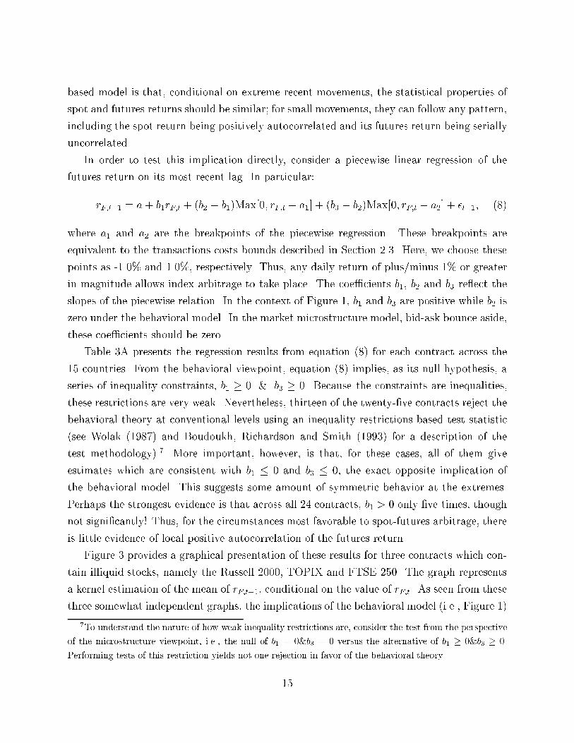
In order to test this implication directly, consider a piecewise linear regression of the

futures return on its most recent lag. In particular:

rF;t+1 = a + b1rF;t + (b2 � b1)Max[0; rF;t � a1] + (b3 � b2)Max[0; rF;t � a2] + �t+1; (8)

where a1 and a2 are the breakpoints of the piecewise regression. These breakpoints are

equivalent to the transactions costs bounds described in Section 2.3. Here, we choose these

points as -1.0% and 1.0%, respectively. Thus, any daily return of plus/minus 1% or greater

in magnitude allows index arbitrage to take place. The coe�cients b1, b2 and b3 re ect the

slopes of the piecewise relation. In the context of Figure 1, b1 and b3 are positive while b2 is

zero under the behavioral model. In the market microstructure model, bid-ask bounce aside,

these coe�cients should be zero.

Table 3A presents the regression results from equation (8) for each contract across the

15 countries. From the behavioral viewpoint, equation (8) implies, as its null hypothesis, a

series of inequality constraints, b1 � 0 & b3 � 0. Because the constraints are inequalities,

these restrictions are very weak. Nevertheless, thirteen of the twenty-�ve contracts reject the

behavioral theory at conventional levels using an inequality restrictions-based test statistic

(see Wolak (1987) and Boudoukh, Richardson and Smith (1993) for a description of the

test methodology).7 More important, however, is that, for these cases, all of them give

estimates which are consistent with b1 � 0 and b3 � 0, the exact opposite implication of

the behavioral model. This suggests some amount of symmetric behavior at the extremes.

Perhaps the strongest evidence is that across all 24 contracts, b1 > 0 only �ve times, though

not signi�cantly! Thus, for the circumstances most favorable to spot-futures arbitrage, there

is little evidence of local positive autocorrelation of the futures return.

Figure 3 provides a graphical presentation of these results for three contracts which con-

tain illiquid stocks, namely the Russell 2000, TOPIX and FTSE 250. The graph represents

a kernel estimation of the mean of rF;t+1, conditional on the value of rF;t. As seen from these

three somewhat independent graphs, the implications of the behavioral model (i.e., Figure 1)

7To understand the nature of how weak inequality restrictions are, consider the test from the perspective

of the microstructure viewpoint, i.e., the null of b1 = 0&b3 = 0 versus the alternative of b1 � 0&b3 � 0.

Performing tests of this restriction yields not one rejection in favor of the behavioral theory.

15

are not borne out. Time-variation of expected futures returns, if any, occur for low current

values of returns. Conditional on high values, the relation looks quite at.8 Of course, the

strongest evidence in the graph is that there is not much time-variation in the estimated ex-

pected return on the futures anywhere, which is not a prediction of behavioral-based models.

One potential point of discussion is that the model described in Figure 1 implies a linear

relation between next period's return and the current period's return. While this is consistent

with almost all the behavioral models described in the literature, it is not necessarily an

appropriate assumption. The more general implication is that, outside the transaction costs

bounds, the spot and futures return take on similar characteristics, linear or nonlinear as

the case may be. In order to address this issue more completely, we provide an analogous

regression to (8) above, namely

rS;t+1� rF;t+1 = a+ b1rF;t+ (b2 � b1)Max[0; rF;t� a1] + (b3� b2)Max[0; rF;t� a2] + �t+1: (9)

Under more general versions of the model of Section 2.3, we would expect b1 = b3 = 0, that

is, the spot index and futures return to behave the same under conditions for spot-futures

arbitrage. Table 3B provides results for the regression in (9) across all the countries.

In contrast to this behavioral-based implication, 21 of the 24 contracts reject the hy-

pothesis, b1 = b3 = 0, in favor of the microstructure alternative, b1 � 0; b3 � 0, at the 5%

level. This is especially surprising given that some of these contracts include, for the most

part, actively traded stocks. Almost all the b1 and b3 coe�cients are positive (i.e., only 4

negative estimates amongst 50), which again implies that the time-variation of the expected

spot index returns is both greater than that of its corresponding futures contract and more

positively autocorrelated. To the extent that the microstructure based theory would imply

that all three coe�cients (b1; b2; b3) should be positive, 70 of 75 of them are. Since these

coe�cients represent relations over di�erent (and apparently independent) data ranges and

across 15 somewhat unrelated countries, this evidence, in our opinion, is strong.

4.3 Autocorrelations and Volume

One obvious implication of the nontrading-based model of Section 2.2 is that there should

be some relation between the spot index properties and volume on that index, whereas the

8The exception here is the FTSE 250 for current values of rF;t > 1:5%. However, for the post 1994

sample period we have here for this contract, there are hardly any observations. Thus, the results fall into

the so-called Star-Trek region of the data, and are unreliable.

16

futures should for the most part be unrelated to volume. Of course, behavioral-based models

may also imply some correlation between volume and autocorrelations (e.g., as in Chordia

and Swaminathan (1998)), but it is clearly a necessary result of the nontrading explanation.

In order to investigate this implication, we collected data from Datastream on overall

stock market volume for each of the 15 countries. While this does not represent volume for

the stocks underlying the index, it should be highly correlated with trading in these stocks

because all the indices we look at are broad-based, market indices. That is, on days in which

stock market volume is low, it seems reasonable to assume that large, aggregate subsets of

this volume will also be relatively low. During the sample periods for each country, there has

been a tendency for volume to increase (partly due to increased equity values and greater

participation in equity markets). The standard approach is to avoid the nonstationarity

issue and look at levels of detrended volume. For the US stock market, Figure 4 graphs the

two volume series, and illustrates the potential di�erences between the two series. For the

purposes of estimation, the detrended series looks more useful.

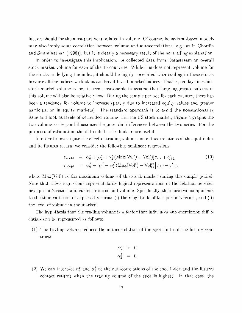
In order to investigate the e�ect of trading volumes on autocorrelations of the spot index

and its futures return, we consider the following nonlinear regressions:

rS;t+1 = �s0 + [�s

1 + �s2 (Max(Vols)� Volst )] rS;t + �st+1 (10)

rF;t+1 = �f0 +

h�f1 + �

f2 (Max(Vols)� Volst)

irF;t + �

ft+1;

where Max(Vols) is the maximum volume of the stock market during the sample period.

Note that these regressions represent fairly logical representations of the relation between

next period's return and current returns and volume. Speci�cally, there are two components

to the time-variation of expected returns: (i) the magnitude of last period's return, and (ii)

the level of volume in the market.

The hypothesis that the trading volume is a factor that in uences autocorrelation di�er-

entials can be represented as follows:

(1) The trading volume reduces the autocorrelation of the spot, but not the futures con-

tract:

�s2 > 0

�f2 = 0

(2) We can interpret �s1 and �

f1 as the autocorrelations of the spot index and the futures

contact returns when the trading volume of the spot is highest. In that case, the

17

autocorrelation of the spot as well as the futures should be close to zero:

�s1 = 0

�f1 = 0

Some observations are in order. Hypothesis (1) is an obvious implication of index returns

being driven by nontrading-based models, and the most important component of our hy-

potheses. Note that it is possible that �s2 = 0, in which case �s

1 represents the autocorrelation

of the index return in a world in which volume plays no role. With respect to hypothesis

(2), it appears to be redundant given (1). However, we want to be able to test whether

the negative relation is strong enough to bring forth the desired result that the spot index

return autocorrelation becomes zero at the highest level of the trading volume. Finally, an

important hypothesis to test is whether the futures contract's autocorrelation is independent

of trading volume.

Table 4 provides results for each of the 24 stock indices across the 15 countries. First,

there is a negative relation between the trading volume and the autocorrelation of the spot

index return for most of the countries (i.e., �s2 > 0). While the estimators are individually

signi�cant at the 5% level for only a few of the indices (e.g., the Russell 2000's estimate

is 0.54 with standard error 0.19), 21 of 24 of them are positive. Moreover, relative to the

futures return coe�cient on volume (i.e., �f2), about 70% have values of �s

2 > �f2 . While

only a few of these are individually signi�cant at the 5% level (i.e., S&P 500, Russell 2000,

NYSE, FTSE 250, Switzerland, Amsterdam, Hong Kong, and Belgium), only one contract

goes in the direction opposite to that implied by the nontrading-based theory.

Second, independent of volume, the relation between futures return autocorrelations and

trading volume is very weak. Even though many of the autocorrelation coe�cients, �f2 , are

positive, they tend to be very small in magnitude and are thus both economically and statis-

tically insigni�cant. Furthermore, the estimates at high levels of nontrading imply negative

autocorrelation in futures returns, which is consistent with the Table 2 results. Combining

the estimates of �f1 and �

f2 together in equation (10) implies that the autocorrelations of

futures returns are rarely positive irrespective of volume levels. This result is consistent with

the bid-ask bounce e�ect which will be looked at in Section 4.5.

Third, at the highest level of trading, the autocorrelations of the spot and futures return

are for the most part insigni�cantly di�erent from zero. For example, only 3 contracts, all

of which are based on Japanese stock indices (i.e., Nikkei 225, Nikkei 300, and TOPIX),

violate this hypothesis. However, for each of these cases, the autocorrelations are negative

18

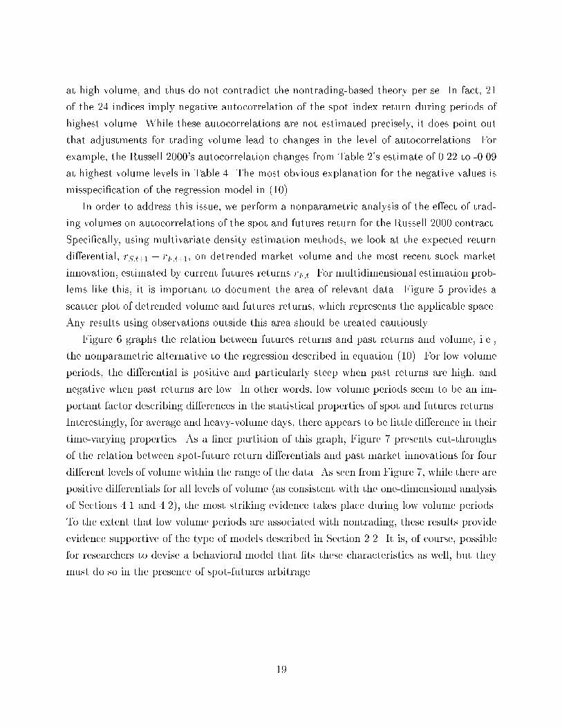
at high volume, and thus do not contradict the nontrading-based theory per se. In fact, 21

of the 24 indices imply negative autocorrelation of the spot index return during periods of

highest volume. While these autocorrelations are not estimated precisely, it does point out

that adjustments for trading volume lead to changes in the level of autocorrelations. For

example, the Russell 2000's autocorrelation changes from Table 2's estimate of 0.22 to -0.09

at highest volume levels in Table 4. The most obvious explanation for the negative values is

misspeci�cation of the regression model in (10).

In order to address this issue, we perform a nonparametric analysis of the e�ect of trad-

ing volumes on autocorrelations of the spot and futures return for the Russell 2000 contract.

Speci�cally, using multivariate density estimation methods, we look at the expected return

di�erential, rS;t+1 � rF;t+1, on detrended market volume and the most recent stock market

innovation, estimated by current futures returns rF;t. For multidimensional estimation prob-

lems like this, it is important to document the area of relevant data. Figure 5 provides a

scatter plot of detrended volume and futures returns, which represents the applicable space.

Any results using observations outside this area should be treated cautiously.

Figure 6 graphs the relation between futures returns and past returns and volume, i.e.,

the nonparametric alternative to the regression described in equation (10). For low volume

periods, the di�erential is positive and particularly steep when past returns are high, and

negative when past returns are low. In other words, low volume periods seem to be an im-

portant factor describing di�erences in the statistical properties of spot and futures returns.

Interestingly, for average and heavy-volume days, there appears to be little di�erence in their

time-varying properties. As a �ner partition of this graph, Figure 7 presents cut-throughs

of the relation between spot-future return di�erentials and past market innovations for four

di�erent levels of volume within the range of the data. As seen from Figure 7, while there are

positive di�erentials for all levels of volume (as consistent with the one-dimensional analysis

of Sections 4.1 and 4.2), the most striking evidence takes place during low volume periods.

To the extent that low volume periods are associated with nontrading, these results provide

evidence supportive of the type of models described in Section 2.2. It is, of course, possible

for researchers to devise a behavioral model that �ts these characteristics as well, but they

must do so in the presence of spot-futures arbitrage.

19

4.4 Volatility Ratios

Section 2 provides implications for the variance ratio between the futures and the underlying

index return. The ratios given in Table 1 do not support the behavioral explanation as

futures return volatility exceeds that of the spot index. In this subsection, we explore these

results more closely by addressing two issues: (I) the e�ect of the volatility of interest rates

and dividend yields, and (II) the behavior of the volatility ratios in periods most suited to

spot-futures arbitrage.

With respect to (I), Table 5 provides the ratio of the futures return variance over the

measured spot index return variance, adjusted for the variance (and covariance) of the cost of

carry, �(i�d). Not surprisingly, due to the fact that stock volatility is so much greater than

interest rate volatility, the results from Table 1 carry through here. For every single contract,

the variance ratio exceeds 1, and signi�cantly so for all but one. This result provides strong

evidence in favor of a nontrading-based explanation.

With respect to (II), Section 2.4 showed that the behavioralists imply, for extreme lagged

returns, the variance ratio should be closer to one than for small lagged returns. In practice,

due to heteroskedasticity, one would expect variances to increase during the extreme periods,

but that the ratios stay relatively constant. Since extreme values are more suitable for spot-

futures arbitrage, spot and futures volatility should be closer together (at least outside the

transactions cost range). In contrast to the previous results regarding behavioral hypotheses,

Table 5 provides some (albeit weak) support for the theory. Nineteen of the twenty-�ve

contracts produce greater variance ratios in normal periods; however, only eight of these are

signi�cant at conventional levels. Microstructure-based explanations do not address this issue

per se. However, if extreme moves tend to be associated with high volume environments,

then rational theories would also suggest that the volatility ratio decline here (i.e., due to

the better measurement of the stock index). In any event, the main prediction, namely that

futures volatility exceeds spot volatility, is strongly supported in the data.

4.5 Can Bid-Ask Bounce Explain the Autocorrelation Di�erences?

One possible explanation for the di�erences between spot index and futures' return autocor-

relations is that the futures contract themselves su�er from microstructure biases. That is, a

behavioralist might argue that the true autocorrelation is large and positive, yet the futures'

autocorrelation gets reduced by bid-ask bounce and similar e�ects. In fact, it is well known

that bid-ask bias leads to negative serial correlation in returns (see, for example, Roll (1984)

20

and Blume and Stambaugh (1983)). How large does the bid-ask spread need to be to give

credibility to this explanation?

Consider a variation of the Blume-Stambaugh (1983) model in which the measured futures

price, Fm, is equal to the true price, F , adjusted for the fact that some trades occur at the

o�er or asking price, i.e.,

Fmt = Ft(1 + �t);

where �t equals the adjustment factor. In particular, assume that �t equalss2with probability

p

2(i.e., the ask price), � s

2with probability p

2(i.e., the bid price), or 0 with probability 1� p

(i.e., a trade within the spread). Here, s represents the size of the bid-ask spread, and can be

shown to be directly linked to the volatility of �t. Speci�cally, we can show that �2� = p s2

4. In

words, the additional variance of the futures price is proportional to the size of the spread and

the probability that trades take place at the quotes. Using the approximation ln(1+x) � x,

it is possible to show that the implied autocorrelation of futures returns is given by

�ps2

4�2RF+ 2ps2

: (11)

Table 6 reports the autocorrelation di�erences between the stock index and futures re-

turns. If these di�erences were completely due to bid-ask bias in the futures market, then

equation (11) can be used to back out the relevant bid-ask spread. The last two columns

of Table 6 provide estimates of the size of this spread in percentage terms of the futures

price. The two columns represent two di�erent values of p, the probability of trading at

the ask or bid, equal to either 0.5 or 1.0. Of course, a value of 1.0 is an upper bound on

the e�ect of the bid-ask spread. The implied spreads in general are much larger than those

that occur in practice. To see this, we document actual spreads at the end of the sample

over a week period, and �nd that they are approximately one-tenth the magnitude (i.e., see

column (4) of Table 6). Alternatively, using the actual spreads, and the above model, we

report implied autocorrelations, which are all close to zero. Therefore, the di�erences in

the autocorrelations across the series is clearly not driven by bid-ask bounce in the futures

market.

5 Concluding Remarks

The simple theoretical results in this paper, coupled with the supporting empirical evi-

dence, lead to several conclusions. First, there are signi�cant di�erences between the sta-

tistical properties of spot index and corresponding futures returns even though they cover

21

the same underlying stocks. These di�erences can most easily be associated with market

microstructure-based explanations as behavioral models do not seem to capture the charac-

teristics of the data. Second, in the presence of transactions costs and the most favorable

conditions for behavioral models, the empirical results provide very di�erent conclusions.

When futures-spot arbitrage is possible, the spot and futures contract exhibit the most dif-

ferent behavior, the opposite implication of a behavioral model. Third, an important factor

describing these di�erent properties is the level of volume in the market, which is consistent

with nontrading-based explanations as well as possibly behavioral-based models linked to

volume.

The unique aspect of this paper has been to di�erentiate, rather generally, implications

from two very di�erent schools of thought and provide evidence thereon. Our conclusion

is generally not supportive of the behavioral, partial-adjustment models that have become

popular as of late. What then is going on in the market that can describe these large daily

autocorrelations of portfolio returns?

Previous authors (e.g., Conrad and Kaul (1989) and Mech (1993), among others) have

performed careful empirical analyses of nontrading by taking portfolios that include only

stocks that have traded. Their results, though somewhat diminished, suggest autocorrela-

tions are still positive and large for these portfolios. It cannot be the case that exchange-based

rules, like price continuity on the NYSE, explain these patterns because these results hold

across exchanges and apparently across countries. Whatever the explanation, it must be

endemic to all markets.

Rational models predict that the price of a security is the discounted value of its future

cash ow. Within this context, how should we view a trade for 100 shares when there is little

or no other trading? Does it make sense to discard a theory based on a single investor buying

a small number of shares at a stale over- or undervalued (relative to market information)

price, or a dealer inappropriately not adjusting quotes for a small purchase or sale? Our

view is that the important issue is how many shares can trade at that price (either through

a large order or numerous small transactions). What would researchers �nd if we took

portfolios of stocks that trade meaningfully, and then what would happen if these portfolios

got segmented via size, number of analysts, turnover, et cetera? These are questions which

seem very relevant given the results of this paper.

22

REFERENCES

Atchison, M., K. Butler, and R. Simonds, 1987, \Nonsynchronous Security Trading and

Market Index Autocorrelation," Journal of Finance, 42, 533-553.

Badrinath, S., J. Kale and T. Noe, 1995, \Of Shepherds, Sheep, and the Cross-Autocorrelations

in Equity Returns," Review of Financial Studies 8, 401-430.

Bessembinder, H., and M. Hertzel, 1993, \Return Autocorrelations around Nontrading

Days," Review of Financial Studies, 6, 155-189.

Blume, M., and R. Stambaugh, 1983, \Biases in Computed Returns: An Application to

the Size E�ect," Journal of Financial Economics, 12, 387-404.

Boudoukh, J., M. Richardson and T. Smith, 1993, \Is the Ex-Ante Risk Premium Al-

ways Positive?: A New Approach to Testing Conditional Asset Pricing Models," Journal of

Financial Economics 34, pp.387-409.

Boudoukh, J., M. Richardson and R. Whitelaw, 1994, \A Tale of Three Schools: Insights

on Autocorrelations of Short-Horizon Stock Returns," Review of Financial Studies 7, 539-

573.

Brennan, M., N. Jegadeesh and B. Swaminathan, 1993, \Investment Analysis and The

Adjustment of Stock Prices to Common Information," Review of Financial Studies 6, 799-

824.

Chan, K., 1992, \A further analysis of the lead-lag relationship between the cash market

and stock index futures market," Review of Financial Studies 5, 123-152.

Chordia, T. and B. Swaminathan, 1998, \Trading Volume and Cross-Autocorrelations in

Stock Returns," forthcoming Journal of Finance.

Cohen, K., S. Maier, R. Schwartz, and D. Whitcomb, 1986, The Microstructure of Secu-

rity Markets, Prentice-Hall, Englewood Cli�s, NJ.

Connolly, R., and C. Stivers, 1998, \Conditional Stock Market Return Autocorrelation

and Price Formation: International Evidence from Six Major Equity Markets," working

paper, University of North Carolina.

Conrad, J., and G. Kaul, 1988, \Time Varying Expected Returns," Journal of Business,

61, 409-425.

Conrad, J., and G. Kaul, 1989, \Mean Reversion in Short-Horizon Expected Returns,"

Review of Financial Studies, 2, 225-240.

Conrad, J., and G. Kaul, 1998, \An Anatomy of Trading Strategies," Review of Financial

Studies 11, 489-519.

23

Daniel, K., D. Hirshleifer and A. Subrahmanyam, 1998, \A Theory of Overcon�dence,

Self-Attribution, and Security Market Under- and Overreactions," forthcoming Journal of

Finance.

Fisher, L., 1966, \Some New Stock Market Indexes," Journal of Business, 39, 191-225.

Foster, D. and S. Viswanathan, 1993, \The E�ect of Public Information and Competition

on Trading Volume and Price Volatility," Review of Financial Studies 6, 23-56.

Grinblatt, M. and T. Moskowitz, 1998, \Do Industries Explain Momentum," working

paper, University of Chicago.

Hawawini, G., 1980, \Intertemporal Cross Dependence in Securities Daily Returns and

the Short-Term Intervailing E�ect on Systematic Risk," Journal of Financial and Quantita-

tive Analysis, 15, 139-149.

Holden, A. and A. Subrahmanyam, 1992, \Long-Lived Private Information and Imperfect

Competition," Journal of Finance 47, 247-270.

Jegadeesh, N., and S. Titman, 1993, \Returns on Buying Winners and Selling Losers:

Implications for Market E�ciency," Journal of Finance 48, 65-91.

Jones,C. and S. Slezak, 1998, \The Theoretical Implications of Asymmetric Informa-

tion on the Dynamic and Cross-Section Characteristics of Asset Returns," Working paper,

University of North Carolina.

Llorente, Michaely, R., G. Saar and J. Wang, 1998, \Dynamic Volume-Return Relation

of Individual Stocks," working paper, Cornell University.

Lo, A., and C. MacKinlay, 1988, \Stock Market Prices Do Not Follow Random Walks:

Evidence from a Simple Speci�cation Test," Review of Financial Studies, 1, 41-66.

Lo, A., and C. MacKinlay, 1990a, \When are Contrarian Pro�ts Due to Stock Market

Overreaction?" Review of Financial Studies, 3, 175-205.

Lo, A., and C. MacKinlay, 1990b, \An Econometric Analysis of Nonsynchronous Trad-

ing," Journal of Econometrics, 45, 181-211.

MacKinlay, C. and K. Ramaswamy, 1988, \Index-Futures Arbitrage and the Behavior of

Stock Index Futures Prices," Review of Financial Studies, 1, 137-158.

Mech, T., 1993, \Portfolio Return Autocorrelation," Journal of Financial Economics 34,

307-344.

Miller, M., J. Muthuswamy and R. Whaley, 1994, \Mean Reversion of Standard & Poor's

500 Index Basis Changes: Arbitrage-induced or Statistical Illusion?" Journal of Finance 49,

479-414.

Newey, W., and K. West, 1987, \A Simple, Positive Semi-De�nite, Heteroscedasticity

24

and Autocorrelation Consistent Covariance Matrix," Econometrica, 55, 703-708.

Roll, R., 1984, \A Simple Implicit Measure of the E�ective Bid-Ask Spread," Journal of

Finance 39, pp. 1127-1139.

Rouwenhorst, G., 1998, \International Momentum Strategies," Journal of Finance.

Scholes, M., and J. Williams, 1977, \Estimating Betas from Nonsynchronous Data,"

Journal of Financial Economics, 5, 309-327.

Sias, R. and L. Starks, 1997, \Return Autocorrelation and Institutional Investors," Jour-

nal of Financial Economics 46, 103-131.

Stoll, H. and R. Whaley, 1990, \The Dynamics of Stock Index and Stock Index Futures

Returns," Journal of Financial and Quantitative Analysis 25, 441-468.

Wolak, F., 1987, \An Exact Test for Multiple Inequality and Equality Constraints in the

Linear Regression Model," Journal of the American Statistical Association 82, 782-793.

25

Table1:SampleStatisticsforIndicesandFuturesContracts

Reportedforeachcontractaretheexchange,country,numberofobservations,startdate,enddate,meanandstandarddeviationofindexreturn

andfuturesreturn,openinterestandfuturestradingvolume.

Returns

OpenInterest

TradingVolume

Index

Futures

Contract

Exchange

Country

No

Start

End

Mean

Std

Mean

Std

Mean

Std

Mean

Std

S&P500

CME

US

435006/01/8202/03/99

0.05590.9851

0.05601.1911274693.78130827.85

62089.07

32102.39

RUSSELL2000

CME

US

155802/11/9302/03/99

0.03960.7813

0.03960.9418

5466.76

4002.12

455.17

705.14

NIKKEI225

CME

US

216910/10/9002/03/99-0.02151.4357-0.02041.5385

20324.65

8122.63

1732.23

1905.72

NYSE-STOCK

NYSE

US

436805/06/8202/03/99

0.04950.9081

0.04951.1799

6740.36

3691.51

6132.52

3975.41

MAXIVALUELINEKCBT

US

279105/23/8802/03/99

0.05030.6635

0.05120.9025

2498.05

2006.71

197.13

303.51

FTSE100

LIFFE

UK

384805/03/8402/03/99

0.04300.9486

0.04321.0964

93947.63

67882.48

9041.89

10053.11

FTSE250

LIFFE

UK

128702/25/9402/03/99

0.02140.5607

0.02110.6330

5232.38

1872.38

N/A

N/A

TOPIX

TSE

Japan

271609/05/8802/03/99-0.02411.1789-0.02411.3280

61164.59

41705.49

9940.63

6469.21

NIKKEI225

OSX

Japan

271609/05/8802/03/99-0.02421.4150-0.02441.4166

152646.3

75833.12

37204.19

23681.51

NIKKEI300

OSX

Japan

129602/14/9402/03/99-0.02141.1622-0.02081.3256120634.89

29613.88

7940.81

12508.13

DAX

EUREX

Germany

198107/01/9102/03/99

0.05801.1717

0.05761.2450175100.14

90140.25

18856.4

11907.66

SWISSMARKET

EUREX

Switzerland214711/09/9002/03/99

0.07601.0570

0.07571.0970

23893.42

28975.27

6623.03

8699.17

AEX

AMSTERDAM

Netherlands268110/24/8802/03/99

0.05771.0526

0.05791.1169

21538.75

14465.87

4751.23

5574.94

BELFOX-20

BELFOX

Belgium

137210/29/9302/03/99

0.06650.8718

0.06670.9214

6616.48

4061.94

1429.17

1933.21

HANGSENG

HKFE

HongKong288101/18/8802/03/99

0.04621.7099

0.04591.9631

31604.23

24939.12

11800.48

12777.53

IBEX35PLUS

MEFF

Spain

177104/20/9202/03/99

0.07291.2625

0.07251.4750

36196.55

21435.12

14519.69

15056.57

MIB30

MIF

Italy

109111/28/9402/03/99

0.07921.5513

0.07761.6605

19685.53

9234.24

14008.73

9486.82

OMX-STOCK

OMX

Sweden

237001/02/9002/03/99

0.05301.3241

0.05241.5853

59106.35

68598.88

N/A

N/A

ATX

OTOT

Austria

169208/07/9202/03/99

0.02481.1096

0.02581.2468

30523.44

15544.54

1596.17

1489.93

NIKKEI225

SIMEX

Singapore

314801/06/8702/01/99-0.00841.4153-0.00881.6491

13222.81

11834.87

152646.30

75833.12

NIKKEI300

SIMEX

Singapore

104202/03/9502/03/99-0.01961.2327-0.01941.3230

14816.72

8380.19

N/A

N/A

TORONTO35

TFE

Canada

207102/25/9102/03/99

0.03280.8464

0.03241.0129

14508.86

7204.8

645.20

997.97

AUSTRALIA

SFE

Australia

393701/03/8402/03/99

0.03340.9983

0.03311.4475

23745.64

34674.361345984.04868007.19

CAC40

MATIF

France

269801/03/8802/03/99

0.04011.1692

0.03991.2503

47530.65

62667.04

4910.75

7712.68

26

Table2:DailyAutocorrelationsofIndexandFuturesReturns

Reportedaredailyautocorrelationsofindexandfuturesreturns.The�21

statistictests�Index

=�Future.Standarderrorsareserialcorrelation

andheteroskedasticity-adjustedusingNeweyandWest(1987).

Contract

Exchange

�Index

s.e.

�Future

s.e.

�21

p-value

S&P500

CME

0.0267

0.0269

-0.0386

0.0278

26.5625

0.0000

RUSSELL2000

CME

0.2155

0.0457

0.0668

0.0399

45.5922

0.0000

NIKKEI225

CME

-0.0346

0.0261

-0.0910

0.0264

6.6635

0.0098

NYSE-STOCK

NYSE

0.0589

0.0282

-0.0582

0.0288

45.3751

0.0000

MAXVALUELINE

KCBT

0.1877

0.0309

-0.0270

0.0357

61.6370

0.0000

FTSE100

LIFFE

0.0836

0.0312

0.0262

0.0284

12.3201

0.0004

FTSE250

LIFFE

0.2082

0.0663

0.1201

0.0563

4.6523

0.0310

TOPIX

TSE

0.0985

0.0260

-0.0114

0.0260

44.6339

0.0000

NIKKEI225

OSX

-0.0141

0.0242

-0.0275

0.0246

1.1324

0.2873

NIKKEI300

OSX

0.0132

0.0347

-0.0760

0.0322

33.8410

0.0000

DAX

EUREX

0.0249

0.0277

0.0010

0.0297

4.2482

0.0393

SWISSMARKET

EUREX

0.0539

0.0299

0.0298

0.0288

4.9607

0.0259

AEX

AMSTERDAM

0.0356

0.0254

0.0034

0.0278

6.5739

0.0103

BELFOX-20

BELFOX

0.1510

0.0390

0.1008

0.0355

4.0746

0.0435

HANGSENG

HKFE

0.0124

0.0429

-0.0529

0.0450

21.8761

0.0000

IBEX35PLUS

MEFF

0.1270

0.0294

0.0076

0.0311

37.6380

0.0000

MIB30

MIF

0.0108

0.0369

-0.0379

0.0375

10.0323

0.0015

OMX-STOCK

OMX

0.1179

0.0262

-0.0357

0.0370

18.0804

0.0000

ATX

OTOT

0.0897

0.0374

-0.0102

0.0395

67.2461

0.0000

NIKKEI225

SIMEX

-0.0163

0.0263

-0.0433

0.0299

0.6547

0.4184

NIKKEI300

SIMEX

0.0091

0.0379

-0.0435

0.0369

10.7257

0.0011

TORONTO35

TFE

0.0841

0.0311

-0.0799

0.0702

5.2843

0.0215

AUSTRALIA

SFE

0.1025

0.0290

-0.0744

0.0385

23.5963

0.0000

CAC40

MATF

0.0474

0.0217

0.0129

0.0222

12.4701

0.0004

27

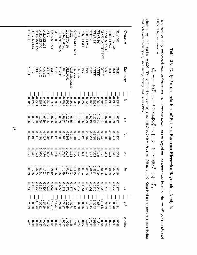
Table3A:DailyAutocorrelationsofFuturesReturns:PiecewiseRegressionAnalysis

Reportedaredailyautocorrelationsoffuturesreturns.Extrememovementsinlaggedfuturesreturnsarebasedonthecut-o�points-1.0%and

1.0%.Theregressionis

rFt+

1

=a+b1 rFt

+(b2�b1 )Max[0;rFt

�a1 ]+(b3�b2 )Max[0;rFt

�a2 ]+�Ft+

1 ;

wherea1

=�0:01anda2

=0:01.The��22

statistictestsH0

:b1

�0&b3

�0vsHa

:b1

6�0orb3

6�0.Standarderrorsareserialcorrelation

andheteroskedasticity-adjustedusingNeweyandWest(1987).

Contract

Exchange

b1

s.e.

b2

s.e.

b3

s.e.

��22

p-value

S&P500

CME

-0.1398

0.0687

0.0136

0.0358

0.0316

0.0876

4.1394

0.0540

RUSSELL2000

CME

-0.1910

0.1209

0.2241

0.0517

-0.0793

0.1855

3.0496

0.0931

NIKKEI225

CME

-0.1901

0.0810

-0.0931

0.0524

0.0129

0.0710

5.5107

0.0255

NYSE-STOCK

NYSE

-0.1435

0.0730

0.0005

0.0334

-0.0320

0.0774

3.8699

0.0626

MAXVALUELINE

KCBT

-0.3946

0.1107

0.1233

0.0421

-0.0106

0.0804

12.7142

0.0006

FTSE100

LIFFE

0.0651

0.1253

0.0552

0.0349

-0.1109

0.1344

0.6804

0.3871

FTSE250

LIFFE

-0.2898

0.2225

0.3097

0.0594

-0.4351

0.2919

3.3905

0.0800

TOPIX

TSE

-0.1021

0.0843

0.0211

0.0429

0.0153

0.0807

1.4645

0.2332

NIKKEI225

OSX

-0.0556

0.0799

-0.0504

0.0468

0.0350

0.0740

0.4832

0.4402

NIKKEI300

OSX

-0.2271

0.1076

0.0129

0.0600

-0.0994

0.1061

6.0696

0.0184

DAX

EUREX

0.0071

0.1330

0.0211

0.0478

-0.0484

0.0877

0.3270

0.5123

SWISSMARKET

EUREX

0.0298

0.1401

0.0891

0.0470

-0.1158

0.0799

2.1042

0.1591

AEX

AMSTERDAM

-0.0921

0.0936

0.1053

0.0374

-0.1173

0.0875

2.5778

0.1238

BELFOX-20

BELFOX

0.2066

0.1667

0.1107

0.0435

-0.0411

0.0972

0.1789

0.5600

HANGSENG

HKFE

-0.1892

0.0932

0.2104

0.0792

-0.1329

0.0827

4.3282

0.0517

IBEX35PLUS

MEFF

0.0207

0.0873

0.1000

0.0557

-0.1616

0.1065

2.2996

0.1432

MIB30

MIF

0.0930

0.1213

0.0473

0.0790

-0.2656

0.0729

13.2769

0.0005

OMX-STOCK

OMX

-0.2223

0.0766

0.2455

0.0517

-0.2149

0.1334

13.5719

0.0004

ATX

OTOT

-0.2811

0.1118

0.1996

0.0608

-0.1043

0.0932

6.3696

0.0172

NIKKEI225

SIMEX

-0.0693

0.0929

0.0638

0.0489

-0.1303

0.0805

4.5310

0.0405

NIKKEI300

SIMEX

-0.2587

0.1209

0.0602

0.0690

-0.0454

0.1133

5.5742

0.0235

TORONTO35

TFE

-0.2504

0.0888

0.2113

0.0523

-0.4903

0.1806

24.1307

0.0000

AUSTRALIA

SFE

-0.1290

0.0557

0.0433

0.0517

-0.1726

0.1775

5.6866

0.0238

CAC40

MATF

-0.0049

0.0886

0.0452

0.0421

-0.0372

0.0703

0.2809

0.5121

28

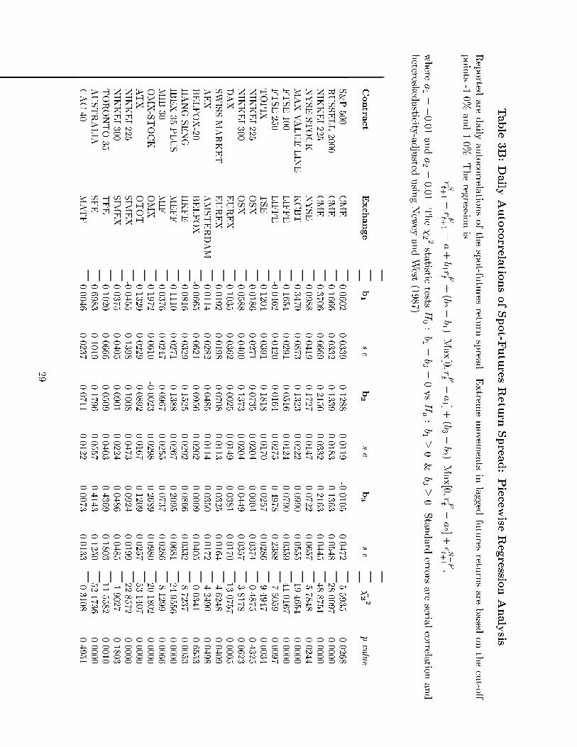
Table3B:DailyAutocorrelationsofSpot-FuturesReturnSpread:PiecewiseRegressionAnalysis

Reportedaredailyautocorrelationsofthespot-futuresreturnspread.Extrememovementsinlaggedfuturesreturnsarebasedonthecut-o�

points-1.0%and1.0%.Theregressionis

rSt+

1�rFt+

1

=a+b1 rFt

+(b2�b1 )Max[0;rFt

�a1 ]+(b3�b2 )Max[0;rFt

�a2 ]+�S�

F

t+1

;

wherea1

=�0:01anda2

=0:01.The��22

statistictestsH0

:b1

=b3

=0vsHa

:b1

�0&

b3

�0.Standarderrorsareserialcorrelationand

heteroskedasticity-adjustedusingNeweyandWest(1987).

Contract

Exchange

b1

s.e.

b2

s.e.

b3

s.e.

��22

p-value

S&P500

CME

0.0602

0.0339

0.1288

0.0119

-0.0105

0.0472

5.5935

0.0268

RUSSELL2000

CME

0.1666

0.0332

0.1339

0.0183

0.1363

0.0548

28.0097

0.0000

NIKKEI225

CME

0.3706

0.0669

0.2150

0.0332

0.2163

0.0445

48.8751

0.0000

NYSE-STOCK

NYSE

0.0988

0.0419

0.1727

0.0147

0.0722

0.0657

5.7848

0.0244

MAXVALUELINE

KCBT

0.3470

0.0873

0.1323

0.0222

0.0990

0.0555

19.4654

0.0000

FTSE100

LIFFE

0.1654

0.0291

0.0516

0.0124

0.0790

0.0359

41.0167

0.0000

FTSE250

LIFFE

-0.0462

0.0420

0.0164

0.0275

0.4978

0.2388

7.5059

0.0097

TOPIX

TSE

0.1204

0.0391

0.1818

0.0170

0.0257

0.0286

9.4947

0.0034

NIKKEI225

OSX

0.0186

0.0271

0.0735

0.0204

0.0004

0.0374

0.4875

0.4325

NIKKEI300

OSX

0.0588

0.0400

0.1373

0.0204

0.0449

0.0357

3.8178

0.0623

DAX

EUREX

0.1035

0.0362

0.0025

0.0149

0.0381

0.0170

13.0757

0.0005

SWISSMARKET

EUREX

0.0192

0.0198

0.0708

0.0113

0.0325

0.0164

4.6248

0.0409

AEX

AMSTERDAM

0.0114

0.0282

0.0485

0.0114

0.0350

0.0172

4.2490

0.0498

BELFOX-20

BELFOX

-0.0665

0.0621

0.0956

0.0202

0.0009

0.0405

0.0341

0.6553

HANGSENG

HKFE

0.0816

0.0329

0.1525

0.0292

0.0866

0.0332

8.7237

0.0053

IBEX35PLUS

MEFF

0.1110

0.0271

0.1388

0.0267

0.2095

0.0681

24.9556

0.0000

MIB30

MIF

0.0376

0.0247

0.0967

0.0255

0.0737

0.0286

8.1299

0.0066

OMX-STOCK

OMX

0.1972

0.0610

-0.0023

0.0298

0.2689

0.0980

20.1802

0.0000

ATX

OTOT

0.1320

0.0229

0.0892

0.0167

0.1209

0.0257

53.1407

0.0000

NIKKEI225

SIMEX

-0.0455

0.1398

0.1008

0.0473

0.0924

0.0199

22.8572

0.0000

NIKKEI300

SIMEX

0.0375

0.0405

0.0901

0.0224

0.0486

0.0485

1.9027

0.1803

TORONTO35

TFE

0.1020

0.0666

0.0509

0.0403

0.4369

0.1803

11.5582

0.0010

AUSTRALIA

SFE

0.6983

0.1019

0.1796

0.0557

0.4143

0.1250

52.1736

0.0000

CAC40

MATF

0.0046

0.0237

0.0711

0.0122

0.0073

0.0133

0.3108

0.4951

29

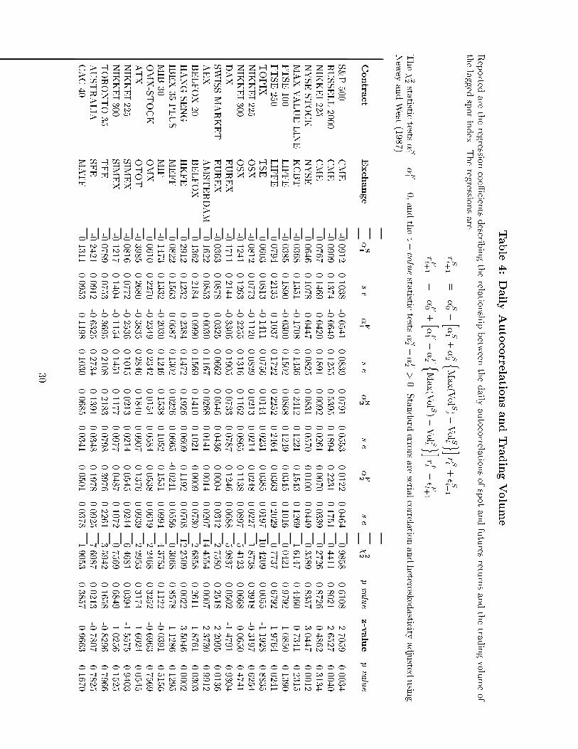
Table4:DailyAutocorrelationsandTradingVolume

Reportedaretheregressioncoe�cientsdescribingtherelationshipbetweenthedailyautocorrelationsofspotandfuturesreturnsandthetradingvolumeof

thelaggedspotindex.Theregressionsare

rSt

+1

=

�S0

+h�

S1

+�S2 nMax(VolS)�VolSt oirSt

+�St

+1

rFt

+1

=

�F0

+h�

F1

+�F2 nMax(VolS)�VolSt oirFt

+�Ft

+1

The�22

statistictests�S1

=�F1

=0,andthez�valuestatistictests�S2

��F2

>0.Standarderrorsareserialcorrelationandheteroskedasticity-adjustedusing

NeweyandWest(1987).

Contract

Exchange

�S1

s.e.

�F1

s.e.

�S2

s.e.

�F2

s.e.

�22

p-value

z-value

p-value

S&P500

CME

-0.0912

0.1038

-0.0541

0.0839

0.0791

0.0553

0.0122

0.0464

0.9858

0.6108

2.7059

0.0034

RUSSELL2000

CME

-0.0909

0.1374

-0.0649

0.1255

0.5395

0.1894

0.2231

0.1751

0.4411

0.8021

2.6527

0.0040

NIKKEI225

CME

-0.0767

0.1469

-0.0420

0.1891

0.0092

0.0261

-0.0070

0.0339

0.2726

0.8726

0.4862

0.3134

NYSE-STOCK

NYSE

-0.0646

0.1078

-0.0447

0.0825

0.0831

0.0570

-0.0100

0.0449

0.3589

0.8357

3.0447

0.0012

MAXVALUELINE

KCBT

-0.0368

0.1351

-0.1708

0.1436

0.2412

0.1221

0.1543

0.1269

1.6147

0.4460

0.7341

0.2315

FTSE100

LIFFE

-0.0385

0.1890

-0.0300

0.1502

0.0868

0.1249

0.0345

0.1016

0.0421

0.9792

1.0850

0.1390

FTSE250

LIFFE

0.0794

0.2135

0.1037

0.1722

0.2252

0.2464

0.0363

0.2029

0.7737

0.6792

1.9764

0.0241

TOPIX

TSE

0.0603

0.0813

-0.1411

0.0756

0.0144

0.0231

0.0385

0.0197

10.4209

0.0055

-1.1928

0.8835

NIKKEI225

OSX

-0.0812

0.0773

-0.1120

0.0829

0.0213

0.0214

0.0248

0.0227

1.8738

0.3918

-0.3197

0.6254

NIKKEI300

OSX

-0.1241

0.1263

-0.2255

0.1316

0.1162

0.0865

0.1138

0.0897

5.4123

0.0668

0.0650

0.4741

DAX

EUREX

-0.1711

0.2144

-0.3306

0.1905

0.0733

0.0787

0.1246

0.0688

5.9837

0.0502

-1.4791

0.9304

SWISSMARKET

EUREX

-0.0363

0.0878

0.0325

0.0662

0.0546

0.0436

0.0004

0.0312

2.7580

0.2518

2.2095

0.0136

AEX

AMSTERDAM

0.1622

0.0853

-0.0030

0.1167

-0.0268

0.0141

0.0014

0.0207

14.4554

0.0007

-2.3730

0.9912

BELFOX-20

BELFOX

-0.1362

0.2184

0.0990

0.1569

0.1410

0.1021

-0.0009

0.0730

2.6858

0.2611

1.8761

0.0303

HANGSENG

HKFE

-0.2912

0.1232

-0.2384

0.1472

0.1926

0.0609

0.1192

0.0708

12.2509

0.0022

3.5046

0.0002

IBEX35PLUS

MEFF

0.0822

0.1563

0.0687

0.1302

0.0226

0.0665

-0.0241

0.0556

0.3068

0.8578

1.1286

0.1295

MIB30

MIF

-0.1473

0.1332

-0.2030

0.1246

0.1538

0.1052

0.1551

0.0994

4.3753

0.1122

-0.0391

0.5156

OMX-STOCK

OMX

0.0610

0.2270

-0.2349

0.2342

0.0154

0.0584

0.0538

0.0619

2.2468

0.3252

-0.6963

0.7569

ATX

OTOT

-0.3985

0.2680

-0.3835

0.2846

0.1840

0.0907

0.1376

0.0939

2.2953

0.3174

1.6024

0.0545

NIKKEI225

SIMEX

-0.0816

0.0772

-0.2536

0.1015

0.0213

0.0214

0.0545

0.0244

6.4681

0.0394

-1.5575

0.9403

NIKKEI300

SIMEX

-0.1217

0.1404

-0.1154

0.1451

0.1177

0.0977

0.0487

0.1072

0.7569

0.6849

1.0256

0.1525

TORONTO35

TFE

-0.0789

0.0753

-0.3695

0.2108

0.2183

0.0798

0.3976

0.2261

3.5942

0.1658

-0.8296

0.7966

AUSTRALIA

SFE

-0.2421

0.0912

-0.6325

0.2734

0.1391

0.0348

0.1978

0.0925

7.6987

0.0213

-0.7807

0.7825

CAC40

MATF

-0.1311

0.0953

-0.1198

0.1030

0.0685

0.0341

0.0501

0.0378

1.9053

0.3857

0.9663

0.1670

30

Table5:VolatilityRatios

Reportedarevolatilityratiosofthefuturesandspotreturns.�is�2(RF

)=�2 �RS

+4(i�d) �.4(i)isde�nedas �ln(1+iat

+1 )�ln(1+iat ) �=6,i.e.,thechange

incontinuouslycompounded2-monthinterestrates.4(d)issimilarlycomputed.�n

and�e

standforthevolatilityratiosforthenormalrangeandextreme

rangeofMt ,respectively.Speci�cally,extrememovementsinlaggedfuturesreturnsarebasedonthecut-o�points-1.0%and1.0%.Theregressionsare

rSt

+1

=

�Sn(1�Ie )+�Se

Ie

+�St

+1

rFt

+1

=

�Fn

(1�Ie )+�Fe

Ie

+�Ft

+1

�St

+12

=

�Sn2(1�Ie )+�Se2

Ie

+"St

+1

�Ft

+12

=

�n�Sn2(1�Ie )+�e �Se2

Ie

+"Ft

+1

whereIe

=0if�0:01�rFt

+1

�0:01;otherwiseIe

=1.Thez-valuestatistictests�n

��e

>0.Standarderrorsareserialcorrelationandheteroskedasticity-

adjustedusingNeweyandWest(1987).

Contract

Exchange

�

s.e.

�n

s.e.

�e

s.e.

z-value

p-value

S&P500

CME

1.4488

0.1231

1.2764

0.0208

1.6581

0.2048

-1.8529

0.9681

RUSSELL2000

CME

1.4456

0.0530

1.5522

0.0557

1.3154

0.0869

2.5419

0.0055

NIKKEI225

CME

1.1450

0.0430

1.2572

0.0721

1.0586

0.0550

2.1472

0.0159

NYSE-STOCK

NYSE

1.6714

0.1171

1.5368

0.0376

1.8408

0.2123

-1.3907

0.9178

MAXVALUELINE

KCBT

1.8343

0.0980

1.9619

0.0986

1.5944

0.1269

3.0624

0.0011

FTSE100

LIFFE

1.3237

0.0356

1.4133

0.0529

1.2004

0.0850

1.7271

0.0421

FTSE250

LIFFE

1.2570

0.0807

1.2663

0.0777

1.2350

0.1540

0.2104

0.4167

TOPIX

TSE

1.2660

0.0391

1.3805

0.0555

1.1646

0.0704

2.0736

0.0191

NIKKEI225

OSX

1.0002

0.0236

1.0539

0.0258

0.9580

0.0361

2.1363

0.0163

NIKKEI300

OSX

1.2975

0.0575

1.3466

0.0983

1.2378

0.0506

0.9608

0.1683

DAX

EUREX

1.1296

0.0337

1.1595

0.0415

1.0891

0.0338

1.7010

0.0445

SWISSMARKET

EUREX

1.0731

0.0209

1.0925

0.0190

1.0477

0.0378

1.0930

0.1372

AEX

AMSTERDAM

1.1189

0.0251

1.1337

0.0267

1.1004

0.0433

0.6728

0.2505

BELFOX-20

BELFOX

1.1133

0.0430

1.1357

0.0557

1.0644

0.0464

1.1090

0.1337

HANGSENG

HKFE

1.3138

0.0396

1.3422

0.0333

1.2956

0.0625

0.6587

0.2550

IBEX35PLUS

MEFF

1.3639

0.0495

1.4767

0.0698

1.2508

0.0533

2.8952

0.0019

MIB30

MIF

1.1397

0.0294

1.1750

0.0418

1.1065

0.0365

1.3303

0.0917

OMX-STOCK

OMX

1.4433

0.0875

1.3577

0.0656

1.5153

0.1497

-0.9774

0.8358

ATX

OTOT

1.2588

0.0250

1.2780

0.0339

1.2342

0.0410

0.7972

0.2127

NIKKEI225

SIMEX

1.1303

0.0499

1.0986

0.0408

1.1613

0.0883

-0.6478

0.7414

NIKKEI300

SIMEX

1.1483

0.0338

1.1595

0.0514

1.1378

0.0418

0.3325

0.3697

TORONTO35

TFE

1.4338

0.2347

1.1669

0.0620

1.9188

0.6497

-1.1478

0.8745

AUSTRALIA

SFE

2.0811

0.3024

2.4615

0.1780

1.8776

0.4293

1.3342

0.0911

CAC40

MATF

1.1442

0.0184

1.1367

0.0253

1.1541

0.0232

-0.5358

0.7039

31

Table6:FuturesReturnAutocorrelationsandtheBid-AskSpread

Table6reportsthedi�erencebetweenautocorrelationsofthespotindexandfuturesreturnforeachcontract,andtheactualestimatedbid-askspreadofeach

futurescontract.UsingaBlume-Stambaugh(1993)bid-askmodel,thetableprovides(I)impliedautocorrelationdi�erencesbasedonactualspreads,and(II)

theimpliedspreadnecessarytoexplaintheactualautocorrelationdi�erences.Lowprobability(i.e.,50%)andhighprobability(i.e.,100%)statesrefertothe

probabilitythatthetradestakeplaceatthequotesratherthanwithinthequotedspreads.

ImpliedAC

ImpliedSpread

Contract

AC

Di�.

Vol.

Spread

lowprob.

highprob.

lowprob.

highprob.

S&P500

0.0653

1.1911

0.037

0.0001

0.0002

0.86

0.61

Russell200

0.1487

0.9418

0.150

0.0032

0.0063

1.03

0.73

Nikkei225

0.0564

1.5385

0.060

0.0002

0.0004

1.03

0.73

NYSE

0.1171

1.1799

0.040

0.0001

0.0003

1.14

0.81

ValueLine

0.2147

0.9025

0.100

0.0015

0.0031

1.18

0.84

FTSE100

0.0574

1.0964

0.150

0.0023

0.0047

0.74

0.53

FTSE250

0.0881

0.6330

NA

NA

NA

0.53

0.38

TOPIX

0.1099

1.3280

0.038

0.0001

0.0002

1.25

0.88

Nikkei225

0.0134

1.4166

0.059

0.0002

0.0004

0.46

0.33

Nikkei300

0.0892

1.3256

0.500

0.0178

0.0356

1.12

0.79

DAX

0.0239

1.2450

0.060

0.0003

0.0006

0.54

0.38

Swiss

0.0241

1.0970

0.014

0.0000

0.0000

0.48

0.34

AEX

0.0322

1.1164

0.089

0.0008

0.0016

0.57

0.40

BELFOX20

0.0502

0.9214

0.217

0.0069

0.0139

0.58

0.41

HangSeng

0.0653

1.9631

0.037

0.0000

0.0001

1.42

1.00

IBEX35

0.1194

1.4750

0.070

0.0003

0.0006

1.44

1.02

MIB30

0.0487

1.6605

0.068

0.0002

0.0004

1.04

0.73

OMX

0.1536

1.5853

0.032

0.0001

0.0001

1.76

1.24

ATX

0.0999

1.2468

0.308

0.0076

0.0153

1.11

0.79

Nikkei225

0.0270

1.6491

0.060

0.0002

0.0003

0.77

0.54

Nikkei300

0.0526

1.3230

0.375

0.0100

0.0201

0.86

0.61

Toronto35

0.1640

1.0129

0.127

0.0020

0.0039

1.16

0.82

Australia

0.1769

1.4475

0.032

0.0001

0.0001

1.72

1.22

CAC40

0.0345

1.2503

NA

NA

NA

0.66

0.46

32

RFt+1

�S+E[4(i� d)]

MtML

= � 2�+�i(1�w) p

MH

= 2�+�i(1�w) p

�����������

��

��

��

��

���

The Adjustment Model

The Nontrading Model

slope=(1� w) P

Figure 1: The theoretical relation between the futures return (RFt+1) and the lagged market inno-

vation (Mt) in the lagged adjustment model with transaction costs (solid line) and the nontradingmodel (dashed line).

33

Figure 2: Autocorrelations of futures and spot returns for 24 indices. The solid line is the 45 degreeline.

34

Figure 3: Nonparametric kernel estimates of the relation between the lagged return (rFt ) and thereturn (rFt+1) on three futures contracts: the Russell 2000, FTSE 250, and TOPIX.

35

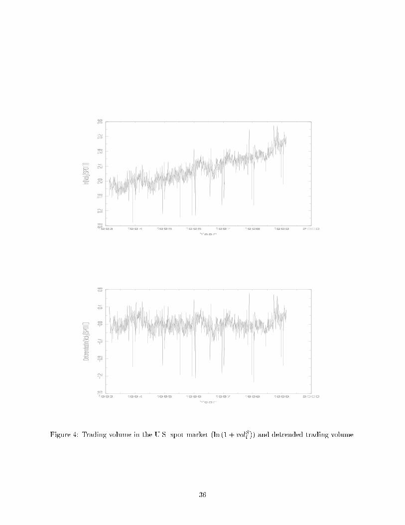
Figure 4: Trading volume in the U.S. spot market (ln (1 + volSt )) and detrended trading volume.

36

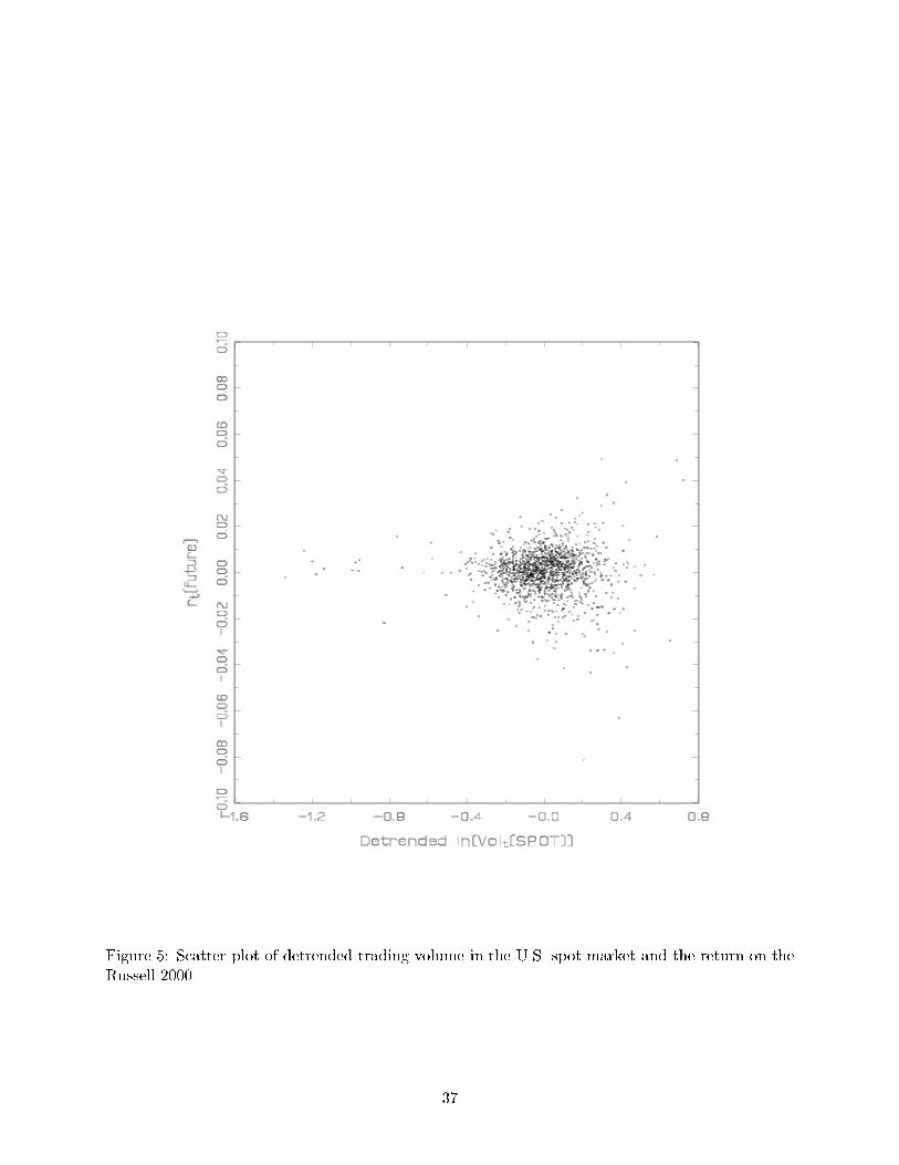
Figure 5: Scatter plot of detrended trading volume in the U.S. spot market and the return on theRussell 2000.

37

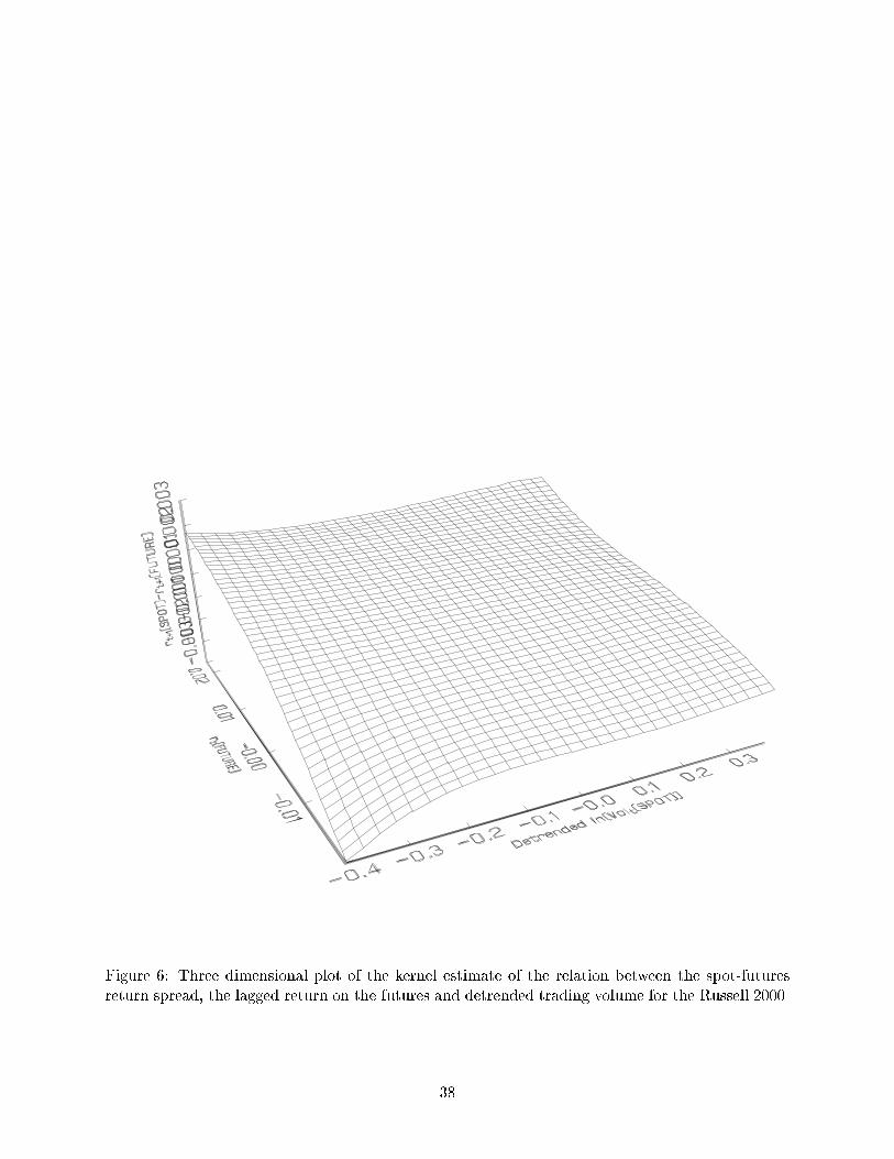
Figure 6: Three dimensional plot of the kernel estimate of the relation between the spot-futuresreturn spread, the lagged return on the futures and detrended trading volume for the Russell 2000.

38

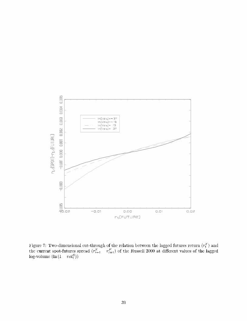
Figure 7: Two-dimensional cut-through of the relation between the lagged futures return (rFt ) andthe current spot-futures spread (rSt+1 � rFt+1) of the Russell 2000 at di�erent values of the laggedlog-volume (ln (1 + volSt )).

39