Embed Size (px)
Citation preview
Bayesian Population Pharmacokinetic/Pharmacodynamic
Modeling to Study the Effect on the Cardiovascular
Syndrome of the QTc Interval Prolongation of
Non-antiarrhythmic Drugs
Giovanni Smania
July 15, 2013


Alla mia intera famiglia,fonte inesauribile di motivazione e supporto.

Contents
1 Introduction 11.1 Physiolgy of the QT Interval and the Drug Effect on it . . . . . . . . . . . . 11.2 Motivation . . . . . . . . . . . . . . . . . . . . . . . . . . . . . . . . . . . . 21.3 Basics of Non Linear Mixed Effect Methods . . . . . . . . . . . . . . . . . . 4
1.3.1 The Basic Model . . . . . . . . . . . . . . . . . . . . . . . . . . . . . 41.3.2 Pharmacokinetic Application of a NLME Model . . . . . . . . . . . 6
1.4 Basics of Bayesian Estimation . . . . . . . . . . . . . . . . . . . . . . . . . . 9
2 Materials and Methods 132.1 Preclinical Protocol . . . . . . . . . . . . . . . . . . . . . . . . . . . . . . . . 13
2.1.1 Pharmacokinetic Data . . . . . . . . . . . . . . . . . . . . . . . . . . 132.1.2 Pharmacodynamic Data . . . . . . . . . . . . . . . . . . . . . . . . . 13
2.2 Clinical Protocol . . . . . . . . . . . . . . . . . . . . . . . . . . . . . . . . . 142.2.1 Pharmacokinetic-Pharmacodynamic (PK-PD) Data . . . . . . . . . 14
2.3 Pharmacokinetic Modelling . . . . . . . . . . . . . . . . . . . . . . . . . . . 142.3.1 NONMEM Model Formulation . . . . . . . . . . . . . . . . . . . . . 15
2.4 PK-PD Modeling of the QT interval . . . . . . . . . . . . . . . . . . . . . . 152.4.1 Modelling the Drug Effect . . . . . . . . . . . . . . . . . . . . . . . . 162.4.2 Modelling the QT-RR Relationship . . . . . . . . . . . . . . . . . . . 172.4.3 Modelling the Circadian Rhythm . . . . . . . . . . . . . . . . . . . . 182.4.4 WinBUGS Model Formulation . . . . . . . . . . . . . . . . . . . . . 19
3 Results 273.1 Pharmacokinetic Analysis . . . . . . . . . . . . . . . . . . . . . . . . . . . . 27
3.1.1 Preclinical Data . . . . . . . . . . . . . . . . . . . . . . . . . . . . . 273.2 Pharmacodynamic Analysis . . . . . . . . . . . . . . . . . . . . . . . . . . . 33
3.2.1 MCMC Convergence Check . . . . . . . . . . . . . . . . . . . . . . . 333.2.2 Preclinical Data . . . . . . . . . . . . . . . . . . . . . . . . . . . . . 363.2.3 Clinical Data . . . . . . . . . . . . . . . . . . . . . . . . . . . . . . . 39
4 Conclusions 43
iii
Abstract
Assessment of the propensity of non-antiarrhythmic drugs in prolonging QT/QTc intervalis critical for the progression of compounds into clinical development. Given the
similarities in QTc response between dogs and humans, dogs are often used in pre-clinicalcardiovascular safety studies. The current regulatory guidelines are based on simple
statistical analyses of QT data, thereby ignoring any potential exposure-effect relationshipand nonlinearity in the underlying physiological fluctuation in QT values. The objective
of this analysis is to adopt a model based approach to assess the QT-prolonging effects indogs and humans of GSK945237, a new compound under development. Pharmacokinetic
and pharmacodynamic data from experiments in conscious dogs and clinical trialsfollowing administration of GSK945237 were used. First, pharmacokinetic modelling wasapplied to derive drug concentrations at the time of each QT measurement. A BayesianPKPD model was then used to describe QT prolongation, which allows discrimination ofdrug-specific effects from other physiological factors known to alter QT interval duration.
Results from this analysis show the drug under investigation is not prone to causehazardous increases in the QT interval for both humans and dogs. Further, the PKPD
model is capable to predict both preclinical and clincal data, suggesting it might be usedfor future translational research in the field of QT prolongation.
Chapter 1
Introduction
1.1 Physiolgy of the QT Interval and the Drug Effect on it
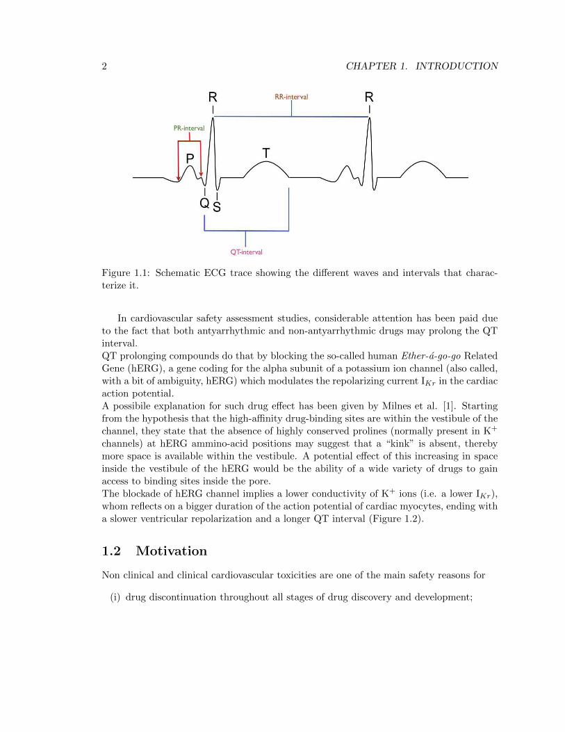
The QT interval is the portion of the Electrocardiographic signal (ECG) in between thebeginning of the QRS complex and the end of the T-wave (Figure 1.1). It represents thetime between the onset of electrical depolarization of the ventricles and the end of theirrepolarization, that is, it reflects the duration of individual action potentials in the cardiacmyocytes.QT interval is affected by several sources of variability of diverse nature. As one wouldexcpect, the QT interval duration is strictly related to the RR interval (i.e. the cardiacperiod). In fact it is well known that in order to improve the detections of threatening QTprolongations, the measured QT has to be corrected for changes in RR interval, taking thename of corrected QT interval (QTc). Other subject-related factors potentially affectingthe QT/QTc interval are:
1. Genetic (long QT syndrome)
2. Food intake
3. Circadian rhythm
4. Sex
5. Obesity
6. Physical activity
7. Blood glucose level
8. Blood pressure
9. Age
1
2 CHAPTER 1. INTRODUCTION
Figure 1.1: Schematic ECG trace showing the different waves and intervals that charac-terize it.
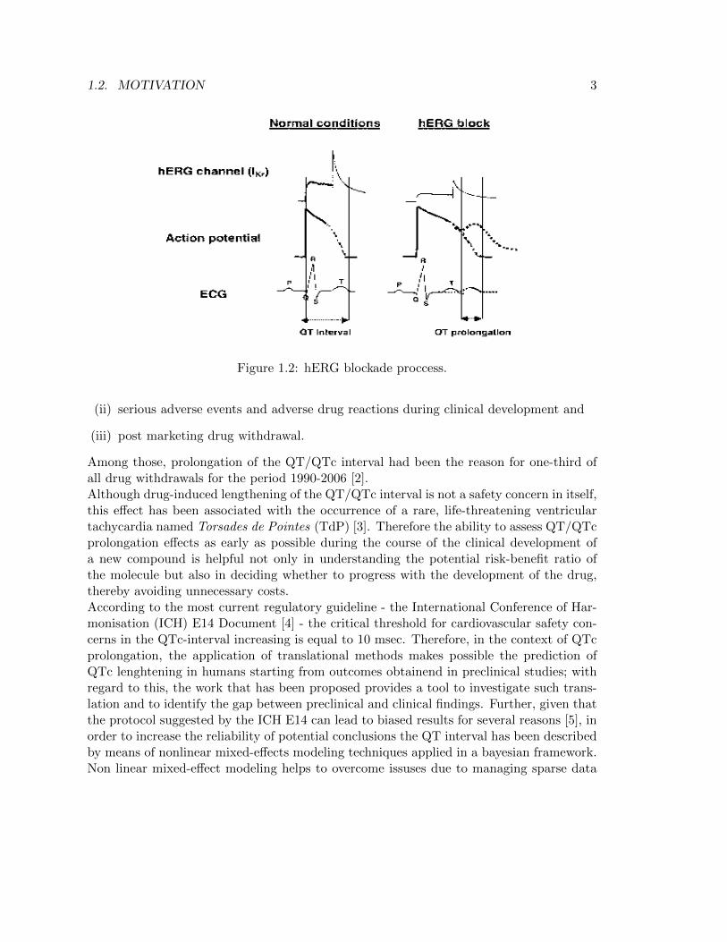
In cardiovascular safety assessment studies, considerable attention has been paid dueto the fact that both antyarrhythmic and non-antyarrhythmic drugs may prolong the QTinterval.QT prolonging compounds do that by blocking the so-called human Ether-a-go-go RelatedGene (hERG), a gene coding for the alpha subunit of a potassium ion channel (also called,with a bit of ambiguity, hERG) which modulates the repolarizing current IKr in the cardiacaction potential.A possibile explanation for such drug effect has been given by Milnes et al. [1]. Startingfrom the hypothesis that the high-affinity drug-binding sites are within the vestibule of thechannel, they state that the absence of highly conserved prolines (normally present in K+
channels) at hERG ammino-acid positions may suggest that a “kink” is absent, therebymore space is available within the vestibule. A potential effect of this increasing in spaceinside the vestibule of the hERG would be the ability of a wide variety of drugs to gainaccess to binding sites inside the pore.The blockade of hERG channel implies a lower conductivity of K+ ions (i.e. a lower IKr),whom reflects on a bigger duration of the action potential of cardiac myocytes, ending witha slower ventricular repolarization and a longer QT interval (Figure 1.2).
1.2 Motivation
Non clinical and clinical cardiovascular toxicities are one of the main safety reasons for
(i) drug discontinuation throughout all stages of drug discovery and development;
1.2. MOTIVATION 3
Figure 1.2: hERG blockade proccess.
(ii) serious adverse events and adverse drug reactions during clinical development and
(iii) post marketing drug withdrawal.
Among those, prolongation of the QT/QTc interval had been the reason for one-third ofall drug withdrawals for the period 1990-2006 [2].Although drug-induced lengthening of the QT/QTc interval is not a safety concern in itself,this effect has been associated with the occurrence of a rare, life-threatening ventriculartachycardia named Torsades de Pointes (TdP) [3]. Therefore the ability to assess QT/QTcprolongation effects as early as possible during the course of the clinical development ofa new compound is helpful not only in understanding the potential risk-benefit ratio ofthe molecule but also in deciding whether to progress with the development of the drug,thereby avoiding unnecessary costs.According to the most current regulatory guideline - the International Conference of Har-monisation (ICH) E14 Document [4] - the critical threshold for cardiovascular safety con-cerns in the QTc-interval increasing is equal to 10 msec. Therefore, in the context of QTcprolongation, the application of translational methods makes possible the prediction ofQTc lenghtening in humans starting from outcomes obtainend in preclinical studies; withregard to this, the work that has been proposed provides a tool to investigate such trans-lation and to identify the gap between preclinical and clinical findings. Further, given thatthe protocol suggested by the ICH E14 can lead to biased results for several reasons [5], inorder to increase the reliability of potential conclusions the QT interval has been describedby means of nonlinear mixed-effects modeling techniques applied in a bayesian framework.Non linear mixed-effect modeling helps to overcome issuses due to managing sparse data
4 CHAPTER 1. INTRODUCTION
coming from different individuals (which is the case for QT measurements in humans),while a bayesian approach fits naturally into decision analysis since it allows to obtain thefull posterior probability plus the credible intervals of a parameter of interest instead ofa puntual estimate with its confidence interval. These two aspects will be treated widelylater (see 1.3 and 1.4).
1.3 Basics of Non Linear Mixed Effect Methods
Non Linear Mixed Effect (NLME) models, also called hirerchical models, are used in pop-ulation analysis related fields such as environmental health, agriculture and pharmacoki-netics/pharmacodynamics.Population analysis is an alternative method to individual analysis that has its strengthin extrapolating information from sparse data coming from different individuals, assumingthat each individual feature comes from a distribution of that feature which is representa-tive of the entire population of interest.The mathematical formulation of the model will be presented (1.3.1), followed by an appliedpharmacokinetic example (1.3.2).
1.3.1 The Basic Model
NLME modelling is more complex than standard modelling techniques, and has to bestratified into two hirerchical steps.
1. Stage 1: Individual-Level model
The individual step aims to define the measure model:
zi,j : the jth measure (j = 1, ..., N) for the ith subject (i = 1, ...,K), collected attime ti,j
ui: vector of additional conditions under which subject i is observed
pi: vector of model parameters specific to subject i (M × 1)
f(ti,j ,ui,pi): non-linear relationship between zi,j and (ti,j ,ui,pi)
εi,j : random error due to uncertainty in the measure denoting within-individualvariabilty
If we consider an additive residual error, the individual model can be written as
zi,j = f(ti,j ,ui,pi) + εi,j . (1.1)
1.3. BASICS OF NON LINEAR MIXED EFFECT METHODS 5
Defining
zi =
zi,1zi,2...
zi,N
fi(pi) =
f(ti,1,ui,pi)f(ti,2,ui,pi)
...f(ti,N ,ui,pi)
εi =
εi,1εi,2...
εi,N
it is possible to summurize equation (1.1) as
zi = fi(pi) + εi (1.2)
where a classical assumption on εi is
εi|pi ∼MVN (0,Ri(pi, ξ))
with ξ costant accros individuals. For example it might need to incorporate a pro-portional error model, therefore ξ will be constant (= σ2) and Ri will be
Ri = σ2fi(pi) = σ2
f(ti,1,ui,pi) 0 · · · 0
0 f(ti,2,ui,pi) · · · 0...
.... . .
...0 0 · · · f(ti,N ,ui,pi)
2. Stage 2: Population-Level model
To account for inter-individual variation of parameters pi among individuals, a modelfor pi has to be specified. The population step provides this model:
ai: vector of characteristics of subject i (named covariates)
ηi: vector of random effects for subject i conveying inter-individual variation
θ: vector of fixed effects expressing features common to the entire population
d: M-dimensional vector function
Then a general model for pi is given by
pi = d(ai,ηi,θ)
where a classical assumption on ηi is
ηi ∼MVN (0,Ω) (1.3)

6 CHAPTER 1. INTRODUCTION
1.3.2 Pharmacokinetic Application of a NLME Model
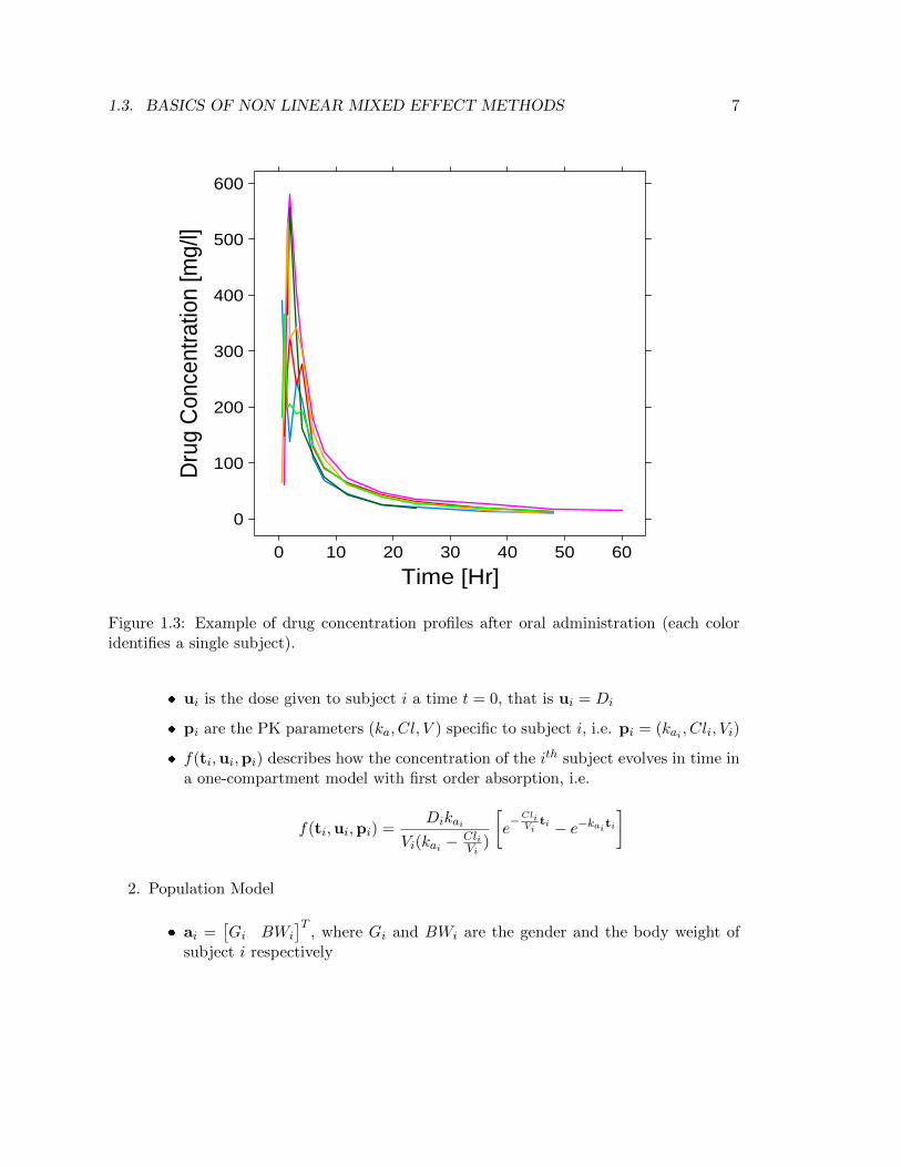
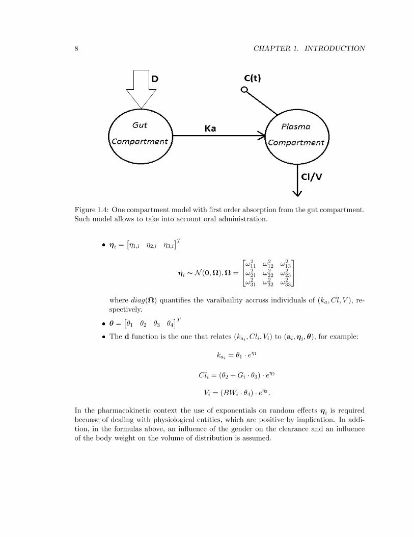
Pharmacokinetics is the study of the time course of drug concentration in different bodyspaces such as plasma, blood, urine, cerebrospinal fluid, and tissues, and aims to describethe different phases encountered by the compound once in the body: absorption, distri-bution, metabolism and elimination. The representation of the body is approximated bysimple compartment models, each describing one body spaces, with the kinetics of the drugdescribed by differential equations.Suppose data from N = 6 subjects is available with the drug given orally. Figure 1.3shows the concetration-time profiles of the different individuals: it can be seen the sim-iliraty in shapes across subjects, but peaks, rises, decays vary considerably. This effectis attributable to inter-subject variation in underlying PK processes. Assuming a One-Compartment model with oral dose D (see Figure 1.4) given at time t = 0 leads to describeconcentration C(t) at time t ≥ 0 as
C(t) =Dka
V (ka − ClV )
[e−
ClVt − e−kat
]where
ka: fractional rate of absorption [1/Hr] of the drug from the gut compartment
Cl: clearence rate [ml/Hr], i.e. the volume of plasma which per unit of time is totallycleared of a substance (e.g. a drug) by the various elimination processes (metabolismand excretion)
V : volume of distribution [ml], i.e. the theoretical volume that a drug would haveto occupy (if it was uniformly distributed), to provide the same concentration as itcurrently is in blood plasma
summarize the PK processes underlying the observed concentration profile of a given sub-ject.
The final goal of a PK analysis is to determine the population mean values of (ka, Cl, V )and how they vary between subjects, elucidating whether part of this variation is associ-ated with subject characteristics (i.e. covariates, such as weight, age, renal function), inorder to develop dosing strategies for subpopulations with certain characteristics (elderly,pediatric, etc.).With respect to the model formulation encountered in 1.3.1, a correlation with the quan-tities in play leads to
1. Individual Model
zi,j is the drug concentration for subject i at time ti,j , that is zi,j = C(ti,j)
1.3. BASICS OF NON LINEAR MIXED EFFECT METHODS 7
Time [Hr]
Dru
g C
once
ntra
tion
[mg/
l]
0
100
200
300
400
500
600
0 10 20 30 40 50 60
Figure 1.3: Example of drug concentration profiles after oral administration (each coloridentifies a single subject).
ui is the dose given to subject i a time t = 0, that is ui = Di
pi are the PK parameters (ka, Cl, V ) specific to subject i, i.e. pi = (kai , Cli, Vi)
f(ti,ui,pi) describes how the concentration of the ith subject evolves in time ina one-compartment model with first order absorption, i.e.
f(ti,ui,pi) =Dikai
Vi(kai − CliVi
)
[e−Cli
Viti − e−kaiti
]
2. Population Model
ai =[Gi BWi
]T, where Gi and BWi are the gender and the body weight of
subject i respectively
8 CHAPTER 1. INTRODUCTION
Figure 1.4: One compartment model with first order absorption from the gut compartment.Such model allows to take into account oral administration.
ηi =[η1,i η2,i η3,i
]Tηi ∼ N (0,Ω),Ω =
ω211 ω2
12 ω213
ω221 ω2
22 ω223
ω231 ω2
32 ω233
where diag(Ω) quantifies the varaibaility accross individuals of (ka, Cl, V ), re-spectively.
θ =[θ1 θ2 θ3 θ4
]T The d function is the one that relates (kai , Cli, Vi) to (ai,ηi,θ), for example:
kai = θ1 · eη1
Cli = (θ2 +Gi · θ3) · eη2
Vi = (BWi · θ4) · eη3 .
In the pharmacokinetic context the use of exponentials on random effects ηi is requiredbecuase of dealing with physiological entities, which are positive by implication. In addi-tion, in the formulas above, an influence of the gender on the clearance and an influenceof the body weight on the volume of distribution is assumed.
1.4. BASICS OF BAYESIAN ESTIMATION 9
1.4 Basics of Bayesian Estimation
In the branch of estimation theory, Bayesian approach refers to the situation in which theinformation available comes from two different sources. Defining y as the observed dataand θ as the quantity to be estimated (a vector of parameters, a signal, etc.), these twofounts are:
Likelihood: the knowledge on the relationship between y and θ, denoted as p(y|θ);
Prior: the probabilistic a priori information on θ, denoted as p(θ);
thus, both y and θ are treated as random variables.Bayes theorem (equation (1.4)) enables to combine these two probability densities in orderto obtain the so-called posterior density function p(θ|y):
p(θ|y) =p(y|θ)p(θ)
p(y)(1.4)
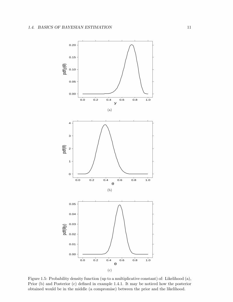
Translating the theorem in practical term: p(θ) represents the prior knowledge we haveon the quantity to be estimated, if such quantity is somehow related to data y, the ob-servation of y (i.e. p(y|θ)) changes our expectations on θ in p(θ|y). In other words, byapplying Bayes theorem we are extracting the estimate by way of a compromise betweenour knowledge on the quantity to be estimated and what the data is telling us (see Figure1.5).It is easy now to deduce the main difference between Bayesian inference and other ap-proaches: through Bayes theorem the entire distribution of the parameters of interest canbe estimated, providing a great amount of information. In fact, the use of posterior distri-bution is indeed wide, both because there are different ways to obtain the point-estimatorof the parameter (such as the posterior mean, the posterior median or the posterior mode)and because it provides the credible intervals, which are a reliable measure (compared toconfidence intervals used in frequentist approach) of the uncertainty of an estimate.In order to be able to evaluate the postierior density function, Bayes theorem of equation(1.4) can be rewritten, using the “Law of Total Probability”, as
p(θ|y) =p(y|θ)p(θ)∫
θ p(y|θ)p(θ)dθ. (1.5)
The denominator of equation (1.5) is a constant and does not depend on θ; hence, inthe intereset of simplifying the formula as much as possible, we may consider
p(θ|y) ∝ p(y|θ)p(θ) (1.6)
Unfortunately, only in a few particular cases p(θ|y) is available in closed form, that iswhen the prior and the posterior come from the same family of distributions, and in this
10 CHAPTER 1. INTRODUCTION
case the prior is said to be conjugate to the likelihood. Example 1.4.1 shows one of thesecases.
Example 1.4.1. Let us consider a drug to be given for relief of chronic pain whose expe-rience with similar compounds has suggested that annual response rates between 0.2 and0.6 could be feasible, then we may interpret this as a distribution with mean = 0.4 andstandard deviation = 0.1. Suppose we now treat n = 20 volunteers with the compund andobserve y = 15 positive responses.
Likelihood. Assuming patients are independent, with common unknown response rateθ, leads to a binomial likelihood (Figure 1.5a):
y ∼ Binomial(θ, n)
p(y|n, θ) =
(n
y
)θy(1− θ)n−y ∝ θy(1− θ)n−y
Prior. A probability distribution which fits with the requests on the response rate isa Beta distribution (with a=9.2 and b=13.8, see Figure 1.5b):
θ ∼ Beta(a, b)
p(θ) =Γ(a+ b)
Γ(a)Γ(b)θa−1(1− θ)b−1 ∝ θa−1(1− θ)b−1
Posterior. Combining the Binomial likelihood and the Beta prior gives the followingposterior distribution
p(θ|y, n) ∝ p(y|θ, n)p(θ)
p(θ|y, n) ∝ θy(1− θ)n−yθa−1(1− θ)b−1 = θy+a−1(1− θ)n−y+b−1
which is still a Beta dsitribution (with different parameters, see Figure 1.5c):
p(θ|y, n) ∝ Beta(y + a, n− y + b)
In most cases p(θ|y) is not analitically tractable and we want to obtain the marginal pos-terior p(θi|y) for each i and calculate properties of p(θi|y) such as the mean (
∫θip(θi|y)dθi)
and the tail areas (∫∞T p(θi|y)dθi). Given that evaluating these integrals analitically is im-
possible, numerical integration becomes vital. WinBUGS [6] is a free software that allowsto obtain every p(θi|y) and compute integrals on them via Markow Chain Monte Carlo(MCMC) techniques.
1.4. BASICS OF BAYESIAN ESTIMATION 11
y
pdf(y
|θ)
0.00
0.05
0.10
0.15
0.20
0.0 0.2 0.4 0.6 0.8 1.0
(a)
θ
pdf(θ
)
0
1
2
3
4
0.0 0.2 0.4 0.6 0.8 1.0
(b)
θ
pdf(θ
|y)
0.00
0.01
0.02
0.03
0.04
0.05
0.0 0.2 0.4 0.6 0.8 1.0
(c)
Figure 1.5: Probability density function (up to a multiplicative constant) of: Likelihood (a),Prior (b) and Posterior (c) defined in example 1.4.1. It may be noticed how the posteriorobtained would be in the middle (a compromise) between the prior and the likelihood.


Chapter 2
Materials and Methods
2.1 Preclinical Protocol
2.1.1 Pharmacokinetic Data
The compound (GSK945237) was administered orally twice daily (Bis In Die, i.e. BID)with approximately 6 hours between doses to nine male and nine female beagle dogs (totalnumber of individuals=18) at total daily doses of 0, 30, 100 and 300 mg/kg/day (0, 15,50 and 150 mg/kg/day BID, respectively). Plasma samples were obtained from bloodcollected into tubes containing EDTA from drug-treated and placebo-control animals atthe following nominal times: predose, 0.25, 0.5, 1, 3, 6, 6.25, 6.5, 7, 9 and 24 hours afterthe first dose.Plasma samples were analyzed for GSK945237 using a validated analytical method basedon protein precipitation, followed by HPLC-MS/MS analysis. Using a 50 µL aliquot ofdog plasma, the lower limit of quantification (LLQ) for GSK945237 was 0.1 ng/L and thehigher limit of quantification (HLQ) was 50 ng/L.
2.1.2 Pharmacodynamic Data
Four male dogs were given placebo and total daily doses of 30, 100 and 300 mg/kg (15, 50and 150 mg/kg administered twice daily approximately 6 hours apart) of test article orallyby gavage on separate days, with at least 7 days between each dose, according to a 4x4latin square crossover paradigm. Dogs were dosed at approximately 9:00 AM on each dayof dosing. ECG waveforms were recorded continuously from 2 hours prior to dosing to 24hours after dosing and all derived parameters were recorded as 1-minute means.According to the aim of the analysis and given the enormous amount of data collectedoverall, raw QT data was diluted every 2 minutes during the absorption phase (roughlyt<2.5hrs and 6hrs<t<8.3hrs, where t is the time after dosing), every 5 minutes duringthe distribution phase (2.3hrs<t<6hrs and 8.3hrs<t<15hrs) and every 15 minutes during
13
14 CHAPTER 2. MATERIALS AND METHODS
the elimination phase (t>15hrs). Also, part of the ECG data collected around the dosingtimes had to be discarded due to the bad quality of the data caused by an abnormal dogsexcitement.
2.2 Clinical Protocol
2.2.1 Pharmacokinetic-Pharmacodynamic (PK-PD) Data
The study was a first-time-in-human to investigate the safety, tolerability, and pharmacoki-netics of escalating single oral doses of GSK945237. The adopted design was a single-blind,randomized, placebo-controlled, dose-rising study conducted in sequential cohorts. Forty-five (45) subjects were enrolled into 6 cohorts. According to a randomization schedule pre-pared prior to study start, 6 subjects received active drug and 3 subjects received placeboat each dose level (50mg, 150mg, 400mg, 1000mg, 2000mg and 2600mg). Each subjectparticipated in one study period and received either GSK945237 or matching placebo.Following a single oral dose of GSK945237, blood samples for pharmacokinetic analysisand ECG waveform samples for pharmacodynamic analysis of GSK945237 were collectedover a 60-hour period from groups receiving doses of 50mg, 250mg and 500mg and overa 120-hour period from groups receiving 1000mg and 1750mg. Bioanalysis of GSK945237plasma concentrations was conducted using a validated analytical method based on solidphase extraction followed by HPLC-MS/MS. The lower limit of quantification (LLQ) forGSK945237 was 10 ng/mL, using a 100 L aliquot of human plasma with a higher limit ofquantification (HLQ) of 5000 ng/mL.
2.3 Pharmacokinetic Modelling
The goal of the pharmacokinetic (PK) modelling in the whole project is to obtain timematched concentration and QT interval values, since this is required for the assessmentof the pharmacokinetic-pharmacodynamic (PK-PD) relationship. In order to do this, PKmodelling has been performed using non-linear mixed effect techniques (see 1.3.2 for anexample) implemented in NONMEM 7.1.2 [7]. Once identified the best PK model forGSK945237, the parameter estimates obtained are used to generate simulated concentra-tion profiles with the same sampling time used to collect QT measurements.Since in human data QT measurements and concentration measurements were collectedsimultaneously, the PK step was executed only for conscious dogs data, where the QTsampling time is usually low (30 sec/1 min) and therefore an equal PK sampling time isnot achievable for obvious reasons.Firstly, provided that the drug administration was oral, a model with first order absorptionhad to be taken into account. Secondly, the BID way of administration made it difficult todescribe the data after the second daily dose since the dogs had free access to food between
2.4. PK-PD MODELING OF THE QT INTERVAL 15
the two daily doses, determining the appearaence of a food effect in the data. Finally, theNONMEM analysis led to the conclusion that a one compartment model with first orderabsorption (Fig.1.4) best decribes the kinetic of the analyzed drug.
2.3.1 NONMEM Model Formulation
The mandatory parameters for a one compartment model with first order absorption are:Rate of Absorption (Ka), Clearance (Cl) and Volume of Distribution (V ). Bioavailability(F ) was also included in the model in order to describe the food effect.After a covariate analysis, it emerged that the Clearance and the Volume of Distributionare affected by the gender and the body weight of the individuals, respectively.The detailed model formulation is (t represents the time variable):
FECl =
θ1 if GENDER=Mθ2 if GENDER=F
=⇒ Cl = FECl · eη1
V = WT · θ3 · eη2
FEKa =
θ4 if First Daily Dose (FDD)θ5 if Second Daily Dose (SDD)
=⇒ Ka = FEKa · eη3 (2.1)
F =
θ6 if DOSE=30 mg/kg and DOSE=SDDθ7 if DOSE=300 mg/kg and DOSE=FDDθ8 if DOSE=300 mg/kg and DOSE=SDD1 otherwise
(2.2)
The residual error model that has produced the lowest objective function value is amixed (proportional and addittive) one:
Y = f(θ,η, t) · (1 + ε1) + ε2 (2.3)
where Y is the observed concentration, f(θ,η, t) the predicted concentration, ε1 ∼N (0, σ21) and ε2 ∼ N (0, σ22).
2.4 PK-PD Modeling of the QT interval
The aim of this section is to define a mathematical model able to decribe the QT interval.Since there are different sources contributing on QT variation, each of them is explored.
16 CHAPTER 2. MATERIALS AND METHODS
2.4.1 Modelling the Drug Effect
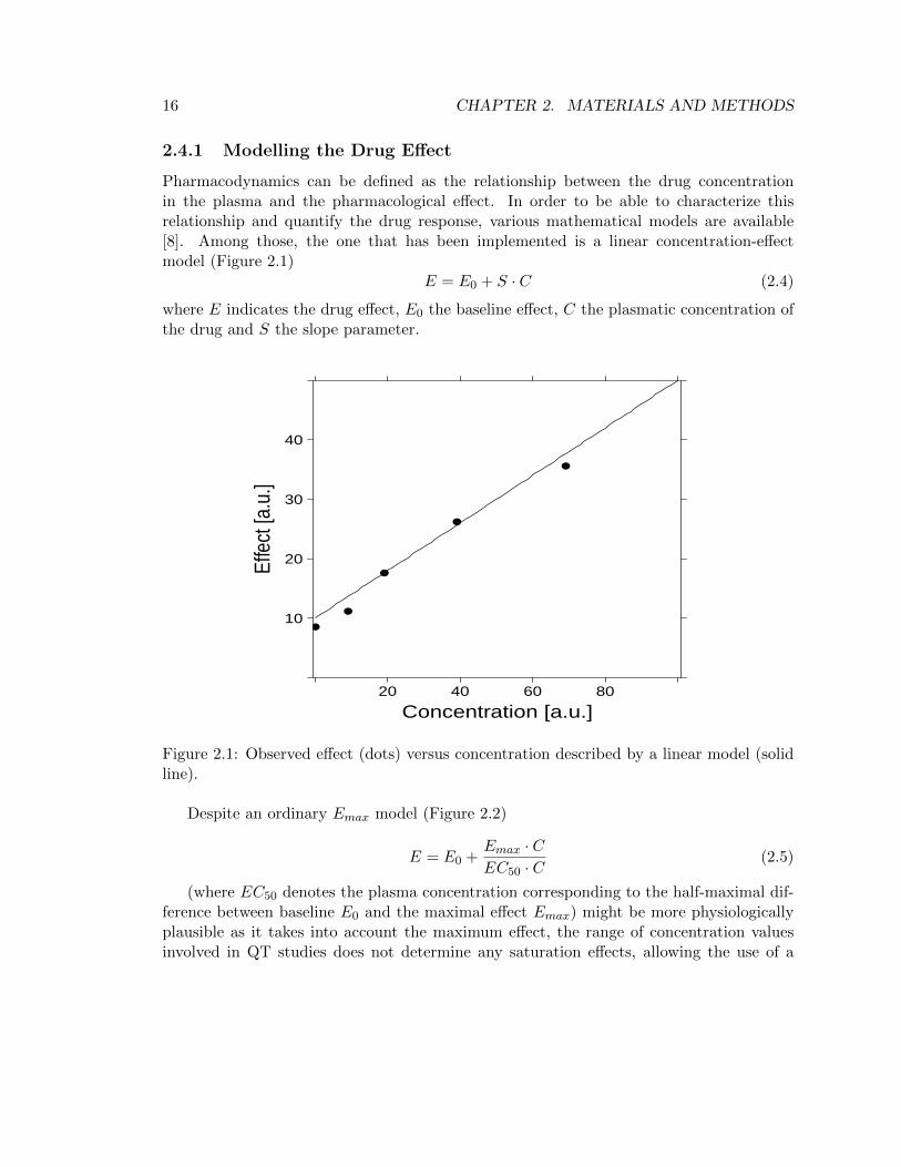
Pharmacodynamics can be defined as the relationship between the drug concentrationin the plasma and the pharmacological effect. In order to be able to characterize thisrelationship and quantify the drug response, various mathematical models are available[8]. Among those, the one that has been implemented is a linear concentration-effectmodel (Figure 2.1)
E = E0 + S · C (2.4)
where E indicates the drug effect, E0 the baseline effect, C the plasmatic concentration ofthe drug and S the slope parameter.
Concentration [a.u.]
Effe
ct [a
.u.]
10
20
30
40
20 40 60 80
Figure 2.1: Observed effect (dots) versus concentration described by a linear model (solidline).
Despite an ordinary Emax model (Figure 2.2)
E = E0 +Emax · CEC50 · C
(2.5)
(where EC50 denotes the plasma concentration corresponding to the half-maximal dif-ference between baseline E0 and the maximal effect Emax) might be more physiologicallyplausible as it takes into account the maximum effect, the range of concentration valuesinvolved in QT studies does not determine any saturation effects, allowing the use of a
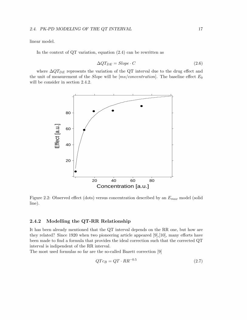
2.4. PK-PD MODELING OF THE QT INTERVAL 17
linear model.
In the context of QT variation, equation (2.4) can be rewritten as
∆QTDE = Slope · C (2.6)
where ∆QTDE represents the variation of the QT interval due to the drug effect andthe unit of measurement of the Slope will be [ms/concentration]. The baseline effect E0
will be consider in section 2.4.2.
Concentration [a.u.]
Effe
ct [a
.u.]
20
40
60
80
20 40 60 80
Figure 2.2: Observed effect (dots) versus concentration described by an Emax model (solidline).
2.4.2 Modelling the QT-RR Relationship
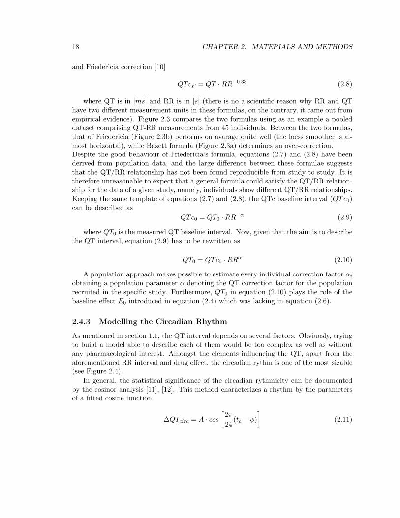
It has been already mentioned that the QT interval depends on the RR one, but how arethey related? Since 1920 when two pioneering article appeared [9],[10], many efforts havebeen made to find a formula that provides the ideal correction such that the corrected QTinterval is indipendent of the RR interval.The most used formulas so far are the so-called Bazett correction [9]
QTcB = QT ·RR−0.5 (2.7)
18 CHAPTER 2. MATERIALS AND METHODS
and Friedericia correction [10]
QTcF = QT ·RR−0.33 (2.8)
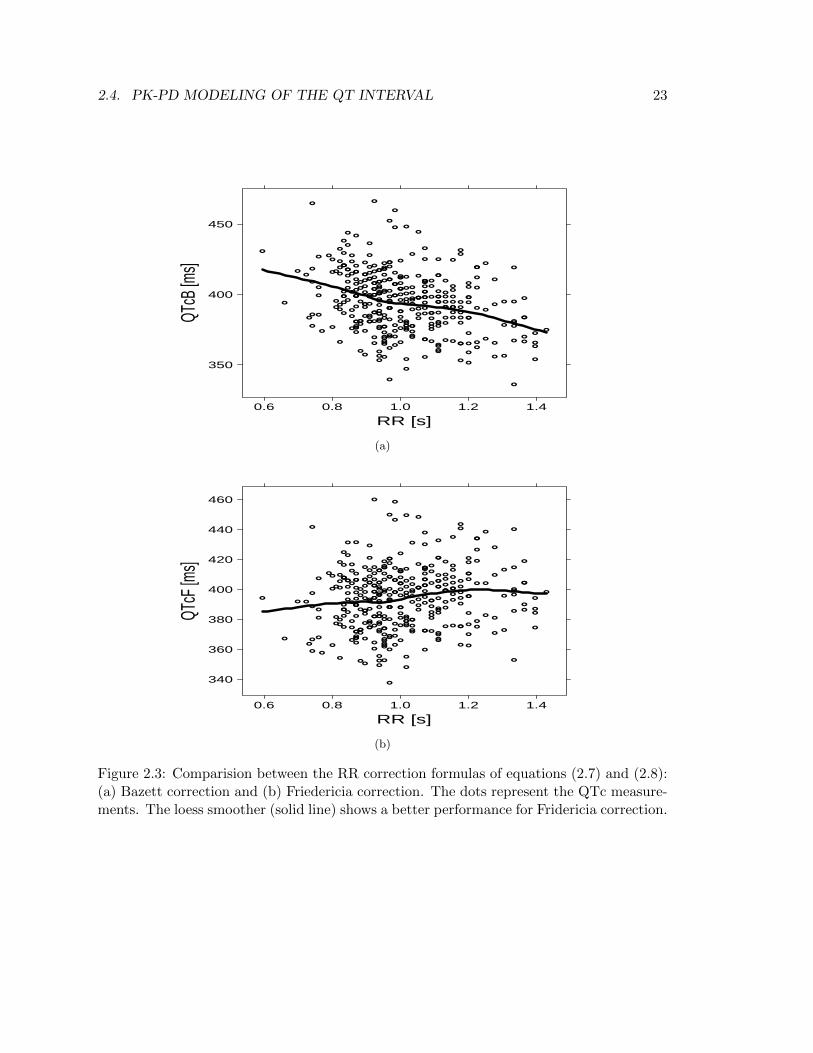
where QT is in [ms] and RR is in [s] (there is no a scientific reason why RR and QThave two different measurement units in these formulas, on the contrary, it came out fromempirical evidence). Figure 2.3 compares the two formulas using as an example a pooleddataset comprising QT-RR measurements from 45 individuals. Between the two formulas,that of Friedericia (Figure 2.3b) performs on avarage quite well (the loess smoother is al-most horizontal), while Bazett formula (Figure 2.3a) determines an over-correction.Despite the good behaviour of Friedericia’s formula, equations (2.7) and (2.8) have beenderived from population data, and the large difference between these formulae suggeststhat the QT/RR relationship has not been found reproducible from study to study. It istherefore unreasonable to expect that a general formula could satisfy the QT/RR relation-ship for the data of a given study, namely, individuals show different QT/RR relationships.Keeping the same template of equations (2.7) and (2.8), the QTc baseline interval (QTc0)can be described as
QTc0 = QT0 ·RR−α (2.9)
where QT0 is the measured QT baseline interval. Now, given that the aim is to describethe QT interval, equation (2.9) has to be rewritten as
QT0 = QTc0 ·RRα (2.10)
A population approach makes possible to estimate every individual correction factor αiobtaining a population parameter α denoting the QT correction factor for the populationrecruited in the specific study. Furthermore, QT0 in equation (2.10) plays the role of thebaseline effect E0 introduced in equation (2.4) which was lacking in equation (2.6).
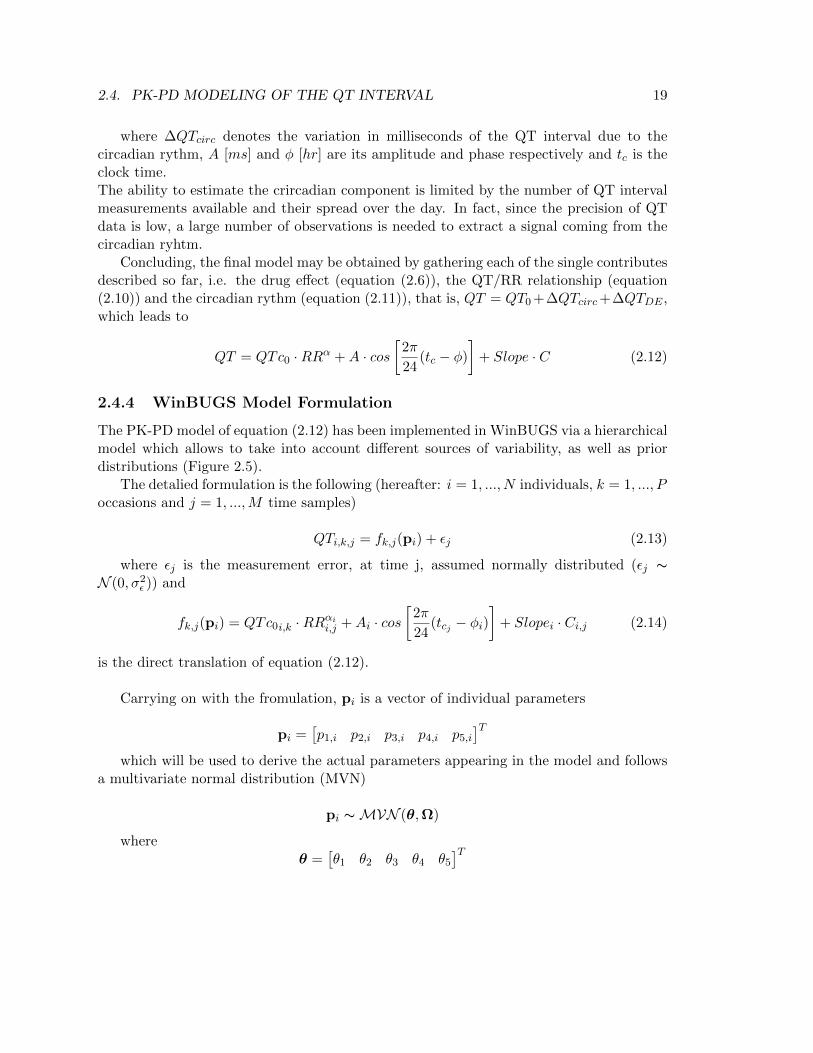
2.4.3 Modelling the Circadian Rhythm
As mentioned in section 1.1, the QT interval depends on several factors. Obviuosly, tryingto build a model able to describe each of them would be too complex as well as withoutany pharmacological interest. Amongst the elements influencing the QT, apart from theaforementioned RR interval and drug effect, the circadian rythm is one of the most sizable(see Figure 2.4).
In general, the statistical significance of the circadian rythmicity can be documentedby the cosinor analysis [11], [12]. This method characterizes a rhythm by the parametersof a fitted cosine function
∆QTcirc = A · cos[
2π
24(tc − φ)
](2.11)
2.4. PK-PD MODELING OF THE QT INTERVAL 19
where ∆QTcirc denotes the variation in milliseconds of the QT interval due to thecircadian rythm, A [ms] and φ [hr] are its amplitude and phase respectively and tc is theclock time.The ability to estimate the crircadian component is limited by the number of QT intervalmeasurements available and their spread over the day. In fact, since the precision of QTdata is low, a large number of observations is needed to extract a signal coming from thecircadian ryhtm.
Concluding, the final model may be obtained by gathering each of the single contributesdescribed so far, i.e. the drug effect (equation (2.6)), the QT/RR relationship (equation(2.10)) and the circadian rythm (equation (2.11)), that is, QT = QT0+∆QTcirc+∆QTDE ,which leads to
QT = QTc0 ·RRα +A · cos[
2π
24(tc − φ)
]+ Slope · C (2.12)
2.4.4 WinBUGS Model Formulation
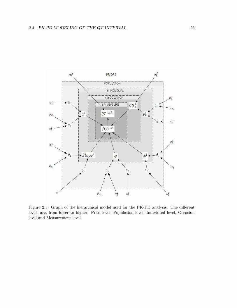
The PK-PD model of equation (2.12) has been implemented in WinBUGS via a hierarchicalmodel which allows to take into account different sources of variability, as well as priordistributions (Figure 2.5).
The detalied formulation is the following (hereafter: i = 1, ..., N individuals, k = 1, ..., Poccasions and j = 1, ...,M time samples)
QTi,k,j = fk,j(pi) + εj (2.13)
where εj is the measurement error, at time j, assumed normally distributed (εj ∼N (0, σ2ε )) and
fk,j(pi) = QTc0i,k ·RRαii,j +Ai · cos
[2π
24(tcj − φi)
]+ Slopei · Ci,j (2.14)
is the direct translation of equation (2.12).
Carrying on with the fromulation, pi is a vector of individual parameters
pi =[p1,i p2,i p3,i p4,i p5,i
]Twhich will be used to derive the actual parameters appearing in the model and follows
a multivariate normal distribution (MVN)
pi ∼MVN (θ,Ω)
whereθ =
[θ1 θ2 θ3 θ4 θ5
]T
20 CHAPTER 2. MATERIALS AND METHODS
represents the vector of the fixed-effects and
Ω =
ω211 ω2
12 ω213 ω2
14 ω215
ω221 ω2
22 ω223 ω2
24 ω225
ω231 ω2
32 ω233 ω2
34 ω235
ω241 ω2
42 ω243 ω2
44 ω245
ω251 ω2
52 ω253 ω2
54 ω255
depicts the random-effect component, i.e. the Between Subject Variabilty (BSV) of the
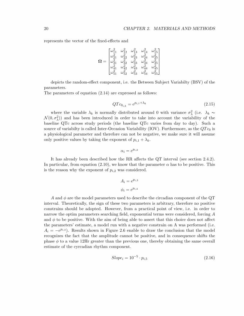
parameters.The parameters of equation (2.14) are expressed as follows:
QTc0i,k = epi,1+λk (2.15)
where the variable λk is normally distributed around 0 with variance σ2λ (i.e. λk ∼N (0, σ2λ)) and has been introduced in order to take into account the variability of thebaseline QTc across study periods (the baseline QTc varies from day to day). Such asource of variabilty is called Inter-Occasion Variability (IOV). Furthermore, as the QTc0 isa physiological parameter and therefore can not be negative, we make sure it will assumeonly positive values by taking the exponent of pi,1 + λk.
αi = epi,2
It has already been described how the RR affects the QT interval (see section 2.4.2).In particular, from equation (2.10), we know that the parameter α has to be positive. Thisis the reason why the exponent of pi,2 was considered.
Ai = epi,3
φi = epi,4
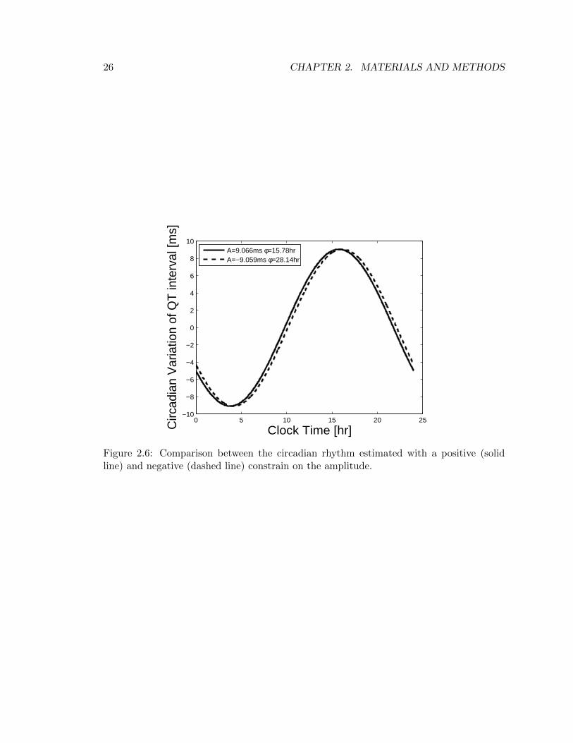
A and φ are the model parameters used to describe the circadian component of the QTinterval. Theoretically, the sign of these two parameters is arbitrary, therefore no positiveconstrains should be adopted. However, from a practical point of view, i.e. in order tonarrow the optim parameters searching field, exponential terms were considered, forcing Aand φ to be positive. With the aim of being able to assert that this choice does not affectthe parameters’ estimate, a model run with a negative constrain on A was performed (i.e.Ai = −epi,3). Results shown in Figure 2.6 enable to draw the conclusion that the modelrecognizes the fact that the amplitude cannot be positive, and in consequence shifts thephase φ to a value 12Hr greater than the previous one, thereby obtaining the same overallestimate of the cyrcadian rhythm component.
Slopei = 10−5 · pi,5 (2.16)
2.4. PK-PD MODELING OF THE QT INTERVAL 21
The formulation of Slope showed above contains a multiplication by 10−5, whose goalcomes from numerical issues. Since Slope parameter is known to be low, equation (2.16)ensures that pi,5 will be a reasonable high number, supporting the algorithm in finding asolution.
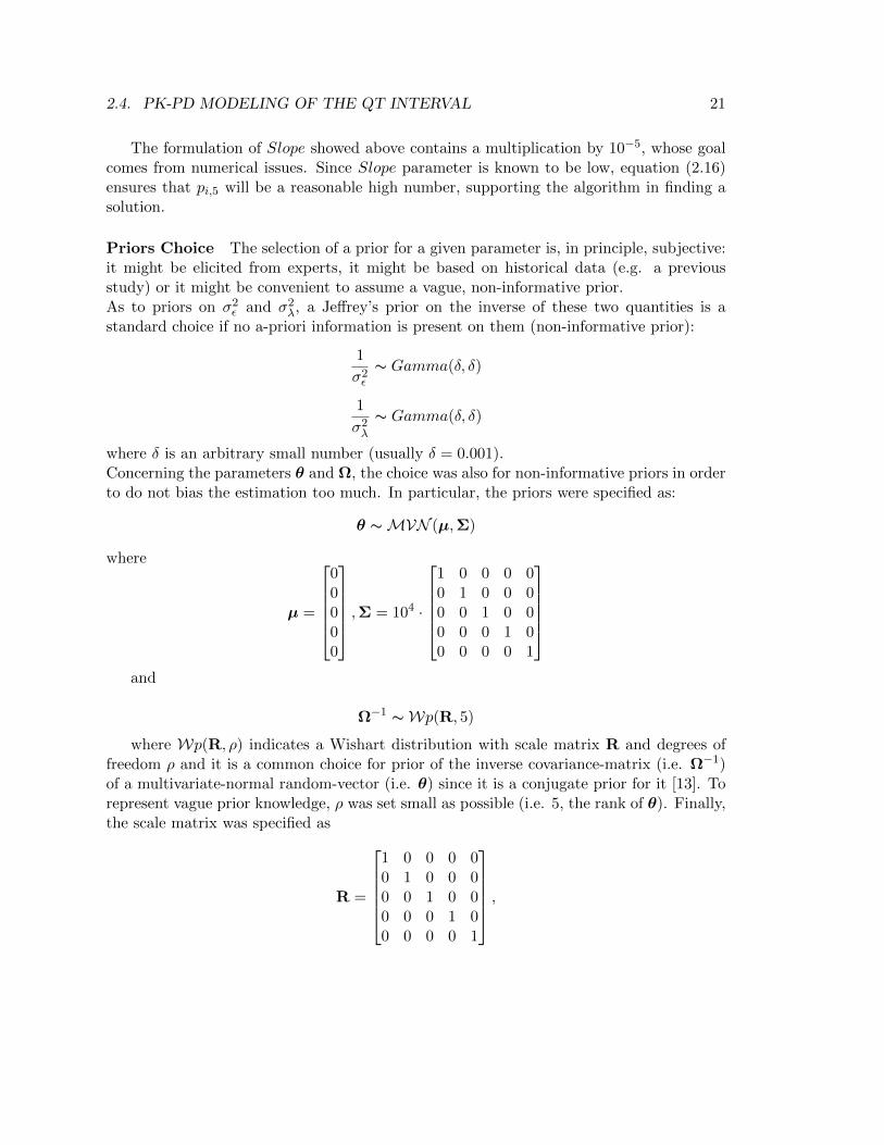
Priors Choice The selection of a prior for a given parameter is, in principle, subjective:it might be elicited from experts, it might be based on historical data (e.g. a previousstudy) or it might be convenient to assume a vague, non-informative prior.As to priors on σ2ε and σ2λ, a Jeffrey’s prior on the inverse of these two quantities is astandard choice if no a-priori information is present on them (non-informative prior):
1
σ2ε∼ Gamma(δ, δ)
1
σ2λ∼ Gamma(δ, δ)
where δ is an arbitrary small number (usually δ = 0.001).Concerning the parameters θ and Ω, the choice was also for non-informative priors in orderto do not bias the estimation too much. In particular, the priors were specified as:
θ ∼MVN (µ,Σ)
where
µ =
00000
,Σ = 104 ·
1 0 0 0 00 1 0 0 00 0 1 0 00 0 0 1 00 0 0 0 1
and
Ω−1 ∼Wp(R, 5)
where Wp(R, ρ) indicates a Wishart distribution with scale matrix R and degrees offreedom ρ and it is a common choice for prior of the inverse covariance-matrix (i.e. Ω−1)of a multivariate-normal random-vector (i.e. θ) since it is a conjugate prior for it [13]. Torepresent vague prior knowledge, ρ was set small as possible (i.e. 5, the rank of θ). Finally,the scale matrix was specified as
R =
1 0 0 0 00 1 0 0 00 0 1 0 00 0 0 1 00 0 0 0 1
,

22 CHAPTER 2. MATERIALS AND METHODS
an arbitrary, as well as common, option given that the choice of R has little effect onthe posterior estimate of Ω [14].
2.4. PK-PD MODELING OF THE QT INTERVAL 23
RR [s]
QTcB
[ms]
350
400
450
0.6 0.8 1.0 1.2 1.4
(a)
RR [s]
QTcF
[ms]
340
360
380
400
420
440
460
0.6 0.8 1.0 1.2 1.4
(b)
Figure 2.3: Comparision between the RR correction formulas of equations (2.7) and (2.8):(a) Bazett correction and (b) Friedericia correction. The dots represent the QTc measure-ments. The loess smoother (solid line) shows a better performance for Fridericia correction.

24 CHAPTER 2. MATERIALS AND METHODS
Clock Time [Hr]
QT
[ms]
340
360
380
400
420
440
8 10 12 14 16 18
8 10 12 14 16 18
340
360
380
400
420
440
Figure 2.4: QT intervals (circles) measured in placebo groups vs clock time. The solid lineis a loess smoother showing a circadian variation in the QT.
2.4. PK-PD MODELING OF THE QT INTERVAL 25
Figure 2.5: Graph of the hierarchical model used for the PK-PD analysis. The differentlevels are, from lower to higher: Prios level, Population level, Individual level, Occasionlevel and Measurement level.
26 CHAPTER 2. MATERIALS AND METHODS
0 5 10 15 20 25−10
−8
−6
−4
−2
0
2
4
6
8
10
Clock Time [hr]Circ
adia
n V
aria
tion
of Q
T in
terv
al [m
s]
A=9.066ms φ=15.78hrA=−9.059ms φ=28.14hr
Figure 2.6: Comparison between the circadian rhythm estimated with a positive (solidline) and negative (dashed line) constrain on the amplitude.
Chapter 3
Results
3.1 Pharmacokinetic Analysis
3.1.1 Preclinical Data
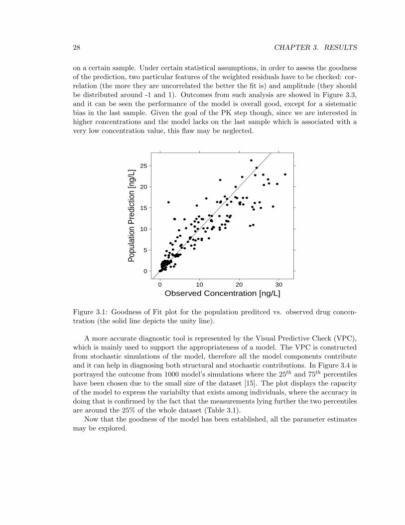
In this section, results from the preclinical PK model of GSK945237 (described in section2.3.1) will be presented and discussed. The outcomes will be interpreted through both anumerical and graphical point of view. All the estimates that are going to be documentedwere obtained in NONMEM adopting the pre-implemented Maximum Likelihood estima-tion algorithm called First Order Conditional Estimation (FOCE) with interaction.A fair diagnostic plot to see how the model works at first glance is the so called Goodnessof Fit (GOF) plot for population prediction (Figure 3.1). The population GOF plot aimsto show the overall behaviour of the model, and the key point to interpret it is that thecloser the black dots are to the unity line the better the prediction is, since this is proofof a good correlation between observed and predicted concentrations. The plot reveals adifficulty in getting the higher concentration values as there is a slight shift of the dots un-der the unity line for measured concentrations in between 23-30 ng/L. Nevertheless, giventhe small number of indivduals involved in the study (18), the model may be acceptedand subjected to further examination. Figure 3.2 illustrates the GOF plot for individualpredicted concentrations, which are obtained by way of a Maximum a Posteriori (MAP)Bayesian estimatation of the indivdual PK parameters using the population estimates aspriors (this step is automatically done by NONMEM). In this case the correlation betweenpredictions and observations is higher than in the population GOF, which is what onewould expect since there is an individual prediction for every subject.The residuals analysis is an alternative way to evaluate the goodness of a model. A residualis defined as the difference between the observed measure and the model prediction, there-fore the lower the residuals are the better the prediction is; on the other hand, weightedresiduals are residuals scaled by a certain weight parameter (for example the variance ofthe measurement error, if we have information on it) that quantifies the confidence we have
27
28 CHAPTER 3. RESULTS
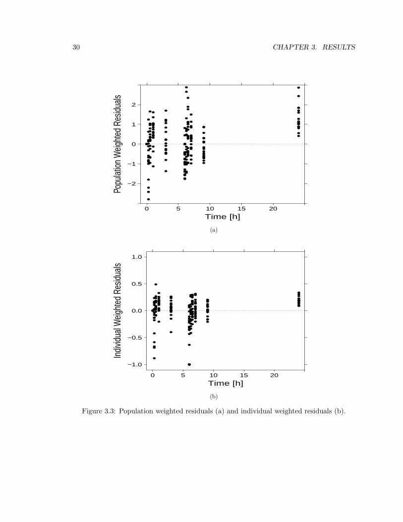
on a certain sample. Under certain statistical assumptions, in order to assess the goodnessof the prediction, two particular features of the weighted residuals have to be checked: cor-relation (the more they are uncorrelated the better the fit is) and amplitude (they shouldbe distributed around -1 and 1). Outcomes from such analysis are showed in Figure 3.3,and it can be seen the performance of the model is overall good, except for a sistematicbias in the last sample. Given the goal of the PK step though, since we are interested inhigher concentrations and the model lacks on the last sample which is associated with avery low concentration value, this flaw may be neglected.
Observed Concentration [ng/L]
Popu
latio
n P
redi
ctio
n [n
g/L]
0
5
10
15
20
25
0 10 20 30
Figure 3.1: Goodness of Fit plot for the population preditced vs. observed drug concen-tration (the solid line depicts the unity line).
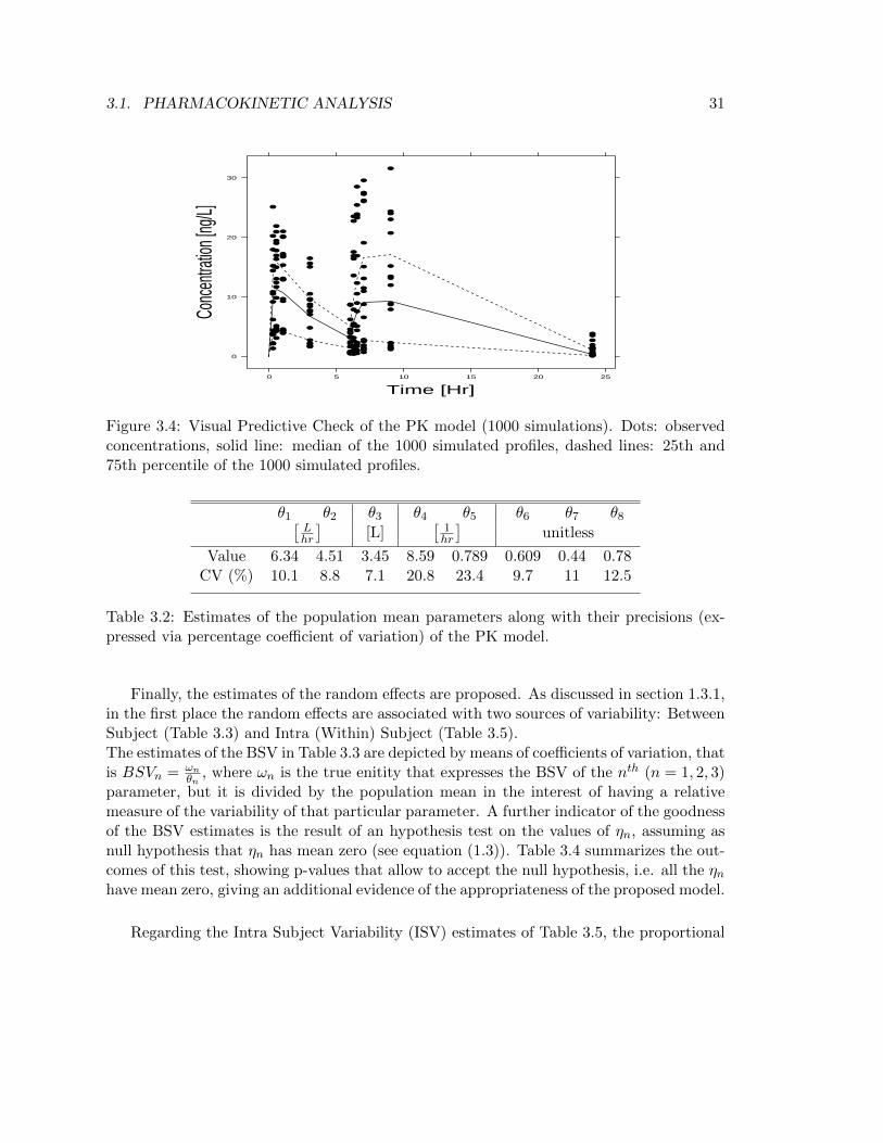
A more accurate diagnostic tool is represented by the Visual Predictive Check (VPC),which is mainly used to support the appropriateness of a model. The VPC is constructedfrom stochastic simulations of the model, therefore all the model components contributeand it can help in diagnosing both structural and stochastic contributions. In Figure 3.4 isportrayed the outcome from 1000 model’s simulations where the 25th and 75th percentileshave been chosen due to the small size of the dataset [15]. The plot displays the capacityof the model to express the variabilty that exists among individuals, where the accuracy indoing that is confirmed by the fact that the measurements lying further the two percentilesare around the 25% of the whole dataset (Table 3.1).
Now that the goodness of the model has been established, all the parameter estimatesmay be explored.

3.1. PHARMACOKINETIC ANALYSIS 29
Observed Concentration [ng/L]
Indi
vidu
al P
redi
ctio
n [n
g/L]
0
10
20
30
0 10 20 30
Figure 3.2: Goodness of Fit plot for the individual preditced vs. observed drug concentra-tion (the solid line depicts the unity line).
Percentage of data above the Percentage of data beneath the75th percentile 25th percentile
28.8% 24.7%
Table 3.1
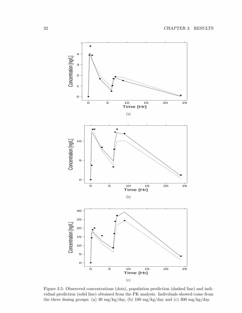
Table 3.2 contains the estimates (with their coefficient of variations) of the fixed effectsof the model. Referring to Figure 3.5 and the values obtained for θ4 and θ5, it should beappear clear why the Ka has been formulated as in equation (2.1): mostly due to the foodeffect, the rate of absorption of the first daily dose is rather higher than the one in thesecond dose. Also, as it may seen from the large variability in the second peak betweenFigures 3.5a, 3.5b and 3.5c, the fact that dogs were fed between the two daily doses hasan influence in the maximum concentration of the second daily dose as well, depending onthe amount of drug administered. In the interest of making the model sensitive to sucheffect, three different bioavailabilities for the three different dose regimens (30, 100 and300 mg/kg) were taken into account (equation (2.2)), where the “full bioavailabilty” (i.e.F = 1) was assumed to be the one on the first daily dose and on the 100 mg/kg dosingregimen.
30 CHAPTER 3. RESULTS
Time [h]
Popu
lation
Weig
hted
Res
iduals
−2
−1
0
1
2
0 5 10 15 20
(a)
Time [h]
Indiv
idual
Weig
hted
Res
iduals
−1.0
−0.5
0.0
0.5
1.0
0 5 10 15 20
(b)
Figure 3.3: Population weighted residuals (a) and individual weighted residuals (b).
3.1. PHARMACOKINETIC ANALYSIS 31
Time [Hr]
Conc
entra
tion [
ng/L]
0
10
20
30
0 5 10 15 20 25
Figure 3.4: Visual Predictive Check of the PK model (1000 simulations). Dots: observedconcentrations, solid line: median of the 1000 simulated profiles, dashed lines: 25th and75th percentile of the 1000 simulated profiles.
θ1 θ2 θ3 θ4 θ5 θ6 θ7 θ8[Lhr
][L]
[1hr
]unitless
Value 6.34 4.51 3.45 8.59 0.789 0.609 0.44 0.78CV (%) 10.1 8.8 7.1 20.8 23.4 9.7 11 12.5
Table 3.2: Estimates of the population mean parameters along with their precisions (ex-pressed via percentage coefficient of variation) of the PK model.
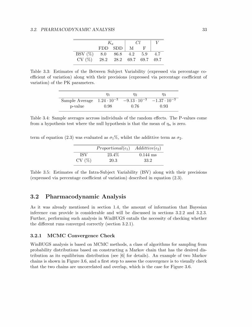
Finally, the estimates of the random effects are proposed. As discussed in section 1.3.1,in the first place the random effects are associated with two sources of variability: BetweenSubject (Table 3.3) and Intra (Within) Subject (Table 3.5).The estimates of the BSV in Table 3.3 are depicted by means of coefficients of variation, thatis BSVn = ωn
θn, where ωn is the true enitity that expresses the BSV of the nth (n = 1, 2, 3)
parameter, but it is divided by the population mean in the interest of having a relativemeasure of the variability of that particular parameter. A further indicator of the goodnessof the BSV estimates is the result of an hypothesis test on the values of ηn, assuming asnull hypothesis that ηn has mean zero (see equation (1.3)). Table 3.4 summarizes the out-comes of this test, showing p-values that allow to accept the null hypothesis, i.e. all the ηnhave mean zero, giving an additional evidence of the appropriateness of the proposed model.
Regarding the Intra Subject Variability (ISV) estimates of Table 3.5, the proportional
32 CHAPTER 3. RESULTS
Time [Hr]
Conc
entra
tion [
ng/L]
0
1
2
3
4
0 5 10 15 20 25
(a)
Time [Hr]
Conc
entra
tion [
ng/L]
0
5
10
0 5 10 15 20 25
(b)
Time [Hr]
Conc
entra
tion [
ng/L]
0
5
10
15
20
25
30
0 5 10 15 20 25
(c)
Figure 3.5: Obsereved concentrations (dots), population prediction (dashed line) and indi-vidual prediction (solid line) obtained from the PK analysis. Indivduals showed come fromthe three dosing groups: (a) 30 mg/kg/day, (b) 100 mg/kg/day and (c) 300 mg/kg/day.
3.2. PHARMACODYNAMIC ANALYSIS 33
Ka Cl VFDD SDD M F
BSV (%) 8.0 86.8 4.2 5.9 4.7CV (%) 28.2 28.2 69.7 69.7 49.7
Table 3.3: Estimates of the Between Subject Variability (expressed via percentage co-efficient of variation) along with their precisions (expressed via percentage coefficient ofvariation) of the PK parameters.
η1 η2 η3
Sample Average 1.24 · 10−3 −9.13 · 10−3 −1.37 · 10−3
p-value 0.98 0.76 0.93
Table 3.4: Sample averages accross individuals of the random effects. The P-values comefrom a hypothesis test where the null hypothesis is that the mean of ηn is zero.
term of equation (2.3) was evaluated as σ1%, whilst the addittive term as σ2.
Proportional(ε1) Addittive(ε2)
ISV 23.4% 0.144 msCV (%) 20.3 33.2
Table 3.5: Estimates of the Intra-Subject Variability (ISV) along with their precisions(expressed via percentage coefficient of variation) described in equation (2.3).
3.2 Pharmacodynamic Analysis
As it was already mentioned in section 1.4, the amount of information that Bayesianinference can provide is considerable and will be discussed in sections 3.2.2 and 3.2.3.Further, performing such analysis in WinBUGS entails the necessity of checking whetherthe different runs converged correctly (section 3.2.1).
3.2.1 MCMC Convergence Check
WinBUGS analysis is based on MCMC methods, a class of algorithms for sampling fromprobability distributions based on constructing a Markov chain that has the desired dis-tribution as its equilibrium distribution (see [6] for details). An example of two Markovchains is shown in Figure 3.6, and a first step to assess the convergence is to visually checkthat the two chains are uncorrelated and overlap, which is the case for Figure 3.6.

34 CHAPTER 3. RESULTS
Iteration
QT0 [
ms]
385
390
395
400
405
0 5000 10000 15000 20000
Figure 3.6: Standard output of a WinBUGS run: two Markov chains of QTc0 parameterin humans.
A problem with MCMC methods is that convergence cannot always be diagnosed asclearly as in optimization methods. Indeed, there are several diagnostic tools that havebeen proposed since GIBBS sampling became popular in Bayesian inference ([16], [17], [18],[19]) and it may be very diffcult to satisfy all these criterions. In order to do not make theconvergence check step too complex and lenghty, only the Gelman-Rubin diagnostic [17]will be performed, along with the assessment of low Monte Carlo (MC) errors, essential forprecise estimation of the posterior distribution [20].Gelman and Rubin method constits in different steps. Firstly, to evaluate the within chainvariance W (hereafter j = 1, ...,m chains, i = 1, ..., n iterations and θij is the ith sample ofthe jth chain of an arbitrary unknown parameter θ) as
W =1
m
m∑j=1
s2j
where s2j is the sample variance of θ in chain j:
s2j =1
n− 1
n∑i=1
(θij − θj)2
and θj is the sample mean of θ in chain j:
θj =1
n
n∑i=1
θij .
3.2. PHARMACODYNAMIC ANALYSIS 35
Secondly, to evaluate the between chain variance B as
B =n
m− 1
m∑j=1
(θj − ¯θ
)2
where ¯θ is the sample mean θ between chains:
¯θ =1
m
m∑j=1
θj .
We can then estimate the variance of the stationary distribution as a weighted averageof W and B, i.e.
σ2θ = (1− 1
n)W +
1
nB,
that is used to define the final parameter of interest, named Potential Scale ReductionFactor (PRF )
PRF =
√σ2θW
(3.1)
which should be as close to 1 as possible to state that the chains converged.
PRF values obtained from Markov chains of parameters of interest in both preclinicaland clinical data are presented in Table 3.6. The same table contains also index ρ ofequation (3.2), which helps to assess the convergence achievement in terms of MC error;particularly, ρ should be less than 5%.
ρ =MCerrorSDestimate
· 100 (3.2)
Table 3.6 suggests convergence of parameters A and φ in clinical data has not beentotally achieved, as indicated by a PRF > 1.5 and a ρ > 5%. Nevertheless, increasing thenumber of iterations does not solve the problem and the reason of a bad convergence mostlikely lays in the low amount of QT samples (8) collected from each patients trhougout theday. Moreover, in both species chains related to the drug effect parameter (i.e. Slope) alsopresent convergence issues, and this might be due to the fact that the parameter is mosltyzero (i.e. the drug effect is moslty absent) therefore chains struggle to overlap and followa straight pattern since sample values range in a very limited interval (see Figure 3.7).

36 CHAPTER 3. RESULTS
PRF
QTc0 α A φ Slope
DOG 1.00 1.01 1.05 1.14 2.21HUMAN 1.00 1.48 2.95 1.89 1.17
ρ (%)
DOG 0.92 0.98 1.29 2.65 6.11HUMAN 1.49 4.76 5.57 5.17 5.69
Table 3.6: Potential Scale Reduction Factors and ρ indices obtained after running theWinBUGS model for both dog and human data.
Iteration
Slope
[ms/n
M]
−0.00010
−0.00005
0.00000
0.00005
0.00010
2000 4000 6000 8000
Figure 3.7: Markov chains of Slope parameter in preclinical data.
3.2.2 Preclinical Data
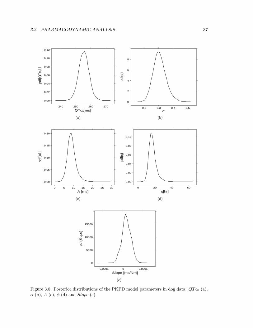
A thorough Bayesian analysis allows to estimate the full posterior distributions of theinvestigated parameters, enabling to extrapolate quantitative information by means ofcomputing precentiles and means of such distributions. In regard to the PKPD model ofequation (2.12), Figure 3.8 illustrates the probabilty density function (pdf ) of parametersQTc0, α, A, φ and Slope in conscious dog data. The shapes of these distributions supplya qualitative idea on the range of values assumed by the parameters. Also, the shape actsas an additional option of convergence inspection; the pdf, in fact, is an alternative way torepresent the run Markov chains for that parameter, thereby it should not contain peaksand troughs since they would be evidence of lack of overlapping between chains as well ascorrelation within chain.
3.2. PHARMACODYNAMIC ANALYSIS 37
QTc0[ms]
pdf(Q
Tc0)
0.00
0.02
0.04
0.06
0.08
0.10
0.12
240 250 260 270
(a)
α
pdf(α
)
0
2
4
6
8
0.2 0.3 0.4 0.5
(b)
A [ms]
pdf(A
)
0.00
0.05
0.10
0.15
0.20
0 5 10 15 20 25 30
(c)
φ[hr]
pdf(φ
)
0.00
0.02
0.04
0.06
0.08
0.10
0 20 40 60
(d)
Slope [ms/Nm]
pdf(S
lope
)
0
5000
10000
15000
−0.0001 0 0.0001
(e)
Figure 3.8: Posterior distributions of the PKPD model parameters in dog data: QTc0 (a),α (b), A (c), φ (d) and Slope (e).

38 CHAPTER 3. RESULTS
Posteriors obtained elucidates a successfull conclusion of the estimation step. Nonethe-less, Figure 3.8e confirms what Table 3.6 had previoulsy told, i.e. a perfect convergence ofSlope Markov chains is difficult to achieve as elicited from the irregular shape of the pdf.
QTc0 α A φ Slope[ms] unitless [ms] [hr] [ msnM ]
10% Credible Interval 251.0 0.251 6.34 12.24 -1.2·10−5
Mean 255.3 0.304 8.77 16.48 1.6·10−5
90% Credible Interval 259.7 0.365 11.93 22.68 4.5·10−5
CV (%) 1.4 14.9 28.1 28.2 136.6
Table 3.7: Mean, 80% credible intervals and precision (expressed as percentage coefficientof variation) of the population parameters of the PKPD model of equation (2.12) for dogdata.
A statistical analysis on the posteriors leads to results in Table 3.7, where the parameterestimates are expressed in terms of posteriors’ mean (i.e. the minimum mean square error(MMSE) estimator). Along with the MMSE estimator there are the 80% credible intervalsand the precision of the estimates expressed as percent coefficient of variation.Once again, the low precision on Slope estimate (136.6%) is an indicator of the problemsarose in finding a complete convergence of the Markov chains for such parameter. An otherinteresting consideration that can be done by looking at Table 3.7 concerns the negative10% credible interval of Slope, which stresses the fact that the drug effect lays around zeroand therefore supports the conclusion that no drug induced QT prolongation takes placein dog.
BSV IOV ISV
QTc0 α A φ Slope? QTc0 σε% % % %
[msnM
][ms] [ms]
10% Credible Interval 41.8 27.7 30.7 26.7 2.0·10−5 10.71 9.26Mean 98.6 41.7 48.6 46.4 3.8·10−5 13.45 9.42
90% Credible Interval 403.1 74.8 96.0 91.2 7.2·10−5 17.50 9.59CV (%) 166.6 153.2 229.1 177.1 164.9 43.0 1.4
?Because of Slope BSV 10% credible interval is negative, Slope BSV has not been represented via coefficient of variation
since such measure is not definable for negative quantities.
Table 3.8: Mean, 80% credible intervals and precision (expressed as percentage coefficientof variation) of the random effects of the PKPD model of equation (2.12) for dog data.
Unlike standard ways of estimation, Basyesian estimation handles every enitity as adistribution, hence posteriors and credible intervals may be obtained also for parameters

3.2. PHARMACODYNAMIC ANALYSIS 39
conveying variability in the model, i.e. Ω (Between Subject Variability), σ2λ (Inter OccasionVariability) and σ2ε (Intra Subject Variability). Table 3.8 contains MMSE estimator and80% credible interval of parameters that quantify each source of variability. It may benoticed that CV values in BSV are all above 100%, reflecting an inaccurate estimate onhow much the parameters vary amongst individuals. Such weakness in detecting reliablemeasures of the BSV is due to the very low number of dogs (4) enrolled in the PD study.
3.2.3 Clinical Data
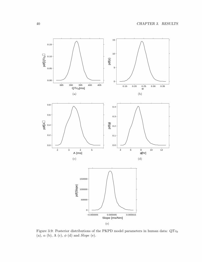
Since there is no difference in the PKPD model between species, the same kind of dissectionperformed for preclinical data in section 3.2.2 will be presented. Starting from the estimatedposterior distributions, Figure 3.9 shows profiles of A and φ are too wavy to concludeMarkov chains for those parameters have fully convegred (Figure 3.9c and 3.9d), reinforcingthe hypothesis made in section 3.2.1 that the number of QT measurements collected perday is too little to be able to extrapolate information on the cyrcadian rhythm.
QTc0 α A φ Slope[ms] unitless [ms] [hr] [ msnM ]
10% Credible Interval 389.7 0.201 2.77 5.97 1.6·10−6
Mean 392.9 0.239 3.44 7.33 4.2·10−6
90% Credible Interval 396.1 0.275 4.09 8.59 7.1·10−6
CV (%) 0.6 12.2 23.0 27.1 52.9
Table 3.9: Mean, 80% credible intervals and precision (expressed as percentage coefficientof variation) of the population parameters of the PKPD model of equation (2.12) for clinicaldata.
BSV IOV ISVQTc0 α A φ Slope QTc0 σε
% [ms]
10% Credible Interval 30.1 27.9 29.0 31.9 61.8 15.2 12.66Mean 44.2 38.9 44.9 63.2 113.2 17.5 13.27
90% Credible Interval 81.5 58.1 69.2 104.4 292.0 20.3 13.94CV (%) 47.7 29.4 35.0 45.6 37.8 23.2 3.8
Table 3.10: Mean, 80% credible intervals and precision (expressed as percentage coefficientof variation) of the random effects of the PKPD model of equation (2.12) for clinical data.
With regards to the MMSE estimates of the model’s parameters, it has to be mentionedthat results from human data lead to the same conclusions in terms of drug effect. Indeed,
40 CHAPTER 3. RESULTS
QTc0[ms]
pdf(Q
Tc0)
0.00
0.05
0.10
0.15
385 390 395 400 405
(a)
α
pdf(α
)
0
5
10
15
0.15 0.20 0.25 0.30 0.35
(b)
A [ms]
pdf(A
)
0.0
0.2
0.4
0.6
0.8
2 3 4 5
(c)
φ[hr]
pdf(φ
)
0.0
0.1
0.2
0.3
0.4
4 6 8 10 12
(d)
Slope [ms/Nm]
pdf(S
lope
)
0
50000
100000
150000
−0.000005 0.000005 0.000015
(e)
Figure 3.9: Posterior distributions of the PKPD model parameters in human data: QTc0(a), α (b), A (c), φ (d) and Slope (e).

3.2. PHARMACODYNAMIC ANALYSIS 41
as reported in Table 3.9, the Slope estimate is again (approximately) zero. Further, Table3.10 confirms that with a reasonable number of individuals (45) estimates of BSV aresufficiently accurate (CVs are less than 50%). Nevertheless, because of the MMSE estimateof Slope is close to zero, the estimated BSV of this parameter is quite high; however, sinceit can be deduced the influence of drug effect in observed data is absent, there is no interestin the knolwedge of how Slope parameter varies among individuals.


Chapter 4
Conclusions
Concerning the assessment of risky QTc increases, according to regulatory guidelines [4] athreshold of 10 msec was used to explore the probability of QTc interval prolongation atthe relevant therapeutic range. In particular, Table 4.1 enables to infer GSK945237 doesnot prolong QTc interval in either humans or dogs since the concentration needed to havea 50% probability of a QTc prolongation grater than 10 msec is approximately hundredtimes bigger than the predicted Cmax.
PC?50 Cmax[nM] [nM]
DOG 3500000 62936.18HUMAN 4200000 13096.86
?concentration associated with a P(QTc increase ≥ 10 msec) = 50%
Table 4.1: PC50 estimates and predicted Cmax in both preclinical and clinical data.
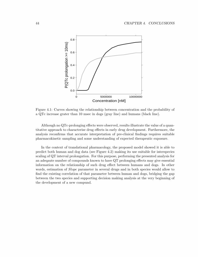
These results differed from typically reported results in telemetered dogs, which areoften based on non-parametric methods and statistical summaries of the data; yet, un-like traditional, data-driven experiments whose outcomes are often vague and ambigous,a model based approach provides a robust method to properly evaluate cardiovascularsafety studies, allowing to advance clear and define conclusions. Moreover, the flexibilityof the proposed approach, characterised by the usage of a Bayesian framework, eases andoptimizes the interpretation of the results, as proven by the opportunity of obtaining theprobability of a QTc prolongation greater than 10 msec (Figure 4.1). In fact, the assess-ment of a probability measure rather than a yes or no answer to the question: “is theQTc prolongation provoked by the drug under investigation matter of concern for furtherdevelopment of the molecule?” gives considerable advantages in a decision analysis context.
43
44 CHAPTER 4. CONCLUSIONS
Concentration [nM]
P(Q
Tc p
rolo
ngat
ion
>= 1
0ms)
0.0
0.2
0.4
0.6
0.8
0 5000000 10000000
Figure 4.1: Curves showing the relationship between concentration and the probability ofa QTc increase grater than 10 msec in dogs (gray line) and humans (black line).
Although no QTc-prolonging effects were observed, results illustrate the value of a quan-titative approach to characterise drug effects in early drug development. Furthermore, theanalysis reconfirms that accurate interpretation of pre-clinical findings requires suitablepharmacokinetic sampling and some understanding of expected therapeutic exposure.
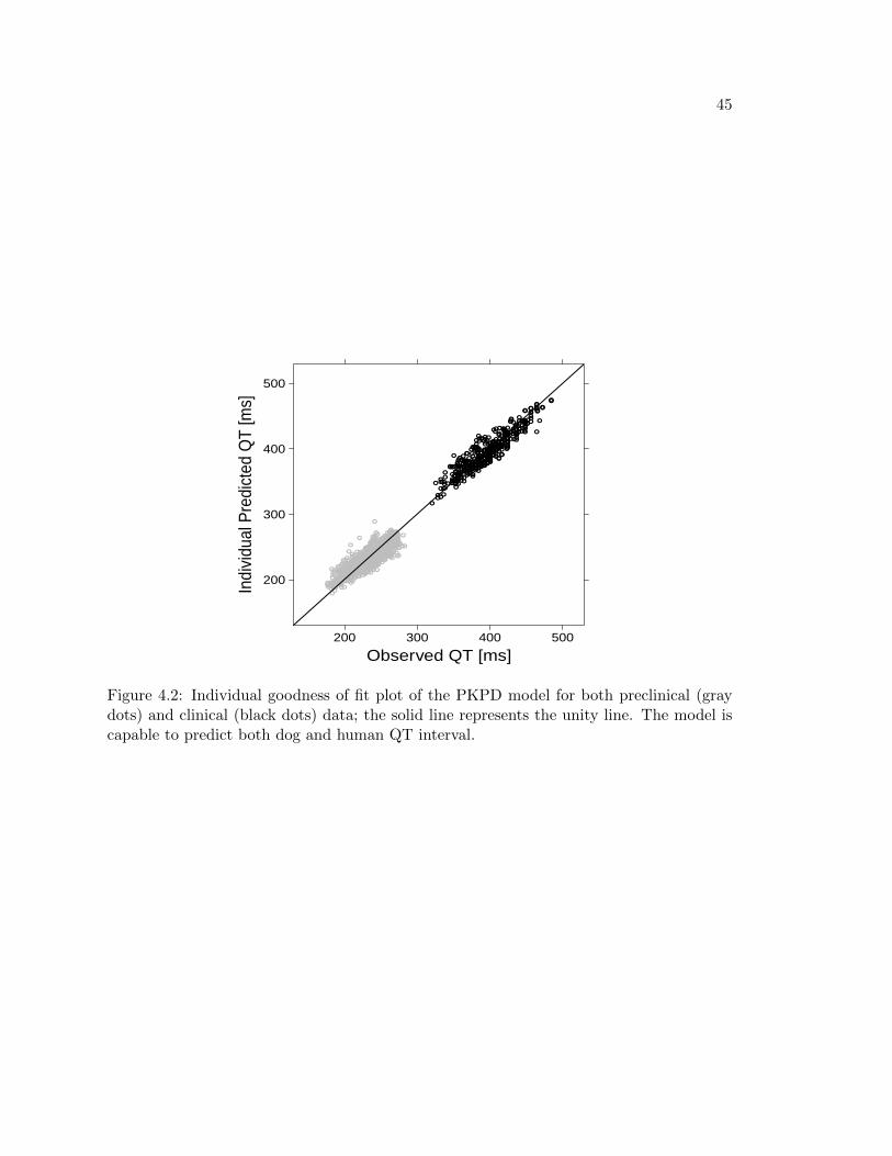
In the context of translational pharmacology, the proposed model showed it is able topredict both human and dog data (see Figure 4.2) making its use suitable for interspeciesscaling of QT interval prolongation. For this purpose, performing the presented analysis foran adeqaute number of compounds known to have QT prolonging effects may give essentialinformation on the relationship of such drug effect between humans and dogs. In otherwords, estimation of Slope parameter in several drugs and in both species would allow tofind the existing correlation of that parameter between human and dogs, bridging the gapbetween the two species and supporting decision making analysis at the very beginning ofthe development of a new compund.
45
Observed QT [ms]
Indi
vidu
al P
redi
cted
QT
[ms]
200
300
400
500
200 300 400 500
Figure 4.2: Individual goodness of fit plot of the PKPD model for both preclinical (graydots) and clinical (black dots) data; the solid line represents the unity line. The model iscapable to predict both dog and human QT interval.

Bibliography
[1] J. Milnes, O. Crociani, A. Arcangeli, J. Hancox, and H. Witchel, “Blockade of HERGPotassium Currents by Fluvoxamine: Incomplete Attenuation by S6 Mutations atF656 or Y652”, British Journal of Pharmacology, vol. 139, pp. 887–898, 2003.
[2] J. Valentin, “Reducing QT Liability and Proarrhythmic Risk in Drug Discovery andDevelopment”, British Journal of Pharmacology, vol. 159, pp. 5–11, 2010.
[3] R. Fenichel, M. Malik, C. Antzelevitch, M. Sanguinetti, D. Roden, S. Priori, J. Ruskin,R. Lipicky, and L. Cantilena, “Drug-induced Torsades de Pointes and Implications forDrug Development”, Journal of Cardiovascular Elettrophysiology, vol. 15, pp. 475–495,2004.
[4] “Guidance for Industry: ICH E14 Clinical Evaluation of QT/QTc IntervalProlongation and Proarrythmic Potential for Non-Antiarrythmic Drugs”, 2005.Department of Health and Human Services, Food and Drug Administration.http://www.fda.gov/downloads/RegulatoryInformation/Guidances/ucm129357.pdf.
[5] A. Chain, K. Krudys, M. Danhof, and O. Della Pasqua, “Assessing the Probabil-ity of Drug-Induced QTc-Interval Prolongation During Clinical Drug Development”,Clinical Pharmacology & Therapeutics, 2011.
[6] D. Lunn, A. Thomas, N. Best, and D. Spiegelhalter, “WinBUGS – a Bayesian mod-elling framework: concepts, structure, and extensibility”, Cambridge, UK: MRC Bio-statistic Unit, vol. 10, pp. 325–337, 2000.
[7] S. Beal, L. Sheiner, A. Boeckmann, and R. Bauer, NONMEM User’s Guides (1989-2009). Icon Development Solutions, Ellicott City, MD, USA, 2009.
[8] J. Gabrielsson and D. Weiner, PK/PD Data Analysis: Concepts and Applications.Stockholm, Sweden: Swedish Pharmaceutical Press, 2007.
[9] H. Bazett, “An analysis of the time relations of electrocardiograms”, Heart, vol. 7,pp. 353–370, 1920.
47
48 BIBLIOGRAPHY
[10] L. Fridericia, “Die systolendauer im elektrokardiogramm bei normalen Menchen undbei Herzkranken”, Acta Med Scand, vol. 53, pp. 469–486, 1920.
[11] W. Nelson, Y. Tong, J. Lee, and F. Halberg, “Methods for cosinorrhythmometry”,Chronobiologia, vol. 6, pp. 305–323, 1979.
[12] Y. Touitou and E. Haus, Biologic Rhythms in Clinical and Laboratory Medicine. Berlin,Germany: Springer Verlag.
[13] K. Murphy, Conjugate Bayesian Analysis of the Gaussian Distribution,2007. The Univeristy of Bristish Columbia. http://www.cs.ubc.ca/ mur-phyk/Papers/bayesGauss.pdf.
[14] “Jaws: repeated measures analysis of variance”. WinBUGS Help Example on the Useof Wishart Distribution.
[15] M. O. Karlsson and N. Holford, “A tutorial on visual predictive check”, 2008. Seven-teenth PAGE meeting, Abstract 1434. www.page-meeting.org/?abstract=1434.
[16] J. Geweke, “Evaluating the accuracy of sampling-based approaches to calculatingposterior moments”, Bayesian Statistics, vol. 4, pp. 169–194, 1992.
[17] A. Gelman and D. Rubin, “Inference from iterative simulation using multiple se-quences”, Statistical Science, vol. 7, pp. 457–511, 1992.
[18] A. Raftery and S. Lewis, “How many iterations in the Gibbs sampler?”, BayesianStatistics, vol. 4, pp. 763–774, 1992.
[19] P. Heidelberger and P. Welch, “Simulation run length control in the presence of aninitial transient”, Operations Research, vol. 31, pp. 1109–1144, 1992.
[20] I. Ntzoufras, Bayesian Modeling Using WinBUGS. Hoboken, NJ, USA: John Wiley& Sons, Inc., 2008.