Bayesian Networks - cs.ru.nl filePractical assignment: develop your own Bayesian network; experiment with learning (structure and classiﬁers) Assessment: ... F.V. Jensen and T. Nielsen,

Bayesian Networks

Probabilistic Graphical Models in AI

Introduction

Peter Lucas

[email protected]

LIACS

Leiden University

Lecture 1: Intro – p. 1

Course Organisation

Lecturer: Peter Lucas

Where I am located: Room 123, Snellius

Structure of course:

Lectures

Seminar: group research, individual scientific paper,and discussions

Practical assignment: develop your own Bayesiannetwork; experiment with learning (structure andclassifiers)

Assessment:

Exam: 35%; seminar: 35% (or Exam only: 60%)

Practical assignment 1 and 2: 15% each (or 20%each when no seminar)

Course information: www.cs.ru.nl/∼peterl/BNLecture 1: Intro – p. 2

Course Aims

Develop complete understanding of basic probabilitytheory (theory)

Knowledge and understanding of differences andsimilarities between various probabilistic graphicalmodels (theory)

Know how to build Bayesian networks from expertknowledge (theory and practice)

Being familiar with basic inference algorithms (theoryand practice)

Understand the basic issues of learning Bayesiannetworks from data (theory and practice)

Be familiar with typical applications (practice)

Critical appraisal of a specialised topic (theory, possiblypractice)


Literature

Compulsory:

K.B. Korb and A.E. Nicholson, Bayesian ArtificialIntelligence, Chapman & Hall, Boca Raton, 2004 or2010

Background:

R.G. Cowell, A.P. Dawid, S.L. Lauritzen and D.J.Spiegelhalter, Probabilistic Networks and ExpertSystems, Springer, New York, 1999

F.V. Jensen and T. Nielsen, Bayesian Networks andDecision Graphs, Springer, New York, 2007

D. Koller and N. Friedman, Probabilistic GraphicalModels: Principles and Techniques, MIT Press,Cambridge, MA, 2009

Various research papers on the mentioned topics


Uncertainty in Daily Life

Empirical evidence:

“If symptoms of fever, shortness of breath(dyspnoea), and coughing are present,and the patient has recently visited China,then the patient has probably SARS”

Subjective belief:

“The Rutte government will resign soon (and afterthe elections will be likely replaced by a VVD,D66, GL, and PvdA government)”

Temporal dimension:

“There is more than 60% chance that the Dutcheconomy will fully recover in the next two years”


Uncertainty Representation

Methods for dealing with uncertainty are not new:

17th century: Fermat, Pascal, Huygens, Leibniz,Bernoulli

18th century: Laplace, De Moivre, Bayes

19th century: Gauss, Boole

Most important research question in early AI(1970–1987):

How to incorporate uncertainty reasoning in logicaldeduction?

Again an important research question in modern AI(e.g. Markov logic)


Early AI Methods of Uncertainty

Rule-based uncertainty representation:

(fever ∧ dyspnoea) ⇒ SARSCF=0.4

Uncertainty calculus (certainty-factor (CF) model,subjective Bayesian method):

CF(fever, B) = 0.6; CF(dyspnoea, B) = 1(B is background knowledge)

Combination functions:

CF(SARS, {fever, dyspnoea} ∪ B)= 0.4 ·max{0,min{CF(fever, B),CF(dyspnoea, B)}}= 0.4 ·max{0,min{0.6, 1}} = 0.24


However · · ·

(fever ∧ dyspnoea) ⇒ SARSCF=0.4

How likely is the occurrence of fever or dyspnoea giventhat the patient has SARS?

How likely is the occurrence of fever or dyspnoea in theabsence of SARS?

How likely is the presence of SARS when just fever ispresent?

How likely is no SARS when just fever is present?


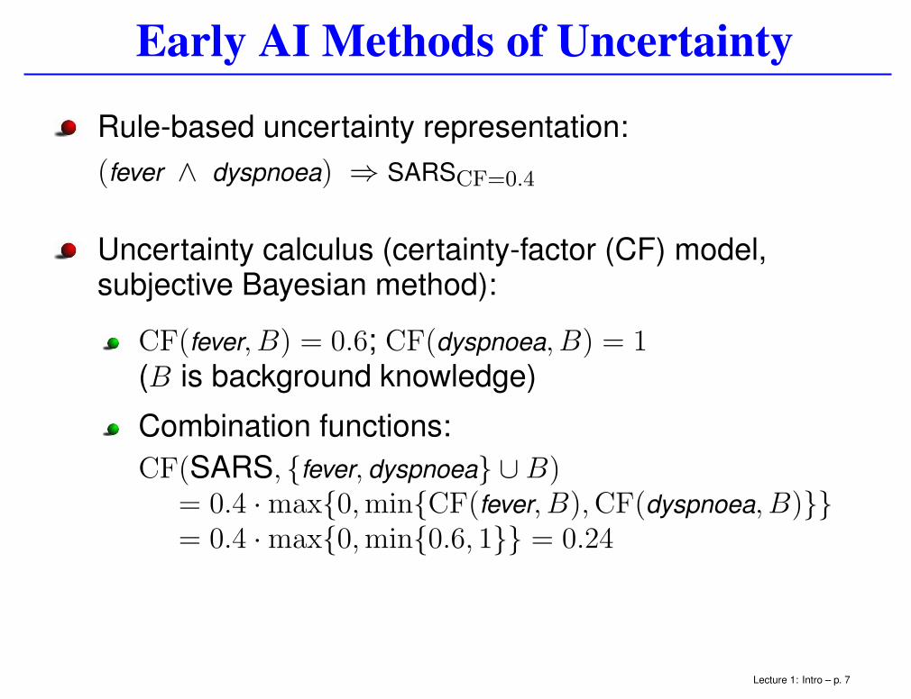
Bayesian Networks

flu (FL)

(yes/no)

SARS (RS)

(yes/no)

fever (FE)

(yes/no)

dyspnoea (DY)

(yes/no)

TEMP

(≤ 37.5/> 37.5)

VisitToChina (CH)

(yes/no)

P (CH,FL,RS,DY,FE,TEMP)

P (FL = y) = 0.1

P (CH = y) = 0.1

P (RS = y | CH = y) = 0.3

P (RS = y | CH = n) = 0.01

P (FE = y | FL = y,RS = y) = 0.95

P (FE = y | FL = n,RS = y) = 0.80

P (FE = y | FL = y,RS = n) = 0.88

P (FE = y | FL = n,RS = n) = 0.001

P (DY = y | RS = y) = 0.9

P (DY = y | RS = n) = 0.05

P (TEMP ≤ 37.5 | FE = y) = 0.1

P (TEMP ≤ 37.5 | FE = n) = 0.99


Reasoning: Evidence Propagation

Nothing known:

NOYES

FLU

noyes

FEVER

noyes

SARS

noyes

VisitToChina

noyes

DYSPNOEA

<=37.5>37.5

TEMP

Temperature >37.5 ◦C:

NOYES

FLU

noyes

FEVER

noyes

SARS

noyes

VisitToChina

noyes

DYSPNOEA

<=37.5>37.5

TEMP


Reasoning: Evidence Propagation

Temperature >37.5 ◦C:

NOYES

FLU

noyes

FEVER

noyes

SARS

noyes

VisitToChina

noyes

DYSPNOEA

<=37.5>37.5

TEMP

I just returned from China:

NOYES

FLU

noyes

FEVER

noyes

SARS

noyes

VisitToChina

noyes

DYSPNOEA

<=37.5>37.5

TEMP


Independence Representation in Graphs

The set of variables X is conditionally independent of theset Z given the set Y , notation X ⊥⊥ Z | Y , iff

P (X | Y, Z) = P (X | Y )

Meaning:

“If we know Y then Z does not have any (extra)effect on our knowledge concerning X (and thuscan be omitted)”

ExampleIf we know that John has fever, then also knowing that hehas a high body temperature has no effect on ourknowledge about flu


Find the Independences

NOYES

FLU

noyes

FEVER

noyes

SARS

noyes

VisitToChina

noyes

DYSPNOEA

<=37.5>37.5

TEMP

Examples:

FLU ⊥⊥ VisitToChina | ∅

FLU ⊥⊥ SARS | ∅

FLU 6⊥⊥ SARS | FEVER, also FLU 6⊥⊥ SARS | TEMP

SARS ⊥⊥ TEMP | FEVER

VisitToChina ⊥⊥ DYSPNOEA | SARS


Probabilistic Reasoning

Interested in conditional probability distributions:

P (XW | E) = P E(XW )

with W set of vertices, for (possibly empty) evidence E(instantiated variables)

Examples

P (FLU = yes | TEMP < 37.5)

P (FLU = yes,VisitToAsia = yes | TEMP < 37.5)

Tendency to focus on conditional probabilitydistributions of single variables


Probabilistic Reasoning (cont)

Joint probability distribution P (X):P (X) = P (X1, X2, . . . , Xn)

marginalisation:

P (Y ) =∑

X\Y

P (X) =∑

X\Y

∏

v∈V

P (Xv | Xπ(v))

conditional probabilities and Bayes’ rule:

P (Y, Z | X) =P (X | Y, Z)P (Y, Z)

P (X)

Many efficient Bayesian reasoning algorithms exist


Naive Probabilistic Reasoning: Evidence

X3

y/n

X1

y/n

X2

y/n

X4

y/n

P (x4 | x3) = 0.4

P (x4 | ¬x3) = 0.1

P (x3 | x1, x2) = 0.3

P (x3 | ¬x1, x2) = 0.5

P (x3 | x1,¬x2) = 0.7

P (x3 | ¬x1,¬x2) = 0.9

P (x1) = 0.6

P (x2) = 0.2

P E(x2) = P (x2 | x4) =P (x4 | x2)P (x2)

P (x4)(Bayes’ rule)

=

∑X3

P (x4|X3)∑

X1P (X3|X1, x2)P (X1)P (x2)∑

X3P (x4 | X3)

∑X1,X2

P (X3 | X1, X2)P (X1)P (X2)≈ 0.14


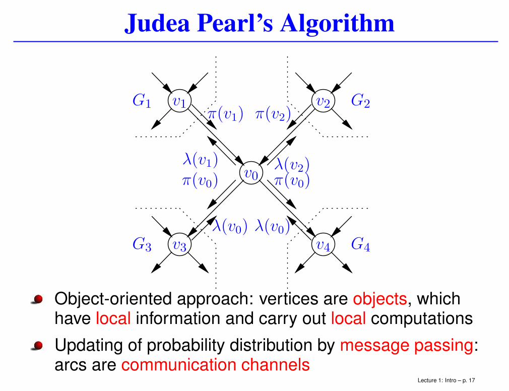
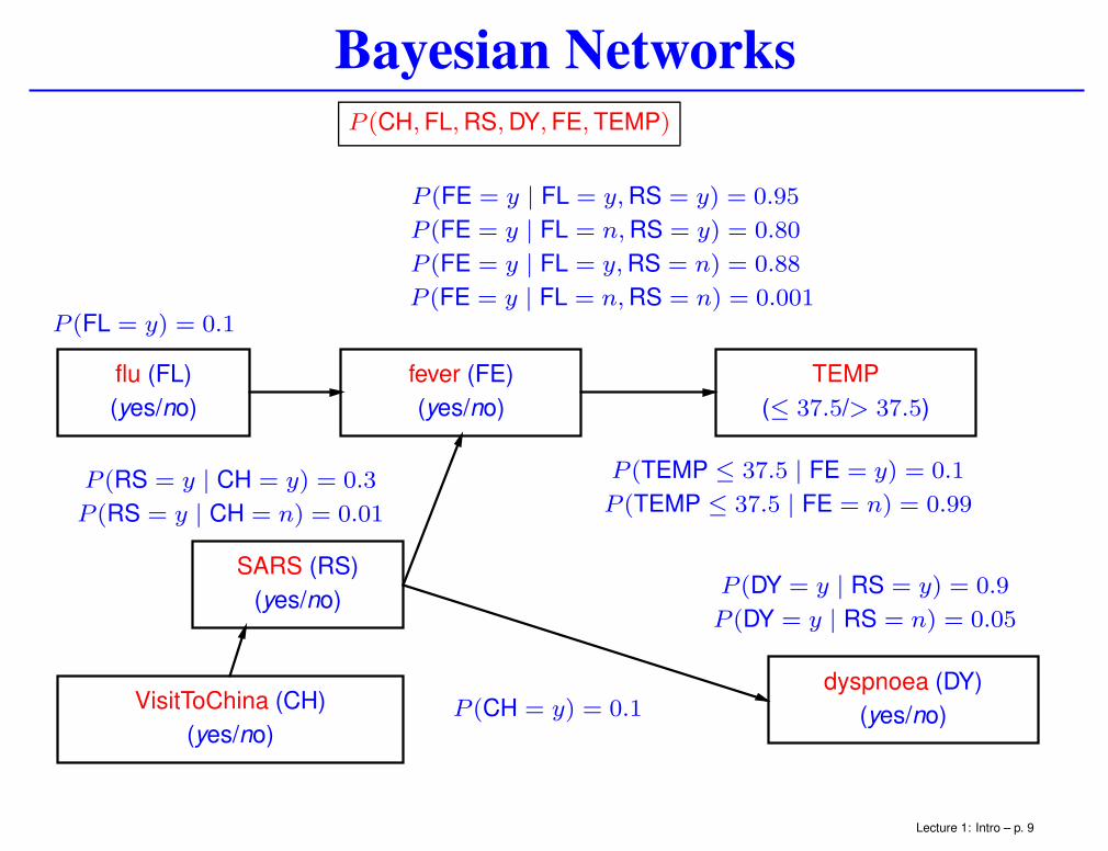
Judea Pearl’s Algorithm

v1G1π(v1)

v3G3

λ(v0)

v2 G2π(v2)

v4 G4

λ(v0)

v0π(v0) π(v0)λ(v1) λ(v2)

Object-oriented approach: vertices are objects, whichhave local information and carry out local computations

Updating of probability distribution by message passing:arcs are communication channels


Data Fusion Lemma

vjEvidence

vi

. . .

. . .. . .

E−vi

E+vi

causalinformation

diagnosticinformation

Data fusion:

P E(Xvi) = P (Xvi | E)= α · causal info for Xvi · diagnostic info for Xvi

= α · π(vi) · λ(vi)

where:

E = E+vi ∪ E−

vi : evidence

α: normalisation constant


Problem Solving

Bayesian networks are declarative, i.e.:

mathematical basis

problem to be solved determined by (1) enteredevidence E (may include decisions); (2) givenhypothesis H: P (H | E) (cf. KB ∧H � E)

Examples:

Description of populations

Maximum a Posteriori (MAP) Assignment forclassification and diagnosis: D = argmaxH P (H | E)

Temporal reasoning, prediction, what-if scenarios

Decision-making based on decision theoryMEU(D | E) = maxd∈D

∑x u(x)P (x | d, E)


Decision Networks

Pneumonia (PN)

(yes/no)

Fever (FE)

(yes/no)

TEMP

(≤ 37.5/

> 37.5)

Coughing (CO)

(yes/no)

Pneumococcus (PP)

(yes/no)

Coverage (CV)

(yes/no)

Therapy (TH)

(penicillin/no-penicillin)U

P (PN = y | PP = y) = 0.77

P (PN = y | PP = n) = 0.01

P (FE = y | PN = y) = 0.95

P (FE = y | PN = n) = 0.001

P (CO = y | PN = y) = 0.80

P (CO = y | PN = n) = 0.05

P (TEMP ≤ 37.5 | FE = y) = 0.1

P (TEMP ≤ 37.5 | FE = n) = 0.99

P (CV = y | PP = y,TH = pc) = 0.80

P (CV = y | PP = n,TH = pc) = 0.0

P (CV = y | PP = y,TH = npc) = 0.0

P (CV = y | PP = n,TH = npc) = 1.0

P (PP = y) = 0.1

u(CV = y) = 100

u(CV = n) = 0


Markov Networks

Structure of a joint probability distribution P can also bedescribed by undirected graphs (instead of directedgraphs as in Bayesian networks)

X2 X5

X6

X4

X3

X1 X7

Together with P (V ) = P (X1, X2, X3, X4, X5, X6, X7):Markov network

Marginalisation (example):

P (¬x2) =∑

X1,X3,X4,X5,X6,X7

P (X1,¬x2, X3, X4, X5, X6, X7)


Manual Construction

Qualitative modelling:

Infection

Body response

to A

Body response

to B

Body response

to C

Colonisation by

bacterium A

Colonisation by

bacterium B

Colonisation by

bacterium C

Fever WBC ESR

People become colonised by bacteria when entering ahospital, which may give rise to infection


Bayesian-network Modelling

Qualitative

causal modelling

Cause → Effect

Inf

BRA BRB BRC

Quantitative

interaction modelling

P (Inf | BRA,BRB,BRC)

BRA

t f

BRB BRB

t f t f

BRC BRC BRC BRC

Inf t f t f t f t f

t 0.8 0.6 0.5 0.3 0.4 0.2 0.3 0.1

f 0.2 0.4 0.5 0.7 0.6 0.8 0.7 0.9


Example BN: non-Hodgkin Lymphoma


Bayesian Network Learning

Bayesian network B = (G,P ), with

digraph G = (V (G), A(G)), and

probability distribution P

general Bayesian

restricted

Structure

Learning

networks

Restricted Structure Learning

tree−augmentedBayesian network

Spectrum

naive Bayesiannetwork

(TAN)

Un


Learning Bayesian Networks

Problems:

for many BNs too many probabilities have to beassessed

complex BNs do not necessarily yield better classifiers

complex BNs may yield better estimates of a probabilitydistribution

Solution:

use simple probabilistic models for classification:

naive (independent) form BN

T ree-Augmented Bayesian Network (TAN)

Forest-Augmented Bayesian Network (FAN)

use background knowledge and clever heuristics


Naive (independent) form BN

C

E1

· · ·E2

Em

C is a class variable

The evidence variables Ei in the evidenceE ⊆ {E1, . . . , Em} are conditionally independent giventhe class variable C

This yields: P (C | E) = P (E|C)P (C)P (E) =

∏E∈E

P (E|C)P (C)∑

C

∏E∈E

P (E|C)P (C)

Classifier: cmax = argmaxC P (C | E)


Learning Structure from Data

Given the following dataset D:

Student Gender IQ High Mark for Maths

1 male low no

2 female average yes

3 male high yes

4 female high yes

and the following Bayesian networks:

G I AG1:

G I AG2:

G I AG3:

G I AG4:

G

I

AG5: ...

Which one is the best?Lecture 1: Intro – p. 28

Being Bayesian about Bayesian Networks

Bayesian statistics: inherent uncertainty in parameters andexploitation of data to update knowledge:

Uncertain parameters:

Θ

X

Probability distribution P (X | Θ), with Θ un-certain parameters with probability density p(Θ)

Assume the Bayesian network structure G comes froma probability distribution, based on data D:

P (G | D)


Research Issues

Inf

BRA BRB BRC

Modelling:

To determine the structure of a network

Generalisation of networks using logics(e.g. Markov logic networks)

Learning:

Structure learning: determine the ‘best’ graph topology

Parameter learning: determine the ‘best’ probabilitydistribution (discrete or continuous)

Inference: increase speed, reduce memory requirements

⇒ you can contribute too · · ·


Documents

Bayesian Networks - cs.ru.nl filePractical assignment: develop your own Bayesian network; experiment with learning (structure and classiﬁers) Assessment: ... F.V. Jensen and T. Nielsen,