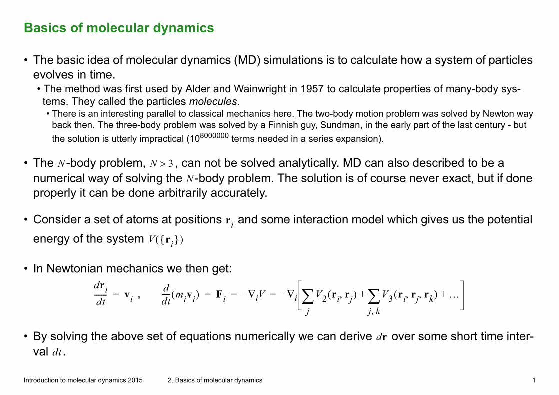
Basics of molecular dynamics

• The basic idea of molecular dynamics (MD) simulations is to calculate how a system of particles evolves in time.• The method was first used by Alder and Wainwright in 1957 to calculate properties of many-body sys-tems. They called the particles molecules.• There is an interesting parallel to classical mechanics here. The two-body motion problem was solved by Newton way

back then. The three-body problem was solved by a Finnish guy, Sundman, in the early part of the last century - but

the solution is utterly impractical (108000000 terms needed in a series expansion).

• The N -body problem, N 3> , can not be solved analytically. MD can also described to be a numerical way of solving the N -body problem. The solution is of course never exact, but if done properly it can be done arbitrarily accurately.

• Consider a set of atoms at positions ri and some interaction model which gives us the potential

energy of the system V ri{ }( )

• In Newtonian mechanics we then get:

dridt------- vi= , d

dt----- mivi( ) Fi Vi∇– V2 ri rj,( ) V3 ri rj rk, ,( ) …+

j k,+

ji∇–= = =

• By solving the above set of equations numerically we can derive dr over some short time inter-val dt .

Introduction to molecular dynamics 2015 2. Basics of molecular dynamics 1

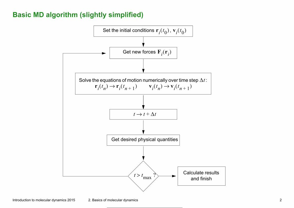
Basic MD algorithm (slightly simplified)

Set the initial conditions , ri t0( ) vi t0( )

Get new forces Fi ri( )

Solve the equations of motion numerically over time step :

Δtri tn( ) ri tn 1+( )→ vi tn( ) vi tn 1+( )→

t t Δt+→

Get desired physical quantities

t tmax ?> Calculate results and finish

Introduction to molecular dynamics 2015 2. Basics of molecular dynamics 2

Δr vΔt12---aΔt

2+≈ a Fm----=,

An alternative view

• MD-simulation of thermal motion over 100 time steps

1

23

45

• Zoom in on 2 time steps (5 atoms):• At time the distances and

hence forces between nearby

atoms are calculated• From these forces we can solve

the equations of motion, and hence get new positions and velocities.

t rij

Fij

• The displace-ment over a time step is denoted .• has to be

much smaller than the dis-tance between nearby atoms.

ΔtΔr

Δr

= position at t ti== position at t ti 1+=

r13 F13,r12 F12,

r14 F14,r15 F15,

Introduction to molecular dynamics 2015 2. Basics of molecular dynamics 3

General considerations

• The above was the simplest possible example, the so called microcanonical or NVE ensemble. This means that the approach preserves the number of atoms N , the volume of the cell V and the energy E . Other ensembles will be dealt with later on in the course. But the NVE ensemble is the most natural one in that it is the true solution of the N -body problem, and corresponds to the real atom motion.

• First MD simulations:• Hard spheres: B. J. Alder, T. E. Wainwright: Phase transition for a Hard Sphere-System, J. Chem. Phys. 27 (1957) 1208

• Continuous potentials: J. B. Gibson, A. N. Goland, M. Milgram, G. H. Vineyard: Dynamics of Radiation Damage, Phys. Rev. 120 (1960) 1229.

• State-of-the-art (2015):• Of the order of 10 000 000 000 atoms can be done on many large supercomputers• In Finland: CSC Cray (louhi.csc.fi): some 100 000 000 atoms with a realistic potential easily possible for thousands of time steps.

• If all N atoms interact with all atoms, one has to in principle calculate N2 interactions. This is prohibitively expensive for millions of atoms.

Introduction to molecular dynamics 2015 2. Basics of molecular dynamics 4

General considerations

• Fortunately, in practice most atomic interactions decrease rapidly in strength as r ∞→ . In that case it is enough to calculate only interactions to nearby atoms.• E.g. in diamond-structured semiconductors (Si, Ge, GaAs...) atoms have 4 covalent bonds, so the calcu-lation can be reduced to 4 neighbours => 4 N interactions.

• In metals atoms more than ~ 5 Å far can usually be neglected => about 80 N interactions

• In ionic systems the interaction V 1 r⁄∝ , i.e. decreases very slowly. It can not be cut off, but there are smart workarounds.

Introduction to molecular dynamics 2015 2. Basics of molecular dynamics 5

Early MD simulations

Introduction to molecular dynamics 2015 2. Basics of molecular dynamics 6

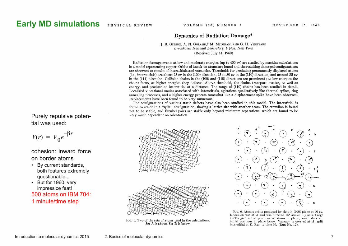
Purely repulsive poten-tial was used:

cohesion: inward force on border atoms • By current standards,

both features extremely questionable...

• But for 1960, very impressice feat!

500 atoms on IBM 704:1 minute/time step

V r( ) V0eβr–=

Early MD simulations

Introduction to molecular dynamics 2015 2. Basics of molecular dynamics 7

Simulation cell

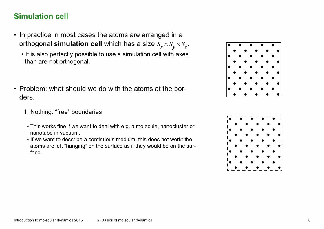
• In practice in most cases the atoms are arranged in a orthogonal simulation cell which has a size Sx Sy× Sz× .

• It is also perfectly possible to use a simulation cell with axes than are not orthogonal.

• Problem: what should we do with the atoms at the bor-ders.

1. Nothing: “free” boundaries

• This works fine if we want to deal with e.g. a molecule, nanocluster or nanotube in vacuum.

• If we want to describe a continuous medium, this does not work: the atoms are left “hanging” on the surface as if they would be on the sur-face.

Introduction to molecular dynamics 2015 2. Basics of molecular dynamics 8

Simulation cell

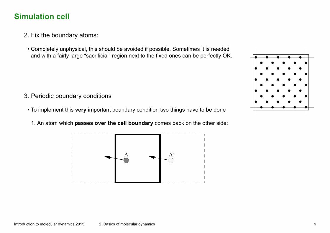
2. Fix the boundary atoms:

• Completely unphysical, this should be avoided if possible. Sometimes it is needed and with a fairly large “sacrificial” region next to the fixed ones can be perfectly OK.

3. Periodic boundary conditions

• To implement this very important boundary condition two things have to be done

1. An atom which passes over the cell boundary comes back on the other side:

A A’

Introduction to molecular dynamics 2015 2. Basics of molecular dynamics 9

Simulation cell

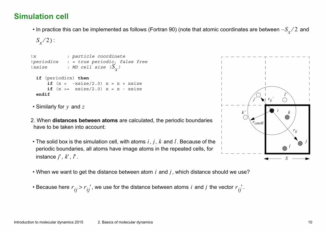
• In practice this can be implemented as follows (Fortran 90) (note that atomic coordinates are between Sx 2⁄– and

Sx 2⁄ ) :

!x : particle coordinate

i

j’

j

kk’

l

l’

rcutoff

rij

rij’

S

!periodicx : = true periodic, false free!xsize : MD cell size (Sx)

if (periodicx) then if (x < -xsize/2.0) x = x + xsize if (x >= xsize/2.0) x = x - xsize endif

• Similarly for y and z

2. When distances between atoms are calculated, the periodic boundaries have to be taken into account:

• The solid box is the simulation cell, with atoms i , j , k and l . Because of the periodic boundaries, all atoms have image atoms in the repeated cells, for

instance j' , k' , l' .

• When we want to get the distance between atom i and j , which distance should we use?

• Because here rij rij'> , we use for the distance between atoms i and j the vector rij' .

Introduction to molecular dynamics 2015 2. Basics of molecular dynamics 10

Simulation cell

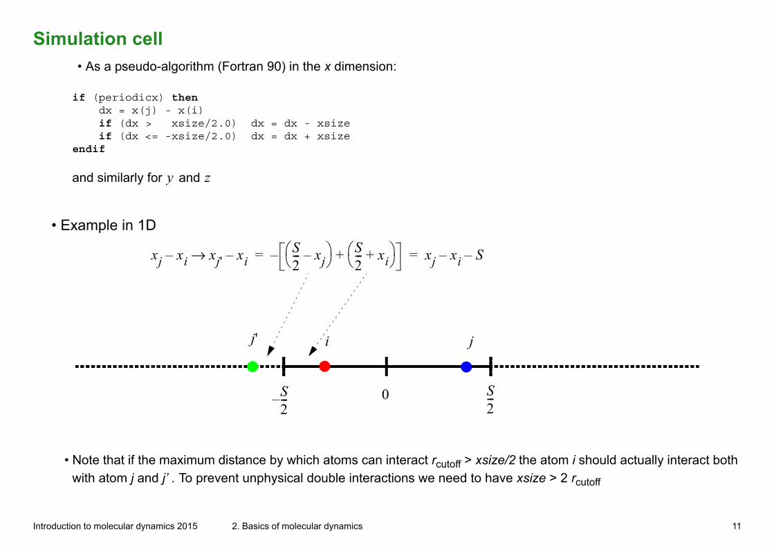
• As a pseudo-algorithm (Fortran 90) in the x dimension:

if (periodicx) then dx = x(j) - x(i) if (dx > xsize/2.0) dx = dx - xsize if (dx <= -xsize/2.0) dx = dx + xsizeendif

and similarly for y and z

• Example in 1D

i jj'

S2---– S

2---0

xj xi– xj' xi–→ S2--- xj– S

2--- xi+ +– xj xi– S–= =

• Note that if the maximum distance by which atoms can interact rcutoff > xsize/2 the atom i should actually interact both

with atom j and j’ . To prevent unphysical double interactions we need to have xsize > 2 rcutoff

Introduction to molecular dynamics 2015 2. Basics of molecular dynamics 11

Simulation cell

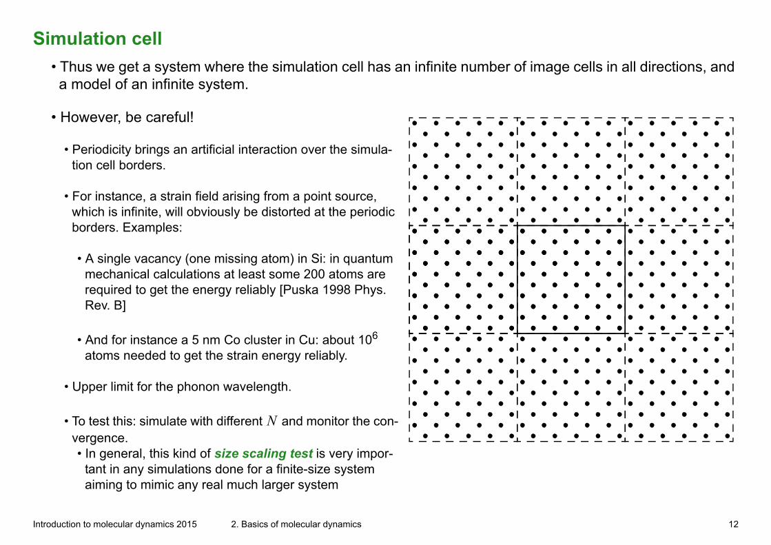
• Thus we get a system where the simulation cell has an infinite number of image cells in all directions, and a model of an infinite system.

• However, be careful!

• Periodicity brings an artificial interaction over the simula-tion cell borders.

• For instance, a strain field arising from a point source, which is infinite, will obviously be distorted at the periodic borders. Examples:

• A single vacancy (one missing atom) in Si: in quantum mechanical calculations at least some 200 atoms are required to get the energy reliably [Puska 1998 Phys. Rev. B]

• And for instance a 5 nm Co cluster in Cu: about 106 atoms needed to get the strain energy reliably.

• Upper limit for the phonon wavelength.

• To test this: simulate with different N and monitor the con-vergence.• In general, this kind of size scaling test is very impor-

tant in any simulations done for a finite-size system aiming to mimic any real much larger system

Introduction to molecular dynamics 2015 2. Basics of molecular dynamics 12

Simulation cell

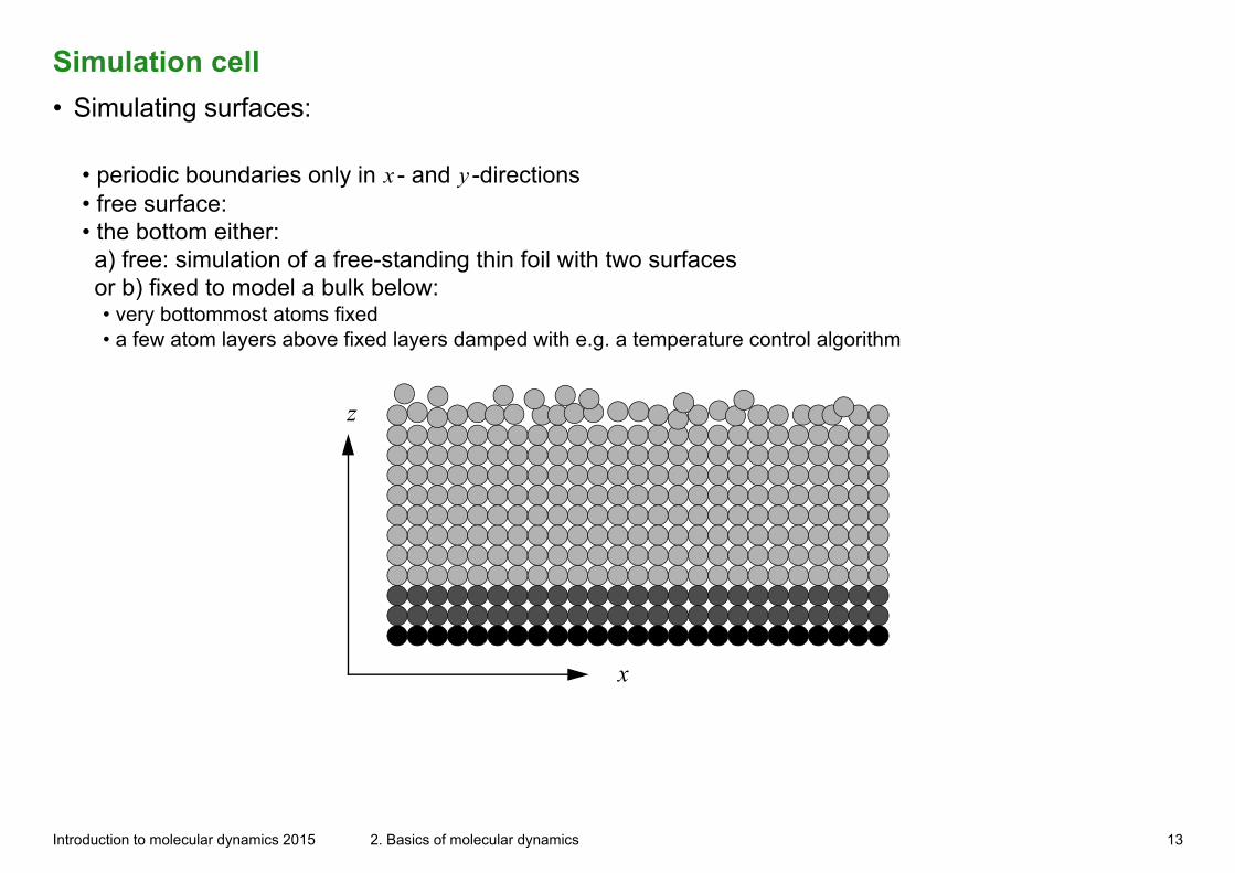
• Simulating surfaces:

• periodic boundaries only in x - and y -directions• free surface:• the bottom either: a) free: simulation of a free-standing thin foil with two surfaces or b) fixed to model a bulk below:• very bottommost atoms fixed• a few atom layers above fixed layers damped with e.g. a temperature control algorithm

x

z

Introduction to molecular dynamics 2015 2. Basics of molecular dynamics 13

Simulation cell

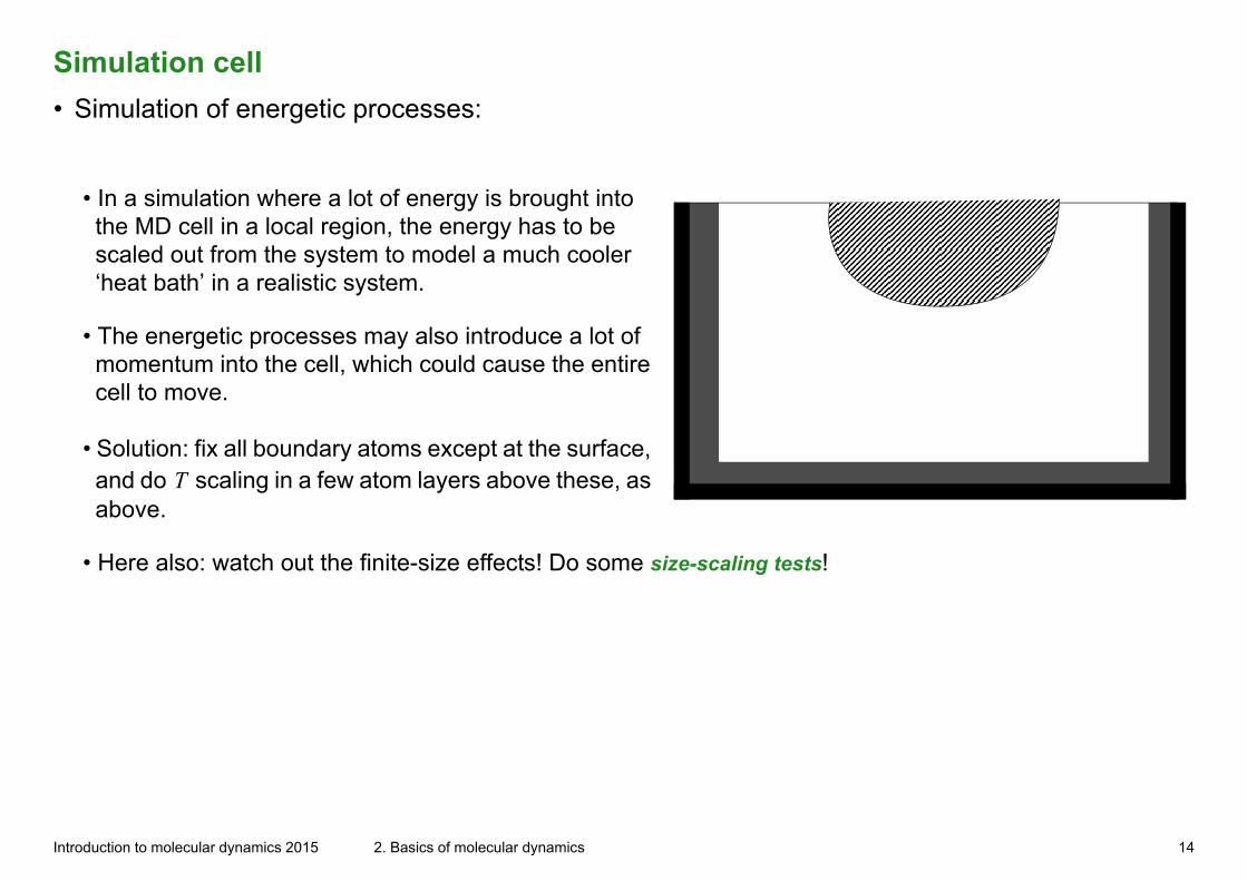
• Simulation of energetic processes:

• In a simulation where a lot of energy is brought into the MD cell in a local region, the energy has to be scaled out from the system to model a much cooler ‘heat bath’ in a realistic system.

• The energetic processes may also introduce a lot of momentum into the cell, which could cause the entire cell to move.

• Solution: fix all boundary atoms except at the surface, and do T scaling in a few atom layers above these, as above.

• Here also: watch out the finite-size effects! Do some size-scaling tests!

Introduction to molecular dynamics 2015 2. Basics of molecular dynamics 14

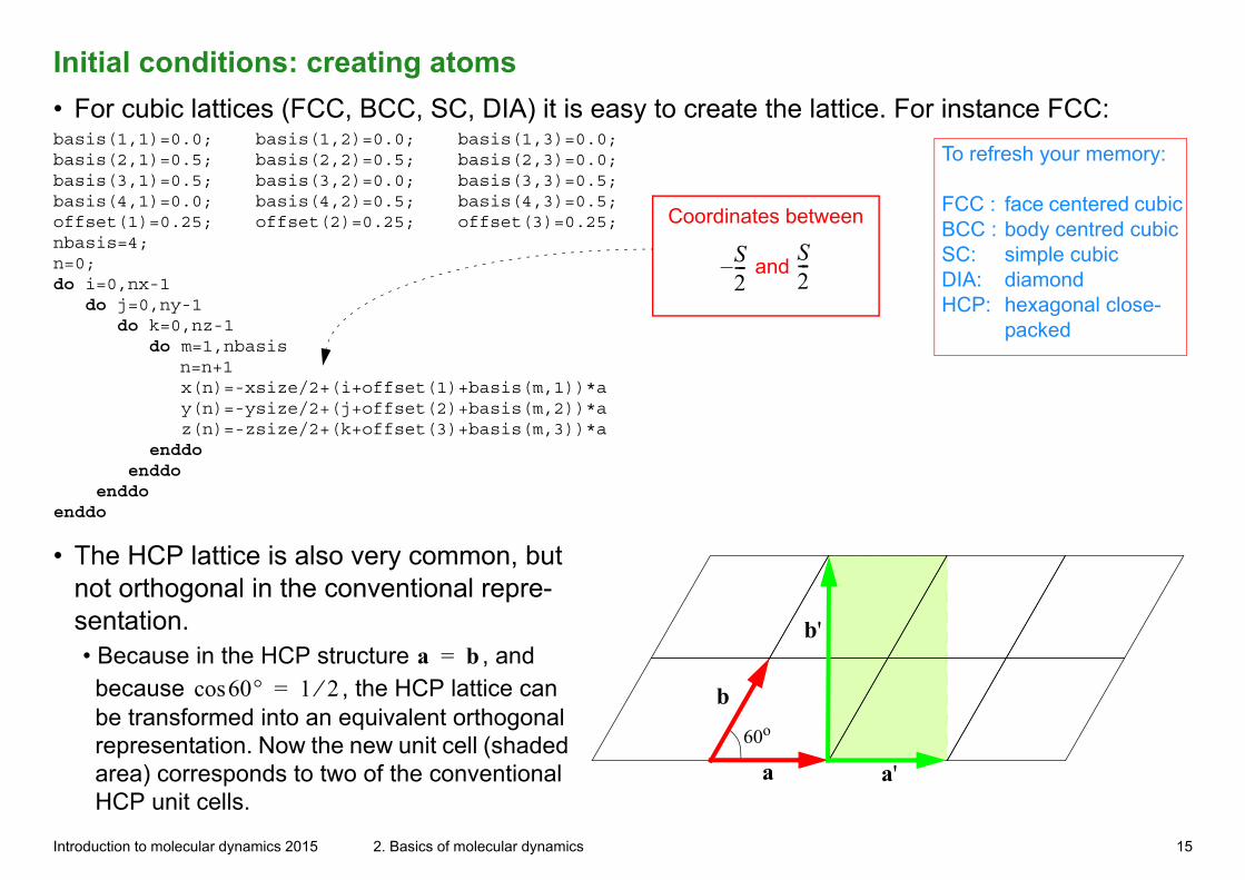
Initial conditions: creating atoms

• For cubic lattices (FCC, BCC, SC, DIA) it is easy to create the lattice. For instance FCC:basis(1,1)=0.0; basis(1,2)=0.0; basis(1,3)=0.0;

To refresh your memory:

FCC : face centered cubicBCC : body centred cubicSC: simple cubicDIA: diamondHCP: hexagonal close-

packed

basis(2,1)=0.5; basis(2,2)=0.5; basis(2,3)=0.0;basis(3,1)=0.5; basis(3,2)=0.0; basis(3,3)=0.5;basis(4,1)=0.0; basis(4,2)=0.5; basis(4,3)=0.5;offset(1)=0.25; offset(2)=0.25; offset(3)=0.25;nbasis=4;n=0;do i=0,nx-1 do j=0,ny-1 do k=0,nz-1 do m=1,nbasis

Coordinates between

and S2---– S

2---

n=n+1 x(n)=-xsize/2+(i+offset(1)+basis(m,1))*a y(n)=-ysize/2+(j+offset(2)+basis(m,2))*a z(n)=-zsize/2+(k+offset(3)+basis(m,3))*a enddo enddo enddoenddo

• The HCP lattice is also very common, but not orthogonal in the conventional repre-sentation.

60o

a'a

b'

b

• Because in the HCP structure a b= , and because 60°cos 1 2⁄= , the HCP lattice can be transformed into an equivalent orthogonal representation. Now the new unit cell (shaded area) corresponds to two of the conventional HCP unit cells.

Introduction to molecular dynamics 2015 2. Basics of molecular dynamics 15

Initial atom velocities

• How do we set the cell temperature to a desired value?

• We have to generate initial atom velocities which correspond to the Maxwell-Boltzmann distribution (which is surprisingly well valid even in crystals):

ρ viα( )

mi2πkBT----------------- 1 2/

12---miviα

2– kBT⁄ exp= ; α x y z, ,= .

• This is just a Gaussian function with suitable scaling, and exactly correct within an ideal gas model for atom velocities

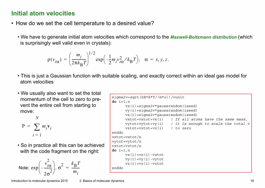
• We usually also want to set the total momentum of the cell to zero to pre-vent the entire cell from starting to move:

P mivi

i 1=

N

=

sigma2v=sqrt(kB*2*T/(m*u))/vunitdo i=1,n

vx(i)=sigma2v*gaussrandom(iseed) vy(i)=sigma2v*gaussrandom(iseed) vz(i)=sigma2v*gaussrandom(iseed) vxtot=vxtot+vx(i) ! If all atoms have the same mass,vytot=vytot+vy(i) ! it is enough to scale the total vvztot=vztot+vz(i) ! to zero

enddovxtot=vxtot/n vytot=vytot/n vztot=vztot/n do i=1,n

vx(i)=vx(i)-vxtotvy(i)=vy(i)-vytotvz(i)=vz(i)-vztot

enddo

• So in practice all this can be achieved with the code fragment on the right:

Note: viα

2

2σ2---------–

exp , σ2 kBT

mi----------=

Introduction to molecular dynamics 2015 2. Basics of molecular dynamics 16

Initial atom velocities

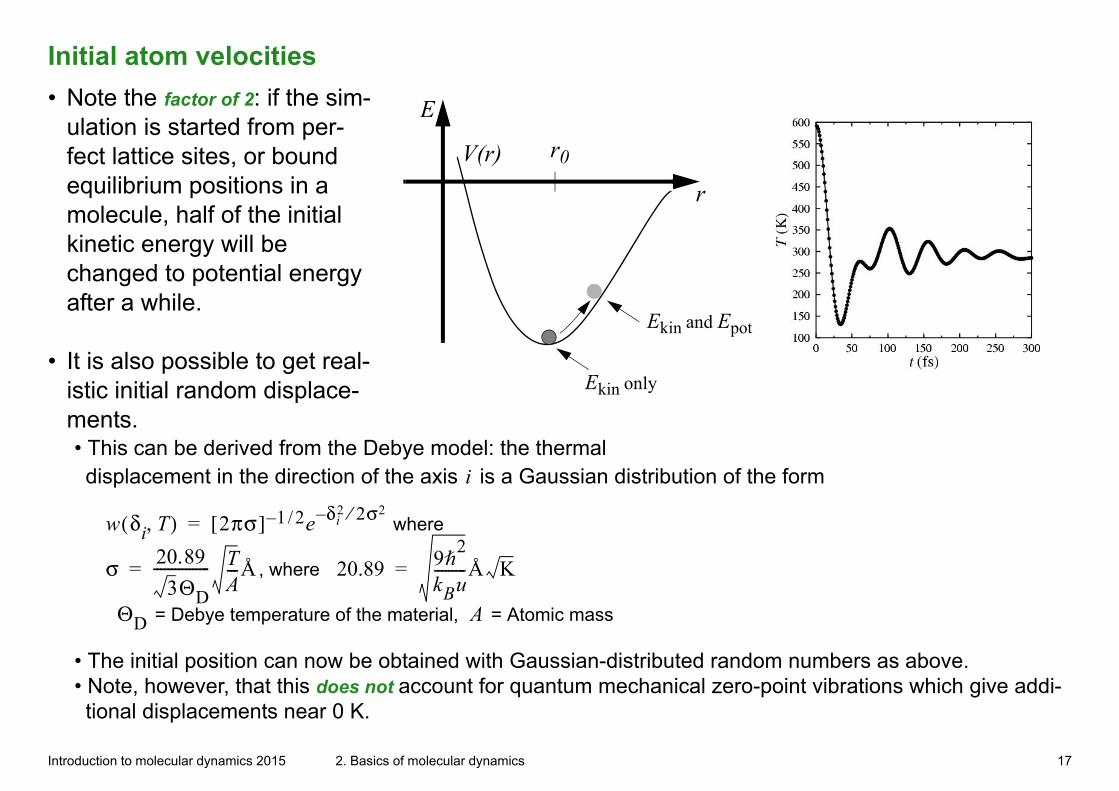
• Note the factor of 2: if the sim-ulation is started from per-fect lattice sites, or bound equilibrium positions in a molecule, half of the initial kinetic energy will be changed to potential energy after a while.

r

V(r) r0

E

Ekin only

Ekin and Epot

• It is also possible to get real-istic initial random displace-ments.• This can be derived from the Debye model: the thermal displacement in the direction of the axis i is a Gaussian distribution of the form

w δi T,( ) 2πσ[ ] 1 2/– e δi2 2σ2⁄–= where

σ 20.893ΘD

---------------- TA---Å= , where 20.89 9h

2

kBu---------Å K=

ΘD = Debye temperature of the material, A = Atomic mass

• The initial position can now be obtained with Gaussian-distributed random numbers as above.• Note, however, that this does not account for quantum mechanical zero-point vibrations which give addi-tional displacements near 0 K.

Introduction to molecular dynamics 2015 2. Basics of molecular dynamics 17

Generating random numbers

(This topic is dealt with in much more detail on the Monte Carlo simulation course)

• Almost all kinds of simuations in physics use random numbers somewhere. As we saw above, MD simulations need them at least for initial velocity generation.

• Computer-generated random numbers are of course not truly random, but if they have been generated with a good algorithm, they start to repeat each other only after a very large (e.g.

1020 ) number of iterations. If the number of random numbers used in the entire simulation is much less than the repeat number, the algorithm probably is good enough for the application.

• Random numbers can be generated for different distributions. This means that if we generate a large number of numbers and make statistics out of them, they will eventually approach some distribution.

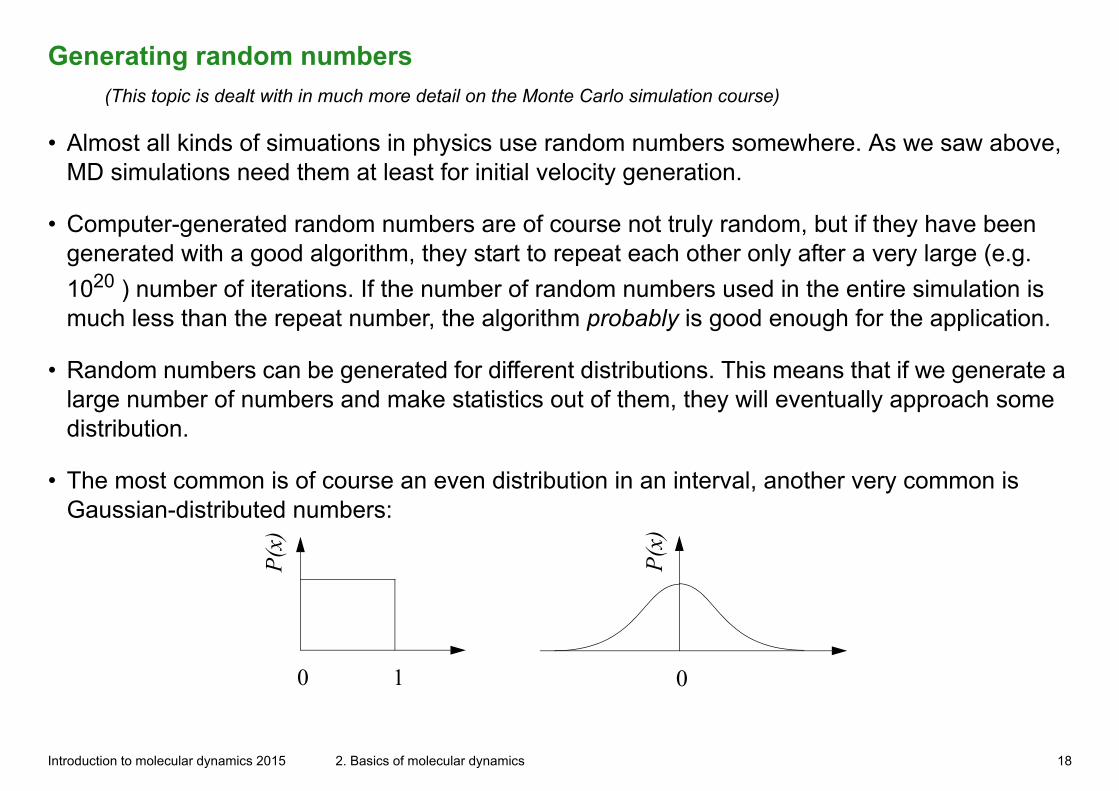
• The most common is of course an even distribution in an interval, another very common is Gaussian-distributed numbers:

0 1

P(x

)

P(x

)0

Introduction to molecular dynamics 2015 2. Basics of molecular dynamics 18

Generating random numbers

• Evenly distributed random numbers:

• Many programming languages offer their own random number generator (e.g. in ANSI-C rand()). A good rule-of-thumb regarding these is: Never use them for anything serious !

• The reason is simply that the language standard only specifies that the generator has to be there, not that it works sen-sibly. Since there are no guarantees it does (there are famous examples of the opposite) it should not be used

• Most random number generators are based on modulo-arithmetics and iteration. In the simplest possible form:

Ij 1+ aIj mod m( )=

• Park and Miller ‘minimal standard’-generator: a 16807= , m 231 1–=

• In the beginning the number I0 i.e. the seed number is chosen randomly.

• This can be done e.g. by using the current system time.

Introduction to molecular dynamics 2015 2. Basics of molecular dynamics 19

Generating random numbers

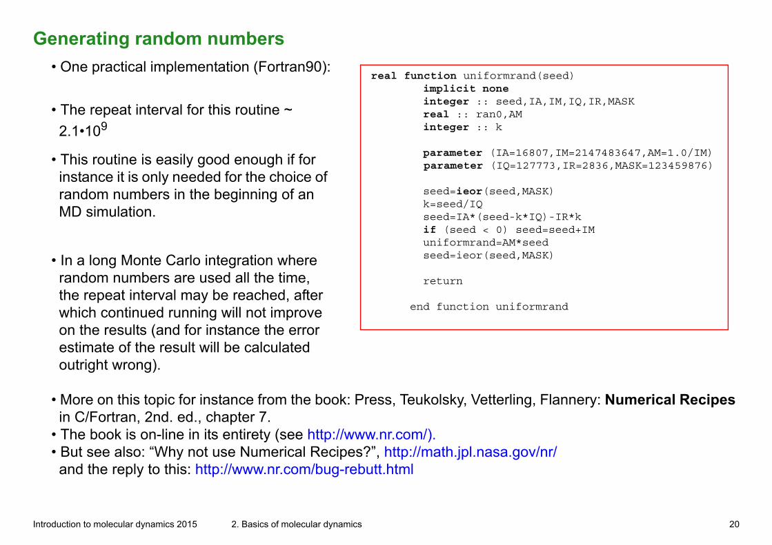
• One practical implementation (Fortran90):real function uniformrand(seed)

implicit none integer :: seed,IA,IM,IQ,IR,MASK real :: ran0,AM integer :: k parameter (IA=16807,IM=2147483647,AM=1.0/IM)

parameter (IQ=127773,IR=2836,MASK=123459876)

seed=ieor(seed,MASK) k=seed/IQ seed=IA*(seed-k*IQ)-IR*k if (seed < 0) seed=seed+IM uniformrand=AM*seed seed=ieor(seed,MASK)

return

end function uniformrand

• The repeat interval for this routine ~

2.1•109

• This routine is easily good enough if for instance it is only needed for the choice of random numbers in the beginning of an MD simulation.

• In a long Monte Carlo integration where random numbers are used all the time, the repeat interval may be reached, after which continued running will not improve on the results (and for instance the error estimate of the result will be calculated outright wrong).

• More on this topic for instance from the book: Press, Teukolsky, Vetterling, Flannery: Numerical Recipes in C/Fortran, 2nd. ed., chapter 7.

• The book is on-line in its entirety (see http://www.nr.com/).• But see also: “Why not use Numerical Recipes?”, http://math.jpl.nasa.gov/nr/ and the reply to this: http://www.nr.com/bug-rebutt.html

Introduction to molecular dynamics 2015 2. Basics of molecular dynamics 20

Generating random numbers

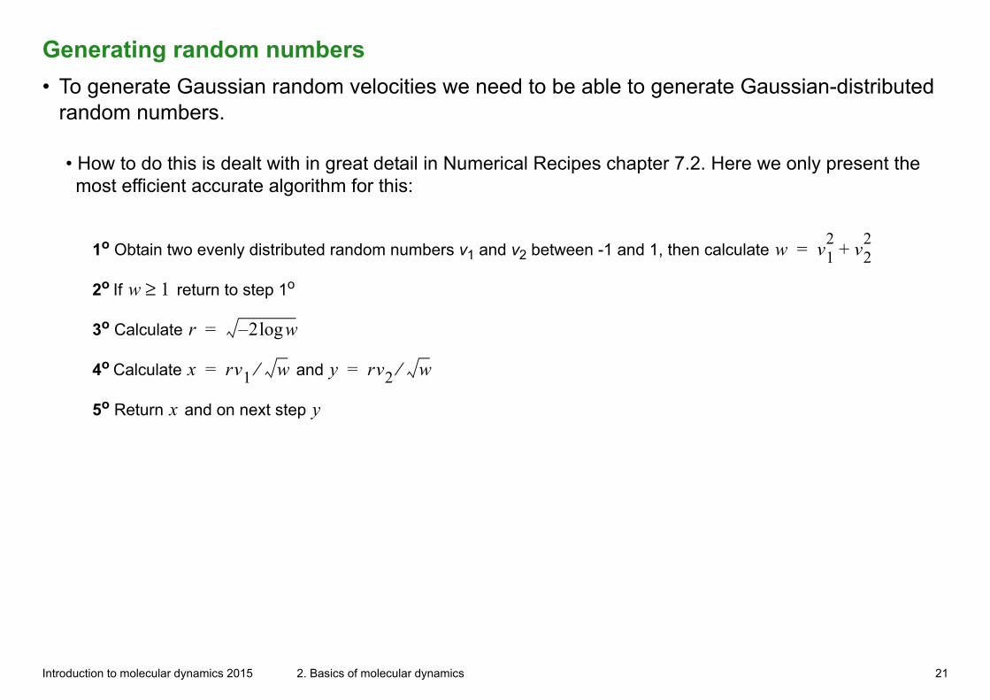
• To generate Gaussian random velocities we need to be able to generate Gaussian-distributed random numbers.

• How to do this is dealt with in great detail in Numerical Recipes chapter 7.2. Here we only present the most efficient accurate algorithm for this:

1o Obtain two evenly distributed random numbers v1 and v2 between -1 and 1, then calculate w v12

v22+=

2o If w 1≥ return to step 1o

3o Calculate r 2 wlog–=

4o Calculate x rv1 w⁄= and y rv2 w⁄=

5o Return x and on next step y

Introduction to molecular dynamics 2015 2. Basics of molecular dynamics 21

Choosing the MD time step

• Depends on the integration algorithm used, but not too strongly.

rV(r)

r0

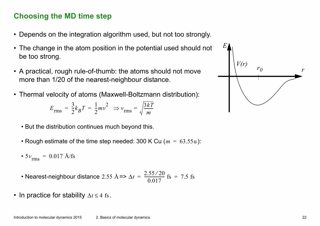
E• The change in the atom position in the potential used should not be too strong.

• A practical, rough rule-of-thumb: the atoms should not move more than 1/20 of the nearest-neighbour distance.

• Thermal velocity of atoms (Maxwell-Boltzmann distribution):

Erms32---kBT

12---mv

2 vrms3kTm

---------== =

• But the distribution continues much beyond this.

• Rough estimate of the time step needed: 300 K Cu (m 63.55u= ):

• 5vrms 0.017 Å/fs=

• Nearest-neighbour distance 2.55 Å=> Δt2.55 20⁄

0.017-------------------- fs 7.5 fs= =

• In practice for stability Δt 4 fs≤ .

Introduction to molecular dynamics 2015 2. Basics of molecular dynamics 22

Choosing the MD time step

• In pure MD there is no way to increase the time step above ~ 10 fs in atom systems at ordinary temperatures (77 K and up).

• If we would want to simulate a process which, say, takes 1 s, we would need at least 1014 time steps!

• This gives an easy way to estimate the order-of-magnitude of the upper limit for the time scale MD can handle in a given time:

• Most realistic classical MD interatomic potentials require at least of the order of 100 flops/atom/time step.

• Say our time step is 1 fs, and we want to simulate a 10000 atom system.

• Hence we need 106 flops/time step. To get to 1 ns = 109 fs we would need 1015 flops. Assuming 1 Gflop/

s processor, the simulation would thus require 1015/109 seconds = 106 s i.e. about 11 days. To get to 1 μs would require some 30 years on this processor.

• Hence we see that ordinary MD is restricted to ≤ 100 ns processes in most practical uses.

Introduction to molecular dynamics 2015 2. Basics of molecular dynamics 23

Choosing the MD step

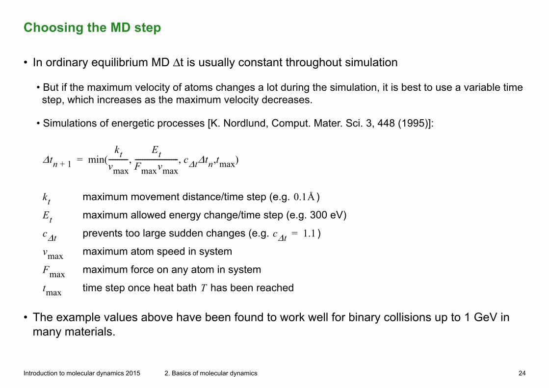
• In ordinary equilibrium MD Δt is usually constant throughout simulation

• But if the maximum velocity of atoms changes a lot during the simulation, it is best to use a variable time step, which increases as the maximum velocity decreases.

• Simulations of energetic processes [K. Nordlund, Comput. Mater. Sci. 3, 448 (1995)]:

Δtn 1+ minkt

vmax-----------

EtFmaxvmax------------------------- cΔtΔtn tmax,, ,( )=

kt maximum movement distance/time step (e.g. 0.1Å )

Et maximum allowed energy change/time step (e.g. 300 eV)

cΔt prevents too large sudden changes (e.g. cΔt 1.1= )

vmax maximum atom speed in system

Fmax maximum force on any atom in system

tmax time step once heat bath T has been reached

• The example values above have been found to work well for binary collisions up to 1 GeV in many materials.

Introduction to molecular dynamics 2015 2. Basics of molecular dynamics 24

Choosing the MD step

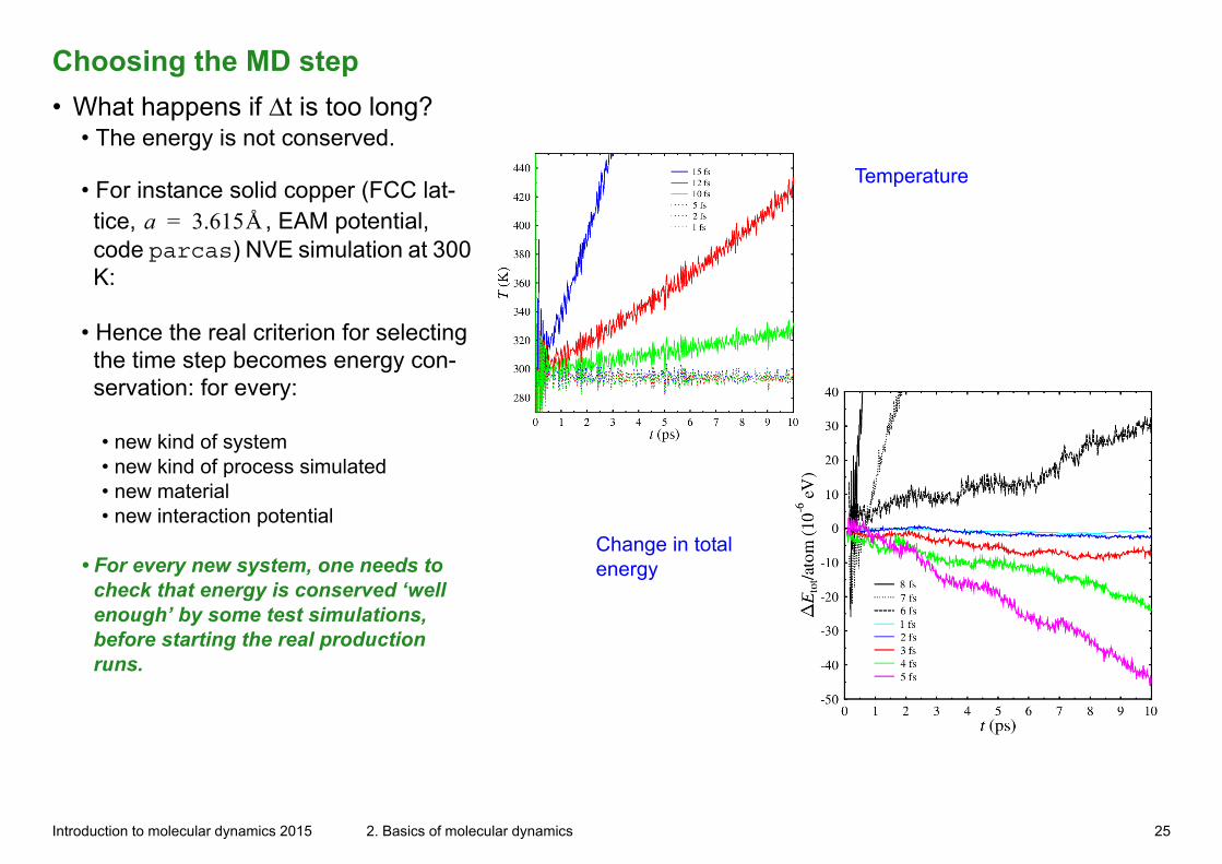
• What happens if Δt is too long?• The energy is not conserved.

Change in total energy

Temperature• For instance solid copper (FCC lat-tice, a 3.615Å= , EAM potential, code parcas) NVE simulation at 300 K:

• Hence the real criterion for selecting the time step becomes energy con-servation: for every:

• new kind of system• new kind of process simulated• new material• new interaction potential

• For every new system, one needs to check that energy is conserved ‘well enough’ by some test simulations, before starting the real production runs.

Introduction to molecular dynamics 2015 2. Basics of molecular dynamics 25

Acceleration methods

• Speeding up MD

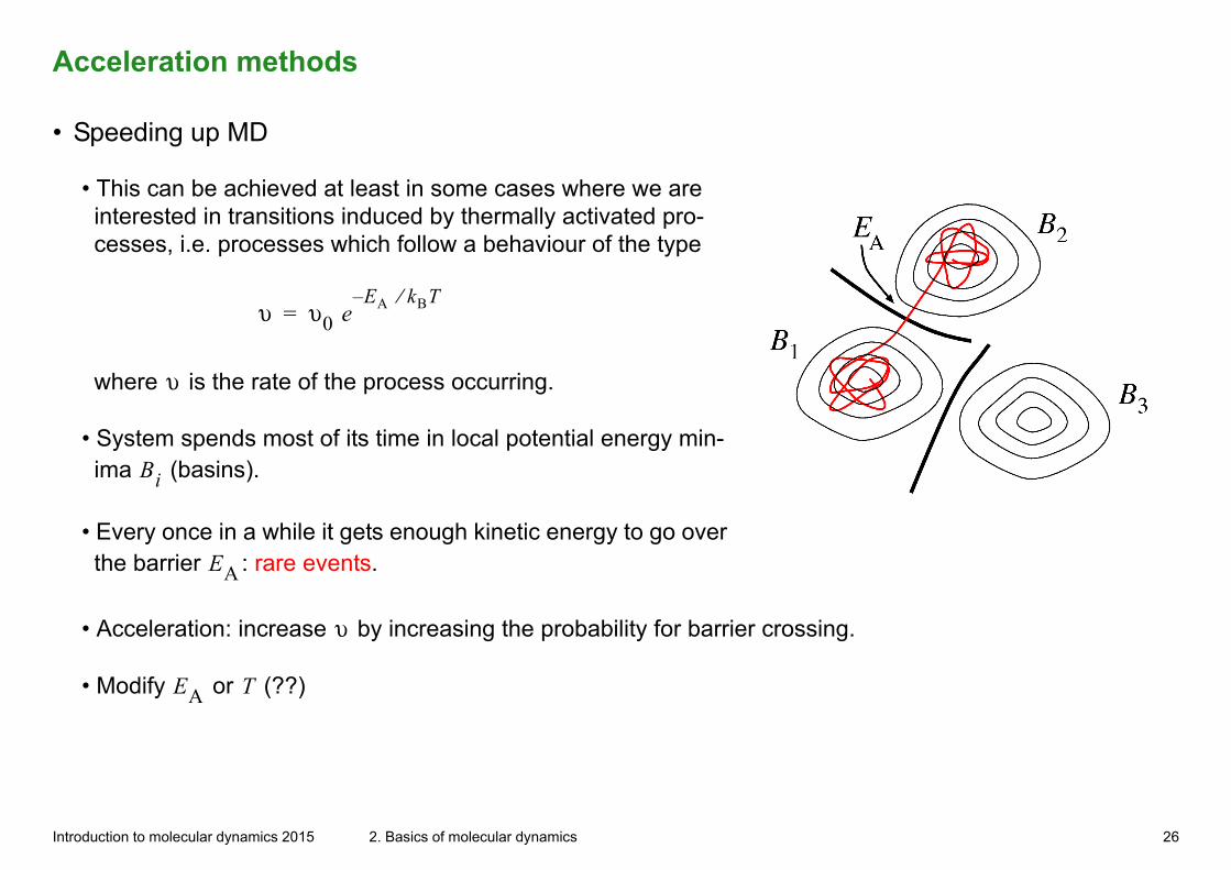
• This can be achieved at least in some cases where we are interested in transitions induced by thermally activated pro-cesses, i.e. processes which follow a behaviour of the type

υ υ0 eE– A kBT⁄

= where υ is the rate of the process occurring.

• System spends most of its time in local potential energy min-ima Bi (basins).

• Every once in a while it gets enough kinetic energy to go over the barrier EA : rare events.

• Acceleration: increase υ by increasing the probability for barrier crossing.

• Modify EA or T (??)

Introduction to molecular dynamics 2015 2. Basics of molecular dynamics 26

Acceleration methods

• Art Voter has presented so called Hyperdynamics [A. F. Voter, J. Chem. Phys. 106 (1997) 4665; Phys. Rev. Lett. 78 (1997) 3908]. It can in some cases speed up MD by a factor of the order of 100-1000, in others not at all.

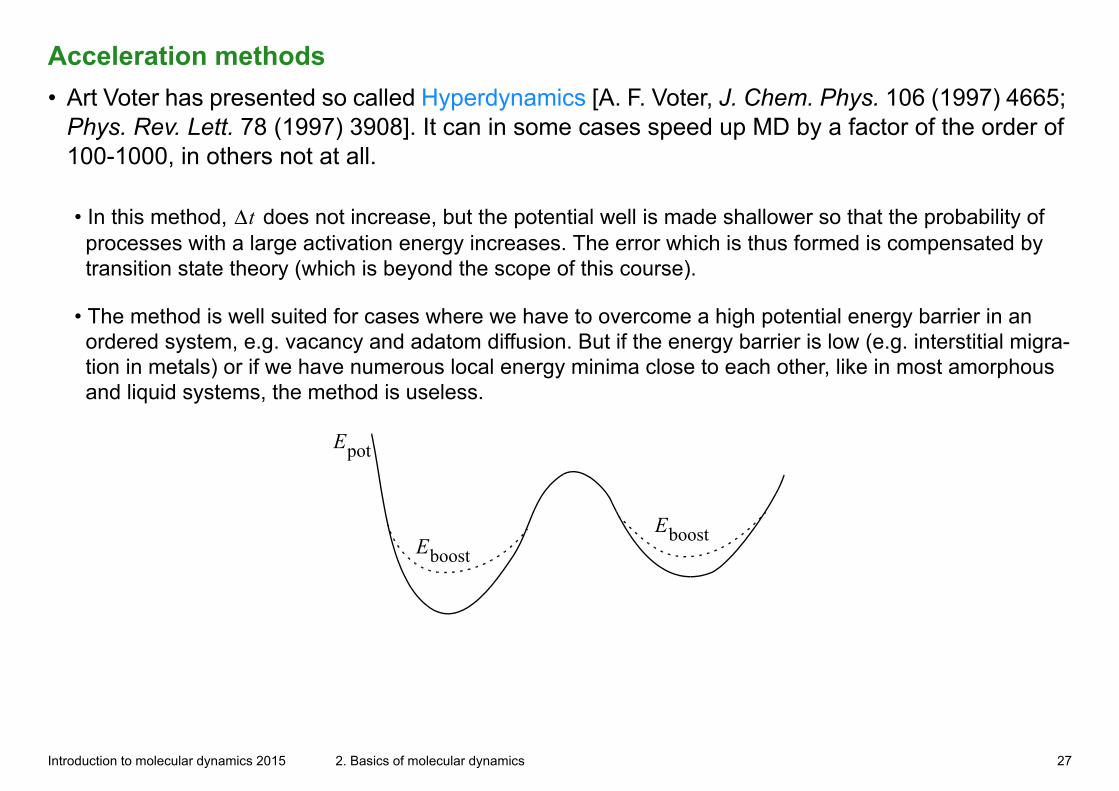
• In this method, Δt does not increase, but the potential well is made shallower so that the probability of processes with a large activation energy increases. The error which is thus formed is compensated by transition state theory (which is beyond the scope of this course).

• The method is well suited for cases where we have to overcome a high potential energy barrier in an ordered system, e.g. vacancy and adatom diffusion. But if the energy barrier is low (e.g. interstitial migra-tion in metals) or if we have numerous local energy minima close to each other, like in most amorphous and liquid systems, the method is useless.

Epot

EboostEboost

Introduction to molecular dynamics 2015 2. Basics of molecular dynamics 27

Acceleration methods

• Temperature accelerated dynamics (TAD)

• There is of course always is the Arrhenius extrapolation method: if we know that in our system there is only one single activated process occurring, and nothing else, we can simulate at higher T and then extrapolate the Arrhenius-like exponential EA– kBT⁄( )exp to lower T to know the rate or time scale at

lower T .

• A smart extension to Arrhenius extrapolation is Art Voter’s TAD method [e.g. Sorensen, Phys. Rev. B 62 (2000) 3658; a review of Voters methods is given in Ann. Rev. Mater. Res. 32 (2002) 321]

• To understand the idea in this, let us consider a system with exactly 2 activation energies (this is just a tutorial example, the method works in principle for any number of activation energies). We want to simu-late what the system does at 300 K, but the processes are so slow nothing happens there. So we will use a higher T , say 800 K.

Introduction to molecular dynamics 2015 2. Basics of molecular dynamics 28

Acceleration methods

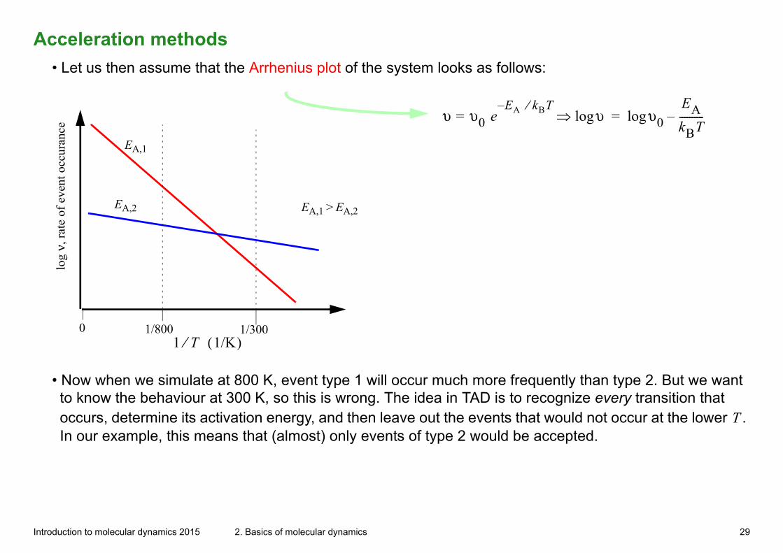
• Let us then assume that the Arrhenius plot of the system looks as follows: lo

g ν,

rate

of e

vent

occ

uran

ce

0 1/800 1/300

EA,1

EA,2 EA,1 > EA,2

1 T⁄ 1/K( )

υ υ0 eE– A kBT⁄

= υlog υ0logEAkBT----------–=

• Now when we simulate at 800 K, event type 1 will occur much more frequently than type 2. But we want to know the behaviour at 300 K, so this is wrong. The idea in TAD is to recognize every transition that occurs, determine its activation energy, and then leave out the events that would not occur at the lower T . In our example, this means that (almost) only events of type 2 would be accepted.

Introduction to molecular dynamics 2015 2. Basics of molecular dynamics 29

Acceleration methods

• In principle this is an excellent idea, but in practice one needs thousands of force evaluations to recognize a transition barrier. Hence the difference between the rates of occurrance needs to be very large for a sig-nificant gain to be achieved. But the gain can be huge (Example: simulating growth of Cu (001) surface at

77 K the speedup factor is 107 !)

• Like hyperdynamics, if there are lots of shallow minima TAD tends to get stuck and never really gets any-where.

• TAD is developing rapidly towards wider applicability, so it will be interesting to follow the progress

• As of 2015, Hyperdynamics, TAD and other similar-in-spirit acceleration methods have found many appli-cations in close-to-equilibrium simulations, typically such involving diffusion and an underlying crystal structure. In completely disordered, inhomogeneous systems (such as bio-systems) and far-from-equilib-rium simulations, no atom-based acceleration method has found wide applicability.

• In biosystems, coarse-graining, i.e. replacing single atoms with larger objects describing e.g. part of a molecule, can often give major speedups. These are beyond the scope of this coarse.

Introduction to molecular dynamics 2015 2. Basics of molecular dynamics 30