Baining Guo

PII: SOOlO-4485(96)00055-3

Computer-Atded Design, Vol 29, No. 4, pp. 269-277, 1997 (” 1997 Elsevier Science Ltd

PrInted in Great Britaln All rights reserved 001 O-4465/97/$17.00 + 0 00

Surface reconstruction: from points to splines Baining Guo

We describe a method for reconstructing an unknown surface X of arbitrary topology, possibly with boundaries, from a set of

scattered points. Our method generates a parametric surface in two steps: first we use 3D a-shapes to construct a simplified surface G that captures the topological structure of X, and then we build a curvature-continuous surface fi based on this structure. Starting from data points scanned on existing physical objects, the method can produce rather compact, accurate geometric models suitable for engineering design and analysis. c~ 1997 Elsevier Science Ltd. All rights reserved.

Keywords: geometric modelling, parametric surface fitting, least squares minimization

INTRODUCTION

The problem of surface reconstruction from scattered points can be stated as follows: given a set of pointslying on an unknown surface X, construct a surface A4 that approximates X. Reconstruction problems of this sort include surface reconstruction from range images and ‘surface from contours’. A range image typically forms a rectangular grid of distances from a view point to an object, whereas contour data come as a stack of contours describing an object. Contour data are usually anisotropic: the distances between the points within a contour are much smaller than the distances between the contours.

In this paper, we describe a method for reconstructing surfaces of arbitrary topology, possibly with boundaries, from scattered data points. Our method generates a parametric surface in two steps: first we u?e 3D a-shapes4 to construct a simplicial surface M that captures the topological structures of X, and then ye build a curvature-continuous surface M based on M. Spline surfaces provide compact, accurate representa- tions with reduced noise, which is usually present in ‘raw’ data points scanned with physical devices. The global parameterizations of the surfaces make them even more attractive for engineering design and analysis.

Currently, most parametric fitting methods are designed to capture the geometry of the unknown surfaces; the topological type is assumed a priori.

Department of Computer Science, York University, 4700 Keele Street, North York, Ontario M3J lP3, Canada Paper received: 15 October 1995. Revised: 15 Mq 1996

Common topological types include rectangles (e.g. see Reference 1, II C), spheres 2, and cylinders “. With the topology known, the main remaining challenge is to handle sparse and noise data-usually by solving a variational formulation of the reconstruction problem (e.g. see Reference 1, II B). The research reported here differs from this line of work in that we emphasize surfaces of arbitrary topology while restricting the data points to be dense and noise-bounded; the behaviours of our method on sparse data are discussed in Reference 7.

There are several promising reconstruction methods for smooth parametric surfaces of arbitrary topology. As examples, we cite the B-spline patch method by Milroy and co-workers” and the neural network approach of Gu and Yan6. Milroy’s method improves the smoothness among a collection of B-spline patches through an optimization process and produces an approximately tangent-plane continuous global surface. Gu and Yan train a neural network to learn the relationship between the parametric variables and the data points.

Implicit surface fitting methods have been very successful in reconstructing surfaces of arbitrary topologies, but these methods appear to have difficulties modelling surfaces with boundaries. An example of implicit surface fitting is the recent work by Lim and co-workers’2, who fit a collection of spherical primitives to scattered data points through a series of non-linear optimization processes. We consider it important to model surface boundaries, for they exist in common objects (e.g. the spout of a teapot).

Moving onto a more technical level,’ let us discuss some of the main features and design trade-offs of our system. An important feature of the system is that it uses a-shapes to infer the topology of the unknown surface. We choose a-shapes for two reasons. First, a reconstruction method based on a;shapes is applicable to a wide variety of situations. Because the entire family of a-shapes and the signatures of the family are efficiently precomputed, we can reconstruct surfaces of arbitrary topology without any data supplementary to the sampled points-we do require the user turning of o. The second reason for using o-shapes is that they handle anisotropically sampled data points well, which is crucial when the data points are taken from serial contours. A penalty for using o-shapes, though, is the increase in computational complexity: we need 0(n’) time for computing the a-shape family of 12 data points-surface reconstruction methods specializing in range and contour data usually have better performances.

Another feature of our system is that it outputs curvature-continuous parametric surfaces as final

269

Surface reconstruction: I3 Guo

results. To produce :I surfxe of known but arbitrary topology, WC make use of Grimm and Hughes’s elegant technique for building manifolds from B-sphne basis functions5. More specifically, we first create an abstract rn_anifold based on the reconstructed simphciai surface M and then embed the manifold into R3 according to the geometry implied in the data points. A nice feature of the Grimm- Hughes constructive manifolds is that they generalize B-splines to surfaces of arbitrary topology while maintaining the ‘built-in’ smoothness of B-splines. This built-in smoothness allows us to concentrate on data fitting to a degree not possible with patch-based B-splines generalizations (c.g. Reference I?).

Several common assumptions underlie the surface reconstruction problem. In general. it is not possible to recover features that are small compared to the satnpling density and noise bound; we assume that the sampled points are dense and noise-bounded enough to allow, the topology of the unknown surface be inferred. The data points must also be uniformly sampled. i.e. the sampling density does not differ greatly from one region to another (see Reference 7 for handling non-uniformly sampled data). We do not assume that the data points are isotropically sampled. Thus at a sampled point x,. the sampling density may

vary with different directions within the tangent plane at x,.

The rest of the paper is structured as follows. In the next section, we outline the construction of simplicial surfaces. paying particular attention to cl-shapes and how they benefit surface reconstructions-a companion paper provides details of our current implementation’. In the third section. we concentrate on fitting parametric surfaces to data points and provide sample results. Finally. we conclude with some suggestions for future work.

SIMPLICIAL SURFACE CONSTRUCTION

Our method first estimates the topological structure of the unknown surface by constructing a simplicial surface M (a polygon mesh with triangular faces). Usually, two approaches are possible for such constructions. One is to exploit the sample structure, such as partial connectivities in multiple view range data”’ and contour arrangements in contour data”. Another approach, the approach used in this paper. is to treat the data as scattered points.

Roughly speaking. the construction of the simplicial surface :2/1 is based on the 3D o-shapes of Edelsbrunner and Mucke”. Specifically. we precompute the entir_e family of o-shapes for the data points and generate M from a chosen (r-shape S,,. A suitable S,, can be interactively chosen because of the following properties of tr-shapes.

(a) The family of o-shapes for a set of size II can be computed in O(n’) timed.

(b) The level of detail in an o-shape is controlled by the parameter (I through an intuitive mechanism: as o decreases, the bulky features of the rr-shape are chiseled into refined ones as in the traditional trade of sculpting.

(c) .4n o-shape family has a set of .signrrturr.s, each of which characterizes a specific topological or geometric property as a function of 0.

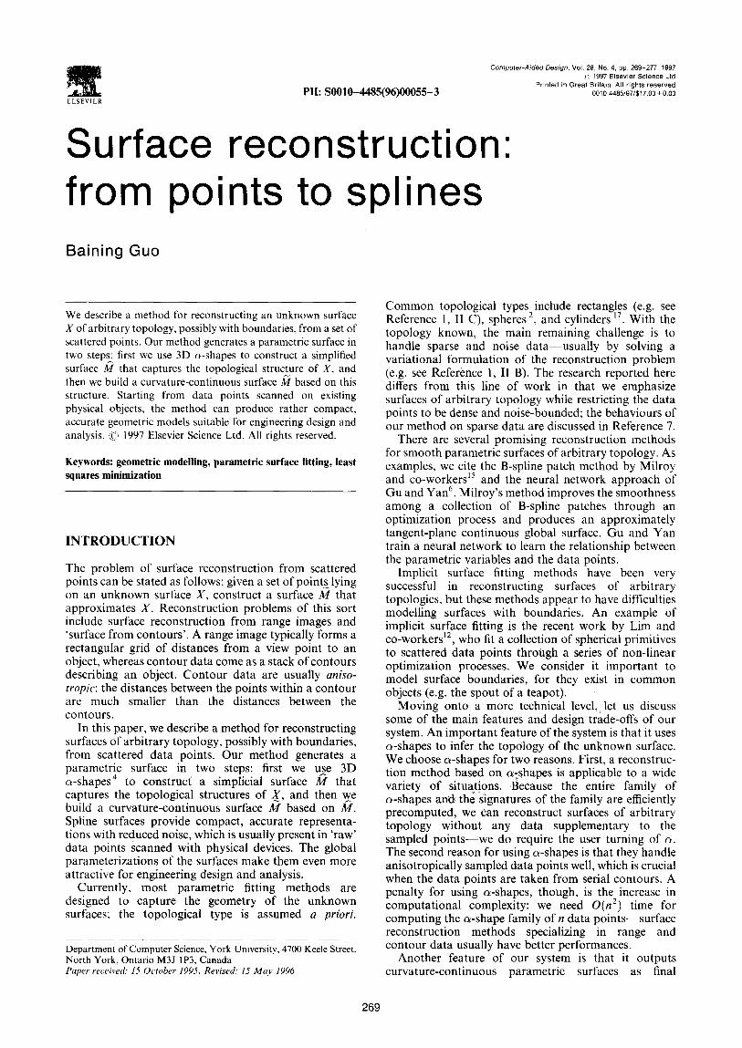
~‘&fr~, I shows an tr-shape family and some of its signatures. The o-shapes used for surface reconstruction should be the ones with the greatest levels of details as permitted by data. We use (t-shape signatures as guides to choose appropriate shapes’.

To facilitate further discussion, let us review some basic concepts about ck-shapes. We start by briefly introducing simplicial complexes’. For a set S of points

Figure I Examples from the II-shape family ofa point set sampled on ;I toI-us. \\lth (I decrcaamg from (a) to(e). In(f). \%e show several signaturea. red (br lue. green) curw is the vol~mw (number of connected components. number of voids) of the o-shape as B function of o

The

270

Surface reconstruction: B Guo

in R’, its convex hull conv(S) is the smallest convex set that contains S. Examples of convex hulls include k- simplex A r = conv(T) defined by a set T of k + 1 points in general position (06 k< 3) and the boundary simplices of AT, {A/r/T’ is a proper subset of T}. A collection Y of simplices form a simplicial complex if it satisfies the following conditions: (a) for a simplex A T of Sq the boundary simplices of AT are in Y, and (b) for two simplices of Sq their intersection is either empty or a simplex in Y. The underlying space IY( of a simplicial complex ,Y is the union of all of its simplices. As an example, the Delaunay triangulation g(S) of the point set S is a simplicial complex, whose underlying space is the convex hull conv(S)4. A simplicial complex Y can have a subcomplex Y’, ,which is a simplicial complex satisfying Y’ c Y.

To define the family of a-shapes S, (0 d a < m), we first specify a family of subcomplexes of g(S) and then derive the o-shapes as the underlying spaces of these subcomplexes. For a k-simplex A r(O< k< 3), let the smallest circumsphere of AT be the smallest sphere 0, that contains T. The subcomplexes we specify are a-complexes YQ(O Q ad oo), where .Y, consists of the following simplices: (a) every simplex A, E g(S), such that the smallest circumsphere Or of A, has radius rT < a and there is no point of S in the open ball bounded by Or, and (b) the boundary simplices of the simplices described in (a). Knowing the a-complexes, we define for each a(Obabco), an a-shape S, = ILYaI. Some examples from the a-shape family are S, = S and S, = conv(S).

The use of a-shapes allows our method to outperform existing surface reconstruction techniques in some areas. A critical aspect of surface reconstruction is local proximity, which determines the ‘neighbours’ of each point Xi in a data set S, i.e. the points of S that are ‘close’ to xi. Since an a-shape is a substructure within the Delaunay triangulation, the neighbours of a vertex in an a-shape are determined by both a ball of radius cr: and the Voronoi neighbourhood. While Q is a global parameter, the Voronoi neighbourhood of each point is adapted locally to variations in sampling, and so is the criterion for neighbours in an a-shape. The local adaptation to the distribution of data points is an important advantage that allows us to better handle anisotropically sampled data points, such as those taken from contour data.

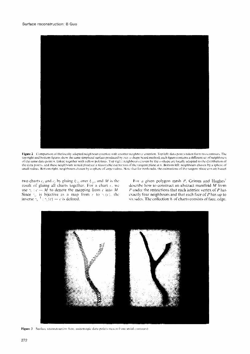
We demonstrate the advantage of the locally adapted neighbour criterion by comparing our method with a successful method whose criterion for neighbours is not locally adapted. In References 9 and 10, Hoppe and co-workers construct oriented tangent planes, from which they define a signed distance function whose zero contour captures the topology of the unknown surface. In both tangent plane estimation and tangent plane orientation, Hoppe determines the neighbours of a point using a ball whose radius is a constant called the sampling parameter (we use latest version of Hoppe’s method’, which differs slightly from Reference 10; the difference does not affect our analysis). Assuming this parameter exists, the user can find it by analysing the data sampling process, or by carefully studying the data. In any case, through the use of a neighbour criterion based solely on the sampling parameter, Hoppe implicitly assumes that the data points are isotropically sampled. For this reason, his method handles only a special type of contour data, namely, those in which the

distances between the contours are comparable with the distances between points within each contour. In Figure 2, we show that as the distances between the contours become larger, Hoppe’s method starts to produce biased tangent plane estimates while the c-shape based method remains effective. Figure 3 provides an experimental example to support our analysis. The data set in this example is not sparse, but it is anisotropic enough to fail a local proximity criterion based on a sample parameter. In fact, the data points in Figure 2 are taken from two consecutive contours in this data set.

The use of a-shapes, however, does present a challenge. An a-shape is the underlying space of a simplicial complex in its most general form. An apparently simple a-shape can have a complicated internal structure of ‘dangling’ faces, voids, and nearly flat tetrahedra. On the other hand, the surface we reconstruct should be a 2D manifold. A challenge facing our simplicial surface co_nstruction is therefore the generation of the surface M from an a-shape. We have developed an algorithm for generating simplicial surfaces, and the algorithm has been found to be effective throughout its application to a variety of data7. The main idea of the algorithm is simple: we construct a simplicial surface by enumerating the faces that are visible from the ‘outside’ of an object. The implementation of this simple idea turned out to be rather involved, as is reported in Reference 7.

After generating an initial simplicial surface 6, we simplify it with re-tiling methods1,‘9. This post- processing is necessary since we assume the-data points are dense, which implies that the initial M has a large number of vertices. The goal of the simplification is to reduce the_ number of the vertices (and geometric details) in A4 while maintaining its topological structure. In our current system, we use Hoppe’s mesh optimization technique”.

PARAMETRIC SURFACE FITTING

After inferring the topology of the unknown surface, we fit a parametric spline surface to the sampled points. The fitting algorithm embeds into R3 an abstract manifold M, which is built with topological informa- tion extracted from the simplicial surface M. The embedding is a C2 Smooth mapping derived from B-splines basis functions.

Constructive manifolds

In a constructive view5, a C2 differentiable manifold M consists of: (a) a finite collection % = {c~}~ of charts, which ,are singly connected open sets in 2D, and (b) transition functions defined on the overlaps of the charts, I+G~, : U;j + Uj;, where an overlap vj,i (may be empty) is a subset of c,. Each transition function +ij is C* bijective with $ij’ = $jl and ~,i(p) w for p E ci = Ui;. For overlaps that involve three charts ci, cj, and ck, the cocycle condition +ij 0 ~jik = ~~~ must hold. The manifold M is the quotient of the disjoint union of all charts with respect to the equivalence relation defined as follows: any two points pi E ci and pi E cj are equivalent if +;,(pi) = pi. Intuitively, a transition function $ii joins

271


Figure 2 top righ of the ss

the data

small x1,

two ch result use 1, Since inverse

Figure 3

m-1 of : C’

: -3,

‘omp;r~-iwn of the loc;~ll~ adapted ncighbour crltwon wth anothc~- netghhour alterion. Top left: data point5 taken from II~CO co1 ItoLl xh. The d bottom figures show the \amc simpliclal surface produced by out cl-shape based method; each figure contains a different set of neig hhours data point Y. linked together with yellow polylincs. Top right: neighhour\ chosen by the cr-shape are locally_ adapted to the dist ribs Ition of

ints. and these neighbours would produce a reasonable estmx~tion of the rangent plane at v. Bottom left: nelghbours chosen by a sp here 01‘ i. Boitom right. nclghhoury chosen by a sphere 01’ large radius. Note that ths- both radii. the estimations of the tangent plane at t : 3i-e biased

ts (‘, and L’, by gluing L;,, over ( ,i. and ‘$1 is the gluing all charts together. For a chart (‘. WC -- M to denote the mapping from c into M. is bijective as a map from c to ?, (c). the ’ : -.( ((,I -- c is defined.

f-or a given polygon mesh P. Grimm and HLI @es’ describe how to construct an abstract manifold M from P under the restrictions that each interior vertex of P has exactly four neighbours and that each face of P 1 has up to $is sides. The collection % of charts consists of fa ice. edge.

272


Vertex Chart Face Overlaps

Vertex Chart Edge Overlaps

Edge Chart Face Overlaps

Edge Chart Vertex Overlaps

Face Chart Vertex Overlaps

Face Chart Edge Overlaps

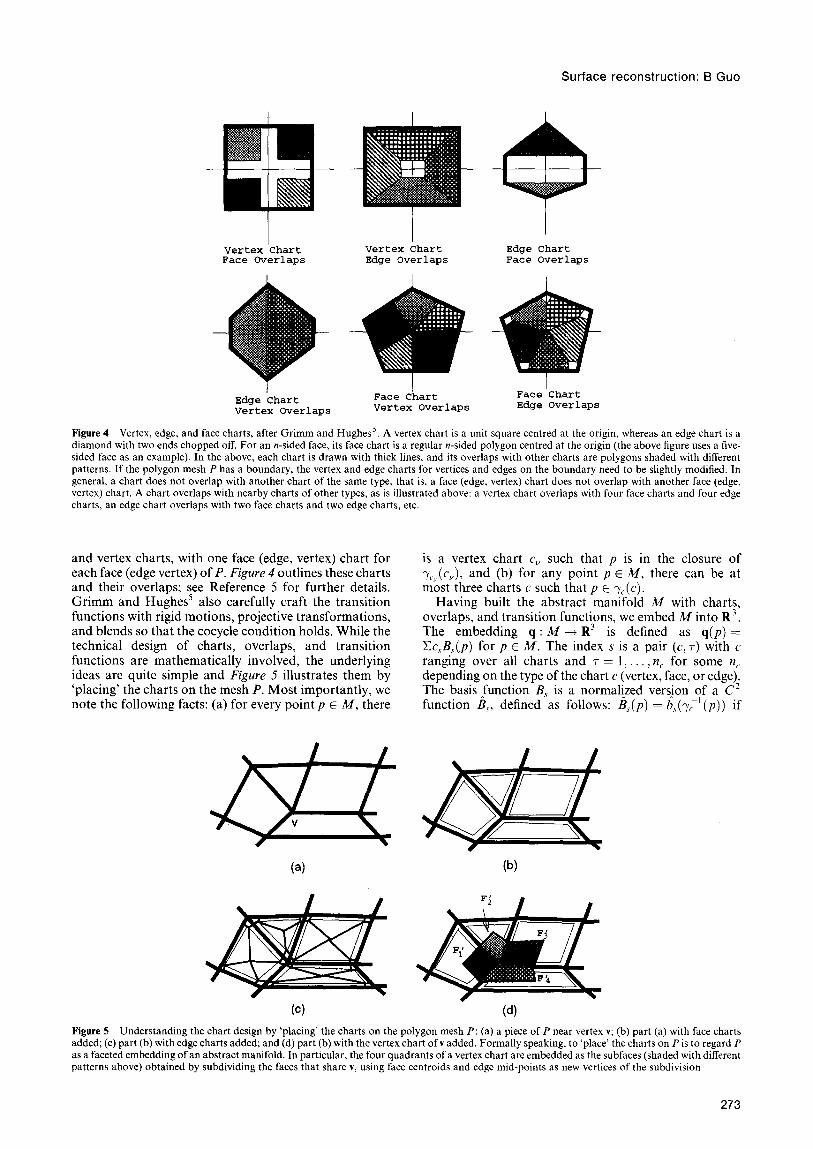
Figure 4 Vertex, edge, and face charts, after Grimm and Hughes 5. A vertex chart is a unit square centred at the origin, whereas an edge chart is a diamond with two ends chopped off. For an n-sided face, its face chart is a regular n-sided polygon centred at the origin (the above figure uses a five- sided face as an example). In the above, each chart is drawn with thick lines, and its overlaps with other charts are polygons shaded with different patterns. If the polygon mesh P has a boundary, the vertex and edge charts for vertices and edges on the boundary need to be slightly modified. In general, a chart does not overlap with another chart of the same type, that is, a face (edge, vertex) chart does not overlap with another face (edge, vertex) chart. A chart overlaps with nearby charts of other types, as is illustrated above: a vertex chart overlaps with four face charts and four edge charts, an edge chart overlaps with two face charts and two edge charts, etc.

and vertex charts, with one face (edge, vertex) chart for each face (edge vertex) of P. Figure 4 outlines these charts and their overlaps; see Reference 5 for further details. Grimm and Hughes’ also carefully craft the transition functions with rigid motions, projective transformations, and blends so that the cocycle condition holds. While the technical design of charts, overlaps, and transition functions are mathematically involved, the underlying ideas are quite simple and Figure 5 illustrates them by ‘placing’ the charts on the mesh P. Most importantly, we note the following facts: (a) for every point p E M, there

is a vertex chart c, such that p is in the closure of y,“(c,,), and (b) for any point p E M, there can be at most three charts c such that p E yc (c)

Having built the abstract manifold M with charts, overlaps, and transition functions, we embed A4 into R 3. The embedding q : A4 + R3 is defined as q(p) =

CC,~B,(~) for p E M. The index s is a pair (c, r) with c ranging over all charts and 7 = I,. . ! n, for some n, depending on the type of the chart c (vertex, face, or edge). The basis function B, is a normal_ed versjon of a C’ function B,, defined as follows: B,(p) = h,s(ycY1(p)) if

(4 (b)

(4 Figure 5 Understanding the chart design by ‘placing’ the charts on the polygon mesh P: (a) a piece of P near vertex v; (b) part (a) with face charts added; (c) part (b) with edge charts added; and (d) part (b) with the vertex chart of v added. Formally speaking, to ‘place’ the charts on P is to regard P as a faceted embedding of an abstract manifold. In particular, the four quadrants of a vertex chart are embedded as the subfaces (shaded with different patterns above) obtained by subdividing the faces that share v, using face centroids and edge mid-points as new vertices of the subdivision

273


p E ?,(c,), and B,(p) = 0 otherwise. Here h, is a C” function over the chart (‘. built from tensor-product B-splines and projective transformations’. The basis functions {II,},. with B, = B,/CB,, thus form a collection of non-negative C’ functions that sum to 1 everywhere on M. Note that each basis function is hal: the support of B, = B,, Tj lies strictly inside the chart c.

Parameterizing data points

The goal of parametric surface fitting is to determine the cmtrol poht.~ {I,,}, so that the embedding of the manifold M best approximates the data points. If the data points {x,. x,,} are known to correspond to points {I),. ./I,,} on the manifold M. then we can determine the control points by solving the following least squares problem

But we do not know {pi. .p,,}. To find the points {11~}~ on the manifold M, we make

use of the following two facts: (a) the polygon mesh P is a rough approximation to the unknown surface. and (b) the charts are designed to ‘cover’ the mesh P in the sense illustrated in Fig-urc> 5. The first fact allows us to map the data points onto the face of P by orthogonally projecting each point to the dosrst face. the face with the minimum distance to the point. It is possible to identify the closest face of a data point by projecting the point to all faces of P, but this would be too costly since we have to repeat this process for all data points. A popular way to speed up the process is to organize the faces of P into a spatial partitioning structure and restrict the projections of ;I

data point to the faces in the nearby partitions. With this strategy incorporated, the total cost of projecting all data points is practically O(U).

The second fact provides a natural way to map the projected data points onto the charts. and hence the manifold M. From the way the charts are designed. we can regard the polygon mesh P as an embedding of the abstract manifold M. When viewed this way. the technique of Grimm and Hughes’ essentially extracts an abstract manifold from a faceted embedding of a manifold and re-embeds it smoothly. Of course. two embeddings of the same manifold gives clues for relating points on one embedding to points on another. To obtain the actual correspondence. let us focus on vertex charts {c,,}!, since {q,(, (L.,,/}, cover P. Consider the vertex chart (’ of a vertex v shared by four faces F,( i = I. 3.3.4). After subdividing these faces using their centroids and edge mid-points. wc obtain, among other things, four quadrilaterals F,‘(i = 1.2.3.4) sharing v. See Figure 5. For each quadrant yi(i = 1.2.3.4) of the chart c, we use rigid motions and projective transformations to bijectively map q, onto F,‘. For the sake of convenience, we denote collectively the mappings of all four quadrants as L. This mapping. which is continuous but not smooth. has an inverse ;,,-I : L(C) - C’.

Now we can combineX orthogonal projections and 1, to find the manifold point pi, for each data point x~. If xi, is projected onto one of F,‘( i = I .2.3.4) as X~ . then -

\vc‘ let pi, = 3, (d(2)). To evaluate B,(/J,>). wt‘ use ?,(x~) and transition functions. Specifically. for anv indexyc’. B,,(pk) = B,,.,,rt,(~~i,) = 0 when the charts (:’ and (’ do not overlap. When c’ and c do overlap. as is the case when c’= c. we set B,!(/J~) = Bi,,r,,(/~,,) = kJ(t.S,, i-r, ‘(x )) k where ~;l,, , is the transition function

from the overlaps C!,, J to C’( I(. Having {B, (1~~ )}, in hand. w’e compute B, (/Jo ) using

B,(p/\ I = 4 ( IJi, )

c - j,,(iJi, J \’

Least squares minimization

With B,(/J,, ) evaluated. wc are ready to solve the least squares problem with the objective X,” , /lx, ~~ !l,c, B, (p, ) 112. To simplify the notation. we concatenate the data points and control points into the vectors

k [xi x,:1’ and c = ic; c,;,]’

and we rewrite X,‘i, l/x, -~ C,~,B,,(p,)11~ as /Ix ~ AcI/’

cvherc A is an 311 x 3~1 matrix consisting of 3 x 3 blocks. with each block being a scalar multiplication of an identity matrix. The scalar factors for the ith row of blocks are {B,([J~)}, with .s ranging over all possible choices. Since /J! F -*( (c) for at most three charts and inside each chart (’ only a fixed number of basis functions are non-zero at ?,- I(p). all but a constant number of blocks in A are zero. In other words, the matrix A is O(n) sparse.

To solve the sparse least squares ,problem, we USC the conjugate gradient methodlh. While this is an iterative method that can take as many as 171 iterations to find the exact solution, far fewer iterations suffice for obtaining :III accurate approximation. At each iteration, the two main operations are the multiplications ATv” and Av”’ for some ,I-vector v” and I??-vector v”‘. Because of the sparsity *of A. each multiplication requires only linear time and storage. Note that the sparsity consideration is relatively important here because the number of data points are usually quite large.

Implementation issues

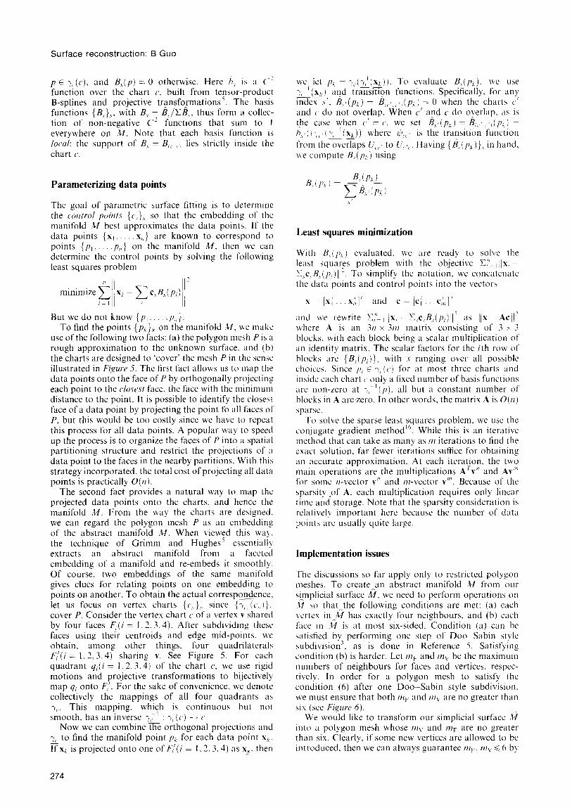
The discussions so far apply only to restricted polygon meshes. To create-an abstract manifold h/ from our simplicial surface A4. we need to perform operations on .2? so that-the following conditions are met: (a) each vertex in_~V has exactly four neighbours. and (b) each face in J4 is at most six-sided. Condition (a) can bc satistied by performing one step of Doo Sabin style subdivision”, as is done in Reference 5. Satisfying condition (b) is harder. Let 171~. and /l?v) be the maximum numbers of neighbours for faces and vertices, respec- tively. In order for a polygon mesh to satisfy the condition (6) after one DoomSabin style subdtvtsion. we must ensure that both /PIN and I+ are no greater than six (see Fi,prc 6).

We would like to transform our simplicial surface ,G into I polygon mesh whose JII~ and I+ are no greater than six. Clearly, if some new vertices are allowed to be introduced. then we can always guarantee /?I~. /?rv d 6 by

274

Surface reconstruction: 6 Guo

(a) 04

(4 (4 Figure 6 (a) A vertex v of too high valence. (b) A Clark-Catmull style subdivision using face centroids and edge mid-points. (c) Taking the dual of(b), we obtain a Doo-Sabin style subdivision of (a), shown in thick lines. Notice the face with too many sides. (d) A face F with too many sides causes another such face (shown in thick line) after a Doo-Sabin style subdivision

performing local operations near vertices with valences that are too high. Adding new vertices, however, does increase the complexity of M as well as the manifold construction. As a remedy, we have derived a successful heuristic algorithm for eliminating vertices of high valence without adding new vertices of any kind. Of course, this is a heuristic algorithm and, like any other heuristic algorithm, can be made to fail on pathological examples.

The basic idea behind our algorithm is simple: we keep deleting the edges emanating from a vertex v whose valence is too high until it is no greater than six. To improve the shapes of the faces at the same time, we sort the angles formed by two successive edges and delete the edges bounding the smallest angle first. Since the algorithm is to make both mv and mF no greater than six, an edge shared by two faces F and F’ will not be deleted if this merges F and F’ into a single face with more than six sides.

In gen_eral, applying_this algorithm to our simplicial surface A4 transforms M into a mesh whose faces are no longer planar. Fortunately, the following Doo-Sabin style subdivision will convert a polygon mesh P with planar or non-planar faces to a mesh P’ with planar faces: (a) subdivide the faces of P into subfaces using face centroids and edge mid-points as in Figure 6b, and (b) compute a dual point pi for every subface F/ and use exactly these points as the vertices of the mesh P’. Note that every vertex Vi of P is surrounded by a set of the new vertices added in step (a) and we can compute the vertices of P’ by finding the dual points of the subfaces around each vertex vi of P. Enumerating in clockwise order the subfaces around vi as {Fi, . . . , Fii}, we project to a common plane the centroid v; of every subface FL. Specifically, if ni < 4, then the dual point pk of a subface FL is just its centroid vb; for n, > 4, we set

where P = 1 /ni Cv; and the indices are all modulo ni. The constant X, is n,(l + cos(27r/ni)) if n, is even and 2nj cos(~/q) otherwise.

Examples and discussions

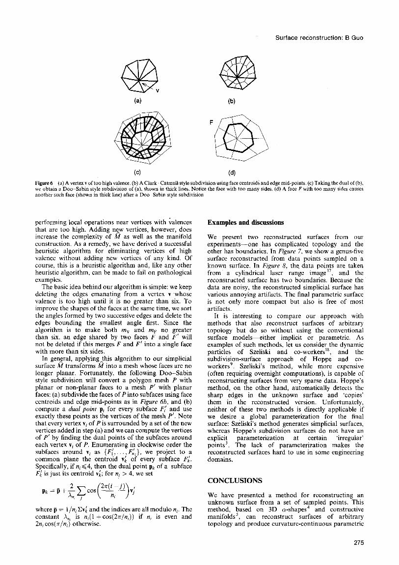
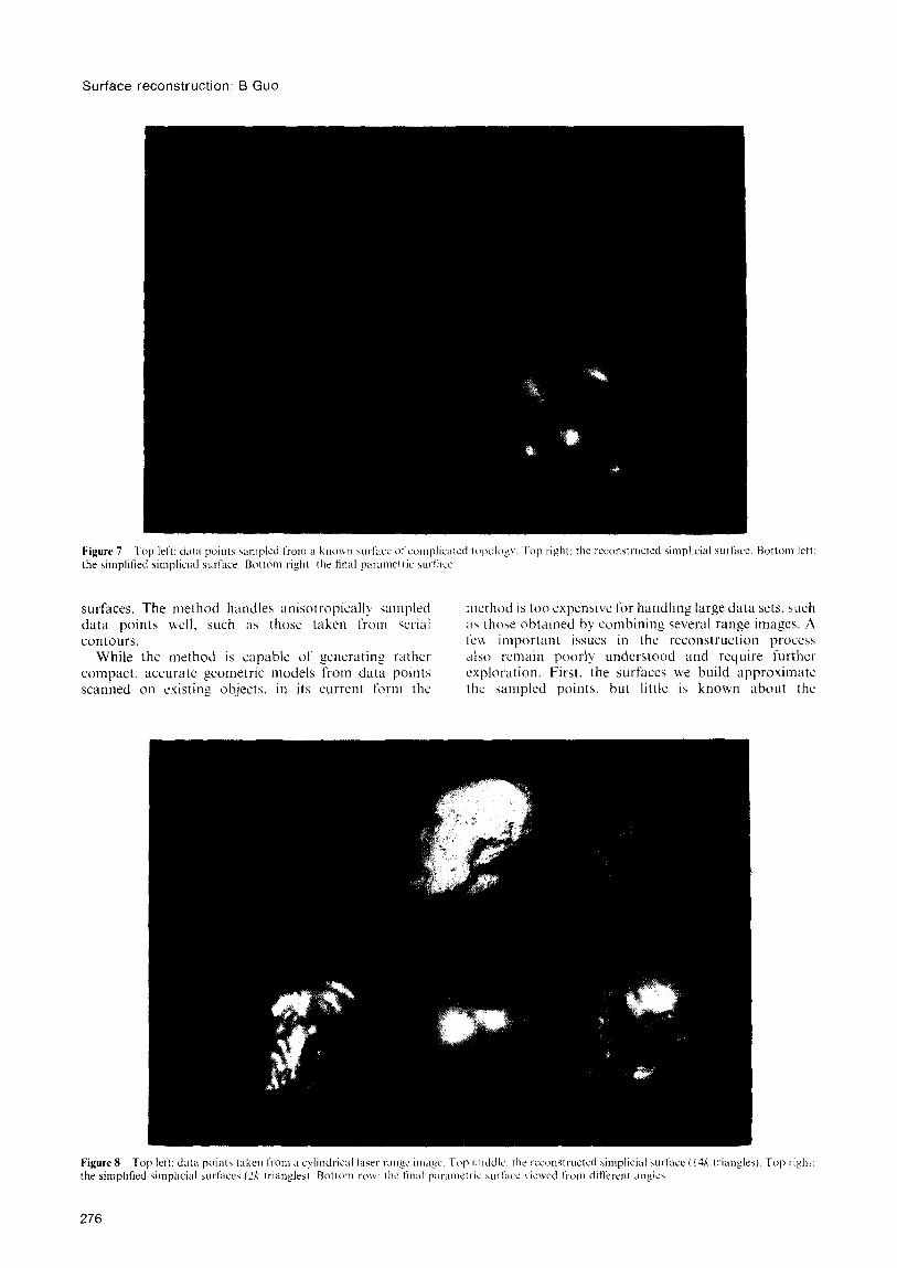
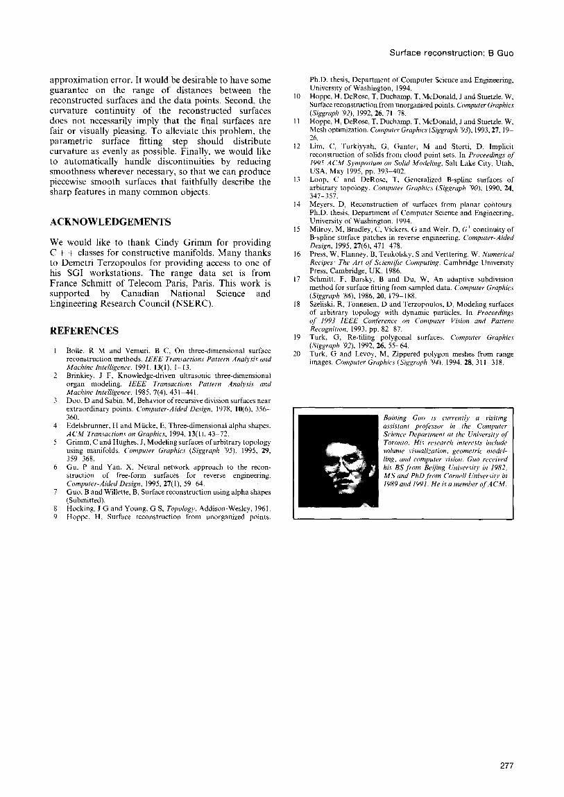
We present two reconstructed surfaces from our experiments-one has complicated topology and the other has boundaries. In Figure 7, we show a genus-five surface reconstructed from data points sampled on a known surface. In Figure 8, the. data points are taken from a cylindrical laser range image17, and the reconstructed surface has two boundaries. Because the’ data are noisy, the reconstructed simplicial surface has various annoying artifacts. The final parametric surface is not only more compact but also is free of most artifacts.

It is interesting to compare our approach with methods that also reconstruct surfaces of arbitrary topology but do so without using the conventional surface models-either implicit or parametric. As examples of such methods, let us consider the dynamic particles of Szeliski and co-workers”, and the subdivision-surface approach of Hoppe and co- workers’. Szeliski’s method, while more expensive (often requiring overnight computations), is capable of reconstructing surfaces from very sparse data. Hoppe’s method, on the other hand, automatically detects the sharp edges in the unknown surface and ‘copies’ them in the reconstructed version. Unfortunately, neither of these two methods is directly applicable if we desire ,a global parameterization for the final surface: Szeliski’s method generates simplicial surfaces, whereas Hoppe’s subdivision surfaces do not have an explicit certain points 3.

parameterization at ‘irregular’ The lack of parameterization makes the

reconstructed surfaces hard to use in some engineering domains.

CONCLUSIONS

We have presented a method for reconstructing an unknown surface from a set of sampled points. This method, based on 3D a-shapes4 and constructive manifolds ‘, can reconstruct surfaces of arbitrary topology and produce curvature-continuous parametric

275


Figure 7 Top left: data points ~mpled liom a kno\~n wrt’~ce of comphca~cd topology Top right: the reconstructed simplicial surli~ce the simplified simpliaal surface. Bottom right: the final parametric wrfax

Bottom hi:

surfaces. The method handles anisotropically sampled method is too expensive for handling large data sets. such data points well. such as those taken from serial as those obtained by combining several range images. A contours. fen important issues in the reconstruction process

While the method is capable of generating rather also remain poorly understood and require further compact. accurate geometric models from data points exploration. First. the surfaces we build approximate scanned on existing objects. in its current form the the sampled points. but little is known about the

Figure 8 Top left: data points taken from ;I cylindrwal laer ~rangc imqx Tc)p mlddlc: the reconstructed simplicial surface ( l41\ triangles). Top right: the simplified simplicial surfaces (3,: triangles). Bottom row the final paramctt-ic wrl;rcc L towed Il-om different angle\

276


approximation error. It would be desirable to have some guarantee on the range of distances between the reconstructed surfaces and the data points. Second, the curvature continuity of the reconstructed surfaces does not necessarily imply that the final surfaces are fair or visually pleasing. To alleviate this problem, the parametric surface fitting step should distribute curvature as evenly as possible. Finally, we would like to automatically handle discontinuities by reducing smoothness wherever necessary, so that we can produce piecewise smooth surfaces that faithfully describe the sharp features in many common objects.

ACKNOWLEDGEMENTS

We would like to thank Cindy Grimm for providing C + + classes for constructive manifolds. Many thanks to Demetri Terzopoulos for providing access to one of his SGI workstations. The range data set is from France Schmitt of Telecom Paris, Paris. This work is supported by Canadian National Science and Engineering Research Council (NSERC).

REFERENCES

Belle, R M and Vemuri, B C, On three-dimensional surface reconstruction methods. IEEE Transactions Pattern Analysis and Machine Intelligence, 1991, 13(l), I-13. Brinkley, J F. Knowledge-driven ultrasonic three-dimensional organ modeling. IEEE Transactions Pattern Analysis and Machine Intelligence, 1985, 7(4), 431-441. Doo, D and Sabin, M, Behavior of recursive division surfaces near extraordinary points. Computer-Aided Design, 1978, 10(6), 356- 360. Edelsbrunner, H and Miicke, E, Three-dimensional alpha shapes. ACM Transactions on Graphics, 1994, 13(l), 43-12. Grimm, C and Hughes, J, Modeling surfaces of arbitrary topology using manifolds. Computer Graphics (Siggraph ‘9.5) 1995, 29, 3599368. Gu, P and Yan, X, Neural network approach to the reconstruction of free-form surfaces for reverse engineering. Computer-Aided Design, 1995, 27(l), 59-64. Guo, B and Willette, B, Surface reconstruction using alpha shapes (Submitted). Hocking, J G and Young, G S, Topology. Addison-Wesley, 1961. Hoppe, H, Surface reconstruction from unorganized points,

10

11

12

13

14

15

16

17

18

19

20

Ph.D. thesis, Department of Computer Science and Engineering, University of Washington, 1994. Hoppe, H, DeRose, T, Duchamp, T, McDonald, J and Stuetzle, W, Surface reconstruction from unorganized points. Computer Graphics (Siggraph ‘92) 1992, 26, 71-78. Hoppe, H, DeRose, T, Duchamp, T, McDonald, J and Stuetzle, W. Mesh optimization. Computer Graphics (Siggraph ‘93), 1993,27,19- 26. Lim, C, Turkiyyah, G, Ganter. M and Storti, D, Implicit reconstruction of solids from cloud point sets. In Proceedings of 1995 ACM Symposium on Solid Modeling, Salt Lake City, Utah, USA, May 1995, pp. 393-402. Loop, C and DeRose, T, Generalized B-spline surfaces of arbitrary topology. Computer Graphics (Siggraph ‘90), 1990, 24, 341-357. Meyers, D, Reconstruction of surfaces from planar cohtours. Ph.D. thesis, Department of Computer Science and Engineering, University of Washington, 1994. Milroy, M, Bradley, C, Vickers, G and Weir, D, G’ continuity of B-spline surface patches in reverse engineering. Computer-Aided Design, 1995, 27(6), 471-478. Press, W, Flanney. B, Teukolsky, S and Verttering, W, Numerical Recipes: The Art af Scienttfk Computing. Cambridge University Press, Cambridge, UK, 1986. Schmitt, F, Barsky, B and Du, W, An adaptive subdivision method for surface fitting from sampled data. Computer Graphics (Siggraph ‘86) 1986, 20, 1799188. Szehski, R, Tonnesen, D and Terzopoulos, D, Modeling surfaces of arbitrary topology with dynamic particles. In Proceedings of 1993 IEEE Conference on Computer Vision and Pattern Recognition, 1993, pp. 82-87. Turk, G, Re-tiling polygonal surfaces. Computer Graphics (Siggraph ‘92) 1992, 26, 55-64. Turk, G and Levoy, M, Zippered polygon meshes from range images. Computer Graphics (Siggraph ‘94). 1994. 28, 31 l-318.

Baining Guo is currently a visiting assistant professor in the Computer Science Department at the University of Toronto. His research interests include volume visualization, geometric modelling, and computer vision. Guo received his BS from Beijing University in 1982, MS and PhD from Cornell University in 1989 and 1991. He is a member of ACM.

277

Documents

Baining Guo