FOCS ‘14 Workshop

Arnab Bhattacharyya Indian Institute of Science

October 18, 2014

Background on Higher-Order Fourier Analysis

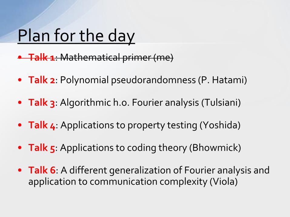
• Talk 1: Mathematical primer (me)

• Talk 2: Polynomial pseudorandomness (P. Hatami)

• Talk 3: Algorithmic h.o. Fourier analysis (Tulsiani)

• Talk 4: Applications to property testing (Yoshida)

• Talk 5: Applications to coding theory (Bhowmick)

• Talk 6: A different generalization of Fourier analysis and application to communication complexity (Viola)

Plan for the day

Given a quartic polynomial 𝑃: 𝔽2𝑛 → 𝔽2, can we decide in poly(𝑛) time whether:

𝑃 = 𝑄1𝑄2 + 𝑄3𝑄4 where 𝑄1,𝑄2,𝑄3,𝑄4 are quadratic polys? Yes! [B. ‘14, B.-Hatami-Tulsiani ‘15]

Teaser

Some Preliminaries

𝔽 = finite field of fixed

prime order

• For example, 𝔽 = 𝔽2 or 𝔽 = 𝔽97 • Theory simpler for fields of large (but fixed) size

Setting

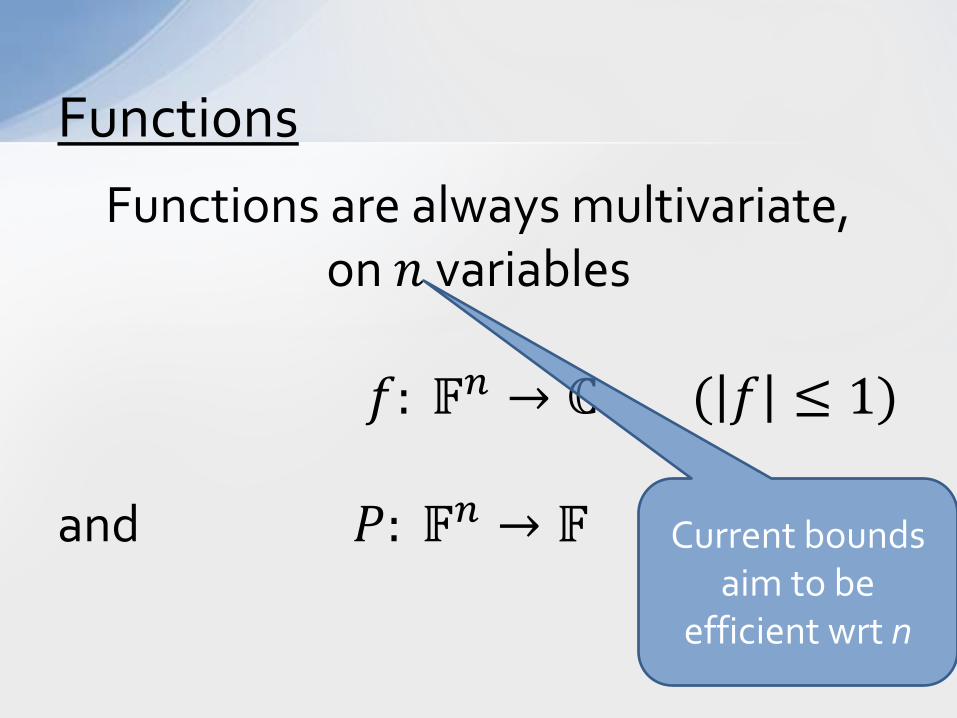
Functions are always multivariate, on 𝑛 variables

𝑓: 𝔽𝑛 → ℂ ( 𝑓 ≤ 1) and 𝑃: 𝔽𝑛 → 𝔽

Functions

Current bounds aim to be

efficient wrt n

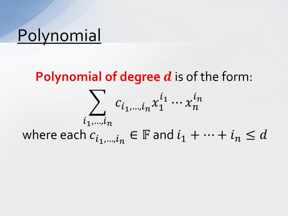
Polynomial of degree 𝒅 is of the form:

� 𝑐𝑖1,…,𝑖𝑛𝑥1𝑖1 ⋯𝑥𝑛

𝑖𝑛

𝑖1,…,𝑖𝑛

where each 𝑐𝑖1,…,𝑖𝑛 ∈ 𝔽 and 𝑖1 + ⋯+ 𝑖𝑛 ≤ 𝑑

Polynomial

Phase Polynomial

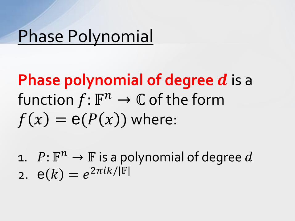
Phase polynomial of degree 𝒅 is a function 𝑓:𝔽𝑛 → ℂ of the form 𝑓 𝑥 = e(𝑃 𝑥 ) where: 1. 𝑃:𝔽𝑛 → 𝔽 is a polynomial of degree 𝑑 2. e 𝑘 = 𝑒2𝜋𝑖𝜋/|𝔽|

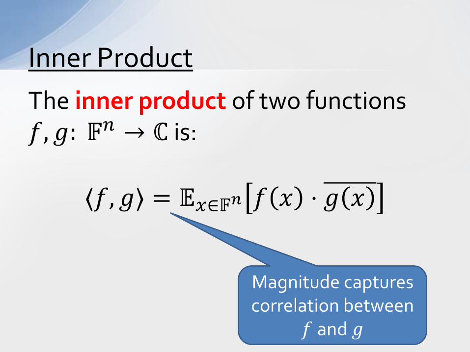
The inner product of two functions 𝑓,𝑔: 𝔽𝑛 → ℂ is:

⟨𝑓,𝑔⟩ = 𝔼𝑥∈𝔽𝑛 𝑓 𝑥 ⋅ 𝑔 𝑥

Inner Product

Magnitude captures correlation between

𝑓 and 𝑔

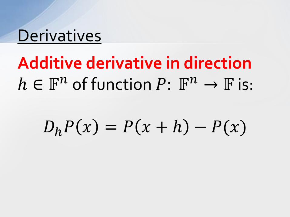
Additive derivative in direction ℎ ∈ 𝔽𝑛 of function 𝑃: 𝔽𝑛 → 𝔽 is:

𝐷ℎ𝑃 𝑥 = 𝑃 𝑥 + ℎ − 𝑃(𝑥)

Derivatives

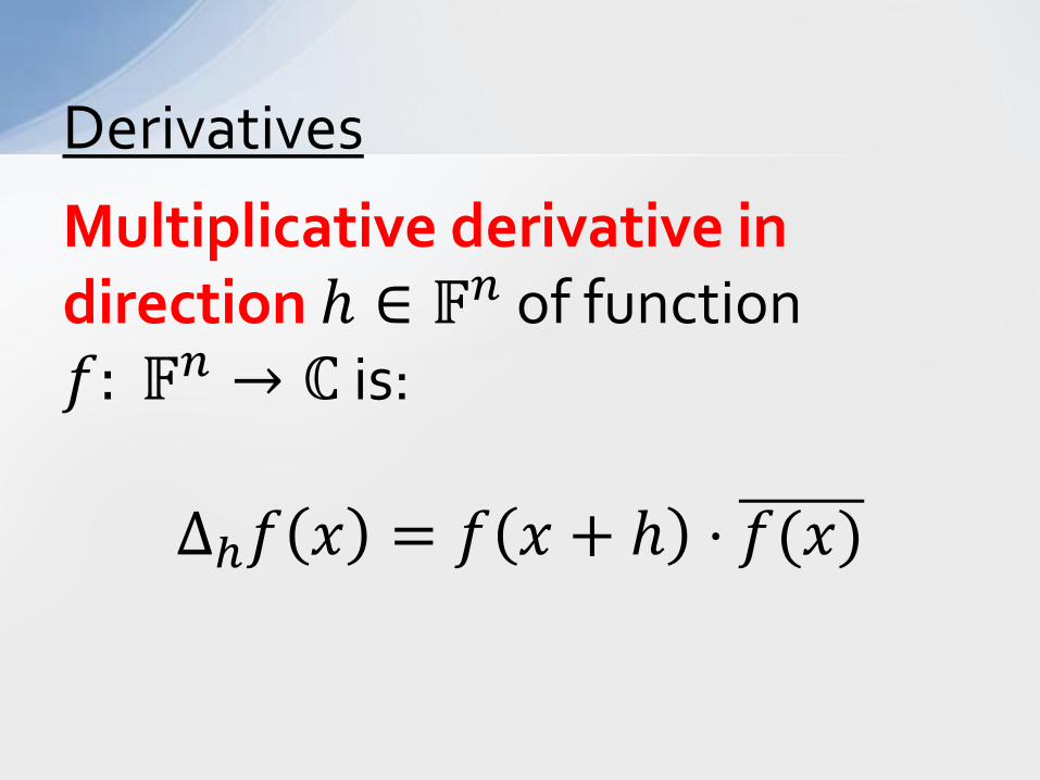
Multiplicative derivative in direction ℎ ∈ 𝔽𝑛 of function 𝑓: 𝔽𝑛 → ℂ is:

Δℎ𝑓 𝑥 = 𝑓 𝑥 + ℎ ⋅ 𝑓(𝑥)

Derivatives

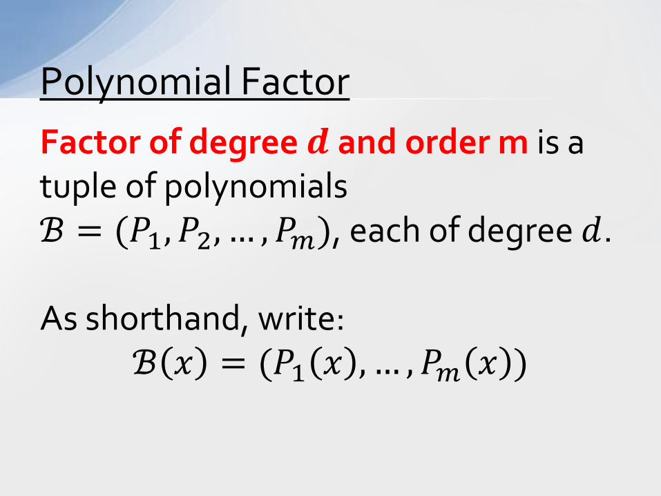
Factor of degree 𝒅 and order m is a tuple of polynomials ℬ = (𝑃1,𝑃2, … ,𝑃𝑚), each of degree 𝑑. As shorthand, write:

ℬ 𝑥 = (𝑃1 𝑥 , … ,𝑃𝑚 𝑥 )

Polynomial Factor

Fourier Analysis over 𝔽

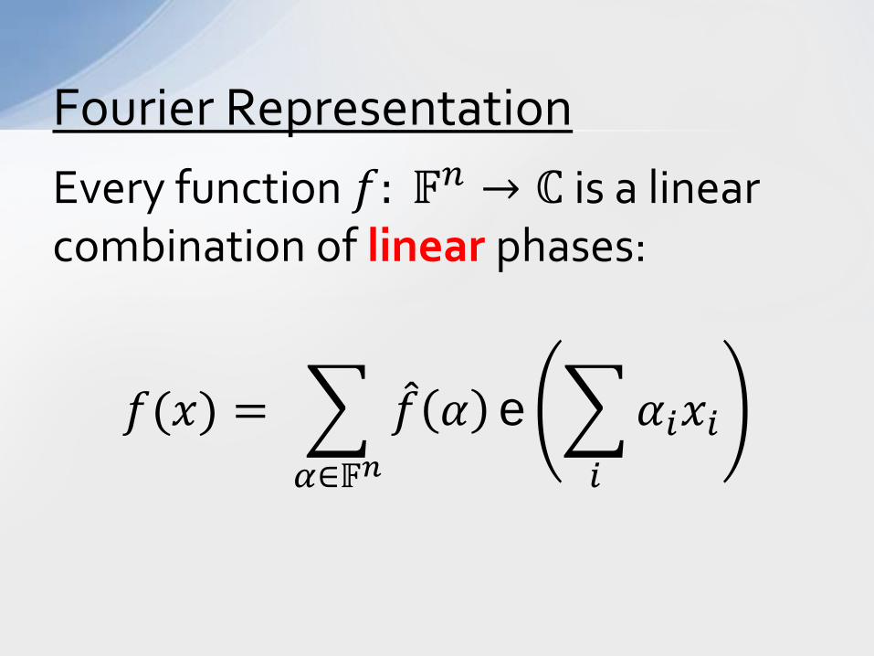
Every function 𝑓: 𝔽𝑛 → ℂ is a linear combination of linear phases:

𝑓(𝑥) = � 𝑓 𝛼𝛼∈𝔽𝑛

e �𝛼𝑖𝑥𝑖𝑖

Fourier Representation

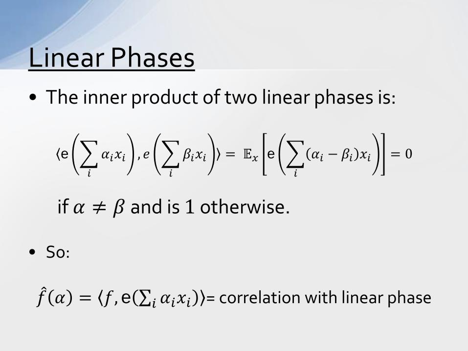
• The inner product of two linear phases is:

e �𝛼𝑖𝑥𝑖𝑖

, 𝑒 �𝛽𝑖𝑥𝑖𝑖

= 𝔼𝑥 e � 𝛼𝑖 − 𝛽𝑖 𝑥𝑖𝑖

= 0

if 𝛼 ≠ 𝛽 and is 1 otherwise.

• So: 𝑓 𝛼 = 𝑓, e ∑ 𝛼𝑖𝑥𝑖𝑖 = correlation with linear phase

Linear Phases

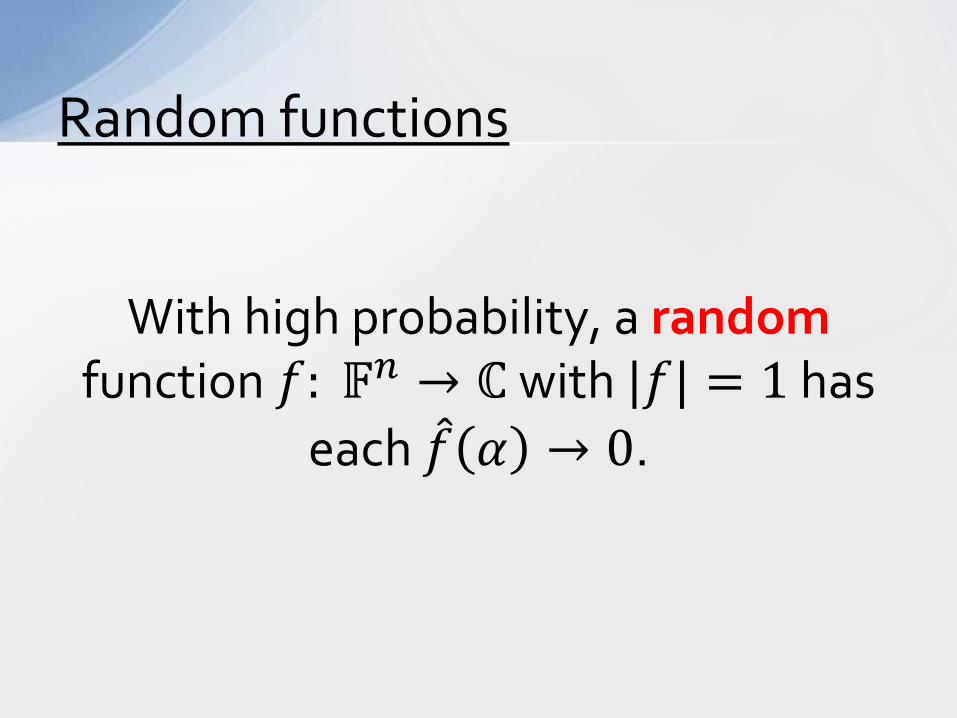
With high probability, a random function 𝑓: 𝔽𝑛 → ℂ with |𝑓| = 1 has

each 𝑓 𝛼 → 0.

Random functions

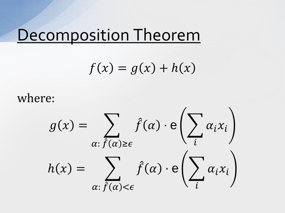
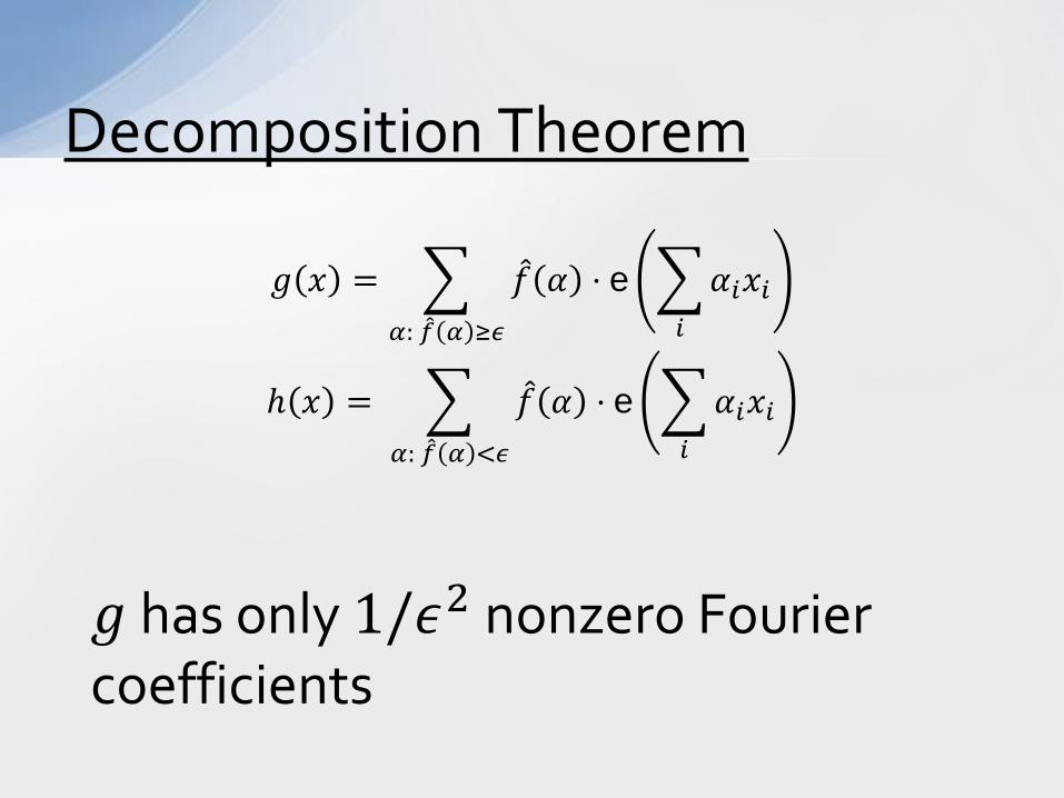
𝑓 𝑥 = 𝑔 𝑥 + ℎ 𝑥 where:

𝑔 𝑥 = � 𝑓 𝛼 ⋅ e �𝛼𝑖𝑥𝑖𝑖𝛼: �̂� 𝛼 ≥𝜖

ℎ 𝑥 = � 𝑓 𝛼 ⋅ e �𝛼𝑖𝑥𝑖𝑖𝛼: �̂� 𝛼 <𝜖

Decomposition Theorem

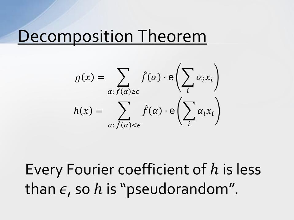
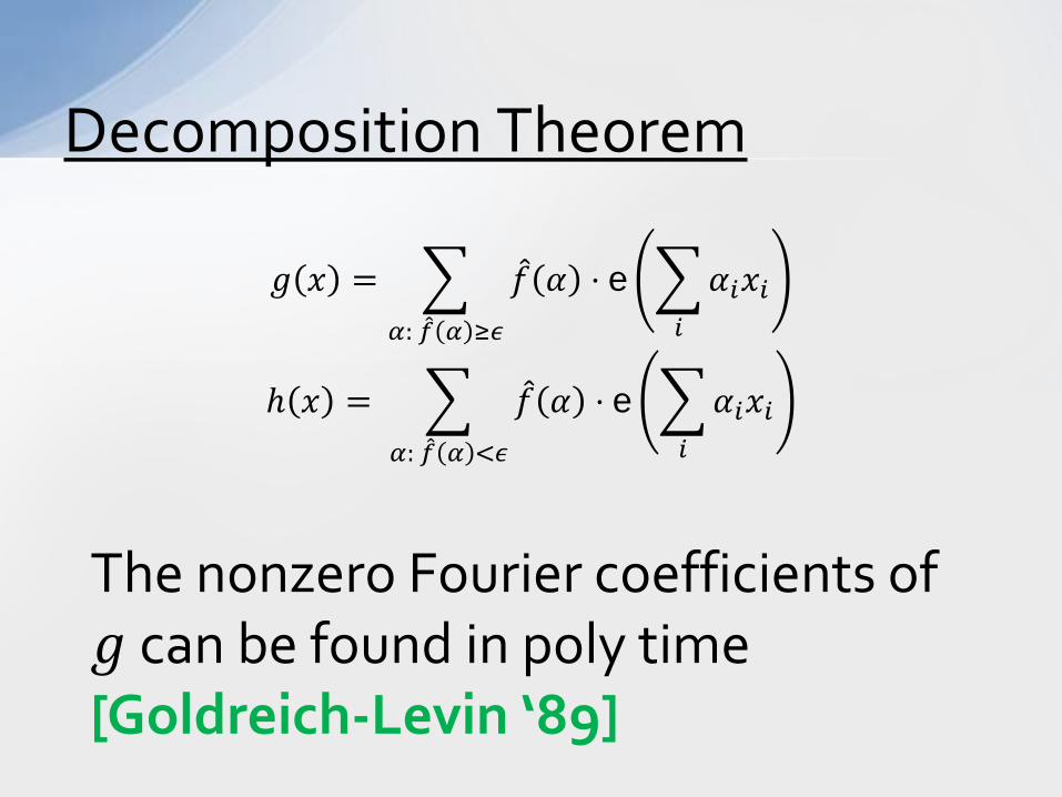
𝑔 𝑥 = � 𝑓 𝛼 ⋅ e �𝛼𝑖𝑥𝑖𝑖𝛼: �̂� 𝛼 ≥𝜖

ℎ 𝑥 = � 𝑓 𝛼 ⋅ e �𝛼𝑖𝑥𝑖𝑖𝛼: �̂� 𝛼 <𝜖

Decomposition Theorem

Every Fourier coefficient of ℎ is less than 𝜖, so ℎ is “pseudorandom”.

𝑔 𝑥 = � 𝑓 𝛼 ⋅ e �𝛼𝑖𝑥𝑖𝑖𝛼: �̂� 𝛼 ≥𝜖

ℎ 𝑥 = � 𝑓 𝛼 ⋅ e �𝛼𝑖𝑥𝑖𝑖𝛼: �̂� 𝛼 <𝜖

Decomposition Theorem

𝑔 has only 1/𝜖2 nonzero Fourier coefficients

𝑔 𝑥 = � 𝑓 𝛼 ⋅ e �𝛼𝑖𝑥𝑖𝑖𝛼: �̂� 𝛼 ≥𝜖

ℎ 𝑥 = � 𝑓 𝛼 ⋅ e �𝛼𝑖𝑥𝑖𝑖𝛼: �̂� 𝛼 <𝜖

Decomposition Theorem

The nonzero Fourier coefficients of 𝑔 can be found in poly time [Goldreich-Levin ‘89]

Elements of Higher-Order Fourier Analysis

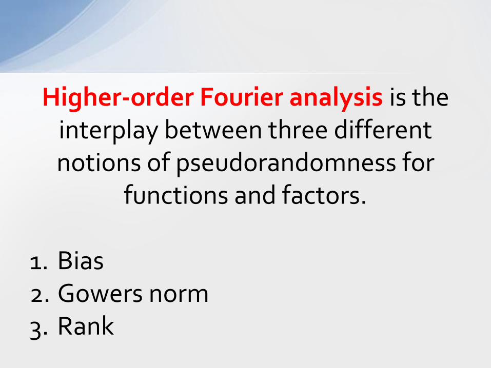
Higher-order Fourier analysis is the interplay between three different notions of pseudorandomness for

functions and factors. 1. Bias 2. Gowers norm 3. Rank

Bias

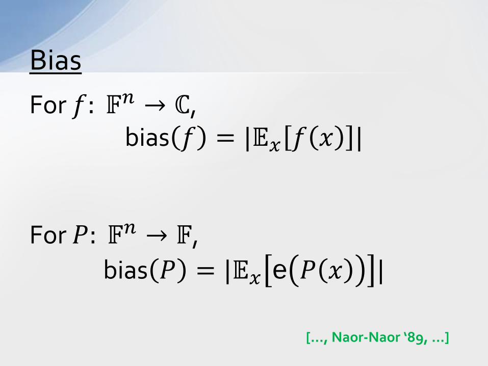
For 𝑓: 𝔽𝑛 → ℂ, bias 𝑓 = |𝔼𝑥 𝑓 𝑥 |

For 𝑃: 𝔽𝑛 → 𝔽,

bias 𝑃 = |𝔼𝑥 e 𝑃 𝑥 |

Bias

[…, Naor-Naor ‘89, …]

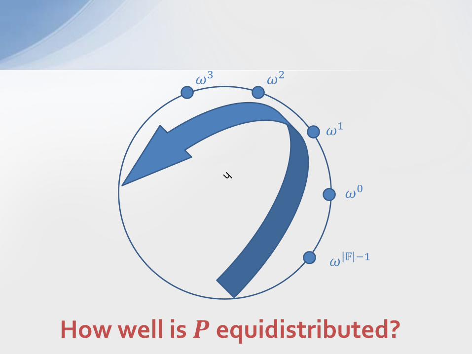
𝜔0

𝜔1

𝜔2 𝜔3

𝜔 𝔽 −1

How well is 𝑷 equidistributed?

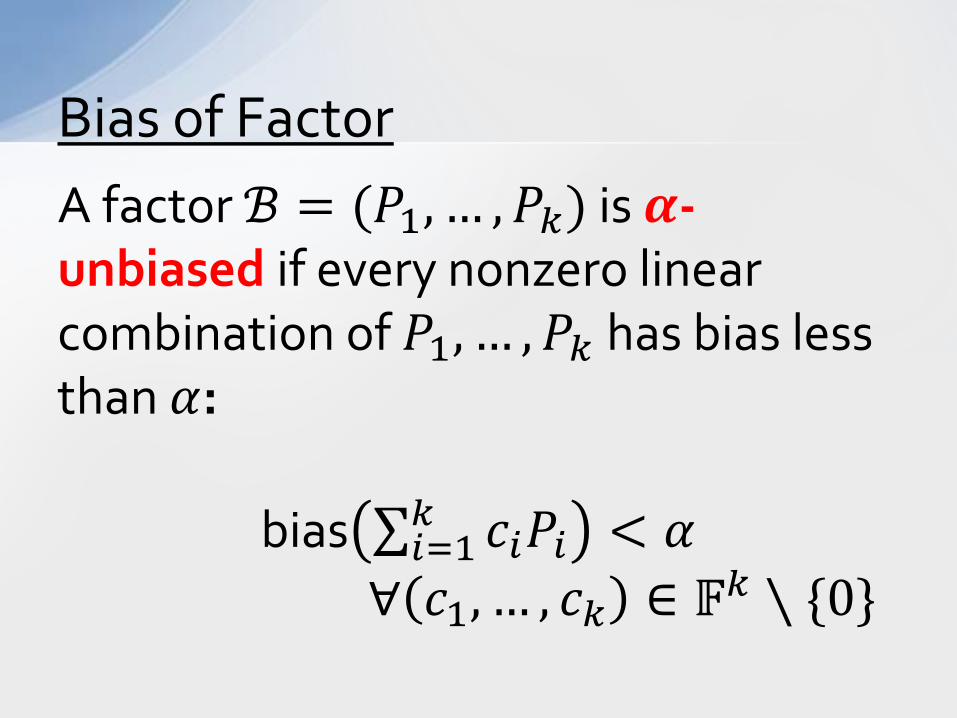
A factor ℬ = (𝑃1, … ,𝑃𝜋) is 𝜶-unbiased if every nonzero linear combination of 𝑃1, … ,𝑃𝜋 has bias less than 𝛼:

bias ∑ 𝑐𝑖𝑃𝑖𝜋𝑖=1 < 𝛼

∀ 𝑐1, … , 𝑐𝜋 ∈ 𝔽𝜋 ∖ {0}

Bias of Factor

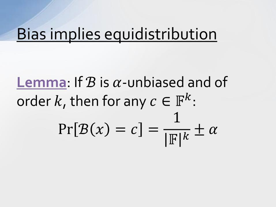
Lemma: If ℬ is 𝛼-unbiased and of order 𝑘, then for any 𝑐 ∈ 𝔽𝜋:

Pr ℬ 𝑥 = 𝑐 =1𝔽 𝜋 ± 𝛼

Bias implies equidistribution

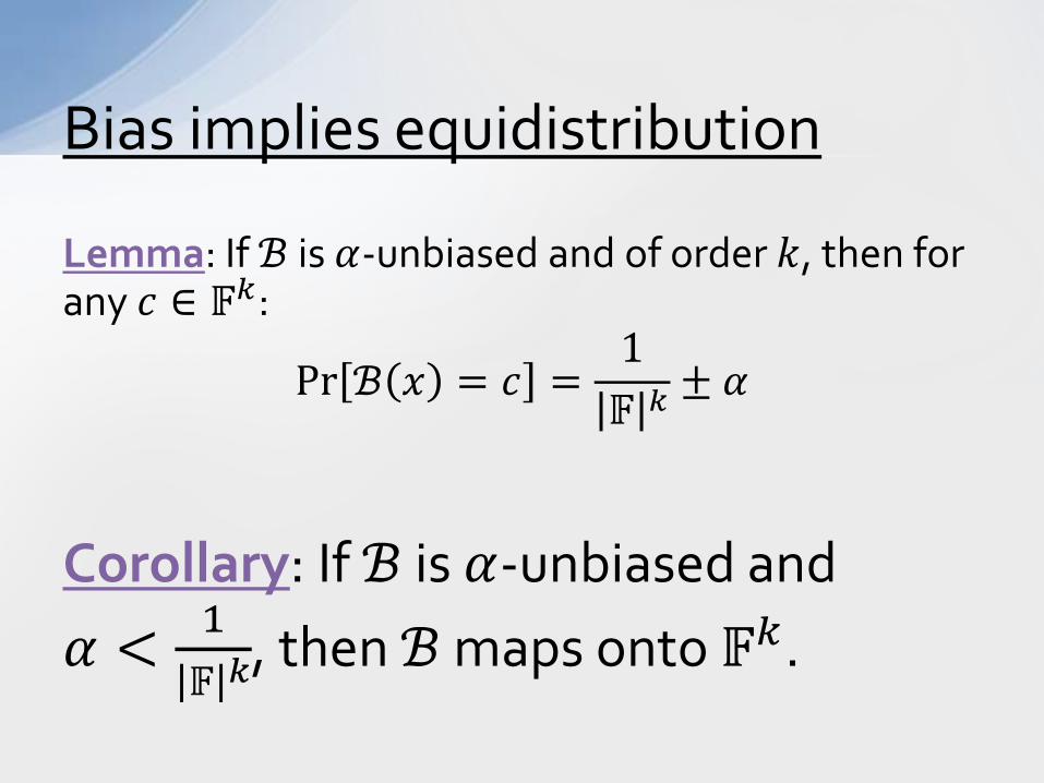
Lemma: If ℬ is 𝛼-unbiased and of order 𝑘, then for any 𝑐 ∈ 𝔽𝜋:

Pr ℬ 𝑥 = 𝑐 =1𝔽 𝜋 ± 𝛼

Bias implies equidistribution

Corollary: If ℬ is 𝛼-unbiased and 𝛼 < 1

𝔽 𝑘, then ℬ maps onto 𝔽𝜋.

Gowers Norm

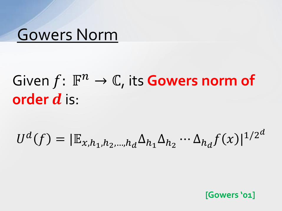
Given 𝑓: 𝔽𝑛 → ℂ, its Gowers norm of order 𝒅 is: 𝑈𝑑 𝑓 = |𝔼𝑥,ℎ1,ℎ2,…,ℎ𝑑Δℎ1Δℎ2 ⋯Δℎ𝑑𝑓 𝑥 |1/2𝑑

Gowers Norm

[Gowers ‘01]

Given 𝑓: 𝔽𝑛 → ℂ, its Gowers norm of order 𝒅 is:

𝑈𝑑 𝑓 = |𝔼𝑥,ℎ1,ℎ2,…,ℎ𝑑Δℎ1Δℎ2 ⋯Δℎ𝑑𝑓 𝑥 |1/2𝑑

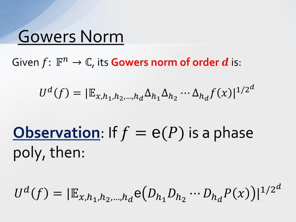
Gowers Norm

Observation: If 𝑓 = e(𝑃) is a phase poly, then: 𝑈𝑑 𝑓 = |𝔼𝑥,ℎ1,ℎ2,…,ℎ𝑑e 𝐷ℎ1𝐷ℎ2 ⋯𝐷ℎ𝑑𝑃 𝑥 |1/2𝑑

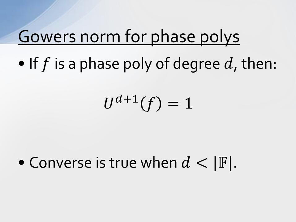
• If 𝑓 is a phase poly of degree 𝑑, then:

𝑈𝑑+1 𝑓 = 1 • Converse is true when 𝑑 < |𝔽|.

Gowers norm for phase polys

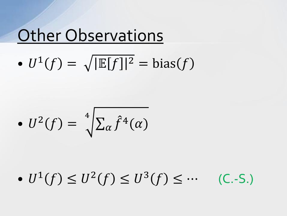
• 𝑈1 𝑓 = 𝔼 𝑓 2 = bias 𝑓

• 𝑈2 𝑓 = ∑ 𝑓4(𝛼)𝛼4

• 𝑈1 𝑓 ≤ 𝑈2 𝑓 ≤ 𝑈3 𝑓 ≤ ⋯ (C.-S.)

Other Observations

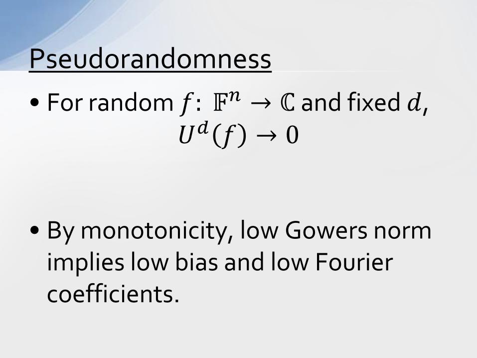
• For random 𝑓: 𝔽𝑛 → ℂ and fixed 𝑑, 𝑈𝑑 𝑓 → 0

• By monotonicity, low Gowers norm

implies low bias and low Fourier coefficients.

Pseudorandomness

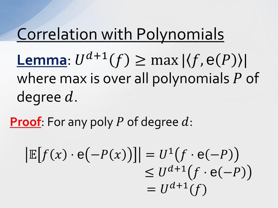
Lemma: 𝑈𝑑+1 𝑓 ≥ max | 𝑓, e 𝑃 | where max is over all polynomials 𝑃 of degree 𝑑.

Correlation with Polynomials

Proof: For any poly 𝑃 of degree 𝑑:

𝔼 𝑓 𝑥 ⋅ e −𝑃 𝑥 = 𝑈1 𝑓 ⋅ e −𝑃 ≤ 𝑈𝑑+1 𝑓 ⋅ e −𝑃

= 𝑈𝑑+1(𝑓)

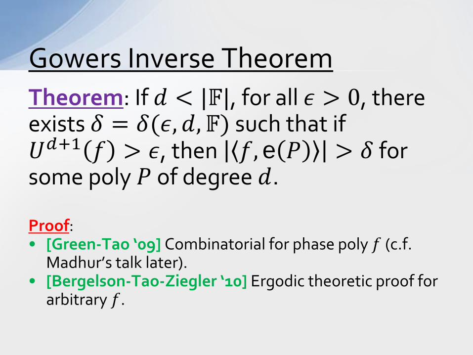
Theorem: If 𝑑 < |𝔽|, for all 𝜖 > 0, there exists 𝛿 = 𝛿(𝜖,𝑑,𝔽) such that if 𝑈𝑑+1 𝑓 > 𝜖, then 𝑓, e 𝑃 > 𝛿 for some poly 𝑃 of degree 𝑑. Proof: • [Green-Tao ‘09] Combinatorial for phase poly 𝑓 (c.f.

Madhur’s talk later). • [Bergelson-Tao-Ziegler ‘10] Ergodic theoretic proof for

arbitrary 𝑓.

Gowers Inverse Theorem

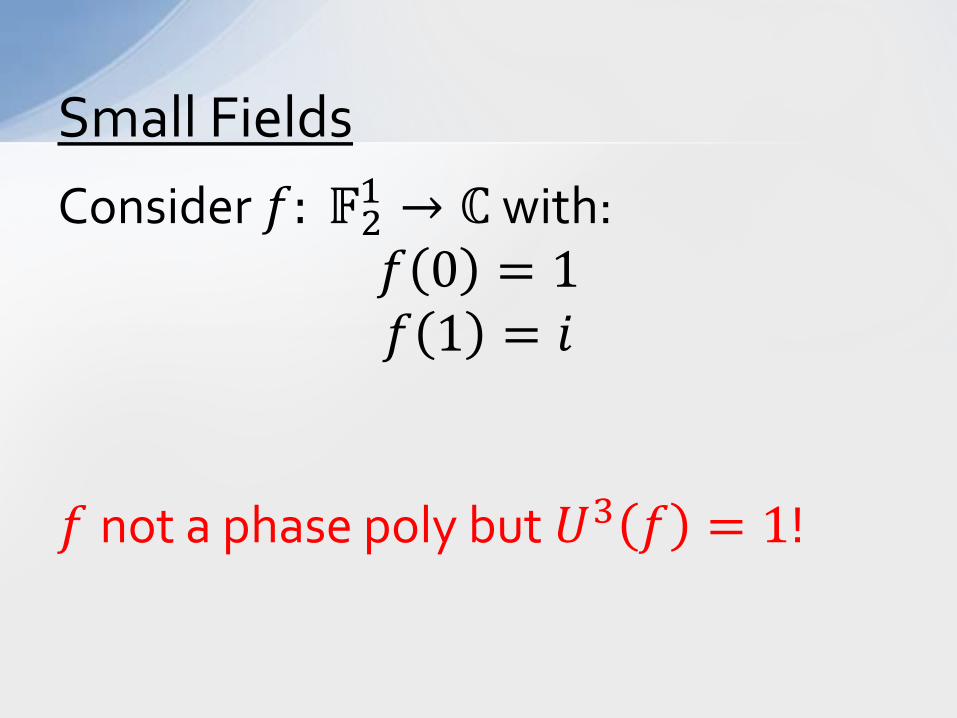
Consider 𝑓: 𝔽21 → ℂ with: 𝑓 0 = 1 𝑓 1 = 𝑖

𝑓 not a phase poly but 𝑈3 𝑓 = 1!

Small Fields

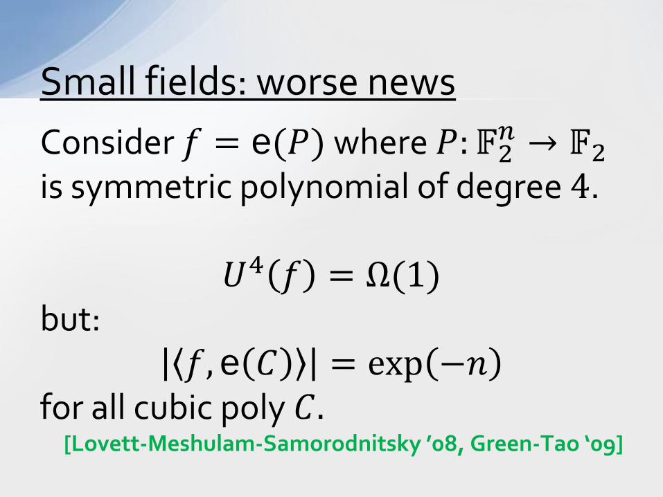
Consider 𝑓 = e(𝑃) where 𝑃:𝔽2𝑛 → 𝔽2 is symmetric polynomial of degree 4.

𝑈4 𝑓 = Ω(1) but:

𝑓, e 𝐶 = exp −𝑛 for all cubic poly 𝐶.

[Lovett-Meshulam-Samorodnitsky ’08, Green-Tao ‘09]

Small fields: worse news

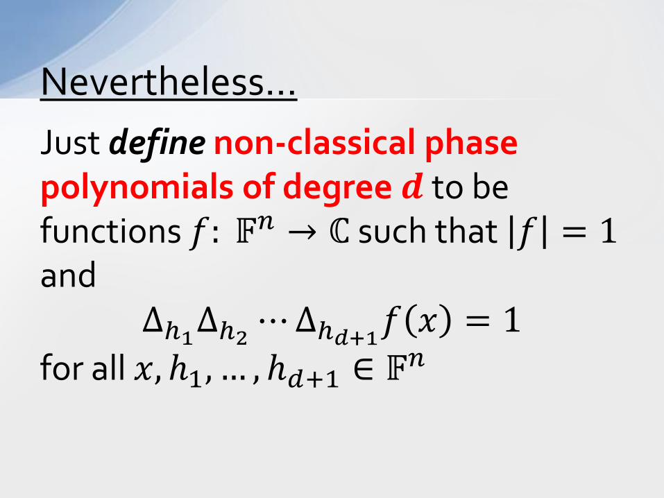
Just define non-classical phase polynomials of degree 𝒅 to be functions 𝑓: 𝔽𝑛 → ℂ such that 𝑓 = 1 and

Δℎ1Δℎ2 ⋯Δℎ𝑑+1𝑓 𝑥 = 1 for all 𝑥, ℎ1, … , ℎ𝑑+1 ∈ 𝔽𝑛

Nevertheless…

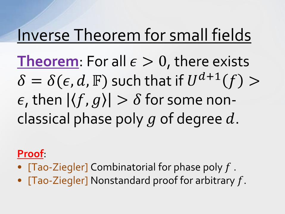
Inverse Theorem for small fields Theorem: For all 𝜖 > 0, there exists 𝛿 = 𝛿(𝜖,𝑑,𝔽) such that if 𝑈𝑑+1 𝑓 >𝜖, then 𝑓,𝑔 > 𝛿 for some non-classical phase poly 𝑔 of degree 𝑑. Proof: • [Tao-Ziegler] Combinatorial for phase poly 𝑓 . • [Tao-Ziegler] Nonstandard proof for arbitrary 𝑓.

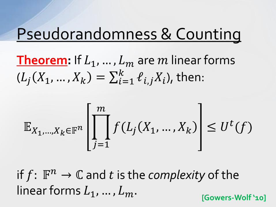
Theorem: If 𝐿1, … , 𝐿𝑚 are 𝑚 linear forms (𝐿𝑗 𝑋1, … ,𝑋𝜋 = ∑ ℓ𝑖,𝑗𝑋𝑖𝜋

𝑖=1 ), then:

𝔼𝑋1,…,𝑋𝑘∈𝔽𝑛 �𝑓(𝐿𝑗 𝑋1, … ,𝑋𝜋

𝑚

𝑗=1

≤ 𝑈𝑡(𝑓)

if 𝑓: 𝔽𝑛 → ℂ and 𝑡 is the complexity of the linear forms 𝐿1, … , 𝐿𝑚.

Pseudorandomness & Counting

[Gowers-Wolf ‘10]

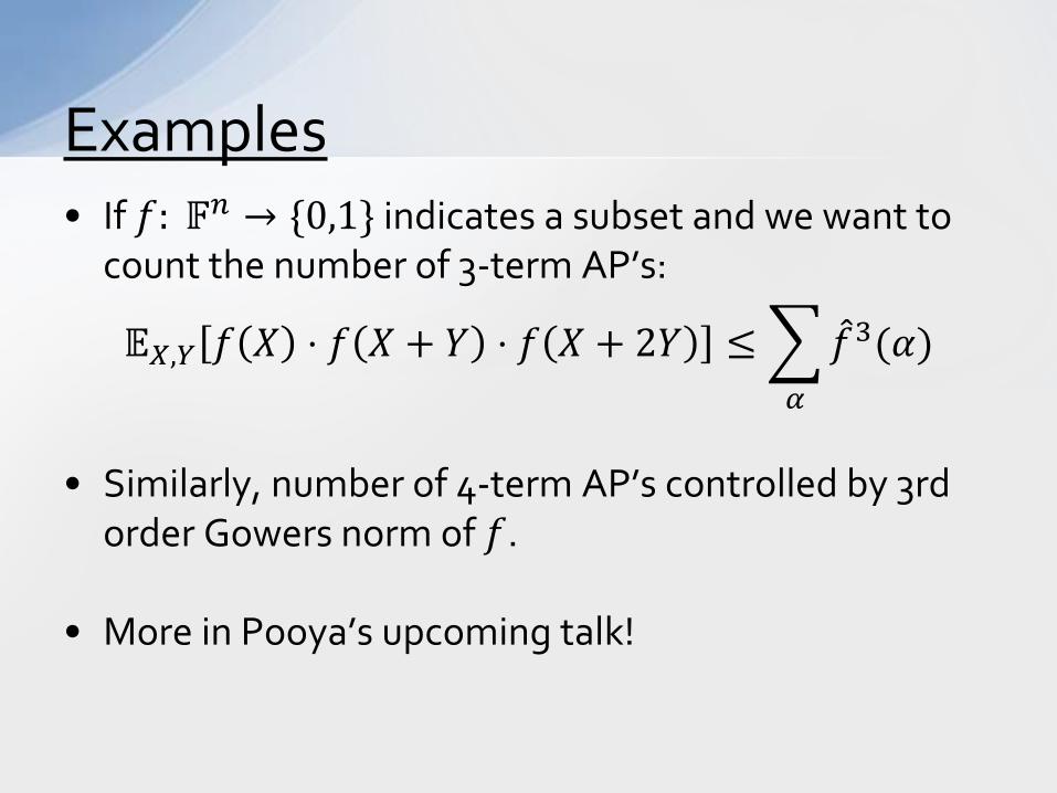
• If 𝑓: 𝔽𝑛 → {0,1} indicates a subset and we want to count the number of 3-term AP’s:

𝔼𝑋,𝑌 𝑓 𝑋 ⋅ 𝑓 𝑋 + 𝑌 ⋅ 𝑓 𝑋 + 2𝑌 ≤�𝑓3(𝛼)𝛼

• Similarly, number of 4-term AP’s controlled by 3rd

order Gowers norm of 𝑓.

• More in Pooya’s upcoming talk!

Examples

Rank

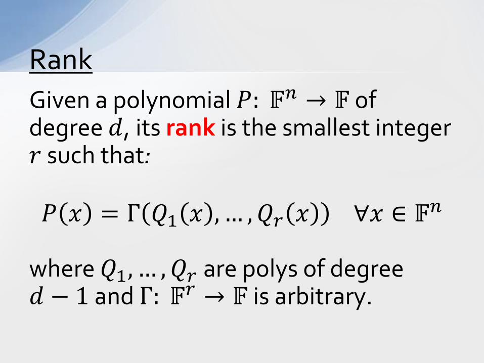
Given a polynomial 𝑃: 𝔽𝑛 → 𝔽 of degree 𝑑, its rank is the smallest integer 𝑟 such that: 𝑃 𝑥 = Γ 𝑄1 𝑥 , … ,𝑄𝑟 𝑥 ∀𝑥 ∈ 𝔽𝑛

where 𝑄1, … ,𝑄𝑟 are polys of degree 𝑑 − 1 and Γ: 𝔽𝑟 → 𝔽 is arbitrary.

Rank

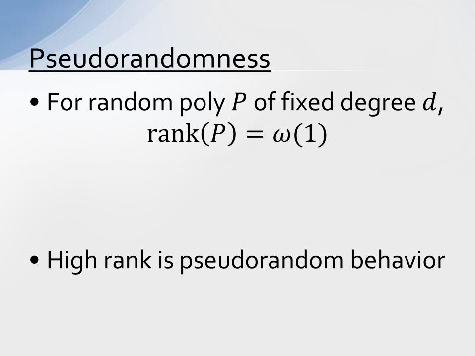
• For random poly 𝑃 of fixed degree 𝑑, rank 𝑃 = 𝜔(1)

• High rank is pseudorandom behavior

Pseudorandomness

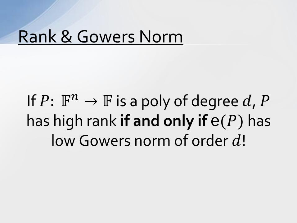
If 𝑃: 𝔽𝑛 → 𝔽 is a poly of degree 𝑑, 𝑃 has high rank if and only if e(𝑃) has

low Gowers norm of order 𝑑!

Rank & Gowers Norm

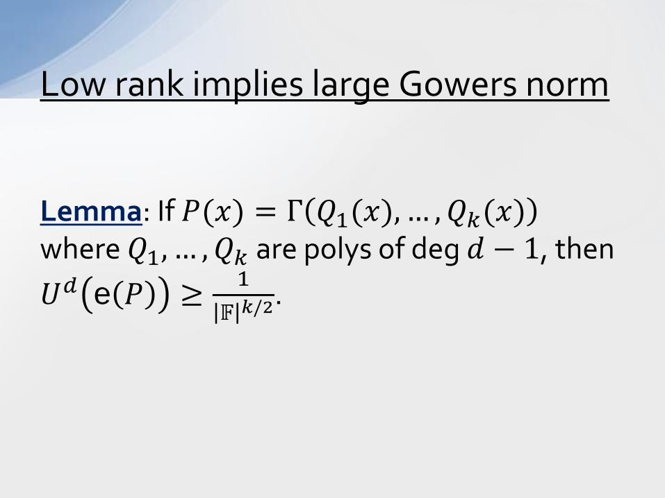
Lemma: If 𝑃(𝑥) = Γ 𝑄1(𝑥), … ,𝑄𝜋(𝑥) where 𝑄1, … ,𝑄𝜋 are polys of deg 𝑑 − 1, then 𝑈𝑑 e 𝑃 ≥ 1

𝔽 𝑘/2.

Low rank implies large Gowers norm

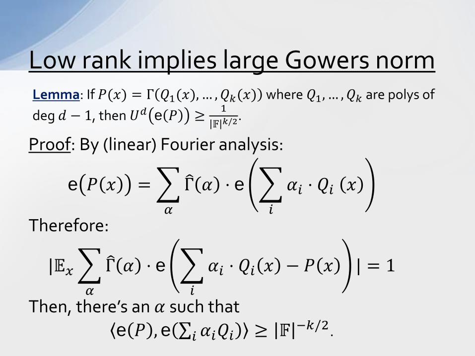
Lemma: If 𝑃(𝑥) = Γ 𝑄1(𝑥), … ,𝑄𝜋(𝑥) where 𝑄1, … ,𝑄𝜋 are polys of deg 𝑑 − 1, then 𝑈𝑑 e 𝑃 ≥ 1

𝔽 𝑘/2.

Low rank implies large Gowers norm

Proof: By (linear) Fourier analysis:

e 𝑃 𝑥 = �Γ� 𝛼 ⋅ e �𝛼𝑖 ⋅ 𝑄𝑖 𝑥𝑖𝛼

Therefore:

|𝔼𝑥�Γ� 𝛼 ⋅ e �𝛼𝑖 ⋅ 𝑄𝑖 𝑥 − 𝑃 𝑥𝑖

| = 1𝛼

Then, there’s an 𝛼 such that e 𝑃 , e ∑ 𝛼𝑖𝑄𝑖𝑖 ≥ 𝔽 −𝜋/2.

Inverse theorem for polys

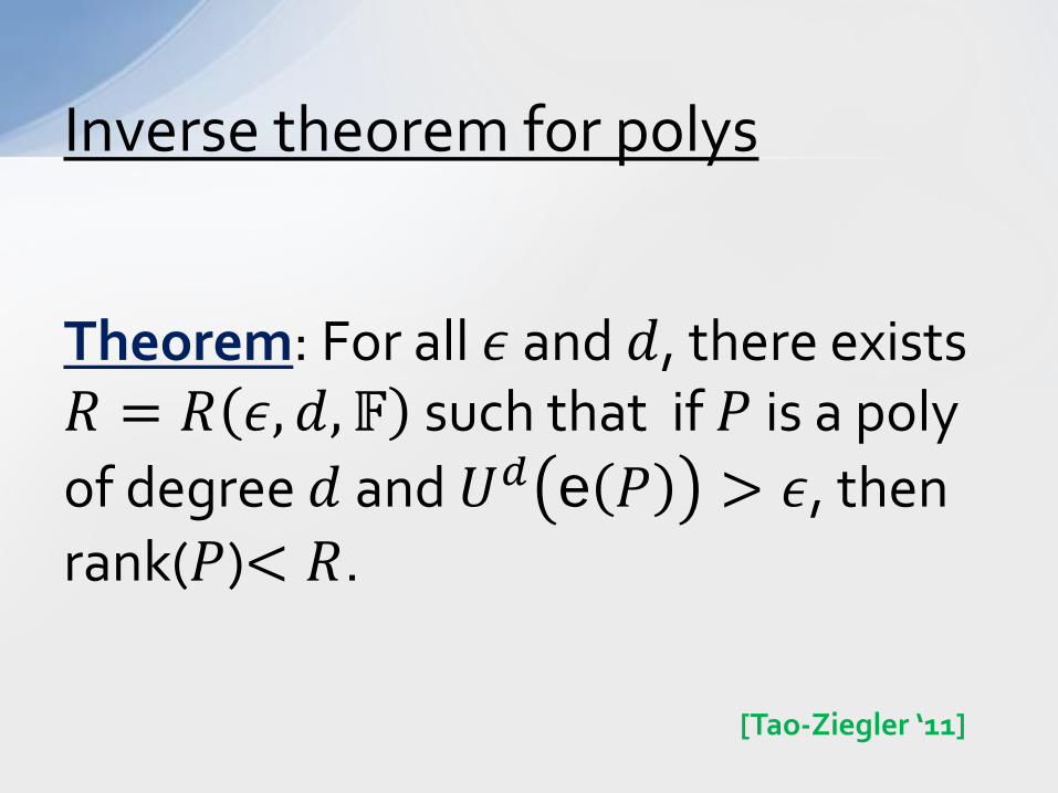
Theorem: For all 𝜖 and 𝑑, there exists 𝑅 = 𝑅 𝜖,𝑑,𝔽 such that if 𝑃 is a poly of degree 𝑑 and 𝑈𝑑 e 𝑃 > 𝜖, then rank(𝑃)< 𝑅.

[Tao-Ziegler ‘11]

Bias-rank theorem

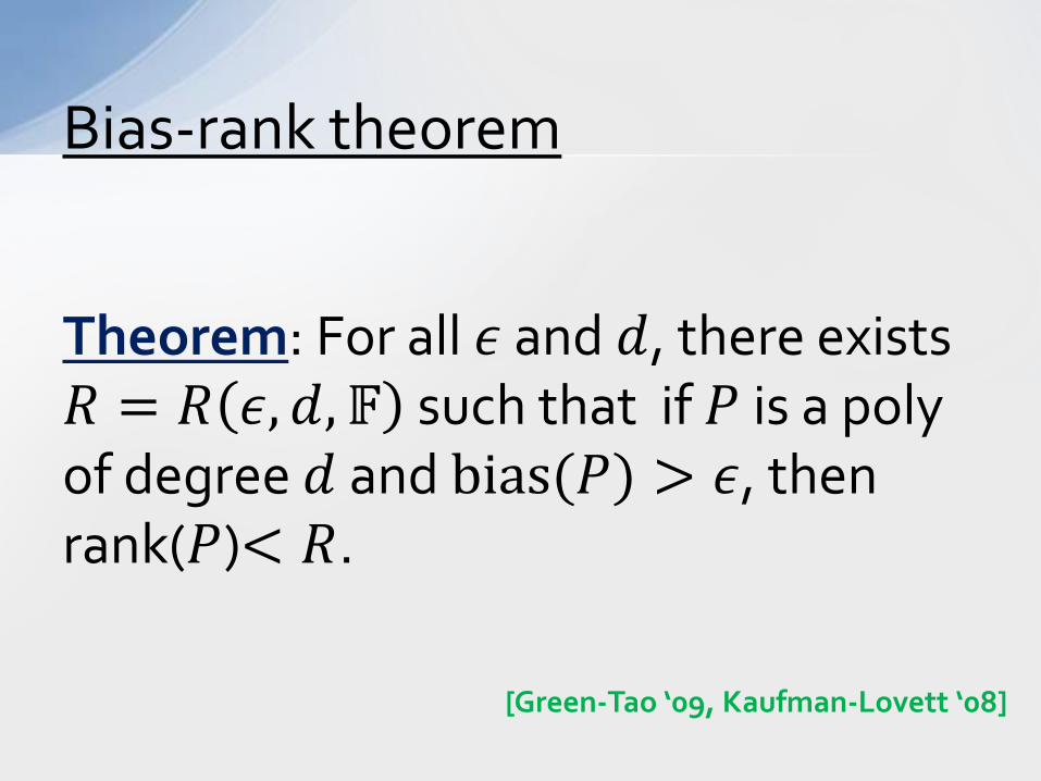
Theorem: For all 𝜖 and 𝑑, there exists 𝑅 = 𝑅 𝜖,𝑑,𝔽 such that if 𝑃 is a poly of degree 𝑑 and bias(𝑃) > 𝜖, then rank(𝑃)< 𝑅.

[Green-Tao ‘09, Kaufman-Lovett ‘08]

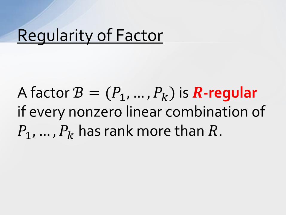
Regularity of Factor

A factor ℬ = (𝑃1, … ,𝑃𝜋) is 𝑹-regular if every nonzero linear combination of 𝑃1, … ,𝑃𝜋 has rank more than 𝑅.

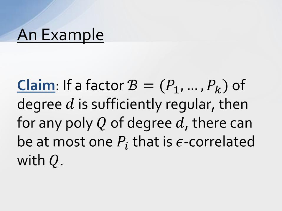
Claim: If a factor ℬ = (𝑃1, … ,𝑃𝜋) of degree 𝑑 is sufficiently regular, then for any poly 𝑄 of degree 𝑑, there can be at most one 𝑃𝑖 that is 𝜖-correlated with 𝑄.

An Example

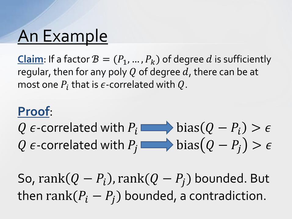
Claim: If a factor ℬ = (𝑃1, … ,𝑃𝜋) of degree 𝑑 is sufficiently regular, then for any poly 𝑄 of degree 𝑑, there can be at most one 𝑃𝑖 that is 𝜖-correlated with 𝑄. Proof: 𝑄 𝜖-correlated with 𝑃𝑖 bias 𝑄 − 𝑃𝑖 > 𝜖 𝑄 𝜖-correlated with 𝑃𝑗 bias 𝑄 − 𝑃𝑗 > 𝜖 So, rank 𝑄 − 𝑃𝑖 , rank(𝑄 − 𝑃𝑗) bounded. But then rank(𝑃𝑖 − 𝑃𝑗) bounded, a contradiction.

An Example

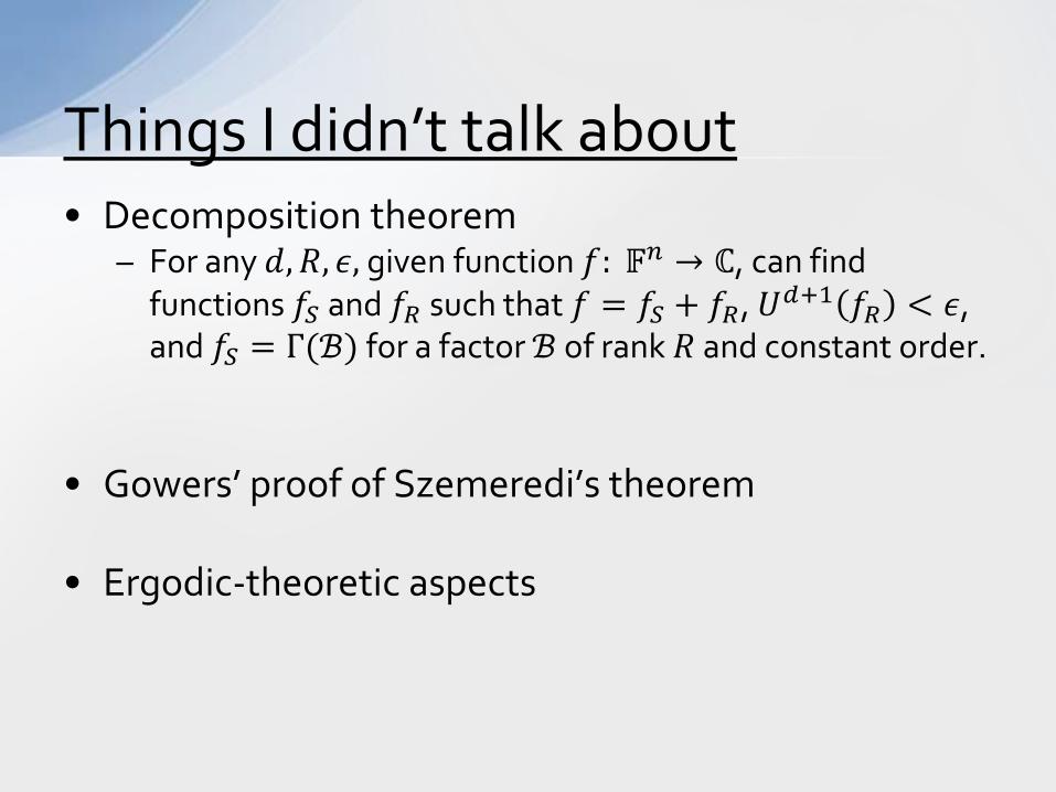
• Decomposition theorem – For any 𝑑,𝑅, 𝜖, given function 𝑓: 𝔽𝑛 → ℂ, can find

functions 𝑓𝑆 and 𝑓𝑅 such that 𝑓 = 𝑓𝑆 + 𝑓𝑅, 𝑈𝑑+1 𝑓𝑅 < 𝜖, and 𝑓𝑆 = Γ(ℬ) for a factor ℬ of rank 𝑅 and constant order.

• Gowers’ proof of Szemeredi’s theorem

• Ergodic-theoretic aspects

Things I didn’t talk about

• Talk 1: Mathematical primer (me)

• Talk 2: Polynomial pseudorandomness (P. Hatami)

• Talk 3: Algorithmic h.o. Fourier analysis (Tulsiani)

• Talk 4: Applications to property testing (Yoshida)

• Talk 5: Applications to coding theory (Bhowmick)

• Talk 6: A different generalization of Fourier analysis and application to communication complexity (Viola)

Plan for the day

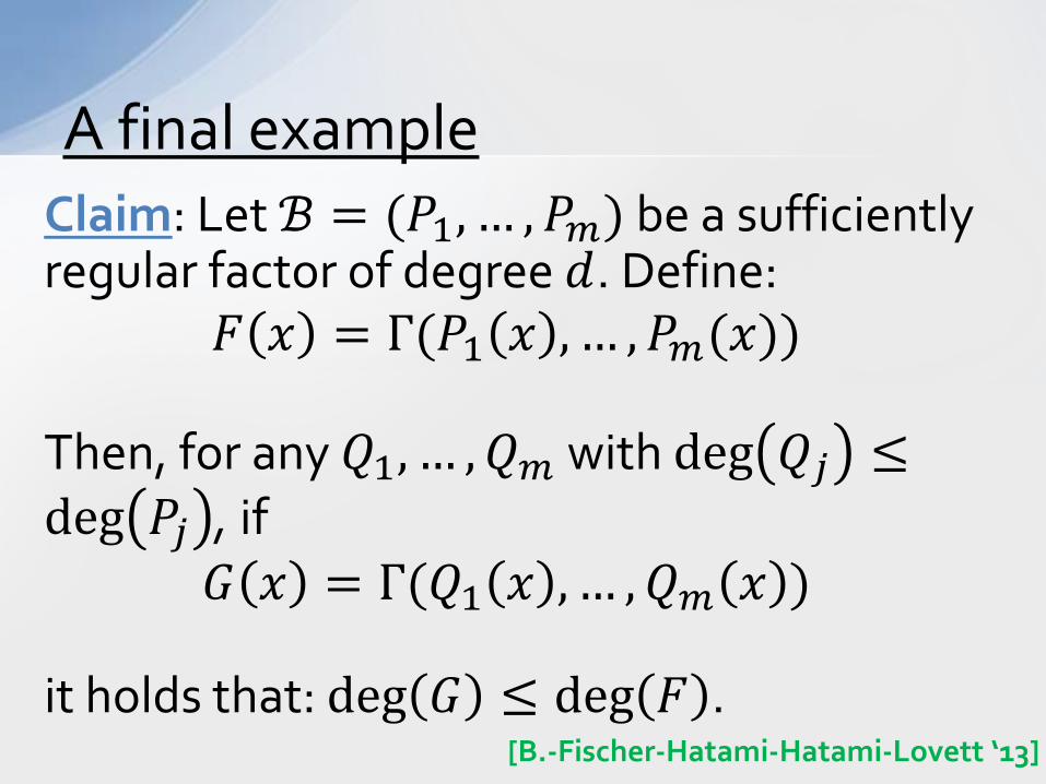
Claim: Let ℬ = (𝑃1, … ,𝑃𝑚) be a sufficiently regular factor of degree 𝑑. Define:

𝐹 𝑥 = Γ(𝑃1 𝑥 , … ,𝑃𝑚(𝑥)) Then, for any 𝑄1, … ,𝑄𝑚 with deg 𝑄𝑗 ≤deg 𝑃𝑗 , if

𝐺 𝑥 = Γ(𝑄1 𝑥 , … ,𝑄𝑚 𝑥 ) it holds that: deg 𝐺 ≤ deg 𝐹 .

A final example

[B.-Fischer-Hatami-Hatami-Lovett ‘13]

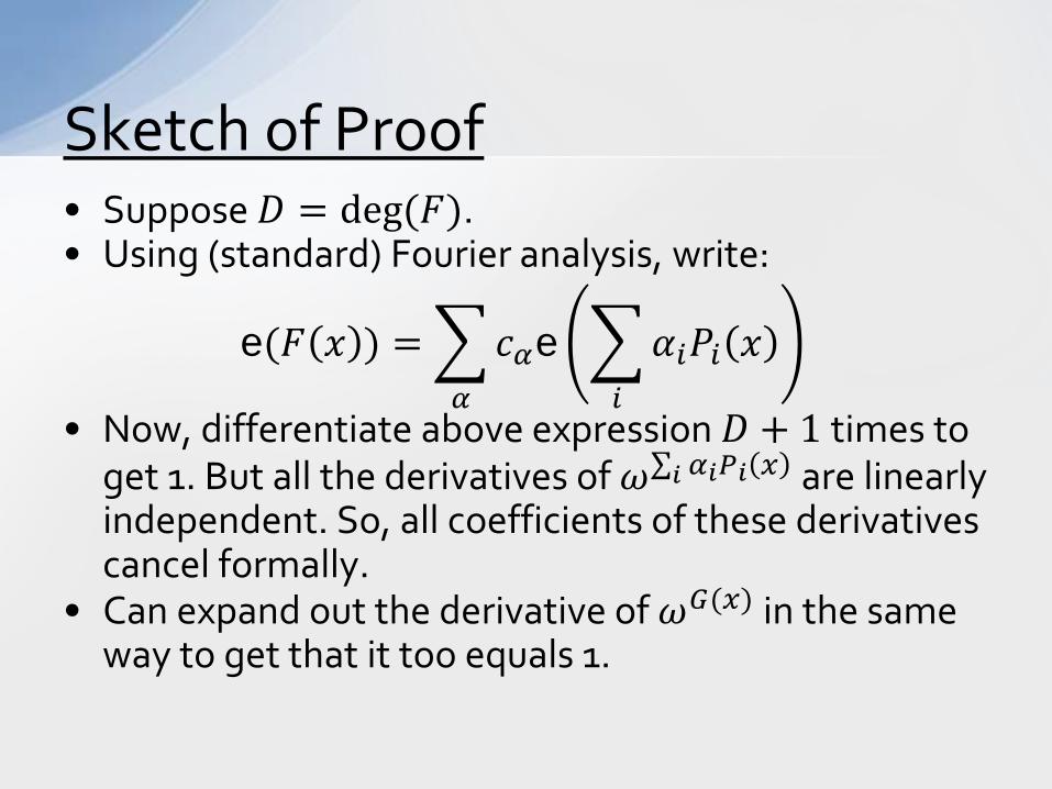
• Suppose 𝐷 = deg(𝐹). • Using (standard) Fourier analysis, write:

e(𝐹 𝑥 ) = �𝑐𝛼e �𝛼𝑖𝑃𝑖 𝑥𝑖𝛼

• Now, differentiate above expression 𝐷 + 1 times to get 1. But all the derivatives of 𝜔∑ 𝛼𝑖𝑃𝑖 𝑥𝑖 are linearly independent. So, all coefficients of these derivatives cancel formally.

• Can expand out the derivative of 𝜔𝐺(𝑥) in the same way to get that it too equals 1.

Sketch of Proof