Back-Calculation of Layer Parametersfor LTPP Test SectionsVolume II: Layered Elastic Analysisfor Flexible and Rigid PavementsPUBLICATION NO. FHWA-RD-01-113 OCTOBER 2002

Research, Development, and TechnologyTurner-Fairbank Highway Research Center6300 Georgetown PikeMcLean, VA 22101-2296

Foreword Deflection basin measurements have been made with the Falling Weight Deflectometer (FWD) on all test sections that are included in the Long Term Pavement Performance (LTPP) program. These deflection basin data are analyzed to obtain the structural-response characteristics of the pavement structure and subgrade that are needed to achieve the overall LTPP program objectives. One of the more common methods for analysis of deflection data is to back-calculate the elastic properties for each layer and provide the elastic layer modulus that are typically used for pavement evaluation and rehabilitation design. This report documents the procedure that was used to back-calculate, in mass, the elastic properties for both flexible and rigid pavements in the LTPP program using layered elastic analyses. Obtaining these elastic layer properties for use in further data analyses and studies regarding pavement performance was the primary objective of this study.

T. Paul Teng, P.E. Director Office of Infrastructure Research and Development

Notice

This document is disseminated under the sponsorship of the Department of Transportation in the interest of information exchange. The U.S. Government assumes no liability for its contents or use thereof. This report does not constitute a standard, specification, or regulation. The U.S. Government does not endorse products or manufacturers. Trade and manufacturers' names appear in this report only because they are considered essential to the object of the document.

Technical Report Documentation Page 1. Report No. FHWA-RD-01-113

2. Government Accession No.

3. Recipient’s Catalog No.

5. Report Date OCTOBER 2002

4. Title and Subtitle Back-Calculation of Layer Parameters for LTPP Test Sections, Volume II: Layered Elastic Analysis for Flexible and Rigid Pavements

6. Performing Organization Code

7. Author(s) H. L. Von Quintus and A. L. Simpson

8. Performing Organization Report No.

10. Work Unit No. (TRAIS) C6B

9. Performing Organization Name and Address Fugro-BRE 8613 Cross Park Drive Austin, TX 78754

11. Contract or Grant No. DTFH61-96-C-00003 13. Type of Report and Period Covered Final Report May 1997 – August 2001

12. Sponsoring Agency Name and Address Office of Engineering R & D Federal Highway Administration 6300 Georgetown Pike McLean, Virginia 22101-2296 14. Sponsoring Agency Code

HCP 30-C

15. Supplementary Notes This report is a project deliverable under the LTPP Data Analysis Technical Support study. ERES Consultants is the prime contractor, and Fugro-BRE is a subcontractor. Fugro-BRE staff members who provided significant contributions to this study include Dr. Peter Jordahl and Mr. Dale Framelli. Contracting Officer’s Technical Representative (COTR): Cheryl Allen Richter, HRDI-13 16. Abstract This report documents the procedure and steps used to back-calculate the layered elastic properties (Young’s modulus and the coefficient and exponent of the nonlinear constitutive equation) from deflection basin measurements for all of the LTPP test sections with a level E data status. The back-calculation process was completed with MDOCOMP4 for both flexible and rigid pavement test sections in the LTPP program. The report summarizes the reasons why MODCOMP4 was selected for the computations and analyses of the deflection data, provides a summary of the results using the linear elastic module (Young’s modulus) for selected test sections, and identifies those factors that can have a significant effect on the results. Results from this study do provide elastic layer properties that are consistent with previous experience and laboratory material studies related to the effect of temperature, stress-state, and season on material load-response behavior. In fact, over 75 percent of the deflection basins analyzed with the linear elastic module of MODCOMP4 resulted in solutions with an RMS error less than 2.5 percent. Those pavements exhibiting deflection-softening behavior with Type II deflections basins were the most difficult to analyze and were generally found to have RMS errors greater than 2 percent. In summary, the nonlinear module of MODCOMP did not significantly improve on the number of reasonable solutions, and it is recommended that nonlinear constitutive equations not be used in a batch mode basis. 17. Key Words MODCOMP, Back-Calculation, Modulus, Young’s Modulus, Elastic Properties, Surface Deflection, Stress Sensitivity

18. Distribution Statement No restrictions. This document is available to the public through the National Technical Information Service, Springfield, Virginia 22161.

19. Security Classif. (of this report) Unclassified

20. Security Classif. (of this page) Unclassified

21. No. of Pages

144

22. Price

Form DOT F 1700.7 (8-72) Reproduction of completed page authorized

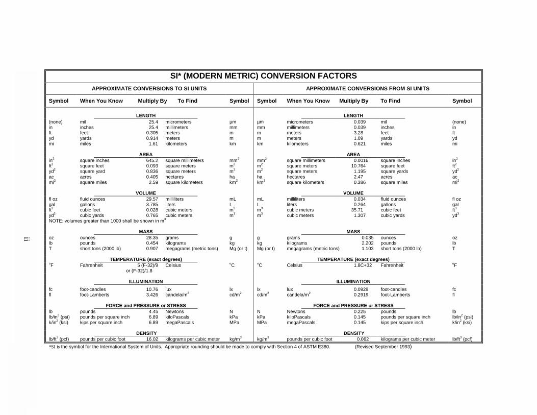
SI* (MODERN METRIC) CONVERSION FACTORS

APPROXIMATE CONVERSIONS TO SI UNITS APPROXIMATE CONVERSIONS FROM SI UNITS

Symbol When You Know Multiply By To Find Symbol Symbol When You Know Multiply By To Find Symbol LENGTH LENGTH (none) mil 25.4 micrometers µm µm micrometers 0.039 mil (none) in inches 25.4 millimeters mm mm millimeters 0.039 inches in ft feet 0.305 meters m m meters 3.28 feet ft yd yards 0.914 meters m m meters 1.09 yards yd mi miles 1.61 kilometers km km kilometers 0.621 miles mi AREA AREA in2 square inches 645.2 square millimeters mm2 mm2 square millimeters 0.0016 square inches in2

ft2 square feet 0.093 square meters m2 m2 square meters 10.764 square feet ft2

yd2 square yard 0.836 square meters m2 m2 square meters 1.195 square yards yd2

ac acres 0.405 hectares ha ha hectares 2.47 acres ac mi2 square miles 2.59 square kilometers km2 km2 square kilometers 0.386 square miles mi2

VOLUME VOLUME fl oz fluid ounces 29.57 milliliters mL mL milliliters 0.034 fluid ounces fl oz gal gallons 3.785 liters L L liters 0.264 gallons gal ft3 cubic feet 0.028 cubic meters m3 m3 cubic meters 35.71 cubic feet ft3

yd3 cubic yards 0.765 cubic meters m3 m3 cubic meters 1.307 cubic yards yd3

NOTE: volumes greater than 1000 shall be shown in m3 MASS MASS oz ounces 28.35 grams g g grams 0.035 ounces oz lb pounds 0.454 kilograms kg kg kilograms 2.202 pounds lb T short tons (2000 lb) 0.907 megagrams (metric tons) Mg (or t) Mg (or t) megagrams (metric tons) 1.103 short tons (2000 lb) T TEMPERATURE (exact degrees) TEMPERATURE (exact degrees) oF Fahrenheit 5 (F-32)/9 Celsius oC oC Celsius 1.8C+32 Fahrenheit oF or (F-32)/1.8 ILLUMINATION ILLUMINATION fc foot-candles 10.76 lux lx lx lux 0.0929 foot-candles fc fl foot-Lamberts 3.426 candela/m2 cd/m2 cd/m2 candela/m2 0.2919 foot-Lamberts fl FORCE and PRESSURE or STRESS FORCE and PRESSURE or STRESS lb pounds 4.45 Newtons N N Newtons 0.225 pounds lb lb/in2 (psi) pounds per square inch 6.89 kiloPascals kPa kPa kiloPascals 0.145 pounds per square inch lb/in2 (psi) k/in2 (ksi) kips per square inch 6.89 megaPascals MPa MPa megaPascals 0.145 kips per square inch k/in2 (ksi)

DENSITY DENSITY

lb/ft3 (pcf) pounds per cubic foot 16.02 kilograms per cubic meter kg/m3 kg/m3 pounds per cubic foot 0.062 kilograms per cubic meter lb/ft3 (pcf) *SI is the symbol for the International System of Units. Appropriate rounding should be made to comply with Section 4 of ASTM E380. (Revised September 1993)

ii

iii

TABLE OF CONTENTS Chapter Page No. 1.0 INTRODUCTION.................................................................................................................. 1 1.1 Background ............................................................................................................. 1 1.2 LTPP Deflection Testing Program.......................................................................... 1 1.3 Objective ................................................................................................................. 2 1.4 Application of Results to Future Studies ................................................................ 3 2.0 SELECTION OF BACK-CALCULATION METHODOLOGY.......................................... 5 2.1 Back-Calculation Methods...................................................................................... 5 2.1.1 Type of Load Application ........................................................................... 6 2.1.2 Type of Material Response Models ............................................................ 6 2.1.3 Summary ..................................................................................................... 7 2.2 Selection Factors ..................................................................................................... 7 2.3 Selection of Software – MODCOMP4.................................................................... 8 2.4 Program Accuracy................................................................................................. 10 3.0 BACK-CALCULATION PROCESS................................................................................... 13 3.1. Test Section Classification .................................................................................... 13 3.1.1 Load-Response Classification ................................................................... 13 3.1.2 Deflection Basin Classification................................................................. 17 3.1.3 Test Section Uniformity Classification ..................................................... 20 3.2 Determination of Inputs ........................................................................................ 20 3.2.1 Deflection Basins ...................................................................................... 24 3.2.2 Pavement Cross-Section............................................................................ 24 3.2.3 Material Properties and Temperatures ...................................................... 24 3.2.4 Layer Sensor Assignments ........................................................................ 24 3.2.5 Poisson’s Ratio.......................................................................................... 24 3.2.6 Multiple Subgrade Layers ......................................................................... 25 3.2.7 Depth to an Apparent Rigid Layer ............................................................ 25 3.2.8 Constitutive Equation................................................................................ 25 3.2.9 Material Densities ..................................................................................... 29 3.2.10 Lateral Earth Pressures.............................................................................. 29 3.3 Trial Computations – Execution of Back-Calculation Process............................. 29 4.0 RESULTS FROM COMPUTATION OF ELASTIC PROPERTIES.................................. 31 4.1 Some Basic Facts from the Back-Calculation Process.......................................... 31 4.2 Computed Parameter Database ............................................................................. 31 4.3 Allowable Maximum RMS Error.......................................................................... 32 4.4 Brief Evaluation of Reasonableness of Solutions ................................................. 39 4.4.1 Longitudinal Variation of Elastic Moduli ................................................. 39 4.4.2 Wheelpath Versus Non-Wheelpath Measurements................................... 46 4.4.3 Seasonal or Monthly Effects ..................................................................... 47 4.4.4 Temperature Effects .................................................................................. 47

iv

TABLE OF CONTENTS, (continued)

Chapter Page No. 4.4.5 Time Effects .............................................................................................. 47 4.4.6 Stress Sensitivity from Linear Solutions................................................... 47 4.5 Linear versus Nonlinear Solutions ........................................................................ 54 5.0 SUMMARY OF FINDINGS AND RECOMMENDATIONS ............................................ 57 5.1 Findings................................................................................................................. 57 5.2 Recommendations ................................................................................................. 58 5.3 Concluding Remarks ............................................................................................. 59 6.0 REFERENCES ................................................................................................................... 61 APPENDICES A. Back-Calculation of Layer Elastic Properties from LTPP-FWD Deflection Basin Data Using MODCOMP User’s Guide.......................................................................... 63 Introduction ........................................................................................................... 63 Purpose of User’s Guide ....................................................................................... 63 Back-Calculation Procedure Overview................................................................. 64 Step 1: IMS Data Extraction ................................................................................. 67 Step 2: Pre-Process the FWD Deflection Data – Execute DEFLAVG4............... 69 Step 3: Create Input Files for MODCOMP4......................................................... 71 Execute MODDATA................................................................................. 71 Execute METRIC...................................................................................... 75 Execute PREMOD3 .................................................................................. 76 Step 4: Trial Computations and Modification of Inputs ....................................... 80 Execute MODSHELL ............................................................................... 80 Execute Program BATCHIT..................................................................... 81 Step 5: Execute MODCOMP4 – Back-Calculate Young’s Modulus and Nonlinear Elastic Properties...................................................................... 83 Step 6: Extract Elastic Properties and Create Summary Output Files .................. 84 Execute BACKSUM2 ............................................................................... 84 Execute BAKSUMNL............................................................................... 84 Execute BAKOUTNL............................................................................... 85 Summary ............................................................................................................... 86 B. Test Section Classification and Subgrade Information for the Back-Calculation Process............................................................................................................................ 87 C. Median Values and Histograms of Young’s Modulus Back-Calculated for Different Materials....................................................................................................................... 101

v

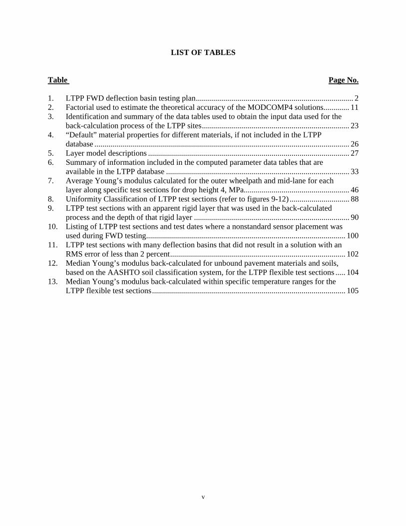
LIST OF TABLES Table Page No. 1. LTPP FWD deflection basin testing plan............................................................................... 2 2. Factorial used to estimate the theoretical accuracy of the MODCOMP4 solutions............. 11 3. Identification and summary of the data tables used to obtain the input data used for the back-calculation process of the LTPP sites.......................................................................... 23 4. “Default” material properties for different materials, if not included in the LTPP database ................................................................................................................................ 26 5. Layer model descriptions ..................................................................................................... 27 6. Summary of information included in the computed parameter data tables that are available in the LTPP database ............................................................................................ 33 7. Average Young’s modulus calculated for the outer wheelpath and mid-lane for each layer along specific test sections for drop height 4, MPa..................................................... 46 8. Uniformity Classification of LTPP test sections (refer to figures 9-12) .............................. 88 9. LTPP test sections with an apparent rigid layer that was used in the back-calculated process and the depth of that rigid layer .............................................................................. 90 10. Listing of LTPP test sections and test dates where a nonstandard sensor placement was

used during FWD testing.................................................................................................... 100 11. LTPP test sections with many deflection basins that did not result in a solution with an

RMS error of less than 2 percent........................................................................................ 102 12. Median Young’s modulus back-calculated for unbound pavement materials and soils, based on the AASHTO soil classification system, for the LTPP flexible test sections ..... 104 13. Median Young’s modulus back-calculated within specific temperature ranges for the LTPP flexible test sections................................................................................................. 105

vi

LIST OF FIGURES Figure No. Page No. 1. Flow chart showing the major steps and decisions used in the linear elastic back-calculation

process.................................................................................................................................. 14 2. Graphical illustration of the definition for the linear response category.............................. 15 3. Graphical illustration of the definition for the deflection-hardening response category ..... 15 4. Graphical illustration of the definition for the deflection-softening response category ...... 16 5. Typical normalized deflection basin .................................................................................... 18 6. Type I normalized deflection basin...................................................................................... 18 7. Type II normalized deflection basin..................................................................................... 19 8. Type III normalized deflection basin ................................................................................... 19 9. Example of a test section with uniform deflections (test section 081053, 15 June 1994) or

low variability in the measured deflections.......................................................................... 21 10. Example of a test section with highly variable deflections (test section 041024, 13 June

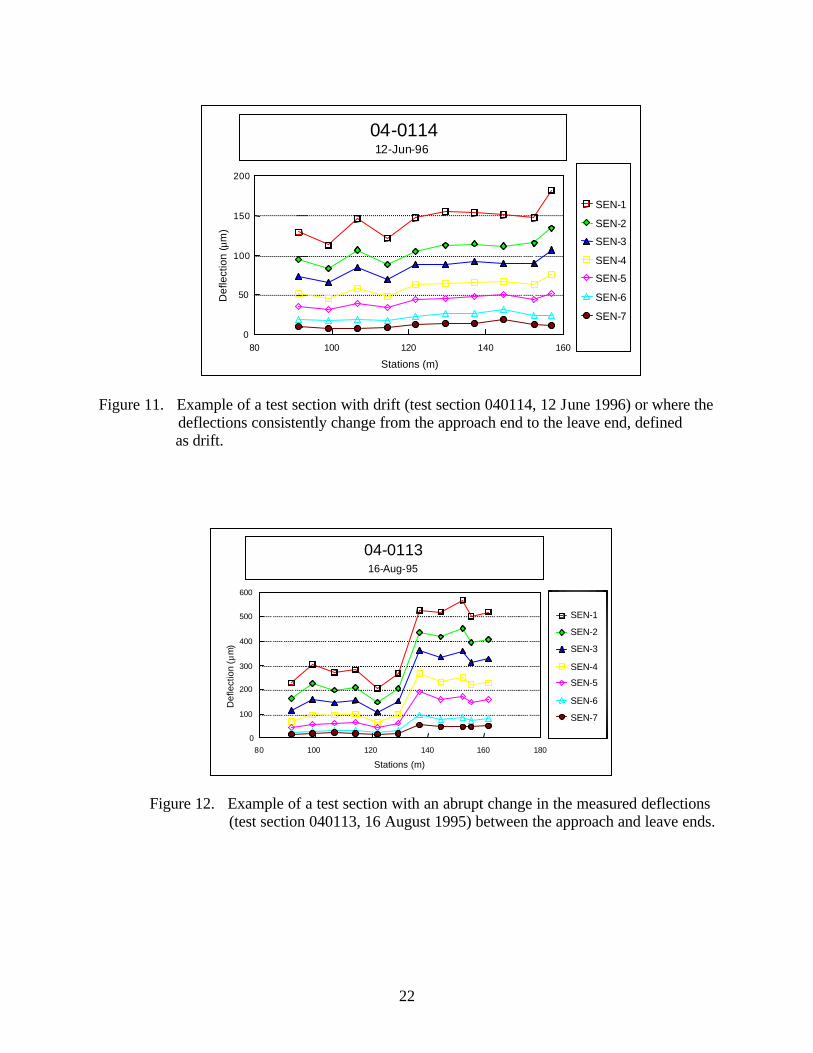
1996) or high variability in the measured deflections.......................................................... 21 11. Example of a test section with drift (test section 040114, 12 June 1996) or where the

deflections consistently change from the approach end to the leave end, defined as drift .. 22 12. Example of a test section with an abrupt change in the measured deflections (test section

040113, 16 August 1995) between the approach and leave ends......................................... 22 13. Graphical illustration of the average Young’s modulus for the pavement layers and

subgrade computed from deflections measured along test section 091803 in August 1994 for different maximum RMS errors ..................................................................................... 35

14. Graphical illustration of the average Young’s modulus for the pavement layers and subgrade computed from deflections measured along test section 131005 in January 1996 for different maximum RMS errors ..................................................................................... 36

15. Graphical illustration of the average Young’s modulus for the pavement layers and subgrade computed from deflections measured along test section 481068 in August 1994 for different maximum RMS errors ..................................................................................... 37

16. Graphical illustration of the average Young’s modulus for the pavement layers and subgrade computed from deflections along test section 081053 in March 1995

for different maximum RMS errors ..................................................................................... 38 17. Distribution of the RMS errors for all of the deflection basins measured on the flexible

pavement test sections that were analyzed with the linear elastic modulus of MODCOMP4 ....................................................................................................................... 40 18. Distribution of the RMS errors for all of the deflection basins measured on the rigid

pavement test sections that were analyzed with the linear elastic module of MODCOMP4 ....................................................................................................................... 41 19. Longitudinal variation of Young’s modulus in the wheelpath for each pavement layer and

subgrade along test section 091803 in August 1994 ............................................................ 42 20. Longitudinal variation of Young’s modulus in the wheelpath for each pavement layer and

subgrade along test section 131005 in January 1996 ........................................................... 43 21. Longitudinal variation of Young’s modulus in the wheelpath for each pavement layer and

subgrade along test section 481068 in August 1994 ............................................................ 44

vii

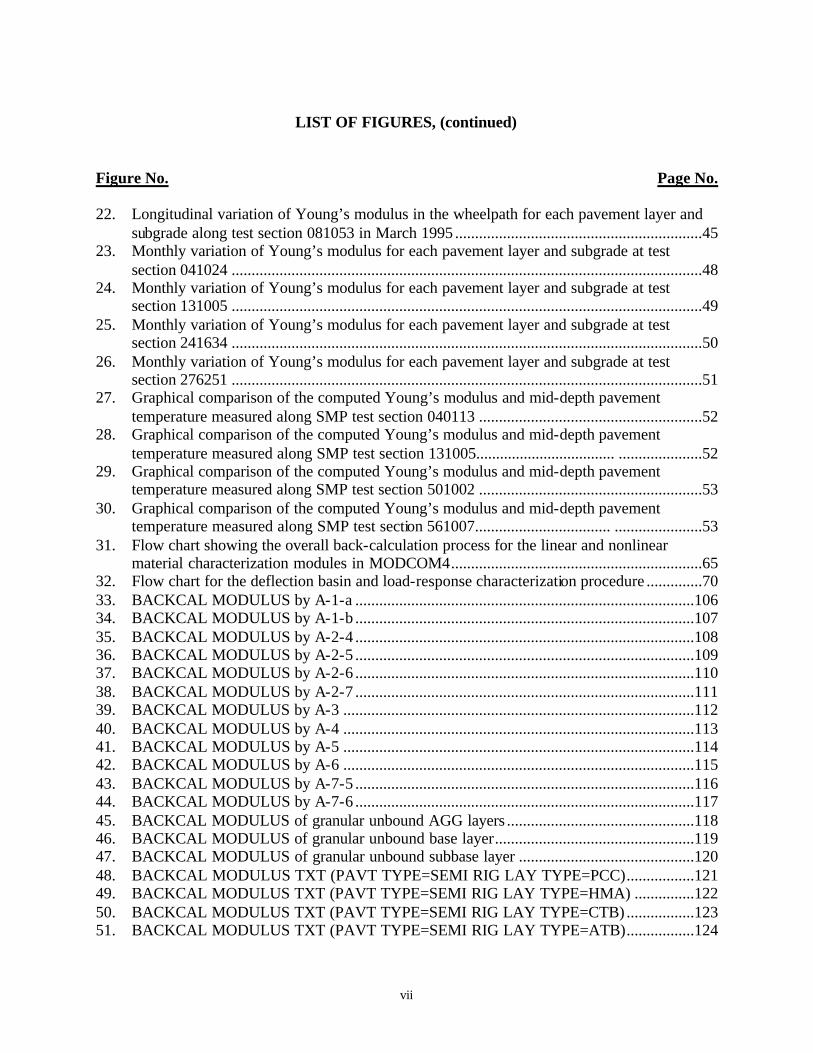
LIST OF FIGURES, (continued)

Figure No. Page No. 22. Longitudinal variation of Young’s modulus in the wheelpath for each pavement layer and

subgrade along test section 081053 in March 1995 ..............................................................45 23. Monthly variation of Young’s modulus for each pavement layer and subgrade at test

section 041024 ......................................................................................................................48 24. Monthly variation of Young’s modulus for each pavement layer and subgrade at test

section 131005 ......................................................................................................................49 25. Monthly variation of Young’s modulus for each pavement layer and subgrade at test

section 241634 ......................................................................................................................50 26. Monthly variation of Young’s modulus for each pavement layer and subgrade at test

section 276251 ......................................................................................................................51 27. Graphical comparison of the computed Young’s modulus and mid-depth pavement

temperature measured along SMP test section 040113 ........................................................52 28. Graphical comparison of the computed Young’s modulus and mid-depth pavement

temperature measured along SMP test section 131005................................... .....................52 29. Graphical comparison of the computed Young’s modulus and mid-depth pavement

temperature measured along SMP test section 501002 ........................................................53 30. Graphical comparison of the computed Young’s modulus and mid-depth pavement

temperature measured along SMP test section 561007.................................. ......................53 31. Flow chart showing the overall back-calculation process for the linear and nonlinear

material characterization modules in MODCOM4...............................................................65 32. Flow chart for the deflection basin and load-response characterization procedure ..............70 33. BACKCAL MODULUS by A-1-a .....................................................................................106 34. BACKCAL MODULUS by A-1-b .....................................................................................107 35. BACKCAL MODULUS by A-2-4 .....................................................................................108 36. BACKCAL MODULUS by A-2-5 .....................................................................................109 37. BACKCAL MODULUS by A-2-6 .....................................................................................110 38. BACKCAL MODULUS by A-2-7 .....................................................................................111 39. BACKCAL MODULUS by A-3 ........................................................................................112 40. BACKCAL MODULUS by A-4 ........................................................................................113 41. BACKCAL MODULUS by A-5 ........................................................................................114 42. BACKCAL MODULUS by A-6 ........................................................................................115 43. BACKCAL MODULUS by A-7-5 .....................................................................................116 44. BACKCAL MODULUS by A-7-6 .....................................................................................117 45. BACKCAL MODULUS of granular unbound AGG layers ...............................................118 46. BACKCAL MODULUS of granular unbound base layer..................................................119 47. BACKCAL MODULUS of granular unbound subbase layer ............................................120 48. BACKCAL MODULUS TXT (PAVT TYPE=SEMI RIG LAY TYPE=PCC).................121 49. BACKCAL MODULUS TXT (PAVT TYPE=SEMI RIG LAY TYPE=HMA) ...............122 50. BACKCAL MODULUS TXT (PAVT TYPE=SEMI RIG LAY TYPE=CTB) .................123 51. BACKCAL MODULUS TXT (PAVT TYPE=SEMI RIG LAY TYPE=ATB).................124

viii

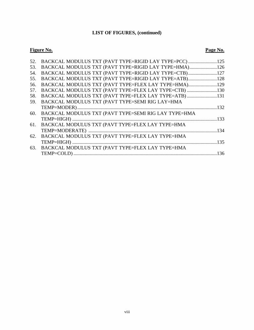
LIST OF FIGURES, (continued) Figure No. Page No. 52. BACKCAL MODULUS TXT (PAVT TYPE=RIGID LAY TYPE=PCC) .......................125 53. BACKCAL MODULUS TXT (PAVT TYPE=RIGID LAY TYPE=HMA)......................126 54. BACKCAL MODULUS TXT (PAVT TYPE=RIGID LAY TYPE=CTB) .......................127 55. BACKCAL MODULUS TXT (PAVT TYPE=RIGID LAY TYPE=ATB).......................128 56. BACKCAL MODULUS TXT (PAVT TYPE=FLEX LAY TYPE=HMA).......................129 57. BACKCAL MODULUS TXT (PAVT TYPE=FLEX LAY TYPE=CTB) ........................130 58. BACKCAL MODULUS TXT (PAVT TYPE=FLEX LAY TYPE=ATB) ........................131 59. BACKCAL MODULUS TXT (PAVT TYPE=SEMI RIG LAY=HMA TEMP=MODER) ................................................................................................................132 60. BACKCAL MODULUS TXT (PAVT TYPE=SEMI RIG LAY TYPE=HMA TEMP=HIGH) ....................................................................................................................133 61. BACKCAL MODULUS TXT (PAVT TYPE=FLEX LAY TYPE=HMA

TEMP=MODERATE) .......................................................................................................134 62. BACKCAL MODULUS TXT (PAVT TYPE=FLEX LAY TYPE=HMA TEMP=HIGH) ....................................................................................................................135 63. BACKCAL MODULUS TXT (PAVT TYPE=FLEX LAY TYPE=HMA TEMP=COLD) ...................................................................................................................136

1

BACK-CALCULATION OF LAYER PARAMETERS FOR LTPP TEST SECTIONS

Volume II: Layered Elastic Analysis for Flexible and Rigid Pavements

1.0 INTRODUCTION 1.1 Background Deflection basin measurements have been made with the Falling Weight Deflectometer (FWD) on all General Pavement Study (GPS) and Specific Pavement Study (SPS) test sections that are included in the Long-Term Pavement Performance (LTPP) program. This deflection-testing program is being conducted periodically to obtain the load-response characteristics of the pavement structure and subgrade. FWD deflection basin tests are conducted about every 2 years for the SPS project sites and about every 5 years for the GPS sites. There are 64 test sections included in the LTPP Seasonal Monitoring Program (SMP), and these sites are tested about every month over a period of 1 to 2 years. These deflection basin data are intended to provide structural-response characteristics that are needed to achieve the overall LTPP program objectives. One of the more common methods for analysis of deflection data is to back-calculate the elastic properties for each layer in the pavement structure and foundation. These analysis methods (referred to as back-calculation programs) provide the elastic layer modulus typically used for pavement evaluation and rehabilitation design. At present, interpretation of deflection basin test results usually is performed with static-linear analyses, and there are numerous computer programs that can be used to calculate these elastic modulus values (Young’s modulus). This report documents the procedure that was used to back-calculate, in mass, the elastic properties for both flexible and rigid pavements in the LTPP program using layered elastic analyses. All data used for this back-calculation study were extracted from the LTPP data release dated October 1997 for the SMP sites and April 1998 for the GPS and SPS sites, and have a level E status (the highest quality data in the LTPP database). All work was completed under the LTPP Data Analysis Technical Support Study (Contract No. DTFH61-96-C-00003). 1.2 LTPP Deflection Testing Program The LTPP deflection basin testing program uses seven sensors placed at 0, 203, 305, 457, 610, 914, and 1524 mm from the center of the load plate to define the shape of the deflection basin. The loading sequence, as stored in the LTPP database for flexible and rigid pavement testing, is summarized in table 1. The following summarizes the general locations for the deflection tests for each different type of pavement.

2

• For flexible pavements, deflection basins are measured both in and between the wheelpaths at a spacing of about 15.2 meters (m). The in-wheelpath measurements are designated in the database as F1, and the between-wheelpath measurements are designated as F3.

• For jointed concrete pavements (JCP), deflection basins are measured at the center of the

slab and at the joints. All mid- lane, center-slab deflections are designated as J1 in the database, and the measurements made at the corners of the slab and along the edge of the slab are designated as J2 and J3, respectively. The center-slab deflections were the only measurements used to back-calculate elastic layer modulus.

• For continuously reinforced concrete pavements (CRCP), deflection basins are measured

along the mid- lane path at a spacing of about 7.6 m and are designated as C1 in the database.

Table 1. LTPP FWD deflection basin testing plan.

Pavement Type Drop Height Number of Drops Target Load, kN Acceptable Load Range, kN

3 3 Seating --- 1 4 26.7 24.0 to 29.4 2 4 40.0 36.0 to 44.0 3 4 53.4 48.1 to 58.7

Flexible

4 4 71.2 64.1 to 78.3 3 3 Seating --- 2 4 40.0 36.0 to 44.0 3 4 53.4 48.1 to 58.7

Rigid, JCP & CRCP

4 4 71.2 64.1 to 78.3 A more complete description of the testing plan and data storage in the database is provided in LTPP Manual for Falling Weight Deflectometer Measurements – Operational Field Guidelines, Version 3.1, dated August 2000. 1.3 Objective The primary objective of this study was to back-calculate the elastic layer properties from deflection basin measurements for use in further data analyses and studies regarding pavement performance. As part of this objective, the elastic layer properties back-calculated from the deflection basin data for the LTPP flexible and rigid pavement test sections were to be included in the LTPP computed parameter database for future use. A secondary objective of this study was to provide any modifications to the current guidelines that have been prepared for use in back-calculating elastic properties. These guidelines include

3

ASTM D5858 and the procedure written by Von Quintus and Killingsworth.(1) Another secondary objective was to identify those LTPP test sections with unusual load-response characteristics. 1.4 Application of Results to Future Studies The elastic properties computed for each structural layer in the pavement structure and subgrade strata can be used in future studies of materials-pavement behavior and performance. In fact, these computed parameters will be needed to achieve some of the stated objectives and “outcomes” identified in the LTPP Strategic Plan that was published in 1999.(18) For example, elastic properties can be used directly in developing or validating load-related distress prediction models based on elastic layer theory or used indirectly for selecting test sections with significantly different properties for studying a particular design issue. The following lists some of the LTPP strategic objectives where the results from this study can be used to achieve those objectives.

• Identify improved designs and design features with accurate service predictions, tendencies, or trends.

o Objective 5 – Development of pavement response and performance models applicable to pavement design and performance prediction.

o Objective 7 – Quantification of the performance impact of specific design features (presence or absence of positive drainage, differing levels of prerehabilitated surface preparation, etc.).

• Identify improved measurement and prediction tools.

o Objective 2 – Materials characterization procedures.

• Determine the environmental effects on pavement performance. o Objective 3 – Determination of environmental effects in pavement design and

performance prediction.

Some specific applications of these results are listed below.

• Selection of test sections for comparing pavement structures with significantly different layer stiffnesses and subgrade support conditions.

• Selection of test sections for analyzing pavement structures with unique material behavior or load-response characteristics (i.e., deflection hardening versus deflection softening).

• Comparison of laboratory-measured properties to the properties computed from deflection basins for developing the calibration adjustments that may be needed when using specific design procedures.

• Application of computed elastic properties for developing or validating distress/performance models that are based on elastic layer theory.

• Application of the computed elastic properties in determining or validating seasonal or climatic effects on pavement performance and material behavior.

5

2.0 SELECTION OF BACK-CALCULATION METHODOLOGY There are three basic approaches to back-calculating layered elastic moduli of pavement structures: 1) the equivalent thickness method (e.g., ELMOD and BOUSDEF), 2) the optimization method (e.g., MODULUS and WESDEF), and 3) the iterative method (e.g., MODCOMP and EVERCALC). Layer thickness is a critical parameter that must be accurately known for nearly all back-calculation programs, regardless of methodology, although some programs claim to be able to determine a limited set of both Young’s modulus and layer thickness (e.g., MICHBACK).(2) Many of the software packages are similar, but the results can be different as a result of the assumptions, iteration technique, back-calculation, or forward-calculation schemes used within the programs. Within the past couple of decades, there have been extensive efforts devoted to improving back-calculation of elastic- layer modulus by reducing the absolute error or root mean squared (RMS) error (difference between measured and calculated deflection basins) to values as small as possible. The absolute error term is the absolute difference between the measured and computed deflection basins expressed as a percent error or difference per sensor; whereas the RMS error term represents the goodness-of- fit between the measured and computed deflection basins. The use of these linear elastic layer programs, however, has been only partly successful in analyzing the deflections measured at the LTPP sites. For example, only about 50 percent of the flexible GPS sites were found to have absolute error terms less than the generally considered reasonable value of 2 percent per sensor. (3,4) In addition, results from use of linear elastic models are highly variable, with an undefined reliability over a wide range of conditions. So the question is: which program should be used to back-calculate Young’s modulus for each structural layer in the pavement structure? The purpose of this section is to document the methodology and software package used for back-calculating pavement layer and subgrade moduli from the deflection basins measured on all LTPP test sections that have a level E data status. 2.1 Back-Calculation Methods The common analysis method is to back-calculate material response parameters for each layer within the pavement structure from the FWD deflection basin measurements. Many of the back-calculation programs are limited by the number and thickness of the layers used to define the pavement structure but, more importantly, assume that the layers are linear elastic. Most unbound pavement materials and soils are nonlinear. Thus, the calculated layer-modulus represents an “effective” Young’s modulus that adjusts for stress-sensitivity and discontinuities or anomalies (such as variations in layer thickness, localized segregation, cracks, and the combinations of similar materials into a single layer).

6

The back-calculation methods can be grouped into four general categories.

• Static (Load Application) – Linear (Material Characterization) Methods. • Static (Load Application) – Nonlinear (Material Characterization) Methods. • Dynamic (Load Application) – Linear (Material Characterization) Methods. • Dynamic (Load Application) – Nonlinear (Material Characterization) Methods.

2.1.1 Type of Load Application. At present, interpretation of deflection basin test results is performed with static analyses. There have been many improvements in back-calculation technology within the past 4 to 5 years. These improvements have spawned standardization procedures and guidelines to ensure that there is consistency within the industry and to improve upon the load-response characterization of the pavement structural layers.(5) ASTM D5858 is a procedure for analyzing deflection basin test results to determine layer elastic moduli (i.e., Young’s modulus). There are no similar standardized procedures for back-calculating materials properties of pavement layers using dynamic analysis techniques. In fact, there are only a few programs that have the capability to do dynamic analyses. Thus, the programs using dynamic analyses were not considered for use in calculating elastic- layer modulus from hundreds of deflection basins measured at the same site. Only the static load application analysis methods were considered appropriate for use in a production mode – mass back-calculation of elastic layer modulus from deflection basins measured along the LTPP test sections. 2.1.2 Type of Material Response Models. Most of the back-calculation procedures that have been used to determine layer moduli are based on elastic layer theory. However, some of the programs based on elastic theory have been modified to account for the viscoelastic (time-dependent) or elastoplastic (inelastic) behavior of materials. Unfortunately, programs that include time-dependent properties or inelastic properties have not been used in a production mode and, more importantly, have not been very successful in producing consistent and reliable solutions. SHRP, as well as others, studied and evaluated many of these back-calculation procedures to select one method for use in characterizing the subgrade and other pavement layers in order to predict the performance of flexible and rigid pavements.(6,7) The program entitled “MODULUS 4.0" was selected for flexible and composite pavements, whereas a new procedure was developed for rigid pavements as part of the SHRP P-020 Data Analysis Project.(8,9) As stated above, many of these programs are limited by the following:

• Number of layers and the thickness of those layers that can be used to describe the pavement structure.

• Assumption that the materials are linear-elastic. Thus, it must be understood that the calculated layer modulus represents an "effective" or "equivalent" elastic modulus that accounts for differences in stress states and any discontinuities

7

or anomalies (such as variations in layer thickness, slippage between two adjacent layers, cracks, and the combinations of similar materials into a single layer). Although there have been extensive efforts devoted to improving back-calculation of layer moduli by reducing the RMS error to values as small as possible, highly variable results from the use of linear elastic models have been found with an undefined reliability over a wide range of conditions. In addition, models that assume a linear response of materials require numerous iterations at varying load levels (different drop heights) to identify the stress sensitivity of unbound pavement materials and soils. From this standpoint, the use of nonlinear elastic layer programs was believed to have merit. Two programs that have been used with some success and contain a nonlinear structural response capability are MODCOMP and a program developed by the Corps of Engineers at the Waterways Experiment Station.(10,11) The Corps of Engineers program has the capability of a true nonlinear response model but has not been used on a large number of projects and does not have a batch mode processor or data management software to facilitate its use in a production mode. Conversely, MODCOMP can be used on a production mode basis, and its convergence is reasonably fast, but it is a quasi-nonlinear response model. Stated differently, for the same load level, the modulus of a layer does not vary horizontally or vertically within that layer in accordance with changes in stress state. The layer modulus is only varied by stress state between load levels and sensor locations. Standardized procedures and guidelines are available to assist in this back-calculation process. Some of these include procedures written under the SHRP program ASTM D5858 and the one documented in report FHWA-RD-97-076, Design Pamphlet for the Back-Calculation of Pavement Layer Moduli in Support of the 1993 AASHTO Guide for the Design of Pavement Structures.(1,5,6) All of these programs and guidelines are based on the use of elastic layer response programs. Viscoelastic or elastoplastic response programs have not been used in a sufficient number of projects to substantiate the reliability and adequacy of their use. Therefore, selection of the back-calculation software and procedures were confined to those that are based on the use of elastic layer theory. 2.1.3 Summary. Although many analyses of deflection data can be undertaken, the studies currently underway within the LTPP program, by definition, require highly focused efforts accomplishable within a short period of time. Thus, the study for back-calculating layer moduli looked only at the computation of material properties using existing software that has the capability to analyze massive amounts of deflection data in a reasonable time frame. These requirements basically restrict the back-calculation methodology to a static load analyzed with a linear or nonlinear elastic response model. 2.2 Selection Factors It should be understood that many different software packages can be used to calculate the elastic modulus of pavement layers and subgrade soils from deflection basins, as demonstrated in report FHWA-RD-97-086, Back-Calculation of Layer Moduli of LTPP GPS Sites.(3) Many of the

8

software packages that have the same type of response model have, in fact, provided reasonably consistent results. The following lists the factors considered for evaluating the different back-calculation programs based on elastic layer theory and were found to be applicable to pavement diagnostic studies and the requirements noted above.

• Accuracy of the Program. One of the most difficult questions to be answered is, “How accurate are the layer moduli back-calculated from measured deflection basins? ” In reality, this is an impossible question to answer conclusively for real basins, but it must be addressed to promote confidence in the computed results.

• Operational Characteristics. The use of the back-calculation software in a batch mode for

evaluating and analyzing deflection measurements from the LTPP database is an extremely important factor. There are hundreds of deflection basins to be analyzed on a per-site basis, considering the different drop heights, the number of test points along a seasonal and GPS/SPS project site, and the different times of year that these deflection basins were measured. Thus, the software program must have the capability for use in a batch mode process.

• Ease of Use of Program. Other important characteristics of the software to be used in

analyzing the deflection basins from the LTPP database are the flexibility and user interaction of the program. To complete mass back-calculation of deflection basin data, the program must be easy to use when setting up each of the data files for the batch runs previously discussed. In addition, results from the software must be easily extracted and entered into the LTPP database. The majority of the inputs to the program should also be available in the database.

• Stability of Program. The stability of the program is another important factor that was

considered in the evaluation and selection of software. Any program considered for analyzing massive quantities of deflection basins must be stable for a diverse set of conditions (pavement type, layer thickness, deflection basins, etc.). In other words, the results rapidly converge within a few iterations, rather than diverge or take many iterations to converge.

• Probability of Success. This issue is another very important factor. The software to be

used in back-calculating layer moduli from tens of thousands of deflection basins needs to have a reasonable probability of finding reasonable layer elastic moduli that are consistent with the structural response program used to calculate the deflection basins. A probability of success of only 50 percent is inadequate for use on this project. MODCOMP4 was found to result in reasonable solutions in over 90 percent of the initial study sections.

2.3 Selection of Software – MODCOMP4 The evaluation focused on two areas: (1) the ability and accuracy of the software to determine elastic- layer moduli of the pavement materials and soils and (2) operational characteristics—ease

9

of use in a production mode, flexibility in analyzing a wide range of pavement structures (flexible and rigid), and material response models. Much of the information used for the software selection process was obtained from previous comparisons and evaluation studies of the software. (See references 3, 7, 12, and 13.) The primary reasons that MODCOMP4 was selected as the program for calculating the elastic properties of pavement structural layers and subgrade soils from FWD deflection basins measured at the LTPP SMP, GPS, and SPS test sections are listed below.

1. First and foremost, the use of a nonlinear constitutive equation to represent the response of unbound pavement materials and soils was believed to provide added value and to result in a higher number of reasonable or adequate solutions. The use of linear elastic response models can be used to estimate the nonlinear properties but require more steps in the back-calculation process. A software package that has the capability to do both is believed to have increased flexibility in its overall usage on this project and in future projects (such as National Cooperative Highway Research Program [NCHRP] Project 1-37A) and should be more adaptable to a wider range of conditions and materials. More importantly, a common opinion of a group of experts was that successful back-calculation using much of the LTPP deflection data would require use of nonlinear characterization.(14) As noted above, MODCOMP was believed to have added value and was selected because it considers different nonlinear constitutive equations in determining the elastic response properties.

2. The process for back-calculating elastic properties only looked at the

computation of material and soil properties using existing software packages that have the capability to analyze large amounts of deflection data in a reasonable time frame. As noted above, this requirement restricted the back-calculation methodology to a static load analyzed with a linear or nonlinear elastic response model. MODCOMP was selected because its convergence is reasonably fast, and it can be used in a production basis to mass-calculate elastic properties from hundreds of deflection basins measured at a site over time.

3. Elastic layer theory was used to calculate a deflection basin under a

specific load for a known set of layer moduli. MODCOMP was used to calculate the layer modulus from these deflection basins. The difference between the calculated and target (or known) modulus was used to estimate the accuracy of the program and to establish a practical error term for the matched deflection basin. The RMS error for each solution and the percent difference between the calculated and the target or known moduli were the parameters considered in the evaluation. The RMS error was found to vary from 0.1 to 1 percent, which is considered very acceptable.

10

4. Another very important fact: The revisions and changes made to the MODCOMP program to correct a problem identified in the 1991 SHRP review study significantly improved the stability and success in achieving reasonable solutions.(7) The probability of success for the limited number of basins reviewed in the preliminary study was in excess of 90 percent, which was considered good for the diverse conditions used in the examples.

5. The majority of the inputs needed to execute MODCOMP in a batch mode

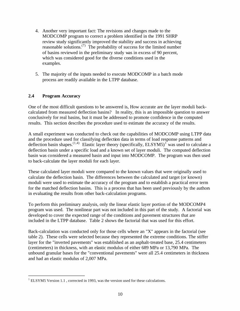
process are readily available in the LTPP database. 2.4 Program Accuracy One of the most difficult questions to be answered is, How accurate are the layer moduli back-calculated from measured deflection basins? In reality, this is an impossible question to answer conclusively for real basins, but it must be addressed to promote confidence in the computed results. This section describes the procedure used to estimate the accuracy of the results. A small experiment was conducted to check out the capabilities of MODCOMP using LTPP data and the procedure used for classifying deflection data in terms of load response patterns and deflection basin shapes.(1,4) Elastic layer theory (specifically, ELSYM5)1 was used to calculate a deflection basin under a specific load and a known set of layer moduli. The computed deflection basin was considered a measured basin and input into MODCOMP. The program was then used to back-calculate the layer moduli for each layer. These calculated layer moduli were compared to the known values that were originally used to calculate the deflection basin. The differences between the calculated and target (or known) moduli were used to estimate the accuracy of the program and to establish a practical error term for the matched deflection basins. This is a process that has been used previously by the authors in evaluating the results from other back-calculation programs. To perform this preliminary analysis, only the linear elastic layer portion of the MODCOMP4 program was used. The nonlinear part was not included in this part of the study. A factorial was developed to cover the expected range of the conditions and pavement structures that are included in the LTPP database. Table 2 shows the factorial that was used for this effort. Back-calculation was conducted only for those cells where an "X" appears in the factorial (see table 2). These cells were selected because they represented the extreme conditions. The stiffer layer for the "inverted pavements" was established as an asphalt-treated base, 25.4 centimeters (centimeters) in thickness, with an elastic modulus of either 689 MPa or 13,790 MPa. The unbound granular bases for the "conventional pavements" were all 25.4 centimeters in thickness and had an elastic modulus of 2,007 MPa. 1 ELSYM5 Version 1.1 , corrected in 1993, was the version used for these calculations.

11

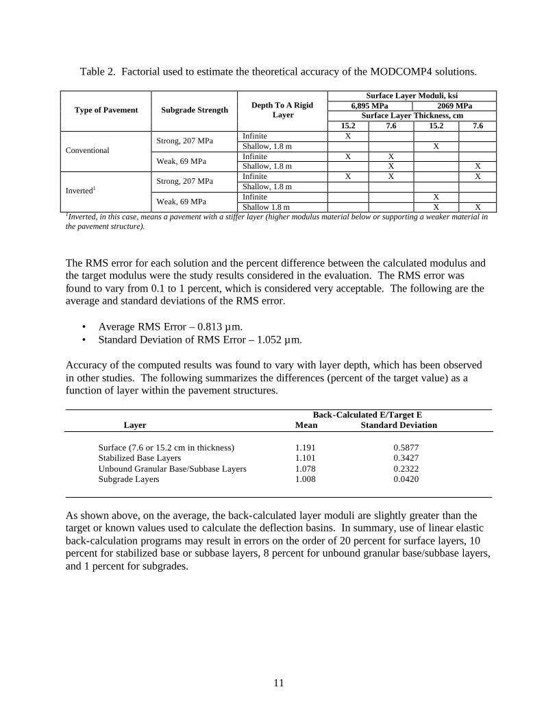
Table 2. Factorial used to estimate the theoretical accuracy of the MODCOMP4 solutions.

Surface Layer Moduli, ksi 6,895 MPa 2069 MPa

Surface Layer Thickness, cm Type of Pavement Subgrade Strength Depth To A Rigid

Layer 15.2 7.6 15.2 7.6

Infinite X Strong, 207 MPa Shallow, 1.8 m X Infinite X X

Conventional Weak, 69 MPa Shallow, 1.8 m X X

Infinite X X X Strong, 207 MPa Shallow, 1.8 m Infinite X

Inverted1

Weak, 69 MPa Shallow 1.8 m X X

1Inverted, in this case, means a pavement with a stiffer layer (higher modulus material below or supporting a weaker material in the pavement structure). The RMS error for each solution and the percent difference between the calculated modulus and the target modulus were the study results considered in the evaluation. The RMS error was found to vary from 0.1 to 1 percent, which is considered very acceptable. The following are the average and standard deviations of the RMS error.

• Average RMS Error – 0.813 µm. • Standard Deviation of RMS Error – 1.052 µm.

Accuracy of the computed results was found to vary with layer depth, which has been observed in other studies. The following summarizes the differences (percent of the target value) as a function of layer within the pavement structures. Back-Calculated E/Target E

Layer Mean Standard Deviation

Surface (7.6 or 15.2 cm in thickness) 1.191 0.5877 Stabilized Base Layers 1.101 0.3427 Unbound Granular Base/Subbase Layers 1.078 0.2322 Subgrade Layers 1.008 0.0420

As shown above, on the average, the back-calculated layer moduli are slightly greater than the target or known values used to calculate the deflection basins. In summary, use of linear elastic back-calculation programs may result in errors on the order of 20 percent for surface layers, 10 percent for stabilized base or subbase layers, 8 percent for unbound granular base/subbase layers, and 1 percent for subgrades.

13

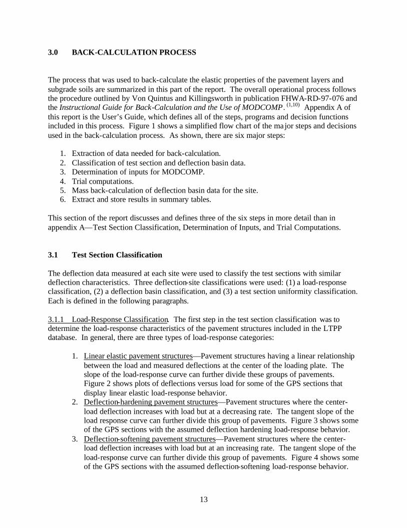
3.0 BACK-CALCULATION PROCESS The process that was used to back-calculate the elastic properties of the pavement layers and subgrade soils are summarized in this part of the report. The overall operational process follows the procedure outlined by Von Quintus and Killingsworth in publication FHWA-RD-97-076 and the Instructional Guide for Back-Calculation and the Use of MODCOMP. (1,10) Appendix A of this report is the User’s Guide, which defines all of the steps, programs and decision functions included in this process. Figure 1 shows a simplified flow chart of the ma jor steps and decisions used in the back-calculation process. As shown, there are six major steps:

1. Extraction of data needed for back-calculation. 2. Classification of test section and deflection basin data. 3. Determination of inputs for MODCOMP. 4. Trial computations. 5. Mass back-calculation of deflection basin data for the site. 6. Extract and store results in summary tables.

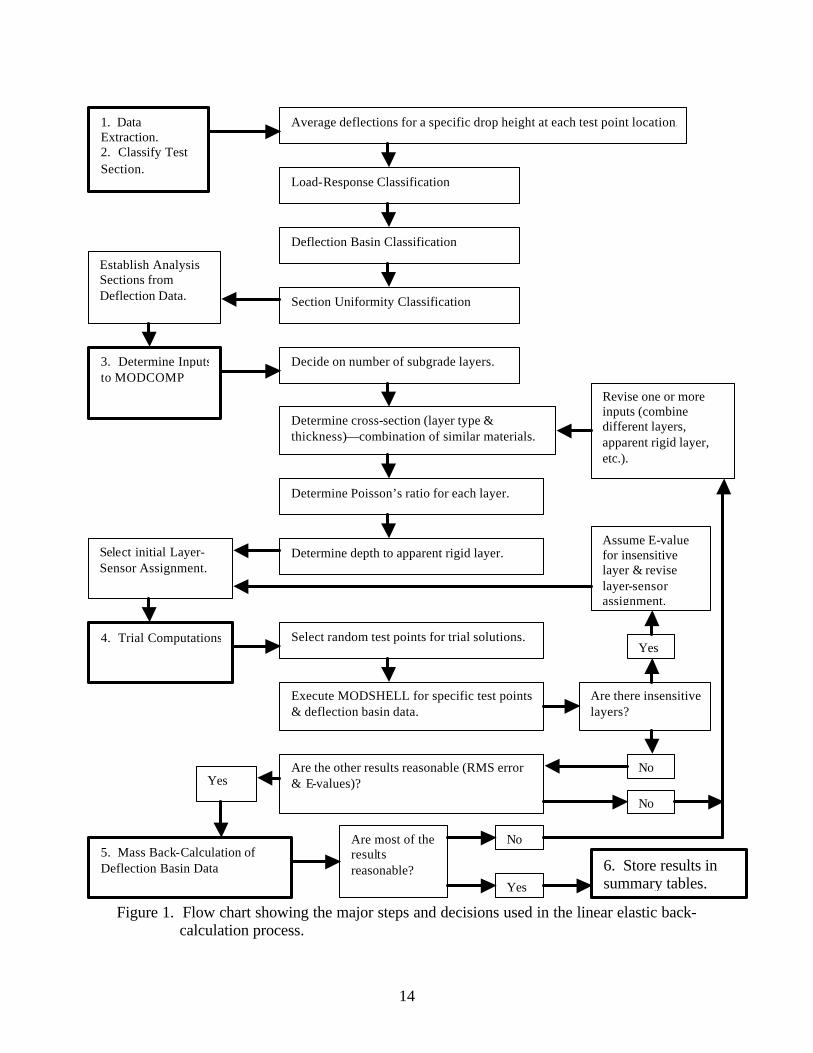
This section of the report discusses and defines three of the six steps in more detail than in appendix A—Test Section Classification, Determination of Inputs, and Trial Computations. 3.1 Test Section Classification The deflection data measured at each site were used to classify the test sections with similar deflection characteristics. Three deflection-site classifications were used: (1) a load-response classification, (2) a deflection basin classification, and (3) a test section uniformity classification. Each is defined in the following paragraphs. 3.1.1 Load-Response Classification. The first step in the test section classification was to determine the load-response characteristics of the pavement structures included in the LTPP database. In general, there are three types of load-response categories:

1. Linear elastic pavement structures—Pavement structures having a linear relationship

between the load and measured deflections at the center of the loading plate. The slope of the load-response curve can further divide these groups of pavements. Figure 2 shows plots of deflections versus load for some of the GPS sections that display linear elastic load-response behavior.

2. Deflection-hardening pavement structures—Pavement structures where the center-load deflection increases with load but at a decreasing rate. The tangent slope of the load response curve can further divide this group of pavements. Figure 3 shows some of the GPS sections with the assumed deflection hardening load-response behavior.

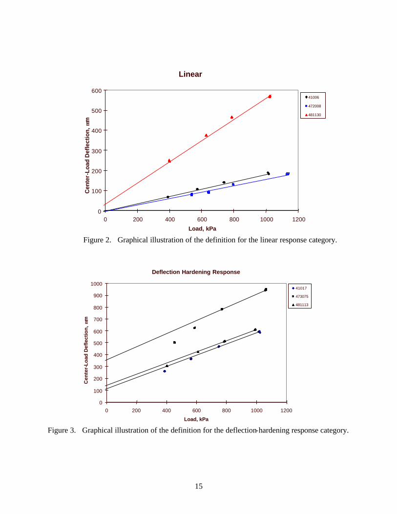
3. Deflection-softening pavement structures—Pavement structures where the center-load deflection increases with load but at an increasing rate. The tangent slope of the load-response curve can further divide this group of pavements. Figure 4 shows some of the GPS sections with the assumed deflection-softening load-response behavior.

14

Figure 1. Flow chart showing the major steps and decisions used in the linear elastic back- calculation process.

1. Data Extraction. 2. Classify Test Section.

Load-Response Classification

Deflection Basin Classification

Section Uniformity Classification

Establish Analysis Sections from Deflection Data.

3. Determine Inputs to MODCOMP

Average deflections for a specific drop height at each test point location.

Decide on number of subgrade layers.

Determine cross-section (layer type & thickness)—combination of similar materials.

Determine Poisson’s ratio for each layer.

Determine depth to apparent rigid layer. Select initial Layer-Sensor Assignment.

4. Trial Computations Select random test points for trial solutions.

Execute MODSHELL for specific test points & deflection basin data.

Are there insensitive layers?

No

Yes

Assume E-value for insensitive layer & revise layer-sensor assignment.

Are the other results reasonable (RMS error & E-values)? Yes

Revise one or more inputs (combine different layers, apparent rigid layer, etc.).

No

5. Mass Back-Calculation of Deflection Basin Data

Are most of the results reasonable?

No

Yes 6. Store results in summary tables.

15

Figure 2. Graphical illustration of the definition for the linear response category.

Figure 3. Graphical illustration of the definition for the deflection-hardening response category.

Linear

0

100

200

300

400

500

600

0 200 400 600 800 1000 1200 Load, kPa

Cent

er-L

oad

Def

lect

ion,

µm

41006 472008 481130

Deflection Hardening Response

0 100 200 300 400 500 600 700 800 900

1000

0 200 400 600 800 1000 1200 Load, kPa

Cen

ter-L

oad

Def

lect

ion,

µm

41017 473075 481113

16

Figure 4. Graphical illustration of the definition for the deflection-softening response category. In determining the load-response behavior of these test sections, a linear model was used (i.e., a linear relationship between load and the deflection measured at the center of the loading plate). The slope and intercept were determined for each set of deflection data, and the multiple correlation coefficient, R2, was determined for these linear relationships for each set of deflection data. The criteria used to characterize the load-response behavior was somewhat judgmental, but was defined by R2 and the deflection intercept plus geometric considerations. The criteria used to establish the load-response behavior are listed below.

• If the R2 was equal to or greater than 0.99 and the intercept was between –10 and 10 µm, the response was considered to be elastic (figure 2).

• If the R2 was equal to or greater than 0.99 but the intercept fell out

of the range from –10 to 10 µm, the response was considered to be deflection hardening if the intercept was positive and deflection softening if it was negative.

• If the value of R2 was less than 0.99, the deflection intercept was

determined for a line through the highest two loads. If the intercept was greater than 20 µm, the response was considered to display deflection hardening (figure 3). If the intercept was a negative value greater in absolute value than –20 µm, the response was considered to be deflection softening (figure 4).

Deflection Softening Response

0 100 200 300 400 500 600 700 800 900

1000

0 200 400 600 800 1000 1200 Load, kPa

Cent

er-L

oad

Def

lect

ion,

µm

41016 81057 531801

17

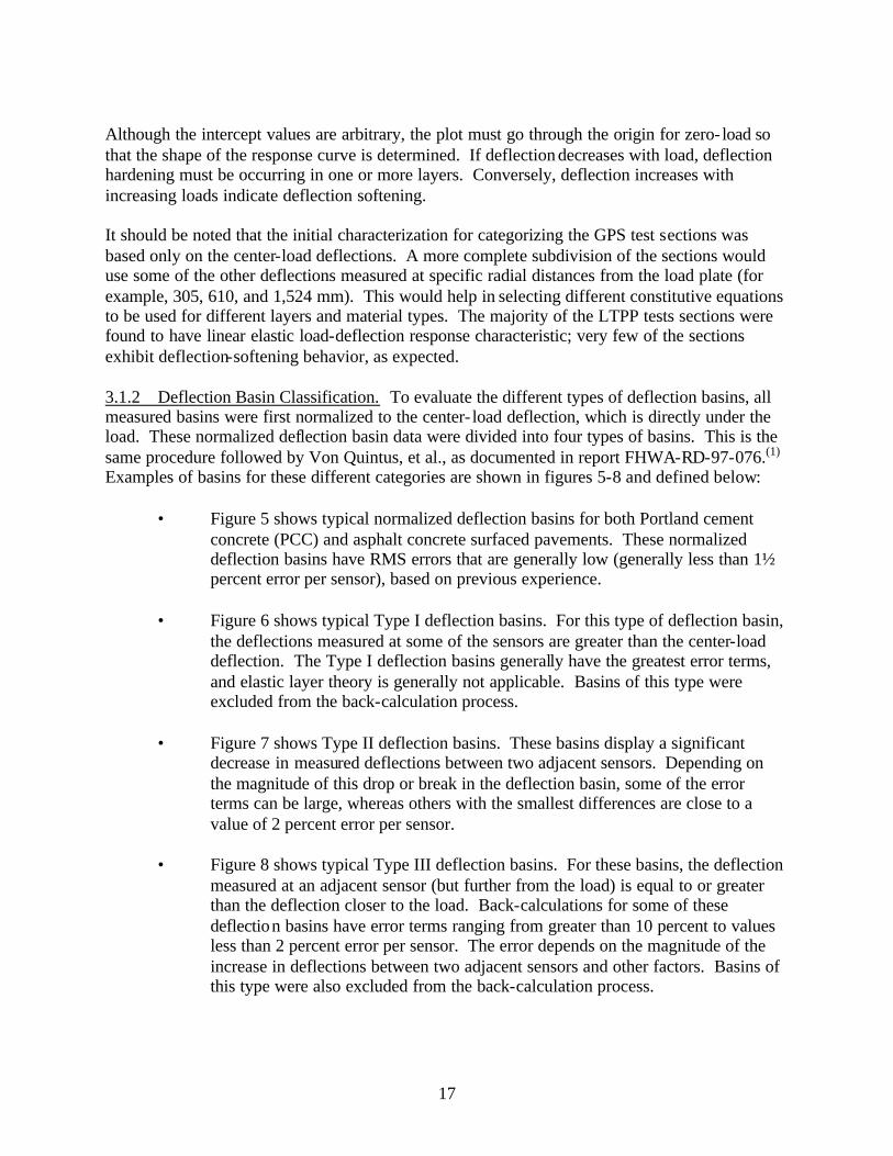
Although the intercept values are arbitrary, the plot must go through the origin for zero- load so that the shape of the response curve is determined. If deflection decreases with load, deflection hardening must be occurring in one or more layers. Conversely, deflection increases with increasing loads indicate deflection softening. It should be noted that the initial characterization for categorizing the GPS test sections was based only on the center-load deflections. A more complete subdivision of the sections would use some of the other deflections measured at specific radial distances from the load plate (for example, 305, 610, and 1,524 mm). This would help in selecting different constitutive equations to be used for different layers and material types. The majority of the LTPP tests sections were found to have linear elastic load-deflection response characteristic; very few of the sections exhibit deflection-softening behavior, as expected. 3.1.2 Deflection Basin Classification. To evaluate the different types of deflection basins, all measured basins were first normalized to the center- load deflection, which is directly under the load. These normalized deflection basin data were divided into four types of basins. This is the same procedure followed by Von Quintus, et al., as documented in report FHWA-RD-97-076.(1)

Examples of basins for these different categories are shown in figures 5-8 and defined below:

• Figure 5 shows typical normalized deflection basins for both Portland cement concrete (PCC) and asphalt concrete surfaced pavements. These normalized deflection basins have RMS errors that are generally low (generally less than 1½ percent error per sensor), based on previous experience.

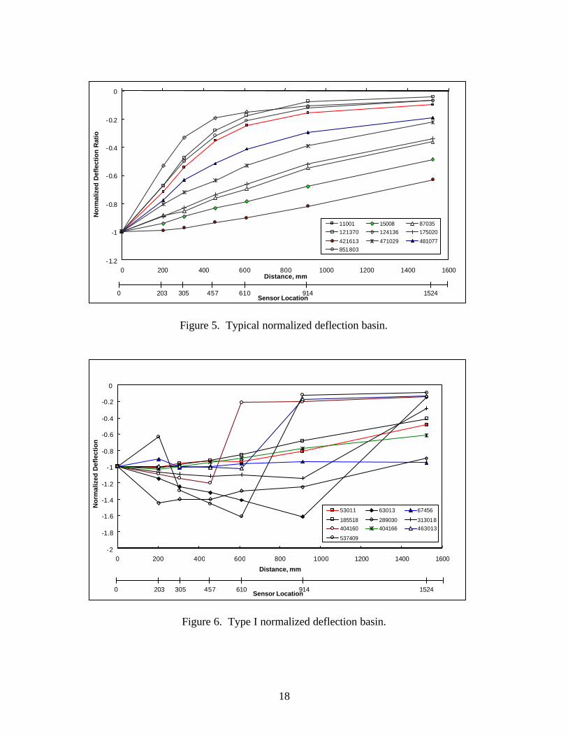
• Figure 6 shows typical Type I deflection basins. For this type of deflection basin,

the deflections measured at some of the sensors are greater than the center-load deflection. The Type I deflection basins generally have the greatest error terms, and elastic layer theory is generally not applicable. Basins of this type were excluded from the back-calculation process.

• Figure 7 shows Type II deflection basins. These basins display a significant

decrease in measured deflections between two adjacent sensors. Depending on the magnitude of this drop or break in the deflection basin, some of the error terms can be large, whereas others with the smallest differences are close to a value of 2 percent error per sensor.

• Figure 8 shows typical Type III deflection basins. For these basins, the deflection

measured at an adjacent sensor (but further from the load) is equal to or greater than the deflection closer to the load. Back-calculations for some of these deflection basins have error terms ranging from greater than 10 percent to values less than 2 percent error per sensor. The error depends on the magnitude of the increase in deflections between two adjacent sensors and other factors. Basins of this type were also excluded from the back-calculation process.

18

Figure 5. Typical normalized deflection basin.

Figure 6. Type I normalized deflection basin.

-1.2

-1

-0.8

-0.6

-0.4

-0.2

0

0 200 400 600 800 1000 1200 1400 1600 Distance, mm

Nor

mal

ized

Def

lect

ion

Rat

io

11001 15008 87035 121370 124136 175020 421613 471029 481077 851803

Sensor Location 0 203 305 457 610 914 1524

-2 -1.8 -1.6 -1.4 -1.2

-1 -0.8 -0.6 -0.4 -0.2

0

0 200 400 600 800 1000 1200 1400 1600 Distance, mm

Nor

mal

ized

Def

lect

ion

Ratio

53011 63013 67456 185518 289030 313018 404160 404166 463013 537409

Sensor Location 0 203 305 457 610 914 1524

19

Figure 7. Type II normalized deflection basin.

Figure 8. Type III normalized deflection basin.

-1.2

-1

-0.8

-0.6

-0.4

-0.2

0

0 200 400 600 800 1000 1200 1400 1600Distance, mm

Nor

mal

ized

Def

lect

ion

Rat

io

13998 63024 189020

295473 415021 429027

Sensor Location0 203 305 457 610 914 1524

-1.2

-1

-0.8

-0.6

-0.4

-0.2

0

0 200 400 600 800 1000 1200 1400 1600 Distance, mm

Nor

mal

ized

Def

lect

ions

41002 41017 41036 54021 63005 204067 307088 566029 567775

Sensor Location 0 203 305 457 610 914 1524

20

In general, Type I and III deflection basins occur most frequently for PCC surfaced pavements. It is believed that these deflection basins may be characteristic of those areas with voids, a loss of support, a severe thermal gradient causing curling of the PCC slab, and/or a combination of these conditions. Conversely, Type II deflection basins occur most frequently for dense-graded asphalt concrete surfaced pavements. As stated above, all Type I and III basins were excluded from the actual back-calculation process. 3.1.3 Test Section Uniformity Classification. The final step included in the classification of each LPPP test section was to determine the uniformity or variability of the deflections measured along the test section. The uniformity of each LTPP test section was classified into one of four different categories, listed below.

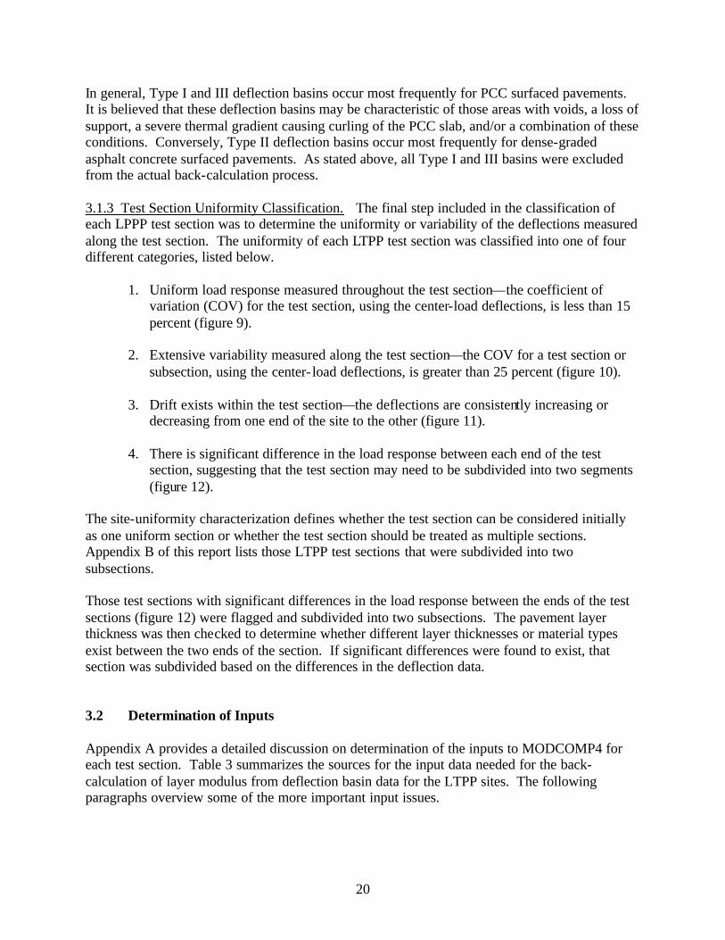
1. Uniform load response measured throughout the test section—the coefficient of variation (COV) for the test section, using the center-load deflections, is less than 15 percent (figure 9).

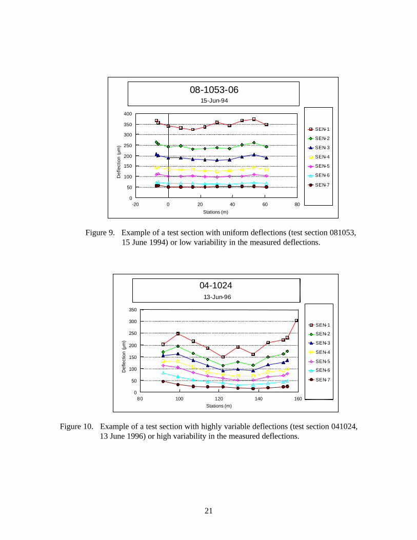
2. Extensive variability measured along the test section—the COV for a test section or

subsection, using the center- load deflections, is greater than 25 percent (figure 10).

3. Drift exists within the test section—the deflections are consistently increasing or decreasing from one end of the site to the other (figure 11).

4. There is significant difference in the load response between each end of the test

section, suggesting that the test section may need to be subdivided into two segments (figure 12).

The site-uniformity characterization defines whether the test section can be considered initially as one uniform section or whether the test section should be treated as multiple sections. Appendix B of this report lists those LTPP test sections that were subdivided into two subsections. Those test sections with significant differences in the load response between the ends of the test sections (figure 12) were flagged and subdivided into two subsections. The pavement layer thickness was then checked to determine whether different layer thicknesses or material types exist between the two ends of the section. If significant differences were found to exist, that section was subdivided based on the differences in the deflection data. 3.2 Determination of Inputs Appendix A provides a detailed discussion on determination of the inputs to MODCOMP4 for each test section. Table 3 summarizes the sources for the input data needed for the back-calculation of layer modulus from deflection basin data for the LTPP sites. The following paragraphs overview some of the more important input issues.

21

Figure 9. Example of a test section with uniform deflections (test section 081053,

15 June 1994) or low variability in the measured deflections.

Figure 10. Example of a test section with highly variable deflections (test section 041024,

13 June 1996) or high variability in the measured deflections.

-20 0 20 40 60 80 0

50 100 150 200 250 300 350 400

Stations (m)

Def

lect

ion

(µm

) SEN-1 SEN-2 SEN-3 SEN-4 SEN-5 SEN-6 SEN-7

08-1053-06 15-Jun-94

80 100 120 140 160 0

50 100 150 200 250 300 350

Stations (m)

Def

lect

ion

(µm

)

SEN-1 SEN-2 SEN-3 SEN-4 SEN-5 SEN-6 SEN-7

04-1024 13-Jun-96

22

Figure 11. Example of a test section with drift (test section 040114, 12 June 1996) or where the deflections consistently change from the approach end to the leave end, defined as drift.

Figure 12. Example of a test section with an abrupt change in the measured deflections

(test section 040113, 16 August 1995) between the approach and leave ends.

80 100 120 140 160 180 0

100 200 300 400 500 600

Stations (m)

Def

lect

ion

(µm

)

SEN-1 SEN-2 SEN-3 SEN-4 SEN-5 SEN-6 SEN-7

04-0113 16-Aug-95

80 100 120 140 160 0

50

100

150

200

Stations (m)

Def

lect

ion

(µm

) SEN-1 SEN-2 SEN-3 SEN-4 SEN-5 SEN-6 SEN-7

04-0114 12-Jun-96

23

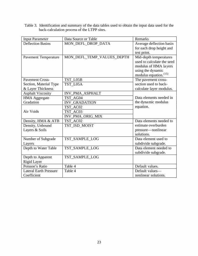
Table 3. Identification and summary of the data tables used to obtain the input data used for the back-calculation process of the LTPP sites. Input Parameter Data Source or Table Remarks Deflection Basins MON_DEFL_DROP_DATA Average deflection basin

for each drop height and test point.

Pavement Temperature MON_DEFL_TEMP_VALUES_DEPTH Mid-depth temperatures used to calculate the seed modulus of HMA layers using the dynamic modulus equation.(15)

TST_L05B Pavement Cross-Section, Material Type & Layer Thickness

TST_L05A The pavement cross-section used to back-calculate layer modulus.

Asphalt Viscosity INV_PMA_ASPHALT TST_AG04 HMA Aggregate

Gradation INV_GRADATION TST_AC02 TST_AC03

Air Voids

INV_PMA_ORIG_MIX

Data elements needed in the dynamic modulus equation.

Density, HMA & ATB TST_AC02 Density, Unbound Layers & Soils

TST_ISD_MOIST Data elements needed to estimate overburden pressure—nonlinear solutions.

Number of Subgrade Layers

TST_SAMPLE_LOG Data element used to subdivide subgrade.

Depth to Water Table TST_SAMPLE_LOG Data element needed to subdivide subgrade.

Depth to Apparent Rigid Layer

TST_SAMPLE_LOG

Poisson’s Ratio Table 4 Default values. Lateral Earth Pressure Coefficient

Table 4 Default values— nonlinear solutions.

24

3.2.1 Deflection Basins. The deflection data were extracted from data table MON_DEFL_DROP_DATA of the LTPP database. MODCOMP limits the number of possible basins for one pavement structure to eight. In the LTPP program, four individual drops at four load levels are collected at each point (refer to table 1). The average deflection basin and applied load for each drop height were used for the computations. A few pavements were studied using two measured basins at each load level versus using the average of the measured basins at each load level. Based on the limited comparisons completed, use of the average deflection basin at each drop height provided back-calculated moduli comparable to those averaged from separate back-calculations for each basin. The differences were generally within the simulation error previously discussed. 3.2.2 Pavement Cross-Section. All layer thickness and material types were extracted from data tables TST_L05B or TST_L05A in the Information Management System (IMS) database. The initial pavement cross-section (combination of pavement layers and subgrade soil stratas) used in the back-calculation process was obtained from previous work completed by Von Quintus and Killingsworth.(3) When the material types and/or layer thicknesses for the approach and leave ends of a test section were significantly different, as defined in Appendix A, that test section was flagged and put aside for further review. The longitudinal variation in the deflection basin data was reviewed carefully to subdivide the test section into two segments with different cross-sections, as noted above. 3.2.3 Material Properties and Temperatures. Various material properties and the temperature during FWD testing were extracted from different data tables in the database. These data were used to calculate the starting or “seed” modulus of the hot mix asphalt (HMA) layers for the linear solutions using the Witczak dynamic modulus regression equation.(15) The mid-depth temperatures during FWD testing were extracted from data table MON_DEFL_TEMP_VALUES_DEPTHS. The material properties were extracted from data tables INV_PMA_ASPHALT (asphalt viscosity), TST_AG04 or INV_GRADATION (gradation), and TST_AC02 and TST_AC03 (bulk and Rice specific gravities to calculate air voids) or INV_PMA_ORIG_MIX (air voids). 3.2.4 Layer-Sensor Assignment. MODCOMP assigns specific sensors to certain layers. Initially, the default layer-sensor assignment was used. In many cases (10 to 25 percent of the test sections), however, the initial layer-sensor assignments were changed manually to reduce the RMS error. One of the primary reasons for changing the automatic layer-sensor assignments was that the computed deflection basin was insensitive to a specific layer. For those cases, Young’s modulus was simply assumed for the insensitive layer, and the sensor was reassigned to an adjacent layer. The assumed value or modulus was based on the initial computations and previous laboratory test results for similar materials. 3.2.5 Poisson’s Ratio. Poisson’s ratio is not available in the LTPP database. This material property was assumed for each type of material and based on previous guidelines. The values of Poisson’s ratio, used for different materials and soils, are given in table 4.

25

3.2.6 Multiple Subgrade Layers. A 6-m boring was drilled adjacent to the pavement at all LTPP sites. This boring is defined as a shoulder probe and used to identify the different soil strata and determine the depth to a rigid layer and water table. The soil profile obtained from the 6-m shoulder probe was used to identify whether the subgrade should be divided into two or more layers, and if so, at what depth. The shoulder probes were obtained from data table TST_SAMPLE_LOG in the IMS. In general, the subgrade was divided into multiple layers when the following conditions were found: (1) significantly different soils were encountered, (2) water or very wet soils were encountered, and (3) extremely stiff or hard soils were noted on the boring log. 3.2.7 Depth to an Apparent Rigid Layer. The soil profile or shoulder probe boring also was used to determine the depth to an apparent rigid layer, and this depth was compared to the calculated depth using the latest revision of MODULUS.(16) In many cases, lower RMS errors were calculated when no apparent rigid layer was used in the back-calculation process. The depth to an apparent rigid layer was kept constant when that depth was determined from the boring log. Appendix B identifies when a rigid layer was used and at what depth for the test section. 3.2.8 Constitutive Equation. MODCOMP4 has the capability to consider different constitutive equations to model the response of the pavement materials and subgrade soils. These constitutive equations are summarized in table 5. Each has been used with some degree of success, and the results from a previous study indicate that the constitutive model used has a definite influence on the results. Obviously, it is desirable to use the same model for all unbound pavement materials and subgrade soils so that the results can be compared across the board. Unfortunately, none of the models used consistently converged to an acceptable solution for all pavements included in this study. The bulk stress and minor principal stress models (refer to table 5) appear to be appropriate for use for both fine-grained and coarse-grained materials converged with fewer iterations and resulted in lower RMS errors. The second stress invariant, vertical stress, and major principal stress models (refer to table 5) were abandoned because of the number of solutions that did not converge when these equations were used. Where convergence was not achieved, different constitutive equations were used in follow-on computations to achieve more desirable results. The octahedral shear stress and Cornell constitutive models were not used. The constitutive equation recommended for use by Von Quintus from a previous study (defined as the so-called Universal Model) uses three parameters, or k-values.(4) That model is unavailable in MODCOMP, and there is an insufficient number of sensors in the LTPP database to support its use to calculate nonlinear elastic properties. Thus, the two equations referred to in the AASHTO Design Guide (the bulk stress and deviator stress models) were used for the first set of runs.(17) The bulk stress model was used for coarse-grained soils, and the deviator stress model was used for fine-grained soils. The minor principal stress model was used in the back-calculation process when the first two did not result in any solution. These three equations are listed below and in table 5.

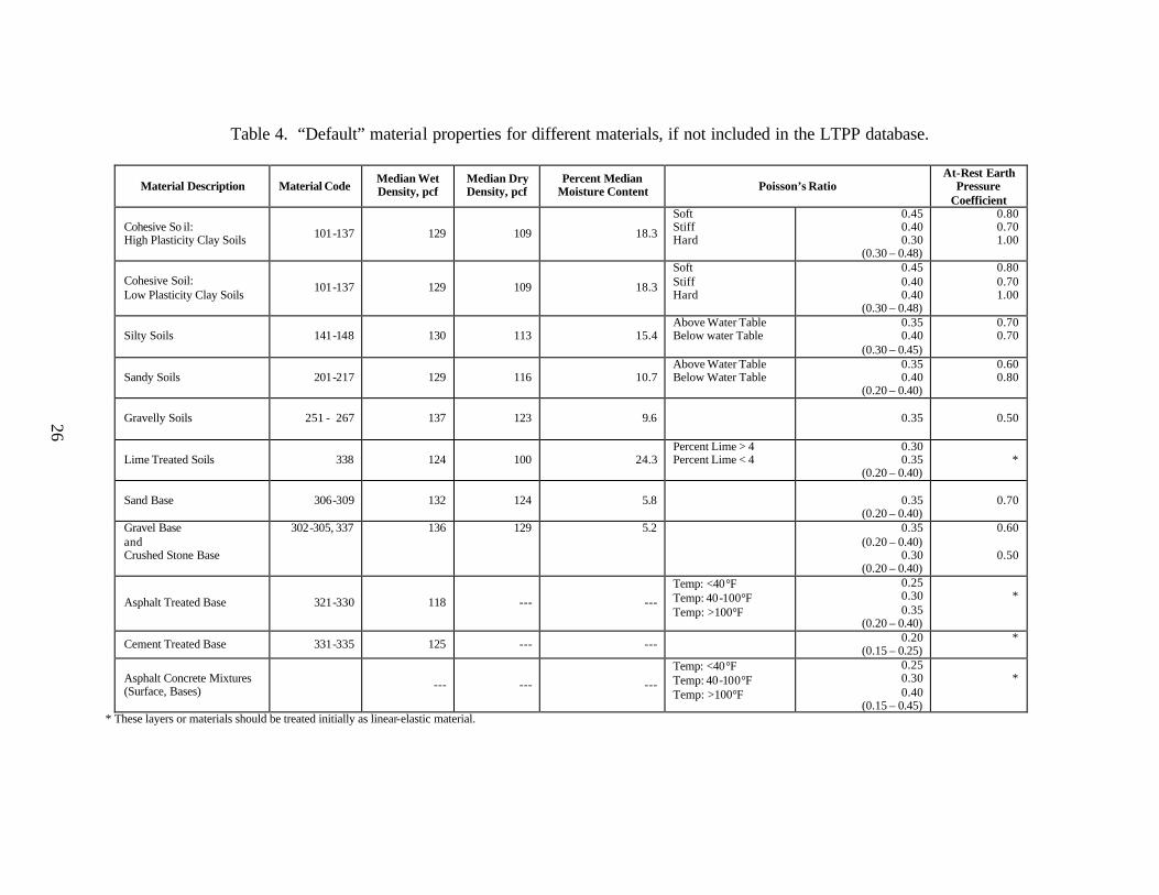
Table 4. “Default” material properties for different materials, if not included in the LTPP database.

Material Description Material Code Median Wet Density, pcf

Median Dry Density, pcf

Percent Median Moisture Content Poisson’s Ratio

At-Rest Earth Pressure

Coefficient

Cohesive So il: High Plasticity Clay Soils 101-137 129 109 18.3

Soft Stiff Hard

0.45 0.40 0.30

(0.30 – 0.48)

0.80 0.70 1.00

Cohesive Soil: Low Plasticity Clay Soils 101-137 129 109 18.3

Soft Stiff Hard

0.45 0.40 0.40

(0.30 – 0.48)

0.80 0.70 1.00

Silty Soils 141-148 130 113 15.4 Above Water Table Below water Table

0.35 0.40

(0.30 – 0.45)

0.70 0.70

Sandy Soils 201-217 129 116 10.7 Above Water Table Below Water Table

0.35 0.40

(0.20 – 0.40)

0.60 0.80

Gravelly Soils 251 - 267 137 123 9.6

0.35

0.50

Lime Treated Soils 338 124 100 24.3 Percent Lime > 4 Percent Lime < 4

0.30 0.35

(0.20 – 0.40)

*

Sand Base 306-309 132 124 5.8

0.35 (0.20 – 0.40)

0.70

Gravel Base and Crushed Stone Base

302-305, 337 136 129 5.2 0.35 (0.20 – 0.40)

0.30 (0.20 – 0.40)

0.60

0.50

Asphalt Treated Base 321-330 118 --- --- Temp: <40°F Temp: 40-100°F Temp: >100°F

0.25 0.30 0.35

(0.20 – 0.40)

*

Cement Treated Base 331-335 125 --- --- 0.20 (0.15 – 0.25)

*

Asphalt Concrete Mixtures (Surface, Bases) --- --- ---

Temp: <40°F Temp: 40-100°F Temp: >100°F

0.25 0.30 0.40

(0.15 – 0.45)

*

* These layers or materials should be treated initially as linear-elastic material.

26

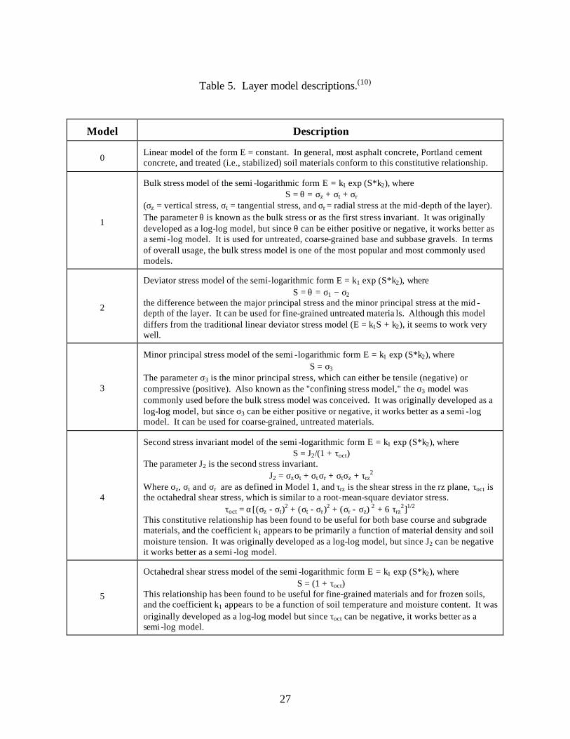
27

Table 5. Layer model descriptions.(10)

Model

Description

0

Linear model of the form E = constant. In general, most asphalt concrete, Portland cement concrete, and treated (i.e., stabilized) soil materials conform to this constitutive relationship.

1

Bulk stress model of the semi -logarithmic form E = k1 exp (S*k2), where S = θ = σz + σt + σr (σz = vertical stress, σt = tangential stress, and σr = radial stress at the mid-depth of the layer). The parameter θ is known as the bulk stress or as the first stress invariant. It was originally developed as a log-log model, but since θ can be either positive or negative, it works better as a semi -log model. It is used for untreated, coarse-grained base and subbase gravels. In terms of overall usage, the bulk stress model is one of the most popular and most commonly used models.

2

Deviator stress model of the semi-logarithmic form E = k1 exp (S*k2), where S = θ = σ1 − σ2 the difference between the major principal stress and the minor principal stress at the mid -depth of the layer. It can be used for fine-grained untreated materia ls. Although this model differs from the traditional linear deviator stress model (E = k1S + k2), it seems to work very well.

3

Minor principal stress model of the semi -logarithmic form E = k1 exp (S*k2), where S = σ3 The parameter σ3 is the minor principal stress, which can either be tensile (negative) or compressive (positive). Also known as the "confining stress model," the σ3 model was commonly used before the bulk stress model was conceived. It was originally developed as a log-log model, but since σ3 can be either positive or negative, it works better as a semi -log model. It can be used for coarse-grained, untreated materials.

4

Second stress invariant model of the semi -logarithmic form E = k1 exp (S*k2), where S = J2/(1 + τoct) The parameter J2 is the second stress invariant. J2 = σzσt + σt σr + σtσz + τrz

2 Where σz, σt and σr are as defined in Model 1, and τrz is the shear stress in the rz plane, τoct is the octahedral shear stress, which is similar to a root-mean-square deviator stress.

τoct = α[(σz - σt)2 + (σt - σr)2 + (σr - σz) 2 + 6 τrz2]1/2

This constitutive relationship has been found to be useful for both base course and subgrade materials, and the coefficient k1 appears to be primarily a function of material density and soil moisture tension. It was originally developed as a log-log model, but since J2 can be negative it works better as a semi -log model.

5

Octahedral shear stress model of the semi -logarithmic form E = k1 exp (S*k2), where S = (1 + τoct) This relationship has been found to be useful for fine-grained materials and for frozen soils, and the coefficient k1 appears to be a function of soil temperature and moisture content. It was originally developed as a log-log model but since τoct can be negative, it works better as a semi -log model.

28

Table 5. Layer model descriptions (continued).(10)

Model

Description

6

Vertical stress model of the log-log form E = k1 S k2, where S = σz The parameter σz is the vertical stress, which is always compressive (i.e., positive). This model is very similar in some respects to Model 7. The difference is that the direction of σz is always vertical, while the direction of σ1 in Model 7 rotates with distance from the load.

7

Major principal stress model of the log-log form E = k1 S k2 (k0)k3, where S = σ1 The parameter σ1 is the major principal stress, which is generally always compressive. Dynatest uses this model in their ELMOD back-calculation program. It is included here for completeness. As used in ELMOD, the overburden stress is not included in the major principal stress, so the overburden stress is not included in MODCOMP3 either.

8

Cornell constitutive model of the log-log form E = k1 S k2 (k0)k3, where S = (θo

2 + θp2) 0.22(1-P200) (1 + τoct) -0.34P200

The parameter θo is the initial bulk stress, due only to overburden stress. The parameter θp is the bulk stress at peak load, including both the overburden stress and the load stress. The parameter τoct is the octahedral shear stress at peak load, which also includes the overburden stress. The parameter P200 is the percentage of the materials gradation that passes the number 200 sieve, and it is a required input for both known and unknown models. It is entered on data file line 5 as the K@(I) parameter (see Table 3 of the MODCOMP User's Manual). The parameter k0 is the lateral earth pressure coefficient, which represents the anisotropy of the overburden stress. The coefficient k1 has been found to be a function of material density and soil moisture content, along with other material properties. The exponent k3 = -0.69, is treated as a constant in the program. The Cornell model has been developed for use with both coarse-grained and fine-grained untreated materials. It has seen limited use, mainly with the glacial materials of the Northeastern U.S.

29

• Model 1, Bulk Stress Model, E = k1 exp (S*k2), where S = θ = σZ + σt + σr. • Model 2, Deviator Stress Model, E = k1 exp (S*k2), where S = σ1 - σ3. • Model 3, Minor Principal Stress Model, E = k1 exp (S*k2), where S = σ3.

3.2.9 Material Densities. Wet and dry densities for the pavement layers and subgrade are included in the LTPP database for many of the test sections and were extracted from data table TST_ISD_MOIST. When the densities were available, they were used in the back-calculation process. However, when the densities were unavailable for a specific layer and site, the median density for that type of material, calculated from all other data, was used. These default values are listed in table 4. 3.2.10 Lateral Earth Pressure. MODCOMP has the capability to consider the effect of overburden pressures in back-calculating nonlinear elastic properties. The lateral earth pressure coefficient (Ko) is used to compute the contribution to the lateral stress at different depths from the overburden pressure. Lateral earth pressure coefficients, however, are not included in the LTPP database. A range of basins with varying conditions was used to evaluate the sensitivity of Ko to obtain reasonable solutions (low RMS error). For reasonable variations (plus or minus 25 percent) around the default values included in MODCOMP, it was found that Ko does not have a significant effect on the calculated results. Because there is no reliable method to estimate the actual Ko value to be used for each section, the values given in table 4 were used and are materials dependent. For a linear elastic solution, Ko has no effect on the back-calculated moduli. 3.3 Trial Computations – Execution of Back-Calculation Process The procedure used to back-calculate the elastic properties of each layer is not fully automated but is an iterative process and requires engineering judgment. To begin the computation process, a limited number of points are randomly selected along the test section and the elastic properties calculated for those basins. The reason for starting with a limited number of basins is to make any necessary revisions to the inputs for reducing the RMS error to an acceptable level in a short period of time, prior to initiating the mass back-calculation of all deflection basins measured at a test section. The number of random test points selected were generally in the range from four to eight and depended on the amount of variation of the measured deflection basins within the subsection. MODSHELL was used to analyze the basins measured at those random test points. MODSHELL is a menu-driven program that enables the creation of new data files, editing of existing data files, processing of files with MODCOMP4, and viewing the output files on the screen. The linear elastic module of MODCOMP was used to calculate the elastic modulus, and those results were used as the starting point for the nonlinear analysis. Results from the initial solutions were reviewed to determine whether the production runs should be executed or changes should be made to the inputs before proceeding to the production runs. The decision on whether to proceed was based on, in order of importance:

30

1. Magnitude of the RMS errors – revisions were made until the RMS error was reduced to

2 percent or less, or to the lowest possible value.

2. Computed elastic modulus (Young’s modulus) – revisions were made if high and low moduli were calculated for the type of materials identified. High and low values for specific materials were based on judgment using the seed values designated in ASTM D5858 and the procedure recommended by Von Quintus and Killingsworth, as guidance.(1,3) If the change made to the input resulted in higher RMS errors or a larger difference between the calculated and measured deflection basin, the revision was not implemented in the mass back-calculations for that test section.

3. Changes in the elastic modulus from one iteration to the other – revisions were made

when the solutions (elastic modulus for each layer) did not begin to converge within the specified number of iterations, generally 10.

If the RMS errors were large (greater than 2 percent) or the calculated elastic moduli were questionable for the type of material, the inputs were checked and adjustments were made to the layer combinations, layer-sensor assignments, and/or the use or omission of an apparent rigid layer. MODSHELL was used to recalculate the elastic moduli with those changes. This iterative process was continued until a “reasonable or acceptable” solution was achieved. As stated above, a reasonable or acceptable solution was one with an RMS error less than or equal to 2 percent with elastic moduli that were considered typical for the material type. These revisions to the input parameters were then used for the mass back-calculation of elastic layer modulus along that test section. For some test sections, extremely high or low moduli were computed for one or more layers in the pavement structure with good RMS error values. When this occurred, changes were made to the inputs, and MODSHELL was used to recalculate Young’s modulus, as noted above. If the final RMS error was less than 2 percent for the trial run that resulted in the extremely high or low moduli and much greater than 2 percent for the other trial runs, the trial run resulting in the high or low moduli was used for the production runs.

31

4.0 RESULTS FROM COMPUTATION OF ELASTIC PROPERTIES This section of the report provides an overview and brief summary of some of the pertinent details from the calculation of elastic properties using MODCOMP4. A detailed analysis and comparison of the results was beyond the scope of work for this study. Thus, the elastic properties calculated from the deflection basin were reviewed to determine whether the results seemed reasonable. Appendix C of this report tabulates the median Young’s modulus calculated for different materials and includes histograms of the calculated Young’s modulus for different materials and soils. 4.1 Some Basic Facts from the Back-Calculation The magnitude of the effort to complete the back-calculation of elastic properties for all deflection basin data in the LTPP database for both the flexible and rigid pavements included:

• 1,650,000+ deflection basins were analyzed with the linear module of MODCOMP. • 100,000+ test points were analyzed with the nonlinear module.

The deflection data were analyzed using more than six PC’s, ranging from a 400-MHz Pentium II with a 2-Gb partition down to a 166-MHz Pentium II with a 1-Gb hard drive. The execution time per solution ranged from approximately:

• 0.1 to 0.5 minutes when using the linear module of MODCOMP. • 2 to 5 minutes when using the nonlinear module.

The total computational time to complete the back-calculation of elastic properties from the deflection basin data for all LTPP test sections was approximately:

• 3,200+ hours for the linear elastic solutions. • 13,200+ hours for the nonlinear solutions.

4.2 Computed Parameter Database The elastic layer properties for the LTPP flexible and rigid pavement test sections have become a part of the LTPP database. The computed elastic layer properties can be found in six LTPP database tables, which are listed below and summarized in table 6.

1. The first table (MON_DEFL_FLX_BAKCAL_BASIN) includes the average deflection basins that were used in the back-calculation process.

2. The second table (MON_DEFL_FLX_BAKCAL_LAYER) includes the material code, thickness, density, and other properties used for each layer in the pavement structure.

32

3. The third table (MON_DEFL_FLX_BAKCAL_POINT) contains the calculated Young’s modulus using MODCOMP for each of the pavement layers, including the subgrade. The computed moduli are provided for each station or deflection basin measured with the FWD that is included in the LTPP database.

4. The fourth table (MON_DEFL_FLX_BAKCAL_SUMMARY) includes summary statistics of Young’s moduli calculated for each load level and structural layer for each deflection survey or site visit.

5. The fifth table (MON_DEFL_FLX_NMODEL_POINT) includes the nonlinear elastic properties for the constitutive equations used in the MODCOMP back-calculation program, as well as Young’s modulus determined for the highest load level used in the deflection-testing program at each test section.

6. The sixth table (MON_DEFL_FLX_NMODEL_SUMMARY) is a summary of the nonlinear solutions. This table identifies the model or constitutive equation used to represent each material type and a summary of Young’s modulus calculated at the highest load level used during the deflection-testing program.

The summary tables (the fourth and sixth tables) also include the average, standard deviation, and minimum and maximum values for those parameters where the mean values were determined and reported. 4.3 Allowable Maximum RMS Error Most back-calculation programs use some sort of iterative or optimization technique to minimize the difference between the calculated (for a specific set of elastic layer properties) and measured deflection basins. Obviously, the absolute error (percent error per sensor) and RMS error (goodness-of-fit) vary from station to station and depend on the pavement’s physical features that have an effect on the deflection basin measured with the FWD. For example, thickness variations, material density variations, surface distortion, and cracks, which may or may not be visible at the surface, can cause small irregularities within the measured deflection basin, which are not consistent with elastic layer theory. These irregularities result in differences between the measured and calculated deflection basins. In fact, some of the differences between the calculated and measured basins are so large that the solution is considered highly questionable or that no elastic layered solution exists for that measured deflection basin for the simulated pavement structure (layer type and thickness). There has been serious discussion and debate over the maximum absolute or RMS error to help decide when an adequate solution or set of layer moduli is considered reasonable and can be used in other analyses. Maximum error values that have been used to judge whether the solution is acceptable vary from 1 to 3 percent for the RMS error and 1 to 2.5 percent for the absolute error or difference.

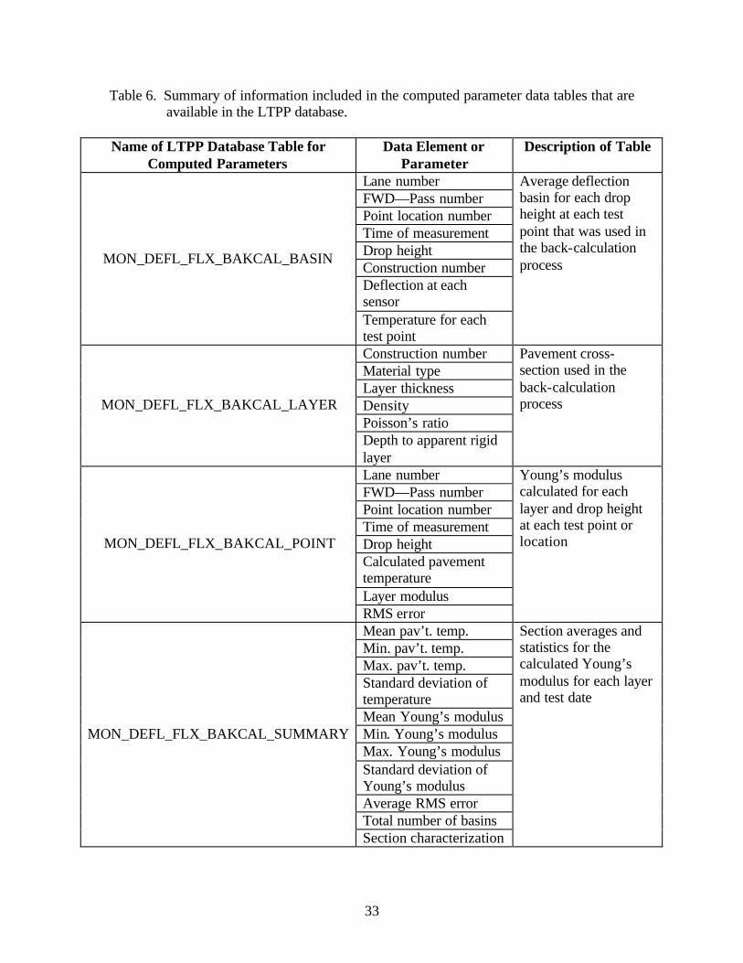
33

Table 6. Summary of information included in the computed parameter data tables that are available in the LTPP database.

Name of LTPP Database Table for

Computed Parameters Data Element or

Parameter Description of Table

Lane number FWD—Pass number Point location number Time of measurement Drop height Construction number Deflection at each sensor

MON_DEFL_FLX_BAKCAL_BASIN

Temperature for each test point

Average deflection basin for each drop height at each test point that was used in the back-calculation process

Construction number Material type Layer thickness Density Poisson’s ratio

MON_DEFL_FLX_BAKCAL_LAYER

Depth to apparent rigid layer

Pavement cross-section used in the back-calculation process

Lane number FWD—Pass number Point location number Time of measurement Drop height Calculated pavement temperature Layer modulus

MON_DEFL_FLX_BAKCAL_POINT

RMS error

Young’s modulus calculated for each layer and drop height at each test point or location

Mean pav’t. temp. Min. pav’t. temp. Max. pav’t. temp. Standard deviation of temperature Mean Young’s modulus Min. Young’s modulus Max. Young’s modulus Standard deviation of Young’s modulus Average RMS error Total number of basins

MON_DEFL_FLX_BAKCAL_SUMMARY

Section characterization

Section averages and statistics for the calculated Young’s modulus for each layer and test date

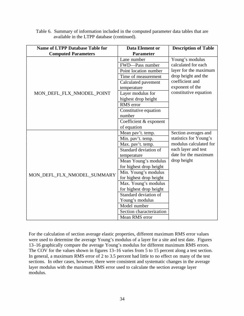
34

Table 6. Summary of information included in the computed parameter data tables that are available in the LTPP database (continued).

Name of LTPP Database Table for Computed Parameters

Data Element or Parameter

Description of Table

Lane number FWD—Pass number Point location number Time of measurement Calculated pavement temperature Layer modulus for highest drop height RMS error Constitutive equation number

MON_DEFL_FLX_NMODEL_POINT

Coefficient & exponent of equation

Young’s modulus calculated for each layer for the maximum drop height and the coefficient and exponent of the constitutive equation

Mean pav’t. temp. Min. pav’t. temp. Max. pav’t. temp. Standard deviation of temperature Mean Young’s modulus for highest drop height Min. Young’s modulus for highest drop height Max. Young’s modulus for highest drop height Standard deviation of Young’s modulus Model number Section characterization

MON_DEFL_FLX_NMODEL_SUMMARY

Mean RMS error

Section averages and statistics for Young’s modulus calculated for each layer and test date for the maximum drop height

For the calculation of section average elastic properties, different maximum RMS error values were used to determine the average Young’s modulus of a layer for a site and test date. Figures 13–16 graphically compare the average Young’s modulus for different maximum RMS errors. The COV for the values shown in figures 13–16 varies from 5 to 15 percent along a test section. In general, a maximum RMS error of 2 to 3.5 percent had little to no effect on many of the test sections. In other cases, however, there were consistent and systematic changes in the average layer modulus with the maximum RMS error used to calculate the section average layer modulus.

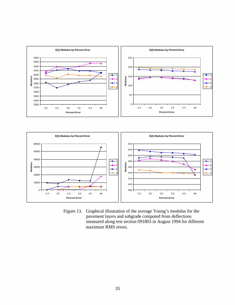
35

Figure 13. Graphical illustration of the average Young’s modulus for the pavement layers and subgrade computed from deflections measured along test section 091803 in August 1994 for different maximum RMS errors.

E(1) Modulus by Percent Error

5300

5400

5500

5600

5700

5800

5900

6000

6100

6200

6300

6400

2.0 2.5 3.0 3.5 4.0 All

Percent Error

Mod

ulus

1

2

3

4

E(2) Modulus by Percent Error

0

50

100

150

200

250

2.0 2.5 3.0 3.5 4.0 All

Percent Error

Mod

ulus

1

2

34

E(3) Modulus by Percent Error

0

10000

20000

30000

40000

50000

60000

2.0 2.5 3.0 3.5 4.0 All

Percent Error

Mod

ulus

1

23

4

E(4) Modulus by Percent Error

380

400

420

440

460

480

500

520

540

2.0 2.5 3.0 3.5 4.0 All

Percent Error

Mod

ulus

1

23

4

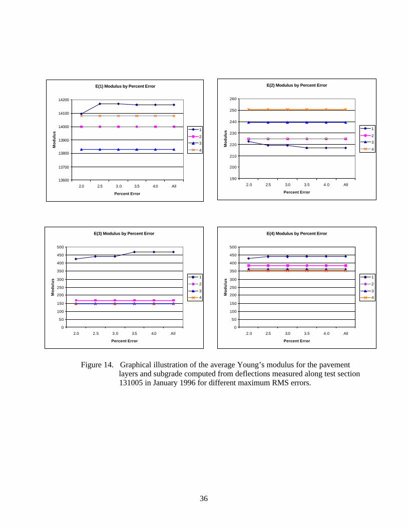
36

Figure 14. Graphical illustration of the average Young’s modulus for the pavement layers and subgrade computed from deflections measured along test section 131005 in January 1996 for different maximum RMS errors.

E(2) Modulus by Percent Error

190

200

210

220

230

240

250

260

2.0 2.5 3.0 3.5 4.0 All

Percent Error

Mod

ulus

1

23

4

E(3) Modulus by Percent Error

0

50

100

150

200

250

300

350

400

450

500

2.0 2.5 3.0 3.5 4.0 All

Percent Error

Mod

ulus

1

2

34

E(4) Modulus by Percent Error

0

50

100

150

200

250

300

350

400

450

500

2.0 2.5 3.0 3.5 4.0 All

Percent Error

Mod

ulus

1

2

34

E(1) Modulus by Percent Error

13600

13700

13800

13900

14000

14100

14200

2.0 2.5 3.0 3.5 4.0 All

Percent Error

Mod

ulus

1

23

4

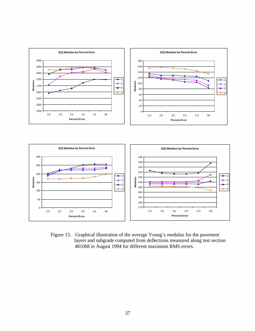
37

Figure 15. Graphical illustration of the average Young’s modulus for the pavement

layers and subgrade computed from deflections measured along test section 481068 in August 1994 for different maximum RMS errors.

E(1) Modulus by Percent Error

1500

1550

1600

1650

1700

1750

1800

1850

1900

2.0 2.5 3.0 3.5 4.0 All

Percent Error

Mod

ulus

1

23

4

E(2) Modulus by Percent Error

0

20

40

60

80

100

120

140

160

180

2.0 2.5 3.0 3.5 4.0 All

Percent Error

Mod

ulus

1

23

4

E(3) Modulus by Percent Error

0

50

100

150

200

250

300

2.0 2.5 3.0 3.5 4.0 All

Percent Error

Mod

ulus

1

2

3

4

E(4) Modulus by Percent Error

178

180

182

184

186

188

190

192

194

196

198

2.0 2.5 3.0 3.5 4.0 All

Percent Error

Mod

ulus

1

23

4

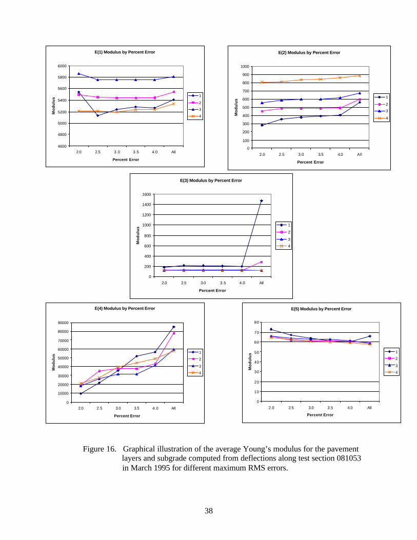
38

Figure 16. Graphical illustration of the average Young’s modulus for the pavement layers and subgrade computed from deflections along test section 081053 in March 1995 for different maximum RMS errors.

E(1) Modulus by Percent Error

4600

4800

5000

5200

5400

5600

5800

6000

2.0 2.5 3.0 3.5 4.0 All

Percent Error

Mod

ulus

1

234

E(2) Modulus by Percent Error

0

100

200

300

400

500

600

700

800

900

1000

2.0 2.5 3.0 3.5 4.0 All

Percent Error

Mod

ulus

1

23

4

E(3) Modulus by Percent Error

0

200

400

600

800

1000

1200

1400

1600

2.0 2.5 3.0 3.5 4.0 All

Percent Error

Mod

ulus

1

2

34

E(4) Modulus by Percent Error

0

10000

20000

30000

40000

50000

60000

70000

80000

90000

2.0 2.5 3.0 3.5 4.0 All

Percent Error

Mod

ulus

12

34

E(5) Modulus by Percent Error

0

10

20

30

40

50

60

70

80

2.0 2.5 3.0 3.5 4.0 All

Percent Error

Mod

ulus

12

34

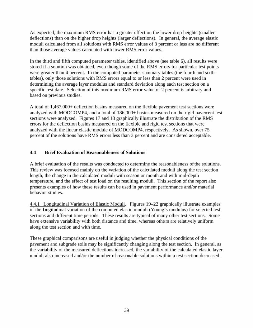
39

As expected, the maximum RMS error has a greater effect on the lower drop heights (smaller deflections) than on the higher drop heights (larger deflections). In general, the average elastic moduli calculated from all solutions with RMS error values of 3 percent or less are no different than those average values calculated with lower RMS error values. In the third and fifth computed parameter tables, identified above (see table 6), all results were stored if a solution was obtained, even though some of the RMS errors for particular test points were greater than 4 percent. In the computed parameter summary tables (the fourth and sixth tables), only those solutions with RMS errors equal to or less than 2 percent were used in determining the average layer modulus and standard deviation along each test section on a specific test date. Selection of this maximum RMS error value of 2 percent is arbitrary and based on previous studies. A total of 1,467,000+ deflection basins measured on the flexible pavement test sections were analyzed with MODCOMP4, and a total of 186,000+ basins measured on the rigid pavement test sections were analyzed. Figures 17 and 18 graphically illustrate the distribution of the RMS errors for the deflection basins measured on the flexible and rigid test sections that were analyzed with the linear elastic module of MODCOMP4, respectively. As shown, over 75 percent of the solutions have RMS errors less than 3 percent and are considered acceptable. 4.4 Brief Evaluation of Reasonableness of Solutions A brief evaluation of the results was conducted to determine the reasonableness of the solutions. This review was focused mainly on the variation of the calculated moduli along the test section length, the change in the calculated moduli with season or month and with mid-depth temperature, and the effect of test load on the resulting moduli. This section of the report also presents examples of how these results can be used in pavement performance and/or material behavior studies. 4.4.1 Longitudinal Variation of Elastic Moduli. Figures 19–22 graphically illustrate examples of the longitudinal variation of the computed elastic moduli (Young’s modulus) for selected test sections and different time periods. These results are typical of many other test sections. Some have extensive variability with both distance and time, whereas othe rs are relatively uniform along the test section and with time. These graphical comparisons are useful in judging whether the physical conditions of the pavement and subgrade soils may be significantly changing along the test section. In general, as the variability of the measured deflections increased, the variability of the calculated elastic layer moduli also increased and/or the number of reasonable solutions within a test section decreased.

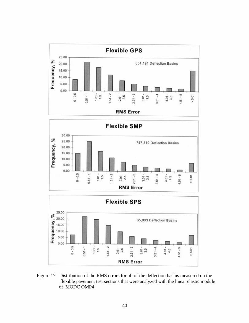
40

Figure 17. Distribution of the RMS errors for all of the deflection basins measured on the

flexible pavement test sections that were analyzed with the linear elastic module of MODC OMP4

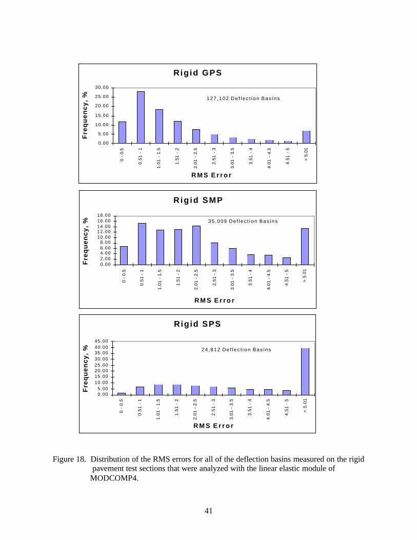
41

Figure 18. Distribution of the RMS errors for all of the deflection basins measured on the rigid pavement test sections that were analyzed with the linear elastic module of MODCOMP4.

Rigid SPS

0.005.00

10.0015.0020.0025.0030.0035.0040.0045.00

0 - 0

.5

0.51

- 1

1.01

- 1.

5

1.51

- 2

2.01

- 2.

5

2.51

- 3

3.01

- 3.

5

3.51

- 4

4.01

- 4.

5

4.51

- 5

> 5.

01

R M S E r r o r

Freq

uenc

y, % 24 ,812 De f l ec t i on Bas ins

Rig id SMP

0.002.004.006.008.00

10.0012.0014.0016.0018.00

0 - 0

.5

0.51

- 1

1.01

- 1.

5

1.51

- 2

2.01

- 2.

5

2.51

- 3

3.01

- 3.

5

3.51

- 4

4.01

- 4.

5

4.51

- 5

> 5.

01R M S E r r o r

Freq

uenc

y, % 35 ,009 De f l ec t i on Bas ins

Rigid GPS

0.00

5.00

10.00

15.00

20.00

25.00

30.00

0 - 0

.5

0.51

- 1

1.01

- 1

.5

1.51

- 2

2.01

- 2

.5

2.51

- 3

3.01

- 3

.5

3.51

- 4

4.01

- 4

.5

4.51

- 5

> 5.

01

R M S E r r o r

Freq

uenc

y, % 1 2 7 , 1 0 2 D e f l e c t i o n B a s i n s

42

Figure 19. Longitudinal variation of Young’s modulus in the wheelpath for each pavement layer and subgrade along test section 091803 in August 1994.

091803, F3 E(1)

0100020003000400050006000700080009000

250 300 350 400 450 500 550

Station

Mod

ulus

Drop 1Drop 2Drop 3Drop 4

091803, F3 E(2)

0

50

100

150

200

250

300

250 300 350 400 450 500 550

Station

Mod

ulus

Drop 1Drop 2Drop 3Drop 4

091803, F3 E(4)

0100200300400500600700800900

250 300 350 400 450 500 550

Station

Mod

ulus

Drop 1Drop 2Drop 3Drop 4

091803, F3 E(3)

0 50000

100000 150000 200000

250 300 350 400 450 500 550 Station

Mod

ulus

Drop 1 Drop 2 Drop 3 Drop 4

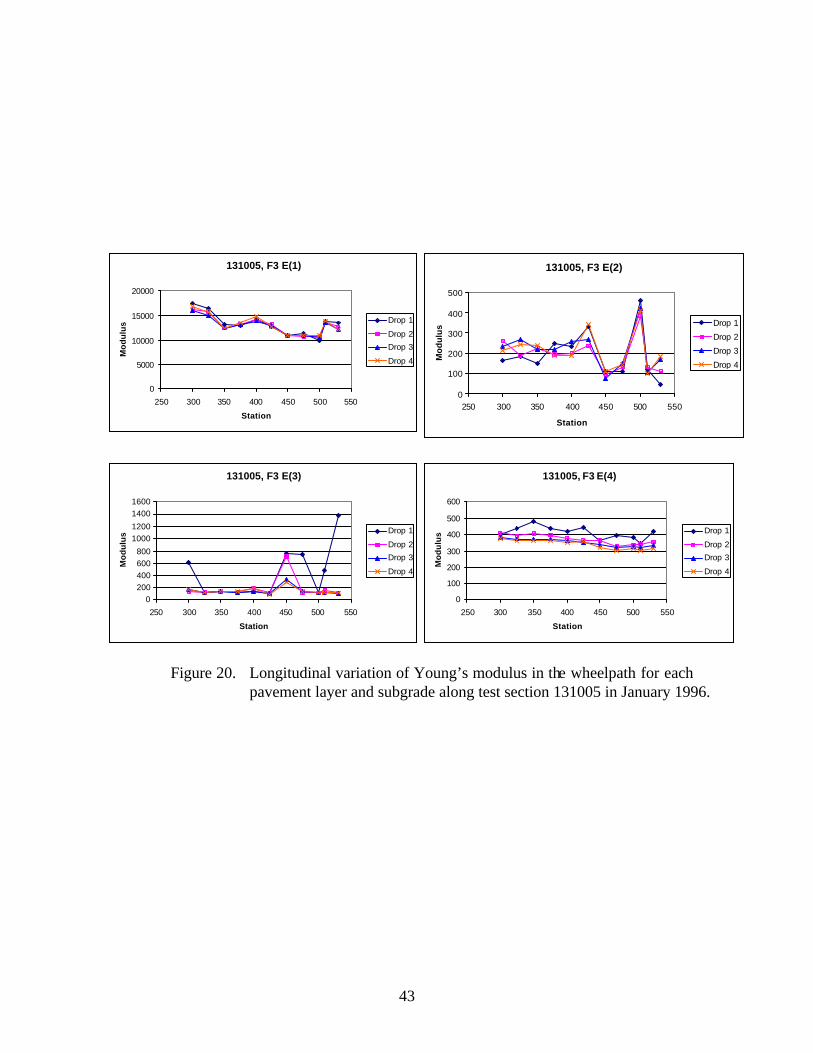
43

Figure 20. Longitudinal variation of Young’s modulus in the wheelpath for each pavement layer and subgrade along test section 131005 in January 1996.

131005, F3 E(1)

0

5000

10000

15000

20000

250 300 350 400 450 500 550Station

Mod

ulus

Drop 1Drop 2Drop 3Drop 4

131005, F3 E(2)

0

100

200

300

400

500

250 300 350 400 450 500 550

Station

Mod

ulus

Drop 1Drop 2Drop 3Drop 4

131005, F3 E(3)

0200400600800

1000120014001600

250 300 350 400 450 500 550Station

Mod

ulus

Drop 1Drop 2Drop 3Drop 4

131005, F3 E(4)

0

100

200

300

400

500

600

250 300 350 400 450 500 550Station

Mod

ulus

Drop 1Drop 2Drop 3Drop 4

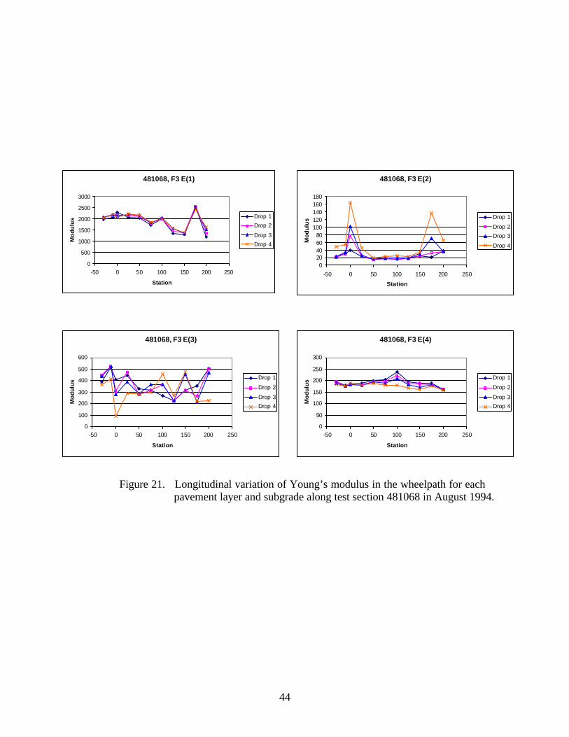
44

Figure 21. Longitudinal variation of Young’s modulus in the wheelpath for each

pavement layer and subgrade along test section 481068 in August 1994.

481068, F3 E(1)

0

500

1000

1500

2000

2500

3000

-50 0 50 100 150 200 250

Station

Mod

ulus

Drop 1Drop 2

Drop 3Drop 4

481068, F3 E(2)

020406080

100120140160180

-50 0 50 100 150 200 250Station

Mod

ulus

Drop 1Drop 2Drop 3Drop 4

481068, F3 E(3)

0

100

200

300

400

500

600

-50 0 50 100 150 200 250

Station

Mod

ulus

Drop 1Drop 2Drop 3Drop 4

481068, F3 E(4)

0

50

100

150

200

250

300

-50 0 50 100 150 200 250

Station

Mod

ulus

Drop 1Drop 2Drop 3Drop 4

45

Figure 22. Longitudinal variation of Young’s modulus in the wheelpath for each pavement layer and subgrade along test section 081053 in March 1995.

081053, F3 E(1)

010002000300040005000600070008000

-50 0 50 100 150 200 250

Station

Mod

ulus

Drop 1Drop 2Drop 3Drop 4

081053, F3 E(2)

0200400600800

1000120014001600

-50 0 50 100 150 200 250

Station

Mod

ulus

Drop 1Drop 2Drop 3Drop 4

081053, F3 E(3)

0

5000

10000

15000

20000

25000

-50 0 50 100 150 200 250

Station

Mod

ulus

Drop 1Drop 2

Drop 3Drop 4

081053, F3 E(4)

0

2000040000

6000080000

100000120000

140000

-50 0 50 100 150 200 250

Station

Mod

ulus

Drop 1Drop 2Drop 3Drop 4

081053, F3 E(5)

0

50

100

150

200

250

300

-50 0 50 100 150 200 250

Station

Mod

ulus

Drop 1Drop 2Drop 3Drop 4

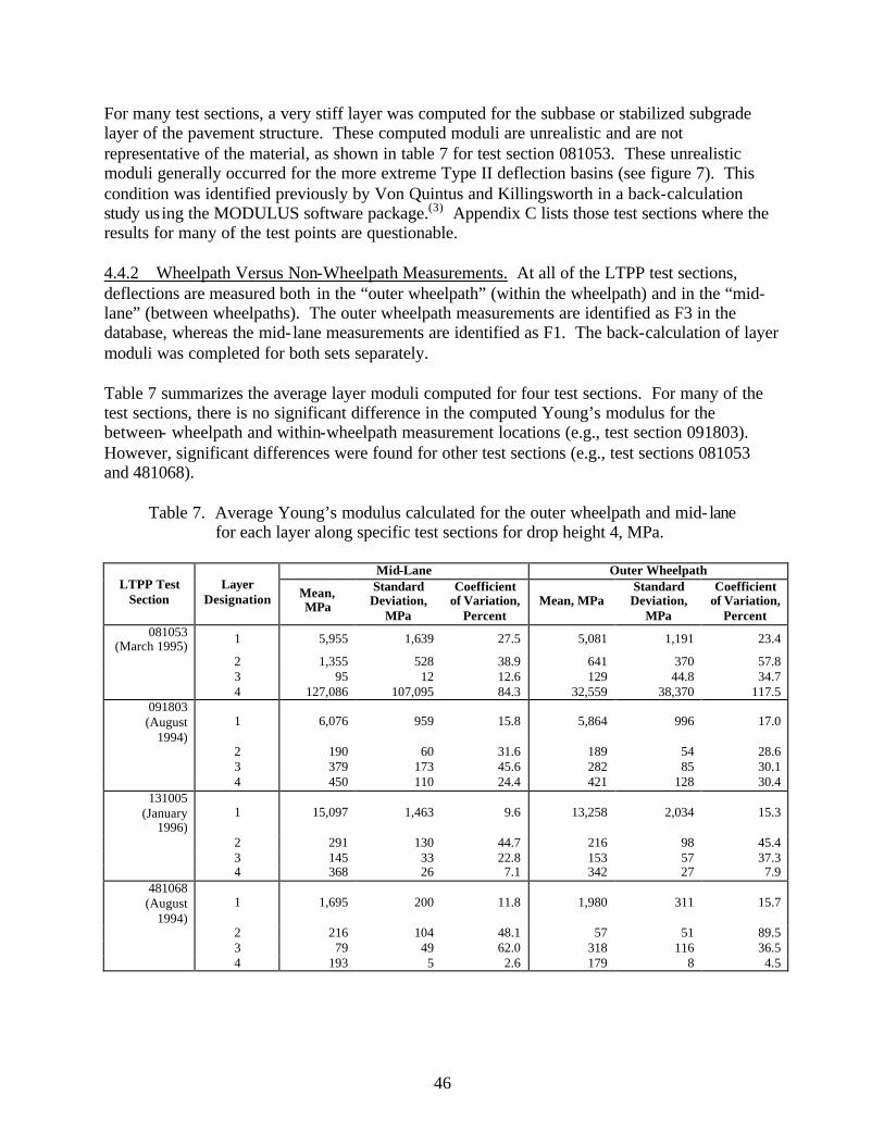
46

For many test sections, a very stiff layer was computed for the subbase or stabilized subgrade layer of the pavement structure. These computed moduli are unrealistic and are not representative of the material, as shown in table 7 for test section 081053. These unrealistic moduli generally occurred for the more extreme Type II deflection basins (see figure 7). This condition was identified previously by Von Quintus and Killingsworth in a back-calculation study using the MODULUS software package.(3) Appendix C lists those test sections where the results for many of the test points are questionable. 4.4.2 Wheelpath Versus Non-Wheelpath Measurements. At all of the LTPP test sections, deflections are measured both in the “outer wheelpath” (within the wheelpath) and in the “mid-lane” (between wheelpaths). The outer wheelpath measurements are identified as F3 in the database, whereas the mid- lane measurements are identified as F1. The back-calculation of layer moduli was completed for both sets separately. Table 7 summarizes the average layer moduli computed for four test sections. For many of the test sections, there is no significant difference in the computed Young’s modulus for the between- wheelpath and within-wheelpath measurement locations (e.g., test section 091803). However, significant differences were found for other test sections (e.g., test sections 081053 and 481068).

Table 7. Average Young’s modulus calculated for the outer wheelpath and mid- lane for each layer along specific test sections for drop height 4, MPa.

Mid-Lane Outer Wheelpath

LTPP Test Section

Layer Designation Mean,

MPa Standard Deviation,

MPa

Coefficient of Variation,

Percent Mean, MPa

Standard Deviation,

MPa

Coefficient of Variation,

Percent 081053

(March 1995) 1 5,955 1,639 27.5 5,081 1,191 23.4

2 1,355 528 38.9 641 370 57.8 3 95 12 12.6 129 44.8 34.7 4 127,086 107,095 84.3 32,559 38,370 117.5 091803 (August

1994) 1 6,076 959 15.8 5,864 996 17.0

2 190 60 31.6 189 54 28.6 3 379 173 45.6 282 85 30.1 4 450 110 24.4 421 128 30.4 131005

(January 1996)

1 15,097 1,463 9.6 13,258 2,034 15.3

2 291 130 44.7 216 98 45.4 3 145 33 22.8 153 57 37.3 4 368 26 7.1 342 27 7.9 481068 (August

1994) 1 1,695 200 11.8 1,980 311 15.7

2 216 104 48.1 57 51 89.5 3 79 49 62.0 318 116 36.5 4 193 5 2.6 179 8 4.5

47

Based on a brief review of the results, there is no consistent difference between the within-wheelpath and non-wheelpath measurements. For some of the test sections, however, low moduli were calculated for layers directly under the surface for within-wheelpath measurement locations. In most such cases, a higher modulus was calculated for the lowest layer, as shown in table 7 for test section 481068. These computations are believed to be unrealistic, even though the computations for both within- and between-wheelpaths were completed in the same within- and between-wheelpaths production run using the same pavement structure. Slight thickness variations, caused by plastic flow or lateral movement of the underlying materials close to the surface, may be a cause of this condition. 4.4.3 Seasonal or Monthly Effects. Figures 23–26 graphically illustrate examples of the monthly variation of the computed elastic moduli for the different layers of selected test sections. As shown, the moduli of the asphalt concrete layers increase for the winter months and decrease for the summer months. In addition, the modulus of the unbound aggregate layers and subgrade soils becomes extremely high during periods of possible freezing temperatures below the surface, as shown by the LTPP test section in Minnesota (276251). 4.4.4 Temperature Effects. Figures 27–30 graphically illustrate examples of the computed elastic moduli for the asphalt concrete surface layer as a function of mid-depth temperature. As shown, the modulus of the asphalt concrete layer increases with decreasing temperatures. However, there are some cases where there are inconsistent changes in modulus with temperature. Some of these test sections were identified as having potential stripping in the HMA layer or were found to have extreme variations in the underlying support layers. Appendix C includes a summary of the overall average Young’s modulus calculated at different temperature intervals for all HMA surface layers. As tabulated and expected, the average layer modulus decreases with increasing pavement temperature. 4.4.5 Time Effects. The SPS projects were used to look at systematic increases in the elastic moduli of the HMA and PCC surface layers as a result of hardening and curing. However, there are insufficient data to identify statistically any changes (increases) in the HMA and PCC moduli with time. 4.4.6 Stress Sensitivity from Linear Elastic Solutions. The linear elastic solutions were used to determine the change in computed elastic moduli (Young’s moduli) with increasing load level. For fine-grained soils, the modulus decreased with increasing load level, as expected. For the coarse-grained soils, the opposite was the case, again an expected result, based on laboratory tests. These unbound materials or soils are stress-sensitive, and consistent changes were calculated with increasing load levels, as shown for some of the layers in figures 19–21.

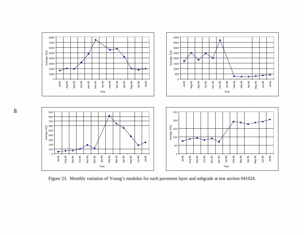
Figure 23. Monthly variation of Young’s modulus for each pavement layer and subgrade at test section 041024.

0

1000

2000

3000

4000

5000

6000

7000

8000

Jul-9

5

Aug-

95

Sep-

95

Oct

-95

Nov

-95

Dec

-95

Jan-

96

Feb-

96

Mar

-96

Apr-9

6

May

-96

Jun-

96

Jul-9

6

Time

Aver

age,

E(1

)

0

100

200

300

400

500

600

700

800

900

Jul-9

5

Aug-

95

Sep-

95

Oct

-95

Nov

-95

Dec

-95

Jan-

96

Feb-

96

Mar

-96

Apr-9

6

May

-96

Jun-

96

Jul-9

6

Time

Aver

age,

E(2

)

0

500

1000

1500

2000

2500

3000

3500

4000

Jul-9

5

Aug-

95

Sep-

95

Oct

-95

Nov

-95

Dec

-95

Jan-

96

Feb-

96

Mar

-96

Apr-9

6

May

-96

Jun-

96

Jul-9

6

Time

Aver

age,

E(3

)

0

50

100

150

200

250

Jul-9

5

Aug-

95

Sep-

95

Oct

-95

Nov

-95

Dec

-95

Jan-

96

Feb-

96

Mar

-96

Apr-9

6

May

-96

Jun-

96

Jul-9

6

TimeAv

erag

e, E

(4)

48

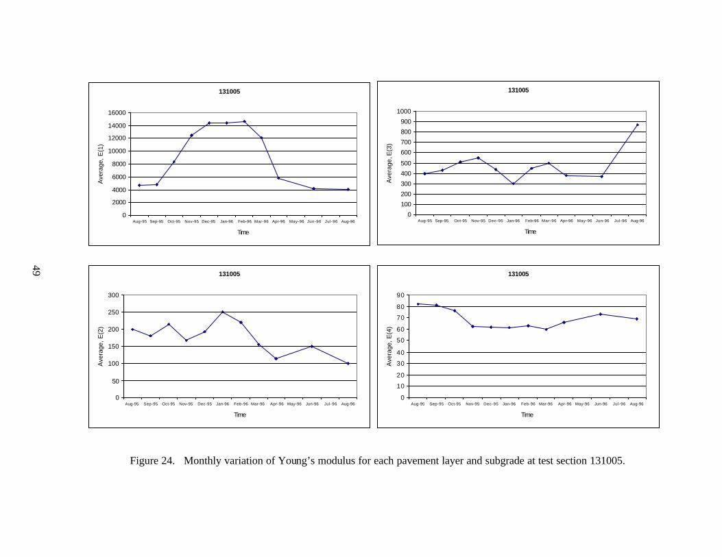
Figure 24. Monthly variation of Young’s modulus for each pavement layer and subgrade at test section 131005.

49

131005

0

2000

4000

6000

8000

10000

12000

14000

16000

Aug-95 Sep-95 Oct-95 Nov-95 Dec-95 Jan-96 Feb-96 Mar-96 Apr-96 May-96 Jun-96 Jul-96 Aug-96

Time

Aver

age,

E(1

)131005

0100200300400500600700800900

1000

Aug-95 Sep-95 Oct-95 Nov-95 Dec-95 Jan-96 Feb-96 Mar-96 Apr-96 May-96 Jun-96 Jul-96 Aug-96

Time

Aver

age,

E(3

)

131005

0

50

100

150

200

250

300

Aug-95 Sep-95 Oct-95 Nov-95 Dec-95 Jan-96 Feb-96 Mar-96 Apr-96 May-96 Jun-96 Jul-96 Aug-96

Time

Aver

age,

E(2

)

131005

0

1020

3040

5060

7080

90

Aug-95 Sep-95 Oct-95 Nov-95 Dec-95 Jan-96 Feb-96 Mar-96 Apr-96 May-96 Jun-96 Jul-96 Aug-96

Time

Aver

age,

E(4

)

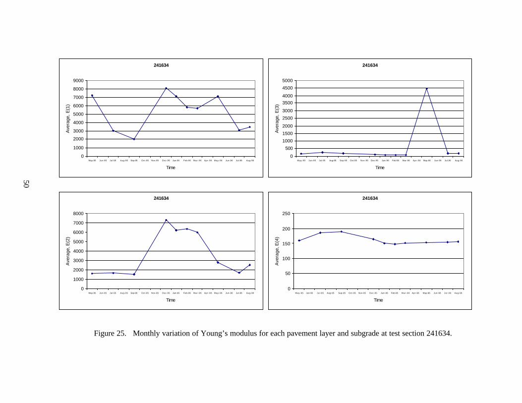
Figure 25. Monthly variation of Young’s modulus for each pavement layer and subgrade at test section 241634.

50

241634

0

50

100

150

200

250

May-95 Jun-95 Jul-95 Aug-95 Sep-95 Oct-95 Nov-95 Dec-95 Jan-96 Feb-96 Mar -96 Apr-96 May-96 Jun-96 Ju l -96 Aug-96

Time

Aver

age,

E(4

)

241634

0

1000

2000

3000

4000

5000

6000

7000

8000

May-95 Jun-95 Jul-95 Aug-95 Sep-95 Oct-95 Nov-95 Dec-95 Jan-96 Feb-96 Mar -96 Apr -96 May-96 Jun-96 Jul-96 Aug-96

Time

Aver

age,

E(2

)241634

0500

100015002000250030003500400045005000

May-95 Jun-95 Jul-95 Aug-95 Sep-95 Oct-95 Nov-95 Dec-95 Jan-96 Feb-96 Mar-96 Apr -96 May-96 Jun-96 Jul-96 Aug-96

Time

Aver

age,

E(3

)

241634

0

1000

20003000

4000

5000

6000

7000

8000

9000

May-95 Jun-95 Jul-95 Aug-95 Sep-95 Oct-95 Nov-95 Dec-95 Jan-96 Feb-96 Mar -96 Apr -96 May-96 Jun-96 Jul-96 Aug-96

Time

Aver

age,

E(1

)

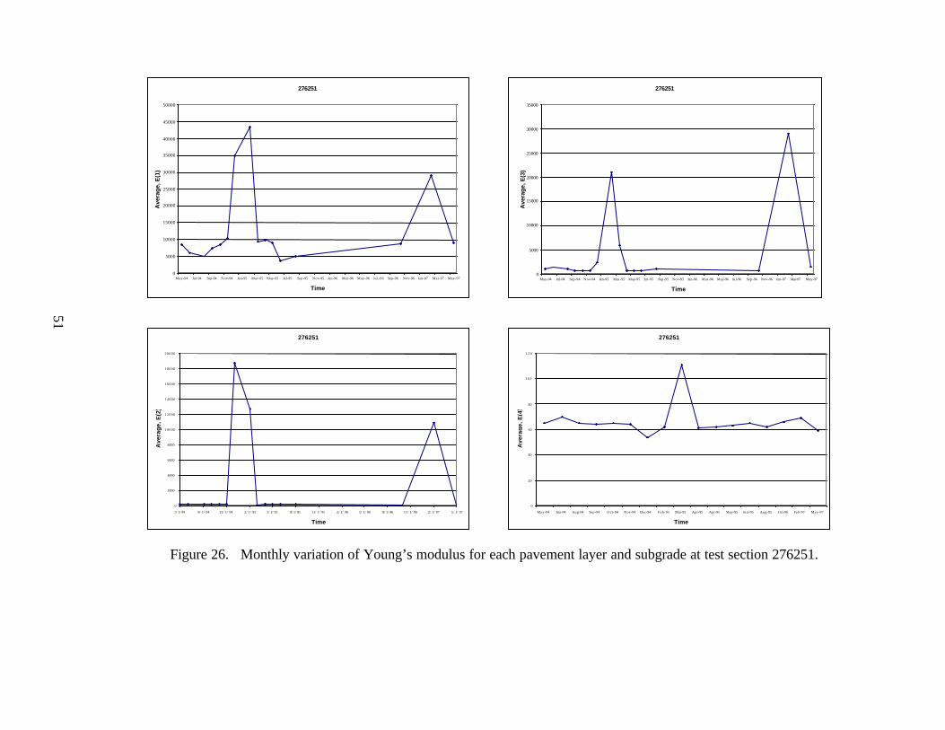
Figure 26. Monthly variation of Young’s modulus for each pavement layer and subgrade at test section 276251.

51

276251

0

5000

10000

15000

20000

25000

30000

35000

40000

45000

50000

May-94 Jul-94 Sep-94 Nov-94 Jan-95 Mar-95 May-95 Jul-95 Sep-95 Nov-95 Jan-96 Mar-96 May-96 Jul-96 Sep-96 Nov-96 Jan-97 Mar-97 May-97

Time

Ave

rage

, E(1

)

276251

0

5000

10000

15000

20000

25000

30000

35000

May-94 Jul-94 Sep-94 Nov-94 Jan-95 Mar-95 May-95 Jul-95 Sep-95 Nov-95 Jan-96 Mar-96 May-96 Jul-96 Sep-96 Nov-96 Jan-97 Mar-97 May-97

Time

Ave

rage

, E(3

)

276251

0

2000

4000

6000

8000

10000

12000

14000

16000

18000

20000

5/1/94 8/1/94 11/1/94 2/1/95 5/1/95 8/1/95 11/1/95 2/1/96 5/1/96 8/1/96 11/1/96 2/1/97 5/1/97

Time

Ave

rage

, E(2

)

276251

0

20

40

60

80

1 0 0

1 2 0

May-94 Jun-94 Aug-94 Sep-94 Oct-94 Nov-94 Dec-94 Feb-95 Mar-95 Apr-95 Apr-95 May-95 Jun-95 Aug-95 Oct-96 Feb-97 May-97

TimeA

vera

ge, E

(4)

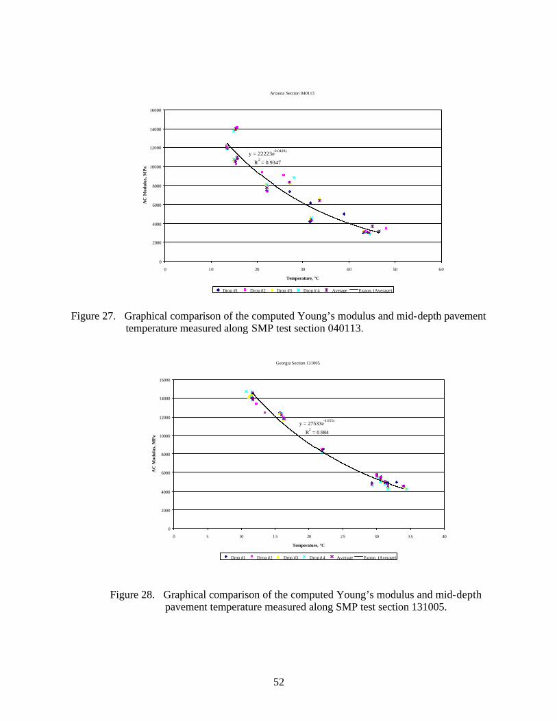
52

Figure 27. Graphical comparison of the computed Young’s modulus and mid-depth pavement

temperature measured along SMP test section 040113.

Figure 28. Graphical comparison of the computed Young’s modulus and mid-depth pavement temperature measured along SMP test section 131005.

Arizona Section 040113

y = 22223e-0.0429x

R2 = 0.9347

0

2000

4000

6000

8000

10000

12000

14000

16000

0 10 20 30 40 50 60

Temperature, °C

AC

Mod

ulus

, MPa

Drop #1 Drop #2 Drop #3 Drop # 4 Average Expon. (Average)

Georgia Section 131005

y = 27533e-0.055x

R2 = 0.984

0

2000

4000

6000

8000

10000

12000

14000

16000

0 5 10 15 20 25 30 35 40

Temperature, °C

AC

Mod

ulus

, MPa

Drop #1 Drop #2 Drop #3 Drop # 4 Average Expon. (Average)

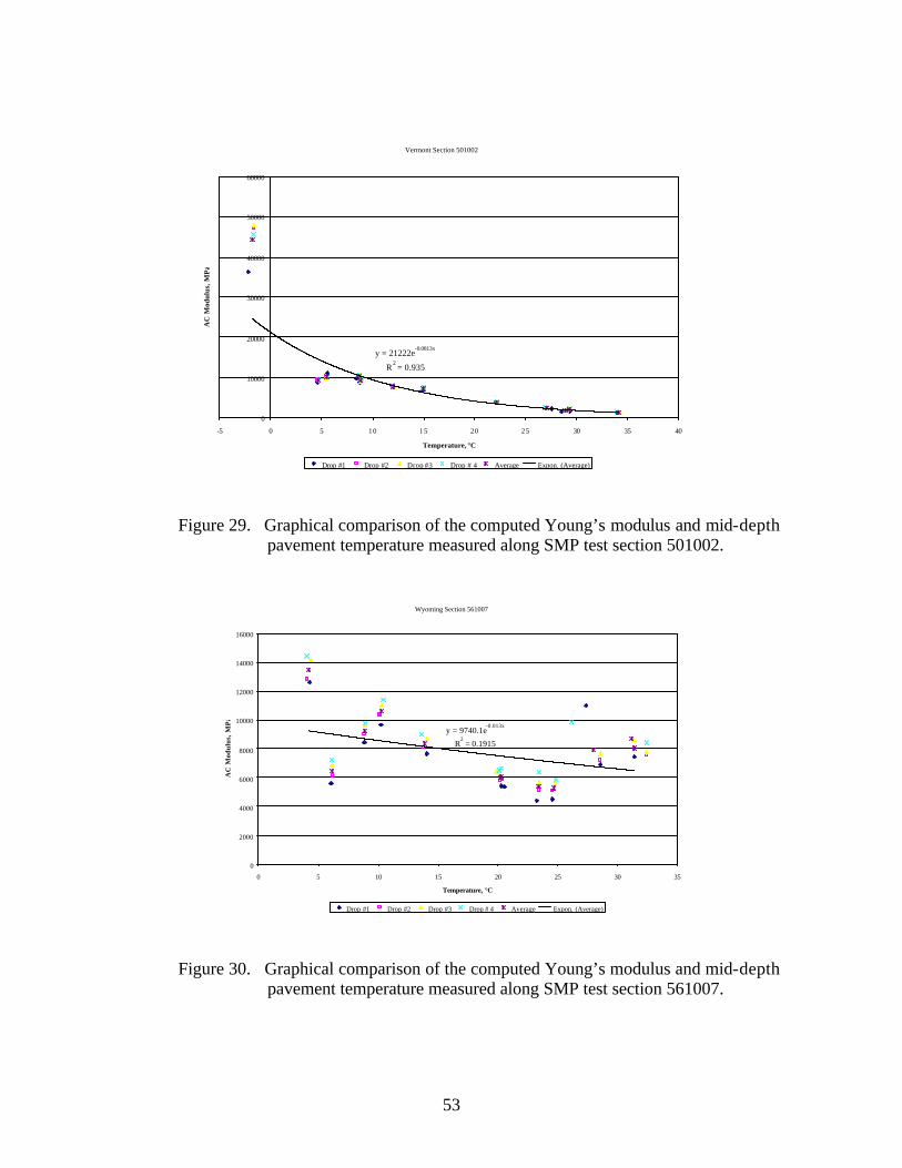
53

Figure 29. Graphical comparison of the computed Young’s modulus and mid-depth pavement temperature measured along SMP test section 501002.

Figure 30. Graphical comparison of the computed Young’s modulus and mid-depth pavement temperature measured along SMP test section 561007.

Vermont Section 501002

y = 21222e-0.0813x

R2 = 0.935

0

10000

20000

30000

40000

50000

60000

-5 0 5 10 15 20 25 30 35 40

Temperature, °C

AC

Mod

ulus

, MPa

Drop #1 Drop #2 Drop #3 Drop # 4 Average Expon. (Average)

Wyoming Section 561007

y = 9740.1e-0.013x

R2 = 0.1915

0

2000

4000

6000

8000

10000

12000

14000

16000

0 5 10 15 20 25 30 35

Temperature, °C

AC

Mod

ulus

, MPa

Drop #1 Drop #2 Drop #3 Drop # 4 Average Expon. (Average)

54

Changes in the stress sensitivity of some layers also were observed along some of the LTPP test sections. For example, layer 2 in test section 091803 (figure 19) and layers 2 and 4 at test section 481068 (figure 21) illustrate consistent changes in the calculated moduli for different drop heights. The question becomes: Is this a real condition or simply an anomaly from the back-calculation process? It is believed that the stress sensitivity can change but is dependent on the physical conditions of the soils or material (moisture content, gradation, permeability, etc.). The HMA layer is assumed to be a linear elastic material—the modulus should not change with changes in load level. However, the computed elastic moduli resulting from the linear solutions were found to increase and decrease consistently with increasing load levels for many test sections (i.e., layer 1 in figure 22). Although these changes in moduli are not consistent with laboratory test results, they have been observed from other back-calculation studies using different programs. This observation could be just an artifact of the back-calculation process, the result of compensating errors or opposite changes in elastic modulus between two different but adjacent layers with increasing drop heights, and/or a stiffening or weakening effect with increased loads. Again, the question becomes, “Is this a real condition or simply an anomaly from the back-calculation process?” It is believed that this condition may be more related to the interface condition between layers near the surface or damage that has occurred (accumulated) in the bound surface layers, rather than the true stress sensitivity of the layer. 4.5 Linear Versus Nonlinear Solutions One of the primary purposes of this study was to compute the nonlinear elastic properties of the pavement materials and subgrade soils. In fact, the largest effort was devoted to calculating these nonlinear elastic properties. One of the questions to be answered at the beginning of the data study was whether the nonlinear solutions were worth the effort. Unfortunately, this question cannot be answered until a detailed comparison is completed between laboratory-derived properties and those computed from deflection basins. Overall, fewer test points had acceptable RMS errors for the nonlinear solutions than for the linear elastic ones. Three possible explanations for this observation are listed below.

1. The first and most likely explanation is that there are more unknowns when using the nonlinear constitutive equations. The more unknowns there are, the more difficult it is to find a solution (the elastic properties for each layer), all other things being equal.

2. A quasi-nonlinear elastic structural response model simply does not adequately simulate

the real-world, nonlinear response of the pavement and soil interaction from vertical loads.

3. Young’s modulus, calculated for the surface layers, varies with drop height at some of the

test sections, as noted above, but for the nonlinear solutions it is assumed to be independent of drop height. This assumption increases the RMS error between the

55

measured and computed deflection basins because elastic layer response models do not simulate real-world conditions.

Another observation was that the HMA elastic moduli (bound layers) for the linear solutions were less than those for the nonlinear solutions but greater than the nonlinear solutions for the unbound layers. There are probably compensating differences between the bound or surface layers and unbound, subsurface layers. The cause for these differences is unknown but may be related to the interface condition of the surface layers/lifts, surface distortion, and/or microcracking of the HMA layers. To begin to answer some of these questions would require a detailed analysis and comparison of the results with the laboratory tests and observations of the cores taken from the test sections, which was beyond the scope of work for this study.

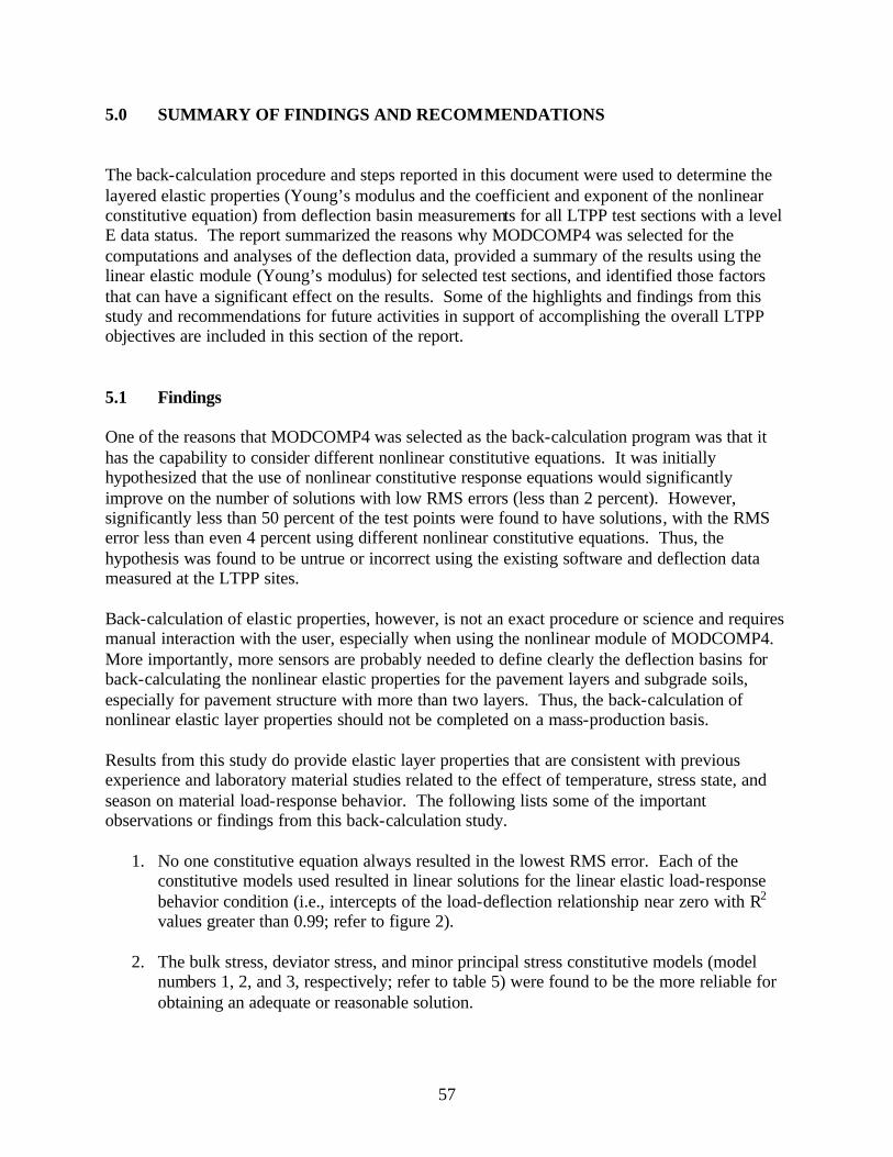
57

5.0 SUMMARY OF FINDINGS AND RECOMMENDATIONS The back-calculation procedure and steps reported in this document were used to determine the layered elastic properties (Young’s modulus and the coefficient and exponent of the nonlinear constitutive equation) from deflection basin measurements for all LTPP test sections with a level E data status. The report summarized the reasons why MODCOMP4 was selected for the computations and analyses of the deflection data, provided a summary of the results using the linear elastic module (Young’s modulus) for selected test sections, and identified those factors that can have a significant effect on the results. Some of the highlights and findings from this study and recommendations for future activities in support of accomplishing the overall LTPP objectives are included in this section of the report. 5.1 Findings One of the reasons that MODCOMP4 was selected as the back-calculation program was that it has the capability to consider different nonlinear constitutive equations. It was initially hypothesized that the use of nonlinear constitutive response equations would significantly improve on the number of solutions with low RMS errors (less than 2 percent). However, significantly less than 50 percent of the test points were found to have solutions, with the RMS error less than even 4 percent using different nonlinear constitutive equations. Thus, the hypothesis was found to be untrue or incorrect using the existing software and deflection data measured at the LTPP sites. Back-calculation of elastic properties, however, is not an exact procedure or science and requires manual interaction with the user, especially when using the nonlinear module of MODCOMP4. More importantly, more sensors are probably needed to define clearly the deflection basins for back-calculating the nonlinear elastic properties for the pavement layers and subgrade soils, especially for pavement structure with more than two layers. Thus, the back-calculation of nonlinear elastic layer properties should not be completed on a mass-production basis. Results from this study do provide elastic layer properties that are consistent with previous experience and laboratory material studies related to the effect of temperature, stress state, and season on material load-response behavior. The following lists some of the important observations or findings from this back-calculation study.

1. No one constitutive equation always resulted in the lowest RMS error. Each of the constitutive models used resulted in linear solutions for the linear elastic load-response behavior condition (i.e., intercepts of the load-deflection relationship near zero with R2 values greater than 0.99; refer to figure 2).

2. The bulk stress, deviator stress, and minor principal stress constitutive models (model

numbers 1, 2, and 3, respectively; refer to table 5) were found to be the more reliable for obtaining an adequate or reasonable solution.

58

3. On the average, over 75 percent of the deflection basins analyzed with the linear elastic module of MODCOMP4 resulted in solutions with an RMS error less than 3 percent and are considered acceptable.

4. Those pavements exhibiting deflection-softening behavior with Type II deflection basins

were the most difficult to analyze and were generally found to have RMS errors greater than 2 percent. Some of these basin analyses resulted in no reasonable solutions or the solutions provided unrealistic layer modulus for the type of material defined in the LTPP database.

5. The use of four layers generally resulted in lower RMS errors than the use of three layers

(i.e., breaking the subgrade into two layers). In many cases, breaking or separating the subgrade into at least two layers significantly improved on the match between the measured and calculated deflection basins.

6. The consideration and use of an apparent depth to a rigid layer is important, and the

results were found to be sensitive to this input parameter element. In other words, a rigid layer must be accounted for when present. However, low RMS error values were obtained for many test sections without specifying an apparent rigid layer at some depth. In fact, there were many cases in which the RMS error was larger when a rigid layer was arbitrarily included at 6 m or more.

5.2 Recommendations The results from this study have shown that elastic layer properties, especially Young’s modulus, can be computed from deflection basins and provide the pavement engineer with useful information on the pavement’s structure and subgrade condition. It is recommended that a detailed analysis of these results be completed to demonstrate their usefulness and to identify problem or unique test sections. It is also recommended that deflection basins, measured in the future along the LTPP test sections (especially the SPS test sections), be used to compute the elastic properties of the pavement and subgrade layers in order to evaluate changes in the layer moduli with time or age. Completing the back-calculation process of the nonlinear elastic properties on a production basis, however, is not recommended. Von Quintus and Killingsworth previously recommended a set of C-values for adjusting the back-calculated moduli from FWD deflections to laboratory-measured resilient moduli or vice versa.(1) These C-values were determined from back-calcula ted layer moduli using the MODULUS and WESDEPTH software packages. In all probability, these C-values are dependent on the back-calculation software package used. Thus, the back-calculated Young’s modulus derived from MODCOMP should be compared with laboratory-measured resilient moduli for the different pavement materials and subgrade soils.

59

5.3 Concluding Remarks The use of MODCOMP, MODULUS, and other software packages to calculate elastic layer properties from FWD deflection basins does not provide reasonable solutions in every case because these programs are not perfect simulations of real-world conditions. Each program has limitations and inaccuracies in simulating the deflection basins. However, as quoted from Von Quintus, Bush, and Baladi in the 1994 International Conference on NDT and Back-Calculation of Moduli:(13) In summary, most participants concurred that there needs to be a standard

baseline of values from which to compare a project, material, or pavement base and that one should not become paralyzed by the imperfection of the procedures. More importantly, research must be merged into practice on a consistent basis and one way to accomplish this is through the standardization process. As such, a procedure needs to be standardized and that procedure should concentrate on user oriented issues.

This study has attempted to implement and apply existing standardized procedures (ASTMD5858 and FHWA-RD-97-076) to back-calculate Young’s modulus and the nonlinear elastic properties for each pavement and subgrade layer. Results from this extensive effort, as well as from other studies, such as FHWA-RD-97-086, are promising and have shown that reasonable solutions for Young’s modulus can be obtained. These computed parameters have been included in the LTPP database for future pavement performance and material studies. These results also provide a baseline of solutions and elastic properties for which the results from future studies can be compared and improved upon. Another quote from Von Quintus, Bush, and Baladi at the 1994 International Conference reads as follows: (13) The question, however, is still: what is the reliability of these values?

Specifically, it was the general consensus of the panel and attendees that the accuracy of back-calculated moduli is model dependent and unknown, as well as those values measured in the laboratory because there is a diversity of opinion on the simulation of field conditions in the laboratory. For example, there is controversy within the industry on whe ther back-calculation procedures should be based on a dynamic or static analysis, and what values actually represent the truth, both in the laboratory or from field measurements.

Unfortunately, the relationship between the computed parameters from this study and resilient moduli from the laboratory repeated- load testing has not yet been established.

6.0 REFERENCES 1. Von Quintus, H.L. and B. Killingsworth, Design Pamphlet for the Backcalculation of

Pavement Layer Moduli in Support of the 1993 AASHTO Guide for the Design of Pavement Structures, Publication No. FHWA-RD-97-076, Washington, DC: Federal Highway Administration, September 1997.

2. Harichandran, R. S. et al, MICHBACK User’s Manual, Version 1.0 for DOS, Michigan

State University, Lansing, MI, 1995. 3. Von Quintus, H. L. and B. Killingsworth, Back-Calculation of Layer Moduli of LTPP

General Pavement Study (GPS) Sites, Publication No. FHWA-RD-97-086, Washington, DC: Federal Highway Administration, July 1997.

4. Von Quintus, H. L. and B. Killingsworth, Analysis Relating to Pavement Material

Characterizations and their Effects on Pavement Performance, Publication No. FHWA-RD-97-086, Washington, DC: Federal Highway Administration, May 1997.

5. May, R. W. and H. L. Von Quintus, The Quest for a Standard Guide to NDT Back-

Calculation, STP 1198, American Society for Testing and Materials, Philadelphia, PA, December 1994.

6. PCS/Law Engineering, SHRP’s Layer Moduli Back-Calculation Procedure, SHRP-P655,

Washington, DC: Strategic Highway Research Program, National Academy of Science, 1993.

7. Strategic Highway Research Program, SHRP Layer Moduli Back-Calculation Procedure-

Software Selection, SHRP Technical Report, Washington, DC: July 1991. 8. Daleiden, J. F., et al., Evaluation of the AASHTO Design Equations and Recommended

Improvements, Report No. SHRP-P394, Washington, DC: Strategic Highway Research Program, National Academy of Science, 1994.

9. Simpson, A. L., et al., Sensitivity Analyses for Selected Pavement Distresses, Report No.

SHRP-P393, Washington, DC: Strategic Highway Research Program, National Academy of Science, 1994.

10. Irwin, L. H., Instructional Guide for Back-Calculation and the Use of MODCOMP,

CLRP Publication No. 94-10, Cornell University, Local Roads Program, Ithaca, NY, March 1994.

11. Telephone conversation with Dr. Vincent Janoo, CREL, November 1997.

62

12. Nondestructive Testing of Pavements and Back-Calculation of Moduli, STP 1026, American Society for Testing and Materials (Editors: Albert J. Bush, III and Gilbert Y. Baladi), Philadelphia, PA, November 1989.

13. Nondestructive Testing of Pavements and Back-Calculation of Moduli, Second Volume,

STP 1198, American Society for Testing and Materials (Editors: Harold L. Von Quintus, Albert J. Bush, III and Gilbert Y. Baladi), Philadelphia, PA, December 1994.

14. Meeting of consultant and agency personnel to discuss the benefits, advantages, and

disadvantages of different back-calculation programs, sponsored by FHWA under the DATS contract, Baltimore, MD: February 1997.

15. Rada, G., C. Richter and P. Jordahl, SHRP’s Layer Moduli Backcalculation Procedure,

Second Volume, STP 1198, American Society for Testing and Materials (Editors: Harold L. Von Quintus, Albert J. Bush, and Gilbert Y. Baladi), Philadelphia, PA, December 1994.

16. Michalak, C.H. and T. Scullion, MODULUS 4.2: User’s Manual, Research Report 1939-

1, Texas Transportation Institute, College Station, TX, 1993. 17. AASHTO Guide for the Design of Pavement Structures, American Association of State

Highway and Transportation Officials, Washington, DC: 1993. 18. LTPP Strategic Analysis Plan, Publication No. FHWA-Rd-01-086, Washington, DC:

Federal Highway Administration, March 2001.

63

Appendix A Back-Calculation of Layer Elastic Properties from LTPP-FWD Deflection Basin Data Using MODCOMP User’s Guide Introduction Back-calculation is a process for estimating the elastic layer modulus in pavement structures that represent in situ conditions under a test load. Back-calculation gets its name from the fact that a load of known size and shape is applied to the pavement and deflections are measured by sensors at known distances from the load. Theoretical predictions are made of the deflections, assuming certain layer properties, and those properties (usually elastic layer modulus) are adjusted until the calculated deflections match the measured deflections within a reasonable RMS error (goodness-of-fit between the measured and calculated deflection basins). Back-calculation of elastic properties is usually performed with static-linear analyses, and there are numerous computer programs or software packages that can be used to calculate the elastic properties of each layer. The MODCOMP4 software package was selected and used for analyzing the LTPP deflection data, because (among other features) it is capable of doing back-calculation for massive quantities of deflection data using both linear (Young’s modulus) and nonlinear (stress dependent elastic modulus) approaches for materials characterization. Nonlinear materials are those for which the modulus depends on the applied stress (i.e., stress-dependent) and is not a single number but a relationship between modulus and stress. Numerous mathematical forms have been used to represent the relationship between modulus and stress. The particular relationship adopted for a layer material is referred to later in this document as a constitutive equation. Purpose of User’s Guide The back-calculation procedure explained in this appendix is a tool that agencies can use in the future to update the computed parameters (elastic properties) of each layer for the LTPP test sections as more and more deflection basin data are measured over time. This User’s Guide is intended to accomplish the following objectives:

1. To describe the features of the software and combination of the individual models so that potential users can determine its applicability to their needs.

2. To list and define those steps and decision functions that are used in the process, especially those requiring engineering judgment of the user.

64

3. To provide users with all of the information necessary for them to operate and use the software packages or models efficiently.

The back-calculation process is a series of DOS-based programs, and the user must be familiar with the use of these types of programs to complete the process. The user should also be experienced and knowledgeable in the back-calculation process and familiar with the LTPP database. The audience intended for this User’s Guide includes pavement materials and design engineers; research engineers; pavement management engineers; and other professionals in Federal, State, and local government; academia; and in private industry. Back-Calculation Procedure Overview The overall operational process for back-calculating the layer modulus basically follows the procedure outlined by Von Quintus and Killingsworth in publication number FHWA-RD-97-076(1) and the Instructional Guide for Back-Calculation and the Use of MODCOMP.(10) This process was developed for back-calculating massive quantities of deflection data that are stored within the LTPP database (the IMS or a centralized location). The procedure used to back-calculate the elastic properties of each layer for the LTPP test sections consists of a number of operations. This User’s Guide identifies and discusses all of the operations (programs and decision functions) included in this process. The procedure is not fully automated but is an iterative process between the different programs and requires engineering judgment of the user. The following lists those major steps that are used in the process:

Step 1 – Extract Data from IMS Step 2 – Preprocess the Extracted FWD Deflection Basin Data and Section Classification Step 3 – Create Input Files for MODCOMP4 Step 4 – Trial Computations and Modification of Inputs Step 5 – Back-Calculate Young’s Modulus and the Nonlinear Elastic Properties Using MODCOMP4

Step 6 – Extract Elastic Properties and Create Summary Output Files An important fact regarding future use of the procedure is that the LTPP database is dynamic, and the programs that are used to extract the data were written based on the database that existed in 1998. These programs may need to be revised as the LTPP database is updated and changed over time. The following identifies and describes briefly the programs used to accomplish the above operations. Figure 31 is a flow chart of the back-calculation procedure.

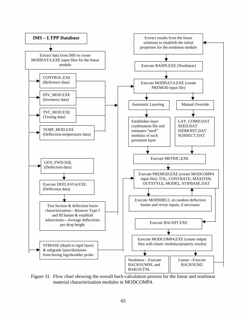
65

Figure 31. Flow chart showing the overall back-calculation process for the linear and nonlinear

material characterization modules in MODCOMP4.

IMS – LTPP Database

CONTROL.EXE (Reference data)

INV_MOD.EXE (Inventory data)

Extract data from IMS to create MODDATA.EXE input files for the linear

module

TST_MOD.EXE (Testing data)

TEMP_MOD.EXE (Deflection-temperature data)

Execute DEFLAVG4.EXE (Deflection data)

Test Section & deflection basin characterization—Remove Type I

and III basins & establish subsections—Average deflections

per drop height

STIBASE (depth to rigid layer) & subgrade layer/thickness from boring log/shoulder probe

Execute MODDATA.EXE (create PREMOD input file)

Execute MODSHELL on random deflection basins and revise inputs, if necessary

Execute PREMOD.EXE (create MODCOMP4 input file); TOL, CONVRATE; MAXITER,

OUTSTYLE, MODEL, STIFBASE.DAT

Execute MODCOMP4.EXE (create output files with elastic modulus/property results)

Nonlinear—Execute BACKSUMNL and BAKOUTNL

Linear—Execute BACKSUM2

Extract results from the linear solutions to establish the initial

properties for the nonlinear module

GEN_FWD.SQL (Deflection data)

Execute BASIN.EXE (Nonlinear)

Establishes layer combination file and estimates “seed” modulus of each pavement layer

Automatic Layering Manual Override

LAY_COMD.DAT SEED.DAT ISDMOIST.DAT SUBSECT.DAT

Execute METRIC.EXE

Execute BACHIT.EXE

66

1. Programs INV_MOD, TST_MOD, and TST_MOD2 obtain materials data from State

highway agency (SHA) inventory files and LTPP materials testing programs that have been collected and stored in the LTPP database. CONTROL gets a list of sections and dates for which deflection data exist, and TEMP_MOD retrieves pavement temperature data taken during the deflection acquisition. Structured Query Language (SQL), a database query tool, statements generated by a SQL script GEN_FWD.SQL are used to obtain the deflections themselves.

2. Program DEFLAVG4 performs averaging and editing on the acquired deflection data.

3. Program MODDATA takes the data acquired in steps 1 and 2, provides estimates of the modulus for each layer, and performs layer combination in accordance with a set of rules in the cases where there are too many layers to analyze separately.

4. Program METRIC converts the values in the MODDATA output to metric units;

MODDATA was originally written for an earlier back-calculation effort in which English units were used.

5. Program PREMOD3 converts the metricated output of MODDATA (containing data sets

for multiple locations [stations] within one section on one or more dates) into individual data files for the averaged deflections at each section, date, location, and drop height to be used by program MODCOMP4.

6. Program BATCHIT creates two batch files based on the output files generated by a single

run of PREMOD3. The first sets up the directory structure to hold the (many) PREMOD3 output files for a specific test section. The second changes to each of the resulting directories in turn and executes MODCOMP4 for each data file within that subdirectory; the data and output files are then compressed together and stored.

7. Program MODCOMP4, written by Dr. Lynne Irwin of the Cornell University Local Roads Program (CLRP), is the program used for the actual back-calculation of layer modulus from the deflection basins.(10)

8. Program BACKSUM2 (for linear back-calculation) obtains desired information from

many MODCOMP4 Asummary@ files and places it in a single file, performing many file manipulation operations to achieve this result.

9. Program BAKSUMNL obtains the same data as BACKSUM2 but from the summary files

for nonlinear runs, which have a slightly different format.

10. Program BAKOUTNL obtains the specific coefficients and exponents for the selected equation form for each layer of the nonlinear solution from the much lengthier Afull-output@ files that are not available from the summary files.

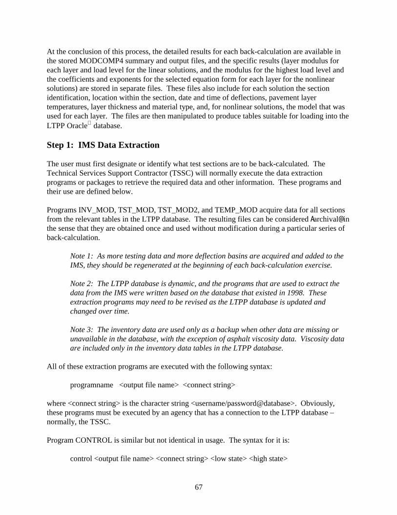
67

At the conclusion of this process, the detailed results for each back-calculation are available in the stored MODCOMP4 summary and output files, and the specific results (layer modulus for each layer and load level for the linear solutions, and the modulus for the highest load level and the coefficients and exponents for the selected equation form for each layer for the nonlinear solutions) are stored in separate files. These files also include for each solution the section identification, location within the section, date and time of deflections, pavement layer temperatures, layer thickness and material type, and, for nonlinear solutions, the model that was used for each layer. The files are then manipulated to produce tables suitable for loading into the LTPP Oracle database. Step 1: IMS Data Extraction The user must first designate or identify what test sections are to be back-calculated. The Technical Services Support Contractor (TSSC) will normally execute the data extraction programs or packages to retrieve the required data and other information. These programs and their use are defined below. Programs INV_MOD, TST_MOD, TST_MOD2, and TEMP_MOD acquire data for all sections from the relevant tables in the LTPP database. The resulting files can be considered Aarchival@ in the sense that they are obtained once and used without modification during a particular series of back-calculation.

Note 1: As more testing data and more deflection basins are acquired and added to the IMS, they should be regenerated at the beginning of each back-calculation exercise. Note 2: The LTPP database is dynamic, and the programs that are used to extract the data from the IMS were written based on the database that existed in 1998. These extraction programs may need to be revised as the LTPP database is updated and changed over time. Note 3: The inventory data are used only as a backup when other data are missing or unavailable in the database, with the exception of asphalt viscosity data. Viscosity data are included only in the inventory data tables in the LTPP database.

All of these extraction programs are executed with the following syntax:

programname <output file name> <connect string> where <connect string> is the character string <username/password@database>. Obviously, these programs must be executed by an agency that has a connection to the LTPP database – normally, the TSSC. Program CONTROL is similar but not identical in usage. The syntax for it is:

control <output file name> <connect string> <low state> <high state>

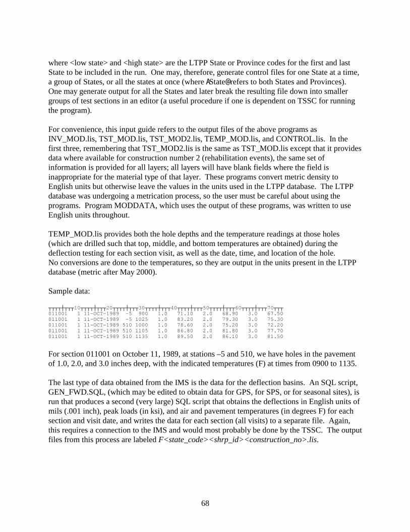
68

where <low state> and <high state> are the LTPP State or Province codes for the first and last State to be included in the run. One may, therefore, generate control files for one State at a time, a group of States, or all the states at once (where AState@ refers to both States and Provinces). One may generate output for all the States and later break the resulting file down into smaller groups of test sections in an editor (a useful procedure if one is dependent on TSSC for running the program). For convenience, this input guide refers to the output files of the above programs as INV_MOD.lis, TST_MOD.lis, TST_MOD2.lis, TEMP_MOD.lis, and CONTROL.lis. In the first three, remembering that TST_MOD2.lis is the same as TST_MOD.lis except that it provides data where available for construction number 2 (rehabilitation events), the same set of information is provided for all layers; all layers will have blank fields where the field is inappropriate for the material type of that layer. These programs convert metric density to English units but otherwise leave the values in the units used in the LTPP database. The LTPP database was undergoing a metrication process, so the user must be careful about using the programs. Program MODDATA, which uses the output of these programs, was written to use English units throughout. TEMP_MOD.lis provides both the hole depths and the temperature readings at those holes (which are drilled such that top, middle, and bottom temperatures are obtained) during the deflection testing for each section visit, as well as the date, time, and location of the hole. No conversions are done to the temperatures, so they are output in the units present in the LTPP database (metric after May 2000). Sample data: ┬┬┬┬┼┬┬┬10┬┬┬┬┼┬┬┬20┬┬┬┬┼┬┬┬30┬┬┬┬┼┬┬┬40┬┬┬┬┼┬┬┬50┬┬┬┬┼┬┬┬60┬┬┬┬┼┬┬┬70┬┬┬011001 1 11-OCT-1989 -5 900 1.0 71.10 2.0 68.90 3.0 67.50011001 1 11-OCT-1989 -5 1025 1.0 83.20 2.0 79.30 3.0 75.30011001 1 11-OCT-1989 510 1000 1.0 78.60 2.0 75.20 3.0 72.20011001 1 11-OCT-1989 510 1105 1.0 86.80 2.0 81.80 3.0 77.70011001 1 11-OCT-1989 510 1135 1.0 89.50 2.0 86.10 3.0 81.50

For section 011001 on October 11, 1989, at stations –5 and 510, we have holes in the pavement of 1.0, 2.0, and 3.0 inches deep, with the indicated temperatures (F) at times from 0900 to 1135. The last type of data obtained from the IMS is the data for the deflection basins. An SQL script, GEN_FWD.SQL, (which may be edited to obtain data for GPS, for SPS, or for seasonal sites), is run that produces a second (very large) SQL script that obtains the deflections in English units of mils (.001 inch), peak loads (in ksi), and air and pavement temperatures (in degrees F) for each section and visit date, and writes the data for each section (all visits) to a separate file. Again, this requires a connection to the IMS and would most probably be done by the TSSC. The output files from this process are labeled F<state_code><shrp_id><construction_no>.lis.

69

Step 2: Preprocess the FWD Deflection Data – Execute DEFLAVG4 As discussed above, the deflection data acquired are passed through program DEFLAVG4, which performs several operations on the data. Deflection data from the IMS consist (normally) of basins from 12 drops (rigid pavements) or 16 drops (flexible pavements), 4 at each drop height, or nominal load. The deflections for each drop at a given drop height are normalized by the load for that drop; the normalized drops are then averaged and the results multiplied by the average load for that drop height. This is done for each of the seven sensors. The program is run by typing in the command prompt: DEFLAVG4<space><Data File Name><return>. The use of the DOS FOR-DO loop will make it possible to execute DEFLAVE4 on all FWD data files in a subdirectory with one command. In performing these operations, the deflection basins are checked for nondecreasing deflections with increasing distance from the load; if this occurs, the drop is omitted from the average. In addition, a test for variation based on that used in the FWD software itself is applied: If an individual (renormalized) deflection value differs from the average by more than (0.08 + 1 percent [average deflection]) mils, that difference is calculated for all sensors and summed. The drop having the largest sum is excluded, and the average is recalculated. If necessary, this process is repeated, leaving only two drops. If they differ from their average by more than the above amount, the average is accepted but marked as Avariant@ in the output file. The criteria of 0.08 mils and 1 percent are from the stated accuracy specifications on the FWD unit itself. If all the drops at a given location and load have nondecreasing deflections, they are all discarded. If all but one is discarded, the remaining value is used, but obviously there can be no check for variation in this case. The number of drops contributing to the final average is recorded in the output file for each drop height; where only two remain and one or more sensors show variation, the deflection values for those sensors are so indicated in the output file. The program name DEFLAVG4.exe indicates the version used for flexible data with four-digit years in the dates. (DEFLAV_R.exe is the same except that it is used with rigid pavement deflection basin data, and uses only data from mid-slab basins [lane numbers J1 or C1].) Output files have the same file name as the input file, with an extension A.AVG.@ A Alog@ file is written for each run, showing the details of the averaging and drop exclusion process. This file has the A.LOG@ extension.

Note 4: Program BASIN is executed external to the back-calculation process to determine the load-response (figures 2-4) and basin (figures 5-8) classification of the deflection basin data. Figure 32 illustrates the flow diagram for characterizing the deflection basin measurements. The load-response classification assists the user in selecting the initial constitutive equation for the nonlinear module of MODCOMP. The BASIN program is not needed for the linear module.

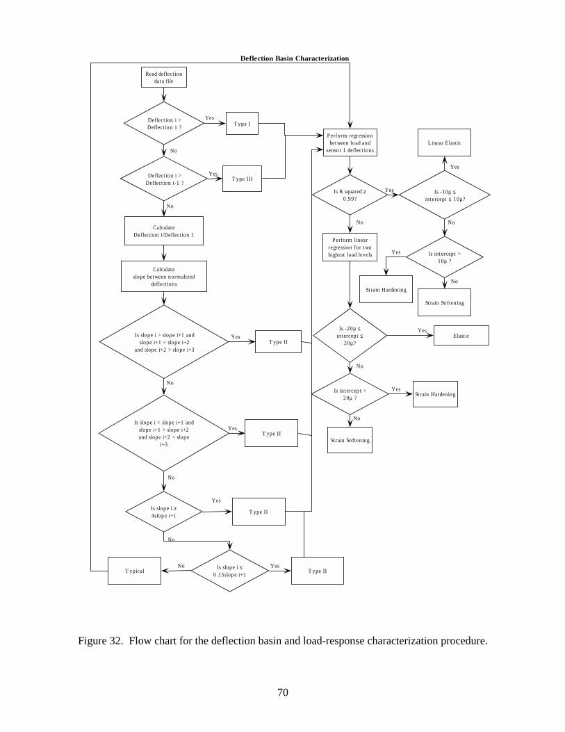
70

Figure 32. Flow chart for the deflection basin and load-response characterization procedure.

Read deflect iondat a file

Deflect ion i >Deflect ion 1 ?

Deflection Basin Characterization

Yes

No

T ype I

Deflect ion i >Deflect ion i-1 ?

T ype IIIYes

No

Calculat eDeflect ion i/Deflect ion 1

Calculat eslope bet ween normalized

deflect ions

Is slope i > slope i+1 andslope i+1 < slope i+2

and slope i+2 > slope i+3

YesT ype II

No

Is slope i < slope i+1 andslope i+1 > slope i+2and slope i+2 < slope

i+3

YesT ype II

No

Is slope i ≥4slope i+1

Yes

T ype II

No

Is slope i ≤0.15slope i+1

YesT ype II

NoT ypical

P erform regressionbet ween load and

sensor 1 deflect ions

Is R squared ≥0 .99?

Yes Is -10µ ≤int ercept ≤ 10µ?

Linear Elast ic

Yes

Is int ercep t >10µ ?

NoNo

St rain Hardening

Yes

St rain Soft ening

No

P erform linearregression for t wohighest load levels

Is int ercep t >20µ ?

Is -20µ ≤int ercep t ≤

20µ?Elast ic

Yes

No

St rain HardeningYes

St rain Soft ening

No

No

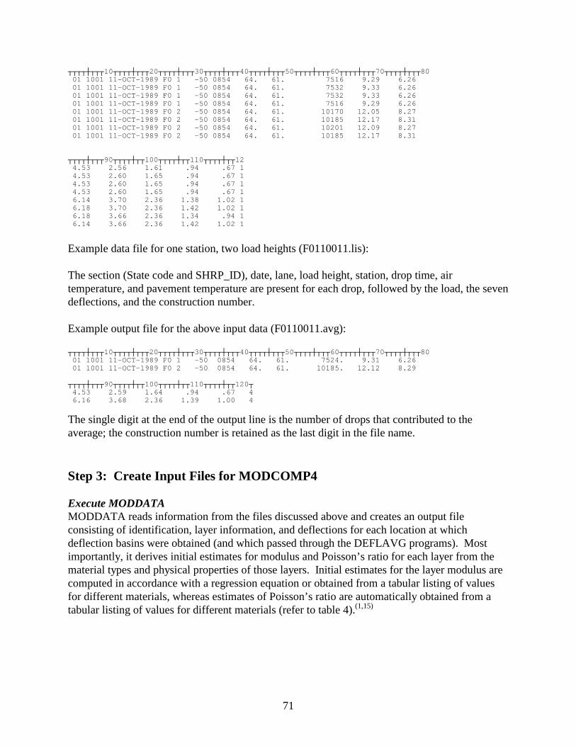
71

┬┬┬┬┼┬┬┬10┬┬┬┬┼┬┬┬20┬┬┬┬┼┬┬┬30┬┬┬┬┼┬┬┬40┬┬┬┬┼┬┬┬50┬┬┬┬┼┬┬┬60┬┬┬┬┼┬┬┬70┬┬┬┬┼┬┬┬8001 1001 11-OCT-1989 F0 1 -50 0854 64. 61. 7516 9.29 6.2601 1001 11-OCT-1989 F0 1 -50 0854 64. 61. 7532 9.33 6.2601 1001 11-OCT-1989 F0 1 -50 0854 64. 61. 7532 9.33 6.2601 1001 11-OCT-1989 F0 1 -50 0854 64. 61. 7516 9.29 6.2601 1001 11-OCT-1989 F0 2 -50 0854 64. 61. 10170 12.05 8.2701 1001 11-OCT-1989 F0 2 -50 0854 64. 61. 10185 12.17 8.3101 1001 11-OCT-1989 F0 2 -50 0854 64. 61. 10201 12.09 8.2701 1001 11-OCT-1989 F0 2 -50 0854 64. 61. 10185 12.17 8.31

┬┬┬┬┼┬┬┬90┬┬┬┬┼┬┬100┬┬┬┬┼┬┬110┬┬┬┬┼┬┬124.53 2.56 1.61 .94 .67 14.53 2.60 1.65 .94 .67 14.53 2.60 1.65 .94 .67 14.53 2.60 1.65 .94 .67 16.14 3.70 2.36 1.38 1.02 16.18 3.70 2.36 1.42 1.02 16.18 3.66 2.36 1.34 .94 16.14 3.66 2.36 1.42 1.02 1

Example data file for one station, two load heights (F0110011.lis): The section (State code and SHRP_ID), date, lane, load height, station, drop time, air temperature, and pavement temperature are present for each drop, followed by the load, the seven deflections, and the construction number. Example output file for the above input data (F0110011.avg): ┬┬┬┬┼┬┬┬10┬┬┬┬┼┬┬┬20┬┬┬┬┼┬┬┬30┬┬┬┬┼┬┬┬40┬┬┬┬┼┬┬┬50┬┬┬┬┼┬┬┬60┬┬┬┬┼┬┬┬70┬┬┬┬┼┬┬┬8001 1001 11-OCT-1989 F0 1 -50 0854 64. 61. 7524. 9.31 6.2601 1001 11-OCT-1989 F0 2 -50 0854 64. 61. 10185. 12.12 8.29

┬┬┬┬┼┬┬┬90┬┬┬┬┼┬┬100┬┬┬┬┼┬┬110┬┬┬┬┼┬┬120┬4.53 2.59 1.64 .94 .67 46.16 3.68 2.36 1.39 1.00 4

The single digit at the end of the output line is the number of drops that contributed to the average; the construction number is retained as the last digit in the file name. Step 3: Create Input Files for MODCOMP4 Execute MODDATA MODDATA reads information from the files discussed above and creates an output file consisting of identification, layer information, and deflections for each location at which deflection basins were obtained (and which passed through the DEFLAVG programs). Most importantly, it derives initial estimates for modulus and Poisson’s ratio for each layer from the material types and physical properties of those layers. Initial estimates for the layer modulus are computed in accordance with a regression equation or obtained from a tabular listing of values for different materials, whereas estimates of Poisson’s ratio are automatically obtained from a tabular listing of values for different materials (refer to table 4).(1,15)

72

Automatic Layering Definition For sections having more than five layers, MODDATA performs layer combinations according to rules established by LTPP in 1993, unless the user overrides the process with desired specific layer combinations.(15)

Note 5: Although the original back-calculation program used with MODDATA could handle only five layers total (including rigid base) and MODCOMP4 can handle many more, it is considered inappropriate to solve for more than five layers when using MODCOMP4.

To run MODDATA, it is best to establish some standard file locations, or paths, ahead of time. The following are suggested: <exepath> The location of the executable programs in this process. <commpath> The location of common data files used for multiple runs of MODDATA on

different deflection data (e.g., the IMS extraction data files). <deflpath> The location of deflection data files generated by DEFLAVG4 or DEFLAV_R. <sectpath> The location of files unique to a specific run of MODDATA. MODDATA can use (but does not require) several input files in addition to those containing the IMS extraction data; when executed, the program requests that each file name be entered in response to a labeled prompt, shown as follows, with the recommended location for each: Enter name of REFERENCE file <sectpath>F0110011.CNT Enter name of INVENTORY DATA file <commpath>INV_MOD.LIS Enter name of MATERIALS TEST file <commpath>TST_MOD.LIS Enter name of DEFLECTION TEMPS file <commpath>TEMP_GPS.LIS Enter name of DEFLECTION DATA file <deflpath>F0110011.LIS ANONE@ CAN BE ENTERED FOR THE NEXT FOUR FILENAMES Enter name of IN-SITU DENSITY DATA file <commpath>ISDMOIST.DAT Enter name of EXTERNAL LAYER COMBINATION file <commpath>LAY_COMB.DAT Enter name of EXT. LAYER MODULUS INPUT file <commpath>SEED.DAT Enter name of STATION SPLIT-LOCATION file <commpath>SUBSECT.DAT Enter name of ERROR OUTPUT file <sectpath>F0110011.ERR Enter name of SUMMARY OUTPUT file <sectpath>F0110011.OUT Enter name of DATA OUTPUT file <sectpath>F0110011.DAT Each file shown in <commpath> will normally contain data for many test sections, and in the case of TEMP_GPS, numerous dates per test section. F0110011.CNT, the control file in the example shown, will have multiple dates for the test section 011001, construction number 1. The program will search each file for the test section identification 011001 and will search for the specific dates in TEMP_GPS and in F0110011.LIS. If a control file containing section identifications for multiple sections is used, the data for each section will be sought within each file.

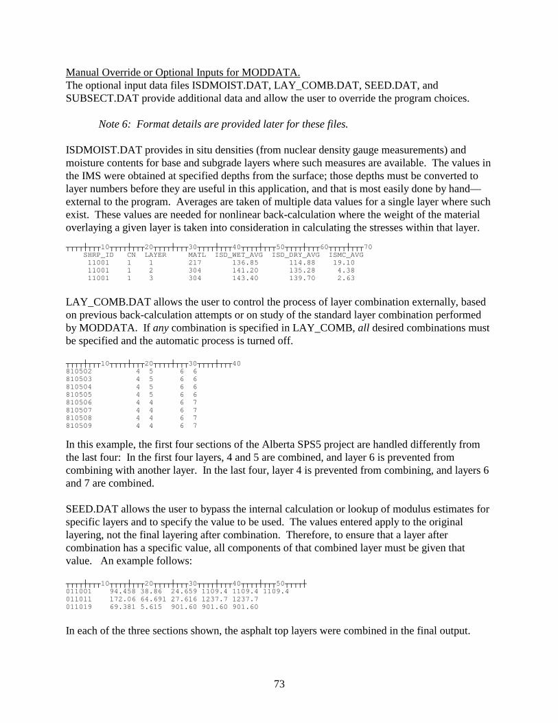
73

Manual Override or Optional Inputs for MODDATA. The optional input data files ISDMOIST.DAT, LAY_COMB.DAT, SEED.DAT, and SUBSECT.DAT provide additional data and allow the user to override the program choices.

Note 6: Format details are provided later for these files. ISDMOIST.DAT provides in situ densities (from nuclear density gauge measurements) and moisture contents for base and subgrade layers where such measures are available. The values in the IMS were obtained at specified depths from the surface; those depths must be converted to layer numbers before they are useful in this application, and that is most easily done by hand—external to the program. Averages are taken of multiple data values for a single layer where such exist. These values are needed for nonlinear back-calculation where the weight of the material overlaying a given layer is taken into consideration in calculating the stresses within that layer.

┬┬┬┬┼┬┬┬10┬┬┬┬┼┬┬┬20┬┬┬┬┼┬┬┬30┬┬┬┬┼┬┬┬40┬┬┬┬┼┬┬┬50┬┬┬┬┼┬┬┬60┬┬┬┬┼┬┬┬70SHRP_ID CN LAYER MATL ISD_WET_AVG ISD_DRY_AVG ISMC_AVG11001 1 1 217 136.85 114.88 19.1011001 1 2 304 141.20 135.28 4.3811001 1 3 304 143.40 139.70 2.63

LAY_COMB.DAT allows the user to control the process of layer combination externally, based on previous back-calculation attempts or on study of the standard layer combination performed by MODDATA. If any combination is specified in LAY_COMB, all desired combinations must be specified and the automatic process is turned off. ┬┬┬┬┼┬┬┬10┬┬┬┬┼┬┬┬20┬┬┬┬┼┬┬┬30┬┬┬┬┼┬┬┬40810502 4 5 6 6810503 4 5 6 6810504 4 5 6 6810505 4 5 6 6810506 4 4 6 7810507 4 4 6 7810508 4 4 6 7810509 4 4 6 7

In this example, the first four sections of the Alberta SPS5 project are handled differently from the last four: In the first four layers, 4 and 5 are combined, and layer 6 is prevented from combining with another layer. In the last four, layer 4 is prevented from combining, and layers 6 and 7 are combined. SEED.DAT allows the user to bypass the internal calculation or lookup of modulus estimates for specific layers and to specify the value to be used. The values entered apply to the original layering, not the final layering after combination. Therefore, to ensure that a layer after combination has a specific value, all components of that combined layer must be given that value. An example follows: ┬┬┬┬┼┬┬┬10┬┬┬┬┼┬┬┬20┬┬┬┬┼┬┬┬30┬┬┬┬┼┬┬┬40┬┬┬┬┼┬┬┬50┬┬┬┬┼011001 94.458 38.86 24.659 1109.4 1109.4 1109.4011011 172.06 64.691 27.616 1237.7 1237.7011019 69.381 5.615 901.60 901.60 901.60

In each of the three sections shown, the asphalt top layers were combined in the final output.

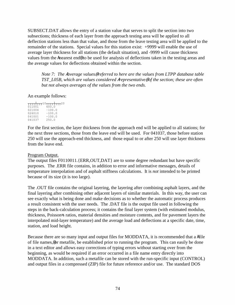
74

SUBSECT.DAT allows the entry of a station value that serves to split the section into two subsections; thickness of each layer from the approach testing area will be applied to all deflection stations less than that value, and those from the leave testing area will be applied to the remainder of the stations. Special values for this station exist: +9999 will enable the use of average layer thickness for all stations (the default situation), and -9999 will cause thickness values from the Anearest end@ to be used for analysis of deflections taken in the testing areas and the average values for deflections obtained within the section.

Note 7: The Aaverage values@ referred to here are the values from LTPP database table TST_L05B, which are values considered Arepresentative@ of the section; these are often but not always averages of the values from the two ends.

An example follows: ┬┬┬┬┼┬┬┬10┬┬┬┬┼┬┬┬20011001 600.0021004 -100.0026010 -100.0041001 -100.0041037 250.0

For the first section, the layer thickness from the approach end will be applied to all stations; for the next three sections, those from the leave end will be used. For 041037, those before station 250 will use the approach-end thickness, and those equal to or after 250 will use layer thickness from the leave end. Program Output. The output files F0110011.{ERR,OUT,DAT} are to some degree redundant but have specific purposes. The .ERR file contains, in addition to error and informative messages, details of temperature interpolation and of asphalt stiffness calculations. It is not intended to be printed because of its size (it is too large). The .OUT file contains the original layering, the layering after combining asphalt layers, and the final layering after combining other adjacent layers of similar materials. In this way, the user can see exactly what is being done and make decisions as to whether the automatic process produces a result consistent with the user needs. The .DAT file is the output file used in following the steps in the back-calculation process; it contains the final layer system (with estimated modulus, thickness, Poisson=s ratios, material densities and moisture contents, and for pavement layers the interpolated mid-layer temperature) and the average load and deflections at a specific date, time, station, and load height. Because there are so many input and output files for MODDATA, it is recommended that a Afile of file names,@or metafile, be established prior to running the program. This can easily be done in a text editor and allows easy corrections of typing errors without starting over from the beginning, as would be required if an error occurred in a file name entry directly into MODDATA. In addition, such a metafile can be stored with the run-specific input (CONTROL) and output files in a compressed (ZIP) file for future reference and/or use. The standard DOS

75

redirection of input from the console to the specified metafile is accomplished using the less-than symbol, as shown below:

MODDATA < metafilename Execute METRIC Program METRIC uses the .DAT file output by MODDATA as input and writes out a file, normally with the same file name and an extension of .MET, containing the same information in metric (SI) units for use in MODCOMP4, as follows:

MODDATA METRIC Layer thickness in m (= inches *.0254) Layer modulus ksi MPa (= ksi *6.894757) Layer density pcf kg/m3 (= pcf *16.01846) Temperature hole depths in mm (= inches *25.4) Interpolated temperatures oF oC (= [deg F-32] *.555555) Depth to refusal ft m (= feet *.3048) FWD load lb force kN (= lbs *.004448222) FWD deflections mils µm (= mils *25.4)

Note 8: Deflection location values (in feet) were not changed because they are descriptive only.

Sample input and output files: English ┬┬┬┬┼┬┬┬10┬┬┬┬┼┬┬┬20┬┬┬┬┼┬┬┬30┬┬┬┬┼┬┬┬40┬┬┬┬┼┬┬┬50┬┬┬┬┼┬┬┬60┬┬┬┬┼┬┬┬70┬┬┬┬┼┬091803 500. 25-AUG-1994 3

1 7 142 SS .0 .35 26.5 .0 .0 125.0 8.02 5 302 GB 12.0 .35 30.0 10.0 132.4 125.0 8.03 3 700 AC 7.2 .32 408.6 102.2 1225.9 153.7 .0 88.5

18-JUL-1989 200. 4.025-AUG-1994 1323. 81. 102. 0 1 F1 1.4 96.9 3.7 88.1 6.2 80.6500. 6038. 5.03 3.48 2.66 1.82 1.20 .77 .43

Metric ┬┬┬┬┼┬┬┬10┬┬┬┬┼┬┬┬20┬┬┬┬┼┬┬┬30┬┬┬┬┼┬┬┬40┬┬┬┬┼┬┬┬50┬┬┬┬┼┬┬┬60┬┬┬┬┼┬┬┬70┬┬┬┬┼┬┬┬091803 500. 25-AUG-1994 3

1 7 142 SS .000 .35 182.7 .0 .0 2002. 8.02 5 302 GB .305 .35 206.8 68.9 912.9 2002. 8.03 3 700 AC .183 .32 2817.2 704.6 8452.3 2462. .0 31.4

18-JUL-1989 200. 1.2225-AUG-1994 1323. 27.2 38.9 0 1 F1 35.6 36.1 94.0 31.2 157.5 27.0500. 26.86 127.8 88.4 67.6 46.2 30.5 19.6 10.9 0

For this example, MODDATA output (English and Metric) for section 091803 (in CT) has three layers after combinations.

• The subgrade has a starting modulus of 26.5 ksi, with no stated upper and lower limits. • The base is 12.0 inches thick, with a starting modulus of 30 ksi, bounded by 10 and 132.4

ksi.

76

• Both base and subgrade have a Poisson’s ratio of 0.35, a density of 125 pcf, and a moisture content of 8 percent. (The upper and lower bounds derived by MODDATA are not used with MODCOMP4.)

• The asphalt layer, in addition to the above parameters, shows a mid-depth temperature of 88.5 F.

• The depth to refusal as determined in July 1989 was 4 feet. • Deflections from August 1994 at station 500 were taken with a load of 6,038 pounds, at

air and pavement surface temperatures of 81 and 102oF, respectively, in mid-lane (F1), with gradient temperatures interpolated to the time of observation of 96.9, 88.1, and 80.6oF at depths of 1.4, 3.7, and 6.2 inches, respectively.

• The single digits 0 and 1 prior to the lane specification are the crack width (not measured except for load-transfer deflection data, which is not used for back-calculation) and load height indicators, respectively.

Execute PREMOD3 Program PREMOD3 takes data from MODDATA (after passing through METRIC), consisting of multiple average deflection basins for different loads at multiple points on multiple dates, and writes out input data files acceptable to MODCOMP4. For linear back-calculation, one data file is required for each average basin studied; for nonlinear studies, the basins for all loads done at one location and time are included in one data file. A very large number (up to 5,000) of data files can be generated by one run of PREMOD3 (e.g., linear studies for a seasonal site). The program allows external user control (again, by auxiliary data files) of the choice of sensors associated in MODCOMP4 with a specific layer (usually done after the first run through MODCOMP4 with automatic assignment), the choice of nonlinear models for specific layers, and the choice and depth of a second subgrade layer and/or a rigid foundation.

Note 9: A second subgrade is often used to model the changes of confining and deviator stresses with depth. A rigid foundation can model the actual presence of a very stiff layer at depth or the effect on the subgrade of a nearly vanishing deviator stress and increasing confining pressure at depth, which may make the subgrade material act as though it were a very stiff layer. In addition, for a thin layer or a layer for which the stiffness is considered known, the modulus can be entered as a Aknown@ value, not subject to change by the program.

A metafile can be established for PREMOD3 runs in a manner similar to that for MODDATA, enabling better batch (unattended) operation, if needed, and providing the opportunity for correcting typing errors without restarting the program. This metafile can use the extension .PMD and a file name showing the SHRP_ID, if desired. It will contain responses to questions asked by PREMOD3, as well as the file names (or ANONE@) of the files described above. When executed, PREMOD3 asks the user for the following information: English (E) or Metric (M) ENTER NAME OF MODDATA OUTPUT FILE <shrp_id>.MET

77

ENTER NAME OF STIFF-BASE-DEPTH FILE, or type NONE: STIFBASE.DAT ENTER NAME OF NON_LINEAR MODELS FILE, or type NONE: MODELS.DAT ENTER NAME OF SENSOR/FIXED-STIFF FILE, or type NONE: SENSOR.DAT ENTER LOG FILE NAME FOR THIS RUN: <shrp_id>.LOG ENTER OUTSTYLE, TOL, CONVRATE, MAX ITER, MODEL NUMBER (use single quotes on CHAR. inputs) Because for this project MODCOMP4 was to be run in metric units, the first question is always answered with an M, and the .MET data file output by METRIC is used for the second. Standard names were established for the next three files, as shown above; the log file name is arbitrary, but the above choice is consistent and recommended. OUTSTYLE is a character variable in MODCOMP4 describing the volume of output requested:

BRIE (brief), LONG, or ALL. BRIEF echoes the input and gives final layer modulus. LONG reports the layer modulus for each iteration, and ALL reports intermediate calculations as well; ALL gives very lengthy output and should be used with care.

TOL is a single character variable in MODCOMP4 describing the allowable tolerance on the fit to the deflections: values of L (low), M (medium) and H (high) are allowed, H (high) is recommended. This applies only to those sensors assigned to specific layers. H (high) tolerance implies a good fit, not large residuals.

CONVRATE is a numeric value indicating a lower limit on the rate of change of modulus between iterations; 1.5 percent is usually used.

MAX ITER is the maximum number of iterations allowed before the program Agives up”—usually 15. If this number is reached, either new starting values or new sensor assignments are probably needed.

MODEL NUMBER has the following allowable values and meanings: 0 Use linear for all layers >0 Nonlinear model to be used for -ALL- base/subgrade layers -1 Use the bulk stress model (model 1) for base/subbase and the deviator stress model (model 2) for subgrade soil -2 Model number to be read in for each layer from external file

With this information, PREMOD3 can generate a MODCOMP4 input data file for each basin (linear) or each set of basins at different load levels but the same location and time (nonlinear). The auxiliary input files for PREMOD3 allow the user to modify the default behavior of the program and/or of MODCOMP4, as follows: STIFBASE.DAT provides information on the desired value of depth to stiff base, if the value calculated within PREMOD3 is inappropriate, and the thickness of a top subgrade layer, if such a layer is desired.

78

Note 10: The internal calculation of the depth to an apparent rigid layer is based on the Texas A&M procedure by G. Rohde, which was taken from the MODULUS 4.0 program.(16)

Values required are the six-character section ID, the depth to stiff base from the top of the pavement, and the thickness of an assumed Atop-subgrade@ layer. Space is available for comments on the origins of the values used. If no value is present for the thickness of the top subgrade layer, such a layer will not be included. If a –1. (decimal point required) is present for the depth to stiff base, no rigid base will be modeled, and the bottom (or only) subgrade will be considered of semi-infinite extent. ┬┬┬┬┼┬┬┬10┬┬┬┬┼┬┬┬20┬┬┬┬┼┬┬┬30┬┬┬┬┼┬┬┬40┬┬┬┬┼┬┬┬50┬┬┬┬┼┬┬┬60┬┬┬┬┼┬┬┬70┬┬┬┬┼┬┬┬80011001 178.5 No Split, Average of Approach and Leave011011 35.9 No Split, Average of Approach and Leave011019 252.6 80.0 Split, Average of Approach and Leave011021 104.85 No Split, Average of Approach and Leave014073 178.6 No Split, Average of Approach and Leave014125 93.95 36.0 Split, Average of Approach and Leave014126 380.35 43.0 Split, Average of Approach and Leave016019 189.5 36.0 Split, Average of Approach and Leave

MODELS.DAT (used only if MODEL NUMBER above = -2) provides the number of the relationship between modulus and stress included within MODCOMP4 for each layer of the pavement system. Zero is entered for layers considered linear (e.g., asphalt, PCC). MODELS.DAT has one line per section. An example follows: ┬┬┬┬┼┬┬┬10┬┬┬┬┼┬┬┬20┬┬┬┬┼┬┬┬30011001 1 1 1 0011011 1 1 1 0011019 1 1 0011021 2 1 0 0014073 1 0 1 0014126 1 1 0016019 1 1 0

Note 11: Most of the subgrade and base layers use model 1.

For the above example, model 2 (deviator stress model) was found to be a better fit for the subgrade for test section 011021, and the subbase layer (a lime-treated soil) of 014073 was found to be linear. SENSOR.DAT provides the user an opportunity to change the association of a particular sensor with a particular layer in the pavement system from the default association provided by the program. This may improve the resultant fit and is used more often with nonlinear problems; finding the best association may require several attempts. In addition, this file is used to enter values for layer moduli that the user wishes MODCOMP4 to consider as fixed values, not subject to variation in the calculation. For each layer, input is in the form LL S EEEEE., where LL is the layer number, S is the number of the sensor to be associated with that layer, and EEEEE. is the fixed modulus for that layer. Obviously, if a fixed value is supplied, one should have no sensor associated with that layer.

79

Because it was desired to be able to associate a sensor with the second (lower) subgrade layer if one was created, for the purposes of this data file, that layer was given an arbitrary designation as layer 10. Because this layer did not exist at the time MODDATA was run, no seed value could then be entered for it; hence, a programming trick allows a seed (NOT a fixed value) to be entered for such a layer if the value of EEEEE. (see above) is negative. Remember that because this file is read into PREMOD3, any modulus values must be in metric units (MPa). An example of the file follows: ┬┬┬┬┼┬┬┬10┬┬┬┬┼┬┬┬20┬┬┬┬┼┬┬┬30┬┬┬┬┼┬┬┬40┬┬┬┬┼┬┬┬50┬┬┬┬┼┬┬┬60┬┬┬┬┼┬┬┬70┬┬┬┬┼┬┬┬80011001 1 0 0. 2 5 0. 3 0 0. 4 1 0. 10 7 -171.011011 1 0 0. 2 0 1270. 3 3 0. 4 0 0. 10 0 -568.011019 1 5 0. 2 3 0. 3 0 0. 10 0 -119.011021 1 5 0. 2 0 0. 3 0 0. 4 0 0. 10 0 -360.014073 1 0 0. 2 5 0. 3 0 0. 4 0 0. 10 0 -961.

Output files from PREMOD3 are named in such a way as to identify them as well as possible and to avoid duplicate names in a single directory containing as many as 5,000 separate files. For Seasonal Monitoring Pavement (SMP) sites, the file naming convention is:

ssstttph.dmy where:

sss = a three-character label for the seasonal site, consisting of the two-digit state code and a letter indicating the specific site within that state, obtained from a data statement within PREMOD3 correlating standard six-character SHRP_ID=s to seasonal ID=s. These letters are not arbitrary but have been assigned previously.

ttt = a three-character label for the station at which the deflections were observed,

using M in the first character if the station was negative (no negative three-digit stations were used) and prefixing two- or single-digit stations with 0 and 00, respectively.

p = a single character in alphabetic sequence indicating the number of times the

present station and load height have been used so far on this particular day. l = a single digit (0,1,3) indicating the lane in which the data was taken (0, test pit

area; 1, mid-lane; 3, outer wheelpath)

d = a single character (A–Z, 1-5) indicating the day of the month of the site visit.

m = a single character (A–L) indicating the month of the site visit.

y = a single character (0–9) indicating the last digit of the year of the site visit. This convention assumed that all visits were within the same decade, which was true for the present data set.

80

It should be noted that the pass number p starts at A for a given SHRP_ID, date, and station, and is incremented until either the corresponding file name has not been already used, or 36 values (26 letters + 10 digits) have been attempted, in which case the program prints an error message and quits. A total of 24 cases (corresponding to six sequences of observations and four load heights at each location) should be the maximum needed. Where multiple data sets were taken at the same location on the same sequence, more values may be needed, but this is a data error and should be fixed in the data. For nonseasonal sites the file-naming convention is:

aaaaaach.lmy where:

aaaaaa = the full 6-character SHRP_ID of the section being studied c = a single character (A–Z, 0-9) indicating the station at which the data was

taken (for flexible sections, 21 stations are used in each lane, and for rigid sections, up to 20 stations are used for the mid-slab deflections, which are the only ones for which back-calculation is attempted).

h = a single digit (1–4) corresponding to the load height used for the current

deflections, corresponding to different nominal loads (6,000; 9,000; 12,000; and 16,000 pounds).

l,m,y = (lane, month, year) as above for seasonal data file names (note that we

assume there will not be two visits for non-seasonal sites in the same month, nor will there be more than one complete sequence on a single day).

Step 4: Trial Computations and Modification of Inputs Execute MODSHELL To begin the computation process, a limited number of points are manually selected at random along the test section to complete the back-calculation of elastic properties. The number of test points selected are generally in the range of three to eight and depend on the amount of variation of the measured deflection basins within the subsection. For test sections with “uniform” load response, three or four deflection basins should be used, whereas six to eight basins should be used for those test sections with load-response characteristics defined as “drift” or “highly variable.”(1) MODSHELL is used to analyze the basins measured at those random test points. Results from these initial solutions are reviewed to determine whether the production runs should be executed

81

or changes should be made to the inputs before proceeding to the production runs. The decision on whether to proceed is based on, in order of importance:

• The magnitude of the RMS errors—revisions should be made until the RMS error is reduced to 2 percent or less, or to the lowest possible value.

• The computed elastic layer modulus (Young’s modulus)—revisions should be made if

“extreme” (high or low) layer moduli are calculated for the type of material identified. • Changes occur in the elastic layer modulus from one iteration to the other near the end of

the computations. If the RMS errors are found to be large (greater than 2 percent) or the calculated layer elastic moduli are questionable for the type of material, the inputs should be checked and adjustments made to the layer combinations, layer-sensor assignments, and/or the use or omission of an apparent rigid layer. MODSHELL is used to recalculate the elastic layer modulus with those changes. This iterative process is continued until “reasonable or acceptable” solutions are achieved. As stated above, a reasonable or acceptable solution is one with an RMS error less than or equal to 2 percent with elastic layer moduli that are considered typical for the material type. The revisions, if any, to the input parameters created by PREMOD are then used for the production runs. For some test sections, extremely high or low layer moduli can be computed for one or more layers in the pavement structure with good RMS error values. If this occurs, changes should be made to the inputs and MODSHELL used to recalculate Young’s modulus, as noted above. If the final RMS error is less than 2 percent for the trial runs that resulted in the extremely high or low moduli and is much greater than 2 percent for the other trial runs, the trial run resulting in the high or low moduli should be used for the production runs. Execute Program BATCHIT Program BATCHIT creates batch files to assist in the automated handling of the many MODCOMP4 input files generated by PREMOD3. The program is executed from the directory containing those output files (see below). BATCHIT examines the extensions of all the data files; the first batch file creates a subdirectory corresponding to each such extension below a directory specified by the user, and moves all files with that extension to that subdirectory. The second batch file causes the system to change to each of those subdirectories in turn, execute MODCOMP4 on each data file, and compress (using PKZIP) the data files and short and long output files into separate ZIP files for future reference. These ZIP files are stored in <startid>/<stateid>. The program assumes that the data files from PREMOD3 are in a directory:

<startid>\<stateid>\<seasid>

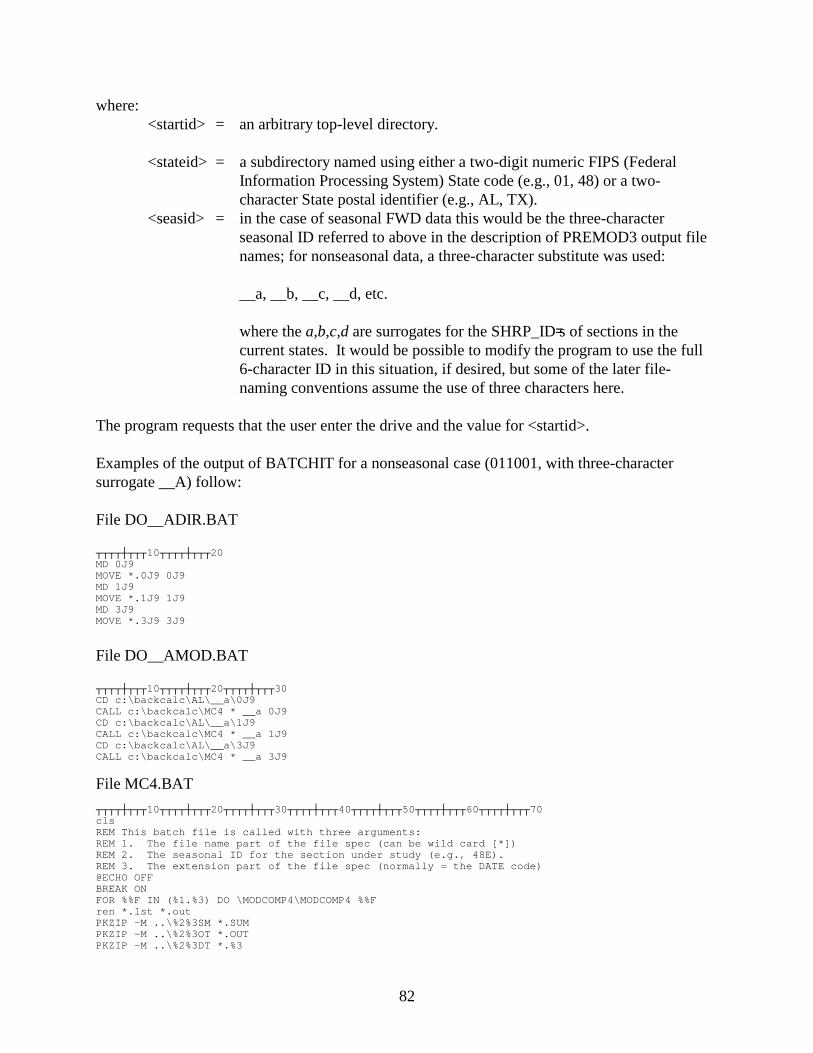
82

where: <startid> = an arbitrary top-level directory.

<stateid> = a subdirectory named using either a two-digit numeric FIPS (Federal

Information Processing System) State code (e.g., 01, 48) or a two-character State postal identifier (e.g., AL, TX).

<seasid> = in the case of seasonal FWD data this would be the three-character seasonal ID referred to above in the description of PREMOD3 output file names; for nonseasonal data, a three-character substitute was used:

__a, __b, __c, __d, etc.

where the a,b,c,d are surrogates for the SHRP_ID=s of sections in the current states. It would be possible to modify the program to use the full 6-character ID in this situation, if desired, but some of the later file-naming conventions assume the use of three characters here.

The program requests that the user enter the drive and the value for <startid>. Examples of the output of BATCHIT for a nonseasonal case (011001, with three-character surrogate __A) follow: File DO__ADIR.BAT ┬┬┬┬┼┬┬┬10┬┬┬┬┼┬┬┬20MD 0J9MOVE *.0J9 0J9MD 1J9MOVE *.1J9 1J9MD 3J9MOVE *.3J9 3J9

File DO__AMOD.BAT ┬┬┬┬┼┬┬┬10┬┬┬┬┼┬┬┬20┬┬┬┬┼┬┬┬30CD c:\backcalc\AL\__a\0J9CALL c:\backcalc\MC4 * __a 0J9CD c:\backcalc\AL\__a\1J9CALL c:\backcalc\MC4 * __a 1J9CD c:\backcalc\AL\__a\3J9CALL c:\backcalc\MC4 * __a 3J9

File MC4.BAT ┬┬┬┬┼┬┬┬10┬┬┬┬┼┬┬┬20┬┬┬┬┼┬┬┬30┬┬┬┬┼┬┬┬40┬┬┬┬┼┬┬┬50┬┬┬┬┼┬┬┬60┬┬┬┬┼┬┬┬70clsREM This batch file is called with three arguments:REM 1. The file name part of the file spec (can be wild card [*])REM 2. The seasonal ID for the section under study (e.g., 48E).REM 3. The extension part of the file spec (normally = the DATE code)@ECHO OFFBREAK ONFOR %%F IN (%1.%3) DO \MODCOMP4\MODCOMP4 %%Fren *.lst *.outPKZIP -M ..\%2%3SM *.SUMPKZIP -M ..\%2%3OT *.OUTPKZIP -M ..\%2%3DT *.%3

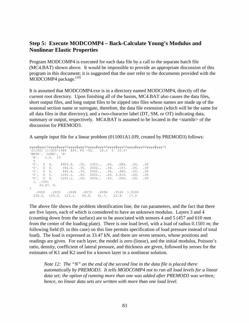
83

Step 5: Execute MODCOMP4 – Back-Calculate Young’s Modulus and Nonlinear Elastic Properties Program MODCOMP4 is executed for each data file by a call to the separate batch file (MC4.BAT) shown above. It would be impossible to provide an appropriate discussion of this program in this document; it is suggested that the user refer to the documents provided with the MODCOMP4 package.(10) It is assumed that MODCOMP4.exe is in a directory named MODCOMP4, directly off the current root directory. Upon finishing all of the basins, MC4.BAT also causes the data files, short output files, and long output files to be zipped into files whose names are made up of the seasonal section name or surrogate, therefore, the data file extension (which will be the same for all data files in that directory); and a two-character label (DT, SM, or OT) indicating data, summary or output, respectively. MC4.BAT is assumed to be located in the <startdir> of the discussion for PREMOD3. A sample input file for a linear problem (011001A1.0J9, created by PREMOD3) follows: ┬┬┬┬┼┬┬┬10┬┬┬┬┼┬┬┬20┬┬┬┬┼┬┬┬30┬┬┬┬┼┬┬┬40┬┬┬┬┼┬┬┬50┬┬┬┬┼┬┬┬60┬┬┬┬┼┬┬┬70011001 11-OCT-1989 854. F0 -50. 20.5 4 33.47

'METR', 'LONG', 'N''H', 1.5, 155

'U', 0 0, 4903.6, .30, 2353., .00, .084, .00, .00'U', 0 0, 382.0, .35, 2002., .36, .157, .00, .00'U', 0 4, 442.6, .35, 2002., .36, .485, .00, .00'U', 0 5, 1201.1, .45, 2002., .43, 3.810, .00, .00'U', 0 0, 1201.1, .45, 2002., .43, .000, .00, .001, .1501

33.47, 0.7

.0000 .2032 .3048 .4572 .6096 .9144 1.5240236.5, 159.0, 115.1, 65.8, 41.7, 23.9, 17.0

The above file shows the problem identification line, the run parameters, and the fact that there are five layers, each of which is considered to have an unknown modulus. Layers 3 and 4 (counting down from the surface) are to be associated with sensors 4 and 5 (457 and 610 mm from the center of the loading plate). There is one load level, with a load of radius 0.1501 m; the following field (0. in this case) on this line permits specification of load pressure instead of total load). The load is expressed as 33.47 kN, and there are seven sensors, whose positions and readings are given. For each layer, the model is zero (linear), and the initial modulus, Poisson’s ratio, density, coefficient of lateral pressure, and thickness are given, followed by zeroes for the estimates of K1 and K2 used for a known layer in a nonlinear solution.

Note 12: The “N” on the end of the second line in the data file is placed there automatically by PREMOD3. It tells MODCOMP4 not to run all load levels for a linear data set; the option of running more than one was added after PREMOD3 was written; hence, no linear data sets are written with more than one load level.

84

Step 6: Extract Elastic Properties and Create Summary Output Files Execute BACKSUM2 Program BACKSUM2 is run to obtain summary information from the MODCOMP4 summary (short) output files for the final iteration of linear back-calculation runs. The data desired are the SHRP_ID, the date, time, and temperature when the deflections were obtained, the location (station and lane), the load applied, the thickness and derived modulus for each layer, and the average error between the observed and predicted deflections for the final values of layer modulus. The program is run from the directory containing the ZIP files created by the second batch file and expands each SM (summary) ZIP file, obtains a directory of the summary files, and extracts the required information from each file in turn. The output for all of the summary files in a given ZIP file is written to a single file, one line per basin, whose location in the directory structure is given by a file DIRECT.NAM in the current directory and whose file name is the first six characters of the ZIP file, which is made up of the three-character seasonal ID (or its surrogate for nonseasonal sections) and the three-character data file extension. If DIRECT.NAM does not exist, the user is prompted for the need to create it, and the program is halted. The program could be modified to assume that the file DIRECT.NAM is in a standard location, instead of being in the current directory. Sample output follows: ┬┬┬┬┼┬┬┬10┬┬┬┬┼┬┬┬20┬┬┬┬┼┬┬┬30┬┬┬┬┼┬┬┬40┬┬┬┬┼┬┬┬50┬┬┬┬┼┬┬┬60┬┬┬┬┼┬┬┬70┬┬┬┬┼

SHRP_ID FWD_DATE TIME LN STN TAC #DRP LOAD ITN %ERR T(1) E(1)

836454 17-JUL-1992 1056. F3 475. T 18.3 4 25.96 4 12.8 .272 1580.

┬┬┬80┬┬┬┬┼┬┬┬90┬┬┬┬┼┬┬100┬┬┬┬┼┬┬110┬┬┬┬┼┬┬120T(2) E(2) T(3) E(3) T(4) E(4)

.914 191. 14.054 147. .000 3450.

Execute BAKSUMNL Program BAKSUMNL does what BACKSUM2 does but for the results of nonlinear calculations. The MODCOMP4 output formats are slightly different, and the results in terms of layer modulus are given only for the highest load value for which a basin was included (remember that for nonlinear processing, the MODCOMP4 data files each contain the basins for a full four load levels done at that time and place). Sample output follows: ┬┬┬┬┼┬┬┬10┬┬┬┬┼┬┬┬20┬┬┬┬┼┬┬┬30┬┬┬┬┼┬┬┬40┬┬┬┬┼┬┬┬50┬┬┬┬┼┬┬┬60┬┬┬┬┼┬┬┬70┬┬┬┬┼┬┬┬80

SHRP_ID FWD_DATE TIME LN STN TAC #DRP LOAD ITN %ERR T(1) MOD E(1) S

040114 06-FEB-1996 827. F1 300. A 10.8 4 28.94 3 3.3 .173 0 9880.0040114 06-FEB-1996 830. F1 325. A 10.8 4 28.65 5 3.8 .173 0 11300.0040114 06-FEB-1996 833. F1 350. A 10.8 4 28.49 4 3.0 .173 0 9860.0040114 06-FEB-1996 836. F1 375. A 10.8 4 28.56 4 3.0 .173 0 11600.0040114 06-FEB-1996 841. F1 400. A 10.9 4 28.08 15 9.0 .173 0 20500.0

┬┬┬┬┼┬┬┬90┬┬┬┬┼┬┬100┬┬┬┬┼┬┬110┬┬┬┬┼┬┬120┬┬┬┬┼┬┬130┬┬┬┬┼┬┬140┬┬┬┬┼┬┬150┬┬┬┬┼┬┬160┬┬┬┬┼┬┬IG T(2) MOD E(2) SIG T(3) MOD E(3) SIG T(4) MOD E(4) SIG T(5) MOD E(5) SIG

L .305 1 347.0 S .914 1 505.0 N 6.228 1 453.0 S .000 0 3450.0 FL .305 1 307.0 N .914 1 646.0 S 6.228 1 510.0 S .000 0 3450.0 FL .305 1 276.0 S .914 1 384.0 S 6.228 1 703.0 N .000 0 3450.0 FL .305 1 339.0 S .914 1 581.0 S 6.228 1 431.0 S .000 0 3450.0 FL .305 1 212.0 N .914 1 158.0 S 6.228 1 1250.0 S .000 0 3450.0 F

85

Note that layer 1 is linear (L), the nonlinear solution for layers 2,3, and 4 is sometimes significant (S) and sometimes not (N), and layer 5 has fixed modulus (F). TAC is the asphalt mid-depth temperature, MOD is the model number assumed for the layer, and #DRP is the number of drops included in the averaged basin. Note also that, at station 400, the MODCOMP4 solution ran out of iterations before converging. Execute BAKOUTNL Program BAKOUTNL operates on the longer output files for nonlinear back-calculation results to obtain information not available from the shorter summary output files. Specifically, BAKOUTNL obtains, in addition to necessary identification information, the coefficients and exponents in the mathematical relation assumed by the user to hold for the particular layer material. In addition the number of the model used, Poisson=s ratio, the coefficient of lateral pressure, and the density of the layer are extracted, as well as the correlation coefficient R for the regression between modulus and stress for the different load levels, showing how well the chosen model actually fits the data.

Note 13: The number obtained is R, not the R-squared that is usually used in this application.

If a linear layer is included in the layer structure, the modulus obtained for that layer under the highest load is retrieved instead of the model parameters. The program is executed for each nonlinear back-calculation, with two parameters, as shown below: BAKOUTNL <infile> <outfile> where <infile> is a long output file of MODCOMP4, and the output is written to <outfile> as one line per layer. Sample output follows: ┬┬┬┬┼┬┬┬10┬┬┬┬┼┬┬┬20┬┬┬┬┼┬┬┬30┬┬┬┬┼┬┬┬40┬┬┬┬┼┬┬┬50┬┬┬┬┼┬┬┬60┬┬┬┬┼┬┬┬70┬┬┬┬┼┬┬┬80┬┬SHRP_ID FWD_DATE DROP LN STN ITER POISS DENS E COEFF EXP

TIME MODEL K0

040114 02-APR-1996 856. F1 300. 4 0 .30 .00 2246.0 9180.0 .00000E+00 .000040114 02-APR-1996 856. F1 300. 4 1 .35 .36 2002.0 .0 .21080E+03 .001040114 02-APR-1996 856. F1 300. 4 1 .35 .43 2002.0 .0 .43790E+03 .009040114 02-APR-1996 856. F1 300. 4 1 .35 .43 2002.0 .0 .11790E+07 -.086040114 02-APR-1996 856. F1 300. 4 0 .20 .00 .0 3447.4 .00000E+00 .000040114 02-APR-1996 932. F3 300. 15 0 .30 .00 2246.0 8030.0 .00000E+00 .000040114 02-APR-1996 932. F3 300. 15 1 .35 .36 2002.0 .0 .14400E+03 .000040114 02-APR-1996 932. F3 300. 15 1 .35 .43 2002.0 .0 .15170E+03 .042040114 02-APR-1996 932. F3 300. 15 1 .35 .43 2002.0 .0 .16290E+10 -.168040114 02-APR-1996 932. F3 300. 15 0 .20 .00 .0 3447.4 .00000E+00 .000040114 02-APR-1996 1016. F1 300. 3 0 .30 .00 2246.0 7650.0 .00000E+00 .000040114 02-APR-1996 1016. F1 300. 3 1 .35 .36 2002.0 .0 .19370E+03 .001040114 02-APR-1996 1016. F1 300. 3 1 .35 .43 2002.0 .0 .21670E+03 .028040114 02-APR-1996 1016. F1 300. 3 1 .35 .43 2002.0 .0 .90830E+09 -.159

86

Note here, for the example, that COEFF and EXP are 0.0 for the linear asphalt layer and the fixed layer. Summary This guide has been prepared to implement and apply existing standardized procedures (ASTM D5858 and FHWA-RD-97-076) to back-calculate Young’s modulus and the nonlinear elastic properties for each pavement and subgrade layer.(1) However, the use of MODCOMP4, as well as other software packages, to calculate elastic layer properties from FWD deflection basins does not always provide reasonable solutions, because the program is not a perfect simulation of real-world conditions. Each program has limitations and inaccuracies in simulating the deflection basins.

87

Appendix B Test Section Classification and Subgrade Information for the Back-Calculation Process Appendix B provides a listing of the LTPP test sections that have extensive variability and drift and those that were subdivided into two subsections. Appendix B also provides a listing of the LTPP test sections where an apparent rigid layer was used in the back-calculation process and the depth to sampling refusal from the shoulder probe drilled at each site.

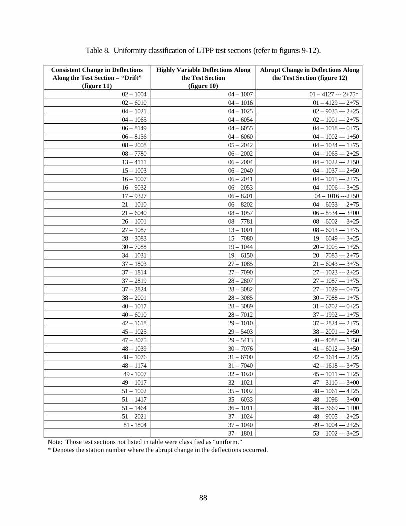
88

Table 8. Uniformity classification of LTPP test sections (refer to figures 9-12).

Consistent Change in Deflections Along the Test Section – “Drift”

(figure 11)

Highly Variable Deflections Along the Test Section

(figure 10)

Abrupt Change in Deflections Along the Test Section (figure 12)

02 – 1004 04 – 1007 01 – 4127 --- 2+75* 02 – 6010 04 – 1016 01 – 4129 --- 2+75 04 – 1021 04 – 1025 02 – 9035 --- 2+25 04 – 1065 04 – 6054 02 – 1001 --- 2+75 06 – 8149 04 – 6055 04 – 1018 --- 0+75 06 – 8156 04 – 6060 04 – 1002 --- 1+50 08 – 2008 05 – 2042 04 – 1034 --- 1+75 08 – 7780 06 – 2002 04 – 1065 --- 2+25 13 – 4111 06 – 2004 04 – 1022 --- 2+50 15 – 1003 06 – 2040 04 – 1037 --- 2+50 16 – 1007 06 – 2041 04 – 1015 --- 2+75 16 – 9032 06 – 2053 04 – 1006 --- 3+25 17 – 9327 06 – 8201 04 – 1016 ---2+50 21 – 1010 06 – 8202 04 – 6053 --- 2+75 21 – 6040 08 – 1057 06 – 8534 --- 3+00 26 – 1001 08 – 7781 08 – 6002 --- 3+25 27 – 1087 13 – 1001 08 – 6013 --- 1+75 28 – 3083 15 – 7080 19 – 6049 --- 3+25 30 – 7088 19 – 1044 20 – 1005 --- 1+25 34 – 1031 19 – 6150 20 – 7085 --- 2+75 37 – 1803 27 – 1085 21 – 6043 --- 3+75 37 – 1814 27 – 7090 27 – 1023 --- 2+25 37 – 2819 28 – 2807 27 – 1087 --- 1+75 37 – 2824 28 – 3082 27 – 1029 --- 0+75 38 – 2001 28 – 3085 30 – 7088 --- 1+75 40 – 1017 28 – 3089 31 – 6702 --- 0+25 40 – 6010 28 – 7012 37 – 1992 --- 1+75 42 – 1618 29 – 1010 37 – 2824 --- 2+75 45 – 1025 29 – 5403 38 – 2001 --- 2+50 47 – 3075 29 – 5413 40 – 4088 --- 1+50 48 – 1039 30 – 7076 41 – 6012 --- 3+50 48 – 1076 31 – 6700 42 – 1614 --- 2+25 48 – 1174 31 – 7040 42 – 1618 --- 3+75 49 - 1007 32 – 1020 45 – 1011 --- 1+25 49 – 1017 32 – 1021 47 – 3110 --- 3+00 51 – 1002 35 – 1002 48 – 1061 --- 4+25 51 – 1417 35 – 6033 48 – 1096 --- 3+00 51 – 1464 36 – 1011 48 – 3669 --- 1+00 51 – 2021 37 – 1024 48 – 9005 --- 2+25 81 - 1804 37 – 1040 49 – 1004 --- 2+25

37 – 1801 53 – 1002 --- 3+25 Note: Those test sections not listed in table were classified as “uniform.” * Denotes the station number where the abrupt change in the deflections occurred.

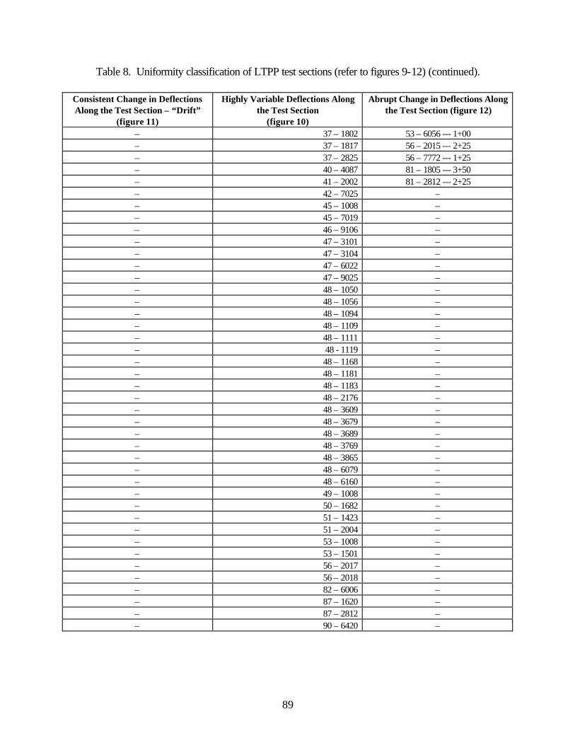
89

Table 8. Uniformity classification of LTPP test sections (refer to figures 9-12) (continued).

Consistent Change in Deflections Along the Test Section – “Drift”

(figure 11)

Highly Variable Deflections Along the Test Section

(figure 10)

Abrupt Change in Deflections Along the Test Section (figure 12)

– 37 – 1802 53 – 6056 --- 1+00 – 37 – 1817 56 – 2015 --- 2+25 – 37 – 2825 56 – 7772 --- 1+25 – 40 – 4087 81 – 1805 --- 3+50 – 41 – 2002 81 – 2812 --- 2+25 – 42 – 7025 – – 45 – 1008 – – 45 – 7019 – – 46 – 9106 – – 47 – 3101 – – 47 – 3104 – – 47 – 6022 – – 47 – 9025 – – 48 – 1050 – – 48 – 1056 – – 48 – 1094 – – 48 – 1109 – – 48 – 1111 – – 48 - 1119 – – 48 – 1168 – – 48 – 1181 – – 48 – 1183 – – 48 – 2176 – – 48 – 3609 – – 48 – 3679 – – 48 – 3689 – – 48 – 3769 – – 48 – 3865 – – 48 – 6079 – – 48 – 6160 – – 49 – 1008 – – 50 – 1682 – – 51 – 1423 – – 51 – 2004 – – 53 – 1008 – – 53 – 1501 – – 56 – 2017 – – 56 – 2018 – – 82 – 6006 – – 87 – 1620 – – 87 – 2812 – – 90 – 6420 –

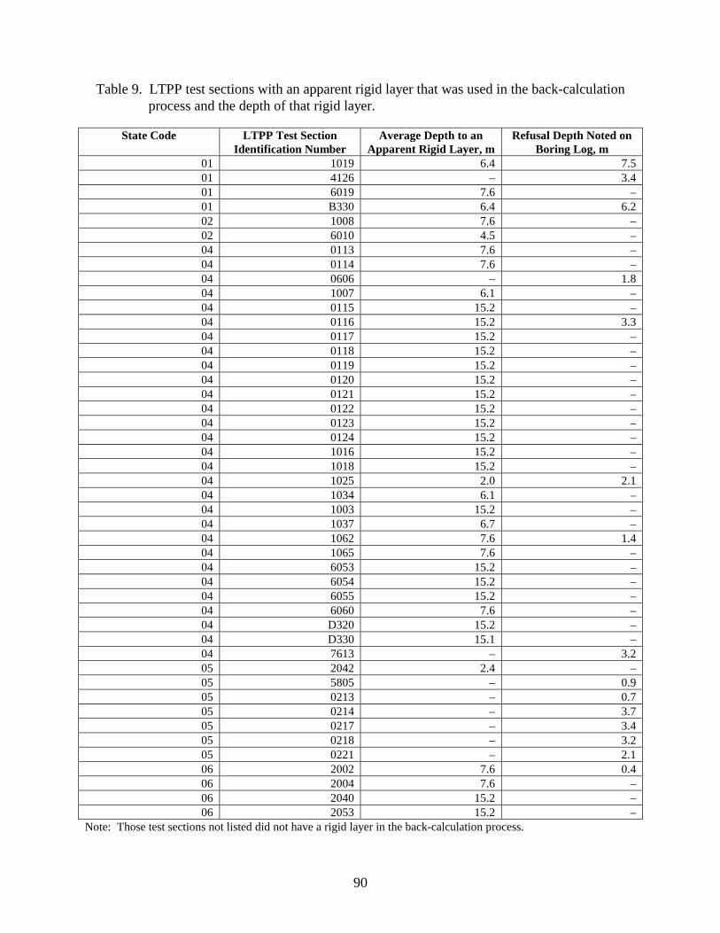
90

Table 9. LTPP test sections with an apparent rigid layer that was used in the back-calculation process and the depth of that rigid layer.

State Code LTPP Test Section Identification Number

Average Depth to an Apparent Rigid Layer, m

Refusal Depth Noted on Boring Log, m

01 1019 6.4 7.5 01 4126 – 3.4 01 6019 7.6 – 01 B330 6.4 6.2 02 1008 7.6 – 02 6010 4.5 – 04 0113 7.6 – 04 0114 7.6 – 04 0606 – 1.8 04 1007 6.1 – 04 0115 15.2 – 04 0116 15.2 3.3 04 0117 15.2 – 04 0118 15.2 – 04 0119 15.2 – 04 0120 15.2 – 04 0121 15.2 – 04 0122 15.2 – 04 0123 15.2 – 04 0124 15.2 – 04 1016 15.2 – 04 1018 15.2 – 04 1025 2.0 2.1 04 1034 6.1 – 04 1003 15.2 – 04 1037 6.7 – 04 1062 7.6 1.4 04 1065 7.6 – 04 6053 15.2 – 04 6054 15.2 – 04 6055 15.2 – 04 6060 7.6 – 04 D320 15.2 – 04 D330 15.1 – 04 7613 – 3.2 05 2042 2.4 – 05 5805 – 0.9 05 0213 – 0.7 05 0214 – 3.7 05 0217 – 3.4 05 0218 – 3.2 05 0221 – 2.1 06 2002 7.6 0.4 06 2004 7.6 – 06 2040 15.2 – 06 2053 15.2 –

Note: Those test sections not listed did not have a rigid layer in the back-calculation process.

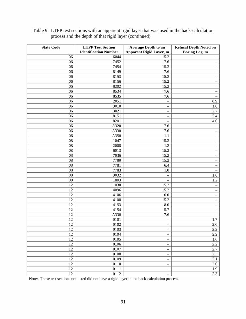
91

Table 9. LTPP test sections with an apparent rigid layer that was used in the back-calculation process and the depth of that rigid layer (continued).

State Code LTPP Test Section Identification Number

Average Depth to an Apparent Rigid Layer, m

Refusal Depth Noted on Boring Log, m

06 6044 15.2 – 06 7452 7.6 – 06 7454 15.2 – 06 8149 7.6 – 06 8153 15.2 – 06 8156 15.2 – 06 8202 15.2 – 06 8534 7.6 – 06 8535 7.6 – 06 2051 – 0.9 06 3010 – 1.8 06 3021 – 2.7 06 8151 – 2.4 06 8201 – 4.0 06 A320 7.6 – 06 A330 7.6 – 06 A350 1.1 – 08 1047 15.2 – 08 2008 1.2 – 08 6013 15.2 – 08 7036 15.2 – 08 7780 15.2 – 08 7781 6.4 – 08 7783 1.0 – 08 3032 – 1.6 09 1803 – 1.2 12 1030 15.2 – 12 4096 15.2 – 12 4106 6.0 – 12 4108 15.2 – 12 4153 8.0 – 12 4154 5.7 – 12 A330 7.6 – 12 0101 – 1.7 12 0102 – 2.0 12 0103 – 2.2 12 0104 – 2.2 12 0105 – 1.6 12 0106 – 2.2 12 0107 – 2.7 12 0108 – 2.3 12 0109 – 2.1 12 0110 – 2.0 12 0111 – 1.9 12 0112 – 2.3

Note: Those test sections not listed did not have a rigid layer in the back-calculation process.

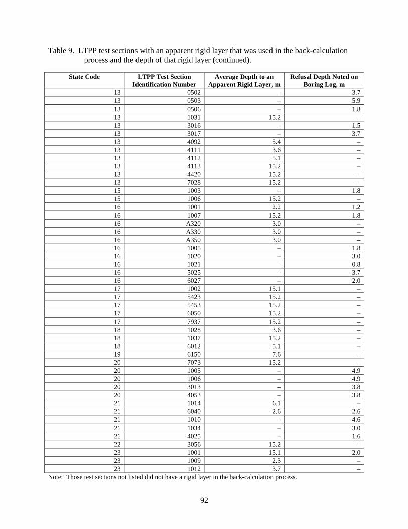
92

Table 9. LTPP test sections with an apparent rigid layer that was used in the back-calculation process and the depth of that rigid layer (continued).

State Code LTPP Test Section Identification Number

Average Depth to an Apparent Rigid Layer, m

Refusal Depth Noted on Boring Log, m

13 0502 – 3.7 13 0503 – 5.9 13 0506 – 1.8 13 1031 15.2 – 13 3016 – 1.5 13 3017 – 3.7 13 4092 5.4 – 13 4111 3.6 – 13 4112 5.1 – 13 4113 15.2 – 13 4420 15.2 – 13 7028 15.2 – 15 1003 – 1.8 15 1006 15.2 – 16 1001 2.2 1.2 16 1007 15.2 1.8 16 A320 3.0 – 16 A330 3.0 – 16 A350 3.0 – 16 1005 – 1.8 16 1020 – 3.0 16 1021 – 0.8 16 5025 – 3.7 16 6027 – 2.0 17 1002 15.1 – 17 5423 15.2 – 17 5453 15.2 – 17 6050 15.2 – 17 7937 15.2 – 18 1028 3.6 – 18 1037 15.2 – 18 6012 5.1 – 19 6150 7.6 – 20 7073 15.2 – 20 1005 – 4.9 20 1006 – 4.9 20 3013 – 3.8 20 4053 – 3.8 21 1014 6.1 – 21 6040 2.6 2.6 21 1010 – 4.6 21 1034 – 3.0 21 4025 – 1.6 22 3056 15.2 – 23 1001 15.1 2.0 23 1009 2.3 – 23 1012 3.7 –

Note: Those test sections not listed did not have a rigid layer in the back-calculation process.

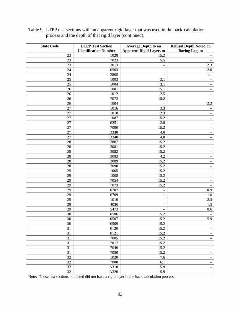
93

Table 9. LTPP test sections with an apparent rigid layer that was used in the back-calculation process and the depth of that rigid layer (continued).

State Code LTPP Test Section Identification Number

Average Depth to an Apparent Rigid Layer, m

Refusal Depth Noted on Boring Log, m

23 1028 15.2 – 23 7023 5.5 – 23 3013 – 2.3 24 0503 – 2.0 24 2805 – 1.1 25 1003 3.1 – 25 1004 3.1 – 26 1001 15.1 – 26 1012 2.5 – 26 7072 15.2 – 26 1004 – 2.2 27 1016 3.3 – 27 1018 2.3 – 27 1087 15.2 – 27 6251 2.8 – 27 7090 15.2 – 27 D330 4.0 – 27 D340 4.0 – 28 2807 15.2 – 28 3081 15.2 – 28 3082 15.2 – 28 3083 4.2 – 28 3089 15.2 – 28 3090 15.2 – 29 1005 15.2 – 29 1008 15.2 – 29 7054 15.2 – 29 7073 15.2 – 29 0707 – 0.9 29 0709 – 1.0 29 1010 – 2.3 29 4036 – 1.5 29 5473 – 0.6 30 0506 15.2 – 30 0507 15.2 5.9 30 0509 15.2 – 31 0120 15.2 – 31 0121 15.2 – 31 7005 15.2 – 31 7017 15.2 – 31 7040 15.2 – 31 7050 15.2 – 32 1020 7.6 – 32 7000 6.1 – 32 A310 5.9 – 32 A320 5.9 –

Note: Those test sections not listed did not have a rigid layer in the back-calculation process.

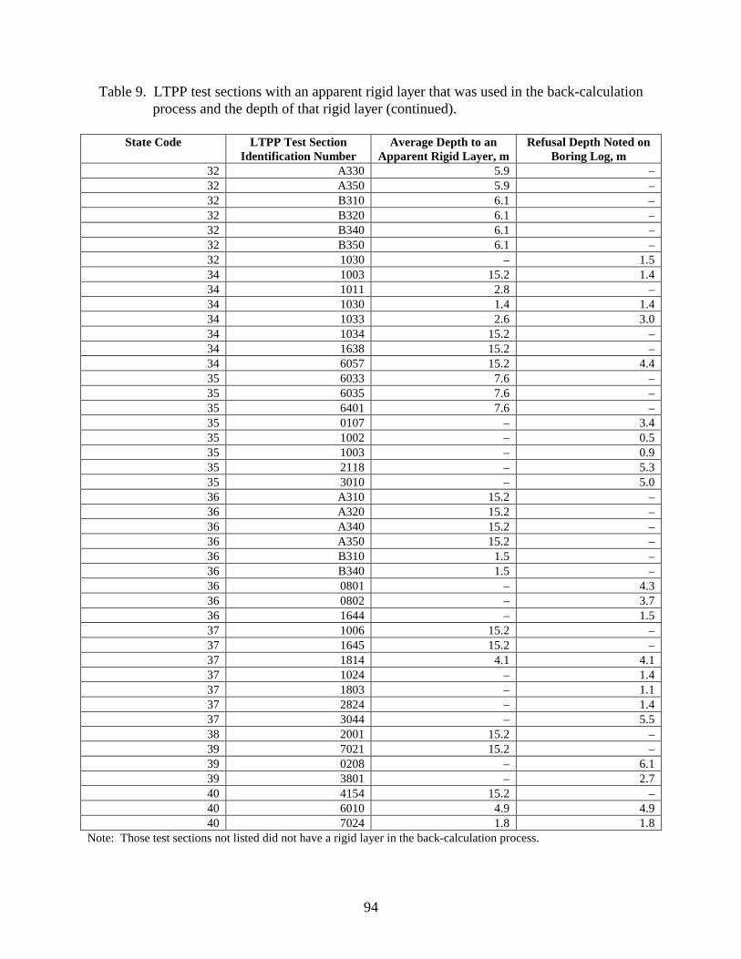
94

Table 9. LTPP test sections with an apparent rigid layer that was used in the back-calculation process and the depth of that rigid layer (continued).

State Code LTPP Test Section

Identification Number Average Depth to an

Apparent Rigid Layer, m Refusal Depth Noted on

Boring Log, m 32 A330 5.9 – 32 A350 5.9 – 32 B310 6.1 – 32 B320 6.1 – 32 B340 6.1 – 32 B350 6.1 – 32 1030 – 1.5 34 1003 15.2 1.4 34 1011 2.8 – 34 1030 1.4 1.4 34 1033 2.6 3.0 34 1034 15.2 – 34 1638 15.2 – 34 6057 15.2 4.4 35 6033 7.6 – 35 6035 7.6 – 35 6401 7.6 – 35 0107 – 3.4 35 1002 – 0.5 35 1003 – 0.9 35 2118 – 5.3 35 3010 – 5.0 36 A310 15.2 – 36 A320 15.2 – 36 A340 15.2 – 36 A350 15.2 – 36 B310 1.5 – 36 B340 1.5 – 36 0801 – 4.3 36 0802 – 3.7 36 1644 – 1.5 37 1006 15.2 – 37 1645 15.2 – 37 1814 4.1 4.1 37 1024 – 1.4 37 1803 – 1.1 37 2824 – 1.4 37 3044 – 5.5 38 2001 15.2 – 39 7021 15.2 – 39 0208 – 6.1 39 3801 – 2.7 40 4154 15.2 – 40 6010 4.9 4.9 40 7024 1.8 1.8

Note: Those test sections not listed did not have a rigid layer in the back-calculation process.

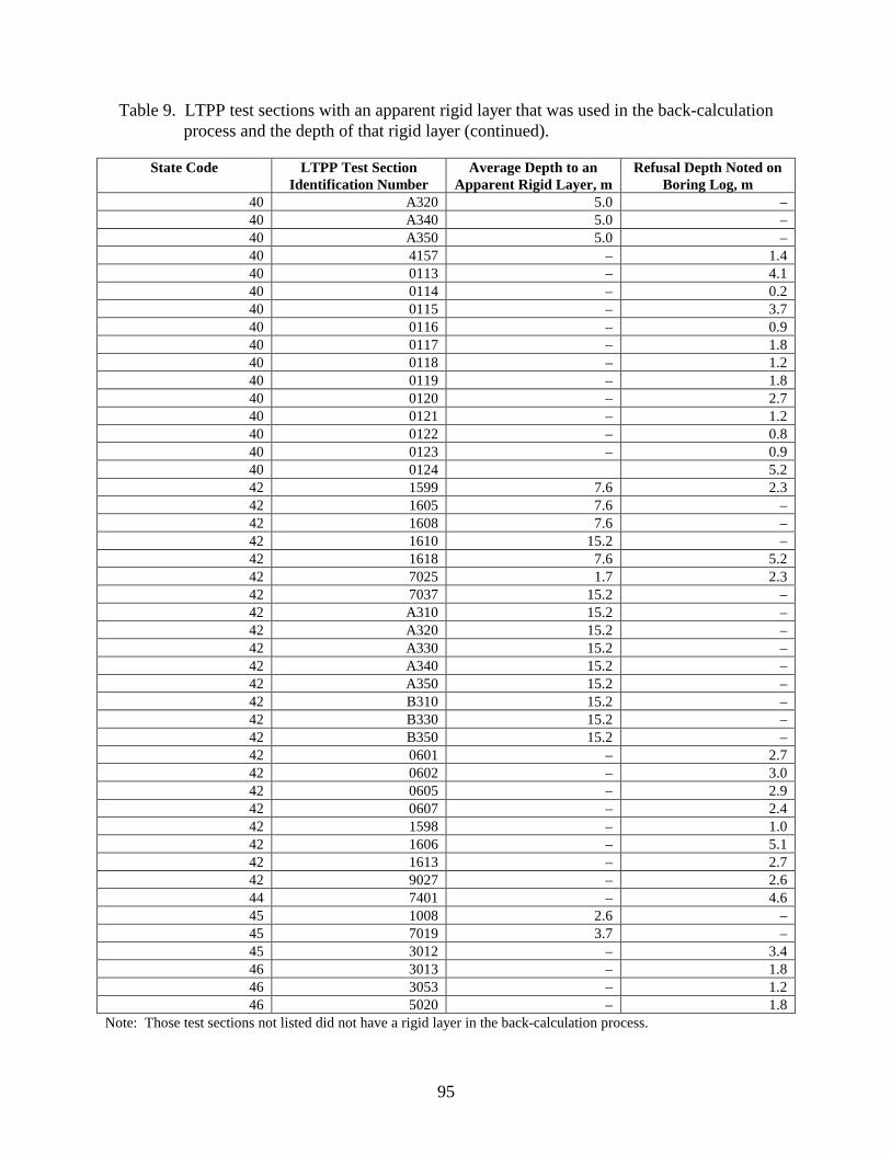
95

Table 9. LTPP test sections with an apparent rigid layer that was used in the back-calculation process and the depth of that rigid layer (continued).

State Code LTPP Test Section Identification Number

Average Depth to an Apparent Rigid Layer, m

Refusal Depth Noted on Boring Log, m

40 A320 5.0 – 40 A340 5.0 – 40 A350 5.0 – 40 4157 – 1.4 40 0113 – 4.1 40 0114 – 0.2 40 0115 – 3.7 40 0116 – 0.9 40 0117 – 1.8 40 0118 – 1.2 40 0119 – 1.8 40 0120 – 2.7 40 0121 – 1.2 40 0122 – 0.8 40 0123 – 0.9 40 0124 5.2 42 1599 7.6 2.3 42 1605 7.6 – 42 1608 7.6 – 42 1610 15.2 – 42 1618 7.6 5.2 42 7025 1.7 2.3 42 7037 15.2 – 42 A310 15.2 – 42 A320 15.2 – 42 A330 15.2 – 42 A340 15.2 – 42 A350 15.2 – 42 B310 15.2 – 42 B330 15.2 – 42 B350 15.2 – 42 0601 – 2.7 42 0602 – 3.0 42 0605 – 2.9 42 0607 – 2.4 42 1598 – 1.0 42 1606 – 5.1 42 1613 – 2.7 42 9027 – 2.6 44 7401 – 4.6 45 1008 2.6 – 45 7019 3.7 – 45 3012 – 3.4 46 3013 – 1.8 46 3053 – 1.2 46 5020 – 1.8

Note: Those test sections not listed did not have a rigid layer in the back-calculation process.

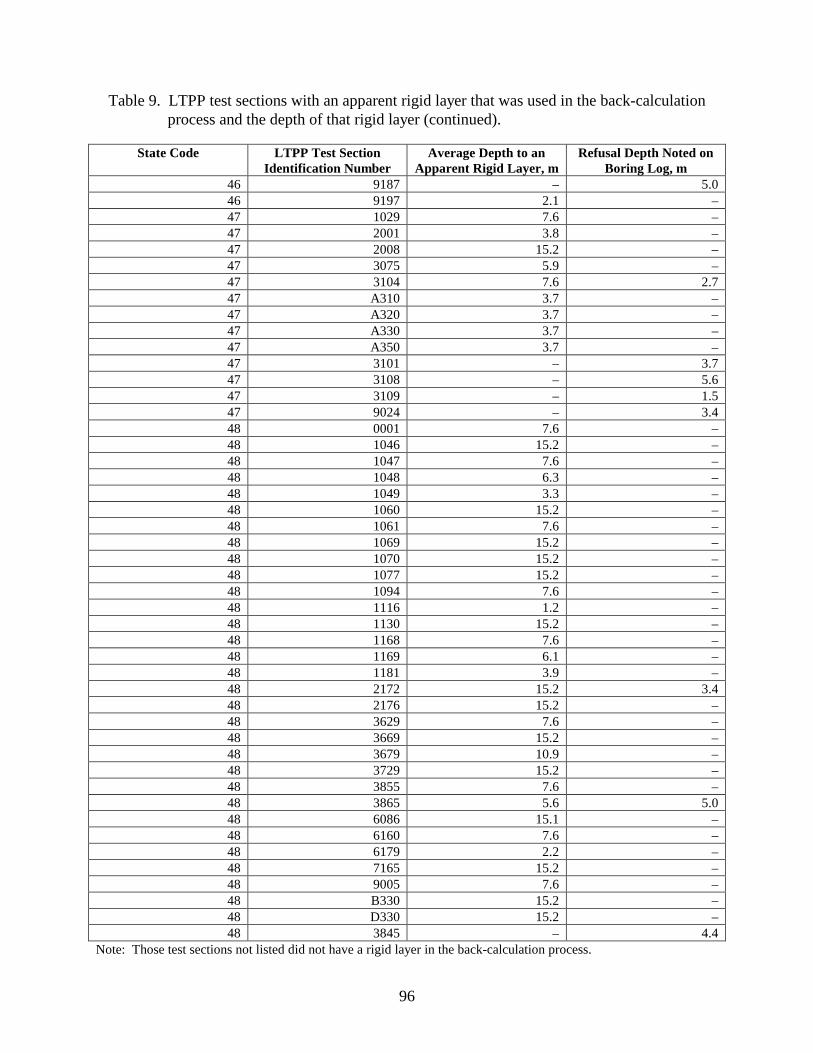
96

Table 9. LTPP test sections with an apparent rigid layer that was used in the back-calculation process and the depth of that rigid layer (continued).

State Code LTPP Test Section Identification Number

Average Depth to an Apparent Rigid Layer, m

Refusal Depth Noted on Boring Log, m

46 9187 – 5.0 46 9197 2.1 – 47 1029 7.6 – 47 2001 3.8 – 47 2008 15.2 – 47 3075 5.9 – 47 3104 7.6 2.7 47 A310 3.7 – 47 A320 3.7 – 47 A330 3.7 – 47 A350 3.7 – 47 3101 – 3.7 47 3108 – 5.6 47 3109 – 1.5 47 9024 – 3.4 48 0001 7.6 – 48 1046 15.2 – 48 1047 7.6 – 48 1048 6.3 – 48 1049 3.3 – 48 1060 15.2 – 48 1061 7.6 – 48 1069 15.2 – 48 1070 15.2 – 48 1077 15.2 – 48 1094 7.6 – 48 1116 1.2 – 48 1130 15.2 – 48 1168 7.6 – 48 1169 6.1 – 48 1181 3.9 – 48 2172 15.2 3.4 48 2176 15.2 – 48 3629 7.6 – 48 3669 15.2 – 48 3679 10.9 – 48 3729 15.2 – 48 3855 7.6 – 48 3865 5.6 5.0 48 6086 15.1 – 48 6160 7.6 – 48 6179 2.2 – 48 7165 15.2 – 48 9005 7.6 – 48 B330 15.2 – 48 D330 15.2 – 48 3845 – 4.4

Note: Those test sections not listed did not have a rigid layer in the back-calculation process.

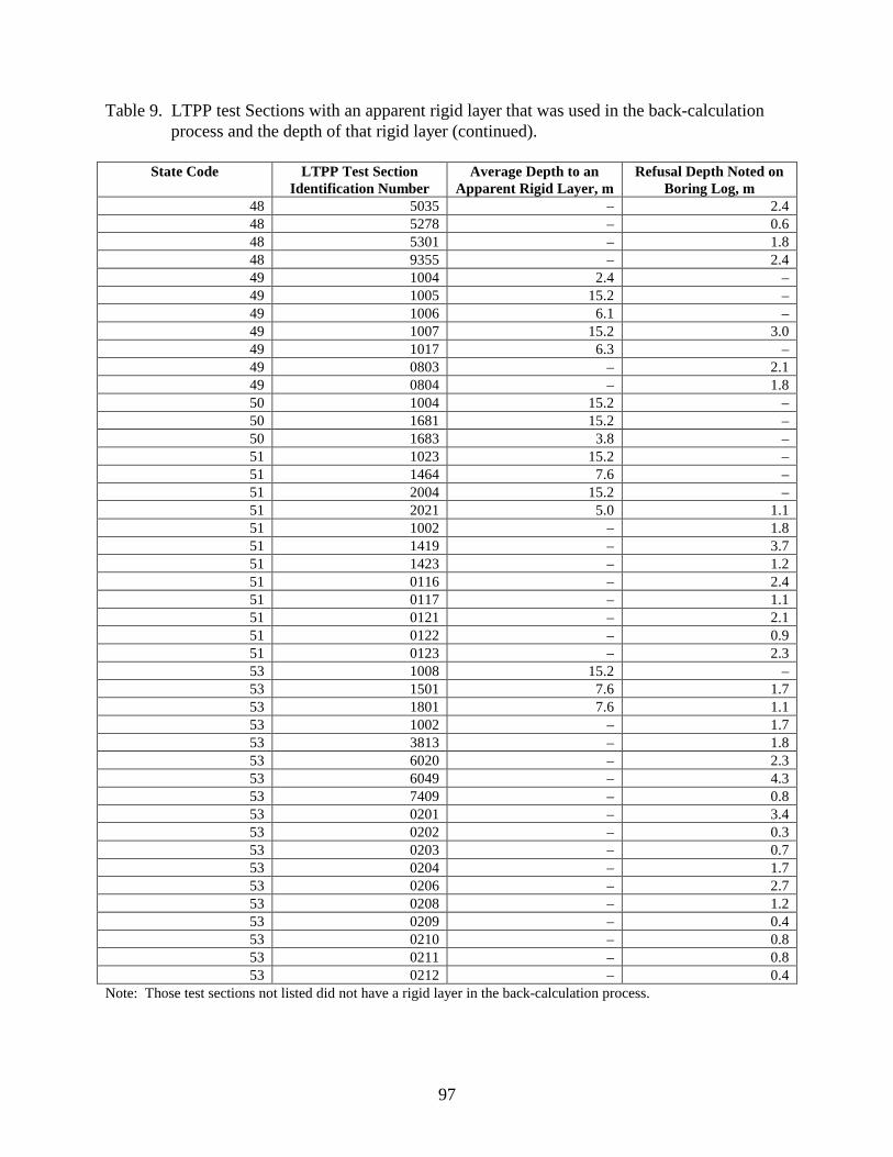
97

Table 9. LTPP test Sections with an apparent rigid layer that was used in the back-calculation process and the depth of that rigid layer (continued).

State Code LTPP Test Section Identification Number

Average Depth to an Apparent Rigid Layer, m

Refusal Depth Noted on Boring Log, m

48 5035 – 2.4 48 5278 – 0.6 48 5301 – 1.8 48 9355 – 2.4 49 1004 2.4 – 49 1005 15.2 – 49 1006 6.1 – 49 1007 15.2 3.0 49 1017 6.3 – 49 0803 – 2.1 49 0804 – 1.8 50 1004 15.2 – 50 1681 15.2 – 50 1683 3.8 – 51 1023 15.2 – 51 1464 7.6 – 51 2004 15.2 – 51 2021 5.0 1.1 51 1002 – 1.8 51 1419 – 3.7 51 1423 – 1.2 51 0116 – 2.4 51 0117 – 1.1 51 0121 – 2.1 51 0122 – 0.9 51 0123 – 2.3 53 1008 15.2 – 53 1501 7.6 1.7 53 1801 7.6 1.1 53 1002 – 1.7 53 3813 – 1.8 53 6020 – 2.3 53 6049 – 4.3 53 7409 – 0.8 53 0201 – 3.4 53 0202 – 0.3 53 0203 – 0.7 53 0204 – 1.7 53 0206 – 2.7 53 0208 – 1.2 53 0209 – 0.4 53 0210 – 0.8 53 0211 – 0.8 53 0212 – 0.4

Note: Those test sections not listed did not have a rigid layer in the back-calculation process.

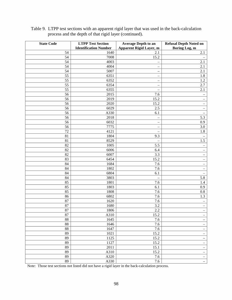
98

Table 9. LTPP test sections with an apparent rigid layer that was used in the back-calculation process and the depth of that rigid layer (continued).

State Code LTPP Test Section Identification Number

Average Depth to an Apparent Rigid Layer, m

Refusal Depth Noted on Boring Log, m

54 1640 2.1 2.1 54 7008 15.2 – 54 4003 – 2.1 54 4004 – 2.1 54 5007 – 2.1 55 6351 – 1.8 55 6352 – 1.2 55 6354 – 2.7 55 6355 – 2.1 56 2015 7.6 – 56 2019 15.2 – 56 2020 15.2 – 56 6029 2.5 – 56 A330 6.1 – 56 2018 – 5.3 56 6032 – 0.9 56 7775 – 3.0 72 4121 – 1.8 81 1804 9.3 – 81 8529 – 1.5 82 1005 5.5 – 82 6006 6.4 – 82 6007 3.3 – 83 6454 15.2 – 84 1684 7.6 – 84 1802 7.6 – 84 6804 6.1 – 84 3803 – 5.8 85 1801 7.6 1.4 85 1803 6.1 0.9 85 1808 7.6 0.8 86 6802 7.6 1.3 87 1620 7.6 – 87 1680 3.2 – 87 1806 2.2 – 87 A310 15.2 – 88 1645 7.6 – 88 1646 7.6 – 88 1647 7.6 – 89 1021 15.2 – 89 1125 15.2 – 89 1127 15.2 – 89 2011 15.1 – 89 A310 15.2 – 89 A320 7.6 – 89 A330 7.6 –

Note: Those test sections not listed did not have a rigid layer in the back-calculation process.

99

Table 9. LTPP test sections with an apparent rigid layer that was used in the back-calculation process and the depth of that rigid layer (continued).

State Code LTPP Test Section Identification Number

Average Depth to an Apparent Rigid Layer, m

Refusal Depth Noted on Boring Log, m

89 A340 7.6 – 89 9018 – 5.6 89 A901 – 1.8 89 A902 – 1.3 90 6400 3.3 – 90 6801 3.3 –

Note: Those test sections not listed did not have a rigid layer in the back-calculation process.

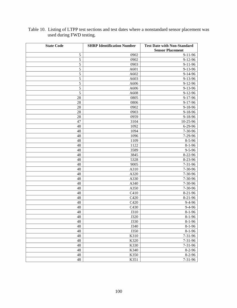
100

Table 10. Listing of LTPP test sections and test dates where a nonstandard sensor placement was used during FWD testing.

State Code SHRP Identification Number Test Date with Non-Standard Sensor Placement

5 0902 9-11-96 5 0902 9-12-96 5 0903 9-11-96 5 A601 9-13-96 5 A602 9-14-96 5 A603 9-13-96 5 A606 9-12-96 5 A606 9-13-96 5 A608 9-12-96

28 0805 9-17-96 28 0806 9-17-96 28 0902 9-18-96 28 0903 9-18-96 28 0959 9-18-96 47 3104 10-25-96 48 1092 6-29-96 48 1094 7-30-96 48 1096 7-29-96 48 1109 8-5-96 48 1122 8-1-96 48 3589 9-5-96 48 3845 8-22-96 48 5328 8-23-96 48 9005 7-31-96 48 A310 7-30-96 48 A320 7-30-96 48 A330 7-30-96 48 A340 7-30-96 48 A350 7-30-96 48 C410 8-21-96 48 C420 8-21-96 48 C420 9-4-96 48 C430 9-4-96 48 J310 8-1-96 48 J320 8-1-96 48 J330 8-1-96 48 J340 8-1-96 48 J350 8-1-96 48 K310 7-31-96 48 K320 7-31-96 48 K330 7-31-96 48 K340 8-2-96 48 K350 8-2-96 48 K351 7-31-96

101

Appendix C Median Values and Histograms of Young’s Modulus Back-Calculated for Different Materials Appendix C is a summary of the results from the back-calculation of elastic properties. It is subdivided into two basic parts. The first part is a tabulation of the test sections for which only a few of the deflection basins (less than 30 percent) had solutions with RMS errors less than 2 percent and the median Young’s modulus for different materials and pavement cross-sections for those solutions with RMS errors of less than 2 percent. The second part includes histograms of the results from the back-calculation of Young’s modulus for different pavement materials and soils.

102

Table 11. LTPP test sections with many deflection basins that did not result in a solution with an RMS error of less than 2 percent.

State Code LTPP Test Section Identification Number

Number of Basins Percentage of Basins with an RMS Error of

Less than 2 Percent 04 0116 264 19.7 04 D320 48 2.1 04 D330 48 16.7 06 A350 107 27.1 12 A330 143 11.2 12 C350 48 8.3 16 A320 36 16.7 16 A350 36 16.7 30 0509 136 14.7 40 B350 48 18.8 56 A330 140 17.9 81 0506 48 20.8 83 0502 164 11.0 83 0503 160 27.5 83 1801 2741 24.3 02 6010 591 10.7 02 9035 156 12.2 04 1002 511 15.3 04 1015 344 17.4 04 1017 1340 11.7 04 1018 564 00.4 04 1025 556 21.8 04 1037 512 26.0 04 6054 300 26.0 04 6055 344 14.5 04 6060 348 10.6 06 2053 167 28.7 06 8149 336 21.4 08 2008 679 25.5 08 7783 344 15.7 12 4103 320 8.4 12 4135 336 00.3 12 4137 327 27.8 12 4153 340 6.5 12 4154 629 15.9 12 9054 388 21.1 13 4093 504 29.0 16 1001 340 23.8 16 1021 428 20.0 16 6027 176 00.6 18 1028 930 28.4 21 1034 583 28.1 26 1010 596 17.3 27 1016 764 11.3 28 3085 344 20.1 30 1001 508 00.2 30 6004 344 00.3

103

Table 11. LTPP test sections with many deflection basins that did not result in a solution with an RMS error of less than 2 percent (continued).

State Code LTPP Test Section Identification Number

Number of Basins Percentage of Basins with an RMS Error of

Less than 2 Percent 30 7075 344 21.5 30 7088 344 21.5 32 7000 344 6.1 37 1992 168 13.7 37 2819 331 22.7 45 1008 330 2.7 45 1024 427 11.2 46 9197 176 13.1 47 1028 516 20.7 47 3104 432 18.3 48 1061 176 13.1 48 1168 344 12.2 48 1169 272 15.4 48 3579 436 6.7 48 3855 328 00.3 49 1004 340 4.1 49 1005 344 4.4 49 1007 340 9.4 49 1008 344 22.1 49 1017 344 19.5 53 1008 932 14.5 53 1501 628 6.4 56 2015 176 9.1 56 2037 173 11.6 56 6029 344 00.3 56 7772 343 17.5

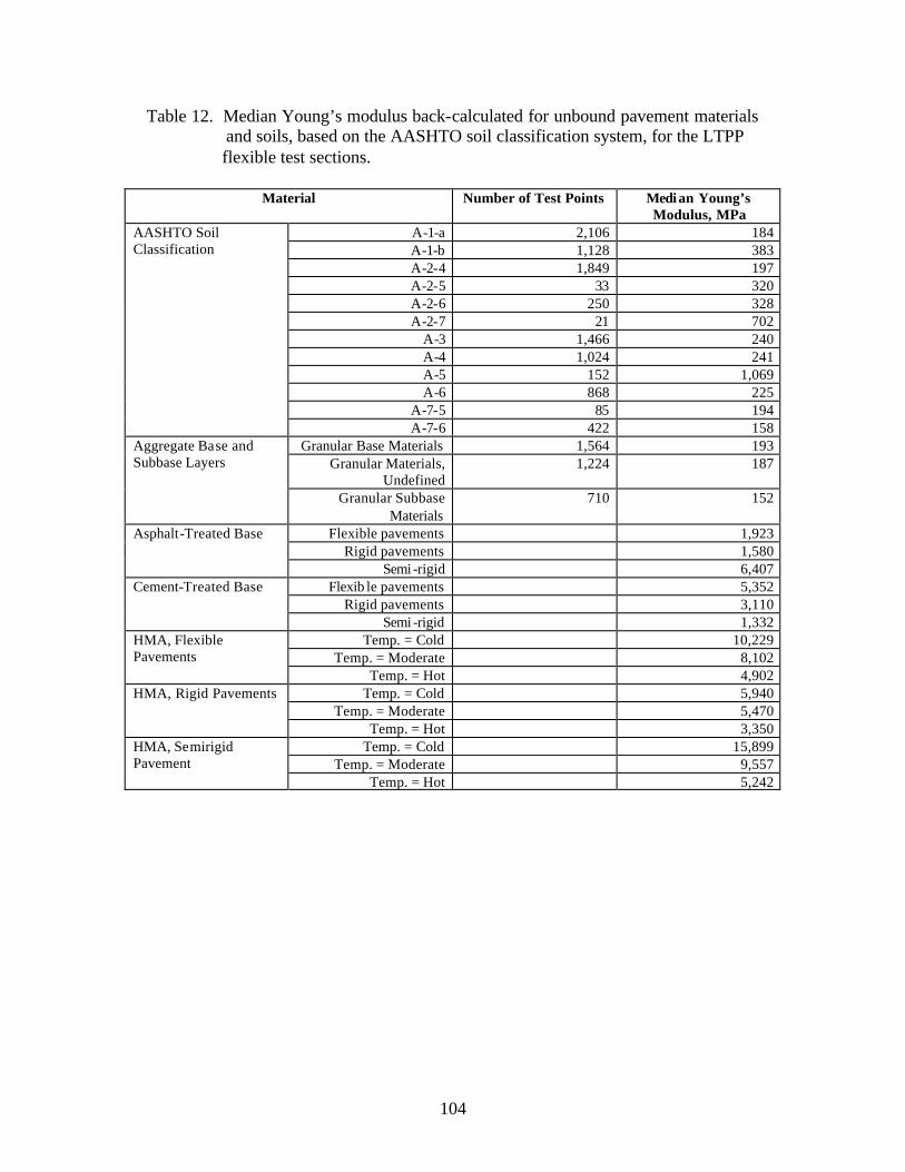
104

Table 12. Median Young’s modulus back-calculated for unbound pavement materials and soils, based on the AASHTO soil classification system, for the LTPP

flexible test sections.

Material Number of Test Points Median Young’s Modulus, MPa

A-1-a 2,106 184 A-1-b 1,128 383 A-2-4 1,849 197 A-2-5 33 320 A-2-6 250 328 A-2-7 21 702

A-3 1,466 240 A-4 1,024 241 A-5 152 1,069 A-6 868 225

A-7-5 85 194

AASHTO Soil Classification

A-7-6 422 158 Granular Base Materials 1,564 193

Granular Materials, Undefined

1,224 187 Aggregate Base and Subbase Layers

Granular Subbase Materials

710 152

Flexible pavements 1,923 Rigid pavements 1,580

Asphalt-Treated Base

Semi -rigid 6,407 Flexib le pavements 5,352

Rigid pavements 3,110 Cement-Treated Base

Semi -rigid 1,332 Temp. = Cold 10,229

Temp. = Moderate 8,102 HMA, Flexible Pavements

Temp. = Hot 4,902 Temp. = Cold 5,940

Temp. = Moderate 5,470 HMA, Rigid Pavements

Temp. = Hot 3,350 Temp. = Cold 15,899

Temp. = Moderate 9,557 HMA, Semirigid Pavement

Temp. = Hot 5,242

105

Table 13. Median Young’s modulus back-calculated within specific temperature ranges for the LTPP flexible test sections.

Temperature Range, Degrees C

Number of Test Points Average Temperature, Degrees C

HMA Young’s Modulus, MPa

-20 to –15 9 -17.5 70,372 -15 to –10 19 -13.3 71,927

-10 to –5 35 -7.1 49,250 -5 to 0 141 -1.6 28,802 0 to 5 315 2.9 15,063

5 to 10 683 7.9 12,745 10 to 15 1,047 12.8 11,354 15 to 20 1,135 17.4 11,639 20 to 25 1,178 22.5 9,518 25 to 30 1,010 27.3 7,484 30 to 35 710 32.4 5,815 35 to 40 392 37.1 7,473 40 to 45 112 42.0 6,229 45 to 50 21 47.5 2,316

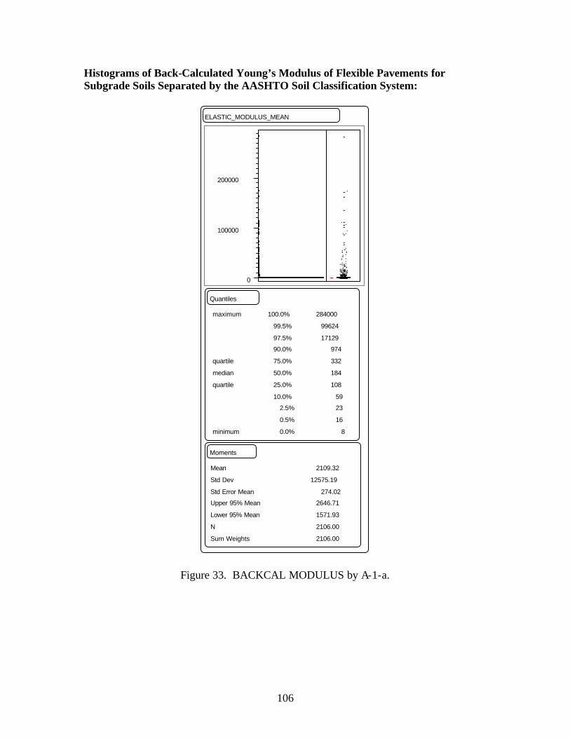
106

Histograms of Back-Calculated Young’s Modulus of Flexible Pavements for Subgrade Soils Separated by the AASHTO Soil Classification System:

Figure 33. BACKCAL MODULUS by A-1-a.

ELASTIC_MODULUS_MEAN

0

100000

200000

Quantiles

maximum

quartile

median

quartile

minimum

100.0%

99.5%

97.5%90.0%

75.0%

50.0%

25.0%

10.0%2.5%

0.5%

0.0%

284000

99624

17129 974

332

184

108

59 23

16

8

Moments

Mean

Std Dev

Std Error MeanUpper 95% Mean

Lower 95% Mean

N

Sum Weights

2109.32

12575.19

274.02 2646.71

1571.93

2106.00

2106.00

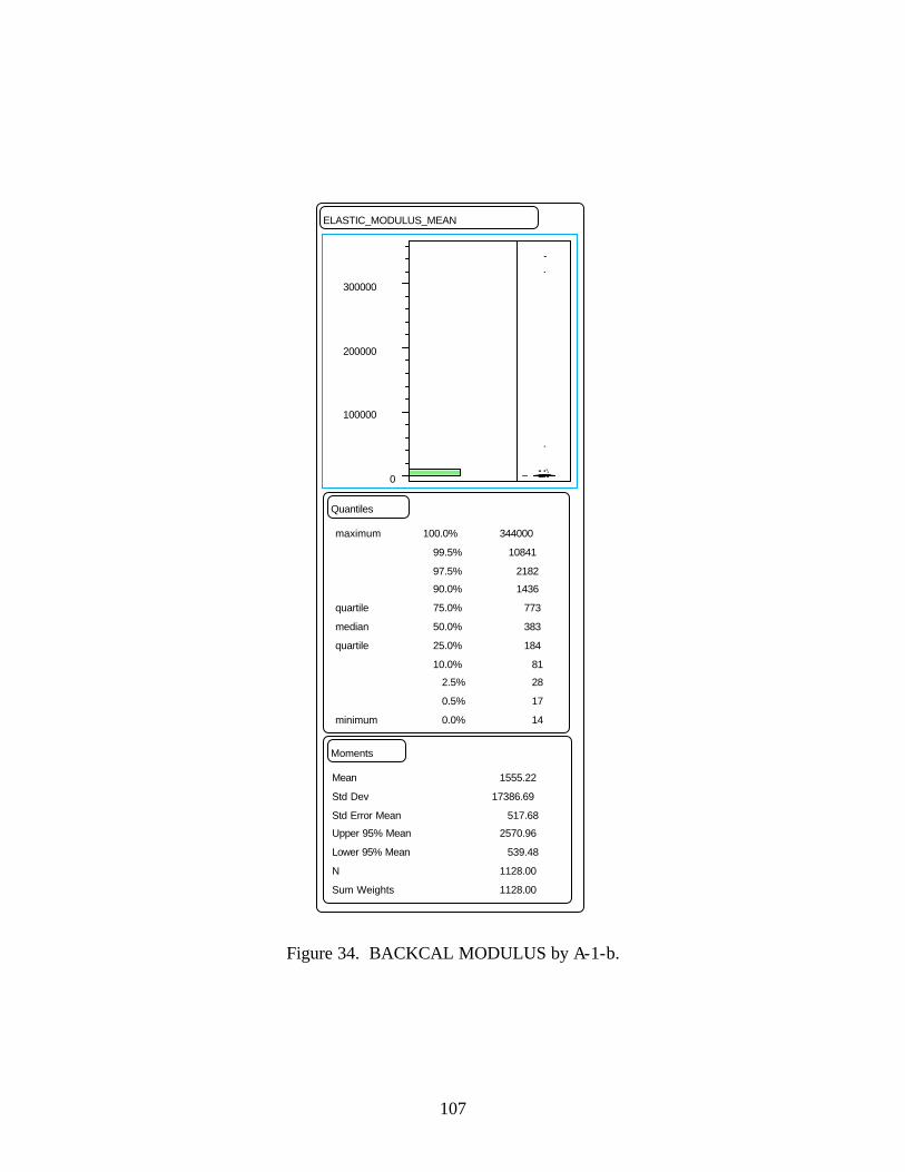
107

Figure 34. BACKCAL MODULUS by A-1-b.

ELASTIC_MODULUS_MEAN

0

100000

200000

300000

Quantiles

maximum

quartile

median

quartile

minimum

100.0%

99.5%

97.5%90.0%

75.0%

50.0%

25.0%

10.0%2.5%

0.5%

0.0%

344000

10841

2182 1436

773

383

184

81 28

17

14

Moments

Mean

Std Dev

Std Error MeanUpper 95% Mean

Lower 95% Mean

N

Sum Weights

1555.22

17386.69

517.68 2570.96

539.48

1128.00

1128.00

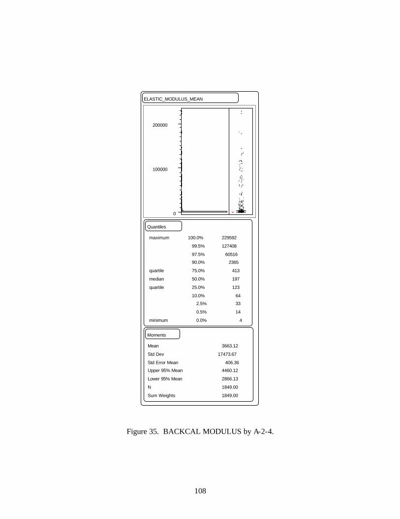
108

Figure 35. BACKCAL MODULUS by A-2-4.

ELASTIC_MODULUS_MEAN

0

100000

200000

Quantiles

maximum

quartile

median

quartile

minimum

100.0%

99.5%

97.5%90.0%

75.0%

50.0%

25.0%

10.0%2.5%

0.5%

0.0%

229592

127408

60516 2365

413

197

123

64 33

14

4

Moments

Mean

Std Dev

Std Error MeanUpper 95% Mean

Lower 95% Mean

N

Sum Weights

3663.12

17473.67

406.36 4460.12

2866.13

1849.00

1849.00

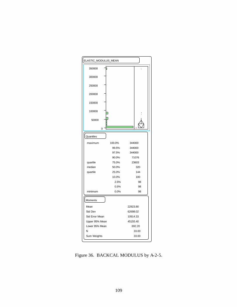
109

Figure 36. BACKCAL MODULUS by A-2-5.

ELASTIC_MODULUS_MEAN

0

50000

100000

150000

200000

250000

300000

350000

Quantiles

maximum

quartilemedian

quartile

minimum

100.0%

99.5%97.5%

90.0%

75.0%50.0%

25.0%

10.0%

2.5%0.5%

0.0%

344000

344000 344000

71076

23603 320

144

100

98 98

98

Moments

Mean

Std Dev

Std Error Mean

Upper 95% MeanLower 95% Mean

N

Sum Weights

22923.80

62698.02

10914.33

45155.40 692.20

33.00

33.00

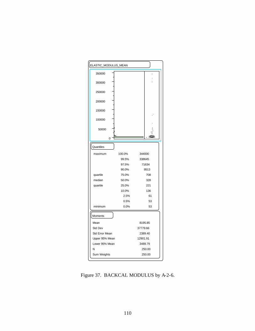
110

Figure 37. BACKCAL MODULUS by A-2-6.

ELASTIC_MODULUS_MEAN

0

50000

100000

150000

200000

250000

300000

350000

Quantiles

maximum

quartile

median

quartile

minimum

100.0%

99.5%

97.5%90.0%

75.0%

50.0%

25.0%

10.0%2.5%

0.5%

0.0%

344000

338645

71634 9513

708

328

221

136 61

53

53

Moments

Mean

Std Dev

Std Error MeanUpper 95% Mean

Lower 95% Mean

N

Sum Weights

8195.85

37779.66

2389.40 12901.91

3489.79

250.00

250.00

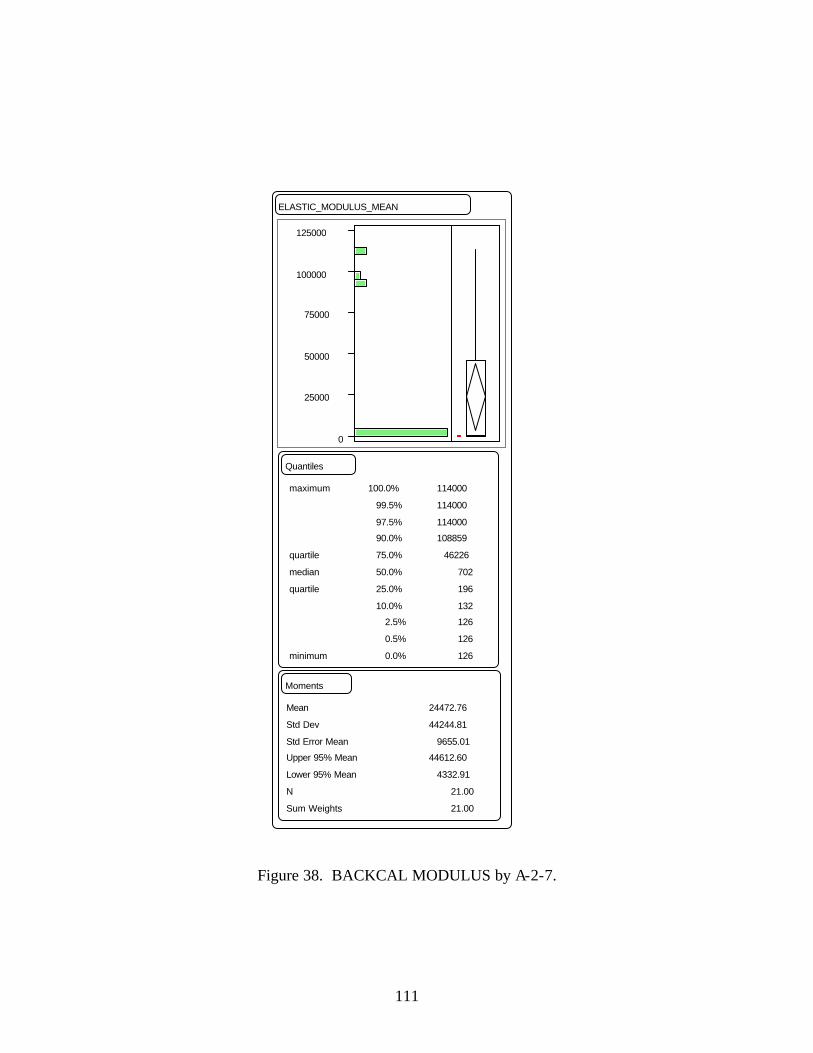
111

Figure 38. BACKCAL MODULUS by A-2-7.

ELASTIC_MODULUS_MEAN

0

25000

50000

75000

100000

125000

Quantiles

maximum

quartile

median

quartile

minimum

100.0%

99.5%

97.5%90.0%

75.0%

50.0%

25.0%

10.0%2.5%

0.5%

0.0%

114000

114000

114000 108859

46226

702

196

132 126

126

126

Moments

Mean

Std Dev

Std Error MeanUpper 95% Mean

Lower 95% Mean

N

Sum Weights

24472.76

44244.81

9655.01 44612.60

4332.91

21.00

21.00

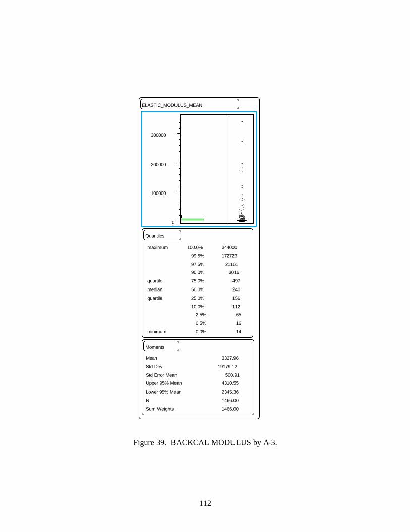
112

Figure 39. BACKCAL MODULUS by A-3.

ELASTIC_MODULUS_MEAN

0

100000

200000

300000

Quantiles

maximum

quartile

median

quartile

minimum

100.0%

99.5%

97.5%90.0%

75.0%

50.0%

25.0%

10.0%2.5%

0.5%

0.0%

344000

172723

21161 3016

497

240

156

112 65

16

14

Moments

Mean

Std Dev

Std Error MeanUpper 95% Mean

Lower 95% Mean

N

Sum Weights

3327.96

19179.12

500.91 4310.55

2345.36

1466.00

1466.00

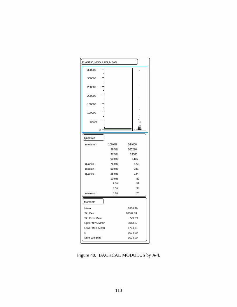
113

Figure 40. BACKCAL MODULUS by A-4.

ELASTIC_MODULUS_MEAN

0

50000

100000

150000

200000

250000

300000

350000

Quantiles

maximum

quartile

median

quartile

minimum

100.0%

99.5%

97.5%90.0%

75.0%

50.0%

25.0%

10.0%2.5%

0.5%

0.0%

344000

165296

19585 1466

473

241

144

89 51

34

25

Moments

Mean

Std Dev

Std Error MeanUpper 95% Mean

Lower 95% Mean

N

Sum Weights

2808.79

18007.74

562.74 3913.07

1704.51

1024.00

1024.00

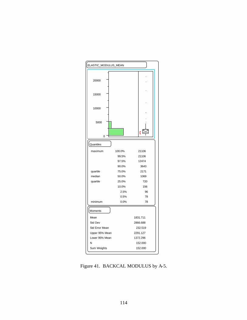
114

Figure 41. BACKCAL MODULUS by A-5.

ELASTIC_MODULUS_MEAN

0

5000

10000

15000

20000

Quantiles

maximum

quartilemedian

quartile

minimum

100.0%

99.5%97.5%

90.0%

75.0%50.0%

25.0%

10.0%

2.5%0.5%

0.0%

21106

21106 12474

3643

2171 1069

720

156

96 78

78

Moments

Mean

Std Dev

Std Error Mean

Upper 95% MeanLower 95% Mean

N

Sum Weights

1831.711

2866.688

232.519

2291.127 1372.296

152.000

152.000

115

Figure 42. BACKCAL MODULUS by A-6.

ELASTIC_MODULUS_MEAN

0

100000

200000

300000

Quantiles

maximum

quartilemedian

quartile

minimum

100.0%

99.5%97.5%

90.0%

75.0%50.0%

25.0%

10.0%

2.5%0.5%

0.0%

291000

79495 42275

1453

419 225

150

87

25 3

1

Moments

Mean

Std Dev

Std Error Mean

Upper 95% MeanLower 95% Mean

N

Sum Weights

3074.16

14896.72

505.63

4066.57 2081.75

868.00

868.00

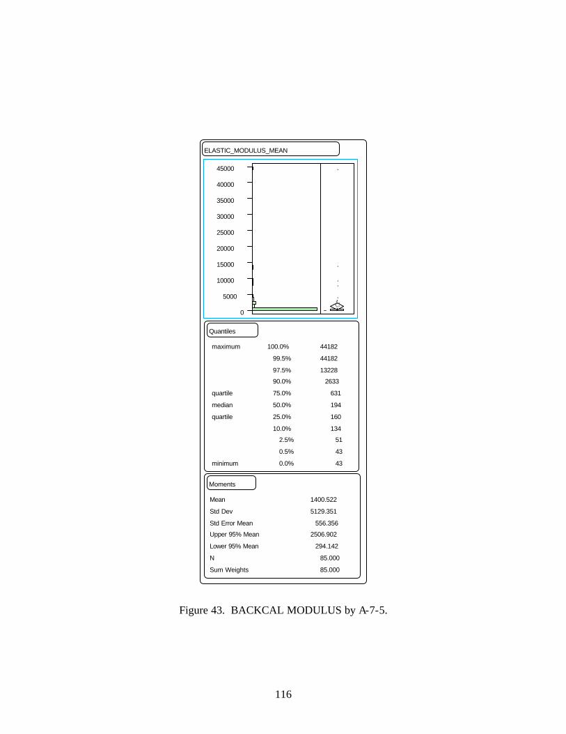
116

Figure 43. BACKCAL MODULUS by A-7-5.

ELASTIC_MODULUS_MEAN

0

5000

10000

15000

20000

25000

30000

35000

40000

45000

Quantiles

maximum

quartile

median

quartile

minimum

100.0%

99.5%

97.5%90.0%

75.0%

50.0%

25.0%

10.0%2.5%

0.5%

0.0%

44182

44182

13228 2633

631

194

160

134 51

43

43

Moments

Mean

Std Dev

Std Error MeanUpper 95% Mean

Lower 95% Mean

N

Sum Weights

1400.522

5129.351

556.356 2506.902

294.142

85.000

85.000

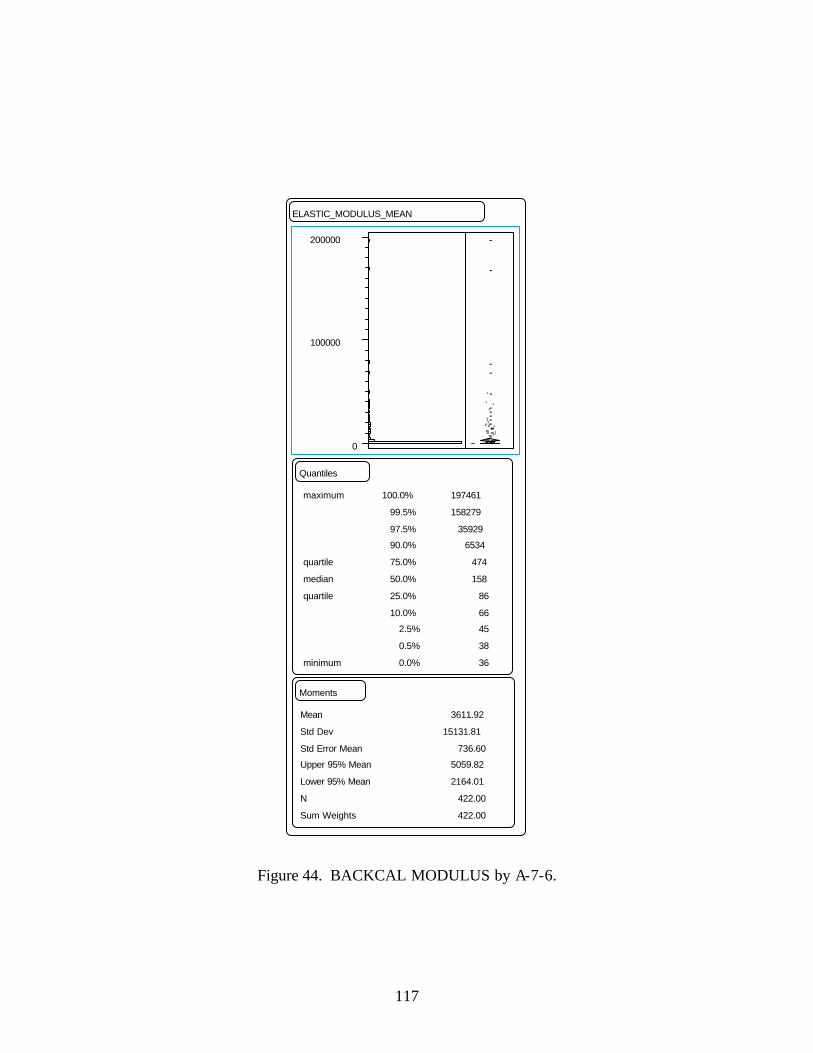
117

Figure 44. BACKCAL MODULUS by A-7-6.

ELASTIC_MODULUS_MEAN

0

100000

200000

Quantiles

maximum

quartile

median

quartile

minimum

100.0%

99.5%

97.5%90.0%

75.0%

50.0%

25.0%

10.0%2.5%

0.5%

0.0%

197461

158279

35929 6534

474

158

86

66 45

38

36

Moments

Mean

Std Dev

Std Error MeanUpper 95% Mean

Lower 95% Mean

N

Sum Weights

3611.92

15131.81

736.60 5059.82

2164.01

422.00

422.00

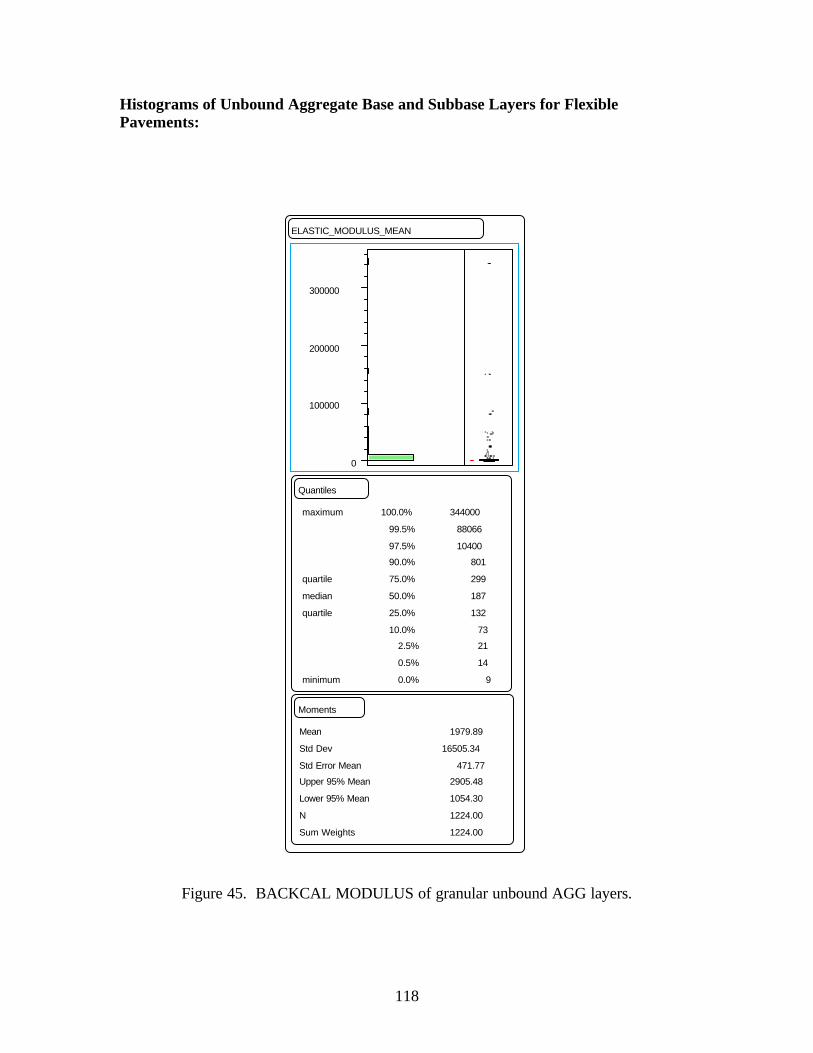
118

Histograms of Unbound Aggregate Base and Subbase Layers for Flexible Pavements:

Figure 45. BACKCAL MODULUS of granular unbound AGG layers.

ELASTIC_MODULUS_MEAN

0

100000

200000

300000

Quantiles

maximum

quartile

median

quartile

minimum

100.0%

99.5%

97.5%90.0%

75.0%

50.0%

25.0%

10.0%2.5%

0.5%

0.0%

344000

88066

10400 801

299

187

132

73 21

14

9

Moments

Mean

Std Dev

Std Error MeanUpper 95% Mean

Lower 95% Mean

N

Sum Weights

1979.89

16505.34

471.77 2905.48

1054.30

1224.00

1224.00

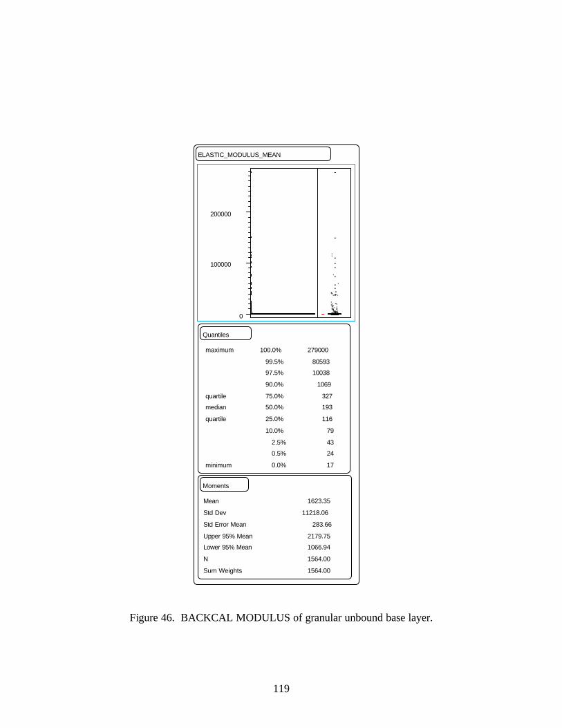
119

Figure 46. BACKCAL MODULUS of granular unbound base layer.

ELASTIC_MODULUS_MEAN

0

100000

200000

Quantiles

maximum

quartilemedian

quartile

minimum

100.0%

99.5%97.5%

90.0%

75.0%50.0%

25.0%

10.0%

2.5%0.5%

0.0%

279000

80593 10038

1069

327 193

116

79

43 24

17

Moments

Mean

Std Dev

Std Error Mean

Upper 95% MeanLower 95% Mean

N

Sum Weights

1623.35

11218.06

283.66

2179.75 1066.94

1564.00

1564.00

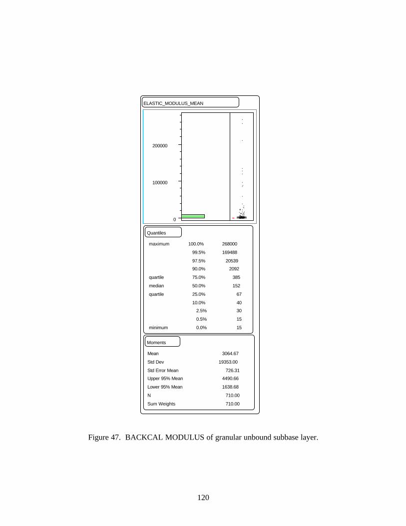
120

Figure 47. BACKCAL MODULUS of granular unbound subbase layer.

ELASTIC_MODULUS_MEAN

0

100000

200000

Quantiles

maximum

quartile

median

quartile

minimum

100.0%

99.5%

97.5%90.0%

75.0%

50.0%

25.0%

10.0%2.5%

0.5%

0.0%

268000

169488

20539 2092

385

152

67

40 30

15

15

Moments

Mean

Std Dev

Std Error MeanUpper 95% Mean

Lower 95% Mean

N

Sum Weights

3064.67

19353.00

726.31 4490.66

1638.68

710.00

710.00

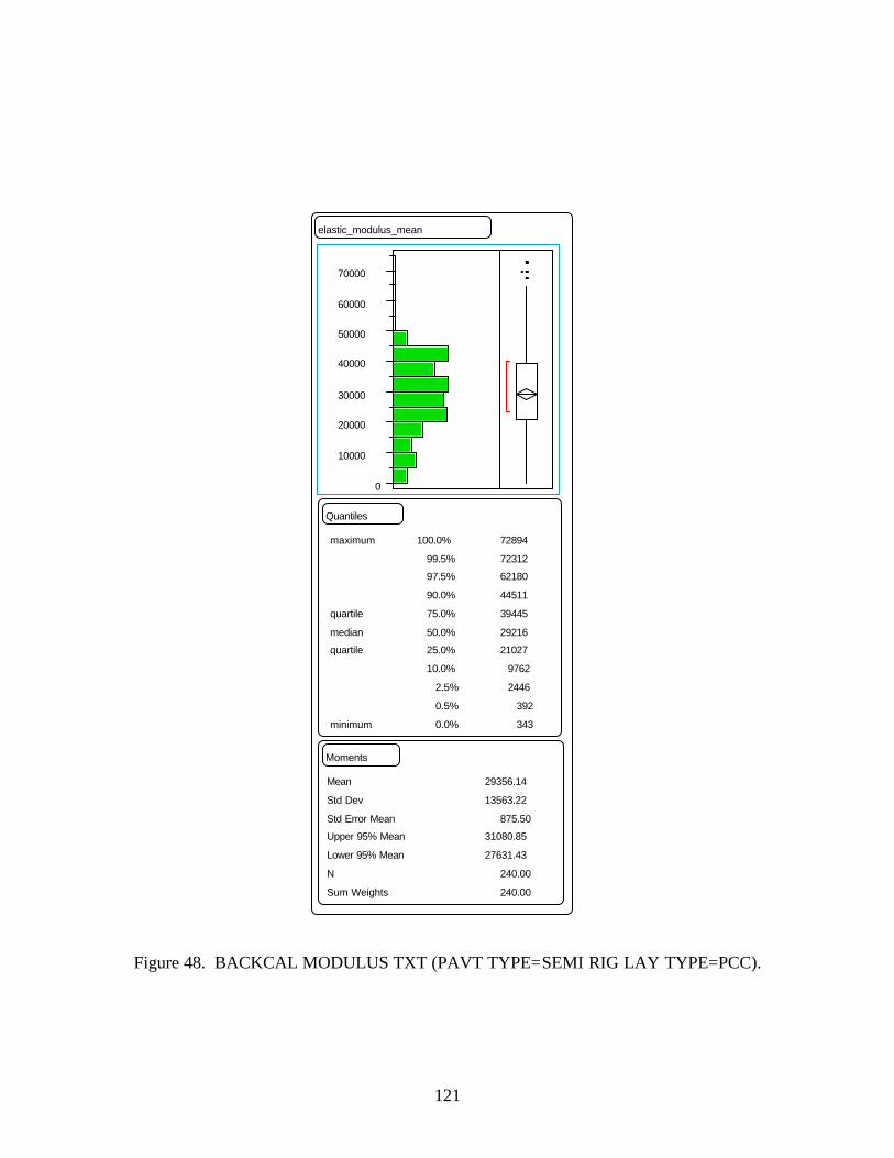
121

Figure 48. BACKCAL MODULUS TXT (PAVT TYPE=SEMI RIG LAY TYPE=PCC).

elastic_modulus_mean

0

10000

20000

30000

40000

50000

60000

70000

Quantiles

maximum

quartile

medianquartile

minimum

100.0%

99.5%97.5%

90.0%

75.0%

50.0%25.0%

10.0%

2.5%

0.5%

0.0%

72894

72312 62180

44511

39445

29216 21027

9762

2446

392

343

Moments

Mean

Std Dev

Std Error MeanUpper 95% Mean

Lower 95% Mean

N

Sum Weights

29356.14

13563.22

875.50 31080.85

27631.43

240.00

240.00

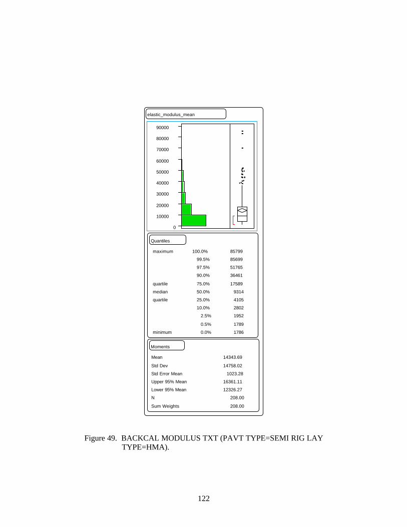
122

Figure 49. BACKCAL MODULUS TXT (PAVT TYPE=SEMI RIG LAY TYPE=HMA).

elastic_modulus_mean

0

10000

20000

30000

40000

50000

60000

70000

80000

90000

Quantiles

maximum

quartile

median

quartile

minimum

100.0%

99.5%

97.5%

90.0%

75.0%

50.0%

25.0%

10.0%

2.5%

0.5%

0.0%

85799

85699

51765

36461

17589

9314

4105

2802

1952

1789

1786

Moments

Mean

Std Dev

Std Error Mean

Upper 95% Mean

Lower 95% Mean

N

Sum Weights

14343.69

14758.02

1023.28

16361.11

12326.27

208.00

208.00

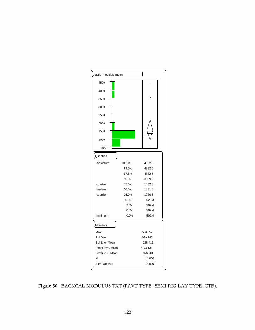
123

Figure 50. BACKCAL MODULUS TXT (PAVT TYPE=SEMI RIG LAY TYPE=CTB).

elastic_modulus_mean

500

1000

1500

2000

2500

3000

3500

4000

4500

Quantiles

maximum

quartilemedian

quartile

minimum

100.0%

99.5%

97.5%

90.0%

75.0%50.0%

25.0%

10.0%

2.5%0.5%

0.0%

4332.5

4332.5

4332.5

3939.2

1482.8 1331.8

1020.3

520.3

509.4 509.4

509.4

Moments

Mean

Std DevStd Error Mean

Upper 95% Mean

Lower 95% Mean

N

Sum Weights

1550.057

1079.140 288.412

2173.134

926.981

14.000

14.000

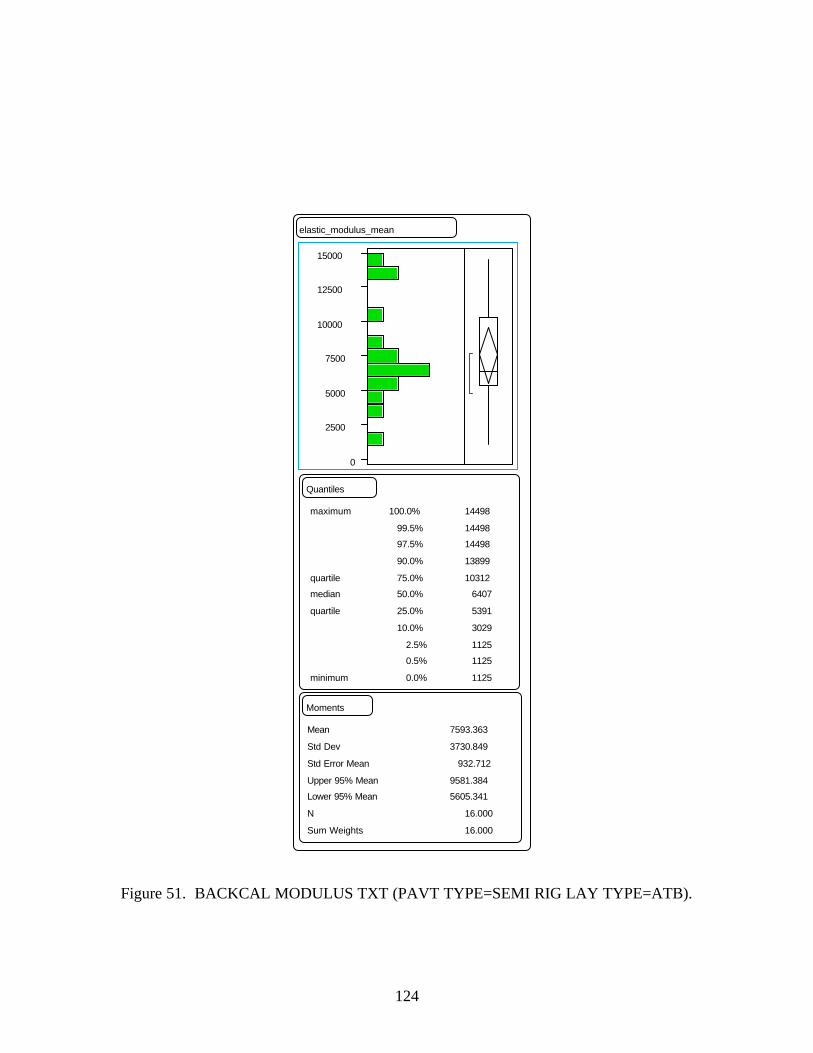
124

Figure 51. BACKCAL MODULUS TXT (PAVT TYPE=SEMI RIG LAY TYPE=ATB).

elastic_modulus_mean

0

2500

5000

7500

10000

12500

15000

Quantiles

maximum

quartilemedian

quartile

minimum

100.0%

99.5%97.5%

90.0%

75.0%50.0%

25.0%

10.0%

2.5%0.5%

0.0%

14498

14498 14498

13899

10312 6407

5391

3029

1125 1125

1125

Moments

Mean

Std Dev

Std Error Mean

Upper 95% MeanLower 95% Mean

N

Sum Weights

7593.363

3730.849

932.712

9581.384 5605.341

16.000

16.000

125

Figure 52. BACKCAL MODULUS TXT (PAVT TYPE=RIGID LAY TYPE=PCC).

elastic_modulus_mean

0

20000

40000

60000

80000

100000

120000

140000

160000

Quantiles

maximum

quartile

medianquartile

minimum

100.0%

99.5%97.5%

90.0%

75.0%

50.0%25.0%

10.0%

2.5%

0.5%

0.0%

163882

112441 85391

61907

51431

41600 33939

26286

5717

150

13

Moments

Mean

Std Dev

Std Error MeanUpper 95% Mean

Lower 95% Mean

N

Sum Weights

43294.07

17417.59

341.72 43964.15

42623.99

2598.00

2598.00

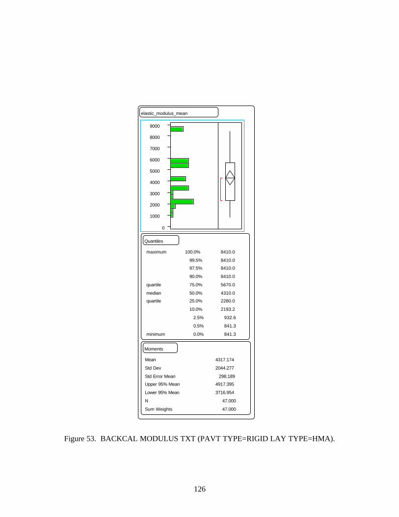
126

Figure 53. BACKCAL MODULUS TXT (PAVT TYPE=RIGID LAY TYPE=HMA).

elastic_modulus_mean

0

1000

2000

3000

4000

5000

6000

7000

8000

9000

Quantiles

maximum

quartile

medianquartile

minimum

100.0%

99.5%97.5%

90.0%

75.0%

50.0%25.0%

10.0%

2.5%

0.5%

0.0%

8410.0

8410.0 8410.0

8410.0

5670.0

4310.0 2280.0

2193.2

932.6

841.3

841.3

Moments

Mean

Std Dev

Std Error MeanUpper 95% Mean

Lower 95% Mean

N

Sum Weights

4317.174

2044.277

298.189 4917.395

3716.954

47.000

47.000

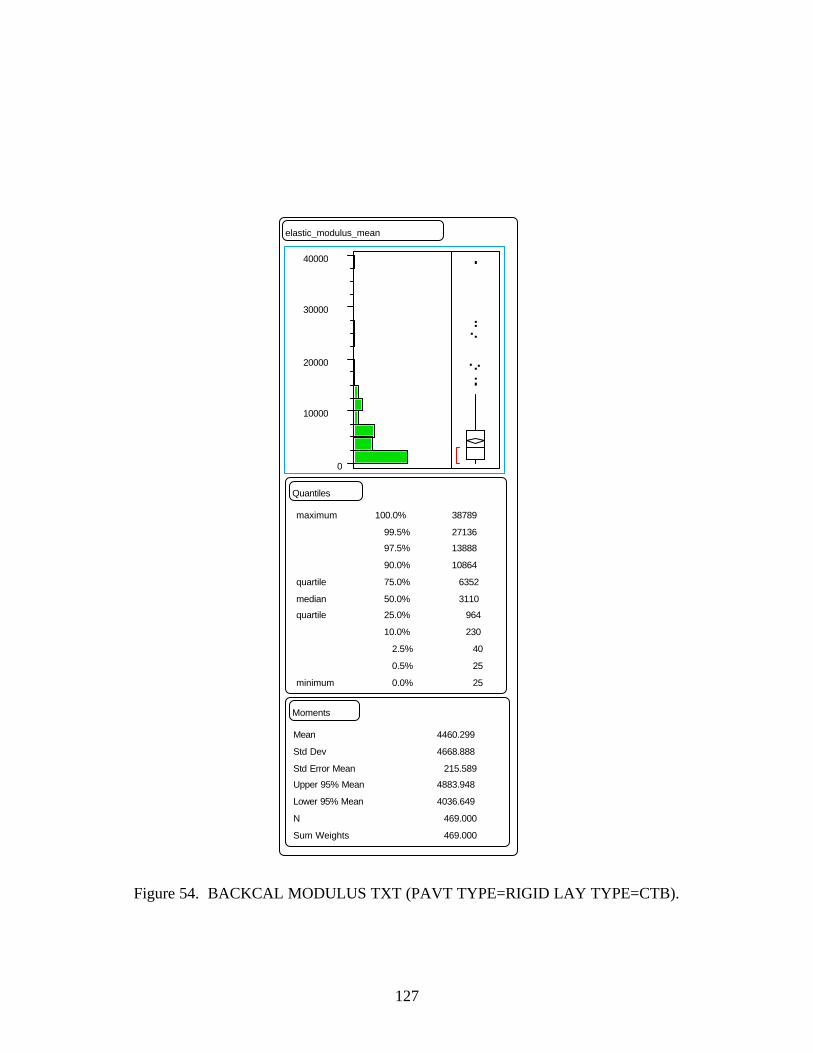
127

Figure 54. BACKCAL MODULUS TXT (PAVT TYPE=RIGID LAY TYPE=CTB).

elastic_modulus_mean

0

10000

20000

30000

40000

Quantiles

maximum

quartile

medianquartile

minimum

100.0%

99.5%97.5%

90.0%

75.0%

50.0%25.0%

10.0%

2.5%

0.5%

0.0%

38789

27136 13888

10864

6352

3110 964

230

40

25

25

Moments

Mean

Std Dev

Std Error MeanUpper 95% Mean

Lower 95% Mean

N

Sum Weights

4460.299

4668.888

215.589 4883.948

4036.649

469.000

469.000

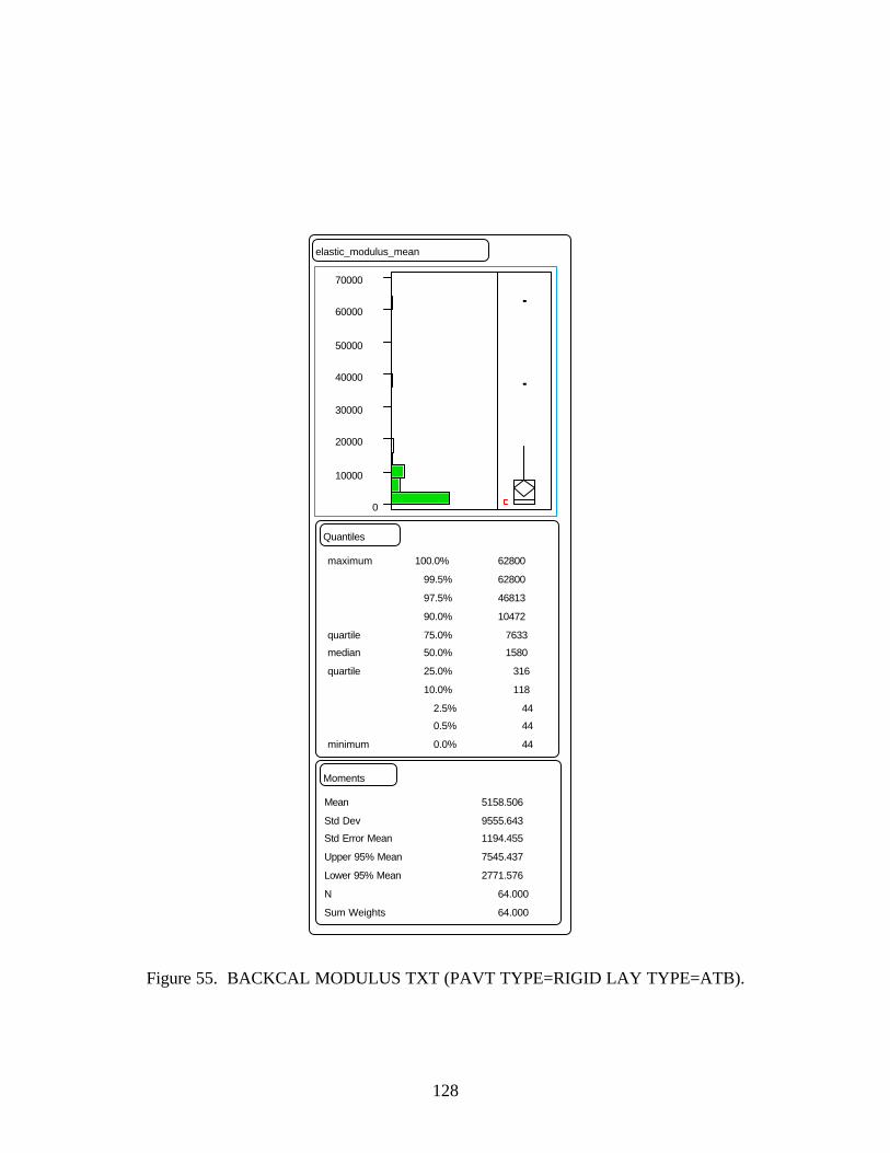
128

Figure 55. BACKCAL MODULUS TXT (PAVT TYPE=RIGID LAY TYPE=ATB).

elastic_modulus_mean

0

10000

20000

30000

40000

50000

60000

70000

Quantiles

maximum

quartilemedian

quartile

minimum

100.0%

99.5%

97.5%

90.0%

75.0%50.0%

25.0%

10.0%

2.5%0.5%

0.0%

62800

62800

46813

10472

7633 1580

316

118

44 44

44

Moments

Mean

Std DevStd Error Mean

Upper 95% Mean

Lower 95% Mean

N

Sum Weights

5158.506

9555.643 1194.455

7545.437

2771.576

64.000

64.000

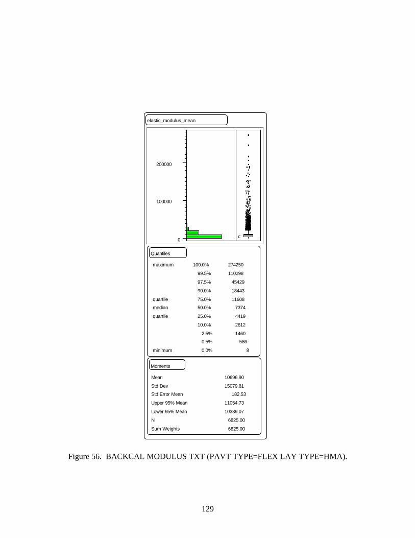
129

Figure 56. BACKCAL MODULUS TXT (PAVT TYPE=FLEX LAY TYPE=HMA).

elastic_modulus_mean

0

100000

200000

Quantiles

maximum

quartilemedian

quartile

minimum

100.0%

99.5%

97.5%

90.0%

75.0%50.0%

25.0%

10.0%

2.5%0.5%

0.0%

274250

110298

45429

18443

11608 7374

4419

2612

1460 586

8

Moments

Mean

Std DevStd Error Mean

Upper 95% Mean

Lower 95% Mean

N

Sum Weights

10696.90

15079.81 182.53

11054.73

10339.07

6825.00

6825.00

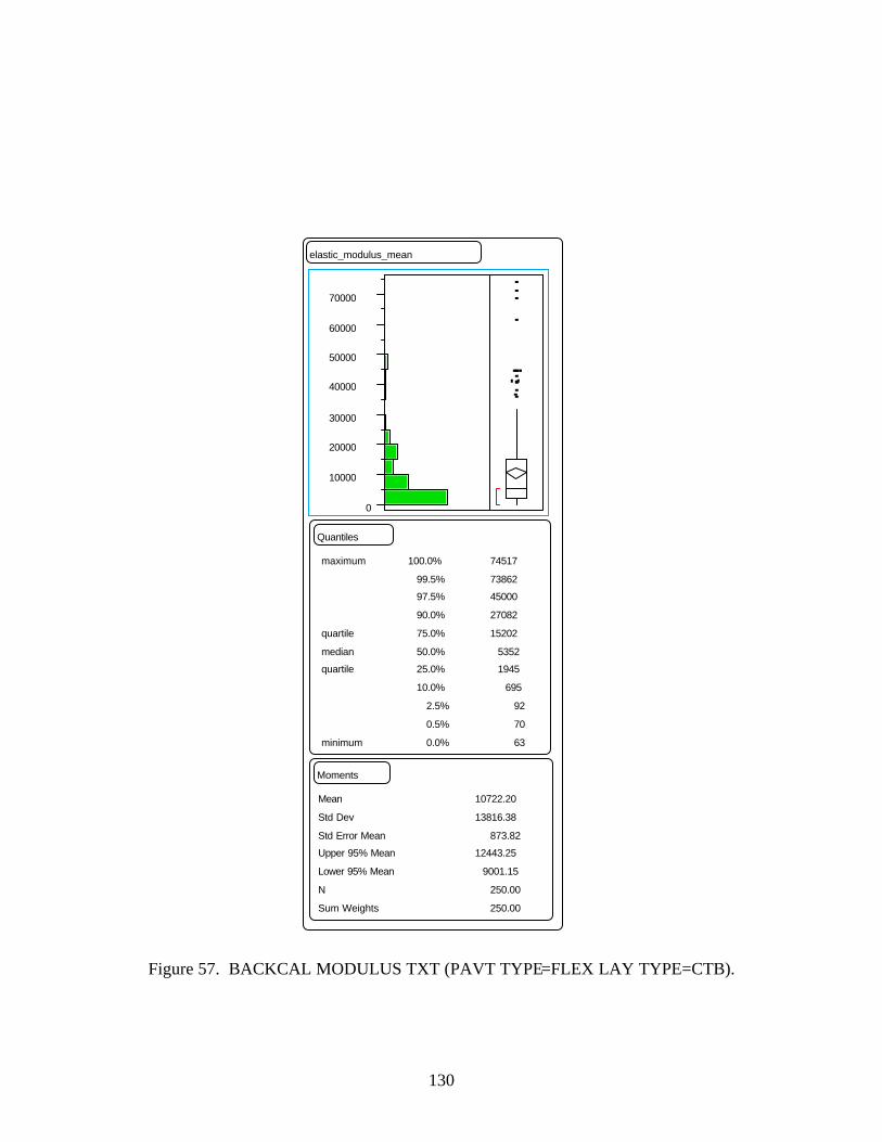
130

Figure 57. BACKCAL MODULUS TXT (PAVT TYPE=FLEX LAY TYPE=CTB).

elastic_modulus_mean

0

10000

20000

30000

40000

50000

60000

70000

Quantiles

maximum

quartile

medianquartile

minimum

100.0%

99.5%97.5%

90.0%

75.0%

50.0%25.0%

10.0%

2.5%

0.5%

0.0%

74517

73862 45000

27082

15202

5352 1945

695

92

70

63

Moments

Mean

Std Dev

Std Error MeanUpper 95% Mean

Lower 95% Mean

N

Sum Weights

10722.20

13816.38

873.82 12443.25

9001.15

250.00

250.00

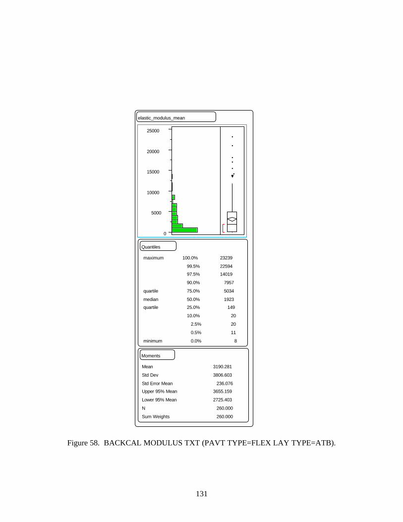
131

Figure 58. BACKCAL MODULUS TXT (PAVT TYPE=FLEX LAY TYPE=ATB).

elastic_modulus_mean

0

5000

10000

15000

20000

25000

Quantiles

maximum

quartile

medianquartile

minimum

100.0%

99.5%97.5%

90.0%

75.0%

50.0%25.0%

10.0%

2.5%

0.5%

0.0%

23239

22594 14019

7957

5034

1923 149

20

20

11

8

Moments

Mean

Std Dev

Std Error MeanUpper 95% Mean

Lower 95% Mean

N

Sum Weights

3190.281

3806.603

236.076 3655.159

2725.403

260.000

260.000

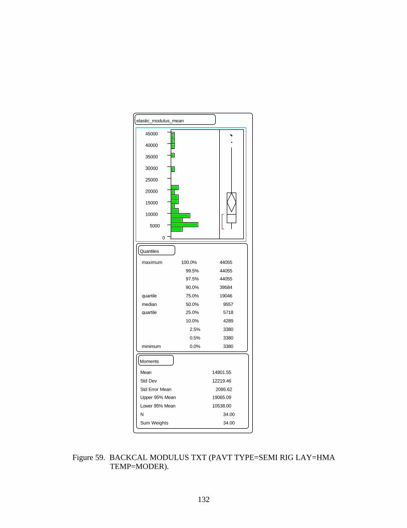
132

elastic_modulus_mean

0

5000

10000

15000

20000

25000

30000

35000

40000

45000

Quantiles

maximum

quartile

medianquartile

minimum

100.0%

99.5%97.5%

90.0%

75.0%

50.0%25.0%

10.0%

2.5%

0.5%

0.0%

44055

44055 44055

39584

19046

9557 5718

4289

3380

3380

3380

Moments

Mean

Std Dev

Std Error MeanUpper 95% Mean

Lower 95% Mean

N

Sum Weights

14801.55

12219.46

2095.62 19065.09

10538.00

34.00

34.00

Figure 59. BACKCAL MODULUS TXT (PAVT TYPE=SEMI RIG LAY=HMA TEMP=MODER).

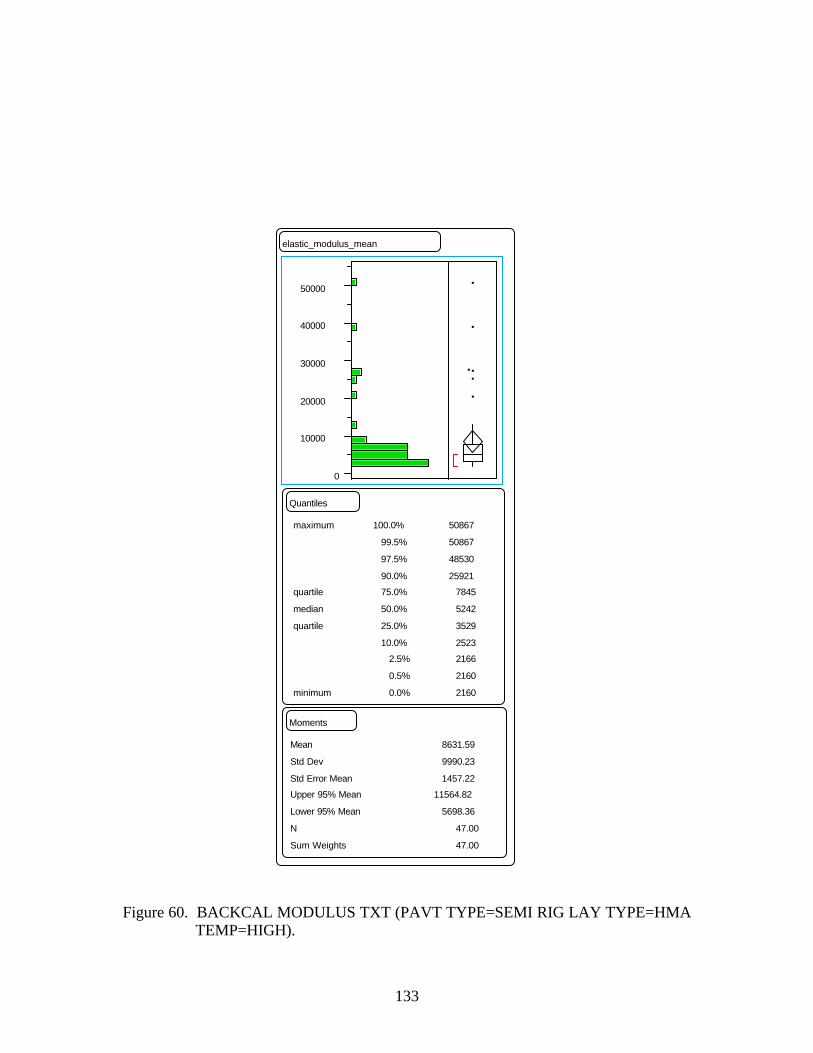
133

elastic_modulus_mean

0

10000

20000

30000

40000

50000

Quantiles

maximum

quartile

median

quartile

minimum

100.0%

99.5%

97.5%

90.0%75.0%

50.0%

25.0%

10.0%2.5%

0.5%

0.0%

50867

50867

48530

25921 7845

5242

3529

2523 2166

2160

2160

Moments

Mean

Std Dev

Std Error MeanUpper 95% Mean

Lower 95% Mean

N

Sum Weights

8631.59

9990.23

1457.22 11564.82

5698.36

47.00

47.00

Figure 60. BACKCAL MODULUS TXT (PAVT TYPE=SEMI RIG LAY TYPE=HMA TEMP=HIGH).

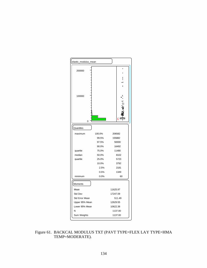
134

elastic_modulus_mean

0

100000

200000

Quantiles

maximum

quartile

medianquartile

minimum

100.0%

99.5%97.5%

90.0%

75.0%

50.0%25.0%

10.0%

2.5%

0.5%

0.0%

206582

155882 50000

16492

11480

8102 5723

3792

2181

1349

60

Moments

Mean

Std Dev

Std Error MeanUpper 95% Mean

Lower 95% Mean

N

Sum Weights

11625.97

17247.09

511.49 12629.55

10622.38

1137.00

1137.00

Figure 61. BACKCAL MODULUS TXT (PAVT TYPE=FLEX LAY TYPE=HMA TEMP=MODERATE).

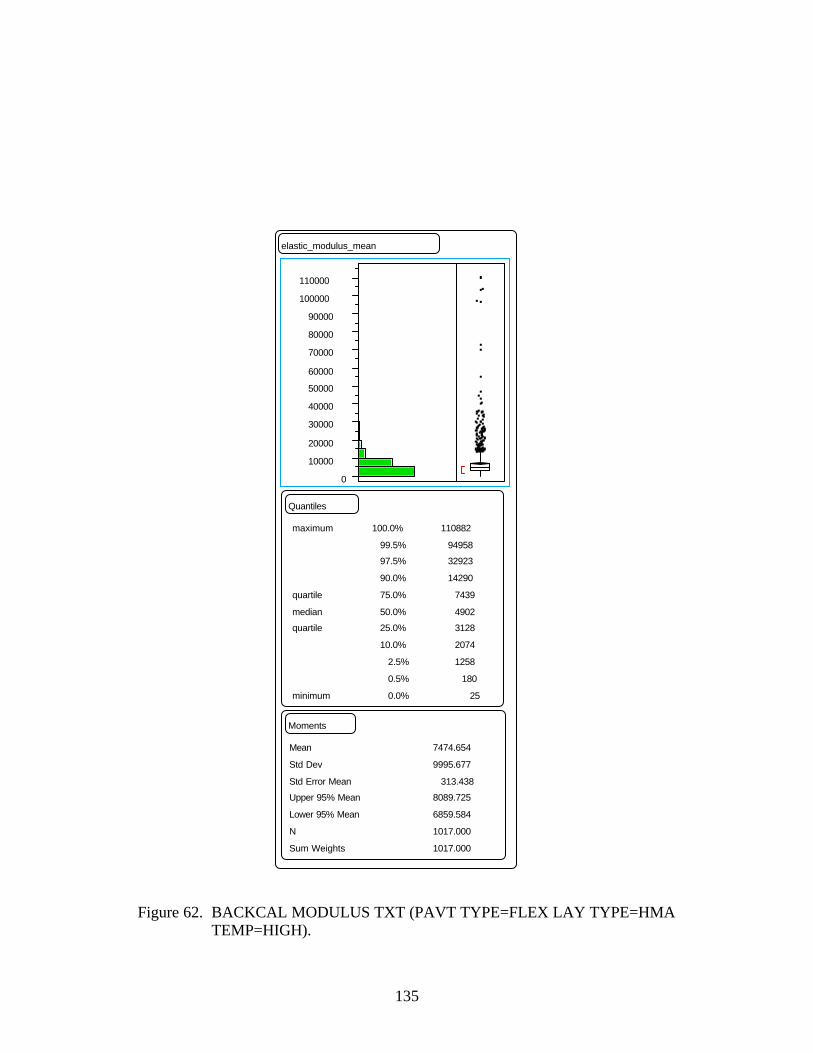
135

elastic_modulus_mean

0

10000

20000

30000

40000

50000

60000

70000

80000

90000

100000

110000

Quantiles

maximum

quartile

medianquartile

minimum

100.0%

99.5%97.5%

90.0%

75.0%

50.0%25.0%

10.0%

2.5%

0.5%

0.0%

110882

94958 32923

14290

7439

4902 3128

2074

1258

180

25

Moments

Mean

Std Dev

Std Error MeanUpper 95% Mean

Lower 95% Mean

N

Sum Weights

7474.654

9995.677

313.438 8089.725

6859.584

1017.000

1017.000

Figure 62. BACKCAL MODULUS TXT (PAVT TYPE=FLEX LAY TYPE=HMA TEMP=HIGH).

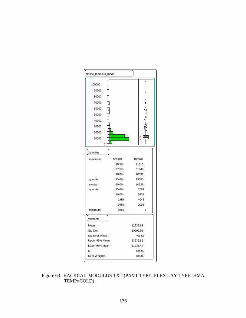
136

elastic_modulus_mean

0

10000

20000

30000

40000

50000

60000

70000

80000

90000

100000

Quantiles

maximum

quartile

medianquartile

minimum

100.0%

99.5%97.5%

90.0%

75.0%

50.0%25.0%

10.0%

2.5%

0.5%

0.0%

103970

71815 51949

20092

13380

10229 7789

5829

4043

2036

8

Moments

Mean

Std Dev

Std Error MeanUpper 95% Mean

Lower 95% Mean

N

Sum Weights

12737.63

10692.96

408.56 13539.82

11935.44

685.00

685.00

Figure 63. BACKCAL MODULUS TXT (PAVT TYPE=FLEX LAY TYPE=HMA TEMP=COLD).