Embed Size (px)
Citation preview

Stirling engine cycle efficiency
Bachelor's thesis
Automation Engineering
Valkeakoski
Nasrollah Naddaf

BACHELOR'S THESIS
Degree programme in Automation Engineering
Valkeakoski
Title Stirling engine cycle efficiency
Author Nasrollah Naddaf
Supervised by Raine Lehto
Approved on _____._____.20_____
Approved by
ABSTRACT
Valkeakoski
Degree Program in Automation Engineering
Author Nasrollah Naddaf Year 2012
Subject of Bachelor’s thesis Stirling engine cycle efficiency
ABSTRACT
This study strives to provide a clear explanation of the Stirling engine and its efficiency
using new automation technology and the Lab View software. This heat engine was
invented by Stirling, a Scottish in 1918. The engine’s working principles are based on
the laws of thermodynamics and ability of volume expansion of ideal gases at different
temperatures. Basically there are three types of Stirling engines: the gamma, beta and
alpha models.
The commissioner of the thesis was HAMK University of Applied Sciences under the
direct supervision of the engineering physics unit. The study focuses on a beta type
engine model (388-232), which is located in the Automation engineering laboratory.
The engine is coupled with a small generator for transforming heat energy to electrical
energy. The heating energy is provided by a special resistor inside the cylinder.
Lab View software and hardware conduct the measurements and control the station.
Measureable variables are defined and their instantaneous values are transferred by suit-
able sensors to a hardware module which can communicate with the interface through a
communication card which is located in the computer.
Measured values for: pressure, volume and other parameters are connected to the Lab
View software through a communication card. The data is processed by a program con-
sist of seven loops with each loop performing a certain function relative to the other
loops. A friendly user interface has been designed so that the user can see the measured
values either graphically or numerically on the screen. Main values include: input
power, output power, efficiency, rpm and temperature as well as the PV diagram. An-
other tab shows analytical and detailed measurements.
All protective and security issues have been taken into account in the program through
the use of automation functions and logics available in the Lab View environments.
Automation system has a great impact on the process outcome. Using powerful inter-
face software to monitor current conditions of the process equipment or their compo-
nents enables users to analyse the behaviour of a variable from different points of view.
It makes it easy to take the right decision based on the conditions in a system.
Keywords; Stirling engine, cycle efficiency and PV graph, data preparation, and Lab
View programming
Pages 4p. +9p appendices

ACKNOWLEDGMENTS
I would like to sincerely thank my supervisor Mr. Raine Lehto who guided me to find a
subject for the thesis and gave me a perfect description of the subject, which was a great
help later finding my way to do my thesis. Again thanks to Mr. Raine Lehto for coming
to school during summer holidays and observing the process of the study and giving me
directions and recommendations.
I am also grateful to Mr. Antti Aimo the Head of the Automation department who gave
me opportunity to do my thesis at HAMK automation laboratory in summer 2012.
Thanks to staff, teachers and assistants who were at school during holidays and helped
me a lot, especially Mr. Osmo Leiniäinen, Assistant for the Automation department who
is really dedicated to offering help to students.
All my acknowledgments and thanks are expressed to my teachers, colleagues and my
family who were supportive and friendly and encouraged me in my bachelor’s studies.

Symbols
Symbol Name Unit name
A Area Square meter ( E Energy Joule (J)
I Current Ampere (A)
F Force Newton (N)
n Molar quantity of gas Mole (mol)
P Power Watt (W)
P Pressure Pascal (pa)
R Gas constant Joule/Kelvin*mole R Resistance Ohm (Ω)
Q Heat Joule (J)
QH Hot side heat Joule (J)
QC Cool side heat Joule (J)
T Temperature Kelvin (K)
TL Low temperature Kelvin (K)
TH High temperature Kelvin (K)
TC Cooling temperature Kelvin (K)
V Volume Cubic meter V Voltage Volt (v)
W Work Joule (J)
Efficiency -
ρ Density kg/

CONTENTS
ABSTRACT I
ACKNOWLEDGMENTS II
SYMBOLS III
1 INTRODUCTION 1
2 STIRLING ENGINE ……………………………………………………… 2
2.1 Operation principles of Stirling engine ………………………………… 2
2.2 Stirling engine’s classification ……………………………………………… 5
2.3 Efficiency of Stirling cycle ……………………………………………… 5
2.4 Calculating power of cycle …………………………………………….. 7
3 PRELIMINARY INSTALLATION AND DATA PREPARATION 8
3.1 Magnetic sensor ……………………………………….. 9
3.2 Position sensor ………………………………………….. 9
3.3 Thermistor ……………………………………………………… 9
3.4 Pressure sensor …………………………………………………. 10
3.5 Power supply and connection box ……………. …………… 10
3.6 Testing and setting up I/O data table ……………................................ 11
4 DATA PROCESSING AND SOFTWARE PROGRAM ……………… 12
4.1 Lab view ………………………………………………… 13
4.2 Properties of Lab View library ………………………………………… 13
4.3 NI communication card and connection terminal………………………… 15
5 SOFTWARE PROGRAM …………………………………………… 16
5.1 rpm loop……………………………………………………………… 17
5.2 Data loop…………………………………………………………… 18
5.3 PV diagram loop………………………………………………………… 19
5.4 Power loop……………………………………………………………… 20
5.5 Feeding loop…………………………………………………………… 23
5.6 Writing data loop……………………………………………………… 25
5.7 Graphic indicator loop………………………………………………… 26
6 RUNNING THE PROGRAM AND FINAL TESTS………………… 27
6.1 Idle test……………………………………………………………… 27
6.2 Load test…………………………………………………………… 28
7 ANALYZING AND STUDY THE RESULTS………………………. 30
8 CHALLENGES ………………………………………………. 33
9 CONCLUSION ……………...................................................... 34
REFERENCES …………… …………… ……………. ……… 35
Appendix 1 USER INTERFACE USER TAB
Appendix 2 USER INTERFACE ANALYTICAL TAB
Appendix 3 IMAGES OF LOOPS 1, 2
Appendix 4 IMAGES OF LOOPS 3, 4
Appendix 5 IMAGES OF LOOPS 5, 6, 7
Appendix 6 IMAGE OF ALL LOOPS IN ONE PANEL
Appendix 7 CIRCUIT DIAGRAM OF POWER SUPPLY AND ELECTRICAL
CONNECTIONS
Appendix 8 COPY OF WRITTEN DATA ON AN EXCEL FILE
Appendix 9 IMAGES OF BETA STIRLING ENGINE
Stirling engine cycle efficiency
1
1 INTRODUCTION
The aim of this thesis was to design a system for the beta Stirling engine which can
monitor the efficiency and PV diagram of the engine. The project includes installing
suitable sensors, performing the power supply and connection circuit and software pro-
gramming in Lab View environment. The engine is located in the HAMK automation
laboratory. A small dynamo (3-4Watt) was coupled to the engine for the purpose of
acting as a generator. At least four live values were needed: pressure, volume, tempera-
ture, and rpm in order to be able to reach the goal.
The machine and its current situation were examined at first. Secondly all the electrical
circuits, the connection box, the BNC terminals, the power supply, and the sensors were
made and installed into the station. The adjustment and calibration of variables was
done according to manufacturer recommendations of the equipments. The provided in-
formation is connected to terminal BNC2110 where it is transferred to the communica-
tion card by a flat cable. The details can be found in related section.
The software programming is performed in the Lab View environment version 2010.
The program consists of two panels: the user interface panel and the block diagram pan-
el. The block diagram contains seven parts or loops. Two loops are data preparation
loops where raw information is acquired and scaled for further usage, the rest of the
loops are for data processing. All the loops are paralleled but have their individual tim-
ing functions. The user interface provides a variety of different information on the
screen either graphically or numerically. It has two tabs: the user tab and the analytical
tab. The analytical tab offers details and related data which are helpful for finding out
the cause of failures.
Many pretests were carried out for finding problems. Each test included observing and
solving problems, ultimately this led to fix the program and making it ready for the final
measurements. During these tests it was revealed that one has to know the theoretical
aspects of an engine in order to be able to design a perfect program, therefore at first
mechanics of a Stirling engine are explained here.
The results were obtained through two final tests: an idle test and a load test. In both
tests the gained efficiency was very close to the theoretical expectations, the obtained
PV diagram was similar to the theoretical models and it supported the theoretical
achievements fully. The measurements were conducted in almost stable conditions,
when next to no noise was present.
Experiences showed when rotational speed of the engine was 210rpm in the idle test
and 240in the load test it had the highest efficiency. The calculation of cycle power
which is a base stone for obtaining efficiency was done by the polygon function of the
Lab View. It calculates the area between the curves of the PV diagram, which is in fact
an irregular polygon.
A friendly user interface is another benefit of using Lab View. It monitors information
more sensibly in front of the user on the screen. The program writes recent data on a
defined excel file or other files automatically if a failure has stopped the engine, or a
user has pressed the write data button. Many improvements were done for securing and
stabilizing the program, the details of these improvements can be found in the instruc-
tions.

Stirling engine cycle efficiency
2
2 STIRLING ENGINE
A Stirling engine is a heat engine which was invented by Robert Stirling in 1918. it is
based on gas properties and thermodynamic laws and principles.
The engine uses an external heat source in contrast with combust engines so there is no
explosion inside the cylinder while working. The gas is expanded and compressed cy-
clically and continuously to produce motion to transforming energy. Fluid gas remains
inside the system and it is displaced from the hot side to the cool side and vice versa
when the engine is operating. There is no exhaustion like normal petrol engine, the en-
gine works very quietly.
The compressible gas can be air, hydrogen, helium, nitrogen or even vapor depending
on the design of the engine. Any source of heat can power the engine, from solid coal
to oil and solar energy, only the heat source must be adjusted to the engine. For example
in a solar energy model the solar concentrator and absorber have to be integrated with
the heating part of the cylinder. The Stirling engine was invented as a safer alternative
for steam engines of the time, when steam engines had poor quality and often caused
explosion because of uncontrollable pressure elevation and primitive technology.
This engine offers the possibility for having high efficiency with less exhaust emissions
in comparison with the internal combustion engine.
The Stirling engine has high performance in many applications and is suitable where:
multi-fueled characteristic is re-
quired;
a very good cooling source is availa-
ble;
quiet operation is required;
relatively low speed operation is
permitted;
constant power output operation is
permitted;
slow changing of engine power out-
put is permitted;
a long warm-up period is permitted.
Figure1 Modern Stirling engine
Modern models of Stirling engine have a relatively high efficiency and can be run even
at low temperature, (figure1) shows a new modern engine which can be run by the heat
of a cup of coffee. (Prof .T. Sundararajan, UT of Madras India.)
2.1 Operating principles of Stirling engine
In its simplest form a Stirling engine consists of a cylinder containing a gas, a piston
and a displacer. The regenerator and a flywheel are other complimentary parts of the
engine. When heat part of cylinder is heated up by an external heat source (figure2), the
temperature rises and gas expands proportional in to the temperature of the heat side.
Total volume is constant and limited by a piston thus expanded gas pushes the piston
down, so the volume of the pressured gas is increased and the gas loses its pressure and

Stirling engine cycle efficiency
3
temperature, then the piston backs to the heat side and compresses the gas by momen-
tum force of the flywheel, when it reaches near its up limit the displacer also pushes the
cooled gas to the heat side of the cylinder so that the gas is compressed and it can be
prepared to do another cycle. The expanding gas pushes the piston down again to pro-
duce mechanical energy for doing work, this cycling will continue till an external heat
source is available.
The flywheel and the regenerator have great roles in the engine’s performance. the fly-
wheel converts the linear movement of a working piston to rotary movement, it gives
needed momentum for the cycle procedure. Regenerator takes heat from gas in the ex-
pansion phase and releases heat to the gas in the compression phase, improving the en-
gine’s efficiency considerably. A Stirling engine and its components are shown in (fig-
ure2) below.
Figure 2 Stirling engine and its components
The cycle of a Stirling engine has four phases; heating, expansion, cooling and com-
pression. Short explanation of each phase is given in the following:
Heating: Heat source provides thermal energy to the engine so that it raises pres-
sure and temperature of gas.
Expansion: in this phase the volume increases, but the pressure and temperature
decrease, mechanical energy is produced from heat energy during this phase of
cycle only.
Cooling: the gas is cooled and temperature and pressure decrease, so the gas is
prepared to be compressed during this cycle.
Compression: the pressure of gas increases whereas its volume decreases; a part
of produced mechanical energy is used for processing of this phase, because it
needs an amount of work to be done.
Illustrations of different phases are shown in (figure 3) below.
Figure 3 phases of Stirling cycle
Heat
regenerator
displacer
piston flywheel
working
piston
Heating
source
Heating Expansion Cooling Compression
Heat
sourc
e
Cooling
source

Stirling engine cycle efficiency
4
The procedure of phase can be illustrated graphically in a PV diagram as it is shown in
(figure 4)
Looking at the graph (figure 4)
of Stirling cycle one can see
that, the volume is constant in
heating phase (1-2) and cool-
ing phase (3-4) while during
Expansion (2-3) and Compres-
sion (4-1) volume is varying
but temperature is constant.
(Pierre Gras, January 07, 2009)
I
Figure 4 PV graph of Stirling cycle
Engine’s working principles derived from thermodynamic laws, following formulas
introduces related parameters. Stirling cycle’ energy (ability to do work produced by a
thermodynamic system) is equal to;
. (2.1)
(2.2)
Where;
E= Energy (J),
P= Pressure (pa),
V=Volume ( ),
n=Molar quantity of gas (mol),
R= universal gas constant (J ,
T= Temperature (K),
As formula shows energy of a cycle depends on pressure and volume, so any changes in
these two main parameters changes output power of engine. In simple words it can be
said, temperature of hot side of engine causes pressure to rise and pushes the piston
move down, piston’s moving down changes volume thus it makes inside
cylinder that forces engine to run. (Prof T Sundararajan, Madras UT, India.)
Stirling engine cycle efficiency
5
Early Stirling engines were inefficient compare to other heat engines. But now its so-
phisticated models are enough efficient and competitive with internal combustion en-
gines, the new ones can be run at either high or low temperature heat in almost all cir-
cumstances.
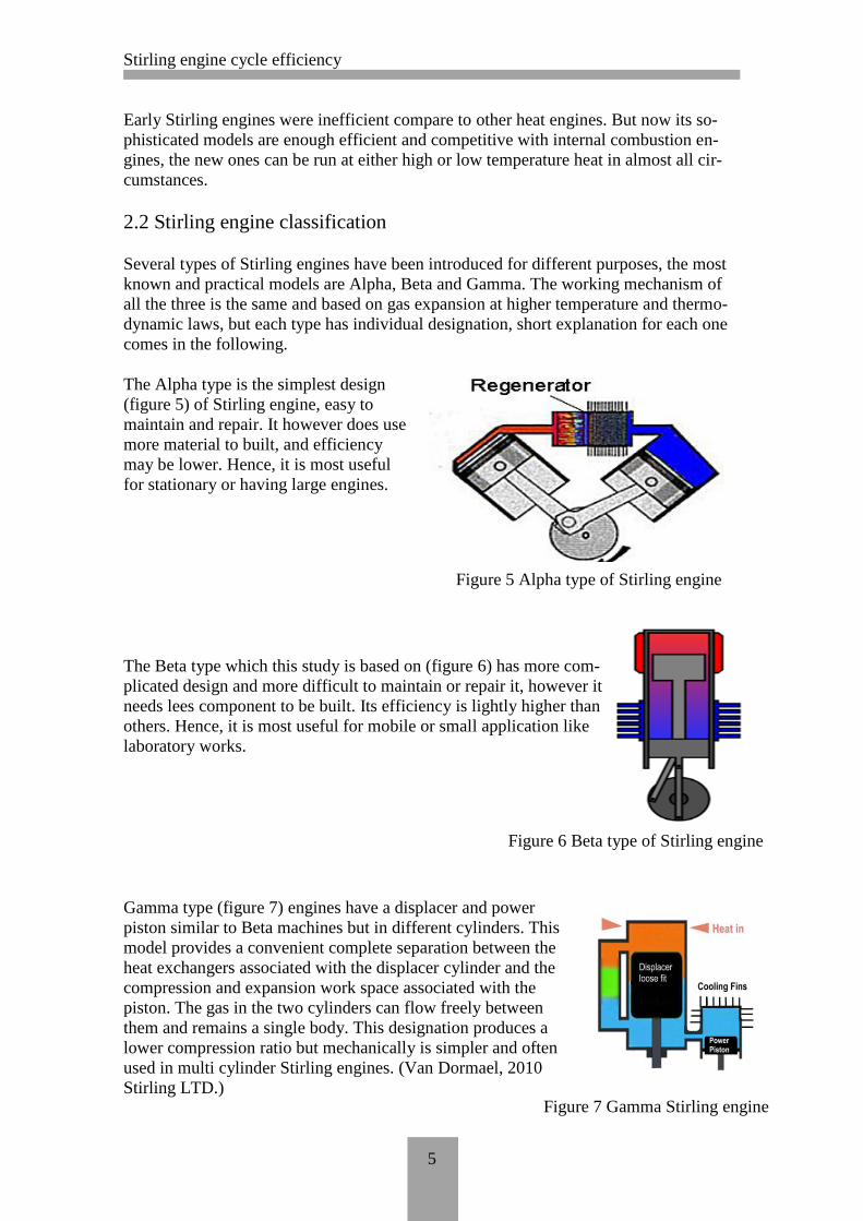
2.2 Stirling engine classification
Several types of Stirling engines have been introduced for different purposes, the most
known and practical models are Alpha, Beta and Gamma. The working mechanism of
all the three is the same and based on gas expansion at higher temperature and thermo-
dynamic laws, but each type has individual designation, short explanation for each one
comes in the following.
The Alpha type is the simplest design
(figure 5) of Stirling engine, easy to
maintain and repair. It however does use
more material to built, and efficiency
may be lower. Hence, it is most useful
for stationary or having large engines.
The Beta type which this study is based on (figure 6) has more com-
plicated design and more difficult to maintain or repair it, however it
needs lees component to be built. Its efficiency is lightly higher than
others. Hence, it is most useful for mobile or small application like
laboratory works.
Gamma type (figure 7) engines have a displacer and power
piston similar to Beta machines but in different cylinders. This
model provides a convenient complete separation between the
heat exchangers associated with the displacer cylinder and the
compression and expansion work space associated with the
piston. The gas in the two cylinders can flow freely between
them and remains a single body. This designation produces a
lower compression ratio but mechanically is simpler and often
used in multi cylinder Stirling engines. (Van Dormael, 2010
Stirling LTD.) Figure 7 Gamma Stirling engine
Figure 5 Alpha type of Stirling engine
Figure 6 Beta type of Stirling engine

Stirling engine cycle efficiency
6
2.3 Efficiency of Stirling cycle
Efficiency is the ratio of the energy delivered (or work done) by a machine to the energy
needed (or work required) in operating the machine. In other word the ratio of effective
or useful output to the total input in a system is efficiency and usually it is shown by
this symbol.
The efficiency is one of the most important decisive factors for every machine when
choosing an appliance for an application. Efficiency always is less than 100%, because
it is not possible to avoid lost energy when transforming it in practice.
Heat engines are often shown by diagrams like the one below.
During each cycle:
w is the net work done by the engine
QH is the energy taken from the (hot) source
QC is the energy given to the (cold) sink
Figure 8 Heat engine’s work procedure diagram
Thermodynamic efficiency (or just efficiency) of an engine is defined to be
(2.3)
This can be rearranged finally to:
(2.4)
If an engine is working with a constant heat and is the rejected heat from system
then efficiency for working nominally will be:
(2.5)
The above formula (2.5) calculates theoretical maximum possible efficiency of a heat
engine. The equation does not much care about lost energy during process, so that in
reality the efficiency of best engines is about half of what can be achieved by this for-
mula.
Stirling engine cycle efficiency
7
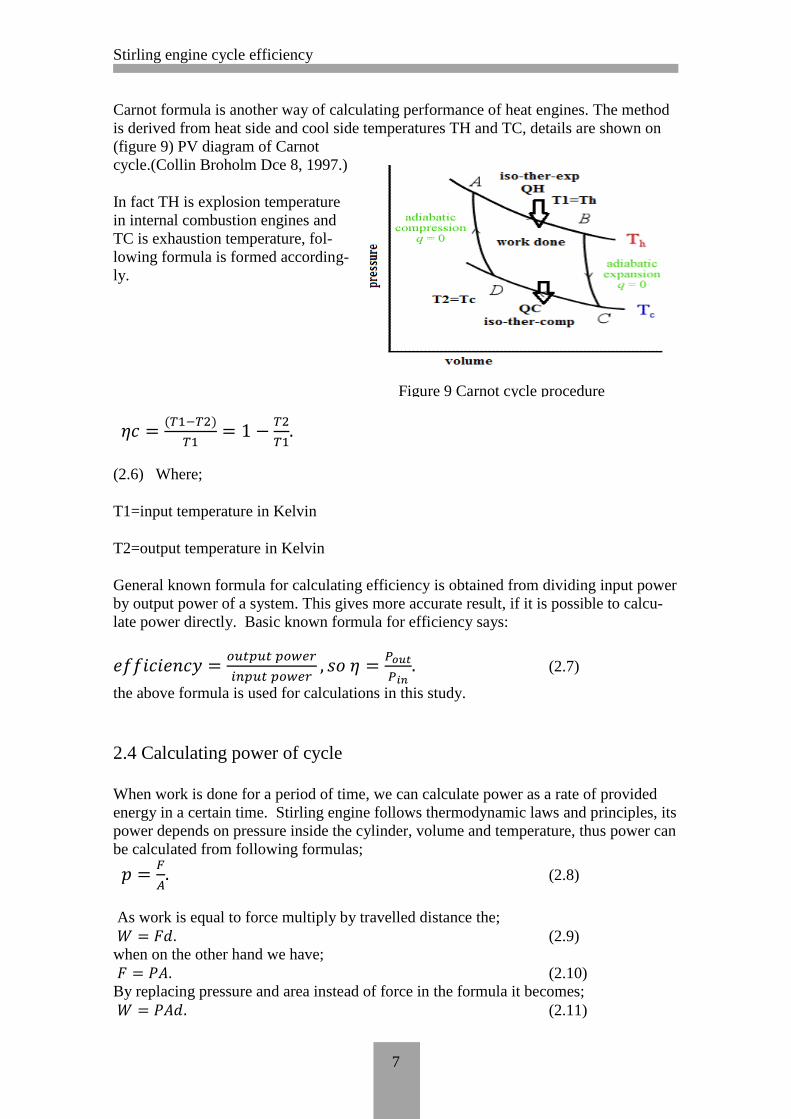
Carnot formula is another way of calculating performance of heat engines. The method
is derived from heat side and cool side temperatures TH and TC, details are shown on
(figure 9) PV diagram of Carnot
cycle.(Collin Broholm Dce 8, 1997.)
In fact TH is explosion temperature
in internal combustion engines and
TC is exhaustion temperature, fol-
lowing formula is formed according-
ly.
(2.6) Where;
T1=input temperature in Kelvin
T2=output temperature in Kelvin
General known formula for calculating efficiency is obtained from dividing input power
by output power of a system. This gives more accurate result, if it is possible to calcu-
late power directly. Basic known formula for efficiency says:
(2.7)
the above formula is used for calculations in this study.
2.4 Calculating power of cycle
When work is done for a period of time, we can calculate power as a rate of provided
energy in a certain time. Stirling engine follows thermodynamic laws and principles, its
power depends on pressure inside the cylinder, volume and temperature, thus power can
be calculated from following formulas;
(2.8)
As work is equal to force multiply by travelled distance the;
(2.9)
when on the other hand we have;
(2.10)
By replacing pressure and area instead of force in the formula it becomes;
(2.11)
Figure 9 Carnot cycle procedure

Stirling engine cycle efficiency
8
When pressure is inserted on a constant area like cross section area of a piston the work
will depend on distance travelled by piston directly, here volume is equal to;
. (2.12)
So final obtained formula of instantaneous work in a cycle is;
(2.13)
power as a rate of provided energy by Stirling cycle for doing work is equal to output
energy or work in a cycle multiply by rotational speed of engine per second so;
(2.14)
Where:
P=pressure/pa
F=force/N
d=Distance travelled/m
A= Cross section area of a piston/
W=work or energy/J
p=power/W
= rotational speed rounds/second
= energy of a cycle
No matter what is the unit of time, it can be second or minute or hour and etc.., but the
result will be power per a period of time. The formula (2.14) is applied by program in
calculation procedure.
By having instantaneous pressure and volume it is possible to calculate the output ener-
gy or work done by machine. If instantaneous measured pressure and volume during a
cycle be optimized on a XY coordinate, where Y is the pressure and X is the volume of
the engine, the result will be an irregular pol-
ygon (figure 10) which its area is the output
energy of cycle of Stirling engine.
Now power can be obtained by multiplying
energy of a cycle by revolution/second of
engine, at the end dividing it by input heating
power gives efficiency of the engine. This
job will be done by LABVIEW program in
this experience. Mechanics of the procedure
is explained later in related program sections.
Figure 10 simulation of a PV diagram
3 PRELIMINARY INSTALLATIONS AND DATA PREPARATION
Selected engine model for this study is an old one. It does not have required infor-
mation what are needed for programming. Values of pressure, volume, temperature and
rpm are inevitable raw information for purpose of this study, therefore the old engine
has been studied and suitable tools are selected to offer initiative data. Pressure, vol-
ume, temperature, rpm, input (heating) voltage values are captured by different sensors
and tools. Sensors are mounted on body of engine in a fair possible location.

Stirling engine cycle efficiency
9
A power supply is made to provide working energy to sensors and other informative
loads. It consists of a transformer, rectifier diodes, capacitors and two voltage regula-
tors IC AN7805. Input voltage is 230VAC and outputs are 24VDC and two separated
5VDC, 5VDC, separation took place to remove experienced noises. Explanation of
mounted equipments comes briefly in the following.
3.1 Magnetic sensor
This sensor (figure 11) is sensitive to magnetic field. If it be opposed to a magnetic
field it sends a specified voltage (10v) out which can be used for acquiring data. In this
case a piece of magnet has been glued on the flywheel of engine which has a permanent
magnetic field. When engine is running and flywheel is turning the glued magnet acti-
vates magnetic sensor one time in each turn of fly-
wheel which is equal to one cycle. Sensor sends
10V for each pass to the program where a counter
edge DAQ max counts rise edges, then rpm loop
calculates engine’s rpm based on counted edge.
Figure 11 magnetic sensor
3.2 Position sensor (volume meter)
This sensor has a linear movement which causes changes of output voltage from low to
high (0v to 10v) and vice versa, so the position of piston can be specified by reading
output voltage of sensor. Instantaneous volume of cylinder can be acquired by scaling
this voltage as changes in volume. It is connected with piston’s rod in a way that covers
full range of volume changes (150cm3) when engine is operating. Piston’s ∆d is 51mm
but position meter ∆d is 32mm, a transferor pulley (figure 13) is made to transfer the
51mm to 32mm physically
Figure 12 position meter sensor Figure13 distance transferor pulley
Position sensor also has a transducer that translates sensed voltages by physical part to
stable readable voltage for software and finally sends them to connection box.
3.3 Pressure sensor
The sensor is a piezoresistive transducer that includes silicon pressure sensor (figure
14) for a wide range of applications. The sensor ranged from 20kpa to 250kpa, its out-

Stirling engine cycle efficiency
10
put varies from 0.2 to 4.9v respectively, thus reading and scaling the voltage gives the
exact instantaneous pressure inside piston when it is working.
Pressure sensor has to be calibrated carefully. When piston is in lowest level the pres-
sure in cylinder is equal to atmospheric pressure, no any extra
pressure is inserted inside. Connection tube can be opened to the
air at maximum volume when calibrating. Its sensitivity is
20mv per one kilo Pascal that means 1v change shows 50kpa
change in pressure,
Figure 14 pressure sensor
3.4 Thermometer
Temperature has a significant role in engine’s working. High temperature decreases
engine’s efficiency and damages almost all components inside cylinder. A temperature
data is needed for controlling the engine when it is overheated. For this purpose a PTC
thermistor has been stuck to the outside wall of cylinder, so that any changes in cylin-
der’s temperature causes change in resistance of thermistor and
acts as a thermometer in the system. Acquired voltage from ther-
mistor is calibrated and monitored by the program as temperature
of cooling water in cool side of engine. Its electrical circuit and
connectivity is explained in connection box circuit.
Figure 15 Thermistor
3.5 Power supply& connection box
The power supply consists of a transformer, pole diodes, capacitors, resistors and an IC.
Transformer takes 220AC as input and gives two separate voltages (12, 24vVAC) as
outputs. Full wave rectification method is used to produce three different dc voltages
(5, 12,24VDC) by the above components. 24 volt is connected to volume (position)
transducer which powers position sensor, 12 volt goes to magnetic sensors and 5 volt
dedicated to pressure sensor and thermal circuit. Connection box provides connections
between sensors and connector terminal BNC2110. All inputs to this box are sensors’
data which are connected through terminals to BNC connectors where ready infor-
mation is transferring to BNC2110 by BNC cables. Two diode indicators on the box
show availability of power supply (red) and generator (blue) output.
Two extra connection plugs are built on the box for load testing. Each plug has its own
switch to be on or off. The box is shown in (figure 17). More details and sub circuits
about this project can be found on electrical circuit drawing which is available in ap-
pendix documents.

Stirling engine cycle efficiency
11
Figure 16 power supply circuit with three separated outputs
Figure 17 connection box with BNC connectors and cables
3.6 Testing and setting up I/O data table
In this step all sensors are powered and connected to connection box where their outputs
are connected to BNC plugs for further usage. Manual tests were conducted using a
digital multimeter and other calibrator tools then obtained results have been compared
with sensors’ specification and manufacturer’s recommendations. After being sure that
all criteria have been met, it is left for software programming.

Stirling engine cycle efficiency
12
The tests showed that it is not possible to send a direct reference of feeding voltage to
BNC connector terminal, because the voltage is over high limit of BNC connector and
its current more than 10 ampere. It can damage the hardware. This reference is needed
in program for calculating efficiency.
An adaptor circuit (voltage divider) is made for
this purpose, which sends out safe and accurate
reference of feeding voltage to the program. It
consists of two 100kΩ resistors which are con-
nected in series to feeding power and transfer
low voltage to BNC connector.
Figure 18 circuit adaptor (voltage divider)
Data table has been set up to show which I/O is dedicated to which variable. The table
also is available as a clear guidance for further maintenance and developments; there are
five Analog inputs, one analog out puts and one digital input in this table. Inputs are
volume, pressure, generator voltage, heating voltage and temperature, the only analog
output is control voltage to feeding transformer, rpm is considered as a digital input,
details are shown (table 1) in the below.
Table1 I/O data table configured to BNC terminal 2110
No Variable I/O connected to type of connection
1 Volume AI0 connection box ∆V BNC cable
2 Pressure AI1 connection box ∆P BNC cable
3 Generator
voltage
AI2 connection box G-v BNC cable
4 Temperature AI3 connection box Temp BNC cable
5 Heating volt-
age
AI4 adaptor terminal BNC cable+ wire
6 rpm PFI8 connection box BNC cable+ wire
7 Control volt-
age
AO1 transformer input socket BNC+ socket
4. DATA PROCESSING AND SOFTWARE PROGRAMMING
Lab View software has been chosen for conducting measurements and documentation
of data of this application. This powerful software produced by National Instrument
Company for measurement, engineering, developing and automation which is widely
used in the world. Program has high flexibility and different functions to establish con-
figuration between different software and systems thus it helps to come close with
Stirling engine cycle efficiency
13
standardization in automation area of work, where numerous systems and brands are
used. Short explanations about it come in the following section.
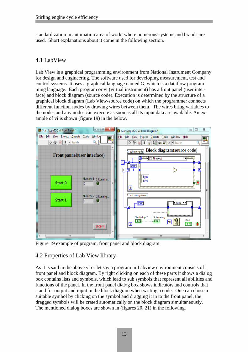
4.1 LabView
Lab View is a graphical programming environment from National Instrument Company
for design and engineering. The software used for developing measurement, test and
control systems. It uses a graphical language named G, which is a dataflow program-
ming language. Each program or vi (virtual instrument) has a front panel (user inter-
face) and block diagram (source code). Execution is determined by the structure of a
graphical block diagram (Lab View-source code) on which the programmer connects
different function-nodes by drawing wires between them. The wires bring variables to
the nodes and any nodes can execute as soon as all its input data are available. An ex-
ample of vi is shown (figure 19) in the below.
Figure 19 example of program, front panel and block diagram
4.2 Properties of Lab View library
As it is said in the above vi or let say a program in Labview environment consists of
front panel and block diagram. By right clicking on each of these parts it shows a dialog
box contains lists and symbols, which lead to sub symbols that represent all abilities and
functions of the panel. In the front panel dialog box shows indicators and controls that
stand for output and input in the block diagram when writing a code. One can chose a
suitable symbol by clicking on the symbol and dragging it in to the front panel, the
dragged symbols will be crated automatically on the block diagram simultaneously.
The mentioned dialog boxes are shown in (figures 20, 21) in the following.

Stirling engine cycle efficiency
14
In block diagram there are functions that appear only on block diagram when writing a
code, like mathematical nodes, Boolean nodes and etc.., these functions participated in
processing data and don’t have representative on front panel. There is a search on dialog
boxes one can write desired function in search box and a group of option will appear on
dialog box that programmer can select the suitable ones.
Figure 20 front panel dialog box Figure 21 block diagram dialog box
Each symbol can be modified by right click on it and selecting property or other visible
menus based on the purpose of programming. When an input or output is created on the
block diagram, they are appeared automatically on the front panel too. All practical and
applied functions are in block diagram dialog box, one can drag analyzer, processor or
calculator nodes in to the block diagram and wire them together purposely to obtain the
expected results. (measurement Automation HAMK, 2012)
Figure 22 simple example mathematical program with while loop
For making a program the needed nodes have to be dragged in to block diagram and be
wired then enclosed by a suitable loop from structure menu, there are different loops
with different properties which can be used for catching the goal of a program. A simple

Stirling engine cycle efficiency
15
program is shown in (figure 22) that has four inputs and one output, if user changes the
values of inputs the results changes respectively.
When it is wanted continuous measuring, the code have to be enclosed by while lop, if
measuring is needed for certain times then for loop is a good option, however there are
different loops for variety of usages in Lab View.
4.3 NI communication card and connector terminal
When a program is written in virtual environment of LabView it needs some special
equipment for interpreting virtual inputs outputs to physical ones and providing com-
munications with measurer instruments and hardware on the plant. Here the job is done
by NI ….. M series card (figure 23), it is installed in the comput-
er and is connected to the BNC terminal 2110 which is the final
step towards physical I/O. The obtained data at connection box
of engine station are brought to connector terminal by BNC ca-
bles, where a huge flat cable connects the BNC terminal to the
NI card in a computer. The image of connector (figure 25) is
shown in front of text.
Figure 24 BNC terminal 2110
Figure 23 communication card M series
Configuration and compatibility between the
hard ware have to be considered very care-
fully; otherwise they may cause complicated
problems and disturb obtained results.
Always it is beneficial to follow manufac-
turers’ recommendation while they know
better what are behind these virtual envi-
ronments. In fact M card is like nerve sys-
tem for software brain which without that
nerve the program is paralyzed and no func-
tion is expected. (NI tutorial online.)
Figure 25 BNC 2110 connected to M card.

Stirling engine cycle efficiency
16
5 SOFTWARE PROGRAM
The program used to gather, calculate, control and display the data in Lab View front
panel on the screen. The main purpose of this program is to draw PV diagram and cal-
culating efficiency of the beta type of Stirling engine. Different types of data have been
acquired for giving analytical ability to the program, using both numerical and graphical
indicators help that data be more visible to users.
Front panel (figure 26) consists of two tabs; user tab and analytical tab. User tab con-
tains controls and indicators which enable users manage engine’s output, while analyti-
cal tab shows details data that are helpful for understanding cause of failures.
Figure 26 user interface (front panel) Stirling engine efficiency-PV diagram
A few numerical inputs and other types of controlling are designed for user tab in front
panel to enable user to have on time and effective control on system. Graphical indica-
tors are available in both tabs and represents instantaneous information of the station. It
is tried to choose suitable font and color to make the user interface more friendly. In-
stantaneous pressure value inside cylinder and temperature is connected to image of
beta type of Stirling engine on front panel, so that it moving up and down harmonically
when engine is working.
Stirling engine cycle efficiency
17
Safety issues are considered when codes were writing. Operator is not able to make
problematic changes to program from front panel, different limitations has been built up
that prevents harmful changes.
Block diagram of the program is divided in to seven parts or let say loops for being eas-
ier to follow it. All loops are working parallel together but each one does certain tasks
and has its own timing regulation. A text box on the loop explains the main targets of a
loop. Two DAQmax are configured, one for anlog inputs (figure 28) another for digital
input (figure 27) (counter). A DAQ assistant(figure 35) is configured for aquiring an
output voltage (1...10V) for contolling feeding transformer. A DAQ can handle one
types of data at a time. There are some loops inside maine loops which are used to
process data. Scale notation or specicific function are explained in text boxes of each
loop. Block diagram is the most important part at acquiring data process so that loops
and their task are described one by one in the following.
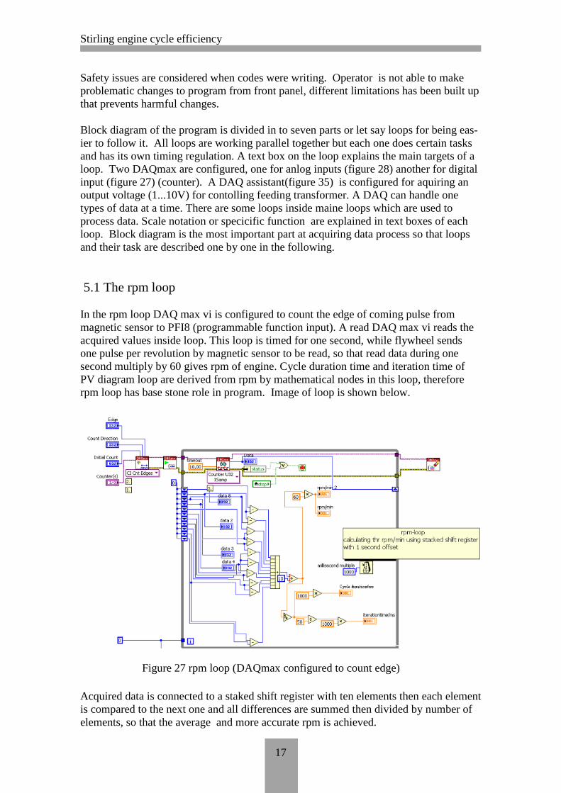
5.1 The rpm loop
In the rpm loop DAQ max vi is configured to count the edge of coming pulse from
magnetic sensor to PFI8 (programmable function input). A read DAQ max vi reads the
acquired values inside loop. This loop is timed for one second, while flywheel sends
one pulse per revolution by magnetic sensor to be read, so that read data during one
second multiply by 60 gives rpm of engine. Cycle duration time and iteration time of
PV diagram loop are derived from rpm by mathematical nodes in this loop, therefore
rpm loop has base stone role in program. Image of loop is shown below.
Figure 27 rpm loop (DAQmax configured to count edge)
Acquired data is connected to a staked shift register with ten elements then each element
is compared to the next one and all differences are summed then divided by number of
elements, so that the average and more accurate rpm is achieved.

Stirling engine cycle efficiency
18
It is decided to have at least 50 points in a cycle for illustration of PV diagram of en-
gine, so that duration time of cycle which is derived from formula (15);
(5.15)
Where;
= revolution per second Obtained cycle duration is divided by 50 and then it is multiplied by 1000 for having
time in milliseconds, thus the result is considered as iteration time of (for loop) inside
PV diagram loop. Final values are sent to other loops using local variable method.
5.2 Data loop
Data loop provides all analog data. A DAQ max vi is configured to measure multiple
analog inputs simultaneously, another read DAQ max vi reads measured data inside
loop and gives them out in an array of data then array is indexed to separate each indi-
vidual measured voltage. Individual voltage is scaled and compensated precisely, be-
fore sending to other loops through local variable function. See (figure 28)
For example total volume of cylinder is 350cm^3 and total change in volume ∆V is
150cm^3 and measured voltage varies from almost (0…10v), therefore multiplying by
15 and then adding 200 gives instantaneous volume of cylinder. The method is applied
to pressure too. Pressure sensor output varies from (0…5v) while its full range is
250kpa, thus value from pressure sensor multiplied by 50 gives real pressure inside cyl-
inder, nothing else is needed because pressure at V max is atmospheric pressure.
Figure 28 data loop (DAQmax configured to acquire analog inputs)
Other acquired values have got proper compensation factor to show real values. As it is
seen (figure 28) temperature is multiplied by 100 gives TC (cooling side temperature) of
Stirling engine cycle efficiency
19
engine in Celsius degree. The engine heating voltage is multiplied by 2 and a dissipation
factor 0.5 is added to it, final value is instantaneous heating voltage (input) of engine in
volt. This loop is timed for one millisecond so it is almost impossible to lose instanta-
neous values considering the highest rpm of this engine which is 500rpm.
5.3 PV diagram loop
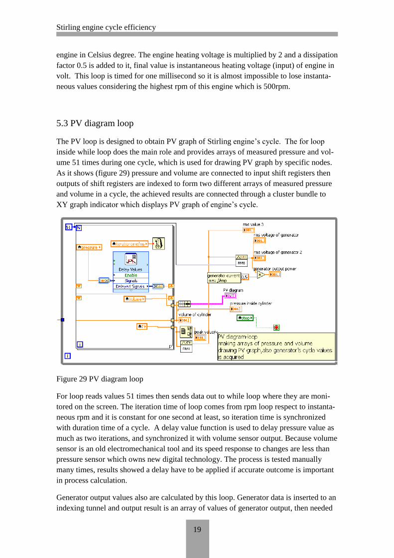
The PV loop is designed to obtain PV graph of Stirling engine’s cycle. The for loop
inside while loop does the main role and provides arrays of measured pressure and vol-
ume 51 times during one cycle, which is used for drawing PV graph by specific nodes.
As it shows (figure 29) pressure and volume are connected to input shift registers then
outputs of shift registers are indexed to form two different arrays of measured pressure
and volume in a cycle, the achieved results are connected through a cluster bundle to
XY graph indicator which displays PV graph of engine’s cycle.
Figure 29 PV diagram loop
For loop reads values 51 times then sends data out to while loop where they are moni-
tored on the screen. The iteration time of loop comes from rpm loop respect to instanta-
neous rpm and it is constant for one second at least, so iteration time is synchronized
with duration time of a cycle. A delay value function is used to delay pressure value as
much as two iterations, and synchronized it with volume sensor output. Because volume
sensor is an old electromechanical tool and its speed response to changes are less than
pressure sensor which owns new digital technology. The process is tested manually
many times, results showed a delay have to be applied if accurate outcome is important
in process calculation.
Generator output values also are calculated by this loop. Generator data is inserted to an
indexing tunnel and output result is an array of values of generator output, then needed

Stirling engine cycle efficiency
20
values of generator in obtained by using different mathematical function of LabView.
But these values do not have anything to do with PV graph just this loop is used for
calculation. A question may arise that why loop’s iteration number is 51 when iteration
time is based on 50? Because it is wanted to produce a closed area on PV graph indica-
tor, adding one or two more iteration does not make changes in final results because the
cycle is a closed continuous one, and iteration time is constant for at least one second
which may cover more than 200 iterations.
5.4 Power loop
Power loop contains all elements to calculate different aspects of power and efficiency.
There are many values in this loop that they are not needed in calculation or in pro-
gramming, these kinds of data has been created for comparing, analyzing and research
about behavior of this engine and system. Explanations of the most important ones
come in the following.
5.4.1Instantaneous power
Arrays of pressure and volume are brought to this loop (figure 30) and connected to the
for loop’s tunnel, then indexed and divided by 1000 that gives instantaneous output en-
ergy of engine. The unit of power is in joule/t, because pressure is considered in kilo
Pascal. Instantaneous power is indexed again and the result is averaged so it produced
cycle average output energy, also by another function maximum and minimum work or
let say energy of a cycle are achieved.
Figure 30 power loop

Stirling engine cycle efficiency
21
5.4.2 Theoretical Maximum work
Theoretical Maximum work of a cycle is calculated by formula (5.16). LabView func-
tions are used to find out max and min volume values in a cycle then the difference be-
tween them which is dv is multiplied by max pressure and the result is theoretical max
power of cycle.
. (5.16)
Where;
Wmax= possible maximum theoretical work
P = maximum pressure
dv= total change in volume
5.4.3 Cycle energy output
It is known that area under the curve is equal to work done by piston. When there is a
closed area consists of upper and lower curves (figure 31) which presents one cycle of
heat engine, then the area between two curves is equal to engine’s output energy in one
cycle. In fact power is rate of provided energy per unit of time, so that energy per cycle
multiply by rpm (as rpm can
be interpreted as cycles per
unit of time) gives output
power of engine in watt per
unit of time, unit time can be
second, minute or etc.
Figure 31 Stirling cycle illustration
As graph shows cycle figure can be considered as an irregular polygon with 50vertices
so the area can be calculated by following formula (5.17):
. (5.17)
Stirling engine cycle efficiency
22
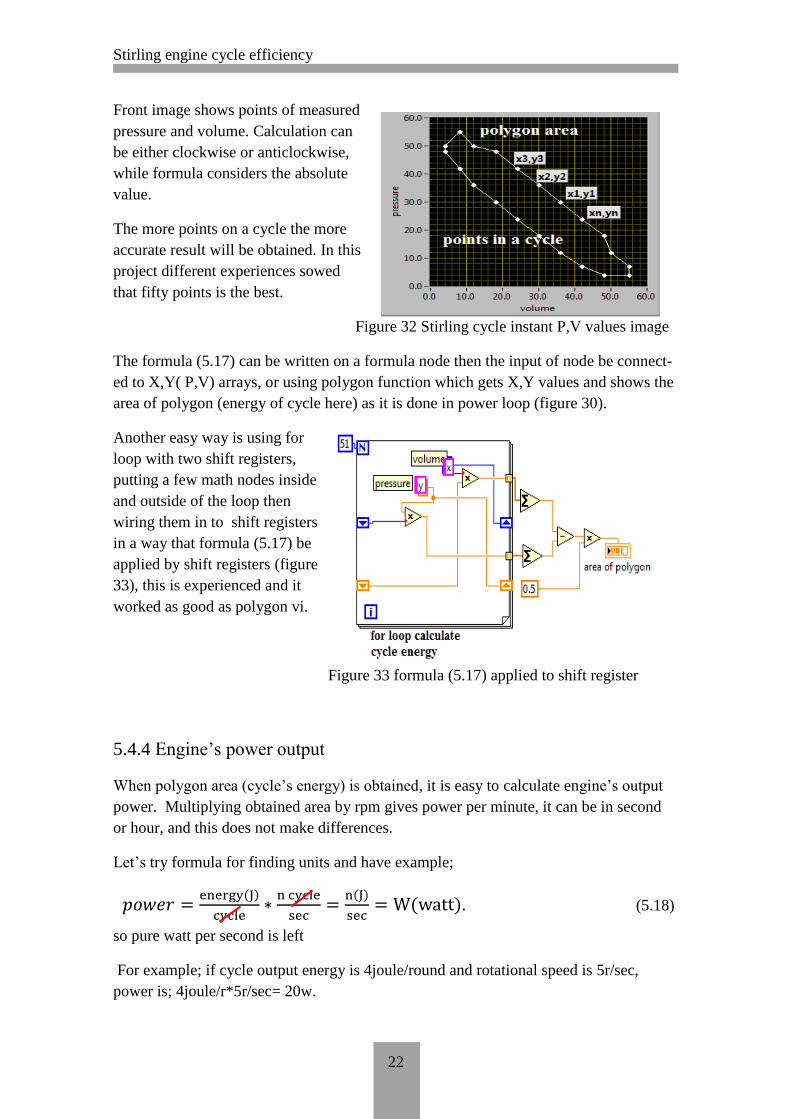
Front image shows points of measured
pressure and volume. Calculation can
be either clockwise or anticlockwise,
while formula considers the absolute
value.
The more points on a cycle the more
accurate result will be obtained. In this
project different experiences sowed
that fifty points is the best.
Figure 32 Stirling cycle instant P,V values image
The formula (5.17) can be written on a formula node then the input of node be connect-
ed to X,Y( P,V) arrays, or using polygon function which gets X,Y values and shows the
area of polygon (energy of cycle here) as it is done in power loop (figure 30).
Another easy way is using for
loop with two shift registers,
putting a few math nodes inside
and outside of the loop then
wiring them in to shift registers
in a way that formula (5.17) be
applied by shift registers (figure
33), this is experienced and it
worked as good as polygon vi.
Figure 33 formula (5.17) applied to shift register
5.4.4 Engine’s power output
When polygon area (cycle’s energy) is obtained, it is easy to calculate engine’s output
power. Multiplying obtained area by rpm gives power per minute, it can be in second
or hour, and this does not make differences.
Let’s try formula for finding units and have example;
. (5.18)
so pure watt per second is left
For example; if cycle output energy is 4joule/round and rotational speed is 5r/sec,
power is; 4joule/r*5r/sec= 20w.

Stirling engine cycle efficiency
23
5.4.5 Engine’s input power
Input power is the power that consumed by heating resistor inside cylinder to provide
heat to hot side of engine. While load is resistive and resistance value of heating ele-
ment is known R=1.2Ω, instant terminal voltage of element also is known to the pro-
gram by AI4, so that input power is calculated by formula (5.21) in power loop.
Power can be calculated directly from formulas for a resistive load;
(5.19)
or;
(5.20)
It is Known that R=V/I, I=V/R, by substituting these fractions in the formula instead of
voltage and current of load gives;
. (5.21)
Where;
P= Power consumed by resistive load (w)
V= terminal voltage of load (v)
I= current of load (A)
R= resistance of load (Ω)
The power is calculate by formula (5.21) because current unknown to the program.
5.4.6 Efficiency of Stirling cycle
Efficiency of Stirling cycle is obtained by formula (2.7) dividing cycle power by input
power. Another efficiency can be calculated here which obtained from dividing genera-
tor power by input power of engine. Let’s name it system efficiency as this is an indi-
vidual station. The iteration time of loop is one second, it means data will be updated
after a second. As it is mentioned already many unnecessary types of data is built espe-
cially in this loop and their indicators are put in hidden option, these data are for the
purpose of maintenance and debugging.
5.5 Feeding loop
Main job of this loop (figure 35) is providing control voltage to feeding transformer.
The output voltage of transformer (engine heating voltage) can be varied from 0to 30v,
it can be controlled either manually or by software. When it is connected to a computer,
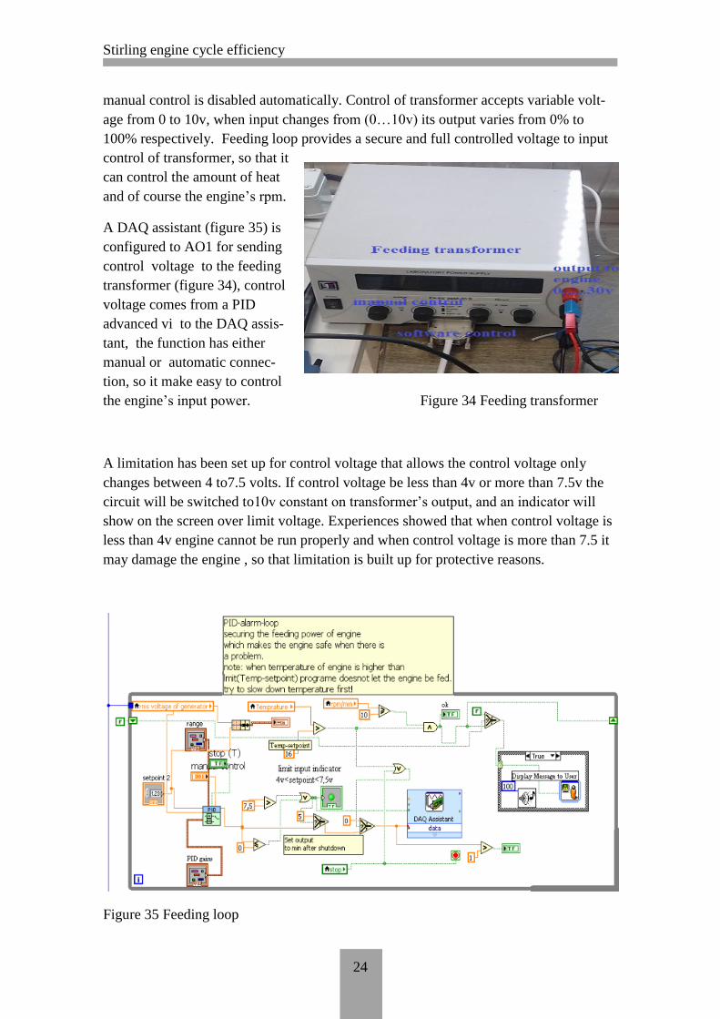
Stirling engine cycle efficiency
24
manual control is disabled automatically. Control of transformer accepts variable volt-
age from 0 to 10v, when input changes from (0…10v) its output varies from 0% to
100% respectively. Feeding loop provides a secure and full controlled voltage to input
control of transformer, so that it
can control the amount of heat
and of course the engine’s rpm.
A DAQ assistant (figure 35) is
configured to AO1 for sending
control voltage to the feeding
transformer (figure 34), control
voltage comes from a PID
advanced vi to the DAQ assis-
tant, the function has either
manual or automatic connec-
tion, so it make easy to control
the engine’s input power. Figure 34 Feeding transformer
A limitation has been set up for control voltage that allows the control voltage only
changes between 4 to7.5 volts. If control voltage be less than 4v or more than 7.5v the
circuit will be switched to10v constant on transformer’s output, and an indicator will
show on the screen over limit voltage. Experiences showed that when control voltage is
less than 4v engine cannot be run properly and when control voltage is more than 7.5 it
may damage the engine , so that limitation is built up for protective reasons.
Figure 35 Feeding loop
Stirling engine cycle efficiency
25
Most of logic nodes are added to this loop for making the station more secure and re-
moving observed possible troubles during this study.
For example if cooling temperature increased over its set point, loop stops DAQ assis-
tant, sets output to zero, sends warning message on control panel by case structure loop
(figure 35), sends a signal to writing data loop for publishing the most recent cycles data
history to an excel file or other directed document and stops writing data when rpm is
less than 10 rounds per minute.
Another important point in this part is that feeding transformer remembers the last input
so if the stop button is pressed and program is stopped but feeding voltage will be on
until the input is changed to zero. This problem damages engine components after few
minutes, thus the problem is solved by adding nodes and programming it in a way that if
program is going to stop for any reason it set the output to zero before stopping.
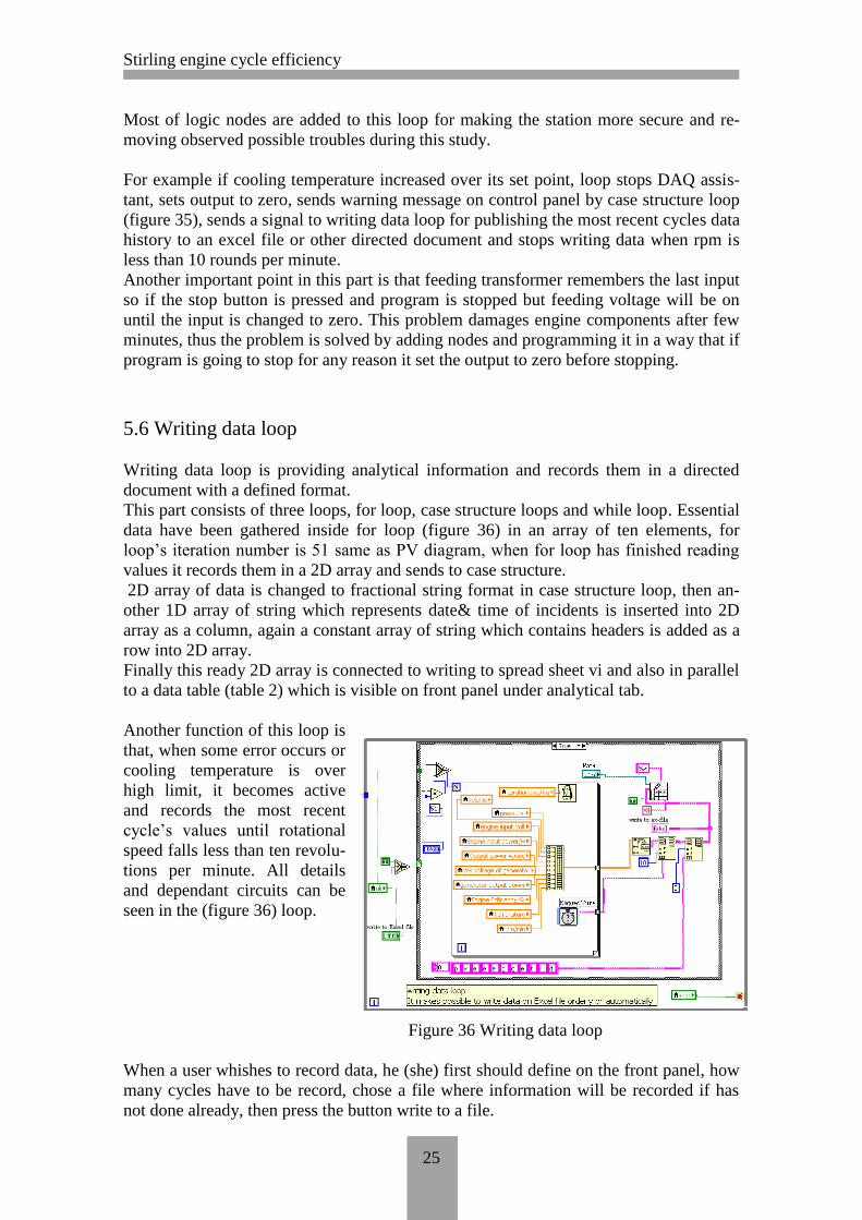
5.6 Writing data loop
Writing data loop is providing analytical information and records them in a directed
document with a defined format.
This part consists of three loops, for loop, case structure loops and while loop. Essential
data have been gathered inside for loop (figure 36) in an array of ten elements, for
loop’s iteration number is 51 same as PV diagram, when for loop has finished reading
values it records them in a 2D array and sends to case structure.
2D array of data is changed to fractional string format in case structure loop, then an-
other 1D array of string which represents date& time of incidents is inserted into 2D
array as a column, again a constant array of string which contains headers is added as a
row into 2D array.
Finally this ready 2D array is connected to writing to spread sheet vi and also in parallel
to a data table (table 2) which is visible on front panel under analytical tab.
Another function of this loop is
that, when some error occurs or
cooling temperature is over
high limit, it becomes active
and records the most recent
cycle’s values until rotational
speed falls less than ten revolu-
tions per minute. All details
and dependant circuits can be
seen in the (figure 36) loop.
Figure 36 Writing data loop
When a user whishes to record data, he (she) first should define on the front panel, how
many cycles have to be record, chose a file where information will be recorded if has
not done already, then press the button write to a file.
Stirling engine cycle efficiency
26
when user open the file he(she) can see all desired information in a neat understandable
format with exact date of occurrence for each iteration. This is a great help for analyz-
ing and diagnostic purposes in a system.
Table 2 Data table includes variables’ name, values, date and time
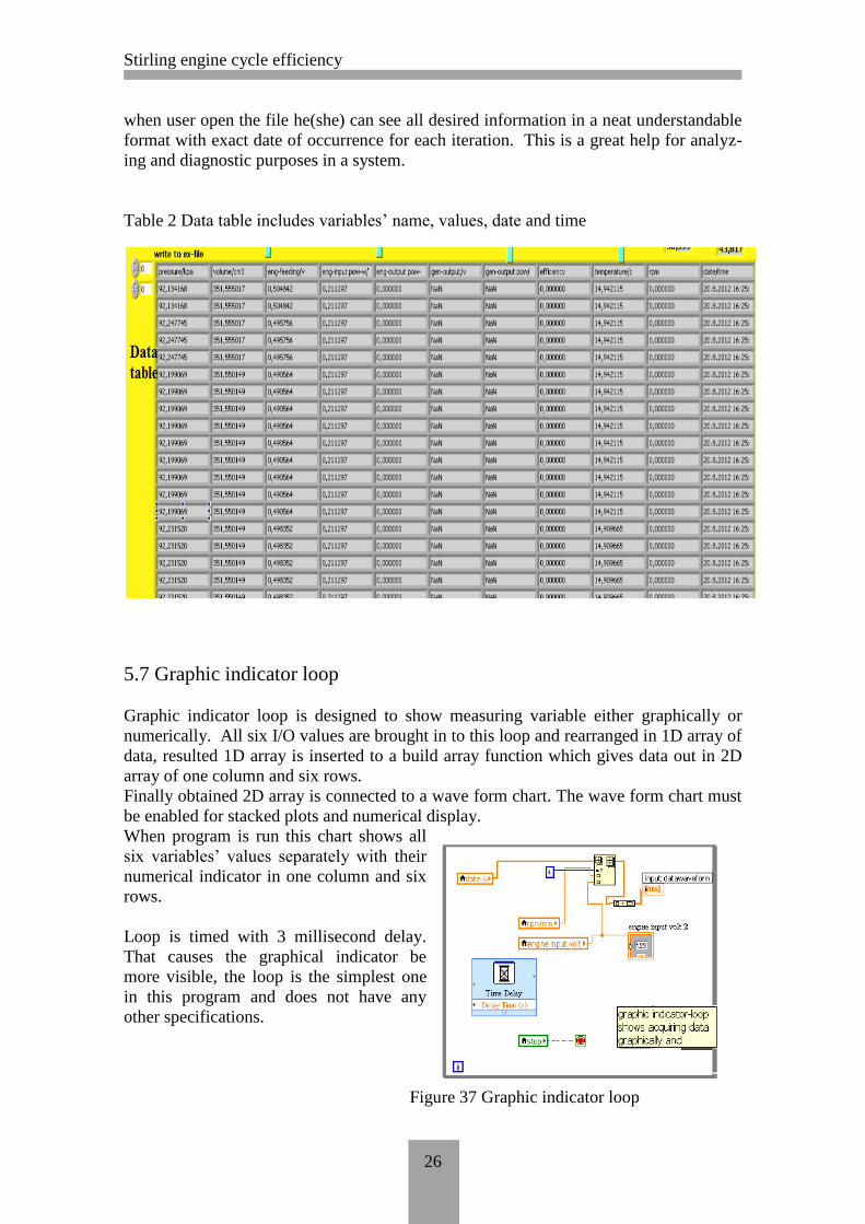
5.7 Graphic indicator loop
Graphic indicator loop is designed to show measuring variable either graphically or
numerically. All six I/O values are brought in to this loop and rearranged in 1D array of
data, resulted 1D array is inserted to a build array function which gives data out in 2D
array of one column and six rows.
Finally obtained 2D array is connected to a wave form chart. The wave form chart must
be enabled for stacked plots and numerical display.
When program is run this chart shows all
six variables’ values separately with their
numerical indicator in one column and six
rows.
Loop is timed with 3 millisecond delay.
That causes the graphical indicator be
more visible, the loop is the simplest one
in this program and does not have any
other specifications.
Figure 37 Graphic indicator loop
Stirling engine cycle efficiency
27
6 RUNNING PROGRAM AND FINAL TEST
When software programming is completed and all possible faults are checked and re-
moved then program is run. The results were about what is expected from theoretical
point of view. This is not obtained in the first run for sure, many pre-tests have been
conducted and corrections have been carried out as much as was needed.
Basically a loop was tested independently when codes were written on it as much as
possible and again it was tested when the loop was bundling to other loops, so that pro-
gram’s debugging has been done in advance step by step.
Doing more tests more defects revealed and improvements took place till result fulfilled
the goal of project.
Final test did not raise unexpected problems. Some decoration have been done on user
interface to give it more visibility and friendly appearance, also changes happened in
calculation methods to make them more understandable.
Two separate tests carried out idle test and load test. Each test consists of ten times re-
cording data at different range of power, recorded result graphed and monitored by ex-
cel. Explanation comes in following.
6.1 Idle test
The Idle test is done in eight different ranges of power. Results showed cycle efficiency
of this beta type of Stirling engine in the best stable conditions is about 19% ±2%. This
result has been carried out through a series of tests with different feeding power and
rotational speeds (rpm). The rpm is proportional to feeding power, any increase or de-
crease in power affects rpm directly.
The test showed that efficiency stands almost constant between 175 to 310rpm. But
when rotational speed is less than 175rpm or more than 310rpm efficiency begin to de-
cline, results are shown in (table 3) and an excel graph (figure 38). Each row (range) of
values was observing for five minutes, after being sure there are no interferences on
engine’s working from previous range of power, and then data has been written down.
Stirling engine has large dead time. Thus if set point is changed process variable does
not follow it instantly, always it fluctuates many times before being stable, so that it
takes plenty of time to complete a series of reliable tests. The engine has high reliability
at constant continuous working but cannot be controlled fast enough. This is the main
disadvantage of Stirling engine while controlling is the first priority in any application
where an engine should be chosen.

Stirling engine cycle efficiency
28
Table3 Data table of idle tests
Note: x axis steps do not
have same length.
Figure 38 Excel graph of efficiency at idle test
Observing above experiences proved that this type of Stirling engine has good perform-
ances when it is running at 175 to 318 rpm. Best suggested rpm rate for idle running is
210 rpm, considering the mechanical wear and tear of this type engine.
6.2 Load test
Load test is done by plugging two small bulbs in to output of generator (table4). Two
kinds of efficiency is considered, cycle efficiency and system efficiency. Cycle effi-
ciency is obtained same as idle test, but system efficiency is calculated from active
power of generator divided by engine’s heating power. Loads are two small bulbs
which are specified as 12v, 2w and 6Ω and are connected in parallel to generator. Ten
different ranges of power are used during test.
Provided power is calculated from formula (5.19);
No input power/w output power/w speed RV/min efficiency%
1 152.6 26.8 336 17.56
2 122.77 25.05 318 20.04
3 95.225 19.03 252 19.98
4 77.8 15.8 210 20.30
5 61.77 12.7 174 20.56
6 60.77 11.2 156 18.43
7 56.7 9.3 132 16.40
8 51.17 8.1 114 15.82

Stirling engine cycle efficiency
29
P=VI.
Where;
P=max produced power
V= voltage connected to loads
I= max current of circuit or generator
It is a resistive circuit so no need extra calculations. Maximum power absorbed by load
circuit is 4 watt and maximum power of generator is experienced 4.1watt in idle test so
that 100% of produced power will be consumed by loads, generator cannot work load
less partly. The data table and it’s excel graph are shown below.
Table4 Load test data table of efficiency
Note: x axis steps
do not have same
length.
Figure 39 Excel graph of efficiency in load test
Looking at above graph one can understand that the best performance of engine at load
test is obtained at rates of 230 to 270rpm.
The efficiency is smoothly 16%±2% as results are shown in (figure 39). The experi-
ences are not far from their theoretical specifications and expectations.
No Input pow-
er/w
Output
power/w
Gen-
rams/v rpm
Engine efficien-
cy%
System efficien-
cy%
1 68.5 10.49 4.1 132 15.31% 2.96%
2 75.4 11.3 4.6 140 14.99% 2.84%
3 85.06 13.2 5 162 15.52% 2.63%
4 106.42 16.3 5.7 198 15.32% 2.24%
5 125.6 19.43 6.3 228 15.47% 2.00%
6 135.9 22.6 6.8 246 16.63% 1.92%
7 139 22.8 7 264 16.40% 1.90%
8 158 24.6 7.2 276 15.57% 1.70%
9 183 27.01 7.6 294 14.76% 1.51%
10 201.6 31 7.8 330 15.38% 1.39%

Stirling engine cycle efficiency
30
From system efficiency graph it is found out that system efficiency is too low, in all
experiences about 80% of cycle energy is remained useless. This happened because of
using very low power generator. The behavior of Stirling engine is in a way that it takes
time to get its nominal continuous power, if a more powerful generator is used it took at
least twenty minutes to be started up and loaded. Optimistically the above table and
graph say system efficiency is about 2% which is nothing compare to input power. The
highest system efficiency is recorded at lowest rpm.
7 ANALYZING AND STUDYING THE RESULTS
Recent experiences say the most sophisticated Stirling engines have efficiency rate
about 30 to 35%, depends on type of engine. This study gives the efficiency rate about
19%±2% for this beta type of Stirling engine, let’s examine the results with comparing
them to theoretical cycle model.
Looking at cycle graph one can recognizes that output energy or net work by a cycle is
equal to supplied heat Qs minus rejected heat Qr. Supplied heat occurs during expan-
sion from phase 3 to 4 and rejected heat is during compression phase from 1 to 2, so
work is equal to Qs-Qr.
Temperature is constant during both
compression and expansion phases,
volume is constant during 2 to 3 and 4
to 1 as it is seen in (figure 40) in the
front of text.
Figure 40 Stirling cycle heat transferring illustration
Process of Stirling engine takes place as comes in the following;
(a) The air is compressed isothermally from state 1 to 2 (TL to TH).
(b) The air at state-2 is passed into the regenerator from the top at a temperature T1. The
air passing through the regenerator matrix gets heated from TL to TH.
(c) The air at state-3 expands isothermally in the cylinder until it reaches state-4.
(d) The air coming at temperature TH (condition 4) enters into regenerator from the
bottom and gets cooled while passing through the regenerator matrix at constant volume
and it comes out at a temperature TL at condition 1, and the cycle is repeated.
(e) It can be shown that the heat absorbed by the air from the regenerator matrix during
the process 2-3 is equal to the heat given by the air to the regenerator matrix during the
process 4-1, and then the exchange of heat with external source will be only during the
isothermal processes. (Prof T Sundararajan Madras UT India.)

Stirling engine cycle efficiency
31
Now we can write, Net works done as;
W = Qs – QR. (7.22)
Where;
QS = Heat supplied during the isothermal process 3-4.
QR=Heat rejected during isothermal phase 1- 2.
For having real example and optimizing it more clearly a theoretical cycle graph is
adapted to measure values of a random cycle at idle test as shown in (figure 41). Total
changes in volume and pressure
can be mentioned while total vol-
ume and pressure are known.
The following values are observed
from a random cycle and matched
to theoretical cycle as below;
V1=V4=351.53cm^3
V2=V3=200cm^3
P1=87.32kpa
P3=204.65kpa
Figure 41 Cycle adapted to random measured data
So from following formulas the net work can be calculated as;
(7.23)
(7.24)
When ,
W net=Qs-QR=
so; (7.25)
W net=
. (7.26)
Where; W= net work output by a cycle
P3= pressure at state 3
P1= pressure at state 1
V1=volume at state 1
V3=volume at state 3
All elements of equation are known from a cycle recorded by program let see;
W=

Stirling engine cycle efficiency
32
For estimating the average power during idle test, obtained rpm’s is averaged
(211.5rpm) from table (3) and multiplied by net work from the equation. Thus it is
enough to multiply cycle energy by rotational speed per second to fine the power of
engine, so;
.
The result makes a real sense between theoretical approach and experimental idle test
for this engine, let’s calculate cycle energy of a monitored rpm (252) in idle test table
and compare results;
.
Again the result proves that theoretical thermodynamic principles support the experi-
mental achievements in this study.
This type of Stirling engine uses a heat regenerator so that it is possible to use Carnot
efficiency formula for calculating its efficiency.
Carnot formula;
.
Where TL and TH are cool side and hot side temperature of engine, these values for
this engine has been defined at nominal power by the manufacturer; TL=345K,
TH=450K.
From given data and Carnot formula;
The following formula also can be used for calculating net work and then efficiency
when ∆volume, TL and TH are known.
(7.27)
(7.28)
So that work=
. (7.29)
V1=V4, V2=V3, so;
(7.30)
Where new parameters are;
n=Molar quantity of gas inside cylinder (mol)
R=Gas universal constant (8.314)

Stirling engine cycle efficiency
33
TH =Hot side temperature (K)
TL=Cool side temperature (K)
The only unknown of equation is molar quantity of gas (n). The (n) quantity can be
calculated through the constant molar volume of ideal gas law (22.414l/mol). Because
cylinder pressure at max volume is equal to atmospheric level. There is no extra pres-
sure inside cylinder, only atmospheric pressure (air) is compressed during phases 2-3.
Therefore according to Ideal gas law one mole of any gas occupies 22.14 liters at STP
(standard temperature and pressure), here the gas is air and volume is 351.53cm^3
which is equal to 0.35153 liter, so n mole quantity cab be obtained by;
Trying the above formula (7.30) gives theoretical maximum energy of a cycle about
7.6J which is not too far from obtained random idle test 5.7J, considering LTP (local
temperature and pressure) conditions. With above tried theoretical formulas one can be
assured that obtained result by the program is acceptable and enough close for proving
its theoretical aspects. (G. Deacon, C. Coulding, Physics education 180-200 (1994))
8 CHALLENGES AND PROBLEMS SOLVING
Serious challenges have been met in both hardware and software parts. Firstly making a
power supply seemed simple, but in practice raised too much problem when all compo-
nents were powered from 30VDC output by different voltage dividers.
Despite of producing very smooth pure Dc voltage it modulated some noises in the cir-
cuit in a way that PV diagram could not be monitored by program, just showed some
confusing points. Too much time is spent on debugging and recalibrating which had no
effect on the results. Ultimately it was solved by powering each sensor from separate
voltage output using voltage regulator IC AN7805, and adding two extra capacitors to
out puts.
Another serious challenge was making a physical ring or let say pulley to transfer the
piston’s displacement scale which is 51mm to position meter displacement scale 32mm.
Attempts were succeeded at last by making a pulley with two grooves and different di-
ameters, so that it can transfer full displacement of piston to position meter.
Hard work was centralizing the smaller groove on top of bigger one, where pulley turns
only 230 degree and backs again cyclically respectively to the piston down up move-
ment. However it is done and worked.
Software troubles were most confusing parts since LABVIEW is a huge program with
numerous functions. It becomes worse when the computer is not compatible with soft-
ware and its DAQ card and components, as it was in this study. For example; moving a
node or a vi function constitutionally and correctly inside a loop caused high disturb-
ances to the program which led to reprogram it from stretch.
Studying then experiencing step by step gave the ability to come them all over and un-
derstanding how to tackle with such a time killer problems. Many programs was written
and removed just for experiencing behavior of nodes and loops. There are tips and tricks
that cannot be experienced theoretically, one have to do something for learning them
especially in making user interface.

Stirling engine cycle efficiency
34
Lack of internet connection to station’s computer was another problem that always hin-
dered process of study. It took a lot of times to go to computer class and searching
something then trying it at laboratory and back again and again if not succeeded.
9 CONCLUSIONS
Using labview software to calculate the efficiency of a beta type of the Stirling engine
was quite useful for touching again the theoretical and practical lessons of engineering
physics. The obtained results met planned goals fully and supported the theoretical ex-
aminations of the Stirling cycle and its PV graph illustration. The highest efficiency was
about 19%±2% with the idle and 16%±2% with the load test, the best range of rpm was
210-240 taking into consideration the efficiency and mechanical wear and tear for this
type of the engine
Comparisons with different tests and data monitored the efficiency of a beta type of the
Stirling engine very closely. The temperature difference (∆T= ) between hot side
and coolside has a significant effect on the output power and efficiency, in a few
observations it seemed that efficiency was proportional to ∆T, the highest temperature
difference ∆T causing the highest efficiency.
Experience showed that if the cooling water tab to the engine is closed when the engine
is running, after a short time the efficiency decreased by 50% and the pressure also
dropped which was normal. But when cooling tab was opened fully again the engine
reacted instantly and backed to its nominal speed. This means that the engine’s response
to ∆T is faster than to the input power and a heating element.
When input power was increased or decreased the engine speed remained constant for a
moment, then followed the set point and crossed it, then fluctuated till it stabilized
around the set point. There was no fluctuating when ∆T was changed. The engine has
high dead time compared to an internal combustion engine, because the heat element
cannot lose or gain heat instantly.
It came to my mind if it were possible to change the TC fast enough technically, the
speed could be controlled desirably by a combination of changes in the input power and
the TC, since control problem is the highest disadvantage of a Stirling engine.
The Stirling engine is mostly suitable for laboratory work and research, the engine has
a high performance in constant continuous operation, thus it has been applied to pro-
duce a large scale of solar electricity in a few locations in the United State up to 1.5GW.
Using software to monitor data on the user interface panel is of great help. It enables the
operator to have a full control on the process plant. But a designer has to know the be-
havior of each signal or variable, and consider them when he /she is going to acquire
analog or digital form of data. Noise or incompatibility between software and hardware
can cause numerous problems and errors in the results.
One should check firstly the compatibility and synchronization between the system’s
components, secondly split the program in to smaller parts and carry out possible manu-
al tests and calibrations, thirdly to improve and finalize the program.

Stirling engine cycle efficiency
35
REFERENCES Measurements and automation tools. Accessed 01.05-12.06.2012
https://moodle2.hamk.fi/course/view.php?id=5396
Robert Stirling Engine. Accessed 01-30.06.2012
http://www.robertstirlingengine.com/principles.php
Hyperphysics& Thermodynamics. Accessed 15.07.2012
http://hyperphysics.phy-astr.gsu.edu/hbase/hframe.html
Stiling online library. Accessed 18.07.2012
http://library.thinkquest.org/C006011/english/sites/stirling.php3?v=2
Stirling engine workshop. Accessed 21.07.2010
//arpa/Portals/0/Documents/ConferencesAndEvents/PastWorkshops/Stirling%20En
gine_readout.pdf
http://newenergydirection.com/blog/2009/06/stirling-engine-efficiency/
Stirling engine cycle efficiency calculation. Accessed 01 -30.07.2012
http://outreach.phas.ubc.ca/phys420/p420_08/Hiroko%20Nakahara/pdfs/StirlingEngine
Proposal.pdf
Buffalo education faculty of physics engineering. Accessed 25.07.2012
http://www.ee.buffalo.edu/faculty/paololiu/edtech/roaldi/tutorials/labview.htm
Stirling engine
Practical types of Stirling engine. Accessed 30.07.2012
http://www.youtube.com/watch?v=BDfe1QYJC04
Stirling engine principles and calculations. Accessed 05.07.2012
http://www.sesusa.org/StirlingPrimer.htm
Lab view online tutorial. Accessed 01.5-30.08.2012
http://www.ni.com/
Stirling engine cycle efficiency
36
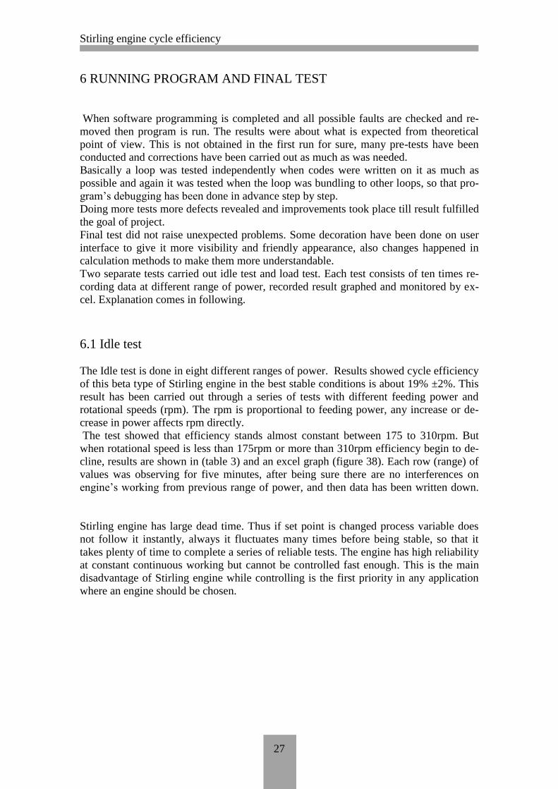
Appendix 1
USER INTERFACE (USER TAB)
Image1: User interface tab (front panel)
Note: Images can be zoomed to be more visible

Stirling engine cycle efficiency
37
Appendix2
USER INTERFACE (ANALYTICAL TAB)

Stirling engine cycle efficiency
38
Appendix3
BLOCK DIAGRAM: RPM LOOP, DATA LOOP.

Stirling engine cycle efficiency
39
Appendix4
BLOCK DIAGRAM: PV DIAGRAM AND POWER LOOPS.

Stirling engine cycle efficiency
40
Appendix5
BLOCK DIAGRAM: FEEDING LOO, WRITING DATA TO A FILE, AND
GRAPHIC LOOPS.
Stirling engine cycle efficiency
41
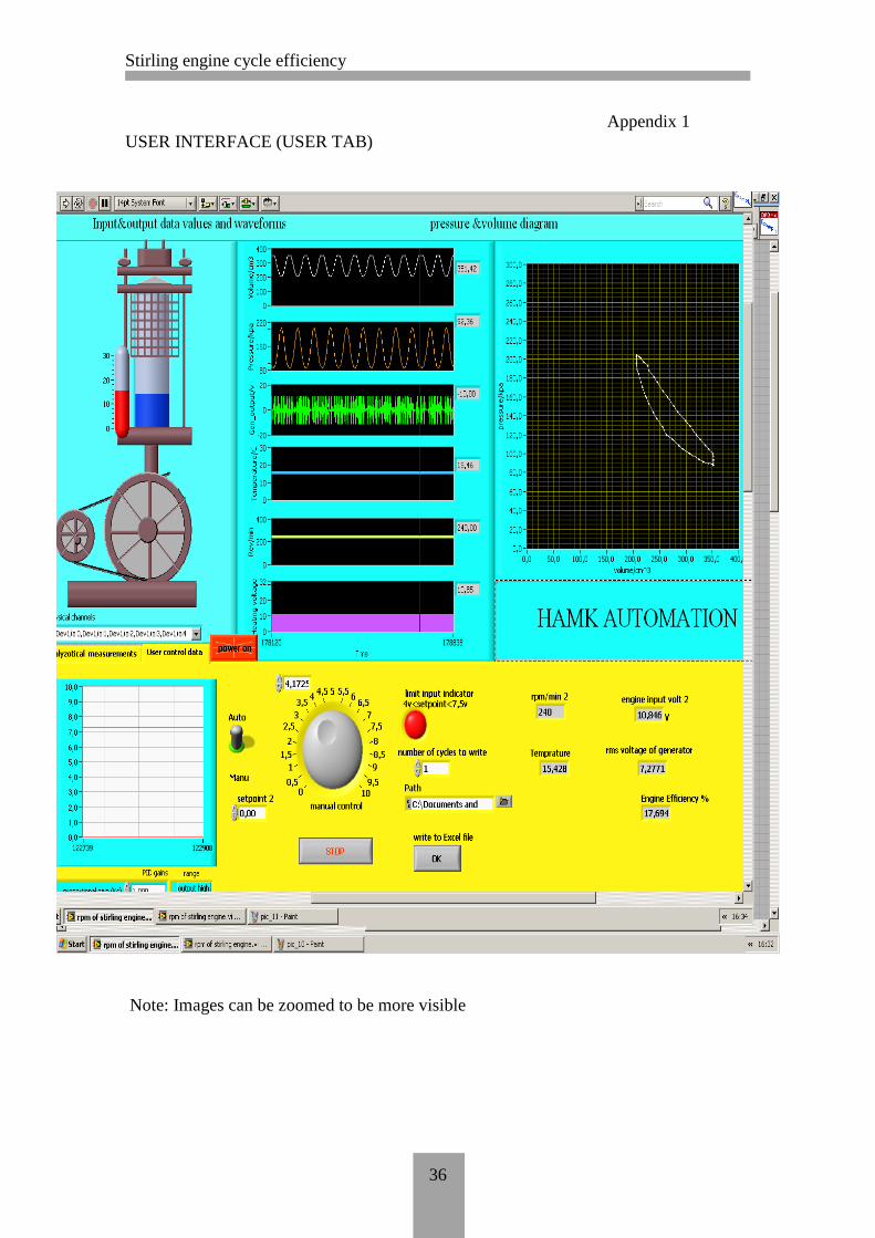
Appendix6
THE WHOLE BLOCK DIAGRAM
Stirling engine cycle efficiency
42
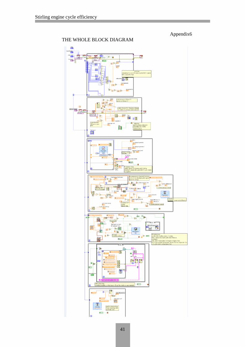
Appendix7
POWER SUPPLY, ELECTRICAL WIRING AND CONNECTION CIRCUIT
Stirling engine cycle efficiency
43
Appendix8
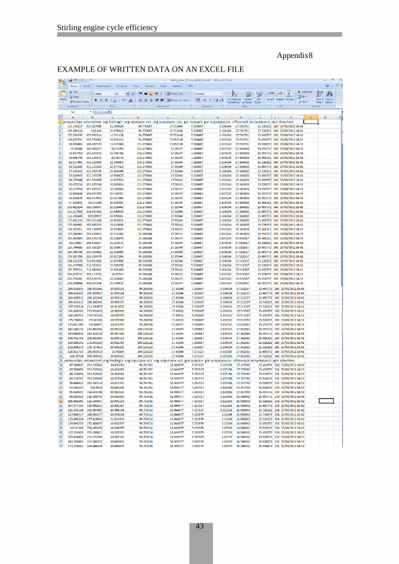
EXAMPLE OF WRITTEN DATA ON AN EXCEL FILE
Stirling engine cycle efficiency
44
Appendix9
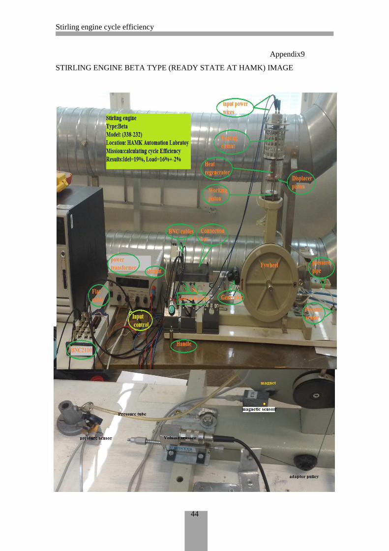
STIRLING ENGINE BETA TYPE (READY STATE AT HAMK) IMAGE