Embed Size (px)
Citation preview
Axiomatic Foundations for Satisficing Behavior∗
Christopher J. TysonNuffield College, Oxford OX1 1NF, [email protected]
January 6, 2005
Abstract
A theory of decision making is proposed that supplies an axiomatic basis for theconcept of “satisficing” postulated by Herbert Simon. After a detailed review ofclassical results that characterize several varieties of preference-maximizing choicebehavior, the axiomatization proceeds by weakening the inter-menu contractionconsistency condition involved in these characterizations. This exercise is shown tobe logically equivalent to dropping the usual cognitive assumption that the decisionmaker fully perceives his preferences among available alternatives, and requiringinstead merely that his ability to perceive a given preference be weakly decreasingwith respect to the relative complexity (indicated by set inclusion) of the choiceproblem at hand. A version of Simon’s hypothesis then emerges when the notion of“perceived preference” is endowed with sufficiently strong ordering properties, andthe axiomatization leads as well to a constraint on the form of satisficing that thedecision maker may legitimately employ.
JEL classification codes: D01, D71, D81.
Keywords: choice function, cognition, revealed preference, threshold.
1. INTRODUCTION
Many writers have felt that the assumption of rationality, in the sense of a one-dimensionalordering of all possible alternatives, is absolutely necessary for economic theorizing. . . . Thereseems to be no logical necessity for this viewpoint; we could just as well build up our economictheory on other assumptions as to the structure of choice functions if the facts seemed to callfor it.
—— kenneth j. arrow (1951).
Half a century ago, Herbert Simon published the first [32] of several early articleschallenging the models of decision making then and now dominant in economic analysis.“[T]he task,” he wrote [p. 99], “is to replace the global rationality of economic man witha kind of rational behavior that is compatible with the access to information and thecomputational capacities that are actually possessed by organisms, including man, in
∗This paper contains material from Chapters 2–3 of the author’s PhD thesis [38].
1
the kinds of environments in which such organisms exist.” In Simon’s view, cognitiveand information-processing constraints on the capabilities of economic agents, togetherwith the complexity of their environment (see [33]), render optimal decision making anunattainable ideal. Rather than attempting a summary of the full argument — spreadover his sixty-odd years of work in the behavioral and cognitive sciences — we refer theinterested reader to [34] and [35], as well as to the three volumes [36] of Simon’s collectedwritings on the subject.
Optimal decision making is ordinarily implemented in economic models by means ofthe maximizing criterion
f(x) = max f [A], (1)
which requires the chosen alternative x to achieve a utility (returned by the function f) noless than the maximum obtainable from the menu A of available options. After offeringa terse review of the basic tools of axiomatic choice theory, Section 2 establishes versionsof the classical results on preference-based choice (namely, Theorems 1–4) that provide abehavioral foundation for this criterion. While the exposition of these results may havesome intrinsic value as a synthesis of widely scattered contributions, the primary purposeof this section is to build up the classical theory in a manner adaptable to the constructionof the alternative theory to follow.
Having dismissed the idea that human decision makers exhibit “global rationality,”Simon suggests that they in fact engage in “satisficing”1 — defined in [36, v. 3, p. 295]as “choos[ing] an alternative that meets or exceeds specified criteria, but that is notguaranteed to be either unique or in any sense the best.” Formulating this hypothesis inutility space leads naturally to the satisficing criterion
f(x) = θ(A), (2)
in which the threshold utility θ(A) for acceptability of an alternative can take on anyvalue less than or equal to the maximum in Equation 1. As this phrasing makes clear,maximizing is then a special case of satisficing, and it follows that any choice-theoreticbasis for the latter will be logically weaker than the classical basis for the former.
Our objective, therefore, is to develop an axiomatic foundation for satisficing behaviorby diluting the conditions that underpin utility maximization. This task is carried out inSection 3, where Simon’s cognitive and information-processing constraints are imaginedto prevent the decision maker from fully perceiving his (strict) preferences among theavailable alternatives.2 Under the maintained “nestedness” assumption that a preferenceperceived in choice problem B is also perceived in each problem A ⊂ B in which it isrelevant, a formal analysis closely paralleling the classical theory leads to a series of newresults (Theorems 5–7) that identify the restrictions on behavior implied by the impositionof different sets of ordering properties (such as acyclicity and transitivity) on the conceptof “perceived preference.” These results uncover a correspondence between failures ofperception and violations of the classical contraction consistency axiom, which statesthat acceptability of an alternative in choice problem B together with its availability inproblem A ⊂ B should imply its acceptability in A. And when sufficiently strong ordering
1Although Simon [36, v. 2, p. 415] identifies this word as Scottish in origin, the O.E.D. finds itsearliest recorded use in the Swiss theologian Henry Bullinger’s [7] comment — presumably about theRomans — That their founders were nourished by suckyng of a wolfe: so haue all that people woluesmindes, neuer satisfised with bloud, euer greedy of dominion and hungryng after riches. . . .
2Extensive discussion of the rationale for this response to Simon’s critique can be found in Chapter 1of [38].
2
f(w) = 0 f(x) = 1 f(y) = 2 f(z) = 3
[wxyz] 7−→ [xyz]
xPw & yPw & zPw
θ([wxyz]) = 1
[wxy] 7−→ [xy]
xPw & yPw
θ([wxy]) = 1
[wxz] 7−→ [z]
xPw & zPw & zPxθ([wxz]) = 3
[wyz] 7−→ [yz]
yPw & zPw
θ([wyz]) = 2
[xyz] 7−→ [z]
zPx & zPy
θ([xyz]) = 3
[wx] 7−→ [x]
xPwθ([wx]) = 1
[wy] 7−→ [y]
yPw
θ([wy]) = 2
[wz] 7−→ [z]
zPwθ([wz]) = 3
[xy] 7−→ [xy]
—
θ([xy]) = 1
[xz] 7−→ [z]
zPxθ([xz]) = 3
[yz] 7−→ [z]
zPy
θ([yz]) = 3
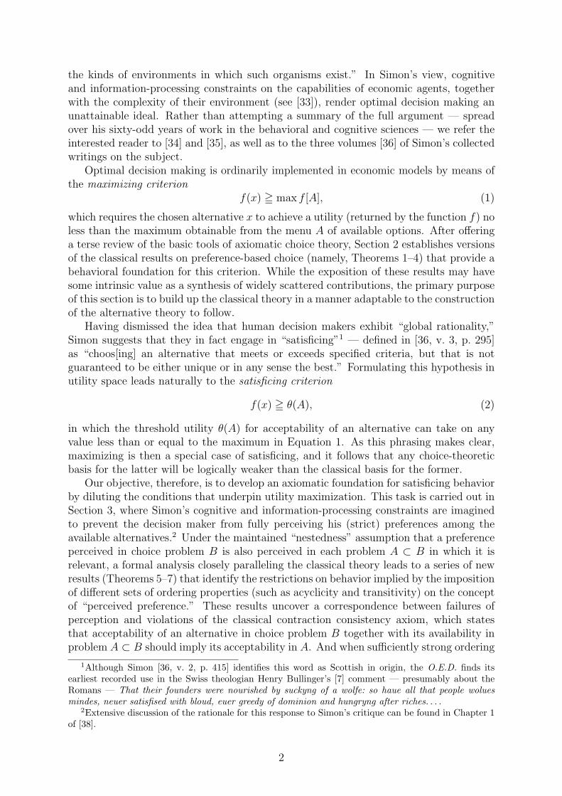
Figure 1: Choice behavior consistent with the satisficing criterion. A menu is a subsetof the space [wxyz]; the binary relation P indicates strict preference; the function fassigns utility values to alternatives; and the function θ assigns threshold utilities tomenus. Within the cells are displayed the mapping from menus to subsets of acceptablealternatives (e.g., [wxy] 7−→ [xy]), the preferences perceived in particular choice problems(e.g., xPw and yPw in problem [wxy]), and the values of θ (e.g., θ([wxy]) = 1).
properties are imposed on the preferences themselves (i.e., on the objects of perceptionor non-perception) through the requirement of acyclicity of the base relation revealed bybinary choice data, a series of modified results (Theorems 8–10) are obtained of whichthe last (Theorem 10) supplies the desired foundation for satisficing.
The main features of our theory are illustrated by the example depicted in Figure 1.Here one cell is allocated to each nontrivial choice problem drawn from the four-elementspace [wxyz] (note the multiplicative notation for enumerated sets), and the upper entryin each shows the subset of acceptable alternatives associated with the menu in ques-tion. The alternatives deemed acceptable are those that are maximal with respect to theperceived preferences shown in the middle entry in the cell (e.g., the perception of xPwmakes w unacceptable in problem [wxz]); or, alternatively, those with utility values nosmaller than the threshold shown in the lower entry (e.g., [v ∈ [wyz] : f(v) = 2] = [yz]).The system of perceived preferences satisfies the nestedness assumption (e.g., the pref-erence yPw perceived in problem [wxyz] is also perceived in problem [wxy] ⊂ [wxyz]).And the decision maker’s behavior violates contraction consistency (e.g., alternative x isdeemed acceptable in problem [wxyz] but not in problem [xyz] ⊂ [wxyz]).
It is in permitting the latter type of violation that our theory departs from classicalmodels of decision making, and the last of the above parenthetical examples thus meritscloser scrutiny. As noted, alternative x is deemed unacceptable in problem [xyz], a factattributable to the preference zPx being perceived in this context. Classical assumptionswould then require that this preference be perceived, and hence that x be deemed un-acceptable, in problem [wxyz] as well. But neither of these requirements follows fromour nestedness assumption (since [wxyz] 6⊂ [xyz]), one which therefore does not implycontraction consistency of the decision maker’s behavior.
3
The purpose of this paper is to demonstrate the relationships among the three differenttypes of constructs illustrated in Figure 1. Specifically, we determine the restrictions onbehavior that characterize maximization of a nested system of perceived preferences —our model of decision making under cognitive and information-processing constraints — aswell as the further restrictions needed for consistency with the satisficing criterion. Thus,in addition to providing a choice-theoretic axiomatization of Herbert Simon’s hypothesis,our analysis also offers a cognitive interpretation of it; an answer to “the crucial questionof why people have the aspiration or satisfaction levels they have” (posed by Elster [9,pp. 26–27] as a challenge to satisficing theory).
This enterprise follows in the long tradition of axiomatic weakenings of the standardeconomic model of decision making delineated by Savage [23, Chapters 2–5]; a traditionexemplified by the contributions of Aumann [4] and Bewley [6] removing the completenessaxiom (part of P1 in [23, p. 18]), by that of Machina and Schmeidler [19] abandoningthe Sure-Thing Principle (P2 in [23, p. 23]), and by those of Schmeidler [24] and Gilboaand Schmeidler [11] effectively doing away with various comparative probability axioms(including P4 in [23, p. 31] and P4* in [19, p. 761]). Like Kreps [17], who considers agentsexhibiting a “preference for flexibility,” we suppress the usual state-space formulation ofuncertainty and focus attention on one of Savage’s implicit assumptions; namely, thatthe decision maker’s behavior is maximal with respect to a fixed preference relation andtherefore satisfies contraction consistency.
A number of more recent papers also relate to one or another aspect of this essay.Baigent and Gaertner [5] characterize a form of “polite” decision making that bears someresemblance to satisficing. Kalai et al. [16] allow for menu-dependence of the preferencerelation (which can then incorporate “multiple rationales”), focusing on the question ofhow much of this variation is needed to rationalize a given pattern of behavior. Guland Pesendorfer [12] consider a decision maker who, as a result of temptation ratherthan of constraints on cognition, may suffer from the provision of extra alternatives.Sheshinski [31] (following Mirrlees [20]) investigates the implications for public policyof choice behavior that fails to reliably maximize the agent’s welfare. And Iyengar andLepper [14] (among others) examine the psychological effects of decision complexity.
2. CLASSICAL CHOICE THEORY
2.1. Choice functions
At a high level of abstraction, axiomatic choice theory expresses the decision makingenvironment as a pair 〈X, A〉, where X denotes an arbitrary nonempty set and A acollection of subsets of X. In this choice space formulation, a set A ∈ A is a menu ofmutually-exclusive alternatives, A itself a list of the choice problems (menus) of interest,and X a full catalog of the alternatives potentially available. The mathematical primitiveof the theory is then a choice function C : A → 2X associating with each A ∈ A a so-called choice set C(A) properly interpreted as the set of alternatives whose selection fromthis menu cannot be ruled out by the theorist.
Under the suggested interpretation, two conditions on C are unobjectionable enoughto be considered part of the definition of a choice function.
Postulate 1 (Availability) C(A) ⊂ A.
Postulate 2 (Decisiveness) A 6= ∅ =⇒ |C(A)| = 1.
4
A third condition has rather more content, requiring the specification of a choice set foreach subset of the catalog X, but will also be taken to hold tacitly throughout.
Postulate 3 (Universality) A = 2X .3
2.2. Binary relations and orderings
We next review some elementary definitions and facts about binary relations, which playa central role in axiomatic choice theory.
A (binary) relation on the set X is a subset of X × X. For example, the equalityrelation is E = [〈x, y〉 : x = y]. We write xRy for 〈x, y〉 ∈ R, the statement “x bearsthe relation R to y.” Given a relation R, we can define its converse R′ = [〈x, y〉 : yRx],complement R = [〈x, y〉 : ¬(xRy)], and symmetric residue R◦ = R ∩ R′. Given a secondrelation Q, the composition of Q with R is QR = [〈x, z〉 : (∃y) xQy & yRz]. The nthpower of R is then defined inductively via Rn = RRn−1 (with R1 = R), and the associatedancestral relation is R∗ =
⋃∞n=1 Rn.
Table 1 lists ten properties that a binary relation may or may not exhibit, whileTable 2 records certain (easily verifiable) logical relationships among them. Inspectionof the second table reveals two families of properties, each with a hierarchical structure.From weakest to strongest, irreflexivity, asymmetry, and acyclicity are antireflexivityproperties; each forbidding elements of X from standing in some relation (R, R2, and R∗,respectively) to themselves. And similarly, residual, cross, and negative transitivity are(for want of a better name) extratransitivity properties; each requiring a product of tworelations to be included in a third.
Table 3 lists five classes of binary relations together with their defining properties.In light of the implications shown in Table 2, we see that the four classes of orderingslisted also have a hierarchical relationship: A proto order is a relation exhibiting theantireflexivity properties, a partial order is a proto order exhibiting transitivity, a weakorder is a partial order exhibiting the extratransitivity properties, and a linear order is aweak order exhibiting weak connectedness. (The class of equivalences is of course logicallyindependent of these four classes of orderings.)
2.3. Revealed preference relations
Let us write P for the binary relation on X that encodes our decision maker’s strictpreferences among the alternatives, so that the preference-maximal members of a givenmenu A are contained in the set P↑ (A) =
[x ∈ A : (∀y ∈ A) yPx
]. The hypothesis that
the chosen alternative will be preference maximal then implies that C(A) ⊂ P↑(A), andwhen this inclusion holds for each A ∈ A we shall write C ⊂ P↑ and say that P suppliesan upper bound for the choice function. In the absence of any further hypotheses we havealso the analogous lower bound inclusions, indicated by P↑⊂ C, and hence the equalityC = P↑ . When the latter holds we shall say that P generates the choice function.
3Herzberger [13, p. 192] dubs this the property of “full extension,” and suggests that any theoryincompatible with it is inherently deficient.
[E]ssentially non-extended choice functions must be ones that satisfy certain rationality con-ditions solely by grace of “gaps” at critical points in their domain. Holding the rationalityconditions constant, these are gaps that cannot be filled. . . . [A] theory of rationality wouldbe better to safeguard itself against such gerrymandered satisfaction of its requirements.
Arrow [2] and Sen [27] have also defended Universality in the archetypical setting of consumer demandtheory.
5

reflexivity: E ⊂ R transitivity: R2 ⊂ Rirreflexivity: R ⊂ E residual transitivity: (R◦)2 ⊂ R◦
symmetry: R ⊂ R′ cross transitivity: RR◦ ∪ R◦R ⊂ Rasymmetry: R2 ⊂ E negative transitivity: R2 ⊂ R
acyclicity: R∗ ⊂ E weak connectedness: R◦ ⊂ E
Table 1: Properties of binary relations. Here R denotes an arbitrary relation, R′ itsconverse, R its complement, R◦ its symmetric residue, R∗ the associated ancestral relation,and E the equality relation.
antecedent properties consequent propertyasymmetry irreflexivityacyclicity asymmetryirreflexivity, transitivity acyclicityacyclicity, weak connectedness transitivityasymmetry, negative transitivity transitivitycross transitivity residual transitivityirreflexivity, weak connectedness residual transitivitynegative transitivity cross transitivitytransitivity, residual transitivity negative transitivity
Table 2: Logical relationships among properties. A relation exhibits the antecedentproperties only if it also exhibits the consequent property.
class of relations defining propertiesproto orders acyclicitypartial orders irreflexivity, transitivityweak orders asymmetry, negative transitivitylinear orders acyclicity, weak connectednessequivalences reflexivity, symmetry, transitivity
Table 3: Classes of binary relations. A relation belongs to a class if and only if it exhibitsthe indicated properties.
6
While this construction illustrates how a hypothesized preference relation can be usedto place restrictions on the choice function, it is also possible to take this function as givenand to construct from it notions of “revealed” preference. Of the many such notions thathave been proposed,4 we shall require only a few.
Definition 1 The global relation Pg is defined by xPgy if and only if for each menu Awith x ∈ A we have y /∈ C(A). The base relation Pb is defined by xPby if and only ify /∈ C([xy]). The separation relation Ps is defined by xPsy if and only if there existsa menu A such that both x ∈ C(A) and y ∈ A \ C(A).
Proposition 1 Pg ⊂ Pb ⊂ Ps. Pg is acyclic. Pb is asymmetric. Ps is irreflexive.
An alternative x bears the global relation to a second alternative y when we know thaty will be rejected in any choice problem in which x is available, while x bears the baserelation to y when we know simply that y will be rejected in a pairwise choice betweenthe two. Weaker still, x bears the separation relation to y when there exists some choiceproblem (not necessarily the pairwise choice) from which we can rule out y but not x.
The base relation has a certain salience as an indicator of preference, since the datumxPby indicates that y will be rejected and hence x chosen when no other alternativesare present to complicate matters. Moreover, the base relation alone would appear tobe sufficient for our purposes in this section in light of Arrow’s [3, p. 16] observationthat within the classical theory “the choice in any environment can be determined bya knowledge of the choices in two-element environments.” But in fact the base andglobal relations will turn out to coincide within the classical theory, and it will facilitatecomparison with later results if we now focus attention on Pg.
The following two conditions demarcate the class of choice functions generated bytheir respective global relations.
Condition 1 (Global Upper Bound) C ⊂ Pg ↑ .
Condition 2 (Global Lower Bound) Pg ↑⊂ C.
By the definition of Pg, the first of these is a tautology that places no restrictions on C.
Proposition 2 Global Upper Bound holds for any choice function.
Note also that Pg includes any other binary relation that supplies an upper bound for C.
Proposition 3 If C ⊂ R↑ , then R ⊂ Pg.
This implies that if a relation R generates the choice function, then Pg ↑⊂ R↑= C ⊂ Pg ↑and hence Pg does as well.
Proposition 4 A choice function is generated by a relation if and only if it is generatedby Pg.
And finally, combining Propositions 2 and 4 shows that Global Lower Bound is necessaryand sufficient for the choice function to be consistent with the preference maximizationhypothesis (a property known as [13, p. 203] “binariness” or [26, p. 309] “normality”of C).
Corollary 1 A choice function is generated by a relation if and only if it satisfies GlobalLower Bound.
4See, for example, the bestiary of revealed preference relations discussed in Herzberger [13].
7
2.4. Proto preference orders
In the present context, the antireflexivity properties are undoubtedly the most appealingamong those listed in Table 1. Indeed, for a relation encoding preference assessments,a violation of irreflexivity can only be described as nonsensical, one of asymmetry ascontradictory, and one of acyclicity as [13, p. 195] “extremely pathological.” These asser-tions are supported by the following result, which shows that the choice function cannotbe consistent with the preference maximization hypothesis unless the maximized relationexhibits all three of the antireflexivity properties.
Proposition 5 Any relation that supplies an upper bound for C is a proto order.5
This fact enables us to strengthen slightly the characterization in Corollary 1.
Proposition 6 A choice function is generated by a proto order if and only if it satisfiesGlobal Lower Bound.
Global Lower Bound can be cast in a more familiar form as the conjunction of twoconditions with long histories in axiomatic choice theory.
Condition 3 (Contraction) A ⊂ B =⇒ C(B) ∩ A ⊂ C(A).6
Condition 4 (Weak Expansion)⋂
k C(Ak) ⊂ C (⋃
k Ak).7
Proposition 7 Contraction and Weak Expansion together are logically equivalent toGlobal Lower Bound.
The first of these conditions requires that if an alternative x is in the choice set associatedwith a particular menu (i.e., B), then it must also be in the choice sets associated witha collection of “contracted” menus (i.e., each A satisfying x ∈ A ⊂ B). Conversely,the second condition requires that if x is in the choice sets associated with a collectionof menus (i.e., Ak for each k in some index set), then it must also be in the choice setassociated with a particular “expanded” menu (i.e.,
⋃k Ak). Since Global Lower Bound
amounts to a combination of these requirements, Proposition 6 can be rephrased as acharacterization of the proto order maximization hypothesis in terms of contraction andexpansion consistency.
Theorem 1 A choice function is generated by a proto order if and only if it satisfiesContraction and Weak Expansion.8
5Cf. Jamison and Lau’s [15, p. 903] Theorem 1.6This is Sen’s [25, p. 384] Property α, or [29, p. 500] “basic contraction consistency.” The condition
seems first to have appeared as Chernoff’s [8, p. 429] Postulate 4, although Nash [21, p. 159] employs aprecursor.
7This is Sen’s [26, p. 314] Property γ, or [29, p. 500] “basic expansion consistency.”8This is Sen’s [26, p. 314] T.9. Incidentally, the theorem answers a question posed by Kreps [18,
p. 15].
8
2.5. Partial preference orders
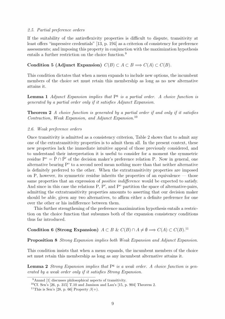
If the suitability of the antireflexivity properties is difficult to dispute, transitivity atleast offers “impressive credentials” [13, p. 194] as a criterion of consistency for preferenceassessments; and imposing this property in conjunction with the maximization hypothesisentails a further restriction on the choice function.9
Condition 5 (Adjunct Expansion) C(B) ⊂ A ⊂ B =⇒ C(A) ⊂ C(B).
This condition dictates that when a menu expands to include new options, the incumbentmembers of the choice set must retain this membership as long as no new alternativeattains it.
Lemma 1 Adjunct Expansion implies that Pg is a partial order. A choice function isgenerated by a partial order only if it satisfies Adjunct Expansion.
Theorem 2 A choice function is generated by a partial order if and only if it satisfiesContraction, Weak Expansion, and Adjunct Expansion.10
2.6. Weak preference orders
Once transitivity is admitted as a consistency criterion, Table 2 shows that to admit anyone of the extratransitivity properties is to admit them all. In the present context, thesenew properties lack the immediate intuitive appeal of those previously considered, andto understand their interpretation it is useful to consider for a moment the symmetricresidue P◦ = P ∩ P′ of the decision maker’s preference relation P. Now in general, onealternative bearing P◦ to a second need mean nothing more than that neither alternativeis definitely preferred to the other. When the extratransitivity properties are imposedon P, however, its symmetric residue inherits the properties of an equivalence — thosesame properties that an expression of positive indifference would be expected to satisfy.And since in this case the relations P, P′, and P◦ partition the space of alternative-pairs,admitting the extratransitivity properties amounts to asserting that our decision makershould be able, given any two alternatives, to affirm either a definite preference for oneover the other or his indifference between them.
This further strengthening of the preference maximization hypothesis entails a restric-tion on the choice function that subsumes both of the expansion consistency conditionsthus far introduced.
Condition 6 (Strong Expansion) A ⊂ B & C(B) ∩ A 6= ∅ =⇒ C(A) ⊂ C(B).11
Proposition 8 Strong Expansion implies both Weak Expansion and Adjunct Expansion.
This condition insists that when a menu expands, the incumbent members of the choiceset must retain this membership as long as any incumbent alternative attains it.
Lemma 2 Strong Expansion implies that Pg is a weak order. A choice function is gen-erated by a weak order only if it satisfies Strong Expansion.
9Anand [1] discusses philosophical aspects of transitivity.10Cf. Sen’s [26, p. 315] T.10 and Jamison and Lau’s [15, p. 904] Theorem 2.11This is Sen’s [28, p. 66] Property β(+).
9
Theorem 3 A choice function is generated by a weak order if and only if it satisfiesContraction and Strong Expansion.12
Incidentally, the conditions that appear in Theorem 3 can be joined together to formthe better-known Weak Axiom of Revealed Preference.
Condition 7 (Weak Axiom) Ps ⊂ Pg.13
Proposition 9 Contraction and Strong Expansion together are logically equivalent to theWeak Axiom.
Note also, recalling Proposition 1, that Pg = Pb = Ps when the Weak Axiom holds.
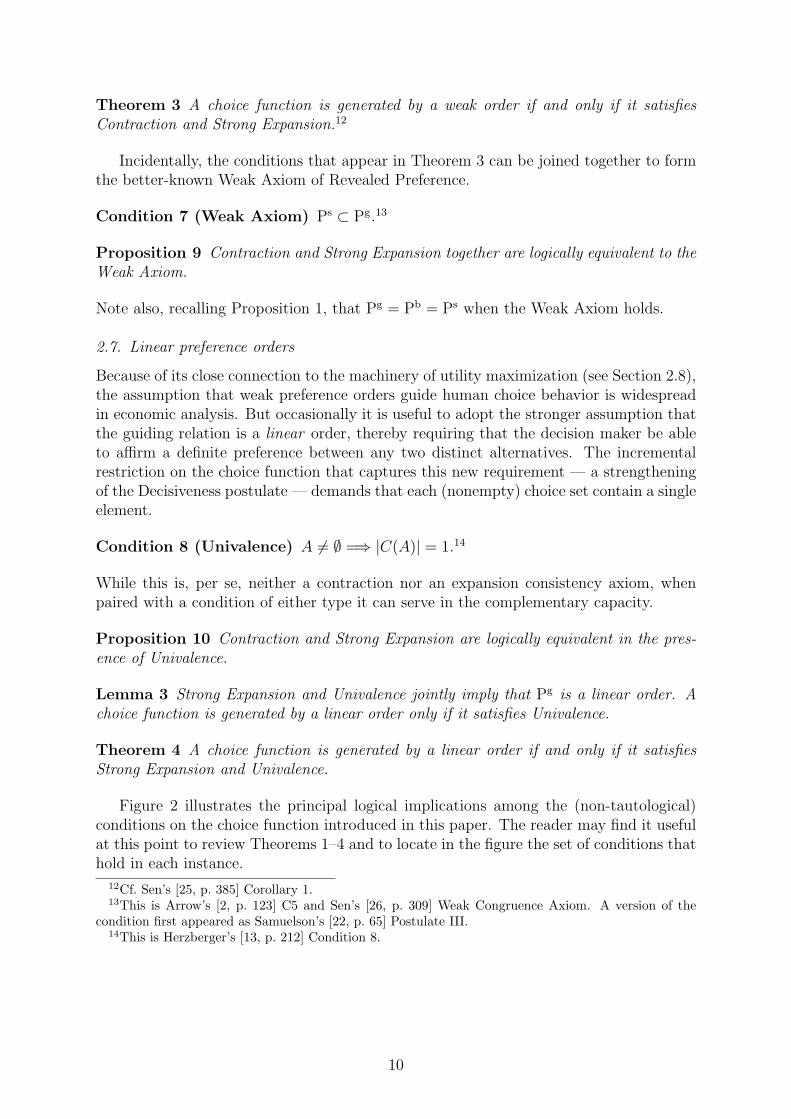
2.7. Linear preference orders
Because of its close connection to the machinery of utility maximization (see Section 2.8),the assumption that weak preference orders guide human choice behavior is widespreadin economic analysis. But occasionally it is useful to adopt the stronger assumption thatthe guiding relation is a linear order, thereby requiring that the decision maker be ableto affirm a definite preference between any two distinct alternatives. The incrementalrestriction on the choice function that captures this new requirement — a strengtheningof the Decisiveness postulate — demands that each (nonempty) choice set contain a singleelement.
Condition 8 (Univalence) A 6= ∅ =⇒ |C(A)| = 1.14
While this is, per se, neither a contraction nor an expansion consistency axiom, whenpaired with a condition of either type it can serve in the complementary capacity.
Proposition 10 Contraction and Strong Expansion are logically equivalent in the pres-ence of Univalence.
Lemma 3 Strong Expansion and Univalence jointly imply that Pg is a linear order. Achoice function is generated by a linear order only if it satisfies Univalence.
Theorem 4 A choice function is generated by a linear order if and only if it satisfiesStrong Expansion and Univalence.
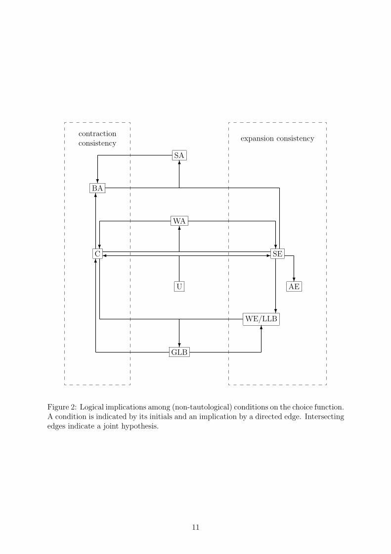
Figure 2 illustrates the principal logical implications among the (non-tautological)conditions on the choice function introduced in this paper. The reader may find it usefulat this point to review Theorems 1–4 and to locate in the figure the set of conditions thathold in each instance.
12Cf. Sen’s [25, p. 385] Corollary 1.13This is Arrow’s [2, p. 123] C5 and Sen’s [26, p. 309] Weak Congruence Axiom. A version of the
condition first appeared as Samuelson’s [22, p. 65] Postulate III.14This is Herzberger’s [13, p. 212] Condition 8.
10
contractionconsistency
expansion consistency
BA
C
SA
WA
U
GLB
SE
AE
WE/LLB
6
? ?
6
-�
6
6
6
?
?
?
?
Figure 2: Logical implications among (non-tautological) conditions on the choice function.A condition is indicated by its initials and an implication by a directed edge. Intersectingedges indicate a joint hypothesis.
11
2.8. Utility representations
An important historical and practical concern of economic theory has been assessing theplausibility of and the axiomatic basis for the utility-maximization model of decisionmaking. This model posits the existence of a function f : X → < that encodes thepreference relation in the sense that xPy if and only if f(x) > f(y), and an obviousconsequence of this encoding is that the maximization operators (applied to menus)associated with P and f coincide. If, moreover, the relation P generates the choicefunction, then for each nonempty menu A we have
C(A) = [x ∈ A : f(x) = max f [A]] , (3)
which is to say that the members of a choice set are those available alternatives that meetthe maximizing criterion. When this is so, we shall say that the function f provides autility representation of the choice function, and we shall call the representation injectivewhen f is one-to-one.
Since a preference relation that can be encoded in a function taking real values willinherit from the relation > on < the properties of a weak order, the utility-maximizationmodel of decision making clearly falls under the purview of Theorem 3 above. But well-known counterexamples show that not every weak order can be thus encoded, with anadditional order-topological property being needed to ensure encodability.15 So as toavoid becoming preoccupied with this issue — one that is irrelevant to the main pointof this essay — we provide here an exact characterization of the class of choice functionsadmitting utility representations only for the very simple case of a finite choice space(i.e., a finite catalog X).
Proposition 11 A choice function on a finite choice space admits a utility representation(resp., an injective utility representation) if and only if it satisfies Contraction and StrongExpansion (resp., Strong Expansion and Univalence).
3. CHOICE THEORY WITHOUT CONTRACTION CONSISTENCY
3.1. Relation systems and nestedness
If our decision maker cannot be relied upon to perceive all of his preferences, then weshall require a model of his cognitive capabilities more elaborate than that embodiedin the relation P. In this case, our being told of the existence of a preference for onealternative over another does not enable us to conclude that the second alternative willnever be chosen when the first is available, since this preference might be imperceptiblein the context of some particularly complex choice problem in which it is relevant. Butif the perceptibility as well as the existence of preferences is to be called into question,then we can certainly devise a formalism that describes the former in the same way thata binary relation describes the latter. Given a menu A, let us write PA for the relationon A that encodes the preferences that the decision maker perceives when faced withthis choice problem. Now, allowing the menu to vary, we collect the associated perceivedpreference relations in a vector P = 〈PA〉A∈A to be referred to as the preference system.The perceived-preference-maximal members of the menu A are then contained in the setP ↑ (A) =
[x ∈ A : (∀y ∈ A) yPAx
], and when C ⊂ P ↑ (resp., P ↑ ⊂ C) — adopting a
notation analogous to that in Section 2.3 — we shall say that P supplies an upper bound
15Here Fishburn [10, p. 27] is a valuable reference for both counterexamples and positive results.
12
(resp., a lower bound) for the choice function. When C = P ↑ , we shall of course saythat P generates the choice function.
Let us call an arbitrary vector R of relations indexed by A a relation system. Theprojection of R is the union
⋃R =
⋃A∈A RA ⊂ X × X of its component relations. A
relation system will be said to exhibit a property normally ascribed to a binary relation(e.g., reflexivity) when each of its component relations exhibits the property, and wecan form derived relation systems (e.g., the system of converse relations) in the obviousfashion. Furthermore, we shall refer to a relation system whose components each belongto a particular class of relations by appending the name of the class (e.g., a system ofproto orders).
It will not have escaped the reader that every choice function is generated by a relationsystem, and so the hypothesis that P generates C excludes no logical possibilities. Thereis, however, a natural intercomponent restriction on the generating system that doesconstrain the choice function, and that interacts with various sets of intracomponent (i.e.,ordering) restrictions in a manner that will soon become apparent. By way of introducingthis restriction, let us suppose that when facing the menu B our decision maker perceivesa preference for one alternative over another. Then, when confronted with a differentmenu A that contains the two alternatives related by the preference and that is in somesense no more complex than B, we might reasonably expect the decision maker againto perceive this relationship on the grounds that only an increase in the complexity ofthe problem could have rendered it imperceptible. Although we have not specified whatit means for one choice problem to be more or less complex than another, we can treatthe set inclusion relation as being demonstrative of weak comparative complexity underthe modest assumption that adding new alternatives to a problem cannot make it anysimpler. We thus define a relation system R to be nested if for any x, y ∈ A ⊂ B we havexRBy only if xRAy (cf. Anand [1, p. 339]), thereby formalizing what we shall take to bea basic property of our decision maker’s preference system.16
3.2. The local relation system
In order to characterize choice behavior governed by preference systems, we shall requirea suitable indicator of perceived preference assembled (like the relations in Section 2.3)from choice function data. Constructing such an indicator poses no small difficulty, sinceit will consist not of a single binary relation, but rather of an entire vector of relationsindexed by A. Nevertheless, we can define an appropriate relation system by exploitingthe presumed nestedness of P.
Definition 2 The local relation system Pl is defined by xPlBy if and only if x, y ∈ B
and for each menu A ⊂ B with x ∈ A we have y /∈ C(A).
Proposition 12 PlX = Pg.
⋃Pl = Pb. Pl is nested and acyclic.
16As always with blanket statements in abstract settings, one can attempt to concoct counterexamples.A choice, say, between execution by firing squad or by electrocution might well be more complex, in thesense that it is more difficult to reach a decision, than a choice among these two modes of execution anddinner with the Queen at Buckingham Palace. Note, however, that this scenario (envisioned by YossiFeinberg) will not violate the nestedness restriction unless, for example, a preference for electrocutionover the firing squad is perceived when dinner is available but not when it isn’t.
For a case in which nestedness clearly is violated, see Sen’s [30, p. 753] “Tea or heroin?” example(pointed out by Nageeb Ali), which illustrates the idea that a menu can have “epistemic importance.”
13
Since an alternative x bears the relation PlB to a second alternative y whenever y will
be rejected in any choice problem included in B and containing x, we can view PlB as a
global relation that searches only the subsets of its subscript.The role of Pl in this section will mirror that of Pg in Section 2, and therefore our
first task is to identify the class of choice functions generated by their respective localrelation systems.
Condition 9 (Local Upper Bound) C ⊂ Pl ↑ .
Condition 10 (Local Lower Bound) Pl ↑⊂ C.
Like its analog in the classical theory, the first of these two conditions is a tautology.
Proposition 13 Local Upper Bound holds for any choice function.
It is also true that Pl includes componentwise any other nested relation system thatsupplies an upper bound for the choice function — a formal expression of the intuitivenotion that the local relation system “generously” declares a perceived preference to existwhenever no contradictory evidence is forthcoming.
Proposition 14 If R is nested and C ⊂ R↑ , then for each menu A we have RA ⊂ PlA.
This implies that if a nested relation system R generates C, then Pl ↑⊂ R↑= C ⊂ Pl ↑and hence Pl does as well.
Proposition 15 A choice function is generated by a nested relation system if and onlyif it is generated by Pl.
And finally, combining Propositions 13 and 15 shows that Local Lower Bound is necessaryand sufficient for the choice function to arise from maximization of a nested preferencesystem.
Corollary 2 A choice function is generated by a nested relation system if and only if itsatisfies Local Lower Bound.
3.3. Preference systems of proto orders
Continuing to proceed in parallel with the classical theory, we now strengthen Corollary 2by establishing the following analogs to Propositions 5 and 6.
Proposition 16 Any nested relation system that supplies an upper bound for C is asystem of proto orders.
Proposition 17 A choice function is generated by a nested system of proto orders if andonly if it satisfies Local Lower Bound.
Despite its arcane appearance, the condition used in this characterization is one that wehave already encountered in a different form.
Proposition 18 Local Lower Bound is logically equivalent to Weak Expansion.
14
Thus we obtain an alternative characterization that excises contraction consistency fromTheorem 1.
Theorem 5 A choice function is generated by a nested system of proto orders if andonly if it satisfies Weak Expansion.
It is worth noting that Theorem 5 links Weak Expansion to the nestedness requirementthat perceived preferences be preserved under contraction of the menu of alternatives.Similarly, Contraction can be linked to the requirement that perceived preferences bepreserved under expansion of the menu. Here the terminological inversion results fromthe inverse relationship between preference and choice: A (perceived) preference for onealternative over another is a reason not to choose the second alternative — but not initself a reason to choose the first.
3.4. Preference systems of partial orders
The credentials of transitivity as a consistency criterion are surely no less impressivein the case of perceived preferences than they are in the case of ordinary preferenceassessments. Once again, imposing this property further constrains the choice function;in fact, it entails precisely the same incremental restriction on C as before.
Lemma 4 Adjunct Expansion implies that Pl is a system of partial orders. A choicefunction is generated by a nested system of partial orders only if it satisfies AdjunctExpansion.
Theorem 6 A choice function is generated by a nested system of partial orders if andonly if it satisfies Weak Expansion and Adjunct Expansion.
When Weak Expansion is supplemented with Adjunct Expansion, the consequencesfor the latent preference system are actually somewhat subtle. As we have seen, WeakExpansion alone suffices to make Pl a nested system of proto orders that generates thechoice function, and the astute reader will have observed that forming the transitiveclosure (Pl)∗ then creates a system of partial orders that generates C as well. Thisartifice fails to invalidate Theorem 6, however, because forming the system of ancestralrelations does not in general preserve nestedness. The latter point should make it clearthat our intercomponent nestedness and intracomponent ordering assumptions on P donot operate independently: On the contrary, without nestedness only very strong (linear)ordering assumptions place any restriction whatsoever on the choice function.
3.5. Preference systems of weak orders
Admitting the extratransitivity properties as consistency criteria for perceived preferencesalso entails the same incremental restriction on the choice function as in the classicaltheory.
Lemma 5 Strong Expansion implies that Pl is a system of weak orders. A choice func-tion is generated by a nested system of weak orders only if it satisfies Strong Expansion.
Theorem 7 A choice function is generated by a nested system of weak orders if and onlyif it satisfies Strong Expansion.
15
While in the case of the preference relation P we could parse the extratransitivityproperties in terms of its symmetric residue P◦ taking on the characteristics of an indif-ference relation (see Section 2.6), in the case of the preference system P these propertiesare not so readily interpretable. We can of course construct the system P◦ of symmetricresidues, but we cannot then interpret an expression of the form xP◦
Ay as an assertion of“perceived indifference” since it does not preclude a contradictory perceived preferenceassessment of the form xPBy (except, under nestedness, when A ⊂ B). And conversely,without the indifference interpretation of P◦ we lack an obvious justification for imposingthe extratransitivity properties on P.17
A more illuminating perspective on the characterization in Theorem 7 focuses insteadon the negative transitivity of the preference system; the requirement, given x, z ∈ A suchthat xPAz, that each y ∈ A satisfy either xPAy or yPAz. This can be phrased as a demandthat the decision maker be able to place any available alternative somewhere on the scaleof value created by a particular perceived preference — to judge it either worse than thebetter alternative or better than the worse alternative. A nested preference system ofweak orders is therefore the structure appropriate to a decision maker who can alwaysfully resolve his opinions at some level of precision, though his ability to discriminateamong alternatives may diminish as the menu expands on which they appear.
3.6. Preference systems of linear orders
Imposing weak connectedness on P once more leads to a familiar restriction on the choicefunction.
Lemma 6 Strong Expansion and Univalence jointly imply that Pl is a system of linearorders. A choice function is generated by a system of linear orders only if it satisfiesUnivalence.
But according to Theorem 4, any choice function satisfying both Strong Expansion andUnivalence is generated simply by a linear order, and this implication brings us to thefollowing conclusion.
Proposition 19 A choice function is generated by a nested system of linear orders ifand only if it is generated by a linear order.
The logic of this result is most easily understood in the light of our commentary onTheorem 7 above. As we have seen, a decision maker possessing a preference system ofweak orders is one who can always fully resolve his opinions, though his discriminatorycapabilities may depend upon the menu he faces. But if the components of P are linearorders then these capabilities cannot in fact depend upon the menu, since a weaklyconnected relation necessarily discriminates between any two distinct alternatives. Therequirement of nestedness then ensures that the components are all drawn from a singlelinear order on X, and the latter will be certain to generate C whenever P does so.
17As Herzberger [13, p. 201] would have it, “Indifference relations representing preferential matching[i.e., indifference] ought to be held subject to quite different rationality conditions from those appropriateto amalgamated mutual nonpreference [i.e., symmetric residue] relations,” and no doubt the same canbe said of relations for which we are driven to the unfortunate locution “amalgamated mutual absenceof perceived preference.”
16
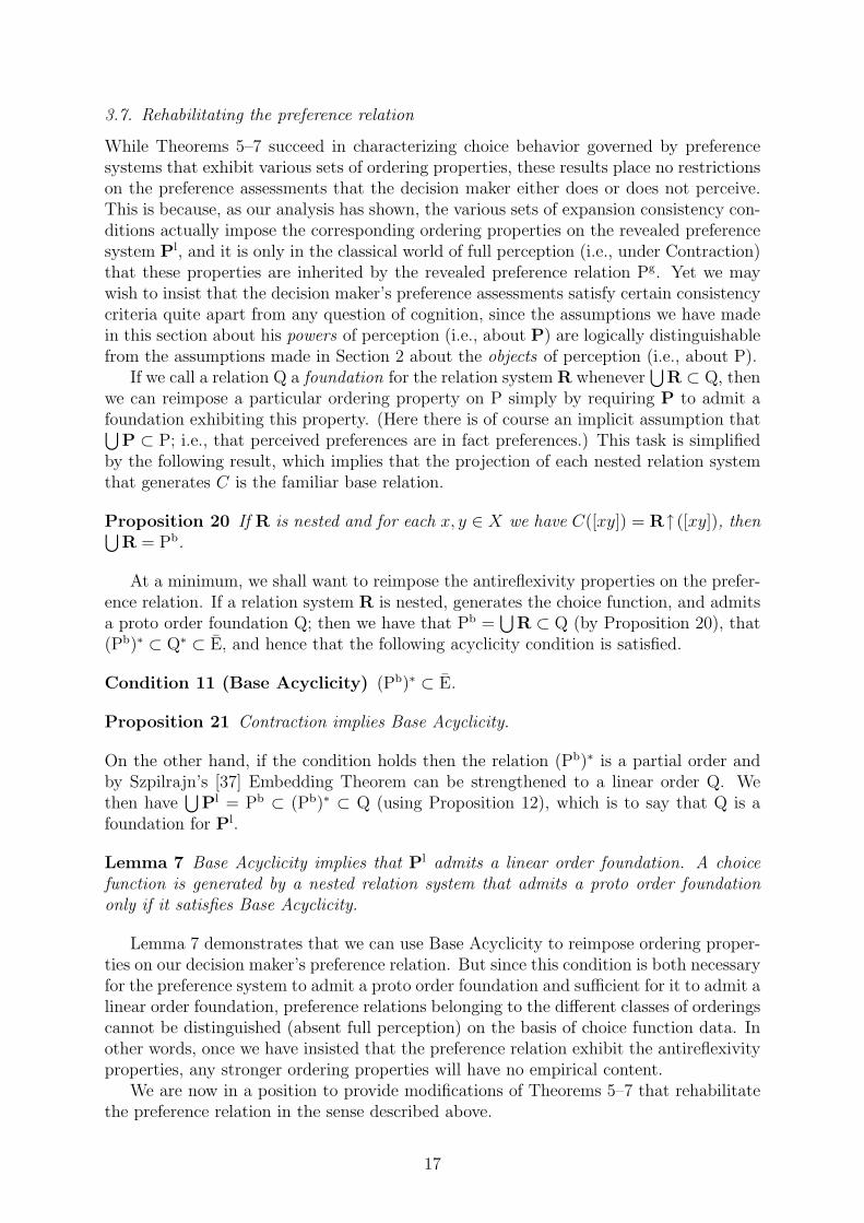
3.7. Rehabilitating the preference relation
While Theorems 5–7 succeed in characterizing choice behavior governed by preferencesystems that exhibit various sets of ordering properties, these results place no restrictionson the preference assessments that the decision maker either does or does not perceive.This is because, as our analysis has shown, the various sets of expansion consistency con-ditions actually impose the corresponding ordering properties on the revealed preferencesystem Pl, and it is only in the classical world of full perception (i.e., under Contraction)that these properties are inherited by the revealed preference relation Pg. Yet we maywish to insist that the decision maker’s preference assessments satisfy certain consistencycriteria quite apart from any question of cognition, since the assumptions we have madein this section about his powers of perception (i.e., about P) are logically distinguishablefrom the assumptions made in Section 2 about the objects of perception (i.e., about P).
If we call a relation Q a foundation for the relation system R whenever⋃
R ⊂ Q, thenwe can reimpose a particular ordering property on P simply by requiring P to admit afoundation exhibiting this property. (Here there is of course an implicit assumption that⋃
P ⊂ P; i.e., that perceived preferences are in fact preferences.) This task is simplifiedby the following result, which implies that the projection of each nested relation systemthat generates C is the familiar base relation.
Proposition 20 If R is nested and for each x, y ∈ X we have C([xy]) = R↑([xy]), then⋃R = Pb.
At a minimum, we shall want to reimpose the antireflexivity properties on the prefer-ence relation. If a relation system R is nested, generates the choice function, and admitsa proto order foundation Q; then we have that Pb =
⋃R ⊂ Q (by Proposition 20), that
(Pb)∗ ⊂ Q∗ ⊂ E, and hence that the following acyclicity condition is satisfied.
Condition 11 (Base Acyclicity) (Pb)∗ ⊂ E.
Proposition 21 Contraction implies Base Acyclicity.
On the other hand, if the condition holds then the relation (Pb)∗ is a partial order andby Szpilrajn’s [37] Embedding Theorem can be strengthened to a linear order Q. Wethen have
⋃Pl = Pb ⊂ (Pb)∗ ⊂ Q (using Proposition 12), which is to say that Q is a
foundation for Pl.
Lemma 7 Base Acyclicity implies that Pl admits a linear order foundation. A choicefunction is generated by a nested relation system that admits a proto order foundationonly if it satisfies Base Acyclicity.
Lemma 7 demonstrates that we can use Base Acyclicity to reimpose ordering proper-ties on our decision maker’s preference relation. But since this condition is both necessaryfor the preference system to admit a proto order foundation and sufficient for it to admit alinear order foundation, preference relations belonging to the different classes of orderingscannot be distinguished (absent full perception) on the basis of choice function data. Inother words, once we have insisted that the preference relation exhibit the antireflexivityproperties, any stronger ordering properties will have no empirical content.
We are now in a position to provide modifications of Theorems 5–7 that rehabilitatethe preference relation in the sense described above.
17
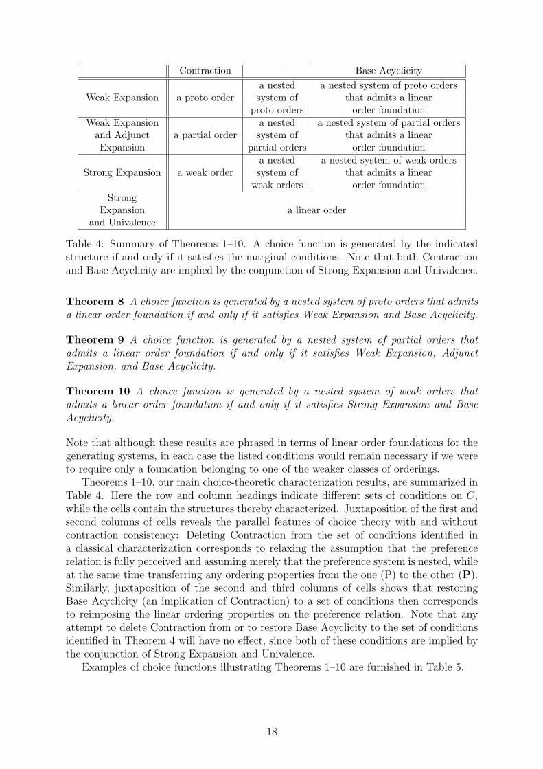
Contraction — Base Acyclicitya nested a nested system of proto orders
Weak Expansion a proto order system of that admits a linearproto orders order foundation
Weak Expansion a nested a nested system of partial ordersand Adjunct a partial order system of that admits a linearExpansion partial orders order foundation
a nested a nested system of weak ordersStrong Expansion a weak order system of that admits a linear
weak orders order foundationStrong
Expansion a linear orderand Univalence
Table 4: Summary of Theorems 1–10. A choice function is generated by the indicatedstructure if and only if it satisfies the marginal conditions. Note that both Contractionand Base Acyclicity are implied by the conjunction of Strong Expansion and Univalence.
Theorem 8 A choice function is generated by a nested system of proto orders that admitsa linear order foundation if and only if it satisfies Weak Expansion and Base Acyclicity.
Theorem 9 A choice function is generated by a nested system of partial orders thatadmits a linear order foundation if and only if it satisfies Weak Expansion, AdjunctExpansion, and Base Acyclicity.
Theorem 10 A choice function is generated by a nested system of weak orders thatadmits a linear order foundation if and only if it satisfies Strong Expansion and BaseAcyclicity.
Note that although these results are phrased in terms of linear order foundations for thegenerating systems, in each case the listed conditions would remain necessary if we wereto require only a foundation belonging to one of the weaker classes of orderings.
Theorems 1–10, our main choice-theoretic characterization results, are summarized inTable 4. Here the row and column headings indicate different sets of conditions on C,while the cells contain the structures thereby characterized. Juxtaposition of the first andsecond columns of cells reveals the parallel features of choice theory with and withoutcontraction consistency: Deleting Contraction from the set of conditions identified ina classical characterization corresponds to relaxing the assumption that the preferencerelation is fully perceived and assuming merely that the preference system is nested, whileat the same time transferring any ordering properties from the one (P) to the other (P).Similarly, juxtaposition of the second and third columns of cells shows that restoringBase Acyclicity (an implication of Contraction) to a set of conditions then correspondsto reimposing the linear ordering properties on the preference relation. Note that anyattempt to delete Contraction from or to restore Base Acyclicity to the set of conditionsidentified in Theorem 4 will have no effect, since both of these conditions are implied bythe conjunction of Strong Expansion and Univalence.
Examples of choice functions illustrating Theorems 1–10 are furnished in Table 5.
18

menu: [wx] [wy] [wz] [xy] [xz] [yz] [wxy] [wxz] [wyz] [xyz] [wxyz]
1. [w] [wy] [wz] [x] [xz] [y] [w] [wz] [wy] [x] [w]satisfies GLB, C, WE/LLB, BA; violates AE, SE, WA, U, SA
2. [w] [wy] [wz] [xy] [xz] [y] [wy] [wz] [wy] [xy] [wy]satisfies GLB, C, WE/LLB, AE, BA; violates SE, WA, U, SA
3. [wx] [w] [w] [x] [x] [yz] [wx] [wx] [w] [x] [wx]satisfies GLB, C, WE/LLB, AE, SE, WA, BA, SA; violates U
4. [w] [w] [w] [x] [x] [y] [w] [w] [w] [x] [w]satisfies GLB, C, WE/LLB, AE, SE, WA, U, BA, SA
5. [w] [y] [wz] [x] [z] [y] [x] [wxz] [yz] [y] [xyz]satisfies WE/LLB; violates GLB, C, AE, SE, WA, U, BA, SA
6. [w] [y] [w] [x] [x] [yz] [xy] [w] [yz] [x] [xy]satisfies WE/LLB, AE; violates GLB, C, SE, WA, U, BA, SA
7. [x] [y] [z] [x] [z] [y] [xy] [xz] [yz] [xyz] [xyz]satisfies WE/LLB, AE, SE; violates GLB, C, WA, U, BA, SA
8. [w] [y] [wz] [xy] [z] [y] [xy] [wxz] [yz] [y] [xyz]satisfies WE/LLB, BA; violates GLB, C, AE, SE, WA, U, SA
9. [x] [y] [z] [x] [x] [y] [xy] [wx] [yz] [xy] [xy]satisfies WE/LLB, AE, BA; violates GLB, C, SE, WA, U, SA
10. [x] [y] [z] [x] [xz] [y] [xy] [xz] [yz] [xyz] [xyz]satisfies WE/LLB, AE, SE, BA, SA; violates GLB, C, WA, U
Table 5: Examples illustrating Theorems 1–10. Choice functions on the four-elementspace X = [wxyz] appear as rows numbered according to the relevant theorem. Cellscontain the choice sets associated with the menus that serve as the corresponding columnheadings. Below each row of data the conditions depicted in Figure 2 are registered asbeing either satisfied or violated by the choice function.
19
3.8. Threshold utility representations
Proposition 11 establishes that a choice function (on a finite choice space) can admita utility representation only if it satisfies Contraction, and thus relaxing this conditionallows our decision maker to behave inconsistently with the utility-maximization model.The targeted generalization of this model posits the existence of functions f : X → <and θ : A → < such that for each menu A we have
C(A) = [x ∈ A : f(x) = θ(A)] ; (4)
i.e., such that the members of a choice set are those available alternatives that meet thesatisficing criterion. In this case we shall say that the vector 〈f, θ〉 provides a thresholdutility representation of the choice function, and we shall again call the representationinjective when the function f is one-to-one.
If the choice function admits a threshold utility representation 〈f, θ〉, then xPsy impliesthat f(x) = θ(A) > f(y) for some menu A; and the following acyclicity condition is anobvious consequence of this implication.
Condition 12 (Separation Acyclicity) (Ps)∗ ⊂ E.
On the other hand, if the condition holds then the relation (Ps)∗ is a partial order andby the Embedding Theorem can be strengthened to a linear order Q. Assuming a finitechoice space (as in Section 2.8), this Q will be encodable in a one-to-one function f thattogether with the mapping θ defined by
θ(A) =
{min f [C(A)] for A 6= ∅0 for A = ∅ (5)
will provide a threshold utility representation for C.18
Proposition 22 A choice function on a finite choice space admits an injective thresholdutility representation if and only if it satisfies Separation Acyclicity.
The logical strength of Separation Acyclicity vis-a-vis earlier conditions is measured bythe following result, which supplies the final implication illustrated in Figure 2.
Proposition 23 Separation Acyclicity implies Base Acyclicity. Strong Expansion andBase Acyclicity jointly imply Separation Acyclicity.
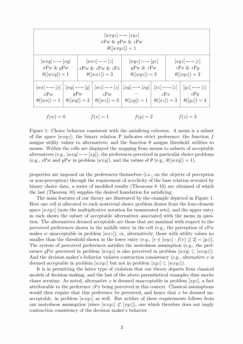
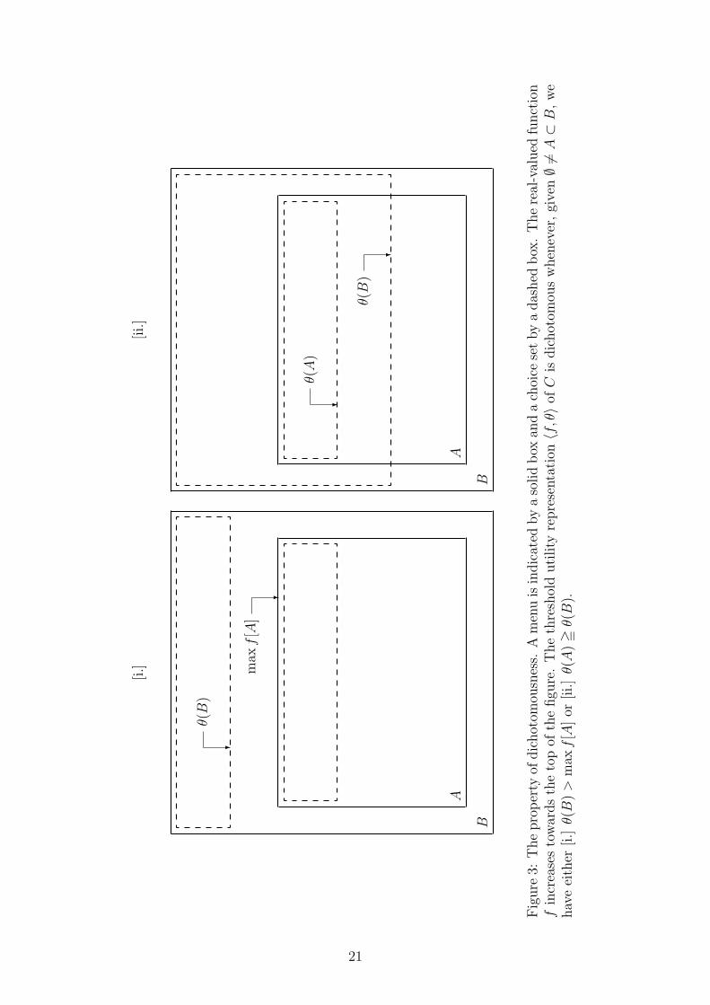
The last two propositions demonstrate that the conditions identified in Theorem 10are sufficient for the choice function to admit a threshold utility representation 〈f, θ〉.Strong Expansion is not necessary for the existence of such a representation, however,and in order to derive the further constraint implied by this condition let us imaginenonempty menus A ⊂ B such that θ(B) 5 max f [A]. Choosing x ∈ A ⊂ B such thatf(x) = max f [A] = θ(B), we have that x ∈ C(B) ∩ A. Strong Expansion then impliesthat C(A) ⊂ C(B), and hence
θ(A) = min f [C(A)] = min f [C(B)] = θ(B). (6)
We can capture this additional property of our construction by calling a thresholdutility representation 〈f, θ〉 dichotomous whenever, given ∅ 6= A ⊂ B, we have either
20
[i.]
B
θ(B
)
?
A
max
f[A
]
?
[ii.]
B
θ(B
)
?
A
θ(A
)
?
Fig
ure
3:T
he
pro
per
tyof
dic
hot
omou
snes
s.A
men
uis
indic
ated
by
aso
lid
box
and
ach
oice
setby
adas
hed
box
.T
he
real
-val
ued
funct
ion
fin
crea
ses
tow
ards
the
top
ofth
efigu
re.
The
thre
shol
dutility
repre
senta
tion
〈f,θ〉
ofC
isdic
hot
omou
sw
hen
ever
,gi
ven∅6=
A⊂
B,w
ehav
eei
ther
[i.]
θ(B
)>
max
f[A
]or
[ii.]
θ(A
)=
θ(B
).
21
θ(B) > max f [A] or θ(A) = θ(B). (See Figure 3.) And our final result characterizes theclass of choice functions that admit representations with this feature.
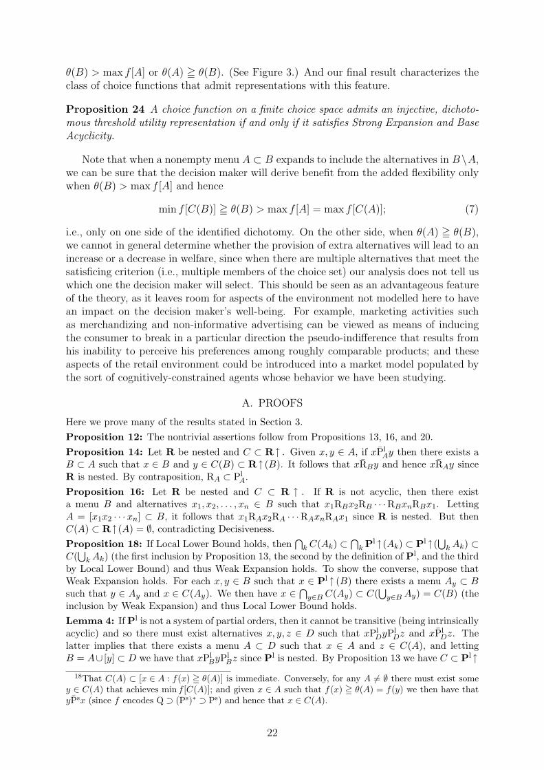
Proposition 24 A choice function on a finite choice space admits an injective, dichoto-mous threshold utility representation if and only if it satisfies Strong Expansion and BaseAcyclicity.
Note that when a nonempty menu A ⊂ B expands to include the alternatives in B\A,we can be sure that the decision maker will derive benefit from the added flexibility onlywhen θ(B) > max f [A] and hence
min f [C(B)] = θ(B) > max f [A] = max f [C(A)]; (7)
i.e., only on one side of the identified dichotomy. On the other side, when θ(A) = θ(B),we cannot in general determine whether the provision of extra alternatives will lead to anincrease or a decrease in welfare, since when there are multiple alternatives that meet thesatisficing criterion (i.e., multiple members of the choice set) our analysis does not tell uswhich one the decision maker will select. This should be seen as an advantageous featureof the theory, as it leaves room for aspects of the environment not modelled here to havean impact on the decision maker’s well-being. For example, marketing activities suchas merchandizing and non-informative advertising can be viewed as means of inducingthe consumer to break in a particular direction the pseudo-indifference that results fromhis inability to perceive his preferences among roughly comparable products; and theseaspects of the retail environment could be introduced into a market model populated bythe sort of cognitively-constrained agents whose behavior we have been studying.
A. PROOFS
Here we prove many of the results stated in Section 3.Proposition 12: The nontrivial assertions follow from Propositions 13, 16, and 20.Proposition 14: Let R be nested and C ⊂ R ↑ . Given x, y ∈ A, if xPl
Ay then there exists aB ⊂ A such that x ∈ B and y ∈ C(B) ⊂ R↑ (B). It follows that xRBy and hence xRAy sinceR is nested. By contraposition, RA ⊂ Pl
A.Proposition 16: Let R be nested and C ⊂ R ↑ . If R is not acyclic, then there exista menu B and alternatives x1, x2, . . . , xn ∈ B such that x1RBx2RB · · ·RBxnRBx1. LettingA = [x1x2 · · ·xn] ⊂ B, it follows that x1RAx2RA · · ·RAxnRAx1 since R is nested. But thenC(A) ⊂ R↑(A) = ∅, contradicting Decisiveness.Proposition 18: If Local Lower Bound holds, then
⋂k C(Ak) ⊂
⋂k Pl ↑(Ak) ⊂ Pl ↑(
⋃k Ak) ⊂
C(⋃
k Ak) (the first inclusion by Proposition 13, the second by the definition of Pl, and the thirdby Local Lower Bound) and thus Weak Expansion holds. To show the converse, suppose thatWeak Expansion holds. For each x, y ∈ B such that x ∈ Pl ↑ (B) there exists a menu Ay ⊂ Bsuch that y ∈ Ay and x ∈ C(Ay). We then have x ∈
⋂y∈B C(Ay) ⊂ C(
⋃y∈B Ay) = C(B) (the
inclusion by Weak Expansion) and thus Local Lower Bound holds.Lemma 4: If Pl is not a system of partial orders, then it cannot be transitive (being intrinsicallyacyclic) and so there must exist alternatives x, y, z ∈ D such that xPl
DyPlDz and xPl
Dz. Thelatter implies that there exists a menu A ⊂ D such that x ∈ A and z ∈ C(A), and lettingB = A∪ [y] ⊂ D we have that xPl
ByPlBz since Pl is nested. By Proposition 13 we have C ⊂ Pl ↑
18That C(A) ⊂ [x ∈ A : f(x) = θ(A)] is immediate. Conversely, for any A 6= ∅ there must exist somey ∈ C(A) that achieves min f [C(A)]; and given x ∈ A such that f(x) = θ(A) = f(y) we then have thatyPsx (since f encodes Q ⊃ (Ps)∗ ⊃ Ps) and hence that x ∈ C(A).
22
and therefore y, z /∈ C(B). But then C(B) ⊂ A ⊂ B and z ∈ C(A) \ C(B), and thus AdjunctExpansion fails.
Now let R be a nested system of partial orders that generates C. If Adjunct Expansionfails, then there must exist both menus C(B) ⊂ A ⊂ B and an alternative x ∈ C(A) \ C(B),and since C = R↑ the latter implies both that x ∈ R↑(A) and that there exists a y1 ∈ B suchthat y1RBx.
[Inductive step begins.] Let yk ∈ B be such that ykRBx. If yk ∈ A then ykRAx since R isnested, contradicting x ∈ R↑ (A). Alternatively, if yk ∈ B \ A then yk /∈ C(B) = R↑ (B) sinceC(B) ⊂ A. But then there exists a yk+1 ∈ B such that yk+1RBykRBx, and therefore yk+1RBxsince R is transitive. [Inductive step ends.]
Using induction, we can construct a set D = [y1y2 · · ·] ⊂ B with the property that yk+1RByk
and hence (since R is nested) yk+1RDyk for each k = 1. But then C(D) = R ↑ (D) = ∅,contradicting Decisiveness.Lemma 5: If Pl is not a system of weak orders, then it cannot be negatively transitive (beingintrinsically asymmetric) and so there must exist alternatives x, y, z ∈ D such that xPl
DyPlDz
and xPlDz. The former implies that there exist both a menu A ⊂ D such that x ∈ A and
y ∈ C(A) and a menu B ⊂ D such that y ∈ B and z ∈ C(B). Decisiveness ensures thatthere exists an alternative w ∈ C(A ∪ B), and since both x ∈ A ∪ B ⊂ D and xPl
Dz we havealso z /∈ C(A ∪ B). If either w ∈ B or y ∈ C(A ∪ B) then we have both C(A ∪ B) ∩ B 6= ∅and z ∈ C(B) \ C(A ∪ B), and thus Strong Expansion fails. Alternatively, if both w /∈ B andy /∈ C(A∪B) then we have both w ∈ C(A∪B)∩A and y ∈ C(A) \C(A∪B), and again StrongExpansion fails.
Now let R be a nested system of weak orders that generates C. If Strong Expansion fails,then there must exist both menus A ⊂ B and alternatives x ∈ C(B)∩A and y ∈ C(A) \C(B),and since C = R ↑ we have yRBx and xRAy and thus xRBy (since R is nested). Moreover,there must also exist an alternative z ∈ B such that zRByR◦
Bx, and since R is cross transitiveit follows that zRBx and hence that x /∈ C(B), contradicting x ∈ C(B).Lemma 6: If Pl is not a system of linear orders, then it cannot be weakly connected (beingintrinsically acyclic) and so there must exist distinct alternatives x, y ∈ D such that x(Pl
D)◦y.This implies that there exist both a menu A ⊂ D such that x ∈ A and y ∈ C(A) and a menuB ⊂ D such that y ∈ B and x ∈ C(B). If x ∈ C([xy]), then we have x ∈ C(A) by StrongExpansion and thus Univalence fails. Alternatively, if y ∈ C([xy]) then we have y ∈ C(B) byStrong Expansion and again Univalence fails.
Now let R be a system of linear orders that generates C. If Univalence fails, then theremust exist distinct alternatives x, y ∈ A such that x, y ∈ C(A) = R↑(A). But this implies thatx(RA)◦y, contradicting the weak connectedness of R.Proposition 20: Let R be nested and for each x, y ∈ X let C([xy]) = R ↑ ([xy]). The latterimplies that xPby if and only if xR[xy]y, and it follows that Pb =
⋃x,y∈X R[xy] ⊂
⋃A∈A RA =⋃
R. Conversely, since R is nested we have xRAy only if xR[xy]y and therefore only if xPby,and it follows that
⋃R =
⋃A∈A RA ⊂ Pb.
Proposition 21: Let Contraction hold. Given x, y ∈ X, if xPby then y /∈ C([xy]) and for anymenu A ⊃ [xy] we have y /∈ C(A) by Contraction, which is to say that xPgy. But then Pb ⊂ Pg
and (Pb)∗ ⊂ (Pg)∗ ⊂ E since Pg is acyclic, and thus Base Acyclicity holds.Proposition 23: Let Separation Acyclicity hold. Since Pb ⊂ Ps by Proposition 1, we have(Pb)∗ ⊂ (Ps)∗ ⊂ E by Separation Acyclicity, and thus Base Acyclicity holds.
Now let Strong Expansion and Base Acyclicity hold. Given x, y ∈ X, if xPsy then thereexists a menu A such that x ∈ C(A) and y ∈ A\C(A). Since both [xy] ⊂ A and x ∈ C(A)∩[xy],Strong Expansion implies that C([xy]) ⊂ C(A) and hence that y /∈ C([xy]), which is to saythat xPby. But then Ps ⊂ Pb and (Ps)∗ ⊂ (Pb)∗ ⊂ E by Base Acyclicity, and thus SeparationAcyclicity holds.
23

REFERENCES
[1] Paul Anand. The philosophy of intransitive preference. Economic Journal, 103(417):337–346, March 1993.
[2] Kenneth J. Arrow. Rational choice functions and orderings. Economica, New Series,26(102):121–127, May 1959.
[3] Kenneth J. Arrow. Social Choice and Individual Values. Yale University Press, New Haven,second edition, 1963. First edition 1951.
[4] Robert J. Aumann. Utility theory without the completeness axiom. Econometrica,30(3):445–462, July 1962.
[5] Nick Baigent and Wulf Gaertner. Never choose the uniquely largest: A characterization.Economic Theory, 8(2):239–249, 1996.
[6] Truman F. Bewley. Knightian decision theory: Part I. Decisions in Economics and Fi-nance, 25(2):79–110, November 2002. Yale University, Cowles Foundation Discussion PaperNo. 807, November 1986.
[7] J. Heinrich Bullinger. A Hundred Sermons upon the Apocalips of Jesu Christe. London,1561. Translated by John Daus.
[8] Herman Chernoff. Rational selection of decision functions. Econometrica, 22(4):422–443,October 1954.
[9] Jon Elster, editor. Rational Choice. New York University Press, Washington Square, NewYork, 1986.
[10] Peter C. Fishburn. Utility Theory for Decision Making. Robert E. Krieger, Huntington,New York, second edition, 1979. First edition 1970.
[11] Itzhak Gilboa and David Schmeidler. Maxmin expected utility with non-unique prior.Journal of Mathematical Economics, 18(2):141–153, 1989.
[12] Faruk Gul and Wolfgang Pesendorfer. Temptation and self-control. Econometrica,69(6):1403–1435, November 2001.
[13] Hans G. Herzberger. Ordinal preference and rational choice. Econometrica, 41(2):187–237,March 1973.
[14] Sheena S. Iyengar and Mark R. Lepper. When choice is demotivating: Can one desiretoo much of a good thing. Journal of Personality and Social Psychology, 79(6):995–1006,December 2000.
[15] Dean T. Jamison and Lawrence J. Lau. Semiorders and the theory of choice. Econometrica,41(5):901–912, September 1973.
[16] Gil Kalai, Ariel Rubinstein, and Ran Spiegler. Rationalizing choice functions by multiplerationales. Econometrica, 70(6):2481–2488, November 2002.
[17] David M. Kreps. A representation theorem for ‘preference for flexibility’. Econometrica,47(3):565–577, May 1979.
[18] David M. Kreps. Notes on the Theory of Choice. Westview Press, Boulder, Colorado, 1988.
[19] Mark J. Machina and David Schmeidler. A more robust definition of subjective probability.Econometrica, 60(4):745–780, July 1992.
24
[20] James A. Mirrlees. Economic policy and nonrational behaviour. University of Californiaat Berkeley, Department of Economics Working Paper No. 8728, February 1987.
[21] John F. Nash, Jr. The bargaining problem. Econometrica, 18(2):155–162, April 1950.
[22] Paul A. Samuelson. A note on the pure theory of consumer’s behaviour. Economica, NewSeries, 5(17):61–71, February 1938.
[23] Leonard J. Savage. The Foundations of Statistics. Dover, New York, second edition, 1972.First edition 1954.
[24] David Schmeidler. Subjective probability and expected utility without additivity. Econo-metrica, 57(3):571–587, May 1989.
[25] Amartya K. Sen. Quasi-transitivity, rational choice, and collective decisions. Review ofEconomic Studies, 36(3):381–393, July 1969.
[26] Amartya K. Sen. Choice functions and revealed preference. Review of Economic Studies,38(3):307–317, July 1971.
[27] Amartya K. Sen. Behaviour and the concept of preference. Economica, New Series,40(159):241–259, August 1973.
[28] Amartya K. Sen. Social choice theory: A re-examination. Econometrica, 45(1):53–89,January 1977.
[29] Amartya K. Sen. Internal consistency of choice. Econometrica, 61(3):495–521, May 1993.
[30] Amartya K. Sen. Maximization and the act of choice. Econometrica, 65(4):745–779, July1997.
[31] Eytan Sheshinski. Bounded rationality and socially optimal limits on choice in a self-selection model. Hebrew University of Jerusalem, Center for the Study of RationalityWorking Paper No. 330, November 2002.
[32] Herbert A. Simon. A behavioral model of rational choice. Quarterly Journal of Economics,69(1):99–118, February 1955.
[33] Herbert A. Simon. Rational choice and the structure of the environment. PsychologicalReview, 63(2):129–138, March 1956.
[34] Herbert A. Simon. Rationality as process and as product of thought. American EconomicReview, 68(2):1–16, May 1978.
[35] Herbert A. Simon. Rational decision making in business organizations. American EconomicReview, 69(4):493–513, September 1979.
[36] Herbert A. Simon. Models of Bounded Rationality. MIT Press, Cambridge, Massachusetts,1982/1997. In three volumes.
[37] Edward Szpilrajn. Sur l’extension de l’ordre partiel. Fundamenta Mathematica, 16:386–389,1930.
[38] Christopher J. Tyson. Revealed Preference Analysis of Boundedly Rational Choice. PhDthesis, Stanford University, September 2003.
25