Automatic model simplification: the generation of replacement sequences and their use in vegetation modelling

Ecological Modelling, 70 (1993) 137-157 137 Elsevier Science Publishers B.V., Amsterdam

Automatic model simplification: the generation of replacement sequences

and their use in vegetation modelling

A . D . M o o r e " a n d I .R . N o b l e b

" CSIRO Dicision of Plant Industry, c / - South Australian Research Institute, Northfield Research Laboratories, GPO Box 1671, Adelaide 5001, Australia

b Ecosystem Dynamics Group, Research School of Biological Sciences, Australian National Unicersity, GPO Box 475, Canberra 2601, Australia

(Received 20 January 1992; accepted 28 October 1992)

ABSTRACT

Moore, A.D. and Noble, I.R., 1993. Automatic model simplification: the generation of replacement sequences and their use in vegetation modelling. Ecol. Modelling, 70: 137-157.

Ideally an ecological model for use in managing landscapes should be predictive, realistic and able to incorporate the effects of large scale disturbances. Models achieving these criteria are usually computationally complex and mathematically intractable. We present an algorithm that takes predictions from a model of successional processes, partitions vegetation state-space according to a user-specified relation for similarity between stands and derives the possible transitions between the discrete states. The result is an approximate representation of the successional pathways, in the form of a directed graph. This representation permits mathematical analysis or rapid simulations. A trade-off exists between the size of the generated graph and the adequacy of its representation of vegetation change (i.e. similarity relation).

We illustrate this with examples based on a qualitative vegetation model we have recently developed (FATE). FATE follows the dynamics of a stand by modelling cohorts of plants within functional groups. In an example we demonstrate that an acceptable compro- mise between graph size and adequacy can be obtained. We believe the algorithm may have wide application in the modelling of ecosystem dynamics.

Correspondence to: A.D. Moore, CSIRO Division of Plant Industry, c / - South Australian Research Institute, Northfield Research Laboratories, GPO Box 1671, Adelaide 5001, Australia.

0304-3800/93/$06.00 © 1993 - Elsevier Science Publishers B.V. All rights reserved

138 A.D. M O O R E AND I.R. NOBLE

INTRODUCTION

Simple, predictive models of vegetation dynamics have great potential to be useful tools in both pure and applied ecology. The desideratum is a vegetation model that is realistic, incorporates the effects of disturbances, and yet is simple enough to permit the performance of Monte Carlo simulations across spatial networks of stands. Such a model would have application both as a basis for theoretical investigations in the nascent discipline of landscape ecology, and also as a "gaming" tool for managers of nature conservation areas. For example, such a landscape simulator could be used by managers to assess the effects of different prescribed burning policies on landscapes in their charge, explicitly taking into ac- count such factors as temporal variation in wildfire risk and the effects of the vegetation mosaic on fire spread.

The difficulty with the above programme lies in finding a model of vegetation change that is both simple and predictive at a useful resolution. Our purpose in this paper is to show that it is possible to achieve this aim through a two-stage process, by taking a predictive vegetation model and producing a simplified approximation to it. By partitioning a continuous vegetation-space into discrete units (Hogeweg et al., 1985), the state of a stand over time may be represented as a scalar (the unit presently occupied) rather than the composition vector required by continuous-space vegetation models (e.g. Van Hulst, 1987; Tilman, 1988). Also, a well-chosen discrete representation of the vegetation-space permits ready treatment of discontinuous change in the vegetation. This is important in the many vegetation types which are subject to relatively frequent, large-scale disturbance (Jackson, 1968; White, 1979; Heinselman, 1981; among many other studies).

If one can construct such a discrete representation of a vegetation-space, and if the probabilities of disturbances can be specified (e.g. Clark, 1989), then very rapid simulations of the trajectory of a stand become possible. The problem therefore becomes one of finding an appropriate classification of the set of possible vegetation compositions. Seeking an appropriate classification involves a trade-off between the needs for resolution of those who are to use the model, the number of states that can be handled, the requirement for dynamic sufficiency (Lewontin, 1974) and the increased efficiency that results if the number of possible transitions between states can be minimised.

One well-known discrete representation of vegetation dynamics is the discrete-time Markov process as applied to vegetation (Horn, 1975; Usher, 1981). Usher (1981) recognised the difficulty of defining states for a Markov vegetation process. He explored the possibility of using numerical

GENERATING REPLACEMENT SEQUENCES 139

classification techniques for this purpose, with limited success. Hogeweg et al. (1985) sought a numerical classification of stages in a salt marsh succession with rather more satisfactory results (their study linked changes in both space and time).

An alternative approach to that of Usher and of Hogeweg et al. is to use a model of biological process to derive the partition of vegetation-space a priori. Noble and Slatyer's (1980) vital attributes model used an extremely simple model of the mechanisms of vegetation change to derive the set of possible pathways for a stand. This set of possible pathways in turn defined the set of possible stand compositions; the compositions and pathways, taken together, were termed a replacement sequence. This approach of a priori derivation permits the discrete representation of the vegetation-space to maintain the dynamic sufficiency of the process model on which it is based: knowledge of the current state of a stand and of external events is sufficient to predict the stand's subsequent trajectory.

The vital attributes scheme was simple enough to permit replacement sequences to be generated by hand. This is unlikely to be the case, however, for any general model with more resolution than that of Noble and Slatyer (1980). We therefore generalise Noble and Slatyer's concept of a replacement sequence and provide an algorithm for generating replacement sequences given an arbitrary biological model. The sequences generated by the algorithm capture the important trajectories predicted by the biological model in a far simpler form.

In order to illustrate the properties and requirements of the algorithm, we use a recently developed, general model of vegetation dynamics (FATE: Moore and Noble, 1990).

DEFINITION OF A REPLACEMENT SEQUENCE

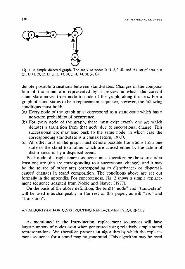
In order to formalise the concept of a replacement sequence, we use the idea of directed graphs. (For an introduction to the mathematics of graphs, see Bollob~s, 1979.) A directed graph is an entity composed of a set of points or nodes, together with a set of ordered pairs denoting paths or arcs from one node to another. Conventionally, the ordered pair (i, j) represents an arc which leaves node i (known as the source node) and goes to node j (known as the destination node). The arcs (i, j) and (j, i) may appear in the same graph, and the arc (i, i) from one node to itself is also permitted. We will denote a directed graph by G(V, E), where V is the set of nodes and E is the set of arcs. Fig. 1 shows a simple graph and its notation.

A replacement sequence is simply a graph in which the nodes denote states of a vegetation stand ("stand-states" henceforth), and the arcs

140 A.D. M O O R E A N D I.R. N O B L E

Fig. 1. A simple directed graph. The set V of nodes is {1, 2, 3, 4}, and the set of arcs E is {(1, i), (1, 2), (2, 1), (2, 3), (3, 3), (3, 4), (4, 3), (4, 4)}.

denote possible transitions between stand-states. Changes in the composition of the stand are represented by a process in which the current stand-state moves from node to node of the graph, along the arcs. For a graph of stand-states to be a rep lacement sequence, however, the following conditions must hold: (a) Every node of the graph must correspond to a stand-state which has a

non-zero probability of occurrence. (b) For every node of the graph, there must exist exactly one arc which

denotes a transition from that node due to successional change. This successional arc may lead back to the same node, in which case the corresponding stand-state is a climax (Horn, 1975).

(c) All o ther arcs of the graph must denote possible transitions from one state of the stand to another which are caused ei ther by the action of disturbance or by a dispersal event.

Each node of a rep lacement sequence must therefore be the source of at least one arc (the arc corresponding to a successional change), and it may be the source of o ther arcs corresponding to disturbance- or dispersal- caused changes in stand composition. The conditions above are set out formally in the appendix. For concreteness, Fig. 2 shows a simple replacement sequence adapted from Noble and Slatyer (1977).

On the basis of the above definition, the terms " n o d e " and "s tand-s ta te" will be used interchangeably in the rest of this paper, as will "arc" and "transi t ion".

AN ALGORITHM FOR CONSTRUCTING REPLACEMENT SEQUENCES

As ment ioned in the Introduction, rep lacement sequences will have large numbers of nodes even when genera ted using relatively simple stand representations. We therefore present an algorithm by which the replacement sequence for a stand may be generated. This algorithm may be used

G E N E R A T I N G REPLACEMENT SEQUENCES 141

1 3 10 20 100?

Eucalyptusspp. (EU) Vl - - m le Acacia genistifolia / (AC) SI .... m I e Dillwynia retorta Daviesia mimosoides (DA) VI m le Poa spp. (GR) Ol - - m - - I

EU.+AC.+DA.+GR----.-~,-EU.+AC.+DA-*GR • EUj+AC+DA+GR ), EU+AC+DA+GRp ~. EU+ACI~-GRp-----~ GRp ) - J J J (o) J i ] ( I ) / / l/ " ~ "

F-,k i l EU. +AC. +DA.+GR. ~-- " /

~ EUj+ACj+GRI ~ EU.+AG+GR ), EU+AC +GR • E A~GFI . l ] (I) J /P / / 1/9

/ f / / / ,-~ ~ 1 t " ~kEU+AC+GR I t - , GRj ~ R /

" J J (0) G :''~ ~ . ~ ) (I>

- (0)

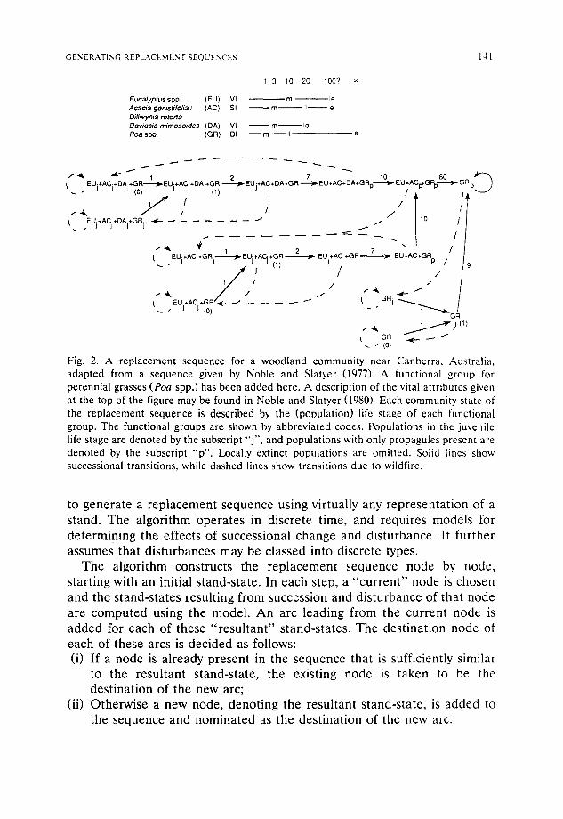
Fig. 2. A replacement sequence for a woodland community near Canberra. Australia, adapted from a sequence given by Noble and Slatyer (1977). A functional group for perennial grasses (Poa spp.) has been added here. A description of the vital attributes given at the top of the figure may be found in Noble and Slatyer (1980). Each community state of the replacement sequence is described by the (population) life stage of each functional group. The functional groups are shown by abbreviated codes. Populations in the juvenile life stage are denoted by the subscript "j", and populations with only propagules present are denoted by the subscript "p". Locally extinct populations are omitted. Solid lines show successional transitions, while dashed lines show transitions due to wildfire.

to generate a replacement sequence using virtually any representat ion of a stand. The algorithm operates in discrete time, and requires models for determining the effects of successional change and disturbance. It fur ther assumes that disturbances may be classed into discrete types.

The algorithm constructs the replacement sequence node by node, starting with an initial stand-state. In each step, a "cur ren t" node is chosen and the stand-states resulting from succession and disturbance of that node are computed using the model. An arc leading from the current node is added for each of these " resu l tan t" stand-states. The destination node of each of these arcs is decided as follows: (i) If a node is already present in the sequence that is sufficiently similar

to the resultant stand-state, the existing node is taken to be the destination of the new arc;

(ii) Otherwise a new node, denoting the resultant stand-state, is added to the sequence and nominated as the destination of the new arc.


The node to be processed in each step is chosen by finding the unpro- cessed node that can be reached from the starting node in minimum time. Termination of the algorithm occurs when either this minimum time exceeds a specified horizon or when all nodes on the sequence have been processed. As a result the algorithm takes a "breadth-first" approach: it determines all the possible trajectories from an initial stand that may occur within a time period before extending any of the trajectories beyond that time period. A breadth-first algorithm has the advantage that it can be terminated once all trajectories that are possible within a specified time have been computed; this is all that is necessary if a limited planning horizon is under consideration. We present the replacement sequence algorithm formally in the Appendix.

In keeping with the discrete nature of the algorithm, it is assumed that disturbances can be classified into discrete types. With disturbances of different types (such as wildfire and storm damage) this is natural enough; where a single disturbance type varies in intensity, it is assumed that disturbance events can be classified according to their severity.

The stand-state resulting from succession through a single time step will, in general, have a different age structure and therefore be distinguishable from the original stand-state. If all non-identical stand compositions were distinguished in the algorithm, all successional transitions would take place after one time step (see the stopping criterion in step 3.3 of the Appendix). Requiring exact equivalence of stands leads to all the possible dynamics predicted by a vegetation model being captured exactly in the replacement sequence, but it also produces sequences having very large numbers of nodes.

In order to reduce the number of nodes, we use a concept of "sufficient similarity" between two stand-states in the replacement sequence algorithm. (In the terms of Lewontin (1974), our concept of sufficient similarity corresponds to membership of the same tolerance set.) Two states that are sufficiently similar should (a) have broadly equivalent compositions, and (b) their age structures and (c) their propagule pools should resemble one another sufficiently so that their subsequent successional development and their responses to disturbances are not greatly different. As described formally in step 3.3 of the replacement sequence algorithm, each node of a sequence represents a series of stands: each stand in the series is sufficiently similar to the others, and a successional transition to another node is deemed to have occurred when the next potential member of the series is no longer sufficiently similar to the initial member.

It is apparent that the similarity relation between stand-states is of central importance to the replacement sequence algorithm. However, the definition of this relation depends upon the representation of a vegetation


stand, that is, upon the model of vegetation processes which is used. Accordingly we shall proceed with an example, generating replacement sequences with the FATE vegetation model of Moore and Noble (1990). It is important to note, however, that the replacement sequence algorithm itself does not depend on any particular vegetation model.

A DEFINITION OF SUFFICIENT SIMILARLY FOR THE FATE MODEL

The FATE model FATE (Functional Attributes in Terrestrial Ecosystems) is a generalised

model of the dynamics of vegetation. It deals with a stand of vegetation covering a "landscape unit" (Naveh and Liebermann, 1985), and uses discrete time steps which are assumed to be large enough to obscure seasonal or other short-term environmental change. The treatment in FATE of the processes controlling vegetation change is firmly within the "Gleasonian" research programme of such workers as Drury and Nisbet (1973) and Connell and Slatyer (1977), having been constructed by explicitly considering the biology of individual plants.

The concept of functional groups (Botkin, 1975) is used to simplify the description of vegetation. Functional groups are sets of plants that have common physiological, reproductive and life history characteristics where variation in each characteristic has specific, ecologically predictive value. The abundance of each population of established plants is measured on a scale of "absent", "low", "med ium" or "high". The size of each cohort in the population is also followed. The dynamics of two propagule pools are followed: propagules which are in innate or induced dormancy are referred to as the "dormant" pool, while propagules which can germinate if environmental conditions are suitable are treated as the "available" pool. (Not all functional groups have a dormant propagule pool.) The abundance of each pool is measured on a scale of "absent", "low" or "high".

The functioning of the individual plants of a functional group is modelled as three sets of processes: life history, responses to local environmental conditions and responses to disturbances. The submodel of life histories is based on that proposed in Harper (1977). Plants pass through a series of four discrete stages: propagules, "germinants" (newly recruited plants), immature and mature plants. Dispersal, recruitment, maturation and senescence are modelled in a simple fashion.

Interactions between plants are assumed to be dominated by interfer- ence competi t ion for a generalised resource. The competitive relationships between plants are expressed by ordering the plants into discrete strata; all plants of the same functional group and life stage are assumed to fall in the same stratum. The amount of the resource available to plants in a stratum


is a function of the total abundance of plants in superior strata. If the plants of a life stage cannot tolerate the current resource level in their stratum, then they all die.

The effect of a disturbance type within FATE is modelled by specifying the proportion of plants in each life stage that are unaffected by the disturbance, killed outright, or that survive to resprout. All resprouting plants in a life stage are assumed to be set back to a single "effective" age, which may be either before or after the age of first reproduction.

Readers are referred to Moore and Noble (1990) for further detail about FATE.

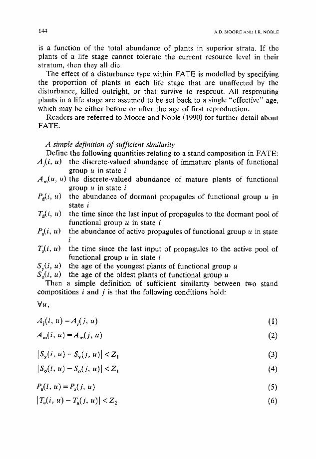
A simple definition of sufficient similarity Define the following quantities relating to a stand composition in FATE:

Aj(i, u) the discrete-valued abundance of immature plants of functional group u in state i

Am(U , u)the discrete-valued abundance of mature plants of functional group u in state i

Pd(i, U) the abundance of dormant propagules of functional group u in state i

Td(i, u) the time since the last input of propagules to the dormant pool of functional group u in state i

Pa(i, u) the abundance of active propagules of functional group u in state i

Ta(i, u) the time since the last input of propagules to the active pool of functional group u in state i

Sy(i, u) the age of the youngest plants of functional group u So(i, u) the age of the oldest plants of functional group u

Then a simple definition of sufficient similarity between two stand compositions i and j is that the following conditions hold:

VU,

A j ( i , u )=Ai ( j ,u )

Am(i ,u)=Zrn(j ,u)

(1)

(e)

[Sy(i, u)- sy(j, u)[ <z,

[So(i,u)-So(j,u)l<zl

(3) (4)

Pa(i, u)=Pa(j, u)

[Ta(i,u)-Ta(j,u)l<z2 (5)

(6)


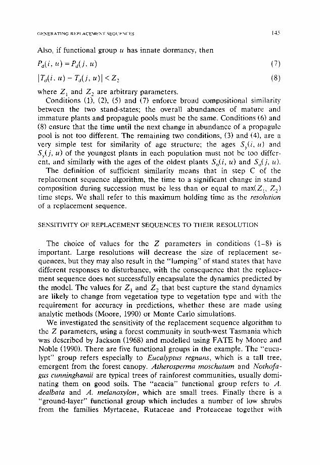
Also, if functional group u has innate dormancy, then

Pd( i, u)= Pd( J, 11) (7)

[Td(i, u ) - Td(j, u)l < Z 2 (8)

where Z~ and Z 2 are arbitrary parameters. Conditions (1), (2), (5) and (7) enforce broad compositional similarity

between the two stand-states; the overall abundances of mature and immature plants and propagule pools must be the same. Conditions (6) and (8) ensure that the time until the next change in abundance of a propagule pool is not too different. The remaining two conditions, (3) and (4), are a very simple test for similarity of age structure; the a g e s Sy(i, tt) and Sy(j, U) of the youngest plants in each population must not be too different, and similarly with the ages of the oldest plants So(i, u) and So(j, ll).

The definition of sufficient similarity means that in step C of the replacement sequence algorithm, the time to a significant change in stand composition during succession must be less than or equal to max(Z~, Z 2) time steps. We shall refer to this maximum holding time as the resolution of a replacement sequence.

SENSITIVITY OF REPLACEMENT SEQUENCES TO THEIR RESOLUTION

The choice of values for the Z parameters in conditions (1-8) is important. Large resolutions will decrease the size of replacement sequences, but they may also result in the " lumping" of stand states that have different responses to disturbance, with the consequence that the replacement sequence does not successfully encapsulate the dynamics predicted by the model. The values for Z~ and Z 2 that best capture the stand dynamics are likely to change from vegetation type to vegetation type and with the requirement for accuracy in predictions, whether these are made using analytic methods (Moore, 1990) or Monte Carlo simulations.

We investigated the sensitivity of the replacement sequence algorithm to the Z parameters, using a forest community in south-west Tasmania which was described by Jackson (1968) and modelled using FATE by Moore and Noble (1990). There are five functional groups in the example. The "eucalypt" group refers especially to Eucalyptus regnans, which is a tall tree, emergent from the forest canopy. Atherosperma moschatum and Nothofa- gus cunninghamii are typical trees of rainforest communities, usually domi- nating them on good soils. The "acacia" functional group refers to A. dealbata and A. melanoxylon, which are small trees. Finally there is a "ground-layer" functional group which includes a number of low shrubs from the families Myrtaceae, Rutaceae and Proteaceae together with


sedges and (on better soils) tussock grasses. A FATE parameter set is given in Moore and Noble (1990). We have generated replacement sequences using only one disturbance type, namely a severe wildfire. Using more than one disturbance type results in large but not insurmountable increases in the size of the replacement sequences.

SensititJity analysis: methods We chose an initial stand-state with all functional groups present only as

propagules (i.e. immediately after a wildfire) and ran a series of 10000 FATE simulations from this starting point. A successional step of one year was performed in each epoch. We then classified the stand-state resulting from the successional step by grouping it with all other stand-states in which the broad composition of each functional group's population was the same. For this purpose we classed populations as being in one of seven states: (a) Mature plants present in high abundance (b) Mature plants present in medium abundance (c) Mature plants present in low abundance (d) Mature plants absent, immature plants present (e) Mature and immature plants both absent, propagules present in high

abundance in either the active or the dormant pool (f) Mature and immature plants both absent, propagules present in low

abundance in at least one pool (g) Locally extinct

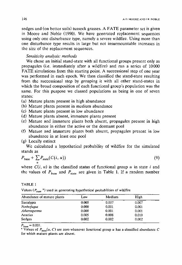
We calculated a hypothetical probability of wildfire for the simulated stands as

Pbase + EPstate(C( i, it)) (9) u

where C(i, u) is the classified status of functional group u in state i and the values of Phase and Pstate a r e given in Table 1. If a random number

TABLE 1

Values (Pstate a) used in generating hypothetical probabilities of wildfire

Abundance of mature plants Low Medium High Eucalypts 0.005 0.007 0.007 Nothofagus 0.000 0.001 0.001 A therosperma 0.000 0.001 0.001 Acacias 0.005 0.008 0.010 Sedges 0.002 0.002 0.002

Pbase = 0 . 0 0 1 . a Values of Pstate(u, C) are zero whenever functional group u has a classified abundance C for which mature plants are absent.

G E N E R A T I N G R E P L A C E M E N T SEQUENCES [ 4 7

from U(0, 1) was less than or equal to the probability of fire, a disturbance event was then simulated using FATE.

The states occupied at each of the epochs 25, 50, 100, 1000 and 2500 years were recorded for each trial. From these results, the probabilities that the stand would be in each of the groups of states developed above at each of the foregoing epochs were calculated. The final result for each resolution was therefore a two-way table (epochs by node-groupings) of probabilities of occurrence. This procedure enabled us to establish the " t rue" probabilities, i.e. those predicted by FATE, of each state-grouping at each time horizon. Since the objective of the replacement sequence algorithm is model simplification, we assessed the adequacy of the predictions of replacement sequences against these " t rue" probabilities. We chose the five epochs given above so as to study both the long-term behaviour of the replacement sequences, but also to place an emphasis on their adequacy at time horizons which are typically considered in management of natural vegetation.

We generated replacement sequences for the forest from the same initial community as in the FATE simulations, using various values for Z~ and Z 2

(all combinations of Z 1 = 5, 10, and 20 years with Z 2 = 5, 10 and 20 years, and also Z1 = 30, Z 2 = 10 years). We classified the nodes of each sequence using the same method as in the FATE simulations, and calculated the probability of fire at each node using Eq. (9). We then carried out a series of 10000 Monte Carlo trials with each replacement sequence. In each trial the trajectory of the stand through the sequence from the initial node was simulated. At each epoch a random number was compared against the probability of fire in the current node. If the random number was less than or equal to the probability of fire, then the current node was set to that resulting from fire, and the time since entry to the current node was set to zero. Otherwise, the time since entry to the current state was incremented; if it equalled the time required for a successional transition, then the current state was set to the state resulting from succession, and the time since entry reset to zero. In each trial, we recorded the state occupied at the same epochs as in the FATE simulations; from these records we calculated two-way tables of probabilities of occurrence, which could ulti- mately be compared against the probabilities predicted by FATE.

Note that since we knew the core matrix of the semi-Markov process corresponding to each replacement sequence (see Moore, 1990), we could have carried out these simulations rather faster by taking a single random number for each state occupancy rather than for each epoch. The somewhat slower approach that we actually used has the twin advantages of simplicity and of not requiring analytic effort, which for more complex disturbance probability functions could prove to be considerable.

148 A.D. M O O R E A N D I.R. N O B L E

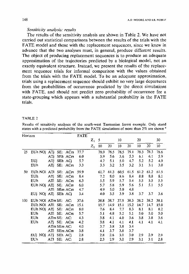
Sensitit:ity analysis: results T h e resu l t s o f the sensi t ivi ty analys is a re shown in T a b l e 2. W e have not

c a r r i ed ou t s ta t i s t ica l c o m p a r i s o n s b e t w e e n the resu l t s o f the tr ials wi th the F A T E m o d e l a n d those wi th the r e p l a c e m e n t s e q u e n c e s , s ince we k n e w in

a d v a n c e t ha t the two ana lyses mus t , in gene ra l , p r o d u c e d i f f e ren t resul ts .

T h e ob jec t o f p r o d u c i n g r e p l a c e m e n t s e q u e n c e s is to p r o d u c e an a d e q u a t e a p p r o x i m a t i o n o f the t r a j ec to r i e s p r e d i c t e d by a b io logica l m o d e l , not an exact ly e q u i v a l e n t s t ruc tu re . I n s t ead , we p r e s e n t the resu l t s o f the r e p l a c e -

m e n t s e q u e n c e t r ia ls for i n f o r m a l c o m p a r i s o n with the va lues o b t a i n e d f r o m the tr ials wi th the F A T E m o d e l . T o be an a d e q u a t e a p p r o x i m a t i o n ,

trials us ing a r e p l a c e m e n t s e q u e n c e s h o u l d exhibi t no very la rge d e p a r t u r e s f r o m the p robab i l i t i e s o f o c c u r r e n c e p r e d i c t e d by the d i rec t s imula t ions

wi th F A T E , a n d shou ld not p r ed i c t z e r o p robab i l i t y o f o c c u r r e n c e for a s t a t e - g r o u p i n g which a p p e a r s wi th a subs t an t i a l p robab i l i t y in the F A T E

trials.

TABLE 2

Results of sensitivity analyses of the south-west Tasmanian forest example. Only stand states with a predicted probability from the FATE simulations of more than 2% are shown a

Horizon FATE Z 1 5

Z 2 10

10 20 30

20 10 20 10 20 10

25

50

100

EUhNOj ATj SE: ACm 77.7 78.9 78.5 78.5 79.1 78.3 78.3 78.6 ATj SEh ACm 6.0 5.9 5.6 5.6 5.3 6.1 6.1 5.9

EUj ATj SEh ACj 5.7 4.7 5.1 5.0 4.7 5.2 5.2 4.9 EUh ATj SE: ACm 3.3 3.3 3.2 3.5 3.2 3.1 3.1 3.0

EUhNOI ATI SE: ACm 59.9 61.7 61.3 60.5 61.5 61.2 61.2 61.5 EUh ATj SE: ACre 8.4 7.2 8.0 8.6 8.4 8.8 8.8 8.1 EUh AT1 SE: ACm 6.3 5.5 5.9 5.7 5.4 5.5 5.5 5.5 EUhNOj ATj SE: ACm 6.0 5.7 5.8 5.9 5.6 5.1 5.1 5.5

ATI SEm ACm 4.7 4.9 5.0 5.0 4.8 EUj NOj ATj SEh ACj 3.4 4.0 3.5 3.9 3.8 3.7 3.7 3.6

EUhNO1 ATmSE: AC: 37.6 38.8 38.7 37.9 38.3 38.2 38.2 38.1 EUh NOI ATI SE: ACre 15.1 15.7 14.9 15.1 15.2 14.7 14.7 15.0 EUhNOj ATj SE: ACm 8.0 7.6 8.4 7.7 8.3 8.1 8.1 8.2 EUh ATI SE: ACm 5.7 5.1 4.8 5.2 5.1 5.0 5.0 5.0 EUh ATm SE: AC: 4.3 3.8 4.1 4.0 3.6 3.8 3.8 3.6 EUh ATj SE: ACm 4.2 3.8 4.1 4.1 4.1 4.1 4.1 4.1

ATm SEm AC: 4.0 3.7 3.8 3.8 3.4 ATI SEm ACm 3.8 4.1 3.7 3.8 3.7

EUj NOj ATj SEh ACj 2.8 2.8 2.6 3.0 3.0 2.9 2.9 2.9 EUh ATI SE: AC: 2.8 2.3 2.9 3.0 2.9 3.1 3.1 2.8

GENERATING REPLACEMENT SEQUENCES

TABLE 2 (continued)

149

Horizon FATE Z l 5 10 20 30

Z: 10 20 10 20 10 20 10

1000

2500

ATh SE: 20.3 20.7 20.3 20.3 20.1 2.9 2.9 2.9 ATI SEh 5.1 4.9 5.2 5.1 5.2 ATm SEm 4.9 5.3 4.9 4.9 4.8 ATj SEh 4.2 4.2 4.3 3.9 4.1 10.9 10.9 11.0

EUh ATm SE: 3.9 3.8 3.7 3.8 4.1 4.0 4.0 3.6 ATm SEm AC: 3.6 3.7 3.6 3.9 3.4 AT1 SEm ACm 3.5 3.1 3.3 3.7 3.5

EUh ATI SE: 3.5 3.3 3.4 3.6 3.4 3.3 3.3 3.4 EUh ATm SE: AC: 3.2 3.3 3.0 2.9 3.2 2.8 2.8 3.3 EUh ATh SE: 2.8 2.7 2.6 2.6 2.7 2.7 2.7 2.7 EUh ATI SE: ACm 2.5 2.7 2.7 2.5 2.4 2.6 2.6 2.6 EUh ATm SE: AC. 2.2 2.4 2.2 2.1 2.3 2.3 2.3 2.3

NOh ATh SE: 2.2 2.3 2.3 2.4 2.2 1.8 1.8 2.0 ATh SE: AC. 2.0 2.1 2.3 2.3 2.2

ATh SE: 40.4 40.7 40.5 41.5 40.7 2.1 2.1 2.0 ATm SEm 14.2 13.8 14.1 14.2 13.9 ATI SEh 12.0 12.4 12.3 12.1 12.0 ATj SEh 10.0 9.9 10.0 8.8 9.8 31.9 31.9 31.4 ATj SEm 2.8 2.8 2.9 3.2 3.2 5.9 5.9 6.3 ATI SEm 2.3 2.3 2.3 2.4 2.5

EUh ATm SE: 2.1 2.4 2.4 2.3 2.2 2.1 2.1 2.2

a Probabilities are given as percentages. Blank entries indicate that a replacement sequence predicted a zero probability of occurrence for a state-grouping. Codes used to describe state-groupings are: EU = eucalypts NO = Nothofagus AT = Atherosperma AC = Acacia SE = "sedges"

h = high abundance of adults m = medium abundance of adults 1 -- low abundance of adults j = immature plants only present : = only propagules present (in high abundance) • = only propagules present (in low abundance).

Assuming that each trial may be equated with a Bernoulli trial, then the standard deviation of the estimate of a probability P given 10000 trials would be given by ~/10000 P(1 - P ) / 1 0 0 0 0 . When P - - 5 0 % , the standard deviation would therefore be 0.5%, while when P = 5%, it would be 0.22%. The true uncertainty may be somewhat higher, as the probabilities of different states occurring are not independent, but this order of uncertainty in Table 2 is entirely acceptable•

A close match (all deviations less than 2%) was maintained at resolutions up to Z 1 = 10, Z 2 = 20. At coarser resolutions, two stand composi-

1 5 0 A.D. M O O R E AND I.R. NOBLE

Years since fire:

5

11

21

23

25

26

31

High

High Low • • o •

Athero. Acacia "Sedges" m 0-4 1 2-3 h 2-4

h 4

High

I ~o~ h .. o .

At hero. Acacia "Sedges" m 0-10 1 8-9 h 8-10

h 10

High

I ~o~ h .. o .

Athero. Acacia "Sedges" m 0-20 i 18-19 h 18-19

h 20

High iHigh ~ ~o

l ~i~ .. o ~ .. Athero. Acacia "Sedges" m 0-22 1 20-21 h 0

h 22 ! •

IHigh I" ~°~w ~ .. o • ~

Athero. Acacia "Sedges" m 0-24 1 22-23 h 1-2

h 24 i |

High

I ~o ~w~h .. o .

Athero. Acacia "Sedges" m 0-25 i 23-24 h 2-3

h 25 | |

H gh IHigh ~

I ~o~ ~ . o . Athero. Acacia "Sedges" m 0-30 1 28-29 h 6-8

h 30

GENERATING REPLACEMENT SEQUENCES 15 l

TABLE 3

Numbers of nodes in replacement sequences generated by varying the values of the parameters Z~ and Z 2

South-west Tasmania Eucalypt woodland

Z 2 Z2

Z 1 5 10 20 Z l 5 10 20

5 1884 907 757 5 17770 12076 8999 10 1026 595 476 10 4928 3065 1949 20 799 3881 230 20 2689 1139 789 30 366

tions on the same success ional pa thway satisfied the similarity re la t ion (Fig.

3): as a c o n s e q u e n c e , a spur ious cyclic success ion a p p e a r e d in the replacement sequence , and the a lgor i thm failed.

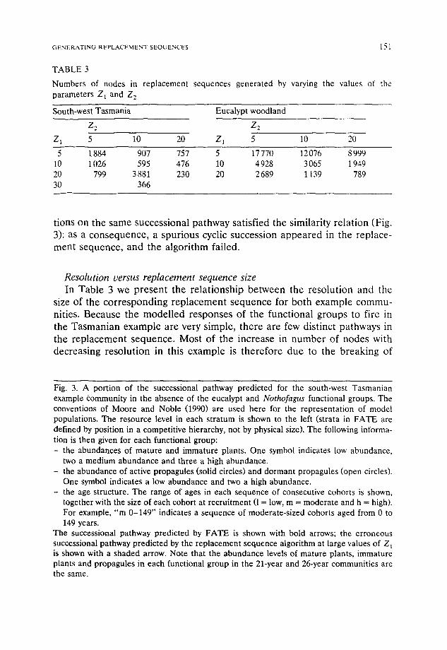
Resolution versus replacement sequence size In Tab le 3 we p r e sen t the re la t ionsh ip be tween the reso lu t ion and the

size of the c o r r e s p o n d i n g r e p l a c e m e n t s e q u e n c e for bo th example c o m m u -

nities. Because the mode l l ed responses of the func t iona l g roups to fire in

the T a s m a n i a n example are very simple, the re are few dist inct pa thways in

the r e p l a c e m e n t sequence . Most o f the increase in n u m b e r o f nodes with

decreas ing reso lu t ion in this example is t he r e fo re due to the b reak ing of

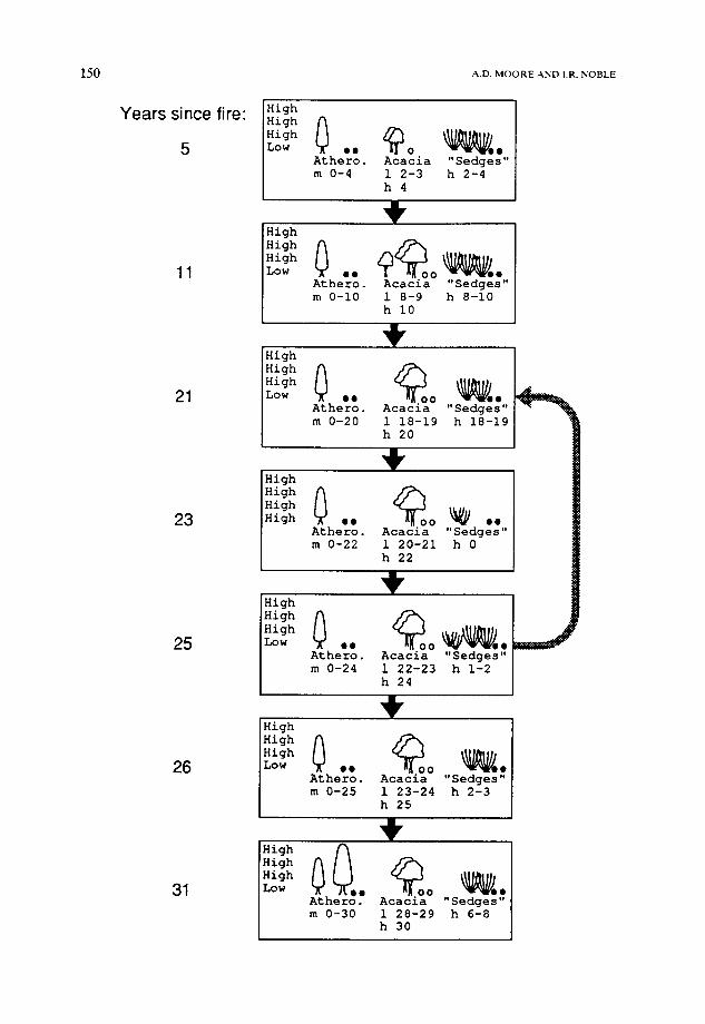
Fig. 3. A portion of the successional pathway predicted for the south-west Tasmanian example community in the absence of the eucalypt and Nothofagus functional groups. The conventions of Moore and Noble (1990) are used here for the representation of model populations. The resource level in each stratum is shown to the left (strata in FATE are defined by position in a competitive hierarchy, not by physical size). The following informa- tion is then given for each functional group: - the abundances of mature and immature plants. One symbol indicates low abundance,

two a medium abundance and three a high abundance. - the abundance of active propagules (solid circles) and dormant propagules (open circles).

One symbol indicates a low abundance and two a high abundance. - the age structure. The range of ages in each sequence of consecutive cohorts is shown,

together with the size of each cohort at recruitment (1 = low, m = moderate and h = high). For example, "m 0-149" indicates a sequence of moderate-sized cohorts aged from 0 to 149 years.

The successional pathway predicted by FATE is shown with bold arrows; the erroneous successional pathway predicted by the replacement sequence algorithm at large values of Z~ is shown with a shaded arrow. Note that the abundance levels of mature plants, immature plants and propagules in each functional group in the 21-year and 26-year communities are the same.

152 A.D. MOORE AND I.R. NOBLE

pathways into smaller segments; as a result the size of the sequence is more or less inversely proportional to the resolution.

For comparison, we have included in Table 3 results from a similar sensitivity analysis carried out on a eucalypt woodland which was also modelled using FATE by Moore and Noble (1990). Because some plants in this community remain unaffected by fire, it exhibits a much greater variety of possible stand compositions. As a consequence the replacement sequences for the eucalypt woodland have many more nodes for a given resolution. Each step in a successional sequence in the eucalypt woodland gives rise to a slightly different stand after a fire: as the resolution decreases, more of these possibilities are sampled, and so the number of distinct pathways in the sequence increases as well as the number of nodes required in each pathway. Halving the resolution therefore results in a typical increase in the size of the replacement sequence by a factor of about three.

DISCUSSION

The replacement sequence algorithm described above performs well in capturing the stand dynamics predicted by the FATE model in the south- west Tasmanian forest community; the dynamics of the FATE model could be adequately summarised in a replacement sequence of a few hundred nodes (Table 3). A modification of the algorithm that requires nonzero intervals between disturbance events results in significantly smaller replacement sequences (Moore, 1989). This modification is appropriate in the case where disturbances cannot follow immediately upon one another, such as when a fire removes sufficient fuel to make the spread of further fires impossible for a time.

We computed the replacement sequences on a microcomputer with an Intel 80486 processor, since if this were not feasible, the practical utility of analyses involving FATE replacement sequences would be questionable. The largest sequence in Table 3 took just over an hour to compute. The generation of replacement sequences is therefore entirely feasible even where complex population age structures appear as a result of disturbance history.

In practice a certain amount of trial and error is likely to be required in setting the values of the parameters Z 1 and Zz. It should be possible to develop heuristic procedures for estimating the adequacy of the predictions made by a replacement sequence relative to the FATE model, using one or more hypothetical disturbance regimes in the manner described above; such heuristic procedures would allow the process of finding suitable values of the arbitrary parameters to be semi-automated.


As discussed in the Introduction, replacement sequences provide a means of very fast simulation of vegetation dynamics. Once a sequence has been derived, the process of simulation is reduced to (1) determining which, if any, disturbance occurs and then either (2a) incrementing the time since the process entered its current state or (2b) performing a table lookup to identity the destination node of a transition. The first of these steps takes the bulk of the time. In the sensitivity analyses, the Monte Carlo simulations using replacement sequences ran about two orders of magnitude faster than the simulations which used the FATE model di- rectly. This improvement in speed of simulation makes landscape-level simulations of the kind proposed in the Introduction a practical possibility on personal computers.

When taken in conjunction with a model for the probabilities of disturbance, the replacement sequences given by the above algorithm define a semi-Markov process for a vegetation stand (Moore, 1990). A number of interesting properties, such as mean times to extinction of vulnerable species, can be derived analytically within the semi-Markov process frame- work. It is possible to carry out the analyses of Moore (1990) on graphs of the magnitude described here; the calculations would, however, require a substantial computing effort by present-day standards.

ACKNOWLEDGEMENTS

This work was carried out while one of us (ADM) was in receipt of an Australian Commonwealth Postgraduate Award. Dr D.G. Green provided useful discussion while the ideas presented here were being developed.

REFERENCES

Bollob~s, B., 1979. Graph Theory: an Introductory Course. Springer-Verlag, New York, NY. Botkin, D.B., 1975. Functional groups of organisms in model ecosystems. In: S.A. Levin

(Editor), Ecosystem Analysis and Prediction. Society of Industrial and Applied Mathe- matics, Philadelphia, pp. 98-102.

Clark, J.S., 1989. Ecological disturbance as a renewal process: theory and application to fire history. Oikos, 56: 17-30.

Connell, J.H. and Slatyer, R.O., 1977. Mechanisms of succession in natural communities and their role in community stability and organisation. Am. Nat., 111: 1119-1144.

Drury, W.H. and Nisbet, I.C., 1973. Succession. J. Arnold Arbor. Harv. Univ., 54: 331-368. Harper, J.L., 1977. Population Biology of Plants. Academic Press, London, 892 pp. Heinselman, M.L., 1981. Fire and succession in the conifer forests of northern North

America. In: D.C. West, H.H. Shugart and D.B. Botkin (Editors), Forest Succession: Concepts and Application. Springer-Verlag, New York, NY, pp. 374-405.

154 a . o . M O O R E A N D I.R. NOBLE

Hogeweg, P., Hesper, B., van Shaik, C.P. and Beeftink, W.G., 1985. Patterns in vegetation succession, an ecomorphological study. In: J. White (Editor), The Population Structure of Vegetation. Dr W. Junk, Dordrecht, Netherlands, pp. 637-666.

Horn, H.S., 1975. Markovian properties of forest succession. In: M.L. Cody and J.M. Diamond (Editors), Ecology and Evolution of Communities. Harvard University Press, Cambridge, MA, pp. 196-211.

Jackson, W.D., 1968. Fire, air, water and earth - an elemental ecology of Tasmania. Proc. Ecol. Soc. Aust., 3: 9-16.

Lewontin, R.C., 1974. The Genetic Basis of Evolutionary Change. Columbia University Press, New York, NY.

Moore, A.D., 1989. Discrete predictive models of vegetation dynamics. Unpublished Ph.D. thesis, Australian National University, Canberra.

Moore, A.D., 1990. The semi-Markov process: a useful tool in the analysis of vegetation dynamics for management. J. Environ. Manage., 30: 111-130.

Moore, A.D. and Noble, I.R., 1990. An individualistic model of vegetation dynamics. J. Environ. Manage., 31: 61-81.

Naveh, Z. and Liebermann, A.S., 1985. Landscape Ecology. Springer-Verlag, New York, NY.

Noble, I.R. and Slatyer, R.O., 1977. Post-fire succession of plants in Mediterranean ecosystems. In: H.A. Mooney and C.E. Conrad (Editors), Proceedings of the Symposium on the Environmental Consequences of Fire and Fuel Management in Mediterranean Ecosystems. General Technical Report WO-3. U.S.DA Forest Service, Washington, DC, pp. 27-36.

Noble, I.R. and Slatyer, R.O., 1980. The use of vital attributes to predict successional changes in plant communities subject to recurrent disturbances. Vegetatio, 43: 5-21.

Tilman, D., 1988. Plant Strategies and the Dynamics and Structure of Plant Communities. Princeton University Press, Princeton, N J, 360 pp.

Usher, M.B., 1981. Modelling ecological succession, with particular reference to Markovian models. Vegetatio, 46: 11-18.

Van Hulst, R., 1987. Invasion models of vegetation dynamics. Vegetatio, 69: 123-131. White, P.S., 1979. Pattern, process and natural disturbance in vegetation. Bot. Rev., 45:

229-299.

APPENDIX

Formal definition o f a replacement sequence, and specification o f the replacement sequence algorithm

Definition o f a replacement sequence. C o n s i d e r the g r a p h R(V, E), wi th

V = {i" i is a s t a n d - s t a t e tha t is phys ica l ly poss ib le in a g iven v e g e t a t i o n stand}.

T h e n R is a r e p l a c e m e n t s e q u e n c e if and on ly if (1) Vi ~ V, 3s(i) : (i, s(i)) ~ E (2) V(i,j) ~ E, e i t h e r j = s(i) or the s t a n d - s t a t e j r e su l t s f r o m the i m p a c t o f

d i s t u r b a n c e o r o f a d i spe r sa l e v e n t u p o n s t a n d - s t a t e i.

GENERATING REPLACEMENT SEQUENCES | 5 5

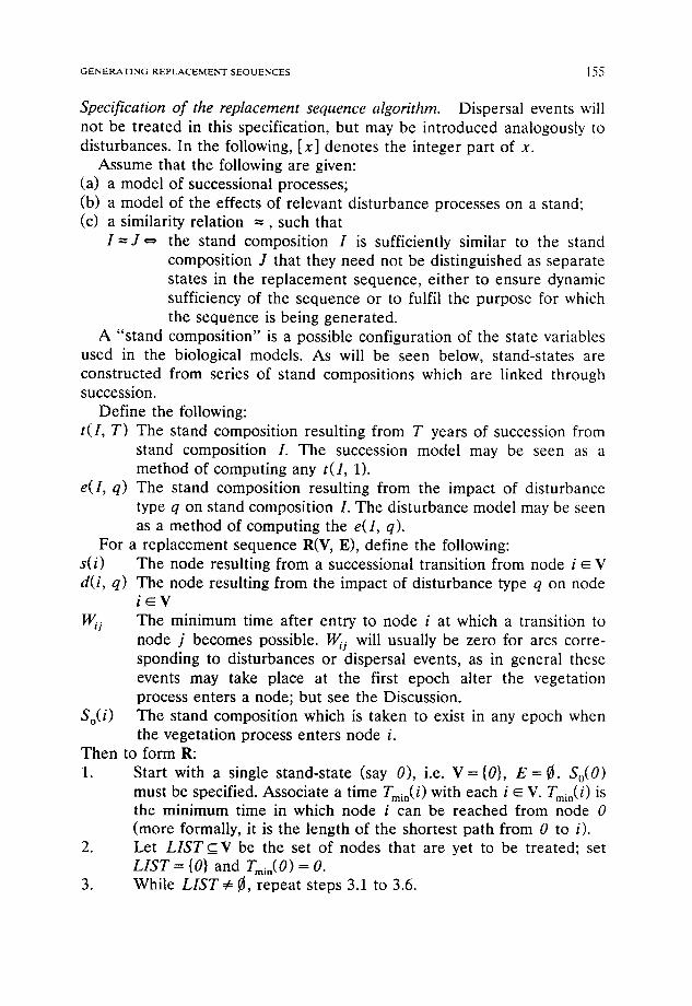
Specification of the replacement sequence algorithm. Dispersal events will not be t reated in this specification, but may be introduced analogously to disturbances. In the following, Ix] denotes the integer part of x.

Assume that the following are given: (a) a model of successional processes; (b) a model of the effects of relevant disturbance processes on a stand; (c) a similarity relation = , such that

I - - - J ,~ the stand composition I is sufficiently similar to the stand composition J that they need not be distinguished as separate states in the replacement sequence, ei ther to ensure dynamic sufficiency of the sequence or to fulfil the purpose for which the sequence is being generated.

A "stand composition" is a possible configuration of the state variables used in the biological models. As will be seen below, stand-states are constructed from series of stand compositions which are linked through succession.

Define the following: t(I, T) The stand composition resulting from T years of succession from

stand composition I. The succession model may be seen as a method of computing any t(I, 1).

e(I, q) The stand composition resulting from the impact of disturbance type q on stand composition I. The disturbance model may be seen as a method of computing the e(I, q).

For a replacement sequence R(V, E), define the following: s(i) The node resulting from a successional transition from node i ~ V d(i, q) The node resulting from the impact of disturbance type q on node

i ~ V W/j The minimum time after entry to node i at which a transition to

node j becomes possible. W 0. will usually be zero for arcs corresponding to disturbances or dispersal events, as in general these events may take place at the first epoch alter the vegetation process enters a node; but see the Discussion.

So(i) The stand composition which is taken to exist in any epoch when the vegetation process enters node i.

Then to form R: 1. Start with a single stand-state (say 0), i.e. V = {0}, E = ~. So(O)

must be specified. Associate a time Train(i) with each i ~ V. Train(i) is the minimum time in which node i can be reached from node 0 (more formally, it is the length of the shortest path from 0 to i).

2. Let LIST__.V be the set of nodes that are yet to be treated; set LIST = {0} and Train(0) = 0.

3. While LIST~ ~J, repeat steps 3.1 to 3.6.

156 A.D. MOORE AND I.R. NOBLE

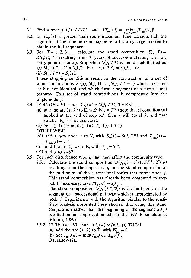
3.1. Find a node j: (j ~ LIST) and (Train(j) = min [Tmi,(k)]). 1~ ~ L I S T

3.2. IF Trnin(j) is greater than some maximum time horizon, halt the algorithm. (The time horizon may be set arbitrarily large in order to obtain the full sequence).

3.3. For T = 1, 2, 3 . . . . calculate the stand composition S(j, T) = t(So(J), T) resulting from T years of succession starting with the entry-point of node j. Stop when S(j, T*) is found such that either (i) S(j, T* - 1) = So(j) but S(j, T * ) , So(j), or

(ii) S(j, T* )= So(j). These stopping conditions result in the construction of a set of stand compositions So(j), S(j, 1) , . . . ,S ( j , T * - 1 ) w h i c h are similar but not identical, and which form a segment of a successional pathway. This set of stand compositions is compressed into the single node j.

3.4. I F : l k : ( k ~ V ) and ( S o ( k ) = S ( j , T * ) ) T H E N (a) add the arc (j, k) to E, with l, Vjk = T* (note that if condition (ii)

applied at the end of step 3.3, then j will equal k, and that strictly Wj.j = oo in this case).

(b) Set Tmi,(k) = min(T~in(k), Tmi.(j) + T*). OTHERWISE (a') add a new node s to V, with So(s)= S(j, T*) and Tmi,(s)=

Tmin( j ) + T *

(b') add the arc (j, s) to E, with Wj.s = T* (c') add s to LIST.

3.5. For each disturbance type q that may affect the community type: 3.5.1. Calculate the stand composition D(j, q) = e(S(j, [T*/2]), q)

resulting from the impact of q on the stand composition at the mid-point of the successional series that forms node j. This stand composition has already been computed in step 3.3. If necessary, take S(j, O)= So(j). The stand composition S(j, [T*/2]) is the mid-point of the segment of a successional pathway which is approximated by node j. Experiments with the algorithm similar to the sensitivity analysis presented here showed that using this stand composition rather than the beginning of the segment So(J) resulted in an improved match to the FATE simulations (Moore, 1989).

3.5.2. IF Elk :(k ~V) and (So(k) --'D(j, q)) THEN (a) add the arc (j, k) to E, with W~, k = 0 (b) Set Tmi,(k)= min(Tmin(k), Tmi,(j)). OTHERWISE

G E N E R A T I N G R E P L A C E M E N T S E Q U E N C E S 157

3.6.

(a') add a new node d to V with So(d)= D(j, q) and Tram (d) = Train(j), since in general a disturbance might hap- pen immediately after entry to state j.

(b') add the arc (j , d) to E, with Wj.,t = 0. (c ') add d to LIST.

Remove j from LIST.

Documents

Automatic model simplification: the generation of replacement sequences and their use in vegetation modelling