Automatic dynamics simpliﬁcation in Fast Multipole Method ...webpages.iust.ac.ir/mozayani/Papers-pdf/razavi-supercomputing2012.pdf · Automatic dynamics simpliﬁcation in Fast

J Supercomput (2012) 62:1537–1559DOI 10.1007/s11227-012-0816-4

Automatic dynamics simplification in Fast MultipoleMethod: application to large flocking systems

Seyed Naser Razavi · Nicolas Gaud ·Abderrafiâa Koukam · Nasser Mozayani

Published online: 16 August 2012© Springer Science+Business Media, LLC 2012

Abstract This paper introduces a novel framework with the ability to adjust simula-tion’s accuracy level dynamically for simplifying the dynamics computation of largeparticle systems to improve simulation speed. Our new approach follows the overallstructure of the well-known Fast Multipole Method (FMM) coming from computa-tional physics. The main difference is that another level of simplification has been in-troduced by combining the concept of motion levels of detail from computer graphicswith the FMM. This enables us to have more control on the FMM execution time andthus to trade accuracy for efficiency whenever possible. At each simulation cycle,the motion levels of detail are updated and the appropriate ones are chosen adap-tively to reduce computational costs. The proposed framework has been tested on thesimulation of a large dynamical flocking system. The preliminary results show a sig-nificant complexity reduction without any remarkable loss in the visual appearanceof the simulation, indicating the potential use of the proposed model in more realisticsituations such as crowd simulation.

S.N. Razavi (�) · N. Gaud · A. Koukam · N. MozayaniSCOMAS Lab, Department of Computer Engineering, Iran University of Science and Technology,Tehran, Irane-mail: [email protected]

N. Mozayanie-mail: [email protected]

S.N. Razavi · N. Gaud · A. Koukam · N. MozayaniMulti-Agent Systems and Applications Group, Laboratoire Systèmes et Transports, UTBM,90010 Belfort, Franceurl: http://www.multiagent.fr

N. Gaude-mail: [email protected]

A. Koukame-mail: [email protected]

mailto:[email protected]


http://www.multiagent.fr



1538 S.N. Razavi et al.

Keywords Dynamics simplification · Fast Multipole Method · Multi-agent basedsimulation · Flocking

1 Introduction

In recent years, simulation of large complex systems has attracted many researchersfrom a growing number of diverse areas and it is appealing to more and more scien-tific domains such as sociology, biology, physics, chemistry, ecology, economy, etc.In many cases, simulation of a complex system requires to compute all the pairwiseinteractions between particles. Assuming N particles, there are totally O(N2) pair-wise interactions which result in a computational cost of O(N2), which is clearlyprohibitive for large values of N . That is, computing the pairwise interactions be-tween particles is the main bottleneck in the simulation of many large complex sys-tems. The challenge of efficiently carrying out the related calculations is generallyknown as the N -body problem.

Among several attempts done to reduce this complexity, we can refer to the FastMultipole Method (FMM) as one of the most successful ones. The FMM is an al-gorithm originally proposed by Rokhlin [1] as a fast scheme for accelerating thenumerical solution of the Laplace equation in two dimensions. It was further im-proved by Greengard and Rokhlin when it was applied to particle simulations [2, 3],and has since been identified as one of the ten most important algorithmic contri-butions in the 20th century [4]. It evaluates pairwise interactions in large ensemblesof N particles in O(N logN ) or even O(N ) time. This is an improvement over theO(N2) time required by direct methods. Since the invention of the FMM, it has beenwidely used for problems arising in diverse areas (molecular dynamics, astrophysics,acoustics, fluid mechanics, scattered data interpolation, etc.) because of its ability toachieve linear time and memory in computing dense matrix vector products to a fixeduser-prescribed accuracy ε.

The main idea used in the FMM is that it considers well-separated or “far-away”groups of particles as one particle. To implement this idea, it imposes a hierarchicalspatial partitioning structure on the computational domains. Based on our previousworks [5, 6], we believe that we can take advantage of this hierarchical structure inseveral ways to further reduce the overall computational cost, of course at the ex-pense of accuracy. In particular, the main goal of this work is to combine the FMMwith simulation acceleration techniques from computer graphics to improve simula-tion speed for N -body simulations while controlling the desired level of accuracy.Simulation acceleration techniques including motion levels of detail often need somehierarchical partitioning of the computational space for dynamics simplification andfortunately this is available in the FMM.

In fact, the FMM algorithm clusters particles into hierarchical groups based ontheir relative positions in the domain, but it deals with each particle in the same groupseparately, computing a different potential for every particle in the group resulting indifferent behaviors for different particles in the same group. However, particle sys-tems generally exhibit a high level spatial coherence, meaning nearby particles be-have in approximately the same way. Therefore, the main idea is that we can compute

Automatic dynamics simplification in Fast Multipole Method 1539

only one approximated behavior for a group, then making all particles in the group tofollow the same behavior. This is achieved by replacing particles inside a cluster byone weighted particle and approximating the motion models of those particles in theforce computations during FMM.

Although there exist simulation acceleration techniques such as given in [7–10],there is no known algorithm for the automatic dynamics simplification of complexphysical or biological systems especially when all the pairwise interactions betweenparticles are needed. In this paper, we limit the scope of our investigation to particlesystems as a first step towards the design of automatic dynamics simplification. Par-ticle systems are commonly used in computer graphics, physically based modeling,and animation of natural phenomena and group behavior. Additionally, they are oftenthe building blocks of highly complex dynamical systems. Therefore, we hope theresults of this paper can lead to the generalization of dynamics simplification for abroader class of dynamical systems (e.g. pedestrians and crowds simulation).

As the preliminary results confirm, this automatic simplification results in a sub-stantial performance improvement, but it introduces a new source of inaccuracy aswell. This is a natural trade-off between accuracy and efficiency common in the fieldof simulation and shared with other simplification techniques. However, to keep theerror of the FMM below a user-prescribed level ε, which is an essential componentof the FMM, we need to be very careful about choosing when and which group’s be-havior can be simplified. Therefore, in addition to a hierarchy of approximate motionmodels, we need a mechanism enabling us to automatically switch between these dif-ferent levels of details. It is important that any switching should be very smooth sothat it does not cause a noticeable change in the flow of the simulation. The creationof the motion levels of detail and the switching mechanism are discussed in Sect. 5.

1.1 Contributions

For dynamics simplification, a mechanism is needed for generating a hierarchy ofapproximated motion models or motion levels of detail in order to perform automaticdynamics simplification of a particle system. Here, we have decided to use the samehierarchical physically based subdivision scheme in the FMM. This way we can takeadvantage of the approximate computations used in the FMM to reduce the com-plexity beside our automatic dynamics simplification. Also, a similarity measure isrequired to compare particles or groups of particles to generate approximated motionmodels and to select between them. For now, we have used the velocity vector angleratio and speed ratio for this purpose, both common in the field. However, it seemsrational to investigate other possibilities such as entropy from information theory orBoltzmann partition function, but we leave this investigation to another occasion inthe future.

To perform automatic dynamics simplification, the original FMM is modified asfollowing: During the upward pass of the FMM, the similarity measures are com-puted for each box in the FMM tree. We then approximate those boxes or groups ofboxes which have satisfied the similarity measure as one weighted particle in the po-tential computations, and apply the same result to all particles inside those boxes orgroups of boxes. This multilevel dynamics simplification can result in a more efficient


computation of pairwise interactions while maintaining the total error below a user-prescribed error level, resulting in no loss or minimal loss in the visual appearanceand the correctness of the simulation. The complete algorithm is given in Sect. 5.

Therefore, at each simulation step the tree is updated based on changing simula-tion requirements as defined by the user or by the nature of simulation. Appropriatemotion levels of detail are adaptively generated based on this subdivision given therequirements for different regions of the simulation and a desired execution time foreach step. We have implemented a prototype system that can automatically gener-ate simplified motion models, select appropriate models, and switch between themseamlessly. Then, the proposed framework is applied to the dynamic simulation of alarge ensemble of flocking agents, which is a common example for N -body systems.The preliminary results are very promising, indicating a significant reduction in thecomplexity of the simulation while maintaining its correctness, and thus the potentialto generalize the framework to the dynamic simulation of more systems.

1.2 Outline

The rest of this paper is organized as follows. Section 2 gives a brief review of somerelated works regarding simulation acceleration techniques and motion levels of de-tail. Section 3 presents an introduction to the FMM which is used to solve our tar-get application in this paper and reviews some of the key concepts relevant to ourproposed model. Section 4 describes the flocking model and its interesting proper-ties which have made this model a well-suited candidate for automatic dynamicssimplification. Section 5 describes the proposed framework, including the automaticgeneration of motion levels of detail and the mechanism used to select appropriatemodels and to switch between them adaptively. Some experimental results are givenin Sect. 6. In particular, it presents the results of our prototype implementation, andcompares its performance against the traditional FMM. Finally, we conclude withsome future research guidelines and perspectives in Sect. 7.

2 Literature review

In this section, various attempts related to level of details done in the field of inter-active computer graphics are summarized. To achieve dynamic realism in computergraphics, often the polygonal geometry of small or distant portions of the model issimplified to reduce the rendering cost without a significant loss in the visual contentof the scene. Therefore, the goal of polygonal simplification in rendering is to reducethe complexity of a polygonal model to a level that can be rendered at interactiverates. In an offline preprocessing step, multiple versions of each object are createdat progressively coarser levels of detail, or LODs. Once the LODs have been createdand stored for every object in the model, complexity can be regulated at run-time bychoosing for each frame which LOD will represent each object. As an object growsmore and more distant, the system switches to coarser and coarser LODs. This typeof simplification is called geometrical simplification or graphical levels of detail. It isimportant to distinguish it from simulation level of detail.


Simulation levels of detail or motion levels of detail techniques have been pro-posed for reducing the computational cost of the dynamic simulation of the charac-ter motion. Motion models can be generated from pre-recorded motion sequences,procedural approaches, kinematics, or based on dynamics computation. Some of theearlier human motion models in computer animation exploited this concept implicitlyby using procedurally generated motion, simplified dynamics and control algorithms,off-line motion mapping, or motion playback [11–13].

Carlson and Hodgins applied simulation LOD techniques to a graphical environ-ment populated with multiple, physically simulated one-legged robots [7]. Three sim-ulation LOD models represent varying animation qualities: a point-mass model withno animated degrees of freedom, a point-mass model with cinematically animateddegrees of freedom, and a fully simulated version. Higher-quality LODs are reservedfor characters at very dynamic moments, as when avoiding or experiencing colli-sions and those near the viewer in the field of view. They demonstrated that a groupof characters that dynamically switches between LODs can sufficiently replicate theperformance of a fully simulated group. In this work, the generation of simulationLODs, switching and selection are designed by hand for a group of legged creatures.However, their experimental results are indicative of the potential of automatic sim-plification of general dynamical systems.

By using the space–time constraint dynamics formulation, Popovic and Witkin in-troduced a motion transformation technique that preserves the essential properties ofanimated character motion with drastically lesser number of degrees of freedom [10].Multon et al. suggested a series of simplified walking models for mobilizing on com-plex terrain, as well as how and when the transition takes place [14].

Other types of simulation acceleration techniques have also been investigated toreduce the total computational simulation costs for a large, complex dynamical sys-tem. Chenney and Forsyth proposed view-dependent culling of dynamic systemsto speed up the computation of dynamics by ignoring what is not visible to theviewer [8], similar to view culling. Faloutsos et al. developed a system that accom-plishes complex tasks by evaluating multiple controllers automatically and selectingan appropriate sequence [15]. The authors use an online machine learning techniqueto build a database that models the effectiveness of each controller for a character ina given state. Run-time queries of the database identify controllers that best suit thecurrent state of the character and its desired final state. The database of controllers issimilar to our simulation LODs because it supports the evaluation, comparison, andselection of controllers. However, the simulation LODs store more controllers andswitch between them more frequently.

Additional graphics researchers are investigating ways to simplify physical simu-lations to reduce computation costs. Grzeszczuk et al. developed a technique that usesneural network approximations to emulate physically simulated characters’ equationsof motion [9]. After the neural network is trained to sufficiently model the origi-nal system, it can produce motions more efficiently than a full dynamic simulation.O’Sullivan and Dingliana investigate the opportunities to replace simulated particleswith simplified counterparts when imperceptible to the viewer [16]. In particular, theyfind inaccurate dynamics are less noticeable in the peripheral vision and when themovements are complex. O’Brien et al. describe a method to automatically simplifyparticle simulations through clustering into spatially localized groups [17].


It is very important to notice that the practitioners of interactive computer graphicsare concerned more with finding better and faster ways to approximate the simulationresults than with accurately simulating the physics of the system. This is very differ-ent from a situation like ours in which the accuracy of the simulation is paramount.However, if we pay careful attention, we will be able to apply the same ideas to thesekinds of applications to reduce the time complexity while preserving accuracy. This isa major feature distinguishing this work from those in the field of computer graphics.Therefore, the work presented in this paper may be considered as a link connectingthe rich body of literature on real-time computer graphics with those in N -body sim-ulations. In fact, there are many useful ideas in interactive computer graphics, whichcan be applied as well to the simulation of large N -body systems to reduce timecomplexity.

3 An introduction to the Fast Multipole Method

Consider the problem of simulating the evolution of stars in a galaxy under gravita-tional forces, or of ions in a medium under electrostatic forces. These problems andmany other similar ones need to compute the interactions among a system of bod-ies or particles and are known as N -body problems. In many of these problems thelong-range interactions between bodies cannot be ignored; however, there is a niceproperty which forms the basis for many approximation algorithms including the FastMultipole Method (FMM) [18]: the magnitude of interactions falls off with distancebetween the interacting bodies. The hierarchically structured FMM is a very efficient,accurate, and hence very promising algorithm for solving such problems and not sur-prisingly it has been applied successfully to a wide variety of applications, such ascomputational astronomy, molecular dynamics, fluid dynamics, radar scattering, etc.

According to the distribution of the particles in the computational domain, thereare two main versions of the FMM: the uniform FMM which works very well whenthe particles in the domain are uniformly distributed, and the so-called adaptive FMMwhich is the method of choice when the distribution of particles in the domain ishighly non-uniform, resulting in a significant saving of both time and space. How-ever, comparing to the uniform FMM, the adaptive one is a much more complicatedalgorithm both to implement and to understand.

Our example N -body application studies the evolution of a large flocking sys-tem of particles acting under the influence of pairwise interactions, interactions withsurrounding obstacles, and group objectives (see Sect. 4.2). It is a classical N -bodysimulation in which every body exerts forces on all others. The simulation proceedsover a large number of time-steps, every time-step computing the net force on everyparticle and updating its position and other attributes.

The most time-consuming phase in every time-step is by far the computation of thepairwise interactions among all the particles in the system. The simplest method to dothis is to compute these pairwise interactions between particles directly. It is clear thatthis direct method has an O(N2) time complexity (with N the number of particles),which is prohibitive for large N . Hierarchical, tree-based methods have thereforebeen developed that reduce the complexity to O(N logN ) for general distributions


or even to O(N ) for uniform distributions, while still maintaining a high degree ofaccuracy [2]. They do this by exploiting a fundamental insight into the physics ofmost systems that N -body problems simulate, an insight that was first provided byIsaac Newton in 1687 A.D.: Since the magnitude of interaction between particles fallsoff rapidly with distance, the effect of a large group of particles may be approximatedby a single equivalent particle, if the group of particles is far enough away from thepoint at which the effect is being evaluated.

The most widely used and promising hierarchical N -body methods are theBarnes–Hut [19] and the Fast Multipole methods [2]. The FMM is more complexto program than the Barnes–Hut method, but provides better control over error andhas better asymptotic complexity, particularly for uniform distributions (althoughthe constant factors in the complexity expressions are larger for the FMM than forBarnes–Hut in three-dimensional simulations). In addition to classical N -body prob-lems, the FMM and its variants are used to solve important problems in domainsranging from fluid dynamics to numerical complex analysis, and have inspired break-through methods in domains as seemingly unrelated as radiosity calculations in 3Dcomputer graphics [20].

As discussed earlier, several versions of the FMM have been proposed, the sim-plest one being the two-dimensional uniform algorithm. This is itself far more com-plex to program than the Barnes–Hut method, but is considerably simpler than theadaptive two-dimensional version and the three-dimensional versions. Since we areinterested in non-uniform distributions, and since the principles are very similar forthe two and three-dimensional cases, we use the adaptive two-dimensional FMM inthis paper. The following section provides a brief review of the adaptive FMM.

3.1 The adaptive Fast Multipole Method in 2D

FMM achieves its performance by introducing a hierarchical partition of a boundingsquare D, enclosing all particles, and two series expansions for each box at each levelof the hierarchy. More precisely, the root of the tree is associated with the square D

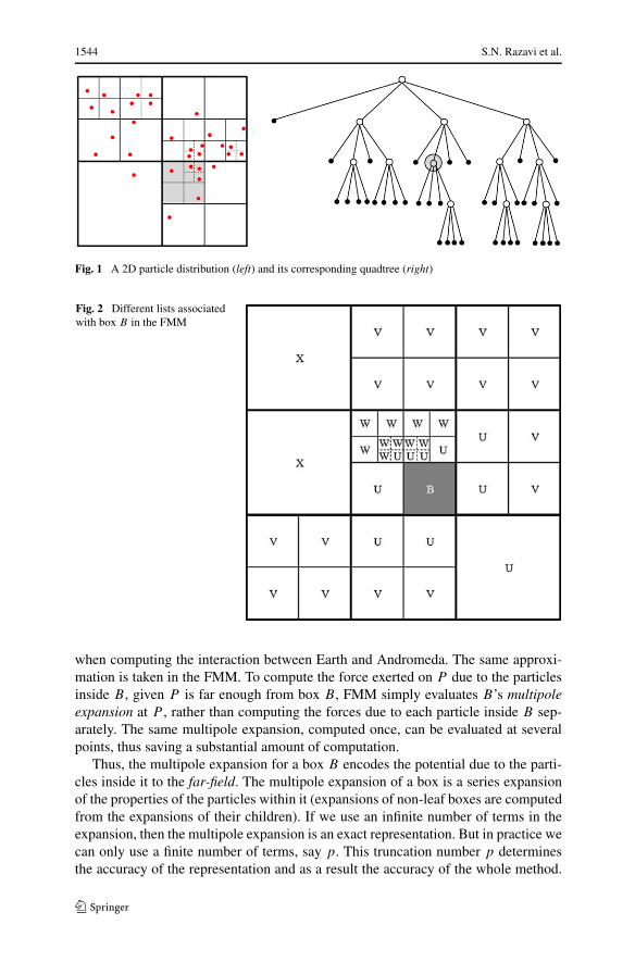
and referred to as level 0. The boxes (squares) at level l + 1 are obtained recursively,subdividing each box at level l into four squares, referred to as its children. The tree isconstructed so that the leaves contain no more than a certain fixed number of particles(say s). Generally, we refer to s as the clustering size of the tree. For non-uniformdistributions, this leads to a potentially unbalanced tree, as shown in Fig. 1 (whichassumes s = 1). This tree is the main data structure used by the FMM.

A key concept in understanding the algorithm is that of well-separatedness.A point or box is said to be well-separated from a box B if it lies outside the do-main of B and B’s neighbors (neighbors are defined as the boxes having at least onecommon vertex to B). In Fig. 2, B’s neighbors are marked with a “U” label. Usingthis concept, the FMM translates Newton’s insight into the following: If a point P

is well-separated from a box B , then B can be represented by a multipole expansionabout its center as far as P is concerned.

For example, if you stand on the Earth and look at the sky, you will see the An-dromeda (a galaxy approximately 2.5 million light-years away containing about onetrillions of stars) as a single star. So, it makes sense to consider it as a single point


Fig. 1 A 2D particle distribution (left) and its corresponding quadtree (right)

Fig. 2 Different lists associatedwith box B in the FMM

when computing the interaction between Earth and Andromeda. The same approxi-mation is taken in the FMM. To compute the force exerted on P due to the particlesinside B , given P is far enough from box B , FMM simply evaluates B’s multipoleexpansion at P , rather than computing the forces due to each particle inside B sep-arately. The same multipole expansion, computed once, can be evaluated at severalpoints, thus saving a substantial amount of computation.

Thus, the multipole expansion for a box B encodes the potential due to the parti-cles inside it to the far-field. The multipole expansion of a box is a series expansionof the properties of the particles within it (expansions of non-leaf boxes are computedfrom the expansions of their children). If we use an infinite number of terms in theexpansion, then the multipole expansion is an exact representation. But in practice wecan only use a finite number of terms, say p. This truncation number p determinesthe accuracy of the representation and as a result the accuracy of the whole method.


Truncating the number of terms in the series is a desired aspect in the FMM. In fact,this truncation serves as a mechanism to trade accuracy for efficiency, which is themain reason justifying the use of an approximation method instead of an exact one.

Turning back to our example, if you look at the Earth from Andromeda, then youwill see the Milky Way galaxy as a single point. Again, exploiting this idea will resultin a tremendous amount of saving in the computations. This is parallel to the so-calledlocal expansion in the FMM. More precisely, representing boxes by their multipoleexpansions is not the only insight exploited by the FMM. If a point P (be it a particleor the center of a box) is well-separated from box B , then the effects of P on particlesinside B can also be represented as a Taylor series or local expansion about the centerof B , which can then be evaluated at the particles inside B . Once again, the effects ofseveral such points can be converted just once each and accumulated into B’s localexpansion, which is then propagated down to B’s descendants and evaluated at everyparticle within B . Thus, the local expansion for a box B encodes the potentials onthe particles inside it due to the sources in the far-field of B . The mathematics ofcomputing multipole expansions, translating them to local expansions, and shiftingboth multipole and local expansions are described in [18].

Now, we have almost all the necessary background to give a brief descriptionof the FMM. But before that, the different lists associated with each box B in theadaptive tree of the FMM algorithm must be defined. These lists contain all boxeswhose contributions need to be processed by B itself when we use an adaptive wayto partition the computational domain. Contributions from more distant boxes areconsidered by B’s ancestors using local-to-local (L2L) translations. Some of theselists are defined only for leaf boxes of the tree, while others are defined for internalboxes as well. The lists for a leaf box B are described in Fig. 2, and their role isdiscussed in more detail in [3, 18]:

• For a leaf box, LUB contains B and its adjacent boxes. If B is not a leaf box, LU

B willbe empty. Since the boxes in LU

B are not well-separated from B , their contributionon B should be computed directly.

• LVB contains the set of the children of the neighbors of the parent of B , which

are not adjacent to B . The interaction from a box v ∈ LVB to B is computed using

multipole-to-multipole (M2M) translations since v and B are well-separated.• For a leaf box, LW

B includes all the descendants of B’s neighbors, which are notadjacent to B but their parents are adjacent to B . Since B is in the far range ofw ∈ LW

B , the contribution from w to B is evaluated using multipole expansionof w. Again, if B is not a leaf box, LW

B will be empty.• Finally, if box B is in the list LW

A , then LXB contains box A. The contribution from

x ∈ LXB to B is evaluated directly since B is in the near-range of x.

3.2 Overall structure of the FMM

Using the lists described in the previous section, the adaptive FMM proceeds in thefollowing steps:

STEP 1: Space partitioning The tree is built by loading particles into an initiallyempty root box and then this root box is partitioned recursively until there are no


more than s particles in each box. Also, for each box B , the lists LUB , LV

B and LWB

are constructed explicitly. As LXB is the dual of LW

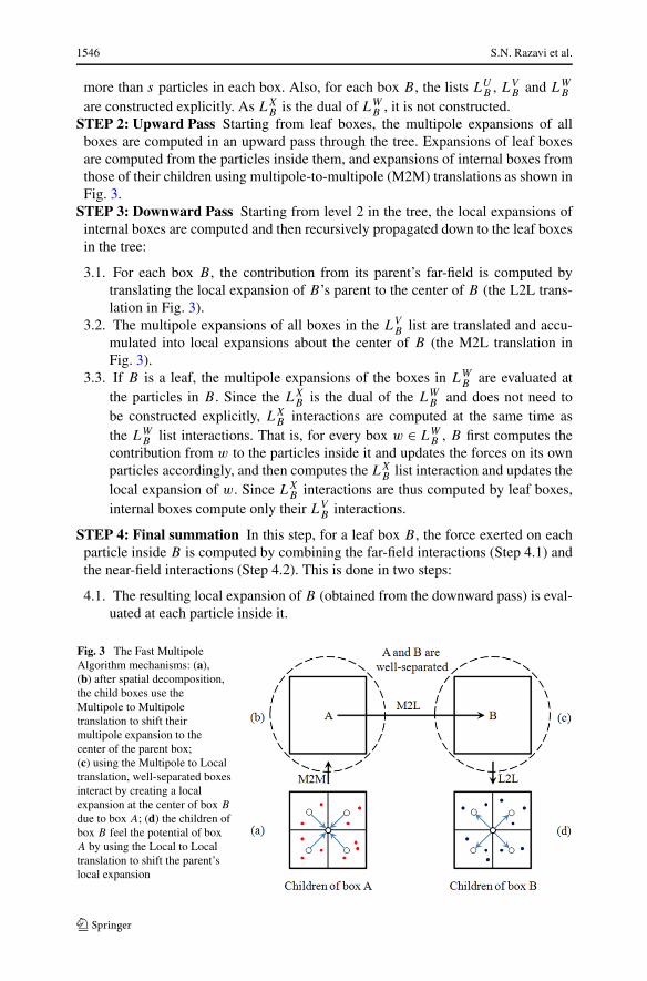
B , it is not constructed.STEP 2: Upward Pass Starting from leaf boxes, the multipole expansions of all

boxes are computed in an upward pass through the tree. Expansions of leaf boxesare computed from the particles inside them, and expansions of internal boxes fromthose of their children using multipole-to-multipole (M2M) translations as shown inFig. 3.

STEP 3: Downward Pass Starting from level 2 in the tree, the local expansions ofinternal boxes are computed and then recursively propagated down to the leaf boxesin the tree:

3.1. For each box B , the contribution from its parent’s far-field is computed bytranslating the local expansion of B’s parent to the center of B (the L2L trans-lation in Fig. 3).

3.2. The multipole expansions of all boxes in the LVB list are translated and accu-

mulated into local expansions about the center of B (the M2L translation inFig. 3).

3.3. If B is a leaf, the multipole expansions of the boxes in LWB are evaluated at

the particles in B . Since the LXB is the dual of the LW

B and does not need tobe constructed explicitly, LX

B interactions are computed at the same time asthe LW

B list interactions. That is, for every box w ∈ LWB , B first computes the

contribution from w to the particles inside it and updates the forces on its ownparticles accordingly, and then computes the LX

B list interaction and updates thelocal expansion of w. Since LX

B interactions are thus computed by leaf boxes,internal boxes compute only their LV

B interactions.

STEP 4: Final summation In this step, for a leaf box B , the force exerted on eachparticle inside B is computed by combining the far-field interactions (Step 4.1) andthe near-field interactions (Step 4.2). This is done in two steps:

4.1. The resulting local expansion of B (obtained from the downward pass) is eval-uated at each particle inside it.

Fig. 3 The Fast MultipoleAlgorithm mechanisms: (a),(b) after spatial decomposition,the child boxes use theMultipole to Multipoletranslation to shift theirmultipole expansion to thecenter of the parent box;(c) using the Multipole to Localtranslation, well-separated boxesinteract by creating a localexpansion at the center of box B

due to box A; (d) the children ofbox B feel the potential of boxA by using the Local to Localtranslation to shift the parent’slocal expansion


4.2. The interactions between all particles in the LUB with all particle inside B are

computed directly.

Our example application iterates over several hundred time-steps, every time-stepexecuting the above steps as well as one more that updates the velocities and positionsof the particles at the end of the time-step. For the problems we have run, almost allthe execution time is spent in computing list interactions. The majority of this time(about 60–70 %) is spent in computing V list interactions, next U list (about 20–30 %) and finally the W and X lists (about 10 %). Building the tree and updating theparticle properties take less than 1 % of the time in sequential implementations.

3.3 Complexity of the adaptive FMM

Assuming that there are N particles and each box contains at most s particles, therewill be about N/s boxes in the tree. Also, each box B has at most 29 boxes in its LV

B

list and 9 boxes in its LUB list. Therefore, the total operations count in the adaptive

FMM is approximately

Np + 29(N/s)p2 + Np + 9Ns

The terms correspond to formation of multipole expansions, translations, evalua-tion of the local expansions at particles, and direct computation of the near-neighborinteractions. By choosing s almost equal to p, the total operation count will be 40Np

or simply O(Np). While p is a small constant comparing to N , the adaptive FMM isa linear time algorithm and is applicable for very large number of particles.

It is worth to notice that the richer analytic structure of the FMM permits a largenumber of modifications and optimizations, which are not available to other hier-archical schemes. These schemes have to do with the use of symmetry relations toreduce the number of shifts [3] as well as schemes which reduce the cost of trans-lation itself [21]. Section 5 discusses how we can use simplified motion models toreduce FMM computational costs for simulation of a large complex system.

4 Flocking

Flocking behavior is the behavior exhibited when a group of birds, called a flock, areforaging or in flight. There are similar behaviors in other groups of animals or insectslike the shoaling behavior of a group of fishes, the swarming behavior of bees, andthe herd behavior of land animals [22]. From the perspective of the mathematicalmodeler, flocking is a collective motion of a large number of self-propelled entitiesand is a collective animal behavior exhibited by many living beings such as birds,fish, bacteria, and insects [23]. It is considered an emergent behavior arising fromsimple rules that are followed by individuals and does not involve any central coordi-nation. Flocking behavior was first simulated on a computer in 1986, when Reynoldsintroduced the first three heuristic rules for flocking behaviors [24]:

1. Separation—avoid crowding neighbors;2. Alignment—steer towards average heading of neighbors; and


3. Cohesion—steer towards average positions of neighbors.

Among the physics-inspired theoretical approaches studying flocking particlessystems, we may mention the work of [25] that mainly focuses on the study of align-ment rules and associated emergent phenomena. References [26] and [27] proposecontinuum models to study alignment and swarming. In [28], a model based on arti-ficial potential function (APF) in a network with fixed or dynamic topologies is pre-sented. It proposes a centralized algorithm for particle systems that leads to irregularcollapse for generic initial states. It also introduces a distributed version that leads toirregular fragmentation (disintegration of a flock into smaller groups combined withviolation of inter-agent constraints). Fragmentation and collapse are two well-knownpitfalls of flocking algorithms most likely occurring for generic set of initial statesand large number of agents [29–32].

Here, we have used a flocking model based on the theoretical framework for de-sign and analysis of distributed flocking algorithms from Refs. [30, 33]. This modelmay be considered as a modified version of APF in [28] trying to avoid traditionalpitfalls of flocking. Reference [34] provides a definition of “flocking” for particle sys-tems that is independent of the method of trajectory generation for particles. In thissense, it has the same role as “Lyapunov stability” for nonlinear dynamical systems.This model is based on a systematic method for construction of collective potentialfunctions for flocking. The flocking behavior is accomplished by a set of physicallaws governing the pairwise interactions between flocking agents and also their inter-actions with the environment.

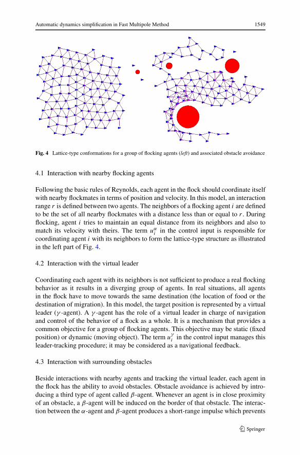
In this model, a lattice-type structure is used to model the geometry of desiredconformation of agents in a flock. In such a conformation, each agent should beequally distanced from all of its neighbors while moving towards its objective thatmay be static or dynamic. As shown in Fig. 4, this lattice-type structure exhibitsa high degree of spatial order among agents and this is exactly where we can usesimplified motion models to reduce complexity. Using the terminology of informationtheory, order means redundancy and the redundancy can be removed from the systemwith no loss or minimal loss in the information contents. This is an important reasonmotivating us to use this flocking system as our target application in this work. Thistype of order exists more or less in many systems and so the work presented in thispaper may be considered as a general framework to reduce complexity in simulatingthose systems.

As flocking occurs in the presence of multiple obstacles, each agent in the flock-ing model is equipped with obstacle avoidance capability. In fact, each agent hasinteractions with three kinds of objects in the environment:

• Nearby flockmates (α-agents),• Obstacles (β-agents), and• A virtual leader (γ -agent).

Each agent in the flock applies a control input that consists of three different termswhich are discussed in the following sections:

ui = uαi + u

βi + u

γ

i


Fig. 4 Lattice-type conformations for a group of flocking agents (left) and associated obstacle avoidance

4.1 Interaction with nearby flocking agents

Following the basic rules of Reynolds, each agent in the flock should coordinate itselfwith nearby flockmates in terms of position and velocity. In this model, an interactionrange r is defined between two agents. The neighbors of a flocking agent i are definedto be the set of all nearby flockmates with a distance less than or equal to r . Duringflocking, agent i tries to maintain an equal distance from its neighbors and also tomatch its velocity with theirs. The term uα

i in the control input is responsible forcoordinating agent i with its neighbors to form the lattice-type structure as illustratedin the left part of Fig. 4.

4.2 Interaction with the virtual leader

Coordinating each agent with its neighbors is not sufficient to produce a real flockingbehavior as it results in a diverging group of agents. In real situations, all agentsin the flock have to move towards the same destination (the location of food or thedestination of migration). In this model, the target position is represented by a virtualleader (γ -agent). A γ -agent has the role of a virtual leader in charge of navigationand control of the behavior of a flock as a whole. It is a mechanism that provides acommon objective for a group of flocking agents. This objective may be static (fixedposition) or dynamic (moving object). The term u

γ

i in the control input manages thisleader-tracking procedure; it may be considered as a navigational feedback.

4.3 Interaction with surrounding obstacles

Beside interactions with nearby agents and tracking the virtual leader, each agent inthe flock has the ability to avoid obstacles. Obstacle avoidance is achieved by intro-ducing a third type of agent called β-agent. Whenever an agent is in close proximityof an obstacle, a β-agent will be induced on the border of that obstacle. The interac-tion between the α-agent and β-agent produces a short-range impulse which prevents


α-agent to further approach the obstacle and hence helps it to avoid that obstacle (seethe right part of Fig. 4). The term u

βi in the control input accounts for all of the in-

teractions between agent i and its nearby obstacles. For more details on the exactdefinitions of uα

i , uβi and u

γ

i the reader may refer to [30].

5 Framework for automatic dynamics simplification

This section presents our proposed method for automatic dynamics simplificationwith application in the simulation of large dynamical systems. Since the proposedmethod follows the overall structure of the FMM (see Sect. 3.2), this section mainlyfocuses on the differences rather than the similarities. We start first by presenting thedetails about computing the Center of Mass (COM) particle for each box or groupof boxes. We then follow the discussion by introducing the criteria used in the newalgorithm to determine when and which boxes in the FMM tree may be merged tosimplify calculations.

Before giving the details of the framework, it should be mentioned that a variantof the FMM, called kernel-independent FMM, is used to implement our flockingsystems [5]. The kernel-independent FMM follows the overall structure of the FMMbut it does not require the analytical expansions (local and multipole expansions) ofthe kernel and only relies on direct evaluations of the kernel. As it is not obviousto derive these expansions for many complex kernels, using the kernel-independentmethod results in more flexibility and hence the framework presented here is a generalframework applicable to a wide variety of N -body systems.

5.1 Approximating motion models

For each box (a leaf box or an internal box in the FMM tree), dynamics simplificationis achieved by approximating its particles dynamics using the particles dynamics ofits center of mass. Given a box B consisting of k particles, the corresponding approx-imated motion model is computed using the following procedure:

1. Compute the position PCOM and velocity VCOM of the center of mass particleusing:

PCOM =∑k

i=1 miPi∑k

i=1 mi

VCOM =∑k

i=1 miVi∑k

i=1 mi

where mi , Pi and Vi represent the mass, position and velocity of the ith particleinside B . Please note that in a different application mi could represent some otherquantity. For example in Coulombic systems, it represents the charge of ith ion ina medium rather than its mass.

2. Using the standard computations in the FMM, first compute the potential of theCOM for box B and then update its velocity and position accordingly.

3. Apply the same results computed for the COM to all particles inside B .


5.2 Pruning the FMM tree

As discussed earlier, we need a mechanism to automatically decide for which boxeswe can use approximated motion models. From now on, we refer to such boxes assimplified boxes. This is a key factor determining the overall success or failure of theautomatic dynamics simplification.

For a given box B , we use the following similarity measures to decide if we canuse dynamics simplification for that box: the speed ratio and the velocity vector angleratio. These computations differ for a leaf box and an internal box:

• If B is a leaf box, we compute these two measures for B from the velocities ofits particles. That is, the relative speed of its particles and also their relative angleshould be within certain limits.

• Otherwise, if B has children, the similarity measures for B are computed by con-sidering the COM particles of its children. Again the relative speed of the COMparticles and their relative angle are constrained to be within certain limits.

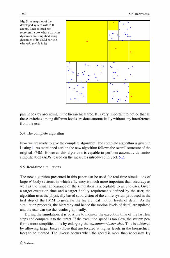
The above computations are done during the upward pass of the FMM algorithm(see Sect. 3.2). If box B satisfies these two conditions, then all of its particles arereplaced by its weighted center of mass particle which is computed directly from itsparticles or indirectly from the center of mass of its children. After this simplifica-tion, the new algorithm continues as the classical FMM. However, when the potentialshave been computed for every particle (a real particle or a weighted center of massparticle), the computed potentials for a COM particle are applied to all of the particlesinside the corresponding simplified box. A snapshot of the developed system for 200particles is given in Fig. 5. Because of dynamics simplification, the number of parti-cles is reduced from 200 to 89 in this system resulting in a considerable reduction inthe execution time.

5.3 Automatic switching between different levels of simulation

Additionally, similarly to geometric simplifications used in computer graphics inwhich special areas have higher priorities (for example, the areas closer to the viewerand more centered in the viewing frustum) and hence should be simulated in moredetail, some events in our framework may require higher resolution to maintain simu-lation correctness and integrity. Referring to Sect. 4.3, recall that the agents (particles)in our flocking system have the ability to avoid obstacles in their path during flight.This obstacle avoidance capability requires higher priority comparing to the otherbehaviors of flocking agents. Fortunately, our framework has the ability to cope withthese critical situations.

For example, when a large box consisting of a large number of agents is near anobstacle, the simulation automatically switches to a higher resolution level. That is,the box automatically decomposes into its children (if it is a non-leaf box) or into itsindividual particles (if it is a leaf box). This is a recursive process which continuesuntil reaching a level with a good enough accuracy. As the particles move away fromthe obstacle, physical properties and spatial positions of those with similar motionmay again be regrouped into a box, or the children boxes may be regrouped into their


Fig. 5 A snapshot of thedeveloped system with 200agents. Each colored boxrepresents a box whose particlesdynamics are simplified usingdynamics of its COM particle(the red particle in it)

parent box by ascending in the hierarchical tree. It is very important to notice that allthese switches among different levels are done automatically without any interferencefrom the user.

5.4 The complete algorithm

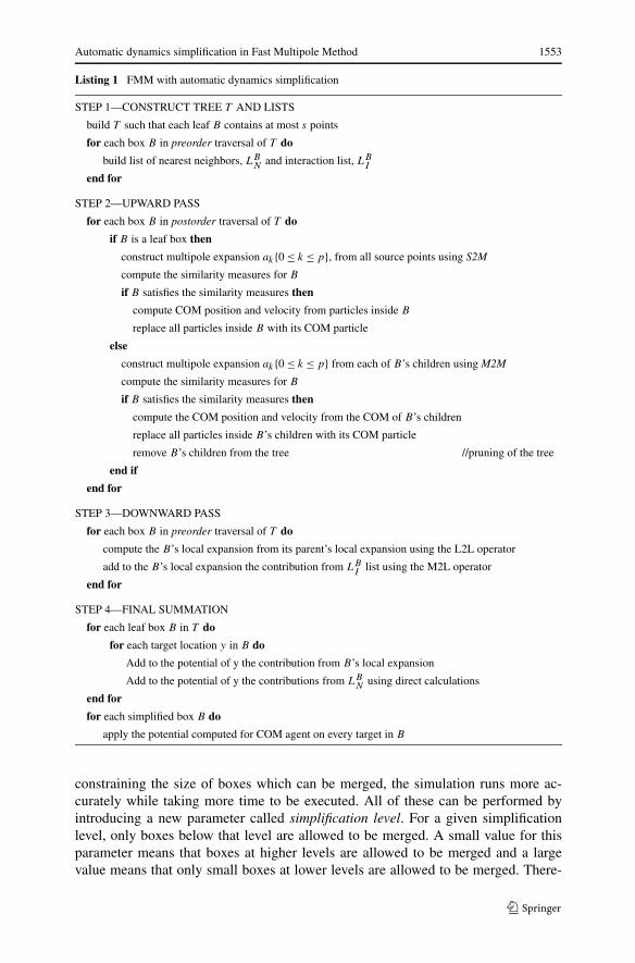
Now we are ready to give the complete algorithm. The complete algorithm is given inListing 1. As mentioned earlier, the new algorithm follows the overall structure of theoriginal FMM. However, this algorithm is capable to perform automatic dynamicssimplification (ADS) based on the measures introduced in Sect. 5.2.

5.5 Real-time simulations

The new algorithm presented in this paper can be used for real-time simulations oflarge N -body systems, in which efficiency is much more important than accuracy aswell as the visual appearance of the simulation is acceptable to an end-user. Givena target execution time and a target fidelity requirements defined by the user, thealgorithm uses the physically based subdivision of the entire system produced in thefirst step of the FMM to generate the hierarchical motion levels of detail. As thesimulation proceeds, the hierarchy and hence the motion levels of detail are updatedand the user can see the results graphically.

During the simulation, it is possible to monitor the execution time of the last fewsteps and compare it to the target. If the execution speed is too slow, the system per-forms more simplifications by enlarging the maximum cluster size. This is achievedby allowing larger boxes (those that are located at higher levels in the hierarchicaltree) to be merged. The inverse occurs when the speed is more than necessary. By


Listing 1 FMM with automatic dynamics simplification

STEP 1—CONSTRUCT TREE T AND LISTS

build T such that each leaf B contains at most s points

for each box B in preorder traversal of T do

build list of nearest neighbors, LBN

and interaction list, LBI

end for

STEP 2—UPWARD PASS

for each box B in postorder traversal of T do

if B is a leaf box then

construct multipole expansion ak{0 ≤ k ≤ p}, from all source points using S2M

compute the similarity measures for B

if B satisfies the similarity measures then

compute COM position and velocity from particles inside B

replace all particles inside B with its COM particle

else

construct multipole expansion ak{0 ≤ k ≤ p} from each of B’s children using M2M

compute the similarity measures for B

if B satisfies the similarity measures then

compute the COM position and velocity from the COM of B’s children

replace all particles inside B’s children with its COM particle

remove B’s children from the tree //pruning of the tree

end if

end for

STEP 3—DOWNWARD PASS

for each box B in preorder traversal of T do

compute the B’s local expansion from its parent’s local expansion using the L2L operator

add to the B’s local expansion the contribution from LBI

list using the M2L operator

end for

STEP 4—FINAL SUMMATION

for each leaf box B in T do

for each target location y in B do

Add to the potential of y the contribution from B’s local expansion

Add to the potential of y the contributions from LBN

using direct calculations

end for

for each simplified box B do

apply the potential computed for COM agent on every target in B

constraining the size of boxes which can be merged, the simulation runs more ac-curately while taking more time to be executed. All of these can be performed byintroducing a new parameter called simplification level. For a given simplificationlevel, only boxes below that level are allowed to be merged. A small value for thisparameter means that boxes at higher levels are allowed to be merged and a largevalue means that only small boxes at lower levels are allowed to be merged. There-


fore, each time we need a faster execution, the simplification level is decreased by oneand this allows larger boxes in higher levels to be merged. Increasing this parameterdoes the inverse.

In summary, the proposed framework has several parameters which enable us tocontrol both the error and the execution time of the simulation. These parameters are:the speed ratio and the velocity vector angle ratio, the maximum number of particlesin each box and the maximum cluster size or the simplification level. The set of theseparameters gives us the potential to apply our framework for real-time applications aswell. Future work is already planned to test this real-time capability of the proposedframework.

6 Experimental results

We have implemented a prototype system in Java which can automatically generatesimulation levels of detail, select appropriate ones and switch between them. In thissection we present the results of our system tested on a large dynamical flockingsystem which is a classic example for N -body systems (see Sect. 4). All experimentswere conducted on a desktop computer configured with one 2.5-GHz Quad-Core IntelPentium processor and 4-GB RAM running a Windows 7 Professional x32 Edition.Our application was developed in Java and the Java VM used to execute the tests wasconfigured with 1-GB memory.

6.1 Simulation of a large dynamical flocking system

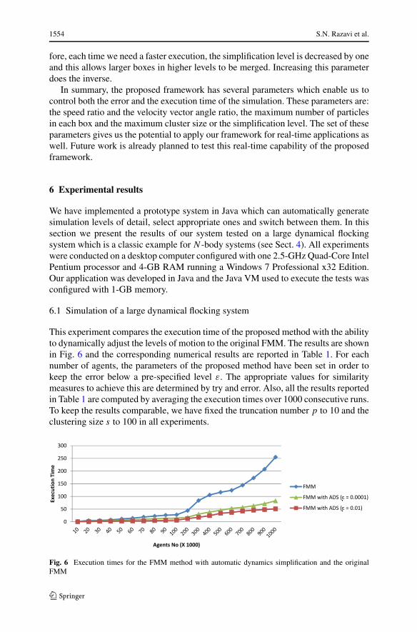
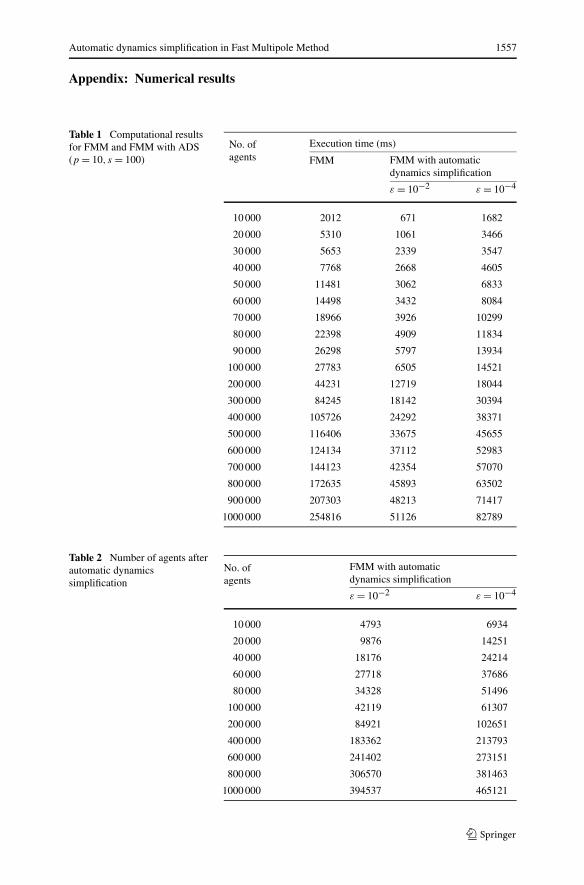
This experiment compares the execution time of the proposed method with the abilityto dynamically adjust the levels of motion to the original FMM. The results are shownin Fig. 6 and the corresponding numerical results are reported in Table 1. For eachnumber of agents, the parameters of the proposed method have been set in order tokeep the error below a pre-specified level ε. The appropriate values for similaritymeasures to achieve this are determined by try and error. Also, all the results reportedin Table 1 are computed by averaging the execution times over 1000 consecutive runs.To keep the results comparable, we have fixed the truncation number p to 10 and theclustering size s to 100 in all experiments.

Fig. 6 Execution times for the FMM method with automatic dynamics simplification and the originalFMM


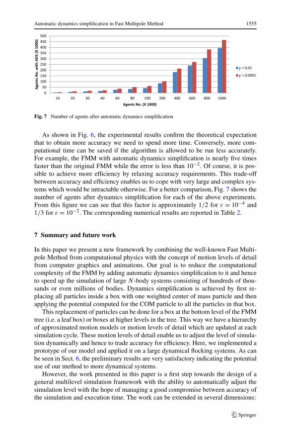
Fig. 7 Number of agents after automatic dynamics simplification

As shown in Fig. 6, the experimental results confirm the theoretical expectationthat to obtain more accuracy we need to spend more time. Conversely, more com-putational time can be saved if the algorithm is allowed to be run less accurately.For example, the FMM with automatic dynamics simplification is nearly five timesfaster than the original FMM while the error is less than 10−2. Of course, it is pos-sible to achieve more efficiency by relaxing accuracy requirements. This trade-offbetween accuracy and efficiency enables us to cope with very large and complex sys-tems which would be intractable otherwise. For a better comparison, Fig. 7 shows thenumber of agents after dynamics simplification for each of the above experiments.From this figure we can see that this factor is approximately 1/2 for ε = 10−4 and1/3 for ε = 10−2. The corresponding numerical results are reported in Table 2.

7 Summary and future work

In this paper we present a new framework by combining the well-known Fast Multi-pole Method from computational physics with the concept of motion levels of detailfrom computer graphics and animations. Our goal is to reduce the computationalcomplexity of the FMM by adding automatic dynamics simplification to it and henceto speed up the simulation of large N -body systems consisting of hundreds of thou-sands or even millions of bodies. Dynamics simplification is achieved by first re-placing all particles inside a box with one weighted center of mass particle and thenapplying the potential computed for the COM particle to all the particles in that box.

This replacement of particles can be done for a box at the bottom level of the FMMtree (i.e. a leaf box) or boxes at higher levels in the tree. This way we have a hierarchyof approximated motion models or motion levels of detail which are updated at eachsimulation cycle. These motion levels of detail enable us to adjust the level of simula-tion dynamically and hence to trade accuracy for efficiency. Here, we implemented aprototype of our model and applied it on a large dynamical flocking systems. As canbe seen in Sect. 6, the preliminary results are very satisfactory indicating the potentialuse of our method to more dynamical systems.

However, the work presented in this paper is a first step towards the design of ageneral multilevel simulation framework with the ability to automatically adjust thesimulation level with the hope of managing a good compromise between accuracy ofthe simulation and execution time. The work can be extended in several dimensions:


• Investigating other possible methods or heuristics for similarity measure instead ofspeed ratio and velocity vector angle ratio. For example, one possibility is to usethe entropy related to the particles inside a box as a measure to decide switchingbetween levels of motion. Also, it is possible to use partition function and energy-based measures for this purpose.

• Designing new experiments to gain a better understanding of the effects of eachparameter such as truncation number p and clustering size s on the execution timeof the simulation and its accuracy.

• Generalizing the proposed framework to be applicable in more dynamical systems,such as simulation of large crowds or simulation of a large number of pedestriansin urban areas.

• Giving a more complete complexity analysis and error analysis and studying theeffects of main parameters such as truncation number and clustering size on thecomplexity and the error of the new method.

• Designing new test to study the functionality of the proposed algorithm for real-time simulation of large N -body systems. This can be achieved through the anal-ysis of specific constraints such as running the simulation within a fixed predeter-mined amount of time and the way to minimize the error in these kinds of config-urations.


Appendix: Numerical results

Table 1 Computational resultsfor FMM and FMM with ADS(p = 10, s = 100)

No. ofagents

Execution time (ms)

FMM FMM with automaticdynamics simplification

ε = 10−2 ε = 10−4

10 000 2012 671 1682

20 000 5310 1061 3466

30 000 5653 2339 3547

40 000 7768 2668 4605

50 000 11481 3062 6833

60 000 14498 3432 8084

70 000 18966 3926 10299

80 000 22398 4909 11834

90 000 26298 5797 13934

100 000 27783 6505 14521

200 000 44231 12719 18044

300 000 84245 18142 30394

400 000 105726 24292 38371

500 000 116406 33675 45655

600 000 124134 37112 52983

700 000 144123 42354 57070

800 000 172635 45893 63502

900 000 207303 48213 71417

1000 000 254816 51126 82789

Table 2 Number of agents afterautomatic dynamicssimplification

No. ofagents

FMM with automaticdynamics simplification

ε = 10−2 ε = 10−4

10 000 4793 6934

20 000 9876 14251

40 000 18176 24214

60 000 27718 37686

80 000 34328 51496

100 000 42119 61307

200 000 84921 102651

400 000 183362 213793

600 000 241402 273151

800 000 306570 381463

1000 000 394537 465121


References

1. Rokhlin V (1983) Rapid solution of integral equations of classical potential theory. J Comput Phys60(2):187–207

2. Greengard L, Rokhlin V (1987) A fast algorithm for particle simulations. J Comput Phys 73(2):325–348

3. Greengard L, Rokhlin V (1988) Rapid evaluation of potential fields in three dimensions. In: Lecturenotes in mathematics, vol 1360. Springer, Berlin, pp 121–141

4. Dongarra J, Sullivan F (2000) The top ten algorithms of the century. Comput Sci Eng 2(1):22–235. Razavi SN, Gaud N, Mozayani N, Koukam A (2011) Multi-agent based simulations using fast mul-

tipole method: application to large scale simulations of flocking dynamical systems. Artif Intell Rev35(1):53–72

6. Razavi SN, Gaud N, Koukam A, Mozayani N (2011) Using motion levels of detail in the fast multipolemethod for simulation of large particle systems. In: WMSCI 2011, Orlando

7. Carlson DA, Hodgins JK (1997) Simulation levels of detail for real-time animation. In: Graphic inter-face, pp 1–8

8. Chenney S, Forsyth D (1997) View-dependent culling of dynamic systems in virtual environments.In: ACM symposium on interactive 3D graphics, New York

9. Grzeszczuk R, Terzopoulos D, Hinton G (1998) Neuroanimator: fast neural network emulation andcontrol of physics-based models. In: SIGGRAPH, New York, pp 9–29

10. Popovic Z, Witkin A (1999) Physically based motion transformation. In: SIGGRAPH, New York,pp 11–20

11. Brudlerlin A, Calvert TW (1996) Knowledge-driven, interactive animation of human running. In:Graphics interface, pp 213–221

12. Granieri JP, Crabtree J, Badler NI (1995) Production and playback of human figure motion for 3dvirtual environments. In: VRAIS, pp 127–135

13. Perlin K (1995) Real time responsive animation with personality. IEEE Trans Vis Comput Graph1(1):5–15

14. Multon F, Valton B, Jouin B, Cozot R (1999) Motion levels of detail for real-time virtual worlds. In:ASTC-VR’99

15. Faloutsos P, van de Panne M, Terzopoulos D (2001) Composable controllers for physics-based char-acter animation. In: SIGGRAPH 2001, New York, pp 251–260

16. O’Sullivan C, Dingliana J (2001) Collisions and perception. ACM Trans Graph 20(3)17. O’Brien D, Fisher S, Lin MC (2001) Automatic simplification of particle system dynamics. In: Com-

puter animation, Seoul, pp 210–25718. Greengard LF (1987) The rapid evaluation of potential fields in Particle systems. Yale University,

New Haven, PhD Thesis19. Barnes JE, Hut P (1986) A hierarchical O(N logN ) force calculation algorithm. Nature

324(6096):446–44920. Hanrahan P, Salzman D, Aupperle L (1991) A rapid hierarchical radiosity algorithm. In: SIGGRAPH,

New York, pp 197–20621. Elliott WD, Board JA (1996) Fast Fourier transform accelerated fast multipole algorithm. SIAM J Sci

Comput 17(2):398–41522. Karaboga D, Akay B (2009) A survey: algorithms simulating bee swarm intelligence. Artif Intell Rev

31(1):61–8523. O’loan OJ, Evans MR (1999) Alternating steady state in one-dimensional flocking. J Phys, A Math

Gen 32(8)24. Reynolds CW (1987) Flocks, herds, and schools: a distributed behavioral model. Comput Graph

21:25–3425. Shimoyama N, Sugawara K, Mizuguchi T, Hayakawa Y, Sano M (1996) Collective motion in a system

of motile elements. Phys Rev Lett 76(20):3870–387326. Mogilner A, Edelstein-Keshet L (1999) A non-local model for a swarm. J Math Biol 38(6):534–57027. Toner J, Tu Y (1998) Flocks, herds, and schools: a quantitative theory of flocking. Phys Rev E

58(4):4828–485828. Tanner HG, Jadbabaie A, Pappas GJ (2003) Stable flocking of mobile agents, part II: dynamic topol-

ogy. In: 42nd IEEE conference on decision and control, Maui, Hawaii, pp 2016–202129. Zhou J, Yu W, Wu X, Small M, Lu JA (2009) Flocking of multi-agent dynamical systems based on

pseudo-leader. arXiv:0905.1037v1 [nlin.CD]

http://arxiv.org/abs/arXiv:0905.1037v1


30. Olfati-Saber R (2006) Flocking for multi-agent dynamic systems: algorithms and theory. IEEE TransAutom Control 51(3):401–420

31. Liu H, Fang H, Mao Y, Cao H, Jia R (2010) Distributed flocking control and obstacle avoidance formulti-agent systems. In: Control conference, Beijing, pp 4536–4541

32. Mousavi MSR, Khaghani M, Vossoughi G (2010) Collision avoidance with obstacles in flocking formulti agent systems. In: Industrial electronics, control & robotics (IECR), Orissa, pp 1–5

33. Olfat-Saber R, Murray RM (2003) Flocking with obstacle avoidance: cooperation with limited com-munication in mobile networks. In: 42nd IEEE conference on in decision and control, Maui, Hawaii,pp 2022–2028

34. Olfati-Saber R, Murray RM (2003) Consensus protocols for networks of dynamic agents. In: Ameri-can control conference, Denver, pp 951–956

Documents

Automatic dynamics simpliﬁcation in Fast Multipole Method ...webpages.iust.ac.ir/mozayani/Papers-pdf/razavi-supercomputing2012.pdf · Automatic dynamics simpliﬁcation in Fast