Automated mapping of large binary objects using … mapping of large binary objects using primitive fragment type classiﬁcation Gregory Contia,*, Sergey Bratusb, Anna Shubinab, Benjamin

Automated mapping of large binary objects using primitivefragment type classification

Gregory Conti a,*, Sergey Bratus b, Anna Shubina b, Benjamin Sangster a, Roy Ragsdale a,Matthew Supan a, Andrew Lichtenberg c, Robert Perez-Alemany a

aUnited States Military Academy at West Point, West Point, NY, United StatesbDartmouth College, Hanover, NH, United StatescSkidmore College, Saratoga Springs, NY, United States

Keywords:

Binary mapping

Binary analysis

File carving

Hex editors

Classification

Reverse engineering

a b s t r a c t

Security analysts, reverse engineers, and forensic analysts are regularly faced with large

binary objects, such as executable and data files, process memory dumps, disk images and

hibernation files, often Gigabytes or larger in size and frequently of unknown, suspect, or

poorly documented structure. Binary objects of this magnitude far exceed the capabilities

of traditional hex editors and textual command line tools, frustrating analysis. This paper

studies automated means to map these large binary objects by classifying regions using

a multi-dimensional, information-theoretic approach. We make several contributions

including the introduction of the binary mapping metaphor and its associated applications,

as well as techniques for type classification of low-level binary fragments. We validate the

efficacy of our approach through a series of classification experiments and an analytic case

study. Our results indicate that automated mapping can help speed manual and auto-

mated analysis activities and can be generalized to incorporate many low-level fragment

classification techniques.

ª 2010 Digital Forensic Research Workshop. Published by Elsevier Ltd. All rights reserved.

1. Introduction

Binary data is ubiquitous. Security analysts are constantly

challenged to gain insight into large binary objects in the form

of data and executable files, file systems, hibernation files,

process memory, or network traffic. Although specialized

tools exist for the studyof commonfile andfile systemformats,

the general case of unknownormalformedbinary objects lacks

all but the most basic tools. Hex editors are the most common

tool employed to perform low-level analysis of binary objects;

however their utility drops off rapidly as file size increases.

Analysts supplement hex editors with command line utilities

suchas grep to search for knownorguessedpatterns and strings

and variants thereof to locate printable ASCII and Unicode

strings, but theseapproachesare rudimentaryanddonot scale.

Large binary objects, sometimes 2 GB or larger, are becoming

more and more common, and an automated approach is

necessary to facilitate effective exploratory analysis.

To address the problem of analysis of large binary objects,

we present binary mapping techniques that compute start

The views expressed in this article are those of the authors and do not reflect the official policy or position of the United States MilitaryAcademy, the Department of the Army, the Department of Defense or the U.S. Government.* Corresponding author.E-mail addresses: [email protected] (G. Conti), [email protected] (S. Bratus), [email protected]

(A. Shubina), [email protected] (B. Sangster), [email protected] (R. Ragsdale), [email protected](M. Supan), [email protected] (A. Lichtenberg), [email protected] (R. Perez-Alemany).

ava i lab le at www.sc ienced i rec t . com

journa l homepage : www.e lsev ier . com/ loca te /d i in

d i g i t a l i n v e s t i g a t i o n 7 ( 2 0 1 0 ) S 3eS 1 2

1742-2876/$ e see front matter ª 2010 Digital Forensic Research Workshop. Published by Elsevier Ltd. All rights reserved.doi:10.1016/j.diin.2010.05.002

and stop offsets for each distinct region within a binary object

as well as the region’s probable primitive data type. We define

primitive types as families of homogeneous data with closely

related binary structure. Examples of primitive types include:

US-ASCII encoded English text, 32-bit x86 protected mode

machine code, random number sequences, image bitmaps;

essentially any group of similar data, possibly encoded,

compressed, or encrypted in the same way. However, one

should not confuse an object of a primitive type with

composite objects. For example, even simple file formats

include a metadata header alongside the actual data payload.

In this paper we treat distinctly structured regions as discrete

types. Our primary use case for binary mapping is the explo-

ration of large files and memory dumps. Binary maps, once

generated, can then be used to guide manual analysis or to

inform further automated analysis. For example, maps of

binary objects can be used to assist humans in navigating to

regions of interest. They can also be used to highlight certain

desired regions and filter those that are less important to the

analyst.

We make several contributions, including a generalized

framework for mapping large binary objects, which will work

withmany low-level binary fragment classifiers.Wealsopresent

a multi-dimensional information-theoretic fragment classifier

tested using 14,000 primitive fragments of 14 distinct types. We

validate our work through a series of classification experiments

and an analytic case study employing an implementation of our

mapping techniques. Our classifier does not assume a priori

knowledge of file formats, such as magic numbers or header/

footer signatures at known offsets, but instead relies upon the

raw structure of the data to identify regions of interest. This

property is important because many primitive types lack the

consistent structure to support the use of naive signature

matching and location semantics. Our framework is designed to

support such tasks as rapidly analyzing undocumented file

formats, identifying internal data structures thatmay be targets

for fuzzing, exploring the behavior of applications generating

binary data files, malware analysis, locating encrypted regions,

and studying process memory dumps.

This paper is organized as follows. Section 2 places our

research in the field of related work. Section 3 studies the

internal structure of binary objects and discusses generalized

binary mapping. Section 4 presents our analytic techniques.

Sections 5 and 6 provide an evaluation of our approach

through experimentation and an analytic case study. Finally,

Section 7 presents our conclusions and promising directions

for future work.

2. Related work

Work related to our study of binary mapping consists

primarily of file classification and file carving research. In the

file type classification field, Li conducted 1-gram analysis of

byte values to create a “fileprint” and used fileprints to classify

both complete and “truncated” files (Li et al., 2005). Stolfo used

n-grams to classify files, including document files, containing

embeddedmalicious software (Stolfo et al., 2005). Hickok used

a combination of file extensions andmagic numbers to rapidly

classify files (Hickok et al., 2005). McDaniel used three

different algorithms based on byte frequency analysis, byte

frequency correlation analysis, and file header/trailer analysis

to perform file type identification (McDaniel and Heydari,

2003). Hall attempted file type identification using entropy

and compressibility by employing a 90 byte sliding window

(Hall and Davis). Karresand used an algorithm based on the

rate of change of byte values and claimed a 99.2% detection

rate of jpeg files, when taking into account signatures

commonly foundwithin such files (Karresand and Shahmehri,

2006).

File carving and the related area of file fragment reas-

sembly are also related to our work. The work of Shanmuga-

sundaram demonstrated that it is possible to reassemble

document fragments by using context models to sequence

fragments. Veenman explored the use of statistical tech-

niques to classify file clusters by file type in order to support

file recovery from cluster-based media, but examined files as

a whole rather than considering their constituent parts

(Veenman, 2007). Richard developed Scalpel, a high perfor-

mance file carver, which used a database of header and footer

signatures, at predictable offsets, to extract files. Scalpel is an

evolution of the Foremost file carver, and Richard’s research

included an in depth performance comparison (Richard and

Roussev, 2005).

Some researchers have explored the idea of classifying

fragments. Calhoun attempted to classify fragments of .jpg, .

gif, .pdf and .bmp files using algorithms based on Fisher’s

linear discriminant and longest common subsequences

(Calhoun and Coles, 2008). Erbacher used a sliding window

algorithm and graphical depictions of statistical values to

visually identify characteristic signatures found in seven file

types: .doc, .exe, .jpg, .pdf, .ppt, .xls, and .zip, but performed

only a small study consisting of five files per type (Erbacher

and Mulholland, 2007). Moody used a 256-byte sliding

window to identify fragments extracted from 25 each of .bmp,

.csv, .dll, .exe, .html, .jpg, .txt, and .xls files, again a very small

sample (Moody and Erbacher, 2008). However, we believe that

inclusion of container files, i.e., file formats commonly used to

hold objects of many varied primitive types such as .pdf, .xls, .

doc, and .ppt, in each of these analyses limits the effective

application of their results to binary mapping because

container file structure can vary widely based on the distri-

bution of primitive types found within. Roussev made

a similar point by suggesting that researchers must under-

stand the “primitive” format of a fragment and whether the

fragment is part of a compound file structure (Roussev and

Garfinkel, 2009). Shamir studied the ability of an attacker to

extract cryptographic keys from large hard drives using a 64

byte sliding window and counting the number of unique bytes

in the window (Shamir and van Someren, 1999). Importantly,

Garfinkel stressed the significance of locating and validating

objects contained within container documents and complex

file formats (Garfinkel, 2007).

The common trend in much of the preceding work is that

researchers have incorporated only small numbers of files and

fragments in their analyses, frequently relied on header and

footer signatures at known offsets, or focused on extracting

files from disk images. In many cases, file fragments, when

used, were arbitrarily derived from complex container objects.

The novelty of our work springs from countering these trends.

d i g i t a l i n v e s t i g a t i o n 7 ( 2 0 1 0 ) S 3eS 1 2S4

We do not seek to classify files themselves; instead we seek to

map and classify regions within files, or other binary objects,

with the goal of conserving analyst time and attention and

informing further machine processing.

3. Mapping the internal structure of binaryobjects

To better understand the value of automated mapping, it is

useful to visually examine the internal structure of an object,

see Fig. 1. The image is a byteplot, a graphical depiction of

a binary object, showing a Microsoft Word 2003 document

(Conti and Dean, 2008; Conti et al., 2008). In a byteplot, each

byte in the binary object is sequentiallymapped to a pixel. The

plotting of byte values in the object starts at the top left of the

image. Subsequent byte values in the object are plotted from

left to right, wrapping at the end of each horizontal row. The

coloring schememaps byte values from 0 (black) to 255 (bright

white). As you examine the image, note the regions of similar

structure. Our goal with automatedmapping is (1) to locate the

start and stop offsets of these distinct regions and (2) to

identify the region’s primitive type. Manual inspection of the

document using a hex editor allowed us to identify some

regions as US-ASCII text, Basic Latin Unicode hyperlinks,

a compressed PNG image, and numerous other data struc-

tures. However, our motivation for binary mapping is to avoid

tedious manual inspection and create an effective automated

approach. Because the number of primitive types is large and

growing, a binary mapping framework must be flexible

enough to incorporate new primitive data types as they are

encountered or as an analyst desires their inclusion.

Accurate classification is a fundamental requirement of

binary mapping. However, to understand classification

requirements, we must first understand the types of content

we desire to identify. The range of possible fragment types is

large, but a useful way to think about the possibilities is in

terms of entropy, the uncertainty (sometimes colloquially

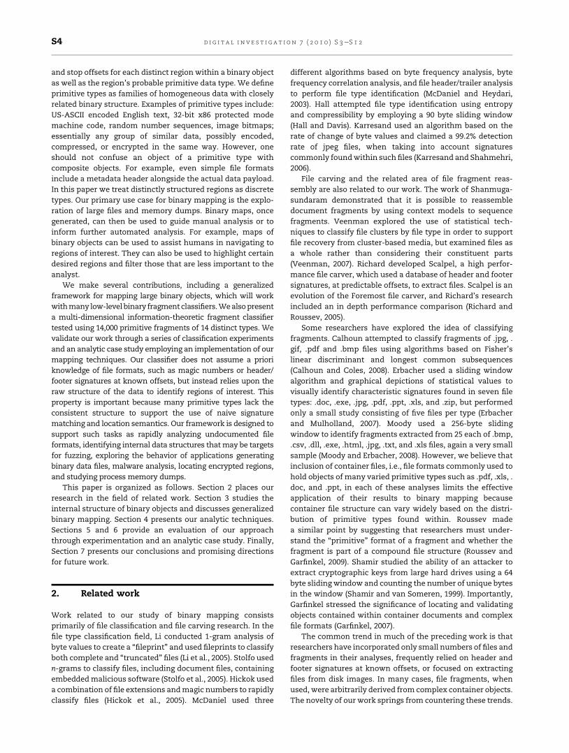
described as randomness), of fragments, see Fig. 2. High

entropy types are indicative of compressed, encrypted, or

random data; medium entropy types, such as machine code

and written human languages, exhibit noticeable structure,

and low entropy types may include uncompressed media and

repeating values, such as is found in padding.We do not claim

that the classification in Fig. 2 is complete, but instead include

it here to demonstrate the hierarchy that is formed when

identifying primitive types. As an example, a binary fragment

may be identified as being of medium entropy and then

further identified as a written language. The written language

may then be categorized as to the encoding scheme and

specific language that was used. As another example, a high

entropy fragment may be encrypted, compressed, or random.

If compressed, the region may be classified by the algorithm

used to create it, such as Run Length Encoding (RLE) or Lempel

Ziv Welch (LZW). A classifier used in binary mapping should

attempt to accurately identify a fragment, but when this is not

possible, the classifier should state that the region as

unknown. We will discuss the practical construction of

a fragment corpus and determining unknowns later in the

paper. The following is a notional example of a binary map.

0000-03FF Data Structure (File Header?)

0400-07FF US-ASCII Text (English)

0800-9FFF Bitmap Image

8000-9FFF Variable Length Array

A000-BFFF Compressed Data (LZW?)

A000-BFFF Basic Latin Unicode (English)

C000-CFFF Unknown Region

D000-D02E Repeating Value (0xFF)

D400-D41C Encrypted Region (AES?)

E000-FFFF Basic Latin Unicode (Hyperlinks?)

.

The creation of such amapwould allow analysts to quickly

identify regions of interest for more detailed examination. In

addition, a map to a binary object can serve as a navigational

aid if integrated directly into interactive analysis tools, e.g.,

double clicking a region immediately jumps the tool’s focus

directly to the desired region. More importantly, a map can

create an efficient interaction metaphor, allowing a user to

filter or highlight various regions or classes of primitive types.

Finally, the map can be modified by the analyst throughout

the analytic process and perhaps even marked up with

Fig. 1 e Internal structure of a 405 KB Microsoft Word 2003

document depicted using the byteplot visualization. Note

the distinct regions of differing structure, including US-

ASCII text (top) and compressed image (middle).

d i g i t a l i n v e s t i g a t i o n 7 ( 2 0 1 0 ) S 3eS 1 2 S5

analyst notes. For example, the analyst may discover a new

primitive type and feed its statistical signature back into the

classification engine for future automated identification.

In some cases, the map will be small. For example, many

image file formats contain a small number of differing regions,

such as a header, footer, and compressed image payload. Even

a small map can facilitate rapid analysis despite large file

sizes. The analyst need only examine a few regions to gain

rapid understanding of a file. In other cases, objects may be

more complex, such as Microsoft Word binary data files or

memory dumps. Automated mapping is useful in these cases

as well, especially when compared to traditional manual

analysis. Such objects can be mapped by the machine, which

then could be used to guide the analyst to regions of interest.

It is important to note that similar regions within binary

objects may differ significantly in size. They may be small,

perhaps only tens of bytes, like the header of a PNG file, or very

large, such as a 1 MB block of encrypted data. The size of the

fragment is important because many classifiers, particularly

those based on statistical techniques, require a minimum

sample size to provide accurate results. We will discuss the

implications of sample size and its impact on our use of

a sliding window algorithm later in the paper.

4. Analytic techniques

To classify fragments we created statistical signatures of

14,000 fragments (1000 fragments of 14 commonly encoun-

tered primitive types). The size of each fragment was 1024

bytes, and they were collected in two ways. Some were

collected directly from files known to consist of a single type,

such as a file containing solely randomnumbers. In the case of

files with headers and/or footers and a core payload of

a desired primitive type, we extracted fragments from the

middle of the file or, if possible, using knowledge of a region’s

exact location. To understand the statistical characteristics of

each type and to facilitate classification, we carefully selected

four statistical tests and used these tests to develop statistical

signatures for each fragment.

4.1. Statistical tests

With the aim of characterizing the structure found in frag-

ments, we considered many statistical tests, but chose four:

Shannon Entropy, Chi Square, Hamming Weight, and Arith-

metic Mean. We chose these tests because we believed they

would highlight statistical differences between primitive

types in ways that would assist classification.

4.1.1. Shannon entropyShannon Entropy (H ) is an established technique for

measuring uncertainty, sometimes colloquially described as

randomness, developed by Claude Shannon (Shannon, 1948).

HðXÞ ¼ �Xn¼1

i¼0

pðXiÞlogbpðXiÞ

In the case of byte-level entropy analysis, X is a random

variable with 256 potential outcomes: {xi: i ¼ 0, ., 255} and

base b ¼ 10. The probability mass function, p(xi) is the proba-

bility of byte value i within a given fragment. We explored

several variations including the use of byte bigrams (2562

possible outcomes) and byte trigrams (2563 possible

outcomes), ultimately choosing to use byte bigrams such that

{xi: i¼ 0,., 65 535}, i.e., treating each two byte sequence as a 16

bit value. We made this choice because we found greater

accuracy using digrams than single byte values (unigrams) in

initial experimentation.

4.1.2. Arithmetic meanThe arithmetic mean is simply the sum of the byte values in

a given fragment divided by the fragment size.

4.1.3. Chi squareThe Chi Square (X2) Goodness of Fit Test is an effective means

of measuring randomness and is sensitive to differences in

random, pseudo random, and compressed data. We used the

test to compare the observed distribution of byte values to

a uniform random distribution.

X2 ¼Xn¼1

i¼0

ðobserved� expectedÞ2expected

For each byte value 0, ., 255 we calculate the sum of the

squared differences between the observed frequency of the

byte in the sample and the expected frequency of the byte in

a uniform random distribution divided by the expected

frequency. We then calculate the upper probability of the Chi

Square distribution using this Chi Square value and 255

degrees of freedom, which yields a value between 0 and 1.

Fig. 2 e Example hierarchy of primitive data types commonly found within binary objects.


As can be seen from Table 1, in cases where data was plain

text (that is, 7-bit as opposed to the 16-bit uniform distribution

itwas compared to), the Chi Square test correctly indicated that

the data was distributed very differently from uniform random

data by returning very low values that got rounded to 0.

4.1.4. Hamming weightHamming Weight is determined by counting the number of

non-zero symbols in a given alphabet. For our experiments we

considered the alphabet to contain just binary data, i.e., an

alphabet of zeroes and ones. We present Hamming Weight as

the fraction of the total number of ones divided by the total

number of bits.

While our primary experiments employed these four

statistical measures, we do not claim they are necessarily the

best possible set. We also explored the use of Monte Carlo Pi,

Serial Correlation, and the Index of Coincidence (Friedman,

1922). Our initial results indicate that Monte Carlo Pi and

Serial Correlation merit further exploration. However, we

found that the Index of Coincidence is closely correlated with

Shannon Entropy, but yields slightly less accurate classifica-

tion results, and may not merit further exploration.

In order to support our classification algorithm, we

normalized each range, when appropriate. For Shannon

entropy and mean, we normalized each value to fall between

0.0 and 1.0 based on the estimated range of possible values

yielded by each calculation. The mean has a minimum value

of 0 and amaximum value of 255, so we divided each value by

255. Shannon entropy for a 1 KB sample has aminimum value

of 0 and a maximum value of 10, so we divided each value by

10. Both Hamming weight and Chi Square values already fell

between 0 and 1 so we did not normalize them.

4.2. Determining statistical signatures of fragments

For this phase of our research, we carefully collected the

samples for our fragment corpus and calculated the statistical

signature of each, using the previously discussed statistical

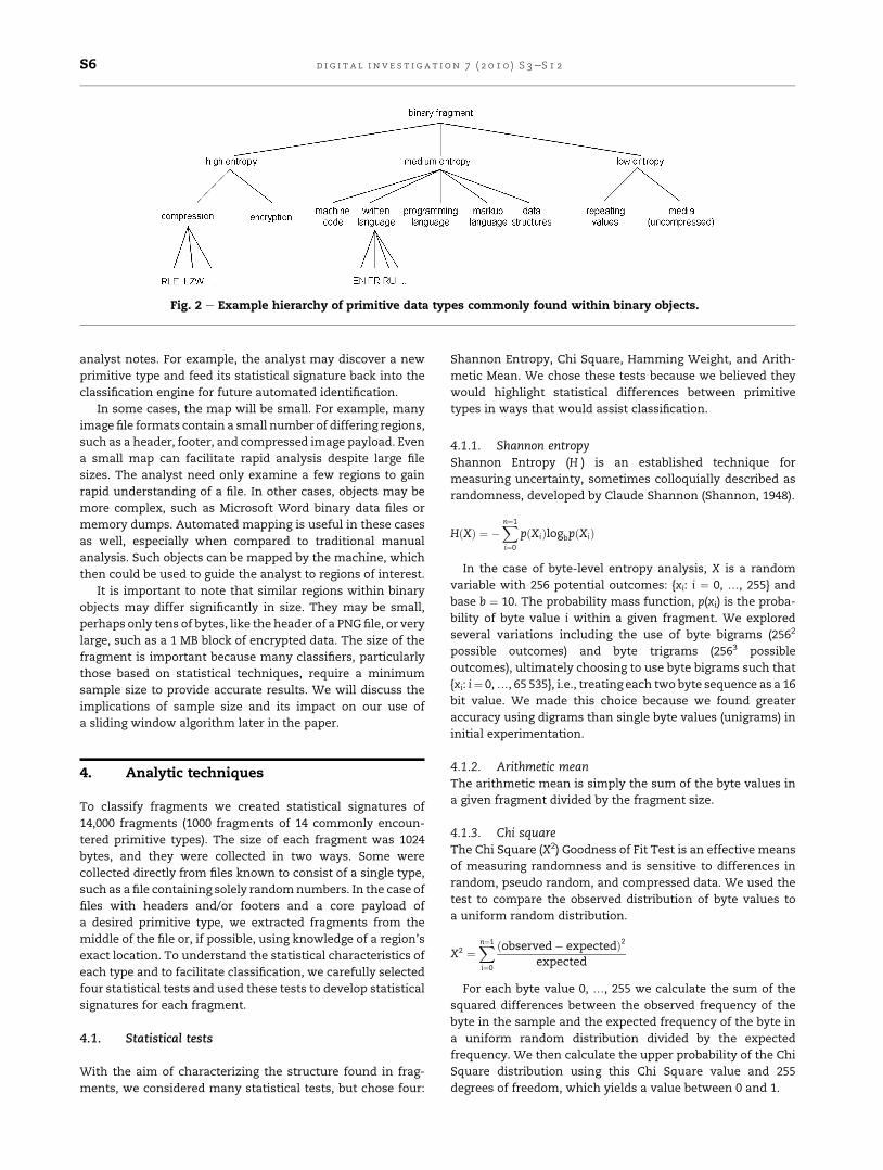
tests. Summary statistics can be seen in Table 1 and individual

fragment statistics are show in Fig. 3.

4.2.1. Test corpus generationIn order to create the statistical signatures required to accu-

rately map an arbitrary binary object, we needed a corpus of

“clean” primitive fragments without any header and footer

values. To this end, we chose source files fromwhichwe could

extract a fragment of a primitive type without extraneous

content such as metadata. To reduce the likelihood of

accidentally including header or footer information in the

primitive fragment samples, we extracted 1 KB samples from

the middle of each file and ensured that each file was at least

double this size, although most source files were significantly

larger. We discuss additional details on test corpus generation

in the following paragraphs.

4.2.1.1. Random. There aremany potential sources of random

(or pseudo random) data. We created our fragments using

data made available at Random.org. We chose Random.org

because its data is based on atmospheric noise and is under-

stood to be a source of high quality random data.

4.2.1.2. Text. For textual data we selected text-only books

from the Project Gutenberg 2006 DVD image (Gutenberg).

Because each document included an identical header, we

removed these headers in order to generate an independent

set of documents. Note that some of these documents

included non-English content, but all documents were enco-

ded in US-ASCII.

4.2.1.3. Machine code. Machine code fragments were

extracted from both Linux ELF and Windows PE files. ELF

files were randomly chosen from a clean install of Ubuntu

9.10 (Karmic Koala), and Windows PE files were gathered

from a Windows XP (Service Pack 3) workstation. From each

of these files we extracted the .text section, i.e., the section

that contains machine code. To confirm our belief that .text

sections contained solely machine code, we manually

inspected a number of samples. In each instance, ELF files

appeared to contain just machine code, however PE files

included a table of strings at the end of each .text section,

perhaps due to the idiosyncrasies of a given compiler. To

Table 1 e Average (3) and standard deviation (s) of Shannon Entropy, Index of Coincidence, Hamming Weight andArithmetic Mean for 1000 fragments in each category. (Fragment size [ 1 KB).

Mean Shannon entropy CHI SQUARE Hamming weight

� s � s � s � s

Random 127.4039 2.3436 9.9826 0.0055 0.4873 0.2968 0.5627 0.0050

Encrypt (AES256/text) 127.4778 2.3122 9.9830 0.0055 0.5008 0.2925 0.5627 0.0052

Compress (bzip2/text) 126.6846 4.2372 9.9802 0.0069 0.2118 0.2480 0.5597 0.0134

Compress (compress/text) 113.7279 8.8724 9.9662 0.0475 0.0681 0.1594 0.5316 0.0149

Compress (deflate (png) 121.7824 12.9482 9.7103 0.7053 0.0460 0.1294 0.5430 0.0444

Compress (LZW (gif)/image) 113.7543 8.2331 9.9455 0.0551 0.0203 0.0932 0.5153 0.0265

Compress (mpeg/music) 126.2643 7.2295 9.8747 0.4421 0.0463 0.1260 0.5560 0.0245

compress (jpeg/image) 130.7620 12.7763 9.7314 0.8792 0.0647 0.1555 0.5744 0.0412

Encoded (base64/zip) 84.4643 0.7402 9.7672 0.0192 0.0000 0.0000 0.5306 0.0037

encoded (uuencoded/zip) 63.7171 0.6968 9.7026 0.0209 0.0000 0.0000 0.4991 0.0053

Machine code (linux elf) 116.4212 14.9786 7.6141 0.4381 0.0000 0.0000 0.4940 0.0429

Machine code (windows PE) 107.3952 18.4625 8.0671 0.7279 0.0022 0.0385 0.4819 0.0497

Bitmap 156.4776 69.1200 6.2298 3.6235 0.0000 0.0000 0.6635 0.1905

Text (mixed) 88.5252 7.4828 7.4389 0.2427 0.0000 0.0000 0.5140 0.0146


address this issue, we ensured that each extracted text

section was at least 2048 bytes, from which we extracted the

middle 1024 bytes.

4.2.1.4. Bitmap. Our bitmap fragments were extracted from

image files which were created by converting JPEG

compressed .jpg files to .bmp format using the batch convert

capability of Adobe Photoshop. The original source files were

collected from a variety of sources, including a college’s

internal use photo archive and personal photo archives

generated by the researchers. We acknowledge that using

these relatively limited image sources may tend to generate

statistically similar fragments and suggest seeking to increase

diversity for future work. However, as you examine the

statistical summary provided in Table 1, note that we were

still able to create a set of bitmap fragments with large stan-

dard deviations across the statistical tests, implying

substantial diversity.

4.2.1.5. Compressed images, audio, and text. For compressed

image examples we chose to extract fragments created by

differing algorithms including Deflate (.png source files), LZW

(.gif source files), and JPEG (.jpg source files). For compressed

audio data we extracted fragments compressed using MPEG-1

Audio Layer 3 (.mp3 source files). In addition we created two

additional sets of fragments by compressing Project Guten-

berg text files. The first fragment class was created using the

Linux compress command line utility (Lempel-Ziv coding) and

the other using bzip2 (Burrows-Wheeler block sorting and

Huffman coding).

4.2.1.6. Encoded. We generated Base64 and Uuencoded

samples using the GNU uuencode command line utility and .

zip files from the Project Gutenberg 2006 DVD. We chose to

encode .zip files instead of .txt files because Base64 and

Uuencoding are commonly used to convert binary data to text

for transmission using text based protocols.

4.2.1.7. Encrypted. There aremyriadways to encrypt data. For

our experiments we chose to use a popular algorithm (AES)

and key length (256 bits) to encrypt Project Gutenberg text files

using the Linux mcrypt utility. We made the decision to use

AES to provide a reasonable representation of encrypted data

for our experiments. However, exploration of differing algo-

rithms, key lengths, and source data (such as compressed

data) merits additional investigation.

When dealing with fragments we believe it is important to

consider encryption, compression, and encoding algorithms to

be an appropriate way to categorize such fragments, as it is

the combination of the underlying algorithm and the source

data it acts upon that generates the unique binary primitive

type irrespective of a given file format. In addition, you may

note that some primitive types are based on the same source

data, e.g., our corpus includes compressed and encrypted

fragments based on the same source text documents. Because

of this, one might assume a statistical bias toward similarity

between primitive types classes. We believe potential simi-

larity is advantageous as we are attempting to differentiate

between types. A bias toward similarity increases the difficulty

of classification, making good classification results harder to

obtain. However, we believe this issue is substantially miti-

gated by the significant transformations that occur when

compressing, encrypting, and encoding the data.

5. Fragment classification

To create a classifier we combined the statistical signatures

developed in the previous section with the k-nearest neighbor

(k-NN) algorithm. k-nearest neighbor is a well understood

Fig. 3 e Distribution of data fragments by primitive fragment class. Note that the bitmap samples show little clustering, but

the high entropy, text, encoded, and machine code primitive types are more densely clustered.


classification algorithm which uses distance between a given

item and its k-nearest neighbors to perform classification. For

example, if k ¼ 3 and an unknown item has type1, type2, and

type1 as its three nearest neighbors, the unknown itemwill be

classified as type1.

Distance is measured using a distance metric. We evalu-

ated two, Manhattan distance and Euclidean distance. Both

metrics scale to N dimensions and perform best when values

in each dimension are normalized, which we have done. In

our experiments N ¼ 4 because we are measuring the

distance between fragments based on four statistical

dimensions: mean, Shannon Entropy, Chi Square, and

Hamming Weight. Ultimately we chose Euclidean distance

because our initial analysis found slightly increased accuracy

over Manhattan distance. When comparing two fragments,

F1 and F2, of four dimensions, Euclidean distance works as

follows. For both F1 and F2 we create a feature vector

populated by the fragment’s normalized mean, Shannon

Entropy, Chi Square, and Hamming Weight values as shown

in the following example:

F1 ¼ (0.1, 0.7, 0.2, 1.0)

F2 ¼ (0.2, 0.8, 0.6, 0.4)

We then calculate the distance (D) between the fragments

by taking the square root of the sumof the squared differences

between each pair of values.

D(F1,F2) ¼ sqrt((0.1e0.2)2 þ (0.7e0.8)2 þ (0.2e0.6)2 þ (1.0e0.4)2)

D(F1,F2) ¼ 0.54

In our experiments we calculated the distance between

each fragment and the other 13,999 fragments in the corpus.

We classified a fragment based on the most frequently

occurring type of its k-nearest neighbors. Ties were broken by

choosing the type with the minimum total distance from the

unknown fragment. During experimentation we tested values

of k ¼ 1 to k ¼ 25 and found that values of k � 3 provided

approximately 1% greater overall accuracy, but that values of

k ¼ 4 to k ¼ 25 did not noticeably increase accuracy beyond

this point. In order to minimize processing requirements we

chose to use k ¼ 3. Our classification results are shown in

Table 2. Rows indicate the actual type of the fragment and

columns indicate the guessed fragment type. An optimal

solution would include 1.0 (e.g., 100% accuracy) along the

diagonal and 0.0 in all other cells. When examining the

matrix, note that confusion is localized within clusters of

Table 2 e Confusion matrix of classification results on a scale of 0 (no matches) to 1 (all matches). Exact classificationoutcomes are shown on the diagonal. Note the increased accuracy within the outlined regions: high entropy, Uuencoded,Base64 encoded, machine code, text and bitmap. Rows indicate actual fragment type and columns are the guessedfragment type.

modnar

)txet/652SEA(tpyrcne

)txet/2 piz b(s ser pmo c

)txet/sserpmoc(sserp

moc

)eg am i/ )fi g(

WZL(sserpmo c

)oidua/gepm(sserp

moc

)egami/)gnp(etalfed(sserp

moc

)egami/gepj(sserp

moc

)piz/46esab(edocne

)p iz /e doc neuu (e docn e

)fle xunil(edoc enihcam

)EP swodni

w(edoc enihcam

t xet

pamtib

random .375 .370 .141 .018 .004 .022 .029 .041 0 0 0 0 0 0 encrypt(AES256/text) .363 .386 .133 .019 .003 .024 .026 .044 0 0 0 .002 0 0 compress(bzip2/text) .160 .163 .306 .078 .049 .073 .072 .097 0 0 0 .002 0 0

compress(compress/text) .022 .030 .072 .588 .176 .040 .035 .031 0 0 0 .002 0 .004 compress(LZW(gif)/image) .009 .007 .054 .148 .661 .041 .056 .024 0 0 0 0 0 0

compress(mpeg/audio) .033 .036 .093 .031 .048 .455 .160 .130 0 0 0 0 0 .014 compress(deflate(png)/image) .030 .037 .081 .027 .061 .177 .424 .101 0 0 .007 .043 0 .012

compress(jpeg/image) .055 .054 .119 .031 .039 .116 .115 .441 0 0 .006 .009 0 .015 encode(base64/zip) 0 0 0 0 0 0 0 0 1 0 0 0 0 0

encode(uuencode/zip) 0 0 0 0 0 0 0 0 0 1 0 0 0 0 machine code(linux elf) 0 0 0 0 0 0 0 0 0 0 .823 .166 0 .011

machine code(windows PE) 0 .003 .001 .002 .001 0 .020 .002 0 0 .224 .721 .012 .014 text 0 0 0 0 0 0 0 0 0 0 0 .007 .987 .006

bitmap 0 0 0 .008 .002 .020 .034 .032 .006 .007 .024 .030 .012 .825


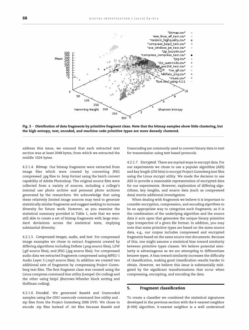
statistically similar fragment types (outlined in the table)

especially in the high entropy (random, encrypted and

compressed) and machine code (ELF and PE) categories. The

greatest classification error is found in the high entropy group

with individual accuracy rates ranging from 0.306 (bzip2/text)

to 0.661 (LZW/gif). However, very little confusion occurs

outside this group (0.017 on average). Using this insight we can

determine accuracy rates for each cluster of similarity:

� Random/Compressed/Encrypted 98.55%

� Base64 Encoded 100%

� Uuencoded 100%

� Machine Code (ELF and PE) 96.7%

� Text 98.7%

� Bitmap 82.5%

When considering how to employ our classifier in binary

mapping applications,we could choose tomap regions based on

the above categories, rather than attempt more precise classifi-

cation. Without sufficiently high classifier accuracy, a mapping

program must cope with the likelihood of frequent misclassifi-

cations even when mapping a single homogenous region.

However, when a classifier has reasonable accuracy inside

a cluster, as is the case for ELF and PE (82.3% and 72.1%, respec-

tively) this information could optionally be passed to the user.

6. System implementation

To test the efficacy of binary mapping we implemented

a binary mapping tool, binmap, using our classifier and a 1 KB

sliding window. We chose a 1 KB window because it exactly

matches the fragment size used to generate the statistical

signatures previously discussed. A differing window size

would increase the likelihood of less accurate classification

because our calculations, especially Shannon Entropy and Chi

Square, vary significantly based on sample size. Binmap takes

as input any arbitrary binary object, including, but not limited

to, complex data files, executable files, process memory

dumps, and hibernation files.

Written in Perl, binmap performs mapping by sliding the

window incrementally through the file, using a step size of 512

bytes. It starts at offset zero and continues until reaching the

end of the file. At each step, we used our classifier to identify

the contents of the window. If at the end of the file, there were

not a full 1024 bytes remaining, we did not attempt classifi-

cation. To perform classification, binmap compared the

statistical signatures of the contents of the window against

the previously derived 14,000 binary fragment signatures

using the same k-NN algorithm (k ¼ 3) and Euclidean distance

metric described earlier. As the window slid through the file,

binmap calculated the start and stop offset of each differing

type of region in the following categories: random/

compressed/encrypted, Base64 encoded, Uuencoded,

machine code, text, bitmap, and unknown. Upon encoun-

tering a different region, binmap would record the current

offset and consider the region contiguous until it detected

a transition to a different type. At this point, binmap would

output the start and end offset and the data type. This process

would begin again by recording the start offset of the new

region and continue until the next transition. Because an

arbitrary binary object would likely contain types that were

not previously analyzed, binmap classifies a region as

unknown if the contents of the window were sufficiently

distant from an existing fragment signature. We chose the

following distance thresholds as the maximum acceptable

distance for each given type: Random/Compressed/Encrypted

(0.362), Base64 Encoded(0.005), Uuencoded(0.125), Machine

Code(0.740), Text(0.432) and Bitmap(0.190). We derived these

values by determining the most distant successful match in

each category from our previous experiments and set this

value as the maximum acceptable distance.

7. Case study

To explore the effectiveness of binmap we used it to analyze

two complex binary objects, a 10.3 MB Microsoft Word 2003

document and a 41.4 MB Firefox browser process memory

dump. We chose these two objects because they contained

a diverse range of primitive types, but were larger than would

be practical to analyze using manual inspection alone. We

used binmap to create a map of each file and then attempted

to determine the maps’ accuracy by manual inspection. This

analysis highlighted important advantages and challenges of

binary mapping which we report below.

Because the files were complex, each map contained

numerous entries, 353 in the Word document and 20,175 in

the process memory dump. Depending on the analyst’s goal,

very high fidelity maps may be desired. In other cases

however, the analyst may be interested in seeking out only

major regions. Toward this end, we modified binmap to filter

out regions that fell below a user selectable minimum size

threshold. Upon rerunning binmap with a minimum size

threshold of 16 KB, the Word document contained 78 map

entries and the process memory dump contained 153 entries,

much more manageable figures, particularly for the process

memory dump. Depending on the type of binary object being

examined and analyst goals, we found that thresholds of 4 KB

to 32 KB, when combined with the grouping of primitive types

we discussed earlier, worked well in highlighting an object’s

high-level structure. Increasing theminimum size also served

to increase accuracy, as this approach required longer

sequences of identically classified regions and minimized the

impact of misclassification at transitions between disparate

primitive types. Another related approach, which we did not

explore, is to sort map entries based on size, allowing the

analyst to examine the largest regions first. We believe an

interactive binary map which is closely integrated with

graphical byteplot and hexadecimal views to be another

promising approach.We also suggest that researchers explore

alternative ways of visualizing mapping data, such as tree-

maps or color coding of byteplots, to assist in analysis

(Treemap Project Home Page).

Binmap performed strongly when detecting transitions

between regions, but classification results were mixed. One of

the challenges of creating a classifier in the laboratory and

then applying it in real-worlduse is copingwith thewide range

of primitive types the classifier was not trained to handle.

When binmap encountered regions it had been trained to


detect it performedwell. Unsurprisingly, it performed lesswell

when encountering a previously unstudied primitive type,

even one with a closely related structure. We believe our

thresholds for the unknown category to be too strict. Instead of

categorizing new regions as unknown, binmap often confused

these regions with bitmaps. We believe this is because our set

of bitmap fragment signatures appeared quite similar to data

structures found in both the word document and the process

memory dump. Misclassification also occurred with padding,

i.e., regions of identical byte values, such as xFF and x00. Upon

reflection, this confusion makes sense because regions of

padding would appear identical to all black and all white

regions found in our bitmap fragments. One future optimiza-

tion is to create regular expression signatures that would

detect padding, before attempting statistical classification. In

general however, we believe that our approach of including

a diverse range of examples in each primitive type category

was beneficial to classification accuracy. For example, if a few

of our machine code examples inadvertently contained some

textual strings, these statistical signatures might assist

matching less clean examples found in real-world data,

particularly at the transition between two different primitive

types. Thus the use of many statistical signatures makes bin-

map resistant to errors in corpus construction. Binmap did

perform well when classifying bitmaps of a 24-bit RGB struc-

ture, as it was trained to do, but frequently misclassified bit-

maps constructed using other encoding schemes. We believe

this issue can be overcome by including statistical signatures

for other appropriate formats such as those found in

programming literature (PixelFormat Enumeration). Bitmap

did performwell when identifying US-ASCII encoded text, but

ran into difficultieswhen classifying 16-bit Basic LatinUnicode

and HTML encoded text. Again, we believe this can be

addressed by explicitly creating representative statistical

signatures for these new primitive types. Binmap also per-

formed well when classifying random/compressed/encrypted

regions and was able to detect transitions between sequences

of embedded compressed images.

The common trend in binmap’s classification accuracy is

that it performed well when classifying primitive types it was

trained for, but often confused similar but distinct primitive

types, such as US-ASCII, Basic Latin Unicode and HTML. We

believe a reasonable solution is to increase the diversity of the

primitive type signatures employed in classification to incor-

porate a wider range of possibilities and we then believe our

approach will work well with other types of fragments.

Techniques such as weighting, clustering, Markov Chains and

simulated annealing should also be explored as ways to

improve classification. As we mentioned earlier in the paper

binary mapping is not wedded to any one classification tech-

nique. We believe a more desirable classification solution is

one that includes regular expression pattern matching and

statistical signature classification combined with knowledge

of file format semantics, if applicable in the given context.

Researchers should also consider techniques that operate at

the individual bit level and do not assume byte-level encoding

schemes. Two desirable goals of classification in support of

binary mapping is to precisely identify transitions between

differing regions and to classify primitive types with the

smallest sample size possible.

8. Conclusions and future work

In thispaperwemadeseveralcontributions:astatisticalanalysis

of 14,000 low-level binary fragments, the presentation and

evaluation of a classifier for identifying 14 primitive binary

fragment types, and the implementation of a binary mapping

application. The statistical techniques we employed included

Shannon Entropy, Hamming Weight, mean, and Chi Squared,

which proveduseful for analyzing low-level binary datawithout

relying on possibly non-existent or untrustworthy metadata.

The classifier used the k-nearest neighbor algorithm and

Euclidean distance to identify unknown fragments and accu-

rately placed them into the following groups: Random/

Compressed/Encrypted, Base64 Encoded, Uuencoded, Machine

Code, Text, and Bitmap. We then developed a binary mapping

implementationandused it tostudytwocomplexbinaryobjects.

Binary mapping is valuable to analysts because it provides

rapid insight into the structure of large, potentially massive,

binary objects by identifying the location of the varying types

of data they contain. Mapping can be employed in such tasks

as memory forensics and the analysis of undocumented file

types, but bears promise for most tasks requiring low-level

analysis of binary data. Binarymappingmay also be employed

in interactive applications, such as hex editors, visual analytic

tools and GUI-based forensic toolkits. The resultant mapping

data can be used to highlight areas of interest for the analyst,

allow rapid navigation to these regions, and facilitate filtering,

ultimately allowing the analyst to cope with very large binary

objects at a level exceeding the capabilities of today’s low-

level analysis tools. In addition, binary mapping generalizes

well and can be used with a different classifier or combination

of classifiers to increase accuracy.

For future work we recommend studying the combination

of statistical classification techniques and traditional signa-

ture matching, perhaps using a plug-in architecture, to

increase the accuracy of classification. Also, we believe that

extending the breadth of the classification capability to

include a wider array of primitive data types will increase the

utility of binary mapping. Finally, we recommend seeking to

counter ways in which an adversary might obfuscate data to

force incorrect classification.

r e f e r e n c e s

Calhoun W, Coles D. Predicting the types of file fragments. In:Digital forensics research conference; 2008.

Conti G, Dean E. Visual forensic analysis and reverse engineeringof binary data. Black Hat USA; 2008.

Conti G, Dean E, Sinda M, Sangster B. Visual reverse engineeringof binary and data files. In: Workshop on visualization forcomputer security; 2008.

Erbacher R, Mulholland J. Identification and localization of datatypes within large-scale file systems. In: Systematicapproaches to digital forensic engineering; 2007.

Friedman William. The index of coincidence and its applicationsin cryptology. Department of Ciphers. Publication 22. Geneva,Illinois, USA: Riverbank Laboratories; 1922.

Garfinkel S. Carving contiguous and fragmented files with fastobject validation. In: Digital forensics research conference;2007.


Gutenberg. The CD and DVD project. Project Gutenberg, http://www.gutenberg.org/wiki/Gutenberg:The_CD_and_DVD_Project.

Hall G, Davis W. Sliding window measurement for file typeidentification. In: White paper, ManTech cyber solutionsinternational.

Hickok D, Lesniak D, Rowe M. File type detection technology. In:Midwest instruction and computing symposium; 2005.

Karresand M, Shahmehri N. File type identification of datafragments by their binary structure. In: IEEE informationassurance workshop; 2006.

Li W, Wang K, Stolfo S, Herzog B. Fileprints: identifying file typesby n-gram analysis. In: IEEE information assurance workshop;2005.

McDaniel M, Heydari M. Content based file type detectionalgorithms. In: Hawaii international conference on systemsciences; 2003.

Moody S, Erbacher R. SADI e statistical analysis for data typeidentification. In: Systematic approaches to digital forensicengineering; 2008.

PixelFormat Enumeration. Net framework developer center.Microsoft developer network, http://msdn.microsoft.com/en-us/library/system.drawing.imaging.pixelformat.aspx.

Richard G, Roussev V. Scalpel: a frugal, high-performance filecarver. In: Digital forensics research workshop; 2005.

Roussev V, Garfinkel S. File fragment classification e the case forspecialized approaches. In: Systematic approaches to digitalforensics engineering; 2009.

Shamir A, van Someren N. Playing hide and seek with storedkeys. In: International conference on financial cryptography;1999.

Shannon C. A mathematical theory of communication. BellSystem Technical Journal July, October, 1948;27:379e423.623e656.

Stolfo S, Wang K, Li W. Fileprint analysis for Malware detection.In: Workshop on rapid Malcode; 2005.

Treemap Project Home Page. Human computer interaction lab,http://www.cs.umd.edu/hcil/treemap/.

Veenman C. Statistical disk cluster classification for filecarving. In: Symposium on information assurance andsecurity; 2007.

Gregory Conti is an Academy Professor and Director of WestPoint’s Cyber Security Research Center. His research includesonline privacy, web-based information disclosure, security datavisualization, and usable security. He is the author of SecurityData Visualization (No Starch Press) and Googling Security(AddisoneWesley). His work can be found at www.gregconti.comand www.rumint.org.

Sergey Bratus is a Research Assistant Professor at DartmouthCollege, affiliated with the Institute for Security, Technology, andSociety (ISTS). Dr. Bratus is interested in a broad range of practicaloperating systems and network security topics, and frequentshacker conferences.

Anna Shubina is a Postdoctorate Fellow at the Institute of Secu-rity, Technology, and Society at Dartmouth College. Her primaryinterest and the subject of her doctoral thesis is Privacy inmoderninformation systems.

Ben Sangster is an Assistant Professor of Computer Science at theUnited States Military Academy, West Point, NY. His researchincludes binary object identification in support of informationassurance, behavior-based information security, and virtualiza-tion of the computer science curriculum.

Roy Ragsdale is a recent graduate of the United States MilitaryAcademy where he majored in computer science. He is currentlyserving as a commissioned officer in the United States ArmyMilitary Intelligence Corps.

Matthew Supan is a recent graduate of the United States MilitaryAcademy where he majored in computer science. He is currentlyserving as a commissioned officer in the United States ArmySignal Corps.

Andrew Lichtenberg is currently a student at Skidmore Collegewhere he is a dual major in Mathematics and Computer Science.

Rober Perez-Alemany is currently a cadet at the United StatesMilitary Academy where he is majoring in Mathematics.


Documents

Automated mapping of large binary objects using … mapping of large binary objects using primitive fragment type classiﬁcation Gregory Contia,*, Sergey Bratusb, Anna Shubinab, Benjamin