Automated Formal Synthesis of Digital Controllers … · Automated Formal Synthesis of Digital Controllers 3 of imprecision in the implementation of the control algorithm and in the

Consist

ent *Complete *

Well D

ocumented*Easyt

oR

euse* *

Evaluated

*CAV*Ar

tifact *

AEC

Automated Formal Synthesis of DigitalControllers for State-Space Physical Plants?

Alessandro Abate1, Iury Bessa2, Dario Cattaruzza1, Lucas Cordeiro1,2,Cristina David1, Pascal Kesseli1, Daniel Kroening1, and Elizabeth Polgreen1

1 University of Oxford, UK2 Federal University of Amazonas, Manaus, Brazil

Abstract. We present a sound and automated approach to synthesizesafe digital feedback controllers for physical plants represented as linear,time-invariant models. Models are given as dynamical equations withinputs, evolving over a continuous state space and accounting for errorsdue to the digitization of signals by the controller. Our counterexampleguided inductive synthesis (CEGIS) approach has two phases: We syn-thesize a static feedback controller that stabilizes the system but thatmay not be safe for all initial conditions. Safety is then verified eithervia BMC or abstract acceleration; if the verification step fails, a coun-terexample is provided to the synthesis engine and the process iteratesuntil a safe controller is obtained. We demonstrate the practical value ofthis approach by automatically synthesizing safe controllers for intricatephysical plant models from the digital control literature.

1 Introduction

Linear Time Invariant (LTI) models represent a broad class of dynamical sys-tems with significant impact in numerous application areas such as life sciences,robotics, and engineering [4, 13]. The synthesis of controllers for LTI modelsis well understood, however the use of digital control architectures adds newchallenges due to the effects of finite-precision arithmetic, time discretization,and quantization noise, which is typically introduced by Analogue-to-Digital(ADC) and Digital-to-Analogue (DAC) conversion. While research on digitalcontrol is well developed [4], automated and sound control synthesis is challenging,particularly when the synthesis objective goes beyond classical stability. Thereare recent methods for verifying reachability properties of a given controller [14].However, these methods have not been generalized to control synthesis. Notethat a synthesis algorithm that guarantees stability does not ensure safety: thesystem might transitively visit an unsafe state resulting in unrecoverable failure.

We propose a novel algorithm for the synthesis of control algorithms forLTI models that are guaranteed to be safe, considering both the continuousdynamics of the plant and the finite-precision discrete dynamics of the controller,

? Supported by EPSRC grant EP/J012564/1, ERC project 280053 (CPROVER) andthe H2020 FET OPEN 712689 SC2.

2 Abate et al.

as well as the hybrid elements that connect them. We account for the presenceof errors originating from a number of sources: quantisation errors in ADC andDAC, representation errors (from the discretization introduced by finite-precisionarithmetic), and roundoff and saturation errors in the verification process (fromfinite-precision operations). Due to the complexity of such systems, we focuson linear models with known implementation features (e.g., number of bits,fixed-point arithmetic). We expect a safety requirement given as a reachabilityproperty. Safety requirements are frequently overlooked in conventional feedbackcontrol synthesis, but play an important role in systems engineering.

We give two alternative approaches for synthesizing digital controllers forstate-space physical plants, both based on CounterExample Guided InductiveSynthesis (CEGIS) [30]. We prove their soundness by quantifying errors causedby digitization and quantization effects that arise when the digital controllerinteracts with the continuous plant.

The first approach uses a naıve technique that starts by devising a digitalcontroller that stabilizes the system while remaining safe for a pre-selected timehorizon and a single initial state; then, it verifies unbounded safety by unfoldingthe dynamics of the system, considering the full hyper-cube of initial states, andchecking a completeness threshold [17], i.e., the number of iterations required tosufficiently unwind the closed-loop state-space system such that the boundariesare not violated for any larger number of iterations. As it requires unfolding upto the completeness threshold, this approach is computationally expensive.

Instead of unfolding the dynamics, the second approach employs abstractacceleration [7] to evaluate all possible progressions of the system simultaneously.Additionally, the second approach uses abstraction refinement, enabling us toalways start with a very simple description regardless of the dynamics complexity,and only expand to more complex models when a solution cannot be found.

We provide experimental results showing that both approaches are able toefficiently synthesize safe controllers for a set of intricate physical plant modelstaken from the digital control literature: the median run-time for our benchmarkset is 7.9 seconds, and most controllers can be synthesized in less than 17.2 seconds.We further show that, in a direct comparison, the abstraction-based approach(i.e., the second approach) lowers the median run-time of our benchmarks by afactor of seven over the first approach based on the unfolding of the dynamics.

Contributions

1. We compute state-feedback controllers that guarantee a given safety property.Existing methods for controller synthesis rely on transfer function represen-tations, which are inadequate to prove safety requirements.

2. We provide two novel algorithms: the first, naıve one, relies on an unfoldingof the dynamics up to a completeness threshold, while the second one isabstraction-based and leverages abstraction refinement and accelerationto improve scalability while retaining soundness. Both approaches providesound synthesis of state-feedback systems and consider the various sources

Automated Formal Synthesis of Digital Controllers 3

of imprecision in the implementation of the control algorithm and in themodeling of the plant.

3. We develop a model for different sources of quantization errors and theireffect on reachability properties. We give bounds that ensure the safety ofour controllers in a hybrid continuous-digital domain.

2 Related Work

CEGIS - Program synthesis is the problem of computing correct-by-designprograms from high-level specifications. Algorithms for this problem have madesubstantial progress in recent years, for instance [16] to inductively synthesizeinvariants for the generation of desired programs.

Program synthesizers are an ideal fit for the synthesis of digital controllers,since the semantics of programs capture the effects of finite-precision arithmeticprecisely. In [27], the authors use CEGIS for the synthesis of switching controllersfor stabilizing continuous-time plants with polynomial dynamics. The workextends to affine systems, but is limited by the capacity of the state-of-the-artSMT solvers for solving linear arithmetic. Since this approach uses switchingmodels instead of linear dynamics for the digital controller, it avoids problemsrelated to finite precision arithmetic, but potentially suffers from state-spaceexplosion. Moreover, in [28] the same authors use a CEGIS-based approach forsynthesizing continuous-time switching controllers that guarantee reach-while-stayproperties of closed-loop systems, i.e., properties that specify a set of goal statesand safe states (constrained reachability). This solution is based on synthesizingcontrol Lyapunov functions for switched systems that yield switching controllerswith a guaranteed minimum dwell time in each mode. However, both approachesare unsuitable for the kind of control we seek to synthesize.

The work in [2] synthesizes stabilizing controllers for continuous plants given astransfer functions by exploiting bit-accurate verification of software-implementeddigital controllers [5]. While this work also uses CEGIS, the approach is restrictedto digital controllers for stable closed-loop systems given as transfer functionmodels: this results in a static check on their coefficients. By contrast, in thecurrent paper we consider a state-space representation of the physical system,which requires ensuring the specification over actual traces of the model, alongsidethe numerical soundness required by the effects of discretisation and finite-precision errors. A state-space model has known advantages over the transferfunction representation [13]: it naturally generalizes to multivariate systems (i.e.,with multiple inputs and outputs); and it allows synthesis of control systems withguarantees on the internal dynamics, e.g., to synthesize controllers that makethe closed-loop system safe. Our work focuses on the safety of internal states,which is usually overlooked in the literature. Moreover, our work integrates anabstraction/refinement (CEGAR) step inside the main CEGIS loop.

The tool Pessoa [21] synthesizes correct-by-design embedded control softwarein a Matlab toolbox. It is based on the abstraction of a physical system to anequivalent finite-state machine and on the computation of reachability properties

4 Abate et al.

thereon. Based on this safety specification, Pessoa can synthesize embeddedcontroller software for a range of properties. The embedded controller softwarecan be more complicated than the state-feedback control we synthesize, andthe properties available cover more detail. However, relying on state-space dis-cretization Pessoa is likely to incur in scalability limitations. Along this researchline, [3, 20] studies the synthesis of digital controllers for continuous dynamics,and [34] extends the approach to the recent setup of Network Control Systems.

Discretization Effects - The classical approach to control synthesis has oftendisregarded digitalization effects, whereas more recently modern techniques havefocused on different aspects of discretization, including delayed response [10] andfinite word length (FWL) semantics, with the goal either to verify (e.g., [9]) orto optimize (e.g., [24]) given implementations.

There are two different problems that arise from FWL semantics. The first isthe error in the dynamics caused by the inability to represent the exact stateof the physical system, while the second relates to rounding and saturationerrors during computation. In [12], a stability measure based on the error ofthe digital dynamics ensures that the deviation introduced by FWL does notmake the digital system unstable. A more recent approach [33] uses µ-calculus todirectly model the digital controller so that the selected parameters are stable bydesign. The analyses in [29, 32] rely on an invariant computation on the discretesystem dynamics using Semi-Definite Programming (SDP). While the former usesbounded-input and bounded-output (BIBO) properties to determine stability, thelatter uses Lyapunov-based quadratic invariants. In both cases, the SDP solveruses floating-point arithmetic and soundness is checked by bounding the error.An alternative is [25], where the verification of given control code is performedagainst a known model by extracting an LTI model of the code by symbolicexecution: to account for rounding errors, an upper bound is introduced in theverification phase. The work in [26] introduces invariant sets as a mechanism tobound the quantization error effect on stabilization as an invariant set that alwaysconverges toward the controllable set. Similarly, [19] evaluates the quantizationerror dynamics and bounds its trajectory to a known region over a finite timeperiod. This technique works for both linear and non-linear systems.

3 Preliminaries

3.1 State-space representation of physical systems

We consider models of physical plants expressed as ordinary differential equations(ODEs), which we assume to be controllable and under full state information(i.e., we have access to all the model variables):

x(t) = Ax(t) +Bu(t), x ∈ Rn, u ∈ Rm, A ∈ Rn×n, B ∈ Rn×m, (1)

where t ∈ R+0 , where A and B are matrices that fully specify the continuous

plant, and with initial states set as x(0). While ideally we intend to work on the


continuous-time plant, in this work Eq. (1) is soundly discretized in time [11] into

xk+1 = Adxk +Bduk (2)

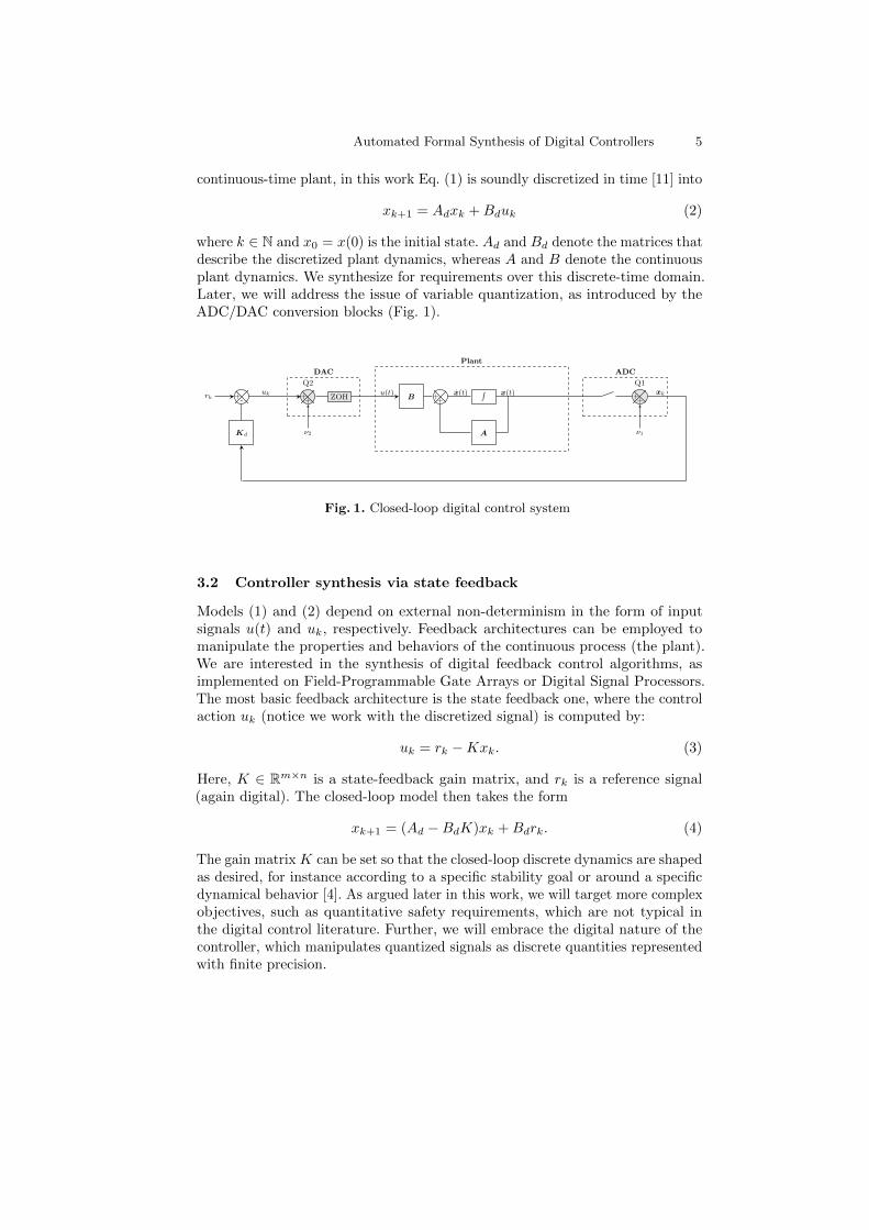
where k ∈ N and x0 = x(0) is the initial state. Ad and Bd denote the matrices thatdescribe the discretized plant dynamics, whereas A and B denote the continuousplant dynamics. We synthesize for requirements over this discrete-time domain.Later, we will address the issue of variable quantization, as introduced by theADC/DAC conversion blocks (Fig. 1).

rk -+

uk

Kd

DAC

++

Q2

ν2

ZOH

Plant

Bu(t)

++ x(t) ∫ x(t)

A

ADC

++

Q1

ν1

xk

Fig. 1. Closed-loop digital control system

3.2 Controller synthesis via state feedback

Models (1) and (2) depend on external non-determinism in the form of inputsignals u(t) and uk, respectively. Feedback architectures can be employed tomanipulate the properties and behaviors of the continuous process (the plant).We are interested in the synthesis of digital feedback control algorithms, asimplemented on Field-Programmable Gate Arrays or Digital Signal Processors.The most basic feedback architecture is the state feedback one, where the controlaction uk (notice we work with the discretized signal) is computed by:

uk = rk −Kxk. (3)

Here, K ∈ Rm×n is a state-feedback gain matrix, and rk is a reference signal(again digital). The closed-loop model then takes the form

xk+1 = (Ad −BdK)xk +Bdrk. (4)

The gain matrix K can be set so that the closed-loop discrete dynamics are shapedas desired, for instance according to a specific stability goal or around a specificdynamical behavior [4]. As argued later in this work, we will target more complexobjectives, such as quantitative safety requirements, which are not typical inthe digital control literature. Further, we will embrace the digital nature of thecontroller, which manipulates quantized signals as discrete quantities representedwith finite precision.

6 Abate et al.

3.3 Stability of closed-loop systems

In this work we employ asymptotic stability in the CEGIS loop, as an objectivefor guessing controllers that are later proven sound over safety requirements.Asymptotic stability is a property that amounts to convergence of the modelexecutions to an equilibrium point, starting from any states in a neighborhood ofthe point (see Figure 3 for the portrait of a stable execution, converging to theorigin). In the case of linear systems as in (4), considered with a zero referencesignal, the equilibrium point of interest is the origin.

A discrete-time LTI system as (4) is asymptotically stable if all the roots of itscharacteristic polynomial (i.e., the eigenvalues of the closed-loop matrix Ad−BdK)are inside the unity circle of the complex plane, i.e., their absolute values arestrictly less than one [4] (this simple sufficient condition can be generalised,however this is not necessary in our work). In this paper, we express this stabilityspecification φstability in terms of a check known as Jury’s criterion [11]: this isan easy algebraic formula to select the entries of matrix K so that the closed-loopdynamics are shaped as desired.

3.4 Safety specifications for dynamical systems

We are not limited to the synthesis of digital stabilizing controllers – a well knowntask in the literature on digital control systems – but target safety requirementswith an overall approach that is sound and automated. More specifically, werequire that the closed-loop system (4) meets given safety specifications. A safetyspecification gives raise to a requirement on the states of the model, such that thefeedback controller (namely the choice of the gains matrix K) must ensure thatthe state never violates the requirement. Note that a stable, closed-loop systemis not necessarily a safe system: indeed, the state values may leave the safe partof the state space while they converge to the equilibrium, which is typical in thecase of oscillatory dynamics. In this work, the safety property is expressed as:

φsafety ⇐⇒ ∀k ≥ 0.

n∧i=1

xi ≤ xi,k ≤ xi, (5)

where xi and xi are lower and upper bounds for the i-th coordinate xi of statex ∈ Rn at the k-th instant, respectively. This means that the states will alwaysbe within an n-dimensional hyper-box.

Furthermore, it is practically relevant to consider the constraints φinput onthe input signal uk and φinit on the initial states x0, which we assume have givenbounds: φinput = ∀k.u ≤ uk ≤ u, φinit =

∧ni=1 xi,0 ≤ xi,0 ≤ xi,0. For the former,

this means that the control input might saturates in view of physical constraints.

3.5 Numerical representation and soundness

The models we consider have two sources of error that are due to numericalrepresentation. The first is the numerical error introduced by the fixed-point


numbers employed to model the plant, i.e., to represent the plant dynamicsAd, Bd and xk. The second is the quantization error introduced by the digitalcontroller, which performs operations on fixed-point numbers. In this section weoutline the notation for the fixed-point representation of numbers, and brieflydescribe the errors introduced. A formal discussion is in Appendix B.1.

Let F〈I,F 〉(x) denote a real number x represented in a fixed point domain,with I bits representing the integer part and F bits representing the decimalpart. The smallest number that can be represented in this domain is cm = 2−F .Any mathematical operations performed at the precision F〈I,F 〉(x) will introduceerrors, for which an upper bound can be given [6].

We will use F〈Ic,Fc〉(x) to denote a real number x represented at the fixed-pointprecision of the controller, and F〈Ip,Fp〉(x) to denote a real number x representedat the fixed-point precision of the plant model (Ic and Fc are determined by thecontroller. We pick Ip and Fp for our synthesis such that Ip ≥ Ic and Fp ≥ Fc).Thus any mathematical operations in our modelled digital controller will be inthe range of F〈Ic,Fc〉, and all other calculations in our model will be carried outin the range of F〈Ip,Fp〉. The physical plant operates in the reals, which meansour verification phase must also account for the numerical error and quantizationerrors caused by representing the physical plant at the finite precision F〈Ip,Fp〉.

Effect on safety specification and stability Let us first consider the effectof the quantization errors on safety. Within the controller, state values aremanipulated at low precision, alongside the vector multiplication Kx. The inputsare computed using the following equation:

uk = −(F〈Ic,Fc〉(K) · F〈Ic,Fc〉(xk)).

This induces two types of the errors detailed above: first, the truncation errordue to representing xk as F〈Ic, Fc〉(xk); and second, the rounding error introducedby the multiplication operation. We represent these errors as non-deterministicadditive noise.

An additional error is due to the representation of the plant dynamics, namely

xk+1 = F〈Ip,Fp〉(Ad)F〈Ip,Fp〉(xk) + F〈Ip,Fp〉(Bd)F〈Ip,Fp〉(uk).

We address this error by use of interval arithmetic [22] in the verification phase.

Previous studies [18] show that the FWL affects the poles and zeros positions,degrading the closed-loop dynamics, causing steady-state errors (see Appendix Bfor details) and eventually de-stabilizing the system [5]. However, since in thispaper we require stability only as a precursor to safety, it is sufficient to checkthat the (perturbed, noisy) model converges to a neighborhood of the equilibriumwithin the safe set (see Appendix A.1).

In the following, we shall disregard these steady-state errors (caused by FWLeffects) when stability is ensured by synthesis, and then verify its safety accountingfor the finite-precision errors.

8 Abate et al.

4 CEGIS of Safe Controllers for LTI Systems

In this section, we describe our technique for synthesizing safe digital feedbackcontrollers using CEGIS. For this purpose, we first provide the synthesizer’sgeneral architecture, followed by describing our two approaches to synthesizingsafe controllers: the first one is a baseline approach that relies on a naıve unfoldingof the transition relation, whereas the second uses abstraction to evaluate allpossible executions of the system.

4.1 General architecture of the program synthesizer

The input specification provided to the program synthesizer is of the form∃P.∀a. σ(a, P ), where P ranges over functions (where a function is representedby the program computing it), a ranges over ground terms, and σ is a quantifier-free formula. We interpret the ground terms over some finite domain D. Thedesign of our synthesizer consists of two phases, an inductive synthesis phaseand a validation phase, which interact via a finite set of test vectors inputsthat is updated incrementally. Given the aforementioned specification σ, theinductive synthesis procedure tries to find an existential witness P satisfying thespecification σ(a, P ) for all a in inputs (as opposed to all a ∈ D). If the synthesisphase succeeds in finding a witness P , this witness is a candidate solution to thefull synthesis formula. We pass this candidate solution to the validation phase,which checks whether it is a full solution (i.e., P satisfies the specification σ(a, P )for all a ∈ D). If this is the case, then the algorithm terminates. Otherwise,additional information is provided to the inductive synthesis phase in the form ofa new counterexample that is added to the inputs set and the loop iterates again.More details about the general architecture of the synthesizer can be found in [8].

4.2 Synthesis problem: statement (recap) and connection toprogram synthesis

At this point, we recall the the synthesis problem that we solve in this work:we seek a digital feedback controller K (see Eq. 3) that makes the closed-loopplant model safe for initial state x0, reference signal rk and input uk as definedin Sec. 3.4. We consider non-deterministic initial states within a specified range,the reference signal to be set to zero, saturation on the inputs, and account fordigitization and quantization errors introduced by the controller.

When mapping back to the notation used for describing the general architec-ture of the program synthesizer, the controller K denotes P , (x0, uk) representsa and φstability ∧ φinput ∧ φinit ∧ φsafety denotes the specification σ.

4.3 Naıve Approach: CEGIS with multi-staged verification

An overview of the algorithm for controller synthesis is given in Fig. 2. Oneimportant observation is that we verify and synthesize a controller over k time


1.Synthesize

Verify

2.Safety 3.Precision 4.Complete Done

Program Search BMC-basedVerifier

Fixed-pointArithmetic

Verifier

CompletenessVerifier

K

C-ex

T/F T/FK K KUNSAT/

model

PASS

InputsUNSAT/K

Increase Precision

Increase Unfolding Bound

Fig. 2. CEGIS with multi-staged verification

steps. We then compute a completeness threshold k [17] for this controller, andverify correctness for k time steps. Essentially, k is the number of iterationsrequired to sufficiently unwind the closed-loop state-space system, which ensuresthat the boundaries are not violated for any other k>k.

Theorem 1. There exists a finite k such that it is sufficient to unwind theclosed-loop state-space system up to k in order to ensure that φsafety holds.

Proof. A stable control system is known to have converging dynamics. Assumethe closed-loop matrix eigenvalues are not repeated (which is sensible to do, sincewe select them). The distance of the trajectory from the reference point (origin)decreases over time within subspaces related to real-valued eigenvalues; however,this is not the case in general when dealing with complex eigenvalues. Considerthe closed-loop matrix that updates the states in every discrete time step, andselect the eigenvalue ϑ with the smallest (non-trivial) imaginary value. Betweenevery pair of consecutive time steps k Ts and (k + 1)Ts, the dynamics projectedon the corresponding eigenspace rotate ϑTs radians. Thus, taking k as the ceilingof 2π

ϑTs, after k≥k steps we have completed a full rotation, which results in a

point closer to the origin. The synthesized k is the completeness threshold. ut

Next, we describe the different phases in Fig. 2 (blocks 1 to 4) in detail.

1. The inductive synthesis phase (synthesize) uses BMC to compute a can-didate solution K that satisfies both the stability criteria (Sec. 3.3) andthe safety specification (Sec. 3.4). To synthesize a controller that satisfiesthe stability criteria, we require that a computed polynomial satisfies Jury’scriterion [11]. The details of this calculation can be found in the Appendix.Regarding the second requirement, we synthesize a safe controller by unfoldingthe transition system k steps and by picking a controller K and a single

10 Abate et al.

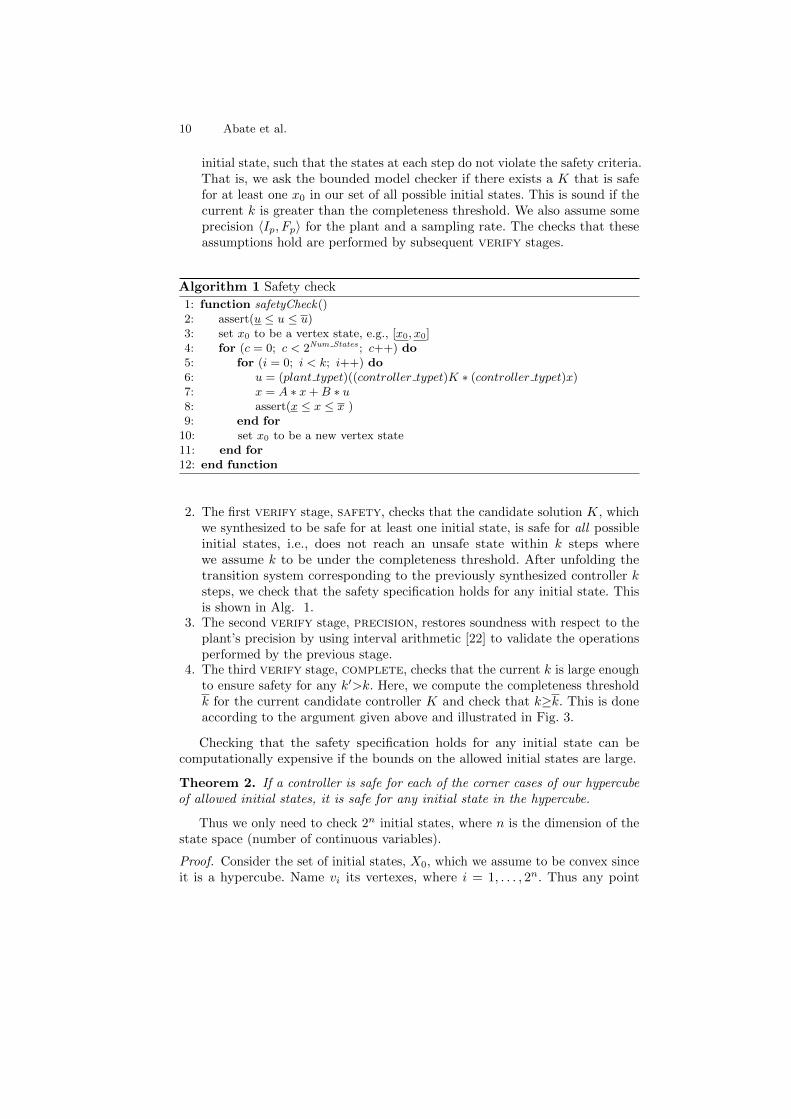
initial state, such that the states at each step do not violate the safety criteria.That is, we ask the bounded model checker if there exists a K that is safefor at least one x0 in our set of all possible initial states. This is sound if thecurrent k is greater than the completeness threshold. We also assume someprecision 〈Ip, Fp〉 for the plant and a sampling rate. The checks that theseassumptions hold are performed by subsequent verify stages.

Algorithm 1 Safety check

1: function safetyCheck()2: assert(u ≤ u ≤ u)3: set x0 to be a vertex state, e.g., [x0, x0]4: for (c = 0; c < 2Num States ; c++) do5: for (i = 0; i < k; i++) do6: u = (plant typet)((controller typet)K ∗ (controller typet)x)7: x = A ∗ x+B ∗ u8: assert(x ≤ x ≤ x )9: end for

10: set x0 to be a new vertex state11: end for12: end function

2. The first verify stage, safety, checks that the candidate solution K, whichwe synthesized to be safe for at least one initial state, is safe for all possibleinitial states, i.e., does not reach an unsafe state within k steps wherewe assume k to be under the completeness threshold. After unfolding thetransition system corresponding to the previously synthesized controller ksteps, we check that the safety specification holds for any initial state. Thisis shown in Alg. 1.

3. The second verify stage, precision, restores soundness with respect to theplant’s precision by using interval arithmetic [22] to validate the operationsperformed by the previous stage.

4. The third verify stage, complete, checks that the current k is large enoughto ensure safety for any k′>k. Here, we compute the completeness thresholdk for the current candidate controller K and check that k≥k. This is doneaccording to the argument given above and illustrated in Fig. 3.

Checking that the safety specification holds for any initial state can becomputationally expensive if the bounds on the allowed initial states are large.

Theorem 2. If a controller is safe for each of the corner cases of our hypercubeof allowed initial states, it is safe for any initial state in the hypercube.

Thus we only need to check 2n initial states, where n is the dimension of thestate space (number of continuous variables).

Proof. Consider the set of initial states, X0, which we assume to be convex sinceit is a hypercube. Name vi its vertexes, where i = 1, . . . , 2n. Thus any point


−1 −0.5 0 0.5 1 1.5−1

−0.5

0

0.5

1

1.5

k=0

k=1

k=2

k=3

k=4

k=5 kth

=6

Continuous

Ts=1.5s

Fig. 3. Completeness threshold for multi-staged verification. Ts is the time step for thetime discretization of the control matrices.

x ∈ X0 can be expressed by convexity as x =∑2n

i=1 αivi, where∑2n

i=1 αi = 1.Then if x0 = x, we obtain

xk = (Ad −BdK)kx = (Ad −BdK)k2n∑i=1

αivi =

2n∑i=1

αi(Ad −BdK)kvi =

2n∑i=1

αixik,

where xik denotes the trajectories obtained from the single vertex vi. We concludethat any k-step trajectory is encompassed, within a convex set, by those generatedfrom the vertices. ut

Illustrative Example We illustrate our approach with an example, extractedfrom [13]. Since we have not learned any information about the system yet, wepick an arbitrary candidate solution (we always choose K = [0 0 0]T in ourexperiments to simplify reproduction), and a precision of Ip = 13, Fp = 3. In thefirst verify stage, the safety check finds the counterexample x0 = [−0.5 0.5 0.5].After adding the new counterexample to its sets of inputs, synthesize finds thecandidate solution K = [0 0 0.00048828125]T , which prompts the safety verifierto return x0 = [−0.5 − 0.5 − 0.5] as the new counterexample.

In the subsequent iteration, the synthesizer is unable to find further suitablecandidates and it returns UNSAT, meaning that the current precision is insuf-ficient. Consequently, we increase the precision the plant is modelled with toIp = 17, Fp = 7. We increase the precision by 8 bits each step in order to becompliant with the CBMC type API. Since the previous counterexamples wereobtained at lower precision, we remove them from the set of counterexamples.Back in the synthesize phase, we re-start the process with a candidate solutionwith all coefficients 0. Next, the safety verification stage provides the firstcounterexample at higher precision, x0 = [−0.5 0.5 0.5] and synthesize finds

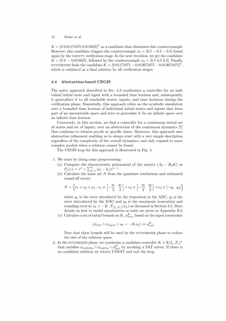
12 Abate et al.

K = [0 0.01171875 0.015625]T as a candidate that eliminates this counterexample.However, this candidate triggers the counterexample x0 = [0.5 −0.5 −0.5] foundagain by the safety verification stage. In the next iteration, we get the candidateK = [0 0 − 0.015625], followed by the counterexample x0 = [0.5 0.5 0.5]. Finally,synthesize finds the candidate K = [0.01171875 −0.013671875 −0.013671875]T ,which is validated as a final solution by all verification stages.

4.4 Abstraction-based CEGIS

The naıve approach described in Sec. 4.3 synthesizes a controller for an indi-vidual initial state and input with a bounded time horizon and, subsequently,it generalizes it to all reachable states, inputs, and time horizons during theverification phase. Essentially, this approach relies on the symbolic simulationover a bounded time horizon of individual initial states and inputs that formpart of an uncountable space and tries to generalize it for an infinite space overan infinite time horizon.

Conversely, in this section, we find a controller for a continuous initial setof states and set of inputs, over an abstraction of the continuous dynamics [7]that conforms to witness proofs at specific times. Moreover, this approach usesabstraction refinement enabling us to always start with a very simple descriptionregardless of the complexity of the overall dynamics, and only expand to morecomplex models when a solution cannot be found.

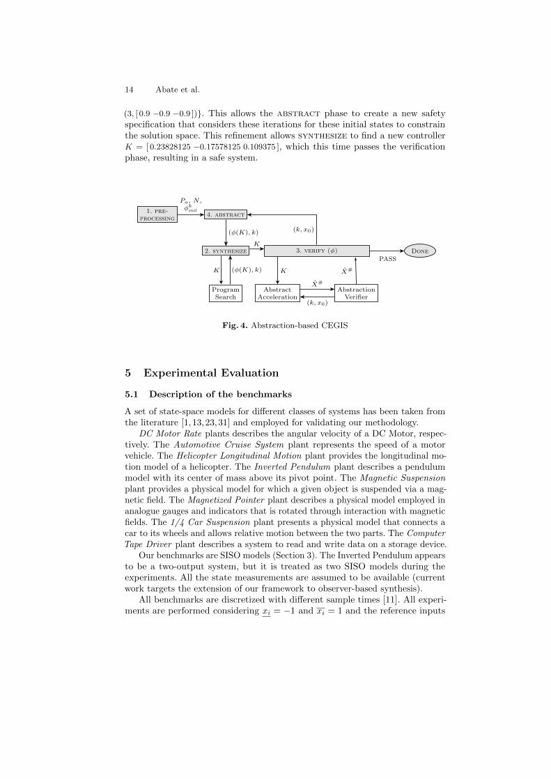
The CEGIS loop for this approach is illustrated in Fig. 4.

1. We start by doing some preprocessing:

(a) Compute the characteristic polynomial of the matrix (Ad − BdK) asPa(z) = zn +

∑ni=1 (ai − ki)zn−i.

(b) Calculate the noise set N from the quantizer resolutions and estimatedround-off errors:

N ={ν1 + ν2 + ν3 : ν1 ∈

[−q1

2

q1

2

]∧ ν2 ∈

[−q2

2

q2

2

]∧ ν3 ∈ [−q3 q3]

}where q1 is the error introduced by the truncation in the ADC, q2 is theerror introduced by the DAC and q3 is the maximum truncation androunding error in uk = −K ·F〈Ic,Fc〉(xk) as discussed in Section 3.5. Moredetails on how to model quantization as noise are given in Appendix B.2.

(c) Calculate a set of initial bounds onK, φKinit , based on the input constraints

(φinit ∧ φinput ∧ uk = −Kxk)⇒ φKinit

Note that these bounds will be used by the synthesize phase to reducethe size of the solution space.

2. In the synthesize phase, we synthesize a candidate controller K ∈ R〈Ic, Fc〉nthat satisfies φstability ∧ φsafety ∧ φKinit by invoking a SAT solver. If there isno candidate solution we return UNSAT and exit the loop.


3. Once we have a candidate solution, we perform a safety verification of theprogression of the system from φinit over time, xk |= φsafety . In order tocompute the progression of point x0 at iteration k, we accelerate the dynamicsof the closed-loop system and obtain:

x =(Ad −BdK)kx0 +

k−1∑i=0

(Ad −BdK)iBn(ν1 + ν2 + ν3) : Bn = [1 · · · 1]T (6)

As this still requires us to verify the system for every k up to infinity, weuse abstract acceleration again to obtain the reach-tube, i.e., the set of allreachable states at all times given an initial set φinit :

X# = AX0 + BnN, X0 = {x : x |= φinit} , (7)

where A =⋃∞k=1(Ad − BdK)k,Bn =

⋃∞k=1

∑ki=0(Ad − BdK)iBn are ab-

stract matrices for the closed-loop system [7], whereas the set N is non-deterministically chosen.We next evaluate X# |= φsafety . If the verification holds we have a solution,and exit the loop. Otherwise, we find a counterexample iteration k andcorresponding initial point x0 for which the property does not hold, which weuse to locally refine the abstraction. When the abstraction cannot be furtherrefined, we provide them to the abstract phase.

4. If we reach the abstract phase, it means that the candidate solution is notvalid, in which case we must refine the abstraction used by the synthesizer.(a) Find the constraints that invalidate the property as a set of counterex-

amples for the eigenvalues, which we define as φΛ. This is a constraint inthe spectrum i.e., transfer function) of the closed loop dynamics.

(b) We use φΛ to further constrain the characteristic polynomial zn +∑ni=1(ai − ki)z

n−i =∏ni=1(z − λi) : |λi| < 1 ∧ λi |= φΛ. These con-

straints correspond to specific iterations for which the system may beunsafe.

(c) Pass the refined abstraction φ(K) with the new constraints and the listof iterations k to the synthesize phase.

Illustrative Example Let us consider the following example with discretizeddynamics

Ad =

2.6207 −1.1793 0.657052 0 00 0.5 0

, Bd =

800

Using the initial state bounds x0 = −0.9 and x0 = 0.9, the input boundsu = −10 and u = 10, and safety specifications xi = −0.92 and xi = 0.92,the synthesize phase in Fig. 4 generates an initial candidate controller K =[ 0.24609375 −0.125 0.1484375 ]. This candidate is chosen for its closed-loop stabledynamics, but the verify phase finds it to be unsafe and returns a list of iterationswith an initial state that fails the safety specification (k, x0)∈{(2, [ 0.9 −0.9 0.9 ]),

14 Abate et al.

(3, [ 0.9 −0.9 −0.9 ])}. This allows the abstract phase to create a new safetyspecification that considers these iterations for these initial states to constrainthe solution space. This refinement allows synthesize to find a new controllerK = [ 0.23828125 −0.17578125 0.109375 ], which this time passes the verificationphase, resulting in a safe system.

1. pre-processing

4. abstract

2. synthesize 3. verify (φ)

PASSDone

ProgramSearch

AbstractAcceleration

AbstractionVerifier

Pa, N ,φkinit

(φ(K), k)

K

K (φ(K), k)

X#

(k, x0)

X#K

(k, x0)

Fig. 4. Abstraction-based CEGIS

5 Experimental Evaluation

5.1 Description of the benchmarks

A set of state-space models for different classes of systems has been taken fromthe literature [1, 13,23,31] and employed for validating our methodology.

DC Motor Rate plants describes the angular velocity of a DC Motor, respec-tively. The Automotive Cruise System plant represents the speed of a motorvehicle. The Helicopter Longitudinal Motion plant provides the longitudinal mo-tion model of a helicopter. The Inverted Pendulum plant describes a pendulummodel with its center of mass above its pivot point. The Magnetic Suspensionplant provides a physical model for which a given object is suspended via a mag-netic field. The Magnetized Pointer plant describes a physical model employed inanalogue gauges and indicators that is rotated through interaction with magneticfields. The 1/4 Car Suspension plant presents a physical model that connects acar to its wheels and allows relative motion between the two parts. The ComputerTape Driver plant describes a system to read and write data on a storage device.

Our benchmarks are SISO models (Section 3). The Inverted Pendulum appearsto be a two-output system, but it is treated as two SISO models during theexperiments. All the state measurements are assumed to be available (currentwork targets the extension of our framework to observer-based synthesis).

All benchmarks are discretized with different sample times [11]. All experi-ments are performed considering xi = −1 and xi = 1 and the reference inputs


rk = 0,∀k > 0. We conduct the experimental evaluation on a 12-core 2.40 GHzIntel Xeon E5-2440 with 96 GB of RAM and Linux OS. We use the Linux timescommand to measure CPU time used for each benchmark. The runtime is limitedto one hour per benchmark.

5.2 Objectives

Using the state-space models given in Section 5.1, our evaluation has the followingtwo experimental goals:

EG1 (CEGIS) Show that both the multi-staged and the abstraction-based CEGISapproaches are able to generate FWL digital controllers in a reasonableamount of time.

EG2 (sanity check) Confirm the stability and safety of the synthesized controllersoutside of our model.

5.3 Results

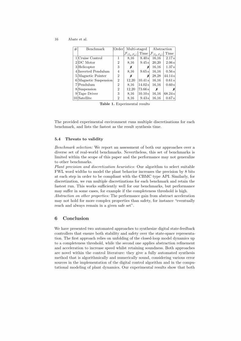
We provide the results in Table 1. Here Benchmark is the name of the respectivebenchmark, Order is the number of continuous variables, F〈Ip,Fp〉 is the fixed-point precision used to model the plant, while Time is the total time required tosynthesize a controller for the given plant with one of the two methods. Timeoutsare indicated by ✗. The precision for the controller, F〈Ic,Fc〉, is chosen to beIc = 8, Fc = 8.

For the majority of our benchmarks, we observe that the abstraction-basedback-end is faster than the basic multi-staged verification approach, and finds onesolution more (9) than the multi-staged back-end (8). In direct comparison, theabstraction-based approach is on average able to find a solution in approximately70% of the time required using the multi-staged back-end, and has a medianrun-time 1.4 s, which is seven times smaller than the multi-staged approach. Thetwo back-ends complement each other in benchmark coverage and together solveall benchmarks in the set. On average our engine spent 52% in the synthesis and48% in the verification phase.

The median run-time for our benchmark set is 9.4 s. Overall, the averagesynthesis time amounts to approximately 15.6 s. We consider these times shortenough to be of practical use to control engineers, and thus affirm EG1.

There are a few instances for which the system fails to find a controller. Forthe naıve approach, the completeness threshold may be too large, thus causing atimeout. On the other hand, the abstraction-based approach may require a veryprecise abstraction, resulting in too many refinements and, consequently, in atimeout. Yet another source of incompleteness is the inability of the synthesizephase to use a large enough precision for the plant model.

The synthesized controllers are confirmed to be safe outside of our modelrepresentation using MATLAB, achieving EG2. A link to the full experimentalenvironment, including scripts to reproduce the results, all benchmarks andthe tool, is provided in the footnote as an Open Virtual Appliance (OVA).3

3 www.cprover.org/DSSynth/controller-synthesis-cav-2017.tar.gz

16 Abate et al.

# Benchmark Order Multi-staged AbstractionF〈Ip,Fp〉 Time F〈Ip,Fp〉 Time

1 Cruise Control 1 8,16 8.40 s 16,16 2.17 s2 DC Motor 2 8,16 9.45 s 20,20 2.06 s3 Helicopter 3 ✗ ✗ 16,16 1.37 s4 Inverted Pendulum 4 8,16 9.65 s 16,16 0.56 s5 Magnetic Pointer 2 ✗ ✗ 28,28 44.14 s6 Magnetic Suspension 2 12,20 10.41 s 16,16 0.61 s7 Pendulum 2 8,16 14.02 s 16,16 0.60 s8 Suspension 2 12,20 73.66 s ✗ ✗

9 Tape Driver 3 8,16 10.10 s 16,16 68.24 s10 Satellite 2 8,16 9.43 s 16,16 0.67 s

Table 1. Experimental results

The provided experimental environment runs multiple discretisations for eachbenchmark, and lists the fastest as the result synthesis time.

5.4 Threats to validity

Benchmark selection: We report an assessment of both our approaches over adiverse set of real-world benchmarks. Nevertheless, this set of benchmarks islimited within the scope of this paper and the performance may not generalizeto other benchmarks.Plant precision and discretization heuristics: Our algorithm to select suitableFWL word widths to model the plant behavior increases the precision by 8 bitsat each step in order to be compliant with the CBMC type API. Similarly, fordiscretization, we run multiple discretizations for each benchmark and retain thefastest run. This works sufficiently well for our benchmarks, but performancemay suffer in some cases, for example if the completeness threshold is high.Abstraction on other properties: The performance gain from abstract accelerationmay not hold for more complex properties than safety, for instance “eventuallyreach and always remain in a given safe set”.

6 Conclusion

We have presented two automated approaches to synthesize digital state-feedbackcontrollers that ensure both stability and safety over the state-space representa-tion. The first approach relies on unfolding of the closed-loop model dynamics upto a completeness threshold, while the second one applies abstraction refinementand acceleration to increase speed whilst retaining soundness. Both approachesare novel within the control literature: they give a fully automated synthesismethod that is algorithmically and numerically sound, considering various errorsources in the implementation of the digital control algorithm and in the compu-tational modeling of plant dynamics. Our experimental results show that both


approaches are able to synthesize safe controllers for most benchmarks within areasonable amount of time fully automatically. In particular, both approachescomplement each other and together solve all benchmarks, which have beenderived from the control literature.

Future work will focus the extension of these approaches to the continuous-time case, to models with output-based control architectures (with the use ofobservers), and to the consideration of more complex specifications.

References

1. Control tutorials for MATLAB and SIMULINK. http://ctms.engin.umich.edu/.2. A. Abate, I. Bessa, D. Cattaruzza, L. C. Cordeiro, C. David, P. Kesseli, and

D. Kroening. Sound and automated synthesis of digital stabilizing controllers forcontinuous plants. In Hybrid Systems: Computation and Control (HSCC), pages197–206. ACM, 2017.

3. A. Anta, R. Majumdar, I. Saha, and P. Tabuada. Automatic verification of controlsystem implementations. In EMSOFT, pages 9–18, 2010.

4. K. Astrom and B. Wittenmark. Computer-controlled systems: theory and design.Prentice Hall information and system sciences series. Prentice Hall, 1997.

5. I. Bessa, H. Ismail, R. Palhares, L. C. Cordeiro, and J. E. C. Filho. Formal non-fragile stability verification of digital control systems with uncertainty. IEEE Trans.Computers, 66(3):545–552, 2017.

6. M. Brain, C. Tinelli, P. Rummer, and T. Wahl. An automatable formal semanticsfor IEEE-754 floating-point arithmetic. In ARITH, pages 160–167. IEEE, 2015.

7. D. Cattaruzza, A. Abate, P. Schrammel, and D. Kroening. Unbounded-time analysisof guarded LTI systems with inputs by abstract acceleration. In 22nd InternationalSymposium on Static Analysis, volume 9291 of LNCS, pages 312–331, 2015.

8. C. David, D. Kroening, and M. Lewis. Using program synthesis for program analysis.In Logic for Programming, Artificial Intelligence, and Reasoning (LPAR-20), LNCS,pages 483–498. Springer, 2015.

9. I. V. de Bessa, H. Ismail, L. C. Cordeiro, and J. E. C. Filho. Verification offixed-point digital controllers using direct and delta forms realizations. DesignAutom. for Emb. Sys., 20(2):95–126, 2016.

10. P. S. Duggirala and M. Viswanathan. Analyzing real time linear control systemsusing software verification. In IEEE Real-Time Systems Symposium, pages 216–226,Dec 2015.

11. S. Fadali and A. Visioli. Digital Control Engineering: Analysis and Design, volume303 of Electronics & Electrical. Elsevier/Academic Press, 2009.

12. I. J. Fialho and T. T. Georgiou. On stability and performance of sampled-datasystems subject to wordlength constraint. IEEE Transactions on Automatic Control,39(12):2476–2481, 1994.

13. G. Franklin, D. Powell, and A. Emami-Naeini. Feedback Control of DynamicSystems. Pearson, 7th edition, 2015.

14. G. Frehse, C. L. Guernic, A. Donze, R. Ray, O. Lebeltel, R. Ripado, A. Girard,T. Dang, and O. Maler. SpaceEx: Scalable verification of hybrid systems. In CAV,volume 6806 of LNCS, pages 379–395. Springer, 2011.

15. R. A. Horn and C. Johnson. Matrix Analysis. Cambridge University Press, 1990.16. S. Itzhaky, S. Gulwani, N. Immerman, and M. Sagiv. A simple inductive synthesis

methodology and its applications. In OOPSLA, pages 36–46. ACM, 2010.

18 Abate et al.

17. D. Kroening and O. Strichman. Efficient computation of recurrence diameters. InVerification, Model Checking, and Abstract Interpretation (VMCAI), volume 2575of LNCS, pages 298–309. Springer, 2003.

18. G. Li. On pole and zero sensitivity of linear systems. IEEE Trans. on Circuits andSystems–I: Fundamental Theory and Applications, 44(7):583–590, 1997.

19. D. Liberzon. Hybrid feedback stabilization of systems with quantized signals.Automatica, 39(9):1543–1554, 2003.

20. J. Liu and N. Ozay. Finite abstractions with robustness margins for temporallogic-based control synthesis. Nonlinear Analysis: Hybrid Systems, 22:1–15, 2016.

21. M. Mazo, Jr., A. Davitian, and P. Tabuada. PESSOA: A tool for embeddedcontroller synthesis. In Computer Aided Verification (CAV), volume 6174 of LNCS,pages 566–569. Springer, 2010.

22. R. E. Moore. Interval analysis, volume 4. Prentice-Hall Englewood Cliffs, 1966.23. V. A. Oliveira, E. F. Costa, and J. B. Vargas. Digital implementation of a magnetic

suspension control system for laboratory experiments. IEEE Transactions onEducation, 42(4):315–322, Nov 1999.

24. A. K. Oudjida, N. Chaillet, A. Liacha, M. L. Berrandjia, and M. Hamerlain. Designof high-speed and low-power finite-word-length PID controllers. Control Theoryand Technology, 12(1):68–83, 2014.

25. J. Park, M. Pajic, I. Lee, and O. Sokolsky. Scalable verification of linear controllersoftware. In Tools and Algorithms for the Construction and Analysis of Systems(TACAS), LNCS, pages 662–679. Springer, 2016.

26. B. Picasso and A. Bicchi. Stabilization of LTI systems with quantized state-quantized input static feedback. In 6th International Workshop on Hybrid Systems:Computation and Control, pages 405–416. Springer, 2003.

27. H. Ravanbakhsh and S. Sankaranarayanan. Counter-example guided synthesis ofcontrol Lyapunov functions for switched systems. In Conference on Decision andControl (CDC), pages 4232–4239, 2015.

28. H. Ravanbakhsh and S. Sankaranarayanan. Robust controller synthesis of switchedsystems using counterexample guided framework. In EMSOFT, pages 8:1–8:10.ACM, 2016.

29. P. Roux, R. Jobredeaux, and P. Garoche. Closed loop analysis of control commandsoftware. In HSCC, pages 108–117. ACM, 2015.

30. A. Solar-Lezama, L. Tancau, R. Bodık, S. A. Seshia, and V. A. Saraswat. Combi-natorial sketching for finite programs. In ASPLOS, pages 404–415. ACM, 2006.

31. R. H. G. Tan and L. Y. H. Hoo. DC-DC converter modeling and simulation usingstate space approach. In IEEE Conference on Energy Conversion, CENCON, pages42–47, Oct 2015.

32. T. E. Wang, P. Garoche, P. Roux, R. Jobredeaux, and E. Feron. Formal analysisof robustness at model and code level. In HSCC, pages 125–134. ACM, 2016.

33. J. Wu, G. Li, S. Chen, and J. Chu. Robust finite word length controller design.Automatica, 45(12):2850–2856, 2009.

34. M. Zamani, M. Mazo, and A. Abate. Finite abstractions of networked controlsystems. In IEEE CDC, pages 95–100, 2014.

A Stability of Closed-loop Models

A.1 Stability of closed-loop models with fixed-point controller error

The proof of Jury’s criterion [11] relies on the fact that the relationship betweenstates and next states is defined by xk+1 = (Ad−BdK)xk, all computed at infinite


precision. When we employ a FWL digital controller, the operation becomes:

xk+1 = Ad · xk − (F〈Ic,Fc〉(K) · F〈Ic,Fc〉(xk)).

xk+1 = (Ad −BdK) · xk +BdKδ,

where δ is the maximum error that can be introduced by the FWL controller inone step, i.e., by reading the states values once and multiplying by K once. Wederive the closed form expression for xn as follows:

x1 = (Ad −BdK)x0 +BdKδ

x2 = (Ad −BdK)2x0 + (Ad −BdK)BdKδ +BdKδ

xn = (Ad −BdK)nx0 + (Ad −BdK)n−1BdKδ + ...+ (Ad −BdK)1BdKδ +BdKδ

= (Ad −BdK)nx0 +

i=n−1∑i=0

(Ad −BdK)iBdkδ.

The definition of asymptotic stability is that the system converges to areference signal, in this case we use no reference signal so an asymptoticallystable system will converge to the origin. We know that the original system withan infinite-precision controller is stable, because we have synthesized it to meetJury’s criterion. Hence, (Ad −BdK)nx0 must converge to zero.

The power series of matrices converges [15] iff the eigenvalues of the matrixare less than 1 as follows:

∑∞i=0 T

i = (I − T )−1, where I is the identity matrixand T is a square matrix. Thus, our system will converge to the value

0 + (I −Ad +BdK)−1Bdkδ .

As a result, if the value (I − Ad + BdK)−1Bdkδ is within the safe space, thenthe synthesized fixed-point controller results in a safe closed-loop model. Theconvergence to a finite value, however, will not make it asymptomatically stable.

B Errors in LTI models

B.1 Errors due to numerical representation

We have used F〈I,F 〉(x) denote a real number x represented in a fixed pointdomain, with I bits representing the integer part and F bits representing thedecimal part. The smallest number that can be represented in this domainis cm = 2−F . The following approximation errors will arise in mathematicaloperations and representation:

1. Truncation: Let x be a real number, and F〈I,F 〉(x) be the same numberrepresented in a fixed-point domain as above. Then F〈I,F 〉(x) = x− δT wherethe error δT = x %cm x, and %cm is the modulus operation performed onthe last bit. Thus, δT is the truncation error and it will propagate acrossoperations.

20 Abate et al.

2. Rounding: The following errors appear in basic operations. Let c1, c2 andc3 be real numbers, and δT1 and δT2 be the truncation errors caused byrepresenting c1 and c2 in the fixed-point domain as above.(a) Addition/Subtraction: these operations only propagate errors coming

from truncation of the operands, namely F〈I,F 〉(c1)±F〈I,F 〉(c2) = c3 +δ3with |δ3| ≤ |δT1|+ |δT2|.

(b) Multiplication: F〈I,F 〉(c1)·F〈I,F 〉(c2) = c3+δ3 with |δ3| ≤ |δT1·F〈I,F 〉(c2)|+ |δT2 · F〈I,F 〉(c1)|+ cm, where cm = 2−F as above.

(c) Division: the operations performed by our controllers in the FWL domaindo not include division. However, we do use division in computations atthe precision of the plant. Here the error depends on whether the divisoris greater or smaller than the dividend: F〈I,F 〉(c1)/F〈I,F 〉(c2) = c3 + δT3

where δT3 is (δT2 · c1 − δT1 · c2)/(δ2T2 − δT2c2),

3. Overflow: The maximum size of a real number x that can be represented ina fixed point domain as F〈I,F 〉(x) is ±(2I−1 + 1 − 2−F ). Numbers outsidethis range cannot be represented by the domain. We check that overflow doesnot occur.

B.2 Modeling quantization as noise

During any given ADC conversion, the continuous signal will be sampled in thereal domain and transformed by F〈Ic, Fc〉(x) (assuming the ADC discretizationis the same as the digital implementation). This sampling uses a threshold whichis defined by the less significant bit (qc = cmc

= 2−Fc) of the ADC and somenon-linearities of the circuitry. The overall conversion is

F〈Ic, Fc〉(y(t)) = yk : yk ∈[y(t)− qc

2y(t) +

qc2

].

If we denote the error in the conversion by νk = yk − y(t) where t = nk, and n isthe sampling time and k the number of steps, then we may define some boundsfor it νk ∈ [− qc2

qc2 ].

We will assume, for the purposes of this analysis, that the domain of the ADCis that of the digital controller (i.e, the quantizer includes any digital gain addedin the code). The process of quantization in the DAC is similar except that it iscalculating F〈Idac, Fdac〉(F〈Ic, Fc〉(x)). If these domains are the same (Ic = Idac,Fc = Fdac), or if the DAC resolution in higher than the ADCs, then the DACquantization error is equal to zero. From the above equations we can now definethe ADC and DAC quantization noises ν1k ∈ [− q12

q12 ] and ν2k ∈ [− q22

q22 ], where

q1 = qc and q2 = qdac . This is illustrated in Fig. 3.2 where Q1 is the quantizer ofthe ADC and Q2 the quantizer for the DAC. These bounds hold irrespective ofwhether the noise is correlated, hence we may use them to over-approximate thenoise effect on the state space progression over time. The resulting dynamics are

xk+1 = Adxk +Bd(uk + ν2k), uk = −Kxk + ν1k,

which result in the following closed-loop dynamics:

xk+1 = (Ad −BdKd)xk +Bdν2k + ν1k .

Documents

Automated Formal Synthesis of Digital Controllers … · Automated Formal Synthesis of Digital Controllers 3 of imprecision in the implementation of the control algorithm and in the