Automated Analysis of Calcium Imaging Data Helen Horan Yang CS229 Final Project, Fall 2012 Introduction

In virtually all biological systems, calcium ions (Ca2+) are essential intracellular signaling molecules, but they are particularly important in the nervous system. Ca2+ is required for neurons to release synaptic vesicles, which is the major method by which they communicate with downstream neurons. Measuring increases in Ca2+ concentration around these release sites is therefore a readout of the neuron’s output signaling, and one can correlate this to particular stimuli presented to characterize the neuron’s response properties (Grienberger and Konnerth, 2012). This information is important for understanding how neural circuits respond to and shape the signals that they receive from the environment to perform complex computations. Calcium imaging is the technique by which one measures these changes in cellular Ca2+ levels. Briefly, cells are made to contain a calcium indicator, a molecule that fluoresces only when it binds Ca2+; fluorescence intensity is thereby a report of Ca2+ concentration and the cells’ responses. This is captured in real time with a fluorescence microscope and a CCD camera. Raw calcium imaging data is in the form of a time series of images where the intensity of each pixel is the fluorescence intensity at that location (Grienberger and Konnerth, 2012). However, the unit of interest is a cell, not a pixel, and typical calcium imaging experiments capture several to several dozen cells in one field of view. To be able to make meaningful biological conclusions, each cell’s responses must be isolated from other cells’ and the background. Despite the recent advances in calcium imaging technology to improve the performance of both calcium indicators and fluorescence microscopes (Grienberger and Konnerth, 2012), the extraction of cellular responses is mostly performed by manually or semiautomatedly selecting regions of interest (ROIs) that correspond to single cells—tracing cell outlines or setting an intensity threshold, for example—(Göbel and Helmchen, 2007; Ozden et al., 2008). Not only is this time consuming, it can introduce noise into the signal if the boundaries of the ROI are not precise and include other cells or background. In some situations, spatial overlap is unavoidable as the microscope captures fluorescence from cells slightly above or below the imaging plane of focus. More clever analysis techniques for isolating cells should be able to improve performance and decrease the amount of human labor required. For this project, I have applied machine learning algorithms to automatically extract cellular responses from my own calcium imaging data, which I was previously isolating by manually outlining ROIs. Data Acquisition and Preprocessing The analyses described below were performed on data collected by imaging a particular cell type in the fruit fly Drosophila visual system known as L2. L2 receives direct input from photoreceptors and functions as an input to a pathway specialized to detect moving dark edges (Clark et al., 2011). Briefly, single flies were stably mounted such that their eyes viewed a screen on which visual stimuli were presented, and the back of the head was exposed to allow the microscope objective access to the brain for imaging. The calcium indicator TN-XXL was expressed specifically in L2; that is, the flies were genetically engineered such that their L2 cells made the TN-XXL protein. L2 axon terminals in the medulla (the neuronal output sites located in a particular brain region) were imaged using two-photon fluorescence microscopy (two longer wavelength photons must be absorbed simultaneously for one to be emitted). When stimulated at 830nm, TN-XXL emits at ~529nm when it is bound to Ca2+ and ~475nm when it is not (Mank et al., 2008). Both channels were collected during imaging and are hereafter referred to as ch1 and ch2, respectively; TN-XXL is therefore ratiometric, and a cell’s Ca2+ response is characterized by ch1/ch2. Imaging data was acquired at a constant frame rate of 10.3Hz using a frame size of 50 x 200 pixels. This field of view fits approximately 6 to 8 L2 terminals. The presented visual stimulus was a light bar with a width of ~2.5° of the fly’s visual field moving in one direction at ~10°/sec on a dark

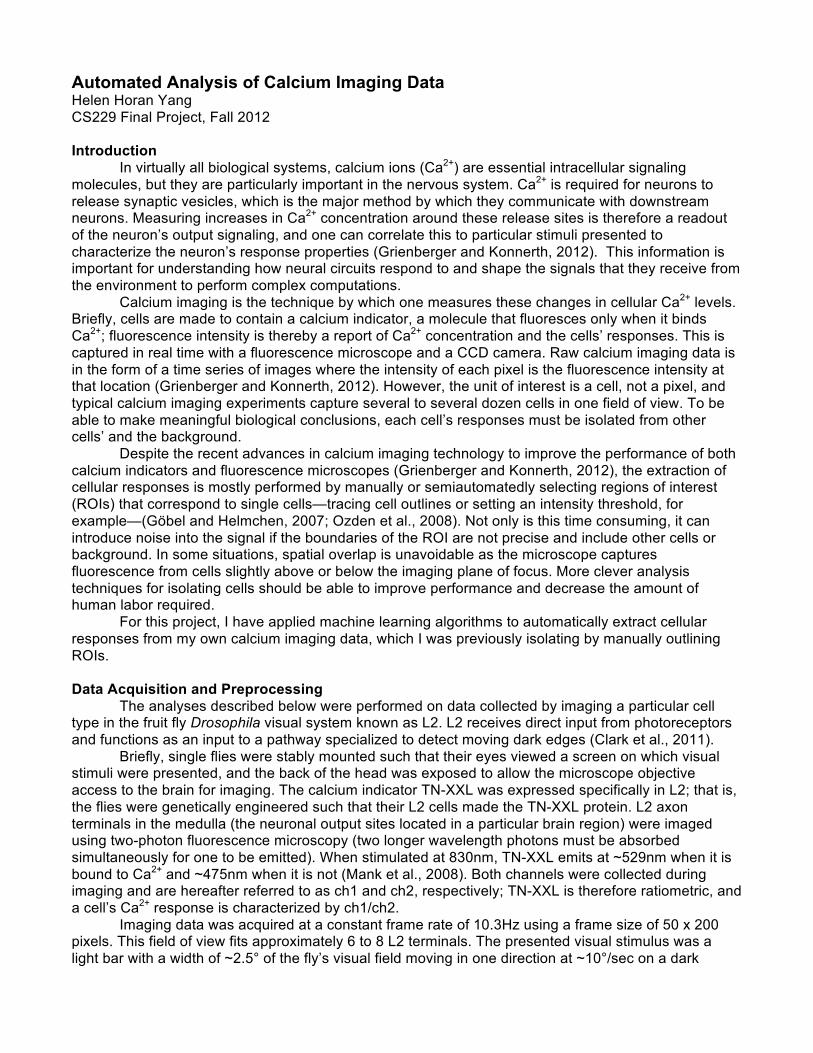
background. The bar was oriented either horizontally and moving vertically or vice versa. The screen was dark for 9 seconds and then the bar moved across the screen in 9 seconds; the bar moved in all 4 possible direction-orientation combinations. 1000 imaging frames were captured while the stimulus was presented. Although the fly is mounted to minimize movement, it is not completely eliminated. Before any analysis was performed, lateral movement artifacts were corrected for by aligning the image time series using an ImageJ macro based on TurboReg, which matches images based on distinctive landmarks (Thévenaz et al., 1998). Alignment was done using ch1, in which cellular structures are more apparent, and ch2 images were shifted to match. Analyses Manual Selection of Regions of Interest Before discussing the approaches I took to automatically extract cellular signals from the aligned image time series, I will first describe the method I had previously been using. The ch1 aligned image time series was collapsed along the temporal dimension by averaging the intensity at each pixel to generate an average image. ROIs corresponding to individual L2 terminals were identified by eye and manually outlined. A background region in which no cellular fluorescence was apparent was also manually defined. For each cell and the background region, the fluorescence intensities were averaged across all of the pixels in the ROI for each frame to generate average ch1 and ch2 time series. The average response of the background region was subtracted from each cell’s responses, and then the ratio between the two channels was determined. The end result is that the calcium response of each L2 cell is described by a single time series of ch1/ch2 ratio values. These ratios generally range between 2 and 3. Figure 1 shows a typical example of the responses derived from 7 cells in one field of view.

K-means for Region of Interest Identification As stated above, the goal of this project is to automatically extract cellular responses from an aligned image time series. For the greatest utility, the method taken should be able to identify these responses using the image time series and as few additional parameters—which must be manually tuned—as possible; furthermore, it should perform comparably to or better than manual ROI selection. This is therefore an unsupervised learning problem. That is, I could train a supervised learning

Figure 1 Responses of cells identified by manual selection of ROIs. (A) Average image for ch1. (B) In color are the ROIs corresponding to individual L2 terminals. The white ROI is background region. (C) Responses of the cells spatially defined in (B). The colors of the ROIs and traces correspond. The color traces are the ch1/ch2 ratio values, and the desaturated traces behind them are the ch1 and ch2 responses before the ratio is taken. The step function at the bottom describes the stimulus, with each different value corresponding to a different direction that the bar moves. Each L2 observes a point in space and responds by decreasing and then increasing its Ca2+ concentration when the bar crosses this region. Adjacent cells respond to adjacent points in space. Black arrows denote the responses to the moving bar.  

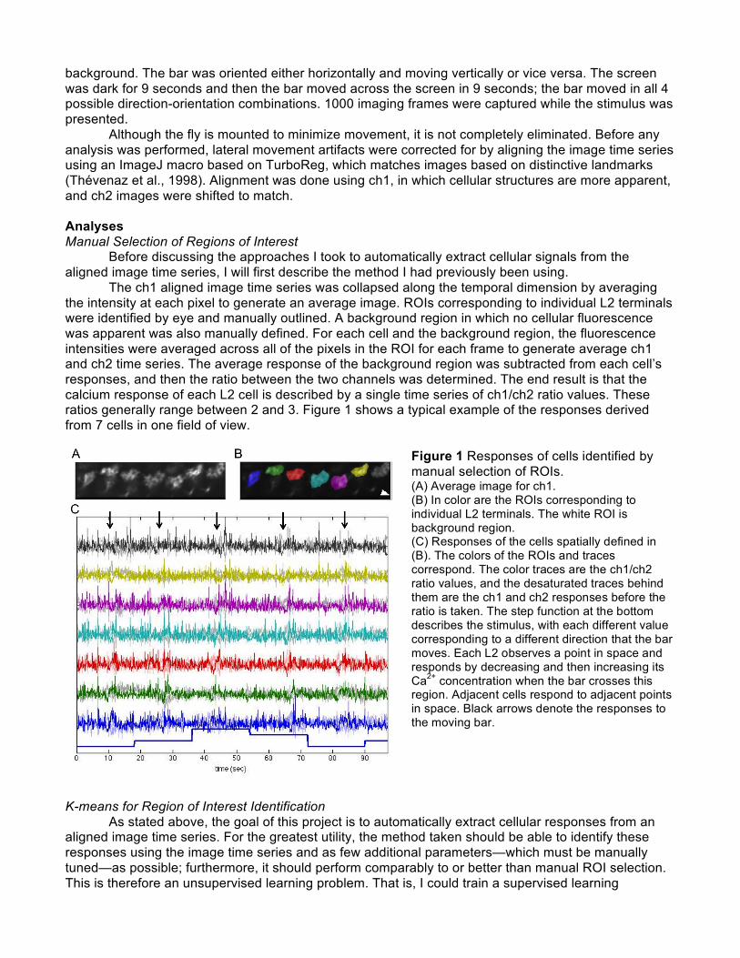
algorithm to identify ROIs by using the set of manually defined ROIs and average images I have already collected, but this would require a large time investment if I wanted to examine other cells in the fly visual system (and there certainly exist cells with similar response properties but different morphologies) or if I do not have enough L2 training data and is unlikely to perform substantially better than manual ROI identification. I applied the k-means clustering algorithm to the aligned image time series data. The image time series data was collapsed from 50 x 200 x 1000, representing spatial width x height x time, to a 10,000 x 1000 matrix, representing pixels x time. That is, each of the m=10,000 pixels is a training example x(i) and is described by n=1000 variables, the value at each time point. Applied to this training set, k-means identifies clusters of similar pixels, which would ideally correspond to individual cells and the background. These can then be analyzed in the same way as the manually identified ROIs to extract the cellular responses. I first performed k-means on the raw intensities of the ch1 image time series using k=10 clusters for the 6-8 cells and the background. Disappointingly, the clusters did not correspond to individual terminals but instead to similar regions in each of terminals (Figure 2A). The identified regions were vaguely similar to the intensity gradients across the cells in the average image, so I hypothesized that similarities among pixels corresponding to a single cell were overwhelmed by differences in the raw intensities within a cell. I therefore calculated the ratio between ch1 and ch2 for each pixel at each time point and performed k-means on this training set. While this did seem to eliminate the effects of raw intensity differences, the clusters were still spread among multiple cells and showed no apparent pattern within a single cell terminal (Figure 2B). However, this did clearly separate the cells from the background, so I repeated the clustering with k=2, which did indeed form a cell cluster and a background cluster (Figure 2C). In the cell cluster, all contiguous pixels were grouped together, and any regions exceeding 100 pixels in area were called cell ROIs (Figure 2D). The extraction of cellular responses from these spatial ROIs was performed as above (Figure 2E). This method of identifying ROIs performed comparably to the manual method over many data sets, not just the one shown in Figure 2; in fact, the cells’ responses to the moving bar seem to be more apparent in these traces, possibly because they are less noisy—the standard deviation

Figure 2 ROIs and cellular responses identified by k-means clustering. (A) Clusters identified by performing k-means on ch1 raw intensities. Each gray scale value is a different cluster. k=10 (B) Clusters identified from ch1/ch2 ratios. k=10 (C) Clusters when k=2. Cluster 1 (black) was used as the background and cell ROIs were extracted from cluster 2 (white). (D) ROIs called as individual cells overlayed on the average ch1 image. (E) Responses of the cells defined in (D). Compared to Figure 1C, the responses to the moving bar (black arrows) are more apparent.

of the ch1/ch2 ratios for each k-means trace was less than that of the manual trace for the same cell (mean difference -0.0691, n=56 cells). Spatiotemporal Independent Component Analysis Identifying ROIs using k-means clustering is an improvement compared to manual ROI selection; however, averaging over ROIs collapses any spatial variability or noise in favor of extracting a purely temporal response. Calcium imaging data can be thought of as a mixture in both space and time of signals from statistically independent sources—that is, cells; extraction of these sources would thereby provide an estimate of the cells’ locations and responses. Unlike ROI analysis, these signals are constrained to be independent and should therefore have less noise from crosstalk in either time or space. Independent component analysis (ICA) can be used to isolate signals from independent sources. In the cocktail party example we discussed in class, the goal was to separate out individual speakers captured on multiple microphones. Specifically, the speakers were the independent component sources to be isolated, and the corresponding acoustic signal over time was the signal of interest; the goal was not to isolate independent time points, each of which has an acoustic signal over all of the microphones. However, calcium imaging data is a time series of images and the decompositions corresponding to both situations in the cocktail party example make sense and generate a set of images and a set of intensity changes over time. Spatial ICA (sICA) seeks a set of mutually independent source images and a corresponding set of unconstrained time courses; temporal ICA (tICA) seeks a set of independent source time courses and a corresponding set of unconstrained images. However, because either space or time is unconstrained, the resulting independent components can be biologically improbable. Spatiotemporal ICA (stICA) maximizes the independence of both space and time, weighting one α and the other α-1 where α is between 0 and 1 (Stone et al., 2002), and is ideal for calcium imaging where the goal is to isolate independent component cells that each have their own spatial location and responses. Following the methods of Mukamel et al. and Stone et al. for stICA using the FastICA algorithm (Hyvärinen and Oja, 2000), I performed stICA on X = the 10,000 x 1000 matrix of ch1/ch2 ratios. Briefly, X was preprocessed such that each row and each column had zero mean, and it was whitened using singular value decomposition, which reduces the number of parameters to be estimated (Hyvärinen and Oja, 2000). stICA was performed with α=0.5 to equally weight the independence of time and space.

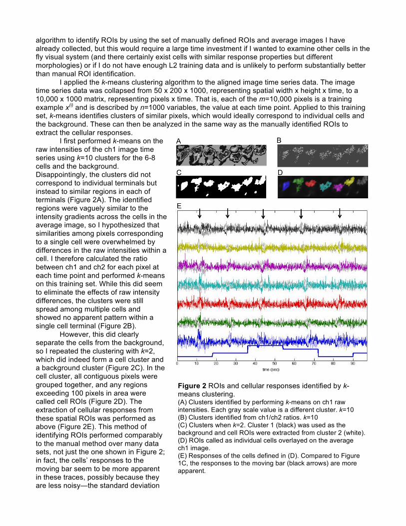
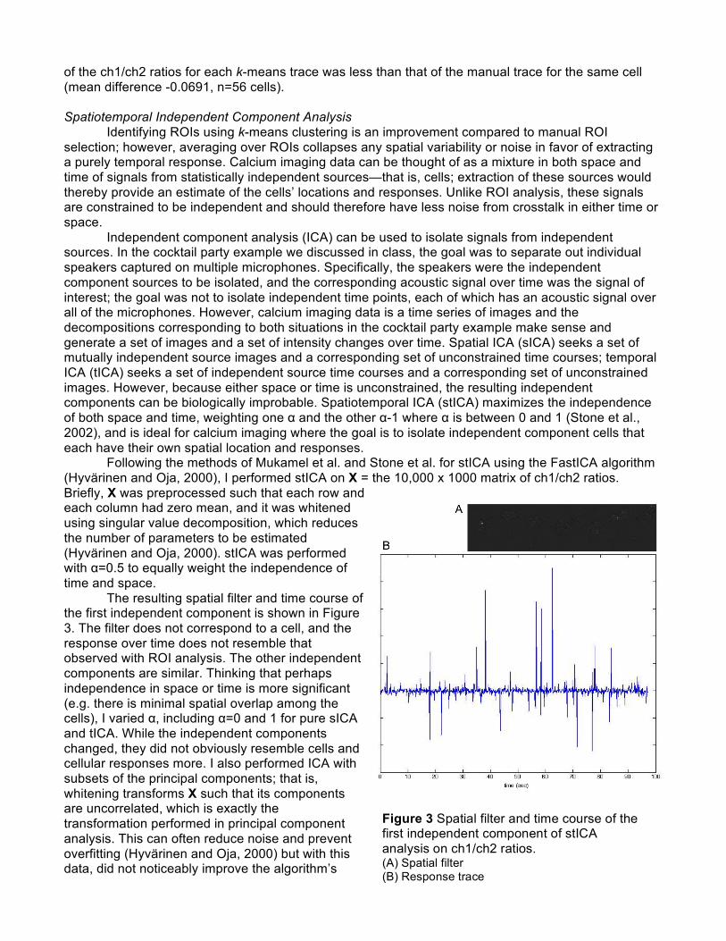
The resulting spatial filter and time course of the first independent component is shown in Figure 3. The filter does not correspond to a cell, and the response over time does not resemble that observed with ROI analysis. The other independent components are similar. Thinking that perhaps independence in space or time is more significant (e.g. there is minimal spatial overlap among the cells), I varied α, including α=0 and 1 for pure sICA and tICA. While the independent components changed, they did not obviously resemble cells and cellular responses more. I also performed ICA with subsets of the principal components; that is, whitening transforms X such that its components are uncorrelated, which is exactly the transformation performed in principal component analysis. This can often reduce noise and prevent overfitting (Hyvärinen and Oja, 2000) but with this data, did not noticeably improve the algorithm’s

Figure 3 Spatial filter and time course of the first independent component of stICA analysis on ch1/ch2 ratios. (A) Spatial filter (B) Response trace

performance. This is likely because none of the principal components explained a large percentage of the variance or contained signals that were obviously non-biological. ch1/ch2 ratios are occasionally abnormally large when a particular ch2 value drops close to zero, so I also tried ICA on data for which any data point that exceeded a threshold was set to that threshold. This eliminated the large spikes observed in Figure 3B but did not significantly change the spatial filters or make the time courses look more like the cellular responses. Finally, I used the ΔF/F (for each pixel, divide by its mean value over time and then subtract 1) of ch1 as X; this is the normalization used when the calcium indicator is not ratiometric and simply fluoresces when it binds Ca2+ and does not when it does not bind. Again, this did not improve performance. I tried various combinations of the above-described variations, but none of them resulted in an algorithm that extracted cellular responses. Discussion Mukamel et al. used stICA to extract cellular responses from calcium imaging data, but I was unable to do so successfully. I hypothesize that this is because my data was collected using a different calcium indicator, which has a much lower signal to noise ratio (SNR). Mukamel et al. used Oregon Green 488 BAPTA-1-AM, which is known to have greater amplitude responses than TN-XXL (Grienberger and Konnerth, 2012). The responses shown in Figures 1C and 2E are typical for this experiment, and examining those, it is apparent that the amplitudes of the responses to the moving bars does not significantly exceed the amplitude of the noise (SNR ~1). In contrast, Mukamel et al. are working with signal to noise ratios one to two orders of magnitude greater than this. Along these same lines, it is also possible that their cells respond more strongly to their stimulus than L2 cells to moving bars. Either way, I hypothesize that the ICA algorithm cannot extract meaningful cellular responses when these responses are difficult to distinguish random fluctuations. Perhaps increasing the imaging time or using a stimulus that causes the cells to respond more often would improve the performance, since there will be more responses, but that would not be useful given my experimental criteria. Nevertheless, I used k-means to identify ROIs corresponding to individual cells and could extract cellular responses in this manner. Compared to manually selecting the cells, this significantly reduces the amount of human labor required; the only parameter that needs to be specified is the minimum area of a cell, which can be set just once since L2 terminals are all approximately the same size. Furthermore, performs slightly better in that the traces have less baseline noise. Overall, this method improves how I analyze my calcium imaging data. References Clark, D.A., Bursztyn, L., Horowitz, M.A., Schnitzer, M.J., and Clandinin, T.R. (2011). Defining the computational structure of the motion detector in Drosophila. Neuron 70, 1165–1177.

Göbel, W., and Helmchen, F. (2007). In vivo calcium imaging of neural network function. Physiology (Bethesda) 22, 358–365.

Grienberger, C., and Konnerth, A. (2012). Imaging calcium in neurons. Neuron 73, 862–885.

Hyvärinen, A., and Oja, E. (2000). Independent component analysis: algorithms and applications. Neural Netw 13, 411–430.

Mank, M., Santos, A.F., Direnberger, S., Mrsic-Flogel, T.D., Hofer, S.B., Stein, V., Hendel, T., Reiff, D.F., Levelt, C., Borst, A., et al. (2008). A genetically encoded calcium indicator for chronic in vivo two-photon imaging. Nat. Methods 5, 805–811.

Mukamel, E.A., Nimmerjahn, A., and Schnitzer, M.J. (2009). Automated analysis of cellular signals from large-scale calcium imaging data. Neuron 63, 747–760.

Ozden, I., Lee, H.M., Sullivan, M.R., and Wang, S.S.-H. (2008). Identification and clustering of event patterns from in vivo multiphoton optical recordings of neuronal ensembles. J. Neurophysiol. 100, 495–503.

Stone, J.V., Porrill, J., Porter, N.R., and Wilkinson, I.D. (2002). Spatiotemporal independent component analysis of event-related fMRI data using skewed probability density functions. NeruoImage. 15, 407-421.

Thévenaz P., Ruttimann U.E., and Unser, M. (1998). A pyramid approach to subpixel registration based on intensity. IEEE Transactions on Image Processing, 7, 27-41.