Auction design with endogenously correlated buyer types

Available online at www.sciencedirect.com

Journal of Economic Theory 147 (2012) 118–141

www.elsevier.com/locate/jet

Auction design with endogenously correlatedbuyer types ✩

Daniel Krähmer

University of Bonn, Institute for Microeconomics and Hausdorff Center for Mathematics,Adenauer Allee 24-42, D-53113 Bonn, Germany

Received 17 February 2010; final version received 21 January 2011; accepted 12 October 2011

Available online 25 November 2011

Abstract

This paper studies optimal auction design when the seller can affect the buyers’ valuations throughan unobservable ex ante investment. The key insight is that the optimal mechanism may have the sellerplay a mixed investment strategy so as to create correlation between the buyers’ otherwise (conditionally)independent valuations. Assuming that the seller announces the mechanism before investing, the paperestablishes conditions on the investment technology so that a mechanism exists which leaves buyers no in-formation rent and leaves the seller indifferent between his investments. Under these conditions, the sellercan, in fact, extract the first best surplus almost fully.© 2011 Elsevier Inc. All rights reserved.

JEL classification: C72; D42; D44; D82

Keywords: Auction; Ex ante investment; Full surplus extraction; Correlation; Mechanism design

✩ Acknowledgments: I thank an associate editor and two anonymous referees for very helpful suggestions. I also thankAlex Gershkov, Paul Heidhues, Angel Hernando-Veciana, Eugen Kovac, Benny Moldovanu, Tymofiy Mylovanov, ZvikaNeeman, Xianwen Shi, Roland Strausz, Dezsö Szalay, Stefan Terstiege, Andriy Zapechelnyuk for useful discussions.Support by the German Science Foundation (DFG) through SFB/TR 15 is gratefully acknowledged.

E-mail address: [email protected].

0022-0531/$ – see front matter © 2011 Elsevier Inc. All rights reserved.doi:10.1016/j.jet.2011.11.015

http://www.sciencedirect.com

http://dx.doi.org/10.1016/j.jet.2011.11.015

http://www.elsevier.com/locate/jet

mailto:[email protected]

http://dx.doi.org/10.1016/j.jet.2011.11.015

D. Krähmer / Journal of Economic Theory 147 (2012) 118–141 119

1. Introduction

In many situations a seller can affect buyers’ valuations by an unobservable ex ante invest-ment in the object for sale. For example, buyers’ valuations for real estate will depend on theeffort spent by the construction company. The company’s effort, such as work care or the qual-ity of materials, can typically not be directly observed or immediately experienced. In publicprocurement, the contractor’s cost often depend on the cooperation by the government agency,for instance through the number of staff provided to deal with problems that occur during theimplementation phase, or on complementary infrastructure investments. Further, in second handmarkets, buyers’ valuations are affected by the unobservable care with which initial owners havetreated the item they sell. A final example is persuasive advertising where the typically unobserv-able campaign expenditures influence buyers’ willingness to pay.

What is the revenue maximizing selling mechanism in such a setting? This is the question Iaddress in this paper. I study a private value environment in which the seller’s investment raisesbuyers’ valuations stochastically. Conditional on the seller’s investment, valuations are condi-tionally independent. I assume that the seller’s investment is unobservable for buyers and thatbuyers’ valuations are their private information. Consequently, if the seller adopts a pure invest-ment strategy, there are independent private values, and buyers can typically secure informationrents.

The purpose of this paper is to show that the seller can reduce information rents by designinga mechanism that induces him to adopt a mixed investment strategy. The key insight is that ifthe seller randomizes, then, because buyers cannot observe investment, their valuations becomecorrelated in equilibrium. The seller can exploit this correlation to reduce buyers’ informationrents. To see intuitively why correlation emerges when the seller randomizes, one may think ofan urn model where each urn corresponds to a pure investment strategy by the seller. Buyers’valuations are drawn independently from one urn, but if the seller randomizes and buyers do notobserve the realized investment, they do not know what the true urn is. Therefore, the realizationof a buyer’s valuation contains information about the true urn and thus about the valuation of therival buyer.

The contribution of the paper is to establish conditions so that a mechanism can be constructedwhich leaves buyers no rent and, at the same time, makes the seller indifferent between hisinvestment options so that randomizing is optimal. The main result is that, under appropriateconditions, the seller can implement any mixed investment strategy and fully extract the resultingsurplus. As a consequence, if his mixed investment strategy places almost full probability masson the efficient investment level, then the seller extracts nearly the first best surplus.

I focus on cases in which the seller announces the mechanism before he chooses his invest-ment. This is plausible for instance in public procurement where an early announcement of theselling procedure is not untypical. Also, in vertical relations downstream firms frequently procureinputs through standardized, pre-announced auction platforms.1

To establish my main result, I first construct mechanisms which leave buyers no informationrent for a given mixed investment strategy by the seller. Following Cremer and McLean [10], theexistence of such mechanisms is guaranteed as long as a buyer’s beliefs are convexly independentacross his types which means that no type’s belief about the rival buyer’s type is in the convex hull

1 Analytically, assuming that the seller announces the mechanism before investing substantially enhances tractability.If the timing is reversed, the choice of mechanism may signal the true investment, leading to an informed principalproblem.

120 D. Krähmer / Journal of Economic Theory 147 (2012) 118–141

of the beliefs of the other types.2 Since in my setup a buyer’s beliefs are endogenous, whetherthey are convexly independent or not is endogenous, too. I show that convex independence holdsfor any mixed strategy by the seller whenever the probability distributions over buyer types,conditional on the various investments, satisfy a certain statistical condition which, intuitively,requires any realization of a buyer’s type to be sufficiently informative about the true investment.3

The more difficult part of my analysis concerns the question if the seller can be made indif-ferent between his investments. In fact, at first sight one may wonder how the seller can extractthe full surplus and, at the same time, be indifferent when each investment generates a differentsurplus. The crucial observation here is that, in my setup, the seller’s investment is his private in-formation. To illuminate this point, notice that the seller’s expected profit is simply the expectedpayments, where payments depend on the buyers’ (reports about their) valuations. When eachbuyer, for each valuation, gets zero utility, then the seller’s expected profit equals the full surpluswhen the expectation is taken with respect to the unconditional distribution of buyer valuations.In contrast, in my setup the seller holds private beliefs about the distribution of buyer valuationswhich, moreover, depends on the actually chosen investment. This has two implications. First,conditional on the investment, the seller’s expected profit will not equal the full surplus generatedby his investment even if buyers get zero utility from the perspective of their own beliefs. (Yet,from an ex ante perspective the seller’s expected profit, averaged over the investment distribution,will equal full ex ante surplus.) Second, because different investments induce different seller be-liefs about the buyers’ valuations, the expected payments, conditional on different investments,respond differently to changes in the payment schedule. It is these differences in beliefs thatprovide the channel through which a payment schedule can be designed that makes the sellerindifferent between his investment opportunities.

When can the conditions for leaving buyers no rent and seller indifference be jointly satisfied?For the simplest case with two buyers, two investment opportunities, and a binary distribution ofbuyer valuations, I present a geometric argument to show that the seller can always implementany mixed investment strategy and fully extract the resulting surplus. I then extend this result tothe case in which there are (weakly) less investments than possible buyer types. For this to work,I require a condition which says that, irrespective of how the seller randomizes, for each pureinvestment there is one buyer valuation that provides the strongest evidence for this investmentto having occurred. This condition is natural in environments in which higher investments in-duce, on average, higher valuations. It will guarantee that within the class of payment schedulesthat leave buyers no rent, there are still enough degrees of freedom to make the seller indifferentbetween his investments. Finally, I consider the case when there are more investments than pos-sible buyer types. Since the number of instruments available to make the seller indifferent is thenumber of buyer types, there is little hope for a general result in this case. Therefore, I confinemyself with considering the model with two buyer types only and demonstrate that there is amechanism which yields the seller the first best profit almost fully.

In a related paper, Obara [24] studies an auction model where buyers can take (hidden) actionsthat influence the joint distribution of their valuations. He demonstrates that this genericallyprevents the seller from extracting full surplus by a mechanism that implements a pure actionprofile by buyers. However, almost full surplus extraction can be attained by a mechanism which

2 [21] was first to point out the possibility of full surplus extraction under correlated valuations. [20] extend this insightto a setup with continuous types.

3 The condition is for instance (yet not only) violated if there is a buyer valuation who is equally likely under eachinvestment so that observing this type is uninformative about investment.


implements a mixed action profile by buyers and has them report not only their valuation butalso the realization of their actions. Similar to my construction, Obara’s mechanism thus exploitscorrelation that is created through mixed strategies. In contrast, in my setup it is the seller whorandomizes, and almost full surplus extraction is achieved without having the seller report aboutthe realization of his action.

Full surplus extraction results have come under criticism from a variety of angles. First, fullsurplus extraction critically relies on risk-neutrality or unlimited liability of buyers or on theabsence of collusion by buyers.4 In principle, these concerns apply to a literal interpretation ofmy construction, too. However, even if the conditions for full surplus extraction are not met,often the correlation among buyer valuations can still be exploited to some extent.5 The spirit ofmy argument is likely to carry over to such situations. In this paper, I consider an environmentin which zero rent mechanisms exist, because this allows me to focus on the question if there isa mechanism which induces the seller to randomize at all.

Second, a recent literature points out that full surplus extraction depends on strong commonknowledge assumptions with respect to the distribution of buyers’ valuations and their higherorder beliefs. Neeman [22] has shown that full surplus extraction relies on the property that anagent’s beliefs about other agents uniquely determine his payoff.6 Parreiras [26] finds that fullsurplus extraction fails if the precision of agents’ information is their private information.7 Whilesome work studies optimal (“robust”) design with weaker common knowledge assumptions,8 itis an open issue how a seller can exploit correlation in such environments. Note, however, thatin my setup the joint distribution of buyers’ valuations emerges endogenously in equilibrium asa result of the seller’s investment. Therefore, if there are no significant exogenous informationsources that affect buyers’ valuations and/or their beliefs, then the common knowledge assump-tion is simply embodied in the equilibrium concept, it is not an ad hoc assumption on players’exogenous beliefs.

A question related to mine has been raised in industrial economics by Spence [29] who studiesthe incentives of a monopolist to invest in product quality. The difference is that in Spence themonopolist cannot price discriminate between consumers. There seems to be relatively little workin the mechanism design literature that considers optimal design with an ex ante action by thedesigner.9 Instead, most work focuses on optimal design with ex ante actions by agents, such asinvestments in their valuation or information acquisition (e.g., [5,9,27], to name only a few).

The paper is organized as follows. The next section presents the model. Section 3 derives thefirst best benchmark. In Section 4, the seller’s problem is described, and Section 5 contains themain argument. Section 6 concludes. All proofs are in Appendix A.

4 See [11,23,19].5 See e.g. [7] who study optimal design when the agents’ beliefs violate convex independence, or [12] who consider

the case when the designer cannot commit to a grand mechanism but only to bilateral contracts with each agent.6 [16] and [2] demonstrate that this property is generic. To the contrary, [14] point out that the genericity of the “beliefs

determine preferences” property depends on the assumption that beliefs and payoffs are exogenous features of an abstract“type” of the agent. They show that when an agent’s beliefs derive from available information, then generically beliefsdo uniquely determine payoffs.

7 For a related observation when agent’s can acquire information about each other, see [6]. For a qualification ofParreiras’ result, see [18].

8 See [4,8].9 An exception is the literature on bilateral trading mechanisms where the seller may invest in the buyer’s valuation.

See [15,28,30].


2. Model

There are one risk-neutral seller and two risk-neutral buyers i = 1,2. The seller has one goodfor sale. Buyer i’s valuation for the good (or, his type) is denoted by θi . For simplicity, buyers’valuations are assumed to be symmetric and can take on the values 0 < θ1 < · · · < θK . In whatfollows, i, j ∈ {1,2} indicates a buyer’s identity, and k, � ∈ {1, . . . ,K} indicates a buyer’s type.The distribution of buyers’ valuations depends on a costly ex ante investment z ∈ {z1, . . . , zM}by the seller. Investing zm costs c(zm) = cm. Given zm, the probability with which a buyer hasvaluation θk is pmk . I assume pmk > 0 for all m,k. This rules out deterministic investment tech-nologies and captures buyer heterogeneity. Let

pm =⎛⎜⎝

pm1...

pmK

⎞⎟⎠

be the type distribution conditional on investment zm. Buyers’ valuations are assumed to be con-ditionally independent, conditional on z. Moreover, I assume that buyers cannot directly observethe seller’s investment choice.

The seller may randomize between investments. A mixed investment profile is denoted byζ = (ζm)Mm=1, where ζm is the probability with which the seller chooses zm. In the analysis, animportant role will be played by the set of totally mixed investment profiles denoted by

�̊M ={ζ

∣∣∣∑m

ζm = 1, ζm > 0 ∀m = 1, . . . ,M

}.

If the seller adopts ζ , the unconditional probability that a buyer’s valuation is θk is∑

n pnkζn.By Bayes’ rule, conditional on observing valuation θk , a buyer’s belief that investment is zm isqkm = pmkζm/

∑n pnkζn, and his belief that his rival has valuation θ� is μk�(ζ ) =∑

m qkmpm�.Let μk(ζ ) be the corresponding belief (column) vector. Hence, we can write

μk(ζ ) =∑m

qkmpm. (1)

Since∑

m qkm = 1, this means that the buyer’s belief about his rival is a convex combination ofthe type distributions. Intuitively, this is because one’s own valuation is a noisy signal of the trueinvestment. This observation will be useful below.

The basic point of the paper rests on the insight that if the seller adopts a mixed investmentstrategy, then valuations are correlated from the point of view of buyers. The reason is that abuyer cannot observe the investment realization. One may think of an urn model where eachpure investment corresponds to one urn. Buyers’ valuations are drawn independently from oneurn, but a buyer does not know from which one. Therefore, the realization of a buyer’s ownvaluation contains information about the true urn and thus about the valuation of the rival buyer.

The objective of the paper is to explore whether the seller can exploit this correlation to ex-tract full surplus. Cremer and McLean [10, Theorem 2] have shown that full surplus extractionis closely related to a certain form of correlation which requires that beliefs be convexly inde-pendent. Formally, a set of vectors (vk)

Kk=1 is convexly independent if no vector is the convex

combination of the other vectors, that is, for no k there are weights β� � 0 with∑

��=k β� = 1 sothat vk =∑

β�v�.
��=k


3. First best

As a benchmark, consider the situation in which the buyers’ valuations are public information.In that case, the seller optimally offers the good to the buyer with the maximal valuation at a priceequal to that valuation. Therefore, for each realization of valuations, the seller can extract the fullex post surplus max{θ1, θ2}, yielding an ex ante profit of

πFB(z) = E[max

{θ1, θ2} ∣∣ z]− c(z).

Suppose there is a unique first best investment level zm̄ given by

zm̄ = arg maxz

πFB(z).

4. Seller’s problem

I now turn to the case in which the seller’s investment is unobservable and the buyers’ valu-ations are their private information. Therefore, the seller designs a mechanism which makes theassignment of the good and payments conditional on communication by the buyers. I considerthe following timing.10

1. Seller publicly proposes and commits to a mechanism.2. Seller privately chooses an investment.11

3. Buyers privately observe their valuation.4. Buyers simultaneously reject or accept the contract.

– If a buyer rejects, he gets his outside option of zero.5. If buyers accept, the mechanism is implemented.

In general, a mechanism may depend on the (identity of the) participating buyers and specifies foreach participating buyer a message set, the probability with which a participating buyer gets theobject, and payments from buyers to the seller contingent on messages submitted by the buyersin stage 5. After a mechanism is proposed, a simultaneous move game of incomplete informationstarts at date 2 where the seller chooses an investment and each buyer chooses an acceptance andreporting strategy.12 I assume that players play a Bayes Nash Equilibrium (in short: equilibrium)of that game. In equilibrium, the seller’s investment is a best reply to buyers’ acceptance andreporting strategies, and buyer’s acceptance and reporting strategies are best replies to the seller’sinvestment and the rival buyer’s acceptance and reporting strategy. The objective of the seller isto design a revenue maximizing mechanism subject to the constraint that an equilibrium is playedin the game that starts after he proposes the mechanism.13

Next, I spell out the seller’s problem formally. I begin by considering direct and incentivecompatible mechanisms. While the set of possible mechanisms available to the seller is much

10 A similar timing is adopted, e.g., in [9]. If the stages 1 and 2 are swapped, signaling issues may contaminate theanalysis.11 My results would hold a forteriori and under weaker assumptions if the seller could ex ante commit to an investmentstrategy.12 This means that a buyer cannot observe the participation decision of the rival buyer, which avoids the complicationthat a buyer’s participation decision reveals information about his type to the other buyer.13 Implicit in this formulation of the seller’s problem is the (standard) assumption that the seller can select his mostpreferred equilibrium.


larger, it will follow by the revelation principle that the search for an optimal mechanism can berestricted to the class of direct and incentive compatible mechanisms. Moreover, I will argue thatthe seller can restrict attention to mechanisms in which all buyer types participate.

A direct mechanism asks each buyer to announce his type after stage 3 and before stage 4,and consists of an assignment rule

xk� = (x1k�, x

2�k

), 0 � x1

k�, x2�k � 1, x1

k� + x2�k � 1,

which specifies the probabilities x1k�, x2

�k with which buyer 1 and 2 obtain the good, conditionalon the buyers’ type announcements (θ1, θ2) = (θk, θ�). Moreover, it consists of a transfer rule

tk� = (t1k�, t

2�k

),

which specifies the transfers t1k�, t2

�k which buyer 1 and 2 pay to the seller, conditional on thebuyers’ type announcements (θ1, θ2) = (θk, θ�). In vector notation:

xik =

⎛⎜⎝

xik1...

xikK

⎞⎟⎠ , t ik =

⎛⎜⎝

t ik1...

t ikK

⎞⎟⎠ .

A direct mechanism is incentive compatible if each buyer has an incentive to announce histype truthfully, given his beliefs about the rival buyer’s type. Note that since a buyer’s beliefsabout the rival buyer’s type depend upon (his beliefs about) the seller’s investment strategy,incentive compatibility has to be defined for a given investment strategy. The expected probabilityof winning and the expected transfers of type k of buyer i, given an investment strategy ζ , whenhe announces type � are respectively given as

K∑r=1

xi�rμkr (ζ ) = ⟨

xi�,μk(ζ )

⟩,

K∑r=1

t i�rμkr (ζ ) = ⟨t i�,μk(ζ )

⟩,

where 〈·,·〉 denotes the scalar product.14 The mechanism is incentive compatible, given ζ , if forall i, k, �:

θk

⟨xik,μk(ζ )

⟩− ⟨t ik,μk(ζ )

⟩� θk

⟨xi�,μk(ζ )

⟩− ⟨t i�,μk(ζ )

⟩. (ICζ )

Finally, a mechanism is individually rational if each type of each buyer, given his beliefs,participates in the mechanism at stage 4. Formally, (x, t) is individually rational, given ζ , if forall i, k:

θk

⟨xik,μk(ζ )

⟩− ⟨t ik,μk(ζ )

⟩� 0. (IRζ )

A direct mechanism that is incentive compatible and individually rational, given ζ , is calledfeasible, given ζ .

I shall say that a direct mechanism is equilibrium feasible w.r.t. ζ if, following the proposal ofthe mechanism, the mechanism is feasible, given ζ , and the seller optimally chooses ζ , given all

14 In what follows, I will adopt both an economic and a geometric interpretation of the scalar product. Interpreting a

vector y ∈ RK as a random variable, the scalar product between y and a belief ν is the expected value of y with respect

to the belief ν. Geometrically, the scalar product is the length of the orthogonal projection of y onto ν multiplied by thelength of ν. In particular, the sign of the scalar product coincides with the sign of the orthogonal projection.


buyer types participate and announce their type truthfully. Let the seller’s expected profit frominvestment zm be given by

πm =∑k,�

[t1k� + t2

�k

]pmkpm� − cm. (2)

Thus, a direct mechanism (x, t) is equilibrium feasible w.r.t. ζ if

πm = πn if ζm, ζn > 0, and πm � πn if ζm > 0, ζn = 0, (IND)

(ICζ ) and (IRζ ) hold.

Condition (IND) means that it is optimal for the seller to adopt the investment strategy ζ . Theformulation explicitly allows for the optimality of a mixed strategy. The second line means thatthe mechanism is feasible, given buyers hold correct beliefs about investment.

The revelation principle now implies that the search for an optimal mechanism can be re-stricted to direct equilibrium feasible mechanisms. Indeed, fix an arbitrary mechanism andconsider some equilibrium outcome of the mechanism as a function of buyer types. Now re-place the original mechanism by a direct mechanism which asks buyers to report their type (afterstage 3) and then implements the outcome of the original mechanism where, if a buyer did notparticipate in the original mechanism, his probability of winning and payments are zero underthe new mechanism. Since the players strategies were an equilibrium under the original mecha-nism, buyers have an incentive to report their types truthfully under the new mechanism given theseller’s investment strategy. Also the seller’s investment strategy is optimal given buyers reporttruthfully. But this means that the new mechanism is equilibrium feasible.

The seller’s problem, therefore, simplifies to choosing a mechanism (x, t) and an investmentprofile ζ which maximizes his profit subject to the constraint that the mechanism be equilibriumfeasible w.r.t. ζ :

maxx,t,ζ

∑πmζm s.t. (IND), (ICζ ), (IRζ ).

5. Mechanisms with endogenous correlation

When the seller is restricted to use a pure investment strategy zm, a buyer’s belief is indepen-dent of his type: μk = pm for all k. In that case, a buyer can typically secure an information rent.The basic insight of this paper is that randomizing between investments may allow the seller toconcede no information rent to buyers.15 By this I mean that a buyer’s expected utility is zero foreach type. For randomizing to occur in equilibrium, the mechanism has to leave the seller indif-ferent between all investments that he uses with positive probability. My approach to the seller’sproblem is to first examine if there are mechanisms that permit an equilibrium of the inducedgame in which the seller randomizes and buyers get no rent. If that is the case, then the sellerextracts the full surplus in ex ante expectation, i.e. as viewed from the point before investmenthas realized. Thus, I say that the respective investment strategy is FSE-implementable.

I focus on extraction of the full ex post efficient surplus. From now on fix x to be the ex postefficient allocation rule which assigns the object to the buyer with the highest valuation. I assumethat ties are broken by tossing a fair coin. Thus,

15 The seller would, a forteriori, need to concede no rent if conditional independence is violated. The point of the paperis that this is still true even though valuations are conditionally independent.


xik� =

⎧⎪⎨⎪⎩

0 if k < �,

1/2 if k = �,

1 if k > �.

I say that an investment strategy ζ is FSE-implementable if there is a direct mechanism (x, t)

which is equilibrium feasible w.r.t. to ζ so that each buyer makes zero rent. Formally, this meansthat, next to the seller’s optimality condition (IND), we have:

(ICζ ) holds, and (IRζ ) is binding for all types k. (ZR)

Condition (ZR) means that, given ζ , the mechanism is incentive compatible, and buyers’ ex-pected utility, conditional on their type, is zero. To describe the set of FSE-implementablestrategies, I proceed in two steps. I first construct mechanisms which satisfy (ZR) for given ζ .I shall refer to those mechanisms as zero rent mechanisms. Then I look among all zero rentmechanisms for one which satisfies the seller’s indifference condition (IND).

Zero rent mechanismsThe construction of zero rent mechanisms follows the existing literature. I consider payment

rules where buyer i’s payment consists of a base payment bik that depends on his own report

θk only and a contingent payment τ ik� which depends on the rival’s announcement θ� as well.

Intuitively, contingent payments serve to elicit a buyer’s belief: when valuations are correlated,there exist contingent payments that entail zero expected payments when telling the truth yet(arbitrarily) large expected payments when lying. Base payments then serve to extract the buyer’sgross utility from truthtelling and may be interpreted as entry fees.

I focus on symmetric mechanisms which treat buyers symmetrically: b1k = b2

k and τ 1k� = τ 2

k�.This allows me to consider only buyer 1 and omit the superindex i. All arguments carry over tobuyer 2. The vector of contingent payments is

τk =⎛⎜⎝

τk1...

τkK

⎞⎟⎠ .

The next result shows that for constructing zero rent mechanisms, one needs only constructappropriate contingent payments. Base payments are then automatically determined by the allo-cation rule and the buyers’ beliefs.

Lemma 1. A zero rent mechanism (x, t) exists if and only if there are contingent payments τ

with16

〈τk,μk〉 = 0, (ZR1)

〈τ�,μk〉 � θk〈x�,μk〉 − θ�〈x�,μ�〉, � �= k. (ZR2)

In this case, base payments are pinned down by bk = θk〈xk,μk〉.

The condition (ZR1) says that the expected contingent payments from telling the truth arezero. Together with bk = θk〈xk,μk〉, this makes sure that the buyer’s utility from reporting truth-fully is zero. The condition (ZR2) guarantees truthtelling: the expected contingent payments from

16 If it does not create confusion, I shall drop the dependency of μ on ζ .


a lie are sufficiently large so that the expected total payments of a lie of type k, 〈τ�,μk〉 + b�,would give negative utility. Geometrically, (ZR1) means that the contingent payments τk are or-thogonal to buyer type k’s beliefs, and (ZR2) says that the projection of the contingent paymentsτ� on the other types’ beliefs μk is sufficiently large.17

Seller indifferenceThe second step is to ask when there are transfers that leave the seller indifferent between

his investment opportunities. It will be useful to re-arrange (2) as follows: Because of symmetry,expected profits are simply twice the expected payments by buyer 1. To compute this expectation,first condition on buyer 1’s type and then average over all types of buyer 1. This yields:

πm = 2∑

k

pmk

(〈τk,pm〉 + bk

)− cm. (3)

Observe that 〈τk,pm〉 + bk can be interpreted as the expected payment of buyer 1 conditional onbuyer 1 being type k and conditional on the seller having invested zm. That is, the expectationover buyer 2’s types is taken with respect to pm. Expected profit πm is then obtained by averagingover all possible types k of buyer 1, conditional on zm.

Notice that if each buyer type gets zero rent, then the expected payments are equal to the fullsurplus provided the expectation is taken with respect to the unconditional distribution of buyertypes, i.e., before the investment has realized. After having chosen investment, however, the sellerhas private information about the true investment. Hence, when calculating expected payments,he averages over all possible buyer types, conditional on zm. Since the unconditional and theconditional distribution of buyer types, conditional on investment, do generally not coincide,this implies that the seller’s profit from investment zm is generally not equal to the full surplusgenerated by that investment.

5.1. Zero rent mechanisms and seller indifference

I now look for FSE-implementable strategies. By Lemma 1 this amounts to looking for contin-gent payments τ that satisfy (ZR1), (ZR2), and (IND) with πm given by (3). To build intuition,I begin with the “binary–binary case” in which there are only two types and two investments.I show that any totally mixed investment strategy is FSE-implementable in this case.

5.2. The binary–binary case

Suppose there are two types k = 1,2 and two investments z1, z2. I assume that the “low” in-vestment z1 is more likely than the “high” investment z2 to bring about the low valuation θ1:p11 > p21. This implies that a low valuation buyer assigns a higher probability than a high val-uation buyer to the event that he faces a low valuation rival buyer: μ11 > μ21 for all ζ ∈ �̊2.Intuitively, valuations are positively correlated.

Fig. 1 illustrates the setup. The horizontal axis displays the first, and the vertical axis thesecond component of a vector. As probability vectors, p1,p2,μ1,μ2 are located on a line wherethe components sum to one. Since μk is a convex combination of p1 and p2, μk is in between p1and p2. Moreover, since observing θ1 (resp. θ2) increases the likelihood that investment is low(resp. high), μ1 is flatter than μ2.

17 See footnote 14.


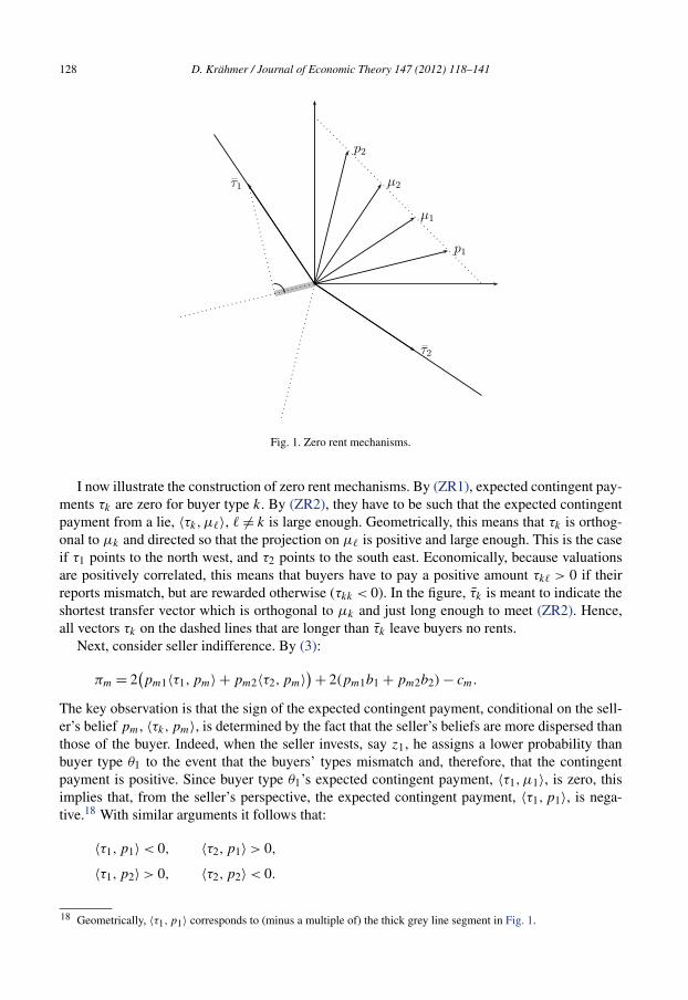
Fig. 1. Zero rent mechanisms.

I now illustrate the construction of zero rent mechanisms. By (ZR1), expected contingent pay-ments τk are zero for buyer type k. By (ZR2), they have to be such that the expected contingentpayment from a lie, 〈τk,μ�〉, � �= k is large enough. Geometrically, this means that τk is orthog-onal to μk and directed so that the projection on μ� is positive and large enough. This is the caseif τ1 points to the north west, and τ2 points to the south east. Economically, because valuationsare positively correlated, this means that buyers have to pay a positive amount τk� > 0 if theirreports mismatch, but are rewarded otherwise (τkk < 0). In the figure, τ̄k is meant to indicate theshortest transfer vector which is orthogonal to μk and just long enough to meet (ZR2). Hence,all vectors τk on the dashed lines that are longer than τ̄k leave buyers no rents.

Next, consider seller indifference. By (3):

πm = 2(pm1〈τ1,pm〉 + pm2〈τ2,pm〉)+ 2(pm1b1 + pm2b2) − cm.

The key observation is that the sign of the expected contingent payment, conditional on the sell-er’s belief pm, 〈τk,pm〉, is determined by the fact that the seller’s beliefs are more dispersed thanthose of the buyer. Indeed, when the seller invests, say z1, he assigns a lower probability thanbuyer type θ1 to the event that the buyers’ types mismatch and, therefore, that the contingentpayment is positive. Since buyer type θ1’s expected contingent payment, 〈τ1,μ1〉, is zero, thisimplies that, from the seller’s perspective, the expected contingent payment, 〈τ1,p1〉, is nega-tive.18 With similar arguments it follows that:

〈τ1,p1〉 < 0, 〈τ2,p1〉 > 0,

〈τ1,p2〉 > 0, 〈τ2,p2〉 < 0.

18 Geometrically, 〈τ1,p1〉 corresponds to (minus a multiple of) the thick grey line segment in Fig. 1.


In other words, the seller who invested zk evaluates the contingent payments τk negatively inexpectation, while the seller who invested z�, � �= k, evaluates them positively. Crucially, thisdifference in expectations implies that the seller’s profit responds differently to changes in thepayment schedule, depending on his investment. Indeed, as τ1 increases uniformly in the reportsof buyer 2, the payments that the seller expects to collect from buyer 1 decrease if he has investedz1 but increase if he has invested z2. Thus, increasing the length of τ1 decreases the expectedprofit from investing z1 and increases the expected profit from z2. Likewise, increasing the lengthof τ2 increases π1 and decreases π2. Thus, an intermediate value argument implies that a solutionto the indifference condition π1 = π2 can be found by either increasing τ1 or τ2. Hence:

Proposition 1. In the binary–binary case, any ζ ∈ �̊2 is FSE-implementable.

The underlying geometric reason why a zero rent mechanism exists that also leaves the sellerindifferent is that μ1 and μ2 are convex combinations of the type distributions p1 and p2. Thisimplies that the line (hyperplane) through μk separates the beliefs μk,pk jointly from the be-liefs μ�,p�, � �= k. This means that a payment vector corresponding to the normal vector of thehyperplane is evaluated differently, depending on which side of the hyperplane one’s belief islocated: the disagreement about the sign of the expected payments between buyer type k and thebuyer type � can be used to construct zero rent mechanisms; at the same time, the disagreementbetween the seller who invested zk and the seller who invested z� can be used to make the sellerindifferent.

It is illuminating to see how the surplus is divided across buyer types and investments. Forthe sake of concreteness, suppose z2 is the efficient investment. Since the seller is indifferent inequilibrium, the seller’s ex ante profit π(ζ ) is equal to his ex post profit:

π(ζ ) = ζ1π1 + ζ2π2 = π1 = π2.

At the same time, since buyers get no rent, the seller extracts the full surplus in expectation:

π(ζ ) = ζ1πFB(z1) + ζ2π

FB(z2).

As surplus is higher at the efficient investment level, this implies that the seller receives less thanthe full surplus at the efficient investment level (πFB(z2) > π2) but more than the full surplus atthe inefficient investment (πFB(z1) < π1). Effectively, when the efficient investment realizes, thepayments of the mechanism shift surplus from the seller to the buyer, and vice versa. Holding thebuyer type fixed and averaging over investments, this means that the buyer gets a positive utilityat the efficient investment but makes a loss at the inefficient one.

Let me emphasize the three main properties used to establish Proposition 1. First, buyer beliefsare convexly independent. Second, the type distributions and buyer beliefs are ordered in a waythat μk and pk can jointly be separated from μ� and p�, � �= k. Third, the seller can be madeindifferent by an intermediate value argument. Next, I turn to the case when there are (weakly)fewer investments than types.

5.3. Less investments than types: M � K

I develop the argument according to the three properties used in the binary–binary case.


Convex independence of beliefsCremer and McLean [10, Theorem 2] have shown that, if beliefs are not convexly independent,

ex post efficient zero rent mechanisms may not exist. In my setup, convex independence ofbeliefs might, in principle, depend on the endogenous investment strategy ζ . However, the nextlemma shows that for totally mixed investment strategies this is not the case. Rather, convexindependence is a property of the primitives (pm)Mm=1 only. To state the lemma, define by

q̄km = pmk∑n pnk

the probability with which investment zm has realized conditional on observing θk when the selleradopts the uniform investment strategy which places weight 1/M on each investment. Denote byq̄k the corresponding probability (column) vector.

Lemma 2. Let (pm)Mm=1 be linearly independent. Then (μk(ζ ))Kk=1 is convexly independent forall ζ ∈ �̊M if and only if (q̄k)

Kk=1 is convexly independent.

The proof uses the separating hyperplane theorem to actually show that (q̄k)Kk=1 is convexly

independent if and only if, for an arbitrary mixed strategy ζ , the posteriors about investments(qk(ζ ))Kk=1 are convexly independent. Hence, the convex independence of beliefs (μk)

Kk=1 is

guaranteed if there is only a single investment strategy so that the induced posteriors about in-vestments are convexly independent.

In light of Theorem 2 by Cremer and McLean [10], Lemma 2 makes clear that if (q̄k)Kk=1

is not convexly independent, then the seller will, in general, not be able to create correlationthat allows him to extract full surplus. While the seller might still benefit from creating cor-relation also in this case, the construction of optimal mechanisms is demanding already in thecase with exogenous beliefs (see [7]). To focus on the question when randomizing by the sellercan occur at all, I restrict attention to the case in which beliefs are convexly independent, andimpose:

Assumption 1.

(a) (pm)Mm=1 is linearly independent,(b) (q̄k)


Assumption 1(b) means that any realization of a buyer’s type is sufficiently informative aboutthe true investment. For example, the condition is violated if there is a type k which is equallylikely under all investments. In this case, observing k is completely uninformative and so q̄k isequal to the “prior” ζ which is always in the convex hull of posteriors. For Assumption 1(b) tohold, the probability that an investment brings about a type k has to be sufficiently dispersedacross investments.19

19 Notice that if there are only two investments and more than two types, then Assumption 1(b) cannot be satisfiedfor dimensionality reason: three beliefs over a binary state space cannot be convexly independent. This implies thatAssumption 1(b) is not generically satisfied. At the same time it is not generically violated, because if it holds, it is notupset by slightly perturbing the type distribution.


Ordering of type distributions and buyer beliefsIn the binary–binary case, the key idea is to exploit belief differences. More precisely, I have

constructed payments so that the seller and a buyer type agree about the sign of the expectedpayments if and only if the seller has chosen the investment for which the buyer type providesthe strongest evidence. I now show how this feature carries over to the general case. Recall that abuyer of type k assigns probability qkm(ζ ) = pmkζm/

∑n pnkζn to the event that investment zm

has realized. Consider a type which provides, among all types, the strongest evidence that zm hasoccurred:

κ(ζ,m) ∈ arg maxk

qkm(ζ ). (4)

Guided by the binary–binary case, I seek to construct payments so that the seller who investszm and the buyer type κ(ζ,m) agree about the sign of the expected payments, but disagree withall other buyer types and sellers who invest differently. Geometrically, I seek to separate pm andμκ(ζ,m) jointly from all other type distributions and buyer beliefs. It turns out that this is possiblein environments in which κ(ζ,m) is independent of ζ . In what follows, I will focus on suchenvironments.20 In Lemma 3 below, I will show that κ(ζ,m) is independent of ζ if and only ifthe following likelihood ratio condition is satisfied.

Assumption 2. For all m there is a k = k(m) so that for all �,n, n �= m, � �= k:

pmk

pm�

� pnk

pn�

. (5)

Assumption 2 says that for each investment zm there is one valuation θk whose likelihoodratio relative to any other valuation θ� is the highest among all investments. This means that anyinvestment brings about some valuation with relatively high likelihood. This is a natural featurewhen investments are ordered, and higher investments induce, on average, higher valuations, asin the next example.21

Example 1. There are as many investments as types, and investment zm brings about valuationθm with some probability ρ and any other valuation with probability (1 − ρ)/(K − 1) < ρ.

Next, I show that Assumption 2 is necessary and sufficient for the same observation to providethe strongest evidence for a given investment, irrespective of the “prior” ζ with which invest-ments are drawn.

Lemma 3. κ(ζ,m) is independent of ζ if and only if Assumption 2 holds. In this case, κ(ζ,m) =k(m).

I now turn to the construction of payments. In the first step, I construct payments for typesk = κ(m) which provide the strongest evidence for some investment.

Lemma 4. Suppose Assumptions 1 and 2 hold, and let ζ ∈ �̊M . Then for all m and for allnumbers smn > 0, n �= m, there is a vector σκ(m) ∈ R

K so that

20 This is somewhat stronger than needed, but makes the argument more transparent.21 Observe that Example 1 also satisfies Assumption 1.


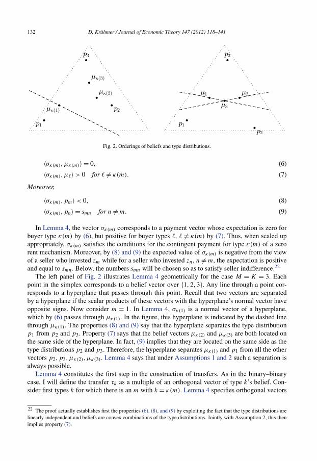
Fig. 2. Orderings of beliefs and type distributions.

〈σκ(m),μκ(m)〉 = 0, (6)

〈σκ(m),μ�〉 > 0 for � �= κ(m). (7)

Moreover,

〈σκ(m),pm〉 < 0, (8)

〈σκ(m),pn〉 = smn for n �= m. (9)

In Lemma 4, the vector σκ(m) corresponds to a payment vector whose expectation is zero forbuyer type κ(m) by (6), but positive for buyer types �, � �= κ(m) by (7). Thus, when scaled upappropriately, σκ(m) satisfies the conditions for the contingent payment for type κ(m) of a zerorent mechanism. Moreover, by (8) and (9) the expected value of σκ(m) is negative from the viewof a seller who invested zm while for a seller who invested zn, n �= m, the expectation is positiveand equal to smn. Below, the numbers smn will be chosen so as to satisfy seller indifference.22

The left panel of Fig. 2 illustrates Lemma 4 geometrically for the case M = K = 3. Eachpoint in the simplex corresponds to a belief vector over {1,2,3}. Any line through a point cor-responds to a hyperplane that passes through this point. Recall that two vectors are separatedby a hyperplane if the scalar products of these vectors with the hyperplane’s normal vector haveopposite signs. Now consider m = 1. In Lemma 4, σκ(1) is a normal vector of a hyperplane,which by (6) passes through μκ(1). In the figure, this hyperplane is indicated by the dashed linethrough μκ(1). The properties (8) and (9) say that the hyperplane separates the type distributionp1 from p2 and p3. Property (7) says that the belief vectors μκ(2) and μκ(3) are both located onthe same side of the hyperplane. In fact, (9) implies that they are located on the same side as thetype distributions p2 and p3. Therefore, the hyperplane separates μκ(1) and p1 from all the othervectors p2,p3,μκ(2),μκ(3). Lemma 4 says that under Assumptions 1 and 2 such a separation isalways possible.

Lemma 4 constitutes the first step in the construction of transfers. As in the binary–binarycase, I will define the transfer τk as a multiple of an orthogonal vector of type k’s belief. Con-sider first types k for which there is an m with k = κ(m). Lemma 4 specifies orthogonal vectors

22 The proof actually establishes first the properties (6), (8), and (9) by exploiting the fact that the type distributions arelinearly independent and beliefs are convex combinations of the type distributions. Jointly with Assumption 2, this thenimplies property (7).


σk for these types, yet not uniquely. To guarantee that for each type k there is a unique or-thogonal vector, I assume that no type can provide the strongest evidence for two differentinvestments.

Assumption 3. Let κ be defined as in (4). If m �= m′, then κ(m) �= κ(m′).

Together with Lemma 4, Assumption 3 implies that for each type distribution, there is a dif-ferent belief so that the two can be separated from all other type distributions and beliefs. Thisis again illustrated by the left panel of Fig. 2. Observe that for each m a distinct μκ(m) can befound so that the points pm and μκ(m) can jointly be separated from all other points. Observethat Example 1 satisfies Assumption 3 with κ(m) = m.

The right panel in Fig. 2 depicts a constellation which is not covered by Assumption 3. Thereis no hyperplane that separates μ3 and exactly one type distribution pm jointly from all otherpoints. Indeed, consider any hyperplane passing through μ3 that leaves μ1 and μ2 on the sameside. Such a hyperplane corresponds to a line located in between the two dashed lines. Therefore,if μ1 and μ2 are separated from μ3, the points p1 and p2 are always on the “other” side. Itfollows that there is no m with κ(m) = 3. With three investments and three types, this impliesthat Assumption 3 is violated.

After having specified orthogonal vectors for all μk with k = κ(m) for some m, I next specifyorthogonal vectors for types � for which there is no m with � = κ(m). For such a type, I define thecorresponding orthogonal vector such that the projection on all other belief vectors is positive. Bythe separating hyperplane theorem, this is always possible since beliefs are convexly independent.Formally, choose σ� so that

〈σ�,μ�〉 = 0 and 〈σ�,μk〉 > 0 ∀k �= �. (10)

Hence, orthogonal vectors σk are now defined for all k, and I set transfers equal to a multiple ofthese:

τk = λkσk.

Then (6) and the left part of (10) imply (ZR1). Moreover, (7) and the right part of (10) imply(ZR2) whenever λk is large enough, that is,

λk � θ�〈xk,μ�〉 − θ�〈x�,μ�〉〈σk,μ�〉 ≡ λ̄k. (11)

Intermediate value argumentIn the final step of the construction, I choose the numbers smn in Lemma 4 so that, similarly to

the binary–binary case, an intermediate value argument can be used to make the seller indifferent.I have the following proposition.

Proposition 2. Under Assumptions 1 to 3, any ζ ∈ �̊M is FSE-implementable.

I illustrate the argument for the case with three investments and three valuations: M = K = 3.Fix an investment zm and let n′ and n′′ be the other two investment indices. Now consider prof-its (3). By Assumption 3, each type k provides the strongest evidence for a unique investment.Therefore I can express the sum over k in (3) as the sum over κ(m), κ(n′), and κ(n′′):


πm = 2pmκ(m) 〈σκ(m),pm〉︸︷︷︸<0

λκ(m) + 2pmκ(n′) 〈σκ(n′), pm〉︸︷︷︸=sn′m>0

λκ(n′)

+ 2pmκ(n′′) 〈σκ(n′′), pm〉︸︷︷︸=sn′′m>0

λκ(n′′) + 2∑

k

pmkbk − cm.

Observe that by Lemma 4, 〈σκ(m),pm〉 < 0 and 〈σκ(n),pm〉 = snm > 0 for n = n′, n′′: the sellerwho invested zm evaluates the payments of the buyer type κ(m) in expectation differently fromthe seller who has not invested zm. Therefore, πm decreases in λκ(m) and increases in λκ(n),n = n′, n′′. I now use this property to construct transfers that leave the seller indifferent. Thecoefficients snm can be chosen in such a way that a change of λκ(m) changes the profits πn′ andπn′′ at the same rate.23 Now, consider some zero rent mechanism, that is, λk � λ̄k for all types k.I now argue that the seller can be made indifferent by appropriately increasing some λk’s (observethat this maintains the zero rent property). Suppose that at the original zero rent mechanism,profits happen to be ranked as π3 > π1 > π2. Now increase λκ(1). Since this decreases π1 andraises π2, there will be a point λ′

κ(1) at which equality holds: π1 = π2. Moreover, at this point it isstill true that π3 > π1, because also π3 increases in λκ(1). Next, increase λκ(3). This decreases π3and raises π1 and π2. In fact, because π1 and π2 increase at the same rate, the equality π1 = π2is maintained when λκ(3) is increased. Hence, there will be a point λ′

κ(3) at which equality holdsbetween all three profits, and the seller is indifferent.

Proposition 2 provides conditions so that any totally mixed strategy is FSE-implementable.Therefore, it directly implies that the seller can attain a profit arbitrarily close to the (ex ante)first best surplus by implementing an investment strategy which places almost full mass on thefirst best investment:

Proposition 3. Under Assumptions 1 to 3, the seller can approximately attain the ex ante firstbest surplus πFB.

Strictly speaking, therefore, the seller’s problem only has an approximate solution: for anymechanism which FSE-implements some investment strategy, there is a better mechanism FSE-implementing a strategy that places slightly more weight on the first best investment. The impor-tant message of Proposition 3 is, however, that by implementing a mixed investment strategy andthus creating correlation between the buyers’ valuations, the seller can do better than by offeringa mechanism that implements a pure investment strategy and leaves a positive rent to the buyers.

For the seller to attain approximate first best, only investment strategies which are close to thefirst best investment need to be FSE-implementable. Therefore, Proposition 3 holds under weakerconditions than Assumptions 1 to 3, which guarantee FSE-implementability for all totally mixedstrategies. In fact, suppose that, instead of globally for all ζ , κ(ζ,m) is independent of ζ andthat Assumption 3 holds in a neighborhood around the first best investment strategy. Then thesame argument that I presented is applicable to show that any totally mixed strategy in thisneighborhood is FSE-implementable, and accordingly, the seller can approximately attain thefirst best.

A caveat of the previous result is that if the seller places almost all probability mass on theefficient investment, the correlation between the buyers’ beliefs gets very small, necessitating

23 This works for sn′m = pn′κ(n′)pn′′κ(n′) and sn′′m = pn′κ(n′′)pn′′κ(n′′) .


large transfer to implement the near first best outcome. Already small amounts of risk aversionor limited liability would suffice to undermine the implementation of the near first best in myconstruction. Still, this does not necessarily mean that in cases with risk aversion or limitedliability, the optimal mechanism has the seller play a pure investment strategy. If risk aversionor limited liability are not too severe, it is likely that the seller would still benefit from reducinginformation rent by creating correlation.

5.4. More investments than types

The previous section shows that when there are fewer investments than types, any totallymixed strategy is FSE-implementable. When there are more investments than types, this willno longer be true in general. The reason is that the number of transfers available to make theseller indifferent is equal to the number of types. Thus, there are K instruments only to satisfyM − 1 � K equations (plus non-negativity constraints on the instruments).24

For this reason, I now specialize the analysis in two respects. First, I focus exclusively on thequestion whether the seller can approximately attain the first best profit. Second, for tractabilityreasons I confine myself with considering the case with two types k = 1,2.

5.4.1. Two typesWith two types, investments are ordered according to the probability with which they bring

about the low valuation. Assume that, possibly after relabeling indices, investments are orderedas z1 < · · · < zM so that low investments are more likely to bring about the low valuation: pm1 >

pn1 if m < n. The next result shows that the seller can almost fully extract the ex ante first bestsurplus.

Proposition 4. Suppose there are two types. Then the seller can approximately attain the firstbest profit πFB.

The idea behind the proof is to let the seller randomize between the first best investment zm̄

and either the next smaller or next larger investment. As in the binary–binary case, transfers canbe found which make the seller indifferent between these two investments. In fact, any multipleof these transfers leaves the seller indifferent, too. The remaining question is then whether withinthis set of transfers one can be found so that, in addition, the seller (weakly) prefers the investmentzm̄ over all other investments zm. This essentially boils down to the question how the differencein profits πm̄ − πm changes as transfers are increased. It turns out that this change is alwayspositive, once the probability ζm̄ with which the seller plays zm̄ is sufficiently large. Therefore, iftransfers are increased, πm̄ − πm becomes arbitrarily large, making the seller prefer zm̄ over zm.

What facilitates the analysis in the two type case is that all type distributions and beliefs areordered on a one-dimensional line. This imposes enough structure to determine the size of theprojections of type distribution pm on transfers τk , which, in turn, is needed to figure out thechange in the profit difference πm̄ − πm. In higher dimensions, there is no such restriction on thelocation of type distributions and beliefs.

24 As in the previous section, the seller could still be made indifferent between (less than) K of his investments. Theproblem is that this does not imply that he prefers those over the remaining investments. If the seller could commit notto use some investments, then he would be back in the case of the previous section. However, given that investments areunobservable, it is questionable that a court could enforce investment commitments.


6. Discussion and conclusion

Let me discuss some assumptions underlying the analysis. First, while I have considered aprivate values auction model, all my results will go through for more general mechanism designproblems with general allocation spaces and (gross) utility functions of agents, including inter-dependent values models. The reason is that by Lemma 1, it is essentially enough to constructappropriate contingent transfers which are orthogonal to an agent’s beliefs. The specific form ofagents’ willingness to pay is irrelevant for the construction of contingent payments, it only pinsdown base payments. Similarly, the restriction to two symmetric buyers is not substantial andjust keeps notation simple.

What is more substantial is the restriction to simple type spaces with the property that anybelief goes along with a distinct valuation (“beliefs determine preferences”). A situation in whichthis need not be true is when buyers possess (imperfect) private information ex ante, and theinformation they receive after the seller’s investment is only additional information. In such acase, convex independence of beliefs and thus full surplus extraction may fail (see, e.g. [22,26]).As argued earlier, then the construction of optimal mechanisms is demanding already in the casein which the seller cannot affect beliefs. I therefore focus on simple type spaces.

Furthermore, I have confined the analysis to mechanisms which do not condition on a re-port by the seller. While under the assumptions of Propositions 2 and 4, mechanisms with buyerreports only cannot be improved upon, this may change once these assumptions are violated:because the seller, after having observed the realization of his investment, holds private infor-mation, too, allowing for mechanisms with seller reports could extend the set of implementableoutcomes. In fact, Obara [24] shows that when it is buyers who choose ex ante actions, havingthem report about the realizations of their actions, can be beneficial. However, in Obara’s setup,agents’ transfers in the extended mechanism can be constructed by standard orthogonality condi-tions. In my setup, this is not true, because here the seller’s transfers are the payments by buyers.Therefore, in my setup, the transfers in the extended mechanism have to respect, in addition, asort of budget balance condition. Dealing with this requires a rather different line of argument.25

I leave the full analysis for future research.I conclude with noting that my analysis raises the more general question about strategies by

which a mechanism designer can influence the joint distribution of the agents’ valuations. A casein point is disclosure. Standard models of disclosure (e.g. [3,13]) typically fix a selling formatsuch as a first price auction and ask how much information the seller optimally wants to discloseto bidders. If the seller has some discretion over the selling format, then disclosing informationin ways such that bidders’ information is correlated may be beneficial.

Appendix A. Proofs

Proof of Lemma 1. For a mechanism with base payments bk and contingent payments τk , thefeasibility constraints (ICζ ) and (IRζ ) are respectively:

θk〈xk,μk〉 − 〈τk,μk〉 − bk � θk〈x�,μk〉 − 〈τ�,μk〉 − b� ∀k, �, (12)

θk〈xk,μk〉 − 〈τk,μk〉 − bk � 0 ∀k, (13)

25 See [1,17].


where (13) is binding under a zero rent mechanism. With this, the if-part is obvious (simply definetk� = τk� + bk). For the only-if-part, define bk = θk〈xk,μk〉 and τk� = tk� − bk . It is straightfor-ward to verify (ZR1) and (ZR2). �Proof of Lemma 2. Let ζ ∈ �̊M . Define by αk =∑

n pnkζn the probability of type k, and recallthat qkm = pmkζm/αk is the posterior over investments conditional on k given ζ . Let qk be thecorresponding probability (column) vector. The lemma follows from the two following claims:

(a) (q̄k)Kk=1 is convexly independent if and only if (qk)


(b) If (pm)Mm=1 is linearly independent, (μk(ζ ))Kk=1 is convexly independent if and only if(qk)


As for (a). By the separating hyperplane theorem (e.g. Ok [25, p. 481]), (q̄k)Kk=1 is convexly

independent if and only if for all k there is a hyperplane which separates q̄�, � �= k from q̄k .Hence, there is a normal vector xk ∈ R

M of the hyperplane so that:

〈xk, q̄�〉 � 0 ∀� �= k and 〈xk, q̄k〉 < 0. (14)

Observe that for all �

q̄�m = α�

ζm

∑n pn�

pm�ζm

α�

= α�

ζm

∑n pn�

q�m. (15)

Let yk ∈ RM be defined by the components ykm = xkm/ζm. Then (14) is equivalent to

α�∑n pn�

〈yk, q�〉 � 0 ∀� �= k andαk∑n pnk

〈yk, qk〉 < 0 (16)

⇔ 〈yk, q�〉 � 0 ∀� �= k and 〈yk, qk〉 < 0. (17)

Consequently, the hyperplane with normal vector yk separates q�, � �= k from qk , and thisproves (a).

As for (b). Consider an arbitrary index k and probability weights β�, � �= k. By (1):

μk =∑��=k

β�μ� ⇔∑m

qkmpm =∑��=k

β�

∑m

q�mpm

⇔∑m

(qkm −

∑��=k

β�q�m

)pm = 0. (18)

Now, if (qk)Kk=1 is convexly independent, then there is an m′ so that qkm′ − ∑

��=k β�q�m′ �= 0.

Since (pm)Mm=1 is linearly independent, the right equation is, therefore, violated. Hence, also thefirst equation is violated, but this means that (μk)

Kk=1 is convexly independent. As for the reverse,

suppose (μk)Kk=1 is convexly independent so that the first equation is violated. Then also the third

equation is violated, and hence qkm −∑��=k β�q�m �= 0 for some m. But this means that (qk)

Kk=1

is convexly independent. �Proof of Lemma 3. Note that κ(ζ,m) = k if and only if

pmkζm∑n pnkζn

� pm�ζm∑n pn�ζn

∀� �= k (19)

⇔∑

(pmkpn� − pm�pnk)ζn � 0 ∀� �= k. (20)
n


Observe that the inequality is true for all ζ if and only if the term in brackets under the sum arepositive for all n �= m. But this is equivalent to Assumption 2. �Proof of Lemma 4. I begin with establishing properties (6), (8) and (9). Fix m. I write thesystem of M equations given by (6) and (9) in matrix notation. Define the K × M-matrix A =(μκ(m),p1, . . . , pm−1,pm+1, . . . , pM) and the row vector v = (0, sm1, . . . , sm,m−1, sm,m+1, . . . ,

smM) ∈ RM . Then the equations in (6) and (9) can be stated as

σTκ(m)A = v, (21)

where the superscript T indicates the transposed. I have to show that for all v there is a solutionσκ(m) to (21). Indeed, observe that the M vectors μκ(m), pn, n �= m, are linearly independent.This is so since the M − 1 vectors pn, n �= m, are linearly independent by Assumption 1, andμκ(m) is a convex combination of all pn’s with a positive weight on pm. Hence, the matrix A

has rank M , and a solution σκ(m) to (21) exists, establishing (6) and (9). Moreover, (6) and (9)together with (1) directly imply inequality (8).

It remains to show (7). I begin with the remark that under Assumption 1, for all k, � there is astrict inequality in (5) for some m and n. To the contrary, suppose that there are k, � �= k so thatpmk/pnk = pm�/pn� for all m and n, then

(q̄km)−1 =∑

n pnk

pmk

=∑

n pn�

pm�

= (q̄�m)−1. (22)

It follows that q̄k = q̄�, a contradiction to the convex independence of (q̄k)Kk=1 posited in As-

sumption 1.Finally, I show inequality (7). The fact that 〈σκ(m),μκ(m)〉 = 0 and (1) imply

〈σκ(m),pm〉 = − ακ(m)

pmκ(m)ζm

∑n�=m

pnκ(m)ζn

ακ(m)

〈σκ(m),pn〉 =∑n�=m

pnκ(m)ζn

pmκ(m)ζm

〈σκ(m),pn〉. (23)

Using this in (1) for μ� gives

〈σκ(m),μ�〉 = pm�ζm

α�

〈σκ(m),pm〉 +∑n�=m

pn�ζn

α�

〈σκ(m),pn〉 (24)

=∑n�=m

[− pnκ(m)ζn

pmκ(m)ζm

· pm�ζm

α�

+ pn�ζn

α�

]〈σκ(m),pn〉 (25)

=∑n�=m

ζn

α�

[−pnκ(m)pm�

pmκ(m)

+ pn�

]〈σκ(m),pn〉. (26)

By Assumption 2, the term in the square bracket is non-negative for all n, �, and, by the remarkat the beginning, is positive for some n, �. Together with the fact that 〈σκ(m),pn〉 > 0 by (9), thisyields the claim. �Proof of Proposition 2. I construct λk � λ̄k so that πm = πn for all m,n. Let

snm =∏

n′ �=m

pn′κ(n), sn =∏n′

pn′κ(n). (27)


Then profits in (3) become

πm = 2pmκ(m)〈σκ(m),pm〉λκ(m) + 2∑n�=m

snλκ(n)

+ 2∑

�: �n with κ(n)=�

pm�〈σ�,pm〉λ� + 2∑

k

pmkbk − cm. (28)

Observe that if λκ(m) is increased, then, since 〈σκ(m),pm〉 < 0 and because κ(m) �= κ(n), n �= m,the profit πm decreases, while all πn, n �= m, increase. Moreover, all πn, n �= m increase at thesame rate 2sm. Therefore, if λκ(m) is increased, then the difference πn − πn′ is unaffected for alln,n′ �= m. I now exploit this property to construct the desired λ step by step.

Let λ′ ∈ RK with λ′

k � λ̄k for all k. If πm(λ′) = πn(λ′) for all m,n we are done. Otherwise,

consider the investments that give the lowest payoff:

Nmin(λ′)=

{n

∣∣∣ πn

(λ′)= min

mπm

(λ′)}. (29)

Moreover, denote by m̂ the next best investment, which is given by:

πm̂

(λ′)> min

mπm

(λ′), πm̂

(λ′)� πm

(λ′) for all m /∈ Nmin

(λ′). (30)

Now consider an arbitrary n0 ∈ Nmin(λ′). Because πm̂ decreases and πn0 increases continuously

in λκ(m̂), there is a λ′′κ(m̂)

> λ′κ(m̂)

so that πm̂(λ′′) = πn0(λ′′), where λ′′ has the same components

as λ′ except of the κ(m̂)-th component, which is λ′′κ(m̂)

.Moreover, because all πn, n �= m̂ increase at the same rate as λ′

κ(m) is increased to λ′′κ(m), we

also have that πm̂(λ′′) = πn(λ′′) for all n ∈ Nmin(λ

′), so that at λ′′:

Nmin(λ′′)= Nmin

(λ′)∪ {m̂}. (31)

Now proceed repeatedly in the same manner. After at most M steps, this yields a λ with λk � λ̄k

for all k, at which all πm are the same. �Proof of Proposition 4. Consider the investment strategy ζ which places probability 1 − η onthe first best investment zm̄ and probability η on zm̄−1. (If m̄ = 1, then randomizing betweenzm̄ and zm̄+1 works.) I show that for all η smaller than some η̄ > 0, ζ is FSE-implementable.Consequently, the seller’s ex ante profit gets arbitrarily close to the first best profit as η goes tozero.

Because beliefs μ1 and μ2 are convexly independent, there are σ1 and σ2 in R2 so that

〈σ�,μ�〉 = 0 and 〈σ�,μk〉 > 0 ∀k �= �. (32)

For k = 1,2, define transfers τk = λkσk with λk � λ̄k , as defined in (11). By (3), the profitdifference between investment m̄ and any other investment n �= m̄ is

πm̄ − πn = 2[pm̄1〈σ1,pm̄〉 − pn1〈σ1,pn〉

]λ1 + 2

[pm̄2〈σ2,pm̄〉 − pn2〈σ2,pn〉

]λ2 + T1,

(33)

where T1 is a constant independent of λ1, λ2. Hence, the seller is indifferent between m̄ andm̄ − 1 if and only if

λ1 = −pm̄2〈σ2,pm̄〉 − pm̄−1,2〈σ2,pm̄−1〉λ2 + T2 (34)

pm̄1〈σ1,pm̄〉 − pm̄−1,1〈σ1,pm̄〉


Fig. 3. Ordering of beliefs and type distributions for M > K = 2 and η = 0.

for some constant T2. With this, I can compare the profit of m and any other investment n:

πm̄ − πn = 2

{−pm̄2〈σ2,pm̄〉 − pm̄−1,2〈σ2,pm̄−1〉

pm̄1〈σ1,pm̄〉 − pm̄−1,1〈σ1,pm̄−1〉 · [pm̄1〈σ1,pm̄〉 − pn1〈σ1,pn〉]

+ [pm̄2〈σ2,pm̄〉 − pn2〈σ2,pn〉

]} · λ2 + T3, (35)

where T3 is some constant. I now show that when η = 0, the coefficient in the curly brackets infront of λ2 is strictly positive for all n �= m̄, m̄ − 1. By continuity, this coefficient will still bestrictly positive for all small η > 0. This implies that by raising λ2, the difference πm̄ − πn canbe made arbitrarily large while keeping πm̄ − πm̄−1 equal to zero. Therefore, the seller prefersthe investments zm̄ and zm̄−1 over all other investments, and randomizing between zm̄ and zm̄−1is optimal.

Indeed, for η = 0, it holds that μ1 = μ2 = pm̄ and, given the orientation of σ1 and σ2:

σ1 =(−pm̄2

pm̄1

), σ2 =

(pm̄2

−pm̄1

). (36)

Thus, we have that 〈σ1,pm̄〉 = 〈σ2,pm̄〉 = 0 and 〈σ1,pn〉 = −〈σ2,pn〉 for all n. Fig. 3 illustrates.With this, the coefficient in front of λ2 gets

{−−pm̄−1,2〈σ2,pm̄−1〉

−pm̄−1,1〈σ1,pm̄−1〉 · [−pn1〈σ1,pn〉]+ [−pn2〈σ2,pn〉

]}(37)

= 〈σ1,pn〉[−pm̄−1,2

pm̄−1,1· pn1 + pn2

]. (38)

I now argue that this expression is positive. Observe first that the term in the square brackets ispositive if and only if

−(1 − pm̄−1,1)pn1 + pm̄−1,1(1 − pn1) > 0 ⇔ pm̄−1,1 > pn1 ⇔ n > m̄ − 1.

(39)


Observe moreover (see Fig. 3) that 〈σ1,pn〉 > 0 if and only if n > m̄. These two observationsimply that the term in front of λ2 in (35) is strictly positive for all n �= m̄, m̄ − 1. This completesthe proof. �References

[1] C. d’Aspremont, J. Cremer, L.-A. Gerard-Varet, Balanced Bayesian mechanisms, J. Econ. Theory 115 (2004) 385–396.

[2] P. Barelli, On the genericity of full surplus extraction in mechanism design, J. Econ. Theory 144 (2009) 1320–1332.[3] D. Bergemann, M. Pesendorfer, Information structures in optimal auctions, J. Econ. Theory 137 (2007) 580–609.[4] D. Bergemann, K. Schlag, Pricing without priors, J. Europ. Econ. Assoc. 6 (2008) 560–569.[5] D. Bergemann, J. Välimäki, Information acquisition and efficient mechanism design, Econometrica 70 (2002) 1007–

1034.[6] S. Bikhchandani, Information acquisition and full surplus extraction, J. Econ. Theory 145 (2010) 2282–2308.[7] S. Bose, J. Zhao, Optimal use of correlated information in mechanism design when full surplus extraction may be

impossible, J. Econ. Theory 135 (2007) 357–381.[8] K.S. Chung, J. Ely, Foundations for dominant strategy mechanisms, Rev. Econ. Stud. 74 (2007) 447–476.[9] J. Cremer, F. Khalil, J.-C. Rochet, Productive information gathering, Games Econ. Behav. 25 (1998) 174–193.

[10] J. Cremer, R.P. McLean, Full extraction of the surplus in Bayesian and dominant strategy auctions, Econometrica 56(1988) 1247–1257.

[11] D. Demougin, D. Garvie, Contractual design with correlated information under limited liability, RAND J. Econ. 22(1991) 477–489.

[12] V. Dequiedt, D. Martimort, Mechanism design with bilateral contracting, 2009, mimeo.[13] J.-J. Ganuza, J.S. Penalva, Signal orderings based on dispersion and the supply of information in auctions, Econo-

metrica 78 (2010) 1007–1030.[14] A. Gizatulina, M. Hellwig, Beliefs, payoffs and information: on robustness of the BDP property in models with

endogenous beliefs, 2011, mimeo.[15] K. Hori, Inefficiency in a bilateral trading problem with cooperative investment, B.E. J. Theoretical Econ. (Con-

trib.) 6 (2006), Article 4.[16] A. Heifetz, Z. Neeman, On the generic (im)possibility of full surplus extraction in mechanism design, Economet-

rica 74 (2006) 213–233.[17] G. Kosenok, S. Severinov, Individually rational, budget-balanced mechanisms and allocation of surplus, J. Econ.

Theory 140 (2008) 126–161.[18] D. Krähmer, R. Strausz, Comment on correlated information, mechanism design and informational rents, J. Econ.

Theory 146 (2011) 2159–2164.[19] J.-J. Laffont, D. Martimort, Mechanism design with collusion and correlation, Econometrica 68 (2000) 309–342.[20] R.P. McAfee, P.R. Reny, Correlated information and mechanism design, Econometrica 60 (1992) 395–421.[21] R. Myerson, Optimal auction design, Math. Methods Operations Res. 6 (1981) 58–73.[22] Z. Neeman, The relevance of private information in mechanism design, J. Econ. Theory 117 (2004) 55–77.[23] J. Robert, Continuity in auctions, J. Econ. Theory 55 (1991) 169–179.[24] I. Obara, The full surplus extraction theorem with hidden actions, B.E. J. Theoretical Econ. (Advanc.) 8 (2008),

Article 8.[25] E. Ok, Real Analysis with Economic Applications, Princeton Univ. Press, Princeton, NJ, 2007.[26] S.O. Parreiras, Correlated information, mechanism design and informational rents, J. Econ. Theory 123 (2005)

210–217.[27] W.P. Rogerson, Contractual solutions to the hold-up problem, Rev. Econ. Stud. 59 (1992) 777–794.[28] P.W. Schmitz, On the interplay of hidden action and hidden information in simple bilateral trading problems, J. Econ.

Theory 103 (2002) 444–460.[29] A.M. Spence, Monopoly, quality, and regulation, Bell J. Econ. 6 (1975) 417–429.[30] R.R. Zhao, Rigidity in bilateral trade with holdup, Theoretical Econ. 3 (2008) 85–121.

Documents

Auction design with endogenously correlated buyer types