Attentional Factorization Machines: Learning the Weight of ... · Attentional Factorization Machines: Learning the Weight of Feature Interactions via Attention Networks Jun Xiao1

Attentional Factorization Machines:Learning the Weight of Feature Interactions via Attention Networks∗

Jun Xiao1 Hao Ye1 Xiangnan He2 Hanwang Zhang2 Fei Wu1 Tat-Seng Chua2

1College of Computer Science, Zhejiang University2School of Computing, National University of Singapore

{junx, wufei}@cs.zju.edu.cn {xiangnanhe, haoyev, hanwangzhang}@gmail.com [email protected]

AbstractFactorization Machines (FMs) are a supervisedlearning approach that enhances the linear regres-sion model by incorporating the second-order fea-ture interactions. Despite effectiveness, FM canbe hindered by its modelling of all feature interac-tions with the same weight, as not all feature inter-actions are equally useful and predictive. For ex-ample, the interactions with useless features mayeven introduce noises and adversely degrade theperformance. In this work, we improve FM bydiscriminating the importance of different featureinteractions. We propose a novel model namedAttentional Factorization Machine (AFM), whichlearns the importance of each feature interactionfrom data via a neural attention network. Extensiveexperiments on two real-world datasets demon-strate the effectiveness of AFM. Empirically, it isshown on regression task AFM betters FM with a8.6% relative improvement, and consistently out-performs the state-of-the-art deep learning meth-ods Wide&Deep [Cheng et al., 2016] and Deep-Cross [Shan et al., 2016] with a much simpler struc-ture and fewer model parameters. Our implementa-tion of AFM is publicly available at: https://github.com/hexiangnan/attentional factorization machine

1 IntroductionSupervised learning is one of the fundamental tasks in ma-chine learning (ML) and data mining. The goal is to in-fer a function that predicts the target given predictor vari-ables (aka. features) as input. For example, real valuedtargets for regression and categorical labels for classifica-tion. It has broad applications including recommendationsystems [Bayer et al., 2017; Zhao et al., 2016], online ad-vertising [Shan et al., 2016; Juan et al., 2016], and imagerecognition [Zhang et al., 2017; Wang et al., 2015].

When performing supervised learning on categorical pre-dictor variables, it is important to account for the inter-actions between them [He and Chua, 2017; Cheng et al.,2016]. As an example, let us consider the toy problem

∗The corresponding author is Xiangnan He.

of predicting customers’ income with three categorical vari-ables: 1) occupation = {banker,engineer,...}, 2) level ={junior,senior}, and 3) gender = {male,female}. While ju-nior bankers have a lower income than junior engineers, itcan be the other way around for customers of senior level —senior bankers generally have a higher income than senior en-gineers. If a ML model assumes independence between pre-dictor variables and ignores the interactions between them, itwill fail to predict accurately, such as linear regression thatassociates a weight for each feature and predicts the target asthe weighted sum of all features.

To leverage the interactions between features, one commonsolution is to explicitly augment a feature vector with prod-ucts of features (aka. cross features), as in polynomial re-gression (PR) where a weight for each cross feature is alsolearned. However, the key problem with PR (and other simi-lar cross feature-based solutions, such as the wide componentof Wide&Deep [Cheng et al., 2016]) is that for sparse datasetswhere only a few cross features are observed, the parametersfor unobserved cross features cannot be estimated.

To address the generalization issue of PR, factorization ma-chines (FMs)1 were proposed [Rendle, 2010], which param-eterize the weight of a cross feature as the inner product ofthe embedding vectors of the constituent features. By learn-ing an embedding vector for each feature, FM can estimatethe weight for any cross feature. Owing to such general-ity, FM has been successfully applied to various applications,ranging from recommendation systems [Wang et al., 2017a;Chen et al., 2016] to natural language processing [Petroni etal., 2015]. Despite great promise, we argue that FM can behindered by its modelling of all factorized interactions withthe same weight. In real-world applications, different pre-dictor variables usually have different predictive power, andnot all features contain useful signal for estimating the tar-get, such as the gender variable for predicting customers’ in-come in the previous example. As such, the interactions withless useful features should be assigned a lower weight as theycontribute less to the prediction. Nevertheless, FM lacks suchcapability of differentiating the importance of feature interac-tions, which may result in suboptimal prediction.

In this work, we improve FM by discriminating the impor-

1In this paper, we focus on the second-order FM, which is themost effective and widely used instance of FMs.

Proceedings of the Twenty-Sixth International Joint Conference on Artificial Intelligence (IJCAI-17)

3119

tance of feature interactions. We devise a novel model namedAFM, which utilizes the recent advance in neural networkmodelling — the attention mechanism [Chen et al., 2017a;2017b] — to enable feature interactions contribute differentlyto the prediction. More importantly, the importance of afeature interaction is automatically learned from data with-out any human domain knowledge. We conduct experimentson two public benchmark datasets of context-aware predic-tion and personalized tag recommendation. Extensive exper-iments show that our use of attention on FM serves two ben-efits: it not only leads to better performance, but also pro-vides insight into which feature interactions contribute moreto the prediction. This greatly enhances the interpretabilityand transparency of FM, allowing practitioners to performdeeper analysis of its behavior.

2 Factorization MachinesAs a general ML model for supervised learning, factorizationmachines were originally proposed for collaborative recom-mendation [Rendle, 2010; Rendle et al., 2011]. Given a realvalued feature vector x ∈ Rn where n denotes the number offeatures, FM estimates the target by modelling all interactionsbetween each pair of features:

yFM (x) = w0 +

n∑i=1

wixi︸︷︷︸linear regression

+

n∑i=1

n∑j=i+1

wijxixj︸︷︷︸pair-wise feature interactions

, (1)

where w0 is the global bias, wi denotes the weight of the i-thfeature, and wij denotes the weight of the cross feature xixj ,which is factorized as: wij = vTi vj , where vi ∈ Rk denotesthe embedding vector for feature i, and k denotes the size ofembedding vector. Note that due to the coefficient xixj , onlyinteractions between non-zero features are considered.

It is worth noting that FM models all feature interactions inthe same way: first, a latent vector vi is shared in estimatingall feature interactions that the i-th feature involves; second,all estimated feature interactions wij have a uniform weightof 1. In practice, it is common that not all features are rele-vant to prediction. As an example, consider the problem ofnews classification with the sentence “US continues takinga leading role on foreign payment transparency”. It is obvi-ous that the words besides “foreign payment transparency”are not indicative of the topic of the (financial) news. Thoseinteractions involving irrelevant features can be consideredas noises that have no contribution to the prediction. How-ever, FM models all possible feature interactions with thesame weight, which may adversely deteriorate its generaliza-tion performance.

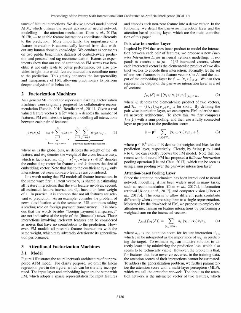
3 Attentional Factorization Machines3.1 ModelFigure 1 illustrates the neural network architecture of our pro-posed AFM model. For clarity purpose, we omit the linearregression part in the figure, which can be trivially incorpo-rated. The input layer and embedding layer are the same withFM, which adopts a sparse representation for input features

and embeds each non-zero feature into a dense vector. In thefollowing, we detail the pair-wise interaction layer and theattention-based pooling layer, which are the main contribu-tion of this paper.

Pair-wise Interaction LayerInspired by FM that uses inner product to model the interac-tion between each pair of features, we propose a new Pair-wise Interaction Layer in neural network modelling. It ex-pands m vectors to m(m − 1)/2 interacted vectors, whereeach interacted vector is the element-wise product of two dis-tinct vectors to encode their interaction. Formally, let the setof non-zero features in the feature vector x be X , and the out-put of the embedding layer be E = {vixi}i∈X . We can thenrepresent the output of the pair-wise interaction layer as a setof vectors:

fPI(E) = {(vi � vj)xixj}(i,j)∈Rx, (2)

where � denotes the element-wise product of two vectors,and Rx = {(i, j)}i∈X ,j∈X ,j>i for short. By defining thepair-wise interaction layer, we can express FM under the neu-ral network architecture. To show this, we first compressfPI(E) with a sum pooling, and then use a fully connectedlayer to project it to the prediction score:

y = pT∑

(i,j)∈Rx

(vi � vj)xixj + b, (3)

where p ∈ Rk and b ∈ R denote the weights and bias for theprediction layer, respectively. Clearly, by fixing p to 1 andb to 0, we can exactly recover the FM model. Note that ourrecent work of neural FM has proposed a Bilinear Interactionpooling operation [He and Chua, 2017], which can be seen asusing a sum pooling over the pair-wise interaction layer.

Attention-based Pooling LayerSince the attention mechanism has been introduced to neuralnetwork modelling, it has been widely used in many tasks,such as recommendation [Chen et al., 2017a], informationretrieval [Xiong et al., 2017], and computer vision [Chen etal., 2017b]. The idea is to allow different parts contributedifferently when compressing them to a single representation.Motivated by the drawback of FM, we propose to employ theattention mechanism on feature interactions by performing aweighted sum on the interacted vectors:

fAtt(fPI(E)) =∑

(i,j)∈Rx

aij(vi � vj)xixj , (4)

where aij is the attention score for feature interaction wij ,which can be interpreted as the importance of wij in predict-ing the target. To estimate aij , an intuitive solution to di-rectly learn it by minimizing the prediction loss, which alsoseems to be technically viable. However, the problem is that,for features that have never co-occurred in the training data,the attention scores of their interactions cannot be estimated.To address the generalization problem, we further parameter-ize the attention score with a multi-layer perceptron (MLP),which we call the attention network. The input to the atten-tion network is the interacted vector of two features, which


3120

0

1

0

0

1

0

𝑥1

𝑥2

𝑥3

𝑥4

𝑥5

𝑥6

𝑥7

𝑥8

Sparse InputEmbedding

LayerPair-wise Interaction

LayerAttention-based Pooling Prediction Score

……

∑0.2

0.4

𝒗𝟐 ⋅ 𝑥2

𝒗𝟒 ⋅ 𝑥4

𝒗𝟔 ⋅ 𝑥6

𝒗𝟖 ⋅ 𝑥8

𝒗𝟐⨀𝒗𝟒 𝑥2𝑥4

𝒗𝟐⨀𝒗𝟔 𝑥2𝑥6

𝒗𝟒⨀𝒗𝟔 𝑥4𝑥6

𝒗𝟐⨀𝒗𝟖 𝑥2𝑥8

𝒗𝟒⨀𝒗𝟖 𝑥4𝑥8

𝒗𝟔⨀𝒗𝟖 𝑥6𝑥8

𝑎24

𝑎26

𝑎46

𝑎28

𝑎48

𝑎68

𝑖𝑗

𝑎𝑖𝑗 𝒗𝒊⨀𝒗𝒋 𝑥𝑖𝑥𝑗

Attention Net

𝑦

Figure 1: The neural network architecture of our proposed Attentional Factorization Machine model.

encodes their interaction information in the embedding space.Formally, the attention network is defined as:

a′ij = hTReLU(W(vi � vj)xixj + b),

aij =exp(a′ij)∑

(i,j)∈Rxexp(a′ij)

,(5)

where W ∈ Rt×k, b ∈ Rt, h ∈ Rt are model parameters, andt denotes the hidden layer size of the attention network, whichwe call attention factor. The attention scores are normalizedthrough the softmax function, a common practice by previouswork. We use the rectifier as the activation function, whichempirically shows good performance.

The output of the attention-based pooling layer is a k di-mensional vector, which compresses all feature interactionsin the embedding space by distinguishing their importance.We then project it to the prediction score. To summarize, wegive the overall formulation of AFM model as:

yAFM (x) = w0 +n∑

i=1

wixi +pTn∑

i=1

n∑j=i+1

aij(vi�vj)xixj ,

(6)where aij has been defined in Equation (5). The model pa-rameters are Θ = {w0, {wi}ni=1, {vi}ni=1, p,W, b, h}.

3.2 LearningAs AFM directly enhances FM from the perspective of datamodelling, it can also be applied to a variety of predictiontasks, including regression, classification and ranking. Dif-ferent objective functions should be used to tailor the AFMmodel learning for different tasks. For regression task wherethe target y(x) is a real value, a common objective function isthe squared loss:

Lr =∑x∈T

(yAFM (x)− y(x))2, (7)

where T denotes the set of training instances. For binary clas-sification or recommendation task with implicit feedback [Heet al., 2017b], we can minimize the log loss. In this paper, wefocus on the regression task and optimize the squared loss.

To optimize the objective function, we employ stochasticgradient descent (SGD) — a universal solver for neural net-work models. The key to implement a SGD algorithm is toobtain the derivative of the prediction model yAFM (x) w.r.t.each parameter. As most modern toolkits for deep learn-ing have provided the functionality of automatic differenti-ation, such as Theano and TensorFlow, we omit the details ofderivatives here.

Overfitting PreventionOverfitting is a perpetual issue in optimizing a ML model.It is shown that FM can suffer from overfitting [Rendle etal., 2011], so the L2 regularization is an essential ingredientto prevent overfitting for FM. As AFM has a stronger rep-resentation ability than FM, it may be even easier to overfitthe training data. Here we consider two techniques to preventoverfitting — dropout andL2 regularization — that have beenwidely used in neural network models.

The idea of dropout is randomly drop some neurons (alongtheir connections) during training [Srivastava et al., 2014]. Itis shown to be capable of preventing complex co-adaptationsof neurons on training data. Since AFM models all pair-wise interactions between features while not all interactionsare useful, the neurons of the pair-wise interaction layer mayeasily co-adapt with each other and result in overfitting. Assuch, we employ dropout on the pair-wise interaction layer toavoid co-adaptations. Moreover, as dropout is disabled duringtesting and the whole network is used for prediction, dropouthas another side effect of performing model averaging withsmaller neural networks, which may potentially improve theperformance [Srivastava et al., 2014].

For the attention network component which is a one-layerMLP, we apply L2 regularization on the weight matrix W toprevent the possible overfitting. That is, the actual objectivefunction we optimize is:

L =∑x∈T

(yAFM (x)− y(x))2 + λ||W||2, (8)

where λ controls the regularization strength. We do not em-ploy dropout on the attention network, as we find the joint useof dropout on both the interaction layer and attention networkleads to some stability issue and degrades the performance.


3121

4 Related WorkFMs [Rendle, 2010] are mainly used for supervised learningunder sparse settings; for example, in situations where cat-egorical variables are converted to sparse feature vector viaone-hot encoding. Distinct from the continuous raw featuresfound in images and audios, input features of the Web domainare mostly discrete and categorical [He and Chua, 2017]. Forprediction with such sparse data, it is crucial to model the in-teractions between features [Shan et al., 2016]. In contrastto matrix factorization (MF) that models the interaction be-tween two entities only [He et al., 2016b], FM is designed tobe a general machine learner for modelling the interactionsbetween any number of entities. By specifying the input fea-ture vector, [Rendle, 2012] shows that FM can subsume manyspecific factorization models such as MF, parallel factor anal-ysis, and SVD++ [Koren, 2008]. As such, FM is recognizedas the most effective linear embedding method for sparse dataprediction. Many variants to FM have been proposed, such asthe neural FM [He and Chua, 2017] that deepens FM underthe neural framework to learn high-order feature interactions,and the field-aware FM [Juan et al., 2016] that associates mul-tiple embedding vectors for a feature to differentiate its inter-action with other features of different fields.

In this work, we contribute improvements of FM by dis-criminating the importance of feature interactions. We areaware of a work similar to our proposal — GBFM [Cheng etal., 2014], which selects “good” features with gradient boost-ing and models only the interactions between good features.For interactions between selected features, GBFM sums themup with the same weight as FM does. As such, GBFM isessentially a feature selection algorithm, which is fundamen-tally different with our AFM that can learn the importance ofeach feature interaction.

Along another line, deep neural networks (aka. deep learn-ing) are becoming increasingly popular and have recentlybeen employed to prediction under sparse settings. Specif-ically, [Cheng et al., 2016] proposes Wide&Deep for Apprecommendation, where the Deep component is a MLP onthe concatenation of feature embedding vectors to learn fea-ture interactions; and [Shan et al., 2016] proposes DeepCrossfor click-through rate prediction, which applies a deep resid-ual MLP [He et al., 2016a] to learn cross features. We pointout that in these methods, feature interactions are implicitlycaptured by a deep neural network, rather than FM that ex-plicitly models each interaction as the inner product of twofeatures. As such, these deep methods are not interpretable,as the contribution of each feature interaction is unknown.By directly extending FM with the attention mechanism thatlearns the importance of each feature interaction, our AMFis more interpretable and empirically demonstrates superiorperformance over Wide&Deep and DeepCross.

5 ExperimentsWe conduct experiments to answer the following questions:

RQ1 How do the key hyper-parameters of AFM (i.e., dropouton feature interactions and regularization on the atten-tion network) impact its performance?

RQ2 Can the attention network effectively learn the impor-tance of feature interactions?

RQ3 How does AFM perform as compared to the state-of-the-art methods for sparse data prediction?

5.1 Experimental SettingsDatasets. We perform experiments with two public datasets:Frappe [Baltrunas et al., 2015] and MovieLens2 [Harperand Konstan, 2015]. The Frappe dataset has been used forcontext-aware recommendation, which contains 96, 203 appusage logs of users under different contexts. The eight contextvariables are all categorical, including weather, city, daytimeand so on. We convert each log (user ID, app ID and contextvariables) to a feature vector via one-hot encoding, obtaining5, 382 features. The MovieLens data has been used for per-sonalized tag recommendation, which contains 668, 953 tagapplications of users on movies. We convert each tag appli-cation (user ID, movie ID and tag) to a feature vector andobtain 90, 445 features.Evaluation Protocol. For both datasets, each log is assigneda target of value 1, meaning the user has used the app underthe context or applied the tag on the movie. We randomly pairtwo negative samples with each log and set their target to−1.As such, the final experimental data for Frappe and Movie-Lens contain 288, 609 and 2, 006, 859 instances, respectively.We randomly split each dataset into three portions: 70% fortraining, 20% for validation, and 10% for testing. The vali-dation set is only used for tuning hyper-parameters, and theperformance comparison is done on the test set. To evaluatethe performance, we adopt root mean square error (RMSE),where a lower score indicates a better performance.Baselines. We compare AFM with the following competitivemethods that are designed for sparse data prediction:

- LibFM [Rendle, 2012]. This is the official C++ imple-mentation for FM. We choose the SGD learner as other meth-ods are all optimized by SGD (or its variants).

- HOFM. This is the TensorFlow implementation3 of thehigher-order FM [Blondel et al., 2016]. We set the order sizeto 3, as the MovieLens data has only three types of predictorvariables (user, item, and tag).

- Wide&Deep [Cheng et al., 2016]. We implement themethod. As the structure (e.g., depth and size of each layer)of a deep neural network is difficult to be fully tuned, we usethe same structure as reported in the paper. The wide part isthe same as the linear regression part of FM, and the deep partis a three-layer MLP with the layer size 1024, 512 and 256.

- DeepCross [Shan et al., 2016]. We implement themethod with the same structure of the original paper. It stacks5 residual units (each unit has two layers) with hidden dimen-sion 512, 512, 256, 128 and 64, respectively.

All models are learned by optimizing the squared loss fora fair comparison. Besides LibFM, all methods are learnedby the mini-batch Adagrad. The batch size for Frappe andMovieLens is set to 128 and 4096, respectively. The em-bedding size is set to 256 for all methods. Without special

2grouplens.org/datasets/movielens/latest3https://github.com/geffy/tffm


3122

0.44

0.45

0.46

0.47

0.48

0.49

0 0.1 0.2 0.3 0.4 0.5 0.6 0.7 0.8

RM

SE(v

alid

atio

n)

Dropout Ratio

MovieLens

AFMFMLibFM

0.31

0.32

0.33

0.34

0.35

0.36

0 0.1 0.2 0.3 0.4 0.5 0.6 0.7 0.8

RM

SE(v

alid

atio

n)

Dropout Ratio

Frappe

AFMFMLibFM

0.00

0.10

0.20

0.30

0.40

0.50

0.60

0 10 20 30 40 50 60 70 80 90 100

RM

SE

Epoch

Frappe

AFM(train)AFM(test)FM(train)FM(test)

0.30

0.31

0.32

0.33

0.34

0.35

0 0.5 1 2 4 8 16

RM

SE(v

alid

atio

n)

λ

Frappe

AFMFMLibFM

0.30

0.31

0.32

0.33

0.34

0.35

1 4 8 16 32 64 128 256

RM

SE(v

alid

atio

n)

Attention Factors

Frappe

AFM

FM

LibFM

0.43

0.44

0.45

0.46

0.47

0.48

0 0.5 1 2 4 8 16

RM

SE(v

alid

atio

n)

λ

MovieLens

AFMFMLibFM

0.43

0.44

0.45

0.46

0.47

0.48

1 4 8 16 32 64 128 256

RM

SE(v

alid

atio

n)

Attention Factors

MovieLens

AFMFMLibFM

0.31

0.33

0.35

0.37

0.39

0.41

0 0.1 0.2 0.3 0.4 0.5 0.6 0.7 0.8

RM

SE(v

alid

atio

n)

Dropout Ratio

Frappe

AFM

FM

LibFM

0.00

0.10

0.20

0.30

0.40

0.50

0.60

0 20 40 60 80 100

RM

SE

Epoch

Frappe


0.00

0.10

0.20

0.30

0.40

0.50

0.60

0 10 20 30 40 50

RM

SE

Epoch

MovieLens

AFM(train)

AFM(test)

FM(train)

FM(test)

0.44

0.45

0.46

0.47

0.48

0.49

0 0.1 0.2 0.3 0.4 0.5 0.6 0.7 0.8

RM

SE(v

alid

atio

n)

Dropout Ratio

MovieLens

AFMFMLibFM

0.31

0.32

0.33

0.34

0.35

0.36

0 0.1 0.2 0.3 0.4 0.5 0.6 0.7 0.8

RM

SE(v

alid

atio

n)

Dropout Ratio

Frappe

AFMFMLibFM

0.00

0.10

0.20

0.30

0.40

0.50

0.60

0 10 20 30 40 50 60 70 80 90 100

RM

SE

Epoch

Frappe


0.30

0.31

0.32

0.33

0.34

0.35

0 0.5 1 2 4 8 16

RM

SE(v

alid

atio

n)

λ

Frappe

AFMFMLibFM

0.30

0.31

0.32

0.33

0.34

0.35

1 4 8 16 32 64 128 256

RM

SE(v

alid

atio

n)

Attention Factors

Frappe

AFM

FM

LibFM

0.43

0.44

0.45

0.46

0.47

0.48

0 0.5 1 2 4 8 16

RM

SE(v

alid

atio

n)

λ

MovieLens

AFMFMLibFM

0.43

0.44

0.45

0.46

0.47

0.48

1 4 8 16 32 64 128 256

RM

SE(v

alid

atio

n)

Attention Factors

MovieLens

AFMFMLibFM

0.31

0.33

0.35

0.37

0.39

0.41

0 0.1 0.2 0.3 0.4 0.5 0.6 0.7 0.8

RM

SE(v

alid

atio

n)

Dropout Ratio

Frappe

AFM

FM

LibFM

0.00

0.10

0.20

0.30

0.40

0.50

0.60

0 20 40 60 80 100

RM

SE

Epoch

Frappe


0.00

0.10

0.20

0.30

0.40

0.50

0.60

0 10 20 30 40 50

RM

SE

Epoch

MovieLens

AFM(train)

AFM(test)

FM(train)

FM(test)

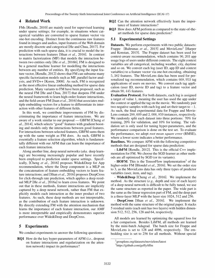
Figure 2: Validation error of AFM and FM w.r.t. different dropoutratios on the pair-wise interaction layer

mention, the attention factor is also 256, same as the em-bedding size. We carefully tuned the L2 regularization forLibFM and HOFM, and the dropout ratio for Wide&Deepand DeepCross. Early stopping strategy is used based on theperformance on validation set. For Wide&Deep, DeepCrossand AFM, we find that pre-training their feature embeddingswith FM leads to a lower RMSE than a random initialization.As such, we report their performance with pre-training.

5.2 Hyper-parameter Investigation (RQ1)First, we explore the effect of dropout on the pair-wise inter-action layer. We set λ to 0, so that no L2 regularization isused on the attention network. We also validate dropout onour implementation of FM by removing the attention compo-nent of AFM. Figure 2 shows the validation error of AFM andFM w.r.t. different dropout ratios; the result of LibFM is alsoshown as a benchmark. We have the following observations:

• By setting the dropout ratio to a proper value, both AFMand FM can be significantly improved. Specifically, forAFM, the optimal dropout ratio on Frappe and MovieLensis 0.2 and 0.5, respectively. This verifies the usefulness ofdropout on the pair-wise interaction layer, which improvesthe generalization of FM and AFM.

• Our implementation of FM offers a better performancethan LibFM. The reasons are twofold. First, LibFM op-timizes with the vanilla SGD, which adopts a fixed learn-ing rate for all parameters; while we optimize FM withAdagrad, which adapts the learning rate for each parame-ter based on its frequency (i.e., smaller updates for frequentand larger updates for infrequent parameters). Second,LibFM prevents overfitting via L2 regularization, while weemploy dropout, which can be more effective due to themodel averaging effect.

• AFM outperforms FM and LibFM by a large margin. Evenwhen dropout is not used and the overfitting issue does ex-ist to a certain extent, AFM achieves a performance sig-nificantly better than the optimal performance of LibFMand FM (cf. the result of dropout ratio equals to 0). Thisdemonstrates the benefits of the attention network in learn-ing the weight of feature interactions.

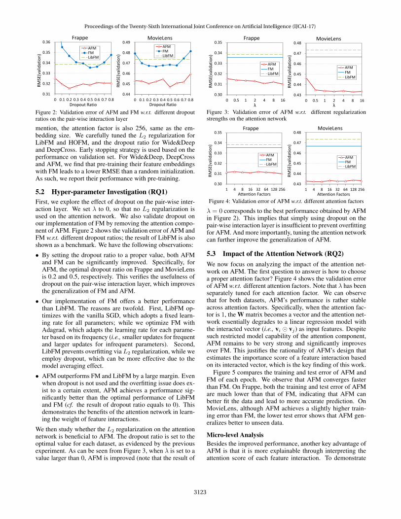
We then study whether the L2 regularization on the attentionnetwork is beneficial to AFM. The dropout ratio is set to theoptimal value for each dataset, as evidenced by the previousexperiment. As can be seen from Figure 3, when λ is set to avalue larger than 0, AFM is improved (note that the result of

0.44

0.45

0.46

0.47

0.48

0.49

0 0.1 0.2 0.3 0.4 0.5 0.6 0.7 0.8

RM

SE(v

alid

atio

n)

Dropout Ratio

MovieLens

AFMFMLibFM

0.31

0.32

0.33

0.34

0.35

0.36

0 0.1 0.2 0.3 0.4 0.5 0.6 0.7 0.8

RM

SE(v

alid

atio

n)

Dropout Ratio

Frappe

AFMFMLibFM

0.00

0.10

0.20

0.30

0.40

0.50

0.60

0 10 20 30 40 50 60 70 80 90 100

RM

SE

Epoch

Frappe


0.30

0.31

0.32

0.33

0.34

0.35

0 0.5 1 2 4 8 16

RM

SE(v

alid

atio

n)

λ

Frappe

AFMFMLibFM

0.30

0.31

0.32

0.33

0.34

0.35

1 4 8 16 32 64 128 256

RM

SE(v

alid

atio

n)

Attention Factors

Frappe

AFM

FM

LibFM

0.43

0.44

0.45

0.46

0.47

0.48

0 0.5 1 2 4 8 16

RM

SE(v

alid

atio

n)

λ

MovieLens

AFMFMLibFM

0.43

0.44

0.45

0.46

0.47

0.48

1 4 8 16 32 64 128 256

RM

SE(v

alid

atio

n)

Attention Factors

MovieLens

AFMFMLibFM

0.31

0.33

0.35

0.37

0.39

0.41

0 0.1 0.2 0.3 0.4 0.5 0.6 0.7 0.8

RM

SE(v

alid

atio

n)

Dropout Ratio

Frappe

AFM

FM

LibFM

0.00

0.10

0.20

0.30

0.40

0.50

0.60

0 20 40 60 80 100

RM

SE

Epoch

Frappe


0.00

0.10

0.20

0.30

0.40

0.50

0.60

0 10 20 30 40 50

RM

SE

Epoch

MovieLens

AFM(train)

AFM(test)

FM(train)

FM(test)

0.44

0.45

0.46

0.47

0.48

0.49

0 0.1 0.2 0.3 0.4 0.5 0.6 0.7 0.8

RM

SE(v

alid

atio

n)

Dropout Ratio

MovieLens

AFMFMLibFM

0.31

0.32

0.33

0.34

0.35

0.36

0 0.1 0.2 0.3 0.4 0.5 0.6 0.7 0.8

RM

SE(v

alid

atio

n)

Dropout Ratio

Frappe

AFMFMLibFM

0.00

0.10

0.20

0.30

0.40

0.50

0.60

0 10 20 30 40 50 60 70 80 90 100

RM

SE

Epoch

Frappe


0.30

0.31

0.32

0.33

0.34

0.35

0 0.5 1 2 4 8 16

RM

SE(v

alid

atio

n)

λ

Frappe

AFMFMLibFM

0.30

0.31

0.32

0.33

0.34

0.35

1 4 8 16 32 64 128 256

RM

SE(v

alid

atio

n)

Attention Factors

Frappe

AFM

FM

LibFM

0.43

0.44

0.45

0.46

0.47

0.48

0 0.5 1 2 4 8 16

RM

SE(v

alid

atio

n)

λ

MovieLens

AFMFMLibFM

0.43

0.44

0.45

0.46

0.47

0.48

1 4 8 16 32 64 128 256

RM

SE(v

alid

atio

n)

Attention Factors

MovieLens

AFMFMLibFM

0.31

0.33

0.35

0.37

0.39

0.41

0 0.1 0.2 0.3 0.4 0.5 0.6 0.7 0.8

RM

SE(v

alid

atio

n)

Dropout Ratio

Frappe

AFM

FM

LibFM

0.00

0.10

0.20

0.30

0.40

0.50

0.60

0 20 40 60 80 100

RM

SE

Epoch

Frappe


0.00

0.10

0.20

0.30

0.40

0.50

0.60

0 10 20 30 40 50

RM

SE

Epoch

MovieLens

AFM(train)

AFM(test)

FM(train)

FM(test)

Figure 3: Validation error of AFM w.r.t. different regularizationstrengths on the attention network

0.44

0.45

0.46

0.47

0.48

0.49

0 0.1 0.2 0.3 0.4 0.5 0.6 0.7 0.8

RM

SE(v

alid

atio

n)

Dropout Ratio

MovieLens

AFMFMLibFM

0.31

0.32

0.33

0.34

0.35

0.36

0 0.1 0.2 0.3 0.4 0.5 0.6 0.7 0.8

RM

SE(v

alid

atio

n)

Dropout Ratio

Frappe

AFMFMLibFM

0.00

0.10

0.20

0.30

0.40

0.50

0.60

0 10 20 30 40 50 60 70 80 90 100

RM

SE

Epoch

Frappe


0.30

0.31

0.32

0.33

0.34

0.35

0 0.5 1 2 4 8 16

RM

SE(v

alid

atio

n)

λ

Frappe

AFMFMLibFM

0.30

0.31

0.32

0.33

0.34

0.35

1 4 8 16 32 64 128 256

RM

SE(v

alid

atio

n)

Attention Factors

Frappe

AFMFMLibFM

0.43

0.44

0.45

0.46

0.47

0.48

0 0.5 1 2 4 8 16

RM

SE(v

alid

atio

n)

λ

MovieLens

AFMFMLibFM

0.43

0.44

0.45

0.46

0.47

0.48

1 4 8 16 32 64 128 256

RM

SE(v

alid

atio

n)

Attention Factors

MovieLens

AFMFMLibFM

0.31

0.33

0.35

0.37

0.39

0.41

0 0.1 0.2 0.3 0.4 0.5 0.6 0.7 0.8

RM

SE(v

alid

atio

n)

Dropout Ratio

Frappe

AFM

FM

LibFM

0.00

0.10

0.20

0.30

0.40

0.50

0.60

0 20 40 60 80 100

RM

SE

Epoch

Frappe


0.00

0.10

0.20

0.30

0.40

0.50

0.60

0 10 20 30 40 50

RM

SE

Epoch

MovieLens


0.44

0.45

0.46

0.47

0.48

0.49

0 0.1 0.2 0.3 0.4 0.5 0.6 0.7 0.8

RM

SE(v

alid

atio

n)

Dropout Ratio

MovieLens

AFMFMLibFM

0.31

0.32

0.33

0.34

0.35

0.36

0 0.1 0.2 0.3 0.4 0.5 0.6 0.7 0.8

RM

SE(v

alid

atio

n)

Dropout Ratio

Frappe

AFMFMLibFM

0.00

0.10

0.20

0.30

0.40

0.50

0.60

0 10 20 30 40 50 60 70 80 90 100

RM

SE

Epoch

Frappe


0.30

0.31

0.32

0.33

0.34

0.35

0 0.5 1 2 4 8 16

RM

SE(v

alid

atio

n)

λ

Frappe

AFMFMLibFM

0.30

0.31

0.32

0.33

0.34

0.35

1 4 8 16 32 64 128 256

RM

SE(v

alid

atio

n)

Attention Factors

Frappe

AFMFMLibFM

0.43

0.44

0.45

0.46

0.47

0.48

0 0.5 1 2 4 8 16

RM

SE(v

alid

atio

n)

λ

MovieLens

AFMFMLibFM

0.43

0.44

0.45

0.46

0.47

0.48

1 4 8 16 32 64 128 256

RM

SE(v

alid

atio

n)

Attention Factors

MovieLens

AFMFMLibFM

0.31

0.33

0.35

0.37

0.39

0.41

0 0.1 0.2 0.3 0.4 0.5 0.6 0.7 0.8

RM

SE(v

alid

atio

n)

Dropout Ratio

Frappe

AFM

FM

LibFM

0.00

0.10

0.20

0.30

0.40

0.50

0.60

0 20 40 60 80 100

RM

SE

Epoch

Frappe


0.00

0.10

0.20

0.30

0.40

0.50

0.60

0 10 20 30 40 50

RM

SE

Epoch

MovieLens


Figure 4: Validation error of AFM w.r.t. different attention factors

λ = 0 corresponds to the best performance obtained by AFMin Figure 2). This implies that simply using dropout on thepair-wise interaction layer is insufficient to prevent overfittingfor AFM. And more importantly, tuning the attention networkcan further improve the generalization of AFM.

5.3 Impact of the Attention Network (RQ2)We now focus on analyzing the impact of the attention net-work on AFM. The first question to answer is how to choosea proper attention factor? Figure 4 shows the validation errorof AFM w.r.t. different attention factors. Note that λ has beenseparately tuned for each attention factor. We can observethat for both datasets, AFM’s performance is rather stableacross attention factors. Specifically, when the attention fac-tor is 1, the W matrix becomes a vector and the attention net-work essentially degrades to a linear regression model withthe interacted vector (i.e., vi � vj) as input features. Despitesuch restricted model capability of the attention component,AFM remains to be very strong and significantly improvesover FM. This justifies the rationality of AFM’s design thatestimates the importance score of a feature interaction basedon its interacted vector, which is the key finding of this work.

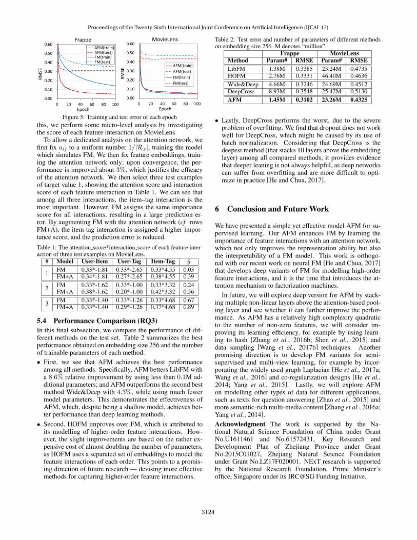
Figure 5 compares the training and test error of AFM andFM of each epoch. We observe that AFM converges fasterthan FM. On Frappe, both the training and test error of AFMare much lower than that of FM, indicating that AFM canbetter fit the data and lead to more accurate prediction. OnMovieLens, although AFM achieves a slightly higher train-ing error than FM, the lower test error shows that AFM gen-eralizes better to unseen data.

Micro-level AnalysisBesides the improved performance, another key advantage ofAFM is that it is more explainable through interpreting theattention score of each feature interaction. To demonstrate


3123

0.44

0.45

0.46

0.47

0.48

0.49

0 0.1 0.2 0.3 0.4 0.5 0.6 0.7 0.8

RM

SE(v

alid

atio

n)

Dropout Ratio

MovieLens

AFMFMLibFM

0.31

0.32

0.33

0.34

0.35

0.36

0 0.1 0.2 0.3 0.4 0.5 0.6 0.7 0.8

RM

SE(v

alid

atio

n)

Dropout Ratio

Frappe

AFMFMLibFM

0.00

0.10

0.20

0.30

0.40

0.50

0.60

0 20 40 60 80 100

RM

SE

Epoch

Frappe


0.30

0.31

0.32

0.33

0.34

0.35

0 0.5 1 2 4 8 16

RM

SE(v

alid

atio

n)

λ

Frappe

AFMFMLibFM

0.30

0.31

0.32

0.33

0.34

0.35

1 4 8 16 32 64 128 256

RM

SE(v

alid

atio

n)

Attention Factors

Frappe

AFMFMLibFM

0.43

0.44

0.45

0.46

0.47

0.48

0 0.5 1 2 4 8 16

RM

SE(v

alid

atio

n)

λ

MovieLens

AFMFMLibFM

0.43

0.44

0.45

0.46

0.47

0.48

1 4 8 16 32 64 128 256

RM

SE(v

alid

atio

n)

Attention Factors

MovieLens

AFMFMLibFM

0.31

0.33

0.35

0.37

0.39

0.41

0 0.1 0.2 0.3 0.4 0.5 0.6 0.7 0.8

RM

SE(v

alid

atio

n)

Dropout Ratio

Frappe

AFM

FM

LibFM

0.00

0.10

0.20

0.30

0.40

0.50

0.60

0 20 40 60 80 100

RM

SE

Epoch

Frappe


0.00

0.10

0.20

0.30

0.40

0.50

0.60

0 20 40 60 80 100

RM

SE

Epoch

MovieLens

AFM(train)

AFM(test)

FM(train)

FM(test)

0.44

0.45

0.46

0.47

0.48

0.49

0 0.1 0.2 0.3 0.4 0.5 0.6 0.7 0.8

RM

SE(v

alid

atio

n)

Dropout Ratio

MovieLens

AFMFMLibFM

0.31

0.32

0.33

0.34

0.35

0.36

0 0.1 0.2 0.3 0.4 0.5 0.6 0.7 0.8

RM

SE(v

alid

atio

n)

Dropout Ratio

Frappe

AFMFMLibFM

0.00

0.10

0.20

0.30

0.40

0.50

0.60

0 20 40 60 80 100

RM

SE

Epoch

Frappe


0.30

0.31

0.32

0.33

0.34

0.35

0 0.5 1 2 4 8 16

RM

SE(v

alid

atio

n)

λ

Frappe

AFMFMLibFM

0.30

0.31

0.32

0.33

0.34

0.35

1 4 8 16 32 64 128 256

RM

SE(v

alid

atio

n)

Attention Factors

Frappe

AFMFMLibFM

0.43

0.44

0.45

0.46

0.47

0.48

0 0.5 1 2 4 8 16

RM

SE(v

alid

atio

n)

λ

MovieLens

AFMFMLibFM

0.43

0.44

0.45

0.46

0.47

0.48

1 4 8 16 32 64 128 256

RM

SE(v

alid

atio

n)

Attention Factors

MovieLens

AFMFMLibFM

0.31

0.33

0.35

0.37

0.39

0.41

0 0.1 0.2 0.3 0.4 0.5 0.6 0.7 0.8

RM

SE(v

alid

atio

n)

Dropout Ratio

Frappe

AFM

FM

LibFM

0.00

0.10

0.20

0.30

0.40

0.50

0.60

0 20 40 60 80 100

RM

SE

Epoch

Frappe


0.00

0.10

0.20

0.30

0.40

0.50

0.60

0 20 40 60 80 100

RM

SE

Epoch

MovieLens

AFM(train)

AFM(test)

FM(train)

FM(test)

Figure 5: Training and test error of each epochthis, we perform some micro-level analysis by investigatingthe score of each feature interaction on MovieLens.

To allow a dedicated analysis on the attention network, wefirst fix aij to a uniform number 1/|Rx|, training the modelwhich simulates FM. We then fix feature embeddings, train-ing the attention network only; upon convergence, the per-formance is improved about 3%, which justifies the efficacyof the attention network. We then select three test examplesof target value 1, showing the attention score and interactionscore of each feature interaction in Table 1. We can see thatamong all three interactions, the item–tag interaction is themost important. However, FM assigns the same importancescore for all interactions, resulting in a large prediction er-ror. By augmenting FM with the attention network (cf. rowsFM+A), the item-tag interaction is assigned a higher impor-tance score, and the prediction error is reduced.Table 1: The attention score*interaction score of each feature inter-action of three test examples on MovieLens.

# Model User-Item User-Tag Item-Tag y

1 FM 0.33*-1.81 0.33*-2.65 0.33*4.55 0.03FM+A 0.34*-1.81 0.27*-2.65 0.38*4.55 0.39

2 FM 0.33*-1.62 0.33*-1.00 0.33*3.32 0.24FM+A 0.38*-1.62 0.20*-1.00 0.42*3.32 0.56

3 FM 0.33*-1.40 0.33*-1.26 0.33*4.68 0.67FM+A 0.33*-1.40 0.29*-1.26 0.37*4.68 0.89

5.4 Performance Comparison (RQ3)In this final subsection, we compare the performance of dif-ferent methods on the test set. Table 2 summarizes the bestperformance obtained on embedding size 256 and the numberof trainable parameters of each method.• First, we see that AFM achieves the best performance

among all methods. Specifically, AFM betters LibFM witha 8.6% relative improvement by using less than 0.1M ad-ditional parameters; and AFM outperforms the second bestmethod Wide&Deep with 4.3%, while using much fewermodel parameters. This demonstrates the effectiveness ofAFM, which, despite being a shallow model, achieves bet-ter performance than deep learning methods.

• Second, HOFM improves over FM, which is attributed toits modelling of higher-order feature interactions. How-ever, the slight improvements are based on the rather ex-pensive cost of almost doubling the number of parameters,as HOFM uses a separated set of embeddings to model thefeature interactions of each order. This points to a promis-ing direction of future research — devising more effectivemethods for capturing higher-order feature interactions.

Table 2: Test error and number of parameters of different methodson embedding size 256. M denotes “million”.

Frappe MovieLensMethod Param# RMSE Param# RMSELibFM 1.38M 0.3385 23.24M 0.4735HOFM 2.76M 0.3331 46.40M 0.4636Wide&Deep 4.66M 0.3246 24.69M 0.4512DeepCross 8.93M 0.3548 25.42M 0.5130AFM 1.45M 0.3102 23.26M 0.4325

• Lastly, DeepCross performs the worst, due to the severeproblem of overfitting. We find that dropout does not workwell for DeepCross, which might be caused by its use ofbatch normalization. Considering that DeepCross is thedeepest method (that stacks 10 layers above the embeddinglayer) among all compared methods, it provides evidencethat deeper leaning is not always helpful, as deep networkscan suffer from overfitting and are more difficult to opti-mize in practice [He and Chua, 2017].

6 Conclusion and Future Work

We have presented a simple yet effective model AFM for su-pervised learning. Our AFM enhances FM by learning theimportance of feature interactions with an attention network,which not only improves the representation ability but alsothe interpretability of a FM model. This work is orthogo-nal with our recent work on neural FM [He and Chua, 2017]that develops deep variants of FM for modelling high-orderfeature interactions, and it is the time that introduces the at-tention mechanism to factorization machines.

In future, we will explore deep version for AFM by stack-ing multiple non-linear layers above the attention-based pool-ing layer and see whether it can further improve the perfor-mance. As AFM has a relatively high complexity quadraticto the number of non-zero features, we will consider im-proving its learning efficiency, for example by using learn-ing to hash [Zhang et al., 2016b; Shen et al., 2015] anddata sampling [Wang et al., 2017b] techniques. Anotherpromising direction is to develop FM variants for semi-supervised and multi-view learning, for example by incor-porating the widely used graph Laplacian [He et al., 2017a;Wang et al., 2016] and co-regularization designs [He et al.,2014; Yang et al., 2015]. Lastly, we will explore AFMon modelling other types of data for different applications,such as texts for question answering [Zhao et al., 2015] andmore semantic-rich multi-media content [Zhang et al., 2016a;Yang et al., 2014].Acknowledgment The work is supported by the Na-tional Natural Science Foundation of China under GrantNo.U1611461 and No.61572431, Key Research andDevelopment Plan of Zhejiang Province under GrantNo.2015C01027, Zhejiang Natural Science Foundationunder Grant No.LZ17F020001. NExT research is supportedby the National Research Foundation, Prime Minister’soffice, Singapore under its IRC@SG Funding Initiative.


3124

References[Baltrunas et al., 2015] Linas Baltrunas, Karen Church, Alexan-

dros Karatzoglou, and Nuria Oliver. Frappe: Understandingthe usage and perception of mobile app recommendations in-the-wild. CoRR, abs/1505.03014, 2015.

[Bayer et al., 2017] Immanuel Bayer, Xiangnan He, Bhargav Kana-gal, and Steffen Rendle. A generic coordinate descent frameworkfor learning from implicit feedback. In WWW, 2017.

[Blondel et al., 2016] Mathieu Blondel, Akinori Fujino, NaonoriUeda, and Masakazu Ishihata. Higher-order factorization ma-chines. In NIPS, 2016.

[Chen et al., 2016] Tao Chen, Xiangnan He, and Min-Yen Kan.Context-aware image tweet modelling and recommendation. InMM, 2016.

[Chen et al., 2017a] Jingyuan Chen, Hanwang Zhang, XiangnanHe, Liqiang Nie, Wei Liu, and Tat-Seng Chua. Attentive collab-orative filtering: Multimedia recommendation with feature- anditem-level attention. In SIGIR, 2017.

[Chen et al., 2017b] Long Chen, Hanwang Zhang, Jun Xiao,Liqiang Nie, Jian Shao, and Tat-Seng Chua. SCA-CNN: spatialand channel-wise attention in convolutional networks for imagecaptioning. In CVPR, 2017.

[Cheng et al., 2014] Chen Cheng, Fen Xia, Tong Zhang, IrwinKing, and Michael R Lyu. Gradient boosting factorization ma-chines. In RecSys, 2014.

[Cheng et al., 2016] Heng-Tze Cheng, Levent Koc, JeremiahHarmsen, et al. Wide & deep learning for recommender systems.In DLRS, 2016.

[Harper and Konstan, 2015] F. Maxwell Harper and Joseph A. Kon-stan. The movielens datasets: History and context. ACM TIIS,2015.

[He et al., 2016a] Kaiming He, Xiangyu Zhang, Shaoqing Ren, andJian Sun. Deep residual learning for image recognition. In CVPR,2016.

[He et al., 2016b] Xiangnan He, Hanwang Zhang, Min-Yen Kan,and Tat-Seng Chua. Fast matrix factorization for online recom-mendation with implicit feedback. In SIGIR, 2016.

[He et al., 2017a] Xiangnan He, Ming Gao, Min-Yen Kan, andDingxian Wang. BiRank: Towards ranking on bipartite graphs.IEEE TKDE, 2017.

[He et al., 2017b] Xiangnan He, Lizi Liao, Hanwang Zhang,Liqiang Nie, Xia Hu, and Tat-Seng Chua. Neural collaborativefilering. In WWW, 2017.

[Juan et al., 2016] Yuchin Juan, Yong Zhuang, Wei-Sheng Chin,and Chih-Jen Lin. Field-aware factorization machines for ctr pre-diction. In RecSys, 2016.

[Koren, 2008] Yehuda Koren. Factorization meets the neighbor-hood: A multifaceted collaborative filtering model. In KDD,2008.

[Petroni et al., 2015] Fabio Petroni, Luciano Del Corro, and RainerGemulla. Core: Context-aware open relation extraction with fac-torization machines. In EMNLP, 2015.

[Rendle et al., 2011] Steffen Rendle, Zeno Gantner, ChristophFreudenthaler, and Lars Schmidt-Thieme. Fast context-awarerecommendations with factorization machines. In SIGIR, 2011.

[Rendle, 2010] Steffen Rendle. Factorization machines. In ICDM,2010.

[Rendle, 2012] Steffen Rendle. Factorization machines with libfm.ACM TIST, 2012.

[He and Chua, 2017] Xiangnan He and Tat-Seng Chua. Neural fac-torization machines for sparse predictive analytics. In SIGIR,2017.

[He et al., 2014] Xiangnan He, Min-Yen Kan, Peichu Xie, and XiaoChen. Comment-based multi-view clustering of web 2.0 items.In WWW, 2014.

[Shan et al., 2016] Ying Shan, T Ryan Hoens, Jian Jiao, HaijingWang, Dong Yu, and JC Mao. Deep crossing: Web-scale mod-eling without manually crafted combinatorial features. In KDD,2016.

[Shen et al., 2015] Fumin Shen, Chunhua Shen, Wei Liu, and HengTao Shen. Supervised discrete hashing. In CVPR, 2015.

[Srivastava et al., 2014] Nitish Srivastava, Geoffrey E Hinton, AlexKrizhevsky, Ilya Sutskever, and Ruslan Salakhutdinov. Dropout:a simple way to prevent neural networks from overfitting. JMLR,2014.

[Wang et al., 2015] Meng Wang, Xueliang Liu, and Xindong Wu.Visual classification by l1-hypergraph modeling. IEEE TKDE,2015.

[Wang et al., 2016] Meng Wang, Weijie Fu, Shijie Hao, DachengTao, and Xindong Wu. Scalable semi-supervised learning by ef-ficient anchor graph regularization. IEEE TKDE, 2016.

[Wang et al., 2017a] Xiang Wang, Xiangnan He, Liqiang Nie andTat-Seng Chua Item Silk Road: Recommending Items from In-formation Domains to Social Users SIGIR, 2017.

[Wang et al., 2017b] Meng Wang, Weijie Fu, Shijie Hao,Hengchang Liu, and Xindong Wu. Learning on big graph:Label inference and regularization with anchor hierarchy. IEEETKDE, 2017.

[Xiong et al., 2017] Chenyan Xiong, Jimie Callan, and Tie-YenLiu. Learning to attend and to rank with word-entity duets. InSIGIR, 2017.

[Yang et al., 2014] Yang Yang, Zheng-Jun Zha, Yue Gao, XiaofengZhu, and Tat-Seng Chua. Exploiting web images for seman-tic video indexing via robust sample-specific loss. IEEE TMM,2014.

[Yang et al., 2015] Yang Yang, Zhigang Ma, Yi Yang, Feiping Nie,and Heng Tao Shen. Multitask spectral clustering by exploringintertask correlation. IEEE TCYB, 2015.

[Zhang et al., 2016a] Hanwang Zhang, Xindi Shang, Huanbo Luan,Meng Wang, and Tat-Seng Chua. Learning from collective intel-ligence: Feature learning using social images and tags. TMM,2016.

[Zhang et al., 2016b] Hanwang Zhang, Fumin Shen, Wei Liu, Xi-angnan He, Huanbo Luan, and Tat-Seng Chua. Discrete collabo-rative filtering. In SIGIR, 2016.

[Zhang et al., 2017] Hanwang Zhang, Zawlin Kyaw, Shih-FuChang, and Tat-Seng Chua. Visual translation embedding net-work for visual relation detection. In CVPR, 2017.

[Zhao et al., 2015] Zhou Zhao, Lijun Zhang, Xiaofei He, and Wil-fred Ng. Expert finding for question answering via graph regu-larized matrix completion. TKDE, 2015.

[Zhao et al., 2016] Zhou Zhao, Hanqing Lu, Deng Cai, Xiaofei He,and Yueting Zhuang. User Preference Learning for Online SocialRecommendation. TKDE, 2016.


3125

Documents

Attentional Factorization Machines: Learning the Weight of ... · Attentional Factorization Machines: Learning the Weight of Feature Interactions via Attention Networks Jun Xiao1