Atomic force microscope cantilever flexural stiffness … · test, cantilever by performing a force curve on a known spring. By measuring the deflection of the known

1. Introduction

Atomic force microscopy (AFM) has beenstruggling with issues of calibration and accuracysince its inception in 1986 [1]. Initially, the emphasiswas on dimensional accuracy since imaging was thefirst focus of AFM. The nonlinearity inherent in thepiezoelectric ceramics used to drive most AFM scan-ners was addressed by either software corrections orincorporation of closed loop sensors. More recently,interest in using AFM to measure nano-scale forces hasprompted researchers to deal with AFM cantileverspring constant calibration issues. This has also ledmanufacturers to develop better cantilevers with tighterproduction tolerances (and hence a smaller spread inspring constants) and researchers to develop bettermethods to calibrate cantilevers in the field.

As spring constant calibration techniques haveproliferated, attempts have been made to comparetechniques to determine which ones have the bestprecision and accuracy. Efforts have also begun instandards organizations such as the Versailles projecton Advanced Materials and Standards (VAMAS), andthe International Organization for Standardization(ISO) to understand which techniques are useful forcomparing data from different laboratories around theworld. One of the Authors (RG) is currently Chairmanof VAMAS Technical Working Area 29 on Nano-mechanics Applied to Scanning Probe Microscopy.Recently a mini round robin (MRR) was conductedamong three national laboratories worldwide in anattempt to provide a foundation for a larger round robinon comparison of flexural stiffness calibration methodsfor AFM. This MRR had several key findings that were

Volume 116, Number 4, July-August 2011Journal of Research of the National Institute of Standards and Technology

703

[J. Res. Natl. Inst. Stand. Technol. 116, 703-727 (2011)]

Atomic Force Microscope Cantilever FlexuralStiffness Calibration: Toward a Standard

Traceable Method

Volume 116 Number 4 July-August 2011

Richard S. Gates, Mark G.Reitsma, John A. Kramar, andJon R. Pratt

National Institute of Standardsand Technology,Gaithersburg, MD 20899

[email protected]@[email protected]@nist.gov

The evolution of the atomic forcemicroscope into a useful tool formeasuring mechanical properties ofsurfaces at the nanoscale has spurred theneed for more precise and accuratemethods for calibrating the springconstants of test cantilevers. Groups withininternational standards organizations suchas the International Organization forStandardization and the Versailles Projecton Advanced Materials and Standards(VAMAS) are conducting studies todetermine which methods are best suitedfor these calibrations and to try toimprove the reproducibility and accuracyof these measurements among differentlaboratories. This paper expands on arecent mini round robin within VAMASTechnical Working Area 29 to measurethe spring constant of a single batch oftriangular silicon nitride cantilevers sent

to three international collaborators.Calibration techniques included referencecantilever, added mass, and two formsof thermal methods. Results are comparedto measurements traceable to theInternational System of Units providedby an electrostatic force balance. A seriesof guidelines are also discussed forprocedures that can improve the runningof round robins in atomic force microscopy.

Key words: AFM; calibration; cantilever;spring constant; stiffness.

Accepted: June 15, 2011

Available online: http://www.nist.gov/jres

useful in streamlining a larger round robin (currentlyunderway) and minimizing the possibility of damage tothe samples during shipping and handling. A summaryreport is available online [2].

The purpose of this paper is to expand on the detailsof the experimental measurements that were madeduring the MRR and also provide additional data onthe same cantilevers using techniques that were notavailable at the time of the MRR in order to establishthe potential accuracy of the techniques.

2. VAMAS TWA 29 Mini Round Robin

The MRR was conducted among three laboratoriesin three countries to evaluate handling and testingprotocols for determining the flexural spring constantsof AFM cantilevers. The laboratories were NationalLaboratories in the United States (The NationalInstitute of Standards and Technology—NIST), theUnited Kingdom (The National Physical Laboratory—NPL), and Japan (The National Institute for MaterialScience—NIMS) and included researchers who werevery familiar with AFM. The study was intended as aninitial foray into cantilever calibration in order to expe-rience logistical, handling, and testing issues that mightcome up in a larger round robin with many differentparticipants. By experiencing and addressing problemsin the MRR it was anticipated that a future round robincould be conducted with fewer problems.

A kit consisting of six similar commercial testcantilevers from a single production batch (siliconnitride, triangular) and a commercial referencecantilever artifact, was mailed to each laboratory insequence. A detailed description of these cantilevers isprovided in Appendix A. Each laboratory was asked toperform cantilever spring constant calibration proce-dures on the test cantilevers using procedures withwhich they were familiar. Drafts of very detailed proce-dures for an added mass method and a referencecantilever method were written by two of the authors(RG & MR) and were included with the test kit and arealso attached to this paper as Appendices B and C.These procedures included explicit instruction on howto calculate the spring constant in each case and reportthe values. The results of the MRR were collected andthe data compared.

All three laboratories performed the referencecantilever method and the statistical analysis of theresults of each laboratory indicated good agreementbetween the results obtained from the three laborato-ries. One of the laboratories (NIST) also conducted

added mass calibrations, and the spring constant valuesobtained were consistent with those obtained withthe reference cantilever method. These results aredescribed in more detail below.

3. Reference Cantilever Method

The reference cantilever method is a straightforwardmethod for obtaining a spring constant for an unknown,test, cantilever by performing a force curve on a knownspring. By measuring the deflection of the known—unknown cantilever couple, the spring constant of theunknown can be calculated. This technique was origi-nally popularized by Tortonese & Kirk [3] whoproduced some of the first microfabricated referencecantilevers used specifically for this purpose. Inpractice in an AFM, the technique actually requirestwo force curves. One on an extremely stiff surfaceapproximated as rigid essentially the z piezo dis-placement effect on the laser spot translation across thephotodiode (the so-called optical lever sensitivity)while the other force curve on the end of the referencespring (the reference cantilever) provides the relation-ship between displacement and laser spot translationfor the springs in series. The defining equation usedto estimate the spring constant of the unknown (test)cantilever is:

(1)

Srigid and Scant are the slopes of the compliance curvesduring contact with either the “rigid” (a very stiff pieceof Si) or reference cantilever surfaces and typicallyhave units of V/nm. The cosine squared correction isneeded to correct geometrically for the inclined angle(ϕ) of the test cantilever in the AFM holder. In thecase of an 11° incline, this works out to be about a 4 %correction. Note that for cantilevers that have very longtips relative to their lengths the geometric correctionbecomes more complex and the torque of the tip mustalso be taken into account [4]. For the case of the MRR,the test cantilevers used have short tips (3 μm) and theyare relatively long (115 μm) so this effect is at the sub-percent level and can be ignored. The second half ofequation 1 represents the “off end correction” factorthat must be applied. Spring constants for reference


704

rigid 2test ref

cant

3

ref endtip

1 cos

.

Sk k

S

Lk kL L

ϕ⎛ ⎞

= −⎜ ⎟⎝ ⎠

⎛ ⎞= ⎜ ⎟⎜ ⎟− Δ⎝ ⎠

where

cantilevers are usually specified at the very end of thecantilever and it is not possible to actually contactthere. By pressing at a specific and known location, theactual stiffness at that location can be used based on theEuler-Bernoulli model for a rectangular cross sectioncantilever which varies as the cube of the length.

The spring constant calculated in the referencecantilever method above is the “intrinsic” spring con-stant—i.e., perpendicular to the long axis of the testcantilever. As such, it is portable and can be used inany AFM instrument by just dividing by the cos2 ϕ ofthe inclined angle to give the vertical (“effective”)component of the spring constant for that particularinstrument.

One key aspect of the reference cantilever procedureis the care needed in defining the precise point of con-tact along the reference cantilever. This feature wasconsidered essential because the spring constant for arectangular reference cantilever varies as the cube ofthe length. Small errors in placement of the contactpoint can therefore have large effects in measured stiff-ness (precision and accuracy). One approach, usedsuccessfully over the years in our laboratory uses aknown length (the tip set back length, ΔLtip) as a visualinternal standard to position the contact point. Thisalignment procedure, provided in Appendix B, wasalso provided to the MRR participants. The referencecantilever procedure provided in Appendix B did notplace any constraints on which force curve (approachor retract) was to be used for the slope estimation. Itwas suggested that force curve ramp length start at500 nm, but it could be adjusted to suit the require-ments of the particular instrument. A minimum of sixmeasurement pairs (on a “rigid” surface and on thereference cantilever) were requested from each partici-pant to determine the statistical repeatability of themeasurement from each laboratory 1.

The main drawback in the reference cantilevermethod is that it requires the AFM tip to actually touchthe surface during use. This can potentially cause dam-age to the tip that may affect future use. Researchersoften get around this by performing the calibration afterthe more delicate imaging and measurements have beenconducted. A second caution is that the referencecantilever calibration value is only as accurate as thereference cantilever itself. Variations in referencecantilevers as great as 30 % have been observed [5, 6]so care must be taken to ensure that accurate values are

used. One significant advantage of the referencecantilever method is that it has the potential to be trace-able to the International System of Units (SystèmeInternational d’Unités or SI). Work is also currentlyunderway at NIST to microfabricate a large batch ofreference cantilevers (NIST SRM 3461) that would bevery uniform and statistically linked to (SI) traceablemeasurements to reduce the current accuracy uncertain-ty in reference cantilevers.

4. Initial VAMAS Data Comparison

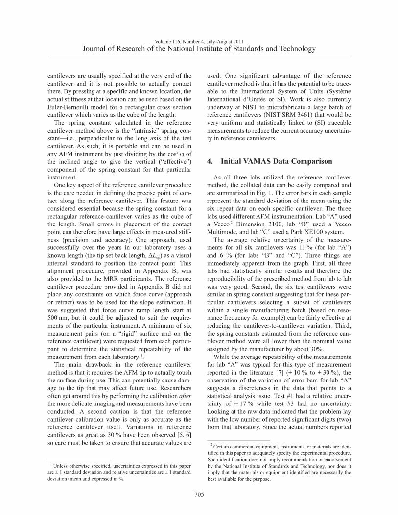
As all three labs utilized the reference cantilevermethod, the collated data can be easily compared andare summarized in Fig. 1. The error bars in each samplerepresent the standard deviation of the mean using thesix repeat data on each specific cantilever. The threelabs used different AFM instrumentation. Lab “A” useda Veeco 2 Dimension 3100, lab “B” used a VeecoMultimode, and lab “C” used a Park XE100 system.

The average relative uncertainty of the measure-ments for all six cantilevers was 11 % (for lab “A”)and 6 % (for labs “B” and “C”). Three things areimmediately apparent from the graph. First, all threelabs had statistically similar results and therefore thereproducibility of the prescribed method from lab to labwas very good. Second, the six test cantilevers weresimilar in spring constant suggesting that for these par-ticular cantilevers selecting a subset of cantileverswithin a single manufacturing batch (based on reso-nance frequency for example) can be fairly effective atreducing the cantilever-to-cantilever variation. Third,the spring constants estimated from the reference can-tilever method were all lower than the nominal valueassigned by the manufacturer by about 30%.

While the average repeatability of the measurementsfor lab “A” was typical for this type of measurementreported in the literature [7] (± 10 % to ± 30 %), theobservation of the variation of error bars for lab “A”suggests a discreteness in the data that points to astatistical analysis issue. Test #1 had a relative uncer-tainty of ± 17 % while test #3 had no uncertainty.Looking at the raw data indicated that the problem laywith the low number of reported significant digits (two)from that laboratory. Since the actual numbers reported


705

1 Unless otherwise specified, uncertainties expressed in this paperare ± 1 standard deviation and relative uncertainties are ± 1 standarddeviation / mean and expressed in %.

2 Certain commercial equipment, instruments, or materials are iden-tified in this paper to adequately specify the experimental procedure.Such identification does not imply recommendation or endorsementby the National Institute of Standards and Technology, nor does itimply that the materials or equipment identified are necessarily thebest available for the purpose.

for the slope of the force curve measurement inEq. (1) (e.g. 0.014 V/nm) had a small first digit, changeof just one digit in the second number is a change ofalmost 10 %. The effect is to blow up or nullify smallvariations in the data, depending on where the data layrelative to the last significant digit and explains thediscrete nature of the data. This highlights the need tospecify a minimum number of significant figures (inthis case three) for the raw data in the round robin.

The procedure for this MRR did not specify whetherto use the approach or retract portion of the forcecurves to calculate the slope of the compliance curves.In retrospect, that was a dangerous omission that couldhave affected the comparison of data from differentlaboratories. It was fortunate that the selected testcantilever had a short (nominally 3 μm) tip that hadretract curves that were very similar in slope toapproach curves so it didn’t matter, but that will notalways be the case. Pratt et al. [8] showed that in somecircumstances, approach and retract slopes can be verydifferent and the spring constants calculated from themwill vary. They attributed the effect to friction betweenthe tip and surface that gets amplified by the geometricleverage of tip height and causes hysteresis in the forcecurves. They recommended an average of both curveslopes be used to reduce the influence of the effect onthe estimated spring constant.

The absolute value of the spring constant of the testcantilever obtained in the reference cantilever methodis based on the value for the reference cantilever;therefore, the accuracy of the method depends on theaccuracy of the reference cantilever. In the case of thisstudy, that absolute value was based on the manufactur-er’s nominal spring constant value which was given as“0.711 N/m” for all five “long” reference cantilevers inthe set. For the purposes of comparing test resultsamong the three laboratories, the actual absolute valuedid not matter since all participants used the exact sameartifact (the long reference cantilever). Essentially, thecomparison provides the relative precisions of thecalibrations and how they might be biased by theinstruments themselves.

The reference cantilever used in the MRR wasselected from a batch of five cantilever sets purchasedfrom the manufacturer (CLCF-NOBO, Veeco Probes,Camarrillo, CA) and utilized the long reference can-tilever with a resonance frequency closest to the nomi-nal value specified in the hope that the nominal springconstant would represent a more accurate value. An esti-mate of the spring constant of the reference cantilever,performed using the Sader method [9] using the web-based Java applet [10] indicated a stiffness of0.70 N/m, which was close to the nominal value. Thissuggested that the manufacturer-assigned value for the


706

Fig. 1. Comparison of reference cantilever calibration results from three different laboratories.

MRR was reasonable for that particular cantilever.Another long reference cantilever from the samepurchased set had a Sader-estimated [10] stiffness of0.57 N/m so there may be significant variation fromchip-to-chip even in a single manufacturer’s batch.

More recently, one of the authors (RG) has beendeveloping the capability at NIST to run the thermalmethod [11] using laser Doppler velocimetry (LDV).Using this technique, the stiffness of the referencecantilever used in the MRR was measured as0.734 N/m ± 0.006 N/m which is only 3 % greater thanthe nominal value originally used for the MRR. Thereference cantilever method values provided in thispaper assume the original 0.711 N/m values.

5. Added Mass Method

A second calibration method, the added massmethod, was utilized at NIST (laboratory “B”) usingthe same commercial AFM instrument that was usedfor the reference method. The method was originallydeveloped by Cleveland [12] to calibrate the springconstant of a cantilever using only the resonancefrequency measurement of a series of experimentswhere small, known, masses are added to the end of thecantilever. The exact procedure is described in detail in

Appendix C. The technique requires some skill on thepart of the operator to be able to apply and removetungsten or gold microspheres on a cantilever withoutdamaging it but the precision of the resulting data isquite good. The largest uncertainty in the overallprocess lies with the estimation of the added masswhich depends mostly on the measurement of thediameter of the spherical mass added. We typically usea calibrated optical microscope with digital imagecapture capabilities to estimate both the sphere dia-meter and the actual location of the sphere on thecantilever (for the offset correction explained inAppendix C). It should be noted that the spring con-stant estimated with the added mass method is theintrinsic one and no angle correction is needed.

One significant advantage of using the added massmethod is that it does not require touching the testcantilever tip to a surface during calibration. Its majordrawback is the complexity of the process and the skillrequired to carefully place microspheres onto the testcantilever surface and remove them without damagingthe cantilever.

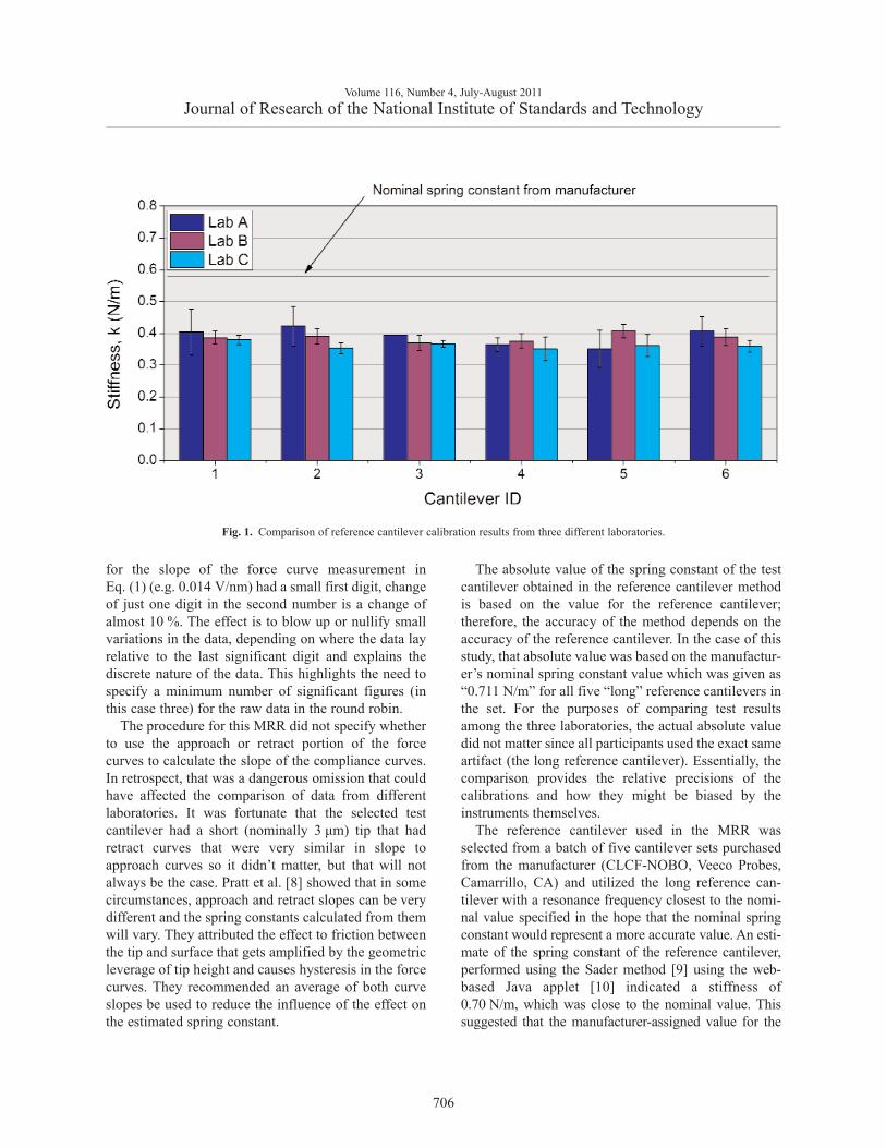
The results obtained on all six test cantilevers arecompared to the reference cantilever method results inFig. 2. The relative uncertainty of the added massmethod was estimated at ± 6 % and is typical for theauthors’ experience with this method.


707

Fig. 2. Comparison of added mass and reference cantilever methods for laboratory “B”.

The results of the two methods agree well statistical-ly and reinforce the previous observation that the sixtest cantilevers are very similar in spring constant andthat the measured calibration values are about 30 %less than the nominal values reported by the manufac-turer. Even though the two data sets are statisticallyequal, there is a consistent trend of the ReferenceCantilever data being slightly less in stiffness than theadded mass data for all six samples that points to a con-sistent bias. This can be partially explained by the useof the nominal 0.711 N/m reference cantilever calibra-tion value used for the MRR. If the value of 0.734 N/m(obtained by LDV Thermal) is used instead, the datacorrects upward by 3 % and the gap between the twodata sets decreases by 50 %. While the scope of theMRR was limited to looking at the precision of thecalibration methods and not the accuracy, the numericalagreement of the two methods was a positive sign thatthese two techniques may also be accurate.

6. Additional Calibration by Thermaland EFB Methods

Three additional techniques were subsequently usedto estimate the spring constants of two of the VAMAStest cantilevers. One method, the thermal method, asimplemented in an AFM, was performed using twodifferent commercial AFM systems. A Veeco Multi-mode AFM (Veeco Instruments, Santa Barbara, CA)which was also used for the added mass and referencecantilever methods in the MRR is described as AFM1.A second commercial instrument—an Asylum MFP-3D (Asylum Research, Santa Barbara, CA) standaloneis described in this paper as AFM2. The second springconstant calibration technique was an experimental ver-sion of the thermal method we have been developing atNIST that utilizes laser Doppler vibrometry—LDV(MSA500, Polytec USA, Hopkinton MA) to measurethe power spectrum for the flexural resonance mode ofthe cantilever. The third calibration technique used wasthe electrostatic force balance (EFB) [13]. This instru-ment, designed and developed at NIST, is capable ofmeasuring nanonewton forces applied to surfaces, andcan measure spring constants with both good precisionand accuracy, since it is SI traceable.

The thermal methods are all based on the originalwork of Hutter and Bechhoeffer [11] and later refinedby several researchers [14, 15]. Based on the equiparti-tion theorem, the thermal method is an energy balancein which the spring constant is obtained throughthe potential energy term. The technique relies on the

measurement of the frequency spectrum obtained whilethe cantilever is in thermal equilibrium with its envi-ronment. Typically, these thermal vibration amplitudesare quite small, and very sensitive, high speed, elec-tronics are required for accurate measurement of boththe frequency and vibrational amplitude.

The thermal methods that were implemented oncommercial AFM’s used the standard setting recom-mended by the instrument manufacturers which includ-ed a setting of 1.09 for the “chi” [16] correction factorfor the Asylum instrument. This correction factor takesinto account the effect of the optical lever detectionsystem used in most AFM instruments which actuallymeasure angle changes in the cantilever end and notabsolute deflection. The equation used to calculate thespring constant is:

(2)

where kB is the Boltzman constant, T is the absolutetemperature, and the <z1

2> term represents the meansquared displacement of the first bending mode of thecantilever. The first (0.971) term is a mode correctionfactor that accounts for the first mode displacementcontribution of the cantilevers [14] and is small (only3 %) compared to the almost 20 % for the chi factorcorrection. Note that the mode correction factor of0.971 used represents an ideal case for rectangularcantilevers as a simplification. Stark et al. [17] usedfinite element analysis to estimate the mode correctionfactor for a particular commercial triangular cantilever(different from the one used in this MRR study) andobtained a value that was slightly lower (0.963).

The chi factor setting used for the Veeco Multimodeinstrument was not stated but based on an applicationnote [18] from the manufacturer it appears to be thesame (1.09) value. AFM thermal calibration alsorequires a force curve be applied to an infinitely stiffsurface to determine the optical lever sensitivity oncethe laser spot is aligned on the cantilever. This determi-nation suffers from the same issues present in the refer-ence cantilever method and in some cases, friction cancause hysteresis in the approach-retract curves andaffect the calibration uncertainty. Once the optical leversensitivity is obtained, precision of this method is usu-ally quite good (repeatability of a percent or two). Itshould also be pointed out that because the optical leversensitivity calibrates the vertical deflection of the tiltedcantilever it estimates the vertical component of thespring constant (the “effective” spring constant). This


708

2 21

0.971,Bk T

kzχ

=

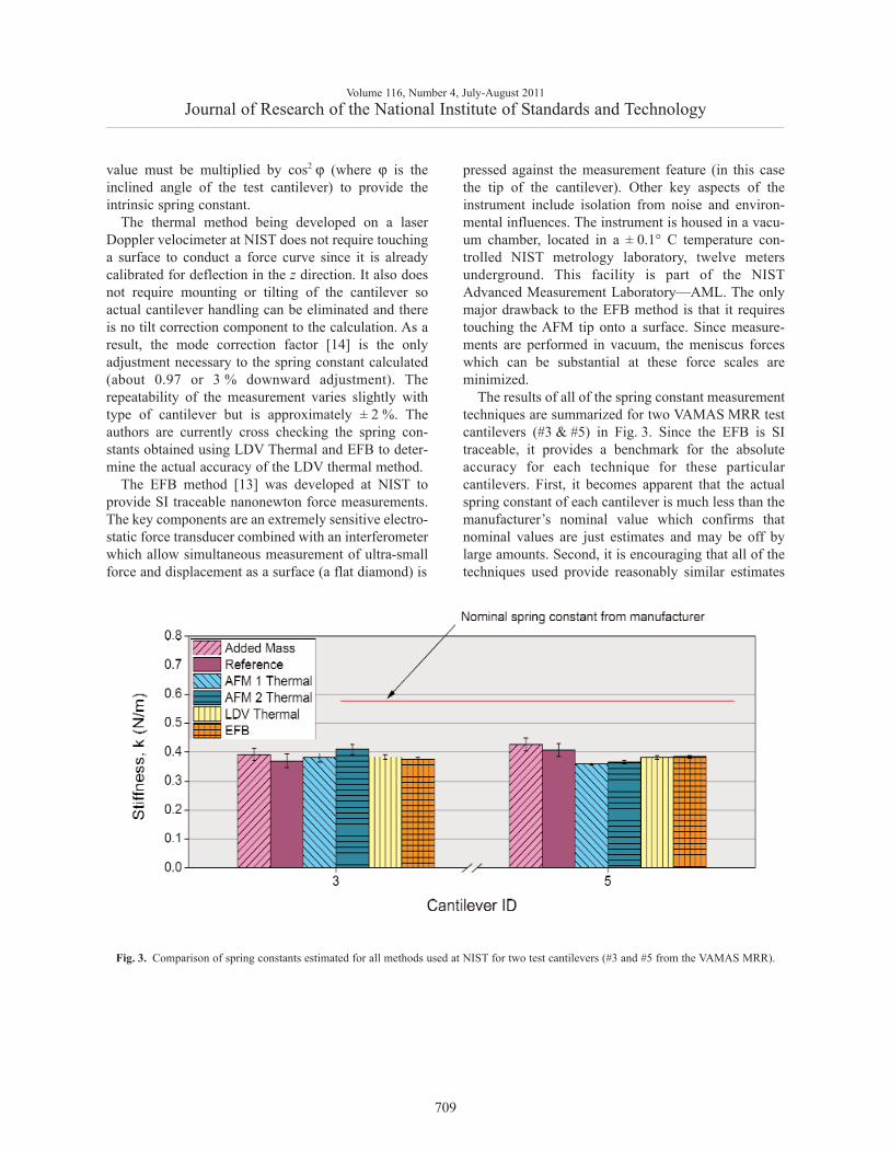
value must be multiplied by cos2 ϕ (where ϕ is theinclined angle of the test cantilever) to provide theintrinsic spring constant.

The thermal method being developed on a laserDoppler velocimeter at NIST does not require touchinga surface to conduct a force curve since it is alreadycalibrated for deflection in the z direction. It also doesnot require mounting or tilting of the cantilever soactual cantilever handling can be eliminated and thereis no tilt correction component to the calculation. As aresult, the mode correction factor [14] is the onlyadjustment necessary to the spring constant calculated(about 0.97 or 3 % downward adjustment). Therepeatability of the measurement varies slightly withtype of cantilever but is approximately ± 2 %. Theauthors are currently cross checking the spring con-stants obtained using LDV Thermal and EFB to deter-mine the actual accuracy of the LDV thermal method.

The EFB method [13] was developed at NIST toprovide SI traceable nanonewton force measurements.The key components are an extremely sensitive electro-static force transducer combined with an interferometerwhich allow simultaneous measurement of ultra-smallforce and displacement as a surface (a flat diamond) is

pressed against the measurement feature (in this casethe tip of the cantilever). Other key aspects of theinstrument include isolation from noise and environ-mental influences. The instrument is housed in a vacu-um chamber, located in a ± 0.1° C temperature con-trolled NIST metrology laboratory, twelve metersunderground. This facility is part of the NISTAdvanced Measurement Laboratory—AML. The onlymajor drawback to the EFB method is that it requirestouching the AFM tip onto a surface. Since measure-ments are performed in vacuum, the meniscus forceswhich can be substantial at these force scales areminimized.

The results of all of the spring constant measurementtechniques are summarized for two VAMAS MRR testcantilevers (#3 & #5) in Fig. 3. Since the EFB is SItraceable, it provides a benchmark for the absoluteaccuracy for each technique for these particularcantilevers. First, it becomes apparent that the actualspring constant of each cantilever is much less than themanufacturer’s nominal value which confirms thatnominal values are just estimates and may be off bylarge amounts. Second, it is encouraging that all of thetechniques used provide reasonably similar estimates


709

Fig. 3. Comparison of spring constants estimated for all methods used at NIST for two test cantilevers (#3 and #5 from the VAMAS MRR).

of the spring constants for each cantilever. If theuncertainties were relaxed to ± two standard deviations(95 % confidence limits) most of the results wouldbe statistically similar. Under tighter scrutiny itappears that the results of the EFB and the LDVthermal are identical and indicate that the LDV methodas applied to these cantilevers is both precise andaccurate.

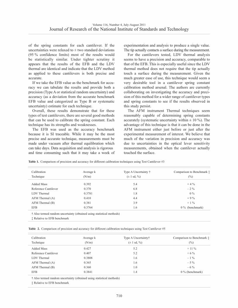
If we take the EFB value as the benchmark for accu-racy we can tabulate the results and provide both aprecision (Type A or statistical random uncertainty) andaccuracy (as a deviation from the accurate benchmarkEFB value and categorized as Type B or systematicuncertainty) estimate for each technique.

Overall, these results demonstrate that for thesetypes of test cantilevers, there are several good methodsthat can be used to calibrate the spring constant. Eachtechnique has its strengths and weaknesses.

The EFB was used as the accuracy benchmarkbecause it is SI traceable. While it may be the mostprecise and accurate technique, measurements must bemade under vacuum after thermal equilibration whichcan take days. Data acquisition and analysis is rigorous and time consuming such that it may take a week of

experimentation and analysis to produce a single value.The tip actually contacts a surface during the measurement.

For the cantilevers tested, LDV thermal analysisseems to have a precision and accuracy, comparable tothat of the EFB. This is especially useful since the LDVthermal method does not require that the tip actuallytouch a surface during the measurement. Given themuch greater ease of use, this technique would seem avery desirable tool in a cantilever spring constantcalibration method arsenal. The authors are currentlycollaborating on investigating the accuracy and preci-sion of this method for a wider range of cantilever typesand spring constants to see if the results observed inthis study persist.

The AFM instrument Thermal techniques seemreasonably capable of determining spring constantsaccurately (systematic uncertainty within ± 10 %). Theadvantage of this technique is that it can be done in theAFM instrument either just before or just after theexperimental measurement of interest. We believe thatmuch of the variation in precision and accuracy wasdue to uncertainties in the optical lever sensitivitymeasurements, obtained when the cantilever actuallytouched the surface.


710

Table 1. Comparison of precision and accuracy for different calibration techniques using Test Cantilever #3

Calibration Average k Type A Uncertainty † Comparison to Benchmark ‡Technique (N/m) (± 1 sd, %) (%)

Added Mass 0.392 5.4 + 4 %Reference Cantilever 0.370 6.8 – 2 %LDV Thermal 0.3781 1.8 0 %AFM Thermal (A) 0.410 4.4 + 9 %AFM Thermal (B) 0.381 3.9 + 1 %EFB 0.3764 1.6 0 % (benchmark)

† Also termed random uncertainty (obtained using statistical methods)‡ Relative to EFB benchmark

Added Mass 0.427 5.2 + 11 %Reference Cantilever 0.407 5.2 + 6 %LDV Thermal 0.3808 1.6 – 1 %AFM Thermal (A) 0.365 1.6 – 5 %AFM Thermal (B) 0.360 1.0 – 6 %EFB 0.3841 1.4 0 % (benchmark)

† Also termed random uncertainty (obtained using statistical methods)‡ Relative to EFB benchmark

Table 2. Comparison of precision and accuracy for different calibration techniques using Test Cantilever #5

Calibration Average k Type A Uncertainty† Comparison to Benchmark ‡Technique (N/m) (± 1 sd, %) (%)

The reference cantilever method was fairly precise(random uncertainty of 5 % to 7 %) and also within6 % of the accurate value using the manufacturersestimated spring constant of 0.711 N/m. If we insteaduse the value of 0.732 N/m measured by the LDVThermal method performed on the reference cantileverthe absolute spring constants will adjust upwards 3.2 %resulting in a measurement bias of + 1 % and + 9 % fortest cantilevers #3 and #5 respectively.

The Added Mass method was also reasonably accu-rate (only 4-11 % difference from the benchmark) andprecise (relative random uncertainty of 5 %). Thismethod also has the advantage that it does not requirethe tip to contact the surface during the measurement.This is offset somewhat by the more complex nature ofhandling microspheres and placing them on the testcantilever.

7. Handling and Use Damage

The initial lesson learned from the MRR was thatsharing delicate samples among participants posesdangers to the outcome of the study in several ways.First, these test chips must be physically handled inorder to make a measurement in an AFM. This involvespicking up the small chips with tweezers and carefullyorienting them in the appropriate AFM chip holder andsecuring them (usually with a small spring clip). Thereis always the danger that participants can accidentlydrop the test sample which would usually break thecantilever and then all future data from that samplewould be unavailable. There is also danger that themere act of squeezing the test sample chip with thetweezers can cause fracture damage to the chip andcreate debris which can settle on part of the cantileverand affect the measurement in a variety of ways, fromchanging the resonance frequency to changing thereflectivity of the laser on the back of the cantilever.Second, damage can be introduced on use eitherthrough wear or accidental contact during alignmentor calibration.

In the MRR, the reference cantilever was suppliedpre-mounted on a steel puck to eliminate the need todirectly handle that particular chip. Despite this precau-tion, inspection of the reference cantilever at NIST afterall of the testing revealed that two of the three originalreference cantilevers on the handle chip (ones not actu-ally used for calibration in the MRR) had been brokenoff during use. One feature of AFM’s is that there isusually a limited view of the intended point of inter-action and if there are other cantilevers on the same

chip (especially longer cantilevers), they can be in-advertently contacting surfaces out of view. It wasthought that additional cantilevers on the chip that werenot tested may have inadvertently contacted the unusedreference cantilevers, breaking them off.

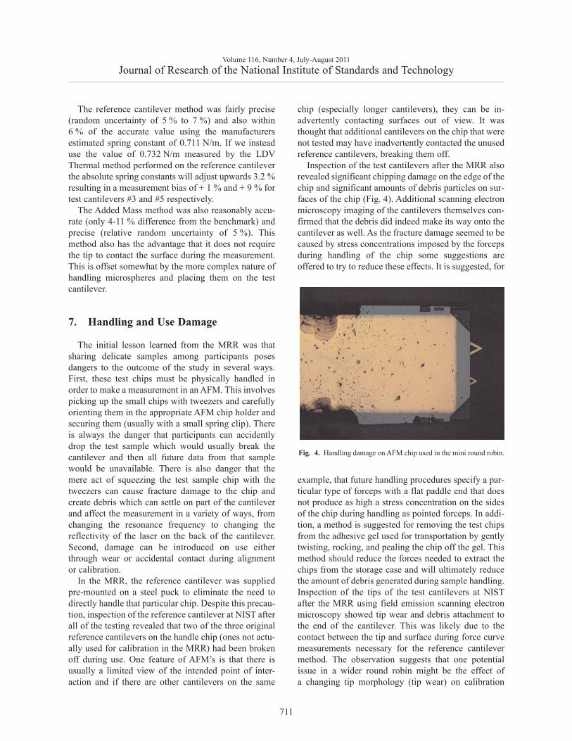
Inspection of the test cantilevers after the MRR alsorevealed significant chipping damage on the edge of thechip and significant amounts of debris particles on sur-faces of the chip (Fig. 4). Additional scanning electronmicroscopy imaging of the cantilevers themselves con-firmed that the debris did indeed make its way onto thecantilever as well. As the fracture damage seemed to becaused by stress concentrations imposed by the forcepsduring handling of the chip some suggestions areoffered to try to reduce these effects. It is suggested, for

example, that future handling procedures specify a par-ticular type of forceps with a flat paddle end that doesnot produce as high a stress concentration on the sidesof the chip during handling as pointed forceps. In addi-tion, a method is suggested for removing the test chipsfrom the adhesive gel used for transportation by gentlytwisting, rocking, and pealing the chip off the gel. Thismethod should reduce the forces needed to extract thechips from the storage case and will ultimately reducethe amount of debris generated during sample handling. Inspection of the tips of the test cantilevers at NISTafter the MRR using field emission scanning electronmicroscopy showed tip wear and debris attachment tothe end of the cantilever. This was likely due to thecontact between the tip and surface during force curvemeasurements necessary for the reference cantilevermethod. The observation suggests that one potentialissue in a wider round robin might be the effect ofa changing tip morphology (tip wear) on calibration


711

Fig. 4. Handling damage on AFM chip used in the mini round robin.

results. As more participants test the same cantilever,this cumulative damage effect may become moresignificant. It is also anticipated that sharper Si can-tilevers may be more sensitive to this effect, thereforeprocedural limitations (e.g., limiting the amount offorce or the stroke length actually applied during forcecurve testing) should be implemented to limit cumula-tive damage from a large round robin among manyparticipants.

8. Conclusions and Recommendationsfor a Future Round Robin

There are several results from this study that revealimportant information about the potential accuracyand precision of the spring constant measurementtechniques used as well as suggestions for improvinghandling and reporting that could streamline futureround robins in this field.

As far as improving the conducting of future roundrobins, there are several recommendations. They aresummarized here in bulleted form as:

• Include flat bladed tweezers in test “kit” to re-duce chip handling damage

• Break off unused cantilevers from test chips• Use chip rocking/twisting method of removal

from storage gel• Report to three or more significant figures• Electronic spreadsheet format with consistent

calculation documentation should be used toreduce the possibility of transcription and calcu-lation errors.

In addition, systematic characterization of thesample and reference cantilevers prior to and aftertesting may help document the effects of a largenumber of participants on the validity of roundrobin results on such methods where small scalechanges may have considerable influence. Opticalmicrographs at several scales and resonance frequencymeasurements of the cantilevers are suggested asmonitoring tools.

The number of test cantilevers (six) used in the MRRstudy was, in retrospect, excessive and increased theworkload while offering little additional insight. It issuggested that the number of primary samples bereduced to one or two in future studies with the addi-tional focus being put onto providing a wider range ofcantilever types (material, shape, size, range of springconstants) that cover the needs of the community.While this MRR was conducted without loss of eithertest or reference cantilevers (at least the ones thatcounted), it is anticipated that a wider round robin withmore participants would increase the likelihood ofaccidental damage to the samples and thought shouldtherefore be given to providing “backup” specimens(both test cantilever and reference artifacts) “just incase” such that participants later in the study are giventheir chance to contribute to their full potential.

All of the spring constant calibration methodsperformed well for this type of cantilever which was asilicon nitride triangular cantilever with a spring con-stant of approximately 0.4 N/m. Not only did all thetechniques have adequate precision (under ± 7 %), theyall agreed within 11 % of an SI traceable benchmarkvalue. The reference cantilever method has the poten-tial for SI traceability and we are currently micro-fabricating a production batch of reference cantileverarrays [5] that would have their accuracy benchmarkestablished through linkage to EFB measurements.

The thermal method seems very capable of providingprecise spring constants with reasonable ease of use. Inthe case of the cantilevers tested, the AFM methods areaccurate to within 10 %. An LDV thermal technique,currently under developmentat NIST, demonstrated aprecision and accuracy similar to the SI traceable EFBtechnique for the cantilever tested. We are currentlyexploring the validity of these measurements over awider range of cantilevers using LDV Thermal and EFBto see if it the observed accuracy continues to persist.

A larger round robin currently underway in VAMASTWA29 will look at expanding the results of this MRRby providing a wider range of cantilevers (differentsize, shape, material, tip, and spring constant) in orderto provide a fuller picture of the capabilities of thesedifferent calibration techniques among differentlaboratories around the world.

712


APPENDIX A.

AFM Cantilever Spring ConstantCalibration VAMAS Mini

Round Robin Test Kit

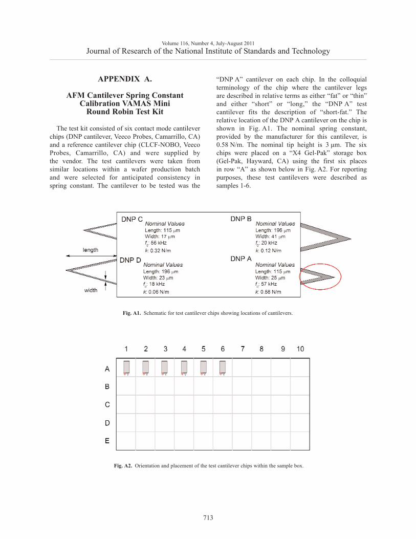
The test kit consisted of six contact mode cantileverchips (DNP cantilever, Veeco Probes, Camarrillo, CA)and a reference cantilever chip (CLCF-NOBO, VeecoProbes, Camarrillo, CA) and were supplied bythe vendor. The test cantilevers were taken fromsimilar locations within a wafer production batchand were selected for anticipated consistency inspring constant. The cantilever to be tested was the

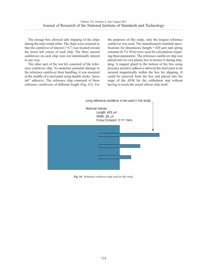
“DNP A” cantilever on each chip. In the colloquialterminology of the chip where the cantilever legsare described in relative terms as either “fat” or “thin”and either “short” or “long,” the “DNP A” testcantilever fits the description of “short-fat.” Therelative location of the DNP A cantilever on the chip isshown in Fig. A1. The nominal spring constant,provided by the manufacturer for this cantilever, is0.58 N/m. The nominal tip height is 3 μm. The sixchips were placed on a “X4 Gel-Pak” storage box(Gel-Pak, Hayward, CA) using the first six placesin row “A” as shown below in Fig. A2. For reportingpurposes, these test cantilevers were described assamples 1-6.


713

Fig. A1. Schematic for test cantilever chips showing locations of cantilevers.

Fig. A2. Orientation and placement of the test cantilever chips within the sample box.

The storage box allowed safe shipping of the chipsduring the mini round robin. The chips were oriented sothat the cantilever of interest (“A”) was located towardthe lower left corner of each chip. The three unusedcantilevers on each chip were not intentionally alteredin any way.

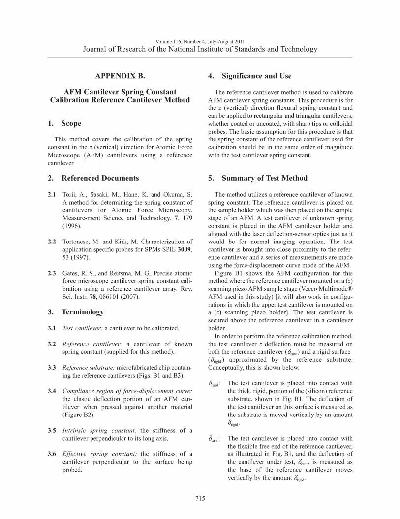
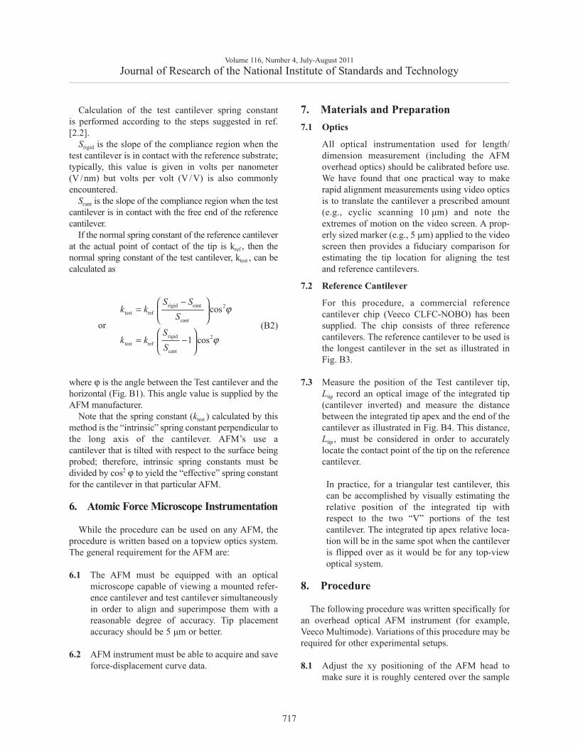
The other part of the test kit consisted of the refer-ence cantilever chip. To minimize potential damage tothe reference cantilever from handling, it was mountedin the middle of a steel puck using double sticky “presstab” adhesive. The reference chip consisted of threereference cantilevers of different length (Fig. A3). For

the purposes of this study, only the longest referencecantilever was used. The manufacturers nominal speci-fications for dimensions (length = 429 μm) and springconstant (0.711 N/m) were used for calculations requir-ing these parameters. The reference cantilever chip wasplaced into its own plastic box to protect it during ship-ping. A magnet glued to the bottom of the box usingpressure sensitive adhesive allowed the steel puck to besecured magnetically within the box for shipping. Itcould be removed from the box and placed into thestage of the AFM for the calibration step withouthaving to touch the actual silicon chip itself.


714

Fig. A3. Reference cantilever chip used for this study.

APPENDIX B.

AFM Cantilever Spring ConstantCalibration Reference Cantilever Method

1. Scope

This method covers the calibration of the springconstant in the z (vertical) direction for Atomic ForceMicroscope (AFM) cantilevers using a referencecantilever.

2. Referenced Documents

2.1 Torii, A., Sasaki, M., Hane, K. and Okuma, S.A method for determining the spring constant ofcantilevers for Atomic Force Microscopy.Measure-ment Science and Technology. 7, 179(1996).

2.2 Tortonese, M. and Kirk, M. Characterization ofapplication specific probes for SPMs SPIE 3009,53 (1997).

2.3 Gates, R. S., and Reitsma, M. G., Precise atomicforce microscope cantilever spring constant cali-bration using a reference cantilever array. Rev.Sci. Instr. 78, 086101 (2007).

3. Terminology

3.1 Test cantilever: a cantilever to be calibrated.

3.2 Reference cantilever: a cantilever of knownspring constant (supplied for this method).

3.3 Reference substrate: microfabricated chip contain-ing the reference cantilevers (Figs. B1 and B3).

3.4 Compliance region of force-displacement curve:the elastic deflection portion of an AFM can-tilever when pressed against another material(Figure B2).

3.5 Intrinsic spring constant: the stiffness of acantilever perpendicular to its long axis.

3.6 Effective spring constant: the stiffness of acantilever perpendicular to the surface beingprobed.

4. Significance and Use

The reference cantilever method is used to calibrateAFM cantilever spring constants. This procedure is forthe z (vertical) direction flexural spring constant andcan be applied to rectangular and triangular cantilevers,whether coated or uncoated, with sharp tips or colloidalprobes. The basic assumption for this procedure is thatthe spring constant of the reference cantilever used forcalibration should be in the same order of magnitudewith the test cantilever spring constant.

5. Summary of Test Method

The method utilizes a reference cantilever of knownspring constant. The reference cantilever is placed onthe sample holder which was then placed on the samplestage of an AFM. A test cantilever of unknown springconstant is placed in the AFM cantilever holder andaligned with the laser deflection-sensor optics just as itwould be for normal imaging operation. The testcantilever is brought into close proximity to the refer-ence cantilever and a series of measurements are madeusing the force-displacement curve mode of the AFM.

Figure B1 shows the AFM configuration for thismethod where the reference cantilever mounted on a (z)scanning piezo AFM sample stage (Veeco Multimode®AFM used in this study) [it will also work in configu-rations in which the upper test cantilever is mounted ona (z) scanning piezo holder]. The test cantilever issecured above the reference cantilever in a cantileverholder.

In order to perform the reference calibration method,the test cantilever z deflection must be measured onboth the reference cantilever (δcant ) and a rigid surface(δrigid ) approximated by the reference substrate.Conceptually, this is shown below.

δrigid : The test cantilever is placed into contact withthe thick, rigid, portion of the (silicon) referencesubstrate, shown in Fig. B1. The deflection ofthe test cantilever on this surface is measured asthe substrate is moved vertically by an amountδrigid .

δcant : The test cantilever is placed into contact withthe flexible free end of the reference cantilever,as illustrated in Fig. B1, and the deflection ofthe cantilever under test, δcant , is measured asthe base of the reference cantilever movesvertically by the amount δrigid .


715

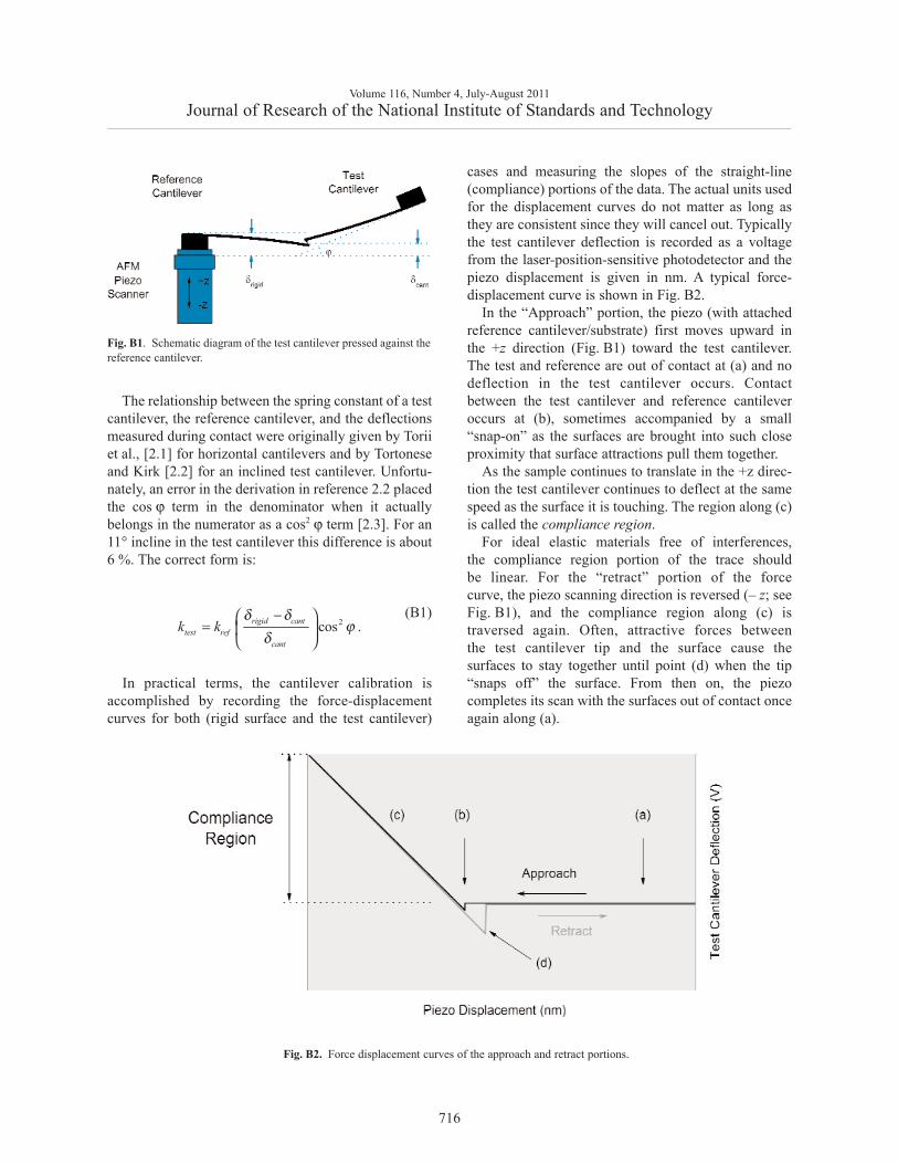
The relationship between the spring constant of a testcantilever, the reference cantilever, and the deflectionsmeasured during contact were originally given by Toriiet al., [2.1] for horizontal cantilevers and by Tortoneseand Kirk [2.2] for an inclined test cantilever. Unfortu-nately, an error in the derivation in reference 2.2 placedthe cos ϕ term in the denominator when it actuallybelongs in the numerator as a cos2 ϕ term [2.3]. For an11° incline in the test cantilever this difference is about6 %. The correct form is:

(B1)

In practical terms, the cantilever calibration isaccomplished by recording the force-displacementcurves for both (rigid surface and the test cantilever)

cases and measuring the slopes of the straight-line(compliance) portions of the data. The actual units usedfor the displacement curves do not matter as long asthey are consistent since they will cancel out. Typicallythe test cantilever deflection is recorded as a voltagefrom the laser-position-sensitive photodetector and thepiezo displacement is given in nm. A typical force-displacement curve is shown in Fig. B2.

In the “Approach” portion, the piezo (with attachedreference cantilever/substrate) first moves upward inthe +z direction (Fig. B1) toward the test cantilever.The test and reference are out of contact at (a) and nodeflection in the test cantilever occurs. Contactbetween the test cantilever and reference cantileveroccurs at (b), sometimes accompanied by a small“snap-on” as the surfaces are brought into such closeproximity that surface attractions pull them together.

As the sample continues to translate in the +z direc-tion the test cantilever continues to deflect at the samespeed as the surface it is touching. The region along (c)is called the compliance region.

For ideal elastic materials free of interferences,the compliance region portion of the trace shouldbe linear. For the “retract” portion of the forcecurve, the piezo scanning direction is reversed (– z; seeFig. B1), and the compliance region along (c) istraversed again. Often, attractive forces betweenthe test cantilever tip and the surface cause thesurfaces to stay together until point (d) when the tip“snaps off” the surface. From then on, the piezocompletes its scan with the surfaces out of contact onceagain along (a).


716

2cos .rigid canttest ref

cant

k kδ δ

ϕδ

−⎛ ⎞= ⎜ ⎟

⎝ ⎠

Fig. B2. Force displacement curves of the approach and retract portions.

Fig. B1. Schematic diagram of the test cantilever pressed against thereference cantilever.

Calculation of the test cantilever spring constantis performed according to the steps suggested in ref.[2.2].

Srigid is the slope of the compliance region when thetest cantilever is in contact with the reference substrate;typically, this value is given in volts per nanometer(V /nm) but volts per volt (V /V) is also commonlyencountered.

Scant is the slope of the compliance region when the testcantilever is in contact with the free end of the referencecantilever.

If the normal spring constant of the reference cantileverat the actual point of contact of the tip is kref , then thenormal spring constant of the test cantilever, ktest , can becalculated as

(B2)

where ϕ is the angle between the Test cantilever and thehorizontal (Fig. B1). This angle value is supplied by theAFM manufacturer.

Note that the spring constant (ktest ) calculated by thismethod is the “intrinsic” spring constant perpendicular tothe long axis of the cantilever. AFM’s use acantilever that is tilted with respect to the surface beingprobed; therefore, intrinsic spring constants must bedivided by cos2 ϕ to yield the “effective” spring constantfor the cantilever in that particular AFM.

6. Atomic Force Microscope Instrumentation

While the procedure can be used on any AFM, theprocedure is written based on a topview optics system.The general requirement for the AFM are:

6.1 The AFM must be equipped with an opticalmicroscope capable of viewing a mounted refer-ence cantilever and test cantilever simultaneouslyin order to align and superimpose them with areasonable degree of accuracy. Tip placementaccuracy should be 5 μm or better.

6.2 AFM instrument must be able to acquire and saveforce-displacement curve data.

7. Materials and Preparation7.1 Optics

All optical instrumentation used for length/dimension measurement (including the AFMoverhead optics) should be calibrated before use.We have found that one practical way to makerapid alignment measurements using video opticsis to translate the cantilever a prescribed amount(e.g., cyclic scanning 10 μm) and note theextremes of motion on the video screen. A prop-erly sized marker (e.g., 5 μm) applied to the videoscreen then provides a fiduciary comparison forestimating the tip location for aligning the testand reference cantilevers.

7.2 Reference Cantilever

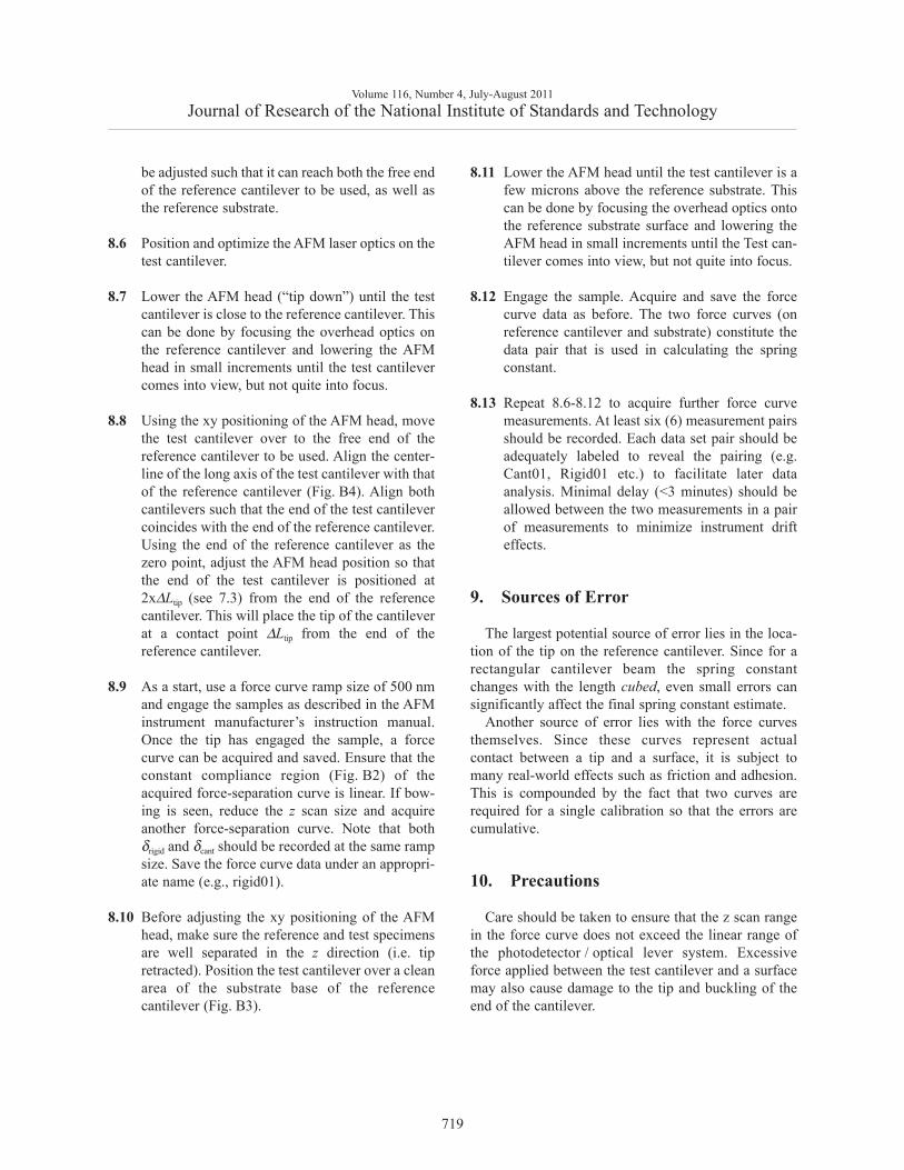
For this procedure, a commercial referencecantilever chip (Veeco CLFC-NOBO) has beensupplied. The chip consists of three referencecantilevers. The reference cantilever to be used isthe longest cantilever in the set as illustrated inFig. B3.

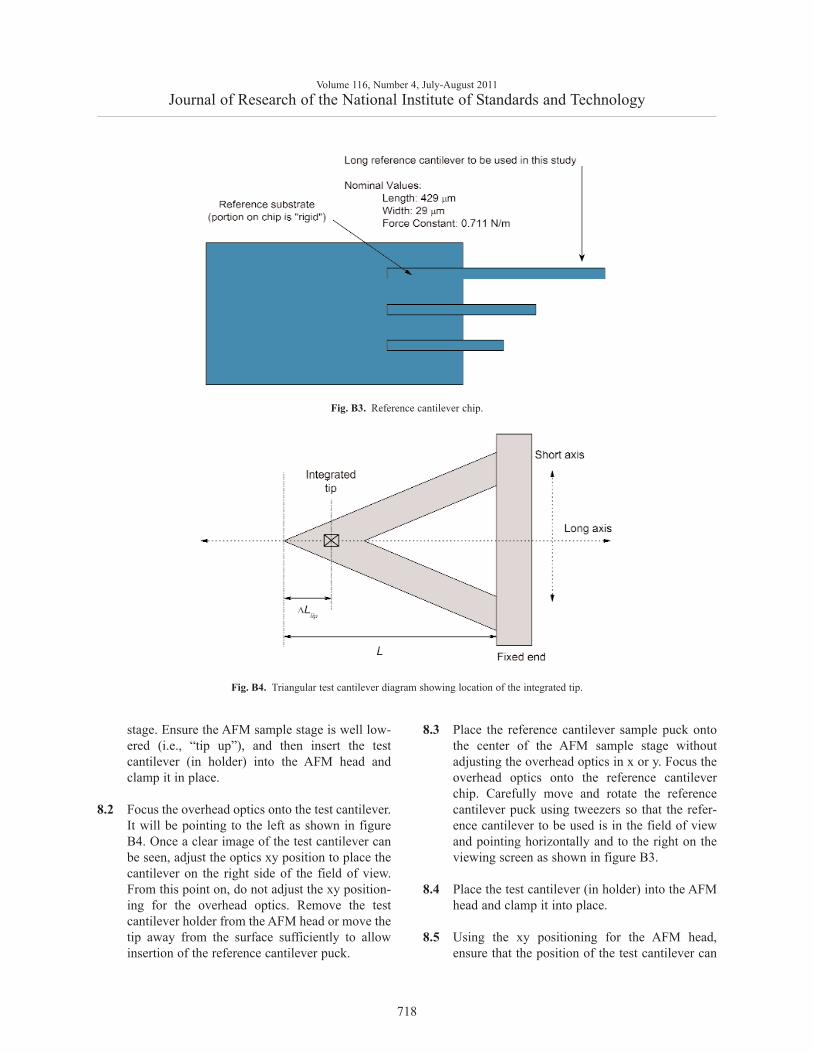
7.3 Measure the position of the Test cantilever tip,Ltip record an optical image of the integrated tip(cantilever inverted) and measure the distancebetween the integrated tip apex and the end of thecantilever as illustrated in Fig. B4. This distance,Ltip , must be considered in order to accuratelylocate the contact point of the tip on the referencecantilever.

In practice, for a triangular test cantilever, thiscan be accomplished by visually estimating therelative position of the integrated tip withrespect to the two “V” portions of the testcantilever. The integrated tip apex relative loca-tion will be in the same spot when the cantileveris flipped over as it would be for any top-viewoptical system.

8. Procedure

The following procedure was written specifically foran overhead optical AFM instrument (for example,Veeco Multimode). Variations of this procedure may berequired for other experimental setups.

8.1 Adjust the xy positioning of the AFM head tomake sure it is roughly centered over the sample


717

rigid cant 2test ref

cant

rigid 2test ref

cant

cos

1 cos

S Sk k

S

Sk k

S

ϕ

ϕ

−⎛ ⎞= ⎜ ⎟

⎝ ⎠⎛ ⎞

= −⎜ ⎟⎝ ⎠

or

stage. Ensure the AFM sample stage is well low-ered (i.e., “tip up”), and then insert the testcantilever (in holder) into the AFM head andclamp it in place.

8.2 Focus the overhead optics onto the test cantilever.It will be pointing to the left as shown in figureB4. Once a clear image of the test cantilever canbe seen, adjust the optics xy position to place thecantilever on the right side of the field of view.From this point on, do not adjust the xy position-ing for the overhead optics. Remove the testcantilever holder from the AFM head or move thetip away from the surface sufficiently to allowinsertion of the reference cantilever puck.

8.3 Place the reference cantilever sample puck ontothe center of the AFM sample stage withoutadjusting the overhead optics in x or y. Focus theoverhead optics onto the reference cantileverchip. Carefully move and rotate the referencecantilever puck using tweezers so that the refer-ence cantilever to be used is in the field of viewand pointing horizontally and to the right on theviewing screen as shown in figure B3.

8.4 Place the test cantilever (in holder) into the AFMhead and clamp it into place.

8.5 Using the xy positioning for the AFM head,ensure that the position of the test cantilever can


718

Fig. B3. Reference cantilever chip.

Fig. B4. Triangular test cantilever diagram showing location of the integrated tip.

be adjusted such that it can reach both the free endof the reference cantilever to be used, as well asthe reference substrate.

8.6 Position and optimize the AFM laser optics on thetest cantilever.

8.7 Lower the AFM head (“tip down”) until the testcantilever is close to the reference cantilever. Thiscan be done by focusing the overhead optics onthe reference cantilever and lowering the AFMhead in small increments until the test cantilevercomes into view, but not quite into focus.

8.8 Using the xy positioning of the AFM head, movethe test cantilever over to the free end of thereference cantilever to be used. Align the center-line of the long axis of the test cantilever with thatof the reference cantilever (Fig. B4). Align bothcantilevers such that the end of the test cantilevercoincides with the end of the reference cantilever.Using the end of the reference cantilever as thezero point, adjust the AFM head position so thatthe end of the test cantilever is positioned at2xΔLtip (see 7.3) from the end of the referencecantilever. This will place the tip of the cantileverat a contact point ΔLtip from the end of thereference cantilever.

8.9 As a start, use a force curve ramp size of 500 nmand engage the samples as described in the AFMinstrument manufacturer’s instruction manual.Once the tip has engaged the sample, a forcecurve can be acquired and saved. Ensure that theconstant compliance region (Fig. B2) of theacquired force-separation curve is linear. If bow-ing is seen, reduce the z scan size and acquireanother force-separation curve. Note that bothδrigid and δcant should be recorded at the same rampsize. Save the force curve data under an appropri-ate name (e.g., rigid01).

8.10 Before adjusting the xy positioning of the AFMhead, make sure the reference and test specimensare well separated in the z direction (i.e. tipretracted). Position the test cantilever over a cleanarea of the substrate base of the referencecantilever (Fig. B3).

8.11 Lower the AFM head until the test cantilever is afew microns above the reference substrate. Thiscan be done by focusing the overhead optics ontothe reference substrate surface and lowering theAFM head in small increments until the Test can-tilever comes into view, but not quite into focus.

8.12 Engage the sample. Acquire and save the forcecurve data as before. The two force curves (onreference cantilever and substrate) constitute thedata pair that is used in calculating the springconstant.

8.13 Repeat 8.6-8.12 to acquire further force curvemeasurements. At least six (6) measurement pairsshould be recorded. Each data set pair should beadequately labeled to reveal the pairing (e.g.Cant01, Rigid01 etc.) to facilitate later dataanalysis. Minimal delay (<3 minutes) should beallowed between the two measurements in a pairof measurements to minimize instrument drifteffects.

9. Sources of Error

The largest potential source of error lies in the loca-tion of the tip on the reference cantilever. Since for arectangular cantilever beam the spring constantchanges with the length cubed, even small errors cansignificantly affect the final spring constant estimate.

Another source of error lies with the force curvesthemselves. Since these curves represent actualcontact between a tip and a surface, it is subject tomany real-world effects such as friction and adhesion.This is compounded by the fact that two curves arerequired for a single calibration so that the errors arecumulative.

10. Precautions

Care should be taken to ensure that the z scan rangein the force curve does not exceed the linear range ofthe photodetector / optical lever system. Excessiveforce applied between the test cantilever and a surfacemay also cause damage to the tip and buckling of theend of the cantilever.


719

11. Results Reporting and Adjustment

For each force-separation curve, isolate thecompliance region portion of the data (shown inFig. B2) and determine the slope of this region. It isrecommended that a graphical assessment ofthe analyzed portion of the data also be made toensure no artifacts are included in the data analysis.

11.2 Sample Calculation

The nominal value given for the spring constant ofthe reference cantilever is the estimated stiffness at theend of the beam. In this method, however, the load isapplied to the reference cantilever at a distance of ΔLtip

from the end (see 7.3) which will result in a slightlygreater stiffness. To correct the calculated data forthe distance between the point of contact betweenthe two cantilevers (ΔLtip) and the end of the referencecantilever we need to apply an off-end loadingcorrection. Since k (spring constant) varies as the cubeof the length (L), the off-end correction is applied as:

(B3)

Indicate how the compliance slope is determined(e.g., linear regression fit to ASCII data; using a soft-ware package) and how much of the compliance curvedata is used.

11.1 Results Reporting Table

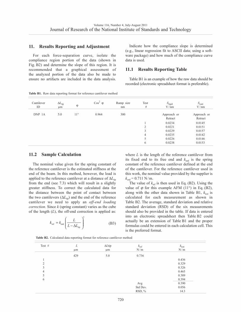
Table B1 is an example of how the raw data should berecorded (electronic spreadsheet format is preferable).

where L is the length of the reference cantilever fromits fixed end to its free end and kend is the springconstant of the reference cantilever defined at the endof the cantilever. For the reference cantilever used inthis work, the nominal value provided by the supplier iskend = 0.711 N/m.

The value of kref is then used in Eq. (B2). Using thevalue of ϕ for this example AFM (11°) in Eq. (B2),along with the other data shown in Table B1, ktest iscalculated for each measurement as shown inTable B2. The average, standard deviation and relativestandard deviation (RSD) of the six measurementsshould also be provided in the table. If data is enteredinto an electronic spreadsheet then Table B2 couldactually be an extension of Table B1 and the properformulas could be entered in each calculation cell. Thisis the preferred format.


720

Table B1. Raw data reporting format for reference cantilever method

Cantilever ΔLtip ϕCos2 ϕ Ramp size Test Srigid Scant

ID μm nm # V / nm V / nm

1 0.0234 0.01452 0.0221 0.01513 0.0229 0.01574 0.0235 0.01425 0.0226 0.01466 0.0238 0.0153

DNP 1A 5.0 11° 0.964 300 Approach or Approach orRetract Retract

3

ref endtip

Lk kL L

⎛ ⎞= ⎜ ⎟⎜ ⎟− Δ⎝ ⎠

Table B2. Calculated data reporting format for reference cantilever method

Test # L ΔLtip kref ktestμm μm N / m N / m

429 5.0 0.7361 0.4362 0.3293 0.3264 0.4655 0.3896 0.394

Avg 0.390Std Dev. 0.056RSD, % 14.3

APPENDIX C.

AFM Cantilever Spring ConstantCalibration Added Mass Procedure

1. Scope

This procedure covers the calibration of AtomicForce Microscope (AFM) cantilever spring con-stants in the z direction (vertical) using the addedmass (“Cleveland”) method, modified for off-endcorrections.

2. Referenced Documents

2.1 Cleveland, J. P., Manne, S., Bocek, D., Hansma,P. K. A nondestructive method for determiningthe spring constant of cantilevers for scanningforce microscopy. Review of ScientificInstruments. 64 (2), 403 (1993).

2.2 Sader, J. E., Mulvaney, P., and White, L. R.Method for the Calibration of Atomic ForceMicroscope Cantilevers. Review of ScientificInstruments 66 (7), 3789 (1995).

2.3 Sader, J. E. Parallel beam approximation forV-shaped atomic force microscope cantilevers.Review of Scientific Instruments 66 (9), 4583(1995).

3. Terminology

3.1 AFM: Atomic Force Microscope

3.2 Resonance frequency f: is the first bending moderesonance frequency, perpendicular to the longaxis of the cantilever.

3.3 Cantilever resonance frequency: f0 is the reso-nance frequency of the cantilever without addedmass.

3.4 Test cantilever: cantilever to be calibrated.

3.5 Cantilever holder: AFM cantilever holder, whichis used to mount the test cantilever in AFM.

3.6 Loaded resonance frequency: fi is the resonancefrequency of the cantilever measured with anadded mass (mi ).

3.7 Cantilever tip: the actual tip apex (point of con-tact) that is made with the surface when an AFMcantilever is used. The length of the cantileverfrom the fixed base to the tip is designated as Lt .

3.8 Cantilever end: the free end of the cantilever.The length of the cantilever from the fixed base tothe free end is designated as Le .

3.9 Intrinsic spring constant: the stiffness of acantilever perpendicular to its long axis.

3.10 Effective spring constant: the stiffness of acantilever perpendicular to the surface beingprobed.

4. Significance and Use

The added mass method is used to calibrate theintrinsic spring constant of AFM cantilevers. It can beapplied to rectangular, triangular, coated or uncoatedcantilevers with sharp tips or colloidal probes. The keyrequirements are that the locations and the masses ofthe spheres added for frequency measurements can bemeasured accurately.

5. Summary of Test Method

5.1 The first flexural mode resonance frequency, f0 ,of the test cantilever is measured.

5.2 A tungsten or gold sphere is placed at the free endof the cantilever.

5.3 The size and position of the sphere on thecantilever is measured (e.g., using a suitable cali-brated microscope).

5.4 The resonance frequency of the cantilever withattached sphere is measured. The sphere is thenremoved.

5.5 Steps 5.2—5.4 are repeated for at least 2 spheres(3 point plot). A larger number of data points


721

(e.g., 5 spheres (6 point plot)) are desirable toreduce the statistical uncertainty. The range ofsphere size depends on the spring constant but ingeneral 5 μm to 15 μm size spheres are used.

5.6 The mass of each spherical mass added (mi ) iscalculated from the measured diameter andknown density of the material.

5.7 The general relationship between added mass,mi , and resonant frequency, fi , is

(C1)

where k is the spring constant of the cantilever. Thequantity m* is called the “effective mass” of thecantilever. If several known masses are added to theend of a cantilever and resonance frequencies are meas-ured for each added mass, a linear plot of added massmi versus (2πfi )–2 will give a straight line with slope ofk and an ordinate intercept of – m*.

6. Atomic Force MicroscopeInstrumentation

This method requires an AFM instrument with hard-ware and software suitable for cantilever resonancefrequency measurement.

7. Materials and Preparation

This method uses a sharp tungsten wire to pickup, maneuver and attach spherical particles to thecantilever. It relies on attractive meniscus forces to pickup the spheres; therefore it may be sensitive to changesin relative humidity. The relative humidity of thelaboratory used for this work was 45 % ± 5 %.

7.1 Spheres

Powder consisting of spherical gold or tungstenspheres. For this purpose, 325 mesh sphericalgold powder can be used (Alpha Aesar #43900,99.9 % purity on a metals basis). Tungsten spher-ical particles donated by Asylum Research (SantaBarbara, CA) are also available to participants.

7.2 Tungsten wire ( for suggested sphere mounting apparatus in 7.5)

For this work, 0.25 mm diameter (Alpha Aesar#10408, 99.95 % purity) tungsten wire was usedto create a sharp micromanipulator probe tip tomanipulate the spherical particles. Other wirematerials that can be sharpened to a fine pointmay also be suitable.

7.3 Electrochemical etching of a tungsten wire

There are a number of different techniques avail-able for tungsten wire etching. It is left to the userto decide the best method by which to electro-chemically etch the end of a tungsten wire downto a fine point (ca. 100 nm radius of curvature).Note that too fine a point is not desirable sinceone wants a large enough area of contact for thesphere to adhere to the tip when the meniscusforms between the contacting surfaces.

7.4 Optical Microscope

All optical instrumentation used for length /dimension measurement must be calibratedbefore use.

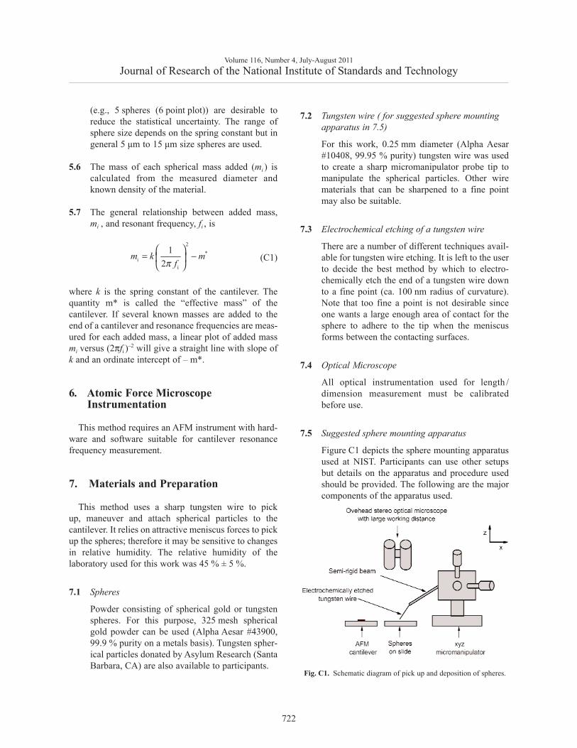
7.5 Suggested sphere mounting apparatus

Figure C1 depicts the sphere mounting apparatusused at NIST. Participants can use other setupsbut details on the apparatus and procedure usedshould be provided. The following are the majorcomponents of the apparatus used.


722

2*

ii

12

m k mfπ

⎛ ⎞= −⎜ ⎟

⎝ ⎠

Fig. C1. Schematic diagram of pick up and deposition of spheres.

7.5.1 Optical microscope: A stereo microscope witha long working distance was used to allowsimultaneous observation and micromanipula-tion. A field of view of 500 μm or less is neces-sary to allow location, pickup, and placementof small spheres onto the cantilevers withsufficient control.

7.5.2 Sphere slide: Tungsten or gold spheres areplaced onto a clean glass microscope slide insuch a way as to provide a large number ofisolated spheres that can be picked up with thetungsten probe.

7.5.3 Probe translation stage: An xyz translationstage capable of at least 10 mm travel in eachdirection is used to manipulate the tungstenprobe above the surfaces. Micrometers on eachaxis provide translation adjustment of each axis.

7.5.4 Etched tungsten wire: An electrochemicallyetched tungsten wire attached to a semi-rigidrod was used to maneuver the spheres (Fig. C1).An example of such a rod would be a tool steelrod approximately 3 mm in diameter and150 mm long.

7.5.5 Pickup and deposition of the spheres is bestaccomplished with a combination of orthogonal(xyz) mechanical translation axes and haptic(tactile feedback) controls as shown in Fig. C1.The translation stage is used for coarse adjust-ment of the probe to a location just above thesurface. By exerting gentle pressure on thesemi-rigid beam with one’s fingers the operatorcan cause the tungsten probe tip to smoothlyapproach the surface in the proximity of asphere (ca.10 μm to 20 μm travel). Release ofpressure then causes the tip to retract smoothlyfrom the surface.

8. Procedure

Using “non-critical” cantilevers for practice, it isrecommended that the individual user decide the micro-manipulation method most suitable to them for mount-ing and removing spheres. It is also recommended thateach user be well rehearsed in their chosen techniquebefore proceeding to calibrate the VAMAS cantilevers.The following steps are based on the suggested spheremounting apparatus described in 7.5 above.

8.1 Ensure the AFM head is raised with sufficientclearance above the sample and place thecantilever holder (containing the test cantilever)into the AFM head. Lock it into place. Focus andoptimize the AFM laser optics onto the testcantilever and perform the resonance frequencyanalysis on the cantilever. Sometimes this isreferred to as “tuning” the cantilever. Once theresonance frequency for the test cantilever hasbeen recorded, remove the holder from the AFMinstrument and transport it to the sphere mountingapparatus under the stereomicroscope (Fig. C1).

8.2 Ensure the surface of the sphere slide is slightlyhigher (z axis) than the cantilever in the cantileverholder (Fig. C1). Focus the overhead optics ontothe sphere slide and select a uniform, symmetricsphere.

8.3 Lower the tungsten tip to within several micro-meters of the target sphere and use gentle, finemotion to establish contact between the tip andsphere. If performing fine motion by hand, asmall force is applied to the semi-rigid beam totraverse the final distance and establish contactwith the sphere. By controlling the (finger) pres-sure to the beam, spheres can be contacted andpicked up in a single, smooth, down-up motion.Furthermore, since spheres can move aroundslightly on the slide before they stick to thetungsten tip, it is found that finger control offersmore freedom of movement and can thus be amore effective technique for pick up than usingthe micromanipulator adjustment micrometersalone.

8.4 After the target sphere has been picked up, makesure the tungsten tip is raised enough beforeremoving the sphere slide and replacing it withthe cantilever holder. Focus the overhead opticssuch that both the tip and the cantilever below itcan be seen.

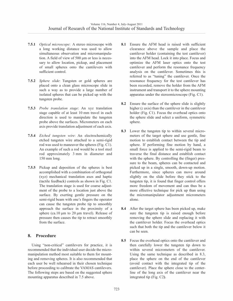
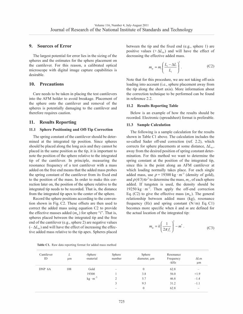
8.5 Focus the overhead optics onto the cantilever andthen carefully lower the tungsten tip down towithin several micrometers of the cantilever.Using the same technique as described in 8.3,place the sphere on the end of the cantilever(avoid contact with the integrated tip of thecantilever). Place the sphere close to the center-line of the long axis of the cantilever near theintegrated tip (Fig. C2).


723

8.6 Once the sphere has been placed onto thecantilever, raise the tungsten tip clear. Record animage of the sphere on the cantilever. Ensure thattwo measurements can be made from theimage(s): (1) The diameter of the sphere, and(2) the position of the (center of) sphere relativeto the integrated tip.

8.7 Place the holder (containing the test cantilever)into the AFM head and lock it into place. Focusand optimize the AFM laser optics (on the testcantilever) and perform a resonance frequencyanalysis on the cantilever as described in 8.1.Once the resonance frequency for the testcantilever has been recorded, remove the holderfrom the AFM instrument and transport it to thesphere mounting apparatus. At this point it iswise to record an additional image of the spherelocation on the cantilever to make sure it hasnot moved during the resonance frequencymeasurement.

8.8 In the same fashion as described in 8.3, removethe sphere from the cantilever.

CAUTION: This is often the most difficult andpotentially damaging part of the procedure. Ifcontacting the sphere with the tungsten tip provesunsuccessful, there are several alternatives thatcan be tried. Switching to a less sharp tungstentip (stronger meniscus forces) that can moreeasily pick up the sphere usually helps butthe sharper tip must be switched back for the

next sphere placement. Spheres can often beremoved by very carefully “flicking” (oscillating)the end of the cantilever with the tungsten tip.IMPORTANT: extra care is required to avoidcatching the edge of the cantilever with thetungsten probe if this later technique is needed.Alternatively, spheres can often be detached bydriving the resonance externally with a moderate-ly high amplitude (for example in an AFM).The sphere has been detached when theresonance peak jumps back to the initial (higher)resonance frequency determined in step 8.2above.

Care must be taken to ensure that the spherehas actually been removed and has not merelymoved to the underside of the cantilever. Aresonance frequency measurement can confirmthis (the frequency should return to the originalresonance frequency (f0 )).

8.9 Repeat steps 8.2 – 8.8. It is recommended that aminimum of two sphere measurements arerecorded, with a difference of >20 % in diameterfor each new sphere added. This will be combinedwith the unloaded (no added mass) resonancefrequency measurement to yield a three pointplot. A five sphere (six total data point) plot ismore desirable.

8.10 Measure the unloaded resonance frequency of thetest cantilever once again as a final step (the valueshould be within 0.5 % of that acquired beforecalibration).


724

Fig. C2. Placement of the sphere on the center line of the cantilever.

9. Sources of Error

The largest potential for error lies in the sizing of thespheres and the estimates for the sphere placement onthe cantilever. For this reason, a calibrated opticalmicroscope with digital image capture capabilities isdesirable.

10. Precautions

Care needs to be taken in placing the test cantileversinto the AFM holder to avoid breakage. Placement ofthe sphere onto the cantilever and removal of thespheres is potentially damaging to the cantilever andtherefore requires caution.

11. Results Reporting11.1 Sphere Positioning and Off-Tip Correction

The spring constant of the cantilever should be deter-mined at the integrated tip position. Since spheresshould be placed along the long axis and they cannot beplaced in the same position as the tip, it is important tonote the position of the sphere relative to the integratedtip of the cantilever. In principle, measuring theresonance frequency of a test cantilever with a massadded on the free end means that the added mass probesthe spring constant of the cantilever from its fixed endto the position of the mass. In order to make this cor-rection later on, the position of the sphere relative to theintegrated tip needs to be recorded. That is, the distancefrom the integrated tip apex to the center of the sphere.

Record the sphere positions according to the conven-tion shown in Fig. C2. These offsets are then used tocorrect the added mass using equation C2 to providethe effective masses added (mie ) for sphere “i”. That is,spheres placed between the integrated tip and the freeend of the cantilever (e.g., sphere 2) are negative values(– ΔLm ) and will have the effect of increasing the effec-tive added mass relative to the tip apex. Spheres placed

between the tip and the fixed end (e.g., sphere 1) arepositive values (+ ΔLm ) and will have the effect ofdecreasing the effective added mass.

(C2)

Note that for this procedure, we are not taking off-axisloading into account (i.e., sphere placement away fromthe tip along the short axis). More information aboutthe correction technique to be performed can be foundin reference 2.2.

11.2 Results Reporting Table

Below is an example of how the results should berecorded. Electronic (spreadsheet) format is preferable.

11.3 Sample Calculation

The following is a sample calculation for the resultsshown in Table C1 above. The calculation includes theso-called Sader off-end correction (ref. 2.2), whichcorrects for sphere placements at some distance, ΔLm ,away from the desired position of spring constant deter-mination. For this method we want to determine thespring constant at the position of the integrated tip,since this is the point along an AFM cantilever atwhich loading normally takes place. For each singleadded mass, use ρ = 19300 kg · m–3 (density of gold),and ρ (4/3)πr3 to determine the mass, mi , of each sphereadded. If tungsten is used, the density should be19250 kg · m–3. Then apply the off-end correctionEq. (C2) to give the effective mass (mie ). The generalrelationship between added mass (kg), resonancefrequency (Hz) and spring constant (N/m) Eq. C1)becomes more specific when k and m are defined forthe actual location of the integrated tip:

(C3)


725

Table C1. Raw data reporting format for added mass method

Cantilever L -Sphere Sphere Sphere ResonanceID μm -material number diameter, μm Frequency ΔLm

-kHz μm

DNP 6A 108 Gold – 0 62.8 –19300 1 3.8 56.0 +1.9kg · m–3 2 5.7 46.8 –1.4

3 9.5 31.2 –1.1– 0 62.8 –

2*

iei

1 .2

m k mfπ

⎛ ⎞= −⎜ ⎟

⎝ ⎠

3

tie i

t

.L L

m mL

⎛ ⎞− Δ= ⎜ ⎟

⎝ ⎠

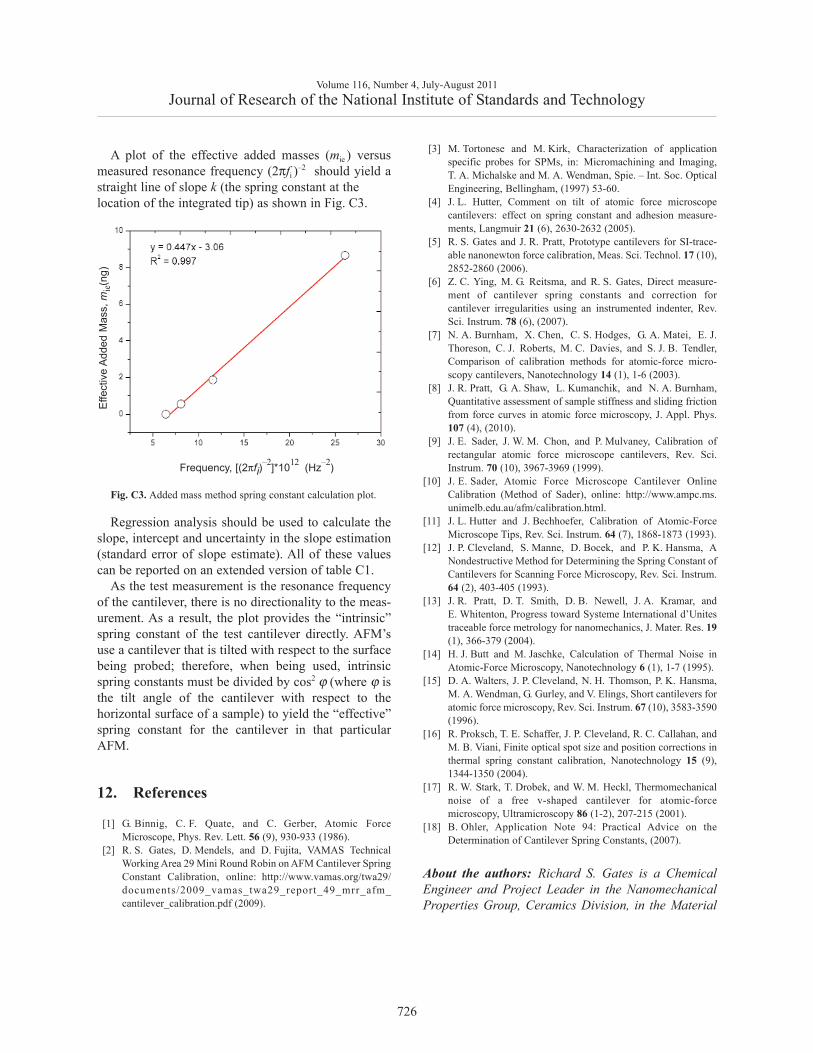
A plot of the effective added masses (mie ) versusmeasured resonance frequency (2πfi )–2 should yield astraight line of slope k (the spring constant at thelocation of the integrated tip) as shown in Fig. C3.

Regression analysis should be used to calculate theslope, intercept and uncertainty in the slope estimation(standard error of slope estimate). All of these valuescan be reported on an extended version of table C1.

As the test measurement is the resonance frequencyof the cantilever, there is no directionality to the meas-urement. As a result, the plot provides the “intrinsic”spring constant of the test cantilever directly. AFM’suse a cantilever that is tilted with respect to the surfacebeing probed; therefore, when being used, intrinsicspring constants must be divided by cos2 ϕ (where ϕ isthe tilt angle of the cantilever with respect to thehorizontal surface of a sample) to yield the “effective”spring constant for the cantilever in that particularAFM.

12. References

[1] G. Binnig, C. F. Quate, and C. Gerber, Atomic ForceMicroscope, Phys. Rev. Lett. 56 (9), 930-933 (1986).

[2] R. S. Gates, D. Mendels, and D. Fujita, VAMAS TechnicalWorking Area 29 Mini Round Robin on AFM Cantilever SpringConstant Calibration, online: http://www.vamas.org/twa29/documents/2009_vamas_twa29_report_49_mrr_afm_cantilever_calibration.pdf (2009).

[3] M. Tortonese and M. Kirk, Characterization of applicationspecific probes for SPMs, in: Micromachining and Imaging,T. A. Michalske and M. A. Wendman, Spie. – Int. Soc. OpticalEngineering, Bellingham, (1997) 53-60.

[4] J. L. Hutter, Comment on tilt of atomic force microscopecantilevers: effect on spring constant and adhesion measure-ments, Langmuir 21 (6), 2630-2632 (2005).

[5] R. S. Gates and J. R. Pratt, Prototype cantilevers for SI-trace-able nanonewton force calibration, Meas. Sci. Technol. 17 (10),2852-2860 (2006).

[6] Z. C. Ying, M. G. Reitsma, and R. S. Gates, Direct measure-ment of cantilever spring constants and correction forcantilever irregularities using an instrumented indenter, Rev.Sci. Instrum. 78 (6), (2007).

[7] N. A. Burnham, X. Chen, C. S. Hodges, G. A. Matei, E. J.Thoreson, C. J. Roberts, M. C. Davies, and S. J. B. Tendler,Comparison of calibration methods for atomic-force micro-scopy cantilevers, Nanotechnology 14 (1), 1-6 (2003).

[8] J. R. Pratt, G. A. Shaw, L. Kumanchik, and N. A. Burnham,Quantitative assessment of sample stiffness and sliding frictionfrom force curves in atomic force microscopy, J. Appl. Phys.107 (4), (2010).

[9] J. E. Sader, J. W. M. Chon, and P. Mulvaney, Calibration ofrectangular atomic force microscope cantilevers, Rev. Sci.Instrum. 70 (10), 3967-3969 (1999).

[10] J. E. Sader, Atomic Force Microscope Cantilever OnlineCalibration (Method of Sader), online: http://www.ampc.ms.unimelb.edu.au/afm/calibration.html.

[11] J. L. Hutter and J. Bechhoefer, Calibration of Atomic-ForceMicroscope Tips, Rev. Sci. Instrum. 64 (7), 1868-1873 (1993).

[12] J. P. Cleveland, S. Manne, D. Bocek, and P. K. Hansma, ANondestructive Method for Determining the Spring Constant ofCantilevers for Scanning Force Microscopy, Rev. Sci. Instrum.64 (2), 403-405 (1993).

[13] J. R. Pratt, D. T. Smith, D. B. Newell, J. A. Kramar, andE. Whitenton, Progress toward Systeme International d’Unitestraceable force metrology for nanomechanics, J. Mater. Res. 19(1), 366-379 (2004).

[14] H. J. Butt and M. Jaschke, Calculation of Thermal Noise inAtomic-Force Microscopy, Nanotechnology 6 (1), 1-7 (1995).

[15] D. A. Walters, J. P. Cleveland, N. H. Thomson, P. K. Hansma,M. A. Wendman, G. Gurley, and V. Elings, Short cantilevers foratomic force microscopy, Rev. Sci. Instrum. 67 (10), 3583-3590(1996).

[16] R. Proksch, T. E. Schaffer, J. P. Cleveland, R. C. Callahan, andM. B. Viani, Finite optical spot size and position corrections inthermal spring constant calibration, Nanotechnology 15 (9),1344-1350 (2004).

[17] R. W. Stark, T. Drobek, and W. M. Heckl, Thermomechanicalnoise of a free v-shaped cantilever for atomic-forcemicroscopy, Ultramicroscopy 86 (1-2), 207-215 (2001).

[18] B. Ohler, Application Note 94: Practical Advice on theDetermination of Cantilever Spring Constants, (2007).

About the authors: Richard S. Gates is a ChemicalEngineer and Project Leader in the NanomechanicalProperties Group, Ceramics Division, in the Material


726

Fig. C3. Added mass method spring constant calculation plot.

Frequency, [(2πfi)–2]*1012 (Hz–2)

Effe

ctiv

e A

dded

Mas

s,m

ie(n

g)

Measurement Laboratory. Mark G. Reitsma is a CivilEngineer and was a Guest Researcher in that Groupuntil joining Asylum Research in May of 2011. John A.Kramar is a Research Chemist and Group Leader inthe Nanoscale Metrology Group, MechanicalMetrology Division, in the Physical MeasurementLaboratory. Jon R. Pratt is a Mechanical Engineer andProject Leader in the Mass and Force Group,Mechanical Metrology Division, in the PhysicalMeasurement Laboratory. The National Institute ofStandards and Technology is an agency of the U.S.Department of Commerce.


727