Atmospheric Environment 37 (2003) 1799–1809

Atmospheric aerosol source identification and estimates ofsource contributions to air pollution in Dundee, UK

Y. Qina, K. Oduyemib,*aDivision of Construction and Environment, University of Abertay Dundee, Dundee DD1 1HG, UK

bCE-CERT, University of California, Riverside, CA 92507, USA

Received 5 October 2002; accepted 9 January 2003

Abstract

Anthropogenic aerosol (PM10) emission sources sampled at an air quality monitoring station in Dundee have been

analysed. However, the information on local natural aerosol emission sources was unavailable. A method that

combines receptor model and atmospheric dispersion model was used to identify aerosol sources and estimate source

contributions to air pollution. The receptor model identified five sources. These are aged marine aerosol source with

some chlorine replaced by sulphate, secondary aerosol source of ammonium sulphate, secondary aerosol source of

ammonium nitrate, soil and construction dust source, and incinerator and fuel oil burning emission source. For the

vehicle emission source, which has been comprehensively described in the atmospheric emission inventory but cannot be

identified by the receptor model, an atmospheric dispersion model was used to estimate its contributions. In Dundee, a

significant percentage, 67.5%, of the aerosol mass sampled at the study station could be attributed to the six sources

named above.

r 2003 Elsevier Science Ltd. All rights reserved.

Keywords: Aerosol; Source contribution; Receptor model; Atmospheric dispersion model

1. Introduction

Identification of airborne pollutant emission sources

and estimation of source contributions to air pollution

are very important in ambient air quality management,

especially in the area where the air quality objectives are

not or are unlikely to be met. In making an air pollution

control strategy, social, economical, political and legal

constraints on air quality management demand a

convenient and accurate method for assessing source

contributions to air pollution.

When source information is comprehensively gath-

ered, atmospheric dispersion model is a useful tool for

assessing the impact of air pollution source on ambient

air quality (Pasquill and Smith, 1983). The source

contribution can be estimated by simulating the trans-

port and dispersion of airborne pollutants. Atmospheric

dispersion models have generally been used in air quality

management, with lots of atmospheric dispersion

models and software packages having been developed.

New advances in atmospheric dispersion theories,

numerical simulation methodologies and computing

techniques are being used to improve model’s predictive

capability, calculation efficiency and interfaces of the

software package. Department of the Environment,

Transport and the Regions, UK (1998) listed a series of

atmospheric dispersion models as a guide to potential

users.

However, an atmospheric model is a source-oriented

model and its predicting precision depends directly on

the precision of the data on the sources in question. The

precise source profiles are not easy to gather, especially

for many small natural or anthropogenic emission

sources. In cases where the source profiles are not

reasonably defined, a receptor model provides another

AE International – Europe

*Corresponding author.

E-mail address: cetko@abertay.ac.uk (K. Oduyemi).

1352-2310/03/$ - see front matter r 2003 Elsevier Science Ltd. All rights reserved.

doi:10.1016/S1352-2310(03)00078-5

means of identifying air pollution sources. In contrast to

the approaches of the atmospheric dispersion model, the

receptor model is a receptor-oriented model. It analyses

the behaviours of airborne pollutants, especially chemi-

cal species of aerosols at the receptor. It is believed that

these behaviours contain information on source compo-

sitions. Receptor models have been used successfully to

identify aerosol emission sources and source contribu-

tions (Hopke, 1991a, b). Several approaches and soft-

ware packages for receptor model analysis have been

developed. Most of the approaches are based on

multivariate data analysis.

Atmospheric dispersion and receptor models are

characteristically different in their applications. Both

of them have advantages and shortcomings. It was usual

that only one kind of model was used in most of the

previous research works on assessing impact of air

pollution sources on the ambient environment. Seigneur

et al. (1999) firstly suggested that atmospheric dispersion

model and receptor model should be combined in a PM

(particulate matters) 24-hour average concentration

modelling. Chow et al. (1999) tried to use both the

receptor model (CMB) and atmospheric model (ISCST-

3) to estimate middle and neighbourhood scale varia-

tions of source contributions in Las Vegas, Nevada.

However, they analysed the model results separately and

did not try to complement the results derived from the

two models.

In this work, urban background air quality data was

monitored in Dundee, using a monitoring station setup

on the roof of the library of the University of Abertay

Dundee. The library is a four-floor building located in

the city centre of Dundee. There is no high building

around the library to prevent air current from any

direction. Concentrations of NO, NO2 and NOx as well

as wind speed, wind direction, ambient temperature and

the amount of rainfall were measured continually

throughout the year 2000. PM10 (particulate matter

with aerodynamic diameter less than 10mm) wassampled for four consecutive days on weekdays and

for three consecutive days at weekends using Partisol

Model 2000 Air Sampler (Rupprecht & Patashnich Co.,

Inc.) at the station. A total of 89 PM10 samples were

taken during a 1-year operational period. Gravimetric

analysis was conducted for all PM10 samples while wet

chemical analysis was conducted on 59 of these samples,

which were collected during the period 9 December 1999

to 31 July 2000. The metal elements of PM10 (Ca, Mg,

Zn, Cu, Ni and Pb) were analysed using an atomic

absorption spectrophotometer (AAS). The ions of PM10

(SO42�, NO3

�, Cl�, NH4+, Na+ and K+) were analysed

using a high-performance liquid chromatography

(HPLC). The sampling and analysis techniques and the

analysed results have already been presented in another

paper (Qin and Oduyemi, 2003). A method that

combines both the receptor model and atmospheric

dispersion model was used to identify aerosol sources

and estimate the source contributions to air pollution.

2. Anthropogenic PM10 emission sources in Dundee

The local government has investigated anthropogenic

airborne pollutant emission sources in Dundee. Here,

spatial distribution and temporal variations of PM10

emission sources are described in greater detail, to

satisfy the requirements of an atmospheric dispersion

model. There are 56 industrial and commercial processes

registered in Dundee. Emission amounts of airborne

pollutants are small for most of these processes. The

Baldovie waste to energy plant (WTE), Dundee Energy

Recycling Limited located in the Baldovie industrial

estate is one of the important air pollution sources in

Dundee. The annual emission amount of PM10 from a

70-m high stack for this plant is about 20.62 t.

Road vehicle emission is the largest anthropogenic

airborne pollutant emission source in the UK, especially

in urban areas (Barratt et al., 1997). Road vehicle

emission is very complex and depends on vehicle type,

fuel, mileage, speed, driving mode, ambient temperature,

etc. Emission factor is usually used to calculate road

vehicle emission. Emission factors for eight different

types of vehicles, at various speeds, for 1997, 1999 and

2005 calendar year vehicles are available in the Atmo-

spheric Emission Inventories, UK (London Research

Centre, 2000). These eight types of vehicles are petrol

cars, petrol light goods vehicles (LGVs), diesel cars,

diesel LGVs, rigid heavy goods vehicles (HGVs),

articulated HGVs, buses and coaches, and motorcycle.

The emission factors of PM10 for the 1999 calendar year

vehicles were used to calculate particulate emission from

road vehicle in Dundee, because 1999 is close to the year

2000 period in which the field experiment was carried

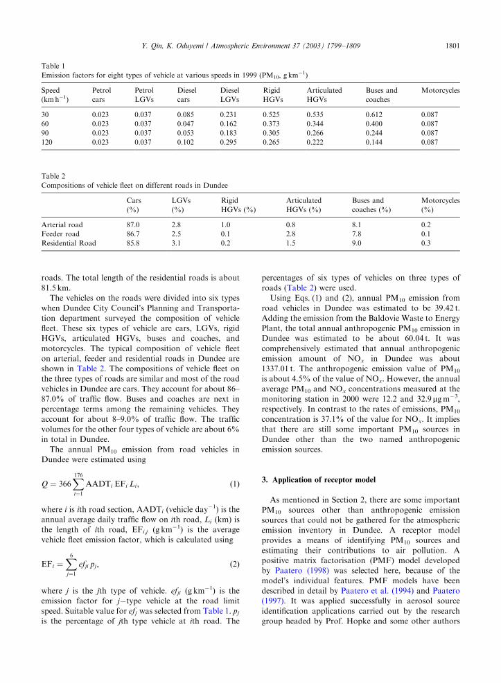
out. These emission factors are shown in Table 1.

Dundee City Council’s Planning and Transportation

department during the past decade counted traffic flows

on 176 major road sections in the Dundee urban area.

The total length of these 176 roads is about 145 km. The

annual average daily traffic flow (AADT) on these roads

varies from less than 1000 vehicles to more than 40,000

vehicles. The road width varies from 10 to 40m. The

vehicle speed limit varies between 30 and 60mile h�1. To

calculate PM10 emission from road vehicles, the roads in

Dundee were divided into three types: arterial roads,

feeder roads and residential roads, based upon AADT

(arterial road, ADDTX20,000; feeder road,

20,000>AADTX10,000; residential road, AAD-

To10,000). Among the 176 major road sections inDundee, 22 of them with a total length of 23.0 km can be

categorised as arterial roads. Forty-three road sections

with a total length of 40.5 km can be categorised as

feeder roads. The remaining road sections are residential

Y. Qin, K. Oduyemi / Atmospheric Environment 37 (2003) 1799–18091800

roads. The total length of the residential roads is about

81.5 km.

The vehicles on the roads were divided into six types

when Dundee City Council’s Planning and Transporta-

tion department surveyed the composition of vehicle

fleet. These six types of vehicle are cars, LGVs, rigid

HGVs, articulated HGVs, buses and coaches, and

motorcycles. The typical composition of vehicle fleet

on arterial, feeder and residential roads in Dundee are

shown in Table 2. The compositions of vehicle fleet on

the three types of roads are similar and most of the road

vehicles in Dundee are cars. They account for about 86–

87.0% of traffic flow. Buses and coaches are next in

percentage terms among the remaining vehicles. They

account for about 8–9.0% of traffic flow. The traffic

volumes for the other four types of vehicle are about 6%

in total in Dundee.

The annual PM10 emission from road vehicles in

Dundee were estimated using

Q ¼ 366X176i¼1

AADTi EFi Li; ð1Þ

where i is ith road section, AADTi (vehicle day�1) is the

annual average daily traffic flow on ith road, Li (km) is

the length of ith road, EFi;j (g km�1) is the average

vehicle fleet emission factor, which is calculated using

EFi ¼X6j¼1

efji pj ; ð2Þ

where j is the jth type of vehicle. efji (g km�1) is the

emission factor for j�type vehicle at the road limitspeed. Suitable value for efj was selected from Table 1. pj

is the percentage of jth type vehicle at ith road. The

percentages of six types of vehicles on three types of

roads (Table 2) were used.

Using Eqs. (1) and (2), annual PM10 emission from

road vehicles in Dundee was estimated to be 39.42 t.

Adding the emission from the Baldovie Waste to Energy

Plant, the total annual anthropogenic PM10 emission in

Dundee was estimated to be about 60.04 t. It was

comprehensively estimated that annual anthropogenic

emission amount of NOx in Dundee was about

1337.01 t. The anthropogenic emission value of PM10

is about 4.5% of the value of NOx. However, the annual

average PM10 and NOx concentrations measured at the

monitoring station in 2000 were 12.2 and 32.9mgm�3,

respectively. In contrast to the rates of emissions, PM10

concentration is 37.1% of the value for NOx. It implies

that there are still some important PM10 sources in

Dundee other than the two named anthropogenic

emission sources.

3. Application of receptor model

As mentioned in Section 2, there are some important

PM10 sources other than anthropogenic emission

sources that could not be gathered for the atmospheric

emission inventory in Dundee. A receptor model

provides a means of identifying PM10 sources and

estimating their contributions to air pollution. A

positive matrix factorisation (PMF) model developed

by Paatero (1998) was selected here, because of the

model’s individual features. PMF models have been

described in detail by Paatero et al. (1994) and Paatero

(1997). It was applied successfully in aerosol source

identification applications carried out by the research

group headed by Prof. Hopke and some other authors

Table 2

Compositions of vehicle fleet on different roads in Dundee

Cars

(%)

LGVs

(%)

Rigid

HGVs (%)

Articulated

HGVs (%)

Buses and

coaches (%)

Motorcycles

(%)

Arterial road 87.0 2.8 1.0 0.8 8.1 0.2

Feeder road 86.7 2.5 0.1 2.8 7.8 0.1

Residential Road 85.8 3.1 0.2 1.5 9.0 0.3

Table 1

Emission factors for eight types of vehicle at various speeds in 1999 (PM10, g km�1)

Speed

(kmh�1)

Petrol

cars

Petrol

LGVs

Diesel

cars

Diesel

LGVs

Rigid

HGVs

Articulated

HGVs

Buses and

coaches

Motorcycles

30 0.023 0.037 0.085 0.231 0.525 0.535 0.612 0.087

60 0.023 0.037 0.047 0.162 0.373 0.344 0.400 0.087

90 0.023 0.037 0.053 0.183 0.305 0.266 0.244 0.087

120 0.023 0.037 0.102 0.295 0.265 0.222 0.144 0.087

Y. Qin, K. Oduyemi / Atmospheric Environment 37 (2003) 1799–1809 1801

(Polissar et al., 1996, 1998; Xie et al., 1998, 1999a–c;

Hopke et al., 1998; Ramadan et al., 2000; Qin et al.,

2002; Battelle and Sonoma Technologies Inc., 2002).

In this work, a two-dimensional matrix data of

aerosol chemical composition from the monitoring

station at University of Abertay Dundee was used in a

two-way PMF model trial. The two-way PMF model

can be written as

Xij ¼Xp

k¼1

GikFkj þ Eij ði ¼ 1;y; n; j ¼ 1;y;mÞ; ð3Þ

where Eij ¼ Xij �Pp

h¼1 GihFhj is a matrix of residuals.

The principle of the two-way PMF model can be

presented as

minimizeQ ¼Xn

i¼1

Xm

j¼1

Eij

Sij

� �2with GihX0;FhjX0; ð4Þ

where Sij is the point-by-point error estimate of Xij ;Eij=Sij is the scaled residual.

The explained variance, EV, was defined in the PMF

model. The explained variances for F are defined as

EVkj ¼ EVj Fkj=Xp

k¼1

Fkj ; ð5Þ

where

EVj ¼1�

Pni¼1 Eij=Sij

� �2Pn

i¼1 Xij=Sij

� �2 : ð6Þ

The explained variances are scaled factors. The

explained variances for F facilitate the answers to two

questions: Which are important chemical components in

any given factor? And, how important is any given

chemical component in the different factors? The

explained variances may, in addition, show factor

characteristics.

3.1. The element matrix for the PMF analysis

A PMF model was applied to analyse the PM10 data

measured at a monitoring station located at the

University of Abertay Dundee. The average concentra-

tions on weekdays (4 days) or at weekends (3 days) for

all the 12 components of PM10 (SO42�, NO3

�, NH4+,

Ca2+, K+, Cl�, Na+, Mg2+, Pb, Ni, Zn and Cu),

average concentration of NOx, easterly wind frequency

(ENE, E and ESE), westerly wind frequency (WSW, W

and WNW) and average wind speed during the sampling

period were selected to compose the input element

matrix for the PMF analysis. Concentrations of PM10

mass and 12 chemical species measured at the monitor-

ing station and their detection limits and precision are

shown in Table 3. On average, the 12 chemical species

hold about 61% of the PM10 mass. A gaseous pollutant,

NOx, was selected because it could serve as a marker for

the road vehicle emission. The result obtained from the

atmospheric dispersion model indicates that 98.8% of

NOx measured at the monitoring station comes from

road vehicle emissions. The wind direction frequencies

and average wind speed were adopted as components of

the element matrix because they are capable of showing

source direction and relationships with wind speed. The

final input element matrix includes concentrations of

chemical species for 59 PM10 samples, average NOx

concentrations and wind condition during the sampling

period.

3.2. Error estimates

Chemical species measured in the ambient environ-

ment vary widely, especially for some trace elements in

aerosols. Huang et al. (1999) thought that the choice of

elements might affect the results of factor analysis

because some elements could degrade the resolution of

factor analysis by varying randomly in response to

analytical uncertainties or by being below detection

limits. One of the major advantages of a PMF model is

that it can handle various elements with different

variation ranges and uncertainties, using error estimates

(Paatero, 1998). The error estimates in a PMF model for

the individual data point values are utilised as point-by-

point weight, using an S matrix (standard deviation

array) for X matrix (elements array). S matrix may becalculated by using four different methods in a PMF

Table 3

Concentrations of PM10 mass and chemical species (mgm�3)

Mass SO42� NO3� NH4

+ Ca2+ K+ Cl� Na+ Mg2+ Pb Ni Zn Cu

Min 5.00 0.422 0 0.080 0 0 0.079 0.070 0 0 0 0 0

Max 36.50 7.455 7.692 3.121 2.310 1.432 2.888 3.915 0.560 0.133 0.093 0.168 0.062

Average 12.20 2.154 1.107 0.670 0.779 0.110 0.980 1.164 0.127 0.021 0.025 0.028 0.024

SD* 6.00 1.543 1.261 0.602 0.526 0.185 0.672 0.656 0.132 0.038 0.025 0.030 0.014

DL 0.05 0.012 0.001 0.042 0.009 0.002 0.005

Precision (%) 23.5 13.5 5.2 0.9 9.0 11.3 4.2 0.5 7.8 14.3 2.4 19.1

SD: standard deviation; DL: detective limit.

Y. Qin, K. Oduyemi / Atmospheric Environment 37 (2003) 1799–18091802

model. In this work, Sij is calculated using

Sij ¼Tj þ Uj

ffiffiffiffiffiffiffiffiffiffiffiffiffiffiffiffiffiffiffiffiffiffiffiffiffiffiffiffiffiffimaxðjXij j; jYij jÞ

pþ VjmaxðjXij j; jYij jÞ ð7Þ

where Yij is the fitted value for element of Xij by the

PMF model, Tj ; Uj and Vj are coefficients. There is no

simple rule for selecting coefficients. An optimal way for

selecting coefficients depends on a basic understanding

of the input data and trial. The element with less

precision may create anomalous single element factor in

factor analysis, which cannot be interpreted physically.

Large values should be used as coefficients for these

elements. Furthermore, different coefficients should be

used for different elements, because different random

errors for elements may be made in the process of

sampling and analysing PM10.

Here, Uj in Eq. 7 was set to 0 for the chemical species

in the element matrix, such as Ca2+, Mg2+, Cu, Pb, Ni,

Zn, NOx and wind speed, for which detection limits are

available (Table 3), Tj was assigned the value of the

detection limit. For the ions and wind direction

frequencies, for which detection limits were unavailable,

an artificial value (based upon the value in the element

matrix) was assigned to Tj : The values of Tj used for 16

of the components in the element matrix are shown in

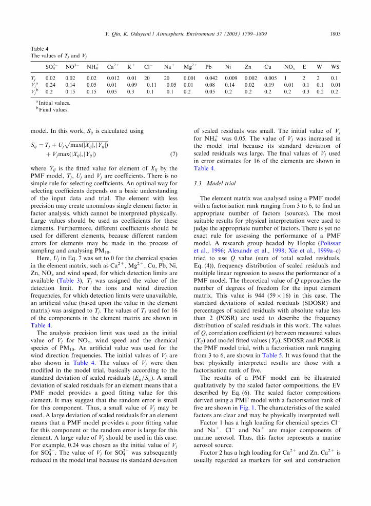
Table 4.

The analysis precision limit was used as the initial

value of Vj for NOx, wind speed and the chemical

species of PM10. An artificial value was used for the

wind direction frequencies. The initial values of Vj are

also shown in Table 4. The values of Vj were then

modified in the model trial, basically according to the

standard deviation of scaled residuals (Eij=Sij). A small

deviation of scaled residuals for an element means that a

PMF model provides a good fitting value for this

element. It may suggest that the random error is small

for this component. Thus, a small value of Vj may be

used. A large deviation of scaled residuals for an element

means that a PMF model provides a poor fitting value

for this component or the random error is large for this

element. A large value of Vj should be used in this case.

For example, 0.24 was chosen as the initial value of Vj

for SO42�. The value of Vj for SO4

2� was subsequently

reduced in the model trial because its standard deviation

of scaled residuals was small. The initial value of Vj

for NH4+ was 0.05. The value of Vj was increased in

the model trial because its standard deviation of

scaled residuals was large. The final values of Vj used

in error estimates for 16 of the elements are shown in

Table 4.

3.3. Model trial

The element matrix was analysed using a PMF model

with a factorisation rank ranging from 3 to 6, to find an

appropriate number of factors (sources). The most

suitable results for physical interpretation were used to

judge the appropriate number of factors. There is yet no

exact rule for assessing the performance of a PMF

model. A research group headed by Hopke (Polissar

et al., 1996; Alexandr et al., 1998; Xie et al., 1999a–c)

tried to use Q value (sum of total scaled residuals,

Eq. (4)), frequency distribution of scaled residuals and

multiple linear regression to assess the performance of a

PMF model. The theoretical value of Q approaches the

number of degrees of freedom for the input element

matrix. This value is 944 (59� 16) in this case. Thestandard deviations of scaled residuals (SDOSR) and

percentages of scaled residuals with absolute value less

than 2 (POSR) are used to describe the frequency

distribution of scaled residuals in this work. The values

of Q; correlation coefficient (r) between measured values(Xij) and model fitted values (Yij), SDOSR and POSR in

the PMF model trial, with a factorisation rank ranging

from 3 to 6, are shown in Table 5. It was found that the

best physically interpreted results are those with a

factorisation rank of five.

The results of a PMF model can be illustrated

qualitatively by the scaled factor compositions, the EV

described by Eq. (6). The scaled factor compositions

derived using a PMF model with a factorisation rank of

five are shown in Fig. 1. The characteristics of the scaled

factors are clear and may be physically interpreted well.

Factor 1 has a high loading for chemical species Cl�

and Na+. Cl� and Na+ are major components of

marine aerosol. Thus, this factor represents a marine

aerosol source.

Factor 2 has a high loading for Ca2+ and Zn. Ca2+ is

usually regarded as markers for soil and construction

Table 4

The values of Tj and Vj

SO42� NO3� NH4

+ Ca2+ K+ Cl� Na+ Mg2+ Pb Ni Zn Cu NOx E W WS

Tj 0.02 0.02 0.02 0.012 0.01 20 20 0.001 0.042 0.009 0.002 0.005 1 2 2 0.1

Vja 0.24 0.14 0.05 0.01 0.09 0.11 0.05 0.01 0.08 0.14 0.02 0.19 0.01 0.1 0.1 0.01

Vjb 0.2 0.15 0.15 0.05 0.3 0.1 0.1 0.2 0.05 0.2 0.2 0.2 0.2 0.3 0.2 0.2

a Initial values.bFinal values.

Y. Qin, K. Oduyemi / Atmospheric Environment 37 (2003) 1799–1809 1803

dust. Factor 2 should therefore represent a soil and

construction dust source.

Factor 3 has a high loading for chemical components

NO3� and NH4

+. NO3� and NH4

+ are secondary

pollutants formed from NOx and NH3. This factor

represents a secondary aerosol source of ammonium

nitrate.

Factor 4 has a high loading for the easterly wind

frequency, SO42� and NH4

+. SO42� is also a secondary

pollutant formed from SO2. This factor should represent

a secondary aerosol source of ammonium suphate. The

analysis of the contribution of wind aspect to chemical

species of PM10 (Qin and Oduyemi, 2003) shows that the

average contributions of easterly wind to SO42� and

Fig. 1. Scaled factor compositions of five factors derived using a PMF model.

Table 5

Assessment of PMF model performances

Three factors (Q ¼ 1630) Four factors (Q ¼ 1255) Five factors (Q ¼ 943) Six factors (Q ¼ 719)

r SDOSR POSR (%) R SDOSR POSR (%) r SDOSR POSR (%) R SDOSR POSR (%)

SO42� 0.76 1.72 74.6 0.92 0.99 94.9 0.91 1.01 94.9 0.90 1.03 96.6

NO3� 0.94 1.76 83.1 0.99 0.45 100.0 1.00 0.41 100.0 1.00 0.37 100.0

NH4+ 0.92 1.44 93.2 0.97 1.00 94.9 0.96 1.00 96.6 0.96 1.04 96.6

Ca2+ 1.00 0.39 100.0 1.00 0.38 100.0 1.00 0.17 100.0 1.00 0.16 100.0

K+ 0.21 1.11 96.6 0.18 1.13 93.2 0.19 1.13 94.9 0.19 1.13 94.9

Cl� 0.98 0.90 98.3 0.98 0.90 98.3 0.99 0.66 100.0 0.99 0.66 100.0

Na+ 0.77 1.46 93.2 0.76 1.51 93.2 0.77 1.48 93.2 0.77 1.46 93.2

Mg2+ 0.30 2.13 57.6 0.30 2.09 62.7 0.84 1.29 88.1 0.87 1.07 89.8

Pb 0.07 0.83 78.0 0.15 0.82 94.9 0.58 0.68 98.3 0.55 0.69 96.6

Ni 0.08 1.35 83.1 0.07 1.35 84.7 0.40 1.26 88.1 0.38 1.25 88.1

Zn 0.44 1.71 74.6 0.44 1.71 72.9 0.74 1.23 89.8 0.69 1.19 91.5

Cu 0.13 1.18 89.8 0.07 1.16 88.1 0.75 0.82 98.3 0.75 0.82 98.3

NOx 0.66 1.52 84.7 0.64 1.47 78.0 0.78 1.23 83.1 0.77 1.18 89.8

E 0.61 1.78 66.1 0.84 1.14 93.2 0.85 1.11 93.2 0.89 0.95 96.6

W 0.46 1.49 81.4 0.47 1.48 81.4 0.49 1.38 81.4 0.98 0.29 100.0

WS 0.28 1.44 83.1 0.35 1.28 86.4 0.31 1.25 84.7 0.80 0.72 96.6

Y. Qin, K. Oduyemi / Atmospheric Environment 37 (2003) 1799–18091804

NH4+ are much higher than the easterly wind frequency,

while the average contributions of westerly wind to these

two species are much lower than westerly wind

frequency. A high loading for the easterly wind in this

factor suggests that the major source of the secondary

ammonium suphate comes from the east, the European

continent.

Factor 5 has a loading for heavy metals (Mg2+, Pb,

Ni, Zn and Cu) and the westerly wind frequency. This

factor can be interpreted as a source coming from

incinerator and fuel oil burning.

The value of Q for the PMF model trial with a

factorisation rank of 5 is 943 (Table 5). This value is

almost equal to the theoretical value. The best fitted

results of the PMF model are that of Ca2+ and NO3+

with a correlation coefficient of 1.00 and a percentage of

scaled residual, with absolute values less than 2, of

100.0%. The fitted results for important species such as

SO42�, NH4

+ and Cl� are well within a correlation

coefficient higher than 0.90 and the percentage of scaled

residual with absolute values less than 2 higher than

90.0%. The performance of the PMF model is reason-

ably good in the model trial with a factorisation rank of

five. The percentages of measured chemical species in

PM10, which can be attributed to these 5 factors, are

85.0%, 94.1%, 84.7%, 99.2%, 61.8%, 92.9%, 89.2%,

81.7%, 49.1%, 51.2%, 73.7% and 76.2% for SO42�,

NO3�, NH4

+, Ca2+, K+, Cl�, Na+, Mg2+, Pb, Ni, Zn

and Cu, respectively.

3.4. Factor mass profiles

As in the analysis in Section 3.3, the factor

characteristics can be illustrated quantitatively using

scaled factors. The mass profiles of the factors could

further confirm the source characteristics quantitatively.

The mass profiles of five factors (12 chemical species),

derived using a PMF model, are shown in Table 6. The

best way to assess the results of factor analysis is to

compare the derived mass profiles with the real source

emission profiles. Unfortunately, measured PM10 pro-

files for the local emission sources are unavailable in

Dundee. The factor mass profiles had to be assessed by

analysing source characteristics or comparing them with

some artificial ideal source profiles. The secondary

pollution sources are virtual sources derived by the

receptor model.

The mass profile of factor 1 has high percentages for

Cl� and Na+. The percentages for Cl�, Na+, SO42�, Ca

and K+ are 43.10%, 38.28%, 13.73%, 2.20% and

1.61%, respectively. The ionic balance in this factor is

reasonably good, with an equivalent anion/cation ratio

of 0.88. In the ideal pure marine aerosol source profile

used in Southern California Air Quality Study (SCAQS)

PM2.5 and PM10 receptor modelling (Watson et al.,

1994), the percentages for Cl�, Na+, SO42�, Ca and K+

are 57.40%, 32.00%, 8.00%, 1.22% and 1.18%,

respectively. The equivalent anion/cation ratio is 1.26.

Percentage of Cl� in factor 1, derived using PMF, is

lower than the value in the ideal fresh pure marine

aerosol profile, while percentages of Na+ and SO42� are

higher than the ideal values. There is a loss reaction of

particulate Cl� in the ambient environment when

gaseous acid species react with sea salt aerosols to

liberate gaseous HCl. The mass profile of factor 1

indicates that it represents an aged marine aerosol

source with some Cl� replaced by SO42�.

The mass profile of factor 2 has a high percentage for

Ca2+, which is 79.91%. Na+, NH4+ and Cl� are three

minor components. The ions are not the major

components in this factor and so the ionic balance is

poor. The equivalent anion/cation ratio is 0.17. The

mass profile also shows that factor 2 represents the

source from soil and construction dust. However, it is

Table 6

Mass profiles of five factors derived using PMF model

Factor 1 Factor 2 Factor 3 Factor 4 Factor 5

SO42� (%) 13.73 0.01 17.20 80.75 16.98

NO3� (%) 0.01 0.07 53.03 0.04 0.03

NH4+ (%) 0.03 4.52 14.38 16.41 2.19

Ca2+ (%) 2.20 79.91 0.01 0.00 1.00

K+ (%) 1.61 0.32 1.27 0.41 0.03

Cl� (%) 43.10 4.08 4.16 0.00 13.67

Na+ (%) 38.28 9.96 8.49 2.06 27.16

Mg2+ (%) 0.51 0.00 1.03 0.00 22.37

Pb (%) 0.00 0.00 0.30 0.05 5.01

Ni (%) 0.32 0.05 0.09 0.01 2.98

Zn (%) 0.00 0.94 0.00 0.00 4.90

Cu (%) 0.22 0.14 0.04 0.27 3.68

Equivalent anion/cation 0.88 0.17 1.11 1.66 0.57

Y. Qin, K. Oduyemi / Atmospheric Environment 37 (2003) 1799–1809 1805

difficult to assess factor 2 quantitatively, because a

reasonable source profile that can describe local soil and

construction dust is unavailable.

The scaled factor composition of factor 3 shows that

the factor represents a secondary aerosol source of

ammonium nitrate. There are only two chemical

components (77.5% NO3� and 22.6% NH4

+; NO3�/

NH4+=3.43) in the artificial ideal source of ammonium

nitrate (Watson et al., 1994). The anion and cation are

fully balanced. The mass profile of factor 3 has high

percentages for NO3�, SO4

2� and NH4+. NO3

� and NH4+

hold about 67.41% of the source mass. The ratio of

NO3�/NH4

+, 3.69, approaches the ideal value. The anion

and cation can be matched in factor 3. The equivalent

anion/cation ratio is 1.11. However, the mass loading of

SO42� in factor 3 is relatively high (17.20%). The mass

profile suggests that factor 3 represents a secondary

aerosol source, which includes both ammonium nitrate

and ammonium sulphate.

The mass profile of factor 4 has high percentages for

SO42� and NH4

+. There are only two chemical compo-

nents (27.3% NH4+ and 72.7% SO4

2�; SO42�/

NH4+=2.66) in the artificial ideal source of ammonium

sulphate (Watson et al., 1994). The anion and cation are

fully balanced. In factor 4, SO42� and NH4

+ hold about

97.16% of the source mass. The ratio of SO42�/NH4

+

(5.35) is about double the ideal value. The equivalent

anion/cation ratio in this factor is 1.66. These suggest

that a fraction of SO42� has not been associated with

NH4+. Analysis of mass profile shows that factor 4

should represent a secondary aerosol source of ammo-

nium sulphate, although its structure is not exactly the

same as the ideal one.

The mass profile of factor 5 is different with the scaled

factor composition. It has a relatively high percentage

for Na+, Mg, SO42� and Cl�. The mass profile of factor

5 cannot be reasonably interpreted as a source coming

from incinerator and fuel oil burning, because there are

high percentages for the loading of marine elements,

Na+ and Cl�.

An evaluation of the mass profiles of factors 3 and 5

shows there are some differences between the character-

istics represented by scale factor components and mass

profile. 17.20% of SO42� in the mass profile of factor 3

indicates that the factor is bias to a pure secondary

aerosol source of ammonium nitrate. The high percen-

tages of Na+ and Cl� in the mass profile of factor 5

means that the factor cannot be reasonably interpreted

as an incinerator and fuel oil burning emission source.

SO42� in factor 3 and Cl� and Na+ in factor 5 should

approach zero.

In a PMF model, four methods can be used to impose

expected characteristics for the factors. One of these

methods, the method of pulling individual factor

elements toward zero (Paatero, 1998), was chosen here

to pull SO42� in factor 3 and Cl� and Na+ in factor 5

toward zero. A matrix, known as the ‘‘Fkey’’ matrix,

controls the pulling down operation. This matrix of

integer value is of the same size as that of factor matrix

F: Each element of ‘‘Fkey’’ controls the behaviour of thecorresponding element in F: Three elements in the‘‘Fkey’’ matrix, which represent SO4

2� in factors 3 and

Cl� and Na+ in factor 5, were identified. A ‘‘Fkey’’

matrix was constructed with zero for all elements, except

for the three elements that control the behaviour of

SO42� in factor 3 and Cl� and Na+ in factor 5. A value

of 9 for these three control elements represents a

‘‘medium-strong’’ pulling. F and G matrices resulting

from the previous model trial without enforced rotation

were used as the initial values for the matrices. With the

same element matrix and error estimates, the SO42� in

factor 3 and Cl� and Na+ in factor 5 were successfully

pulled to zero using the ‘‘Fkey matrix’’.

The scaled factors derived using a PMF model with

enforced rotation are very similar to those without

enforced rotation, except that the component of SO42� in

factor 3 and components of Cl� and Na+ in factor 5 are

zero. The characteristics of all five factors shown by

scaled factors have not changed. There is no obvious

difference in the performance of the PMF model in two

trials without enforced rotation and with enforced

rotation. The calculated Q value for the case with

enforced rotation is 966. It is only about 2.4% higher

than the value without enforced rotation. The correla-

tion coefficients of the measured and fitted values,

standard deviations of scaled residuals and percentages

of scaled residuals with absolute value less than 2 for

cases without rotation and with enforced rotation are

almost the same.

The mass profiles of 5 factors derived by PMF model

with enforced rotation are shown in Table 7. In

comparison with the values in Table 6, there are few

changes in factors 1, 2 and 4, while mass percentages of

SO42� in factor 3 and Cl� and Na+ in factor 5 reduce to

zero. After the enforced rotation has been applied, NO3�

and NH4+ hold about 79.99% of the source mass for

factor 3. The anion and cation are also matched. The

equivalent anion/cation ratio is 0.88. Although, a ratio

of 4.41 for NO3�/NH4

+ is larger than the ideal value, the

mass profile of factor 3 can be reasonably interpreted as

representing the secondary aerosol source of ammonium

nitrate.

The mass profile of factor 5 in Table 7 has a relatively

high percentage for heavy metals and secondary pollu-

tion species of SO42� and NH4

+. This factor can be

interpreted reasonably as a source of incinerator and

fuel oil burning emission.

3.5. Factor mass contributions

The average mass contributions of five factors to

PM10 can be estimated using the values of G matrix in

Y. Qin, K. Oduyemi / Atmospheric Environment 37 (2003) 1799–18091806

the PMF model. These mass contributions are shown in

Table 8 in both mass and percentage formats. On

average, the total chemical species mass contributions to

PM10 for the five factors measured at the study

monitoring station is 6856 ngm�3. About 58.1% of

PM10 mass can be attributed to the five sources

represented by these factors. Factors 1 and 4, with

average percentages of 17.8% and 16.9%, respectively,

are two relatively high and stable mass contributors to

PM10. Factor 1 represents an aged marine aerosol with

some chlorine replaced by sulphate, while factor 4

relates to the second aerosol source of ammonium

sulphate. Factors 3 and 2, with average percentages of

12.1% and 9.5% respectively, are secondary aerosol

source of ammonium nitrate and soil and construction

dust. Factor 5 is the smallest contributor with an

average percentage of 1.8% only. This factor represents

an incinerator and fuel oil burning emission.

4. Application of atmospheric dispersion model

The road vehicle emission and Baldovie waste to

energy plant (WTE) are the two important anthropo-

genic particulate emission sources in Dundee. The

contribution of WTE to the PM10 measured at the

monitoring station may be included in factor 5, which

was identified by the PMF method. However, PMF

model cannot separate a factor which represents road

vehicle emission source in Dundee, even though NOx is

included in the input element matrix to serve as a marker

of road vehicle emission. This may be attributed to the

fact that carbon, the most important chemical species in

particulate emitted by road vehicles, has not been

analysed in this work because the instruments were

unavailable.

The road vehicle PM10 emission is comprehensively

defined in Dundee. The contribution of road vehicle

emission can be estimated using an atmospheric disper-

sion model. ISCST3 (EPA, 1995) was used to simulate

the dispersion of road vehicle emitting PM10 in Dundee.

The performance of the ISCST3 model was evaluated by

comparing predicted and measured NOx concentrations

at the monitoring station. This is because most NOx

come from anthropogenic emissions and these anthro-

pogenic sources have been comprehensively defined for

the source survey carried out in Dundee.

4.1. Inputs to the atmospheric dispersion model

The parameters used to describe emission sources,

receptors and atmospheric dispersion conditions are

needed as inputs to the atmospheric dispersion model.

The data collected in the survey of atmospheric emission

Table 8

Average contributions of five factors to PM10 derived from a PMF model

Factor 1 Factor 2 Factor 3 Factor 4 Factor 5 Sum

Mass (ngm�3) 197471462 9777695 170071996 201671849 1897212 685673056Percentage (%) 17.8712.7 9.577.2 12.179.6 16.9715.1 1.872.4 58.1714.3

Table 7

Mass profiles of five factors derived from a PMF model with enforced rotation

Factor 1 Factor 2 Factor 3 Factor 4 Factor 5

SO42� (%) 15.45 0.02 0.00 82.49 32.16

NO3� (%) 0.00 0.03 65.04 0.18 0.04

NH4+ (%) 0.11 4.29 14.75 16.23 5.01

Ca2+ (%) 2.54 74.58 0.00 0.00 0.04

K+ (%) 1.53 0.24 1.54 0.36 0.00

Cl� (%) 41.69 4.75 5.17 0.01 0.00

Na+ (%) 37.84 15.01 11.57 0.38 0.00

Mg2+ (%) 0.34 0.00 1.46 0.00 36.19

Pb (%) 0.00 0.00 0.34 0.07 8.15

Ni (%) 0.29 0.06 0.11 0.02 4.67

Zn (%) 0.00 0.90 0.00 0.00 7.76

Cu (%) 0.20 0.13 0.01 0.26 5.98

Equivalent anion/cation 0.89 0.15 0.88 1.86 2.41

Y. Qin, K. Oduyemi / Atmospheric Environment 37 (2003) 1799–1809 1807

inventories in Dundee was used as inputs for the source

parameters. There were two NOx sources and one

particulate source (WTE) that could be regarded as

point emission sources in Dundee. On vehicle emissions,

13 out of 176 road sections surveyed, with annual

average daily traffic flow (AADT)X25,000, were re-

garded as discrete line emission sources (Owen et al.,

1999, 2000). The remaining 163 road sections were

aggregated into 58 area emission sources, using a scale

of 1000� 1000m2. These annual averaged emission rateswere used as the average emission. The temporal

variations of the source were described by entering daily

and monthly variation factors (EPA, 1995).

Wind speed, wind direction and ambient temperature

were measured at the monitoring station. Some para-

meters used in the atmospheric dispersion model to

describe the construction of atmospheric boundary were

unavailable. Some reasonable empirical assumptions

had to be used as input. ISCST3 (EPA, 1995) is a

convenient Gaussian plume dispersion model, but it is

not suitable in calm conditions. For this reason, the

wind speed was taken to be 0.5m s�1 when the observed

wind speed was less than this value. It is assumed that

atmospheric stability in Dundee was C (slightly un-

stable) during the period 11:00–15:00, D (neutral) during

the periods 06:00–10:00 and 16:00–02:00, and E (slightly

stable) during the period 03:00–05:00, respectively.

According to these assumptions, the frequencies of

unstable, neutral and stable atmosphere were 20.8%,

66.7% and 12.5%, respectively. The wind profile

exponent (a) was taken to be 0.20 in slightly unstableatmosphere, 0.25 in neutral atmosphere and 0.30 in

slightly stable atmosphere. A total of 7470 relevant

hourly meteorological parameters measured at the

monitoring station, were entered into the atmospheric

model.

4.2. Evaluation of the atmospheric dispersion model

ISCST3 (EPA, 1995) was first used to simulate the

transport of NOx in Dundee. A total of 7470 hourly

mean NOx concentrations at the monitoring station

were predicted and compared with measured NOx

concentrations. Six typical statistical techniques were

used to evaluate the performance of the atmospheric

dispersion model (Hanna and Paine, 1989). They are

mean bias ðCp � CoÞ; normalised mean square errorðCp � CoÞ=ðCpÞðCoÞ; correlation coefficient, percentageof Cp within a factor of two of Co; maximum overall

concentration and the average of top 25 concentrations

[ %C (Top 25)]. Cp is the predicted concentration and Co is

the observed concentration.

The average concentration of the 7470 predicted NOx

concentrations is 28.71mgm�3 while the average con-

centration for the observed NOx concentrations is

31.20mgm�3. Mean bias is �2.49mgm�3. The average

predicted NOx concentration is only about 8.0% lower

than the average observed concentration. Normalised

mean square error is significantly low with a value of

0.88. The correlation coefficient r is 0.59 for a total of

7470-paired NOx concentrations. Percentage of Cpwithin a factor of two of Co is 52.3%. The maximum

overall predicted NOx concentration is 0.2227mgm�3,

while maximum overall observed concentration is

0.4680mgm�3. The average of top 25 concentrations

[ %C (Top 25)] is 0.0719mgm�3 for the predicted NOx

concentrations and 0.0663mgm�3 for the observed NOx

concentrations. The evaluation of the results shows that

the performance of ISCST3 model in simulating the

transport of NOx in Dundee is reasonably good. The

simulated results of the model are reliable.

4.3. Contribution of road vehicle emission

ISCST3 model was then used to simulate the

dispersion of anthropogenic PM10 emissions in Dundee.

7470 hourly PM10 concentrations at the monitoring

station were predicted. These hourly concentrations

were aggregated into 89 groups according the PM10

sampling periods to calculate average concentrations.

The contributions of anthropogenic emission sources

were estimated by comparing predicted concentration

with measured PM10 concentration at the study station.

The average value for the 89 predicted PM10

concentrations is 1.15mgm�3; 98.4% of these come

from road vehicle emissions. The average value for the

89 observed PM10 concentrations is 12.2 mgm�3. The

average contribution of road vehicle emission to PM10

measured at the monitoring station is about 9.4%.

5. Conclusions

A method that combines both the receptor model and

atmospheric dispersion model have been used to identify

aerosol source and estimate the source contributions to

air pollution in Dundee. For the sources that were not

well defined in the atmospheric emission inventories,

receptor model was used to identify the PM10 emission

sources and estimate the source contribution. For the

sources that were comprehensively defined in the atmo-

spheric emission inventories but could not be identified

by a receptor model, an atmospheric dispersion model

was used to estimate the source contributions. This way,

reliable results that include more source information

could be established.

A total of six aerosol sources have been identified in

Dundee. These sources are aged marine aerosol source

with some chlorine replaced by sulphate, the second

aerosol source of ammonium sulphate, secondary

aerosol source of ammonium nitrate, soil and construc-

tion dust source, road vehicle emission source and

Y. Qin, K. Oduyemi / Atmospheric Environment 37 (2003) 1799–18091808

incinerator and fuel oil burning emission source. About

67.5% of the PM10 mass measured at the monitoring

station located at the University of Abertay Dundee

could be attributed to these six sources. The average

mass contributions of six sources to PM10 measured at

the study station are 17.8%, 16.9%, 12.1%, 9.5%, 9.5%

and 1.8%, respectively.

References

Alexandr, V., Polissar, A.V., Hopke, P.K., Paatero, P., 1998.

Atmospheric aerosol over Alaska—2. Elemental composi-

tion and sources. Journal of Geophysical Research Atmo-

spheres 103 (D15), 19045–19057.

Barratt, B., Beevers, S., Buckingham, C., Carslaw, D., Fuller

Gm Hedley, S., Hutchinson, D., Rice, J., 1997. The AIM

project and air quality in London 1996. The South East

Institute of Public Health, Tunbridge Wells, Kent, UK.

Battelle and Sonoma Technologies Inc., 2002. Source appor-

tionment analysis of air quality monitoring data: phase 1,

http://www.marama.org

Chow, J.C., Watson, J.G., Green, M.C., Lowenthal, D.H.,

DuBois, D.W., Kohl, S.D., Egami, R.T., Gillies, J., Rogers,

C.F., Frazier, C.A., 1999. Middle- and neighbourhood-scale

variation of PM10 source contributions in Las Vegas

Nevada. Journal of the Air and Waste Management

Association 49, 641–654.

Department of the Environment, Transport and the Regions,

1998. Selection and use of dispersion models. LAQM.TG3

(98). The Publications Centre.

EPA, 1995. User’s guide for the industrial source complex

(ISC3) dispersion model, Vol. II—description of model

algorithms. EPA-454/B-95-003a.

Hopke, P.K., 1991a. An introduction to receptor modeling.

Chemometric and Intelligent Laboratory Systems, 10, 21–43.

Hopke, P.K., 1991b. Data handling in science and technology.

In: Hopke, P.K. (Ed.), Receptor Modeling for Air Quality

Management, Vol. 7. Elsevier Science Publishers B.V.,

Amsterdam, pp. 149–212.

Hopke, P.K., Paatero, P., Jia, H., Ross, R.T., Harshman, R.A.,

1998. Three-way (PARAFAC) factor analysis: examination

and comparison of alternative computational methods as

applied to ill-conditioned data. Chemometrics and Intelli-

gent Laboratory Systems 43, 25–42.

Huang, S.L., Rahn, K.A., Arimoto, R., 1999. Testing and

optimizing two factor-analysis techniques on aerosol at

Narragansett, Rhode Island. Atmospheric Environment 33

(14), 2169–2185.

London Research Centre, 2000. Atmospheric emission

inventories. http://www.london-research.gov.uk/emission/

webhtm.htm

Owen, B., Edmunds, H.A., Carruthers, D.J., Raper, D.W.,

1999. Use of a new generation urban scale dispersion model

to estimate the concentration of oxides of nitrogen and

sulphur dioxide in a large urban area. The Science of Total

Environment 235, 277–291.

Owen, B., Edmunds, H.A., Carruthers, D.J., Singles, R.J.,

2000. Prediction of total oxides of nitrogen and nitrogen

dioxide concentrations in a large urban area using a new

generation urban scale dispersion model with integral

chemical model. Atmospheric Environment 34, 379–406.

Paatero, P., Tapper, U., 1994. Positive matrix factorisation: a

non-negative factor model with optimal utilisation of error

estimates of data values. Environmetrics 5, 111–126.

Paatero, P., 1997. Least squares formulation of robust non-

negative factor analysis. Chemometrics and Intelligent

Laboratory systems 38, 223–242.

Paatero, P., 1998. User’s guide for positive matrix factorisation

programs PMF2 and PMF3. University of Helsinki,

Helsinki.

Pasquill, F., Smith, F.B., 1983. Atmospheric Diffusion, 3rd

Edition. Wiley, New York.

Polissar, A.V., Hopke, P.K., Malm, W.C., Sisler, F., 1996. The

ratio of aerosol optical absorption coefficients to sulfur

concentrations, as an indicator of smoke from forest fires

when sampling in polar regions. Atmospheric Environment

30, 1147–1157.

Polissar, A.V., Hopke, P.K., Malm, W.C., Sisler, J.F., 1998.

Atmospheric aerosol over Alaska—1. Spatial and seasonal

variability. Journal of Geophysical Research 103 (D15),

19035–19044.

Qin, Y., Oduyemi, K., 2003. Chemical composition of atmo-

spheric aerosol in Dundee, UK. Atmospheric Environment

37, 93–104.

Qin, Y., Oduyemi, K., Chan, L.Y., 2002. Comparative testing

of PMF and CFA models. Chemometrics and Intelligent

Laboratory Systems 61, 75–87.

Ramadan, Z., Song, X.H., Hopke, P.K., 2000. Identification of

sources of Phoenix aerosol by positive matrx factorization.

Journal of the Air and Waste Management Association 50,

1308–1320.

Watson, J.G., Chow, J.C., Lu, Z., Fujuta, E.M., Lowenthal,

D.H., Lawson, D.R., 1994. Chemical mass balance source

apportionment of PM10 during the southern California air

quality study. Aerosol Science and Technology 21, 1–3.

Xie, Y.L., Hopke, P.K., Paatero, P., 1998. Positive matrix

factorization applied to a curve resolution problem. Journal

of Chemometrics 12 (6), 357–364.

Xie, Y.L., Hopke, P.K., Paatero, P., Barrie, L.A., Li, S.M.,

1999a. Identification of source nature and seasonal varia-

tions of arctic aerosol by positive matrix factorization.

Journal of the Atmospheric Science 56, 249–260.

Xie, Y.L., Hopke, P.K., Paatero, P., Barrie, L.A., Li, S.M.,

1999b. Locations and preferred pathways of possible

sources of Arctic aerosol. Atmospheric Environment 33

(14), 2229–2239.

Xie, Y.L., Hopke, P.K., Paatero, P., Barrie, L.A., Li, S.M.,

1999c. Identification of source nature and seasonal varia-

tions of Arctic aerosol by the multilinear engine. Atmo-

spheric Environment 33 (16), 2549–2562.

Y. Qin, K. Oduyemi / Atmospheric Environment 37 (2003) 1799–1809 1809