Embed Size (px)
DESCRIPTION
annual energy outlook 2013
Citation preview
Assumptions to the Annual Energy Outlook 2013
May 2013
Independent Statistics & Analysis
www.eia.gov
U.S. Department of Energy
Washington, DC 20585

This report was prepared by the U.S. Energy Information Administration (EIA), the statistical and analytical agency within the U.S. Department of Energy. By law, EIA’s data, analyses, and forecasts are independent of approval by any other officer or employee of the United States Government. The views in this report therefore should not be construed as representing those of the Department of Energy or other Federal agencies.
Table of Contents
Introduction .................................................................................................................................................. 3
Macroeconomic Activity Module ................................................................................................................ 17
International Energy Module ...................................................................................................................... 21
Residential Demand Module ...................................................................................................................... 27
Commercial Demand Module ..................................................................................................................... 39
Industrial Demand Module ......................................................................................................................... 53
Transportation Demand Module ................................................................................................................ 75
Electricity Market Module ........................................................................................................................ 101
Oil and Gas Supply Module ....................................................................................................................... 119
National Gas Transmission and Distribution Module ............................................................................... 135
Liquid Fuels Market Module ..................................................................................................................... 145
Coal Market Module ................................................................................................................................. 161
Renewable Fuels Module .......................................................................................................................... 175
Appendix A: Handling of Federal and Selected state Legislation and Regulation in the AEO ................. 187

Introduction

This page inTenTionally lefT blank

3U.S. Energy Information Administration | Assumptions to the Annual Energy Outlook 2013
Introduction
This report presents the major assumptions of the National Energy Modeling System (NEMS) used to generate the projections in the Annual Energy Outlook 2013 [1] (AEO2013), including general features of the model structure, assumptions concerning energy markets, and the key input data and parameters that are the most significant in formulating the model results. Detailed documentation of the modeling system is available in a series of documentation reports [2].
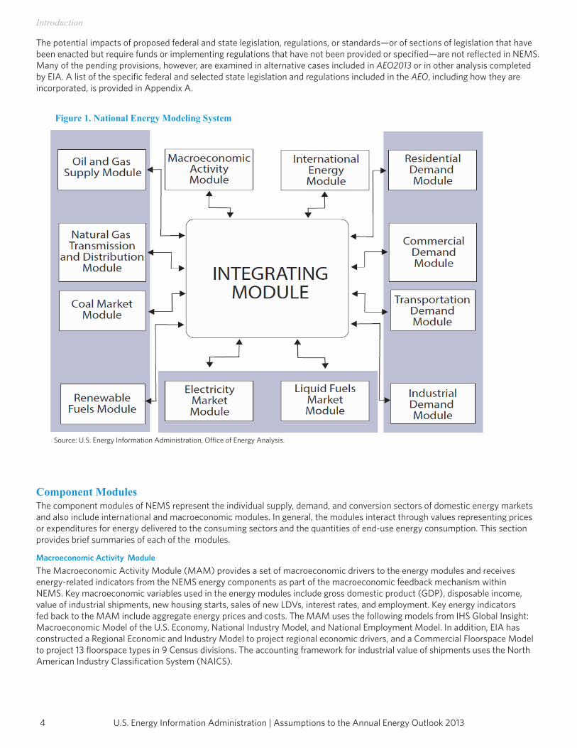
The National Energy Modeling SystemProjections in the AEO2013 are generated using the NEMS, developed and maintained by the Office of Energy Analysis of the U.S. Energy Information Administration (EIA). In addition to its use in developing the Annual Energy Outlook (AEO) projections, NEMS is also used to complete analytical studies for the U.S. Congress, the Executive Office of the President, other offices within the U.S. Department of Energy, and other Federal agencies. NEMS is also used by other nongovernment groups, such as the Electric Power Research Institute, Duke University, and Georgia Institute of Technology. In addition, the AEO projections are used by analysts and planners in other government agencies and nongovernment organizations.The projections in NEMS are developed with the use of a market-based approach, subject to regulations and standards. For each fuel and consuming sector, NEMS balances energy supply and demand, accounting for economic competition among the various energy fuels and sources. The time horizon of NEMS extends to 2040. To represent regional differences in energy markets, the component modules of NEMS function at the regional level: the 9 Census divisions for the end-use demand modules; production regions specific to oil, natural gas, and coal supply and distribution; 22 regions and subregions of the North American Electric Reliability Corporation for electricity; and 8 refining regions that are a subset of the 5 Petroleum Administration for Defense Districts (PADDs). Maps illustrating the regional formats used in each module are included in this report. Only selected regional results are presented in AEO2013, which predominantly focus on the national results. Complete regional and detailed results are available on the EIA Analyses and Projections Home Page (www.eia.gov/analysis/).NEMS is organized and implemented as a modular system (Figure 1). The modules represent each of the fuel supply markets, conversion sectors, and end-use consumption sectors of the energy system. The modular design also permits the use of the methodology and level of detail most appropriate for each energy sector. NEMS executes each of the component modules to solve for prices of energy delivered to end users and the quantities consumed, by product, region, and sector. The delivered fuel prices encompass all the activities necessary to produce, import, and transport fuels to end users. The information flows also include other data on such areas as economic activity, domestic production, and international petroleum supply. NEMS calls each supply, conversion, and end-use demand module in sequence until the delivered prices of energy and the quantities demanded have converged within tolerance, thus achieving an economic equilibrium of supply and demand in the consuming sectors. A solution is reached for each year from 2012 through 2040. Other variables, such as petroleum product imports, crude oil imports, and several macroeconomic indicators, also are evaluated for convergence. Each NEMS component represents the impacts and costs of legislation and environmental regulations that affect that sector. NEMS accounts for all combustion-related carbon dioxide (CO2) emissions, as well as emissions of sulfur dioxide (SO2), nitrogen oxides (NOx), and mercury from the electricity generation sector.The integrating module of NEMS controls the execution of each of the component modules. To facilitate modularity, the components do not pass information to each other directly but communicate through a central data storage location. This modular design provides the capability to execute modules individually, thus allowing decentralized development of the system and independent analysis and testing of individual modules. This modularity allows use of the methodology and level of detail most appropriate for each energy sector. NEMS solves by calling each supply, conversion, and end-use demand module in sequence until the delivered prices of energy and the quantities demanded have converged within tolerance, thus achieving an economic equilibrium of supply and demand in the consuming sectors. Solution is reached annually through the projection horizon. Other variables are also evaluated for convergence such as petroleum product imports, crude oil imports, and several macroeconomic indicators.The version of NEMS used for AEO2013 generally represents current legislation and environmental regulations, including recent government actions for which implementing regulations were available as of September 30, 2012, such as: the new light-duty vehicle (LDV) greenhouse gas (GHG) and corporate average fuel economy (CAFE) standards for model years 2017 to 2025 [3] released in October 2012; the Clean Air Interstate Rule (CAIR), which was reinstated as binding legislation after the Cross- State Air Pollution Rule (CSAPR) [4] was vacated on August 21, 2012; updated handling of the U.S. Environmental Protection Agency’s (EPA) National Emissions Standards for Hazardous Air Pollutants for industrial boilers and process heaters [5] based on regulations released in March 2011; the Mercury and Air Toxics Standards [6] issued by the EPA in December 2011; California’s cap-and-trade program authorized by Assembly Bill 32 (AB 32), the Global Warming Solutions Act of 2006 [7], issued in September 2006; and the California Low Carbon Fuel Standard (LCFS) [8] finalized in January 2010.
U.S. Energy Information Administration | Assumptions to the Annual Energy Outlook 20134
Introduction
The potential impacts of proposed federal and state legislation, regulations, or standards—or of sections of legislation that have been enacted but require funds or implementing regulations that have not been provided or specified—are not reflected in NEMS. Many of the pending provisions, however, are examined in alternative cases included in AEO2013 or in other analysis completed by EIA. A list of the specific federal and selected state legislation and regulations included in the AEO, including how they are incorporated, is provided in Appendix A.
Component ModulesThe component modules of NEMS represent the individual supply, demand, and conversion sectors of domestic energy markets and also include international and macroeconomic modules. In general, the modules interact through values representing prices or expenditures for energy delivered to the consuming sectors and the quantities of end-use energy consumption. This section provides brief summaries of each of the modules.
Macroeconomic Activity ModuleThe Macroeconomic Activity Module (MAM) provides a set of macroeconomic drivers to the energy modules and receives energy-related indicators from the NEMS energy components as part of the macroeconomic feedback mechanism within NEMS. Key macroeconomic variables used in the energy modules include gross domestic product (GDP), disposable income, value of industrial shipments, new housing starts, sales of new LDVs, interest rates, and employment. Key energy indicators fed back to the MAM include aggregate energy prices and costs. The MAM uses the following models from IHS Global Insight: Macroeconomic Model of the U.S. Economy, National Industry Model, and National Employment Model. In addition, EIA has constructed a Regional Economic and Industry Model to project regional economic drivers, and a Commercial Floorspace Model to project 13 floorspace types in 9 Census divisions. The accounting framework for industrial value of shipments uses the North American Industry Classification System (NAICS).
Source: U.S. Energy Information Administration, Office of Energy Analysis.
Figure 1. National Energy Modeling System

5U.S. Energy Information Administration | Assumptions to the Annual Energy Outlook 2013
Introduction
International Energy ModuleThe International Energy Module (IEM) uses assumptions of economic growth and expectations of future U.S. and world petroleum and other liquids production and consumption, by year, to project the interaction of U.S. and international petroleum and other liquids markets. The IEM computes Brent and West Texas Intermediate (WTI) prices, provides a world crude-like liquids supply curve, and generates a worldwide oil supply/demand balance for each year of the projection period. The supply-curve calculations are based on historical market data and a world oil supply/demand balance, which is developed from reduced-form models of international petroleum and other liquids supply and demand, current investment trends in exploration and development, and long-term resource economics by country and territory. The oil production estimates include both petroleum and other liquids supply recovery technologies. The IEM also provides, for each year of the projection period, endogenous and exogenous assumptions for petroleum products for import and export in the United States. In interacting with the rest of NEMS, the IEM changes Brent and WTI prices in response to changes in expected production and consumption of crude oil and other liquids in the United States.
Residential and Commercial Demand ModulesThe Residential Demand Module projects energy consumption in the residential sector by Census division, housing type, and end use, based on delivered energy prices, the menu of equipment available, the availability of renewable sources of energy, and changes in the housing stock. The Commercial Demand Module projects energy consumption in the commercial sector by Census division, building type, and category of end use, based on delivered prices of energy, availability of renewable sources of energy, and changes in commercial floorspace. Both modules estimate the equipment stock for the major end-use services, incorporating assessments of advanced technologies, representations of renewable energy technologies, and the effects of both building shell and appliance standards. The modules also include projections of distributed generation. The Commercial Demand Module also incorporates combined heat and power (CHP) technology. Both modules incorporate changes to “normal” heating and cooling degree-days by Census division, based on a 30-year historical trend and on state-level population projections. The Residential Demand Module projects an increase in the average square footage of both new construction and existing structures, based on trends in new construction and remodeling.
Industrial Demand ModuleThe Industrial Demand Module (IDM) projects the consumption of energy for heat and power, as well as the consumption of feedstocks and raw materials in each of 21 industry groups, subject to the delivered prices of energy and macroeconomic estimates of employment and the value of shipments for each industry. As noted in the description of the MAM, the representation of industrial activity in NEMS is based on the NAICS. The industries are classified into three groups—energy-intensive manufacturing, non-energy-intensive manufacturing, and nonmanufacturing. Seven of eight energy-intensive manufacturing industries are modeled in the IDM, including energy-consuming components for boiler/steam/cogeneration, buildings, and process/assembly use of energy. Energy demand for petroleum and other liquids refining (the eighth energy-intensive manufacturing industry) is modeled in the Liquid Fuels Market Module (LFMM) as described below, but the projected consumption is reported under the industrial totals. There are several updates and upgrades in the representations of select industries. AEO2013 includes an upgraded representation for the aluminum industry. Instead of assuming that technological development for a particular process occurs on a predetermined or exogenous path based on engineering judgment, these upgrades allow IDM technological change to be modeled endogenously, while using more detailed process representation. The upgrade allows for explicit technological change, and therefore energy intensity, to respond to economic, regulatory, and other conditions. The combined cement and lime industry was upgraded in the Annual Energy Outlook 2012 (AEO2012). For subsequent AEOs other energy-intensive industries will be similarly upgraded. The bulk chemicals model has been enhanced in several respects: baseline natural gas liquids (NGL) feedstock data were aligned with Manufacturing Energy Consumption Survey 2006 data; an updated propane pricing mechanism reflecting natural gas price influences was used to allow for price competition between liquid petroleum gases feedstock and petroleum-based (naphtha) feedstock; and propylene supplied by the refining industry is now specifically accounted for in the LFMM. Nonmanufacturing models were significantly revised as well. The construction and mining models were augmented to better reflect NEMS assumptions regarding energy efficiencies in (off-road) vehicles and buildings, as well as coal, oil, and natural gas extraction productivity. The agriculture model was similarly augmented in AEO2012. The IDM also includes a generalized representation of CHP. The methodology for CHP systems simulates the utilization of installed CHP systems based on historical utilization rates and is driven by end-use electricity demand. To evaluate the economic benefits of additional CHP capacity, the model also includes an appraisal incorporating historical capacity factors and regional acceptance rates for new CHP facilities.

U.S. Energy Information Administration | Assumptions to the Annual Energy Outlook 20136
Introduction
There are also enhancements to the IDM to account for regulatory changes. This includes California’s AB 32 that allows for representation of a cap-and-trade program developed as part of California’s GHG reduction goals for 2020. Another regulatory update is included for the handling of National Emissions Standards for Hazardous Air Pollutants for industrial boilers, to address the maximum degree of emission reduction using maximum achievable control technology.
Transportation Demand ModuleThe Transportation Demand Module projects consumption of energy by mode and fuel—including petroleum products, electricity, methanol, ethanol, compressed natural gas (CNG), liquefied natural gas (LNG), and hydrogen—in the transportation sector, subject to delivered energy prices, macroeconomic variables such as GDP, and other factors such as technology adoption. The Transportation Demand Module includes legislation and regulations, such as the Energy Policy Act of 2005 (EPACT2005), the Energy Improvement and Extension Act of 2008 (EIEA2008), and the American Recovery and Reinvestment Act of 2009 (ARRA2009), which contain tax credits for the purchase of alternatively fueled vehicles. Representations of LDV CAFE and GHG emissions standards, HDV fuel consumption and GHG emissions standards, and biofuels consumption reflect standards enacted by NHTSA and the EPA, as well as provisions in the Energy Independence and Security Act of 2007 (EISA2007). The air transportation component of the Transportation Demand Module represents air travel in domestic and foreign markets and includes the industry practice of parking aircraft in both domestic and international markets to reduce operating costs, as well as the movement of aging aircraft from passenger to cargo markets. For passenger travel and air freight shipments, the module represents regional fuel use and travel demand for three aircraft types: regional, narrow-body, and wide-body. An infrastructure constraint, which is also modeled, can potentially limit overall growth in passenger and freight air travel to levels commensurate with industry-projected infrastructure expansion and capacity growth. The Transportation Demand Module projects energy consumption for freight and passenger rail and marine vessels by mode and fuel, subject to macroeconomic variables such as the value and type of industrial shipments.
Electricity Market ModuleThere are three primary submodules of the Electricity Market Module (EMM)—capacity planning, fuel dispatching, and finance and pricing. The capacity expansion submodule uses the stock of existing generation capacity, the cost and performance of future generation capacity, expected fuel prices, expected financial parameters, expected electricity demand, and expected environmental regulations to project the optimal mix of new generation capacity that should be added in future years. The fuel dispatching submodule uses the existing stock of generation equipment types, their operation and maintenance costs and performance, fuel prices to the electricity sector, electricity demand, and all applicable environmental regulations to determine the least-cost way to meet that demand. The submodule also determines transmission and pricing of electricity. The finance and pricing submodule uses capital costs, fuel costs, macroeconomic parameters, environmental regulations, and load shapes to estimate generation costs for each technology. All specifically identified options promulgated by the EPA for compliance with the Clean Air Act Amendments of 1990 are explicitly represented in the capacity expansion and dispatch decisions. All financial incentives for power generation expansion and dispatch specifically identified in EPACT2005 have been implemented. Several States, primarily in the northeast, have enacted air emission regulations for CO2 that affect the electricity generation sector, and those regulations are represented in AEO2013. The AEO2013 Reference case also imposes a limit on CO2 emissions for specific covered sectors, including the electric power sector, in California, as represented in California’s AB 32. The AEO2013 Reference case reinstates the CAIR after the court vacated CSAPR in August 2012. CAIR incorporates a cap and trade program for annual emissions of SO2 and annual and seasonal emissions of NOx from fossil power plants. Reductions in mercury emissions from coal- and oil-fired power plants also are reflected through the inclusion of the Mercury and Air Toxics Standards for power plants, finalized by the EPA on December 16, 2011. Although currently there is no Federal legislation in place that restricts GHG emissions, regulators and the investment community have continued to push energy companies to invest in technologies that are less GHG-intensive. The trend is captured in the AEO2013 Reference case through a 3-percentage-point increase in the cost of capital, when evaluating investments in new coal-fired power plants, new coal-to-liquids (CTL) plants without carbon capture and storage, and pollution control retrofits.
Renewable Fuels ModuleThe Renewable Fuels Module (RFM) includes submodules representing renewable resource supply and technology input information for central-station, grid-connected electricity generation technologies, including conventional hydroelectricity, biomass (dedicated biomass plants and co-firing in existing coal plants), geothermal, landfill gas, solar thermal electricity, solar photovoltaics, and both onshore and offshore wind energy. The RFM contains renewable resource supply estimates representing the regional opportunities for renewable energy development. Investment tax credits (ITCs) for renewable fuels are incorporated, as currently enacted, including a permanent 10-percent ITC for business investment in solar energy (thermal nonpower uses
7U.S. Energy Information Administration | Assumptions to the Annual Energy Outlook 2013
Introduction
as well as power uses) and geothermal power (available only to those projects not accepting the production tax credit [PTC] for geothermal power). In addition, the module reflects the increase in the ITC to 30 percent for solar energy systems installed before January 1, 2017. The extension of the credit to individual homeowners under EIEA2008 is reflected in the Residential and Commercial Demand Modules. PTCs for wind, geothermal, landfill gas, and some types of hydroelectric and biomass-fueled plants also are represented, based on the laws in effect on October 31, 2012. They provide a credit of up to 2.2 cents per kilowatthour for electricity produced in the first 10 years of plant operation. For AEO2013, new wind plants coming on line before January 1, 2013, are eligible to receive the PTC; other eligible plants must be in service before January 1, 2014. The law has subsequently been amended to extend the PTC for wind by an additional year. Furthermore, eligible plants of any type will qualify if construction begins prior to the expiration date, regardless of when the plant enters commercial service. This change was made after the completion of AEO2013 and is not reflected in the analysis. As part of ARRA2009, plants eligible for the PTC may instead elect to receive a 30-percent ITC or an equivalent direct grant. AEO2013 also accounts for new renewable energy capacity resulting from state renewable portfolio standard programs, mandates, and goals.
Oil and Gas Supply ModuleThe Oil and Gas Supply Module represents domestic crude oil and natural gas supply within an integrated framework that captures the interrelationships among the various sources of supply—onshore, offshore, and Alaska—by all production techniques, including natural gas recovery from coalbeds and low-permeability formations of sandstone and shale. The framework analyzes cash flow and profitability to compute investment and drilling for each of the supply sources, based on the prices for crude oil and natural gas, the domestic recoverable resource base, and the state of technology. Oil and natural gas production activities are modeled for 12 supply regions, including 6 onshore, 3 offshore, and 3 Alaskan regions. The Onshore Lower 48 Oil and Gas Supply Submodule evaluates the economics of future exploration and development projects for crude oil and natural gas at the play level. Crude oil resources include conventional, structurally reservoired resources as well as highly fractured continuous zones, such as the Austin chalk and Bakken shale formations. Production potential from advanced secondary recovery techniques (such as infill drilling, horizontal continuity, and horizontal profile) and enhanced oil recovery (such as CO2 flooding, steam flooding, polymer flooding, and profile modification) are explicitly represented. Natural gas resources include high-permeability carbonate and sandstone, tight gas, shale gas, and coalbed methane. Domestic crude oil production quantities are used as inputs to the LFMM in NEMS for conversion and blending into refined petroleum products. Supply curves for natural gas are used as inputs to the Natural Gas Transmission and Distribution Module (NGTDM) for determining natural gas wellhead prices and domestic production.
Natural Gas Transmission and Distribution ModuleThe NGTDM represents the transmission, distribution, and pricing of natural gas, subject to end-use demand for natural gas and the availability of domestic natural gas and natural gas traded on the international market. The module tracks the flows of natural gas and determines the associated capacity expansion requirements in an aggregate pipeline network, connecting the domestic and foreign supply regions with 12 Lower 48 U.S. demand regions. The 12 Lower 48 regions align with the 9 Census divisions, with three subdivided, and Alaska handled separately. The flow of natural gas is determined for both a peak and off-peak period in the year, assuming a historically based seasonal distribution of natural gas demand. Key components of pipeline and distributor tariffs are included in separate pricing algorithms. An algorithm is included to project the addition of CNG retail fueling capability. The module also accounts for foreign sources of natural gas, including pipeline imports and exports to Canada and Mexico, as well as LNG imports and exports.
Liquids Fuels Market ModuleThe LFMM projects prices of petroleum products, crude oil and product import activity, as well as domestic refinery operations, subject to demand for petroleum products, availability and price of imported petroleum, and domestic production of crude oil, NGL, and biofuels—ethanol, biodiesel, biomass-to-liquids (BTL), CTL, gas-to-liquids (GTL), and coal-and-biomass-to-liquids (CBTL). Costs, performance, and first dates of commercial availability for the advanced liquid fuels technologies [9] are reviewed and updated annually. The module represents refining activities in eight domestic U.S. regions, and a Maritime Canada/Caribbean refining region (created to represent short-haul international refineries that predominantly serve U.S. markets). In order to better represent policy, import/export patterns, and biofuels production, the eight U.S. regions were defined by subdividing three of the five U.S. PADDs. All nine refining regions are defined below:
Region 1. PADD I – East Coast Region 2. PADD II – Interior Region 3. PADD II – Great Lakes
U.S. Energy Information Administration | Assumptions to the Annual Energy Outlook 20138
Introduction
Region 4. PADD III – Gulf Coast Region 5. PADD III – Interior Region 6. PADD IV – Mountain Region 7. PADD V – California Region 8. PADD V – Other Region 9. Maritime Canada/Caribbean
The capacity expansion submodule uses the stock of existing generation capacity, the cost and performance of future generation capacity, expected fuel prices, expected financial parameters, expected electricity demand, and expected environmental regulations to project the optimal mix of new generation capacity that should be added in future years. The LFMM models the costs of automotive fuels, such as conventional and reformulated gasoline, and includes production of biofuels for blending in gasoline and diesel. Fuel ethanol and biodiesel are included in the LFMM, because they are commonly blended into petroleum products. The module allows ethanol blending into gasoline at 10 percent by volume, 15 percent by volume (E15) in states that lack explicit language capping ethanol volume or oxygen content, and up to 85 percent by volume (E85) for use in flex-fuel vehicles. Crude and refinery product imports are represented by supply curves defined by the NEMS IEM. Products also can be imported from refining region 9 (Maritime Canada/Caribbean). Refinery product exports are provided by the IEM. Capacity expansion of refinery process units and nonpetroleum liquid fuels production facilities is also modeled in the LFMM. The model uses current liquid fuels production capacity, the cost and performance of each production unit, expected fuel and feedstock costs, expected financial parameters, expected liquid fuels demand, and relevant environmental policies to project the optimal mix of new capacity that should be added in the future. The LFMM includes representation of the renewable fuels standard (RFS) specified in EISA2007, which mandates the use of 36 billion gallons of ethanol equivalent renewable fuel by 2022. Both domestic and imported biofuels count toward the RFS. Domestic ethanol production is modeled for three feedstock categories: corn, cellulosic plant materials, and advanced feedstock materials. Starch-based ethanol plants are numerous (more than 190 are now in operation, with a total maximum sustainable nameplate capacity of more than 14 billion gallons annually), and they are based on a well-known technology that converts starch and sugar into ethanol. Ethanol from cellulosic sources is a new technology with only a few small pilot plants in operation. Ethanol from advanced feedstocks—produced at ethanol refineries that ferment and distill grains other than corn, and reduce GHG emissions by at least 50 percent—is also a new technology modeled in the LFMM. Fuels produced by Fischer-Tropsch synthesis and through a pyrolysis process are also modeled in the LFMM, based on their economics relative to competing feedstocks and products. The five processes modeled are CTL, CBTL, GTL, BTL, and pyrolysis. Two California-specific policies are also represented in the LFMM: the LCFS and the AB 32 cap-and-trade program. The LCFS requires the carbon intensity (amount of GHG per unit of energy) of transportation fuels sold for use in California to decrease according to a schedule published by the California Air Resources Board. California’s AB 32 cap-and-trade program is established to help California achieve its goal of reducing CO2 emissions to 1990 levels by 2020. Working with other NEMS modules (IDM, EMM and Emissions Policy Module), the LFMM provides emissions allowances and actual emissions of CO2 from California refineries, and NEMS provides the mechanism (carbon price) to trade allowances such that the total CO2 emissions cap is met.
Coal Market ModuleThe Coal Market Module (CMM) simulates mining, transportation, and pricing of coal, subject to end-use demand for coal differentiated by heat and sulfur content. U.S. coal production is represented in the CMM by 41 separate supply curves— differentiated by region, mine type, coal rank, and sulfur content. The coal supply curves respond to capacity utilization of mines, mining capacity, labor productivity, and factor input costs (mining equipment, mining labor, and fuel requirements). Projections of U.S. coal distribution are determined by minimizing the cost of coal supplied, given coal demands by region and sector; environmental restrictions; and accounting for minemouth prices, transportation costs, and coal supply contracts. Over the projection period, coal transportation costs in the CMM vary in response to changes in the cost of rail investments.The CMM produces projections of U.S. steam and metallurgical coal exports an dimports in the context of world coal trade, determining the pattern of world coal trade flows that minimizes production and transportation costs while meeting a specified set of regional world coal import demands, subject to constraints on export capacities and trade flows. The international coal market component of the module computes trade in 3 types of coal for 17 export regions and 20 import regions U.S. coal production and distribution are computed for 14 supply regions and 16 demand regions.
9U.S. Energy Information Administration | Assumptions to the Annual Energy Outlook 2013
Introduction
Annual Energy Outlook 2013 casesIn preparing projections for AEO2013, EIA evaluated a wide range of trends and issues that could have major implications for U.S. energy markets between now and 2040. Besides the Reference case, AEO2013 presents detailed results for five alternative cases that differ from each other due to fundamental assumptions concerning the domestic economy and world oil market conditions. These alternative cases include the following:Economic Growth - • In the Reference case, population grows by 0.9 percent per year, nonfarm employment by 1.0 percent per year, and labor
productivity by 1.9 percent per year from 2011 to 2040. Economic output as measured by real GDP increases by 2.5 percent per year from 2011 through 2040, and growth in real disposable income per capita averages 1.4 percent per year.
• The Low Economic Growth case assumes lower growth rates for population (0.8 percent per year) and labor productivity (1.4 percent per year), resulting in lower nonfarm employment (0.8 percent per year), higher prices and interest rates, and lower growth in industrial output. In the Low Economic Growth case, economic output as measured by real GDP increases by 1.9 percent per year from 2011 through 2040, and growth in real disposable income per capita averages 1.2 percent per year.
• The High Economic Growth case assumes higher growth rates for population (1.0 percent per year) and labor productivity (2.1 percent per year), resulting in higher nonfarm employment (1.1 percent per year). With higher productivity gains and employment growth, inflation and interest rates are lower than in the Reference case, and consequently economic output grows at a higher rate (2.9 percent per year) than in the Reference case (2.5 percent). Disposable income per capita grows by 1.6 percent per year, compared with 1.4 percent in the Reference case.
Price Cases – For AEO2013, the benchmark oil price is being re-characterized to represent Brent crude oil instead of WTI crude oil. This change, which is being made to better reflect the marginal price refineries pay for imported light, sweet crude oil, used to produce petroleum product for consumers.. EIA will continue to report the WTI price, as it is a critical reference point for evaluation of the growing production in the mid-continent. EIA will also continue to report the Imported Refiner Acquisition Cost (IRAC). The historical record shows substantial variability in oil prices, and there is arguably even more uncertainty about future prices in the long term. AEO2013 considers three oil price cases (Reference, Low Oil Price, and High Oil Price) to allow an assessment of alternative views on the future course of oil prices. The Low and High Oil Price cases reflect a wide range of potential price paths, resulting from variation in demand by countries outside the Organization for Economic Cooperation and Development (OECD) for petroleum and other liquid fuels due to different levels of economic growth. The Low and High Oil Price cases also reflect different assumptions about decisions by members of the Organization of the Petroleum Exporting Countries (OPEC) regarding the preferred rate of oil production and about the future finding and development costs and accessibility to conventional structurally reservoired oil resources outside the United States.• In the Reference case, real oil prices (in 2011 dollars) rise from $109 per barrel in 2011 to $163 per barrel in 2040. The
Reference case represents EIA’s current judgment regarding exploration and development costs and accessibility of oil resources. It also assumes that OPEC producers will choose to maintain their share of the market and will schedule investments in incremental production capacity so that OPEC’s oil production will represent between 40 and 43 percent of the world’s total petroleum and other liquids production over the projection period.
• In the Low Oil Price case, crude oil prices are $75 per barrel (2011 dollars) in 2040. The low price results from lower demand for petroleum and other liquid fuels in the non-OECD nations. Lower demand is derived from lower economic growth relative to the Reference case. In this case, GDP growth in the non-OECD countries is lower on average relative to the Reference case in each projection year, beginning in 2013. The OECD projections are affected only by the price impact. On the supply side, OPEC countries increase their oil production to obtain a 49-percent share of total world petroleum and other liquids production in 2040, and oil resources outside the United States are more accessible and/or less costly to produce (as a result of technology advances, more attractive fiscal regimes, or both) than in the Reference case.
• In the High Oil Price case, oil prices reach about $237 per barrel (2011 dollars) in 2040. The high prices result from higher demand for petroleum and other liquid fuels in the non-OECD nations. Higher demand is measured by higher economic growth relative to the Reference case. In this case, GDP growth in the non-OECD countries is higher on average relative to the Reference case in each projection year, beginning in 2013. The OECD projections are affected only by the price impact. On the supply side, OPEC countries reduce their market share to between 37 and 40 percent and oil resources outside the United States are less accessible and/or more costly to produce than in the Reference case.
In addition to these cases, 22 additional alternative cases presented in Table 1.1 explore the impact of changing key assumptions on individual sectors.
U.S. Energy Information Administration | Assumptions to the Annual Energy Outlook 201310
Introduction
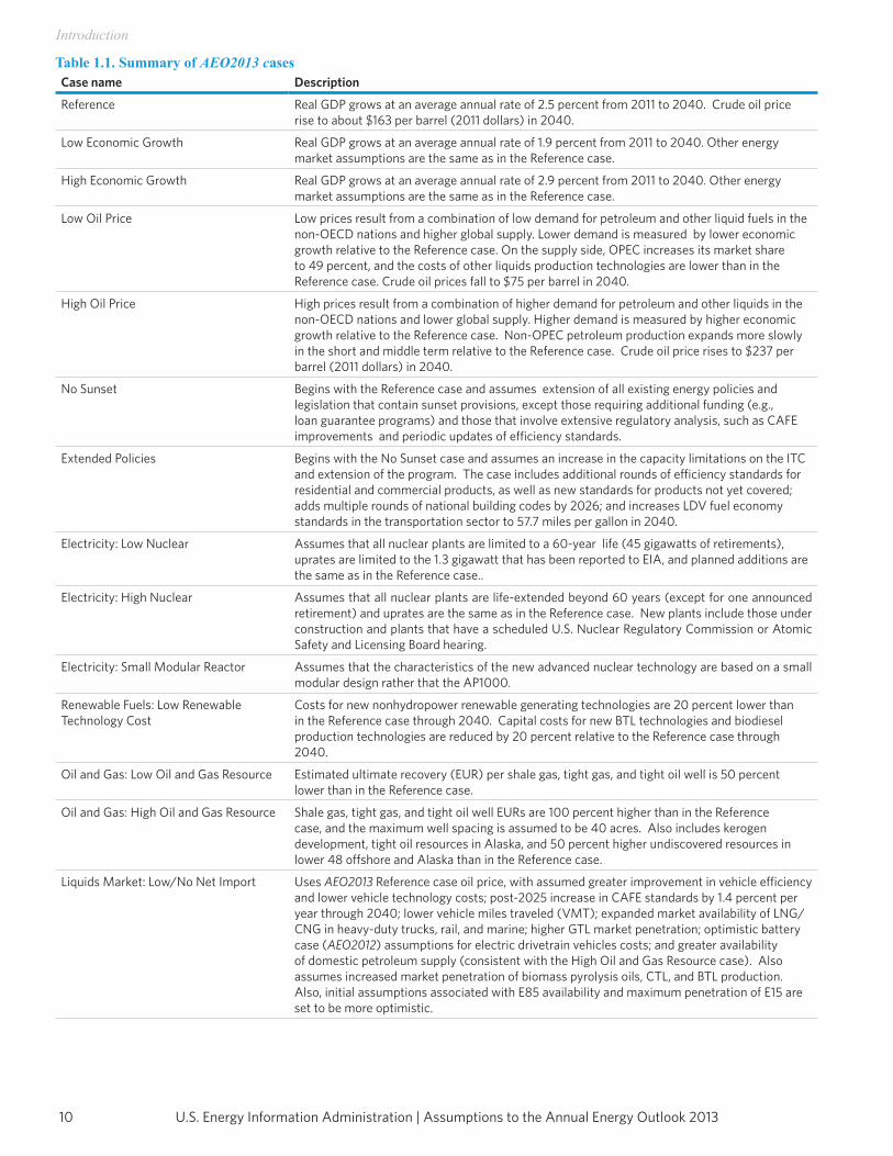
Table 1.1. Summary of AEO2013 casesCase name Description
Reference Real GDP grows at an average annual rate of 2.5 percent from 2011 to 2040. Crude oil price rise to about $163 per barrel (2011 dollars) in 2040.
Low Economic Growth Real GDP grows at an average annual rate of 1.9 percent from 2011 to 2040. Other energy market assumptions are the same as in the Reference case.
High Economic Growth Real GDP grows at an average annual rate of 2.9 percent from 2011 to 2040. Other energy market assumptions are the same as in the Reference case.
Low Oil Price Low prices result from a combination of low demand for petroleum and other liquid fuels in the non-OECD nations and higher global supply. Lower demand is measured by lower economic growth relative to the Reference case. On the supply side, OPEC increases its market share to 49 percent, and the costs of other liquids production technologies are lower than in the Reference case. Crude oil prices fall to $75 per barrel in 2040.
High Oil Price High prices result from a combination of higher demand for petroleum and other liquids in the non-OECD nations and lower global supply. Higher demand is measured by higher economic growth relative to the Reference case. Non-OPEC petroleum production expands more slowly in the short and middle term relative to the Reference case. Crude oil price rises to $237 per barrel (2011 dollars) in 2040.
No Sunset Begins with the Reference case and assumes extension of all existing energy policies and legislation that contain sunset provisions, except those requiring additional funding (e.g.,loan guarantee programs) and those that involve extensive regulatory analysis, such as CAFEimprovements and periodic updates of efficiency standards.
Extended Policies Begins with the No Sunset case and assumes an increase in the capacity limitations on the ITC and extension of the program. The case includes additional rounds of efficiency standards for residential and commercial products, as well as new standards for products not yet covered; adds multiple rounds of national building codes by 2026; and increases LDV fuel economy standards in the transportation sector to 57.7 miles per gallon in 2040.
Electricity: Low Nuclear Assumes that all nuclear plants are limited to a 60-year life (45 gigawatts of retirements), uprates are limited to the 1.3 gigawatt that has been reported to EIA, and planned additions are the same as in the Reference case..
Electricity: High Nuclear Assumes that all nuclear plants are life-extended beyond 60 years (except for one announced retirement) and uprates are the same as in the Reference case. New plants include those under construction and plants that have a scheduled U.S. Nuclear Regulatory Commission or Atomic Safety and Licensing Board hearing.
Electricity: Small Modular Reactor Assumes that the characteristics of the new advanced nuclear technology are based on a small modular design rather that the AP1000.
Renewable Fuels: Low Renewable Technology Cost
Costs for new nonhydropower renewable generating technologies are 20 percent lower than in the Reference case through 2040. Capital costs for new BTL technologies and biodiesel production technologies are reduced by 20 percent relative to the Reference case through 2040.
Oil and Gas: Low Oil and Gas Resource Estimated ultimate recovery (EUR) per shale gas, tight gas, and tight oil well is 50 percent lower than in the Reference case.
Oil and Gas: High Oil and Gas Resource Shale gas, tight gas, and tight oil well EURs are 100 percent higher than in the Reference case, and the maximum well spacing is assumed to be 40 acres. Also includes kerogen development, tight oil resources in Alaska, and 50 percent higher undiscovered resources in lower 48 offshore and Alaska than in the Reference case.
Liquids Market: Low/No Net Import Uses AEO2013 Reference case oil price, with assumed greater improvement in vehicle efficiency and lower vehicle technology costs; post-2025 increase in CAFE standards by 1.4 percent per year through 2040; lower vehicle miles traveled (VMT); expanded market availability of LNG/CNG in heavy-duty trucks, rail, and marine; higher GTL market penetration; optimistic battery case (AEO2012) assumptions for electric drivetrain vehicles costs; and greater availability of domestic petroleum supply (consistent with the High Oil and Gas Resource case). Also assumes increased market penetration of biomass pyrolysis oils, CTL, and BTL production. Also, initial assumptions associated with E85 availability and maximum penetration of E15 are set to be more optimistic.
11U.S. Energy Information Administration | Assumptions to the Annual Energy Outlook 2013
Introduction
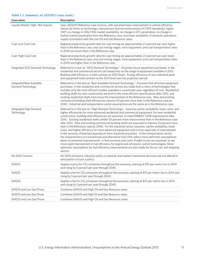
Table 1.1. Summary of AEO2013 cases (cont.)Case name Description
Liquids Market: High Net Imports Uses AEO2013 Reference case oil price, with assumed lower improvement in vehicle efficiency (driven by limits on technology improvement and non-enforcement of CAFE standards), higher VMT, no change in LNG/CNG market availability, no change in GTL penetration, no change in biofuel market penetration from the Reference case, and lower availability of domestic petroleum supply (consistent with the Low Oil and Gas Resource case).
Coal: Low Coal Cost Regional productivity growth rates for coal mining are approximately 2.5 percent per year higher than in the Reference case, and coal mining wages, mine equipment, and coal transportation rates in 2040 are lower than in the Reference case.
Coal: High Coal Cost Regional productivity growth rates for coal mining are approximately 2.5 percent per year lower than in the Reference case, and coal mining wages, mine equipment, and coal transportation rates in 2040 are higher than in the Reference case.
Integrated 2012 Demand Technology Referred to in text as “2012 Demand Technology.” Assumes future equipment purchases in the residential and commercial sectors are based only on the range of equipment available in 2012. Building shell efficiency is held constant at 2012 levels. Energy efficiency of new industrial plant and equipment held constant at the 2013 level over the projection period.
Integrated Best AvailableDemand Technology
Referred to in the text as “Best Available Demand Technology.” Assumes that all future equipment purchases in the residential and commercial sectors are made from a menu of technologies that includes only the most efficient models available in a particular year, regardless of cost. Residential building shells for new construction are built to the most efficient specifications after 2012, and existing residential shells have twice the improvement of the Reference case. New and existing commercial building shell efficiencies improve 50 percent more than in the Reference case by 2040. Industrial and transportation sector assumptions are the same as in the Reference case.
Integrated High DemandTechnology
Referred to in the text as “High Demand Technology.” Assumes earlier availability, lower costs, and higher efficiencies for more advanced residential and commercial equipment. For new residential construction, building shell efficiencies are assumed to meet ENERGY STAR requirements after 2016. Existing residential shells exhibit 50 percent more improvement than in the Reference case after 2012. New and existing commercial building shells are assumed to improve 25 percent more than in the Reference case by 2040. For the industrial sector, assumes earlier availability, lower costs, and higher efficiency for more advanced equipment and a more rapid rate of improvement in the recovery of biomass byproducts from industrial processes. In the transportation sector, the characteristics of conventional and alternative-fuel LDVs reflect more optimistic assumptions about incremental improvements in fuel economy and costs. Freight trucks are assumed to see more rapid improvement in fuel efficiency for engine and emissions control technologies. More optimistic assumptions for fuel efficiency improvements are also made for the air, rail, and shipping sectors.
No GHG Concern No GHG emissions reduction policy is enacted, and market investment decisions are not altered in anticipation of such a policy.
GHG10 Applies a price for CO2 emissions throughout the economy, starting at $10 per metric ton in 2014 and rising by 5 percent per year through 2040.
GHG15 Applies a fee for CO2 emissions throughout the economy, starting at $15 per metric ton in 2014 and rising by 5 percent per year through 2040.
GHG25 Applies a fee for CO2 emissions throughout the economy, starting at $25 per metric ton in 2014 and rising by 5 percent per year through 2040.
GHG10 and Low Gas Prices Combines GHG10 and High Oil and Gas Resource cases.
GHG15 and Low Gas Prices Combines GHG15 and High Oil and Gas Resource cases.
GHG25 and Low Gas Prices Combines GHG25 and High Oil and Gas Resource cases.

U.S. Energy Information Administration | Assumptions to the Annual Energy Outlook 201312
Introduction
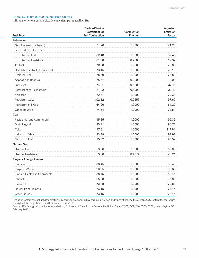
Carbon dioxide emissions CO2 emissions from energy use are dependent on the carbon content of the fossil fuel, the fraction of the fuel consumed in combustion, and the consumption of that fuel. The product of the carbon content at full combustion and the combustion fraction yields an adjusted CO2 factor for each fossil fuel. The emissions factors are expressed in millions of metric tons of carbon dioxide emitted per quadrillion Btu of energy use, or equivalently, in kilograms of CO2 per million Btu. The adjusted emissions factors are multiplied by the energy consumption of the fossil fuel to arrive at the CO2 emissions projections.For fuel uses of energy, all of the carbon is assumed to be oxidized, so the combustion fraction is equal to 1.0 (in keeping with international conventions). Previously, a small fraction of the carbon content of the fuel was assumed to remain unoxidized. The carbon in nonfuel use of energy, such as for asphalt and petrochemical feedstocks, is assumed to be sequestered in the product and not released to the atmosphere. For energy categories that are mixes of fuel and nonfuel uses, the combustion fractions are based on the proportion of fuel use. In calculating CO2 emissions for motor gasoline, the direct emissions from renewable blending stock (ethanol) is omitted. Similarly, direct emissions from biodiesel are omitted from reported CO2 emissions.Any CO2 emitted by biogenic renewable sources, such as biomass and alcohols, is considered balanced by the CO2 sequestration that occurred in its creation. Therefore, following convention, net emissions of CO2 from biogenic renewable sources are assumed to be zero in reporting energy-related CO2 emissions; however, to illustrate the potential for these emissions in the absence of any offsetting sequestration, as might occur under related land use change, the CO2 emissions from biogenic fuel use are calculated and reported separately.Table 1.2 presents the assumed CO2 coefficients at full combustion, the combustion fractions, and the adjusted CO2 emission factors used for AEO2013.
13U.S. Energy Information Administration | Assumptions to the Annual Energy Outlook 2013
Introduction
Table 1.2. Carbon dioxide emission factorsmillion metric tons carbon dioxide equivalent per quadrillion Btu
Fuel Type
Carbon Dioxide Coefficient at
Full CombustionCombustion
Fraction
Adjusted Emission
Factor
Petroleum
Gasoline (net of ethanol) 71.26 1.0000 71.26
Liquefied Petroleum Gas
Used as Fuel 62.48 1.0000 62.48
Used as Feedstock 61.60 0.2000 12.32
Jet Fuel 70.88 1.0000 70.88
Distillate Fuel (net of biodiesel) 73.15 1.0000 73.15
Residual Fuel 78.80 1.0000 78.80
Asphalt and Road Oil 75.61 0.0000 0.00
Lubricants 74.21 0.5000 37.11
Petrochemical Feedstocks 71.02 0.4099 29.11
Kerosene 72.31 1.0000 72.31
Petroleum Coke 102.12 0.9557 97.60
Petroleum Still Gas 64.20 1.0000 64.20
Other Industrial 74.54 1.0000 74.54
Coal
Residential and Commercial 95.35 1.0000 95.35
Metallurgical 93.71 1.0000 93.71
Coke 117.81 1.0000 117.81
Industrial Other 93.88 1.0000 93.98
Electric Utility1 95.52 1.0000 95.52
Natural Gas
Used as Fuel 53.06 1.0000 53.06
Used as Feedstocks 53.06 0.4374 23.21
Biogenic Energy Sources
Biomass 88.45 1.0000 88.45
Biogenic Waste 90.65 1.0000 90.65
Biofuels Heats and Coproducts 88.45 1.0000 88.45
Ethanol 65.88 1.0000 65.88
Biodiesel 73.88 1.0000 73.88
Liquids from Biomass 73.15 1.0000 73.15
Green Liquids 73.15 1.0000 73.15
1Emission factors for coal used for electricity generation are specified by coal supply region and types of coal, so the average CO2 content for coal varies throughout the projection. The 2009 average was 95.52.Source: U.S. Energy Information Administration, Emissions of Greenhouse Gases in the United States 2009, DOE/EIA-0573(2009), (Washington, DC, February 2010).

U.S. Energy Information Administration | Assumptions to the Annual Energy Outlook 201314
Introduction
Notes and sources[1] Energy Information Administration, Annual Energy Outlook 2013 (AEO2013), DOE/EIA-0383(2013), (Washington, DC, April 2013).[2] NEMS documentation reports are available on the EIA Homepage (www.eia.gov/analysis/model-documentation.cfm).[3] U.S. Environmental Protection Agency and National Highway Traffic Safety Administration, “2017 and Later Model Year Light- Duty Vehicle Greenhouse Gas Emissions and Corporate Average Fuel Economy Standards,” Federal Register, Vol. 77, No. 199, 40 CFR Parts 85, 86, and 600, and 49 CFR Parts 523, 531, 533, et al. (Washington, DC: October 15, 2012), website www. gpo. gov/fdsys/pkg/FR-2012-10-15/html/2012-21972.htm.[4] U.S. Environmental Protection Agency, “Cross-State Air Pollution Rule (CSAPR)” (Washington, DC: January 14, 2013), website http://epa.gov/airtransport. CSAPR was scheduled to begin on January 1, 2012; however, the U.S. Court of Appeals for the D.C. Circuit issued a stay delaying implementation while it addresses legal challenges to the rule that have been raised by several power companies and States. CSAPR is included in AEO2013 despite the stay, because the Court of Appeals had not made a final ruling at the time AEO2013 was published.[5] U.S. Congress, “Clean Air Act: Chapter 85—Air Pollution Prevention and Control,” 42 U.S.C. 7412 (2011), website www.gpo.gov/fdsys/pkg/USCODE-2011-title42/pdf/USCODE-2011-title42-chap85.pdf.[6] U.S. Environmental Protection Agency, “Mercury and Air Toxics Standards (MATS)” (Washington, DC: March 27, 2012),website www.epa.gov/mats.[7] California Environmental Protection Agency, Air Resources Board, “Assembly Bill No. 32: Global Warming Solutions Act” (Sacramento, CA: September 27, 2006), website www.arb.ca.gov/cc/ab32/ab32.htm.[8] California Environmental Protection Agency, Air Resources Board, “Low Carbon Fuel Standard Program” (Sacramento, CA: January 11, 2013), website www.arb.ca.gov/fuels/lcfs/lcfs.htm. U.S. Environmental Protection Agency, “Mercury and Air Toxics Standards,” website www.epa.gov/mats.[9] Alternative other liquids technologies include all biofuels technologies plus CTL and GTL.

Macroeconomic Activity Module

This page inTenTionally lefT blank
17U.S. Energy Information Administration | Assumptions to the Annual Energy Outlook 2013
Macroeconomic Activity Module
The Macroeconomic Activity Module (MAM) represents interactions between the U.S. economy and energy markets. The rate of growth of the economy, measured by the growth in gross domestic product (GDP), is a key determinant of growth in the demand for energy. Associated economic factors, such as interest rates and disposable income, strongly influence various elements of the supply and demand for energy. At the same time, reactions to energy markets by the aggregate economy, such as a slowdown in economic growth resulting from increasing energy prices, are also reflected in this module. A detailed description of the MAM is provided in the EIA publication, Model Documentation Report: Macroeconomic Activity Module (MAM) of the National Energy Modeling System, (2012), (Washington, DC, October 2012).
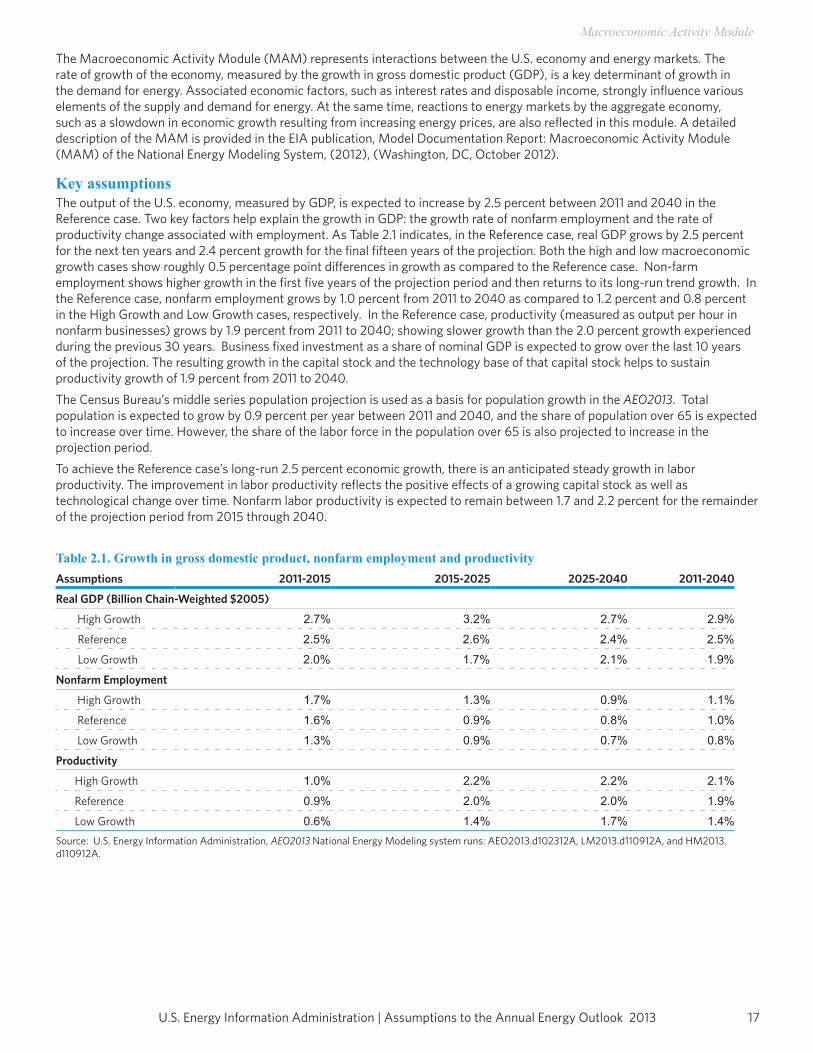
Key assumptionsThe output of the U.S. economy, measured by GDP, is expected to increase by 2.5 percent between 2011 and 2040 in the Reference case. Two key factors help explain the growth in GDP: the growth rate of nonfarm employment and the rate of productivity change associated with employment. As Table 2.1 indicates, in the Reference case, real GDP grows by 2.5 percent for the next ten years and 2.4 percent growth for the final fifteen years of the projection. Both the high and low macroeconomic growth cases show roughly 0.5 percentage point differences in growth as compared to the Reference case. Non-farm employment shows higher growth in the first five years of the projection period and then returns to its long-run trend growth. In the Reference case, nonfarm employment grows by 1.0 percent from 2011 to 2040 as compared to 1.2 percent and 0.8 percent in the High Growth and Low Growth cases, respectively. In the Reference case, productivity (measured as output per hour in nonfarm businesses) grows by 1.9 percent from 2011 to 2040; showing slower growth than the 2.0 percent growth experienced during the previous 30 years. Business fixed investment as a share of nominal GDP is expected to grow over the last 10 years of the projection. The resulting growth in the capital stock and the technology base of that capital stock helps to sustain productivity growth of 1.9 percent from 2011 to 2040.The Census Bureau’s middle series population projection is used as a basis for population growth in the AEO2013. Total population is expected to grow by 0.9 percent per year between 2011 and 2040, and the share of population over 65 is expected to increase over time. However, the share of the labor force in the population over 65 is also projected to increase in the projection period. To achieve the Reference case’s long-run 2.5 percent economic growth, there is an anticipated steady growth in labor productivity. The improvement in labor productivity reflects the positive effects of a growing capital stock as well as technological change over time. Nonfarm labor productivity is expected to remain between 1.7 and 2.2 percent for the remainder of the projection period from 2015 through 2040.
Table 2.1. Growth in gross domestic product, nonfarm employment and productivityAssumptions 2011-2015 2015-2025 2025-2040 2011-2040
Real GDP (Billion Chain-Weighted $2005)
High Growth 2.7% 3.2% 2.7% 2.9%
Reference 2.5% 2.6% 2.4% 2.5%
Low Growth 2.0% 1.7% 2.1% 1.9%
Nonfarm Employment
High Growth 1.7% 1.3% 0.9% 1.1%
Reference 1.6% 0.9% 0.8% 1.0%
Low Growth 1.3% 0.9% 0.7% 0.8%
Productivity
High Growth 1.0% 2.2% 2.2% 2.1%
Reference 0.9% 2.0% 2.0% 1.9%
Low Growth 0.6% 1.4% 1.7% 1.4%Source: U.S. Energy Information Administration, AEO2013 National Energy Modeling system runs: AEO2013.d102312A, LM2013.d110912A, and HM2013.d110912A.

U.S. Energy Information Administration | Assumptions to the Annual Energy Outlook 201318
Macroeconomic Activity ModuleTo reflect uncertainty in the projection of U.S. economic growth, the AEO2013 uses High and Low Economic Growth cases to project the possible impacts of alternative economic growth assumptions on energy markets. The High Economic Growth case incorporates higher population, labor force and productivity growth rates than the Reference case. Due to the higher productivity gains, inflation and interest rates are lower than the Reference case. Investment, disposable income and industrial production are greater. Economic output is projected to increase by 2.9 percent per year between 2011 and 2040. The Low Economic Growth case assumes lower population, labor force, and productivity gains, with resulting higher prices and interest rates and lower industrial output growth. In the Low Economic Growth case, economic output is expected to increase by 1.9 percent per year over the projection horizon.

International Energy Module

This page inTenTionally lefT blank
21U.S. Energy Information Administration | Assumptions to the Annual Energy Outlook 2013
International Energy Module
The LFMM International Energy Module (IEM) simulates the interaction between U.S. and global petroleum markets. It uses assumptions of economic growth and expectations of future U.S. and world crude-like liquids production and consumption to estimate the effects of changes in U.S. liquid fuels markets on the international petroleum market. For each year of the forecast, the LFMM IEM computes BRENT and WTI prices, provides a supply curve of world crude-like liquids, and generates a worldwide oil supply- demand balance with regional detail. The IEM also provides, for each year of the projection period, endogenous and exogenous assumptions for petroleum products for import and export in the United States.Changes in the oil price (BRENT) are computed in response to:
1. The difference between projected U.S. total crude-like liquids production and the expected U.S. total crude-like liquids production at the current oil price (estimated using the current oil price and the exogenous U.S. total crude-like liquids supply curve for each year).
and2. The difference between projected U.S. total crude-like liquids consumption and the expected U.S. total crude-like liquids
consumption at the current oil price (estimated using the current oil price and the exogenous U.S. total crude-like liquids demand curve).
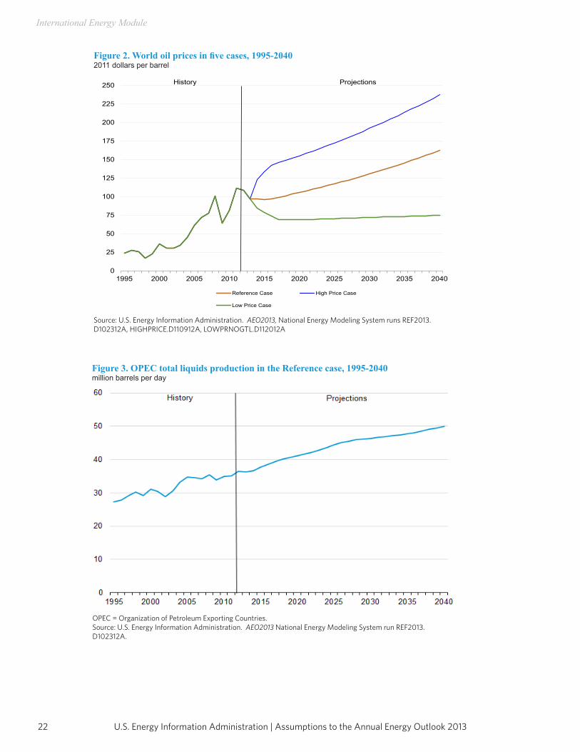
Key assumptionsThe level of oil production by OPEC is a key factor influencing the oil price projections incorporated into AEO2013. Non-OPEC production, worldwide regional economic growth rates and the associated regional demand for oil are additional factors affecting the world oil price.In the Reference case, real oil prices rise from a $109 per barrel (2011 dollars) in 2012 to $163 per barrel in 2040. The Reference case represents EIA’s current judgment regarding exploration and development costs and accessibility of oil resources. It also assumes that OPEC producers will choose to maintain their share of the market and will schedule investments in incremental production capacity so that OPEC’s oil production will represent about 42 percent of the world’s total petroleum and other liquids production over the projection period. In the Low Oil Price case, crude oil prices are $75 per barrel (2011 dollars) in 2040. In the Low Oil Price case, the low price results from lower demand for petroleum and other liquid fuels in the non-OECD nations. Lower demand is derived from lower economic growth relative to the Reference case. In this case, GDP growth in the non-OECD countries is 1.1 lower on average relative to Reference case in each projection year, beginning in 2013. The OECD projections are affected only by the price impact. On the supply side, OPEC countries increase their oil production to obtain a 43-percent share of total world petroleum and other liquids production, and oil resources outside the United States are more accessible and/or less costly to produce (as a result of technology advances, more attractive fiscal regimes, or both) than in the Reference case. In the High Oil Price case, oil prices reach about $237 per barrel (2011 dollars) in 2040. In the High Oil Price case, the high prices result from higher demand for petroleum and other liquid fuels in the non-OECD nations. Higher demand is measured by higher economic growth relative to the Reference case. In this case, GDP growth in the non-OECD countries is 0.6 percent higher on average relative to Reference case in each projection year, beginning in 2013. The OECD projections are affected only by the price impact. On the supply side, OPEC countries are assumed to reduce their market share slightly, and oil resources outside the United States are assumed to be less accessible and/or more costly to produce than in the Reference case.OPEC oil production in the Reference case is assumed to increase throughout the projection (Figure 3), at a rate that enables the organization to maintain an approximately constant market share over the projection period. OPEC is assumed to be an important source of additional production because its member nations hold a major portion of the world’s total reserves— exceeding 1200 billion barrels, about 73 percent of the world’s estimated total, at the beginning of 2012. [1] Despite investment from foreign sources, Iraq’s oil production is not assumed to maintain steady growth until after 2015 as infrastructure limitations as well as security and legislative issues are assumed to slow development for the next five years.Non-U.S., non-OPEC oil production projections in the AEO2013 are developed in two stages. Projections of liquids production before 2015 are based largely on a project-by-project assessment of major fields, including volumes and expected schedules, with consideration given to the decline rates of active projects, planned exploration and development activity, and country- specific geopolitical situations and fiscal regimes. Incremental production estimates from existing and new fields after 2015 are estimated based on country-specific consideration of economics and ultimate technically recoverable resource estimates. The non-OPEC production path for the Reference case is shown in Figure 4.
U.S. Energy Information Administration | Assumptions to the Annual Energy Outlook 201322
International Energy Module
Figure 2. World oil prices in five cases, 1995-20402011 dollars per barrel
Source: U.S. Energy Information Administration. AEO2013, National Energy Modeling System runs REF2013. D102312A, HIGHPRICE.D110912A, LOWPRNOGTL.D112012A
Figure 3. OPEC total liquids production in the Reference case, 1995-2040million barrels per day
OPEC = Organization of Petroleum Exporting Countries.Source: U.S. Energy Information Administration. AEO2013 National Energy Modeling System run REF2013. D102312A.
0
25
50
75
100
125
150
175
200
225
250
1995 2000 2005 2010 2015 2020 2025 2030 2035 2040
Reference Case High Price Case
Low Price Case
History Projections
23U.S. Energy Information Administration | Assumptions to the Annual Energy Outlook 2013
International Energy Module
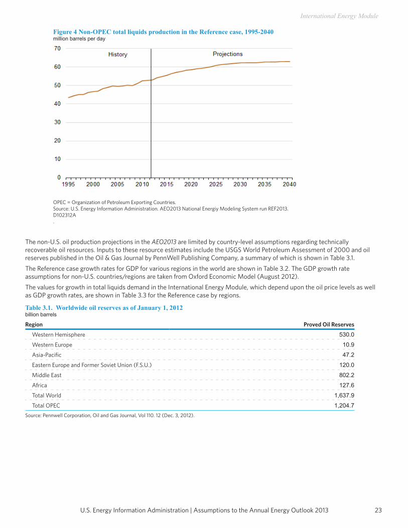
Figure 4 Non-OPEC total liquids production in the Reference case, 1995-2040million barrels per day
OPEC = Organization of Petroleum Exporting Countries.Source: U.S. Energy Information Administration. AEO2013 National Energiy Modeling System run REF2013. D102312A.
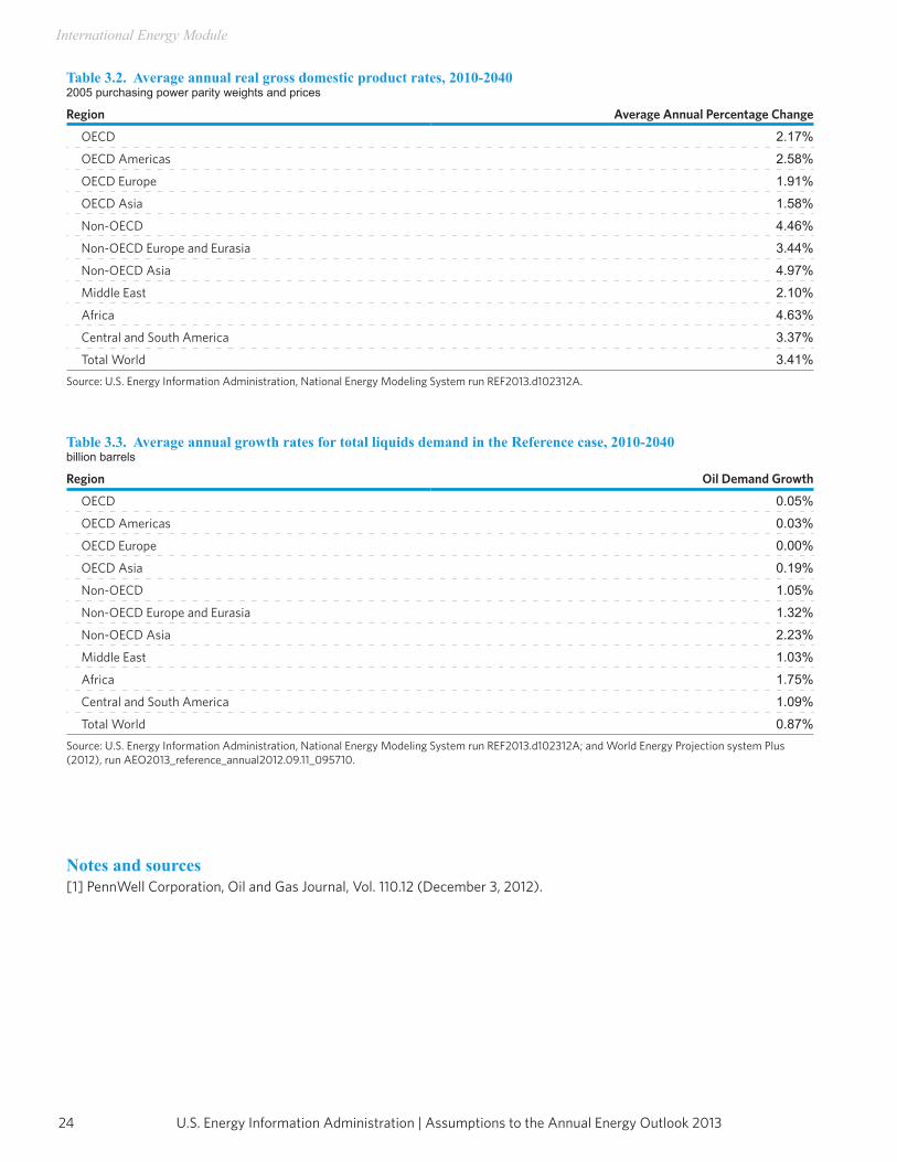
The non-U.S. oil production projections in the AEO2013 are limited by country-level assumptions regarding technically recoverable oil resources. Inputs to these resource estimates include the USGS World Petroleum Assessment of 2000 and oil reserves published in the Oil & Gas Journal by PennWell Publishing Company, a summary of which is shown in Table 3.1.The Reference case growth rates for GDP for various regions in the world are shown in Table 3.2. The GDP growth rate assumptions for non-U.S. countries/regions are taken from Oxford Economic Model (August 2012).The values for growth in total liquids demand in the International Energy Module, which depend upon the oil price levels as well as GDP growth rates, are shown in Table 3.3 for the Reference case by regions.
Table 3.1. Worldwide oil reserves as of January 1, 2012billion barrels
Region Proved Oil Reserves
Western Hemisphere 530.0
Western Europe 10.9
Asia-Pacific 47.2
Eastern Europe and Former Soviet Union (F.S.U.) 120.0
Middle East 802.2
Africa 127.6
Total World 1,637.9
Total OPEC 1,204.7Source: Pennwell Corporation, Oil and Gas Journal, Vol 110. 12 (Dec. 3, 2012).
U.S. Energy Information Administration | Assumptions to the Annual Energy Outlook 201324
International Energy Module
Table 3.2. Average annual real gross domestic product rates, 2010-2040 2005 purchasing power parity weights and prices
Region Average Annual Percentage Change
OECD 2.17%
OECD Americas 2.58%
OECD Europe 1.91%
OECD Asia 1.58%
Non-OECD 4.46%
Non-OECD Europe and Eurasia 3.44%
Non-OECD Asia 4.97%
Middle East 2.10%
Africa 4.63%
Central and South America 3.37%
Total World 3.41%Source: U.S. Energy Information Administration, National Energy Modeling System run REF2013.d102312A.
Table 3.3. Average annual growth rates for total liquids demand in the Reference case, 2010-2040billion barrels
Region Oil Demand Growth
OECD 0.05%
OECD Americas 0.03%
OECD Europe 0.00%
OECD Asia 0.19%
Non-OECD 1.05%
Non-OECD Europe and Eurasia 1.32%
Non-OECD Asia 2.23%
Middle East 1.03%
Africa 1.75%
Central and South America 1.09%
Total World 0.87%Source: U.S. Energy Information Administration, National Energy Modeling System run REF2013.d102312A; and World Energy Projection system Plus(2012), run AEO2013_reference_annual2012.09.11_095710.
Notes and sources[1] PennWell Corporation, Oil and Gas Journal, Vol. 110.12 (December 3, 2012).

Residential Demand Module

This page inTenTionally lefT blank

27U.S. Energy Information Administration | Assumptions to the Annual Energy Outlook 2013
Residential Demand Module
The NEMS Residential Demand Module projects future residential sector energy requirements based on projections of the number of households and the stock, efficiency, and intensity of energy-consuming equipment. The Residential Demand Module projections begin with a base year estimate of the housing stock, the types and numbers of energy-consuming appliances servicing the stock, and the “unit energy consumption” (UEC) by appliance (in million Btu per household per year). The projection process adds new housing units to the stock, determines the equipment installed in new units, retires existing housing units, and retires and replaces appliances. The primary exogenous drivers for the module are housing starts by type (single-family, multifamily and mobile homes) and by Census Division, and prices for each energy source for each of the nine Census Divisions (see Figure 5).The Residential Demand Module also requires projections of available equipment and their installed costs over the projection horizon. Over time, equipment efficiency tends to increase because of general technological advances and also because of Federal and/or State efficiency standards. As energy prices and available equipment change over the projection horizon, the module includes projected changes to the type and efficiency of equipment purchased as well as projected changes in the usage intensity of the equipment stock.
Figure 5. United States Census Divisions
Source: U.S. Energy Information Administration, Office of Energy Analysis.
Pacific
East South Central
South Atlantic
MiddleAtlantic
NewEngland
WestSouth
Central
WestNorth
Central EastNorth
CentralMountain
AK
WAMT
WYID
NVUT
CO
AZNM
TX
OK
IA
KS MOIL
IN
KY
TN
MS AL
FL
GA
SC
NC
WV
PANJ
MD
DE
NY
CT
VT ME
RIMA
NH
VA
WI
MI
OH
NE
SD
MNND
AR
LA
OR
CA
HI
Middle AtlanticNew England
East North CentralWest North Central
PacificWest South CentralEast South Central
South AtlanticMountain
U.S. Energy Information Administration | Assumptions to the Annual Energy Outlook 201328
Residential Demand Module
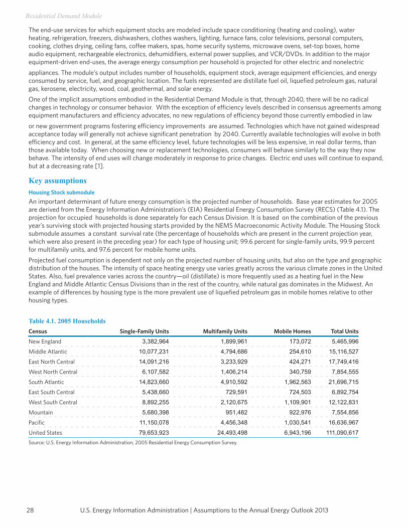
The end-use services for which equipment stocks are modeled include space conditioning (heating and cooling), water heating, refrigeration, freezers, dishwashers, clothes washers, lighting, furnace fans, color televisions, personal computers, cooking, clothes drying, ceiling fans, coffee makers, spas, home security systems, microwave ovens, set-top boxes, home audio equipment, rechargeable electronics, dehumidifiers, external power supplies, and VCR/DVDs. In addition to the major equipment-driven end-uses, the average energy consumption per household is projected for other electric and nonelectricappliances. The module’s output includes number of households, equipment stock, average equipment efficiencies, and energy consumed by service, fuel, and geographic location. The fuels represented are distillate fuel oil, liquefied petroleum gas, natural gas, kerosene, electricity, wood, coal, geothermal, and solar energy.One of the implicit assumptions embodied in the Residential Demand Module is that, through 2040, there will be no radical changes in technology or consumer behavior. With the exception of efficiency levels described in consensus agreements among equipment manufacturers and efficiency advocates, no new regulations of efficiency beyond those currently embodied in lawor new government programs fostering efficiency improvements are assumed. Technologies which have not gained widespread acceptance today will generally not achieve significant penetration by 2040. Currently available technologies will evolve in both efficiency and cost. In general, at the same efficiency level, future technologies will be less expensive, in real dollar terms, than those available today. When choosing new or replacement technologies, consumers will behave similarly to the way they now behave. The intensity of end uses will change moderately in response to price changes. Electric end uses will continue to expand, but at a decreasing rate [1].
Key assumptionsHousing Stock submoduleAn important determinant of future energy consumption is the projected number of households. Base year estimates for 2005 are derived from the Energy Information Administration’s (EIA) Residential Energy Consumption Survey (RECS) (Table 4.1). The projection for occupied households is done separately for each Census Division. It is based on the combination of the previous year’s surviving stock with projected housing starts provided by the NEMS Macroeconomic Activity Module. The Housing Stock submodule assumes a constant survival rate (the percentage of households which are present in the current projection year, which were also present in the preceding year) for each type of housing unit; 99.6 percent for single-family units, 99.9 percent for multifamily units, and 97.6 percent for mobile home units.Projected fuel consumption is dependent not only on the projected number of housing units, but also on the type and geographic distribution of the houses. The intensity of space heating energy use varies greatly across the various climate zones in the United States. Also, fuel prevalence varies across the country—oil (distillate) is more frequently used as a heating fuel in the New England and Middle Atlantic Census Divisions than in the rest of the country, while natural gas dominates in the Midwest. An example of differences by housing type is the more prevalent use of liquefied petroleum gas in mobile homes relative to other housing types.
Table 4.1. 2005 HouseholdsCensus Single-Family Units Multifamily Units Mobile Homes Total Units
New England 3,382,964 1,899,961 173,072 5,465,996
Middle Atlantic 10,077,231 4,794,686 254,610 15,116,527
East North Central 14,091,216 3,233,929 424,271 17,749,416
West North Central 6,107,582 1,406,214 340,759 7,854,555
South Atlantic 14,823,660 4,910,592 1,962,563 21,696,715
East South Central 5,438,660 729,591 724,503 6,892,754
West South Central 8,892,255 2,120,675 1,109,901 12,122,831
Mountain 5,680,398 951,482 922,976 7,554,856
Pacific 11,150,078 4,456,348 1,030,541 16,636,967
United States 79,653,923 24,493,498 6,943,196 111,090,617Source: U.S. Energy Information Administration, 2005 Residential Energy Consumption Survey.
29U.S. Energy Information Administration | Assumptions to the Annual Energy Outlook 2013
Residential Demand Module
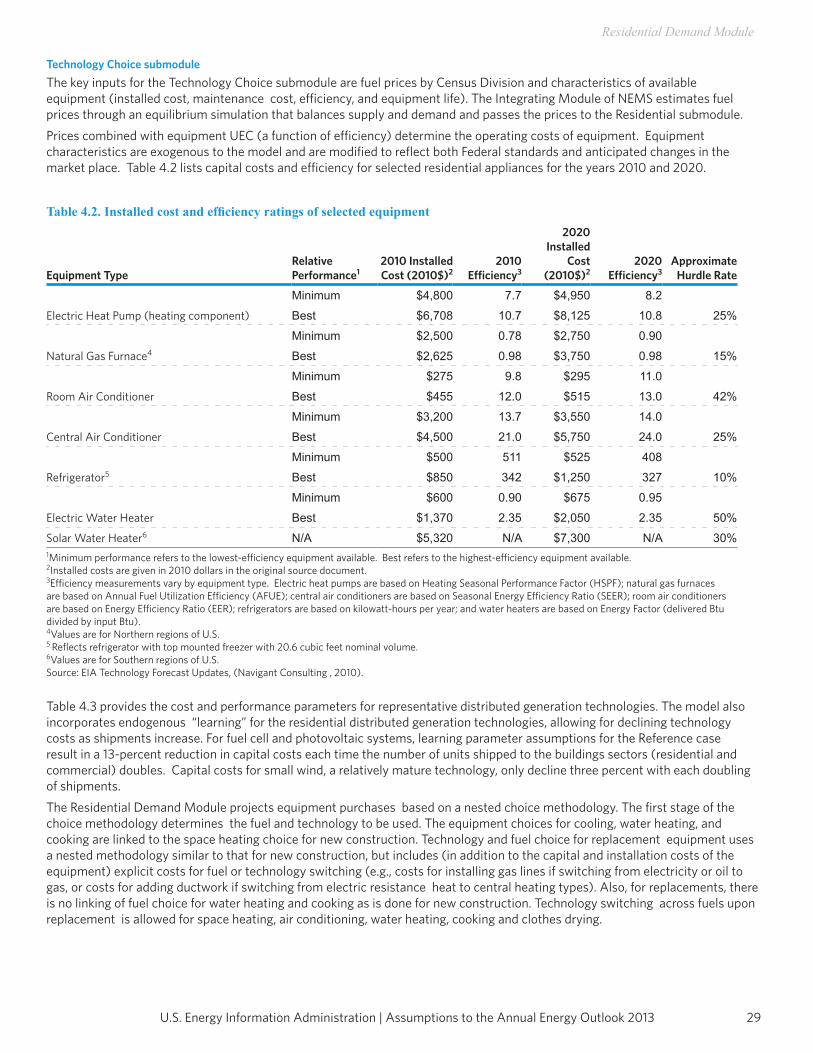
Technology Choice submoduleThe key inputs for the Technology Choice submodule are fuel prices by Census Division and characteristics of available equipment (installed cost, maintenance cost, efficiency, and equipment life). The Integrating Module of NEMS estimates fuel prices through an equilibrium simulation that balances supply and demand and passes the prices to the Residential submodule.Prices combined with equipment UEC (a function of efficiency) determine the operating costs of equipment. Equipment characteristics are exogenous to the model and are modified to reflect both Federal standards and anticipated changes in the market place. Table 4.2 lists capital costs and efficiency for selected residential appliances for the years 2010 and 2020.
Table 4.2. Installed cost and efficiency ratings of selected equipment
Equipment TypeRelative Performance1
2010 Installed Cost (2010$)2
2010 Efficiency3
2020 Installed
Cost (2010$)2
2020 Efficiency3
Approximate Hurdle Rate
Minimum $4,800 7.7 $4,950 8.2
25%Electric Heat Pump (heating component) Best $6,708 10.7 $8,125 10.8
Minimum $2,500 0.78 $2,750 0.90
15%Natural Gas Furnace4 Best $2,625 0.98 $3,750 0.98
Minimum $275 9.8 $295 11.0
42%Room Air Conditioner Best $455 12.0 $515 13.0
Minimum $3,200 13.7 $3,550 14.0
25%Central Air Conditioner Best $4,500 21.0 $5,750 24.0
Minimum $500 511 $525 408
10%Refrigerator5 Best $850 342 $1,250 327
Minimum $600 0.90 $675 0.95
50%Electric Water Heater Best $1,370 2.35 $2,050 2.35
Solar Water Heater6 N/A $5,320 N/A $7,300 N/A 30%1Minimum performance refers to the lowest-efficiency equipment available. Best refers to the highest-efficiency equipment available.2Installed costs are given in 2010 dollars in the original source document.3Efficiency measurements vary by equipment type. Electric heat pumps are based on Heating Seasonal Performance Factor (HSPF); natural gas furnaces are based on Annual Fuel Utilization Efficiency (AFUE); central air conditioners are based on Seasonal Energy Efficiency Ratio (SEER); room air conditioners are based on Energy Efficiency Ratio (EER); refrigerators are based on kilowatt-hours per year; and water heaters are based on Energy Factor (delivered Btu divided by input Btu).4Values are for Northern regions of U.S.5 Reflects refrigerator with top mounted freezer with 20.6 cubic feet nominal volume.6Values are for Southern regions of U.S.Source: EIA Technology Forecast Updates, (Navigant Consulting , 2010).
Table 4.3 provides the cost and performance parameters for representative distributed generation technologies. The model also incorporates endogenous “learning” for the residential distributed generation technologies, allowing for declining technology costs as shipments increase. For fuel cell and photovoltaic systems, learning parameter assumptions for the Reference case result in a 13-percent reduction in capital costs each time the number of units shipped to the buildings sectors (residential and commercial) doubles. Capital costs for small wind, a relatively mature technology, only decline three percent with each doubling of shipments.The Residential Demand Module projects equipment purchases based on a nested choice methodology. The first stage of the choice methodology determines the fuel and technology to be used. The equipment choices for cooling, water heating, and cooking are linked to the space heating choice for new construction. Technology and fuel choice for replacement equipment uses a nested methodology similar to that for new construction, but includes (in addition to the capital and installation costs of the equipment) explicit costs for fuel or technology switching (e.g., costs for installing gas lines if switching from electricity or oil to gas, or costs for adding ductwork if switching from electric resistance heat to central heating types). Also, for replacements, there is no linking of fuel choice for water heating and cooking as is done for new construction. Technology switching across fuels upon replacement is allowed for space heating, air conditioning, water heating, cooking and clothes drying.
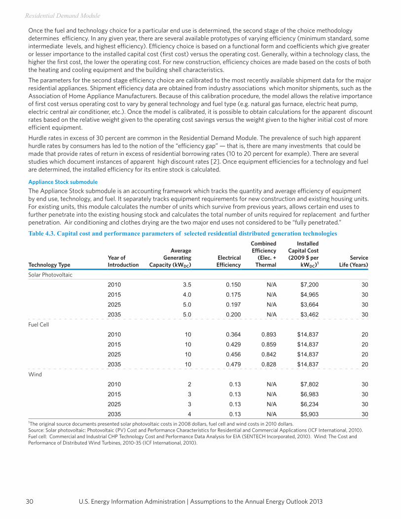
U.S. Energy Information Administration | Assumptions to the Annual Energy Outlook 201330
Residential Demand Module
Once the fuel and technology choice for a particular end use is determined, the second stage of the choice methodology determines efficiency. In any given year, there are several available prototypes of varying efficiency (minimum standard, some intermediate levels, and highest efficiency). Efficiency choice is based on a functional form and coefficients which give greater or lesser importance to the installed capital cost (first cost) versus the operating cost. Generally, within a technology class, the higher the first cost, the lower the operating cost. For new construction, efficiency choices are made based on the costs of both the heating and cooling equipment and the building shell characteristics.The parameters for the second stage efficiency choice are calibrated to the most recently available shipment data for the major residential appliances. Shipment efficiency data are obtained from industry associations which monitor shipments, such as the Association of Home Appliance Manufacturers. Because of this calibration procedure, the model allows the relative importance of first cost versus operating cost to vary by general technology and fuel type (e.g. natural gas furnace, electric heat pump, electric central air conditioner, etc.). Once the model is calibrated, it is possible to obtain calculations for the apparent discount rates based on the relative weight given to the operating cost savings versus the weight given to the higher initial cost of more efficient equipment.Hurdle rates in excess of 30 percent are common in the Residential Demand Module. The prevalence of such high apparent hurdle rates by consumers has led to the notion of the “efficiency gap” — that is, there are many investments that could be made that provide rates of return in excess of residential borrowing rates (10 to 20 percent for example). There are several studies which document instances of apparent high discount rates [2]. Once equipment efficiencies for a technology and fuel are determined, the installed efficiency for its entire stock is calculated.
Appliance Stock submoduleThe Appliance Stock submodule is an accounting framework which tracks the quantity and average efficiency of equipment by end use, technology, and fuel. It separately tracks equipment requirements for new construction and existing housing units. For existing units, this module calculates the number of units which survive from previous years, allows certain end uses to further penetrate into the existing housing stock and calculates the total number of units required for replacement and further penetration. Air conditioning and clothes drying are the two major end uses not considered to be “fully penetrated.”
Table 4.3. Capital cost and performance parameters of selected residential distributed generation technologies
Technology TypeYear of Introduction
Average Generating
Capacity (kWDC)Electrical
Efficiency
Combined Efficiency
(Elec. + Thermal
Installed Capital Cost (2009 $ per
kWDC)1Service
Life (Years)
Solar Photovoltaic
2010 3.5 0.150 N/A $7,200 30
2015 4.0 0.175 N/A $4,965 30
2025 5.0 0.197 N/A $3,664 30
2035 5.0 0.200 N/A $3,462 30
Fuel Cell
2010 10 0.364 0.893 $14,837 20
2015 10 0.429 0.859 $14,837 20
2025 10 0.456 0.842 $14,837 20
2035 10 0.479 0.828 $14,837 20
Wind
2010 2 0.13 N/A $7,802 30
2015 3 0.13 N/A $6,983 30
2025 3 0.13 N/A $6,234 30
2035 4 0.13 N/A $5,903 301The original source documents presented solar photovoltaic costs in 2008 dollars, fuel cell and wind costs in 2010 dollars.Source: Solar photovoltaic: Photovoltaic (PV) Cost and Performance Characteristics for Residential and Commercial Applications (ICF International, 2010). Fuel cell: Commercial and Industrial CHP Technology Cost and Performance Data Analysis for EIA (SENTECH Incorporated, 2010). Wind: The Cost and Performance of Distributed Wind Turbines, 2010-35 (ICF International, 2010).
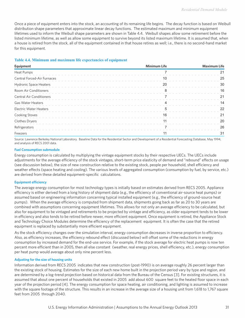
31U.S. Energy Information Administration | Assumptions to the Annual Energy Outlook 2013
Residential Demand Module
Once a piece of equipment enters into the stock, an accounting of its remaining life begins. The decay function is based on Weibull distribution shape parameters that approximate linear decay functions. The estimated maximum and minimum equipment lifetimes used to inform the Weibull shape parameters are shown in Table 4.4. Weibull shapes allow some retirement before the listed minimum lifetime, as well as allow some equipment to survive beyond its listed maximum lifetime. It is assumed that, when a house is retired from the stock, all of the equipment contained in that house retires as well; i.e., there is no second-hand market for this equipment.
Table 4.4. Minimum and maximum life expectancies of equipmentEquipment Minimum Life Maximum Life
Heat Pumps 7 21
Central Forced-Air Furnaces 10 25
Hydronic Space Heaters 20 30
Room Air Conditioners 8 16
Central Air Conditioners 7 21
Gas Water Heaters 4 14
Electric Water Heaters 5 22
Cooking Stoves 16 21
Clothes Dryers 11 20
Refrigerators 7 26
Freezers 11 31Source: Lawrence Berkeley National Laboratory. Baseline Data for the Residential Sector and Development of a Residential Forecasting Database, May 1994, and analysis of RECS 2001 data.
Fuel Consumption submoduleEnergy consumption is calculated by multiplying the vintage equipment stocks by their respective UECs. The UECs include adjustments for the average efficiency of the stock vintages, short-term price elasticity of demand and “rebound” effects on usage (see discussion below), the size of new construction relative to the existing stock, people per household, shell efficiency and weather effects (space heating and cooling). The various levels of aggregated consumption (consumption by fuel, by service, etc.) are derived from these detailed equipment-specific calculations.
Equipment efficiencyThe average energy consumption for most technology types is initially based on estimates derived from RECS 2005. Appliance efficiency is either derived from a long history of shipment data (e.g., the efficiency of conventional air-source heat pumps) or assumed based on engineering information concerning typical installed equipment (e.g., the efficiency of ground-source heat pumps). When the average efficiency is computed from shipment data, shipments going back as far as 20 to 30 years are combined with assumptions concerning equipment lifetimes. This allows for not only an average efficiency to be calculated, but also for equipment to be vintaged and retirements to be projected by vintage and efficiency, as older equipment tends to be lower in efficiency and also tends to be retired before newer, more efficient equipment. Once equipment is retired, the Appliance Stock and Technology Choice Modules determine the efficiency of the replacement equipment. It is often the case that the retired equipment is replaced by substantially more efficient equipment.As the stock efficiency changes over the simulation interval, energy consumption decreases in inverse proportion to efficiency. Also, as efficiency increases, the efficiency rebound effect (discussed below) will offset some of the reductions in energy consumption by increased demand for the end-use service. For example, if the stock average for electric heat pumps is now ten percent more efficient than in 2005, then all else constant (weather, real energy prices, shell efficiency, etc.), energy consumption per heat pump would average about only nine percent less.
Adjusting for the size of housing unitsInformation derived from RECS 2005 indicates that new construction (post-1990) is on average roughly 26 percent larger than the existing stock of housing. Estimates for the size of each new home built in the projection period vary by type and region, and are determined by a log-trend projection based on historical data from the Bureau of the Census [3]. For existing structures, it is assumed that about one percent of households that existed in 2005 add about 600 square feet to the heated floor space in each year of the projection period [4]. The energy consumption for space heating, air conditioning, and lighting is assumed to increase with the square footage of the structure. This results in an increase in the average size of a housing unit from 1,618 to 1,767 square feet from 2005 through 2040.
U.S. Energy Information Administration | Assumptions to the Annual Energy Outlook 201332
Residential Demand Module
Adjusting for weather and climateWeather in any given year always includes short-term deviations from the expected longer-term average (or climate). Recognition of the effect of weather on space heating and air conditioning is necessary to avoid inadvertently projecting abnormal weather conditions into the future. The residential module adjusts space heating and air conditioning UECs by Census Division using data on heating and cooling degree-days (HDD and CDD). Short-term projections are informed by the National Oceanic and Atmospheric Administration’s (NOAA) 15-month outlook from their Climate Prediction Center[5], which often encompasses the first forecast year (2013 in the case of AEO2013). Projections of degree days beyond that are informed by a 30-year linear trend of each state’s degree days, which are then population-weighted to the Census division level. In this way, the projection accounts for projected population migrations across the nation and continues any realized historical changes in degree days at the state level.A ten-percent increase in HDD would increase space heating consumption by ten percent over what it would have otherwise been, while a ten-percent increase in CDD would increase cooling consumption by about 12.5 percent.
Short-term price effect and efficiency reboundIt is assumed that energy consumption for a given end-use service is affected by the marginal cost of providing that service. That is, all else equal, a change in the price of a fuel will have an opposite, but less than proportional, effect on fuel consumption. The current value for the short-term elasticity parameter for non-electric fuels is -0.15 [6]. This value implies that for a 1-percent increase in the price of a fuel, there will be a corresponding decrease in energy consumption of -0.15 percent. Changes in equipment efficiency also affect the marginal cost of providing a service. For example, a 10-percent increase in efficiency will reduce the cost of providing the end-use service by 10 percent. Based on the short-term efficiency rebound parameter, the demand for the service will rise by 1.5 percent (-10 percent multiplied by -0.15). Only space heating, cooling, and lighting are assumed to be affected by both elasticitiesand the efficiency rebound effect. For electricity, the short-term elasticity parameter is set to -0.30 to account for successful deployment of smart grid projects funded under the American Recovery and Reinvestment Act of 2009 (ARRA09).
Shell efficiencyThe shell integrity of the building envelope is an important determinant of the heating and cooling load for each type of household. In the NEMS Residential Demand Module, the shell integrity is represented by an index, which changes over time to reflect improvements in the building shell. The shell integrity index is dimensioned by vintage of house, type of house, fuel type, service (heating and cooling), and Census Division. The age, type, location, and type of heating fuel are important factors in determining the level of shell integrity. Housing units heated with electricity tend to have less air infiltration rates than homes that use other fuels. Homes are classified by age as new (post-2005) or existing. Existing homes are represented by the RECS 2005 survey and are assigned a shell index value based on the mix of homes that exist in the base year (2005). The improvement over time in the shell integrity of these homes is a function of two factors—an assumed annual efficiency improvement and improvements made when real fuel prices increase (no price-related adjustment is made when fuel prices fall). For new construction, building shell efficiencyis determined by the relative costs and energy bill savings for several levels of heating and cooling equipment, in conjunction with the building shell attributes. The packages represented in NEMS range from homes that meet the International Energy Conservation Code (IECC) [7] to homes that are built with the most efficient shell components. Shell efficiency in new homes increases over time when energy prices rise, or the cost of more efficient equipment falls, all else equal.
Legislation and regulationsAmerican Recovery and Reinvestment Act of 2009 (ARRA09)The ARRA09 legislation passed in February 2009 provides energy efficiency funding for Federal agencies, State Energy Programs, and block grants, as well as a sizable increase in funding for weatherization. To account for the impact of this funding, it is assumed that the total funding is aimed at increasing the efficiency of the existing housing stock. The assumptions regarding the energy savings for heating and cooling are based on evaluations of the impact of weatherization programs over time. Further, it is assumed each house requires a $2,600 investment to achieve the heating and cooling energy savings cited in [8] and that the efficiency measures last approximately 20 years. Assumptions for funding amounts and timing were revised downward and further into the future based on analysis of the weatherization program by the Inspector General of the Department of Energy [9].The ARRA09 provisions remove the cap on the 30-percent tax credit for ground-source heat pumps, solar PV, solar thermal water heaters, and small wind turbines through 2016. Additionally, the cap for the tax credits for other energy efficiency improvements, such as windows and efficient furnaces, was increased to $1,500 through the end of 2010. Several tax credits were extended
33U.S. Energy Information Administration | Assumptions to the Annual Energy Outlook 2013
Residential Demand Module
at reduced credit levels through the end of 2011 as part of the Tax Relief, Unemployment Insurance Reauthorization, and Job Creation Act of 2010. These tax credits were further extended through the end of 2013 as part of the American Taxpayer Relief Act of 2012, but this legislation was passed too late to be included in AEO2013.Successful deployment of smart grid projects based on ARRA09 funding could stimulate more rapid investment in smart grid technologies, especially smart meters on buildings and homes, which would make consumers more responsive to electricity price changes. To represent this, the price elasticity of demand for residential electricity was increased for the services that have the ability to alter energy intensity (e.g., lighting)
Energy Improvement and Extension Act of 2008 (EIEA 2008)EIEA 2008 extends and amends many of the tax credits that were made available to residential consumers in EPACT 2005. The tax credits for energy-efficient equipment can now be claimed through 2016, while the $2,000 cap for solar technologies has been removed. Additionally, the tax credit for ground-source (geothermal) heat pumps was increased to $2,000. The production tax credits for dishwashers, clothes washers, and refrigerators were extended by one to two years, depending on the efficiency level and product. See the EPACT 2005 section below for more details about product coverage
Energy Independence and Security Act of 2007 (EISA 2007)EISA 2007 contains several provisions that impact projections of residential energy use. Standards for general service incandescent light bulbs are phased in over 2012-2014, with a more restrictive standard specified in 2020. It is estimated that these standards require 29 percent less watts per bulb in the first phase-in, increasing to 67 percent in 2020. EISA also updates the dehumidifier standard specified in EPACT 2005, resulting in a seven-percent increase in electricity savings relative to the EPACT 2005 requirement. New efficiency standards for external power supplies are set for July 1, 2008, reducing electricity use in both the active and no-load modes. Standards are also set for boilers (September 2012) and dishwashers (January 2010). Lastly, DOE is instructed to create standards for manufactured housing, requiring compliance to the latest International Energy Conservation Code (IECC) by the end of 2011.
Energy Policy Act of 2005 (EPACT05)The passage of the EPACT05 in August 2005 provides additional minimum efficiency standards for residential equipment and provides tax credits to producers and purchasers of energy-efficient equipment and builders of energy-efficient homes. The standards contained in EPACT05 include: 190 watt maximum for torchiere lamps in 2006; dehumidifier standards for2007 and 2012; and ceiling fan light kit standards in 2007. For manufactured homes that are 30 percent better than the latest code, a $1,000 tax credit can be claimed in 2006 and 2007. Likewise, builders of homes that are 50 percent better than code can claim a $2,000 credit over the same period. The builder tax credits and production tax credits are assumed to be passed through to the consumer in the form of lower purchase cost. EPACT05 includes production tax credits for energy-efficient refrigerators, dishwashers, and clothes washers in 2006 and 2007, with dollar amounts varying by type of appliance and level of efficiency met, subject to annual caps. Consumers can claim a 10 percent tax credit in 2006 and 2007 for several types of appliances specified by EPACT05, including: energy-efficient gas, propane, or oil furnaces or boilers, energy-efficient central air conditioners, air and ground source heat pumps, hot water heaters, and windows. Lastly, consumers can claim a 30 percent tax credit in 2006 and 2007 for purchases of solar PV, solar water heaters, and fuel cells, subject to a cap.
Residential alternative casesTechnology casesIn addition to the Reference case, the Residential Demand Module contributes alternate assumptions to five side cases developed to examine the effect of different assumptions of technology and policy on energy use. Three cases are devoted to technology assumptions in the demand sectors: the 2012 Technology case, a High Technology case, and a Best Available Technology case. Two cases, the Integrated Low Technology and High Technology cases, combine demand sector technology assumptions with alternative technology assumptions for renewable and fossil fuel electricity generation technologies. Two cases examine policy continuation impacts: the No Sunset case and the Extended Policies case.The 2012 Technology assumptions specify that all future equipment purchases are made based only on equipment available in 2012. These cases further assume that existing building shell efficiencies will not improve beyond 2012 levels. The 2012 Technology assumptions are implemented in the 2012 Integrated Demand Technology case.The High Technology assumptions include earlier availability, lower costs, and/or higher efficiencies for more advanced equipment than the Reference case. Equipment assumptions developed by engineering technology experts reflect the potential impact on technology given increased research and development into more advanced technologies [10]. In the High Technology cases, all new construction is assumed to meet Energy Star specifications after 2016. In addition, consumers are assumed to evaluate energy efficiency investments at a discount rate of seven percent real. The High Technology assumptions are implemented in the Integrated High Demand Technology case.

U.S. Energy Information Administration | Assumptions to the Annual Energy Outlook 201334
Residential Demand Module
The Best Available Demand Technology case assumptions require that all equipment purchases from 2013 forward are based on the highest available efficiency in the High Technology case in a particular modeled year, disregarding the economic costs of such a case. This case is designed to show how much the choice of the highest-efficiency equipment could affect energy consumption. In this case, all new construction is built to the most efficient specifications after 2012. In addition, consumers are assumed to evaluate energy efficiency investments at a discount rate of seven percent real.
Policy casesThe No Sunset case assumes the extension of all existing energy policies and legislation that contain sunset provisions. For the residential sector, this primarily involves tax credits for distributed generation and efficient end-use equipment. The Extended Policy case assumes additional rounds of appliance standards for most end-use equipment while maintaining the No Sunset tax credit assumptions for distributed generation, solar water heaters, and geothermal heat pumps. Standard levels are established based on current Energy Star guidelines. The Extended Policy case also adds multiple rounds of building codes by 2026.

35U.S. Energy Information Administration | Assumptions to the Annual Energy Outlook 2013
Residential Demand Module
Notes and sources[1] The Model Documentation Report contains additional details concerning model structure and operation. Refer to Energy Information Administration, Model Documentation Report: Residential Sector Demand Module of the National Energy Modeling System, DOE/EIA-M067(2012), (December 2012). http://www.eia.gov/forecasts/nemsdoc/residential/pdf/m067%282012%29.pdf[2] Among the explanations often mentioned for observed high average implicit discount rates are: market failures, (i.e., cases where incentives are not properly aligned for markets to result in purchases based on energy economics alone); unmeasured technology costs (i.e., extra costs of adoption which are not included or difficult to measure, like employee down-time); characteristics of efficient technologies viewed as less desirable than their less-efficient alternatives (such as equipment noise levels or lighting quality characteristics); and the risk inherent in making irreversible investment decisions. Examples of market failures/barriers include: decision-makers having less than complete information, cases where energy equipment decisions are made by parties not responsible for energy bills (e.g., landlord/tenants, builders/ home buyers), discount horizons which are truncated (which might be caused by mean occupancy times that are less than the simple payback time and that could possibly be classified as an information failure), and lack of appropriate credit vehicles for making efficiency investments. The use of high implicit discount rates in NEMS merely recognizes that such rates are typically found to apply to energy-efficiency investments.[3] U.S. Bureau of Census, Series C25 Data from various years of publications.[4] Sources: U.S. Bureau of Census, Annual Housing Survey 2001 and Professional Remodeler, 2002 Home Remodeling
Study.[5] National Oceanic and Atmospheric Administration, National Weather Service, Experimental Monthly Degree Day Forecast, http://www.cpc.ncep.noaa.gov/pacdir/DDdir/ddforecast.txt. Explanation of forecast available at http://www.cpc.ncep.noaa.gov/pacdir/DDdir/N1.html.[6] See Dahl, Carol, A Survey of Energy Demand Elasticities in Support of the Development of the NEMS, October 1993. [7] The IECC established guidelines for builders to meet specific targets concerning energy efficiency with respect toheating and cooling load.[8] Oak Ridge National Laboratory, Estimating the National Effects of the U.S. Department of Energy’s WeatherizationAssistance Program with State-Level Data: A Metaevaluation Using Studies from 1993 to 2005, September 2005.[9] U.S. Department of Energy, Office of Inspector General, Office of Audit Services, Special Report: Progress in Implementing the Department of Energy’s Weatherization Assistance Program under the American Recovery and Reinvestment Act, February 2010.[10] The high technology assumptions are based on Energy Information Administration, Technology Forecast Updates- Residential and Commercial Building Technologies-Advanced Adoption Case (Navigant Consulting, September 2011).

This page inTenTionally lefT blank

Commercial Demand Module

This page inTenTionally lefT blank

39U.S. Energy Information Administration | Assumptions to the Annual Energy Outlook 2013
Commercial Demand Module
The NEMS Commercial Sector Demand Module generates projections of commercial sector energy demand through 2040. The definition of the commercial sector is consistent with EIA’s State Energy Data System (SEDS). That is, the commercial sector includes business establishments that are not engaged in transportation or in manufacturing or other types of industrial activity (e.g., agriculture, mining or construction). The bulk of commercial sector energy is consumed within buildings; however, street lights, pumps, bridges, and public services are also included if the establishment operating them is considered commercial. Since most of commercial energy consumption occurs in buildings, the commercial module relies on the data from the EIA Commercial Buildings Energy Consumption Survey (CBECS) for characterizing the commercial sector activity mix as well as the equipment stock and fuels consumed to provide end use services [1].The commercial module projects consumption by fuel [2] at the Census division level using prices from the NEMS energy supply modules and macroeconomic variables from the NEMS Macroeconomic Activity Module (MAM), as well as external data sources (technology characterizations, for example). Energy demands are projected for ten end-use services [3] for eleven building categories [4] in each of the nine Census divisions (see Figure 5). The model begins by developing projections of floorspace for the 99 building category and Census division combinations. Next, the ten end-use service demands required for the projected floorspace are developed. The electricity generation and water and space heating supplied by distributed generation and combined heat and power technologies are projected. Technologies are then chosen to meet the projected service demands for the seven major end uses [5]. Once technologies are chosen, the energy consumed by the equipment stock (both existing and purchased equipment) is developed to meet the projected end-use service demands [6].
Key assumptionsThe key assumptions made by the commercial module are presented in terms of the flow of the calculations described above. The sections below summarize the assumptions in each of the commercial module submodules: floorspace, service demand, distributed generation, technology choice, and end-use consumption. The submodules are executed sequentially in the order presented, and the outputs of each submodule become the inputs to subsequently executed submodules. As a result, key projection drivers for the floorspace submodule are also key drivers for the service demand submodule, and so on.
Floorspace submoduleFloorspace is projected by starting with the previous year’s stock of floorspace and eliminating a portion to represent the age- related removal of buildings. Total floorspace is the sum of the surviving floorspace plus new additions to the stock derived from the MAM floorspace growth projection [7].
Existing floorspace and attritionExisting floorspace is based on the estimated floorspace reported in the 2003 Commercial Buildings Energy Consumption Survey (Table 5.1). Over time, the 2003 stock is projected to decline as buildings are removed from service (floorspace attrition). Floorspace attrition is estimated by a logistic decay function, the shape of which is dependent upon the values of two parameters: average building lifetime and gamma. The average building lifetime refers to the median expected lifetime of a particular building type. The gamma parameter corresponds to the rate at which buildings retire near their median expected lifetime. The current values for the average building lifetime and gamma vary by building type as presented in Table 5.2 [8].
New construction additions to floorspaceThe commercial module develops estimates of projected commercial floorspace additions by combining the surviving floorspace estimates with the total floorspace projection from MAM. A total NEMS floorspace projection is calculated by applying the MAM assumed floorspace growth rate within each Census division and MAM building type to the corresponding NEMS Commercial Demand Module’s building types based on the CBECS building type shares. The NEMS surviving floorspace from the previous year is then subtracted from the total NEMS floorspace projection for the current year to yield new floorspace additions [9].
Service demand submoduleOnce the building stock is projected, the Commercial Demand module develops a projection of demand for energy-consuming services required for the projected floorspace. The module projects service demands for the following explicit end-use services: space heating, space cooling, ventilation, water heating, lighting, cooking, refrigeration, personal computer office equipment, and other office equipment [10]. The service demand intensity (SDI) is measured in thousand Btu of end-use service demand per square foot and differs across service, Census division, and building type. The SDIs are based on a hybrid engineering and statistical approach of CBECS consumption data [11]. Projected service demand is the product of square feet and SDI for all end uses across the eleven building categories with adjustments for changes in shell efficiency for space heating and cooling.
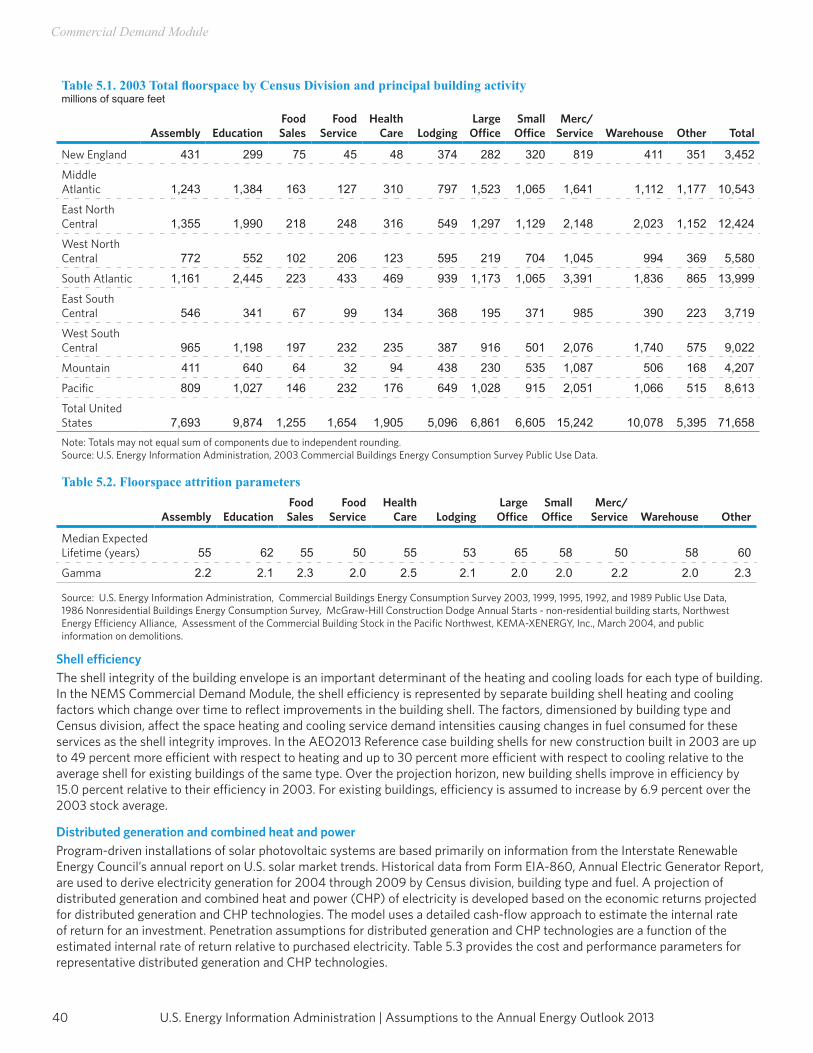
U.S. Energy Information Administration | Assumptions to the Annual Energy Outlook 201340
Commercial Demand Module
Table 5.1. 2003 Total floorspace by Census Division and principal building activity millions of square feet
Assembly EducationFood Sales
Food Service
Health Care Lodging
Large Office
Small Office
Merc/ Service Warehouse Other Total
New England 431 299 75 45 48 374 282 320 819 411 351 3,452
Middle Atlantic 1,243 1,384 163 127 310 797 1,523 1,065 1,641 1,112 1,177 10,543
East North Central 1,355 1,990 218 248 316 549 1,297 1,129 2,148 2,023 1,152 12,424
West North Central 772 552 102 206 123 595 219 704 1,045 994 369 5,580
South Atlantic 1,161 2,445 223 433 469 939 1,173 1,065 3,391 1,836 865 13,999
East South Central 546 341 67 99 134 368 195 371 985 390 223 3,719
West South Central 965 1,198 197 232 235 387 916 501 2,076 1,740 575 9,022
Mountain 411 640 64 32 94 438 230 535 1,087 506 168 4,207
Pacific 809 1,027 146 232 176 649 1,028 915 2,051 1,066 515 8,613
Total United States 7,693 9,874 1,255 1,654 1,905 5,096 6,861 6,605 15,242 10,078 5,395 71,658Note: Totals may not equal sum of components due to independent rounding.Source: U.S. Energy Information Administration, 2003 Commercial Buildings Energy Consumption Survey Public Use Data.
Table 5.2. Floorspace attrition parameters
Assembly EducationFood Sales
Food Service
Health Care Lodging
Large Office
Small Office
Merc/ Service Warehouse Other
Median Expected Lifetime (years) 55 62 55 50 55 53 65 58 50 58 60
Gamma 2.2 2.1 2.3 2.0 2.5 2.1 2.0 2.0 2.2 2.0 2.3
Source: U.S. Energy Information Administration, Commercial Buildings Energy Consumption Survey 2003, 1999, 1995, 1992, and 1989 Public Use Data, 1986 Nonresidential Buildings Energy Consumption Survey, McGraw-Hill Construction Dodge Annual Starts - non-residential building starts, Northwest Energy Efficiency Alliance, Assessment of the Commercial Building Stock in the Pacific Northwest, KEMA-XENERGY, Inc., March 2004, and public information on demolitions.
Shell efficiencyThe shell integrity of the building envelope is an important determinant of the heating and cooling loads for each type of building. In the NEMS Commercial Demand Module, the shell efficiency is represented by separate building shell heating and cooling factors which change over time to reflect improvements in the building shell. The factors, dimensioned by building type and Census division, affect the space heating and cooling service demand intensities causing changes in fuel consumed for these services as the shell integrity improves. In the AEO2013 Reference case building shells for new construction built in 2003 are up to 49 percent more efficient with respect to heating and up to 30 percent more efficient with respect to cooling relative to the average shell for existing buildings of the same type. Over the projection horizon, new building shells improve in efficiency by 15.0 percent relative to their efficiency in 2003. For existing buildings, efficiency is assumed to increase by 6.9 percent over the 2003 stock average.
Distributed generation and combined heat and powerProgram-driven installations of solar photovoltaic systems are based primarily on information from the Interstate Renewable Energy Council’s annual report on U.S. solar market trends. Historical data from Form EIA-860, Annual Electric Generator Report, are used to derive electricity generation for 2004 through 2009 by Census division, building type and fuel. A projection of distributed generation and combined heat and power (CHP) of electricity is developed based on the economic returns projected for distributed generation and CHP technologies. The model uses a detailed cash-flow approach to estimate the internal rate of return for an investment. Penetration assumptions for distributed generation and CHP technologies are a function of the estimated internal rate of return relative to purchased electricity. Table 5.3 provides the cost and performance parameters for representative distributed generation and CHP technologies.

41U.S. Energy Information Administration | Assumptions to the Annual Energy Outlook 2013
Commercial Demand Module
The model also incorporates endogenous “learning” for new distributed generation and CHP technologies, allowing for declining technology costs as shipments increase. For fuel cell and photovoltaic systems, parameter assumptions for the AEO2013 Reference case result in a 13-percent reduction in capital costs each time the number of units shipped to the buildings sectors (residential and commercial) doubles. Doubling the number of microturbines shipped results in a 10-percent reduction in capital costs and doubling the number of distributed wind systems shipped results in a 3-percent reduction.
Technology Choice SubmoduleThe technology choice submodule develops projections of the results of the capital purchase decisions for equipment fueled by the three major fuels (electricity, natural gas, and distillate fuel). Capital purchase decisions are driven by assumptions concerning behavioral rule proportions and time preferences, described below, as well as projected fuel prices, average utilization of equipment (the capacity factors), relative technology capital costs, and operating and maintenance (O&M) costs.
Decision typesIn each projection year, equipment is potentially purchased for three “decision types.” Equipment must be purchased for newly added floorspace and to replace the portion of equipment in existing floorspace that is projected to wear out [12]. Equipment is also potentially purchased for retrofitting equipment that has become economically obsolete. The purchase of retrofit equipment occurs only if the annual operating costs of a current technology exceed the annualized capital and operating costs of a technology available as a retrofit candidate.
Behavioral rulesThe commercial module allows the use of three alternate assumptions about equipment choice behavior. These assumptions constrain the equipment selections to three choice sets, which are progressively more restrictive. The choice sets vary by decision type and building type:•• Unrestricted Choice Behavior - This rule assumes that commercial consumers consider all types of equipment that meet a
given service, across all fuels, when faced with a capital purchase decision.•• Same Fuel Behavior - This rule restricts the capital purchase decision to the set of technologies that consume the same fuel
that currently meets the decision maker’s service demand.•• Same Technology Behavior - Under this rule, commercial consumers consider only the available models of the same
technology and fuel that currently meet service demand, when facing a capital stock decision.Under any of the above three behavior rules, equipment that meets the service at the lowest annualized lifecycle cost is chosen. Table 5.4 illustrates the proportions of floorspace subject to the different behavior rules for space heating technology choices in large office buildings.
Time preferencesCommercial building owners’ time preferences regarding current versus future expenditures are assumed to be distributed among seven alternate time preference premiums. Adding the risk-adjusted time preference premiums to the 10-year Treasury note rate from MAM results in implicit discount rates, also known as hurdle rates, applicable to the assumed proportions of commercial floorspace. The effect of the use of this distribution of discount rates is to prevent a single technology from dominating purchase decisions in the lifecycle cost comparisons. The distribution used for AEO2013 assigns some floorspace a very high discount or hurdle rate to simulate floorspace which will never retrofit existing equipment and which will only purchase equipment with the lowest capital cost. Discount rates for the remaining six segments of the distribution get progressively lower, simulating increased sensitivity to the fuel costs of the equipment that is purchased. The share of floorspace assigned to each rate in the distribution varies by end-use service. Table 5.5 illustrates the distribution of time preference premiums for space heating and lighting in 2015. The proportion of floorspace assumed for the 0.0 time preference premium represents an estimate of the federally-owned commercial floorspace that is subject to purchase decisions in a given year. The federal sector is expected to purchase energy-efficient equipment to meet the federal buildings performance standards of the Energy Policy Act of 2005 and the Energy Independence and Security Act of 2007 whenever cost-effective. For federal purchase decisions relating to energy conservation, cost-effectiveness is determined using a discount rate based on long-term Treasury bond rates, approximated in the commercial module by the 10-year Treasury note rate. For lighting, the proportion of floorspace assumed for the 0.0 time preference premium is increased to include all federal floorspace starting in 2009 to represent the EISA 2007 provision that all federal buildings be equipped with energy-efficient lighting fixtures and bulbs to the maximum extent feasible, including when replacing bulbs in existing fixtures.
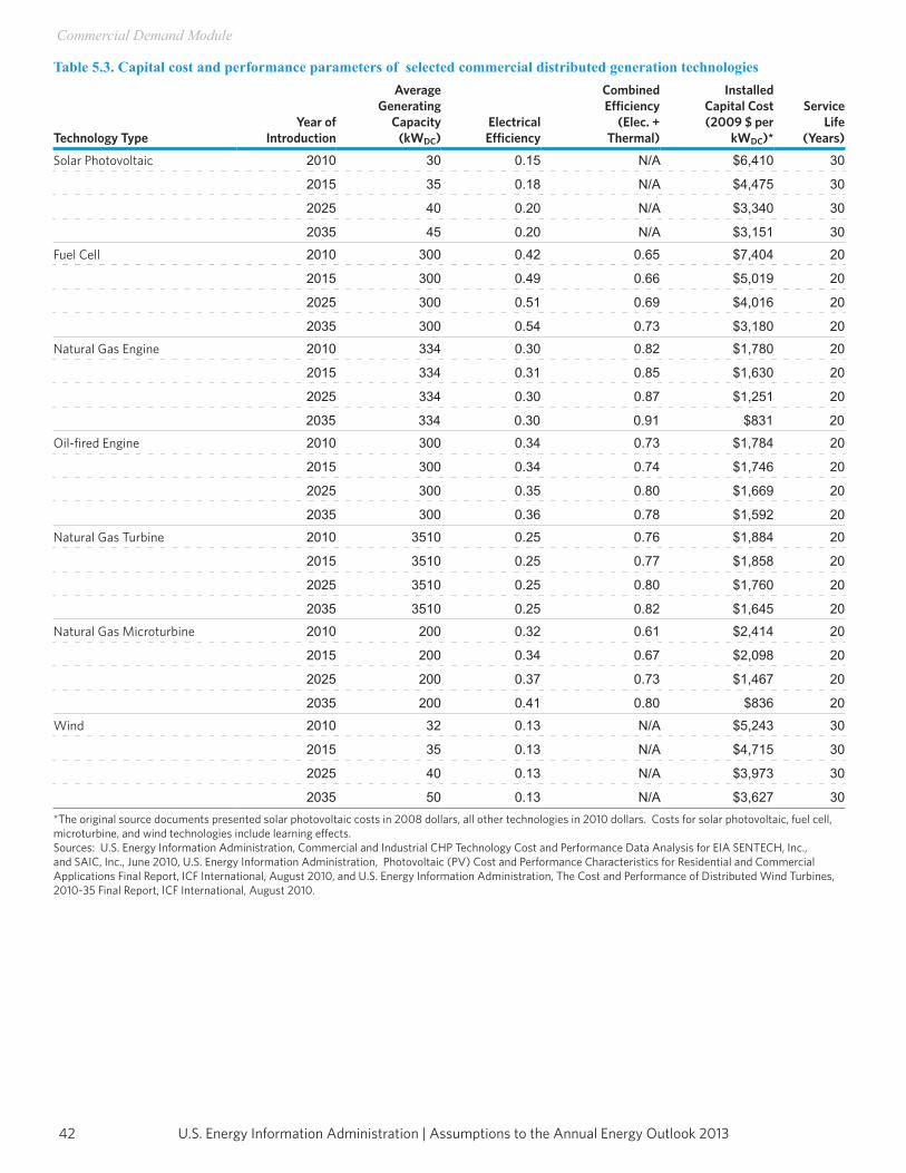
U.S. Energy Information Administration | Assumptions to the Annual Energy Outlook 201342
Commercial Demand Module
Table 5.3. Capital cost and performance parameters of selected commercial distributed generation technologies
Technology TypeYear of
Introduction
Average Generating
Capacity (kWDC)
Electrical Efficiency
Combined Efficiency
(Elec. + Thermal)
Installed Capital Cost (2009 $ per
kWDC)*
Service Life
(Years)
Solar Photovoltaic 2010 30 0.15 N/A $6,410 30
2015 35 0.18 N/A $4,475 30
2025 40 0.20 N/A $3,340 30
2035 45 0.20 N/A $3,151 30
Fuel Cell 2010 300 0.42 0.65 $7,404 20
2015 300 0.49 0.66 $5,019 20
2025 300 0.51 0.69 $4,016 20
2035 300 0.54 0.73 $3,180 20
Natural Gas Engine 2010 334 0.30 0.82 $1,780 20
2015 334 0.31 0.85 $1,630 20
2025 334 0.30 0.87 $1,251 20
2035 334 0.30 0.91 $831 20
Oil-fired Engine 2010 300 0.34 0.73 $1,784 20
2015 300 0.34 0.74 $1,746 20
2025 300 0.35 0.80 $1,669 20
2035 300 0.36 0.78 $1,592 20
Natural Gas Turbine 2010 3510 0.25 0.76 $1,884 20
2015 3510 0.25 0.77 $1,858 20
2025 3510 0.25 0.80 $1,760 20
2035 3510 0.25 0.82 $1,645 20
Natural Gas Microturbine 2010 200 0.32 0.61 $2,414 20
2015 200 0.34 0.67 $2,098 20
2025 200 0.37 0.73 $1,467 20
2035 200 0.41 0.80 $836 20
Wind 2010 32 0.13 N/A $5,243 30
2015 35 0.13 N/A $4,715 30
2025 40 0.13 N/A $3,973 30
2035 50 0.13 N/A $3,627 30*The original source documents presented solar photovoltaic costs in 2008 dollars, all other technologies in 2010 dollars. Costs for solar photovoltaic, fuel cell, microturbine, and wind technologies include learning effects. Sources: U.S. Energy Information Administration, Commercial and Industrial CHP Technology Cost and Performance Data Analysis for EIA SENTECH, Inc., and SAIC, Inc., June 2010, U.S. Energy Information Administration, Photovoltaic (PV) Cost and Performance Characteristics for Residential and Commercial Applications Final Report, ICF International, August 2010, and U.S. Energy Information Administration, The Cost and Performance of Distributed Wind Turbines, 2010-35 Final Report, ICF International, August 2010.
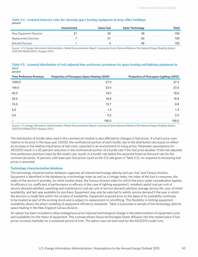
43U.S. Energy Information Administration | Assumptions to the Annual Energy Outlook 2013
Commercial Demand Module
Table 5.4. Assumed behavior rules for choosing space heating equipment in large office buildingspercent
Unrestricted Same Fuel Same Technology Total
New Equipment Decision 21 30 49 100
Replacement Decision 7 31 62 100
Retrofit Decision 1 4 95 100Source: U.S. Energy Information Administration, Model Documentation Report: Commercial Sector Demand Module of the National Energy Modeling System, DOE/EIA-M066(2012) (August 2012).
Table 5.5. Assumed distribution of risk-adjusted time preference premiums for space heating and lighting equipment in 2015percent
Time Preference Premium Proportion of Floorspace-Space Heating (2015) Proportion of Floorspace-Lighting (2015)
1000.0 27.0 27.0
100.0 23.0 23.0
45.0 19.0 18.6
25.0 18.6 18.6
15.0 10.7 8.8
6.5 1.5 1.5
0.0 0.2 2.5
-- 100.0 100.0Source: U.S. Energy Information Administration, Model Documentation Report: Commercial Sector Demand Module of the National Energy Modeling System, DOE/EIA-M066(2012) (August 2012).
The distribution of hurdle rates used in the commercial module is also affected by changes in fuel prices. If a fuel’s price rises relative to its price in the base year (2003), the nonfinancial portion of each hurdle rate in the distribution decreases to reflect an increase in the relative importance of fuel costs, expected in an environment of rising prices. Parameter assumptions for AEO2013 result in a 30-percent reduction in the nonfinancial portion of a hurdle rate if the fuel price doubles. If the risk-adjusted time preference premium input by the model user results in a hurdle rate below the assumed financial discount rate for the commercial sector, 15 percent, with base year fuel prices (such as the 0.0 rate given in Table 5.5), no response to increasing fuel prices is assumed.
Technology characterization databaseThe technology characterization database organizes all relevant technology data by end use, fuel, and Census division. Equipment is identified in the database by a technology index as well as a vintage index, the index of the fuel it consumes, the index of the service it provides, its initial market share, the Census division index for which the entry under consideration applies, its efficiency (or coefficient of performance or efficacy in the case of lighting equipment), installed capital cost per unit of service demand satisfied, operating and maintenance cost per unit of service demand satisfied, average service life, year of initial availability, and last year available for purchase. Equipment may only be selected to satisfy service demand if the year in which the decision is made falls within the window of availability. Equipment acquired prior to the lapse of its availability continues to be treated as part of the existing stock and is subject to replacement or retrofitting. This flexibility in limiting equipment availability allows the direct modeling of equipment efficiency standards. Table 5.6 provides a sample of the technology data for space heating in the New England Census division.An option has been included to allow endogenous price-induced technological change in the determination of equipment costs and availability for the menu of equipment. This concept allows future technologies faster diffusion into the market place if fuel prices increase markedly for a sustained period of time. The option was not exercised for the AEO2013 model runs.
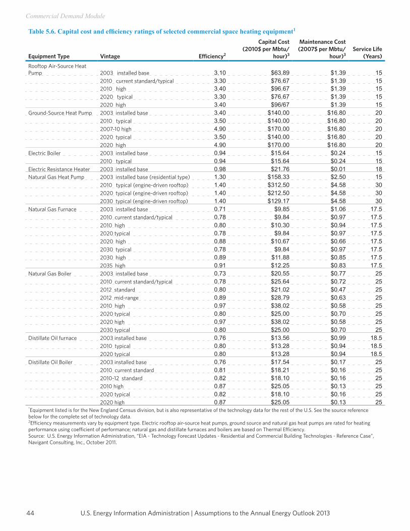
U.S. Energy Information Administration | Assumptions to the Annual Energy Outlook 201344
Commercial Demand Module
Table 5.6. Capital cost and efficiency ratings of selected commercial space heating equipment1
Equipment Type Vintage Efficiency2
Capital Cost (2010$ per Mbtu/
hour)3
Maintenance Cost (2007$ per Mbtu/
hour)3Service Life
(Years)Rooftop Air-Source Heat Pump 2003 installed base 3.10 $63.89 $1.39 15
2010 current standard/typical 3.30 $76.67 $1.39 152010 high 3.40 $96.67 $1.39 152020 typical 3.30 $76.67 $1.39 152020 high 3.40 $96/67 $1.39 15
Ground-Source Heat Pump 2003 installed base 3.40 $140.00 $16.80 202010 typical 3.50 $140.00 $16.80 202007-10 high 4.90 $170.00 $16.80 202020 typical 3.50 $140.00 $16.80 202020 high 4.90 $170.00 $16.80 20
Electric Boiler 2003 installed base 0.94 $15.64 $0.24 152010 typical 0.94 $15.64 $0.24 15
Electric Resistance Heater 2003 installed base 0.98 $21.76 $0.01 18Natural Gas Heat Pump 2003 installed base (residential type) 1.30 $158.33 $2.50 15
2010 typical (engine-driven rooftop) 1.40 $312.50 $4.58 302020 typical (engine-driven rooftop) 1.40 $212.50 $4.58 302030 typical (engine-driven rooftop) 1.40 $129.17 $4.58 30
Natural Gas Furnace 2003 installed base 0.71 $9.85 $1.06 17.52010 current standard/typical 0.78 $9.84 $0.97 17.52010 high 0.80 $10.30 $0.94 17.52020 typical 0.78 $9.84 $0.97 17.52020 high 0.88 $10.67 $0.66 17.52030 typical 0.78 $9.84 $0.97 17.52030 high 0.89 $11.88 $0.85 17.52035 high 0.91 $12.25 $0.83 17.5
Natural Gas Boiler 2003 installed base 0.73 $20.55 $0.77 252010 current standard/typical 0.78 $25.64 $0.72 252012 standard 0.80 $21.02 $0.47 252012 mid-range 0.89 $28.79 $0.63 252010 high 0.97 $38.02 $0.58 252020 typical 0.80 $25.00 $0.70 252020 high 0.97 $38.02 $0.58 252030 typical 0.80 $25.00 $0.70 25
Distillate Oil furnace 2003 installed base 0.76 $13.56 $0.99 18.52010 typical 0.80 $13.28 $0.94 18.52020 typical 0.80 $13.28 $0.94 18.5
Distillate Oil Boiler 2003 installed base 0.76 $17.54 $0.17 252010 current standard 0.81 $18.21 $0.16 252010-12 standard 0.82 $18.10 $0.16 252010 high 0.87 $25.05 $0.13 252020 typical 0.82 $18.10 $0.16 252020 high 0.87 $25.05 $0.13 25
*Equipment listed is for the New England Census division, but is also representative of the technology data for the rest of the U.S. See the source reference below for the complete set of technology data.2Efficiency measurements vary by equipment type. Electric rooftop air-source heat pumps, ground source and natural gas heat pumps are rated for heating performance using coefficient of performance; natural gas and distillate furnaces and boilers are based on Thermal Efficiency.Source: U.S. Energy Information Administration, “EIA - Technology Forecast Updates - Residential and Commercial Building Technologies - Reference Case”, Navigant Consulting, Inc., October 2011.
45U.S. Energy Information Administration | Assumptions to the Annual Energy Outlook 2013
Commercial Demand Module
End-Use Consumption SubmoduleThe end-use consumption submodule calculates the consumption of each of the three major fuels (electricity, natural gas, and distillate fuel oil) for the ten end-use services plus fuel consumption for combined heat and power and district services. For the ten end-use services, energy consumption is calculated as the end-use service demand met by a particular type of equipment divided by its efficiency and summed over all existing equipment types. This calculation includes dimensions for Census division, building type, and fuel. Consumption of the five minor fuels (residual fuel oil, liquefied petroleum gas, motor gasoline, kerosene, and coal) is projected based on historical trends.
Equipment efficiencyThe average energy consumption of a particular appliance is based initially on estimates derived from the 2003 CBECS. As the stock efficiency changes over the model simulation, energy consumption decreases nearly as much as, but not quite proportionally to the efficiency increase. The difference is due to the calculation of efficiency using the harmonic average and also the efficiency rebound effect discussed below. For example, if on average, electric heat pumps are now 10 percent more efficient than in 2003, then all else constant (weather, real energy prices, shell efficiency, etc.), energy consumption per heatpump would now average about 9 percent less. The Service Demand and Technology Choice Submodules together determine the average efficiency of the stocks used in adjusting the initial average energy consumption.
Adjusting for weather and climateWeather in any given year always includes short-term deviations from the expected longer-term average (or climate). Recognition of the effect of weather on space heating and air conditioning is necessary to avoid projecting abnormal weather conditions into the future. In the commercial module, proportionate adjustments are made to space heating and air conditioning demand by Census division. These adjustments are based on National Oceanic and Atmospheric Administration (NOAA) data for Heating Degree Days (HDD) and Cooling Degree Days (CDD). Short-term projections are informed by the National Oceanic and Atmospheric Administration’s (NOAA) 15-month outlook from their Climate Prediction Center[13], which often encompasses the first forecast year. Projections of degree days beyond that are informed by a 30-year linear trend of each state’s degree days, which are then population-weighted to the Census division level. In this way, the projection accounts for projected population migrations across the nation and continues any realized historical changes in degree days at the state level. A 10-percent increase in HDD would increase space heating consumption by 10 percent over what it would have been, while a ten-percent increase in CDD would increase cooling consumption by about 12.5 percent.
Short-term price effect and efficiency reboundIt is assumed that energy consumption for a given end-use service is affected by the marginal cost of providing that service. That is, all else equal, a change in the price of a fuel will have an inverse, but less than proportional, effect on fuel consumption. The current value for the short-term price elasticity parameter is -0.25 for all major end uses except refrigeration. A value of -0.1 is currently used for commercial refrigeration. A value of -0.05 is currently used for PC and non-PC office equipment and other minor uses of electricity. For example, for lighting, this value implies that for a 1 percent increase in the price of a fuel, there will be a corresponding decrease in energy consumption of 0.25 percent. Another way of affecting the marginal cost of providing a service is through equipment efficiency. As equipment efficiency changes over time, so will the marginal cost of providing the end-use service. For example, a 10-percent increase in efficiency will reduce the cost of providing the service by 10 percent. The short-term elasticity parameter for efficiency rebound effects is -0.15 for affected end uses; therefore, the demand for the service will rise by 1.5 percent (-10 percent x -0.15). Currently, all services are affected by the short-term price effect and services affected by efficiency rebound are space heating and cooling, water heating, ventilation and lighting.
Legislation and regulationsAmerican Recovery and Reinvestment Act of 2009 (ARRA09)The ARRA09 legislation passed in February 2009 provides energy efficiency funding for federal agencies, State Energy Programs, and block grants. To account for the impact of this funding, states are assumed to adopt and enforce the ASHRAE 90.1-2007 standard by 2018 for building shell measures, and all Public buildings (federal, state, and local) are assumed to use the 10-year Treasury note rate for purchase decisions related to both new construction and replacement equipment while stimulus funding is available. A percentage of the State Energy Program and Conservation Block Grant funding is assumed to be used for solar photovoltaic and small wind turbine installations. Additional stimulus funding is applied to fuel cell installations.The ARRA09 provisions remove the cap on the 30-percent Business Investment Tax Credit for wind turbines. The Investment Tax Credit is still available for systems installed through 2016. These credits are directly incorporated into the cash-flow approach for distributed generation systems.
U.S. Energy Information Administration | Assumptions to the Annual Energy Outlook 201346
Commercial Demand Module
Energy Imropovement and Extension Act of 2008 (EIEA08)The EIEA08 legislation passed in October 2008 extends the Business Investment Tax Credit provisions of the Energy Policy Act of 2005 and expands the credit to include additional technologies. The Business Investment Tax Credits of 30 percent for solar energy systems and fuel cells and 10 percent for microturbines are extended through 2016. The cap on the fuel cell credit has been increased from $500 to $1,500 per half kilowatt of capacity. The EIEA08 provisions expand the Investment Tax Credit to include a 10-percent credit for CHP systems and ground-source heat pumps and a 30-percent credit for wind turbines with the wind credit capped at $4,000. The expanded credits are available for systems installed through 2016. These credits are directly incorporated into the cash-flow approach for distributed generation systems, including CHP, and factored into the installed capital cost assumptions for solar hot water heaters and ground-source heat pumps.
Energy Independence and Security Act of 2007 (EISA07)The EISA07 legislation passed in December 2007 provides standards for specific explicitly modeled commercial equipment. The EISA07 requires specific energy-efficiency measures in commercial walk-in coolers and walk-in freezers effective January 1, 2009. Incandescent and halogen lamps must meet standards for maximum allowable wattage based on lumen output starting in 2012 and metal halide lamp fixtures using lamps between 150 and 500 watts are required to have a minimum ballast efficiency ranging from 88 to 94 percent, depending on ballast type, effective January 1, 2009.The EISA07 requirement for federal buildings to use energy-efficient lighting fixtures and bulbs to the maximum extent possible is represented by adjusting the proportion of the commercial sector assumed to use the 10-year Treasury note rate as an implicit discount or hurdle rate for lighting.
Energy Policy Act of 2005 (EPACT05)The passage of the EPACT05 in August 2005 provides additional minimum efficiency standards for commercial equipment. Some of the standards for explicitly modeled equipment, effective January 1, 2010, include an Energy Efficiency Rating (EER) ranging from 10.8 to 11.2 for small package air conditioning and heating equipment; daily electricity consumption limits by volume for commercial refrigerators, freezers, and refrigerator-freezers; and electricity consumption limits per 100 pounds of ice produced based on equipment type and capacity for automatic ice makers. The EPACT05 adds standards for medium base compact fluorescent lamps effective January 1, 2006, for ballasts for Energy Saver fluorescent lamps effective in 2009 and 2010, and bans the manufacture or import of mercury vapor lamp ballasts effective January 1, 2008.Several efficiency standards in the EPACT05 pertain to equipment not explicitly represented in the NEMS Commercial Demand Module. For low voltage dry-type transformers, effects of the standard are included in estimating the share of projected miscellaneous electricity use attributable to transformer losses. For illuminated exit signs, traffic signals, and commercial premise spray valves, assumed energy reductions are calculated based on per-unit savings relative to a baseline unit and the estimated share of installed units and sales that already meet the standard. Total projected reductions are phased in over time to account for stock turnover. Under the EPACT05 standards, illuminated exit signs and traffic signal modules must meet ENERGY STAR program requirements as of January 1, 2006. The requirements limit input power demand to 5 watts or less per face for exit signs. Nominal wattages for traffic signal modules are limited to 8 to 15 watts, based on module type. Effective January 1, 2007, low voltage dry-type distribution transformers are required to meet the National Electrical Manufacturers Association Class I Efficiency Levels with minimum efficiency levels ranging from 97 percent to 98.9 percent based on output. Commercial pre-rinse spray valves [14] must have a maximum flow rate of 1.6 gallons per minute, effective January 1, 2006 with energy reductions attributed to hot water use.The EPACT05 expands the Business Investment Tax Credit to 30 percent for solar property installed in 2006 and 2007. Business Investment Tax Credits of 30 percent for fuel cells and 10 percent for microturbine power plants are also available for property installed in 2006 and 2007. The EPACT05 tax credit provisions were extended in December 2006 to cover equipment installed in 2008. These credits are directly incorporated into the cash-flow approach for distributed generation systems and factored into the installed capital cost assumptions for solar hot water heaters.
Energy Policy Act of 1992 (EPACT92)A key assumption incorporated in the technology selection process is that the equipment efficiency standards described in the EPACT92 constrain minimum equipment efficiencies. The effects of standards are modeled by modifying the technology database to eliminate equipment that no longer meets minimum efficiency requirements. Some of the EPACT92 standards implemented in the module include: gas and oil-fired boilers—minimum combustion efficiency of 0.80 and 0.83, respectively, amended to minimum thermal efficiency of 0.80 and 0.81, respectively, in 2012; gas and oil-fired furnaces—minimum thermal efficiency of
47U.S. Energy Information Administration | Assumptions to the Annual Energy Outlook 2013
Commercial Demand Module
0.80 and 0.81, respectively; electric water heaters—minimum energy factor of 0.85; and gas and oil water heaters—minimum thermal efficiency of 0.80 and 0.78, respectively. A fluorescent lamp ballast standard effective in 2005 mandates electronic ballasts with a minimum ballast efficacy factor of 1.17 for 4-foot, 2-lamp ballasts and 0.63 for 8-foot, 2-lamp ballasts. Fluorescent lamps and incandescent reflector lamb bulbs must meet amended standard levels for minimum average lamp efficacy in 2012. Recent updates for commercial refrigeration equipment include maximum energy consumption standards for refrigerated vending machines and display cases based on volume.The 10-percent Business Investment Tax Credit for solar energy property included in EPACT92 is directly incorporated into the cash-flow approach for projecting distributed generation by commercial photovoltaic systems. For solar hot water heaters, the tax credit is factored into the installed capital cost assumptions used in the technology choice submodule.
Energy efficiency programsSeveral energy efficiency programs affect the commercial sector. These programs are designed to stimulate investment in more efficient building shells and equipment for heating, cooling, lighting, and other end uses. The commercial module includes several features that allow projected efficiency to increase in response to voluntary programs (e.g., the distribution of risk-adjusted time preference premiums and shell efficiency parameters). Retrofits of equipment for space heating, air conditioning and lighting are incorporated in the distribution of premiums given in Table 5.5. Also the shell efficiency of new and existing buildings is assumed to increase from 2003 through 2040. Shells for new buildings increase in efficiency by 15.0 percent over this period, while shells for existing buildings increase in efficiency by 6.9 percent.
Commercial alternative casesTechnology casesIn addition to the AEO2013 Reference case, three side cases were developed to examine the effect of equipment and building standards on commercial energy use—a 2012 Demand Technology case, a High Demand Technology case, and a Best Available Demand Technology case. These side cases were analyzed in integrated runs with the NEMS demand and supply modules and thus include supply responses to the altered commercial consumption patterns of the three cases. AEO2013 also analyzed a Low Renewable Technology Cost case.The 2012 Demand Technology case assumes that all future equipment purchases are made based only on equipment available in 2012. This case assumes building shell efficiency to be fixed at 2012 levels. In the High Demand Technology case, depending on technology or end use, equipment costs are lower, efficiencies are higher, and equipment is available sooner than in the Reference case. Energy efficiency investments are evaluated at 7 percent real rather than the distribution of hurdle rates assumed for the Reference case. Equipment assumptions were developed by engineering technology experts, considering the potential impact on technology given increased research and development into more advanced technologies. In addition to equipment improvements, building shell efficiencies are assumed to improve 25 percent more than in the Reference case after 2012. Existing building shells, therefore, increase by 8.6 percent relative to 2003 levels and new building shells by 18.8 percent relative to their efficiency in 2003 by 2040.The Best Available Demand Technology case assumes that all equipment purchases after 2012 are based on the highest available efficiency for each type of technology in the High Demand Technology case in a particular simulation year, disregarding the economic costs of such a case. It is designed to show how much the choice of the highest-efficiency equipment could affect energy consumption. Shell efficiencies in this case are assumed to improve 50 percent more than in the Reference case after 2012, i.e., existing shells increase by 10.4 percent relative to 2003 levels and new building shells by 22.5 percent relative to their efficiency in 2003 by 2040.
Fuel shares, where appropriate for a given end use, are allowed to change in the technology cases as the available technologies from each technology type compete to serve certain segments of the commercial floorspace market. For example, in the Best Available Technology case, the most efficient gas furnace technology competes with the most efficient electric heat pump technology. This contrasts with the Reference case, in which a greater number of technologies for each fuel with varying efficiencies all compete to serve the heating end use. In general, the fuel choice will be affected as the available choices are constrained or expanded, and will thus differ across the cases.The Low Renewable Cost case, which focuses on electricity generation, incorporates alternative assumptions for non-hydro renewable energy technologies in the power sector, the industrial sector, and the buildings sectors, including residential and commercial photovoltaic and wind systems. In this case, assumptions regarding non-renewable technologies are not changed from the Reference case. It assumes that costs for residential and commercial photovoltaic and wind systems are 20 percent below Reference case assumptions beginning in 2013 and continuing through the projection period.
U.S. Energy Information Administration | Assumptions to the Annual Energy Outlook 201348
Commercial Demand Module
Analysis casesTwo integrated analysis cases were completed for the AEO2013: the No Sunset and Extended Policies cases. Both cases are based upon Reference case assumptions, with additional changes made to extend existing tax credits and policies beyond those prescribed by current law.In the No Sunset case, the 30-percent solar photovoltaic investment tax credit (ITC) that is scheduled to revert to a 10-percent credit in 2016 is, instead, assumed to be extended indefinitely at 30 percent. Additional tax credits for the purchase of other renewable and combined heat and power equipment, such as ground-source heat pumps and fuel cells, are also assumed to be extended indefinitely as opposed to expiring in 2016.The Extended Policies case adopts the same assumptions as the No Sunset case and includes additional changes. For instance, federal equipment efficiency standards are updated at particular intervals consistent with the provisions in the existing law, with the levels based on ENERGY STAR specifications, or Federal Energy Management Program (FEMP) purchasing guidelines for federal agencies. Standards are also introduced for products that currently are not subject to federal efficiency standards. Updated national building energy codes reach 30-percent improvement in 2020 relative to the American Society of Heating, Refrigerating and Air-Conditioning Engineers (ASHRAE) Building Energy Code 90.1-2004 in the commercial sector. Two subsequent rounds in 2023 and 2026 each add an assumed 5-percent incremental improvement to building energy codes.The equipment standards and building codes assumed for the Extended Policies case are meant to illustrate the potential effects of these polices on energy consumption for buildings. No cost-benefit analysis or evaluation of impacts on consumer welfare was completed in developing the assumptions. Likewise, no technical feasibility analysis was conducted, although standards were not allowed to exceed “maximum technologically feasible” levels described in DOE’s technical support documents.

49U.S. Energy Information Administration | Assumptions to the Annual Energy Outlook 2013
Commercial Demand Module
Notes and sources[1] U.S. Energy Information Administration, 2003 Commercial Buildings Energy Consumption Survey (CBECS) Public UseFiles, web site www.eia.gov/emeu/cbecs/cbecs2003/public_use_2003/cbecs_pudata2003.html.[2] The fuels accounted for by the commercial module are electricity, natural gas, distillate fuel oil, residual fuel oil, liquefied petroleum gas (LPG), coal, motor gasoline, and kerosene. Current commercial use of biomass (wood, municipal solid waste) is also included. In addition to these fuels the use of solar energy is projected based on an exogenous estimate of existing solar photovoltaic system installations, projected installations due to state and local incentive programs, and the potential endogenous penetration of solar photovoltaic systems and solar thermal water heaters. The use of wind energy is projected based on an estimate of existing distributed wind turbines and the potential endogenous penetration of wind turbines in the commercial sector.[3] The end-use services in the commercial module are heating, cooling, water heating, ventilation, cooking, lighting, refrigeration, PC and non-PC office equipment and a category denoted other to account for all other minor end uses.[4] The 11 building categories are assembly, education, food sales, food services, health care, lodging, large offices, small offices, mercantile/services, warehouse and other.[5] Minor end uses are modeled based on penetration rates and efficiency trends.[6] The detailed documentation of the commercial module contains additional details concerning model structure and operation. Refer to U.S. Energy Information Administration, Model Documentation Report: Commercial Sector Demand Module of the National Energy Modeling System, DOE/EIA M066(2012), (August 2012).[7] The commercial floorspace equations of the Macroeconomic Activity Model are estimated using the McGraw-Hill Construction Research & Analytics database of historical floorspace estimates. The McGraw-Hill Construction estimate for commercial floorspace in the U.S. is approximately 16 percent lower than the estimate obtained from the CBECSused for the Commercial module. See F.W. Dodge, Building Stock Database Methodology and 1991 Results, ConstructionStatistics and Forecasts, F.W. Dodge, McGraw-Hill.[8] The commercial module performs attrition for 9 vintages of floorspace developed using stock estimates from the previous 5 CBECS and historical floorspace additions data from McGraw-Hill Construction data.[9] In the event that the computation of additions produces a negative value for a specific building type, it is assumed to be zero.[10] “Other office equipment” includes copiers, fax machines, typewriters, cash registers, server computers, and other miscellaneous office equipment. A tenth category denoted “other” includes equipment such as elevators, escalators, medical, and other laboratory equipment, laundry, communications equipment, security equipment, transformers and miscellaneous electrical appliances. Commercial energy consumed outside of buildings and for combined heat and power is also included in the “other” category.[11] Based on 2003 CBECS end-use-level consumption data developed using the methodology described in Estimation ofEnergy End-Use Intensities, web site www.eia.doe.gov/emeu/cbecs/tech_end_use.html. [12] The proportion of equipment retiring is inversely related to the equipment life.[13] National Oceanic and Atmospheric Administration, National Weather Service, Experimental Monthly Degree Day Forecast, http://www.cpc.ncep.noaa.gov/pacdir/DDdir/ddforecast.txt. Explanation of forecast available at http://www.cpc.ncep.noaa.gov/pacdir/DDdir/N1.html.[14] Commercial pre-rinse spray valves are handheld devices used to remove food residue from dishes and flatware before cleaning.

This page inTenTionally lefT blank

Industrial Demand Module

This page inTenTionally lefT blank
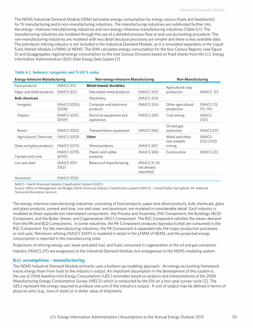
53U.S. Energy Information Administration | Assumptions to the Annual Energy Outlook 2013
Industrial Demand Module
The NEMS Industrial Demand Module (IDM) estimates energy consumption by energy source (fuels and feedstocks) for 15 manufacturing and 6 non-manufacturing industries. The manufacturing industries are subdivided further into the energy- intensive manufacturing industries and non-energy-intensive manufacturing industries (Table 6.1). The manufacturing industries are modeled through the use of a detailed process-flow or end-use accounting procedure. The non-manufacturing industries are modeled with less detail because processes are simpler and there is less available data. The petroleum refining industry is not included in the Industrial Demand Module, as it is simulated separately in the Liquid Fuels Market Module (LFMM) of NEMS. The IDM calculates energy consumption for the four Census Regions (see Figure 5) and disaggregates regional energy consumption to the nine Census Divisions based on fixed shares from the U.S. Energy Information Administration (EIA) State Energy Data System [1].
Table 6.1. Industry categories and NAICS codes
Energy-Intensive Manufacturing Non-energy-Intensive Manufacturing Non-Manufacturing
Food products (NAICS 311) Metal-based durables Agricultural crop production (NAICS 111)Paper and allied products (NAICS 322) Fabricated metal products (NAICS 332)
Bulk chemicals Machinery (NAICS 333)
Inorganic (NAICS 32512-32518)
Computer and electronic products
(NAICS 334) Other agricultural production
(NAICS 112, 113, 115)
Organic (NAICS 32511, 32519)
Electrical equipment and appliances
(NAICS 335) Coal mining (NAICS 2121)
Resins (NAICS 3252) Transportation equipment (NAICS 336)Oil and gas extraction (NAICS 211)
Agricultural Chemicals (NAICS 3253) Other Metal and other non-metallic mining
(NAICS 2122-2123)
Glass and glass products (NAICS 3272) Wood products (NAICS 321)
Cement and Lime(NAICS 32731, 32741)
Plastic and rubber products
(NAICS 326) Construction (NAICS 23)
Iron and steel (NAICS 3311-3312)
Balance of manufacturing (NAICS 31-33 not already classified)
Aluminum (NAICS 3313)NAICS = North American Industry Classification System (2007).Source: Office of Management and Budget, North American Industry Classification system (NAICS) - United States (Springfield, VA. National Technical Information Service).
The energy-intensive manufacturing industries, consisting of food products, paper and allied products, bulk chemicals, glass and glass products, cement and lime, iron and steel, and aluminum, are modeled in considerable detail. Each industry is modeled as three separate but interrelated components: the Process and Assembly (PA) Component, the Buildings (BLD) Component, and the Boiler, Steam, and Cogeneration (BSC) Component. The BSC Component satisfies the steam demand from the PA and BLD Components. In some industries, the PA Component produces byproducts that are consumed in the BSC Component. For the manufacturing industries, the PA Component is separated into the major production processes or end uses. Petroleum refining (NAICS 32411) is modeled in detail in the LFMM of NEMS, and the projected energy consumption is reported in the manufacturing total.Projections of refining energy use, lease and plant fuel, and fuels consumed in cogeneration in the oil and gas extraction industry (NAICS 211) are exogenous to the Industrial Demand Module, but endogenous to the NEMS modeling system.
Key assumptions - manufacturing The NEMS Industrial Demand Module primarily uses a bottom-up modeling approach. An energy accounting framework traces energy flows from fuels to the industry’s output. An important assumption in the development of this system is the use of 2006 baseline Unit Energy Consumption (UEC) estimates based on analysis and interpretations of the 2006 Manufacturing Energy Consumption Survey (MECS) which is conducted by the EIA on a four-year survey cycle [2]. The UECs represent the energy required to produce one unit of the industry’s output. A unit of output may be defined in terms of physical units (e.g., tons of steel) or in dollar value of shipments.
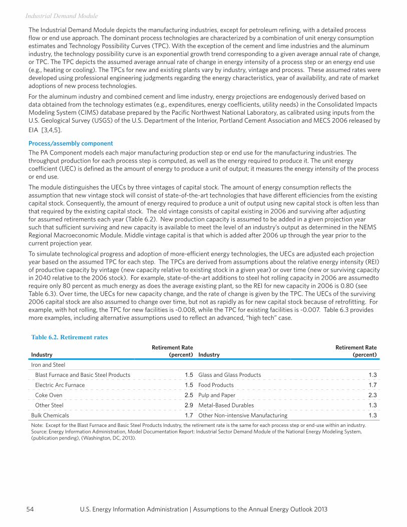
U.S. Energy Information Administration | Assumptions to the Annual Energy Outlook 201354
Industrial Demand Module
The Industrial Demand Module depicts the manufacturing industries, except for petroleum refining, with a detailed process flow or end use approach. The dominant process technologies are characterized by a combination of unit energy consumption estimates and Technology Possibility Curves (TPC). With the exception of the cement and lime industries and the aluminum industry, the technology possibility curve is an exponential growth trend corresponding to a given average annual rate of change, or TPC. The TPC depicts the assumed average annual rate of change in energy intensity of a process step or an energy end use (e.g., heating or cooling). The TPCs for new and existing plants vary by industry, vintage and process. These assumed rates were developed using professional engineering judgments regarding the energy characteristics, year of availability, and rate of market adoptions of new process technologies.For the aluminum industry and combined cement and lime industry, energy projections are endogenously derived based on data obtained from the technology estimates (e.g., expenditures, energy coefficients, utility needs) in the Consolidated Impacts Modeling System (CIMS) database prepared by the Pacific Northwest National Laboratory, as calibrated using inputs from the U.S. Geological Survey (USGS) of the U.S. Department of the Interior, Portland Cement Association and MECS 2006 released by EIA [3,4,5].
Process/assembly componentThe PA Component models each major manufacturing production step or end use for the manufacturing industries. The throughput production for each process step is computed, as well as the energy required to produce it. The unit energy coefficient (UEC) is defined as the amount of energy to produce a unit of output; it measures the energy intensity of the process or end use. The module distinguishes the UECs by three vintages of capital stock. The amount of energy consumption reflects the assumption that new vintage stock will consist of state-of-the-art technologies that have different efficiencies from the existing capital stock. Consequently, the amount of energy required to produce a unit of output using new capital stock is often less than that required by the existing capital stock. The old vintage consists of capital existing in 2006 and surviving after adjusting for assumed retirements each year (Table 6.2). New production capacity is assumed to be added in a given projection year such that sufficient surviving and new capacity is available to meet the level of an industry’s output as determined in the NEMS Regional Macroeconomic Module. Middle vintage capital is that which is added after 2006 up through the year prior to the current projection year. To simulate technological progress and adoption of more-efficient energy technologies, the UECs are adjusted each projection year based on the assumed TPC for each step. The TPCs are derived from assumptions about the relative energy intensity (REI) of productive capacity by vintage (new capacity relative to existing stock in a given year) or over time (new or surviving capacity in 2040 relative to the 2006 stock). For example, state-of-the-art additions to steel hot rolling capacity in 2006 are assumedto require only 80 percent as much energy as does the average existing plant, so the REI for new capacity in 2006 is 0.80 (see Table 6.3). Over time, the UECs for new capacity change, and the rate of change is given by the TPC. The UECs of the surviving 2006 capital stock are also assumed to change over time, but not as rapidly as for new capital stock because of retrofitting. For example, with hot rolling, the TPC for new facilities is -0.008, while the TPC for existing facilities is -0.007. Table 6.3 provides more examples, including alternative assumptions used to reflect an advanced, “high tech” case.
Table 6.2. Retirement rates
IndustryRetirement Rate
(percent) IndustryRetirement Rate
(percent)
Iron and Steel
Blast Furnace and Basic Steel Products 1.5 Glass and Glass Products 1.3
Electric Arc Furnace 1.5 Food Products 1.7
Coke Oven 2.5 Pulp and Paper 2.3
Other Steel 2.9 Metal-Based Durables 1.3
Bulk Chemicals 1.7 Other Non-intensive Manufacturing 1.3Note: Except for the Blast Furnace and Basic Steel Products Industry, the retirement rate is the same for each process step or end-use within an industry. Source: Energy Information Administration, Model Documentation Report: Industrial Sector Demand Module of the National Energy Modeling System, (publication pending), (Washington, DC, 2013).

55U.S. Energy Information Administration | Assumptions to the Annual Energy Outlook 2013
Industrial Demand Module
For the new submodules cement and lime and aluminum, baseline capacity baseline capacity (as of year 2008) is assumed to retire at a linear rate over a fixed period of time (20 years). Incremental, or added, capacity after 2008 is assumed to retire according to a logistic survival function. In addition, for the cement industry, retirement of existing wet process kiln technology is assumed to be permanent; only dry process kilns can be added to replace retired wet kilns or to satisfy needed additional capacity.The concepts of REI and TPCs are a means of embodying assumptions regarding new technology adoption in the manufacturing industry and the associated change in energy consumption of capital without characterizing individual technologies in detail. The approach reflects the assumption that industrial plants will change energy consumption as owners replace old equipment with new, sometimes more-efficient equipment, add new capacity, add new products, or upgrade their energy management practices. The reasons for the increased efficiency are not likely to be directly attributable to technology choice decisions, changing energy prices, or other factors readily subject to modeling. Instead, the module uses the REI and TPC concepts to characterize intensity trends for bundles of technologies available for major process steps or end use.There are two exceptions to the general approach in the PA component. The first is for electric motor technology choice implemented for 9 industries to simulate their electric machine drive energy end use. Machine drive electricity consumption in the food industry, the five metal-based durables industries, and the three non-intensive manufacturing industries is calculated by a motor stock model. The beginning stock of motors is modified over the projection horizon as motors are added to accommodate growth in shipments for each sector, as motors are retired and replaced, and as failed motors are rewound. When an old motor fails, an economic choice is made on whether to repair or replace the motor. When a new motor is added, either to accommodate growth or as a replacement, the motor must meet the minimum efficiency standard and a premium efficiency motor is also available. Table 6.4 provides the beginning stock efficiency for seven motor size groups in each of the three industry groups, as well as efficiencies for EPACT minimum and premium motors [7]. As the motor stock changes over the projection horizon, the overall efficiency of the motor population changes as well.The second exception in the PA component is the Cement and Lime and Aluminum submodules. The methodology is described below.The addition of the cement and lime submodule and aluminum submodule are the first two of several enhancements of the energy-intensive industries within the Industrial Demand Module. Instead of the aggregate energy intensity evolving according to TPCs curves for both new and vintage equipment for the process flows, the new submodules utilize detailed technology choice for each process flows. The new modules calculate surviving capacity based on retirement and needed capacity based on shipments and surviving capacity. Existing capital equipment retires linearly and new capital equipment retires according to an non-linear “S” curve over the useful life of the equipment. The exact shape of the “S” curve can be obtained by parameters adjusted by the user, New capital equipment information (capital and operating costs, energy use, and emissions) were obtained from the Consolidated Impacts Modeling System (CIMS) database. Each step of the process flow allows for multiple technology choices whose fuel type and efficiency are known at the national level, as regional fuel breakouts are fixed using available EIA data.
Combined cement and lime industryFor the cement process flow, each step (raw material grinding, kiln – both rotation and burner, finished grinding) allows for multiple technology choices whose fuel type and efficiency are known at the national level, as regional fuel breakouts are fixed using available EIA data.Cement has both dry and wet mill processes. Some technologies are available to both processes, while others are available to only one process. The technology choices within each group are:
1. Raw materials grinding: ball mill, roller mill2. Kilns (rotators): rotary long with preheat, precalcining, and computer control (dry process only), rotary preheat
with high-efficiency cooler (dry only), rotary preheat, precalcine with efficient cooler (dry process only), rotary wet standard with waste heat recovery boiler and cogeneration (wet process only)
3. Kilns (burners): standard fired by natural gas, efficient fired by natural gas, standard fired by oil, efficient fired by oil, standard fired by coal, standard fired by petroleum coke, standard fired by hazardous waste, standard fired by residue- derived fuel
4. Finished grinders: standard ball mill, finishing ball mill with high-efficiency separator, standard roller mill, finishing roller mill with high-efficiency separator
The technology slate in each of these process steps evolves over time and depends on the relative cost of equipment, cost of fuel, and fuel efficiency.

U.S. Energy Information Administration | Assumptions to the Annual Energy Outlook 201356
Industrial Demand Module
The base year technology slate is determined from the latest CIMS database and calibrated for the base year 2008 with dry and wet mill capacity cement fuel use data from the Portland Cement Association, the USGS, and the 2006 MECS. All new cement capacity, both for replacement and increased production, is assumed to be dry cement capacity. Existing wet capacity is assumed to retire at a linear rate over 20 years with no replacement. Imported clinker, additives, and fly-ash are assumed to make constant percentage contributions to the finished product and thus “displace” a certain amount of domestic clinker production, and therefore energy use.Lime shipments are estimated using a fixed percentage of stone, clay and glass shipments. Lime shipments, plus cement shipments, are presented together as the consolidated cement and lime output. Energy consumption and technology evolution in the lime industry are driven by the same methods implemented for cement, with different, industry-specific equipment choices.
Process/assembly component for Aluminum industryFor the aluminum process flow, each step (alumina production, anode production, and electrolysis for primary aluminum production, and melting for secondary production), allows for multiple technology choices whose fuel type and efficiency are known, as well as other operating characteristics. Technology shares are known at the national level, with regional fuel breakouts based on fixed allocations using available EIA data.The aluminum industry has both primary and secondary production processes, which vary greatly in their energy demands. As such, the extents of these processes are based on the aluminum industry’s projected production and its historical share of production processes attenuated by relevant regional energy prices. Therefore, the fraction of total throughput from each aluminum production process varies over the model projections.
Some technologies are available to both processes, while others are available to only one process. The technology choices within each production processing group are:
1. Primary smelting (Hall-Heroult electrolysis cell) is represented as smelting in four pre-bake anode technologies that denote standard and retrofitted choices and one inert anode wetted cathode choice.
2. Anode production, used in primary production only, is represented by three natural gas-fired furnaces under various configurations in forming and baking pre-bake anodes and the formation of Söderberg anodes. Note that anodes are a major requirement for the Hall-Heroult process.
3. Alumina production (Bayer Process) is used in primary production only and selects between existing natural gas facilities and those with retrofits.
4. Secondary production selects between two natural gas-fired melters – i.e., a standard and a melter with high efficiency: The technology slate in each of these process steps evolves over time and depends on the relative cost of equipment, cost of fuel, and fuel efficiency. The base year technology slate is determined from the latest CIMS database and calibrated for the base year 2006 MECS and the USGS. All new capacities for aluminum production, both for replacement and increased production needs, are now assumed to be either pre-existing primary production or new secondary production, based on historical trend data and projected energy prices. Similar to the energy-intensive technology of the cement industry, the assumed lifespan of existing and new production capacity is assumed to be 20 and 30 years, respectively. In addition, production that has been idled is allowed to re-enter production before new equipment is built.
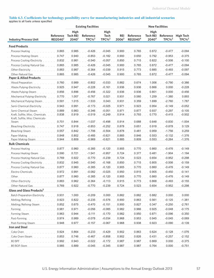
57U.S. Energy Information Administration | Assumptions to the Annual Energy Outlook 2013
Industrial Demand Module
Table 6.3. Coefficients for technology possibility curve for manufacturing industries and all industrial scenariosapplies to all fuels unless specified
Industry/Process Unit
Existing Facilities New Facillities
Reference REI20401
High Tech REI
20401Reference
TPC%2
High Tech
TPC%2REI
20063Reference REI20404
High Tech REI
20404Reference
TPC%2High Tech
TPC%2
Food ProductsProcess Heating 0.865 0.985 -0.426 -0.045 0.900 0.765 0.872 -0.477 -0.094
Process Heating-Steam 0.747 0.940 -0.853 -0.182 0.900 0.650 0.792 -0.953 -0.375Process Cooling-Electricity 0.832 0.981 -0.540 -0.057 0.850 0.715 0.822 -0.506 -0.100
Process Cooling-Natural Gas 0.865 0.985 -0.426 -0.045 0.900 0.765 0.872 -0.477 -0.094Other-Electricity 0.883 0.987 -0.364 -0.039 0.915 0.773 0.885 -0.493 -0.097Other-Natural Gas 0.865 0.985 -0.426 -0.045 0.900 0.765 0.872 -0.477 -0.094
Paper & Allied ProductsWood Preparation 0.760 0.989 -0.802 -0.033 0.882 0.674 1.006 -0.790 -0.386Waste Pulping-Electricity 0.925 0.947 -0.228 -0.161 0.936 0.936 0.866 0.000 -0.228Waste Pulping-Steam 0.856 0.896 -0.456 -0.322 0.936 0.936 0.801 0.000 -0.456Mechanical Pulping-Electricity 0.770 1.007 -0.767 0.021 0.931 0.580 1.259 -1.380 0.893Mechanical Pulping-Steam 0.591 1.015 -1.533 0.043 0.931 0.359 1.699 -2.760 1.787
Semi-Chemical-Electricity 0.943 0.991 -0.173 -0.025 0.971 0.923 0.954 -0.149 -0.052Semi-Chemical-Steam 0.889 0.983 -0.346 -0.051 0.971 0.877 0.937 -0.297 -0.105Kraft, Sulfite, Misc. Chemicals 0.838 0.919 -0.519 -0.249 0.914 0.793 0.770 -0.415 -0.502Kraft, Sulfite, Misc Chemicals-Steam 0.701 0.844 -1.037 -0.498 0.914 0.688 0.648 -0.830 -1.004Bleaching-Electricity 0.747 0.918 -0.853 -0.252 0.878 0.651 0.918 -0.878 0.129Bleaching-Steam 0.557 0.842 -1.706 -0.504 0.878 0.481 0.959 -1.756 0.259Paper Making 0.848 0.802 -0.485 -0.621 0.885 0.846 0.553 -0.132 -1.376Paper Making-Steam 0.944 0.809 -0.969 -0.621 0.885 0.809 0.553 -0.264 -1.376
Bulk ChemicalsProcess Heating 0.877 0.960 -0.385 -0.120 0.905 0.770 0.860 -0.476 -0.149Process Heating-Steam 0.590 0.721 -1.541 -0.957 0.724 0.377 0.481 -1.904 -1.194Process Heating-Natural Gas 0.769 0.922 -0.770 -0.239 0.724 0.523 0.654 -0.952 -0.298Process Cooling-Electricity 0.832 0.945 -0.540 -0.168 0.850 0.715 0.805 -0.506 -0.159Process Cooling-Natural Gas 0.877 0.960 -0.385 -0.120 0.905 0.770 0.860 -0.476 -0.149Electro-Chemicals 0.972 0.991 -0.082 -0.025 0.950 0.815 0.905 -0.450 -0.141Other 0.877 0.960 -0.385 -0.120 0.905 0.770 0.860 -0.476 -0.149Other-Electricity 0.883 0.962 -0.364 -0.113 0.915 0.773 0.868 -0.493 -0.155Other-Natural Gas 0.769 0.922 -0.770 -0.239 0.724 0.523 0.654 -0.952 -0.298
Glass and Glass Products5
Batch Preparation-Electricity 0.931 1.000 -0.209 0.000 0.882 0.882 0.882 0.000 0.000Melting/Refining 0.923 0.822 -0.235 -0.576 0.900 0.863 0.561 -0.125 -1.381Melting/Refining-Steam 0.852 0.675 -0.470 -0.151 0.900 0.827 0.347 -0.250 -2.761Forming 0.981 0.971 -0.056 -0.085 0.982 0.966 0.925 -0.048 -0.175Forming-Steam 0.963 0.944 -0.111 -0.170 0.982 0.950 0.871 -0.096 -0.350Post-Forming 0.974 0.989 -0.078 -0.034 0.968 0.953 0.945 -0.045 -0.069Post-Forming-Steam 0.948 0.977 -0.157 -0.067 0.968 0.938 0.923 -0.090 -0.139
Iron and SteelCoke Oven 0.924 0.864 -0.233 -0.429 0.902 0.863 0.624 -0.128 -1.076Coke Oven-Steam 0.853 0.746 -0.467 -0.858 0.902 0.826 0.431 -0.257 -2.152BF/BPF 0.992 0.943 -0.022 -0.172 0.987 0.987 0.869 0.000 -0.375BF/BOF-Stem 0.985 0.889 -0.045 -0.345 0.987 0.987 0.764 0.000 -0.751
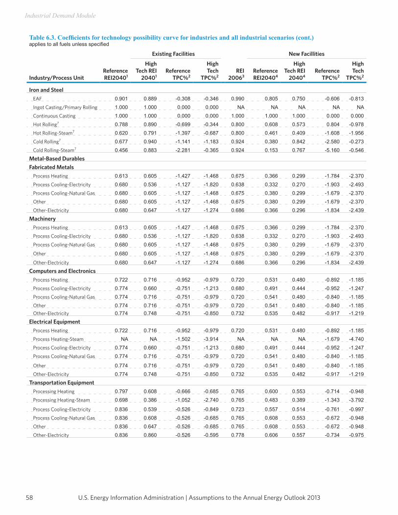
U.S. Energy Information Administration | Assumptions to the Annual Energy Outlook 201358
Industrial Demand Module
Table 6.3. Coefficients for technology possibility curve for industries and all industrial scenarios (cont.)applies to all fuels unless specified
Industry/Process Unit
Existing Facilities New Facillities
Reference REI20401
High Tech REI
20401Reference
TPC%2
High Tech
TPC%2REI
20063Reference REI20404
High Tech REI
20404Reference
TPC%2
High Tech
TPC%2
Iron and SteelEAF 0.901 0.889 -0.308 -0.346 0.990 0.805 0.750 -0.606 -0.813Ingot Casting/Primary Rolling 1.000 1.000 0.000 0.000 NA NA NA NA NAContinuous Casting 1.000 1.000 0.000 0.000 1.000 1.000 1.000 0.000 0.000Hot Rolling7 0.788 0.890 -0.699 -0.344 0.800 0.608 0.573 0.804 -0.978Hot Rolling-Steam7 0.620 0.791 -1.397 -0.687 0.800 0.461 0.409 -1.608 -1.956Cold Rolling7 0.677 0.940 -1.141 -1.183 0.924 0.380 0.842 -2.580 -0.273Cold Rolling-Steam7 0.456 0.883 -2.281 -0.365 0.924 0.153 0.767 -5.160 -0.546
Metal-Based DurablesFabricated Metals
Process Heating 0.613 0.605 -1.427 -1.468 0.675 0.366 0.299 -1.784 -2.370Process Cooling-Electricity 0.680 0.536 -1.127 -1.820 0.638 0.332 0.270 -1.903 -2.493Process Cooling-Natural Gas 0.680 0.605 -1.127 -1.468 0.675 0.380 0.299 -1.679 -2.370Other 0.680 0.605 -1.127 -1.468 0.675 0.380 0.299 -1.679 -2.370Other-Electricity 0.680 0.647 -1.127 -1.274 0.686 0.366 0.296 -1.834 -2.439
MachineryProcess Heating 0.613 0.605 -1.427 -1.468 0.675 0.366 0.299 -1.784 -2.370Process Cooling-Electricity 0.680 0.536 -1.127 -1.820 0.638 0.332 0.270 -1.903 -2.493Process Cooling-Natural Gas 0.680 0.605 -1.127 -1.468 0.675 0.380 0.299 -1.679 -2.370
Other 0.680 0.605 -1.127 -1.468 0.675 0.380 0.299 -1.679 -2.370
Other-Electricity 0.680 0.647 -1.127 -1.274 0.686 0.366 0.296 -1.834 -2.439Computers and Electronics
Process Heating 0.722 0.716 -0.952 -0.979 0.720 0.531 0.480 -0.892 -1.185Process Cooling-Electricity 0.774 0.660 -0.751 -1.213 0.680 0.491 0.444 -0.952 -1.247Process Cooling-Natural Gas 0.774 0.716 -0.751 -0.979 0.720 0.541 0.480 -0.840 -1.185Other 0.774 0.716 -0.751 -0.979 0.720 0.541 0.480 -0.840 -1.185Other-Electricity 0.774 0.748 -0.751 -0.850 0.732 0.535 0.482 -0.917 -1.219
Electrical EquipmentProcess Heating 0.722 0.716 -0.952 -0.979 0.720 0.531 0.480 -0.892 -1.185Process Heating-Steam NA NA -1.502 -3.914 NA NA NA -1.679 -4.740Process Cooling-Electricity 0.774 0.660 -0.751 -1.213 0.680 0.491 0.444 -0.952 -1.247Process Cooling-Natural Gas 0.774 0.716 -0.751 -0.979 0.720 0.541 0.480 -0.840 -1.185
Other 0.774 0.716 -0.751 -0.979 0.720 0.541 0.480 -0.840 -1.185Other-Electricity 0.774 0.748 -0.751 -0.850 0.732 0.535 0.482 -0.917 -1.219
Transportation EquipmentProcessing Heating 0.797 0.608 -0.666 -0.685 0.765 0.600 0.553 -0.714 -0.948Processing Heating-Steam 0.698 0.386 -1.052 -2.740 0.765 0.483 0.389 -1.343 -3.792
Process Cooling-Electricity 0.836 0.539 -0.526 -0.849 0.723 0.557 0.514 -0.761 -0.997Process Cooling-Natural Gas 0.836 0.608 -0.526 -0.685 0.765 0.608 0.553 -0.672 -0.948Other 0.836 0.647 -0.526 -0.685 0.765 0.608 0.553 -0.672 -0.948Other-Electricity 0.836 0.860 -0.526 -0.595 0.778 0.606 0.557 -0.734 -0.975
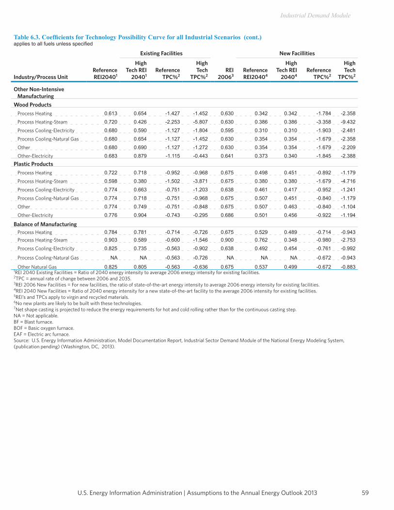
59U.S. Energy Information Administration | Assumptions to the Annual Energy Outlook 2013
Industrial Demand Module
Table 6.3. Coefficients for Technology Possibility Curve for all Industrial Scenarios (cont.)applies to all fuels unless specified
Industry/Process Unit
Existing Facilities New Facillities
Reference REI20401
High Tech REI
20401Reference
TPC%2
High Tech
TPC%2REI
20063Reference REI20404
High Tech REI
20404Reference
TPC%2
High Tech
TPC%2
Other Non-Intensive ManufacturingWood Products
Process Heating 0.613 0.654 -1.427 -1.452 0.630 0.342 0.342 -1.784 -2.358Process Heating-Steam 0.720 0.426 -2.253 -5.807 0.630 0.386 0.386 -3.358 -9.432Process Cooling-Electricity 0.680 0.590 -1.127 -1.804 0.595 0.310 0.310 -1.903 -2.481Process Cooling-Natural Gas 0.680 0.654 -1.127 -1.452 0.630 0.354 0.354 -1.679 -2.358Other 0.680 0.690 -1.127 -1.272 0.630 0.354 0.354 -1.679 -2.209Other-Electricity 0.683 0.879 -1.115 -0.443 0.641 0.373 0.340 -1.845 -2.388
Plastic ProductsProcess Heating 0.722 0.718 -0.952 -0.968 0.675 0.498 0.451 -0.892 -1.179Process Heating-Steam 0.598 0.380 -1.502 -3.871 0.675 0.380 0.380 -1.679 -4.716Process Cooling-Electricity 0.774 0.663 -0.751 -1.203 0.638 0.461 0.417 -0.952 -1.241Process Cooling-Natural Gas 0.774 0.718 -0.751 -0.968 0.675 0.507 0.451 -0.840 -1.179Other 0.774 0.749 -0.751 -0.848 0.675 0.507 0.463 -0.840 -1.104Other-Electricity 0.776 0.904 -0.743 -0.295 0.686 0.501 0.456 -0.922 -1.194
Balance of ManufacturingProcess Heating 0.784 0.781 -0.714 -0.726 0.675 0.529 0.489 -0.714 -0.943Process Heating-Steam 0.903 0.589 -0.600 -1.546 0.900 0.762 0.348 -0.980 -2.753Process Cooling-Electricity 0.825 0.735 -0.563 -0.902 0.638 0.492 0.454 -0.761 -0.992
Process Cooling-Natural Gas NA NA -0.563 -0.726 NA NA NA -0.672 -0.943
Other Natural Gas 0.825 0.805 -0.563 -0.636 0.675 0.537 0.499 -0.672 -0.8831REI 2040 Existing Facilities = Ratio of 2040 energy intensity to average 2006 energy intensity for existing facilities.2TPC = annual rate of change between 2006 and 2035.3REI 2006 New Facilities = For new facilities, the ratio of state-of-the-art energy intensity to average 2006 energy intensity for existing facilities.4REI 2040 New Facilities = Ratio of 2040 energy intensity for a new state-of-the-art facility to the average 2006 intensity for existing facilities.5REI’s and TPCs apply to virgin and recycled materials.6No new plants are likely to be built with these technologies.7Net shape casting is projected to reduce the energy requirements for hot and cold rolling rather than for the continuous casting step. NA = Not applicable.BF = Blast furnace. BOF = Basic oxygen furnace. EAF = Electric arc furnace. Source: U.S. Energy Information Administration, Model Documentation Report, Industrial Sector Demand Module of the National Energy Modeling System, (publication pending) (Washington, DC, 2013).
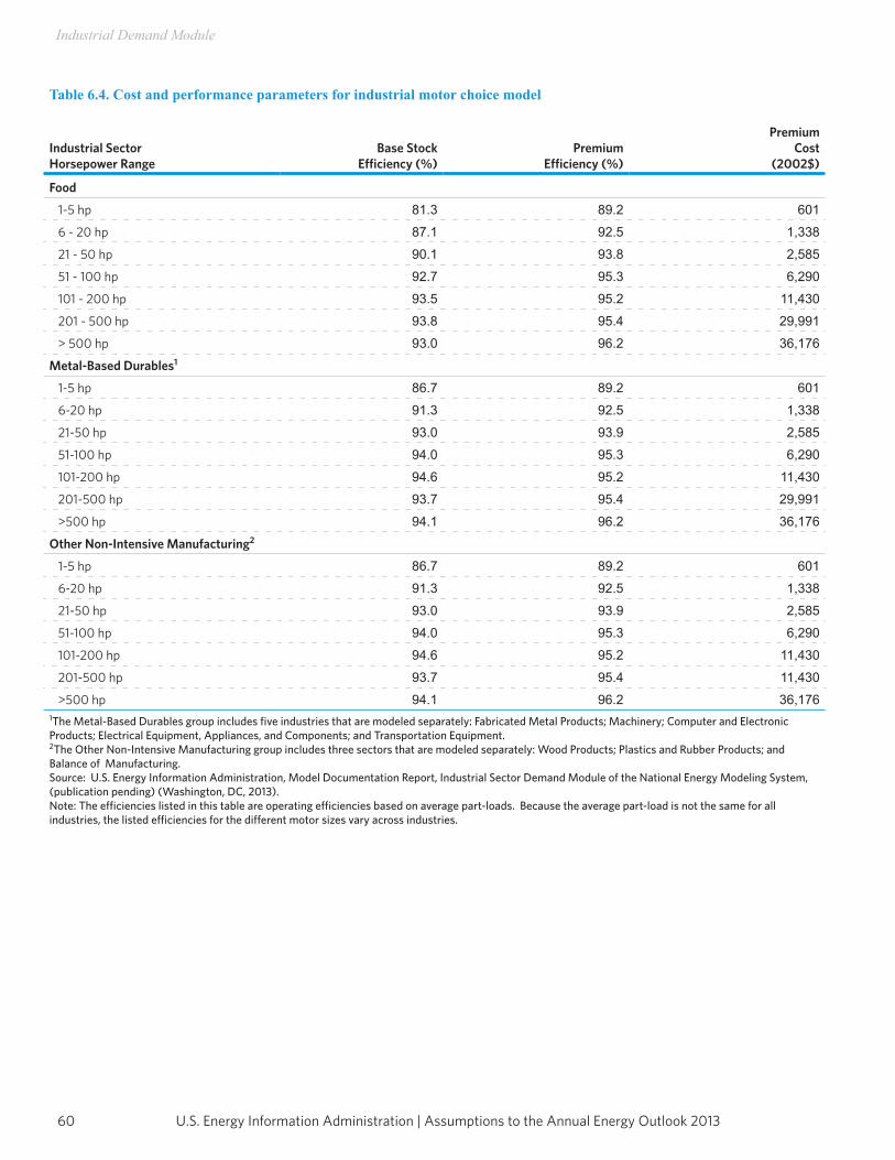
U.S. Energy Information Administration | Assumptions to the Annual Energy Outlook 201360
Industrial Demand Module
Table 6.4. Cost and performance parameters for industrial motor choice model
Industrial Sector Horsepower Range
Base Stock Efficiency (%)
Premium Efficiency (%)
PremiumCost
(2002$)
Food
1-5 hp 81.3 89.2 601
6 - 20 hp 87.1 92.5 1,338
21 - 50 hp 90.1 93.8 2,585
51 - 100 hp 92.7 95.3 6,290
101 - 200 hp 93.5 95.2 11,430
201 - 500 hp 93.8 95.4 29,991
> 500 hp 93.0 96.2 36,176
Metal-Based Durables1
1-5 hp 86.7 89.2 601
6-20 hp 91.3 92.5 1,338
21-50 hp 93.0 93.9 2,585
51-100 hp 94.0 95.3 6,290
101-200 hp 94.6 95.2 11,430
201-500 hp 93.7 95.4 29,991
>500 hp 94.1 96.2 36,176
Other Non-Intensive Manufacturing2
1-5 hp 86.7 89.2 601
6-20 hp 91.3 92.5 1,338
21-50 hp 93.0 93.9 2,585
51-100 hp 94.0 95.3 6,290
101-200 hp 94.6 95.2 11,430
201-500 hp 93.7 95.4 11,430
>500 hp 94.1 96.2 36,1761The Metal-Based Durables group includes five industries that are modeled separately: Fabricated Metal Products; Machinery; Computer and Electronic Products; Electrical Equipment, Appliances, and Components; and Transportation Equipment.2The Other Non-Intensive Manufacturing group includes three sectors that are modeled separately: Wood Products; Plastics and Rubber Products; and Balance of Manufacturing. Source: U.S. Energy Information Administration, Model Documentation Report, Industrial Sector Demand Module of the National Energy Modeling System, (publication pending) (Washington, DC, 2013). Note: The efficiencies listed in this table are operating efficiencies based on average part-loads. Because the average part-load is not the same for all industries, the listed efficiencies for the different motor sizes vary across industries.
61U.S. Energy Information Administration | Assumptions to the Annual Energy Outlook 2013
Industrial Demand Module
Petrochemical feedstock requirementThis subroutine estimates feedstock requirements for the major petrochemical intermediates such as ethylene, propylene, and butadiene. The primary feedstocks used to produce these chemicals are natural gas liquids (NGL) (ethane, propane, butane) and petrochemical (oil-based) feedstocks (gas oil, naphtha) [6]. Biomass is a potential raw material source, but it is assumed that there will be no biomass-based capacity over the projection period because of economic barriers. The type of feedstock not only determines the source of feedstock but also the energy for heat and power requirements to produce the chemicals.To determine the relative amounts of feedstock (NGL or oil-based) baseline intensities, feedstock consumption intensities are derived from the 2006 MECS. Feedstock consumption of both types grows or declines with organic chemicals shipment value. It should be noted that there is no change in the feedstock intensity over time, i.e., all feedstock TPCs are assumed to be zero. Unlike most other processes represented in manufacturing PA components, chemical yields are governed by basic chemical stoichiometry which allows for specific yields under set conditions of pressure and temperature. For the projected LPG feedstock quantities, a further subdivision is made into refinery-produced propylene and ethane. All ethane produced by the NEMS Oil and Gas Supply Module is absorbed by the chemical model. The remaining balance of LPG feedstock requirement is a mixture of pentanes plus, butane, and propane.
Buildings component The total buildings energy demand by industry for each region is a function of regional industrial employment and output. Building energy consumption was estimated for building lighting, HVAC (heating, ventilation, and air conditioning), facility support, and on-site transportation. Space heating was further divided to estimate the amount provided by direct combustion of fossil fuels and that provided by steam (Table 6.5). Energy consumption in the BLD Component for an industry is estimated based on regional employment and output growth for that industry using the 2006 MECS as a basis.
Boiler, steam, and cogeneration componentThe steam demand and byproducts from the PA and BLD Components are passed to the BSC Component, which applies a heat rate and a fuel share equation (Table 6.6) to the boiler steam requirements to compute the required energy consumption.The boiler fuel shares apply only to the fuels that are used in boilers for steam-only applications. Fuel use for the portion of the steam demand associated with combined heat and power (CHP) is described in the next section. Some fuel switching for the remainder of the boiler fuel use is assumed and is calculated with a logit-sharing equation where fuels shares are a function of fuel prices. The equation is calibrated to 2006 so that the 2006 fuel shares are produced for the relative prices that prevailed in2006.The byproduct fuels, production of which is estimated in the PA Component, are assumed to be consumed without regard to price, independent of purchased fuels. The boiler fuel share equations and calculations are based on the 2006 MECS and information from the Council of Industrial Boiler Owners. [8]
Combined heat and powerCHP plants, which are designed to produce both electricity and useful heat, have been used in the industrial sector for many years. The CHP estimates in the module are based on the assumption that the historical relationship between industrial steam demand and CHP will continue in the future, and that the rate of additional CHP penetration will depend on the economics of retrofitting CHP plants to replace steam generated from existing non-CHP boilers. The technical potential for CHP is primarily based on supplying thermal requirements (i.e., matching thermal loads). Capacity additions are then determined by the interaction of CHP investment payback periods (with the time-value of money included) derived using operating hours reported in EIA’s published statistics, market penetration rates for investments with those payback periods, and regional deployment for these systems as characterized by the “collaboration coefficients” in Table 6.8. Assumed installed costs for the CHP systems are given in Table 6.7.
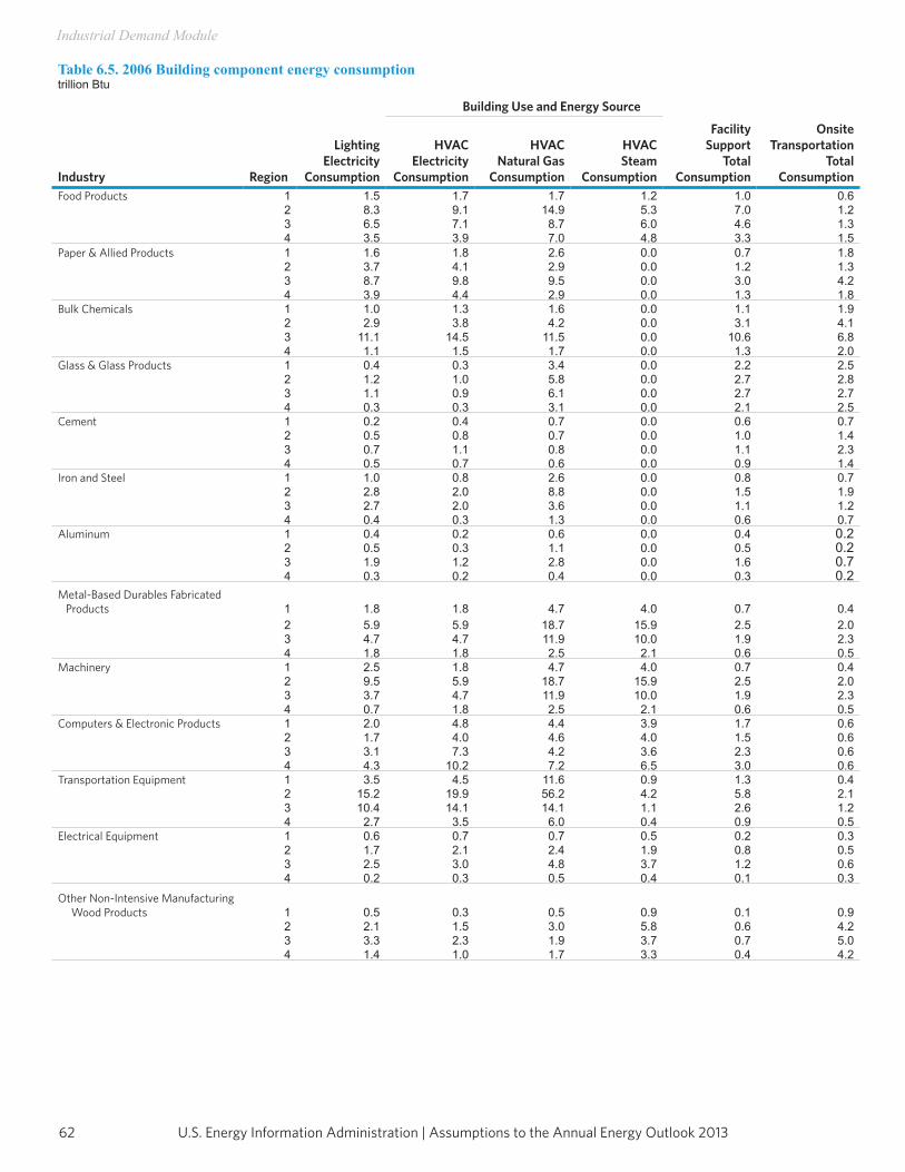
U.S. Energy Information Administration | Assumptions to the Annual Energy Outlook 201362
Industrial Demand Module
Table 6.5. 2006 Building component energy consumption trillion Btu
Industry
Building Use and Energy Source
Region
Lighting Electricity
Consumption
HVAC Electricity
Consumption
HVAC Natural Gas
Consumption
HVAC Steam
Consumption
Facility Support
Total Consumption
Onsite Transportation
Total Consumption
Food Products 1 1.5 1.7 1.7 1.2 1.0 0.62 8.3 9.1 14.9 5.3 7.0 1.23 6.5 7.1 8.7 6.0 4.6 1.34 3.5 3.9 7.0 4.8 3.3 1.5
Paper & Allied Products 1 1.6 1.8 2.6 0.0 0.7 1.82 3.7 4.1 2.9 0.0 1.2 1.33 8.7 9.8 9.5 0.0 3.0 4.24 3.9 4.4 2.9 0.0 1.3 1.8
Bulk Chemicals 1 1.0 1.3 1.6 0.0 1.1 1.92 2.9 3.8 4.2 0.0 3.1 4.13 11.1 14.5 11.5 0.0 10.6 6.84 1.1 1.5 1.7 0.0 1.3 2.0
Glass & Glass Products 1 0.4 0.3 3.4 0.0 2.2 2.52 1.2 1.0 5.8 0.0 2.7 2.83 1.1 0.9 6.1 0.0 2.7 2.74 0.3 0.3 3.1 0.0 2.1 2.5
Cement 1 0.2 0.4 0.7 0.0 0.6 0.72 0.5 0.8 0.7 0.0 1.0 1.43 0.7 1.1 0.8 0.0 1.1 2.34 0.5 0.7 0.6 0.0 0.9 1.4
Iron and Steel 1 1.0 0.8 2.6 0.0 0.8 0.72 2.8 2.0 8.8 0.0 1.5 1.93 2.7 2.0 3.6 0.0 1.1 1.24 0.4 0.3 1.3 0.0 0.6 0.7
Aluminum 1 0.4 0.2 0.6 0.0 0.4 0.22 0.5 0.3 1.1 0.0 0.5 0.23 1.9 1.2 2.8 0.0 1.6 0.74 0.3 0.2 0.4 0.0 0.3 0.2
Metal-Based Durables Fabricated Products 1 1.8 1.8 4.7 4.0 0.7 0.4
2 5.9 5.9 18.7 15.9 2.5 2.03 4.7 4.7 11.9 10.0 1.9 2.34 1.8 1.8 2.5 2.1 0.6 0.5
Machinery 1 2.5 1.8 4.7 4.0 0.7 0.42 9.5 5.9 18.7 15.9 2.5 2.03 3.7 4.7 11.9 10.0 1.9 2.34 0.7 1.8 2.5 2.1 0.6 0.5
Computers & Electronic Products 1 2.0 4.8 4.4 3.9 1.7 0.62 1.7 4.0 4.6 4.0 1.5 0.63 3.1 7.3 4.2 3.6 2.3 0.64 4.3 10.2 7.2 6.5 3.0 0.6
Transportation Equipment 1 3.5 4.5 11.6 0.9 1.3 0.42 15.2 19.9 56.2 4.2 5.8 2.13 10.4 14.1 14.1 1.1 2.6 1.24 2.7 3.5 6.0 0.4 0.9 0.5
Electrical Equipment 1 0.6 0.7 0.7 0.5 0.2 0.32 1.7 2.1 2.4 1.9 0.8 0.53 2.5 3.0 4.8 3.7 1.2 0.64 0.2 0.3 0.5 0.4 0.1 0.3
Other Non-Intensive Manufacturing Wood Products 1 0.5 0.3 0.5 0.9 0.1 0.9
2 2.1 1.5 3.0 5.8 0.6 4.23 3.3 2.3 1.9 3.7 0.7 5.04 1.4 1.0 1.7 3.3 0.4 4.2
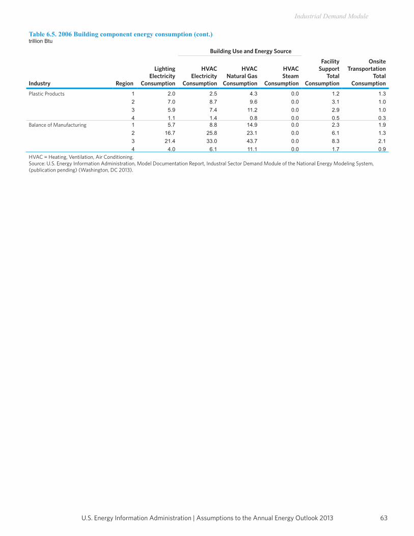
63U.S. Energy Information Administration | Assumptions to the Annual Energy Outlook 2013
Industrial Demand Module
Table 6.5. 2006 Building component energy consumption (cont.) trillion Btu
Industry
Building Use and Energy Source
Region
Lighting Electricity
Consumption
HVAC Electricity
Consumption
HVAC Natural Gas
Consumption
HVAC Steam
Consumption
Facility Support
Total Consumption
Onsite Transportation
Total Consumption
Plastic Products 1 2.0 2.5 4.3 0.0 1.2 1.32 7.0 8.7 9.6 0.0 3.1 1.03 5.9 7.4 11.2 0.0 2.9 1.04 1.1 1.4 0.8 0.0 0.5 0.3
Balance of Manufacturing 1 5.7 8.8 14.9 0.0 2.3 1.92 16.7 25.8 23.1 0.0 6.1 1.33 21.4 33.0 43.7 0.0 8.3 2.14 4.0 6.1 11.1 0.0 1.7 0.9
HVAC = Heating, Ventilation, Air Conditioning.Source: U.S. Energy Information Administration, Model Documentation Report, Industral Sector Demand Module of the National Energy Modeling System, (publication pending) (Washington, DC 2013).
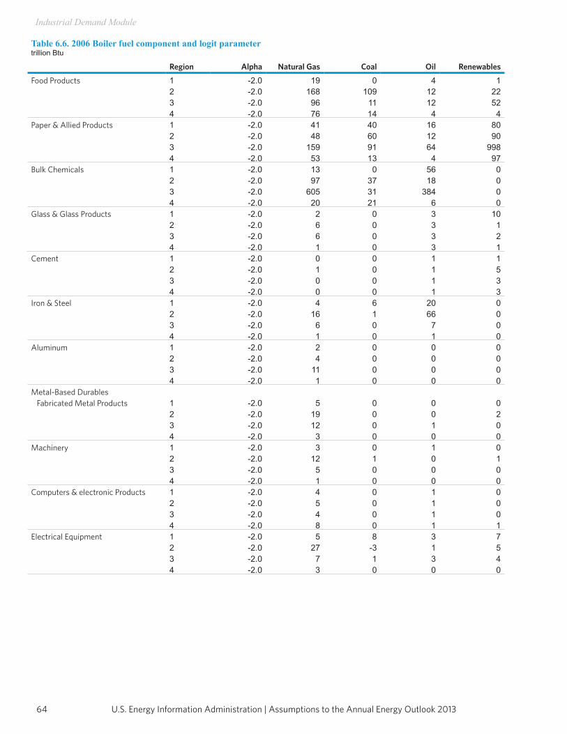
U.S. Energy Information Administration | Assumptions to the Annual Energy Outlook 201364
Industrial Demand Module
Table 6.6. 2006 Boiler fuel component and logit parameter trillion Btu
Region Alpha Natural Gas Coal Oil Renewables
Food Products 1 -2.0 19 0 4 12 -2.0 168 109 12 223 -2.0 96 11 12 524 -2.0 76 14 4 4
Paper & Allied Products 1 -2.0 41 40 16 802 -2.0 48 60 12 903 -2.0 159 91 64 9984 -2.0 53 13 4 97
Bulk Chemicals 1 -2.0 13 0 56 02 -2.0 97 37 18 03 -2.0 605 31 384 04 -2.0 20 21 6 0
Glass & Glass Products 1 -2.0 2 0 3 102 -2.0 6 0 3 13 -2.0 6 0 3 24 -2.0 1 0 3 1
Cement 1 -2.0 0 0 1 12 -2.0 1 0 1 53 -2.0 0 0 1 34 -2.0 0 0 1 3
Iron & Steel 1 -2.0 4 6 20 02 -2.0 16 1 66 03 -2.0 6 0 7 04 -2.0 1 0 1 0
Aluminum 1 -2.0 2 0 0 02 -2.0 4 0 0 03 -2.0 11 0 0 04 -2.0 1 0 0 0
Metal-Based Durables Fabricated Metal Products 1 -2.0 5 0 0 0
2 -2.0 19 0 0 23 -2.0 12 0 1 04 -2.0 3 0 0 0
Machinery 1 -2.0 3 0 1 02 -2.0 12 1 0 13 -2.0 5 0 0 04 -2.0 1 0 0 0
Computers & electronic Products 1 -2.0 4 0 1 02 -2.0 5 0 1 03 -2.0 4 0 1 04 -2.0 8 0 1 1
Electrical Equipment 1 -2.0 5 8 3 72 -2.0 27 -3 1 53 -2.0 7 1 3 44 -2.0 3 0 0 0
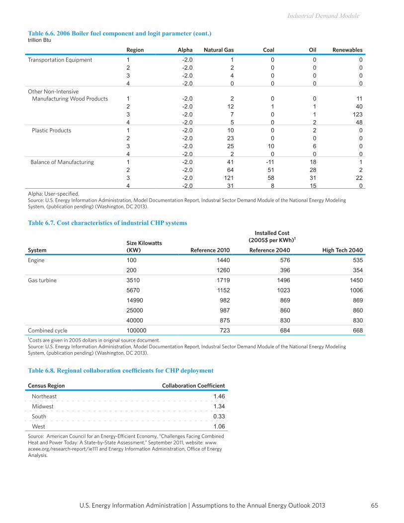
65U.S. Energy Information Administration | Assumptions to the Annual Energy Outlook 2013
Industrial Demand Module
Table 6.6. 2006 Boiler fuel component and logit parameter (cont.) trillion Btu
Region Alpha Natural Gas Coal Oil Renewables
Transportation Equipment 1 -2.0 1 0 0 02 -2.0 2 0 0 03 -2.0 4 0 0 04 -2.0 0 0 0 0
Other Non-Intensive Manufacturing Wood Products 1 -2.0 2 0 0 11
2 -2.0 12 1 1 403 -2.0 7 0 1 1234 -2.0 5 0 2 48
Plastic Products 1 -2.0 10 0 2 02 -2.0 23 0 0 03 -2.0 25 10 6 04 -2.0 2 0 0 0
Balance of Manufacturing 1 -2.0 41 -11 18 12 -2.0 64 51 28 23 -2.0 121 58 31 224 -2.0 31 8 15 0
Alpha: User-specified.Source: U.S. Energy Information Administration, Model Documentation Report, Industral Sector Demand Module of the National Energy Modeling System, (publication pending) (Washington, DC 2013).
Table 6.7. Cost characteristics of industrial CHP systems
SystemSize Kilowatts (KW)
Installed Cost (2005$ per KWh)1
Reference 2010 Reference 2040 High Tech 2040
Engine 100 1440 576 535
200 1260 396 354
Gas turbine 3510 1719 1496 1450
5670 1152 1023 1006
14990 982 869 869
25000 987 860 860
40000 875 830 830
Combined cycle 100000 723 684 6681Costs are given in 2005 dollars in original source document.Source: U.S. Energy Information Administration, Model Documentation Report, Industral Sector Demand Module of the National Energy Modeling System, (publication pending) (Washington, DC 2013).
Table 6.8. Regional collaboration coefficients for CHP deployment
Census Region Collaboration Coefficient
Northeast 1.46
Midwest 1.34
South 0.33
West 1.06Source: American Council for an Energy-Efficient Economy, “Challenges Facing Combined Heat and Power Today: A State-by-State Assessment,” September 2011, website: www.aceee.org/research-report/ie111 and Energy Information Administration, Office of Energy Analysis.
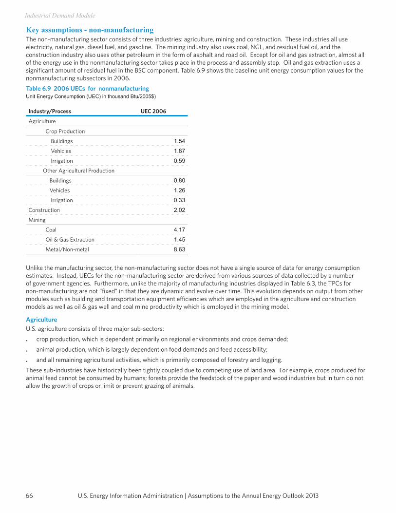
U.S. Energy Information Administration | Assumptions to the Annual Energy Outlook 201366
Industrial Demand Module
Key assumptions - non-manufacturingThe non-manufacturing sector consists of three industries: agriculture, mining and construction. These industries all use electricity, natural gas, diesel fuel, and gasoline. The mining industry also uses coal, NGL, and residual fuel oil, and the construction industry also uses other petroleum in the form of asphalt and road oil. Except for oil and gas extraction, almost all of the energy use in the nonmanufacturing sector takes place in the process and assembly step. Oil and gas extraction uses a significant amount of residual fuel in the BSC component. Table 6.9 shows the baseline unit energy consumption values for the nonmanufacturing subsectors in 2006.Table 6.9 2006 UECs for nonmanufacturing Unit Energy Consumption (UEC) in thousand Btu/2005$)
Industry/Process UEC 2006
Agriculture
Crop Production
Buildings 1.54
Vehicles 1.87
Irrigation 0.59
Other Agricultural Production
Buildings 0.80
Vehicles 1.26
Irrigation 0.33
Construction 2.02
Mining
Coal 4.17
Oil & Gas Extraction 1.45
Metal/Non-metal 8.63
Unlike the manufacturing sector, the non-manufacturing sector does not have a single source of data for energy consumption estimates. Instead, UECs for the non-manufacturing sector are derived from various sources of data collected by a number of government agencies. Furthermore, unlike the majority of manufacturing industries displayed in Table 6.3, the TPCs for non-manufacturing are not “fixed” in that they are dynamic and evolve over time. This evolution depends on output from other modules such as building and transportation equipment efficiencies which are employed in the agriculture and construction models as well as oil & gas well and coal mine productivity which is employed in the mining model.
AgricultureU.S. agriculture consists of three major sub-sectors:
• crop production, which is dependent primarily on regional environments and crops demanded;
• animal production, which is largely dependent on food demands and feed accessibility;
• and all remaining agricultural activities, which is primarily composed of forestry and logging. These sub-industries have historically been tightly coupled due to competing use of land area. For example, crops produced for animal feed cannot be consumed by humans; forests provide the feedstock of the paper and wood industries but in turn do not allow the growth of crops or limit or prevent grazing of animals.
67U.S. Energy Information Administration | Assumptions to the Annual Energy Outlook 2013
Industrial Demand Module
However, energy consumption in these industries is tied to specialized equipment, which often determines the fuel requirement with little flexibility. Within each of these sub-industries the key energy-using equipment can be broken into three major categories: off-road vehicles, buildings, and other equipment, which is primarily irrigation equipment for crop production. Agriculture TPCs are calculated within the NEMS model by further subdividing consumption in each sub-industry based on the equipment in which the energy is used: off-road vehicles, which are trucks, tractors, and other specialty vehicles; buildings, which require lighting and temperature control; and other equipment, which covers a variety of both common (e.g., pumps) and specialty (for example cotton gins) equipment used in all the various types of agricultural production. Thus, changes in efficiencies in heavy and medium-duty vehicles from the Transportation Sector Module and changes in lighting and heating efficiencies from the Commercial Sector Demand Module are used to dynamically modify the agriculture TPCs.Baseline energy consumption data for the two agriculture sectors (crops and other agriculture) is based on data from the Census of Agriculture and a special tabulation from the National Agricultural Statistics Service (USDA-NASS). Expenditures for four energy sources are collected from crop farms and livestock farms as part of the Agricultural Resource Management Survey (ARMS). These data are converted from dollar expenditures to energy quantities using fuel prices from NASS and EIA.
MiningThe mining sector is comprised of three sectors: coal mining, and metal and nonmetal mining, and oil and gas extraction, Energy use is based on what equipment is used at the mine and onsite vehicles used. All mines use extraction equipment and lighting, but only coal and metal and nonmetal mines use grinding and ventilation. As with the agriculture module described above, TPCs are influenced by efficiency changes in buildings and transportation equipment. Coal mining production is obtained from Coal Market Module (CMM). Currently, it is assumed that 70 percent of the coal is mined at the surface and the rest is mined underground. As these shares evolve, however, so does the energy consumed since surface mines use less energy overall than underground mining. Moreover, the energy consumed for coal mining depends on coal mine productivity which is also obtained from the CMM. Diesel and electricity are the predominant fuels used in coal mining. Electricity used for coal grinding is calculated using the raw grinding process step from the cement submodule. In metal and non-metal mining, energy use is similar to coal mining. Output used for metal and non-metal mining is derived from the Macro Analysis Module’s (MAM) variable for “other” mining which also provides the shares of each. For oil and natural gas extraction, production is derived from the OGSM module. Energy use depends upon the fuel extracted as well as whether the well is conventional, or unconventional, e.g. extraction from tight and shale formations, percentage of dry wells, and well depth.
ConstructionConstruction uses diesel fuel, gasoline, asphalt and road oil, as well as electricity and natural gas. Asphalt and road oil are tied to state and local government real investment in highways and streets, and this investment is derived from the MAM. TPCs for diesel and gasoline fuels are directly tied to the Transportation Sector Module’s heavy and medium duty vehicle efficiency projections. For non-vehicular construction equipment, TPCs are a weighted average of vehicular TPCs and highway investment.
Legislation and regulationsEnergy Improvement and Extension Act of 2008Under EIEA2008 Title I, “Energy Production Incentives,” Section 103 provides an Investment Tax Credit (ITC) for qualifying Combined Heat and Power (CHP) systems placed in service before January 1, 2017. Systems with up to 15 megawatts of electrical capacity qualify for an ITC up to 10 percent of the installed cost. For systems between 15 and 50 megawatts, the percentage tax credit declines linearly with the capacity, from 10 percent to 3 percent. To qualify, systems must exceed 60-percent fuel efficiency, with a minimum of 20 percent each for useful thermal and electrical energy produced. The provision was modeled in AEO2012 by adjusting the assumed capital cost of industrial CHP systems to reflect the applicable credit.
The Energy Independence and Security Act of 2007Under EISA2007, the motor efficiency standards established under the Energy Policy Act of 1992 (EPACT) are superseded for purchases made after 2011. Section 313 of EISA2007 increases or creates minimum efficiency standards for newly manufactured, general purpose electric motors. The efficiency standards are raised for general purpose, integral-horsepower induction motors with the exception of fire pump motors. Minimum standards were created for seven types of poly-phase, integral-horsepower induction motors and NEMA design “B” motors (201-500 horsepower) that were not previously covered by EPACT standards. The industrial module’s motor efficiency assumptions reflect the EISA2007 efficiency standards for new motors added after 2011.
U.S. Energy Information Administration | Assumptions to the Annual Energy Outlook 201368
Industrial Demand Module
Energy Policy Act of 1992 (EPACT)EPACT contains several implications for the industrial module. These implications concern efficiency standards for boilers, furnaces, and electric motors. The industrial module uses heat rates of at least 1.25 (80 percent efficiency) and 1.22 (82 percent efficiency) for gas and oil burners, respectively. These efficiencies meet the EPACT standards. EPACT mandates minimum efficiencies for all motors up to 200 horsepower purchased after 1998. The choices offered in the motor efficiency assumptions are all at least as efficient as the EPACT minimums.
Clean Air Act Amendments of 1990 (CAAA90)The CAAA90 contains numerous provisions that affect industrial facilities. Three major categories of such provisions are as follows: process emissions, emissions related to hazardous or toxic substances, and SO2 emissions. Process emissions requirements were specified for numerous industries and/or activities (40 CFR 60). Similarly, 40 CFR 63 requires limitations on almost 200 specific hazardous or toxic substances. These specific requirements are not explicitly represented in the NEMS industrial model because they are not directly related to energy consumption projections.Section 406 of the CAAA90 requires the Environmental Protection Agency (EPA) to regulate industrial SO2 emissions at such time that total industrial SO2 emissions exceed 5.6 million tons per year (42 USC 7651). Since industrial coal use, the main source of SO2 emissions, has been declining, EPA does not anticipate that specific industrial SO2 regulations will be required (Environmental Protection Agency, National Air Pollutant Emission Trends: 1990-1998, EPA-454/R-00-002, March 2000, Chapter 4). Further, since industrial coal use is not projected to increase, the industrial cap is not expected be a factor in industrial energy consumption projections. (Emissions due to coal-to-liquids CHP plants are included with the electric power sector because they are subject to the separate emission limits of large electricity generating plants.)
The Energy Independence and Security Act of 2007Under EISA2007, the motor efficiency standards established under the Energy Policy Act of 1992 (EPACT) are superseded for purchases made after 2011. Section 313 of EISA2007 increases or creates minimum efficiency standards for newly manufactured, general purpose electric motors. The efficiency standards are raised for general purpose, integral-horsepower induction motors with the exception of fire pump motors. Minimum standards were created for seven types of poly-phase, integral-horsepower induction motors and NEMA design “B” motors (201-500 horsepower) that were not previously covered by EPACT standards. The industrial module’s motor efficiency assumptions reflect the EISA2007 efficiency standards for new motors added after 2011.
Energy Policy Act of 1992 (EPACT)EPACT contains several implications for the industrial module. These implications concern efficiency standards for boilers, furnaces, and electric motors. The industrial module uses heat rates of at least 1.25 (80 percent efficiency) and 1.22 (82 percent efficiency) for gas and oil burners, respectively. These efficiencies meet the EPACT standards. EPACT mandates minimum efficiencies for all motors up to 200 horsepower purchased after 1998. The choices offered in the motor efficiency assumptions are all at least as efficient as the EPACT minimums.
Clean Air Act Amendments of 1990 (CAAA90)The CAAA90 contains numerous provisions that affect industrial facilities. Three major categories of such provisions are as follows: process emissions, emissions related to hazardous or toxic substances, and SO2 emissions. Process emissions requirements were specified for numerous industries and/or activities (40 CFR 60). Similarly, 40 CFR 63 requires limitations on almost 200 specific hazardous or toxic substances. These specific requirements are not explicitly represented in the NEMS industrial model because they are not directly related to energy consumption projections.

69U.S. Energy Information Administration | Assumptions to the Annual Energy Outlook 2013
Industrial Demand Module
Section 406 of the CAAA90 requires the Environmental Protection Agency (EPA) to regulate industrial SO2 emissions at such time that total industrial SO2 emissions exceed 5.6 million tons per year (42 USC 7651). Since industrial coal use, the main source of SO2 emissions, has been declining, EPA does not anticipate that specific industrial SO2 regulations will be required (Environmental Protection Agency, National Air Pollutant Emission Trends: 1990-1998, EPA-454/R-00-002, March 2000, Chapter 4). Further, since industrial coal use is not projected to increase, the industrial cap is not expected be a factor in industrial energy consumption projections. (Emissions due to coal-to-liquids CHP plants are included with the electric power sector because they are subject to the separate emission limits of large electricity generating plants.)
Maximum Achievable Control Technology for Industrial Boilers (Boiler MACT)Section 112 of the Clean Air Act (CAA) requires the regulation of air toxics through implementation of the National Standards for Hazardous Air Pollutants (NESHAP) for industrial, commercial, and institutional boilers. The final regulations, known as Boiler MACT, are modeled in the AEO2013. Pollutants covered by Boiler MACT include the hazardous air pollutants (HAP), hydrogen chloride (HCI), mercury (HG), dioxin/furan, carbon monoxide (CO), and particulate matter (PM). Generally, industries comply with the Boiler MACT regulations by including regular maintenance and tune-ups for smaller facilities and emission limits and performance tests for larger facilities. Boiler MACT is modeled as an upgrade cost in the Macroeconomic Activity Module (MAM). These upgrade costs are classified as “nonproductive costs” which are not associated with efficiency improvements. The effect of these costs in the MAM is a reduction in shipments coming into the Industrial Demand Module.
California Assembly Bill 32: Emissions cap-and-trade as part of the Global Warming Solutions Act of 2006 (AB32)AB32 established a comprehensive, multi-year program to reduce Green House Gas (GHG) emissions in California, including a cap-and-trade program. In addition to the cap-and-trade program, AB32 also authorizes the low carbon fuel standard (LCFS); energy efficiency goals and programs in transportation, buildings; and industry; combined heat and power goals; and renewable portfolio standards.For AEO2013, the cap-and-trade provisions were modeled for industrial facilities, refineries, and fuel providers. GHG emissions include both non-CO2 and specific non-CO2 GHG emissions. The allowance price, representing the incremental cost of complying with AB32 cap-and-trade, is modeled in the NEMS Electricity Market Module via a region specific emissions constraint. This allowance price, when added to market fuel prices, results in higher effective fuel prices in the demand sectors. Limited banking and borrowing, as well as a price containment reserve and offsets, have been modeled in the NEMS. AB32 is not modeled explicitly in the Industrial Module, but enters the module implicitly through higher effective fuel prices and macroeconomic effects of higher prices, all of which affect energy demand and emissions.
Industrial alternative casesTechnology casesThe Integrated High Demand Technology case inputs assume earlier availability, lower costs, and higher efficiency of more advanced equipment, based on engineering judgments and research compiled by Focis Associates in a 2005 study for EIA (Tables 6.3 and 6.7) [9]. The Integrated High Demand Technology case inputs also assume that the rate at which biomass byproducts will be recovered from industrial processes 0.7 percent per year, as opposed to 0.4 percent per year in the Reference case. The availability of additional biomass leads to an increase in biomass-based cogeneration. Changes in aggregate energy intensity can result both from changing equipment and production efficiency and from changes in the composition of industrial output.The Integrated 2012 Demand Technology case inputs hold the energy efficiency of industrial plant and equipment constant at the 2013 level over the projection period.The IDM is used as part of the Low Renewable Technology Cost case. In this case, costs for non-hydropower renewable generating technologies are 20 percent lower than Reference case levels through 2040.

U.S. Energy Information Administration | Assumptions to the Annual Energy Outlook 201370
Industrial Demand Module
Resource CasesTwo resource cases are used in AEO2013. The Industrial High Resource Case is a combination of High Economic Growth, High Oil & Gas Resource, and Industrial High Technology cases. The Industrial Low Resource Case is a combination of Low Economic Growth and Low Oil & Gas Resource cases. The intent is to examine the impact on industrial output, the mix of production, and energy consumption of changes in the level of oil and natural gas. In the Industrial High Resource Case, Higher oil and natural gas production drive more rapid growth in industrial output and change in mix of production by industry when compared with the Reference case. The impact of the greater oil and natural gas production are wide-spread and increase the probability of realizing the higher level of economic growth reflected in the High Economic Growth case and of achieving the technological advancements of the High Industrial Technology case.In the Industrial Low Resource case oil and natural gas production is lower and prices higher than in the Reference Case, resulting in slower growth in industrial output. The lower oil and natural gas production levels result in a slower advance in the U.S. economy when compared with the Reference Case.

71U.S. Energy Information Administration | Assumptions to the Annual Energy Outlook 2013
Industrial Demand Module
Notes and sources[1] U.S. Energy Information Administration, State Energy Data System, based on energy consumption by State through 2009, as downloaded in August, 2011, from www.eia.gov/state/seds/. [2] U. S. Energy Information Administration, Manufacturing Energy Consumption Survey, website www.eia.doe.gov/ emeu/mecs/. [3] Roop, Joseph M. “The Industrial Sector in CIMS-US,” Pacific Northwest National Laboratory, 28th Industrial Energy Technology Conference, May, 2006.[4] Portland Cement Association, U.S. and Canadian Portland Cement Industry Plant Information Summary, cement data was made available under a non-disclosure agreement, website www.cement.org/.[5] U.S. Department of the Interior, U.S. Geological Survey, Minerals Yearbook, cement data was made available under a non-disclosure agreement, website www.minerals.usgs.gov/minerals/pubs/commodity/cement/.[6] In NEMS, NGLs are reported as Liquefied Petroleum Gas (LPG).[7] U.S., Department of Energy(2007). Motor Master+ 4.0 software database; available at updated link www1.eere.energy.gov/manufacturing/tech_deployment/software_motormaster.html. [8] Personal correspondence with the Council of Industrial Boiler Owners.[9] U.S. Energy Information Administration, Industrial Technology and Data Analysis Supporting the NEMS Industrial Model (Focis Associates, October 2005).

This page inTenTionally lefT blank

Transportation Demand

This page inTenTionally lefT blank

75U.S. Energy Information Administration | Assumptions to the Annual Energy Outlook 2013
Transportation Demand Module
The NEMS Transportation Demand Module estimates transportation energy consumption across the nine Census Divisions (see Figure 5) and over ten fuel types. Each fuel type is modeled according to fuel-specific and associated technology attributes applicable by transportation mode. Total transportation energy consumption is the sum of energy use in eight transport modes: light-duty vehicles (cars and light trucks), commercial light trucks (8,501-10,000 lbs gross vehicle weight), freight trucks (>10,000 lbs gross vehicle weight), buses, freight and passenger aircraft, freight and passenger rail, freight shipping, and miscellaneous transport such as recreational boating. Light-duty vehicle fuel consumption is further subdivided into personal usage and commercial fleet consumption.
Key assumptions Light-duty vehicle assumptions The light-duty vehicle Manufacturers Technology Choice Component (MTCC) includes 86 advanced technology input assumptions specific to cars and light trucks (Tables 7.1 and 7.2) that include incremental fuel economy improvement, incremental cost, incremental weight change, first year of introduction, and fractional horsepower change.The vehicle sales share module holds the share of vehicle sales by manufacturers constant within a vehicle size class at 2008 levels based on National Highway Traffic and Safety Administration (NHTSA) data [1]. Environmental Protection Agency (EPA) size class sales shares are projected as a function of income per capita, fuel prices, and average predicted vehicle prices based on endogenous calculations within the MTCC [2].The MTCC utilizes 86 technologies for each size class and manufacturer based on the cost-effectiveness of each technology and an initial availability year. The discounted stream of fuel savings is compared to the marginal cost of each technology to determine cost effectiveness and market penetration. The fuel economy module assumes the following: • The financial parameters used to determine technology economic effectiveness are evaluated based on the need to
improve fuel economy to meet CAFE standards versus consumer willingness to pay for fuel economy improvement beyond those minimum requirements.
• Fuel economy standards for light duty vehicles reflect current law through model year 2025, according to NHTSA model year2011 final rulemaking, joint EPA and NHTSA rulemaking for 2012 through 2016, and joint EPA and NHTSA rulemaking for 2017 through 2025. CAFE standards enacted for model years 2022 through 2025 will undergo a midterm evaluation by NHTSA and could be subject to change. For model years 2026 through 2040, fuel economy standards are held constant at model year 2025 levels with fuel economy improvements still possible based on continued improvements in economic effectiveness.
• Expected future fuel prices are calculated based on an extrapolation of the growth rate between a five-year moving average of fuel price 3 years and 4 years prior to the present year. This assumption is founded upon an assumed lead time of 3 to 4 years to significantly modify the vehicles offered by a manufacturer.
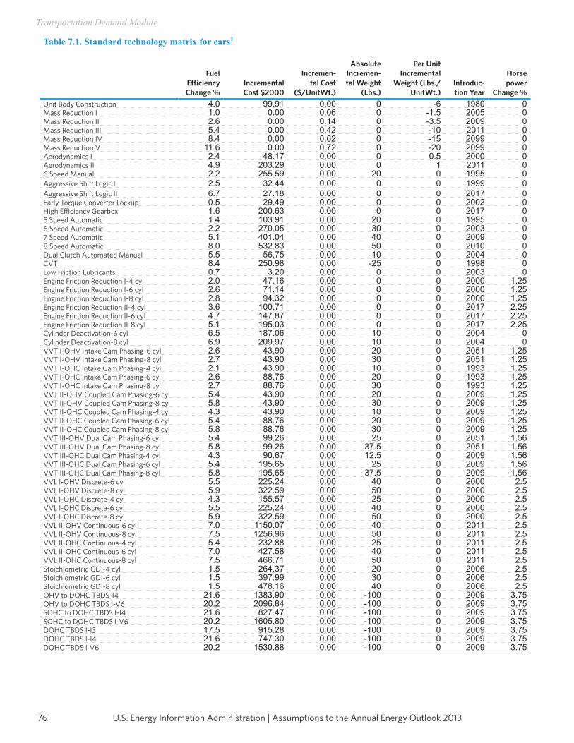
U.S. Energy Information Administration | Assumptions to the Annual Energy Outlook 201376
Transportation Demand Module
Table 7.1. Standard technology matrix for cars1
FuelEfficiencyChange %
Incremental Cost $2000
Incremen- tal Cost
($/UnitWt.)
Absolute Incremen- tal Weight
(Lbs.)
Per Unit Incremental
Weight (Lbs./UnitWt.)
Introduc-tion Year
Horse power
Change %Unit Body Construction 4.0 99.91 0.00 0 -6 1980 0Mass Reduction I 1.0 0.00 0.06 0 -1.5 2005 0Mass Reduction II 2.6 0.00 0.14 0 -3.5 2009 0Mass Reduction III 5.4 0.00 0.42 0 -10 2011 0Mass Reduction IV 8.4 0.00 0.62 0 -15 2099 0Mass Reduction V 11.6 0.00 0.72 0 -20 2099 0Aerodynamics I 2.4 48.17 0.00 0 0.5 2000 0Aerodynamics II 4.9 203.29 0.00 0 1 2011 06 Speed Manual 2.2 255.59 0.00 20 0 1995 0Aggressive Shift Logic I 2.5 32.44 0.00 0 0 1999 0Aggressive Shift Logic II 6.7 27.18 0.00 0 0 2017 0Early Torque Converter Lockup 0.5 29.49 0.00 0 0 2002 0High Efficiency Gearbox 1.6 200.63 0.00 0 0 2017 05 Speed Automatic 1.4 103.91 0.00 20 0 1995 06 Speed Automatic 2.2 270.05 0.00 30 0 2003 07 Speed Automatic 5.1 401.04 0.00 40 0 2009 08 Speed Automatic 8.0 532.83 0.00 50 0 2010 0Dual Clutch Automated Manual 5.5 56.75 0.00 -10 0 2004 0CVT 8.4 250.98 0.00 -25 0 1998 0Low Friction Lubricants 0.7 3.20 0.00 0 0 2003 0Engine Friction Reduction I-4 cyl 2.0 47.16 0.00 0 0 2000 1.25Engine Friction Reduction I-6 cyl 2.6 71.14 0.00 0 0 2000 1.25Engine Friction Reduction I-8 cyl 2.8 94.32 0.00 0 0 2000 1.25Engine Friction Reduction II-4 cyl 3.6 100.71 0.00 0 0 2017 2.25Engine Friction Reduction II-6 cyl 4.7 147.87 0.00 0 0 2017 2.25Engine Friction Reduction II-8 cyl 5.1 195.03 0.00 0 0 2017 2.25Cylinder Deactivation-6 cyl 6.5 187.06 0.00 10 0 2004 0Cylinder Deactivation-8 cyl 6.9 209.97 0.00 10 0 2004 0VVT I-OHV Intake Cam Phasing-6 cyl 2.6 43.90 0.00 20 0 2051 1.25VVT I-OHV Intake Cam Phasing-8 cyl 2.7 43.90 0.00 30 0 2051 1.25VVT I-OHC Intake Cam Phasing-4 cyl 2.1 43.90 0.00 10 0 1993 1.25VVT I-OHC Intake Cam Phasing-6 cyl 2.6 88.76 0.00 20 0 1993 1.25VVT I-OHC Intake Cam Phasing-8 cyl 2.7 88.76 0.00 30 0 1993 1.25VVT II-OHV Coupled Cam Phasing-6 cyl 5.4 43.90 0.00 20 0 2009 1.25VVT II-OHV Coupled Cam Phasing-8 cyl 5.8 43.90 0.00 30 0 2009 1.25VVT II-OHC Coupled Cam Phasing-4 cyl 4.3 43.90 0.00 10 0 2009 1.25VVT II-OHC Coupled Cam Phasing-6 cyl 5.4 88.76 0.00 20 0 2009 1.25VVT II-OHC Coupled Cam Phasing-8 cyl 5.8 88.76 0.00 30 0 2009 1.25VVT III-OHV Dual Cam Phasing-6 cyl 5.4 99.26 0.00 25 0 2051 1.56VVT III-OHV Dual Cam Phasing-8 cyl 5.8 99.26 0.00 37.5 0 2051 1.56VVT III-OHC Dual Cam Phasing-4 cyl 4.3 90.67 0.00 12.5 0 2009 1.56VVT III-OHC Dual Cam Phasing-6 cyl 5.4 195.65 0.00 25 0 2009 1.56VVT III-OHC Dual Cam Phasing-8 cyl 5.8 195.65 0.00 37.5 0 2009 1.56VVL I-OHV Discrete-6 cyl 5.5 225.24 0.00 40 0 2000 2.5VVL I-OHV Discrete-8 cyl 5.9 322.59 0.00 50 0 2000 2.5VVL I-OHC Discrete-4 cyl 4.3 155.57 0.00 25 0 2000 2.5VVL I-OHC Discrete-6 cyl 5.5 225.24 0.00 40 0 2000 2.5VVL I-OHC Discrete-8 cyl 5.9 322.59 0.00 50 0 2000 2.5VVL II-OHV Continuous-6 cyl 7.0 1150.07 0.00 40 0 2011 2.5VVL II-OHV Continuous-8 cyl 7.5 1256.96 0.00 50 0 2011 2.5VVL II-OHC Continuous-4 cyl 5.4 232.88 0.00 25 0 2011 2.5VVL II-OHC Continuous-6 cyl 7.0 427.58 0.00 40 0 2011 2.5VVL II-OHC Continuous-8 cyl 7.5 466.71 0.00 50 0 2011 2.5Stoichiometric GDI-4 cyl 1.5 264.37 0.00 20 0 2006 2.5Stoichiometric GDI-6 cyl 1.5 397.99 0.00 30 0 2006 2.5Stoichiometric GDI-8 cyl 1.5 478.16 0.00 40 0 2006 2.5OHV to DOHC TBDS-I4 21.6 1383.90 0.00 -100 0 2009 3.75OHV to DOHC TBDS I-V6 20.2 2096.84 0.00 -100 0 2009 3.75SOHC to DOHC TBDS I-I4 21.6 827.47 0.00 -100 0 2009 3.75SOHC to DOHC TBDS I-V6 20.2 1605.80 0.00 -100 0 2009 3.75DOHC TBDS I-I3 17.5 915.28 0.00 -100 0 2009 3.75DOHC TBDS I-I4 21.6 747.30 0.00 -100 0 2009 3.75DOHC TBDS I-V6 20.2 1530.88 0.00 -100 0 2009 3.75
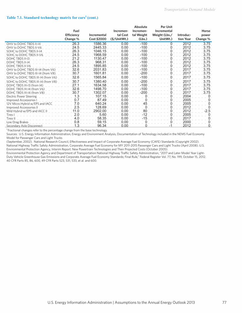
77U.S. Energy Information Administration | Assumptions to the Annual Energy Outlook 2013
Transportation Demand Module
Table 7.1. Standard technology matrix for cars1 (cont.)
FuelEfficiencyChange %
Incremental Cost $2000
Incremen- tal Cost
($/UnitWt.)
Absolute Incremen- tal Weight
(Lbs.)
Per Unit Incremental
Weight (Lbs./UnitWt.)
Introduc-tion Year
Horse power
Change %OHV to DOHC TBDS II-I4 26.3 1586.36 0.00 -100 0 2012 3.75OHV to DOHC TBDS II-V6 24.5 2445.33 0.00 -100 0 2012 3.75SOHC to DOHC TBDS II-I4 26.3 1046.15 0.00 -100 0 2012 3.75SOHC to DOHC TBDS II-V6 24.5 1968.59 0.00 -100 0 2012 3.75DOHC TBDS II-I3 21.2 1130.47 0.00 -100 0 2012 3.75DOHC TBDS II-I4 26.3 968.31 0.00 -100 0 2012 3.75DOHC TBDS II-V6 24.5 1895.85 0.00 -100 0 2012 3.75OHV to DOHC TBDS III-I4 (from V6) 32.6 2031.83 0.00 -100 0 2017 3.75OHV to DOHC TBDS III-I4 (from V8) 30.7 1601.81 0.00 -200 0 2017 3.75SOHC to DOHC TBDS III-I4 (from V6) 32.6 1565.84 0.00 -100 0 2017 3.75SOHC to DOHC TBDS III-I4 (from V8) 30.7 1380.40 0.00 -200 0 2017 3.75DOHC TBDS III-I3 (from I4) 27.1 1634.58 0.00 -100 0 2017 3.75DOHC TBDS III-I4 (from V6) 32.6 1498.70 0.00 -100 0 2017 3.75DOHC TBDS III-I4 (from V8) 30.7 1302.07 0.00 -200 0 2017 3.75Electric Power Steering 1.3 107.15 0.00 0 0 2004 0Improved Accessories I 0.7 87.49 0.00 0 0 2005 012V Micro Hybrid w/EPS and IACC 7.0 640.24 0.00 45 0 2005 0Improved Accessories II 2.5 128.69 0.00 0 0 2012 0Mild Hybrid w/EPS and IACC II 11.0 2902.00 0.00 80 0 2012 -2.5Tires I 2.0 5.60 0.00 -12 0 2005 0Tires II 4.0 58.35 0.00 -15 0 2017 0Low Drag Brakes 0.8 59.15 0.00 0 0 2000 0Secondary Axle Disconnect 1.3 96.34 0.00 0 -1 2012 01 Fractional changes refer to the percentage change from the base technology.Sources: U.S. Energy Information Administration, Energy and Environment Analysis, Documentation of Technology included in the NEMS Fuel Economy Model for Passenger Cars and Light Trucks(September, 2002). National Research Council, Effectiveness and Impact of Corporate Average Fuel Economy (CAFE) Standards (Copyright 2002). National Highway Traffic Safety Administration, Corporate Average Fuel Economy for MY 2011-2015 Passenger Cars and Light Trucks (April 2008). U.S. Environmental Protection Agency, Interim Report: New Powertrain Technologies and Their Projected Costs (October 2005).Environmental Protection Agency and Department of Transportation National Highway Traffic Safety Administration, “2017 and Later Model Year Light-Duty Vehicle Greenhouse Gas Emissions and Corporate Average Fuel Economy Standards; Final Rule,” Federal Register Vol. 77, No. 199, October 15, 2012. 40 CFR Parts 85, 86, 600, 49 CFR Parts 523, 531, 533, et al. and 600.
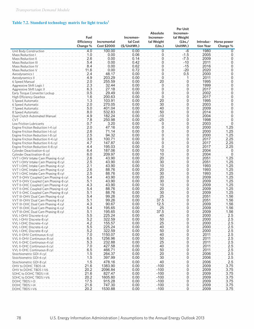
U.S. Energy Information Administration | Assumptions to the Annual Energy Outlook 201378
Transportation Demand Module
Table 7.2. Standard technology matrix for light trucks1
FuelEfficiencyChange %
Incremental Cost $2000
Incremen- tal Cost
($/UnitWt.)
Absolute Incremen- tal Weight
(Lbs.)
Per Unit Incremen- tal Weight
(Lbs./UnitWt.)
Introduc-tion Year
Horse powerChange %
Unit Body Construction 4.0 100.00 0.00 0 -6 1980 0Mass Reduction I 1.0 0.00 0.06 0 -1.5 2005 0Mass Reduction II 2.6 0.00 0.14 0 -7.5 2009 0Mass Reduction III 5.4 0.00 0.42 0 -10 2011 0Mass Reduction IV 8.4 0.00 0.62 0 -15 2016 0Mass Reduction V 11.6 0.00 0.72 0 -20 2020 0Aerodynamics I 2.4 48.17 0.00 0 0.5 2000 0Aerodynamics II 4.9 203.29 0.00 0 1 2011 06 Speed Manual 2.0 255.59 0.00 20 0 1995 0Aggressive Shift Logic I 2.3 32.44 0.00 0 0 1999 0Aggressive Shift Logic II 6.3 27.18 0.00 0 0 2017 0Early Torque Converter Lockup 0.5 29.49 0.00 0 0 2002 0High Efficiency Gearbox 1.6 200.63 0.00 0 0 2017 05 Speed Automatic 1.3 103.91 0.00 20 0 1995 06 Speed Automatic 2.0 270.05 0.00 30 0 2003 07 Speed Automatic 5.0 401.04 0.00 40 0 2009 08 Speed Automatic 8.0 532.83 0.00 50 0 2014 0Dual Clutch Automated Manual 4.9 182.24 0.00 -10 0 2004 0CVT 7.8 250.98 0.00 -25 0 1998 0Low Friction Lubricants 0.7 3.20 0.00 0 0 2003 0Engine Friction Reduction I-4 cyl 2.0 47.16 0.00 0 0 2000 1.25Engine Friction Reduction I-6 cyl 2.6 71.14 0.00 0 0 2000 1.25Engine Friction Reduction I-8 cyl 2.5 94.32 0.00 0 0 2000 1.25Engine Friction Reduction II-4 cyl 3.6 100.71 0.00 0 0 2017 2.25Engine Friction Reduction II-6 cyl 4.7 147.87 0.00 0 0 2017 2.25Engine Friction Reduction II-8 cyl 4.4 195.03 0.00 0 0 2017 2.25Cylinder Deactivation-6 cyl 6.4 187.06 0.00 10 0 2004 0Cylinder Deactivation-8 cyl 6.0 209.97 0.00 10 0 2004 0VVT I-OHV Intake Cam Phasing-6 cyl 2.6 43.90 0.00 20 0 2051 1.25VVT I-OHV Intake Cam Phasing-8 cyl 2.5 43.90 0.00 30 0 2051 1.25VVT I-OHC Intake Cam Phasing-4 cyl 2.1 43.90 0.00 10 0 1993 1.25VVT I-OHC Intake Cam Phasing-6 cyl 2.6 88.76 0.00 20 0 1993 1.25VVT I-OHC Intake Cam Phasing-8 cyl 2.5 88.76 0.00 30 0 1993 1.25VVT II-OHV Coupled Cam Phasing-6 cyl 5.4 43.90 0.00 20 0 2009 1.25VVT II-OHV Coupled Cam Phasing-8 cyl 5.1 43.90 0.00 30 0 2009 1.25VVT II-OHC Coupled Cam Phasing-4 cyl 4.3 43.90 0.00 10 0 2009 1.25VVT II-OHC Coupled Cam Phasing-6 cyl 5.4 88.76 0.00 20 0 2009 1.25VVT II-OHC Coupled Cam Phasing-8 cyl 5.1 88.76 0.00 30 0 2009 1.25VVT III-OHV Dual Cam Phasing-6 cyl 5.4 99.26 0.00 25 0 2051 1.56VVT III-OHV Dual Cam Phasing-8 cyl 5.1 99.26 0.00 37.5 0 2051 1.56VVT III-OHC Dual Cam Phasing-4 cyl 4.3 90.67 0.00 12.5 0 2009 1.56VVT III-OHC Dual Cam Phasing-6 cyl 5.4 195.65 0.00 25 0 2009 1.56VVT III-OHC Dual Cam Phasing-8 cyl 5.1 195.65 0.00 37.5 0 2009 1.56VVL I-OHV Discrete-6 cyl 5.5 225.24 0.00 40 0 2000 2.5VVL I-OHV Discrete-8 cyl 5.2 322.59 0.00 50 0 2000 2.5VVL I-OHC Discrete-4 cyl 4.2 155.57 0.00 25 0 2000 2.5VVL I-OHC Discrete-6 cyl 5.5 225.24 0.00 40 0 2000 2.5VVL I-OHC Discrete-8 cyl 5.2 322.59 0.00 50 0 2000 2.5VVL II-OHV Continuous-6 cyl 7.0 1150.07 0.00 40 0 2011 2.5VVL II-OHV Continuous-8 cyl 6.5 1256.96 0.00 50 0 2011 2.5VVL II-OHC Continuous-4 cyl 5.3 232.88 0.00 25 0 2011 2.5VVL II-OHC Continuous-6 cyl 7.0 427.58 0.00 40 0 2011 2.5VVL II-OHC Continuous-8 cyl 6.5 466.71 0.00 50 0 2011 2.5Stoichiometric GDI-4 cyl 1.5 264.37 0.00 20 0 2006 2.5Stoichiometric GDI-6 cyl 1.5 397.99 0.00 30 0 2006 2.5Stoichiometric GDI-8 cyl 1.5 478.16 0.00 40 0 2006 2.5OHV to DOHC TBDS-I4 21.6 1383.90 0.00 -100 0 2009 3.75OHV to DOHC TBDS I-V6 20.2 2096.84 0.00 -100 0 2009 3.75SOHC to DOHC TBDS I-I4 21.6 827.47 0.00 -100 0 2009 3.75SOHC to DOHC TBDS I-V6 20.2 1605.80 0.00 -100 0 2009 3.75DOHC TBDS I-I3 17.5 915.28 0.00 -100 0 2009 3.75DOHC TBDS I-I4 21.6 747.30 0.00 -100 0 2009 3.75DOHC TBDS I-V6 20.2 1530.88 0.00 -100 0 2009 3.75
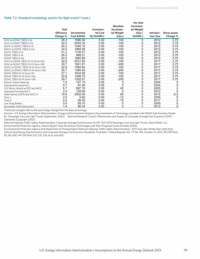
79U.S. Energy Information Administration | Assumptions to the Annual Energy Outlook 2013
Transportation Demand Module
Table 7.2. Standard technology matrix for light trucks1 (cont.)
FuelEfficiencyChange %
Incremental Cost $2000
Incremen- tal Cost
($/UnitWt.)
Absolute Incremen- tal Weight
(Lbs.)
Per Unit Incremen- tal Weight
(Lbs./UnitWt.)
Introduc-tion Year
Horse powerChange %
OHV to DOHC TBDS II-I4 26.3 1586.36 0.00 -100 0 2012 3.75OHV to DOHC TBDS II-V6 24.5 2445.33 0.00 -100 0 2012 3.75SOHC to DOHC TBDS II-I4 26.3 1046.15 0.00 -100 0 2012 3.75SOHC to DOHC TBDS II-V6 24.5 1968.59 0.00 -100 0 2012 3.75DOHC TBDS II-I3 21.2 1130.47 0.00 -100 0 2012 3.75DOHC TBDS II-I4 26.3 968.31 0.00 -100 0 2012 3.75DOHC TBDS II-V6 24.5 1895.85 0.00 -100 0 2012 3.75OHV to DOHC TBDS III-I4 (from V6) 32.6 2031.83 0.00 -100 0 2017 3.75OHV to DOHC TBDS III-I4 (from V8) 30.7 1601.81 0.00 -200 0 2017 3.75SOHC to DOHC TBDS III-I4 (from V6) 32.6 1565.84 0.00 -100 0 2017 3.75SOHC to DOHC TBDS III-I4 (from V8) 30.7 1380.40 0.00 -200 0 2017 3.75DOHC TBDS III-I3 (from I4) 27.1 1634.58 0.00 -100 0 2017 3.75DOHC TBDS III-I4 (from V6) 32.6 1498.70 0.00 -100 0 2017 3.75DOHC TBDS III-I4 (from V8) 30.7 1302.07 0.00 -200 0 2017 3.75Electric Power Steering 1.0 107.15 0.00 0 0 2004 0Improved Accessories I 0.7 87.49 0.00 0 0 2005 012V Micro Hybrid w/EPS and IACC 6.7 697.79 0.00 45 0 2005 0Improved Accessories II 2.4 128.69 0.00 0 0 2012 0Mild Hybrid w/EPS and IACC II 10.6 2902.00 0.00 80 0 2012 -2.5Tires I 2.0 5.60 0.00 -12 0 2005 0Tires II 4.0 58.35 0.00 -15 0 2017 0Low Drag Brakes 0.8 59.15 0.00 0 0 2000 0Secondary Axle Disconnect 1.4 96.34 0.00 0 -1 2012 01Fractional changes refer to the percentage change from the base technology.Sources: U.S. Energy Information Administration. Energy and Environment Analysis, Documentation of Technology included in the NEMS Fuel Economy Model for Passenger Cars and Light Trucks (September, 2002). National Research Council, Effectiveness and Impact of Corporate Average Fuel Economy (CAFE) Standards (Copyright 2002). National Highway Traffic Safety Administration, Corporate Average Fuel Economy for MY 2011-2015 Passenger Cars and Light Trucks (April 2008). U.S. Environmental Protection Agency, Interim Report: New Powertrain Technologies and Their Projected Costs (October 2005).Environmental Protection Agency and Department of Transportation National Highway Traffic Safety Administration, “2017 and Later Model Year Light-Duty Vehicle Greenhouse Gas Emissions and Corporate Average Fuel Economy Standards; Final Rule,” Federal Register Vol. 77, No. 199, October 15, 2012. 40 CFR Parts 85, 86, 600, 49 CFR Parts 523, 531, 533, et al. and 600.
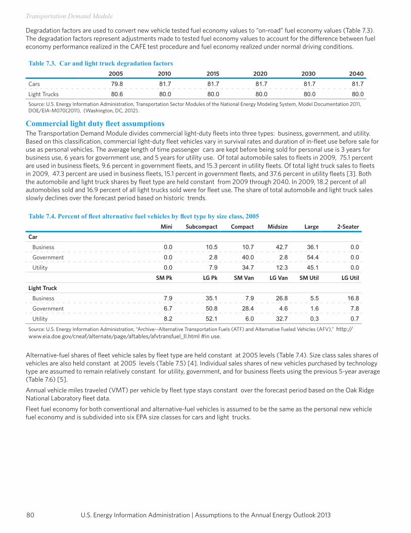
U.S. Energy Information Administration | Assumptions to the Annual Energy Outlook 201380
Transportation Demand Module
Degradation factors are used to convert new vehicle tested fuel economy values to “on-road” fuel economy values (Table 7.3). The degradation factors represent adjustments made to tested fuel economy values to account for the difference between fuel economy performance realized in the CAFE test procedure and fuel economy realized under normal driving conditions.
Table 7.3. Car and light truck degradation factors2005 2010 2015 2020 2030 2040
Cars 79.8 81.7 81.7 81.7 81.7 81.7
Light Trucks 80.6 80.0 80.0 80.0 80.0 80.0Source: U.S. Energy Information Administration, Transportation Sector Modules of the National Energy Modeling System, Model Documentation 2011, DOE/EIA-M070(2011), (Washington, DC, 2012).
Commercial light duty fleet assumptions The Transportation Demand Module divides commercial light-duty fleets into three types: business, government, and utility. Based on this classification, commercial light-duty fleet vehicles vary in survival rates and duration of in-fleet use before sale for use as personal vehicles. The average length of time passenger cars are kept before being sold for personal use is 3 years for business use, 6 years for government use, and 5 years for utility use. Of total automobile sales to fleets in 2009, 75.1 percent are used in business fleets, 9.6 percent in government fleets, and 15.3 percent in utility fleets. Of total light truck sales to fleets in 2009, 47.3 percent are used in business fleets, 15.1 percent in government fleets, and 37.6 percent in utility fleets [3]. Both the automobile and light truck shares by fleet type are held constant from 2009 through 2040. In 2009, 18.2 percent of all automobiles sold and 16.9 percent of all light trucks sold were for fleet use. The share of total automobile and light truck sales slowly declines over the forecast period based on historic trends.
Table 7.4. Percent of fleet alternative fuel vehicles by fleet type by size class, 2005Mini Subcompact Compact Midsize Large 2-Seater
Car
Business 0.0 10.5 10.7 42.7 36.1 0.0
Government 0.0 2.8 40.0 2.8 54.4 0.0
Utility 0.0 7.9 34.7 12.3 45.1 0.0
SM Pk LG Pk SM Van LG Van SM Util LG Util
Light Truck
Business 7.9 35.1 7.9 26.8 5.5 16.8
Government 6.7 50.8 28.4 4.6 1.6 7.8
Utility 8.2 52.1 6.0 32.7 0.3 0.7
Source: U.S. Energy Information Administration, “Archive--Alternative Transportation Fuels (ATF) and Alternative Fueled Vehicles (AFV),” http://www.eia.doe.gov/cneaf/alternate/page/aftables/afvtransfuel_II.html #in use.
Alternative-fuel shares of fleet vehicle sales by fleet type are held constant at 2005 levels (Table 7.4). Size class sales shares of vehicles are also held constant at 2005 levels (Table 7.5) [4]. Individual sales shares of new vehicles purchased by technology type are assumed to remain relatively constant for utility, government, and for business fleets using the previous 5-year average (Table 7.6) [5].Annual vehicle miles traveled (VMT) per vehicle by fleet type stays constant over the forecast period based on the Oak Ridge National Laboratory fleet data.Fleet fuel economy for both conventional and alternative-fuel vehicles is assumed to be the same as the personal new vehicle fuel economy and is subdivided into six EPA size classes for cars and light trucks.
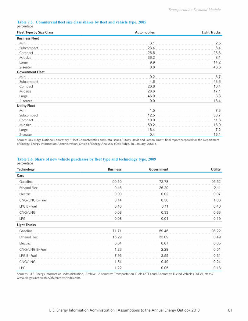
81U.S. Energy Information Administration | Assumptions to the Annual Energy Outlook 2013
Transportation Demand Module
Table 7.5. Commercial fleet size class shares by fleet and vehicle type, 2005percentage
Fleet Type by Size Class Automobiles Light Trucks
Business FleetMini 3.1 2.5Subcompact 23.4 8.4Compact 26.6 23.3Midsize 36.2 8.1Large 9.9 14.22-seater 0.8 43.6
Government FleetMini 0.2 6.7Subcompact 4.6 43.6Compact 20.6 10.4Midsize 28.6 17.1Large 46.0 3.82-seater 0.0 18.4
Utility FleetMini 1.5 7.3Subcompact 12.5 38.7Compact 10.0 11.8Midsize 59.2 18.9Large 16.4 7.22-seater 0.4 16.1
Source: Oak Ridge National Laboratory, “Fleet Characteristics and Data Issues,” Stacy Davis and Lorena Truett, final report prepared for the Department of Energy, Energy Information Administration, Office of Energy Analysis, (Oak Ridge, Tn, January 2003).
Table 7.6. Share of new vehicle purchases by fleet type and technology type, 2009percentage
Technology Business Government Utility
Cars
Gasoline 99.10 72.78 95.52
Ethanol Flex 0.46 26.20 2.11
Electric 0.00 0.02 0.07
CNG/LNG Bi-Fuel 0.14 0.56 1.08
LPG Bi-Fuel 0.16 0.11 0.40
CNG/LNG 0.08 0.33 0.63
LPG 0.08 0.01 0.19
Light Trucks
Gasoline 71.71 59.46 98.22
Ethanol Flex 16.29 35.09 0.49
Electric 0.04 0.07 0.05
CNG/LNG Bi-Fuel 1.28 2.29 0.51
LPG Bi-Fuel 7.93 2.55 0.31
CNG/LNG 1.54 0.49 0.24
LPG 1.22 0.05 0.18Sources: U.S. Energy Information Administration, Archive - Alternative Transportation Fuels (ATF) and Alternative Fueled Vehicles (AFV), http://www.eia.gov/renewable/afv/archive/index.cfm.
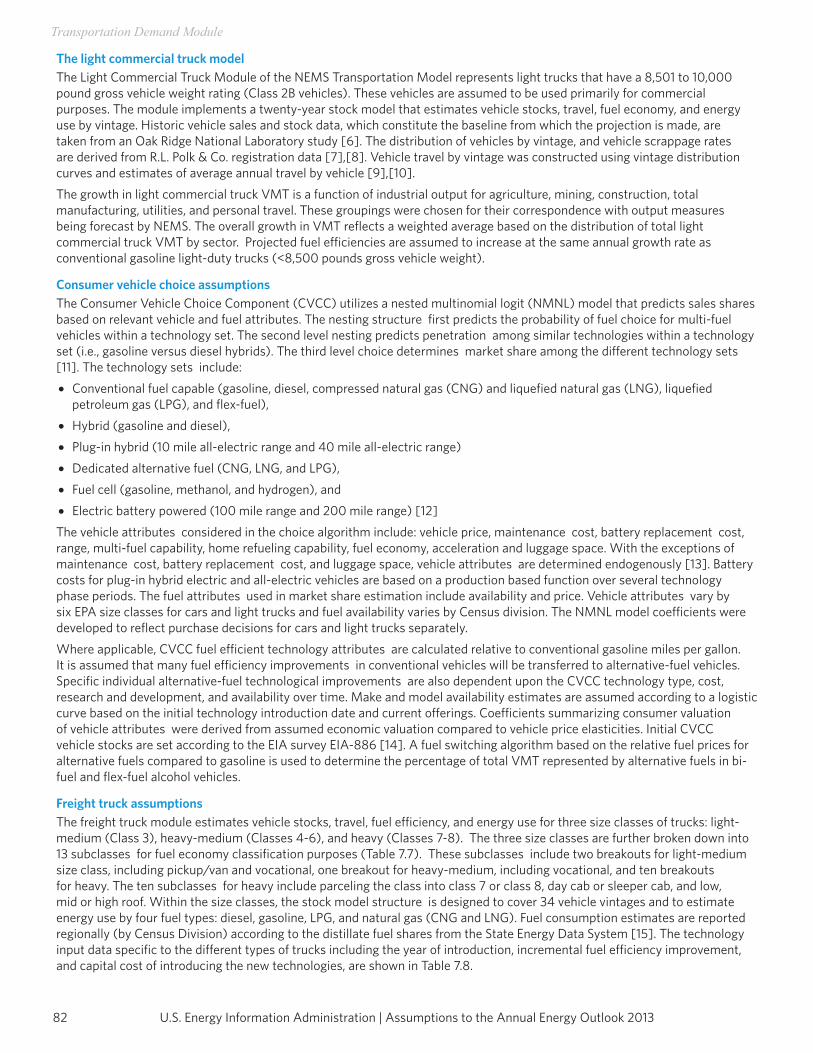
U.S. Energy Information Administration | Assumptions to the Annual Energy Outlook 201382
Transportation Demand Module
The light commercial truck modelThe Light Commercial Truck Module of the NEMS Transportation Model represents light trucks that have a 8,501 to 10,000 pound gross vehicle weight rating (Class 2B vehicles). These vehicles are assumed to be used primarily for commercial purposes. The module implements a twenty-year stock model that estimates vehicle stocks, travel, fuel economy, and energy use by vintage. Historic vehicle sales and stock data, which constitute the baseline from which the projection is made, are taken from an Oak Ridge National Laboratory study [6]. The distribution of vehicles by vintage, and vehicle scrappage rates are derived from R.L. Polk & Co. registration data [7],[8]. Vehicle travel by vintage was constructed using vintage distribution curves and estimates of average annual travel by vehicle [9],[10]. The growth in light commercial truck VMT is a function of industrial output for agriculture, mining, construction, total manufacturing, utilities, and personal travel. These groupings were chosen for their correspondence with output measures being forecast by NEMS. The overall growth in VMT reflects a weighted average based on the distribution of total light commercial truck VMT by sector. Projected fuel efficiencies are assumed to increase at the same annual growth rate as conventional gasoline light-duty trucks (<8,500 pounds gross vehicle weight).
Consumer vehicle choice assumptionsThe Consumer Vehicle Choice Component (CVCC) utilizes a nested multinomial logit (NMNL) model that predicts sales shares based on relevant vehicle and fuel attributes. The nesting structure first predicts the probability of fuel choice for multi-fuel vehicles within a technology set. The second level nesting predicts penetration among similar technologies within a technology set (i.e., gasoline versus diesel hybrids). The third level choice determines market share among the different technology sets [11]. The technology sets include:• Conventional fuel capable (gasoline, diesel, compressed natural gas (CNG) and liquefied natural gas (LNG), liquefied
petroleum gas (LPG), and flex-fuel),• Hybrid (gasoline and diesel),• Plug-in hybrid (10 mile all-electric range and 40 mile all-electric range)• Dedicated alternative fuel (CNG, LNG, and LPG),• Fuel cell (gasoline, methanol, and hydrogen), and• Electric battery powered (100 mile range and 200 mile range) [12]The vehicle attributes considered in the choice algorithm include: vehicle price, maintenance cost, battery replacement cost, range, multi-fuel capability, home refueling capability, fuel economy, acceleration and luggage space. With the exceptions of maintenance cost, battery replacement cost, and luggage space, vehicle attributes are determined endogenously [13]. Battery costs for plug-in hybrid electric and all-electric vehicles are based on a production based function over several technology phase periods. The fuel attributes used in market share estimation include availability and price. Vehicle attributes vary by six EPA size classes for cars and light trucks and fuel availability varies by Census division. The NMNL model coefficients were developed to reflect purchase decisions for cars and light trucks separately. Where applicable, CVCC fuel efficient technology attributes are calculated relative to conventional gasoline miles per gallon. It is assumed that many fuel efficiency improvements in conventional vehicles will be transferred to alternative-fuel vehicles. Specific individual alternative-fuel technological improvements are also dependent upon the CVCC technology type, cost, research and development, and availability over time. Make and model availability estimates are assumed according to a logistic curve based on the initial technology introduction date and current offerings. Coefficients summarizing consumer valuation of vehicle attributes were derived from assumed economic valuation compared to vehicle price elasticities. Initial CVCC vehicle stocks are set according to the EIA survey EIA-886 [14]. A fuel switching algorithm based on the relative fuel prices for alternative fuels compared to gasoline is used to determine the percentage of total VMT represented by alternative fuels in bi- fuel and flex-fuel alcohol vehicles.
Freight truck assumptionsThe freight truck module estimates vehicle stocks, travel, fuel efficiency, and energy use for three size classes of trucks: light- medium (Class 3), heavy-medium (Classes 4-6), and heavy (Classes 7-8). The three size classes are further broken down into 13 subclasses for fuel economy classification purposes (Table 7.7). These subclasses include two breakouts for light-medium size class, including pickup/van and vocational, one breakout for heavy-medium, including vocational, and ten breakouts for heavy. The ten subclasses for heavy include parceling the class into class 7 or class 8, day cab or sleeper cab, and low, mid or high roof. Within the size classes, the stock model structure is designed to cover 34 vehicle vintages and to estimate energy use by four fuel types: diesel, gasoline, LPG, and natural gas (CNG and LNG). Fuel consumption estimates are reported regionally (by Census Division) according to the distillate fuel shares from the State Energy Data System [15]. The technology input data specific to the different types of trucks including the year of introduction, incremental fuel efficiency improvement, and capital cost of introducing the new technologies, are shown in Table 7.8.
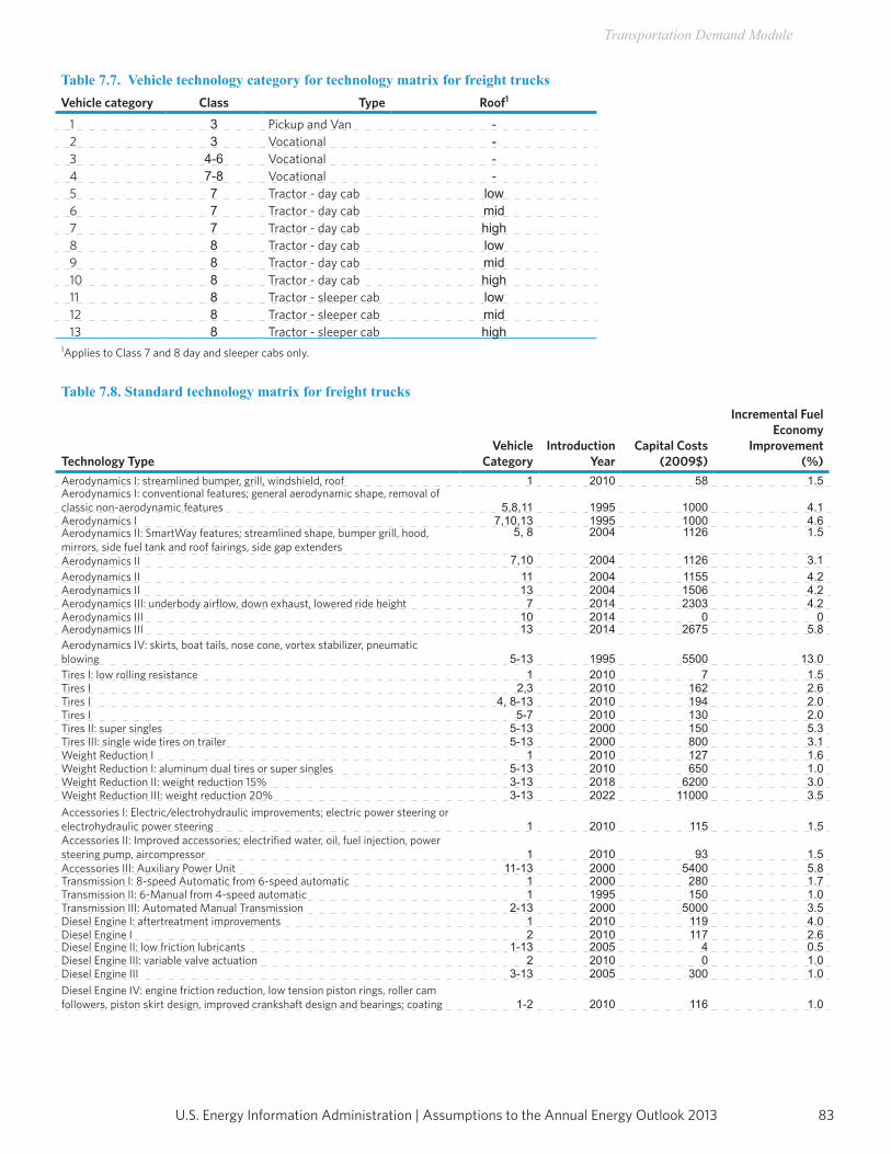
83U.S. Energy Information Administration | Assumptions to the Annual Energy Outlook 2013
Transportation Demand Module
Table 7.7. Vehicle technology category for technology matrix for freight trucksVehicle category Class Type Roof1
1 3 Pickup and Van -2 3 Vocational -3 4-6 Vocational -4 7-8 Vocational -5 7 Tractor - day cab low6 7 Tractor - day cab mid7 7 Tractor - day cab high8 8 Tractor - day cab low9 8 Tractor - day cab mid10 8 Tractor - day cab high11 8 Tractor - sleeper cab low12 8 Tractor - sleeper cab mid13 8 Tractor - sleeper cab high
1Applies to Class 7 and 8 day and sleeper cabs only.
Table 7.8. Standard technology matrix for freight trucks
Technology TypeVehicle
CategoryIntroduction
YearCapital Costs
(2009$)
Incremental Fuel Economy
Improvement (%)
Aerodynamics I: streamlined bumper, grill, windshield, roof 1 2010 58 1.5Aerodynamics I: conventional features; general aerodynamic shape, removal ofclassic non-aerodynamic features 5,8,11 1995 1000 4.1Aerodynamics I 7,10,13 1995 1000 4.6Aerodynamics II: SmartWay features; streamlined shape, bumper grill, hood,mirrors, side fuel tank and roof fairings, side gap extenders
5, 8 2004 1126 1.5
Aerodynamics II 7,10 2004 1126 3.1Aerodynamics II 11 2004 1155 4.2Aerodynamics II 13 2004 1506 4.2Aerodynamics III: underbody airflow, down exhaust, lowered ride height 7 2014 2303 4.2Aerodynamics III 10 2014 0 0Aerodynamics III 13 2014 2675 5.8Aerodynamics IV: skirts, boat tails, nose cone, vortex stabilizer, pneumaticblowing 5-13 1995 5500 13.0Tires I: low rolling resistance 1 2010 7 1.5Tires I 2,3 2010 162 2.6Tires I 4, 8-13 2010 194 2.0Tires I 5-7 2010 130 2.0Tires II: super singles 5-13 2000 150 5.3Tires III: single wide tires on trailer 5-13 2000 800 3.1Weight Reduction I 1 2010 127 1.6Weight Reduction I: aluminum dual tires or super singles 5-13 2010 650 1.0Weight Reduction II: weight reduction 15% 3-13 2018 6200 3.0Weight Reduction III: weight reduction 20% 3-13 2022 11000 3.5Accessories I: Electric/electrohydraulic improvements; electric power steering orelectrohydraulic power steering 1 2010 115 1.5Accessories II: Improved accessories; electrified water, oil, fuel injection, powersteering pump, aircompressor 1 2010 93 1.5Accessories III: Auxiliary Power Unit 11-13 2000 5400 5.8Transmission I: 8-speed Automatic from 6-speed automatic 1 2000 280 1.7Transmission II: 6-Manual from 4-speed automatic 1 1995 150 1.0Transmission III: Automated Manual Transmission 2-13 2000 5000 3.5Diesel Engine I: aftertreatment improvements 1 2010 119 4.0Diesel Engine I 2 2010 117 2.6Diesel Engine II: low friction lubricants 1-13 2005 4 0.5Diesel Engine III: variable valve actuation 2 2010 0 1.0Diesel Engine III 3-13 2005 300 1.0Diesel Engine IV: engine friction reduction, low tension piston rings, roller camfollowers, piston skirt design, improved crankshaft design and bearings; coating 1-2 2010 116 1.0
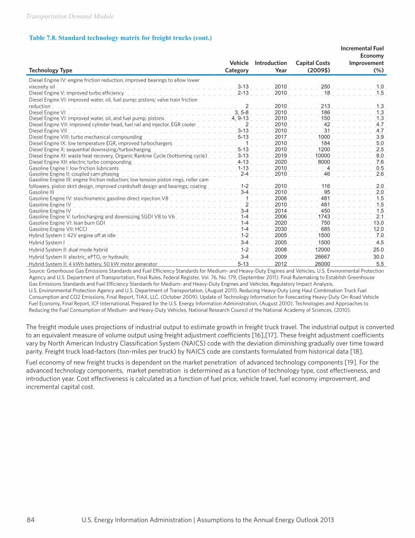
U.S. Energy Information Administration | Assumptions to the Annual Energy Outlook 201384
Transportation Demand Module
Table 7.8. Standard technology matrix for freight trucks (cont.)
Technology TypeVehicle
CategoryIntroduction
YearCapital Costs
(2009$)
Incremental Fuel Economy
Improvement (%)
Diesel Engine IV: engine friction reduction, improved bearings to allow lower viscosity oil 3-13 2010 250 1.0Diesel Engine V: improved turbo efficiency 2-13 2010 18 1.5Diesel Engine VI: improved water, oil, fuel pump; pistons; valve train friction reduction 2 2010 213 1.3Diesel Engine VI 3, 5-8 2010 186 1.3Diesel Engine VI: improved water, oil, and fuel pump; pistons 4, 9-13 2010 150 1.3Diesel Engine VII: improved cylinder head, fuel rail and injector, EGR cooler 2 2010 42 4.7Diesel Engine VII 3-13 2010 31 4.7Diesel Engine VIII: turbo mechanical compounding 5-13 2017 1000 3.9Diesel Engine IX: low temperature EGR, improved turbochargers 1 2010 184 5.0Diesel Engine X: sequential downsizing/turbocharging 5-13 2010 1200 2.5Diesel Engine XI: waste heat recovery, Organic Rankine Cycle (bottoming cycle) 3-13 2019 10000 8.0Diesel Engine XII: electric turbo compounding 4-13 2020 8000 7.6Gasoline Engine I: low friction lubricants 1-13 2010 4 0.5Gasoline Engine II: coupled cam phasing 2-4 2010 46 2.6Gasoline Engine III: engine friction reduction; low tension piston rings, roller cam followers, piston skirt design, improved crankshaft design and bearings; coating 1-2 2010 116 2.0Gasoline III 3-4 2010 95 2.0Gasoline Engine IV: stoichiometric gasoline direct injection V8 1 2006 481 1.5Gasoline Engine IV 2 2010 481 1.5Gasoline Engine IV 3-4 2014 450 1.5Gasoline Engine V: turbocharging and downsizing SGDI V8 to V6 1-4 2006 1743 2.1 Gasoline Engine VI: lean burn GDI 1-4 2020 750 13.0 Gasoline Engine VII: HCCI 1-4 2030 685 12.0 Hybrid System I: 42V engine off at idle 1-2 2005 1500 7.0 Hybrid System I 3-4 2005 1500 4.5 Hybrid System II: dual mode hybrid 1-2 2008 12000 25.0 Hybrid System II: electric, ePTO, or hydraulic 3-4 2009 26667 30.0 Hybrid System II: 4 kWh battery, 50 kW motor generator 5-13 2012 26000 5.5 Source: Greenhouse Gas Emissions Standards and Fuel Efficiency Standards for Medium- and Heavy-Duty Engines and Vehicles, U.S. Environmental Protection Agency and U.S. Department of Transportation, Final Rules, Federal Register, Vol. 76, No. 179, (September 2011). Final Rulemaking to Establish Greenhouse Gas Emissions Standards and Fuel Efficiency Standards for Medium- and Heavy-Duty Engines and Vehicles, Regulatory Impact Analysis,U.S. Environmental Protection Agency and U.S. Department of Transportation, (August 2011). Reducing Heavy-Duty Long Haul Combination Truck Fuel Consumption and CO2 Emissions, Final Report, TIAX, LLC. (October 2009). Update of Technology Information for Forecasting Heavy-Duty On-Road Vehicle Fuel Economy, Final Report, ICF International, Prepared for the U.S. Energy Information Administration, (August 2010). Technologies and Approaches to Reducing the Fuel Consumption of Medium- and Heavy-Duty Vehicles, National Research Council of the National Academy of Sciences, (2010).
The freight module uses projections of industrial output to estimate growth in freight truck travel. The industrial output is converted to an equivalent measure of volume output using freight adjustment coefficients [16],[17]. These freight adjustment coefficients vary by North American Industry Classification System (NAICS) code with the deviation diminishing gradually over time toward parity. Freight truck load-factors (ton-miles per truck) by NAICS code are constants formulated from historical data [18].Fuel economy of new freight trucks is dependent on the market penetration of advanced technology components [19]. For the advanced technology components, market penetration is determined as a function of technology type, cost effectiveness, and introduction year. Cost effectiveness is calculated as a function of fuel price, vehicle travel, fuel economy improvement, and incremental capital cost.
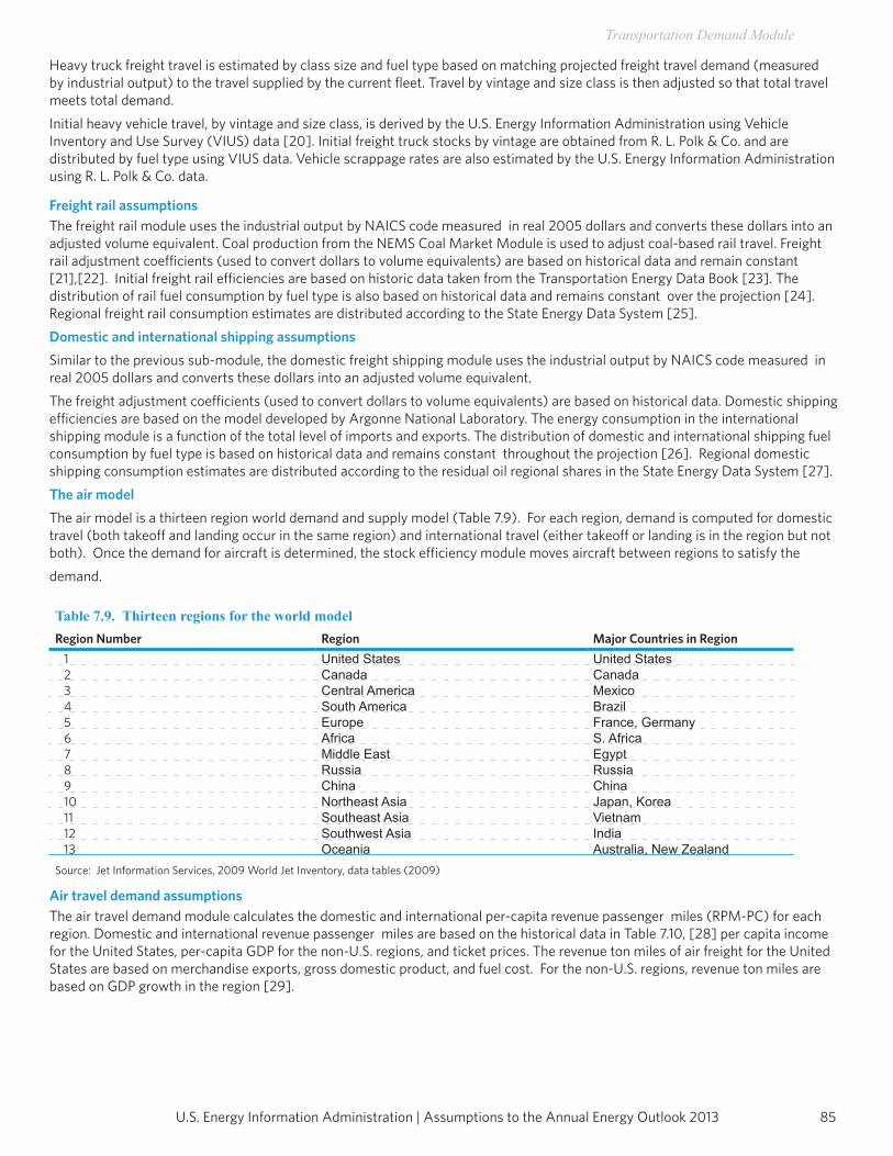
85U.S. Energy Information Administration | Assumptions to the Annual Energy Outlook 2013
Transportation Demand Module
Heavy truck freight travel is estimated by class size and fuel type based on matching projected freight travel demand (measured by industrial output) to the travel supplied by the current fleet. Travel by vintage and size class is then adjusted so that total travel meets total demand.Initial heavy vehicle travel, by vintage and size class, is derived by the U.S. Energy Information Administration using Vehicle Inventory and Use Survey (VIUS) data [20]. Initial freight truck stocks by vintage are obtained from R. L. Polk & Co. and are distributed by fuel type using VIUS data. Vehicle scrappage rates are also estimated by the U.S. Energy Information Administration using R. L. Polk & Co. data.
Freight rail assumptionsThe freight rail module uses the industrial output by NAICS code measured in real 2005 dollars and converts these dollars into an adjusted volume equivalent. Coal production from the NEMS Coal Market Module is used to adjust coal-based rail travel. Freight rail adjustment coefficients (used to convert dollars to volume equivalents) are based on historical data and remain constant [21],[22]. Initial freight rail efficiencies are based on historic data taken from the Transportation Energy Data Book [23]. The distribution of rail fuel consumption by fuel type is also based on historical data and remains constant over the projection [24]. Regional freight rail consumption estimates are distributed according to the State Energy Data System [25].Domestic and international shipping assumptionsSimilar to the previous sub-module, the domestic freight shipping module uses the industrial output by NAICS code measured in real 2005 dollars and converts these dollars into an adjusted volume equivalent.The freight adjustment coefficients (used to convert dollars to volume equivalents) are based on historical data. Domestic shipping efficiencies are based on the model developed by Argonne National Laboratory. The energy consumption in the international shipping module is a function of the total level of imports and exports. The distribution of domestic and international shipping fuel consumption by fuel type is based on historical data and remains constant throughout the projection [26]. Regional domestic shipping consumption estimates are distributed according to the residual oil regional shares in the State Energy Data System [27]. The air modelThe air model is a thirteen region world demand and supply model (Table 7.9). For each region, demand is computed for domestic travel (both takeoff and landing occur in the same region) and international travel (either takeoff or landing is in the region but not both). Once the demand for aircraft is determined, the stock efficiency module moves aircraft between regions to satisfy the demand.
Table 7.9. Thirteen regions for the world modelRegion Number Region Major Countries in Region
1 United States United States2 Canada Canada3 Central America Mexico4 South America Brazil5 Europe France, Germany6 Africa S. Africa7 Middle East Egypt8 Russia Russia9 China China10 Northeast Asia Japan, Korea11 Southeast Asia Vietnam12 Southwest Asia India13 Oceania Australia, New Zealand
Source: Jet Information Services, 2009 World Jet Inventory, data tables (2009)
Air travel demand assumptionsThe air travel demand module calculates the domestic and international per-capita revenue passenger miles (RPM-PC) for each region. Domestic and international revenue passenger miles are based on the historical data in Table 7.10, [28] per capita income for the United States, per-capita GDP for the non-U.S. regions, and ticket prices. The revenue ton miles of air freight for the United States are based on merchandise exports, gross domestic product, and fuel cost. For the non-U.S. regions, revenue ton miles are based on GDP growth in the region [29].
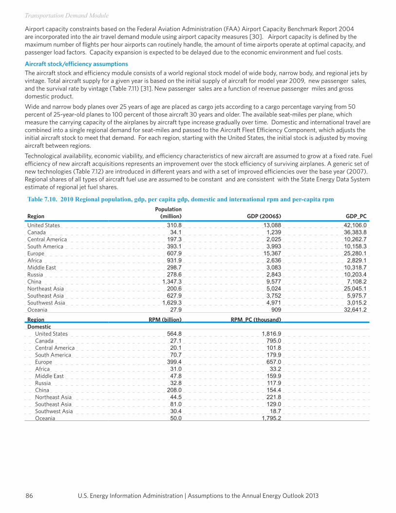
U.S. Energy Information Administration | Assumptions to the Annual Energy Outlook 201386
Transportation Demand Module
Airport capacity constraints based on the Federal Aviation Administration (FAA) Airport Capacity Benchmark Report 2004 are incorporated into the air travel demand module using airport capacity measures [30]. Airport capacity is defined by the maximum number of flights per hour airports can routinely handle, the amount of time airports operate at optimal capacity, and passenger load factors. Capacity expansion is expected to be delayed due to the economic environment and fuel costs.
Aircraft stock/efficiency assumptionsThe aircraft stock and efficiency module consists of a world regional stock model of wide body, narrow body, and regional jets by vintage. Total aircraft supply for a given year is based on the initial supply of aircraft for model year 2009, new passenger sales, and the survival rate by vintage (Table 7.11) [31]. New passenger sales are a function of revenue passenger miles and gross domestic product.Wide and narrow body planes over 25 years of age are placed as cargo jets according to a cargo percentage varying from 50 percent of 25-year-old planes to 100 percent of those aircraft 30 years and older. The available seat-miles per plane, which measure the carrying capacity of the airplanes by aircraft type increase gradually over time. Domestic and international travel are combined into a single regional demand for seat-miles and passed to the Aircraft Fleet Efficiency Component, which adjusts the initial aircraft stock to meet that demand. For each region, starting with the United States, the initial stock is adjusted by moving aircraft between regions.Technological availability, economic viability, and efficiency characteristics of new aircraft are assumed to grow at a fixed rate. Fuel efficiency of new aircraft acquisitions represents an improvement over the stock efficiency of surviving airplanes. A generic set of new technologies (Table 7.12) are introduced in different years and with a set of improved efficiencies over the base year (2007). Regional shares of all types of aircraft fuel use are assumed to be constant and are consistent with the State Energy Data System estimate of regional jet fuel shares.
Table 7.10. 2010 Regional population, gdp, per capita gdp, domestic and international rpm and per-capita rpm
RegionPopulation
(million) GDP (2006$) GDP_PCUnited States 310.8 13,088 42,106.0Canada 34.1 1,239 36,383.8Central America 197.3 2,025 10,262.7South America 393.1 3,993 10,158.3Europe 607.9 15,367 25,280.1Africa 931.9 2,636 2,829.1Middle East 298.7 3,083 10,318.7Russia 278.6 2,843 10,203.4China 1,347.3 9,577 7,108.2Northeast Asia 200.6 5,024 25,045.1Southeast Asia 627.9 3,752 5,975.7Southwest Asia 1,629.3 4,971 3,015.2Oceania 27.9 909 32,641.2
Region RPM (billion) RPM_PC (thousand)Domestic
United States 564.8 1,816.9Canada 27.1 795.0Central America 20.1 101.8South America 70.7 179.9Europe 399.4 657.0Africa 31.0 33.2Middle East 47.8 159.9Russia 32.8 117.9China 208.0 154.4Northeast Asia 44.5 221.8Southeast Asia 81.0 129.0Southwest Asia 30.4 18.7Oceania 50.0 1,795.2
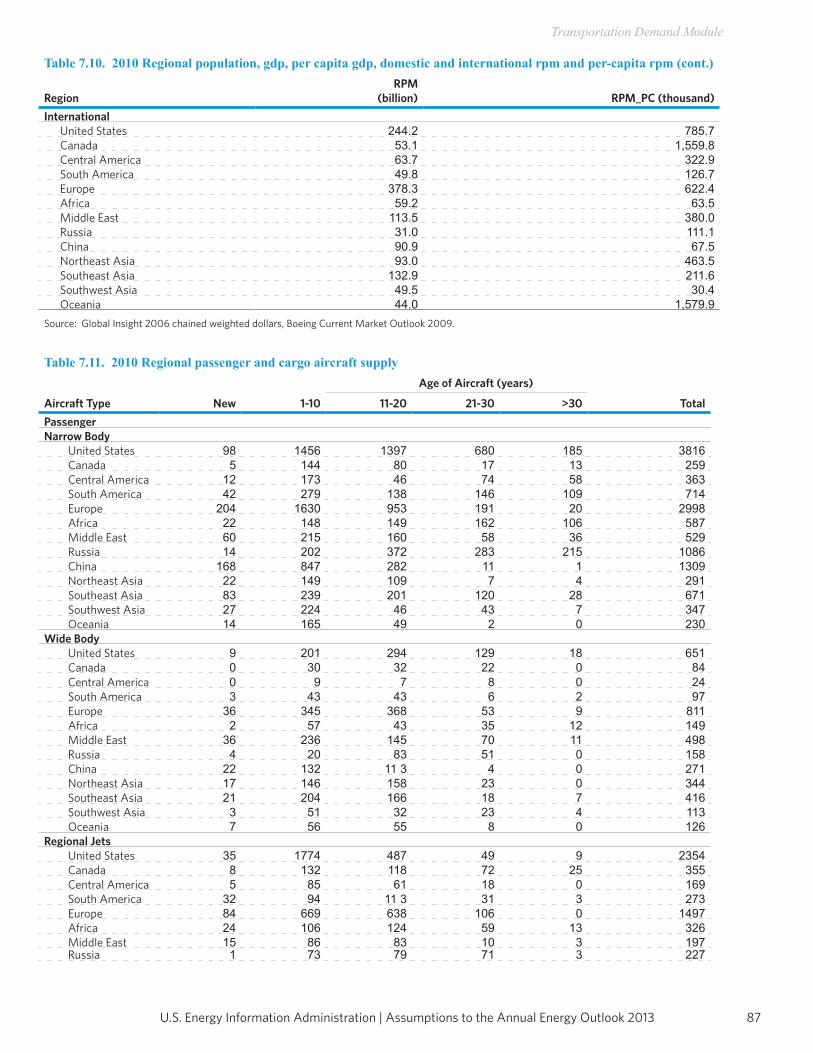
87U.S. Energy Information Administration | Assumptions to the Annual Energy Outlook 2013
Transportation Demand Module
Table 7.10. 2010 Regional population, gdp, per capita gdp, domestic and international rpm and per-capita rpm (cont.)
RegionRPM
(billion) RPM_PC (thousand)International
United States 244.2 785.7Canada 53.1 1,559.8Central America 63.7 322.9South America 49.8 126.7Europe 378.3 622.4Africa 59.2 63.5Middle East 113.5 380.0Russia 31.0 111.1China 90.9 67.5Northeast Asia 93.0 463.5Southeast Asia 132.9 211.6Southwest Asia 49.5 30.4Oceania 44.0 1,579.9
Source: Global Insight 2006 chained weighted dollars, Boeing Current Market Outlook 2009.
Table 7.11. 2010 Regional passenger and cargo aircraft supply
Aircraft Type New
Age of Aircraft (years)
1-10 11-20 21-30 >30 TotalPassengerNarrow Body
United States 98 1456 1397 680 185 3816 Canada 5 144 80 17 13 259 Central America 12 173 46 74 58 363 South America 42 279 138 146 109 714 Europe 204 1630 953 191 20 2998 Africa 22 148 149 162 106 587 Middle East 60 215 160 58 36 529 Russia 14 202 372 283 215 1086 China 168 847 282 11 1 1309 Northeast Asia 22 149 109 7 4 291 Southeast Asia 83 239 201 120 28 671 Southwest Asia 27 224 46 43 7 347 Oceania 14 165 49 2 0 230
Wide BodyUnited States 9 201 294 129 18 651 Canada 0 30 32 22 0 84 Central America 0 9 7 8 0 24 South America 3 43 43 6 2 97 Europe 36 345 368 53 9 811 Africa 2 57 43 35 12 149 Middle East 36 236 145 70 11 498 Russia 4 20 83 51 0 158 China 22 132 11 3 4 0 271 Northeast Asia 17 146 158 23 0 344 Southeast Asia 21 204 166 18 7 416 Southwest Asia 3 51 32 23 4 113 Oceania 7 56 55 8 0 126
Regional JetsUnited States 35 1774 487 49 9 2354 Canada 8 132 118 72 25 355 Central America 5 85 61 18 0 169 South America 32 94 11 3 31 3 273 Europe 84 669 638 106 0 1497 Africa 24 106 124 59 13 326 Middle East 15 86 83 10 3 197 Russia 1 73 79 71 3 227
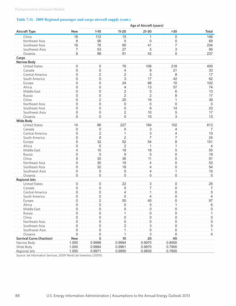
U.S. Energy Information Administration | Assumptions to the Annual Energy Outlook 201388
Transportation Demand Module
Table 7.11. 2009 Regional passenger and cargo aircraft supply (cont.)Age of Aircraft (years)
Aircraft Type New 1-10 11-20 21-30 >30 TotalChina 18 112 15 1 0 146 Northeast Asia 8 56 5 0 0 69 Southeast Asia 18 78 90 41 7 234 Southwest Asia 7 53 27 5 3 95 Oceania 6 98 91 42 0 237
CargoNarrow Body
United States 0 0 76 106 218 400 Canada 0 0 4 8 21 33Central America 0 2 2 5 8 17South America 0 0 3 17 42 62Europe 0 0 24 68 10 102Africa 0 0 4 13 57 74Middle East 0 0 2 5 6 13Russia 0 5 2 2 8 17China 0 2 20 16 1 39 Northeast Asia 0 0 0 0 0 0 Southeast Asia 0 0 0 8 14 23Southwest Asia 0 0 2 10 5 17Oceania 0 0 0 10 3 13
Wide BodyUnited States 14 86 227 184 102 613 Canada 0 0 0 3 4 7 Central America 0 2 1 3 4 10 South America 0 8 2 7 7 24 Europe 5 32 52 54 8 151 Africa 0 0 2 1 1 4 Middle East 4 10 18 18 5 55 Russia 0 5 9 5 0 19 China 9 35 36 11 0 91 Northeast Asia 0 30 19 4 0 53 Southeast Asia 0 32 18 4 0 54 Southwest Asia 0 0 5 4 1 10 Oceania 0 0 0 0 0 0
Regional JetsUnited States 0 0 22 3 0 25 Canada 0 0 0 7 0 7Central America 0 0 4 1 0 5 South America 0 0 0 4 0 4 Europe 0 2 55 40 0 97 Africa 0 0 0 5 1 6 Middle East 0 0 0 0 0 0 Russia 0 0 1 0 0 1 China 0 0 0 0 0 0 Northeast Asia 0 0 0 0 0 0 Southeast Asia 0 0 2 3 0 5 Southwest Asia 0 0 1 0 0 1 Oceania 0 0 1 3 0 4
Survival Curve (fraction) New 5 10 20 40Narrow Body 1.000 0.9998 0.9994 0.9970 0.8000 Wide Body 1.000 0.9984 0.9961 0.9870 0.7900 Regional Jets 1.000 0.9971 0.9950 0.9830 0.7800 Source: Jet Information Services, 2009 World Jet Inventory (2009).
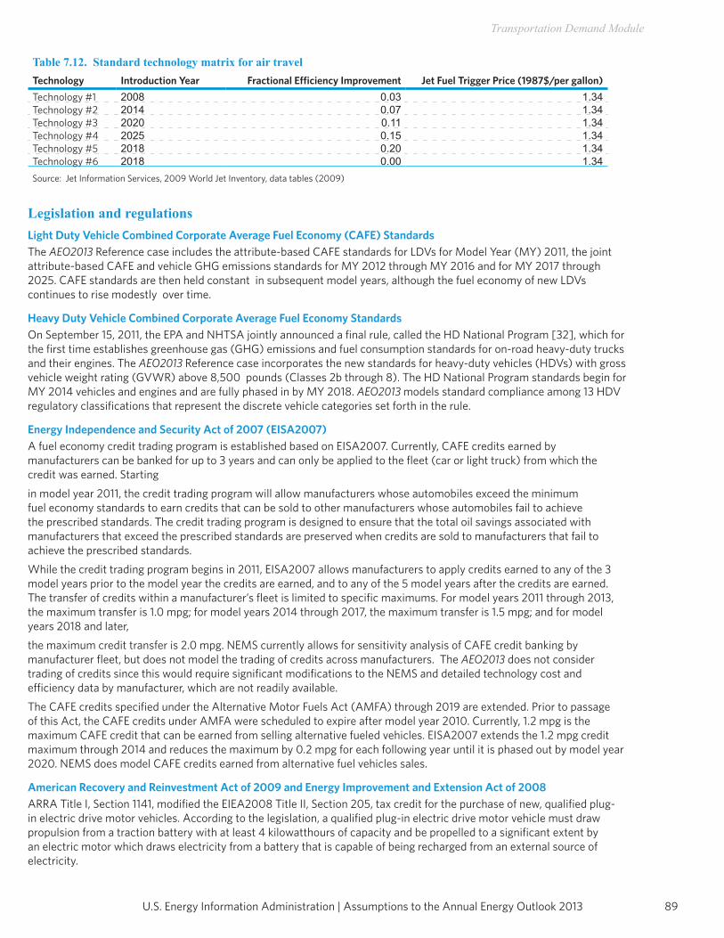
89U.S. Energy Information Administration | Assumptions to the Annual Energy Outlook 2013
Transportation Demand Module
Table 7.12. Standard technology matrix for air travelTechnology Introduction Year Fractional Efficiency Improvement Jet Fuel Trigger Price (1987$/per gallon)Technology #1 2008 0.03 1.34Technology #2 2014 0.07 1.34Technology #3 2020 0.11 1.34Technology #4 2025 0.15 1.34Technology #5 2018 0.20 1.34Technology #6 2018 0.00 1.34Source: Jet Information Services, 2009 World Jet Inventory, data tables (2009)
Legislation and regulationsLight Duty Vehicle Combined Corporate Average Fuel Economy (CAFE) StandardsThe AEO2013 Reference case includes the attribute-based CAFE standards for LDVs for Model Year (MY) 2011, the joint attribute-based CAFE and vehicle GHG emissions standards for MY 2012 through MY 2016 and for MY 2017 through 2025. CAFE standards are then held constant in subsequent model years, although the fuel economy of new LDVs continues to rise modestly over time.
Heavy Duty Vehicle Combined Corporate Average Fuel Economy StandardsOn September 15, 2011, the EPA and NHTSA jointly announced a final rule, called the HD National Program [32], which for the first time establishes greenhouse gas (GHG) emissions and fuel consumption standards for on-road heavy-duty trucks and their engines. The AEO2013 Reference case incorporates the new standards for heavy-duty vehicles (HDVs) with gross vehicle weight rating (GVWR) above 8,500 pounds (Classes 2b through 8). The HD National Program standards begin for MY 2014 vehicles and engines and are fully phased in by MY 2018. AEO2013 models standard compliance among 13 HDV regulatory classifications that represent the discrete vehicle categories set forth in the rule.
Energy Independence and Security Act of 2007 (EISA2007)
A fuel economy credit trading program is established based on EISA2007. Currently, CAFE credits earned by manufacturers can be banked for up to 3 years and can only be applied to the fleet (car or light truck) from which the credit was earned. Startingin model year 2011, the credit trading program will allow manufacturers whose automobiles exceed the minimum fuel economy standards to earn credits that can be sold to other manufacturers whose automobiles fail to achieve the prescribed standards. The credit trading program is designed to ensure that the total oil savings associated with manufacturers that exceed the prescribed standards are preserved when credits are sold to manufacturers that fail to achieve the prescribed standards.While the credit trading program begins in 2011, EISA2007 allows manufacturers to apply credits earned to any of the 3 model years prior to the model year the credits are earned, and to any of the 5 model years after the credits are earned. The transfer of credits within a manufacturer’s fleet is limited to specific maximums. For model years 2011 through 2013, the maximum transfer is 1.0 mpg; for model years 2014 through 2017, the maximum transfer is 1.5 mpg; and for model years 2018 and later,the maximum credit transfer is 2.0 mpg. NEMS currently allows for sensitivity analysis of CAFE credit banking by manufacturer fleet, but does not model the trading of credits across manufacturers. The AEO2013 does not consider trading of credits since this would require significant modifications to the NEMS and detailed technology cost and efficiency data by manufacturer, which are not readily available.The CAFE credits specified under the Alternative Motor Fuels Act (AMFA) through 2019 are extended. Prior to passage of this Act, the CAFE credits under AMFA were scheduled to expire after model year 2010. Currently, 1.2 mpg is the maximum CAFE credit that can be earned from selling alternative fueled vehicles. EISA2007 extends the 1.2 mpg credit maximum through 2014 and reduces the maximum by 0.2 mpg for each following year until it is phased out by model year 2020. NEMS does model CAFE credits earned from alternative fuel vehicles sales.
American Recovery and Reinvestment Act of 2009 and Energy Improvement and Extension Act of 2008ARRA Title I, Section 1141, modified the EIEA2008 Title II, Section 205, tax credit for the purchase of new, qualified plug-in electric drive motor vehicles. According to the legislation, a qualified plug-in electric drive motor vehicle must draw propulsion from a traction battery with at least 4 kilowatthours of capacity and be propelled to a significant extent by an electric motor which draws electricity from a battery that is capable of being recharged from an external source of electricity.
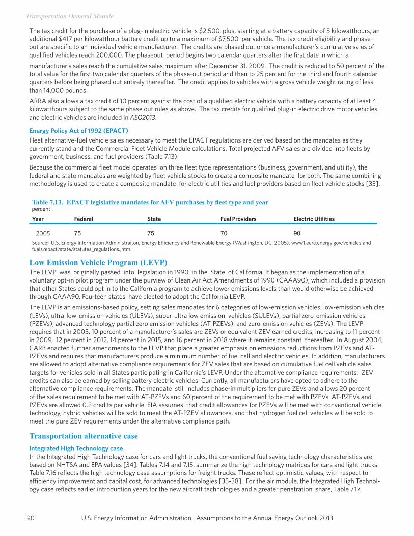
U.S. Energy Information Administration | Assumptions to the Annual Energy Outlook 201390
Transportation Demand Module
The tax credit for the purchase of a plug-in electric vehicle is $2,500, plus, starting at a battery capacity of 5 kilowatthours, an additional $417 per kilowatthour battery credit up to a maximum of $7,500 per vehicle. The tax credit eligibility and phase-out are specific to an individual vehicle manufacturer. The credits are phased out once a manufacturer’s cumulative sales of qualified vehicles reach 200,000. The phaseout period begins two calendar quarters after the first date in which amanufacturer’s sales reach the cumulative sales maximum after December 31, 2009. The credit is reduced to 50 percent of the total value for the first two calendar quarters of the phase-out period and then to 25 percent for the third and fourth calendar quarters before being phased out entirely thereafter. The credit applies to vehicles with a gross vehicle weight rating of less than 14,000 pounds.ARRA also allows a tax credit of 10 percent against the cost of a qualified electric vehicle with a battery capacity of at least 4 kilowatthours subject to the same phase out rules as above. The tax credits for qualified plug-in electric drive motor vehicles and electric vehicles are included in AEO2013.
Energy Policy Act of 1992 (EPACT)Fleet alternative-fuel vehicle sales necessary to meet the EPACT regulations are derived based on the mandates as they currently stand and the Commercial Fleet Vehicle Module calculations. Total projected AFV sales are divided into fleets by government, business, and fuel providers (Table 7.13).Because the commercial fleet model operates on three fleet type representations (business, government, and utility), the federal and state mandates are weighted by fleet vehicle stocks to create a composite mandate for both. The same combining methodology is used to create a composite mandate for electric utilities and fuel providers based on fleet vehicle stocks [33].
Table 7.13. EPACT legislative mandates for AFV purchases by fleet type and yearpercent
Year Federal State Fuel Providers Electric Utilities
2005 75 75 70 90Source: U.S. Energy Information Administraiton, Energy Efficiency and Renewable Energy (Washington, DC, 2005), www1.eere.energy.gov/vehicles and fuels/epact/state/statutes_regulations.,html.
Low Emission Vehicle Program (LEVP)The LEVP was originally passed into legislation in 1990 in the State of California. It began as the implementation of a voluntary opt-in pilot program under the purview of Clean Air Act Amendments of 1990 (CAAA90), which included a provision that other States could opt in to the California program to achieve lower emissions levels than would otherwise be achieved through CAAA90. Fourteen states have elected to adopt the California LEVP.The LEVP is an emissions-based policy, setting sales mandates for 6 categories of low-emission vehicles: low-emission vehicles (LEVs), ultra-low-emission vehicles (ULEVs), super-ultra low emission vehicles (SULEVs), partial zero-emission vehicles (PZEVs), advanced technology partial zero emission vehicles (AT-PZEVs), and zero-emission vehicles (ZEVs). The LEVP requires that in 2005, 10 percent of a manufacturer’s sales are ZEVs or equivalent ZEV earned credits, increasing to 11 percent in 2009, 12 percent in 2012, 14 percent in 2015, and 16 percent in 2018 where it remains constant thereafter. In August 2004, CARB enacted further amendments to the LEVP that place a greater emphasis on emissions reductions from PZEVs and AT-PZEVs and requires that manufacturers produce a minimum number of fuel cell and electric vehicles. In addition, manufacturers are allowed to adopt alternative compliance requirements for ZEV sales that are based on cumulative fuel cell vehicle sales targets for vehicles sold in all States participating in California’s LEVP. Under the alternative compliance requirements, ZEV credits can also be earned by selling battery electric vehicles. Currently, all manufacturers have opted to adhere to the alternative compliance requirements. The mandate still includes phase-in multipliers for pure ZEVs and allows 20 percent of the sales requirement to be met with AT-PZEVs and 60 percent of the requirement to be met with PZEVs. AT-PZEVs and PZEVs are allowed 0.2 credits per vehicle. EIA assumes that credit allowances for PZEVs will be met with conventional vehicle technology, hybrid vehicles will be sold to meet the AT-PZEV allowances, and that hydrogen fuel cell vehicles will be sold to meet the pure ZEV requirements under the alternative compliance path.
Transportation alternative caseIntegrated High Technology caseIn the Integrated High Technology case for cars and light trucks, the conventional fuel saving technology characteristics are based on NHTSA and EPA values [34]. Tables 7.14 and 7.15, summarize the high technology matrices for cars and light trucks. Table 7.16 reflects the high technology case assumptions for freight trucks. These reflect optimistic values, with respect to efficiency improvement and capital cost, for advanced technologies [35-38]. For the air module, the Integrated High Technol-ogy case reflects earlier introduction years for the new aircraft technologies and a greater penetration share, Table 7.17.
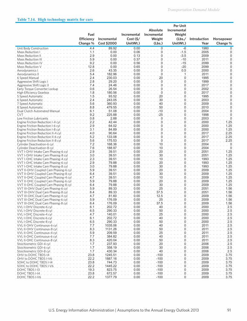
91U.S. Energy Information Administration | Assumptions to the Annual Energy Outlook 2013
Transportation Demand Module
Table 7.14. High technology matrix for cars
Fuel Efficiency Change %
Incremental Cost $2000
Incremental Cost ($/UnitWt.)
Absolute Incremental
Weight (Lbs.)
Per Unit Incremental
Weight (Lbs./
UnitWt.)Introduction
YearHorsepower
Change %Unit Body Construction 4.4 89.92 0.00 0 -6 1980 0Mass Reduction I 1.1 0.00 0.06 0 -1.5 2005 0Mass Reduction II 2.9 0.00 0.13 0 -3.5 2009 0Mass Reduction III 5.9 0.00 0.37 0 -10 2011 0Mass Reduction IV 9.2 0.00 0.56 0 -15 2099 0Mass Reduction V 12.8 0.00 0.65 0 -20 2099 0Aerodynamics I 2.6 43.35 0.00 0 0.5 2000 0Aerodynamics II 5.4 182.96 0.00 0 1 2011 06 Speed Manual 2.4 230.03 0.00 20 0 1995 0Aggressive Shift Logic I 2.8 29.20 0.00 0 0 1999 0Aggressive Shift Logic II 7.4 24.46 0.00 0 0 2017 0Early Torque Converter Lockup 0.6 26.54 0.00 0 0 2002 0High Efficiency Gearbox 1.8 180.56 0.00 0 0 2017 05 Speed Automatic 1.5 93.52 0.00 20 0 1995 06 Speed Automatic 2.4 243.05 0.00 30 0 2003 07 Speed Automatic 5.6 360.93 0.00 40 0 2009 08 Speed Automatic 8.8 479.55 0.00 50 0 2010 0Dual Clutch Automated Manual 6.1 51.08 0.00 -10 0 2004 0CVT 9.2 225.88 0.00 -25 0 1998 0Low Friction Lubricants 0.8 2.88 0.00 0 0 2003 0Engine Friction Reduction I-4 cyl 2.2 42.44 0.00 0 0 2000 1.25Engine Friction Reduction I-6 cyl 2.9 64.02 0.00 0 0 2000 1.25Engine Friction Reduction I-8 cyl 3.1 84.89 0.00 0 0 2000 1.25Engine Friction Reduction II-4 cyl 4.0 90.64 0.00 0 0 2017 2.25Engine Friction Reduction II-6 cyl 5.2 133.08 0.00 0 0 2017 2.25Engine Friction Reduction II-8 cyl 5.6 175.53 0.00 0 0 2017 2.25Cylinder Deactivation-6 cyl 7.2 168.36 0.00 10 0 2004 0Cylinder Deactivation-8 cyl 7.6 188.97 0.00 10 0 2004 0VVT I-OHV Intake Cam Phasing-6 cyl 2.9 39.51 0.00 20 0 2051 1.25VVT I-OHV Intake Cam Phasing-8 cyl 3.0 39.51 0.00 30 0 2051 1.25VVT I-OHC Intake Cam Phasing-4 cyl 2.3 39.51 0.00 10 0 1993 1.25VVT I-OHC Intake Cam Phasing-6 cyl 2.9 79.88 0.00 20 0 1993 1.25VVT I-OHC Intake Cam Phasing-8 cyl 3.0 79.88 0.00 30 0 1993 1.25VVT II-OHV Coupled Cam Phasing-6 cyl 5.9 39.51 0.00 20 0 2009 1.25VVT II-OHV Coupled Cam Phasing-8 cyl 6.4 39.51 0.00 30 0 2009 1.25VVT II-OHC Coupled Cam Phasing-4 cyl 4.7 39.51 0.00 10 0 2009 1.25VVT II-OHC Coupled Cam Phasing-6 cyl 5.9 79.88 0.00 20 0 2009 1.25VVT II-OHC Coupled Cam Phasing-8 cyl 6.4 79.88 0.00 30 0 2009 1.25VVT III-OHV Dual Cam Phasing-6 cyl 5.9 89.33 0.00 25 0 2051 1.56VVT III-OHV Dual Cam Phasing-8 cyl 6.4 89.33 0.00 37.5 0 2051 1.56VVT III-OHC Dual Cam Phasing-4 cyl 4.7 81.60 0.00 12.5 0 2009 1.56VVT III-OHC Dual Cam Phasing-6 cyl 5.9 176.09 0.00 25 0 2009 1.56VVT III-OHC Dual Cam Phasing-8 cyl 6.4 176.09 0.00 37.5 0 2009 1.56VVL I-OHV Discrete-6 cyl 6.1 202.72 0.00 40 0 2000 2.5VVL I-OHV Discrete-8 cyl 6.5 290.33 0.00 50 0 2000 2.5VVL I-OHC Discrete-4 cyl 4.7 140.01 0.00 25 0 2000 2.5VVL I-OHC Discrete-6 cyl 6.1 202.72 0.00 40 0 2000 2.5VVL I-OHC Discrete-8 cyl 6.5 290.33 0.00 50 0 2000 2.5VVL II-OHV Continuous-6 cyl 7.7 1035.06 0.00 40 0 2011 2.5VVL II-OHV Continuous-8 cyl 8.3 1131.26 0.00 50 0 2011 2.5VVL II-OHC Continuous-4 cyl 5.9 209.59 0.00 25 0 2011 2.5VVL II-OHC Continuous-6 cyl 7.7 384.82 0.00 40 0 2011 2.5VVL II-OHC Continuous-8 cyl 8.3 420.04 0.00 50 0 2011 2.5Stoichiometric GDI-4 cyl 1.7 237.93 0.00 20 0 2006 2.5Stoichiometric GDI-6 cyl 1.7 358.19 0.00 30 0 2006 2.5Stoichiometric GDI-8 cyl 1.7 430.34 0.00 40 0 2006 2.5OHV to DOHC TBDS-I4 23.8 1245.51 0.00 -100 0 2009 3.75OHV to DOHC TBDS I-V6 22.2 1887.16 0.00 -100 0 2009 3.75SOHC to DOHC TBDS I-I4 23.8 744.73 0.00 -100 0 2009 3.75SOHC to DOHC TBDS I-V6 22.2 1445.22 0.00 -100 0 2009 3.75DOHC TBDS I-I3 19.3 823.75 0.00 -100 0 2009 3.75DOHC TBDS I-I4 23.8 672.57 0.00 -100 0 2009 3.75DOHC TBDS I-V6 22.2 1377.79 0.00 -100 0 2009 3.75
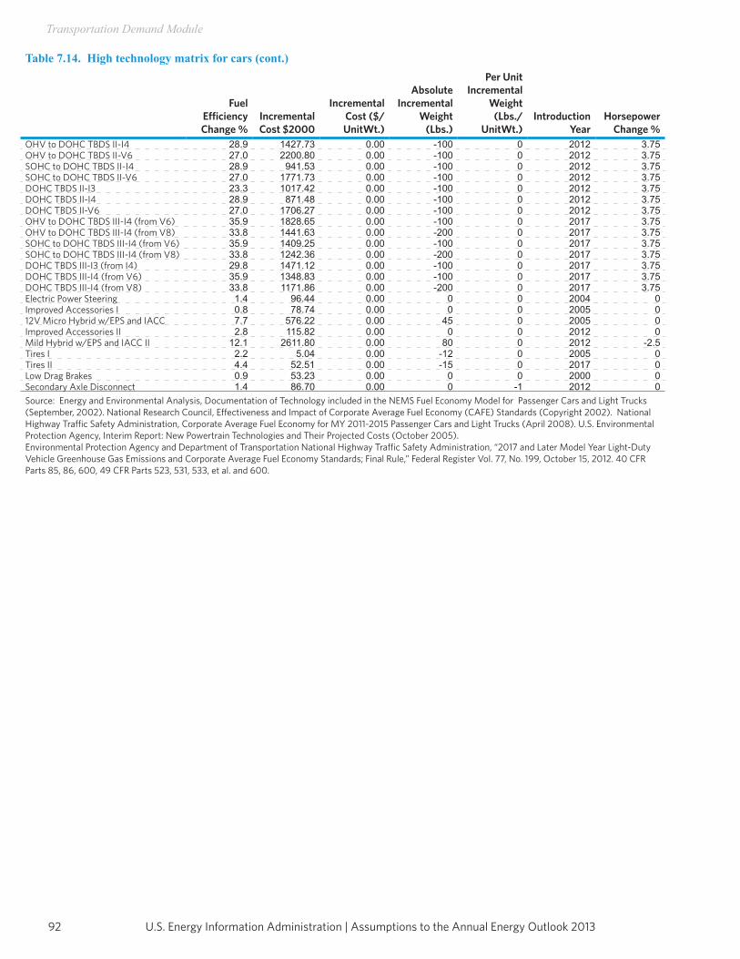
U.S. Energy Information Administration | Assumptions to the Annual Energy Outlook 201392
Transportation Demand Module
Table 7.14. High technology matrix for cars (cont.)
Fuel Efficiency Change %
Incremental Cost $2000
Incremental Cost ($/UnitWt.)
Absolute Incremental
Weight (Lbs.)
Per Unit Incremental
Weight (Lbs./
UnitWt.)Introduction
YearHorsepower
Change %OHV to DOHC TBDS II-I4 28.9 1427.73 0.00 -100 0 2012 3.75OHV to DOHC TBDS II-V6 27.0 2200.80 0.00 -100 0 2012 3.75SOHC to DOHC TBDS II-I4 28.9 941.53 0.00 -100 0 2012 3.75SOHC to DOHC TBDS II-V6 27.0 1771.73 0.00 -100 0 2012 3.75DOHC TBDS II-I3 23.3 1017.42 0.00 -100 0 2012 3.75DOHC TBDS II-I4 28.9 871.48 0.00 -100 0 2012 3.75DOHC TBDS II-V6 27.0 1706.27 0.00 -100 0 2012 3.75OHV to DOHC TBDS III-I4 (from V6) 35.9 1828.65 0.00 -100 0 2017 3.75OHV to DOHC TBDS III-I4 (from V8) 33.8 1441.63 0.00 -200 0 2017 3.75SOHC to DOHC TBDS III-I4 (from V6) 35.9 1409.25 0.00 -100 0 2017 3.75SOHC to DOHC TBDS III-I4 (from V8) 33.8 1242.36 0.00 -200 0 2017 3.75DOHC TBDS III-I3 (from I4) 29.8 1471.12 0.00 -100 0 2017 3.75DOHC TBDS III-I4 (from V6) 35.9 1348.83 0.00 -100 0 2017 3.75DOHC TBDS III-I4 (from V8) 33.8 1171.86 0.00 -200 0 2017 3.75Electric Power Steering 1.4 96.44 0.00 0 0 2004 0Improved Accessories I 0.8 78.74 0.00 0 0 2005 012V Micro Hybrid w/EPS and IACC 7.7 576.22 0.00 45 0 2005 0Improved Accessories II 2.8 115.82 0.00 0 0 2012 0Mild Hybrid w/EPS and IACC II 12.1 2611.80 0.00 80 0 2012 -2.5Tires I 2.2 5.04 0.00 -12 0 2005 0Tires II 4.4 52.51 0.00 -15 0 2017 0Low Drag Brakes 0.9 53.23 0.00 0 0 2000 0Secondary Axle Disconnect 1.4 86.70 0.00 0 -1 2012 0Source: Energy and Environmental Analysis, Documentation of Technology included in the NEMS Fuel Economy Model for Passenger Cars and Light Trucks (September, 2002). National Research Council, Effectiveness and Impact of Corporate Average Fuel Economy (CAFE) Standards (Copyright 2002). National Highway Traffic Safety Administration, Corporate Average Fuel Economy for MY 2011-2015 Passenger Cars and Light Trucks (April 2008). U.S. Environmental Protection Agency, Interim Report: New Powertrain Technologies and Their Projected Costs (October 2005).Environmental Protection Agency and Department of Transportation National Highway Traffic Safety Administration, “2017 and Later Model Year Light-Duty Vehicle Greenhouse Gas Emissions and Corporate Average Fuel Economy Standards; Final Rule,” Federal Register Vol. 77, No. 199, October 15, 2012. 40 CFR Parts 85, 86, 600, 49 CFR Parts 523, 531, 533, et al. and 600.
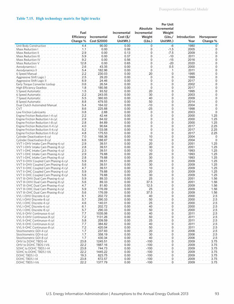
93U.S. Energy Information Administration | Assumptions to the Annual Energy Outlook 2013
Transportation Demand Module
Table 7.15. High technology matrix for light trucks
Fuel Efficiency Change %
Incremental Cost $2000
Incremental Cost ($/UnitWt.)
Absolute Incremental
Weight (Lbs.)
Per Unit Incremental
Weight (Lbs./
UnitWt.)Introduction
YearHorsepower
Change %Unit Body Construction 4.4 90.00 0.00 0 -6 1980 0Mass Reduction I 1.1 0.00 0.06 0 -1.5 2005 0Mass Reduction II 2.9 0.00 0.13 0 -7.5 2009 0Mass Reduction III 5.9 0.00 0.37 0 -10 2011 0Mass Reduction IV 9.2 0.00 0.56 0 -15 2016 0Mass Reduction V 12.8 0.00 0.65 0 -20 2020 0Aerodynamics I 2.6 43.35 0.00 0 0.5 2000 0Aerodynamics II 5.4 182.96 0.00 0 1 2011 06 Speed Manual 2.2 230.03 0.00 20 0 1995 0Aggressive Shift Logic I 2.5 29.20 0.00 0 0 1999 0Aggressive Shift Logic II 6.9 24.46 0.00 0 0 2017 0Early Torque Converter Lockup 0.6 26.54 0.00 0 0 2002 0High Efficiency Gearbox 1.8 180.56 0.00 0 0 2017 05 Speed Automatic 1.5 93.52 0.00 20 0 1995 06 Speed Automatic 2.2 243.05 0.00 30 0 2003 07 Speed Automatic 5.5 360.93 0.00 40 0 2009 08 Speed Automatic 8.8 479.55 0.00 50 0 2014 0Dual Clutch Automated Manual 5.4 164.02 0.00 -10 0 2004 0CVT 8.6 225.88 0.00 -25 0 1998 0Low Friction Lubricants 0.8 2.88 0.00 0 0 2003 0Engine Friction Reduction I-4 cyl 2.2 42.44 0.00 0 0 2000 1.25Engine Friction Reduction I-6 cyl 2.9 64.02 0.00 0 0 2000 1.25Engine Friction Reduction I-8 cyl 2.8 84.89 0.00 0 0 2000 1.25Engine Friction Reduction II-4 cyl 4.0 90.64 0.00 0 0 2017 2.25Engine Friction Reduction II-6 cyl 5.2 133.08 0.00 0 0 2017 2.25Engine Friction Reduction II-8 cyl 4.8 175.53 0.00 0 0 2017 2.25Cylinder Deactivation-6 cyl 7.0 168.36 0.00 10 0 2004 0Cylinder Deactivation-8 cyl 6.6 188.97 0.00 10 0 2004 0VVT I-OHV Intake Cam Phasing-6 cyl 2.9 39.51 0.00 20 0 2051 1.25VVT I-OHV Intake Cam Phasing-8 cyl 2.8 39.51 0.00 30 0 2051 1.25VVT I-OHC Intake Cam Phasing-4 cyl 2.3 39.51 0.00 10 0 1993 1.25VVT I-OHC Intake Cam Phasing-6 cyl 2.9 79.88 0.00 20 0 1993 1.25VVT I-OHC Intake Cam Phasing-8 cyl 2.8 79.88 0.00 30 0 1993 1.25VVT II-OHV Coupled Cam Phasing-6 cyl 5.9 39.51 0.00 20 0 2009 1.25VVT II-OHV Coupled Cam Phasing-8 cyl 5.6 39.51 0.00 30 0 2009 1.25VVT II-OHC Coupled Cam Phasing-4 cyl 4.7 39.51 0.00 10 0 2009 1.25VVT II-OHC Coupled Cam Phasing-6 cyl 5.9 79.88 0.00 20 0 2009 1.25VVT II-OHC Coupled Cam Phasing-8 cyl 5.6 79.88 0.00 30 0 2009 1.25VVT III-OHV Dual Cam Phasing-6 cyl 5.9 89.33 0.00 25 0 2051 1.56VVT III-OHV Dual Cam Phasing-8 cyl 5.6 89.33 0.00 37.5 0 2051 1.56VVT III-OHC Dual Cam Phasing-4 cyl 4.7 81.60 0.00 12.5 0 2009 1.56VVT III-OHC Dual Cam Phasing-6 cyl 5.9 176.09 0.00 25 0 2009 1.56VVT III-OHC Dual Cam Phasing-8 cyl 5.6 176.09 0.00 37.5 0 2009 1.56VVL I-OHV Discrete-6 cyl 6.1 202.72 0.00 40 0 2000 2.5VVL I-OHV Discrete-8 cyl 5.7 290.33 0.00 50 0 2000 2.5VVL I-OHC Discrete-4 cyl 4.6 140.01 0.00 25 0 2000 2.5VVL I-OHC Discrete-6 cyl 6.1 202.72 0.00 40 0 2000 2.5VVL I-OHC Discrete-8 cyl 5.7 290.33 0.00 50 0 2000 2.5VVL II-OHV Continuous-6 cyl 7.7 1035.06 0.00 40 0 2011 2.5VVL II-OHV Continuous-8 cyl 7.2 1131.26 0.00 50 0 2011 2.5VVL II-OHC Continuous-4 cyl 5.8 209.59 0.00 25 0 2011 2.5VVL II-OHC Continuous-6 cyl 7.7 384.82 0.00 40 0 2011 2.5VVL II-OHC Continuous-8 cyl 7.2 420.04 0.00 50 0 2011 2.5Stoichiometric GDI-4 cyl 1.7 237.93 0.00 20 0 2006 2.5Stoichiometric GDI-6 cyl 1.7 358.19 0.00 30 0 2006 2.5Stoichiometric GDI-8 cyl 1.7 430.34 0.00 40 0 2006 2.5OHV to DOHC TBDS-I4 23.8 1245.51 0.00 -100 0 2009 3.75OHV to DOHC TBDS I-V6 22.2 1887.16 0.00 -100 0 2009 3.75SOHC to DOHC TBDS I-I4 23.8 744.73 0.00 -100 0 2009 3.75SOHC to DOHC TBDS I-V6 22.2 1445.22 0.00 -100 0 2009 3.75DOHC TBDS I-I3 19.3 823.75 0.00 -100 0 2009 3.75DOHC TBDS I-I4 23.8 672.57 0.00 -100 0 2009 3.75DOHC TBDS I-V6 22.2 1377.79 0.00 -100 0 2009 3.75
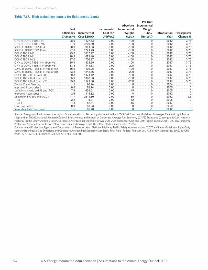
U.S. Energy Information Administration | Assumptions to the Annual Energy Outlook 201394
Transportation Demand Module
Table 7.15. High technology matrix for light trucks (cont.)
Fuel Efficiency Change %
Incremental Cost $2000
Incremental Cost ($/UnitWt.)
Absolute Incremental
Weight (Lbs.)
Per Unit Incremental
Weight (Lbs./
UnitWt.)Introduction
YearHorsepower
Change %OHV to DOHC TBDS II-I4 28.9 1427.73 0.00 -100 0 2012 3.75OHV to DOHC TBDS II-V6 27.0 2200.80 0.00 -100 0 2012 3.75SOHC to DOHC TBDS II-I4 28.9 941.53 0.00 -100 0 2012 3.75SOHC to DOHC TBDS II-V6 27.0 1771.73 0.00 -100 0 2012 3.75DOHC TBDS II-I3 23.3 1017.42 0.00 -100 0 2012 3.75DOHC TBDS II-I4 28.9 871.48 0.00 -100 0 2012 3.75DOHC TBDS II-V6 27.0 1706.27 0.00 -100 0 2012 3.75OHV to DOHC TBDS III-I4 (from V6) 35.9 1828.65 0.00 -100 0 2017 3.75OHV to DOHC TBDS III-I4 (from V8) 33.8 1441.63 0.00 -200 0 2017 3.75SOHC to DOHC TBDS III-I4 (from V6) 35.9 1409.25 0.00 -100 0 2017 3.75SOHC to DOHC TBDS III-I4 (from V8) 33.8 1242.36 0.00 -200 0 2017 3.75DOHC TBDS III-I3 (from I4) 29.8 1471.12 0.00 -100 0 2017 3.75DOHC TBDS III-I4 (from V6) 35.9 1348.83 0.00 -100 0 2017 3.75DOHC TBDS III-I4 (from V8) 33.8 1171.86 0.00 -200 0 2017 3.75Electric Power Steering 1.1 96.44 0.00 0 0 2004 0Improved Accessories I 0.8 78.74 0.00 0 0 2005 012V Micro Hybrid w/EPS and IACC 7.4 628.01 0.00 45 0 2005 0Improved Accessories II 2.6 115.82 0.00 0 0 2012 0Mild Hybrid w/EPS and IACC II 11.7 2611.80 0.00 80 0 2012 -2.5Tires I 2.2 5.04 0.00 -12 0 2005 0Tires II 4.4 52.51 0.00 -15 0 2017 0Low Drag Brakes 0.9 53.23 0.00 0 0 2000 0Secondary Axle Disconnect 1.5 86.70 0.00 0 -1 2012 0
Source: Energy and Environmental Analysis, Documentation of Technology included in the NEMS Fuel Economy Model for Passenger Cars and Light Trucks (September, 2002). National Research Council, Effectiveness and Impact of Corporate Average Fuel Economy (CAFE) Standards (Copyright 2002). National Highway Traffic Safety Administration, Corporate Average Fuel Economy for MY 2011-2015 Passenger Cars and Light Trucks (April 2008). U.S. Environmental Protection Agency, Interim Report: New Powertrain Technologies and Their Projected Costs (October 2005).Environmental Protection Agency and Department of Transportation National Highway Traffic Safety Administration, “2017 and Later Model Year Light-Duty Vehicle Greenhouse Gas Emissions and Corporate Average Fuel Economy Standards; Final Rule,” Federal Register Vol. 77, No. 199, October 15, 2012. 40 CFR Parts 85, 86, 600, 49 CFR Parts 523, 531, 533, et al. and 600.
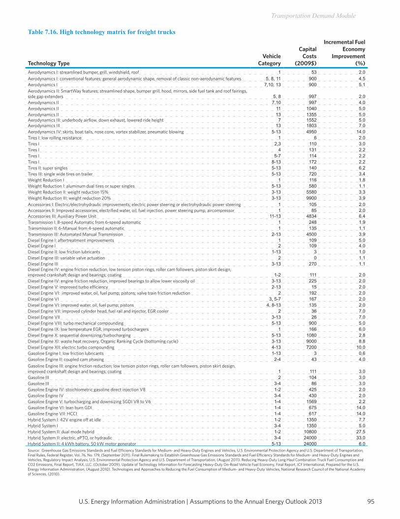
95U.S. Energy Information Administration | Assumptions to the Annual Energy Outlook 2013
Transportation Demand Module
Table 7.16. High technology matrix for freight trucks
Technology TypeVehicle
Category
Capital Costs
(2009$)
Incremental Fuel Economy
Improvement (%)
Aerodynamics I: streamlined bumper, grill, windshield, roof 1 53 2.0 Aerodynamics I: conventional features; general aerodynamic shape, removal of classic non-aerodynamic features 5, 8, 11 900 4.5 Aerodynamics I 7,10, 13 900 5.1 Aerodynamics II: SmartWay features; streamlined shape, bumper grill, hood, mirrors, side fuel tank and roof fairings, side gap extenders 5, 8 997 2.0 Aerodynamics II 7,10 997 4.0 Aerodynamics II 11 1040 5.0 Aerodynamics II 13 1355 5.0 Aerodynamics III: underbody airflow, down exhaust, lowered ride height 7 1552 5.0Aerodynamics III 13 1803 7.0Aerodynamics IV: skirts, boat tails, nose cone, vortex stabilizer, pneumatic blowing 5-13 4950 14.0Tires I: low rolling resistance 1 6 2.0Tires I 2,3 110 3.0Tires I 4 131 2.2Tires I 5-7 114 2.2Tires I 8-13 172 2.2Tires II: super singles 5-13 140 6.2Tires III: single wide tires on trailer 5-13 720 3.4Weight Reduction I 1 116 1.8Weight Reduction I: aluminum dual tires or super singles 5-13 580 1.1Weight Reduction II: weight reduction 15% 3-13 5580 3.3Weight Reduction III: weight reduction 20% 3-13 9900 3.9Accessories I: Electric/electrohydraulic improvements; electric power steering or electrohydraulic power steering 1 105 2.0Accessories II: Improved accessories; electrified water, oil, fuel injection, power steering pump, aircompressor 1 85 2.0Accessories III: Auxiliary Power Unit 11-13 4834 6.4Transmission I: 8-speed Automatic from 6-speed automatic 1 248 1.9Transmission II: 6-Manual from 4-speed automatic 1 135 1.1Transmission III: Automated Manual Transmission 2-13 4500 3.9Diesel Engine I: aftertreatment improvements 1 109 5.0Diesel Engine I 2 109 4.0Diesel Engine II: low friction lubricants 1-13 3 1.0Diesel Engine III: variable valve actuation 2 0 1.1Diesel Engine III 3-13 270 1.1Diesel Engine IV: engine friction reduction, low tension piston rings, roller cam followers, piston skirt design, improved crankshaft design and bearings; coating 1-2 111 2.0Diesel Engine IV: engine friction reduction, improved bearings to allow lower viscosity oil 3-13 225 2.0Diesel Engine V: improved turbo efficiency 2-13 15 2.0Diesel Engine VI: improved water, oil, fuel pump; pistons; valve train friction reduction 2 192 2.0Diesel Engine VI 3, 5-7 167 2.0 Diesel Engine VI: improved water, oil, fuel pump; pistons 4, 8-13 135 2.0Diesel Engine VII: improved cylinder head, fuel rail and injector, EGR cooler 2 36 7.0Diesel Engine VII 3-13 26 7.0Diesel Engine VIII: turbo mechanical compounding 5-13 900 5.0Diesel Engine IX: low temperature EGR, improved turbochargers 1 166 6.0Diesel Engine X: sequential downsizing/turbocharging 5-13 1080 2.8Diesel Engine XI: waste heat recovery, Organic Ranking Cycle (bottoming cycle) 3-13 9000 8.8Diesel Engine XII: electric turbo compounding 4-13 7200 10.0Gasoline Engine I: low friction lubricants 1-13 3 0.6Gasoline Engine II: coupled cam phasing 2-4 43 4.0Gasoline Engine III: engine friction reduction; low tension piston rings, roller cam followers, piston skirt design, improved crankshaft design and bearings; coating 1 111 3.0Gasoline III 2 104 3.0Gasoline III 3-4 86 3.0Gasoline Engine IV: stoichiometric gasoline direct injection V8 1-2 425 2.0Gasoline Engine IV 3-4 430 2.0Gasoline Engine V: turbocharging and downsizing SGDI V8 to V6 1-4 1569 2.2Gasoline Engine VI: lean burn GDI 1-4 675 14.0Gasoline Engine VII: HCCI 1-4 617 14.0Hybrid System I: 42V engine off at idle 1-2 1350 7.7Hybrid System I 3-4 1350 5.0Hybrid System II: dual mode hybrid 1-2 10800 27.5Hybrid System II: electric, ePTO, or hydraulic 3-4 24000 33.0Hybrid System II: 4 kWh battery, 50 kW motor generator 5-13 24000 6.0Source: Greenhouse Gas Emissions Standards and Fuel Efficiency Standards for Medium- and Heavy-Duty Engines and Vehicles, U.S. Environmental Protection Agency and U.S. Department of Transportation, Final Rules, Federal Register, Vol. 76, No. 179, (September 2011). Final Rulemaking to Establish Greenhouse Gas Emissions Standards and Fuel Efficiency Standards for Medium- and Heavy-Duty Engines and Vehicles, Regulatory Impact Analysis, U.S. Environmental Protection Agency and U.S. Department of Transportation, (August 2011). Reducing Heavy-Duty Long Haul Combination Truck Fuel Consumption and CO2 Emissions, Final Report, TIAX, LLC. (October 2009). Update of Technology Information for Forecasting Heavy-Duty On-Road Vehicle Fuel Economy, Final Report, ICF International, Prepared for the U.S. Energy Information Administration, (August 2010). Technologies and Approaches to Reducing the Fuel Consumption of Medium- and Heavy-Duty Vehicles, National Research Council of the National Academy of Sciences, (2010).
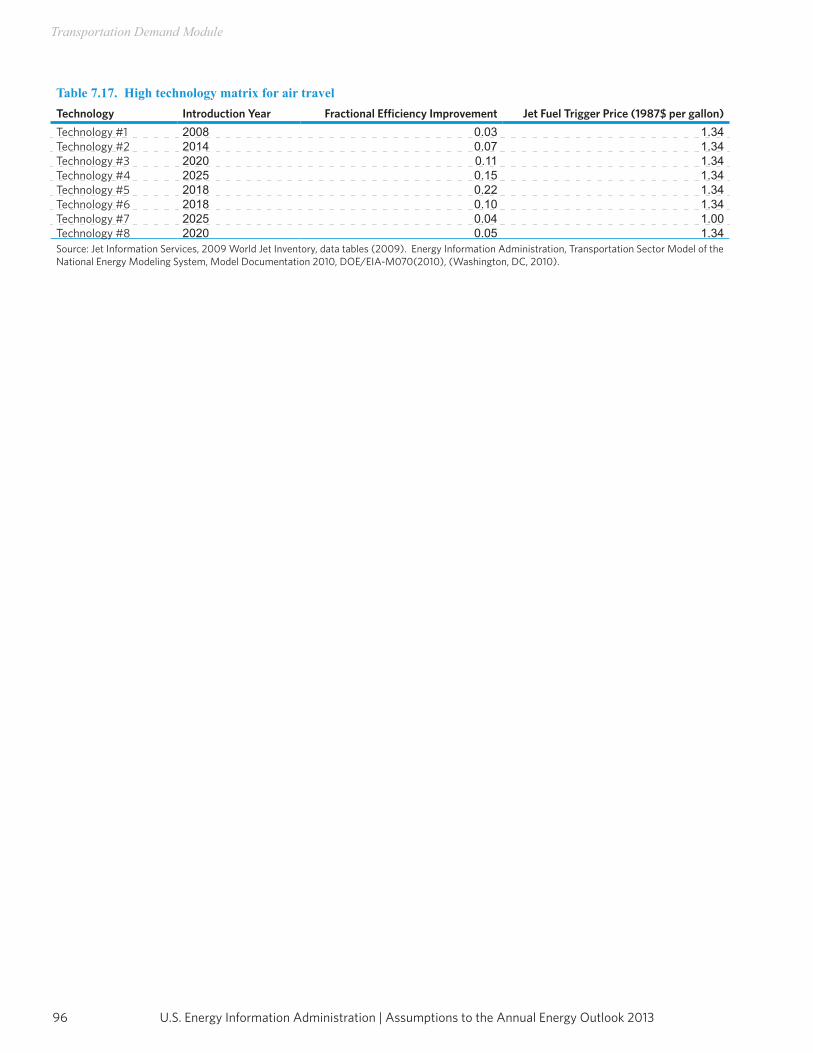
U.S. Energy Information Administration | Assumptions to the Annual Energy Outlook 201396
Transportation Demand Module
Table 7.17. High technology matrix for air travelTechnology Introduction Year Fractional Efficiency Improvement Jet Fuel Trigger Price (1987$ per gallon)Technology #1 2008 0.03 1.34Technology #2 2014 0.07 1.34Technology #3 2020 0.11 1.34Technology #4 2025 0.15 1.34Technology #5 2018 0.22 1.34Technology #6 2018 0.10 1.34Technology #7 2025 0.04 1.00Technology #8 2020 0.05 1.34Source: Jet Information Services, 2009 World Jet Inventory, data tables (2009). Energy Information Administration, Transportation Sector Model of the National Energy Modeling System, Model Documentation 2010, DOE/EIA-M070(2010), (Washington, DC, 2010).
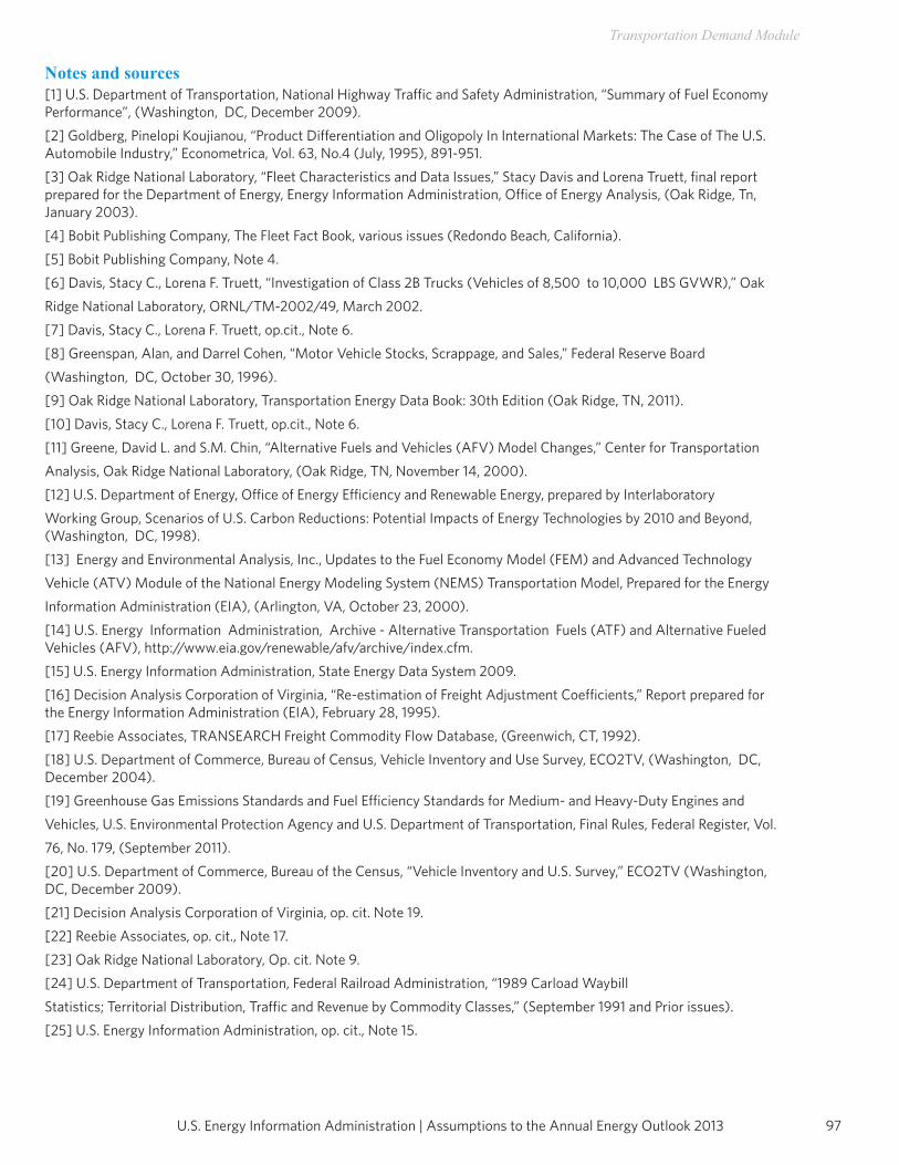
97U.S. Energy Information Administration | Assumptions to the Annual Energy Outlook 2013
Transportation Demand Module
Notes and sources[1] U.S. Department of Transportation, National Highway Traffic and Safety Administration, “Summary of Fuel Economy Performance”, (Washington, DC, December 2009). [2] Goldberg, Pinelopi Koujianou, “Product Differentiation and Oligopoly In International Markets: The Case of The U.S. Automobile Industry,” Econometrica, Vol. 63, No.4 (July, 1995), 891-951.[3] Oak Ridge National Laboratory, “Fleet Characteristics and Data Issues,” Stacy Davis and Lorena Truett, final report prepared for the Department of Energy, Energy Information Administration, Office of Energy Analysis, (Oak Ridge, Tn, January 2003). [4] Bobit Publishing Company, The Fleet Fact Book, various issues (Redondo Beach, California). [5] Bobit Publishing Company, Note 4.[6] Davis, Stacy C., Lorena F. Truett, “Investigation of Class 2B Trucks (Vehicles of 8,500 to 10,000 LBS GVWR),” OakRidge National Laboratory, ORNL/TM-2002/49, March 2002. [7] Davis, Stacy C., Lorena F. Truett, op.cit., Note 6.[8] Greenspan, Alan, and Darrel Cohen, “Motor Vehicle Stocks, Scrappage, and Sales,” Federal Reserve Board(Washington, DC, October 30, 1996). [9] Oak Ridge National Laboratory, Transportation Energy Data Book: 30th Edition (Oak Ridge, TN, 2011). [10] Davis, Stacy C., Lorena F. Truett, op.cit., Note 6.[11] Greene, David L. and S.M. Chin, “Alternative Fuels and Vehicles (AFV) Model Changes,” Center for TransportationAnalysis, Oak Ridge National Laboratory, (Oak Ridge, TN, November 14, 2000).[12] U.S. Department of Energy, Office of Energy Efficiency and Renewable Energy, prepared by InterlaboratoryWorking Group, Scenarios of U.S. Carbon Reductions: Potential Impacts of Energy Technologies by 2010 and Beyond, (Washington, DC, 1998).[13] Energy and Environmental Analysis, Inc., Updates to the Fuel Economy Model (FEM) and Advanced TechnologyVehicle (ATV) Module of the National Energy Modeling System (NEMS) Transportation Model, Prepared for the EnergyInformation Administration (EIA), (Arlington, VA, October 23, 2000).[14] U.S. Energy Information Administration, Archive - Alternative Transportation Fuels (ATF) and Alternative Fueled Vehicles (AFV), http://www.eia.gov/renewable/afv/archive/index.cfm.[15] U.S. Energy Information Administration, State Energy Data System 2009.[16] Decision Analysis Corporation of Virginia, “Re-estimation of Freight Adjustment Coefficients,” Report prepared for the Energy Information Administration (EIA), February 28, 1995).[17] Reebie Associates, TRANSEARCH Freight Commodity Flow Database, (Greenwich, CT, 1992).
[18] U.S. Department of Commerce, Bureau of Census, Vehicle Inventory and Use Survey, ECO2TV, (Washington, DC, December 2004).[19] Greenhouse Gas Emissions Standards and Fuel Efficiency Standards for Medium- and Heavy-Duty Engines andVehicles, U.S. Environmental Protection Agency and U.S. Department of Transportation, Final Rules, Federal Register, Vol.76, No. 179, (September 2011).[20] U.S. Department of Commerce, Bureau of the Census, “Vehicle Inventory and U.S. Survey,” ECO2TV (Washington, DC, December 2009).[21] Decision Analysis Corporation of Virginia, op. cit. Note 19. [22] Reebie Associates, op. cit., Note 17.[23] Oak Ridge National Laboratory, Op. cit. Note 9.[24] U.S. Department of Transportation, Federal Railroad Administration, “1989 Carload WaybillStatistics; Territorial Distribution, Traffic and Revenue by Commodity Classes,” (September 1991 and Prior issues). [25] U.S. Energy Information Administration, op. cit., Note 15.
U.S. Energy Information Administration | Assumptions to the Annual Energy Outlook 201398
Transportation Demand Module
Notes and sources[26] U.S. Army Corps of Engineers, Waterborne Commerce of the United States, (Waterborne Statistics Center: NewOrleans, LA, 1993).[27] U.S. Energy Information Administration, op. cit., Note 15. [28] U.S. Department of Transportation, Research and Innovative Technology Administration, Bureau of Transportation Statistics, Air Carrier Summary Data (Form 41, Schedules T-1 and T-2), (2011). http://www.transtats.bts.gov/DataIndex. asp; link: Air Carrier Summary Data (Form 41 and 298C Summary Data). [29] U.S. Department of Transportation, Research and Innovative Technology Administration, Bureau of TransportationStatistics, op. cit., Note 28. [30] U.S. Department of Transportation, Federal Aviation Administration, Airport Capacity Benchmark Report, 2004 (2004).[31] Jet Information Services Inc., World Jet Inventory: Year-End 2009, (December 2009). [32] Greenhouse Gas Emissions Standards and Fuel Efficiency Standards for Medium- and Heavy-Duty Engines andVehicles, U.S. Environmental Protection Agency and U.S. Department of Transportation, Final Rules, Federal Register, Vol.76, No. 179, (September 2011).
[33] Energy Information Administration, op. cit. Note 14. [34] Energy and Environmental Analysis, Inc., “Documentation of Technologies Included in the NEMS Fuel Economy Model for Passenger Cars and Light Trucks,” Prepared for the U.S. Energy Information Administration, (Arlington, VA, September 30, 2002). [35] Final Rulemaking to Establish Greenhouse Gas Emissions Standards and Fuel Efficiency Standards for Medium- and Heavy-Duty Engines and Vehicles, Regulatory Impact Analysis, U.S. Environmental Protection Agency and U.S. Department of Transportation, (August 2011). [36] Reducing Heavy-Duty Long Haul Combination Truck Fuel Consumption and CO2 Emissions, Final Report, TIAX, LLC. (October 2009).[37] Update of Technology Information for Forecasting Heavy-Duty On-Road Vehicle Fuel Economy, Final Report, ICF International, Prepared for the U.S. Energy Information Administration, (August 2010).[38] Technologies and Approaches to Reducing the Fuel Consumption of Medium- and Heavy-Duty Vehicles, NationalResearch Council of the National Academy of Sciences, (2010).

Electricity Market Module

This page inTenTionally lefT blank
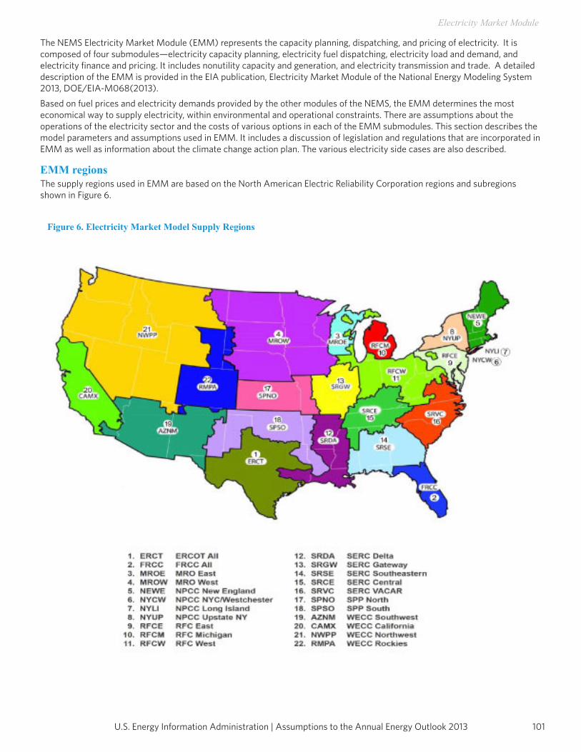
101U.S. Energy Information Administration | Assumptions to the Annual Energy Outlook 2013
Electricity Market Module
The NEMS Electricity Market Module (EMM) represents the capacity planning, dispatching, and pricing of electricity. It is composed of four submodules—electricity capacity planning, electricity fuel dispatching, electricity load and demand, and electricity finance and pricing. It includes nonutility capacity and generation, and electricity transmission and trade. A detailed description of the EMM is provided in the EIA publication, Electricity Market Module of the National Energy Modeling System 2013, DOE/EIA-M068(2013).Based on fuel prices and electricity demands provided by the other modules of the NEMS, the EMM determines the most economical way to supply electricity, within environmental and operational constraints. There are assumptions about the operations of the electricity sector and the costs of various options in each of the EMM submodules. This section describes the model parameters and assumptions used in EMM. It includes a discussion of legislation and regulations that are incorporated in EMM as well as information about the climate change action plan. The various electricity side cases are also described.
EMM regions The supply regions used in EMM are based on the North American Electric Reliability Corporation regions and subregions shown in Figure 6.
Figure 6. Electricity Market Model Supply Regions
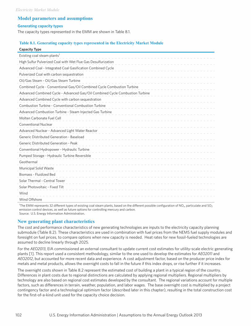
U.S. Energy Information Administration | Assumptions to the Annual Energy Outlook 2013102
Electricity Market Module
Model parameters and assumptions Generating capacity types The capacity types represented in the EMM are shown in Table 8.1.
Table 8.1. Generating capacity types represented in the Electricity Market ModuleCapacity Type
Existing coal steam plants1
High Sulfur Pulverized Coal with Wet Flue Gas Desulfurization
Advanced Coal - Integrated Coal Gasification Combined Cycle
Pulverized Coal with carbon sequestration
Oil/Gas Steam - Oil/Gas Steam Turbine
Combined Cycle - Conventional Gas/Oil Combined Cycle Combustion Turbine
Advanced Combined Cycle - Advanced Gas/Oil Combined Cycle Combustion Turbine
Advanced Combined Cycle with carbon sequestration
Combustion Turbine - Conventional Combustion Turbine
Advanced Combustion Turbine - Steam Injected Gas Turbine
Molten Carbonate Fuel Cell
Conventional Nuclear
Advanced Nuclear - Advanced Light Water Reactor
Generic Distributed Generation - Baseload
Generic Distributed Generation - Peak
Conventional Hydropower - Hydraulic Turbine
Pumped Storage - Hydraulic Turbine Reversible
Geothermal
Municipal Solid Waste
Biomass - Fluidized Bed
Solar Thermal - Central Tower
Solar Photovoltaic - Fixed Tilt
Wind
Wind Offshore1The EMM represents 32 different types of existing coal steam plants, based on the different possible configuration of NOx, particulate and SO2 emission control devices, as well as future options for controlling mercury and carbon.Source: U.S. Energy Information Administration.
New generating plant characteristics The cost and performance characteristics of new generating technologies are inputs to the electricity capacity planning submodule (Table 8.2). These characteristics are used in combination with fuel prices from the NEMS fuel supply modules and foresight on fuel prices, to compare options when new capacity is needed. Heat rates for new fossil-fueled technologies are assumed to decline linearly through 2025.For the AEO2013, EIA commissioned an external consultant to update current cost estimates for utility-scale electric generating plants [1]. This report used a consistent methodology, similar to the one used to develop the estimates for AEO2011 and AEO2012, but accounted for more recent data and experience. A cost adjustment factor, based on the producer price index for metals and metal products, allows the overnight costs to fall in the future if this index drops, or rise further if it increases.The overnight costs shown in Table 8.2 represent the estimated cost of building a plant in a typical region of the country. Differences in plant costs due to regional distinctions are calculated by applying regional multipliers. Regional multipliers by technology are also based on regional cost estimates developed by the consultant. The regional variations account for multiple factors, such as differences in terrain, weather, population, and labor wages. The base overnight cost is multiplied by a project contingency factor and a technological optimism factor (described later in this chapter), resulting in the total construction cost for the first-of-a-kind unit used for the capacity choice decision.
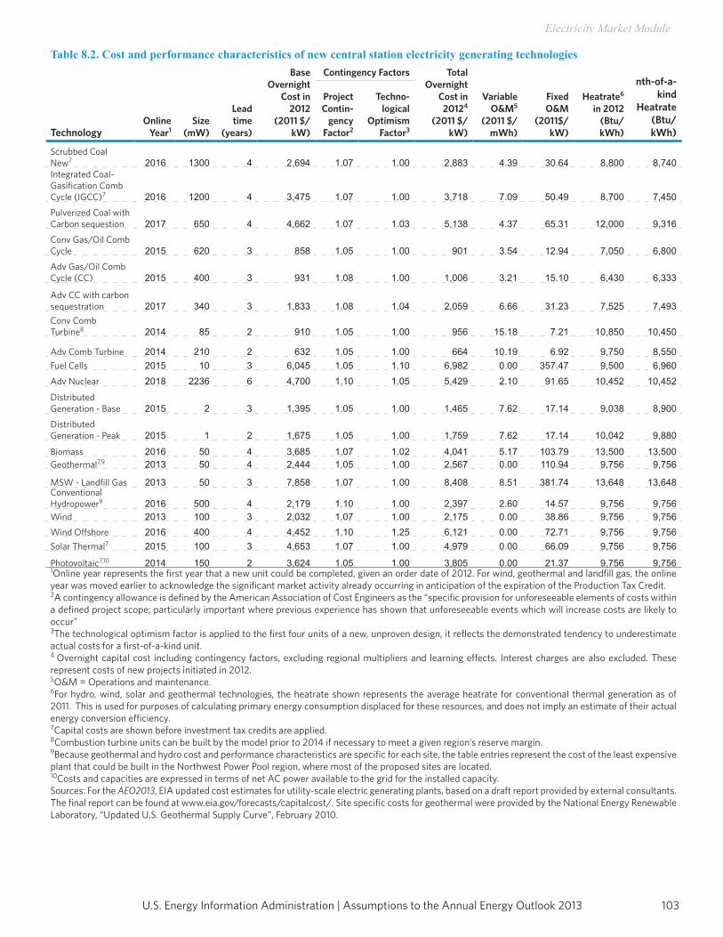
103U.S. Energy Information Administration | Assumptions to the Annual Energy Outlook 2013
Electricity Market Module
Table 8.2. Cost and performance characteristics of new central station electricity generating technologies
TechnologyOnline
Year1Size
(mW)
Lead time
(years)
Base Overnight
Cost in 2012
(2011 $/kW)
Contingency Factors Total Overnight
Cost in 20124
(2011 $/kW)
VariableO&M5
(2011 $/mWh)
FixedO&M
(2011$/kW)
Heatrate6
in 2012(Btu/kWh)
nth-of-a-kind
Heatrate(Btu/kWh)
Project Contin-
gencyFactor2
Techno-logical
OptimismFactor3
Scrubbed Coal New7 2016 1300 4 2,694 1.07 1.00 2,883 4.39 30.64 8,800 8,740 Integrated Coal-Gasification Comb Cycle (IGCC)7 2016 1200 4 3,475 1.07 1.00 3,718 7.09 50.49 8,700 7,450 Pulverized Coal with Carbon sequestion 2017 650 4 4,662 1.07 1.03 5,138 4.37 65.31 12,000 9,316Conv Gas/Oil Comb Cycle 2015 620 3 858 1.05 1.00 901 3.54 12.94 7,050 6,800 Adv Gas/Oil Comb Cycle (CC) 2015 400 3 931 1.08 1.00 1,006 3.21 15.10 6,430 6,333
Adv CC with carbon sequestration 2017 340 3 1,833 1.08 1.04 2,059 6.66 31.23 7,525 7,493 Conv Comb Turbine8 2014 85 2 910 1.05 1.00 956 15.18 7.21 10,850 10,450
Adv Comb Turbine 2014 210 2 632 1.05 1.00 664 10.19 6.92 9,750 8,550 Fuel Cells 2015 10 3 6,045 1.05 1.10 6,982 0.00 357.47 9,500 6,960 Adv Nuclear 2018 2236 6 4,700 1.10 1.05 5,429 2.10 91.65 10,452 10,452
Distributed Generation - Base 2015 2 3 1,395 1.05 1.00 1,465 7.62 17.14 9,038 8,900 Distributed Generation - Peak 2015 1 2 1,675 1.05 1.00 1,759 7.62 17.14 10,042 9,880
Biomass 2016 50 4 3,685 1.07 1.02 4,041 5.17 103.79 13,500 13,500 Geothermal7,9 2013 50 4 2,444 1.05 1.00 2,567 0.00 110.94 9,756 9,756
MSW - Landfill Gas 2013 50 3 7,858 1.07 1.00 8,408 8.51 381.74 13,648 13,648Conventional Hydropower9 2016 500 4 2,179 1.10 1.00 2,397 2.60 14.57 9,756 9,756Wind 2013 100 3 2,032 1.07 1.00 2,175 0.00 38.86 9,756 9,756Wind Offshore 2016 400 4 4,452 1.10 1.25 6,121 0.00 72.71 9,756 9,756Solar Thermal7 2015 100 3 4,653 1.07 1.00 4,979 0.00 66.09 9,756 9,756
Photovoltaic7,10 2014 150 2 3,624 1.05 1.00 3,805 0.00 21.37 9,756 9,7561Online year represents the first year that a new unit could be completed, given an order date of 2012. For wind, geothermal and landfill gas, the online year was moved earlier to acknowledge the significant market activity already occurring in anticipation of the expiration of the Production Tax Credit. 2A contingency allowance is defined by the American Association of Cost Engineers as the “specific provision for unforeseeable elements of costs within a defined project scope; particularly important where previous experience has shown that unforeseeable events which will increase costs are likely to occur” 3The technological optimism factor is applied to the first four units of a new, unproven design, it reflects the demonstrated tendency to underestimate actual costs for a first-of-a-kind unit.4 Overnight capital cost including contingency factors, excluding regional multipliers and learning effects. Interest charges are also excluded. These represent costs of new projects initiated in 2012. 5O&M = Operations and maintenance. 6For hydro, wind, solar and geothermal technologies, the heatrate shown represents the average heatrate for conventional thermal generation as of 2011. This is used for purposes of calculating primary energy consumption displaced for these resources, and does not imply an estimate of their actual energy conversion efficiency.7Capital costs are shown before investment tax credits are applied. 8Combustion turbine units can be built by the model prior to 2014 if necessary to meet a given region’s reserve margin. 9Because geothermal and hydro cost and performance characteristics are specific for each site, the table entries represent the cost of the least expensive plant that could be built in the Northwest Power Pool region, where most of the proposed sites are located.10Costs and capacities are expressed in terms of net AC power available to the grid for the installed capacity. Sources: For the AEO2013, EIA updated cost estimates for utility-scale electric generating plants, based on a draft report provided by external consultants. The final report can be found at www.eia.gov/forecasts/capitalcost/. Site specific costs for geothermal were provided by the National Energy Renewable Laboratory, “Updated U.S. Geothermal Supply Curve”, February 2010.
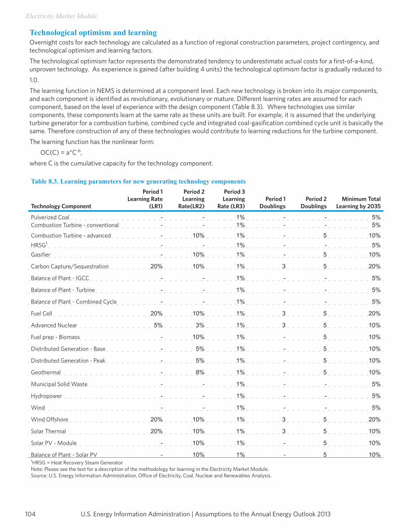
U.S. Energy Information Administration | Assumptions to the Annual Energy Outlook 2013104
Electricity Market Module
Table 8.3. Learning parameters for new generating technology components
Technology Component
Period 1Learning Rate
(LR1)
Period 2Learning
Rate(LR2)
Period 3Learning
Rate (LR3)Period 1
DoublingsPeriod 2
DoublingsMinimum Total
Learning by 2035
Pulverized Coal - - 1% - - 5%Combustion Turbine - conventional - - 1% - - 5%
Combustion Turbine - advanced - 10% 1% - 5 10%HRSG1 - - 1% - - 5%Gasifier - 10% 1% - 5 10%
Carbon Capture/Sequestration 20% 10% 1% 3 5 20%
Balance of Plant - IGCC - - 1% - - 5%
Balance of Plant - Turbine - - 1% - - 5%
Balance of Plant - Combined Cycle - - 1% - - 5%
Fuel Cell 20% 10% 1% 3 5 20%
Advanced Nuclear 5% 3% 1% 3 5 10%
Fuel prep - Biomass - 10% 1% - 5 10%
Distributed Generation - Base - 5% 1% - 5 10%
Distributed Generation - Peak - 5% 1% - 5 10%
Geothermal - 8% 1% - 5 10%
Municipal Solid Waste - - 1% - - 5%
Hydropower - - 1% - - 5%
Wind - - 1% - - 5%
Wind Offshore 20% 10% 1% 3 5 20%
Solar Thermal 20% 10% 1% 3 5 10%
Solar PV - Module - 10% 1% - 5 10%
Balance of Plant - Solar PV - 10% 1% - 5 10%1HRSG = Heat Recovery Steam GeneratorNote: Please see the text for a description of the methodology for learning in the Electricity Market Module.Source: U.S. Energy Information Administration, Office of Electricity, Coal, Nuclear and Renewables Analysis.
Technological optimism and learning Overnight costs for each technology are calculated as a function of regional construction parameters, project contingency, and technological optimism and learning factors.The technological optimism factor represents the demonstrated tendency to underestimate actual costs for a first-of-a-kind, unproven technology. As experience is gained (after building 4 units) the technological optimism factor is gradually reduced to1.0.The learning function in NEMS is determined at a component level. Each new technology is broken into its major components, and each component is identified as revolutionary, evolutionary or mature. Different learning rates are assumed for each component, based on the level of experience with the design component (Table 8.3). Where technologies use similar components, these components learn at the same rate as these units are built. For example, it is assumed that the underlying turbine generator for a combustion turbine, combined cycle and integrated coal-gasification combined cycle unit is basically the same. Therefore construction of any of these technologies would contribute to learning reductions for the turbine component.The learning function has the nonlinear form: OC(C) = a*C-b, where C is the cumulative capacity for the technology component.
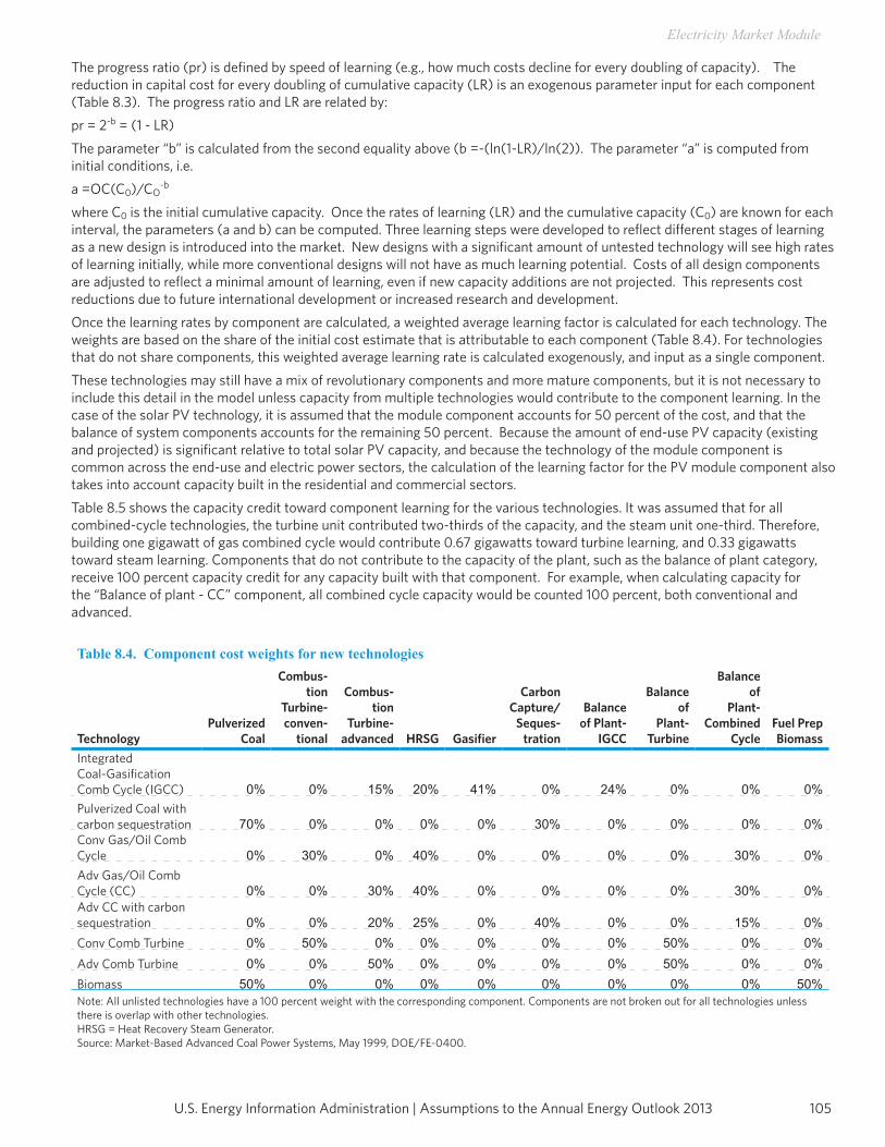
105U.S. Energy Information Administration | Assumptions to the Annual Energy Outlook 2013
Electricity Market Module
The progress ratio (pr) is defined by speed of learning (e.g., how much costs decline for every doubling of capacity). The reduction in capital cost for every doubling of cumulative capacity (LR) is an exogenous parameter input for each component (Table 8.3). The progress ratio and LR are related by: pr = 2-b = (1 - LR) The parameter “b” is calculated from the second equality above (b =-(ln(1-LR)/ln(2)). The parameter “a” is computed from initial conditions, i.e. a =OC(C0)/CO
-b where C0 is the initial cumulative capacity. Once the rates of learning (LR) and the cumulative capacity (C0) are known for each interval, the parameters (a and b) can be computed. Three learning steps were developed to reflect different stages of learning as a new design is introduced into the market. New designs with a significant amount of untested technology will see high rates of learning initially, while more conventional designs will not have as much learning potential. Costs of all design components are adjusted to reflect a minimal amount of learning, even if new capacity additions are not projected. This represents cost reductions due to future international development or increased research and development.Once the learning rates by component are calculated, a weighted average learning factor is calculated for each technology. The weights are based on the share of the initial cost estimate that is attributable to each component (Table 8.4). For technologies that do not share components, this weighted average learning rate is calculated exogenously, and input as a single component.These technologies may still have a mix of revolutionary components and more mature components, but it is not necessary to include this detail in the model unless capacity from multiple technologies would contribute to the component learning. In the case of the solar PV technology, it is assumed that the module component accounts for 50 percent of the cost, and that the balance of system components accounts for the remaining 50 percent. Because the amount of end-use PV capacity (existing and projected) is significant relative to total solar PV capacity, and because the technology of the module component is common across the end-use and electric power sectors, the calculation of the learning factor for the PV module component also takes into account capacity built in the residential and commercial sectors.Table 8.5 shows the capacity credit toward component learning for the various technologies. It was assumed that for all combined-cycle technologies, the turbine unit contributed two-thirds of the capacity, and the steam unit one-third. Therefore, building one gigawatt of gas combined cycle would contribute 0.67 gigawatts toward turbine learning, and 0.33 gigawatts toward steam learning. Components that do not contribute to the capacity of the plant, such as the balance of plant category, receive 100 percent capacity credit for any capacity built with that component. For example, when calculating capacity for the “Balance of plant - CC” component, all combined cycle capacity would be counted 100 percent, both conventional and advanced. Table 8.4. Component cost weights for new technologies
TechnologyPulverized
Coal
Combus-tion
Turbine-conven-
tional
Combus-tion
Turbine-advanced HRSG Gasifier
CarbonCapture/
Seques-tration
Balanceof Plant-
IGCC
Balance of
Plant-Turbine
Balance of
Plant-Combined
CycleFuel PrepBiomass
IntegratedCoal-Gasification Comb Cycle (IGCC) 0% 0% 15% 20% 41% 0% 24% 0% 0% 0%Pulverized Coal with carbon sequestration 70% 0% 0% 0% 0% 30% 0% 0% 0% 0%Conv Gas/Oil Comb Cycle 0% 30% 0% 40% 0% 0% 0% 0% 30% 0%Adv Gas/Oil Comb Cycle (CC) 0% 0% 30% 40% 0% 0% 0% 0% 30% 0%Adv CC with carbon sequestration 0% 0% 20% 25% 0% 40% 0% 0% 15% 0%Conv Comb Turbine 0% 50% 0% 0% 0% 0% 0% 50% 0% 0%Adv Comb Turbine 0% 0% 50% 0% 0% 0% 0% 50% 0% 0%Biomass 50% 0% 0% 0% 0% 0% 0% 0% 0% 50%Note: All unlisted technologies have a 100 percent weight with the corresponding component. Components are not broken out for all technologies unless there is overlap with other technologies.HRSG = Heat Recovery Steam Generator.Source: Market-Based Advanced Coal Power Systems, May 1999, DOE/FE-0400.
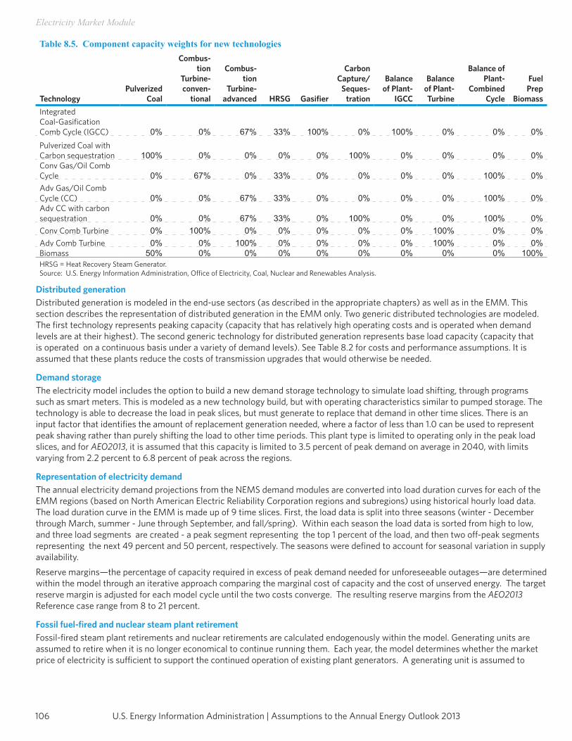
U.S. Energy Information Administration | Assumptions to the Annual Energy Outlook 2013106
Electricity Market Module
Table 8.5. Component capacity weights for new technologies
TechnologyPulverized
Coal
Combus-tion
Turbine-conven-
tional
Combus-tion
Turbine-advanced HRSG Gasifier
CarbonCapture/
Seques-tration
Balanceof Plant-
IGCC
Balance of Plant-Turbine
Balance ofPlant-
CombinedCycle
Fuel Prep
BiomassIntegratedCoal-Gasification Comb Cycle (IGCC) 0% 0% 67% 33% 100% 0% 100% 0% 0% 0%Pulverized Coal with Carbon sequestration 100% 0% 0% 0% 0% 100% 0% 0% 0% 0%Conv Gas/Oil Comb Cycle 0% 67% 0% 33% 0% 0% 0% 0% 100% 0%Adv Gas/Oil Comb Cycle (CC) 0% 0% 67% 33% 0% 0% 0% 0% 100% 0%Adv CC with carbon sequestration 0% 0% 67% 33% 0% 100% 0% 0% 100% 0%Conv Comb Turbine 0% 100% 0% 0% 0% 0% 0% 100% 0% 0%Adv Comb Turbine 0% 0% 100% 0% 0% 0% 0% 100% 0% 0%Biomass 50% 0% 0% 0% 0% 0% 0% 0% 0% 100%HRSG = Heat Recovery Steam Generator.Source: U.S. Energy Information Administration, Office of Electricity, Coal, Nuclear and Renewables Analysis.
Distributed generation Distributed generation is modeled in the end-use sectors (as described in the appropriate chapters) as well as in the EMM. This section describes the representation of distributed generation in the EMM only. Two generic distributed technologies are modeled. The first technology represents peaking capacity (capacity that has relatively high operating costs and is operated when demand levels are at their highest). The second generic technology for distributed generation represents base load capacity (capacity that is operated on a continuous basis under a variety of demand levels). See Table 8.2 for costs and performance assumptions. It is assumed that these plants reduce the costs of transmission upgrades that would otherwise be needed.
Demand storage The electricity model includes the option to build a new demand storage technology to simulate load shifting, through programs such as smart meters. This is modeled as a new technology build, but with operating characteristics similar to pumped storage. The technology is able to decrease the load in peak slices, but must generate to replace that demand in other time slices. There is an input factor that identifies the amount of replacement generation needed, where a factor of less than 1.0 can be used to represent peak shaving rather than purely shifting the load to other time periods. This plant type is limited to operating only in the peak load slices, and for AEO2013, it is assumed that this capacity is limited to 3.5 percent of peak demand on average in 2040, with limits varying from 2.2 percent to 6.8 percent of peak across the regions.
Representation of electricity demand The annual electricity demand projections from the NEMS demand modules are converted into load duration curves for each of the EMM regions (based on North American Electric Reliability Corporation regions and subregions) using historical hourly load data. The load duration curve in the EMM is made up of 9 time slices. First, the load data is split into three seasons (winter - December through March, summer - June through September, and fall/spring). Within each season the load data is sorted from high to low, and three load segments are created - a peak segment representing the top 1 percent of the load, and then two off-peak segments representing the next 49 percent and 50 percent, respectively. The seasons were defined to account for seasonal variation in supply availability.Reserve margins—the percentage of capacity required in excess of peak demand needed for unforeseeable outages—are determined within the model through an iterative approach comparing the marginal cost of capacity and the cost of unserved energy. The target reserve margin is adjusted for each model cycle until the two costs converge. The resulting reserve margins from the AEO2013 Reference case range from 8 to 21 percent.
Fossil fuel-fired and nuclear steam plant retirement Fossil-fired steam plant retirements and nuclear retirements are calculated endogenously within the model. Generating units are assumed to retire when it is no longer economical to continue running them. Each year, the model determines whether the market price of electricity is sufficient to support the continued operation of existing plant generators. A generating unit is assumed to
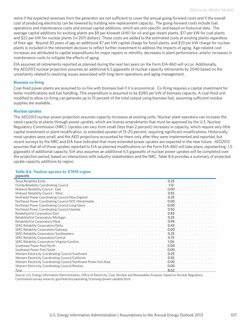
107U.S. Energy Information Administration | Assumptions to the Annual Energy Outlook 2013
Electricity Market Module
retire if the expected revenues from the generator are not sufficient to cover the annual going-forward costs and if the overall cost of producing electricity can be lowered by building new replacement capacity. The going-forward costs include fuel, operations and maintenance costs and annual capital additions, which are unit-specific and based on historical data. The average capital additions for existing plants are $8 per kilowatt (kW) for oil and gas steam plants, $17 per kW for coal plants and $22 per kW for nuclear plants (in 2011 dollars). These costs are added to the estimated costs at existing plants regardless of their age. Beyond 30 years of age an additional $7 per kW capital charge for fossil plants, and $33 per kW charge for nuclear plants is included in the retirement decision to reflect further investment to address the impacts of aging. Age-related cost increases are attributed to capital expenditures for major repairs or retrofits, decreases in plant performance, and/or increases in maintenance costs to mitigate the effects of aging.EIA assumes all retirements reported as planned during the next ten years on the Form EIA-860 will occur. Additionally, the AEO2013 nuclear projection assumes an additional 6.5 gigawatts of nuclear capacity retirements by 2040 based on the uncertainty related to resolving issues associated with long-term operations and aging management.
Biomass co-firing Coal-fired power plants are assumed to co-fire with biomass fuel if it is economical. Co-firing requires a capital investment for boiler modifications and fuel handling. This expenditure is assumed to be $280 per kW of biomass capacity. A coal-fired unit modified to allow co-firing can generate up to 15 percent of the total output using biomass fuel, assuming sufficient residue supplies are available.
Nuclear uprates The AEO2013 nuclear power projection assumes capacity increases at existing units. Nuclear plant operators can increase the rated capacity at plants through power uprates, which are license amendments that must be approved by the U.S. Nuclear Regulatory Commission (NRC). Uprates can vary from small (less than 2 percent) increases in capacity, which require very little capital investment or plant modification, to extended uprates of 15-20 percent, requiring significant modifications. Historically, most uprates were small, and the AEO projections accounted for them only after they were implemented and reported, but recent surveys by the NRC and EIA have indicated that more extended power uprates are expected in the near future. AEO2013 assumes that all of those uprates reported to EIA as planned modifications on the Form EIA-860 will take place, representing 1.5 gigawatts of additional capacity. EIA also assumes an additional 6.5 gigawatts of nuclear power uprates will be completed over the projection period, based on interactions with industry stakeholders and the NRC. Table 8.6 provides a summary of projected uprate capacity additions by region.
Table 8.6. Nuclear uprates by EMM regiongigawattsTexas Reliability Entity 0.25Florida Reliability Coordinating Council 1.12Midwest Reliability Council - East 0.00Midwest Reliability Council - West 0.55Northeast Power Coordinating Council/New England 0.25Northeast Power Coordinating Council/NYC-Westchester 0.00Northeast Power Coordinating Council/Long Island 0.00Northeast Power Coordinating Council/Upstate 0.50ReliabilityFirst Corporation/East 0.82ReliabilityFirst Corporation/Michigan 0.25ReliabilityFirst Corporation/West 0.99SERC Reliability Corporation/Delta 0.43SERC Reliability Corporation/Gateway 0.00SERC Reliability Corporation/Southeastern 0.25SERC Reliability Corporation/Central 0.75SERC Reliability Corporation/Virginia-Carolina 1.06Southwest Power Pool/North 0.00Southwest Power Pool/South 0.00Western Electricity Coordinating Council/Southwest 0.25Western Electricity Coordinating Council/California 0.55Western Electricity Coordinating Council/Northwest Power Pool Area 0.00Western Electricity Coordinating Council/Rockies 0.00Total 8.02Source: U.S. Energy Information Administration, Office of Electricity, Coal, Nuclear and Renewables Analysis, based on Nuclear Regulatory Commission survey www.nrc.gov/reactors/operating/licensing/power-updates.html.
U.S. Energy Information Administration | Assumptions to the Annual Energy Outlook 2013108
Electricity Market Module
Interregional electricity trade Both firm and economy electricity transactions among utilities in different regions are represented within the EMM. In general, firm power transactions involve the trading of capacity and energy to help another region satisfy its reserve margin requirement, while economy transactions involve energy transactions motivated by the marginal generation costs of different regions. The flow of power from region to region is constrained by the existing and planned capacity limits as reported in the North American Electric Reliability Corporation and Western Electricity Coordinating Council Summer and Winter Assessment of Reliability of Bulk Electricity Supply in North America. Known firm power contracts are obtained from NERC’s Electricity Supply and Demand Database 2007 and information provided in the 2012 Summer and Winter Assessments. They are locked in for the term of the contract. Contracts that are scheduled to expire by 2016 are assumed not to be renewed. Because there is no information available about expiration dates for contracts that go beyond 2016, they are assumed to be phased out by 2025. The EMM includes an option to add interregional transmission capacity. In some cases it may be more economic to build generating capacity in a neighboring region, but additional costs to expand the transmission grid will be incurred as well. Explicitly expanding the interregional transmission capacity may also make the transmission line available for additional economy trade.Economy transactions are determined in the dispatching submodule by comparing the marginal generating costs of adjacent regions in each time slice. If one region has less expensive generating resources available in a given time period (adjusting for transmission losses and transmission capacity limits) than another region, the regions are assumed to exchange power.
International electricity trade Two components of international firm power trade are represented in the EMM—existing and planned transactions, and unplanned transactions. Data on existing and planned transactions are obtained from the North American Electric Reliability Corporation’s Electricity Supply and Demand Database 2007. Unplanned firm power trade is represented by competing Canadian supply with U.S. domestic supply options. Canadian supply is represented via supply curves using cost data from the Department of Energy report, “Northern Lights: The Economic and Practical Potential of Imported Power from Canada,” (DOE/PE-0079). International economy trade is determined endogenously based on surplus energy expected to be available from Canada by region in each time slice. Canadian surplus energy is determined using Canadian electricity supply and demand projections from the MAPLE-C model developed for Natural Resources Canada.
Electricity pricing Electricity pricing is projected for 22 electricity market regions in AEO2013 for fully competitive, partially competitive and fully regulated supply regions. The price of electricity to the consumer comprises the price of generation, transmission, and distribution, including applicable taxes. Transmission and distribution are considered to remain regulated in the AEO; that is, the price of transmission and distribution is based on the average cost to build, operate and maintain these systems. In competitive regions, an algorithm allows customers to compete for better rates among rate classes as long as the overall average cost is met. The price of electricity in the regulated regions consists of the average cost of generation, transmission, and distribution for each customer class. In the competitive regions, the generation component of price is based on marginal cost, which is defined as the cost of the last (or most expensive) unit dispatched. The competitive generation price includes the marginal cost (fuel and variable operations and maintenance costs), taxes, and a reliability price adjustment, which represents what customers are willing to pay for added capacity to avoid outages in periods of high demand. For the AEO2013, the difference between EIA’s reliability costs and the historical Independent System Operator capacity, ancillary service, and uplift charges was added to the competitive generation price. The price of electricity in the regions with a competitive generation market consists of the competitive cost of generation summed with the average costs of transmission and distribution. The price for mixed regions reflects a load-weighted average of the competitive price and the regulated price, based on the percent of electricity load in the region subject to deregulation. In competitively supplied regions, a transition period is assumed to occur (usually over a ten-year period) from the effective date of restructuring, with a gradual shift to marginal cost pricing.The Reference case assumes a transition to full competitive pricing in the three New York regions and in the ReliabilityFirst Corporation/ East region, and a 97-percent transition to competitive pricing in New England (Vermont being the only fully- regulated state in that region). Six regions fully regulate their electricity supply, including the Florida Reliability Coordinating Council, three of the SERC Reliability Corporation subregions - Southeastern (SRSE), Central (SRCE) and Virginia-Carolina (SRVC) - Southwest Power Pool Regional Entity/North (SPNO), and the Western Electricity Coordinating Council / Rockies (RMPA). The Texas Reliability Entity, which in the past was considered fully competitive by 2010, is now only 88-percent competitive, since many cooperatives have declined to become competitive or allow competitive energy to be sold to their customers. California returned to almost fully regulated pricing in 2002, after beginning a transition to competition in 1998, with only 7 percent competitive supply sold currently in the Western Electricity Coordinating Council (WECC)/ California region. All other regions reflect a mix of both competitive and regulated prices.

109U.S. Energy Information Administration | Assumptions to the Annual Energy Outlook 2013
Electricity Market Module
There have been ongoing changes to pricing structures for ratepayers in competitive states since the inception of retail competition. The AEO has incorporated these changes as they have been incorporated into utility tariffs. These have included transition period rate reductions and freezes instituted by various states, and surcharges in California relating to the 2000-2001 energy crisis in the state. Since price freezes for most customers have ended or will end in the next year or two, a large survey of utility tariffs found that many costs related to the transition to competition were now explicitly added to the distribution portion, and sometimes the transmission portion of the customer bill, regardless of whether or not the customer bought generation service from a competitive or regulated supplier. There are some unexpected costs relating to unforeseen events. For instance, as a result of volatile fuel markets, state regulators have had a hard time enticing retail suppliers to offer competitive supply to residential and smaller commercial and industrial customers. They have often resorted to procuring the energy themselves through auction or competitive bids or have allowed distribution utilities to procure the energy on the open market for their customers for a fee. For AEO2013, typical charges that all customers must pay on the distribution portion of their bill (depending on where they reside) include: transition charges (including persistent stranded costs), public benefits charges (usually for efficiency and renewable energy programs), administrative costs of energy procurement, and nuclear decommissioning costs. Costs added to the transmission portion of the bill include the Federally Mandated Congestion Charges (FMCC), a bill pass-through associated with the Federal Energy Regulatory Commission passage of Standard Market Design (SMD) to enhance reliability of the transmission grid and control congestion. Additional costs not included in historical data sets have been added in adjustment factors to the transmission and distribution operations and maintenance costs, which impact the cost of both competitive and regulated electricity supply. Since most of these costs, such as transition costs, are temporary in nature, they are gradually phased out throughout the projection. Regions found to have these added costs include the Northeast Power Coordinating Council/ New England and New York regions, the ReliabilityFirst Corporation/ East and West regions, and the WECC/ California region.
Fuel price expectations Capacity planning decisions in the EMM are based on a life cycle cost analysis over a 30-year period. This requires foresight assumptions for fuel prices. Expected prices for coal, natural gas and oil are derived using rational expectations, or ‘perfect foresight.’ In this approach, expectations for future years are defined by the realized solution values for these years in a prior run. The expectations for the world oil price and natural gas wellhead price are set using the resulting prices from a prior run. The markups to the delivered fuel prices are calculated based on the markups from the previous year within a NEMS run. Coal prices are determined using the same coal supply curves developed in the Coal Market Module. The supply curves produce prices at different levels of coal production, as a function of labor productivity, and costs and utilization of mines. Expectations for each supply curve are developed in the EMM based on the actual demand changes from the prior run throughout the projection horizon, resulting in updated mining utilization and different supply curves.The perfect foresight approach generates an internally consistent scenario for which the formation of expectations is consistent with the projections realized in the model. The NEMS model involves iterative cycling of runs until the expected values and realized values for variables converge between cycles.
Nuclear fuel prices Nuclear fuel prices are calculated through an offline analysis which determines the delivered price to generators in mills per kilowatthour. To produce reactor grade uranium, the uranium (U308) must first be mined, and then sent through a conversion process to prepare for enrichment. The enrichment process takes the fuel to a given purity of U-235, typically 3-5 percent for commercial reactors in the United States. Finally, the fabrication process prepares the enriched uranium for use in a specific type of reactor core. The price of each of the processes is determined, and the prices are summed to get the final price of the delivered fuel. The one mill per kilowatthour charge that is assessed on nuclear generation to go to the DOE’s Nuclear Waste Fund is also included in the final nuclear price. The analysis uses forecasts from Energy Resources International for the underlying uranium prices.
Legislation and regulationsClean Air Act Amendments of 1990 (CAAA90) and Clean Air Interstate Rule (CAIR) Currently, regulation of SO2 and NOX emissions is administered under the Clean Air Interstate Rule (CAIR), and the AEO2013 assumes that CAIR remains a binding regulation throughout the projection period. CAIR was initially promulgated in 2005, but has been challenged in court several times. The Cross-State Air Pollution Rule (CSAPR) was released by EPA in July 2011 and was intended to replace CAIR, but it was vacated by the U.S. Court of Appeals for the District of Columbia Circuit, and CAIR was reinstated.
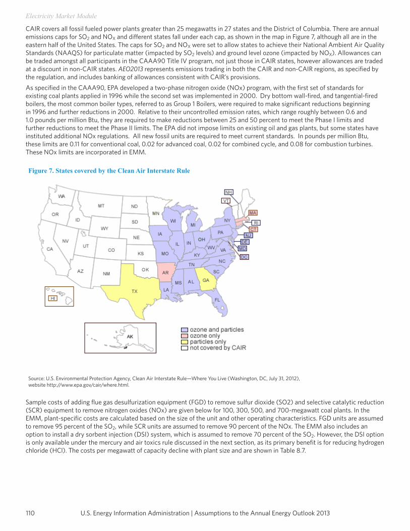
U.S. Energy Information Administration | Assumptions to the Annual Energy Outlook 2013110
Electricity Market Module
CAIR covers all fossil fueled power plants greater than 25 megawatts in 27 states and the District of Columbia. There are annual emissions caps for SO2 and NOX and different states fall under each cap, as shown in the map in Figure 7, although all are in the eastern half of the United States. The caps for SO2 and NOX were set to allow states to achieve their National Ambient Air Quality Standards (NAAQS) for particulate matter (impacted by SO2 levels) and ground level ozone (impacted by NOX). Allowances can be traded amongst all participants in the CAAA90 Title IV program, not just those in CAIR states, however allowances are traded at a discount in non-CAIR states. AEO2013 represents emissions trading in both the CAIR and non-CAIR regions, as specified by the regulation, and includes banking of allowances consistent with CAIR’s provisions.As specified in the CAAA90, EPA developed a two-phase nitrogen oxide (NOx) program, with the first set of standards for existing coal plants applied in 1996 while the second set was implemented in 2000. Dry bottom wall-fired, and tangential-fired boilers, the most common boiler types, referred to as Group 1 Boilers, were required to make significant reductions beginning in 1996 and further reductions in 2000. Relative to their uncontrolled emission rates, which range roughly between 0.6 and 1.0 pounds per million Btu, they are required to make reductions between 25 and 50 percent to meet the Phase I limits and further reductions to meet the Phase II limits. The EPA did not impose limits on existing oil and gas plants, but some states have instituted additional NOx regulations. All new fossil units are required to meet current standards. In pounds per million Btu, these limits are 0.11 for conventional coal, 0.02 for advanced coal, 0.02 for combined cycle, and 0.08 for combustion turbines. These NOx limits are incorporated in EMM.
Sample costs of adding flue gas desulfurization equipment (FGD) to remove sulfur dioxide (SO2) and selective catalytic reduction (SCR) equipment to remove nitrogen oxides (NOx) are given below for 100, 300, 500, and 700-megawatt coal plants. In the EMM, plant-specific costs are calculated based on the size of the unit and other operating characteristics. FGD units are assumed to remove 95 percent of the SO2, while SCR units are assumed to remove 90 percent of the NOx. The EMM also includes an option to install a dry sorbent injection (DSI) system, which is assumed to remove 70 percent of the SO2. However, the DSI option is only available under the mercury and air toxics rule discussed in the next section, as its primary benefit is for reducing hydrogen chloride (HCl). The costs per megawatt of capacity decline with plant size and are shown in Table 8.7.
Figure 7. States covered by the Clean Air Interstate Rule
Source: U.S. Environmental Protection Agency, Clean Air Interstate Rule—Where You Live (Washington, DC, July 31, 2012), website http://www.epa.gov/cair/where.html.
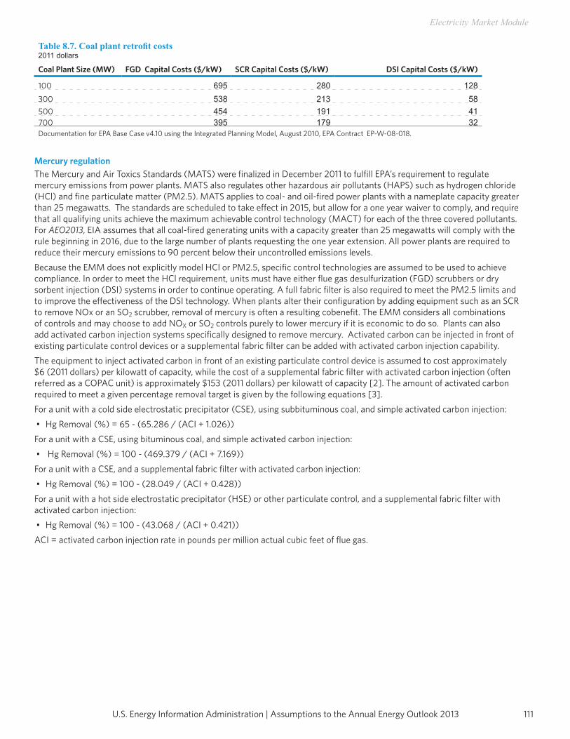
111U.S. Energy Information Administration | Assumptions to the Annual Energy Outlook 2013
Electricity Market Module
Table 8.7. Coal plant retrofit costs 2011 dollars
Coal Plant Size (MW) FGD Capital Costs ($/kW) SCR Capital Costs ($/kW) DSI Capital Costs ($/kW)
100 695 280 128300 538 213 58500 454 191 41700 395 179 32Documentation for EPA Base Case v4.10 using the Integrated Planning Model, August 2010, EPA Contract EP-W-08-018.
Mercury regulationThe Mercury and Air Toxics Standards (MATS) were finalized in December 2011 to fulfill EPA’s requirement to regulate mercury emissions from power plants. MATS also regulates other hazardous air pollutants (HAPS) such as hydrogen chloride (HCl) and fine particulate matter (PM2.5). MATS applies to coal- and oil-fired power plants with a nameplate capacity greater than 25 megawatts. The standards are scheduled to take effect in 2015, but allow for a one year waiver to comply, and require that all qualifying units achieve the maximum achievable control technology (MACT) for each of the three covered pollutants. For AEO2013, EIA assumes that all coal-fired generating units with a capacity greater than 25 megawatts will comply with the rule beginning in 2016, due to the large number of plants requesting the one year extension. All power plants are required to reduce their mercury emissions to 90 percent below their uncontrolled emissions levels.
Because the EMM does not explicitly model HCl or PM2.5, specific control technologies are assumed to be used to achieve compliance. In order to meet the HCl requirement, units must have either flue gas desulfurization (FGD) scrubbers or dry sorbent injection (DSI) systems in order to continue operating. A full fabric filter is also required to meet the PM2.5 limits and to improve the effectiveness of the DSI technology. When plants alter their configuration by adding equipment such as an SCR to remove NOx or an SO2 scrubber, removal of mercury is often a resulting cobenefit. The EMM considers all combinations of controls and may choose to add NOX or SO2 controls purely to lower mercury if it is economic to do so. Plants can also add activated carbon injection systems specifically designed to remove mercury. Activated carbon can be injected in front of existing particulate control devices or a supplemental fabric filter can be added with activated carbon injection capability.The equipment to inject activated carbon in front of an existing particulate control device is assumed to cost approximately $6 (2011 dollars) per kilowatt of capacity, while the cost of a supplemental fabric filter with activated carbon injection (often referred as a COPAC unit) is approximately $153 (2011 dollars) per kilowatt of capacity [2]. The amount of activated carbon required to meet a given percentage removal target is given by the following equations [3]. For a unit with a cold side electrostatic precipitator (CSE), using subbituminous coal, and simple activated carbon injection:•• Hg Removal (%) = 65 - (65.286 / (ACI + 1.026))
For a unit with a CSE, using bituminous coal, and simple activated carbon injection: •• Hg Removal (%) = 100 - (469.379 / (ACI + 7.169))
For a unit with a CSE, and a supplemental fabric filter with activated carbon injection: •• Hg Removal (%) = 100 - (28.049 / (ACI + 0.428))
For a unit with a hot side electrostatic precipitator (HSE) or other particulate control, and a supplemental fabric filter with activated carbon injection: •• Hg Removal (%) = 100 - (43.068 / (ACI + 0.421))
ACI = activated carbon injection rate in pounds per million actual cubic feet of flue gas.
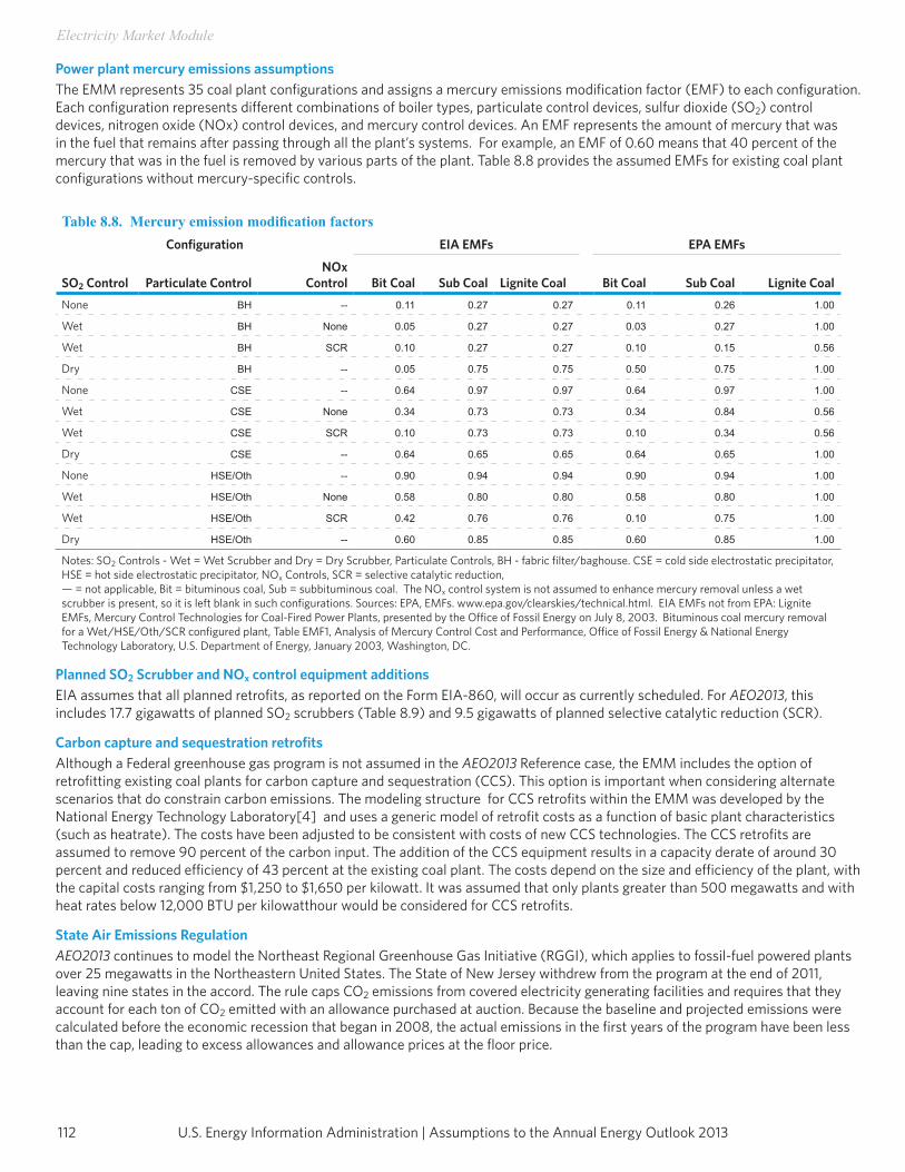
U.S. Energy Information Administration | Assumptions to the Annual Energy Outlook 2013112
Electricity Market Module
Power plant mercury emissions assumptions The EMM represents 35 coal plant configurations and assigns a mercury emissions modification factor (EMF) to each configuration. Each configuration represents different combinations of boiler types, particulate control devices, sulfur dioxide (SO2) control devices, nitrogen oxide (NOx) control devices, and mercury control devices. An EMF represents the amount of mercury that was in the fuel that remains after passing through all the plant’s systems. For example, an EMF of 0.60 means that 40 percent of the mercury that was in the fuel is removed by various parts of the plant. Table 8.8 provides the assumed EMFs for existing coal plant configurations without mercury-specific controls.
Table 8.8. Mercury emission modification factorsConfiguration EIA EMFs EPA EMFs
SO2 Control Particulate ControlNOx
Control Bit Coal Sub Coal Lignite Coal Bit Coal Sub Coal Lignite CoalNone BH -- 0.11 0.27 0.27 0.11 0.26 1.00
Wet BH None 0.05 0.27 0.27 0.03 0.27 1.00
Wet BH SCR 0.10 0.27 0.27 0.10 0.15 0.56
Dry BH -- 0.05 0.75 0.75 0.50 0.75 1.00
None CSE -- 0.64 0.97 0.97 0.64 0.97 1.00
Wet CSE None 0.34 0.73 0.73 0.34 0.84 0.56
Wet CSE SCR 0.10 0.73 0.73 0.10 0.34 0.56
Dry CSE -- 0.64 0.65 0.65 0.64 0.65 1.00
None HSE/Oth -- 0.90 0.94 0.94 0.90 0.94 1.00
Wet HSE/Oth None 0.58 0.80 0.80 0.58 0.80 1.00
Wet HSE/Oth SCR 0.42 0.76 0.76 0.10 0.75 1.00
Dry HSE/Oth -- 0.60 0.85 0.85 0.60 0.85 1.00
Notes: SO2 Controls - Wet = Wet Scrubber and Dry = Dry Scrubber, Particulate Controls, BH - fabric filter/baghouse. CSE = cold side electrostatic precipitator, HSE = hot side electrostatic precipitator, NOx Controls, SCR = selective catalytic reduction, — = not applicable, Bit = bituminous coal, Sub = subbituminous coal. The NOx control system is not assumed to enhance mercury removal unless a wet scrubber is present, so it is left blank in such configurations. Sources: EPA, EMFs. www.epa.gov/clearskies/technical.html. EIA EMFs not from EPA: Lignite EMFs, Mercury Control Technologies for Coal-Fired Power Plants, presented by the Office of Fossil Energy on July 8, 2003. Bituminous coal mercury removal for a Wet/HSE/Oth/SCR configured plant, Table EMF1, Analysis of Mercury Control Cost and Performance, Office of Fossil Energy & National Energy Technology Laboratory, U.S. Department of Energy, January 2003, Washington, DC.
Planned SO2 Scrubber and NOx control equipment additionsEIA assumes that all planned retrofits, as reported on the Form EIA-860, will occur as currently scheduled. For AEO2013, this includes 17.7 gigawatts of planned SO2 scrubbers (Table 8.9) and 9.5 gigawatts of planned selective catalytic reduction (SCR).
Carbon capture and sequestration retrofits Although a Federal greenhouse gas program is not assumed in the AEO2013 Reference case, the EMM includes the option of retrofitting existing coal plants for carbon capture and sequestration (CCS). This option is important when considering alternate scenarios that do constrain carbon emissions. The modeling structure for CCS retrofits within the EMM was developed by the National Energy Technology Laboratory[4] and uses a generic model of retrofit costs as a function of basic plant characteristics (such as heatrate). The costs have been adjusted to be consistent with costs of new CCS technologies. The CCS retrofits are assumed to remove 90 percent of the carbon input. The addition of the CCS equipment results in a capacity derate of around 30 percent and reduced efficiency of 43 percent at the existing coal plant. The costs depend on the size and efficiency of the plant, with the capital costs ranging from $1,250 to $1,650 per kilowatt. It was assumed that only plants greater than 500 megawatts and with heat rates below 12,000 BTU per kilowatthour would be considered for CCS retrofits.
State Air Emissions RegulationAEO2013 continues to model the Northeast Regional Greenhouse Gas Initiative (RGGI), which applies to fossil-fuel powered plants over 25 megawatts in the Northeastern United States. The State of New Jersey withdrew from the program at the end of 2011, leaving nine states in the accord. The rule caps CO2 emissions from covered electricity generating facilities and requires that they account for each ton of CO2 emitted with an allowance purchased at auction. Because the baseline and projected emissions were calculated before the economic recession that began in 2008, the actual emissions in the first years of the program have been less than the cap, leading to excess allowances and allowance prices at the floor price.
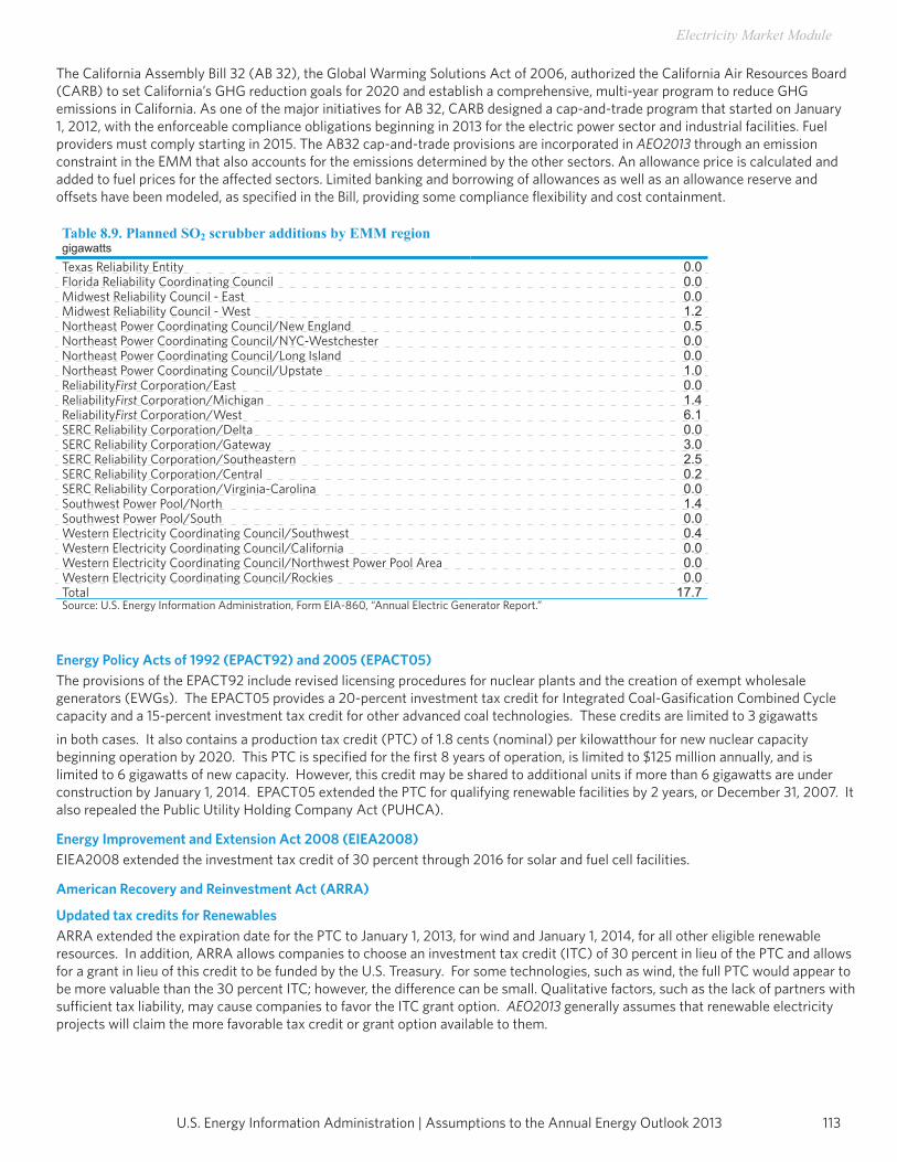
113U.S. Energy Information Administration | Assumptions to the Annual Energy Outlook 2013
Electricity Market Module
The California Assembly Bill 32 (AB 32), the Global Warming Solutions Act of 2006, authorized the California Air Resources Board (CARB) to set California’s GHG reduction goals for 2020 and establish a comprehensive, multi-year program to reduce GHG emissions in California. As one of the major initiatives for AB 32, CARB designed a cap-and-trade program that started on January 1, 2012, with the enforceable compliance obligations beginning in 2013 for the electric power sector and industrial facilities. Fuel providers must comply starting in 2015. The AB32 cap-and-trade provisions are incorporated in AEO2013 through an emission constraint in the EMM that also accounts for the emissions determined by the other sectors. An allowance price is calculated and added to fuel prices for the affected sectors. Limited banking and borrowing of allowances as well as an allowance reserve and offsets have been modeled, as specified in the Bill, providing some compliance flexibility and cost containment.
Table 8.9. Planned SO2 scrubber additions by EMM regiongigawattsTexas Reliability Entity 0.0Florida Reliability Coordinating Council 0.0Midwest Reliability Council - East 0.0Midwest Reliability Council - West 1.2Northeast Power Coordinating Council/New England 0.5Northeast Power Coordinating Council/NYC-Westchester 0.0Northeast Power Coordinating Council/Long Island 0.0Northeast Power Coordinating Council/Upstate 1.0ReliabilityFirst Corporation/East 0.0ReliabilityFirst Corporation/Michigan 1.4ReliabilityFirst Corporation/West 6.1SERC Reliability Corporation/Delta 0.0SERC Reliability Corporation/Gateway 3.0SERC Reliability Corporation/Southeastern 2.5SERC Reliability Corporation/Central 0.2SERC Reliability Corporation/Virginia-Carolina 0.0Southwest Power Pool/North 1.4Southwest Power Pool/South 0.0Western Electricity Coordinating Council/Southwest 0.4Western Electricity Coordinating Council/California 0.0Western Electricity Coordinating Council/Northwest Power Pool Area 0.0Western Electricity Coordinating Council/Rockies 0.0Total 17.7Source: U.S. Energy Information Administration, Form EIA-860, “Annual Electric Generator Report.”
Energy Policy Acts of 1992 (EPACT92) and 2005 (EPACT05) The provisions of the EPACT92 include revised licensing procedures for nuclear plants and the creation of exempt wholesale generators (EWGs). The EPACT05 provides a 20-percent investment tax credit for Integrated Coal-Gasification Combined Cycle capacity and a 15-percent investment tax credit for other advanced coal technologies. These credits are limited to 3 gigawattsin both cases. It also contains a production tax credit (PTC) of 1.8 cents (nominal) per kilowatthour for new nuclear capacity beginning operation by 2020. This PTC is specified for the first 8 years of operation, is limited to $125 million annually, and is limited to 6 gigawatts of new capacity. However, this credit may be shared to additional units if more than 6 gigawatts are under construction by January 1, 2014. EPACT05 extended the PTC for qualifying renewable facilities by 2 years, or December 31, 2007. It also repealed the Public Utility Holding Company Act (PUHCA).
Energy Improvement and Extension Act 2008 (EIEA2008) EIEA2008 extended the investment tax credit of 30 percent through 2016 for solar and fuel cell facilities.
American Recovery and Reinvestment Act (ARRA)
Updated tax credits for Renewables ARRA extended the expiration date for the PTC to January 1, 2013, for wind and January 1, 2014, for all other eligible renewable resources. In addition, ARRA allows companies to choose an investment tax credit (ITC) of 30 percent in lieu of the PTC and allows for a grant in lieu of this credit to be funded by the U.S. Treasury. For some technologies, such as wind, the full PTC would appear to be more valuable than the 30 percent ITC; however, the difference can be small. Qualitative factors, such as the lack of partners with sufficient tax liability, may cause companies to favor the ITC grant option. AEO2013 generally assumes that renewable electricity projects will claim the more favorable tax credit or grant option available to them.

U.S. Energy Information Administration | Assumptions to the Annual Energy Outlook 2013114
Electricity Market Module
Loan guarantees for renewablesARRA provided $6 billion to pay the cost of guarantees for loans authorized by the Energy Policy Act of 2005. While most renewable projects which started construction prior to September 30, 2011 are potentially eligible for these loan guarantees, the application and approval of guarantees for specific projects is a highly discretionary process, and has thus far been limited. While AEO2013 includes projects that have received loan guarantees under this authority, it does not assume automatic award of the loans to potentially eligible technologies.
Support for CCSARRA provided $3.4 billion for additional research and development on fossil energy technologies. A portion of this funding is expected to be used to fund projects under the Clean Coal Power Initiative program, focusing on projects that capture and sequester greenhouse gases. To reflect the impact of this provision, AEO2013 Reference case assumes that an additional 1 gigawatt of coal capacity with CCS will be stimulated by 2018.
Smart grid expenditures ARRA provides $4.5 billion for smart grid demonstration projects. While somewhat difficult to define, smart grid technologies generally include a wide array of measurement, communications, and control equipment employed throughout the transmission and distribution system that will enable real-time monitoring of the production, flow, and use of power from the generator to the consumer. Among other things, these smart grid technologies are expected to enable more efficient use of the transmission and distribution grid, lower line losses, facilitate greater use of renewables, and provide information to utilities and their customers that will lead to greater investment in energy efficiency and reduced peak load demands. The funds provided will not fund a widespread implementation of smart grid technologies, but could stimulate more rapid investment than would otherwise occur.Several changes were made throughout the NEMS to represent the impacts of the smart grid funding provided in ARRA. In the electricity module, it was assumed that line losses would fall slightly, peak loads would fall as customers shifted their usage patterns, and customers would be more responsive to pricing signals. Historically, line losses, expressed as the percentage of electricity lost, have been falling for many years as utilities make investments to replace aging or failing equipment.Smart grid technologies also have the potential to reduce peak demand through the increased deployment of demand response programs. In AEO2013, it is assumed that the Federal expenditures on smart grid technologies will stimulate efforts that reduce peak demand from what they otherwise would be, with the amount of total peak load reduction growing from 2.2 percent initially to 3.5 percent by 2040, although the shifts vary by region. Load is shifted to offpeak hours, so net energy consumed remains largely constant.
FERC Orders 888 and 889 FERC issued two related rules (Orders 888 and 889) designed to bring low-cost power to consumers through competition, ensure continued reliability in the industry, and provide for open and equitable transmission services by owners of these facilities. Specifically, Order 888 requires open access to the transmission grid currently owned and operated by utilities. The transmission owners must file nondiscriminatory tariffs that offer other suppliers the same services that the owners provide for themselves. Order 888 also allows these utilities to recover stranded costs (investments in generating assets that are unrecoverable due to consumers selecting another supplier). Order 889 requires utilities to implement standards of conduct and an Open Access Same- Time Information System (OASIS) through which utilities and non-utilities can receive information regarding the transmission system. As a result, utilities have functionally or physically unbundled their marketing functions from their transmission functions.These orders are represented in EMM by assuming that all generators in a given region are able to satisfy load requirements anywhere within the region. Similarly, it is assumed that transactions between regions will occur if the cost differentials between them make such transactions economical.
Electricity alternative cases Nuclear Alternative casesFor AEO2013, three alternate cases were run for nuclear power plants to address uncertainties about the operating lives of existing reactors, the potential for new nuclear capacity, and capacity uprates at existing plants. These scenarios are discussed in the Issues in Focus article, “Nuclear Power in AEO2013” in the full AEO2013 report.

115U.S. Energy Information Administration | Assumptions to the Annual Energy Outlook 2013
Electricity Market Module
•• The Low Nuclear case assumes that all existing reactors will not receive a second license renewal and are retired within 60 years of operation. The reported retirement at Oyster Creek occurs as currently planned, at the end of 2019. Kewaunee is also retired in this case, at the end of 2014, based on an announcement by Dominion Resources in late 2012. Additionally, two units that are currently out of service are assumed to be permanently shut down in the Low Nuclear case. San Onofre 2 and Crystal River 3 are not currently operating, but are assumed to be returned to service in 2015 in the Reference case. In the Low Nuclear Case both units are assumed to retire in 2013. In the Reference case, existing plants are assumed to run as long as they continue to be economic, implicitly assuming that a second 20-year license renewal will be obtained for most plants reaching 60 years of age before 2040. The Low Nuclear case was run to analyze the impact of additional nuclear retirements, which could occur if the oldest plants do not receive a second license extension. In this case, 45 gigawatts of nuclear capacity are assumed to be retired by 2040. This case assumes that no new nuclear capacity will be added throughout the projection, excluding the capacity already planned and under construction. The case also assumes that only those capacity uprates reported to EIA will be completed. In contrast, the Reference case assumes additional uprates based on Nuclear Regulatory Commission (NRC) surveys and industry reports.
•• The High Nuclear case assumes that all existing nuclear units will receive a second license renewal and operate beyond 60 years (excluding one announced retirement). In the Reference case, beyond the announced retirement of Oyster Creek, an additional 6.5 gigawatts of nuclear capacity is assumed to be retired through 2040, reflecting uncertainty surrounding future aging impacts and/or costs. This case was run to provide a more optimistic outlook where all licenses are renewed and all plants are assumed to find it economic to continue operating beyond 60 years. The High Nuclear case also assumes additional planned nuclear capacity is completed based on combined license (COL) applications with the NRC. The Reference case assumes 5.5 gigawatts of planned capacity are added, while the High Nuclear case includes 13.3 gigawatts of planned capacity additions.
•• The Small Modular Reactor case assumes that new advanced nuclear plants built in the forecast will be based on a smaller modular design rather than the larger AP1000 design used in the Reference case. The overnight costs are assumed to be the same as in the Reference case, but the construction lead time is reduced from six years to three years for the smaller design. The fixed operating and maintenance costs are assumed to be higher for the smaller design. To account for the necessary time for design certification, the first available online date for the small reactors is assumed to be 2025.

U.S. Energy Information Administration | Assumptions to the Annual Energy Outlook 2013116
Electricity Market Module
Notes and sources[1] Review of Power Plant Cost and Performance Assumptions for NEMS, Science Applications International Corporation, April 2013. The costs shown Table 8.2 and used for the AEO2013 were based on a draft report provided in September 2012 and may vary slightly from the published final report.[2] These costs were developed using the National Energy Technology Laboratory Mercury Control Performance andCost Model, 1998.[3] U.S. Department of Energy, Analysis of Mercury Control Cost and Performance, Office of Fossil Energy & NationalEnergy Technology Laboratory, January 2003.[4] Retrofitting Coal-Fired Power Plants for Carbon Dioxide Capture and Sequestration - Exploratory Testing of NEMS forIntegrated Assessments, DOE/NETL-2008/1309, P.A. Geisbrecht, January 18, 2009.

Oil and Gas Supply Module

This page inTenTionally lefT blank
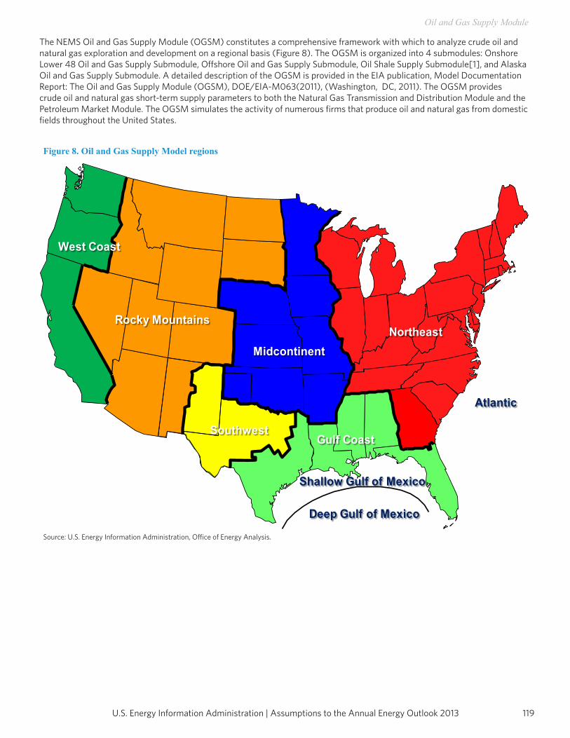
119U.S. Energy Information Administration | Assumptions to the Annual Energy Outlook 2013
Oil and Gas Supply Module
The NEMS Oil and Gas Supply Module (OGSM) constitutes a comprehensive framework with which to analyze crude oil and natural gas exploration and development on a regional basis (Figure 8). The OGSM is organized into 4 submodules: Onshore Lower 48 Oil and Gas Supply Submodule, Offshore Oil and Gas Supply Submodule, Oil Shale Supply Submodule[1], and Alaska Oil and Gas Supply Submodule. A detailed description of the OGSM is provided in the EIA publication, Model Documentation Report: The Oil and Gas Supply Module (OGSM), DOE/EIA-M063(2011), (Washington, DC, 2011). The OGSM provides crude oil and natural gas short-term supply parameters to both the Natural Gas Transmission and Distribution Module and the Petroleum Market Module. The OGSM simulates the activity of numerous firms that produce oil and natural gas from domestic fields throughout the United States.
Figure 8. Oil and Gas Supply Model regions
Source: U.S. Energy Information Administration, Office of Energy Analysis.
Rocky Mountain - 5
Rocky Mountains
West Coast
Midcontinent Northeast
Gulf Coast Southwest
Atlantic
Shallow Gulf of Mexico
Deep Gulf of Mexico
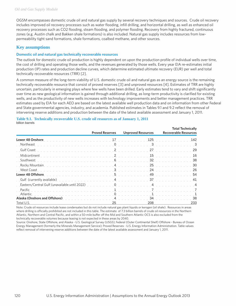
U.S. Energy Information Administration | Assumptions to the Annual Energy Outlook 2013120
Oil and Gas Supply Module
OGSM encompasses domestic crude oil and natural gas supply by several recovery techniques and sources. Crude oil recovery
includes improved oil recovery processes such as water fl ooding, infi ll drilling, and horizontal drilling, as well as enhanced oil
recovery processes such as CO2 fl ooding, steam fl ooding, and polymer fl ooding. Recovery from highly fractured, continuous
zones (e.g. Austin chalk and Bakken shale formations) is also included. Natural gas supply includes resources from low-
permeability tight sand formations, shale formations, coalbed methane, and other sources.
Key assumptionsDomestic oil and natural gas technically recoverable resourcesThe outlook for domestic crude oil production is highly dependent on upon the production profi le of individual wells over time,
the cost of drilling and operating those wells, and the revenues generated by those wells. Every year EIA re-estimates initial
production (IP) rates and production decline curves, which determine estimated ultimate recovery (EUR) per well and total
technically recoverable resources (TRR) [2].
A common measure of the long-term viability of U.S. domestic crude oil and natural gas as an energy source is the remaining
technically recoverable resource that consist of proved reserves [3] and unproved resources [4]. Estimates of TRR are highly
uncertain, particularly in emerging plays where few wells have been drilled. Early estimates tend to vary and shift signifi cantly
over time as new geological information is gained through additional drilling, as long-term productivity is clarifi ed for existing
wells, and as the productivity of new wells increases with technology improvements and better management practices. TRR
estimates used by EIA for each AEO are based on the latest available well production data and on information from other Federal
and State governmental agencies, industry, and academia. Published estimates in Tables 9.1 and 9.2 refl ect the removal of
intervening reserve additions and production between the date of the latest available assessment and January 1, 2011.
Table 9.1. Technically recoverable U.S. crude oil resources as of January 1, 2011billion barrels
Proved Reserves Unproved ResourcesTotal Technically
Recoverable Resources
Lower 48 Onshore 17 125 142 Northeast 0 3 3 Gulf Coast 2 27 29 Midcontinent 2 15 16 Southwest 6 32 38 Rocky Mountain 4 25 30 West Coast 3 24 26Lower 48 Off shore 5 49 54 Gulf (currently available) 4 37 41 Eastern/Central Gulf (unavailable until 2022) 0 4 4 Pacifi c 1 7 7 Atlantic 0 1 1Alaska (Onshore and Off shore) 4 34 38Total U.S. 25 208 233Note: Crude oil resources include lease condensates but do not include natural gas plant liquids or kerogen (oil shale). Resources in areas
where drilling is offi cially prohibited are not included in this table. The estimate of 7.3 billion barrels of crude oil resources in the Northern
Atlantic, Northern and Central Pacifi c, and within a 50-mile buff er off the Mid and Southern Atlantic OCS is also excluded from the
technically recoverable volumes because leasing is not expected in these areas by 2040.
Source: Onshore, State Off shore, and Alaska - U.S. Geological Survey (USGS); Federal (Outer Continental Shelf) Off shore - Bureau of Ocean
Energy Management (formerly the Minerals Management Service); Proved Reserves - U.S. Energy Information Administration. Table values
refl ect removal of intervening reserve additions between the date of the latest available assessment and January 1, 2011.
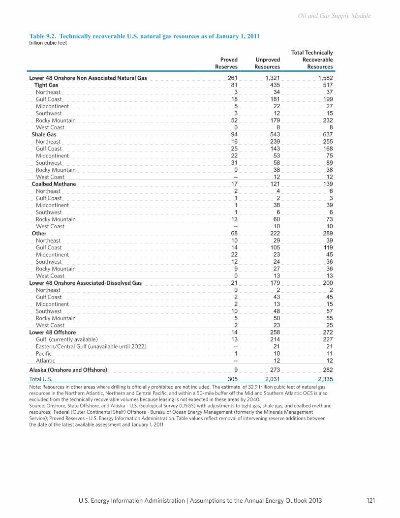
121U.S. Energy Information Administration | Assumptions to the Annual Energy Outlook 2013
Oil and Gas Supply Module
Table 9.2. Technically recoverable U.S. natural gas resources as of January 1, 2011trillion cubic feet
Proved Reserves
Unproved Resources
Total Technically Recoverable
Resources
Lower 48 Onshore Non Associated Natural Gas 261 1,321 1,582 Tight Gas 81 435 517 Northeast 3 34 37 Gulf Coast 18 181 199 Midcontinent 5 22 27 Southwest 3 12 15 Rocky Mountain 52 179 232 West Coast 0 8 8 Shale Gas 94 543 637 Northeast 16 239 255 Gulf Coast 25 143 168 Midcontinent 22 53 75 Southwest 31 58 89 Rocky Mountain 0 38 38 West Coast -- 12 12 Coalbed Methane 17 121 139 Northeast 2 4 6 Gulf Coast 1 2 3 Midcontinent 1 38 39 Southwest 1 6 6 Rocky Mountain 13 60 73 West Coast -- 10 10 Other 68 222 289 Northeast 10 29 39 Gulf Coast 14 105 119 Midcontinent 22 23 45 Southwest 12 24 36 Rocky Mountain 9 27 36 West Coast 0 13 13Lower 48 Onshore Associated-Dissolved Gas 21 179 200 Northeast 0 2 2 Gulf Coast 2 43 45 Midcontinent 2 13 15 Southwest 10 48 57 Rocky Mountain 5 50 55 West Coast 2 23 25Lower 48 Offshore 14 258 272 Gulf (currently available) 13 214 227 Eastern/Central Gulf (unavailable until 2022) -- 21 21 Pacific 1 10 11 Atlantic -- 12 12Alaska (Onshore and Offshore) 9 273 282Total U.S. 305 2,031 2,335Note: Resources in other areas where drilling is officially prohibited are not included. The estimate of 32.9 trillion cubic feet of natural gas resources in the Northern Atlantic, Northern and Central Pacific, and within a 50-mile buffer off the Mid and Southern Atlantic OCS is also excluded from the technically recoverable volumes because leasing is not expected in these areas by 2040. Source: Onshore, State Offshore, and Alaska - U.S. Geological Survey (USGS) with adjustments to tight gas, shale gas, and coalbed methaneresources; Federal (Outer Continental Shelf) Offshore - Bureau of Ocean Energy Management (formerly the Minerals Management Service); Proved Reserves - U.S. Energy Information Administration. Table values reflect removal of intervening reserve additions between the date of the latest available assessment and January 1, 2011
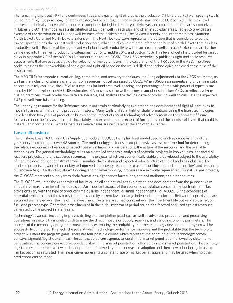
U.S. Energy Information Administration | Assumptions to the Annual Energy Outlook 2013122
Oil and Gas Supply Module
The remaining unproved TRR for a continuous-type shale gas or tight oil area is the product of (1) land area, (2) well spacing (wells per square mile), (3) percentage of area untested, (4) percentage of area with potential, and (5) EUR per well. The play-level unproved technically recoverable resource assumptions for tight oil, shale gas, tight gas, and coalbed methane are summarized in Tables 9.3-9.4. The model uses a distribution of EUR per well in each play and often in sub-play areas. Table 9.5 provides an example of the distribution of EUR per well for each of the Bakken areas. The Bakken is subdivided into three areas: Montana, North Dakota Core, and North Dakota Extension. The North Dakota Core represents the portion that is considered to be the “sweet spot” and has the highest well production rates, while the “Extension” area refers to the bulk of North Dakota that has less productive wells. Because of the significant variation in well productivity within an area, the wells in each Bakken area are further delineated into three well productivity categories: top 15%, middle 70%, and bottom 15%. This level of detail is provided for select plays in Appendix 2.C of the AEO2013 Documentation for the OGSM. The USGS periodically publishes tight and shale resource assessments that are used as a guide for selection of key parameters in the calculation of the TRR used in the AEO. The USGS seeks to assess the recoverability of shale gas and tight oil based on the wells drilled and technologies deployed at the time of the assessment. The AEO TRRs incorporate current drilling, completion, and recovery techniques, requiring adjustments to the USGS estimates, as well as the inclusion of shale gas and tight oil resources not yet assessed by USGS. When USGS assessments and underlying data become publicly available, the USGS assumptions for land area, well spacing, and percentage of area with potential typically are used by EIA to develop the AEO TRR estimates. EIA may revise the well spacing assumptions in future AEOs to reflect evolving drilling practices. If well production data are available, EIA analyzes the decline curve of producing wells to calculate the expected EUR per well from future drilling.The underlying resource for the Reference case is uncertain particularly as exploration and development of tight oil continues to move into areas with little to no production history. Many wells drilled in tight or shale formations using the latest technologies have less than two years of production history so the impact of recent technological advancement on the estimate of future recovery cannot be fully ascertained. Uncertainty also extends to areal extent of formations and the number of layers that could be drilled within formations. Two alternative resource cases are discussed at the end of this chapter.
Lower 48 onshoreThe Onshore Lower 48 Oil and Gas Supply Submodule (OLOGSS) is a play-level model used to analyze crude oil and natural gas supply from onshore lower 48 sources. The methodology includes a comprehensive assessment method for determining the relative economics of various prospects based on financial considerations, the nature of the resource, and the available technologies. The general methodology relies on a detailed economic analysis of potential projects in known fields, enhanced oil recovery projects, and undiscovered resources. The projects which are economically viable are developed subject to the availability of resource development constraints which simulate the existing and expected infrastructure of the oil and gas industries. For crude oil projects, advanced secondary or improved oil recovery techniques (e.g. infill drilling and horizontal drilling) and enhanced oil recovery (e.g. CO2 flooding, steam flooding, and polymer flooding) processes are explicitly represented. For natural gas projects, the OLOGSS represents supply from shale formations, tight sands formations, coalbed methane, and other sources.The OLOGSS evaluates the economics of future crude oil and natural gas exploration and development from the perspective of an operator making an investment decision. An important aspect of the economic calculation concerns the tax treatment. Tax provisions vary with the type of producer (major, large independent, or small independent). For AEO2013, the economics of potential projects reflect the tax treatment provided by current laws for large independent producers. Relevant tax provisions are assumed unchanged over the life of the investment. Costs are assumed constant over the investment life but vary across region, fuel, and process type. Operating losses incurred in the initial investment period are carried forward and used against revenues generated by the project in later years.Technology advances, including improved drilling and completion practices, as well as advanced production and processing operations, are explicitly modeled to determine the direct impacts on supply, reserves, and various economic parameters. The success of the technology program is measured by estimating the probability that the technology development program will be successfully completed. It reflects the pace at which technology performance improves and the probability that the technology project will meet the program goals. There are four possible curves which represent the adoption of the technology: convex, concave, sigmoid/logistic and linear. The convex curve corresponds to rapid initial market penetration followed by slow market penetration. The concave curve corresponds to slow initial market penetration followed by rapid market penetration. The sigmoid/logistic curve represents a slow initial adoption rate followed by rapid increase in adoption and then slow adoption again as the market becomes saturated. The linear curve represents a constant rate of market penetration, and may be used when no other predictions can be made.
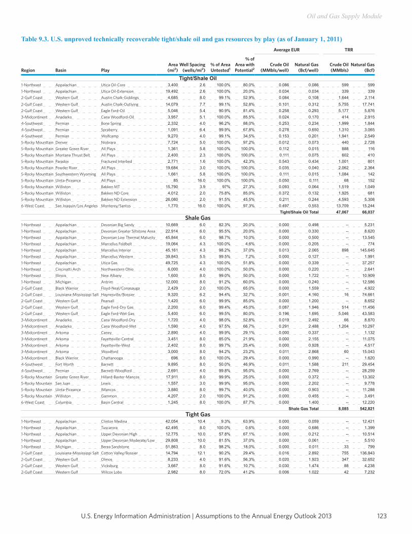
123U.S. Energy Information Administration | Assumptions to the Annual Energy Outlook 2013
Oil and Gas Supply Module
Table 9.3. U.S. unproved technically recoverable tight/shale oil and gas resources by play (as of January 1, 2011)Average EUR TRR
Region Basin PlayArea (mi2)
Well Spacing (wells/mi2)
% of Area Untested1
% of Area with Potential2
Crude Oil (MMbls/well)
Natural Gas (Bcf/well)
Crude Oil (MMbls)
Natural Gas (Bcf)
Tight/Shale Oil1-Northeast Appalachian Utica Oil-Core 3,400 2.6 100.0% 80.0% 0.086 0.086 599 5991-Northeast Appalachian Utica Oil-Extension 19,492 2.6 100.0% 20.0% 0.034 0.034 339 3392-Gulf Coast Western Gulf Austin Chalk-Giddings 4,685 8.0 99.1% 52.9% 0.084 0.108 1,644 2,114
2-Gulf Coast Western Gulf Austin Chalk-Outlying 14,079 7.7 99.1% 52.8% 0.101 0.312 5,755 17,7412-Gulf Coast Western Gulf Eagle Ford-Oil 5,046 5.4 90.9% 81.4% 0.258 0.293 5,177 5,8763-Midcontinent Anadarko Cana Woodford-Oil 3,957 5.1 100.0% 85.5% 0.024 0.170 414 2,9154-Southwest Permian Bone Spring 2,332 4.0 96.2% 88.0% 0.253 0.234 1,999 1,8444-Southwest Permian Spraberry 1,091 6.4 99.9% 67.8% 0.278 0.650 1,310 3,0654-Southwest Permian Wolfcamp 9,270 4.0 99.1% 34.5% 0.153 0.201 1,941 2,5495-Rocky Mounttain Denver Niobrara 7,724 5.0 100.0% 97.2% 0.012 0.073 440 2,7285-Rocky Mounttain Greater Green River All Plays 1,361 5.8 100.0% 100.0% 0.112 0.015 888 1165-Rocky Mounttain Montana Thrust Belt All Plays 2,400 2.3 100.0% 100.0% 0.111 0.075 602 4105-Rocky Mounttain Paradox Fractured Interbed 2,771 1.6 100.0% 42.3% 0.543 0.434 1,001 8015-Rocky Mounttain Powder River All Plays 19,684 3.0 100.0% 100.0% 0.035 0.040 2,062 2,3645-Rocky Mounttain Southwestern Wyoming All Plays 1,661 5.8 100.0% 100.0% 0.111 0.015 1,084 1425-Rocky Mounttain Uinta-Piceance All Plays 85 16.0 100.0% 100.0% 0.050 0.111 68 1525-Rocky Mounttain Williston Bakken MT 15,790 3.9 97% 27.3% 0.093 0.064 1,519 1,0495-Rocky Mounttain Williston Bakken ND Core 4,012 2.0 75.8% 85.0% 0.372 0.132 1,925 6815-Rocky Mounttain Williston Bakken ND Extension 26,080 2.0 91.5% 45.5% 0.211 0.244 4,593 5,3086-West Coast San Joaquin/Los Angeles Monterey/Santos 1,770 16.0 100.0% 97.3% 0.497 0.553 13,709 15,244
Tight/Shale Oil Total 47,067 66,037Shale Gas
1-Northeast Appalachian Devonian Big Sandy 10,669 6.0 82.3% 20.0% 0.000 0.498 -- 5,2311-Northeast Appalachian Devonian Greater Siltstone Area 22,914 6.0 95.5% 20.0% 0.000 0.330 -- 8,6201-Northeast Appalachian Devonian Low Thermal Maturity 45,844 6.0 98.7% 10.0% 0.000 0.500 -- 13,5451-Northeast Appalachian Marcellus Foldbelt 19,064 4.3 100.0% 4.6% 0.000 0.205 -- 7741-Northeast Appalachian Marcellus Interior 45,161 4.3 98.2% 37.0% 0.013 2.065 898 145,6451-Northeast Appalachian Marcellus Western 39,843 5.5 99.5% 7.2% 0.000 0.127 -- 1,9911-Northeast Appalachian Utica Gas 49,725 4.3 100.0% 51.8% 0.000 0.339 -- 37,2571-Northeast Cincinatti Arch Northwestern Ohio 6,000 4.0 100.0% 50.0% 0.000 0.220 -- 2,6411-Northeast Illinois New Albany 1,600 8.0 99.0% 50.0% 0.000 1.722 -- 10,9091-Northeast Michigan Antrim 12,000 8.0 91.2% 60.0% 0.000 0.240 -- 12,5862-Gulf Coast Black Warrior Floyd-Neal/Conasauga 2,429 2.0 100.0% 65.0% 0.000 1.559 -- 4,9222-Gulf Coast Louisiana-Mississippi Salt Haynesville/Bossier 9,320 6.2 94.4% 32.7% 0.001 4.160 16 74,6612-Gulf Coast Western Gulf Pearsall 1,420 6.0 99.9% 85.0% 0.000 1.200 -- 8,6522-Gulf Coast Western Gulf Eagle Ford-Dry Gas 2,200 6.0 99.4% 45.0% 0.087 1.946 514 11,4562-Gulf Coast Western Gulf Eagle Ford-Wet Gas 5,400 6.0 99.5% 80.0% 0.196 1.695 5,046 43,5833-Midcontinent Anadarko Cana Woodford-Dry 1,720 4.0 98.0% 52.8% 0.019 2.492 66 8,8703-Midcontinent Anadarko Cana Woodford-Wet 1,590 4.0 97.5% 66.7% 0.291 2.488 1,204 10,2973-Midcontinent Arkoma Caney 2,890 4.0 99.9% 29.1% 0.000 0.337 -- 1,1323-Midcontinent Arkoma Fayetteville-Central 3,451 8.0 85.0% 21.9% 0.000 2.155 -- 11,0753-Midcontinent Arkoma Fayetteville-West 2,402 8.0 99.7% 25.4% 0.000 0.928 -- 4,5173-Midcontinent Arkoma Woodford 3,000 8.0 94.2% 23.2% 0.011 2.868 60 15,0433-Midcontinent Black Warrior Chattanooga 696 8.0 100.0% 29.4% 0.000 0.990 -- 1,6204-Southwest Fort Worth Barnett 9,895 8.0 50.0% 46.9% 0.011 1.588 211 29,4544-Southwest Permian Barnett-Woodford 2,691 4.0 99.8% 95.0% 0.000 2.769 -- 28,2595-Rocky Mountain Greater Green River Hillard-Baxter-Mancos 17,911 8.0 99.9% 25.0% 0.000 0.372 -- 13,3025-Rocky Mountain San Juan Lewis 1,557 3.0 99.9% 95.0% 0.000 2.202 -- 9,7785-Rocky Mountain Uinta-Piceance lMancos 3,880 8.0 99.7% 40.0% 0.000 0.903 -- 11,2885-Rocky Mountain Williston Gammon 4,207 2.0 100.0% 91.2% 0.000 0.455 -- 3,4916-West Coast Columbia Basin Central 1,245 8.0 100.0% 87.7% 0.000 1.400 -- 12,220
Shale Gas Total 8,085 542,821Tight Gas
1-Northeast Appalachian Clinton Medina 42,054 10.4 9.3% 63.9% 0.000 0.059 -- 12,4211-Northeast Appalachian Tuscarora 42,495 8.0 100.0% 0.6% 0.000 0.686 -- 1,3991-Northeast Appalachian Upper Devonian High 12,775 10.0 57.8% 67.1% 0.000 0.212 -- 10,5141-Northeast Appalachian Upper Devonian Moderate/Low 29,808 10.0 81.5% 37.0% 0.000 0.061 -- 5,5101-Northeast Michigan Berea Sandstone 51,863 8.0 98.2% 18.0% 0.000 0.011 33 7992-Gulf Coast Louisiana-Mississippi Salt Cotton Valley/Bossier 14,794 12.1 90.2% 29.4% 0.016 2.892 755 136,8432-Gulf Coast Western Gulf Olmos 8,233 4.0 91.6% 56.3% 0.020 1.923 347 32,6522-Gulf Coast Western Gulf Vicksburg 3,667 8.0 91.6% 10.7% 0.030 1.474 88 4,2382-Gulf Coast Western Gulf Wilcox Lobo 2,982 8.0 72.0% 41.2% 0.006 1.022 42 7,232
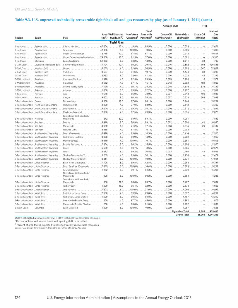
U.S. Energy Information Administration | Assumptions to the Annual Energy Outlook 2013124
Oil and Gas Supply Module
Table 9.3. U.S. unproved technically recoverable tight/shale oil and gas resources by play (as of January 1, 2011) (cont.)Average EUR TRR
Region Basin PlayArea (mi2)
Well Spacing (wells/mi2)
% of Area Untested1
% of Area with Potential2
Crude Oil (MMbls/well)
Natural Gas (Bcf/well)
Crude Oil (MMbls)
Natural Gas
(Bcf)
Tight Gas1-Northeast Appalachian Clinton Medina 42,054 10.4 9.3% 63.9% 0.000 0.059 -- 12,4211-Northeast Appalachian Tuscarora 42,495 8.0 100.0% 0.6% 0.000 0.686 -- 1,3991-Northeast Appalachian Upper Devonian High 12,775 10.0 57.8% 67.1% 0.000 0.212 -- 10,5141-Northeast Appalachian Upper Devonian Moderate/Low 29,808 10.0 81.5% 37.0% 0.000 0.061 -- 5,5101-Northeast Michigan Berea Sandstone 51,863 8.0 98.2% 18.0% 0.000 0.011 33 7992-Gulf Coast Louisiana-Mississippi Salt Cotton Valley/Bossier 14,794 12.1 90.2% 29.4% 0.016 2.892 755 136,8432-Gulf Coast Western Gulf Olmos 8,233 4.0 91.6% 56.3% 0.020 1.923 347 32,6522-Gulf Coast Western Gulf Vicksburg 3,667 8.0 91.6% 10.7% 0.030 1.474 88 4,2382-Gulf Coast Western Gulf Wilcox Lobo 2,982 8.0 72.0% 41.2% 0.006 1.022 42 7,2323-Midcontinent Anadarko Cherokee/Redfork 1,978 4.0 72.5% 29.9% 0.009 0.920 16 1,5773-Midcontinent Anadarko Cleveland 2,562 4.0 97.1% 45.1% 0.043 0.892 192 4,0033-Midcontinent Anadarko Granite Wash/Atoka 7,790 4.0 96.1% 28.2% 0.075 1.679 635 14,1823-Midcontinent Arkoma Arkoma 1,000 8.0 69.3% 32.2% 0.000 1.297 -- 2,3174-Southwest Permian Abo 1,578 8.0 56.9% 78.9% 0.037 0.713 400 4,0384-Southwest Permian Canyon 9,602 8.0 60.3% 75.2% 0.007 0.228 368 7,9385-Rocky Mountain Denver Denver/jules 4,500 16.0 87.8% 86.1% 0.000 0.244 -- 13,2545-Rocky Mountain North Central Montana High Potential 2,000 4.0 77.0% 88.9% 0.000 0.612 -- 3,3505-Rocky Mountain North Central Montana Low Potential 3,000 4.0 99.3% 74.7% 0.000 0.212 -- 1,8895-Rocky Mountain North Central Montana Moderate Potential 2,000 4.0 97.5% 79.3% 0.000 0.335 -- 2,075
5-Rocky Mountain PiceanceSouth Basin Williams Fork/ Mesaverde 272 32.0 98.6% 83.7% 0.000 1.091 -- 7,849
5-Rocky Mountain San Juan Dakota 3,918 8.0 74.9% 99.1% 0.002 0.300 41 6,9805-Rocky Mountain San Juan Mesaverde 3,689 8.0 71.2% 47.4% 0.003 0.345 26 3,4325-Rocky Mountain San Juan Pictured Cliffs 3,958 4.0 67.8% 0.7% 0.000 0.203 -- 155-Rocky Mountain Southwestern Wyoming Deep Mesaverde 16,416 4.0 99.8% 10.9% 0.000 0.414 -- 2,9555-Rocky Mountain Southwestern Wyoming Fort Union/Fox Hills 3,858 8.0 99.9% 4.9% 0.000 0.702 -- 1,0605-Rocky Mountain Southwestern Wyoming Frontier (Deep) 16,619 4.0 100.0% 6.7% 0.000 2.581 -- 10,8035-Rocky Mountain Southwestern Wyoming Frontier Moxa Arch 2,334 8.0 84.2% 15.5% 0.000 1.198 -- 2,9205-Rocky Mountain Southwestern Wyoming Lance 5,500 8.0 90.7% 8.6% 0.000 6.605 -- 22,6755-Rocky Mountain Southwestern Wyoming Lewis 5.172 8.0 99.2% 36.8% 0.003 0.460 42 6,9555-Rocky Mountain Southwestern Wyoming Shallow Mesaverde (1) 5,239 4.0 95.0% 50.1% 0.000 1.250 -- 12,4725-Rocky Mountain Southwestern Wyoming Shallow Mesaverde (2) 6,814 8.0 100.0% 49.0% 0.000 0.671 -- 17,9145-Rocky Mountain Uinta-Piceance Basin Flank Mesaverde 1,708 8.0 99.8% 42.8% 0.000 0.988 -- 5,7675-Rocky Mountain Uinta-Piceance Deep Synclinal Mesaverde 2,893 8.0 100.0% 14.4% 0.000 0.989 -- 3,2975-Rocky Mountain Uinta-Piceance Iles/Mesaverde 1,172 8.0 99.1% 94.3% 0.000 0.730 -- 6,395
5-Rocky Mountain Uinta-PiceanceNorth Basin Williams Fork/Mesaverde 908 8.0 100.0% 90.2% 0.000 0.654 -- 4,286
5-Rocky Mountain Uinta-PiceanceSouth Basin Williams Fork/Mesaverde 636 32.0 98.6% 83.7% 0.000 0.467 -- 7,834
5-Rocky Mountain Uinta-Piceance Tertiary East 1,600 16.0 96.4% 32.9% 0.000 0.578 -- 4,6935-Rocky Mountain Uinta-Piceance Tertiary West 1,603 8.0 100.0% 21.0% 0.000 4.066 -- 10,9495-Rocky Mountain Wind River Fort Union/Lance Deep 2,500 4.0 99.9% 79.6% 0.000 0.537 -- 4,2675-Rocky Mountain Wind River Fort Union/Lance Shallow 1,500 8.0 99.5% 94.8% 0.000 1.167 -- 13,2125-Rocky Mountain Wind River Mesaverde/Frontier Deep 250 4.0 97.7% 45.0% 0.000 1.992 -- 8765-Rocky Mountain Wind River Mesaverde/Frontier Shallow 250 4.0 90.6% 91.6% 0.000 1.252 -- 1,0396-West Coast Columbia Basin Centered 1,500 8.0 100.0% 49.9% 0.000 1.257 -- 7,528
Tight Gas Total 2,985 435,405Grand Total 58,066 1,044,263
EUR = estimated ultimate recovery; TRR = technically recoverable resource. 1 Percent of total wells (area times well spacing) left to be drilled. 2 Percent of area that is expected to have technically recoverable resources.Source: U.S. Energy Information Administration, Office of Energy Analysis.
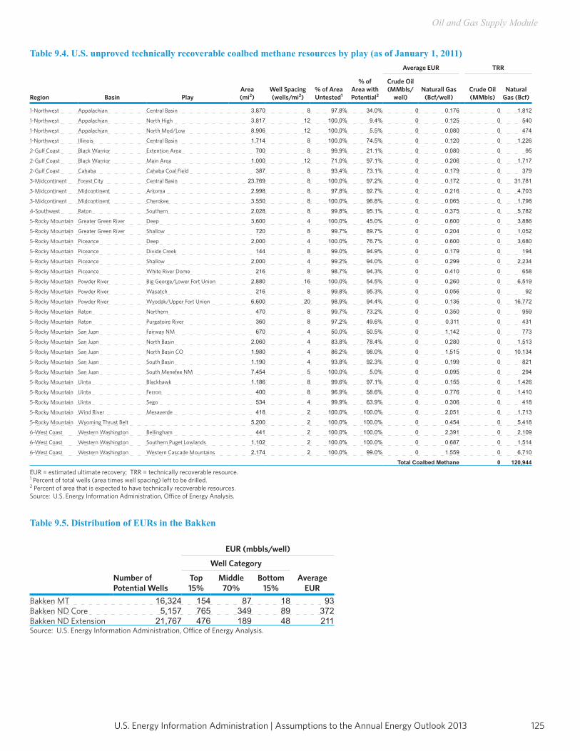
125U.S. Energy Information Administration | Assumptions to the Annual Energy Outlook 2013
Oil and Gas Supply Module
Table 9.4. U.S. unproved technically recoverable coalbed methane resources by play (as of January 1, 2011)Average EUR TRR
Region Basin PlayArea (mi2)
Well Spacing (wells/mi2)
% of Area Untested1
% of Area with Potential2
Crude Oil (MMbls/
well)Naturall Gas
(Bcf/well)Crude Oil (MMbls)
Natural Gas (Bcf)
1-Northwest Appalachian Central Basin 3,870 8 97.8% 34.0% 0 0.176 0 1,812
1-Northwest Appalachian North High 3,817 12 100.0% 9.4% 0 0.125 0 540
1-Northwest Appalachian North Mod/Low 8,906 12 100.0% 5.5% 0 0.080 0 474
1-Northwest Illinois Central Basin 1,714 8 100.0% 74.5% 0 0.120 0 1,226
2-Gulf Coast Black Warrior Extention Area 700 8 99.9% 21.1% 0 0.080 0 95
2-Gulf Coast Black Warrior Main Area 1,000 12 71.0% 97.1% 0 0.206 0 1,717
2-Gulf Coast Cahaba Cahaba Coal Field 387 8 93.4% 73.1% 0 0.179 0 379
3-Midcontinent Forest City Central Basin 23,769 8 100.0% 97.2% 0 0.172 0 31,781
3-Midcontinent Midcontinent Arkoma 2,998 8 97.8% 92.7% 0 0.216 0 4,703
3-Midcontinent Midcontinent Cherokee 3,550 8 100.0% 96.8% 0 0.065 0 1,798
4-Southwest Raton Southern 2,028 8 99.8% 95.1% 0 0.375 0 5,782
5-Rocky Mountain Greater Green River Deep 3,600 4 100.0% 45.0% 0 0.600 0 3,886
5-Rocky Mountain Greater Green River Shallow 720 8 99.7% 89.7% 0 0.204 0 1,052
5-Rocky Mountain Piceance Deep 2,000 4 100.0% 76.7% 0 0.600 0 3,680
5-Rocky Mountain Piceance Divide Creek 144 8 99.0% 94.9% 0 0.179 0 194
5-Rocky Mountain Piceance Shallow 2,000 4 99.2% 94.0% 0 0.299 0 2,234
5-Rocky Mountain Piceance White River Dome 216 8 98.7% 94.3% 0 0.410 0 658
5-Rocky Mountain Powder River Big George/Lower Fort Union 2,880 16 100.0% 54.5% 0 0.260 0 6,519
5-Rocky Mountain Powder River Wasatch 216 8 99.8% 95.3% 0 0.056 0 92
5-Rocky Mountain Powder River Wyodak/Upper Fort Union 6,600 20 98.9% 94.4% 0 0.136 0 16,772
5-Rocky Mountain Raton Northern 470 8 99.7% 73.2% 0 0.350 0 959
5-Rocky Mountain Raton Purgatoire River 360 8 97.2% 49.6% 0 0.311 0 431
5-Rocky Mountain San Juan Fairway NM 670 4 50.0% 50.5% 0 1,142 0 773
5-Rocky Mountain San Juan North Basin 2,060 4 83.8% 78.4% 0 0,280 0 1,513
5-Rocky Mountain San Juan North Basin CO 1,980 4 86.2% 98.0% 0 1,515 0 10,134
5-Rocky Mountain San Juan South Basin 1,190 4 93.8% 92.3% 0 0,199 0 821
5-Rocky Mountain San Juan South Menefee NM 7,454 5 100.0% 5.0% 0 0.095 0 294
5-Rocky Mountain Uinta Blackhawk 1,186 8 99.6% 97.1% 0 0.155 0 1,426
5-Rocky Mountain Uinta Ferron 400 8 96.9% 58.6% 0 0.776 0 1,410
5-Rocky Mountain Uinta Sego 534 4 99.9% 63.9% 0 0.306 0 418
5-Rocky Mountain Wind River Mesaverde 418 2 100.0% 100.0% 0 2,051 0 1,713
5-Rocky Mountain Wyoming Thrust Belt 5,200 2 100.0% 100.0% 0 0.454 0 5,418
6-West Coast Western Washington Bellingham 441 2 100.0% 100.0% 0 2,391 0 2,109
6-West Coast Western Washington Southern Puget Lowlands 1,102 2 100.0% 100.0% 0 0.687 0 1,514
6-West Coast Western Washington Western Cascade Mountains 2,174 2 100.0% 99.0% 0 1.559 0 6,710
Total Coalbed Methane 0 120,944
EUR = estimated ultimate recovery; TRR = technically recoverable resource.1 Percent of total wells (area times well spacing) left to be drilled. 2 Percent of area that is expected to have technically recoverable resources. Source: U.S. Energy Information Administration, Office of Energy Analysis.
Table 9.5. Distribution of EURs in the Bakken
Number of Potential Wells
EUR (mbbls/well)
Well Category
Average EUR
Top 15%
Middle 70%
Bottom 15%
Bakken MT 16,324 154 87 18 93Bakken ND Core 5,157 765 349 89 372Bakken ND Extension 21,767 476 189 48 211Source: U.S. Energy Information Administration, Office of Energy Analysis.
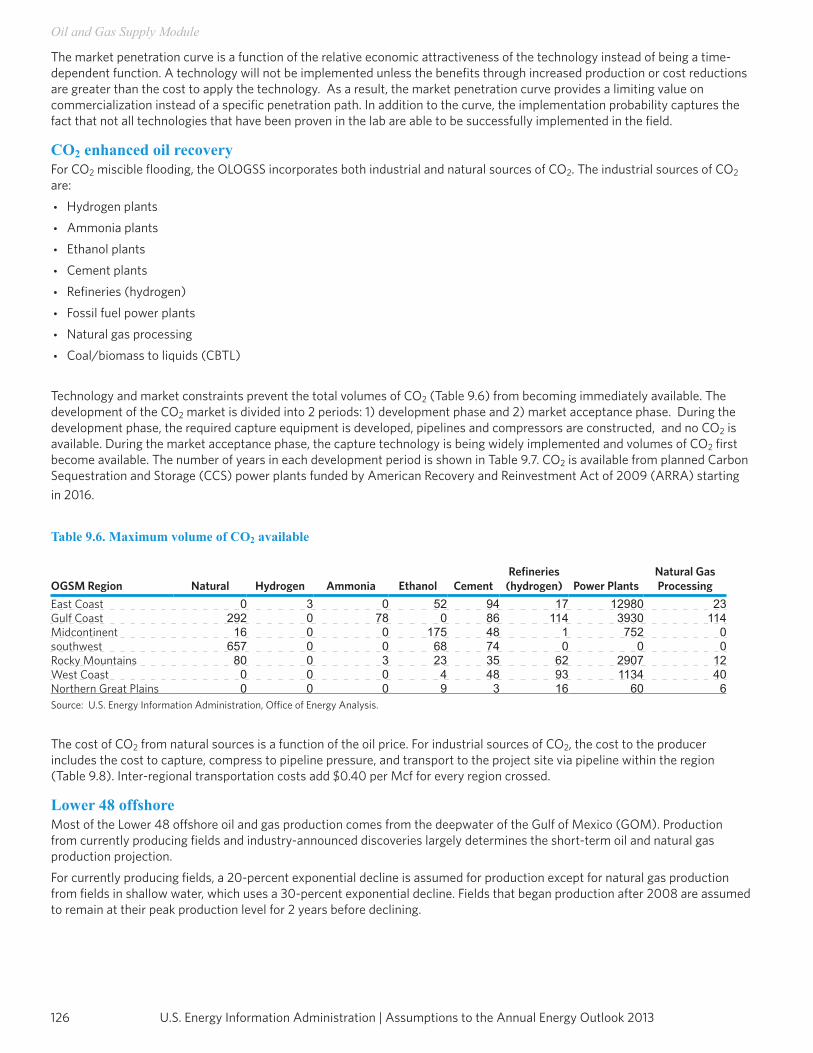
U.S. Energy Information Administration | Assumptions to the Annual Energy Outlook 2013126
Oil and Gas Supply Module
The market penetration curve is a function of the relative economic attractiveness of the technology instead of being a time- dependent function. A technology will not be implemented unless the benefits through increased production or cost reductions are greater than the cost to apply the technology. As a result, the market penetration curve provides a limiting value on commercialization instead of a specific penetration path. In addition to the curve, the implementation probability captures the fact that not all technologies that have been proven in the lab are able to be successfully implemented in the field.
CO2 enhanced oil recoveryFor CO2 miscible flooding, the OLOGSS incorporates both industrial and natural sources of CO2. The industrial sources of CO2 are:• Hydrogen plants• Ammonia plants• Ethanol plants• Cement plants• Refineries (hydrogen)• Fossil fuel power plants• Natural gas processing• Coal/biomass to liquids (CBTL)
Technology and market constraints prevent the total volumes of CO2 (Table 9.6) from becoming immediately available. The development of the CO2 market is divided into 2 periods: 1) development phase and 2) market acceptance phase. During the development phase, the required capture equipment is developed, pipelines and compressors are constructed, and no CO2 is available. During the market acceptance phase, the capture technology is being widely implemented and volumes of CO2 first become available. The number of years in each development period is shown in Table 9.7. CO2 is available from planned Carbon Sequestration and Storage (CCS) power plants funded by American Recovery and Reinvestment Act of 2009 (ARRA) starting in 2016.
Table 9.6. Maximum volume of CO2 available
OGSM Region Natural Hydrogen Ammonia Ethanol CementRefineries
(hydrogen) Power PlantsNatural Gas Processing
East Coast 0 3 0 52 94 17 12980 23Gulf Coast 292 0 78 0 86 114 3930 114Midcontinent 16 0 0 175 48 1 752 0southwest 657 0 0 68 74 0 0 0Rocky Mountains 80 0 3 23 35 62 2907 12West Coast 0 0 0 4 48 93 1134 40Northern Great Plains 0 0 0 9 3 16 60 6Source: U.S. Energy Information Administration, Office of Energy Analysis.
The cost of CO2 from natural sources is a function of the oil price. For industrial sources of CO2, the cost to the producer includes the cost to capture, compress to pipeline pressure, and transport to the project site via pipeline within the region (Table 9.8). Inter-regional transportation costs add $0.40 per Mcf for every region crossed.
Lower 48 offshoreMost of the Lower 48 offshore oil and gas production comes from the deepwater of the Gulf of Mexico (GOM). Production from currently producing fields and industry-announced discoveries largely determines the short-term oil and natural gas production projection.For currently producing fields, a 20-percent exponential decline is assumed for production except for natural gas production from fields in shallow water, which uses a 30-percent exponential decline. Fields that began production after 2008 are assumed to remain at their peak production level for 2 years before declining.
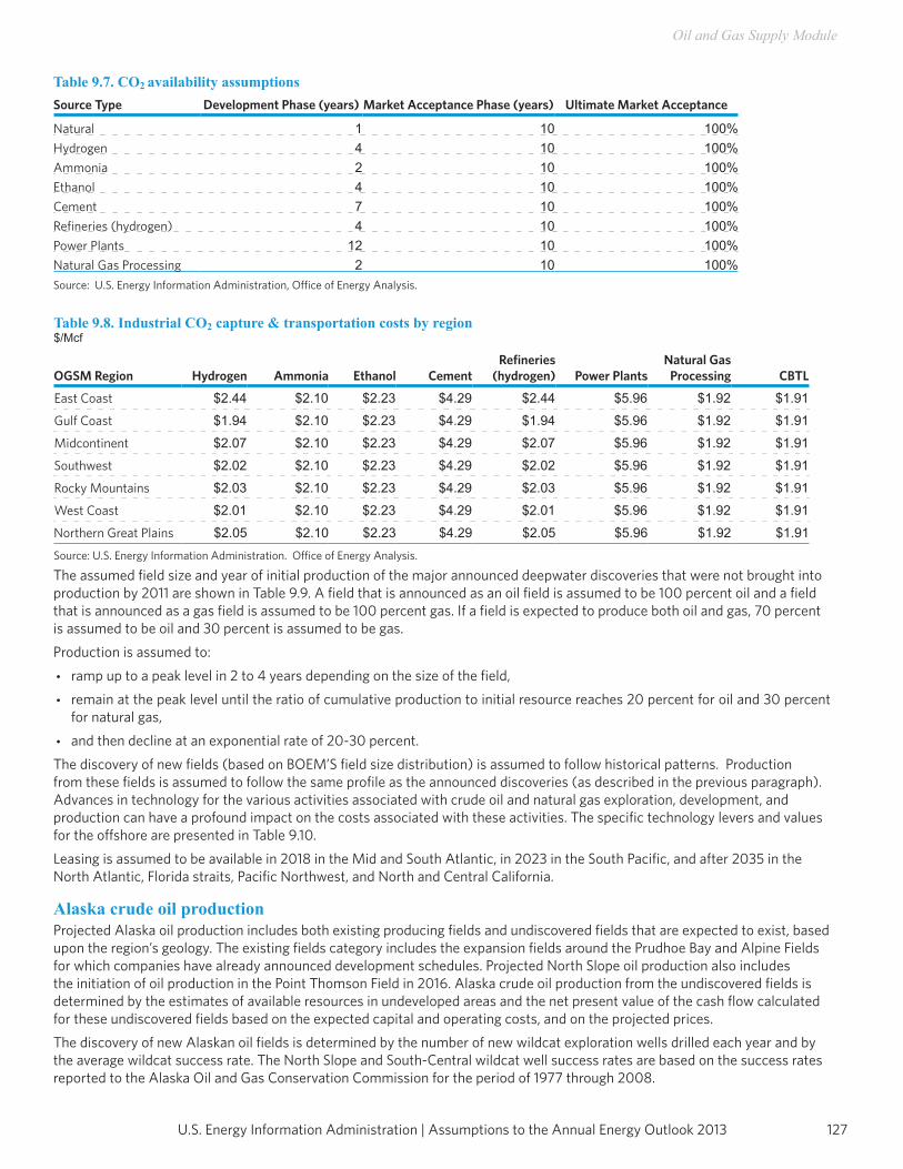
127U.S. Energy Information Administration | Assumptions to the Annual Energy Outlook 2013
Oil and Gas Supply Module
Table 9.7. CO2 availability assumptionsSource Type Development Phase (years) Market Acceptance Phase (years) Ultimate Market Acceptance
Natural 1 10 100%Hydrogen 4 10 100%Ammonia 2 10 100%Ethanol 4 10 100%Cement 7 10 100%Refineries (hydrogen) 4 10 100%Power Plants 12 10 100%Natural Gas Processing 2 10 100%Source: U.S. Energy Information Administration, Office of Energy Analysis.
Table 9.8. Industrial CO2 capture & transportation costs by region$/Mcf
OGSM Region Hydrogen Ammonia Ethanol CementRefineries
(hydrogen) Power PlantsNatural Gas
Processing CBTL
East Coast $2.44 $2.10 $2.23 $4.29 $2.44 $5.96 $1.92 $1.91
Gulf Coast $1.94 $2.10 $2.23 $4.29 $1.94 $5.96 $1.92 $1.91
Midcontinent $2.07 $2.10 $2.23 $4.29 $2.07 $5.96 $1.92 $1.91
Southwest $2.02 $2.10 $2.23 $4.29 $2.02 $5.96 $1.92 $1.91
Rocky Mountains $2.03 $2.10 $2.23 $4.29 $2.03 $5.96 $1.92 $1.91
West Coast $2.01 $2.10 $2.23 $4.29 $2.01 $5.96 $1.92 $1.91
Northern Great Plains $2.05 $2.10 $2.23 $4.29 $2.05 $5.96 $1.92 $1.91
Source: U.S. Energy Information Administration. Office of Energy Analysis.
The assumed field size and year of initial production of the major announced deepwater discoveries that were not brought into production by 2011 are shown in Table 9.9. A field that is announced as an oil field is assumed to be 100 percent oil and a field that is announced as a gas field is assumed to be 100 percent gas. If a field is expected to produce both oil and gas, 70 percent is assumed to be oil and 30 percent is assumed to be gas.Production is assumed to:• ramp up to a peak level in 2 to 4 years depending on the size of the field,• remain at the peak level until the ratio of cumulative production to initial resource reaches 20 percent for oil and 30 percent
for natural gas,• and then decline at an exponential rate of 20-30 percent.The discovery of new fields (based on BOEM’S field size distribution) is assumed to follow historical patterns. Production from these fields is assumed to follow the same profile as the announced discoveries (as described in the previous paragraph). Advances in technology for the various activities associated with crude oil and natural gas exploration, development, and production can have a profound impact on the costs associated with these activities. The specific technology levers and values for the offshore are presented in Table 9.10.Leasing is assumed to be available in 2018 in the Mid and South Atlantic, in 2023 in the South Pacific, and after 2035 in the North Atlantic, Florida straits, Pacific Northwest, and North and Central California.
Alaska crude oil productionProjected Alaska oil production includes both existing producing fields and undiscovered fields that are expected to exist, based upon the region’s geology. The existing fields category includes the expansion fields around the Prudhoe Bay and Alpine Fields for which companies have already announced development schedules. Projected North Slope oil production also includes the initiation of oil production in the Point Thomson Field in 2016. Alaska crude oil production from the undiscovered fields is determined by the estimates of available resources in undeveloped areas and the net present value of the cash flow calculated for these undiscovered fields based on the expected capital and operating costs, and on the projected prices.The discovery of new Alaskan oil fields is determined by the number of new wildcat exploration wells drilled each year and by the average wildcat success rate. The North Slope and South-Central wildcat well success rates are based on the success rates reported to the Alaska Oil and Gas Conservation Commission for the period of 1977 through 2008.
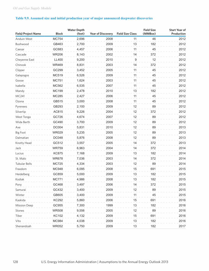
U.S. Energy Information Administration | Assumptions to the Annual Energy Outlook 2013128
Oil and Gas Supply Module
Table 9.9. Assumed size and initial production year of major announced deepwater discoveries
Field/Project Name BlockWater Depth
(feet) Year of Discovery Field Size ClassField Size
(MMBoe)Start Year of
Production
Anduin West MC754 2,696 2008 11 46 2012
Bushwood GB463 2,700 2009 13 182 2012
Caesar GC683 4,457 2006 11 45 2012
Cascade WR206 8,143 2002 14 372 2012
Cheyenne East LL400 9,200 2010 9 12 2012
Chinook WR469 8,831 2003 14 372 2012
Clipper GC299 3,452 2005 11 45 2012
Galapogos MC519 6,526 2009 11 45 2012
Goose MC751 1,624 2003 11 45 2012
Isabella MC562 6,535 2007 11 45 2012
Mandy MC199 2,478 2010 13 182 2012
MC241 MC285 2,427 2006 11 45 2012
Ozona GB515 3,000 2008 11 45 2012
Pyrenees GB293 2,100 2009 12 89 2012
Silvertip AC815 9,226 2004 12 372 2012
West Tonga GC726 4,674 2007 12 89 2012
Wide Berth GC490 3,700 2009 12 89 2012
Axe DC004 5,831 2010 12 89 2013
Big Foot WR029 5,235 2005 12 89 2013
Dalmatian DC048 5,876 2008 12 89 2013
Knotty Head GC512 3,557 2005 14 372 2013
Jack WR759 6,963 2004 14 372 2014
Lucius KC875 7,168 2009 13 182 2014
St. Malo WR678 7,036 2003 14 372 2014
Tubular Bells MC725 4,334 2003 12 89 2014
Freedom MC948 6,095 2008 15 691 2015
Heidelberg GC859 5,000 2009 13 182 2015
Kodiak MC771 4,986 2008 13 182 2015
Pony GC468 3,497 2006 14 372 2015
Samurai GC432 3,400 2009 12 89 2015
Winter GB605 3,400 2009 11 45 2015
Kaskida KC292 5,860 2006 15 691 2016
Mission Deep GC955 7,300 1999 13 182 2016
Stones WR508 9,556 2005 12 89 2016
Tiber KC102 4,132 2009 15 691 2016
Vito MC984 4,038 2009 13 182 2016
Shenandoah WR052 5,750 2009 13 182 2017
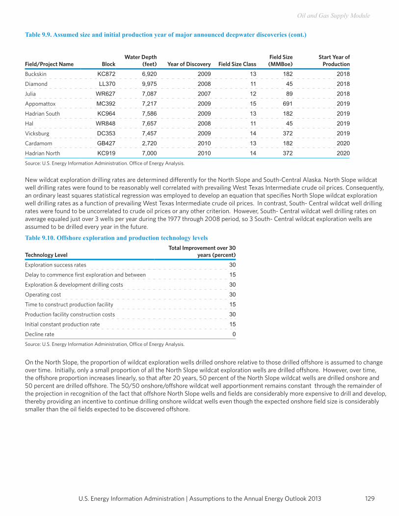
129U.S. Energy Information Administration | Assumptions to the Annual Energy Outlook 2013
Oil and Gas Supply Module
Table 9.9. Assumed size and initial production year of major announced deepwater discoveries (cont.)
Field/Project Name BlockWater Depth
(feet) Year of Discovery Field Size ClassField Size
(MMBoe)Start Year of
Production
Buckskin KC872 6,920 2009 13 182 2018
Diamond LL370 9,975 2008 11 45 2018
Julia WR627 7,087 2007 12 89 2018
Appomattox MC392 7,217 2009 15 691 2019
Hadrian South KC964 7,586 2009 13 182 2019
Hal WR848 7,657 2008 11 45 2019
Vicksburg DC353 7,457 2009 14 372 2019
Cardamom GB427 2,720 2010 13 182 2020
Hadrian North KC919 7,000 2010 14 372 2020
Source: U.S. Energy Information Administration. Office of Energy Analysis.
New wildcat exploration drilling rates are determined differently for the North Slope and South-Central Alaska. North Slope wildcat well drilling rates were found to be reasonably well correlated with prevailing West Texas Intermediate crude oil prices. Consequently, an ordinary least squares statistical regression was employed to develop an equation that specifies North Slope wildcat exploration well drilling rates as a function of prevailing West Texas Intermediate crude oil prices. In contrast, South- Central wildcat well drilling rates were found to be uncorrelated to crude oil prices or any other criterion. However, South- Central wildcat well drilling rates on average equaled just over 3 wells per year during the 1977 through 2008 period, so 3 South- Central wildcat exploration wells are assumed to be drilled every year in the future.
Table 9.10. Offshore exploration and production technology levels
Technology LevelTotal Improvement over 30
years (percent)
Exploration success rates 30
Delay to commence first exploration and between 15
Exploration & development drilling costs 30
Operating cost 30
Time to construct production facility 15
Production facility construction costs 30
Initial constant production rate 15
Decline rate 0
Source: U.S. Energy Information Administration, Office of Energy Analysis.
On the North Slope, the proportion of wildcat exploration wells drilled onshore relative to those drilled offshore is assumed to change over time. Initially, only a small proportion of all the North Slope wildcat exploration wells are drilled offshore. However, over time, the offshore proportion increases linearly, so that after 20 years, 50 percent of the North Slope wildcat wells are drilled onshore and 50 percent are drilled offshore. The 50/50 onshore/offshore wildcat well apportionment remains constant through the remainder of the projection in recognition of the fact that offshore North Slope wells and fields are considerably more expensive to drill and develop, thereby providing an incentive to continue drilling onshore wildcat wells even though the expected onshore field size is considerably smaller than the oil fields expected to be discovered offshore.

U.S. Energy Information Administration | Assumptions to the Annual Energy Outlook 2013130
Oil and Gas Supply Module
The size of the new oil fields discovered by wildcat exploration drilling is based on the expected field sizes of the undiscovered Alaska oil resource base, as determined by the U.S. Geological Survey for the onshore and State offshore regions of Alaska, and by the Bureau of Ocean Energy Management (BOEM) (formerly known as the U.S. Minerals Management Service) for the Federal offshore regions of Alaska. It is assumed that the largest undiscovered oil fields will be found and developed first and in preference to the small and midsize undiscovered fields. As the exploration and discovery process proceeds and as the largest oil fields are discovered and developed, the discovery and development process proceeds to find and develop the next largest set of oil fields. This large to small discovery and development process is predicated on the fact that developing new infrastructure in Alaska, particularly on the North Slope, is an expensive undertaking and that the largest fields enjoy economies of scale, which ake them more profitable and less risky to develop than the smaller fields.Oil and gas exploration and production currently are not permitted in the Arctic National Wildlife Refuge. The projections for Alaska oil and gas production assume that this prohibition remains in effect throughout the projection period.Three uncertainties are associated with the Alaska oil projections. First, whether the heavy oil deposits located on the North Slope, which exceed 20 billion barrels of oil-in-place, will be producible in the foreseeable future at recovery rates exceeding a few percent. Second, the oil production potential of the North Slope shale formations is unknown at this time. Third, the North Slope offshore oil resource potential, especially in the Chukchi Sea, is untested.In June 2011, Alyeska Pipeline Service Company released a report regarding potential operational problems that might occur as Trans-Alaska Pipeline System (TAPS) throughput declines from the current production levels.[6] Although the onset of TAPS low flow problems could begin at around 550,000 barrels per day, absent any mitigation, the severity of the TAPS operational problems is expected to increase significantly as throughput declines. As the types and severity of problems multiplies, the investment required to mitigate those problems is expected to increase significantly. Because of the many and diverse operational problems expected to occur below 350,000 barrels per day of throughput, considerable investment might be required to keep the pipeline operational below this threshold. Thus, North Slope fields are assumed to be shut down, plugged, and abandoned when the following 2 conditions are simultaneously satisfied: 1) TAPS throughput would have to be at or below 350,000 barrels per day and 2) total North Slope oil production revenues would have to be at or below $5.0 billion per year.
Legislation and regulationsThe Outer Continental Shelf Deep Water Royalty Act (Public Law 104-58) gave the Secretary of the Interior the authority to suspend royalty requirements on new production from qualifying leases and required that royalty payments be waived automatically on new leases sold in the 5 years following its November 28, 1995 enactment. The volume of production on which no royalties were due for the 5 years was assumed to be 17.5 million barrels of oil equivalent (BOE) in water depths of 200 to 400 meters, 52.5 million BOE in water depths of 400 to 800 meters, and 87.5 million BOE in water depths greater than 800 meters. In any year during which the arithmetic average of the closing prices on the New York Mercantile Exchange for light sweet crude oil exceeded $28 per barrel or for natural gas exceeded $3.50 per million Btu, any production of crude oil or natural gas was subject to royalties at the lease-stipulated royalty rate. Although automatic relief expired on November 28, 2000, the act provided the Minerals Management Service (MMS) the authority to include royalty suspensions as a feature of leases sold in the future. In September 2000, the MMS issued a set of proposed rules and regulations that provide a framework for continuing deep water royalty relief on a lease-by-lease basis. In the model it is assumed that relief will be granted at roughly the same levels as provided during the first 5 years of the act.Section 345 of the Energy Policy Act of 2005 provides royalty relief for oil and gas production in water depths greater than 400 meters in the Gulf of Mexico from any oil or gas lease sale occurring within 5 years after enactment. The minimum volumes of production with suspended royalty payments are:
(1) 5,000,000 barrels of oil equivalent (BOE) for each lease in water depths of 400 to 800 meters; (2) 9,000,000 BOE for each lease in water depths of 800 to 1,600 meters;(3)12,000,000 BOE for each lease in water depths of 1,600 to 2,000 meters; and(4) 16,000,000 BOE for each lease in water depths greater than 2,000 meters.The water depth categories specified in Section 345 were adjusted to be consistent with the depth categories in the Offshore Oil and Gas Supply Submodule. The suspension volumes are 5,000,000 BOE for leases in water depths of 400 to 800 meters; 9,000,000 BOE for leases in water depths of 800 to 1,600 meters; 12,000,000 BOE for leases in water depths of 1,600 to 2,400 meters; and 16,000,000 for leases in water depths greater than 2,400 meters. Examination of the resources available at 2,000 to 2,400 meters showed that the differences between the depths used in the model and those specified in the bill would not materially affect the model result.
131U.S. Energy Information Administration | Assumptions to the Annual Energy Outlook 2013
Oil and Gas Supply ModuleThe MMS published its final rule on the “Oil and Gas and Sulphur Operations in the Outer Continental Shelf Relief or Reduction in Royalty Rates Deep Gas Provisions” on January 26, 2004, effective March 1, 2004. The rule grants royalty relief for natural gas roduction from wells drilled to 15,000 feet or deeper on leases issued before January 1, 2001, in the shallow waters (less than 200 meters) of the Gulf of Mexico. Production of gas from the completed deep well must begin before 5 years after the effective date of the final rule. The minimum volume of production with suspended royalty payments is 15 billion cubic feet for wells drilled to at least 15,000 feet and 25 billion cubic feet for wells drilled to more than 18,000 feet. In addition, unsuccessful wells drilled to a depth of at least 18,000 feet would receive a royalty credit for 5 billion cubic feet of natural gas. The ruling also grants royalty suspension for volumes of not less than 35 billion cubic feet from ultra-deep wells on leases issued before January 1, 2001.Section 354 of the Energy Policy Act of 2005 established a competitive program to provide grants for cost-shared projects to enhance oil and natural gas recovery through CO2 injection, while at the same time sequestering CO2 produced from the combustion of fossil fuels in power plants and large industrial processes.From 1982 through 2008, Congress did not appropriate funds needed by the MMS to conduct leasing activities on portions of the Federal Outer Continental Shelf (OCS) and thus effectively prohibited leasing. Further, a separate Executive ban in effect since 1990 prohibited leasing through 2012 on the OCS, with the exception of the Western Gulf of Mexico and portions of the Central and Eastern Gulf of Mexico. When combined, these actions prohibited drilling in most offshore regions, including areas along the Atlantic and Pacific coasts, the eastern Gulf of Mexico, and portions of the central Gulf of Mexico. In 2006, the Gulf of Mexico Energy Security Act imposed yet a third ban on drilling through 2022 on tracts in the Eastern Gulf of Mexico that are within 125 miles of Florida, east of a dividing line known as the Military Mission Line, and in the Central Gulf of Mexico within 100 miles of Florida.On July 14, 2008, President Bush lifted the Executive ban and urged Congress to remove the Congressional ban. On September 30, 2008, Congress allowed the Congressional ban to expire. Although the ban through 2022 on areas in the Eastern and Central Gulf of Mexico remains in place, the lifting of the Executive and Congressional bans removed regulatory obstacles to development of the Atlantic and Pacific OCS.
Oil and gas supply alternative casesTight Oil and Shale Gas Resource casesEstimates of technically recoverable tight/shale crude oil and natural gas resources are particularly uncertain and change over time as new information is gained through drilling, production, and technology experimentation. Over the last decade, as more tight/shale formations have gone into production, the estimate of technically recoverable tight oil and shale gas resources has increased. However, these increases in technically recoverable resources embody many assumptions that might not prove to be true over the long term and over the entire tight/shale formation. For example, these resource estimates assume that crude oil and natural gas production rates achieved in a limited portion of the formation are representative of the entire formation, even though neighboring well production rates can vary by as much as a factor of three within the same play. Moreover, the tight/shale formation can vary significantly across the petroleum basin with respect to depth, thickness, porosity, carbon content, pore pressure, clay content, thermal maturity, and water content. Additionally, technological improvements and innovations may allow development of crude oil and natural gas resources that have not been identified yet so are not included in the Reference case. Two cases were developed with alternate crude oil and natural gas resource assumptions. These cases do not represent an upper and lower bound on future domestic oil and natural gas supply but rather provide a framework to examine the impact of higher and lower domestic supply on energy demand, imports, and prices (see ‘Issues in Focus’ articles).High Oil and Gas Resource case. This case is designed to address what might happen if domestic crude oil production continued to increase through the projection period, reaching over 10 million barrels per day. This case includes (1) 100 percent higher estimated ultimate recovery (EUR) per tight oil, tight gas, and shale gas well than in the reference case and a maximum well spacing of 40 acres to reflect the possibility that additional layers of low permeability zones are identified and developed, compared with well spacing that ranges from 20 to 406 acres with an average of 100 acres in the Reference case; (2) kerogen development reaching 135,000 barrels per day by 2025; (3) tight oil development in Alaska increasing the total Alaska TRR by 1.9 billion barrels; and (4) 50 percent higher technically recoverable undiscovered resources in Alaska and the offshore lower 48 states than in the Reference case. A few offshore Alaska fields are assumed to be discovered and thus developed earlier than in the Reference case. The total unproved technically recoverable resources are 557 billion barrels of crude oil and 6,771 trillion cubic feet compared to 197 billion barrels of crude oil and 2,022 trillion cubic feet of dry natural gas in the Reference case. Proved reserves of oil and natural gas are the same in all three cases; 25 billion barrels of crude oil and 305 trillion cubic feet of dry natural gas. Additionally, given the higher natural gas resource in this case, the maximum penetration rate for gas-to-liquids (GTL) was increased to 10 percent per year from a nominal rate of 5 percent per year in the Reference case.

U.S. Energy Information Administration | Assumptions to the Annual Energy Outlook 2013132
Oil and Gas Supply Module
Low Oil and Gas Resource case. In this case, the EUR per tight oil, tight gas, and shale gas well is assumed to be 50 percent lower than in the Reference case, increasing the per-unit cost of developing the resource. The total unproved technically recoverable crude oil resource is decreased to 168 billion barrels and the natural gas resource is decreased to 1500 trillion cubic feet, compared to 197 billion barrels of crude oil and 2,022 trillion cubic feet of natural gas assumed in the Reference case.
Notes and sources[1] The current development of tight oil plays has shifted industry focus and investment away from the development of U.S. oil shale (kerogen) resources. Considerable technological development is required prior to the large-scale in-situ production of oil shale being economically feasible. Consequently, the Oil Shale Supply Submodule assumes that large- scale in-situ oil shale production is not commercially feasible prior to 2040.[2] Technically recoverable resources are resources in accumulations producible using current recovery technology but without reference to economic profitability.[3] Proved reserves are the estimated quantities that analysis of geological and engineering data demonstrate with reasonable certainty to be recoverable in future years from known reservoirs under existing economic and operating conditions.[4] Unproved resources include resources that have been confirmed by exploratory drilling and undiscovered resources, which are located outside oil and gas fields in which the presence of resources has been confirmed by exploratory drilling; they include resources from undiscovered pools within confirmed fields when they occur as unrelated accumulations controlled by distinctly separate structural features or stratigraphic conditions.[5] Donald L. Gautier and others, U.S. Department of the Interior, U.S. Geological Survey, 1995 National Assessment of the United States Oil and Gas Resources, (Washington, D.C., 1995); U.S. Department of the Interior, Minerals Management Service, Report to Congress: Comprehensive Inventory of U.S. OCS Oil and Natural Gas Resources, (February 2006); and 2003 estimates of conventionally recoverable hydrocarbon resources of the Gulf of Mexico and Atlantic Outer Continental Shelf as of January 1, 2003.[6] Alyeska Pipeline Service Company, Low Flow Impact Study, Final Report, June 15, 2011, Anchorage, Alaska, at www.alyeska-pipe.com/Inthenews/LowFlow/LoFIS_Summary_Report_P6%2027_FullReport.pdf

Natural Gas Transmission and Distribution Module

This page inTenTionally lefT blank
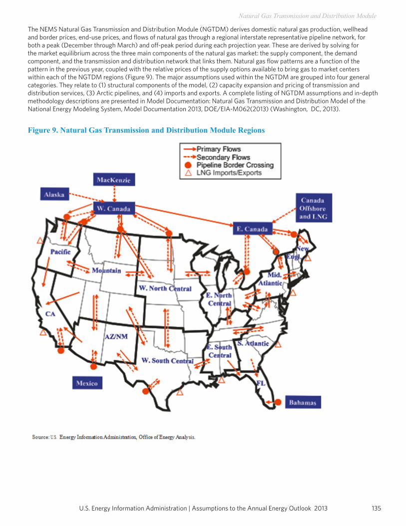
135U.S. Energy Information Administration | Assumptions to the Annual Energy Outlook 2013
Natural Gas Transmission and Distribution Module
The NEMS Natural Gas Transmission and Distribution Module (NGTDM) derives domestic natural gas production, wellhead and border prices, end-use prices, and flows of natural gas through a regional interstate representative pipeline network, for both a peak (December through March) and off-peak period during each projection year. These are derived by solving for the market equilibrium across the three main components of the natural gas market: the supply component, the demand component, and the transmission and distribution network that links them. Natural gas flow patterns are a function of the pattern in the previous year, coupled with the relative prices of the supply options available to bring gas to market centers within each of the NGTDM regions (Figure 9). The major assumptions used within the NGTDM are grouped into four general categories. They relate to (1) structural components of the model, (2) capacity expansion and pricing of transmission and distribution services, (3) Arctic pipelines, and (4) imports and exports. A complete listing of NGTDM assumptions and in-depth methodology descriptions are presented in Model Documentation: Natural Gas Transmission and Distribution Model of the National Energy Modeling System, Model Documentation 2013, DOE/EIA-M062(2013) (Washington, DC, 2013).
Figure 9. Natural Gas Transmission and Distribution Module Regions
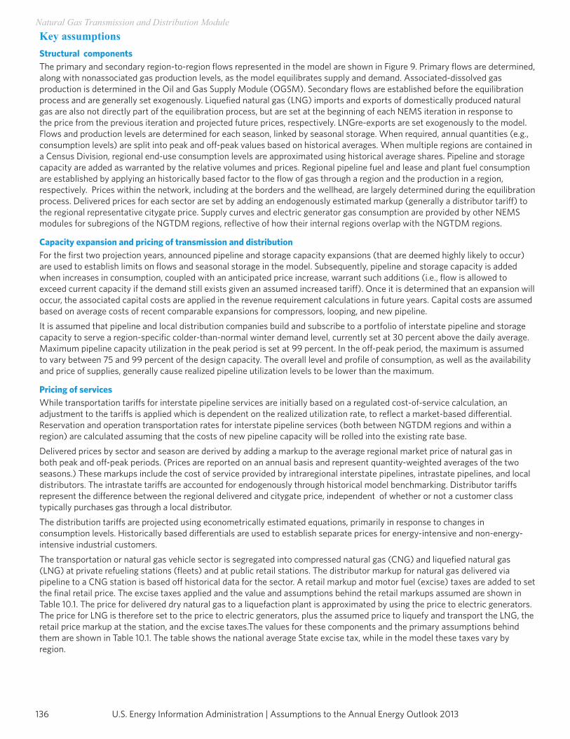
U.S. Energy Information Administration | Assumptions to the Annual Energy Outlook 2013136
Natural Gas Transmission and Distribution ModuleKey assumptionsStructural componentsThe primary and secondary region-to-region flows represented in the model are shown in Figure 9. Primary flows are determined, along with nonassociated gas production levels, as the model equilibrates supply and demand. Associated-dissolved gas production is determined in the Oil and Gas Supply Module (OGSM). Secondary flows are established before the equilibration process and are generally set exogenously. Liquefied natural gas (LNG) imports and exports of domestically produced natural gas are also not directly part of the equilibration process, but are set at the beginning of each NEMS iteration in response to the price from the previous iteration and projected future prices, respectively. LNGre-exports are set exogenously to the model. Flows and production levels are determined for each season, linked by seasonal storage. When required, annual quantities (e.g., consumption levels) are split into peak and off-peak values based on historical averages. When multiple regions are contained in a Census Division, regional end-use consumption levels are approximated using historical average shares. Pipeline and storage capacity are added as warranted by the relative volumes and prices. Regional pipeline fuel and lease and plant fuel consumption are established by applying an historically based factor to the flow of gas through a region and the production in a region, respectively. Prices within the network, including at the borders and the wellhead, are largely determined during the equilibration process. Delivered prices for each sector are set by adding an endogenously estimated markup (generally a distributor tariff) to the regional representative citygate price. Supply curves and electric generator gas consumption are provided by other NEMS modules for subregions of the NGTDM regions, reflective of how their internal regions overlap with the NGTDM regions.
Capacity expansion and pricing of transmission and distributionFor the first two projection years, announced pipeline and storage capacity expansions (that are deemed highly likely to occur) are used to establish limits on flows and seasonal storage in the model. Subsequently, pipeline and storage capacity is added when increases in consumption, coupled with an anticipated price increase, warrant such additions (i.e., flow is allowed to exceed current capacity if the demand still exists given an assumed increased tariff). Once it is determined that an expansion will occur, the associated capital costs are applied in the revenue requirement calculations in future years. Capital costs are assumed based on average costs of recent comparable expansions for compressors, looping, and new pipeline.It is assumed that pipeline and local distribution companies build and subscribe to a portfolio of interstate pipeline and storage capacity to serve a region-specific colder-than-normal winter demand level, currently set at 30 percent above the daily average. Maximum pipeline capacity utilization in the peak period is set at 99 percent. In the off-peak period, the maximum is assumed to vary between 75 and 99 percent of the design capacity. The overall level and profile of consumption, as well as the availability and price of supplies, generally cause realized pipeline utilization levels to be lower than the maximum.
Pricing of servicesWhile transportation tariffs for interstate pipeline services are initially based on a regulated cost-of-service calculation, an adjustment to the tariffs is applied which is dependent on the realized utilization rate, to reflect a market-based differential. Reservation and operation transportation rates for interstate pipeline services (both between NGTDM regions and within a region) are calculated assuming that the costs of new pipeline capacity will be rolled into the existing rate base.Delivered prices by sector and season are derived by adding a markup to the average regional market price of natural gas in both peak and off-peak periods. (Prices are reported on an annual basis and represent quantity-weighted averages of the two seasons.) These markups include the cost of service provided by intraregional interstate pipelines, intrastate pipelines, and local distributors. The intrastate tariffs are accounted for endogenously through historical model benchmarking. Distributor tariffs represent the difference between the regional delivered and citygate price, independent of whether or not a customer class typically purchases gas through a local distributor.The distribution tariffs are projected using econometrically estimated equations, primarily in response to changes in consumption levels. Historically based differentials are used to establish separate prices for energy-intensive and non-energy-intensive industrial customers.The transportation or natural gas vehicle sector is segregated into compressed natural gas (CNG) and liquefied natural gas (LNG) at private refueling stations (fleets) and at public retail stations. The distributor markup for natural gas delivered via pipeline to a CNG station is based off historical data for the sector. A retail markup and motor fuel (excise) taxes are added to set the final retail price. The excise taxes applied and the value and assumptions behind the retail markups assumed are shown in Table 10.1. The price for delivered dry natural gas to a liquefaction plant is approximated by using the price to electric generators. The price for LNG is therefore set to the price to electric generators, plus the assumed price to liquefy and transport the LNG, the retail price markup at the station, and the excise taxes.The values for these components and the primary assumptions behind them are shown in Table 10.1. The table shows the national average State excise tax, while in the model these taxes vary by region.
137U.S. Energy Information Administration | Assumptions to the Annual Energy Outlook 2013
Natural Gas Transmission and Distribution ModuleTable 10.1. Assumptions related to CNG and LNG fuel pricesYear CNG CNG LNG LNG
fl eet retail fl eet retail
Retail markup after dry gas pipeline delivery, with no excise tax (2010$/dge) 0.80 0.93 1.39 1.58
Capacity (dge/day) 1600 1100 4000 4000
Usage (percent of capacity) 80 60 80 60
Capital cost (million 2010$) 0.80 0.5 1.0 1.0
Capital recovery (years) 5 10 5 10
Weighted average cost of capital (rate) 0.10 0.15 0.10 0.15
Operating cost (2010$/dge) 0.34 0.51 0.41 0.59
Charge for liquefying and delivering LNG (2010$/dge -- -- 0.75 0.75
Federal excise tax (nominal$/dge) 0.21 0.21 0.42 0.42
State excise tax (nominal$/dge) 0.15 0.15 0.24 0.24
Fuel loss for liquefying and delivering LNG (percent of input volumes) -- -- 10 10
Fuel loss at station (percent of input volumes) 0 0.5 1.0 2.0
Source: U.S. Energy Information Administration, U.S. Tax Code and State Tax Codes.
Note: dge is diesel-gallon equivalent
Pipelines from arctic areas into AlbertaThe outlook for natural gas production from the North Slope of Alaska is aff ected strongly by its extreme distance from
the necessary infrastructure to transport it to major commercial markets. At present there are three basic options for
commercializing the natural gas that has been produced in association with the Prudhoe Bay oil fi elds and reinjected, and is
therefore relatively low-cost to recover: build a pipeline to the lower 48 states via Alberta, produce and transport the natural
gas as liquid fuel in a gas-to-liquid (GTL) plant, or pipe the natural gas to a seaport, liquefy and ship it overseas. The GTL option
was not considered for AEO2013. Which, if any, of the other two options that is determined within the model to be economically
viable fi rst is assumed to have primary access to the proved, low-cost, reserves on the North Slope and preclude the economic
viability of the other option. The assumptions associated with the LNG option are provided in a later section. The primary
assumptions associated with estimating the cost of North Slope Alaskan gas in Alberta, as well as for Mackenzie Delta gas into
Alberta, are shown in Table 10.2. A calculation is performed to estimate a regulated, levelized tariff for each pipeline. Additional
items are added to account for the wellhead price, treatment costs, pipeline fuel costs, and a risk premium to refl ect the potential
impact on the market price if the pipeline comes on line.
To assess the market value of Alaskan and Mackenzie Valley gas against the lower 48 market, a price diff erential of $0.75 (2011
dollars per Mcf) is assumed between the price in Alberta and the average lower 48 wellhead price. The resulting cost of Alaska
gas, relative to the lower 48 wellhead price, is approximately $6.30 (2011 dollars per Mcf), with some variation across the
projection due to changes in gross domestic product. Construction of an Alaska-to-Alberta pipeline is projected to commence if
the assumed total costs for Alaska gas in the lower 48 States exceed the average lower 48 gas price in each of the previous two
years, on average over the previous fi ve years (with greater weight applied to more recent years), and as expected to average
over the next three years. An adjustment is made if prices were declining over the previous fi ve years. Once the assumed four-
year construction period is complete, expansion can occur if the price exceeds the initial trigger price by $6.87 (2011 dollars
per Mcf). Supplies to fi ll an expanded pipeline are assumed to require new gas wells. When the Alaska-to-Alberta pipeline is
built in the model, additional pipeline capacity is added to bring the gas across the border into the United States. For accounting
purposes, the model assumes that all of the Alaska gas will be consumed in the United States and that suffi cient economical
supplies are available at the North Slope to fi ll the pipeline over the depreciation period.
Natural gas production from the Mackenzie Delta is assumed to be suffi cient to fi ll a pipeline over the projection period should
one be built connecting the area to markets in the south. The basic methodology used to represent the decision to build a
Mackenzie pipeline is similar to the process used for an Alaska-to-lower 48 pipeline, using the primary assumed parameters
listed in Table 10.2.
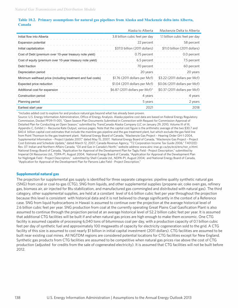
U.S. Energy Information Administration | Assumptions to the Annual Energy Outlook 2013138
Natural Gas Transmission and Distribution Module
Table 10.2. Primary assumptions for natural gas pipelines from Alaska and Mackenzie delta into Alberta, Canada
Alaska to Alberta Mackenzie Delta to Alberta
Initial flow into Alberta 3.8 billion cubic feet per day 1.1 billion cubic feet per day
Expansion potential 22 percent 58 percent
Initial capitalization $37.0 billion (2011 dollars) $11.0 billion (2011 dollars)
Cost of Debt (premium over 10-year treasury note yield) 0.75 percent 0.0 percent
Cost of equity (premium over 10-year treasury note yield) 6.5 percent 7.5 percent
Debt fraction 70 percent 60 percent
Depreciation period 20 years 20 years
Minimum wellhead price (including treatment and fuel costs) $1.76 (2011 dollars per Mcf) $3.22 (2011 dollars per Mcf)
Expected price reduction $1.04 (2011 dollars per Mcf) $0.06 (2011 dollars per Mcf)
Additional cost for expansion $6.87 (2011 dollars per Mcf)* $0.37 (2011 dollars per Mcf)
Construction period 4 years 4 years
Planning period 5 years 2 years
Earliest start year 2021 2018*Includes added cost to explore for and produce natural gas beyond what has already been proven.Source: U.S. Energy Information Administration, Office of Energy Analysis. Alaska pipeline cost data are based on Federal Energy Regulatory Commission, Docket PF09-11-001, “Open Season Plan Documents Submitted in Connection with Request for Commission Approval of Detailed Plan for Conducting an Open Season,” submitted by TransCanada Alaska Company LLC on January 29, 2010, Volume III of III, Appendix C, Exhibit J – Recourse Rate Output, various pages. Note that the capital cost figure is the arithmetic average of the two $30.7 and $40.4 billion capital cost estimates that include the mainline gas pipeline and the gas treatment plant, but which exclude the gas field line from Point Thomson to the gas treatment plant. National Energy Board of Canada, “Mackenzie Gas Project – Hearing Order GH-1-2004, Supplemental Information – Project Update 2007,” dated May 15, 2007; National Energy Board of Canada, “Mackenzie Gas Project – Project Cost Estimate and Schedule Update,” dated March 12, 2007; Canada Revenue Agency, “T2 Corporation Income Tax Guide 2006,” T4012(E)Rev. 07. Indian and Northern Affairs Canada, “Oil and Gas in Canada’s North,” website address www.ainc-inac.gc.ca/ps/ecd/env/nor_e.html. National Energy Board of Canada, “Application for Approval of the Development Plan for Taglu Field - Project Description,” submitted by Imperial Oil Resources Ltd., TDPA-P1, August 2004; National Energy Board of Canada, “Application for Approval of the Development Plan for Niglintgak Field - Project Description,” submitted by Shell Canada Ltd., NDPA-P1, August 2004; and National Energy Board of Canada, “Application for Approval of the Development Plan for Parsons Lake Field - Project Description,”
Supplemental natural gasThe projection for supplemental gas supply is identified for three separate categories: pipeline quality synthetic natural gas (SNG) from coal or coal-to-gas (CTG), SNG from liquids, and other supplemental supplies (propane-air, coke oven gas, refinery gas, biomass air, air injected for Btu stabilization, and manufactured gas commingled and distributed with natural gas). The third category, other supplemental supplies, are held at a constant level of 6.6 billion cubic feet per year throughout the projection because this level is consistent with historical data and it is not believed to change significantly in the context of a Reference case. SNG from liquid hydrocarbons in Hawaii is assumed to continue over the projection at the average historical level of 2.6 billion cubic feet per year. SNG production from coal at the currently operating Great Plains Coal Gasification Plant is also assumed to continue through the projection period at an average historical level of 52.2 billion cubic feet per year. It is assumed that additional CTG facilities will be built if and when natural gas prices are high enough to make them economic. One CTG facility is assumed capable of processing 6,040 tons of bituminous coal per day, with a production capacity of 0.1 billion cubic feet per day of synthetic fuel and approximately 100 megawatts of capacity for electricity cogeneration sold to the grid. A CTG facility of this size is assumed to cost nearly $1 billion in initial capital investment (2011 dollars). CTG facilities are assumed to be built near existing coal mines. All NGTDM regions are considered potential locations for CTG facilities except for New England. Synthetic gas products from CTG facilities are assumed to be competitive when natural gas prices rise above the cost of CTG production (adjusted for credits from the sale of cogenerated electricity). It is assumed that CTG facilities will not be built before 2012.
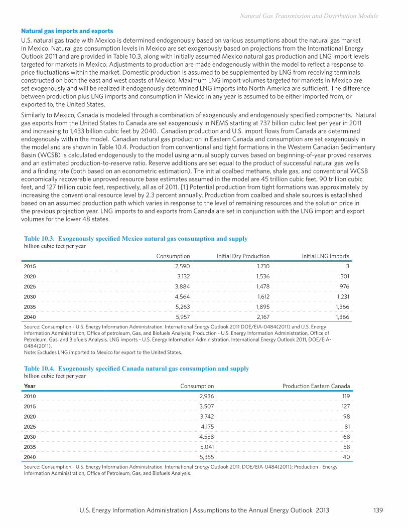
139U.S. Energy Information Administration | Assumptions to the Annual Energy Outlook 2013
Natural Gas Transmission and Distribution Module
Natural gas imports and exportsU.S. natural gas trade with Mexico is determined endogenously based on various assumptions about the natural gas market in Mexico. Natural gas consumption levels in Mexico are set exogenously based on projections from the International Energy Outlook 2011 and are provided in Table 10.3, along with initially assumed Mexico natural gas production and LNG import levels targeted for markets in Mexico. Adjustments to production are made endogenously within the model to reflect a response to price fluctuations within the market. Domestic production is assumed to be supplemented by LNG from receiving terminals constructed on both the east and west coasts of Mexico. Maximum LNG import volumes targeted for markets in Mexico are set exogenously and will be realized if endogenously determined LNG imports into North America are sufficient. The difference between production plus LNG imports and consumption in Mexico in any year is assumed to be either imported from, or exported to, the United States.Similarly to Mexico, Canada is modeled through a combination of exogenously and endogenously specified components. Natural gas exports from the United States to Canada are set exogenously in NEMS starting at 737 billion cubic feet per year in 2011 and increasing to 1,433 billion cubic feet by 2040. Canadian production and U.S. import flows from Canada are determined endogenously within the model. Canadian natural gas production in Eastern Canada and consumption are set exogenously in the model and are shown in Table 10.4. Production from conventional and tight formations in the Western Canadian Sedimentary Basin (WCSB) is calculated endogenously to the model using annual supply curves based on beginning-of-year proved reserves and an estimated production-to-reserve ratio. Reserve additions are set equal to the product of successful natural gas wells and a finding rate (both based on an econometric estimation). The initial coalbed methane, shale gas, and conventional WCSB economically recoverable unproved resource base estimates assumed in the model are 45 trillion cubic feet, 90 trillion cubic feet, and 127 trillion cubic feet, respectively, all as of 2011. [1] Potential production from tight formations was approximately by increasing the conventional resource level by 2.3 percent annually. Production from coalbed and shale sources is established based on an assumed production path which varies in response to the level of remaining resources and the solution price in the previous projection year. LNG imports to and exports from Canada are set in conjunction with the LNG import and export volumes for the lower 48 states.
Table 10.3. Exogenously specified Mexico natural gas consumption and supplybillion cubic feet per year
Consumption Initial Dry Production Initial LNG Imports
2015 2,590 1.710 3
2020 3,132 1,536 501
2025 3,884 1,478 976
2030 4,564 1,612 1,231
2035 5,263 1,895 1,366
2040 5,957 2,167 1,366Source: Consumption - U.S. Energy Information Administration. International Energy Outlook 2011 DOE/EIA-0484(2011) and U.S. Energy Information Administration, Office of petroleum, Gas, and Biofuels Analysis; Production - U.S. Energy Information Administration, Office of Petroleum, Gas, and Biofuels Analysis. LNG imports - U.S. Energy Information Administration, International Energy Outlook 2011, DOE/EIA-0484(2011).Note: Excludes LNG imported to Mexico for export to the United States.
Table 10.4. Exogenously specified Canada natural gas consumption and supplybillion cubic feet per year
Year Consumption Production Eastern Canada
2010 2,936 119
2015 3,507 127
2020 3,742 98
2025 4,175 81
2030 4,558 68
2035 5,041 58
2040 5,355 40Source: Consumption - U.S. Energy Information Administration. International Energy Outlook 2011, DOE/EIA-0484(2011); Production - EnergyInformation Administration, Office of Petroleum, Gas, and Biofuels Analysis.
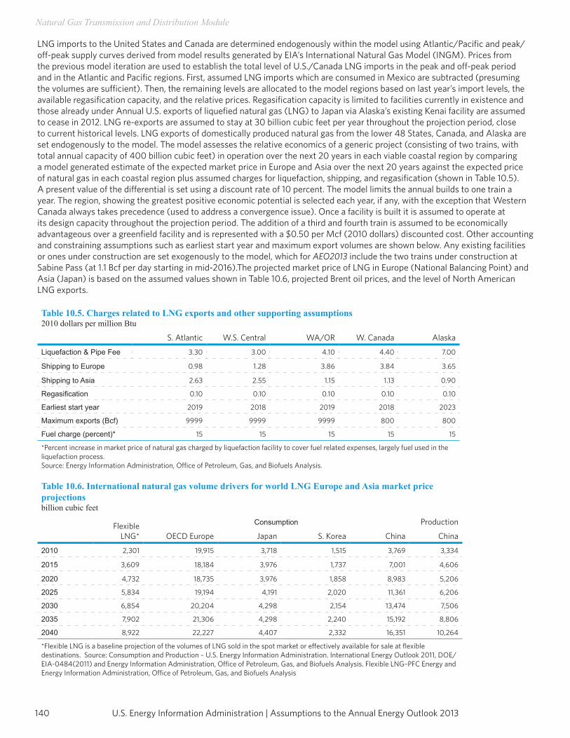
U.S. Energy Information Administration | Assumptions to the Annual Energy Outlook 2013140
Natural Gas Transmission and Distribution Module
LNG imports to the United States and Canada are determined endogenously within the model using Atlantic/Pacific and peak/off-peak supply curves derived from model results generated by EIA’s International Natural Gas Model (INGM). Prices from the previous model iteration are used to establish the total level of U.S./Canada LNG imports in the peak and off-peak period and in the Atlantic and Pacific regions. First, assumed LNG imports which are consumed in Mexico are subtracted (presuming the volumes are sufficient). Then, the remaining levels are allocated to the model regions based on last year’s import levels, the available regasification capacity, and the relative prices. Regasification capacity is limited to facilities currently in existence and those already under Annual U.S. exports of liquefied natural gas (LNG) to Japan via Alaska’s existing Kenai facility are assumed to cease in 2012. LNG re-exports are assumed to stay at 30 billion cubic feet per year throughout the projection period, close to current historical levels. LNG exports of domestically produced natural gas from the lower 48 States, Canada, and Alaska are set endogenously to the model. The model assesses the relative economics of a generic project (consisting of two trains, with total annual capacity of 400 billion cubic feet) in operation over the next 20 years in each viable coastal region by comparing a model generated estimate of the expected market price in Europe and Asia over the next 20 years against the expected price of natural gas in each coastal region plus assumed charges for liquefaction, shipping, and regasification (shown in Table 10.5). A present value of the differential is set using a discount rate of 10 percent. The model limits the annual builds to one train a year. The region, showing the greatest positive economic potential is selected each year, if any, with the exception that Western Canada always takes precedence (used to address a convergence issue). Once a facility is built it is assumed to operate at its design capacity throughout the projection period. The addition of a third and fourth train is assumed to be economically advantageous over a greenfield facility and is represented with a $0.50 per Mcf (2010 dollars) discounted cost. Other accounting and constraining assumptions such as earliest start year and maximum export volumes are shown below. Any existing facilities or ones under construction are set exogenously to the model, which for AEO2013 include the two trains under construction at Sabine Pass (at 1.1 Bcf per day starting in mid-2016).The projected market price of LNG in Europe (National Balancing Point) and Asia (Japan) is based on the assumed values shown in Table 10.6, projected Brent oil prices, and the level of North American LNG exports.
Table 10.5. Charges related to LNG exports and other supporting assumptions2010 dollars per million Btu
S. Atlantic W.S. Central WA/OR W. Canada Alaska
Liquefaction & Pipe Fee 3.30 3.00 4.10 4.40 7.00
Shipping to Europe 0.98 1.28 3.86 3.84 3.65
Shipping to Asia 2.63 2.55 1.15 1.13 0.90
Regasification 0.10 0.10 0.10 0.10 0.10
Earliest start year 2019 2018 2019 2018 2023
Maximum exports (Bcf) 9999 9999 9999 800 800
Fuel charge (percent)* 15 15 15 15 15
*Percent increase in market price of natural gas charged by liquefaction facility to cover fuel related expenses, largely fuel used in the liquefaction process. Source: Energy Information Administration, Office of Petroleum, Gas, and Biofuels Analysis.
Table 10.6. International natural gas volume drivers for world LNG Europe and Asia market price projectionsbillion cubic feet
Flexible LNG*
Consumption Production
OECD Europe Japan S. Korea China China
2010 2,301 19,915 3,718 1,515 3,769 3,334
2015 3,609 18,184 3,976 1,737 7,001 4,606
2020 4,732 18,735 3,976 1,858 8,983 5,206
2025 5,834 19,194 4,191 2,020 11,361 6,206
2030 6,854 20,204 4,298 2,154 13,474 7,506
2035 7,902 21,306 4,298 2,240 15,192 8,806
2040 8,922 22,227 4,407 2,332 16,351 10,264
*Flexible LNG is a baseline projection of the volumes of LNG sold in the spot market or effectively available for sale at flexible destinations. Source: Consumption and Production – U.S. Energy Information Administration. International Energy Outlook 2011, DOE/EIA-0484(2011) and Energy Information Administration, Office of Petroleum, Gas, and Biofuels Analysis. Flexible LNG–PFC Energy and Energy Information Administration, Office of Petroleum, Gas, and Biofuels Analysis

141U.S. Energy Information Administration | Assumptions to the Annual Energy Outlook 2013
Natural Gas Transmission and Distribution Module
Legislation and regulationsThe methodology for setting reservation fees for transportation services is initially based on a regulated rate calculation, but is ultimately consistent with FERC’s alternative ratemaking and capacity release position in that it allows some flexibility in the rates pipelines ultimately charge. The methodology is market-based in that rates for transportation services will respond positively to increased demand for services while rates will decline should the demand for services decline.Section 116 of the Military Construction Appropriations and Emergency Hurricane Supplemental Appropriations Act, 2004 (H.R.4837) gives the Secretary of Energy the authority to issue Federal loan guarantees for an Alaska natural gas transportation project, including the Canadian portion, that would carry natural gas from northern Alaska, through the Canadian border south of 68 degrees north latitude, into Canada, and to the lower 48 States. This authority would expire 2 years after the final certificate of public convenience and necessity is issued. In aggregate the loan guarantee would not exceed: (1) 80 percent of total capital costs (including interest during construction); (2) $18 billion (indexed for inflation at the time of enactment); or (3) a term of 30 years. The Act also promotes streamlined permitting and environmental review, an expedited court review process, and protection of rights-of-way for the pipeline. The assumed costs of borrowing money for the pipeline were reduced to reflect the decreased risk as a result of the loan guarantee.Section 706 of the American Jobs Creation Act of 2004 (H.R.4520) provided a 7-year cost-of-investment recovery period for the Alaska natural gas pipeline, as opposed to the previously allowed 15-year recovery period, for tax purposes. The provision is effective for property placed in service after 2013 (or treated as such) and is assumed to have minimal impact on the decision to build the pipeline.Section 707 of the American Jobs Creation Act extended the 15-percent tax credit previously applied to costs related to enhanced oil recovery to construction costs for a gas treatment plant that supplies natural gas to a 2 trillion Btu per day pipeline, lies in Northern Alaska, and produces carbon dioxide for injection into hydrocarbon-bearing geological formations. A gas treatment plan on the North Slope that feeds gas into an Alaska pipeline to Canada is expected to satisfy this requirement. The provision is effective for costs incurred after 2004. The impact of this tax credit is assumed to be factored into the cost estimates filed by the participating companies.Section 312 of the Energy Policy Act of 2005 authorizes the Federal Energy Regulatory Commission (FERC) to allow natural gas storage facilities to charge market-based rates if it was believed that they would not exert market power. Storage rates are allowed to vary in the model from regulation-based rates, depending on market conditions.
Notes and sources[1] Coalbed, shale gas, and tight sands unproved resource based on the National Energy Board of Canada’s “Canada’s Energy Future: Energy supply and demand projections to 2035,” November 2011.

This page inTenTionally lefT blank

Liquid Fuels Market Module

This page inTenTionally lefT blank
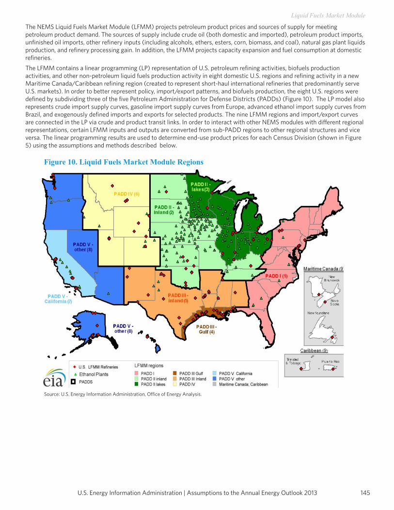
145U.S. Energy Information Administration | Assumptions to the Annual Energy Outlook 2013
Liquid Fuels Market Module
The NEMS Liquid Fuels Market Module (LFMM) projects petroleum product prices and sources of supply for meeting petroleum product demand. The sources of supply include crude oil (both domestic and imported), petroleum product imports, unfinished oil imports, other refinery inputs (including alcohols, ethers, esters, corn, biomass, and coal), natural gas plant liquids production, and refinery processing gain. In addition, the LFMM projects capacity expansion and fuel consumption at domestic refineries.The LFMM contains a linear programming (LP) representation of U.S. petroleum refining activities, biofuels production activities, and other non-petroleum liquid fuels production activity in eight domestic U.S. regions and refining activity in a new Maritime Canada/Caribbean refining region (created to represent short-haul international refineries that predominantly serve U.S. markets). In order to better represent policy, import/export patterns, and biofuels production, the eight U.S. regions were defined by subdividing three of the five Petroleum Administration for Defense Districts (PADDs) (Figure 10). The LP model also represents crude import supply curves, gasoline import supply curves from Europe, advanced ethanol import supply curves from Brazil, and exogenously defined imports and exports for selected products. The nine LFMM regions and import/export curves are connected in the LP via crude and product transit links. In order to interact with other NEMS modules with different regional representations, certain LFMM inputs and outputs are converted from sub-PADD regions to other regional structures and vice versa. The linear programming results are used to determine end-use product prices for each Census Division (shown in Figure 5) using the assumptions and methods described below.
Figure 10. Liquid Fuels Market Module Regions
Source: U.S. Energy Information Administration, Office of Energy Analysis.
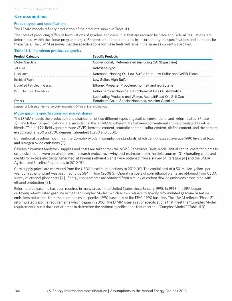
U.S. Energy Information Administration | Assumptions to the Annual Energy Outlook 2013146
Liquid Fuels Market Module
Key assumptionsProduct types and specificationsThe LFMM models refinery production of the products shown in Table 11.1.The costs of producing different formulations of gasoline and diesel fuel that are required by State and Federal regulations are determined within the linear programming (LP) representation of refineries by incorporating the specifications and demands for these fuels. The LFMM assumes that the specifications for these fuels will remain the same as currently specified.
Table 11.1. Petroleum product categoriesProduct Category Specific Products
Motor Gasoline Conventional, Reformulated (including CARB gasoline)
Jet Fuel Kerosene-type
Distillates Kerosene, Heating Oil, Low-Sulfur, Ultra-Low-Sulfur and CARB Diesel
Residual Fuels Low Sulfur, High Sulfur
Liquefied Petroleum Gases Ethane, Propane, Propylene, normal- and iso-Butane
Petrochemical Feedstock Petrochemical Naphtha, Petrochemical Gas Oil, Aromatics
OthersLubricating Products and Waxes, Asphalt/Road Oil, Still GasPetroleum Coke, Special Naphthas, Aviation Gasoline
Source: U.S. Energy Information Administration, Office of Energy Analysis.
Motor gasoline specifications and market sharesThe LFMM models the production and distribution of two different types of gasoline: conventional and reformulated (Phase 2). The following specifications are included in the LFMM to differentiate between conventional and reformulated gasoline blends (Table 11.2): Reid vapor pressure (RVP), benzene content, aromatic content, sulfur content, olefins content, and the percent evaporated at 200 and 300 degrees Fahrenheit (E200 and E300). Conventional gasoline must meet the Complex Model II compliance standards which cannot exceed average 1990 levels of toxic and nitrogen oxide emissions [2].Cellulosic biomass feedstock supplies and costs are taken from the NEMS Renewable Fuels Model. Initial capital costs for biomass cellulosic ethanol were obtained from a research project reviewing cost estimates from multiple sources [3]. Operating costs and credits for excess electricity generated at biomass ethanol plants were obtained from a survey of literature [4] and the USDA Agricultural Baseline Projections to 2019 [5].Corn supply prices are estimated from the USDA baseline projections to 2019 [6]. The capital cost of a 50-million-gallon- per-year corn ethanol plant was assumed to be $84 million (2008 $). Operating costs of corn ethanol plants are obtained from USDA survey of ethanol plant costs [7]. Energy requirements are obtained from a study of carbon dioxide emissions associated with ethanol production [8].Reformulated gasoline has been required in many areas in the United States since January 1995. In 1998, the EPA began certifying reformulated gasoline using the “Complex Model,” which allows refiners to specify reformulated gasoline based on emissions reductions from their companies’ respective 1990 baselines or the EPA’s 1990 baseline. The LFMM reflects “Phase 2” reformulated gasoline requirements which began in 2000. The LFMM uses a set of specifications that meet the “Complex Model” requirements, but it does not attempt to determine the optimal specifications that meet the “Complex Model.” (Table 11.3).
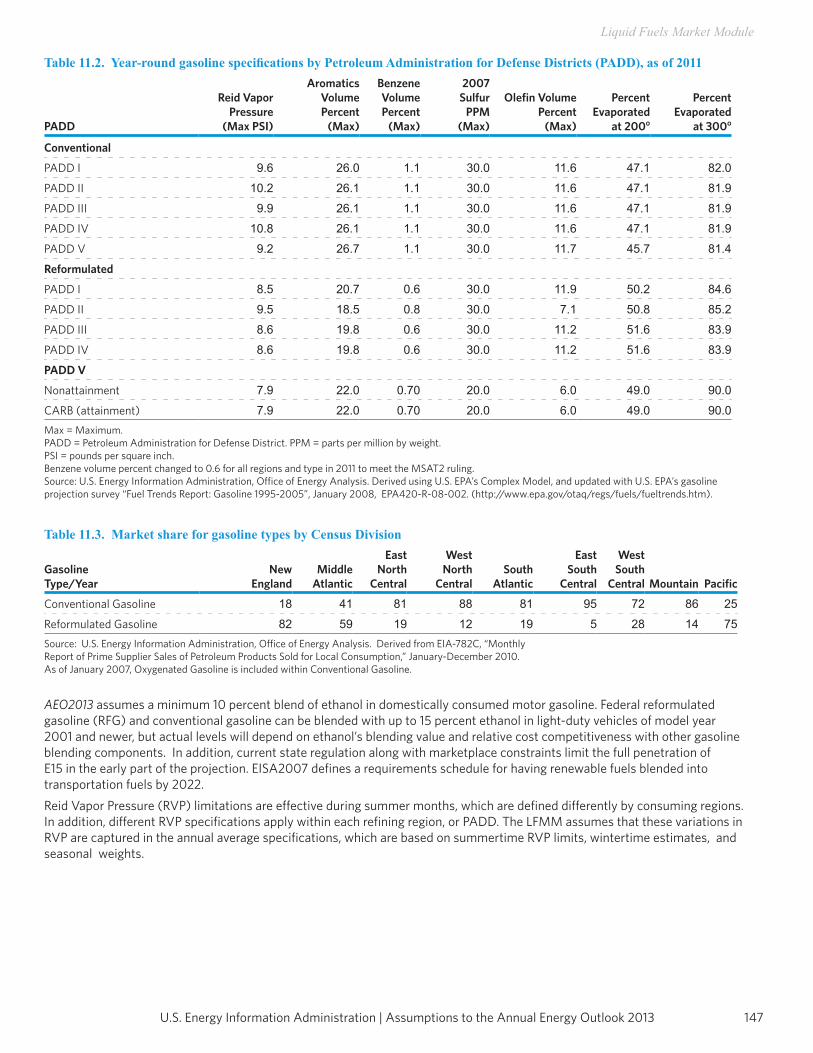
147U.S. Energy Information Administration | Assumptions to the Annual Energy Outlook 2013
Liquid Fuels Market Module
Table 11.2. Year-round gasoline specifications by Petroleum Administration for Defense Districts (PADD), as of 2011
PADD
Reid VaporPressure
(Max PSI)
Aromatics VolumePercent
(Max)
BenzeneVolumePercent
(Max)
2007 Sulfur
PPM(Max)
Olefin VolumePercent
(Max)
PercentEvaporated
at 200o
PercentEvaporated
at 300o
Conventional
PADD I 9.6 26.0 1.1 30.0 11.6 47.1 82.0
PADD II 10.2 26.1 1.1 30.0 11.6 47.1 81.9
PADD III 9.9 26.1 1.1 30.0 11.6 47.1 81.9
PADD IV 10.8 26.1 1.1 30.0 11.6 47.1 81.9
PADD V 9.2 26.7 1.1 30.0 11.7 45.7 81.4
Reformulated
PADD I 8.5 20.7 0.6 30.0 11.9 50.2 84.6
PADD II 9.5 18.5 0.8 30.0 7.1 50.8 85.2
PADD III 8.6 19.8 0.6 30.0 11.2 51.6 83.9
PADD IV 8.6 19.8 0.6 30.0 11.2 51.6 83.9
PADD V
Nonattainment 7.9 22.0 0.70 20.0 6.0 49.0 90.0
CARB (attainment) 7.9 22.0 0.70 20.0 6.0 49.0 90.0Max = Maximum.PADD = Petroleum Administration for Defense District. PPM = parts per million by weight.PSI = pounds per square inch.Benzene volume percent changed to 0.6 for all regions and type in 2011 to meet the MSAT2 ruling.Source: U.S. Energy Information Administration, Office of Energy Analysis. Derived using U.S. EPA’s Complex Model, and updated with U.S. EPA’s gasoline projection survey “Fuel Trends Report: Gasoline 1995-2005”, January 2008, EPA420-R-08-002. (http://www.epa.gov/otaq/regs/fuels/fueltrends.htm).
Table 11.3. Market share for gasoline types by Census Division
GasolineType/Year
New England
Middle Atlantic
EastNorth
Central
WestNorth
CentralSouth
Atlantic
EastSouth
Central
WestSouth
Central Mountain Pacific
Conventional Gasoline 18 41 81 88 81 95 72 86 25
Reformulated Gasoline 82 59 19 12 19 5 28 14 75Source: U.S. Energy Information Administration, Office of Energy Analysis. Derived from EIA-782C, “MonthlyReport of Prime Supplier Sales of Petroleum Products Sold for Local Consumption,” January-December 2010.As of January 2007, Oxygenated Gasoline is included within Conventional Gasoline.
AEO2013 assumes a minimum 10 percent blend of ethanol in domestically consumed motor gasoline. Federal reformulated gasoline (RFG) and conventional gasoline can be blended with up to 15 percent ethanol in light-duty vehicles of model year 2001 and newer, but actual levels will depend on ethanol’s blending value and relative cost competitiveness with other gasoline blending components. In addition, current state regulation along with marketplace constraints limit the full penetration of E15 in the early part of the projection. EISA2007 defines a requirements schedule for having renewable fuels blended into transportation fuels by 2022.Reid Vapor Pressure (RVP) limitations are effective during summer months, which are defined differently by consuming regions. In addition, different RVP specifications apply within each refining region, or PADD. The LFMM assumes that these variations in RVP are captured in the annual average specifications, which are based on summertime RVP limits, wintertime estimates, and seasonal weights.
U.S. Energy Information Administration | Assumptions to the Annual Energy Outlook 2013148
Liquid Fuels Market Module
Within the LFMM, total gasoline demand is disaggregated into demand for conventional and reformulated gasoline by applying assumptions about the annual market shares for each type. In AEO2013 the annual market shares for each region reflect actual 2010 market shares and are held constant throughout the projection. (See Table 11.3 for AEO2013 market share assumptions.)
Diesel fuel specifications and market sharesIn order to account for ultra-low-sulfur diesel (ULSD) regulations related to Clean Air Act Amendments of 1990 (CAAA90), ultra- low-sulfur diesel is differentiated from other distillates. In NEMS, the California portion of the Pacific Region (Census Division 9) is required to meet CARB standards. Both Federal and CARB standards currently limit sulfur to 15 ppm.AEO2013 incorporates the ULSD regulation finalized in December 2000. ULSD is highway diesel that contains no more than 15 ppm sulfur at the pump.Demand for highway-grade diesel is assumed to be equivalent to the total transportation distillate demand. Historically, highway-grade diesel supplies have nearly matched total transportation distillate sales, although some highway-grade diesel has gone to non-transportation uses such as construction and agriculture.AEO2013 incorporates the “nonroad, locomotive, and marine” (NRLM) diesel regulation finalized in May 2004. The final NRLM rule established a new ULSD limit of 15 ppm for nonroad diesel by mid-2010. For locomotive and marine diesel, the rule established an ULSD limit of 15 ppm in mid-2012.
End-Use product pricesEnd-use petroleum product prices are based on marginal costs of production plus production-related fixed costs plus distribution costs and taxes. The marginal costs of production are determined within the LP and represent variable costs of production, including additional costs for meeting reformulated fuels provisions of the CAAA90. Environmental costs associated with controlling pollution at refineries are implicitly assumed in the annual update of the refinery investment costs for the processing units.The costs of distributing and marketing petroleum products are represented by adding product-specific distribution costs to the marginal refinery production costs (product wholesale prices). The distribution costs are derived from a set of base distribution markups (Table 11.4).State and Federal taxes are also added to transportation fuels to determine final end-use prices (Tables 11.5 and 11.6). Recent tax trend analysis indicates that State taxes increase at the rate of inflation, therefore, State taxes are held constant in real terms throughout the projection. This assumption is extended to local taxes which are assumed to average 2 cents per gallon [10]. Federal taxes are assumed to remain at current levels in accordance with the overall AEO2013 assumption of current laws and regulations. Federal taxes are not held constant but deflated as follows:
Federal Tax product, year = Current Federal Tax product /GDP Deflator year
Crude oil qualityIn the LFMM, the quality of crude oil is characterized by average gravity and sulfur levels. Both domestic and imported crude oil are divided into nine categories as defined by the ranges of gravity and sulfur shown in Table 11.7.A “composite” crude oil with the appropriate yields and qualities is developed for each category by averaging the characteristics of specific crude oil streams in the category. In the LFMM, the domestic and foreign categories are the same, and the composite crudes for each category are derived from both domestic and foreign crude characteristics. For domestic crude oil, estimates of total regional production are made first, then shared out to each of the nine categories based on their API gravity and sulfur content. For imported crude oil, a separate supply curve is provided for each category.
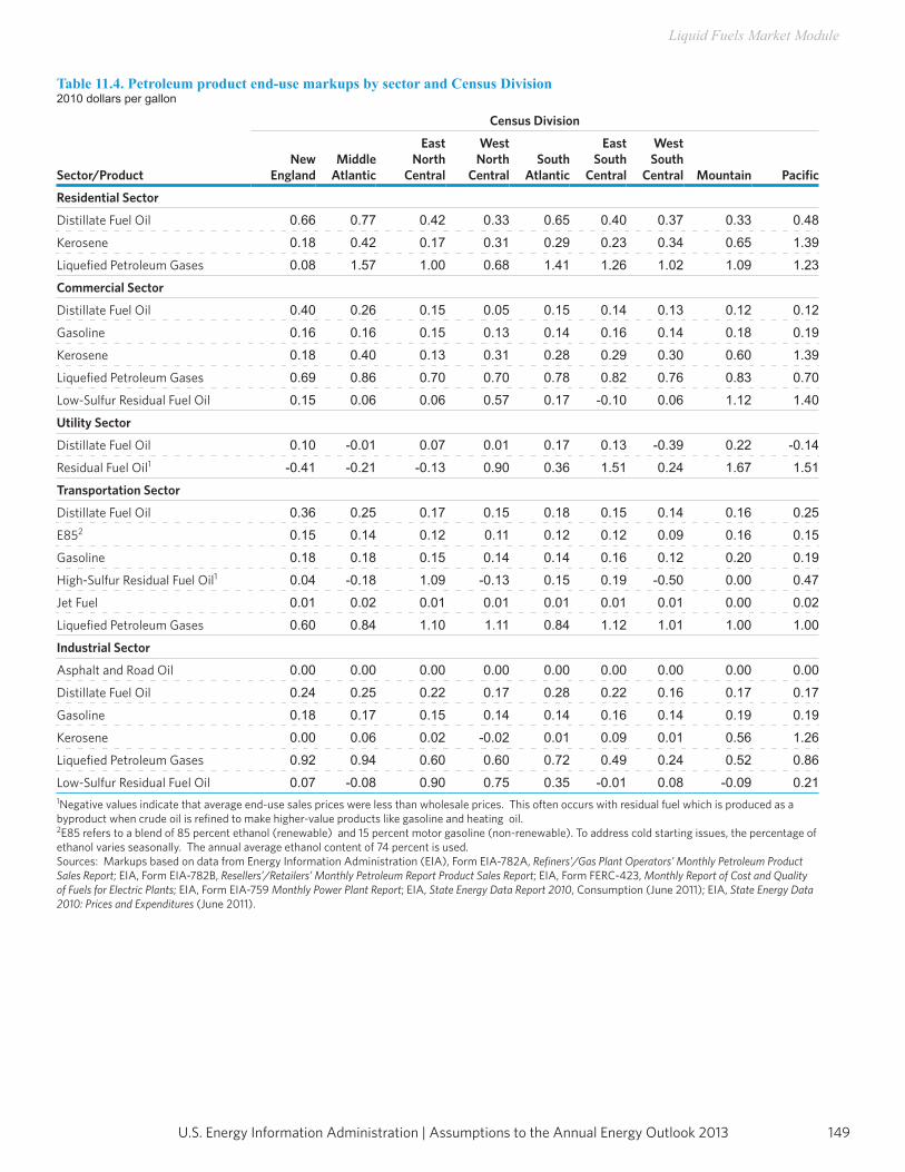
149U.S. Energy Information Administration | Assumptions to the Annual Energy Outlook 2013
Liquid Fuels Market Module
Table 11.4. Petroleum product end-use markups by sector and Census Division2010 dollars per gallon
Sector/Product
Census Division
NewEngland
MiddleAtlantic
EastNorth
Central
WestNorth
CentralSouth
Atlantic
EastSouth
Central
WestSouth
Central Mountain Pacific
Residential Sector
Distillate Fuel Oil 0.66 0.77 0.42 0.33 0.65 0.40 0.37 0.33 0.48
Kerosene 0.18 0.42 0.17 0.31 0.29 0.23 0.34 0.65 1.39
Liquefied Petroleum Gases 0.08 1.57 1.00 0.68 1.41 1.26 1.02 1.09 1.23
Commercial Sector
Distillate Fuel Oil 0.40 0.26 0.15 0.05 0.15 0.14 0.13 0.12 0.12
Gasoline 0.16 0.16 0.15 0.13 0.14 0.16 0.14 0.18 0.19
Kerosene 0.18 0.40 0.13 0.31 0.28 0.29 0.30 0.60 1.39
Liquefied Petroleum Gases 0.69 0.86 0.70 0.70 0.78 0.82 0.76 0.83 0.70
Low-Sulfur Residual Fuel Oil 0.15 0.06 0.06 0.57 0.17 -0.10 0.06 1.12 1.40
Utility Sector
Distillate Fuel Oil 0.10 -0.01 0.07 0.01 0.17 0.13 -0.39 0.22 -0.14
Residual Fuel Oil1 -0.41 -0.21 -0.13 0.90 0.36 1.51 0.24 1.67 1.51
Transportation Sector
Distillate Fuel Oil 0.36 0.25 0.17 0.15 0.18 0.15 0.14 0.16 0.25
E852 0.15 0.14 0.12 0.11 0.12 0.12 0.09 0.16 0.15
Gasoline 0.18 0.18 0.15 0.14 0.14 0.16 0.12 0.20 0.19
High-Sulfur Residual Fuel Oil1 0.04 -0.18 1.09 -0.13 0.15 0.19 -0.50 0.00 0.47
Jet Fuel 0.01 0.02 0.01 0.01 0.01 0.01 0.01 0.00 0.02
Liquefied Petroleum Gases 0.60 0.84 1.10 1.11 0.84 1.12 1.01 1.00 1.00
Industrial Sector
Asphalt and Road Oil 0.00 0.00 0.00 0.00 0.00 0.00 0.00 0.00 0.00
Distillate Fuel Oil 0.24 0.25 0.22 0.17 0.28 0.22 0.16 0.17 0.17
Gasoline 0.18 0.17 0.15 0.14 0.14 0.16 0.14 0.19 0.19
Kerosene 0.00 0.06 0.02 -0.02 0.01 0.09 0.01 0.56 1.26
Liquefied Petroleum Gases 0.92 0.94 0.60 0.60 0.72 0.49 0.24 0.52 0.86
Low-Sulfur Residual Fuel Oil 0.07 -0.08 0.90 0.75 0.35 -0.01 0.08 -0.09 0.211Negative values indicate that average end-use sales prices were less than wholesale prices. This often occurs with residual fuel which is produced as a byproduct when crude oil is refined to make higher-value products like gasoline and heating oil.2E85 refers to a blend of 85 percent ethanol (renewable) and 15 percent motor gasoline (non-renewable). To address cold starting issues, the percentage ofethanol varies seasonally. The annual average ethanol content of 74 percent is used.Sources: Markups based on data from Energy Information Administration (EIA), Form EIA-782A, Refiners’/Gas Plant Operators’ Monthly Petroleum Product Sales Report; EIA, Form EIA-782B, Resellers’/Retailers’ Monthly Petroleum Report Product Sales Report; EIA, Form FERC-423, Monthly Report of Cost and Quality of Fuels for Electric Plants; EIA, Form EIA-759 Monthly Power Plant Report; EIA, State Energy Data Report 2010, Consumption (June 2011); EIA, State Energy Data 2010: Prices and Expenditures (June 2011).
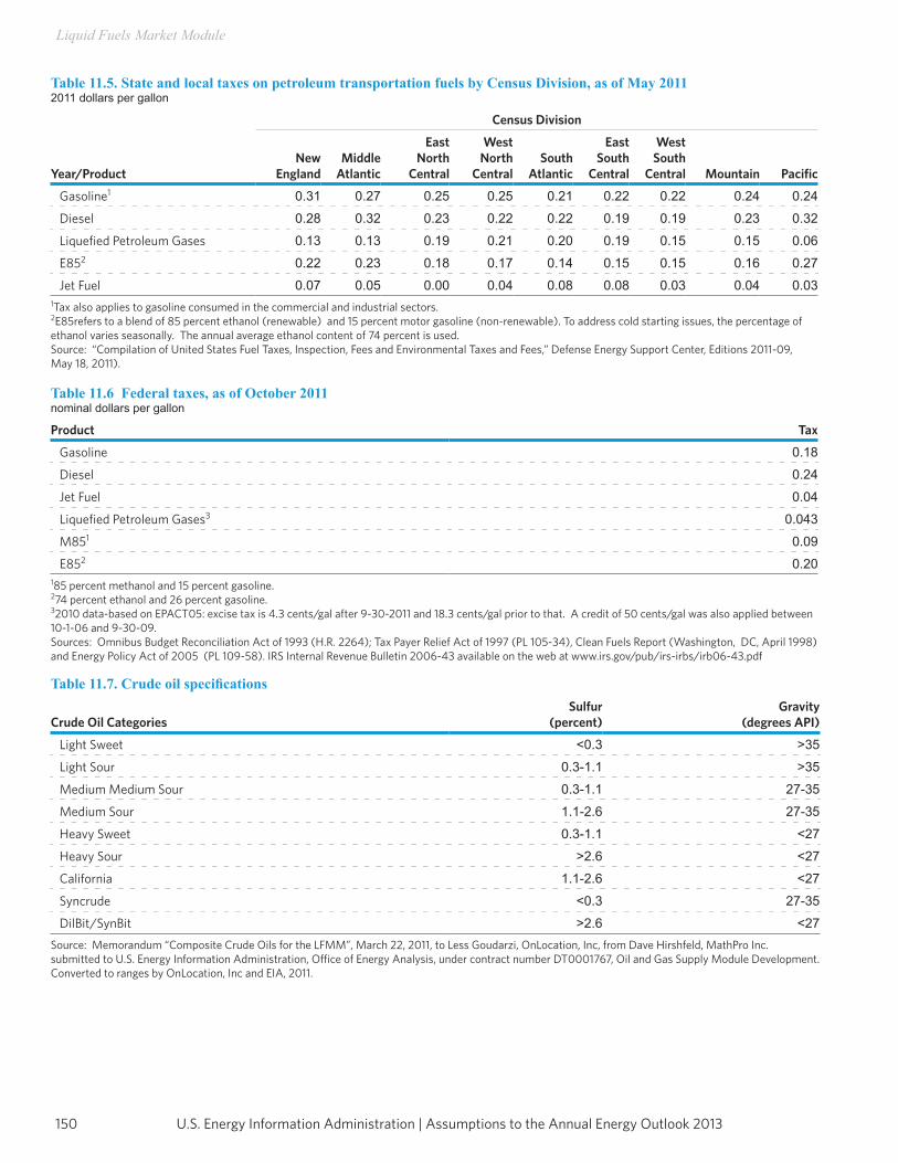
U.S. Energy Information Administration | Assumptions to the Annual Energy Outlook 2013150
Liquid Fuels Market Module
Table 11.5. State and local taxes on petroleum transportation fuels by Census Division, as of May 20112011 dollars per gallon
Year/Product
Census Division
NewEngland
MiddleAtlantic
EastNorth
Central
WestNorth
CentralSouth
Atlantic
EastSouth
Central
WestSouth
Central Mountain Pacific
Gasoline1 0.31 0.27 0.25 0.25 0.21 0.22 0.22 0.24 0.24
Diesel 0.28 0.32 0.23 0.22 0.22 0.19 0.19 0.23 0.32
Liquefied Petroleum Gases 0.13 0.13 0.19 0.21 0.20 0.19 0.15 0.15 0.06
E852 0.22 0.23 0.18 0.17 0.14 0.15 0.15 0.16 0.27
Jet Fuel 0.07 0.05 0.00 0.04 0.08 0.08 0.03 0.04 0.031Tax also applies to gasoline consumed in the commercial and industrial sectors.2E85refers to a blend of 85 percent ethanol (renewable) and 15 percent motor gasoline (non-renewable). To address cold starting issues, the percentage of ethanol varies seasonally. The annual average ethanol content of 74 percent is used.Source: “Compilation of United States Fuel Taxes, Inspection, Fees and Environmental Taxes and Fees,” Defense Energy Support Center, Editions 2011-09, May 18, 2011).
Table 11.6 Federal taxes, as of October 2011nominal dollars per gallon
Product Tax
Gasoline 0.18
Diesel 0.24
Jet Fuel 0.04
Liquefied Petroleum Gases3 0.043
M851 0.09
E852 0.20185 percent methanol and 15 percent gasoline.274 percent ethanol and 26 percent gasoline.32010 data-based on EPACT05: excise tax is 4.3 cents/gal after 9-30-2011 and 18.3 cents/gal prior to that. A credit of 50 cents/gal was also applied between 10-1-06 and 9-30-09.Sources: Omnibus Budget Reconciliation Act of 1993 (H.R. 2264); Tax Payer Relief Act of 1997 (PL 105-34), Clean Fuels Report (Washington, DC, April 1998) and Energy Policy Act of 2005 (PL 109-58). IRS Internal Revenue Bulletin 2006-43 available on the web at www.irs.gov/pub/irs-irbs/irb06-43.pdf
Table 11.7. Crude oil specifications
Crude Oil CategoriesSulfur
(percent)Gravity
(degrees API)
Light Sweet <0.3 >35
Light Sour 0.3-1.1 >35
Medium Medium Sour 0.3-1.1 27-35
Medium Sour 1.1-2.6 27-35
Heavy Sweet 0.3-1.1 <27
Heavy Sour >2.6 <27
California 1.1-2.6 <27
Syncrude <0.3 27-35
DilBit/SynBit >2.6 <27Source: Memorandum “Composite Crude Oils for the LFMM”, March 22, 2011, to Less Goudarzi, OnLocation, Inc, from Dave Hirshfeld, MathPro Inc. submitted to U.S. Energy Information Administration, Office of Energy Analysis, under contract number DT0001767, Oil and Gas Supply Module Development. Converted to ranges by OnLocation, Inc and EIA, 2011.
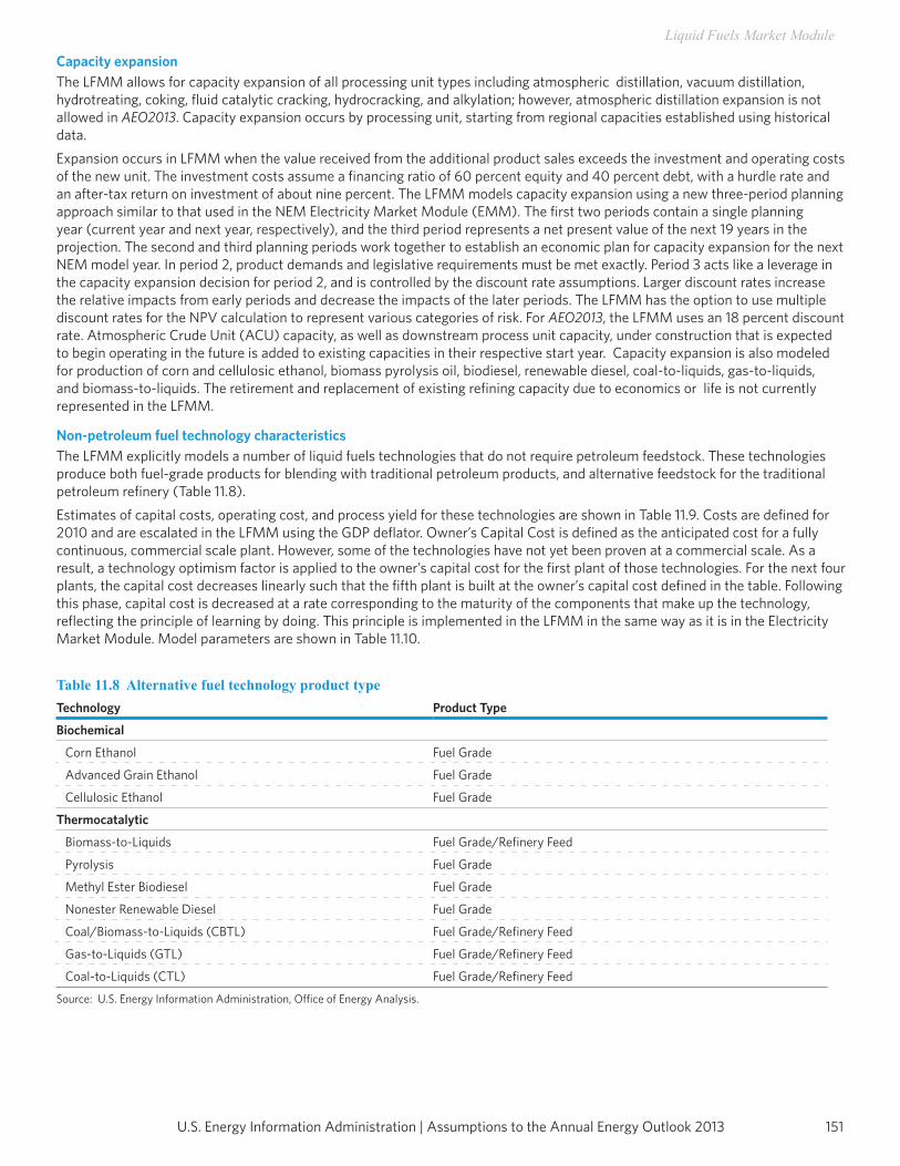
151U.S. Energy Information Administration | Assumptions to the Annual Energy Outlook 2013
Liquid Fuels Market Module
Capacity expansionThe LFMM allows for capacity expansion of all processing unit types including atmospheric distillation, vacuum distillation, hydrotreating, coking, fluid catalytic cracking, hydrocracking, and alkylation; however, atmospheric distillation expansion is not allowed in AEO2013. Capacity expansion occurs by processing unit, starting from regional capacities established using historical data.Expansion occurs in LFMM when the value received from the additional product sales exceeds the investment and operating costs of the new unit. The investment costs assume a financing ratio of 60 percent equity and 40 percent debt, with a hurdle rate and an after-tax return on investment of about nine percent. The LFMM models capacity expansion using a new three-period planning approach similar to that used in the NEM Electricity Market Module (EMM). The first two periods contain a single planning year (current year and next year, respectively), and the third period represents a net present value of the next 19 years in the projection. The second and third planning periods work together to establish an economic plan for capacity expansion for the next NEM model year. In period 2, product demands and legislative requirements must be met exactly. Period 3 acts like a leverage in the capacity expansion decision for period 2, and is controlled by the discount rate assumptions. Larger discount rates increase the relative impacts from early periods and decrease the impacts of the later periods. The LFMM has the option to use multiple discount rates for the NPV calculation to represent various categories of risk. For AEO2013, the LFMM uses an 18 percent discount rate. Atmospheric Crude Unit (ACU) capacity, as well as downstream process unit capacity, under construction that is expected to begin operating in the future is added to existing capacities in their respective start year. Capacity expansion is also modeled for production of corn and cellulosic ethanol, biomass pyrolysis oil, biodiesel, renewable diesel, coal-to-liquids, gas-to-liquids, and biomass-to-liquids. The retirement and replacement of existing refining capacity due to economics or life is not currently represented in the LFMM.
Non-petroleum fuel technology characteristicsThe LFMM explicitly models a number of liquid fuels technologies that do not require petroleum feedstock. These technologies produce both fuel-grade products for blending with traditional petroleum products, and alternative feedstock for the traditional petroleum refinery (Table 11.8).Estimates of capital costs, operating cost, and process yield for these technologies are shown in Table 11.9. Costs are defined for 2010 and are escalated in the LFMM using the GDP deflator. Owner’s Capital Cost is defined as the anticipated cost for a fully continuous, commercial scale plant. However, some of the technologies have not yet been proven at a commercial scale. As a result, a technology optimism factor is applied to the owner’s capital cost for the first plant of those technologies. For the next four plants, the capital cost decreases linearly such that the fifth plant is built at the owner’s capital cost defined in the table. Following this phase, capital cost is decreased at a rate corresponding to the maturity of the components that make up the technology, reflecting the principle of learning by doing. This principle is implemented in the LFMM in the same way as it is in the Electricity Market Module. Model parameters are shown in Table 11.10.
Table 11.8 Alternative fuel technology product typeTechnology Product Type
Biochemical
Corn Ethanol Fuel Grade
Advanced Grain Ethanol Fuel Grade
Cellulosic Ethanol Fuel Grade
Thermocatalytic
Biomass-to-Liquids Fuel Grade/Refinery Feed
Pyrolysis Fuel Grade
Methyl Ester Biodiesel Fuel Grade
Nonester Renewable Diesel Fuel Grade
Coal/Biomass-to-Liquids (CBTL) Fuel Grade/Refinery Feed
Gas-to-Liquids (GTL) Fuel Grade/Refinery Feed
Coal-to-Liquids (CTL) Fuel Grade/Refinery Feed
Source: U.S. Energy Information Administration, Office of Energy Analysis.
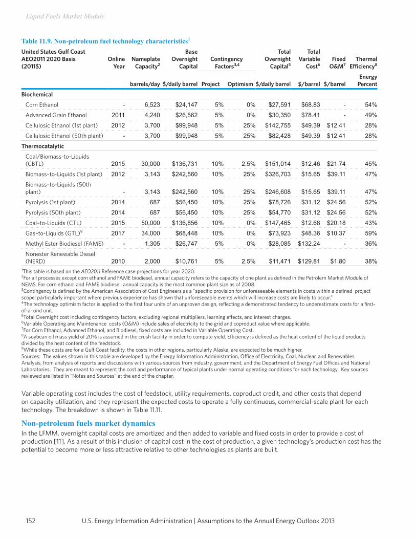
U.S. Energy Information Administration | Assumptions to the Annual Energy Outlook 2013152
Liquid Fuels Market Module
Table 11.9. Non-petroleum fuel technology characteristics1
United States Gulf Coast AEO2011 2020 Basis (2011$)
Online Year
Nameplate Capacity2
Base Overnight
CapitalContingency
Factors3,4
Total Overnight
Capital5
Total Variable
Cost6Fixed
O&M7Thermal
Efficiency8
barrels/day $/daily barrel Project Optimism $/daily barrel $/barrel $/barrelEnergy
Percent
Biochemical
Corn Ethanol - 6,523 $24,147 5% 0% $27,591 $68.83 - 54%
Advanced Grain Ethanol 2011 4,240 $26,562 5% 0% $30,350 $78.41 - 49%
Cellulosic Ethanol (1st plant) 2012 3,700 $99,948 5% 25% $142,755 $49.39 $12.41 28%
Cellulosic Ethanol (50th plant) - 3,700 $99,948 5% 25% $82,428 $49.39 $12.41 28%
Thermocatalytic
Coal/Biomass-to-Liquids (CBTL) 2015 30,000 $136,731 10% 2.5% $151,014 $12.46 $21.74 45%
Biomass–to-Liquids (1st plant) 2012 3,143 $242,560 10% 25% $326,703 $15.65 $39.11 47%
Biomass–to-Liquids (50th plant) - 3,143 $242,560 10% 25% $246,608 $15.65 $39.11 47%
Pyrolysis (1st plant) 2014 687 $56,450 10% 25% $78,726 $31.12 $24.56 52%
Pyrolysis (50th plant) 2014 687 $56,450 10% 25% $54,770 $31.12 $24.56 52%
Coal–to-Liquids (CTL) 2015 50,000 $136,856 10% 0% $147,465 $12.68 $20.18 43%
Gas–to-Liquids (GTL)9 2017 34,000 $68,448 10% 0% $73,923 $48.36 $10.37 59%
Methyl Ester Biodiesel (FAME) - 1,305 $26,747 5% 0% $28,085 $132.24 - 36%
Nonester Renewable Diesel (NERD) 2010 2,000 $10,761 5% 2.5% $11,471 $129.81 $1.80 38%
1This table is based on the AEO2011 Reference case projections for year 2020.2For all processes except corn ethanol and FAME biodiesel, annual capacity refers to the capacity of one plant as defined in the Petrolem Market Module ofNEMS. For corn ethanol and FAME biodiesel, annual capacity is the most common plant size as of 2008.3Contingency is defined by the American Association of Cost Engineers as a “specific provision for unforeseeable elements in costs within a defined project scope; particularly important where previous experience has shown that unforeseeable events which will increase costs are likely to occur.”4The technology optimism factor is applied to the first four units of an unproven design, reflecting a demonstrated tendency to underestimate costs for a first- of-a-kind unit.5Total Overnight cost including contingency factors, excluding regional multipliers, learning effects, and interest charges.6Variable Operating and Maintenance costs (O&M) include sales of electricity to the grid and coproduct value where applicable.7For Corn Ethanol, Advanced Ethanol, and Biodiesel, fixed costs are included in Variable Operating Cost.8A soybean oil mass yield of 20% is assumed in the crush facility in order to compute yield. Efficiency is defined as the heat content of the liquid products divided by the heat content of the feedstock.9While these costs are for a Gulf Coast facility, the costs in other regions, particularly Alaska, are expected to be much higher.Sources: The values shown in this table are developed by the Energy Information Administration, Office of Electricity, Coal, Nuclear, and Renewables Analysis, from analysis of reports and discussions with various sources from industry, government, and the Department of Energy Fuel Offices and National Laboratories. They are meant to represent the cost and performance of typical plants under normal operating conditions for each technology. Key sources reviewed are listed in “Notes and Sources” at the end of the chapter.
Variable operating cost includes the cost of feedstock, utility requirements, coproduct credit, and other costs that depend on capacity utilization, and they represent the expected costs to operate a fully continuous, commercial-scale plant for each technology. The breakdown is shown in Table 11.11.
Non-petroleum fuels market dynamicsIn the LFMM, overnight capital costs are amortized and then added to variable and fixed costs in order to provide a cost of production [11]. As a result of this inclusion of capital cost in the cost of production, a given technology’s production cost has the potential to become more or less attractive relative to other technologies as plants are built.
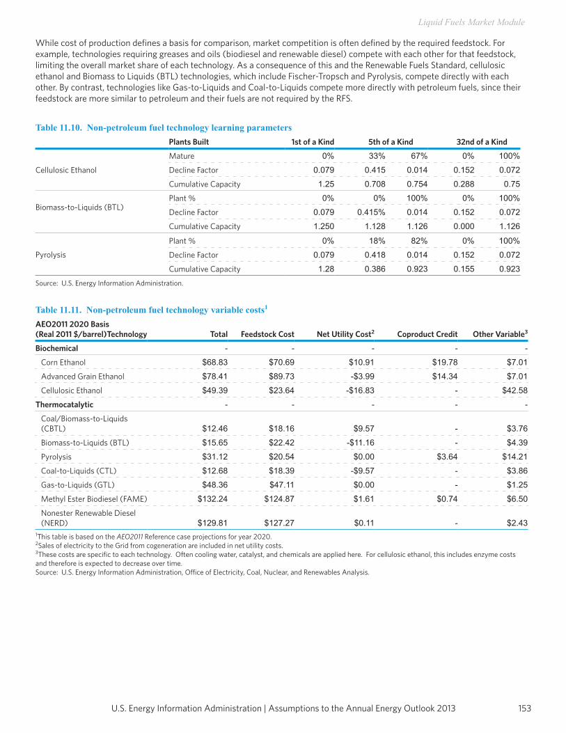
153U.S. Energy Information Administration | Assumptions to the Annual Energy Outlook 2013
Liquid Fuels Market Module
While cost of production defines a basis for comparison, market competition is often defined by the required feedstock. For example, technologies requiring greases and oils (biodiesel and renewable diesel) compete with each other for that feedstock, limiting the overall market share of each technology. As a consequence of this and the Renewable Fuels Standard, cellulosic ethanol and Biomass to Liquids (BTL) technologies, which include Fischer-Tropsch and Pyrolysis, compete directly with each other. By contrast, technologies like Gas-to-Liquids and Coal-to-Liquids compete more directly with petroleum fuels, since their feedstock are more similar to petroleum and their fuels are not required by the RFS.
Table 11.10. Non-petroleum fuel technology learning parametersPlants Built 1st of a Kind 5th of a Kind 32nd of a Kind
Cellulosic Ethanol
Mature 0% 33% 67% 0% 100%
Decline Factor 0.079 0.415 0.014 0.152 0.072
Cumulative Capacity 1.25 0.708 0.754 0.288 0.75
Biomass-to-Liquids (BTL)Plant % 0% 0% 100% 0% 100%
Decline Factor 0.079 0.415% 0.014 0.152 0.072
Cumulative Capacity 1.250 1.128 1.126 0.000 1.126
Pyrolysis
Plant % 0% 18% 82% 0% 100%
Decline Factor 0.079 0.418 0.014 0.152 0.072
Cumulative Capacity 1.28 0.386 0.923 0.155 0.923
Source: U.S. Energy Information Administration.
Table 11.11. Non-petroleum fuel technology variable costs1
AEO2011 2020 Basis (Real 2011 $/barrel)Technology Total Feedstock Cost Net Utility Cost2 Coproduct Credit Other Variable3
Biochemical - - - - -
Corn Ethanol $68.83 $70.69 $10.91 $19.78 $7.01
Advanced Grain Ethanol $78.41 $89.73 -$3.99 $14.34 $7.01
Cellulosic Ethanol $49.39 $23.64 -$16.83 - $42.58
Thermocatalytic - - - - -
Coal/Biomass-to-Liquids (CBTL) $12.46 $18.16 $9.57 - $3.76
Biomass-to-Liquids (BTL) $15.65 $22.42 -$11.16 - $4.39
Pyrolysis $31.12 $20.54 $0.00 $3.64 $14.21
Coal-to-Liquids (CTL) $12.68 $18.39 -$9.57 - $3.86
Gas-to-Liquids (GTL) $48.36 $47.11 $0.00 - $1.25
Methyl Ester Biodiesel (FAME) $132.24 $124.87 $1.61 $0.74 $6.50
Nonester Renewable Diesel (NERD) $129.81 $127.27 $0.11 - $2.43
1This table is based on the AEO2011 Reference case projections for year 2020.2Sales of electricity to the Grid from cogeneration are included in net utility costs.3These costs are specific to each technology. Often cooling water, catalyst, and chemicals are applied here. For cellulosic ethanol, this includes enzyme costs and therefore is expected to decrease over time.Source: U.S. Energy Information Administration, Office of Electricity, Coal, Nuclear, and Renewables Analysis.
U.S. Energy Information Administration | Assumptions to the Annual Energy Outlook 2013154
Liquid Fuels Market Module
Biofuels supplyThe LFMM provides supply functions on an annual basis through 2040 for ethanol produced from corn, non-corn grain, and cellulosic biomass to produce transportation fuel. The LFMM provides supply functions on an annual basis though 2040 for soy oil, other seed-based oils, and grease used as feedstock for biodiesel and renewable diiesel.• Corn feedstock supplies and costs are provided exogenously to NEMS. Feedstock costs reflect credits for co-products (livestock
feed, corn oil, etc.). Feedstock supplies and costs reflect the competition between corn and its co-products and alternative crops, such as soybeans and their co-products.
• Cellulosic (biomass) feedstock supply and costs are provided by the Renewable Fuels Module in NEMS.To model the Renewable Fuels Standard in EISA2007, several assumptions were required.• The penetration of cellulosic ethanol into the market is limited before 2016 to several planned projects with aggregate
nameplace capacity of approximately 250 million gallons per year. Planned capacity through 2016 for Pyrolysis and Biomass-to-Liquids processes is not allowed to exceed 95 million gallons.
• Methyl ester biodiesel production contributes 1.5 credits towards the advanced mandate.• Renewable diesel fuel, including that from Pyrolysis oil, and Fischer-Tropsch diesel contribute 1.7 credits toward the cellulosic
mandate.• Cellulosic drop-in gasoline contributes 1.54 credits toward the cellulosic mandate.• Imported Brazilian sugarcane ethanol counts towards the advanced renewable mandate. Supply curves for sugarcane ethanol
imports allow for substantial penetration by 2022 into the U.S. advanced fuel supply pool, after which sugarcane ethanol remains competitive due to its relatively low production cost, availability, and the expiration of the 54 cents/ gallon import tariff on Jan. 1, 2012.
• Separate biofuel waivers can be activated by the EPA for each of the four RFS fuel categories. In years beyond 2022, the RFS mandate levels continue to increase toward 36 billion gallons
• It is assumed that biodiesel and BTL diesel may be consumed in diesel engines without significant infrastructure modification (either vehicles or delivery infrastructure).
• Ethanol is assumed to be consumed as E10, E15 or E85, with no intermediate blends. The cost of placing E85 pumps at the most economic stations is spread over diesel and gasoline.
• To accommodate the ethanol requirements in particular, transportation modes are expanded or upgraded for E10, E15 and E85, and it is assumed that most ethanol originates from the Midwest, with nominal transportation costs of a few cents per gallon.
• For E85 dispensing stations, it is assumed the average cost of a retrofit and new station is about $45,000 per station.Interregional transportation is assumed to be by rail, ship, barge, and truck, and the associated costs are included in LFMM.
Non-petroleum fossil fuel supplyGas-to-liquids (GTL) facilities convert natural gas into distillates, and are assumed to be built if the prices for lower-sulfur distillates reach a high enough level to make them economic. The earliest start date for a GTL facility is set at 2018. It is also assumed that coal-to-liquids (CTL) facilities will be built when low-sulfur distillate prices are high enough to make them economic. Additionally, a process which allows co-firing of coal with biomass (CBTL) is modeled in the LFMM, but not made available for AEO2013. A 50,000-barrel-per-day CTL facility is assumed to cost about $7 billion in initial capital investment (2009 dollars) while a 30,000-barrel-per-day CBTL facility is expected to cost about $4.4 billion. These facilities could be built near existing refineries. For the East Coast, potential CTL facilities could be built near the Delaware River basin; for the Central region, near the Illinois River basin or near Billings, Montana; and for the West Coast, in the vicinity of Puget Sound in Washington State. It is further assumed that CTL facilities can only be built after 2017.
Combined heat and power (CHP)Electricity consumption at the refinery and other liquid fuels production facilities is a function of the throughput of each unit. Sources of electricity consist of refinery power generation, utility purchases, and CHP from other liquid fuels producers (including cellulosic/advanced ethanol, coal and biomass to liquids). Power generators and CHP plants are modeled in the LFMM linear program as separate units, and are allowed to compete along with purchased electricity. Operating characteristics for these electricity producers are based on historical parameters and available data. Sales to the grid or own use decisions are made on an economic basis within the LP solution. The price for electricity sales to the grid is set to the marginal energy price for baseload generation (provided by the EMM).
155U.S. Energy Information Administration | Assumptions to the Annual Energy Outlook 2013
Liquid Fuels Market Module
Short-term methodologyPetroleum balance and price information for 2012 and 2013 are projected at the U.S. level in the Short-Term Energy Outlook, (STEO). The LFMM adopts the STEO results for 2012 and 2013, using regional estimates derived from the national STEO projections.
Legislation and regulationThe Tax Payer Relief Act of 1997 reduced excise taxes on liquefied petroleum gases and methanol produced from natural gas. The reductions set taxes on these products equal to the Federal gasoline tax on a Btu basis.Title II of CAAA90 established regulations for oxygenated and reformulated gasoline and on-highway diesel fuel. These are explicitly modeled in the LFMM. Reformulated gasoline represented in the LFMM meets the requirements of phase 2 of the Complex Model, except in the Pacific region where it meets CARB 3 specifications.AEO2013 reflects “Tier 2” Motor Vehicle Emissions Standards and Gasoline Sulfur Control Requirements requires that the average annual sulfur content of all gasoline used in the United States be 30 ppm annual average.AEO2013 reflects Heavy-Duty Engine and Vehicle Standards and Highway Diesel Fuel Sulfur Control Requirements. All highway diesel is required to contain no more than 15 ppm sulfur at the pump.AEO2013 reflects nonroad locomotive and marine (NRLM) diesel requirements that nonroad diesel supplies contain no more than 15 ppm sulfur. For locomotive and marine diesel, the action establishes a NRLM limit of 15 ppm in mid-2012.AEO2013 represents major provisions in the Energy Policy Act of 2005 (EPACT05) concerning the petroleum industry, including removal of the oxygenate requirement in RFG.AEO2013 includes provisions outlined in the Energy Independence and Security Act of 2007 (EISA2007) concerning the petroleum industry, including a Renewable Fuels Standard (RFS) increasing total U.S. consumption of renewable fuels. In order to account for the possibility that RFS targets might be unattainable at reasonable cost, LFMM includes a provision for purchase of waivers. In essence, the LFMM RFS waivers function as maximum allowed RIN pricesAEO2013 includes the EPA Mobil Source Air Toxics (MSAT 2) rule which includes the requirement that all gasoline products (including reformulated and conventional gasoline) produced at a refinery during a calendar year will need to contain no more than 0.62 percent benzene by volume. This does not include gasoline produced or sold in California, which is already covered by the current California Phase 3 Reformulated Gasoline Program.AEO2013 includes California’s Low Carbon Fuel Standard which aims to reduce the Carbon Intensity (CI) of gasoline and diesel fuels in that State by about 10% respectively from 2012 through 2020. AEO2013 incorporates the cap-and-trade program within the California Assembly Bill (AB 32), the Global Warming Solutions Act of 2006. The program started January 1, 2012, with enforceable compliance obligations beginning in 2013. Petroleum refineries are given allowances (calculated in the LFMM) in the cap-and-trade system based on the volumetric output of aviation gasoline, motor gasoline, kerosene-type jet fuel, distillate fuel oil, renewable liquid fuels and asphalt. Suppliers of RBOB and Distillate Fuel Oil #1 and #2 are required to comply starting in 2015 if the emissions from full combustion of these products are greater than or equal to 25,000 MTCO2e in any year 2011-2014.AEO2013 does not include mandates passed in 2010 by Connecticut, Maine, New York, and New Jersey that aim to lower the sulfur content of all heating oil to ultra-low-sulfur diesel over different time schedules. Nor does it include transition to a 2% biodiesel content in the case of Maine and Connecticut. These will be added next AEO cycle.Due to the uncertainty surrounding compliance options, AEO2013 did not include any explicit modeling treatment of the International Maritime Organization’s “MARPOL Annex 6” rule covering cleaner marine fuels and ocean ship engine emissions.
Liquids fuels alternative casesLow/no net imports caseIn the reference case, maximum market penetration for gas-to-liquids (GTL) and coal-to-liquids (CTL) was defined at a nominal 5 percent per year. Given the expectation for high net exports in this case, this maximum penetration rate was increased to 10 percent per year. Capacity expansion of biomass pyrolysis production was also allowed to increase beyond the base build level, but at a higher investment cost. In addition, assumptions associated with E85 availability and E15 market penetration were more optimistic, such that E85 availability was nearly three times the reference case level in 2040, and E15 penetration was about 15% higher than the reference case in 2040. Additional changes were made in two NEMS models (OGSM and TDM) resulting in higher domestic crude and natural gas production (described in section “Oil and gas supply alternative cases”, High resource

U.S. Energy Information Administration | Assumptions to the Annual Energy Outlook 2013156
Liquid Fuels Market Module
case), and lower liquid fuels demand. As described in the “Transportation demand alternative cases” section in the TDM chapter, the methodology used to achieve lower demands includes the use of more optimistic assumptions about improvements in LDV fuel economy and reductions in LDV technology costs, lower vehicle miles traveled (VMT) due to changes in consumer behavior, an extension of the LDV CAFE standards beyond 2025 at an average annual rate of 1.4 percent through 2040, expanded market availability of LNG/CNG in heavy-duty trucks, rail and marine, and use of assumptions from the optimistic battery case (AEO2012) for electric vehicle battery and drivetrain costs.
High net imports caseNo changes were made to the LFMM for this scenario. Changes were made in two NEMS models (OGSM and TDM) such that domestic crude production was lowered (described in section “Oil and gas supply alternative cases”, Low resource case), and the domestic liquid fuels demand was increased, as compared to the AEO2013 reference case. As described in the “Transportation demand alternative cases” section in the TDM chapter, an increase in domestic liquids fuels demand was achieve by assuming lower improvement in vehicle efficiency (driven by limits on technology improvement and non-enforcement of CAFE standards), and higher VMT.

157U.S. Energy Information Administration | Assumptions to the Annual Energy Outlook 2013
Liquid Fuels Market Module
Notes and sources[1] U.S. Environmental Protection Agency, “Tier 2” Motor Vehicle Emissions Standards and Gasoline Sulfur Control Requirements, February 2000 (Washington, DC).[2] Federal Register, U.S. Environmental Protection Agency, 40 CFR Part 80, Regulation of Fuels and Fuel Additives: Standards for Reformulated and Conventional Gasoline, Rules and Regulations, p. 7800, (Washington, DC, February 1994).[3] Marano, John, “Alternative Fuels Technology Profile: Cellulosic Ethanol”, March 2008. [4] Ibid.[5] U.S. Department of Agriculture, “USDA Agricultural Baseline Projections to 2019,” February 2009, www.ers.usda.gov/publications/oce091.[6] Ibid[7] Shapouri Hosein; Gallagher, Paul; and Graboski, Mike. USDA’s 1998 Ethanol Cost-of-Production Survey. January 2002.[8] Marland, G. and A.F. Turhollow. 1991. “CO2 Emissions from the Production and Combustion of Fuel Ethanol from Corn.” Energy, 16(11/12):1307-1316.[9] U.S. Environmental Protection Agency, Regulatory Impact Analysis: Heavy-Duty Engine and Vehicle Standards and Highway Diesel Fuel Sulfur Requirements, EPA420-R-00-026 (Washington, DC, December 2000).[10] American Petroleum Institute, How Much We Pay for Gasoline: 1996 Annual Review, May 1997.[11] Economic lifetime is 15 years for cellulosic ethanol, biomass Fischer-Tropsch, and Pyrolysis Oil. It is 20 years for all others. Required rate of return is calculated using a 60:40 debt to equity ratio and the capital asset pricing model for the cost of equity.[12] www.agrievolution.com/atti/brasile_02.ppt.

This page inTenTionally lefT blank

Coal Market Module

This page inTenTionally lefT blank
161U.S. Energy Information Administration | Assumptions to the Annual Energy Outlook 2013
Coal Market Module
The NEMS Coal Market Module (CMM) provides projections of U.S. coal production, consumption, exports, imports, distribution, and prices. The CMM comprises three functional areas: coal production, coal distribution, and coal exports. A detailed description of the CMM is provided in the EIA publication, Coal Market Module of the National Energy Modeling System 2013, DOE/EIA-M060(2013) (Washington, DC, 2013).
Key assumptionsCoal productionThe coal production submodule of the CMM generates a different set of supply curves for the CMM for each year of the projection. Combinations of 14 supply regions, nine coal types (unique groupings of thermal grade and sulfur content), and two mine types (underground and surface), result in 41 separate supply curves. Supply curves are constructed using an econometric formulation that relates the minemouth prices of coal for the supply regions and coal types to a set of independent variables. The independent variables include: capacity utilization of mines, mining capacity, labor productivity, the user cost of capital of mining equipment, the cost of factor inputs (labor and fuel), and other mine supply costs.The key assumptions underlying the coal production modeling are:• As capacity utilization increases, higher minemouth prices for a given supply curve are projected. The opportunity to add
capacity is allowed within the modeling framework if capacity utilization rises to a pre-determined level, typically in the 80 percent range. Likewise, if capacity utilization falls, mining capacity may be retired. The amount of capacity that can be added or retired in a given year depends on the level of capacity utilization, the supply region, and the mining process (underground or surface). The volume of capacity expansion permitted in a projection year is based upon historical patterns of capacity additions.
• Between 1980 and 2000, U.S. coal mining productivity increased at an average rate of 6.6 percent per year, from 1.93 to 6.99 short tons per miner per hour. The major factors underlying these gains were inter-fuel price competition, structural change in the industry, and technological improvements in coal mining. Since 2000, however, growth in overall U.S. coal mining productivity has been negative, declining at a rate of 2.7 percent per year to 5.19 short tons per miner-hour in 2011. By region, productivity in all of the coal producing basins represented in the NEMS Coal Market Module has declined some during the past decade. In the Central Appalachian coal basin, which has been mined extensively, productivity declined by 50 percent between 2000 and 2011, corresponding to an average decline of 6.1 percent per year. While productivity declines have been more moderate at the highly productive mines in Wyoming’s Powder River Basin, overall coal mining productivity still fell by 27 percent between 2000 and 2011, corresponding to an average rate of decline of 2.8percent per year.
• Over the projection period, labor productivity is expected to decline in a number of coal supply regions, reflecting the trend of the previous decade. Higher stripping ratios and the added labor needed to maintain more extensive underground mines offset productivity gains achieved from improved equipment, automation, and technology. Productivity in some areas of the East is projected to decline as operations move from mature coalfields to marginal reserve areas. Regulatory restrictions on surface mines and fragmentation of underground reserves limit the benefits that can be achieved by Appalachian producers from economies of scale.
• In the CMM, different rates of productivity improvement are assumed for each of the 41 coal supply curves used to represent U.S. coal supply. These estimates are based on recent historical data and expectations regarding the penetration and impact of new coal mining technologies [2]. Data on labor productivity are provided on a quarterly and annual basis by individual coal mines and preparation plants on the U.S. Mine Safety and Health Administration’s Form 7000-2, “Quarterly Mine Employment and Coal Production Report” and the U.S. Energy Information Administration’s Form EIA-7A, “Coal Production and Preparation Report”. In the Reference case, overall U.S. coal mining labor productivity declines at rate of 1.4 percent per year between 2011 and 2040. Reference case projections of coal mining productivity by region are provided in Table 12.1.
• In the AEO2013 Reference case, the wage rate for U.S. coal miners increases by 1.0 percent per year and mine equipment costs are assumed to remain constant in 2011 dollars (i.e., increase at the general rate of inflation) over the projection period.
Coal distributionThe coal distribution submodule of the CMM determines the least-cost (minemouth price plus transportation cost) supplies of coal by supply region for a given set of coal demands in each demand sector using a linear programming algorithm. Production and distribution are computed for 14 supply (Figure 11) and 16 demand regions (Figure 12) for 49 demand subsectors. The projected levels of coal-to-liquids, industrial steam, coking, and residential/commercial coal demand are provided by the liquid fuel market, industrial, commercial, and residential demand modules, respectively; electricity coal demands are projected by the EMM; coal imports and coal exports are projected by the CMM based on non-U.S. supply availability, endogenously determined U.S. import demand, and exogenously determined world coal import demands (non-U.S.).
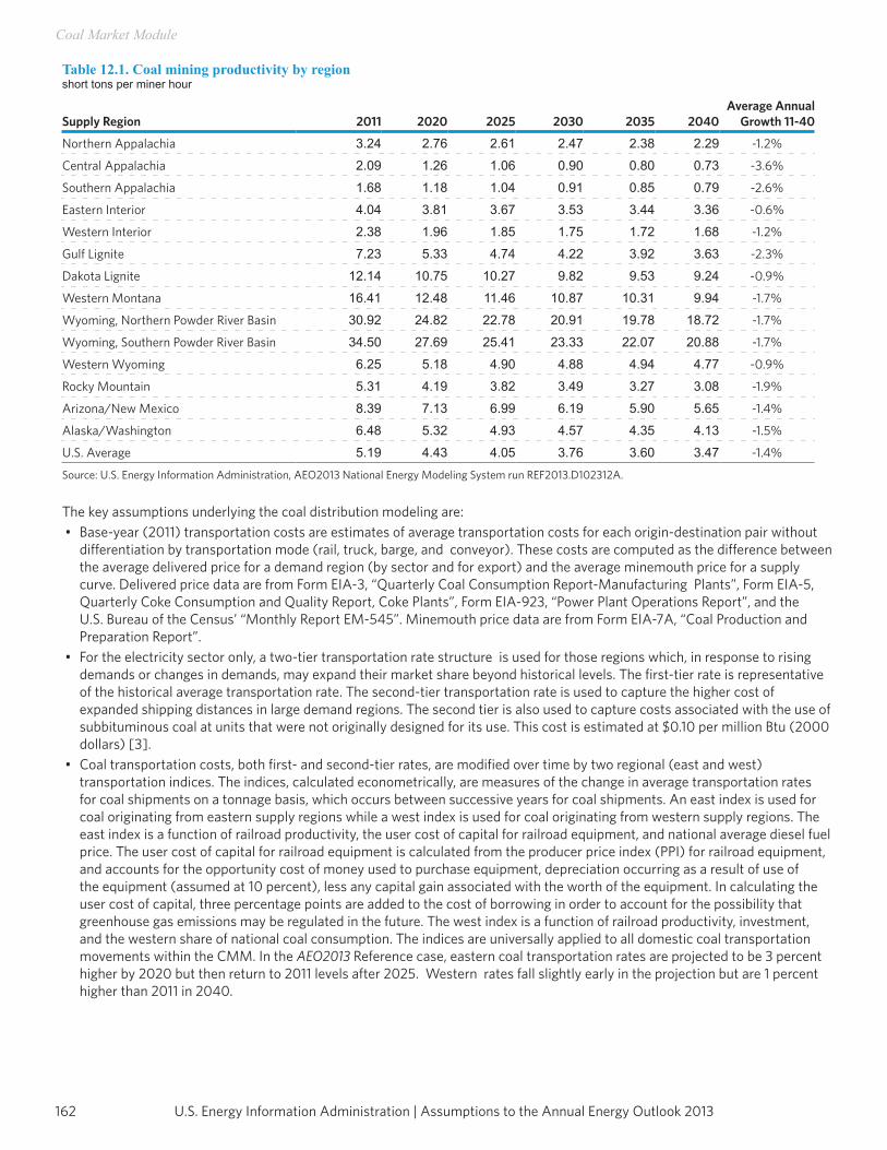
U.S. Energy Information Administration | Assumptions to the Annual Energy Outlook 2013162
Coal Market Module
Table 12.1. Coal mining productivity by regionshort tons per miner hour
Supply Region 2011 2020 2025 2030 2035 2040Average Annual
Growth 11-40
Northern Appalachia 3.24 2.76 2.61 2.47 2.38 2.29 -1.2%
Central Appalachia 2.09 1.26 1.06 0.90 0.80 0.73 -3.6%
Southern Appalachia 1.68 1.18 1.04 0.91 0.85 0.79 -2.6%
Eastern Interior 4.04 3.81 3.67 3.53 3.44 3.36 -0.6%
Western Interior 2.38 1.96 1.85 1.75 1.72 1.68 -1.2%
Gulf Lignite 7.23 5.33 4.74 4.22 3.92 3.63 -2.3%
Dakota Lignite 12.14 10.75 10.27 9.82 9.53 9.24 -0.9%
Western Montana 16.41 12.48 11.46 10.87 10.31 9.94 -1.7%
Wyoming, Northern Powder River Basin 30.92 24.82 22.78 20.91 19.78 18.72 -1.7%
Wyoming, Southern Powder River Basin 34.50 27.69 25.41 23.33 22.07 20.88 -1.7%
Western Wyoming 6.25 5.18 4.90 4.88 4.94 4.77 -0.9%
Rocky Mountain 5.31 4.19 3.82 3.49 3.27 3.08 -1.9%
Arizona/New Mexico 8.39 7.13 6.99 6.19 5.90 5.65 -1.4%
Alaska/Washington 6.48 5.32 4.93 4.57 4.35 4.13 -1.5%
U.S. Average 5.19 4.43 4.05 3.76 3.60 3.47 -1.4%
Source: U.S. Energy Information Administration, AEO2013 National Energy Modeling System run REF2013.D102312A.
The key assumptions underlying the coal distribution modeling are:• Base-year (2011) transportation costs are estimates of average transportation costs for each origin-destination pair without
differentiation by transportation mode (rail, truck, barge, and conveyor). These costs are computed as the difference between the average delivered price for a demand region (by sector and for export) and the average minemouth price for a supply curve. Delivered price data are from Form EIA-3, “Quarterly Coal Consumption Report-Manufacturing Plants”, Form EIA-5, Quarterly Coke Consumption and Quality Report, Coke Plants”, Form EIA-923, “Power Plant Operations Report”, and the U.S. Bureau of the Census’ “Monthly Report EM-545”. Minemouth price data are from Form EIA-7A, “Coal Production and Preparation Report”.
• For the electricity sector only, a two-tier transportation rate structure is used for those regions which, in response to rising demands or changes in demands, may expand their market share beyond historical levels. The first-tier rate is representative of the historical average transportation rate. The second-tier transportation rate is used to capture the higher cost of expanded shipping distances in large demand regions. The second tier is also used to capture costs associated with the use of subbituminous coal at units that were not originally designed for its use. This cost is estimated at $0.10 per million Btu (2000 dollars) [3].
• Coal transportation costs, both first- and second-tier rates, are modified over time by two regional (east and west) transportation indices. The indices, calculated econometrically, are measures of the change in average transportation rates for coal shipments on a tonnage basis, which occurs between successive years for coal shipments. An east index is used for coal originating from eastern supply regions while a west index is used for coal originating from western supply regions. The east index is a function of railroad productivity, the user cost of capital for railroad equipment, and national average diesel fuel price. The user cost of capital for railroad equipment is calculated from the producer price index (PPI) for railroad equipment, and accounts for the opportunity cost of money used to purchase equipment, depreciation occurring as a result of use of the equipment (assumed at 10 percent), less any capital gain associated with the worth of the equipment. In calculating the user cost of capital, three percentage points are added to the cost of borrowing in order to account for the possibility that greenhouse gas emissions may be regulated in the future. The west index is a function of railroad productivity, investment, and the western share of national coal consumption. The indices are universally applied to all domestic coal transportation movements within the CMM. In the AEO2013 Reference case, eastern coal transportation rates are projected to be 3 percent higher by 2020 but then return to 2011 levels after 2025. Western rates fall slightly early in the projection but are 1 percent higher than 2011 in 2040.
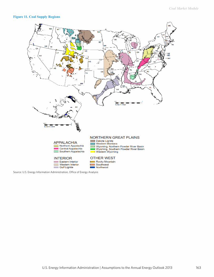
163U.S. Energy Information Administration | Assumptions to the Annual Energy Outlook 2013
Coal Market Module
Figure 11. Coal Supply Regions
Source: U.S. Energy Information Administration, Office of Energy Analysis
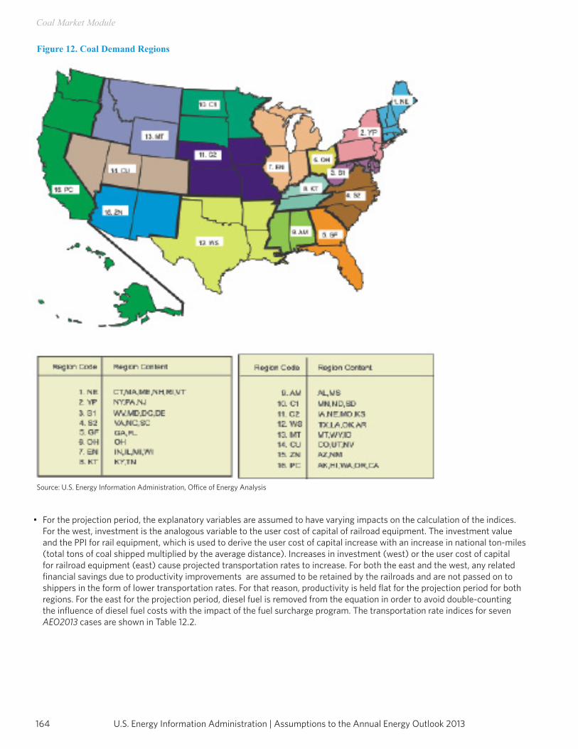
U.S. Energy Information Administration | Assumptions to the Annual Energy Outlook 2013164
Coal Market Module
• For the projection period, the explanatory variables are assumed to have varying impacts on the calculation of the indices.For the west, investment is the analogous variable to the user cost of capital of railroad equipment. The investment value and the PPI for rail equipment, which is used to derive the user cost of capital increase with an increase in national ton-miles (total tons of coal shipped multiplied by the average distance). Increases in investment (west) or the user cost of capital for railroad equipment (east) cause projected transportation rates to increase. For both the east and the west, any related financial savings due to productivity improvements are assumed to be retained by the railroads and are not passed on to shippers in the form of lower transportation rates. For that reason, productivity is held flat for the projection period for both regions. For the east for the projection period, diesel fuel is removed from the equation in order to avoid double-counting the influence of diesel fuel costs with the impact of the fuel surcharge program. The transportation rate indices for seven AEO2013 cases are shown in Table 12.2.
Figure 12. Coal Demand Regions
Source: U.S. Energy Information Administration, Office of Energy Analysis
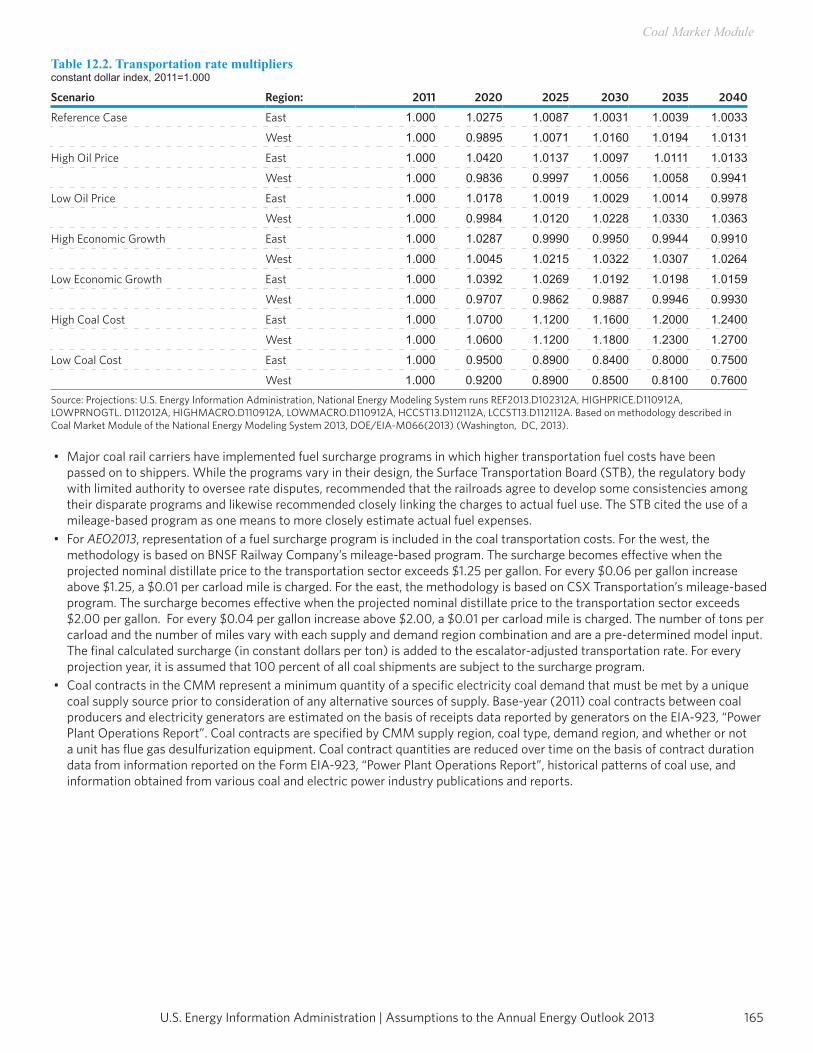
165U.S. Energy Information Administration | Assumptions to the Annual Energy Outlook 2013
Coal Market Module
Table 12.2. Transportation rate multipliersconstant dollar index, 2011=1.000
Scenario Region: 2011 2020 2025 2030 2035 2040
Reference Case East 1.000 1.0275 1.0087 1.0031 1.0039 1.0033
West 1.000 0.9895 1.0071 1.0160 1.0194 1.0131
High Oil Price East 1.000 1.0420 1.0137 1.0097 1.0111 1.0133
West 1.000 0.9836 0.9997 1.0056 1.0058 0.9941
Low Oil Price East 1.000 1.0178 1.0019 1.0029 1.0014 0.9978
West 1.000 0.9984 1.0120 1.0228 1.0330 1.0363
High Economic Growth East 1.000 1.0287 0.9990 0.9950 0.9944 0.9910
West 1.000 1.0045 1.0215 1.0322 1.0307 1.0264
Low Economic Growth East 1.000 1.0392 1.0269 1.0192 1.0198 1.0159
West 1.000 0.9707 0.9862 0.9887 0.9946 0.9930
High Coal Cost East 1.000 1.0700 1.1200 1.1600 1.2000 1.2400
West 1.000 1.0600 1.1200 1.1800 1.2300 1.2700
Low Coal Cost East 1.000 0.9500 0.8900 0.8400 0.8000 0.7500
West 1.000 0.9200 0.8900 0.8500 0.8100 0.7600Source: Projections: U.S. Energy Information Administration, National Energy Modeling System runs REF2013.D102312A, HIGHPRICE.D110912A, LOWPRNOGTL. D112012A, HIGHMACRO.D110912A, LOWMACRO.D110912A, HCCST13.D112112A, LCCST13.D112112A. Based on methodology described in Coal Market Module of the National Energy Modeling System 2013, DOE/EIA-M066(2013) (Washington, DC, 2013).
• Major coal rail carriers have implemented fuel surcharge programs in which higher transportation fuel costs have been passed on to shippers. While the programs vary in their design, the Surface Transportation Board (STB), the regulatory body with limited authority to oversee rate disputes, recommended that the railroads agree to develop some consistencies among their disparate programs and likewise recommended closely linking the charges to actual fuel use. The STB cited the use of a mileage-based program as one means to more closely estimate actual fuel expenses.
• For AEO2013, representation of a fuel surcharge program is included in the coal transportation costs. For the west, the methodology is based on BNSF Railway Company’s mileage-based program. The surcharge becomes effective when the projected nominal distillate price to the transportation sector exceeds $1.25 per gallon. For every $0.06 per gallon increase above $1.25, a $0.01 per carload mile is charged. For the east, the methodology is based on CSX Transportation’s mileage-based program. The surcharge becomes effective when the projected nominal distillate price to the transportation sector exceeds $2.00 per gallon. For every $0.04 per gallon increase above $2.00, a $0.01 per carload mile is charged. The number of tons per carload and the number of miles vary with each supply and demand region combination and are a pre-determined model input. The final calculated surcharge (in constant dollars per ton) is added to the escalator-adjusted transportation rate. For every projection year, it is assumed that 100 percent of all coal shipments are subject to the surcharge program.
• Coal contracts in the CMM represent a minimum quantity of a specific electricity coal demand that must be met by a unique coal supply source prior to consideration of any alternative sources of supply. Base-year (2011) coal contracts between coal producers and electricity generators are estimated on the basis of receipts data reported by generators on the EIA-923, “Power Plant Operations Report”. Coal contracts are specified by CMM supply region, coal type, demand region, and whether or not a unit has flue gas desulfurization equipment. Coal contract quantities are reduced over time on the basis of contract duration data from information reported on the Form EIA-923, “Power Plant Operations Report”, historical patterns of coal use, and information obtained from various coal and electric power industry publications and reports.
U.S. Energy Information Administration | Assumptions to the Annual Energy Outlook 2013166
Coal Market Module
• Coal-to-liquids (CTL) facilities are assumed to be economic when low-sulfur distillate prices reach high enough levels. These plants are assumed to be co-production facilities with generation capacity of 845 MW (300 MW for the grid and 545 MW to support the conversion process) and the capability of producing 50,000 barrels of liquid fuels per day. The technology assumed is similar to an integrated gasification combined cycle, first converting the coal feedstock to gas, and then subsequently converting the syngas to liquid hydrocarbons using the Fisher-Tropsch process. Of the total amount of coal consumed at each plant, 46 percent of the energy input is retained in the product with the remaining energy used for conversion and for the production of power sold to the grid. For AEO2013, coal-biomass-to-liquids (CBTL) are not modeled. CTL facilities produce paraffinic naptha used in plastics production and blendable naptha used in motor gasoline (together about 43 percent of the total by volume) and distillate fuel oil (about 57 percent).
Coal imports and exportsCoal imports and exports are modeled as part of the CMM’s linear program that provides annual projections of U.S. steam and metallurgical coal exports, in the context of world coal trade. The CMM projects steam and metallurgical coal trade flows from 17 coal-exporting regions of the world to 20 import regions for three coal types (coking, bituminous steam, and subbituminous). It includes five U.S. export regions and four U.S. import regions. The linear program determines the pattern of world coal trade flows that minimize the production and transportation costs of meeting U.S. import demand and a pre-specified set of regional world coal import demands. It does this subject to constraints on export capacity and trade flows. The key assumptions underlying coal export modeling are:• Coal buyers (importing regions) tend to spread their purchases among several suppliers in order to reduce the impact of
potential supply disruptions, even though this may add to their purchase costs. Similarly, producers choose not to rely on any one buyer and instead endeavor to diversify their sales.
• Coking coal is treated as homogeneous. The model does not address quality parameters that define coking coals. The values of these quality parameters are defined within small ranges and affect world coking coal flows very little.
The data inputs for coal trade modeling are:• World steam and metallurgical coal import demands for the AEO2013 cases are shown in Tables 12.3 and 12.4. U.S. coal
exports are determined, in part, by these estimates of world coal import demand. • Step-function coal export supply curves for all non-U.S. supply regions. The curves provide estimates of export prices per
metric ton, inclusive of minemouth and inland freight costs, as well as the capacities for each of the supply steps.• Ocean transportation rates (in dollars per metric ton) for feasible coal shipments between international supply regions and
international demand regions. The rates take into account typical vessel sizes and route distances in thousands of nautical miles between supply and demand regions.
Coal qualityEach year the values of base year coal production, heat, sulfur and mercury content and carbon dioxide emissions for each coal source in CMM are calibrated to survey data. Surveys used for this purpose are the Form EIA-923, a survey of the origin, cost and quality of fossil fuels delivered to generating facilities, the Form EIA-3, which records the origin, cost, and quality of coal delivered to U.S. manufacturers, transformation and processing plants, and commercial and institutional users, and the Form EIA-5, which records the origin, cost and quality of coal delivered to domestic industrial consumers. Estimates of coal quality for the export and residential/commercial sectors aremade using the survey data for coal delivered to coking coal and industrial steam coal consumers. Mercury content data for coal by supply region and coal type, in units of pounds of mercury per trillion Btu, shown in Table 71, were derived from shipment- level data reported by electricity generators to the Environmental Protection Agency in its 1999 Information Collection Request. Carbon dioxide emission factors for each coal type are shown in Table 12.5 in pounds of carbon dioxide emitted per million Btu [4].
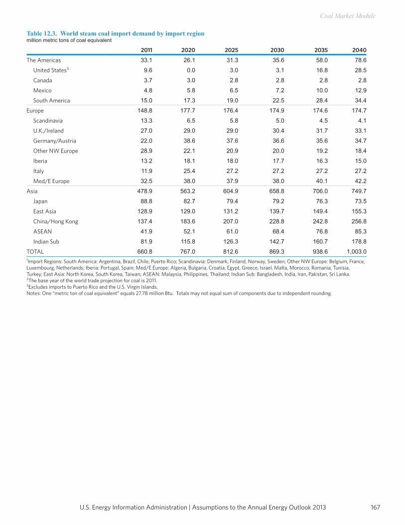
167U.S. Energy Information Administration | Assumptions to the Annual Energy Outlook 2013
Coal Market Module
Table 12.3. World steam coal import demand by import regionmillion metric tons of coal equivalent
2011 2020 2025 2030 2035 2040
The Americas 33.1 26.1 31.3 35.6 58.0 78.6
United States3 9.6 0.0 3.0 3.1 16.8 28.5
Canada 3.7 3.0 2.8 2.8 2.8 2.8
Mexico 4.8 5.8 6.5 7.2 10.0 12.9
South America 15.0 17.3 19.0 22.5 28.4 34.4
Europe 148.8 177.7 176.4 174.9 174.6 174.7
Scandinavia 13.3 6.5 5.8 5.0 4.5 4.1
U.K./Ireland 27.0 29.0 29.0 30.4 31.7 33.1
Germany/Austria 22.0 38.6 37.6 36.6 35.6 34.7
Other NW Europe 28.9 22.1 20.9 20.0 19.2 18.4
Iberia 13.2 18.1 18.0 17.7 16.3 15.0
Italy 11.9 25.4 27.2 27.2 27.2 27.2
Med/E Europe 32.5 38.0 37.9 38.0 40.1 42.2
Asia 478.9 563.2 604.9 658.8 706.0 749.7
Japan 88.8 82.7 79.4 79.2 76.3 73.5
East Asia 128.9 129.0 131.2 139.7 149.4 155.3
China/Hong Kong 137.4 183.6 207.0 228.8 242.8 256.8
ASEAN 41.9 52.1 61.0 68.4 76.8 85.3
Indian Sub 81.9 115.8 126.3 142.7 160.7 178.8
TOTAL 660.8 767.0 812.6 869.3 938.6 1,003.01Import Regions: South America: Argentina, Brazil, Chile, Puerto Rico; Scandinavia: Denmark, Finland, Norway, Sweden; Other NW Europe: Belgium, France, Luxembourg, Netherlands; Iberia: Portugal, Spain; Med/E Europe: Algeria, Bulgaria, Croatia, Egypt, Greece, Israel, Malta, Morocco, Romania, Tunisia,Turkey; East Asia: North Korea, South Korea, Taiwan; ASEAN: Malaysia, Philippines, Thailand; Indian Sub: Bangladesh, India, Iran, Pakistan, Sri Lanka. 2The base year of the world trade projection for coal is 2011.3Excludes imports to Puerto Rico and the U.S. Virgin Islands.Notes: One “metric ton of coal equivalent” equals 27.78 million Btu. Totals may not equal sum of components due to independent rounding.
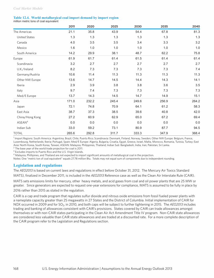
U.S. Energy Information Administration | Assumptions to the Annual Energy Outlook 2013168
Coal Market Module
Table 12.4. World metallurgical coal import demand by import regionmillion metric tons of coal equivalent
2011 2020 2025 2030 2035 2040
The Americas 21.1 35.8 43.9 54.4 67.8 81.3
United States 1.3 1.3 1.3 1.3 1.3 1.3
Canada 4.0 3.5 3.5 3.4 3.3 3.2
Mexico 1.6 1.0 1.0 1.0 1.0 1.0
South America 14.2 29.9 38.1 48.7 62.2 75.8
Europe 61.9 61.7 61.4 61.5 61.4 61.4
Scandinavia 3.2 2.7 2.7 2.7 2.7 2.7
U.K./Ireland 8.2 7.3 7.3 7.3 7.3 7.4
Germany/Austria 10.6 11.4 11.3 11.3 11.3 11.3
Other NW Europe 13.6 14.7 14.5 14.4 14.3 14.1
Iberia 2.9 3.9 3.8 3.8 3.6 3.5
Italy 9.7 7.4 7.3 7.3 7.3 7.3
Med/E Europe 13.7 14.3 14.5 14.7 14.9 15.1
Asia 171.0 232.2 245.4 249.6 256.9 264.2
Japan 72.1 74.8 70.9 64.1 61.2 58.3
East Asia 38.7 37.3 38.5 39.6 40.8 42.0
China/Hong Kong 27.2 60.9 62.9 65.0 67.2 69.4
ASEAN4 0.0 0.0 0.0 0.0 0.0 0.0
Indian Sub 33.0 59.2 73.1 80.9 87.7 94.5
TOTAL 265.6 292.8 311.7 333.3 347.9 368.41 Import Regions: South America: Argentina, Brazil, Chile, Puerto Rico; Scandinavia: Denmark, Finland, Norway, Sweden; Other NW Europe: Belgium, France, Luxembourg, Netherlands; Iberia: Portugal, Spain; Med/E Europe: Algeria, Bulgaria, Croatia, Egypt, Greece, Israel, Malta, Morocco, Romania, Tunisia, Turkey; East Asia: North Korea, South Korea, Taiwan; ASEAN: Malaysia, Philippines, Thailand; Indian Sub: Bangladesh, India, Iran, Pakistan, Sri Lanka. 2 The base year of the world trade projection for coal is 2011. 3 Excludes imports to Puerto Rico and the U.S. Virgin Islands. 4 Malaysia, Phillipines, and Thailand are not expected to import significant amounts of metallurgical coal in the projection. Notes: One “metric ton of coal equivalent” equals 27.78 million Btu. Totals may not equal sum of components due to independent rounding.
Legislation and regulationsThe AEO2013 is based on current laws and regulations in effect before October 31, 2012. The Mercury Air Toxics Standard MATS), finalized in December 2011, is included in the AEO2013 Reference case as well as the Clean Air Interstate Rule (CAIR).
MATS sets emissions limits for mercury, other heavy metals, and acid gases from coal and oil power plants that are 25 MW or greater. Since generators are expected to request one-year extensions for compliance, MATS is assumed to be fully in place by 2016 rather than 2015 as stated in the regulation.CAIR is a cap and trade program that regulates sulfur dioxide and nitrous oxide emissions from fossil fueled power plants with a nameplate capacity greater than 25 megawatts in 27 States and the District of Columbia. Initial implementation of CAIR for NOX occurred in 2009 and for SO2, in 2010, and both caps will be subject to further tightening in 2015. The AEO2013 includes trading and banking of allowances consistent with CAIR’s provisions. States covered by CAIR can trade allowances amongst themselves or with non-CAIR states participating in the Clean Air Act Amendment Title IV program. Non-CAIR state allowances are considered less valuable than CAIR state allowances and are traded at a discounted rate. For a more complete description of the CAIR program refer to the Legislation and Regulations section.
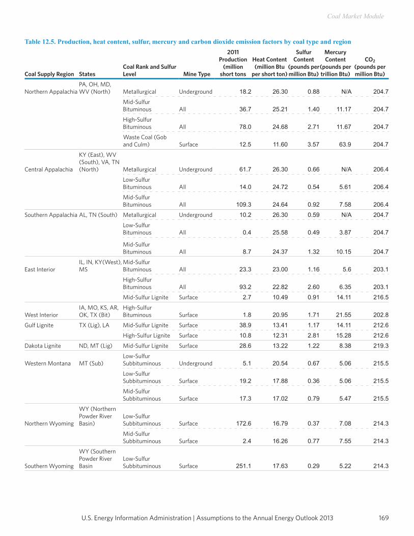
169U.S. Energy Information Administration | Assumptions to the Annual Energy Outlook 2013
Coal Market Module
Table 12.5. Production, heat content, sulfur, mercury and carbon dioxide emission factors by coal type and region
Coal Supply Region StatesCoal Rank and Sulfur Level Mine Type
2011 Production
(million short tons
Heat Content (million Btu
per short ton)
Sulfur Content
(pounds per million Btu)
Mercury Content
(pounds per trillion Btu)
CO2 (pounds per million Btu)
Northern AppalachiaPA, OH, MD, WV (North) Metallurgical Underground 18.2 26.30 0.88 N/A 204.7
Mid-Sulfur Bituminous All 36.7 25.21 1.40 11.17 204.7
High-Sulfur Bituminous All 78.0 24.68 2.71 11.67 204.7
Waste Coal (Gob and Culm) Surface 12.5 11.60 3.57 63.9 204.7
Central Appalachia
KY (East), WV (South), VA, TN (North) Metallurgical Underground 61.7 26.30 0.66 N/A 206.4
Low-Sulfur Bituminous All 14.0 24.72 0.54 5.61 206.4
Mid-Sulfur Bituminous All 109.3 24.64 0.92 7.58 206.4
Southern Appalachia AL, TN (South) Metallurgical Underground 10.2 26.30 0.59 N/A 204.7
Low-Sulfur Bituminous All 0.4 25.58 0.49 3.87 204.7
Mid-Sulfur Bituminous All 8.7 24.37 1.32 10.15 204.7
East InteriorIL, IN, KY(West), MS
Mid-Sulfur Bituminous All 23.3 23.00 1.16 5.6 203.1
High-Sulfur Bituminous All 93.2 22.82 2.60 6.35 203.1
Mid-Sulfur Lignite Surface 2.7 10.49 0.91 14.11 216.5
West InteriorIA, MO, KS, AR, OK, TX (Bit)
High-Sulfur Bituminous Surface 1.8 20.95 1.71 21.55 202.8
Gulf Lignite TX (Lig), LA Mid-Sulfur Lignite Surface 38.9 13.41 1.17 14.11 212.6
High-Sulfur Lignite Surface 10.8 12.31 2.81 15.28 212.6
Dakota Lignite ND, MT (Lig) Mid-Sulfur Lignite Surface 28.6 13.22 1.22 8.38 219.3
Western Montana MT (Sub)Low-Sulfur Subbituminous Underground 5.1 20.54 0.67 5.06 215.5
Low-Sulfur Subbituminous Surface 19.2 17.88 0.36 5.06 215.5
Mid-Sulfur Subbituminous Surface 17.3 17.02 0.79 5.47 215.5
Northern Wyoming
WY (Northern Powder River Basin)
Low-Sulfur Subbituminous Surface 172.6 16.79 0.37 7.08 214.3
Mid-Sulfur Subbituminous Surface 2.4 16.26 0.77 7.55 214.3
Southern Wyoming
WY (Southern Powder River Basin
Low-Sulfur Subbituminous Surface 251.1 17.63 0.29 5.22 214.3
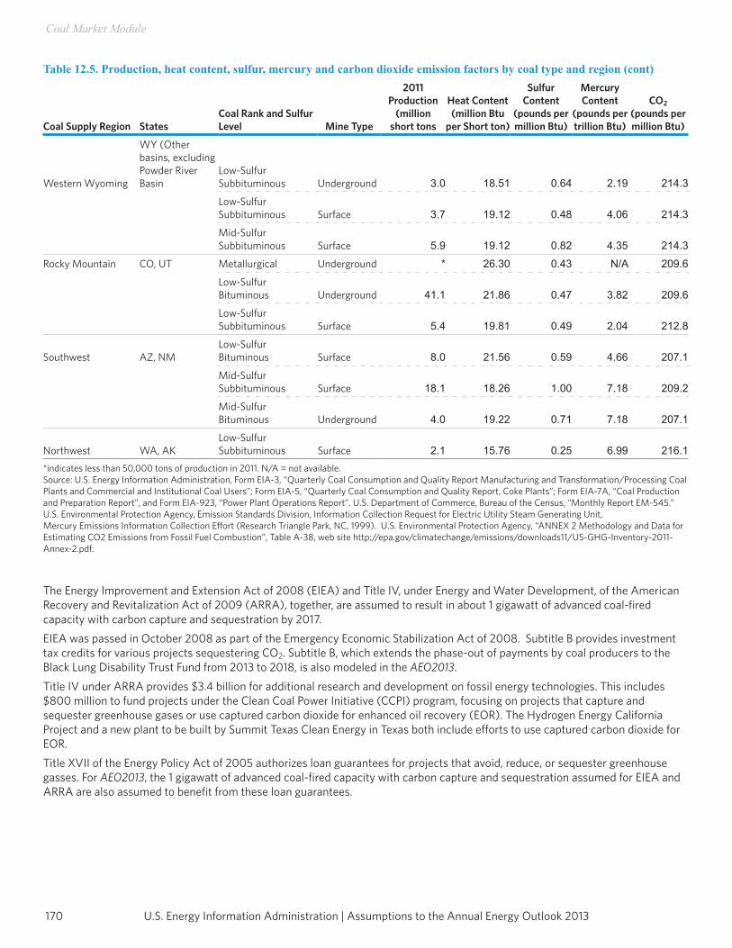
U.S. Energy Information Administration | Assumptions to the Annual Energy Outlook 2013170
Coal Market Module
Table 12.5. Production, heat content, sulfur, mercury and carbon dioxide emission factors by coal type and region (cont)
Coal Supply Region StatesCoal Rank and Sulfur Level Mine Type
2011 Production
(million short tons
Heat Content (million Btu
per Short ton)
Sulfur Content
(pounds per million Btu)
Mercury Content
(pounds per trillion Btu)
CO2 (pounds per million Btu)
Western Wyoming
WY (Other basins, excluding Powder River Basin
Low-Sulfur Subbituminous Underground 3.0 18.51 0.64 2.19 214.3
Low-Sulfur Subbituminous Surface 3.7 19.12 0.48 4.06 214.3
Mid-Sulfur Subbituminous Surface 5.9 19.12 0.82 4.35 214.3
Rocky Mountain CO, UT Metallurgical Underground * 26.30 0.43 N/A 209.6
Low-Sulfur Bituminous Underground 41.1 21.86 0.47 3.82 209.6
Low-Sulfur Subbituminous Surface 5.4 19.81 0.49 2.04 212.8
Southwest AZ, NMLow-Sulfur Bituminous Surface 8.0 21.56 0.59 4.66 207.1
Mid-Sulfur Subbituminous Surface 18.1 18.26
1.00 7.18 209.2
Mid-Sulfur Bituminous Underground 4.0 19.22 0.71 7.18 207.1
Northwest WA, AKLow-Sulfur Subbituminous Surface 2.1 15.76 0.25 6.99 216.1
*indicates less than 50,000 tons of production in 2011. N/A = not available.Source: U.S. Energy Information Administration, Form EIA-3, “Quarterly Coal Consumption and Quality Report Manufacturing and Transformation/Processing Coal Plants and Commercial and Institutional Coal Users”; Form EIA-5, “Quarterly Coal Consumption and Quality Report, Coke Plants”; Form EIA-7A, “Coal Production and Preparation Report”, and Form EIA-923, “Power Plant Operations Report”. U.S. Department of Commerce, Bureau of the Census, “Monthly Report EM-545.” U.S. Environmental Protection Agency, Emission Standards Division, Information Collection Request for Electric Utility Steam Generating Unit,Mercury Emissions Information Collection Effort (Research Triangle Park, NC, 1999). U.S. Environmental Protection Agency, “ANNEX 2 Methodology and Data for Estimating CO2 Emissions from Fossil Fuel Combustion”, Table A-38, web site http://epa.gov/climatechange/emissions/downloads11/US-GHG-Inventory-2011- Annex-2.pdf.
The Energy Improvement and Extension Act of 2008 (EIEA) and Title IV, under Energy and Water Development, of the American Recovery and Revitalization Act of 2009 (ARRA), together, are assumed to result in about 1 gigawatt of advanced coal-fired capacity with carbon capture and sequestration by 2017.EIEA was passed in October 2008 as part of the Emergency Economic Stabilization Act of 2008. Subtitle B provides investment tax credits for various projects sequestering CO2. Subtitle B, which extends the phase-out of payments by coal producers to the Black Lung Disability Trust Fund from 2013 to 2018, is also modeled in the AEO2013.Title IV under ARRA provides $3.4 billion for additional research and development on fossil energy technologies. This includes $800 million to fund projects under the Clean Coal Power Initiative (CCPI) program, focusing on projects that capture and sequester greenhouse gases or use captured carbon dioxide for enhanced oil recovery (EOR). The Hydrogen Energy California Project and a new plant to be built by Summit Texas Clean Energy in Texas both include efforts to use captured carbon dioxide for EOR.Title XVII of the Energy Policy Act of 2005 authorizes loan guarantees for projects that avoid, reduce, or sequester greenhouse gasses. For AEO2013, the 1 gigawatt of advanced coal-fired capacity with carbon capture and sequestration assumed for EIEA and ARRA are also assumed to benefit from these loan guarantees.

171U.S. Energy Information Administration | Assumptions to the Annual Energy Outlook 2013
Coal Market Module
Beginning in 2008, electricity generating units of 25 megawatts or greater were required to hold an allowance for each ton of CO2 emitted in nine Northeastern States as part of the Regional Greenhouse Gas Initiative (RGGI). The States currently participating in RGGI include Connecticut, Maine, Maryland, Massachusetts, Rhode Island, Vermont, New York, New Hampshire, and Delaware. RGGI is modeled in AEO2013 as an emissions reduction program for the Central Atlantic region.AEO2013 includes representation of California Assembly Bill 32 (AB32), the Global Warming Solution Act of 2006. As modeled, AB32 imposes a limit on power sector CO2 emissions for electricity sector power plants serving California beginning in 2012 and declining at a uniform annual rate through 2020.
Coal alternative casesCoal Cost casesIn the Reference case, coal mine labor productivity is assumed to decline on average by 1.4 percent per year through 2040. Miner wage rates increase by about 0.9 percent per year, and mine equipment costs remain constant in 2011 dollars. Eastern coal transportation rates are projected to be similar to 2011 levels in 2040. Western rates are 1 percent higher in 2040 than in 2011. In two alternative coal cost cases, productivity, average miner wages, equipment cost, and transportation rate assumptions were modified for 2013 through 2040 in order to examine the impacts on U.S. coal supply, demand, distribution and prices.In the Low Coal Cost case, coal mine labor productivity is assumed to increase at an average rate of 0.9 percent per year through 2040. Coal mining wages, mine equipment costs, and other mine supply costs all are assumed to be about 25 percent lower in 2040 in real terms in the Low Coal Cost case than in the Reference case. Coal transportation rates, excluding the impact of fuel surcharges, are assumed to be 25 percent lower by 2040.In the High Coal Cost case, coal mine labor productivity is assumed to decline at an average rate of 4.3 percent per year through 2040. Coal mining wages, mine equipment costs, and other mine supply costs all are assumed to be about 32 percent higher in 2040 in real terms in the High Coal Cost case than in the Reference case. Compared to the Reference case, coal transportation rates are assumed to be 25 percent higher by 2040. The low and high coal cost cases represent fully integrated NEMS runs, with feedback from the Macroeconomic Activity, International, supply, conversion, and end-use demand modules.
No Greenhouse Gas Concern caseIn the Reference case, to reflect the market reaction to potential future GHG regulation, a 3-percentage-point increase in the cost of capital for investments in new coal-fired power plants without carbon capture and sequestration technology is assumed. These assumptions affect cost evaluations for the construction of new capacity but not the actual operating costs for new existing plants. This adjustment was first implemented for AEO2009. Beginning with AEO2012, a 3-percentage-point increase in the cost of capital for investments in retrofits at existing coal plants is also applied for emission control equipment (excluding CCS).The No GHG concern case excludes the 3-percentage point increase in the cost of capital.

U.S. Energy Information Administration | Assumptions to the Annual Energy Outlook 2013172
Coal Market Module
Notes and sources[1] Energy Information Administration, The U.S. Coal Industry, 1970-1990: Two Decades of Change, DOE/EIA-0559, (Washington, DC, November 1992). [2] Stanley C. Suboleski, et.al., Central Appalachia: Coal Mine Productivity and Expansion, Electric Power Research Institute, EPRI IE-7117, (September 1991). [3] The estimated cost of switching to subbituminous coal, $0.10 per million Btu (2000 dollars), was derived by Energy Ventures Analysis, Inc. and was recommended for use in the CMM as part of an Independent Expert Review of the Annual Energy Outlook 2002’s Powder River Basin production and transportation rates. Barbaro, Ralph and Seth Schwartz. Review of the Annual Energy Outlook 2002 Reference Case Forecast for PRB Coal, prepared for the Energy Information Administration (Arlington, VA: Energy Ventures Analysis, Inc., August 2002). [4] U.S. Environmental Protection Agency, “Climate Change—Regulatory Initiative: Greenhouse Gas Reporting Program”, website www.epa.gov/climatechange/emissions/

Renewable Fuels Module

This page inTenTionally lefT blank

175U.S. Energy Information Administration | Assumptions to the Annual Energy Outlook 2013
Renewable Fuels Module
The NEMS Renewable Fuels Module (RFM) provides natural resources supply and technology input information for projections of new central-station U.S. electricity generating capacity using renewable energy resources. The RFM has seven submodules representing various renewable energy sources: biomass, geothermal, conventional hydroelectricity, landfill gas, solar thermal, solar photovoltaics, and wind [1].Some renewables, such as landfill gas (LFG) from municipal solid waste (MSW) and other biomass materials, are fuels in the conventional sense of the word, while others, such as water, wind, and solar radiation, are energy sources that do not involve the production or consumption of a fuel. Commercial market penetration of renewable technologies varies widely. Hydroelectric power, one of the oldest electric generation technologies, accounted for roughly 8 percent of electric power generation in 2011; newer power systems using biomass, geothermal, LFG, solar, or wind energy contribute a combined 5 percent.The submodules of the RFM interact primarily with the Electricity Market Module (EMM). Because of the high level of integration with the EMM, the final outputs (levels of consumption and market penetration over time) for renewable energy technologies are largely dependent upon the EMM. Because some types of biomass fuel can be used for either electricity generation or for the production of liquid fuels, such as ethanol, there is also some interaction with the Petroleum Market Module (PMM), which contains additional representation of some biomass feedstocks that are used primarily for liquid fuels production.Projections for residential and commercial grid-connected photovoltaic systems are developed in the end-use demand modules and not in the RFM; see the Distributed Generation and Combined Heat and Power description in the “Commercial Demand Module” and “Residential Demand Module” sections of the report. Descriptions for biomass energy production in industrial settings, such as the pulp and paper industries can be found in the “Industrial Demand Module” section of the report..
Key assumptions Nonelectric renewable energy uses In addition to projections for renewable energy used in central station electricity generation, AEO2013 contains projections of nonelectric renewable energy uses for industrial and residential wood consumption, solar residential and commercial hot water heating, biofuels blending in transportation fuels, and residential and commercial geothermal (ground-source) heat pumps. Assumptions for these projections are found in the residential, commercial, industrial, and petroleum marketing module sections of this report. Additional minor renewable energy applications occurring outside energy markets, such as direct solar thermal industrial applications or direct lighting, off-grid electricity generation, and heat from geothermal resources used directly (e.g., district heating and greenhouses) are not included in the projections.
Electric power generation The RFM considers only grid-connected central station electricity generation systems. The RFM submodules that interact with the EMM are the central station grid-connected biomass, geothermal, conventional hydroelectricity, landfill gas, solar (thermal and photovoltaic), and wind submodules, which provide specific data or estimates that characterize the respective resource. A set of technology cost and performance values is provided directly to the EMM and is central to the build and dispatch decisions of the EMM. The technology cost and performance values are summarized in Table 8.2 in the chapter discussing the EMM.
U.S. Energy Information Administration | Assumptions to the Annual Energy Outlook 2013176
Renewable Fuels Module
Capital costs Capital costs for renewable technologies are affected by several factors. Capital costs for technology to exploit some resources, especially geothermal, hydroelectric, and wind power resources, are assumed to be dependent on the quality, accessibility, and/ or other site-specific factors in the areas with exploitable resources. These factors can include additional costs associated with reduced resource quality; need to build or upgrade transmission capacity from remote resource areas to load centers; or local impediments to permitting, equipment transport, and construction in good resource areas due to siting issues, inadequate infrastructure, or rough terrain.Short-term cost adjustment factors increase technology capital costs as a result of a rapid U.S. buildup in a single year, reflecting limitations on the infrastructure (for example, limits on manufacturing, resource assessment, and construction expertise) to accommodate unexpected demand growth. These factors, which are applied to all new electric generation capacity, are a function of past production rates and are further described in The Electricity Market Module of the National Energy Modeling System: Model Documentation Report, available at www.eia.gov/analysis/model-documentation.cfm.Also assumed to affect all new capacity types are costs associated with construction commodities. Through much of the period from 2000 to 2008, the installed cost for most new plants was observed to increase. Although several factors contributed to this cost escalation, some of which may be more or less important to specific types of new capacity, much of the overall cost increase was correlated with increases in the cost of construction materials, such as bulk metals, specialty metals, and concrete. Capital costs are specifically linked to the projections for the metals producer price index found in the Macroeconomic Module of NEMS. Independent of the other two factors, capital costs for all electric generation technologies, including renewable technologies, are assumed to decline as a function of growth in installed capacity for each technology.For a description of NEMS algorithms lowering generating technologies’ capital costs as more units enter service (learning), see “Technological Optimism and Learning” in the EMM chapter of this report. A detailed description of the RFM is provided in the EIA publication, Renewable Fuels Module of the National Energy Modeling System, Model Documentation 2011, DOE/ EIA-M069(2011) (Washington, DC, 2011).
Solar Electric SubmoduleBackgroundThe Solar Electric Submodule currently includes both solar thermal (also referred to as “concentrating solar power” or CSP) and photovoltaic (PV), technologies. The representative solar thermal technology assumed for cost estimation is a 100-megawatt central-receiver tower without integrated energy storage, while the representative solar PV technology is a 150-megawatt array of flat plate PV modules using single-axis tracking. PV is assumed available in all EMM regions, while CSP is available only in the Western regions with the arid atmospheric conditions that result in the most cost-effective capture of direct sunlight. Cost estimates for both technologies are based on a forthcoming report by SAIC to be published in early 2013, see: the “Documentations & Assumptions” section of www.eia.gov/forecasts/aeo/er/index.cfm). Technology- specific performance characteristics are obtained from information provided by the National Renewable Energy Laboratory (NREL).
Assumptions •• NEMS represents the Energy Policy Act of 1992 (EPACT92) permanent 10-percent investment tax credit (ITC) for solar electric
power generation by tax-paying entities. In addition, the current 30-percent ITC, scheduled to expire at the end of 2016, is also represented to qualifying new capacity installations.
•• Existing capacity and planned capacity additions are based on EIA survey data from the Form EIA-860, “Annual Electric Generator Report” and Form EIA-860M, “Monthly Update to the Annual Electric Generator Report”. Planned capacity additions under construction or having all regulatory approvals and having an expected completion date prior to the expiration of the 30-percent ITC were included in the model’s planned capacity additions, according to respondents’ planned completion dates.
•• Capacity factors for solar technologies are assumed to vary by time of day and season of the year, such that nine separate capacity factors are provided for each modeled region, three for time of day and for each of three broad seasonal groups (summer, winter, and spring/fall). Regional capacity factors vary from national averages based on climate and latitude.
•• Solar resources are well in excess of conceivable demand for new capacity; energy supplies are considered unlimited within regions (at specified daily, seasonal, and regional capacity factors). Therefore, solar resources are not estimated in NEMS. In the regions where CSP technology is not modeled, the level of direct, normal insolation (the kind needed for that technology) is assumed to be insufficient to make that technology commercially viable through the projection horizon.
177U.S. Energy Information Administration | Assumptions to the Annual Energy Outlook 2013
Renewable Fuels Module
Wind-Electric Power SubmoduleBackgroundBecause of limits to windy land areas, wind is considered a finite resource, so the submodule calculates maximum available capacity by Electricity Market Module Supply Regions. The minimum economically viable average wind speed is about 15 mph at a hub-height of 80 m, and wind speeds are categorized by annual average wind speed based on a classification system originally from the Pacific Northwest Laboratory (see http://rredc.nrel.gov/wind/pubs/atlas/tables/1-1T.html). The RFM tracks wind capacity (megawatts) by resource quality and costs within a region, and moves to the next best wind resource when one category is exhausted. Wind resource data on the amount and quality of wind per EMM region come from the National Renewable Energy Laboratory [2]. The technological performance, cost, and other wind data used in NEMS are based on a forthcoming report by SAIC to be published in early 2013, see: the “Documentations & Assumptions” section of www.eia.gov/forecasts/aeo/er/index.cfm). Maximum wind capacity, capacity factors, and incentives are provided to the EMM for capacity planning and dispatch decisions. These form the basis on which the EMM decides how much power generation capacity is available from wind energy. The fossil-fuel heat rate equivalents for wind are used for energy consumption calculation purposes only.
Assumptions •• Only grid-connected (utility and nonutility) generation is included. Projections for distributed wind generation are included in
the commercial and residential modules. •• In the wind submodule, wind supply costs are affected by three modeling measures addressing: (1) average wind speed, (2)
distance from existing transmission lines, and (3) resource degradation, transmission network upgrade costs, and market factors.
•• Available wind resource is reduced by excluding all windy lands not suited for the installation of wind turbines because of: excessive terrain slope (greater than 20 percent); reservation of land for non-intrusive uses (such as National Parks, wildlife refuges, and so forth); inherent incompatibility with existing land uses (such as urban areas, areas surrounding airports and water bodies, including offshore locations); insufficient contiguous windy land to support a viable wind plant (less than 5 square kilometers of windy land in a 100-square-kilometer area). Half of the wind resource located on military reservations, U.S. Forest Service land, state forested land, and all non-ridge-crest forest areas are excluded from the available resource base to account for the uncertain ability to site projects at such locations. These assumptions are detailed in the Draft Final Report to EIA titled, “Incorporation of Existing Validated Wind Data into NEMS,” November 2003.
•• Capital costs for wind technologies are assumed to increase in response to (1) declining natural resource quality, such as terrain slope, terrain roughness, terrain accessibility, wind turbulence, wind variability, or other natural resource factors, as the best sites are utilized, (2) increasing cost of upgrading existing local and network distribution and transmission lines to accommodate growing quantities of remote wind power, and (3) market conditions, such as the increasing costs of alternative land uses, including aesthetic or environmental reasons. Capital costs are left unchanged for some initial share, then increased by 10, 25, 50 percent, and finally 100 percent, to represent the aggregation of these factors
•• Proportions of total wind resources in each category vary by EMM region. For all EMM regions combined, about 1 percent of windy land (107 GW of 11,600 GW in total resource) is available with no cost increase, 3.4 percent (390 GW) is available with a 10 percent cost increase, 2 percent (240 GW) is available with a 25-percent cost increase, and over 90 percent is available with a 50- or 100-percent cost increase.
•• Depending on the EMM region, the cost of competing fuels, and other factors, wind plants can be built to meet system capacity requirements or as a “fuel saver” to displace generation from existing capacity. For wind to penetrate as a fuel saver, its total capital and fixed operations and maintenance costs minus applicable subsidies must be less than the variable operating costs, including fuel, of the existing (non-wind) capacity. When competing in the new capacity market, wind is assigned a capacity credit that declines based on its estimated contribution to regional reliability requirements.
•• Because of downwind turbulence and other aerodynamic effects, the model assumes an average spacing between turbine rows of 5 rotor diameters and a lateral spacing between turbines of 10 rotor diameters. This spacing requirement determines the amount of power that can be generated from wind resources, about 6.5 megawatts per square kilometer of windy land, and is factored into requests for generating capacity by the EMM.
•• Capacity factors for each wind class are calculated as a function of overall wind market growth. The capacity factors are assumed to be limited to about 50 percent for a typical Class 6 site. As better wind resources are depleted, capacity factors are assumed to go down, corresponding with the use of less desirable sites. By 2040, the typical wind plant build will have a somewhat lower capacity factor than those found in the best wind resource areas. Capacity factors in the Reference case increase to about 45 percent in the best wind class resulting from taller towers, more reliable equipment, and advanced technologies, although, as noted, these may not represent the best available sites because of other site-specific factors.
U.S. Energy Information Administration | Assumptions to the Annual Energy Outlook 2013178
Renewable Fuels Module
•• AEO2013 does not allow plants constructed after 2012 to claim the federal Production Tax Credit (PTC), a 2.2-cent-per-kilowatt- hour tax incentive for wind that wasset to expire on December 31, 2012 for wind only. After completion of this case, the law was changed to allow wind plants under construction by December 31, 2013 to qualify for the PTC. Wind plants are assumed to depreciate capital expenses using the Modified Accelerated Cost Recovery Schedule with a 5-year tax life.
Offshore wind resources are represented as a separate technology from onshore wind resources. Offshore resources are modeled with a similar model structure as onshore wind. However, because of the unique challenges of offshore construction and the somewhat different resource quality, the assumptions with regard to capital cost, learning-by-doing cost reductions, and variation of resource exploitation costs and performance differ significantly from onshore wind.. •• Like onshore resources, offshore resources are assumed to have an upwardly sloping supply curve, in part influenced by the same
factors that determine the onshore supply curve (such as distance to load centers, environmental or aesthetic concerns, variable terrain/seabed) but also explicitly by water depth.
•• Because of the more difficult maintenance challenge offshore, performance for a given annual average wind power density level is assumed to be somewhat reduced by reduced turbine availability. Offsetting this, however, is the availability of resource areas with higher overall power density than is assumed available onshore. Capacity factors for offshore are limited to be about 50 percent for a Class 7 site.
•• Cost reductions in the offshore technology result in part from learning reductions in onshore wind technology as well as from cost reductions unique to offshore installations, such as foundation design and construction techniques. Because offshore technology is significantly less mature than onshore wind technology, offshore-specific technology learning occurs at a somewhat faster rate than on-shore technology. A technological optimism factor (see EMM documentation: www.eia.gov/ analysis/model-documentation.cfm) is included for offshore wind to account for the substantial cost of establishing the unique construction infrastructure required for this technology.
Geothermal-Electric Power SubmoduleBackgroundBeginning in AEO2011, all geothermal supply curve data came from the National Renewable Energy Laboratory’s updated U.S. geothermal supply curve assessment. The report, released in February 2010, assigns cost estimates to the U.S. Geological Survey’s (USGS) 2008 geothermal resource assessment. Some data from the 2006 report, “The Future of Geothermal Energy,” prepared by the Massachusetts Institute of Technology, was also incorporated into the NREL report; however, this would be more relevant to deep, dry, and unknown geothermal resources, something which EIA did not include in its supply curve. NREL took the USGS data and used the Geothermal Electricity Technology Evaluation Model (GETEM), an Excel-based techno-economic systems analysis tool, to estimate the costs [3]. Only resources with temperatures above 110 degrees Celsius were considered. There are approximately 125 of these known, hydrothermal resources which EIA used in its supply curve. Each of these sites also has what NREL classified as “near-field enhanced geothermal energy system potential” which are in areas around the identified site that lack the permeability of fluids that are present in the hydrothermal potential. Therefore, there are 250 total points on the supply curve since each of the 125 hydrothermal sites has corresponding enhanced geothermal system (EGS) potential.In the past, EIA cost estimates were broken down into cost-specific components. Unfortunately, this level of detail was not available in the NREL data. A site-specific capital cost and fixed operations and maintenance cost were provided. Both types of technology, both flash and binary, are also included with capacity factors ranging from 90 to 95 percent. While the source of the data was changed beginning in AEO2011, the site-by-site matrix input that acts as the supply curve has been retained.
Assumptions •• Existing and identified planned capacity data are obtained directly by the EMM from Form EIA-860 and Form EIA-860m. •• The permanent investment tax credit of 10 percent available in all projection years, based on the EPACT, applies to all geothermal
capital costs, except through December 2013 when the 2.2-cent production tax credit is available to this technology and is assumed chosen instead. Projects that have begun construction and are beyond the exploratory drilling phase by that date are eligible for this production tax credit.
•• Plants are not assumed to retire unless their retirement is reported to EIA. The Geysers units are not assumed to retire but instead are assigned the 35-percent capacity factors reported to EIA reflecting their reduced performance in recent years.
179U.S. Energy Information Administration | Assumptions to the Annual Energy Outlook 2013
Renewable Fuels Module
Biomass Electric Power Submodule Background Biomass consumed for electricity generation is modeled in two parts in NEMS. Capacity in the wood products and paper industries, the so-called captive capacity, is included in the industrial sector module as cogeneration. Generation in the electricity sector is represented in the EMM. Fuel costs are calculated in NEMS and passed to EMM, while capital and operating costs and performance characteristics are assumed as shown in Table 8.2. Fuel costs are provided in sets of regional supply schedules. Projections for ethanol are produced by the Petroleum Market Module (PMM), with the quantities of biomass consumed for ethanol decremented from, and prices obtained from, the EMM regional supply schedules.
Assumptions •• Existing and planned capacity data are obtained from Form EIA-860 and Form EIA-860m. •• The conversion technology represented is an 80-MW dedicated combustion plant. The cost estimates for this technology are
based on a forthcoming report by SAIC to be published in early 2013, see: the “Documentations & Assumptions” section of www.eia.gov/forecasts/aeo/er/index.cfm).
•• Biomass co-firing can occur up to a maximum of 15 percent of fuel used in coal-fired generating plantsFuel supply schedules are a composite of four fuel types: forestry materials, wood residues, agricultural residues, and energy crops. Feedstock potential from agricultural residues and dedicated energy crops are calculated from a version of the Policy Analysis (POLYSYS) agricultural model that uses the same oil prices as the rest of NEMS. Forestry residues are calculated from inventories conducted by the U.S. Forest Service and Oak Ridge National Laboratory. The forestry materials component is made up of logging residues, rough rotten salvageable dead wood, and excess small pole trees.[4] The wood residue component consists of primary mill residues, silvicultural trimmings, and urban wood such as pallets, construction waste, and demolition debris that are not otherwise used [5]. Agricultural residues are wheat straw, corn stover, and a number of other major agricultural crops [6]. Energy crop data are for hybrid poplar, willow, and switchgrass grown on existing cropland. POLYSYS assumes that the additional cropland needed for energy crops will displace existing pasturelands. The lands in the Conservation Reserve Program are preserved [7]. The maximum amount of resources in each coal region is shown in Table 13.1.
Table 13.1. Maximum U.S. biomass resources, by coal demand region and type in 2035trillion Btu
Coal Demand Region States Agricultural Sector Forestry Residue
Urban Wood Waste/Mill
Residue
1 (NE) CT, MA, ME, NH, RI, VT 6 115 40
2 (YP) NY, PA, NJ 164 162 88
3 (S1) WV, MD, DC, DE 174 91 37
4 (S2) VA, NC, SC 167 364 58
5 (GF) GA, FL 104 358 87
6 (OH) OH 266 60 37
7 (EN) IN, IL, MI, WI 1323 155 81
8 (KT) KY, TN 353 167 43
9 (AM) AL, MS 194 332 43
10 (C1) MN, ND, SD 279 57 31
11 (C2) IA, NE, MO, KS 2183 77 45
12 (WS) TX, LA, OK, AR 689 269 86
13 (MT) MT, WY, ID 78 61 26
14 (CU) CO, UT, NV 32 59 51
15 (ZN) AZ, NM 12 73 41
16 (PC) AK, HI, WA, OR, CA 84 239 122Sources: U.S. Billion-Ton Update (Oak Ridge National Lab, 2011) and the Policy Analysis (POLYSYS) model developed by the University of Tennessee’s Department of Agricultural Economics.
U.S. Energy Information Administration | Assumptions to the Annual Energy Outlook 2013180
Renewable Fuels Module
Landfill-Gas-to-Electricity Submodule Background Landfill-gas-to-electricity capacity competes with other technologies using supply curves that are based on the amount of “high,” “low,” and “very low” methane-producing landfills located in each EMM region. An average cost-of-electricity for each type of landfill is calculated using gas collection system and electricity generator costs and characteristics developed by EPA’s “Energy Project Landfill Gas Utilization Software” (E-PLUS) [8] .
Assumptions •• Gross domestic product (GDP) and population are used as the drivers in an econometric equation that establishes the supply
of landfill gas. •• Recycling is assumed to account for 50 percent of the waste stream in 2010 (consistent with EPA’s recycling goals). •• The waste stream is characterized into three categories: readily, moderately, and slowly decomposable material. •• Emission parameters are the same as those used in calculating historical methane emissions in EIA’s Emissions of Greenhouse
Gases in the United States 2003 [9].•• The ratio of “high,” “low,” and “very low” methane production sites to total methane production is calculated from data
obtained for 156 operating landfills contained in the Government Advisory Associates METH2000 database [10].•• Cost-of-electricity for each site was calculated by assuming each site to be a 100-acre by 50-foot deep landfill and by applying
methane emission factors for “high,” “low,” and “very low” methane emitting wastes.
Conventional hydroelectricity The conventional hydroelectricity submodule represents U.S. potential for new conventional hydroelectric capacity of 1 megawatt or greater from new dams, existing dams without hydroelectricity, and from adding capacity at existing hydroelectric dams. Summary hydroelectric potential is derived from reported lists of potential new sites assembled from Federal Energy Regulatory Commission (FERC) license applications and other survey information, plus estimates of capital and other costs prepared bythe Idaho National Engineering and Environmental Laboratory (INEEL) [11]. Annual performance estimates (capacity factors) were taken from the generally lower but site-specific FERC estimates rather than from the general estimates prepared by INEEL, and only sites with estimated costs of 10 cents per kilowatthour or lower are included in the supply. Pumped storage hydro, considered a nonrenewable storage medium for fossil and nuclear power, is not included in the supply; moreover, the supply does not consider offshore or in-stream hydro, efficiency or operational improvements without capital additions, or additional potential from refurbishing existing hydroelectric capacity.In the hydroelectricity submodule, sites are first arrayed by NEMS region from least to highest cost per kilowatthour. For any year’s capacity decisions, only those hydroelectric sites whose estimated levelized costs per kilowatthour are equal to or lessthan an EMM-determined avoided cost (the least cost of other technology choices determined in the previous decision cycle) are submitted. Next, the array of below-avoided-cost sites is parceled into three increasing cost groups, with each group characterized by the average capacity-weighted cost and performance of its component sites. Finally, the EMM receives from the conventional hydroelectricity submodule the three increasing-cost quantities of potential capacity for each region, providing the number of megawatts potential along with their capacity-weighted average overnight capital cost, operations and maintenance cost, and average capacity factor. After choosing from the supply, the EMM informs the hydroelectricity submodule, which decrements available regional potential in preparation for the next capacity decision cycle.
Legislation and regulations Renewable electricity tax credits The RFM includes the investment and energy production tax credits codified in the Energy Policy Act of 1992 (EPACT92) as amended. The investment tax credit established by EPACT92 provides a credit to Federal income tax liability worth 10 percent of initial investment cost for a solar, geothermal, or qualifying biomass facility. This credit was raised to 30 percent through 2016 for some solar projects and extended to residential projects. This change is reflected in the RFM, commercial demand, and residential demand modules. The production tax credit, as established by EPACT92, applied to wind and certain biomass facilities. As amended, it provides a 2.2-cent tax credit for every kilowatthour of electricity produced for the first 10 years of operation for a wind facility constructed by December 31, 2012 or by December 31, 2013 for other eligible facilities. The value of the credit, originally 1.5 cents, is adjusted annually for inflation. With the various amendments, the production tax credit is available for electricity produced from qualifying geothermal, animal waste, certain small-scale hydroelectric, landfill gas, municipal solid waste, and additional biomass resources. Wind, poultry litter, geothermal, and “closed loop” [12] biomass resources receive a
181U.S. Energy Information Administration | Assumptions to the Annual Energy Outlook 2013
Renewable Fuels Module
2.2-cent tax credit for the first 10 years of facility operations. All other renewable resources receive a 1.1 cent (that is, one-half the value of the credit for other resources) tax credit for the first 10 years of facility operations. EIA assumes that biomass facilities obtaining the PTC will use “open-loop” fuels, as “closed-loop” fuels are assumed to be unavailable and/or too expensive for widespread use during the period that the tax credit is available. The investment and production tax credits are exclusive of one another, and may not both be claimed for the same geothermal facility (which is eligible to receive either.The American Taxpayer Relief Act passed in January of 2012 extends the wind PTC expiration date until December 31, 2013. In addition, it modifies the requirement for all fuels that plants be operational by the expiration date to allow any plant under construction by the expiration date to qualify. However, due to the timing of the legislation, this update is not included in the AEO2013 Reference case.
State RPS programs EIA represents various State-level policies generally referred to as Renewable Portfolio Standards (RPS). These policies vary significantly among States, but typically require the addition of renewable generation to meet a specified share of State-wide generation. Any non-discretionary limitations on meeting the generation or capacity target are modeled to the extent possible. However, because of the complexity of the various requirements, the regional target aggregation, and nature of some of the limitations, the measurement of compliance is assumed to be approximate.Regional renewable generation targets were estimated using the renewable generation targets in each State within the region. In many cases, regional boundaries intersect State boundaries; in these cases State requirements were divided among relevant regions based on sales. Using State-level RPS compliance schedules and preliminary estimates of projected sales growth, EIA estimated the amount of renewable generation required in each State within a region. Required generation in each State was then summed to the regional level for each year, and a regional renewable generation share of total sales was determined, as shown in Table 13.2.Only targets with established enforcement provisions or established State funding mechanisms were included in the calculation; Non-enforceable goals were not included.. Compliance enforcement provisions vary significantly among States and most States have established procedures for waiving compliance through the use of “alternative compliance” payments, penalty payments, discretionary regulatory waivers, or retail price impact limits. Because of the variety of mechanisms, even within a given electricity market region, these limits are not modeled.
Alternative renewable case Low Renewable Cost case The Low Renewable Cost case examines the effect of reducing renewable technology capital costs by 20 percent below Reference case values throughout the projection period.For wind, biomass, LFG, geothermal, and solar technologies, this cost reduction is achieved by a applying a 20% reduction in the base overnight capital costs assumed in the Reference case. For geothermal and hydro, the capital cost of each individual site that is modeled is reduced by 20% compared to the Reference case. Biomass prices are also assumed to be reduced 20 percent for a given quantity of fuel supplied. Other assumptions within NEMS are unchanged from the Reference case.For the Low Renewable Cost case, demand-side improvements are also assumed in the renewable energy technology options of residential demand, commercial demand, industrial demand, and PMM modules. Details on these assumptions can be found in the corresponding sections of this report.
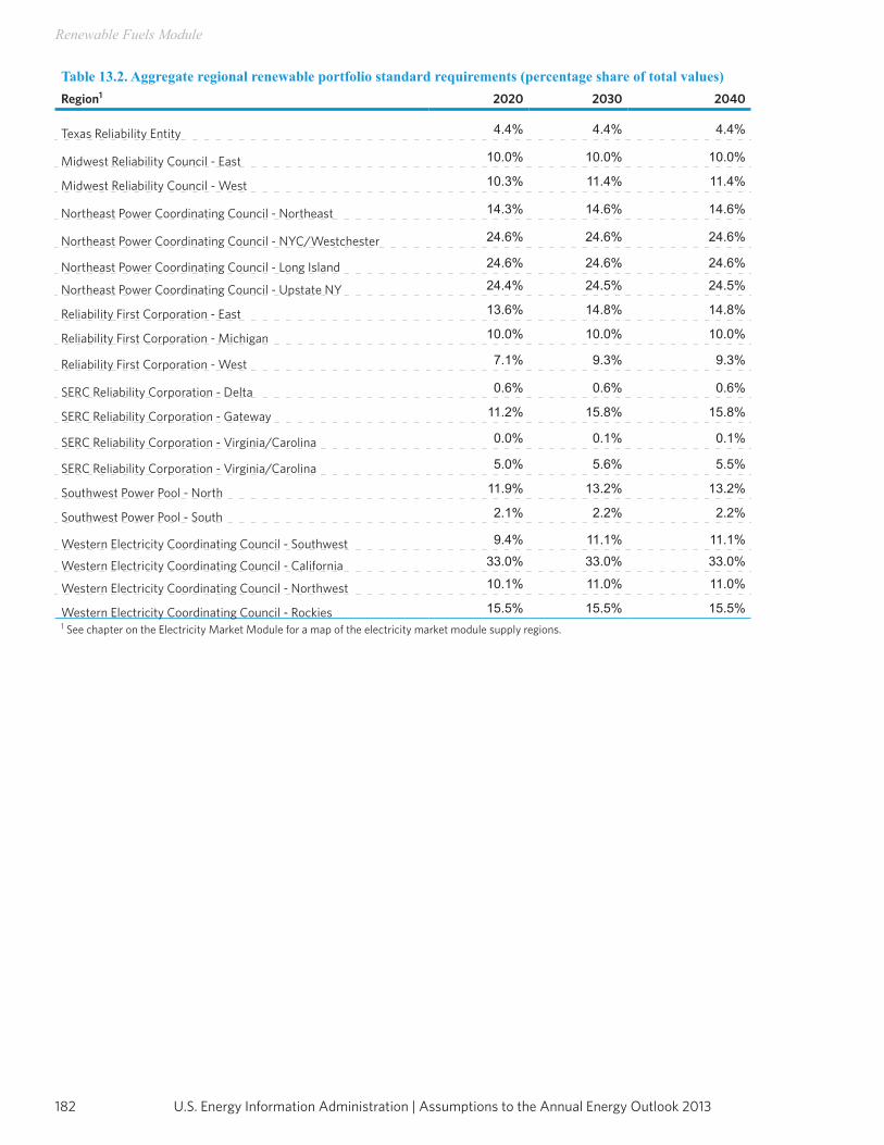
U.S. Energy Information Administration | Assumptions to the Annual Energy Outlook 2013182
Renewable Fuels Module
Table 13.2. Aggregate regional renewable portfolio standard requirements (percentage share of total values)Region1 2020 2030 2040
Texas Reliability Entity 4.4% 4.4% 4.4%
Midwest Reliability Council - East 10.0% 10.0% 10.0%
Midwest Reliability Council - West 10.3% 11.4% 11.4%
Northeast Power Coordinating Council - Northeast 14.3% 14.6% 14.6%
Northeast Power Coordinating Council - NYC/Westchester 24.6% 24.6% 24.6%
Northeast Power Coordinating Council - Long Island 24.6% 24.6% 24.6%
Northeast Power Coordinating Council - Upstate NY 24.4% 24.5% 24.5%
Reliability First Corporation - East 13.6% 14.8% 14.8%
Reliability First Corporation - Michigan 10.0% 10.0% 10.0%
Reliability First Corporation - West 7.1% 9.3% 9.3%
SERC Reliability Corporation - Delta 0.6% 0.6% 0.6%
SERC Reliability Corporation - Gateway 11.2% 15.8% 15.8%
SERC Reliability Corporation - Virginia/Carolina 0.0% 0.1% 0.1%
SERC Reliability Corporation - Virginia/Carolina 5.0% 5.6% 5.5%
Southwest Power Pool - North 11.9% 13.2% 13.2%
Southwest Power Pool - South 2.1% 2.2% 2.2%
Western Electricity Coordinating Council - Southwest 9.4% 11.1% 11.1%
Western Electricity Coordinating Council - California 33.0% 33.0% 33.0%
Western Electricity Coordinating Council - Northwest 10.1% 11.0% 11.0%
Western Electricity Coordinating Council - Rockies 15.5% 15.5% 15.5%1 See chapter on the Electricity Market Module for a map of the electricity market module supply regions.

183U.S. Energy Information Administration | Assumptions to the Annual Energy Outlook 2013
Renewable Fuels Module
Notes and sources[1] For a comprehensive description of each submodule, see U. S. Energy Information Administration, Office of Integrated Analysis and Forecasting, Model Documentation, Renewable Fuels Module of the National Energy Modeling System, DOE/EIA-M069(2011), (Washington, DC, August 2011).[2] Revising the Long Term Multipliers in NEMS: Quantifying the Incremental Transmission Costs Due to Wind Power, Report to EIA from Princeton Energy Resources International, LLC. May 2007.[3] The one exception applies to the Salton Sea resource area. For that site, EIA used cost estimates provided by R.W. Beck, Inc. rather than NREL.[4] U.S. Department of Energy. U.S. Billion-Ton Update: Biomass Supply for a Bioenergy and Bioproducts Industry. August 2011. [5] U.S. Department of Energy. U.S. Billion-Ton Update: Biomass Supply for a Bioenergy and Bioproducts Industry. August 2011. [6] De la Torre Ugarte, D. “Biomass and bioenergy applications of the POLYSYS modeling framework” Biomass and Bioenergy 18 (2000): 291-308. [7] De la Torre Ugarte, D. “Biomass and bioenergy applications of the POLYSYS modeling framework” Biomass and Bioenergy 18 (2000): 291-308. [8] U.S. Environmental Protection Agency, Atmospheric Pollution Prevention Division, Energy Project Landfill GasUtilization Software (E-PLUS) Version 1.0, EPA-430-B-97-006 (Washington, DC, January 1997).[9] U.S. Energy Information Administration, “Emissions of Greenhouse Gases in the United States 2003”, DOE/EIA-0573(2003) (Washington, DC, December 2004), www.eia.gov/oiaf/1605/archive/gg04rpt/index.html. [10] Governmental Advisory Associates, Inc., METH2000 Database, Westport, CT, January 25, 2000.[11] Douglas G. Hall, Richard T. Hunt, Kelly S. Reeves, and Greg R. Carroll, Idaho National Engineering and Environmental Laboratory, “Estimation of Economic Parameters of U.S. Hydropower Resources” INEEL/EXT-03-00662 (Idaho Falls, Idaho, June 2003), //hydropower.inel. gov/resourceassessment/index.html.[12] Closed-loop biomass are crops produced explicitly for energy production. Open-loop biomass are generally wastes or residues that are a byproduct of some other process, such as crops grown for food, forestry, landscaping, or wood milling.

This page inTenTionally lefT blank

Appendix A: Handling of federal and selected state legislation and
regulation in the AEO

This page inTenTionally lefT blank
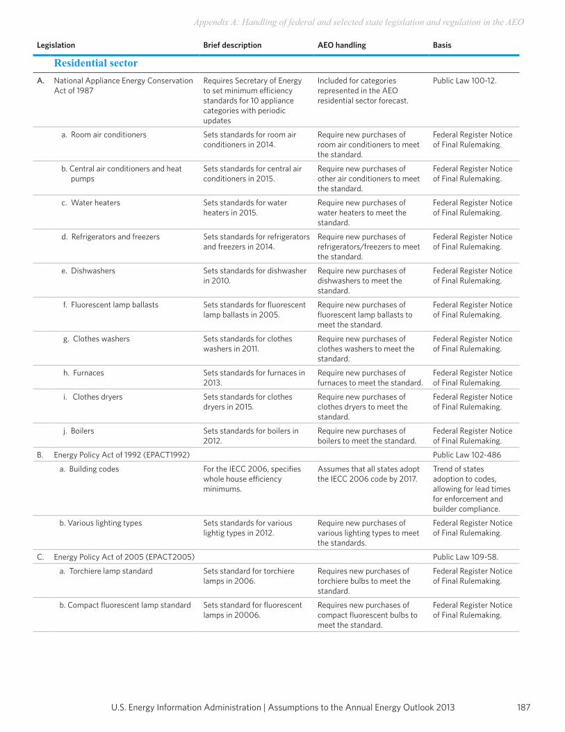
187U.S. Energy Information Administration | Assumptions to the Annual Energy Outlook 2013
Appendix A: Handling of federal and selected state legislation and regulation in the AEO
Legislation Brief description AEO handling Basis
Residential sectorA. National Appliance Energy Conservation
Act of 1987Requires Secretary of Energy to set minimum efficiency standards for 10 appliance categories with periodic updates
Included for categories represented in the AEO residential sector forecast.
Public Law 100-12.
a. Room air conditioners Sets standards for room air conditioners in 2014.
Require new purchases of room air conditioners to meet the standard.
Federal Register Notice of Final Rulemaking.
b. Central air conditioners and heat pumps
Sets standards for central air conditioners in 2015.
Require new purchases of other air conditioners to meet the standard.
Federal Register Notice of Final Rulemaking.
c. Water heaters Sets standards for water heaters in 2015.
Require new purchases of water heaters to meet the standard.
Federal Register Notice of Final Rulemaking.
d. Refrigerators and freezers Sets standards for refrigerators and freezers in 2014.
Require new purchases of refrigerators/freezers to meet the standard.
Federal Register Notice of Final Rulemaking.
e. Dishwashers Sets standards for dishwasher in 2010.
Require new purchases of dishwashers to meet the standard.
Federal Register Notice of Final Rulemaking.
f. Fluorescent lamp ballasts Sets standards for fluorescent lamp ballasts in 2005.
Require new purchases of fluorescent lamp ballasts to meet the standard.
Federal Register Notice of Final Rulemaking.
g. Clothes washers Sets standards for clothes washers in 2011.
Require new purchases of clothes washers to meet the standard.
Federal Register Notice of Final Rulemaking.
h. Furnaces Sets standards for furnaces in 2013.
Require new purchases of furnaces to meet the standard.
Federal Register Notice of Final Rulemaking.
i. Clothes dryers Sets standards for clothes dryers in 2015.
Require new purchases of clothes dryers to meet the standard.
Federal Register Notice of Final Rulemaking.
j. Boilers Sets standards for boilers in 2012.
Require new purchases of boilers to meet the standard.
Federal Register Notice of Final Rulemaking.
B. Energy Policy Act of 1992 (EPACT1992) Public Law 102-486
a. Building codes For the IECC 2006, specifies whole house efficiency minimums.
Assumes that all states adopt the IECC 2006 code by 2017.
Trend of states adoption to codes, allowing for lead times for enforcement and builder compliance.
b. Various lighting types Sets standards for various lightig types in 2012.
Require new purchases of various lighting types to meet the standards.
Federal Register Notice of Final Rulemaking.
C. Energy Policy Act of 2005 (EPACT2005) Public Law 109-58.
a. Torchiere lamp standard Sets standard for torchiere lamps in 2006.
Requires new purchases of torchiere bulbs to meet the standard.
Federal Register Notice of Final Rulemaking.
b. Compact fluorescent lamp standard Sets standard for fluorescent lamps in 20006.
Requires new purchases of compact fluorescent bulbs to meet the standard.
Federal Register Notice of Final Rulemaking.
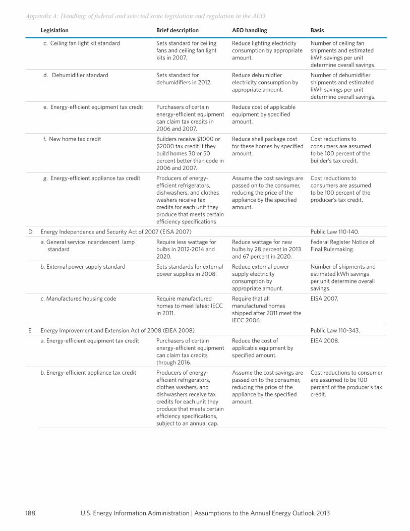
U.S. Energy Information Administration | Assumptions to the Annual Energy Outlook 2013188
Appendix A: Handling of federal and selected state legislation and regulation in the AEO
Legislation Brief description AEO handling Basis
c. Ceiling fan light kit standard Sets standard for ceiling fans and ceiling fan light kits in 2007.
Reduce lighting electricity consumption by appropriate amount.
Number of ceiling fan shipments and estimated kWh savings per unit determine overall savings.
d. Dehumidifier standard Sets standard for dehumidifiers in 2012.
Reduce dehumidfier electricity consumption by appropriate amount.
Number of dehumidifiershipments and estimated kWh savings per unit determine overall savings.
e. Energy-efficient equipment tax credit Purchasers of certain energy-efficient equipment can claim tax credits in 2006 and 2007.
Reduce cost of applicableequipment by specified amount.
f. New home tax credit Builders receive $1000 or$2000 tax credit if they build homes 30 or 50 percent better than code in 2006 and 2007.
Reduce shell package cost for these homes by specified amount.
Cost reductions to consumers are assumed to be 100 percent of the builder’s tax credit.
g. Energy-efficient appliance tax credit Producers of energy-efficient refrigerators, dishwashers, and clothes washers receive tax credits for each unit they produce that meets certain efficiency specifications
Assume the cost savings are passed on to the consumer, reducing the price of the appliance by the specifiedamount.
Cost reductions to consumers are assumed to be 100 percent of the producer’s tax credit.
D. Energy Independence and Security Act of 2007 (EISA 2007) Public Law 110-140.
a. General service incandescent lamp standard
Require less wattage for bulbs in 2012-2014 and 2020.
Reduce wattage for new bulbs by 28 percent in 2013 and 67 percent in 2020.
Federal Register Notice of Final Rulemaking.
b. External power supply standard Sets standards for external power supplies in 2008.
Reduce external power supply electricity consumption byappropriate amount.
Number of shipments andestimated kWh savings per unit determine overall savings.
c. Manufactured housing code Require manufactured homes to meet latest IECC in 2011.
Require that all manufactured homes shipped after 2011 meet the IECC 2006
EISA 2007.
E. Energy Improvement and Extension Act of 2008 (EIEA 2008) Public Law 110-343.
a. Energy-efficient equipment tax credit Purchasers of certain energy-efficient equipment can claim tax credits through 2016.
Reduce the cost of applicable equipment by specified amount.
EIEA 2008.
b. Energy-efficient appliance tax credit Producers of energy-efficient refrigerators, clothes washers, and dishwashers receive tax credits for each unit they produce that meets certain efficiency specifications, subject to an annual cap.
Assume the cost savings are passed on to the consumer, reducing the price of the appliance by the specifiedamount.
Cost reductions to consumer are assumed to be 100 percent of the producer’s tax credit.
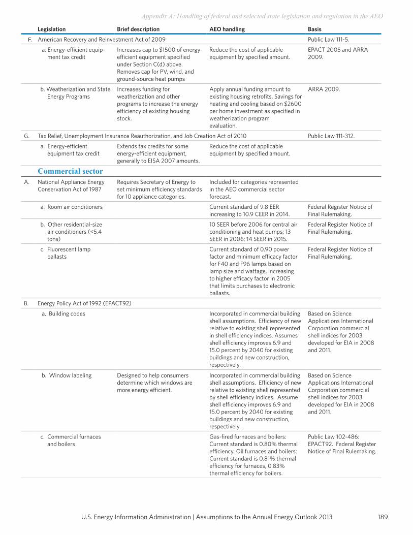
189U.S. Energy Information Administration | Assumptions to the Annual Energy Outlook 2013
Appendix A: Handling of federal and selected state legislation and regulation in the AEO
Legislation Brief description AEO handling Basis
F. American Recovery and Reinvestment Act of 2009 Public Law 111-5.
a. Energy-efficient equip- ment tax credit
Increases cap to $1500 of energy- efficient equipment specified under Section C(d) above. Removes cap for PV, wind, and ground-source heat pumps
Reduce the cost of applicableequipment by specified amount.
EPACT 2005 and ARRA 2009.
b. Weatherization and State Energy Programs
Increases funding for weatherization and other programs to increase the energy efficiency of existing housing stock.
Apply annual funding amount toexisting housing retrofits. Savings for heating and cooling based on $2600 per home investment as specified in weatherization programevaluation.
ARRA 2009.
G. Tax Relief, Unemployment Insurance Reauthorization, and Job Creation Act of 2010 Public Law 111-312.
a. Energy-efficient equipment tax credit
Extends tax credits for some energy-efficient equipment, generally to EISA 2007 amounts.
Reduce the cost of applicable equipment by specified amount.
Commercial sectorA. National Appliance Energy
Conservation Act of 1987Requires Secretary of Energy to set minimum efficiency standards for 10 appliance categories.
Included for categories represented in the AEO commercial sector forecast.
a. Room air conditioners Current standard of 9.8 EER increasing to 10.9 CEER in 2014.
Federal Register Notice of Final Rulemaking.
b. Other residential-size air conditioners (<5.4 tons)
10 SEER before 2006 for central air conditioning and heat pumps; 13 SEER in 2006; 14 SEER in 2015.
Federal Register Notice of Final Rulemaking.
c. Fluorescent lamp ballasts
Current standard of 0.90 power factor and minimum efficacy factor for F40 and F96 lamps based on lamp size and wattage, increasing to higher efficacy factor in 2005 that limits purchases to electronic ballasts.
Federal Register Notice of Final Rulemaking.
B. Energy Policy Act of 1992 (EPACT92)
a. Building codes Incorporated in commercial building shell assumptions. Efficiency of new relative to existing shell represented in shell efficiency indices. Assumes shell efficiency improves 6.9 and 15.0 percent by 2040 for existing buildings and new construction, respectively.
Based on Science Applications International Corporation commercial shell indices for 2003 developed for EIA in 2008 and 2011.
b. Window labeling Designed to help consumers determine which windows are more energy efficient.
Incorporated in commercial building shell assumptions. Efficiency of new relative to existing shell represented by shell efficiency indices. Assume shell efficiency improves 6.9 and 15.0 percent by 2040 for existing buildings and new construction, respectively.
Based on Science Applications International Corporation commercial shell indices for 2003 developed for EIA in 2008 and 2011.
c. Commercial furnaces and boilers
Gas-fired furnaces and boilers: Current standard is 0.80% thermal efficiency. Oil furnaces and boilers: Current standard is 0.81% thermal efficiency for furnaces, 0.83% thermal efficiency for boilers.
Public Law 102-486: EPACT92. Federal Register Notice of Final Rulemaking.
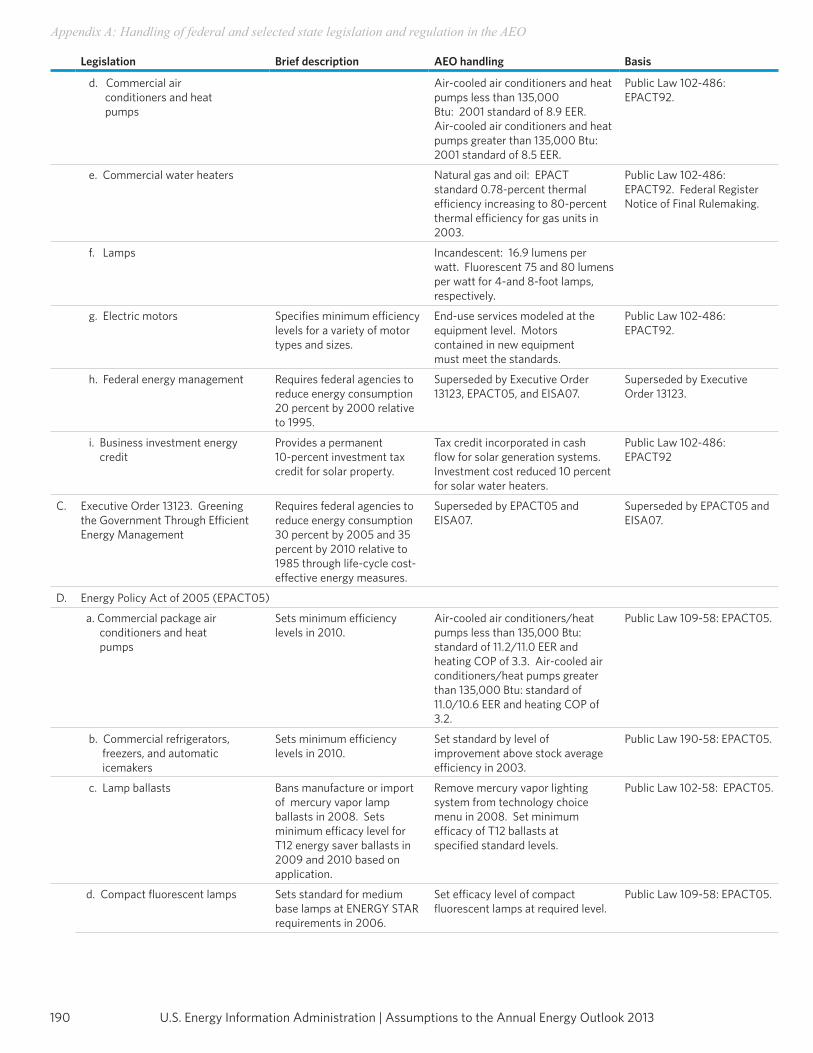
U.S. Energy Information Administration | Assumptions to the Annual Energy Outlook 2013190
Appendix A: Handling of federal and selected state legislation and regulation in the AEO
Legislation Brief description AEO handling Basis
d. Commercial air conditioners and heat pumps
Air-cooled air conditioners and heat pumps less than 135,000 Btu: 2001 standard of 8.9 EER. Air-cooled air conditioners and heat pumps greater than 135,000 Btu: 2001 standard of 8.5 EER.
Public Law 102-486: EPACT92.
e. Commercial water heaters Natural gas and oil: EPACT standard 0.78-percent thermal efficiency increasing to 80-percent thermal efficiency for gas units in 2003.
Public Law 102-486: EPACT92. Federal Register Notice of Final Rulemaking.
f. Lamps Incandescent: 16.9 lumens per watt. Fluorescent 75 and 80 lumens per watt for 4-and 8-foot lamps, respectively.
g. Electric motors Specifies minimum efficiency levels for a variety of motor types and sizes.
End-use services modeled at the equipment level. Motors contained in new equipment must meet the standards.
Public Law 102-486: EPACT92.
h. Federal energy management Requires federal agencies to reduce energy consumption 20 percent by 2000 relative to 1995.
Superseded by Executive Order 13123, EPACT05, and EISA07.
Superseded by Executive Order 13123.
i. Business investment energy credit
Provides a permanent 10-percent investment tax credit for solar property.
Tax credit incorporated in cash flow for solar generation systems. Investment cost reduced 10 percent for solar water heaters.
Public Law 102-486: EPACT92
C. Executive Order 13123. Greening the Government Through Efficient Energy Management
Requires federal agencies to reduce energy consumption 30 percent by 2005 and 35 percent by 2010 relative to 1985 through life-cycle cost-effective energy measures.
Superseded by EPACT05 and EISA07.
Superseded by EPACT05 and EISA07.
D. Energy Policy Act of 2005 (EPACT05)
a. Commercial package air conditioners and heat pumps
Sets minimum efficiency levels in 2010.
Air-cooled air conditioners/heat pumps less than 135,000 Btu: standard of 11.2/11.0 EER and heating COP of 3.3. Air-cooled air conditioners/heat pumps greater than 135,000 Btu: standard of 11.0/10.6 EER and heating COP of 3.2.
Public Law 109-58: EPACT05.
b. Commercial refrigerators, freezers, and automatic icemakers
Sets minimum efficiency levels in 2010.
Set standard by level of improvement above stock average efficiency in 2003.
Public Law 190-58: EPACT05.
c. Lamp ballasts Bans manufacture or import of mercury vapor lamp ballasts in 2008. Sets minimum efficacy level for T12 energy saver ballasts in 2009 and 2010 based on application.
Remove mercury vapor lighting system from technology choice menu in 2008. Set minimum efficacy of T12 ballasts at specified standard levels.
Public Law 102-58: EPACT05.
d. Compact fluorescent lamps Sets standard for medium base lamps at ENERGY STAR requirements in 2006.
Set efficacy level of compact fluorescent lamps at required level.
Public Law 109-58: EPACT05.
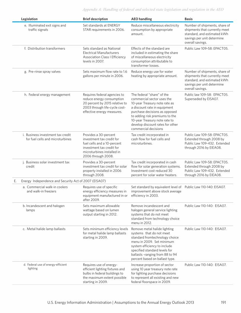
191U.S. Energy Information Administration | Assumptions to the Annual Energy Outlook 2013
Appendix A: Handling of federal and selected state legislation and regulation in the AEO
Legislation Brief description AEO handling Basis
e. Illuminated exit signs and traffic signals
Set standards at ENERGY STAR requirements in 2006.
Reduce miscellaneous electricity consumption by appropriate amount.
Number of shipments, share of shipments that currently meet standard, and estimated kWh savings per unit determine overall savings.
f. Distribution transformers Sets standard as National Electrical Manufacturers Association Class I Efficiency levels in 2007.
Effects of the standard are included in estimating the share of miscellaneous electricity consumption attributable to transformer losses.
Public Law 109-58: EPACT05.
g. Pre-rinse spray valves Sets maximum flow rate to 1.6 gallons per minute in 2006.
Reduce energy use for water heating by appropriate amount.
Number of shipments, share of shipments that currently meet standard, and estimated kWh savings per unit determine overall savings.
h. Federal energy management Requires federal agencies to reduce energy consumption 20 percent by 2015 relative to 2003 through life-cycle cost-effective energy measures.
The federal “share” of the commercial sector uses the 10-year Treasury note rate as a discount rate in equipment purchase decisions as opposed to adding risk premiums to the 10-year Treasury note rate to develop discount rates for other commercial decisions
Public law 109-58: EPACT05. Superseded by EISA07.
i. Business investment tax credit for fuel cells and microturbines
Provides a 30-percent investment tax credit for fuel cells and a 10-percent investment tax credit for microturbines installed in 2006 through 2008.
Tax credit incorporated in cash flow for fuel cells and microturbines.
Public Law 109-58: EPACT05. Extended through 2008 by Public Law 109-432. Extended through 2016 by EIEA08.
j. Business solar investment tax credit
Provides a 30-percent investment tax credit for solar property installed in 2006 through 2008.
Tax credit incorporated in cash flow for solar generation systems. Investment cost reduced 30 percent for solar water heaters.
Public Law 109-58: EPACT05. Extended through 2008 by Public Law 109-432. Extended through 2016 by EIEA08.
E. Energy Independence and Security Act of 2007 (EISA07)
a. Commercial walk-in coolers and walk-in freezers
Requires use of specific energy efficiency measures in equipment manufactured in or after 2009.
Set standard by equivalent level of improvement above stock average efficiency in 2003.
Public Law 110-140: EISA07.
b. Incandescent and halogen lamps
Sets maximum allowable wattage based on lumen output starting in 2012.
Remove incandescent and halogen general service lighting systems that do not meet standard from technology choice menu in 2012.
Public Law 110-140: EISA07.
c. Metal halide lamp ballasts Sets minimum efficiency levels for metal halide lamp ballasts starting in 2009.
Remove metal halide lighting systems that do not meet standard fromtechnology choice menu in 2009. Set minimum system efficiency to include specified standard levels for ballasts -ranging from 88 to 94 percent based on ballast type.
Public Law 110-140: EISA07.
d. Federal use of energy-efficient lighting
Requires use of energy- efficient lighting fixtures and bulbs in federal buildings to the maximum extent possible starting in 2009.
Increase proportion of sector using 10 year treasury note rate for lighting purchase decisions to represent all existing and new federal floorspace in 2009.
Public Law 110-140: EISA07.
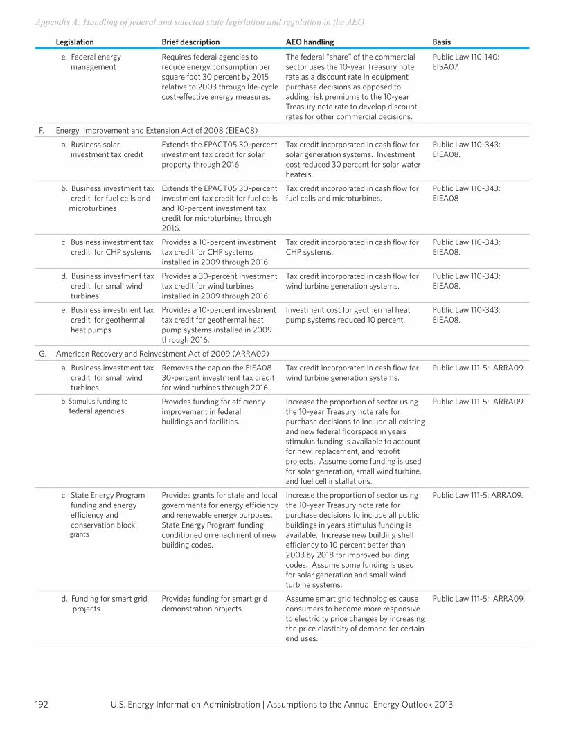
U.S. Energy Information Administration | Assumptions to the Annual Energy Outlook 2013192
Appendix A: Handling of federal and selected state legislation and regulation in the AEO
Legislation Brief description AEO handling Basis
e. Federal energy management
Requires federal agencies to reduce energy consumption per square foot 30 percent by 2015 relative to 2003 through life-cycle cost-effective energy measures.
The federal “share” of the commercial sector uses the 10-year Treasury note rate as a discount rate in equipment purchase decisions as opposed to adding risk premiums to the 10-year Treasury note rate to develop discount rates for other commercial decisions.
Public Law 110-140: EISA07.
F. Energy Improvement and Extension Act of 2008 (EIEA08)
a. Business solar investment tax credit
Extends the EPACT05 30-percent investment tax credit for solar property through 2016.
Tax credit incorporated in cash flow for solar generation systems. Investment cost reduced 30 percent for solar water heaters.
Public Law 110-343: EIEA08.
b. Business investment tax credit for fuel cells and microturbines
Extends the EPACT05 30-percent investment tax credit for fuel cells and 10-percent investment tax credit for microturbines through 2016.
Tax credit incorporated in cash flow for fuel cells and microturbines.
Public Law 110-343: EIEA08
c. Business investment tax credit for CHP systems
Provides a 10-percent investment tax credit for CHP systems installed in 2009 through 2016
Tax credit incorporated in cash flow for CHP systems.
Public Law 110-343: EIEA08.
d. Business investment tax credit for small wind turbines
Provides a 30-percent investment tax credit for wind turbines installed in 2009 through 2016.
Tax credit incorporated in cash flow for wind turbine generation systems.
Public Law 110-343: EIEA08.
e. Business investment tax credit for geothermal heat pumps
Provides a 10-percent investment tax credit for geothermal heat pump systems installed in 2009 through 2016.
Investment cost for geothermal heat pump systems reduced 10 percent.
Public Law 110-343: EIEA08.
G. American Recovery and Reinvestment Act of 2009 (ARRA09)
a. Business investment tax credit for small wind turbines
Removes the cap on the EIEA08 30-percent investment tax credit for wind turbines through 2016.
Tax credit incorporated in cash flow for wind turbine generation systems.
Public Law 111-5: ARRA09.
b. Stimulus funding to federal agencies
Provides funding for efficiency improvement in federal buildings and facilities.
Increase the proportion of sector using the 10-year Treasury note rate for purchase decisions to include all existing and new federal floorspace in years stimulus funding is available to account for new, replacement, and retrofit projects. Assume some funding is used for solar generation, small wind turbine, and fuel cell installations.
Public Law 111-5: ARRA09.
c. State Energy Program funding and energy efficiency and conservation block grants
Provides grants for state and local governments for energy efficiency and renewable energy purposes. State Energy Program funding conditioned on enactment of new building codes.
Increase the proportion of sector using the 10-year Treasury note rate for purchase decisions to include all public buildings in years stimulus funding is available. Increase new building shell efficiency to 10 percent better than 2003 by 2018 for improved building codes. Assume some funding is used for solar generation and small wind turbine systems.
Public Law 111-5: ARRA09.
d. Funding for smart grid projects
Provides funding for smart grid demonstration projects.
Assume smart grid technologies cause consumers to become more responsive to electricity price changes by increasing the price elasticity of demand for certain end uses.
Public Law 111-5; ARRA09.
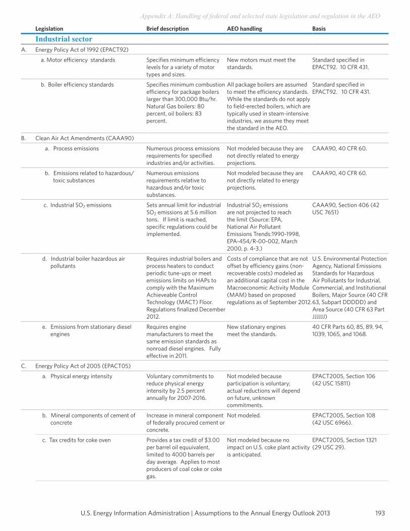
193U.S. Energy Information Administration | Assumptions to the Annual Energy Outlook 2013
Appendix A: Handling of federal and selected state legislation and regulation in the AEO
Legislation Brief description AEO handling Basis
Industrial sectorA. Energy Policy Act of 1992 (EPACT92)
a. Motor efficiency standards Specifies minimum efficiencylevels for a variety of motortypes and sizes.
New motors must meet thestandards.
Standard specified inEPACT92. 10 CFR 431.
b. Boiler efficiency standards Specifies minimum combustion efficiency for package boilers larger than 300,000 Btu/hr. Natural Gas boilers: 80 percent, oil boilers: 83 percent.
All package boilers are assumed to meet the efficiency standards. While the standards do not apply to field-erected boilers, which are typically used in steam-intensive industries, we assume they meet the standard in the AEO.
Standard specified inEPACT92. 10 CFR 431.
B. Clean Air Act Amendments (CAAA90)
a. Process emissions Numerous process emissionsrequirements for specifiedindustries and/or activities.
Not modeled because they are not directly related to energy projections.
CAAA90, 40 CFR 60.
b. Emissions related to hazardous/ toxic substances
Numerous emissionsrequirements relative tohazardous and/or toxicsubstances.
Not modeled because they are not directly related to energy projections.
CAAA90, 40 CFR 60.
c. Industrial SO2 emissions Sets annual limit for industrialSO2 emissions at 5.6 milliontons. If limit is reached,specific regulations could beimplemented.
Industrial SO2 emissions are not projected to reach the limit (Source: EPA, National Air Pollutant Emissions Trends:1990-1998, EPA-454/R-00-002, March 2000, p. 4-3.)
CAAA90, Section 406 (42 USC 7651)
d. Industrial boiler hazardous air pollutants
Requires industrial boilers and process heaters to conduct periodic tune-ups or meet emissions limits on HAPs to comply with the Maximum Achieveable Control Technology (MACT) Floor. Regulations finalized December 2012.
Costs of compliance that are not offset by efficiency gains (non-recoverable costs) modeled as an additional capital cost in the Macroeconomic Activity Module (MAM) based on proposed regulations as of September 2012.
U.S. Environmental Protection Agency, National Emissions Standards for Hazardous Air Pollutants for Industrial, Commercial, and Institutional Boilers, Major Source (40 CFR 63, Subpart DDDDD) and Area Source (40 CFR 63 Part JJJJJJ)
e. Emissions from stationary diesel engines
Requires enginemanufacturers to meet thesame emission standards asnonroad diesel engines. Fully effective in 2011.
New stationary engines meet the standards.
40 CFR Parts 60, 85, 89, 94,1039, 1065, and 1068.
C. Energy Policy Act of 2005 (EPACT05)
a. Physical energy intensity Voluntary commitments toreduce physical energyintensity by 2.5 percentannually for 2007-2016.
Not modeled becauseparticipation is voluntary;actual reductions will dependon future, unknowncommitments.
EPACT2005, Section 106 (42 USC 15811)
b. Mineral components of cement of concrete
Increase in mineral component of federally procured cement or concrete.
Not modeled. EPACT2005, Section 108 (42 USC 6966).
c. Tax credits for coke oven Provides a tax credit of $3.00per barrel oil equuivalent, limited to 4000 barrels per day average. Applies to most producers of coal coke or coke gas.
Not modeled because no impact on U.S. coke plant activity is anticipated.
EPACT2005, Section 1321 (29 USC 29).
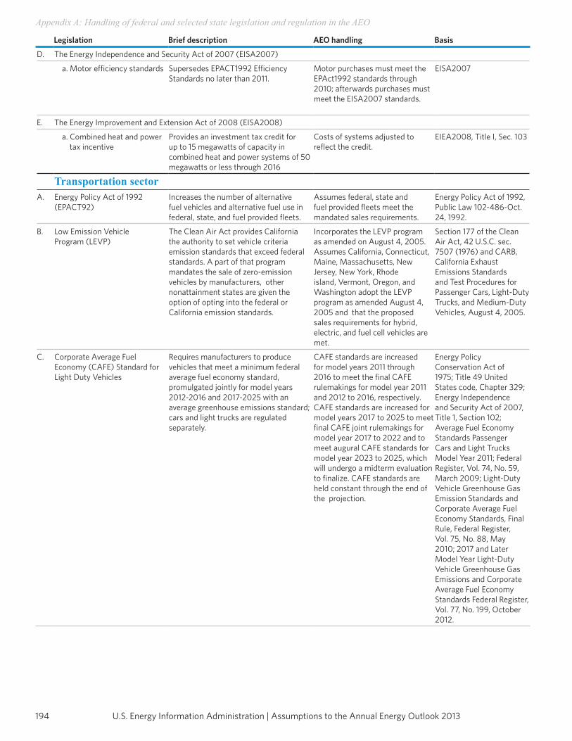
U.S. Energy Information Administration | Assumptions to the Annual Energy Outlook 2013194
Appendix A: Handling of federal and selected state legislation and regulation in the AEO
Legislation Brief description AEO handling Basis
D. The Energy Independence and Security Act of 2007 (EISA2007)
a. Motor efficiency standards Supersedes EPACT1992 Efficiency Standards no later than 2011.
Motor purchases must meet the EPAct1992 standards through 2010; afterwards purchases must meet the EISA2007 standards.
EISA2007
E. The Energy Improvement and Extension Act of 2008 (EISA2008)
a. Combined heat and power tax incentive
Provides an investment tax credit for up to 15 megawatts of capacity in combined heat and power systems of 50 megawatts or less through 2016
Costs of systems adjusted to reflect the credit.
EIEA2008, Title I, Sec. 103
Transportation sectorA. Energy Policy Act of 1992
(EPACT92)Increases the number of alternative fuel vehicles and alternative fuel use in federal, state, and fuel provided fleets.
Assumes federal, state and fuel provided fleets meet the mandated sales requirements.
Energy Policy Act of 1992, Public Law 102-486-Oct. 24, 1992.
B. Low Emission Vehicle Program (LEVP)
The Clean Air Act provides California the authority to set vehicle criteria emission standards that exceed federal standards. A part of that program mandates the sale of zero-emission vehicles by manufacturers, other nonattainment states are given the option of opting into the federal or California emission standards.
Incorporates the LEVP program as amended on August 4, 2005. Assumes California, Connecticut, Maine, Massachusetts, New Jersey, New York, Rhode island, Vermont, Oregon, and Washington adopt the LEVP program as amended August 4, 2005 and that the proposed sales requirements for hybrid, electric, and fuel cell vehicles are met.
Section 177 of the Clean Air Act, 42 U.S.C. sec. 7507 (1976) and CARB, California Exhaust Emissions Standards and Test Procedures for Passenger Cars, Light-Duty Trucks, and Medium-Duty Vehicles, August 4, 2005.
C. Corporate Average Fuel Economy (CAFE) Standard for Light Duty Vehicles
Requires manufacturers to produce vehicles that meet a minimum federal average fuel economy standard, promulgated jointly for model years 2012-2016 and 2017-2025 with an average greenhouse emissions standard; cars and light trucks are regulated separately.
CAFE standards are increased for model years 2011 through 2016 to meet the final CAFE rulemakings for model year 2011 and 2012 to 2016, respectively. CAFE standards are increased for model years 2017 to 2025 to meet final CAFE joint rulemakings for model year 2017 to 2022 and to meet augural CAFE standards for model year 2023 to 2025, which will undergo a midterm evaluation to finalize. CAFE standards are held constant through the end of the projection.
Energy Policy Conservation Act of 1975; Title 49 United States code, Chapter 329; Energy Independence and Security Act of 2007, Title 1, Section 102; Average Fuel Economy Standards Passenger Cars and Light Trucks Model Year 2011; Federal Register, Vol. 74, No. 59, March 2009; Light-Duty Vehicle Greenhouse Gas Emission Standards and Corporate Average Fuel Economy Standards, Final Rule, Federal Register, Vol. 75, No. 88, May 2010; 2017 and Later Model Year Light-Duty Vehicle Greenhouse Gas Emissions and Corporate Average Fuel Economy Standards Federal Register, Vol. 77, No. 199, October 2012.
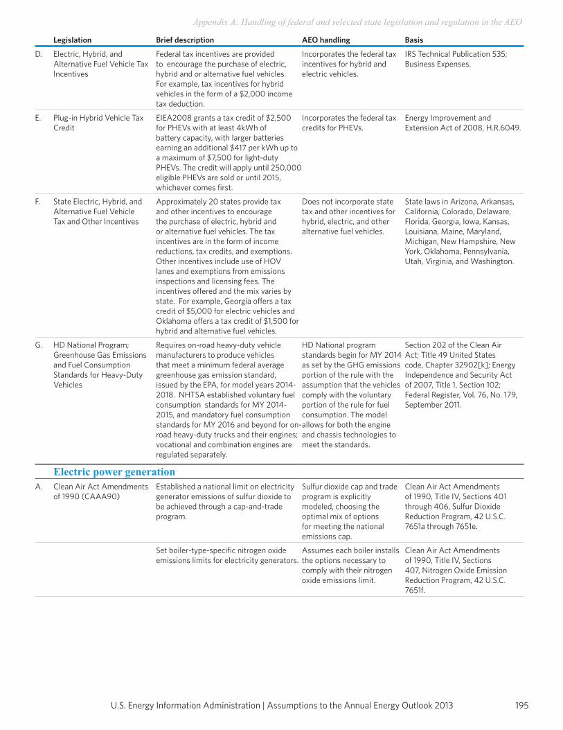
195U.S. Energy Information Administration | Assumptions to the Annual Energy Outlook 2013
Appendix A: Handling of federal and selected state legislation and regulation in the AEO
Legislation Brief description AEO handling Basis
D. Electric, Hybrid, and Alternative Fuel Vehicle Tax Incentives
Federal tax incentives are provided to encourage the purchase of electric, hybrid and or alternative fuel vehicles. For example, tax incentives for hybrid vehicles in the form of a $2,000 income tax deduction.
Incorporates the federal tax incentives for hybrid and electric vehicles.
IRS Technical Publication 535; Business Expenses.
E. Plug-in Hybrid Vehicle Tax Credit
EIEA2008 grants a tax credit of $2,500 for PHEVs with at least 4kWh of battery capacity, with larger batteries earning an additional $417 per kWh up to a maximum of $7,500 for light-duty PHEVs. The credit will apply until 250,000 eligible PHEVs are sold or until 2015, whichever comes first.
Incorporates the federal tax credits for PHEVs.
Energy Improvement andExtension Act of 2008, H.R.6049.
F. State Electric, Hybrid, and Alternative Fuel Vehicle Tax and Other Incentives
Approximately 20 states provide tax and other incentives to encourage the purchase of electric, hybrid and or alternative fuel vehicles. The tax incentives are in the form of income reductions, tax credits, and exemptions. Other incentives include use of HOV lanes and exemptions from emissions inspections and licensing fees. The incentives offered and the mix varies by state. For example, Georgia offers a tax credit of $5,000 for electric vehicles and Oklahoma offers a tax credit of $1,500 for hybrid and alternative fuel vehicles.
Does not incorporate state tax and other incentives for hybrid, electric, and other alternative fuel vehicles.
State laws in Arizona, Arkansas, California, Colorado, Delaware, Florida, Georgia, Iowa, Kansas, Louisiana, Maine, Maryland, Michigan, New Hampshire, New York, Oklahoma, Pennsylvania,Utah, Virginia, and Washington.
G. HD National Program; Greenhouse Gas Emissions and Fuel Consumption Standards for Heavy-Duty Vehicles
Requires on-road heavy-duty vehicle manufacturers to produce vehicles that meet a minimum federal average greenhouse gas emission standard, issued by the EPA, for model years 2014-2018. NHTSA established voluntary fuel consumption standards for MY 2014-2015, and mandatory fuel consumption standards for MY 2016 and beyond for on-road heavy-duty trucks and their engines; vocational and combination engines are regulated separately.
HD National program standards begin for MY 2014 as set by the GHG emissions portion of the rule with the assumption that the vehicles comply with the voluntary portion of the rule for fuel consumption. The model allows for both the engine and chassis technologies to meet the standards.
Section 202 of the Clean Air Act; Title 49 United States code, Chapter 32902[k]; Energy Independence and Security Act of 2007, Title 1, Section 102; Federal Register, Vol. 76, No. 179, September 2011.
Electric power generationA. Clean Air Act Amendments
of 1990 (CAAA90)Established a national limit on electricity generator emissions of sulfur dioxide to be achieved through a cap-and-trade program.
Sulfur dioxide cap and trade program is explicitly modeled, choosing the optimal mix of options for meeting the national emissions cap.
Clean Air Act Amendments of 1990, Title IV, Sections 401 through 406, Sulfur Dioxide Reduction Program, 42 U.S.C. 7651a through 7651e.
Set boiler-type-specific nitrogen oxide emissions limits for electricity generators.
Assumes each boiler installs the options necessary to comply with their nitrogen oxide emissions limit.
Clean Air Act Amendments of 1990, Title IV, Sections 407, Nitrogen Oxide Emission Reduction Program, 42 U.S.C. 7651f.
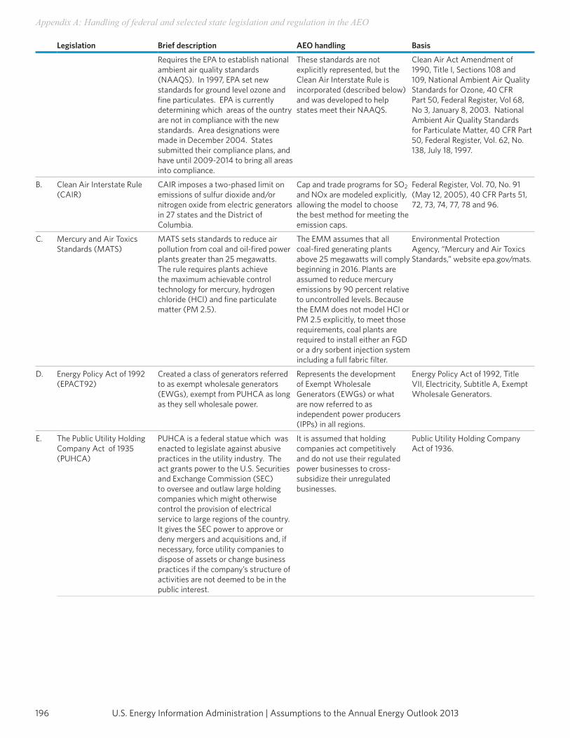
U.S. Energy Information Administration | Assumptions to the Annual Energy Outlook 2013196
Appendix A: Handling of federal and selected state legislation and regulation in the AEO
Legislation Brief description AEO handling Basis
Requires the EPA to establish national ambient air quality standards (NAAQS). In 1997, EPA set new standards for ground level ozone and fine particulates. EPA is currently determining which areas of the ountry are not in compliance with the new standards. Area designations were made in December 2004. States submitted their compliance plans, and have until 2009-2014 to bring all areas into compliance.
These standards are not explicitly represented, but the Clean Air Interstate Rule is incorporated (described below) and was developed to help states meet their NAAQS.
Clean Air Act Amendment of 1990, Title I, Sections 108 and 109, National Ambient Air Quality Standards for Ozone, 40 CFR Part 50, Federal Register, Vol 68, No 3, January 8, 2003. National Ambient Air Quality Standardsfor Particulate Matter, 40 CFR Part 50, Federal Register, Vol. 62, No. 138, July 18, 1997.
B. Clean Air Interstate Rule (CAIR)
CAIR imposes a two-phased limit on emissions of sulfur dioxide and/or nitrogen oxide from electric generators in 27 states and the District of Columbia.
Cap and trade programs for SO2 and NOx are modeled explicitly, allowing the model to choose the best method for meeting the emission caps.
Federal Register, Vol. 70, No. 91(May 12, 2005), 40 CFR Parts 51, 72, 73, 74, 77, 78 and 96.
C. Mercury and Air Toxics Standards (MATS)
MATS sets standards to reduce air pollution from coal and oil-fired power plants greater than 25 megawatts. The rule requires plants achieve the maximum achievable control technology for mercury, hydrogen chloride (HCl) and fine particulate matter (PM 2.5).
The EMM assumes that all coal-fired generating plants above 25 megawatts will comply beginning in 2016. Plants are assumed to reduce mercury emissions by 90 percent relative to uncontrolled levels. Because the EMM does not model HCl or PM 2.5 explicitly, to meet those requirements, coal plants are required to install either an FGD or a dry sorbent injection system including a full fabric filter.
Environmental Protection Agency, “Mercury and Air Toxics Standards,” website epa.gov/mats.
D. Energy Policy Act of 1992 (EPACT92)
Created a class of generators referred to as exempt wholesale generators (EWGs), exempt from PUHCA as long as they sell wholesale power.
Represents the development of Exempt Wholesale Generators (EWGs) or what are now referred to as independent power producers (IPPs) in all regions.
Energy Policy Act of 1992, Title VII, Electricity, Subtitle A, Exempt Wholesale Generators.
E. The Public Utility Holding Company Act of 1935 (PUHCA)
PUHCA is a federal statue which was enacted to legislate against abusive practices in the utility industry. The act grants power to the U.S. Securities and Exchange Commission (SEC) to oversee and outlaw large holding companies which might otherwise control the provision of electrical service to large regions of the country. It gives the SEC power to approve or deny mergers and acquisitions and, if necessary, force utility companies to dispose of assets or change business practices if the company’s structure of activities are not deemed to be in the public interest.
It is assumed that holding companies act competitively and do not use their regulated power businesses to cross-subsidize their unregulated businesses.
Public Utility Holding CompanyAct of 1936.
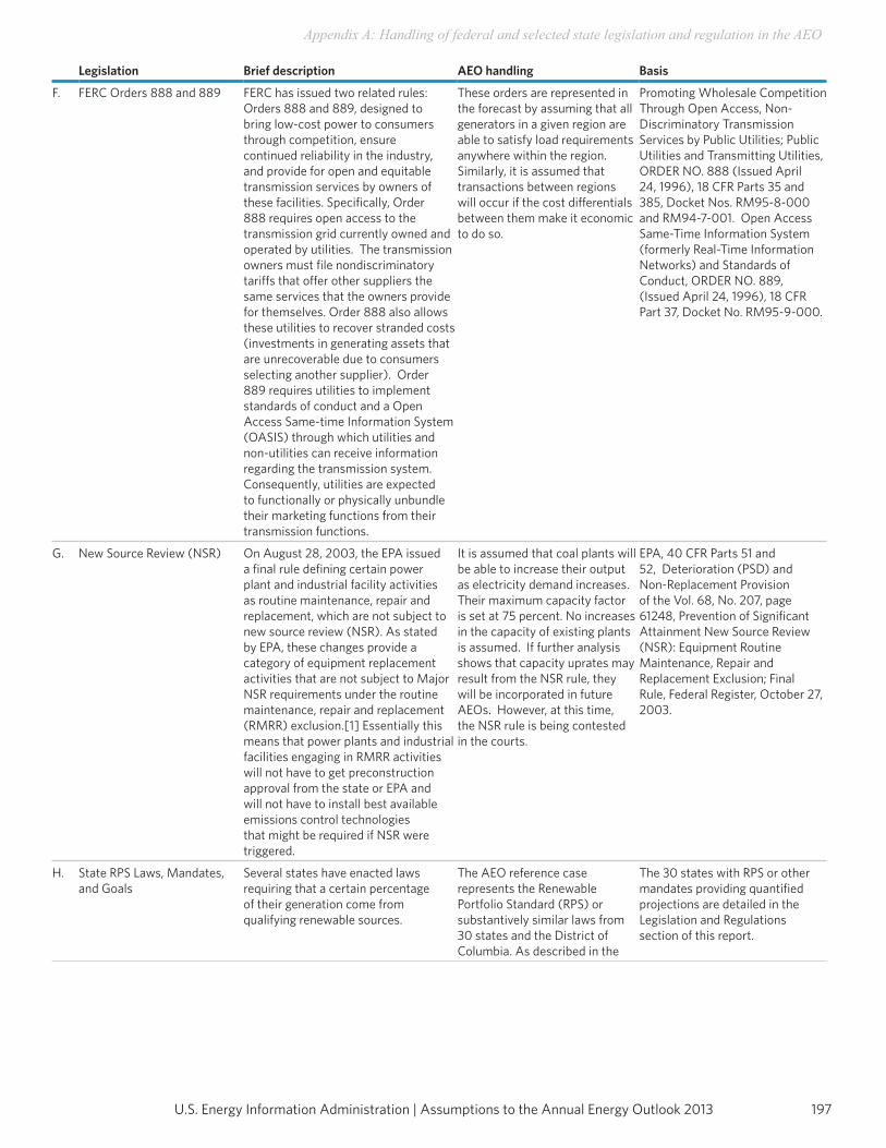
197U.S. Energy Information Administration | Assumptions to the Annual Energy Outlook 2013
Appendix A: Handling of federal and selected state legislation and regulation in the AEO
Legislation Brief description AEO handling Basis
F. FERC Orders 888 and 889 FERC has issued two related rules: Orders 888 and 889, designed to bring low-cost power to consumers through competition, ensure continued reliability in the industry, and provide for open and equitable transmission services by owners of these facilities. Specifically, Order 888 requires open access to the transmission grid currently owned and operated by utilities. The transmission owners must file nondiscriminatory tariffs that offer other suppliers the same services that the owners provide for themselves. Order 888 also allows these utilities to recover stranded costs (investments in generating assets that are unrecoverable due to consumers selecting another supplier). Order 889 requires utilities to implement standards of conduct and a Open Access Same-time Information System (OASIS) through which utilities and non-utilities can receive information regarding the transmission system. Consequently, utilities are expected to functionally or physically unbundle their marketing functions from their transmission functions.
These orders are represented in the forecast by assuming that all generators in a given region are able to satisfy load requirements anywhere within the region. Similarly, it is assumed that transactions between regions will occur if the cost differentials between them make it economic to do so.
Promoting Wholesale Competition Through Open Access, Non-Discriminatory Transmission Services by Public Utilities; Public Utilities and Transmitting Utilities, ORDER NO. 888 (Issued April 24, 1996), 18 CFR Parts 35 and 385, Docket Nos. RM95-8-000 and RM94-7-001. Open Access Same-Time Information System (formerly Real-Time Information Networks) and Standards of Conduct, ORDER NO. 889, (Issued April 24, 1996), 18 CFR Part 37, Docket No. RM95-9-000.
G. New Source Review (NSR) On August 28, 2003, the EPA issued a final rule defining certain power plant and industrial facility activities as routine maintenance, repair and replacement, which are not subject to new source review (NSR). As stated by EPA, these changes provide a category of equipment replacement activities that are not subject to Major NSR requirements under the routine maintenance, repair and replacement (RMRR) exclusion.[1] Essentially this means that power plants and industrial facilities engaging in RMRR activities will not have to get preconstruction approval from the state or EPA and will not have to install best available emissions control technologies that might be required if NSR were triggered.
It is assumed that coal plants will be able to increase their output as electricity demand increases. Their maximum capacity factor is set at 75 percent. No increases in the capacity of existing plants is assumed. If further analysis shows that capacity uprates may result from the NSR rule, they will be incorporated in future AEOs. However, at this time, the NSR rule is being contested in the courts.
EPA, 40 CFR Parts 51 and 52, Deterioration (PSD) and Non-Replacement Provision of the Vol. 68, No. 207, page 61248, Prevention of Significant Attainment New Source Review (NSR): Equipment Routine Maintenance, Repair and Replacement Exclusion; Final Rule, Federal Register, October 27, 2003.
H. State RPS Laws, Mandates, and Goals
Several states have enacted laws requiring that a certain percentage of their generation come from qualifying renewable sources.
The AEO reference case represents the Renewable Portfolio Standard (RPS) orsubstantively similar laws from 30 states and the District of Columbia. As described in the
The 30 states with RPS or other mandates providing quantified projections are detailed in the Legislation and Regulations section of this report.
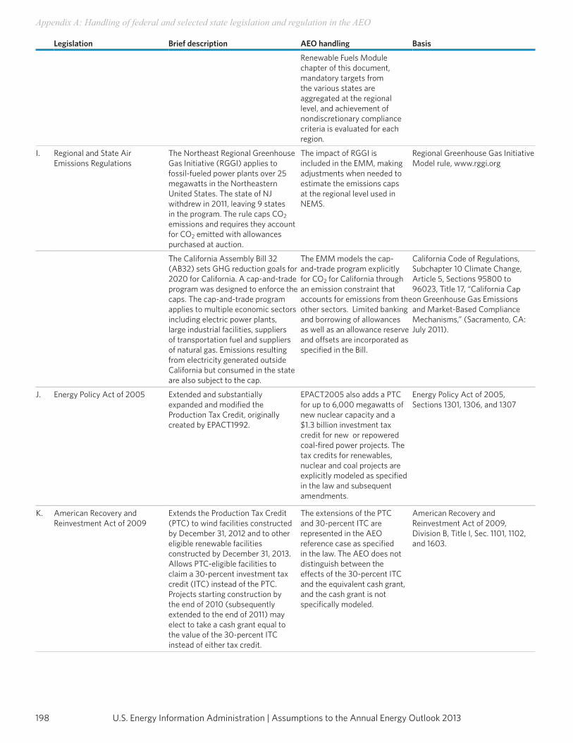
U.S. Energy Information Administration | Assumptions to the Annual Energy Outlook 2013198
Appendix A: Handling of federal and selected state legislation and regulation in the AEO
Legislation Brief description AEO handling Basis
Renewable Fuels Module chapter of this document,mandatory targets from the various states are aggregated at the regional level, and achievement of nondiscretionary compliance criteria is evaluated for each region.
I. Regional and State Air Emissions Regulations
The Northeast Regional Greenhouse Gas Initiative (RGGI) applies to fossil-fueled power plants over 25 megawatts in the Northeastern United States. The state of NJ withdrew in 2011, leaving 9 states in the program. The rule caps CO2 emissions and requires they account for CO2 emitted with allowances purchased at auction.
The impact of RGGI is included in the EMM, making adjustments when needed to estimate the emissions caps at the regional level used in NEMS.
Regional Greenhouse Gas Initiative Model rule, www.rggi.org
The California Assembly Bill 32 (AB32) sets GHG reduction goals for 2020 for California. A cap-and-trade program was designed to enforce the caps. The cap-and-trade program applies to multiple economic sectors including electric power plants, large industrial facilities, suppliers of transportation fuel and suppliers of natural gas. Emissions resulting from electricity generated outside California but consumed in the state are also subject to the cap.
The EMM models the cap-and-trade program explicitly for CO2 for California through an emission constraint that accounts for emissions from the other sectors. Limited banking and borrowing of allowances as well as an allowance reserve and offsets are incorporated as specified in the Bill.
California Code of Regulations, Subchapter 10 Climate Change, Article 5, Sections 95800 to 96023, Title 17, “California Cap on Greenhouse Gas Emissions and Market-Based Compliance Mechanisms,” (Sacramento, CA: July 2011).
J. Energy Policy Act of 2005 Extended and substantially expanded and modified the Production Tax Credit, originally created by EPACT1992.
EPACT2005 also adds a PTC for up to 6,000 megawatts of new nuclear capacity and a $1.3 billion investment tax credit for new or repowered coal-fired power projects. The tax credits for renewables, nuclear and coal projects are explicitly modeled as specified in the law and subsequent amendments.
Energy Policy Act of 2005, Sections 1301, 1306, and 1307
K. American Recovery and Reinvestment Act of 2009
Extends the Production Tax Credit (PTC) to wind facilities constructed by December 31, 2012 and to other eligible renewable facilitiesconstructed by December 31, 2013. Allows PTC-eligible facilities to claim a 30-percent investment tax credit (ITC) instead of the PTC. Projects starting construction by the end of 2010 (subsequently extended to the end of 2011) may elect to take a cash grant equal to the value of the 30-percent ITC instead of either tax credit.
The extensions of the PTC and 30-percent ITC are represented in the AEOreference case as specified in the law. The AEO does not distinguish between the effects of the 30-percent ITC and the equivalent cash grant, and the cash grant is not specifically modeled.
American Recovery and Reinvestment Act of 2009, Division B, Title I, Sec. 1101, 1102, and 1603.
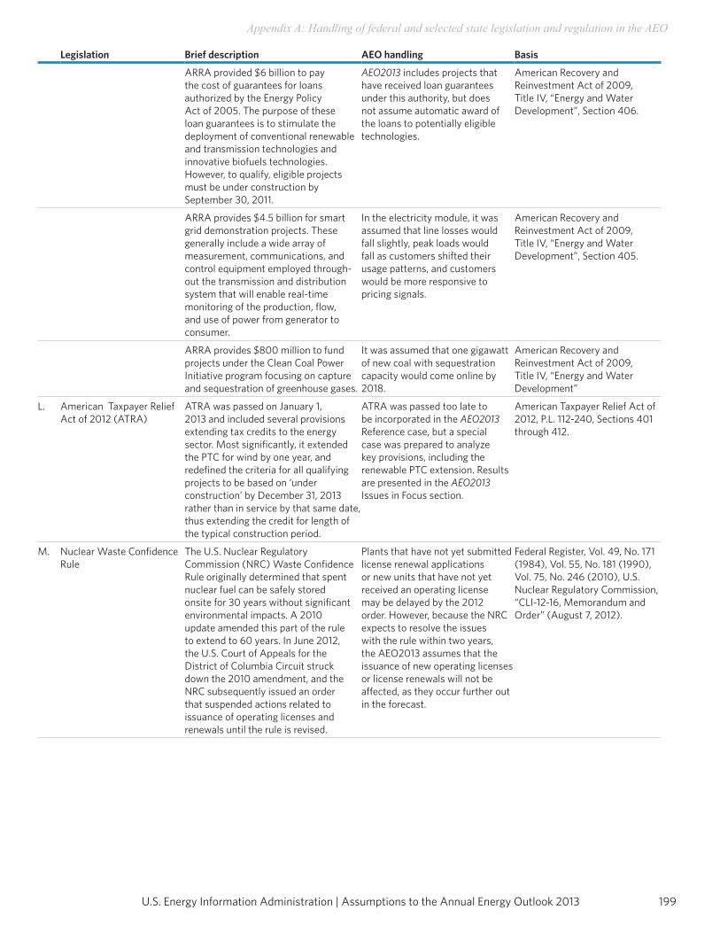
199U.S. Energy Information Administration | Assumptions to the Annual Energy Outlook 2013
Appendix A: Handling of federal and selected state legislation and regulation in the AEO
Legislation Brief description AEO handling Basis
ARRA provided $6 billion to pay the cost of guarantees for loans authorized by the Energy Policy Act of 2005. The purpose of these loan guarantees is to stimulate the deployment of conventional renewable and transmission technologies and innovative biofuels technologies. However, to qualify, eligible projects must be under construction by September 30, 2011.
AEO2013 includes projects that have received loan guarantees under this authority, but does not assume automatic award of the loans to potentially eligible technologies.
American Recovery and Reinvestment Act of 2009, Title IV, “Energy and Water Development”, Section 406.
ARRA provides $4.5 billion for smart grid demonstration projects. These generally include a wide array of measurement, communications, and control equipment employed through-out the transmission and distribution system that will enable real-time monitoring of the production, flow, and use of power from generator to consumer.
In the electricity module, it wasassumed that line losses wouldfall slightly, peak loads wouldfall as customers shifted theirusage patterns, and customerswould be more responsive topricing signals.
American Recovery and Reinvestment Act of 2009, Title IV, “Energy and Water Development”, Section 405.
ARRA provides $800 million to fund projects under the Clean Coal Power Initiative program focusing on capture and sequestration of greenhouse gases.
It was assumed that one gigawatt of new coal with sequestration capacity would come online by 2018.
American Recovery and Reinvestment Act of 2009, Title IV, “Energy and WaterDevelopment”
L. American Taxpayer Relief Act of 2012 (ATRA)
ATRA was passed on January 1, 2013 and included several provisions extending tax credits to the energy sector. Most significantly, it extended the PTC for wind by one year, and redefined the criteria for all qualifying projects to be based on ‘under construction’ by December 31, 2013 rather than in service by that same date, thus extending the credit for length of the typical construction period.
ATRA was passed too late to be incorporated in the AEO2013 Reference case, but a special case was prepared to analyze key provisions, including the renewable PTC extension. Results are presented in the AEO2013 Issues in Focus section.
American Taxpayer Relief Act of 2012, P.L. 112-240, Sections 401 through 412.
M. Nuclear Waste Confidence Rule
The U.S. Nuclear Regulatory Commission (NRC) Waste Confidence Rule originally determined that spent nuclear fuel can be safely stored onsite for 30 years without significant environmental impacts. A 2010 update amended this part of the rule to extend to 60 years. In June 2012, the U.S. Court of Appeals for the District of Columbia Circuit struck down the 2010 amendment, and the NRC subsequently issued an order that suspended actions related to issuance of operating licenses and renewals until the rule is revised.
Plants that have not yet submitted license renewal applications or new units that have not yet received an operating license may be delayed by the 2012 order. However, because the NRC expects to resolve the issues with the rule within two years, the AEO2013 assumes that the issuance of new operating licenses or license renewals will not be affected, as they occur further out in the forecast.
Federal Register, Vol. 49, No. 171(1984), Vol. 55, No. 181 (1990), Vol. 75, No. 246 (2010), U.S. Nuclear Regulatory Commission, “CLI-12-16, Memorandum and Order” (August 7, 2012).
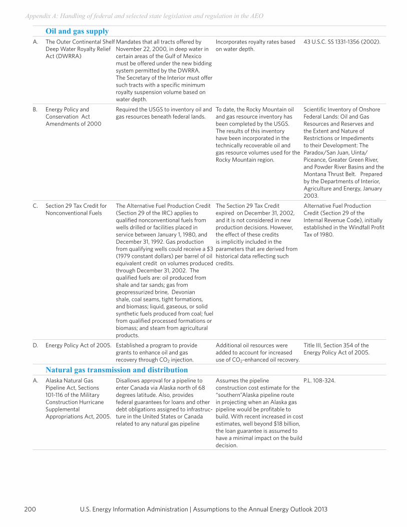
U.S. Energy Information Administration | Assumptions to the Annual Energy Outlook 2013200
Appendix A: Handling of federal and selected state legislation and regulation in the AEO
Oil and gas supplyA. The Outer Continental Shelf
Deep Water Royalty Relief Act (DWRRA)
Mandates that all tracts offered by November 22, 2000, in deep water in certain areas of the Gulf of Mexico must be offered under the new bidding system permitted by the DWRRA. The Secretary of the Interior must offer such tracts with a specific minimum royalty suspension volume based on water depth.
Incorporates royalty rates based on water depth.
43 U.S.C. SS 1331-1356 (2002).
B. Energy Policy and Conservation Act Amendments of 2000
Required the USGS to inventory oil and gas resources beneath federal lands.
To date, the Rocky Mountain oil and gas resource inventory has been completed by the USGS. The results of this inventory have been incorporated in the technically recoverable oil and gas resource volumes used for the Rocky Mountain region.
Scientific Inventory of Onshore Federal Lands: Oil and Gas Resources and Reserves and the Extent and Nature of Restrictions or Impediments to their Development: The Paradox/San Juan, Uinta/Piceance, Greater Green River, and Powder River Basins and the Montana Thrust Belt. Prepared by the Departments of Interior, Agriculture and Energy, January 2003.
C. Section 29 Tax Credit for Nonconventional Fuels
The Alternative Fuel Production Credit (Section 29 of the IRC) applies to qualified nonconventional fuels from wells drilled or facilities placed in service between January 1, 1980, and December 31, 1992. Gas production from qualifying wells could receive a $3 (1979 constant dollars) per barrel of oil equivalent credit on volumes produced through December 31, 2002. The qualified fuels are: oil produced from shale and tar sands; gas from geopressurized brine, Devonian shale, coal seams, tight formations, and biomass; liquid, gaseous, or solid synthetic fuels produced from coal; fuel from qualified processed formations or biomass; and steam from agricultural products.
The Section 29 Tax Credit expired on December 31, 2002, and it is not considered in new production decisions. However, the effect of these credits is implicitly included in the parameters that are derived from historical data reflecting such credits.
Alternative Fuel Production Credit (Section 29 of the Internal Revenue Code), initially established in the Windfall Profit Tax of 1980.
D. Energy Policy Act of 2005. Established a program to provide grants to enhance oil and gas recovery through CO2 injection.
Additional oil resources were added to account for increased use of CO2-enhanced oil recovery.
Title III, Section 354 of the Energy Policy Act of 2005.
Natural gas transmission and distributionA. Alaska Natural Gas
Pipeline Act, Sections 101-116 of the Military Construction Hurricane Supplemental Appropriations Act, 2005.
Disallows approval for a pipeline toenter Canada via Alaska north of 68 degrees latitude. Also, provides federal guarantees for loans and other debt obligations assigned to infrastruc-ture in the United States or Canada related to any natural gas pipeline
Assumes the pipeline construction cost estimate for the “southern”Alaska pipeline route in projecting when an Alaska gas pipeline would be profitable to build. With recent increased in cost estimates, well beyond $18 billion, the loan guarantee is assumed to have a minimal impact on the build decision.
P.L. 108-324.
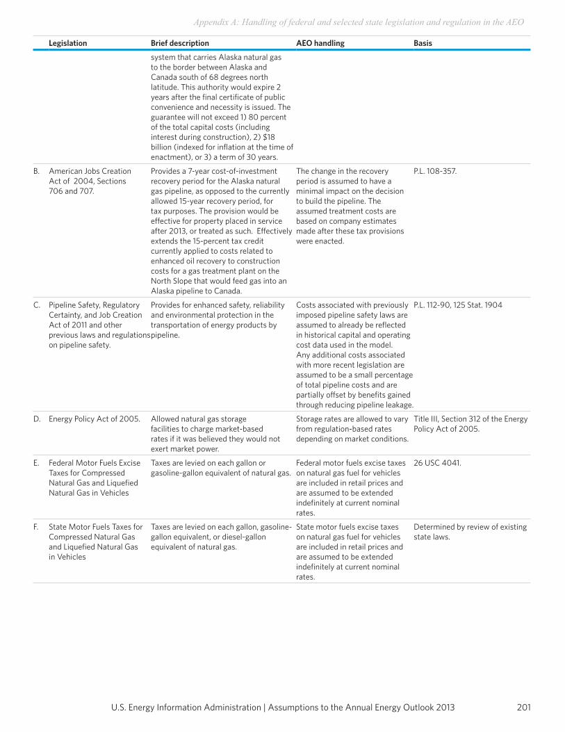
201U.S. Energy Information Administration | Assumptions to the Annual Energy Outlook 2013
Appendix A: Handling of federal and selected state legislation and regulation in the AEO
Legislation Brief description AEO handling Basis
system that carries Alaska natural gas to the border between Alaska andCanada south of 68 degrees north latitude. This authority would expire 2 years after the final certificate of public convenience and necessity is issued. The guarantee will not exceed 1) 80 percent of the total capital costs (including interest during construction), 2) $18 billion (indexed for inflation at the time of enactment), or 3) a term of 30 years.
B. American Jobs Creation Act of 2004, Sections 706 and 707.
Provides a 7-year cost-of-investment recovery period for the Alaska natural gas pipeline, as opposed to the currently allowed 15-year recovery period, for tax purposes. The provision would be effective for property placed in service after 2013, or treated as such. Effectively extends the 15-percent tax credit currently applied to costs related to enhanced oil recovery to construction costs for a gas treatment plant on the North Slope that would feed gas into an Alaska pipeline to Canada.
The change in the recovery period is assumed to have a minimal impact on the decision to build the pipeline. The assumed treatment costs are based on company estimates made after these tax provisions were enacted.
P.L. 108-357.
C. Pipeline Safety, Regulatory Certainty, and Job Creation Act of 2011 and other previous laws and regulations on pipeline safety.
Provides for enhanced safety, reliability and environmental protection in the transportation of energy products by pipeline.
Costs associated with previously imposed pipeline safety laws are assumed to already be reflected in historical capital and operating cost data used in the model. Any additional costs associated with more recent legislation are assumed to be a small percentage of total pipeline costs and are partially offset by benefits gained through reducing pipeline leakage.
P.L. 112-90, 125 Stat. 1904
D. Energy Policy Act of 2005. Allowed natural gas storagefacilities to charge market-basedrates if it was believed they would not exert market power.
Storage rates are allowed to vary from regulation-based rates depending on market conditions.
Title III, Section 312 of the Energy Policy Act of 2005.
E. Federal Motor Fuels Excise Taxes for Compressed Natural Gas and Liquefied Natural Gas in Vehicles
Taxes are levied on each gallon or gasoline-gallon equivalent of natural gas.
Federal motor fuels excise taxes on natural gas fuel for vehicles are included in retail prices and are assumed to be extended indefinitely at current nominal rates.
26 USC 4041.
F. State Motor Fuels Taxes for Compressed Natural Gas and Liquefied Natural Gas in Vehicles
Taxes are levied on each gallon, gasoline-gallon equivalent, or diesel-gallon equivalent of natural gas.
State motor fuels excise taxes on natural gas fuel for vehicles are included in retail prices and are assumed to be extended indefinitely at current nominal rates.
Determined by review of existing state laws.
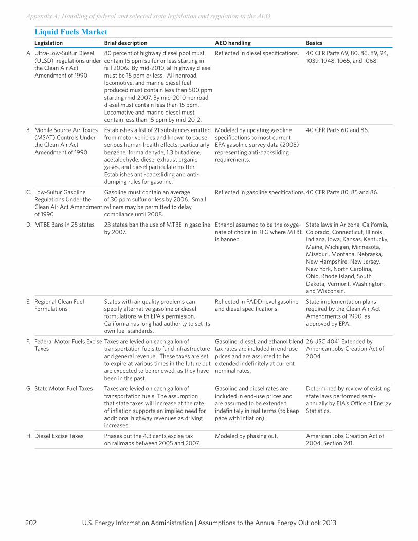
U.S. Energy Information Administration | Assumptions to the Annual Energy Outlook 2013202
Appendix A: Handling of federal and selected state legislation and regulation in the AEO
Liquid Fuels MarketLegislation Brief description AEO handling Basics
A Ultra-Low-Sulfur Diesel (ULSD) regulations under the Clean Air Act Amendment of 1990
80 percent of highway diesel pool must contain 15 ppm sulfur or less starting in fall 2006. By mid-2010, all highway diesel must be 15 ppm or less. All nonroad, locomotive, and marine diesel fuel produced must contain less than 500 ppm starting mid-2007. By mid-2010 nonroad diesel must contain less than 15 ppm. Locomotive and marine diesel must contain less than 15 ppm by mid-2012.
Reflected in diesel specifications. 40 CFR Parts 69, 80, 86, 89, 94, 1039, 1048, 1065, and 1068.
B. Mobile Source Air Toxics(MSAT) Controls Under the Clean Air Act Amendment of 1990
Establishes a list of 21 substances emitted from motor vehicles and known to cause serious human health effects, particularly benzene, formaldehyde, 1.3 butadiene, acetaldehyde, diesel exhaust organic gases, and diesel particulate matter. Establishes anti-backsliding and anti-dumping rules for gasoline.
Modeled by updating gasoline specifications to most current EPA gasoline survey data (2005) representing anti-backsliding requirements.
40 CFR Parts 60 and 86.
C. Low-Sulfur Gasoline Regulations Under the Clean Air Act Amendment of 1990
Gasoline must contain an average of 30 ppm sulfur or less by 2006. Small refiners may be permitted to delay compliance until 2008.
Reflected in gasoline specifications. 40 CFR Parts 80, 85 and 86.
D. MTBE Bans in 25 states 23 states ban the use of MTBE in gasoline by 2007.
Ethanol assumed to be the oxyge- nate of choice in RFG where MTBE is banned
State laws in Arizona, California, Colorado, Connecticut, Illinois, Indiana, Iowa, Kansas, Kentucky,Maine, Michigan, Minnesota,Missouri, Montana, Nebraska,New Hampshire, New Jersey,New York, North Carolina,Ohio, Rhode Island, SouthDakota, Vermont, Washington,and Wisconsin.
E. Regional Clean Fuel Formulations
States with air quality problems can specify alternative gasoline or diesel formulations with EPA’s permission. California has long had authority to set its own fuel standards.
Reflected in PADD-level gasoline and diesel specifications.
State implementation plansrequired by the Clean Air ActAmendments of 1990, asapproved by EPA.
F. Federal Motor Fuels Excise Taxes
Taxes are levied on each gallon of transportation fuels to fund infrastructure and general revenue. These taxes are set to expire at various times in the future but are expected to be renewed, as they have been in the past.
Gasoline, diesel, and ethanol blend tax rates are included in end-use prices and are assumed to be extended indefinitely at current nominal rates.
26 USC 4041 Extended byAmerican Jobs Creation Act of 2004
G. State Motor Fuel Taxes Taxes are levied on each gallon of transportation fuels. The assumption that state taxes will increase at the rate of inflation supports an implied need for additional highway revenues as driving increases.
Gasoline and diesel rates are included in end-use prices and are assumed to be extended indefinitely in real terms (to keep pace with inflation).
Determined by review of existing state laws performed semi-annually by EIA’s Office of Energy Statistics.
H. Diesel Excise Taxes Phases out the 4.3 cents excise tax on railroads between 2005 and 2007.
Modeled by phasing out. American Jobs Creation Act of 2004, Section 241.
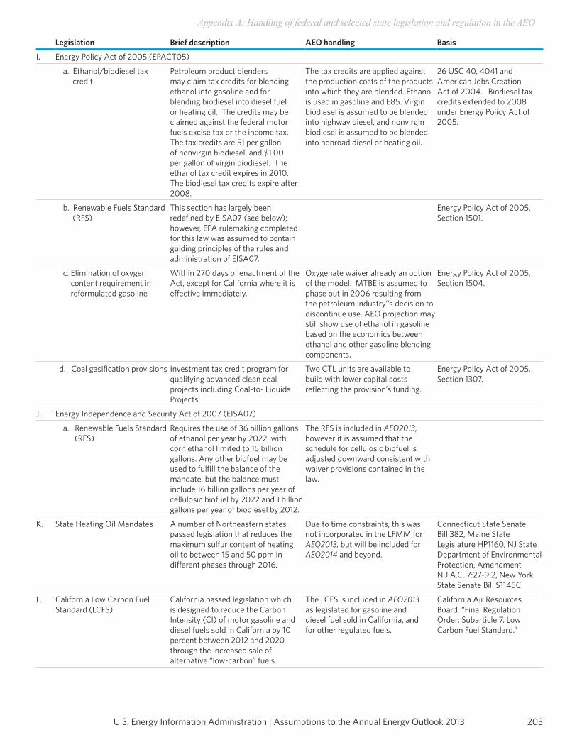
203U.S. Energy Information Administration | Assumptions to the Annual Energy Outlook 2013
Appendix A: Handling of federal and selected state legislation and regulation in the AEO
Legislation Brief description AEO handling Basis
I. Energy Policy Act of 2005 (EPACT05)
a. Ethanol/biodiesel tax credit
Petroleum product blenders may claim tax credits for blending ethanol into gasoline and for blending biodiesel into diesel fuel or heating oil. The credits may be claimed against the federal motor fuels excise tax or the income tax. The tax credits are 51 per gallon of nonvirgin biodiesel, and $1.00 per gallon of virgin biodiesel. The ethanol tax credit expires in 2010. The biodiesel tax credits expire after 2008.
The tax credits are applied against the production costs of the products into which they are blended. Ethanol is used in gasoline and E85. Virgin biodiesel is assumed to be blended into highway diesel, and nonvirgin biodiesel is assumed to be blended into nonroad diesel or heating oil.
26 USC 40, 4041 and American Jobs Creation Act of 2004. Biodiesel tax credits extended to 2008 under Energy Policy Act of 2005.
b. Renewable Fuels Standard (RFS)
This section has largely been redefined by EISA07 (see below); however, EPA rulemaking completed for this law was assumed to contain guiding principles of the rules and administration of EISA07.
Energy Policy Act of 2005, Section 1501.
c. Elimination of oxygen content requirement in reformulated gasoline
Within 270 days of enactment of the Act, except for California where it is effective immediately.
Oxygenate waiver already an option of the model. MTBE is assumed to phase out in 2006 resulting from the petroleum industry’’s decision to discontinue use. AEO projection may still show use of ethanol in gasoline based on the economics between ethanol and other gasoline blending components.
Energy Policy Act of 2005, Section 1504.
d. Coal gasification provisions Investment tax credit program for qualifying advanced clean coal projects including Coal-to- Liquids Projects.
Two CTL units are available to build with lower capital costs reflecting the provision’s funding.
Energy Policy Act of 2005, Section 1307.
J. Energy Independence and Security Act of 2007 (EISA07)
a. Renewable Fuels Standard (RFS)
Requires the use of 36 billion gallons of ethanol per year by 2022, with corn ethanol limited to 15 billion gallons. Any other biofuel may be used to fulfill the balance of the mandate, but the balance must include 16 billion gallons per year of cellulosic biofuel by 2022 and 1 billion gallons per year of biodiesel by 2012.
The RFS is included in AEO2013, however it is assumed that the schedule for cellulosic biofuel is adjusted downward consistent with waiver provisions contained in the law.
K. State Heating Oil Mandates A number of Northeastern states passed legislation that reduces the maximum sulfur content of heating oil to between 15 and 50 ppm in different phases through 2016.
Due to time constraints, this was not incorporated in the LFMM for AEO2013, but will be included for AEO2014 and beyond.
Connecticut State Senate Bill 382, Maine State Legislature HP1160, NJ State Department of Environmental Protection, Amendment N.J.A.C. 7:27-9.2, New York State Senate Bill S1145C.
L. California Low Carbon Fuel Standard (LCFS)
California passed legislation which is designed to reduce the Carbon Intensity (CI) of motor gasoline and diesel fuels sold in California by 10 percent between 2012 and 2020 through the increased sale of alternative “low-carbon” fuels.
The LCFS is included in AEO2013 as legislated for gasoline and diesel fuel sold in California, andfor other regulated fuels.
California Air Resources Board, “Final Regulation Order: Subarticle 7. Low Carbon Fuel Standard.”
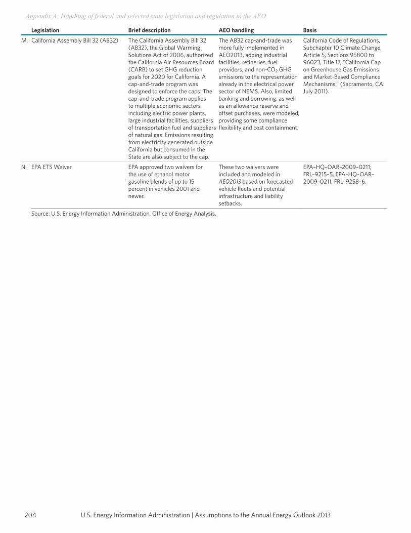
U.S. Energy Information Administration | Assumptions to the Annual Energy Outlook 2013204
Appendix A: Handling of federal and selected state legislation and regulation in the AEO
Legislation Brief description AEO handling Basis
M. California Assembly Bill 32 (AB32) The California Assembly Bill 32 (AB32), the Global Warming Solutions Act of 2006, authorized the California Air Resources Board (CARB) to set GHG reduction goals for 2020 for California. A cap-and-trade program was designed to enforce the caps. The cap-and-trade program applies to multiple economic sectors including electric power plants, large industrial facilities, suppliers of transportation fuel and suppliers of natural gas. Emissions resulting from electricity generated outside California but consumed in the State are also subject to the cap.
The AB32 cap-and-trade was more fully implemented in AEO2013, adding industrial facilities, refineries, fuel providers, and non-CO2 GHG emissions to the representation already in the electrical power sector of NEMS. Also, limited banking and borrowing, as well as an allowance reserve and offset purchases, were modeled, providing some compliance flexibility and cost containment.
California Code of Regulations, Subchapter 10 Climate Change, Article 5, Sections 95800 to 96023, Title 17, “California Cap on Greenhouse Gas Emissions and Market-Based Compliance Mechanisms,” (Sacramento, CA: July 2011).
N. EPA ETS Waiver EPA approved two waivers for the use of ethanol motor gasoline blends of up to 15 percent in vehicles 2001 and newer.
These two waivers were included and modeled in AEO2013 based on forecasted vehicle fleets and potential infrastructure and liability setbacks.
EPA–HQ–OAR–2009–0211; FRL–9215–5, EPA–HQ–OAR–2009–0211; FRL–9258–6.
Source: U.S. Energy Information Administration, Office of Energy Analysis.
205U.S. Energy Information Administration | Assumptions to the Annual Energy Outlook 2013
Appendix A: Handling of federal and selected state legislation and regulation in the AEO
Abbreviations:AB: Assembly BillAB32: California Assembly Bill 32ACI: Activated carbon injectionAEO: Annual Energy OutlookAEO2012: Annual Energy Outlook 2012 AFUE: Average Fuel Use EfficiencyANWR: Artic National Wildlife RefugeARRA2009: American Recovery and Reinvestment Act of 2009ASHRAE: American Society of Heating Refrigerating, and Air-Conditioning EngineersBlue Chip: Blue Chip ConsensusBTL: Biomass-to-liquidsBtu: British Thermal UnitCAFE: Corporate Average Fuel EconomyCAIR: Clean Air Interstate RuleCARB: California Air Resources BoardCBECS: Commercial Building Energy Consumption SurveyCBO: Congressional Budget OfficeCBTL: Coal- and biomass-to-liquidsCCS: Carbon capture and storageCFR: Code of Federal RegulationsCHP: Combined heat and powerCI: Carbon intensityCMM: Coal Market ModuleCNG: Compressed natural gasCO2: Carbon dioxideCO2-EOR: Carbon dioxide-enhanced oil recoveryCSAPR: Cross-State Air Pollution RuleCTL: Coal-to-liquidsDG: Distributed generation DGE: Diesel gallon equivalentDOE: U.S. Department of EnergyDOT: Department of TransportationDSI: Direct sorbent injectionDWRRA: Deep Water Royalty Relief ActE10: Motor gasoline blend containing up to 10 percent ethanolE15: Motor gasoline blend containing up to 15 percent ethanolE85: Motor fuel containing up to 85 percent ethanolEERE: Energy Efficiency and Renewable EnergyEER: Energy Efficient RatioEIA: U.S. Energy Information AdministrationEIEA2008: Energy Improvement and Extension Act of 2008EISA2007: Energy Independence and Security Act of 2007EOR: Enhanced oil recoveryEPA: U.S. Environmental Protection AgencyEPACT92: Energy Polic y Act of 1992EPACT05: Energy Policy Act of 2005EUR: Estimated ultimate recoveryEV: Electric vehicleEVA: Energy Ventures AnalysisEWGs: Exempt Wholesale GeneratorsFFV: Flex-fuel vehicleFEMP: Federal Energy Management ProgramFERC: Federal Energy Regulatory CommissionFGD: Flue gas desulfurizationHDV: Heavy-duty VehiclesHERS: Home Energy System RatingHVAC: Heating, Ventilation, and Air Conditioning GDP: Gross domestic procductGHG: Greenhouse Gases
U.S. Energy Information Administration | Assumptions to the Annual Energy Outlook 2013206
Appendix A: Handling of federal and selected state legislation and regulation in the AEO
Abbreviations:GTL: Gas-to-liquidsGVWR: Gross vehicle weight ratingHAP: Hazardous air pollutantHB: House BillHCI: Hydrogen chlorideHD: Heavy-dutyHDV: Heavy-duty vehicleHERS: Home Energy System RatingHEV: Hybrid electric vehicleHg: MercuryHVAC: Heating Ventilation, and Air ConditioningICE: Internal combustion engineIDM: Industrial Demand ModuleIEA: International Energy AgencyIECC2006: 2006 International Energy Conversion CodeIEM: International Energy ModuleIHSGI: IHS Global InsightINFORUM: Interindustry Forecasting Project at the University of MarylandIOU: Investor-owned utilityIREC: Interstate Renewable Energy CouncilITC: Investment Tax CreditkWh: KilowatthourLBNL: Lawrence Berkeley National LaboratoryLCFS: Low Carbon Fuel StandardLDV: Light-duty vehicleLED: Light-emitting diodeLFMM: Liquid Fuels Market ModuleLNG: Liquefied natural gasMARAD: Maritime AdministrationMATS: Mercury and Air Toxics StandardsMAM: Macroeconomic Activity ModuleMCF: Thousand Cubic FeetMEF: Modified Energy Factormmt: Million metric tonsMMTCO2e: Million metric tons carbon dioxide equivalentmpg: Miles per gallonMSAT: Mobile Source Air ToxicsMSRP: Manufacturer’s suggested retail priceMTBE: Methyl Tertiary-Butyl EtherMY: Model yearNAICS: North American Industry Classification SystemNEMS: National Energy Modeling SystemNERC: North American Electric Reliability CorportionNGL: Natural gas liquidsNGPL: Natural gas plant liquidsNGTDM: Natural Gas Transmission and Distribution ModuleNGV: Natural gas vehicleNHTSA: National Highway Traffic Safety AdministrationNOx: Nitrogen oxidesNRC: U.S. Nuclear Regulatory CommissionOASIS: Open Access Same-Time Information SystemOECD: Organization for Economic Cooperation and DevelopmentOMB: Office of Management and BudgetOPEC: Organization of the Petroleum Exporting CountriesP&G: Purvin & GertzPADD: Petroleum Administration for Defense DistrictPCs: Personal computersPHEV: Plug-in Hybrid Electric Vehicles

207U.S. Energy Information Administration | Assumptions to the Annual Energy Outlook 2013
Appendix A: Handling of federal and selected state legislation and regulation in the AEO
Abbreviations:P.L.: Public LawPM: Particulate matterPM25: Particulate matter less than 2.5 microns diameterPMM: Petroleum Market ModulePPM: Parts Per MillionPTC: Production tax creditPUHCA: Public Utility Holding Company Act of 1935PV: Solar photovoltaicRAC: U.S. Refiner Acquisition CostRECS: Residential Enegy Consumption SurveyRFM: Renewable Fuels ModuleRFS: Renewable fuel standardRGGI: Regional Greenhouse Gas InitiativeRPS: Renewable portfolio standardSB: Senate BillSCR: Selective catalytic reductionSEER: Strategic Energy and Economic Research, Inc.SEIA: Solar Energy Industries AssociationSNCR: Selective noncatalytic reductionSO2: Sulfur dioxideSTEO: Short-Term Energy OutlookTAPS: Trans-Alaska Pipeline SystemTRR: Technically recoverable resourceUEC: Unit energy consumptionUSLD: Ultra-Low-Sulfur DieselU.S.C.: United States CodeUPS: Uninterruptible power supplyUSGS: United States Geological’s SurveyVIUS: Vehicle Inventory and Use SurveyVMT: Vehicle miles traveledWTI: West Texas IntermediateZEV: Zero Emission Vehicle