Assumed Density Filtering Methods For Learning Bayesian Neural Networks

Soumya Ghosh Francesco Maria Delle Fave Jonathan Yedidia

{soumya.ghosh, francesco.dellefave, yedidia}@disneyresearch.comDisney Research, 222 Third Street, Cambridge, MA 02142, USA.

Abstract

Buoyed by the success of deep multilayer neural net-works, there is renewed interest in scalable learning ofBayesian neural networks. Here, we study algorithmsthat utilize recent advances in Bayesian inference toefficiently learn distributions over network weights. Inparticular, we focus on recently proposed assumed den-sity filtering based methods for learning Bayesian neu-ral networks – Expectation and Probabilistic backpropa-gation. Apart from scaling to large datasets, these tech-niques seamlessly deal with non-differentiable activa-tion functions and provide parameter (learning rate, mo-mentum) free learning. In this paper, we first rigorouslycompare the two algorithms and in the process developseveral extensions, including a version of EBP for con-tinuous regression problems and a PBP variant for bi-nary classification. Next, we extend both algorithms todeal with multiclass classification and count regressionproblems. On a variety of diverse real world bench-marks, we find our extensions to be effective, achievingresults competitive with the state-of-the-art.

1 Introduction

Neural networks employing multilayer architectures are ex-pressive models capable of capturing complex relationshipsbetween input-output pairs. Deep architectures employingrectified linear units (ReLU) (Nair and Hinton 2010), whentrained on massive datasets using backpropagation (Rumel-hart et al. 1986) based stochastic gradient techniques andimproved regularization schemes like dropout (Srivastava etal. 2014) and drop-connect (Wan et al. 2013), demonstratestate-of-the-art performance on a variety of learning tasksspanning computer vision (Wan et al. 2013; Krizhevsky et al.2012), natural language processing (Sutskever et al. 2014)and reinforcement learning (Mnih et al. 2015).

Fostered by these successes, there is renewed interest inBayesian neural network models (MacKay 1992) that ac-count for uncertainty in network parameters. These modelsare attractive for several reasons. They naturally provide cal-ibrated estimates of prediction uncertainty by propagatingparameter uncertainties into predictions. By retaining dis-tributions over parameters and averaging over them rather

Copyright © 2016, Association for the Advancement of ArtificialIntelligence (www.aaai.org). All rights reserved.

than relying on a single point estimate, they also tend to bemore robust to overfitting. Furthermore, standard stochas-tic gradient descent training using backpropagation requiresa large number of possibly layer-specific hyperparameters,such as learning rate and momentum, to be tuned on a perdataset basis through computationally expensive procedures.In contrast, a Bayesian view of neural networks makes therich literature on probabilistic inference available, allowingfor the design of “parameter free” algorithms.

A variety of probabilistic inference algorithms includingHamiltonian Monte Carlo, variational inference, Laplace ap-proximation, and expectation propagation, have been stud-ied for learning weight distributions in Bayesian neural net-works (Neal 1995; Hinton and Van Camp 1993; Graves2011; MacKay 1992; Jylanki, Nummenmaa, and Vehtari2014). However, these methods either fail to scale to largedatasets and architectures and/or provide poor posterior es-timates. Promising recent work has focused on improvingboth scalability and accuracy (Soudry, Hubara, and Meir2014; Hernandez-Lobato and Adams 2015; Balan et al.2015; Blundell et al. 2015). The algorithms developed by(Balan et al. 2015) and (Blundell et al. 2015) rely on stochas-tic gradients, either for approximating the posterior throughstochastic gradient Langevin dynamics (SGLD) (Wellingand Teh 2011) or for optimizing the variational free en-ergy. Although these algorithms maintain parameter uncer-tainty they are plagued by the same hyperparameter se-lection problems exhibited by classical stochastic gradi-ent descent learning. An orthogonal direction is providedby (Soudry, Hubara, and Meir 2014; Hernandez-Lobato andAdams 2015), where the authors build upon the onlineBayesian inference algorithm known as assumed density fil-tering (ADF) (Opper 1998) to develop methods for learningBayesian neural networks — expectation backpropagation(EBP) and probabilistic backpropagation (PBP). These algo-rithms are scalable, accurate, and parameter-free, and havebeen shown to be extremely competitive with standard back-propagation both in terms of generalization error and speedof training, for regression and classification tasks.

Despite these advantages, several factors hamper the useof PBP and EBP. First, they assume certain tractabilitieswhich make developing extensions for handling importantpractical problems of multiclass classification and countregression problems difficult. Further, PBP as presented

by (Hernandez-Lobato and Adams 2015) only handles con-tinuous regression problems, while EBP (Soudry, Hubara,and Meir 2014), works only for binary classification prob-lems and for architectures employing units with signed ac-tivations. This makes a direct comparison of the two algo-rithms difficult.

In this paper, we address these issues. We first develop anEBP variant capable of handling networks with rectified lin-ear units. Next, we demonstrate how PBP can be used for bi-nary classification problems and EBP for continuous regres-sion. Together, these extensions allow us to perform thor-ough empirical evaluations of the two algorithms. Our maincontribution, however, lies in extending both algorithms tothe problems of multiclass classification and count regres-sion. To model these problems, we use softmax transformedand exponentiated neural network outputs to parametrizecategorical and Poisson distributions. These distributions in-duce additional intractabilities in the model. To cope, wedevelop efficient approximations that lead to both accurateposteriors and competitive results on standard benchmarks.

2 Neural Networks as Statistical Models

Given a dataset D = {x,y} = {xn

, y

n

}Nn=1 of feature x

n

2RD and response y

n

2 Y pairs, we assume that there exists anoisy functional mapping between x

n

and y

n

. We model thismapping via a conditional distribution p(y | x,W) and areinterested in the related problems of estimating the posteriordistribution over parameters W ,

p(W | y,x) = p(y,W | x)Rp(y | x,W)p(W)dW

, (1)

and predicting responses y⇤ for new features x⇤, using theposterior predictive distribution,

p(y⇤ | x⇤,D) =

Zp(y⇤ | x⇤,W)p(W | y,x)dW . (2)

We further assume that the conditional distribution factor-izes over data instances p(y | x,W) =

Qn

p(yn

| xn

,W),and that each factor belongs to a parametric distribution fam-ily (e.g., Gaussian). We use a fully connected multilayerfeedforward neural network (MLN) g, to parameterize thesefactors.

We use a MLN with L layers, each containing D

l

hiddenunits. All layers, with the exception of the output layer, alsocontain an additional bias unit. The network is parameter-ized by W = {W

l

}Ll=1 a collection of D

l

⇥ (Dl�1 + 1)

weight matrices, where the +1 accounts for the bias node.The layer outputs are denoted {z

l

}Ll=0, with z0 represent-

ing the input x

n

and z

L

= g(xn

,W) corresponding tothe network output. The output of an intermediate layerz

l

, l 2 {1, . . . , L � 1} is computed via a non linear ac-tivation, a, of its inputs u

l

= Wl

[zl�1, 1]T . Following

recent successes (Nair and Hinton 2010), we restrict our at-tention to rectified linear activations, z

il

= max(0, uil

) for aneuron i in layer l and we constrain the output layer to havelinear activations. The parametric form of the distributionp(y

n

| g(xn

,W)) is task dependent and is further described

in subsequent sections. Finally, we endow the weights Wwith a zero mean Gaussian prior,

W | � ⇠LY

l=1

VlY

i=1

VL+1Y

j=1

N (wijl

| 0,��1),� ⇠ Gamma(↵�

,�

�

)

(3)

where w

ijl

= Wl

[i, j] and � is a Gamma distributed preci-sion parameter.

3 Learning Network Weight Distributions

The posterior and posterior predictive distributions de-scribed in Equations 1 and 2 can not be computed exactlyand we need to resort to approximate Bayesian inferencetechniques. We study the ADF-based algorithms — PBP andEBP. To cope with the intractable posterior, both algorithmsmake a fully factorized approximation. PBP uses the follow-ing approximation,

q(W,�) = q(� | a�

, b

�

)LY

l=1

VlY

i=1

Vl�1+1Y

j=1

q(wijl

| #ijl

)

= Gamma(� | a�

, b

�

)LY

l=1

VlY

i=1

Vl�1+1Y

j=1

N (wijl

| mijl

, v

ijl

),

(4)

approximating the marginal posterior distribution ofnetwork weights with a set of univariate Gaussiansparametrized by #

ijl

= {mijl

, v

ijl

}. The continuous weightEBP variant1 makes a similar but more restrictive assump-tion, artificially constraining the variances (v

ijl

) to one.While the unconstrained approximations of PBP are ex-pected to be more accurate, it comes at the cost of additionalmemory requirements. PBP requires storage of an additionalvariance parameter per synaptic weight. On the other hand,the cruder EBP approximation requires no more memorythan traditional backpropagation-based learning. It is thusimportant to quantify the benefits of the more sophisticatedapproximation employed by PBP, both in terms of poste-rior estimation and generalization performance. We addressthese tradeoffs through careful experiments.

Assumed density filtering is an online inference algorithmthat incrementally updates the posterior over W after ob-serving new evidence. Consider the Bayes update to the ap-proximate marginal posterior of weight w

ijl

after observinga new data pair (y

n

, x

n

),

q(wijl

) =1

Zp(y

n

| xn

, w

ijl

)q(wijl

| #n�1ijl

), (5)

where Z is the appropriate normalization constant and #n�1ijl

denotes posterior parameters after having observed Dn�1 =

{(yn�1, xn�1), . . . , (y1, x1)}. In general, the updated pos-

terior (q) no longer has a simple parametric form and needs1In this paper, we restrict ourselves to the continuous weight

version of EBP which appears to both perform better than the bi-nary version at tasks considered in this paper and is conceptuallycloser to PBP and backpropagation.

to be projected back to the parametric family of the approxi-mate posterior by minimizing KL [q(w

ijl

) || q(wijl

| #ijl

)]with respect to #

ijl

. For Gaussian approximating fami-lies, the minimization yields the following update equa-tions (Minka 2001b),

m

n

ijl

= m

n�1ijl

+ v

n�1ijl

@ ln Z@m

n�1ijl

,

v

n

ijl

= v

n�1ijl

� (vn�1ijl

)2

2

4 @ ln Z@m

n�1ijl

!2

� 2@ ln Z@v

n�1ijl

3

5.

(6)

For EBP only the mean updates are required since v

ijl

is constrained to 1. The posterior updates in Equation (6)require the log marginal likelihood, ln Z = ln

Rp(y

n

|x

n

,W))q(W,�)dWd�. This quantity can be computed ef-ficiently in a forward pass, wherein distributions are propa-gated forward through the network.

Forward propagation of distributions. Recall that theoutput of a neuron i in layer l is some transformation of itsinputs z

il

= a(uil

). For propagating distributions throughthe neuron, we observe that the mean (µ

il

) and variance (⌧il

)of its scaled inputs u

il

= w

T

il

z

l�1/pD

l�1 is given by,

µ

il

=1pD

l�1

Dl�1X

j=1

m

ijl

E [zjl�1]

⌧

il

=1

D

l�1

Dl�1X

j=1

E⇥w

2ijl

⇤E⇥z

2jl�1

⇤� m

2ijl

E [zjl�1]

2,

(7)

where w

il

contains the D

l�1 elements of the i

th row ofW

l

. Appealing to the central limit theorem, we have u

il

⇠N (µ

il

, ⌧

il

), an approximation that is increasingly accuratewith increasing D

l�1. With the Gaussian approximation inhand, we can compute the moments of the neuron output z

il

with respect to N (µil

, ⌧

il

). For ReLU activations2,

E [zil

] = µ

il

�

✓µ

ilp⌧

il

◆+ ⌧

il

N (µil

| 0, ⌧il

)

E⇥z

2il

⇤= (µ2

il

+ ⌧

il

)�

✓µ

ilp⌧

il

◆+ µ

il

⌧

il

N (µil

| 0, ⌧il

),

(8)

where �(a) =Ra

�1 N (0, 1) is a probit function. Assum-ing that the correlations between outputs of a layer can beignored (Soudry, Hubara, and Meir 2014), we have, z

l

⇠N (⌫

l

, l

), where ⌫l

= [E [zil

] , . . . ,E [zDll] , 1]

T and l

isa diagonal matrix containing [(E

⇥z

2il

⇤� E [z

il

]2), . . . , 0]T

along the diagonal and we have appended the mean (1) andvariance (0) of the bias unit. Starting with E [z0] = [x

n

; 1]we can recursively compute the distribution of the activa-tions z

l

of intermediate layers, culminating in the means

2See appendix for derivations:http://www.disneyresearch.com/publication/assumed-density-filtering/

(⌫L

) and variances ( L

) of the linear output layer z

L

=g(x

n

,W) ⇠ N (⌫L

, L

). We can thus approximate,

ln Z ⇡ lnZ

p(yn

| zL

)N (zL

| ⌫L

, L

)dzL

. (9)

The only requirement for the forward propagation is thatthe moments E [z

il

] and E⇥z

2il

⇤be computable. These com-

putations involve convolving the (squared) neuron activa-tions with a Gaussian distribution, E [z

il

] =Ra(u

il

)N (uil

|µ

il

, ⌧

il

)duil

and are easily computable for a wide variety ofcommonly used activations including rectified linear, sig-moidal and linear activations. Interestingly, discontinuous

activations such as sign(uil

) =

⇢+1 if u

il

> 0�1 if u

il

< 0., pose no

additional complications as long as the Gaussian convolu-tion of the discontinuous pieces is computable. Discontinu-ities are smoothed away by the Gaussian convolution, allow-ing the algorithms to seamlessly deal with complex non lin-earities. Figure (1) displays the expected activations for thesigned and the rectified linear activation functions. Other ac-tivation functions could be utilized, but fully exploring thisspace is left as future work.

�4 �2 0 2 4

E[uil]

�1.5

�1.0

�0.5

0.0

0.5

1.0

1.5E[z

il]

Sign

tau =0.01

tau =1.0

tau =9.0

�4 �2 0 2 4

E[uil]

�1

0

1

2

3

4

5

6

ReLU

tau =0.01

tau =1.0

tau =9.0

Figure 1: Expected activations of a neuron with sign (left) andrectified linear (right) non linearities. As the variance of the inputdecreases the expected responses tend towards the activations theyapproximate.

Backward propagation of gradients. The gradients ofln Z required in Equation (6) can be computed by re-verse mode differentiation analogously to standard back-propagation. Powerful automatic differentiation tools likeTheano (Bergstra et al. 2010) can be used to automate thisprocess.

Following (Hernandez-Lobato and Adams 2015), we in-corporate the prior terms N (w

ijl

| 0,��1) into the approxi-mate posterior using expectation propagation (EP) (Minka2001a). In our experimental evaluations, we replicate thesettings of the original algorithms by learning the hyper-parameters governing � via moment matching for PBP andfixing them such that E [�] = ↵

�

/�

�

is small, for EBP.These algorithms share several resemblances with back-

propagation. Similar to backpropagation, each iteration re-quires a forward pass followed by a backward pass. How-ever, in the forward pass, distributions rather than point esti-mates are propagated through the network and the marginalprobability of the target variable instead of the loss associ-ated with the network prediction is computed. In the back-

ward pass gradients of the log marginal probability are prop-agated backwards and used to update weight distributions.

4 Multiclass and Count Regression Problems

Multiclass classification involves categorizing features x

n

into one of C classes. We model the labels as C dimensionalcategorical random variables, y

n

2 {0, 1}C , with the k

th

element of yn

set to one, if yn

= k. This categorical distri-bution is parametrized by a softmax transformed output of aMLN with C output units, z

L

= g(xn

,W) 2 RC

p(y | W,x) =NY

n=1

�(yT

n

z

L

), (10)

where �(aj

) = e

aj/

PC

k=1 eak is the softmax function.

As explained in the previous section, learning the poste-rior distribution over network weights requires the computa-tion of Equation (9), which for softmax likelihoods (Equa-tion (10)) is,

ln Z ⇡ lnZ

e

yTn zL�lse(zL)N (z

L

|⌫L

, L

)dzL

, (11)

where lse(a) is shorthand for the log-sum-exp functionln (P

j

e

aj ). Unfortunately, this integral is analytically in-tractable. Furthermore, since Equation (6) needs to be com-puted for every (x

n

, y

n

) pair and every epoch, any approx-imation we use needs to be efficient. Based on these obser-vations, we first develop a bound using Jensen’s inequality,

ln Z �Z

N (zL

|⌫L

, L

) ln(eyT zL�lse(zL))dz

L

= Eq�

⇥y

T

z

L

� lse(zL

)⇤= y

T

⌫

L

� Eq� [lse(z

L

)] ,

(12)

where for notational convenience we denote the approximateposterior N (z

L

|⌫L

, L

) as q

�

. This lower bound is itselfintractable, owing to the intractability of E

q� [lse(zL

)]. Wecope by upper bounding the offending expectation (Blei andLafferty 2006),

Eq�

2

4lnX

j

e

zLj

3

5 lnX

j

Eq� [ezLj ] = ln

X

j

e

⌫Lj+ Lj/2,

(13)which leads to a tractable lower bound,

ln Z � y

T

⌫

L

� lse(⌫L

+

L

/2), (14)

where L

is a vector contains the diagonal elements of L

.Approximating the normalization constant with the lowerbound leads to the following gradients,

@ ln Z@ ⌫

L

= (y � t),@ ln Z@

L

= �1

2T,

ln t = (⌫L

+

L

/2) � lse(⌫L

+

L

/2),(15)

where T is a diagonal matrix whose diagonal is populatedby t. These are backpropagated through the network to ob-tain the gradients necessary for posterior updates (Equa-tion (6)). The bound in Equation (14) is sometimes referred

to as the “log bound”, and is attractive for our purposes be-cause of its efficiency — there are no additional free pa-rameters to estimate via expensive numerical methods andbeing a zeroth order Taylor series approximation no hes-sians need to be computed. Although more accurate alter-nate bounds have been proposed (Khan 2012), approximat-ing the lse expectation remains a challenging open problem.As an alternative, we observe that updating the posterior ap-proximation over network weights only requires the avail-ability of 5

�

ln Z. This allows us to sidestep the difficultproblem of accurately bounding the lse function. We utilizerecently proposed stochastic approximation techniques thatdirectly provide unbiased estimates of 5

�

ln Z through aMonte Carlo approximation (Paisley, Blei, and Jordan 2012;Kingma and Welling 2013; Rezende, Mohamed, and Wier-stra 2014; Titsias and Lazaro-Gredilla 2014). Assumingmild regularity conditions we have,

5�

ln Z =1

Z

5�

Eq� [p(yn

| zL

)]

=1

Z

Eq� [p(yn

| zL

) 5�

ln q(zL

| �)]

⇡ 1

Z

"1

S

SX

s=1

p(yn

| z(s)L

) 5�

ln q(z(s)L

| �)#,

(16)

where {z(s)L

}Ss=1 ⇠ q(z(s)

L

| �). Unfortunately, this esti-mator is known to have high variance and further variancereduction techniques are required (Paisley, Blei, and Jordan2012). However, since z

L

are continuous random variables,an alternate lower variance estimator of the gradient pro-posed by (Kingma and Welling 2013) becomes available tous. The basic idea is to transform the random variable to besampled (z

L

) such that the randomness is independent of theparameters (�) with respect to which gradients are desired.The following deterministic transformation can be used inour case of Gaussian distributed z

L

,

✏

(s) ⇠ N (0, I), z

(s)L

= t(�, ✏s) = ⌫

L

+ L✏

s (17)

where LL

T = L

. Following this re-parameterization,computing the gradient

5�

ln Z ⇡ 1

Z

"1

S

SX

s=1

5�

p(yn

| t(�, ✏(s)))#, (18)

is just a matter of applying the chain rule. Backpropagatingthis estimator through the network provides us with the de-sired gradients necessary for posterior updates.

We predict class labels for unseen features using anotherMonte Carlo approximation to the posterior predictive dis-tribution.

Count Regression involves learning a mapping betweendata instances x

n

and counts yn

2 Z+ = {0, 1, 2 . . . , }. Wemodel the count observations as Poisson distributed randomvariables,

p(yn

| ⇢) = ⇢

yn

y

n

!e

�⇢, (19)

and parametrize the non-negative rate parameter as ⇢ = e

zL ,with z

L

= g(xn

,W) 2 R1 being the output of a MLN

g with a single output unit. As with softmax classificationEquation (9) for Poisson regression,

ln Z ⇡ lnZ

e

zLyn�e

zL�ln yn!N (zL

|⌫L

,

L

)dzL

, (20)

is intractable. Here, we use an accurate approximation whichinduces an exponential family posterior predictive distribu-tion (Chan and Vasconcelos 2009; El-Sayyad 1973). The ap-proximation is attractive because it provides straightforwardprocedures for predicting responses on unseen data by, forexample, using the distributions mode.

Since we use an exponential link function (ezL ),our model implies that the log of the Poisson rateparameter ln ⇢ = z

L

follows a Gaussian distribu-tion. A Gaussian N (µ,�2) is well approximated by alog-Gamma(��2

,�

2e

µ) distribution for large ��2. This al-lows us to approximate the distribution of the rate parameteras,

⇢ ⇠ Gamma( �1L

,

L

e

⌫L). (21)The Gamma-Poisson conjugacy then provides us a conve-nient approximation to Equation (20):

ln Z ⇡ lnZ 1

0Poi(y

n

| ⇢)Gamma(⇢ | �1L

,

L

e

⌫L)d⇢

= ln�(y

n

+ 1/ L

)

�(yn

+ 1)�(1/ L

)

✓

L

e

⌫L

1 + ⌫

L

e

L

◆yn✓

1

1 +

L

e

⌫L

◆1/ L

,

(22)

where the expression inside the logarithm is just the prob-ability mass function of a negative binomial distributionNB(mean = e

⌫L, scale =

L

) and follows from standardGamma-Poisson conjugacy. Predictions for held out data x⇤involves computing,

RPoi(y⇤ | e

g(x⇤,W))q�

(W,�)dWd�.

The approximations listed in Equations 21 and 22 lead toa negative binomial approximation to the posterior predic-tive distribution: y⇤ ⇠ NB(eµ⇤

, ⇤). We use the mode of thenegative binomial distribution, b(1� ⇤)e⌫⇤c if ⇤ < 1 andzero otherwise, for making predictions.

5 Regression and Binary Classification

Binary Classification We are interested in categorizing x

n

into one of two classes. The class labels are binary randomvariables y

n

= {+1,�1}, modeled using probit likelihoods,

p(y | W,x) =NY

n=1

�(yn

z

L

) (23)

where, zL

= g(xn

,W) 2 R1 is the output of a MLN g.Probit likelihoods allow the analytical computation of ln Z,

⇡ lnZ�(y

n

z

L

)N (zL

|⌫L

,

L

)dzL

= ln �✓

y

n

⌫

Lp1 +

L

◆.

(24)

Our model is similar to those considered by (Soudry,Hubara, and Meir 2014) for binary classification problems.However, our algorithms also work with ReLU activationsand we develop the analogous PBP extension.

Continuous Regression Here the responses yn

2 R1 arereal random variables, and we model them as Gaussian dis-tributed random variables,

p(y | W,x, �) =NY

n=1

N (yn

| g(xn

,W), ��1) (25)

The mean of the Gaussian is parametrized by z

L

=g(x

n

,W) 2 R1 and � ⇠ Gamma(↵�

,�

�

) controls the vari-ance. This regression model was used in conjunction withPBP in (Hernandez-Lobato and Adams 2015). We addition-ally learn it using EBP.

6 Experiments

In this section, we empirically evaluate the proposed exten-sions. We begin by comparing EBP — extended to incor-porate rectified linear units — and PBP on continuous re-gression and binary classification problems replicating thedatasets and architectures described in the original works.Next, we present experiments for vetting the multiclass andcount regression extensions.

For regression, we use the UCI3 datasets usedby (Hernandez-Lobato and Adams 2015). To replicatethe experimental settings, we use networks with one 50 unithidden layer for all but the two largest datasets, (Proteinand Year Prediction, datasets 7 and 10 in Figure (2)) using100 hidden units instead. All datasets are standardized tohave features with zero mean and unit standard deviation.The datasets are split such that the train and test sets followa 90/10 ratio. We repeat the random splitting process10 times for each dataset (except Year Prediction, wherecomputational concerns limit us to a single experiment)and report the average performance across the splits aftertraining for 100 epochs. We measure error using root meansquared error (RMSE). Figure (2) presents the mean testerrors achieved by the two algorithms along with associatedstandard deviations. We find that PBP significantly outper-forms EBP on most regression datasets. The RMSE scoreachieved by PBP averaged over all datasets and splits is2.65 ± 2.81, compared to EBP’s 3.87 ± 4.03. We also finda similar trend holds for predictive log likelihoods, PBP’s�1.34 ± 2.15 compared to EBP’s �2.11 ± 2.20, indicatinga better fit to data. Experiments with deeper architecturesare available in the appendix and are consistent with theseobservations.

Next, for binary classification we use the datasets madeavailable by (Soudry, Hubara, and Meir 2014), summarizedin the appendix. Again, following the authors’ settings, weuse an architecture with a single hidden layer containing 120rectified linear units. We then follow the experimental proto-col used for regression. The training and test error percent-age is available in Figure 2. Consistent with regression, wefind that PBP achieves both a lower error rate of 0.07± 0.06and a higher test log likelihood �0.33 ± 0.45, when com-pared to EBP’s 0.27 ± 0.12 and �0.50 ± 0.15.

3https://archive.ics.uci.edu/ml/datasets.html, see appendix fordataset details.

−6 −4 −2 0 2 4 6GrounG7ruth

−6

−4

−2

0

2

4

6

−6 −4 −2 0 2 4 63B3 (0.074)

−6 −4 −2 0 2 4 6(B3 (0.084)

−6 −4 −2 0 2 4 6B3 (0.783)

1 2 3 4 5 6 7 8 9 10DDtDset

0

2

4

6

8

10

12

14

7est

(rr

Rr (5

06

()

(B33B3

1 2 3 4 5 6DDtDset

05

1015202530354045

Test

(rr

or (1

00 -%

Dcc)

(%33%3

0 20 40 60 80

(pochs

1.5

2.0

2.5

3.0

3.5

4.0

Test

(rr

or (1

00 -

%ac

c)

(%33%3%ayesB%3 (%lundell15)(%3 real(Cheng15)(%3 Einary(Cheng15)

0 20 40 60 80Epochs

24

26

28

30

32

34

36

38

Mea

n Ab

solu

te D

evia

tion

PoissonGaussian+rounding

Figure 2: Top: Posterior distributions inferred by different approaches on toy data. The numbers in parenthesis represent average point wiseKL divergence from the ground truth. Bottom: Test errors for different tasks. From left to right, we have RMSE errors on regression datasets,0-1 error for binary classification datasets, classification performance on MNIST and test mean absolute deviation for count regression.

For multiclass problems we have two available approxi-mations — log bound and stochastic. In preliminary experi-ments, we found the stochastic approximation to be more ef-fective and only consider it in this section. Following (Balanet al. 2015), we first compare the posterior predictive densi-ties learned by EBP and PBP on synthetic data. We generateten 2D data points from two well separated classes and traina network with a single ten ReLU hidden layer and a two di-mensional softmax output layer. We place a vague Gaussianprior on the weights N (w | 0, 100). We also compute theposterior predictive density using standard backpropagationand the gold standard “ground-truth” density by averagingover 20, 000 samples from the No-U-Turn sampler (Hoff-man and Gelman 2014) after a burn-in of 5000. The resultingdistributions are visualized in Figure (2), with darker huesindicating higher probability of belonging to the appropriateclass. For quantitative evaluations, Figure (2) also includespoint wise KL divergence over an evenly spaced discretegrid spanning [�6, 6]⇥[�6, 6] between the ground-truth andthe competing methods. Both ADF algorithms incorporateuncertainty in parameter estimates and perform significantlybetter than backpropagation which tends to be overconfidentin its predictions even far from the observed data. The moreflexible approximation employed by PBP produces marginalimprovements over EBP. In general, both EBP and PBP tendto underestimate the uncertainty, a byproduct of performingmultiple ADF passes over the data wherein the same datapoints are repeatedly incorporated into the approximate pos-terior without discounting for having previously observedthem (Minka 2001a).

Next, we focus on the MNIST hand written digit dataset

which contains 60, 000 training and 10, 000 test images.Without using accuracy enhancing methods like generativepre-training, data augmentation or convolutions we focus onmeasuring the performance of a vanilla feedforward neu-ral networks on this dataset. We employ a two hidden layerarchitecture, each containing 400 rectified linear units andtrain for a hundred epochs. In addition to internal com-parisons, we also compare against the Bayes by backpropmethod of (Blundell et al. 2015)4 and the method reportedin (Cheng et al. 2015), which does not provide well cali-brated probabilities, who use identical architectures. The re-sults are displayed in Figure (2). Interestingly, on MNISTboth EBP and PBP perform quite well and are better than(Cheng et al. 2015) while being comparable to (Blundell etal. 2015). Furthermore, unlike (Blundell et al. 2015), our al-gorithms are parameter free, and do not require a separatevalidation set to tune hyperparameters. Finally, we note thatin recent, as yet unpublished work (Balan et al. 2015) re-port improved results using their SGLD based algorithm. Athorough comparison with their work is left for the future.

Finally, we test our count regression model on a realworld bike rental demand forecasting problem (Fanaee-Tand Gama 2013). Given a combination of historical usagepatterns and weather data from the Capital Bikeshare pro-gram in Washington, D.C., logged on an hourly basis be-tween 2011 and 2012, the goal is to forecast hourly bikerental demand. A sensible alternative to count regression isto use Gaussian regression (Equation (25)) and to round thecontinuous predictions to the nearest integer. Moreover, the

4The numbers are reproduced from their paper

continuous regression model in Equation (25) has access toa precision � parameter that the Poisson model does not,allowing it to capture over-dispersion effects that the Pois-son model can not. This extra flexibility makes the Gaus-sian regression with rounding a strong benchmark to com-pare against. On a network with a single hidden layer con-taining 100 units, we train both models using PBP for a100 epochs on ten 90/10 splits. Average test error, mea-sured via mean absolute deviation, as a function of epochsis displayed in Figure (2). We find that our Poisson modelachieves lower errors, requires fewer training epochs andachieves higher predictive log likelihoods �3.2108 ± 0.03compared to �5.12± 0.04 achieved by the Gaussian model.

7 Conclusion

In this paper, we developed extensions to PBP and EBP,two scalable online algorithms for training Bayesian neu-ral networks, to multiclass and count regression problemsand found the proposed extensions to be effective, produc-ing competitive results. We also developed an EBP variantfor ReLU and continuous regression problems and a PBPvariant for binary classification allowing us to compare thetwo algorithms. We found that on most datasets the more so-phisticated posterior approximation employed by PBP leadsto better generalization performance and posterior estimates.

References

Balan, A. K.; Rathod, V.; Murphy, K.; and Welling, M. 2015.Bayesian dark knowledge. arXiv abs/1506.04416.Bergstra, J.; Breuleux, O.; Bastien, F.; Lamblin, P.; Pascanu,R.; Desjardins, G.; Turian, J.; Warde-Farley, D.; and Bengio,Y. 2010. Theano: a CPU and GPU math expression compiler.In SciPy, 1–7.Blei, D., and Lafferty, J. 2006. Correlated topic models. InNIPS. 147–154.Blundell, C.; Cornebise, J.; Kavukcuoglu, K.; and Wierstra,D. 2015. Weight uncertainty in neural networks. In ICML.Chan, A. B., and Vasconcelos, N. 2009. Bayesian Poissonregression for crowd counting. In ICCV, 545–551.Cheng, Z.; Soudry, D.; Mao, Z.; and Lan, Z. 2015. Train-ing binary multilayer neural networks for image classifica-tion using expectation backpropagationn. arXiv preprintarXiv:1503.03562.El-Sayyad, G. 1973. Bayesian and classical analysis of pois-son regression. J. Royal Stat. Soc. Series B (Methodological)445–451.Fanaee-T, H., and Gama, J. 2013. Event labeling combiningensemble detectors and background knowledge. Prog. in AI1–15.Graves, A. 2011. Practical variational inference for neuralnetworks. In NIPS, 2348–2356.Hernandez-Lobato, J. M., and Adams, R. 2015. Probabilis-tic backpropagation for scalable learning of bayesian neuralnetworks. In ICML, 1861–1869.Hinton, G. E., and Van Camp, D. 1993. Keeping the neuralnetworks simple by minimizing the description length of theweights. In COLT, 5–13.Hoffman, M. D., and Gelman, A. 2014. The no-u-turn sam-pler: Adaptively setting path lengths in hamiltonian montecarlo. JMLR 15(1):1593–1623.

Jylanki, P.; Nummenmaa, A.; and Vehtari, A. 2014. Expecta-tion propagation for neural networks with sparsity-promotingpriors. JMLR 15(1):1849–1901.Khan, M. 2012. Variational learning for latent Gaussianmodel of discrete data. Ph.D. Thesis, Dept. of Computer Sci-ence, UBC.Kingma, D. P., and Welling, M. 2013. Auto-encoding varia-tional bayes. arXiv preprint arXiv:1312.6114.Krizhevsky, A.; Krizhevsky, A.; Sutskever, I.; and Hinton,G. E. 2012. Imagenet classification with deep convolutionalneural networks. In NIPS, 1097–1105.MacKay, D. J. 1992. A practical Bayesian framework forbackpropagation networks. Neural computation 4(3):448–472.Minka, T. P. 2001a. Expectation propagation for approximatebayesian inference. In UAI ’01, 362–369.Minka, T. P. 2001b. A family of algorithms for approximateBayesian inference. Ph.D. Dissertation, MIT.Mnih, V.; Kavukcuoglu, K.; Silver, D.; Rusu, A. A.; Veness,J.; Bellemare, M. G.; Graves, A.; Riedmiller, M.; Fidjeland,A. K.; Ostrovski, G.; et al. 2015. Human-level controlthrough deep reinforcement learning. Nature 518(7540):529–533.Nair, V., and Hinton, G. E. 2010. Rectified linear units im-prove restricted Boltzmann machines. In ICML, 807–814.Neal, R. M. 1995. Bayesian Learning for Neural Networks.Ph.D. Dissertation, University of Toronto.Opper, M. 1998. On-line learning in neural networks. chapterA Bayesian Approach to On-line Learning, 363–378.Paisley, J.; Blei, D. M.; and Jordan, M. I. 2012. VariationalBayesian inference with stochastic search. In ICML.Rezende, D. J.; Mohamed, S.; and Wierstra, D. 2014.Stochastic backpropagation and approximate inference indeep generative models. In ICML, 1278–1286.Rumelhart, D. E.; Rumelhart, D. E.; Hinton, G. E.; andWilliams, R. J. 1986. Learning representations by back-propagating errors. Nature 323(Oct):533–536+.Soudry, D.; Hubara, I.; and Meir, R. 2014. Expectation back-propagation: Parameter-free training of multilayer neural net-works with continuous or discrete weights. In NIPS. 963–971.Srivastava, N.; Hinton, G.; Krizhevsky, A.; Sutskever, I.; andSalakhutdinov, R. 2014. Dropout: A simple way to preventneural networks from overfitting. JMLR 15(1):1929–1958.Sutskever, I.; Sutskever, I.; Vinyals, O.; and Le, Q. V. 2014.Sequence to sequence learning with neural networks. InNIPS, 3104–3112.Titsias, M., and Lazaro-Gredilla, M. 2014. Doubly stochas-tic variational Bayes for non-conjugate inference. In ICML,1971–1979.Wan, L.; Zeiler, M.; Zhang, S.; Cun, Y. L.; and Fergus, R.2013. Regularization of neural networks using dropconnect.In ICML, 1058–1066.Welling, M., and Teh, Y. W. 2011. Bayesian learning viastochastic gradient Langevin dynamics. In ICML, 681–688.

Supplementary Material for

Assumed Density Filtering Methods for Scalable Learning of Bayesian Neural

Networks

1 Rectified Linear Units

In the forward pass, we need to compute E [zil] and E⇥z

2il

⇤.

Here we derive the expression in Equation 8 of the main text.We know that zil = max(0, uil). The expectation can be

computed as follows,

E [zil] =

Z +1

�1max(0, uil)N (uil | µil, ⌧il)duil

=

Z 1

0uilN (uil | µil, ⌧il)duil

(1)

Dropping the subscripts and substituting m =u� µ

⌧

1/2we

have,

E [zil] =

Z 1

�µp⌧

(µ+ ⌧

1/2m)

exp(�m

2/2)p

2⇡dm

= µ

Z 1

�µp⌧

exp(�m

2/2)p

2⇡dm+

p⌧

Z 1

�µp⌧

m

exp(�m

2/2)p

2⇡dm

= µ�

✓µp⌧

◆+ ⌧N (µ | 0, ⌧)

(2)Next, we show how to compute the second moment.

E⇥z

2il

⇤=

Z 1

0u

2ilN (uil | µil, ⌧il)duil (3)

Again dropping the subscripts and substituting m =u� µ

⌧

1/2

we have,

E⇥z

2il

⇤=

Z 1

�µp⌧

(µ+ ⌧

1/2m)2

exp(�m

2/2)p

2⇡dm

= µ

2�

✓µp⌧

◆+

2µp⌧p

2⇡exp(�µ

2/2⌧) + ⌧

Z 1

�µp⌧

m

2 e�m2/2

p2⇡

dm

= µ

2�

✓µp⌧

◆+

2µp⌧p

2⇡exp(�µ

2/2⌧)�

p⌧µp2⇡

exp(�µ

2/2⌧) + ⌧�

✓µp⌧

◆

(4)

Copyright c� 2015, Association for the Advancement of ArtificialIntelligence (www.aaai.org). All rights reserved.

Rearranging terms we have,

E⇥z

2il

⇤= (µ2 + ⌧)�

✓µp⌧

◆+ µ⌧N (µ | 0, ⌧) (5)

2 Multiclass posterior predictive distribution

The posterior predictive distribution for a new feature x⇤ canbe calculated through a Monte Carlo approximation.

p(y⇤ | x⇤,D) =

Zp(y⇤ | x⇤,W)p(W,� | y,x)dWd�

⇡Z

p(y⇤ | x⇤,W)q(W,� | y,x)dWd�

=

Zp(y⇤ | x⇤,W)q(W | #)dW

⇡Z

�(zL)N (zL | ⌫L, L)dzL

⇡ 1

S

X

s

z

sL, z

sL ⇠ N (zL | ⌫L, L)

(6)Our experiments used S = 100 samples.

3 Continuous regression and Binary

classification experiments

Descriptions of datasets

We used ten UCI regression datasets for comparing PBPagainst rectified linear EBP. Table 1 summarizes the charac-teristics of the different datasets. The order of the presenteddatasets correspond to the labeling 1 through 10 used in themain paper For binary classification, we used text classifica-tion datasets summarized in Table 2.

Test log likelihoods

In Figure 1 we present the per dataset test log-likelihoodsachieved by PBP and EBP on continuous regression andbinary classification. Notice that on a large majority PBPachieves higher predictive log-likelihoods.

Multi layer experiments

We also compared the performance of EBP and PBP on mul-tilayer architectures. Table 3 we summarize results from 2and 5 layer networks on regression datasets.

Figure 1: Test log likelihoods on regression (left) and classification datasets(right)

Dataset RMSE EBP 2layer RMSE PBP 2layer RMSE EBP 5layer RMSE PBP 5layer1 Boston 3.14± 0.93 2.79± 0.16 9.33± 1.0 3.28± 0.152 Concrete 5.30± 0.77 5.24± 0.11 6.33± 0.91 6.96± 0.163 Energy Efficiency 1.38± 0.17 0.90± 0.04 3.54± 3.03 1.08± 0.064 Kin8nm 0.07± 0.22 0.07± 0.00 0.18± 0.09 0.10± 0.005 Naval Propulsion 0.007± 0.00 0.003± 0.00 0.007± 0.00 0.006± 0.006 Power Plant 4.21± 0.23 4.03± 0.03 4.56± 0.25 4.48± 0.047 Protein Structure 2.14± 0.17 4.25± 0.02 2.04± 0.15 3.47± 0.048 Wine 0.71± 0.06 0.64± 0.00 0.82± 0.04 0.65± 0.019 Yacht 1.14± 0.45 0.85± 0.05 5.58± 5.77 1.92± 0.23

10 Year Prediction 9.21 8.21 NA 8.93

Table 3: RMSE test error rates for EBP and PBP using 2 layer and 5 layer architectures.

4 Multiclass Experiments

Here we present additional results for the multiclass experi-ments.

Log bound vs Stochastic approximation

We evaluated the differences between log bound andstochastic approximations by measuring their performanceon three multi class datasets – MNIST, UCI HAR, a six classhuman activity recognition dataset and Sensorless Drive Di-agnosis Data Set, a 11 class dataset for detecting malfunc-tioning components. On each dataset we trained a networkwith 2 hidden layers of 400 units each and trained for a 100epochs using both PBP and EBP. Figure 2 summarizes theperformance of the two approximations, averaged over alldatasets and the two algorithms (EBP and PBP). This clearlydemonstrates the superior performance of the stochastic ap-proximation. For this experiment, we used 100 samples, but

a similar trend holds even with a single sample.

Stochastic approximation quality

First, we study the effect of the number of stochastic sam-ples S on the ln Z approximation quality. We generate syn-thetic 10 and 100 class datasets by sampling Gaussian dis-tributed xn and W and then conditionally sampling our mul-ticlass model to generate yn. We ensure that each class con-tains ⇡ 100 examples. We then train on these datasets for50 epochs, using both PBP and EBP for different settingsof S = {1, 10, 100} repeating the process 20 times. Theaverage training log likelihoods achieved by the differentapproximations are displayed in Figure 3. As expected, thevariance decreases with increasing S. We find that approxi-mations with S = 1 exhibit high variance but the variancedecreases rapidly with increasing S, with S = 100 exhibit-ing only marginally lower variance than S = 10. The dis-

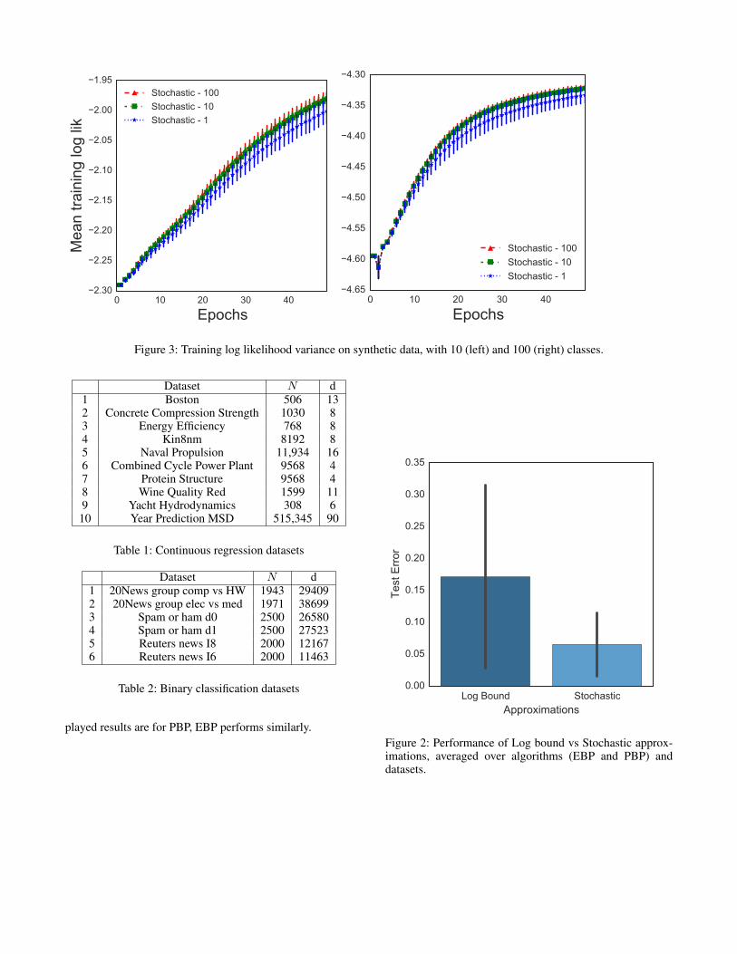
Figure 3: Training log likelihood variance on synthetic data, with 10 (left) and 100 (right) classes.

Dataset N d1 Boston 506 132 Concrete Compression Strength 1030 83 Energy Efficiency 768 84 Kin8nm 8192 85 Naval Propulsion 11,934 166 Combined Cycle Power Plant 9568 47 Protein Structure 9568 48 Wine Quality Red 1599 119 Yacht Hydrodynamics 308 610 Year Prediction MSD 515,345 90

Table 1: Continuous regression datasets

Dataset N d1 20News group comp vs HW 1943 294092 20News group elec vs med 1971 386993 Spam or ham d0 2500 265804 Spam or ham d1 2500 275235 Reuters news I8 2000 121676 Reuters news I6 2000 11463

Table 2: Binary classification datasets

played results are for PBP, EBP performs similarly.Figure 2: Performance of Log bound vs Stochastic approx-imations, averaged over algorithms (EBP and PBP) anddatasets.