Asset Pricing

Pricing

Determining a fair value (price) for an investment is an important task.

At the beginning of the semester, we dealt with the pricing of bonds. We also talked about the pricing of stocks using deterministic cash flow techniques.

Here, we deal with the pricing issue within a single-period random cash flow framework.

Single-period random cash flow pricing

Within the single-period random cash flow framework, asset pricing is about (1) quantifying the amount of risk, and (2) determining the amount of required (expected) rate of return for bearing this amount of risk.

The standard pricing approach introduced in this topic, i.e., the CAPM, is based on one particular result that we learned in the previous topic: portfolio theory.

Earlier: the one-fund theorem

When the risk-free asset is available, any efficient portfolio (any point on the EEF) can be expressed as a combination of the tangent portfolio and the risk-free asset: a straight line.

In order to have this property, we need the following assumptions: (A1) every investor is a mean-variance optimizer, (A2) the risk-free asset is available; every investor can borrow and lend any amount at the risk-free rate, and (A3) no transaction costs.

More assumptions, I

With (A1), (A2), and (A3), we know that everyone will purchase a single fund of risky assets, i.e., the tangent portfolio, and they may, in addition, borrow or lend at the risk-free rate (the one-fund theorem).

An additional assumption (A4): homogeneous expectation; that is, everyone agrees on the probabilistic structure of assets; everyone assigns to the returns of assets the same expected returns, the same variances, and the same covariances.

With (A4), everyone will use the same risky fund, i.e., the same one fund.

More assumptions, II

With (A1) – (A4), we know that everyone uses the same (tangent) risky fund—demand.

Assumption (A5): the market is in equilibrium. The equilibrium in this setting means the market is clear: supply equals demand.

We know that the demand is the tangent portfolio. The supply of all risky assets is called the “market portfolio” in

Finance. (A5) says supply equals demand. Thus, the tangent portfolio

(one fund) is the market portfolio: the tangent portfolio consists of all risky assets in equilibrium.

Since the market portfolio is the tangent portfolio, the market portfolio is efficient, i.e., the market portfolio is on the EEF.

With (A1) – (A5), we have the CAPM

E(ri) = rf + i * (E(rm) – rf), where i is Cov(i, m) / Var(m).

See the proof (handout).

The proof is based on 3 logics (tricks)

Logic 1: Convexity: for any asset i and the market portfolio, m, the 2 assets form a feasible set: a curve that (1) has a bullet shape, and (2) passes through i and m. (handout)

Logic 2: m is efficient. Thus, the curve cannot cross the EEF.

Logic 3: m is on the curve and the EEF. Thus, the slope of the curve at m equals to the slope of the EEF.

Then, we have the CAPM with some derivatives (to get the slopes) and algebras.

Interpret the CAPM, I

E(ri) = rf + i * (E(rm) – rf), where i is Cov(i, m) / Var(m).

Beta is the risk exposure/measure for individual asset.

Beta is a normalized (by the variance of the market portfolio) version of the covariance of the asset with the market portfolio.

Covariance is about the timing of payoffs. So, risk exposure is about timing. The expected (required) rate of return for the asset is

proportional to its covariance with the market.

Interpret the CAPM, II

When the covariance is zero, the beta is zero. The expected return is simply the risk-free rate.

Question: what is the covariance of the risk-free asset with the market portfolio?

When the covariance is negative, the beta is negative and the expected return is lower than the risk-free rate.

A negative-beta asset requires an unusually low expected return because when it is added to a well-diversified portfolio, it reduces the overall portfolio risk. This asset perform well (poorly) when everything else does poorly (well). This asset provides a form of insurance.

Can you name a stock that may have a negative beta?

Interpret the CAPM, III

The CAPM changes the concept of the risk of an asset/portfolio from that of standard deviation (var.) to that of beta.

It is still true that we measure the risk of one’s portfolio in terms of standard deviation (var.).

But this does not translate into a concern for the standard deviations of individual assets.

For individual assets, the proper risk measure is beta.

The CAPM as a pricing formula, I

The CAPM is an asset pricing model. However, the CAPM formula does not contain prices

explicitly (only returns). To see that the CAPM is a pricing model, let us

recognize that the CAPM is a single-period random cash flow model.

That is, let the price today be P, and later sold at price Q. P is known and Q is random. Then, the return r = (Q – P) / P.

The CAPM as a pricing formula, II

Putting r = (Q – P) / P into the CAPM: E(r) = rf + * (E(rm) – rf), we have: (E(Q) – P) / P = rf + * (E(rm) – rf).

Solving for P, we have: P = E(Q) / [1 + rf + * (E(rm) – rf)].

Holding the random payoff Q constant, the higher the beta (risk), the lower the current price P.

What else can we do about the CAPM (or any asset pricing model)?

The CAPM relates the amount of the relevant risk for an asset to the amount of the expected return (and risk premium) to induce investment flow from equity investors. Thus, the expected return can be viewed as the required rate of return demanded by equity holders. This gives us an estimate of cost of equity.

The CAPM gives us an estimate of expected return for an asset (including an portfolio or a fund). One can compare the expected return of a (mutual) fund to its realized return and say something about the ability and performance of the fund. If realized returns are on average higher than expected returns, we say the fund manager has selection ability.

Performance evaluation, I

There are many ways to examine the issue of performance.

The most popular method is to use a regression of historical returns to find out the “alpha”– the average return that cannot be explained by an asset pricing model, such as the CAPM.

Performance evaluation, II

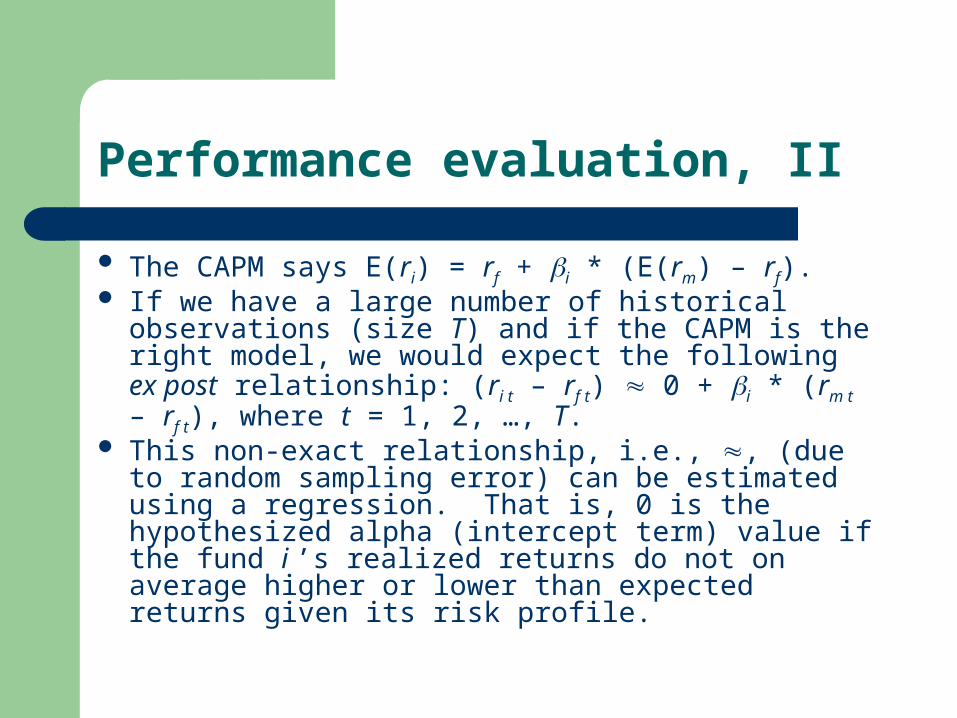
The CAPM says E(ri) = rf + i * (E(rm) – rf). If we have a large number of historical observations

(size T) and if the CAPM is the right model, we would expect the following ex post relationship: (ri t – rf t) 0 + i * (rm t – rf t), where t = 1, 2, …, T.

This non-exact relationship, i.e., , (due to random sampling error) can be estimated using a regression. That is, 0 is the hypothesized alpha (intercept term) value if the fund i ’s realized returns do not on average higher or lower than expected returns given its risk profile.

Performance evaluation, III

The inputs of the regression are: (ri t – rf t) and (rm t – rf t).

The outputs of the regression include the alpha coefficient and the beta coefficient.

Performance evaluation, IV

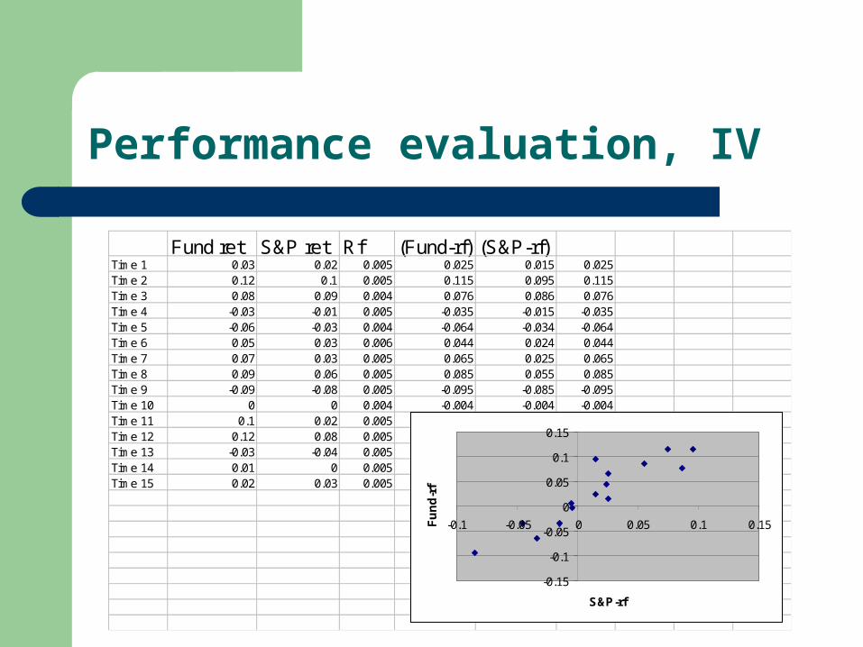
Fund ret S&P ret Rf (Fund-rf) (S&P-rf)Time 1 0.03 0.02 0.005 0.025 0.015 0.025Time 2 0.12 0.1 0.005 0.115 0.095 0.115Time 3 0.08 0.09 0.004 0.076 0.086 0.076Time 4 -0.03 -0.01 0.005 -0.035 -0.015 -0.035Time 5 -0.06 -0.03 0.004 -0.064 -0.034 -0.064Time 6 0.05 0.03 0.006 0.044 0.024 0.044Time 7 0.07 0.03 0.005 0.065 0.025 0.065Time 8 0.09 0.06 0.005 0.085 0.055 0.085Time 9 -0.09 -0.08 0.005 -0.095 -0.085 -0.095Time 10 0 0 0.004 -0.004 -0.004 -0.004Time 11 0.1 0.02 0.005 0.095 0.015 0.095Time 12 0.12 0.08 0.005 0.115 0.075 0.115Time 13 -0.03 -0.04 0.005 -0.035 -0.045 -0.035Time 14 0.01 0 0.005 0.005 -0.005 0.005Time 15 0.02 0.03 0.005 0.015 0.025 0.015

-0.15

-0.1

-0.05

0

0.05

0.1

0.15

-0.1 -0.05 0 0.05 0.1 0.15

S&P-rf

Fu

nd

-rf

Performance evaluation, V

The previous regression has an alpha of ? (t stat = ?) and an beta of ? (t stat = ?).

Please run the regression and put these number into a short report. Due next meeting.

What can you say about the riskness of the fund’s investment strategy?

What can you say about the fund manager’s ability? See MIP, pp. 767-768.

Evaluating portfolio performance

MIP, Chapter 12

3 elements of evaluation

1. What was the account’s performance?– Calculating and measuring (raw) rates of return

2. Why did the account produce the observed performance?

– Performance attribution– The sources of performance relative to benchmarks or a

particular asset pricing model

3. Is the account’s performance due to luck or skill?– Drawing conclusions about the quality of performance– Performance appraisal based on risk-adjusted measures, e.g.,

alpha