applied sciences

Article

Assessment of the Length and Depth ofDelamination-Type Defects Using UltrasonicGuided Waves

Vykintas Samaitis * , Liudas Mažeika and Regina RekuvieneProf. K.Baršauskas Ultrasound Research Insititute, Kaunas University of Technology, K. Baršausko St. 59,LT-51423 Kaunas, Lithuania; liudas.mazeika@ktu.lt (L.M.); regina.rekuviene@ktu.lt (R.R.)* Correspondence: vykintas.samaitis@ktu.lt; Tel.: +370-(37)-351-162

Received: 2 July 2020; Accepted: 27 July 2020; Published: 29 July 2020�����������������

Abstract: Fiber-reinforced composite laminates are being increasingly used in various engineeringcomponents in the sectors of aerospace and green energy. Due to impacts throughout the service lifeof the structure, matrix breakage and delaminations significantly altering the structural integrity ofthe laminate can occur. Hence, robust guided wave structural health monitoring systems are requiredto ensure continuous safety of engineering structures. In this paper, the ultrasonic method based onthe analysis of A0 mode reflecting within the defected area has been proposed to extract the lengthand the depth of the delamination-type defect. The technique proposed in this study extracts thedepth of the damage by analyzing the magnitude variations of direct A0 mode which are caused bythe difference of wave velocities in the upper and lower sub-laminates. This results in an altering andfrequency-dependent forward-scattered amplitude of direct A0 mode. Furthermore, the proposedapproach uses previously obtained information about the depth of the defect, which allows for thedetermination of the phase velocities of A0 and S0 modes in the upper and lower sub-laminates. As aresult, the accuracy of the damage length estimation is increased. The performance of the proposedmethod was proven with 2D and 3D numerical simulations and experiments on samples with artificialdefects. The method validation results showed that the proposed method with some limitations iscapable of extracting the length of delamination with an approximate error below 6%.

Keywords: structural health monitoring; composites; ultrasonic testing; guided waves; delamination

1. Introduction

Delamination is one of the most common defects found in fiber-reinforced composite laminatesdue to their weak transverse tensile and inter-laminar shear strengths [1]. Such defects may be causedby an impact and tend to develop internally between the neighboring fiber layers of the laminate.This results in loss of the strength of the structure without any visual evidence. As a result, sophisticatednon-destructive testing and signal processing techniques are of great significance for the structuralintegrity assessment of fiber reinforced laminates. Ultrasonic guided wave structural health monitoring(SHM) emerged as one of the most powerful tools which uses a network of embedded sensors to detectand continuously track the development of such defects in various industrial fields [2]. SHM systemsusually employ ultrasonic guided waves which propagate in elongated thin-walled structures, possesslow attenuation and are sensitive to the integral elastic properties of the material; thus, they can beused to infer large structures with only a few coupled transducers. Numerous researches have targetednon-linear, multimodal behavior, scattering and energy leakage of guided waves for the detection andsizing of delamination-type defects [3–7].

By interaction of guided waves with delamination, waves are scattered and converted to othermodes [8]. The mechanism of wave scattering depends on the type of the guided wave mode as well

Appl. Sci. 2020, 10, 5236; doi:10.3390/app10155236 www.mdpi.com/journal/applsci

Appl. Sci. 2020, 10, 5236 2 of 19

as on the depth and size of the defect. Various investigations have demonstrated that A0 and S0 modesof guided waves propagate in the two regions divided by the delamination individually and theninteract with each other after exiting the defect [9,10]. The anti-symmetric modes are found to bemore suitable for the assessment of delaminations as they show higher sensitivity to delaminationlocated at different through-thickness positions compared to the symmetric mode [11]. A few studieson A0 mode interaction with asymmetrical and symmetrical delaminations in laminated compositeswere presented by Ramadas et al. [12,13]. It was found that, in the case of symmetrical delamination,incident A0 mode and converted A0 (A0›S0›A0) mode propagate after the exit of delamination. In thecase of an asymmetrical defect, an additional S0 mode (A0›S0›S0) appears upon the interaction with thedefect. The authors also proposed the method for the assessment of the delamination size based on thetime-of-flight measurement of A0 mode [14]. However, such a method appeared to be valid at lowdispersion regions of A0 mode as the velocities in the upper and lower sub-laminate layer of the defectwere assumed to be equal to the velocity in the entire structure. In case of sub-surface delaminations,the velocities in sub-laminates can be essentially different, which leads to high errors.

Lamb wave scattering and conversion at the leading and trailing edge of delamination is anothertopic which has been extensively studied by numerous research groups. For example, Schaal et al. [15]estimated frequency-dependent scattering coefficients for fundamental Lamb wave modes separatelyat the leading and trailing edges of delamination. Hu et al. [16] developed a technique to locate thedelamination-type defects by using two embedded transducers and an S0 mode by measuring signalsreflected from the tip of the defect. A study on S0 mode interaction with the delamination-type defectwas presented, which showed that, at each end of delamination, the transmitted and reflected A0/S0

modes are being generated with each mode having different reflection and transmission coefficientsdepending on the local bending stiffness of the structure. An extensive study on Lamb wave modeconversion in a 2D plate containing a finite length delamination parallel with the surface was presentedby Shkerdin and Glorieux [17]. Mode conversions between Lamb wave modes and between Rayleighwave and Lamb modes were analyzed. It was found that the transmission coefficients of Lambwaves are both defect length- and depth-dependent, and they vary for different transmitted modes.Birt et al. [18] studied the dependencies between the magnitude of the reflected S0 mode and the widthof delamination.

As a result of such complex scattering and mode conversion, various linear acoustic tools for thedetection and localization of delamination-type defects can be developed. For example, by measuringthe time-of-flight (ToF) of the reflected and transmitted waves, the existence and location of delaminationcan be estimated [8,19]. Additionally, by analyzing the ToF and velocities of the modes propagatingat the layers divided by delamination, the length of the defect can be assessed [20,21]. However,the success of the above-mentioned methods is strongly influenced by the dispersion and superpositionof the modes of guided waves. The defects are mostly weak reflectors, while the monitoring systemtends to detect and locate them in a large structure by using a small number of sensors. This leads to alow signal-to-noise ratio (SNR), which further complicates the signal analysis and the estimation of thetime of flight (ToF).

Most of the researches in the field of linear acoustics are currently targeting the detection,localization and sizing of delamination-type defects. However, the assessment of the depth of a defectis no less important for the evaluation of defect severity. There are only a few works available whichdiscuss the depth estimation of a delamination-type defect. Recently, Eremin et al. [22] analyzed therelationship between the length and depth of delamination with the scattering resonance frequenciesof delamination. Munian et al. [23] analyzed the reflection of A0 mode as a function of the depth-wiseposition of delamination. It was concluded that mid-plane delamination scatters less energy of theasymmetric mode, meanwhile, off mid-plane delaminations additionally introduce a reflection ofconverted S0 mode. Gupta et al. [24] exploited S0 mode to analyze its reflection from delaminationsituated at different depths and ply layups. Reflection coefficients as a function of the through-thicknesslocation of delamination were estimated for various ply layups, which showed the importance of the

Appl. Sci. 2020, 10, 5236 3 of 19

defect position and the composition of the material to the detectability of delamination. Recently,Murat et al. [25,26] analyzed the scattering of A0 mode from delaminations of different sizes which weresituated at different depths. It was observed that the delamination length exerts strong influence onthe scattering directivity, while its depth influences the magnitude of the scattered wave. Despite somepromising results, the abovementioned works in general have discussed the fundamental influence ofthe defect depth on the scattering of guided wave modes. There is still a lack of methods to extract thedepth of the defect without any initial knowledge about its through-thickness location when dispersionis involved.

This paper proposes the SHM method to extract the absolute depth and size of asymmetricaldelamination-type defects in plate-like structures with parallel surfaces. The technique proposed inthis study extracts the depth of the damage by analyzing the amplitude variation patterns of directA0 mode at different excitation frequencies. These magnitude variations are caused by the differenceof wave velocities in the upper and lower sub-laminates due to their uneven thicknesses. This leadsto the varying phase differences of the wave-packets at the trailing edge of the defect and resultsin an altering forward scattered amplitude of the direct A0 mode. Hence, in comparison with thepredefined reference dependencies, the absolute values of the delamination depth can be extracted.Such magnitude variation is related to the excitation frequency as the phase velocity of A0 mode isfrequency and thickness dependent. As a result, different magnitude variation patterns at differentexcitation frequencies can be observed. Having such patterns at different frequencies allow to increasethe accuracy of damage depth estimation. This is very important in the presence of strong dispersion,as the rapid changes in velocity of guided wave modes can introduce large errors. Furthermore,the information on the damage depth can be exploited for the assessment of the defect length as theactual depth of the defect determines the phase velocities of A0 and S0 modes in the upper and lowersub-laminates. Then, the delamination size can be evaluated by measuring the ToF between the wavepackets of the converted and direct A0 modes. Hence, the approach proposed in this research canprovide information about the absolute depth and the length of the damage employing a few timetraces measured at a series of different excitation frequencies. The technique proposed in this study isessentially different from the currently existing ones as it uses multiple excitation frequencies, whichleads to different patterns of A0 mode magnitude variation and, subsequently, to better resolution.Most of the available research studies use constant a-priori wave velocities for damage size estimationwhich is not valid in the presence of dispersion. The technique proposed in this paper can be usedeven in the presence of the dispersion of A0 mode as it exploits the dependency of the phase velocityon the thickness of the layers above and below the defect.

This paper focuses on the proof of the concept of the proposed delamination depth and lengthestimation method by analyzing a single delamination-type defect. However, in further studies, it isexpected to extend the presented method to extract features of multiple parallel delaminations whichare a common outcome of low velocity impact damage.

2. Method for Assessment of Delamination Parameters

2.1. Interaction of A0 Mode with Delamination-Type Defect

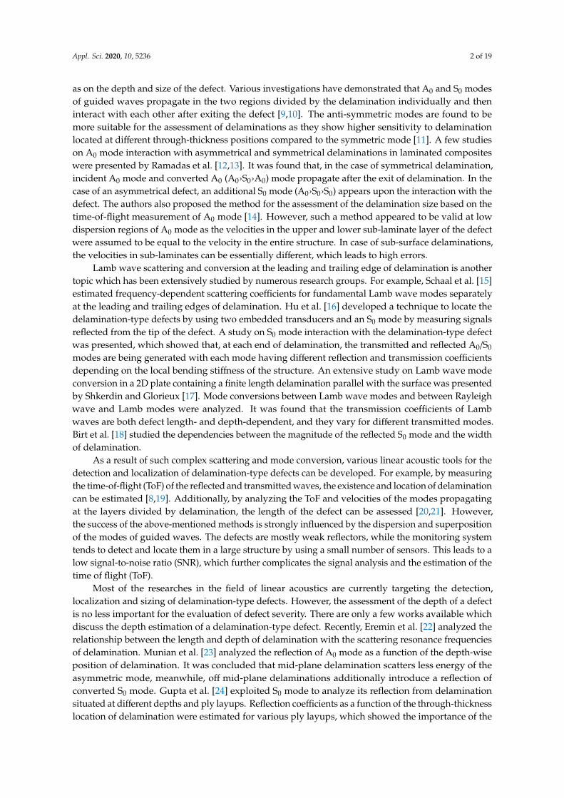
Let us analyze a composite plate with length l and thickness h which is shown in Figure 1. It willbe investigated with the 2D approach, which means that the plate is infinite along the y axis. Let usconsider that the delamination-type defect is present in the structure, which is l1 long and situated atdistances of l0 and l2 from the source (excitation) and monitoring (reception) points, respectively, at adepth of h1 with respect to the top surface. The delamination is parallel to the surface of the sample(Figure 1).

Appl. Sci. 2020, 10, 5236 4 of 19

Appl. Sci. 2020, 10, x FOR PEER REVIEW  4 of 19 

[29,30],  in‐phase and out‐of‐phase excitation  [31], etc.  In  this research  the  fundamental dispersion 

zone has been selected and the excitation frequencies were limited from 50 kHz up to 200 kHz. At 

such frequencies, the wavelengths of A0 mode varies from 17.2 mm (at 50 kHz), to 5.6 mm (at 200 

kHz) at 4mm GFRP plate (Ex = 10 GPa, Ez = 35.7 GPa; υxz = 0.325, υzx = 0.091, υyx = 0.35; Gxz = 2.8 GPa; ρ = 

1800 kg/m3). This shows that both A0, S0 and higher order A1 and S1 modes can exist at such a constant 

wavelength (see Figure 2a). However, using a Plexiglas wedge (2700 m/s) as a coupling medium and 

normal incidence angles, the fundamental A0 mode is being generated most effectively (see Figure 

2b), and sophisticated mode isolation techniques were not applied. 

 

Figure 1. Schematic diagram of  considered example of a  composite plate with delamination‐type 

damage. 

  

(a)  (b) 

Figure 2. Phase velocity dispersion curves of 4 mm glass fibre reinforced plastic (GFRP) plate (a) and 

excitation angle versus frequency using Plexiglas as coupling medium (b). 

The signal of A0 mode excited at the source point and measured at the monitoring point after 

propagation  through  the delaminated area will be  the subject of all  the upcoming  investigations. 

Upon the interaction of A0 mode with the delamination‐type defect, the reflection, transmission and 

mode conversion occur at each end of the damage. In such a way, at the leading edge of the damage, 

the  incident A0 mode reflects back, and  in the forward direction  it splits  into wave packets which 

accordingly propagate on the sub‐laminates above and below the defect. Moreover, mode conversion 

occurs at the leading edge; therefore, part of the energy transforms into S0 mode as well (see Figure 

3a).  Similarly,  at  the  trailing  edge  of  the  damage,  both  A0  and  S0  modes  are  reflecting  back, 

propagating forward and converting to each other (see Figure 3b). This representation does not take 

into account the scattering coefficients of each reflected/converted mode. 

Figure 1. Schematic diagram of considered example of a composite plate with delamination-type damage.

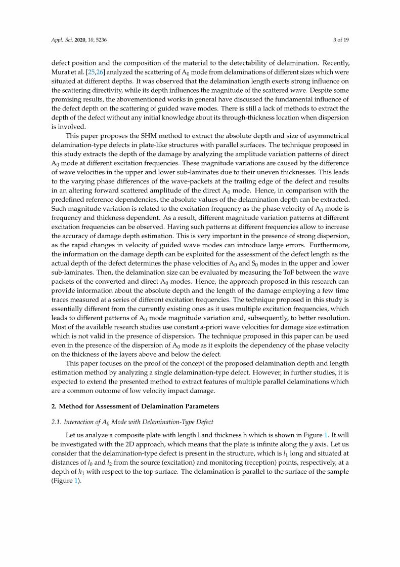
The fundamental A0 mode has been selected in this paper. As multiple guided wave modes arebeing generated simultaneously, different strategies exist to excite isolated modes, such as angle beamexcitation [27], element width selection [28], inter-element spacing or interdigital transducers [29,30],in-phase and out-of-phase excitation [31], etc. In this research the fundamental dispersion zonehas been selected and the excitation frequencies were limited from 50 kHz up to 200 kHz. At suchfrequencies, the wavelengths of A0 mode varies from 17.2 mm (at 50 kHz), to 5.6 mm (at 200 kHz)at 4 mm GFRP plate (Ex = 10 GPa, Ez = 35.7 GPa; υxz = 0.325, υzx = 0.091, υyx = 0.35; Gxz = 2.8 GPa;ρ = 1800 kg/m3). This shows that both A0, S0 and higher order A1 and S1 modes can exist at sucha constant wavelength (see Figure 2a). However, using a Plexiglas wedge (2700 m/s) as a couplingmedium and normal incidence angles, the fundamental A0 mode is being generated most effectively(see Figure 2b), and sophisticated mode isolation techniques were not applied.

Appl. Sci. 2020, 10, x FOR PEER REVIEW  4 of 19 

[29,30],  in‐phase and out‐of‐phase excitation  [31], etc.  In  this research  the  fundamental dispersion 

zone has been selected and the excitation frequencies were limited from 50 kHz up to 200 kHz. At 

such frequencies, the wavelengths of A0 mode varies from 17.2 mm (at 50 kHz), to 5.6 mm (at 200 

kHz) at 4mm GFRP plate (Ex = 10 GPa, Ez = 35.7 GPa; υxz = 0.325, υzx = 0.091, υyx = 0.35; Gxz = 2.8 GPa; ρ = 

1800 kg/m3). This shows that both A0, S0 and higher order A1 and S1 modes can exist at such a constant 

wavelength (see Figure 2a). However, using a Plexiglas wedge (2700 m/s) as a coupling medium and 

normal incidence angles, the fundamental A0 mode is being generated most effectively (see Figure 

2b), and sophisticated mode isolation techniques were not applied. 

 

Figure 1. Schematic diagram of  considered example of a  composite plate with delamination‐type 

damage. 

  

(a)  (b) 

Figure 2. Phase velocity dispersion curves of 4 mm glass fibre reinforced plastic (GFRP) plate (a) and 

excitation angle versus frequency using Plexiglas as coupling medium (b). 

The signal of A0 mode excited at the source point and measured at the monitoring point after 

propagation  through  the delaminated area will be  the subject of all  the upcoming  investigations. 

Upon the interaction of A0 mode with the delamination‐type defect, the reflection, transmission and 

mode conversion occur at each end of the damage. In such a way, at the leading edge of the damage, 

the  incident A0 mode reflects back, and  in the forward direction  it splits  into wave packets which 

accordingly propagate on the sub‐laminates above and below the defect. Moreover, mode conversion 

occurs at the leading edge; therefore, part of the energy transforms into S0 mode as well (see Figure 

3a).  Similarly,  at  the  trailing  edge  of  the  damage,  both  A0  and  S0  modes  are  reflecting  back, 

propagating forward and converting to each other (see Figure 3b). This representation does not take 

into account the scattering coefficients of each reflected/converted mode. 

Figure 2. Phase velocity dispersion curves of 4 mm glass fibre reinforced plastic (GFRP) plate (a) andexcitation angle versus frequency using Plexiglas as coupling medium (b).

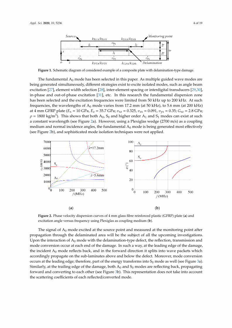
The signal of A0 mode excited at the source point and measured at the monitoring point afterpropagation through the delaminated area will be the subject of all the upcoming investigations.Upon the interaction of A0 mode with the delamination-type defect, the reflection, transmission andmode conversion occur at each end of the damage. In such a way, at the leading edge of the damage,the incident A0 mode reflects back, and in the forward direction it splits into wave packets whichaccordingly propagate on the sub-laminates above and below the defect. Moreover, mode conversionoccurs at the leading edge; therefore, part of the energy transforms into S0 mode as well (see Figure 3a).Similarly, at the trailing edge of the damage, both A0 and S0 modes are reflecting back, propagatingforward and converting to each other (see Figure 3b). This representation does not take into accountthe scattering coefficients of each reflected/converted mode.

Appl. Sci. 2020, 10, 5236 5 of 19Appl. Sci. 2020, 10, x FOR PEER REVIEW  5 of 19 

   

(a)  (b) 

Figure 3. Graphic representation of A0 mode interaction with delamination‐type defect at the leading 

(a) and trailing edge (b). 

In this research, only the forward scattered wave‐packets of A0 mode will be considered; they 

are squared red in Figure 3b. Mathematically, the spectrum of the signal of A0 mode UIA0(f) which 

arrives first to the monitoring (reception) point can be expressed as: 

𝑈IA 𝑓 𝑈sA 𝑓 ⋅ 𝐻 𝑓, 𝑐 , 𝑙 ⋅ 𝑘T01A ⋅ 𝐻 𝑓, 𝑐 , 𝑙 ⋅ 𝑘T10S ⋅ 𝐻 𝑓, 𝑐 , 𝑙 𝑈sA 𝑓 ⋅ 𝐻 𝑓, 𝑐 , 𝑙 ⋅ 𝑘T02A ⋅ 𝐻 𝑓, 𝑐 , 𝑙 ⋅ 𝑘T20S ⋅ 𝐻 𝑓, 𝑐 , 𝑙

𝑈sA 𝑓 ⋅ 𝐻 𝑓, 𝑐 , 𝐿 𝑙 ⋅𝑘T01A ⋅ 𝐻 𝑓, 𝑐 , 𝑙 ⋅ 𝑘T10S

𝑘T02A ⋅ 𝐻 𝑓, 𝑐 , 𝑙 ⋅ 𝑘T20S, 

(1)

𝐻 𝑓, 𝑐p, 𝑙 𝑒 𝑒 p ,  (2)

where UsA0(f) is the frequency spectrum of the excitation signal of A0 mode; H(f,cp,l) is the transfer 

function of the waves propagating in the corresponding layer; cpA0(f), cpS0(f) are the phase velocities of 

A0 and S0 modes, respectively; l is the propagation distance (l0, l2–propagation distances in the defect‐

free area before and after the defect, respectively, l1–length of the defect); L is the separation between 

the source and the monitoring points (L = l0 + l1 + l2); and α(f) is the frequency dependent attenuation 

function; kT01A, kT02A, kT10S and kT20S are the transmission coefficients for A0 and S0 modes at the leading 

and trailing edges of the delamination, respectively, for the layer above and below the defect. The 

estimation of such reflection and transmission coefficients was out of the scope of this study. They 

essentially depend on the guided wave mode, the delamination depth, the material properties and 

the total thickness of the plate, and they should be determined for each particular case separately. 

The wave packet described by Equation (1) is A0 mode, which is a superposition of the signals 

traveling at upper and lower sub‐laminates. This wave‐packet converts from A0 mode to S0 mode at 

the leading edge and back to A0 at the trailing edge of the defect. Due to this reason, this wave packet 

UIA0(f) arrives earlier compared to the direct transmission of A0 mode which does not convert within 

the defected area. This happens due to the reason that S0 mode possesses a greater group velocity at 

low frequencies compared to A0 mode. In this research, such a wave‐packet shall be referred to as 

“first A0 arrival”. Consequently, the frequency spectrum of the direct transmission of A0 mode can be 

written as: 

𝑈IIA 𝑓 𝑈sA 𝑓 ⋅ 𝐻 𝑓, 𝑐 , 𝑙 ⋅ 𝑘T01A ⋅ 𝐻 𝑓, 𝑐 , 𝑙 ⋅ 𝑘T10A ⋅ 𝐻 𝑓, 𝑐 , 𝑙 𝑈sA 𝑓 ⋅ 𝐻 𝑓, 𝑐 , 𝑙 ⋅ 𝑘T02A ⋅ 𝐻 𝑓, 𝑐 , 𝑙 ⋅ 𝑘T20A ⋅ 𝐻 𝑓, 𝑐 , 𝑙

𝑈sA 𝑓 ⋅ 𝐻 𝑓, 𝑐 , 𝐿 𝑙 ⋅𝑘T01A ⋅ 𝐻 𝑓, 𝑐 , 𝑙 ⋅ 𝑘T10A

𝑘T02A ⋅ 𝐻 𝑓, 𝑐 , 𝑙 ⋅ 𝑘T20A. 

(3)

The  “direct A0  transmission” described  by Equation  (3)  is  the wave‐packet which does  not 

convert to other modes at the leading and trailing edges of delamination.   

Figure 3. Graphic representation of A0 mode interaction with delamination-type defect at the leading(a) and trailing edge (b).

In this research, only the forward scattered wave-packets of A0 mode will be considered; they aresquared red in Figure 3b. Mathematically, the spectrum of the signal of A0 mode UIA0(f ) which arrivesfirst to the monitoring (reception) point can be expressed as:

UIA0( f ) = UsA0( f ) ·H(

f , cp0A0 , l0)· kT01A ·H

(f , cp1S0 , l1

)· kT10S ·H

(f , cp0A0 , l2

)+UsA0( f ) ·H

(f , cp0A0 , l0

)· kT02A ·H

(f , cp2S0 , l1

)· kT20S ·H

(f , cp0A0 , l2

)=

(UsA0( f ) ·H

(f , cp0A0 , L− l1

))·

kT01A ·H(

f , cp1S0 , l1)· kT10S+

+kT02A ·H(

f , cp2S0 , l1)· kT20S

,(1)

H(

f , cp, l)= e−α( f )xe

− jl fcp( f ) , (2)

where UsA0(f ) is the frequency spectrum of the excitation signal of A0 mode; H(f,cp,l) is the transferfunction of the waves propagating in the corresponding layer; cpA0(f ), cpS0(f ) are the phase velocitiesof A0 and S0 modes, respectively; l is the propagation distance (l0, l2–propagation distances in thedefect-free area before and after the defect, respectively, l1–length of the defect); L is the separationbetween the source and the monitoring points (L = l0 + l1 + l2); and α(f ) is the frequency dependentattenuation function; kT01A, kT02A, kT10S and kT20S are the transmission coefficients for A0 and S0 modesat the leading and trailing edges of the delamination, respectively, for the layer above and below thedefect. The estimation of such reflection and transmission coefficients was out of the scope of this study.They essentially depend on the guided wave mode, the delamination depth, the material propertiesand the total thickness of the plate, and they should be determined for each particular case separately.

The wave packet described by Equation (1) is A0 mode, which is a superposition of the signalstraveling at upper and lower sub-laminates. This wave-packet converts from A0 mode to S0 mode atthe leading edge and back to A0 at the trailing edge of the defect. Due to this reason, this wave packetUIA0(f ) arrives earlier compared to the direct transmission of A0 mode which does not convert withinthe defected area. This happens due to the reason that S0 mode possesses a greater group velocity atlow frequencies compared to A0 mode. In this research, such a wave-packet shall be referred to as“first A0 arrival”. Consequently, the frequency spectrum of the direct transmission of A0 mode can bewritten as:

UIIA0( f ) = UsA0( f ) ·H(

f , cp0A0 , l0)· kT01A ·H

(f , cp1A0 , l1

)· kT10A ·H

(f , cp0A0 , l2

)+UsA0( f ) ·H

(f , cp0A0 , l0

)· kT02A ·H

(f , cp2A0 , l1

)· kT20A ·H

(f , cp0A0 , l2

)=

(UsA0( f ) ·H

(f , cp0A0 , L− l1

))·

kT01A ·H(

f , cp1A0 , l1)· kT10A+

+kT02A ·H(

f , cp2A0 , l1)· kT20A

.(3)

Appl. Sci. 2020, 10, 5236 6 of 19

The “direct A0 transmission” described by Equation (3) is the wave-packet which does not convertto other modes at the leading and trailing edges of delamination.

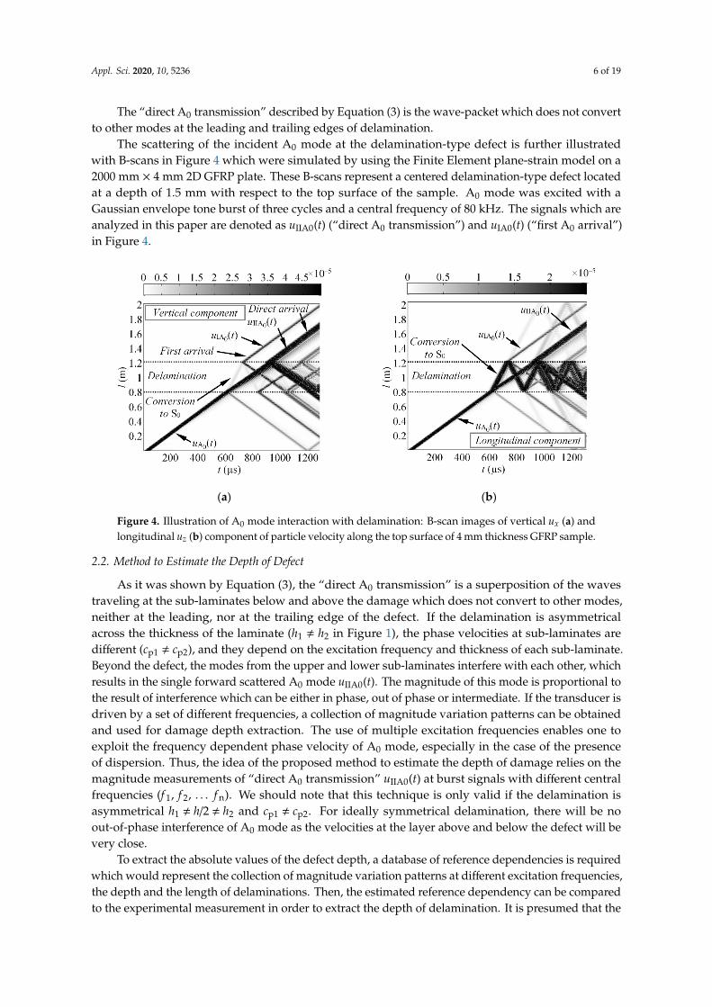
The scattering of the incident A0 mode at the delamination-type defect is further illustratedwith B-scans in Figure 4 which were simulated by using the Finite Element plane-strain model on a2000 mm × 4 mm 2D GFRP plate. These B-scans represent a centered delamination-type defect locatedat a depth of 1.5 mm with respect to the top surface of the sample. A0 mode was excited with aGaussian envelope tone burst of three cycles and a central frequency of 80 kHz. The signals which areanalyzed in this paper are denoted as uIIA0(t) (“direct A0 transmission”) and uIA0(t) (“first A0 arrival”)in Figure 4.

Appl. Sci. 2020, 10, x FOR PEER REVIEW  6 of 19 

The scattering of the incident A0 mode at the delamination‐type defect is further illustrated with 

B‐scans in Figure 4 which were simulated by using the Finite Element plane‐strain model on a 2000 

mm×4 mm 2D GFRP plate. These B‐scans represent a centered delamination‐type defect located at a 

depth of 1.5 mm with respect to the top surface of the sample. A0 mode was excited with a Gaussian 

envelope tone burst of three cycles and a central frequency of 80 kHz. The signals which are analyzed 

in this paper are denoted as uIIA0(t) (“direct A0 transmission”) and uIA0(t) (“first A0 arrival”) in Figure 

4. 

   

(a)  (b) 

Figure 4. Illustration of A0 mode interaction with delamination: B‐scan images of vertical ux (a) and 

longitudinal uz  (b)  component of particle velocity along  the  top  surface of 4 mm  thickness GFRP 

sample. 

2.2. Method to Estimate the Depth of Defect 

As it was shown by Equation (3), the “direct A0 transmission” is a superposition of the waves 

traveling at the sub‐laminates below and above the damage which does not convert to other modes, 

neither at the leading, nor at the trailing edge of the defect. If the delamination is asymmetrical across 

the thickness of the laminate (h1 ≠ h2 in Figure 1), the phase velocities at sub‐laminates are different 

(cp1 ≠ cp2), and they depend on the excitation frequency and thickness of each sub‐laminate. Beyond 

the defect, the modes from the upper and lower sub‐laminates interfere with each other, which results 

in the single forward scattered A0 mode uIIA0(t). The magnitude of this mode is proportional to the 

result of interference which can be either in phase, out of phase or intermediate. If the transducer is 

driven by a set of different frequencies, a collection of magnitude variation patterns can be obtained 

and used  for damage depth extraction. The use of multiple excitation  frequencies enables one  to 

exploit the frequency dependent phase velocity of A0 mode, especially in the case of the presence of 

dispersion. Thus,  the  idea of  the proposed method  to estimate  the depth of damage relies on  the 

magnitude measurements of “direct A0 transmission” uIIA0(t) at burst signals with different central 

frequencies  (f1,  f2, …  fn). We  should  note  that  this  technique  is  only  valid  if  the delamination  is 

asymmetrical h1 ≠ h/2 ≠ h2 and cp1 ≠ cp2. For ideally symmetrical delamination, there will be no out‐of‐

phase interference of A0 mode as the velocities at the layer above and below the defect will be very 

close. 

To  extract  the  absolute  values  of  the  defect  depth,  a database  of  reference  dependencies  is 

required which would represent the collection of magnitude variation patterns at different excitation 

frequencies, the depth and the length of delaminations. Then, the estimated reference dependency 

can be compared to the experimental measurement in order to extract the depth of delamination. It 

is presumed that the reference dependency which best matches the experiments is the one that gives 

the closest definition of the damage depth in the structure. The step‐by‐step procedure of the damage 

depth estimation can be outlined as follows: 

Figure 4. Illustration of A0 mode interaction with delamination: B-scan images of vertical ux (a) andlongitudinal uz (b) component of particle velocity along the top surface of 4 mm thickness GFRP sample.

2.2. Method to Estimate the Depth of Defect

As it was shown by Equation (3), the “direct A0 transmission” is a superposition of the wavestraveling at the sub-laminates below and above the damage which does not convert to other modes,neither at the leading, nor at the trailing edge of the defect. If the delamination is asymmetricalacross the thickness of the laminate (h1 , h2 in Figure 1), the phase velocities at sub-laminates aredifferent (cp1 , cp2), and they depend on the excitation frequency and thickness of each sub-laminate.Beyond the defect, the modes from the upper and lower sub-laminates interfere with each other, whichresults in the single forward scattered A0 mode uIIA0(t). The magnitude of this mode is proportional tothe result of interference which can be either in phase, out of phase or intermediate. If the transducer isdriven by a set of different frequencies, a collection of magnitude variation patterns can be obtainedand used for damage depth extraction. The use of multiple excitation frequencies enables one toexploit the frequency dependent phase velocity of A0 mode, especially in the case of the presenceof dispersion. Thus, the idea of the proposed method to estimate the depth of damage relies on themagnitude measurements of “direct A0 transmission” uIIA0(t) at burst signals with different centralfrequencies (f 1, f 2, . . . f n). We should note that this technique is only valid if the delamination isasymmetrical h1 , h/2 , h2 and cp1 , cp2. For ideally symmetrical delamination, there will be noout-of-phase interference of A0 mode as the velocities at the layer above and below the defect will bevery close.

To extract the absolute values of the defect depth, a database of reference dependencies is requiredwhich would represent the collection of magnitude variation patterns at different excitation frequencies,the depth and the length of delaminations. Then, the estimated reference dependency can be comparedto the experimental measurement in order to extract the depth of delamination. It is presumed that the

Appl. Sci. 2020, 10, 5236 7 of 19

reference dependency which best matches the experiments is the one that gives the closest definition ofthe damage depth in the structure. The step-by-step procedure of the damage depth estimation can beoutlined as follows:

1. The source of guided waves E is driven by burst with Gaussian envelope of central frequency f 1

to introduce A0 mode in the investigated structure.2. Time trace uA0(t) is received with sensor Rref, which represents the structure without the damage

(the reference signal). Meanwhile, the other receiver R1 captures time history uIIA0(t) whichrepresents the response of the structure at the monitoring point beyond the defect.

3. Ratio uA0expf 1(t) of peak-to-peak amplitudes of waveforms uA0(t) and uIIA0(t) is estimated at theburst central frequency f 1.

4. Steps 1–3 are repeated over for other excitation frequencies f N = (f 1, f 2, . . . f n). As a consequence,the experimental dataset UA0exp(f ) = {f N, uA0expf 1(t), uA0expf 2(t), . . . , uA0expf n(t)} is collected,where f N denotes the burst central frequencies used for the excitation of A0 mode.

5. The experimental dataset UA0exp(f ) is compared to the prescribed database of referencedependencies UA0ref(f,h,l) (where h, l are the depth and the length of damage, respectively).Based upon this concept, the goal is to select the single reference dependency that is the closest tothe experimental data. The criteria to characterize the similarity of two datasets include standarddeviation as follows:

hopt = argminh

(mean

l(ustd(h, l))

), (4)

whereustd(h, l) = std

f

(UA0ref( f , h, l) −UA0 exp( f )

), (5)

where hopt is the value which corresponds to the delamination depth where the reference dependencybest matches the experimental dataset; UA0ref(f,h,l) is the calculated reference dependency; UA0exp(f ) isthe experimental dataset; h and l are the depth and the length of delamination, respectively; and “std”and “mean” denote the standard deviation and the arithmetic average, respectively.

If the structure is defect-free, function UA0exp(f ) is close to monotonic and does not feature essentialamplitude variations. Meanwhile, if the variation in the magnitude ratio is observed, it can be relatedto the presence of a defect at a particular depth. The proposed depth estimation technique reliesunder the assumption, that velocities of direct A0 mode in the upper and lower sub laminates aresimilar and the single wave packet is captured after the exit of delamination. In case of very large andasymmetric defects, two wave packets of A0 mode can appear after the exit of the defect. In such acase, the inspection frequency must be decreased, or the number of signal cycles increased in order tomaintain a single wave packet and to observe magnitude variation patterns.

2.3. Method to Assess the Length of Defect

If the depth of the defect is determined, its length can be estimated from the delay between “directA0 transmission” uIIA0(t) and “first A0 arrival” uIA0(t) which can be denoted as ∆tA0. Delay ∆tA0 isproportional to the excitation frequency and the propagation path of S0 mode, which itself is actuallydetermined by the length of the defect (Figure 5). The time delay between two neighboring wavepackets can be estimated according to:

∆tA0 = argmaxt

[HT

∣∣∣uIIA0(t)∣∣∣]− argmax

t

[HT

∣∣∣uIA0(t)∣∣∣], (6)

where uIA0(t) and uIIA0(t) are the wave packets of “first A0 arrival” and “direct A0 transmission”,and HT denotes the Hilbert transform. Then, the length of the defect at a particular depth h can becalculated as:

Ldef = meanf

∆tA0(h, f )·cgA0

( f )·cgS0( f )

cgS0( f ) − cgA0

( f )

. (7)

Appl. Sci. 2020, 10, 5236 8 of 19

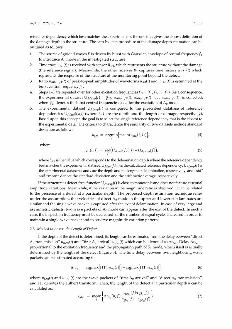
The Equation (7) calculates mean defect length from a set of defect lengths obtained at differentexcitation frequencies. If multiple burst central frequencies are used to excite the guided waves,the group velocity values of A0 and S0 modes should be taken at different central frequencies, whichallow one to consider the dispersion.Appl. Sci. 2020, 10, x FOR PEER REVIEW  8 of 19 

 

Figure 5. Bscan  image of  the vertical component of particle velocity, which shows delay between 

converted and direct A0 modes beyond the defect. 

As the “direct A0 transmission” uIIA0(t) is the result of the interference between the wave packets 

propagating above and below the defect, the maximum of the wave after the exit of delamination 

(uIIA0(t)) may be shifted and no longer correspond to the wave energy velocity. Hence the delay ΔtA0 

in Equation (6) will be estimated with some error. The best way here would be to calculate the delay 

according to the mean energy (mass center) of the signal [32]. However, in such case the time window 

covering entire signal should be selected. Such a task is not trivial due to the dispersion of A0 mode 

signals, presence of other modes and reflections from object boundaries. Additionally, the different 

frequency components of the dispersed A0 mode are redistributed in the envelope of the signal. The 

lower frequency components are concentrated at the tail of the signal. So, the energy of wave packet 

uIIA0(t) should be related to a particular frequency and velocity which are used for estimation of the 

time  of  flight. By using  a maximum  or Hilbert  envelope  of  the  signal  it  can be  assumed  that  it 

corresponds to the dominant frequency of the signal and gives sufficient ToF accuracy. 

It is noteworthy that, for the reliable operation of the method, direct uIIA0(t) and converted modes 

uIA0(t) must be separated in the time domain to an adequate extent in order to be able to measure the 

time delay between the two wave packets. Thus, there exists the minimum size of a defect that can 

be evaluated by using this approach. Such a minimum detectable defect is frequency dependent, so 

higher frequency signals can be used to improve sizing accuracy. It is important that the depth of the 

defect  strongly  influences  the  accuracy  of  the  delamination  length  estimation,  especially  in  the 

presence of significant dispersion. If the depth of the defect is unknown, such an approach becomes 

valid in non‐dispersive regions only. However, by using the proposed delamination depth estimation 

technique, the thicknesses and velocities  in the upper and  lower sub‐laminate can be determined, 

which leads to the improved accuracy of the delamination length evaluation. 

3. Estimation of Reference Dependencies 

As mentioned previously, the proposed technique to estimate the depth of delamination relies 

on reference calculations, which means that the experimental signals must be compared to the model‐

based  predictions.  In  order  to  extract  the  depth  of  the  damage,  the  dependencies  between  the 

magnitude of  “direct A0  transmission” UA0ref(f,h,l),  excitation  frequency  (f)  and depth  (h)  at  fixed 

defect lengths (l) will be calculated. In this study, for the sake of simplicity, the estimation of reference 

dependencies shall be demonstrated on the 2D model of a GFRP plate. 

3.1. Theoretical Formulation of Reference Dataset 

In  the  case  of  depth  assessment,  our  goal  is  to  predict  the waveform  of  A0 mode which 

propagates within the defect. Equation (3) can be rewritten in a short form as: 

Figure 5. Bscan image of the vertical component of particle velocity, which shows delay betweenconverted and direct A0 modes beyond the defect.

As the “direct A0 transmission” uIIA0(t) is the result of the interference between the wave packetspropagating above and below the defect, the maximum of the wave after the exit of delamination(uIIA0(t)) may be shifted and no longer correspond to the wave energy velocity. Hence the delay∆tA0 in Equation (6) will be estimated with some error. The best way here would be to calculate thedelay according to the mean energy (mass center) of the signal [32]. However, in such case the timewindow covering entire signal should be selected. Such a task is not trivial due to the dispersionof A0 mode signals, presence of other modes and reflections from object boundaries. Additionally,the different frequency components of the dispersed A0 mode are redistributed in the envelope ofthe signal. The lower frequency components are concentrated at the tail of the signal. So, the energyof wave packet uIIA0(t) should be related to a particular frequency and velocity which are used forestimation of the time of flight. By using a maximum or Hilbert envelope of the signal it can beassumed that it corresponds to the dominant frequency of the signal and gives sufficient ToF accuracy.

It is noteworthy that, for the reliable operation of the method, direct uIIA0(t) and converted modesuIA0(t) must be separated in the time domain to an adequate extent in order to be able to measurethe time delay between the two wave packets. Thus, there exists the minimum size of a defect thatcan be evaluated by using this approach. Such a minimum detectable defect is frequency dependent,so higher frequency signals can be used to improve sizing accuracy. It is important that the depth ofthe defect strongly influences the accuracy of the delamination length estimation, especially in thepresence of significant dispersion. If the depth of the defect is unknown, such an approach becomesvalid in non-dispersive regions only. However, by using the proposed delamination depth estimationtechnique, the thicknesses and velocities in the upper and lower sub-laminate can be determined,which leads to the improved accuracy of the delamination length evaluation.

3. Estimation of Reference Dependencies

As mentioned previously, the proposed technique to estimate the depth of delamination relies onreference calculations, which means that the experimental signals must be compared to the model-basedpredictions. In order to extract the depth of the damage, the dependencies between the magnitude of“direct A0 transmission” UA0ref(f,h,l), excitation frequency (f ) and depth (h) at fixed defect lengths (l)

Appl. Sci. 2020, 10, 5236 9 of 19

will be calculated. In this study, for the sake of simplicity, the estimation of reference dependenciesshall be demonstrated on the 2D model of a GFRP plate.

3.1. Theoretical Formulation of Reference Dataset

In the case of depth assessment, our goal is to predict the waveform of A0 mode which propagateswithin the defect. Equation (3) can be rewritten in a short form as:

UIIA0( f ) =(UsA0( f ) ·H

(f , cp0A0 , L− l1

))·

kT01A ·H(

f , cp1A0 , l1)· kT10A+

+kT02A ·H(

f , cp2A0 , l1)· kT20A

= UA0( f ) ·

(UA0ad( f ) + UA0bd( f )

),

(8)

where UA0ad(f ) and UA0bd(f ) represent the propagation of A0 mode above and below the delamination,respectively. Waveforms uA0ad(t) and uA0bd(t) can be predicted according to the theory of linearacoustics which states that the output waveform of the system is the convolution of the input signal andthe system impulse response. Consequently, each of the signals uA0ad(t) and uA0bd(t) can be expressedby the equations:

uA0ad(t, lk, h1m, fl) = kT01A · kT10A ·Re{

FT−1{

FT(uref(t, fl)) · e−α( f )lk e− jlk f

cp( f h1m)

}}, (9)

uA0bd(t, lk, h2m, fl) = kT02A · kT20A ·Re{

FT−1{

FT(uref(t, fl)) · e−α( f )lk e− jlk f

cp( f h2m)

}}(10)

where uref(t, fl) is the theoretical incident signal at a particular excitation frequency (l = 1 ÷M, M is thetotal number of frequencies used to drive the emitter); α(f ) is the attenuation function; lk is the lengthof the defect (k = 1 ÷ N, where N is the total number of length incrementations); cp(f,h1m) and cp(f,h2m)are the phase velocities for the layer above (h1m) and below the defect (h2m) which depend on the levelof defect asymmetry; h1m and h2m are the thicknesses of the layer above and below the defect; and FTdenotes the Fourier transform. The in phase or out of phase interference of these signals defines thepeak to peak amplitude of “direct A0 transmission” uA0ref(lk,h1m,h2m,fl) at excitation frequency fl:

uA0ref(lk, h1m, h2m, fl) = maxt

(uA0ad(t, lk, h1m, fl) + uA0bd(t, lk, h2m, fl)

)−min

t

(uA0ad(t, lk, h1m, fl) + uA0bd(t, lk, h2m, fl)

).

(11)

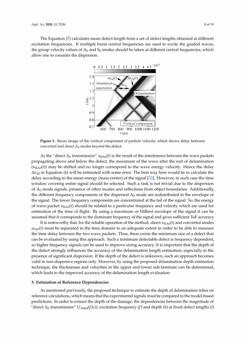
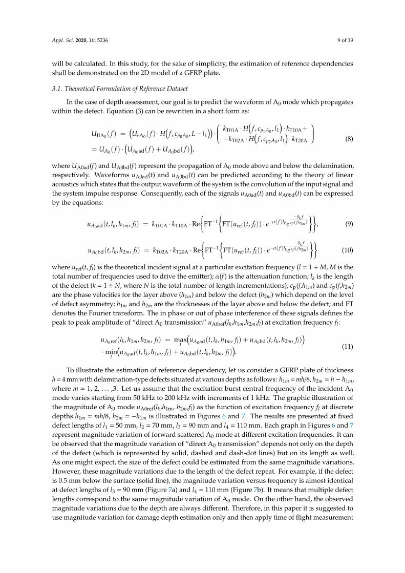
To illustrate the estimation of reference dependency, let us consider a GFRP plate of thicknessh = 4 mm with delamination-type defects situated at various depths as follows: h1m = mh/8, h2m = h − h1m,where m = 1, 2, . . . ,3. Let us assume that the excitation burst central frequency of the incident A0

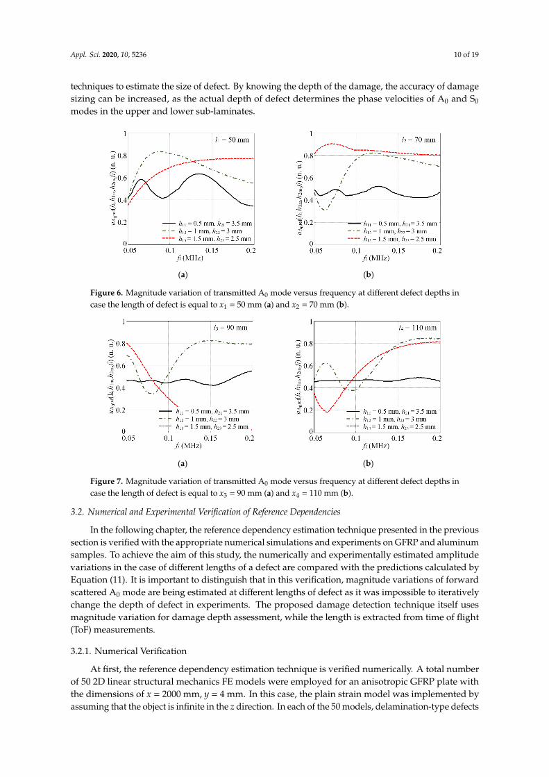
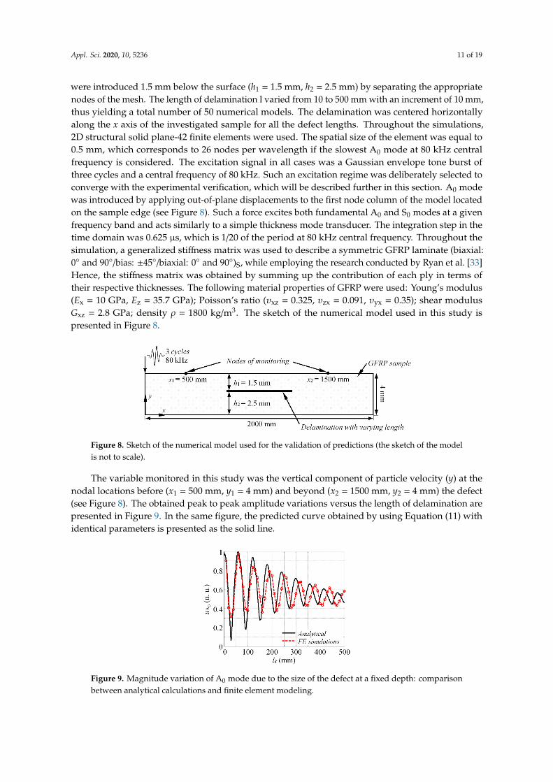
mode varies starting from 50 kHz to 200 kHz with increments of 1 kHz. The graphic illustration ofthe magnitude of A0 mode uA0ref(lk,h1m, h2m,fl) as the function of excitation frequency fl at discretedepths h1m = mh/8, h2m = −h1m is illustrated in Figures 6 and 7. The results are presented at fixeddefect lengths of l1 = 50 mm, l2 = 70 mm, l3 = 90 mm and l4 = 110 mm. Each graph in Figures 6 and 7represent magnitude variation of forward scattered A0 mode at different excitation frequencies. It canbe observed that the magnitude variation of “direct A0 transmission” depends not only on the depthof the defect (which is represented by solid, dashed and dash-dot lines) but on its length as well.As one might expect, the size of the defect could be estimated from the same magnitude variations.However, these magnitude variations due to the length of the defect repeat. For example, if the defectis 0.5 mm below the surface (solid line), the magnitude variation versus frequency is almost identicalat defect lengths of l3 = 90 mm (Figure 7a) and l4 = 110 mm (Figure 7b). It means that multiple defectlengths correspond to the same magnitude variation of A0 mode. On the other hand, the observedmagnitude variations due to the depth are always different. Therefore, in this paper it is suggested touse magnitude variation for damage depth estimation only and then apply time of flight measurement

Appl. Sci. 2020, 10, 5236 10 of 19

techniques to estimate the size of defect. By knowing the depth of the damage, the accuracy of damagesizing can be increased, as the actual depth of defect determines the phase velocities of A0 and S0

modes in the upper and lower sub-laminates.Appl. Sci. 2020, 10, x FOR PEER REVIEW  10 of 19 

   

(a)  (b) 

Figure 6. Magnitude variation of transmitted A0 mode versus frequency at different defect depths in 

case the length of defect is equal to x1 = 50 mm (a) and x2 = 70 mm (b). 

   

(a)  (b) 

Figure 7. Magnitude variation of transmitted A0 mode versus frequency at different defect depths in 

case the length of defect is equal to x3 = 90 mm (a) and x4 = 110 mm (b). 

3.2. Numerical and Experimental Verification of Reference Dependencies 

In  the  following  chapter,  the  reference  dependency  estimation  technique  presented  in  the 

previous section is verified with the appropriate numerical simulations and experiments on GFRP 

and  aluminum  samples.  To  achieve  the  aim  of  this  study,  the  numerically  and  experimentally 

estimated amplitude variations  in  the case of different  lengths of a defect are compared with  the 

predictions  calculated  by  Equation  (11).  It  is  important  to  distinguish  that  in  this  verification, 

magnitude variations of forward scattered A0 mode are being estimated at different lengths of defect 

as it was impossible to iteratively change the depth of defect in experiments. The proposed damage 

detection technique itself uses magnitude variation for damage depth assessment, while the length 

is extracted from time of flight (ToF) measurements. 

3.2.1. Numerical Verification 

At first, the reference dependency estimation technique is verified numerically. A total number 

of 50 2D linear structural mechanics FE models were employed for an anisotropic GFRP plate with 

the dimensions of x = 2000 mm, y = 4 mm. In this case, the plain strain model was implemented by 

assuming  that  the object  is  infinite  in  the z direction.  In each of  the 50 models, delamination‐type 

Figure 6. Magnitude variation of transmitted A0 mode versus frequency at different defect depths incase the length of defect is equal to x1 = 50 mm (a) and x2 = 70 mm (b).

Appl. Sci. 2020, 10, x FOR PEER REVIEW  10 of 19 

   

(a)  (b) 

Figure 6. Magnitude variation of transmitted A0 mode versus frequency at different defect depths in 

case the length of defect is equal to x1 = 50 mm (a) and x2 = 70 mm (b). 

   

(a)  (b) 

Figure 7. Magnitude variation of transmitted A0 mode versus frequency at different defect depths in 

case the length of defect is equal to x3 = 90 mm (a) and x4 = 110 mm (b). 

3.2. Numerical and Experimental Verification of Reference Dependencies 

In  the  following  chapter,  the  reference  dependency  estimation  technique  presented  in  the 

previous section is verified with the appropriate numerical simulations and experiments on GFRP 

and  aluminum  samples.  To  achieve  the  aim  of  this  study,  the  numerically  and  experimentally 

estimated amplitude variations  in  the case of different  lengths of a defect are compared with  the 

predictions  calculated  by  Equation  (11).  It  is  important  to  distinguish  that  in  this  verification, 

magnitude variations of forward scattered A0 mode are being estimated at different lengths of defect 

as it was impossible to iteratively change the depth of defect in experiments. The proposed damage 

detection technique itself uses magnitude variation for damage depth assessment, while the length 

is extracted from time of flight (ToF) measurements. 

3.2.1. Numerical Verification 

At first, the reference dependency estimation technique is verified numerically. A total number 

of 50 2D linear structural mechanics FE models were employed for an anisotropic GFRP plate with 

the dimensions of x = 2000 mm, y = 4 mm. In this case, the plain strain model was implemented by 

assuming  that  the object  is  infinite  in  the z direction.  In each of  the 50 models, delamination‐type 

Figure 7. Magnitude variation of transmitted A0 mode versus frequency at different defect depths incase the length of defect is equal to x3 = 90 mm (a) and x4 = 110 mm (b).

3.2. Numerical and Experimental Verification of Reference Dependencies

In the following chapter, the reference dependency estimation technique presented in the previoussection is verified with the appropriate numerical simulations and experiments on GFRP and aluminumsamples. To achieve the aim of this study, the numerically and experimentally estimated amplitudevariations in the case of different lengths of a defect are compared with the predictions calculated byEquation (11). It is important to distinguish that in this verification, magnitude variations of forwardscattered A0 mode are being estimated at different lengths of defect as it was impossible to iterativelychange the depth of defect in experiments. The proposed damage detection technique itself usesmagnitude variation for damage depth assessment, while the length is extracted from time of flight(ToF) measurements.

3.2.1. Numerical Verification

At first, the reference dependency estimation technique is verified numerically. A total numberof 50 2D linear structural mechanics FE models were employed for an anisotropic GFRP plate withthe dimensions of x = 2000 mm, y = 4 mm. In this case, the plain strain model was implemented byassuming that the object is infinite in the z direction. In each of the 50 models, delamination-type defects

Appl. Sci. 2020, 10, 5236 11 of 19

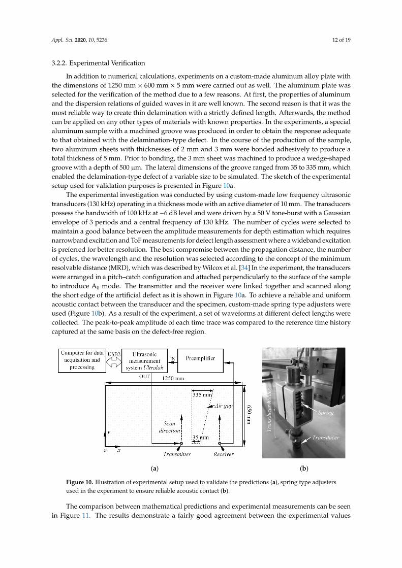
were introduced 1.5 mm below the surface (h1 = 1.5 mm, h2 = 2.5 mm) by separating the appropriatenodes of the mesh. The length of delamination l varied from 10 to 500 mm with an increment of 10 mm,thus yielding a total number of 50 numerical models. The delamination was centered horizontallyalong the x axis of the investigated sample for all the defect lengths. Throughout the simulations,2D structural solid plane-42 finite elements were used. The spatial size of the element was equal to0.5 mm, which corresponds to 26 nodes per wavelength if the slowest A0 mode at 80 kHz centralfrequency is considered. The excitation signal in all cases was a Gaussian envelope tone burst ofthree cycles and a central frequency of 80 kHz. Such an excitation regime was deliberately selected toconverge with the experimental verification, which will be described further in this section. A0 modewas introduced by applying out-of-plane displacements to the first node column of the model locatedon the sample edge (see Figure 8). Such a force excites both fundamental A0 and S0 modes at a givenfrequency band and acts similarly to a simple thickness mode transducer. The integration step in thetime domain was 0.625 µs, which is 1/20 of the period at 80 kHz central frequency. Throughout thesimulation, a generalized stiffness matrix was used to describe a symmetric GFRP laminate (biaxial:0◦ and 90◦/bias: ±45◦/biaxial: 0◦ and 90◦)S, while employing the research conducted by Ryan et al. [33]Hence, the stiffness matrix was obtained by summing up the contribution of each ply in terms oftheir respective thicknesses. The following material properties of GFRP were used: Young’s modulus(Ex = 10 GPa, Ez = 35.7 GPa); Poisson’s ratio (υxz = 0.325, υzx = 0.091, υyx = 0.35); shear modulusGxz = 2.8 GPa; density ρ = 1800 kg/m3. The sketch of the numerical model used in this study ispresented in Figure 8.

Appl. Sci. 2020, 10, x FOR PEER REVIEW  11 of 19 

defects were  introduced 1.5 mm below  the  surface  (h1 = 1.5 mm, h2 = 2.5 mm) by  separating  the 

appropriate nodes of  the mesh. The  length of delamination  l varied  from 10  to 500 mm with an 

increment of 10 mm, thus yielding a total number of 50 numerical models. The delamination was 

centered  horizontally  along  the  x  axis  of  the  investigated  sample  for  all  the  defect  lengths. 

Throughout the simulations, 2D structural solid plane‐42 finite elements were used. The spatial size 

of the element was equal to 0.5 mm, which corresponds to 26 nodes per wavelength if the slowest A0 

mode at 80 kHz central frequency  is considered. The excitation signal  in all cases was a Gaussian 

envelope tone burst of three cycles and a central frequency of 80 kHz. Such an excitation regime was 

deliberately selected to converge with the experimental verification, which will be described further 

in  this section. A0 mode was  introduced by applying out‐of‐plane displacements  to  the  first node 

column of the model located on the sample edge (see Figure 8). Such a force excites both fundamental 

A0 and S0 modes at a given frequency band and acts similarly to a simple thickness mode transducer. 

The integration step in the time domain was 0.625 μs, which is 1/20 of the period at 80 kHz central 

frequency.  Throughout  the  simulation,  a  generalized  stiffness  matrix  was  used  to  describe  a 

symmetric GFRP laminate (biaxial: 0° and 90°/bias: ±45°/biaxial: 0° and 90°)S, while employing the 

research conducted by Ryan et al. [33] Hence, the stiffness matrix was obtained by summing up the 

contribution of each ply in terms of their respective thicknesses. The following material properties of 

GFRP were used: Young’s modulus (Ex = 10 GPa, Ez = 35.7 GPa); Poisson’s ratio (υxz = 0.325, υzx = 0.091, 

υyx = 0.35); shear modulus Gxz = 2.8 GPa; density ρ = 1800 kg/m3. The sketch of the numerical model 

used in this study is presented in Figure 8. 

 

Figure 8. Sketch of the numerical model used for the validation of predictions (the sketch of the model 

is not to scale). 

The variable monitored in this study was the vertical component of particle velocity (y) at the 

nodal locations before (x1 = 500 mm, y1 = 4 mm) and beyond (x2 = 1500 mm, y2 = 4 mm) the defect (see 

Figure 8). The obtained peak  to peak amplitude variations versus  the  length of delamination are 

presented in Figure 9. In the same figure, the predicted curve obtained by using Equation (11) with 

identical parameters is presented as the solid line. 

 

Figure 9. Magnitude variation of A0 mode due to the size of the defect at a fixed depth: comparison 

between analytical calculations and finite element modeling. 

 

Figure 8. Sketch of the numerical model used for the validation of predictions (the sketch of the modelis not to scale).

The variable monitored in this study was the vertical component of particle velocity (y) at thenodal locations before (x1 = 500 mm, y1 = 4 mm) and beyond (x2 = 1500 mm, y2 = 4 mm) the defect(see Figure 8). The obtained peak to peak amplitude variations versus the length of delamination arepresented in Figure 9. In the same figure, the predicted curve obtained by using Equation (11) withidentical parameters is presented as the solid line.

Appl. Sci. 2020, 10, x FOR PEER REVIEW  11 of 19 

defects were  introduced 1.5 mm below  the  surface  (h1 = 1.5 mm, h2 = 2.5 mm) by  separating  the 

appropriate nodes of  the mesh. The  length of delamination  l varied  from 10  to 500 mm with an 

increment of 10 mm, thus yielding a total number of 50 numerical models. The delamination was 

centered  horizontally  along  the  x  axis  of  the  investigated  sample  for  all  the  defect  lengths. 

Throughout the simulations, 2D structural solid plane‐42 finite elements were used. The spatial size 

of the element was equal to 0.5 mm, which corresponds to 26 nodes per wavelength if the slowest A0 

mode at 80 kHz central frequency  is considered. The excitation signal  in all cases was a Gaussian 

envelope tone burst of three cycles and a central frequency of 80 kHz. Such an excitation regime was 

deliberately selected to converge with the experimental verification, which will be described further 

in  this section. A0 mode was  introduced by applying out‐of‐plane displacements  to  the  first node 

column of the model located on the sample edge (see Figure 8). Such a force excites both fundamental 

A0 and S0 modes at a given frequency band and acts similarly to a simple thickness mode transducer. 

The integration step in the time domain was 0.625 μs, which is 1/20 of the period at 80 kHz central 

frequency.  Throughout  the  simulation,  a  generalized  stiffness  matrix  was  used  to  describe  a 

symmetric GFRP laminate (biaxial: 0° and 90°/bias: ±45°/biaxial: 0° and 90°)S, while employing the 

research conducted by Ryan et al. [33] Hence, the stiffness matrix was obtained by summing up the 

contribution of each ply in terms of their respective thicknesses. The following material properties of 

GFRP were used: Young’s modulus (Ex = 10 GPa, Ez = 35.7 GPa); Poisson’s ratio (υxz = 0.325, υzx = 0.091, 

υyx = 0.35); shear modulus Gxz = 2.8 GPa; density ρ = 1800 kg/m3. The sketch of the numerical model 

used in this study is presented in Figure 8. 

 

Figure 8. Sketch of the numerical model used for the validation of predictions (the sketch of the model 

is not to scale). 

The variable monitored in this study was the vertical component of particle velocity (y) at the 

nodal locations before (x1 = 500 mm, y1 = 4 mm) and beyond (x2 = 1500 mm, y2 = 4 mm) the defect (see 

Figure 8). The obtained peak  to peak amplitude variations versus  the  length of delamination are 

presented in Figure 9. In the same figure, the predicted curve obtained by using Equation (11) with 

identical parameters is presented as the solid line. 

 

Figure 9. Magnitude variation of A0 mode due to the size of the defect at a fixed depth: comparison 

between analytical calculations and finite element modeling. 

 

Figure 9. Magnitude variation of A0 mode due to the size of the defect at a fixed depth: comparisonbetween analytical calculations and finite element modeling.

Appl. Sci. 2020, 10, 5236 12 of 19

3.2.2. Experimental Verification

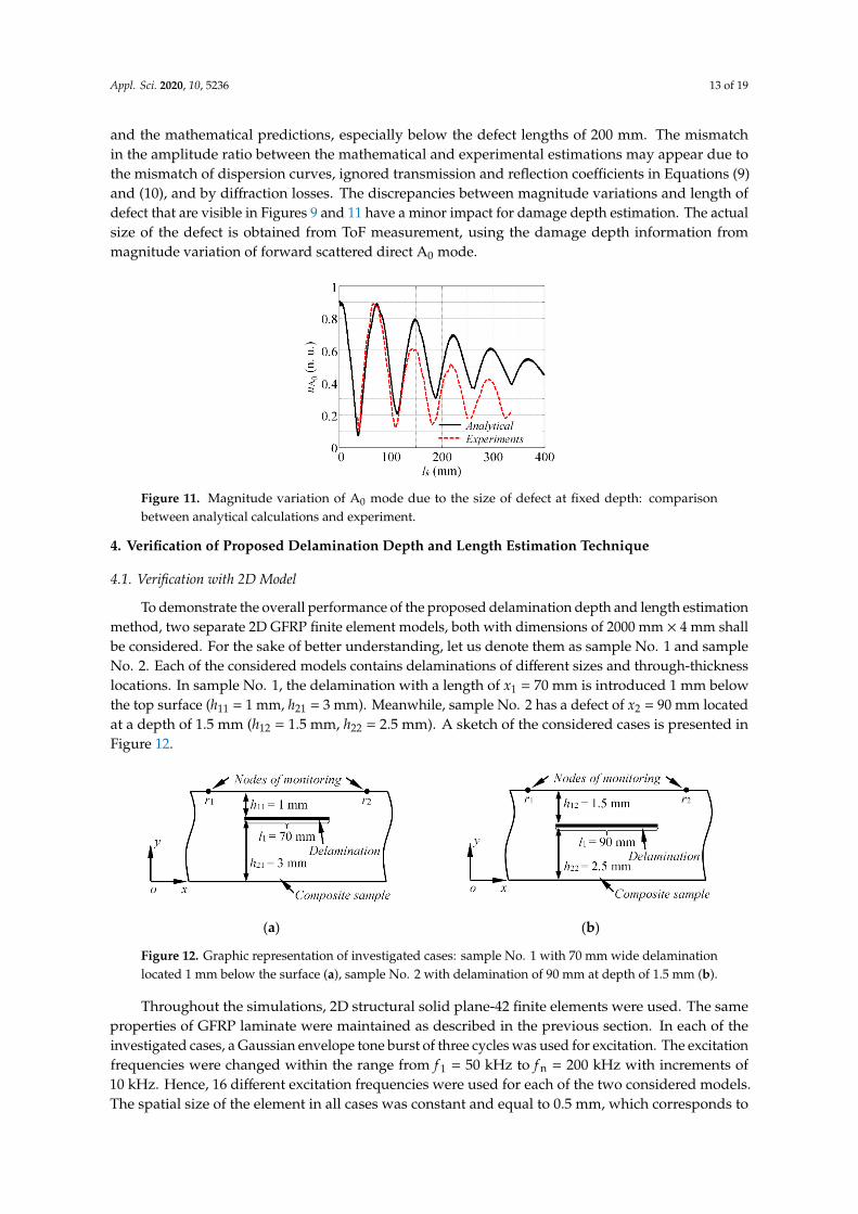
In addition to numerical calculations, experiments on a custom-made aluminum alloy plate withthe dimensions of 1250 mm × 600 mm × 5 mm were carried out as well. The aluminum plate wasselected for the verification of the method due to a few reasons. At first, the properties of aluminumand the dispersion relations of guided waves in it are well known. The second reason is that it was themost reliable way to create thin delamination with a strictly defined length. Afterwards, the methodcan be applied on any other types of materials with known properties. In the experiments, a specialaluminum sample with a machined groove was produced in order to obtain the response adequateto that obtained with the delamination-type defect. In the course of the production of the sample,two aluminum sheets with thicknesses of 2 mm and 3 mm were bonded adhesively to produce atotal thickness of 5 mm. Prior to bonding, the 3 mm sheet was machined to produce a wedge-shapedgroove with a depth of 500 µm. The lateral dimensions of the groove ranged from 35 to 335 mm, whichenabled the delamination-type defect of a variable size to be simulated. The sketch of the experimentalsetup used for validation purposes is presented in Figure 10a.

The experimental investigation was conducted by using custom-made low frequency ultrasonictransducers (130 kHz) operating in a thickness mode with an active diameter of 10 mm. The transducerspossess the bandwidth of 100 kHz at −6 dB level and were driven by a 50 V tone-burst with a Gaussianenvelope of 3 periods and a central frequency of 130 kHz. The number of cycles were selected tomaintain a good balance between the amplitude measurements for depth estimation which requiresnarrowband excitation and ToF measurements for defect length assessment where a wideband excitationis preferred for better resolution. The best compromise between the propagation distance, the numberof cycles, the wavelength and the resolution was selected according to the concept of the minimumresolvable distance (MRD), which was described by Wilcox et al. [34] In the experiment, the transducerswere arranged in a pitch–catch configuration and attached perpendicularly to the surface of the sampleto introduce A0 mode. The transmitter and the receiver were linked together and scanned alongthe short edge of the artificial defect as it is shown in Figure 10a. To achieve a reliable and uniformacoustic contact between the transducer and the specimen, custom-made spring type adjusters wereused (Figure 10b). As a result of the experiment, a set of waveforms at different defect lengths werecollected. The peak-to-peak amplitude of each time trace was compared to the reference time historycaptured at the same basis on the defect-free region.

Appl. Sci. 2020, 10, x FOR PEER REVIEW  12 of 19 

3.2.2. Experimental Verification 

In addition to numerical calculations, experiments on a custom‐made aluminum alloy plate with 

the dimensions of 1250 mm × 600 mm × 5 mm were carried out as well. The aluminum plate was 

selected for the verification of the method due to a few reasons. At first, the properties of aluminum 

and the dispersion relations of guided waves in it are well known. The second reason is that it was 

the most  reliable way  to  create  thin delamination with  a  strictly defined  length. Afterwards,  the 

method can be applied on any other types of materials with known properties. In the experiments, a 

special aluminum sample with a machined groove was produced  in order  to obtain  the response 

adequate to that obtained with the delamination‐type defect. In the course of the production of the 

sample,  two  aluminum  sheets with  thicknesses  of  2 mm  and  3 mm were  bonded  adhesively  to 

produce a  total  thickness of 5 mm. Prior  to bonding,  the 3 mm sheet was machined  to produce a 

wedge‐shaped groove with a depth of 500 μm. The lateral dimensions of the groove ranged from 35 

to 335 mm, which enabled the delamination‐type defect of a variable size to be simulated. The sketch 

of the experimental setup used for validation purposes is presented in Figure 10a. 

The experimental investigation was conducted by using custom‐made low frequency ultrasonic 

transducers  (130  kHz)  operating  in  a  thickness mode with  an  active  diameter  of  10 mm.  The 

transducers possess the bandwidth of 100 kHz at −6 dB level and were driven by a 50 V tone‐burst 

with a Gaussian envelope of 3 periods and a central frequency of 130 kHz. The number of cycles were 

selected  to maintain  a  good  balance  between  the  amplitude measurements  for depth  estimation 

which requires narrowband excitation and ToF measurements for defect length assessment where a 

wideband excitation is preferred for better resolution. The best compromise between the propagation 

distance,  the number of  cycles,  the wavelength and  the  resolution was  selected  according  to  the 

concept of the minimum resolvable distance (MRD), which was described by Wilcox et al. [34] In the 

experiment,  the  transducers  were  arranged  in  a  pitch–catch  configuration  and  attached 

perpendicularly to the surface of the sample to introduce A0 mode. The transmitter and the receiver 

were linked together and scanned along the short edge of the artificial defect as it is shown in Figure 

10a. To achieve a reliable and uniform acoustic contact between the transducer and the specimen, 

custom‐made spring type adjusters were used (Figure 10b). As a result of the experiment, a set of 

waveforms at different defect lengths were collected. The peak‐to‐peak amplitude of each time trace 

was compared to the reference time history captured at the same basis on the defect‐free region. 

   

(a)  (b) 

Figure 10. Illustration of experimental setup used to validate the predictions (a), spring type adjusters 

used in the experiment to ensure reliable acoustic contact (b). 

The comparison between mathematical predictions and experimental measurements can be seen 

in Figure 11. The results demonstrate a fairly good agreement between the experimental values and 

the mathematical predictions, especially below the defect lengths of 200 mm. The mismatch in the 

amplitude  ratio between  the mathematical  and  experimental  estimations may  appear due  to  the 

Figure 10. Illustration of experimental setup used to validate the predictions (a), spring type adjustersused in the experiment to ensure reliable acoustic contact (b).

The comparison between mathematical predictions and experimental measurements can be seenin Figure 11. The results demonstrate a fairly good agreement between the experimental values

Appl. Sci. 2020, 10, 5236 13 of 19

and the mathematical predictions, especially below the defect lengths of 200 mm. The mismatchin the amplitude ratio between the mathematical and experimental estimations may appear due tothe mismatch of dispersion curves, ignored transmission and reflection coefficients in Equations (9)and (10), and by diffraction losses. The discrepancies between magnitude variations and length ofdefect that are visible in Figures 9 and 11 have a minor impact for damage depth estimation. The actualsize of the defect is obtained from ToF measurement, using the damage depth information frommagnitude variation of forward scattered direct A0 mode.

Appl. Sci. 2020, 10, x FOR PEER REVIEW  13 of 19 

mismatch of dispersion curves, ignored transmission and reflection coefficients in Equations (9) and 

(10), and by diffraction losses. The discrepancies between magnitude variations and length of defect 

that are visible in Figures 9 and 11 have a minor impact for damage depth estimation. The actual size 

of  the  defect  is  obtained  from  ToF  measurement,  using  the  damage  depth  information  from 

magnitude variation of forward scattered direct A0 mode. 

 

Figure  11. Magnitude variation of A0 mode due  to  the  size of defect  at  fixed depth:  comparison 

between analytical calculations and experiment. 

4. Verification of Proposed Delamination Depth and Length Estimation Technique 

4.1. Verification with 2D Model 

To  demonstrate  the  overall  performance  of  the  proposed  delamination  depth  and  length 

estimation method, two separate 2D GFRP finite element models, both with dimensions of 2000 mm 

× 4 mm shall be considered. For the sake of better understanding, let us denote them as sample No. 1 

and  sample No.  2. Each  of  the  considered models  contains delaminations  of different  sizes  and 

through‐thickness  locations.  In  sample No.  1,  the  delamination with  a  length  of  x1  =  70 mm  is 

introduced 1 mm below the top surface (h11 = 1 mm, h21 = 3 mm). Meanwhile, sample No. 2 has a 

defect of x2 = 90 mm  located at a depth of 1.5 mm  (h12 = 1.5 mm, h22 = 2.5 mm). A  sketch of  the 

considered cases is presented in Figure 12. 

Throughout the simulations, 2D structural solid plane‐42 finite elements were used. The same 

properties of GFRP  laminate were maintained as described  in the previous section. In each of the 

investigated  cases,  a Gaussian  envelope  tone  burst  of  three  cycles was  used  for  excitation.  The 

excitation frequencies were changed within the range from f1 = 50 kHz to fn = 200 kHz with increments 

of 10 kHz. Hence, 16 different excitation frequencies were used for each of the two considered models. 

The spatial size of the element in all cases was constant and equal to 0.5 mm, which corresponds to 

12 up to 37 nodes per wavelength for the slowest A0 in a frequency range of f1, f2, …, fn. A0 mode was 

introduced  into the structure by applying the out‐of‐plane nodal displacements to the edge of the 

sample in the same way as it was demonstrated in Figure 8. The integration step in the time domain 

varied from 1 μs for the lowest excitation frequency f1 = 50 kHz to 0.25 μs for fn = 200 kHz. The variable 

monitored in this study was a vertical component of the particle velocity (y) at nodal locations r1 (x1 

= 750 mm, y1 = 4 mm) and r2 (x2 = 1250 mm, y2 = 4 mm). 

   

(a)  (b) 

Figure 11. Magnitude variation of A0 mode due to the size of defect at fixed depth: comparisonbetween analytical calculations and experiment.

4. Verification of Proposed Delamination Depth and Length Estimation Technique

4.1. Verification with 2D Model

To demonstrate the overall performance of the proposed delamination depth and length estimationmethod, two separate 2D GFRP finite element models, both with dimensions of 2000 mm × 4 mm shallbe considered. For the sake of better understanding, let us denote them as sample No. 1 and sampleNo. 2. Each of the considered models contains delaminations of different sizes and through-thicknesslocations. In sample No. 1, the delamination with a length of x1 = 70 mm is introduced 1 mm belowthe top surface (h11 = 1 mm, h21 = 3 mm). Meanwhile, sample No. 2 has a defect of x2 = 90 mm locatedat a depth of 1.5 mm (h12 = 1.5 mm, h22 = 2.5 mm). A sketch of the considered cases is presented inFigure 12.

Appl. Sci. 2020, 10, x FOR PEER REVIEW  13 of 19 

mismatch of dispersion curves, ignored transmission and reflection coefficients in Equations (9) and 

(10), and by diffraction losses. The discrepancies between magnitude variations and length of defect 

that are visible in Figures 9 and 11 have a minor impact for damage depth estimation. The actual size 

of  the  defect  is  obtained  from  ToF  measurement,  using  the  damage  depth  information  from 

magnitude variation of forward scattered direct A0 mode. 

 

Figure  11. Magnitude variation of A0 mode due  to  the  size of defect  at  fixed depth:  comparison 

between analytical calculations and experiment. 

4. Verification of Proposed Delamination Depth and Length Estimation Technique 

4.1. Verification with 2D Model 

To  demonstrate  the  overall  performance  of  the  proposed  delamination  depth  and  length 

estimation method, two separate 2D GFRP finite element models, both with dimensions of 2000 mm 

× 4 mm shall be considered. For the sake of better understanding, let us denote them as sample No. 1 

and  sample No.  2. Each  of  the  considered models  contains delaminations  of different  sizes  and 

through‐thickness  locations.  In  sample No.  1,  the  delamination with  a  length  of  x1  =  70 mm  is 

introduced 1 mm below the top surface (h11 = 1 mm, h21 = 3 mm). Meanwhile, sample No. 2 has a 

defect of x2 = 90 mm  located at a depth of 1.5 mm  (h12 = 1.5 mm, h22 = 2.5 mm). A  sketch of  the 

considered cases is presented in Figure 12. 

Throughout the simulations, 2D structural solid plane‐42 finite elements were used. The same 

properties of GFRP  laminate were maintained as described  in the previous section. In each of the 

investigated  cases,  a Gaussian  envelope  tone  burst  of  three  cycles was  used  for  excitation.  The 

excitation frequencies were changed within the range from f1 = 50 kHz to fn = 200 kHz with increments 

of 10 kHz. Hence, 16 different excitation frequencies were used for each of the two considered models. 

The spatial size of the element in all cases was constant and equal to 0.5 mm, which corresponds to 

12 up to 37 nodes per wavelength for the slowest A0 in a frequency range of f1, f2, …, fn. A0 mode was 

introduced  into the structure by applying the out‐of‐plane nodal displacements to the edge of the 

sample in the same way as it was demonstrated in Figure 8. The integration step in the time domain 

varied from 1 μs for the lowest excitation frequency f1 = 50 kHz to 0.25 μs for fn = 200 kHz. The variable 

monitored in this study was a vertical component of the particle velocity (y) at nodal locations r1 (x1 

= 750 mm, y1 = 4 mm) and r2 (x2 = 1250 mm, y2 = 4 mm). 

   

(a)  (b) 

Figure 12. Graphic representation of investigated cases: sample No. 1 with 70 mm wide delaminationlocated 1 mm below the surface (a), sample No. 2 with delamination of 90 mm at depth of 1.5 mm (b).

Throughout the simulations, 2D structural solid plane-42 finite elements were used. The sameproperties of GFRP laminate were maintained as described in the previous section. In each of theinvestigated cases, a Gaussian envelope tone burst of three cycles was used for excitation. The excitationfrequencies were changed within the range from f 1 = 50 kHz to f n = 200 kHz with increments of10 kHz. Hence, 16 different excitation frequencies were used for each of the two considered models.The spatial size of the element in all cases was constant and equal to 0.5 mm, which corresponds to

Appl. Sci. 2020, 10, 5236 14 of 19

12 up to 37 nodes per wavelength for the slowest A0 in a frequency range of f 1, f 2, . . . , f n. A0 modewas introduced into the structure by applying the out-of-plane nodal displacements to the edge ofthe sample in the same way as it was demonstrated in Figure 8. The integration step in the timedomain varied from 1 µs for the lowest excitation frequency f 1 = 50 kHz to 0.25 µs for f n = 200 kHz.The variable monitored in this study was a vertical component of the particle velocity (y) at nodallocations r1 (x1 = 750 mm, y1 = 4 mm) and r2 (x2 = 1250 mm, y2 = 4 mm).

4.1.1. Estimation of Defect Depth

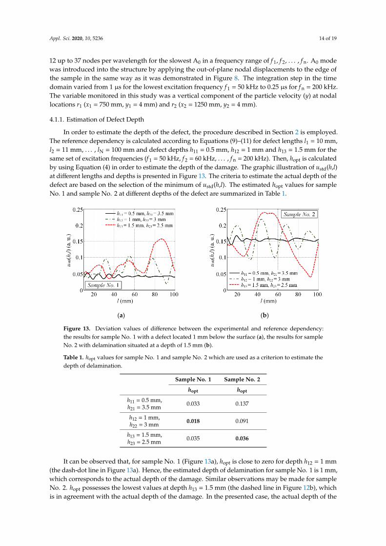
In order to estimate the depth of the defect, the procedure described in Section 2 is employed.The reference dependency is calculated according to Equations (9)–(11) for defect lengths l1 = 10 mm,l2 = 11 mm, . . . , lN = 100 mm and defect depths h11 = 0.5 mm, h12 = 1 mm and h13 = 1.5 mm for thesame set of excitation frequencies (f 1 = 50 kHz, f 2 = 60 kHz, . . . , f n = 200 kHz). Then, hopt is calculatedby using Equation (4) in order to estimate the depth of the damage. The graphic illustration of ustd(h,l)at different lengths and depths is presented in Figure 13. The criteria to estimate the actual depth of thedefect are based on the selection of the minimum of ustd(h,l). The estimated hopt values for sampleNo. 1 and sample No. 2 at different depths of the defect are summarized in Table 1.

Appl. Sci. 2020, 10, x FOR PEER REVIEW  14 of 19 

Figure 12. Graphic representation of investigated cases: sample No. 1 with 70 mm wide delamination 

located 1 mm below the surface (a), sample No. 2 with delamination of 90 mm at depth of 1.5 mm (b). 

4.1.1. Estimation of Defect Depth 

In order to estimate the depth of the defect, the procedure described in Section 2 is employed. 

The reference dependency is calculated according to Equations (9)–(11) for defect lengths l1 = 10 mm, 

l2 = 11 mm, …, lN = 100 mm and defect depths h11 = 0.5 mm, h12 = 1 mm and h13 = 1.5 mm for the same 

set of excitation frequencies (f1 = 50 kHz, f2 = 60 kHz, …, fn = 200 kHz). Then, hopt is calculated by using 

Equation  (4)  in order  to  estimate  the depth of  the damage. The graphic  illustration of ustd(h,l) at 

different lengths and depths is presented in Figure 13. The criteria to estimate the actual depth of the 

defect are based on the selection of the minimum of ustd(h,l). The estimated hopt values for sample No. 

1 and sample No. 2 at different depths of the defect are summarized in Table 1.   

Table 1. hopt values for sample No. 1 and sample No. 2 which are used as a criterion to estimate the 

depth of delamination. 

 Sample No. 1  Sample No. 2 

hopt  hopt 

h11 = 0.5 mm, 

h21 = 3.5 mm 0.033  0.137 

h12 = 1 mm, 

h22 = 3 mm 0.018  0.091 

h13 = 1.5 mm, 

h23 = 2.5 mm 0.035  0.036 

It can be observed that, for sample No. 1 (Figure 13a), hopt is close to zero for depth h12 = 1 mm 

(the dash‐dot line in Figure 13a). Hence, the estimated depth of delamination for sample No. 1 is 1 

mm, which corresponds to the actual depth of the damage. Similar observations may be made for 

sample No. 2. hopt possesses the lowest values at depth h13 = 1.5 mm (the dashed line in Figure 12b), 

which is in agreement with the actual depth of the damage. In the presented case, the actual depth of 

the damage was included in the database. In order to evaluate the performance of the method in case 

of absence of actual depth in database, another set of magnitude patterns has been generated with 

depth increments of 0.4 mm (h11 = 0.4 mm, h12 = 0.8 mm, h13 = 1.2 mm, h14 = 1.6 mm, h15 = 2 mm). In the 

case for sample No. 1 the minimum values of the hopt were close for both h12 = 0.8 mm and h13 = 1.2 

mm, however  the absolute minimum was obtained  for depth h12 = 0.8 mm. For sample No. 2 hopt 

possesses the  lowest values at depth h14 = 1.6 mm. The amount of error of course depends on  the 

depth increments in the database. Such database in general is computationally inexpensive (in this 

case UA0ref(11 × 5 × 90), hence can be calculated small depth increments according to the desired depth 

estimation accuracy. 

   

(a)  (b) 

Figure 13. Deviation values of difference between the experimental and reference dependency:the results for sample No. 1 with a defect located 1 mm below the surface (a), the results for sampleNo. 2 with delamination situated at a depth of 1.5 mm (b).

Table 1. hopt values for sample No. 1 and sample No. 2 which are used as a criterion to estimate thedepth of delamination.

Sample No. 1 Sample No. 2

hopt hopt

h11 = 0.5 mm,h21 = 3.5 mm 0.033 0.137

h12 = 1 mm,h22 = 3 mm 0.018 0.091

h13 = 1.5 mm,h23 = 2.5 mm 0.035 0.036

It can be observed that, for sample No. 1 (Figure 13a), hopt is close to zero for depth h12 = 1 mm(the dash-dot line in Figure 13a). Hence, the estimated depth of delamination for sample No. 1 is 1 mm,which corresponds to the actual depth of the damage. Similar observations may be made for sampleNo. 2. hopt possesses the lowest values at depth h13 = 1.5 mm (the dashed line in Figure 12b), whichis in agreement with the actual depth of the damage. In the presented case, the actual depth of the

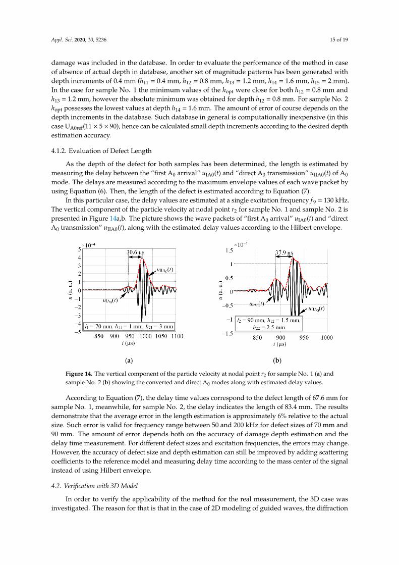
Appl. Sci. 2020, 10, 5236 15 of 19

damage was included in the database. In order to evaluate the performance of the method in caseof absence of actual depth in database, another set of magnitude patterns has been generated withdepth increments of 0.4 mm (h11 = 0.4 mm, h12 = 0.8 mm, h13 = 1.2 mm, h14 = 1.6 mm, h15 = 2 mm).In the case for sample No. 1 the minimum values of the hopt were close for both h12 = 0.8 mm andh13 = 1.2 mm, however the absolute minimum was obtained for depth h12 = 0.8 mm. For sample No. 2hopt possesses the lowest values at depth h14 = 1.6 mm. The amount of error of course depends on thedepth increments in the database. Such database in general is computationally inexpensive (in thiscase UA0ref(11 × 5 × 90), hence can be calculated small depth increments according to the desired depthestimation accuracy.

4.1.2. Evaluation of Defect Length

As the depth of the defect for both samples has been determined, the length is estimated bymeasuring the delay between the “first A0 arrival” uIA0(t) and “direct A0 transmission” uIIA0(t) of A0

mode. The delays are measured according to the maximum envelope values of each wave packet byusing Equation (6). Then, the length of the defect is estimated according to Equation (7).

In this particular case, the delay values are estimated at a single excitation frequency f 9 = 130 kHz.The vertical component of the particle velocity at nodal point r2 for sample No. 1 and sample No. 2 ispresented in Figure 14a,b. The picture shows the wave packets of “first A0 arrival” uIA0(t) and “directA0 transmission” uIIA0(t), along with the estimated delay values according to the Hilbert envelope.

Appl. Sci. 2020, 10, x FOR PEER REVIEW  15 of 19 

Figure 13. Deviation values of difference between the experimental and reference dependency: the 

results for sample No. 1 with a defect located 1 mm below the surface (a), the results for sample No. 

2 with delamination situated at a depth of 1.5 mm (b). 

4.1.2. Evaluation of Defect Length 

As  the depth of  the defect  for both samples has been determined,  the  length  is estimated by 

measuring the delay between the “first A0 arrival” uIA0(t) and “direct A0 transmission” uIIA0(t) of A0 

mode. The delays are measured according to the maximum envelope values of each wave packet by 

using Equation (6). Then, the length of the defect is estimated according to Equation (7). 

In this particular case, the delay values are estimated at a single excitation frequency  f9 = 130 

kHz. The vertical component of the particle velocity at nodal point r2 for sample No. 1 and sample 

No. 2 is presented in Figure 14a,b. The picture shows the wave packets of “first A0 arrival” uIA0(t) and 

“direct A0  transmission”  uIIA0(t),  along with  the  estimated  delay  values  according  to  the Hilbert 

envelope. 

According to Equation (7), the delay time values correspond to the defect length of 67.6 mm for 

sample No. 1, meanwhile, for sample No. 2, the delay indicates the length of 83.4 mm. The results 

demonstrate that the average error in the length estimation is approximately 6% relative to the actual 

size. Such error is valid for frequency range between 50 and 200 kHz for defect sizes of 70 mm and 

90 mm. The amount of error depends both on the accuracy of damage depth estimation and the delay 

time measurement.  For different defect  sizes  and  excitation  frequencies,  the  errors may  change. 

However, the accuracy of defect size and depth estimation can still be improved by adding scattering 

coefficients  to  the reference model and measuring delay  time according  to  the mass center of  the 

signal instead of using Hilbert envelope. 

   

(a)  (b) 

Figure 14. The vertical component of the particle velocity at nodal point r2 for sample No. 1 (a) and 

sample No. 2 (b) showing the converted and direct A0 modes along with estimated delay values. 

4.2. Verification with 3D Model 

In order  to verify  the  applicability of  the method  for  the  real measurement,  the  3D  case was 

investigated. The reason for that is that in the case of 2D modeling of guided waves, the diffraction does 

not  affect  the  signals,  in  contrary  to  the  3D  case when diffraction  takes place,  and  signals  can  be 

overlapped  with  boundary  reflections.  There  are  many  signal  processing  methods  which  work 

perfectly in the case of 1D or 2D models; however, they still fail when they are applied for real structures 

or 3D models. So, the verification of the method for a 3D case is very important for the assessment of 

the potential of the method for in situ applications.   

For this purpose, a 3D GFRP numerical model with the dimensions of 600 mm × 300 mm × 4 mm 

was employed with a square (90 mm × 90 mm) delamination‐type defect, located at 1.6 mm below the 

top surface. The defect was centered both according to the x and z axes (Figure 15). The structure was 

Figure 14. The vertical component of the particle velocity at nodal point r2 for sample No. 1 (a) andsample No. 2 (b) showing the converted and direct A0 modes along with estimated delay values.

According to Equation (7), the delay time values correspond to the defect length of 67.6 mm forsample No. 1, meanwhile, for sample No. 2, the delay indicates the length of 83.4 mm. The resultsdemonstrate that the average error in the length estimation is approximately 6% relative to the actualsize. Such error is valid for frequency range between 50 and 200 kHz for defect sizes of 70 mm and90 mm. The amount of error depends both on the accuracy of damage depth estimation and thedelay time measurement. For different defect sizes and excitation frequencies, the errors may change.However, the accuracy of defect size and depth estimation can still be improved by adding scatteringcoefficients to the reference model and measuring delay time according to the mass center of the signalinstead of using Hilbert envelope.

4.2. Verification with 3D Model

In order to verify the applicability of the method for the real measurement, the 3D case wasinvestigated. The reason for that is that in the case of 2D modeling of guided waves, the diffraction

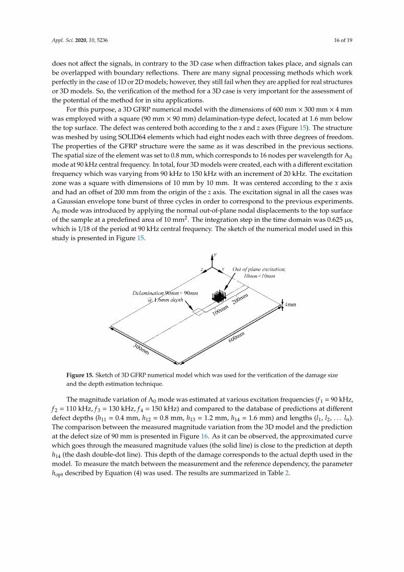
Appl. Sci. 2020, 10, 5236 16 of 19

does not affect the signals, in contrary to the 3D case when diffraction takes place, and signals canbe overlapped with boundary reflections. There are many signal processing methods which workperfectly in the case of 1D or 2D models; however, they still fail when they are applied for real structuresor 3D models. So, the verification of the method for a 3D case is very important for the assessment ofthe potential of the method for in situ applications.

For this purpose, a 3D GFRP numerical model with the dimensions of 600 mm × 300 mm × 4 mmwas employed with a square (90 mm × 90 mm) delamination-type defect, located at 1.6 mm belowthe top surface. The defect was centered both according to the x and z axes (Figure 15). The structurewas meshed by using SOLID64 elements which had eight nodes each with three degrees of freedom.The properties of the GFRP structure were the same as it was described in the previous sections.The spatial size of the element was set to 0.8 mm, which corresponds to 16 nodes per wavelength for A0

mode at 90 kHz central frequency. In total, four 3D models were created, each with a different excitationfrequency which was varying from 90 kHz to 150 kHz with an increment of 20 kHz. The excitationzone was a square with dimensions of 10 mm by 10 mm. It was centered according to the x axisand had an offset of 200 mm from the origin of the z axis. The excitation signal in all the cases wasa Gaussian envelope tone burst of three cycles in order to correspond to the previous experiments.A0 mode was introduced by applying the normal out-of-plane nodal displacements to the top surfaceof the sample at a predefined area of 10 mm2. The integration step in the time domain was 0.625 µs,which is 1/18 of the period at 90 kHz central frequency. The sketch of the numerical model used in thisstudy is presented in Figure 15.

Appl. Sci. 2020, 10, x FOR PEER REVIEW  16 of 19 

meshed by using SOLID64 elements which had eight nodes each with three degrees of freedom. The 

properties of the GFRP structure were the same as it was described in the previous sections. The spatial 

size of the element was set to 0.8 mm, which corresponds to 16 nodes per wavelength for A0 mode at 

90  kHz  central  frequency.  In  total,  four  3D models were  created,  each with  a  different  excitation 

frequency which was varying from 90 kHz to 150 kHz with an increment of 20 kHz. The excitation zone 

was a square with dimensions of 10 mm by 10 mm. It was centered according to the x axis and had an 

offset of 200 mm from  the origin of  the z axis. The excitation signal  in all the cases was a Gaussian 

envelope tone burst of three cycles in order to correspond to the previous experiments. A0 mode was 

introduced by applying the normal out‐of‐plane nodal displacements to the top surface of the sample 

at a predefined area of 10 mm2. The integration step in the time domain was 0.625 μs, which is 1/18 of 

the  period  at  90  kHz  central  frequency.  The  sketch  of  the  numerical model  used  in  this  study  is 

presented in Figure 15. 

The magnitude variation of A0 mode was estimated at various excitation frequencies (f1 = 90 kHz, 

f2 = 110 kHz, f3 = 130 kHz, f4 = 150 kHz) and compared to the database of predictions at different defect 

depths (h11 = 0.4 mm, h12 = 0.8 mm, h13 = 1.2 mm, h14 = 1.6 mm) and lengths (l1, l2, … ln). The comparison 

between the measured magnitude variation from the 3D model and the prediction at the defect size 

of  90 mm  is presented  in Figure  16. As  it  can be observed,  the  approximated  curve which goes 

through the measured magnitude values (the solid line) is close to the prediction at depth h14 (the 

dash double‐dot line). This depth of the damage corresponds to the actual depth used in the model. 

To measure the match between the measurement and the reference dependency, the parameter hopt 

described by Equation (4) was used. The results are summarized in Table 2. 

 

Figure 15. Sketch of 3D GFRP numerical model which was used for the verification of the damage 

size and the depth estimation technique. 

 

Figure 16. Comparison between simulated magnitude variation of A0 mode (the magenta solid line) 

and the predicted variations and different depths and damage length of 90 mm. 

Figure 15. Sketch of 3D GFRP numerical model which was used for the verification of the damage sizeand the depth estimation technique.

The magnitude variation of A0 mode was estimated at various excitation frequencies (f 1 = 90 kHz,f 2 = 110 kHz, f 3 = 130 kHz, f 4 = 150 kHz) and compared to the database of predictions at differentdefect depths (h11 = 0.4 mm, h12 = 0.8 mm, h13 = 1.2 mm, h14 = 1.6 mm) and lengths (l1, l2, . . . ln).The comparison between the measured magnitude variation from the 3D model and the predictionat the defect size of 90 mm is presented in Figure 16. As it can be observed, the approximated curvewhich goes through the measured magnitude values (the solid line) is close to the prediction at depthh14 (the dash double-dot line). This depth of the damage corresponds to the actual depth used in themodel. To measure the match between the measurement and the reference dependency, the parameterhopt described by Equation (4) was used. The results are summarized in Table 2.

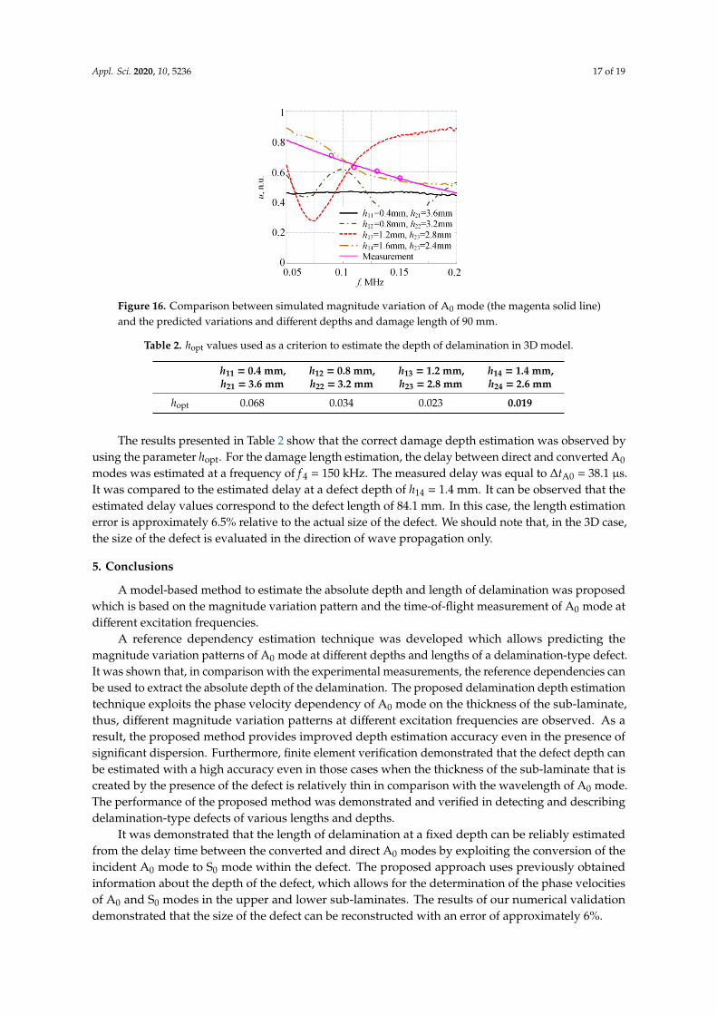
Appl. Sci. 2020, 10, 5236 17 of 19

Appl. Sci. 2020, 10, x FOR PEER REVIEW  16 of 19 

meshed by using SOLID64 elements which had eight nodes each with three degrees of freedom. The 

properties of the GFRP structure were the same as it was described in the previous sections. The spatial 

size of the element was set to 0.8 mm, which corresponds to 16 nodes per wavelength for A0 mode at 

90  kHz  central  frequency.  In  total,  four  3D models were  created,  each with  a  different  excitation 

frequency which was varying from 90 kHz to 150 kHz with an increment of 20 kHz. The excitation zone 

was a square with dimensions of 10 mm by 10 mm. It was centered according to the x axis and had an 

offset of 200 mm from  the origin of  the z axis. The excitation signal  in all the cases was a Gaussian 

envelope tone burst of three cycles in order to correspond to the previous experiments. A0 mode was 

introduced by applying the normal out‐of‐plane nodal displacements to the top surface of the sample 

at a predefined area of 10 mm2. The integration step in the time domain was 0.625 μs, which is 1/18 of 

the  period  at  90  kHz  central  frequency.  The  sketch  of  the  numerical model  used  in  this  study  is 

presented in Figure 15. 

The magnitude variation of A0 mode was estimated at various excitation frequencies (f1 = 90 kHz, 

f2 = 110 kHz, f3 = 130 kHz, f4 = 150 kHz) and compared to the database of predictions at different defect 

depths (h11 = 0.4 mm, h12 = 0.8 mm, h13 = 1.2 mm, h14 = 1.6 mm) and lengths (l1, l2, … ln). The comparison 

between the measured magnitude variation from the 3D model and the prediction at the defect size 

of  90 mm  is presented  in Figure  16. As  it  can be observed,  the  approximated  curve which goes 

through the measured magnitude values (the solid line) is close to the prediction at depth h14 (the 

dash double‐dot line). This depth of the damage corresponds to the actual depth used in the model. 

To measure the match between the measurement and the reference dependency, the parameter hopt 

described by Equation (4) was used. The results are summarized in Table 2. 

 

Figure 15. Sketch of 3D GFRP numerical model which was used for the verification of the damage 

size and the depth estimation technique. 

 

Figure 16. Comparison between simulated magnitude variation of A0 mode (the magenta solid line) 

and the predicted variations and different depths and damage length of 90 mm. 

Figure 16. Comparison between simulated magnitude variation of A0 mode (the magenta solid line)and the predicted variations and different depths and damage length of 90 mm.

Table 2. hopt values used as a criterion to estimate the depth of delamination in 3D model.

h11 = 0.4 mm,h21 = 3.6 mm

h12 = 0.8 mm,h22 = 3.2 mm

h13 = 1.2 mm,h23 = 2.8 mm

h14 = 1.4 mm,h24 = 2.6 mm

hopt 0.068 0.034 0.023 0.019

The results presented in Table 2 show that the correct damage depth estimation was observed byusing the parameter hopt. For the damage length estimation, the delay between direct and converted A0

modes was estimated at a frequency of f 4 = 150 kHz. The measured delay was equal to ∆tA0 = 38.1 µs.It was compared to the estimated delay at a defect depth of h14 = 1.4 mm. It can be observed that theestimated delay values correspond to the defect length of 84.1 mm. In this case, the length estimationerror is approximately 6.5% relative to the actual size of the defect. We should note that, in the 3D case,the size of the defect is evaluated in the direction of wave propagation only.

5. Conclusions

A model-based method to estimate the absolute depth and length of delamination was proposedwhich is based on the magnitude variation pattern and the time-of-flight measurement of A0 mode atdifferent excitation frequencies.

A reference dependency estimation technique was developed which allows predicting themagnitude variation patterns of A0 mode at different depths and lengths of a delamination-type defect.It was shown that, in comparison with the experimental measurements, the reference dependencies canbe used to extract the absolute depth of the delamination. The proposed delamination depth estimationtechnique exploits the phase velocity dependency of A0 mode on the thickness of the sub-laminate,thus, different magnitude variation patterns at different excitation frequencies are observed. As aresult, the proposed method provides improved depth estimation accuracy even in the presence ofsignificant dispersion. Furthermore, finite element verification demonstrated that the defect depth canbe estimated with a high accuracy even in those cases when the thickness of the sub-laminate that iscreated by the presence of the defect is relatively thin in comparison with the wavelength of A0 mode.The performance of the proposed method was demonstrated and verified in detecting and describingdelamination-type defects of various lengths and depths.

It was demonstrated that the length of delamination at a fixed depth can be reliably estimatedfrom the delay time between the converted and direct A0 modes by exploiting the conversion of theincident A0 mode to S0 mode within the defect. The proposed approach uses previously obtainedinformation about the depth of the defect, which allows for the determination of the phase velocitiesof A0 and S0 modes in the upper and lower sub-laminates. The results of our numerical validationdemonstrated that the size of the defect can be reconstructed with an error of approximately 6%.

Appl. Sci. 2020, 10, 5236 18 of 19

The main value of the proposed technique lies in multi-frequency excitation, which leads todifferent magnitude patterns of A0 mode for delamination depth assessment and more accurate velocityvalues for defect length estimation. Hence, such a technique can be used even in the presence of thedispersion of A0 mode and provide information about the absolute depth and length of the damage byemploying a few time traces measured at slightly different frequencies.

Author Contributions: V.S.: Conceptualization, Methodology, Software, Validation, Investigation, Writing—OriginalDraft, Visualization, Supervision. L.M.: Conceptualization, Methodology, Writing—Review and Editing, Supervision.R.R.: Validation, Formal analysis, Investigation, Data Curation, Writing—Original Draft, Visualization. All authorshave read and agreed to the published version of the manuscript.

Funding: This research received no external funding.

Conflicts of Interest: The authors declare no conflict of interest.

References

1. Ip, K.; Mai, Y. Delamination Detection in Smart Composite Beams using Lamb Waves. Smart Mater. Struct.2004, 13, 544–551. [CrossRef]

2. Shoja, S.; Berbyuk, V.; Boström, A. Delamination Detection in Composite Laminates using Low FrequencyGuided Waves: Numerical Simulations. Compos. Struct. 2018, 203, 826–834. [CrossRef]

3. Ramadas, C.; Balasubramaniam, K.; Joshi, M.; Krishnamurthy, C.V. Characterisation of Rectangular TypeDelaminations in Composite Laminates through B- and D-Scan Images Generated using Lamb Waves.NDT E Int. 2011, 44, 281–289. [CrossRef]

4. Santos, M.; Perdigão, J. Leaky Lamb Waves for the Detection and Sizing of Defects in Bonded AluminiumLap Joints. NDT E Int. 2005, 38, 561–568. [CrossRef]

5. Sohn, H.; Dutta, D.; Yang, J.Y.; Park, H.J.; DeSimio, M.; Olson, S.; Swenson, E. Delamination Detectionin Composites through Guided Wave Field Image Processing. Compos. Sci. Technol. 2011, 71, 1250–1256.[CrossRef]

6. Zhao, G.; Wang, B.; Wang, T.; Hao, W.; Luo, Y. Detection and Monitoring of Delamination in CompositeLaminates using Ultrasonic Guided Wave. Compos. Struct. 2019, 225, 111161. [CrossRef]

7. Panda, R.S.; Rajagopal, P.; Balasubramaniam, K. Characterization of Delamination-Type Damages inComposite Laminates using Guided Wave Visualization and Air-Coupled Ultrasound. Struct. Health Monit.2017, 16, 142–152. [CrossRef]

8. Feng, B.; Ribeiro, A.L.; Ramos, H.G. Interaction of Lamb Waves with the Edges of a Delamination in CFRPComposites and a Reference-Free Localization Method for Delamination. Measurement 2018, 122, 424–431.[CrossRef]

9. Hayashi, T.; Kawashima, K. Multiple Reflections of Lamb Waves at a Delamination. Ultrasonics 2002, 40,193–197. [CrossRef]

10. Guo, N.; Cawley, P. The Interaction of Lamb Waves with Delaminations in Composite Laminates. J. Acoust.Soc. Am. 1993, 94, 2240–2246. [CrossRef]

11. Li, F.; Peng, H.; Sun, X.; Wang, J.; Meng, G. Wave Propagation Analysis in Composite Laminates Containing aDelamination using a Three-Dimensional Spectral Element Method. Math. Probl. Eng. 2012, 2012. [CrossRef]

12. Ramadas, C.; Balasubramaniam, K.; Joshi, M.; Krishnamurthy, C.V. Interaction of the Primary Anti-SymmetricLamb Mode (Ao) with Symmetric Delaminations: Numerical and Experimental Studies. Smart Mater. Struct.2009, 18, 085011. [CrossRef]

13. Ramadas, C.; Balasubramaniam, K.; Joshi, M.; Krishnamurthy, C.V. Interaction of Guided Lamb Waveswith an Asymmetrically Located Delamination in a Laminated Composite Plate. Smart Mater. Struct. 2010,19, 065009. [CrossRef]

14. Ramadas, C.; Janardhan Padiyar, M.; Balasubramaniam, K.; Joshi, M.; Krishnamurthy, C.V. Delamination SizeDetection using Time of Flight of Anti-Symmetric (Ao) and Mode Converted Ao Mode of Guided LambWaves. J. Intell. Mater. Syst. Struct. 2010, 21, 817–825. [CrossRef]

15. Schaal, C.; Zhang, S.; Samajder, H.; Mal, A. An Analytical Study of the Scattering of Ultrasonic GuidedWaves at a Delamination-Like Discontinuity in a Plate. Proc. Inst. Mech. Eng. Part C 2017, 231, 2947–2960.[CrossRef]

Appl. Sci. 2020, 10, 5236 19 of 19

16. Hu, N.; Shimomukai, T.; Yan, C.; Fukunaga, H. Identification of Delamination Position in Cross-Ply LaminatedComposite Beams using S0 Lamb Mode. Compos. Sci. Technol. 2008, 68, 1548–1554. [CrossRef]

17. Shkerdin, G.; Glorieux, C. Lamb Mode Conversion in a Plate with a Delamination. J. Acoust. Soc. Am. 2004,116, 2089–2100. [CrossRef]

18. Birt, E.A. Damage Detection in Carbon-Fibre Composites using Ultrasonic Lamb Waves. Insight 1998, 40, 335.19. Liu, Z.; Yu, H.; He, C.; Wu, B. Delamination Detection in Composite Beams using Pure Lamb Mode Generated

by Air-Coupled Ultrasonic Transducer. J. Intell. Mater. Syst. Struct. 2014, 25, 541–550. [CrossRef]20. Li, B.; Ye, L.; Li, Z.; Ma, Z.; Kalhori, H. Quantitative Identification of Delamination at Different Interfaces

using Guided Wave Signals in Composite Laminates. J. Reinf. Plast. Compos. 2015, 34, 1506–1525. [CrossRef]21. Petculescu, G.; Krishnaswamy, S.; Achenbach, J.D. Group Delay Measurements using Modally Selective

Lamb Wave Transducers for Detection and Sizing of Delaminations in Composites. Smart Mater. Struct. 2007,17, 015007. [CrossRef]

22. Eremin, A.; Golub, M.; Glushkov, E.; Glushkova, N. Identification of Delamination Based on the Lamb WaveScattering Resonance Frequencies. NDT E International 2019, 103, 145–153. [CrossRef]

23. Munian, R.K.; Mahapatra, D.R.; Gopalakrishnan, S. Lamb Wave Interaction with Composite Delamination.Compos. Struct. 2018, 206, 484–498. [CrossRef]

24. Gupta, S.; Rajagopal, P. Effect of Ply Orientation and through-Thickness Position of Delamination on theReflection of Fundamental Symmetric S0 Lamb Mode in GFRP Composite Plate Structures. Ultrasonics 2018,90, 109–119. [CrossRef]

25. Murat, B.I.S.; Khalili, P.; Fromme, P. Guided Waves for the Detection and Classification of Impact Damage inComposites. In Proceedings of the AIP Conference Proceedings, Bolse, Idaho, 20–25 July 2014; AIP Publishing:Melville, NY, USA, 2015; Volume 1650, pp. 1064–1071.

26. Murat, B.I.S.; Khalili, P.; Fromme, P. Scattering of Guided Waves at Delaminations in Composite Plates.J. Acoust. Soc. Am. 2016, 139, 3044–3052. [CrossRef]

27. Veit, G.; Bélanger, P. An Ultrasonic Guided Wave Excitation Method at Constant Phase Velocity usingUltrasonic Phased Array Probes. Ultrasonics 2020, 102, 106039. [CrossRef]

28. Xu, B.; Giurgiutiu, V. Single Mode Tuning Effects on Lamb Wave Time Reversal with Piezoelectric WaferActive Sensors for Structural Health Monitoring. J. Nondestruct. Eval. 2007, 26, 123. [CrossRef]

29. Bellan, F.; Bulletti, A.; Capineri, L.; Masotti, L.; Yaralioglu, G.G.; Degertekin, F.L.; Khuri-Yakub, B.T.; Guasti, F.;Rosi, E. A New Design and Manufacturing Process for Embedded Lamb Waves Interdigital TransducersBased on Piezopolymer Film. Sens. Actuators A Phys. 2005, 123–124, 379–387. [CrossRef]

30. Grondel, S.; Paget, C.; Delebarre, C.; Assaad, J.; Levin, K. Design of Optimal Configuration for GeneratingA0 Lamb Mode in a Composite Plate using Piezoceramic Transducers. J. Acoust. Soc. Am. 2002, 112, 84.[CrossRef]

31. Seung, B.K.; Hoon, S. Instantaneous Reference-Free Crack Detection Based on Polarization Characteristics ofPiezoelectric Materials. Smart Mater. Struct. 2007, 16, 2375.

32. Rokhlin, S.I.; Lewis, D.K.; Graff, K.F.; Adler, L. Real-time Study of Frequency Dependence of Attenuationand Velocity of Ultrasonic Waves during the Curing Reaction of Epoxy Resin. J. Acoust. Soc. Am. 1986, 79,1786–1793. [CrossRef]

33. Ryan, S.; Wicklein, M.; Mouritz, A.; Riedel, W.; Schäfer, F.; Thoma, K. Theoretical Prediction of DynamicComposite Material Properties for Hypervelocity Impact Simulations. Int. J. Impact Eng. 2009, 36, 899–912.[CrossRef]

34. Wilcox, P.; Lowe, M.; Cawley, P. The Effect of Dispersion on Long-Range Inspection using Ultrasonic GuidedWaves. NDT E Int. 2001, 34, 1–9. [CrossRef]

© 2020 by the authors. Licensee MDPI, Basel, Switzerland. This article is an open accessarticle distributed under the terms and conditions of the Creative Commons Attribution(CC BY) license (http://creativecommons.org/licenses/by/4.0/).