WP/04/72

Are Uniform Tariffs Optimal?

Mary Amiti

© 2004 International Monetary Fund WP/04/72

IMF Working Paper

Research Department

Are Uniform Tariffs Optimal?

Prepared by Mary Amiti1

Authorized for distribution by Shang-Jin Wei

April 2004

Abstract

This Working Paper should not be reported as representing the views of the IMF. The views expressed in this Working Paper are those of the author(s) and do not necessarily represent those of the IMF or IMF policy. Working Papers describe research in progress by the author(s) and are published to elicit comments and to further debate.

This paper analyzes whether uniform tariffs give rise to the highest welfare compared with tariffs that either escalate or de-escalate along the value chain of production. We show that countries may be better off with de-escalating tariffs where tariff rates are higher on intermediate inputs and lower on final goods. The key point is that higher tariffs can encourage agglomeration of intermediate input suppliers and final goods producers in one country. With high tariffs on intermediate inputs, the benefits of close proximity to final goods producers may outweigh the benefits of locating according to comparative advantage, which is more likely when the share of intermediate inputs in producing final goods is high. De-escalating tariffs yield the highest welfare when the benefits of agglomeration are very high. These benefits of agglomeration accrue to both countries in the form of lower prices. JEL Classification Numbers: F10, F12, F15 Keywords: Agglomeration, downstream firms, tariffs, trade liberalization, upstream firms,

vertical ilinks Author’s E-Mail Address: mamiti@imf.org

1 I would like to thank Caroline Freund, Will Martin, Martin Richardson, Maurice Schiff, David Tarr, and participants at the festschrift in honor of Peter Lloyd for valuable comments.

- 2 -

Contents Page

I. Introduction.................................................................................................................3 II. Model ..........................................................................................................................4

A. Utility .................................................................................................................5 B. Manufacturing....................................................................................................5 C. Agriculture .........................................................................................................6

III. Equilibrium .................................................................................................................7 A. Consumers..........................................................................................................7 B. Firms ..................................................................................................................7 C. Product Markets and Factor Markets.................................................................8 IV. Results.........................................................................................................................9

A. Upstream Firms................................................................................................11 B. Downstream Firms...........................................................................................11 C. Trade Liberalization.........................................................................................12 V. Conclusions...............................................................................................................14 Table 1. Results..................................................................................................................16 References ..........................................................................................................................17

- 3 -

I. INTRODUCTION

Tariff rates vary widely along the production chain. Most industries are characterized by escalatingtariffs where tariffs are lowest on raw materials and increase as one goes up the value chain.Dividing the value chain into first stage, semiprocessed and fully processed, World Bank figuresindicate that 48 out of 86 countries had escalating tariffs in their industrial products between1994 and 2000.2 For example, in 2000 Mauritius had an average tariff rate of 3.1 percent on thefirst stage, 4 percent on semiprocessed, and 44.4 percent on the final stage. Some countries haduniform tariff rates, for example Chile had an average tariff rate of 9 percent on all productionstages; and other countries had a mix of increasing and then decreasing tariff rates from one stageto the next. Bolivia was the only country to report, on average, de-escalating tariffs with a 10percent tariff rate on the first stage and semiprocessed, and 9.3 percent on final goods. Given theselarge disparities in tariff rates, this raises the question of how to proceed with tariff reform.

A guiding principle for tariff reform in developing countries in the 1970s and 1980s has beenthe "concertina theorem", which involves reducing tariffs on those goods with the highest tariffsfirst (Michaely, Papageorgiou, and Choski, 1991). This idea dates back to Meade (1955) whoconcluded that the welfare gains will be larger if tariffs on those goods with the highest tariffsare reduced first. This result was formalized by a number of authors, including Bertrand andVanek (1971), Lloyd (1974), and Falvey (1988) for a small, open, perfectly competitive economy.However, by introducing pure intermediate inputs that are not produced domestically, Lopezand Panagariya (1992) showed that applying the concertina theorem does not always lead towelfare improvements and may, in fact, be welfare reducing. In general, taking account of verticalstructures of production stages complicates the effects of trade liberalization as demonstrated inthe effective protection literature (see Corden, 1971).3

This paper analyzes whether uniform tariffs do, in fact, give rise to the highest welfare comparedwith either escalating or de-escalating tariffs. We show that countries may be better off withde-escalating tariffs where tariff rates are higher on intermediate inputs and lower on finalgoods. The key point is that higher tariffs can encourage agglomeration of intermediate inputsuppliers and final goods producers in one country. With high tariffs on intermediate inputs,the benefits of close proximity to final goods producers may outweigh the benefits of locatingaccording to comparative advantage, which is more likely when the share of intermediate inputsin producing final goods is high. De-escalating tariffs yield the highest welfare when the benefitsof agglomeration are very high and this is the case when varieties of inputs and final goods havea low elasticity of substitution. The lower the substitution, the higher the value of each variety inthe production of final goods and the utility of consumers. These benefits of agglomeration accrueto both countries in the form of lower prices.

2Figures for many of the countries were only available for one of the years during this sampleperiod. See www.worldbank.org/trade.3Other arguments for uniform tariffs are based on political economy grounds. See Rodrik andPanagariya (1993). There are also many arguments for nonuniform tariffs, such as terms of tradeeffects and profit shifting reasons. See Tarr (2002) for a survey.

- 4 -

We extend the previous literature by allowing all varieties of inputs to be produced domesticallyor abroad, rather than only allowing for imported intermediate inputs as in Lopez and Panagariya(1992), and by introducing imperfect competition. We build on the new economic geographyliterature to analyze piecemeal tariff reform between two countries that differ in relative factorendowments. To date, most new economic geography models have combined upstream anddownstream industries into one sector within one-factor models (see Krugman and Venables,1995). Here, we assume that the manufacturing sector comprises two distinct vertically linkedindustries that differ in relative factor intensities and are monopolistically competitive, as in Amiti(2004a). There are tariffs on intermediate inputs and final goods, and both industries are alsosubject to real resource trade costs such as freight costs. Trade liberalization takes the form ofsymmetric tariff reductions between the two countries.

The rest of the paper is organized as follows. Section II sets out the formal model. Section IIIsolves for equilibrium. Section IV presents the results on industrial location and draws out thewelfare implications. Section V concludes.

II. MODEL

The model has two factors of production, labor and capital; and the industries differ in factorintensities. The two factors of production are immobile between two countries that differ in termsof relative factor endowments, where country l is assumed to be labor abundant and countryk is capital abundant. Both countries have access to the same technology; and consumers ineach country have identical homothetic preferences. There are two imperfectly competitivemanufacturing industries, upstream and downstream industries, that are vertically linked throughan input-output structure; and a perfectly competitive ‘agricultural’ industry, with constant returnsto scale technology, employing labor and capital.

Upstream firms produce intermediate inputs, using labor and capital, which they sell to firms inthe downstream industry. Downstream firms combine intermediate inputs with labor and capitalto produce final manufacturing goods, which they sell to consumers. The market structure in eachof the vertically linked industries is assumed to be Chamberlinian monopolistic competition: thereare many firms in both industries, each employing increasing returns to scale technology andproducing differentiated goods. Each firm can choose to locate in either country and it draws onthe labor and capital available in the country in which it locates.

Trade costs are modelled as tariffs and real resource costs. Tariff rates can differ between upstreamand downstream firms. We include positive real resource costs throughout the analysis for tworeasons. One is that production patterns are indeterminate if all trade costs were zero because thenumber of industries is greater than the number of factors. Two, allowing for real resource costsin transporting goods highlights that even if we can reduce tariff rates to zero we cannot reducethe cost of shipping goods between countries to zero and these real resource costs affect location.

- 5 -

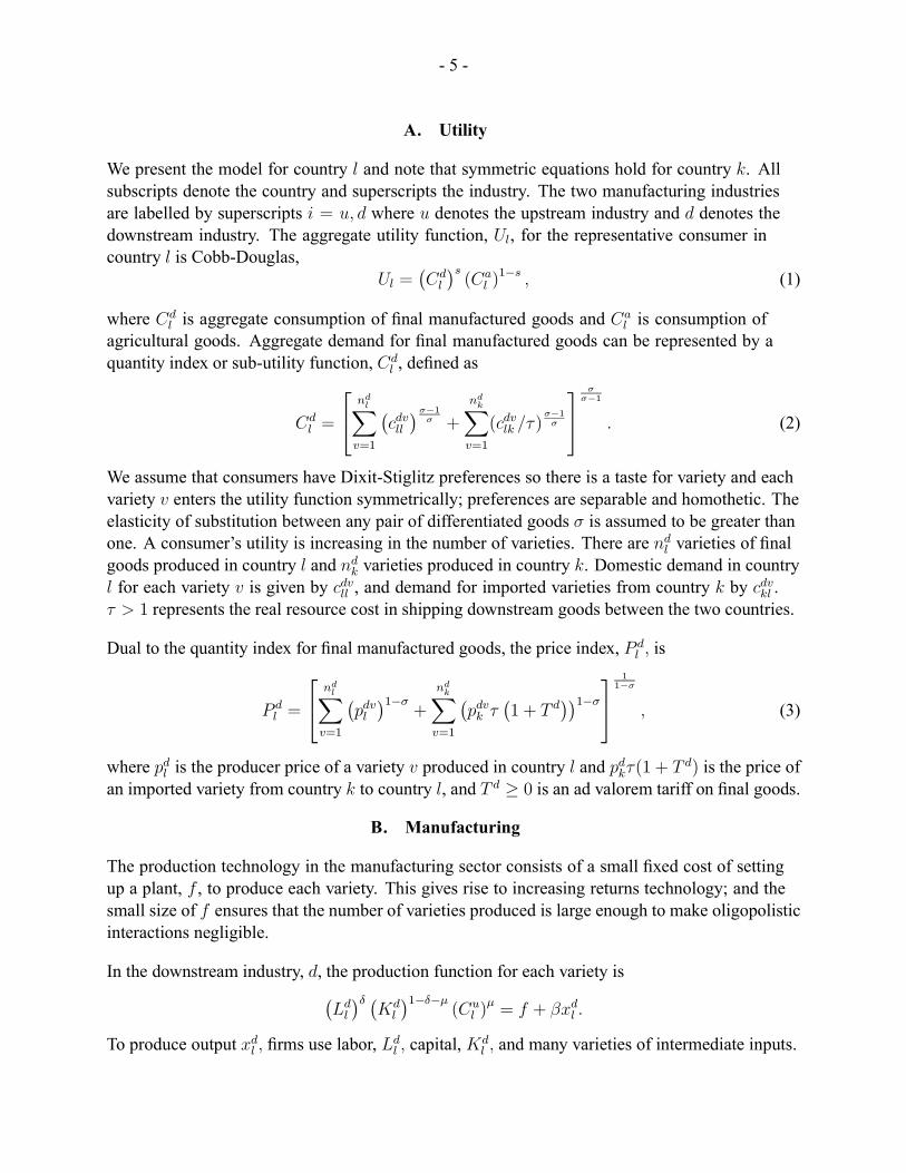
A. Utility

We present the model for country l and note that symmetric equations hold for country k. Allsubscripts denote the country and superscripts the industry. The two manufacturing industriesare labelled by superscripts i = u, d where u denotes the upstream industry and d denotes thedownstream industry. The aggregate utility function, Ul, for the representative consumer incountry l is Cobb-Douglas,

Ul =¡Cdl

¢s(Ca

l )1−s , (1)

where Cdl is aggregate consumption of final manufactured goods and Ca

l is consumption ofagricultural goods. Aggregate demand for final manufactured goods can be represented by aquantity index or sub-utility function, Cd

l , defined as

Cdl =

ndlXv=1

¡cdvll¢σ−1

σ +

ndkXv=1

(cdvlk /τ )σ−1σ

σ

σ−1

. (2)

We assume that consumers have Dixit-Stiglitz preferences so there is a taste for variety and eachvariety v enters the utility function symmetrically; preferences are separable and homothetic. Theelasticity of substitution between any pair of differentiated goods σ is assumed to be greater thanone. A consumer’s utility is increasing in the number of varieties. There are ndl varieties of finalgoods produced in country l and ndk varieties produced in country k. Domestic demand in countryl for each variety v is given by cdvll , and demand for imported varieties from country k by cdvkl .τ > 1 represents the real resource cost in shipping downstream goods between the two countries.

Dual to the quantity index for final manufactured goods, the price index, P dl , is

P dl =

ndlXv=1

¡pdvl¢1−σ

+

ndkXv=1

¡pdvk τ

¡1 + T d

¢¢1−σ1

1−σ

, (3)

where pdl is the producer price of a variety v produced in country l and pdkτ(1 + T d) is the price ofan imported variety from country k to country l, and T d ≥ 0 is an ad valorem tariff on final goods.

B. Manufacturing

The production technology in the manufacturing sector consists of a small fixed cost of settingup a plant, f , to produce each variety. This gives rise to increasing returns technology; and thesmall size of f ensures that the number of varieties produced is large enough to make oligopolisticinteractions negligible.

In the downstream industry, d, the production function for each variety is¡Ldl

¢δ ¡Kd

l

¢1−δ−µ(Cu

l )µ = f + βxdl .

To produce output xdl , firms use labor, Ldl , capital, Kd

l , and many varieties of intermediate inputs.

- 6 -

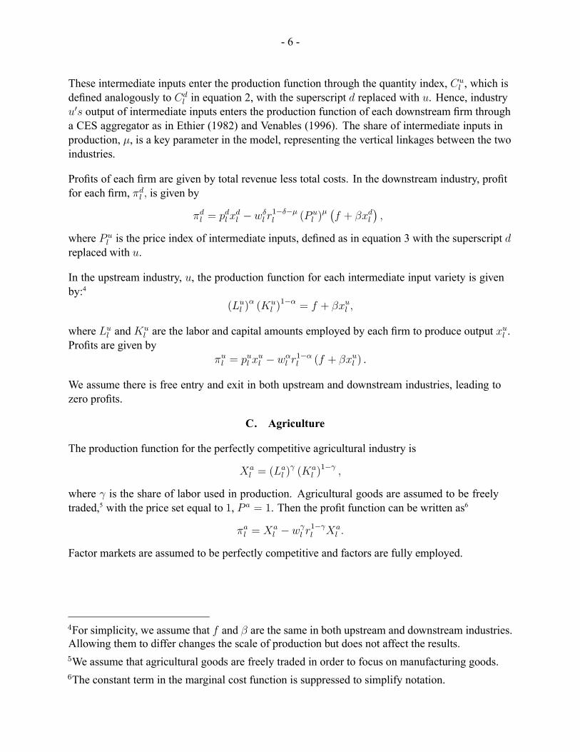
These intermediate inputs enter the production function through the quantity index, Cul , which is

defined analogously to Cdl in equation 2, with the superscript d replaced with u. Hence, industry

u0s output of intermediate inputs enters the production function of each downstream firm througha CES aggregator as in Ethier (1982) and Venables (1996). The share of intermediate inputs inproduction, µ, is a key parameter in the model, representing the vertical linkages between the twoindustries.

Profits of each firm are given by total revenue less total costs. In the downstream industry, profitfor each firm, πdl , is given by

πdl = pdl xdl − wδ

l r1−δ−µl (P u

l )µ ¡f + βxdl

¢,

where P ul is the price index of intermediate inputs, defined as in equation 3 with the superscript d

replaced with u.

In the upstream industry, u, the production function for each intermediate input variety is givenby:4

(Lul )

α (Kul )1−α = f + βxul ,

where Lul andKu

l are the labor and capital amounts employed by each firm to produce output xul .Profits are given by

πul = pul xul − wα

l r1−αl (f + βxul ) .

We assume there is free entry and exit in both upstream and downstream industries, leading tozero profits.

C. Agriculture

The production function for the perfectly competitive agricultural industry is

Xal = (L

al )

γ (Kal )1−γ ,

where γ is the share of labor used in production. Agricultural goods are assumed to be freelytraded,5 with the price set equal to 1, P a = 1. Then the profit function can be written as6

πal = Xal − wγ

l r1−γl Xa

l .

Factor markets are assumed to be perfectly competitive and factors are fully employed.

4For simplicity, we assume that f and β are the same in both upstream and downstream industries.Allowing them to differ changes the scale of production but does not affect the results.5We assume that agricultural goods are freely traded in order to focus on manufacturing goods.6The constant term in the marginal cost function is suppressed to simplify notation.

- 7 -

III. EQUILIBRIUM

We solve for equilibrium in four steps. First, we solve the representative consumer’s utilitymaximization problem to derive the demand for final goods. Second, we solve for each firm’sprofit maximization problem in each industry i to derive producer prices, and downstream firms’demand for intermediate inputs. Using the free entry and exit condition, we derive the numberof units each manufacturing firm must produce to cover fixed cost. Third, we determine productmarket clearing conditions and fourth, solve the factor market clearing conditions.

A. Consumers

The representative consumer’s utility maximizing problem is solved using two-stage budgeting. Instage 1 the consumer allocates expenditure between manufactures and agriculture by maximizingthe utility function, equation 1, subject to the budget constraint, which gives

Cal = (1− s)Yl, (4)

P dl C

dl = sYl. (5)

The budget constraint is given by Yl = wlLl + rlKl +Gl, where Gl = pdkTdcdkln

dk + pukT

ucuklnuk is

the tariff revenue collected in country l, which is assumed to be distributed back to consumers. Instage 2 the consumer maximizes the subutility function, Cd

l (equation 2), subject to the budgetconstraint, sYl in equation 5, to derive demand functions for each variety of manufactured goodproduced in country l and each imported variety produced in country k, respectively:

cdll =¡pdl¢−σ ¡

P dl

¢σ−1sYl, (6)

cdkl = τ1−σ¡1 + T d

¢−σ ¡pdk¢−σ ¡

P dl

¢σ−1sYl. (7)

B. Firms

Now we consider firm behavior in the manufacturing sector and in agriculture.

Manufacturing

In the manufacturing sector, upstream and downstream firms choose a variety and pricing so as tomaximize profits, taking as given the variety choice and pricing strategy of the other firms in theindustry. Each firm will produce a distinct variety since it can always do better by introducinga new product variety than by sharing in the production of an existing type. In the downstreamindustry, each firm maximizes profits with respect to quantity to derive producer prices:

∂πdl∂xdl

= 0 ⇒ pdl = wδl r1−δ−µl (P u

l )µ βσ

σ − 1 .

This gives the usual marginal revenue equals marginal cost condition, with producer price asa constant markup over marginal cost. The producer price, pdl , received by a firm in countryl is the same whether the good is sold domestically or exported; and the tariff-inclusive

- 8 -

price is pdlk = pdl τ¡1 + T d

¢.7 We choose units of measurement so that βσ = σ − 1, then

pdl = wδl r1−δ−µl (P µ

l )µ. A proportion, δ, of downstream industry’s revenue is spent on labor,

1 − δ − µ on capital and µ on intermediate inputs. Hence total expenditure on upstreamintermediate inputs is given by eul = µndl p

dl x

dl . The demand functions for each variety of

intermediate input produced domestically and abroad are analogous to consumers’ demandfunctions for final manufactured goods:

cull = (pul )−σ (P u

l )σ−1 eul , (8)

cukl = τ1−σ (1 + T u)−σ (puk)−σ (P u

l )σ−1 eul . (9)

Similarly, in the upstream industry, each firm maximizes profit with respect to quantity:

∂πul∂xul

= 0 ⇒ pul = wαl r1−αl . (10)

We can derive the number of varieties produced in each industry by imposing the free entry andexit condition, which leads to zero profits. This condition determines the quantity of outputrequired to cover fixed costs. With

πil = 0, xil =f (σ − 1)

β, i = u, d. (11)

Without loss of generality, firm size is scaled so that profits are equal to zero at size 1, by settingf = 1/σ. Note that the equilibrium scale of output is independent of price and the numberof firms. This is a direct consequence of Dixit-Stiglitz preferences and a constant elasticity ofsubstitution. Then the complementary slack condition implies that at least one of the followingequations must hold with equality,

xil ≤ 1, nil ≥ 0, i = u, d. (12)

For example, if output in industry i, xil, is less than one then firms would earn negative profits sothe equilibrium number of firms in that industry, nil, would equal zero.

Agriculture

In the agricultural industry, profit maximization implies price equals marginal cost,

1 = wγl r1−γl . (13)

Recall that agriculture is the numeraire good.

C. Product Markets and Factor Markets

We are now ready to solve for equilibrium in the product and factor markets. Product market

7In a monopolistically competitive model, segmented and integrated market solutions areequivalent.

- 9 -

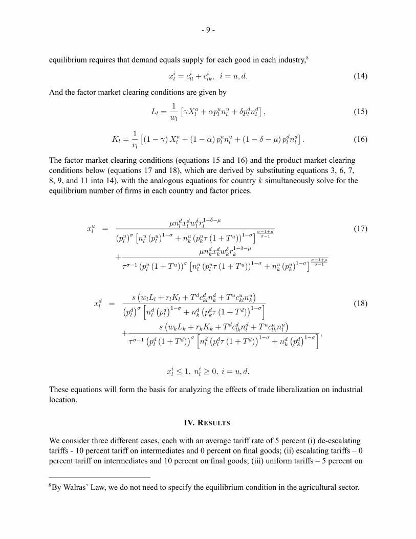
equilibrium requires that demand equals supply for each good in each industry,8

xil = cill + cilk, i = u, d. (14)

And the factor market clearing conditions are given by

Ll =1

wl

£γXa

l + αpul nul + δpdl n

dl

¤, (15)

Kl =1

rl

£(1− γ)Xa

l + (1− α) pul nul + (1− δ − µ) pdl n

dl

¤. (16)

The factor market clearing conditions (equations 15 and 16) and the product market clearingconditions below (equations 17 and 18), which are derived by substituting equations 3, 6, 7,8, 9, and 11 into 14), with the analogous equations for country k simultaneously solve for theequilibrium number of firms in each country and factor prices.

xul =µndl x

dlw

δl r1−δ−µl

(pul )σ £nul (pul )1−σ + nuk (p

ukτ (1 + T u))1−σ

¤σ−1+µσ−1

(17)

+µndkx

dkw

δkr1−δ−µk

τσ−1 (pul (1 + T u))σ£nul (p

ul τ (1 + T u))1−σ + nuk (p

uk)1−σ¤σ−1+µσ−1

xdl =s¡wlLl + rlKl + T dcdkln

dk + T ucukln

uk

¢¡pdl¢σ h

ndl¡pdl¢1−σ

+ ndk¡pdkτ (1 + T d)

¢1−σi (18)

+s¡wkLk + rkKk + T dcdlkn

dl + T uculkn

ul

¢τσ−1

¡pdl (1 + T d)

¢σ hndl¡pdl τ (1 + T d)

¢1−σ+ ndk

¡pdk¢1−σi ,

xil ≤ 1, nil ≥ 0, i = u, d.

These equations will form the basis for analyzing the effects of trade liberalization on industriallocation.

IV. RESULTS

We consider three different cases, each with an average tariff rate of 5 percent (i) de-escalatingtariffs - 10 percent tariff on intermediates and 0 percent on final goods; (ii) escalating tariffs – 0percent tariff on intermediates and 10 percent on final goods; (iii) uniform tariffs – 5 percent on

8By Walras’ Law, we do not need to specify the equilibrium condition in the agricultural sector.

- 10 -

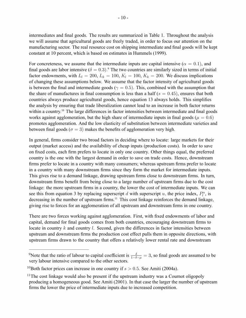
intermediates and final goods. The results are summarized in Table 1. Throughout the analysiswe will assume that agricultural goods are freely traded, in order to focus our attention on themanufacturing sector. The real resource cost on shipping intermediate and final goods will be keptconstant at 10 percent, which is based on estimates in Hummels (1999).

For concreteness, we assume that the intermediate inputs are capital intensive (α = 0.1), andfinal goods are labor intensive (δ = 0.3).9 The two countries are similarly sized in terms of initialfactor endowments, with Ll = 200, Lk = 100, Kl = 100, Kk = 200. We discuss implicationsof changing these assumptions below. We assume that the factor intensity of agricultural goodsis between the final and intermediate goods (γ = 0.5). This, combined with the assumption thatthe share of manufactures in final consumption is less than a half (s = 0.45), ensures that bothcountries always produce agricultural goods, hence equation 13 always holds. This simplifiesthe analysis by ensuring that trade liberalization cannot lead to an increase in both factor returnswithin a country.10 The large differences in factor intensities between intermediate and final goodsworks against agglomeration, but the high share of intermediate inputs in final goods (µ = 0.6)promotes agglomeration. And the low elasticity of substitution between intermediate varieties andbetween final goods (σ = 3) makes the benefits of agglomeration very high.

In general, firms consider two broad factors in deciding where to locate: large markets for theiroutput (market access) and the availability of cheap inputs (production costs). In order to saveon fixed costs, each firm prefers to locate in only one country. Other things equal, the preferredcountry is the one with the largest demand in order to save on trade costs. Hence, downstreamfirms prefer to locate in a country with many consumers; whereas upstream firms prefer to locatein a country with many downstream firms since they form the market for intermediate inputs.This gives rise to a demand linkage, drawing upstream firms close to downstream firms. In turn,downstream firms benefit from being close to a large number of upstream firms due to the costlinkage: the more upstream firms in a country, the lower the cost of intermediate inputs. We cansee this from equation 3 by replacing superscript d with superscript u, the price index, P u

l , isdecreasing in the number of upstream firms.11 This cost linkage reinforces the demand linkage,giving rise to forces for an agglomeration of all upstream and downstream firms in one country.

There are two forces working against agglomeration. First, with fixed endowments of labor andcapital, demand for final goods comes from both countries, encouraging downstream firms tolocate in country k and country l. Second, given the differences in factor intensities betweenupstream and downstream firms the production cost effect pulls them in opposite directions, withupstream firms drawn to the country that offers a relatively lower rental rate and downstream

9Note that the ratio of labour to capital coefficient is δ1−δ−µ = 3, so final goods are assumed to be

very labour intensive compared to the other sectors.10Both factor prices can increase in one country if s > 0.5. See Amiti (2004a).11The cost linkage would also be present if the upstream industry was a Cournot oligopolyproducing a homogeneous good. See Amiti (2001). In that case the larger the number of upstreamfirms the lower the price of intermediate inputs due to increased competition.

- 11 -

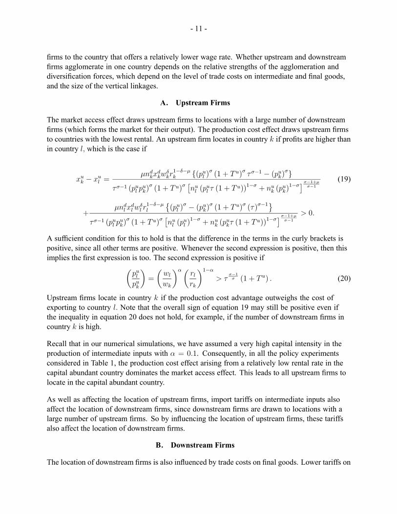
firms to the country that offers a relatively lower wage rate. Whether upstream and downstreamfirms agglomerate in one country depends on the relative strengths of the agglomeration anddiversification forces, which depend on the level of trade costs on intermediate and final goods,and the size of the vertical linkages.

A. Upstream Firms

The market access effect draws upstream firms to locations with a large number of downstreamfirms (which forms the market for their output). The production cost effect draws upstream firmsto countries with the lowest rental. An upstream firm locates in country k if profits are higher thanin country l, which is the case if

xuk − xul =µndkx

dkw

δkr1−δ−µk {(pul )σ (1 + T u)σ τσ−1 − (puk)σ}

τσ−1 (pul puk)

σ (1 + T u)σ£nul (p

ul τ (1 + T u))1−σ + nuk (p

uk)1−σ¤σ−1+µσ−1

(19)

+µndl x

dlw

δl r1−δ−µl

©(pul )

σ − (puk)σ (1 + T u)σ (τ )σ−1ª

τσ−1 (pul puk)

σ (1 + T u)σ£nul (p

ul )1−σ + nuk (p

ukτ (1 + T u))1−σ

¤σ−1+µσ−1

> 0.

A sufficient condition for this to hold is that the difference in the terms in the curly brackets ispositive, since all other terms are positive. Whenever the second expression is positive, then thisimplies the first expression is too. The second expression is positive ifµ

pulpuk

¶=

µwl

wk

¶αµrlrk

¶1−α> τ

σ−1σ (1 + T u) . (20)

Upstream firms locate in country k if the production cost advantage outweighs the cost ofexporting to country l. Note that the overall sign of equation 19 may still be positive even ifthe inequality in equation 20 does not hold, for example, if the number of downstream firms incountry k is high.

Recall that in our numerical simulations, we have assumed a very high capital intensity in theproduction of intermediate inputs with α = 0.1. Consequently, in all the policy experimentsconsidered in Table 1, the production cost effect arising from a relatively low rental rate in thecapital abundant country dominates the market access effect. This leads to all upstream firms tolocate in the capital abundant country.

As well as affecting the location of upstream firms, import tariffs on intermediate inputs alsoaffect the location of downstream firms, since downstream firms are drawn to locations with alarge number of upstream firms. So by influencing the location of upstream firms, these tariffsalso affect the location of downstream firms.

B. Downstream Firms

The location of downstream firms is also influenced by trade costs on final goods. Lower tariffs on

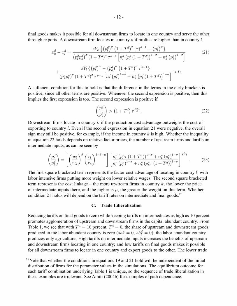
- 12 -

final goods makes it possible for all downstream firms to locate in one country and serve the otherthrough exports. A downstream firm locates in country k if profits are higher than in country l,

xdk − xdl =sYk

©¡pdl¢σ ¡

1 + T d¢σ(τ)σ−1 − ¡pdk¢σª¡

pdl pdk

¢σ(1 + T d)σ τσ−1

hndl¡pdl (1 + T d)

¢1−σ+ ndk

¡pdk¢1−σi (21)

+sYl©¡pdl¢σ − ¡pdk¢σ ¡1 + T d

¢στσ−1

ª(pukp

ul )

σ (1 + T d)σ τσ−1hndl¡pdl¢1−σ

+ ndk¡pdk (1 + T d)

¢1−σi > 0.

A sufficient condition for this to hold is that the difference in the terms in the curly brackets ispositive, since all other terms are positive. Whenever the second expression is positive, then thisimplies the first expression is too. The second expression is positive ifµ

pdlpdk

¶>¡1 + T d

¢τσ−1σ . (22)

Downstream firms locate in country k if the production cost advantage outweighs the cost ofexporting to country l. Even if the second expression in equation 21 were negative, the overallsign may still be positive, for example, if the income in country k is high. Whether the inequalityin equation 22 holds depends on relative factor prices, the number of upstream firms and tariffs onintermediate inputs, as can be seen byµ

pdlpdk

¶=

"µwl

wk

¶δ µrlrk

¶1−δ−µ#"nul (p

ul τ (1 + T u))1−σ + nuk (p

uk)1−σ

nul (pul )1−σ + nuk (p

ukτ (1 + T u))1−σ

# µσ−1

. (23)

The first square bracketed term represents the factor cost advantage of locating in country l, withlabor intensive firms putting more weight on lower relative wages. The second square bracketedterm represents the cost linkage – the more upstream firms in country k, the lower the priceof intermediate inputs there, and the higher is µ, the greater the weight on this term. Whethercondition 21 holds will depend on the tariff rates on intermediate and final goods.12

C. Trade Liberalization

Reducing tariffs on final goods to zero while keeping tariffs on intermediates as high as 10 percentpromotes agglomeration of upstream and downstream firms in the capital abundant country. FromTable 1, we see that with T u = 10 percent, T d = 0, the share of upstream and downstream goodsproduced in the labor abundant country is zero (shul = 0, shdl = 0), the labor abundant countryproduces only agriculture. High tariffs on intermediate inputs increases the benefits of upstreamand downstream firms locating in one country; and low tariffs on final goods makes it possiblefor all downstream firms to locate in one country and export goods to the other. The lower trade

12Note that whether the conditions in equations 19 and 21 hold will be independent of the initialdistribution of firms for the parameter values in the simulations. The equilibrium outcome foreach tariff combination underlying Table 1 is unique, so the sequence of trade liberalization inthese examples are irrelevant. See Amiti (2004b) for examples of path dependence.

- 13 -

costs on final goods reduces the importance of downstream firms locating in country l to be closeto consumers. Even though the lower relative wage rate attracts downstream firms to the laborabundant country, the tariff of 10 percent on intermediates makes it too costly for downstreamfirms to locate in the low wage country and import intermediates.

In contrast, escalating tariffs works against agglomeration. With T u = 0, T d = 10 percent, allintermediate inputs are still produced in the capital abundant country but now the labor abundantcountry produces 44 percent of final goods. Low trade costs on intermediates means that thelower relative wage cost in the labor abundant country draws downstream firms there and the hightariff on final goods increases the importance of downstream firms locating in both countries closeto consumers. As more downstream firms locate in the labor abundant country they bid up therelative wage rate until it no longer becomes profitable for any more downstream firms to locatethere.

Interestingly, both countries are better off with the de-escalating tariffs that results inagglomeration than with escalating tariffs. The utility in the capital abundant country isUk = 1003.8 with de-escalating tariffs compared with Uk = 975.9 with escalating tariffs.Surprisingly, the labor abundant country is also better off with the agglomeration in the capitalabundant country rather than producing 44 percent of final goods. Its utility with de-escalatingtariffs is Ul = 931.6 compared with Ul = 923.7 with escalating tariffs. The basic intuition is thatthe labor abundant country also shares in the benefits of agglomeration through lower prices offinal goods. The benefits are so high in this example because the share of intermediate input ishigh at µ = 0.6 and the elasticity of substitution is low at σ = 3. The low elasticity of substitutionmakes varieties very imperfect substitutes. So the the benefit of differentiated varieties in theproduction of final goods is very high (see equation 3 with the subscript d replaced with u). Alower elasticity of substitution would reduce the benefits of agglomeration.

With uniform tariff rates at 5 percent, the labor abundant country produces 17 percent of finalgoods. Given that the capital abundant country produces 83 percent of final goods under uniformtariffs there are still some gains from agglomeration so the utility with uniform tariffs is higher inboth countries compared with escalating tariffs, but not as high as with de-escalating tariffs wherethe full benefits of agglomeration are gained. So in our example, the worst case scenario is that ofescalating tariffs.

Reducing tariffs to zero on both intermediate inputs and final goods does not result in completespecialization based on comparative advantage since there is still a 10 percent real resourcecost in shipping intermediates and final goods. At zero tariff rates, the labor abundant countryproduces 41 percent of final goods and achieves the highest utility, however zero tariff rateslead to lower utility in the capital abundant country compared with de-escalating tariffs thatresults in agglomeration. In this example, aggregate world welfare is highest with agglomeration.Lower shipping costs, τ , could change this result. Recall that we maintained τ = 10 percent onintermediates and final goods to highlight that these costs would still exist even when tariffs havesuccessfully been reduced to zero. Positive shipping costs could prevent complete specializationbased on comparative advantage and differential shipping rates on intermediates and final goods

- 14 -

can lead to different patterns of industrial location.

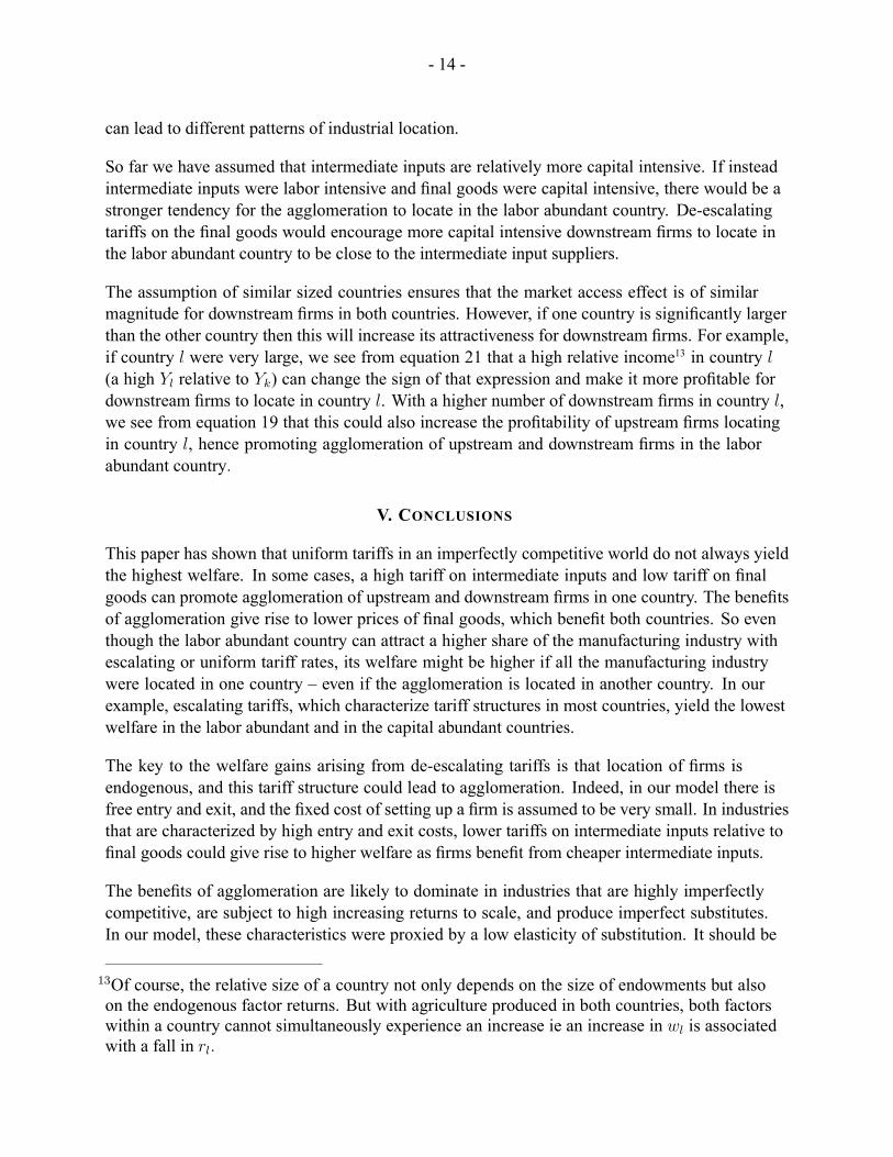
So far we have assumed that intermediate inputs are relatively more capital intensive. If insteadintermediate inputs were labor intensive and final goods were capital intensive, there would be astronger tendency for the agglomeration to locate in the labor abundant country. De-escalatingtariffs on the final goods would encourage more capital intensive downstream firms to locate inthe labor abundant country to be close to the intermediate input suppliers.

The assumption of similar sized countries ensures that the market access effect is of similarmagnitude for downstream firms in both countries. However, if one country is significantly largerthan the other country then this will increase its attractiveness for downstream firms. For example,if country l were very large, we see from equation 21 that a high relative income13 in country l(a high Yl relative to Yk) can change the sign of that expression and make it more profitable fordownstream firms to locate in country l. With a higher number of downstream firms in country l,we see from equation 19 that this could also increase the profitability of upstream firms locatingin country l, hence promoting agglomeration of upstream and downstream firms in the laborabundant country.

V. CONCLUSIONS

This paper has shown that uniform tariffs in an imperfectly competitive world do not always yieldthe highest welfare. In some cases, a high tariff on intermediate inputs and low tariff on finalgoods can promote agglomeration of upstream and downstream firms in one country. The benefitsof agglomeration give rise to lower prices of final goods, which benefit both countries. So eventhough the labor abundant country can attract a higher share of the manufacturing industry withescalating or uniform tariff rates, its welfare might be higher if all the manufacturing industrywere located in one country – even if the agglomeration is located in another country. In ourexample, escalating tariffs, which characterize tariff structures in most countries, yield the lowestwelfare in the labor abundant and in the capital abundant countries.

The key to the welfare gains arising from de-escalating tariffs is that location of firms isendogenous, and this tariff structure could lead to agglomeration. Indeed, in our model there isfree entry and exit, and the fixed cost of setting up a firm is assumed to be very small. In industriesthat are characterized by high entry and exit costs, lower tariffs on intermediate inputs relative tofinal goods could give rise to higher welfare as firms benefit from cheaper intermediate inputs.

The benefits of agglomeration are likely to dominate in industries that are highly imperfectlycompetitive, are subject to high increasing returns to scale, and produce imperfect substitutes.In our model, these characteristics were proxied by a low elasticity of substitution. It should be

13Of course, the relative size of a country not only depends on the size of endowments but alsoon the endogenous factor returns. But with agriculture produced in both countries, both factorswithin a country cannot simultaneously experience an increase ie an increase in wl is associatedwith a fall in rl.

- 15 -

noted that the model presented is highly stylized and abstracts from many other important factors,for example there could be additional benefits of agglomeration, such as learning externalities, butthere could also be costs, such as congestion and pollution. In practice, it is difficult to identifyand properly measure these characteristics. However, further research along these lines could aidthe tariff reform process.

- 16 -

Tabl

e 1:

Res

ults

L

abou

r ab

unda

nt c

ount

ry

uT

d

T

u lsh

d l

shlw

lrw l

U

r lU

lU

0.

10

0.00

0

00.

350.

712.

33

4.66

931.

60

0 0.

10

0 0.

440.

380.

652.

50

4.23

923.

71

0.05

0.

05

0 0.

170.

360.

692.

41

4.47

929.

63

0.00

0.

00

0 0.

410.

380.

662.

51

4.31

931.

82

Cap

ital a

bund

ant c

ount

ry

uT

d

T

u ksh

d k

shkw

krw k

U

r kU

kU

lk

UU

+0.

10

0.00

1

10.

550.

463.

77

3.13

1003

.80

1935

.40

0 0.

10

1 0.

560.

510.

493.

33

3.21

975.

9118

99.6

20.

05

0.05

1

0.83

0.54

0.47

3.60

3.

1498

9.23

1918

.86

0 0.

00

1 0.

590.

510.

493.

37

3.25

987.

4919

19.3

1 N

otes

: Th

e re

al re

sour

ce c

ost, τ,

is se

t at 1

0% in

all

polic

y ex

perim

ents

. Tu –

tarif

f rat

e on

ups

tream

goo

ds (i

nter

med

iate

inpu

ts).

Td – ta

riff r

ate

on d

owns

tream

goo

ds (f

inal

goo

ds).

shlu –

shar

e of

ups

tream

indu

stry

loca

ted

in la

bour

abu

ndan

t cou

ntry

. sh

ld – sh

are

of d

ownt

ream

indu

stry

loca

ted

in la

bour

abu

ndan

t cou

ntry

. w

l, r l

– fa

ctor

pric

es in

labo

ur a

bund

ant c

ount

ry.

Ulw - r

eal r

etur

ns to

wor

kers

in la

bour

abu

ndan

t cou

ntry

. U

lr - rea

l ret

urns

to c

apita

lists

in la

bour

abu

ndan

t cou

ntry

. U

l - a

ggre

gate

util

ity in

the

labo

ur a

bund

ant c

ount

ry.

Ul+

Uk –

agg

rega

te w

orld

util

ity.

All

k su

bscr

ipte

d va

riabl

es re

fer t

o th

e ca

pita

l abu

ndan

t cou

ntry

.

- 17 -

REFERENCES

Amiti, Mary, 2001, "Regional Specialisation and Technological Leapfrogging," Journal ofRegional Science, Vol. 41(February), pp. 149-172.

——,2004a, "Location of Vertically Linked Industries: Agglomeration versus ComparativeAdvantage," European Economic Review, forthcoming.

——, 2004b, "How the Sequence of Trade Liberalization affects Industrial Location,"(unpublished; Washington; International Monetary Fund).

Bertrand, Trent J., and Jaroslav Vanek, 1971, "The Theory of Tariffs, Taxes and Subsidies: SomeAspects of the Second Best," American Economic Review, Vol. 61(October), pp. 925-31.

Buffie, Edward F., 2001, Trade Policy in Developing Countries (Cambridge, England: UniversityPress).

Corden, Max, 1971, The Theory of Protection (Oxford, England: University Press).

Dicken, Peter, 1998, Global Shift: Transforming the World, Third edition (London: Paul Chapmanpublishing).

Dixit, Avinash K. and Gene M. Grossman, 1982, "Trade and Protection with MultistageProduction,". Review of Economic Studies Vol. XLIX (October), pp. 583-94.

Dixit, A.K. and J.E. Stiglitz, 1977, "Monopolistic Competition and Optimum Product Diversity,"American Economic Review, Vol. 67, pp. 297-308.

Ethier, W., 1982, "National and International Returns to Scale in the Modern Theory ofInternational Trade," American Economic Review, Vol. 72, pp. 389-405.

Falvey, Rodney E., 1988, "Tariffs, Quotas and Piecemeal Policy Reform," Journal of InternationalEconomics, Vol. 25, pp. 177-83.

Fujita Masahisa, Paul Krugman and Anthony J. Venables, 1999. The Spatial Economy: Cities,Regions and International TradeMIT Press.

Helpman, Elhanan and Paul R. Krugman. 1989, Trade Policy and Market Structure, The MITPress, pp.138-40.

Hummels, David, 1999, "Toward a Geography of Trade Costs" Purdue University, unpublishedpaper.

Khor, Martin 2001. Third World Network-Africa Secretariat, Vol. 11/12.

Krugman, Paul, 1991, "History versus Expectations," Quarterly Journal of Economics, Vol.106(2), pp. 651-67.

———– and Anthony J. Venables, 1995, "Globalization and the Inequality of Nations," QuarterlyJournal of Economics, Vol. 110(4), pp. 857-80.

Lloyd, Peter J., 1974, "A More General Theory of Price Distortions in Open Economies," Journalof International Economics, Vol. 4, pp. 365-86.

- 18 -

López, Ramón and Arvind Panagariya, 1992, "On the Theory of Piecemeal Tariff Reform: TheCase of Pure Imported Intermediate Inputs," American Economic Review, Vol. 82(3), pp.615-625.

Michaely, Michael, Demetris Papageorgiou, and Armeane Choksi, 1991,.Liberalizing ForeignTrade: Lessons of Experience in the Developing World, Oxord: Blackwell, 1991.

Michalopoulos, Constantine, 1999, "Trade Policy and Market Access Issues for DevelopingCountries: Implications for the Millennium Round," World Bank Working Paper 2214.

Rodrik, Dani and Arvind Panagariya, 1993, "Political Economy Arguments for a Uniform Tariff,"International Economic Review Vol. 34(3), pp. 685-703.

Tarr, David G., 2002, Arguments For and Against Uniform Tariffs, in: Bernard Hoekman, AadityaMattoo and Philip English, eds., Development, Trade, and the WTO, The World Bank,Washington DC.

UNCTAD, 1998, Market Access: Developments since the Uruguay Round, Implications,Opportunities and Challenges.