Embed Size (px)
Citation preview
Aquaplanet Configurations in CESM2
CESM Simpler Models Breakout
Jim Benedict*, Amy Clement, Brian Medeiros*RSMAS, University of Miami
*Visiting Scientist, NCAR (Climate & Global Dynamics)
20 June 2017

J. Benedict // CESM2 Simpler Models – Aquaplanet // June 2017
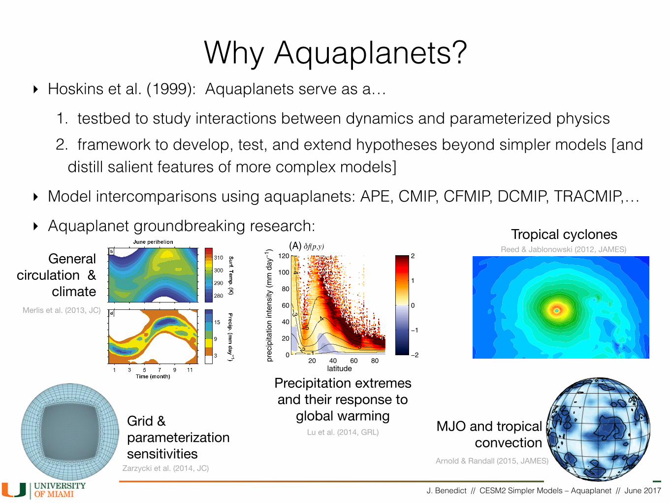
Why Aquaplanets?‣ Hoskins et al. (1999): Aquaplanets serve as a…
1. testbed to study interactions between dynamics and parameterized physics 2. framework to develop, test, and extend hypotheses beyond simpler models [and
distill salient features of more complex models]
‣ Model intercomparisons using aquaplanets: APE, CMIP, CFMIP, DCMIP, TRACMIP,…
‣ Aquaplanet groundbreaking research:
J. Benedict // CESM2 Simpler Models – Aquaplanet // June 2017
Why Aquaplanets?‣ Hoskins et al. (1999): Aquaplanets serve as a…
1. testbed to study interactions between dynamics and parameterized physics 2. framework to develop, test, and extend hypotheses beyond simpler models [and
distill salient features of more complex models]
‣ Model intercomparisons using aquaplanets: APE, CMIP, CFMIP, DCMIP, TRACMIP,…
‣ Aquaplanet groundbreaking research:
Grid & parameterization sensitivities
indicates the fractional increase of precipitation intensity, were it following the Clausius-Clapeyron (CC)relation, would be scaled as
ϵ ≈ LR!1v T!2
0 δT ; (4)
where L is the latent heat of vaporization, Rv is gas constant for water vapor, δT is 3 K for the sstmagexperiments, and T0 is chosen to be the local SST. The corresponding CC slope, α ¼ δp
p =δT , rangesapproximately 7 to 8% per Kelvin warming for the control SST profile (1). The actual stretching factor,however, is estimated together with the shift factor δy by minimizing the fractional variance associated withthe residual term in (3) and turns out to be markedly smaller than the CC rate. Interestingly, the resultant shiftδy turns out to be the same as the shift of zonal mean zonal wind as well as the shift of the PDF of ω500.
Figure 2 shows the result of fitting (3) to the change of the precipitation PDF in response to the sstmagforcing at T340 resolution. The fitted PDF change accounts for 90% of the variance of the total fractionalprecipitation change associated with δf(p, y) poleward of 13° latitude, with 45% contributed from thepoleward shift. Thus, the poleward shift of the subtropical and midlatitude circulation, together with theattendant shift of the transients, account substantially for the increase (decrease) of precipitation at allintensities at the poleward (equatorward) flank of the mean jet/storm track. It should be noted that thethermodynamic pattern (Figure 2d) and the pattern associated with the poleward shift are not orthogonal toeach other and that the former accounts for 80% of total fractional precipitation change variance, withapproximately 25% shared between them. At the poleward flank of the mean jet, the dynamical shift and thethermodynamics work in concert to give rise to three times as frequent the 10!4 extreme events under 3 Kwarming as the control. The best fit for the thermodynamics corresponds to α≈5%/K or a depreciation of theCC rate by 30%. This depreciation rate is consistent with the earlier scaling analysis on the extremes simulated bythe GFDL AM2.1 [Chen et al., 2011] and CMIP3 models [e.g., O’Gorman and Schneider, 2009b]. In the latter, thesub-CC rate of the thermodynamic contribution was attributed to the notion that the extreme precipitation scales
20 40 60 800
20
40
60
80
100
120
latitude
prec
ipita
tion
inte
nsity
(m
m d
ay−1
)
prec
ipita
tion
inte
nsity
(m
m d
ay−1
)pr
ecip
itatio
n in
tens
ity (
mm
day
−1)
−5−5
−4
−4
−3
−3−2−1 −2
−1
0
1
2
20 40 60 800
20
40
60
80
100
120
latitude
−5−5
−4
−4
−3
−3−2−1 −2
−1
0
1
2
20 40 60 800
20
40
60
80
100
120
latitude
prec
ipita
tion
inte
nsity
(m
m d
ay−1
)
−5−5
−4
−4
−3
−3−2−1 −2
−1
0
1
2
latitude
−5−5
−4
−4
−3
−3−2−120 40 60 80
0
20
40
60
80
100
120
−2
−1
0
1
2
(A) (B)
(D) (C)
Figure 2. Fractional change of the probability density function of daily precipitation in response to 3 K SST warming in T340CAM3 simulations. In each panel, the control log10 (PDF) is overlaid as black contours. The color contours are for (a) totalchange, (b) change due to a poleward shift of the 500 hPa ω PDF, (c) the sum of the changes in Figures 2b and 2d, and (d)change due to the increase of moisture inferred from the depreciated CC rate. Both Figures 2b and 2d are derived fromminimizing the error of fitting equation (3) to the simulated PDF changes.
Geophysical Research Letters 10.1002/2014GL059532
LU ET AL. ©2014. American Geophysical Union. All Rights Reserved. 2974
SLD in section 5.2. This reveals the impact of thedynamical core on the simplified simulations, and alsoassesses the convergence-with-resolution characteristics.
The overarching question is whether such simple-physicsexperiments can help shed light on physics-dynamics inter-actions and whether there are similarities to full-physics
Figure 2. Snapshot of the tropical cyclone at day 10 for each dynamical core (FV, SE, EUL and SLD) with fullCAM 5 physics at the highest respective resolution and L30 used for this study (as labeled). (left) Longitude-heightcross section of the wind speed through the center latitude of the vortex as a function of the radius from the vortexcenter. (right) Horizontal cross section of the wind speed at a height of 100 m.
REED AND JABLONOWSKI: TROPICAL CYCLONE TEST CASEM04001 M04001
12 of 25
Precipitation extremes and their response to
global warming
Tropical cyclones
MJO and tropical convection
General circulation &
climateMerlis et al. (2013, JC)
Zarzycki et al. (2014, JC)
Lu et al. (2014, GRL)
Reed & Jablonowski (2012, JAMES)
Arnold & Randall (2015, JAMES)

J. Benedict // CESM2 Simpler Models – Aquaplanet // June 2017
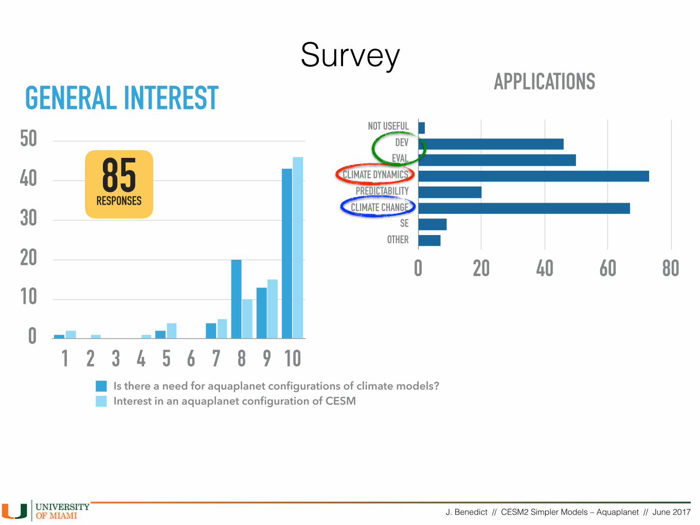
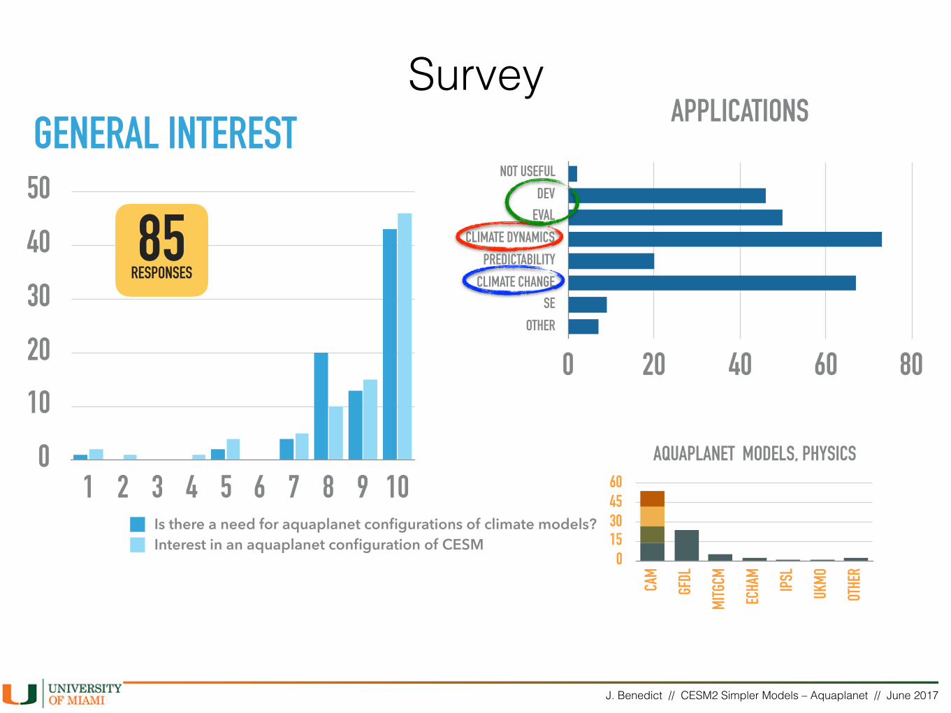
GENERAL INTEREST
0
10
20
30
40
50
1 2 3 4 5 6 7 8 9 10Is there a need for aquaplanet configurations of climate models?Interest in an aquaplanet configuration of CESM
85 RESPONSES
Survey
J. Benedict // CESM2 Simpler Models – Aquaplanet // June 2017
GENERAL INTEREST
0
10
20
30
40
50
1 2 3 4 5 6 7 8 9 10Is there a need for aquaplanet configurations of climate models?Interest in an aquaplanet configuration of CESM
85 RESPONSES
SurveyAPPLICATIONS
NOT USEFUL
DEVEVAL
CLIMATE DYNAMICS
PREDICTABILITY
CLIMATE CHANGESE
OTHER
0 20 40 60 80
J. Benedict // CESM2 Simpler Models – Aquaplanet // June 2017
GENERAL INTEREST
0
10
20
30
40
50
1 2 3 4 5 6 7 8 9 10Is there a need for aquaplanet configurations of climate models?Interest in an aquaplanet configuration of CESM
AQUAPLANET MODELS, PHYSICS
015304560
CAM
GFDL
MITG
CM
ECHA
M
IPSL
UKMO
OTHE
R
85 RESPONSES
SurveyAPPLICATIONS
NOT USEFUL
DEVEVAL
CLIMATE DYNAMICS
PREDICTABILITY
CLIMATE CHANGESE
OTHER
0 20 40 60 80

J. Benedict // CESM2 Simpler Models – Aquaplanet // June 2017
EXPERIENCE WITH CESM AQUAPLANETCESM SCRIPTS
CAM SCRIPTCUSTOM
OTHER
0 15 30
CAM3CAM4CAM5
OTHER
0 15 30
Survey

J. Benedict // CESM2 Simpler Models – Aquaplanet // June 2017
EXPERIENCE WITH CESM AQUAPLANETCESM SCRIPTS
CAM SCRIPTCUSTOM
OTHER
0 15 30
CAM3CAM4CAM5
OTHER
0 15 30
FOR THOSE WHO HAVE NOT RUN CESM AQUAPLANET, WHY?
FAIL
AVAILABILITY
TIME
NO INTEREST
DIFFERENT MODEL
OTHER
0 5 10 15 20
Survey

J. Benedict // CESM2 Simpler Models – Aquaplanet // June 2017
EXPERIENCE WITH CESM AQUAPLANETCESM SCRIPTS
CAM SCRIPTCUSTOM
OTHER
0 15 30
CAM3CAM4CAM5
OTHER
0 15 30
FOR THOSE WHO HAVE NOT RUN CESM AQUAPLANET, WHY?
FAIL
AVAILABILITY
TIME
NO INTEREST
DIFFERENT MODEL
OTHER
0 5 10 15 20
Survey
SHOULD A SLAB OCEAN BE
SUPPORTED?
4%
96%
AOGCM?
42%
58%
Yes
NoNo
Yes

J. Benedict // CESM2 Simpler Models – Aquaplanet // June 2017
EXPERIENCE WITH CESM AQUAPLANETCESM SCRIPTS
CAM SCRIPTCUSTOM
OTHER
0 15 30
CAM3CAM4CAM5
OTHER
0 15 30
FOR THOSE WHO HAVE NOT RUN CESM AQUAPLANET, WHY?
FAIL
AVAILABILITY
TIME
NO INTEREST
DIFFERENT MODEL
OTHER
0 5 10 15 20
SOM W/ICE PREFERENCE
02040
YES/
ON
YES/
OFF NO
OTHE
R(?)
Survey
SHOULD A SLAB OCEAN BE
SUPPORTED?
4%
96%
AOGCM?
42%
58%
Yes
NoNo
Yes

J. Benedict // CESM2 Simpler Models – Aquaplanet // June 2017
CESM2 Aquaplanet: Prescribed SST
Neale & Hoskins(2001, ASL)
Medeiros et al. (2015, CD)

J. Benedict // CESM2 Simpler Models – Aquaplanet // June 2017
CESM2 Aquaplanet: Prescribed SST‣ Newly developed component set (“compset”) for CESM2-aquaplanet
• QPCx: Aquaplanet with prescribed (analytic) SST • QSCx: Slab ocean aquaplanet • “x” corresponds to choice of physics package: 4, 5, or 6
‣ Default (zonally uniform) SST profile for QPCx: QOBS (but can easily be modified)Neale & Hoskins
(2001, ASL)
Medeiros et al. (2015, CD)

J. Benedict // CESM2 Simpler Models – Aquaplanet // June 2017
CESM2 Aquaplanet: Prescribed SST‣ Newly developed component set (“compset”) for CESM2-aquaplanet
• QPCx: Aquaplanet with prescribed (analytic) SST • QSCx: Slab ocean aquaplanet • “x” corresponds to choice of physics package: 4, 5, or 6
‣ Default (zonally uniform) SST profile for QPCx: QOBS (but can easily be modified)
‣ Standard APE orbital parameters (obliquity = eccentricity = 0; diurnal cycle retained), zonally uniform ozone and GHGs
Neale & Hoskins(2001, ASL)
Medeiros et al. (2015, CD)

J. Benedict // CESM2 Simpler Models – Aquaplanet // June 2017
CESM2 Aquaplanet: Prescribed SST‣ Newly developed component set (“compset”) for CESM2-aquaplanet
• QPCx: Aquaplanet with prescribed (analytic) SST • QSCx: Slab ocean aquaplanet • “x” corresponds to choice of physics package: 4, 5, or 6
‣ Default (zonally uniform) SST profile for QPCx: QOBS (but can easily be modified)
‣ Standard APE orbital parameters (obliquity = eccentricity = 0; diurnal cycle retained), zonally uniform ozone and GHGs
‣ No sea ice
‣ Aerosols: only sea salt, all others* removed
Neale & Hoskins(2001, ASL)
Medeiros et al. (2015, CD)
J. Benedict // CESM2 Simpler Models – Aquaplanet // June 2017
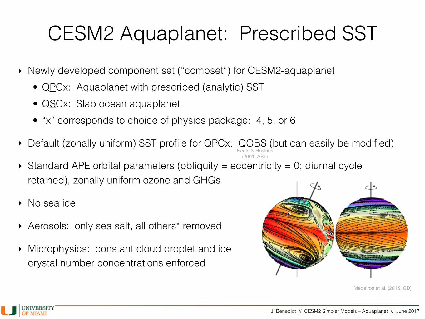
CESM2 Aquaplanet: Prescribed SST‣ Newly developed component set (“compset”) for CESM2-aquaplanet
• QPCx: Aquaplanet with prescribed (analytic) SST • QSCx: Slab ocean aquaplanet • “x” corresponds to choice of physics package: 4, 5, or 6
‣ Default (zonally uniform) SST profile for QPCx: QOBS (but can easily be modified)
‣ Standard APE orbital parameters (obliquity = eccentricity = 0; diurnal cycle retained), zonally uniform ozone and GHGs
‣ No sea ice
‣ Aerosols: only sea salt, all others* removed
‣ Microphysics: constant cloud droplet and ice crystal number concentrations enforced
Neale & Hoskins(2001, ASL)
Medeiros et al. (2015, CD)
J. Benedict // CESM2 Simpler Models – Aquaplanet // June 2017
CESM2 Aquaplanet: Slab Ocean (SOM)

J. Benedict // CESM2 Simpler Models – Aquaplanet // June 2017
CESM2 Aquaplanet: Slab Ocean (SOM)
‣ Newly developed compset for CESM2 SOM aquaplanet: QSCx • “x” corresponds to choice of physics package: 4, 5, or 6

J. Benedict // CESM2 Simpler Models – Aquaplanet // June 2017
CESM2 Aquaplanet: Slab Ocean (SOM)
‣ Newly developed compset for CESM2 SOM aquaplanet: QSCx • “x” corresponds to choice of physics package: 4, 5, or 6
‣ Imposed surface boundary conditions: contained within “forcing” file • Initial SST: QOBS • Implied oceanic heat transport (“q-flux”): Set to zero globally by default, users
must customize (instructions and short NCL script provided… it’s easy!) • Slab depth: 30 m globally
‣ No sea ice
‣ All other settings identical to prescribed-SST aquaplanet
J. Benedict // CESM2 Simpler Models – Aquaplanet // June 2017
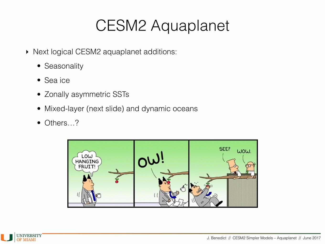
CESM2 Aquaplanet‣ Next logical CESM2 aquaplanet additions:
• Seasonality
• Sea ice
• Zonally asymmetric SSTs
• Mixed-layer (next slide) and dynamic oceans
• Others…?

J. Benedict // CESM2 Simpler Models – Aquaplanet // June 2017
CESM2 “Aquaplanet”: Mixed-layer Ocean
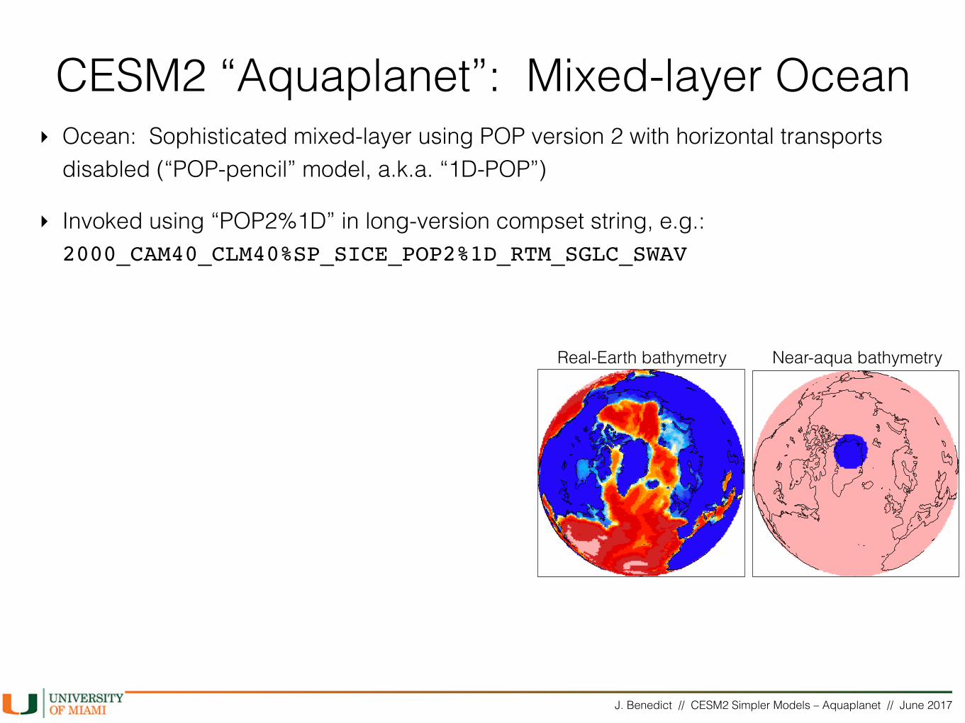
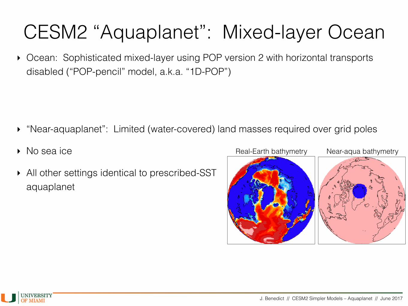
Real-Earth bathymetry Near-aqua bathymetry
J. Benedict // CESM2 Simpler Models – Aquaplanet // June 2017
CESM2 “Aquaplanet”: Mixed-layer Ocean‣ Ocean: Sophisticated mixed-layer using POP version 2 with horizontal transports
disabled (“POP-pencil” model, a.k.a. “1D-POP”)
Real-Earth bathymetry Near-aqua bathymetry
J. Benedict // CESM2 Simpler Models – Aquaplanet // June 2017
CESM2 “Aquaplanet”: Mixed-layer Ocean‣ Ocean: Sophisticated mixed-layer using POP version 2 with horizontal transports
disabled (“POP-pencil” model, a.k.a. “1D-POP”)
‣ Invoked using “POP2%1D” in long-version compset string, e.g.: 2000_CAM40_CLM40%SP_SICE_POP2%1D_RTM_SGLC_SWAV
Real-Earth bathymetry Near-aqua bathymetry

J. Benedict // CESM2 Simpler Models – Aquaplanet // June 2017
CESM2 “Aquaplanet”: Mixed-layer Ocean‣ Ocean: Sophisticated mixed-layer using POP version 2 with horizontal transports
disabled (“POP-pencil” model, a.k.a. “1D-POP”)
‣ Invoked using “POP2%1D” in long-version compset string, e.g.: 2000_CAM40_CLM40%SP_SICE_POP2%1D_RTM_SGLC_SWAV
‣ “Near-aquaplanet”: Limited (water-covered) land masses required over grid poles
‣ No sea ice Real-Earth bathymetry Near-aqua bathymetry
J. Benedict // CESM2 Simpler Models – Aquaplanet // June 2017
CESM2 “Aquaplanet”: Mixed-layer Ocean‣ Ocean: Sophisticated mixed-layer using POP version 2 with horizontal transports
disabled (“POP-pencil” model, a.k.a. “1D-POP”)
‣ Invoked using “POP2%1D” in long-version compset string, e.g.: 2000_CAM40_CLM40%SP_SICE_POP2%1D_RTM_SGLC_SWAV
‣ “Near-aquaplanet”: Limited (water-covered) land masses required over grid poles
‣ No sea ice
‣ All other settings identical to prescribed-SST aquaplanet
Real-Earth bathymetry Near-aqua bathymetry

J. Benedict // CESM2 Simpler Models – Aquaplanet // June 2017
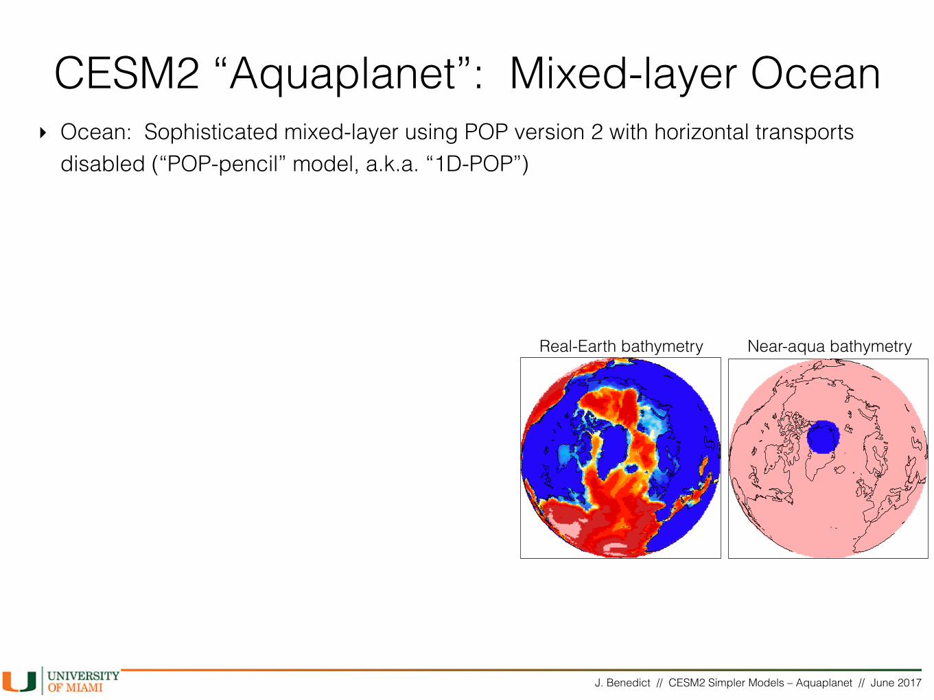
CESM2 “Aquaplanet”: Mixed-layer Ocean‣ Ocean: Sophisticated mixed-layer using POP version 2 with horizontal transports
disabled (“POP-pencil” model, a.k.a. “1D-POP”)
‣ Invoked using “POP2%1D” in long-version compset string, e.g.: 2000_CAM40_CLM40%SP_SICE_POP2%1D_RTM_SGLC_SWAV
‣ “Near-aquaplanet”: Limited (water-covered) land masses required over grid poles
‣ No sea ice
‣ All other settings identical to prescribed-SST aquaplanet
‣ Technical setup of near-aquaplanet version almost completed
Real-Earth bathymetry Near-aqua bathymetry

J. Benedict // CESM2 Simpler Models – Aquaplanet // June 2017
CESM2 “Aquaplanet”: Mixed-layer Ocean‣ Ocean: Sophisticated mixed-layer using POP version 2 with horizontal transports
disabled (“POP-pencil” model, a.k.a. “1D-POP”)
‣ Invoked using “POP2%1D” in long-version compset string, e.g.: 2000_CAM40_CLM40%SP_SICE_POP2%1D_RTM_SGLC_SWAV
‣ “Near-aquaplanet”: Limited (water-covered) land masses required over grid poles
‣ No sea ice
‣ All other settings identical to prescribed-SST aquaplanet
‣ Technical setup of near-aquaplanet version almost completed
‣ Remaining tasks… near-aquaplanet specific:
• Ocean initialization
• Implied oceanic transports (“G terms”)
Real-Earth bathymetry Near-aqua bathymetry

J. Benedict // CESM2 Simpler Models – Aquaplanet // June 2017
CESM2 “Aquaplanet”: Mixed-layer Ocean‣ Ocean: Sophisticated mixed-layer using POP version 2 with horizontal transports
disabled (“POP-pencil” model, a.k.a. “1D-POP”)
‣ Invoked using “POP2%1D” in long-version compset string, e.g.:2000_CAM40_CLM40%SP_SICE_POP2%1D_RTM_SGLC_SWAV
‣ “Near-aquaplanet”: Limited (water-covered) land masses required over grid poles
‣ No sea ice
‣ All other settings identical to prescribed-SSTaquaplanet
‣ Technical setup of near-aquaplanet versionalmost completed
‣ Remaining tasks… near-aquaplanet specific:
• Ocean initialization
• Implied oceanic transports (“G terms”)
Real-Earth bathymetry Near-aqua bathymetry