Embed Size (px)
Citation preview
Tel-Aviv University
The Raymond and Beverly Sackler Faculty of Exact Sciences
School of Mathematical Sciences
Approximation Algorithms
for NP-Hard Problems in
Combinatorial Optimization
Thesis Submitted for the Degree of
“Doctor of Philosophy”
by
Danny Segev
Under the Supervision of Professor Refael Hassin
Submitted to the Senate of Tel-Aviv University
September 2007
Thesis Prepared Under the Supervision of
Professor Refael Hassin
ii
Acknowledgements
First and foremost, I would like to thank my advisor, Prof. Refael Hassin, who has provideda never-ending stream of knowledge and motivation throughout my graduate studies. His eye-opening insight into problem-solving techniques and amazing ability to predict which researchdirections will ultimately be fruitful made each of our meetings an incomparable learning expe-rience. It is also a pleasure to thank Prof. Arie Tamir for many invaluable discussions. I havetremendously benefited from his expertise in numerous mathematical fields.
I would also like to thank my other coauthors, for suggesting interesting problems to inves-tigate, for coming up with new algorithmic approaches, and for not throwing heavy objects inmy general direction whenever the need arises. More specifically, I was privileged to collaboratewith Prof. Chandra Chekuri, Dr. Guy Even, Danny Feldman, Prof. Amos Fiat, Iftah Gamzu,Prof. Anupam Gupta, Prof. Jochen Konemann, Dr. Asaf Levin, Dr. Jerome Monnot, Prof. OjasParekh, Gil Segev, and Prof. Micha Sharir.
Last but not least, I am indebted to my fellow graduate students for their friendship, sup-port, and stimulating conversations. Admitting in advance that some names may have beenmistakenly forgotten, the list includes Amitai Armon, Dr. Adi Avidor, Yaron Azrieli, Dr. AmirBeck, Dr. Nili Beck, Amir Epstein, Dr. Ronny Hadani, Dr. Nir Halman, Danny Hefetz, NiritKlunover, Meital Levy, Tom Meyerovitch, Dr. Einat Or, Dr. Yossi Richter, Dr. Liam Roditty,Dr. Shlomi Rubinstein, Oded Schwartz, Dr. Eran Shmaya, Prof. Amit Singer, Roee Teper, andDanny Vilenchik.
iii
iv
Abstract
This thesis broadly focuses on the design and analysis of algorithmic tools leading to approxi-mation algorithms with provably good performance guarantees. We were especially interestedin problems that have highly practical importance yet possess a fundamental structure, suchas integer covering, network design, graph partitioning, and discrete location problems. In par-ticular, our main contributions revolve around algorithmic ideas and proof methods that arebased on mathematical programming, polyhedral combinatorics, duality, and randomization.The highlights of this work can be briefly described as follows:
1. We devise the first polylogarithmic approximation for the generalized connectivity problem.
2. We present the first non-trivial approximation for the k-Steiner forest problem.
3. We propose the first non-trivial approximation for the k-generalized connectivity problem.
4. We improve on the currently best approximation for directed Steiner network.
5. We present a unified framework for approximating partial covering problems, and demon-strate the applicability of our method in diverse settings.
v
vi
Contents
Acknowledgements iii
Abstract v
1 Introduction 1
2 Generalized Connectivity 112.1 Technical Overview . . . . . . . . . . . . . . . . . . . . . . . . . . . . . . . . . . . 112.2 A Polylogarithmic Approximation for Generalized Connectivity . . . . . . . . . . 12
2.2.1 Preliminaries . . . . . . . . . . . . . . . . . . . . . . . . . . . . . . . . . . 122.2.2 Approximating the density version . . . . . . . . . . . . . . . . . . . . . . 132.2.3 Integrality gap . . . . . . . . . . . . . . . . . . . . . . . . . . . . . . . . . 15
2.3 An O(k1/2+ε) Approximation for Directed Steiner Network . . . . . . . . . . . . 162.3.1 A lower bound for bunches . . . . . . . . . . . . . . . . . . . . . . . . . . 172.3.2 Junction trees and their density . . . . . . . . . . . . . . . . . . . . . . . . 182.3.3 Finding low-density junctions trees . . . . . . . . . . . . . . . . . . . . . . 20
2.4 A Polylogarithmic Approximation for Set Connector . . . . . . . . . . . . . . . . 23
3 k-Steiner Forest 253.1 Technical Overview . . . . . . . . . . . . . . . . . . . . . . . . . . . . . . . . . . . 253.2 A Bicriteria Prize-Collecting Algorithm . . . . . . . . . . . . . . . . . . . . . . . 27
3.2.1 Constructing dense trees with small costs . . . . . . . . . . . . . . . . . . 273.2.2 A greedy prize-collecting approach . . . . . . . . . . . . . . . . . . . . . . 30
3.3 The k-Steiner Forest Algorithm . . . . . . . . . . . . . . . . . . . . . . . . . . . . 323.3.1 An integer program and its Lagrangian relaxation . . . . . . . . . . . . . 323.3.2 Setting up the prize-collecting solutions . . . . . . . . . . . . . . . . . . . 333.3.3 Assembling an approximate integral solution . . . . . . . . . . . . . . . . 35
3.4 Proof of Theorem 3.3: The√
d-Dependent Bound . . . . . . . . . . . . . . . . . . 373.5 Concluding Remarks . . . . . . . . . . . . . . . . . . . . . . . . . . . . . . . . . . 38
4 k-Generalized Connectivity 414.1 Results and Technical Highlights . . . . . . . . . . . . . . . . . . . . . . . . . . . 414.2 The k-Generalized Connectivity Algorithm . . . . . . . . . . . . . . . . . . . . . 43
4.2.1 Preprocessing . . . . . . . . . . . . . . . . . . . . . . . . . . . . . . . . . . 44
vii
4.2.2 Component-wise embedding . . . . . . . . . . . . . . . . . . . . . . . . . . 444.2.3 The main procedure . . . . . . . . . . . . . . . . . . . . . . . . . . . . . . 45
4.3 Proof of the Subtree Augmentation Theorem . . . . . . . . . . . . . . . . . . . . 474.3.1 Scenario I: |A1| ≥ k/(3α log n) . . . . . . . . . . . . . . . . . . . . . . . . 484.3.2 Scenario II: |B0| > ψ(n) . . . . . . . . . . . . . . . . . . . . . . . . . . . . 494.3.3 Scenario III: |A1| < k/(3α log n) and |B0| ≤ ψ(n) . . . . . . . . . . . . . . 50
4.4 Approximate k-Group Steiner Trees . . . . . . . . . . . . . . . . . . . . . . . . . 504.5 Concluding Remarks . . . . . . . . . . . . . . . . . . . . . . . . . . . . . . . . . . 54
5 A Unified Approach to Approximating Partial Covering Problems 555.1 The Suggested Method . . . . . . . . . . . . . . . . . . . . . . . . . . . . . . . . . 55
5.1.1 Technical overview . . . . . . . . . . . . . . . . . . . . . . . . . . . . . . . 555.1.2 Designing LMP algorithms . . . . . . . . . . . . . . . . . . . . . . . . . . 56
5.2 The Generalized Partial Cover Algorithm . . . . . . . . . . . . . . . . . . . . . . 565.2.1 Preliminaries . . . . . . . . . . . . . . . . . . . . . . . . . . . . . . . . . . 565.2.2 Obtaining S1 and S2 . . . . . . . . . . . . . . . . . . . . . . . . . . . . . . 575.2.3 Composing an additional solution . . . . . . . . . . . . . . . . . . . . . . . 595.2.4 Deriving the approximation factor . . . . . . . . . . . . . . . . . . . . . . 60
5.3 Applications . . . . . . . . . . . . . . . . . . . . . . . . . . . . . . . . . . . . . . . 615.3.1 Set cover, in terms of ∆ . . . . . . . . . . . . . . . . . . . . . . . . . . . . 615.3.2 Set cover, in terms of f . . . . . . . . . . . . . . . . . . . . . . . . . . . . 625.3.3 Laminar cover . . . . . . . . . . . . . . . . . . . . . . . . . . . . . . . . . 625.3.4 Totally unimodular cover and k-interval cover . . . . . . . . . . . . . . . . 625.3.5 Edge cover . . . . . . . . . . . . . . . . . . . . . . . . . . . . . . . . . . . 635.3.6 Multicut . . . . . . . . . . . . . . . . . . . . . . . . . . . . . . . . . . . . . 64
5.4 Prize-Collecting Algorithms . . . . . . . . . . . . . . . . . . . . . . . . . . . . . . 645.4.1 Every weighted set system is in IH(∆) . . . . . . . . . . . . . . . . . . . . 645.4.2 Every weighted set system is in If . . . . . . . . . . . . . . . . . . . . . . 665.4.3 Laminar cover . . . . . . . . . . . . . . . . . . . . . . . . . . . . . . . . . 675.4.4 k-interval cover . . . . . . . . . . . . . . . . . . . . . . . . . . . . . . . . . 69
5.5 Concluding Remarks . . . . . . . . . . . . . . . . . . . . . . . . . . . . . . . . . . 70
6 Path Hitting in Acyclic Graphs 716.1 Results and Techniques . . . . . . . . . . . . . . . . . . . . . . . . . . . . . . . . 716.2 Path Hitting in Trees . . . . . . . . . . . . . . . . . . . . . . . . . . . . . . . . . . 72
6.2.1 A linear program and its dual . . . . . . . . . . . . . . . . . . . . . . . . . 726.2.2 An exact algorithm for descending paths . . . . . . . . . . . . . . . . . . . 736.2.3 An algorithm for arbitrary paths . . . . . . . . . . . . . . . . . . . . . . . 75
6.3 Edge Cover with Assignment . . . . . . . . . . . . . . . . . . . . . . . . . . . . . 766.3.1 A reduction to edge cover . . . . . . . . . . . . . . . . . . . . . . . . . . . 766.3.2 An LP-relaxation . . . . . . . . . . . . . . . . . . . . . . . . . . . . . . . . 77
6.4 Path Hitting in Spiders . . . . . . . . . . . . . . . . . . . . . . . . . . . . . . . . 796.4.1 Notation . . . . . . . . . . . . . . . . . . . . . . . . . . . . . . . . . . . . . 79
viii
6.4.2 A reformulation of descending demand paths . . . . . . . . . . . . . . . . 806.4.3 An algorithm for arbitrary paths . . . . . . . . . . . . . . . . . . . . . . . 816.4.4 Analysis . . . . . . . . . . . . . . . . . . . . . . . . . . . . . . . . . . . . . 826.4.5 An improved analysis for stars . . . . . . . . . . . . . . . . . . . . . . . . 87
7 Robust Subgraphs for Trees and Paths 897.1 Results and Techniques . . . . . . . . . . . . . . . . . . . . . . . . . . . . . . . . 897.2 α-Path-Robust Subgraphs . . . . . . . . . . . . . . . . . . . . . . . . . . . . . . . 917.3 α-Tree-Robust Subgraphs . . . . . . . . . . . . . . . . . . . . . . . . . . . . . . . 93
7.3.1 Tree decomposition schemes . . . . . . . . . . . . . . . . . . . . . . . . . . 937.3.2 A bound on the size of a minimum α-tree-robust subgraph . . . . . . . . 96
7.4 Polynomial-Time Algorithms . . . . . . . . . . . . . . . . . . . . . . . . . . . . . 987.4.1 An algorithm for 0.353-path-robust path . . . . . . . . . . . . . . . . . . . 987.4.2 An algorithm for 1/2-tree-robust tree . . . . . . . . . . . . . . . . . . . . 1007.4.3 An algorithm for 1/2-tree-robust subgraph . . . . . . . . . . . . . . . . . 103
7.5 Additional Proofs . . . . . . . . . . . . . . . . . . . . . . . . . . . . . . . . . . . . 1057.5.1 Proof of Lemma 7.5 . . . . . . . . . . . . . . . . . . . . . . . . . . . . . . 1057.5.2 Proof of Lemma 7.17 . . . . . . . . . . . . . . . . . . . . . . . . . . . . . . 106
Bibliography 108
ix
x
Chapter 1
Introduction
Traditionally, mathematical study in combinatorial analysis was concerned with existence andenumeration problems involving discrete objects. However, in the last few decades there hasbeen a growing interest in the field of combinatorial optimization, in which we aim at findingan optimal solution under some predetermined objective function. Unfortunately, the theoryof computational complexity, that deals with the resources required during computation, per-ceives many discrete optimization settings as unlikely to admit polynomial-time algorithms.Nevertheless, by relaxing the strict requirement to efficiently identify an optimal solution forevery instance, it may still be possible to design fairly good algorithms. A well-established ap-proach of this nature is to devise approximation algorithms, which are polynomial-time heuris-tics guaranteed to construct slightly sub-optimal solutions for all instances of the problem underconsideration.
This thesis broadly focuses on the design and analysis of algorithmic tools leading to approx-imation algorithms with provably good performance guarantees. We were especially interestedin problems that have highly practical importance yet possess a fundamental structure, suchas integer covering, network design, graph partitioning, and discrete location problems. In par-ticular, our main contributions revolve around algorithmic ideas and proof methods that arebased on mathematical programming, polyhedral combinatorics, duality, and randomization.The remainder of this chapter provides a succinct overview of these findings, along with a briefdescription of related work.
Generalized Connectivity and its Applications (Chapters 2-4)
Network design problems have received a great deal of attention in the computer science andoperations research communities, as they play an instrumental role in combinatorial optimiza-tion and algorithm engineering. While most computational tasks in this increasingly-popularresearch field are directly motivated by practical scenarios, only a handful of these real-lifemodels have also been established as useful tools in developing new algorithmic techniques orin understanding the limits of tractability. Our first and foremost objective is to single out awell-hidden problem of the latter nature, and to demonstrate some of its unexpected applica-tions.
1
2 Chapter 1: Introduction
An instance of the generalized connectivity problem consists of an undirected graph G =(V, E), whose edges are coupled with non-negative costs specified by a real-valued functionc : E → R+. An additional ingredient of the input is a collection D = (S1, T1), . . . , (Sd, Td)of distinct demands, each of which comprises a pair of disjoint vertex sets. Following well-established network design models, we say that a subgraph H ⊆ G connects a demand (Si, Ti)when it contains a path with one endpoint in Si and another in Ti. The objective is to identifya minimum cost subgraph that connects all demands in D. Similarly, in the k-generalizedconnectivity problem, given an integer parameter k, rather than asking to link each and every(Si, Ti) ∈ D, we are interested in connecting at least k demands. It is important to note thatthere is no loss of generality in restricting feasible solutions to be forests, rather than allowingmore intricate configurations, as any inclusion-wise minimal solution to the problem underconsideration is necessarily acyclic.
Alon, Awerbuch, Azar, Buchbinder and Naor [2] seem to have been the first to introduce thegeneralized connectivity paradigm, as a unified machinery for blending multiple-choice decisionsinto network formation settings. In spite of appearance, the prevailing algorithmic challenge isto determine for each demand which vertex pair should be connected; once these representa-tives are singled out, the computational task becomes that of assembling an appropriate Steinerforest, for which constant-factor approximations are known [1, 62]. Alon et al. demonstratedthat generalized connectivity captures a diverse collection of extensively-studied optimizationproblems, such as set cover, non-metric facility location, tree multicast, and group Steiner tree.However, their main contribution in this context was to devise a multiplicative-update onlinealgorithm for computing log-competitive fractional solutions, and to propose provably-goodrounding procedures for the above-mentioned special cases by exercising problem-specific ar-guments. Nevertheless, approximating the generalized connectivity problem in its unconfinedform, where one makes no structural assumptions about the underlying graph and collection ofdemands, has remained a foundational research objective.
Having already encountered a formidable obstruction in the journey to constructing near-optimal solutions, we proceed by arguing that k-generalized connectivity poses an intrinsicdilemma, that of deciding upon the particular subset of demands to be connected, which mayvery well be significantly harder to deal with. For this purpose, we note that even the seeminglymanageable setting of singleton demands1 corresponds to the k-Steiner forest problem. Haji-aghayi and Jain [68] have recently related the inapproximability of k-Steiner forest to that ofdense k-subgraph, in which given an undirected graph we wish to identify a subset of k verticeswhose induced subgraph has a maximum number of edges. Specifically, this relation states thata polynomial-time α(n)-approximation for k-Steiner forest can be employed as a subroutineto efficiently find a k-vertex subgraph whose density is Ω(α−2(n)) times that of an optimalsolution. We remark that the currently best approximation guarantee for the dense k-subgraphproblem is O(n−δ), for some universal constant δ < 1/3, due to Feige, Kortsarz and Peleg [45];this long-standing bound will be immediately improved as a consequence of achieving an o(nδ/2)factor for k-Steiner forest. Hajiaghayi and Jain [68] did not provide any algorithmic result forthe latter, and posed this objective as an important open problem for future research.
1That is, |Si| = |Ti| = 1 for every 1 ≤ i ≤ d.
3
New results
1. We present the first polylogarithmic approximation for generalized connectivity, attaininga performance guarantee of O(log2 n log2 d). We also prove that the cut-covering relaxationof this problem has an O(log3 n log2 d) integrality gap. The finer details of our approachare provided in Chapter 2.
2. We devise the first non-trivial approximation for the k-Steiner forest problem, which isbased on a novel extension of the Lagrangian relaxation technique. Our main findingis a polynomial-time algorithm that approximates k-Steiner forest to within a factor ofO(minn2/3,
√d · log d). This result appears in Chapter 3.
3. We propose the first non-trivial approximation for the k-generalized connectivity problem,which is derived via a novel synthesis of techniques originating in probabilistic embeddingsof finite metrics, network design, and randomization. More specifically, we present apolynomial-time Monte Carlo algorithm that approximates k-generalized connectivity towithin a factor of O(n2/3 · polylog(n, k)). The specifics of this algorithm are formallydescribed in Chapter 4.
Application 1: Directed Steiner network
An instance of the directed Steiner network problem consists of an arc-weighted directed graphG = (V,E) and a collection of distinct source-sink pairs, to which we refer as (s1, t1), . . . , (sk, tk).The objective is to construct a minimum weight subgraph that connects all input pairs, where(si, ti) is said to be connected by F ⊆ G when the latter contains an si-ti path.
It is worth noting that, in undirected graphs, the computational task of connecting mul-tiple source-sink pairs has been explored and exploited. In particular, Agrawal, Klein andRavi [1] devised the currently best approximation algorithm, achieving a performance guaran-tee of 2(1−1/k), which was extended to a broader class of network design problems by Goemansand Williamson [62, 63]. Nevertheless, it comes as no surprise that directed graphs make theproblem significantly harder to deal with; more specifically, Dodis and Khanna [38] proved thatdirected Steiner network cannot be approximated to within a factor of O(2log1−ε n) for any fixedε > 0, unless NP ⊆ TIME(npolylog(n)). In terms of upper bounds, Charikar et al. [25] proposedthe currently best approximation algorithm, which was rigorously shown to construct feasi-ble subgraphs whose cost is O(k2/3) times that of an optimal solution. However, their paperconcludes by posing two fundamental objectives as open problems for future research:
1. Can one improve on the performance guarantee of O(k2/3)?
2. Can one determine whether the suggested analysis is indeed tight? Up until now, theworst known example provided a lower bound of Ω(
√k).
In Section 2.3, we present a polynomial-time algorithm that approximates directed Steinernetwork to within a factor of O(k1/2+ε), for any fixed ε > 0. We also prove a lower boundof Ω(k2/3/ log k) on the approximation ratio achieved by the algorithm of Charikar et al. [25],thereby showing that their analysis is essentially tight.
4 Chapter 1: Introduction
Application 2: Set connector
In an attempt to simplify the upcoming discussion, we begin by introducing a number of essentialdefinitions. Given an undirected graph G = (V, E), a division is a family V = X1, . . . , Xh ofpairwise-disjoint vertex subsets. For a set of edges F ⊆ E, let F/V be the multigraph obtainedfrom (V, F ) by coalescing each subset Xi ∈ V into a single vertex (henceforth, V-terminal).Finally, we say that F ⊆ E weakly connects V if all V-terminals reside in the same connectedcomponent of F/V.
In the set connector problem, we are given an edge-weighted graph G = (V, E) and acollection V1, . . . ,Vm of distinct divisions. The objective is to detect a minimum weight edgeset F ⊆ E that simultaneously weakly connects all input divisions. Needless to say, generalizedconnectivity can be viewed as a special case of set connector, in which each division consistsof two disjoint vertex sets. On the other hand, it is important to mention that the seeminglyobvious reduction in the opposite direction, where each division Vi = X1, . . . , Xh is replacedby a collection of demands (Xr, Xs) : 1 ≤ r < s ≤ h, is incorrect.
The set connector problem has recently been investigated by Fukunaga and Nagamochi [52],whose main contribution was a fractional packing theorem, leading to an approximation guar-antee of 2(α− 1) via LP-rounding methods, where α = maxi(
∑X∈Vi
|X|). However, this resultdoes not ensure a reasonable upper bound for all possible instances, as α may very well be Ω(n);to our knowledge, a non-trivial approximation has not been suggested yet.
In Section 2.4, we present the first polylogarithmic approximation for set connector, showingthat a performance guarantee of O(log3 n log2(mn)) can be achieved in polynomial time.
Related work
We proceed by demonstrating that generalized connectivity emerges from two of the mostfundamental problems in combinatorial optimization, namely, those of computing Steiner forestsand group Steiner trees. Noting that these problems have received a great deal of attentionin the computer science and operations research communities, it is beyond the scope of thiswriting to do justice and present an exhaustive survey of previous work. We refer the reader todirectly related papers [1, 32, 35, 57, 58, 62, 63, 111] and to the references therein for a morecomprehensive review of the literature.
When the underlying collection D consists of singleton demands, we obtain the Steiner forestproblem, in which the goal is to compute a minimum cost forest connecting all given demands.This problem is known to be APX-hard [8, 101], since it contains Steiner tree as a special case.On the positive side, Agrawal, Klein and Ravi [1] devised the currently best approximationalgorithm, achieving a performance guarantee of 2(1 − 1/|D|). This result was extended toa broader class of network design problems by Goemans and Williamson [62, 63]. Quite sur-prisingly, recent investigation into game-theoretic properties and structural attributes of thesealgorithms has led to the discovery of constant-factor approximations for multicommodity rent-or-buy [47, 66, 89], stochastic Steiner tree [47, 67], and prize-collecting Steiner forest [65, 68, 115].The problem in question was also considered in the context of online computation, admitting anO(log n)-competitive algorithm due to Berman and Coulston [20], who improved on an earlierratio of O(log2 n) attained by Awerbuch, Azar and Bartal [11].
5
Now suppose that S1 = · · · = Sd = r, where r is some specified vertex. In this case,generalized connectivity captures the group Steiner tree problem, asking to construct a mini-mum cost tree that spans r and at least one vertex from each of the sets T1, . . . , Td. For theseparticular settings, Halperin and Krauthgamer [71] established an Ω(log2−ε d) hardness of ap-proximation for any fixed ε > 0, unless NP has quasi-polynomial Las-Vegas algorithms. Thisfinding holds even for hierarchically well-separated trees, thus matching the integrality gap ofexisting LP-relaxations, due to Halperin, Kortsarz, Krauthgamer, Srinivasan and Wang [70].Following a sequence of initial results [19, 25, 112], Garg, Konjevod and Ravi [58] were the firstto obtain a polylogarithmic approximation for group Steiner tree, by devising a randomizedrounding scheme that guarantees a performance ratio of O(log n log d log N), where N denotesthe maximum cardinality of an input set; a similar upper bound follows from an alternativerounding method, suggested by Zosin and Khuller [120]. Shortly thereafter, Charikar, Chekuri,Goel and Guha [26] proposed a sequential derandomization, whereas Srinivasan [117] providedan NC-derandomization. Finally, a purely combinatorial algorithm for approximating groupSteiner trees was developed by Chekuri, Even and Kortsarz [32].
It is interesting to note that when the set of demands is D = (r, v) : v ∈ V , k-generalizedconnectivity captures the rooted k-MST problem, asking to find a minimum cost tree that spansat least k vertices, one of which is r. We remark that this version of the problem is equivalentto its classic version, in which no root vertex is specified (see, for example, [57]). Following asequence of initial results [12, 108, 111], Blum, Ravi and Vempala [22] were the first to obtaina constant-factor approximation for k-MST. This factor was improved to 3 by Garg [56], laterto 2 + ε by Arora and Karakostas [5], and finally to 2 by Garg [57]. A concurrent line of workstudied the special case of computing the k-MST of points in the Euclidean plane, culminatingto a PTAS due to Arora [4], and independently Mitchell [96].
As previously mentioned, the approximability of k-generalized connectivity is closely relatedto that of the dense k-subgraph problem. The currently best approximation guarantee forthe latter problem is O(n−δ), for some universal constant δ < 1/3, due to Feige, Kortsarzand Peleg [45], superceding an earlier O(n−0.3885) factor given by Kortsarz and Peleg [88].Additional approaches whose performance depends on the ratio k/n have emerged over theyears, for example, a greedy heuristic proposed by Asahiro, Iwama, Tamaki and Tokuyama [9],and SDP-based algorithms developed by Feige and Langberg [46] and by Han, Ye and Zhang [72].For the case k = Ω(n), Arora, Karger and Karpinski [6] devised a PTAS in dense graphs.
References
• C. Chekuri, G. Even, A. Gupta, and D. Segev. Set connectivity problems in undirectedgraphs and the directed Steiner network problem. Manuscript, 2007.
• D. Segev and G. Segev. Approximate k-Steiner forests via the Lagrangian relaxation tech-nique with internal preprocessing. In Proceedings of the 14th Annual European Symposiumon Algorithms, pages 600–611, 2006.
• D. Segev and G. Segev. k-generalized connectivity via collapsing hierarchically well-separated trees. Manuscript, 2007.
6 Chapter 1: Introduction
A Unified Approach to Approximating Partial Covering Prob-
lems (Chapter 5)
For over three decades the set cover problem and its ever-growing list of generalizations, variants,and special cases have attracted the attention of researchers in the fields of discrete optimiza-tion, complexity theory, and combinatorics. Essentially, these problems are concerned withidentifying a minimum cost collection of sets that covers a given set of elements, possibly withadditional side constraints. While such settings may appear to be very simple at first glance,they still capture computational tasks of great theoretical and practical importance, as thereader may verify by consulting directly related surveys [13, 55, 77, 100] and the referencestherein.
We focus our attention on the generalized partial cover problem, whose input consists of aground set of elements U and a family S of subsets of U . In addition, each element e ∈ U isassociated with a profit p(e), whereas each subset S ∈ S has a cost c(S). The objective is tofind a minimum cost subcollection S ′ ⊆ S such that the combined profit of the elements coveredby S ′ is at least P , a specified profit bound. When all elements are endowed with unit profits,we obtain the well-known partial cover problem, in which the goal is to cover a given numberof elements by picking subsets of minimum total cost.
Numerous computational problems can be formulated or interpreted as special cases ofgeneralized partial cover, although this fact may be well-hidden. For most of these problems,novel techniques in the design of approximation algorithms have emerged over the years, andit is clearly beyond the scope of this writing to present an exhaustive overview. However,from the abundance of greedy schemes, local-search heuristics, randomized methods, and LP-based algorithms a simple observation is revealed: There is currently no unified approach toapproximating partial covering problems.
New results
Preliminaries. The main contribution of Chapter 5 is to establish a formal relationship be-tween the partial cover and the prize-collecting versions of a given covering problem. In theprize-collecting set cover problem there is no strict requirement to cover any element; however,if the subsets we pick leave an element e ∈ U uncovered, we incur a penalty of π(e). Theobjective is to find a subcollection S ′ ⊆ S that minimizes the cost of S ′ plus the penalties ofthe uncovered elements. A polynomial-time algorithm for this problem is said to be Lagrangianmultiplier preserving with factor r (henceforth, r-LMP) if for every instance I it constructs asolution that satisfies C + rΠ ≤ r · OPT(I), where C is the total cost of the subsets picked,and Π is the sum of penalties over all uncovered elements. We further denote by Ir the fam-ily of weighted set systems (U,S, c) that possess the following property: There is an r-LMPalgorithm for all prize-collecting instances (U,S, c, π), π : U → Q+. In other words, for everypenalty function π the corresponding instance admits an r-LMP approximation.
The main result. At the heart of our method is an algorithm for the generalized partial coverproblem that computes an approximate solution by making use of an r-LMP prize-collectingalgorithm in black-box fashion. Very informally, we prove that any instance defined on a
7
weighted set system in Ir can be approximated to within a factor of (4/3 + ε)r, for any fixedε > 0. As a result, we present a unified framework for approximating problems that can beformulated or interpreted as special cases of generalized partial cover. We demonstrate theapplicability of our method on a diverse collection of covering problems, for some of whichwe obtain the first non-trivial approximability bounds. These results, along with a detaileddescription of previous work, are formally presented in Sections 5.3 and 5.4.
References
• J. Konemann, O. Parekh, and D. Segev. A unified approach to approximating partialcovering problems. In Proceedings of the 14th Annual European Symposium on Algorithms,pages 468–479, 2006.
Path Hitting in Acyclic Graphs (Chapter 6)
The input to the path hitting problem consists of two families of paths, D and H, in a commonundirected graph G = (V, E), where each path p ∈ H is associated with a non-negative cost cp.We refer to D and H as the sets of demand and hitting paths, respectively. When p ∈ H andq ∈ D share at least one mutual edge, we say that p hits (or intersects) q. The objective is tofind a minimum cost subset of H whose members collectively hit those of D. As we demonstratein the sequel, numerous special cases of path hitting have been extensively studied; however,to the best of our knowledge, the present writing is the first to address this problem in itsgenerality.
Arbitrary graphs are well-understood. A rather straightforward lower bound on theapproximability of path hitting can be derived by observing that it is at least as hard toapproximate as set cover. Given an instance of the latter problem, with a ground set U =e1, . . . , en and a collection S1, . . . , Sm of subsets of U , we construct a path hitting instance asfollows. The graph G is bipartite and complete with sides x1, . . . , xn and y1, . . . , yn. Thedemand paths are (x1, y1), . . . , (xn, yn). For each subset Si there is a corresponding hittingpath pi that traverses the edges (xj , yj) : ej ∈ Si but none of the edges (xj , yj) : ej /∈ Si.It is easy to see that for every I ⊆ 1, . . . ,m the subset of paths pi : i ∈ I hits all demandpaths if and only if
⋃i∈I Si = U . Therefore, path hitting cannot be approximated within a
factor of (1− ε) ln |D| for any ε > 0, unless NP ⊂ TIME(nO(log log n)) [44]. On the positive side,path hitting can be viewed as a special case of set cover: The set of elements to cover is D andthe collection of subsets corresponds to H, meaning that a path p ∈ H covers the demand pathsit intersects, with cost cp. This interpretation immediately implies an O(log |D|) approximationfor path hitting, by applying the greedy set cover algorithm [36, 82, 92].
Implicit demands. Another related observation is that path hitting generalizes the multicutproblem, in which given an undirected graph with non-negative edge costs and a collection ofk pairs of vertices, s1, t1, . . . , sk, tk, we seek a minimum cost set of edges whose removaldisconnects each of these pairs. The latter problem can be restated as that of simultaneouslyhitting each si-ti path using an edge set of minimum total cost. However, in this context the de-mand paths are represented implicitly, by specifying which pairs should be disconnected. While
8 Chapter 1: Introduction
Garg, Vazirani and Yannakakis [59] devised an O(log k) approximation for the multicut problem,a hardness result of Ω(log log n) has recently been obtained by Chawla, Krauthgamer, Kumar,Rabani and Sivakumar [30], assuming a stronger version of the Unique Games Conjecture [85].
Motivation for studying restricted topologies
In light of these observations, we focus our attention on the approximability of the path hittingproblem confined to instances in which the underlying graph is a tree, a spider2, or a star.Although such restricted settings may appear to be very simple at first glance, we proceed bydemonstrating that they still generalize some of the most basic covering problems in graphs.
Edge dominating set. Let G = (V, E) be an undirected graph, where each edge e ∈ E isassociated with a non-negative cost ce. An edge e is said to dominate an edge f if e∩f 6= ∅. Thegoal is to find a subset E′ ⊆ E of minimum total cost such that each edge of G is dominatedby at least one member of E′. We note that this problem is known to generalize both edgecover and vertex cover (see, for example, [102]). Even when restricted to stars, path hittingcaptures the edge dominating set problem as a special case. Assuming that V = v1, . . . , vn,we construct a star S on the vertex set r, x1, . . . , xn, with r serving as a center. The demandand hitting paths are D = H = 〈xi, r, xj〉 : (vi, vj) ∈ E, and the cost of 〈xi, r, xj〉 is c(vi,vj).There is a one-to-one correspondence between these two instances, since E′ ⊆ E dominates alledges of G if and only if 〈xi, r, xj〉 : (vi, vj) ∈ E′ hits each demand path in D. Carr, Fujito,Konjevod and Parekh [24] were the first to have achieved significant progress with respect tothe weighted version of the edge dominating set problem, for which they proposed a 21/10-approximation. This factor was improved to 2 by Fujito and Nagamochi [51] and independentlyby Parekh [102].
Tree augmentation. Given an undirected tree T = (V, E) and a set of auxiliary edgesE ⊆ V × V coupled with non-negative costs, the tree augmentation problem asks to identify aminimum cost subset of E whose addition to T makes the newly formed graph 2-edge connected.Menger’s Theorem allows us to interpret this problem as a special case of path hitting: Thedemand paths are D = E, whereas for each (u, v) ∈ E the unique path in T connecting u and v
plays the role of a hitting path. Since tree augmentation has enjoyed sustained interest spanningdecades, it is beyond the scope of this writing to present an inclusive overview, and the readeris referred to a short survey of directly related results [41, Sec. 1]. Nevertheless, we remark thatthere are several tree augmentation algorithms that achieve an approximation guarantee of 2(for example, those in [48, 86] and variants of [62, 81]). In addition, an improved factor of 3/2for the unweighted case was obtained by Even, Feldman, Kortsarz and Nutov [41].
Tree multicut. The relation to the multicut problem described earlier implies that when theinput graph is a tree T = (V, E) and H = E, path hitting reduces to multicut on a tree. Garget al. [60] proved that this problem is at least as hard to approximate as vertex cover. Theyalso presented a primal-dual algorithm that constructs a feasible solution whose cost is at mosttwice the optimum. An LP-rounding algorithm with a similar approximation guarantee has
2A spider is a subdivision of a star or, alternatively, the result of identifying the roots of a collection of disjoint
paths.
9
recently been suggested by Levin and Segev [90]. We note that the hardness proof of Garg et al.can be easily modified to show that the problem of hitting subtrees of a given tree using its setof edges is at least as hard to approximate as set cover. Therefore, in an attempt to achieve asub-logarithmic approximation factor, assuming that D consists of paths, rather than arbitrarysubtrees, is indeed necessary.
New results
The main contribution of Chapter 6 are LP-based approximation algorithms for path hittingon trees, spiders, and stars. For these restricted topologies, we attain performance guaranteesof 4, 3.219, and 8/3, respectively. As a secondary objective, we make a concentrated effort tounify the algorithmic methods utilized in approximating previously studied special cases.
References
• O. Parekh and D. Segev. Path hitting in acyclic graphs. Algorithmica, to appear. Alsoin: Proceedings of the 14th Annual European Symposium on Algorithms, pages 564–575,2006.
Robust Subgraphs for Trees and Paths (Chapter 7)
Consider an optimization problem that requires to find, for a given vertex-weighted or edge-weighted graph G = (V,E), a subgraph H of minimum or maximum weight that meets severaldesign criteria. In many such problems one of these criteria is specified by a parameter k, oftenexpressing a bound on the size of the subgraph. Some extensively studied problems of this typeare the k-center and k-median problems, in which H is a collection of k stars spanning V (see,for example, [95]); k-MST, in which H is a tree on k vertices, and k-TSP, in which H is a simplecycle on k vertices [5, 56, 57]; optimal dispersion, in which H is a clique of k vertices [45, 75],and many more.
When studying a problem of this type, a fundamental question is the existence of a small-sized robust subgraph, that is, a subgraph containing an optimal or near-optimal solutionfor every possible value of the parameter k. This subgraph can be viewed as a compact datastructure: Whenever a value of k is specified, we will extract the solution H from this subgraph.In problems where a robust subgraph exists, we will also be interested in finding and maintainingsuch a subgraph by applying low complexity algorithms.
New results
In Chapter 7 we address two of the most basic problems, those of finding small robust subgraphscontaining heavy paths and heavy trees of any size from 1 to |V |. In these cases, we provesurprising bounds on the size of a robust subgraph for a variety of approximation ratios. Forboth problems we show that in every complete weighted graph on n vertices there exists asubgraph with approximately αn/(1 − α2) edges, containing an α-approximate solution forevery 1 ≤ k ≤ n−1. In the analysis of the tree problem, we also describe a new result regarding
10 Chapter 1: Introduction
balanced decomposition of trees. This result is of independent interest, and we hope that itmight have applications other than the one in this chapter.
We also consider variants in which the subgraph itself is restricted to be a path or a tree.We describe polynomial time algorithms for the problems of finding a path-robust path anda tree-robust tree. These algorithms constructively prove several existence theorems, and areaccompanied by corresponding proofs of negative results. In addition, we present a polyno-mial time algorithm that finds a tree-robust subgraph, which is near-optimal with respect tocardinality and total weight simultaneously.
References
• R. Hassin and D. Segev. Robust subgraphs for trees and paths. ACM Transactions onAlgorithms, 2(2):263–281, 2006. Also in: Proceedings of the 9th Scandinavian Workshopon Algorithm Theory, pages 51–63, 2004.
Chapter 2
Generalized Connectivity
The main findings of this chapter can be briefly summarized as follows:
1. We present the first polylogarithmic approximation for generalized connectivity, attaininga performance guarantee of O(log2 n log2 d). We also prove that the cut-covering relaxationof this problem has an O(log3 n log2 d) integrality gap.
2. We devise a polynomial-time algorithm that approximates directed Steiner network towithin a factor of O(k1/2+ε), for any fixed ε > 0. We also prove a lower bound ofΩ(k2/3/ log k) on the approximation ratio achieved by the algorithm of Charikar et al. [25],thereby showing that their analysis is essentially tight.
3. We propose the first polylogarithmic approximation for set connector, showing that aperformance guarantee of O(log3 n log2(mn)) can be achieved in polynomial time.
2.1 Technical Overview
The principal contributions of this chapter have their roots in a rather elementary technique,whose well-grounded effectiveness has recently been highlighted in the context of non-uniformbuy-at-bulk network design [33, 34, 69]. Roughly speaking, our fundamental game plan is toapproximately reduce a multi-commodity connectivity problem to the density version of itssingle-source variant via the so-called junction scheme. As single-source settings tend to ex-hibit useful structural properties, a reduction of this nature may shed new light on the originalmulti-commodity problem, hopefully enabling us to efficiently construct near-optimal solutions.We proceed by informally describing the nuts and bolts of utilizing junction schemes in approx-imation algorithms.
The junction scheme. Given a connectivity problem that asks to link a collection of vertexpairs (or sets), a subgraph F ⊆ G is called a partial solution if it is feasible for a non-empty sub-set of the input pairs; the density of F is defined as the ratio between its cost and the number ofpairs it connects. Following greedy covering arguments (see, for instance, [76, Chap. 3] or [118,Chap. 2]), repeating a subroutine for assembling approximate minimum-density subgraphs ul-timately leads to a complete solution, while incurring an additional logarithmic factor in theperformance guarantee. Motivated by this objective, the first step is to establish the existence
11
12 Chapter 2: Generalized Connectivity
of an “easy-to-compute” partial solution providing near-optimal density, or more specifically,the existence of a junction vertex through which pairs are connected (in some problem-specificway). Having already fixed upon a particular vertex to serve as a junction by means of exhaus-tive enumeration, the second step typically consists of guessing which pairs should be connectedto this junction, which may very well be a challenging task. However, when the single-sourcevariant admits a polynomial-time LP-rounding procedure, a bucketing-and-scaling mechanismallows one to bound the integrality gap of minimum-density junction structures, at the cost oflosing polylogarithmic factors (see, for example, [33, 34]). In general, both of these conceptualsteps, i.e., proving the existence of a junction-type solution and constructing a near-optimalsubgraph of this class, are non-trivial.
Problem-specific adaptations. For the generalized connectivity problem, it turns out thatwe can indeed establish the existence of good-density junction-type solutions. In this case, thesingle-source variant happens to coincide with group Steiner tree, allowing us to employ knownalgorithms for rounding fractional solutions to its linear formulation [58, 70, 120]. With respectto directed Steiner network, proving the existence of good junction subgraphs is far from beingenough, as its single-source variant corresponds to directed Steiner tree [25, 71, 119]; unfortu-nately, no polylogarithmic integrality gap is currently known for the natural LP-relaxation ofdirected Steiner tree. Nevertheless, we take advantage of several structural characteristics, andreduce the minimum-density junction problem on directed graphs to generalized connectivity onundirected trees. Finally, as previously noted, set connector does not admit a naive reduction togeneralized connectivity, in spite of appearance. Therefore, to approximate the former problem,we present a refined reduction, along with an iterative greedy heuristic.
2.2 A Polylogarithmic Approximation for Generalized Connectivity
In what follows, we present the first polylogarithmic approximation for the generalized connec-tivity problem. Having already mentioned that our approach is based on the junction scheme,we focus on constructing partial solutions of near-optimal “density”; an algorithm of this naturemay be repeatedly applied in greedy fashion to approximate the original problem, incurring anadditional logarithmic factor in the performance guarantee. The finer details of our approachand its analysis are formally described in Section 2.2.2. Noting that the junction scheme doesnot necessarily yield an upper bound in terms of an optimal fractional solution, we also establisha polylogarithmic integrality gap for generalized connectivity by delving into the intrinsic struc-ture of multi-commodity flows in hierarchically well-separated trees. A succinct description ofthis result appears in Section 2.2.3.
2.2.1 Preliminaries
Notation and definitions. We refer to each vertex in⋃d
i=1(Si ∪ Ti) as a terminal. Whena subgraph F ⊆ G connects only a subset of demands, we call it a partial solution. Havingthe latter definition in mind, let D(F ) denote the set of demands in D connected by F , andlet c(F ) =
∑e∈F c(e) denote its cost. Finally, the density of F is given by density(F ) =
c(F )/|D(F )|, i.e., the ratio between its cost and the number of demands it connects.
2.2. A Polylogarithmic Approximation for Generalized Connectivity 13
Relating between density and accumulated cost. Prior to formally defining the minimumdensity version of generalized connectivity, let us make some simplifications. By a simple aver-aging argument, if a forest F ⊆ G consists of several trees, there must be some tree T ⊆ F whosedensity is at most density(F ). Moreover, given an algorithm for constructing a dense solutionthat contains a predetermined root vertex r, we can handle the unrooted density variant as wellby testing all vertices as possible roots. In terms of the junction scheme for generalized connec-tivity, this argument proves the existence of an r-rooted tree of optimal density. Consequently,we define the following problem.
Definition 2.1. An instance of minimum density generalized connectivity (MDGC) consists ofan edge-weighted graph G = (V,E), a collection of demands D = (S1, T1), . . . , (Sd, Td), anda root vertex r. The objective is to identify a minimum density r-rooted tree.
In the remainder of this section, we focus our attention on approximating MDGC rather thandirectly dealing with the minimum cost version for two reasons. First, a ρ-approximation forthe former problem immediately leads to a performance guarantee of O(ρ log d) for generalizedconnectivity, via a standard repeated covering procedure (see, for instance, [76, Chap. 3] or [118,Chap. 2]). Second, the minimum density version will considerably simplify the analysis of otherapplications studied in this chapter.
2.2.2 Approximating the density version
Suppose we knew in advance the subset of demands (Si1 , Ti1), . . . , (Sih , Tih) connected by aminimum density r-rooted tree. Then, the computational task in question would be to find alow-cost tree connecting the groups Si1 , Ti1 , . . . , Sih , Tih to r; this is essentially an instance ofthe group Steiner tree problem. However, we obviously do not have such prior knowledge. Towork around this difficulty, we formulate an LP-relaxation which is derived from that of groupSteiner tree, and employ a bucketing-and-scaling mechanism to round its optimal solution.
LP-relaxation. For each demand (Si, Ti), we set up a variable yi that indicates whether bothSi and Ti are connected to r. In addition, for each edge e ∈ E, there is a corresponding variablexe, indicating whether e is picked. Our elementary constraint requires that each demand (Si, Ti)chosen by its yi is indeed connected to the root. Hence, for each cut (U, V \U) that separates r
from some Si or Ti, we must have∑
e∈δ(U) xe ≥ yi, where δ(U) denotes the set of edges crossing(U, V \ U). By linearizing the original objective function
∑e c(e)xe/
∑i yi, and normalizing∑
i yi, we obtain the following linear program:
minimize∑
e∈E
c(e)xe (LPD)
subject tod∑
i=1
yi = 1
∑
e∈δ(U)
xe ≥ yi∀U ⊆ V ∀ 1 ≤ i ≤ d such that:(1) r ∈ U ; (2) U ∩ Si = ∅ or U ∩ Ti = ∅
14 Chapter 2: Generalized Connectivity
xe, yi ∈ [0, 1] ∀ e ∈ E, 1 ≤ i ≤ d
Note that although LPD has exponentially many constraints, it admits a polynomial-time sepa-ration oracle; therefore, we can efficiently compute an optimal fractional solution (x∗, y∗) usingstandard techniques. Alternatively, one can formulate an equivalent, yet polynomial size, linearprogram by utilizing flow variables (see, e.g., [58, 120]). Letting F ∗ ⊆ G be a minimum densitysolution to the given MDGC instance, it is not difficult to verify that OPT(LPD) provides alower bound on the optimal density, that is,
∑e∈E c(e)x∗e ≤ density(F ∗).
The bucketing-and-scaling reduction. Since (x∗, y∗) does not necessarily set y∗i ∈ 0, 1,even with proper scaling, this fractional solution does not explicitly allow us to identify whichpairs should be connected. To this end, each demand (Si, Ti) ∈ D with y∗i ≥ 1/(2d) is placedin one of ` = dlog2(2d)e classes, depending on its y∗i value. Specifically, for every 1 ≤ j ≤ `, wedefine a class Ij = i : y∗i ∈ (2−j , 2−j+1]. Since there are d demands and ` classes, a simpleaveraging argument implies that if Ij∗ is a class over which the sum of y∗i ’s is maximized, then∑
i∈Ij∗ y∗i ≥ 1/(2`) while |Ij∗ | ≥ 2j∗/(4`).Having detected Ij∗ , we proceed by forming a group Steiner tree instance (henceforth, Π),
asking to connect the root vertex r to at least one representative of every terminal group in⋃i∈Ij∗Si, Ti. Now consider the natural LP-relaxation of this instance, formally defined as
follows:
minimize∑
e∈E
c(e)xe (LPΠ)
subject to∑
e∈δ(U)
xe ≥ 1∀U ⊆ V ∀ i ∈ Ij∗ such that:(1) r ∈ U ; (2) U ∩ Si = ∅ or U ∩ Ti = ∅
xe ≥ 0 ∀ e ∈ E
Note that the main constraint in LPΠ is nearly identical to the one in LPD, with an additionalrestriction stating that yi = 1 if i ∈ Ij∗ , and yi = 0 otherwise. With this observation in mind,it is easy to verify that x = 2j∗x∗ constitutes a feasible solution to LPΠ, as y∗i ≥ 2−j∗ forevery i ∈ Ij∗ . Furthermore, the objective function value of x with respect to LPΠ is at most2j∗ ∑
e∈E c(e)x∗e.
Putting it all together. At this point in time, we round the fractional solution x, and obtain atree F ⊆ G that connects r to representatives of at least 3|Ij∗ |/2 groups in
⋃i∈Ij∗Si, Ti. Such
a procedure can be implemented by manipulating an O(log2 n log d)-approximation for groupSteiner tree due to Garg, Konjevod and Ravi [58], not before noting that it connects a constantfraction of the input groups while incurring only an O(log2 n) loss in the performance guarantee1.Consequently, the overall cost of F is O(log2 n)
∑e∈E c(e)xe = O(2j∗ log2 n)
∑e∈E c(e)x∗e. On
the other hand, the number of demands (Si, Ti) ∈ Ij∗ for which r is connected to both Si andTi is at least |Ij∗ |/2; implying that |D(F )| ≥ |Ij∗ |/2 ≥ 2j∗/(8`). Since ` = dlog2(2d)e, we have
density(F ) = O
(2j∗ log2 n ·∑e∈E c(e)x∗e
2j∗/`
)= O(log2 n log d) · density(F ∗) .
1Needless to say, the additional factor of O(log d) emerges from the necessity to connect all groups, which is
not a major concern in our setting.
2.2. A Polylogarithmic Approximation for Generalized Connectivity 15
Lemma 2.2. MDGC can be approximated to within a factor of O(log2 n log d).
Theorem 2.3. There is a polynomial-time algorithm that approximates generalized connectivityto within a factor of O(log2 n log2 d).
2.2.3 Integrality gap
As previously mentioned, the junction scheme does not automatically yield an integrality gapresult in multi-commodity settings, even when it depends upon an LP-relaxation of the cor-responding single-source problem (see, for example, [33, 34]). The primary bottleneck is ourexistence proof of low-density rooted trees, which compares the densities of integral solutions.In what follows, we take advantage of a reduction to instances in which the input graph is atree, and prove that a natural LP-relaxation of generalized connectivity has a polylogarithmicintegrality gap. The resulting upper bound is worse than the one stated in Theorem 2.3 by alogarithmic factor.
LP-relaxation. We consider the natural cut relaxation, in the spirit of Section 2.2.2, with avariable xe for each edge e ∈ E, and a crossing constraint for each cut (U, V \U) that separatesa demand (Si, Ti).
minimize∑
e∈E
c(e)xe (LPGC)
subject to∑
e∈δ(U)
xe ≥ 1∀U ⊆ V ∀ 1 ≤ i ≤ d such thatSi ⊆ U and Ti ⊆ V \ U
xe ∈ [0, 1] ∀ e ∈ E
The remainder of this section is devoted to proving the next theorem.
Theorem 2.4. The integrality gap of LPGC is O(log3 n log2 d).
Integrality gap on rooted trees. We begin by arguing that, when the underlying graph isa rooted tree of height h, the integrality gap of LPGC is O(minh, log n · h log2 d). For thispurpose, consider a generalized connectivity instance on a tree H = (V, E) of height h. We canassume without loss of generality that all terminals are at the leaves of H.
Let x∗ be an optimal solution to LPGC, of value OPT(LPGC). We assign a level `(i) to eachdemand (Si, Ti) as follows. Noting that x∗ supports a unit flow from Si to Ti, let us arbitrarilyfix such a flow. Since the underlying graph is a tree, this flow must travel upwards towards theroot, turn at some vertex, and then travel downwards towards the leaves. Let f j
i be the totalSi-Ti flow that turns at level j of H. We remark that since
∑j f j
i = 1 and there are only h
levels, there must be a level j for which f ji ≥ 1/h; we set `(i) to be such a level.
Now let Hj = Hj1 , . . . , Hj
p be the collection of vertex-disjoint subtrees rooted as level j
of H, with respective roots r1, . . . , rp. Let Djt be the restriction of level-j assigned demands
to the tree Hjt ; in other words, if `(i) = j then (S′i, T
′i ) ∈ Dj
t , where S′i and T ′i denote thevertex subsets of Si and Ti that appear in Hj
t , respectively. We move on to demonstrate thatthere is an index 1 ≤ s ≤ p such that OPT(LPD) ≤ h · OPT(LPGC)/d for some rs-rooted
16 Chapter 2: Generalized Connectivity
MDGC instance on Hjs with a demand set Dj
s. For a demand (Si, Ti), let z(i, t) be the totalSi-Ti flow routed in Hj
t , and let OPTjt =
∑e∈Hj
tc(e)x∗e. Since the subtrees at level j are
disjoint,∑
t
∑i z(i, t) ≥ d/h whereas
∑t OPTj
t ≤ OPT(LPGC). Therefore, there is an indexs such that OPTj
s/∑
i z(i, s) ≤ h · OPT(LPGC)/d. We define a candidate solution (x′, y′) toLPD on Hj
s by setting x′e = x∗e/∑
i z(i, s) for each e ∈ Hjs and y′i = z(i, s)/
∑i z(i, s) for each
demand (Si, Ti). By construction, the entire Si-Ti flow in Hjs goes through the root rs, implying
that (x′, y′) is indeed a feasible solution to LPD; in addition, our scaling method ensures that∑e c(e)x′e ≤ h ·OPT(LPGC)/d, as desired.Based on the above claim, in conjunction with a specialization of Lemma 2.2 to rooted trees2,
we can construct an rs-rooted tree F ⊆ Hjs of density O(minh, log n ·h log d) ·OPT(LPGC)/d.
Note that F is also a partial solution to the original generalized connectivity instance. Therefore,when we discard all demands connected by F , the fractional solution x∗ remains feasible for theresidual problem. Using standard covering arguments, these findings establish the existence ofan integral solution of cost O(minh, log n · h log2 d) · OPT(LPGC), which proves the desiredintegrality gap.
Integrality gap on arbitrary graphs. We attain an upper bound for general graphs asfollows. A feasible LP solution on the input graph is transformed into a feasible solutionon a rooted tree obtained by probabilistically embedding the given metric into a distributionover dominating tree metrics [16, 17, 43]. Consequently, an integrality gap of α on rooted treestranslates to a gap of O(α log n) on general graphs. The height of the resulting tree is guaranteedto be O(log ∆), where ∆ is the original aspect ratio. Standard scaling tricks can be used toensure that the ratio of the largest edge cost to the smallest edge cost in the original graph isbounded by a polynomial in n, with a negligible increase in the objective function value. Thismodification ensures that the probabilistic embedding will produce O(log n)-height trees. Wethen apply the previously obtained bound for rooted trees.
2.3 An O(k1/2+ε) Approximation for Directed Steiner Network
The main result of this section is a polynomial-time algorithm that approximates directedSteiner network to within a factor of O(k1/2+ε), for any fixed ε > 0. Along the way, wedemonstrate that our analysis is essentially tight. We also prove a lower bound of Ω(k2/3/ log k)on the approximation ratio achieved by the algorithm of Charikar et al. [25]. We remind thereader that an instance of directed Steiner network consists of a directed graph G = (V, E), withnon-negative arc costs specified by c : E → R+, and a collection D = (s1, t1), . . . , (sk, tk) ofdistinct source-sink pairs. The objective is to construct a minimum cost subgraph that connectsall input pairs, where (si, ti) ∈ D is said to be connected by a given subgraph when the lattercontains an si-ti path.
2In trees of height h, we save an additional logarithmic factor, by observing that the rounding method of Garg
et al. [58] connects a constant fraction of the input groups while incurring only an O(minh, log n) loss in the
performance guarantee.
2.3. An O(k1/2+ε) Approximation for Directed Steiner Network 17
2.3.1 A lower bound for bunches
The O(k2/3)-approximation proposed by Charikar et el. [25] repeatedly connects new pairsby minimum density “bunches” (in the transitive closure of G) until all source-sink pairs areconnected. A bunch is simply the union of an in-star and an out-star that share a commonarc or center; hence, a minimum density bunch can be computed efficiently. Most of the effortin establishing the O(k2/3) upper bound is devoted to proving the existence of a bunch whosedensity does not exceed that of an optimal solution by a factor of more than O(k2/3 log1/3 k).However, the best possible lower bound provided by Charikar et al. [25] for the density ofbunches was Ω(
√k); improving on this bound had been posed as an open question. In what
follows, we demonstrate that their analysis is indeed tight up to polylogarithmic factors, byproving the next theorem.
Theorem 2.5. There are instances of the directed Steiner network problem in which the densityof every bunch is Ω(k2/3/ log k) ·OPT/k.
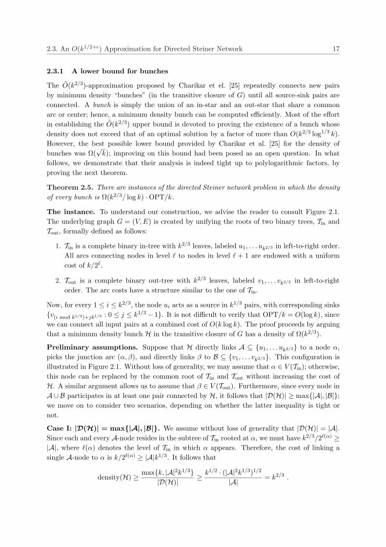
The instance. To understand our construction, we advise the reader to consult Figure 2.1.The underlying graph G = (V, E) is created by unifying the roots of two binary trees, Tin andTout, formally defined as follows:
1. Tin is a complete binary in-tree with k2/3 leaves, labeled u1, . . . uk2/3 in left-to-right order.All arcs connecting nodes in level ` to nodes in level ` + 1 are endowed with a uniformcost of k/2`.
2. Tout is a complete binary out-tree with k2/3 leaves, labeled v1, . . . vk2/3 in left-to-rightorder. The arc costs have a structure similar to the one of Tin.
Now, for every 1 ≤ i ≤ k2/3, the node ui acts as a source in k1/3 pairs, with corresponding sinksv(i mod k1/3)+jk1/3 : 0 ≤ j ≤ k1/3− 1. It is not difficult to verify that OPT/k = O(log k), sincewe can connect all input pairs at a combined cost of O(k log k). The proof proceeds by arguingthat a minimum density bunch H in the transitive closure of G has a density of Ω(k2/3).
Preliminary assumptions. Suppose that H directly links A ⊆ u1, . . . uk2/3 to a node α,picks the junction arc (α, β), and directly links β to B ⊆ v1, . . . vk2/3. This configuration isillustrated in Figure 2.1. Without loss of generality, we may assume that α ∈ V (Tin); otherwise,this node can be replaced by the common root of Tin and Tout without increasing the cost ofH. A similar argument allows us to assume that β ∈ V (Tout). Furthermore, since every node inA∪ B participates in at least one pair connected by H, it follows that |D(H)| ≥ max|A|, |B|;we move on to consider two scenarios, depending on whether the latter inequality is tight ornot.
Case I: |D(H)| = max|A|, |B|. We assume without loss of generality that |D(H)| = |A|.Since each and every A-node resides in the subtree of Tin rooted at α, we must have k2/3/2`(α) ≥|A|, where `(α) denotes the level of Tin in which α appears. Therefore, the cost of linking asingle A-node to α is k/2`(α) ≥ |A|k1/3. It follows that
density(H) ≥ maxk, |A|2k1/3|D(H)| ≥ k1/2 · (|A|2k1/3)1/2
|A| = k2/3 .
18 Chapter 2: Generalized Connectivity
u1 u2 u3 uk2/3
v1 v2 v3 vk2/3
`+1
`k `/2
`+1
`k `/2
®
¯
A
B
Figure 2.1: The directed Steiner network instance.
Case II: |D(H)| > max|A|, |B|. We begin by proving 2`(β) ≤ 2k1/3|A|/|D(H)|, notingthat the inequality 2`(α) ≤ 2k1/3|B|/|D(H)| can be easily validated by exercising symmetricalarguments. For a node u ∈ A, let φ(u) = v ∈ B : (u, v) ∈ D. In other words, φ(u) is the setof pairs connected by H in which u participates. Note that
|D(H)| =∑
u∈A|φ(u)| ≤ |A| ·max
u∈A|φ(u)| .
Now let Imin = mini : vi ∈ B and Imax = maxi : vi ∈ B. The crucial observation is that forevery u ∈ A, we have |i′ − i′′| ≥ k1/3 for every pair of indices i′, i′′ such that both vi′ and vi′′
belong to φ(u). Therefore, Imax−Imin ≥ k1/3(maxu∈A |φ(u)|−1) ≥ k1/3 ·maxu∈A |φ(u)|/2, wherethe last inequality holds since maxu∈A |φ(u)| ≥ 2, or otherwise |D(H)| = |A|. On the other hand,as the subtree of Tout rooted at β has k2/3/2`(β) leaves, it follows that Imax − Imin ≤ k2/3/2`(β).By combining these bounds on Imax − Imin, we have
2`(β) ≤ 2k1/3
maxu∈A |φ(u)| ≤2k1/3|A||D(H)| .
We conclude the proof by observing that each A-node has a linking cost of k/2`(α), whereasB-nodes have individual linking costs of k/2`(β), implying that
density(H) ≥ maxk|A|/2`(α), k|B|/2`(β)|D(H)| = max
k|A|
2k1/3|B| ,k|B|
2k1/3|A|
=k2/3
2·max
|A||B| ,
|B||A|
≥ k2/3
2.
2.3.2 Junction trees and their density
In retrospect, one can view the algorithm proposed by Charikar et al. [25] as an application ofthe junction scheme, restricted to a very simple structure that can be easily computed. Our
2.3. An O(k1/2+ε) Approximation for Directed Steiner Network 19
approach follows the same paradigm. However, instead of being interested in bunches, whoseheight is extremely limited, we focus our attention on junction subgraphs of arbitrary height,shooting for a provable density of O(
√k).
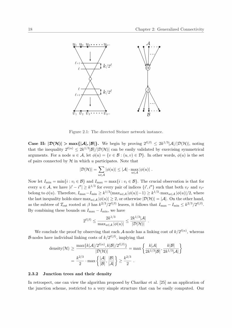
Definitions and notation. An r-rooted junction tree J ⊆ G is defined as the union of anin-tree Tin and an out-tree Tout, both rooted at r ∈ V (see Figure 2.2). It is worth pointing outthat the trees Tin and Tout are allowed to overlap in both nodes and arcs. Note that a sufficientcondition for J to connect a node pair (si, ti) ∈ D is that si ∈ Tin while ti ∈ Tout. Followingpreviously used notation, let D(J ) denote the set of source-sink pairs connected by J , and letc(J ) =
∑e∈J c(e) denote its cost. In addition, the density of J is given by c(J )/|D(J )|.
s1
s2
s6
s4
s5
s3
r t1
t2
t3
t4
t5
t6
Figure 2.2: A junction tree.
Bounding the density of junction trees. With the above definitions in mind, we say thata junction tree J ⊆ G is ρ-optimal if density(J ) ≤ ρ ·OPT/k, where OPT denotes the cost ofan optimal solution. In the following lemma, we establish the existence of
√k-optimal junction
trees; this result is complemented by proving a coinciding lower bound, which is tight up toconstant multiplicative factors.
Lemma 2.6. A minimum density junction tree is√
k-optimal.
Proof. LetH∗ ⊆ G be a minimum cost subgraph that connects all node pairs in D. In addition,for 1 ≤ i ≤ k, let pi ⊆ H∗ be a directed si-ti path in H∗; when si and ti are connected by morethan one path, pi is arbitrarily picked. The proof proceeds by distinguishing between two cases:
1. There is a node r ∈ V that appears in at least√
k of the paths p1, . . . , pk. In this case,consider the junction tree J formed by the union of all paths in p1, . . . , pk passing throughr. Since J is a subgraph of H∗, its cost is at most OPT. Therefore, by observing that Jconnects at least
√k pairs, we have density(J ) ≤ OPT/
√k =
√k ·OPT/k.
2. There is no such node. In particular, every arc of H∗ appears in at most√
k of the pathsp1, . . . , pk. Hence, by creating
√k copies of each arc, all node pairs can be connected via
arc-disjoint paths. Since the overall duplication cost is√
k · OPT, at least one of thesepaths is associated with a cost of at most
√k · OPT/k. This path constitutes a (trivial)
junction tree whose density is at most√
k ·OPT/k.
20 Chapter 2: Generalized Connectivity
Lemma 2.7. There are directed Steiner network instances in which every junction tree isΩ(√
k)-optimal.
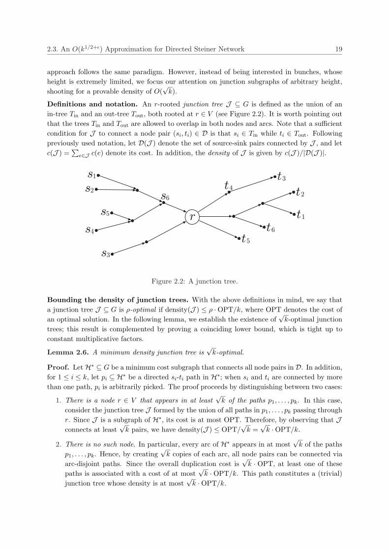
Proof. Consider the following instance of directed Steiner network, schematically described inFigure 2.3:
1. The input graph consists of four layers, with nodes x1, . . . , x√k in the first layer, u1, . . . , u√k
in the second, v1, . . . , v√k in the third, and y1, . . . , y√k in the fourth.
2. For every 1 ≤ i ≤√
k, there are two√
k-cost arcs, (xi, ui) and (vi, yi). In addition, everyui is linked to all vj ’s by zero-cost arcs.
3. The collection of k distinct pairs to be connected is D = (xi, yj) : 1 ≤ i, j ≤√
k.
x1
u1
p
k
x2
u2
p
k
xi
ui
p
kp
k
xp
k
up
k
v1
y1
p
k
v2
y2
p
k
vi
y i
p
kp
k
vp
k
yp
k
Figure 2.3: An example demonstrating that the density of any junction tree is Ω(√
k) ·OPT/k.
Note that the instance under consideration has a unique optimal solution, in which all arcsmust be picked. Since the overall cost is 2k, we have OPT/k = 2. Now let H be a minimumdensity junction tree. Without loss of generality, we may assume that the root of H belongs tou1, . . . , u√k, v1, . . . , v√k. Consequently, c(H) = (1 + |D(H)|)
√k, implying that the density of
H is at least√
k.
2.3.3 Finding low-density junctions trees
Overview. We have already observed that junction trees are strongly related to directed Steinertrees [25, 71, 119]. In particular, identifying a low-density junction tree would have been ratherstraightforward, should the natural LP-relaxation of directed Steiner tree had a reasonablysmall integrality gap; unfortunately, Zosin and Khuller [120] demonstrated that the latter gapis Ω(
√k). To overcome this difficulty, given a fixed accuracy parameter ε > 0, we limit our
2.3. An O(k1/2+ε) Approximation for Directed Steiner Network 21
attention to junction trees of height 1/ε, while incurring an O(kε) penalty in the performanceguarantee via a height restriction lemma due to Zelikovsky [119]. We then reduce the problemof finding a low density (1/ε)-height junction tree to MDGC (see Section 2.2.1), blowing up thefinal approximation ratio by only logarithmic factors. In essence, the remainder of this sectionwill be devoted to proving the next lemma.
Lemma 2.8. For any fixed ε > 0, there is a polynomial-time algorithm that constructs ajunction tree J ⊆ G satisfying density(J ) = O(kε) · density(J ∗), where J ∗ is a minimumdensity junction tree.
Preliminaries. For ease of presentation, it would be convenient to assume that 1/ε is aninteger. In addition, we can assume without loss of generality that G is transitively closed.Finally, we may assume that the root r of J ∗ is known in advance; otherwise, all nodes can betested as potential roots by means of exhaustive search.
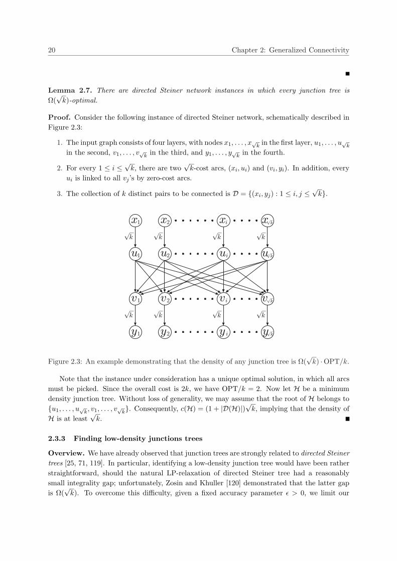
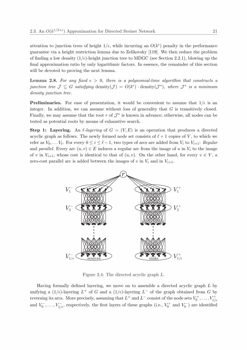
Step 1: Layering. An `-layering of G = (V, E) is an operation that produces a directedacyclic graph as follows. The newly formed node set consists of ` + 1 copies of V , to which werefer as V0, . . . V`. For every 0 ≤ i ≤ `− 1, two types of arcs are added from Vi to Vi+1: Regularand parallel. Every arc (u, v) ∈ E induces a regular arc from the image of u in Vi to the imageof v in Vi+1, whose cost is identical to that of (u, v). On the other hand, for every v ∈ V , azero-cost parallel arc is added between the images of v in Vi and in Vi+1.
r
V1+
V2+
V1/²+
V1¡
V2¡
V¡
1/² sources sinks
Figure 2.4: The directed acyclic graph L.
Having formally defined layering, we move on to assemble a directed acyclic graph L byunifying a (1/ε)-layering L+ of G and a (1/ε)-layering L− of the graph obtained from G byreversing its arcs. More precisely, assuming that L+ and L− consist of the node sets V +
0 , . . . , V +1/ε
and V −0 , . . . , V −
1/ε, respectively, the first layers of these graphs (i.e., V +0 and V −
0 ) are identified
22 Chapter 2: Generalized Connectivity
as one layer, V0, while other layers are kept separated, as shown in Figure 2.4. It is instructiveto omit nodes from V0, V +
1/ε and V −1/ε as follows: Only r is left in V0; only sinks are left in V +
1/ε;and only sources are left in V −
1/ε.The next claim is an immediate consequence of a well-known result due to Zelikovsky [119,
Thm. 2], stating that any rooted tree in a transitively closed graph can be transformed into an`-level tree defined on the same set of nodes, while blowing up the overall cost by O(`k1/`). Inthis context, k denotes the number of leaves in the original tree.
Claim 2.9. There exists an r-rooted tree Tr ⊆ L that satisfies the following properties:
1. For every (si, ti) ∈ D(J ∗), Tr connects r to both si ∈ V −1/ε and ti ∈ V +
1/ε.
2. c(Tr) = O(kε) · c(J ∗).
We remark that any r-rooted tree Tr ⊆ L can be efficiently translated to a junction treeJ ⊆ G such that c(J ) ≤ c(Tr), and such that D(J ) consists of all source-sink pairs (si, ti) forwhich both si ∈ V −
1/ε and ti ∈ V +1/ε are reachable from r in Tr.
Step 2: Path splitting. We proceed by creating an undirected tree T as follows. Considerthe spider formed by constructing a collection of O(n1/ε) vertex-disjoint paths, one for eachpath in L connecting r to a node in V +
1/ε ∪ V −1/ε, and unifying their roots. We repeatedly merge
common prefixes of these paths, until every branching corresponds to an actual branching in L.Alternatively, one can also provide a recursive definition:
1. When u ∈ V +1/ε ∪ V −
1/ε, the resulting tree consists of the singleton vertex u.
2. When u ∈ V +i , for some 0 ≤ i ≤ 1/ε − 1, we begin by recursively computing a fresh
collection of rooted trees, Tv : v ∈ V +i+1. The root of each Tv is then joined to u by
an edge whose cost is equal to that of the arc (u, v) in L. The case u ∈ V −i is handled
analogously.
With the underlying tree T in place, we create an instance of MDGC by setting up a uniquedemand (Si, Ti) for each node pair (si, ti) ∈ D. Specifically, since each source node si ∈ V −
1/ε has
just been duplicated O(n1/ε) times, its corresponding vertex set Si is defined to be the collectionof leaves in T that are duplicates of si. Similarly, the set Ti contains all duplicates of ti ∈ V +
1/ε.It is not difficult to verify that there is a one-to-one correspondence between r-rooted trees inL and T , namely, for each tree Tr ⊆ L there is a matching tree T ′r ⊆ T of identical cost, suchthat T ′r connects r to both Si and Ti if and only if Tr connects r to both si ∈ V −
1/ε and ti ∈ V +1/ε.
Moreover, this bijection can be efficiently computed.Consequently, it remains to approximate an MDGC instance defined on a (1/ε)-height tree
spanning O(n1/ε) vertices. As a result of specializing Lemma 2.2 to rooted trees (see footnoteon page 16), such instances can be approximated to within a factor of O(log k). By combiningthe latter observation with an additional O(kε) factor lost during our layering step, Lemma 2.8follows.
Summary. Lemma 2.8, in conjunction with Lemma 2.6 and a standard repeated coveringprocedure, immediately implies the main result of this section, formally stated in the followingtheorem.
2.4. A Polylogarithmic Approximation for Set Connector 23
Theorem 2.10. The directed Steiner network problem can be approximated to within a factorof O(k1/2+ε), for any fixed ε > 0.
2.4 A Polylogarithmic Approximation for Set Connector
The main result of this section is a polylogarithmic performance guarantee for set connector.We remind the reader that an instance of the latter problem consists of an undirected graphG = (V, E), whose edges are associated with non-negative costs specified by c : E → R+. Asmentioned in Chapter 1, given a collection of divisions V1, . . . ,Vm, the objective is to constructa minimum cost subset of edges F ⊆ E that simultaneously weakly connects all input divisions.Our principal finding in this context can be briefly summarized as follows.
Theorem 2.11. The set connector problem admits an O(log3 n log2(mn)) approximation.
Prior to proving the above theorem, we demonstrate that a naive reduction to generalizedconnectivity, in which each division Vi = X1, . . . , Xh is replaced by a collection of demands(Xr, Xs) : 1 ≤ r < s ≤ h is incorrect. To this end, consider a set connector instance definedon a complete graph with vertex set v1, v2, v3, v4, and suppose that we are given a singledivision V1 = X1, X2, X3, where X1 = v1, X2 = v2 and X3 = v3, v4. It is not difficultto verify that F = (v1, v3), (v2, v4) forms a feasible solution to this instance. However, F isinfeasible for the resulting generalized connectivity instance, since it does not contain a pathwith one endpoint in X1 and the other in X2.
Proof of Theorem 2.11. The proof proceeds by relating the approximability of set connectorto that of generalized connectivity. We say that X ∈ Vi is covered by an edge set F ⊆ E whenthe subgraph (V, F ) contains a path connecting a vertex in X to a vertex in Y 6= X, for someY ∈ Vi. Note that the optimal solution F ∗ covers every set in
⋃mi=1 Vi. In addition, given a set
of edges F ⊆ E that covers all sets in⋃m
i=1 Vi, we can create a new set connector instance asfollows. For each division Vi = X1, . . . , Xh, let Gi(F ) be a graph on the vertex set 1, . . . , h,in which r and s are joined by an edge when Xr and Xs are connected by F . Since all vertexsets are covered, Gi(F ) consists of at most h/2 connected components, C1, . . . , C`. We defineV ′i = Y1, . . . , Y`, where Yt =
⋃j∈Ct
Xj , noting that |V ′i| ≤ |Vi|/2. It is easy to ascertain thatF ∗ remains a feasible solution to the new instance induced by V ′1, . . . ,V ′m, and furthermore,any feasible solution to this instance can be combined with F to form a feasible solution withrespect to V1, . . . ,Vm. We conclude that an α-approximation for covering
⋃mi=1 Vi implies an
O(α log β)-approximation for the set connector problem, where β = maxi |Vi| ≤ n.We now show that a generalized connectivity heuristic can be straightforwardly employed as
a subroutine, to detect an approximate edge set covering all sets in⋃m
i=1 Vi. For this purpose,an instance of the former problem is assembled as follows. For each division Vi = X1, . . . , Xh,we introduce a collection of h demands (X1, (
⋃hj=1 Xj) \ X1), . . . , (Xh, (
⋃hj=1 Xj) \ Xh). We
observe that F ⊆ E covers⋃m
i=1 Vi if and only if this edge set constitutes a feasible solution tothe generalized connectivity instance obtained via the above reduction. Therefore, by pluggingin the O(log2 n log2 d)-approximation for generalized connectivity stated in Theorem 2.3, weattain a performance guarantee of O(log3 n log2(mn)) for set connector.
24 Chapter 2: Generalized Connectivity

Chapter 3
k-Steiner Forest
In this chapter, we present the first non-trivial approximation algorithm for the k-Steiner forestproblem, which is based on a novel extension of the Lagrangian relaxation technique. Webelieve that the approach illustrated in the current writing is of independent interest, and maybe applicable in other settings as well. Our main result is the following.
Theorem 3.1. There is a polynomial-time algorithm that approximates the k-Steiner forestproblem to within a factor of O(minn2/3,
√d · log d).
3.1 Technical Overview
Prior to providing a succinct outline of the approach we suggest, from which certain technicaldetails are omitted for ease of exposition, an important remark is in place. Even though d =O(n2), the reader should bear in mind that the terms n2/3 and
√d, appearing in the above
theorem, are incomparable. Indeed, it is tempting to speculate that an instance with arbitrarydemands can be reduced to one with d ≤ n−1, by eliminating cycles in the demand graph (V,D).However, since the optimal subset of k demands to be connected is not known in advance, areduction of this nature does not seem possible.
A slightly different view. The algorithm we propose and its analysis are based on viewingk-Steiner forest as a partial covering problem with exponentially many “sets”. For this purpose,let T denote the collection of all trees in the input graph G. Then, one can think of the k-Steinerforest problem as that of computing a minimum cost subset of trees F ⊆ T that connects atleast k demands in D. Although F is clearly a forest in any optimal solution, it would beimperative to allow the trees in this subset to overlap in both vertices and edges; therefore,F will be referred to as a collection of trees rather than as a forest. We precede any furtherdiscussion with the observation that, while this new point of view is conceptually simpler, itdoes not lead to any straightforward approximability result. It is not difficult to verify that, forthe particular settings we consider, existing partial cover algorithms [14, 50, 54, 84, 116] eitherprovide exponential approximation factors or have an exponential running time.
A seemingly useful method. Suppose that the requirement to connect at least k demands isnot enforced; instead, if the collection of trees we construct leaves a demand (si, ti) unconnected,
25
26 Chapter 3: k-Steiner Forest
we incur a penalty of π(i). The prize-collecting Steiner forest problem asks to find a collectionF ⊆ T that minimizes the cost of F plus the penalties of the unconnected demands. Connectionsbetween the prize-collecting and the partial variants of numerous optimization problems havebeen the subject of an ever-growing line of work, in which the Lagrangian relaxation techniqueplays an instrumental role. Schematically speaking, this technique assembles a near-optimalsolution to the partial variant by employing successive calls to an approximation algorithm forthe prize-collecting variant. However, in all previous applications the latter algorithm had tosatisfy two structural properties, stated here in terms of prize-collecting Steiner forest:
1. Pay penalties at the same rate as OPT. For every instance I, the solution weobtain satisfies C + αΠ ≤ α ·OPT(I), where C is the total cost of the trees picked by thealgorithm, and Π is the sum of penalties over all unconnected demands. Intuitively, aninequality of this form guarantees an α-approximation even when all penalties are inflatedby a factor of α.
2. Allow solutions to be combined. Lagrangian duality, in conjunction with the firstproperty we mention, establishes that any optimal solution to the original k-Steiner forestproblem can be approximated by a convex combination of two prize-collecting solutions.Nevertheless, such a characterization does not appear to be of much help, unless there isan efficient method for combining these solutions into an approximate integral one.
Once again, existing algorithms are not applicable. It is not difficult to verify thatthe LP-rounding technique suggested by Bienstock, Goemans, Simchi-Levi and Williamson [21]can be adapted to approximate prize-collecting Steiner forest to within a factor of 3. In fact,Hajiaghayi and Jain [68] have recently proposed a primal-dual algorithm for this problem thatachieves a similar approximation guarantee, and have also derived an improved factor of 2.54by means of randomized rounding. Unfortunately, penalties are not paid-for at the same rateas OPT by any of these algorithms. Furthermore, we argue that this difficulty is not the pri-mary factor limiting the applicability of previously advocated methods; rather, the fundamentalquestion is: How do we combine the prize-collecting solutions?
It is worth noting that, regardless of the problem-specific scheme we may apply to combinethese solutions, most algorithms that follow the Lagrangian relaxation framework acquire anadditional lower bound on the optimal cost through preprocessing. Specifically, an exhaustivesearch is conducted in order to “guess” certain attributes of an arbitrary optimal solution,according to which the given instance is modified in advance. Examples for attributes that werefound to be useful in approximating directly related problems include the optimal diameter [35,56], a constant number of edges in the optimal solution [64, 73, 90, 110], or a combination ofboth vertices and edges [5].
“Discarding” expensive trees via internal preprocessing. Intuitively, the k-Steiner forestproblem would be much easier to approximate, given that our prize-collecting algorithm avoidspicking overly-priced trees. However, we are not aware of any way of achieving this objective byutilizing the above-mentioned form of preprocessing. The new approach we propose does notinvolve a preliminary step of preprocessing; instead, an analogous effect is obtained by addingextra requirements to internal procedures. To clarify this statement, suppose that ∆ ≥ 0
3.2. A Bicriteria Prize-Collecting Algorithm 27
estimates the minimum cost of a k-Steiner forest to within some constant factor (for example,∆ ∈ [OPT, 2 · OPT]). Then, we would like the prize-collecting algorithm to behave as if alltrees with cost greater than ∆ were explicitly eliminated from T , a hypothetical scenario whoseoptimal cost is denoted by OPT∆. In Section 3.2, we show that this task can be accomplishedin bicriteria fashion, establishing the next theorem.
Theorem 3.2. There is a polynomial-time algorithm that finds a collection F ⊆ T , consistingof trees with individual costs of at most 4minn2/3,
√d∆, such that
c(F) + 12min
n2/3,√
dH(d) ·Π(F) ≤ 12min
n2/3,
√dH(d) ·OPT∆ .
Here, c(F) is the total cost of the trees in F and Π(F) is the sum of penalties over all demandsleft unconnected by F .
Putting it all together. In Section 3.3, we formulate the k-Steiner forest problem as aninteger program, and augment it with additional valid constraints stating that trees in T witha cost greater than ∆ cannot be picked. While these constraints are clearly redundant withrespect to the original problem, they play an important role in its Lagrangian relaxation, byenabling us to make use of the algorithm described in Theorem 3.2. Consequently, the prize-collecting solutions we construct pay penalties at an optimal rate, and at the same time consistof trees whose cost can be bounded in terms of ∆. The strategy we apply to combine thesesolutions has its roots in a greedy procedure suggested by Levin and Segev [90] for partiallycovering general set systems.
Notation. We conclude this section by introducing some notation. Given a tree T ∈ T , weuse c(T ) =
∑e∈E(T ) c(e) to denote the total cost of the edges in T . Furthermore, when F is
a collection of trees, the notation c(F) is used as a shorthand for∑
T∈F c(T ). For a collectionF ⊆ T , we denote by D(F) the set of demands connected by at least one tree in F , excludingthe case where F consists of a single tree T , which is abbreviated by writing D(T ) instead ofD(T).
3.2 A Bicriteria Prize-Collecting Algorithm
The main result of this section is a constructive proof of Theorem 3.2. We remind the readerthat a prize-collecting instance consists of an undirected graph G = (V, E) with non-negativeedge costs specified by c : E → R+. An additional ingredient of the input is a collection ofdemands D = (s1, t1), . . . , (sd, td), where the penalty we incur for leaving a demand (si, ti)unconnected is π(i). Now suppose that the individual cost of every tree in the constructedsolution should not exceed ∆, a given budget; we denote by OPT∆ the cost of an optimalsolution satisfying this extra restriction.
3.2.1 Constructing dense trees with small costs
In what follows, we examine the intrinsic structure of connectivity under budget constraints, anddevelop an essential tool that will allow us to considerably simplify the proof of Theorem 3.2.For this purpose, we define the density of a tree T ∈ T to be the ratio between its cost and the
28 Chapter 3: k-Steiner Forest
number of demands it connects, and let T∆ denote the collection of trees in T whose cost is atmost ∆. Having introduced this notation, we claim that the minimum density of a tree in T∆
can be efficiently approximated, while keeping the factor by which the budget ∆ is exceededwithin an acceptable magnitude. This result is formally described in the next theorem.
Theorem 3.3. There is a polynomial-time algorithm that finds a tree T ∈ T whose densityis at most 12 minn2/3,
√d times the minimum density of a tree in T∆, ensuring that c(T ) ≤
4minn2/3,√
d∆ at the same time.
For sake of simplicity, we prove a weaker version of the above theorem, in which the termminn2/3,
√d is replaced by n2/3. An analogous proof for the
√d-dependent bound is provided
in Section 3.4.
Initial assumptions. To avoid special treatment of degenerate cases, it will be convenient toassume throughout this section that the input graph contains at least one tree with c(T ) ≤ ∆and D(T ) 6= ∅. As explained in Section 3.3, this requirement can be easily enforced. Wetherefore consider the case where minT∈T∆
density(T ) < ∞. Let T ∗ be a tree of minimumdensity over all trees in T∆, and let q = |D(T ∗)|. By conducting an exhaustive search, we mayalso assume that the number of connected demands q and an arbitrary vertex r ∈ V (T ∗) areknown in advance.
The vertex-augmentation lemma. Noting that the demands in D are distinct, T ∗ mustbe comprised of many vertices whenever q is sufficiently large. By combining this intuitiveobservation with further structural properties, we demonstrate in Lemma 3.4 how to extend agiven tree to a new tree that connects Ω(q) demands or contains Ω(
√q) additional vertices. To
bound the overall cost of the augmenting edges, our approach depends upon a constant-factorapproximation for the rooted quota-MST problem. In this generalization of k-MST, each vertexv ∈ V is associated with a non-negative profit p(v), and the objective is to compute a minimumcost tree rooted at r that collects a total profit of at least P , a specified quota. The proof ofLemma 3.4 requires to approximate instances with p(v) ∈ 0, . . . , d, a subproblem that reducesback to k-MST in a straightforward way (see, for example, [12]). Consequently, such instancescan be approximated to within a factor of 2 [57].
Lemma 3.4. Let T be a tree that contains r. Then, we can find in polynomial time a tree T+
satisfying T ⊆ T+, c(T+) ≤ c(T ) + 2c(T ∗) and at least one of the following properties:
1. |V (T+)| ≥ |V (T )|+√q/2.
2. |D(T+)| ≥ 3q/8.
Proof. We assume without loss of generality that |D(T )| < q/2, since the claim can be estab-lished in the opposite case by defining T+ = T . For 0 ≤ j ≤ 2, let Aj be the set of demands inD(T ∗) with exactly j endpoints in V (T ), that is, Aj = (si, ti) ∈ D(T ∗) : |si, ti ∩ V (T )| = j.The proof proceeds by considering two cases, depending on the cardinality of V (T ∗) \ V (T ); tobetter understand the forthcoming analysis, we advise the reader to consult Figure 3.1.Case 1: |V (T ∗) \ V (T )| ≥ √
q/2. This inequality implies, in particular, that T ∗ connects r
to at least√
q/2 vertices not belonging to T . Hence, we can obtain a tree T that connects r to
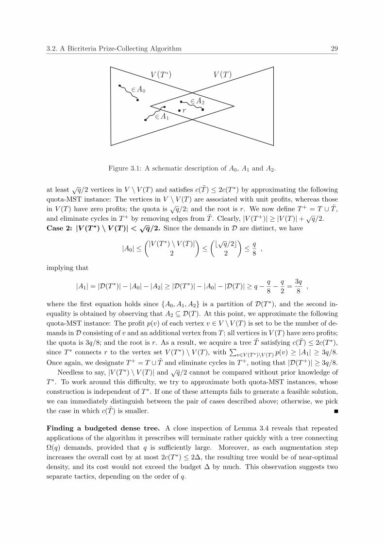
3.2. A Bicriteria Prize-Collecting Algorithm 29
T( )VT( )V *
0A2
1A2
2A2
r
Figure 3.1: A schematic description of A0, A1 and A2.
at least√
q/2 vertices in V \ V (T ) and satisfies c(T ) ≤ 2c(T ∗) by approximating the followingquota-MST instance: The vertices in V \ V (T ) are associated with unit profits, whereas thosein V (T ) have zero profits; the quota is
√q/2; and the root is r. We now define T+ = T ∪ T ,
and eliminate cycles in T+ by removing edges from T . Clearly, |V (T+)| ≥ |V (T )|+√q/2.
Case 2: |V (T ∗) \ V (T )| <√
q/2. Since the demands in D are distinct, we have
|A0| ≤(|V (T ∗) \ V (T )|
2
)≤
(b√q/2c2
)≤ q
8,
implying that
|A1| = |D(T ∗)| − |A0| − |A2| ≥ |D(T ∗)| − |A0| − |D(T )| ≥ q − q
8− q
2=
3q
8,
where the first equation holds since A0, A1, A2 is a partition of D(T ∗), and the second in-equality is obtained by observing that A2 ⊆ D(T ). At this point, we approximate the followingquota-MST instance: The profit p(v) of each vertex v ∈ V \V (T ) is set to be the number of de-mands inD consisting of v and an additional vertex from T ; all vertices in V (T ) have zero profits;the quota is 3q/8; and the root is r. As a result, we acquire a tree T satisfying c(T ) ≤ 2c(T ∗),since T ∗ connects r to the vertex set V (T ∗) \ V (T ), with
∑v∈V (T ∗)\V (T ) p(v) ≥ |A1| ≥ 3q/8.
Once again, we designate T+ = T ∪ T and eliminate cycles in T+, noting that |D(T+)| ≥ 3q/8.Needless to say, |V (T ∗) \ V (T )| and
√q/2 cannot be compared without prior knowledge of
T ∗. To work around this difficulty, we try to approximate both quota-MST instances, whoseconstruction is independent of T ∗. If one of these attempts fails to generate a feasible solution,we can immediately distinguish between the pair of cases described above; otherwise, we pickthe case in which c(T ) is smaller.
Finding a budgeted dense tree. A close inspection of Lemma 3.4 reveals that repeatedapplications of the algorithm it prescribes will terminate rather quickly with a tree connectingΩ(q) demands, provided that q is sufficiently large. Moreover, as each augmentation stepincreases the overall cost by at most 2c(T ∗) ≤ 2∆, the resulting tree would be of near-optimaldensity, and its cost would not exceed the budget ∆ by much. This observation suggests twoseparate tactics, depending on the order of q.
30 Chapter 3: k-Steiner Forest
Case 1: q < 9n2/3. Interpreting c : E → R+ as a length function, we compute the shortestpath P connecting any demand in D. Note that the cost of this solution does not exceed ∆,since T ∗ connects at least one demand and c(T ∗) ≤ ∆. In addition,
density(P ) =c(P )|D(P )| ≤ c(T ∗) ≤ 9n2/3 · c(T ∗)
q= 9n2/3 · c(T ∗)
|D(T ∗)| = 9n2/3 · density(T ∗) .
Case 2: q ≥ 9n2/3. Starting with a trivial tree T that consists of the single vertex r, werepeatedly extend T by applying the algorithm proposed in Lemma 3.4, as long as |D(T )| <
3q/8. In each step, we either add to T at least√
q/2 new vertices, or discover that it alreadyconnects at least 3q/8 demands. It follows that the resulting tree satisfies
c(T ) ≤(
n√q/2
+ 1)· 2c(T ∗) ≤
(2n2/3
3+ 1
)· 2c(T ∗) ≤ 4n2/3c(T ∗) ≤ 4n2/3∆ ,
and at the same time
density(T ) =c(T )|D(T )| ≤
4n2/3c(T ∗)3q/8
≤ 11n2/3 · c(T ∗)|D(T ∗)| = 11n2/3 · density(T ∗) .
3.2.2 A greedy prize-collecting approach
We are now ready to conclude the proof of Theorem 3.2, by enclosing the algorithm for con-structing budgeted dense trees within a greedy heuristic. The principal idea that guides ouralgorithm can be informally described as follows. In each step, we identify a tree T ∈ T of near-optimal density, whose cost does not significantly exceed ∆. However, rather than picking T
right away, its density is compared to the minimum available penalty π(i∗), scaled by some fac-tor that will be specified later. Based on the outcome of this comparison, we decide whether topick T or to tentatively pay the penalty π(i∗) and leave the corresponding demand (si∗ , ti∗) un-connected. In an attempt to highlight the intimate relationship between Theorems 3.2 and 3.3,let α(n, d) be the approximation guarantee of the latter theorem with respect to the optimaldensity, and let β(n, d) be the maximal factor by which the budget ∆ is exceeded. As previouslymentioned, α(n, d) = 12 minn2/3,
√d and β(n, d) = 4 minn2/3,
√d.
The algorithm. In what follows, F denotes the collection of trees we construct, while Rdenotes the set of remaining demands; P and price(·) are used for purposes of analysis.
1. Initialize F ← ∅, R← D and P ← ∅.
2. While R 6= ∅
(a) Apply the algorithm given in Theorem 3.3 to identify a tree T ∈ T that approximatesthe following instance: The underlying graph and edge costs are still G = (V, E) andc : E → R+, respectively; the collection of demands is R; and the budget is ∆.
(b) Let (si∗ , ti∗) be a demand that minimizes π(i) over all demands in R, breaking tiesarbitrarily.
3.2. A Bicriteria Prize-Collecting Algorithm 31
(c) If density(T ) ≤ α(n, d)H(d)π(i∗), add T to F , eliminate from R all newly connecteddemands, and for each of them define price(i) = density(T ). Otherwise, add i∗ to P,eliminate (si∗ , ti∗) from R, and define price(i∗) = α(n, d)H(d)π(i∗).
3. Return F .
Analysis. We first argue that F consists of trees with individual costs of at most β(n, d)∆.This follows from the observation that each of these trees was obtained during step 2a, implyingthat c(T ) ≤ β(n, |R|)∆ ≤ β(n, d)∆ for every T ∈ F , according to Theorem 3.3. In addition,the overall cost of the trees in F is
∑T∈F c(T ), whereas the demands left unconnected by F
have a total penalty of at most∑
i∈P π(i). We remark that the latter term is an upper boundon the sum of penalties, and not the exact sum, since it is quite possible that F connects oneor more demands in (si, ti) : i ∈ P. Therefore, we can complete the proof of Theorem 3.2 byverifying that ∑
T∈Fc(T ) + α(n, d)H(d)
∑
i∈Pπ(i) ≤ α(n, d)H(d) ·OPT∆ . (3.1)
Let F∗ ⊆ T∆ be an optimal solution to the prize-collecting instance at hand, and let Qbe the index set of demands not connected by F∗, that is, Q = i : (si, ti) /∈ D(F∗). Notethat
∑T∈F∗ c(T ) +
∑i∈Q π(i) = OPT∆. Bearing these definitions in mind, each index i /∈ Q
is assigned to a tree in F∗ that connects (si, ti), making an arbitrary choice in case of multipleoptions. In the remainder of this section, we use φ : 1, . . . , d\Q → F∗ to denote the resultingassignment and φ−1(T ) to denote the inverse image of T under φ. We proceed by establishingtwo crucial properties of the suggested pricing method.
Lemma 3.5.∑
i∈φ−1(T ) price(i) ≤ α(n, d)H(d)c(T ) for every T ∈ F∗.
Proof. Let φ−1(T ) = i1, . . . , iq, where the elements of φ−1(T ) are indexed by the order theywere eliminated from R, breaking ties arbitrarily. For any 1 ≤ ` ≤ q, consider the iteration inwhich i` was eliminated. At this particular moment, density(T ) ≤ c(T )/(q − ` + 1), since T
connects the set of demands (si` , ti`), . . . , (siq , tiq) ⊆ R, and possibly other demands as well;moreover, the cost of T is clearly within the given budget, as the individual cost of every treein F∗ is at most ∆. Combined with Theorem 3.3, these observations imply that in the currentiteration we find a tree T ′ with density(T ′) ≤ α(n, |R|) · density(T ) ≤ α(n, d) · c(T )/(q− ` + 1).Finally, since the condition stated in step 2c yields price(i`) ≤ density(T ′), it follows that
∑
i∈φ−1(T )
price(i) =q∑
`=1
price(i`) ≤ α(n, d)q∑
`=1
c(T )q − ` + 1
= α(n, d)H(q)c(T ) ≤ α(n, d)H(d)c(T ) .
Lemma 3.6. price(i) ≤ α(n, d)H(d)π(i) for every 1 ≤ i ≤ d.
Proof. Consider the iteration in which i was eliminated from R. If i was simultaneously addedto P, then this index obviously corresponds to the demand minimizing π(i) over all demands in
32 Chapter 3: k-Steiner Forest
R, and we set price(i) = α(n, d)H(d)π(i). Otherwise, the tree T we find in the current iterationis of density no greater than α(n, d)H(d)π(i∗), implying that
price(i) = density(T ) ≤ α(n, d)H(d)π(i∗) ≤ α(n, d)H(d)π(i) .
Noting that our pricing method simultaneously guarantees∑
T∈F c(T ) =∑
i/∈P price(i) and∑i∈P α(n, d)H(d)π(i) =
∑i∈P price(i), we derive the desired bound (3.1) from Lemmas 3.5
and 3.6:∑
T∈Fc(T ) + α(n, d)H(d)
∑
i∈Pπ(i) =
∑
i/∈Pprice(i) +
∑
i∈Pprice(i) =
∑
i/∈Qprice(i) +
∑
i∈Qprice(i)
=∑
T∈F∗
∑
i∈φ−1(T )
price(i) +∑
i∈Qprice(i) ≤ α(n, d)H(d)
∑
T∈F∗c(T ) + α(n, d)H(d)
∑
i∈Qπ(i)
= α(n, d)H(d) ·OPT∆ .
3.3 The k-Steiner Forest Algorithm
Having already laid the foundations of our approach, we turn to describe the main resultof this chapter, namely, a polynomial-time algorithm that approximates the k-Steiner forestproblem to within a factor of O(minn2/3,
√d · log d). Given an instance of the problem under
consideration, we use OPT to denote the minimum cost of a forest that connects at least k
demands. By conducting an exhaustive search, we may assume that a constant-factor estimate∆ ∈ [OPT, 2 · OPT] of the optimal cost is known in advance. Furthermore, straightforwardarguments allow us to assume that each edge has a strictly positive cost and that the shortestpath connecting any demand is of length at most ∆.
3.3.1 An integer program and its Lagrangian relaxation
As mentioned earlier, the algorithm we propose and its analysis are based on viewing k-Steinerforest as an exponential-size partial covering problem, with the objective of computing a mini-mum cost subset of trees F ⊆ T that connects at least k demands. This perspective motivatesa natural integer programming formulation, which is surprisingly augmented with additionalvalid constraints stating that trees with cost greater than ∆ cannot be picked.
OPT = minimize∑
T∈Tc(T )xT
subject tod∑
i=1
zi ≤ d− k (3.2)
∑
T :(si,ti)∈D(T )
xT + zi ≥ 1 ∀ 1 ≤ i ≤ d (3.3)
xT = 0 ∀T ∈ T : c(T ) > ∆ (3.4)
xT , zi ∈ 0, 1 ∀T ∈ T , 1 ≤ i ≤ d (3.5)
3.3. The k-Steiner Forest Algorithm 33
In this formulation, the variable xT indicates whether the tree T is chosen for the collectionwe construct, whereas zi indicates whether the demand (si, ti) is not connected. Constraint(3.2) forces any feasible solution to connect at least k demands. Constraint (3.3) ensures thatwe either pick at least one tree that connects (si, ti), or specify that this demand remainsunconnected by setting zi = 1. Last but not least, the additional constraint (3.4) appears to becompletely redundant at the moment, since OPT ≤ ∆.
We now relax the complicating constraint (3.2), and lift it to the objective function multipliedby λ ≥ 0. The resulting Lagrangian relaxation is:
LR(λ) = minimize∑
T∈Tc(T )xT + λ
(d∑
i=1
zi − (d− k)
)
subject to∑
T :(si,ti)∈D(T )
xT + zi ≥ 1 ∀ 1 ≤ i ≤ d (3.6)
xT = 0 ∀T ∈ T : c(T ) > ∆ (3.7)
xT , zi ∈ 0, 1 ∀T ∈ T , 1 ≤ i ≤ d (3.8)
We remark that, excluding the constant term of −λ(d − k) in the objective function, LR(λ)describes a closely related instance of the prize-collecting Steiner forest problem, in which alldemands are coupled with a uniform penalty of λ. However, the current formulation retainsthe extra restriction imposing an upper bound of ∆ on the individual cost of every tree picked,which turns out to be of great importance. Indeed, simple examples demonstrate that theoptimal cost may fluctuate by a factor of Ω(d) should this restriction be discarded, renderingany prize-collecting scheme obsolete. We refer to the above-mentioned instance as Iλ,∆, and useOPT(Iλ,∆) to denote its optimum value. It is easy to verify that LR(λ) = OPT(Iλ,∆)−λ(d−k)provides a lower bound on OPT for any λ ≥ 0, by observing that an optimal solution to theoriginal problem is also a feasible solution to LR(λ), whose cost is at most OPT.
3.3.2 Setting up the prize-collecting solutions
Preliminaries. In what follows, we apply the techniques developed in Section 3.2 to approxi-mate the cost of an optimal k-Steiner forest by a convex combination of prize-collecting solutions,each of which consists of trees whose individual costs do not significantly exceed ∆. At thispoint, we remind the reader that, given any λ ≥ 0, the polynomial-time algorithm describedin Theorem 3.2 provides a bicriteria approximation for Iλ,∆. To simplify the oncoming discus-sion, it would be convenient to interpret the resulting solution in terms of the indicators (x, z)defined above. For this purpose, let xλ indicate which trees were picked by the algorithm, andlet zλ indicate which demands were left unconnected. Clearly, (xλ, zλ) satisfies the constraints(3.6) and (3.8), but not necessarily (3.7). However, recalling that α(n, d) = 12minn2/3,
√d
and β(n, d) = 4 minn2/3,√
d, Theorem 3.2 guarantees c(T ) ≤ β(n, d)∆ for every T ∈ T withxλ
T = 1, while
∑
T∈Tc(T )xλ
T + α(n, d)H(d)d∑
i=1
λzλi ≤ α(n, d)H(d) ·OPT(Iλ,∆) . (3.9)
34 Chapter 3: k-Steiner Forest
The binary search. Intuitively speaking, increasingly larger values of λ compel the prize-collecting algorithm to connect all demands, as even a single penalty becomes unaffordable.Similar reasoning suggests that very few demands would be connected when λ is sufficientlysmall. In the next lemma, we obtain concrete bounds for this asymptotic behavior.
Lemma 3.7. When λ > d∆, the solution (xλ, zλ) connects all demands. On the other hand,we may assume without loss of generality that (x0, z0) connects strictly less than k demands.
Proof. Let λ > d∆, and suppose that the collection of trees picked by the algorithm leavesat least one demand unconnected when we approximate Iλ,∆. Then, this outcome contradictsinequality (3.9), since
∑
T∈Tc(T )xλ
T + α(n, d)H(d)d∑
i=1
λzλi > α(n, d)H(d) · d∆ ≥ α(n, d)H(d) ·OPT(Iλ,∆) .
To better understand the second inequality, note that we have previously assumed the shortestpath connecting any demand to be of length at most ∆. Therefore, we can construct a feasiblesolution to Iλ,∆ by separately picking for each demand (si, ti) an arbitrary shortest si-ti path,implying that OPT(Iλ,∆) ≤ d∆.
We establish the second part of the claim by observing that when (x0, z0) connects at least k
demands, it is already a feasible solution to the original k-Steiner forest problem whose objectivevalue is
∑
T∈Tc(T )x0
T ≤ α(n, d)H(d) ·OPT(I0,∆) = α(n, d)H(d) · LR(0) ≤ α(n, d)H(d) ·OPT .
This observation determines an initial interval over which we conduct a binary search, con-sisting of a polynomially-bounded number of calls to the prize-collecting algorithm. As a result,we find λ− ≤ λ+ along with approximate solutions (xλ− , zλ−) and (xλ+
, zλ+) satisfying the
following properties:
1. λ+ − λ− ≤ cmin/d, where cmin > 0 denotes the minimum cost of an edge in the inputgraph.
2. The solution (xλ− , zλ−) connects k− ≤ k demands, whereas (xλ+, zλ+
) connects k+ ≥ k
demands.
For the remainder of this section, we use F− and F+ to denote the collections of trees thatwere picked by (xλ− , zλ−) and (xλ+
, zλ+), respectively. In addition, we assume without loss
of generality that k− < k, as F− by itself provides an approximation factor of α(n, d)H(d)when k− = k; this claim follows from a straightforward application of the inequalities (3.9) andLR(λ−) ≤ OPT.
Fractionally approximating OPT. Even though we can exercise inequality (3.9) to showthat the cost of F− comes within a factor of α(n, d)H(d) of optimal, this solution is clearly
3.3. The k-Steiner Forest Algorithm 35
infeasible. The situation is quite the opposite with respect to F+, which is a feasible solutionwhose cost may be arbitrarily large in comparison to OPT. Having observed these facts, weargue that the cost of an optimal k-Steiner forest can be approximated by a convex combinationof F− and F+, an essential characterization on which the forthcoming analysis will depend.
Lemma 3.8. Let ξ be the solution to ξk+ + (1 − ξ)k− = k, that is, ξ = (k − k−)/(k+ − k−).Then,
ξ∑
T∈F+
c(T ) + (1− ξ)∑
T∈F−c(T ) ≤ 2α(n, d)H(d) ·OPT .
Proof. We begin by deriving an upper bound on the cost of F+ and F− in terms of OPT,α(n, d) and additional parameters that have emerged during the above-mentioned binary search.To this end, we plug the fact that LR(λ+) = OPT(Iλ+,∆) − λ+(d − k) ≤ OPT into inequality(3.9) to obtain
∑
T∈F+
c(T ) ≤ α(n, d)H(d)
(OPT(Iλ+,∆)− λ+
d∑
i=1
zλ+
i
)
= α(n, d)H(d)(OPT(Iλ+,∆)− λ+(d− k+)
)
= α(n, d)H(d)(LR(λ+) + λ+(k+ − k)
)
≤ α(n, d)H(d)(OPT + λ+(k+ − k)
), (3.10)
noting that a similar argument yields∑
T∈F−c(T ) ≤ α(n, d)H(d)
(OPT + λ−(k− − k)
). (3.11)
By combining (3.10) and (3.11), we have
ξ∑
T∈F+
c(T ) + (1− ξ)∑
T∈F−c(T ) ≤ α(n, d)H(d)
(OPT + ξλ+(k+ − k) + (1− ξ)λ−(k− − k)
)
≤ α(n, d)H(d)(OPT + ξ
(λ− +
cmin
d
)(k+ − k) + (1− ξ)λ−(k− − k)
)
= α(n, d)H(d)(
OPT + λ−(ξ(k+ − k) + (1− ξ)(k− − k)
)+ ξcmin · k+ − k
d
)
≤ α(n, d)H(d) (OPT + cmin)
≤ 2α(n, d)H(d) ·OPT .
The second inequality follows from observing that k+ ≥ k and λ+ − λ− ≤ cmin/d, whereas thethird inequality holds since ξk+ + (1− ξ)k− = k, ξ ∈ [0, 1] and k+ − k ≤ d.
3.3.3 Assembling an approximate integral solution
In the following, we focus our attention on combining F− and F+ into a single collection oftrees F , trying to balance between two contradicting objectives. On the one hand, we wouldlike F to connect a sufficient number of demands; on the other hand, the factor by which thecost of F deviates from OPT should be minimized. Roughly speaking, this collection is created
36 Chapter 3: k-Steiner Forest
by augmenting F− with a carefully chosen subset Q ⊆ F+, connecting at least k−k− demandsthat were left unconnected by F−. For this purpose, we specialize a greedy procedure that hasbeen recently suggested by Levin and Segev [90] for partially covering general set systems.
Lemma 3.9. There is a polynomial-time algorithm that finds a subset of trees Q ⊆ F+ con-necting at least k − k− demands in D(F+) \ D(F−), such that
∑
T∈Qc(T ) ≤ ξ
∑
T∈F+
c(T ) + maxT∈F+
c(T ) .
Proof. Let (U,S, c) be a weighted set system, consisting of a ground set U and a family ofsubsets S ⊆ 2U , the members of which are associated with non-negative costs specified byc : S → R+. Given an additional parameter u ≤ |U |, Levin and Segev [90] show how to identifyin polynomial time a subcollection Q ⊆ S covering at least u elements, such that
∑
S∈Qc(S) ≤ u
|U |∑
S∈Sc(S) + max
S∈Sc(S) .
With this result in mind, we proceed by demonstrating that the specific settings underconsideration can be viewed as a set system in disguise. From this perspective, the set ofelements U is comprised of the demands connected by F+ but not by F−. In addition, for eachtree T ∈ F+ there is a corresponding subset ST = D(T ) \ D(F−), whose cost is fixed as c(T ).Now suppose that we would like to connect at least k − k− demands in D(F+) \ D(F−). Byobserving that |U | = |D(F+)\D(F−)| ≥ k+−k−, it follows that we can efficiently find a subsetof trees Q ⊆ F+ possessing the required property, with
∑
T∈Qc(T ) ≤ k − k−
k+ − k−∑
T∈F+
c(T ) + maxT∈F+
c(T ) = ξ∑
T∈F+
c(T ) + maxT∈F+
c(T ) .
We complete the construction of an approximate k-Steiner forest by defining F = F− ∪ Q,noting that this collection constitutes a feasible solution, as it connects at least k demands.With the latter observation in mind, we are now ready to establish the main result of thischapter, claiming that the cost of F is within a factor of O(minn2/3,
√d · log d) of optimal.
The underlying idea is to decompose the overall cost into three parts, and separately boundeach of them by utilizing previously stated results, including the upper bound on the individualcost of every tree in F+:
∑
T∈Fc(T ) =
∑
T∈F−c(T ) +
∑
T∈Qc(T )
≤ ξ∑
T∈F−c(T ) +
(1− ξ)
∑
T∈F−c(T ) + ξ
∑
T∈F+
c(T )
+ max
T∈F+c(T )
≤ (ξ + 2)α(n, d)H(d) ·OPT + 2β(n, d) ·OPT
= O(min
n2/3,
√d· log d
)·OPT .
3.4. Proof of Theorem 3.3: The√
d-Dependent Bound 37
The first inequality is an immediate consequence of Lemma 3.9. The second inequality isimplied by Lemma 3.8, the observation that
∑T∈F− c(T ) ≤ α(n, d)H(d) · OPT, which is a
weaker version of inequality (3.11) obtained by recalling that k− < k, and the fact that c(T ) ≤β(n, d)∆ ≤ 2β(n, d) ·OPT for every T ∈ F+. The last equation holds since ξ ∈ [0, 1], α(n, d) =12minn2/3,
√d and β(n, d) = 4 minn2/3,
√d.
3.4 Proof of Theorem 3.3: The√
d-Dependent Bound
In what follows, we prove a simplified version of Theorem 3.3, in which the term minn2/3,√
dis replaced by
√d. It is important to mention that the oncoming discussion exploits initial
assumptions similar to those in Section 3.2.1. For simplicity of presentation, given an arbitrarytree T ∈ T we use E(T ) to denote the set of demands in D with at least one endpoint in V (T ),that is, E(T ) = (si, ti) ∈ D : si, ti ∩ V (T ) 6= ∅.The demand-augmentation lemma. Recall that the former version of Theorem 3.3, inwhich minn2/3,
√d had been replaced by n2/3, was established by claiming that a partially
constructed solution can be extended to connect Ω(q) demands or to contain Ω(√
q) additionalvertices. This argument, in turn, provides a reasonable bound on the number of augmentationsteps when q is sufficiently large. Under the present circumstances, we achieve a correspondingeffect by showing how to extend a given tree to a new tree that connects Ω(q) demands or hasat least one endpoint in Ω(q) additional demands.
Lemma 3.10. Let T be a tree that contains r. Then, we can find in polynomial time a tree T+
satisfying T ⊆ T+, c(T+) ≤ c(T ) + 2c(T ∗) and at least one of the following properties:
1. |E(T+)| ≥ |E(T )|+ q/2.
2. |D(T+)| ≥ q/4.
Proof. We assume without loss of generality that |D(T )| < q/4, since the claim can be finalizedin the opposite case by defining T+ = T . For 0 ≤ j ≤ 2, let Aj be the set of demands in D(T ∗)with exactly j endpoints in V (T ), that is, Aj = (si, ti) ∈ D(T ∗) : |si, ti ∩ V (T )| = j.The proof proceeds by considering two cases, depending on the cardinality of A1; to betterunderstand the forthcoming analysis, we advise the reader to consult Figure 3.1, appearing inSection 3.2.1.Case 1: |A1| < q/4. In the current setting, we have
|A0| = |D(T ∗)| − |A1| − |A2| ≥ |D(T ∗)| − |A1| − |D(T )| ≥ q − q
4− q
4=
q
2,
where the first equation holds since A0, A1, A2 is a partition of D(T ∗), and the succeedinginequality is obtained by observing that A2 ⊆ D(T ). At this point, we approximate the followingquota-MST instance: The profit p(v) of each vertex v ∈ s1, . . . , sd \ V (T ) is set to be thenumber of demands inD of the form (v, ti), where ti ∈ t1, . . . , td\V (T ); other vertices have zeroprofits; the quota is q/2; and the root is r. As a result, we find a tree T satisfying c(T ) ≤ 2c(T ∗),since T ∗ connects r to the vertex set V (T ∗) \ V (T ), with
∑v∈V (T ∗)\V (T ) p(v) ≥ |A0| ≥ q/2. We
38 Chapter 3: k-Steiner Forest
now define T+ = T ∪ T , and eliminate cycles in T+ by removing edges from T . Clearly,|E(T+)| ≥ |E(T )|+ q/2.Case 2: |A1| ≥ q/4. We approximate the following quota-MST instance: The profit p(v)of each vertex v ∈ V \ V (T ) is set to be the number of demands in D consisting of v and anadditional vertex from T ; all vertices in V (T ) have zero profits; the quota is q/4; and the root isr. Consequently, we acquire a tree T satisfying c(T ) ≤ 2c(T ∗), since T ∗ connects r to the vertexset V (T ∗)\V (T ), with
∑v∈V (T ∗)\V (T ) p(v) ≥ |A1| ≥ q/4. Once again, we designate T+ = T ∪ T
and eliminate cycles in T+, noting that |D(T+)| ≥ q/4.As previously mentioned, |A1| and q/4 cannot be compared without prior knowledge of T ∗.
To resolve this difficulty, we try to approximate both quota-MST instances, whose constructionis independent of T ∗. If one of these attempts fails to generate a feasible solution, we canimmediately distinguish between the pair of cases described above; otherwise, we pick the casein which c(T ) is smaller.
Finding a budgeted dense tree. As in the former proof, Lemma 3.10 suggests that repeatedapplications of the algorithm it prescribes will terminate rather quickly with a tree connectingΩ(q) demands, provided that q is sufficiently large. Moreover, as each augmentation stepincreases the overall cost by at most 2c(T ∗) ≤ 2∆, the resulting tree would be of near-optimaldensity, and its cost would not exceed the budget ∆ by much. This observation allows us toemploy two separate strategies, depending on the order of q.Case 1: q < 6
√d. Interpreting c : E → R+ as a length function, we compute the shortest
path P connecting any demand in D. Note that the cost of this solution does not exceed ∆,since T ∗ connects at least one demand and c(T ∗) ≤ ∆. In addition,
density(P ) =c(P )|D(P )| ≤ c(T ∗) ≤ 6
√d · c(T ∗)
q= 6
√d · c(T ∗)|D(T ∗)| = 6
√d · density(T ∗) .
Case 2: q ≥ 6√
d. Starting with a trivial tree T that consists of the single vertex r, werepeatedly extend T by applying the algorithm proposed in Lemma 3.10, as long as |D(T )| <
q/4. In each step, we either add to E(T ) at least q/2 new demands, or discover that T alreadyconnects at least q/4 demands. It follows that the resulting tree satisfies
c(T ) ≤(
d
q/2+ 1
)· 2c(T ∗) ≤
(√d
3+ 1
)· 2c(T ∗) ≤ 3
√d · c(T ∗) ≤ 3
√d∆ ,
and at the same time
density(T ) =c(T )|D(T )| ≤
3√
d · c(T ∗)q/4
≤ 12√
d · c(T ∗)|D(T ∗)| = 12
√d · density(T ∗) .
3.5 Concluding Remarks
Handling arbitrary profits. A careful examination of Section 3.3 reveals that our algorithmcan be easily adapted to approximate the quota-Steiner forest problem without any loss in theperformance guarantee. In this generalization of k-Steiner forest, each demand is endowed with
3.5. Concluding Remarks 39
a non-negative profit, and the objective is to find a minimum cost forest that connects a subsetof demands whose overall profit meets some specified quota.
k-multicut via budgeted sparsest cut. Very recently, Golovin, Nagarajan and Singh [64]have devised an O(log2 n log log n) approximation for the k-multicut problem, in which we wishto disconnect at least k demands by removing from the input graph an edge set of minimumcost. At the same time, Engelberg, Konemann, Leonardi and Naor [40] proposed a bicrite-ria (O(log2 n log log n), O(log2 n log log n)) approximation for the seemingly unrelated budgetedsparsest cut problem, asking to identify a cut of minimum sparsity, subject to a budget constrainton its cost. We can show how to make use of a bicriteria (α(n), β(n)) approximation for the latterproblem to construct a feasible k-multicut whose cost is within a factor of O(α(n) log n + β(n))of optimal; the techniques are almost identical to those in Sections 3.2 and 3.3. As a result, wenearly match the performance guarantee achieved by Golovin et al. [64] via a completely dif-ferent approach, and offer an alternative way of approximating k-multicut. A challenging openquestion for future research is whether existing algorithms for sparsest cut with non-uniformdemands [7, 10, 29, 91] can be modified to cope with the budgeted version of this problem.
40 Chapter 3: k-Steiner Forest
Chapter 4
k-Generalized Connectivity
In this chapter, we present the first non-trivial approximation algorithm for the k-generalizedconnectivity problem, which is derived via a novel synthesis of techniques originating in prob-abilistic embeddings of finite metrics, network design, and randomization. We believe that thefundamental approach illustrated in the current writing is of independent interest, and may beapplicable in other settings as well. Our main result is the following.
Theorem 4.1. There is a polynomial-time Monte Carlo algorithm that approximates the k-generalized connectivity problem to within a factor of O(n2/3 · polylog(n, k)).
4.1 Results and Technical Highlights
Prior to providing a succinct overview of the main technical contributions we wish to accentuate,an important remark is in place. It is tempting to speculate that an instance with arbitrarydemands can be conveniently reduced to one with singleton demands, by adding zero-costedges joining vertices in Si to a super-source and vertices in Ti to a super-sink. However,elementary examples demonstrate that these auxiliary vertices may reside on paths connectingnewly-defined demands, rendering them infeasible in terms of the original graph. Furthermore,trying to circumvent this undesirable scenario by introducing directed arcs results in instances ofdirected Steiner network, for which the currently best approximation guarantee is O(|D|1/2+ε),due to Chekuri, Even, Gupta and Segev [31] (see Chapter 2). As the number of demands in Dmay quite possibly be exponential in n, one should bear in mind that a reduction of this naturecannot yield reasonable upper bounds.
Component-wise embedding into shallow HSTs. As can only be expected, it soon be-comes clear that k-generalized connectivity would be somewhat easier to handle should theshortest-path metric induced by c : E → R+ be probabilistically embedded into a hierarchi-cally well-separated tree (henceforth, HST). However, known embedding methods [16, 17, 43]may produce trees whose height has a logarithmic dependence on the aspect ratio1, while theapproximation guarantee we obtain subsumes a factor polynomial in this height. Therefore,it would be imperative to manipulate one of the previously mentioned methods into creating
1That is, the ratio between the maximal and minimal pairwise distances.
41
42 Chapter 4: k-Generalized Connectivity
shallow HSTs. To this end, existing algorithms employ a preprocessing step, in which very shortedges are either contracted or have their length slightly increased, striving to arrive at a polyno-mial “scale of distances” (see, for example, [16, 18, 94]). Nevertheless, it is worth pointing outthat, whenever the optimal forest is not necessarily connected, we are not aware of any way toaccomplish this objective without eliminating very long edges, as all near-optimal forests mightbe comprised of short trees, each pair of which is extremely distant apart. Unfortunately, thelatter operation partitions the input graph into an arbitrary number of connected components,characterized by an aspect ratio polynomial in n. While each individual component can beindependently embedded into an O(log n)-height HST, we precede any further discussion withthe observation that this approach does not lead to straightforward approximability results.Even under a highly improbable assumption, such as that of knowing in advance the numberof demands to be connected in each HST, different trees remain interrelated, since vertices ofa particular demand are likely to be split between several components. Further details areprovided in Section 4.2.
Enforcing structural properties by collapsing HSTs. A long-established game plan forapproximating numerous network design problems has been that of greedily identifying sub-graphs of low density, typically measured by the ratio between their marginal cost and thenumber of newly connected demands. Playing an instrumental role in diverse contexts, suchstructures are commonly known as junction trees [33, 34, 42], bunches [25], and matching-basedaugmentations [109], to name a few. Motivated by this generic strategy, our principal methodfor proving the existence of “easy-to-compute” subgraphs of this nature, formally accounted forin Section 4.2, can be roughly described as follows:
1. By definition, the optimal solution contains a collection of (possibly intersecting) pathsp1, . . . , pk, each connecting a distinct demand. At the moment, these paths form anarbitrary forest in each HST.
2. Now consider the endpoints of p1, . . . , pk, whose lowest common ancestors are scatteredacross different levels of the constructed HSTs, each of logarithmic height. Clearly, theremust be at least one level ` in which Ω(k/ log n) lowest common ancestors reside.
3. Once we guess `, the “upper part” of each HST is collapsed by eliminating all vertices inlevels 1, . . . , `− 1. Furthermore, level ` vertices are unified over all HSTs to create a newsuper-root. Consequently, Ω(k/ log n) of the paths p1, . . . , pk are transformed into a singlesubtree, as their lowest common ancestors have just been merged.
Ensuring proper translation. Needless to say, the aforementioned strategy for imposingstructural properties does not appear to be of much help, unless it eventually leads to an efficientmethod for detecting low-cost subgraphs that connect many demands; Section 4.3 is devotedto communicating the specifics of such a procedure. At this point in time, it is importantto remark that the unification of all level ` vertices brings on unorthodox circumstances, inwhich merely identifying a subgraph containing a path with one endpoint in s ∈ Si and anotherin t ∈ Ti does not automatically mean that (Si, Ti) is connected. To better understand thisstatement, we note that when s and t reside in different HSTs, or when their lowest common
4.2. The k-Generalized Connectivity Algorithm 43
ancestor appears in a level strictly lower than `, the post-unification s-t path is not induced byan original HST. The foremost algorithmic tool that allows us to work around this difficultyis a randomized polylogarithmic approximation for k-group Steiner tree, formally described inSection 4.4. In this variant2, given an additional parameter k, the objective is to construct aminimum cost subgraph that connects a predetermined root to members of at least k groups.Technically speaking, our approach capitalizes on the integrality gap of an LP-relaxation forgroup Steiner tree [58], in conjunction with tail bounds on the distribution of empty bins in theclassical occupancy problem, due to Kamath, Motwani, Palem and Spirakis [83].
Probabilistically approximating metrics by HSTs. We conclude this section by intro-ducing the nuts and bolts of probabilistically embedding general metrics into hierarchicallywell-separated trees. The following list of definitions and results is by no means intended topresent an all-inclusive overview of the subject; rather, it merely aims at providing the barenecessities for a smooth transition to the upcoming technical part. Avid readers are referred todirectly related tutorials and book chapters [79, 80, 93] for an in-depth exposition.
Let M be a metric space defined over a finite collection V of n points. In what follows, itwould be convenient to denote by dM(u, v) the distance between u and v.
Definition 4.2. A metric space N over V dominates M if dN (u, v) ≥ dM(u, v) for everyu, v ∈ V .
Definition 4.3. Let S be a family of metrics over V , and let D be a distribution over S.We say that (S,D) α-probabilistically approximates M if every metric in S dominates M andEN∼D [dN (u, v)] ≤ α · dM(u, v) for every u, v ∈ V .
Definition 4.4 ([16]). A k-hierarchically well-separated tree (k-HST) is defined as a rootededge-weighted tree satisfying the following properties:
1. All edges joining a vertex to its children have identical weights.
2. Edge weights along paths from the root to a leaf decrease by a multiplicative factor of atleast k.
Theorem 4.5 ([43]). Every finite metric space can be α-probabilistically approximated by adistribution over k-HSTs, where α = O(k log n). Moreover, there is a polynomial-time algorithmthat samples from this distribution.
4.2 The k-Generalized Connectivity Algorithm
The main result of this section is a constructive proof of Theorem 4.1, namely, a polynomial-time Monte Carlo algorithm that approximates k-generalized connectivity to within a factor ofO(n2/3 · polylog(n, k)). As mentioned earlier, the forthcoming argumentation will be dedicatedto enforcing structural properties of component-wise embedding into shallow HSTs, and toestablishing the existence of low-cost subgraphs that connect many demands. We also providea condensed outline of our primary building block, the subtree augmentation theorem, whosefiner details will be presented in Section 4.3.
2A detailed overview of group Steiner tree appears in Chapter 1.
44 Chapter 4: k-Generalized Connectivity
4.2.1 Preprocessing
The preliminary objective. In ideal settings, we would have been fortunate enough toprobabilistically embed the shortest-path metric induced by c : E → R+ into a shallow HST bystraightforwardly exercising Theorem 4.5. However, the embedding method of Fakcharoenphol,Rao and Talwar [43] delivers O(log ∆)-height trees (∆ is the original aspect ratio), whereas ∆may very well be arbitrarily large in terms of n. With these considerations in mind, we proceedby employing an initial preprocessing step, in which prohibitively long edges are eliminatedwhile negligibly short edges have their length increased, so that each connected component ofthe resulting graph is characterized by an O(n2) aspect ratio.
Necessary alterations. Given an instance of the problem in question, we use OPT to denotethe minimum cost of a forest connecting at least k demands. Furthermore, by conducting anexhaustive search, we can assume without loss of generality that cmax, the maximum cost of anedge in a fixed optimal forest F∗, is known in advance. Having this additional parameter athand, the underlying graph and edge costs are adjusted as follows:
1. Edges whose cost is strictly greater than cmax are discarded.
2. Each edge whose cost is at most cmax/n accepts this value as its updated cost.
Repercussions. We precede any false impression by immediately acknowledging that edgedeletions may indeed subdivide the input graph into a collection of connected components, towhich we refer as C1, . . . , CJ (see Figure 4.1, part (a)). On the other hand, each componentCj has an aspect ratio of at most n2, as all pairwise distances within Cj lie in the interval[cmax/n, ncmax]. Moreover, noting that F∗ remains intact, the minimum cost of a feasible forestcannot exceed 2 ·OPT, since F∗ accommodates at most n−1 edges, the individual cost of whichwas incremented by no more than cmax/n ≤ OPT/n. For ease of presentation, we continue todenote by OPT the cost of an optimal solution.
4.2.2 Component-wise embedding
Having already laid crucial foundations for attaining shallow trees, we move on to utilize theprobabilistic embedding method of Fakcharoenphol et al. [43], whose algorithmic guaranteesare formally described in Theorem 4.5. Specifically, each component Cj is embedded into adistinct 2-HST, independently of its counterparts, as illustrated in Figure 4.1, part (b). For theremainder of this section, we denote by Tj the hierarchically well-separated tree correspondingto Cj , and by OPTT the minimum cost of a forest in T =
⋃Jj=1 Tj connecting at least k demands.
Bounding the cost inflation. At this point in time, we argue that OPTT = O(log n) ·OPTwith constant probability. Following fairly standard arguments (see, for instance, [58, Thm.5.3]), based on intermixing linearity of expectation and Theorem 4.5, it is not difficult to verifythat E [OPTT ] ≤ c log n · OPT, for some constant c > 0. Consequently, Markov’s inequalityimplies Pr [OPTT ≤ 2c log n ·OPT] ≥ 1/2. In addition, we remark that since T1, . . . , TJ havejust been sampled from distributions over dominating metrics, any subgraph HT ⊆ T can beeffortlessly mapped to a forest H ⊆ G of asymptotically identical cost, while preserving its
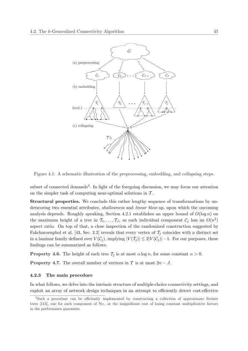
4.2. The k-Generalized Connectivity Algorithm 45
G
C1 J¡1C JCC2
T2T1 J¡1T JT
(a) preprocessing
(b) embedding
(c) collapsing
level l
R
lT |
Figure 4.1: A schematic illustration of the preprocessing, embedding, and collapsing steps.
subset of connected demands3. In light of the foregoing discussion, we may focus our attentionon the simpler task of computing near-optimal solutions in T .
Structural properties. We conclude this rather lengthy sequence of transformations by un-derscoring two essential attributes, shallowness and linear blow-up, upon which the oncominganalysis depends. Roughly speaking, Section 4.2.1 establishes an upper bound of O(log n) onthe maximum height of a tree in T1, . . . , TJ , as each individual component Cj has an O(n2)aspect ratio. On top of that, a close inspection of the randomized construction suggested byFakcharoenphol et al. [43, Sec. 2.2] reveals that every vertex of Tj coincides with a distinct setin a laminar family defined over V (Cj), implying |V (Tj)| ≤ 2|V (Cj)|−1. For our purposes, thesefindings can be summarized as follows.
Property 4.6. The height of each tree Tj is at most α log n, for some constant α > 0.
Property 4.7. The overall number of vertices in T is at most 2n− J .
4.2.3 The main procedure
In what follows, we delve into the intrinsic structure of multiple-choice connectivity settings, andexploit an array of network design techniques in an attempt to efficiently detect cost-effective
3Such a procedure can be efficiently implemented by constructing a collection of approximate Steiner
trees [113], one for each component of HT , at the insignificant cost of losing constant multiplicative factors
in the performance guarantee.
46 Chapter 4: k-Generalized Connectivity
partial solutions. With this objective in mind, we present a randomized bi-criteria heuristicfor connecting a substantial number of demands, while keeping the factor by which OPTT isexceeded within an acceptable magnitude. This result is formally described in the next theorem.
Theorem 4.8. There is a polynomial-time algorithm that finds, with constant probability, asubgraph H ⊆ T satisfying the following properties:
1. H connects Ω(k/ log n) demands in D.
2. The cost of H is O(n2/3 · polylog(n, k)) ·OPTT .
Needless to say, Theorem 4.8 allows us to validate the main result of this chapter, statingthat k-generalized connectivity can be approximated to within a factor of O(n2/3 ·polylog(n, k))by employing a polynomial-time Monte Carlo algorithm (see Theorem 4.1). To rigorouslyestablish the latter claim, our bi-criteria heuristic should be repeatedly applied O(log n log k)times, provided that its success probability is amplified in anticipation via O(log log n+log log k)independent repetitions.
Preliminaries. To avoid conflicting notation and terminology throughout this section, it wouldbe convenient to fix attention on a particular optimal forest F∗ ⊆ T . In adherence to customaryconventions, D(F∗) will stand for the collection of demands connected by F∗, noting that|D(F∗)| ≥ k. With respect to each demand (Si, Ti) ∈ D(F∗), we pick for purposes of analysisan ordered pair of representatives, Rep(Si, Ti) = (si, ti), such that F∗ contains the unique pathconnecting si ∈ Si and ti ∈ Ti. Now consider the assortment of vertex pairs Rep(Si, Ti) :(Si, Ti) ∈ D(F∗), whose lowest common ancestors might be scattered across different levels ofT1, . . . , TJ . However, since Property 4.6 places an upper bound of α log n on the height of eachtree Tj , there must be at least one level ` in which k/(α log n) or more lowest common ancestorsreside. For sake of simplicity, we designate the corresponding subset of demands by D(F∗|`),and assume without loss of generality that ` is known in advance.
Collapsing T1, . . . , TJ . Having this additional parameter at hand, the “upper part” of eachHST is pruned by eliminating all vertices in levels 1, . . . , `− 1, along with their incident edges.Furthermore, a conjoined tree T |` is assembled by unifying level ` vertices over all HSTs intoa super-root R, as shown in Figure 4.1, part (c). Consequently, the (not necessarily disjoint)paths connecting representatives of demands in D(F∗|`) currently constitute a single subtreeF∗|` ⊆ T |`, as their lowest common ancestors have just been incorporated into R. Clearly,c(F∗|`) ≤ c(F∗) = OPTT .
The subtree augmentation theorem. We proceed by admitting that the unification of alllevel ` vertices may lead to unexpected circumstances, in which merely identifying a subtreeH ⊆ T |` containing a path with one endpoint in s ∈ Si and another in t ∈ Ti does notautomatically mean that (Si, Ti) is connected in T . To better understand this statement, notethat when s and t reside in different HSTs, or when their lowest common ancestor appears ina level strictly lower than `, the unique s-t path in T |` is not induced by an original HST. Todefend against such a displeasing scenario, we define the `-restricted connectivity of H to bethe number of demands (Si, Ti) ∈ D for which there exist si ∈ Si ∩ V (H) and ti ∈ Ti ∩ V (H)whose lowest common ancestor in T is a level ` vertex. This measure will be abbreviated by
4.3. Proof of the Subtree Augmentation Theorem 47
RC`(H), noting that any subtree H ⊆ T |` can be easily translated to a forest in T of identicalcost, ensuring that RC`(H) demands are connected at the same time.
Having introduced this notation, we propose in Theorem 4.9 a randomized algorithm forextending any subtree H rooted at R to a new subtree H+, while insisting that the latter ischaracterized by a sufficiently large `-restricted connectivity or by a significantly larger vertexset. Even though one has no control over which of these potential outcomes materializes, thereis nevertheless a delicate trade-off between two contradicting objectives. More specifically, whena sufficiently large `-restricted connectivity is obtained, we guarantee that the marginal costof H+ can be upper bounded via an auxiliary parameter ψ(n), whose value will be determinedlater. In the opposite case, we ascertain an effective lower bound on the vertex set growth interms of ψ(n), while simultaneously incurring a negligible marginal cost. In light of the ratherintricate arguments utilized for establishing Theorem 4.9, we have chosen to present the finerdetails of its proof in Section 4.3.
Theorem 4.9. Let H ⊆ T |` be a subtree rooted at R. Then, with probability at least 1/4, wecan efficiently extend H to a subtree H+ satisfying at least one of the following properties:
1. RC`(H+) ≥ k/(6α log n) and c(H+) = c(H) + O(ψ(n) log n log2 k) ·OPTT .
2. |V (H+)| − |V (H)| ≥ ψ1/2(n) and c(H+) ≤ c(H) + OPTT .
Proof of Theorem 4.8. Starting with a trivial subtree H that consists of the singular super-root R, we repeatedly extend H by applying the subtree augmentation theorem as long asRC`(H) < k/(6α log n), not before amplifying its success probability in advance through O(log n)independent repetitions. With constant probability, in each step we either plug into H at leastψ1/2(n) new vertices, while incurring a marginal cost of at most OPTT , or discover that it al-ready satisfies RC`(H) ≥ k/(6α log n), paying a one-time penalty of O(ψ(n) log n log2 k)·OPTT .Therefore, to account for the overall cost of H, it remains to bound the maximum possi-ble number of iterations. For this purpose, we observe that since T |` consists of at most2n− J vertices (see Property 4.7), an `-restricted connectivity of Ω(k/ log n) is attained withind(2n − J)/ψ1/2(n)e iterations; otherwise, H is eventually augmented with strictly more than2n− J new vertices, which is obviously not a feasible turn of events. It follows that by settingψ(n) = n2/3, the suggested algorithm constructs a subtree whose overall cost is
c(H) = O
(n
ψ1/2(n)+ ψ(n) log n log2 k
)·OPTT = O
(n2/3 · polylog(n, k)
)·OPTT .
4.3 Proof of the Subtree Augmentation Theorem
In what follows, we provide a detailed proof of Theorem 4.9, not before encouraging the readerto consult Figure 4.2 while browsing through the forthcoming analysis. Prior to delving intotechnicalities, we point out that, as an immediate consequence of collapsing T1, . . . , TJ , thecollection of paths connecting representatives of demands in D(F∗|`) has been transfigured to
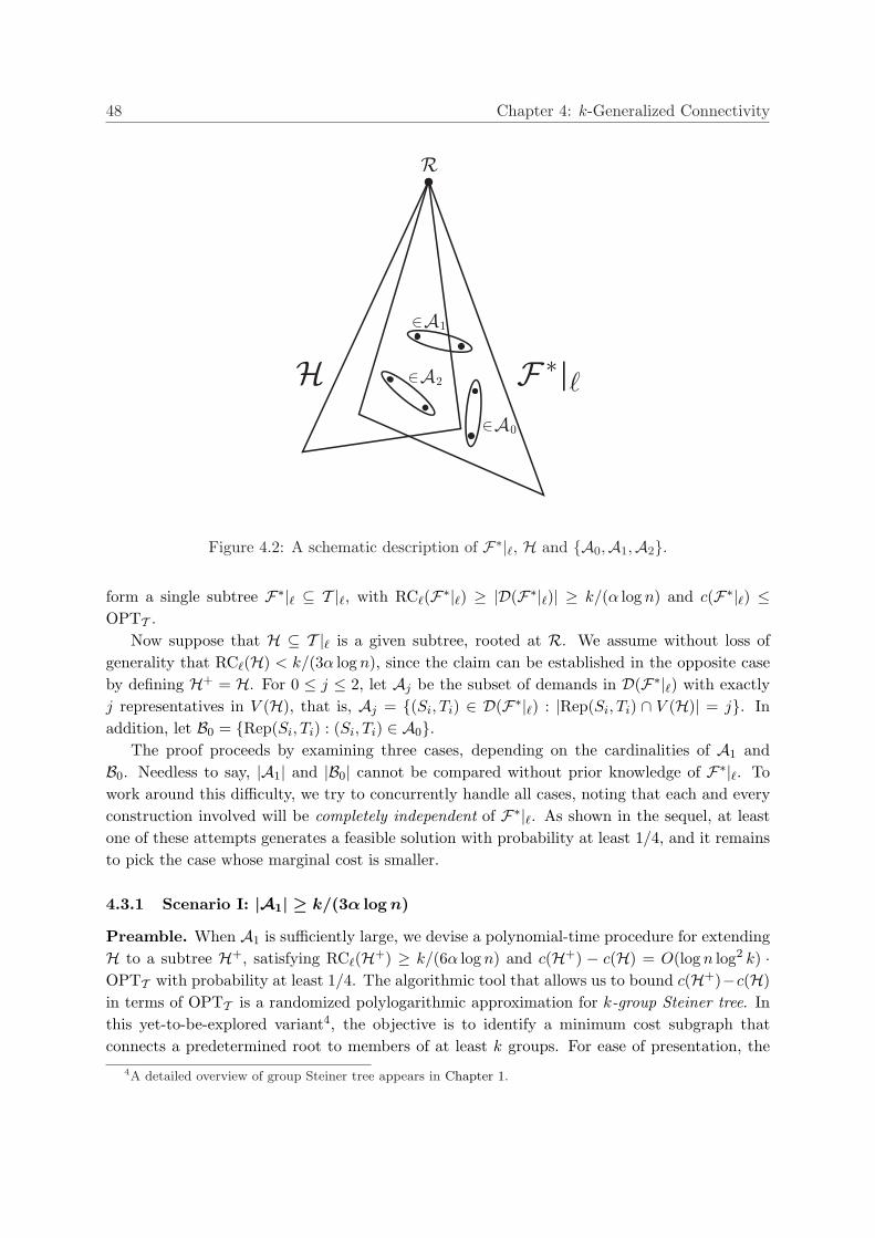
48 Chapter 4: k-Generalized Connectivity
R
H lF |*
0A2
2A2
1A2
Figure 4.2: A schematic description of F∗|`, H and A0,A1,A2.
form a single subtree F∗|` ⊆ T |`, with RC`(F∗|`) ≥ |D(F∗|`)| ≥ k/(α log n) and c(F∗|`) ≤OPTT .
Now suppose that H ⊆ T |` is a given subtree, rooted at R. We assume without loss ofgenerality that RC`(H) < k/(3α log n), since the claim can be established in the opposite caseby defining H+ = H. For 0 ≤ j ≤ 2, let Aj be the subset of demands in D(F∗|`) with exactlyj representatives in V (H), that is, Aj = (Si, Ti) ∈ D(F∗|`) : |Rep(Si, Ti) ∩ V (H)| = j. Inaddition, let B0 = Rep(Si, Ti) : (Si, Ti) ∈ A0.
The proof proceeds by examining three cases, depending on the cardinalities of A1 andB0. Needless to say, |A1| and |B0| cannot be compared without prior knowledge of F∗|`. Towork around this difficulty, we try to concurrently handle all cases, noting that each and everyconstruction involved will be completely independent of F∗|`. As shown in the sequel, at leastone of these attempts generates a feasible solution with probability at least 1/4, and it remainsto pick the case whose marginal cost is smaller.
4.3.1 Scenario I: |A1| ≥ k/(3α log n)
Preamble. When A1 is sufficiently large, we devise a polynomial-time procedure for extendingH to a subtree H+, satisfying RC`(H+) ≥ k/(6α log n) and c(H+) − c(H) = O(log n log2 k) ·OPTT with probability at least 1/4. The algorithmic tool that allows us to bound c(H+)−c(H)in terms of OPTT is a randomized polylogarithmic approximation for k-group Steiner tree. Inthis yet-to-be-explored variant4, the objective is to identify a minimum cost subgraph thatconnects a predetermined root to members of at least k groups. For ease of presentation, the
4A detailed overview of group Steiner tree appears in Chapter 1.
4.3. Proof of the Subtree Augmentation Theorem 49
proof of Theorem 4.10 is deferred to Section 4.4.
Theorem 4.10. When the underlying graph is a tree, there is a randomized polynomial-timealgorithm that constructs, with probability at least 1/4, a feasible k-group Steiner tree whose costis within a factor of O(log n log2 k) of optimal.
The algorithm. For simplicity of presentation, we assume that there are at least as manyS-represented A1-demands as there are T -represented ones; strictly speaking,
|(Si, Ti) ∈ A1 : V (H) ∩ Rep(Si, Ti) ∈ Si| ≥ |(Si, Ti) ∈ A1 : V (H) ∩ Rep(Si, Ti) ∈ Ti| .
With this assumption in mind, consider the following k-group Steiner tree instance:
1. For each demand (Si, Ti) ∈ D, we set up a corresponding group Gi ⊆ Ti, comprising ofall vertices ti ∈ Ti for which there exists si ∈ Si ∩ V (H) such that the lowest commonancestor of si and ti in T is a level ` vertex.
2. The goal is to connect the super-root R to members of at least k/(6α log n) groups.
Now let us focus on a particular S-represented A1-demand (Si, Ti), where Rep(Si, Ti) =(si, ti), si ∈ V (H), and ti /∈ V (H). When the group Gi corresponding to this demand isassembled, we inevitably have ti ∈ Gi, implying in retrospect that F∗|` is a subtree connectingRto a member of Gi. Since our initial assumption provides a lower bound of |A1|/2 ≥ k/(6α log n)on the number of such demands, one can safely argue that the k-group Steiner tree instanceunder consideration has a feasible solution of cost c(F∗|`) ≤ OPTT . Consequently, guided byTheorem 4.10, we obtain with probability at least 1/4 a subtree H ⊆ T |`, connecting R to atleast k/(6α log n) groups, with c(H) = O(log n log2 k) ·OPTT . As RC`(H ∪ H) ≥ k/(6α log n),the desired claim is derived by setting H+ = H ∪ H.
4.3.2 Scenario II: |B0| > ψ(n)
Preamble. The oncoming discussion will be devoted to communicating the finer details of apolynomial-time procedure for extending H to a subtree H+, satisfying |V (H+)| − |V (H)| ≥ψ1/2(n) and c(H+) − c(H) ≤ OPTT . Having stated this objective, our principal method forupper bounding c(H+) − c(H) depends upon a well-hidden similarity to the k-Steiner treeproblem, in which given an edge-weighted graph and a designated subset of terminal vertices, wewish to detect a minimum cost subgraph connecting a predetermined root to at least k terminals.It is worth noting that Chudak, Roughgarden and Williamson [35] suggested a constant-factorapproximation for the latter problem; however, rather than dealing with general networks, wemay restrict attention to tree graphs, collectively forming a tractable special case5.
The algorithm. We begin by considering the next k-Steiner tree instance:
1. The set of terminals is V (T |`) \ V (H).5When the underlying graph is acyclic, k-Steiner tree can be solved to optimality by means of dynamic
programming. We have chosen not to specify a polynomial-time implementation due to its fairly straightforward
description.
50 Chapter 4: k-Generalized Connectivity
2. The goal is to connect R to at least ψ1/2(n) terminals.
Since B0 consists of strictly more than ψ(n) representatives, each of which corresponds to adistinct vertex pair, it follows that F∗|` contains at least ψ1/2(n) vertices not belonging to H.This observation equivalently argues that the k-Steiner tree instance under consideration has afeasible solution of cost c(F∗|`) ≤ OPTT . Consequently, by applying an exact polynomial-timealgorithm, we acquire a subtree H ⊆ T |`, connecting R to at least ψ1/2(n) vertices other thanthose already spanned by H, with c(H) ≤ OPTT . Once again, the claim is derived by settingH+ = H ∪ H.
4.3.3 Scenario III: |A1| < k/(3α log n) and |B0| ≤ ψ(n)
Preamble. We conclude the proof of Theorem 4.9 by offering a polynomial-time procedurefor extending H to a subtree H+, satisfying RC`(H+) ≥ k/(3α log n) and c(H+) − c(H) =O(ψ(n) log k)·OPTT . Having introduced this final objective, our current approach for boundingthe overall augmentation cost makes use of an O(log k) approximation for partial set cover, dueto Slavık [116]. In the latter problem, given a weighted family of subsets defined over a finiteground set, the goal is to cover at least k elements by picking subsets of minimum total cost.
The algorithm. Noting that A0,A1,A2 is a partition of D(F∗|`) and |A2| ≤ RC`(H) <
k/(3α log n), we can lower bound the number of A0-demands right away by |D(F∗|`)| − |A1| −|A2| ≥ k/(3α log n). With this inequality in mind, consider the following partial set coverinstance:
1. The ground set of elements is D.
2. For each pair of vertices s, t whose lowest common ancestor in T is a level ` vertex, weset up a corresponding subset Q(s, t) ⊆ D, comprising of all demands (Si, Ti) for whichs ∈ Si and t ∈ Ti. The cost of picking Q(s, t) is identical to that of connecting s and t inT |`.
3. The goal is to cover at least k/(3α log n) elements.
We first assert that Q(Rep(Si, Ti)) : (Si, Ti) ∈ A0 is a feasible solution to the partial setcover instance in question, of cardinality |B0|. Furthermore, the combined cost of these subsetsis at most |B0| · OPTT ≤ ψ(n) · OPTT , since the unique path connecting Rep(Si, Ti) is asubgraph of F∗|`, for every (Si, Ti) ∈ A0. Consequently, by finishing off the partial coveringalgorithm of Slavık with proper subset-to-path translation, we identify a subtree H ⊆ T |`, withRC`(H) ≥ k/(3α log n) and c(H) = O(ψ(n) log k) · OPTT . The desired claim is derived bysetting H+ = H ∪ H.
4.4 Approximate k-Group Steiner Trees
The main result of this section is a constructive proof of Theorem 4.10, namely, a random-ized polynomial-time algorithm for approximating k-group Steiner tree to within a factor of
4.4. Approximate k-Group Steiner Trees 51
O(log n log2 k), provided that the underlying graph is a tree6. We remind the reader that suchinstances consist of an undirected tree T = (V, E) with non-negative edge costs specified byc : E → R+. An additional ingredient of the input is a collection of vertex sets G1, . . .Gt,interchangeably referred to as groups, and a predetermined root vertex R. The objective is toidentify a minimum cost subgraph that connects R to members of at least k groups.
Connecting a fixed proportion. To simplify upcoming analysis, we introduce an auxiliarysubroutine, the specifics of which are formally stated in Lemma 4.11. Roughly speaking, wedemonstrate how to manipulate the cut-covering relaxation of group Steiner tree, to effectivelycompete in bi-criteria fashion against any subtree that connects a fixed proportion of the givengroups.
Lemma 4.11. Let Tt/2 ⊆ T be a minimum cost subtree that connects R to members of at leastt/2 groups. Then, we can construct a subtree T ⊆ T satisfying with probability at least 1/2 thefollowing properties:
1. T connects R to members of at least t/3 groups.
2. c(T ) = O(log n log t) · c(Tt/2).
Proof. Consider the following linear program:
minimize∑
e∈E
c(e)xe (LPt/2)
subject tot∑
i=1
yi ≥ t/2
∑
e∈δ(U)
xe ≥ yi∀U ⊆ V, 1 ≤ i ≤ t :R ∈ U and Gi ⊆ V \ U
xe ≥ 0, 0 ≤ yi ≤ 1 ∀ e ∈ E, 1 ≤ i ≤ t
It is not difficult to verify that OPT(LPt/2) provides a lower bound on c(Tt/2). With thisobservation in mind, we compute an optimal fractional solution (x∗, y∗), noting that LPt/2
admits a polynomial-time separation oracle, as violated cuts can be efficiently detected byemploying a minimum cut procedure.
We proceed by applying the randomized algorithm of Garg et al. [58], to find an approximategroup Steiner tree, connecting R to members of each and every group Gi for which y∗i ≥ 1/4.Note that the number of such groups is at least t/3, since
t
2≤
t∑
i=1
y∗i =∑
i:y∗i ∈[1/4,1]
y∗i +∑
i:y∗i ∈[0,1/4)
y∗i ≤∣∣∣∣
i : y∗i ≥14
∣∣∣∣ +(
t−∣∣∣∣
i : y∗i ≥14
∣∣∣∣)· 14
,
or equivalently, |i : y∗i ≥ 1/4| ≥ t/3. Therefore, with probability at least 1/2 (see [58, Thm.4.1]), we obtain a tree T that satisfies the above-mentioned connectivity requirement, as well as
6While this restricted claim will be more than enough for our purposes, we remark that it can be easily
extended to general graphs via probabilistic embedding methods (see Section 4.1), at the cost of losing an
additional logarithmic factor.
52 Chapter 4: k-Generalized Connectivity
c(T ) = O(log n log t) ·OPT(LP1/4), where LP1/4 is defined by the following group Steiner treerelaxation:
minimize∑
e∈E
c(e)xe (LP1/4)
subject to∑
e∈δ(U)
xe ≥ 1∀U ⊆ V, 1 ≤ i ≤ t :
y∗i ≥ 1/4, R ∈ U and Gi ⊆ V \ U
xe ≥ 0 ∀ e ∈ E
We conclude by observing that OPT(LP1/4) ≤ 4 · OPT(LPt/2), since 4x∗ is a feasible solutionto LP1/4.
The k-group Steiner tree algorithm. In what follows, T designates the subtree we con-struct, G denotes the collection of yet-to-be-connected groups, and k stands for the residualconnectivity requirement.
1. Initialize T ← ∅, G ← G1, . . . ,Gt and k ← k.
2. While k > 650
(a) Randomly partition the groups in G to k clusters C1, . . . , Ck.
(b) Construct d8 log log ke random trees by independently applying Lemma 4.11 witha modified collection of groups, in which all groups residing in each cluster Ci aretemporarily merged into a single group.
(c) Pick a tree T + of minimum cost, over all trees created in step 2b that connect atleast k/3 groups in G.
(d) Set T ← T ∪ T +. Update G and k accordingly.
3. Compute a minimum cost tree T + connecting R to members of at least k groups in G bymeans of exhaustive search7, and return T ∪ T +.
Analysis. Let T ∗ ⊆ T be an optimal solution to the k-group Steiner tree instance underconsideration; in other words, T ∗ is a minimum cost tree that connects R to members of atleast k groups. We say that a particular iteration of step 2 is successful when it simultaneouslysatisfies the following conditions:
1. At least one of the d8 log log ke newly formed trees connects R to k/3 or more groups inG.
2. c(T +) = O(log n log k) · c(T ∗).Otherwise, this iteration is said to have failed. We remark that a failure-free termination of ouralgorithm guarantees O(log k) iterations, each incurring a marginal cost of O(log n log k) ·c(T ∗).Consequently, Theorem 4.10 can be established by arguing that the probability of ever meetinga failure does not exceed 3/4, which is asserted through the next sequence of lemmas.
7Since the underlying graph is a tree, this task can be accomplished by guessing the optimal members in
O(n650) time, and picking an edge-minimal subtree that connects them to R.
4.4. Approximate k-Group Steiner Trees 53
Lemma 4.12. Let Z denote the number of empty bins, when n balls are placed independentlyand uniformly at random in n bins. Then, Pr [Z > n/2] ≤ 2 exp(−n/200).
Proof. Using techniques based on martingale analysis, Kamath et al. [83, Thm. 2] providedan upper bound on the probability that Z deviates from its expectation µ, stating that for anyθ > 0,
Pr [|Z − µ| > θµ] ≤ 2 exp(−θ2µ2(n− 1/2)
n2 − µ2
).
Since µ = n(1− 1/n)n, we have
Pr[Z >
n
2
]≤ Pr
[|Z − µ| > n
2− µ
]≤ Pr
[|Z − µ| > n
10µ· µ
]≤ 2 exp
(− n2(n− 1/2)
100(n2 − µ2)
)
≤ 2 exp(−n− 1/2
100
)≤ 2 exp
(− n
200
),
where the second inequality holds since µ ≤ n/e, and the third inequality follows from applyingthe previously mentioned upper bound with θ = n/(10µ).
Lemma 4.13. A single iteration fails with probability at most 2 exp(−k/200) + 1/(8 log k).
Proof. Let us examine a random partition of the groups in G to k clusters. Since T ∗ spansat least k groups other than those already connected by T , Lemma 4.12 implies that withprobability at least 1−2 exp(−k/200), no less than k/2 of the clusters C1, . . . , Ck contain a groupwhich is connected by T ∗ but not by T . In this case, Lemma 4.11 guarantees that each randomtree connects R to at least k/3 new groups and carries a total cost of O(log n log k) · c(T ∗),with probability at least 1/2. Noting that d8 log log ke trees are constructed, the current failureprobability cannot exceed
2 exp(− k
200
)+
(12
)d8 log log ke≤ 2 exp
(− k
200
)+
18 log k
,
where the above inequality holds since 8 log log k ≥ log(8 log k), as k ≥ 3, with room to spare.
Lemma 4.14. All iterations are successful with probability at least 1/4.
Proof. Let I be the number of step 2 iterations. For 1 ≤ j ≤ I, let kj denote the residualconnectivity requirement at the beginning of iteration j. By Lemma 4.13, iteration j fails withprobability at most 2 exp(−kj/200) + 1/(8 log k). Furthermore, when iteration j is successful,we have kj+1 ≤ 2kj/3. It follows that the overall failure probability is at most
I∑
j=1
(2 exp
(− kj
200
)+
18 log k
)≤ 2
I∑
j=1
exp(−(2/3)jk
200
)+
I8 log k
.
We first observe that I/(8 log k) ≤ 1/4, since I ≤ dlog3/2(k/650)e; otherwise (2/3)I−1k ≤650, and iteration I should never have taken place. We conclude the proof by showing that
54 Chapter 4: k-Generalized Connectivity
∑Ij=1 exp(−(2/3)jk/200) ≤ 1/4. For this purpose, let aj = exp(−(2/3)jk/200). Note that
(2/3)I−1k > 650 implies aI ≤ 1/8. In addition, since maxj aj = aI , we have
aj = exp(−(2/3)jk
200
)=
(exp
(−(2/3)j+1k
200
))3/2
= a3/2j+1 ≤ aj+1 · √aI .
Therefore,
I∑
j=1
exp(−(2/3)jk
200
)=
I∑
j=1
aj ≤ aI∞∑
j=0
(√
aI)j =
aI1−√aI
≤ 1/81−
√1/8
<14
.
4.5 Concluding Remarks
|D|-dependent bound. As mentioned in Section 4.1, an aspiration to arrive at singletondemands by introducing zero-cost arcs joining vertices in Si to a super-source and vertices inTi to a super-sink, results in instances of directed Steiner network. It is worth noting that thecurrently best approximation guarantee for the latter problem has recently been improved byChekuri, Even, Gupta and Segev [31], who established an upper bound of O(|D|1/2+ε) throughLP-based methods (see Chapter 2). Nevertheless, we can show that by embedding the originalmetric into an O(nε)-HST and exploiting certain structural properties achieved by the above-mentioned transformation, an identical approximation ratio can be attained for k-generalizedconnectivity via an efficient combinatorial approach.
Restricted linking. Throughout this chapter, it was convenient to presume that a particulardemand (Si, Ti) may be connected by linking any vertex in Si to any vertex in Ti. However,numerous practical applications motivate a more realistic setting, in which each demand is as-sociated with a predetermined list Li ⊆ Si × Ti of allowed linking options. We remark that byslightly remodeling a label-cover based construction due to Dodis and Khanna [38, Thm. 4.2],this newly defined variant turns up as being Ω(2log1−ε n)-hard, unless NP ⊆ TIME(npolylog(n)).On the other hand, a careful examination of Sections 4.2 and 4.3 reveals that our algorithmcan be easily adapted to approximate link-restricted connectivity without any loss in the per-formance guarantee.
Derandomization? While probabilistic embeddings into tree metrics have played an instru-mental role in attacking numerous network design problems over the last decade, many HST-based algorithms were eventually derandomized (see, for example, [26, 27, 32, 43]). Being anincreasingly-popular research field, derandomization techniques in this context often operate byadopting the method of pessimistic estimators, by exercising a modified region growing scheme,or by exploiting ad-hoc arguments. Recalling that our approach employs component-wise em-bedding into an arbitrary collection of interrelated HSTs, it would be interesting to investigatewhether one of these techniques offers a way of achieving a deterministic derivative without asignificant deterioration in the approximation ratio.
Chapter 5
A Unified Approach to
Approximating Partial Covering
Problems
The main result of this chapter can be summarized as follows.
Theorem 5.1. Let I be a generalized partial cover instance defined on an underlying weightedset system (U,S, c), and suppose that (U,S, c) ∈ Ir for some r ≥ 1. Then, for any ε > 0, wecan find a feasible solution to I whose cost is at most (4/3+ ε)r times the optimum, within timepolynomial in |S|1/ε and the input length of I.
5.1 The Suggested Method
5.1.1 Technical overview
To simplify the presentation, it is convenient to state our approach in terms of the Lagrangianrelaxation technique. Here is a rough outline of how the proof of Theorem 5.1 will proceed. Webegin by formulating the generalized partial cover problem as an integer program. Next, wedualize the complicating constraint that places a lower bound of P on the total profit. Moreprecisely, we lift this constraint to the objective function multiplied by an auxiliary variableλ, and obtain its corresponding Lagrangian relaxation. For any fixed λ ≥ 0, the new programdescribes, up to a constant term, a prize-collecting set cover instance with non-uniform penalties.We now conduct a binary search, using the r-LMP prize-collecting algorithm as a subroutine,to find sufficiently close λ1 ≥ λ2 that satisfy: For λ1, the algorithm constructs a solution S1 ⊆ Ssuch that the total profit of the elements covered by S1 is at least P ; For λ2, it constructs asolution S2 ⊆ S with a total profit of at most P .
Although we can exploit the r-LMP property to show that the cost of S2 is within factor r
of optimum, this solution is not necessarily feasible. The situation is quite the opposite withrespect to S1, which is a feasible solution whose cost may be arbitrarily large. Having observedthese facts, we create an additional feasible solution S3 by augmenting S2 with a carefully chosensubset of S1. The cost of this subset is bounded by extending the arguments used by Levin
55
56 Chapter 5: A Unified Approach to Approximating Partial Covering Problems
and Segev [90] and independently by Golovin, Nagarajan and Singh [64] for approximating thek-multicut problem. Finally, we establish Theorem 5.1 by proving that the cost of the cheaperof S1 and S3 is at most (4/3 + ε)r times the cost of an optimal solution.
5.1.2 Designing LMP algorithms
The performance guarantee of our algorithm, as stated in Theorem 5.1, depends on the ex-istence of an LMP prize-collecting algorithm for a given covering problem. Indeed, this de-pendence appears to be the primary factor limiting the employment of Lagrangian relaxationsin most problems of interest. The latter drawback was pointed out by Chudak, Roughgardenand Williamson [35], who asked whether it is possible to devise more general variants of theLagrangian relaxation framework that apply to a broader class of problems. We answer thisquestion in the affirmative, by developing prize-collecting algorithms with the LMP property forsome of the most fundamental integer covering problems. These results, along with a detaileddescription of previous work, are formally presented in Sections 5.3 and 5.4.
Even though the algorithms we suggest are rather problem-specific, a principal idea isbrought into play in the majority of the applications we consider. Intuitively, ensuring aninequality of the form C + rΠ ≤ r · OPT means that the solutions we construct are efficientwhen it comes to paying penalties. Technically speaking, such a solution guarantees an r-approximation even when all penalties are inflated by a factor of r. Given a prize-collectinginstance, our general approach is to create a new instance of the underlying full coverage prob-lem, in which penalties are represented as alternative covering options with inflated costs. Wethen propose a tailor-made algorithm, or modify the analysis of an existing one, to find a solu-tion to the resulting instance, and show that it can be interpreted as an approximate solutionto the original problem.
5.2 The Generalized Partial Cover Algorithm
The main result of this section is a constructive proof of Theorem 5.1. Recall that a generalizedpartial cover instance I is defined with respect to an underlying weighted set system, consistingof a ground set U and a family of subsets S ⊆ 2U , where each S ∈ S has a cost c(S). Theadditional ingredients of I are profits p(e), specified for each element e ∈ U , and a requirementparameter P . Now suppose that (U,S, c) ∈ Ir for some r ≥ 1, meaning that there is an r-LMPalgorithm A for all prize-collecting instances (U,S, c, π), π : U → Q+.
5.2.1 Preliminaries
The method we suggest and its analysis will be based on a natural integer programming formu-lation of the generalized partial cover problem. In the following, let Se ⊆ S be the collection ofsets that contain e ∈ U , and let PU =
∑e∈U p(e).
minimize∑
S∈Sc(S)xS (GC)
subject to∑
S∈Se
xS + ze ≥ 1 ∀ e ∈ U (5.1)
5.2. The Generalized Partial Cover Algorithm 57
∑
e∈U
p(e)ze ≤ PU − P (5.2)
xS , ze ∈ 0, 1 ∀S ∈ S, e ∈ U (5.3)
In this formulation, the variable xS indicates whether we pick the set S, whereas ze indicateswhether the element e is uncovered. Constraint (5.1) guarantees that we either pick at leastone set that contains e, or specify that this element is uncovered by setting ze = 1. Constraint(5.2) forces any feasible solution to cover elements with a total profit of at least P .
Essential to the subsequent analysis will be the fact that the LP-relaxation of (GC), ob-tained by replacing constraint (5.3) with xS ≥ 0 and ze ≥ 0, has an integrality gap of O(r).Unfortunately, this prerequisite is not satisfied even in the case of unit profits, as the nextexample illustrates. Consider an instance in which the ground set U consists of n elements, andthe family S contains a single set S = U with cost n. When we are required to cover at leastone element, the integral optimum is clearly n. However, by setting xS = 1/n and ze = 1− 1/n
for every e ∈ U , we define a feasible fractional solution whose cost is 1. This example, as wellas additional constructions of similar nature, demonstrate that an unbounded integrality gapmay arise whenever a small number of sets in the optimal solution contribute a large fractionof its cost.
Therefore, an inevitable part of our algorithm is a preprocessing step in which, given a fixedaccuracy parameter ε > 0, we “guess” the b1/εc most expensive sets in the optimal solution,whose cost we denote by OPT. More precisely, we enumerate all O(|S|1/ε) subsets S ′ ⊆ Sof cardinality at most b1/εc, test each such subset as the correct guess, and return the bestsolution we find. For a given subset S ′, we include it as part of the solution to be constructed,eliminate the sets in S ′ from S, remove all covered elements from U and from the remainingsets, and update the profit requirement. Any set whose cost is greater than minS∈S′ c(S) is alsoeliminated. Consequently, the cost of each remaining set is at most ε ·OPT.
In the remainder of this section we will bypass the preprocessing step, and assume that themaximum cost of a set in S is at most ε · OPT. For ease of presentation, we also assume thatc(S) > 0 for every S ∈ S and that p(e) > 0 for every e ∈ U , since zero-cost sets can be pickedin advance and zero-profit elements can be discarded.
5.2.2 Obtaining S1 and S2
We now dualize the profit constraint (5.2), and lift it to the objective function multiplied byλ ≥ 0. The resulting Lagrangian relaxation is:
LR(λ)= minimize∑
S∈Sc(S)xS + λ
(∑
e∈U
p(e)ze − (PU − P )
)
subject to∑
S∈Se
xS + ze ≥ 1 ∀ e ∈ U
xS , ze ∈ 0, 1 ∀S ∈ S, e ∈ U
We remark that, excluding the constant term of −λ(PU − P ) in the objective function, LR(λ)is an integer programming formulation of the prize-collecting set cover problem, in which each
58 Chapter 5: A Unified Approach to Approximating Partial Covering Problems
element e ∈ U is associated with a penalty λp(e). We refer to this instance as Iλ, and useOPT(Iλ) to denote its optimum value. It is not difficult to verify that LR(λ) = OPT(Iλ) −λ(PU −P ) is at most OPT for any λ ≥ 0, by observing that an optimal solution to (GC) is alsoa feasible solution to LR(λ), whose cost is at most OPT.
Since the underlying weighted set system of Iλ is identical to that of I, we may apply theprize-collecting algorithm A to approximate Iλ. Let xλ indicate which sets in S were picked bythe algorithm, and let zλ indicate which elements were left uncovered. In terms of (xλ, zλ), ther-LMP property of A is equivalent to
∑
S∈Sc(S)xλ
S + r∑
e∈U
λp(e)zλe ≤ r ·OPT(Iλ) , (5.4)
an inequality that, in particular, leads to the following observation.
Lemma 5.2. When λ > (∑
S∈S c(S))/mine∈U p(e), the solution (xλ, zλ) covers all elements.On the other hand, (x0, z0) does not cover any element.
Proof. Let λ > (∑
S∈S c(S))/mine∈U p(e), and suppose that there is an element e ∈ U forwhich zλ
e = 1, that is, e is not covered by any set the algorithm A picks when we approximateIλ. Then (xλ, zλ) no longer satisfies inequality (5.4), as
∑
S∈Sc(S)xλ
S + r∑
e∈U
λp(e)zλe ≥ rλp(e) > r
p(e)mine∈U p(e)
∑
S∈Sc(S) ≥ r
∑
S∈Sc(S) ≥ r ·OPT(Iλ) ,
where the last inequality holds since S is a feasible solution to Iλ.Now let λ = 0, and note that each element of the instance I0 has a zero penalty. Therefore,
by deciding not to pick any set and instead pay all penalties we obtain a feasible solution withzero cost, implying that OPT(I0) = 0. Since (x0, z0) satisfies inequality (5.4), it follows thatthis solution cannot pick any set, as all sets in S have strictly positive costs by assumption.
This observation allows us to conduct a binary search, consisting of a polynomially-boundednumber of calls to the prize-collecting algorithm A, as a result of which we find λ1 ≥ λ2 thatsatisfy:
1. λ1 − λ2 ≤ εcmin/PU , where cmin = minS∈S c(S) > 0.
2. The elements covered by (xλ1 , zλ1) have a total profit of P1 ≥ P , and at the same timethose covered by (xλ2 , zλ2) have a total profit of P2 ≤ P .
For ease of notation, we designate by S1 and S2 the subsets of S that were picked by thesolutions (xλ1 , zλ1) and (xλ2 , zλ2), respectively. Without loss of generality, P1 > P , or otherwiseS1 is already a feasible solution whose cost is at most r ·LR(λ1) ≤ r ·OPT. Similarly, we assumethat P2 < P . The analysis of our algorithm crucially depends on the next lemma, which is aconsequence of the r-LMP property.
Lemma 5.3. Let α = (P −P2)/(P1−P2) ∈ (0, 1). Then, αc(S1)+(1−α)c(S2) ≤ r(1+ ε)OPT.
5.2. The Generalized Partial Cover Algorithm 59
Proof. By combining inequality (5.4) with the fact that LR(λ) = OPT(Iλ)−λ(PU−P ) ≤ OPTfor every λ ≥ 0, we have
c(S1) =∑
S∈Sc(S)xλ1
S
≤ r
(OPT(Iλ1)− λ1
∑
e∈U
p(e)zλ1e
)
= r (OPT(Iλ1)− λ1 (PU − P1))
= r(LR(λ1) + λ1(P1 − P ))
≤ r(OPT + λ1(P1 − P )) . (5.5)
A similar argument shows that c(S2) ≤ r(OPT + λ2(P2 − P )). Therefore,
αc(S1) + (1− α)c(S2) ≤ αr(OPT + λ1(P1 − P )) + (1− α)r(OPT + λ2(P2 − P ))
≤ r ·OPT + αr
(λ2 +
εcmin
PU
)(P1 − P ) + (1− α)rλ2(P2 − P )
= r ·OPT + rλ2 (α(P1 − P ) + (1− α)(P2 − P )) + rαεcmin · P1 − P
PU
≤ r ·OPT + rεcmin
≤ r(1 + ε)OPT .
The second inequality follows from observing that P1 > P and λ1 ≤ λ2 + εcmin/PU . The thirdinequality holds since α(P1 − P ) + (1− α)(P2 − P ) = 0, α < 1 and P1 − P ≤ PU .
5.2.3 Composing an additional solution
Up until now, the only feasible solution we have at our possession is S1, as this subset of Scovers elements with an overall profit of P1 > P . Inequality (5.5) places an upper bound ofr · OPT + rλ1(P1 − P ) on the cost of S1. However, the latter term may be arbitrarily largein comparison to OPT, implying that S1 cannot approximate the instance I by itself. Thesituation is quite the opposite with respect to S2: Although this solution covers elements withan insufficient profit of P2 < P , a similar bound of r ·OPT + rλ2(P2 − P ) on its cost actuallyyields the inequality c(S2) ≤ r ·OPT, since in this case rλ2(P2 − P ) ≤ 0.
At this point, we are concerned with creating an additional feasible solution S3, by aug-menting S2 with a carefully chosen subset S ′ ⊆ S1. To attain feasibility, we must ensure thatof the elements that were left uncovered by S2, a subcollection with a total profit of at leastP − P2 is covered by S ′. We construct this augmenting subset as follows. Let U ′ ⊆ U be thecollection of elements that are covered by S1 but not by S2. We assign each element e ∈ U ′ toan arbitrary set in S1 \ S2 that contains it, and denote by ϕ(S) the total profit of the elementsassigned to S. Without loss of generality, we assume that S1 \ S2 = S1, . . . , Sk, where thesesets are indexed by non-decreasing order of the ratio c(Si)/ϕ(Si). Finally, let S ′ = S1, . . . , Sq,where q is the minimal index for which
∑qi=1 ϕ(Si) ≥ P − P2. Note that such an index exists,
since∑k
i=1 ϕ(Si) ≥ P1 − P2 and P1 > P . The next lemma bounds the cost of S3 = S2 ∪ S ′.Lemma 5.4. c(S3) ≤ c(S2) + αc(S1 \ S2) + ε ·OPT.
60 Chapter 5: A Unified Approach to Approximating Partial Covering Problems
Proof. By assumption, the cost of each set in S is at most ε · OPT. Therefore, it is suffi-cient to prove that c(S ′ \ Sq) =
∑q−1i=1 c(Si) ≤ αc(S1 \ S2). To this end, consider a random
variable K that takes the values 1, . . . , k, such that Pr [K = i] = ϕ(Si)/∑k
l=1 ϕ(Sl), and letR = c(SK)/ϕ(SK). Since the sets in S1 \S2 are indexed by non-decreasing order of c(Si)/ϕ(Si),we have E [R|1 ≤ K ≤ q − 1] ≤ E [R]. As α = (P − P2)/(P1 − P2), this inequality implies∑q−1
i=1 c(Si) ≤ αc(S1 \ S2), since
E [R] =k∑
i=1
c(Si)ϕ(Si)
· ϕ(Si)∑kl=1 ϕ(Sl)
=1∑k
l=1 ϕ(Sl)
k∑
i=1
c(Si) ≤ 1P1 − P2
c(S1 \ S2)
and
E [R|1 ≤ K ≤ q − 1] =q−1∑
i=1
c(Si)ϕ(Si)
· ϕ(Si)∑q−1l=1 ϕ(Sl)
=1∑q−1
l=1 ϕ(Sl)
q−1∑
i=1
c(Si) ≥ 1P − P2
q−1∑
i=1
c(Si) .
The last inequality holds since∑q−1
l=1 ϕ(Sl) < P − P2, by the minimality of q.
5.2.4 Deriving the approximation factor
We now conclude the proof of Theorem 5.1, by demonstrating that the cost of the cheaper ofS1 and S3 is within factor (4/3 + O(
√ε))r of optimum. An appropriate choice of ε restores the
original form of the theorem.
Lemma 5.5. minc(S1), c(S3) ≤ (4/3 + O(√
ε))r ·OPT.
Proof. To simplify the analysis, we begin by introducing a new parameter, β = c(S2)/OPT ∈[0, r], and bound the cost of S1 and S3 in terms of OPT, α and β. We first observe that
c(S1) =αc(S1)
α≤ r(1 + ε)OPT− (1− α)c(S2)
α=
r(1 + ε)− (1− α)βα
OPT ,
where the first inequality follows from Lemma 5.3, and the last equation is obtained by substi-tuting c(S2) = β ·OPT. In addition, Lemma 5.4 implies that
c(S3) ≤ c(S2) + αc(S1 \ S2) + ε ·OPT
≤ (1− α)c(S2) + αc(S1) + αc(S2) + ε ·OPT
≤ r(1 + ε)OPT + αc(S2) + ε ·OPT
= (r(1 + ε) + αβ + ε)OPT ,
where the third inequality and the last equation follow from Lemma 5.3 and the definition ofβ, respectively. Finally, we bound the resulting approximation factor by considering the worstpossible choice for the parameters α and β, to conclude that
minc(S1), c(S3) ≤ min
r(1 + ε)− (1− α)βα
, r(1 + ε) + αβ + ε
OPT
≤ maxα∈(0,1)β∈[0,r]
min
r(1 + ε)− (1− α)βα
, r(1 + ε) + αβ
OPT + ε ·OPT
5.3. Applications 61
=(
43
+ O(√
ε))
r ·OPT .
The last equation is proved in Lemma 5.6.
Lemma 5.6.
maxα∈(0,1)β∈[0,r]
min
r(1 + ε)− (1− α)βα
, r(1 + ε) + αβ
=
(43
+ O(√
ε))
r .
Proof. Suppose that α ≤ √ε. In this case, the claim easily follows by observing that for
any choice of β ∈ [0, r] we have r(1 + ε) + αβ ≤ r(1 + ε) +√
εr = (1 + O(√
ε))r. We nowconsider the case α >
√ε. For fixed α ∈ (
√ε, 1), let fα(β) = (r(1 + ε) − (1 − α)β)/α and
gα(β) = r(1 + ε) + αβ. Note that fα and gα are monotone-decreasing and monotone-increasinglinear functions of β, respectively. In addition, these functions intersect in the interval [0, r],since fα(0) = (1 + ε)r/α > (1 + ε)r = gα(0) and fα(r) = (1 + ε/α)r < (1 + ε + α)r = gα(r),where the middle inequality holds since α >
√ε. Therefore, maxβ∈[0,r] minfα(β), gα(β) is
attained at this intersection point, which is β∗ = (1− α2/(1− α + α2))(1 + ε)r, and its value isfα(β∗) = gα(β∗) = (1 + ε)r/(1− α + α2). The value of α that maximizes the last expression isα∗ = 1/2. It follows that β∗ = 2(1 + ε)r/3 and
maxα∈(
√ε,1)
β∈[0,r]
minfα(β), gα(β) =43(1 + ε)r =
(43
+ O(√
ε))
r .
5.3 Applications
In what follows, we demonstrate the applicability of our method on a diverse collection ofcovering problems, which is by no means exhaustive. Rather, the problems we have chosen tostudy are only meant to illustrate that the LMP property is applicable in a variety of settings.For the majority of these problems, we propose the first algorithm that approximates theirgeneralized partial cover version. For others, our algorithms offer approximation guaranteesthat compete with the currently best known results.
5.3.1 Set cover, in terms of ∆
Kearns [84, Thm. 5.15] seems to have been the first to study the partial cover problem, showingthat the greedy set cover algorithm [82, 92] can be adapted to provide an approximation factorof 2H(|U |) + 3. A slightly different algorithm was suggested by Slavık [116], who obtaineda factor of H(min∆, k), where ∆ is the maximum size of a set in S and k is the coveragerequirement. We remark that the partial cover problem contains set cover as a special case,implying that it cannot be approximated within a factor of (1− ε) ln |U | for any ε > 0, unlessNP ⊂ TIME(nO(log log n)) [44].
To the best of our knowledge, the greedy heuristic has not been studied in the contextof generalized partial cover, and in fact no algorithm is currently known for this problem.In Section 5.4.1 we prove that every weighted set system (U,S, c) is in IH(∆), where ∆ =maxS∈S |S|. The next theorem follows.
62 Chapter 5: A Unified Approach to Approximating Partial Covering Problems
Theorem 5.7. The generalized partial set cover problem can be approximated within a factorof (4/3 + ε)H(∆), for any fixed ε > 0.
5.3.2 Set cover, in terms of f
Let fe be the number of sets in S that contain the element e ∈ U ; fe is also known as thefrequency of e. A recent line of work, that was initiated by Bshouty and Burroughs [23] andHochbaum [78] in the context of partial vertex cover, is approximating partial cover in terms off , the maximum frequency of any element. Based on the local-ratio method, Bar-Yehuda [14]devised an algorithm for generalized partial cover whose approximation guarantee is f , a resultthat was independently obtained by Fujito [50] using a prima-dual algorithm. Gandhi, Khullerand Srinivasan [54] achieved a similar ratio for partial cover.
The main result of Section 5.4.2 is a combinatorial f -LMP algorithm for the prize-collectingset cover problem, showing that every weighted set system (U,S, c) is in If , where f =maxe∈U fe. Combined with Theorem 5.1, this result allows us to approximate the general-ized partial set cover problem within a factor of (4/3 + ε)f , which is slightly worse than thecurrently best.
5.3.3 Laminar cover
Let G = (V,E) be an undirected graph, in which each edge e ∈ E has a non-negative costc(e), and let F = V1, . . . , Vk ⊆ 2V be a laminar family of vertex sets, meaning that Vi ∩ Vj ∈∅, Vi, Vj for every i 6= j. We say that an edge e covers Vi if it has exactly one endpoint in Vi.The objective is to find a minimum cost set of edges that collectively cover all sets in F . Notethat every instance of this problem induces a weighted set system (F ,S, c), where for each edgee ∈ E there is an analogous subset Se ∈ S, consisting of all vertex sets Vi ∈ F covered by e.Laminar cover can be approximated by applying various techniques, most of which actually dealwith the more general tree augmentation problem, and produce solutions whose cost is withinfactor 2 of optimum. We refer the reader to a short survey of these results [41, Sec. 1]. For theunweighted case, Nagamochi [98] proposed a (1.875 + ε)-approximation for any fixed ε > 0, aratio that was later improved to 3/2 by Even, Feldman, Kortsarz and Nutov [41].
In the generalized partial laminar cover problem, each Vi ∈ F is associated with a profitp(Vi). The goal is to identify a minimum cost set of edges E′ ⊆ E such that the overall profitof the sets in F covered by E′ is at least P , a specified profit bound. We are not aware of anyapproximability result for this problem, even for the seemingly simple case of unit profits. InSection 5.4.3 we prove that (F ,S, c) ∈ I2 for every weighted set system induced by a laminarcover instance, to obtain the following theorem.
Theorem 5.8. The generalized partial laminar cover problem can be approximated within afactor of 8/3 + ε, for any fixed ε > 0.
5.3.4 Totally unimodular cover and k-interval cover
The element-set incidence matrix MSU of a set system (U,S) has a row for every element e ∈ U
and a column for every set S ∈ S; its entry in row e and column S is 1 when e ∈ S and 0
5.3. Applications 63
otherwise. Totally unimodular cover (TUC) is a special case of the set cover problem in whichMS
U is totally unimodular, that is, every square submatrix of this matrix has determinant0, 1 or −1. We remark that although TUC is known to have integral LP solutions (see, forexample, [37, Sec. 6.5]), this property does not extend to its partial covering version, whichhas not been explicitly studied yet. A particularly interesting problem captured by the lattervariant is partial bipartite vertex cover: While the approximability of the unit-profit case is stillopen, arbitrary profits render the problem NP-hard, since it generalizes minimum knapsackeven when the given graph is a star. We omit the straightforward reduction.
As illustrated in Section 5.4.2, the prize-collecting set cover problem can be formulated asan integer program whose constraint matrix is [MS
U , I]. Simple linear algebra arguments showthat whenever MS
U is totally unimodular then so is [MSU , I], implying that we obtain a 1-LMP
algorithm by solving prize-collecting TUC to optimality as a linear program. The next theoremfollows.
Theorem 5.9. The generalized partial TUC problem can be approximated within a factor of4/3 + ε, for any fixed ε > 0.
We say that MSU is a k-interval matrix if it contains at most k blocks of consecutive 1’s
in each row. The k-interval cover problem (k-IC) is a special case of set cover in which MSU
is a k-interval matrix. In Section 5.4.4 we present a k-LMP rounding algorithm for the prize-collecting k-IC problem, that makes use of our 1-LMP algorithm for the corresponding variantof totally unimodular cover. We derive the following result as a corollary of Theorem 5.1.
Theorem 5.10. The generalized partial k-IC problem can be approximated within a factor of(4/3 + ε)k, for any fixed ε > 0.
This provides, for instance, the first algorithm that approximates partial rectangle stabbingin Rd, noting that the resulting factor of (4/3 + ε)d nearly matches the d-approximation ofGaur, Ibaraki and Krishnamurti [61] for the full coverage version of this problem. In addition,we obtain an alternative, albeit non-combinatorial, (4/3 + ε)f -approximation for partial setcover with maximum element frequency f .
5.3.5 Edge cover
Given an undirected graph G = (V, E) with non-negative edge costs, edge cover is the problemof finding a minimum cost set of edges that contains at least one edge incident to each vertex.Clearly, this problem is equivalent to the special case of set cover in which each subset consistsof exactly two elements. We note that edge cover is actually a matching problem in disguise,implying its polynomial time solvability [39, 97]. Plesnık [105] proved that unit-profit partialedge cover, which is also known as the k-edge cover problem, can be solved to optimality byreducing it to standard edge cover. However, when arbitrary profits are allowed, this problembecomes NP-hard, as it generalizes minimum knapsack. Since Parekh [103, Sec. 2.3] suggesteda polynomial-time algorithm for prize-collecting edge cover, we obtain the following theorem.
Theorem 5.11. Generalized partial edge cover can be approximated within a factor of 4/3 + ε,for any fixed ε > 0.
64 Chapter 5: A Unified Approach to Approximating Partial Covering Problems
5.3.6 Multicut
On trees. The input to this problem consists of an edge-weighted tree T = (V,E) and acollection of k distinct pairs of vertices, s1, t1, . . . , sk, tk. The objective is to find a minimumcost set of edges whose removal from T disconnects each of the given pairs. It is important tonote that, once again, we are facing a special case of set cover: The elements to cover are theinput pairs, and an edge e ∈ E covers si, ti if it resides on the unique path in T connectingsi and ti. Garg, Vazirani and Yannakakis [60] presented a primal-dual 2-approximation for thisproblem, which was also shown to be at least as hard to approximate as vertex cover.
The corresponding partial cover problem, in which we are required to disconnect a specifiednumber of pairs, has recently been studied by Levin and Segev [90] and independently byGolovin et al. [64], who achieved an approximation guarantee of 8/3 + ε, for any fixed ε > 0.Since the former authors provide a 2-LMP algorithm for the prize-collecting multicut problem,we immediately obtain the following theorem, extending the factor of 8/3 + ε to the case ofarbitrary profits.
Theorem 5.12. When the underlying graph is a tree, the generalized partial multicut problemcan be approximated within a factor of 8/3 + ε, for any fixed ε > 0.
General graphs. When the input graph is no longer restricted to be a tree, the multicut prob-lem becomes significantly harder to approximate. While Garg et al. [59] devised an O(log k)-approximation using the region growing method, a hardness result of Ω(log log n) was givenby Chawla, Krauthgamer, Kumar, Rabani and Sivakumar [30], assuming a stronger version ofthe Unique Games Conjecture [85]. Based on Racke’s hierarchical decomposition method [107],Alon, Awerbuch, Azar, Buchbinder and Naor [2] have shown how to simulate multicuts in gen-eral graphs by multicuts in the corresponding decomposition tree. As observed by Golovinet al. [64], this method extends to approximate the partial multicut problem within factorO(α log2 n log log n), given an α-approximation for the more restricted tree case. Their argu-ments can be easily combined with Theorem 5.12 to derive the next result for arbitrary profits.
Theorem 5.13. On arbitrary graphs, the generalized partial multicut problem can be approxi-mated within a factor of O(log2 n log log n).
5.4 Prize-Collecting Algorithms
5.4.1 Every weighted set system is in IH(∆)
In the following, we present an H(∆)-LMP algorithm for all instances of the prize-collectingset cover problem, regardless of any special structure the underlying weighted set system mayexhibit. We remind the reader that a prize-collecting instance IPC consists of a ground set U
and a family of subsets S ⊆ 2U , with ∆ = maxS∈S |S|. In addition, the cost of picking a setS ∈ S is c(S), and the penalty we incur for leaving an element e ∈ U uncovered is π(e).
The decision not to pick any of the sets that contain an element e, and instead pay itspenalty, can be interpreted as picking an implicit singleton e, whose cost is π(e). Therefore,we can transform IPC to an instance of the standard set cover problem. However, simpleexamples demonstrate that a straightforward approach of this nature does not guarantee the
5.4. Prize-Collecting Algorithms 65
LMP property. To this end, rather than setting the cost of each singleton e to π(e), we inflateit by a factor of H(∆). As shown in the sequel, this simple adjustment ensures that a greedilyconstructed solution is indeed H(∆)-LMP. A formal description of this algorithm is given inFigure 5.1.
1. Construct a set cover instance ISC as follows:
(a) The ground set is U .
(b) The family of subsets is S ∪ P, where P = e : e ∈ U.(c) The cost of S ∈ S is c(S), and the cost of e ∈ P is H(∆)π(e).
2. Apply the greedy set cover algorithm [82, 92] to obtain an approximate solution for ISC .That is, as long as the sets that were picked so far do not fully cover U , pick a set minimizingthe average cost at which it covers new elements.
3. Let Sgr and Pgr be the collections of sets that were picked from S and P, respectively. ReturnSgr.
Figure 5.1: The H(∆)-LMP prize-collecting algorithm
Note that, with respect to IPC , the cost of picking the sets in Sgr is∑
S∈Sgrc(S), whereas
the elements left uncovered by Sgr have a total penalty of at most∑e∈Pgr
π(e). We remarkthat the latter term is not the exact sum of penalties, since Pgr may contain redundant sets.
Lemma 5.14.∑
S∈Sgrc(S) + H(∆)
∑e∈Pgr
π(e) ≤ H(∆) ·OPT(IPC).
Proof. Let S∗ ⊆ S be an optimal solution to IPC , and let P∗ ⊆ P be the set of singletonse for which no set in S∗ covers the element e. It is easy to verify that the cost of S∗, as asolution to IPC , is
∑S∈S∗ c(S)+
∑e∈P∗ π(e) = OPT(IPC). At this point, each element e ∈ U
is assigned to a set in S∗ ∪ P∗ that covers it, making an arbitrary choice in case of multiplepossibilities. Let φ : U → S∗ ∪ P∗ be the resulting assignment. By definition of P∗, we haveφ(e) ∈ S∗ for all elements covered by S∗, and φ(e) = e ∈ P∗ otherwise.
In each iteration of the greedy set cover algorithm, we distribute the cost of the set that hasjust been picked among the newly covered elements, and denote by price(e) the cost share of e.This charging scheme ensures that the cost of Sgr ∪ Pgr with respect to ISC is exactly the sumof cost shares over all elements in U , that is,
∑
S∈Sgr
c(S) +∑
e∈Pgr
H(∆)π(e) =∑
e∈U
price(e) .
Therefore, to complete the proof it is sufficient to show that∑
e∈U price(e) ≤ H(∆) ·OPT(IPC).We remark that by following the classic analysis, one can bound
∑e∈U price(e) in terms of
OPT(ISC); however, it is quite possible that OPT(ISC) is significantly larger than OPT(IPC),as each singleton e was given a cost H(∆)π(e) instead of π(e).
Nevertheless, using standard arguments we can prove that∑
e∈φ−1(S) price(e) ≤ H(|S|)c(S)for every S ∈ S∗, where φ−1(S) = e ∈ U : φ(e) = S. In addition, price(e) ≤ H(∆)π(e) for
66 Chapter 5: A Unified Approach to Approximating Partial Covering Problems
every e ∈ U , since the algorithm had the option of picking e at cost H(∆)π(e) when theelement e was first covered. It follows that
∑
e∈U
price(e) =∑
e/∈P∗price(e) +
∑
e∈P∗price(e) =
∑
S∈S∗
∑
e∈φ−1(S)
price(e) +∑
e∈P∗price(e)
≤∑
S∈S∗H(|S|)c(S) +
∑
e∈P∗H(∆)π(e) ≤ H(∆) ·OPT(IPC) .
5.4.2 Every weighted set system is in If
In what follows, we propose an f -LMP algorithm for the prize-collecting set cover problem,where f is the maximum frequency of an element in the given set system. We assume thatthe reader is familiar with the notation introduced in Section 5.4.1, and suggest the followingnatural LP-relaxation of the problem under consideration:
minimize∑
S∈Sc(S)xS +
∑
e∈U
π(e)ze (P)
subject to∑
S∈Se
xS + ze ≥ 1 ∀ e ∈ U
xS , ze ≥ 0 ∀S ∈ S, e ∈ U
whose dual is given by
maximize∑
e∈U
ye (D)
subject to∑
e∈S
ye ≤ c(S) ∀S ∈ S
0 ≤ ye ≤ π(e) ∀ e ∈ U
Our method is based on modifying the primal-dual algorithm of Bar-Yehuda and Even [15].It is not difficult to verify that although the latter algorithm constructs a solution whose cost isat most (f + 1)OPT(P), it does not satisfy the LMP property. For this purpose, we employ anadditional elimination phase, in which redundant penalties are discarded. Figure 5.2 providesa detailed description of the algorithm.
Lemma 5.15. (x, z) is a feasible solution to (P), satisfying∑
S∈S c(S)xS + f∑
e∈U π(e)ze ≤f ·OPT(P).
Proof. We first argue that for every element e ∈ U either∑
S∈SexS ≥ 1 or ze = 1, establishing
in particular the feasibility of (x, z). This follows from observing that step 2 guarantees that(x, z) satisfies
∑S∈Se
xS + ze ≥ 1, whereas step 3 ensures that∑
S∈SexS ≥ 1 and ze = 1 do not
occur simultaneously.Now let P = e ∈ U : ze = 1. Note that ye = π(e) for every e ∈ P, since ze = 1 implies
that its corresponding dual constraint ye ≤ π(e) is tight. In addition, c(S) =∑
e∈S\P ye for
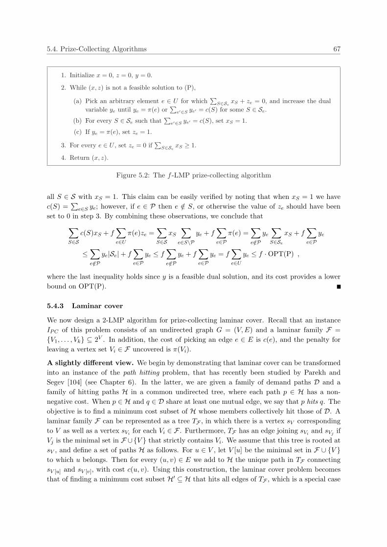
5.4. Prize-Collecting Algorithms 67
1. Initialize x = 0, z = 0, y = 0.
2. While (x, z) is not a feasible solution to (P),
(a) Pick an arbitrary element e ∈ U for which∑
S∈SexS + ze = 0, and increase the dual
variable ye until ye = π(e) or∑
e′∈S ye′ = c(S) for some S ∈ Se.
(b) For every S ∈ Se such that∑
e′∈S ye′ = c(S), set xS = 1.
(c) If ye = π(e), set ze = 1.
3. For every e ∈ U , set ze = 0 if∑
S∈SexS ≥ 1.
4. Return (x, z).
Figure 5.2: The f -LMP prize-collecting algorithm
all S ∈ S with xS = 1. This claim can be easily verified by noting that when xS = 1 we havec(S) =
∑e∈S ye; however, if e ∈ P then e /∈ S, or otherwise the value of ze should have been
set to 0 in step 3. By combining these observations, we conclude that∑
S∈Sc(S)xS + f
∑
e∈U
π(e)ze =∑
S∈SxS
∑
e∈S\Pye + f
∑
e∈Pπ(e) =
∑
e/∈Pye
∑
S∈Se
xS + f∑
e∈Pye
≤∑
e/∈Pye|Se|+ f
∑
e∈Pye ≤ f
∑
e/∈Pye + f
∑
e∈Pye = f
∑
e∈U
ye ≤ f ·OPT(P) ,
where the last inequality holds since y is a feasible dual solution, and its cost provides a lowerbound on OPT(P).
5.4.3 Laminar cover
We now design a 2-LMP algorithm for prize-collecting laminar cover. Recall that an instanceIPC of this problem consists of an undirected graph G = (V,E) and a laminar family F =V1, . . . , Vk ⊆ 2V . In addition, the cost of picking an edge e ∈ E is c(e), and the penalty forleaving a vertex set Vi ∈ F uncovered is π(Vi).
A slightly different view. We begin by demonstrating that laminar cover can be transformedinto an instance of the path hitting problem, that has recently been studied by Parekh andSegev [104] (see Chapter 6). In the latter, we are given a family of demand paths D and afamily of hitting paths H in a common undirected tree, where each path p ∈ H has a non-negative cost. When p ∈ H and q ∈ D share at least one mutual edge, we say that p hits q. Theobjective is to find a minimum cost subset of H whose members collectively hit those of D. Alaminar family F can be represented as a tree TF , in which there is a vertex sV correspondingto V as well as a vertex sVi for each Vi ∈ F . Furthermore, TF has an edge joining sVi and sVj ifVj is the minimal set in F ∪V that strictly contains Vi. We assume that this tree is rooted atsV , and define a set of paths H as follows. For u ∈ V , let V [u] be the minimal set in F ∪ V to which u belongs. Then for every (u, v) ∈ E we add to H the unique path in TF connectingsV [u] and sV [v], with cost c(u, v). Using this construction, the laminar cover problem becomesthat of finding a minimum cost subset H′ ⊆ H that hits all edges of TF , which is a special case
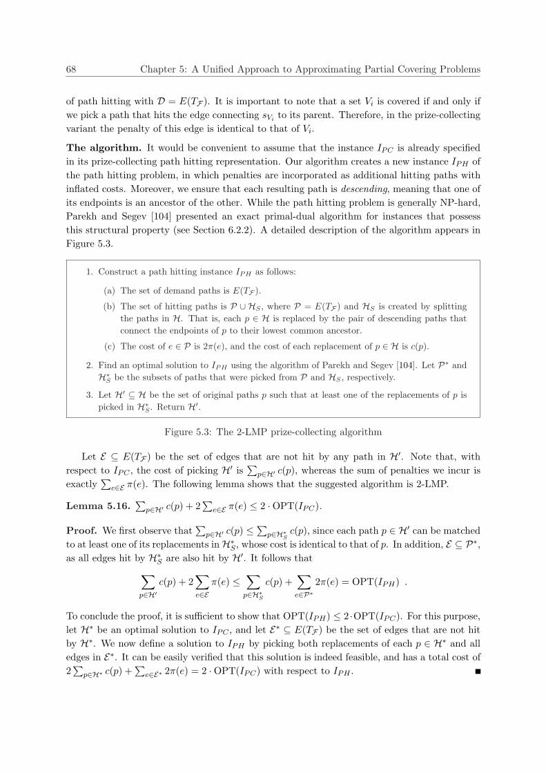
68 Chapter 5: A Unified Approach to Approximating Partial Covering Problems
of path hitting with D = E(TF ). It is important to note that a set Vi is covered if and only ifwe pick a path that hits the edge connecting sVi to its parent. Therefore, in the prize-collectingvariant the penalty of this edge is identical to that of Vi.
The algorithm. It would be convenient to assume that the instance IPC is already specifiedin its prize-collecting path hitting representation. Our algorithm creates a new instance IPH ofthe path hitting problem, in which penalties are incorporated as additional hitting paths withinflated costs. Moreover, we ensure that each resulting path is descending, meaning that one ofits endpoints is an ancestor of the other. While the path hitting problem is generally NP-hard,Parekh and Segev [104] presented an exact primal-dual algorithm for instances that possessthis structural property (see Section 6.2.2). A detailed description of the algorithm appears inFigure 5.3.
1. Construct a path hitting instance IPH as follows:
(a) The set of demand paths is E(TF ).
(b) The set of hitting paths is P ∪ HS , where P = E(TF ) and HS is created by splittingthe paths in H. That is, each p ∈ H is replaced by the pair of descending paths thatconnect the endpoints of p to their lowest common ancestor.
(c) The cost of e ∈ P is 2π(e), and the cost of each replacement of p ∈ H is c(p).
2. Find an optimal solution to IPH using the algorithm of Parekh and Segev [104]. Let P∗ andH∗S be the subsets of paths that were picked from P and HS , respectively.
3. Let H′ ⊆ H be the set of original paths p such that at least one of the replacements of p ispicked in H∗S . Return H′.
Figure 5.3: The 2-LMP prize-collecting algorithm
Let E ⊆ E(TF ) be the set of edges that are not hit by any path in H′. Note that, withrespect to IPC , the cost of picking H′ is
∑p∈H′ c(p), whereas the sum of penalties we incur is
exactly∑
e∈E π(e). The following lemma shows that the suggested algorithm is 2-LMP.
Lemma 5.16.∑
p∈H′ c(p) + 2∑
e∈E π(e) ≤ 2 ·OPT(IPC).
Proof. We first observe that∑
p∈H′ c(p) ≤ ∑p∈H∗S c(p), since each path p ∈ H′ can be matched
to at least one of its replacements inH∗S , whose cost is identical to that of p. In addition, E ⊆ P∗,as all edges hit by H∗S are also hit by H′. It follows that
∑
p∈H′c(p) + 2
∑
e∈Eπ(e) ≤
∑
p∈H∗Sc(p) +
∑
e∈P∗2π(e) = OPT(IPH) .
To conclude the proof, it is sufficient to show that OPT(IPH) ≤ 2 ·OPT(IPC). For this purpose,let H∗ be an optimal solution to IPC , and let E∗ ⊆ E(TF ) be the set of edges that are not hitby H∗. We now define a solution to IPH by picking both replacements of each p ∈ H∗ and alledges in E∗. It can be easily verified that this solution is indeed feasible, and has a total cost of2
∑p∈H∗ c(p) +
∑e∈E∗ 2π(e) = 2 ·OPT(IPC) with respect to IPH .
5.4. Prize-Collecting Algorithms 69
5.4.4 k-interval cover
In what follows, we present a k-LMP algorithm for the prize-collecting k-IC problem. We assumethat the given instance IPC consists of a ground set U , each element of which is endowed witha penalty π(e), and a family of subsets S ⊆ 2U , where the cost of picking a set S ∈ S is c(S).Moreover, the element-set matrix MS
U is now a k-interval matrix. In other words, for everyelement e ∈ U there is a partition Se,1, . . . ,Se,ke of Se to ke ≤ k subsets, such that the columnscorresponding to the sets in each Se,i appear consecutively in MS
U .Our algorithm has its roots in a rounding scheme devised by Gaur et al. [61] for approxi-
mating the rectangle stabbing problem. Consider the following LP-relaxation of prize-collectingk-IC, which is a specialization of the one suggested in Section 5.4.2:
minimize∑
S∈Sc(S)xS +
∑
e∈U
π(e)ze (P)
subject toke∑
i=1
∑
S∈Se,i
xS + ze ≥ 1 ∀ e ∈ U
xS , ze ≥ 0 ∀S ∈ S, e ∈ U
We begin by solving the linear program (P) to obtain an optimal fractional solution (x∗, z∗).For every element e ∈ U , let i(e) be the index that maximizes
∑S∈Se,i
x∗S , breaking ties arbi-trarily. Based on these indices, we construct a new program
minimize∑
S∈Sc(S)xS + k
∑
e∈U
π(e)ze (P∗)
subject to∑
S∈Se,i(e)
xS + ze ≥ 1 ∀ e ∈ U
xS , ze ≥ 0 ∀S ∈ S, e ∈ U
Note that the constraint matrix of (P∗) can be written as [M, I], where M is a matrix thatcontains a single block of consecutive 1’s in each row. Such matrices form a well-known classof totally unimodular matrices (see, for example, [99, page 544]), implying that (P∗) is in facta relaxation of the prize-collecting TUC problem. Therefore, as a result of the discussion inSection 5.3.4, the linear program (P∗) has an integral optimal solution (x, z). Since this solutionis also feasible to (P), the next lemma shows that the algorithm is indeed k-LMP.
Lemma 5.17.∑
S∈S c(S)xS + k∑
e∈U π(e)ze ≤ k ·OPT(P).
Proof. We first claim that (kx∗, z∗) is a feasible solution to (P∗). As the non-negativity con-straints are clearly satisfied, it remains to prove that
∑S∈Se,i(e)
kx∗S + z∗e ≥ 1 for every elemente ∈ U . To this end, note that since i(e) maximizes
∑S∈Se,i
x∗S , the feasibility of (x∗, z∗) for (P)implies that
∑
S∈Se,i(e)
kx∗S + z∗e ≥k
ke
ke∑
i=1
∑
S∈Se,i
x∗S + z∗e ≥ke∑
i=1
∑
S∈Se,i
x∗S + z∗e ≥ 1 .
70 Chapter 5: A Unified Approach to Approximating Partial Covering Problems
Now since (x, z) is an optimal solution to (P∗), we conclude that∑
S∈Sc(S)xS + k
∑
e∈U
π(e)ze = OPT(P∗) ≤∑
S∈Sc(S)(kx∗S) + k
∑
e∈U
π(e)z∗e = k ·OPT(P) .
5.5 Concluding Remarks
Improved approximation factor. Very informally, Theorem 5.1 states that, given an r-LMPalgorithm for the prize-collecting version of a covering problem, we can approximate its partialcoverage version to within factor (4/3 + ε)r of optimum. However, as mentioned in Section 5.3,by employing problem-specific techniques a slightly better factor is achievable in some specialcases. In light of this observation, it would be interesting to investigate whether the ratio(4/3 + ε)r can be improved, perhaps initially just for unit profits.
More than LMP. In an attempt to specialize the framework suggested in this chapter to agiven application, a seemingly promising idea is to require additional structural properties fromthe prize-collecting solutions. Based on these properties, the greedy approach we propose inSection 5.2.3 for combining S1 and S2 may be replaced by an alternative procedure, resultingin an improved bound on the cost of the final solution.
Implicit subsets. A close inspection of Section 5.2.1 reveals that the main part of our algorithmis repeated O(|S|1/ε) times, once for each guess of the b1/εc most expensive sets in the optimalsolution. Therefore, it cannot be directly applied to partial covering problems with a compactimplicit representation of exponentially many sets, such as facility location with outliers [28],k-MST [57], k-Steiner forest [68, 114], etc. A challenging open question for future research iswhether our method can be extended to approximate problems of this class.
Chapter 6
Path Hitting in Acyclic Graphs
The main contribution of this chapter are LP-based approximation algorithms for path hittingon trees, spiders, and stars. As a secondary objective, we make a concentrated effort to unify thealgorithmic methods utilized in approximating previously studied special cases. Our findings,and the techniques by which we derive them, can be summarized as follows.
6.1 Results and Techniques
Descending paths. We begin by presenting a natural LP-relaxation of path hitting in trees,that results from formulating this problem as an integer covering program. Simple examplesillustrate that there are instances for which this linear program does not have an integral optimalsolution. Nevertheless, we constructively prove the existence of such a solution when the pathsin D and H are descending, that is, each path has the property that one of its endpoints is anancestor of the other, with respect to an arbitrary root we fix in advance. Our proof shows howto extend the algorithm of Garg et al. [60] so that it constructs an integral primal solution anda dual solution that satisfy complementary slackness conditions1.
General paths. We make use of this integrality result to approximate the general problem,where D and H may contain non-descending paths, as follows. We first define a new set ofhitting paths H′ by performing path splitting, a preprocessing step in which each hitting path isreplaced by two descending paths of equal cost. Then, using the optimal fractional solution weidentify a new set of demand paths D′, all of which are descending. Finally, we solve the problemof hitting D′ using a minimum cost subset of H′ to optimality, and translate the solution weobtain to a corresponding feasible subset of H whose cost is within factor 4 of optimum. Whenexactly one of D and H consists of descending paths, a simplification of our analysis yieldsan improved factor of 2, thus providing a new tree augmentation method and recovering themulticut algorithm of Levin and Segev [90]. These results are described in Section 6.2.
A new variant of edge cover. In an attempt to outdo the above-mentioned algorithm, weintroduce and study the edge cover with assignment problem. Let G = (V, E) be an undirectedmultigraph with edge costs ce for each e ∈ E and assignment costs sv,e for each v ∈ V and
1Arie Tamir noted that this result can also be established by proving that the underlying constraints matrix
is totally balanced and applying Kolen’s algorithm (see, for example, [87]).
71
72 Chapter 6: Path Hitting in Acyclic Graphs
e ∈ δ(v). A subset E′ ⊆ E is called an edge cover if every vertex v ∈ V is adjacent to someedge in E′. The objective is to find an edge cover E′ and a function φ : V → E′ that assignseach vertex to an adjacent edge in E′ so as to minimize the sum of edge costs and assignmentcosts. When there are no assignment costs we obtain the standard edge cover problem, whichis a matching problem in disguise that can be solved in polynomial time [39, 97, 106]. Wedemonstrate that edge cover with assignment can be interpreted as an equivalent edge coverproblem, which is created by modifying the given multigraph and its edge costs. This reductionenables us to derive a polyhedral description of the former problem by adapting that of thelatter [3, 39]. However, rather than using this description we consider a simplified set of validconstraints, and prove that the resulting linear program has an integrality gap of exactly 4/3.These results are given in Section 6.3.
Spiders and stars. One possible direction for improving the approximation factor of 4 is toavoid the path splitting step. In Section 6.4 we prove that this task can be accomplished whenthe input graph is a spider. In this case, we solve the LP-relaxation right away and utilizeits optimal solution to identify a new set of descending demand paths D′. We then formulatethe problem of hitting D′ using a subset of H as an instance of edge cover with assignment inan auxiliary multigraph, whose construction involves multiple calls to the exact algorithm fordescending paths. Finally, we solve the resulting problem, and prove that after translating itssolution back to the original graph we obtain a feasible subset of H with cost of at most 3.219times the optimum. Our analysis is based on combining the integrality result for descendingpaths and the integrality gap of the simplified relaxation of edge cover with assignment. Wealso show that the suggested algorithm provides an 8/3-approximation in stars.
6.2 Path Hitting in Trees
The main result of this section is an algorithm for path hitting in trees, with an approximationguarantee of 4. We begin by presenting a natural LP-relaxation of path hitting and its dual.Next, we extend the algorithm of Garg et al. [60] for multicuts in trees2, and utilize comple-mentary slackness conditions to prove that the new algorithm constructs an optimal solutionwhen the paths in D and H are descending. Finally, we show how to manipulate this algorithmin order to approximate the general problem.
6.2.1 A linear program and its dual
Our algorithms and their analysis will be based on the following LP-relaxation of the pathhitting problem:
minimize∑
p∈Hcpxp (PH)
subject to∑
p∈H:p∩q 6=∅xp ≥ 1 ∀ q ∈ D (6.1)
xp ≥ 0 ∀ p ∈ H (6.2)
2In fact, its simplified version that appears in Chapter 18 of [118].
6.2. Path Hitting in Trees 73
In an integral solution, the variable xp indicates whether we pick the path p ∈ H, and constraint(6.1) ensures that each demand path is intersected by at least one of the hitting paths we pick.The dual of this linear program is:
maximize∑
q∈Dyq (DPH)
subject to∑
q∈D:q∩p6=∅yq ≤ cp ∀ p ∈ H (6.3)
yq ≥ 0 ∀ q ∈ D (6.4)
To better understand (DPH), we first consider integral solutions to this program. The variablesyq : q ∈ D specify the number of copies we pick from each demand path q, and the objectiveis to maximize their sum. The primal costs now serve as capacities, and constraint (6.3) statesthat for each path p ∈ H the total number of copies of demand paths that are intersected by p
does not exceed its capacity cp. Therefore, the dual program can be viewed as a fractional pathpacking problem.
6.2.2 An exact algorithm for descending paths
In the following we consider the special case in which D and H consist of descending paths. Weassume that the tree T = (V, E) is rooted at an arbitrary vertex, which is fixed in advance. Forv ∈ V , we denote by depth(v) the length of the unique path in T connecting v to the root. Inaddition, for u 6= v ∈ V we denote by [u, v] the unique path in T connecting u and v. Finally,for each path q ∈ D ∪ H the endpoints of q are designated by uq and lq, with the conventionthat depth(uq) < depth(lq).
The algorithm. Starting with an empty set of hitting paths P and the trivial dual solutiony = 0, we proceed as follows.
1. For each v ∈ V , in non-increasing order of depth in T ,
(a) For each q ∈ D such that uq = v, we increase the dual variable yq as much as possible,without violating the capacity constraints.
(b) We augment P by adding, in an arbitrary order, the paths inH whose dual constraintbecame tight during this iteration (henceforth, saturated paths).
2. For each p ∈ P , in reverse order of addition, if P \ p is a feasible solution we eliminatep from P .
Analysis. Let P be the set of hitting paths produced by the algorithm, and let y be thecorresponding dual solution. When step 1 terminates, each demand path q ∈ D is intersectedby at least one saturated hitting path, or otherwise yq could have been further increased,contradicting the maximality of y. It follows that P is indeed a feasible primal solution, asfeasibility is maintained throughout step 2. In addition, since we never violate the capacityconstraints, y is a feasible dual solution.
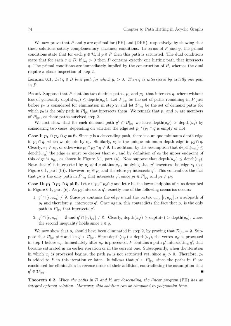
74 Chapter 6: Path Hitting in Acyclic Graphs
We now prove that P and y are optimal for (PH) and (DPH), respectively, by showing thatthese solutions satisfy complementary slackness conditions. In terms of P and y, the primalconditions state that for each p ∈ H, if p ∈ P then this path is saturated. The dual conditionsstate that for each q ∈ D, if yq > 0 then P contains exactly one hitting path that intersectsq. The primal conditions are immediately implied by the construction of P , whereas the dualrequire a closer inspection of step 2.
Lemma 6.1. Let q ∈ D be a path for which yq > 0. Then q is intersected by exactly one pathin P .
Proof. Suppose that P contains two distinct paths, p1 and p2, that intersect q, where withoutloss of generality depth(up1) ≤ depth(up2). Let P |p2 be the set of paths remaining in P justbefore p2 is considered for elimination in step 2, and let D|p2 be the set of demand paths forwhich p2 is the only path in P |p2 that intersects them. We remark that p1 and p2 are membersof P |p2 , as these paths survived step 2.
We first show that for each demand path q′ ∈ D|p2 we have depth(uq′) > depth(uq) byconsidering two cases, depending on whether the edge set p1 ∩ p2 ∩ q is empty or not.
Case I: p1 ∩ p2 ∩ q = ∅. Since q is a descending path, there is a unique minimum depth edgein p1 ∩ q, which we denote by e1. Similarly, e2 is the unique minimum depth edge in p2 ∩ q.Clearly, e1 6= e2, or otherwise p1∩ p2∩ q 6= ∅. In addition, by the assumption that depth(up1) ≤depth(up2) the edge e2 must be deeper than e1, and by definition of e2 the upper endpoint ofthis edge is up2 , as shown in Figure 6.1, part (a). Now suppose that depth(uq′) ≤ depth(uq).Note that q′ is intersected by p2 and contains uq′ , implying that q′ traverses the edge e1 (seeFigure 6.1, part (b)). However, e1 ∈ p1 and therefore p1 intersects q′. This contradicts the factthat p2 is the only path in P |p2 that intersects q′, since p1 ∈ P |p2 and p1 6= p2.
Case II: p1 ∩ p2 ∩ q 6= ∅. Let e ∈ p1∩p2∩q and let r be the lower endpoint of e, as describedin Figure 6.1, part (c). As p2 intersects q′, exactly one of the following scenarios occurs:
1. q′ ∩ [r, up2 ] 6= ∅. Since p1 contains the edge e and the vertex up1 , [r, up2 ] is a subpath ofp1 and therefore p1 intersects q′. Once again, this contradicts the fact that p2 is the onlypath in P |p2 that intersects q′.
2. q′ ∩ [r, up2 ] = ∅ and q′ ∩ [r, lp2 ] 6= ∅. Clearly, depth(uq′) ≥ depth(r) > depth(uq), wherethe second inequality holds since e ∈ q.
We now show that p2 should have been eliminated in step 2, by proving that D|p2 = ∅. Sup-pose that D|p2 6= ∅ and let q′ ∈ D|p2 . Since depth(uq′) > depth(uq), the vertex uq′ is processedin step 1 before uq. Immediately after uq′ is processed, P contains a path p′ intersecting q′, thatbecame saturated in an earlier iteration or in the current one. Subsequently, when the iterationin which uq is processed begins, the path p2 is not saturated yet, since yq > 0. Therefore, p2
is added to P in this iteration or later. It follows that p′ ∈ P |p2 , since the paths in P areconsidered for elimination in reverse order of their addition, contradicting the assumption thatq′ ∈ D|p2 .
Theorem 6.2. When the paths in D and H are descending, the linear program (PH) has anintegral optimal solution. Moreover, this solution can be computed in polynomial time.
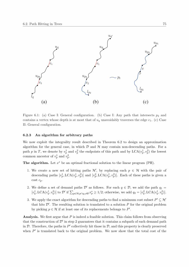
6.2. Path Hitting in Trees 75
(a) (c)(b)
e1
e2
lq
uq
up2 p2
e1
e2
up2
uq
lp2
uq`
e
r
lp2
up2
up1
Figure 6.1: (a) Case I: General configuration. (b) Case I: Any path that intersects p2 andcontains a vertex whose depth is at most that of uq unavoidably traverses the edge e1. (c) CaseII: General configuration.
6.2.3 An algorithm for arbitrary paths
We now exploit the integrality result described in Theorem 6.2 to design an approximationalgorithm for the general case, in which D and H may contain non-descending paths. For apath p in T , we denote by v1
p and v2p the endpoints of this path and by LCA(v1
p, v2p) the lowest
common ancestor of v1p and v2
p.
The algorithm. Let x∗ be an optimal fractional solution to the linear program (PH).
1. We create a new set of hitting paths H′, by replacing each p ∈ H with the pair ofdescending paths [v1
p, LCA(v1p, v
2p)] and [v2
p, LCA(v1p, v
2p)]. Each of these paths is given a
cost cp.
2. We define a set of demand paths D′ as follows. For each q ∈ D, we add the path q1 =[v1
q , LCA(v1q , v
2q )] to D′ if
∑p∈H:p∩q1 6=∅ x∗p ≥ 1/2; otherwise, we add q2 = [v2
q ,LCA(v1q , v
2q )].
3. We apply the exact algorithm for descending paths to find a minimum cost subset P ′ ⊆ H′that hits D′. The resulting solution is translated to a solution P for the original problemby picking p ∈ H if at least one of its replacements belongs to P ′.
Analysis. We first argue that P is indeed a feasible solution. This claim follows from observingthat the construction of D′ in step 2 guarantees that it contains a subpath of each demand pathin D. Therefore, the paths in P ′ collectively hit those in D, and this property is clearly preservedwhen P ′ is translated back to the original problem. We now show that the total cost of the
76 Chapter 6: Path Hitting in Acyclic Graphs
paths in P is within factor 4 of optimum. Since the cost of P ′ provides an upper bound on thatof P , the next lemma is sufficient.
Lemma 6.3.∑
p∈P ′ cp ≤ 4 ·OPT(PH).
Proof. Consider the linear program (PHD′,H′), which is obtained by specializing the pathhitting relaxation for D′ and H′. We define a solution x to this program by setting xp1 = xp2 =2x∗p for each p ∈ H with replacement paths p1 = [v1
p, LCA(v1p, v
2p)] and p2 = [v2
p,LCA(v1p, v
2p)].
Constraint (6.1), combined with the definition of D′, ensures that∑
p∈H:p∩q 6=∅ x∗p ≥ 1/2 forevery q ∈ D′, immediately implying that x is a feasible solution to (PHD′,H′). Moreover,the cost of x is exactly 4
∑p∈H cpx
∗p and therefore OPT(PHD′,H′) ≤ 4 · OPT(PH). Since the
algorithm for descending paths finds an integral optimal solution to (PHD′,H′), we conclude that∑p∈P ′ cp ≤ 4 ·OPT(PH).
Theorem 6.4. Path hitting in trees can be approximated to within a factor of 4 in polynomialtime.
6.3 Edge Cover with Assignment
We temporarily deviate from the general theme of this chapter and study the edge cover withassignment problem, formally defined in Section 6.1. This section introduces several tools thatwill allow us to obtain an improved approximation guarantee for path hitting when the inputgraph is a spider, as well as significantly simplify the presentation. We demonstrate that edgecover with assignment can be reduced to an equivalent edge cover problem, by modifying thegiven multigraph and its edge costs. We also consider a simple LP-relaxation of this problemand prove that its integrality gap is 4/3.
6.3.1 A reduction to edge cover
Let I be an instance of the edge cover with assignment problem, consisting of a multigraphG = (V, E) with edge costs ce for each e ∈ E and assignment costs sv,e for each v ∈ V ande ∈ δ(v). Consider the following instance I ′ of the edge cover problem:
1. The new multigraph is G′, with a vertex set V ′ = V ∪ a, b and an edge set E′ =E ∪ (a, b) ∪ (u, a) : u ∈ V . In other words, we add a new edge (a, b) and connect a toeach original vertex.
2. The cost of an original edge e = (u, v) is c′e = ce + su,e + sv,e; the cost of a new edge (u, a)is c′(u,a) = mine∈δG(u)(ce + su,e); and the cost of (a, b) is c′(a,b) = 0.
Lemma 6.5. For each solution to I there exists a corresponding solution to I ′ of no greatercost, and vice versa.
Proof. Let F ⊆ E be an edge cover in G and let φ : V → F be a function that assigns eachvertex to an adjacent edge in F . We denote by F1 the subset of F that consists of edges towhich exactly one of their endpoints was assigned by φ. For e ∈ F1, we use φ−1(e) to denote
6.3. Edge Cover with Assignment 77
the single endpoint of e that was assigned to it. Similarly, F2 ⊆ F is the collection of edgesto which both of their endpoints were assigned. Note that for e ∈ F1 the cost of the edge(φ−1(e), a) in G′ represents the cheapest option of covering φ−1(e) by an adjacent edge f andsetting φ(φ−1(e)) = f , without assigning the other endpoint of f . In addition, the cost of e ∈ F2
in G′ corresponds to that of picking e in G and assigning both of its endpoints to it. Therefore,the set of edges F2∪(φ−1(e), a) : e ∈ F1∪(a, b) is an edge cover in G′ whose cost is at most∑
e∈F ce +∑
v∈V sv,φ(v).Conversely, let F ⊆ E′ be an edge cover in G′. For each e ∈ F ∩ E, we pick e in G and
assign both of its endpoints to it. For each (u, a) ∈ F \ E, we pick the edge e that minimizesthe sum ce + su,e over all edges in δG(u), and assign u to e. It is quite possible that a vertexis assigned multiple times during this process, a situation in which one of these assignmentsis chosen arbitrarily. Arguments similar to those of the opposite claim show that we obtain afeasible solution to I whose cost is at most
∑e∈F c′e.
Theorem 6.6. Edge cover with assignment can be solved to optimality as an edge cover problem.
6.3.2 An LP-relaxation
Essential to our analysis will be the following LP-relaxation of edge cover with assignment:
minimize∑
e∈E
cexe +∑
v∈V
∑
e∈δ(v)
sv,eyv,e (ECA)
subject to∑
e∈δ(v)
yv,e ≥ 1 ∀ v ∈ V (6.5)
yv,e ≤ xe ∀ v ∈ V, e ∈ δ(v) (6.6)
xe, yv,e ≥ 0 ∀ v ∈ V, e ∈ δ(v) (6.7)
In an integral solution, the variable xe indicates whether we pick the edge e, whereas yv,e
indicates whether the vertex v is assigned to e. Constraint (6.5) ensures that each vertex isassigned to some adjacent edge, and constraint (6.6) states that the assignment of vertices isrestricted to edges that we pick. To avoid confusion, we denote by OPTf (·) the cost of anoptimal fractional solution to a given linear program. Similarly, OPTi(·) is the cost of anoptimal integral solution.
The integrality gap of (ECA) is at least 4/3, as exemplified by a triangle with unit edgecosts and zero assignment costs. In this particular instance, setting the value of each variable to1/2 results in a feasible fractional solution, implying that OPTf (ECA) ≤ 3/2 while we clearlyhave OPTi(ECA) = 2. In the remainder of this section we show that this simple example is theworst possible, by proving the subsequent theorem.
Theorem 6.7. The integrality gap of (ECA) is exactly 4/3.
Our proof relies on the next result, which is part of the folklore of matching theory. Its proofcan be found in [103, Cor. 2.11].
78 Chapter 6: Path Hitting in Acyclic Graphs
Lemma 6.8. The integrality gap of the following LP-relaxation of edge cover is 4/3:
min
∑
e∈E
cexe :∑
e∈δ(v)
xe ≥ 1 ∀ v ∈ V, xe ≥ 0 ∀ e ∈ E
(EC)
Given an instance I of the edge cover with assignment problem, let I ′ be the edge coverinstance generated by the reduction in Section 6.3.1. Using similar notation, consider thespecialization of the linear program (EC) for I ′, after picking in advance the auxiliary edge(a, b) with zero cost:
minimize∑
e=(u,v)∈E
(ce + su,e + sv,e)xe +∑
u∈V
mine∈δG(u)
(ce + su,e)x(u,a) (ECI′)
subject to∑
e∈δG(u)
xe + x(u,a) ≥ 1 ∀u ∈ V (6.8)
xe, x(u,a) ≥ 0 ∀ e ∈ E, u ∈ V (6.9)
Lemma 6.5 can be restated to claim that for every integral solution to (ECAI) there isa corresponding integral solution to (ECI′) of no greater cost and vice versa, showing thatOPTi(ECAI) = OPTi(ECI′). In addition, Lemma 6.8 implies that OPTi(ECI′) ≤ (4/3) ·OPTf (ECI′). Therefore, we can prove Theorem 6.7 by constructing a feasible fractional solutionto (ECI′) whose cost is at most OPTf (ECAI), since we would then have
OPTi(ECAI) = OPTi(ECI′) ≤ 43OPTf (ECI′) ≤ 4
3OPTf (ECAI) .
Let (x∗, y∗) be an optimal fractional solution to (ECAI). We define a candidate solution x
to the linear program (ECI′) by:
1. For each original edge e = (u, v) ∈ E, xe = miny∗u,e, y∗v,e.
2. For each u ∈ V , x(u,a) =∑
e=(u,v)∈δG(u)(y∗u,e −miny∗u,e, y
∗v,e).
Lemma 6.9. x is a feasible solution to (ECI′).
Proof. Clearly, x is non-negative, and it remains to show that this solution satisfies constraint(6.8) for each original vertex u ∈ V . By definition of x we have
∑
e∈δG(u)
xe + x(u,a) =∑
e=(u,v)∈δG(u)
miny∗u,e, y∗v,e+
∑
e=(u,v)∈δG(u)
(y∗u,e −miny∗u,e, y∗v,e)
=∑
e∈δG(u)
y∗u,e
≥ 1 ,
where the last inequality follows from constraint (6.5).
Lemma 6.10. The cost of x is at most OPTf (ECAI).
6.4. Path Hitting in Spiders 79
Proof. In terms of y∗, we can bound the cost of x by∑
e=(u,v)∈E
(ce + su,e + sv,e)xe +∑
u∈V
minf∈δG(u)
(cf + su,f )x(u,a)
=∑
e=(u,v)∈E
(ce + su,e + sv,e)miny∗u,e, y∗v,e
+∑
u∈V
minf∈δG(u)
(cf + su,f )∑
e=(u,v)∈δG(u)
(y∗u,e −miny∗u,e, y∗v,e)
≤∑
e=(u,v)∈E
(ce + su,e + sv,e)miny∗u,e, y∗v,e
+∑
u∈V
∑
e=(u,v)∈δG(u)
(ce + su,e)(y∗u,e −miny∗u,e, y∗v,e) .
For each e = (u, v) ∈ E, the coefficient ce in the right hand side of this bound is multiplied by
miny∗u,e, y∗v,e+ (y∗u,e −miny∗u,e, y
∗v,e) + (y∗v,e −miny∗u,e, y
∗v,e)
= y∗u,e + y∗v,e −miny∗u,e, y∗v,e
= maxy∗u,e, y∗v,e
≤ x∗e ,
where the last inequality holds since y∗u,e ≤ x∗e and y∗v,e ≤ x∗e, by constraint (6.6). In addition,for each u ∈ V and e = (u, v) ∈ δG(u), the coefficient su,e is multiplied by
miny∗u,e, y∗v,e+ (y∗u,e −miny∗u,e, y
∗v,e) = y∗u,e .
It follows that the cost of x is at most∑
e∈E
cex∗e +
∑
u∈V
∑
e∈δG(u)
su,ey∗u,e = OPTf (ECAI) .
6.4 Path Hitting in Spiders
The main result of this section is an improved algorithm for path hitting in spiders that con-structs a solution whose cost is within factor 3.219 of optimum. We initially consider the specialcase in which all demand paths are descending, and show how to exploit a number of structuralproperties in order to formulate this problem as edge cover with assignment. To approximatethe general problem, we combine this formulation together with new insight into some of theresults presented in Sections 6.2 and 6.3.
6.4.1 Notation
We assume that the given spider S = (V, E) is rooted at its center r, and use A to denote theset of paths emerging from r, to which we also refer as the arms of S. The subset H1 ⊆ H is the

80 Chapter 6: Path Hitting in Acyclic Graphs
set of hitting paths that are contained in a single arm of S, of which H1a are those contained in
a ∈ A. Similarly, H2 ⊆ H is the set of hitting paths that go through two arms of S, of which H2a
are those that go through a ∈ A and an additional arm. For a path p ∈ H2a, we use deptha(p)
to denote the depth of the endpoint of p that resides on a. A demand path q that is containedin a is said to be located below a hitting path p ∈ H2
a if the depth of the upper endpoint of q isat least deptha(p). In this case, p and q are edge-disjoint.
6.4.2 A reformulation of descending demand paths
In what follows we consider the special case in which the objective is to find a minimum costsubset of H that hits a collection of descending paths D′. Let H∗ ⊆ H be an optimal solutionto this problem. We observe that, with respect to each arm a ∈ A, the set of paths H∗ satisfiestwo structural properties.
Property 6.11. If H∗ ∩ H2a = ∅, then the set of paths H∗ ∩ H1
a is an optimal solution to theproblem of hitting the paths in D′ that are contained in a using a subset of H1
a.
Property 6.12. If H∗ ∩ H2a 6= ∅, let pa be the path that maximizes deptha(p) over all paths
in H∗ ∩ H2a. Then H∗ ∩H1
a is an optimal solution to the problem of hitting the demand pathsbelow pa using a subset of H1
a.
These observations enable us to reformulate the subproblem we consider as an instance ofedge cover with assignment in an auxiliary multigraph, by interpreting the cost of each subsetH∗∩H1
a as an assignment cost. Specifically, we begin by finding for each arm a ∈ A an optimalsolution to the problem of hitting the paths in D′ that are contained in a using a subset of H1
a.Since both D′ and H1
a consist of descending paths, this solution can be obtained by applyingthe algorithm described in Section 6.2.2, and we denote its cost by OPTa,∅. We then find foreach a ∈ A and p ∈ H2
a an optimal solution to the problem of hitting the demand paths below p
using a subset of H1a. Once again, we apply the algorithm for descending paths and use OPTa,p
to denote the cost of the resulting solution.We remark that some of the single-arm problems that have just been solved may not be
feasible, and we indicate such a scenario by setting OPTa,∅ = ∞ or OPTa,p = ∞. Based onthese computations, we define an instance of edge cover with assignment on a multigraph G asfollows:
1. The set of vertices is A ∪ v∅.
2. For each a′ 6= a′′ ∈ A and p ∈ H2a′ ∩H2
a′′ , we add an edge ep = (a′, a′′) with cost cp.
3. For each a ∈ A, we add an edge (a, v∅) of zero cost.
4. The assignment costs are: sa,ep = OPTa,p for each a ∈ A and p ∈ H2a; sa,(a,v∅) = OPTa,∅
for each a ∈ A; and sv∅,(a,v∅) = 0 for each a ∈ A.
We now prove that the above reduction is indeed correct, by clarifying the equivalencebetween the original instance of path hitting and the resulting instance of edge cover withassignment.
6.4. Path Hitting in Spiders 81
Lemma 6.13. There exist an edge cover F ⊆ E(G) and an assignment function φ : V (G) → F
whose total cost is at most∑
p∈H∗ cp.
Proof. We construct (F, φ) as follows. The set of edges F is defined to be the (disjoint) unionof ep : p ∈ H∗ ∩ H2 and (a, v∅) : a ∈ A. Note that the latter set by itself is an edge coverof zero cost. A vertex a ∈ A is assigned to epa if H∗ ∩ H2
a 6= ∅, where pa is the path thatmaximizes deptha(p) over all paths in H∗ ∩H2
a. Otherwise, a is assigned to (a, v∅). The vertexv∅ is assigned to an arbitrary adjacent edge. This construction guarantees that the cost of (F, φ)is exactly
∑
p∈H∗∩H2
cp +∑a∈A:
H∗∩H2a 6=∅
OPTa,pa +∑a∈A:
H∗∩H2a=∅
OPTa,∅
=∑
p∈H∗∩H2
cp +∑a∈A:
H∗∩H2a 6=∅
∑
p∈H∗∩H1a
cp +∑a∈A:
H∗∩H2a=∅
∑
p∈H∗∩H1a
cp
=∑
p∈H∗∩H2
cp +∑
a∈A
∑
p∈H∗∩H1a
cp
=∑
p∈H∗cp ,
where the first equality follows from the definition of OPTa,p and OPTa,∅, combined withProperties 6.11 and 6.12.
Lemma 6.14. Let F ⊆ E(G) be an edge cover in G, and let φ : V (G) → F be an assignmentfunction. Then (F, φ) can be translated to a subset of H that hits D′ with an identical cost.
Proof. We initially pick all paths p ∈ H2 for which ep ∈ F . Then, for each a ∈ A and p ∈ H2a,
if φ(a) = ep we add a minimum cost subset of H1a that hits the demand paths below p, whose
total cost is exactly OPTa,p. In addition, for each a ∈ A such that φ(a) = (a, v∅) we add aminimum cost subset of H1
a that hits the paths in D′ contained in a, with a total cost of OPTa,∅.Clearly, the set of paths we obtain hits all demand paths and its cost is equal to that of (F, φ).
6.4.3 An algorithm for arbitrary paths
In the following we design an improved algorithm for path hitting in spiders. The currentalgorithm departs from our approach for general trees in two aspects. First, we skip the pathsplitting step and add an elimination step in which redundant demand paths are discarded.Second, we solve the problem of hitting descending paths using the reduction to edge coverwith assignment. It is important to note that the additional elimination step is not reallynecessary, and its purpose is to allow a considerably simplified analysis.
The algorithm. Let x∗ be an optimal fractional solution to the linear program (PH).
1. We define a set of descending demand paths D′ by3:3Recall that v1
q and v2q denote the endpoints of a given path q.
82 Chapter 6: Path Hitting in Acyclic Graphs
(a) For each q ∈ D, we add the path q1 = [v1q , LCA(v1
q , v2q )] to D′ if ∑
p∈H:p∩q1 6=∅ x∗p ≥ 1/2and otherwise we add q2 = [v2
q , LCA(v1q , v
2q )].
(b) While there is a pair q′ 6= q′′ ∈ D′ such that q′ is a subpath of q′′, we eliminate q′′
from D′.
2. We find a minimum cost subset P ⊆ H that hits D′ as follows:
(a) We reduce this problem to edge cover with assignment, as described in Section 6.4.2.
(b) We find an optimal solution to the resulting instance (see Theorem 6.6) and translateit back to the original problem, as specified in Lemma 6.14.
6.4.4 Analysis
We first observe that P is indeed a feasible solution. The construction ofD′ in step 1a guaranteesthat it contains a subpath of each demand path in D. In addition, for each path q′′ that iseliminated in step 1b we leave in D′ a witness ensuring that q′′ is hit by P , in the form of asubpath of q′′. In what follows we prove the next theorem.
Theorem 6.15. The cost of P is at most (4(1 +√
2)/3) ·OPT(PH) < 3.219 ·OPT(PH).
Let I denote the instance of edge cover with assignment that is produced by step 2a of thealgorithm. Using notation similar to that in Section 6.4.2, consider the specialization of theLP-relaxation (ECA) for I, after picking in advance some edge (a, v∅) and assigning v∅ to thisedge (with zero cost):
minimize∑
p∈H2
cpxep +∑
a∈A
∑
p∈H2a
OPTa,pya,ep +∑
a∈AOPTa,∅ya,(a,v∅) (ECAI)
subject to∑
p∈H2a
ya,ep + ya,(a,v∅) ≥ 1 ∀ a ∈ A (6.10)
ya,(a,v∅) ≤ x(a,v∅) ∀ a ∈ A (6.11)
ya,ep ≤ xep ∀ a ∈ A, p ∈ H2a (6.12)
xep , x(a,v∅), ya,ep , ya,(a,v∅) ≥ 0 ∀ a ∈ A, p ∈ H2 (6.13)
As specified in step 2b, the set of paths P is a translation of an optimal integral solutionto (ECAI). According to Lemma 6.14 this translation is cost-preserving, therefore
∑p∈P cp =
OPTi(ECAI). In addition, Theorem 6.7 states that the integrality gap of (ECA) is 4/3, andwe have
∑p∈P cp ≤ (4/3) · OPTf (ECAI). It follows that we can prove Theorem 6.15 by
showing that the linear program (ECAI) has a fractional solution (x, y) whose cost is at most(1 +
√2)OPTf (PH).
Constructing (x, y). Let θ ≥ 2 be a fitting parameter, whose value will be determined later.Using x∗, the optimal solution to (PH), we define (x, y) as follows:
1. The fractional edges we pick are xep = θx∗p for each p ∈ H2, and x(a,v∅) = 1 for each a ∈ A.
6.4. Path Hitting in Spiders 83
2. The fractional assignment of each a ∈ A is determined according to two cases. LetH2
a = p1, . . . , pk, where we assume that these paths are indexed by non-increasing orderof depth in a.
(a) If∑k
i=1 x∗pi≥ 1/θ, let I(a) be the minimal index for which
∑I(a)i=1 x∗pi
≥ 1/θ. Thenya,(a,v∅) = 0, and
ya,epi=
θx∗piif 1 ≤ i ≤ I(a)− 1
1− θ∑I(a)−1
j=1 x∗pjif i = I(a)
0 if I(a) + 1 ≤ i ≤ k
(b) If∑k
i=1 x∗pi< 1/θ, then ya,(a,v∅) = 1− θ
∑ki=1 x∗pi
, and ya,epi= θx∗pi
for 1 ≤ i ≤ k.
As we observed earlier, the value of some OPT’s in the objective function of (ECAI) mightbe ∞, meaning that we should ensure that the corresponding variables in (x, y) are set to 0.However, we will indirectly prove this property by showing that the cost of (x, y) is finite.Meanwhile, the next lemma establishes the feasibility of (x, y).
Lemma 6.16. (x, y) is a feasible solution to (ECAI).
Proof. Consider an arm a ∈ A and letH2a = p1, . . . , pk, where deptha(p1) ≥ · · · ≥ deptha(pk).
By definition of y we have∑k
i=1 ya,epi+ ya,(a,v∅) = 1 and constraint (6.10) is satisfied. In ad-
dition, constraint (6.11) is also satisfied, since ya,(a,v∅) ≤ 1 = x(a,v∅). It remains to consider
constraint (6.12). If∑k
i=1 x∗pi≥ 1/θ, let I(a) be the minimal index for which
∑I(a)i=1 x∗pi
≥ 1/θ.Then
1. For 1 ≤ i ≤ I(a)− 1, ya,epi= θx∗pi
= xepi.
2. ya,epI(a)= 1− θ
∑I(a)−1i=1 x∗pi
≤ θx∗pI(a)= xepI(a)
.
3. For I(a) + 1 ≤ i ≤ k, ya,epi= 0.
Otherwise,∑k
i=1 x∗pi< 1/θ and we have ya,epi
= θx∗pi= xepi
for every 1 ≤ i ≤ k.
Bounding the assignment cost of (x, y). We are now concerned with bounding the totalfractional assignment cost of some a ∈ A in terms of θ and x∗. Specifically, we relate this costto that of the hitting paths in H1
a. We assume that the arm a contains at least one path in D′,or otherwise OPTa,∅ = 0 and OPTa,p = 0 for every p ∈ H2
a. As before, let H2a = p1, . . . , pk,
where deptha(p1) ≥ · · · ≥ deptha(pk).
Lemma 6.17. If∑k
i=1 x∗pi< 1/θ, then
OPTa,∅ya,(a,v∅) +k∑
i=1
OPTa,pi ya,epi≤ sup
α∈[0, 1θ)
2− α(2 + θ)
(1− α)(1− 2α)
∑
p∈H1a
cpx∗p .
84 Chapter 6: Path Hitting in Acyclic Graphs
Proof. We say that a path q ∈ D′ is complete if q ∈ D. Otherwise, q is said to be a partial path.Note that since x∗ is a feasible solution to (PH), constraint (6.1) ensures that
∑p∈H:p∩q 6=∅ x∗p ≥ 1
for each complete path q. In addition, step 1a of the algorithm guarantees that∑
p∈H:p∩q 6=∅ x∗p ≥1/2 for each partial path. Let β =
∑ki=1 x∗pi
. We observe that∑
p∈H1a:p∩q 6=∅ x∗p ≥ 1 − β for
complete paths q that are contained in a, since
∑
p∈H1a:p∩q 6=∅
x∗p + β =∑
p∈H1a:p∩q 6=∅
x∗p +k∑
i=1
x∗pi≥
∑
p∈H1a:p∩q 6=∅
x∗p +∑
p∈H2a:p∩q 6=∅
x∗p ≥ 1 .
A similar argument shows that∑
p∈H1a:p∩q 6=∅ x∗p ≥ 1/2−β for partial paths q that are contained
in a.We first consider the problem of hitting the demand paths in D′ below pk using a minimum
cost subset of H1a, whose LP-relaxation we denote by (PH1). Recall that the cost of an optimal
solution to this problem, OPTa,pk, was computed by applying the descending paths algorithm
given in Section 6.2.2. Theorem 6.2 proves that OPTa,pkis a lower bound on the cost of any
feasible solution to (PH1). However, all demand paths in D′ below pk are complete, implyingthat x′p = x∗p/(1−β) (for p ∈ H1
a) is a feasible solution to (PH1), since (∑
p∈H1a:p∩q 6=∅ x∗p)/(1−β) ≥
1 for each complete path q. It follows that
OPTa,pk≤ 1
1− β
∑
p∈H1a
cpx∗p . (6.14)
Since S is a spider, its root r is the upper endpoint of all partial paths in D′. Therefore,from the set of partial paths that are contained in the arm a at most one path survives step 1b(the shortest one). We will assume that such a path q′ ∈ D′ indeed survives, as the boundin the alternative case is dominated by the bound we present below. We now consider theproblem of hitting all paths in D′ that are contained in a using a minimum cost subset of H1
a,whose LP-relaxation we denote by (PH2). Recall that the cost of an (integral) optimal solutionto (PH2) is OPTa,∅, and let Iq′ be the set of paths in H1
a that intersect q′. Using argumentssimilar to those of the previous case, we can define a feasible solution x′ to (PH2) by settingx′p = x∗p/(1/2− β) for each p ∈ Iq′ and x′p = x∗p/(1− β) for each p ∈ H1
a \ Iq′ . It follows that
OPTa,∅ ≤1
1/2− β
∑
p∈Iq′
cpx∗p +
11− β
∑
p∈H1a\Iq′
cpx∗p . (6.15)
Inequalities (6.14) and (6.15) show that the total fractional assignment cost of a is
OPTa,∅ya,(a,v∅) +k∑
i=1
OPTa,pi ya,epi
≤ 1
1/2− β
∑
p∈Iq′
cpx∗p +
11− β
∑
p∈H1a\Iq′
cpx∗p
(1− θ
k∑
i=1
x∗pi
)+
k∑
i=1
1
1− β
∑
p∈H1a
cpx∗p
θx∗pi
=
1
1/2− β
∑
p∈Iq′
cpx∗p +
11− β
∑
p∈H1a\Iq′
cpx∗p
(1− θβ) +
1
1− β
∑
p∈H1a
cpx∗p
θβ
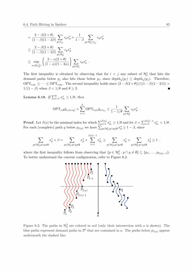
6.4. Path Hitting in Spiders 85
=2− β(2 + θ)
(1− β)(1− 2β)
∑
p∈Iq′
cpx∗p +
11− β
∑
p∈H1a\Iq′
cpx∗p
≤ 2− β(2 + θ)(1− β)(1− 2β)
∑
p∈H1a
cpx∗p
≤ supα∈[0, 1
θ)
2− α(2 + θ)
(1− α)(1− 2α)
∑
p∈H1a
cpx∗p .
The first inequality is obtained by observing that for i < j any subset of H1a that hits the
demand paths below pj also hits those below pi, since deptha(pi) ≥ deptha(pj). Therefore,OPTa,p1 ≤ · · · ≤ OPTa,pk
. The second inequality holds since (2−β(2+ θ))/((1−β)(1− 2β)) >
1/(1− β) when β < 1/θ and θ ≥ 2.
Lemma 6.18. If∑k
i=1 x∗pi≥ 1/θ, then
OPTa,∅ya,(a,v∅) +k∑
i=1
OPTa,pi ya,epi≤ 1
1− 1/θ
∑
p∈H1a
cpx∗p .
Proof. Let I(a) be the minimal index for which∑I(a)
i=1 x∗pi≥ 1/θ and let β =
∑I(a)−1i=1 x∗pi
< 1/θ.For each (complete) path q below pI(a) we have
∑p∈H1
a:p∩q 6=∅ x∗p ≥ 1− β, since
∑
p∈H1a:p∩q 6=∅
x∗p + β =∑
p∈H1a:p∩q 6=∅
x∗p +I(a)−1∑
i=1
x∗pi≥
∑
p∈H1a:p∩q 6=∅
x∗p +∑
p∈H2a:p∩q 6=∅
x∗p ≥ 1 ,
where the first inequality follows from observing that p ∈ H2a : p ∩ q 6= ∅ ⊆ p1, . . . , pI(a)−1.
To better understand the current configuration, refer to Figure 6.2.
ap1
p2
p3
pk-1
pk
pI(a)-1
pI(a) q
Figure 6.2: The paths in H2a are colored in red (only their intersection with a is shown). The
blue paths represent demand paths in D′ that are contained in a. The paths below pI(a) appearunderneath the dashed line.
86 Chapter 6: Path Hitting in Acyclic Graphs
Consider the problem of hitting the paths in D′ below pI(a) using a subset of H1a, whose LP-
relaxation we denote by (PH1), and recall that its optimum is OPTa,pI(a). Note that all demand
paths in D′ below pI(a) are complete, therefore x′p = x∗p/(1 − β) (for p ∈ H1a) is a feasible
solution to (PH1), as (∑
p∈H1a:p∩q 6=∅ x∗p)/(1 − β) ≥ 1 for each complete path q. It follows that
OPTa,pI(a)≤ (
∑p∈H1
acpx
∗p)/(1 − β). The last inequality shows that the fractional assignment
cost of a is
OPTa,∅ya,(a,v∅) +k∑
i=1
OPTa,pi ya,epi≤
I(a)∑
i=1
1
1− β
∑
p∈H1a
cpx∗p
ya,epi
≤ 11− 1/θ
∑
p∈H1a
cpx∗p .
The first inequality holds since ya,(a,v∅) = 0, ya,epi= 0 for every i > I(a), and OPTa,p1 ≤
· · · ≤ OPTa,pI(a). The second inequality follows from the observation that
∑I(a)i=1 ya,epi
= 1 andβ < 1/θ.
Bounding the overall cost of (x, y). We now show that the fitting parameter θ can bedetermined such that the total cost of (x, y) is at most (1 +
√2)
∑p∈H cpx
∗p, completing the
proof of Theorem 6.15. Let ρ denote the ratio between the fractional costs of the paths in H2
and the paths in H, that is,
ρ =
∑p∈H2 cpx
∗p∑
p∈H cpx∗p∈ [0, 1] .
By definition of x and the bounds in Lemmas 6.17 and 6.18, the cost of (x, y) with respect tothe linear program (ECAI) is
∑
p∈H2
cpxep +∑
a∈A
∑
p∈H2a
OPTa,pya,ep +∑
a∈AOPTa,∅ya,(a,v∅)
≤ θ∑
p∈H2
cpx∗p + max
sup
α∈[0, 1θ)
2− α(2 + θ)
(1− α)(1− 2α)
,
11− 1/θ
∑
a∈A
∑
p∈H1a
cpx∗p
= θ∑
p∈H2
cpx∗p + sup
α∈[0, 1θ)
2− α(2 + θ)
(1− α)(1− 2α)
∑
a∈A
∑
p∈H1a
cpx∗p
=
(ρθ + (1− ρ) sup
α∈[0, 1θ)
2− α(2 + θ)
(1− α)(1− 2α)
) ∑
p∈Hcpx
∗p ,
where the first equality follows from the observation that supα∈[0,1/θ)(2−α(2+ θ))/((1−α)(1−2α)) ≥ 1/(1 − 1/θ). Although we do not control the parameter ρ, we can bound the ratiobetween the cost of (x, y) and
∑p∈H cpx
∗p by considering the worst possible choice for ρ. Using
elementary calculus, it is easy to verify that
maxρ∈[0,1]
minθ≥2
(ρθ + (1− ρ) sup
α∈[0, 1θ)
2− α(2 + θ)
(1− α)(1− 2α)
)= 1 +
√2 ,
which is attained at ρ = 1/2 and θ = 1 +√
2.
6.4. Path Hitting in Spiders 87
6.4.5 An improved analysis for stars
The special case in which S is a star enables us to derive improved bounds on the fractionalassignment cost of each a ∈ A. Specifically, we observe that OPTa,pi = 0 for every 1 ≤ i ≤ k,since there are no demand paths below pi. By fixing these constants in the proofs of Lemmas 6.17and 6.18 we obtain, respectively, the following bounds for θ = 2:
Lemma 6.19. If∑k
i=1 x∗pi< 1/2, then
OPTa,∅ya,(a,v∅) +k∑
i=1
OPTa,pi ya,epi≤ 2
∑
p∈H1a
cpx∗p .
Lemma 6.20. If∑k
i=1 x∗pi≥ 1/2, then
OPTa,∅ya,(a,v∅) +k∑
i=1
OPTa,pi ya,epi= 0 .
By definition of x and Lemmas 6.19 and 6.20, we conclude that the cost of (x, y) is∑
p∈H2
cpxep +∑
a∈A
∑
p∈H2a
OPTa,pya,ep +∑
a∈AOPTa,∅ya,(a,v∅)
≤ 2∑
p∈H2
cpx∗p + 2
∑
a∈A
∑
p∈H1a
cpx∗p = 2
∑
p∈Hcpx
∗p ,
resulting in an improved approximation guarantee of 8/3.
88 Chapter 6: Path Hitting in Acyclic Graphs
Chapter 7
Robust Subgraphs for Trees and
Paths
The main contributions of this chapter are surprising upper bounds on the size of path-robustand tree-robust subgraphs. For both problems, we prove that in every complete weighted graphon n vertices there exists a subgraph with approximately αn/(1− α2) edges, containing an α-approximate solution for every 1 ≤ k ≤ n− 1. We also consider variants in which the subgraphitself is restricted to be a path or a tree. In this context, we describe polynomial-time algorithmsand corresponding proofs of negative results.
7.1 Results and Techniques
Basic definitions. Let G = (V,E) be a complete graph with vertex set V = 1, . . . , n andnon-negative edge weights w(e), e ∈ E. For a subgraph H ⊆ G we denote |H| = |E(H)| andw(H) =
∑e∈E(H) w(e). For a set of edges E′ ⊆ E we denote by G[E′] the subgraph of G whose
vertices are the endpoints of edges in E′ and whose edges are E′.For 1 ≤ k ≤ n − 1, let P ∗
k and T ∗k be a maximum weight k-edge path and a maximumweight k-edge tree in G, respectively. A subgraph H ⊆ G is called α-path-robust if for every1 ≤ k ≤ n − 1, there exists a path P ⊆ H, such that |P | ≤ k and w(P ) ≥ αw(P ∗
k ). Similarly,H is called α-tree-robust if for every 1 ≤ k ≤ n− 1 there exists a tree T ⊆ H, such that |T | ≤ k
and w(T ) ≥ αw(T ∗k ). For 0 ≤ α ≤ 1, let pα(G,w) and tα(G,w) be the minimum number ofedges in an α-path-robust subgraph and an α-tree-robust subgraph of (G, w), respectively. Wedefine
pαn = max
(G,w):|V (G)|=npα(G,w) ,
tαn = max(G,w):|V (G)|=n
tα(G,w) .
Path robustness. As a first attempt of attacking the problems of finding small α-path-robustand α-tree-robust subgraphs, one might consider using a maximum weight Hamiltonian pathand a maximum spanning tree, respectively. However, simple examples illustrate that for everyα > 0 there are graphs in which these subgraphs are not α-path-robust or α-tree-robust.
89
90 Chapter 7: Robust Subgraphs for Trees and Paths
In Section 7.2 we show that for α < 1, lim supn→∞ pαn/n ≤ α/(1 − α2), which follows from
an upper bound on the number of edges in a minimum α-path-robust subgraph. A generaloverview of the method we use to obtain this bound is the following:
1. Consider (G,w) and let P = P ∗1 , . . . , P ∗
n−1.
2. We first define a collection of subsets of P, Pii∈I , such that⋃
i∈I Pi = P. These subsetsare not necessarily pairwise disjoint.
3. For each i ∈ I, we independently find a subgraph Hi ⊆ G that α-covers Pi, namely, forevery P ∈ Pi there exists a path P ′ ⊆ Hi, such that |P ′| ≤ |P | and w(P ′) ≥ αw(P ).
4. Let H =⋃
i∈I Hi, then pα(G,w) ≤ |H|.
Tree robustness. In Section 7.3 we prove a corresponding bound of lim supn→∞ tαn/n ≤α/(1− α2) for the minimum α-tree-robust subgraph problem. As before, we define a collectionof subsets Tii∈I of T = T ∗1 , . . . , T ∗n−1 such that
⋃i∈I Ti = T . For every i ∈ I an α-cover
Hi ⊆ G is found for Ti, and tα(G,w) ≤ |H|, where H =⋃
i∈I Hi.However, there are two major differences between the analysis in this case and the analysis
of the minimum α-path-robust subgraph. One difference is that throughout our analysis weconsider rational values of α. The result is then extended to arbitrary values of α using a simpleanalytical argument. Another difference is that the method we apply to find the subgraphs Hi,that α-cover the subsets of trees we define, is much more involved. We prove the existence ofsmall enough subgraphs Hi using tree decomposition schemes.
Definition 7.1. A tree decomposition scheme is a triple (r, p, c), r ∈ N, 1/r ≤ p ≤ 1, c ∈ N, suchthat for every n-edge tree T there exist E1, . . . , Er ⊆ E(T ) that satisfy the following conditions:
1. E1, . . . , Er is a partition of E(T ).
2. |Ei| ≤ pn + 1, for every 1 ≤ i ≤ r.
3. The total number of connected components in T [E1], . . . , T [Er] is at most c.
In Section 7.3 we also prove that for every r ∈ N and ε > 0 there exists a tree decompositionscheme (r, p, c) such that p ≤ 1/r + ε and c = O (r log(1/ε)). We also present a polynomial timealgorithm that finds such decomposition.
Restricted subgraphs. In Section 7.4 we present a polynomial time algorithm that finds a0.353-path-robust path. We also provide an example for a graph in which no path is α-path-robust for α > 0.843. We then describe a polynomial time algorithm that finds a 1/2-tree-robusttree, and provide an example for a graph in which no tree is α-tree-robust for α > 0.866. Finally,we present a polynomial time algorithm that finds a 1/2-tree-robust subgraph H, such that |H|is at most twice the number of edges in a minimum cardinality 1/2-tree-robust subgraph, andw(H) is at most twice the weight of a minimum weight 1/2-tree-robust subgraph.
7.2. α-Path-Robust Subgraphs 91
7.2 α-Path-Robust Subgraphs
Before we describe how our general method is applied to obtain the bound on the number ofedges in a minimum α-path-robust subgraph, we present several helpful observations.
Lemma 7.2. Let 0 ≤ α < 1. Let P be a k-edge path, where k ≥ 1/(1 − α). There existsE′ ⊆ E(P ) such that
1. P [E′] can be completed into a path P ′ using at most one additional edge.
2. |P ′| = dα(k + 1)e.
3. w(P ′) ≥ αw(P ).
Proof. Let Ck+1 be the (k + 1)-edge cycle created by connecting the two endpoints of P .Randomly choose a vertex s ∈ V (Ck+1) and let P ⊆ Ck+1 be the dα(k+1)e-edge path beginningat s and traversing edges clockwise. Note that since k + 1 > 1/(1− α), dα(k + 1)e ≤ k, and P
is indeed a path. Since an edge e ∈ E(Ck+1) belongs to P with probability dα(k + 1)e/(k + 1),the expected weight of P is
dα(k + 1)ek + 1
∑
e∈E(Ck+1)
w(e) ≥ αw(Ck+1) ≥ αw(P ) .
Therefore, there exists a path P ′ ⊆ Ck+1 such that |P ′| = dα(k+1)e and w(P ′) ≥ αw(P ). Notethat P ′ uses at most one edge not in P .
Corollary 7.3. Let 0 ≤ α < 1 and k ≥ 1/(1− α). Then w(P ∗dα(k+1)e) ≥ αw(P ∗
k ).
Corollary 7.4. Let 0 ≤ α < 1 and k ≥ 1/(1− α). There exist E′ ⊆ E(P ∗k ) such that
1. G[E′] can be completed into a path P using at most one additional edge.
2. |P | ≤ dα(k + 1)e.
3. w(P ) ≥ αw(P ∗k ).
Given (G,w), |V (G)| = n, and 0 < α < 1, we define P[i, j] = P ∗i , . . . , P ∗
j for i ≤ j. Wedefine P ′ = P[1, 3d(1+α2)/(α(1−α))e− 1]. In addition, we define Pi = P[Li, Ui], i = 1, . . . , R,where
1. U1 = n− 1.
2. Ui = Li−1 − 1, i = 2, . . . , R.
3. Li = dα(dα(Ui + 1)e+ 1)e, i = 1, . . . , R.
4. R = dlogα−2(αn/(3(1− α)))e.
92 Chapter 7: Robust Subgraphs for Trees and Paths
As Lemma 7.5c shows, LR ≤ 3d(1 + α2)/(α(1− α))e, and indeed P ′ ∪(⋃R
i=1 Pi
)= P.
We α-cover P ′ using H ′ =⋃
P∈P ′ P , which is a subgraph whose number of edges is boundedby (3d(1 + α2)/(α(1 − α))e)2/2 ≤ (9(1 + α)/(α(1 − α)))2/2. Note that since Ui ≥ d(1 +α2)/(α(1− α))e for every 1 ≤ i ≤ R, we have dα(Ui + 1)e ≤ Ui and Ui ≥ 1/(1− α). Therefore,by Corollary 7.3 we can use P ∗
dα(Ui+1)e as an α-cover for P[dα(Ui + 1)e, Ui]. In addition, whenUi ≥ d(1+α2)/(α(1−α))e we have dα(dα(Ui+1)e+1)e ≤ dα(Ui+1)e and dα(Ui+1)e ≥ 1/(1−α).Therefore, by Corollary 7.4 it is sufficient to add at most one edge to P ∗
dα(Ui+1)e to obtain an α-cover for P[dα(dα(Ui +1)e+1)e, dα(Ui +1)e] = P[Li, dα(Ui +1)e]. It follows that Pi = P[Li, Ui]can be α-covered by a subgraph Hi ⊆ G such that |Hi| ≤ dα(Ui + 1)e+ 1.
Let H = H ′ ∪ (⋃R
i=1 Hi), then H is an α-path-robust subgraph.
Lemma 7.5.
a. Ui ≤ α2i−2n + 2∑2i−1
j=0 αj, for every i ≥ 1.
b. |Hi| ≤ α2i−1n + 3∑2i
j=0 αj, for every i ≥ 1.
c. LR ≤ 3d(1 + α2)/(α(1− α))e.
Proof. See Section 7.5.
Lemma 7.6.
|H| ≤ α
1− α2n +
31− α
⌈logα−2
αn
3(1− α)
⌉+
92
(1 + α
α(1− α)
)2
.
Proof. Since H = H ′ ∪ (⋃R
i=1 Hi), by Lemma 7.5b and 7.5c we have
|H| ≤R∑
i=1
|Hi|+ |H ′|
≤R∑
i=1
α2i−1n + 3
2i∑
j=0
αj
+
92
(1 + α
α(1− α)
)2
≤ n∞∑
i=1
α2i−1 + 3R∞∑
j=0
αj +92
(1 + α
α(1− α)
)2
=α
1− α2n +
31− α
⌈logα−2
αn
3(1− α)
⌉+
92
(1 + α
α(1− α)
)2
.
Theorem 7.7. lim supn→∞ pαn/n ≤ α/(1− α2).
7.3. α-Tree-Robust Subgraphs 93
7.3 α-Tree-Robust Subgraphs
We follow the general scheme outlined in Section 7.1 and define a collection of subsets Tii∈I
of T = T ∗1 , . . . , T ∗n−1 such that⋃
i∈I Ti = T . We then independently find for every i ∈ I asubgraph Hi ⊆ G that α-covers Ti. However, finding a small enough subgraph Hi is significantlyharder in this case.
To demonstrate this difficulty, consider for example α = 1/2. Since a 2k-edge path can berepresented as a union of two disjoint k-edge paths, w(P ∗
k ) ≥ w(P ∗2k)/2. However, a 2k-edge
tree cannot generally be decomposed into equal size trees. In addition, simple examples showthat there are graphs in which w(T ∗k ) < w(T ∗2k)/2.
Therefore, we do not expect that simple arguments can be used to prove claims similar toCorollaries 7.3 and 7.4. In the following we study tree decomposition schemes, allowing us toachieve analogous results.
7.3.1 Tree decomposition schemes
Our main result in this section is the following:
Theorem 7.8. For every r ∈ N and ε > 0 there exists a tree decomposition scheme (r, p, c)such that p ≤ 1/r + ε and c = O(r log(1/ε)). Such a decomposition can be found in O(rn) time.
Before we turn to describe our tree decomposition algorithm, that provides a constructiveproof for Theorem 7.8, we present a well known result regarding centroid decomposition in trees.
Definition 7.9. A centroid of a tree T is a vertex v that minimizes over all vertices the size ofthe largest connected component of T − v.
Definition 7.10. Let T be a tree. A centroid decomposition of T is a partition (T ′, T ′′) of T suchthat T ′ and T ′′ are edge-disjoint subtrees of T , |T |/3 ≤ |T ′|, |T ′′| ≤ 2|T |/3, and V (T ′)∩V (T ′′) =v, where v is a centroid of T .
Lemma 7.11 ([49]). Let T be a tree with n > 2 vertices. A centroid decomposition of T exists,and can be found in O(n) time.
Our decomposition algorithm uses procedure Accumulate-Edges, shown in Figure 7.1.The input for this procedure consists of: a lower bound L; an upper bound U ; a set of edges A;and a tree T . We assume that the arguments of Accumulate-Edges always satisfy L+1 ≤ U ,A ∩ E(T ) = ∅, |A| ≤ L and |A|+ |T | > L.
Accumulate-Edges recursively transfers edges from the tree T to the edge set A, untilL ≤ |A| ≤ U . If we initially have |A| + |T | ≤ U , then A ∪ T is returned. If this condition isnot satisfied, we find a centroid decomposition (T ′, T ′′) of T , where |T ′| ≤ |T ′′|. If the smallertree, T ′, can be added to A without exceeding the upper bound U , we replace A by A∪ T ′ andcontinue to transfer edges from T ′′. Otherwise, it is sufficient to transfer edges from T ′ to A.
Note that the bounds L and U are kept unchanged in the recursive calls. Let Ai and Ti
be the additional input for the i-th call to Accumulate-Edges. When a recursive call ismade, the procedure guarantees that there is always a sufficient number of edges in Ti for the
94 Chapter 7: Robust Subgraphs for Trees and Paths
Accumulate-Edges(L, U,A, T )if |A|+ |T | ≤ U then return (A ∪ T, ∅)(T ′, T ′′) ← centroid decomposition of T , where |T ′| ≤ |T ′′|if |A|+ |T ′| ≤ U then
A ← A ∪ T ′
if |A| ≥ L then return (A, T ′′)else return Accumulate-Edges(L,U,A, T ′′)
(A′, ST ) ← Accumulate-Edges(L,U,A, T ′)return (A′, ST ∪ T ′′)
Figure 7.1: The Accumulate-Edges procedure
procedure to terminate, that is, |Ai| + |Ti| > L for every i ≥ 1. It follows that the argumentsfor the next recursive call satisfy the initial assumptions.
It is important to note that Accumulate-Edges never attempts to perform a centroiddecomposition when |Ti| = 1. In this case,
|Ai|+ |Ti| = |Ai|+ 1 ≤ L + 1 ≤ U ,
and the procedure terminates since the condition “if |A|+ |T | ≤ U” is satisfied.This procedure also returns the collection of subtrees of T that were not transferred to A.
Lemma 7.12. Procedure Accumulate-Edges performs O(log(|T |/(U − L))) recursive calls,and returns a set of edges A′ such that A1 ⊆ A′ and L ≤ |A′| ≤ U .
Proof. If the “if |A| ≥ L” condition is satisfied within O(log(|T |/(U − L))) calls, then ob-viously the lemma holds. We now assume this is not the case. Let t be the minimal in-teger for which |Tt| ≤ U − L. Since a centroid decomposition is performed in each call,|Ti| ≤ max1, (2/3)i−1|T | for every i ≥ 1, and t = O(log(|T |/(U − L))).
We claim that when this occurs the procedure terminates, and returns a set of edges A′ =At ∪ Tt, such that L ≤ |A′| ≤ U . We first observe that |A′| ≥ L, since |Ai|+ |Ti| ≥ L for everyi ≥ 1. In addition, we have |At| ≤ L and therefore
|A′| = |At|+ |Tt| ≤ L + (U − L) = U ,
and the procedure terminates.
Lemma 7.13. Accumulate-Edges runs in O(|T |) time.
Proof. By our assumption on the input of Accumulate-Edges, it is sufficient to keep trackof the transferred edges. Therefore, by Lemma 7.11 the time required by the i-th call is O(|Ti|)time, for every i ≥ 1. Since a centroid decomposition is performed in each call, we have|Ti| ≤ (2/3)i−1|T |, except possibly for the last call, and since
∑i |Ti| ≤
∑i(2/3)i−1|T | ≤ 3|T |,
the running time of Accumulate-Edges is O(|T |).
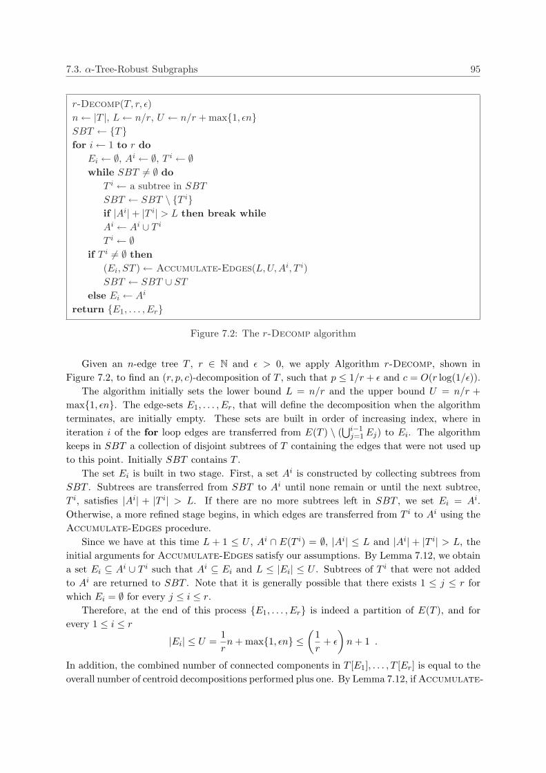
7.3. α-Tree-Robust Subgraphs 95
r-Decomp(T, r, ε)n ← |T |, L ← n/r, U ← n/r + max1, εnSBT ← Tfor i ← 1 to r do
Ei ← ∅, Ai ← ∅, T i ← ∅while SBT 6= ∅ do
T i ← a subtree in SBT
SBT ← SBT \ T iif |Ai|+ |T i| > L then break whileAi ← Ai ∪ T i
T i ← ∅if T i 6= ∅ then
(Ei, ST ) ← Accumulate-Edges(L,U,Ai, T i)SBT ← SBT ∪ ST
else Ei ← Ai
return E1, . . . , Er
Figure 7.2: The r-Decomp algorithm
Given an n-edge tree T , r ∈ N and ε > 0, we apply Algorithm r-Decomp, shown inFigure 7.2, to find an (r, p, c)-decomposition of T , such that p ≤ 1/r + ε and c = O(r log(1/ε)).
The algorithm initially sets the lower bound L = n/r and the upper bound U = n/r +max1, εn. The edge-sets E1, . . . , Er, that will define the decomposition when the algorithmterminates, are initially empty. These sets are built in order of increasing index, where initeration i of the for loop edges are transferred from E(T ) \ (
⋃i−1j=1 Ej) to Ei. The algorithm
keeps in SBT a collection of disjoint subtrees of T containing the edges that were not used upto this point. Initially SBT contains T .
The set Ei is built in two stage. First, a set Ai is constructed by collecting subtrees fromSBT . Subtrees are transferred from SBT to Ai until none remain or until the next subtree,T i, satisfies |Ai| + |T i| > L. If there are no more subtrees left in SBT , we set Ei = Ai.Otherwise, a more refined stage begins, in which edges are transferred from T i to Ai using theAccumulate-Edges procedure.
Since we have at this time L + 1 ≤ U , Ai ∩ E(T i) = ∅, |Ai| ≤ L and |Ai| + |T i| > L, theinitial arguments for Accumulate-Edges satisfy our assumptions. By Lemma 7.12, we obtaina set Ei ⊆ Ai ∪ T i such that Ai ⊆ Ei and L ≤ |Ei| ≤ U . Subtrees of T i that were not addedto Ai are returned to SBT . Note that it is generally possible that there exists 1 ≤ j ≤ r forwhich Ei = ∅ for every j ≤ i ≤ r.
Therefore, at the end of this process E1, . . . , Er is indeed a partition of E(T ), and forevery 1 ≤ i ≤ r
|Ei| ≤ U =1rn + max1, εn ≤
(1r
+ ε
)n + 1 .
In addition, the combined number of connected components in T [E1], . . . , T [Er] is equal to theoverall number of centroid decompositions performed plus one. By Lemma 7.12, if Accumulate-
96 Chapter 7: Robust Subgraphs for Trees and Paths
Edges is called in iteration i of the for loop, it terminates within O(log(|T i|/(U−L))) recursivecalls. Since |T i| ≤ n and U − L = max1, εn, we have |T i|/(U − L) ≤ 1/ε. This implies thatthe overall number of centroid decompositions is O(r log(1/ε)). In addition, by Lemma 7.13algorithm r-Decomp runs in O(rn) time. Theorem 7.8 follows.
7.3.2 A bound on the size of a minimum α-tree-robust subgraph
The following observations will be subsequently used to obtain an upper bound on the numberof edges in a minimum α-tree-robust subgraph.
Lemma 7.14. Let (r, p, c) be a tree decomposition scheme. Let 1 ≤ z ≤ r − 1. Let T be ak-edge tree. There exist E′ ⊆ E(T ) and a new set of edges A′, |A′| ≤ c, such that
1. T ′ = G[E′ ∪A′] is a tree.
2. |T ′| ≤ z(bpkc+ 1) + c.
3. w(T ′) ≥ (z/r) · w(T ).
Proof. Since (r, p, c) is a tree decomposition scheme, E(T ) can be represented as a union ofr disjoint subsets E1, . . . , Er such that |Ei| ≤ bpkc + 1 for every 1 ≤ i ≤ r, and such that thecombined number of connected components in T [E1], . . . , T [Er] is at most c. Without loss ofgenerality we assume that w(E1) ≥ · · · ≥ w(Er). Let E′ =
⋃zi=1 Ei. By adding at most c new
edges we can complete T [E′] into a tree T ′ that satisfies |T ′| ≤ z(bpkc+ 1) + c. In addition,
w(T ′) ≥z∑
i=1
w(Ei) ≥ z
r
r∑
i=1
w(Ei) =z
rw(T ) .
Corollary 7.15. Let (r, p, c) be a tree decomposition scheme. Let 1 ≤ z ≤ r − 1. Then forevery k ≥ 1,
w(T ∗z(bpkc+1)+c) ≥z
rw(T ∗k ) .
Corollary 7.16. Let (r, p, c) be a tree decomposition scheme. Let 1 ≤ z ≤ r − 1. For everyk ≥ 1, there exist E′ ⊆ E(T ∗k ) and A′ ⊆ E(G), |A′| ≤ c, such that:
1. T = G[E′ ∪A′] is a tree.
2. |T | ≤ z(bpkc+ 1) + c.
3. w(T ) ≥ (z/r) · w(T ∗k ).
We now prove an upper bound on the number of edges in a minimum α-tree-robust subgraph,when 0 < α < 1 is rational. In this case we can write α = z/r, where z, r ∈ N and 1 ≤ z ≤ r−1.Assume that (r, p, c) is a tree decomposition scheme that satisfies zp < 1.
Given (G,w), |V (G)| = n, and 0 < α < 1, we define T [i, j] = T ∗i , . . . , T ∗j for i ≤ j. Wedefine T ′ = T [1, 2d(1+ cp)/(p(1− zp))e− 1]. In addition, we define Ti = T [Li, Ui], i = 1, . . . , R,where
7.3. α-Tree-Robust Subgraphs 97
1. U1 = n− 1.
2. Ui = Li−1 − 1, i = 2, . . . , R.
3. Li = z(bp(z(bpUic+ 1) + c)c+ 1) + c, i = 1, . . . , R.
4. R = dlog(zp)−2(pn/2)e.
As Lemma 7.17c shows, LR ≤ 2d(1 + cp)/(p(1− zp))e, and indeed T ′ ∪(⋃R
i=1 Ti
)= T .
We z/r-cover T ′ using H ′ =⋃
T∈T ′ T , which is a subgraph whose number of edges isbounded by (2d(1 + cp)/(p(1 − zp))e)2/2 ≤ 2((1 + cp)/(p(1 − zp)) + 1)2. Note that sinceUi ≥ d(1 + cp)/(p(1− zp))e for every 1 ≤ i ≤ R, we have z(bpUic+ 1) + c ≤ Ui. Therefore, byCorollary 7.15 we can use T ∗z(bpUic+1)+c as a z/r-cover for T [z(bpUic + 1) + c, Ui]. In addition,when Ui ≥ d(1 + cp)/(p(1− zp))e we have z(bp(z(bpUic+ 1) + c)c+ 1) + c ≤ z(bpUic+ 1) + c.Therefore, by Corollary 7.16 it is sufficient to add at most c edges to T ∗z(bpUic+1)+c such that itbecomes a z/r-cover for T [z(bp(z(bpUic+1)+c)c+1)+c, z(bpUic+1)+c] = T [Li, z(bpUic+1)+c].It follows that Ti = T [Li, Ui] can be z/r-covered by a subgraph Hi ⊆ G such that |Hi| ≤z(bpUic+ 1) + 2c.
If we define H = H ′ ∪ (⋃R
i=1 Hi), then H is a z/r-tree-robust subgraph.
Lemma 7.17.
a. Ui ≤ (zp)2i−2n + (z + c)∑2i−1
j=0 (zp)j, for every i ≥ 1.
b. |Hi| ≤ (zp)2i−1n + (z + 2c)∑2i
j=0(zp)j, for every i ≥ 1.
c. LR ≤ 2d(1 + cp)/(p(1− zp))e.
Proof. See Section 7.5.
Lemma 7.18.
|H| ≤ zp
1− (zp)2n +
z + 2c
1− zp
⌈log(zp)−2
12pn
⌉+ 2
(1 + cp
p(1− zp)+ 1
)2
.
Proof. Since H = H ′ ∪ (⋃R
i=1 Hi), by Lemma 7.17b and 7.17c we have
|H| ≤R∑
i=1
|Hi|+ |H ′|
≤R∑
i=1
(zp)2i−1n + (z + 2c)
2i∑
j=0
(zp)j
+ 2
(1 + cp
p(1− zp)+ 1
)2
≤ n∞∑
i=1
(zp)2i−1 + (z + 2c)R∞∑
j=0
(zp)j + 2(
1 + cp
p(1− zp)+ 1
)2
=zp
1− (zp)2n +
z + 2c
1− zp
⌈log(zp)−2
12pn
⌉+ 2
(1 + cp
p(1− zp)+ 1
)2
.
98 Chapter 7: Robust Subgraphs for Trees and Paths
Lemma 7.19. lim supn→∞ tz/rn /n ≤ (z/r)/(1− (z/r)2).
Proof. Let ε > 0. There exists ε′ > 0 that satisfies ε′ < 1/z − 1/r and
z(
1r + ε′
)
1− (z
(1r + ε′
))2 ≤z/r
1− (z/r)2+ ε .
By Theorem 7.8 there exists a tree decomposition scheme (r, p, c) that satisfies p ≤ 1/r + ε′ andc = O(r log(1/ε′)). In addition,
zp ≤ z
(1r
+ ε′)
< z
(1r
+(
1z− 1
r
))= 1 .
Therefore, by Lemma 7.18 every complete weighted graph (G,w), |V (G)| = n, contains asubgraph H ⊆ G such that H is z/r-tree-robust and
|H| ≤ zp
1− (zp)2n +
z + 2c
1− zp
⌈log(zp)−2
12pn
⌉+ 2
(1 + cp
p(1− zp)+ 1
)2
.
Since the function f(x) = x/(1− x2) is monotone increasing over (0, 1), we have
lim supn→∞
tzrn
n≤ zp
1− (zp)2≤ z
(1r + ε′
)
1− (z
(1r + ε′
))2 ≤z/r
1− (z/r)2+ ε .
Theorem 7.20 generalizes the bound in Lemma 7.19 to arbitrary values of α.
Theorem 7.20. lim supn→∞ tαn/n ≤ α/(1− α2), for every 0 < α < 1.
Proof. Let ε > 0. There exists ε′ > 0 that satisfies α + ε′ < 1 and
α + ε′
1− (α + ε′)2≤ α
1− α2+ ε .
In addition, there exist z, r ∈ N such that α ≤ z/r ≤ α + ε′ and 1 ≤ z ≤ r − 1. Since tαnis a monotone increasing function of α, and the function f(x) = x/(1 − x2) is also monotoneincreasing over (0, 1), we have by Lemma 7.19
lim supn→∞
tαnn≤ lim sup
n→∞tz/rn
n≤ z/r
1− (z/r)2≤ α + ε′
1− (α + ε′)2≤ α
1− α2+ ε .
7.4 Polynomial-Time Algorithms
7.4.1 An algorithm for 0.353-path-robust path
We now prove that every complete weighted graph contains a 0.353-path-robust path, that canbe found in polynomial time. We also show that there exists a complete weighted graph inwhich no path is α-path-robust for α > 0.843. Our algorithm for finding a 0.353-path-robustpath is based on robust matchings.
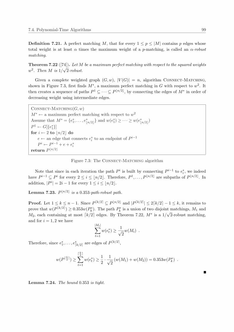
7.4. Polynomial-Time Algorithms 99
Definition 7.21. A perfect matching M , that for every 1 ≤ p ≤ |M | contains p edges whosetotal weight is at least α times the maximum weight of a p-matching, is called an α-robustmatching.
Theorem 7.22 ([74]). Let M be a maximum perfect matching with respect to the squared weightsw2. Then M is 1/
√2-robust.
Given a complete weighted graph (G,w), |V (G)| = n, algorithm Connect-Matching,shown in Figure 7.3, first finds M∗, a maximum perfect matching in G with respect to w2. Itthen creates a sequence of paths P 1 ⊆ · · · ⊆ P bn/2c, by connecting the edges of M∗ in order ofdecreasing weight using intermediate edges.
Connect-Matching(G,w)M∗ ← a maximum perfect matching with respect to w2
Assume that M∗ = e∗1, . . . , e∗bn/2c and w(e∗1) ≥ · · · ≥ w(e∗bn/2c)P 1 ← G[e∗1]for i ← 2 to bn/2c do
e ← an edge that connects e∗i to an endpoint of P i−1
P i ← P i−1 + e + e∗ireturn P bn/2c
Figure 7.3: The Connect-Matching algorithm
Note that since in each iteration the path P i is built by connecting P i−1 to e∗i , we indeedhave P i−1 ⊆ P i for every 2 ≤ i ≤ bn/2c. Therefore, P 1, . . . , P bn/2c are subpaths of P bn/2c. Inaddition, |P i| = 2i− 1 for every 1 ≤ i ≤ bn/2c.
Lemma 7.23. P bn/2c is a 0.353-path-robust path.
Proof. Let 1 ≤ k ≤ n− 1. Since P dk/2e ⊆ P bn/2c and |P dk/2e| ≤ 2dk/2e − 1 ≤ k, it remains toprove that w(P dk/2e) ≥ 0.353w(P ∗
k ). The path P ∗k is a union of two disjoint matchings, M1 and
M2, each containing at most dk/2e edges. By Theorem 7.22, M∗ is a 1/√
2-robust matching,and for i = 1, 2 we have
|Mi|∑
t=1
w(e∗t ) ≥1√2w(Mi) .
Therefore, since e∗1, . . . , e∗dk/2e are edges of P dk/2e,
w(P d k2e) ≥
d k2e∑
t=1
w(e∗t ) ≥12· 1√
2(w(M1) + w(M2)) = 0.353w(P ∗
k ) .
Lemma 7.24. The bound 0.353 is tight.
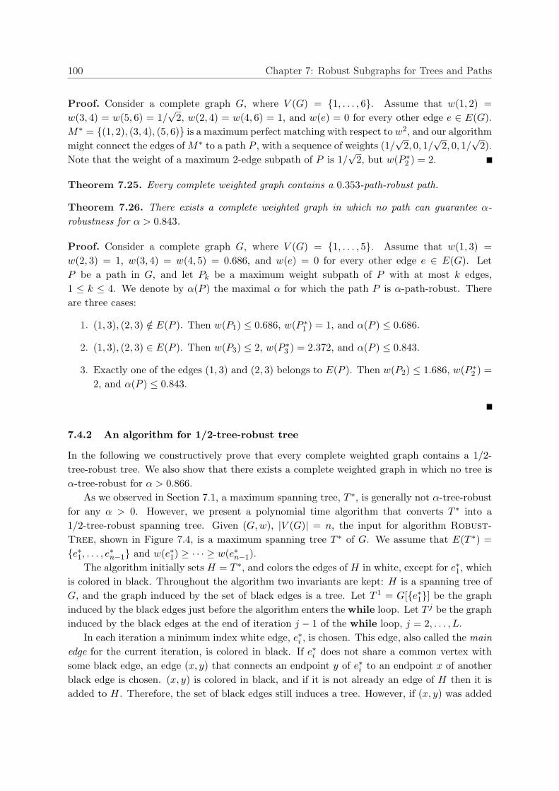
100 Chapter 7: Robust Subgraphs for Trees and Paths
Proof. Consider a complete graph G, where V (G) = 1, . . . , 6. Assume that w(1, 2) =w(3, 4) = w(5, 6) = 1/
√2, w(2, 4) = w(4, 6) = 1, and w(e) = 0 for every other edge e ∈ E(G).
M∗ = (1, 2), (3, 4), (5, 6) is a maximum perfect matching with respect to w2, and our algorithmmight connect the edges of M∗ to a path P , with a sequence of weights (1/
√2, 0, 1/
√2, 0, 1/
√2).
Note that the weight of a maximum 2-edge subpath of P is 1/√
2, but w(P ∗2 ) = 2.
Theorem 7.25. Every complete weighted graph contains a 0.353-path-robust path.
Theorem 7.26. There exists a complete weighted graph in which no path can guarantee α-robustness for α > 0.843.
Proof. Consider a complete graph G, where V (G) = 1, . . . , 5. Assume that w(1, 3) =w(2, 3) = 1, w(3, 4) = w(4, 5) = 0.686, and w(e) = 0 for every other edge e ∈ E(G). LetP be a path in G, and let Pk be a maximum weight subpath of P with at most k edges,1 ≤ k ≤ 4. We denote by α(P ) the maximal α for which the path P is α-path-robust. Thereare three cases:
1. (1, 3), (2, 3) /∈ E(P ). Then w(P1) ≤ 0.686, w(P ∗1 ) = 1, and α(P ) ≤ 0.686.
2. (1, 3), (2, 3) ∈ E(P ). Then w(P3) ≤ 2, w(P ∗3 ) = 2.372, and α(P ) ≤ 0.843.
3. Exactly one of the edges (1, 3) and (2, 3) belongs to E(P ). Then w(P2) ≤ 1.686, w(P ∗2 ) =
2, and α(P ) ≤ 0.843.
7.4.2 An algorithm for 1/2-tree-robust tree
In the following we constructively prove that every complete weighted graph contains a 1/2-tree-robust tree. We also show that there exists a complete weighted graph in which no tree isα-tree-robust for α > 0.866.
As we observed in Section 7.1, a maximum spanning tree, T ∗, is generally not α-tree-robustfor any α > 0. However, we present a polynomial time algorithm that converts T ∗ into a1/2-tree-robust spanning tree. Given (G,w), |V (G)| = n, the input for algorithm Robust-
Tree, shown in Figure 7.4, is a maximum spanning tree T ∗ of G. We assume that E(T ∗) =e∗1, . . . , e∗n−1 and w(e∗1) ≥ · · · ≥ w(e∗n−1).
The algorithm initially sets H = T ∗, and colors the edges of H in white, except for e∗1, whichis colored in black. Throughout the algorithm two invariants are kept: H is a spanning tree ofG, and the graph induced by the set of black edges is a tree. Let T 1 = G[e∗1] be the graphinduced by the black edges just before the algorithm enters the while loop. Let T j be the graphinduced by the black edges at the end of iteration j − 1 of the while loop, j = 2, . . . , L.
In each iteration a minimum index white edge, e∗i , is chosen. This edge, also called the mainedge for the current iteration, is colored in black. If e∗i does not share a common vertex withsome black edge, an edge (x, y) that connects an endpoint y of e∗i to an endpoint x of anotherblack edge is chosen. (x, y) is colored in black, and if it is not already an edge of H then it isadded to H. Therefore, the set of black edges still induces a tree. However, if (x, y) was added
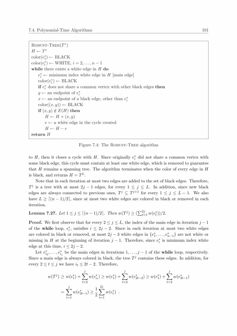
7.4. Polynomial-Time Algorithms 101
Robust-Tree(T ∗)H ← T ∗
color(e∗1) ← BLACKcolor(e∗i ) ← WHITE, i = 2, . . . , n− 1while there exists a white edge in H do
e∗i ← minimum index white edge in H [main edge]color(e∗i ) ← BLACKif e∗i does not share a common vertex with other black edges theny ← an endpoint of e∗ix ← an endpoint of a black edge, other than e∗icolor((x, y)) ← BLACKif (x, y) /∈ E(H) then
H ← H + (x, y)e ← a white edge in the cycle createdH ← H − e
return H
Figure 7.4: The Robust-Tree algorithm
to H, then it closes a cycle with H. Since originally e∗i did not share a common vertex withsome black edge, this cycle must contain at least one white edge, which is removed to guaranteethat H remains a spanning tree. The algorithm terminates when the color of every edge in H
is black, and returns H = TL.Note that in each iteration at most two edges are added to the set of black edges. Therefore,
T j is a tree with at most 2j − 1 edges, for every 1 ≤ j ≤ L. In addition, since new blackedges are always connected to previous ones, T j ⊆ T j+1 for every 1 ≤ j ≤ L − 1. We alsohave L ≥ d(n − 1)/2e, since at most two white edges are colored in black or removed in eachiteration.
Lemma 7.27. Let 1 ≤ j ≤ d(n− 1)/2e. Then w(T j) ≥ (∑2j
t=1 w(e∗t ))/2.
Proof. We first observe that for every 2 ≤ j ≤ L, the index of the main edge in iteration j − 1of the while loop, e∗i , satisfies i ≤ 2j − 2. Since in each iteration at most two white edgesare colored in black or removed, at most 2j − 3 white edges in e∗1, . . . , e∗n−1 are not white ormissing in H at the beginning of iteration j − 1. Therefore, since e∗i is minimum index whiteedge at this time, i ≤ 2j − 2.
Let e∗i2 , . . . , e∗ij
be the main edges in iterations 1, . . . , j − 1 of the while loop, respectively.Since a main edge is always colored in black, the tree T j contains these edges. In addition, forevery 2 ≤ t ≤ j we have it ≤ 2t− 2. Therefore,
w(T j) ≥ w(e∗1) +j∑
t=2
w(e∗it) ≥ w(e∗1) +j∑
t=2
w(e∗2t−2) ≥ w(e∗1) +j∑
t=2
w(e∗2t−1)
=j∑
t=1
w(e∗2t−1) ≥12
2j∑
t=1
w(e∗t ) .
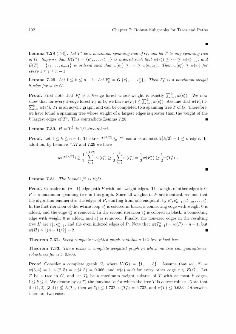
102 Chapter 7: Robust Subgraphs for Trees and Paths
Lemma 7.28 ([53]). Let T ∗ be a maximum spanning tree of G, and let T be any spanning treeof G. Suppose that E(T ∗) = e∗1, . . . , e∗n−1 is ordered such that w(e∗1) ≥ · · · ≥ w(e∗n−1), andE(T ) = e1, . . . , en−1 is ordered such that w(e1) ≥ · · · ≥ w(en−1). Then w(e∗i ) ≥ w(ei) forevery 1 ≤ i ≤ n− 1.
Lemma 7.29. Let 1 ≤ k ≤ n − 1. Let F ∗k = G[e∗1, . . . , e∗k]. Then F ∗
k is a maximum weightk-edge forest in G.
Proof. First note that F ∗k is a k-edge forest whose weight is exactly
∑ki=1 w(e∗i ). We now
show that for every k-edge forest Fk in G, we have w(Fk) ≤∑k
i=1 w(e∗i ). Assume that w(Fk) >∑ki=1 w(e∗i ). Fk is an acyclic graph, and can be completed to a spanning tree T of G. Therefore,
we have found a spanning tree whose weight of k largest edges is greater than the weight of thek largest edges of T ∗. This contradicts Lemma 7.28.
Lemma 7.30. H = TL is 1/2-tree-robust.
Proof. Let 1 ≤ k ≤ n − 1. The tree T dk/2e ⊆ TL contains at most 2dk/2e − 1 ≤ k edges. Inaddition, by Lemmas 7.27 and 7.29 we have
w(T dk/2e) ≥ 12
2dk/2e∑
t=1
w(e∗t ) ≥12
k∑
t=1
w(e∗t ) =12w(F ∗
k ) ≥ 12w(T ∗k ) .
Lemma 7.31. The bound 1/2 is tight.
Proof. Consider an (n−1)-edge path P with unit weight edges. The weight of other edges is 0.P is a maximum spanning tree in this graph. Since all weights in P are identical, assume thatthe algorithm enumerates the edges of P , starting from one endpoint, by e∗1, e
∗n−1, e
∗n−2, . . . , e
∗2.
In the first iteration of the while loop e∗2 is colored in black, a connecting edge with weight 0 isadded, and the edge e∗3 is removed. In the second iteration e∗4 is colored in black, a connectingedge with weight 0 is added, and e∗5 is removed. Finally, the non-zero edges in the resultingtree H are e∗1, e∗n−1, and the even indexed edges of P . Note that w(T ∗n−1) = w(P ) = n− 1, butw(H) ≤ b(n− 1)/2c+ 2.
Theorem 7.32. Every complete weighted graph contains a 1/2-tree-robust tree.
Theorem 7.33. There exists a complete weighted graph in which no tree can guarantee α-robustness for α > 0.866.
Proof. Consider a complete graph G, where V (G) = 1, . . . , 5. Assume that w(1, 2) =w(3, 4) = 1, w(2, 5) = w(4, 5) = 0.366, and w(e) = 0 for every other edge e ∈ E(G). LetT be a tree in G, and let Tk be a maximum weight subtree of T with at most k edges,1 ≤ k ≤ 4. We denote by α(T ) the maximal α for which the tree T is α-tree-robust. Note thatif (1, 2), (3, 4) * E(T ), then w(T4) ≤ 1.732, w(T ∗4 ) = 2.732, and α(T ) ≤ 0.633. Otherwise,there are two cases:
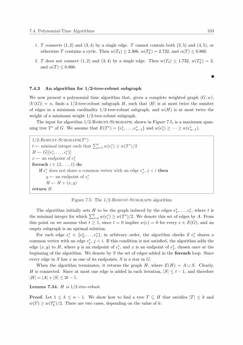
7.4. Polynomial-Time Algorithms 103
1. T connects (1, 2) and (3, 4) by a single edge. T cannot contain both (2, 5) and (4, 5), orotherwise T contains a cycle. Then w(T4) ≤ 2.366, w(T ∗4 ) = 2.732, and α(T ) ≤ 0.866.
2. T does not connect (1, 2) and (3, 4) by a single edge. Then w(T3) ≤ 1.732, w(T ∗3 ) = 2,and α(T ) ≤ 0.866.
7.4.3 An algorithm for 1/2-tree-robust subgraph
We now present a polynomial time algorithm that, given a complete weighted graph (G,w),|V (G)| = n, finds a 1/2-tree-robust subgraph H, such that |H| is at most twice the numberof edges in a minimum cardinality 1/2-tree-robust subgraph, and w(H) is at most twice theweight of a minimum weight 1/2-tree-robust subgraph.
The input for algorithm 1/2-Robust-Subgraph, shown in Figure 7.5, is a maximum span-ning tree T ∗ of G. We assume that E(T ∗) = e∗1, . . . , e∗n−1 and w(e∗1) ≥ · · · ≥ w(e∗n−1).
1/2-Robust-Subgraph(T ∗)t ← minimal integer such that
∑ti=1 w(e∗i ) ≥ w(T ∗)/2
H ← G[e∗1, . . . , e∗t ]x ← an endpoint of e∗1foreach i ∈ 2, . . . , t do
if e∗i does not share a common vertex with an edge e∗j , j < i theny ← an endpoint of e∗iH ← H + (x, y)
return H
Figure 7.5: The 1/2-Robust-Subgraph algorithm
The algorithm initially sets H to be the graph induced by the edges e∗1, . . . , e∗t , where t is
the minimal integer for which∑t
i=1 w(e∗i ) ≥ w(T ∗)/2. We denote this set of edges by A. Fromthis point on we assume that t ≥ 1, since t = 0 implies w(e) = 0 for every e ∈ E(G), and anempty subgraph is an optimal solution.
For each edge e∗i ∈ e∗2, . . . , e∗t , in arbitrary order, the algorithm checks if e∗i shares acommon vertex with an edge e∗j , j < i. If this condition is not satisfied, the algorithm adds theedge (x, y) to H, where y is an endpoint of e∗i , and x is an endpoint of e∗1, chosen once at thebeginning of the algorithm. We denote by S the set of edges added in the foreach loop. Sinceevery edge in S has x as one of its endpoints, S is a star in G.
When the algorithm terminates, it returns the graph H, where E(H) = A ∪ S. Clearly,H is connected. Since at most one edge is added in each iteration, |S| ≤ t − 1, and therefore|H| = |A|+ |S| ≤ 2t− 1.
Lemma 7.34. H is 1/2-tree-robust.
Proof. Let 1 ≤ k ≤ n − 1. We show how to find a tree T ⊆ H that satisfies |T | ≤ k andw(T ) ≥ w(T ∗k )/2. There are two cases, depending on the value of k:
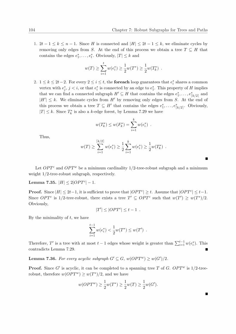
104 Chapter 7: Robust Subgraphs for Trees and Paths
1. 2t − 1 ≤ k ≤ n − 1. Since H is connected and |H| ≤ 2t − 1 ≤ k, we eliminate cycles byremoving only edges from S. At the end of this process we obtain a tree T ⊆ H thatcontains the edges e∗1, . . . , e
∗t . Obviously, |T | ≤ k and
w(T ) ≥t∑
i=1
w(e∗i ) ≥12w(T ∗) ≥ 1
2w(T ∗k ) .
2. 1 ≤ k ≤ 2t−2. For every 2 ≤ i ≤ t, the foreach loop guarantees that e∗i shares a commonvertex with e∗j , j < i, or that e∗i is connected by an edge to e∗1. This property of H impliesthat we can find a connected subgraph H ′ ⊆ H that contains the edges e∗1, . . . , e
∗dk/2e and
|H ′| ≤ k. We eliminate cycles from H ′ by removing only edges from S. At the end ofthis process we obtain a tree T ⊆ H ′ that contains the edges e∗1, . . . , e
∗dk/2e. Obviously,
|T | ≤ k. Since T ∗k is also a k-edge forest, by Lemma 7.29 we have
w(T ∗k ) ≤ w(F ∗k ) =
k∑
i=1
w(e∗i ) .
Thus,
w(T ) ≥dk/2e∑
i=1
w(e∗i ) ≥12
k∑
i=1
w(e∗i ) ≥12w(T ∗k ) .
Let OPT c and OPTw be a minimum cardinality 1/2-tree-robust subgraph and a minimumweight 1/2-tree-robust subgraph, respectively.
Lemma 7.35. |H| ≤ 2|OPT c| − 1.
Proof. Since |H| ≤ 2t−1, it is sufficient to prove that |OPT c| ≥ t. Assume that |OPT c| ≤ t−1.Since OPT c is 1/2-tree-robust, there exists a tree T ′ ⊆ OPT c such that w(T ′) ≥ w(T ∗)/2.Obviously,
|T ′| ≤ |OPT c| ≤ t− 1 .
By the minimality of t, we have
t−1∑
i=1
w(e∗i ) <12w(T ∗) ≤ w(T ′) .
Therefore, T ′ is a tree with at most t− 1 edges whose weight is greater than∑t−1
i=1 w(e∗i ). Thiscontradicts Lemma 7.29.
Lemma 7.36. For every acyclic subgraph G′ ⊆ G, w(OPTw) ≥ w(G′)/2.
Proof. Since G′ is acyclic, it can be completed to a spanning tree T of G. OPTw is 1/2-tree-robust, therefore w(OPTw) ≥ w(T ∗)/2, and we have
w(OPTw) ≥ 12w(T ∗) ≥ 1
2w(T ) ≥ 1
2w(G′).
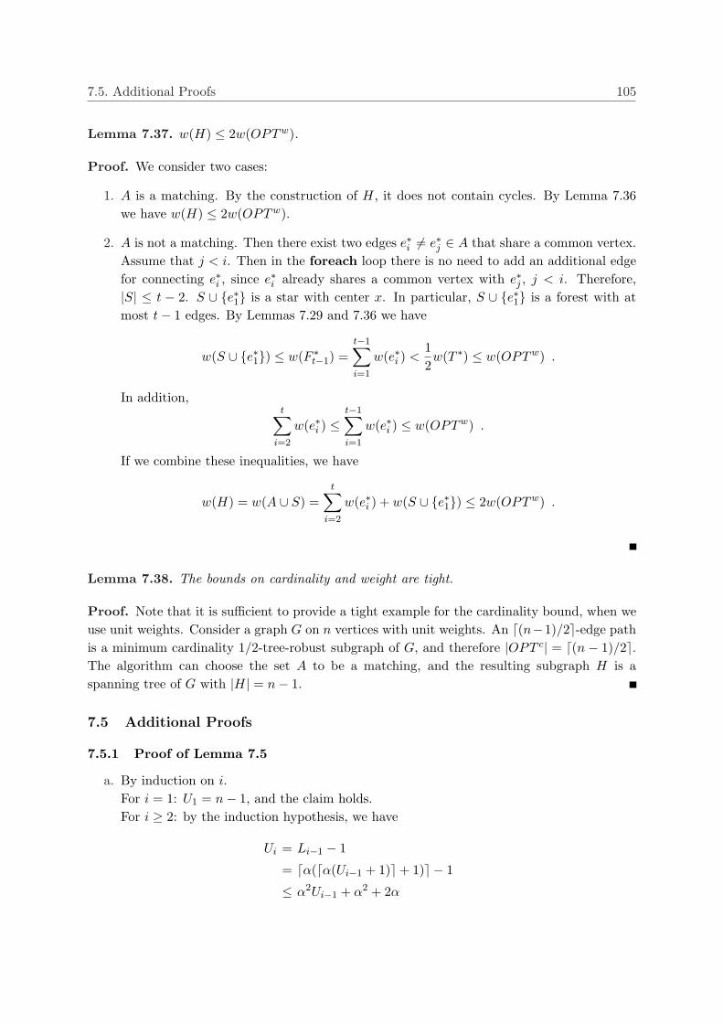
7.5. Additional Proofs 105
Lemma 7.37. w(H) ≤ 2w(OPTw).
Proof. We consider two cases:
1. A is a matching. By the construction of H, it does not contain cycles. By Lemma 7.36we have w(H) ≤ 2w(OPTw).
2. A is not a matching. Then there exist two edges e∗i 6= e∗j ∈ A that share a common vertex.Assume that j < i. Then in the foreach loop there is no need to add an additional edgefor connecting e∗i , since e∗i already shares a common vertex with e∗j , j < i. Therefore,|S| ≤ t − 2. S ∪ e∗1 is a star with center x. In particular, S ∪ e∗1 is a forest with atmost t− 1 edges. By Lemmas 7.29 and 7.36 we have
w(S ∪ e∗1) ≤ w(F ∗t−1) =
t−1∑
i=1
w(e∗i ) <12w(T ∗) ≤ w(OPTw) .
In addition,t∑
i=2
w(e∗i ) ≤t−1∑
i=1
w(e∗i ) ≤ w(OPTw) .
If we combine these inequalities, we have
w(H) = w(A ∪ S) =t∑
i=2
w(e∗i ) + w(S ∪ e∗1) ≤ 2w(OPTw) .
Lemma 7.38. The bounds on cardinality and weight are tight.
Proof. Note that it is sufficient to provide a tight example for the cardinality bound, when weuse unit weights. Consider a graph G on n vertices with unit weights. An d(n−1)/2e-edge pathis a minimum cardinality 1/2-tree-robust subgraph of G, and therefore |OPT c| = d(n− 1)/2e.The algorithm can choose the set A to be a matching, and the resulting subgraph H is aspanning tree of G with |H| = n− 1.
7.5 Additional Proofs
7.5.1 Proof of Lemma 7.5
a. By induction on i.For i = 1: U1 = n− 1, and the claim holds.For i ≥ 2: by the induction hypothesis, we have
Ui = Li−1 − 1
= dα(dα(Ui−1 + 1)e+ 1)e − 1
≤ α2Ui−1 + α2 + 2α
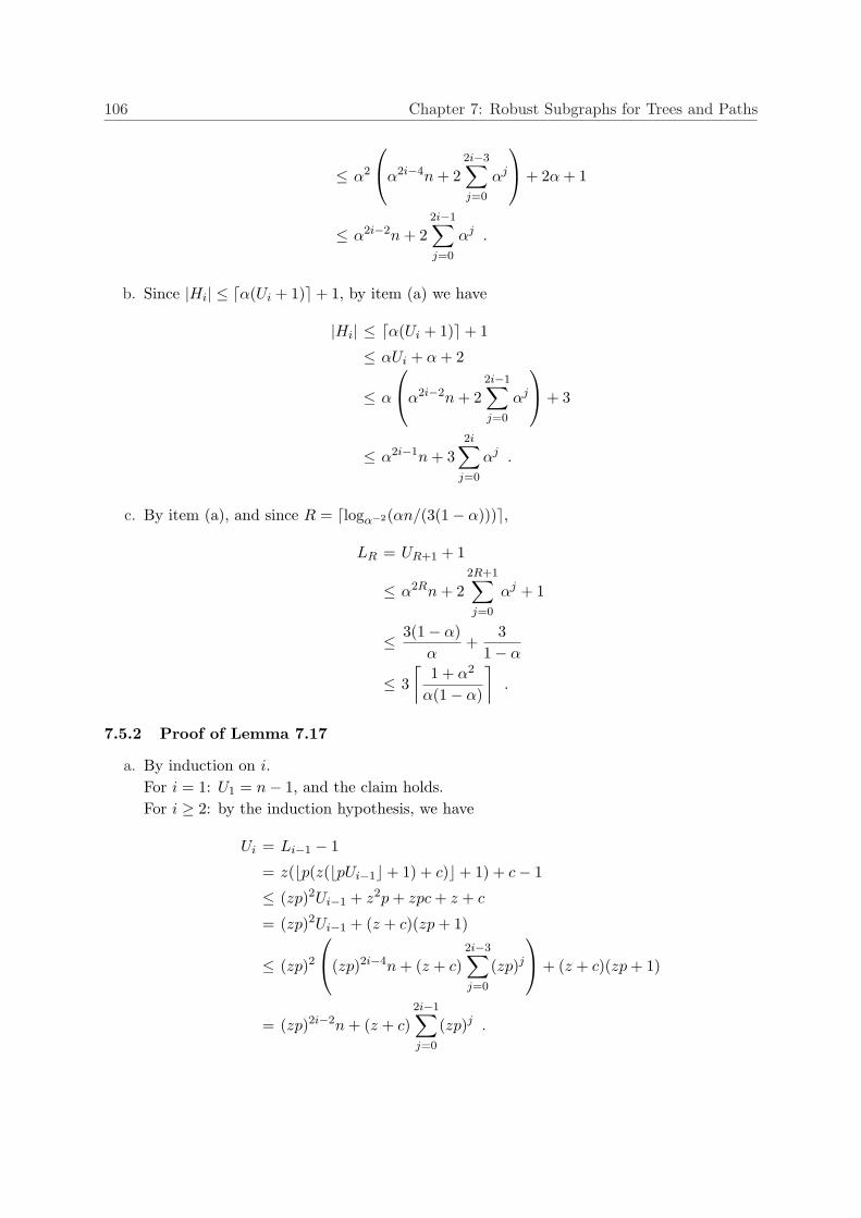
106 Chapter 7: Robust Subgraphs for Trees and Paths
≤ α2
α2i−4n + 2
2i−3∑
j=0
αj
+ 2α + 1
≤ α2i−2n + 22i−1∑
j=0
αj .
b. Since |Hi| ≤ dα(Ui + 1)e+ 1, by item (a) we have
|Hi| ≤ dα(Ui + 1)e+ 1
≤ αUi + α + 2
≤ α
α2i−2n + 2
2i−1∑
j=0
αj
+ 3
≤ α2i−1n + 32i∑
j=0
αj .
c. By item (a), and since R = dlogα−2(αn/(3(1− α)))e,
LR = UR+1 + 1
≤ α2Rn + 22R+1∑
j=0
αj + 1
≤ 3(1− α)α
+3
1− α
≤ 3⌈
1 + α2
α(1− α)
⌉.
7.5.2 Proof of Lemma 7.17
a. By induction on i.For i = 1: U1 = n− 1, and the claim holds.For i ≥ 2: by the induction hypothesis, we have
Ui = Li−1 − 1
= z(bp(z(bpUi−1c+ 1) + c)c+ 1) + c− 1
≤ (zp)2Ui−1 + z2p + zpc + z + c
= (zp)2Ui−1 + (z + c)(zp + 1)
≤ (zp)2
(zp)2i−4n + (z + c)
2i−3∑
j=0
(zp)j
+ (z + c)(zp + 1)
= (zp)2i−2n + (z + c)2i−1∑
j=0
(zp)j .
7.5. Additional Proofs 107
b. Since |Hi| ≤ z(bpUic+ 1) + 2c, by item (a) we have
|Hi| ≤ z(bpUic+ 1) + 2c
≤ (zp)Ui + z + 2c
≤ (zp)
(zp)2i−2n + (z + c)
2i−1∑
j=0
(zp)j
+ z + 2c
≤ (zp)2i−1n + (z + 2c)2i∑
j=0
(zp)j .
c. By item (a), and since R = dlog(zp)−2(pn/2)e
LR = UR+1 + 1
≤ (zp)2Rn + (z + c)2R+1∑
j=0
(zp)j + 1
≤ 2p
+2(z + c)1− zp
≤ 2⌈
1 + cp
p(1− zp)
⌉.
108 Chapter 7: Robust Subgraphs for Trees and Paths
Bibliography
[1] A. Agrawal, P. N. Klein, and R. Ravi. When trees collide: An approximation algorithmfor the generalized Steiner problem on networks. SIAM Journal on Computing, 24(3):440–456, 1995.
[2] N. Alon, B. Awerbuch, Y. Azar, N. Buchbinder, and J. Naor. A general approach toonline network optimization problems. ACM Transactions on Algorithms, 2(4):640–660,2006.
[3] J. Araoz, W. H. Cunningham, J. Edmonds, and J. Green-Krotki. Reductions to 1-matching polyhedra. Networks, 13:455–473, 1983.
[4] S. Arora. Polynomial time approximation schemes for Euclidean traveling salesman andother geometric problems. Journal of the ACM, 45(5):753–782, 1998.
[5] S. Arora and G. Karakostas. A 2 + ε approximation algorithm for the k-MST problem.Mathematical Programming, 107(3):491–504, 2006.
[6] S. Arora, D. R. Karger, and M. Karpinski. Polynomial time approximation schemesfor dense instances of NP-hard problems. Journal of Computer and System Sciences,58(1):193–210, 1999.
[7] S. Arora, J. R. Lee, and A. Naor. Euclidean distortion and the sparsest cut. In Proceedingsof the 37th Annual ACM Symposium on Theory of Computing, pages 553–562, 2005.
[8] S. Arora, C. Lund, R. Motwani, M. Sudan, and M. Szegedy. Proof verification and thehardness of approximation problems. Journal of the ACM, 45(3):501–555, 1998.
[9] Y. Asahiro, K. Iwama, H. Tamaki, and T. Tokuyama. Greedily finding a dense subgraph.Journal of Algorithms, 34(2):203–221, 2000.
[10] Y. Aumann and Y. Rabani. An O(log k) approximate min-cut max-flow theorem andapproximation algorithm. SIAM Journal on Computing, 27(1):291–301, 1998.
[11] B. Awerbuch, Y. Azar, and Y. Bartal. On-line generalized Steiner problem. TheoreticalComputer Science, 324(2-3):313–324, 2004.
[12] B. Awerbuch, Y. Azar, A. Blum, and S. Vempala. New approximation guarantees forminimum-weight k-trees and prize-collecting salesmen. SIAM Journal on Computing,28(1):254–262, 1998.
109
110 BIBLIOGRAPHY
[13] E. Balas and M. Padberg. Set partitioning: A survey. SIAM Review, 18(4):710–760, 1976.
[14] R. Bar-Yehuda. Using homogeneous weights for approximating the partial cover problem.Journal of Algorithms, 39(2):137–144, 2001.
[15] R. Bar-Yehuda and S. Even. A linear-time approximation algorithm for the weightedvertex cover problem. Journal of Algorithms, 2(2):198–203, 1981.
[16] Y. Bartal. Probabilistic approximations of metric spaces and its algorithmic applications.In Proceedings of the 37th Annual IEEE Symposium on Foundations of Computer Science,pages 184–193, 1996.
[17] Y. Bartal. On approximating arbitrary metrices by tree metrics. In Proceedings of the30th Annual ACM Symposium on the Theory of Computing, pages 161–168, 1998.
[18] Y. Bartal, M. Charikar, and D. Raz. Approximating min-sum k-clustering in metricspaces. In Proceedings of the 33rd Annual ACM Symposium on the Theory of Computing,pages 11–20, 2001.
[19] C. D. Bateman, C. S. Helvig, G. Robins, and A. Zelikovsky. Provably good routing treeconstruction with multi-port terminals. In Proceedings of the International Symposiumon Physical Design, pages 96–102, 1997.
[20] P. Berman and C. Coulston. On-line algorithms for Steiner tree problems (extended ab-stract). In Proceedings of the 29th Annual ACM Symposium on the Theory of Computing,pages 344–353, 1997.
[21] D. Bienstock, M. X. Goemans, D. Simchi-Levi, and D. P. Williamson. A note on the prizecollecting traveling salesman problem. Mathematical Programming, 59:413–420, 1993.
[22] A. Blum, R. Ravi, and S. Vempala. A constant-factor approximation algorithm for thek-MST problem. Journal of Computer and System Sciences, 58(1):101–108, 1999.
[23] N. H. Bshouty and L. Burroughs. Massaging a linear programming solution to give a 2-approximation for a generalization of the vertex cover problem. In Proceedings of the 15thAnnual Symposium on Theoretical Aspects of Computer Science, pages 298–308, 1998.
[24] R. D. Carr, T. Fujito, G. Konjevod, and O. Parekh. A 2 110 -approximation algorithm for
a generalization of the weighted edge-dominating set problem. Journal of CombinatorialOptimization, 5(3):317–326, 2001.
[25] M. Charikar, C. Chekuri, T.-Y. Cheung, Z. Dai, A. Goel, S. Guha, and M. Li. Approx-imation algorithms for directed Steiner problems. Journal of Algorithms, 33(1):73–91,1999.
[26] M. Charikar, C. Chekuri, A. Goel, and S. Guha. Rounding via trees: Deterministicapproximation algorithms for group Steiner trees and k-median. In Proceedings of the30th Annual ACM Symposium on the Theory of Computing, pages 114–123, 1998.
BIBLIOGRAPHY 111
[27] M. Charikar, C. Chekuri, A. Goel, S. Guha, and S. A. Plotkin. Approximating a finitemetric by a small number of tree metrics. In Proceedings of the 39th Annual IEEESymposium on Foundations of Computer Science, pages 379–388, 1998.
[28] M. Charikar, S. Khuller, D. M. Mount, and G. Narasimhan. Algorithms for facility locationproblems with outliers. In Proceedings of the 12th Annual ACM-SIAM Symposium onDiscrete Algorithms, pages 642–651, 2001.
[29] S. Chawla, A. Gupta, and H. Racke. Embeddings of negative-type metrics and an im-proved approximation to generalized sparsest cut. In Proceedings of the 16th AnnualACM-SIAM Symposium on Discrete Algorithms, pages 102–111, 2005.
[30] S. Chawla, R. Krauthgamer, R. Kumar, Y. Rabani, and D. Sivakumar. On the hardnessof approximating multicut and sparsest-cut. Computational Complexity, 15(2):94–114,2006.
[31] C. Chekuri, G. Even, A. Gupta, and D. Segev. Set connectivity problems in undirectedgraphs and the directed Steiner network problem. Manuscript, 2007.
[32] C. Chekuri, G. Even, and G. Kortsarz. A greedy approximation algorithm for the groupSteiner problem. Discrete Applied Mathematics, 154(1):15–34, 2006.
[33] C. Chekuri, M. T. Hajiaghayi, G. Kortsarz, and M. R. Salavatipour. Approximationalgorithms for non-uniform buy-at-bulk network design. In Proceedings of the 47th AnnualIEEE Symposium on Foundations of Computer Science, pages 677–686, 2006.
[34] C. Chekuri, M. T. Hajiaghayi, G. Kortsarz, and M. R. Salavatipour. Approximationalgorithms for node-weighted buy-at-bulk network design. In Proceedings of the 18thAnnual ACM-SIAM Symposium on Discrete Algorithms, pages 1265–1274, 2007.
[35] F. A. Chudak, T. Roughgarden, and D. P. Williamson. Approximate k-MSTs and k-Steiner trees via the primal-dual method and Lagrangean relaxation. Mathematical Pro-gramming, 100(2):411–421, 2004.
[36] V. Chvatal. A greedy heuristic for the set covering problem. Mathematics of OperationsResearch, 4(3):233–235, 1979.
[37] W. J. Cook, W. H. Cunningham, W. R. Pulleyblank, and A. Schrijver. CombinatorialOptimization. John Wiley and Sons, New York, 1997.
[38] Y. Dodis and S. Khanna. Designing networks with bounded pairwise distance. In Pro-ceedings of the 31st Annual ACM Symposium on Theory of Computing, pages 750–759,1999.
[39] J. Edmonds and E. L. Johnson. Matching: A well-solved class of integer linear programs.In Combinatorial Structures and their Applications, pages 89–92. Gordon and Breach,New York, 1970.
112 BIBLIOGRAPHY
[40] R. Engelberg, J. Konemann, S. Leonardi, and J. Naor. Cut problems in graphs with abudget constraint. Journal of Discrete Algorithms, 5(2):262–279, 2007.
[41] G. Even, J. Feldman, G. Kortsarz, and Z. Nutov. A 3/2-approximation algorithm foraugmenting the edge-connectivity of a graph from 1 to 2 using a subset of a given edgeset. In Proceedings of the 4th International Workshop on Approximation Algorithms forCombinatorial Optimization Problems, pages 90–101, 2001.
[42] G. Even, G. Kortsarz, and W. Slany. On network design problems: Fixed cost flows andthe covering Steiner problem. ACM Transactions on Algorithms, 1(1):74–101, 2005.
[43] J. Fakcharoenphol, S. Rao, and K. Talwar. A tight bound on approximating arbitrarymetrics by tree metrics. Journal of Computer and System Sciences, 69(3):485–497, 2004.
[44] U. Feige. A threshold of lnn for approximating set cover. Journal of the ACM, 45(4):634–652, 1998.
[45] U. Feige, G. Kortsarz, and D. Peleg. The dense k-subgraph problem. Algorithmica,29(3):410–421, 2001.
[46] U. Feige and M. Langberg. Approximation algorithms for maximization problems arisingin graph partitioning. Journal of Algorithms, 41(2):174–211, 2001.
[47] L. Fleischer, J. Konemann, S. Leonardi, and G. Schafer. Simple cost sharing schemesfor multi-commodity rent-or-buy and stochastic Steiner tree. In Proceedings of the 38thAnnual ACM Symposium on Theory of Computing, pages 663–670, 2006.
[48] G. N. Frederickson and J. JaJa. Approximation algorithm for several graph augmentationproblems. SIAM Journal on Computing, 10(2):270–283, 1981.
[49] G. N. Frederickson and D. B. Johnson. Generating and searching sets induced by net-works. In Proceedings of the 7th International Colloquium on Automata, Languages andProgramming, pages 221–233, 1980.
[50] T. Fujito. On approximation of the submodular set cover problem. Operations ResearchLetters, 25(4):169–174, 1999.
[51] T. Fujito and H. Nagamochi. A 2-approximation algorithm for the minimum weight edgedominating set problem. Discrete Applied Mathematics, 118(3):199–207, 2002.
[52] T. Fukunaga and H. Nagamochi. The set connector problem in graphs. In Proceedings ofthe 12th International Conference on Integer Programming and Combinatorial Optimiza-tion, pages 484–498, 2007.
[53] D. Gale. Optimal assignments in an ordered set: An application of matroid theory. Journalof Combinatorial Theory, 4:176–180, 1968.
[54] R. Gandhi, S. Khuller, and A. Srinivasan. Approximation algorithms for partial coveringproblems. Journal of Algorithms, 53(1):55–84, 2004.
BIBLIOGRAPHY 113
[55] R. S. Garfinkel and G. L. Nemhauser. Optimal set covering: A survey. In A. M. Geoffrion,editor, Perspectives on Optimization, pages 164–183, 1972.
[56] N. Garg. A 3-approximation for the minimum tree spanning k vertices. In Proceedings ofthe 37th Annual IEEE Symposium on Foundations of Computer Science, pages 302–309,1996.
[57] N. Garg. Saving an epsilon: A 2-approximation for the k-MST problem in graphs. InProceedings of the 37th Annual ACM Symposium on Theory of Computing, pages 396–402,2005.
[58] N. Garg, G. Konjevod, and R. Ravi. A polylogarithmic approximation algorithm for thegroup Steiner tree problem. Journal of Algorithms, 37(1):66–84, 2000.
[59] N. Garg, V. V. Vazirani, and M. Yannakakis. Approximate max-flow min-(multi)cuttheorems and their applications. SIAM Journal on Computing, 25(2):235–251, 1996.
[60] N. Garg, V. V. Vazirani, and M. Yannakakis. Primal-dual approximation algorithms forintegral flow and multicut in trees. Algorithmica, 18(1):3–20, 1997.
[61] D. R. Gaur, T. Ibaraki, and R. Krishnamurti. Constant ratio approximation algorithmsfor the rectangle stabbing problem and the rectilinear partitioning problem. Journal ofAlgorithms, 43(1):138–152, 2002.
[62] M. X. Goemans and D. P. Williamson. A general approximation technique for constrainedforest problems. SIAM Journal on Computing, 24(2):296–317, 1995.
[63] M. X. Goemans and D. P. Williamson. The primal-dual method for approximation al-gorithms and its application to network design problems. In D. S. Hochbaum, editor,Approximation Algorithms for NP-Hard Problems. PWS Publishing Company, 1996.
[64] D. Golovin, V. Nagarajan, and M. Singh. Approximating the k-multicut problem. InProceedings of the 17th Annual ACM-SIAM Symposium on Discrete Algorithms, pages621–630, 2006.
[65] A. Gupta, J. Konemann, S. Leonardi, R. Ravi, and G. Schafer. An efficient cost-sharingmechanism for the prize-collecting Steiner forest problem. In Proceedings of the 18thAnnual ACM-SIAM Symposium on Discrete Algorithms, pages 1153–1162, 2007.
[66] A. Gupta, A. Kumar, M. Pal, and T. Roughgarden. Approximation via cost-sharing: Asimple approximation algorithm for the multicommodity rent-or-buy problem. In Proceed-ings of the 44th Annual IEEE Symposium on Foundations of Computer Science, pages606–615, 2003.
[67] A. Gupta and M. Pal. Stochastic Steiner trees without a root. In Proceedings of the 32ndInternational Colloquium on Automata, Languages and Programming, pages 1051–1063,2005.
114 BIBLIOGRAPHY
[68] M. T. Hajiaghayi and K. Jain. The prize-collecting generalized Steiner tree problem viaa new approach of primal-dual schema. In Proceedings of the 17th Annual ACM-SIAMSymposium on Discrete Algorithms, pages 631–640, 2006.
[69] M. T. Hajiaghayi, G. Kortsarz, and M. R. Salavatipour. Approximating buy-at-bulk andshallow-light k-Steiner trees. In Proceedings of the 9th International Workshop on Ap-proximation Algorithms for Combinatorial Optimization Problems, pages 152–163, 2006.
[70] E. Halperin, G. Kortsarz, R. Krauthgamer, A. Srinivasan, and N. Wang. Integralityratio for group Steiner trees and directed Steiner trees. SIAM Journal on Computing,36(5):1494–1511, 2007.
[71] E. Halperin and R. Krauthgamer. Polylogarithmic inapproximability. In Proceedings ofthe 35th Annual ACM Symposium on Theory of Computing, pages 585–594, 2003.
[72] Q. Han, Y. Ye, and J. Zhang. An improved rounding method and semidefinite program-ming relaxation for graph partition. Mathematical Programming, 92(3):509–535, 2002.
[73] R. Hassin and A. Levin. An efficient polynomial time approximation scheme for theconstrained minimum spanning tree problem using matroid intersection. SIAM Journalon Computing, 33(2):261–268, 2004.
[74] R. Hassin and S. Rubinstein. Robust matchings. SIAM Journal on Discrete Mathematics,15(4):530–537, 2002.
[75] R. Hassin, S. Rubinstein, and A. Tamir. Approximation algorithms for maximum disper-sion. Operations Research Letters, 21(3):133–137, 1997.
[76] D. S. Hochbaum, editor. Approximation Algorithms for NP-Hard Problems. PWS Pub-lishing Company, 1996.
[77] D. S. Hochbaum. Approximating covering and packing problems: Set cover, vertex cover,independent set, and related problems. In D. S. Hochbaum, editor, Approximation Al-gorithms for NP-Hard Problems, chapter 3, pages 94–143. PWS Publishing Company,1997.
[78] D. S. Hochbaum. The t-vertex cover problem: Extending the half integrality frameworkwith budget constraints. In Proceedings of the 1st International Workshop on Approxi-mation Algorithms for Combinatorial Optimization, pages 111–122, 1998.
[79] P. Indyk. Algorithmic applications of low-distortion geometric embeddings. Tutorial in:Proceedings of the 42nd Annual IEEE Symposium on Foundations of Computer Science,pages 10–33, 2001.
[80] P. Indyk and J. Matousek. Low distortion embeddings of finite metric spaces. In J. E.Goodman and J. O’Rourke, editors, Handbook of Discrete and Computational Geometry.CRC Press LLC, 2nd edition, 2004.
BIBLIOGRAPHY 115
[81] K. Jain. A factor 2 approximation algorithm for the generalized Steiner network problem.Combinatorica, 21(1):39–60, 2001.
[82] D. S. Johnson. Approximation algorithms for combinatorial problems. Journal of Com-puter and System Sciences, 9(3):256–278, 1974.
[83] A. Kamath, R. Motwani, K. V. Palem, and P. G. Spirakis. Tail bounds for occupancy andthe satisfiability threshold conjecture. In Proceedings of the 35th Annual IEEE Symposiumon Foundations of Computer Science, pages 592–603, 1994.
[84] M. J. Kearns. The Computational Complexity of Machine Learning. MIT Press, 1990. Theapproximation guarantee of the partial cover algorithm we refer to is stated in Theorem5.15.
[85] S. Khot. On the power of unique 2-prover 1-round games. In Proceedings of the 34thAnnual ACM Symposium on Theory of Computing, pages 767–775, 2002.
[86] S. Khuller and R. Thurimella. Approximation algorithms for graph augmentation. Journalof Algorithms, 14(2):214–225, 1993.
[87] A. Kolen and A. Tamir. Covering problems. In P. B. Mirchandani and R. L. Francis,editors, Discrete Location Theory, pages 263–304. Wiley-Interscience Series in DiscreteMathematics and Optimization, 1990.
[88] G. Kortsarz and D. Peleg. On choosing a dense subgraph. In Proceedings of the 34thAnnual IEEE Symposium on Foundations of Computer Science, pages 692–701, 1993.
[89] A. Kumar, A. Gupta, and T. Roughgarden. A constant-factor approximation algorithmfor the multicommodity rent-or-buy problem. In Proceedings of the 43rd Annual IEEESymposium on Foundations of Computer Science, pages 333–344, 2002.
[90] A. Levin and D. Segev. Partial multicuts in trees. Theoretical Computer Science, 369(1-3):384–395, 2006.
[91] N. Linial, E. London, and Y. Rabinovich. The geometry of graphs and some of its algo-rithmic applications. Combinatorica, 15(2):215–245, 1995.
[92] L. Lovasz. On the ratio of optimal integral and fractional covers. Discrete Mathematics,13:383–390, 1975.
[93] J. Matousek. Lectures on Discrete Geometry, volume 212 of Graduate Texts in Mathe-matics. Springer, 2002.
[94] M. Mendel and A. Naor. Maximum gradient embeddings and monotone clustering. InProceedings of the 10th International Workshop on Approximation Algorithms for Com-binatorial Optimization Problems, pages 242–256, 2007.
[95] P. B. Mirchandani and R. L. Francis. Discrete Location Theory. Wiley-Interscience Seriesin Discrete Mathematics and Optimization, 1990.
116 BIBLIOGRAPHY
[96] J. S. B. Mitchell. Guillotine subdivisions approximate polygonal subdivisions: A simplepolynomial-time approximation scheme for geometric TSP, k-MST, and related problems.SIAM Journal on Computing, 28(4):1298–1309, 1999.
[97] K. G. Murty and C. Perin. A 1-matching blossom type algorithm for edge coveringproblems. Networks, 12:379–391, 1982.
[98] H. Nagamochi. An approximation for finding a smallest 2-edge-connected subgraph con-taining a specified spanning tree. Discrete Applied Mathematics, 126(1):83–113, 2003.
[99] G. L. Nemhauser and L. A. Wolsey. Integer and Combinatorial Optimization. John Wileyand Sons, 1988.
[100] M. W. Padberg. Covering, packing and knapsack problems. Annals of Discrete Mathe-matics, 4:265–287, 1979.
[101] C. H. Papadimitriou and M. Yannakakis. Optimization, approximation, and complexityclasses. Journal of Computer and System Sciences, 43(3):425–440, 1991.
[102] O. Parekh. Edge dominating and hypomatchable sets. In Proceedings of the 13th AnnualACM-SIAM Symposium on Discrete Algorithms, pages 287–291, 2002.
[103] O. Parekh. Polyhedral Techniques for Graphic Covering Problems. PhD thesis, Depart-ment of Mathematical Sciences, Carnegie Mellon University, 2002.
[104] O. Parekh and D. Segev. Path hitting in acyclic graphs. Algorithmica, to appear. Alsoin: Proceedings of the 14th Annual European Symposium on Algorithms, pages 564–575,2006.
[105] J. Plesnık. Constrained weighted matchings and edge coverings in graphs. Discrete AppliedMathematics, 92(2–3):229–241, 1999.
[106] W. R. Pulleyblank. Matchings and extensions. In Handbook of Combinatorics, volume 1.MIT Press, 1995.
[107] H. Racke. Minimizing congestion in general networks. In Proceedings of the 43rd AnnualIEEE Symposium on Foundations of Computer Science, pages 43–52, 2002.
[108] S. Rajagopalan and V. V. Vazirani. Logarithmic approximation of minimum weight k-trees. Unpublished manuscript, 1995.
[109] R. Ravi. Matching based augmentations for approximating connectivity problems. InProceedings of the 7th Latin American Theoretical Informatics Symposium, pages 13–24,2006.
[110] R. Ravi and M. X. Goemans. The constrained minimum spanning tree problem (extendedabstract). In Proceedings of the 5th Scandinavian Workshop on Algorithm Theory, pages66–75, 1996.
BIBLIOGRAPHY 117
[111] R. Ravi, R. Sundaram, M. V. Marathe, D. J. Rosenkrantz, and S. S. Ravi. Spanning trees– short or small. SIAM Journal on Discrete Mathematics, 9(2):178–200, 1996.
[112] G. Reich and P. Widmayer. Beyond Steiner’s problem: A VLSI oriented generalization.In Proceedings of the 15th International Workshop on Graph-Theoretic Concepts in Com-puter Science, pages 196–210, 1989.
[113] G. Robins and A. Zelikovsky. Tighter bounds for graph Steiner tree approximation. SIAMJournal on Discrete Mathematics, 19(1):122–134, 2005.
[114] D. Segev and G. Segev. Approximate k-Steiner forests via the Lagrangian relaxation tech-nique with internal preprocessing. In Proceedings of the 14th Annual European Symposiumon Algorithms, pages 600–611, 2006.
[115] Y. Sharma, C. Swamy, and D. P. Williamson. Approximation algorithms for prize collect-ing forest problems with submodular penalty functions. In Proceedings of the 18th AnnualACM-SIAM Symposium on Discrete Algorithms, pages 1275–1284, 2007.
[116] P. Slavık. Improved performance of the greedy algorithm for partial cover. InformationProcessing Letters, 64(5):251–254, 1997.
[117] A. Srinivasan. New approaches to covering and packing problems. In Proceedings of the12th Annual ACM-SIAM Symposium on Discrete Algorithms, pages 567–576, 2001.
[118] V. V. Vazirani. Approximation Algorithms. Springer, 2001.
[119] A. Zelikovsky. A series of approximation algorithms for the acyclic directed Steiner treeproblem. Algorithmica, 18(1):99–110, 1997.
[120] L. Zosin and S. Khuller. On directed Steiner trees. In Proceedings of the 13th AnnualACM-SIAM Symposium on Discrete Algorithms, pages 59–63, 2002.