Applications of wavelet transforms in earthquake, …nathaz/journals/(1999)Applications_of...Engineering Structures 21 (1999) 149–167 Applications of wavelet transforms in earthquake,

Engineering Structures 21 (1999) 149–167

Applications of wavelet transforms in earthquake, wind and oceanengineering

Kurtis Gurley, Ahsan KareemDepartment of Civil Engineering and Geological Sciences, University of Notre Dame, Notre Dame, IN 46556, USA

Received December 1996; revised version accepted June 1997

Abstract

The analysis, identification, characterization and simulation of random processes utilizing both the continuous and discrete wavelettransform is addressed. The wavelet transform is used to decompose random processes into localized orthogonal basis functions,providing a convenient format for the modeling, analysis, and simulation of non-stationary processes. The time and frequencyanalysis made possible by the wavelet transform provides insight into the character of transient signals through time-frequencymaps of the time variant spectral decomposition that traditional approaches miss. In the relatively short life of the wavelet transform,it has found use in a wide variety of applications. This applications-orientated paper will briefly discuss the development of thecontinuous and discrete wavelet transform for digital signal analysis and present numerous examples where the authors have foundwavelet analysis useful in their studies concerning the identification and characterization of transient random processes involvingocean engineering, wind and earthquakes. 1998 Elsevier Science Ltd. All rights reserved.

1. Introduction

Non-stationary signals are frequently encountered in avariety of engineering fields (e.g. wind, ocean, and earth-quake engineering). The inability of conventional Four-ier analysis to preserve the time dependence and describethe evolutionary spectral characteristics of non-station-ary processes requires tools which allow time and fre-quency localization beyond customary Fourier analysis.The spectral analysis of nonstationary signals cannotdescribe the local transient features due to averagingover the duration of the signal. For example, theresponse of a linear system to unit amplitude stationarywhite noise and the impulse response function of thesystem will have identical spectral descriptions, but bothwill have drastically different time histories. One will becharacterized by a filtered white noise, while the otherwill represent a decaying signal. An FFT based methodcalled the short-term Fourier transform (STFT) providestime and frequency localization to establish a local spec-trum for any time instant. The key feature of the STFT isthe application of the Fourier transform to a time varyingsignal when the signal is viewed through a narrow win-dow centered at a timet. The local frequency content is

0141-0296/99/$—see front matter 1998 Elsevier Science Ltd. All rights reserved.PII: S0141 -0296(97 )00139-9

then obtained at timet. The window is moved to a newtime and the process is repeated. High resolution cannotbe obtained in both time and frequency domains simul-taneously. The window must be chosen for locatingsharp peaks or low frequency features, because of theinverse relation between window length and the corre-sponding frequency bandwidth [1].

This drawback can be alleviated if one has the flexi-bility to allow the resolution in time and frequency tovary in the time-frequency plane to reach a multi-resol-ution representation of the process. Accordingly, thetime-frequency window would narrow automatically toobserve high frequency contents of a signal and widento capture low frequency phenomena. This is possible ifthe analysis is viewed as a filter bank consisting of band-pass filters with constant relative bandwidths. Fouriermethods of signal decomposition use infinite sines andcosines as basis functions, whereas the wavelet trans-form uses a set of orthogonal basis functions which arelocal. A short duration, high frequency phenomenon isburied in a Fourier representation with the backgroundaveraged spectral content, whereas wavelet transform-ation allows the retention of local transient signal charac-teristics beyond the capabilities of the infinite harmonic

150 K. Gurley, A. Kareem / Engineering Structures 21 (1999) 149–167

basis functions by allowing a multi-resolution represen-tation of a process.

1.1. Brief wavelet overview

Digital signal analysis using wavelet transforms beginswith the generation of a single parent wavelet. The signalis then decomposed into a series of basis functions offinite length consisting of dilated (stretched) and trans-lated (shifted) versions of this parent wavelet function,i.e. wavelets of different scales and positions in time orspace. This process is similar to Fourier analysis, wherethe parent wavelet is analogous to the sine wave, andthe basis functions in Fourier decomposition are sinewaves of various amplitude, phase and frequency vari-ations of the parent sine wave.

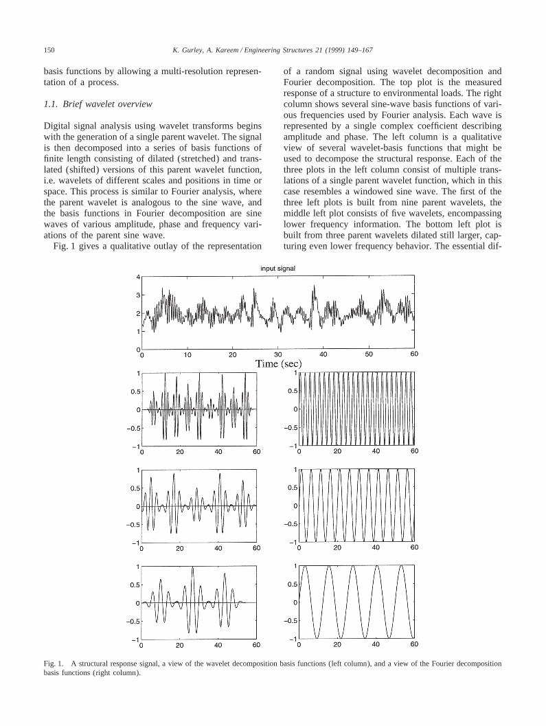
Fig. 1 gives a qualitative outlay of the representation

Fig. 1. A structural response signal, a view of the wavelet decomposition basis functions (left column), and a view of the Fourier decompositionbasis functions (right column).

of a random signal using wavelet decomposition andFourier decomposition. The top plot is the measuredresponse of a structure to environmental loads. The rightcolumn shows several sine-wave basis functions of vari-ous frequencies used by Fourier analysis. Each wave isrepresented by a single complex coefficient describingamplitude and phase. The left column is a qualitativeview of several wavelet-basis functions that might beused to decompose the structural response. Each of thethree plots in the left column consist of multiple trans-lations of a single parent wavelet function, which in thiscase resembles a windowed sine wave. The first of thethree left plots is built from nine parent wavelets, themiddle left plot consists of five wavelets, encompassinglower frequency information. The bottom left plot isbuilt from three parent wavelets dilated still larger, cap-turing even lower frequency behavior. The essential dif-

151K. Gurley, A. Kareem / Engineering Structures 21 (1999) 149–167

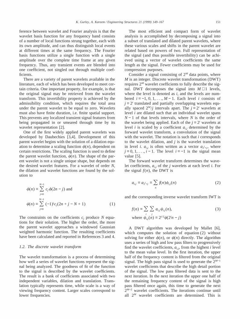
ference between wavelet and Fourier analysis is that thewavelet basis function for any frequency band consistsof a number of local functions strung together, each withits own amplitude, and can thus distinguish local eventsat different times at the same frequency. The Fourierbasis functions utilize a single function with a singleamplitude over the complete time frame at any givenfrequency. Thus, any transient events are blended intoone coefficient, not singled out through multiple coef-ficients.

There are a variety of parent wavelets available in theliterature, each of which has been developed to meet cer-tain criteria. One important property, for example, is thatthe original signal may be retrieved from the wavelettransform. This invertibility property is achieved by theadmissibility condition, which requires the total areaunder the parent wavelet to be equal to zero. Waveletsmust also have finite duration, i.e. finite spatial support.This prevents any localized transient signal features frombeing propagated in or smeared through time by itswavelet representation [2].

One of the first widely applied parent wavelets wasdeveloped by Daubechies [3,4]. Development of thisparent wavelet begins with the solution of a dilation equ-ation to determine a scaling functionf(n), dependent oncertain restrictions. The scaling function is used to definethe parent wavelet function,c(n). The shape of the par-ent wavelet is not a single unique shape, but depends onthe desired wavelet features. For a wavelet of orderN,the dilation and wavelet functions are found by the sol-ution to

f(n) = ON−1

j=0

cj f(2n − j ) and

c(n) = ON−1

j=0

(−1)j cj (2n + j − N + 1) (1)

The constraints on the coefficientscj produceN equa-tions for their solution. The higher the order, the morethe parent wavelet approaches a windowed Gaussianweighted harmonic function. The resulting coefficientshave been calculated and reported in References 3 and 4.

1.2. The discrete wavelet transform

The wavelet transformation is a process of determininghow well a series of wavelet functions represent the sig-nal being analyzed. The goodness of fit of the functionto the signal is described by the wavelet coefficients.The result is a bank of coefficients associated with twoindependent variables, dilation and translation. Trans-lation typically represents time, while scale is a way ofviewing frequency content. Larger scales correspond tolower frequencies.

The most efficient and compact form of waveletanalysis is accomplished by decomposing a signal intoa subset of translated and dilated parent wavelets, wherethese various scales and shifts in the parent wavelet arerelated based on powers of two. Full representation ofthe signal (and thus possible invertibility) can be achi-eved using a vector of wavelet coefficients the samelength as the signal. Fewer coefficients may be used forcompression purposes.

Consider a signal consisting of 2M data points, whereM is an integer. Discrete wavelet transformation (DWT)requires 2M wavelet coefficients to fully describe the sig-nal. DWT decomposes the signal intoM + 1 levels,where the level is denoted asi, and the levels are num-bered i = −1, 0, 1, . . .,M − 1. Each leveli consists ofj = 2i translated and partially overlapping wavelets equ-ally spaced 2M/j intervals apart. Thej = 2i wavelets atlevel i are dilated such that an individual wavelet spansN − 1 of that levels intervals, whereN is the order ofthe wavelet being applied. Each of thej = 2i wavelets atlevel i is scaled by a coefficientai,j determined by theforward wavelet transform, a convolution of the signalwith the wavelet. The notation is such thati correspondsto the wavelet dilation, andj is the wavelet translationin level i. ai,j is often written as a vectora2i+j , wherej = 0, 1, . . .,i − 1. The level i = −1 is the signal meanvalue [5].

The forward wavelet transform determines the wave-let coefficients,ai,j of the j wavelets at each leveli. Forthe signalf (n), the DWT is

ai,j = a2i+j = On

f(n)ci,j (n) (2)

and the corresponding inverse wavelet transform IWT is

f (n) = Oi

Oj

ai,j ci,j (n), (3)

whereci,j (n) = 2i /2c(2in − j )

A DWT algorithm was developed by Mallet [6],which computes the solution of equation (2) withoutsolving for eitherf(n), or c(n) directly. The algorithmuses a series of high and low pass filters to progressivelyfind the wavelet coefficients,ai,j, from the highesti levelto the mean value level. In the first iteration, the upperhalf of the frequency content is filtered from the originalsignal. The high pass signal is used to generate the 2M−1

wavelet coefficients that describe the high detail portionof the signal. The low pass filtered data is sent to thenext iteration. In the next iteration the upper one half ofthe remaining frequency content of the signal is highpass filtered once again, this time to generate the next2M−2 wavelet coefficients. The iterations continue untilall 2M wavelet coefficients are determined. This is


referred to as Mallet’s tree algorithm or Mallet’s pyra-mid algorithm [6].

1.3. The continuous wavelet transform

While the DWT is the most efficient and compact, itspower of two relationship in scale fixes its frequencyresolution. Often it is desired to differentiate betweensmaller frequency bands than DWT allows. This is poss-ible by using scales that are more closely spaced togetherthan the 2i relationship, and is the basis for the continu-ous wavelet transform (CWT). The form of the CWT is

a(i,j ) = E`

−`

f(t)c(i,j,t) dt (4)

wherei corresponds to dilation, andj to translation. Fora finite digitally sampled signal, the integral will bereplaced with a summation, and the timet is replacedby the discreten.

The scale may be selected over whatever range theuser desires. The number of coefficients necessary todescribe the signal may be very much larger than thesignal length, as the CWT oversamples the signal andwavelet coefficients contain partial redundancies ofinformation. Also, CWT need not contain informationover the complete range of frequencies contained in thesignal. The user may select a very narrow range of scalesto isolate and pull details from a particular frequencyband. In this case the complete signal can no longer beretrieved, since any information in unsampled scales islost.

2. Applications of wavelet analysis

The present research concerns the use of wavelets to aidin the analysis and simulation of non-stationary data.Multi-scale decomposition of processes utilizing wave-lets reveals events otherwise hidden in the original timehistory. The wavelet coefficients,ai,j, can be utilized ina variety of techniques to draw out useful signal infor-mation. Wavelet coefficients may be used to derive anestimate of the power spectrum. The wavelet coefficientsalso provide the scalogram, which describes the signalenergy on a time-scale domain. This facilitates identifi-cation of time-varying energy flux, spectral evolution,and transient bursts not readily discernible using timeor frequency domain methods. The property of accurateenergy representation lends itself well to signal recon-struction and simulation. The reduction of noise in ameasured signal may be accomplished by altering wave-let coefficients below a case specific threshold. A varietyof examples are provided herein to demonstrate theseengineering applications of wavelet transforms.

2.1. Wavelet filterbank signal decomposition

The DWT is a convenient and efficient method of moni-toring the performance of time dependent dynamic sys-tems. While Fourier coefficients do not contain timeinformation, the coefficients describing the localizedbasis functions do reflect time dependence. Both thebank of octave band filtered time series, and their wave-let domain representation as wavelet coefficients provideunique insights into transient events within a time series.An example of each is provided below.

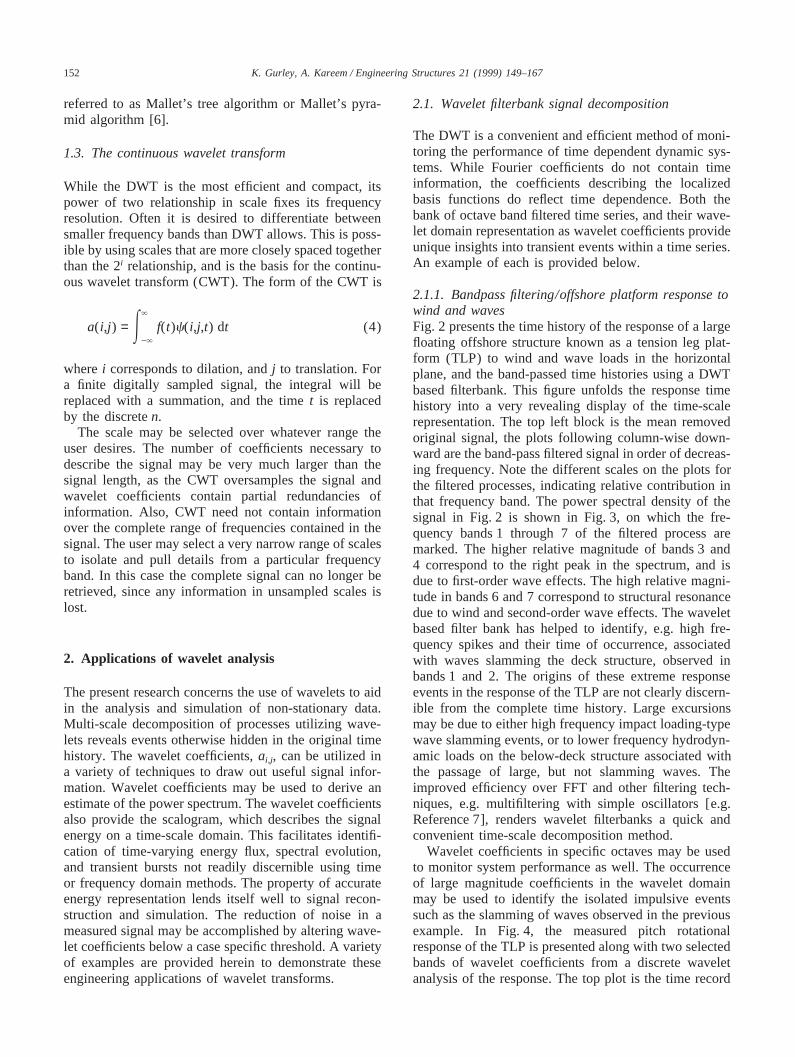
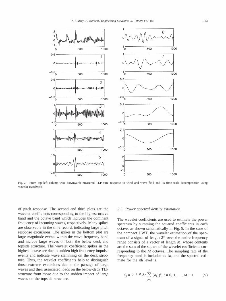
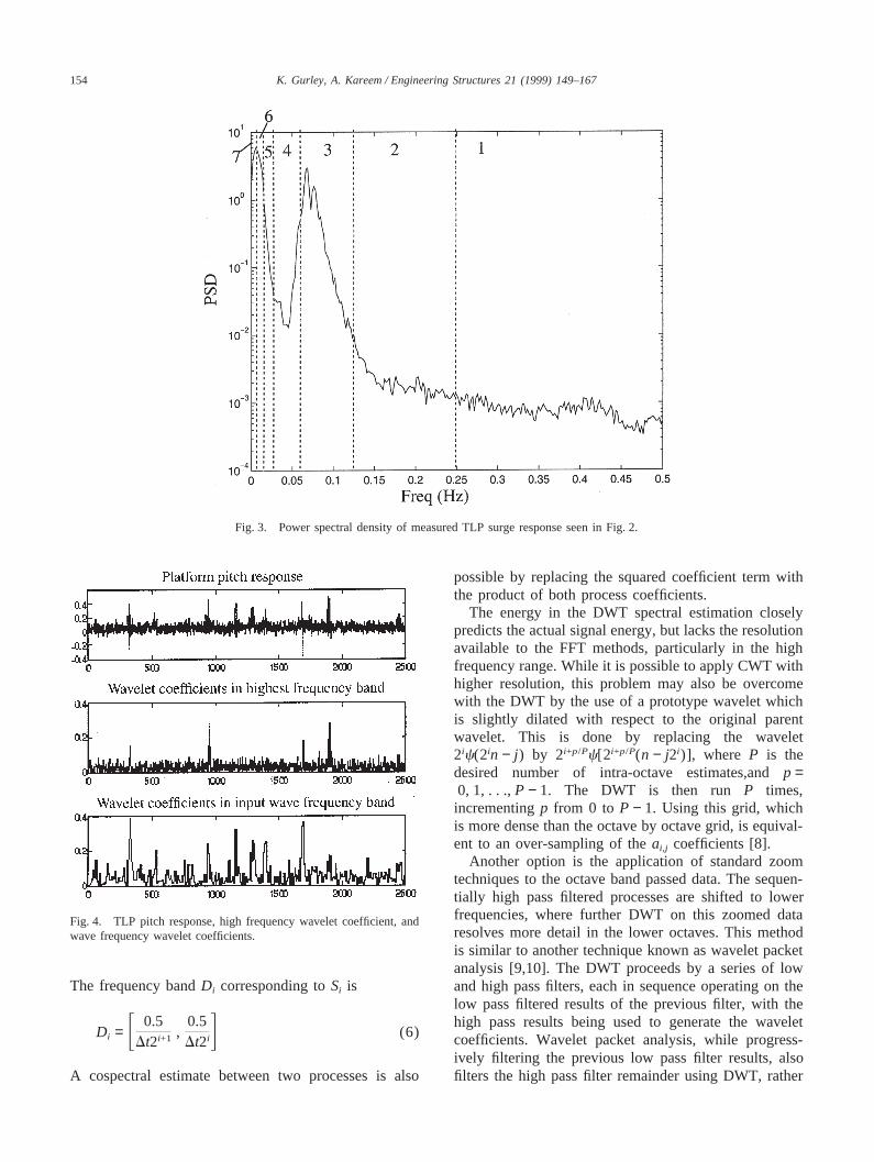
2.1.1. Bandpass filtering/offshore platform response towind and wavesFig. 2 presents the time history of the response of a largefloating offshore structure known as a tension leg plat-form (TLP) to wind and wave loads in the horizontalplane, and the band-passed time histories using a DWTbased filterbank. This figure unfolds the response timehistory into a very revealing display of the time-scalerepresentation. The top left block is the mean removedoriginal signal, the plots following column-wise down-ward are the band-pass filtered signal in order of decreas-ing frequency. Note the different scales on the plots forthe filtered processes, indicating relative contribution inthat frequency band. The power spectral density of thesignal in Fig. 2 is shown in Fig. 3, on which the fre-quency bands 1 through 7 of the filtered process aremarked. The higher relative magnitude of bands 3 and4 correspond to the right peak in the spectrum, and isdue to first-order wave effects. The high relative magni-tude in bands 6 and 7 correspond to structural resonancedue to wind and second-order wave effects. The waveletbased filter bank has helped to identify, e.g. high fre-quency spikes and their time of occurrence, associatedwith waves slamming the deck structure, observed inbands 1 and 2. The origins of these extreme responseevents in the response of the TLP are not clearly discern-ible from the complete time history. Large excursionsmay be due to either high frequency impact loading-typewave slamming events, or to lower frequency hydrodyn-amic loads on the below-deck structure associated withthe passage of large, but not slamming waves. Theimproved efficiency over FFT and other filtering tech-niques, e.g. multifiltering with simple oscillators [e.g.Reference 7], renders wavelet filterbanks a quick andconvenient time-scale decomposition method.

Wavelet coefficients in specific octaves may be usedto monitor system performance as well. The occurrenceof large magnitude coefficients in the wavelet domainmay be used to identify the isolated impulsive eventssuch as the slamming of waves observed in the previousexample. In Fig. 4, the measured pitch rotationalresponse of the TLP is presented along with two selectedbands of wavelet coefficients from a discrete waveletanalysis of the response. The top plot is the time record


Fig. 2. From top left column-wise downward: measured TLP sure response to wind and wave field and its time-scale decomposition usingwavelet transforms.

of pitch response. The second and third plots are thewavelet coefficients corresponding to the highest octaveband and the octave band which includes the dominantfrequency of incoming waves, respectively. Many spikesare observable in the time record, indicating large pitchresponse excursions. The spikes in the bottom plot arelarge magnitude events within the wave frequency bandand include large waves on both the below deck andtopside structure. The wavelet coefficient spikes in thehighest octave are due to sudden high frequency impulseevents and indicate wave slamming on the deck struc-ture. Thus, the wavelet coefficients help to distinguishthose extreme excursions due to the passage of largewaves and their associated loads on the below-deck TLPstructure from those due to the sudden impact of largewaves on the topside structure.

2.2. Power spectral density estimation

The wavelet coefficients are used to estimate the powerspectrum by summing the squared coefficients in eachoctave, as shown schematically in Fig. 5. In the case ofthe compact DWT, the wavelet estimation of the spec-trum of a signal of length 2M over the entire frequencyrange consists of a vector of lengthM, whose contentsare the sum of the square of the wavelet coefficients cor-responding to theM octaves. The sampling rate of thefrequency band is included asDt, and the spectral esti-mate for theith level is

Si = 2i+2−M Dt O2i

j=1

(ai,j )2, i = 0, 1, %, M − 1 (5)


Fig. 3. Power spectral density of measured TLP surge response seen in Fig. 2.

Fig. 4. TLP pitch response, high frequency wavelet coefficient, andwave frequency wavelet coefficients.

The frequency bandDi corresponding toSi is

Di = F 0.5Dt2i+1 ,

0.5Dt2iG (6)

A cospectral estimate between two processes is also

possible by replacing the squared coefficient term withthe product of both process coefficients.

The energy in the DWT spectral estimation closelypredicts the actual signal energy, but lacks the resolutionavailable to the FFT methods, particularly in the highfrequency range. While it is possible to apply CWT withhigher resolution, this problem may also be overcomewith the DWT by the use of a prototype wavelet whichis slightly dilated with respect to the original parentwavelet. This is done by replacing the wavelet2ic(2in − j ) by 2i+p/Pc[2i+p/P(n − j2i )], where P is thedesired number of intra-octave estimates,andp =0, 1, . . .,P − 1. The DWT is then run P times,incrementingp from 0 to P − 1. Using this grid, whichis more dense than the octave by octave grid, is equival-ent to an over-sampling of theai,j coefficients [8].

Another option is the application of standard zoomtechniques to the octave band passed data. The sequen-tially high pass filtered processes are shifted to lowerfrequencies, where further DWT on this zoomed dataresolves more detail in the lower octaves. This methodis similar to another technique known as wavelet packetanalysis [9,10]. The DWT proceeds by a series of lowand high pass filters, each in sequence operating on thelow pass filtered results of the previous filter, with thehigh pass results being used to generate the waveletcoefficients. Wavelet packet analysis, while progress-ively filtering the previous low pass filter results, alsofilters the high pass filter remainder using DWT, rather


Fig. 5. Summation of wavelet coefficients to estimate power spectrum.

than using the high pass results to generate coefficients.The octave-banded signal information offered by DWTis thus further split up into sub-octaves using waveletpackets.

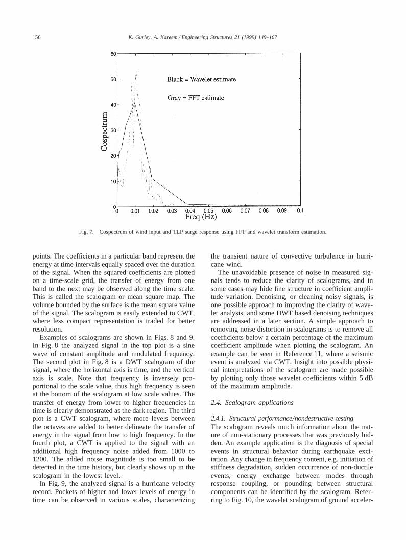
Fig. 6 shows several power spectrum estimates of ameasured earthquake acceleration record. Included arean FFT estimate, an octave band estimate using DWT,and an intra-octave band estimate using DWT and zoo-ming techniques. Fig. 7 is the cospectral estimate of TLPsurge response and the measured input wind velocityinput using DWT and FFT techniques. Smoothing of theFFT estimate with segment averaging renders its resol-

Fig. 6. Wavelet and FFT based spectral estimations of earthquake acceleration record.

ution inferior to that of the wavelet estimate at low fre-quencies. The FFT spectral estimates are the average ofeight segments, while the wavelet estimate is based onthe full data record.

2.3. Time-frequency signal representation: scalogram

The local wavelet coefficients are well suited for analyz-ing non-stationary events such as transient and evol-utionary phenomena. For DWT there are 2i coefficientsto describe the energy at theith frequency band, fori =0, 1, . . .,M − 1, where the signal consists of 2M data


Fig. 7. Cospectrum of wind input and TLP surge response using FFT and wavelet transform estimation.

points. The coefficients in a particular band represent theenergy at time intervals equally spaced over the durationof the signal. When the squared coefficients are plottedon a time-scale grid, the transfer of energy from oneband to the next may be observed along the time scale.This is called the scalogram or mean square map. Thevolume bounded by the surface is the mean square valueof the signal. The scalogram is easily extended to CWT,where less compact representation is traded for betterresolution.

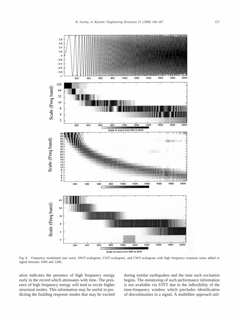
Examples of scalograms are shown in Figs. 8 and 9.In Fig. 8 the analyzed signal in the top plot is a sinewave of constant amplitude and modulated frequency.The second plot in Fig. 8 is a DWT scalogram of thesignal, where the horizontal axis is time, and the verticalaxis is scale. Note that frequency is inversely pro-portional to the scale value, thus high frequency is seenat the bottom of the scalogram at low scale values. Thetransfer of energy from lower to higher frequencies intime is clearly demonstrated as the dark region. The thirdplot is a CWT scalogram, where more levels betweenthe octaves are added to better delineate the transfer ofenergy in the signal from low to high frequency. In thefourth plot, a CWT is applied to the signal with anadditional high frequency noise added from 1000 to1200. The added noise magnitude is too small to bedetected in the time history, but clearly shows up in thescalogram in the lowest level.

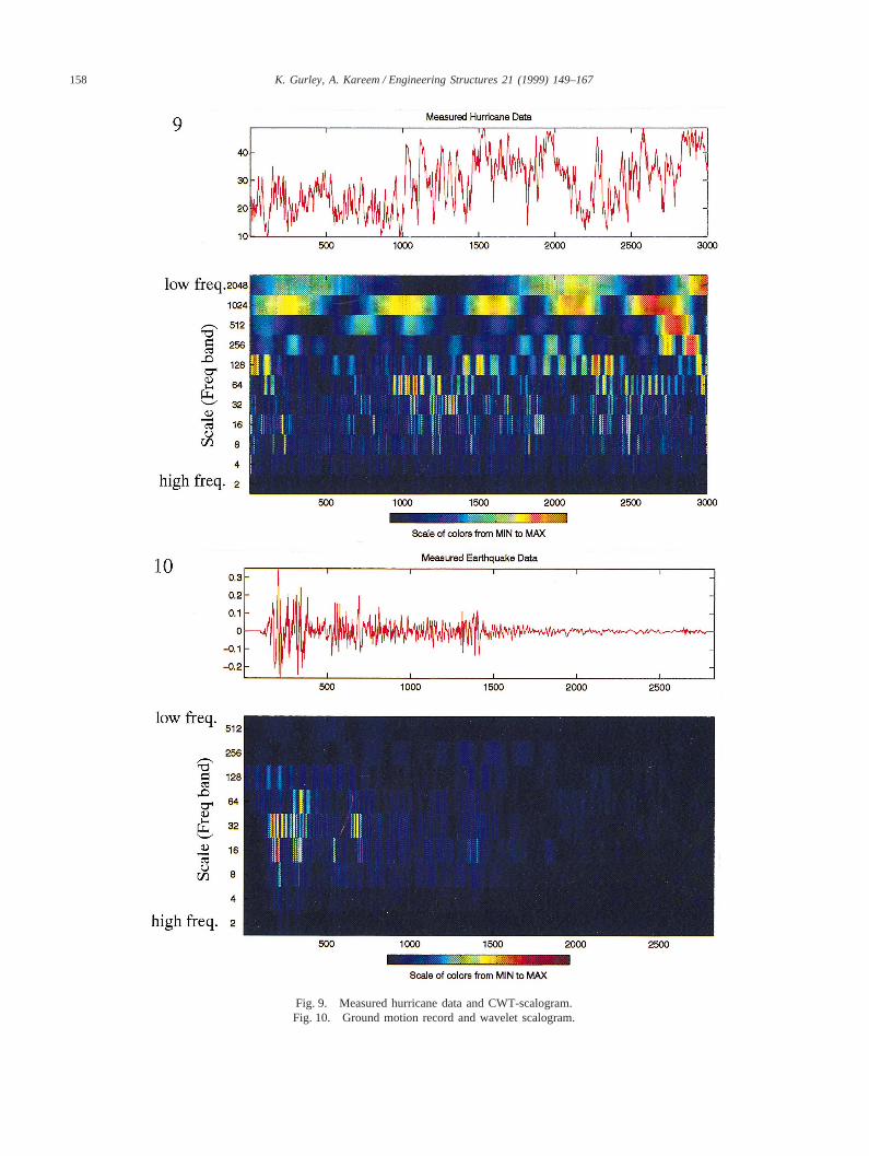
In Fig. 9, the analyzed signal is a hurricane velocityrecord. Pockets of higher and lower levels of energy intime can be observed in various scales, characterizing

the transient nature of convective turbulence in hurri-cane wind.

The unavoidable presence of noise in measured sig-nals tends to reduce the clarity of scalograms, and insome cases may hide fine structure in coefficient ampli-tude variation. Denoising, or cleaning noisy signals, isone possible approach to improving the clarity of wave-let analysis, and some DWT based denoising techniquesare addressed in a later section. A simple approach toremoving noise distortion in scalograms is to remove allcoefficients below a certain percentage of the maximumcoefficient amplitude when plotting the scalogram. Anexample can be seen in Reference 11, where a seismicevent is analyzed via CWT. Insight into possible physi-cal interpretations of the scalogram are made possibleby plotting only those wavelet coefficients within 5 dBof the maximum amplitude.

2.4. Scalogram applications

2.4.1. Structural performance/nondestructive testingThe scalogram reveals much information about the nat-ure of non-stationary processes that was previously hid-den. An example application is the diagnosis of specialevents in structural behavior during earthquake exci-tation. Any change in frequency content, e.g. initiation ofstiffness degradation, sudden occurrence of non-ductileevents, energy exchange between modes throughresponse coupling, or pounding between structuralcomponents can be identified by the scalogram. Refer-ring to Fig. 10, the wavelet scalogram of ground acceler-


Fig. 8. Frequency modulated sine wave, DWT-scalogram, CWT-scalogram, and CWT-scalogram with high frequency transient noise added tosignal between 1000 and 1200.

ation indicates the presence of high frequency energyearly in the record which attenuates with time. The pres-ence of high frequency energy will tend to excite higherstructural modes. This information may be useful in pre-dicting the building response modes that may be excited

during similar earthquakes and the time such excitationbegins. The monitoring of such performance informationis not available via STFT due to the inflexibility of thetime-frequency window which precludes identificationof discontinuities in a signal. A multifilter approach util-


Fig. 9. Measured hurricane data and CWT-scalogram.Fig. 10. Ground motion record and wavelet scalogram.


izing simple oscillators has been addressed by otherresearchers to avoid the STFT shortcomings and presenttime dependent frequency fluctuations [7,12]. Thisapproach has its own shortcomings which are discussedlater in the paper.

The propagation of waves in a medium of a structureis widely studied in engineering and science, namely,identification of material properties, crack detection andhealth monitoring of structures via ultrasound, and moni-toring the structural vibration characteristics usingimpact type techniques. Central to most techniques is thequantification of dispersive features of wave propagationin structures, i.e. wave velocity at different frequencies.The time-frequency analysis offers a most attractive toolfor examining and mapping wave propagation at differ-ent frequencies. Hodges et al. [13] utilized a STFTapproach for the analysis of a string, at beam and a cylin-drical shell. By measuring strain at two locations on astructure excited by an arbitrary impact force, traveltimes of waves between the measurement locations wereobtained from the peaks in the time-frequency plots. Intheir study, a shortcoming was noted in this approachdue to inflexibility in the arbitrary selection of time andfrequency resolutions. This can be attributed to the factthat the time window for the STFT can either be chosenfor resolving sharp local peaks or for identifying lowfrequency features, but it is impossible to accommodateboth desired features due to Heisenberg’s uncertaintyprinciple [14,15]. An improvement is possible usingWigner–Ville Distribution, but this approach has itslimitations as well [16]. The wavelet transform offersalternative techniques by providing additional flexibilityin terms of allowing the resolution in time and frequencyto vary in the time-frequency plane, thus considerablyreducing analysis.

2.4.2. Ground motion analysisThe time-dependent frequency content of ground motionrecords provides information on the non-stationary spec-tral characteristics of the motion, i.e. frequency depen-dence of ground motion durations, time above a thres-hold, interval duration, shape wave duration, andidentification of energy bursts in the signature. The time-frequency analysis of non-stationary ground motion rec-ords has been undertaken by researchers using a multi-filter approach [7,12]. The STFT technique has its short-comings due to the fixed time-frequency relations asalluded to earlier. Following Arnold [17], multifiltertechniques have been employed in seismic applications.A set of simple oscillators is used as a multifilter [7].This approach has the advantage over STFT techniquesas a constant damping in the oscillators has the sameeffect as varying the length of the data window such thatit is inversely proportional to frequency. As noted earl-ier, this is a desired feature for obtaining details of timevariations in the high frequency range. Kameda [7] also

formulates an evolutionary power spectrum in terms offilter outputs. Scherer [12] utilizes this approach toobtain time-frequency contours of the evolutionarypower spectra. Here, the shortcoming of time leakage isreduced by approximating and removing the effects offilter inertness. The application of wavelet analysis willimprove resolution while reducing the leakage, thus ren-dering a wavelet based method as the tool of choice fora time-frequency analysis of ground motion. Fig. 10illustrates a time-frequency description of the 1940El Centro earthquake. The El Centro ground motion rec-ord contains energy at a wide band of frequencies whichmay result in exciting higher modes of a buildingdepending on the energy distribution. The arrival ofenergy bursts at different times can be noted in the timehistory and more clearly from the scalogram. Waveletbased analysis may lead to improved understanding ofthe events noted in ground motion in light of geophysicalreasoning that relates these energy bursts to S-wavearrivals. Similar results are presented by Sherer et al.[18] using a multifilter technique. However, the presentapproach offers more flexibility and versatility to ana-lyze a wide range of records with varying frequency con-tents.

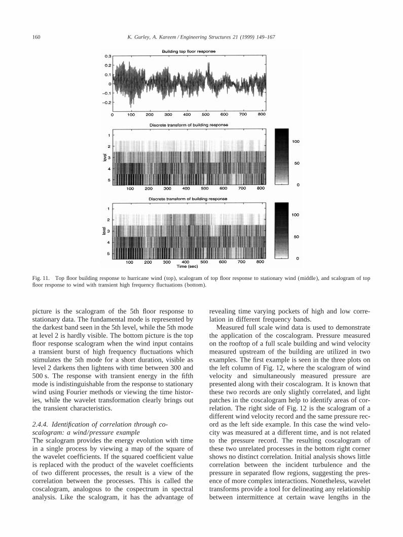
2.4.3. Transient building response to wind stormsWavelet analysis of hurricane wind time histories, whichcontain significant contributions from convective turbu-lence, provides useful information regarding the distri-bution of energy as a function of time. The response ofa slender structure to wind may contain contributionsfrom the fundamental mode and higher modes dependingon how the turbulent structure of the wind changes intime. The relative contribution of each mode may varysignificantly or the total building response may suddenlyincrease for apparently the same mean wind speed dueto instantaneous changes in the distribution of energy atdifferent frequencies. Such a response behavior cannotbe identified through classical spectral techniques, whilewavelet analysis is ideal for such an analysis.

As an example, a 600 ft tall, 100 ft square, buildingis modeled with five modes, and subjected to high(100 ft/sec at 30 ft) wind as correlated point loads alongits face. Fig. 11 is a scalogram of the response at the topfloor of the building for two input cases. The scalogramplots energy with respect to time (x-axis) and scale (y-axis), where here the scale is marked as levels. Thelevels 1 through five are five frequency bands, withlevel 1 containing energy from one half the cutoff fre-quency up to the cutoff. Level 2 contains energy from1/4 to 1/2 of cutoff, and so on. Levels 2 through 5 con-tain all five modes of building response, with the funda-mental mode in the 5th level, the second mode in the4th level, the third and fourth modes in level 3, and thehighest mode in level 2. The top plot in Fig. 11 is theresponse of the top floor to stationary input. The middle


Fig. 11. Top floor building response to hurricane wind (top), scalogram of top floor response to stationary wind (middle), and scalogram of topfloor response to wind with transient high frequency fluctuations (bottom).

picture is the scalogram of the 5th floor response tostationary data. The fundamental mode is represented bythe darkest band seen in the 5th level, while the 5th modeat level 2 is hardly visible. The bottom picture is the topfloor response scalogram when the wind input containsa transient burst of high frequency fluctuations whichstimulates the 5th mode for a short duration, visible aslevel 2 darkens then lightens with time between 300 and500 s. The response with transient energy in the fifthmode is indistinguishable from the response to stationarywind using Fourier methods or viewing the time histor-ies, while the wavelet transformation clearly brings outthe transient characteristics.

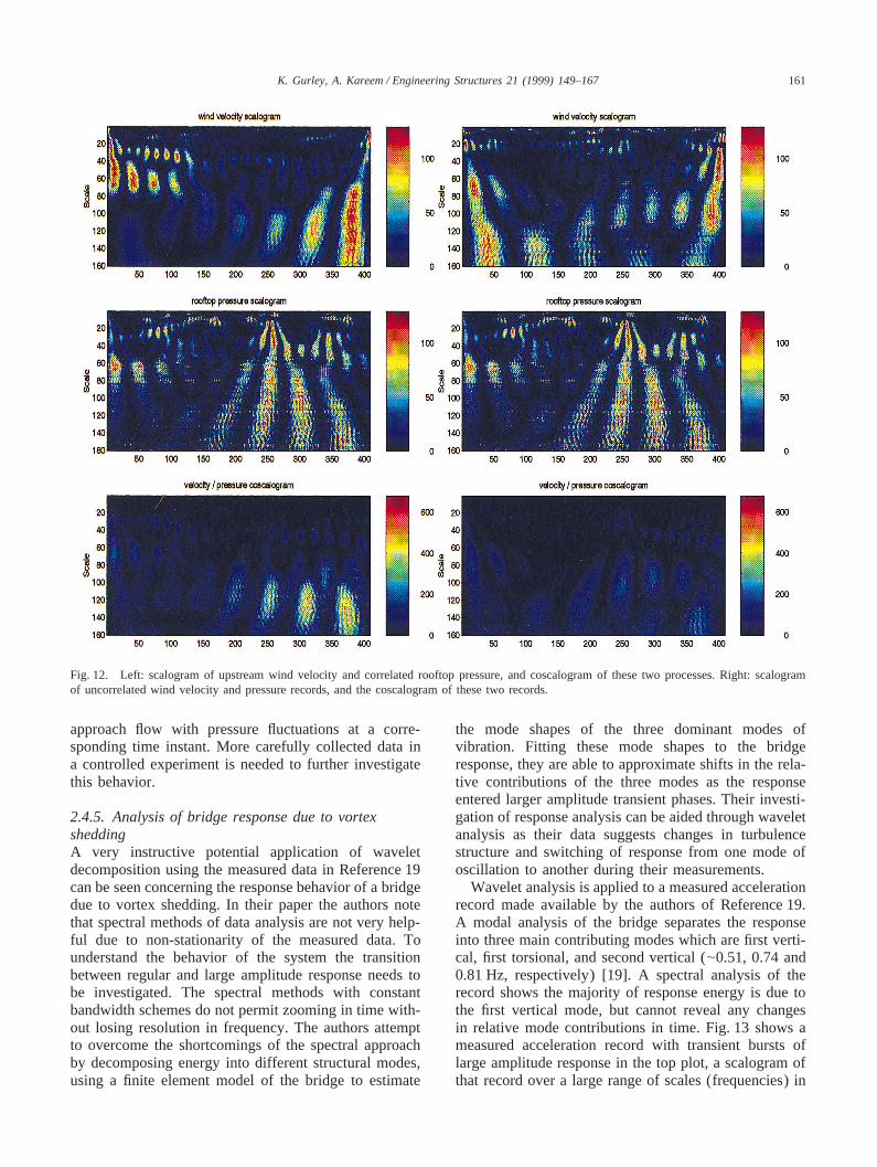
2.4.4. Identification of correlation through co-scalogram: a wind/pressure exampleThe scalogram provides the energy evolution with timein a single process by viewing a map of the square ofthe wavelet coefficients. If the squared coefficient valueis replaced with the product of the wavelet coefficientsof two different processes, the result is a view of thecorrelation between the processes. This is called thecoscalogram, analogous to the cospectrum in spectralanalysis. Like the scalogram, it has the advantage of

revealing time varying pockets of high and low corre-lation in different frequency bands.

Measured full scale wind data is used to demonstratethe application of the coscalogram. Pressure measuredon the rooftop of a full scale building and wind velocitymeasured upstream of the building are utilized in twoexamples. The first example is seen in the three plots onthe left column of Fig. 12, where the scalogram of windvelocity and simultaneously measured pressure arepresented along with their coscalogram. It is known thatthese two records are only slightly correlated, and lightpatches in the coscalogram help to identify areas of cor-relation. The right side of Fig. 12 is the scalogram of adifferent wind velocity record and the same pressure rec-ord as the left side example. In this case the wind velo-city was measured at a different time, and is not relatedto the pressure record. The resulting coscalogram ofthese two unrelated processes in the bottom right cornershows no distinct correlation. Initial analysis shows littlecorrelation between the incident turbulence and thepressure in separated flow regions, suggesting the pres-ence of more complex interactions. Nonetheless, wavelettransforms provide a tool for delineating any relationshipbetween intermittence at certain wave lengths in the


Fig. 12. Left: scalogram of upstream wind velocity and correlated rooftop pressure, and coscalogram of these two processes. Right: scalogramof uncorrelated wind velocity and pressure records, and the coscalogram of these two records.

approach flow with pressure fluctuations at a corre-sponding time instant. More carefully collected data ina controlled experiment is needed to further investigatethis behavior.

2.4.5. Analysis of bridge response due to vortexsheddingA very instructive potential application of waveletdecomposition using the measured data in Reference 19can be seen concerning the response behavior of a bridgedue to vortex shedding. In their paper the authors notethat spectral methods of data analysis are not very help-ful due to non-stationarity of the measured data. Tounderstand the behavior of the system the transitionbetween regular and large amplitude response needs tobe investigated. The spectral methods with constantbandwidth schemes do not permit zooming in time with-out losing resolution in frequency. The authors attemptto overcome the shortcomings of the spectral approachby decomposing energy into different structural modes,using a finite element model of the bridge to estimate

the mode shapes of the three dominant modes ofvibration. Fitting these mode shapes to the bridgeresponse, they are able to approximate shifts in the rela-tive contributions of the three modes as the responseentered larger amplitude transient phases. Their investi-gation of response analysis can be aided through waveletanalysis as their data suggests changes in turbulencestructure and switching of response from one mode ofoscillation to another during their measurements.

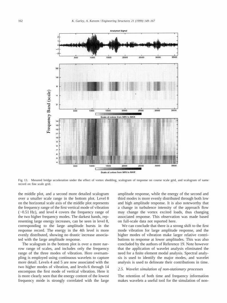
Wavelet analysis is applied to a measured accelerationrecord made available by the authors of Reference 19.A modal analysis of the bridge separates the responseinto three main contributing modes which are first verti-cal, first torsional, and second vertical (|0.51, 0.74 and0.81 Hz, respectively) [19]. A spectral analysis of therecord shows the majority of response energy is due tothe first vertical mode, but cannot reveal any changesin relative mode contributions in time. Fig. 13 shows ameasured acceleration record with transient bursts oflarge amplitude response in the top plot, a scalogram ofthat record over a large range of scales (frequencies) in


Fig. 13. Mesured bridge acceleration under the effect of vortex shedding, scalogram of response on course scale grid, and scalogram of samerecord on fine scale grid.

the middle plot, and a second more detailed scalogramover a smaller scale range in the bottom plot. Level 8on the horizontal scale axis of the middle plot representsthe frequency range of the first vertical mode of vibration(|0.51 Hz), and level 4 covers the frequency range ofthe two higher frequency modes. The darkest bands, rep-resenting large energy increases, can be seen in level 8,corresponding to the large amplitude bursts in theresponse record. The energy in the 4th level is moreevenly distributed, showing no drastic increase associa-ted with the large amplitude response.

The scalogram in the bottom plot is over a more nar-row range of scales, and includes only the frequencyrange of the three modes of vibration. Here oversam-pling is employed using continuous wavelets to capturemore detail. Levels 4 and 5 are now associated with thetwo higher modes of vibration, and levels 6 through 14encompass the first mode of vertical vibration. Here itis more clearly seen that the energy content of the lowestfrequency mode is strongly correlated with the large

amplitude response, while the energy of the second andthird modes is more evenly distributed through both lowand high amplitude response. It is also noteworthy thata change in turbulence intensity of the approach flowmay change the vortex excited loads, thus changingassociated response. This observation was made basedon full-scale data not reported here.

We can conclude that there is a strong shift to the firstmode vibration for large amplitude response, and thehigher modes of vibration make larger relative contri-butions to response at lower amplitudes. This was alsoconcluded by the authors of Reference 19. Note howeverthat the application of wavelet analysis eliminated theneed for a finite element modal analysis. Spectral analy-sis is used to identify the major modes, and waveletanalysis is used to delineate their contributions in time.

2.5. Wavelet simulation of non-stationary processes

The retention of both time and frequency informationmakes wavelets a useful tool for the simulation of non-


stationary signals. This can be done given either a parentnon-stationary signal, or a target spectrum and modulatorfunction for each octave. Given a parent non-stationarysignal, e.g. a local wind velocity record, an ensemble ofsignals may be simulated whose average statisticsclosely resemble those of the parent process. The parentsignal is discrete wavelet transformed (DWT), and thecoefficients are multiplied by a Gaussian white noise ofunit variance w(n). The inverse wavelet transform(IWT) then produces a simulation statistically similar tothe parent process.

x̂(n) = IWT(w(n)*DWT( x(n))) (7)

The concept of a modulated stationary process cent-ered at narrow-banded frequencies to model groundmotion has been used extensively [7,20–25]. In this rep-resentation each component process is modulated by adifferent modulating function,

x(t) = Oj

mj (t)sj (t) (8)

where mj and sj represent thejth modulator and thestationary component process, respectively. There aredifferent approaches to modellingmj andsj to describex.One such choice is to normalize the modulator such that

E`

−`

m2j (t) dt = 1 (9)

andsj is constant over a frequency band.The DWT provides an elegant framework to perform

such modelling [23,26]. The measured wavelet coef-ficients ai,j and spectrum may be used to estimate themodulator function from a parent signal by applying

mi,j = Ai Î2i+2−Muai,j uÎSi

(10)

whereAi is a level-dependent amplitude constant andSi

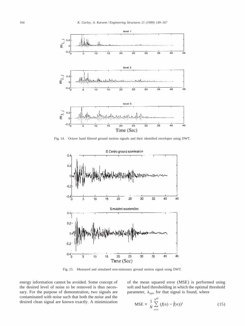
is the energy corresponding to theith octave from thepower spectrum. An example of identified modulatorfunctions using equation (10) is given in Fig. 14. Herean earthquake ground motion record is broken intooctave bands using DWT, the filtered time histories ofseveral bands are shown along with the resulting modu-lator function.

Given a target spectrum and modulator functions, thesimulation is done by first finding the energy containedin each octave from the target spectrum. The waveletcoefficients for the simulated process are multiplied withthe appropriate modulator, and normalized such that theenergy equals that in the corresponding octave. Thesemodulated and normalized coefficients are then multi-

plied through by white noise and inverse wavelet trans-formed. The process is represented by [26]

x̂(n) = IWT Sw(n)* Smi,jÎSi

Î2i+2−M DD (11)

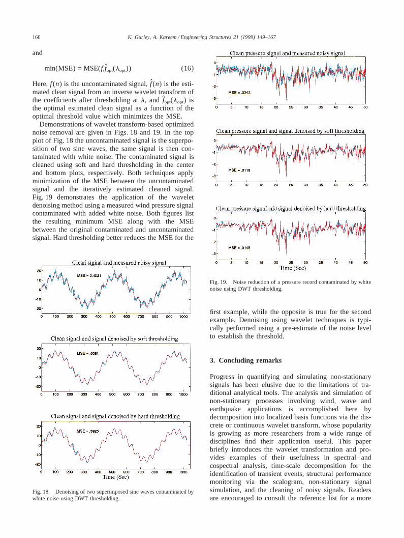
Fig. 15 shows a measured and a wavelet simulatedearthquake ground motion record, and Fig. 16 comparesthe power spectral density of both records. Both the non-stationary characteristics and the energy distribution arewell represented in the simulation. Fig. 17 is an exampleof measured non-stationary wind velocity and a waveletsimulation. Again the non-stationary characteristics arewell represented.

2.6. Denoising

Small details in a signal are manifested in the wavelettransform as small magnitude coefficients. These lowenergy processes may distort the true signal if they areassumed to be due to noise. Their removal isaccomplished in the wavelet domain by eliminating orreducing coefficients under a certain magnitude thres-hold. The inverse wavelet transform then gives back a‘cleaned’ or denoised signal without the small details inthe original signal. Two thresholding methods con-sidered here are hard and soft thresholding.

Hard thresholding sets to zero the coefficients belowthe threshold through

ahardi,j = S 0,ai,j , l

ai,j ,ai,j $ lD (12)

where l is the assigned threshold. Soft thresholdingalters the coefficients, for example

asofti,j = sign(ai,j ) (uai,j u − l) + (13)

where+ indicates that if the sign ofasio,fjt does not equal

the sign ofai,j, asio,fjt is set to zero [27]. Equation (13)

results in a smooth reduction of all coefficients towardzero, and sets equal to zero those closest to the origin.Each method has advantages, depending on the proper-ties of the signal being cleaned. An example of a thres-hold parameter defined in terms of noise level is foundin Reference 27, and written as

l = s Î2log(n)/În (14)

wheres is a noise scale parameter, andn is the numberof points in the signal.

For qualitative analysis, an iterative increase in thethreshold will clean the signal to a desired level, but, asis the problem with all noise reduction methods, a trade-off between removing noise and removing important low


Fig. 14. Octave band filtered ground motion signals and their identified envelopes using DWT.

Fig. 15. Measured and simulated non-stationary ground motion signal using DWT.

energy information cannot be avoided. Some concept ofthe desired level of noise to be removed is thus neces-sary. For the purpose of demonstration, two signals arecontaminated with noise such that both the noise and thedesired clean signal are known exactly. A minimization

of the mean squared error (MSE) is performed usingsoft and hard thresholding in which the optimal thresholdparameter,lopt, for that signal is found, where

MSE =1N ON

M

n=1

(f(n) − f̂(n))2 (15)


Fig. 16. Power spectral density of measured earthquake ground motion and wavelet simulated signals.

Fig. 17. Measured wind velocity and a simulation using DWT.


and

min(MSE) = MSE(f,f̂opt(lopt)) (16)

Here,f (n) is the uncontaminated signal,f̂ (n) is the esti-mated clean signal from an inverse wavelet transform ofthe coefficients after thresholding atl, and f̂opt(lopt) isthe optimal estimated clean signal as a function of theoptimal threshold value which minimizes the MSE.

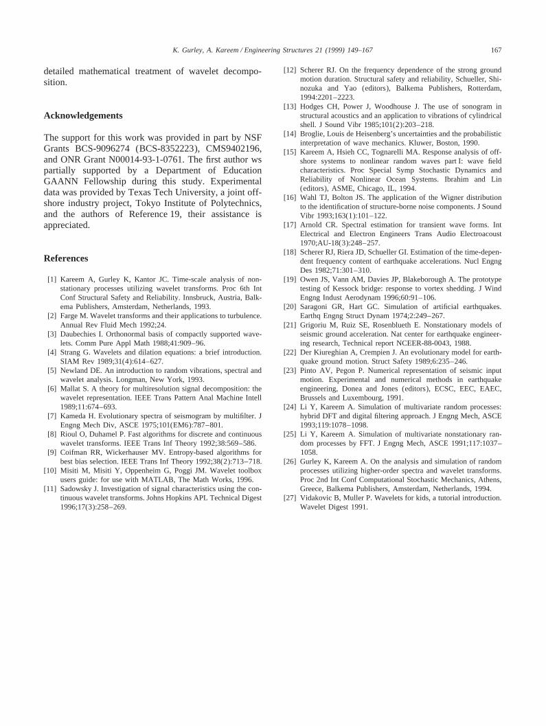
Demonstrations of wavelet transform-based optimizednoise removal are given in Figs. 18 and 19. In the topplot of Fig. 18 the uncontaminated signal is the superpo-sition of two sine waves, the same signal is then con-taminated with white noise. The contaminated signal iscleaned using soft and hard thresholding in the centerand bottom plots, respectively. Both techniques applyminimization of the MSE between the uncontaminatedsignal and the iteratively estimated cleaned signal.Fig. 19 demonstrates the application of the waveletdenoising method using a measured wind pressure signalcontaminated with added white noise. Both figures listthe resulting minimum MSE along with the MSEbetween the original contaminated and uncontaminatedsignal. Hard thresholding better reduces the MSE for the

Fig. 18. Denoising of two superimposed sine waves contaminated bywhite noise using DWT thresholding.

Fig. 19. Noise reduction of a pressure record contaminated by whitenoise using DWT thresholding.

first example, while the opposite is true for the secondexample. Denoising using wavelet techniques is typi-cally performed using a pre-estimate of the noise levelto establish the threshold.

3. Concluding remarks

Progress in quantifying and simulating non-stationarysignals has been elusive due to the limitations of tra-ditional analytical tools. The analysis and simulation ofnon-stationary processes involving wind, wave andearthquake applications is accomplished here bydecomposition into localized basis functions via the dis-crete or continuous wavelet transform, whose popularityis growing as more researchers from a wide range ofdisciplines find their application useful. This paperbriefly introduces the wavelet transformation and pro-vides examples of their usefulness in spectral andcospectral analysis, time-scale decomposition for theidentification of transient events, structural performancemonitoring via the scalogram, non-stationary signalsimulation, and the cleaning of noisy signals. Readersare encouraged to consult the reference list for a more


detailed mathematical treatment of wavelet decompo-sition.

Acknowledgements

The support for this work was provided in part by NSFGrants BCS-9096274 (BCS-8352223), CMS9402196,and ONR Grant N00014-93-1-0761. The first author wspartially supported by a Department of EducationGAANN Fellowship during this study. Experimentaldata was provided by Texas Tech University, a joint off-shore industry project, Tokyo Institute of Polytechnics,and the authors of Reference 19, their assistance isappreciated.

References

[1] Kareem A, Gurley K, Kantor JC. Time-scale analysis of non-stationary processes utilizing wavelet transforms. Proc 6th IntConf Structural Safety and Reliability. Innsbruck, Austria, Balk-ema Publishers, Amsterdam, Netherlands, 1993.

[2] Farge M. Wavelet transforms and their applications to turbulence.Annual Rev Fluid Mech 1992;24.

[3] Daubechies I. Orthonormal basis of compactly supported wave-lets. Comm Pure Appl Math 1988;41:909–96.

[4] Strang G. Wavelets and dilation equations: a brief introduction.SIAM Rev 1989;31(4):614–627.

[5] Newland DE. An introduction to random vibrations, spectral andwavelet analysis. Longman, New York, 1993.

[6] Mallat S. A theory for multiresolution signal decomposition: thewavelet representation. IEEE Trans Pattern Anal Machine Intell1989;11:674–693.

[7] Kameda H. Evolutionary spectra of seismogram by multifilter. JEngng Mech Div, ASCE 1975;101(EM6):787–801.

[8] Rioul O, Duhamel P. Fast algorithms for discrete and continuouswavelet transforms. IEEE Trans Inf Theory 1992;38:569–586.

[9] Coifman RR, Wickerhauser MV. Entropy-based algorithms forbest bias selection. IEEE Trans Inf Theory 1992;38(2):713–718.

[10] Misiti M, Misiti Y, Oppenheim G, Poggi JM. Wavelet toolboxusers guide: for use with MATLAB, The Math Works, 1996.

[11] Sadowsky J. Investigation of signal characteristics using the con-tinuous wavelet transforms. Johns Hopkins APL Technical Digest1996;17(3):258–269.

[12] Scherer RJ. On the frequency dependence of the strong groundmotion duration. Structural safety and reliability, Schueller, Shi-nozuka and Yao (editors), Balkema Publishers, Rotterdam,1994:2201–2223.

[13] Hodges CH, Power J, Woodhouse J. The use of sonogram instructural acoustics and an application to vibrations of cylindricalshell. J Sound Vibr 1985;101(2):203–218.

[14] Broglie, Louis de Heisenberg’s uncertainties and the probabilisticinterpretation of wave mechanics. Kluwer, Boston, 1990.

[15] Kareem A, Hsieh CC, Tognarelli MA. Response analysis of off-shore systems to nonlinear random waves part I: wave fieldcharacteristics. Proc Special Symp Stochastic Dynamics andReliability of Nonlinear Ocean Systems. Ibrahim and Lin(editors), ASME, Chicago, IL, 1994.

[16] Wahl TJ, Bolton JS. The application of the Wigner distributionto the identification of structure-borne noise components. J SoundVibr 1993;163(1):101–122.

[17] Arnold CR. Spectral estimation for transient wave forms. IntElectrical and Electron Engineers Trans Audio Electroacoust1970;AU-18(3):248–257.

[18] Scherer RJ, Riera JD, Schueller GI. Estimation of the time-depen-dent frequency content of earthquake accelerations. Nucl EngngDes 1982;71:301–310.

[19] Owen JS, Vann AM, Davies JP, Blakeborough A. The prototypetesting of Kessock bridge: response to vortex shedding. J WindEngng Indust Aerodynam 1996;60:91–106.

[20] Saragoni GR, Hart GC. Simulation of artificial earthquakes.Earthq Engng Struct Dynam 1974;2:249–267.

[21] Grigoriu M, Ruiz SE, Rosenblueth E. Nonstationary models ofseismic ground acceleration. Nat center for earthquake engineer-ing research, Technical report NCEER-88-0043, 1988.

[22] Der Kiureghian A, Crempien J. An evolutionary model for earth-quake ground motion. Struct Safety 1989;6:235–246.

[23] Pinto AV, Pegon P. Numerical representation of seismic inputmotion. Experimental and numerical methods in earthquakeengineering, Donea and Jones (editors), ECSC, EEC, EAEC,Brussels and Luxembourg, 1991.

[24] Li Y, Kareem A. Simulation of multivariate random processes:hybrid DFT and digital filtering approach. J Engng Mech, ASCE1993;119:1078–1098.

[25] Li Y, Kareem A. Simulation of multivariate nonstationary ran-dom processes by FFT. J Engng Mech, ASCE 1991;117:1037–1058.

[26] Gurley K, Kareem A. On the analysis and simulation of randomprocesses utilizing higher-order spectra and wavelet transforms.Proc 2nd Int Conf Computational Stochastic Mechanics, Athens,Greece, Balkema Publishers, Amsterdam, Netherlands, 1994.

[27] Vidakovic B, Muller P. Wavelets for kids, a tutorial introduction.Wavelet Digest 1991.

Documents

Applications of wavelet transforms in earthquake, …nathaz/journals/(1999)Applications_of...Engineering Structures 21 (1999) 149–167 Applications of wavelet transforms in earthquake,