Embed Size (px)
Citation preview
Snohomish County PUD – 2017 Integrated Resource Plan Appendix B| B-1
APPENDIX B: PORTFOLIO OPTIMIZATION
MODEL
PUBLIC UTILITY DISTRICT #1 OF SNOHOMISH COUNTY
Prepared by
Generation, Power, Rates, and Transmission Management Division
Snohomish County PUD – 2017 Integrated Resource Plan Appendix B| B-2
PORTFOLIO OPTIMIZATION MODEL
Appendix B provides further information on the Portfolio Optimization model used in the IRP,
as well as the substantive assumptions used to inform inputs that the model uses. The content is
organized as follows:
1. Methodology
2. Model Inputs:
a. Supply-Side Assumptions
b. Demand Response Resource Assumptions
1. Portfolio Optimization Model Methodology
The 2017 IRP uses a Portfolio Optimizer tool developed in-house to solve for the least cost
portfolio that satisfies PUD-defined Planning Standards in a given scenario. The Optimizer
requires as inputs, the outputs of the Probabilistic Load Resource Balance Model1. Specifically,
the Probabilistic Load Resource Balance Model outputs that describe the performance of existing
resources within the existing portfolio, customer load, and the resulting possible Load Resource
Balance positions at different likelihoods and points in time across the 2018-2037 study period.
The Portfolio Optimizer model uses those inputs and combines it with information about
potential demand-side and supply-side resources that could be added to a portfolio and then
calculates the following attributes of possible new portfolio combinations:
The ability to meet PUD Planning standards for resource adequacy on an energy and capacity
basis;
The ability to meet Renewable Portfolio Standard (RPS) compliance obligations under the
target compliance methodology;
The incremental carbon dioxide air emissions associated with generation from new supply-
side portfolio additions; and
1 Described in detail in Appendix A
Snohomish County PUD – 2017 Integrated Resource Plan Appendix B| B-3
The cost of adding new resources, the value of any resulting surplus energy, and the Net
Present Value of the resulting portfolio.
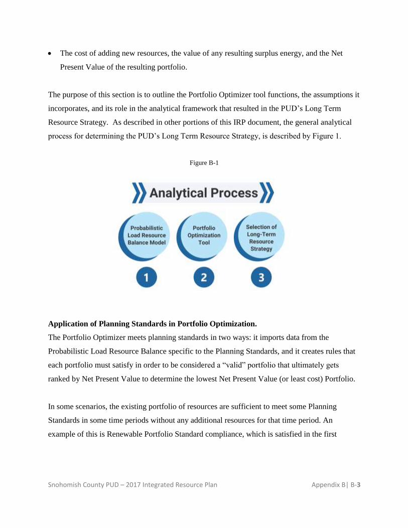
The purpose of this section is to outline the Portfolio Optimizer tool functions, the assumptions it
incorporates, and its role in the analytical framework that resulted in the PUD’s Long Term
Resource Strategy. As described in other portions of this IRP document, the general analytical
process for determining the PUD’s Long Term Resource Strategy, is described by Figure 1.
Figure B-1
Application of Planning Standards in Portfolio Optimization.
The Portfolio Optimizer meets planning standards in two ways: it imports data from the
Probabilistic Load Resource Balance specific to the Planning Standards, and it creates rules that
each portfolio must satisfy in order to be considered a “valid” portfolio that ultimately gets
ranked by Net Present Value to determine the lowest Net Present Value (or least cost) Portfolio.
In some scenarios, the existing portfolio of resources are sufficient to meet some Planning
Standards in some time periods without any additional resources for that time period. An
example of this is Renewable Portfolio Standard compliance, which is satisfied in the first
Snohomish County PUD – 2017 Integrated Resource Plan Appendix B| B-4
several years of most scenarios by the renewable generation attributes of resources in the existing
portfolio.
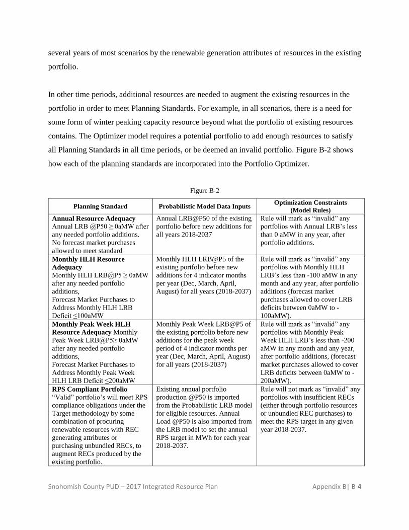
In other time periods, additional resources are needed to augment the existing resources in the
portfolio in order to meet Planning Standards. For example, in all scenarios, there is a need for
some form of winter peaking capacity resource beyond what the portfolio of existing resources
contains. The Optimizer model requires a potential portfolio to add enough resources to satisfy
all Planning Standards in all time periods, or be deemed an invalid portfolio. Figure B-2 shows
how each of the planning standards are incorporated into the Portfolio Optimizer.
Figure B-2
Planning Standard Probabilistic Model Data Inputs Optimization Constraints
(Model Rules)
Annual Resource Adequacy Annual LRB @P50 ≥ 0aMW after
any needed portfolio additions.
No forecast market purchases
allowed to meet standard
Annual LRB@P50 of the existing
portfolio before new additions for
all years 2018-2037
Rule will mark as “invalid” any
portfolios with Annual LRB’s less
than 0 aMW in any year, after
portfolio additions.
Monthly HLH Resource
Adequacy Monthly HLH LRB@P5 ≥ 0aMW
after any needed portfolio
additions,
Forecast Market Purchases to
Address Monthly HLH LRB
Deficit ≤100aMW
Monthly HLH LRB@P5 of the
existing portfolio before new
additions for 4 indicator months
per year (Dec, March, April,
August) for all years (2018-2037)
Rule will mark as “invalid” any
portfolios with Monthly HLH
LRB’s less than -100 aMW in any
month and any year, after portfolio
additions (forecast market
purchases allowed to cover LRB
deficits between 0aMW to -
100aMW).
Monthly Peak Week HLH
Resource Adequacy Monthly
Peak Week LRB@P5≥ 0aMW
after any needed portfolio
additions,
Forecast Market Purchases to
Address Monthly Peak Week
HLH LRB Deficit ≤200aMW
Monthly Peak Week LRB@P5 of
the existing portfolio before new
additions for the peak week
period of 4 indicator months per
year (Dec, March, April, August)
for all years (2018-2037)
Rule will mark as “invalid” any
portfolios with Monthly Peak
Week HLH LRB’s less than -200
aMW in any month and any year,
after portfolio additions, (forecast
market purchases allowed to cover
LRB deficits between 0aMW to -
200aMW).
RPS Compliant Portfolio
“Valid” portfolio’s will meet RPS
compliance obligations under the
Target methodology by some
combination of procuring
renewable resources with REC
generating attributes or
purchasing unbundled RECs, to
augment RECs produced by the
existing portfolio.
Existing annual portfolio
production @P50 is imported
from the Probabilistic LRB model
for eligible resources. Annual
Load @P50 is also imported from
the LRB model to set the annual
RPS target in MWh for each year
2018-2037.
Rule will not mark as “invalid” any
portfolios with insufficient RECs
(either through portfolio resources
or unbundled REC purchases) to
meet the RPS target in any given
year 2018-2037.
Snohomish County PUD – 2017 Integrated Resource Plan Appendix B| B-5
How the Portfolio Optimizer Works.
Broadly speaking, the portfolio optimizer works from a starting point of the Load Resource
Balance of the existing portfolio at a given performance likelihood (ex: Monthly HLH LRB @
P5), that then adds and evaluates different combinations of possible resources to satisfy Planning
Standards. The Optimizer calculates the incremental cost of each resulting portfolio, the
incremental carbon emissions associated with each portfolio, and the optimal combination of
renewable resources and unbundled RECs to meet RPS requirements.
For example, a given scenario may have an annual energy need of 15aMW in the years 2032-
2037 that needs be fulfilled in order to satisfy the planning standard that the Annual Load
Resource balance be equal to or greater than 0aMW. When the optimization runs, the Optimizer
will cycle through all of the possible resources from the resource menu, including both supply
and demand side resources, and evaluate them at different possible delivery dates (a 15aMW
biomass delivered in the year 2027 for example). As the optimizer evaluates different resources
at different delivery dates, it determines whether the planning standard has been met, and what
the NPV of the resulting portfolio will be. In the given example, it would continue to optimize by
trying different combinations of resources until it has found the most cost-effective way to meet
the 2032-2037 annual energy need of 15aMW. In the actual model, all planning standards and
portfolio needs are simultaneously considered across the 2018-2037 study period.
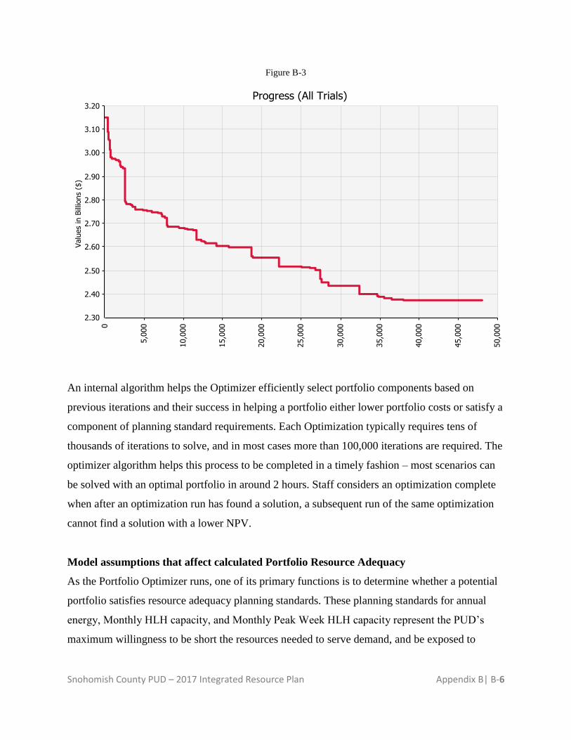
Figure 2 shows an example of how the NPV of the portfolio is improved over the course of
optimization by finding incrementally better combinations to address portfolio needs. In the case
of the pictured optimization, the original NPV of the portfolio was $3.15 billion, but was reduced
to $2.37 billion after the optimizer had cycled through almost 50,000 iterations of possible
portfolio combinations.
Snohomish County PUD – 2017 Integrated Resource Plan Appendix B| B-6
Figure B-3
An internal algorithm helps the Optimizer efficiently select portfolio components based on
previous iterations and their success in helping a portfolio either lower portfolio costs or satisfy a
component of planning standard requirements. Each Optimization typically requires tens of
thousands of iterations to solve, and in most cases more than 100,000 iterations are required. The
optimizer algorithm helps this process to be completed in a timely fashion – most scenarios can
be solved with an optimal portfolio in around 2 hours. Staff considers an optimization complete
when after an optimization run has found a solution, a subsequent run of the same optimization
cannot find a solution with a lower NPV.
Model assumptions that affect calculated Portfolio Resource Adequacy
As the Portfolio Optimizer runs, one of its primary functions is to determine whether a potential
portfolio satisfies resource adequacy planning standards. These planning standards for annual
energy, Monthly HLH capacity, and Monthly Peak Week HLH capacity represent the PUD’s
maximum willingness to be short the resources needed to serve demand, and be exposed to
Snohomish County PUD – 2017 Integrated Resource Plan Appendix B| B-7
wholesale market prices to serve demand over the study period. These planning standards are
given in Figure B-2. The determination of portfolio adequacy is based in large part on
assumptions of existing resource generation, and assumptions of generation of potential resource
additions.
Existing resource generation is based upon simulations done in the Probabilistic Load Resource
Balance Model for each scenario. This model produces estimates for load, resource generation,
and the resulting portfolio position as a variety of likelihood’s and time periods. Embedded in
that model are the following assumptions:
1. All contracted resources with contracts set to expire over the study period, will expire as
specified in the contract without extension. The associated resource generation does not
contribute to the PUD’s portfolio after that time in the portfolio model. Over the study
period, three wind contracts and two smaller bio-fueled projects are set to expire.
2. The PUD’s BPA contract represents a significant proportion of its resource portfolio, and
the current terms of the PUD’s agreement are set to expire in 2028. While it is possible
that terms of that agreement could change post-2028, the IRP models that in the 2028-
2037 period, the BPA contract functions as if under the existing terms of the agreement.
There was not sufficient information available to assume any specific deviations from the
terms of the current agreement.
3. With the exception of the Climate Change scenario, which includes anticipated changes
in local and regional hydrology due to climate change, existing resource generation is
based on probabilistic simulations of their historic generation under current operating
parameters. As a result, an underlying assumption of the existing portfolio load resource
balance used by the Portfolio optimizer is that resources perform within the bounds of
their historical production and operating constraints of those resources don’t change
dramatically.
Snohomish County PUD – 2017 Integrated Resource Plan Appendix B| B-8
2. Supply-Side Resource Assumptions
The Portfolio Optimization Model considers supply-side resources and demand-side resources in
an integrated portfolio approach to arrive at candidate portfolios for each scenario. The purpose
of this section is to outline how supply-side resources were modelled for consideration in the
Portfolio Optimization Model.
The Portfolio Optimization Model’s purpose is to find the most cost effective resource
combination to meet portfolio needs in a scenario, such that all Planning Standards are satisfied.
Planning standards measure energy, capacity and Renewable Portfolio Standard compliance and
as a result these attributes need to be assigned to potential resources, along with their costs of
acquisition.
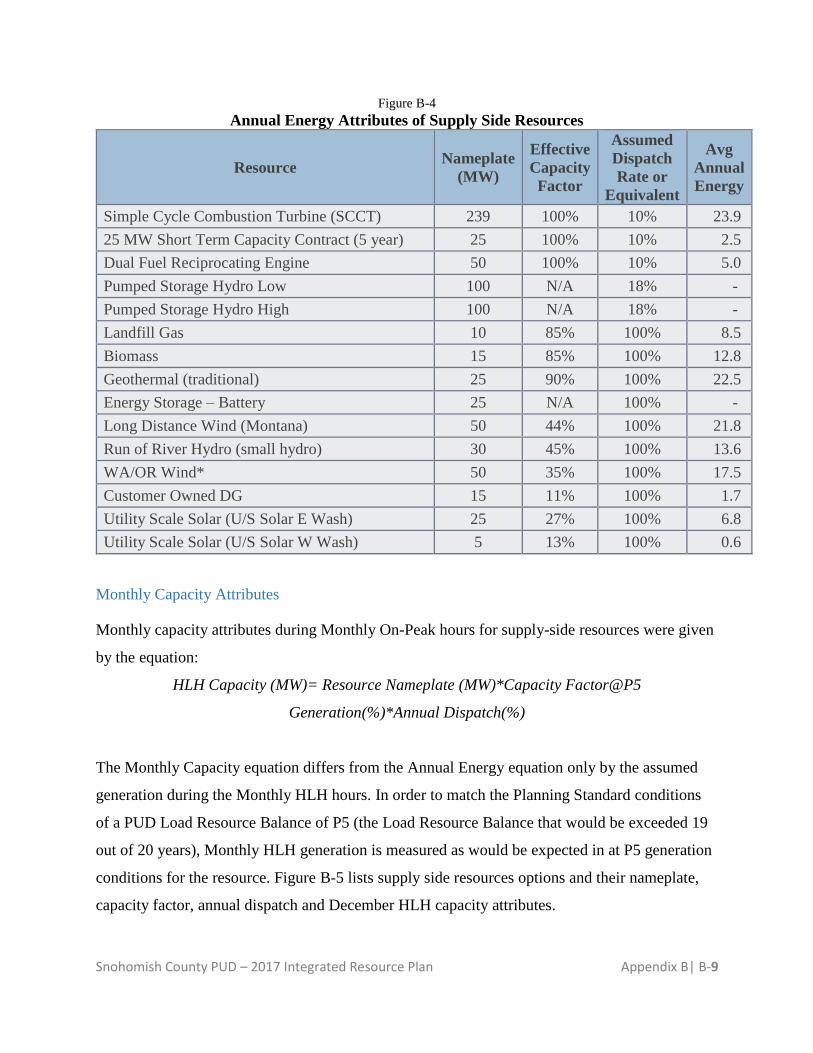
Annual Energy Attributes
Annual Energy attributes for supply-side resources were given by the equation:
Annual Energy (MW)= Resource Nameplate (MW)*Capacity Factor@P50
Generation(%)*Annual Dispatch(%)
Figure B-4 lists supply side resources options, their nameplate, capacity factor, annual dispatch
and annual energy attributes. Note that some storage supply-side resources that transfer energy
from one time period to another have no net annual energy attributes (marked with an * below).
Snohomish County PUD – 2017 Integrated Resource Plan Appendix B| B-9
Figure B-4
Annual Energy Attributes of Supply Side Resources
Resource Nameplate
(MW)
Effective
Capacity
Factor
Assumed
Dispatch
Rate or
Equivalent
Avg
Annual
Energy
Simple Cycle Combustion Turbine (SCCT) 239 100% 10% 23.9
25 MW Short Term Capacity Contract (5 year) 25 100% 10% 2.5
Dual Fuel Reciprocating Engine 50 100% 10% 5.0
Pumped Storage Hydro Low 100 N/A 18% -
Pumped Storage Hydro High 100 N/A 18% -
Landfill Gas 10 85% 100% 8.5
Biomass 15 85% 100% 12.8
Geothermal (traditional) 25 90% 100% 22.5
Energy Storage – Battery 25 N/A 100% -
Long Distance Wind (Montana) 50 44% 100% 21.8
Run of River Hydro (small hydro) 30 45% 100% 13.6
WA/OR Wind* 50 35% 100% 17.5
Customer Owned DG 15 11% 100% 1.7
Utility Scale Solar (U/S Solar E Wash) 25 27% 100% 6.8
Utility Scale Solar (U/S Solar W Wash) 5 13% 100% 0.6
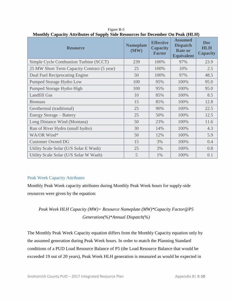
Monthly Capacity Attributes
Monthly capacity attributes during Monthly On-Peak hours for supply-side resources were given
by the equation:
HLH Capacity (MW)= Resource Nameplate (MW)*Capacity Factor@P5
Generation(%)*Annual Dispatch(%)
The Monthly Capacity equation differs from the Annual Energy equation only by the assumed
generation during the Monthly HLH hours. In order to match the Planning Standard conditions
of a PUD Load Resource Balance of P5 (the Load Resource Balance that would be exceeded 19
out of 20 years), Monthly HLH generation is measured as would be expected in at P5 generation
conditions for the resource. Figure B-5 lists supply side resources options and their nameplate,
capacity factor, annual dispatch and December HLH capacity attributes.
Snohomish County PUD – 2017 Integrated Resource Plan Appendix B| B-10
Figure B-5
Monthly Capacity Attributes of Supply Side Resources for December On Peak (HLH)
Resource Nameplate
(MW)
Effective
Capacity
Factor
Assumed
Dispatch
Rate or
Equivalent
Dec
HLH
Capacity
Simple Cycle Combustion Turbine (SCCT) 239 100% 97% 23.9
25 MW Short Term Capacity Contract (5 year) 25 100% 10% 2.5
Dual Fuel Reciprocating Engine 50 100% 97% 48.5
Pumped Storage Hydro Low 100 95% 100% 95.0
Pumped Storage Hydro High 100 95% 100% 95.0
Landfill Gas 10 85% 100% 8.5
Biomass 15 85% 100% 12.8
Geothermal (traditional) 25 90% 100% 22.5
Energy Storage – Battery 25 50% 100% 12.5
Long Distance Wind (Montana) 50 23% 100% 11.6
Run of River Hydro (small hydro) 30 14% 100% 4.3
WA/OR Wind* 50 12% 100% 5.9
Customer Owned DG 15 3% 100% 0.4
Utility Scale Solar (U/S Solar E Wash) 25 3% 100% 0.8
Utility Scale Solar (U/S Solar W Wash) 5 1% 100% 0.1
Peak Week Capacity Attributes
Monthly Peak Week capacity attributes during Monthly Peak Week hours for supply-side
resources were given by the equation:
Peak Week HLH Capacity (MW)= Resource Nameplate (MW)*Capacity Factor@P5
Generation(%)*Annual Dispatch(%)
The Monthly Peak Week Capacity equation differs from the Monthly Capacity equation only by
the assumed generation during Peak Week hours. In order to match the Planning Standard
conditions of a PUD Load Resource Balance of P5 (the Load Resource Balance that would be
exceeded 19 out of 20 years), Peak Week HLH generation is measured as would be expected in
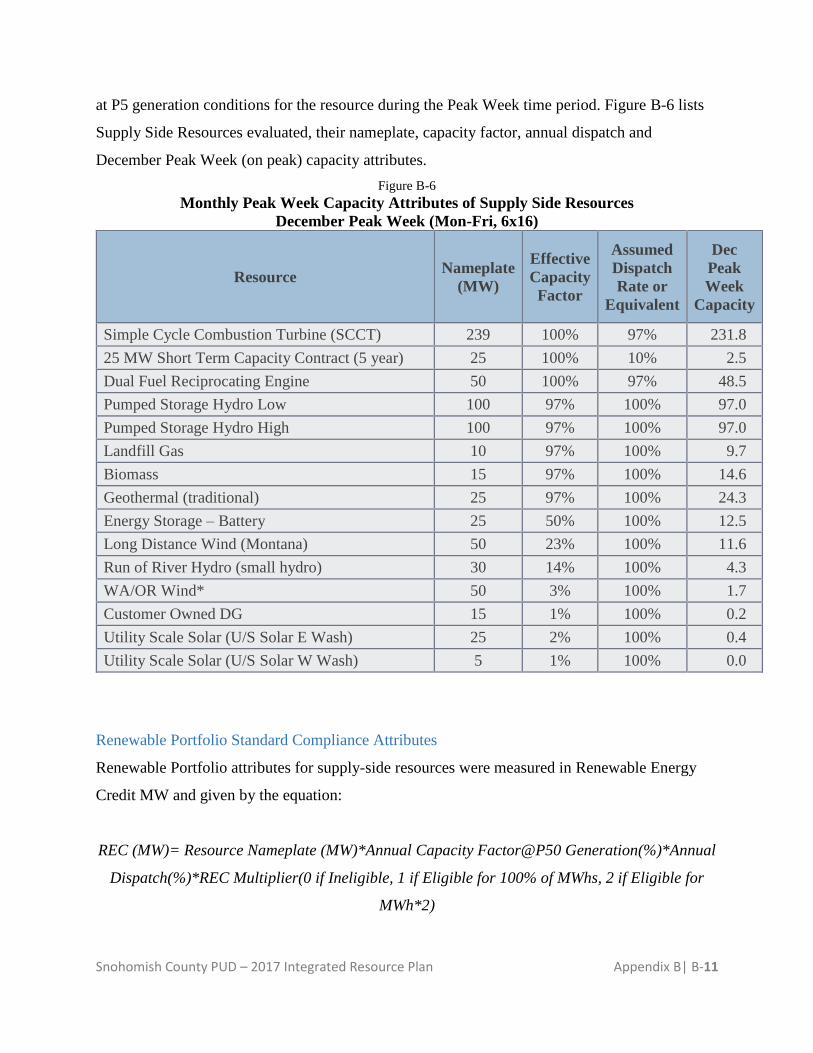
Snohomish County PUD – 2017 Integrated Resource Plan Appendix B| B-11
at P5 generation conditions for the resource during the Peak Week time period. Figure B-6 lists
Supply Side Resources evaluated, their nameplate, capacity factor, annual dispatch and
December Peak Week (on peak) capacity attributes.
Figure B-6
Monthly Peak Week Capacity Attributes of Supply Side Resources
December Peak Week (Mon-Fri, 6x16)
Resource Nameplate
(MW)
Effective
Capacity
Factor
Assumed
Dispatch
Rate or
Equivalent
Dec
Peak
Week
Capacity
Simple Cycle Combustion Turbine (SCCT) 239 100% 97% 231.8
25 MW Short Term Capacity Contract (5 year) 25 100% 10% 2.5
Dual Fuel Reciprocating Engine 50 100% 97% 48.5
Pumped Storage Hydro Low 100 97% 100% 97.0
Pumped Storage Hydro High 100 97% 100% 97.0
Landfill Gas 10 97% 100% 9.7
Biomass 15 97% 100% 14.6
Geothermal (traditional) 25 97% 100% 24.3
Energy Storage – Battery 25 50% 100% 12.5
Long Distance Wind (Montana) 50 23% 100% 11.6
Run of River Hydro (small hydro) 30 14% 100% 4.3
WA/OR Wind* 50 3% 100% 1.7
Customer Owned DG 15 1% 100% 0.2
Utility Scale Solar (U/S Solar E Wash) 25 2% 100% 0.4
Utility Scale Solar (U/S Solar W Wash) 5 1% 100% 0.0
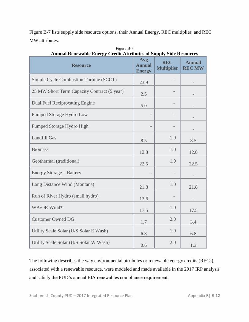
Renewable Portfolio Standard Compliance Attributes
Renewable Portfolio attributes for supply-side resources were measured in Renewable Energy
Credit MW and given by the equation:
REC (MW)= Resource Nameplate (MW)*Annual Capacity Factor@P50 Generation(%)*Annual
Dispatch(%)*REC Multiplier(0 if Ineligible, 1 if Eligible for 100% of MWhs, 2 if Eligible for
MWh*2)
Snohomish County PUD – 2017 Integrated Resource Plan Appendix B| B-12
Figure B-7 lists supply side resource options, their Annual Energy, REC multiplier, and REC
MW attributes:
Figure B-7
Annual Renewable Energy Credit Attributes of Supply Side Resources
Resource
Avg
Annual
Energy
REC
Multiplier
Annual
REC MW
Simple Cycle Combustion Turbine (SCCT)
23.9 -
-
25 MW Short Term Capacity Contract (5 year)
2.5 -
-
Dual Fuel Reciprocating Engine
5.0 -
-
Pumped Storage Hydro Low - -
-
Pumped Storage Hydro High - -
-
Landfill Gas
8.5 1.0
8.5
Biomass
12.8 1.0
12.8
Geothermal (traditional)
22.5 1.0
22.5
Energy Storage – Battery - -
-
Long Distance Wind (Montana)
21.8 1.0
21.8
Run of River Hydro (small hydro)
13.6 -
-
WA/OR Wind*
17.5 1.0
17.5
Customer Owned DG
1.7 2.0
3.4
Utility Scale Solar (U/S Solar E Wash)
6.8 1.0
6.8
Utility Scale Solar (U/S Solar W Wash)
0.6 2.0
1.3
The following describes the way environmental attributes or renewable energy credits (RECs),
associated with a renewable resource, were modeled and made available in the 2017 IRP analysis
and satisfy the PUD’s annual EIA renewables compliance requirement.
Snohomish County PUD – 2017 Integrated Resource Plan Appendix B| B-13
The environmental attributes or RECs associated with energy produced by a Washington state
eligible renewable resource can be purchased separately from the energy itself. The assumption
for unbundled RECs is that the seller of the REC owns or contracts for the renewable resource
and may have RECs surplus to their own compliance need or are trying to maximize the revenue
from the energy and REC streams for their project portfolio.
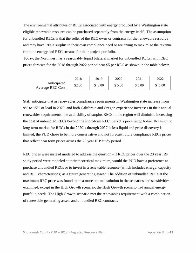
Today, the Northwest has a reasonably liquid bilateral market for unbundled RECs, with REC
prices forecast for the 2018 through 2022 period near $5 per REC as shown in the table below:
2018 2019 2020 2021 2022
Anticipated
Average REC Cost $2.00 $ 3.00 $ 5.00 $ 5.00 $ 5.00
Staff anticipate that as renewables compliance requirements in Washington state increase from
9% to 15% of load in 2020, and both California and Oregon experience increases in their annual
renewables requirements, the availability of surplus RECs in the region will diminish, increasing
the cost of unbundled RECs beyond the short-term REC market’s price range today. Because the
long term market for RECs in the 2020’s through 2037 is less liquid and price discovery is
limited, the PUD chose to be more conservative and not forecast future compliance RECs prices
that reflect near term prices across the 20 year IRP study period.
REC prices were instead modeled to address the question - if REC prices over the 20 year IRP
study period were modeled at their theoretical maximum, would the PUD have a preference to
purchase unbundled RECs or to invest in a renewable resource (which includes energy, capacity
and REC characteristics) as a future generating asset? The addition of unbundled RECs at the
maximum REC price was found to be a more optimal solution in the scenarios and sensitivities
examined, except in the High Growth scenario; the High Growth scenario had annual energy
portfolio needs. The High Growth scenario met the renewables requirement with a combination
of renewable generating assets and unbundled REC contracts.
Snohomish County PUD – 2017 Integrated Resource Plan Appendix B| B-14
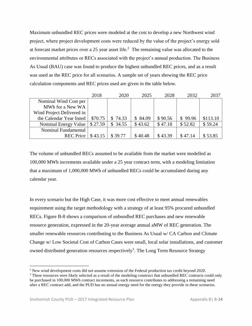
Maximum unbundled REC prices were modeled at the cost to develop a new Northwest wind
project, where project development costs were reduced by the value of the project’s energy sold
at forecast market prices over a 25 year asset life.2 The remaining value was allocated to the
environmental attributes or RECs associated with the project’s annual production. The Business
As Usual (BAU) case was found to produce the highest unbundled REC prices, and as a result
was used as the REC price for all scenarios. A sample set of years showing the REC price
calculation components and REC prices used are given in the table below.
2018 2020 2025 2028 2032 2037
Nominal Wind Cost per
MWh for a New WA
Wind Project Delivered in
the Calendar Year listed $70.75 $ 74.33 $ 84.09 $ 90.56 $ 99.96 $113.10
Nominal Energy Value $ 27.59 $ 34.55 $ 43.62 $ 47.18 $ 52.82 $ 59.24
Nominal Fundamental
REC Price $ 43.15 $ 39.77 $ 40.48 $ 43.39 $ 47.14 $ 53.85
The volume of unbundled RECs assumed to be available from the market were modelled as
100,000 MWh increments available under a 25 year contract term, with a modeling limitation
that a maximum of 1,000,000 MWh of unbundled RECs could be accumulated during any
calendar year.
In every scenario but the High Case, it was more cost effective to meet annual renewables
requirement using the target methodology with a strategy of at least 95% procured unbundled
RECs. Figure B-8 shows a comparison of unbundled REC purchases and new renewable
resource generation, expressed in the 20-year average annual aMW of REC generation. The
smaller renewable resources contributing to the Business As Usual w/ CA Carbon and Climate
Change w/ Low Societal Cost of Carbon Cases were small, local solar installations, and customer
owned distributed generation resources respectively3. The Long Term Resource Strategy
2 New wind development costs did not assume extension of the Federal production tax credit beyond 2020. 3 These resources were likely selected as a result of the modeling construct that unbundled REC contracts could only
be purchased in 100,000 MWh contract increments, as each resource contributes to addressing a remaining need
after a REC contract add, and the PUD has no annual energy need for the energy they provide in these scenarios.
Snohomish County PUD – 2017 Integrated Resource Plan Appendix B| B-15
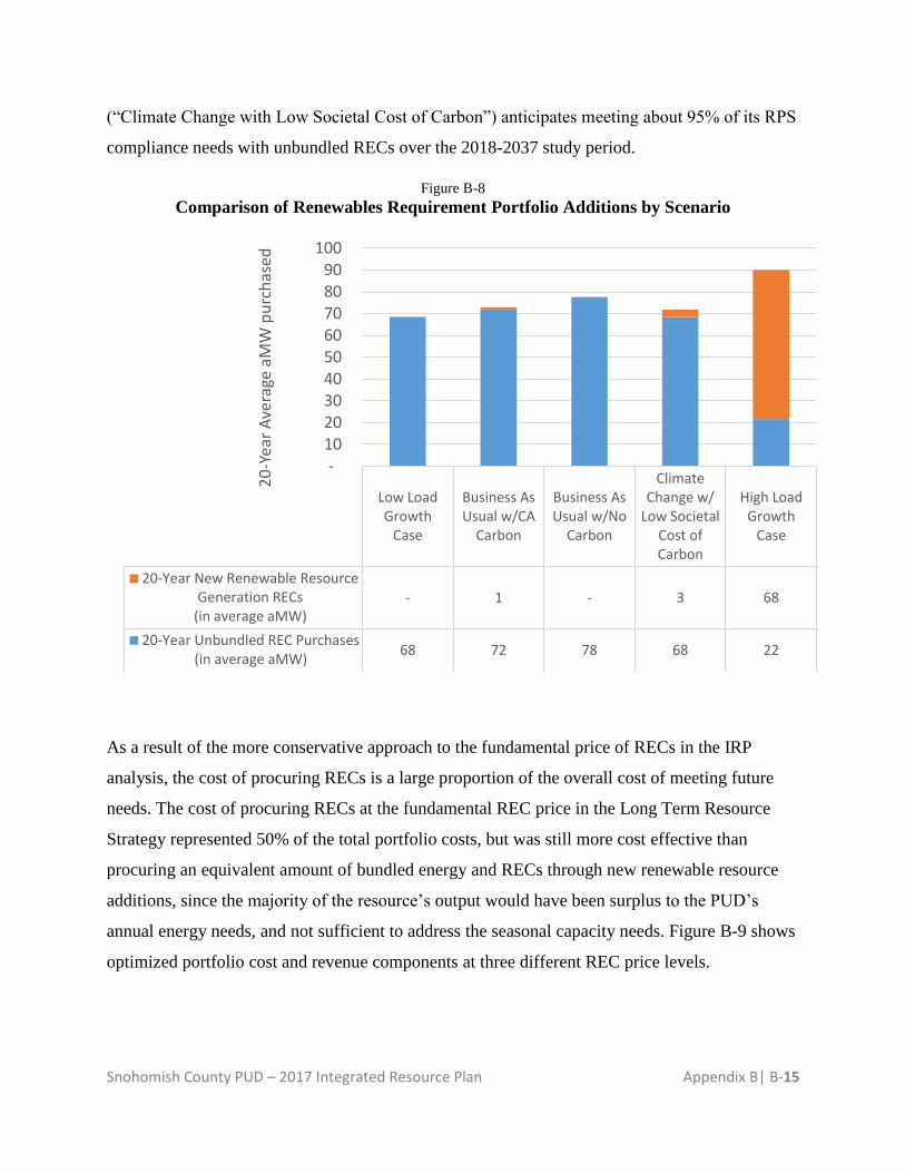
(“Climate Change with Low Societal Cost of Carbon”) anticipates meeting about 95% of its RPS
compliance needs with unbundled RECs over the 2018-2037 study period.
Figure B-8
Comparison of Renewables Requirement Portfolio Additions by Scenario
As a result of the more conservative approach to the fundamental price of RECs in the IRP
analysis, the cost of procuring RECs is a large proportion of the overall cost of meeting future
needs. The cost of procuring RECs at the fundamental REC price in the Long Term Resource
Strategy represented 50% of the total portfolio costs, but was still more cost effective than
procuring an equivalent amount of bundled energy and RECs through new renewable resource
additions, since the majority of the resource’s output would have been surplus to the PUD’s
annual energy needs, and not sufficient to address the seasonal capacity needs. Figure B-9 shows
optimized portfolio cost and revenue components at three different REC price levels.
Low LoadGrowth
Case
Business AsUsual w/CA
Carbon
Business AsUsual w/No
Carbon
ClimateChange w/
Low SocietalCost ofCarbon
High LoadGrowth
Case
20-Year New Renewable ResourceGeneration RECs
(in average aMW)- 1 - 3 68
20-Year Unbundled REC Purchases(in average aMW)
68 72 78 68 22
- 10 20 30 40 50 60 70 80 90
1002
0-Y
ear
Ave
rage
aM
W p
urc
has
ed
Snohomish County PUD – 2017 Integrated Resource Plan Appendix B| B-16
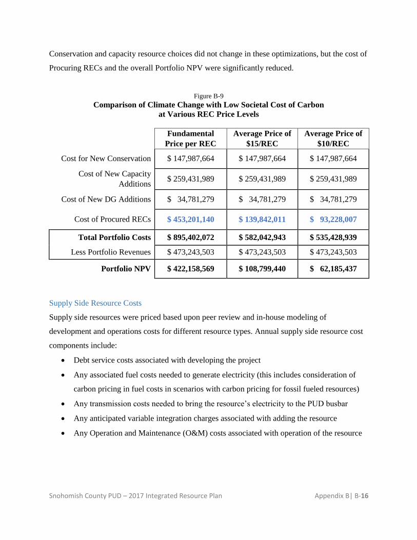
Conservation and capacity resource choices did not change in these optimizations, but the cost of
Procuring RECs and the overall Portfolio NPV were significantly reduced.
Figure B-9
Comparison of Climate Change with Low Societal Cost of Carbon
at Various REC Price Levels
Fundamental
Price per REC
Average Price of
$15/REC
Average Price of
$10/REC
Cost for New Conservation $ 147,987,664 $ 147,987,664 $ 147,987,664
Cost of New Capacity
Additions $ 259,431,989 $ 259,431,989 $ 259,431,989
Cost of New DG Additions $ 34,781,279 $ 34,781,279 $ 34,781,279
Cost of Procured RECs $ 453,201,140 $ 139,842,011 $ 93,228,007
Total Portfolio Costs $ 895,402,072 $ 582,042,943 $ 535,428,939
Less Portfolio Revenues $ 473,243,503 $ 473,243,503 $ 473,243,503
Portfolio NPV $ 422,158,569 $ 108,799,440 $ 62,185,437
Supply Side Resource Costs
Supply side resources were priced based upon peer review and in-house modeling of
development and operations costs for different resource types. Annual supply side resource cost
components include:
Debt service costs associated with developing the project
Any associated fuel costs needed to generate electricity (this includes consideration of
carbon pricing in fuel costs in scenarios with carbon pricing for fossil fueled resources)
Any transmission costs needed to bring the resource’s electricity to the PUD busbar
Any anticipated variable integration charges associated with adding the resource
Any Operation and Maintenance (O&M) costs associated with operation of the resource
Snohomish County PUD – 2017 Integrated Resource Plan Appendix B| B-17
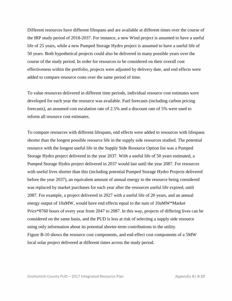
Different resources have different lifespans and are available at different times over the course of
the IRP study period of 2018-2037. For instance, a new Wind project is assumed to have a useful
life of 25 years, while a new Pumped Storage Hydro project is assumed to have a useful life of
50 years. Both hypothetical projects could also be delivered in many possible years over the
course of the study period. In order for resources to be considered on their overall cost
effectiveness within the portfolio, projects were adjusted by delivery date, and end effects were
added to compare resource costs over the same period of time.
To value resources delivered in different time periods, individual resource cost estimates were
developed for each year the resource was available. Fuel forecasts (including carbon pricing
forecasts), an assumed cost escalation rate of 2.5% and a discount rate of 5% were used to
inform all resource cost estimates.
To compare resources with different lifespans, end effects were added to resources with lifespans
shorter than the longest possible resource life in the supply side resources studied. The potential
resource with the longest useful life in the Supply Side Resource Option list was a Pumped
Storage Hydro project delivered in the year 2037. With a useful life of 50 years estimated, a
Pumped Storage Hydro project delivered in 2037 would last until the year 2087. For resources
with useful lives shorter than this (including potential Pumped Storage Hydro Projects delivered
before the year 2037), an equivalent amount of annual energy to the resource being considered
was replaced by market purchases for each year after the resources useful life expired, until
2087. For example, a project delivered in 2027 with a useful life of 20 years, and an annual
energy output of 10aMW, would have end effects equal to the sum of 10aMW*Market
Price*8760 hours of every year from 2047 to 2087. In this way, projects of differing lives can be
considered on the same basis, and the PUD is less at risk of selecting a supply side resource
using only information about its potential shorter-term contributions to the utility.
Figure B-10 shows the resource cost components, and end effect cost components of a 5MW
local solar project delivered at different times across the study period.
Snohomish County PUD – 2017 Integrated Resource Plan Appendix B| B-18
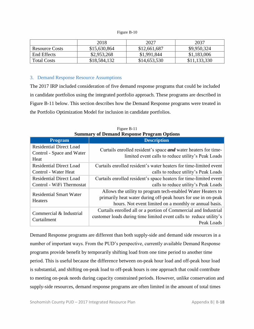
Figure B-10
2018 2027 2037
Resource Costs $15,630,864 $12,661,687 $9,950,324
End Effects $2,953,268 $1,991,844 $1,183,006
Total Costs $18,584,132 $14,653,530 $11,133,330
3. Demand Response Resource Assumptions
The 2017 IRP included consideration of five demand response programs that could be included
in candidate portfolios using the integrated portfolio approach. These programs are described in
Figure B-11 below. This section describes how the Demand Response programs were treated in
the Portfolio Optimization Model for inclusion in candidate portfolios.
Figure B-11
Summary of Demand Response Program Options
Program Description
Residential Direct Load
Control - Space and Water
Heat
Curtails enrolled resident’s space and water heaters for time-
limited event calls to reduce utility’s Peak Loads
Residential Direct Load
Control - Water Heat
Curtails enrolled resident’s water heaters for time-limited event
calls to reduce utility’s Peak Loads
Residential Direct Load
Control - WiFi Thermostat
Curtails enrolled resident’s space heaters for time-limited event
calls to reduce utility’s Peak Loads
Residential Smart Water
Heaters
Allows the utility to program tech-enabled Water Heaters to
primarily heat water during off-peak hours for use in on-peak
hours. Not event limited on a monthly or annual basis.
Commercial & Industrial
Curtailment
Curtails enrolled all or a portion of Commercial and Industrial
customer loads during time limited event calls to reduce utility’s
Peak Loads
Demand Response programs are different than both supply-side and demand side resources in a
number of important ways. From the PUD’s perspective, currently available Demand Response
programs provide benefit by temporarily shifting load from one time period to another time
period. This is useful because the difference between on-peak hour load and off-peak hour load
is substantial, and shifting on-peak load to off-peak hours is one approach that could contribute
to meeting on-peak needs during capacity constrained periods. However, unlike conservation and
supply-side resources, demand response programs are often limited in the amount of total times
Snohomish County PUD – 2017 Integrated Resource Plan Appendix B| B-19
they can be used, and how clustered those uses can be. For example, while an Industrial
customer may enroll in a voluntary curtailment program to curtail its load for a total of 120 hours
in a year, it is less likely that customer would be willing to curtail all 120 hours from Monday-
Friday in one specific week, or 500 hours over the course of a year. For this reason, Demand
Response programs required a tailored modelling methodology to be considered in the Portfolio
Optimization Model.
Another characteristic of Demand Response programs is that they don’t reduce overall demand
like conservation – instead they primarily shift demand from one time period to another.
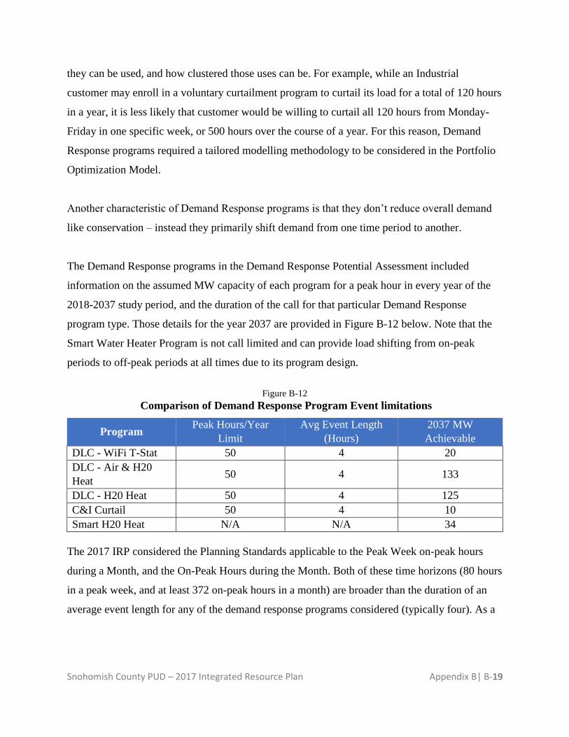
The Demand Response programs in the Demand Response Potential Assessment included
information on the assumed MW capacity of each program for a peak hour in every year of the
2018-2037 study period, and the duration of the call for that particular Demand Response
program type. Those details for the year 2037 are provided in Figure B-12 below. Note that the
Smart Water Heater Program is not call limited and can provide load shifting from on-peak
periods to off-peak periods at all times due to its program design.
Figure B-12
Comparison of Demand Response Program Event limitations
Program Peak Hours/Year
Limit
Avg Event Length
(Hours)
2037 MW
Achievable
DLC - WiFi T-Stat 50 4 20
DLC - Air & H20
Heat 50 4 133
DLC - H20 Heat 50 4 125
C&I Curtail 50 4 10
Smart H20 Heat N/A N/A 34
The 2017 IRP considered the Planning Standards applicable to the Peak Week on-peak hours
during a Month, and the On-Peak Hours during the Month. Both of these time horizons (80 hours
in a peak week, and at least 372 on-peak hours in a month) are broader than the duration of an
average event length for any of the demand response programs considered (typically four). As a
Snohomish County PUD – 2017 Integrated Resource Plan Appendix B| B-20
result, some modeling assumptions were needed to measure the potential impact of an available
demand response program across the planning standard time periods.
The most significant modeling assumption made was that all Demand Response program “call
events” could occur within each annual December Planning Standard period. This assumption
supposes that all 50 annual program hours could occur during a December Peak Week, and
would therefore also occur during the December On-Peak hour period. While this assumption
may not be realistic, it allowed the PUD to see if generic demand response programs could be
cost-effective under favorable conditions, in order to provide the PUD enough information to
determine if it should explore specific deliveries of potential demand response programs.
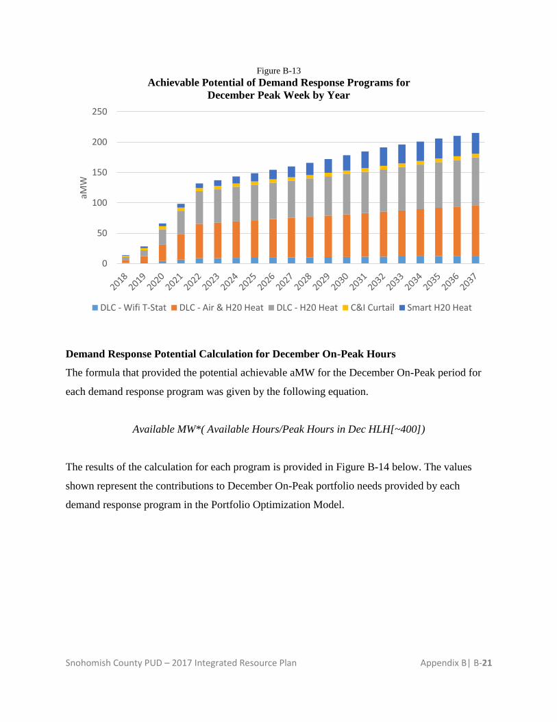
Demand Response Potential Calculation for December Peak Week
The formula that provided the potential achievable aMW for the December Peak Week period
for each demand response program was given by the following equation:
Annual Achievable MW* (Peak Hours per Year Limit/Peak Hours in Week[80])
The results of the calculation for each program is provided in Figure 3 below. The values shown
represent the contributions to December Peak Week portfolio needs provided by each demand
response program in the Portfolio Optimization Model.
Snohomish County PUD – 2017 Integrated Resource Plan Appendix B| B-21
Figure B-13
Achievable Potential of Demand Response Programs for
December Peak Week by Year
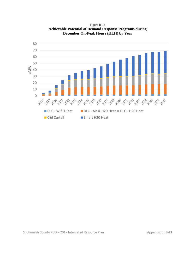
Demand Response Potential Calculation for December On-Peak Hours
The formula that provided the potential achievable aMW for the December On-Peak period for
each demand response program was given by the following equation.
Available MW*( Available Hours/Peak Hours in Dec HLH[~400])
The results of the calculation for each program is provided in Figure B-14 below. The values
shown represent the contributions to December On-Peak portfolio needs provided by each
demand response program in the Portfolio Optimization Model.
0
50
100
150
200
250
aMW
DLC - Wifi T-Stat DLC - Air & H20 Heat DLC - H20 Heat C&I Curtail Smart H20 Heat
Snohomish County PUD – 2017 Integrated Resource Plan Appendix B| B-22
Figure B-14
Achievable Potential of Demand Response Programs during
December On-Peak Hours (HLH) by Year
0
10
20
30
40
50
60
70
80
aMW
DLC - Wifi T-Stat DLC - Air & H20 Heat DLC - H20 Heat
C&I Curtail Smart H20 Heat