Embed Size (px)
Citation preview

Appendix ATensor Algebra, Linear Algebra, MatrixAlgebra, Multilinear Algebra
The key word “algebra” is derived from the name and the workof the nineth-century scientist Mohammed ibn Musa al-Khowarizmiwho was born in what is now Uzbekistan and worked in Bagdad atthe court of Harun al-Rashid’s son. “al-jabr” appears in the title ofhis book Kitab al-jabr wail muqabala where he discusses symbolicmethods for the solution of equations, K. Vogel: Mohammed IbnMusa Alchwarizmi’s Algorismus; Das forested Lehrbuch zum Rechnenmit indischen Ziffern, 1461, Otto Zeller Verlagsbuchhandlung, Aalen1963). Accordingly what is an algebra and how is it tied to the notionof a vector space, a tensor space, respectively? By an algebra wemean a set S of elements and a finite set M of operations. Eachoperation .opera/k is a single-valued function assigning to every finiteordered sequence .x1; : : : ; xn/ of n D n.k/ elements of S a value.opera/k .x1; : : : ; xk/ D xl in S. In particular for .opera/k.x1; x2/ theoperation is called binary, for .opera/k.x1; x2; x3/ ternary, in generalfor .opera/k.x1; : : : ; xn/ n-ary. For a given set of operation symbols.opera/1, .opera/2; : : :, .opera/k we define a word. In linear algebrathe set M has basically two elements, namely two internal relations.opera/1 worded “addition” (including inverse addition: subtraction)and .opera/2 worded “multiplication” (including inverse multiplication:division). Here the elements of the set S are vectors over the field R
of real numbers as long as we refer to linear algebra. In contrast, inmultilinear algebra the elements of the set S are tensors over the fieldof real numbers R. Only later modules as generalizations of vectors oflinear algebra are introduced in which the “scalars” are allowed to befrom an arbitrary ring rather than the field R of real numbers.
Let us assume that you as a potential reader are in some way familiar with theelementary notion of a threedimensional vector space Xwith elements called vectorsx 2 R3, namely the intuitive space “ we locally live in”. Such an elementary vectorspace X is equipped with a metric to be referred to as threedimensional Euclidean.
E. Grafarend and J. Awange, Applications of Linear and Nonlinear Models,Springer Geophysics, DOI 10.1007/978-3-642-22241-2,
571
© Springer-Verlag Berlin Heidelberg 2012

572 A Tensor Algebra, Linear Algebra, Matrix Algebra, Multilinear Algebra
As a real threedimensional vector space we are going to give it a linear andmultilinear algebraic structure. In the context of structure mathematics based upon
(a) Order structure(b) Topological structure(c) Algebraic structure
an algebra is constituted if at least two relations are established, namely oneinternal and one external. We start with multilinear algebra, in particular with themultilinearity of the tensor product before we go back to linear algebra, in particularto Clifford algebra.
A-1 Multilinear Functions and the Tensor Space Tpq
Let X be a finite dimensional linear space, e.g. a vector space over the field R of realnumbers, in addition denote by X
� its dual space such that n D dimX D dimX�.
Complex, quaternion and octonian numbersC, H and O as well as rings will only beintroduced later in the context. For p; q 2 Z
C being an element of positive integernumbers we introduce
Tpq .X;X
�/
as the p-contravariant, q-covariant tensor space or space of multilinear functions
f W X� � : : : � X� � X � : : : �X �! R
p dimX��q dimX :
If we assume x1; : : : ;xp 2 X� and x1; : : : ;xq 2 X, then
�
�
�
�
x1 ˝ : : :˝ xp ˝ x1 ˝ : : :˝ xq 2 Tpq .X
�;X/
holds. Multilinearity is understood as linearity in each variable. “˝” identifiesthe tensor product, the Cartesian product of elements .x1; : : : ;xp;x1; : : : ;xq/.
�
�
�
Example A.1: Bilinearity of the tensor product x1 ˝ x2For every x1;x2 2 X, x;y 2 X and r 2 R bilinearity implies
.x C y/˝ x2 D x ˝ x2 C y ˝ x2 .internal left-linearity/x1 ˝ .x C y/ D x1 ˝ x C x1 ˝ y .internal right-linearity/rx ˝ x2 D r.x ˝ x2/ .external left-linearity/x1 ˝ ry D r.x1 ˝ y/ .external right-linearity/: |
A-1 Multilinear Functions and the Tensor Space Tpq 573
The generalization of bilinearity of x1 ˝ x2 2 T02 to multilinearity of
x1 ˝ : : :˝ xp ˝ x1 ˝ : : :˝ xq 2 Tpq
is obvious.
Definition A.1. (multilinearity of tensor space Tpq ):
For every x1; : : : ;xp 2 X� and x1; : : : ;xq 2 X as well as u; v 2 X
�, x;y 2 X
and r 2 R multilinearity implies
.uC v/˝ x2 ˝ : : :˝ xp ˝ x1 ˝ : : :˝ xqD u˝ x2 ˝ : : :˝ xp ˝ x1 ˝ : : :˝ xq C v˝ x2 ˝ : : :˝ xp ˝ x1˝ : : :˝ xq .internal left-linearity/
x1 ˝ : : :˝ xp ˝ .x C y/˝ x2 ˝ : : :xqD x1 ˝ : : :˝ xp ˝ x ˝ x2 ˝ : : :˝ xq C x1 ˝ : : :˝ xp ˝ y ˝ x2˝ : : :˝ xq .internal right-linearity/
ru˝ x2 ˝ : : :˝ xp ˝ x1 ˝ : : :˝ xqD r.u˝ x2 ˝ : : :˝ xp ˝ x1 ˝ : : :˝ xq/ .external left-linearity/
x1 ˝ : : :˝ xp ˝ rx ˝ x2 ˝ : : :˝ xqD r.x1 ˝ : : :˝ xp ˝ x ˝ x2 ˝ : : :˝ xq/ .external right-linearity/:
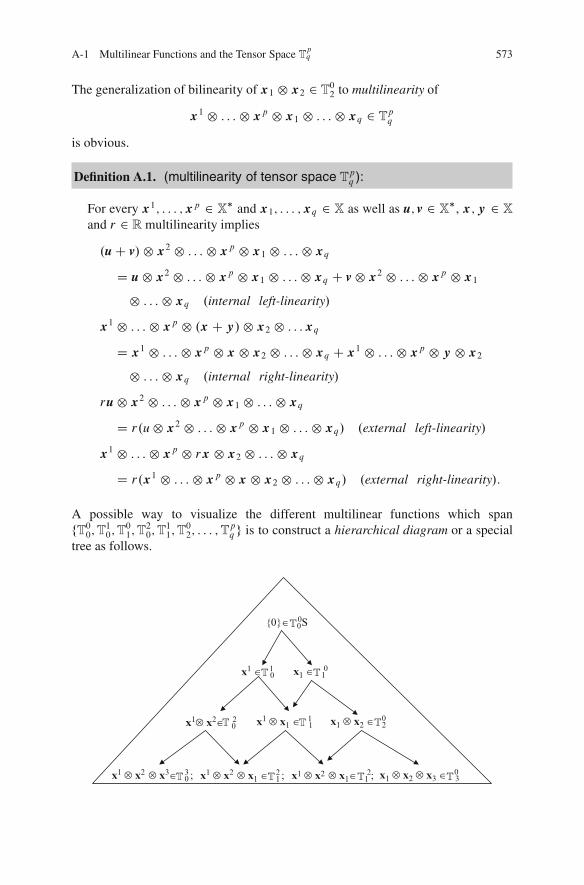
A possible way to visualize the different multilinear functions which spanfT00;T10;T01;T20;T11;T02; : : : ;Tpq g is to construct a hierarchical diagram or a specialtree as follows.
{0}∈ 00S
x1 ∈ 10 x1 ∈ 1
0
x1⊗ x2∈ 02 x1 ⊗ x1 ∈ 11 x1 ⊗ x2 ∈ 2
0
x1 ⊗ x2 ⊗ x3∈ 30 ; x1 ⊗ x2 ⊗ x1 ∈ 21 ; x1 ⊗ x2 ⊗ x1∈ 12; x1 ⊗ x2 ⊗ x3 ∈ 03

574 A Tensor Algebra, Linear Algebra, Matrix Algebra, Multilinear Algebra
When we learnt first about the tensor product symbolised by “˝” as well as itsmultilinearity we were left with the problem of developing an intuitive under-standing of x1 ˝ x2 , x1 ˝ x1 and higher order tensor products. Perhaps it ishelpful to represent ”the involved vectors” in a contravariant or in a covariantbasis. For instances, x1 D e1x1 C e2x2 C e3x3 or x1 D e1x1 C e2x2 C e3x3 isa left representation of a three-dimensional vector in a 3-left basis fe1; e2; e3gl ofcontravariant type or in a 3-left basis fe1; e2; e3gl of covariant type. Think in terms ofx1 or x1 as a three-dimensional position vector with right coordinates fx1; x2; x3g orfx1; x2; x3g , respectively. Since the intuitive algebras of vectors is commutative wemay also represent the three-dimensional vector in a in a 3-right basis fe1; e2; e3grof contravariant type or in a 3-right basis fe1; e2; e3gr of covariant type such thatx1 D x1e1 C x2e2 C x3e3 or x1 D x1e1 C x2e2 C x3e3 is a right representationof a three-dimensional position vector which coincides with its left representationthanks to commutativity. Further on, the tensor product x ˝ y enjoys the left andright representations
�e1x1 C e2x2 C e3x3
�˝ �e1y1 C e2y2 C e3y3� D
3X
iD1
3X
jD1ei ˝ ej xi yj
and
�x1e1 C x2e2 C x3e3
�˝ �y1e1 C y2e2 C y3e3� D
3X
iD1
3X
jD1xiyj ei ˝ ej
which coincides again since we assumed a commutative algebra of vectors. Theproduct of coordinates .xiyj /; i; j 2 f1; 2; 3g is often called the dyadic product.Please do not miss the alternative covariant representation of the tensor productx˝ y which we introduced so far in the contravariant basis, namely
�e1x1 C e2x2 C e3x3
�˝ �e1y1 C e2y2 C e3y3� D
3X
iD1
3X
jD1ei ˝ ej xi yj
of left type and
�x1e1 C x2e2 C x3e3
�˝ �y1e1 C y2e2 C y3e3� D
3X
iD1
3X
jD1xi yj ei ˝ ej
of right type. In a similar way we produce
x˝ y˝ z D3;3;3X
i;j;kD1ei ˝ ej ˝ ekxiyj zk D
3;3;3X
i;j;kD1xi yj zkei ˝ ej ˝ ek
of contravariant type and

A-1 Multilinear Functions and the Tensor Space Tpq 575
x˝ y˝ z D3;3;3X
i;j;kD1ei ˝ ej ˝ ekxiyj zk D
3;3;3X
i;j;kD1xi yj zkei ˝ ej ˝ ek
of covariant type. “Mixed covariant-contravariant” representations of the tensorproduct x1 ˝ y1 are
x1 ˝ y1 D3X
iD1
3X
jD1ei ˝ ejxiyj D
3X
iD1
3X
jD1xiyj ei ˝ ej
or
x1 ˝ y1 D3X
iD1
3X
jD1ei ˝ ejxiyj D
3X
iD1
3X
jD1xiyj ei ˝ ej :
In addition, we have to explain the notion x1 2 X�; x1 2 X: While the vector x1 is
an element of the vector space X , x1 is an element of its dual space. What is a dualspace? Indeed the dual space X
� is the space of linear functions over the elementsof X. For instance, if the vector space X is equipped with inner product, namelyhei je j i D gij ; i; j 2 f1; 2; 3g, with respect to the base vectors fe1; e2; e3g whichspan the vector space X, then
ej D3X
iD1ei gij
transforms the covariant base vectors fe1; e2; e3g into the contravariant base vectorsfe1; e2; e3g D span X
� by means of Œgij � D G�1, the inverse of the matrix Œgij � DG 2 R
3�3 . Similarly the coordinatesgij of the metric tensor g are used for “raising”or “lowering” the indices of the coordinates xi ; xj , respectively, for instance
xi D3X
jD1gij xj ; xi D
3X
jD1gij x
j :
In a finite dimensional vector space, the power of a linear space X and its dualX? does not show up. In contrast, in an infinite dimensional vector space X the
dual space X? is the space of linear functionals which play an important role
in functional analysis. While through the tensor product “˝” which operated onvectors, e.g. x˝ y, we constructed the p-contravariant, q-covariant tensor space orspace of multilinear functions Tpq .X;X�/ , e.g. T20;T
02;T
11 , we shall generalise the
representation of the elements of Tpq by means of
f DnDdim X
�X
i1;:::;ipD1ei1 ˝ : : :˝ eipfi1:::ip 2 T
p0

576 A Tensor Algebra, Linear Algebra, Matrix Algebra, Multilinear Algebra
f DnDdim X
�X
i1;:::;iqD1ei1 ˝ : : :˝ eiqf
i1:::iq 2 T0q
f DnDdim X
�X
i1;:::;ipD1
nDdim XX
j1;:::;jqD1ei1 ˝ : : :˝ eip ˝ ej1 ˝ : : :˝ ejqf
i1;:::;ipj1;:::;jq
2 Tpq
for instance
f D3X
i;jD1ei ˝ ej fij D
3X
i;jD1fij ei ˝ ej 2 T
20
f D3X
i;jD1ei ˝ ej f ij D
3X
i;jD1f ij ei ˝ ej 2 T
02
f D3X
i;jD1ei ˝ ej f i
j D3X
i;jD1f ij ei ˝ ej 2 T
11
We have to emphasize that the tensor coordinates fi1;:::;ip ; fi1;:::;iq , f
i1;:::;ipj1;:::;jp
are nolonger of dyadic or product type. For instance, for
�
�
�
�(2,0)-tensor : bilinear functions:
f DnX
i;jD1ei ˝ ej fij D
nX
i;jD1fij ei ˝ ej 2 T
20
fij ¤ fifj�
�
�
�(2,1)-tensor : trilinear functions:
f DnX
i;j;kD1ei ˝ ej ˝ ekf k
ij DnX
i;jD1f kij ei ˝ ej ˝ ek 2 T
21
f kij ¤ fifj f k
�
�
�
�
(3,1)-tensor : ternary functions:
f DnX
i;j;k;lD1ei ˝ ej ˝ ek ˝ el f l
ijk DnX
i;jD1f lijkei ˝ ej ˝ ek ˝ el 2 T
31
f lijk ¤ fifj fkf l

A-1 Multilinear Functions and the Tensor Space Tpq 577
holds. Table A.1 is a list of .p; q/-tensors as they appear in various sciences.Of special importance is the decomposition of multilinear functions as elementsof the space T
pq into their symmetric, antisymetric and residual constituents we are
going to outline.
Table A.1 Various examples of tensor spaces Tpq (p& q W rank of
tensor) (2,0) tensor, tensor space T20
Metric tensor DifferentialGauss curvature tensor geometryRicci curvature tensor
Gravity gradient tensor GravitationFaraday tensor, Maxwell tensor ElectromagneticTensor of dielectric constantTensor of permeability
Strain tensor, stress tensor Continuum mechanics
Energy momentum tensor MechanicsElectromagnetismGeneral relativity
Second order multipole Gravitostaticstensor Magnetostatics
Electrostatics
Variance-covariance Mathematicalmatrix statistics
Table A.2 Various examples of tensor spaces Tpq (p C q W rank of
tensor) (2,1) tensor, tensor space T21
Cartaan torsion tensor DifferentialDeometry
Third order multipole Gravitostaticstensor Magnetostatics
Electrostatics
skewness tensor MathematicalThird momentum tensor Statisticsof probability distribution
Tensor of piezoelectric Coupling of stressconstant and electrostatic field

578 A Tensor Algebra, Linear Algebra, Matrix Algebra, Multilinear Algebra
Table A.3 Various examples of tensor spaces Tpq (p C q W rank of
tensor) (3,1) tensor, (2,2) tensor, tensor space T31, T
22
Riemann curvature tensor DifferentialGeometry
Fourth order multipole Gravitostaticstensor Magnetostatics
Electrostatics
Hooke tensor Stress-strain relationConstitutive equationContinuum mechanicsElasticity, viscosticity
Curtosis tensor MathematicalFourth moment tensor of Statisticsa probability distribution
A-2 Decomposition of Multilinear Functions intoSymmetric Multilinear Functions, AntisymmetricMulti-linear Functions and Residual MultilinearFunctions TT pq D S
pq ˚ Apq ˚ R
pq
Tpq as the space of multilinear functions follows the decomposition T
pq D S
pq ˚
Apq ˚R
pq into the subspace Spq of symmetric multilinear functions, the subspace Ap
q
of antisymmetric multilinear functions and the subspace Rpq of residual multilinear
functions:
Box A.2i. (Antisymmetry of the symbols fi1:::ip ):
fij D �fj ifijk D �fikj ; fjki D �fj ik; fkij D �fkj i
fijkl D �fijlk; fjkli D �fjkil ; fklij D �fklj i ; fkijk D �flikj
Box A.2ii. (Symmetry of the symbols fi1:::ip ):
fij D fj ifijk D fikj ; fjki D fj ik; fkij D fkj i
fijkl D fijlk; fjkli D fjkil ; fklij D fklj i ; fkijk D flikj

A-2 Decomposition of Multilinear Functions into Symmetric Multilinear Functions 579
Box A.2iii. (The interior product of bases, span Sp, n D dim X D dimX
� D3):
S1 W 11Šei
S2 W 12Š.ei ˝ ej C ej ˝ ei /
DW ei _ ej ; ei _ ej D Cej _ e i
S3 W 13Š.ei ˝ ej ˝ ek C ei ˝ ek ˝ ej C ej ˝ ek ˝ ei
C ej ˝ ei ˝ ek C ek ˝ ei ˝ ej C ek ˝ ej ˝ ei /DW ei _ ej _ ek
ei _ ej _ ek D ei _ ek _ ej D ek _ e i _ ej D ek _ ej _ e i D ej _ ek _ ei
D ej _ ei _ ek
Box A.2iv. (The exterior product of bases, span Ap, nD dim XD dimX�D 3):
A1 W 11Šei
A2 W 12Š.ei ˝ ej � ej ˝ ei /
DW ei ^ ej ; e i ^ ej D �ej ^ e i
A3 W 13Š.ei ˝ ej ˝ ek � ei ˝ ek ˝ ej C ej ˝ ek ˝ ei
� ej ˝ ei ˝ ek C ek ˝ ei ˝ ej � ek ˝ ej ˝ ei /DW ei ^ ej ^ ek
ei ^ ej ^ ek D �e i ^ ek ^ ej D Cek ^ ei ^ ej D �ek ^ ej ^ e i
D ej ^ ek ^ ei D �ej ^ e i ^ ek

580 A Tensor Algebra, Linear Algebra, Matrix Algebra, Multilinear Algebra
Box A.2v. (Sp, symmetric multilinear functions):
T10 � S
1 3 f D8<
:
nD dimX�
X
iD1ei fi
9=
;
T20 � S
2 3 f D8<
:1
2Š
nD dimX�
X
i;jD1ei _ ej fij
9=
;
D8<
:
nD dimX�
X
i�jei _ ej f.ij /jf.ij / WD 1
2Š.fij C fj i /
9=
;
T30 � S
3 3 f D8<
:1
3Š
nD dimX�
X
i;j;kD1e i _ ej _ ekfijk
9=
;D8<
:
nX
i<j<k
ei _ ej _ ekf.ijk/jf.ijk/
WD 1
3Š.fijk C fikj C fjki C fj ik C fkij C fkj i /
9=
;
Tp0 � S
p 3 f D8<
:1
pŠ
nD dimX�
X
i1;i2;:::;ipD1ei1 _ ee2 _ : : : _ eip fi1i2:::ip
9=
;
D8<
:
nD dimX�
X
i1�i2�:::�ipei1 _ ei2 _ : : : _ eipf.i1i2:::ip/jf.i1i2:::ip/
WD 1
pŠ.fi1:::ip�1ip C fi1:::ip ip�1 C : : :C fip:::i1i2 C fip:::i2i1 /
9=
;:
�
�
Corollary: dimSpD
�nCp� 1
p
�, in particular if nDp, then dimS
pD�2p� 1p
�.
Box A.2vi. (Ap, antisymmetric multilinear functions):
T10 � A1 3 f D
8<
:
nD dimX�
X
iD1ei fi
9=
;

A-2 Decomposition of Multilinear Functions into Symmetric Multilinear Functions 581
T20 � A2 3 f D
8<
:1
2Š
nD dimX�
X
i;jD1ei ^ ej fij
9=
;
D8<
:
nD dimX�
X
i<j
ei ^ ej fŒij �jfŒij � WD 1
2Š.fij C fj i /
9=
;
T30 � A3 3 f D
8<
:1
3Š
nD dimX�
X
i;j;kD1ei ^ ej ^ ekfijk
9=
;
D8<
:
nX
i<j<k
ei ^ ej ^ ekfŒijk�jfŒijk�
WD 1
3Š.fijk � fikj C fjki � fj ik C fkij � fkj i /
9=
;
Tp0 � Ap 3 f D
8<
:1
pŠ
nD dimX�
X
i1;i2;:::;ipD1ei1 ^ ee2 ^ : : : ^ eip fi1i2:::ip
9=
;
D8<
:
nD dimX�
X
i1<i2<:::<ip
ei1 ^ ei2 ^ : : : ^ eipfŒi1i2:::ip�jfŒi1i2:::ip �
WD 1
pŠ.fi1:::ip�1ip � fi1:::ip ip�1 C : : :C fip:::i1i2 � fip:::i2i1 /
9=
;:
�
�
Corollary: dim Ap D nŠ=.pŠ.n�p/Š/D�n
p
�in particular if nDp, then dim ApD1.
Box A.2vii. (Aq, antisymmetric multilinear functions, exterior productProposition):
(a) For every x1; : : : ;xi�1;xiC1; : : : ;xq 2 X as well as x;y 2 X and r; s 2 R
multilinearity implies
x1 ^ : : : ^ xi�1 ^ .rx C sy/ ^ xiC1 ^ : : : ^ xqD r.x1 ^ : : : ^ xi�1 ^ x ^ xiC1 ^ : : : ^ xqC s.x1 ^ : : : ^ xi�1 ^ y ^ xiC1 ^ : : : ^ xq:

582 A Tensor Algebra, Linear Algebra, Matrix Algebra, Multilinear Algebra
(b) For every permutation � of f1; 2; : : : ; qg we have
x�1 ^ x�2 ^ : : : ^ x�q D sign .�/x1 ^ x2 ^ : : : ^ xq:(c) Let A 2 Aq.X/, B 2 As.X/; then
B ^ A D .�1/qsA ^B:(d) For every q, 0 � q � n, the tensor space Aq of antisymmetric multilinear
functions has dimension
dim Aq D�n
q
�D nŠ=.qŠ.n � q/Š/:
As detailed examples we like to decompose fT10;T01;T20;T02g in R2 and R
3,respectively, into symmetric and antisymmetric constituents.
Example A.2. (Tpq D Spq ˚ Ap
q ˚ Rpq , decomposition of multilinear functions
into symmetric and antisymmetric constituents):
As a first example of the decomposition of multilinear functions (tensor space)into symmetric and antisymmetric constituents we consider a linear space X (vectorspace) of dimension dimX D n D 2. Its dual space X�, dimX
� D dimX D n D 2,is spanned by orthonormal contravariant base vectors fe1; e2g. Choose q D 0,p D 1 and p D 2.
X D span fe1; e2g versus X� D span fe1; e2g
T10 D A1 D S
1 3 f D(
2X
iD1ei fi
)
D e1f1 C e2f2 2 X
T20 D A2 ˚ S
2
T20 3 f D
8<
:
2X
i;jD1ei ˝ ej fij
9=
;
D e1 ˝ e1f11 C e1 ˝ e2f12 C e2 ˝ e1f21 C e2 ˝ e2f22D e1 ˝ e1f11 C e2 ˝ e2f22 C 1
2.e1 ˝ e2 � e2 ˝ e1/f12
C 1
2.e1 ˝ e2 C e2 ˝ e1/f12 � 1
2.e1 ˝ e2 � e2 ˝ e1/f21
C 1
2.e1 ˝ e2 C e2 ˝ e1/f21
D e1 _ e1f11C e2 _ e2f22C e1 ^ e2.f12� f21/=2Ce1 _ e2.f12Cf21/=2dimS
2 D 3; dim A2 D 1:

A-2 Decomposition of Multilinear Functions into Symmetric Multilinear Functions 583
As a second example of the decomposition of multilinear functions (tensor space)into symmetric and antisymmetric constituents we consider a linear space X (vectorspace) of dimension dimX D n D 3, spanned by orthonormal contravariant basevectors fe1; e2; e3g. Choose p D 0, q D 1 and 2.
spanX D fe1; e2; e3g
T01 D A1 D S1 3 f D
(3X
iD1ei f
i
)
D e1f 1 C e2f 2 C e3f 3 2 X
T02 D A2 ˚ S2
T02 3 f D
8<
:
3X
i;jD1ei ˝ ej f ij
9=
;
D(
3X
iD1ei ˝ e1f i1 C
3X
iD1ei ˝ e2f i2 C
3X
iD1ei ˝ e3f i3
)
D e1 ˝ e1f 11 C e2 ˝ e1f 21 C e3 ˝ e1f 31 C e1 ˝ e2f 12 C e2 ˝ e2f 22
C e3 ˝ e2f 32 C e1 ˝ e3f 13 C e2 ˝ e3f 23 C e3 ˝ e3f 33
C 1
2.e1 ˝ e2 � e2 ˝ e1/f 12 C 1
2.e1 ˝ e2 C e2 ˝ e1/f 12
� 12.e1 ˝ e2 � e2 ˝ e1/f 21 C 1
2.e1 ˝ e2 C e2 ˝ e1/f 12
C 1
2.e2 ˝ e3 � e3 ˝ e2/f 23 C 1
2.e2 ˝ e3 C e3 ˝ e2/f 23
� 12.e2 ˝ e3 � e3 ˝ e2/f 32 C 1
2.e2 ˝ e3 C e3 ˝ e2/f 32
C 1
2.e3 ˝ e1 � e1 ˝ e3/f 31 C 1
2.e3 ˝ e1 C e1 ˝ e3/f 31
� 12.e3 ˝ e1 � e1 ˝ e3/f 13 C 1
2.e3 ˝ e1 C e1 ˝ e3/f 13 |
Since the subspaces Spq , Ap
q and Rpq are independent, Spq ˚ Ap
q ˚ Rpq denotes
the direct sum of subspace Spq , Ap
q and Rpq . Unfortunately T
pq as the space of
multilinear functions cannot be completely decomposed in the space of symmetricand antisymmetric multilinear functions: For instance, the dimension identitiesapply dimTp D np , dimSp D .nCp�1
p /, dim Ap D .np/ with respect of a vectorspace X of dimension dimX D n, such that dimRp D dimTp �dim Sp �dim Ap Dnp � .nCpC1
p / � .np/ < np , in general. There is one exception, namely the (2,0) or(1,1) or (0,2) tensor space where the dimension of the subspace R
20 , R1
1 or R02 of
residual multilinear functions is zero. An example is dimR2 D n2 � .nC1
2 / � .n2/ Dn2 � .nC 1/n=2� n.n � 1/2 D 0.

584 A Tensor Algebra, Linear Algebra, Matrix Algebra, Multilinear Algebra
A-3 Matrix Algebra, Array Algebra, Matrix Norm andInner Product
Symmetry and antisymmetry of the symbols fi1:::ip can be visualized by thetrees of Box A.2i and A.2ii. With respect to the symbols of the interiorproduct “_” and the exterior product “^” (“wedge product”) we are able toredefine symmetric and antisymmetric functions according to Box A.2iii–vi.Note the isomorphism of tensor algebra T
pq and array algebra, namely of
(a) Œfi � 2 Rn (onedimensional array, “column vector”,
dim Œfi � D n � 1)(b) Œfij � 2 R
n�n (twodimensional array, column-row array, “matrix”,dim Œfij � D n � n)
(c) Œfijk � 2 Rn�n�n (threedimensional array, “indexed matrix”,
dim Œfijk � D n � n � n)
etc. For the base space x 2 ˝ � R3 to be threedimensional Euclidean we had
answered the question how to measure the length of a vector (“norm”) and the anglebetween two vectors (“inner product”). The same question will finally been raisedfor tensors tpq 2 T
pq . The answer is constructively based on the vectorization of the
arrays Œfij �, Œfijk �, : : : Œfi1:::ip � by taking advantage of the symmetry-antisymmetrystructure of the arrays and later on applying the Euclidean norm and the Euclideaninner product to the vectorized array.
For a 2-contravariant, 0-covariant tensor we shall outline the procedure.
(a) Firstly let F D Œfij � be the quadratic matrix of dimension dimF D n � n,an element of T20. Accordingly vecF is the vector
vecF D
2
666664
fi1fi2:::
fin�1
fin
3
777775; dim vecF D n2 � 1
which is generated by stacking the elements of the matrix F columnwise in avector. The Euclidean norm and the Euclidean inner product of vecF , vecG ,respectively is
�
�
�
�
kvecF k2 WD .vecF /T .vecF / D trF TF ;
hvecF jvecG i WD .vecF /T vecG D trF TG :
(b) Secondly let F D Œfij � D Œfj i � be the symmetric matrix of dimensiondimF Dn�n, an element of S2. Accordingly vechF (read “vector half”) is

A-3 Matrix Algebra, Array Algebra, Matrix Norm and Inner Product 585
the n.nC 1/=2 � 1 vector which is generated by stacking the elements on andunder the main diagonal of the matrix F columnwise in a vector:
F D Œfij � D Œfj i � D F T H) vechF WD
2
666666666664
f11:
fn1
f22:
f2n
:
fnn
3
777777777775
; dim vechF D n.nC 1/=2
vechF D H vecF ; dimH D n.nC 1/=2 � n2:
The Euclidean norm and the Euclidean inner product of vechF , vechG ,respectively is
F D Œfij � D Œfj i � D F T
G D Œgij � D Œgj i � D GT
#
H)
�
�
�
�
kvechF k2 WD .vechF /T .vechF /
hvechF jvechG i WD .vechF /T .vechG /:
(c) Thirdly let F D Œfij � D �Œfj i � be the antisymmetric matrix of dimensiondimF D n � n, an element of A2. Accordingly veckF (read “vector skew”)is the n.n� 1/=2� 1 vector which is generated by stacking the elements underthe main diagonal of the matrix F columnwise in a vector:
F D Œfj i �D �Œfj i �D �F T H) veckF WD
2
666666666664
f21:
fn1
f32
:
fn2
:
fn�1n
3
777777777775
; dim veckF Dn.n� 1/=2
veckF D K vecF ; dimK D n.n � 1/=2 � n2:
The Euclidean norm and the Euclidean inner product of veckF , veckG ,respectively

586 A Tensor Algebra, Linear Algebra, Matrix Algebra, Multilinear Algebra
F D Œfij � D �Œfj i � D �F T
G D Œgij � D �Œgj i � D �GT
#
H)
�
�
�
�
kveckF k2 WD .veckF /T .veckF /
hveckF jveckG i WD .veckF /T .veckG /:
You will find the forms (a) vec F and (b) VechF in the standard book of(Harville, 1997, Chap. 16, 2001, Chap. 16) including many examples. Here wewill present Example A.3 in computing the norm as well as the inner product ofa 2-contravariant, 0-covariant tensor for the operator vec, vech and veck. The veckoperator has been introduced by (Grafarend and Schaffrin, 1993, pp. 418–419).
Example A.3. (Norm and inner product of a 2-contravariant, 0-covarianttensor):
.a/ A WD2
4a d g
b e h
c f k
3
5 ; dim A D 3 � 3 H) vec A D Œa; b; c; d; e; f; g; h; k�T ;
dim vec A D 9 � 1k vec Ak2 D .vec A/T .vec A/ D tr ATA D a2 C : : :C k2
.b/ A WD2
4a b c
b d e
c e f
3
5D AT ; dim A D 3 � 3 H) vech A D Œa; b; c; d; e; f �T ;
dim vech A D 6 � 1vech A D H vec A
8 H WD
2
66666664
1 0 0 0 0 0 0 0 0
0 1=2 0 1=2 0 0 0 0 0
0 0 1=2 0 0 0 0 0 0
0 0 0 0 1 0 0 0 0
0 0 0 0 0 1=2 0 1=2 0
0 0 0 0 0 0 0 0 1
3
77777775
; dimH D 6 � 9
kvech Ak2 D .vech A/T .vech A/ D a2 C b2 C c2 C d2 C e2 C f 2
(Henderson and Searle (1978, p. 68–69))
.c/ A WD
2
664
0 �a �b �ca 0 �d �eb d 0 �fc e f 0
3
775D �AT ; dim A D 3 � 3 H)
veck A D Œa; b; c; d; e; f �T ; dim veck A D 6 � 1veck A D K vec A

A-4 The Hodge Star Operator, Self Duality 587
8 K WD 1
2
2
66666664
0 1 0 0 �1 0 0 0 0 0 0 0 0 0 0 0
0 0 1 0 0 0 0 0 �1 0 0 0 0 0 0 0
0 0 0 1 0 0 0 0 0 0 0 0 �1 0 0 0
0 0 0 0 0 0 1 0 0 �1 0 0 0 0 0 0
0 0 0 0 0 0 0 1 0 0 0 0 0 �1 0 0
0 0 0 0 0 0 0 0 0 0 0 1 0 0 �1 0
3
77777775
;
dimK D 6 � 16kveck Ak2 D a2 C b2 C c2 C d2 C e2 C f 2 |
A-4 The Hodge Star Operator, Self Duality
In Chap. 3, we took advantage of the Hodge star operator, for instance fortransforming an overdetermined system of linear equations (inconsistent system)into a system of condition equations. There we referred to multilinear operations“join” and“meet”.The most important operator of the algebra of antisymmetric multilinear functionsis the “Hodge star operator” which we shall present finally. In addition, we shallbring to you the surprising special feature of skew algebra called “selfduality”.The algebra Ap
q of antisymmetric multilinear functions has been based on theexterior product “^” (“wedge product”). There has been created a duality operatorcalled the Hodge star operator � which is a linear map of Ap �! An�p wheren D dimX D dimX
� denotes the dimension of the base space X � R3. The
basic idea of such a map of antisymmetric multilinear functions f 2 Ap intoantisymmetric linear functions �f 2 An�p originates according to Box A.2vii fromthe following situation: The multilinear base of Ap is spanned by
f1; ei1 ; ei1 ^ ei2 ; : : : ei1 ^ e i2 ^ : : : ^ eip g
once we focus on p D 0; 1; 2; : : : n, respectively. Obviously for any dimensionnumber n and p-contravariant, q-covariant index of the skew tensor space Ap
q thereis an associated cobasis, namely
n D 1 ; p D 0; 1 W
8<
:
basis W f1; ei1gassociatedcobasis W fei1 ; 1g
n D 2 ; p D 0; 1; 2 W
8<
:
basis W f1; ei1 ; ei1 ^ ei2gassociatedcobasis W fei1 ^ ei2 ; ei2 ; 1g

588 A Tensor Algebra, Linear Algebra, Matrix Algebra, Multilinear Algebra
n D 3 ; p D 0; 1; 2; 3 W
8<
:
basis W f1; ei1 ; ei2 ^ ei3 ; e i1 ^ ei2 ^ ei3gassociatedcobasis W fei1 ^ e i2 ^ ei3 ; ei2 ^ ei3 ; ei3 ; 1g:
in general, for arbitrary n 2 N, p D 0; 1; : : : ; n � 1; n�
�
�
�
basis Wf1; ei1 ; : : : ; e i1 ^ : : : ^ eingassociated cobasis Wfei1 ^ ei2 ^ : : : ^ ein�1 ^ ein ; ei2 ^ : : : e in�1 ^ e in ; : : : ; e in�1 ^ ein ; ein ; 1;
as long as we concentrate on p-contravariant Ap only. A similar set-up of basis-associated cobasis for q-covariant Aq and mixed Ap
q can be made. The linear mapAp �! An�p, the Hodge star operator
�
�
�
�
�.ei1 ^ : : : ^ eip / WD 1
.n � p/Š�i1:::ipipC1:::in
eipC1 ^ : : : ^ ein
maps by means of the permutation symbol
�i1 ::: ipipC1 ::: in
WD
2
6666664
C 1 for an even permutationof f1; 2; : : : ; n � 1; ng
� 1 for an odd permutationof f1; 2; : : : ; n � 1; ng
0 otherwise
– sometimes called Eddington’s epsilons – on orthonormal (“unimodular”) base ofAp onto an orthonormal (“unimodular”) base of An�p.
For antisymmetric multilinear functions also called antisymmetric tensor-valuedfunctions represented in an orthonormal (“unimodular”) base the Hodge staroperator is the following linear map
Tp0 � Ap 3 f D
8<
:1
pŠ
nDdimX�
X
i1;:::;ipD1
ei1 ^ : : : ^ eip fi1:::ip
9=
;;
�Tp0 �An�p 3 � f WD
8<
:1
.n � p/ŠnDdimX�
X
ipC1;:::;in
nDdimXX
i1;:::;ip
1
pŠ�i1:::ipipC1:::in
eipC1 ^ : : : ^ einfi1:::ip
9=
;:
As soon as the base space x 2 ˝ � R3 is not covered by Cartesian coordinates,
rather by curvilinear coordinates, its coordinates base

A-4 The Hodge Star Operator, Self Duality 589
fb1;b2;b3g D fdy1; dy2; dy3g versus fb1;b2;b3g D�@
@y1;@
@y2;@
@y3
�
of contravariant versus covariant type is neither orthogonal nor normalized. It is forthis reason that finally we present �f , the Hodge star operator of an antisymmetricmultilinear function f , also called the dual of f , in a general coordinate base.
Definition A.2. (Hodge star operator, the dual of an antisymmetric multilin-ear function):
If an antisymmetric .p; 0/ multilinear function is an element of the skew algebraAp with respect, to a general base fbi1 ^ : : : ^ bipg is given
f D8<
:1
pŠ
nDdimX�
X
i1;:::;ipD1bi1 ^ : : : ^ bip fi1:::ip
9=
;
then the Hodge star operator, the dual of f , can be uniquely represented by
(a) �f D8<
:1
.n � p/ŠnDdimX�
X
ipC1;:::;in
nDdimX�
X
i1;:::ip
nDdimX�
X
j1;:::;jp
1
pŠbipC1 ^ : : : ^ bip
� pg�i1:::ip ipC1:::ingi1j1 : : : gipjpfj1:::jp
)
(b) �f D8<
:1
.n�p/ŠnDdimX�
X
ipC1;:::;in
nDdimX�
X
i1;:::;ip
1
pŠbipC1 ^ : : : ^ binpg�i1:::ipipC1:::inf
i1:::ip
9=
;
(c) .�f /k1:::kn�p D(nDdimX�P
i1;:::ip
pg�i1:::ipk1:::kn�pf
i1:::ip
)
as an element of the skew algebra An�p in the general associated cobase fbpC1^: : :^bingwith respect to the base space x 2 X � R
n of dimension n D dimX DdimX
� and Œgkl � D G�1 D adjG=detG ,pg Dpjgkl j.
If we extend the algebra Ap of antisymmetric multilinear functions by �1 D e1 ^: : : en 2 An and �e1 ^ : : : ^ en D 1 2 A0 D R, respectively, let us collect someproperties of �f , the dual of f .
�
�
�
�
Proposition A.1. (Hodge star operator, the dual of an antisymmetric multi-linear function):
Let the linearly ordered base fe1; : : : ; eng be orthonormal (“unimodular”).Then the Hodge star operator of an antisymmetric multilinear function f , thedual of f , with respect to fe1; : : : eng satisfies the following:

590 A Tensor Algebra, Linear Algebra, Matrix Algebra, Multilinear Algebra
(a) � maps antisymmetric p-contravariant tensor-valued functions to antisymmet-ric .n � p/-contravariant tensor-valued functions:� W Ap �! An�p
(b)
( �1 D e1 ^ : : : ^ en DW e for every 1 2 A0; e 2 A
�e D 1 for every e 2 An; 1 2 Ap
(c) � � f D .�1/p.n�p/f for every f 2 Ap
(d) f ^ �f D kf k2e1 ^ : : : ^ en with respect to the norm
kf k2 WD 1
pŠ
nDdimXX
i1;:::;ipD1fi1:::ip f
i1:::ip :
Example A.4. (Hodge star operator n D dimX D dimX� D 3, spanX
� Dfe1; e2; e3g, Ap �! An�p):
n D 3 ; p D 0 W � 1 D e1 ^ e2 ^ e3
n D 3 ; p D 1 W � ei1 D 1
2�i1i2i3ei2 ^ ei3
2
66666664
�e1 D 1
2.e2 ^ e3 � e3 ^ e2/ D e2 ^ e3
�e2 D 1
2.e3 ^ e1 � e1 ^ e3/ D e3 ^ e1
�e3 D 1
2.e1 ^ e2 � e2 ^ e1/ D e1 ^ e2
n D 3 ; p D 2 W � ei1 ^ ei2 D �i1i2i3e i3
2
64
�e1 ^ e2 D e3�e2 ^ e3 D e1�e3 ^ e1 D e2
n D 3 ; p D 3 W � ei1 ^ ei2 ^ e i3 D 1 |
Example A.5. (Hodge star operator of an antisymmetric tensor-valued func-tion, n D dimX D dimX
� D 3, Ap �! An�p):
Throughout we apply the summation convention over repeated indices.
n D 3 ; p D 0 W(
f “0-differential form”
�f D fdx1 ^ dx2 ^ dx3 “3-differential form’’

A-4 The Hodge Star Operator, Self Duality 591
n D 3 ; p D 1 W
8ˆˆˆ<
ˆˆ:
f D dxi1fi1 “1-differential form”
�f D 1
2�i1i2i3dxi2 ^ dxi3fi1
D f1dx2 ^ dx3 C f2dx3 ^ dx1C f3dx1 ^ dx2 “2-differential form”
n D 3 ; p D 2 W
8ˆˆ<
ˆˆ:
f D 1
2dxi1 ^ dxi2fi1i2 “2-differential form”
�f D 1
2�i1i2
i3dxi3fi1i2
D f23dx1 C f31dx2 C f12dx3 “1-differential form”
n D 3 ; p D 3 W
8ˆ<
ˆ:
f D 1
6dxi1 ^ dxi2 ^ dxi3fi1i2i3 “3-differential form”
�f D 1
6�i1i2i3fi1i2i3 D f123 “0-differential form” |
Example A.6. (Hodge star operator, n D dimX D dimX� D 3, “�” product
(cross product)):
By means of the Hodge star operator we are able to interpret the “�” product(“cross product”) in threedimensional vector space. If the vectorsx;y 2X, dimX D3, presented in the orthonormal (“unimodular”) base fe1; e2; e3g the followingequivalence between �x ^ y and x � y holds:
x D e ixi ; y D ejyj .summation convention
x 2 X ; y 2 X i; j 2 f1; 2; 3; g/
#
H)
x ^ y D ei ^ ejxiyj
D e1 ^ e2.x1y2 � x2y1/C e2 ^ e3.x2y3 � x3y2/C e3 ^ e1.x3y1 � x1y3/
H) �.x ^ y/ D �.e1 ^ e2/.x1y2 � x2y1/C �.e2 ^ e3/.x2y3 � x3y2/C �.e3 ^ e1/.x3y1 � x1y3/ D �kij ekxiyj
�.x ^ y/ D e3.x1y2 � x2y1/C e1.x2y3 � x3y2/C e2.x3y1 � x1y3/D e1.x2y3 � x3y2/C e2.x3y1 � x1y3/C e3.x1y2 � x2y1/
x � y D ei � ejxixjei � ej WD � k
ij ek
#
H)�
�
�
�
x � y D �.x ^ y/ |

592 A Tensor Algebra, Linear Algebra, Matrix Algebra, Multilinear Algebra
Example A.7. (Hodge star operator, n D dimX D dimX� D 4;X 2 R
4,Minkwinski space, self-duality (Atiyah et al., 1978)):
By means of the Examples A-5–A-7 we like to make you familiar with (a) the Hodgestar operator of an antisymmetric tensor-valued function overR3, (b) its equivalenceto the “x” product (“cross product”) and (c) selfduality in a fourdimensional space.Such a selfduality plays a key role in differential geometry and physics as beingemphasized by Atiyah et al. (1978).
�
�
�
Historical Aside
Thus we have constructed an anticommutative algebra by implement-ing the “exterior product” “^”, also called “wedge product”, initiated byH. Grassmann in “Ausdehnungslehre” (second version published in 1882).See also his collected works, H. Grassmann (1911). In addition the work byG. Peano (Calcolo geometrico secondo, l’Ausdehnungslehre di Grassmann,Fratelli Bocca Editori, Torino 1888) should be mentioned here. The historicaldevelopment may be documented by the work of Forder (1960). A modernversion of the “wedge product” is given by Berman (1961). In particular wemention the contribution by Barnabei et al. (1985) where by avoiding the notionof the dual X� of a linear space X and based upon operations like union,intersection, and complement – i.e. known in Boolean algebra – have developeda double algebra with exterior products of type one (“wedge product”, “thejoin”) and of type two (“the meet”), namely “to restore H. Grassmanns originalideas to full geometrical power”. The star operator “�” has been introduced byW. V. D. Hodge, being implemented into algebra in the work Hodge (1941) andHodge and Pedoe (1968), pp. 232–309). Here the star operation has been called“dual Grassmann coordinates”; in addition “intersections and joins” have beenintroduced.
A-5 Linear Algebra
Multilinear algebra is built on linear algebra we are going into now. At first we givea careful definition of linear algebra which secondly we deepen by the diagrams“Ass”, “Uni” and “Comm”. The subalgebra “ring with identity” which is of centralimportance for solving polynomial equations by means of Groebner bases, theBuchberger algorithm and the multipolynomial resultant method is our third subject.Section 4 introduces the motion of division algebra and the non-associative algebra.Fifthly, we confront you with Lie algebra (“God is a lie Group”); in particular withWitt algebra. Section 6 compares Lie algebra and Killing analysis. Here we addsome notes on the difficulties of a composition algebra in Sect. 7. Finally in Sect. 8

A-5 Linear Algebra 593
matrix algebra is presented again, but this time as a division algebra. As examplesof a division algebra as well as composition algebra we introduce complex algebra(Clifford algebra C l.0; 1/ ) in Sect. 9 and quaternion algebra in Sect. 10 (Cliffordalgebra C l.0; 2/ ) which is followed by an interesting letter of W. R. Hamilton(16 October 1943) to his son reproduced in Sect. 11. Octonian algebra (Cliffordalgebra with respect to H � H) in Sect. 12 is an example for a “non associative”algebra as well as a composition algebra. Of course, we have reserved “Sect. 13”for the fundamental Hurwitz theorem of composition algebra and the fundamentalFrobenius theorem of division algebra.
A-51 Definition of a Linear Algebra
Up to now we have succeeded to introduce the base space X of vectors x 2 X D R3
equipped with a metric and specialized to be threedimensional Euclidean. We haveextended the base space to a tensor space, namely from vector-valued functions totensor-valuedfunctions on fRn; gij g. Now we proceed to give linear and multilinearfunctions an algebraic structure, namely by the definition of two binary operations,(two internal relations) .opera/1 D ˛, .opera/2 D � and one binary operation(external relation) .opera/3 D ˇ.
Definition A.51. (linear algebra over the field of real numbers, linearity ofvector space X):
Let R be the field of real numbers. A linear algebra over R or R-algebraconsists of a set X of objects, two internal relations (either “additive” or“multiplicative”) and one external relation
.opera/1 DW ˛ W X �X �! X
.opera/2 DW ˇ W R �X �! X or X �R �! X
.opera/3 DW � W X �X �! X:
1 With respect to the internal relation ˛ (“join”) X as a linear space is a vectorspace over R, an Abelian group written “additively” or “multiplicatively” :
x;y ; z 2 X
additively written multiplicatively writtenAbelian group Abelian group
˛.x;y/ DW x C y ˛.x;y/ DW x ı y.G1C/ .x C y/C z D x C .y C z/ .G1ı/ .x ı y/ ı z D x ı .y ı z/
.additive associativity/ .multiplicative associativity/

594 A Tensor Algebra, Linear Algebra, Matrix Algebra, Multilinear Algebra
.G2C/ x C 0 D x .G2ı/ x ı 1 D x.additive identity; .multiplicative identity;neutral element/ neutral element/
.G3C/ x C .�x/ D 0 .G3ı/ x ı x�1 D 1.additive inverse/ .multiplicative inverse/
.G4C/ x C y D y C x .G4ı/ x ı y D y ı x.additive commutativity; .multiplicative commutativity;Abelian axiom/ Abelian axiom/:
The triplet of axioms f.G1C/; .G2C/; .G3C/g or f.G1ı/; .G2ı/; .G3ı/gconstitutes the set of group axioms.
2 With respect to the external relation ˇ the following compatibility conditionsare satisfied:
x;y 2 X;r; s 2 R
ˇ.r;x/ DWr � x.D1C/ r � .x C y/ D .x C y/ � r .D1ı/ r � .x ı y/ D .x ı y/ � r
D r � x C r � y D .r � x/ ı yD x � r C y � r D x ı .y ı r/.1st additive distributivity/ .1st multiplicative
distributivity/
.D2C/ .r C s/ � x D x � .r C s/ .D2ı/ .r ı s/ � x D x � .r ı s/D r � x C s � x D r � .s � x/D x � r C x � s D .x � r/ � s.2nd additive distributivity/ .2nd multiplicative
distributivity/
.D3/ 1 � x D x � 1 D x.left and right identity/
3 With respect to the internal relation � (“meet”) the following compatibilityconditions are satisfied:
x;y ; z 2 X; r 2 R
�.x;y/ DW x � y.G1�/ .x � y/ � z D x � .y � z/
.associativity w.r.t internal multiplication/

A-5 Linear Algebra 595
.D1 � C/ x � .y C z/ D x � y C x � z.x C y/ � z D x � zC y � z
.left and right additive distributivityw.r.t internal multiplication/
.D1 � ı/ x � .y ı z/ D .x � y/ ı z.x ı y/ � z D x ı .y � z/
.left and right multiplicative distributivityw.r.t internal multiplication/
.D2 � �/ r � .x � y/ D .r � x/ � y.x � y/ � r D x � .yr/.left and right distributivity of internaland external multiplication/
Please, in the following pay attention to the 3 axiom sets of the linear algebra.We specify now the three axiomatic sets called “associativity” (ass), “unity” (Uni)and “commutativity” (comm).
A-52 The Diagrams “Ass”, “Uni” and “Comm”
Conventionally a linear algebra is minimally constituted by the triplet (X; ˛; ˇ/where X as a linear space is a vector space equipped with the linear maps˛ W X � X �! X and ˇ W R � X �! X satisfying the axioms (Ass) and (Uni)according to the following diagrams:
(Uni):(Ass):The diagram
The square
Commutes.
a × idb × id id × b
α
αid × a
Commutes.
(Comm):
The triangle
α α
× ×
×
× ×× ×

596 A Tensor Algebra, Linear Algebra, Matrix Algebra, Multilinear Algebra
Axiom (Ass) expresses the requirement that the multiplication ˛ is associativewhereas Axiom (Uni) means that the element ˇ.1/ of X is a left as well as a rightunit for ˛. The algebra .X; ˛; ˇ/ is commutative if in addition it satisfies the axiom(Comm): commutes where �X;X is the flip switching the factors: �X;X.x ı y/ Dy ı x. |Indeed we have expressed a set of axioms both explicitly as well as in a diagram-matic approach which minimally constitute a linear algebra .X; ˛; ˇ/. In addition,beside the first internal relation ˛ called “join” we have experienced a secondinternal relation � called “meet” which had to be made compatible with the otherrelations ˛ and ˇ, respectively. Actually the diagram for the axiom (Dis) is left asan exercise.Obviously we have experienced the words “addition” and “multiplication” forvarious binary operations. Note that in the linear algebra isomorphic to the vectorspace as its geometric counterpart we have not specified the inner multiplication�.x;y/ 2 X. In a threedimensional vector space of Euclidean type
�.x;y/ DW �.x ^ y/ D x � y
namely the star � of the exterior product x ^ y or the “cross product” x � y, forx 2 R
3, y 2 R3 is an example. Sometimes
�.x;y/ DW Œx;y �
is written by rectangular brackets.
�
�
�
Historical Aside
Following a proposal of L. Kronecker (“Uber die algebraisch auflosbarenGleichungen (Abhandlung, 1929) the axiom of commutativity .G4C/ or .G4ı/is called after N. H. Abel (Memoire sur un classe particuliere d’equationsresolable algebraique, Crelle’s J. reine angewandte Mathematik 4 (1828)131–156 Oeuvres vol. 1, pp. 478–514, vol. 2, pp. 217–243, 329–331 editedby S. Lie and L. Sylow, Christiana 1881) who dealt with a particular class ofequations of all degrees which are solvable by radicals, e.g. the cyclotomicequation xn�1 D 0. N. H. Abel has proved the following general theorem: If theroots of an equation are such that all roots can be expressed as rational functionsof one of them, say x, and if any two of the roots, say r1x and r2x where r1 andr2 are rational functions are connected in such a way that r2r1x D r1r2x, thenthe equation can be solved by radicals. Refer r2r1x D r1r2x to .G1/.

A-5 Linear Algebra 597
A-53 Ringed Spaces: The Subalgebra “Ring with Identity”
In .G2ı/ the neutral element 1 as well as in .G3ı/ the inverse element has beenmultiplied from the right. Similarly left multiplication .G2ı/ by the neutral element1 as well as .G3ı/ by the inverse element are defined. Indeed it can be shown thatthere exist exactly one neutral element which is both left-neutral and right-neutralas well as exactly one inverse element which is both left-inverse and right-inverse.A subalgebra is called a “ring with identity” if the following seven conditions hold:
A ring with identity .G3�/ is a division ring if every nonzero element of thering has a multiplicative inverse. A commutative ring is a ring with commutativemultiplication .G4�/. Modules are generalizations of the vector spaces of linearalgebra in which the “scalars” are allowed to be from an arbitrary ring, rather than afield of real numbers. They will be discussed as soon as we introduce superalgebras.Now we take reference to�
�
�
�
Lemma A.53. (anticommutativity): x ı x D 0 for all x 2 X” x ı y D�y ı x for all x;y 2 X. “ı” is used in the notation “^” accordingly.
Proof.
“ H) ”x ı y C y ı x D x ı x C x ı y C y ı x C y ı yD x ı .x C y/C y ı .x C y/ D .x C y/ ı .x C y/ D 0
“(H ”x D y H) x ı x D �x ı x H) x ı x D 0:
|Later on we refer to the following algebras.

598 A Tensor Algebra, Linear Algebra, Matrix Algebra, Multilinear Algebra
A-54 Definition of a Division Algebra and Non-AssociativeAlgebra
Definition A.23. (division algebra):
A R-algebra is called division algebra over R, if all non-null elements ofX
0 WDX n f0g form additionally a group with respect to inner multiplication� DW x ı y , namely
x;y; z 2 Xnf0g.G1ı/ .x ı y/ ı z D x ı .y ı z/
(associativity of inner multiplication)
.G2ı/ x ı 1 D x(identity of inner multiplication)
.G3ı/ x ı x�1 D 1(inverse of inner multiplication)
Definition A.24. (non-associative algebra):
A weaking of a R-algebra is the non-associative algebra over R, if the axioms1 , 2 and 3 of linear algebra according to Definition A.21 hold with theexception of .G1ı/, that is the associativity of inner multiplication is cancelled.
A-55 Lie Algebra, Witt Algebra
“perhaps god is a lie group”
Many physicists believe that all modern physics is based on the operation called“Lie algebra”. Indeed more than 1000 textbooks and papers are written on thismost important subject. Indeed many physicists believe in “perhaps god is a liegroup”. Here, we can give a very short notice of “Lie algebra”. We skip a note ofcomparison “Lie algebra” and its brother “Killing analysis”.
Definition A.25. (Lie algebra):
A non-associative algebra is called Lie algebra over R, if the following opera-tions with respect to inner multiplication � WD x ı y hold:

A-5 Linear Algebra 599
.L1/ x ı x D 0
.L2/ .x ı y/ ı zC .y ı z/ ı x C .z ı x/ ı y D 0:.Jacobi identity/
The examples of the Lie algebra are numerous. As a special Lie algebra we presentthe Witt algebra which is applied to Laurent polynomials.
Example A.8. (Witt algebra on the ring of Laurent polynomials (Chen,1995)):
The Witt algebra W is the complex Lie algebra of polynomial fields on the unitcircle S
1. An element of W is a linear combination of the elements of the formein� @
@�, where � is a real parameter, and the Lie bracket of W is given by
�eim�
@
@�; ein�
@
@�
D i.n�m/ei.mCn/ @
@�:
A-56 Definition of a Composition Algebra
Various algebras are generated by adding an additional structure to the minimal setof axioms of a linear algebra blocked by (a), (b) and (c). Later on we use such anadditional structure for matrix algebra.
Definition A.26. (composition algebra):
A non-associative algebra with 1 as identity of inner multiplication is calledcomposition algebra over R, if there exists a regular quadratic formQ WX �!R
which is compatible with the corresponding operations that is the followingoperations hold:
.K1/ Q W X �! R is a regular quadratic form;
x; y; z 2 R; r 2 R
Q.r � x/ D r2 �Q.x/ .quadratic form/
Q.xCyC z/DQ.xC y/CQ.xC z/CQ.yC z/�Q.x/�Q.y/�Q.z/Q.r � x C y/� r �Q.x C y/ D .r � 1/ � Œr �Q.x/�Q.y/�Q.x/ D 0” x D 0 .regularity/
.K2/ Q.x ^ y/ D Q.x/ �Q.y/ .multiplicativity/
Q.1/ D 1

600 A Tensor Algebra, Linear Algebra, Matrix Algebra, Multilinear Algebra
The quadratic form introduced by Definition A.55 leads to the topological notion ofscalar products, norm and metric we already used:
Lemma A.56. (scalar product, norm, metric):
In a composition algebra with a positive-definite quadratic form a scalar product(“inner product”) is defined by the bilinear form h�j�i W X � X
� �! R with
hxjyi WD 1
2ŒQ.x C y/ �Q.x/�Q.y/�I
a norm is defined by k � k W X �! R with
kxk WD CŒQ.x/�1=2
and metric is defined by the bilinear form
.x;y/ WD CŒQ.x � y/�1=2:
Thus to the algebraic structure a topological structure is added, if in addition
.K3/ Q.x/ 0
for all x 2 X holds.
Proof.�
�
�
�
(i) scalar product
h�j�i W X �X �! R is a scalar product since
.1/ hxjyi D 1
2ŒQ.x C y/ �Q.x/�Q.y/�
D 1
2ŒQ.y C x/ �Q.y/ �Q.x/� D hyjxi .symmetry/
.2/ hx C yjzi D 1
2ŒQ.x C y C z/�Q.x C y/ �Q.z/�
D 1
2ŒQ.x C z/ �Q.x/�Q.z/�
C 1
2ŒQ.y C z/ �Q.y/ �Q.z/�
D hxjzi C hyjzi .additivity/

A-5 Linear Algebra 601
.3/ hrxjyi D 1
2ŒQ.rx C y/ �Q.rx/�Q.y/�
D 1
2rŒQ.x C y/ �Q.x/�Q.y/�
D r � hxjyi .homogenity/
.4/ hxjxi D 1
2ŒQ.x C x/�Q.x/�Q.x/�
D 1
2ŒQ.2x/� 2 �Q.x/� D Q.x/ 0 .positivity/
�
�
�
�(ii) norm
k � k W X �! R is a norm since
.N1/ kxk D CŒQ.x/�1=2 0(positivity) and
kxk D 0 ” x D 0
.N2/ krxk D CŒQ.rx/�1=2D CŒr2 �Q.x/�1=2Djr j � kxk(homogenity)
.N3/ kx C yk D CŒQ.xCy/�1=2 D CŒQ.x/CQ.y/C 2hxjyi�1=2
D Chkxk2 C kyk2 C 2kxk � kyk
i1=2 � kxk C kyk:.Cauchy-Schwarz’ inequality/“triangle inequality”/
�
�
�
�(iii) metric
W X �X �! R is a metric since
.M1/ .x;y/ D CŒQ.x � y/�1=2 D kx � yk 0 .posi tivi ty/
and
.x;y/ D 0 ” x � y D 0 ” x D y.M2/ .x;y/ D kx � yk D j � 1j � ky � xk D .y ;x/ .symmetry/
.M3/ .x;y/ D kx � yk D k.x � z/C .z � y/k� kx � zk C kz � xk D .x; z/C .z;y/
(triangle inequality) |

602 A Tensor Algebra, Linear Algebra, Matrix Algebra, Multilinear Algebra
We treat in the next section a special case of a division algebra, namely matrixalgebra.
A-6 Matrix Algebra Revisited, Generalized Inverses
It is known that every nonsingular matrix A has a unique inverse, usually denotedby A�1 such that AA�1 D A�1A D I, where I is the unit matrix. A matrix has ainverse only if it is square, and even then only if it is nonsingular, or alternativelyif its columns or rows are linearly independent. Over the many years past it wasfelt the need of some kind of partial inverse of a matrix that is singular or evenrectangularsingular matrix. By the term generalized inverse of a given matrix A weshall mean a matrix X associated in some way with the matrix A that (a) exists fora class of matrices larger than the class of nonsingular matrices, (b) has some of theproperties of the usual inverse, and (c) reduces to the usual inverse when A is nonsingular. Some others have used the term “pseudoinvese” rather than general inversewithout specifying the chosen type of general inverse.For a given matrix A, the matrix equation AXA D A alone characterizes thosegeneralized inverses X that are of use in analyzing the solutions of the linear systemAx D b. For other purposes, other relationships play an essential role. Thus if weare concerned with least squares properties, the equation AXA D A is not enoughand must be supplemented by other relations. There results a more restricted class ofgeneralized inverses. Here we are limited to generalized inverses finite matrices, butextension to infinite-dimensional space and to differential and integral operationsare very well known.E.H. Moore is attributed to have written one of the first papers on the topicof generalized inverses called by him the “general reciprocal” of any finitematrix,square or rectangular. His first publication on the subject was an abstracttalk given at a meeting of the American Mathematical Society which appeared in1920. Details of his talk were published only in 1935 (Moore, 1920), Moore (1935);(Moore and Nashed, 1974) after Moore’s death! Little note was taken of Moore’sdiscovery for 30 years after his first publication, during which time generalizedinverses were taken for matrices by C. L. Siegel and for operators by Tseng (1936),Tseng (1949a)–Tseng (1949c), Tseng (1956), Murray and von Neumann (1936) andmany others. A surprising revival of interest in general inverses appeared in 1950swhen least squares properties were analyzed. The important properties were realizedby Bjerhammar (1951a), Bjerhammar (1951b), (1968), one swedish colleagueteaching LESS and geodetic applications of the subject. In 1955 R. Penrose extendedA. Bjerhammar’s results on linear systems and showed that E.H. Moore inversesatisfied four equations of type (a) AXA D A, (b)XAX D X, (c) AX
0 D AX, and(d) XA
0 D XA nowadays called the axioms of the Moore-Penrose inverse, oftendenoted by AC.There are excellent textbooks on matrix algebra and generalized inverses ofmatrices including many examples upto 500! We like to mention the excellent text

A-6 Matrix Algebra Revisited, Generalized Inverses 603
of Ben-Israel and Greville (1974), Bjerhammar (1973), Gere and Weaver (1965),Graybill (1963), Mardia et al. (1979), Nashed (1974), Rao and Mitra (1971), Raoand Rao (1998), Scarle (1982), Styan (1983). Here we will be unable to competewith the dense information given by these special texts.
We assume that the reader is familiar with the standard notion of a matrixas a rectangular array of numbers offered by any undergraduate text of appliedmathematics. Familiarity of various notion, for instance the dimension of a matrixof type n � m, multiplication and addition of two matrices of type (a) “Cayley”or simply the matrix product C WDA:B, (b)“Kronecker-Zehfuss” denoted by C WDB˝ A, (c) “Katri-Rao” denoted by C WD Bˇ A, and (d)“Hadamard” attributed byK WD G �H.
How are the various matrix product defined? Who defined the variousalgebras?
Matrix algebra is the special division algebra over the field of real numbers. Thereis a natural generalization in terms of complex numbers for instance.
The three axioms
Let A D Œaij � 2 Rn�m be a rectangular matrix
1 A;B;C 2 Rnm; first set of axiom ˛.A;B/ DW ACB
.G1C/ .ACB/C C D AC .B C C /
.G2C/ AC 0 D A
.G3C/ A �A D 0
.G4C/ ACB D B C A
2 A;B 2 Rnm ; second set of axiom r; s 2 R; ˇ.r;A/ DW r � A
.D1C/ r � .ACB/ D r � AC r �B
.D2C/ .r C s/ � A D r � AC sA
.D3/ 1 � A D A
3 “multiplication of matrices”
(a) “Cayley-product” (just “the matrix product”)
A D Œaij � 2 Rn�l ; dim A D n � l
B D Œbij � 2 Rl�m ; dimB D l �m
#
H) C WD A �B D Œcij � 2 Rnm ;
dimC D n �m cij WDlP
kD1aikbkl :

604 A Tensor Algebra, Linear Algebra, Matrix Algebra, Multilinear Algebra
The product was introduced by Cayley (1857); see also his CollectedWorks, vol. 2, 475–496. A historical perspective is given in Feldmann(1962).
(b) “Kronecker-Zehfuß-product”
A D Œaij � 2 Rn�m ; dim A D n �m
B D Œbij � 2 Rk�l dimB D k � l
#
H) C WD B ˝ A D Œcij � 2 Rkn�lm;
dimC D kn � lm; B ˝ A WD ŒbijA�:
The product was early referenced to L. Kronecker by Mac Duffee (1946).The other reference is Zehfuss (1858). See also Henderson et al. (1983)and Horn and Johnson (1990). Reference is also made to Steeb (1991) andGraham (1981).
(c) “Khatri-Rao-product” (two rectangular matrices of identical columnnumber)
A D Œa1; : : : ; am� 2 Rn�m ; dim A D n �m
B D Œb1; : : : ;bm� 2 Rk�m ; dimB D k �m
#
H) C WD B ˇ A WD Œb1 ˝ a1; : : : ;bm ˝ am� 2 Rkn�m
dimC D kn �m:
“two rectangular matrices of identical column numbers are multiplied.”The product was introduced by Khatri and Rao (1968).
(d) “Hadamard product” (two rectangular matrices of the same dimension,elementwise product)
G D Œgij � 2 Rn�m ; dimG D n �m
H D Œhij � 2 Rm�m ; dimH D n �m
#
H) K WD G �H D Œkij � 2 Rn�m ;
dimK D n �m; kij WD gij hij .no summation/:
“two rectangular matrices of the same dimension define the elementwiseproduct.”The product was introduced by Hadamard (1899). See also Moutard(1894), as well as Hadamard (1949) and Schur (1911) and Horn andJohnson (1991) and Styan (1973).

A-6 Matrix Algebra Revisited, Generalized Inverses 605
Example:
(a)
A D�1 2 3
4 5 6
2 Z
2�3; B D2
42 3
4 5
6 7
3
5 2 Z3�2 H)
(b)
H) A �B D�28 34
64 79
2 Z
2�2 .“integer numbers”/:
A D�1 2 3
4 5 6
2 Z
2�3 ; B D2
41 2
3 4
5 6
3
5 2 Z3�2 H) B ˝A D ŒbijA�
D2
4
2
41 2
3 4
5 6
3
5˝ A
3
5 D
2
6666666664
1 2 3 2 4 6
4 5 6 8 10 12
3 6 8 4 8 12
12 15 18 16 20 24
5 10 15 6 12 18
20 25 30 24 30 36
3
7777777775
2 Z6�6
(c)
A D�1 2 3
4 5 6
2 Z
2�3; B D2
41 2 3
4 5 6
7 8 9
3
5 2 Z3�3
H) B ˇ A D2
4
2
41
4
7
3
5˝2
41
4
3
5 ;
2
42
5
8
3
5˝2
42
5
3
5 ;
2
43
6
9
3
5˝2
43
6
3
5
3
5
D
2
66666664
1 4 9
4 10 18
4 10 18
16 25 36
7 16 27
23 40 54
3
77777775
2 Z6�3

606 A Tensor Algebra, Linear Algebra, Matrix Algebra, Multilinear Algebra
(d)
G D�1 2 3
4 5 6
2 Z
2�3 ; H D�2 3 4
5 6 7
2 Z
2�3
H) G �H D Œgij hij � D�2 6 12
20 30 42
2 Z
2�3:
A-61 Special Matrices: Helmert, Hankel, and Vandemonte
All the quoted textbooks review effectively special matrices of various types:symmetric, antisymmetric, diagonal, unity, zero, triangular, idempotent, normal,orthogonal, orthonormal, positive-definite, positive-semidefinite, permutation, andcommutation matrices.Here, we review only orthonormal matrices of various representations. The Helmertrepresentation of orthonomal matrix is given in various forms. In addition, we giveexamples for an orthogonal matrix, for instance the Hankel matrix of power sumsand the Vandermonde matrix.
Definition (orthogonal matrix) :
The matrix A is called orthogonal if AA0 and A0A are diagonal matrices. (The rowsand columns of A are orthogonal.)
Definition (orthonormal matrix): The matrix A is called orthonormal ifAA0 D A0A D I. (The rows and columns of A are orthonormal.)
Facts (representation of a 22 orthonormal matrix) X 2 SO.2/: A 2 � 2 orthonormalmatrix X 2 SO.2/ is an element of the special orthogonal group SO(2) defined by
SO.2/ WD fX 2 R2�2 jX0X D I2 and det X D C1g
8<
:X D
�x1 x2
x3 x4
2 R
2�2ˇˇˇˇˇ
x21 C x22 D 1x1x3 C x2x4x23 C x24 D 1
D 0; x1x4 � x2x3 D C19=
;
(a)
X D�
cos� sin �� sin � cos�
2 R
2�2; � 2 Œ0; 2�
is a trigonometric representation of X 2 SO.2/.

A-6 Matrix Algebra Revisited, Generalized Inverses 607
(b)
X D"
xp1 � x2
�p1 � x2 x
#
2 R2�2; x 2 ŒC1;�1�
is an algebraic representation of X 2 SO.2/
x211C x212D 1; x11x21Cx12x22D �x
p1�x2C x
p1� x2D 0; x221Cx222D 1
�:
(c)
X D"
1�x21Cx2 C 2x
1Cx2� 2x1Cx2
1�x21Cx2
#
2 R2�2; x 2 R
is called a stereographic projection of X (stereographic projection of SO(2) S1
onto L1).
(d)
X D .I2 C S/.I2 � S/�1; S D�0 x
�x 0;
where S D �S0 is a skew matrix (antisymmetric matrix), is called a Cayley-Lipschitzrepresentation of X 2 SO.2/. (e) X 2 SO.2/ is a commutative group (“Abel”)(Example: X1 2 SO.2/, X2 2 SO.2/, then X1X2 D X2X1) (SO(n) for n D 2 is theonly commutative group, SO(nj n ¤ 2) is not “Abel”).
Facts (representation of an n � n orthonormal matrix) X 2 SO.n/:
An n � n orthonormal matrix X 2 SO.n/ is an element of the special orthogonalgroup SO(n) defined by
SO.n/ WD fX 2 Rn�njX0X D In and det X D C1g:
As a differentiable manifold SO(n) inherits a Riemann structure from the ambientspace n2 with a Euclidean metric (vecX0 2 R
n2 ; dim vecX0 D n2). Any atlas ofthe special orthogonal group SO(n) has at least four distinct charts and there is onewith exactly four charts. (“minimal atlas”: Lusternik-Schnirelmann category) (a)
X D .In C S/.In � S/�1;
where
S D �S0

608 A Tensor Algebra, Linear Algebra, Matrix Algebra, Multilinear Algebra
is a skew matrix (antisymmetric matrix), is called a Cayley-Lipschitz representationof X 2 SO.n/. (nŠ=2.n� 2/Š is the number of independent parameters/coordinatesof X) (b) If each of the matrices R1; : : : ;Rk is an n � n orthonormal matrix, thentheir product
R1R2 � � �Rk�1Rk 2 SO.n/
is an n � n orthonormal matrix.
Facts (orthonormal matrix: Helmert representation):
Let a0 D Œa1; : : : ; an� represent any row vector such that ai ¤ 0 .i 2 f1; : : : ; ng/ isany row vector whose elements are all nonzero. Suppose that we require an n � northonormal matrix, one row which is proportional to a0. In what follows one suchmatrix R is derived. Let Œr0
1; : : : ; r0n� represent the rows of R and take the first row
r01 to be the row of R that is proportional to a0. Take the second row r0
2 to beproportional to the n-dimensional row vector
Œa1;�a21=a2; 0; 0; : : : ; 0�; .H2/
the third row r03 proportional to
�a1; a2;�.a21 C a22/=a3; 0; 0; : : : ; 0
.H3/
and more generally the first through nth rows r01; : : : ; r0
n proportional to
"
a1; a2; : : : ; ak�1;�k�1X
iD1a2i =ak; 0; 0; : : : ; 0
#
.Hn � 1/
for k 2 f2; : : : ; ng;
respectively confirm to yourself that the n-1 vectors (Hn�1) are orthogonal to eachother and to the vector a0. In order to obtain explicit expressions for r0
1; : : : ; r0n it
remains to normalize a0 and the vectors (Hn�1). The Euclidean norm of the kth ofthe vectors (Hn�1) is
8<
:
k�1X
iD1a2i C
k�1X
iD1a2i
!2.a2k
9=
;
1=2
D(
k�1X
iD1a2i
! kX
iD1a2i
!.
a2k
) 1=2
:
Accordingly for the orthonormal vectors r01; : : : ; r0
n we finally find
(1st row) r01 D
"nX
iD1a2i
#�1=2.a1; : : : ; an/

A-6 Matrix Algebra Revisited, Generalized Inverses 609
(kth row) r0k D
2
66664
a2k k�1PiD1
a2i
! kP
iD1a2i
!
3
77775
�1=2
�
a1; a2; : : : ; ak�1;�k�1X
iD1
a2ia k; 0; 0; : : : ; 0
!
.nth row/ r0n D
2
6664
a2n�n�1PiD1
a2i
� �nP
iD1a2i
�:
3
7775
�1=2"
a1; a2; : : : ; an�1;�n�1X
iD1
a2ian
#
:
The recipe is complicated: When a0 D Œ1; 1; : : : ; 1; 1�, the Helmert factors in the1st row, : : : ; kth row,. . . , nth row simplify to
r01 D n�1=2Œ1; 1; : : : ; 1; 1� 2n
r0k D Œk.k � 1/��1=2Œ1; 1; : : : ; 1; 1� k; 0; 0; : : : ; 0; 0� 2n
r0n D Œn.n � 1/��1=2Œ1; 1; : : : ; 1; 1 � n� 2 R
n:
The orthonormal matrix2
66666666664
r01
r02
� � �r0k�1r0k
� � �r0n�1r0n
3
77777777775
2 SO.n/
is known as the Helmert matrix of order n. (Alternatively the transposes of such amatrix are called the Helmert matrix.)
Example (Helmert matrix of order 3):
2
664
1=p3 1=
p3 1=
p3
1=p2 �1=p2 0
1=p6 1=
p6 �2=p6
3
775 2 SO.3/:
Check that the rows are orthogonal and normalized.

610 A Tensor Algebra, Linear Algebra, Matrix Algebra, Multilinear Algebra
Example (Helmert matrix of order 4):
2
66664
1=2 1=2 1=2 1=2
1=p2 �1=p2 0 0
1=p6 1=
p6 �2=p6 0
1=p12 1=
p12 1=
p12 �3=p12
3
777752 SO.4/:
Check that the rows are orthogonal and normalized.
Example (Helmert matrix of order n):
2
66666666664
1=pn 1=
pn 1=
pn 1=
pn � � � 1=
pn 1=
pn
1=p2 �1=p2 0 0 � � � 0 0
1=p6 1=
p6 �2=p6 0 � � � 0 0
� � � � � �1p
.n�1/.n�2/1p
.n�1/.n�2/1p
.n�1/.n�2/ � � � � � �1�.n�1/p.n�1/.n�2/ 0
1pn.n�1/
1pn.n�1/
1pn.n�1/ � � � � � � 1p
n.n�1/1�npn.n�1/
3
77777777775
2 SO.n/:
Check that the rows are orthogonal and normalized. An example is the nth row
1
n.n � 1/ C � � � C1
n.n � 1/ C.1 � n/2n.n � 1/ D
n� 1n.n � 1/ C
1 � 2nC n2n.n � 1/
D n2 � nn.n � 1/ D
n.n � 1/n.n � 1/ D 1;
where .n � 1/ terms 1=Œn.n � 1/� have to be summed.
Definition (orthogonal matrix):
A rectangular matrix A D Œaij � 2 Rn�m is called “a Hankel matrix” if the nCm�1
distinct elements of A,
2
666664
a11a21� � �an�11an1 an2 � � � anm
3
777775
only appear in the first column and last row.

A-6 Matrix Algebra Revisited, Generalized Inverses 611
Example: Hankel matrix of power sums
Let A 2 Rn�m be a nm rectangular matrix (n 6 m) whose entries are power sums.
A WD
2
6666666664
nP
iD1˛ixi
nP
iD1˛i x
2i � � �
nP
iD1˛ix
mi
nP
iD1˛ix
2i
nP
iD1˛i x
3i � � �
nP
iD1˛ix
mC1i
::::::
::::::
nP
iD1˛ix
ni
nP
iD1˛ix
nC1i � � �
nP
iD1˛ix
nCm�1i
3
7777777775
A is a Hankel matrix.
Definition (Vandermonde matrix):
Vandermonde matrix: V 2 Rn�n
V W D
2
66664
1 1 � � � 1
x1 x2 � � � xn:::
::::::
:::
xn�11 xn�1
2 � � � xn�1n
3
77775;
det V DY
i;ji>j
n
.xi � xj /:
Example: Vandermonde matrix V 2 R3�3
V WD
2
64
1 1 1
x1 x2 x3
x21 x22 x
23
3
75 ; det V D .x2 � x1/.x3 � x2/.x3 � x1/:
Example: Submatrix of a Hankel matrix of power sums Consider the submatrixP D Œa1; a2; : : : ; an� of the Hankel matrix A 2 R
n�m .n 6 m/ whose entries arepower sums. The determinant of the power sums matrix P is
det P D
nY
iD1˛i
! nY
iD1xi
!
.det V/2;
where det V is the Vandermonde determinant. Example: Submatrix P 2 R3�3 of a
3 � 4 Hankel matrix of power sums (n D 3, m D 4)

612 A Tensor Algebra, Linear Algebra, Matrix Algebra, Multilinear Algebra
A D
2
6664
˛1x1 C ˛2x2 C ˛3x3 ˛1x21 C ˛2x
22 C ˛3x
23 ˛1x
31 C ˛2x
32 C ˛3x
33 ˛1x
41 C ˛2x
42 C ˛3x
43
˛1x21 C ˛2x
22 C ˛3x
23 ˛1x
31 C ˛2x
32 C ˛3x
33 ˛1x
41 C ˛2x
42 C ˛3x
43 ˛1x
51 C ˛2x
52 C ˛3x
53
˛1x31 C ˛2x
32 C ˛3x
33 ˛1x
41 C ˛2x
42 C ˛3x
43 ˛1x
51 C ˛2x
52 C ˛3x
53 ˛1x
61 C ˛2x
62 C ˛3x
63
3
7775
P D Œa1; a2; a3�
2
6664
˛1x1 C ˛2x2 C ˛3x3 ˛1x21 C ˛2x
22 C ˛3x
23 ˛1x
31 C ˛2x
32 C ˛3x
33
˛1x21 C ˛2x
22 C ˛3x
23 ˛1x
31 C ˛2x
32 C ˛3x
33 ˛1x
41 C ˛2x
42 C ˛3x
43
˛1x31 C ˛2x
32 C ˛3x
33 ˛1x
41 C ˛2x
42 C ˛3x
43 ˛1x
51 C ˛2x
52 C ˛3x
53
3
7775:
A-62 Scalar Measures of Matrices
All reference textbooks review various scalar measures of matrices like
• Linear independence• Column and row rank• Rank identities
to which we refer. Permanently, we referred to a special technique called IPM(“Inverse Partitioned Matrix”) of a symmetric matrix we will review now.
Facts: (Inverse Partitional Matrix/IPM/of a symmetric matrix):
Let the symmetric matrix A be partitioned as
A WD"
A11 A12
A012 A22
#
; A011 D A11; A0
22 D A22:
Then its Cayley inverse A�1 is symmetric and can be partitioned as well as
A�1 D2
4A11 A12
A0
12 A22
3
5
�1
D2
4ŒI C A�1
11 A12.A22 � A0
12A�111 A12/
�1A0
12�A�111 �A�1
11 A12.A22 � A0
12A�111 A12/
�1
�.A22 � A0
12A�111 A12/
�1A0
12A�111 .A22 � A0
12A�111 A12/
�1
3
5 ;
if A�111 exists;
A�1 D2
4A11 A12
A0
12 A22
3
5
�1
D2
4.A11 � A0
12A�122 A12/
�1 �.A11 � A0
12A�122 A12/
�1A12A�122
�A�122 A0
12.A11 � A0
12A�122 A12/
�1 ŒI C A�122 A0
12.A11 � A12A�122 A0
12/�1A12�A�1
22
3
5 ;
A-6 Matrix Algebra Revisited, Generalized Inverses 613
if A�122 exists:
S11 WD A22 � A012A�1
11 A12 and S22 WD A11 � A012A�1
22 A12
are the minors determined by properly chosen rows and columns of the matrix Acalled “Schur complements” such that
A�1 D"
A11 A12
A012 A22
#�1D".IC A�1
11 A12S�111 A0
12/A�111 �A�1
11 A12S�111
�S�111 A0
12A�111 S�1
11
#
if A�111 exists;
A�1 D"
A11 A12
A012 A22
#�1D"
S�122 �S�1
22 A12A�122
�A�122 A0
12S�122 ŒIC A�1
22 A012S�1
22 A12�A�122
#
if A�122 exists;
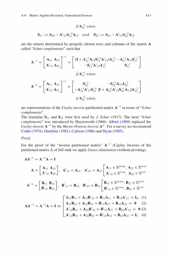
are representations of the Cayley inverse partitioned matrix A�1 in terms of “Schurcomplements”.The formulae S11 and S22 were first used by J. Schur (1917). The term “Schurcomplements” was introduced by Haynsworth (1968). Albert (1969) replaced theCayley inverse A�1 by the Moore-Penrose inverse AC. For a survey we recommendCottle (1974), Ouellette (1981), Carlson (1986) and Styan (1985).
Proof.
For the proof of the “inverse partitioned matrix” A�1 (Cayley inverse) of thepartitioned matrix A of full rank we apply Gauss elimination (without pivoting).
AA�1 D A�1A D I
A D�
A11 A12
A012 A22
; A0
11 D A11; A022 D A22
"A11 2 R
m�m; A12 2 Rm�l
A012 2 R
l�m; A22 2 Rl�l
A�1 D�
B11 B12B012 B22
; B0
11 D B11; B022 D B22
"B11 2 R
m�m; B12 2 Rm�l
B012 2 R
l�m; B22 2 Rl�l
AA�1 D A�1A D I,
2
6664
A11B11 C A12B012 D B11A11 C B12A0
12 D Im .1/
A11B12 C A12B22 D B11A12 C B12A22 D 0 .2/
A012B11 C A22B0
12 D B012A11 C B22A0
12 D 0 .3/
A012B12 C A22B22 D B0
12A12 C B22A22 D Il : .4/
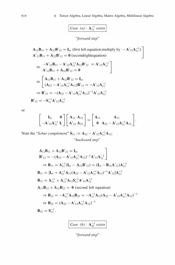
614 A Tensor Algebra, Linear Algebra, Matrix Algebra, Multilinear Algebra
Case (a) W A�111 exists
“forward step”
A11B11 CA12B012 D Im .first left equation:multiply by �A0
12A�111 /
A012B11 C A22B0
12 D 0 .secondrightequation)
#
, �A012B11 �A0
12A�111 A12B0
12 D A012A�1
11
A012B11 CA22B0
12 D 0
#
,"
A11B11 C A12B012 D Im
.A22 � A012A�1
11 A12/B012 D �A0
12A�111
) B012 D �.A22 �A0
12A�111 A12/
�1A012A�1
11
B012 D �S�1
11 A012A�1
11
or"
Im 0
�A012A�1
11 Il
#"A11 A12
A012 A22
#
D"
A11 A12
0 A22 � A012A�1
11 A12
#
:
Note the “Schur complement” S11 WD A22 �A012A�1
11 A12.
“backward step”
A11B11 C A12B012 D Im
B012 D �.A22 � A0
12A�111 A12/
�1A012A�1
11
#
) B11 D A�111 .Im � A12B0
12/ D .Im � B12A012/A�1
11
B11 D ŒIm C A�111 A12.A22 �A0
12A�111 A12/
�1A012�A�1
11
B11 D A�111 C A�1
11 A12S�111 A0
12A�111
A11B12 C A12B22 D 0 .second left equation/
) B12 D �A�111 A12B22 D �A�1
11 A12.A22 � A012A�1
11 A12/�1
, B22 D .A22 �A012A�1
11 A12/�1
B22 D S�111 :
Case (b) W A�122 exists
“forward step”

A-6 Matrix Algebra Revisited, Generalized Inverses 615
A11B12 C A12B22 D 0 .third right equation)
A012B12 C A22B22 D Il .fourth left equation: multiply by � A12A�1
22 /
#
, A11B12 C A12B22 D 0
�A12A�122 A0
12B12 �A12B22 D �A12A�122
#
,"
A012B12 C A22B22 D Il
.A11 � A12A�122 A0
12/B12 D �A12A�122
) B12 D �.A11 �A12A�122 A0
12/�1A0
12A�122
B12 D �S�122 A12A�1
22 or"
Im �A12A�122
0 Il
#"A11 A12
A012 A22
#
D"
A11 �A12A�122 A0
12 0
A012 A22
#
:
Note the “Schur complement”
S22 WD A11 � A12A�122 A0
12:
“backward step”
A012B12 C A22B22 D Il
B12 D �.A11 � A12A�122 A0
12/�1A12A�1
22
#
) B22 D A�122 .Il � A0
12B012/ D .Il � B0
12A12/A�122
B22 D ŒIl C A�122 A0
12.A11 � A12A�122 A0
12/�1A12�A�1
22
B22 D A�122 C A�1
22 A012S�1
22 A12A�122
A012B11 C A22B0
12 D 0 .third left equation/
) B012 D �A�1
22 A012B11 D �A�1
22 A012.A11 � A12A�1
22 A012/
�1
,B11 D .A11 � A12A�1
22 A012/
�1
B11 D S�122 :
|
The representations B11;B12;B21DB012;B22 in terms of A11;A12;A21 D A0
12;A22
have been derived by Banachiewicz (1937). Generalizations are referred to Ando(1979), Brunaldi and Schneider (1963), Burns et al. (1974), Carlson (1980), Meyer(1973) and Mitra (1982), Li and Mathias (2000). We leave the proof of the followingfact as an exercise.

616 A Tensor Algebra, Linear Algebra, Matrix Algebra, Multilinear Algebra
Fact (Inverse Partitioned Matrix /IPM/ of a quadratic matrix):
Let the quadratic matrix A be partitioned as
A WD"
A11 A12
A21 A22
#
:
Then its Cayley inverse A�1 can be partitioned as well as
A�1 D"
A11 A12
A21 A22
#�1D"
A�111 C A�1
11 A12S�111 A21A�1
11 �A�111 A12S�1
11
�S�111 A21A�1
11 S�111
#
;
if A�111 exists
A�1 D"
A11 A12
A21 A22
#�1D"
S�122 �S�1
22 A12A�122
�A�122 A21S�1
22 A�122 CA�1
22 A21S�122 A12A�1
22
#
;
if A�122 exists
and the “Schur complements” are defined by
S11 WD A22 �A21A�111 A12 and S22 WD A11 � A12A�1
22 A21:
Facts: Cayley Inverse, DG matrix identity, SMW matrix identity, sum of twomatrices
.DG id/ BD.AC CBD/�1 D .B�1 C DA�1C/�1DA�1(Duncan-Guttman matrix identity):
.SMW id/ .AC CBD/�1 D A�1 � A�1C.B�1 C DA�1C/�1DA�1(Sherman - Morrison - Woodbury matrix identity):
Duncan (1944) calls (DG) the Sherman-Morrison-Woodbury matrix identity. If thematrix A is singular consult Henderson and Searle (1981a), Henderson and Searle(1981b), Ouellette (1981), Hager (1989), Stewart (1977) and Riedel (1992). (SMW)has been noted by Duncan (1944) and Guttman (1946): The result is directly derivedfrom the identity
.AC CBD/.AC CBD/�1 D I
) A.ACCBD/�1 CCBD.AC CBD/�1 D I
.AC CBD/�1 D A�1 � A�1CBD.AC CBD/�1

A-6 Matrix Algebra Revisited, Generalized Inverses 617
A�1 D .AC CBD/�1 C A�1CBD.AC CBD/�1
DA�1 D D.AC CBD/�1 C DA�1CBD.AC CBD/�1
DA�1 D .ICDA�1CB/D.AC CBD/�1
DA�1 D .B�1 C DA�1C/BD.AC CBD/�1
.B�1 C DA�1C/�1DA�1 D BD.AC CBD/�1:
Up to now we presented IPM of a symmetric matrix. Alternatively, we review rankfactorization of a symmetric and positive semidefinite/definite matrix.
Facts (rank factorization):
(a) If the n � n matrix is symmetric and positive semidefinite, then its rankfactorization is
A D"
G1
G2
#�
G01 G0
2
;
where G1 is a lower triangular matrix of the order O.G1/ D rk A � rk A withrk G2 D rk A, whereas G2 has the format O.G2/ D .n � rk A/ � rk A: In thiscase we speak of a Choleski decomposition.
(b) In case that the matrix A is positive definite, the matrix block G2 is not neededanymore: G1 is uniquely determined. There holds
A�1 D .G�11 /
0G�11 :
Various notions, for instance submatrices adjoint, traces and determinants, as scalarmeasures of a matrix are given by D. A. Harville (2001, examples, Sects. 2,5 and 13)to which we refer. We already introduced vector-valued matrix forms by means ofthe operations vec, vech and veck. Please pay attention to the vec-forms
(a) vecA � B � C0 D .A˝ C/vecB(b) .A/0vecB D tr.A � B0/(c) vec xy0 D x˝ y
(d) vec(A � B/ D .B0 ˝ In/vecA D .B0 ˝ A/vecIm
D .Iq ˝ A/vecB; for all A 2 Rn�m; B 2 R
m�q
given by Pukelsheim (1977), pp. 324, 326 or Harville (2001), examples,Sect. 16, 22 pp.

618 A Tensor Algebra, Linear Algebra, Matrix Algebra, Multilinear Algebra
A-63 Three Basic Types of Generalized Inverses
In Chaps. 1, 3 and 5 we obtained the complete class of solution of equation “AxD y00and showed that every solution can be expressed in the form x D Gy where G isthe properly chosen generalized inverse. Here we inquire to find solutions for suchgeneralized inverses which are of the following type
.i/ rk A D rk .AA0/ D n W “minimum norm”
Consistent system of observation equations: Underdetermine.
Theorem (“minimum norm”: Rao and Mitra (1971), pp. 44–47)
Let G be a generalized inverse of the matrix A such that Gy is a minimum normsolution of the equation Ax D y; rkA D rk .AA0/ D n. Then it is necessary andsufficient that
(a) kxk2 D kGyk2 D Min
Ax D yor
(b) AGA D A and .GA/0 D GA. or(c) A�
mr D A0.AA0/� (reflexive generalized inverse which is minimum norm).
If we use the weighted generalized inverse of the typenMin
Ax D ykxk2 D x0Gx
o
we get the Gx-MINOS solution of Chap. 1, case (a), case (b) and case (c).
.ii/ rk A D rk .A0A/ D m W “generalized least-squares solution for Ax D y”
Inconsistent system of linear observation equations: overdetermine.
Theorem (“Least-squares”: Rao and Mitra (1971), pp. 48–50)
Let G be a matrix (not necessarily a generalized inverse) such that Gy is a least-squares solution of Ax D y such that rkA D rk .A0A/ D m. Then it is necessaryand sufficient that
(a) ky �Axk2 D min .inconsistent/or
(b) AGA D A and .GA/0 D GA:or
(c) Alr D .A0A/�A (reflexive generalized inverse which is least-squares).
If we use the weighted generalized inverse of the typenMin
xky � Axk2Gy
D
.y � Ax/0Gy.y � Ax/o
we enjoy receiving the Gy-LESS solution of Chap. 3,
case (a), case (b) and case (c).

A-7 Complex Algebra, Quaternion Algebra, Octonian Algebra, Clifford Algebra 619
.iii/ rkA < min fm; ng W “generalized inverse for a minimum norm least-squares solution”
Inconsistent system of linear observation equations with a datum defect:overdetermine-underdetermined. ut
Here we start with a definition
Definition (“MINOLESS”: Rao and Mitra (1971), p. 51)
G is said to be a minimum norm, least-squares generalized inverse of the matrix A,if G is A�
l and for any y 2 Y
kGykm � kxkm for all x 2 fx j ky � Axkm � ky � Azkm for all z 2 X
where k:kn and k:km are norms in Xm and Y
n respectively. Finally we will refer tothe basic results generating “MINOLESS”.
Theorem (“MINOLESS”: Rao and Mitra (1971), pp. 50–54,64)
Let G be a matrix such that Gy is a minimum norm, least-squares solution of theinconsistent equation Ax D yC i. Then it is necessary and sufficient that x D ACynamely, (a) AGA D A, (b) .AG/0 D AG, (c) GAG/ D G, (d) .GA/0 D GA(Penrose 1955). or
AC D A0AŒ.A0A/2��A0 D .IC A0A/�A0ŒA0A.IC A0A/�A��A� or
AC D k lim�!1kX
kD1A0.IC AA0/�k D k lim�!1
kX
kD1.IC A0A/�kA0 or
AC D � lim�! 0CA0.�IC AA0/�1 D � lim�! 0C.I�C A0A/�1A0
If we use the weighted norms kxk2Px and ky � Axk2Py , we receive the Gx-minimumnorm, Gy- least squares solution of Chap. 5, case (a), case (b) and case (c).
A-7 Complex Algebra, Quaternion Algebra, OctonianAlgebra, Clifford Algebra, Hurwitz Theorem
The greatest advantage of Clifford algebra is the following fact: We are able to writedown the field equations namely “rot” and “div” equation of gravitational field andelectromagnetic field in one equation. The related literature is very rich and wecould recommend the book by Meetz and Engl (1980). A more detailed introductioninto Clifford algebra and its fascinating chess board as well as Clifford analysis islisted in Grafarend (2004) with more than 300 references. From some point of view,the variona algebra presented here are rather out of fashion. Indeed

620 A Tensor Algebra, Linear Algebra, Matrix Algebra, Multilinear Algebra
• Complex algebra, Clifford algebra Cl.0; 1/• Quaternion algebra, Clifford algebra Cl.0; 2/
A-71 Complex Algebra as a Division Algebra as wellas a Composition Algebra, Clifford algebra Cl.0; 1/
Here we present to you “complex algebra” and refer it to Clifford algebra C l.0; 1/.The “complex algebra” C due to C. F. Gauß is a division algebra over R as well asa composition algebra.
x 2 C
x D e0x0 C e1x1 subject to fx0; x1g 2 R2
span C D f1; e1g
1 x;y; z 2 R2
˛.x;y/ DW x C y :
The axioms .G1C/, .G2C/, .G3C/, .G4C/ of an Abelian group apply.
2 x;y 2 R2; r; s 2 R
ˇ.r;x/ DW r � x:
The axioms .D1C/, .D2C/, .D3/ of additive distributivity apply.
3 One way to explicitly describe a multiplicative group with finitely manyelements is to give a table listing the multiplications just representing the map� W C � C �! C.
�
�
�
�multiplication diagram, Cayley diagram
1 e1
1 1 e1
e1 e1 �1
Note that in the multiplication table each entry of a group appears exactly oncein each row and column. The multiplication has to be read from left to rightthat is, the entry at the intersection of the row headed by e1 and the columnheaded by e1 is the product e1 � e1. Such a table is called a Cayley diagramof the multiplicative group.

A-7 Complex Algebra, Quaternion Algebra, Octonian Algebra, Clifford Algebra 621
Here note in addition the associativity of the internal multiplication given inthe table. Such a “complex algebra” C is not a Lie algebra since neither x �x D 0 .L1/ nor .x �y/� zCC.y � z/�xC .z�x/�y D 0 (Jacobi identity).L2/ hold. Just by means of the multiplication table compute
x � x D 1f.x0/2 � .x1/2g C 2e1x0x1 6D 0:
4 Begin with the choice
x�1 D 1
.x0/2 C .x1/2 .1x0 � e1x1/
in order to end up with
x � x�1 D .1x0 C e1x1/ � 1x0 � e1x1.x0/2 C .x1/2 D 1
Accordingly .G1�/, .G2�/, .G3�/ of a division algebra apply.
5 Begin with the choice
Q.x/ D Q.1x0 C e1x1/ WD .x0/2 C .x1/2
in order to prove (K1), (K2) and (K3). We only focus on (K2i):
Q.x � y/ D Q.x/ �Q.y/ .multiplicativity/
Q.x � y/ D Qf1.x0y0 � x1y1/C e1.x1y0 C x0y1/gD .x0/.y0/2 C .x1/2.y1/2 C .x1/2.y0/2 C .x0/2.y1/2
Q.x/ �Q.y/ D f.x0/2 C .x1/2g � f.y0/2 C .y1/2gD .x0/2.y0/2 C .x1/2.y1/2 C .x1/2.y0/2 C .x0/2.y1/2�
�
�
�
Q.x � y/ D Q.x/ �Q.y/ q:e:d:
How can be one dream about such a complex algebra C? Gauss (1887) had beenmotivated in his number theory to introduce complex numbers with i WD p�1 asthe “imaginary unit”. Identify 1x0 with the “real part” and e1x1 D ix1 with the“imaginary part” of x and we are left with the standard theory of complex numbers.x�1 is based upon the complex conjugate 1x0�e1x1 of x being divided by the normof x. There is a remarkable isomorphism between complex numbers and complexalgebra.The proper algebraic interpretation of complex numbers is in terms of Cliffordalgebra C l.0; 1/. Observe g.e1; e1/ D �1 which interprets the binary operationof the base vector which spans the vector part of a complex number. Now translatethe multiplication table into the language of the Clifford product, namely

622 A Tensor Algebra, Linear Algebra, Matrix Algebra, Multilinear Algebra
�
�
!
1�^ 1 D 1; 1
�^ e1 D e1e1
�^ 1 D e1; e1�^ e1 D �1
in order to convince yourself that the Clifford algebra C l.0; 1/ is algebraicallyisomorphic to the space of complex numbers. |How can we relate complex numbers to Clifford algebra C l1? Observe g.e1; e1/ D�1 which interprets the binary operation of the base vector which spans the vectorpart of a complex number. While the scalar part of a complex number is an elementof A0, its vector part can be considered to be an element ofA1. The direct sum
A0 ˚A1
of spaces A0, A1 is algebraically isomorphic to the space of complex numbers,being an element of the Clifford algebra C l1. |
A-72 Quaternion Algebra as a Division Algebra as wellas a Composition Algebra, Clifford algebra Cl.0; 2/
Next we review “quaternion algebra” quoting W. R. Hamilton and refer it to Cliffordalgebra C l.0; 2/. The ”quaternion algebra” H due to Hamilton (1843) is a divisionalgebra over R as well as a composition algebra:
x 2 H
x D 1x0 C e1x1 C e2x2 C e3x3 subject to fx0; x1; x2; x3g 2 R4
span H D f1; e1; e2; e3g
1 x;y ; z 2 R4
˛.x;y/ DW x C y :
The axioms .G1C/, .G2C/, .G3C/, .G4C/ of an Abelian additive groupapply.
2 x;y 2 R4; r; s 2 R
ˇ.r;y/ DW r � x:
The axioms .D1C/, .D2C/, .D3/ of additive distributivity apply.

A-7 Complex Algebra, Quaternion Algebra, Octonian Algebra, Clifford Algebra 623
3 One way to explicitly describe a multiplicative group with finitely manyelements is to give a table listing the multiplications just representing the map� W H �H �! H.
�
�
�
�
multiplication table, Cayley diagram
1 e1 e2 e3
1 1 e1 e2 e3
e1 e1 �1 e3 �e2e2 e2 �e3 �1 e1
e3 e3 e2 �e1 �1
:
Note that in the multiplication table each antry of a group appears exactly oncein each row and column. The multiplication has to be read from left to rightthat is, the entry at the intersection of the row headed by e1 and the columnheaded by e2 is the product e1 � e2. Such a table is called a Cayley diagram ofthe multiplicative group.Here note in addition the associativity of the internal multiplication given bythe table, e.g. e1 � .e2 � e3/ D e1 � e1 D �1 D e3 � e3 D .e1 � e2/ � e3 or
x � y D 1
xıyı �3X
kD1xkyk
!
CX
i;j;k
ek.xıyk C xkyı C �kij xiyj /
such that .x � y/ � z D x � .y � z/.Such a “Hamilton algebra” H is not a Lie algebra since neither x � x D 0
(L1) nor .x � y/ � zC .y � z/ � x C .z � x/ � y D 0 (L2) (Jacobi identity)hold. Just by means of the multiplication table compute
x � x D 1f.xı/2 � .x1/2 � .x2/2 � .x3/2gC 2e1xıx1 C 2e2xıx2 C 2e3xıx3 6D 0
4 Begin with the choice
x�1 D 1
.xı/2 C .x1/2 C .x2/2 C .x3/2 .1xı � e1x1 � x2x2 � e2x3/
in order to to end up with
x � x�1D Œ1xıC e1x1C e2x2C e3x3� � 1xı � e1x1 � e2x2 � e3x3.xı/2C .x1/2C .x2/2C .x3/2 D 1:
Accordingly .G1�/, .G2�/, .G3�/ of a division algebra apply.
5 Begin with the choice

624 A Tensor Algebra, Linear Algebra, Matrix Algebra, Multilinear Algebra
Q.x/ D Q.1C e1x1 C e2x2 C e3x3/ WD .x0/2 C .x1/2 C .x2/2 C .x3/2
in order to prove .K1/. .K2/ and .K3/.
The laborious proofs are left as an exercise.How can one dream about such a “quaternion algebra” H? Hamilton (16 October1843) invented quaternion numbers as outlined in a letter (1865) to his sonA. H. Hamilton for the following reason:
“If I may be allowed to speak of myself in connexion with the subject,I might do so in a way which would bring you in, by referring to anantequaternionic time, when you were a mere child, but had caught fromme the conception of a Vector, as represented by a Triplet; and indeedI happen to be able to put the finger of memory upon the year andmonth – October, 1843 – when having recently returned from visits to Corkand Parsonstown, connected with a Meeting of the British Association, thedesire to discover the laws of the multiplication referred to regained withme a certain strength and carnestness, which had for years been dormant,but was then on the point of being gratified, and was occasionally talkedof with you. Every morning in the early part of the above cited month, onmy coming down to breakfast, your (then) little brother William Edwin, andyourself, used to ask me, “Well, Papa, can you multiply triplets”? WheretoI was always obliged to reply, with a sad shake of the head: “No, I can onlyadd and subtract them.”
But on the 16th day of the same month – which happened to be a Monday,and a Council day of the Royal Irish Academy – I was walking in to attendand preside, and your mother was walking with me, along the Royal Canal,to which she had perhaps driven; and although she talked with me nowand then, yet an under-current of thought was going on in my mind, whichgave at last a result, whereof it is not too much to say that I felt at oncethe importance. An electric circuit seemed to close; and a spark flashedforth. The herald (as I foresaw, immediately) of many long years to comeof definitely directed thought and work, by myself if spared, and at allevents on the part of others, if should even be allowed to live long enoughdistinctly to communicate the discovery. Nor could I resist the impulse –unphilosophical as it may have been – to cut with a knife on a stoneof Brougham Bridge, as we passed it, the fundamental formula with thesymbols, i; j; k; namely
i 2 D j 2 D k2 D ijk D �1

A-7 Complex Algebra, Quaternion Algebra, Octonian Algebra, Clifford Algebra 625
which contains the Solution of the Problem, but of course, as an inscription,has long since moldered away. A more durable notice remains, however, on theCouncil Books of the Academy for that day (October 16th, 1843), which recordsthe fact, that I then asked for and obtained base to read a Paper on Quaternion, atthe First General Meeting of the Session: which reading took place accordingly,on Monday the 13th of the November following.”
Obviously the vector part e1x1Ce2x2Ce3x3 D ix1Cj x2Ckx3 of a quaternionnumber replaces the imaginary part of a complex number, the scalar part 1x0 thereal part. The quaternian conjugate
1xı �3X
kD1ekx
k DW x�
substitutes the complex conjugate of ta complex number, leading to the quaternioninverse
x�1 D x�
Q.x/:
The proper algebraic interpretation of quaternion numbers is in terms of Cliffordalgebra C l.0; 2/. If n D dimX D 2 is the dimension of the linear space X whichwe base the Clifford algebra on, its basis elements are
f1; e1; e2; e1 �^ e2gsubject to
e1�^ e2 C e2 �^ e1 D 0;
e1�^ e1 D g.e1; e1/1 D �1 ; e2 �^ e2 D g.e2; e2/1 D �1;
.e2�^ e2/2 D .e1 �^ e2/ �^ .e1 �^ e2/ D �e2 �^ .e1 �^ e1/ �^ e1 D Ce2 �^ e2 D �1
.e2�^ e2/ �^ e1 D �e2 �^ .e1 �^ e1/ D e2
.e2�^ e2/ �^ e2 D e1 �^ .e2 �^ e2/ D �e1
and
e3 WD e1 �^ e2by classical notation. Obviously
x D 1xı C e1x1 C e2x2 C e1 �^ e2x3 2 C l.0; 2/
is an element of Clifford algebra C l.0; 2/.There is an algebraic isomorphism between the quaternion algebra H of vectors andthe quaternion algebra of matrices, namely either M.R4�4/ of 4 � 4 real matricesor M.C2�2/ of 2 � 2 complex matrices.

626 A Tensor Algebra, Linear Algebra, Matrix Algebra, Multilinear Algebra
Firstly we define the 4 � 4 real matrix basis E and decompose it into thefour constituents ˙ 0, ˙ 1, ˙ 2, ˙ 3 of 4 � 4 real Pauli matrices which form amultiplicative group of the multiplication table of Hamilton type
E WD
2
664
1 e1 e2 e3
�e1 1 �e3 e2
�e2 e3 1 �e1�e3 �e2 e1 1
3
775 D 1˙ 0 C e1˙ 1 C e2˙ 2 C e3˙ 3 2 R
4�4
˙ 0 D
2
664
1 0 0 0
0 1 0 0
0 0 1 0
0 0 0 1
3
775 ; ˙ 1 WD
2
664
0 1 0 0
�1 0 0 0
0 0 0 �10 0 1 0
3
775 ;
˙ 2 D
2
664
0 0 1 0
0 0 0 1
�1 0 0 0
0 �1 0 0
3
775 ; ˙ 3 WD
2
664
0 0 0 1
0 0 �1 00 1 0 0
�1 0 0 0
3
775 ;
�
�
�
�
multiplication table, Cayley diagram
˙ 0 ˙ 1 ˙ 2 ˙ 3
˙ 0 ˙ 0 ˙ 1 ˙ 2 ˙ 3
˙ 1 ˙ 1 �˙ 0 ˙ 3 �˙ 2
˙ 2 ˙ 2 �˙ 3 �˙ 0 ˙ 1
˙ 3 ˙ 3 ˙ 2 �˙ 1 �˙ 0
or
˙ 0˙ 0 D ˙ 0;˙ 0˙ i D ˙ i˙ 0 D ˙ i for all i 2 f1; 2; 3g˙ i˙ j D �ıij˙ 0 C �ijk˙ k for all i; j; k 2 f1; 2; 3g
LetA, B, C 2 M (R4�4, Hamilton) constituted by means of
2
664
a1 a2 a3 a4�a2 a1 �a4 a3�a3 a4 a1 �a2�a4 �a3 a2 a1
3
775 DW A
2
664
b1 b2 b3 b4�b2 b1 �b4 b3
�b3 b4 b1 �b2�b4 �b3 b2 b1
3
775 DW B

A-7 Complex Algebra, Quaternion Algebra, Octonian Algebra, Clifford Algebra 627
such that the Cayley-product
AB D
2
664
c1 c2 c3 c4
�c2 c1 �c4 c3�c3 c4 c1 �c2�c4 �c3 c2 c1
3
775 DW C 2M .R4�4; Hamilton/
c1 D a1b1 � a2b2 � a3b3 � a4b4c2 D a1b2 C a2b1 C a3b4 � a4b3c3 D a1b3 � a2b4 C a3b1 C a4b2c4 D a1b4 C a2b3 � a3b2 C a4b1
fulfilling the axioms .G1ı/, .G2ı/, .G3ı/ of a non-Abelian multiplicative group,namely
.G1ı/ .AB/C D A.BC/ .associativity/
.G2ı/ AI D A .identity/
.G3ı/ AA�1 D I .inverse/;
but .G4ı/ does not apply, in particular
detA D a21 C a22 C a23 C a24; detB D b21 C b22 C b23 C b24det .AB/ D .detA/.detB/:
Secondly we define the 2 � 2 complex matrix basis E and decompose it into thefour constituents ˙0, ˙1, ˙2, ˙3 of 2 � 2 complex Pauli matrices which form amultiplicative group of the multiplication table of Hamilton type
E WD"1C ie1 e2 C ie3�e2 C ie3 1 � ie1
#
D 1˙ 0 C e1˙ 1 C e2˙ 2 C e3˙3 2 C2�2
˙ 0 WD�1 0
0 1
; ˙ 1 WD
�i 0
0 �i;
˙ 2 WD�0 1
1 0
; ˙ 3 WD
�0 i
i 0
�
�
�
�
multiplication table, Cayley diagram

628 A Tensor Algebra, Linear Algebra, Matrix Algebra, Multilinear Algebra
˙0 ˙1 ˙2 ˙3
˙0 ˙0 ˙1 ˙2 ˙3
˙1 ˙1 �˙0 ˙3 �˙2
˙2 ˙2 �˙3 �˙0 ˙1
˙3 ˙3 ˙2 �˙1 �˙0
:
Note thatE 2 C2�2 is “Hermitean”. LetA,B,C 2M .C2�2, Hamilton) constituted
by means of
"a1 C ia2 a3 C ia4�a3 C ia4 a1 � ia2
#
DW A"b1 C ib2 b3 C ib4�b3 C ib4 b1 � ib2
#
DW B
such that the Cayley-product
AB D"c1 C ic2 c3 C ic4�c3 C ic4 c1 � ic2
#
DW C 2M .C2; Hamilton/
det .AB/ D .detA/.detB/ D �a21 C a22 C a23 C a24� �b21 C b22 C b23 C b24
�
D c21 C c22 C c23 C c24c1 C ic2 D .a1 C ia2/.b1 C ib2/C .a3 C ia4/.�b3 C ib4/
D a1b1 � a2b2 � a3b3 � a4b4 C i.a1b2 C a2b1 C a3b4 � a4b3/c3 C ic4 D .a1 C ia2/.b3 C ib4/C .a3 C ia4/.b1 � ib2/
D a1b3 � a2b4 C a3b1 C a4b2 C i.a1b4 C a2b3 � a3b2 C a4b1/
fulfilling the axioms .G1ı/, G2ı/, .G3ı/ of a non-Abelian multiplicative group.The spinor
s WD"1C ie1e2 C ie3
#
D"s1
s2
#
as a vector of length zero relates to the 2 � 2 complex matrix basis by
E D"
s1 s2
�s�2 s
�1
#
: |

A-7 Complex Algebra, Quaternion Algebra, Octonian Algebra, Clifford Algebra 629
A-73 Octanian Algebra as a Non-Associative Algebraas well as a Composition Algebra, Clifford algebrawith Respect to H � H
The octanian algebra O also called “the algebra of octaves” due to Graves (1843)and Cayley (1845) is a composition algebra over R as well as a non-associativealgebra:
x 2 O
x D 1xıC e1x1C e2x2C e3x3C e4x4C e5x5C e6x6C e7x7 subject to
fxı; x1; : : : ; x6; x7g 2 R8
spanO D f1; e1; e2; e3; e4; e5; e6; e7g
1 x;y; z 2 R8
˛.x;y/ DW x C y
The axioms .G1C/, .G2C/, .G3C/, .G4C/ of an Abelian additive groupapply.
2 x;y 2 R8; r; s 2 R
ˇ.r;x/ DW r � x
The axioms .D1C/, .D2C/, .D3/ of additive distributivity apply.3 One way to explicitly describe a multiplicative group with finitely many
elements is to give a table listing the multiplications just representing the map� W O �O �! O.
�
�
�
�
multiplication table, Cayley diagram
1 e1 e2 e3 e4 e5 e6 e7
1 1 e1 e2 e3 e4 e5 e6 e7
e1 e1 �1 e3 �e2 e5 �e4 �e7 e6
e2 e2 �e3 �1 e1 �e6 e7 �e4 �e5e3 e3 e2 �e1 �1 e7 �e6 e5 �e4e4 e4 �e5 �e6 �e7 �1 �e1 �e2 �e3e5 e5 e4 �e7 e6 �e1 �1 �e3 e2
e6 e6 e7 e4 �e5 �e2 e3 �1 �e1e7 e7 �e6 e5 e4 �e3 �e2 e1 �1
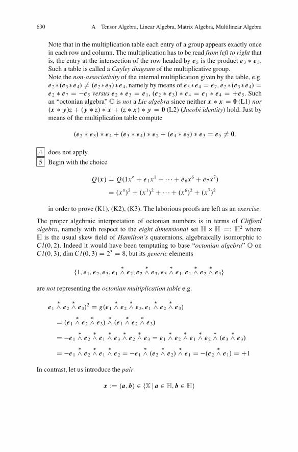
630 A Tensor Algebra, Linear Algebra, Matrix Algebra, Multilinear Algebra
Note that in the multiplication table each entry of a group appears exactly oncein each row and column. The multiplication has to be read from left to right thatis, the entry at the intersection of the row headed by e5 is the product e3 � e5.Such a table is called a Cayley diagram of the multiplicative group.Note the non-associativity of the internal multiplication given by the table, e.g.e2�.e3�e4/ 6D .e2�e3/�e4, namely by means of e3�e4 D e7, e2�.e3�e4/ De2 � e7 D �e5 versus e2 � e3 D e1, .e2 � e3/ � e4 D e1 � e4 D Ce5. Suchan “octonian algebra” O is not a Lie algebra since neither x � x D 0 (L1) nor.x � y/zC .y � z/ � x C .z � x/ � y D 0 (L2) (Jacobi identity) hold. Just bymeans of the multiplication table compute
.e2 � e3/ � e4 C .e3 � e4/ � e2 C .e4 � e2/ � e3 D e5 6D 0:
4 does not apply.
5 Begin with the choice
Q.x/ D Q.1xı C e1x1 C � � � C e6x6 C e7x7/D .xı/2 C .x1/2 C � � � C .x6/2 C .x7/2
in order to prove (K1), (K2), (K3). The laborious proofs are left as an exercise.
The proper algebraic interpretation of octonian numbers is in terms of Cliffordalgebra, namely with respect to the eight dimensional set H � H DW H2 whereH is the usual skew field of Hamilton’s quaternions, algebraically isomorphic toC l.0; 2/. Indeed it would have been temptating to base “octonian algebra” O onC l.0; 3/, dimC l.0; 3/ D 23 D 8, but its generic elements
f1; e1; e2; e3; e1 �^ e2; e2 �^ e3; e3 �^ e1; e1 �^ e2 �^ e3g
are not representing the octonian multiplication table e.g.
e1�^ e2 �^ e3/2 D g.e1 �^ e2 �^ e3; e1 �^ e2 �^ e3/
D .e1 �^ e2 �^ e3/ �^ .e1 �^ e2 �^ e3/
D �e1 �^ e2 �^ e1 �^ e3 �^ e2 �^ e3 D e1 �^ e2 �^ e1 �^ e2 �^ .e3 �^ e3/
D �e1 �^ e2 �^ e1 �^ e2 D �e1 �^ .e2 �^ e2/ �^ e1 D �.e2 �^ e1/ D C1
In contrast, let us introduce the pair
x WD .a;b/ 2 fX j a 2 H;b 2 Hg
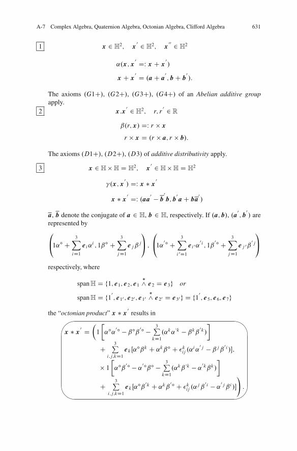
A-7 Complex Algebra, Quaternion Algebra, Octonian Algebra, Clifford Algebra 631
1 x 2 H2; x
0 2 H2; x
00 2 H2
˛.x;x0 DW x C x0
/
x C x0 D .aC a0
;bC b0
/:
The axioms .G1C/, .G2C/, .G3C/, .G4C/ of an Abelian additive groupapply.
2 x:x0 2 H
2; r; r0 2 R
ˇ.r;x/ DW r � xr � x D .r � a; r � b/:
The axioms .D1C/, .D2C/, .D3/ of additive distributivity apply.
3 x 2 H �H D H2; x
0 2 H �H D H2
�.x;x0
/ DW x � x0
x � x0 DW .aa0 � b0
b;b0
aC ba0
/
a, b denote the conjugate of a 2 H, b 2 H, respectively. If .a;b/, .a0
;b0
/ arerepresented by0
@1˛ı C3X
iD1ei ˛
i ; 1ˇı C3X
jD1ej ˇ
j
1
A ;
0
@1˛0ı C
3X
i 0D1ei 0˛
0i ; 1ˇ0ı C
3X
jD1ej 0ˇ
0j
1
A
respectively, where
spanH D f1; e1; e2; e1 �^ e2 D e3g or
spanH D f10
; e10 ; e20 ; e10
�^ e20 D e30g D f10
; e5; e6; e7g
the “octonian product” x � x0
results in�
�
�
x � x0 D�1
�˛ı˛0ı � ˇıˇ0ı �
3P
kD1.˛k˛‘k � ˇkˇ0k/
C3P
i;j;kD1ekŒ˛
ıˇk C ˛kˇı C �kij .˛i˛0j � ˇjˇ0i /�;
� 1�˛ıˇ0ı � ˛0ıˇı �
3P
kD1.˛kˇ‘k � ˛0kˇk/
C3P
i;j;kD1ekŒ˛
ıˇ0k C ˛kˇ0ı C �kij .˛j ˇ0i � ˛0j ˇi /�
!
:

632 A Tensor Algebra, Linear Algebra, Matrix Algebra, Multilinear Algebra
the axioms .D1 � C/, .D2 � �/ of distributivity apply. The pair .1; 0/ is theneutral element.
4 Begin with the choice of
.1st/ the transpose x WD a;�b/ of x 2 H2
.2nd/ x � x D Q.x/ or x � x D .aaC bb; 0/
.3rd/ x�1 D x
Q.x/if x 6D 0
in order to end up with
x � x�1 D 1:
A historical perspective of octonian numbers is given by Van Der Waerden(1950). Reference is made to Graves (1848) and A. Caley: Collected Mathe-matical Papers, vol. 1, p. 127 and vol. 11, pp. 368–371. |
The exceptional role of the examples on complex, quaternion and octonian algebraillustrating Clifford algebra C l.0; 1/, C l.0; 2/ as well as Clifford algebra withrespect to H
2 is established by the following theorems:�
�
�
Theorem (“Hurwitz’ theorem of composition algebras”):
A complete list of composition algebras over R consists of(a) the real numbers R,
(b) the complex numbers C,
(c) the quaternions H,
(d) the octonians O .
�
�
�
Theorem (“Frobenius’ theorem of division algebras”):
The only finite-dimensional division algebra over R are(˛) the real numbers R,
(ˇ) the complex numbers C,
(� ) the quaternions H .
Historical Aside
For details consult the historical texts Hurwitz (1898), Frobenius (1878) as well asHazlett (1917). A more recent reference is Jacobson (1974), pp. 425 and 430.

A-7 Complex Algebra, Quaternion Algebra, Octonian Algebra, Clifford Algebra 633
A-74 Clifford Algebra
We already took advantage of the notion of Clifford algebra when we referredto complex algebra, quaternion algebra, and octonian algebra. Here we finallyconfront you with the definition of “orthogonal clifford algebra C l.p; q/”. But onour way to Clifford algebra we have to generalize at first the notion of a basis, inparticular its bilinear form.�
�
�
Theorem (bilinear form):
Suppose that the bracket h�j�i or g.�; �/ W X�X� �! R is a bilinear form ona finite dimensional linear space X, e. g. a vector space, over the field R ofreal numbers, in addition X
� its dual space such that n D dimX� D dimX.
There exists a basis fe1; : : : ; eng such that
(a) hei j ej i D 0 or g.ei ; ej / D 0 for i 6D j
(b)
2
664
hei1 j ei1i D C1 or g.ei1 ; e i1 / D C1 for 1 � i1 < p ;hei2 j ei2i D �1 or g.e i2 ; ei2 / D �1 for p C 1 � i2 � p C q D r ;hei3 j ei3i D 0 or g.e i3 ; ei3 / D 0 for r C 1 � i3 � n
holds.
The numbers r and p are determined exclusively by the bilinear form. r is called therank, r � p D q is called the index and the ordered pair .p; q/ the signature. Thetheorem assures that any two spaces of the same dimension with bilinear forms ofthe same signature are isometrically isomorphic. A scalar product (“inner product”)in this context is a nondegenerate bilinear form, i.e., a form with rank equal tothe dimension of X. When dealing with low dimensional spaces as we do, we willoften indicate the signature with a series of plus and minus signs and zeroes whereappropriate. For example, the signature of R41 may be written .C C C�/ insteadof .3; 1/. If the bilinear form is nondegenerate, a basis with the properties listed incorresponding Theorem is called an orthonormal basis (“unimodular”) for X withrespect to the bilinear form.
Definition (orthogonal Clifford algebra C l.p; q/):
The orthogonal Clifford algebraC l.p; q/ is the algebra of polynomials generatedby the direct sum of the space of multilinear functions
˚nmD0�^m
.X�/
on a linear space X, respectively its dual X� over the field of real numbers Rnp ofdimension

634 A Tensor Algebra, Linear Algebra, Matrix Algebra, Multilinear Algebra
dim˚nmD0�^m
.X�/ D 2n
and signature .p; q/, namely�
�
�
�
1f0 CnDdimX
�
P
i1D1ei1fi1 C
nDdimX�
P
i1;i2D1ei1
�^ ei2fi1i2
CnDdimX
�
P
i1;i2;i3D1ei1
�^ ei2 �^ ei3fi1i2i3 C � � � CnDdimX
�
P
i1;:::;inD1ei1
�^ � � � �^ einfi1���in
subject to the Clifford product, also called the Clifford dualizer,
"
#
$
%
.i/ ei�^ ej D �ej �^ ei for i 6D j
.ii/
2
664
ei1�^ ei1 D g.ei1 ; ei1/ D C1 for 1 � i1 � p ;
ei2�^ ei2 D g.ei2 ; ei2/ D �1 for p C 1 � i2 � p C q D r ;
ei3�^ ei3 D g.ei3 ; ei3/ D 0 for r C 1 � i3 � n ;
or
e1�^ ej C ej �^ ei
D 2g.ei ; ej /ıij 1 subject to
2
664
g.e i1 ; ei1 / D C1 for 1 � i1 � pg.e i2 ; ei2 / D �1 for pC 1� i2�pC qD rg.e i3 ; ei3 / D 0 for r C 1 � i3 � n
1 being the neutral element. If ek�^ ek D 0 or g.ek; ek/ D 0 holds uniformly
the orthogonal Clifford algebra C l.p; q/ reduces to the polynomial algebra ofantisym-metric multilinear functions
˚nmD0Am D ˚nmD0�m.X�/ D �.X�/
dim ˚nmD0 Am D dim ˚nmD0 �m.X�/ D dim .X�/ D 2n
represented by
"
#
$
%
1f0 C 1
1Š
nDdimX�
X
i1D1ei1fi1 C
1
2Š
nDdimX�
X
i1;i2D1ei1 ^ ei2fi1i2
C 13Š
nDdimX�
X
i1;i2;i3D1ei1 ^ ei2 ^ ei3fi1i2i3 C � � � C
1
nŠ
nDdimX�
X
i1;:::;inD1ei1 ^ � � � ^ e infi1���in :

A-7 Complex Algebra, Quaternion Algebra, Octonian Algebra, Clifford Algebra 635
�
�
�
Example: Clifford product: x � y, x � y 2 X; signX D .3; 0/Let x � y 2 X be a real three-dimensional vector space X of signature (3,0).then x � y (read: “x Clifford y”) with respect to a set of the bases fe1; e2; e3gaccounts for
x�^ y D
3X
iD1
3X
jD1ei
�^ ej xiyj D3X
iD1
3X
jD1xiyj ei
�^ ej
x�^ y D .e1x1 C e2x2 C e3x3/
�^.e1y1 C e2y2 C e3y3/
x�^ y D 1.x1y1 C x2y2 C x3y3/C e1 ^ e2.x1y2 � x2y1/
C e2 ^ e3.x2y3 � x3y2/C e3 ^ e1.x3y1 � x1y3/
Indeed x�^ y as a Clifford number is decomposed into a scalar part and an
antisymmetric tensor part with respect to the bilinear basis fe1 ^ e2; e2 ^ e3;e3 ^ e1g.
Tensor algebra or the algebra of multilinear functions, namely
1f0 CnDdimX
�
X
i1D1ei1fi1 C
nDdimX�
X
i1;i2D1ei ˝ ei2fi1i2
CnDdimX
�
X
i1;i2;i3D1ei1 ˝ ei2 ˝ ei3fi1i2i3 C � � � C
nDdimX�
X
i1;:::;inD1ei1 ˝ � � � ˝ einfi1���in
2 ˚nmD0 ˝ .X�/ D ˝.X/ D T C ˚ T �
subject to
"T C D ˚hD0 ˝2h .X/ .“even”/
T � D ˚kD0 ˝2kC1 .X/ .“odd”/
is the sum of two spaces, T C and T �, respectively, in particular
C lC 3 1f0C 1
2Š
nX
i1;i2D1ei1
�^ ei2fi1i2 C1
4Š
nX
i1;i2;i3;i4
ei1�^ ei2 �^ e i3 �^ ei4fi1i2i3i4 C � � � ;
C l� 3 1
1Š
nX
i1D1ei1fi1 C
1
3Š
nX
i1;i2;i3D1ei1
�^ ei2 �^ ei3fi1i2i3 C � � � :

636 A Tensor Algebra, Linear Algebra, Matrix Algebra, Multilinear Algebra
Obviously C lC as well as C l� are subalgebras of C l . Let the Clifford numbers zbe divided into zC 2 C lC and z� 2 C l�, then the properties
�
�
�
�zC �^ zC 2 C lC; z� �^ z� 2 C lC; zC �^ z� 2 C l�
prove that C l.p; q/ is graded over the cydric group Z2 D f0; 1g. |

Appendix BSampling Distributions and Their Use:Confidence Intervals and Confidence Regions
We begin with sampling distributions by two sections on the transformation ofrandom variables. A first confidence interval for Gauss-Laplace normal distributionobservations �1�2 known is constructed, including its famous Three Sigma Rule.The second confidence interval of Gauss-Laplace i.i.d. observations is derived forthe sample mean b� BLUE of �1 when the variance is known. We take advantageof the forward-backward Helmert transformation leading to Helmert chi-square 2 probability distribution (Helmert, 1875). In contrast, the sampling distributionsfrom Gauss-Laplace i.i.d. normal distributions within the third confidence intervalis analyzed for the mean, but an unknown variance. Our basis is student’st-distribution on the random variable
pn.b� � �/=b� where the sample mean b� –
is BLUE of � whereas the sample confidence for the “true” mean �, variance�2 unknown which is based on student’s probability distribution. In detail, wederive the related Uncertainty Principle generated by the Magic Triangle of (a)length of the confidence interval, (b) coefficient of negative confidence called theuncertainty number and (c) the number of observations. For more details we referto Lemma B.12 of W.S. Gosset. The sampling from the Gauss-Laplace normaldistribution, namely the fourth confidence interval for the variance is reviewed: Weintroduce the missing confidence interval for the “true” variance �2: Table B.18as a flow chart summarizes the various steps in computing a confidence intervalfor the variance. This time the related Uncertainty Principle is built on (a) thecoefficient of complementary confidence ˛, also called uncertainty number (b) thenumber of observations, n, and (c) the length ı�2.n; ˛/ of the confidence intervalthe “true” variance �2. The most detailed sampling theory from multidimensionalGauss-Laplace normal distribution, namely for the confidence region for the fixedparameters in the linear Gauss–Markov, is stated by an extensive Example B.19.We need the Principle Component Analysis PCA, also called Singular ValueDecomposition (SVD) or Eigenvalue Analysis (EIGEN). Theorem B.17 summarizesthe marginal distributions special linear Gauss–Markov model with datum defect.In our appendix we concentrate on multidimensional variance analysis, namelysampling form the multivariate Gauss-Laplace normal distribution. In short
E. Grafarend and J. Awange, Applications of Linear and Nonlinear Models,Springer Geophysics, DOI 10.1007/978-3-642-22241-2,
637
© Springer-Verlag Berlin Heidelberg 2012

638 B Sampling Distributions and Their Use: Confidence Intervals and Confidence Regions
introduction we review the distribution of sample mean and variance-covariance.We define the k-dimensional noncentral WHISHART distribution by (B377) and thecharacteristic function of a vector-valued random variate of type Gauss-Laplacedistribution. Our highlight is the distribution of xN and SN of type WHISHART.Another highlight is the distribution related to the correlation coefficients originatedby R.A. Fisher (1915), programmed by F.N. David (1954).
B-1 A First Vehicle: Transformation of Random Variables
If the probability density function (pdf ) of a random vector yD Œy1; : : : ; yn�0 isknown, but we want to derive the probability density function (pdf ) of a randomvector x D Œx1; : : : ; xn�
0 (pdf ) which is generated by an injective mapping x =g(y)or xi D gi Œy1; : : : ; yn� for all i 2 f1; : : : ; ng we need the results of Lemma B.1.
Lemma B.1. (transformation of pdf):
Let the random vector y WD Œy1; : : : ; yn�0 be transformed into the random vector
x D Œx1; : : : ; xn�0 by an injective mapping xDg.y/ or xi Dgi Œy1; : : : ; yn� for all
i 2 f1; : : : ; ng which is of continuity class C1 (first derivatives are continuous).
Let the Jacobi matrix Jx W D .@gi =@yi / be regular (det Jx ¤ 0), then the inversetransformation yDg � 1.x/ or yi Dg�1
i Œx1; : : : ; xn� is unique. Let fx.x1; : : : ; xn/be the unknown pdf, but fy.y1; : : : ; yn/ the given pdf, then
fx.x1; : : : ; xn/ D f .g�11 .x1; : : : ; xn/; : : : ; g
�11 .x1; : : : ; xn//
ˇdet Jy
ˇ
with respect to the Jacobi matrix
Jy WD�@yi
@xj
D�@g�1
i
@xj
for all i; j 2 f1; : : : ; ng holds. Before we sketch the proof we shall present twoexamples in order to make you more familiar with the notation.
Example B.1. (“counter example”):
The vector-valued random variable .y1; y2/ is transformed into the vector-valuedrandom variable .x1; x2/ by means of
x1 D y1 C y2; x2 D y21 C y22
Jx W D�@x
@y0
D�@x1=@y1 @x1=@y2
@x2=@y1 @x2=@y2
D�1 1
2y1 2y2

B-1 A First Vehicle: Transformation of Random Variables 639
x21 D y21 C 2y1y2 C y22 ; x2 C 2y1y2 D y21 C 2y1y2 C y22x21 D x2 C 2y1y2; y2 D .x21 � x2/=.2y1/
x1 D y1 C y2 D y1 C1
2
x21 � x2y1
; x1y1 D y21 C1
2.x21 � x2/
y21 � x1y1 C1
2.x21 � x2/ D 0
y1 D �1
2x1 ˙
sx214� 12.x21 � x2/
y2 D1
2x1
sx214� 12.x21 � x2/:
At first we have computed the Jacobi matrix Jx , secondly we aimed at an inversionof the direct transformation .y1; y2/ 7! .x1; x2/. As the detailed inversion stepproves, namely the solution of a quadratic equation, the mapping xDg.y/ is notinjective.
Example B.2.
Suppose .x1; x2/ is a random variable having pdf
fx.x1; x2/ D�
exp .�x1 � x2/; x1 0; x2 00 ; otherwise:
We require to find the pdf of the random variable
.x1 C x2; x2=x1/:
The transformation
y1 D x1 C x2; y2 D x2
x1
has the inverse
x1 D y1
1C y2 ; x2 Dy1y2
1C y2 :
The transformation provides a one-to-one mapping between points in the firstquadrant of the .x1; x2/ – plane P2x and in the first quadrant of the .y1; y2/ – planeP2y . The absolute value of the Jacobian of the transformation for all points in the
first quadrant is

640 B Sampling Distributions and Their Use: Confidence Intervals and Confidence Regions
ˇˇˇˇ@.x1; x2/
@.y1; y2/
ˇˇˇˇ D
ˇˇˇˇ
@x1@y1
@x1@y2
@x2@y1
@x2@y2
ˇˇˇˇDˇˇˇˇ.1C y2/�1 �y1.1C y2/�2y2.1C y2/�1 y1.1C y2/�2Œ.1C y2/ � y2�
ˇˇˇˇ
D y1.1C y2/�3 C y1y2.1C y2/�3 D y1
.1C y2/2 :
Hence we have found for the pdf of .y1; y2/
fy.y1; y2/ D"
exp.�y1/ y1.1Cy2/2 ; y1 > 0; y2 > 0
0 ; otherwise:
Incidentally it should be noted that y1 and y2 are independent random variables,namely
fy.y1; y2/ D f1.y1/f .y2/ D y1 exp.�y1/.1C y2/�2: |
Proof. The probability that the random variables y1; : : : ; yn take on values in theregion˝y is given by
Z� � �
˝y
Zfy.y1; : : : ; yn/dy1 � � �dyn:
If the random variables of this integral are transformed by the functionxi Dgi .y1; : : : ; yn/ for all i 2 f1; : : : ; ng which map the region ˝y onto theregions˝x, we receive
Z� � �
˝y
Zfy.y1; : : : ; yn/dy1 � � �dyn
DZ� � �
˝x
Zfy.g
�11 .x1; : : : ; xn/; : : : ; g
�1n .x1; : : : ; xn//
ˇˇdet Jy
ˇˇ dx1 � � �dxn
from the standard theory of transformation of hypervolume elements, namely
dy1 � � �dyn D j det Jy jdx1 � � �dxnor
�.dy1 ^ � � � ^ dyn/ D j det Jy j � .dx1 ^ � � � ^ dxn/:Here we have taken advantage of the oriented hypervolume element dy1 ^ � � � ^ dyn(Grassmann product, skew product, wedge product) and the Hodge star operator *applied to the n – differential form dy1 ^ � � � ^ dyn 2 �n (the exterior algebra�n).

B-1 A First Vehicle: Transformation of Random Variables 641
The star * : �p ! �n�p in Rn maps a p – differential form onto a .n � p/ –
differential form, in general. Here p D n, n � p D 0 applies. Finally we define
fx.x1; : : : ; xn/ WD f .g�11 .x1; : : : ; xn/; : : : ; g
�1n .x1; : : : ; xn//j det Jyj
as a function which is certainly non-negative and integrated over˝x to one. |In applying the transformation theorems of pdf we meet quite often the problem thatthe function xi D gi .y1; : : : ; yn/ for all i 2 f1; : : : ; ng is given but not the inversefunction yi Dg�1
i .x1; : : : ; xn/ for all i 2 f1; : : : ; ng. Then the following results arehelpful.
Corollary B.1. (Jacobian):
If the inverse Jacobian j det Jx j D j det.@gi =@yj /j is given, we are able to compute
j det Jyj D j det@g�1
i .x1; : : : ; xn/
@xjj D j det Jj�1 D j det
@gi .y1; : : : ; yn/
@yjj�1:
Example B.3. (Jacobian):
Let us continue Example B.2. The inverse map
y D�g�11 .y1; y2/
g�12 .y1; y2/
D�x1 C x2
x2= x1
) @y
@x0 D�
1 1
�x2= x21 1= x1
jy D jJyj Dˇˇˇ @y@x0
ˇˇˇ D 1
x1C x2
x21D x1 C x2
x21
jx D jJxj D j�1y D jJyj�1 D
ˇˇˇˇ@x
@y0
ˇˇˇˇ D
x21x1 C x2 D
x21y1
allows us to compute the Jacobian Jx from Jy . The direct map
x D�g1.y1; y2/
g2.y1; y2/
D�x1
x2
D�y1=.1C y2/y1y2=.1C y2/
leads us to the final version of the Jacobian.
jx D jJxj D y1
.1C y2/2 :
For the special case that the Jacobi matrix is given in a partitioned form, the resultsof Corollary B.3 are useful.

642 B Sampling Distributions and Their Use: Confidence Intervals and Confidence Regions
Corollary B.2. (Jacobian):
If the Jacobi matrix Jx is given in the partitioned form
jJxj D�@gi
@yj
�D�
UV
;
then
det Jx Dqj det JxJ0
x j Dp
det.UU0/ detŒVV0 � .VU0/.UU0/�1UV0�
if det.UU0/ ¤ 0
det Jx Dqj det JxJ0
x j Dp
det.VV0/ detŒUU0 � UV0.VV0/�1VU0�;
if det.VV0/ ¤ 0j det Jyj D j det Jxj�1:
Proof. The Proof is based upon the determinantal relations of a partitioned matrixof type
det
�A UV D
D det A det.D � VA�1U/ if det A ¤ 0
det
�A UV D
D det D det.A � UD�1U/ if det D ¤ 0
det
�A UV D
D D det A �V.adjA/U;
which have been introduced by Frobenius (1908) and Schur (1917).
B-2 A Second Vehicle: Transformation of Random Variables
Previously we analyzed the transformation of the pdf under an injective map ofrandom variables y 7! g.y/Dx. Here we study the transformation of polarcoordinates Œ�1; �2; : : : ; �n�1; r� 2 Y as parameters of an Euclidian observationspace to Cartesian coordinates Œy1; : : : ; yn� 2 Y. In addition we introduce thehypervolume element of a sphere S
n�1 � Y; dim YDn. First, we give threeexamples. Second, we summarize the general results in Lemma B.4.

B-2 A Second Vehicle: Transformation of Random Variables 643
Example B.4. (polar coordinates: “2d”):
Table B.1 collects characteristic elements of the transformation of polar coordinates.�1; r/ of type “longitude, radius” to Cartesian coordinates .y1; y2/; their domainand range, the planar elements dy1; dy2 as well as the circle S1 embedded into E
2 WDfR2; ıklg, equipped with the canonical metric I2D Œıkl � and its total measure ofarc !1.
Table B.1
Cartesian and polar coordinates of a two-dimensional observation space, totalmeasure of the arc of the circle
.�1; r/ 2 Œ0; 2� � �0;1Œ; .y1; y2/ 2 R2
dy1dy2 D rdrd�1S1 WD fy 2 R
2jy21 C y22 D 1g
!1 D2Z
0
d�1 D 2:
Example B.5. (polar coordinates: “3d”):
Table B.2 is a collectors’ item for characteristic elements of the transformationof polar coordinates .�1; �2; r/ of type “longitude, latitude, radius” to Cartesiancoordinates .y1; y2; y3/; their domain and range, the volume element dy1; dy2; dy3as well as of the sphere S
2 embedded into E3 WD fR3; ıklg equipped with the
canonical metric I3 D Œıkl � and its total measure of surface !2.
Table B.2
Cartesian and polar coordinates of a three-dimensional observation space, totalmeasure of the surface of the circle
y1 D r cos�2 cos�1; y2 D r cos�2 sin �1; y3 D r sin�2
.�1; �2; r/ 2 Œ0; 2� � � � 2;
2Œ� �0; rŒ; .y1; y2/ 2 R
2
.y1; y2; y3/;2 R3
dy1dy2dy3 D r2dr cos�2d�1d�2
S2 WD fy 2 R
�jy21 C y22 C y23 D 1g
!2 D2Z
0
d�1
C=2Z
�=2d�2 cos�2 D 4:

644 B Sampling Distributions and Their Use: Confidence Intervals and Confidence Regions
Example B.6. (polar coordinates: “4d”):
Table B.3 is a collection of characteristic elements of the transformation of polarcoordinates .�1; �2; �3; r/ to Cartesian coordinates .y1; y2; y3; y4/; their domain andrange, the hypervolume element dy1; dy2; dy3; dy4 as well as of the 3 - sphere S
3
embedded into E4 WD fR4; ıklg equipped with the canonical metric I4D Œıkl � and
its total measure of hypersurface.
Table B.3
Cartesian and polar coordinates of a four-dimensional observation space totalmeasure of the hypersurface of the 3-sphere
y1 D r cos �3 cos�2 cos �1; y2 D r cos �3 cos �2 sin�1;
y3 D r cos �3 sin�2; y4 D r sin�3
.�1; �2; �3; r/ 2 Œ0; 2� � ��
2;
2Œ� ��
2;
2Œ� �0; 2Œ
dy1dy2dy3dy4 D r3 cos2 �3 cos �2drd�3d�2d�1
Jy WD @.y1; y2; y3; y4/
@.�1; �2; �3; r/
D
2
6664
�r cos �3 cos �2 sin �1 �r cos�3 sin�2 cos �1 �r sin �3 cos �2 cos �1 cos �3 cos �2 cos�1Cr cos �3 cos �2 cos �1 �r cos�3 sin�2 sin�1 �r sin�3 cos �2 sin�1 cos �3 cos �2 sin�1
0 Cr cos �3 cos �2 �r sin�3 sin�2 cos �3 cos �20 0 r cos�3 sin�3
3
7775
j det Jy j D r3 cos2 �3 cos�2
S3 WD fy 2 R
4jy21 C y22 C y23 C y24 D 1g!3 D 22:
Lemma B.2. (polar coordinates, hypervolume element, hypersurface element):
Let
2
66666666666664
y1y2
y3y4� � �yn�3yn�2yn�1yn
3
77777777777775
D r
2
66666666666664
cos�n�1 � cos�n�2 � cos�n�3 � � � � � cos�2 � cos �1cos�n�1 � cos�n�2 � cos�n�3 � � � � � cos�2 � sin �1cos�n�1 � cos�n�2 � cos�n�3 � � � � � sin �2cos�n�1 � cos�n�2 � � � � � cos�3� � �cos�n�1 � cos�n�2 � sin �n�3cos�n�1 � cos�n�2cos�n�1 � sin �n�2sin �n�1
3
77777777777775

B-2 A Second Vehicle: Transformation of Random Variables 645
be a transformation of polar coordinates .�1; �2; : : :,�n�2; �n�1; r/ to Cartesiancoordinates .y1; y2; : : :,yn�1; yn/, their domain and range given by
.�1; �2; : : : ; �n�2; �n�1; r/ 2 Œ0; 2� � � � 2;C
2Œ � � � � � � �
2;
C2Œ � � �
2;C
2Œ � �0;1Œ ;
then the local hypervolume element
dy1 � � �dynD rn�1dr cosn�2 �n�1 cosn�3 �n�2 : : : cos2 �3 cos�2d�n�1d�n�2 : : : d�3d�2d�1;
as well as the global hypersurface element
!n�1 D 2 � .n�1/=2
� .n�12/WD
C=2Z
�=2cos�n�2
n�1d�n�1 � � �C=2Z
�=2cos�2d�2
2Z
0
d�1;
where �.X/ is the gamma function. Before we care for the proof, let us defineEuler’s gamma function.
Definition B.1. (Euler’s gamma function):
� .x/ D1Z
0
e�t tx�1dt .x > 0/
is Euler’s gamma function which enjoys the recurrence relation
� .x C 1/ D x� .x/
subject to
� .1/ D 1 or �
�1
2
�D p
� .2/ D 1 �
�3
2
�D 1
2�
�1
2
�D 1
2
p
� � � � � �� .nC 1/ D nŠ �
�p
q
�D p � q
q�
�p � qq
�
if n is integer, n 2 ZC if
p
qis a rational number, p=q 2 Q
C.

646 B Sampling Distributions and Their Use: Confidence Intervals and Confidence Regions
Example B.7. (Euler’s gamma function):
(a) � .1/ D 1 .i/ �
�1
2
�D p
(b) � .2/ D 1 .ii/ �
�3
2
�D 1
2�
�1
2
�D 1
2
p
(c) � .3/ D 1 � 2 D 2 .iii/ �
�5
2
�D 3
2�
�3
2
�D 3
4
p
(d) � .4/ D 1 � 2 � 3 D 6 .iv/ �
�7
2
�D 5
2�
�5
2
�D 15
8
p:
Proof. Our proof of Lemma B.4 will be based upon computing the image of thetangent space TyS
n�1 � En of the hypersphere S
n�1 � En. Let us embed the
hypersphere Sn�1 parameterized by .�1; �2; : : : ; �n�2; �n�1/ in E
n parameterizedby .y1; : : : ; yn/, namely y 2 E
n,
y D e1r cos�n�1 cos�n�2 � � � cos�2 cos�1
C e2r cos�n�1 cos�n�2 � � � cos�2 sin �1 C � � �C en�1r cos�n�1 sin�n�2
C enr sin �n�1:
Note that �1 is a parameter of type longitude, 0 � �1 � 2 , while �2; : : : ; �n�1are parameters of type latitude, �=2 < �2 < C=2; : : : ;�=2 < �n�1 < C=2(open intervals). The images of the tangent vectors which span the local tangentspace are given in the orthonormal n- leg fe1; e2; : : : ; en�1; enj0g by
g1 WD D�1y D � e1r cos�n�1 cos�n�2 � � � cos�2 sin �1
C e2r cos�n�1 cos�n�2 � � � cos�2 cos�1
g2 WD D�2y D � e1r cos�n�1 cos�n�2 � � � sin �2 cos�1
� e2r cos�n�1 cos�n�2 � � � sin �2 sin �1
C e3r cos�n�1 cos�n�2 � � � cos�2
: : :
gn�1 WD D�n�1y D � e1r sin �n�1 cos�n�2 � � � cos�2 cos�1 � � � �� en�1r sin �n�1 sin �n�2
C enr cos�n�1

B-2 A Second Vehicle: Transformation of Random Variables 647
gn WD D�ny D e1r cos�n�1 cos�n�2 � � � cos�2 cos�1
C e2r cos�n�1 cos�n�2 � � � sin �2 sin �1 C � � �C en�1r cos�n�1 cos�n�2
C enr sin �n�1 D y=r:
fg1; : : : ; gn�1g span the image of the tangent space in En. gn is the hypersphere
normal vector, kgnk D 1. From the inner products hgi jgj i D gij , i; j 2 f1; : : : ; ng,we derive the Gauss matrix of the metric G WD Œgij �.
hg1jg1i D r2 cos2 �n�1 cos2 �n�2 � � � cos2 �3 cos2 �2
hg2jg2i D r2 cos2 �n�1 cos2 �n�2 � � � cos2 �3
� � �hgn�1jgn�1i D r2;hgnjgni D 1:
The off-diagonal elements of the Gauss matrix of the metric are zero. Accordingly
pdet Gn D
pdet Gn�1 D rn�1.cos�n�1/n�2.cos�n�2/n�3 � � � .cos�3/2 cos�2:
The square rootp
det Gn,p
det Gn�1 elegantly represents the Jacobian determinant
Jy WD @.y1; y2; : : : ; yn/
@.�1; �2; : : : ; �n�1; r/Dp
det Gn:
Accordingly we have found the local hypervolume elementp
det Gn dr d�n�1d�n�2 � � �d�3 d�2 d�1. For the global hypersurface element !n�1, we integrate
2Z
0
d�1 D 2
C=2Z
�=2cos�2d�2 D Œsin �2�
C=2�=2 D 2
C=2Z
�=2cos2 �3d�3 D 1
2Œcos�3 sin�3 � �3�C=2�=2 D �=2

648 B Sampling Distributions and Their Use: Confidence Intervals and Confidence Regions
C=2Z
�=2cos3 �4d�4 D 1
3Œcos2 �4 sin �4 � 2 sin�4�
C=2�=2 D �
4
3
: : :
C=2Z
�=2.cos�n�1/n�2d�n�1 D 1
n � 2Œ.cos�n�1/n�3�C=2�=2
C 1
n � 3
C=2Z
�=2.cos�n�1/n�4d�n�1
recursively. As soon as we substitute the gamma function, we arrive at !n�1.
B-3 A First Confidence Interval of Gauss–Laplace NormallyDistributed Observations �, � 2 Known, the ThreeSigma Rule
The first confidence interval of Gauss-Laplace normally distributed observationsconstrained to .�; �2/ known, will be computed as an introductory example. Anapplication is the Three Sigma Rule.In the empirical sciences, estimates of certain quantities derived from observationsare often given in the form of the estimate plus or minus a certain amount. Forinstance, the distance between a benchmark on the Earth’s surface and a satelliteorbiting the Earth may be estimated to be
.20; 101; 104:132˙ 0:023/m
with the idea that the first factor is very unlikely to be outside the range
20; 101; 104:155m to 20; 101; 104:109m :
A cost accountant for a publishing company in trying to allow for all factors whichenter into the cost of producing a certain book,
actual production costs, proportion of plant overhead, proportion of executivesalaries,
may estimate the cost to be 21˙ 1; 1 Euro per volume with the implication that thecorrect cost very probably lies between 19.9 and 22.1 Euro per volume. The Bureauof Labor Statistics may estimate the number of unemployed in a certain area to be2:4˙ 0:3 million at a given time though intuitively it should be between 2.1 and 2.7million. What we are saying is that in practice we are quite accustomed to seeingestimates in the form of intervals. In order to give precision to these ideas we shall

B-3 A First Confidence Interval of Gauss–Laplace Normally Distributed Observations 649
consider a particular example. Suppose that a random sample x 2 fR; pdf g is takenfrom a Gauss-Laplace normal distribution with known mean � and known variance�2. We ask the key question.
What is the probability � of the random interval .� � c�; � C c�/ to coverthe mean � as a quantile c of the standard deviation �?
To put this question into a mathematical form we write the probabilistic two-sidedinterval identity.
P.x1 < X < x2/ D P.� � c� < X < �C c�/ D �;x2D�Cc�Z
x1D��c�
1
�p2
exp
�� 1
2�2.x � �/2
�dx D �
with a left boundary l Dx1 and a right boundary r Dx2. The length of the intervalis x2 � x1 D r � l . The center of the interval is .x1 C x2/=2 or �. Here we havetaken advantage of the Gauss-Laplace pdf in generating the cumulative probability
P.x1 < X < x2/ D F.x2/ � F.x1/
F.x2/ � F.x1/ D F.�C c�/ � F.�C c�/:
Typical values for the confidence coefficient � are � D 0:95 (� D 95% or 1�� D 5%negative confidence), � D 0:99 (� D 1% or 1 � � D 1% negative confidence) or� D 0:999 (� D 999%O or 1 � � D 1%O negative confidence).Consult Fig. B.1 for a geometric interpretation. The confidence coefficient � is ameasure of the probability mass between x1 D � � c� and x2 D � C c� . For agiven confidence coefficient �
x2Z
x1
f .xj�; �2/dx D �
establishes an integral equation. To make this point of view to be better under-stoodlet us transform the integral equations to its standard form.
x 7! z D 1�.x � �/, x D �C �z
x2D�Cc�Z
x1D��c�
1
�p2
exp
�� 1
2�2.x � �/2
�dx D
CcZ
�c
1p2
exp
��12
z2�d z D �
x2Z
x1
f .xj�; �2/dx DCcZ
�cf .zj0; 1/d z D �:

650 B Sampling Distributions and Their Use: Confidence Intervals and Confidence Regions
μ–3σ μ–2σ μ–σ μ μ+σ μ+2σ μ+3σx
f(x)
Fig. B.1 Probability mass in a two-sided confidence interval x1 < X < x2 or � � c� < X <
�C c� , three cases: (a) c D 1, (b) c D 2 and (c) c D 3
The special Helmert transformation maps x to z, now being standard Gauss-Laplace normal:��1 is the dilatation factor, also called scale variation, but � thetranslation parameter.The Gauss-Laplace pdf is symmetric, namely f .�x/ D f .Cx/ or f .�z/ Df .Cz/. Accordingly we can write the integral identity
x2Z
x1
f .xj�; �2/dx D 2x2Z
0
f .xj�; �2/dx D �
,CcZ
�cf .zj0; 1/d z D 2
cZ
0
f .zj0; 1/d z D �:
The classification of integral equations tells us that
�.z/ D 2zZ
0
f .z�/d z�
is a linear Volterra integral equation the first kind.

B-3 A First Confidence Interval of Gauss–Laplace Normally Distributed Observations 651
In case of a Gauss-Laplace standard normal pdf, such an integral equation is solvedby a table. In a forward computation
F.z/ WDzZ
�1f .z�j0; 1/d z� or ˚.z/ WD
zZ
�1
1
2exp
��12
z�2�d z�
are tabulated in a regular grid. For a given value F.z1/ or F.z2/, z1 or z2are determined by interpolation. C.F. Gauss did not use such a procedure. Hetook advantage of the Gauss inequality which has been reviewed in this contextby Pukelsheim (1994). There also the Vysochanskii-Petunin inequality has beendiscussed. We follow here a two-step procedure. First, we divide the domainz 2 Œ0; 1� into two intervals z 2 Œ0; 1� and z 2 Œ1;1�. In the first interval f .z/ isisotonic, differentiable and convex, f 00.z/ D f .z/.z2 � 1/ < 0; while in the secondinterval isotonic, differentiable and concave, f 00.z/ D f .z/.z2�1/ > 0. z D 1 is thepoint of inflection. Second, we setup Taylor series of f .z/ in the interval z 2 Œ0; 1�at the point z D 0, while in the interval z 2 Œ1;1� at the point z D 1 and z 2 Œ2;1�at the point z D 2.Three examples of such a forward solution of the characteristic linear Volterraintegral equation of the first kind will follow. They establish:
The One Sigma Rule
The Two Sigma Rule The Three Sigma Rule
Box B.1. (Operational calculus applied to the Gauss-Laplace probabilitydistribution):
“generating differential equations”
f 00.z/C 2f 0.z/C f .z/ D 0
subject to
C1Z
�1f .z/d z D 1

652 B Sampling Distributions and Their Use: Confidence Intervals and Confidence Regions
“recursive differentiation”
f .z/ D 1p2
exp
��12
z2�
f 0.z/ D �zf .z/ DW g.z/f 00.z/ D g0.z/ D �f .z/ � zg.z/ D .z2 � 1/f .z/f 000.z/ D 2zf .z/C .z2 � 1/g.z/ D .�z3 C 3z/f .z/
f .4/.z/ D .�3z2 C 3/f .z/C .�z3 C 3z/g.z/ D .z4 � 6z2 C 3/f .z/f .5/.z/ D .4z3 � 12z/f .z/C .z4 � 6z2 C 3/g.z/ D .�z5 C 10z3 � 15z/f .z/
f .6/.z/ D .�5z4 C 30z2 � 15/f .z/C .�z5 C 10z3 � 15z/g.z/
D .z6 � 15z4 C 45z2 � 15/f .z/f .7/.z/ D .6z5 � 60z3 C 90z/f .z/C .z6 � 15z4 C 45z2 � 15/g.z/
D .�z7 C 21z5 � 105z3 C 105z/f .z/
f .8/.z/ D .�7z6 C 105z4 � 315z2 C 105/f .z/C.�z7 C 21z5 � 105z3 C 105z/f .z/
D .z8 � 28z6 C 210z4 � 420z2 C 105/f .z/f .9/.z/ D .8z7 � 168z5 C 840z3 � 840z/f .z/
C.z8 � 28z6 C 210z4 � 420z2 C 105/g.z/D .�z9 C 36z7 � 378z5 C 1260z3 � 945z/f .z/
f .10/.z/ D .�9z8 C 252z6 � 1890z4 C 3780z2 � 945/f .z/CC.�z9 C 36z7 � 378z5 C 1260z3 � 945/g.z/
D .z10 � 45z8 C 630z6 � 3150z4 C 4725z2 � 945/f .z/
“upper triangle representation of the matrix transforming f .z/! f n.z/”
2
6666666666666666664
f .z/f 0.z/f 00.z/f 000.z/f .4/.z/f .5/.z/f .6/.z/f .7/.z/f .8/.z/f .9/.z/f .10/.z/
3
7777777777777777775
D f .z/
2
6666666666666666664
1 0 0 0 0 0 0 0 0 0 0
0 �1 0 0 0 0 0 0 0 0 0
�1 0 1 0 0 0 0 0 0 0 0
0 3 0 �1 0 0 0 0 0 0 0
3 0 �6 0 1 0 0 0 0 0 0
0 �15 0 10 0 �1 0 0 0 0 0
�15 0 45 0 �15 0 1 0 0 0 0
0 105 0 �105 0 21 0 �1 0 0 0
105 0 �420 0 210 0 �28 0 1 0 0
0 �945 0 1260 0 �378 0 36 0 �1 0�945 0 �4725 0 �3150 0 630 0 �45 0 1
3
7777777777777777775
2
6666666666666666664
1
zz2
z3
z4
z5
z6
z7
z8
z9
z10
3
7777777777777777775
:

B-3 A First Confidence Interval of Gauss–Laplace Normally Distributed Observations 653
B-31 The Forward Computation of a First Confidence Intervalof Gauss–Laplace Normally Distributed Observations:�; � 2 Known
We can avoid solving the linear Volterra integral equation of the first kind if wepush forward the integration for a fixed value z.
Example B.8. (Series expansion of the Gauss-Laplace integral, firstinterval):
Let us solve the integral
�.z D 1/ WD 21Z
0
f .z�/d z�
in the first interval 0 � z � 1 by Taylor expansion with respect to the successivedifferentiation of f .z/ outlined in Box B.1 and the specific derivatives f n.0/ givenin Table B.4. Based on those auxiliary results, Box B.2 presents us the detailedinterpretation. First, we expand exp.�z2=2/ up to order O.14/. The specific Taylorseries are uniformly convergent. Accordingly, in order to compute the integral,second we integrate termwise up to order O.15/. For the specific value zD 1, wehave computed the coefficient of confidence �.1/ D 0:683. The result
P.� � � < X < �C �/ D 0:683
is known as the One Sigma Rule.
68.3% of the sample are in the interval ��� 1�; �C 1� Œ, 0.317% outside. Ifwe make three experiments, one experiment is outside the one interval.
Box B.2. A specific integral
“expansion of the exponential function”
expx D 71C x
1ŠC x2
2ŠC x3
3ŠC � � � C xn
nŠCO.n/ 8 jxj <1
x WD �1
2z2
exp
��1
2z2�D 1� 1
2z2C 1
8z4 � 1
48z6C 1
384z8� 1
3840z10C 1
46080z12CO.14/

654 B Sampling Distributions and Their Use: Confidence Intervals and Confidence Regions
“the specific integral”
zZ
0
f .z�/d z� D 1p2
zZ
0
exp�z�2
�d z� D 1p
2
�z � 1
6z3 C 1
40z5 � 1
336z7
C 1
3456z9 � 1
42240z11 C 1
599040z13 CO.15/
�
“the specific values z D 1”
�.1/ D 21Z
0
f .z/d z
D 2p2
�1 � 1
6C 1
40� 1
336C 1
3456� 1
42240C 1
599040CO.15/
�
D 2p2.1 � 0:166;667C 0:025;000/
�0:002;976C 0:000;289�0; 000;024C 0:000;002/
D 2p20:855;624 D 0:682;689
D 0:683
“coefficient of confidence”
0:683 D 1 � 317:311 � 10�3 D 1 � 13:
Table B.4 (Special values of derivatives- Gauss-Laplace probability distribution):
z D 0
1p2D 0:398; 942
f .0/ D 1p2; f 0.0/ D 0;
f 00.0/ D � 1p2;1
2Šf 00.0/ D �0:199; 471

B-3 A First Confidence Interval of Gauss–Laplace Normally Distributed Observations 655
f 000.0/ D 0; f .4/.0/ D C 3p2;1
4Šf .4/.0/ D C0:049; 868
f .5/.0/ D 0; f .6/.0/ D � 15p2;1
6Šf .6/.0/ D �0:008; 311:
Example B.9. (Series expansion of the Gauss-Laplace integral, 2nd inter-val):
Let us solve the integrals
�.z D 2/ WD 2
2Z
0
f .z�/d z� D 21Z
0
f .z�/d z�C22Z
1
f .z�/d z�
�.z D 2/ D �.z D 1/C 22Z
1
f .z�/d z�;
namely in the second interval 1 � z � 2. First, we setup Taylor series of f .z/“around the point z D 1”. The derivatives of f .z/ “at the point z=1” are collectedup to order 10 in Table B.5. Second, we integrate the Taylor series termwise andreceive the specific integral of Box B.3. Note that termwise integrated is permittedsince the Taylor series are uniformly convergent. The detailed computation up toorder O(12) has led us to the coefficient of confidence �.2/ D 0:954. The result
P.� � 2� < X < �C 2�/ D 0:954
is known as the Two Sigma Rule.
95.4% of the sample interval ��� 2�; �C 2� Œ, 0.046% outside. If we make22 experiments, one experiment is outside the 2� interval.
Box B.3. (A specific integral):
“expansion of the exponential function”
f .z/ WD 1p2
exp
��12
z2�
f .z/ D f .1/C 1
1Šf 0.1/.z� 1/C 1
2Šf 00.1/.z � 1/2 C � � � C 1
10Šf 10.1/.z� 1/10
C O.11/

656 B Sampling Distributions and Their Use: Confidence Intervals and Confidence Regions
“the specific integral”
2Z
1
f .z�/d z� D f .1/.z � 1/C 1
2
1
1Šf 0.1/.z� 1/2 C 1
3
1
2Šf 00.1/.z� 1/3
C 1
4
1
3Šf 000.1/.z� 1/4 C 1
5
1
4Šf .4/.1/.z� 1/5
C 1
6
1
5Šf .5/.1/.z � 1/6 C � � � C 1
11
1
10Šf .10/.1/.z� 1/11 C O.12/
case z D 2
�.2/ D �.1/C 22Z
1
f .z/d z D�.1/C 2.0:241; 971
� 0:120; 985C 0:020; 122� 0:004; 024� 0:002; 016C 0:000; 768C 0:000; 120� 0:000; 088� 0:000; 002� 0:000; 050C O.12//
D 0:682; 690C 0:271; 632D 0:954
“coefficient of confidence”
0:954 D 1 � 45:678 � 10�3 D 1 � 1
22:
Table B.5 (Special values of derivatives – Gauss-Laplace probability distri-bution):
z D 1
1p2D 0:398; 942; exp
��12
�D 0:606; 531
f .1/ D 1p2
exp
��12
�D 0:241; 971
f 0.1/ D �f .1/ D � 1p2
exp
��12
�D �0:241; 971; f 00.1/ D 0
f 000.1/ D 2f .1/ D 2p2
exp
��12
�D 0:482; 942

B-3 A First Confidence Interval of Gauss–Laplace Normally Distributed Observations 657
1
3Šf 000.1/ D C0:080; 490
f .4/.1/ D �2f .1/ D �0:482; 9421
4Šf .4/.1/ D �0:020; 122
f .5/.1/ D �6f .1/ D � 6p2
exp
��12
�D �1:451; 826
1
5Šf .5/.1/ D �0:012; 098
f .6/.1/ D 16f .1/ D 16p2
exp
��12
�D 3:871; 536
1
6Šf .6/.1/ D 0:005; 377
f .7/.1/ D 20f .1/ D 20p2
exp
��12
�D 4:829; 420
1
7Šf .7/.1/ D 0:000; 958
f .8/.1/ D �132f .1/ D �31:940; 1721
8Šf .8/.1/ D �0:000; 792
f .9/.1/ D �28f .1/ D �6:775; 1881
9Šf .9/.1/ D �0:000; 019
f .10/.1/ D �8234f .1/ D �1992:3891
10Šf .10/.1/ D �0:000; 549:
Example B.10. (Series expansion of the Gauss-Laplace integral, third inter-val):
Let us solve the integrals
�.z D 3/ WD 2
3Z
0
f .z/d z D 21Z
0
f .z/d zC 22Z
1
f .z/d zC 23Z
2
f .z/d z
�.z D 3/ D �.z D 1/C �.z D 2/C 23Z
2
f .z/d z;

658 B Sampling Distributions and Their Use: Confidence Intervals and Confidence Regions
namely in the third interval 2 � z � 3. First, we setup Taylor series of f(z) “aroundthe point z D 2”. The derivatives of f .z/ “at the point z D 2” are collected up toorder 10 in Table B.6. Second, we integrate the Taylor series termwise and receivethe specific integral of Box B.4. Note that termwise integration is permitted sincethe Taylor series are uniformly convergent. The detailed computation up to orderO(12) leads us to the coefficient of confidence �.3/ D 0:997. The result
P.� � 3� < X < �C 3�/ D 0:997is known as the Three Sigma Rule.
99.7% of the sample are in the interval �� � 3�; �C 3�Œ, 0.003% outside.If we make 377 experiments, one experiment is outside the 3� interval.
Table B.6 (Special values of derivatives Gauss-Laplace probability distribu-tion):
z D 21p2D 0:398; 942; exp .�2/ D 0:135; 335
f .2/ D 1p2
exp .�2/ D 0:053; 991
f 0.2/ D �2f .2/ D �0:107; 982
f 00.2/ D 3f .2/; 1
2Šf 00.2/ D C0:080; 986
f 000.2/ D �2f .2/; 1
3Šf 000.2/ D �0:017; 997
f .4/.2/ D �5f .2/; 1
4Šf .4/.2/ D �0:011; 248
f .5/.2/ D 18f .2/; 1
5Šf .5/.2/ D C0:008; 099
f .6/.2/ D �11f .2/; 1
6Šf .6/.2/ D �0:000; 825
f .7/.2/ D �86f .2/; 1
7Šf .7/.2/ D �0:000; 921
f .8/.2/ D C249f .2/; 1
8Šf .8/.2/ D C0:000; 333
f .9/.2/ D 190f .2/; 1
9Šf .9/.2/ D C0:000; 028
f .10/.2/ D �2621f .2/; 1
10Šf .10/.2/ D �0:000; 039:

B-3 A First Confidence Interval of Gauss–Laplace Normally Distributed Observations 659
Box B.4 (A specific integral)
“expansion of the exponential function”
f .z/ WD 1p2
exp
��12
z2�
f .z/ D f .2/C 1
1Šf 0.2/.z� 2/C 1
3Šf 00.2/.z� 2/2 C � � � C 1
10Šf .10/.2/.z� 2/10
CO.11/“the specific integral”
zZ
2
f .z�/d z� D f .2/.z� 2/C 1
2
1
1Šf 0.2/.z� 2/2 C 1
3
1
2Šf 00.2/.z � 2/3
C 1
4
1
3Šf 000.2/.z � 2/4 C 1
5
1
4Šf .4/.2/.z� 2/5
C 1
6
1
5Šf .5/.2/.z� 2/6 C � � � C 1
11
1
10Šf .10/.2/.z� 2/11 CO.12/
case z D 3
�.3/ D �.1/C �.2/C 23Z
2
f .z/d z
D 0:682; 690C 0:271; 672C 2.0:053; 991� 0:053; 991C 0:026; 995� 0:004; 499� 0:002; 250C 0:001; 350� 0:000; 118C 0:000; 037C 0:000; 003� 0:000; 004CO.12// D 0:682; 690C 0:271; 632C 0:043; 028D 0:997
“coefficient of confidence”
0:997 D 1 � 2:65 � 10�3 D 1 � 1
377:
B-32 The Backward Computation of a First ConfidenceInterval of Gauss–Laplace Normally DistributedObservations: �; � 2 Known
Finally we solve the Volterra integral equation of the first kind by the techniqueof series inversion, also called series reversion. Let us recognize that the interval

660 B Sampling Distributions and Their Use: Confidence Intervals and Confidence Regions
integration of a Taylor series expanded Gauss-Laplace normal density distributionled us to a univariate homogeneous polynomial of arbitrary order. Such a univariatehomogeneous polynomial y D a1x C a2x2 C � � � C anxn (“input”) can be reversedas a univariate homogeneous polynomial x D b1y C b2y2 C � � � C bnyn (“output”)as outlined in Table B.7. Consult Abramowitz and Stegun (1965), p. 16 for a review,but Grafarend (1996) for a derivation based upon Computer Algebra.
Table B.7 (Series inversion (Grafarend, 1996)):
“input: univariate homogeneous polynomial”
y D a1x C a2x2 C a3x3 C a4x4 C a5x5 C a6x6 C a7x7 CO.x8/
“output: reverse univariate homogeneous polynomial”
x D b1y C b2y2 C b3y3 C b4y4 C b5y5 C b6y6 C b7y7 CO.y8/
“coefficient relation”
(a) a1b1 D 1(b) a31b2 D �a2(c) a51b3 D 2a22 � a1a3(d) a71b4 D 5a1a2a3 � a21a4 � 5a32(e) a91b5 D 6a21a2a4 C 3a21a23 C 14a42 � a31a5 � 21a1a22a3(f) a111 b6 D 7a31a2a5C7a31a2a4C84a1a32a3�a41a6�28a1a2a23�42a52�28a21a22a4(g) a131 b7 D 6a41a2a6 C 8a41a2a5 C 4a41a24 C 120a21a32a4 C 180a21a22a23 C 132a62� a51a7 � 36a31a22a5 � 72a31a2a3a4 � 12a31a33 � 330a1a42a3.
Example B.11. (Solving the Volterra integral equation of the first kind):
Let us define the coefficient of confidence � D 0:90 or 90%. We want to know thequantile c0:90 which determines the probability identity
P.� � c� < X < �C c�/ D 0:90:
If you follow the detailed computation of Table B.5, namely the input as well as theoutput data up to order O(5), you find the quantile
c0:90 D 1:64;
as well as the confidence interval
P.� � 1:64� < X < �C 1:64�/ D 0:90:

B-3 A First Confidence Interval of Gauss–Laplace Normally Distributed Observations 661
90% of the sample are in the interval �� � 1:64�; �C 1:64�Œ, 10% outside. If wemake 10 experiments one experiment is outside the 1.62� interval.
Table B.8 (Series inversion quantile c0:90):
(i) input
�.z/ D 21Z
0
f .z�/d z� C 2zZ
0
f .z�/d z� D 0:682; 689C 2Œf .1/.z� 1/
C 1
2
1
1Šf 0.1/.z� 1/2 C � � � C 1
n
1
.n � 1/Šf.n�1/.1/.z� 1/n CO.nC 1/�
1
2Œ�.z/ � 0:682; 689�D f .1/.z� 1/C 1
2
1
1Šf 0.1/.z� 1/2 C � � �
C 1
n
1
.n � 1/Šf.n�1/.1/.z� 1/n CO.nC 1/�
y D a1x C a2x2 C � � � C anxn CO.nC 1/x WD z � 1y WD .0:900; 000� 0:682; 689/=2D 0:108; 656a1 WD f .1/ D 0:241; 971
a2 WD 1
2
1
1Šf 0.1/ D �0:241; 971
a3 WD 1
3
1
2Šf 00.1/ D 0
a4 WD 1
4
1
3Šf 000.1/ D 0:020; 125
a5 WD 1
5
1
4Šf .4/.1/ D �0:004; 024� � �
an WD 1
n
1
.n� 1/Šf.n�1/.1/:
(ii) output
b1 D 1
a1D 4:132; 726
b2 D � 1a31a2 D 8:539; 715

662 B Sampling Distributions and Their Use: Confidence Intervals and Confidence Regions
b3 D 1
a51.2a22 � a1a3/ D 35:292; 308
b4 D 1
a71.5a1a2a3 � a21a4 � 5a32/ D 158:070
b5 D 1
a91.6a21a2a4 C 3a21a23 C 14a42 � a31a5 � 21a1a22a3/ D 475:452; 152
b1y D 0:449; 045; b2y2 D 0:100; 821;b3y
3 D 0:045; 273; b4y4 D 0:022; 032;b5y
5 D 0:007; 201x D b1y C b2y2 C b3y3 C b4y4 C b5y5 CO.6/ D 0:624; 372z D xC 1 D 1:624; 372 D c0:90:
At this end we would like to give some sample references on computing the “inverseerror function”
y D F.x/ WDxZ
0
1p2
exp
��12
z2�d z DW erfx versus
x D F�1.y/ D inverfy;
namely Carlitz (1963) and Strecok (1968).
B-4 Sampling from the Gauss–Laplace Normal Distribution:A Second Confidence Interval for the Mean, VarianceKnown
The second confidence interval of Gauss-Laplace i.i.d. observations will be con-structed for the mean b� BLUUE of �, when the variance �2 is known. “n” is thesize of the sample, namely to agree to the number of observations. Before we presentthe general sampling distribution we shall work through two examples. ExampleB.12 has been chosen for a sample size n D 2, while Example B.12 for nD 3observations. Afterwards the general result is obvious and sufficiently motivated.
Example B.12. (Gauss-Laplace i.i.d. observations, observation space Y,dim Y)
In order to derive the marginal distributions of b� BLUUE of � and b�2 BIQUUEof �2 for a two dimensional Euclidean observation space we have to introduce
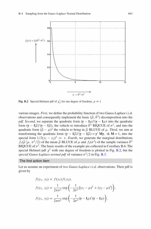
B-4 Sampling from the Gauss–Laplace Normal Distribution: 663
ˆx: = σ2 / σ2
ˆf2(x) = f2(σ2 / σ2 )
Fig. B.2 Special Helmert pdf of 2p for one degree of freedom, p D 1
various images. First, we define the probability function of two Gauss-Laplace i.i.d.observations and consequently implement the basic .b�;b�2/ decomposition into thepdf. Second, we separate the quadratic form .y � 1�/0.y � 1�/ into the quadraticform .y � 1b�/0.y � 1b�/, the vehicle to introduce b�2 BIQUUE of �2, and into thequadratic form .b� � �/2 the vehicle to bring in b� BLUUE of �. Third, we aim attransforming the quadratic form .y � 1b�/0.y � 1b�/D y0 My; rk MD 1, into thespecial form 1=2.y1 � y2/2 DW x. Fourth, we generate the marginal distributionsf1.b�
ˇˇ�; �2=2/ of the mean b� BLUUE of � and f2.�2/ of the sample varianceb�2
BIQUUE of �2. The basic results of the example are collected in Corollary B.6. Thespecial Helmert pdf 2 with one degree of freedom is plotted in Fig. B.2, but thespecial Gauss-Laplace normal pdf of variance �2=2 in Fig. B.3.
The first action item
Let us assume an experiment of two Gauss-Laplace i.i.d. observations. Their pdf isgiven by
f .y1; y2/ D f .y1/f . y2/;
f .y1; y2/ D 1
2�2exp
�� 1
2�2Œ.y1 � �/2 C .y2 � �/2�
�;
f .y1; y2/ D 1
2�2exp
�� 1
2�2.y � 1�/0.y � 1�/
�:

664 B Sampling Distributions and Their Use: Confidence Intervals and Confidence Regions
–5 –4 –3 –2 –1 0 1 2 3 4 50
0.1
0.2
0.3
0.4
f1(z | 0, 1)
ˆ s2
2z = (m − m)/
Fig. B.3 Special Gauss-Laplace normal pdf of .b�� �/=�2=2
The second action item
The coordinates of the observation vector have been denoted by Œy1; y2�0 D
y2Y; dim YD 2. The quadratic form .y � 1�/0.y � 1�/ allows the fundamentaldecomposition
y � 1� D .y � 1b�/C 1.b� � �/.y � 1�/0.y � 1�/ D .y � 1b�/0.y � 1b�/C 101.b� � �/2
.y � 1�/0.y � 1�/ D b�2 C 2.b�� �/2:
Here, b� is BLUUE of � and b�2 BIQUUE of �2. The detailed computation provesour statement.
Œ.y1 �b�/C .b�� �/�2 C Œ.y2 �b�/C .b� � �/�2
D .y1 �b�/2 C .y2 �b�/2 C 2.b�� �/2 C 2.b�� �/Œ.y1 �b�/C .y2 �b�/�D .y1 �b�/2 C .y2 �b�/2 C 2.b�� �/2 C 2b�.y1 �b�/C 2b�.y2 �b�/� 2.y1 �b�/� � 2.y2 �b�/�

B-4 Sampling from the Gauss–Laplace Normal Distribution: 665
b� D 1
2.y1 C y2/
b�2 D .y1 �b�/2 C .y2 �b�/2:
As soon as we substituteb� andb�2 we arrive at
.y1 � �/2 C .y2 � �/2 D Œ.y1 �b�/C .b� � �/�2 C Œ.y2 �b�/C .b� � �/�2
D b�2 C 2.b�� �/2;
since the residual terms vanish:
2b�.y1 �b�/C 2b�.y2 �b�/� 2.y1 �b�/�� 2.y2 �b�/�D 2b�y1 � 2b�2 C 2b�y2 � 2b�2 � 2�y1 C 2�b� � 2�y2 C 2�b�D 2b�.y1 C y2/� 4b�2 � 2�.y1 C y2/C 4�b�D 4b�2 � 4b�2 � 4�b�C 4�b� D 0:
The third action item
The cumulative pdf
dF D f .y1; y2/dy1dy2 D f1.b�/f2.x/db�dx D f1.b�/f2�b�2
�2
�db� d
b�2
�2
has to be decomposed into the first pdf f1.b� j� ; �2=n/ representing the pdf ofthe sample mean b� and the second pdf f2.x/ of the new variable x WD .y1 �y2/
2=.2�2/ D b�2=�2 representing the sample varianceb�2, normalized by �2.
How can the second decomposition f1f2 be understood?
Let us replace the quadratic form .y � 1�/0.y � 1�/ D b�2 C 2.b� � �/2 in thecumulative pdf
dF D f .y1; y2/dy1dy2 D 1
2�2exp
�� 1
2�2.y � 1�/0.y � 1�/
�dy1dy2
D 1
2�2exp
�� 1
2�2Œb�2 C 2.b�� �/2�
�dy1dy2
dF D f .y1; y2/dy1dy2
D 1p2� 1
�p2
exp
��12
.b�� �/2�2=2
�� 1p
2� 1p
2�exp
��12
b�2
�2
�dy1dy2:

666 B Sampling Distributions and Their Use: Confidence Intervals and Confidence Regions
The quadratic formb�2, conventionally given in terms of the residual vector y � 1b�will be rewritten in terms of the coordinates Œy1; y2�0 D y of the observation vector.
b�2 D .y1 �b�/2 C .y2 �b�/2 D�y1 � 1
2.y1 C y2/
2C�y2 � 1
2.y1 C y2/
2
b�2 D 1
4.y1 � y2/2 C 1
4.y2 � y1/2 D 1
2.y1 � y2/2:
The fourth action item
The new variable x WD 12�2.y1 � y2/2 will be introduced in the cumulative pdf
dF D f .y1; y2/dy1dy2. The new surface element db�dx will be related to the oldsurface element dy1dy2.
db�dx Dˇˇˇˇ det
"Dy1b� Dy2b�
Dy1x Dy2x
#ˇˇˇˇ dy1dy2 D jJjdy1dy2
Dy1b� WD@b�@y1D 1
2; Dy2b� WD
@b�@y2D �1
2
Dy1x WD@x
@y1D y1 � y2
�2; Dy2x WD
@x
@y2D �y1 � y2
�2:
The absolute value of the Jacobi determinant amounts to
jJj Dˇˇˇˇ det
"12
12
y1�y2�2� y1�y2
�2
# ˇˇˇˇ D y1 � y2
�2; jJj�1 D �2
y1 � y2 :
In consequence, we have derived
dy1dy2 D �2
y1 � y2 db�dx D�p2pxdb�dx
based upon
x D 1
2�2.y1 � y2/2)
p2x D 1
�.y1 � y2/:
In collecting all detailed partial results we can formulate a corollary.

B-4 Sampling from the Gauss–Laplace Normal Distribution: 667
Corollary B.3. (marginal probability distributions ofb�; �2 given, and b�2):
The cumulative pdf of a set of two observations is represented by
dF D f .y1; y2/dy1dy2Df1.b� j�; �2=2/f2.x/db�dx subject to
f1.b� j�; ; �2=2/ WD 1p2� 1
�p2
exp
��12
.b�� �/2�2=2
�
f2.x/ D f2
�b�2
�2
�WD 1p
2
1px
exp
��12x
�subject to
C1Z
�1f1.b�/ db� D 1 and
C1Z
0
f2.x/ dx D 1:
f1.b�/ is the pdf of the sample mean b� D .y1 C y2/=2 and f2.x/ the pdf of thesample variance b�2 D .y1 � y2/2=2 D �2x. f1.b�/ is a Gauss-Laplace pdf withmean� and variance �2=n, while f2.x/ is a Helmert 2 with one degree of freedom.
Example B.13. (Gauss-Laplace i.i.d. observations, observation space Y,dim YD 3):
In order to derive the marginal distribution of b� BLUUE of � and b�2 BIQUUE of�2 for a three-dimensional Euclidean observation space, we have to act in variousscenes. First, we introduce the probability function of three Gauss-Laplace i.i.d.observations and consequently implement the .b�; b�2/ decomposition in the pdf.Second, we force the quadratic form .y � 1b�/0.y � 1b�/ to be decomposed into b�2
and .b���/2, actually a way to introduce the sample varianceb�2 BIQUUE ofb�2 andthe sample meanb� BLUUE of �. Third, we succeed to transform the quadratic form.y � 1b�/0.y � 1b�/ D yMy; rkM D 2 into the canonical form z21 C z22 by means ofŒz1; z2�
0 D HŒy1; y2; y3�0. Fourth, we produce the right inverse H�k D H0 in order to
invert H, namely Œy1; y2; y3�0 D H0Œz1; z2�0. Fifth, in order to transform the originalquadratic form ��2.y�1b�/0.y�1b�/ into the canonical form z21Cz22Cz23 we reviewthe general Helmert transformation z D ��1H.y��/ and its inverse y�� D �H0zsubject to H 2 SO.3/ and identify its parameters translation, rotation and dilatation(scale). Sixth, we summarize the marginal probability distributions f1.b� j� ; �2=3/of the sample mean b� BLUUE of � and f2.2b�2=�2/ of the sample variance b�2
BIQUUE of �2. The special Helmert pdf 2 with two degrees of freedom is plottedin Fig. B.4 while the special Gauss-Laplace normal pdf of variance �2=3 in Fig. B.5.The basic results of the example are collected in Corollary B.7.

668 B Sampling Distributions and Their Use: Confidence Intervals and Confidence Regions
f2(2s2 | s2)ˆ
x := 2s2 | s2
Fig. B.4 Special Helmert pdf of 2p for two degrees of freedom, p D 2
3ˆ )s2
f1(m | m,
ˆ(m − m) / s2
3
Fig. B.5 Special Gauss-Laplace normal pdf of .b�� �/= �2
3

B-4 Sampling from the Gauss–Laplace Normal Distribution: 669
The first action item
Let us assume an experiment of three Gauss-Laplace i.i.d. observations. Their pdfis given by
f .y1; y2; y3/ D f .y1/f . y2/f . y3/;
f .y1; y2; y3/ D .2/�3=2��3 exp
�� 1
2�2Œ.y1 � �/2C .y2��/2C .y3 ��/2�
�;
f .y1; y2; y3/ D .2/�3=2��3 exp
�� 1
2�2.y � 1�/0.y � 1�/
�:
The coordinates of the observation vector have been denoted by Œy1; y2; y3�0D y2Y,dimY D 2.
The second action item
The coordinates of the observation vector have been denoted byD y2Y, dimYD 2.The quadratic form .y1 � 1�/0.y2 � 1�/ allows the fundamental decomposition
y � 1� D .y � 1b�/C 1.b� � �/;.y � 1�/0.y � 1�/ D .y � 1b�/0.y � 1b�/C 101.b� � �/2
.y � 1�/0.y � 1�/ D 2b�2 C 3.b�� �/2:
Here, b� is BLUUE of � and b�2 BIQUUE of �2. The detailed computation provesour statement.
Œ.y1 �b�/C .b� � �/�2 C Œ.y2 �b�/C .b�� �/�2 C Œ.y3 �b�/C .b� � �/�2
D .y1 �b�/2 C .y2 �b�/2 C .y3 �b�/2 C 3.b�� �/2 C 2b�.y1 �b�/C 2b�.y2 �b�/C 2b�.y3 �b�/� 2.y1 �b�/�� 2.y2 �b�/� � 2.y3 �b�/�
b�BLUUE of� W b� D 1
3.y1 C y2 C y3/
b�2 BIQUUE of �2 W b�2 D 1
2Œ.y1 �b�/2 C .y2 �b�/2 C .y3 �b�/2�:
As soon as we substituteb� andb�2 we arrive at
.y1 � �/2 C .y2 � �/2 C .y3 � �/2
D Œ.y1 �b�/2C .b���/�2C Œ.y2 �b�/2C .b���/2�2C Œ.y3 �b�/2C .b���/2�2
D 2b�2 C 3.b�� �/2:

670 B Sampling Distributions and Their Use: Confidence Intervals and Confidence Regions
The third action item
Let us begin with transforming the cumulative probability function
dF D f .y1; y2; y3/dy1dy2dy3
D .2/�3=2��3 exp
�� 1
2�2.y � 1�/0.y � 1�/
�dy1dy2dy3
D .2/�3=2��3 exp
�� 1
2�2Œ2b�2 C 3.b� � �/2�
�dy1dy2dy3
into its canonical form. In detail, we transform the quadratic form b�2 BIQUUE of�2 canonically.
y1 �b� D y1 � 13y1 � 1
3.y2 C y3/ D 2
3y1 � 1
3.y2 C y3/ D 2
3y1 � 1
3y2 � 1
3y3
y2 �b� D y2 � 13y2 � 1
3.y1 C y3/ D �1
3y1 C 2
3y2 � 1
3y3
y3 �b� D y3 � 13y3 � 1
3.y1 C y2/ D �1
3y1 � 1
3y2 C 2
3y3
as well as
.y1 �b�/2 D 4
9y21 C
1
9y22 C
1
9y23 �
4
9y1y2 C 2
9y2y3 � 4
9y3y1
.y2 �b�/2 D 1
9y21 C
4
9y22 C
1
9y23 �
4
9y1y2 � 4
9y2y3 C 2
9y3y1
.y3 �b�/2 D 1
9y21 C
1
9y22 C
4
9y23 C
2
9y1y2 � 4
9y2y3 � 4
9y3y1
and
.y1 �b�/2 C .y2 �b�/2 C .y3 �b�/2 D 2
3.y21 C y22 C y23 � y1y2 � y2y3 � y3y1/:
We shall prove
.y � 1b�/0.y � 1b�/ D y0My D z21 C z22; rkM D 2; M 2 R3�3
that the symmetric matrix M,
M D2
42 �1 �1�1 2 �1�1 �1 2
3
5
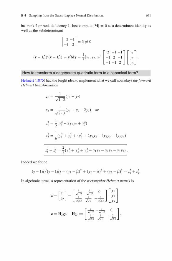
B-4 Sampling from the Gauss–Laplace Normal Distribution: 671
has rank 2 or rank deficiency 1. Just compute jMj D 0 as a determinant identity aswell as the subdeterminant
ˇˇˇ 2 �1�1 2
ˇˇˇ D 3 ¤ 0
.y � 1b�/0.y � 1b�/ D y0My D 1
3Œy1; y2; y3�
2
42 �1 �1�1 2 �1�1 �1 2
3
5
2
4y1
y2y3
3
5 :
How to transform a degenerate quadratic form to a canonical form?
Helmert (1875) had the bright idea to implement what we call nowadays the forwardHelmert transformation
z1 D 1p1 � 2.y1 � y2/
z2 D 1p2 � 3.y1 C y2 � 2y3/ or
z21 D1
2.y21 � 2y1y2 C y22/
z22 D1
6.y21 C y22 C 4y23 C 2y1y2 � 4y2y3 � 4y3y1/
z21 C z22 D2
3.y21 C y22 C y23 � y1y2 � y2y3 � y3y1/ :
Indeed we found
.y � 1b�/0.y � 1b�/ D .y1 �b�/2 C .y2 �b�/2 C .y3 �b�/2 D z21 C z22:
In algebraic terms, a representation of the rectangular Helmert matrix is
z D�
z1z2
D"
1p1�2 � 1p
1�2 0
1p2�3
1p2�3 � 2p
2�3
#2
4y1y2
y3
3
5
z D H23y; H23 WD"
1p1�2 � 1p
1�2 0
1p2�3
1p2�3 � 2p
2�3
#
:
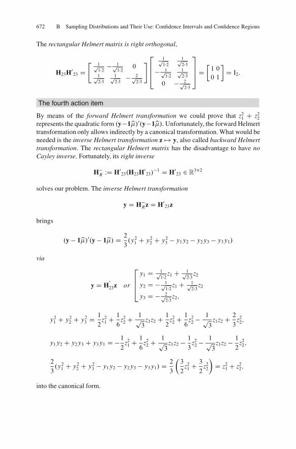
672 B Sampling Distributions and Their Use: Confidence Intervals and Confidence Regions
The rectangular Helmert matrix is right orthogonal,
H23H023 D
"1p1�2 � 1p
1�2 0
1p2�3
1p2�3 � 2p
2�3
#2
664
1p1�2
1p2�3
� 1p1�2
1p2�3
0 � 2p2�3
3
775 D
�1 0
0 1
D I2:
The fourth action item
By means of the forward Helmert transformation we could prove that z21 C z22represents the quadratic form .y�1b�/0.y�1b�/. Unfortunately, the forward Helmerttransformation only allows indirectly by a canonical transformation. What would beneeded is the inverse Helmert transformation z 7! y, also called backward Helmerttransformation. The rectangular Helmert matrix has the disadvantage to have noCayley inverse. Fortunately, its right inverse
H�R WD H0
23.H23H023/
�1 D H023 2 R
3�2
solves our problem. The inverse Helmert transformation
y D H�Rz D H0
23z
brings
.y � 1b�/0.y � 1b�/ D 2
3.y21 C y22 C y23 � y1y2 � y2y3 � y3y1/
via
y D H0
23z or
2
664
y1 D 1p1�2 z1 C 1p
2�3 z2
y2 D � 1p1�2 z1 C 1p
2�3 z2
y3 D � 2p2�3 z2;
y21 C y22 C y23 D1
2z21 C
1
6z22 C
1p3
z1z2 C 1
2z22 C
1
6z22 �
1p3
z1z2 C 2
3z22;
y1y2 C y2y3 C y3y1 D �12
z21 C1
6z22 C
1p3
z1z2 � 13
z22 �1p3
z1z2 � 12
z22;
2
3.y21 C y22 C y23 � y1y2 � y2y3 � y3y1/ D
2
3
�3
2z21 C
3
2z22
�D z21 C z22;
into the canonical form.

B-4 Sampling from the Gauss–Laplace Normal Distribution: 673
The fifth action item
Let us go back to the partitioned pdf in order to inject the canonical representationof the deficient quadratic form y0My; M 2 R
3�3, rkM D 2. Here we meet first theproblem to transform
dF D .2/�3=2��3 exp
�� 1
2�2Œ2b�2 C 3.b� � �/2�
�dy1dy2dy3
by an extended vector Œz1; z2; z3�0 DW z into the canonical form dF D .2/�3=2exp
�� 12.z21 C z22 C z23/
�d z1d z2d z3, which is generated by the general forward
Helmert transformation
z D ��1H.y � 1�/
2
4z1z2z3
3
5 D 1
�
2
664
1p1�2
1p1�2 0
1p2�3
1p2�3 � 2p
2�31p3
1p3
1p3
3
775
2
4y1 � �y2 � �y3 � �
3
5
or its backward Helmert transformation, also called the general inverse Helmerttransformation
2
4y1 � �y2 � �y3 � �
3
5 D �
2
664
1p1�2
1p2�3
1p3
1p1�2
1p2�3
1p3
0 � 2p2�3
1p3
3
775
2
4z1z2z3
3
5 :
y � 1� D �H0z
thanks to the orthonormality of the quadratic Helmert matrix H3, namely H3H03 D
H03H3 D I3 or H�1
3 D H03.
Secondly, notice the transformation of the volume element
dy1dy2dy3 D d.y1 � �/d.y2 � �/d.y3 � �/ D �3d z1d z2d z3;
which is due to the Jacobi determinant
J D �3 ˇˇH0ˇˇ D �3 jHj D �3:
Let us prove that
z3 WDp3��1.b� � �/ D b� � �
�p3

674 B Sampling Distributions and Their Use: Confidence Intervals and Confidence Regions
brings the first marginal density
f1 D�b�j�; �
2
3
�WD 1p
2� 1
�p3
� exp
�� 1
2�23.b�� �/2
�
into the canonical form
f1.z3 j0; 1/ D 1p2
exp
��12
z23
�:
Let us computeb� � � as well as 3.b�� �/2 which concludes the proof.
z3 D ��1�1p3;1p3;1p3
2
4y1 � �y2 � �y3 � �
3
5
z3 D ��1 y1 C y2 C y3 � 3�p3
y1 C y2 C y33
D b� ) y1 C y2 C y3 D 3b�
3
775
) z3 D 3��1b� � �p3; z23 D
1
�23.b�� �/2:
Indeed the extended Helmert matrix H3 is ingenious to decompose
1
�2.y � 1b�/0.y � 1b�/ D z21 C z22 C z23
into a canonical quadratic form relating z21 C z22 to b�2 and z23 to .b� � �/2. At thispoint, we have to interpret the general Helmert transformation z D ��1H.y � �/:Structure elements of the Helmert transformation
scale or dilatation ��1
rotation H
translation �
��1 2RC produces a dilatation or a scale change, H2SO.3/ WD fH2R3�3 jH0H DI3 and jHj D C1g a rotation (3 parameters) and 1� 2 R
3 a translation. Please,prove for yourself that the quadratic Helmert matrix is orthonormal, that is HH0 DH0H D I3 and jHj D C1.

B-4 Sampling from the Gauss–Laplace Normal Distribution: 675
The sixth action item
Finally we are left with the problem to split the cumulative pdf into one part f1.b�/which is a marginal distribution of the arithmetic meanb� BLUUE of � and anotherpart f2.b�/which is a marginal distribution of the standard deviationb� ,b�2 BIQUUEof �2, Helmert’s 22 with two degrees of freedom.First let us introduce polar coordinates .�1; r/ which represent the Cartesian coor-dinates z1D r cos�1, z2D r sin �1. The index 1 is needed for later generalization tohigher dimension. As a longitude, the domain of �1 is �1 2 Œ0; 2� or 0 � �1 � 2 .The new random variable z21 C z22 D kzk2 DW x or radius r relates to Helmert’s
2 D z21 C z22 D2b�2
�2D 1
�2.y � 1b�/0.y � 1b�/ :
Secondly, the marginal distribution of the arithmetic meanb�, b� BLUUE of �,
f1
�b� j� ; �p
3
�db� D f1.z3 j0; 1 /d z3 � N
��;
�p3
�
is a Gauss-Laplace normal distribution with mean � and variance �2=3 gener-ated by
dF1 D f1�b� j� ; �p
3
�db� D f1.z3 j0; 1/d z3
D .2/�1=2 exp
��12
z23
�d z3
C1Z
�1
C1Z
�1.2/�1 exp
��12.z21 C z22/
�d z1d z2 or
f1
�b� j� ; �p
3
�db� D .2/�1=2
p3
�exp
�� 3
2�2.b�� �/2
�db�:
Third, the marginal distribution of the sample variance 2b�2=�2 D z21 C z22 DW x,Helmert’s 2 distribution for p D n � 1 D 2 degrees of freedom,
f2.2b�2=�2/ D f2.x/ D 1
2p=2� .p
2/xp2 �1 exp
�x2
�
is generated by
dF2 DC1Z
�1.2/�1=2 exp
��12
z23
�d z3
2Z
0
d�1.2/�1 12
exp
��12x
�dx

676 B Sampling Distributions and Their Use: Confidence Intervals and Confidence Regions
dF2 D .2/�1!2 12
exp
��12x
�dx subject to !2 D
2Z
0
d�1 D 2
dF2 D 1
2exp
��12x
�dx
and
x WD z21 C z22 D r2) dx D 2rdr; dr D dx
2r
d z1d z2 D rdrd�1 D1
2dxd�1
is the transformation of the surface element d z1d z2. In collecting all detailed resultslet us formulate a corollary.
Corollary B.7. (marginal probability distributions ofb�, �2 given, and ofb�2):
The cumulative pdf of a set of three observations is represented by
dF D f .y1; y2; y3/dy1dy2dy3 D f1�b�j�; �
2
3
�f2.x/db�dx
subject to
f1
�b�j�; �
2
3
�WD 1p
2� 1
�=p3� exp
��12
.b� � �/2�2=3
�
f2.x/ D 1
2exp
��12x
�
subject to
x WD z21 C z22 D 2b�2=�2; dx D 2
�2db�2
and
1Z
�1f1.b�/ db� D 1 versus
1Z
0
f2.x/ dx D 1:
f1.b�/ is the pdf of the sample mean b�D .y1 C y2 C y3/=3 and f2.x/ the pdfof the sample variance b�2D .y0 � 1b�/0.y � 1b�/=2 normalized by �2. f1.b�/ is a

B-4 Sampling from the Gauss–Laplace Normal Distribution: 677
Gauss-Laplace pdf with meanb� and variance �2=3, while f2.x/ a Helmert 2 withtwo degrees of freedom.In summary, an experiment with three Gauss-Laplace i.i.d. observations is charac-terized by two marginal probability densities, one for the meanb� BLUUE of � andanother one forb�2 BIQUUE of �2:
Marginal probability densities n D 3, Gauss-Laplace i.i.d. observations
b� W f1�b� j� ; �p
3
�db� b�2 W f2.2b�2=�2/db�2
D .2/�1=2 1
�=p3
exp
��12
.b� � �/2�2=3
�db� D b�2
�2exp
��b�
2
�2
�db�2
or or
f1.z3 j0; 1/d z3 f2.x/dx
D .2/�1=2 exp
��12
z23
�d z3 D 1
2exp
��12x
�dx
z3 WD b� � �3�
x WD 2b�2
�2
B-41 Sampling Distributions of the Sample Mean b�, � 2
Known, and of the Sample Variance b� 2
The two examples have prepared us for the general sampling distribution of thesample mean b�, �2 known, and of the sample varianceb�2 for Gauss-Laplace i.i.d.observations, namely samples of size n. By means of Lemma B.8 on the rectangularHelmert transformation and Lemma B.9 on the quadratic Helmert transformationwe prepare for Theorem B.10 which summaries both the pdfs for b� BLUUE of �,�2 known, for the standard deviationb� and forb�2 BIQUUE of �2. Corollary B.11focusses on the pdf of
�
� D qb� where�
� is an unbiased estimation of the standarddeviation � , namely Ef��g D � .
Lemma B.3. (rectangular Helmert transformation):
The rectangular Helmert matrix Hn�1;n 2 Rn�.n�1/ transforms the degenerate
quadratic form
.n � 1/b�2 WD .y � 1b�/0.y� 1b�/ D y0My; rkMDn�1
subject to
b� D 1
n10y

678 B Sampling Distributions and Their Use: Confidence Intervals and Confidence Regions
into the canonical form
.n � 1/b�2 D z0n�1zn�1 D z21 C � � � C z2n�1:
The special Helmert transformation yn 7! Hn�1;nyn D zn�1 is represented by
Hn�1;n WD2
6666664
1p1�2
1p1�2 0 0 � � � 0 0
1p2�3
1p2�3 � 2p
2�3 0 � � � 0 0
� � � � � � � � � � � � � � � � � � � � �1p
.n�1/.n�2/1p
.n�1/.n�2/1p
.n�1/.n�2/1p
.n�1/.n�2/ � � � � n�1p.n�1/.n�2/ 0
1pn.n�1/
1pn.n�1/
1pn.n�1/
1pn.n�1/ � � � 1p
n.n�1/ � npn.n�1/
3
7777775
:
The inverse Helmert transformation z 7! y D H�Rz D H0z or yn D H0
n�1�nzn isbased on its right inverse which thanks to the right orthogonality Hn�1;nH0
n;n�1 DIn�1 coincides with its transpose,
H�R D H0.HH0/�1 D H0 2 R
n�.n�1/:
Lemma B.4. (quadratic Helmert transformation):
The quadratic Helmert matrix H 2 Rn�n, also called extended Helmert matrix or
augmented Helmert matrix, transforms the quadratic form
1
�2.y � 1�/0.y � 1�/ D 1
�2Œ.y � 1b�/C 1.b�� �/�0Œ.y � 1b�/C 1.b�� �/�
subject to
b� D 1
n10y
by means of
z D ��1H.y � 1�/ or y D �H0.z � 1�/
into the canonical form
1
�2.y � 1�/0.y � 1�/ D z21 C � � � C z2n�1 C z2n D
n�1X
jD1z2j C z2n
z2n D n.b� � �/2:

B-4 Sampling from the Gauss–Laplace Normal Distribution: 679
Such a Helmert transformation y 7! z D ��1H.y � 1�/ is represented bydisplaylines
H WD2
6666666666666664
1p1�2
1p1�2 0 0 � � � 0 0
1p2�3
1p2�3 � 2p
2�3 0 � � � 0 0
1p3�4
1p3�4
1p3�4 � 3p
34� � � 0 0
� � � � � �1p
.n�1/.n�2/1p
.n�1/.n�2/1p
.n�1/.n�2/1p
.n�1/.n�2/ � � � � n�1p.n�1/.n�2/ 0
1pn.n�1/
1pn.n�1/
1pn.n�1/
1pn.n�1/ � � � 1p
n.n�1/ � npn.n�1/
1pn
1pn
1pn
1pn
� � � 1pn
1pn
3
7777777777777775
Since the quadratic Helmert matrix is orthonormal, the inverse Helmert transfor-mation is generated by
z 7! y � 1� D �H0z:
The proofs for Lemmas B.8 and B.9 are based on generalizations of the special casesfor n D 2, Example B.11, and for n D 3, Example B.12. Any proof will be omittedhere.The highlight of this paragraph is the following theorem.
Theorem B.10. (marginal probability distribution of .b�; �2/ and b�2):
The cumulative pdf of a set of n observations is represented by
dF D f .y1; : : : ; yn/dy1 � � �dynD f1.b�/f4.b�/db�db� D f1.b�/f2.b�2/db�db�2
as the product of the marginal pdf f1.b�/ of the sample mean b�D n�11yand the marginal pdf f2.b�/ of the sample standard deviation b� Dp.y � 1b�/0.y � 1b�/=.n� 1/, also called r.m.s. (root mean square error), or
the marginal pdf f2.b�2/ of the sample variance b�2. Those marginal pdfs arerepresented by
dF1 D f1.b�/db�dF4 D f4.b�/db� and dF2 D f2.b�2/db�2;
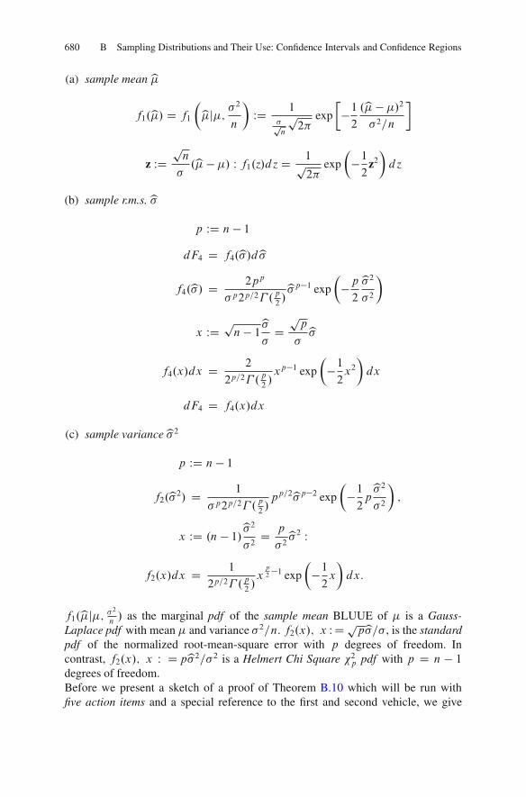
680 B Sampling Distributions and Their Use: Confidence Intervals and Confidence Regions
(a) sample mean b�
f1.b�/ D f1�b�j�; �
2
n
�WD 1
�pn
p2
exp
��12
.b� � �/2�2=n
z WDpn
�.b� � �/ W f1.z/d z D 1p
2exp
��12
z2�d z
(b) sample r.m.s.b�
p WD n � 1dF4 D f4.b�/db�
f4.b�/ D 2pp
�p2p=2� .p
2/b�p�1 exp
��p2
b�2
�2
�
x WD pn � 1b��Dpp
�b�
f4.x/dx D 2
2p=2� .p
2/xp�1 exp
��12x2�dx
dF4 D f4.x/dx
(c) sample varianceb�2
p WD n � 1
f2.b�2/ D 1
�p2p=2� .p
2/pp=2b�p�2 exp
��12pb�2
�2
�;
x WD .n � 1/b�2
�2D p
�2b�2 W
f2.x/dx D 1
2p=2� .p
2/xp2 �1 exp
��12x
�dx:
f1.b�j�; �2n / as the marginal pdf of the sample mean BLUUE of � is a Gauss-Laplace pdf with mean � and variance �2=n. f2.x/; x WDppb�=� , is the standardpdf of the normalized root-mean-square error with p degrees of freedom. Incontrast, f2.x/; x W Dpb�2=�2 is a Helmert Chi Square 2p pdf with p D n � 1degrees of freedom.Before we present a sketch of a proof of Theorem B.10 which will be run withfive action items and a special reference to the first and second vehicle, we give

B-4 Sampling from the Gauss–Laplace Normal Distribution: 681
some historical comments. Kullback (1934) refers the marginal pdf f1.b�/ of the“arithmetic mean” b� to Poisson (1827), Haussdorff (1901) and Irwins (1937). Hehas also solved the problem to find the marginal pdf of the “geometric mean”.The marginal pdf f2.b�2/ of the sample variance b�2 has been originally derivedby Helmert (1875), Helmert (1876a), Helmert (1876b). A historical discussion ofHelmert’s distribution is offered by David (1957), Kruskal (1946), Lancaster (1965),Lancaster (1966), Pearson (1931) and Sheynin (1995).The marginal pdf f4.b�/ has not found any interest in practice so far. The reason maybe found in the effect that b� is not an unbiased estimate of the standard deviation� , namely Efb�gD� . According to Czuber (1891), p. 162, Roseen (1948), p. 37,Schmetterer (1956), p. 203, Stoom (1967), p. 199, 218, Fisz (1971), p. 240 andRichter and Mammitzsch (1973), p. 42 have documented that
�
� Drp
2
�p2
�
�
�p C 12
�b� D qb�
is an unbiased estimation�
� of the standard deviation � , namely Efb�g D � . p Dn � 1 again denotes the number of degrees of freedom. Schaffrin (1979), p. 240 hasproven that
b�p WDp.y � 1b�/0.y � 1�/
r
p � 12
D b�p2pp
2p � 1
r
p � 12
is an asymptotic (“from above”) unbiased estimation b�p of the standard deviation� . Let us implement
�
� BLUUE of � into the marginal pdf f .b�/:
Corollary B.8. (marginal probability distributions of�
� for Gauss-Laplace i.i.d.observations, Ef��g D �):
The marginal pdf of�
� , an unbiased estimation of the standard deviation, isrepresented by
dF4 D f4.�
�/d�
�
f4.�
�/ D 2pp
�p2p=2
� p
�p C 12
�
p2
� p2� pC1
p2
��
�p�1 exp
0
BBB@�
0
BB@
�
�p C 12
�
�p2
�
1
CCA
2
�
�2
1
CCCA

682 B Sampling Distributions and Their Use: Confidence Intervals and Confidence Regions
Fig. B.6 Marginal pdf for the sample standard deviation�
� (r.m.s.)
and
dF4 D f4.x/dx
x WDp2
�
�
�p C 12
�
�p2
� b�
f4.x/ D 2
2p=2�p2
�xp�1 exp
��12x2�
subject to
Efxg D p2�
�p C 12
�
�p2
� :
Figure B.6 illustrates the marginal pdf for “degrees of freedom” p 2 f1; 2; 3; 4; 5g.

B-4 Sampling from the Gauss–Laplace Normal Distribution: 683
Proof.
The first action item
The pdf of n Gauss-Laplace i.i.d. observations is given by
f .y1; : : : ; yn/ D f .y1/ � � �f .yn/ DnY
iD1f .yi /
f .y1; : : : ; yn/ D .2/�n=2��n exp
�� 1
2�2.y � 1�/0.y � 1�/
�:
The coordinates of the observation space Y have been denoted by Œy1; : : : ; yn�0 D y.Note dim Y D n.
The second action item
The quadratic form .y� 1�/0.y � 1�/ > 0 allows the fundamental decomposition
y � 1� D .y� 1b�/C 1.b�� �/;.y � 1�/0.y � 1�/ D .y� 1b�/0.y � 1b�/C 101.b� � �/2
101 D n
.y � 1�/0.y � 1�/ D .n � 1/b�2 C n.b� � �/2:
Here,b� is BLUUE of � andb�2 BIQUUE of �2. The decomposition of the quadratic.y�1�/0.y�1�/ into the sample varianceb�2 and the square .b���/2 of the shiftedsample meanb��� has already been proved for n D 2 and n=3. The general resultis obvious.
The third action item
Let us transform the cumulative probability into its canonical forms.
dF D f .y1; : : : ; yn/dy1 � � �dynD .2/�n=2��n exp
�� 1
2�2.y � 1�/0.y� 1�/
�dy1 � � �dyn
D .2/�n=2��n exp
�� 1
2�2
�.n � 1/b�2 C n.b� � �/2
�dy1 � � �dyn
z D ��1H.y� 1�/ or y � 1� D �H0z1
�2.y � 1�/0.y � 1�/ D z21 C z22 C � � � C z2n�1 C z2n:
Here, we have substituted the divert Helmert transformation (quadratic Helmertmatrix H) and its inverse. Again ��1 is the scale factor, also called dilatation,

684 B Sampling Distributions and Their Use: Confidence Intervals and Confidence Regions
H an orthonormal matrix, also called rotation matrix, and 1� 2 Rn the translation,
also called shift.
dF D f .y1; : : : ; yn/dy1 � � �dynD 1p
2exp
��12
z2n1
.2/.n�1/=2
�exp
��12.z21 C � � � C z2n/
�dz1dz2 � � � dzn�1dzn
based upon
dy1dy2 � � �dyn�1dyn D �nd z1d z2 � � �d zn�1d zn
J D �njH0j D �njHj D �n:
J again denotes the absolute value of the Jacobian determinant introduced by thefirst vehicle.
The fourth action item
First, we identify the marginal distribution of the sample meanb�.
dF1 D f1�b�j�; �
2
n
�db�:
According to the specific structure of the quadratic Helmert matrix zn is gener-ated by
zn D ��1�1pn; : : : ;
1pn
2
64
y1 � �:::
yn � �
3
75 D ��1 y1 C � � � C yn � n�p
n;
upon substituting
b� D 1
n10y D y1 C � � � C yn
n) y1 C � � � C yn D nb�)
zn D ��1 n.b� � �/pn
) z2n D n.b� � �/2�2
; d zn D 1
�
pn db�:
Let us implement d zn in the marginal distribution.
dF1 D 1p2
exp
��12
z2n
�d zn�

B-4 Sampling from the Gauss–Laplace Normal Distribution: 685
�C1Z
�1� � �
C1Z
�1.2/�.n�1/=2 exp
��12.z21 C � � � C z2n�1/
d z1 � � �d zn�1;
C1Z
�1� � �
C1Z
�1.2/�.n�1/=2 exp
��12.z21 C � � � C z2n�1/
d z1 � � �d zn�1 D 1
dF1 D 1p2
exp
��12
z2n
�d zn
dF1 D 1p2
1�pn
exp
�12
.b� � �/2�2
n
!
db� D f1�b�j�; �
2
n
�db�:
The fifth action item
Second, we identify the marginal distribution of the sample varianceb�2. We departthe ansatz
dF2 D f2.b�/db� D f2.b�2/db�2
in order to determine the marginal distribution f2.b�/ of the sample root-mean-square errors b� and the marginal distribution f2.b�2/ of the sample variance b�2.A first version of the marginal probability distribution dF2 is
dF2 D 1p2
1Z
�1exp
��12
z2n
�d zn�
� 1
.2/.n�1/=2 exp
��12.z21 C � � � C z2n�1/
d z1 � � �d zn�1:
Transform the Cartesian coordinates .z1 C � � � C zn�1/ 2 Rn�1 to spherical
coordinates .˚1; ˚2; : : : ; ˚n�2; rn�1/. From the operational point of view,p D n�1,the number of “degrees of freedom”, is an optional choice. Let us substitute theglobal hypersurface element !n�1 or !p into dF2, namely
1p2
1Z
�1exp
��12
z2n
�d zn D 1
dF2 D 1
2.n�1/=2 rn�2 exp
��12r2�dr�

686 B Sampling Distributions and Their Use: Confidence Intervals and Confidence Regions
�C=2Z
�=2cosn�3�n�2d�n�2
C=2Z
�=2cosn�4�n�3d�n�3 � � �
C=2Z
�=2cos�2d�2
2Z
0
d�1
dF2 D 1
.2/p=2rp�1 exp
��12r2�dr�
�C=2Z
�=2cosp�2�p�1
C=2Z
�=2cosp�3�p�2d�p�2 � � �
C=2Z
�=2cos2�3d�3
C=2Z
�=2cos�2d�2
2Z
0
d�1
!n�1 D !p D 2
�
�n � 12
�.n�1/=2 D 2
�p2
�p=2
D=2Z
�=2cosp�2�p�1d�p�1
=2Z
�=2cosp�3�p�2d�p�2 � � �
=2Z
�=2cos2�3d�3
=2Z
�=2cos�2d�2
2Z
0
d'1
dF2 D !p
.2/p=2rp�1 exp
��12r2�dr
dF2 D 2
2p=2��p
2
� rp�1 exp
��12r2�dr :
The marginal distribution of the r.m.s. f2.b�/ is generated as soon as we substitute
the radius r Dq
z21 C � � � C z2n�1 Dpn � 1 b�1=� . Alternatively the marginal
distribution of the sample variance f2.b�2/ is produced when we substitute the radiussquare r2 D z21 C � � � C z2n�1 D .n � 1/b�2=�2.Project A
r D pn � 1 b�=� D ppb��) dr D
pp
�db�
dF2 D f2.b�/db�
f2.b�/ D 2pp
�p2p=2b�p�1 exp
��12
p
�2b�2�:

B-4 Sampling from the Gauss–Laplace Normal Distribution: 687
Indeed, f2.b�/ establishes the marginal distribution of the root-mean-square errorb�with p D n � 1 degrees of freedom.
Project B
x WD r2 D .n � 1/b�2
�2D pb�
2
�2DW 2p )
2
64dx D 2rdrdr D dx
2rD 1
2
dxpx
rp�1dr D 1
2xp2 �1dx
dF2 D f2.x/dx
f2.x/ WD 1
2p=2� .p
2/xp2 �1 exp
��12x
�:
Finally, we have derived Helmert’s Chi Square 2p distribution f2.x/dxDdF2 bysubstituting r2, rp�1 and dr in factor of x WD r2 and dx D 2rdr .
Project CReplace the radical coordinate squared r2 D .n � 1/b�2=�2 D pb�2=�2 by rescalingon the basis p=�2
x D r2 D z21 C � � � C z2n�1 D z21 C � � � C z2p D .n� 1/b�2
�2D p
�2b�2
dx D p
�2db�
within Helmert’s 2p with p D n � 1 degrees of freedom
dF2 D f2.b�2/db�2
f2.b�2/ D 1
�p2p=2� .p
2/pp=2b�p�2 exp
��12
p
�2b�2�:
Recall that f2.b�2/ establishes the marginal distribution of the sample varianceb�2
with pDn � 1 degrees of freedom. Both, the marginal pdf f2.b�/ of the samplestandard deviation b� , also called root-mean-square error, and the marginal pdff2.b�2/ of the sample varianceb�2 document the dependence on the variance �2 andits power �p .
“Here is our journey’s end.”(W. Shakespeare: Hamlet) |

688 B Sampling Distributions and Their Use: Confidence Intervals and Confidence Regions
B-42 The Confidence Interval for the Sample Mean,Variance Known
An application of Theorem B.10 is Lemma B.12 where we construct the confidenceinterval for the sample mean b�, BLUUE of �, variance �2 known, on the basis ofits sampling distribution. Example B.14 is an example of a random sample of sizen D 4.
Lemma B.12. (confidence interval for the sample mean, variance known):
The sampling distribution of the sample meanb� D n�1 10y, BLUUE of �, is Gauss-Laplace normal,
�
� � N .b�j�; �2=n/, if the observations yi ; i 2 f1; : : : ; ng, areGauss-Laplace i.i.d. The “true” mean � is an element of the two-sided confidenceinterval.
� 2�b� � �pnc1�˛=2;b�C �p
nc1�˛=2Œ
with confidence
P
�b� � �p
nc1�˛=2 < � < b�C �p
nc1�˛=2
�D 1 � ˛
of level 1 � ˛. For three values of the coefficient of confidence � D 1 � ˛, TableB.9 is a list of associated quantiles c1�˛=2.
Example B.14. (confidence interval for the sample mean b�, �2 known):
Suppose that a random sample
y WD
2
664
y1y2y3y4
3
775 D
2
664
1:2
3:4
0:6
5:6
3
775 ; b� D 2:7; �2 D 9; r:m:s: W 3
of four observation is known from a Gauss-Lapace normal distribution withunknown mean � and a known standard deviation � D 3. b� BLUUE of � is thearithmetic mean. We intend to determine upper and lower limits which are rathercertain to contain the unknowns parameter� between them. Previously, for samplesof size 4 we have known that the random variable
z D b� � ��pn
D b� � �32

B-4 Sampling from the Gauss–Laplace Normal Distribution: 689
is normally distributed with mean zero and unit variance. b� is the sample mean2.7 and 3/2 is �=
pn. The probability � D 1 � ˛ that z will be between any two
arbitrarily chosen numbers c1 D �c and c2 D c is
P f�c1 < z < Cc2g Dc2Z
c1
f .z/d z D � D 1 � ˛;
P f�c < 2 < Ccg DCcZ
�cf .z/d z D � D 1 � ˛;
cZ
�1f .z/d z D 1 � ˛
2;
�cZ
�1f .z/d z D ˛
2:
� is the coefficient of confidence, ˛ the coefficient of negative confidence, also calledcomplementary coefficient of confidence. The four representations of the probability� D 1 � ˛ to include z in the confidence interval �c < z < Cc have led to thelinear Voltera integral equation of the first kind
cZ
�1f .z/d z D 1� ˛
2D 1C �
2:
Three values of the coefficient of confidence � or its compliment ˛ are popular andlisted in Table B.9.
Table B.9 (Values of the coefficient of confidence):
� 0:950 0:990 0:999
˛ 0:050 0:010 0:001˛2
0:025 0:005 0:000; 5
1 � ˛2D 1C�
20:975 0:995 0:999; 5
In solving the linear Voltera integral equation of the first kind
zZ
�1f .z�/d z� D 1 � 1
2˛.z/ D 1
2Œ1C �.z/�:
Table B.10 collects the quantiles c1�˛=2 given the coefficients of confidence on theircomplements which we listed in Table B.10.

690 B Sampling Distributions and Their Use: Confidence Intervals and Confidence Regions
Table B.10 (Quantiles for the confidence interval of the sample mean,variance unknown):
1 � ˛2D 1C�
2� ˛ c1�˛=2
0:975 0:95 0:05 1:960
0:995 0:99 0:01 2:576
0:999; 5 0:999 0:001 3:291
Given the quantiles c1�˛=2, we are going to construct the confidence interval forthe sample mean b�, the variance �2 to be known. For this purpose, we convert theforward transformationsb�! z D pn.b� � �/=� to �.
b�� �pn
z D �
b�1 WD b� � �pnc1�˛=2 < � < b�C �p
nc1�˛=2 DW b�2:
The interval b�1 < � < b�2 for the fixed value z D c1�˛=2 contains the “true” mean� with probability � D 1 � ˛.
P
�b� � �p
nc1� ˛
2< � < b�C �p
nc1� ˛
2
�
DcZ
�cf .z/d z D
b�2Z
b�1
f
�b�j�; �
2
n
�db� D � D 1 � ˛
since
b�2Z
�1f .b�/db� D
b�C �p
nc1�˛=2Z
�1f .b�/db� D
c1�˛=2Z
�1f .b�/db� D 1 � ˛
2:
An animation of the coefficient of confidence and the probability functions of aconfidence interval is offered by Figs. B.7 and B.8.
b�1 D b� � c1�˛=2 �pn; b�2 D b�C c1�˛=2 �p
n
Let us specify all the integrals to our example
c1�˛=2Z
�1f .z/d z D 1 � ˛=2

B-4 Sampling from the Gauss–Laplace Normal Distribution: 691
ˆf(m | m, σ2) ˆf(m | m, σ2)
a / 2 a / 2g = 1-a
m1ˆm1ˆ
μ m2ˆ
Fig. B.7 Two-sidedconfidence interval� 2�b�1;b�2Œ; f .b�j�; �2=n/pdf :
m1 = m − c1−a /2mˆ ˆ
n
σ m1 = m + c1−a /2ˆ ˆn
σ
Fig. B.8 Two-sided confidence interval, quantile c1�˛=2
1:960Z
�1f .z/d z D 0:975;
2:576Z
�1f .z/d z D 0:995;
3:291Z
�1f .z/d z D 0:999; 5:
Those data lead to a triplet of confidence intervals.
case .a/ D 0:95; D 0:05; c1�˛=2 D 1:960
P
�2:7 � 3
21:96 < � < 2:7C 3
21:96
�D 0:95
P f�0:24 < � < C5:64g D 0:95case .b/ D 0:99; D 0:01; c1�˛=2 D 2:576
P
�2:7 � 3
22:576 < � < 2:7C 3
22:576
�D 0:99
P f�1:164 < � < 6:564g D 0:99case .c/ D 0:999; D 0:001; c1�˛=2 D 3:291
P
�2:7 � 3
23:291 < � < 2:7C 3
23:291
�D 0:999
P f�2:236 < � < 7:636g D 0:999 :
With probability 95% the “true” mean � is an element of the interval ]�0.24,C5.64[. In contrast, with probability 99% the “true” mean � is an element of thelarger interval ]�1.164, C6.564[. Finally, with probability 99.9% the “true” mean� is an element of the largest interval [�2.236,C7.636].

692 B Sampling Distributions and Their Use: Confidence Intervals and Confidence Regions
B-5 Sampling from the Gauss–Laplace Normal Distribution:A Third Confidence Interval for the Mean, VarianceUnknown
In order to derive the sampling distributions for the sample mean, variance un-known, of Gauss-Laplace i.i.d. observation B51 introduces two examples (two andthree observations, respectively, for generating Student’s t distribution. Lemma B.13reviews Student’s t-distribution of the random variable
pn0.b� � �/=b� where the
sample mean b� is BLUUE of �, whereas the sample variance b�2 is BIQUUE of�2. B52 by means of Lemma B.13 introduces the confidence interval for the “true”mean � variance �2 unknown, which is based on Student’s probability distribution.For easy computation, Table B.12 is its flow chart. B53 discusses The UncertainlyPrinciple generated by The Magic Triangle of (a) length of confidence interval,(b) coefficient of negative confidence, also called the uncertainty number, and (c) thenumber of observations. Various figures and examples pave the way for the routineanalyst’s use of the confidence interval for the mean, variance unknown.
B-51 Student’s Sampling Distribution of the Random Variable.b� � �/=b�
Two examples for nD 2 or nD 3Gauss-Laplace i.i.d. observations keep us to deriveStudent’s t-distribution for the random variable
pn.b� � �/=b� where b� is BLUUE
of �, whereas p D n�1 is BIQUUE of 2. Lemma B.12 and its proof is the highlightof this paragraph in generating the sampling probability distribution of Student’s t .
Example B.15 (Student’s t-distribution for two Gauss-Laplace i.i.d. observa-tions):
First, assume an experiment of two Gauss-Laplace i.i.d. observations called y1 andy2: We want to prove that .y1 C y2/=2 and .y1 � y2/2=2 or the sample meanb� andthe sample varianceb�2 are stochastically independent. y1 and y2 are elements of thejoint pdf.
f .y1; y2/ D f .y1/f .y2/
f .y1; y2/ D 1
2�2exp
�� 1
2�2Œ.y1 � �/2 C .y2 � �/2�
�
f .y1; y2/ D 1
2�2exp
�� 1
2�2.y � 1�/0.y � 1�/
�:
The quadratic form .y � 1�/0.y � 1�/ is decomposed into the sample varianceb�2,BIQUUE of �2, and the deviate of the sample mean b�, BLUUE of �, from � bymeans of the fundamental separation

B-5 Sampling from the Gauss–Laplace Normal Distribution: A Third Confidence 693
y � 1� D y � 1b�C 1.b� � �/.y � 1�/0.y � 1�/ D .y � 1b�/0.y � 1b�/C 101.b� � �/2
.y � 1�/0.y � 1�/ D b�2 C 2.b�� �/2
f .y1; y2/ D 1
2�2exp
�� 1
2�2b�2�
exp
�� 2
2�2.b� � �/2
�:
The joint pdf f .y1; y2/ is transformed into a special form if we replace
b� D .y1 C y2/=2;
b�2 D .y1 �b�/2 C .y2 �b�/2 D 1
2.y1 � y2/2;
namely
f .y1; y2/ D 1
2�2exp
�� 1
2�21
2.y1 � y2/2
�exp
�� 1�2.y1 C y22
� �/2�:
Obviously the product decomposition of the joint pdf documented that (y1+y2)/2and (y1-y2)2/2 orb� andb�2 are independent random variables.Second, we intend to derive the pdf of Student’s random variable t WD p2.b� ��/=b� , the deviate of the sample meanb� form the “true” mean �, normalized by thesample standard deviationsb� . Let us introduce the direct Helmert transformation
z1 D 1
�
y1 � y2p2D b��; z2 D
p2
�
�y1 C y22
� ��D 2
�
b� � �p2;
or
�z1z2
D 1
�
"1p2� 1p
21p2
1p2
#�y1 � �y2 � �
;
as well as the inverse
�y1 � �y2 � �
D �
"1p2
1p2
� 1p2
1p2
#�z1z2
;
which brings the jointpdf dF Df .y1; y2/dy1dy2 D f .z1; z2/d z1d z2 into thecanonical form.

694 B Sampling Distributions and Their Use: Confidence Intervals and Confidence Regions
dF D 1p2
exp
��12
z21
�1p2
exp
��12
z22
�d z1d z2
1
�2dy1dy2 D
ˇˇˇˇ
1p2
1p2
� 1p2
1p2
ˇˇˇˇd z1d z2 D d z1d z2:
The Helmert random variable x WD z21 or z1 D px replaces the random variable z1such that
d z1d z2 D 1
2
1pxdxd z2
dF D 1p2
1
2px
exp
��12x
�1p2
exp
��12
z22
�dxd z2
is the joint pdf of x and z2. Finally, we introduce Student’s random variable
t W D p2b�� �b�
z2 Dp2
�.b�� �/) b�� � D �p
2z2
z1 Dpx D b�
�) b� D �z1 D �
px
t D z2px, z2 D
px t ) z22 D x t2 :
Let us transform dF D f .x; z2/dxd z2 to dF Df .t; x/dtdx, namely from the jointpdf of the Helmert random variable x and the Gauss-Laplace normal variate z2 tothe joint pdf of the Student random variable t and the Helmert random variable x.
d z2dx DˇˇˇˇDt z2 Dxz2Dtx Dxx
ˇˇˇˇ dt dx
d z2dx Dˇˇˇˇˇ
px
p22x�3=2t
0 1
ˇˇˇˇˇdt dx
d z2dx Dpx dt dx
dF D f .t; x/dtdx
f .t; x/ D 1
2
1
2exp
��12.1C t2/x
:

B-5 Sampling from the Gauss–Laplace Normal Distribution: A Third Confidence 695
The marginal distribution of Student’s random variable t , namely dF3 D f3.t/dt ,is generated by
f3.t/ WD 1
2
1
2
1Z
0
exp
��12.1C t2/x
dx
subject to the standard integral
1Z
0
exp.�ˇx/dx D�� 1ˇ
exp .�ˇx/1
0
D 1
ˇ
ˇ WD 1
2.1C t2/; 1
ˇD 2
1C t2
such that
f3.t/ D 1
2
1
1C t2 ;
dF3 D 1
2
1
1C t2 dt
and characterized by a pdf f3.t/ which is reciprocal to .1C t2/.
Example B.16. (Student’s t-distribution for three Gauss-Laplace i.i.d. obser-vations):
First, assume an experiment of three Gauss-Laplace i.i.d. observations called y1; y2and y3: We want to derive the joint pdf f .y1; y2; y3/ in terms of the sample meanb�, BLUUE of �, and the sample varianceb�2, BIQUUE of �2.
f .y1; y2; y3/ D f .y1/f .y2/f .y3/
f .y1; y2; y3/ D 1
.2/3=2�3exp
�� 1
2�2Œ.y1 � �/2 C .y2 � �/2 C .y3 � �/2�
�
f .y1; y2; y3/ D 1
.2/3=2�3exp
�� 1
2�2.y � 1�/0.y � 1�/
�:
The quadratic form .y � 1�/0.y � 1�/ is decomposed into the sample varianceb�2
and the deviate sample meanb� from the “true” mean� by means of the fundamentalseparation
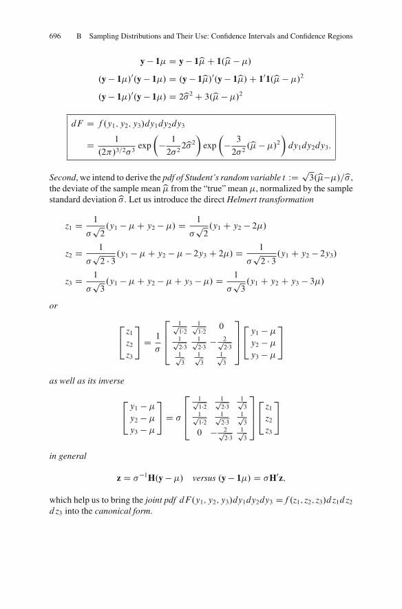
696 B Sampling Distributions and Their Use: Confidence Intervals and Confidence Regions
y � 1� D y � 1b�C 1.b� � �/.y � 1�/0.y � 1�/ D .y � 1b�/0.y � 1b�/C 101.b� � �/2
.y � 1�/0.y � 1�/ D 2b�2 C 3.b� � �/2
dF D f .y1; y2; y3/dy1dy2dy3D 1
.2/3=2�3exp
�� 1
2�22b�2
�exp
�� 3
2�2.b� � �/2
�dy1dy2dy3:
Second, we intend to derive the pdf of Student’s random variable t WD p3.b���/=b� ,the deviate of the sample meanb� from the “true” mean �, normalized by the samplestandard deviationb� . Let us introduce the direct Helmert transformation
z1 D 1
�p2.y1 � �C y2 � �/ D 1
�p2.y1 C y2 � 2�/
z2 D 1
�p2 � 3.y1 � �C y2 � � � 2y3 C 2�/ D
1
�p2 � 3.y1 C y2 � 2y3/
z3 D 1
�p3.y1 � �C y2 � �C y3 � �/ D 1
�p3.y1 C y2 C y3 � 3�/
or
2
4z1z2z3
3
5 D 1
�
2
664
1p1�2
1p1�2 0
1p2�3
1p2�3 � 2p
2�31p3
1p3
1p3
3
775
2
4y1 � �y2 � �y3 � �
3
5
as well as its inverse
2
4y1 � �y2 � �y3 � �
3
5 D �
2
664
1p1�2
1p2�3
1p3
1p1�2
1p2�3
1p3
0 � 2p2�3
1p3
3
775
2
4z1z2z3
3
5
in general
z D ��1H.y � �/ versus .y � 1�/ D �H0z;
which help us to bring the joint pdf dF.y1; y2; y3/dy1dy2dy3 Df .z1; z2; z3/d z1d z2d z3 into the canonical form.
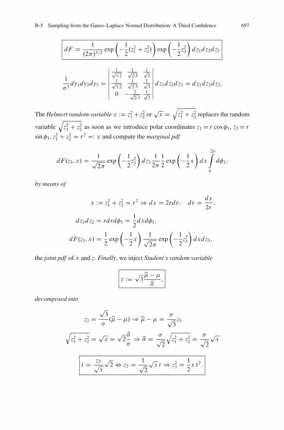
B-5 Sampling from the Gauss–Laplace Normal Distribution: A Third Confidence 697
dF D 1
.2/3=2exp
��12.z21 C z22/
�exp
��12
z23
�d z1d z2d z3
1
�3dy1dy2dy3 D
ˇˇˇˇˇˇ
1p1�2
1p2�3
1p3
1p1�2
1p2�3
1p3
0 � 2p2�3
1p3
ˇˇˇˇˇˇ
d z1d z2d z3 D d z1d z2d z3:
The Helmert random variable x WD z21C z22 orpx D
qz21 C z22 replaces the random
variableq
z21 C z22 as soon as we introduce polar coordinates z1D r cos�1, z2D rsin �1, z21 C z22 D r2 DW x and compute the marginal pdf
dF.z3; x/ D 1p2
exp
��12
z23
�d z3
1
2
1
2exp
��12x
�dx
2Z
0
d�1;
by means of
x WD z21 C z22 D r2) dx D 2rdr; dr D dx
2r;
d z1d z2 D rdrd�1 D 1
2dxd�1;
dF.z3; x/ D 1
2exp
��12x
�1p2
exp
��12
z23
�dxd z3;
the joint pdf of x and z. Finally, we inject Student’s random variable
t WD p3b� � �b�
;
decomposed into
z3 Dp3
�.b� � �/) b� � � D �p
3z3
qz21 C z22 D
px D p2b�
�) b� D �p
2
qz21 C z22 D
�p2
px
t D z3px
p2, z3 D 1p
2
px t ) z23 D
1
2x t2:
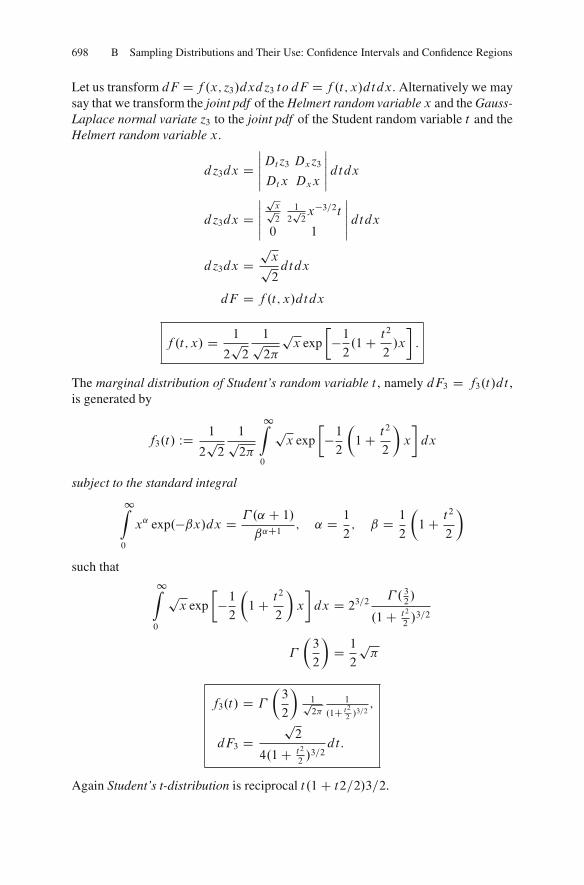
698 B Sampling Distributions and Their Use: Confidence Intervals and Confidence Regions
Let us transform dF Df .x; z3/dxd z3 to dF Df .t; x/dtdx. Alternatively we maysay that we transform the joint pdf of the Helmert random variable x and the Gauss-Laplace normal variate z3 to the joint pdf of the Student random variable t and theHelmert random variable x.
d z3dx DˇˇˇˇDt z3 Dxz3Dtx Dxx
ˇˇˇˇdtdx
d z3dx Dˇˇˇˇˇ
pxp2
1
2p2x�3=2t
0 1
ˇˇˇˇˇdtdx
d z3dx Dpxp2dtdx
dF D f .t; x/dtdx
f .t; x/ D 1
2p2
1p2
px exp
��12.1C t2
2/x
:
The marginal distribution of Student’s random variable t , namely dF3 D f3.t/dt ,is generated by
f3.t/ WD 1
2p2
1p2
1Z
0
px exp
��12
�1C t2
2
�x
dx
subject to the standard integral
1Z
0
x˛ exp.�ˇx/dx D � .˛ C 1/ˇ˛C1 ; ˛ D 1
2; ˇ D 1
2
�1C t2
2
�
such that1Z
0
px exp
��12
�1C t2
2
�x
dx D 23=2 � . 3
2/
.1C t 2
2/3=2
�
�3
2
�D 1
2
p
f3.t/ D �
�3
2
�1p2
1
.1C t2
2 /3=2;
dF3 Dp2
4.1C t 2
2/3=2
dt:
Again Student’s t-distribution is reciprocal t.1C t2=2/3=2.

B-5 Sampling from the Gauss–Laplace Normal Distribution: A Third Confidence 699
Lemma B.13. Student’s t-distribution for the derivate of the mean .b���/=b�(Gosset, 1908)):
Let the random vector of observations y D Œy1; : : : ; yn�0 be Gauss-Laplace i.i.d.
Student’s random variable
t WD b� � �b�pn;
where the sample mean b� is BLUUE of � and the sample varianceb�2 is BIQUUEof �2; associated to the pdf
f .t/ D � .pC12/
� .p
2/
1pp
1
.1C t 2
p/.pC1/=2 :
p D n � 1 is the “degree of freedom” of Student’s distribution fp.t/. Gosset(1908) published the t-distribution of the ratio
pn.b���/=b� under the pseudonym
“Student”: The probable error of a mean.
Proof.
The joint probability distribution of the random variable zn WD pn.b� � �/=� andthe Helmert random variable x WD z21 C � � � C z2n�1 D .n� 1/b�2=�2 represented by
dF D f1.zn/f2.x/d zndx
due to the effect that zn and z21C� � �C z2n�1 orb��� and .n�1/b�2 are stochasticallyindependent. Let us take reference to the specific pdfs with n and n�1 D p degreesof freedom
dF1 D f1.zn/d zn and dF2 D f2.x/dx;
f1.zn/ D 1p2
exp
��12
z2n
�and f2.x/ D 1
� .p
2/
�1
2
�p=2x.p�2/=2 exp
��12x
�;
or
dF1 D f1.b�/db� and dF2 D f2.b�2/db�2;
f1.b�/ Dpn
�p2
exp
��n2
.b���/2�2
�and
f2.b�2/ D 1
�p2p=2� .p=2/pp=2b�p�2
exp
��12
p
�2b�2�
we derived earlier. Here, let us introduce Student’s random variable

700 B Sampling Distributions and Their Use: Confidence Intervals and Confidence Regions
t WD znpx
pn � 1 D b� � �
b�pn or zn D
pxp
n � 1t Dpxppt:
By means of the Jacobi matrix J and its absolute Jacobi determinant jJj�dt
dx
D�Dzn t Dxt
Dznx Dxx
�d zndx
D J
�d zndx
J D2
4
pppx� 12x�3=2zn
pp
0 1
3
5 ; jJj Dpppx; jJj�1 D
pxpp
we transform the surface element d zndx to the surface element jJj�1dtdx, namely
d zndx Dpxppdtdx:
Lemma B.14. (Gamma Function):
Our final action item is to calculate the marginal probability distributionsdF3D f3.t/dt of Student’s random variable t , namely
dF3 D f3.t/dt
f3.t/ WD 1p2p
1
� .p=2/
�1
2
�p=2 1Z
0
x.p�1/=2 exp
��12
�1C t2
p
�x
�dx:
Consult (Grobner and Hofreiter, 1973, p. 55), for the standard integral
1Z
0
x˛ exp.�ˇx/dx D ˛Š
ˇ˛C1 D� .˛ C 1/ˇ˛C1 and
1Z
0
x.p�1/=2 exp
��12
�1C t2
p
�x
dx D 2.pC1/=2 � .
pC12/
.1C t 2
p/.pC1/=2 ;
where p D n � 1 is the rank of the quadratic Helmert matrix Hn. Notice a resultof the gamma function � .pC1
2/ D .
p�12/Š. In summary, substituting the standard
integral

B-5 Sampling from the Gauss–Laplace Normal Distribution: A Third Confidence 701
dF3 D f3.t/dt
f3.t/ D� .
pC12/
� .p
2/
1pp
1
.1C t 2
p/.pC1/=2
resulted in Student’s t distribution, namely the pdf of Student’s random variable.b� � �/=b� .
B-52 The Confidence Interval for the Mean, VarianceUnknown
Lemma B.12 is the basis for the construction of the confidence interval of the “true”mean, variance unknown, which we summarize in Lemma B.13, Example B.17contains all details for computing such a confidence interval, namely Table B.11,a collection of the most popular values of the coefficient of confidence, as well asTables B.12, B.13 and B.14, listing the quantiles for the confidence interval of theStudent random variable with p D n� 1 degrees of freedom. Figures B.9 and B.10illustrate the probability of two-sided confidence interval for the mean, varianceunknown, and the limits of the confidence interval. Table B.15 as a flow chart pavesthe way for the “fast computation” of the confidence interval for the “true” mean,variance unknown.
Lemma B.15. (confidence interval for the sample mean, varianceunknown):
The random variable t D pn.b� � �/=b� characterized by the ratio of the deviateof the sample mean b� D n�110y, BLUUE of �, from the “true” mean � and thestandard deviation b� , b�2 D .y � 1b�/0.y � 1b�/=.n � 1/ BIQUUE of the “true”variance �2, has the Student t-distribution with p D n � 1 “degrees of freedom”.The “true” mean � is an element of the two-sided confidence interval
� 2�b� � b�pnc1�˛=2; b�C b�p
nc1�˛=2Œ
with confidence
P
�b� � b�p
nc1�˛=2 < � < b�C b�p
nc1�˛=2
�D 1� ˛
of level 1�˛. For three values of the coefficient of confidence � D 1�˛, Table B.12is a list of associated quantiles c1�˛=2.

702 B Sampling Distributions and Their Use: Confidence Intervals and Confidence Regions
Example B.17. (confidence interval for the example mean b�, �2 unknown):
Suppose that a random sample2
664
y1
y2y3y4
3
775 D
2
664
1:2
3:4
0:6
5:6
3
775 ; b� D 2:7; b�2 D 5:2; b� D 2:3
of four observations is characterized by the sample mean b� D 2:7 and the samplevarianceb�2 D 5:2. 2.2:7 � �/=2:3 D pn.b� � �/=b� D t has Student’s pdf withp D n�1 D 3 degrees of freedom. The probability � D 1�˛ that t will be betweenany two arbitrarily chosen numbers c1 D �c and c2 D Cc is
Pf�c1 < t < c2g Dc2Z
c1
f .t/dt D � D 1 � ˛
Pf�c < t < cg DCcZ
�cf .t/dt D � D 1 � ˛
Pf�c < t < cg DcZ
�1f .t/dt �
�cZ
�1f .t/dt D � D 1 � ˛
cZ
�1f .t/dt D 1 � ˛
2;
�cZ
�1f .t/dt D˛
2
� is the coefficient of confidence, ˛ the coefficient of negative confidence, also calledcomplementary coefficient of confidence. The four representations of the probability� D 1�˛ to include t in the confidence interval�c < t < Cc have led to the linearVolterra integral equation of the first kind
cZ
�1f .t/dt D 1 � ˛
2D 1
2.1C �/:
Three values of the coefficient of confidence � or its complement ˛ are popular andlisted in Table B.10.
Table B.11 (Values of the coefficient of confidence):
� 0:950 0:990 0:999
˛ 0:050 0:010 0:001˛2
0:025 0005 0:000; 5
1 � ˛2D 1C�
20:975 0:995 0:999; 5

B-5 Sampling from the Gauss–Laplace Normal Distribution: A Third Confidence 703
In solving the linear Volterra integral equation of the first kind
tZ
�1f .t�/dt� D 1 � 1
2˛.t/ D 1
2Œ1C �.t/�;
which depends on the degrees of freedom p D n � 1, Tables B.12–B.14 collectthe quantiles c1�˛=2=
pn given the coefficients of confidence or their complements
which we listed in Table B.11.
Table B.12 (Quantiles c1�˛=2=pn for the confidence interval of the Student
random variable with p D n � 1 degrees of freedom):
1 � ˛=2 D .1C �/=2 D 0:975; � D 0:95; ˛ D 0:05p n 1p
nc1�˛=2 p n 1p
nc1�˛=2
1 2 8:99 14 15 0:554
2 3 2:48 19 20 0:468
3 4 1:59 24 25 0:413
4 5 1:24 29 30 0:373
5 6 1:05 39 40 0:320
6 7 0:925 49 50 0:284
7 8 0:836 99 100 0:198
8 9 0:769 199 200 0:139
9 10 0:715 499 500 0:088
Table B.13 (Quantiles c1�˛=2=pn for the confidence interval of the Student
random variable with p D n � 1 degrees of freedom):
1 � ˛=2 D .1C �/=2 D 0:995; � D 0:990; ˛ D 0:010p n 1p
nc1�˛=2 p n 1p
nc1�˛=2
1 2 45:01 14 15 0:769
2 3 5:73 19 20 0:640
3 4 2:92 24 25 0:559
4 5 2:06 29 30 0:503
5 6 1:65 39 40 0:428
6 7 1:40 49 50 0:379
7 8 1:24 99 100 0:263
8 9 1:12 199 200 0:184
9 10 1:03 499 500 0:116

704 B Sampling Distributions and Their Use: Confidence Intervals and Confidence Regions
Table B.14 (Quantiles c1�˛=2=pn for the confidence interval of the Student
random variable with p D n � 1 degrees of freedom):
1 � ˛=2 D .1C �/=2 D 0:999:5; � D 0:999; ˛ D 0:001p n c1�˛=2 c1�˛=2=
pn p n c1�˛=2 c1�˛=2=
pn
1 2 636:619 450:158 14 15 4:140 1:069
2 3 31:598 18:243 19 20 3:883 0:868
3 4 12:941 6:470 24 25 3:725 0:745
4 5 8:610 3:851 29 30 3:659 0:668
5 6 6:859 2:800 30 41 3:646 0:655
6 7 5:959 2:252 40 41 3:551 0:555
7 8 5:405 1:911 60 61 3:460 0:443
8 9 5:041 1:680 120 121 3:373 0:307
9 10 4:781 1:512 1 1 3:291 0
Since Student’s pdf depends on p D n � 1, we have tabulated c1�˛=2=pn for
the confidence interval we are going to construct. The Student’s random variablet Dpn.b� � �/=b� is solved for �, evidently our motivation to introduce theconfidence intervalb�1 < � < b�2
t D pnb�� �b�) b�� � D b�p
nt ) � D b� � b�p
nt
b�1 WD b� � b�pnc1�˛=2 < � < b�C b�p
nc1�˛=2 DW b�2:
The interval b�1 < � < b�2 for the fixed value t D c1�˛=2 contains the “true” mean� with probability � D 1 � ˛.
P
�b�� b�p
nc1�˛=2 < � < b�C b�p
nc1�˛=2
�
DCcZ
�cf .t/dt D � D 1 � ˛
because of
cZ
�1f .t/dt D
c1�˛=2Z
�1f .t/dt D 1 � ˛
2:

B-5 Sampling from the Gauss–Laplace Normal Distribution: A Third Confidence 705
t
a / 2 a / 2g = 1–a
f(t)
−c1−a / 2 +c1−a / 2
Fig. B.9 Two-sidedconfidence interval� 2�b�1;b�2Œ, Student’s pdffor p D 3 degrees of freedom.n D 4/b�1 Db��b�c1�˛=2=
pn,
b�2 Db�Cb�c1�˛=2=pn
m1ˆ m2m ˆ
ˆ ˆm – sc1−a /2 / n ˆ ˆm + sc1−a /2 / n
Fig. B.10 Two-sided confidence interval for the “true” mean �, quantile c1�˛=2
Figures B.9 and B.10 illustrate the coefficient of confidence and the probabilityfunction of a confidence interval.Let us specify all the integrals to our example.
c1�˛=2Z
�1f .t/dt D 1 � ˛=2
c0:975Z
�1f .t/dt D 0:975;
c0:995Z
�1f .t/dt D 0:995;
c0:999;5Z
�1f .t/dt D0:999; 5:
These data substituted into Tables B.12–B.14 lead to the triplet of confidenceintervals for the “true” mean.
case .a/ W � D 0:95; ˛ D 0:05; 1 � ˛=2 D 0:975p D 3; n D 4; c1�˛=2=
pn D 1:59
Pf2:7 � 2:3 � 1:59 < � < 2:7C 2:3 � 1:59g D 0:95
Pf�0:957 < � < 6:357g D 0:95:
case .b/ W � D 0:99; ˛ D 0:01; 1 � ˛=2 D 0:995p D 3; n D 4; c1�˛=2=
pn D 2:92

706 B Sampling Distributions and Their Use: Confidence Intervals and Confidence Regions
Pf2:7 � 2:3 � 2:92 < � < 2:7C 2:3 � 2:92g D 0:99
Pf�4:016 < � < 9:416g D 0:99:
case .c/ W � D 0:999; ˛ D 0:001; 1� ˛=2 D 0:999; 5
p D 3; n D 4; c1�˛=2=pn D 6:470Pf2:7 � 2:3 � 6:470 < � < 2:7C 2:3 � 6:470g D 0:999
Pf�12:181 < � < 17:581g D 0:999:
The results may be summarized as follows:
With probability 95% the “true” mean � is an element of the interval � �0:957, C6:357Œ. In contrast, with probability 99% the “true” mean � is anelement of the larger interval � � 4:016, C9:416Œ. Finally, with probability99.9is an element of the largest interval ��12:181,C17:581Œ. If we comparethe confidence intervals for the mean �, �2 known, versus �2 unknown, werealize much larger intervals for the second model. Such a result is not toomuch a surprise, since the model “�2 unknown” is much weaker than themodel “�2 known”.
Table B.15 (Flow chart: Confidence interval for the mean �, �2 unknown):
Choose a coefficient of confidence g according toTable B11.
Solve the linear Volterra integral equation of the first kindF(c1−a / 2) = 1−a / 2 = (1 + g ) / 2 by Table B12, Table B13 or TableB14 for a Student pdf with p = n−1 degrees of freedom: readc1−α / 2 / n.
Compute the sample mean m and the sample standard deviation s.
ˆ ˆ ˆ ˆ ˆ
ˆˆ
Compute sc1−a / 2 / n and m−sc1−a / 2 / n, m + sc1−a / 2 / n.
g

B-5 Sampling from the Gauss–Laplace Normal Distribution: A Third Confidence 707
B-53 The Uncertainty Principle
Figure B.11 is the graph of the function
��.nI˛/ WD 2b�c1�˛=2=pn;
where �� is the length of the confidence interval of the “true” mean �; �2
unknown. The independent variable of the function is the number of observations n.The function ��.nI˛/ is plotted for fixed values of the coefficient of comple-mentary confidence ˛, namely ˛ D 10%; 5%; 1%: For reasons given later thecoefficient of complementary confidence ˛ is called uncertainty number. The graphfunction��.nI˛/ illustrates two important facts.
Fact #1: For a constant uncertainty number ˛, the length of the confidence interval�� is smaller the larger the number of observations n is chosen.
Fact #2: For a constant number of observations n, the smaller the number ofuncertainly ˛ is chosen, the larger is the confidence interval��.
Evidently, the diversive influences of (a) the length of the confidence interval��; (b) the uncertainly number ˛ and (c) the number of observations n, whichwe collected in The Magic Triangle of Figure B.12, constitute The UncertainlyPrinciple, in formula
��.n� 1/ W k�˛;
Fig. B.11 Length of the confidence interval for the mean against the number of observations
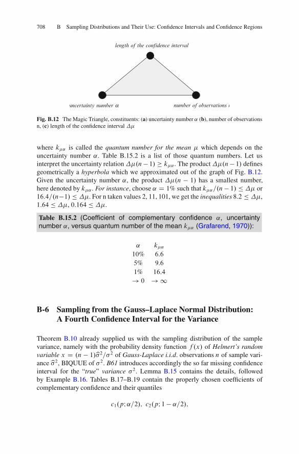
708 B Sampling Distributions and Their Use: Confidence Intervals and Confidence Regions
length of the confidence interval
uncertainty number a number of observations n
Fig. B.12 The Magic Triangle, constituents: (a) uncertainty number ˛ (b), number of observationsn, (c) length of the confidence interval ��
where k�˛ is called the quantum number for the mean � which depends on theuncertainty number ˛. Table B.15.2 is a list of those quantum numbers. Let usinterpret the uncertainty relation��.n� 1/ k�˛ . The product��.n� 1/ definesgeometrically a hyperbola which we approximated out of the graph of Fig. B.12.Given the uncertainty number ˛, the product ��.n � 1/ has a smallest number,here denoted by k�˛ . For instance, choose ˛ D 1% such that k�˛=.n� 1/ � �� or16:4=.n�1/ � ��. For n taken values 2, 11, 101, we get the inequalities 8:2 � ��,1:64 � ��, 0:164 � ��.
Table B.15.2 (Coefficient of complementary confidence ˛, uncertaintynumber ˛, versus quantum number of the mean k�˛ (Grafarend, 1970)):
˛ k�˛10% 6:6
5% 9:6
1% 16:4
! 0 !1
B-6 Sampling from the Gauss–Laplace Normal Distribution:A Fourth Confidence Interval for the Variance
Theorem B.10 already supplied us with the sampling distribution of the samplevariance, namely with the probability density function f .x/ of Helmert’s randomvariable x D .n � 1/b�2=�2 of Gauss-Laplace i.i.d. observations n of sample vari-anceb�2, BIQUUE of �2. B61 introduces accordingly the so far missing confidenceinterval for the “true” variance �2. Lemma B.15 contains the details, followedby Example B.16. Tables B.17–B.19 contain the properly chosen coefficients ofcomplementary confidence and their quantiles
c1.pI˛=2/; c2.pI 1 � ˛=2/;

B-6 Sampling from the Gauss–Laplace Normal Distribution: A Fourth 709
dependent on the “degrees of freedom” p D n � 1. Table B.20 as a flow chartsummarizes various steps in computing a confidence interval for the variance �2.B62 reviews The Uncertainty Principle which is built on (a) the coefficient ofcomplementary confidence ˛, also called uncertainty number, (b) the number ofobservations n and (c) the length��2.nI˛/ of the confidence interval for the “true”variance �2.
B-61 The Confidence Interval for the Variance
Lemma B.15 summaries the construction of a two-sided confidence interval forthe “true” variance based upon Helmert’s Chi Square distribution of the randomvariable .n�1/b�2=�2 where b�2 is BIQUUE of �2. Example B.18 introduces arandom sample of size n D 100 with an empirical variance b�2 D 20:6. Basedupon coefficients of confidence and complementary confidence given in Table B.14,related confidence intervals are computed. The associated quantiles for Helmert’sChi Square distribution are tabulated in Table B.15 .� D 0:95/, Table B.18.� D 0:99/ and Table B.19 .� D 0:998/: Finally, Table B.20 as a flow chartpares the way for the “fast computation” of the confidence interval for the “true”variance �2.
Lemma B.16. (confidence interval for the variance):
The random variable x D .n � 1/b�2=�2, also called Helmert’s 2, characterizedby the ration of the sample variance b�2 BIQUUE of �2, and the “true” variance�2, has the 2' pdf of p D n � 1 degrees of freedom, if the random observationsyi ; i 2 f1; : : : ng are Gauss-Laplace i.i.d. The “true” variance �2 is an element ofthe two-sided confidence interval
�2 2 � .n � 1/b�2c2.pI 1 � ˛=2/;
.n � 1/b�2c1.pI˛=2/Œ
with confidence
P
�.n � 1/b�2
c2.pI 1 � ˛=2/ < �2 <
.n � 1/b�2c1.pI˛=2/
�D 1 � ˛ D �
of level 1 � ˛. Tables D.8, D.18 and D.16 list the quantiles c1.pI 1 � ˛=2/and c2.pI˛=2/ associated to three values of Table B.19 of the coefficient ofcomplementary confidence 1 � ˛.In order to make yourself more familiar with Helmert’s Chi Square distribution werecommend to solve the problems of Exercise B.1.

710 B Sampling Distributions and Their Use: Confidence Intervals and Confidence Regions
Exercise B.1. (Helmert’s Chi Square 2' distribution):
Helmert’s random variable x WD .n � 1/b�2=�2 D pb�2=�2 has the non-symmetric 2' pdf. Prove that the first four central moments are,
(a) 1 D 0, Efxg D � D p(b) 2 D �2x D 2p(c) 3 D .2p/3=2.8=p/1=4 (coefficient of skewness 23 =
22 D
p8=p/
(d) 4 D 6�4.1C 2p/ (coefficient of curtosis 4=22 � 3 D 3C 12=p/.Guide
.a/Efxg D p
�2Efb�2g
Efb�2g D �2.unbiasedness/
3
5) Efxg D p
.b/
Dfb�2g D 2
n � 1�4 D 2
p�4
Dfxg D p2
�4Dfb�2g
3
775) Dfxg D 2p:
Example B.18. (confidence interval for the sample variance b�2):
Suppose that a random sample .y1; : : : yn/ 2 Y of size n D 100 has led to anempirical varianceb�2 D 20:6. xD .n�1/b�2=�2 or 99 � 20:6=�2 D 2039:4=�2 hasHelmert’s pdf with p D n� 1 D 99 degrees of freedom. The probability � D 1�˛that x will be between c1.pI˛=2/ and c2.pI 1 � ˛=2/ is
Pfc1.pI˛=2/<x < c2.pI 1�˛=2/g Dc2Z
c1
f .x/dx D � D 1 � ˛
Pfc1.pI˛=2/<x < c2.pI 1�˛=2/g Dc2Z
0
f .x/dx �c1Z
0
f .x/dx D � D 1 � ˛
c2Z
0
f .x/dx D F.c2/ D 1 � ˛=2 D .1C �/=2;
c1Z
0
f .x/dx D F.c1/ D ˛=2 D .1 � �/=2
Pfc1.pI˛=2/<x < c2.pI 1�˛=2/g D F.c2/� F.c1/D .1C �/=2� .1� �/=2D�
c1.pI˛=2/ < x < c2.pI 1 � ˛=2/, c1.pI˛=2/ < .n � 1/b�2
�2< c2.pI 1 � ˛=2/

B-6 Sampling from the Gauss–Laplace Normal Distribution: A Fourth 711
or
1
c2<
�2
.n � 1/b�2 <1
c1, .n � 1/b�2
c2< �2 <
.n � 1/b�2c1
P
�.n � 1/b�2
c2.pI 1 � ˛=2/ < �2 <
.n � 1/b�2c1.pI˛=2/
�D 1 � ˛ D �:
Since Helmert’s pdf f .xIp/ is now-symmetric there arises the question how todistribute the confidence � or the complementary confidence ˛ D � � 1 on theconfidence interval limits c1 and c2, respectively. If we setup F.c1/ D ˛=2, we definea cumulative probability half of the complementary confidence. If F.c2/ � F.c1/ DPfc1.pI˛=2/ < x < c2.pI 1 � ˛=2/g D 1 � ˛ D � is the cumulative probabilitycontained in the interval c1 < x < c2, we derive F.c2/ D 1 � ˛=2. Accordinglyc1.pI˛=2/ < x < c2.pI 1�˛=2/ is the confidence interval based upon the quantilec1 with cumulative probability ˛=2 and the quantile c2 with cumulative probability1 � ˛=2. The four representations of the cumulative probability of the confidenceinter-val c1 < x < c2 establish two linear Volterra integral equations of the firstkind
c1Z
0
f .x/dx D ˛=2 and
c2Z
0
f .x/dx D 1 � ˛=2;
dependent on the degree of freedom p D n � 1 of Helmert’s pdf f .x; p/.As soon as we have established the confidence interval c1.pI˛=2/ < x < c2.pI 1�˛=2/ for Helmert’s random variable x D .n�1/b�2=�2 D pb�2=�2, we are left withthe problem of how to generate a confidence interval for the “true” variance �2, thesample varianceb�2 given. If we take the reciprocal interval c�1
2 < x�1 < c�11 for
Helmert’s inverse random variable 1=x D �2=Œ.n � 1/b�2�, we are able to multiplyboth sides by .n � 1/b�2. In summary, a confidence interval which corresponds toc1 < x < c2 is .n� 1/b�2=c2 < �2 < .n � 1/b�2=c1.Three values of the coefficient of confidence � or of complementary confidence˛ D 1 � � which are most popular we list in Table B.16.
Table B.16 (Values of the coefficient of confidence � ,c1.pI˛=2/ and c2.pI 1�˛=2/):
˛ 0:950 0:990 0:998
˛=2 0:050 0:010 0:002
˛=2 0:025 0:005 0:001
1 � ˛=2 0:975 0:995 0:999

712 B Sampling Distributions and Their Use: Confidence Intervals and Confidence Regions
In solving the linear Volterra integral equations of the first kind
c1Z
0
f .x/dx D F.c1/ D ˛=2 and
c2Z
0
f .x/dx DF.c2/ D 1 � ˛=2;
which depend on the degrees of freedom p D n � 1, Tables B.17–B.19 collect thequantiles c1.pI˛=2/ and c2.pI 1 � ˛=2/ for given values p and ˛.
Table B.17 (Quantiles c1.pI˛=2/, c2.pI 1 � ˛=2/ for the confidence intervalof the Helmert random variable with p D n � 1 degrees of freedom):
˛=2 D 0:025; 1 � ˛=2 D 0:975; ˛ D 0:05; � D 0:95
p n c1.pI˛=2/ c2.pI 1 � ˛=2/ p n c1.pI˛=2/ c2.pI 1 � ˛=2/1 2 0:000 5:02 14 15 5:63 26:1
2 3 0:506 7:38 19 20 8:91 32:9
3 4 0:216 9:35 24 25 12:4 39:4
4 5 0:484 11:1 29 30 16:0 45:7
5 6 0:831 12:8 39 40 23:7 58:1
6 7 1:24 14:4 49 50 31:6 70:2
7 8 1:69 16:0 99 100 73:4 128
8 9 2:18 17:5
9 10 2:70 19:0
Table B.18 (Quantiles c1.pI˛=2/, c2.pI 1 � ˛=2/ for the confidence intervalof the Helmert random variable with p D n � 1 degrees of freedom):
˛=2 D 0:005; 1 � ˛=2 D 0:995; ˛ D 0:01; � D 0:99
p n c1.pI˛=2/ c2.pI 1 � ˛=2/ p n c1.pI˛=2/ c2.pI 1 � ˛=2/1 2 0:000 7:88 8 9 1:34 22:0
2 3 0:010 9 10 1:73 23:6
3 4 0:072
4 5 0:207 14 15 4:07 31:3
19 20 6:84 38:6
5 6 0:412 24 25 9:89 45:6
6 7 0:676 29 30 13:1 52:3
7 8 0:989
39 40 20 65:5
49 50 27:2 78:2
99 100 66:5 139

B-6 Sampling from the Gauss–Laplace Normal Distribution: A Fourth 713
0.5
f(x)
0 c1(p;a / 2) c2 (p;1−a / 2)
Fig. B.13 Two-sided confidence interval �2 2�p�2=c2; p�2=c1Œ Helmert’s pdf, f(x)
Table B.19 (Quantiles c1.pI˛=2/, c2.pI 1 � ˛=2/ for the confidence intervalof the Helmert random variable with p D n � 1 degrees of freedom):
˛=2 D 0:001; 1 � ˛=2 D 0:999; ˛ D 0:002; � D 0:998
p n c1.pI˛=2/ c2.pI 1 � ˛=2/ p n c1.pI˛=2/ c2.pI 1 � ˛=2/1 2 0:00 10:83 9 10 1:15 27:88
2 3 0:00 13:82 14 15 3:04 36:12
3 4 0:02 16:27 19 20 5:41 43:82
4 5 0:09 18:47 24 25 8:1 51:2
5 6 0:21 20:52 29 30 11:0 58:3
6 7 0:38 22:46 50 51 24:7 86:7
7 8 0:60 24:32 70 71 39:0 112:3
8 9 0:86 26:13 99 100 60:3 147:4
100 101 61:9 149:4
Those data collected in Tables B.17–B.19 lead to the triplet of confidence intervalsfor the “true” variance
case .a/ W � D 0:95; ˛ D 0:05; ˛=2 D 0:025; 1 � ˛=2 D 0:975p D 99; n D 100; c1.pI˛=2/ D 73:4; c2.pI 1 � ˛=2/ D 128
P
�99 � 20:6
128< �2 <
99 � 20:673:4
�D 0:95
Pf15:9 < �2 < 27:8g D 0:95:

714 B Sampling Distributions and Their Use: Confidence Intervals and Confidence Regions
Fig. B.14 Two-sided confidence interval for the “true” variance �2, quantiles c1.pI˛=2/ andc2.pI 1� ˛=2/
case .b/ W � D 0:99; ˛ D 0:01; ˛=2 D 0:005; 1 � ˛=2 D 0:995p D 99; n D 100; c1.pI˛=2/ D 66:5; c2.pI 1 � ˛=2/ D 139
P
�99 � 20:6
139< �2 <
99 � 20:666:5
�D 0:99
Pf14:7 < �2 < 30:7g D 0:99:
case .c/ W � D 0:998; ˛ D 0:002; ˛=2 D 0:001; 1 � ˛=2 D 0:999p D 99; n D 100; c1.pI˛=2/ D 60:3; c2.pI 1 � ˛=2/ D 147:3
P
�99 � 20:6
147:3< �2 <
99 � 20:660:3
�D 0:996
Pf13:8 < �2 < 33:8g D 0:998:
The results can be summarized as follows. With probability 95%, the“true” variance �2 is an element of the interval [15.9, 27.8]. In contrast,with probability 99%, the “true” variance is an element of the largerinterval [14.7, 30.7]. Finally, with probability 99.8% the “true” variance is anelement of the largest interval [13.8, 33.8]. If we compare the confidenceintervals for the variance �2, we realize much larger intervals for smallercomplementary confidence namely 5%, 1% and 0.2%. Such a result issubject of The Uncertainty Principle.

B-6 Sampling from the Gauss–Laplace Normal Distribution: A Fourth 715
Table B.20 (Flow chart – confidence interval for the variance �2):
Compute the sample variance s2and the quantiles
.
Choose a coefficient of confidence g according to Table B16.
Solve thelinear Volterra integral equation of the first kindF(c1(p;a /2)) – a / 2, F(c2(p;1−a / 2))−1−a / 2
by Table B17, Table B18 or Table B19 for a Helmert pdf withp = n−1 degrees of freedom.
s2 ∈ ] [(n−1)s2 (n−1)s2
c2(p;a / 2) c1(p;a / 2)
B-62 The Uncertainty Principle
Figure B.15 is the graph of the function
��2.nI˛/ WD .n � 1/b�2�
1
c1.n � 1I˛=2/ �1
c2.n � 1I 1 � ˛=2/�;
where ��2 is the length of the confidence interval of the “true” variance �2.The independent variable of the functions is the number of observations n. Thefunction ��2.nI˛/ is plotted for fixed values of the coefficient of complementaryconfidence ˛, namely ˛ D 5%, 1%, 0.2%. For reasons given later on the coefficientof complementary confidence ˛ is called uncertainty number. The graph of thefunction��2.nI˛/ illustrates two important facts.
• Fact #1: For a contrast uncertainty number ˛; the length of the confidence interval��2 is smaller, the larger number of observations n is chosen.
• Fact #2: For a contrast number of observations n, the smaller the number ofuncertainty ˛ is chosen, the larger is the confidence interval��2.
Evidently, the divisive influences of (a) the length of the confidence interval ��2,(b) the uncertainty number ˛ and (c) the number of observations n, which wecollect in The Magic Triangle of Fig. B.16, constitute The Uncertainty Principle,formulated by the inequality
��2.n � 1/ k�2˛;

716 B Sampling Distributions and Their Use: Confidence Intervals and Confidence Regions
Fig. B.15 Length of the confidence interval for the variance against the number of observations
length of the confidence interval
uncertainty number a number of observations n
Fig. B.16 The magic triangle, constituents: (a) uncertainty number ˛ (b), number of observationsn, (c) length of the confidence interval ��2
where k�2˛ is called quantum number for the variance �2. The quantum numberdepends on the uncertainty number ˛. Let us interpret the uncertainty relation��2.n � 1/ k�2˛. The product ��2.n � 1/ defines geometrically a hyperbolawhich we approximated to the graph of Fig. B.15. Given the uncertainty number˛, the product ��2.n � 1/ has a smallest number denoted by k�2˛. For instance,choose ˛ D 1% such that k�2˛=.n � 1/ � ��2 or 42=.n � 1/ � ��2. For thenumber of observations n, for instance n D 2; 11; 101, we find the inequalities42 � ��2; 4:2 � ��2; 0:42 � ��2.Table B.21 (Coefficient of complementary confidence ˛, uncertaintynumber ˛, versus quantum number of the mean k�2˛ (Grafarend, 1970):
˛ k�2˛10% 19:5
5% 25:9
1% 42:0
! 0 !1
At the end, pay attention to the quantum numbers k�2˛ listed in Table B.21.

B-7 Sampling from the Multidimensional Gauss–Laplace Normal Distribution 717
B-7 Sampling from the Multidimensional Gauss–LaplaceNormal Distribution: The Confidence Region for theFixed Parameters in the Linear Gauss–Markov Model
Example B.19. (special linear Gauss–Markov model, marginal probabilitydistributions):
For a simple linear Gauss–Markov model Efyg D A�, A 2 Rn�m, rkA D m,
namely n D 3, m D 2, Dfyg D I�2 of Gauss-Laplace i.i.d. observations, we aregoing to compute
• The sample pdf ofb� BLUUE of �• The sample pdf ofb�2 BIQUUE of �2.
We follow the action within seven items. First, we identify the pdf of Gauss-Laplacei.i.d. observations y 2 R
n. Second, we review the estimations of b� BLUUE of �as well as b�2 BIQUUE of �2. Third, we decompose the Euclidean norm of theobservation space ky �Efygk2 into the Euclidean norms ky �Ab�k2 and kb� � �k2.Fourth, we present the eigenspace A0A analysis and the eigenspace synthesis of theassociated matrices M WD In � A.A0A/�1A0 and N WD A0A within the Eulideannorms ky � A�k2 D y0My and kb� � �k2A0A D .b� � �/0N.b� � �/, respectively.The eigenspace representation leads us to canonical random variables .z1; : : : ; zn�m/relating to the norm ky � A�k2 D y0My and .zn�mC1; : : : ; zn/ relating to the normkb���k2N which are standard Gauss-Laplace normal. Fifth, we derive the cumulativeprobability of Helmert’s random variable x WD .n � rkA/b�2=�2 D .n �m/b�2=�2and of the unknown parameter vectorb� BLUUE of � or its canonical counterpartb�BLUUE of �, multivariate Gauss-Laplace normal. Action six generates the marginalpdf ofb� orb�, both BLUUE of � or �, respectively. Finally, action seven leads us toHelmert’s Chi Square distribution 2p with p D n� rkA D n�m (here: n�m D 1)“degrees of freedom”.
The first action item
Let us assume an experiment of three Gauss-Laplace i.i.d. observationsŒy1; y2; y3�
0 D y which constitute the coordinates of the observation space Y,dim The observationsyi , i 2 f1; 2; 3g are related to a parameter space � withcoordinates Œ�1; �2� D � in the sense to generate a straight line yfkg D �1 C �2k.The fixed effects �j ; j 2 f1; 2g, define geometrically a straight line, statistically aspecial linear Gauss–Markov model of one variance component, namely

718 B Sampling Distributions and Their Use: Confidence Intervals and Confidence Regions
the first moment
Efyg D A� � E8<
:
2
4y1y2y3
3
5
9=
;D2
41 k11 k21 k3
3
5��1�2
D2
41 0
1 1
1 2
3
5��1�2
; rkA D 2:
The central second moment
Dfyg D In�2 � Dfyg D D8<
:
2
4y1y2
y3
3
5
9=
;D2
41 0 0
0 1 0
0 0 1
3
5 �2; �2 < 0:
k represents the abscissa as a fixed random, y the ordinate as the observation,naturally a random effect. Samples of the straight line are taken at k1 D 0,k2 D 1, k3 D 2, this calling for y.k1/ D y.0/ D y1, y.k2/ D y.1/ D y2,y.k3/ D y.2/ D y3, respectively. Efyg is a consistent equation. Alternatively, wemay sayEfyg 2 R.A/. The matrix A 2 R
3�2 is rank deficient by p D n�rkA D 1,also called “degree of freedom”. The dispersion matrix Dfyg, the central momentof second order, is represented as a linear model, too, namely by one-variancecomponent �2. The joint probability function of the three Gauss-Laplace i.i.d.observations
dF D f .y1; y2; y3/dy1dy2dy3 D f .y1/f .y2/f .y3/dy1dy2dy3
f .y1; y2; y3/ D .2/�3=2��3 exp
�� 1
2�2.y �Efyg/0.y �Efyg/
�
will be transformed by means of the special linear Gauss–Markov model with one-variance component.
The second action item
For such a transformation, we needb� BLUUE of � andb�2 BIQUUE �2.
b� BLUUE of � W
2
666666664
b� D .A0A/�1A0y;
A0A D�3 3
3 5
; .A0A/�1 D 1
6
�5 �3�3 3
;
b� D 1
6
�5 2 �1�3 0 3
2
4y1y2
y3
3
5 ;
b�2 BIQUUE of �2 W
2
6666664
b�2 D 1
n � rkA.y � A�/0.y � A�/
D 1
n � rkAy0.In �A.A0A/�1A0/y;
b�2 D 1
6.y21 � 4y1y2 C 2y1y3 C 4y22 � 4y2y3 C y23/:
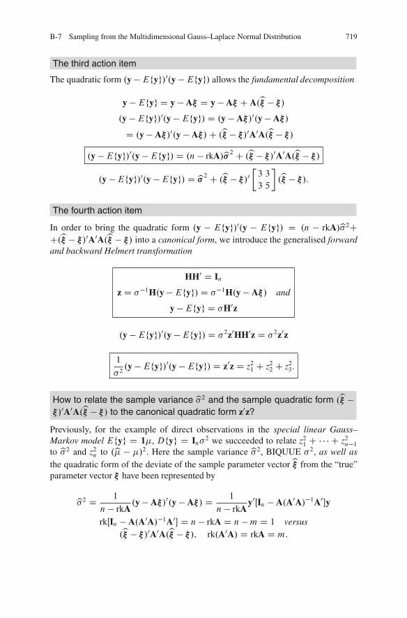
B-7 Sampling from the Multidimensional Gauss–Laplace Normal Distribution 719
The third action item
The quadratic form .y� Efyg/0.y� Efyg/ allows the fundamental decomposition
y � Efyg D y � A� D y �A� C A.b� � �/.y � Efyg/0.y � Efyg/ D .y � A�/0.y� A�/
D .y � A�/0.y �A�/C .b� � �/0A0A.b� � �/
.y �Efyg/0.y �Efyg/ D .n � rkA/b� 2 C .b� � �/0A0A.b� � �/
.y �Efyg/0.y �Efyg/ D b� 2 C .b� � �/0�3 3
3 5
.b� � �/:
The fourth action item
In order to bring the quadratic form .y � Efyg/0.y � Efyg/ D .n � rkA/b�2CC.b� � �/0A0A.b� � �/ into a canonical form, we introduce the generalised forwardand backward Helmert transformation
HH0 D In
z D ��1H.y� Efyg/ D ��1H.y � A�/ and
y �Efyg D �H0z
.y �Efyg/0.y �Efyg/ D �2z0HH0z D �2z0z
1
�2.y � Efyg/0.y � Efyg/ D z0z D z21 C z22 C z23:
How to relate the sample variance b�2 and the sample quadratic form .b� ��/0A0A.b� � �/ to the canonical quadratic form z0z?
Previously, for the example of direct observations in the special linear Gauss–Markov model Efyg D 1�, Dfyg D In�2 we succeeded to relate z21 C � � � C z2n�1to b�2 and z2n to .b� � �/2. Here the sample variance b�2, BIQUUE �2, as well asthe quadratic form of the deviate of the sample parameter vectorb� from the “true”parameter vector � have been represented by
b�2 D 1
n � rkA.y� A�/0.y �A�/ D 1
n � rkAy0ŒIn � A.A0A/�1A0�y
rkŒIn � A.A0A/�1A0� D n � rkA D n �m D 1 versus.b� � �/0A0A.b� � �/; rk.A0A/ D rkA D m:

720 B Sampling Distributions and Their Use: Confidence Intervals and Confidence Regions
The eigenspace of the matrices M and N, namely
M WD In � A.A0A/�1A and N WD A0A
D 1
6
2
41 �2 1
�2 4 �21 �2 1
3
5 D�3 3
3 5
;
will be analyzed.
The eigenspace analysis of the The eigenspace analysis of the
matrix M j 2 f1; : : : ; ng matrices N;N�1 i 2 f1; : : : ; mgV0MV U0NU D Diag.�1; : : : ; �m/ D �N
D"
V0
1
V0
2
#
M ŒV1;V2� U0N�1U D Diag.�1; : : : ; �m/ D �N�1
D Diag.�1; : : : ; �n�m; 0; : : : ; 0/ D �M
�1 D 1
�1; : : : ; �m D 1
�m
�1 D 1
�1; : : : ; �m D 1
�m
rkM D n�m rkN D rkN�1 D m
Orthonormality of the eigencolumns Orthonormality of the eigencolumns
V0
1V1 D In�m; V0
2V2 D Im
V0
1V2 D 0 2 R.n�m/�m
2
4 V0
1
V0
2
3
5h
V1 V2
iD2
4 In�m 0
0 Im
3
5
U0U D Im
v01v1 D 1
v01v2 D 0: : :
v0n�1vn D 0v0nvn D 1
u01u1 D 1
u01u2 D 0: : :
u0m�1um D 0u0mum D 1
V 2 SO.n/ W eigencolumns W.M� �j In/vj D 0
eigenvaluesjM � �j Inj D 0
U 2 SO.m/ W eigencolumns W.N � �j In/uj D 0eigenvaluesjN � �i Imj D 0
in particular

B-7 Sampling from the Multidimensional Gauss–Laplace Normal Distribution 721
eigenspace analysis of the matrix M;
rkM D n�m; M 2 R3�3; A 2 R
3�2; rkM D 1
�M D Diag.1; 0; 0/
V D ŒV1; V2� D
2
664
0:4082 0:7024 0:5830
�0:8165 0:5667 �0:11090:4082 0:4307 �0:8049
3
775
V1 2 R3�1 V2 2 R
3�2
eigenspace analysis of the matrix N;
rkN D m; N 2 R2�2; rkN D 2
�N D Diag.0:8377; 7:1623/
U D"0:8112 0:5847
�0:5847 0:8112
#
U 2 R2�2
to be completed by
eigenspace synthesis of the matrix M
M D V�MV0
M D ŒV1;V2��M
"V0
1
V0
2
#
D ŒV1;V2� Diag.�1; : : : ; �n�m; 0; : : : ; 0/
"V0
1
V0
2
#
M D V1 Diag.�1; : : : ; �n�m/V0
1
eigenspace synthesis of the matrix N;N � 1
N D U�NU0; N�1 D U�N�1U0
N D U Diag.�1; : : : ; �m/U0
N�1 D U Diag.�1; : : : ; �m/U0
in particular
M D2
64
0:4082
�0:81650:4082
3
75�1
h0:4082 �0:8165 0:4082
iN D
"0:8112 0:5847
�0:5847 0:8112
#"�1 0
0 �2
#
"0:8112 �0:58470:5847 0:8112
#
�1 D 1 versus �1 D 0:8377; �2 D 7:1623
N�1 D�0:8112 0:5847
�0:5847 0:8112 �
�1 0
0 �2
�0:8112 �0:58470:5847 0:8112
�1 D 1 versus �1 D ��11 D 1:1937; �2 D ��1
2 D 0:1396:
The non-vanishing eigenvalues of the matrix M have been denoted by.�1; : : : ; �n�m/, m eigenvalues are zero such that eigen, 0; : : : ; 0/. The eigenvaluesof the regular matrix N span eigen .N/ D .�1; : : : ; �m/. Since the dispersion matrixDfb�g D .A0A/�1�2 D N�1�2 is generated by the inverse of the matrix A0A D N,we have computed, in addition, the eigenvalues of the matrix N�1 by means ofeigen.N�1/ D .�1; : : : ; �m/. The eigenvalues of N and N�1, respectively, arerelated by
�1 D ��11 ; : : : ; �m D ��1
m or �1 D ��11 ; : : : ; �m D ��1
m :

722 B Sampling Distributions and Their Use: Confidence Intervals and Confidence Regions
In the example, the matrix M had only one non-vanishing eigenvalue �1 D 1. Incontrast, the regular matrix N was characterized by two eigenvalues �1 D 0:8377
and �2 D 7:1623, its inverse matrix N�1 by �1 D 1:1937 and �2 D 0:1396.The two quadratic forms, namely
y0My D y0V�MV0y versus .b� � �/0N.b� � �/ D .b� � �/0U�MU0.b� � �/;
build up the original quadratic form
1
�2.y �Efyg/0.y �Efyg/ D 1
�2y0MyC 1
�2.b� � �/0N.b� � �/
D 1
�2y0V�MV0yC 1
�2.b� � �/0U�NU0.b� � �/
in terms of the canonical random variables
V0y D y� , y D Vy� and U0.b� � �/ Db�� �
such that
1
�2.y �Efyg/0.y �Efyg/ D 1
�2.y�/0�My� C 1
�2.b� � �/�N.b� � �/
1
�2.y �Efyg/0.y �Efyg/ D 1
�2
n�mX
jD1.y�j /2�j C 1
�2
mX
iD1.b�i � �i /2�i
1
�2.y �Efyg/0.y �Efyg/ D z21 C � � � C z2n�m C z2
n�mC1C � � � C z2n:
The quadratic form z0z splits up into two terms, namely
z21 C � � � C z2n�m
D 1
�2
n�mX
jD1.y�j /2�j
and
z2n�mC1 C � � � C z2n
D 1
�2
mX
iD1.b�i � �i /2�j
here
z21 D1
�2y21� D
b�2
�2and
z22 C z23 D1
�2Œ.b�1 � �1/2�1 C .b�2 � �2/2�2�; or
z21 D1
6�2.y21 � 4y1y2 C 2y1y3 C 4y22 � 4y2y3 C y23/ and

B-7 Sampling from the Multidimensional Gauss–Laplace Normal Distribution 723
z22 C z23 D1
�2Œ0:8377.b�1 � �1/2 C 7:1623.b�2 � �2/2� D 1
�2.b� � �/0
�3 3
3 5
.b� � �/:
The fifth action item
We are left with the problem to transform the cumulative probability dF Df .y1; y2;y3/dy1dy2dy3 into the canonical form dF Df .z1; z2; z3/d z1d z2d z3. Here we takeadvantage of Corollary B.3. First, we introduce Helmert’s random variable x WD z21and the random variablesb�1 and b�2 of the unknown parameter vector b� of fixedeffects .b� � �/0A0A.b� � �/ D z22 C z23 D kzk2A0A if we denote z WD Œz2; z3�0.
d z1d z2 Dp
det A0A db�1db�2 Dp6 db�1db�2;
according to Corollary B.3 is special representation of the surface element by meansof the matrix of the metric A0A. In summary, the volume element
d z1d z2d z3 D dxpx
pdet A0A db�1db�2
leads to the first canonical representation of the cumulative probability
dF D 1p2
exp
��12x
�dxpx
jA0Aj1=22�2
exp
�� 1
2�2.b� � �/0A0A.b� � �/
db�1db�2:
The left pdf establishes Helmert’s pdf of x D z21 D b�2=�2, dx D ��2db�2. Incontrast, the right pdf characterizes the bivariate Gauss-Laplace pdf of kb� � �k2.Unfortunately, the bivariate Gauss-Laplace A0A normal pdf is not given in thecanonical form. Therefore, second we do correlate kb� � �k2A0A by means ofeigenspace synthesis.
A0A D U�A0AU0 D U Diag.�1; �2/U0 D U Diag
�1
�1;1
�2
�U0
kb� � �k2A0A WD .b� � �/0A0A.b� � �/ D .b� � �/0U Diag
�1
�1;1
�2
�U0.b� � �/
jA0Aj1=2 D p�1�2 D 1p�1�2
b� � � WD U0.b� � �/,b� � � D U.b� � �/
kb� � �k2A0A D .b� � �/0 Diag
�1
�1;1
�2
�.b� � �/ D kb� � �k2D

724 B Sampling Distributions and Their Use: Confidence Intervals and Confidence Regions
kb� � �k2A0A D .b� � �/0�3 3
3 5
.b� � �/
D .b� � �/02
64
1
1:19370
01
0:1396
3
75 .b�� �/ D kb� � �k2D:
By means of the canonical variablesb� D U0b� we derive the cumulative probability
dF D 1
�p2
1px
exp
��12x
�dx
1
2�2p�1�2
� exp
�� 1
2�2
�.b�1 � �1/2
�1C .b�2 � �2/2
�2
�db�1db�2 or
dF D f .x/f .b�1/f .b�2/dxdb�1db�2:Third, we prepare ourselves for the cumulative probability dF D f .z1; z2; z3/d z1d z2d z3. We depart from the representation of the volume element
d z1d z2d z3 D dx
2px
pdet A0Adb�1db�2
subject to
x D z21 D1
�2b�2 D 1
�2y0My
b� D .A0A/�1A0y:
The Helmert random variable is a quadratic form of the coordinates .y1; y2; y3/of the observation vector y. In contrast, b� BLUUE of � is a linear form of thecoordinates .y1; y2; y3/ of observation vector y. The transformation of the volumeelement
dxdb�1db�2 D jJxjdy1dy2dy3is based upon the Jacobi matrix Jx.y1; y2; y3/
Jx D
2
64
D1x D2x D3x
D1b�1 D2
b�1 D3b�1
D1b�2 D2
b�2 D3b�2
3
75 D
"a0
.A0A/�1A0
#1 � 32 � 3

B-7 Sampling from the Multidimensional Gauss–Laplace Normal Distribution 725
a D2
4D1x
D2x
D3x
3
5 D 2
�2My D 1
3�2
2
4y1 � 2y2 C y3�2y1 C 4y2 � 2y3y1 � 2y2 C y3
3
5
x D 1
�2y0My D 1
6�2.y21 � 4y1y2 C 2y1y3 C 4y22 � 4y2y3 C y23 /
.A0A/�1A0 D 1
6
�5 2 �1�3 0 3
Jx D 1
6�2
2
42y1 � 4y2 C 2y3 �4y1 C 8y2 � 4y3 2y1 � 4y2 C 2y3
5 2 �1�3 0 3
3
5
det Jx Dp
det.A0A/�1 detŒa0a � a0A.A0A/�1A0a�
det Jx Dp
detŒa0a � a0A.A0A/�1A0a�p
det.A0A/
a0a D 4
�4y0M0My D 4
�4y0My
a0A.A0A/�1A0a D 4
�4y0M0A.A0A/�1A0My
D 4
�4y0ŒI3 �A.A0A/�1A0�A.A0A/�1A0ŒI3 � A.A0A/�1A0�y D 0
det Jx D 2p
y0My
�2p
det.A0A/
j det Jyj D j det Jx j�1 D �2
2
pdet.A0A/p
y0My:
The various representations of the Jacobian will finally lead us to the special formof the volume element
1
2dx db�1 db�2 D 1
�2
py0My
jA0Aj1=2 dy1dy2dy3
and the cumulative probability

726 B Sampling Distributions and Their Use: Confidence Intervals and Confidence Regions
dF D 1
�3.2/3=2exp
��12.z21 C z22 C z23/
d z1d z2d z3
D 1
�p2
exp
��12x
�dxpx
jA0Aj1=22�2
exp
�� 1
2�2.b� � �/0A0A.b� � �/
db�1db�2
D 1
�3.2/3=2exp
��12.y � Efyg/0.y � Efyg/
dy1dy2dy3:
The sixth action item
The first target is to generate the marginal pdf of the unknown parameter vectorb�,BLUUE of �.
dF1 D1Z
0
1p2
exp
��12x
�dxpx
jA0Aj1=22�2
exp
�� 1
2�2.b� � �/0A0A.b� � �/
�db�1db�2
dF1 D1Z
0
1p2
exp
��12x
�dxpx
1
2�2p�1�2
exp
� 1
2�2
2X
iD1
.b�i � �i /2�i
!
db�1db�2
Let us substitute the standard integral
1Z
0
1p2
exp
��12x
�dxpxD 1;
in order to have derived the marginal probability
dF1 D f1.b�j�; .A0A/�1�2/db�1db�2
f1.b�/ WD jA0Aj1=22�2
exp
�� 1
2�2.b� � �/0A0A.b� � �/
�
dF1 D f1.b�j�;�N�1�2/db�1db�2
f1.b�/ D 1
2�21p�1�2
exp
�12
2X
iD1
.b�i � �i /2�i
!
:
The seventh action item
The second target is to generate the marginal pdf of Helmert’s random variablex WD b�2=�2, b�2 BIQUUE �2, namely Helmert’s Chi Square pdf 2p with p Dn � rkA (here p D 1) “degree of freedom”.

B-7 Sampling from the Multidimensional Gauss–Laplace Normal Distribution 727
dF2 D 1p2
exp
��12x
�dxpx
C1Z
�1
C1Z
�1
jA0Aj1=22�2
exp
�� 1
2�2kb� � �k2A0A
�db�1db�2:
Let us substitute the integral
C1Z
�1
C1Z
�1
jA0Aj1=22�2
exp
�� 1
2�2kb� � �k2A0A
�db�1db�2 D 1
in order to have derived the marginal distribution
dF2 D f2.x/dx; 0 � x � 1
f2.x/ D 1
2p=2� .p=2/xp�22 exp
��12x
�; subject to
p D n � rkA D n �m; here W p D 1; �
�1
2
�D p
f2.x/ D 1p2
1px
exp
��12x
�:
The results of the example will be generalized in Lemma B.
Theorem B.11. (marginal probability distributions, special linear Gauss-Markov model):
Efyg D A�
Dfyg D In�2subject to
"A 2 R
n�m; rkA D m; Efyg 2 R.A/�2 2 R
C
defines a special linear Gauss–Markov model of fixed effects � 2 Rm and �2 2 R
Cbased upon Gauss-Laplace i.i.d. observations y WD Œy1; : : : ; yn�0.
b� D .A0A/�1A0y subject to
"Efb�g D �Dfb�g D .A0A/�1�2
and
b�2 D 1
n � rkA.y� A�/0.y �A�/ subject to
2
4Efb�2g D b�2
Dfb�2g D 2�4
n � rkA

728 B Sampling Distributions and Their Use: Confidence Intervals and Confidence Regions
identify b� BLUUE � and b�2 BIQUUE of �2. The cumulative pdf of the multidi-mensional Gauss-Laplace probability distribution of the observation vector y DŒy1; : : : ; yn�
0 2 Y
f .yjEfyg;Dfyg D In�2/dy1 � � �dyn
D 1
.2/n=2�nexp
�� 1
2�2.y �Efyg/0.y �Efyg/
�dy1 � � �dyn
D f1.b�/f2.b�2/db�1 � � �db�mdb�2
can be split into two marginal pdfs f1.b�/ of b�, BLUUE of �, and f2.b�2/ of b�2,BIQUUE of �2.
(i) b� BLUUE of �The marginal pdf ofb�;BLUUE of �, is represented by(1st version)
dF1 D f1.b�/d�1 � � �d�m
f1.b�/ D 1
.2/m=2�m
ˇˇA0A
ˇˇ1=2 exp
�� 1
2�2.b� � �/0A0A.b� � �/
�d�1 � � �d�m or
(2nd version)
dF1 D f1.b�/d�1 � � �d�m
f1.b�/ D 1
.2/m=2.�2/m=2.�1�2 � � ��m�1�m/�1=2 exp
� 1
2�2
mX
iD1
.b�i � �/2�i
!
;
by means of Principal Component Analysis PCA also called Singular ValueDecomposition (SVD) or Eigenvalue Analysis (EIGEN) of .A0A/�1,
� D U0��
b� D U0�b�
subject to
"U0�.A0A/�1U� D � D Diag.�1; �2; : : : ; �m�1; �m/
U0�U� D Im; det U� D C1
f1.b�j�;��2/ D f .b�1/f .b�2/ � � �f .b�m�1/f .b�m/
f .b�i / D 1
�p�ip2
exp
�� 1
2�2.b�i � �i /2
�i
�8i 2 f1; : : : ; mg:
The transformed fixed effects .b�1; : : : ;b�m/, BLUUE of .�1; : : : ; �m/, are mutu-ally independent and Gauss-Laplace normal
b�i � N .�i j�2�i / 8i 2 f1; : : : ; mg:

B-7 Sampling from the Multidimensional Gauss–Laplace Normal Distribution 729
(third version)
zi WD b�i � �p�2�i
W f1.zi /d zi D 1p2
exp
��12
z2i
�d zi 8i 2 f1; : : : ; mg:
(ii) b�2 BIQUUE �2
The marginal pdf ofb�2, BIQUUE �2, is represented by(first version)
p D n � rkA
dF2 D f2.b�2/db�2
f2.b�2/ D 1
�p2p=2� .p=2/pp=2b�p�2 exp
��12pb�2
�2
�:
(second version)
dF2 D f2.x/dx
x WD .n � rkA/b�2
�2D p
�2b�2 D 1
�2.y �A�/0.y �A�/
f2.x/ D 1
2p=2� .p=2/xp2 �1 exp
��12x
�:
f2(x) as the standard pdf of the normalized sample variance is a Helmert ChiSquare 2p pdf with p D n � rkA “degree of freedom”.
Proof.
The first action item
First, let us decompose the quadratic form ky�Efygk2 into estimates 1Efyg ofEfyg.y � Efyg D y �1Efyg C .1Efyg � Efyg/y � Efyg D y �Ab� C A.b� � �/
and
.y�Efyg/0.y�Efyg/D .y�1Efyg/0.y�1Efyg/C .1Efyg�Efyg/0.1Efyg�Efyg/ky � Efygk2 D ky �1Efygk2 C k1Efyg � Efygk2
.y �Efyg/0.y �Efyg/ D .y �A�/0.y �A�/C .b� � �/0A0A.b� � �/ky � Efygk2 D ky � A�k2 C kb� � �k2A0A :
Here, we took advantage of the orthogonality relation.

730 B Sampling Distributions and Their Use: Confidence Intervals and Confidence Regions
.b� � �/0A0.y �A�/0 D .b� � �/0A0.In � A.A0A/�1A0/y
D .b� � �/0.A0 � A0A.A0A/�1A0/y D 0:
The second action item
Second, we implementb�2 BIQUUE of �2 into the decomposed quadratic form.
ky � A�k2 D .y � A�/0.y� A�/ D y0.In � A.A0A/�1A0/y
D y0My D .n � rkA/b�2
ky �Efygk2 D .n � rkA/b�2 C .b� � �/0A0A.b� � �/
ky �Efygk2 D y0MyC .b� � �/0N.b� � �/:
The matrix of the normal equations N WD A0A; rkN D rkA0A D rkA D m, andthe matrix of the variance component estimation M WD In � A.A0A/�1A0, rkM Dn � rkA D n � m have been introduced since their rank forms the basis of thegeneralized forward and backward Helmert transformation.
HH0 D Inz D ��1H.y� Efyg/ D ��1H.y � A�/ and
y �Efyg D �H0z1
�2.y � Efyg/0.y � Efyg/ D z0H0Hz D z0z
1
�2ky � Efygk2 D kzk2:
The standard canonical variable z 2 Rn has to be associated with norms ky � Ab�k
and kb� � �kA0A.
The third action item
Third, we take advantage of the eigenspace representation of the matrices .M;N/and their associated norms.
y0My D y0V�MV0y versus .b� � �/0N.b� � �/ D .b� � �/0U�NU0.b� � �/�M D Diag.�1; : : : ; �n�m; 0; : : : ; 0/
2 Rn D R
n�m � Rm
versus�N D Diag.�1; : : : ; �m/:
2 Rm
m eigenvalues of the matrix M are zero, but n�rkA D n�m is the number of its non-vanishing eigenvalues which we denote by .�1; : : : ; �n�m/. In contrast,m D rkA is

B-7 Sampling from the Multidimensional Gauss–Laplace Normal Distribution 731
the n-m number of eigenvalues of the matrix N, all non-zero. The canonical randomvariable
V0y D y� , y D Vy� and U0.b� � �/ Db�� �
lead to
1
�2.y �Efyg/0.y �Efyg/ D 1
�2.y�/�My� C 1
�2.b�� �/0�N.b� � �/
1
�2.y �Efyg/0.y �Efyg/ D 1
�2
n�mX
jD1.y�j /2�j C 1
�2
mX
iD1.b�i � �i /2�i
1
�2.y �Efyg/0.y �Efyg/ D z21 C � � � C z2n�m C z2n�mC1 C � � � C z2n
subject to
z21 C � � � C z2n�m and z2n�mC1 C � � � C z2n
D 1�2
n�mPjD1
.y�j /2�j D 1
�2
mP
iD1.b�i � �i /2�i
kzk2 D z0z D z21 C � � � C z2n�m C z2n�mC1 C � � � C z2n
D 1
�2y0MyC 1
�2.b� � �/0N.b� � �/
D 1
�2ky �Efygk2 D 1
�2.y � Efyg/0.y � Efyg/:
Obviously, the eigenspace synthesis of the matrices N D A0A and M D In��A.A0A/�1A0 has guided us to the proper structure synthesis of the generalizedHelmert transformation.
The fourth action item
Fourth, the norm decomposition unable us to split the cumulative probability
dF D f .y1; : : : ; yn/dy1 � � �dyninto the pdf of the Helmert random variable x WD z21 C � � � C z2n�m D ��2.n �rkA/b�2 D ��2.n � m/b�2 and the pdf of the difference random parameter vectorz2n�mC1 C � � � C z2n D ��2.b� � �/0A0A.b� � �/.
dF D f .z1; : : : ; zn�m; zn�mC1; : : : ; zn/d z1 � � �d zn�md zn�mC1d zn
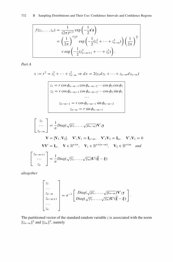
732 B Sampling Distributions and Their Use: Confidence Intervals and Confidence Regions
f .z1; : : : ; zn/ D 1
.2/n=2exp
��12
z0z�
D�1
2
� n�m2
exp
��12.z21 C � � � C z2n�m/
��1
2
�m2
� exp
��12.z2n�mC1 C � � � C z2n/
�:
Part A
x WD r2 D z21 C � � � C z2n�m) dx D 2.z1d z1 C � � � C zn�md zn�m/
z1 D r cos�n�m�1 cos�n�m�2 � � � cos�2 cos�1z2 D r cos�n�m�1 cos�n�m�2 � � � cos�2 sin�1
� � �zn�m�1 D r cos�n�m�1 sin �n�m�2
zn�m D r sin �n�m�1
2
4z1� � �
zn�m
3
5 D 1
�Diag.
p�1; : : : ;
p�n�m/V0
1y
V D ŒV1;V2�; V01V1 D In�m; V0
2V2 D Im; V01V2 D 0
VV0 D In; V 2 Rn�n; V1 2 R
n�.n�m/; V2 2 Rn�m and
2
4zn�mC1� � �zn
3
5 D 1
�Diag.
p�1; : : : ;
p�m/U0.b� � �/
altogether
2
66666664
z1: : :
zn�mzn�mC1: : :
zn
3
77777775
D ��1"
Diag.p�1; : : : ;
p�n�m/V0
1y
Diag.p�1; : : : ;
p�m/U0.b� � �/
#
:
The partitioned vector of the standard random variable z is associated with the normkzn�mk2 and kzmk2, namely

B-7 Sampling from the Multidimensional Gauss–Laplace Normal Distribution 733
kzn�mk2 C kzmk2
D z21 C � � � C z2n�m C z2n�mC1 C � � � C z2n
D 1
�2y0V1Diag.
p�1; : : : ;
p�n�m/Diag.
p�1; : : : ;
p�n�m/V0
1y
C 1
�2.b� � �/0U Diag.
p�1; : : : ;
p�m/Diag.
p�1; : : : ;
p�m/U0.b� � �/
D 1
�2y0V1Diag.�1; : : : ; �n�m/V0
1yC 1
�2.b� � �/0U Diag.�1; : : : ; �m/U0.b� � �/
D d z1d z2 � � �d zn�m�1d zn�mD rn�m�1dr.cos�n�m�1/n�m�1.cos�n�m�2/n�m�2
� � � cos2 �3 cos�2d�n�m�1d�n�m�2 � � �d�3d�2d�1:
The representation of the local .n�m/ dimensional hypervolume element in termsof polar coordinates .�1; �2; : : : ; �n�m�1; r/ has already been given by Lemma B.4.Here, we only transform the random variable r to Helmert’s random variable x.
x WD r2 W dx D 2rdr; dr D dx
2px; rn�m�1 D x.n�m�1/=2
rn�m�1dr D 1
2x.n�m�1/=2dx:
Part A concludes with the representation of the left pdf in terms of Helmert’s polarcoordinates
dF` D�1
2
� n�m2
exp� 12.z21 C � � � C z2n�m/d z1 � � �d zn�m
D 1
2
�1
2
� n�m2
xn�m�2
2 dx.cos�n�m�1/n�m�1.cos�n�m�2/n�m�2
� � � cos2 �3 cos�2d�n�m�1d�n�m�2 � � �d�3d�2d�1:
Part BPart B focuses on the representation of the right pdf, first in terms of the randomvariablesb�, second in terms of the canonical random variablesb�.
dFr D�1
2
�m2
exp
��12.z2n�mC1 C � � � C z2n/
�d zn�mC1 � � �d zn
z2n�mC1 C � � � C z2n D1
�2.b� � �/0A0A.b� � �/
d zn�mC1 � � �d zn D 1
�m=2jA0Aj1=2db�1 � � �db�m:

734 B Sampling Distributions and Their Use: Confidence Intervals and Confidence Regions
The computation of the local m-dimensional hyper volume element d zn�mC1 � � �d znhas followed Corollary B.3 which is based upon the matrix of the metric ��2A0A.The first representation of the right pdf is given by
dFr D�1
2
�m2
exp
��12.z2n�mC1 C � � � C z2n/
�d zn�mC1 � � �d zn
D�1
2
�m2 jA0Aj1=2
�m=2exp
�� 1
2�2.b� � �/0A0A.b� � �/
�db�1 � � �db�m:
Let us introduce the canonical random variables .b�1; : : : ;b�m/ which are generatedby the correlating quadratic form kb� � �k2A0A.
.b� � �/0A0A.b� � �/ D .b� � �/0U Diag
�1
�1; : : : ;
1
�m
�U0.b� � �/:
Here, we took advantage of the eigenspace synthesis of the matrix A0A DW N and.A0A/�1 DW N�1. Such an inverse normal matrix is the representing dispersionmatrix Dfb�g D .A0A/�1�2 D N�1�2.
UU0 D Im � U 2 SO.m/ WD fU 2n�m jUU0 D Im; jUj D C1gN WD A0A D U Diag.�1; : : : ; �m/U0 versus
N�1 WD .A0A/�1 D U Diag.�1; : : : ; �m/U0 subject to
�1 D ��11 ; : : : ; �m D ��1
m or �1 D ��11 ; : : : ; �m D ��1
m
jA0Aj1=2 D p�1 � � ��m D 1p�1 � � ��m
b�� � WD U0.b� � �/,b� � � WD U0.b� � �/
kb� � �k2A0A DW .b� � �/0A0A.b� � �/ D .b� � �/0Diag
�1
�1; : : : ;
1
�m
�.b� � �/:
The local m-dimensional hypervolume element db�1 � � �db�m is transformed to thelocal m-dimensional hypervolume element db�1 � � �db�m by
db�1 � � �db�m D jUjdb�1 � � �db�m D db�1 � � �db�m:Accordingly we have derived the second representation of the right pdf f .b�/.
dFr D�1
2
�m2 1
�m=2p�1 � � ��m
� exp
�� 1
2�2.b� � �/0Diag
�1
�1; : : : ; y
1
�m
�.b�� �/
�db�1 � � �db�m:

B-7 Sampling from the Multidimensional Gauss–Laplace Normal Distribution 735
Part CPart C is an attempt to merge the left and right pdf
dF D dF`dFr D 1
2
�1
2
� n�m2
x.n�m�2/=2dxd!n�m�1
��1
2
�m2 jA0Aj1=2
�mexp
��12.b� � �/0A0A.b� � �/
�db�1 � � �db�m or
dF D dF`dFr D 1
2
�1
2
� n�m2
x.n�m�2/=2dxd!n�m�1
��1
2
�m2 1
�mp�1 � � ��m
exp
�� 1
2�2.b�� �/0Diag
�1
�1; : : : ;
1
�m
�.b���/
�db�1 � � �db�m:
The local .n � m � 1/-dimensional hypersurface element has been denoted byd!n�m�1 according to Lemma B.4.
The fifth action item
Fifth, we are going to compute the marginal pdf ofb� BLUUE of �.
dF1 D f1.b�/db�1 � � �db�mas well as
dF1 D f1.b�/db�1 � � �db�minclude the first marginal pdf f1.b�/ and f1.b�/, respectively.The definition
f1.b�/ WD1Z
0
dx
Zd!n�m�1
1
2
�1
2
� n�m2
x.n�m�2/=2
��1
2
�m2 jA0Aj1=2.�2/m=2
exp
��12.b� � �/0A0A.b� � �/
�
subject to
1Z
0
dx
Zd!n�m�1
1
2
�1
2
� n�m2
x.n�m�2/=2 D 1
leads us to
f1.b�/ D�1
2
�m2 jA0Aj1=2
�mexp
��12.b� � �/0A0A.b� � �/
�:

736 B Sampling Distributions and Their Use: Confidence Intervals and Confidence Regions
Unfortunately, such a general multivariate Gauss-Laplace normal distributioncannot be tabulated. An alternative is offered by introducing canonical unknownparametersb� as random variables.The definition
f1.b�/ WD1Z
0
dx
Zd!n�m�1
1
2
�1
2
� n�m2
x.n�m�2/=2
��1
2
�m2 1
�m.�1�2 � � ��m�1�m/�1=2
� exp
�� 1
2�2.b�� �/0Diag
�1
�1; : : : ;
1
�m
�.b� � �/
�
subject to
1Z
0
dx
Zd!n�m�1
1
2
�1
2
� n�m2
x.n�m�2/=2 D 1
alternatively leads us to
f1.b�/ D�1
2
�m2 1
�m1p
�1 � � ��mexp
� 1
2�2
mX
iD1
.b�i � �/2�i
!
f1.b�1; : : : ;b�m/ D f1.b�1/ � � �f1.b�m/
f1.b�i / WD 1
�p�ip2
exp
��12
.b�i � �/2�i
�8i 2 f1; : : : ; mg:
Obviously the transformed random variables .b�1; : : : ; yb�m/ BLUUE of .�1; : : : ; �m/are mutually independent and Gauss-Laplace normal.
The sixth action item
Sixth, we shall compute the marginal pdf of Helmert’s random variable x D.n � rkA/b�2=�2 D .n �m/b�2=�2,b�2 BIQUUE �2,
dF2 D f2.x/dxincludes the second marginal pdf f2.x/.The definition
f2.x/ WDZd!n�m�1
1
2
�1
2
�n�m2
x.n�m�2/=2 �C1Z
�1db�1 � � �
C1Z
�1db�m
�1
2
�m2 jA0Aj1=2
�m
� exp
�� 1
2�2.b� � �/0A0A.b� � �/
�

B-7 Sampling from the Multidimensional Gauss–Laplace Normal Distribution 737
subject to
!n�m�1 DZd!n�m�1 D 2 � .n�m�1/=2
� .n�m�12
/;
according to Lemma B.4
C1Z
�1� � �
C1Z
�1db�1 � � �db�m
�1
2
�m2 jA0Aj1=2
�mexp
�� 1
2�2.b� � �/0A0A.b� � �/
�
DC1Z
�1d z1 � � �
C1Z
�1d zm
�1
2
�m2
exp
��12.z21 C � � � C z2m/
�
leads us to
p WD n � rkA D n �mp�
�n�m � 1
2
�D �
�1
2
��
�n �m � 1
2
�D �
n �m2
�D �
p2
�
f2.x/ D 1
2p=2� .p=2/xp2 �1 exp
��12x
�;
namely the standard pdf of the normalised sample variance, known as Helmert’s ChiSquare pdf 2p with p D n � rkA D n �m “degree of freedom”. If you substitutex D .n�rkA/b�2=�2 D .n�m/b�2=�2, dx D .n�rkA/��2db�2 D .n�m/��2db�2we arrive at the pdf of the sample varianceb�2, in particular
dF2 D f2.b�2/db�2
f2.b�2/ D 1
�r2p=2� .p=2/pp=2b�p�2 exp
��12pb�2
�2
�:
Here is our proof’s end.
Theorem B.12. (marginal probability distributions, special linear Gauss–Markov model with datum defect):
Efyg D A�
Dfyg D V�2subject to
A 2n�m; r WD rkA < minfn;mgEfyg 2 R.A/V 2n�n; rkV D n

738 B Sampling Distributions and Their Use: Confidence Intervals and Confidence Regions
defines a special linear Gauss–Markov model with datum defect of fixed effects� 2Rm and a positive definite variance-covariance matrix Dfyg D ˙ y ofmultivariate Gauss-Laplace distributed observations y WD Œy1; : : : ; yn�0.
b� D ACy subject to
2
64
b� D Ly “linear”
kLA � Imk2 D min “minimum bias”
trDfb�g D tr L˙ yL0 D min “best” and
b�2 D 1
n � rkA.y �Ab�/0˙�1
y .y � Ab�/ subject to
2
64Efb�2g D �2
Dfb�2g D 2�4
n � rkA
identifyb� BLIMBE of � andb�2 BIQUUE of �2.Part AThe cumulative pdf of the multivariate Gauss-Laplace probability distribution ofthe observation vector y D Œy1; : : : ; yn�0 2 Y
f .yjEfyg; Dfyg D ˙ y/dy1 � � �dyn
D 1
.2/n=21
j˙ y j1=2 exp
��12.y � Efyg/0˙�1
y .y� Efyg/�dy1 � � �dyn
is transformed by
˙ yDW0Diag.�1; : : : ; �n/WDW0Diag.p�1; : : : ;
p�n/Diag.
p�1; : : : ;
p�n/W
˙ 1=2y WD Diag.
p�1; : : : ;
p�n/W
˙ y D .˙ 1=2y /0˙ 1=2
y versus
˙�1y DW0Diag
�1
�1; : : : ;
1
�n
�W
DW0Diag
�1p�1; : : : ;
1p�n
�Diag
�1p�1; : : : ;
1p�n
�W
˙�1=2 WD Diag
�1p�1; : : : ;
1p�n
�W
˙�1 D .˙�1=2y /0˙�1=2
y
subject to the orthogonality condition
WW0 D In
ky � Efygk2˙�1yWD .y � Efyg/0˙�1
y .y� Efyg/

B-8 Multidimensional Variance Analysis, Sampling from the Multivariate 739
D .y �Efyg/0W0Diag
�1p�1; : : : ;
1p�n
�Diag
�1p�1; : : : ;
1p�n
�
�W.y �Efyg/0
D .y� � Efy�g/0.y� � Efy�g/ DW ky� �Efy�gk2Insubject to the star or canonical coordinates
y� D Diag
�1p�1; : : : ;
1p�n
�Wy D ˙�1=2
y y
f .yjEfy�g;Dfy�g D In/dy�1 � � �dy�
n
D 1
.2/n=2exp
��12.y� � Efy�g/0.y� �Efy�g/
�dy�
1 � � �dy�n
D 1
.2/n=2exp
��12ky� �Efy�gk2
�dy�
1 � � �dy�n
into the canonical Gauss-Laplace pdf.Part BThe marginal pdf ofb� BLUUE of �, is represented by
(1st version)
dF1 D f1.b�/d�1 � � �d�n:
B-8 Multidimensional Variance Analysis, Sampling fromthe Multivariate Gauss–Laplace Normal Distribution
Let x1; : : : ; xN denote a random sample from as k-variate Gauss-Laplace normaldistribution with � as the mean vector and ˙ as the variance-covariance matrix,such that
.B 370/ xi WD .Xi;1; : : : ;Xi;k/0
for i 2 f1; : : : ; N g. Let X�1 WD .x1; : : : ; xN /. The joint density of the random sam-ple is generated by the product of N multivariate normal densities. Let us denote theparameter space by f�;˙ I� 2 R
k;˙ positive definiteg DW ˝ . Here we describeestimation of the parameters from a multivariate Gauss-Laplace normal distributionand describe properties of these estimates. In addition, we care for inference for asimple, multiple, and partial correlation coefficients based on the normal randomsample. Of course, we have to proof that we can assume a multivariate Gauss-Laplace normal distribution. We add some methods for assessing Gauss-Laplacenormality and describe suitable transformation to normality.

740 B Sampling Distributions and Their Use: Confidence Intervals and Confidence Regions
B-81 Distribution of Sample Mean and Variance-Covariance
By the representation of the sample mean of the random sample x1; : : : ; xN by(B371) and the sample variance-covariance matrix by (B372)–(B375), namely thek � k dimensional matrix SN=.N � 1/ D fSjlg for all j; l 2 f1; : : : ; kg subject
to XDNP
iD1Xi;j =N . The sample variance-covariance matrix has k variances Sjj for
j 2 f1; : : : ; kg and k.k � 1/=2 possibly distinct covariances. Sjl for j; l; j; l 2f1; : : : ; kg. The generalized sample variance is the scalar quality jSN=.N � 1/jwhich determines the degree of “peakedness” of the joint density of x1; : : : ; xN andis a normal summary measure of variability in the sample.
�
�
�
�Table B.1 Sample mean, sample variance-covariance matrix
Sample mean
x^
N WDNP
iD1
xi (B371)
Sample variance-covariance matrix
SN WD NP
iD1
.xi � x^
N /.xi � x^
N /0 D NP
iD1
xi x0
i �N xi � x^
N xi � x^
N0 (B372)
SN =.N � a/ DW fSjl g for j; l 2 f1; : : : ; kg (B373)
Sjl WD NP
iD1
.Xi;j � X^
j /.Xi l � Xl /=.N � 1/ (B374)
Subject to
X^
j D NP
iD1
Xi;j N (B375)
Given a univariate random sample X1; : : : ;XN from a N.�; � 2/ population, thatthe sample mean X^ has a normal distribution with mean � and variance � 2=N ,the static .N � 1/S2=� 2 is distributed as a �2 variable and the two distributions areindependent. The corresponding distributional result for the k-variable situations isgiven by our previous result. We first define a multivariate distribution called theWishart distribution which is derived from the multivariate Gauss-Laplace normaldistribution as its sampling distribution of the sample statistics
NX
iD1.Xi �XN /.Xi �XN /
0 .B 376/
The Wishart distribution is a multivariate extension of the chi-square distribution.
Definition B.18. Wishart distribution
A random k-dimensional matrix W is said to follow a k-dimensional noncentralWishart distribution. Wk.˙ ; m; x/ with m degrees of freedom, parameter ˙ ,

B-8 Multidimensional Variance Analysis, Sampling from the Multivariate 741
and noncentrality parameter � WD �0P�1�0=2 if W can be represented as,
W WDmP
jD1xixj where xj for all j 2 f1; : : : ; mg are i:i:i:Nk.�;
P/ vectors. Provide
m:k the density function of W is
f .WI�;˙ / D jWj.m�k�1/=2 expftr.�˙�1W=2/g2km=2j˙ jm=2�k.m=2/ .B 377/
where �k.m=2/Dk.k�1/=4˘kjD1� . 12 .m C 1 � j // is the multivariate Gamma
functions. If�D 0, we say that W follows a central Wishart distribution Wk.˙ ; m/;since ˙ is p.d., it is clear that � D 0 if and only if � D 0. The additivityproperty of Wishart matrices states that if Wj
ind
� Wk.˙ ; mj /; j D 1; : : : ; J , thenJP
jD1Wj �Wk
�˙ ;
JP
jD1mj
�.
End of Definition B.18: Wishart distribution
Intermezzo
Before we proceed we must introduce results about the Fourier transform ofa random vector, namely called “characteristic function” being generalized inAppendix C to the “characteristic functional” for random functions, namelystochastic processes. We will introduce some lemmas and definitions.
Definition B.19. Characteristic function of a random vector
The characteristic function of a random vector X is Efexp i t 0xg define for everyvector t .
Definition B.20. Decomposition of a complex-valued function
Let the complex-valued function g.x/ be written as
g.x/ D g1.x/C ig2.x/ .B 378/
where g1.x/ and g2.x/ are real-valued. Then the expected value of g.X/ is
Efg.X/g D Efg1.x/g C iEfg2.x/g .B 379/
in particular,
Efexp.i t 0x/g D Efcos.t 0x/g C iEfsin.t 0x/g .B 380/

742 B Sampling Distributions and Their Use: Confidence Intervals and Confidence Regions
Lemma B.18. Product rule for independent variables
Let X0 WD .X.1/0X.2/0/. If X.1/ and X.2/ are independent and g.x/ D g.1/.x.1//g.2/.x.2//, then
Efg.X/g D Efg.1/.X.1//gEfg.2/.X.2//g .B 381/
Lemma B.19. Components of independent distribution data
If the component of X are independently distributed, then
Efexp.i t 0XN /g DNY
jD1Efi tjXj g .B 382/
Theorem B.20. Characteristic function of a vector-valued random variant oftype Gauss-Laplace distribution
The characteristic function of X which is Gauss-Laplace distribution according toN.�;˙ / is
Efexp.i t 0X/g D exp
�t 0�C 1
2t 0˙ t
�.B 383/
for any real vector t .
Theorem B.21. Characteristic function �.t/
If the random vector X has the density f .x/ and the characteristic function f .t/,then
f .x/ D 1
.2/
C1Z
�1: : :
C1Z
�1exp.�i t 0x/N .t/d!1 : : : d! .B 384/
and
f N .!/ D EfCi!0Xg DC1Z
�1: : :
C1Z
�1exp.Ci!0x/f .x/dx1 : : : dx .B 385/
illustrating synthesis and analysis
Here ends our intermezzo

B-8 Multidimensional Variance Analysis, Sampling from the Multivariate 743
f N .!/ D EfCi!0Xg DC1Z
�1: : :
C1Z
�1exp.Ci!0x/f .x/dx1 : : : dx .B 386/
Results: Distribution of xN and SN
Let x1; : : : ; xN denote a random sample from the Gauss-Laplace normal distribu-tion Nk.�; � /.
(a) The distribution of xN is Nk.��=N/(b) For N 2, SN follows a Wishart distribution Wk.˙
01N � 1/
(c) xN and SN are independently distributed.
Proof
Efexp.i t 0xN /g DNY
jD1Efexp.i t 0j xj /=N g D exp.t 0�C 1
2t 0.˙=N/t .B 387/
for N D 2 it follows
S2 D�x1� 1
2.x1 C x2/
�x1� 1
2.x1 C x2/
0C�x2 � 1
2.x1 C x2/
�x2 � 1
2.x1Cx2/
0
) S2 D 1
2.x1 � x2/.x1 � x2/0 .B 388/
Obviously .x1 � x2/p2 is distributed according to Nk.0;˙ / and S2 according to
Wk.˙ ; 1/
S3 D�
x1 � 13.x1 C x2 C x3/
�x1 � 1
3.x1 C x2 C x3/
0
C�
x2 � 13.x1 C x2 C x3/
�x2 � 1
3.x1 C x2 C x3/
0
C�
x3 � 13.x1 C x2 C x3/
�x3 � 1
3.x1 C x2 C x3/
0.B 389/
S3 D S2 C 2
3.x3 � x2 /.x3 � x2 /
0 .B 390/
subject to
x2 D1
3.2x2 C x3/ .B 391/

744 B Sampling Distributions and Their Use: Confidence Intervals and Confidence Regions
in general
xm D1
mC 1.mxm C xmC1/ and
SmC1 D Sm C m
mC 1.xmC1 � xm/.xmC1 � xm/0 .B 392/
B-82 Distribution Related to Correlation Coefficients
Since xi for all i 2 f1; : : : ; m C 1g are mutually independent and therefore�xmC1;Sm
�are functions only of xi for i 2 f1; : : : ; mg, it follows that
�xmC1;Sm
�
are independent of xmC1.By the hypothesis of induction we enjoy the independence of xm and Sm
xmC1;Sm and xmC1 .B 393/
are mutually independent. Thus, Sm is independent of�xm; xmC1
�and therefore
independent of xmC1�xm which follows aNk�0; mC1
m˙�mC1m
�xmC1 � xm
�.xmC1�
xm/0 are distributed as Wk .˙; 1/. Note that
cov�xi � xm; xn
� D 0 (B 394)
Which implies thath�
x1 � xN�; : : : ;
�xN � xN
�0i0is uncorrelated and therefore
independent of xN . In consequence, Sn is distributed independently of xN .
Results: Maximum likelihood estimation if � andP
Based on a random sample x1; : : : ; xN from a Nk .�; ˙/ distribution, the maximumlikelihood estimates of � and
Pare
b�ML D1
N
NX
iD1xi D xN ; .B 395/
and
bML D 1
N
NX
iD1
�xi � xN
� xi � X
^N
�0 D N � 1N
SN .B 396/
Proof
The likelihood function L .�; ˙ I x1; : : : ; xN / has the form shown on the rightside. The MLE’s of � and ˙ are denoted by b�ML and b
ML, and are the

B-8 Multidimensional Variance Analysis, Sampling from the Multivariate 745
values that maximize L .�; ˙ I x1; : : : ; xN /. Since ˙�1 is p.d., the distance�xN ��
�0˙�1 �xN ��
�in the exponent of the likelihood function is positive
unless� D XN . The MLE of � is then xN , since it is the value of � that maximizesthe likelihood function. We next maximize the following function with respect to˙ :
L.b�ML;˙/ Dexp
�� 12tr
�˙�1PN
iD1�xi � xN
� xi � X
^N
�0�
.2/Nk=2 j˙ jN=2 .B 397/
With AD˙;B D PNiD1
�xi � xN
� xi �X
^N
�0, and bDN=2, we can show that
bMLD 1
N
PNiD1
�xi � xN
� xi �X
^N
�0maximizes L.b�ML;˙/. The maximum
likelihood is
Lb�ML; bML
�D exp � Nk
2
.2/Nk=2 jbMLjN=20.B 397/
which completes the proof.
Corollary: Invariance property of MLE
Using the invariance property of MLE’s which states that the MLE of a function
g .�/ of a parameter � is gb�ML
�, we see that
1. The MLE of the function �0˙�1� is b�0MLb�1MLb�ML,
2. The MLE ofp�lj , the (l,j)th element of
Pis given by
pb�lj , the square root of
the MLE of the(l,j)th entry in bP
ML
Although the estimator b�ML is an unbiased estimator of �; bML is a biasedestimator of ˙ . analogous to the univariate case, an unbiased estimator of ˙ isb D 1
N�1SN . The unbiased estimators of� abd˙ denoted byb� and b respectivelyare complete sufficient statistics.Of course, you have realized that we gave no space to derive the Wishart distri-bution. Instead we refer to his works in Wishart (1928), Wishart (1931), Wishart(1955) as well as Wishart and Bartlett (1932). the general theory of multivariatestatistical analysis including the Gauss-Laplace multivariate normal distribution,the estimation of the mean vector and the variance-covariance matrix the distributionof sample correlation coefficients, the generalized t2 statistics and the distributionof the sample covariance matrix can be taken from the excellent review of Anderson(1958) including 413 references. finally we advice the readers to consider the worksof Koch (1988a), Koch (1988b), pp. 160–173
B.8 Distributions related to correlation coefficientsTraditionally we divide simple, multiple and partial correlations. Here we restrictour study to the analysis of the simple correlation based on i id bivariateGauss-Laplace normal samples.

746 B Sampling Distributions and Their Use: Confidence Intervals and Confidence Regions
�Xi;j;Xi;l
�for all i 2 f1; : : : ; N g .B 399/
where Xi;j and Xi;l denote the j th and l th components of the k - l dimensionalvector x. SupposeE
�Xi;j
� D�j ;E .Xi;l/ D�l , var�Xi;j
� D � zj ; var .Xi;l/ D � z
l andcorr
�Xi;j;Xi;l
� D jl .The exact sampling distribution of was first derived by Fisher (1955) who showedthat for D 0 the statistic
pN � 2^p1� is distributed as t with (N-2) degrees
of freedom. He introduced the Z-transformation,
Z WD 1
2
�1C ^=1 � ^� .B 400/
and proved that even for relative small samples it is approximately Gauss-Laplacenormally distributed, and that as N increases the variance of the Z-transformationrapidly becomes nearly independent of converging to 1=.N � 3/. In 1938,F. N. David (1938) published tables of the exact sampling distribution of ^ for D 0.0:1/0:9,N DB.1/25; 50; 100; 200; 400; ^D�1.0:01/C1, and investigatedthe accuracy of the approximate distributions suggested by R.H. Fisher. She foundapproximate formulas for the mean/variance of Z: They were “extraordinarilyaccurate even for the low values of N provided jj is not too near unity”. Hotdling(1953) intensively studied the mathematical properties of the distribution functionof ^ and the suggested improvements of the Z-transformation in terms of ahypergeometric function. Beside discussing methods of interpolating the density healso calculated moments of ^. From the vast reference list of the subject we liketo mention the contribution of Soper et al. (1955), Kraemer (1973), Wilcox (1997)and Green (1952) as well as Khan (1994).
Example B: Correlation coefficient, “iid” Gauss-Laplace two dimensional normal
We start from the two dimensional Gauss-Laplace normal observations .xi ; yi /for N-independent identical distributed data .“i id 00/ estimated by BLUUE andBIQUUE. By a special decomposition we shift the sample distribution into twonormal distributions relating to.b�1;b�2/ on the one side and to
�b�21b�
22b�12
�or�b�21b�
2212
�on the other side.
b12 indicates the sample correlation coefficient via the characteristic function basedon Fourier-Stieltjes integration we derive the sampling distribution of the correlationcoefficientb12 .12/ using tables of David (1954).“N independently, identically distributed observations : iid”“Gauss-Laplace normal, two-dimensional observations: .xi ; yi / for all i 2f1; : : : ; N g”

B-8 Multidimensional Variance Analysis, Sampling from the Multivariate 747
“Probability density”
f .x; y/ D 1
2
1
�1�2p1 � 2 exp� 1
2 .1 � 2/
�".x � �1/�12
C 2 .xi�1/ .y � �2/�1�2
C .y � �2/2�22
#
.B 31/
f .x1; : : : ; xN ; y1; : : : ; yN / DNY
iD1f .xi ; yi / D f .x1; y1/ � � � .xN ; yN /
D
1
2�1�2p1 � 2
!N
exp
� 1
2 .1 � 2/NX
iD1
.xi � �1/2
�21� 2 .xi � �1/ .yi � �2/
�1�2C .y � i �mu2/
2
�22
!!
.B 32/
BLUUE W �1 D1
N
NX
iD1xi D k0x=N .B 33/
BLUUE W �2 D1
N
NX
iD1yi D k0y=N .B 34/
BIQUUE:
�^21 D
1
N � 1NX
iD1
�xi � �1
�2 D �x � k�1�0 �
x � k�1�= .N � 1/ .B 35/
�^22 D
1
N � 1NX
iD1
�yi � �1
�2 D �y � k�1�0 �
y � k�2�= .N � 1/ .B 36/
�12 D1
N � 1NX
iD1.xi ��1 /.yi ��2 / D .x�k�1 /0.y�k�2 /=.N � 1/ .B 37/
“Decomposition”

748 B Sampling Distributions and Their Use: Confidence Intervals and Confidence Regions
NX
iD1.xi ��1/2 D
NX
iD1Œ.xi �b�1/.�1��1 /�2 D .N�1/�1 2CN.�1��1 /2 .B39/
NX
iD1.yi ��2/2 D
NX
iD1Œ.yi �b�2/.�2 ��2 /�2 D .N� 1/�2 2CN.�2��2 /2 .B40/
NX
iD1.xi ��2/.yi ��2/D .N� 1/12�1 �2 C N.�1 � �1 /.�2 � �2 / .B41/
f .x1; : : : ; xN ; y1; : : : ; yN / D
1
2�1�2p1 � 2
!N
� exp
�� N
2.1�2/�.�1 �b�1/2
�21� 212.�1 �b�1/.�2 �b�2/
�1�2C .�2 �b�2/2
�22
�
� exp
�� N � 12.1� 212/
�b�21�21� 212b12b�1b�2
�1�2C b�
22
�22
�.B42/
“Product of two normal distributions”
First part, marginal distribution
C1Z
�1
C1Z
�1
0
B@
1
2�1�2
q1 � 212
1
CA exp
� N
2.1� 212/
".�1 �b�1/2
�21
� 212.�1 �b�1/.�2 �b�2/�1�2
C .�2 �b�2/2�22
#
db�1db�2
!
.B43/
“Fourier-Stieltjes analysis”
f �.!/ DZ.exp i!x/f .x/dx , .B44/
, f .x/ D 1
2
C1Z
�1.exp i!x/f .x//f ^.!/d! .B45/
First part of the marginal normal distribution

B-8 Multidimensional Variance Analysis, Sampling from the Multivariate 749
1
2�1�2p1 � 12
Z C1Z
�1db�1db�2 exp� N
2.1� 12/21 � i t1�21
.�1 �b�1/2
� expC N
2.1� 212/212
1 � i t2�1�2
.�1 �b�1/.�2 �b�2/2
� exp� N
2.1� 12/21 � i t3�22
.�2 �b�2/2 .B46/
“abbreviations”
�1 WD N
2.1� 212/.�1 �b�1/2
�21D �1.b�1/ .B47/
expCit1�1 D exp it1N
2.1� 212/.�1 �b�1/2
�21
�2 WD N
2.1� 212/212
.�1 �b�1/.�2 �b�2/�1�2
D �2.b�1;b�2/ .B48/
expCit2�2 D expCit2N
2.1� 212/212
.�1 �b�1/.�2 �b�2/�1�2
“First part of the marginal normal distribution”
1
2�1�2
q1 � 212
Z C1Z
�1exp� N
2.1� 212/�1 � i!1�21
.�1 �b�1/2
� 212.1C i!2/�1�2
.�1 �b�1/.�2 �b�2/
C 1 � i!3�22
.�2 �b�2/2db�1dcmu2
D .1 � 212/1=2Œ.1 � i!1/.1 � i!3/� 212.1C i!2/2�1=2
.B49/
“Check yourself the integral’
expŒ�˛x2 C ˇxy � �y2�dxdy”
“Second part of the marginal normal distribution”

750 B Sampling Distributions and Their Use: Confidence Intervals and Confidence Regions
.1 � 212/N�12
Œ.1� it1/.1� it3/� 212.1C it2/�N�12
exp
�N � 1
2.1�212/�b�21�21� 212b12b�1b�2
�1�2C b�
22
�22
�
.B50/
f .x1; : : : ; nN ; y1; : : : ; yN /dx1 : : : dxN dy1 : : : dyN
) f .x1; y1/ : : : f .xN ; yN /dx1dy1 : : : dxN dyN
f .b�1;b�2/f .b�1;b�2;b�12/db�1db�2db�1db�2db�12 .B51/
f .x1; : : : ; xN ; y1; : : : ; yN / D p1.b�1;b�2/p2.b�1;b�2;b�12/“first”
f N1 .t1; t2; t3/ f1.b�1;b�2/
pN1 .t1; t2; t3/ D.1� 212/
N�12
Œ.1 � i t1/.1 � i t3/� 212.1C i t2/2�.B52/
“second”
p.g1; g2; g3/ D .1 � 212/N�12
.2n/3
Z Z C1Z
�1
exp.�i!1�1 � i!/2�2 � i!3�3/Œ.1 � i t1/.1 � i t3/� 212.1C i t2/2�
� d!1d!2d!3 .B53/
p.b12/ D .1 � 212/N�12
.N � 3/Š .1 �b212/
N�42
dN�2
d.b12/
N�20
B@
arccos.�12b�12/q1 � 212b212
1
CA (B.1)
End of Lemma Example
As a specific example, we consider the confidence interval of the confidencecoefficient 0.95 on the correlation of 0.782 observed by a sample of ten. UsingGraph 4 of David (1954) we find the two limits are 0.34 and 0.98 . This result leadsus to the interval 0:34 < 12 < 0:98 (Anderson 1958, p 72).
Lemma B (probability interval for the correlation coefficient, functional determi-nant: David 1954, pp. xxxv–xxxviii):
ˇˇˇ
@.x1; : : : ; xN ; y1; : : : ; yN /
@.b�1;b�2I�1; : : : ; �N�1; �1; : : : ; �N�1/
ˇˇˇ D N
subject to the Helmert transformation

B-8 Multidimensional Variance Analysis, Sampling from the Multivariate 751
x1 D b�1 C 1p2 � 1�1 C
1p3 � 2�2 C � � � C
1pN.N � 1/�N�1
x2 D b�1 � 1p2 � 1�1 C
1p3 � 2�2 C � � � C
1pN.N � 1/�N�1
x3 D b�1 � 2p3 � 2�2 C � � � C
1pN.N � 1/�N�1
: : :
xN D b�1 � 1pN.N � 1/�N�1
y1 D b�2 C 1p2 � 1�1 C
1p3 � 2�2 C � � � C
1pN.N � 1/�N�1
y2 D b�2 � 1p2 � 1�1 C
1p3 � 2�2 C � � � C
1pN.N � 1/�N�1
y3 D b�2 � 2p3 � 2�2 C � � � C
1pN.N � 1/�N�1
: : :
yN D b�2 � 1pN.N � 1/�N�1
p.b�1;b�2; �j ; �j / D p.xi ; y; i/ˇˇˇˇ
@.xi ; yi /
@.b�1;b�2; �j ; �j /
ˇˇˇˇ
for all j D 1; 2; : : : ; N � 1I i D 1; 2; : : : ; N

Appendix CStatistical Notions, Random Eventsand Stochastic Processes
Definitions and lemmas relating to statistics, random events as well as stochasticprocesses are given, neglecting their proofs. First, we review statistical momentsof a probability distribution of random vectors and list the Gauss-Laplace normaldistribution by introducing the notion of a quasi-normal distribution. As the end ofAppendix C1 we take reference to two lemmas about the Gauss-Laplace 3� rule,namely the Gauss-Laplace inequality and the Vysochainskii-Potunin inequality.Appendix C2 reviews the spatial linear error propagation as well as the generalnonlinear error propagation based on yDg.x/ introducing the moments of second,third and fourth order. The special role Jacobi matrix as well as the Hesse matrix isclassified. Appendix C3 reviews useful identities likeEfyy0˝j g andEfyy0˝yy0gas well as D Ef.y �Efyg/.y �Efyg/0˝ .y �Efyg/g relating to the matrix ofobliquity and � WD Ef.y � Efyg/.y � Efyg/0 ˝ .y � Efyg/.y � Efyg/0g C : : :relating to the matrix of courtosis.
Appendix C.4 newly introduces scalar-valued stochastic processes of one param-eter enriched by Appendix C.5 reviewing characteristics of a one parameterstochastic processes like non-stationary, stationary and cryodic stochastic pro-cesses. Extensive simple examples are presented in Appendix C.6 including ARIMAprocesses namely. Appendix C.7 introduce the important WIENER process of typeORNSTEIN- UHLENBECK, WIENER process with drift integrated WIENERprocess. The spectral analysis of one parameter is enriched by 14 exampleslike the DIRAC representation, spectral densities, band limited white noise. Anextensive introduction into scalar-, vector-, and tensor-valued stochastic processesin Appendix C.9 refers to the characteristic functional the moment representationsof stochastic processes for scalar-valued and vector-valued qualities, for statis-tical homogeneous and isotropic fields of multi-point systems. The Appendix isspecified by Example C.9.1 on the topic of two-dimensional Euclidean networksunder the postulates of homogeneity and isotropy in the statistical sense, byExample C.9.2 on criterion matrices for absolute coordinates in a space time astro-nomic frame of reference, for instance represented in scalar-valued spherical har-monic, by Example C.9.3 on space gravity spectroscopy illustrating the benefits of
E. Grafarend and J. Awange, Applications of Linear and Nonlinear Models,Springer Geophysics, DOI 10.1007/978-3-642-22241-2,
753
© Springer-Verlag Berlin Heidelberg 2012

754 C Statistical Notions, Random Events and Stochastic Processes
TAYLOR-KARMAN structured criterion matrices, by Example C.9.4 on Nonlocalprediction and Example C.9.5 on Nonlocal Time Series Analysis.
C-1 Moments of a Probability Distribution,the Gauss–Laplace Normal Distribution and theQuasi-Normal Distribution
First, we define the moments of a probability distribution of a vector valued randomfunction and explain the notion of a Gauss-Laplace normal distribution and itsmoments. Especially we define the terminology of a quasi - Gauss-Laplace normaldistribution.
Definition C.1. (statistical moments of a probability distribution):
(1) The expectation or first moment of a continuous random vector ŒXi � for all i D1; : : : ; n of a probability density f .x1; : : : xn/ is defined as the mean vector � WDŒ�1; : : : ; �n� of EfXig D �i
�i WD EfXig DZ C1
�1: : :
Z C1
�1xif .x1; : : : ; xn/dx1 : : : dxn: (C1)
The first moment related to the random vector Œei � WD ŒXi � EfXig� is called firstcentral moment
i WD EfXi ��i g D EfXig � �i D 0: (C2)
(2) The second moment of a continuous random vector ŒXi � for all i D 1; : : : ; n ofa probability density f .x1; : : : ; xn/ is the mean matrix
�ij WD EfXiXj g DZ C1
�1: : :
Z C1
�1xixj f .x1; : : : ; xn/dx1 � � �dxn: (C3)
The second moment related to the random vector Œei � WD ŒXi �EfXi g� is calledvariance - covariance matrix or dispersion matrix Œ�ij �, especially variance ordispersion �2 for i D j or covariance for i ¤ j :
ii D �2i D V fXig D DfXi g WD Ef.Xi ��i /2g (C4)
ij D �ij D C fXi ;Xj g WD Ef.Xi ��i /.Xj � �j /g (C5)
Dfxg D Œ�ij � D ŒC fXi ;Xj g� D Ef.x�Efxg/.x�Efxg/0g: (C6)
x WD ŒX1; : : : ;Xn�0 is a collection of the n� 1 random vector. The random variables
Xi ;Xj for i ¤ j are called with respect to the central moment of second orderuncorrelated if �ij D 0fori ¤ j . (3) The third central moment with respect to therandom vector Œei � WD ŒXi �EfXig� defined by

C-1 Moments of a Probability Distribution, the Gauss–Laplace Normal 755
ijk WD Efeiej ekg D Ef.Xi � �i /.Xj ��j /.Xk � �k/g (C7)
contains for i D j D k the vector of obliquity with the components
� i WD Efe3i g (C8)
Uncorrelation with respect to the central moment up to third order is defined by
Efen1i1 en2i2 en3i3 g D3Y
jD1Efenjij g
2
481 � i1 ¤ i2 ¤ i3 � n
and0 � n1 C n2 C n3 � 3:
(C9)
(4) The fourth central moment relative to the random vector Œei � WD ŒXi �EfXig�
ijk` WD Efeiej eke`g D Ef.Xi � �i /.Xj ��j /.Xk ��k/.X` � �`/g (C10)
leads for i1 D i2 D i3 D i4 to the vector of curtosis with the components
i WD Efe4i g � 3f�2i g2 (C11)
Uncorrelation with respect the central moments up the fourth order is defined by
Efen1i1 en2i2 en3i3 en4i4 g D4Y
jD1Efenjij g
2
481 � i1 ¤ i2 ¤ i3 ¤ i4 � n
und0 � n1 C n2 C n3 C n4 � 4 :
(C12)
(5) The central moments of the nth order relative to the random vector Œei � WDŒXi �EfXig� are defined by
i1:::in WD Efei1 : : : eing D Ef.Xi1 � �i1/ : : : .Xin � �in/g (C13)
A special distribution is the Gauss-Laplace normal distribution of random vectorsin R
n: Note that alternative distributions on manifolds exist in large numbers, forinstance the von Mises distribution on S
2 or the Fisher distribution on S3 of Chap. 7.
Definition C.2. (Gauss-Laplace normal distribution):
An n � 1 random vector x WD ŒX1; : : : ;Xn�0 is a Gauss-Laplace normal distribution
if its probability density f .x1; : : : xi / has the representation
f .x/ D .2/�n=2j˙ j�1=2 expŒ�12.x � Efxg/0˙�1.x � Efxg/� (C14)

756 C Statistical Notions, Random Events and Stochastic Processes
Symbolically we can writex � N .�;˙ / (C15)
with the moment of first order or mean vector � WD Efxg and the central momentof second order or variance – covariance matrix˙ WD Ef.x�Efxg/.x�Efxg/0g:The moments of the Gauss-Laplace normal distribution are given next.
Lemma C.3. (moments of the Gauss-Laplace normal distribution):
Let the n � 1 random vector x WD ŒX1; : : : ;Xn�0 follow a Gauss-Laplace normal
distribution. Then all central moments of odd order disappear and the centralmoments of even order are product sums of the central moments of second orderexclusively.
Efei1 : : : eing D 08n D 2mC 1;m D 1; : : : ;1 (C16)
Efei1 : : : eing D fct.�2i1 ; �i1i2 ; : : : ; �2i2; : : : ; �2in /8n D 2m;m D 1; : : : ;1 (C17)
ij D �ij ; i i D �2i ; (C18)
ijk D 0; (C19)
ijk` D ij k` C ikj` C i`jk; (C20)
iijj D iijj C 2ij ij D �2i �2j C 2�2ij ; i i i i D 3.�2i /2 (C21)
ijk`m D 0; (C22)
i1i2:::i2m�2i2m�1i2m D i1i2:::i2m�2i2m�1i2m C i1i2:::i2m�3i2m�1i2m�2i2m C : : :Ci2i3:::i2m�1i1i2m: (C23)
The vector of obliquity WD Œ 1; : : : ; m�0 and the vector of curtosis WDŒ�1; : : : ; �m�
0 vanish.A weaker assumption compared to the Gauss-Laplace normal distribution is theassumption that the central moments up to the order four are of the form (C18)–(C21). Thus we allow for a larger class of distributions which have a similarstructure compared to (C18)–(C21).
Definition C.4. (quasi-Gauss-Laplace normal distribution):
A random vector x is quasi-Gauss-Laplace normally distributed if it has a contin-uous symmetric probability distribution f .x/ which allows a representation of itscentral moments up to the order four of type (C18)–(C21).Of special importance is the computation of error bounds for the Gauss-Laplacenormal distribution, for instance. As an example, we have the case called the 3�

C-2 Error Propagation 757
rule which states that the probability for the random variable for X falling away,from its mean by more than three standard deviations (SDs) is at most 5%,
P fjX � �j 3�g � 4
81< 0:05: (C24)
Another example is the Gauss-Laplace inequality, that bounds the probability forthe deviation from the mode �.
Lemma C.5. (Gauss inequality):
The expected squared deviation from the mode � is
P fjX � �j rg � 4�2
9r2forallr
p4=3 � (C25)
P fjX � �j rg � 1 � .r=p3�/forallr �p4=3 � (C26)
subject to �2 WD Ef.X� �/2g.Alternatively, we take advantage of the Vysochanskii–Potunin inequality.
Lemma C.6. (Vysochanskii–Potunin inequality):
The expected squared deviation from an arbitrary point ˛ 2 is
P fjX � ˛j rg � 42
9r2forallr
p8=3 (C27)
P fjX � ˛j rg � 42
3r2� 13
forallr �p8=3 (C28)
subject to 2 WD Ef.X � ˛/2g:References about the two inequalities are Gauss (1823), Pukelsheim (1994).
C-2 Error Propagation
At the beginning we note some properties of operators “expectation E” and “dis-persion D”. Those derivatives can be taken from Pukelsheim (1993) and Teuniseen(1989b, 1990). Afterwards we review the special and general, in particular nonlinearerror propagation.
Lemma C.7. (expectation operators EfXg ):
E is defined as a linear operator in the space of random variables in Rn, also called
expectation operator. For arbitrary constants ˛; ˇ; ı 2 R there holds the identity

758 C Statistical Notions, Random Events and Stochastic Processes
Ef˛Xi C ˇXi C ıg: (C29)
Let A and B be two m � n and m � ` matrices and ı an m � 1 vector of constantsx WD ŒXi ; : : : ;Xn�
0 and y WD ŒYi ; : : : ;Yn�0 two n � 1 and ` � 1 random vectors
such thatEfAXC BXC ıg D AEfxg C BEfyg C ı (C30)
holds. The expectation operator E is not multiplicative that is
EfXiXj g D EfXigEfXj g C C fXi ;Xj g ¤ EfXigEfXj g; (C31)
if Xi and Xj are correlated.
Lemma C.8. (special error propagation):
Let y be an n � 1 dimensional random vector which depends linear of the m � 1dimensional random vector x by means of a constant n � m dimensional matrix Aand of a constant dimensional vector ı of the form y WD Ax C ı. Then hold the“error propagation law”
Dfyg D DfAxC ıg D ADfxgA0: (C32)
The dispersion function D is not addition, in consequence a nonlinear operatorthat is
DfXi C Xj g D DfXig CDfXj g C 2C fXi ;Xj g ¤ DfXi g CDfXj g; (C33)
if Xi and Xj are correlated.The “special error propagation law” holds for a linear transformation x !y D Ax C ı. The “general nonlinear error propagation” will be presented byLemmas C.7 and C.8. The detailed proofs are taken from Chap. 8, Examples.
Corollary C.9. (“nonlinear error propagation”):
Let y D g.x/ be a scalar valued function between one random variable x and onerandom variable y. g(x) is assumed to allow a Taylor expansion around the fixedapproximation point �0 W
g.x/ D g.�0/C g0.�0/.x � �0/C 12g00.�0/.x � �0/2 CO.3/
D �0 C �1.x � �0/C �2g.�0/2 CO.3/ : (C34)
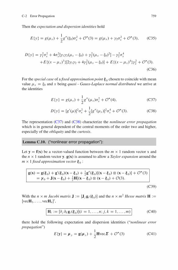
C-2 Error Propagation 759
Then the expectation and dispersion identities hold
Efyg D g.�x/C 1
2g00.�0/�2x CO�.3/ D g.�x/C �2�2x CO�.3/; (C35)
Dfyg D �21 �2x C 4�2x Œ�1�2.�x � �0/C �22 .�x � �0/2� � �22 �4xCEf.x � �x/3gŒ2�1�2 C 4�22 .�x � �0/�CEf.x � �x/4g�22 CO�.3/:
(C36)
For the special case of a fixed approximation point �0 chosen to coincide with meanvalue �x D �0 and x being quasi - Gauss-Laplace normal distributed we arrive atthe identities
Efyg D g.�x/C 1
2g00.�x/�2x CO�.4/; (C37)
Dfyg D Œg0.�/�2�2x C1
2Œg00.�x/�2�4x CO�.3/: (C38)
The representation (C37) and (C38) characterize the nonlinear error propagationwhich is in general dependent of the central moments of the order two and higher,especially of the obliquity and the curtosis.
Lemma C.10. (“nonlinear error propagation”):
Let y D f.x/ be a vector-valued function between the m � 1 random vector x andthe n � 1 random vector y. g.x/ is assumed to allow a Taylor expansion around them � 1 fixed approximation vector �0 W
g.x/ D g.�0/C g0.�0/.x � �0/C 12g00.�0/Œ.x � �0/˝ .x � �0/�CO�.3/
D 0 C J.x � �0/C 12HŒ.x � �0/˝ .x � �0/CO.3/:
(C39)
With the n �m Jacobi matrix J WD ŒJjgi .�0/� and the n � m2 Hesse matrix H WDŒvecH1; : : : ; vecHn�
0;
Hi WD Œ@j @kgi .�0/�.i D 1; : : : ; nI j; k D 1; : : : ; m/ (C40)
there hold the following expectation and dispersion identities (“nonlinear errorpropagation”)
Efyg D �y D g.�x/C1
2Hvec˙ CO�.3/ (C41)

760 C Statistical Notions, Random Events and Stochastic Processes
Dfyg D †y D J†J 0 C 1
2J � Œ† ˝ .�x � �0/0 C .�x � �0/0 ˝†�H0
C 12
HŒ† ˝ .�x � �0/C .�x � �0/˝†�J0
C 14
H Œ† ˝ .�x � �0/.�x � �0/0 C .�x � �0/.�x � �0/0 ˝†C.�x � �0/˝† ˝ .�x � �0/0 C .�x � �0/0 ˝† ˝ .�x � �0/�H0
C12
J �Ef.x� �x/.x ��x/0 ˝ .x � �x/0gH0
C12
H �Ef.x� �x/˝ .x � �x/.x ��x/0gJ0
C14
H � ŒEf.x ��x/.x� �x/0 ˝ .x ��x/g � .�x � �0/0
C.�x � �0/ �Ef.x� �x/0 ˝ .x � �x/.x � �x/0gC.I˝ .�x � �0// �Ef.x� �x/.x � �x/0 ˝ .x� �x/0gCEf.x ��x/˝ .x ��x/.x� �x/0g � ..�x � �0/0/˝ I/�H0
C14
H � f.x ��x/.x � �x/0 ˝ .x ��x/.x � �x/0g�vec†.vec†/0�H0 CO�.3/:
(C42)
In the special case that the fixed approximations vector �0 coincides to themean vector �x D �0 and the random vector x is quasi-Gauss-Laplace normallydistributed the following identities hold:
Efyg D �y D g.�x/C 12Hvec† CO�.4/ .C � 43/
Dfyg D †y D J†J 0 � 14Hvec†.vec†/0H0
C14
H �Ef.x� �x/.x � �x/0 ˝ .x � �x/.x � �x/
0g �H0 CO�.3/
D J†J0 C 1
4HŒ† ˝† CEf.x� �x/
0 ˝† ˝ .x ��x/g� �H0 CO�.3/:
(C44)
C-3 Useful Identities
Notable identities about higher order moments are the following.

C-3 Useful Identities 761
Lemma C.11. (identities: higher order moments):
(a) Kronecker-Zehfuss products #1
Efyy0g D Ef.y�Efyg/.y� Efyg/0g C EfygEfyg0 (C45)
Efyy0˝ yg D Ef.y�Efyg/.y� Efyg/0˝ .y �Efyg/gCEfyy0g ˝ Efyg C Efy˝ Efyg0˝ ygCEfyg ˝Efyy0g � 2Efyg ˝ Efyg0˝Efyg (C46)
Efyy0˝ yy0g D G �‰ ˝ Efyg0 �Efyg0˝‰�‰ 0 ˝ Efyg �Efyg ˝‰ 0 CEfyy0g ˝ Efyy0gCEfy0˝ Efyy0g ˝ yg C Efy˝ ygEfy˝ yg0�2EfygEfyg0˝ EfygEfyg0: (C47)
(b) Kronecker products #2
‰ W D Ef.y�Efyg/.y� Efyg/0˝ .y �Efyg/g (C48)
G W D Ef.y�Efyg/.y� Efyg/0˝ .y �Efyg/.y� Efyg/0g�Ef.y�Efyg/.y� Efyg/0˝ Ef.y�Efyg/.y� Efyg/0g�Ef.y�Efyg/0˝ Ef.y� Efyg/.y�Efyg/0g ˝ .y �Efyg/g�Ef.y�Efyg/˝ .y �Efyg/gEf.y� Efyg/0˝ .y � Efyg/0g: (C49)
The n2�nmatrix‰ contains the components of obliquity, the n2�n2 matrixG thecomponents of curtosis relative to the n � 1 central random vector y � Efyg.
(c) Covariances between linear and quadratic forms
C fF1yC d1;F2yC d2g WD Ef.F1yC d1 � EfF1yC d1g/.F2yC d2�EfF2yC d2g/0g D F1†F 2
(C50)
(linear error propagation)
CfFyC d; y0Hyg WD Ef.FyC d � EfFyC d g/.y0Hy� Efy0Hyg/gD FŒEfyy0˝ y0g �EfygEfy0˝ y0g�vecH
D 1
2F‰ 0vec.HCH0/C F†.HCH0/Efyg (C51)

762 C Statistical Notions, Random Events and Stochastic Processes
C fy0Gy; y0Hyg WD Ef.y0Gy �Efy0Gyg/.y0Hy� Efy0Hyg/gD .vecG/0ŒEfyy0˝ yy0g � Efy˝ ygEfy0˝ y0g�vecH
D 1
4Œvec.GCG0/�0Gvec.HCH0/
�12Œvec.GCG0/�0.‰ 0 ˝ Efyg C‰ ˝ Efyg0/vec.HCH0/
C12
trŒ.GCG0/†.HCH0/†�C Efyg0.GCG0/†.HCH0/Efyg:(C52)
(d) quasi-Gauss-Laplace-normally distributed data
C fF1yC ı;F2yC ı2g D F1†F 2 (C53)
(independent from any distribution)
C fFyC ı; y0Hyg D F†.HCH0/Efyg (C54)
C fy0Gy; y0Hyg D 1
2trŒ.GCG0/˙ .HCH0/˙ �
CEfyg0.GCG0/˙ .HCH0/Efyg: (C55)
C-4 Scalar – Valued Stochastic Processes of One Parameter
We have previously reviewed the moments of a probability distribution up to orderfour. The deviation was based on integration from minus infinity to plus infinity, Adifferent concept is needed if we work with distributions on manifolds. For instance,we are confronted with the problem to find a distributions for data on a circle or asphere or on a hypersphere. As mentioned before, directional measurements, alsocalled angular observations or longitudinal data are not Gauss-Laplace distributed,but enjoy a von Mises-Fisher distribution in S
� � RC1
Example C.4.1: p=1 (von Mises, 1918)
f .�j�; �/ D Œ2I0.�/��1 expŒ� cos.� � ��/� (C56)
Example C.4.2: p=2, (Fisher, 1953)

C-4 Scalar – Valued Stochastic Processes of One Parameter 763
f .�;˚ k ��;�˚ ; �/ D �
4 sinh �expŒcos˚ cos�˚ cos.� � ��/C sin˚ sin�˚�
D �
4 sinh �exp � < �jX > (C57)
Here, we have introduced the circular normal distribution CN.�; �/ parameterizedby the mean direction �.0 � �� 2/ and by the concentration parameter�.� > 0/, the reciprocal of a dispersion measure. The spherical normal distribu-tion CN.�� ; �˚; �/ is parameterize by the “longitudinal direction, lateral meandirection .�� ; �˚/” and the concentration parameter �, the reciprocal dispersionmeasure. We note that the p-spherical normal distribution is an element of theexponential class.Most important examples of the circular normal (R. von Mises) distributions arephase observation within the Global Positioning System (“Global Problem Solver”)according to Cai et al.(2007) and the spherical normal (Fisher) distribution forspherical harmonic analysis-synthesis (Fourier-Legendre functions) describing thegravitational field within gravities, electrostatics and magnetostaties according toFisher et al. (1981), Kent (1983), Mardia (1972), Man (2005), Mc Fadden and Jones(1981) and Roberts and Ursell (1960).There have been made studies to consider an ellipsoidal reference to analyzethe proper reference field of celestial bodies like the Earth, the Moon, or anyother planetary body. The ellipsoid-of-revolution is the equilibrium figure of typeMacLaurin which represents to first order of the Earth, the Moon, Mars or otherplanets even the Jacobi triaxial reference figure is a better approximation following,for instance Chandra Sekhar (1969). We leave the question: what is the characteristicdistribution of a ellipsoid-of-revolution or a triaxial ellipsoid open!A random event X is the result of a random experiment under a given condition.If these conditions change it might have an influence on the result of randomexperiment, namely to the probability distribution. If we consider the varyingconditions on the random quantities X D X.t/, we arrive at the random effectswhich depend on the deterministic parameter t. We illustrate the new detaileddefinition of one parameter stochastic process.
Example C.4.1
We measure the temperature of a point continuously by a sensor for 3 years.Naturally we model the sensor recording by a graph shown in Fig. C.1. Actuallywe find a random variable which is function of the continuous parameter “time t”,namely X.t/. Every year we receive a temperature profile which is a deterministicfunction of time t W xD x.t/; 0 � t � 1. In this form x.t/ is understoodas realization of the random variable X.t/. Neglecting the influence of climatechanges the function x D x.t/ is cyclic. We introduce the generalized randomexperiment “continuous measurement of temperature over one year” and refer it tofX.t/j0 � t � tg. Actually one could represent climate changes by a trend function.The character of a generalized random experiment is very obvious since for closelymeasuring points ti and tiC1 range in the second up to the minute.

764 C Statistical Notions, Random Events and Stochastic Processes
Fig. C.1 Graph of the function f(t) over a period of 1 year or 12 months. Two years recording:trajectories of the stochastic process
Example C.4.2
Alternatively we consider the length L=60 mm of Nylon wires and the designcondition of a variance of 0.5 mm produced by one machine under equal conditions.If we analyzed the dependence of the diameter of a function of the distance tfrom the initial point, we receive for any measurement of the wire a functionx D x.t/; 0 � t � L. These functions differ from wire to wire, but these isno significant difference between the functional different wires. Indeed we assumechanges to the constant condition of the wire. The random variations of the diameterare in the range of ˙0.02 mm and caused by the experimental conditions. Let usrefer to the random wire diameter as a function of the one parameter t , we areable to define by a “continuous measurement of the various diameter of a wire as adependence of the initial point” the generalized random experiment and formalizeit by fX.t/; 0 � t � Lg.In contrast to random experiments which resulted in real numbers, such as general-ized random experiment generates random functions, also called stochastic processor random process. We have called our parameter “t” derived from the term “time”,but it can be any parameter for instance “position”, “placement”,“pressure” etc.Finally we are able to define a stochastic process of one parameter.
Definition C.4.2: Stochastic process

C-5 Characteristic of One Parameter Stochastic Processes 765
A stochastic process of one parameter t 2 T , the parameter space, and the statez 2 Z, the state space, is defined as the set of random quantities fX.t/; t 2 T g .
If the set of parameter is finite or measurable infinite, we refer to a stochasticprocess with discrete time. Such processes are summarized as a sequence of randomquantities fX1;X2; : : : g. If the parameter t 2 T is interval, we refer to stochasticprocess with continuous time. A stochastic process fX.t/; t 2 Tg is called discrete ifthe state space z is a finite or measurable infinite. In contrast we refer to a continuousstochastic process if he state space is an interval.
Stochastic process
discrete stochasticprocess withdiscrete time
discrete stochasticprocess with
continuous time
continuous stochasticprocess withdiscrete time
continuous stochasticprocess with
continuous time
������������
��
��
���
������������
������
If we consider various realization of X.t/ for all t 2 T , we call them trajectory ofthe stochastic process. For a discrete stochastic process with continuous time thetrajectories are “step functions”
C-5 Characteristic of One Parameter Stochastic Processes
The most important function in connection with stochastic process is the distributionfunction of Xt ; t 2 T, namely F.x/ D P.Xt � x/. But with the set of thedistributions fFt.x/; t 2 Tg a stochastic ic process is not uniquely determined. Acomplete characterization of a stochastic process it is necessary to have informationon all n-type ft1; t2; � � � ; tn�1; tng for the discrete set N WD f1; 2; � � � ; n � 1; ngwith ti 2 T and the information of the distribution function of random vectorsfX.t1/;X.t2/; � � � ;X.tn�1/;X.tn/g, namely
Ft1;t2;���tn�1;tn .x1; x2; � � � ; xn�1; xn/ WD P.X.t1/ � x1; � � � ;X.tn/ � xn/The set of distribution functions will be introduced by Table C.5.1 as well asthe trend function, the covariance function, the variance function, the correlationfunction and the symmetry condition.

766 C Statistical Notions, Random Events and Stochastic Processes
Table C.5.1 Characteristics of one parameter stochastic process
“Distribution functions of an n-dimensional random vector”
Ft1;t2;���tn�1;tn .x1; x2; � � � ; xn�1; xn/WD P fX.t1/ � x1;X.t2/ � x2; � � � ;X.tn�1/ � xn�1;X.tn/ � xng (C58)
“Trend function”EfXtg D �.t/ for t 2 T (C59)
�.t/ DC1R�1
xft .x/dx (C60)
“Covariance function and stochastic process”
Cov.s; t/ WD CovfXs;Xt gD EfŒXs �EfXsg�ŒXt � EfXtg�g
for all s; t 2 T (C61)
Cov.s; t/ D EfXs;Xt g � �.s/�.t/ (C62)
“Variance function”
VarfXsg DW Cov.t; t/ (C63)
“Correlation function”
.s; t/ DW CovfXs;Xt g � .pVarfXsg
pVarfXt g/ (C64)
“Symmetry”
Cov.s; t/ DW Cov.t; s/ (C65)lim
jt�sj!1Cov.s; t/ D lim
jt�sj.s; t/ D 0 (C66)
End of Table C.5.2
Of special importance are those stochastic processes which do not depend on theabsolute values of ti , but are functions of the distances between the points. They areconsidered as functions of the relative positions.
Definition 5.1 (Stationary in the narrow sense)
A stochastic process fXt ; t 2 Tg is stationary in the narrow sense if for all n 2f1; 2; � � � g for arbitrary subject to ti 2 T and ti C h 2 T holds

C-5 Characteristic of One Parameter Stochastic Processes 767
Ft1;t2;���tn�1;tn .x1; x2; � � � ; xn�1; xn/ D Ft1Ch;t2Ch;���tn�1Ch;tnCh.x1; x2; � � � ; xn�1; xn/(C67)
A special property is for
�.t/ D EfX.t/g D �.const/ (C68)
VarfX.t/g D .const/ (C69)
End of Definition 5.1
Special case n D 2, for instance, t1 D 0; t2 D t � s; h D s will lead us to
F0;t�s.X1x2/ D Fs;t .x1x2/ D F.�/ for � WD t � s (C70)
Cov.s; t/ D Cov.s; s C �/ D Cov.�/ for � WD t � s (C71)
“Symmetry”:Cov.�/ D Cov.��/ D Cov.j� j/ (C72)
limj� j!1
Cov.�/ D 0 (C73)
Another generalization is achieving of the treat stochastic process ”of higher order”
Definition 5.2: (stationary in the wider sense):
A stochastic process of second order is stationary in the wider sense if theconditions
1. �.t/ D const and2. Cov.j� j/ D CovfXs;Xtg
End of Definition 5.2
Besides the condition of stationary another support property of a stochastic processis the set of conditions which hold for increments of stochastic process fX.t/; t 2 Tgin the interval Œt1; t2� for t1 < t2, namely the random difference
Xt2 �Xt1
In general such increments may be negative. The concept of incremental stochasticprocesses will lead us later to the concept of Kolmogov’s structure functions whichis very popular in the applied sciences.
Definition 5.3: (Stationary increments):
A stochastic process fX.t/; t 2 Tg is called homogenous or stationary incremental,if the increments fX.t2 C �/g � fX.t1 C �/g for all � have identical probabilitydistributions for any fixed t1 and t2
End of Definition 5.3
The great advantage of the incremental stochastic process in applications has theorigin in the fact that a stationary stochastic process is not necessary.

768 C Statistical Notions, Random Events and Stochastic Processes
Definition 5.4: (Stochastic processes with incremental properties):
A stochastic process fX.t/; t 2 Tg has independent increment for all n D 3; 4; � � �and values ft1; t2; � � � ; tn�1; tng subject to the order ft1 < t2 < � � � < tn�1 < tng andti 2 T with increments
Xt2 � Xt1 ;Xt3 � Xt2 ; � � � ;Xtn�1 � Xtn�2 ;Xtn � Xtn�1 (C74)
being independent.
End of Definition 5.4
Try to consider that the point tn�1 is placed in the future the point tn at present time,is general for n > 1 all points ft1; t2; � � � ; tn�1; tng in the past. The event at tnC1 fora Markov process depends only on the events at tn:
Definition 5.5: (Simple Markov process):
A stochastic process fX.t/jt 2 Tg has the property of a Markov process is for alln 2 f1; 2; � � � ; g if for all n 2 f1; 2; � � � g.n C 1/ tuple ft1; t2; � � � ; tn�1; tng orderedaccording to ft1 < t2 < � � � < tn�1 < tng the probability relation
P fXtnC12 ZnC1jX.tn/ 2 Zn;X.tn�1/ 2 Zn�1; � � � ;X.t1/ 2 Z1g
D P fX.tn�1/ 2 Zn�1jX.tn/ 2 Zng (C75)
End of Definition 5.5
Stochastic processes with the property of a simple Markov process is characterizedby independent increments.
Lemma 5.6: Markov process
A Markov process is in narrow sense stationary if and only if the one-dimensionalprobability is independent of the time such that
F.x/ D P fXt � tg D x for all t 2 T (C76)
End of Lemma 5.6
Markov process with a finite state space are called Markov chains, otherwise theyare called continuous Markov chains.
Definition 5.7: (Continuity in the squared mean):
A stochastic process of second order fX.t/jt 2 Tg located in the point t0 is in thesquared mean continuous if

C-6 Simple Examples of One Parameter Stochastic Processes 769
limh!0
E.ŒX.t0 C h/� X.t0/�2/ D 0 (C77)
The stochastic process fX.t/jt 2 Tg is in the domain T0 D T in the quadratic meancontinuous if the stochastic process has this property for all t 2 T0
End of Definition 5.7
Lemma 5.8: Squared mean and its covariance function
A stochastic process of second order fX.t/jt 2 Tg is continuous in the point t0 ifits covariance function Cov.s; t/ is characterized by .s; t/ D .t0t0/ and its trendfunction �.t/ is continuous in the point t D t0.
End of Lemma 5.8
C-6 Simple Examples of One Parameter Stochastic Processes
Simple examples of one parameter stochastic process are introduced divided in twotypes of stochastic processes, first with continuous time and second with discretetime:
(i) Process with linear realizations(ii) Cosine oscillations with random amplitude
(iii) Cosine oscillations with random amplitude and random phase(iv) Superposition of two uncorrelated random functions(v) Impulse modulation
(vi) Randomly retarded pulse modulation(vii) Random sequences with discrete signals
(viii) Random sequences of moving averages of order n: MA.n/(ix) Random sequences of moving averages of order n: MA.n/(x) Random sequences of unlimited order
(xi) Autoregressive sequences of first order AR.1/(xii) Autoregressive sequences of first order r: AR.r/
(xiii) ARMA (r,s) models.
We present here simple examples of stochastic processes. Statements with respectto stationarity relate always to stationarity in the wide sense.
Ex 1: Processes with Linear Scalisations
Examples of stochastic processes with continuous time

770 C Statistical Notions, Random Events and Stochastic Processes
Example 6.1 Process with linear realizations
Many linear models can be characterized by the simple linear model X.t/ D V t CW , V andW are random effects with the meanEfX.t/jt 0g called trend functionsand the variance-covariance function EfŒX.s/ � EfX.s/g�ŒX.t/ � EfX.t/g� DEfŒVs CW �ŒV t C w�g � �.s/�.t/ DW ˙.s; t/.A first result is the variance-covariance function oriented to our model.
˙.s; t/ D st Var.V /C .s C t/ Cov.V;W /C Var.W / (C78)
A second result is the special caseW = constant. In such a case we find the variance-covariance function˙.s; t/ D st Var.V /
End of Example 6.1
Ex 2: Cosine Oscillations with Random Amplitudes
Example 6.2 Cosine oscillation with random amplitude
Here we assume the cosine model X.t/DA cos!t , where A is a non-negativerandom effect, the amplitude subject to EfAg < 1. Here we realize the trendfunction of oscillations of type EfX.t/g D EfAg cos!t . The variance-covariancefunction for such a simple model is given byEfŒX.s/�EfX.s/g�ŒX.t/�EfX.t/g� DEfŒA cos!s�ŒA cos!t�g � �.s/�.t/ D ŒEfAg2 �EfAg�2.cos!s/.cos!t/ DW˙.s; t/ Let us denote the variance �2 D Var.A/ such that we receive the variance-covariance function˙.s; t/, namely
˙.s; t/ D �2.cos!s/.cos!t/ (C79)
End of Example 6.2
Ex 3: Cosine Oscillations with Random Amplitudes and Phase
Example 6.3 Cosine oscillation with random amplitude and random phase
This time we assume the cosine model X.t/ D A cos.!t C ˚/, where A is a non-negative random effect and finite variance. The phase is a random effect, equallydistributed ˚ 2 Œ0; 2�, The two random effects A and ˚ are independently fromeach other in the statistical sense. Such a stochastic process fX.t/ 2 .�1;C1/gcan be considered as the outputs of the larger number of similar oscillators,arbitrarily chosen when applied at different time instances. Because of

C-6 Simple Examples of One Parameter Stochastic Processes 771
Efcos.!t C ˚/g D 1
2
2Z
0
cos.!t C ˚/d˚
D 1
2Œsin.!t C˚/�20 D 0 (C80)
We experience a zero trend function. According the variance-covariance functionwe may represent by
˙.s; t/ D EfŒA cos.!s C ˚/�ŒA cos.!t C ˚/�gd˚
D EfA2g 12
2Z
0
cos.!s C ˚/ cos.!t C ˚/d˚
D EfA2g 12
2Z
0
1
2fcos.t � s/ cosŒ!.s C t/C 2˚�gd˚ (C81)
The first term characterizes a constant, while the second term approaches zero suchthe resulting variance-covariance function is proportional to the difference � DW t�s
˙.�/ D ˙.t � s/ D 1
2EfA2g cos!t (C82)
Such a process is stationary.
End of Example 6.3
Ex 4: Superposition of Two Uncorrelated Random Function
Example 6.4 Superposition of two uncorrelated random functions
Let A and B be two uncorrelated random functions characterized by EfAg DEfBg D 0 and var.A/ D var.B/ D �2 < 1, The derived stochastic processis defined by fX.t/; t 2 .�1;C1/g, namely by
X.t/ D A cos!t C B sin!t (C83)
Because of var.X.t// D �2 <1we have an example of random process of secondorder. Due to
EfX.t/g D EfAg cos!t C EfBg sin!t D 0 (C84)

772 C Statistical Notions, Random Events and Stochastic Processes
Fig. C.2 Pulse demodulationof a binary system
We are able to compute the variance-covariance function ˙.s; t/ D EfX.t/X.s/gassuming EfA;Bg D EfAgEfBg D 0 due to uncorrelation
˙.s; t/ D EfA2 cos!s cos!t C B2 sin!s sin!tgCEfAB cos!s sin!t C sin!s cos!tg
D �2.cos!s cos!t C sin!s sin!t/
CEfABg.cos!s sin!t C sin!s cos!t/ (C85)
˙.s; t/ D �2 cos!t for � DW t � s (C86)
Again we gain a stochastic process which depends only on the difference t � s DW �which is stationary.
End of Example 6.4
Ex 5: Pulse Modulation
Example 6.5 Pulse modulation
A source generates at each time interval T time units of independent from each othera sign “1” or “0” with the probability 1-p or � . The transfer of a “1” or “0” appearsin this way that T time units produce a pulse with the amplitude A. In this way theygenerate a random signal, namely a stochastic process fX.t/; t 2 .�1;C1/g, withthis property:
X.t/ D�0 with probability �
A with probability .1 � �/:
We start from the partial sequence, for instance
� � � 1 0 1 1 0 1 � � � ,illustrated by Fig. C.2. We have chosen the initial value t D 0 in such a way that westart the transmission of a message.Finally we review the trend function of the process as a constant and the covariancefunction as a non stationary process.

C-6 Simple Examples of One Parameter Stochastic Processes 773
Fig. C.3 Randomly retardedpulse demodulation of abinary system
EfX.t/g D AP fX.t/ D Ag COP fX.t/ D 0g D A.1� p/ (C87)
nT � s; t < .nC 1/T; n D 0;˙1;˙2; � � �EfX.s/;X.t/g D EfX.s/;X.t/jX.s/ D AgP fX.s/jX.s/ D Ag
CEfX.s/;X.t/jX.s/ D 0gP fX.s/jX.s/ D 0gD A2.1 � p/ (C88)
Form ¤ n, the process X.s/ and X.t/ are independent due tomT � s � .mC 1/Tand nT � t < .n C 1/T . Accordingly the variance-covariance function is notstationary:
˙.s; t/ D Cov.s; t/
D�A2p.1 � p/ for all nT � t < .nC 1/T; for all n D 0;˙1;˙2; � � �0 otherwise:
(C89)
End of Example 6.5
Ex 6: Random Retarded Pulse Modulation
Example 6.6: Randomly retarded pulse modulation
With regard to our previous example of a stochastic process fX.t/; t 2 .�1;C1/g,we consider another stochastic process fY.t/DfX.t � 1/g subject to t 2.�1;C1/ assuming that D 2 Œ0; T � is a random variable of a trajectoryfX.t/; t 2 .�1; C1/g shifted to the right producing the other stochasticprocess fY.t/; t 2 .�1;C1/g. We illustrate the transfer by a random number� � � 101101 � � � under the constraint DD 0. The trend function of such a process ischaracterized by EfX.t �D/g D A.1� p/ as we have seen before.X.s/ and X.t/ are independent if and only if when the inequality jt � sj > T holdsor if s and t at the points nT C D for n D 0;˙1;˙2; � � � are disjunct. Let us callthe random event by B . The complementary event is denoted by B . The related

774 C Statistical Notions, Random Events and Stochastic Processes
Fig. C.4 Covariancefunction of a randomlyretarded pulse modulation
probability values are called P.B/ D .t � s/=T and P.B/ D 1 � .t � s/=T . Forall jt � sj � T to variance-covariance function is represented by
˙.s; t/ D EfX.s/;X.t/jBgP fBg C EfX.s/;X.t/jBg �EfX.s/gEfX.t/gD EfX.s/;X.t/jBgP fBg C EfŒX.s/�2gP fBg �EfX.s/gEfX.t/gD ŒA.1 � p/�2jt � sj=T CA2.1 � p/.1 � jt � sj=T / � ŒA.1 � p/�2
(C90)
˙.� WD t � s/ D�A2p.1 � p/.1 � j� j=T / forj� j � T0 otherwise:
(C91)
The random process of second order fY.t/; t 2 .�1;C1/g is therefore stationaryillustrated by its variance covariance-function of Fig. C.4
Example of stochastic processes with discrete time
Stochastic processes with discrete time scale can be understood as a randomsequence. Here we restrict us to stationary random sequences as a first order model.They play a dominant role in signal transform and signal transfer.
End of Example 6.6
Ex 7: Random Sequences with Discrete Signals
Example C6.7 Random sequences with discrete signals
Let f� � � ;X�2;X�1;X0;X1;X2; � � � g be a random sequence of uncorrelated identicaldistributed random events characterized by
EfXig D 0; VarfXi g D �2 <1; i 2 f0;˙1;˙2; � � �Due to the restricted range of variances we model a random process of second order,its trend function is zero.

C-6 Simple Examples of One Parameter Stochastic Processes 775
EfXig D 0; for all i 2 f0;˙1;˙2; � � �
cov.�/ D��2 for all � D 0I0 for � ¤ 0: (C92)
Its covariance function with odd numbers s and t is characterized by the formCov.s; t/ D EfXsXt g such that Cov.s; t/ D EfXsgEfXtg D 0 for s ¤ t andCov.s; t/ D EfX2g D �2 for s D t . Obviously beside the property of stationarityof random sequences it is important the property of independent increments.
End of Example 6.7
Ex 8: Random Sequences of Moving Averages of Ordern W MA.n/
Example C.6.8 Random sequences of moving averages of order n: MA(n)
A random signal may be given by
Yt DnX
iD0ciXt�1for allt 2 f0;˙1;˙2; � � � g
where fXig is a random sequence of independent effects with parameter. The naturalnumber n and the sequence of real restricted real numbers c0; c1; � � � ; cn�1; cnare given. The construction of the Yt are influenced by the momentary date Xt
as well as n previous values f� � � ;X�2;X�1;X0;X1;X2; � � � g. Such a relation iscalled Principle of moving averages characterized by the process of second orderXt ; t 2 f0;˙1;˙2; � � � g.
VarfYtg D �2nX
iD0ci ci <1 for all t 2 f0;˙1;˙2; � � � g (C93)
“trend function”EfXtg D 0 for al l t 2 f0;˙1;˙2; � � � g .C 93/
“covariance function”
cov.s; t/ D EfYsYt g D E8<
:
"nX
iD0ciXs�i
#
Œ
nX
jD0cjXt�j �
9=
;
D E
8<
:
2
4X
i D 0nnX
jD0ci cjXs�iXt�j
3
5
9=
;(C94)

776 C Statistical Notions, Random Events and Stochastic Processes
“if jt � sj > n , then EfXs�iXt�j g D 0 subject to s � i ¤ t � j ”,
“if s � i D t � j , then”
cov.s; t/ D EfnX
0�i�n;0�jt�sj�i�nci cjt�sjCiX2
s�i g
D �2n�jt�sjX
iD0ci cjt�sjCi (C95)
As a summary, the covariance function cov.s; t/ D cov.t/ subject to � WD t � s isas a sequence of moving average stationary
cov.�/ D��2.c0cj� j C c1cj� jC1 � � � C cn�j� jcn/ for 0 � j� j � nI0 for j� j > n: (C96)
End of Example C 6.8
Ex 9: Random Sequences with Constant Coefficients of MovingAverages of Order n W MA.n/
Example C.6.9 Random sequences of moving averages of order n: MA(n)
A special case if the coefficient ci in our previous example is the setup c D 1=.nC1/for i 2 f0; 1; � � � ; n � 1; ng. The sequence of moving average of order n can bedefined by
Yt D 1
nC 1nX
iD0Xt�i for all t 2 f0;˙1;˙2; � � � g (C97)
cov.�/ D"
�2
nC11 � j� j
nC1�for 0 � j� j � nI
0 otherwise:(C98)
“MA” summarizes “moving average” of order n.
End of Example C 6.9
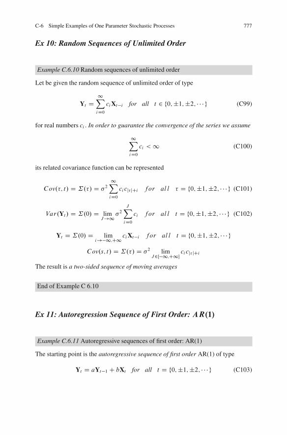
C-6 Simple Examples of One Parameter Stochastic Processes 777
Ex 10: Random Sequences of Unlimited Order
Example C.6.10 Random sequences of unlimited order
Let be given the random sequence of unlimited order of type
Yt D1X
iD0ciXt�i for all t 2 f0;˙1;˙2; � � � g (C99)
for real numbers ci . In order to guarantee the convergence of the series we assume
1X
iD0ci <1 (C100)
its related covariance function can be represented
Cov.�; t/ D ˙.�/ D �21X
iD0ci cj� jCi for al l � D f0;˙1;˙2; � � � g (C101)
Var.Yt / D ˙.0/ D limJ!1 �2
JX
iD0ci for al l t D f0;˙1;˙2; � � � g (C102)
Yt D ˙.0/ D limi!�1;C1 ciXt�i for al l t D f0;˙1;˙2; � � � g
Cov.s; t/ D ˙.�/ D �2 limJ2Œ�1;C1�
ci cj� jCi
The result is a two-sided sequence of moving averages
End of Example C 6.10
Ex 11: Autoregression Sequence of First Order: AR.1/
Example C.6.11 Autoregressive sequences of first order: AR(1)
The starting point is the autoregressive sequence of first order AR(1) of type
Yt D aYt�1 C bXt for all t D f0;˙1;˙2; � � � g (C103)

778 C Statistical Notions, Random Events and Stochastic Processes
limited by jaj < 1 and b as well as the random sequence fXg. The instant state Yt
depends only of the previous state Yt�1 as well as a random disturbance Xt subjectto fXg D 0 and Ef.Xt � EfXt g/2g D b2�2. Applying n times of the series we gain
Yt D anYt�n C bn�1X
iD0aiXt�i (C104)
limn!1an D 0 .C 105/ ) Yt D b
1X
iD0aiXt�� (C105)
“Special Case”
ci DW bai W limJ!1
JX
iD0
�bai
�2 D b2 limJ!1
JX
iD0a2i D b2
1 � a2 forJ <1(C106)
For an autoregressive sequence of first order of a stationary random process wearrive a the characteristic covariance function
Cov.�/ D .b�/2 limJ!1
JX
iD0aiaj� jCi D aj� j.b�/2 lim
J!1
JX
iD0a2i (C107)
Cov.�/ D .b�/2
1 � a2 aj� j for � D 0;˙1;˙2; � � � (C108)
End of Example C 6.11
Ex 12: Autoregression Sequence of First Order r: AR.r/
Example C 6.12 autoregressive sequences of order r: AR(r)
An autoregressive sequence of order r called “AR(r)” is the random sequenceYt ; t D 0;˙1;˙2; � � � over the set of real numbers a1; a2; � � � ; ar�1; ar namely
Yt C a1Yt�1 C a2Yt�2 C � � � C ar�1Yt�.r�1/ C arYt�r D bXt (C109)
The set Xi is a random sequence of parameters

C-6 Simple Examples of One Parameter Stochastic Processes 779
Is the setup Yt D limJ!1
JP
iD1ctXt�1 for
1PiD0
ci < 1 for a stationary sequence
transformable in an autoregressive sequence of order r ?
For solving this problem we have to solve for the relation of constants
c0 D bc1 C a1c0 D 0
c2 C a1c1 C a2c0 D 0cr C a1cr�1 C � � � C arc0 D 0
ci C a1ci�1 C � � � C arci�r D 0 (C110)
A non-trivial solution of the equation leads us to the algebraic equation
yr D a1yr�1 C � � � C ar�1y C ar D 0 (C111)
Example: y2 C a1y C a2 D 0For an autoregressive sequence of second order, namely r=1, we study the equationof quadratic order, namely by the eigen values �1 and �2. For the case �1 ¤ �2 wecompute the covariance function.
Cov.�/ D Cov.0/.1� �21/�j� jC1
2 � .1 � �22/�j� jC11
.�2 � �1/.1 � �1�2/ (C112)
Alternatively, for the case �1 D �2 D � we calculate the covariance function:
Cov.�/ D Cov.0/
�1C 1 � �2
1C �2 j� j��j� j for � D 0;˙1;˙2; � � � (C113)
subject to
Cov.0/ D VarfYt g
Cov.0/ D 1C a2.1 � a2/Œ.1C a2/2 � a21�
(C114)
If �1 and �2 are complex, then there exist � and ! subject to
�1 D � exp.i !/; �2 D � exp.�i !/ (C115)

780 C Statistical Notions, Random Events and Stochastic Processes
Cov.�/ D Cov.0/˛�j� j sin.!j� j C ˇ/ for � D 0;˙1;˙2; � � � (C116)
˛ WD 1
sinˇ; ˇ D arctan
�1C �21 � �2 tan!
�(C117)
Example: Numerical example
Let us introduce the numerical example for the autoregressive sequence
Yt � 0:6 Yt�1 C 0:05 Yt�2 D 2Xt for t D 0;˙1;˙2; � � � (C118)
subject to
VarfXt g D 1 (C119)
Obviously the impact of the term at the time instant t-2 on Y is small, at leastcompared to term on the time instant t-1. The related algebraic equation of secondorder can be represented by
Y2 � 0:6 y C 0:05 D 0 (C120)
Their solution is �1 D 0:1 and �2 D 0:5. Indeed compared to one, they are smallthan one. The solution leads to a stationary autoregressive sequence characterizedby the covariance functions
Cov.�/ D 7:017 � .0:5/j� j � 1:063 � .0:1/j� j (C121)
subject to
� D 0;˙1;˙2; � � �Cov.0/ D VarfYt g D 5:954
More details can be taken from Andel (1984)
End of Example C.6.12
Ex 13: ARMA (r,s) Models
Example C.6.13 ARMA(r,s) models

C-7 Wiener Processes 781
As a combination of random sequences of moving averages and of auto regressivesequences we introduce the ARMA(r,s) of the order
�YtCa1Yt�1C � � � Car�1Yt�.r�1/CarYt�r D b0XtCb1Xt�1C � � � Cbs�1Xt�.s�1/CbsXt�s
�
(C122)
In practice, ARMA model we used to model time series as a sequence of realnumbers determined by observing the state variables in discrete time instants. Veryoften, time series are not realizations of stationary random sequences of typefYt ; t D 0;˙1;˙2; � � � g with constant trend functions EfYtg D �.t/, but thetransformation
Z.t/ D EffY.t/g � EfY.t/gg (C123)
reduced mean
EfZig D EŒfYt g �EfYtg� D 0 (C124)
reduced covariance matrix
DfZg D EŒfYt1g � EfYt1g� D ŒYt2EfYt2g� D cov.t1; t2/ (C125)
leads approximately to proper fit of ARMA models. They are called trend reducedmoving average interregressive sequences being “nearly stationary”. Very efficientsoftware exist nowadays.
End of Example C.6.13: ARMA(r,s)
C-7 Wiener Processes
First, we define a Wiener Process by three axioms, namely by stationary incrementsof a random function, together with path continuity. The relation to a random walkis outlined. Especially the probability density of an ordered n-dimensional WienerProcess is reviewed. Secondly, special Wiener A Process of type (a) Ornstein-Uhlenbeck (b) WIENER Process with drift and (c) integrated WIENER Processare introduced
C-71 Definition of the Wiener Processes
The English botanician R. Brown published in the year 1828 the random movementof microscopic small organic and inorganic particles suspended in liquids illustratedin Fig. C.3. We observe a totally irregular motion of particles, nowadays calledBrownian motion. Its first analytical treatment, we owe Bachelier (1900) and

782 C Statistical Notions, Random Events and Stochastic Processes
Fig. C.5 Trajectory of a twodimensional Brownianmotion of 30 s distance(Perrin 1916)
Einstein (1905). Both found that a two-dimensional Gauss-Laplace distribution canmodel the typical Brownian motion. They spoke a chaotic movement of microscopicsmall particles. Wiener (1923) built up his theory of stochastic process withindependent increments to model this Brownian motion we will define first.
Definition C.7.1: Wiener Process
A stochastic process fX.t/; t 0g with continuous time and the state space Z D.�1;C1/ is called Wiener Process when it can be described as a path-continuousprocess by the following axioms.
(i) X.0/ D 0 (C 126)(ii) fX.t/; t 0g has stationary increments (C 127)
(iii) for all t > 0, X.t/ is Gauss-Laplace normally distributed (C 128)
End of Definition C.7.1: Wiener
Because of the stationarity of the increments, the difference X.t/ � X.s/ for alls; t 0 are Gauss-Laplace normally distributed with expectation EfX.t/ �X.s/g D 0 and variance �2jt � sj. Since the increments are independent theincrements are a Markov-Wiener process. If � D 1, then we call the process“standard Wiener”.
Continuity and differentiability
EfjX.t/ �X.s/j2g D VarfX.t/ � X.t/g D �2jt � sj (C129)
limh!0
EfjX.t C h/ �X.t/j2g D limh! �2jhj D 0 (C130)
“In the mean square sense the Wiener Process is continuous”
Wiener Process and the random walk

C-7 Wiener Processes 783
There is a intimate contact of Wiener Process and “a random walk” of a particle.The random walk of a particle can be described by
X.t/ D .X1 C X2 C � � � C XŒt=�t�/�x (C131)
“In the time interval starting by x D 0, a particle moves in the time difference �tby �x as a length unit to the left and the right with probability 1/2”.
X.t/ D�C1 if the jump is to the right�1 if the jump is to the left
(C132)
“t=�t” is the largest even number smaller or equal “t=�t”
P.Xt D 1/ D P.Xt D �1/ D 1=2 (C133)
EfXig D 0 and VarfXi g D 1)
) EfX.t/g D 0 and VarfX.t/g D .�x/2Œt=�t��t ! 0) EfX.t/g D 0, VarfX.t/g D �2t
Multidimensional distribution and conditional probability
Let fX.t/g for t 0 be a Wiener Process. We ask the question what is distributionof the sum of independent Gauss-Laplace normally distributed incremental qualitiesof type
X.ti / D X.t1/C .X.t2/X.t1//C � � � C .X.ti /X.ti�1//subject to
i D 2; 3; � � � ; n � 1; nThe result will lead us to the Special Wiener Process of type Gauss Process
Lemma C.7.2: Probability density of an n-dimensional Wiener Process
Let us assume 0 < t1 < t2 < � � � < tn�1 < tn for an ordered n-dimensional WienerProcess of the random vectors fX1;X2; � � � ;X.tn�1/;X.tn/g characterized byindependent Gauss-Laplace normally distributed increments of a Wiener Process.Then the probability density has the property

784 C Statistical Notions, Random Events and Stochastic Processes
ft1;t2;��� ;tn�1;tn .X1;X2; � � � ;X.tn�1/;X.tn//
D ft1.X1/ft2�t1 .X2 � X1/ � � �ftn�1�tn�2 .Xn�1 � Xn�2/ftn�tn�1 .Xn � Xn�1/
(C134)
and has the structure
ft1;t2;��� ;tn�1;tn .X1;X2; � � � ;X.tn�1/;X.tn//
D expf�12Œx21t1C .x2 � x1/2
t2 � t1 C � � � C .xn�1 � xn�2/2
tn�1 � tn�2C .xn � xn�1/2
tn � tn�1�g
�.2/n=2�npt1.t2 � t1/ � � � .tn�1 � tn�2/.tn � tn�1/ (C135)
End of Lemma C.7.2: n-dimensional Wiener Process
Proof of Lemma 7.2
For the proof we depart from the one dimensional probability density of fXtg oftype Wiener Process.
First assumption
ft .x/ D � expŒ�x2=.2�2t/��p2t� (C136)
Second assumption
Let fs;t .x1x2/ the probability density of the random vector fX.s/X.t/g subject tothe order 0 < s < t characterized by
fs;t .x1x2/dx1dx2 D P.X.s/ D x1;X.t/ D x2/dx1dx2 (C137)
P.X.s/ D x1;X.t/ D x2/ D P.X.s/ D x1;X.t/ � X.s/ D x2 � x1/dx1dx2(C138)
fs;t .x1x2/dx1dx2 D P.X.s/ D x1/P.X.t/ �X.s/ D x2 � x1/dx1dx2 (C139)
“independent increments”
fs;t .x1x2/ D fs.x1/ft .x2 � x1/ (C140)
Third assumption
fs;t .x1x2/ D expf�Œtx21 � 2sx1x2 C sx21 �g � 2�2ps.t � s/ (C141)

C-7 Wiener Processes 785
“correlation coefficient, covariance function”
s; t D Cps=t (C142)
CovfX.s/;X.t/g D �2s for 0 < s � t
CovfX.s/;X.t/ �X.s/g D 0 (C143)
CovfX.s/;X.t/g D CovfX.s/;X.s/C X.t/ � X.s/gD CovfX.s/;X.s/g C CovfX.s/;X.t/ �X.s/gD CovfX.s/;X.s/g D VarfX.s/g D �2 (C144)
“conditional probability density”
Condition: X.t/ D b
fX.s/.xjX.t/ D b/ D fs;t .x; t/� ft .b/ (C145)
fX.s/.xjX.t/ D b/ D expf�.x � stb/2 �
r2s
t.t � s/�g (C146)
EfX.s/jX.t/ D bg D s
tb; VarfX.s/jX.t/ D bg D �2 s
t.t � s/ (C147)
maxVarfX.s/jX.t/ D bg , s D t=2 (C148)
Finally, a generalization from ft .t/; fs;t .s; t/ to ft1t2���tn�1tn leads us to Lemma C 7.2
End of proof for Lemma C.7.2
At this end we will define the Gauss process.
Definition C.7.3: Gauss process
A stochastic process X.t/; t 2 T is a Gauss Process of type (C135), if for arbitraryvectors .t1; t2; � � � ; tn�1; tn/ ordered as t1 < t2 < � � � < tn�1 < tn and n D 1; 2; � � �are random vectors fX.t1/;X.t2/; � � � ;X.tn�1/;X.tn/g of an n-dimensional Gauss-Laplace normal distribution.
End of Definition C.7.3: Gauss process
C-72 Special Wiener Processes: Ornstein–Uhlenbeck, WienerProcesses with Drift, Integral Wiener Processes
Here we only introduce special Wiener Process of type

786 C Statistical Notions, Random Events and Stochastic Processes
(i) Ornstein-Uhlenbeck(ii) Wiener Process with drift and
(iii) integrated Wiener Process
It has to be remembered that the trajectories of a Wiener Process are nowheredifferentiable. Particles in motion have an infinite velocity when modeled a WienerProcess. In order to overcome this difficulty, Ornstein and Uhlenbeck developeda stochastic model for modeling the velocity of particles, an important issue inContinuum mechanics.
Definition 7.3: Ornstein-Uhlenbeck Process
Let fX.t/; t 0g be a Wiener Process with the parameter � . Then we call
V.t/ D Œexp.�˛t/�X.exp.˛t// (C149)
subject to ˛ > 0, a stochastic process fV.t/;�1 < t < C1g an Ornstein-Uhlenbeck Process.
End of Definition: Ornstein-Uhlenbeck Process
What are the characteristic properties of the Ornstein-Uhlenbeck Process?
Property 1: Probability density
fV.t/.x/ D Œexp.�x2=2�2/�� .p2�/ (C150)
Property 1: Expectations
EfV.t/g D 0; VarfV.t/g D �2 (C151)
Cov.s; t/ D �2Œexp.�2˛.t � s//� for s � t (C152)
Proof for the covariance function
Cov.s; t/ D Cov.V .s/; V .t// D EfV.s/V .t/gD expŒ�˛.s C t/�EfX.exp2˛s/X.exp2˛t/gD expŒ�˛.s C t/�Cov.X.exp2˛s/X.exp2˛t//
D expŒ�˛.s C t/��2Œexp.2˛.t � s//� (C153)
It has to be mentioned that the Ornstein-Uhlenbeck Process is stationary in thewider sense. As a Gauss Process it is also stationary in the narrow sense. In sum-mary, the Ornstein-Uhlenbeck Process is an instationary Wiener Process whichis stationary process due to the action of time transformation and normalization.In comparison to the Wiener Process, the Ornstein-Uhlenbeck has the followingdifferences

C-7 Wiener Processes 787
1. The Ornstein-Uhlenbeck Process has no independent increments2. The trajectories of an Ornstein-Uhlenbeck Process are in the quadratic
mean differentiable
Wiener Process with drift
Another example for the transformation of an instationary process to a stationaryprocess is the Wiener Process with drift.
Definition 7.4: Wiener Process with drift
A stochastic process fW.t/; t 0g with independent increments is called a WienerProcess with drift, if the following properties hold:
(i)W.0/ D 0 (C154)
(ii) Each increment has the property W.t/ � W.s/ is Gauss-Laplace normallydistributed with second order statistics
(iii)EfW.t/g D �.t � s/ (C155)
(iv)VarfW.t/g D �2jt � sj (C156)
End of Definition 7.4: drifted Wiener Process
An equivalent formulation is next:
“fW.t/; t 0g is a Wiener Process with drift, if it has the structure
W.t/ D �t C X.t/ (C157)
where fX.t/; t 0g is a Wiener Process subject to �2 D VarfX.1/g and � anarbitrary constant, called as drift parameter”.
Obviously, a Wiener Process with drift is generated by the super position of type“additive” of a Wiener Process with a deterministically growing decreasing part.The deterministic part is a trend function of type �.t/ D �t .The one dimension probability density distribution of a “Wiener Process with drift”can be characterized by
fW.t/.x/ D expŒ�.x � �t/2=.2�/�� Œp2t��; �1; x;C1 (C158)
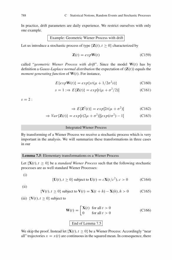
788 C Statistical Notions, Random Events and Stochastic Processes
In practice, drift parameters are daily experience. We restrict ourselves with onlyone example.
Example: Geometric Wiener Process with drift
Let us introduce a stochastic process of type fZ.t/; t 0g characterized by
Z.t/ D expW.t/ (C159)
called “geometric Wiener Process with drift”. Since the model W.t/ has bydefinition a Gauss-Laplace normal distribution the expectation of .Z.t// equals themoment generating function of W.t/. For instance,
EfexpW.t/g D expfst.�C 1=2�2s/g (C160)
s D 1 W) EfZ.t/g D expŒt.�C �2=2/� (C161)
s D 2 W
) EfZ2.t/g D expŒ2t.�C �2/� (C162)
) VarfZ.t/g D expŒt.2�C �2/�Œexp.t�2/ � 1� (C163)
Integrated Wiener Process
By transforming of a Wiener Process we receive a stochastic process which is veryimportant in the analysis. We will summarize these transformations in three casesin our
Lemma 7.5: Elementary transformations os a Wiener Process
Let fX.t/; t 0g be a standard Wiener Process such that the following stochasticprocesses are as well standard Wiener Processes:
(i)fU.t/; t 0g subject to U.t/ D cX.t=c2/; c > 0 (C164)
(ii)fV.t/; t 0g subject to V.t/ D X.t C h/� X.h/; h > 0 (C165)
(iii) fV.t/; t 0g subject to
W.t/ D�
X.t/ for all t > 00 for all t > 0
(C166)
End of Lemma 7.5
We skip the proof. Instead let fX.t/; t 0g be a Wiener Process: Accordingly “nearall” trajectories x D x.t/ are continuous in the squared mean. In consequence, there

C-7 Wiener Processes 789
exist the integrals u.t/ DtR
0
x.y/dy for “nearly all” trajectories x D x.t/. These
integrals are realizations of the random integral.
u.t/ DtZ
0
x.y/dy (C167)
u.t/ is the symbol for the integral acting on “nearly all” trajectories of a WienerProcess subject to the probability distribution fU.t/; t 0g defines a stochasticprocess called integrated Wiener Process.
Stochastic integration
Assume the Riemenn integration for 0 D t0 < t1 < � � � < tn�1 < tn D 1 subject to�ti D ti � ti�1 for forward computations and i D 1; 2; � � � ; n � 1; n
u.t/ D limn!1;�ti!0
fnX
iD1ŒX.ti /� X.ti�1/��ti (C168)
u.t/ is the lines of a sum of independent Gauss-Laplace normally distributedrandom variables as well Gauss-Laplace normally distributed: An integratedWiener Process is being analyzed by
.a/ Trend function:
EftZ
0
X.y/dyg DtZ
0
EfX.y/gdy D E.t/ D 0 (C169)
.b/ Covariance function:
Covfu.s/; u.t/g D EfsZ
0
X.z/d z
tZ
0
X.y/dyg DsZ
0
tZ
0
EfX.z/X.y/gdyd z
D �2
sZ
0
tZ
0
min.y; z/dyd z D �2sZ
0
yZ
0
zd zdy C �2sZ
0
tZ
y
y dz dy
D �2sZ
0
1
zy2dy C �2
sZ
0
y.t � y/dy (C170)

790 C Statistical Notions, Random Events and Stochastic Processes
Covfu.s/; u.t/g D �2
6.3t � s/s2 for s � t (C171)
Varfu.t/g D �2
3t3 for s D t (C172)
An integrated wiener Process is not stationary, in general. But it can be proven thatthe stochastic process V.t/ WD u.tC�/�u.t/ for V.t/ 2 fV.t/; t 0g is stationaryfor all � > 0.
White noise
A stochastic process, Z.t/ 2 fZ.t/; t 0g subject to
Z.t/ WD dX.t/� dt D X.t/ (C173)
or
dX.t/ WD Z.t/dt (C174)
cannot be computed by standard differentiation: We have to introduce stochasticintegration, for instance
bZ
a
f .t/dX.t/ D limn!1;�ti!0
fnX
iD1f .ti�1/ŒX.ti / �X.ti�1/�g (C175)
bZ
a
f .t/dX.t/ D f .b/X.b/� f .a/X.a/ �bZ
a
X.t/df .t/ (C176)
The representation reminds us to “partial integration”. As the limit of the sumof independent Gauss-Laplace normally distributed random variables we have tocompute the expectation of type
EfbZ
a
f .t/dX.t/g D 0 (C177)

C-7 Wiener Processes 791
VarfnX
iD1f .ti�1/ŒX.ti / �X.ti�1/�
DnX
iD1f 2.ti�1/VarfX.ti /� X.ti�1/g
D �2nX
iD1f 2.ti�1/.ti � ti�1/ D �2
nX
iD1f 2.ti�1/�ti (C178)
The limit approaches the variance of the stochastic integral of type
VarfbZ
a
f .t/dX.t/g D �2bZ
a
f 2.t/dt (C179)
This result leads to the definition of White Noise
Definition C.7.6: White Noise
A stochastic process fZ.t/; t 0g is called “White Noise” if for any arbitraryinterval Œa; b� of continuously differentiable functions f .t/, namely
bZ
a
f .t/dZ.t/ D f .b/X.b/ � f .a/X.a/ �bZ
a
X.t/df .t/ (C180)
where fX.t/; t 0g is a Wiener Process.
End of Definition C.7.6: White Noise
?Why we call stochastic process “White Noise”?
The origin of the question is the definition of the “generalized derivative”. To thisend we define ”the Dirac Delta function” as a “generalized function”
ı.t/ WD limh!0
�1=h for � h=2 � t � Ch=20 otherwise
(C181)
or
ı.t/ WD�1 for t D 00 otherwise
(C182)

792 C Statistical Notions, Random Events and Stochastic Processes
Properties of Dirac’s Delta function
(i)
C1Z
�1f .t/ı.t � t0/dt D f .t0/ (C183)
(ii) Heaviside functions
H.t/ WD�1 for t 00 for t < 0
(C184)
“The Dirac’s Delta function is the formal derivative of the Heavide function”
ı.t/ D @H.t/=@t (C185)
(iii) Covariance function
CovfZ.s/;Z.t/g D CovŒ@X.s/=@s; @X.t/=@t
D @
@s
@
@tCovfX.s/;X.t/g D @
@s
@
@tmin.s; t/
D @
@sH.s � t/ (C186)
CovfZ.s/;Z.t/g D ı.s � t/ (C187)
the covariance function is a measure of the statistically independence betweenZ.s/ and Z.t/, have a function of the small distances between the point s andthe point t, namely js � t j.
“How can we illustrate the Dirac function?”Let fN.t/; t 0g be an arbitrary numbering process following our Definition C.7.6.The instants of the process at the points T1; T2; � � � ; admit the representation in termsof the Heavide function N 0.t/ in terms of the Dirac function:
N.t/ D1X
iD1H.t � Ti/; @N.t/=@t D
1X
iD1ı.t � Ti / (C188)
Figure C.6 an illustration of the numbering process.The theory of stochastic integration has led us to the concept of generalized function,namely the Dirac function and Heaviside function, and to the notion of White Noise.More general notions like the concept of Colored Noise and finally to the notion ofits stochastic processes.

C-8 Special Analysis of One Parameter Stationary Stochastic Process 793
Fig. C.6 Dirac numbering system
C-8 Special Analysis of One Parameter StationaryStochastic Process
C.8: Spectral analysis of one parameter stationary stochastic processes
Statistic or stochastic processes are conventionally divided into three classes wehave already touched:
Class onegeneral instationaryprocess
Class twostationaryprocess
Class threeergodic stationaryprocess
In real life, of course, we have live the property that all natural process areinstationary. It is the task of modeling real world process, for instance by a firstorder trend model or by taking increments of higher order to come more closely tothe case of stationary processes for higher order increments. We will come back tothis problem.For formal reasons we introduce first real-valued and complex-valued stochasticprocess. Second we study the structure of process with a discrete spectrum. At theend, we introduce stochastic process with a continuous spectrum enriched byexamples.
C-81 Foundations: Ergodic and Stationary Processes
C.8.1: Foundations: Ergodic and stationary processes
We move on towards complex-valued stochastic processes defined by the followingaxioms:
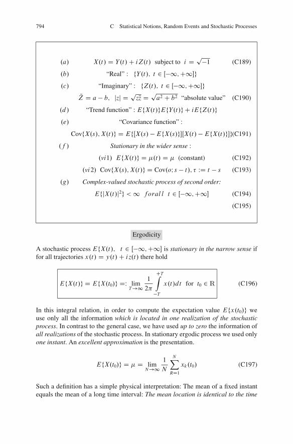
794 C Statistical Notions, Random Events and Stochastic Processes
.a/ X.t/ D Y.t/C iZ.t/ subject to i D p�1 (C189)
.b/ “Real” W fY.t/; t 2 Œ�1;C1�g
.c/ “Imaginary” W fZ.t/; t 2 Œ�1;C1�gNZ D a � b; jzj D pzNz D pa2 C b2 “absolute value” (C190)
.d/ “Trend function” W EfX.t/gEfY.t/g C iEfZ.t/g.e/ “Covariance function” W
CovfX.s/;X.t/g D EfŒX.s/ �EfX.s/g�ŒX.t/� EfX.t/g�g(C191)
.f / Stationary in the wider sense W.vi1/ EfX.t/g D �.t/ D � (constant) (C192)
.vi2/ CovfX.s/;X.t/g D Cov.oI s � t/; � WD t � s (C193)
.g/ Complex-valued stochastic process of second order:
EfjX.t/j2g <1 foral l t 2 Œ�1;C1� (C194)
(C195)
Ergodicity
A stochastic process EfX.t/; t 2 Œ�1;C1� is stationary in the narrow sense iffor all trajectories x.t/ D y.t/C iz.t/ there hold
EfX.t/g D EfX.t0/g DW limT!1
1
2
CTZ
�Tx.t/dt for t0 2 R (C196)
In this integral relation, in order to compute the expectation value Efx.t0/g weuse only all the information which is located in one realization of the stochasticprocess. In contrast to the general case, we have used up to zero the information ofall realizations of the stochastic process. In stationary ergodic process we used onlyone instant. An excellent approximation is the presentation.
EfX.t0/g D � D limN!1
1
N
NX
RD1xk.t0/ (C197)
Such a definition has a simple physical interpretation: The mean of a fixed instantequals the mean of a long time interval: The mean location is identical to the time

C-8 Special Analysis of One Parameter Stationary Stochastic Process 795
average. In essence, This is the property of ergodic stationary processes. Analoguewe can define the covariance function for a such processes namely
Cov.�/ D limT!1
1
2
CTZ
�TŒx.t/ � �px.t C �/ � �dt (C198)
The treatment of ergodic stationary processes is reasonable for cases in which wehave only one time like realization of the stochastic process. Of course increasingthe length of the interval Œ�T;CT � improves the estimation of EfX.t0/g D �.
Here we also take reference the Euler’s representations:
exp˙ix D cos x ˙ i sin x (C199)
sinx D 1
2iŒexp.ix/� exp.�ix/� (C200)
cos.x/ D 1
2Œexp.ix/C exp.�ix/� (C201)
C-82 Processes with Discrete Spectrum
C.8.2: Processes with discrete spectrum
We start with general structure of stationary processes with discrete spectrum: weassume that all stationary process are ergodic.
Ex 1: Special Stationary Ergodic Processes
Example 8.1: Special stationary ergodic processes
Let fX.t/; t 0g be a stochastic process structure by
lrX.t/ D X˝.t/; X a complex random variable (C202)
EfXg D 0; E.jX j2/ <1; EfX.t/X.t C �/g D ˝.t/˝.t C �/EfX2g(C203)
� D 0 W ˝.t/˝.t/ D j˝.t/j2 D constant (C204)
“ansatz” W ˝.t/ D j˝.t/ expŒi!.t/� for !.t/ real function (C205)
“ansatz” W !.t C �/� !.t/ ¤ f .t/ W dŒ!.t C �/ � !.t/�=dt D 0 (C206)

796 C Statistical Notions, Random Events and Stochastic Processes
or d!.t/=dt D constant (C207)
“ansatz” W !.t/ is a function of two constants; I ! and � W (C208)
˝.t/j˝.t/j expŒi.! C �/� (C209)
End of Example 8.1: Special stationary ergodic processes
Lemma 8.1: decomposition of a complex stationary ergodic process
A stochastic process fX.t/; t 0g of the structure X.t/ D X˝.t/ is stationary inthe wider sense if and only if
X.t/ D X exp.i!t/ (C210)
subject to EfXg D 0; Efjxj2g <1; s DW EfjX j2g; Cov.�/ D s exp.�i!�/End Lemma 8.1
The real part of a complex stochastic process describes a cosine oscillation with arandom amplitude and phase
y.t/ D a cos.!t C �/ (C211)
The parameter ! is called frequency.
We generalize to two stationary processes as a linear combination: we refer to X1and X2 as two complex random variables with zero expectation and two constantparameter f!1; !ı
1 D 0; !2; !ı2 D 0g. We assume that the two complex random
functionsX1 and X2 are uncorrelated such that EfX1X2g D 0 or EfX1 �X2g D 0.Our intention is to get the form of the covariance function:
X.t/ D X1 exp.i!1t/CX2 exp.i!2t/ (C212)
covfX.t/X.t C �/gD EfŒX1 exp.i!1t/CX2 exp.i!2t/�Œ NX1 exp.�i!1t/C NX2 exp.�i!2t/�gD EfŒX1 NX2 exp.�i!1�/CX1 NX2 exp.i.!1 � !2/t � i!2�/�gCEfŒX2 NX1 exp.�i!2�/CX2 NX2 exp.i.!2 � !1/t � i!1�/�g (C213)
s1 DW EfjX1j2g; s2 DW EfjX2j2g (C214)
Cov.�/ D s1 exp.�i!1�/C s2 exp.�i!2�/ (C215)

C-8 Special Analysis of One Parameter Stationary Stochastic Process 797
Ex 2: Special Correlation Function of a Stationary Stochastic Processes
Example 8.2: Special correlation function of a stationary stochastic process
A special complex stationary stochastic process may be real-valued. For instancewe define
X1 D 1
2.AC iB/ and X2 DW NX1 D 1
2.A� ıB/ (C216)
A and B are two real-valued functions. In consequence of our representationX.t/ DX1 exp.i!1t/CX2 exp.i!2t/ we specialize here to
X.t/ D A cos!t � B sin!t (C217)
A, B are uncorrelated. We received the covariance function
Cov.�/ D 2s cos!� (C218)
subject to s WD EfjX1j2g D EfjX2j2gEnd of Example 8.2: Special correlation function
For pairwise uncorrelated stationary stochastic processes the general ansatz of typeX.t/ DPn
kD1 exp.i!kt/ subject to !j ¤ !k for j ¤ k and i; j D 1; 2; : : : ; n�1; nand EfXkg D 0 will lead us to the covariance function
Cov.�/ DnX
kD1sk.i!k�/ and sk D EfjXkj2g for k 2 f1; 2; : : : ; n � 1; ng
(C219)
in particular
Cov.� D 0/ D EfjX.t/j2g DnX
kD1sk (C220)
In summary, the oscillation X.t/ is an additive superposition of a harmonicoscillation. This average energy per time unit is the same of circle average energiesper time unit, an appropriate interpretation of our last representation.In order to achieve a real-valued function, we have specialize to
(a) an even number n,(b) and a pair of valuesXk being conjugate complex.
Let the set f!1; !2; : : : g define the spectrum. We have to divide the various spectruminto two classes: small band processes and broad band processes, an entry into filtertheory with many application in all sciences.

798 C Statistical Notions, Random Events and Stochastic Processes
Ex 3: Dirac Representation of a Covariance Function
Example 8.3: Dirac representation of covariance function
We use the infinitely generalized covariance function for application of a Diracfunction representation.
Cov.�/ D limK!1
KX
kD1sk
C1Z
�1exp.i!�/s.! � !k/d! (C221)
Cov.�/ DC1Z
�1exp.i!�/s.!/d! (C222)
subject to
s.!/ D limK!1
KX
kD1skı.! � !k/ (C223)
The generalized function s.! is denoted by “spectral density” of a stationarystochastic process, formally equivalent to the Fourier transform.
End of Example 8.3: spectral density
C-83 Processes with Continuous Spectrum
C.8.3 Processes with continuous spectrum
Here we present first the spectral decomposition of the covariance function of astochastic process with continuous spectrum. Second we present Kolmogorov’sspectral decomposition theorem.
C8-31 Spectral decomposition of a covariance function
Let fX.t/; t 2 Rg be a complex-valued stationary stochastic process describedby its covariance function. Then there exists a real-valued function S.!/ such thatcov.�/ enjoys the representation.
Cov.�/ DC1Z
�1exp.i!�/dS.!/ (C224)
called the spectral function of the process. Note the domain t 2 Œ�1;C1�
Cov.0/ D S.1/� S.�1/ D EfjX j2g <1 (C225)

C-8 Special Analysis of One Parameter Stationary Stochastic Process 799
The spectral function is determined only up to an additive constant c. Mostcommonly c is chosen to S.�1/ D 0. If there exists the first derivative S.!/ DdS.!/=d!, we find the spectral density of the stochastic process: The covariancefunction of this stationary process is the Fourier transform of the spectral density.Since S.!/ has to be a decreasing function we find also its property.
Cov.�/ DC1Z
�1exp.i!�/s.!/d! (C226)
s.!/ 0; (C227)
C1Z
�1s.!/d! <1 (C228)
The set f!; s.!/ > 0g defines the continuous spectrum of the stationary stochasticprocess. The term
Cov.0/ D S.1/� S.�1/ DC1Z
�1s.!/d! (C229)
is called average power of the spectrum. If we describe the stationary stochasticprocess Xt by harmonic oscillations with random amplitude and random phase, weare able to express
exp.i!t/ D expŒi t.!C 2k/� for all k 2 f1; 2; : : : g or k 2 Œ�;C� (C230)
Cov.�/ DCZ
�exp.i�!/s.!/d! for � D 0;˙1;˙2; : : : (C231)
IfC1R�1
Cov.�/d� < 1 for stationary stochastic processes, holds, we are able to
introduce the inverse Fourier transform by
s.!/ D 1
2
C1Z
�1exp.�i!�/Cov.�/d� (C232)

800 C Statistical Notions, Random Events and Stochastic Processes
s.!2/ � s.!1/ D i
2
C1Z
�1
exp.�!2�/ � exp.�i!1�/�
Cov.�/d� (C233)
Ex 4: Fourier Spectral Density
Example 8.4: Fourier spectral density
Assume real-valued constants a and cjaj < 1 . Here we will analyze the covariancefunction for an autoregressive stationary sequence of first order and compute itsspectral density.
s.!/ D 1
2
C1X
�D�1Cov.�/ exp.�i�!/
D e
2
" �1X
�D�1a�� exp.�i�!/C
1X
�D0a� exp.�i�!/
#
D c
2
" 1X
�D1a� exp.i�!/C
1X
�D0a� exp.�i�!/
#
(C234)
s.!/ D c
2
�a exp.i!/
1 � a exp.i!/C 1
1 � a exp.i!/
(C235)
End of Example: Fourier spectral density
Assume a real-valued stochastic process whose covariance function Cov.�/ DCov.��/, namely Cov.�/ D ŒCov.�/C Cov.��/�=2, can be represented by
Cov.�/ DC1Z
�1cos.!�/s.!/d! (C236)
Cov.�/ D 2C1Z
�1cos.!�/s.!/d! .cos.!�/ D cos.�!�// (C237)

C-8 Special Analysis of One Parameter Stationary Stochastic Process 801
s.!/ D 1
2
C1Z
�1cos.!�/Cov.�/d� (C238)
s.!/ D 1
C1Z
0
cos.!�/Cov.�/d� (C239)
Correlation time
In practice the notion of “correlation time” or “correlation length” is very appro-priate:
�0 WD 1
Cov.0/
C1Z
0
Cov.�/d� (C240)
or
�0 WD s.0/
2C1R
0
s.!/d!
(C241)
For j� j � �0 there is a unstable correlation or statistical dependence between X.t/and X.t/C � . This correlation decreases for growing j� j; j� j > �0.
Ex 5: Stationary Infinite Random Sequence
Example 8.5: Stationary infinite random sequence
The infinite random sequence f� � � ;�X1;X0;CX1; � � � g may be structuredaccording to Xt D atX subject to t D 0;˙1;˙2; � � � : The complex randomvariable is structured according to EfXg D 0 as well as VarfXg D �2. The randomsequence f� � � ;�X1;X0;CX1; � � � g is the wider sense stationary if and only if theconstants ! within the set-up.
at D exp.i t!/ for t D 0;˙1;˙2; � � � (C242)
are represented. In the stationary case, the harmonic oscillations Xt will be givenby the random amplitude and the random phase as well as a constant frequency !.For such a case a set-up of the covariance-function will be calculated.
exp.i t!/ D exp i t.! C 2k/ for t 2;˙1;˙2; � � � (C243)

802 C Statistical Notions, Random Events and Stochastic Processes
Cov.�/ DCZ
�exp.i t!/s.!/d! for � 2;˙1;˙2; � � � , (C244)
,s.!/ D 1
2
C1X
�D�1exp.�i t!/Cov.�/ (C245)
If we specialize to X real-valued and uncorrelated we achieve a pure randomsequence subject to
Cov.�/ D �2 , s.!/ D �2=.2/ (C246)
End of Example 8.5: random sequence
Ex 6: Spectral Density of a Random Telegraph Signal
Example 8.6: spectral density of a random telegraph signal
Given the covariance function, we intend to find a representation of the spectraldensity for a random telegraph signal.
Cov.�/ D a exp.�bj� j/ for a > 0; b > 0 (C247)
s.!/ D 1
2
C1Z
�1exp.�i!�/a exp.�bj� j/d!
D a
2
8<
:
0Z
�1exp.�i!�/d� C
C1Z
0
expŒ�.b � i!/��d�9=
;
D a
2
�1
b � i! C1
b C i!�
(C248)
s.!/ D ab
.!2 C b2/ (C249)
The correlation time is calculated to �0 D 1=b! this result is illustrated by Figs. C.7and C.8, namely by the spectral structure of the covariance function and its spectraldensity
End of Example: spectral density telegraph signal

C-8 Special Analysis of One Parameter Stationary Stochastic Process 803
Fig. C.7 Covariance of Example 8.6
Fig. C.8 Spectral density of Example 8.6
Ex 7: Spectral Representation of a Pulse Modulation
Example 8.7: Spectral density of a pulse modulation
We start with the covariance function of a pulse modulation and study its spectraldensity.
Cov.�/ D�a.T � j� j/ for j� j � T0 for j� j > T (C250)
s.!/ D a
2
CTZ
�TŒexp.�i!�/�.T � j� j/d�
D a
2
8<
:T
TZ
�Texp.�i!�/d� �
CTZ
0
� exp.i!�/d� �CTZ
0
� exp.�i!�/d�9=
;
D a
2
8<
:2T
!sin.!�/ � 2
CTZ
0
� cos.!�/d�
9=
;(C251)
s.!/ D a
1 � cos!T
!2(C252)
Figures C.7 and C.8 illustrate the covariance function and the spectral density ofa pulse modulation. A slight modification of our example proves that it is notautomatic for stationarity.

804 C Statistical Notions, Random Events and Stochastic Processes
Fig. C.9 Covariance ofExample 8.7
Fig. C.10 Spectral density of Example 8.7
Cov.�/ D2
4a.T � �2/ for j� j � 0
for a > 0; T > 00 for j� j < 0
(C253)
s.!/ cannot be the spectral density of a stationary stochastic process.
Alternatively, we like to resent the covariance function Cov.�/ be a Dirac delta-function ı.�/. In this case we find
ı.�/ D 1
2
C1Z
�1exp.�i!�/d� (C254)
s.!/ D 1
2
C1Z
�1exp.�i!�/ı.�/d� D 1
2(C255)
by formal inversion.
End of Example 8.7: pulse modulation

C-8 Special Analysis of One Parameter Stationary Stochastic Process 805
Fig. C.11 Spectral density ofa harmonic function
Ex 8: Spectral Density and Spectral Function of a Harmonic Oscillation
Example 8.8: Spectral density and spectral function of a harmonic oscillation
Given a harmonic oscillation with a given covariance function, we will derive thestructure of the spectral density function as well as the spectral function.
Cov.�/ D a cos!0� (C256)
s.!/ D a
2
C1Z
�1exp.�i!�/ cos.!0�/d�
D a
4
1Z
�1exp.�i!�/Œexp.�i!0�/ � exp.�i!0�/�d�
D a
4
8<
:
1Z
�1expŒi.!0 C !/��C
1Z
�1expŒ�i.!0 � !/��
9=
;d� (C257)
s.!/ D a
2fı.!0 � !/C ı.!0 C !/g (C258)
S.!/ D2
40 for ! < �!0a=2 for � !0 < ! � �!0 step functiona for ! > !0
(C259)
We illustrate the spectral density as well as the spectral function of a harmonicoscillation by Fig. C.11 as well as Fig. C.12. It has to be emphasized that all threefunctions Cov.�/; s.!/ and S.!/ are stationary functions.
End of Example 8.8: Spectral function of harmonic oscillation

806 C Statistical Notions, Random Events and Stochastic Processes
Fig. C.12 Spectral functionof type step function for aharmonic oscillation
Ex 9: Spectral Density Function of a Damped Harmonic Oscillation
Example 8.9: Spectral density functions of a damped harmonic oscillation
Given the covariance function of a damped harmonic oscillation, we want to findthe spectral density of this stationary stochastic process,
Cov.�/ D a exp.�bj� j/ cos!0� (C260)
s.!/ D a
1Z
0
exp.�b�/ cos.!�/ cos.!0�/d�
D a
2
1Z
0
exp.�b�/Œcos.! � !0/� C cos.!0 C !/��d� (C261)
s.!/ D ab
2
�1
b2 C .! � !0/2C 1
b2 C .! C !0/2�
(C262)
!0 is called the eigen function of the stochastic process of type stationary. A typicalexample is the fading of a radio signal.
End of Example 8.9: Damped harmonic oscillation
Ex 10: Spectral Density of White Noise
Example 8.10: Spectral density of white noise
Perviously we introduced the concept of “white noise” as a real-valued stationaryprocess with continuous time of type Wiener process. Given its covariance function,we are interested in the spectral density function.
Cov.�/ D 2s0ı.�/ (C263)

C-8 Special Analysis of One Parameter Stationary Stochastic Process 807
s.!/ D 1
1Z
�1exp.�i!�/2s0ı.�/d� D S0 (C264)
A comparative formulation of a white noise process is the following:
White noise is a real-valued process whose spectral density is a constant
Comment
the spectral density of a white noise process has only the property s.!/ 0, but not
the property1R
�1s.!/d! <1. Accordingly, a white noise process with an average
power spectrum fulfilss.!/d! D1 (C265)
does exist only in theory not in practice. A comparison is “the mass point” or“the point mass”, which also exist only “in theory”. Nevertheless it is reasonableapproximation of any reality.A stationary process can always be considered as a excellent approximation of whitenoise if the covariance betweenZ.t/ andZ.tC�/ for growing values j� j extremelyfast goes to zero.
Example:
Let us denote the variations of the absolute value of the force by Z.t/ acting ona particle of a liquid medium at the time t and leading to a Brownian motion.Per second, the resulting force leads to approximately 1021 collisions with otherparticles. Therefore the stochastic variables Z.t/ and Z.t C �/ are stochasticallyindependent (“uncorrelated”) if j� j is of the order of 10�18 seconds. If we assume acovariance function of type Cov.�/ D exp.�bj� j/ for b > 0, the number b has tobe larger than 10�17 seconds.
End of Example 8.10: White noise
Ex 11: Band Limit of White Noise
Example 8.11: Band limited white noise
A stationary stochastic process with a constant spectral density function S.!/ D s0for ! 2 f�1;C1g does not in practice. But a stationary stochastic process withthe spectral density

808 C Statistical Notions, Random Events and Stochastic Processes
Fig. C.13 Spectral density ofband limited white noiseprocess
Fig. C.14 Covariancefunction of a band limitedwhite noise process
s.!/ D�s0 for �˝=1 � ! � C˝=20 otherwise
(C266)
exists
Cov.�/ DC˝=2Z
�˝=2exp.i!�/so D 2s0 sin.˝�/=2
�(C267)
The average power of the process is proportional to Cov .0/ D s0˝ . The parameter˝ is called the band width of the process. A white noise process is generated by thelimit of a band limited white noise illustrated by Figs. C.13 and C.14.
End of Example 8.11: band limited white noise
C-84 Spectral Decomposition of the Mean andVariance-Covariance Function
C.8.4: Spectral decomposition of the expectation and the variance-covariancefunction
The decomposition of the spectrum of a stationary process fY.x/; x 2 Rg subjectto R 2 f�1;C1g applied to orthogonal increments of various order has manyrepresentations, if they do not overlap in the intervals
Œx1; x2�; Œx3; x4� or Œx1; x2; x3�; Œx4; x5; x6� etc
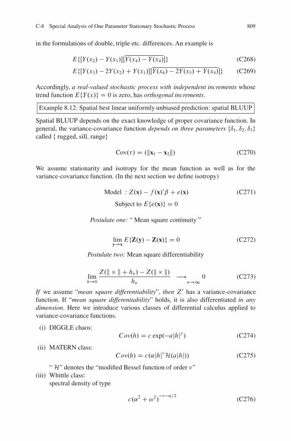
C-8 Special Analysis of One Parameter Stationary Stochastic Process 809
in the formulations of double, triple etc. differences. An example is
EfŒY.x2/ � Y.x1/�ŒY.x4/ � Y.x4/�g (C268)
EfŒY.x3/ � 2Y.x2/C Y.x1/�ŒY.x6/ � 2Y.x5/C Y.x4/�g (C269)
Accordingly, a real-valued stochastic process with independent increments whosetrend function EfY.x/g D 0 is zero, has orthogonal increments.
Example 8.12: Spatial best linear uniformly unbiased prediction: spatial BLUUP
Spatial BLUUP depends on the exact knowledge of proper covariance function. Ingeneral, the variance-covariance function depends on three parameters fı1; ı2; ı3gcalled f rugged, sill, rangeg
Cov.�/ D .kx1 � x2k/ (C270)
We assume stationarity and isotropy for the mean function as well as for thevariance-covariance function. (In the next section we define isotropy)
Model W Z.x/ � f .x/0ˇ C e.x/ (C271)
Subject to Efe.x/g D 0
Postulate one: “ Mean square continuity ”
limy!x
EfZ.y/� Z.x/g D 0 (C272)
Postulate two: Mean square differentiability
limh!0
Z.k � k C hn/�Z.k � k/hn
�!n!1
0 (C273)
If we assume “mean square differentiability”, then Z0 has a variance-covariancefunction. If “mean square differentiability” holds, it is also differentiated in anydimension. Here we introduce various classes of differential calculus applied tovariance-covariance functions.
(i) DIGGLE chaos:Cov.h/ D c exp.�ajhj� / (C274)
(ii) MATERN class:Cov.h/ D c.˛jhj�H.ajhj// (C275)
“ H” denotes the “modified Bessel function of order �”(iii) Whittle class:
spectral density of type
c.˛2 C !2/���˛=2(C276)

810 C Statistical Notions, Random Events and Stochastic Processes
(iv) Stochastic process on curved spaces like the sphere or the ellipsoid: no Maternclasses, the characic functions have a discrete spectrum, for instance in termsof harmonic functions.
End of Example 8.12: spatial BLUUP
Let us give some references: Brown et al. (1994), Brus (2007), Bueso et al.(1999), Christenson (1991), Diggle and Lophaven (2006), Fedorov and Muller(2007), Groeningen et al. (1999), Kleijnen (2004), Muller et al. (2004), Mullerand Pazman (2003), Muller (2005), Omre (1987), Omre and Halvorsen (1989),Pazman and Muller (2001), Pilz (1991), Pilz et al. (1997), Pilz and Spock (2006),PilzSpock(2008), Spock (1997), Spock(2008), Stein (1999), Yaglom (1987), Zhuand Stein (2006).
Up to now we assumed a stochastic process of type fX.t/; t 2 Rg, R D f�1;C1gas a complex stationary process of second order. Then there exist a stochasticprocess of second order fU.!/; ! 2 Rg with orthogonal increments which can berepresented by
X.t/ DC1Z
�1exp.i!t/dU.!/ (C277)
The process fU.!/; ! 2 Rg of the process fX.t/; t 2 Rg is called the relatedspectral process. Its unknown additive constant we fix by the postulate
P fU.�1/ D 0g D 1 (C278)
subject to
EfU.!/g DW 0 (C279)
EfŒjU.!/j2�g � S.!/ (C280)
EfŒjdU.!/j2�g � dS.!/ (C281)
Our generalization was introduced by A. N. Kolmogorov: Compare this representa-tion with our previous model
X.t/ D limk!1
KX
kD1exp.i!t/Xk (C282)
and

C-9 Scalar-, Vector-, and Tensor Valued Stochastic Processes 811
Xt DC1Z
�1exp.i!t/dU.!/ (C283)
The orthogonality of the Kolmogorov stochastic process fU.t/; t 0g correspondsin case of a discrete spectrum to the concept of uncorrelation. Convergence in thesquared mean of type
C1R�1
exp.i!t/dU.!/ D lima!�1b!C1
limn!C1�!k!0
nP
kD1exp.i!k�1t/ŒU.!k/� U.!k�1/�
(C284)
emphasizes the various weighting functions of frequencies: The frequency !k�1 inthe range Œ!k�1; !k� receives the random weight U.!k/ � U.!k�1/. A analogueversion of the inversion process leads to
U.!2/ � U.!1/ D i
2
C1Z
�1
exp.i!2t/ � exp.i!1t/
tX.t/dt (C285)
In practice, Kolmogorov stochastic processes are applied in linear filters for prog-nosis or prediction.
C-9 Scalar-, Vector-, and Tensor Valued Stochastic Processesof Multi-Parameter Systems
Appendix C.9: Scalar-, vector- and tensor-valued stochastic processes of multi-parameter systems
We have experienced the generalization of a scalar-valued stochastic process dueto A.N. Kolmogorov. Another generalization due to him is the concept of thestructure functions for more general vector-valued and tensor-valued for incrementsof various order as well as their power spectrum or multi-parameter systems.
First we introduce the notion of the characteristic functional replacing the notionof the characteristic function for random function. Second, the moment represen-tation for stochastic processes is outlined. Third we generalize the notion fromscalar-valued and vector-valued stochastic processes to tensor-valued stochasticprocesses of multi-point parameter systems. In particular, we introduce the notion
812 C Statistical Notions, Random Events and Stochastic Processes
of homogeneous and isotropic stochastic fields and extent the Taylor-Karmanstructured criterion matrices to distributions of the sphere.
C-91 Characteristic Functional
Let us begin with the definition of the characteristic functional.
�
YxŒ�� D Efexp.iY.�//g D EfigbZ
a
�.x/Y.x/dx (C286)
�
Y.�/ as the characteristic functional elates uniquely to the random functionY.x/ of a fixed complex number. If the characteristic functional of a specificrandom function is known we are able to derive the probability density distributionfX1;:::;XN .YX ; : : : ; YXN /.
Example
If a scalar-valued function in a three dimensional field x WD .x1; x2; x3/ exists defineits characteristic functional by
�
YY Œ�� WD Efexp.iZ C1Z
�1
ZY.x1; x2; x3/�.x1; x2; x3//dx1dx2 (C287)
The domain of integration is very often chosen to be spherical coordinates ofellipsoidal coordinates .u; v;w/ for u 2 f0; 2g; v 2 f�=2 < v < C=2g andw 2 f0 < w < 1g as a first chart. A second chart is needed to cover totally theintersection surfaces, for instance by meta-longitude, meta-latitude.
End of Example
Probability distribution for random functions and the characteristic functional
As a generalization of the characteristic function for random events, the concept ofthe characteristic functionals for random functions or stochastic processes has beendeveloped. Here we aim at reviewing the theory. We apply the concept of randomfunctions for multi-functions of type scalar-valued and vector-valued functionswhich have been first applied in the statistical theory turbulence.
what is the characteristic functional?
We summarize in Table C.9.1 the detailed notion of a scalar-valued as well as avector-valued characteristic functional illustrated by an example by introducing the“Fourier-Stieljes functional”.

C-9 Scalar-, Vector-, and Tensor Valued Stochastic Processes 813
Table C.9.1 Probability distribution of a random function and the characteristicfunctional
“Scalar-valued characteristic functionals”
“Random function over an interval [a,b] with N-variables”
fY.x/; x 2 RN g is called a random function if the density function
fx1;x2;:::;xN�1;xN ŒY.x1/; Y.x2/; : : : ; Y.xN�1/; Y.xN /� (C288)
exist at .x1; x2; : : : ; xN�1; xN / points.
“Fourier representation of the distribution function”
�
Yx1;:::;xN .�1; : : : ; �N / WD EfexpŒi.PN
kD1 �kYk/�gD R C1
�1: : :R
expfiPNkD1 �kYkgfx1;:::;xN .Y1; : : : ; YN /dY1 : : : dYN
(C289)
subject
Y1 WD Y.x1/; : : : ; Yk WD Y.xk/ (C290)
“Existence condition”
Y Œ�1; : : : ; �N � DbR
a
�.x/dx (C291)
“Vector-valued characteristic functionals”
“at any point P of the domain D place a set of base vectors e˛.Pi / at fixedpoints Pi for ˛ D 1; 2; : : : ; n � 1; n; i D 1; 2; : : : ; N � 1;N .
Y ˛i D; Y.P � i/je˛.Pi / > (C292)
“Vector-valued characteristic functionals”
�
YYŒ�� W �.x; y; z/ DPn˛D1 �˛.Pi /Y.Pi / (C293)
End of Table C.9.1: characteristic functional

814 C Statistical Notions, Random Events and Stochastic Processes
C-92 The Moment Representation of Stochastic Processes forScalar Valued and Vector Valued Quantities
The moment representation of stochastic processes is the standard tool of statisticalanalysis. If a random function is given by its probability function, then we find aunique representation of its moments. But the inverse process of a given momentrepresentation converted in its probability function is not unique. Therefore wepresent only the direct representation of moments for a given probability function.At first we derive for a given scalar-valued probability function its momentrepresentation in Table C.9.2. In Table C.9.3 we generalize this result for stochasticprocesses which are vector-valued. An example is presented for second orderstatistics, namely for the Gauss-Laplace normal distribution and its first and secondorder moments.
Table C.9.2 Moment representation of stochastic processes for scalarquantities
“scalar-valued stochastic processes”
“moment representation”
Y.x/; x 2 RN is a random function, for instance applied in turbulence theory.
Define the set of random function fx1; x2; : : : ; xN�1; xN g 3 R
with the probability distribution f .x1; x2; : : : ; xN�1; xN /.Then the moment representation is the polynomial
Mp1;p2;:::;�N�1;�N WD Efx1; x2; : : : ; xN�1; xN g
D RRC1: : :�1
RRx�11 x
�22 : : : x
�N�1
N�1 x�NN f fx1; x2; : : : ; xN�1; xN g
�dx1dx2 : : : dxN�1dxN
(C294)
(nonnegative even numbers) p1; : : : ; pN W �1; �2; : : : ; pN�1; pN 2 NN
Œp� WD �1 C p2 C � � � C pN�1 C �N (C295)
is called the order of the moment representation

C-9 Scalar-, Vector-, and Tensor Valued Stochastic Processes 815
Table C.9.2 Continued
“central moment representation”
fx1 � Efx1g; x2 � Efx2g; : : : ; xN�1 �EfxN�1g; xN � EfxN gg (C296)B�1�2:::pN�1;pN WD Ef.x1 �Efx1g/�1 ;
.x2 �Efx2g/�2 ; : : : ; .xN�1 � EfxN�1g/�N�1 ;
.xN � EfxN g/�N g(C297)
“Characteristic function”
˚.�1; : : : ; �N / WDRR
C1: : :�1
RRexpfiPk �kxkgf fx1; x2; : : : ; xN�1; xN gdx1dx2 : : : dxN�1dxN
(C298)
“differentiate at point �1 D 0; : : : ; �N .0/”
.i/Œ��M �1p2:::pN�1;pN Dh
@Œ��
@�p11 :::@�
pNN
˚.�1; : : : ; �N /i
�1D0;:::;�ND0(C299)
“semi-invariants”
‰ WD ln˚ (C300)
S�1;:::;�N WD.i/Œ��.�1/Œ��
h@Œ��
@��11 @�
�22 :::@�
�N�1N�1 @�
pNN
‰.�1; : : : ; �N /i
�1D0;:::;�ND0(C301)
“transformation of semi invariants to moments of order”
Si D M1; S2 D M2 �M21 D B2;
S3 DM3 � 3M2M1 C 2M31 D B3
S4 D B1 � 3B22 ; S5 D B5 � 10B3B2 (C302)
End of Table C.9.2: Moment representation of stochastic processes

816 C Statistical Notions, Random Events and Stochastic Processes
Table C.9.3 Moment representation of stochastic processes for vector-valued quantities
“Vector-valued stochastic processes”
“moment representation”
“multi-linear functions of a vector field Gauss-Laplace distributed”
�
YYŒ�� W �.x/ DPn˛D1 �˛.Px/Y˛.Pi / (C303)
for a set of base vectors e˛.Pi / at fixed pointsP˛; ˛ D 1; 2; : : : ; n � 1; nI i D 1; 2; : : : ; N � 1;N
“one-point n-dimensional Gauss-Laplace distribution”
Y.P˛/ � f.P˛/
f.PN / D C exp
12
NP
i;j
gij .P˛/.Yi˛ �EfYig/.Yj
˛ �EfYj˛g/!
(C304)
“gauge”
RR C1: : :�1
RRf .P˛/dY1dY2 : : : dYN�1dYN WD 1 (C305)
“two-point n-dimensional Gauss-Laplace distribution: covariance function”
B˛;ˇ.P˛; Pˇ/ D EfŒY ˛.P˛/� EfY ˛g�ŒY ˇ.Pˇ/ �EfY ˇg�g (C306)
Y.P˛/; Y.Pˇ/ � f .P˛; Pˇ/ (C307)
f .P˛; Pˇ/ D D exp� 12
PNi;jD1 gij .P˛; Pˇ/.Y i˛ �EfY i˛g/.Y iˇ �EfY iˇg/
�
(C308)
Example : Gauss-Laplace normal distribution, character’s functional
“ansatz”

C-9 Scalar-, Vector-, and Tensor Valued Stochastic Processes 817
Table C.9.3 Continued
A.�/ D EfX.�/g WD EfbR
a
�.Y /Y.x/gdx DbR
a
EfY.x/gdx (C309)
B.�/ DbR
a
bR
a
B.x1; x2/�.x1/�.x2/dx1dx2 (C310)
“multi-point functions”
�
Y.Y /Œ�.x/� WD expfibR
a
�.x/EfY.x/gdx � 12
bR
a
bR
a
B.x1; x2/�.x1/�.x2/dx1dx2
(C311)
in general: multi-point functional seriesFourier-Stieljes functional series
Gauss-Laplace normal distribution functional:first and second order moments
An example is the central moment of fourth order of type two-pointssubject to a Gauss-Laplace normal distribution:
B˛ˇ;�ı .P1; P2/ D B˛;ˇ.P1/B�ı .P2/C
CB˛;� .P1; P2/Bˇı.P1; P2/C B˛ı.P1; P2/B
ˇı.P1; P2/ (C312)
general rule by JSSERLIS: on a formula for the product moment coefficientin any number of variables Biometrika 12(1918) No. 138
First and Second order moments of a probability density
and the uncertainty relation
bR
a
ŒY.x/� EfY.x/��0.x/dx D 0 (C313)
bR
a
bR
a
B.x1; x2/�.x1/�.x2/dx1dx2 D 0 (C314)

818 C Statistical Notions, Random Events and Stochastic Processes
C-93 Tensor-Valued Statistical Homogeneous and IsotropicField of Multi-Point Systems
First, we introduce the ideal structure of a variance-covariance matrix of multi-pointsystems in an Euclidean space called
homogenous and isotropic in the statistical sense.
Such a notion generalized the concept of stationary functions so far introduced.Throughout we use the terminology “signal” and “signal analysis”.Let us begin with the notion of an ideal structure of the variance-covariance matrixof scalar value called signal, a multi-point function. An example is the gravity forceas a one-point function, namely the distance between two-points as a two-pointfunction or the angle between to a reference point and two targets as a three-pointfunction. Here, we are interested in a criterion matrix of vector-vector signals whichare multi-point functions. An example is the placement vector between networkpoints determined by an adjustment process, namely a vector-valued one-pointfunction proportional to the difference vector between network points, a vector-valued two-point function.Let S.X1; � � � ;X˛/ be a scalar-valued function between placement vectorsX1; � � � ;X˛ with in a three dimensional Euclidean space. The variance-covarianceof the scalar-valued signal at placement vectors X1; � � � ;X˛ and X˛C1; � � � ;Xˇ isdefined by
P.X1; � � � ;X˛;X˛C1; � � � ;Xˇ/ WD EfŒS.X1; � � � ;X˛/ �EfS.X1; � � � ;X˛/g�� ŒS.X˛C1; � � � ;Xˇ/� EfS.X˛C1; � � � ;Xˇ/g�g (C315)
For the special case X1; � � � ;X˛;X˛C1; � � � ;Xˇ the multi-point function agrees toP.X1; � � � ;X˛;X˛C1; � � � ;Xˇ/ to the variance in the other case to the covariance.
Definition C.9.1: Homogeneity and isotropy of a scalar-valued multi-pointfunction
The scalar-valued multi-point functionP.X1; � � � ;X˛;X˛C1; � � � ;Xˇ/ is called
homogenous in the statistical sense. if it is translational invariant, namely
X.X1C t; � � � ;X˛C t;X˛C1C t; � � � ;XˇC t/ D
X.X1; � � � ;X˛;X˛C1; � � � ;Xˇ/
(C316)t is called the translational vector. The function
Pis called the isotropic, if it is
rotational invariant in the sense of
X.RX1; � � � ;RX˛;RX˛C1; � � � ;RXˇ/ D
X.X1; � � � ;X˛;X˛C1; � � � ;Xˇ/
(C317)R is called the rotational matrix.

C-9 Scalar-, Vector-, and Tensor Valued Stochastic Processes 819
End of Definition C.9.1: homogeneity and isotropy
The following representation theorems apply:Lemma C.9.2: homogeneity and isotropy of a scalar-valued multi-point function
The scalar-valued multi-point function is homogenous in the statistical sense if andonly if it is a function of the difference vectors X2 � X1; � � � ;Xˇ � Xˇ�1:X
.X1; � � � ;X˛;X˛C1; � � � ;Xˇ/ DX
.X2�X1; � � � ;X˛C1 �X˛; � � � ;Xˇ �Xˇ�1/(C318)
This function is isotropic in the statistical sense,
P.X1; � � � ;X˛;X˛C1; � � � ;Xˇ/
DX
.jX1j; < X1;X2 >;< X1;X3 >; � � � ; < Xˇ�1;Xˇ >; jXˇj/ (C319)
is a function of all scalar products including the length of the vectors X1;
� � � ;X˛;X˛C1; � � � ;Xˇ.
The functionP.X1; � � � ;X˛;X˛C1; � � � ;Xˇ/ is homogenous and isotropic in the
statistical sense if
P.X1; � � � ;X˛;X˛C1; � � � ;Xˇ/
DX
.jX2 �X1j; < X2 � X1jX3 � X2 >; � � � ;; � � � ; < Xˇ � Xˇ�1jXˇ�1 �Xˇ�2 >; jXˇ �Xˇ�1j/ (C320)
is a function of all scalar products including the length of the difference vectorsX2 � X1; � � � ;X˛C1 � X˛;Xˇ � Xˇ�1.End of Lemma C.9.2: homogeneity and isotropy
As a basic result we take advantage of the property that a scalar-valued functionP
of type multi-points is homogenous and isotropic in the statistical sense if
P.X1; � � � ;X˛;X˛C1; � � � ;Xˇ/ (C321)
DX
.jX2 � X1j; jX3 � X1j; � � � ; jXˇ � Xˇ�2j; jXˇ � Xˇ�1j/
is a function of length of all difference vectors X� � Xı for all 1 � ı < � � 1. Fora proof we need the decomposition

820 C Statistical Notions, Random Events and Stochastic Processes
< X;Y > D 1
2.jXj2 C jYj2 � jX � Yj2/
D 1
2.jXC Yj2 � jX � Yj2/ (C322)
Example: four-point function, var-cov function
Choose a scalar-values two-point function as the distance S.X1;X2/ between twopoints X1 and X2. The criterion matrix of a variance-covariance function under thepostulate of homogeneity and isotropy in the statistical sense
P.X1;X2;X3;X4/ as
a four-point function described by ˇ.ˇ � 1/=2 D 6 quantities, for instance
P.X1;X2;X3;X4/
DX
.jX2 � X1j; jX3 �X1j; jX4 �X1j; jX3 �X2j; jX4 � X2j; jX4 � X3j/(C323)
End of example: var-cov function, 4 points
Another example is a scalar-valued three-point function of the type angularobservation A.X1;X2;X3/ between a fixed point X1 and the two moving pointsX2 and X3.The situation of vector-valued functions between placement vectors X1; � � � ;X˛ ina three-dimensional Euclidian space based on the representation
S.X1; � � � ;X˛/ D3X
iD1Si .X1; � � � ;X˛/ei .X1; � � � ;X˛/ (C324)
is slightly more complicated. the Euclidean space is spanned by the base vectorsfe1; e2; e3g fixed to a reference point. The variance-covariance of a vector signals atplacements X1; � � � ;X˛ and X˛C1; � � � ;Xˇ is defined as the second order tensor
XWDX
i;j
.X1; � � � ;X˛;X˛C1; � � � ;Xˇ/ei .X1; � � � ;X˛/˝ ej .X˛C1; � � � ;Xˇ/
(C325)when we have applied the sum notion convention over repeated indices.
Pi;j .X1; � � � ;X˛;X˛C1; � � � ;Xˇ/ WD EfŒSi .X1; � � � ;X˛/�EfSi.X1; � � � ;X˛/g�� ŒSj .X˛C1; � � � ;Xˇ/ �EfSj .X˛C1; � � � ;Xˇ/g�g (C326)
We remark that all Latin indices run 1; 2; 3 but all Greek indices label the numberof multi-points. For the case X1 D X˛C1; � � � ;X˛ D Xˇ we denote the multi-pointfunction
Pi;j .X1; � � � ;X˛;X˛C1; � � � ;Xˇ/ as the local variance covariance matrix
for the general case nonlocal covariance

C-9 Scalar-, Vector-, and Tensor Valued Stochastic Processes 821
Definition C.9.3: Homogeneity and isotropy in the statistical sense of a tensorvalued multi-point function
The multi point tensor valued functionP.X1; � � � ;X˛;X˛C1; � � � ;Xˇ/ is called
homogenous in the statistical sense, if it is translational invariant in the sense of
X.X1C t; � � � ;X˛C t;X˛C1C t; � � � ;XˇC t/ D
X.X1; � � � ;X˛;X˛C1; � � � ;Xˇ/
(C327)Where t denotes the translational vectorIn contrast the multi-point tensor-valued function
P.X1; � � � ;X˛;X˛C1; � � � ;Xˇ/ is
called isotropic in the statistical sense if it is rotational invariant in the sense of
X.RX1; � � � ;RX˛;RX˛C1; � � � ;RXˇ/ D R
X.X1; � � � ;X˛;X˛C1; � � � ;Xˇ/R
(C328)where R denotes the rotation matrix element of the SO.3/ group
End of tensor-valued multi-point functions
of key importance are the following representations for tensor-valued multi-pointhomogenous and isotropic functions
Lemma C.9.4: homogeneity and isotropy in the statistical sense of tensor-valuedsymmetric multi-point functions
A second order symmetric tensor-valued multi-point function is homogenous if,
X.X1; � � � ;X˛;X˛C1; � � � ;Xˇ/ D
X.X2 �X1; � � � ;X˛C1 �X˛; � � � ;Xˇ �Xˇ�1/
(C329)is a function of difference vector .X2 �X1; � � � ;X˛C1 �X˛; � � � ;Xˇ �Xˇ�1/. Thisfunction is isotropic if
P.X1; � � � ;X˛;X˛C1; � � � ;Xˇ/
D �0.jX1j; < X1;X2 >;< X1;X3 >; � � � ; < Xˇ�1;Xˇ >; jXˇj/ıij ei ˝ ej
CXˇ
�D1Xˇ
�����.jX1j; < X1;X2 >;< X1;X3 >; � � � ; < Xˇ�1;Xˇ >; jXˇj/
�Œ.X� ˝X�/C .X� ˝X� /� (C330)
for a certain isotropic scalar-valued function �0 and ��� for all 1 � � � � � ˇ
Finally such a function is homogenous and isotropic in the statistical sense, if andonly if

822 C Statistical Notions, Random Events and Stochastic Processes
P.X1; � � � ;X˛;X˛C1; � � � ;Xˇ/
D �0.jX2 � X1j; jX3 � X1j; � � � ; jXˇ �Xˇ�2j; jXˇ �Xˇ�1j/ıij .ei ˝ ej /
CXˇ
�D2Xˇ
�����.jX2 �X1j; jX3 �X1j; � � � ; jXˇ �Xˇ�1j/
�Œ.X� � X��1/˝ .X� � X��1/C .X� � X��1/˝ .X� � X��1/� (C331)
holds for a certain homogenous and isotropic scalar-valued functions �0 and ��� forall 2 � � � � � ˇ
End of Lemma C.9.4: tensor-valued function var-cov functions
For the applications the Taylor-Karman structure for the case ˇD 2 is mostimportant:Corollary C.9.5: ˇ D 2, Taylor-Karman structure for two-point tensor functionhomogeneity and isotropy
A symmetric second order two-point tensor-function is homogenous and isotropicin the statistical sense if and only if
˙ .X1;X2/
D �0.jX2 � X1j/ıij .ei ˝ ej /
C �22.jX2 �X1j/Œ.jX1 �X2j/˝ .jX2 �X1j/�D �0.jX2 � X1j/ıij C �22.jX2 � X1j/ < X2 � X1; ei >< X2 �X1; ej >
D ˙ij .X1;X2/.ei ˝ ej / (C332)
(summation convention)
and
˙ij D �0.jX2 �X1j/ıij C Œ�22.jX2 � X1j/jX2 � X1j2 C �0.jX2 �X1j/�
� �0.jX2 �X1j/ �Xi�Xi
jX2 � X1j2(C333)

C-9 Scalar-, Vector-, and Tensor Valued Stochastic Processes 823
˙ij .X1X2/ D ˙m.jX2 � X1j/ıij (C334)
C fŒ˙l.jX2 �X1j/�˙m.jX2 � X1j/� �Xi�Xi
jX2 �X1j2
˙m and˙l are the homogenous and isotropic scalar-values functions
End of Corollary C.9.5: ˇ D 2, Taylor-Karman structure
The representation of the symmetric second-order two-point tensor-valued functionunder the postulate of homogeneity and isotropy has been analyzed by G. J. Taylor(1935) and T. Karman (1937) dealing with problems of Hydrodynamics. It wasintroduced into Geodetic sciences by E. Grafarend(1970, 1972). Most often thehomogenous and isotropic scalar-valued function˙m and˙l are called
longitudinal and lateral
correlation function. It has been C.C. Wang who wrote first the symmetric secondorder two-point tensor-valued function being homogenous and isotropic if
˙.X1X2/ D a1.X2 �X1/ıij ŒeiX1˝ ejX2�C a2.X2 �X1/Œ.X2 �X1/˝ .X2 �X1/�
(C335)holds. This representations refers to a1.X2�X1/ D b1.jX2�X1j/ and a2.X2�X1/ Db2.jX2�X1j/ according to C. C. Wang (1970 p, 214/215) as scalar-valued isotropicfunctions. In case we decompose the difference vector
X2 �X1 D < X2 �X1jei .X1/ >< X2 � X1; ej .X2/ > Œe
iX1 ˝ ejX2� DD �Xi�Xj Œe
iX1 ˝ ejX2� (C336)
˙ij .X1X2/ D b1.jX2 � X1j/ıij C b2.jX2 �X1j/�Xi�Xj
for any choice of the basis ei1 ; ej2 . A special choice is to put parallel to the basicvector X2 � X1 such that
˙11 D b1.jX2 � X1j/C b2.jX2 � X1j/jX2 �X1j2 (C337)
˙22 D ˙22 D b1.jX2 � X1j/ (C338)
The base vector e2 and e3 are orthogonal to the “longitudinal direction” X2 � X1.For such a reason
b1.jX2 � X1j/ WD ˙m.jX2 � X1j/ (C339)
and

824 C Statistical Notions, Random Events and Stochastic Processes
Fig. C15 Longitudinal andlateral correlation: Two-pointfunction
b2.jX2 �X1j/ WD 1
jX2 � X1j2f˙l.jX2 � X1j/�˙m.jX2 � X1j/g (C340)
of the scalar-valued isotropic functions˙l.jX2�X1j/ and˙m.jX2�X1j/. The resultis illustrated in Fig. C.9.1A two-dimensional Euclidean example is the vector-valued one-point function of anetwork point. Let
˙ D
2
664
�x1x1 �x1y1 �x1x2 �x1y2�y1x1 �y1y1 �y1x2 �y1y2�x2x1 �x2y1 �x2x2 �x2y2�y2x1 �y2y1 �y2x2 �y2y2
3
775 (C341)
be the variance-covariance matrix of the two-dimensional network of two pointswith Cartesian coordinates. The variance-covariance matrix will be characterizedby the variance �x1x1 D �2x1 of the X-coordinate of the first point, the covariance�x1y1 of the x; y coordinates of the first point and the second point and so on. Thediscrete variance-covariance matrix
˙ D EfŒX �EfXg�ŒX � EfXg�g (C342)
or
˙ij .X1;X2/ D EfŒxi .X1/� EfxiX1g�Œxj � EfxjX2g�g (C343)
or
xi .X1/ D fx1X1; x2X1g DW fx1; y1gxj .X2/ D fx1X2; x2X2g DW fx2; y2g

C-9 Scalar-, Vector-, and Tensor Valued Stochastic Processes 825
Fig. C16 Homogenous and isotropic dispersion situation: (a) general, (b)homogenous and(c) homogenous-isotropic
are the estimated coordinates of the Cartesian vectors of the first network pointX1 or the second network point X2. The two-point functions ˙ij .X1;X2/ are thecoordinates labeling the tensor of second order. The local variances and covariancesare usually illustrated by local error ellipses:
˙ij .X1;X2 D X1/ (C344)
and
˙ij .X1 D X2;X2/;
��x1x1 �x1y1�y1x1 �y1y1
and
��x2x2 �x2y2�y2x2 �y2y2
(C345)
The nonlocal covariances are contained in the function ˙ij .X1;X2/ for the caseX1 ¤ X2, in particular
��x1x2 �x1y2�y1x1 �y1y2
(C346)
Figure C.9.2 illustrates the postulates of homogeneity and isotropy for variance-covariance matrices of cartesian coordinates left, we illustrate the general dis-persion situation in two-dimensional networks, of course those local dispersionellipses. In the center, the homogenous dispersion situation: At each network points,due the translation invariance all dispersion ellipses are equal. In the right side,the homogenous and isotropic dispersion situation of type Taylor-Karman is finallyillustrated.
“All dispersion ellipses are equal and circular”

826 C Statistical Notions, Random Events and Stochastic Processes
Fig. C17 Correlation figures of type (a) ellipse and (b) hyperboloid
Finally we illustrate“longitudinal” and “lateral” within homogenous and isotropicnetworks by Fig. C16, namely the characteristic figures of type (a) ellipse and(b) hyperboloid. Those characteristicfunctions ˙l and ˙m are described the eigen values of the variance-covariancematrix. If the eigenvalues are positive, then the correlation figure is an ellipse.But if the two eigen values change sign (either “C” or “�” or “�” or “C”) thecharacteristic function has to be illustrated by a hyperboloid.
Ex 1: Two-Dimensional Euclidean Networks Under the Postulatesof Homogeneous and Isotropy in the Statistical Sense
Example C.9.1: Two-dimensional Euclidean networks under the postulates ofhomogeneity and isotropy in the statistical sense
Two-dimensional network in a Euclidean space are presented in terms of thepostulates homogeneity and isotropy in the statistical sense. At the beginning,we assume a variance-covariance matrix of absolute cartesian net coordinates oftype homogenous and isotropic, in particular with Taylor Karman structure. Givensuch a dispersion matrix, we derive the associated variance-covariance matrix ofcoordinate differences, a special case of the Kolmogorov structure function, anddirections, angles and distances. In order to write more simple formulae, we assumequantities of type EfYg D 0Definition C.9.6: Variance covariance matrix of Cartesian coordinate, coordi-nate differences, azimuths, angular observations and distances in two-dimensionEuclidean networks

C-9 Scalar-, Vector-, and Tensor Valued Stochastic Processes 827
Let ıxi .X1/ be absolute Cartesian coordinates ıxi .X1/ � ıxi .X2/ relative cartesiancoordinates or coordinate differences, ı˛.X1;X2/ the azimuths of a line observationpoint X1 to a target point X2, the difference ı˛.X1;X2/ to ı˛X1;X3/ as angularobservations or azimuth differences and ıs.X1X2/ the distances from the point X1
to the point X2. Then
˙ij .X1;X2/ D Efıxi .X1/ıxj .X2/g (C347)
˚ij .X1;X2;X3;X4/ D EfŒıxi .X1/ � ıxi .X2/�Œıxj .X3/� ıxj .X4/�g(C348)
�.X1;X2;X3/ D EfŒı˛.X1;X2/ı˛.X3;X4/�g (C349)
�.X1;X2;X3;X4;X5;X6/ D EfŒı˛.X1;X2/� ı˛.X1;X3/�
� Œı˛.X4;X5/� ı˛.X4;X6/�g˘.X1;X2;X3;X4/ D Efıs.X1;X2/� ıs.X3;X4/g (C350)
are the derived variance-covariance matrices for the increments Y.x1; � � � ; xi / �y.x1; � � � ; xi / D ıy.x1; � � � ; xi /fıxi :ıxi � ıxj ; ı˛; ı˛i � ı˛j ; ısg with respect to amodel y.
End of Definition C: derived var-cov matrices
Let the variance-covariance matrix ˙ij .X1;X2/ of absolute Cartesian coordinatesof the homogenous and isotropic type the characteristic isotropic functions ˙l and˙m given. Then we derive the variance-covariance of
Lemma C.9.7: Representation of derived variance-covariance matrices of Taylor-Karman structured variance-covariance of absolute Cartesian coordinates.
Let the variance-covariance matrix of absolute Cartesian �ij .X1;X2/ be isotropicand homogenous in terms of the Taylor-Karman structure be given. Then the derivedvariance-covariance matrices are structured according to
˚ij .X1;X2;X3;X4/ D ˙ij .X1;X3/�˙ij .X1;X4/
�˙ij .X2;X3/�˙ij .X2;X4/ (C351)
�.X1;X2;X3;X4/ D ai .X1;X2/aj .X3;X4/˚ij .X1;X2;X3;X4/
(C352)
�.X1;X2;X3;X4;X5;X6/ D �.X1;X2;X4;X5/ ��.X1;X2;X4;X6/
��.X1;X3;X4;X5/C�.X1;X3;X4;X6/ (C353)
˘.X1;X2;X3;X4/ D bi.X1;X2/bj .X3;X4/˚ij .X1;X2;X3;X4/ (C354)
subject to

828 C Statistical Notions, Random Events and Stochastic Processes
˙ij .Xˇ;X˛/ D ˙m.jXˇ � X˛j/ıij C Œ˙l .jXˇ �X˛j/�˙m.jXˇ � X˛j/�bi .Xˇ;X˛/bj .Xˇ;X˛/ (C355)
a1.X˛;Xˇ/ WD �Œ Py.X˛/� Py.Xˇ/�� ŒPs.Xˇ;X˛/� (C356)
a2.X˛;Xˇ/ WD CŒ Px.X˛/� Px.Xˇ/�� ŒPs2.x˛; xˇ/� (C357)
b1.X˛;Xˇ/ WD CŒ Px.X˛/� Px.Xˇ/�� ŒPs2.x˛; xˇ/� D cos Pˇ˛ (C358)
b2.X˛;Xˇ/ WD CŒ Py.X˛/ � Py.Xˇ/�� ŒPs2.x˛; xˇ/� D sin Pˇ˛ (C359)
End of Lemma C.9.7: Taylor-Karman derived structures
For the proof, we apply summation convention with respect to two identical indices.In addition, the derivations are based on
ı˛.X1;X2/ D a1.X1;X2/Œıx.X1/� ıx.X2/�C a2.X1;X2/Œıy.X1/ � ıy.X2/�
(C360)
ıs.X1;X2/ D b1.X1;X2/Œıx.X1/ � ıx.X2/�C b2.X1;X2/Œıy.X1/� ıy.X2/�
(C361)
In order to be informed about local variance-covariance we need special resultsabout the situation X1DX3;X2DX4:
Lemma C.9.8: derived local variance-covariance matrices of a Taylor-Karmanstructure variance-covariance matrix of absolute Cartesian coordinates
˚ij .X1;X2/ D 2Œ˙m.0/ıij .jX2 � X1j/�D ˚m.jX2 � X1j/ıij C Œ˚l .jX2 �X1j/�� ˚m.jX2 � X1j/�bi .X1;X2/bj .X1;X2/ (C362)
˚l.jX2 �X1j/ D 2Œ˙l .0/�˙l.jX2 � X1j/� (C363)
˚m.jX2 �X1j/ D 2Œ˙m.0/�˙m.jX2 � X1j/� (C364)
�.X1;X2/ D 2ai .X1;X2/aj .X1;X2/Œ˙m.0/ıij �˙.X1;X2/�
D Œ˚m.jX2 � X1j/�� ŒjX2 � X1j2� (C365)

C-9 Scalar-, Vector-, and Tensor Valued Stochastic Processes 829
�.X1;X2;X3/ D �.X1;X2/� 2�.X1;X2;X1;X3/C�.X1;X3/
D ˚m.jX2 �X1j/jX2 �X1j2
C ˚.jX3 �X1j/jX3 �X1j2
� ai .X1;X2/aj .X1;X3/
�Œ˚ij .X1;X2/� ˚ij .X2;X3/ �˚ij .X1;X3/�
D ˚m.jX2 �X1j/ < X3 �X2;X3 � X1
jX2 �X1j2jX3 �X1j2
�˚m.jX3 � X2j/< X2 �X1;X3 � X2 >
jX2 � X1j2jX3 � X2j2
C˚m.jX3 � X2j/< X2 �X1;X3 � X1 >
jX2 � X1j2jX3 � X1j2CŒ˚m.jX2 �X1j/ �˚.jX3 �X2j/�
� ŒjX2 � X1j2jX3 � X1j2� < X2 � X1;X3 �X1 >�
ŒjX2 � X1j2jX3 � X1j2jX3 � X2j2(C366)
˘.X1;X2/� 2bi.X1;X2/j˙m.0/ıij �˙ij .X1;X2/ D ˚m.jX2 � X1j/ (C367)
End of Lemma C 9.8: Derived local var-cov matrices
The results can be interpreted as following.
First, the scalar-valued functions �.X1;X2/;�.X1;X2;X3/ and ˘.X1;X2/ arehomogenous and isotropic. Second, of the local variance-covariance matrix ofCartesian coordinate differences has the structure of nonlocal covariance matrixof absolute Cartesian coordinates as long as we depart from a Taylor-Karmanmatrix: Third, not every homogenous and isotropic local variance-covariance matrixof Cartesian coordinate differences produces derived homogenous and isotropicfunctions as we illustrated in our next example.
Of course, not every homogenous and isotropic local variance-covariance matrix oftype coordinate difference has the structure of being derived by the transformationof absolute coordinates into coordinate difference. For instance, for the special caseX1 D X2 the variance-covariance matrix ˙ij .X1;X2/ due to ˙m.0/ D ˙l.0/ canbe characterized by circles. The limits
˙ij .X1;X1/ D ˙ij .X1; limX2!X1
X2/ D limX2!X1
˙ij .X1;X2/ (C368)
are fixed for any direction of approximation. However, due to ˚m.jX2 � X1j/ ¤˚l.jX2 � X1j/ lead us to symmetry breaking in a two-dimensional EUCLIDEAN

830 C Statistical Notions, Random Events and Stochastic Processes
space: Though we have started from a homogenous and isotropic variance-covariance matrix of absolute Cartesian coordinates into relative coordinates orcoordinate differences the variance-covariance matrix ˚ij .X1;X2;X3;X4/ is nothomogenous and isotropic, a result mentioned first by W. Baarda (1977): The erroreclipses are not circular. In a three dimensional Euclidean space. In contrast, wereceive rotational symmetric ellipsoids based on the difference vector X2 �X1 withrespect to the axis of rotation and circles as intersection surfaces orthogonal to thevector X2 � X1.
In order to summarize our results we present
Lemma C.9.9: Circular two-point functions
The image of the two-point function ˚ij .X1;X2/ D ˚.X1;X2;X1;X2/ is a circle ifand only if ˚l.jX2 � X1j/ D ˚m.jX2 � X1j/ or ˙l.jX2 � X1j/ D �m.jX2 � X1j/End of Lemma C.9.9: Circular two-point functions
The result is illustrated by an example: Assume network points with a distancefunction jX2 � X1j D 1. In this distance the longitudinal and the lateral correlationfunctions are assumed to the values 1/2 and 1/4. Then there holds
˙l.0/ D ˙m.0/ D 1 (C369)
˙l D 1
2; ˙m D 1
4(C370)
˚l D 1; ˚m D 3
2; �.1/ D 3
2; ˘.1/ D 1 (C371)
Lemma C.9.10: Derived local variance-covariance matrix for a variance-covariance matrix of absolute Cartesian coordinate of Special Taylor-Karmanstructure ˙l D ˙m
Let the variance-covariance matrix of absolute Cartesian coordinates with SpecialTaylor-Karman structure ˙l D ˙m for homogenous and isotropic signals given.Then the derived variance-covariance matrices are structured accordingly to
˚ij .X1;X2/ D 2Œ˙m.0/�˙m.jX2 � X1j/�ıijD ˚.jX2 � X1j/�ıij (C372)
˚l.jX2 � X1j/ D ˚m.jX2 �X1j/ D 2Œ˙m.0/�˙m.jX2 � X1j/� (C373)

C-9 Scalar-, Vector-, and Tensor Valued Stochastic Processes 831
�.X1;X2/ D 2
jX2 � X1j2Œ˙m.0/�˙m.jX2 �X1j/�
D 1
jX2 � X1j˚m.jX2 � X1j/ (C374)
�.X1;X2;X3/ D 1
jX2 � X1j2jX3 � X1j2�Œ˚m.jX2 �X1j/ < X3 �X2jX3 �X1 > �
� ˚m.jX3 �X1j/ < X2 �X1;X3 �X2 >
C˚m.jX3 � X2j/ < X3 �X1;X2 � X1 >� (C375)
˘.X1;X2/ D 2Œ˙m.0/�˙m.jX2 � X1j/� D ˚m.jX2 �X1j/ (C376)
End of Lemma C 9.10: Special Taylor-Karman matrix
Our example is characterized now by a homogenous and isotropic variance-covariance matrix of Cartesian absolute coordinates which are the gradient of ahomogenous and isotropic scalar-valued function. In addition, we assume that thescalar valued function is an element of a two-dimensional Markov process of firstorder. Its variance-covariance matrix is characterized by normalized longitudinaland lateral correlation function which possess the distance function s WD jX2 � X1jbetween network points d the characteristic distance,K0 andK1 the modified Besselfunction of the second kind of zero and first order. The characteristic distance d isthe only variable or degree of freedom. Within the parameter d we depend on ourexperience with geodetic networks. Due to the property ˙l.0/ D ˙l.0/ we callthe longitudinal and lateral normalized. In order to find the scale for the variance-covariance matrix we have to multiply by the variance �2. The modified Besselfunction K0 and K1 are tabulated in Table C18 in the range 0.1(0.1)8 where wefollowed M. Abramowtz and I. Stegun (1970 p. 378-379).In Fig. C18 we present the characteristic functions of type absolute coordinates˙l.X/ D �4x�2 C 2K0.X/C 4x�1K1.X/C 2xK1.X/ and ˙m.X/ D C4x�2 �2K0.X/�2K0.X/�4x�1K1.X/. Next is the representation of the derived functions˚l.X/D˘.X/ D 2˙m.0/� 2˙l.X/; ˚m.X/D 2˙m.0/� 2˙m.X/ and�.X/ D2x�2j˙m.0/ � ˙m.X/j D x�2˚m.X/. Figures C19 and C20 illustrate the variousvariance-covariance functions.An explicit example is a two-dimensional network in Fig. C21. Let point one be thecenter of a fixed (x,y) Cartesian coordinate system. In consequence, we measurenine points by distance observations assuming the distance between point one andpoint two is unity, namely
1;p2; 2;p5;p8
The related characteristic functions for a characteristic distance d=1 are approxi-mately given in Table C18. The variance-covariance matrix of absolute Cartesian

832 C Statistical Notions, Random Events and Stochastic Processes
Fig. C18 Modified Bessel function K0.X/ and K1.X/ longitudinal and lateral function ofabsolute Cartesian coordinates f1.X/ DW ˙l.X/ and f2.X/ DW ˙m.X/, longitudinal and lateralcorrelation of relative Cartesian coordinates f3 WD ˚m.X/ and f4 WD ˚l.X/, variances ofdirections f5 WD �.X/ and distances ˘.X/ DW �.X/ of a two-dimensional conservation Markovprocess of first order
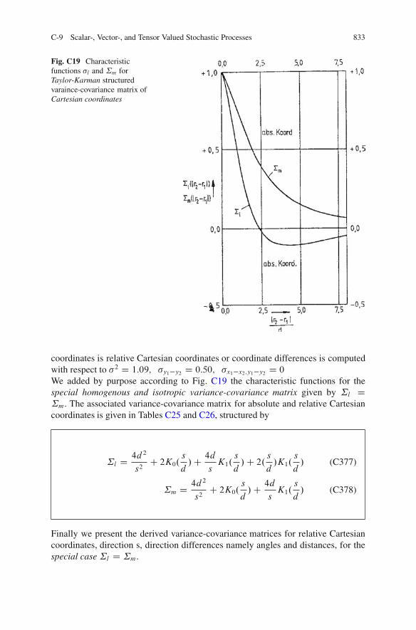
C-9 Scalar-, Vector-, and Tensor Valued Stochastic Processes 833
Fig. C19 Characteristicfunctions �l and ˙m forTaylor-Karman structuredvaraince-covariance matrix ofCartesian coordinates
coordinates is relative Cartesian coordinates or coordinate differences is computedwith respect to �2 D 1:09; �y1�y2 D 0:50; �x1�x2;y1�y2 D 0We added by purpose according to Fig. C19 the characteristic functions for thespecial homogenous and isotropic variance-covariance matrix given by ˙l D˙m. The associated variance-covariance matrix for absolute and relative Cartesiancoordinates is given in Tables C25 and C26, structured by
˙l D 4d2
s2C 2K0.
s
d/C 4d
sK1.
s
d/C 2. s
d/K1.
s
d/ (C377)
˙m D 4d2
s2C 2K0.
s
d/C 4d
sK1.
s
d/ (C378)
Finally we present the derived variance-covariance matrices for relative Cartesiancoordinates, direction s, direction differences namely angles and distances, for thespecial case ˙l D ˙m.

834 C Statistical Notions, Random Events and Stochastic Processes
Fig. C20 Derivedvariance-covariance functionsfor Taylor-Karman structuredvariance-covariance matrix ofCartesian coordinates
˚l.s/ D ˘.s/ D 2˙m.0/� 2˙m.s/;
D 2C�8d2
s2
�� 4K0
sd
���8d
s
�K1
sd
�� 4
sd
�K1
sd
�
(C379)
˚m.s/ D ˘.s/ D 2˙m.0/� 2˙m.s/;
D 2 ��8d2
s2
�� 4K0
sd
�C�8d
s
�K1
sd
�; (C380)
�.s/ D ˘.s/ D 2
s2Œ˙m.0/�˙m.s/� ;
D 2
s2
�1 �
�4d2
s2
�� 2K0
sd
�C 4
sd
�K1
sd
�(C381)
Example 9.1 is based on our contribution E. Grafarend and B. Schaffrin (1979) onthe subject of criterion matrices of type homogenous and isotropic. Other statisticalproperties like anisotropic or non-isotropic correlation functions were treated byG. K. Batchelor (1946), S. Chandrasekhar (1950) and E. Grafarend (1971, 1972)on the subject of axisymmetric turbulence.

C-9 Scalar-, Vector-, and Tensor Valued Stochastic Processes 835
Fig. C21 Two dimensionalnetwork
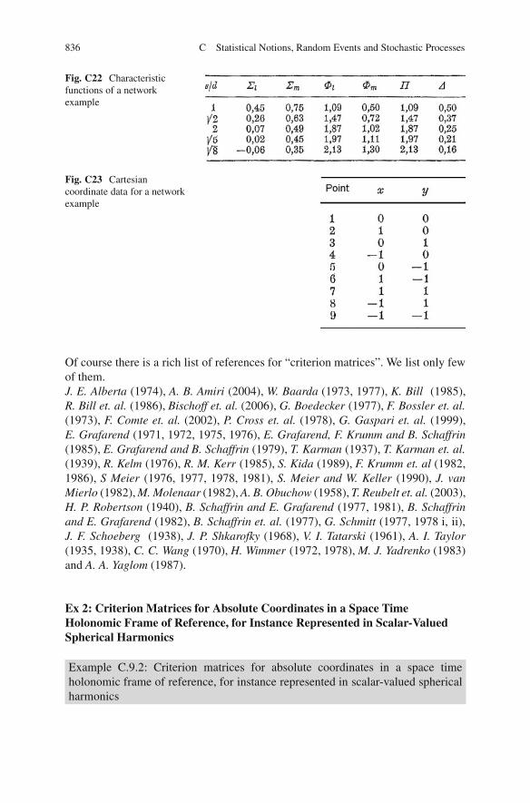
836 C Statistical Notions, Random Events and Stochastic Processes
Fig. C22 Characteristicfunctions of a networkexample
Fig. C23 Cartesiancoordinate data for a networkexample
Of course there is a rich list of references for “criterion matrices”. We list only fewof them.J. E. Alberta (1974), A. B. Amiri (2004), W. Baarda (1973, 1977), K. Bill (1985),R. Bill et. al. (1986), Bischoff et. al. (2006), G. Boedecker (1977), F. Bossler et. al.(1973), F. Comte et. al. (2002), P. Cross et. al. (1978), G. Gaspari et. al. (1999),E. Grafarend (1971, 1972, 1975, 1976), E. Grafarend, F. Krumm and B. Schaffrin(1985), E. Grafarend and B. Schaffrin (1979), T. Karman (1937), T. Karman et. al.(1939), R. Kelm (1976), R. M. Kerr (1985), S. Kida (1989), F. Krumm et. al (1982,1986), S Meier (1976, 1977, 1978, 1981), S. Meier and W. Keller (1990), J. vanMierlo (1982), M. Molenaar (1982), A. B. Obuchow (1958), T. Reubelt et. al. (2003),H. P. Robertson (1940), B. Schaffrin and E. Grafarend (1977, 1981), B. Schaffrinand E. Grafarend (1982), B. Schaffrin et. al. (1977), G. Schmitt (1977, 1978 i, ii),J. F. Schoeberg (1938), J. P. Shkarofky (1968), V. I. Tatarski (1961), A. I. Taylor(1935, 1938), C. C. Wang (1970), H. Wimmer (1972, 1978), M. J. Yadrenko (1983)and A. A. Yaglom (1987).
Ex 2: Criterion Matrices for Absolute Coordinates in a Space TimeHolonomic Frame of Reference, for Instance Represented in Scalar-ValuedSpherical Harmonics
Example C.9.2: Criterion matrices for absolute coordinates in a space timeholonomic frame of reference, for instance represented in scalar-valued sphericalharmonics

C-9 Scalar-, Vector-, and Tensor Valued Stochastic Processes 837
Fig. C24 Derivedvariance-covariance functionsfor a special Taylor-Karmanstructure variance-covariancematrix of type ˙l D ˙m forCartesian coordinates
Conventional geodetic networks have been adjusted by methods of Total LeastSquares and optimized in different reference frames. The advantage of a rigourouslythree dimensional adjustment in a uniform reference frame is obvious, especiallyunder the influence of subdtic geodetic networks within various Global PositioningSystems (GPS, Global Problem Solver). Numerical results in a three dimensional,Total Least Squares approach are presented for instance by K. Bergbauer et. al.(1979) K. Euler et. al. (1982), E. Grafarend (1991), G. Hein and H. Landau (1983),and by W. Jorge and H. G. Wenzel (1973).
The diagnosis of a geodetic network is rather complicated since the measure ofquality, namely the variance-covariance matrix of three dimensional coordinates ofCartesian type contains 3g.3gC 1/=2 independent elements. The integer number gaccounts for the number of ground stations.
Example: g = 100

838 C Statistical Notions, Random Events and Stochastic Processes
Fig. C25 Homogenousisotropic normalizedvariance-covariance matrix ofabsolute coordinates from anetwork example

C-9 Scalar-, Vector-, and Tensor Valued Stochastic Processes 839
Fig. C26 Special homogenous isotropic normalized variance-covariance matrix of absolutecoordinates for a network example case ˙l D ˙m
Fig. C27 Special homogenous isotropic normalized variance-covariance matrix of relativecoordinates for a network example case ˙l D ˙m
The number of independent elements with in the coordinate variance-covariancematrix amounts to 45,150.
Example: g = 1,000
The number of independent elements within the coordinate variance-covariancematrix amounts to 4,501,500.
Example: g = 5,000 (GPS)

840 C Statistical Notions, Random Events and Stochastic Processes
The number of independent elements within the coordinate variance-covariancematrix amounts to 125,507,500 !In a definition, the same number of unknown variance-covariance elements ofvertical deflections and gravity disturbances.
The open big problem
In light of the great number of elements of the variance-covariance matrix it is anopen question how to achieve any measure of quality of geodetic network based onGPS. We think the only way to get away from this number of millions of unknownsis to design an idealized variance-covariance matrix again called criterion matrix.Comparing the real situation of the variance-covariance with an idealized one, wereceive an objective measure of quality of the geodetic network.
Here we are aiming for designing a three-dimensional criterion matrices forabsolute coordinates in a holonomic frame of reference and for functionals ofthe “disturbing potential”. In a first section we extensively discuss the notion ofcriterion matrix on a surface of a moving frame of type homogenous and isotropicon the sphere which is a generalization of the classical Taylor-Karman structure fora vectorized stochastic process. The vector values stochastic process on the sphereis found. In detail we review the representation of the criterion matrix in scalar- andvector-valued spherical harmonics. In section two we present the criterion matricesfor functionals of the disturbing potential. The property of harmonicity is takeninto account for the case that a representation in terms of scalar-valued sphericalharmonics exists. At the end, we present a numerical example.
Example C.9.21: Criterion matrices for absolute coordinates in a space timeholonomic frame if reference
The variance-covariance matrix of absolute Cartesian coordinates in the fixedorthonormal frame of equatorial type, holonomic in spacetime, is transformed intoa moving frame, e.g. of spherical type. In the moving frame longitudinal and lateralcharacteristic functions are derived. The postulates of spherical homogenity andspherical isotropy are reviewed extending to the classical Taylor-Karman structurewith respect to three dimensional Cartesian coordinates into three dimensions.Finally the spherical harmonic representation of the coordinate criterion matrix isintroduced.
Transformation of the coordinate criterion matrix from a fixed into a moving frameof reference
F� ! e� WWe depart from the fixed orthonormal frame fF
e1�; Fe2�; Fe3�g which we transform
into a moving one fee1�; ee2�; ee3�; g by

C-9 Scalar-, Vector-, and Tensor Valued Stochastic Processes 841
F� ! e� D RE.�; �; 0/F� (C382)
RE.�; �; 0/ WD R3.0/R2.2��/R3.�/ is the three dimensional euler rotation matrix
including geometric longitude � and geometric latitude �. As an example assume arepresentation of a placement vector x
eby spherical coordinates .�; �; r/ such that
x D F1�r cos� cos� C F2�r sin� cos� C F3�r sin � (C383)
e1� D �x;� � kx;�k D �e�
e2� D �x;� � kx;�k D �e�
e3� D �x;r � kx;rk D �er (C384)
x;� denotes ıx=ı� etc.
e� ! f�
Now let us rotate the orthonormal frame fe1�; e2�; e3�; g into the orthonormal frameff1�; f2�; f3�; g by means of the South azimuth ˛
e� ! f� D R3.˛/e� �
2
4f1�f2�f3�
3
5
D2
4cos˛ sin˛ 0� sin ˛ cos˛ 00 0 1
3
5
2
4e1�e2�e3�
3
5 (C385)
The transformation e� ! f� on the unit sphere orientates f1� into the direction ofthe great circle connecting the points .�; �; r/ and .�0; �0; r 0/ For this reason theunit vector f1� will be called “longitudinal direction”. In contrast, f2� points indirection orthogonal to f1�, but still in the tangential plane of the unit sphere. Thuswe call the unit vector f2� “lateral direction”. Obviously f3� D e3� holds
F� ! g! f�
There is an alternative way to connect the triads F� and f�. Consider the sphericalposition of a point in the “orbit” of the great circle passing through the pointsx; x0, respectively. For a given set of “Keplerian elements” f˝; i; !g - ˝ the rightascension of the ascending node, i the inclination and ! the angle measured inthe “orbit” - we transform the fixed orthonormal frame fF1�;F2�;F3�g into theorthonormal “great circle moving frame” fg1; g2; g3g D ff3�; f1�; f2�; g by
F� ! g D R3.!/R1.i/R3.˝/F (C386)
g! F� D R3.�˝/R1.�i/R3.�!/F (C387)

842 C Statistical Notions, Random Events and Stochastic Processes
Fig. C28 Moving and fixedframe of reference on thesphere : two point correlationfunction
or explicitly
2
4g1g2g3
3
5 D2
4cos! cos˝ � sin! cos i sin˝ cos! sin˝ C sin! cos i cos˝ C sin! sin i
� sin! cos˝ � cos! cos i sin˝ � sin! sin˝ C cos! cos i cos˝ cos! sin isin i sin˝ � sin i cos˝ cos i
3
5
(C388)
:
2
4F1�F2�F3�
3
5 (C389)
g3 D sin i sin˝F1� � sin i cos˝F2� C cos iF3� (C390)
represents the “great circle normal” parameterized by the longitude 2�˝ and the
latitude 2� i . g1 and g2 span the “great circle plane”, namely g1 is directed towards
the spherical point x.
Figure C28 illustrates the various fames of type “fixed” and “moving”.
fg1; g2; g3g D ff3�; f1�; f2�; g, g2 is the vector product of g3 and g1
Transformation of variance-covariance matrices
Next we compute the Cartesian coordinates variance-covariance matrix.

C-9 Scalar-, Vector-, and Tensor Valued Stochastic Processes 843
†.x; x0/ D †i�j�.x; x0/fFi� ˝ Fj�g†.x; x0/ D †i�j�.x; x0/ffi�.x/˝ fj�.x0/g†.x; x0/ D †ij .x; x0/fgi .x/˝ gj .x0/g (C391)
wherei; j"f1; 2; 3g holds
.˙ij 0
/ D2
4˙x;x0 ˙x;y0 ˙x;z0
˙y;x0 ˙y;y0 ˙y;z0
˙z;x0 ˙z;y0 ˙z;z0
3
5 (C392)
.˙ij 0
/ D EfŒxi �Efxi g�ŒXj 0 � EfXj 0g�g D Ef"i"j 0g (C393)
˙.x; x0/ WD Ef".x/"T .x0/g (C394)
Note that the variance-covariance matrix ˙ij 0
.x; x0/ is a two-point tensor fieldpaying attention to the fact that the coordinate errors ".x/ and ".x/ are functionsof the point x; x0, respectively. Now let us transform˙� $ ˙� $ ˙ .
˙�3�0 D RE.�; �; ˛/˙
�3�3RT
E.�0; �0; ˛0/
D R3.�˝/R1.�i/R3.�!/˙3�3R3.�!0/RT1 .�i 0/RT
3 .�˝ 0/
˙�3�0 D RE.�; �; ˛/˙
�RTE.�
0; �0; ˛0/ (C395)
D RE.�; �; ˛/˙�R.�!;�i;�˝/˙3�3RT .�!0;�i 0;�˝ 0/ � RT
E.�0; �0; ˛0/
˙3�0 D RT .�!0;�i 0;�˝ 0/˙3�3R.�!;�i;�˝/D RT .�!0;�i 0;�˝ 0/RT
E.�; �; ˛/˙�3�3RE.�
0; �0; ˛0/ � R.�!0;�i 0;�˝ 0/
A detailed write-up of the variance-covariance matrix ˙� is
.˙ij 0
/ D2
4˙ll 0 ˙lm0 ˙lr 0
˙ml 0 ˙mm0 ˙mr 0
˙rl 0 ˙rm0 ˙rr 0
3
5 (C396)
indicating the “longitudinal” base vector f1� D fl�, “lateral” base vector f2� D fm�and the “radical” base vector f3� D fr� D er . In terms of spherical coordinates˙�; ˙ , respectively, can be written
˙�3�0.x; x0/ D ˙�.�; �; r; �0; �0; r 0/ (C397)
˙3�0.x; x0/ D ˙.!; i;˝; r; !0; i 0;˝ 0; r 0/ (C398)
˙ll 0 D Ef"l.x/"l 0.x0/g;; ˙l l 0.x; x0/ffl .x/˝ fl 0.x0/g

844 C Statistical Notions, Random Events and Stochastic Processes
˙lm0 D Ef"l.x/"m0.x0/g;; ˙lm0.x; x0/ffl .x/˝ fm0.x0/g
˙lr 0 D Ef"l.x/"r 0.x0/g;; ˙lr 0.x; x0/ffl .x/˝ fr 0.x0/g (C399)
The characteristic function ˙ll 0.x; x0/ is called longitudinal correlation function,˙mm0.x; x0/ lateral correlation function, ˙lm0.x; x0/ cross correlation functionbetween the longitudinal error "l.x/ at the point x and the lateral error "m0.x0/ at thepoint x0.
Spherically homogenous and spherically isotropic coordinate criterion matrices ina surface moving frame
terrestrial geodetic networks constitute points on the earths surface. Once wewant to develop an idealized variance-covariance matrix of the coordinates ofthe network points, we have to reflect the restriction given by the closed surface.A three dimensional criterion matrix of Taylor-Karman type is therefore not suitedsince it assumes extension of a network in three dimension up to infinity. a moresuitable concept of a coordinate criterion matrix starts from the representationwhere the radial part is treated separately from the longitudinal-lateral part.Again the nature of the coordinate criterion matrix as a second order two-pointtensor field will help us to construct homogenous and isotropic representations.The spherically homogeneity-isotropy-postulate reflects the intuitive notion os anidealized variance-covariance matrix.
Definition (spherical homogeneity and spherical isotropy of a tensor-valued two-point function):
The two-point second order tensor function ˙.x; x0/ is called spherically homoge-nous, if it is translational invariant in the sense of
†3�3.! C �; i;˝; r; !0 C �; i 0;˝ 0; r 0/ D †3�3.!; i;˝; r; !0; i 0;˝ 0; r 0/ (C400)
for all � 2 Œ0; 2�; i D i 0;˝ D ˝ 0; r D r 0, where !0D! C holds. It is calledspherically isotropic, if it is rotational invariant in the sense of
˙3�3.!� � !�s ; i
�;˝�; r; !�0 � !�s ; i
�0
;˝�0
; r 0/
D R3.ıs/˙3�3.! � !s; i;˝; r; !0 � !s; i 0;˝ 0; r 0/R3.ıs/ (C401)
for all ı"Œ0; 2�; r D r 0; where !0D! C , !�0 D!� C holds. R3.ıs/ indicatesa local rotation around the intersection points xs of the great circle through x; x0and through x�; x�0
, respectively. xs has the common coordinates .˝; i; !s and.˝�; i�; !s� with respect to the locally rotated frames.
End of Definition

C-9 Scalar-, Vector-, and Tensor Valued Stochastic Processes 845
Corollary (spherical homogeneity and spherical isotropy of a tensor-valued two-point function):
The two-point second order tensor function ˙.x; x0/ is spherically homogenous, ifit is a function of . ; i;˝; r/ only:
˙.!; i;˝; r; !0; i 0;˝ 0; r/ D ˙.!; i;˝; r; ! � !s; ; r/ (C402)
It is spherically homogenous and isotropic, if it is a function of . ; r/ only
˙.!; i;˝; r; !0; i 0;˝ 0; r/ D ˙. ; i;˝; r/ (C403)
such that
˙.x; x0/ D f˙0. ; r/ıij C˙22. ; r/ < x0 � xjfi > �
� < x0 � xjfi >g.fi ˝ fj / (C404)
holds for some spherically isotropic and homogenous scalar-valued functions˙0 and ˙22
End of Corollary
Let us interpret the definition of the corollary, especially with respect to Fig. C28.Two points x; x0 are connected to the sphere of radius r D r 0 D r0 by a great circlesuch that D 2 arcsin.kx; x0k=2r0/ is the spherical distance if these points.
Obviously a “translation” of the configuration x; x0 is generated by ! ! !C�; ! !!0 C � where the location of x; x0 in the great circle / “orbit” plane is measuredby !;!0. The “rotation” of the configuration x; x0 is more complicated. Assumetherefore an alternative configuration x�; x�0
of two point connected by anothergreat circle. Note the spherical distances of x; x0 and x�; x�0
respectively, coincide.The great circles intersect at xs, : The location of Xs within the plane x; x0 isdescribed by !s with respect to the ascending node, while within the plane x�; x�0
by !�s . the angle between the two great circles is denoted by ıs .
The configuration x; x0 and x�; x�0
is described with respect to xs by! � !s; i;˝; !0 � !s; i 0;˝ 0 and !� � !�
s ; i�;˝�; !�0 � !�
s ; i�0
;˝�0
respectively.Now it should be obvious that the two configurations under the spherical isotropypostulate coincide once we rotate around xs by the angle ıs.
We expressed˙�. given in the F �-frame in terms of the g-frame, namely by
˙ D RT3 .�!/RT1 .�i/RT3 .�˝/˙�R3.�˝/R1.�i/R3.�!/ (C405)
Introducing ! D .! � !s/C !s we compute the variance-covariance matrix ˙

846 C Statistical Notions, Random Events and Stochastic Processes
˙ D RT3 .! �!s/RT
3 .!s/RT1 .�i/RT
3 .�˝/˙�R3.�˝ 0/R1.�i 0/R3.!s/R3.!0 �!s/(C406)
˙ D RT3 .! � !s/˙sR3.!
0 � !s/ (C407)
in terms of the variance-covariance matrix ˙s in the g.xs/-frame. Now we areprepared to introduce
Corollary (spherical Taylor-Karman structure):
Denote the variance-covariance matrix ˙i�j�0
in the f �- and e�- frame by
f ˙i�j�0 D
�˙ll 0. ; r/ 0
0 ˙mm0. ; r/
� f ˙2�2
(C408)
e˙i�j�
0 D�˙110 ˙120
˙210 ˙220
� e˙2�2
(C409)
and transform f ˙ ! e˙ by
e˙ D�
cos˛ � sin˛sin ˛ cos˛
f ˙ D
�cos˛0 sin˛0� sin ˛0 cos˛0
(C410)
Then
˙110 D ˙ll 0. ; r/ cos ˛ cos˛0 C˙mm0. ; r/ sin ˛ sin ˛0
˙120 D ˙ll 0. ; r/ cos ˛ sin ˛0 �˙mm0. ; r/ sin ˛ cos˛0
˙210 D ˙ll 0. ; r/ sin ˛ cos˛0 �˙mm0. ; r/ cos˛ sin ˛0
˙220 D ˙ll 0. ; r/ sin ˛ sin ˛0 C˙mm0. ; r/ cos˛ cos˛0 (C411)
˙lm0 D ˙ml 0 D 0 (C412)
holds for spherically homogenous and isotropic scalar-valued functions˙ll 0. ; r/,˙mm0. ; r/ called longitudinal and lateral correlation functions on the sphere.
End of Corollary
The corollary extends results of G.J. Taylor (1935), T. Karman (1937) andC. Wang (1970 p. 214-215) and has been given for a special variance-covariancetwo-point tensor field of potential type by H. Moritz (1972 p. 111). Here it hasbeen generalized for any vector-valued field. Note that incase of homogenity andisotropy the cross-correlation functions˙lm0 and˙ml 0 may vanish.
The classical planar Taylor-Karman structure is constrained within.

C-9 Scalar-, Vector-, and Tensor Valued Stochastic Processes 847
Let us put ˛ D ˛0 such that cos˛ cos˛0 D cos2 ˛ D 1� sin2 ˛; sin ˛ sin˛0 D sin2 ˛etc. can be rewritten
˙110 D ˙mm0. /C Œ˙l l 0. / �˙mm0. /� cos2 ˛
˙120 D Œ˙l l 0. / �˙mm0. /� sin ˛ cos˛ D ˙210
˙220 D ˙mm0. /C Œ˙l l 0. / �˙mm0. /� sin2 ˛ (C413)
which is the standard Taylor-Karman form
Representation of the coordinate criterion matrix in scalar spherical harmonics
Let us assume a coordinate variance-covariance matrix which is homogenous andisotropic in the sphere. With reference to (C412) we postulate a coordinate vectorof potential type, in addition, namely
" D gradR � "i D @iR .i D 1; 2; 3/ (C414)
where .@i / D . @@x; @@y; @@z / nd R the scalar potential. Now the variance-covariance
matrix of absolute coordinates can be represented by
˙ij 0 D Ef"i.x/"j 0
.x0/g D @i@j 0EfR.x/R.x0/g (C415)
where we used the commutator relation @iEDE@i of differentiation and integrationoperators. Denote the scalar-valued variance-covariance functionEfR.x/R.x0/g DWK.x; x0/. Once we postulate homogeneity and isotropy of two-point functionK.x; x0/ on the sphere we arrive at
K.x; x0/ D K.r; r 0; / (C416)
For a harmonic coordinate error potential, @i@iR D 0, we find for the covariancefunctionK.r; r 0; /
@i @iK.r; r0; / D Ef@[email protected]/R.x0/g D 0 (C417)
@j 0@j 0K.r; r 0; / D EfR.x/@j 0@j 0R.x0/g D 0 (C418)
Case 1 .kxk D kx0k/On a sphere .kxk D kx0k/ D r0 the scalar-valued variance-covariance functionK. / which fulfils (C414 - C 417) may be represented by
K. / D1X
nD0knPn.cos / (C419)

848 C Statistical Notions, Random Events and Stochastic Processes
where Pn are the Legendre polynomials. The constants kn depend, of course, on thechoice of r0
Case 2 .kxk ¤ kx0k/Denote .kxkD r; kx0kD r 0/. the scalar-valued variance-covariance functionK.r; r 0; / which fulfils (C414 - C 417) may be represented by
K D K.r; r 0; /
D1X
nD01kn.
r20rr 0 /
nC1Pn.cos /C
1X
nD02kn.
rr 0
r0/
n
Pn.cos / (C420)
where the coefficients 1kn; 2kn represent the influence of the decreasing andincreasing solution, by Legendre polynomials with respect to r; r 0, respectively.We can only hope that the covariances K.r; r 0; / decrease with respect to r; r 0,respectively in order to be allowed to discriminate 2kn D 0. In the following we maethis assumption, thus representing
K.x; x0/ D K.r; r 0; / D1X
nD0kn.
r20rr 0 /
nC1Pn.cos / (C421)
Next let us assume the coordinate variance-covariance matrix (C420) is of potentialtype. Then longitudinal and lateral correlation functions on the sphere if radius rcan be represented by
˙ll 0. / D d2
d 2K. / (C422)
˙mm0. / D 1
sin
1
d K. / (C423)
˙ll 0. / D d
d .˙mm0 sin (C424)
if �.x; x0/ is homogenous and isotropic on the sphere.
End of Corollary
Note that the result ˙ll 0 D dd .sin ˙mm0/ for the sphere corresponds to ˙ll 0 D
dds.s˙mm0/ for a harmonic field in the plane.
s Dq.x0 � x/2 C .y0 � y/2 is the Euclidean distance in the plane which
corresponds to at the distance on the sphere.

C-9 Scalar-, Vector-, and Tensor Valued Stochastic Processes 849
Corollary (longitudinal and lateral correlation functions on the sphere of harmonictype):
Let us assume that the coordinate variance-covariance matrix id homogenous,isotropic and harmonic on the sphere in the sense of the definition. Longitudinaland lateral correlation functions on the sphere can be represented by
˙ll 0. / D1X
nD0kn
��.n2 C 3nC 2/cos2
sin2 C .nC 1/
:
�Pn.cos / � Œn2 C 3nC 2�2 cos
sin2 PnC1.cos /
�
C Œn2 C 3nC 2� 1
sin2 PnC2.cos /g (C425)
˙mm0. / D �X
nD01kn nC 1
sin2 Œcos Pn.cos /
�PnC1.cos / (C426)
End of Corollary
For the proof of the above corollary we have made successive use of the recurrencerelation .x2 � 1/dPn.x/=dx D �.nC 1/ŒxPn.x/ � PnC1.x/�;x D cos ; d=d D .dx=d /.d=dx/ D � sin d=dx
Representation of the coordinate criterion matrix in vector spherical harmonics
Previously we restricted the coordinate criterion matrix being homogenous andisotropic on the sphere to be of potential type. Here we generalize the coordinatecriterion matrix to be of potential and “turbulent” type. Thus according to the Lamelemma – for more details see A. Ben Menahem - S. J. Singh (1981) - we representthe coordinate vector
" D gradRC rotA (C427)
where we gauge the vector potential A by divA D 0. In vector analysis gradRis called the longitudinal vector field, rotA the transversal vector field. In orderto base the analysis only on scalar potentials, the source-free vector field rotA isdecomposed SCT where S is the poloidal part while T is the toroidal part such that
" D gradRC rot rot.erS/C rot.erT/ (C428)
.R; S; T / are the three scalar potentials we were looking for. The variance-covariance matrix of absolute coordinates can now be structured according to

850 C Statistical Notions, Random Events and Stochastic Processes
˙.x; x0/ D Ef".x/gD grad ˝ grad 0EfR.x/R.x0/gCrot rot ˝ rot 0rot 0erer 0EfS.x/S.x0/gCrot ˝ rot 0erer 0EfT .x/T .x0/g (C429)
where we have assumedEfR.X/S.X0/g D 0;EfR.X/T .X0/g D 0;EfS.X/T .X0/gD 0 holds for a coordinate variance-covariance matrix ˙.xx0/ homogenous andisotropic on the sphere. Thus with respect to the more general representation is
˙.x; x0/ D grad ˝ grad 0K
C rot rot ˝ rot 0rot 0erer 0L
C rot ˝ rot 0erer 0M (C430)
where K WD EfR.X/R.X0/g; L WD EfS.X/S.X0/g;M WD EfT .X/T .X0/g aresupposed to be the scalar-valued two point covariance functions depending on.r; r 0; / for .˙.x; x0// homogenous and isotropic on the sphere.
The representation of the criterion matrix .˙.x; x0// in terms of vector sphericalharmonics is achieved once we introduce the spherical surface harmonics.
enm.��/ D
2
6666664
q2.2nC 1/ .n�m/Š
.nCm/ŠPnm.sin �/ cosm� 8m > 0
p2.2nC 1/Pn.sin�/ 8m D 0
q2.2nC 1/ .n�jmj/Š
.nCjmj/ŠPnjmj.sin�/ sin jmj� 8m < 0:
(C431)
where Pnm.sin�/ are the associated Legendre functions
Pnm.x/ D 1
2nnŠ.1 D x2/m=2 d
nCm
dxnCm .x2 � 1/n (C432)
Note that the quantum numbers run nD 0; 1; � � � ;1Im D �n;�nC 1; � � � ; 0; � � � ;n � 1; n. The base functions enm.�; �/ are orthonormal in the sense
1
4
2Z
0
d�
C=2Z
�=2d� cos� eklenm D ıkn ılm (C433)

C-9 Scalar-, Vector-, and Tensor Valued Stochastic Processes 851
Finally a vector field " can be represented in terms of vector spherical harmonicsby
" D Unmanm C Vnmbnm CWnmcnm (C434)2
666664
anm WD er enm.�; �/
bnm WD r grad enm.�; �/
cnm WD �x grad enm.�; �/:
(C435)
For more details on vector spherical harmonics we refer to standard textbooks, heree.g. to E. Grafarend (1982).
˙.x; x0/ D Ef".x/˝ ".x0/gD Unmn0m0anm ˝ an0m0
CVnmn0m0bnm ˝ bn0m0
CWnmn0m0cnm ˝ cn0m0 (C436)
which is due to < ajb >D< ajc >D< bjc >D 0. Unmn0m0 etc. are sphericalcovariance functions.
Example C 9.22: Towards criterion matrices for functionals of the distributingpotential in a space-time holonomic frame if reference
The geodetic observational equations in their linearized form contain besideunknown Cartesian coordinate corrections in an orthonormal reference frame,being holonomic in space-time, the disturbance of the potential and its derivativesas unknowns . for a complete set-up of a criterion matrix of geodetic unknownswe have therefore present thoughts about a homogenous and isotropic variance-covariance matrix of the potential disturbance and its derivatives, The postulates ofhomogeneity and isotropy will lead again to the extension of an classical Talyor-Karman structure. finally the representation of the criterion matrix of potentialrelated quantities in terms of scalar spherical harmonics is introduced. Since thepotential disturbance is harmonic function, vector spherical harmonics are notneeded.
We begin the transformation of the gravity criterion matrix from spherical intoCartesian coordinates.
With reference to the linearized observational equations the unknowns .bı�� ;cı�� ;bı�/ have to be equipped with a criterion matrix, reasonable to be homogenous and

852 C Statistical Notions, Random Events and Stochastic Processes
isotropic on the sphere. In order to take advantage of lemma and corollaries of thesecond chapter, we better transform the spherical coordinates of the disturbancegravity vector ı� into Cartesian ones and then apply the variance-covariance“propagation” on the transformation formula.
ı�i WD �i � �i D2
4�� cos�� cos˚��� sin�� cos˚��� sin˚�
3
5 �2
4�� cos�� cos���� sin�� cos���� sin ��
3
5
D2
4�.� C ı�/ cos.�� C ı��/ cos.�� C ı��/�.� C ı�/ sin.�� C ı��/ cos.�� C ı��/
�.� C ı�/ sin.�� C ı��/
3
5
�2
4�� cos�� cos���� sin�� cos���� sin ��
3
5 (C437)
ı�i:D2
4�.� C ı�/.cos�� � ı�� sin��/.cos�� � ı�� sin��/�.� C ı�/.sin�� C ı�� cos��/.cos�� � ı�� sin ��/
�.� C ı�/.sin�� C ı�� cos��/
3
5
�2
4�� cos�� cos���� sin�� cos���� sin ��
3
5 (C438)
ı�i:D2
4�ı� cos�� cos�� C ı��� sin�� cos�� C ı��� cos�� sin ���ı� sin�� cos�� � ı��� cos�� cos�� � ı��� sin�� sin ��
�ı� sin�� � ı��� cos��
3
5
(C439)2
4ı�1
ı�2ı�3
3
5 :D2
4C� sin�� cos�� C� cos�� sin �� � cos�� cos���� cos�� cos�� �� sin�� sin �� � sin�� cos��
0 �� cos�� � sin��
3
5
2
4ı��
ı��ı�
3
5
(C440)2
4ı�1
ı�2ı�3
3
5 :D
2
64��2 C�1�2.�21 C �22 /�1=2 �1��1
C�1 ��2�3.�21 C �22 /�1=2 �2��1
0 �.�21 C �22 /�1=2 �3��1
3
75
2
4ı��
ı��ı�
3
5 (C441)
The variance-covariance matrix Dfcı�i .x/;bı�j 0.x0/g as a function of the variance-
covariance matrix Df.bı�� ;cı�� ; bı�/.x/; .bı�� ;cı�� ; bı�/.x0/g based on the trans-formation ( C 438) is given. finally the Cartesian variance-covariance matrixDfcı�i .x/;bı�j 0.x0/g in the fixed frame F � should be transformed into the movingframe f � according to (C381).

C-9 Scalar-, Vector-, and Tensor Valued Stochastic Processes 853
Fig. C29 Normalized covariance function K. / D 5P
nD0
knPn.cos / for kn D 1nC2
Thus we refer to�˙l l 0; �
˙lm0 ; �
˙lr 0 ; �
˙ml 0 ; �
˙mm0; � � � ; �˙rr 0 (C442)
as the longitudinal correlation function �˙l l 0 , the lateral correlation function �˙mm0 etc.of the gravity disturbance vector ı�i .In order to construct a homogenous and isotropic criterion matrix for functionals ofthe disturbing potential in a surface moving frame we refer to the introduction whichapplies here, too. Again we make use of the definition of homogeneity and isotropyof the tensor-valued two-point function �˙.X;X
0/ on the sphere, the basic lemmaand the corollary for the spherical Taylor-Karman structure. Just by adding the lefthand index � on ˙ within formula (C410) (C411), we arrive at the correspondingformulae for longitudinal, lateral and cross-correlation of the gravity disturbancevector ı� .For the representation of the criterion matrix for functionals of the disturbingpotential in scalar spherical harmonics we once more refer to (C417). All resultscan be transferred, especially (C 420 - C 425) once we write K.r; r 0; / as thescalar-valued two-point function EfŒcıw � E.cıw/�xŒcıw � E.cıw/�x0g homogenousand isotropic on the sphere. Besides the first-order functionals of the potential ıwand their variance-covariance matrices, higher order functionals, e.g. for gravitygradients, and their variance-covariance matrices can be easily obtained, a projectfor the future.

854 C Statistical Notions, Random Events and Stochastic Processes
Fig. C30 Normalized covariance function K. / D5P
nD0
knPn.cos / for kn D 1.nC2/.n2�2nC2/
A numerical example of the homogenous and isotropic two-point functionK.x; x0; / on the space
For demonstration purpose plots C29 - C31 show the normalized covariancefunctionsK.X;X0/ D K.r; r 0; /
D K. / D5P
nD0knPn.cos / for case 1
.kXk D kmathbf X0k D r0/ and three different choices of the coefficients kn.The coefficients are chosen in such a manner that their sum equals the unity (soas to normalize the covariance function) and the covariance function approacheszero as tends to . As an example for the construction of a criterion matrix, thecoefficients kn could be estimated for an ideal network and its variance-covariancematrix; that is derived covariance functionK.x; x0/.We have taken a part of Appendix C 9.2 from our contribution E. Grafarend,I. Krumm and B. Schaffrin (Manuscripta geodetica 10 (1988) 3-22). Sphericalhomogeneity and isotropy in tensor-valued two-point functions have been intro-duced by E. Grafarend (1976) and H. Moritz (1972, 1978).
Ex 3: Space Gravity Spectroscopy: The Benefits of Taylor–KarmanStructured Criterion Matrices
Example C.9.3. Space gravity spectroscopy: the benefits of Taylor-Karman struc-tured criterion matrices (eg, P. Marinkovice et. al. (2003))

C-9 Scalar-, Vector-, and Tensor Valued Stochastic Processes 855
Fig. C31 Normalized covariance function K. / D 5P
nD0
knPn.cos / for kn D 1n2C3
As soon as the space spectroscopy was successfully performed, for instance bymeans of semi-continuous ephemeris of LEO-GPS tracked satellites, the problemof data validation appeared. It is for this purpose that a stochastic model for thehomogenous isotropic analysis of measurements, obtained as “directly” measuredvalues in LEO satellite missions (CHAMP, GRACE, GOCE), is studied. Anisotropic analysis is represented by the homogenous distribution os measured valuesand the statistical properties of the model are calculated. In particular a correlationstructure function is defined by the third order tensor (Taylor-Karman tensor), forthe ensemble average of a set of incremental differences in measured components.Specifically, Taylor-Karman correlation tensor is calculated with the assumptionthat the analyzed random function is of a “potential type”. The special class ofhomogenous and isotropic correlation functions is introduced. Finally, a successfulapplication of the concept is presented in the case study CHAMP and a comparisonbetween modeled and estimated correlations is performed.
Example C.9.31. Introduction
A significant problem of LEO satellites, both in geometry and gravity space,is the association of quality standards to Cartesian ephemeris in terms ofvariance-covariance matrix valued-functions. as a pessimistic measure of thequality standards os LEO satellite ephemeris, a three dimensional Taylor-Karmanstructured criterion matrix has been proposed, named in honor of Taylor (1938) andKarman (1938), the founders of the statistical theory of turbulence.

856 C Statistical Notions, Random Events and Stochastic Processes
The concept of the Taylor-Karman criterion matrices was first introduced byE. Grafarend (1979) and subsequently further developed by B. Schaffrin andE. Grafarend (1982), H. Wimmer (1982), and E. Grafarend et. al. (1985, 1986).with this contribution we extend the application of the Taylor-Karman structuredmatrices to the third-dimension, namely to the long-arc orbit analysis.
If we assume the vector-valued stochastic process to be the gradient of a randomscalar-valued potential, in particular its longitudinal and lateral correlation functionor the “correlation function along-track and across-track”, what would be the struc-ture of a three-dimensional Taylor-Karman variance-covariance matrix. In order toanswer this question, a three-dimensional correlation tensor and its decompositionin the case of homogeneity and isotropy is studied with the emphasis on R
3.Additionally, we deal with a special class of homogenous and isotropic tensor-valued correlation functions. They are derived, analyzed and applied to the datavalidation process. The theoretical concept for the application of the previouslydiscussed criterion matrix in the geometric and gravitational analysis of LEOsatellite ephemeris is presented. Finally the case study CHAMP is used for theapplication of our theory concept followed by the results and conclusion.
Example C.9.32: Homogenous and isotropic variance-covariance tensor and cor-relation functions in a three-dimensional Euclidean space
Example C.9.321: Notions of homogeneity and isotropy
The notions of homogeneity and isotropy for functions on R� are briefly explained
as the following. The general context for these two definitions involves the action ofa transitive group of motions on a homogenous and space belongs to the extensivetheory of Lie groups (F. W. Warner (1983), A. M. Yaglom (1987)). However, it isimportant to clarify the different notions of homogeneity and isotropy exist dueto the variety of homogenous spaces and transitive group actions on these spaces.The terminology introduced associates the notion of homogeneity and isotropy with
Fig. C32 Graphical representation of the longitudinal and lateral correlation functions

C-9 Scalar-, Vector-, and Tensor Valued Stochastic Processes 857
the functions on R� that are invariant under the translation group acting on R
� .The notion of isotropy is defined for functions on R
� that are invariant under theorthogonal group acting on R
�.
Table C.9.9: Tensor-valued correlation function of second-order“two-point correlation function”
˙.x�; x��/ D3P
i;jD1ei ej˙ij .x�; x��/ D
3P
i;jD1˙ij .x�; x��/ei ej (C443)
r WD kx�; x��k and r WD x�; x��
˙ij .r/ D ˙m.r/ıij C Œ˙l .r/ �˙m.r/��xi�xj
r2; i; j 2 f1; 2; 3g (C444)
“Cartesian versus spherical coordinates”
�x1 D �x WD .x��1 � x�
1 / D r cosˇ cos˛
�x2 D �y WD .x��2 � x�
2 / D r cosˇ sin ˛ (C445)
�x3 D �z WD .x��3 � x�
3 / D r sinˇ
“continuity of a potential type”
˙l.r/ D dŒr˙m.r/�
drD ˙m.r/C r d˙m.r/dr
(C446)
End of Table C.9.9
Example C.9.322: Homogenous and isotropic variance-covariance tensor (correla-tion tensor)
Taylor (1938) proved that he homogenous random field X.t/ correlation function˙.r/ D< X.tC r/X.t/ > depends only on the length r D krk of the vector r andnot on its direction, where < ::: > denoted the ensemble average. If the correlationfunction ˙.r/ of the homogenous random field X.t/ in R
� has the property, thenthe field X.t/ is said to be an isotropic random field in R
�. The correspondingcorrelation function ˙.r/ is then called an isotropic correlation function in R
�
( or an n-dimensional isotropic correlation function). Process, which satisfy theintroduced postulates of homogeneity and isotropy, are said to be (widely) stationary(M. J. Yadrenko (1983)). Note that for an isotropic random field in R
�, all directionsin space are obviously equivalent.
The decomposition of a homogenous and isotropic variance-covariance tensor-valued function, shown in box 1, was introduced by von Karman and Howarth

858 C Statistical Notions, Random Events and Stochastic Processes
Fig. C33 Graphical representation of the correlation tensor transformation
(1938) by means of a more general and direct method than the one used byG. J. Taylor(1938). Additionally, Robertson (1940) refined and reviewed theT. Karman and L. Howard equation in the light of a classical invariant tensortheory.
The decomposition of ˙ij .kx� � x��k/, with a special emphasis on nD 3, isperformed in terms of Cartesian coordinates and with respect to the orthonormalframe of reference fe1; e2; e3j0g attached to the origin 0 of a three-dimensionalEuclidean space. kx� � x��k denotes the Euclidean distance r between the twopoints x� and x�� of E� WD fR�; ıij . Longitudinal and lateral correlation functions˙l and ˙m, are the structural elements of such a homogenous and isotropic tensor-valued variance-covariance function which appear in the spherical tensor ˙m.r/ıijas well as in the oriented tensor Œ˙l .r/�˙m.r/��xi�xj =r
2 for all i; j 2 f1; 2; 3g,see (C443) and Fig. C.32. ıij denotes the Kronecker or unit matrix, �xi theCartesian coordinate difference between the points x� and x��. These differences arealso represented in terms of relative spherical coordinates .˛; ˇ; r/, (C444). Finallythe continuity condition of a potential type is formulated by (C445) which providesthe unique relation between˙l and˙m (G. J. Taylor (1938); H. M. Obuchow (1958);E. Grafarend (1979)).Due to its complexity, it is necessary to further elaborate on the previous equationset. The correlation tensor ˙ij .r/ was transformed to a special coordinate systemO 0x0
1x02x
02 in R
� instead of the initial setOx1x2x3. The new setO 0x01x
02x
03 is selected
in such a way so that its origin O 0 is shifted by the vector x�� with respect to theorigin O , as illustrated in Fig. C15. This means that O 0 coincides with the terminalpoint of the vector x�� that refers to the initial coordinates, while the axis O 0x0
1 liesalong the vector x� � x��.

C-9 Scalar-, Vector-, and Tensor Valued Stochastic Processes 859
Fig. C34 The behavior of Tatarski’s correlation function for different values of shape parameter�.d D 900/ and scale parameter d.� D 3=2/
˙ij , introduced here are explanatory functions, are the components of the correla-tion tensor˙ij .r/ in the new set of coordinates. The functions˙ 0
ij .r/ clearly dependonly on the length r D krk of the vector r, since the direction of r is fixed in thenew set of coordinates. In the space R� exist a reflection which leaves the points x�and x�� D .O 0/ unmoved and it replaces the axis O 0x0
j by �O 0x0j , where j ¤ 1 is
a fixed number. However, it does not change the directions of all other coordinatesaxes O 0x0
l ; l 2 f1; 2; 3g and l ¤ j . It follows that
˙ 0ij .r/ D �˙ 0
ij .r/ D 0textrmfori ¤ j (C447)
Hence, only the diagonal elements ˙ 0ij .r/ of ˙ij .r/ can differ from zero. Further
more, if i ¤ j and j ¤ 1, then the axis O 0x0i by its rotation around the axis O 0x0
j ,can be transformed to the axis O 0x0
1. Hence
˙ 022.r/ D ˙ 0
33.r/ (C448)
The tensor ˙ 0ij and, consequently,˙ij are symmetric and their components˙ 0
ij .r/
can take at most only tow non-equal non-zero values at the already introduceslongitudinal correlation function˙ 0
i i .r/ D ˙l.r/ and the lateral correlation function˙ 022.r/ D ˙ 0
33.r/ D ˙m.r/, which specify in a unique way the correlation tensor.In order to obtain the explicit form of ˙ij .r/, as the function of ˙l.r/ and ˙m.r/,the unit vectors of the old coordinate axes Ox1;Ox2;Ox3 along the axes of thenew system O 0x0
1; O0x02; O
0x03 must be resolved and then ˙ij .r/ can be represented
as linear combination of the functions ˙ 0kl .r/; .k ¤ i; l ¤ j and k; l 2 f1; 2; 3g/,
which leads to (C442) and (C443).

860 C Statistical Notions, Random Events and Stochastic Processes
Example C.1. homogenous and isotropic correlation functions
It was shown in the pervious section that for a homogenous and isotropic randomfields defined on the Euclidean space R
�, the correlation between x� and x��depends only on the Euclidean distance kx� � x��k. Therefore as shown in TableC32, we can distinguish a homogenous and isotropic correlation function on R
�
with the real valued function˙.r/ defined on Œ0;1/ and we denote by ˚n the classof all continuous permissible functions ˙.r/ W Œ0;1/ ! such that ˙.0/ D 1 (weare working in terms od correlation not covariance) and the symmetric function˙.k:k/ is a positive definite on R
�. The characterization of classes ˚n, also shownin Table C.9.10, is a well known result of J. F. Schoenberg (1938). The function˙.r/ W Œ0;1/ ! R is an element of ˚n if and only if it abmits a representationin the form of (C450), where W is a probability measure on Œ0;1/; J.n�2/=2 is theBessel function of the first kind of order .n � 2/=2 and � stands for the Gammafunction. Hence in for geodesy relevant spaces R� and R
�, (C450) reduces to theform presented in (C452).
Table C.9.10: Isotropic correlation and Schoenberg’s characterization
“homogenous and isotropic correlation function”˙.x�; x��/ D ˙.kx�; x��k/; x�; x�� 2 R
� (C449)r WD kx�; x��k
“the characterization of the ˚n class”˙n.r/ D
R
Œ0;1/
˝n.r�/dW.�/ (C450)
˝n.r�/ D � .n=2/. 2r /.n�2/=2
J.n�2/=2.r/ (C451)“reduction of the ˝n for n D 2 and n D 3”
˝2.r/ D J0.r/ and ˝3.r/ D r�1 sin r (C452)
End of Table C.9.10
Table C.9.11: Special classes of correlation functions
“Tatarski’s class”
˙Œ��.r/ D 21��
� .�/. rd/�K�.
rd/ (C 453)
“Shkarofsky’s class”
˙Œ�;ı�.r/ D . r2
d2Cı2/�=2K�.. r2
d2Cı2/1=2/
ı�K�.ı/(C454)
End of Table C.9.11

C-9 Scalar-, Vector-, and Tensor Valued Stochastic Processes 861
Example C.2. Tatarski’s class of homogenous and isotropic correlationfunctions
Many analytical candidate models for ˙ have been suggested in the literature (forexample, Buell, (1972); Haslett, (1989)), but we refer to Tatarski (1962) as beingthe first who elaborated on such correlation functions which fulfill all the conditionspresented in the previous section. The Tatarski’s correlation function class is shownin Table C.9.11 and illustrated by Fig. C.34. In addition to V. J. Tatarski’s class, avery general family of correlation function models due to J. P. Shkarofsky (1968)is introduced, that came as the generalization of Tatarski’s correlation functionfamily. These two classes, which have been proved to be the members of ˚3(Shkarofsky, (1968) and of ˚1 classes; Gneiting et. al. (1999)), can be applied tomany geodetic problems, (e.g. Grafarend (1979); Meier (1982); Wimmer (1982);Grafarend (1985)).
In equation of Table C.9.11, K� stands for a modified Bessel function of order�; d > 0 is a scale parameter, and ı > 0 and � are shape parameters. In the case ofı D 0 J. P. Shkarofsky’s class reduces to V. J. Tatarski’s class.
The special case of Tatarski’s class appears if the shape parameter � is sum ofa non-negative integer k and 1=2. Then the right-hand side of the equation canbe written as a product of exp.�r=d/ and a polynomial of degree k in r=d (eg.T. Gneiting, (1999)). In particular, in the case of nD 3 dimensional Markov processof the p D 1 order, shown in Fig. C34, the shape parameter is expressed as� D .2p C 1/=.n� 1/ D 3=2 and results in the flowing simplification of (C454):
˙Œ3=2�.r/ D .1C r
d/ exp.� r
d/ (C455)
Example C.3. Three dimensional Taylor-Karman criterion matrix in thegeometric and gravitational analysis of LEO satellite ephemeris
WE have so far analyzed the theoretical background and solution for design of thehomogenous and isotropic Taylor-Karman correlation tensor. The question is, howthis theoretical concept applies to the geometric and gravitational analysis of LEOsatellite ephemeris.
The basic idea is, that the errors in the position vectors of LEO satellites constitutea vector-valued stochastic process. Following this concept, a satellite orbit of LEO-GPS tracked satellites is an homogenous and anisotropic field of error vectorsand the error situation is described by the covariance function. As it is wellknown, the error situation os a newly determined position in a three-dimensionalEuclidean space is the best, when the error ellipsoid is sphere (isotropy) with the

862 C Statistical Notions, Random Events and Stochastic Processes
minimal radius and if the error situation is uniform over the complete satellite orbit(homogeneity). This “ideal” situation can be explained by the three-dimensionalTaylor-Karman structured criterion matrix of W. Baarda - E. Grafarend (potential)type. Then the correlations between the vectors of pseudo-observations of satelliteephemeris described by the longitudinal and lateral correlation functions.
The characteristic correlation functions can be estimated by matching the correlationtensor with a three-dimensional Markov process of 1st order and with theintroduction of some additional information about the underlying process. Thecorrelation analysis is performed with the assumption that the vector valued three-dimensional random function is of “potential type” (E. Grafarend (1979)), i.e. thegradient of a random scalar function “signal s.x/”. The structure of the randomfunction s.x/ is outlined as an n-dimensional Markov process of the pth order.Figure C35 illustrates the case n D 3 and p D 1:
One of the simples differential equation os such a process has the form given by
.�2 � ˛2/ps.x/ D e.x/ (C456)
where e.x/ is a white noise. If the Laplace operator can be applied to thehomogenous random scalar function, then it transforms this function into a newhomogenous random function, having the spectral density that corresponds to thespectral density of the correlation function of (C453) and (C454), see P. Whittle(1954), V. Heine (1955) and P. Whittle (1963). Hence the homogenous solution ofC455 (if it exist) must have the spectral density that corresponds to the spectraldensity of the correlation function.
Table C.9.9 summarizes the representation of the homogenous and isotropic corre-lation functions of type
(i) Signal correlation function˙ ,(ii) Longitudinal correlation function˙l and
(iii) Lateral correlation function˙m
Example C.9.34: Results and conclusions
Case study: Champ
As the numerical test in this study, we processed two data sets: two three-dimensional fx.tk/; y.tk/; z.tk/g and fx.td /; y.td /; z.td /g Cartesian ephemeristime-series of CHAMP satellite orbit for the test period from day 140 to 150 of2001 (20 May to 30 May, both inclusive). We analyzed in total 27,360 tripletsof satellite positions. Both time series are indexed with a 30 s sampling rate andreferenced to a kinematic (index k) and a dynamic CHAMP orbit (index d ). Thedynamic orbit used as a reference, provides us with ephemeris differences betweenthe two orbits. The estimation of (“real”) auto and cross correlations between the

C-9 Scalar-, Vector-, and Tensor Valued Stochastic Processes 863
Fig. C35 The six point interaction in the grid; the three-dimensional Markov process of the 1st
order (auto regressive process); the gray rectangle represents the same process in two-dimensions
vectors of pseudo-observations as functions of time, can be performed as Priestley(1981).
According to Tables C.9.10 and C.9.11 the Taylor-Karman structured (“ideal”)correlations are computed from the three-dimensional fx.tk/; y.tk/; z.tk/g timeseries. The adopted scale parameter is d D .2=3/Rchar , where Rchar is thecharacteristic length of the process. The characteristic length is defined by thearc length of 2400 seconds (80 points for the 30 second sampling rate). The bothparameters are experimentally estimated. For further details on the scale parameterand characteristic length, please see Wimmer (1982).
The numerical results of the study are graphically presented in Fig. C37. The grayarea represents the estimated (“real”) correlation situation along the satellite arcas presupposed by Austen et al. (2001). The high auto and low cross-correlationsbetween CHAMP satellite positions for approximately 20 min of an orbit arc arevery evident. The Taylor-Karman structured correlation (black line), as theoreti-cally assumed, gives an upper bound of the “real” correlation situation along thesatellite orbit.

864 C Statistical Notions, Random Events and Stochastic Processes
Fig. C36 The behavior of the longitudinal and lateral correlation functions, (C456) and (C 458),for different values of the scale parameter d.� D 3=2/
Table C.9.12 Longitudinal and lateral correlation function for a homogenousand isotropic vector-valued random field of potential type, 1st order Markovprocess
“condition for a process of potential type”
˙.x/! 2p
r2
rR
0
x˙.x/ dx !
! ˙l.r/ D ddrŒr˙m.r/�
“input”
˙.r/ D 2�1=2
� .3=2/. rd/3=2K3=2.
rd/ D .1C r
d/ exp.� r
d/ (C457)
“output”
˙l.r/ D �6. rd /�2 C exp�. rd/Œ4C 2. r
d/C 6. r
d/�1 C 6. r
d/�2� (C458)
˙m.r/ D �6. rd /�2 C exp�. rd/Œ2C 6. r
d/�1 C 6. r
d/�2� (C459)
End of Table C 9.12

C-9 Scalar-, Vector-, and Tensor Valued Stochastic Processes 865
Fig. C37 Graphical representation of the numerical study results (20 minute correlation length,40 points for the 30 second sampling rate)
Ex 4: Nonlinear Prediction
Example C.9.4: Nonlinear Prediction
For direct interpolation, extrapolation or filtering without trend analysis, linearprediction gives poor results, asking for a more general concept, namely nonlinearprediction. A set of functional series of Volterra type for nonlinear prediction ofscalar-, vector-, in general, tensor-valued signals is set-up. Optimizing the Helmertor Work Meister point error, a set of linear integral equations, generalizing theWeiner-Hopf integral equations. Multi-point-correlation functions (MPCF) arecharacteristic for those equations. A criterion for linear prediction, namely thevanishing of all MPCFs beside the two-point-correlation, is formulated solutionsof the discrete integral equations and the prediction error tensor of rank two arereviewed. A structure analysis of PCFs of homogenous and isotropic vector fieldsproves the number of characteristic functions to be 2.n D 2/; 4.n D 3/; 10.n D 4/and 26.n D 5/.
The methods of statistical prediction were developed relating to stochastic processesby two famous scientists, by the Russian A. N. Kolmorogov (1941) and by theAmerican N. Wiener (1941), nearly at the same time during the Second World War.

866 C Statistical Notions, Random Events and Stochastic Processes
The world-wide resonance to these milestones began rather late: the work ofA. N. Kolmorogov was due to the bad documentation of Eastern publications inWestern countries nearly unknown, the great works of N. Wiener appeared asa classified report of section D2 of the American National Defence ResearchCommittee. At that time the difficult formula apparatus made the acceptancerather impossible. Nowadays, the difficulties are only history, the number ofpublications about linear filtering, interpolation and extrapolation, reaches tenthousands. For example, the American Journal JRE, Transactions on InformationTheory, New York appears regularly every year with a literature report about theState-of-the-Art. Notable are the works of R. Kalman (1960) who succeeded to solveelegant by the celebrated perdition equation, the Wiener-Hopf integral equation intransforming to a differential equation which is much easier to solve. The methodsbecame very well known as a method of data analysis applied to Navigation of theApollo Spacecraft.
In practice we begin with a two-step procedure. First, we analyze the observedvalues with respect to trend: we fit a data set to a harmonic function, to a exponentialfunction or a polynomial with respect to “position”. Second, we analyze the dataafter the trend fit to a Wiener-Kolmogorov prediction assuming a linear relationbetween the predicted signal and the reduced unknown signal. The coefficients inthis linear relation depend on the distance between the points and its direction.It is well known how to operate with the discrete approximation of the classicalWiener-Hopf integral equation.
The two step procedure accounts for the typical results that (a) the direct applicationof a linear Kolmogorov-Wiener prediction gives too inconsistent results, namely toolarge mean-square-errors of the predicted signal. The remarkable disadvantage ofthe two step procedure, in contrast is the immense computer work. Thus the centralquestion is: is the two-step-procedure necessary when a concept for nonlinearprediction exists.
For all statistical prediction concepts the correlation function between various pointsis the key quantity. In practice, the computational problems are greatly reducedif we are able to find out whether the predicted signal is subject to a statisticalhomogenous and isotropic process. It is a key information if a correlation functiondepends only on the distance between the involved points or is a function of thedifference vector, namely isotropy and homogeneity, our special topic in a specialsection.
Example C.9.41: The hierarchy for the equations in nonlinear prediction of scalar-valued signals
We review shortly the characteristical equations which are given in nonlinearprediction. Before hand we agree to the following notation: All Greek indices runf1; 2; � � � ; N � 1;N g counting the number of points P˛ with a signal s.P˛/. The

C-9 Scalar-, Vector-, and Tensor Valued Stochastic Processes 867
signal may be a scalar signal, a vector signal or a tensor signal. A natural assumptionis the “simple prediction model” that the predicted signal s.P / at the point P isa linear function of the observed signal s.P˛/ for ˛ 2 f1; 2; � � � ; N � 1;N g.The coefficients which describe the linear relation are dented by a.PP˛/. Theinconsistency between the predicted signal and the observed signal is denoted bythe letter “"00 leading the prediction variance Ef".P /".P /g, namely assuming that
the difference s.P / �NP
˛D1a.P; P˛/s.P˛/ is random.
Nonlinear prediction is defined by a nonlinear relation between the predicted signaland the observed signal, for instance the sum of a linear and a quadratic relationdescribed by our previous formula. The postulate os a minimum mean square errorleads to the problem to estimate the coefficients a and b. Of course, we couldcontinue with signal functions which depends of arbitrary power series. The openquestion is which is signal relation of arbitrary powers.
In order to give an answer to our key question, we have to change our notionfrom discrete to an integral concept. We arrive in this concept if we switch overto a continuous distribution of points P , namely from fP;P˛g to fr; r0g. In aone-dimensional problem we integrate over a measured line, in a two-dimensionalproblem we integrate over a surface. The integral set-up, in contrast, is reviewedby formula .C461/ � .C464/ O.s3/ expresses the order of neglected terms inthe functional series SŒs.r0�. We refer to a type of Taylor series in a generalizedHilbert space referred to V. Volterra (1959), called Volterra functional series. Thecoefficient functions given by .C462/ are called as variational derivatives in ageneralized Hilbert space.
A special criticism originates from the continuous version of the Volterra series.Help comes from the application of functional analysis, namely the Dirac functionas a generalized function illustrated by formulae (C464) and (C465). It is easy nowthe switch from the continuum to the discrete, namely for a regular grid. Nowadaysthe integral version is “simple” to end up with a discrete formulation, introducedalready by N. Wiener.
Up to now we have introduced a set-up of our prediction formulae for scalar signals.In relating our work to practical problems we have to generalize to vector-valuedfunctions.
Table C.9.13 Discrete and continuous Volterra series for scalar signals
“discrete 2nd order Volterra series”
s.P / DNP
˛D1a.P; P˛/s.P˛/C
NP
˛D1
NP
ˇD1b.P; P˛; Pˇ/s.P˛/s.Pˇ/C ".P / (C460)
“continuous 2nd order Volterra series”

868 C Statistical Notions, Random Events and Stochastic Processes
s.r/ D Rdnr0a.r; r0/s.r0/C R dnr0 R dnr00a.r; r0; r00/s.r0/s.r00/CO.s3/C ".r/ .C461/
“continuous 3rd order Volterra series”s.r/ D R
dnr0a.r; r0/s.r0/C R
dnr0 R dnr00a.r; r0; r00/s.r0/s.r00/C R
dnr0 R dnr00 R dnr000a.r; r0; r00; r000/s.r0/s.r00/s.r000/CO.s4/C ".r/ .C462/
“variational derivatives”
a.r; r0/ D ıs.r/ıs.r0/
.C463/
a.r; r0; r00/ D 1
2Š
ı2s.r/ıs.r0/ıs.r00/
a.r; r0; r00; r000/ D 1
3Š
ı3s.r/ıs.r0/ıs.r00/ıs.r000/
“from continuous to discrete via Dirac functions: example”C1R�1
dnr0f .r0/ı.r; r0/ D f .r/ (C464)
ı.r; r0/ WD2
4!1 for r D r0;C1R�1
dnr0ı.r; r0/ D 10 otherwise:
s.P / D R dnr0a.P; r0/s.r0/ (C465)
DNP
˛D1K˛dnr0ı.P; r0/ D
NP
˛D1a.P; P˛/s.P˛/
End of Table C.9.12
Example C.9.42: The hierarchy of the equations in nonlinear prediction of vector-valued signals
In order to take care of practice, we will present finally the concept of predictionof vector-valued signals set-up by vector-valued Volterra series of type (C641).The partial variational derivatives of the vector-valued functions, also called signalSi.r/, are given by (C459) upto order O.s3. We let the indices of Latin type run1; 2; � � � ; n�1; n where n is the maximum dimension number. We apply the Einsteinsummation convention, namely the addition with respect to identical numberedindices.
In order to fill the deflections depend on the position r of the measurements. Inorder to determine the unknown coefficients of the nonlinear prediction “ansatz”,we choose risk function to be optimized. For instance, we may choose the traceof the variance function T1D t r�ij rDmin, called Helmert point error, or thedeterminant of the variance function T2 D det�ij r D min, called Werkmeister

C-9 Scalar-, Vector-, and Tensor Valued Stochastic Processes 869
point error, as two basic invariants called Hilbert invariants. Such an optimaldesign leads to a linear integral equation, a system of first kind, for the unknowntensors aij .r; r0/, aijk.r; r0; r00/ etc. If we only refer to terms up to second order,namely to quadratic signal terms, we have eliminated cubic, biquadratic etc. term,the standard concept of linear prediction.
The first nonlinear term, the quadratic terms, lead to the concept of
two-point correlation functions:˚ij .r; r0/ WD Efsi .r/sj .r0/g
three-point correlation functions:˚ijk.r; r0; r00/ WD Efsi .r/sj .r0/sk.r00/g
andfour-point correlation functions:
˚ijkl .r; r0; r00; r000/ WD Efsi .r/sj .r0/sk.r00/sl .r000/gThe term “multipoint functions” is to be understood that tensor valued functionsbetween multipoints appear as correlation functions. With respect to linearprediction newly three-point and four-point correlation functions appear. Let usformulate the discrete version of the integral equations: here run all the bar indices.1; 2; � � � ; Nn/ up to the numberNn. Indeed, we approximated the integral (C470),(C471) etc. by (C472), (C473) etc. Indeed we switched from continuum to discreteby our summation convention by neglecting the summation signs. For instance, thetwo-point and three-point functions aim.r; r1/; aimn.r; r1; r2/ are written aP�im ; b
P�ıimn
in the discrete versions.
In summary, our matrices have NnŒ.Nn/2 C .Nn/� elements. They correspond tothe correlation functions˚i;j ; ˚i;j ;k and ˚i;j ;k;l . Finally we restrict us to predictionterms of to second order when we write (C473) to (C476). Here we advantage oftwo conventions: “Extensor” calculus developed by Craig (1930–1939) abbreviates(a) as the multiindex the series i1i2; � � � i1. Again we sum up indices in brackets. Inthe new version of H. V. Craig’s multiindex we gain our characteristic equations(C476) - (C 479). The convention coefficients ai .i/ have their origin in thegeneralized Taylor series with the condition that higher order coefficients are gettingsmaller with increasing multiindex degree. If we apply the fundamental predictionequation (C475) we have to sum up the coefficients ai;i ; ai ; i1; i2; ai ; i1; i2; i3 etc.With the generalized variance-covariance matrix, function of the coordinates ofthe position vector r. The Helmert point error reduces proportional to the numberof prediction coefficients as long as the inequality (C481) holds. If we fix thecoefficient functions aij .r; r0/ for the distance zero to one, the following coefficientsaijk.r; r0; r00/; aijkl .r; r0; r00; r000/ are smaller than one.

870 C Statistical Notions, Random Events and Stochastic Processes
Table C.9.44 Discrete and continuous Volterra series for vectors
continuous 2nd order Volterra series
si .r/ DnP
jD1Rdnr0aij .r; r0/sj .r0/
CnP
jD1
nP
kD1Rdnr0 R dnr00aijk.r; r0; r00/sj r0skr00 C o.s3/ (C466)
aij .r; r0/ D ısi .r/ısj .r0/
; aijk.r; r0; r00/ D ı2si .r/ısj .r0/ısk.r00/
(C467)
Variance function as a tensor of 2nd order
�ij .r/ D E˚Œsi .r/�
Rdn.r1/ai i1 .r; r1/si1 .r1/�R
dn.r1/Rdn.r2/ai i1i2 .r; r1; r2/si1.r1/si2.r2/ � � � � �
Œsj .r/ �Rdn.r1/ajj1.r; r1/sj1.r1/�R
dn.r1/Rdn.r2/ajj1j2.r; r1; r2/sj1.r1/sj2.r2/� � � � �
�
(C468)
J1 D t r�ij .r/ D min; J2 D det�ij .r/ D min (C469)
from continuous to discrete: multipoint correlation functions
˚ij .r; r0/ D R dnr1aim.r; r1/˚jm.r0; r1/CRdnr1
Rdnr2aimn.r; r1; r2/˚jmn.r; r1; r2/ (C470)
˚ijk.r; r0; r00/ D R dnr1aim.r; r1/˚jkm.r0; r00; r1/CRdnr1
Rdnr2aimn.r; r1; r2/˚jkmn.r0; r00; r1; r2/ (C471)
˚P˛jk D aP�im ˚˛�
jm C bP�ıimn˚˛�ıjmn; ˚
P˛ˇ
ijk D aP�im ˚˛ˇ�
jkm C bP�ıimn˚˛ˇ�ı
jkmn
(C472)
˚jk D aim˚jm C bimn˚jmn; ˚ijk D aim˚jkm C bimn˚jkmn(C473)
ai1 D ci1; ai2 D ci2; � � � ; aim D cim; � � � ; aiNn D ciNnbi11 D ciNnC1; bi12 D ciNnC2; � � � ; bi1n D ciNn C n; � � � ; bi1Nn D ciNn CNnbi21 D ci2NnC1; bi22 D ci2NnC2; � � � ; bi2n D ci2Nn C n; � � � ; bi2Nn D ci2Nn CNnbi31 D ci3NnC1; bi32 D ci3NnC2; � � � ; bi3n D ci3Nn C n; � � � ; bi3Nn D ci3Nn CNn
:::
bim1 D cimNnC1; bim2 D cimNnC2; � � � ; bimn D cimNn C n; � � � ;

C-9 Scalar-, Vector-, and Tensor Valued Stochastic Processes 871
bimNn D cimNn CNnbiNnNn D ci.Nn/2 �Nn (C474)
˚�0�0 D C�0 0˚ 0�0 ; C�0�0 D ˚�0�0˚�1�0�0 (C475)
˚i.j / � .ai.i/; ˚.j /.i// D 0 (C476)
˚ij1 � .ai i1 ; ˚j1i1 /� .ai i1i2 ; ˚j1i1i2 /� � � � D 0 (C477)
˚ij1j2 � .ai i1 ; ˚j1j2i1 / � .ai i1i2 ; ˚j1j2i1i2 /� � � � D 0 (C478)
.ai i1 ; ˚j1i1 / DRdnr1aii1 .r; r1/˚j1i1 /.r
0; r1/ (C479)
.ai i1i2 ; ˚j1j2i1i2 / DRdnr1
Rdnr2aii1i2 .r; r1; r2/˚j1j2i1i2 /.r
0; r00; r1; r2/
(C480)
�ij .r/ D ..ıi.i/ � ai.i//; ˚j.i//� ..ıi.i/ � ai.i//; aj.j /˚.i/.j // (C481)
2tr.ai.i/; ˚j.i// > tr.ai.i/; aj.j /; ˚.i/.j // (C482)
Table C.9.44: Volterra series
Example C.4. Structure analysis
Here we analyst the structure of multipoint functions of higher order with respectto statistical assumptions of homogeneity and isotropy. These assumptions madeour prediction formula much simpler. If we were not assuming this statisticalproperty, we had to compute for every point and every direction an independenthigher order correlation function. For instance, if we had to calculate two-point-correlation functions in two dimensions every 1 Gon, we had to live with 1600different correlation functions. If we would be bale to assume isotropy, the numberof characteristic functions would reduce to two functions only! In the case of three-point-functions the reductions range from 3200 non-isotropic functions to four incase of isotropy. Of course, we will prove these results.
The structure of these multi-point-functions of statistically homogenous andisotropic vector-valued signals follow from the form invariance of the functions withrespect to rotations and mirror functions of the coordinate system. Alternatively, wehave to postulate invariance against transformations of the complete orthogonalitygroup O.n/. Form invariance of a multi-point-correlation functions is to be

872 C Statistical Notions, Random Events and Stochastic Processes
Fig. C38 Projections: longitudinal and lateral components for two-, three- and four pointcorrelation functions, isotropy-homogeneity assumption
understood with respect to base functions which leads to scalar quantities. Ournext section offers a better understanding of these theoretical results. As a shortintroduction to two-point-correlation os vector-valued signals we illustrate thetheory of characteristic functions for two-point-functions, for three-point-functionsand four-point-functions by Fig. C38.
In case of a vector valued functions the structure of the correlation function usedfor linear prediction is generated the coordinates si .r/ at the point r or P1 andsj .r0/ at the point r0 or P2 and the projected coordinate components along theconnection line P1P2 (along track) and orthogonal to the line P1P2 (cross track)called “longitudinal” and “lateral” sp and sn (“parallel” p, “normal” n). Thesecharacteristic functions ˚nn resp. ˚pp given by the two-point correlation functionsillustrated in Fig. C38.

C-9 Scalar-, Vector-, and Tensor Valued Stochastic Processes 873
Table C.15 Characteristic functions for two-point- and three-point correla-tion functions of vector-valued signals
“homogenous and isotropic two-point-function”
˚nn.r/ D Efsn.r/sn.r0/g; ˚pp.r/ D Efsp.r/sp.r0/g,˚pn.r/ D ˚np.r/ D 0 (C483)
˚j .r; r0/ D Efsi .r/sj .r0/g D ˚nnıij � Œ˚pp.r/ � ˚nn.r/��xi�xjr2(C484)
“homogenous and isotropic three-point-function”
˚nnp.r1; r2/ D Efsn.r/; sn.r0/; sp.r00/g˚npn.r1; r2/ D Efsn.r/; sp.r0/; sn.r00/g˚pnn.r1; r2/ D Efsp.r/; sn.r0/; sn.r00/g˚ppp.r1; r2/ D Efsp.r/; sp.r0/; sp.r00/g
9>>=
>>;(C485)
˚ijk.r; r0; r00/ D xi 0 �xijr�r0j ıjk˚pnn.r1; r2/C
xj 0 �xjjr�r0j ıik˚npn.r1; r2/C
D xk00 �xkx100 �x1 ıij˚nnp.r1; r2/C
.xi 0�xi /.xj 0�xj /.xk00 �xk/jr�r0j2.x100 �x1/ �
�f˚ppp.r1; r2/� ˚pnn.r1; r2/ �˚npn.r1; r2/� ˚nnp.r1; r2/g (C486)
End of Table: characteristic functions
In Table C 16, we present only results.How is the detailed proof of our results?This is here our central interest.
We begin with the definition of the popular scalar product and the norm of a Hilbertspace by equations (c 484) and (c 488), extend by the variance-covariance function(C489) by Craig calculus generalizations of a Hilbert space are given by (C490)and (C491). In terms of Craig calculus we compute Helmert’s optimal designof unknown coefficients by (C492), (C493), (C494) and (C495) and in contrastWerkmeister’s optimal design by (C496), (C497) and (C498), again of the unknowncoefficients.
Table C.16 Optimal variance function
Hilbert space: scalar product, norm
.f; g/ D R˝
f!g!dP! (C487)

874 C Statistical Notions, Random Events and Stochastic Processes
jf2j Dp.f; f / D
rR
˝
jf!j2dP! (C488)
Variance function of vector-valued signals, Craig calculus
�ij .r/ D ."i .r/; "j .r// D ..ıi.i/ � ai.i//; ˚j.i//� ..ıi.i/ � ai.i//; aj.j /˚i.j //(C489)
Hilbert optimal design, Craig calculus
J1 D tr �ij .r/ D ..ıi.i/ � ai.i//; ˚j.i//� ..ıi.i/ � ai.i//; aj.j /˚i.j // D minıJ1ŒaI.i/� D 0; ı2J1ŒaI.i/� > 0
�
(C490)
.dJ1Œai.i/C"bi.i/�
d"/"D0 D 0; .
d2J1Œai.i/C"bi.i/�d"2
/"D0 > 0
J1Œai.i/ C "bi.i/� D tr ..ıi.i/ � .ai.i/ C "bi.i///; ˚j.i//�tr ..ıi.i/ � .ai.i/ C "bi.i///; .aj.j / C "bj.j //˚i.j //
.dJ1Œai.i/C"bi.i/�
d"/"D0 D 0 W tr .bi.i/; .˚j.i/ � aj.j /˚i.j // D 0
9>>>>>>>=
>>>>>>>;
(C491)
.d2J1Œai.i/C"bi.i/�
d"2/"D0 > 0 W tr .bi.k/; bj.l/˚.k/.l// > 0 (C492)
positive definiteness of the correlation function
trRdnr0 R dnr00bik.r; r0/bj i .r; r00/˚kl .r; r00/ > 0 (C493)
Werkmeister optimal design, Craig calculus
J2 D det�ij .r/ D f..ı1.i/ � a1.i//; ˚1.i// � ..ı1.i/ � a1.i//; a1.j /˚.i/.j //gf..ı2.i/ � a2.i//; ˚2.i//� ..ı2.i/ � a2.i//; a2.j /˚.i/.j //g�f..ı1.i/ � a1.i//; ˚2.i//� ..ı1.i/ � a1.i//; a2.j /˚.i/.j //2g
9=
;
(C494)ıJ2Œai.i/� D 0; ı2J2Œai.i/� > 0
.dJ1Œai.i/C"bi.i/�
d"/"D0 D 0; .
d2J1Œai.i/C"bi.i/�d"2
/"D0 > 0
J2Œai.i/ C "bi.i/� D A0 C A1"C A2"2 C A3"3 CA4"4
.d2J1Œai.i/C"bi.i/�
d"2/"D0 D 0 W A1 D 0
9>>>>>>=
>>>>>>;
(C495)

C-9 Scalar-, Vector-, and Tensor Valued Stochastic Processes 875
.d2J1Œai.i/C"bi.i/�
d"2/"D0 > 0 W A2 > 0 (C496)
End of Table: Craig optimal design
Finally, we study in more detail the concept of structure functions. We illustratethe form invariance of its base invariants which are invariant in terms of rotationaland mirror symmetry. Let us call the base vector ei .r/ relating to signal si .r/ at theplacement vector r; ej .r0/ relating to signal sj .r0/ at placement vector r0 etc. Theset-up of base vectors by (C449) and corresponding structure functions by (C580)are given. They lead us to the combination of base invariants ˚1;˚2 followingTaylor (1935), and Karman (1937), ˚3;˚4; ˚5 etc in Table (C501)–(C505). finally,we summarize up to order three the various isotropic and homogenous correlationfunctions in Table C.17, (C501)–(C505). They are based on the work of Karmanand Howarth (1938), and Obuchow (1958). Let us present finally the numberof characteristic functions for homogenous and isotropic correlation functions ofhigher order for vector-valued signals, collected in Table C.18.
Table C.17 Scalar products of base invariants
base invariants
xixi ; xj 0xj 0 ; xk00xk00 ; xl 000xl 000 ; etc.ei ei 0; eiei 00 ; eiei 000 ; etc.ei 0ei 00; ei 0ei 000 ; etc.etc.xiei ; xi ei 0 ; xi ei 00; xi ei 000 ; etc.xi 0ei 0; xi 0ei 00 ; xi 0ei 000 ; etc.xi 00ei 00; xi 00ei 000 ; etc.etc.
9>>>>>>>>>>>=
>>>>>>>>>>>;
(C497)
base functions
˚1.ei / D ˚iei˚2.ei ; ej 0/ D eiej 0˚ij 0.r; r0/˚3.ei ; ej 0; ek00/ D eiej 0ek00˚ij 0k00.r; r0; r00/˚4.ei ; ej 0; ek00 ; el 000/ D ei ej 0ek00el 000˚ij 0k00l 000.r; r0; r00; r000/� � �
9>>>>>=
>>>>>;
(C498)
combinations of base invariants
˚1 D ˚1.ei / D ˚1ei (C499)

876 C Statistical Notions, Random Events and Stochastic Processes
˚2.ei ; ej 0/ D ei ej 0˚ij 0.r; r0/ D eiej 0f�xi�xj 0a1.r/C ıij 0a2.r/g(C500)
(Taylor (1935), Karman (1937))
˚3.ei ; ej 0; ek00/ D eiej 0ek00˚ij 0k00.r; r0; r00/ DD eiej 0ek00f�xi�xj 0�xk00a1.r1; r2/C�xiıj 0k00a2.r1; r2/C
C�xj 0ıik00a3.r1; r2/C�xk00ıij 0a4.r1; r2/g (C 501)
˚4.ei ; ej 0; ek00 ; el 000/ D eiej 0ek00el 000˚ij 0k00l 000.r; r0; r00; r000/ DD eiej 0ek00el 000f�xi�xj 0�xk00�xl 000a1.r1; r2; r3/
C�xi�xj 0ık00l 000a2.r1; r2; r3/CC�xj 0�xl 000ıik00a3.r1; r2; r3/C�xi�xk00ıj 0l 000a4.r1; r2; r3/CC�xi�xl 000ıj 0k00a5.r1; r2; r3/C�xj 0�xk00ıil 000a6.r1; r2; r3/CC�xk00�xl 000ıij 0a7.r1; r2; r3/C ıij 0ık00l 000a8.r1; r2; r3/CCıik00ıj 0l 000a9.r1; r2; r3/C ıj 0k00ıil 000a10.r1; r2; r3/g
9>>>>>>>>>=
>>>>>>>>>;
(C502)
˚4.ei ; ej 0; ek00 ; el 000 ; em0000/ D ei ej 0ek00el 000em0000˚ij 0k00l 000m0000.r; r0; r00; r000; r0000/ DD eiej 0ek00el 000em0000f�xi�xj 0�xk00�xl 000�xm0000a1.r1; r2; r3; r4/
C�xi�xj 0�xk00ıl 000m0000a2CC�xi�xj 0�xm0000ık00l 000a3 C�xi�xj 0�xl 0000ık00m0000a4C�xi�xl 000�xm0000ıj 0k00a5CC�xi�xk00�xm0000ıj 0l 000a6 C�xi�xk00�xl 000ıj 0m0000a7C�xk00�xl 000�xm0000ıij 0a8CC�xj 0�xl 000�xm0000ıik00a9 C�xj 0�xk00�xm0000ıil 000a10C�xj 0�xk00�xl 000ıim0000a11CC�xiıj 0k00ıl 000m0000a12 C�xj 0ıik00ıl 000m0000a13 C�xk00ıij 0ıl 000m0000a14CC�xl 000ıij 0ık00m0000a15 C�xm0000ıij 0ık00l 000a16 C�xiıj 0l 000ık00m0000a17CC�xj 0ıil 000ık00m0000a18 C�xk00ıil 000ıj 0m0000a19 C�xl 000ıik00ıj 0m0000a20CC�xm0000ıik00ıj 0l 000a21 C�xiık00l 000ıj 0m0000a22 C�xj 0ıim0000ık00l 000a23CC�xk00ıim0000ıj 0l 000a24 C�xl 000ıim0000ıj 0k00a25 C�xm0000ıil 000ıj 0k00a26g
9>>>>>>>>>>>>>>>>>>>>>>>>=
>>>>>>>>>>>>>>>>>>>>>>>>;
(C503)
End of Table: Scalar products of basic invariants

C-9 Scalar-, Vector-, and Tensor Valued Stochastic Processes 877
Table C.18: Isotropic and homogenous correlation functions, two- andthree- point functions, normal and longitudinal components
˚11.r; r0/ D a1.r/r2 C a2.r/ D ˚pp˚12.r; r0/ D ˚12.r; r0/ D ˚pn D ˚np D 0˚22.r; r0/ D ˚33.r; r0/ D ˚nn
9=
;(C 504)
˚111 D r21 .x00
1 � x1/a1.r1; r2/C r1Œa2.r1; r2/C a3.r1; r2/�C.x00
1 � x1/a4.r1; r2/ D ˚ppp˚112 D r21 .x
00
3 � x2/a1.r1; r2/C .x00
2 � x2/a4.r1; r2/˚113 D r21 .x00
3 � x3/a1.r1; r2/C .x00
3 � x3/a4.r1; r2/˚121 D 0; ˚122 D r1a2 D ˚pnn; ˚123 D 0˚131 D 0; ˚132 D 0; ˚133 D r1a2 D ˚pnn˚211 D 0; ˚212 D r1a3 D ˚npn; ˚213 D 0˚231 D ˚232 D ˚233 D 0˚311 D ˚312 D ˚313 D r1a3 D ˚npn˚321 D ˚322 D ˚323 D 0˚331 D .x00
1 � x1/a4 D ˚nnp; ˚332 D .x00
2 � x2/a4;˚333 D .x00
3 � x3/a4
9>>>>>>>>>>>>>>>>>>>>=
>>>>>>>>>>>>>>>>>>>>;
(C505)
a1.r/ D ˚pp�˚nnr2
; a2.r/ D ˚nn
a1.r2; r2/ D ˚ppp�˚pnn�˚npn�˚nnpr21 .x
00
1 �x1/a2.r2; r2/ D ˚pnn
r1
a3.r2; r2/ D ˚npnr1
a4.r2; r2/ D ˚nnp
.x00
1 �x1/
9>>>>=
>>>>;
(C506)
˚ij .r; r0/ D ˚nn.r/ıij C Œ˚pp.r/ �˚nn.r/��xi�xjr2(C507)
˚ijk.r; r0; r00/ D �xir1ıjk˚nnn C �xj
r1ıik˚npn C .x00
k �xk/.x00
1 �x1/ ıij˚nnpC�xi�xj .x
00
k �xk/r21 .x
00
1 �x1/ .˚ppp �˚pnn �˚npn �˚nnp/(C508)
˚ij 0k0.r; r0 D r00/ D �xi�xj 0�xk0a1.r1/C�xiıj 0k0a2.r1/
C.�xj 0ıik0 C�xk0ıij 0/a3.r1/
D ˚ppp.r1/�˚pnn.r1/�2˚nnp.r1/r31
�xi�xj 0�xk0
C˚pnn.r1/�xir1 ıj 0k0 C .�xj 0 ıik0 C�xk0 ıij 0 /
r1˚nnp.r1/
(C509)
End of Table: Isotropy and homogenity

878 C Statistical Notions, Random Events and Stochastic Processes
Table C.19:Number of characteristic functions for multi-point functionsbased on vector-valued signals
multi-point correlation functions number of characteristic functions
2 23 44 105 26
End of Table: characteristic functions
Ex 5: Nonlocal Time Series Analysis
Example: Nonlocal time series analysis
Classical time series analysis, for instance Earth tide measurements, is based onlocal harmonic and disharmonic effects. Here we present a nonlocal conceptto analyze on a global scale measurements at different locations. The toolof the generalized harmonic analysis base on correlation functions of higherorder between vector-valued signals at different points and at different times.Its polyspectrum is divided into poly-coherence and poly-phase. A 3d-filder ofKolmogorov-Wiener type is designed for an array analysis. The optional distancebetween stations and the optimal registration time- Nyquist frequency- is given toavoid aliasing.
Standard procedures of signal analysis treat a registered time series of one stationonly. It is our target here to combine various observation stations: we are interestedin the global picture handled by array analysis. We like to refer to applications inseismology and tidal analysis, the great success of tomography. A 3d- or multi-channel filter makes possible to arrange an optimal signal-to-noise ratio in terms ofan optimal design of the station distance and an optimal design of the registrationtime, namely statistical accuracy of numbers which decide upon a linear or nonlinearfilter.
In the first section we introduce the classical nonlocal analysis forN D 2 stations fora vector-valued signal. We assume no correlation between the signal components.The mono-spectrum, namely the Fourier-transform of scalar-valued correlationfunctions is separated by coherence- and phase-graphs. The second section is astraight forward approach to registered vector-valued signals between N D 2
stations. Support has the origin in the analysis of coherence surface and of phasesurface of Fourier-transformed correlation-tensors. Poly-spectra of signal space-time functions form the basis of N� stations analysis in the third section. We
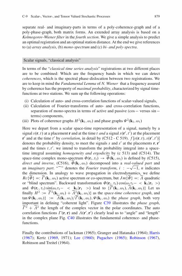
C-9 Scalar-, Vector-, and Tensor Valued Stochastic Processes 879
separate real- and imaginary-parts in terms of a poly-coherence-graph and of apoly-phase-graph, both matrix forms. An extended array analysis is based on aKolmogorov-Wiener filter in the fourth section. We give a simple analysis to predictan optimal registration and an optimal station distance. At the end we give referencesto (a) array analysis, (b) mono-spectrum and (c) bi- and poly-spectra.
Scalar signals, “classical analysis”
In terms of the “classical time series analysis” registrations at two different placesare to be combined: Which are the frequency bands in which we can detectcoherences, which is the spectral phase-dislocation between two registrations. Weare to keep in mind the Fundamental Lemma of N. Wiener that a frequency assuredby coherence has the property of maximal probability, characterized by signal time-functions at two stations. We sum up the following operations:
(i) Calculation of auto- and cross-correlation functions of scalar-valued signals,(ii) Calculation of Fourier-transforms of auto- and cross-correlation functions,
separation of mono-spectra in terms of active and passive (cos� versus sin�terms) components,
(iii) Plots of coherence graphsH2.k1; !1/ and phase graphs �2.k1; !1/
Here we depart from a scalar space-time representation of a signal, namely by asignal s.r; t/ at a placement r and at the time t and a signal s.r0; t 0/ at the placementr0 and at the time t 0 by correlation, in detail by (C512 - C 519). f Œs.r; t/; s.r0; t 0/�denotes the probability density, to meet the signals s and s0 at the placements r; r0and the times t; t 0. we intend to transform the probability integral into a space-time integral assuming homogeneity and ergodicity by (c 513) and (C514). Thespace-time complex mono-spectrum ˚.ri ; t1/ ! e.ki ; !1/ is defined by (C515),direct and inverse, (C516), e.ki ; !1/ decomposed into a real-valued part andan imaginary part. “e” denotes the Fourier transform, i W �p�1, n indicatesthe dimension. In analogy to wave propagation in electrodynamics, we defineRcfeg DW e� .ki ; !1/ active spectrum or co-spectrum, but Jmfeg DW e� quadraticor “blind spectrum”. Backward transformation ˚.ri ; �1/ cos.!1�1� < k1jr1 >/and ˚.ri ; �1/ sin.!1�1� < k1jr1 >/ lead to fe� .ki ; !1/;e�.ki ; !1/g Let usfinally H2 WD e� 2.ki ; !1/ C e�2.ki ; !1/g as the space-time coherence graph, andtan�.ki ; !1/g WD e�.ki ; !1/=e� .ki ; !1/; �.ki ; !1/ the phase graph, both veryimportant in defining “coherent light”. Figure C39 illustrates the phase graph,e� 2 C e�2 the length of the complex vector in the polar coordinates. The autocorrelation functions � .r; r/ and �.r0; r0/ clearly lead us to “angle” and “length”in the complex plane Fig. C40 illustrates the fundamental coherence- and phase-functions.
Finally the contributions of lackman (1965); Granger and Hatanaka (1964); Harris(1967); Kertz (1969, 1971); Lee (1960); Pugachev (1965); Robinson (1967),Robinson and Treitel (1964).

880 C Statistical Notions, Random Events and Stochastic Processes
Table C.20: Variance-covariance function of a scalar signal, direct andinverse Fourier transform, space-time representation
EŒs.r; t/s.r0; t 0/� WD ˚.r; r0; t; t 0/ (C510)
WDC1R�1
ds.r; t/C1R�1
ds.r0; t 0/s.r; t/s.r0; t 0/f Œs.r; t/s.r0; t/� (C511)
˚.r0 � r; t 0 � t/ D limT;x;y!1
18T xy
CTR
�Tdt
CxR�xdx
CyR�ydy (C512)
s.x; y; t/sŒx C .x0 C x/; y C .y0 C y/; t C .t 0 C t/� (C513)
r0 � r WD r1; t 0 � t WD �1 (C514)
e.k1; !1/ D .2/�nC12
C1R�1
dnr1C1R�1
d�1˚.r1; �1/ expCi.!1�1 � k1r1/
(C515)
˚.r1; �1/ D .2/�nC12
C1R�1
dnk1C1R�1
d!1e.k1; !1/ exp�i.!1�1 � k1r1/
(C516)
e.k1; !1/ D ReŒe�C i ImŒe� D e� .k1; !1/C i e�.k1; !1/ (C 517)
e�.k1; !1/ WD .2/�nC12
C1R�1
dnr1C1R�1
d�1˚.r1; �1/ cos.!1�1 � k1r1/ (C518)
e� .k1; !1/ WD .2/�nC12
C1R�1
dnr1C1R�1
d�1˚.r1; �1/ sin.!1�1 � k1r1/ (C519)
H2 WD e� 2.k1; !1/C e�2.k1; !1/ (C520)
tg�.k1; !1/ WDe�2.k1; !1/e� 2.k1; !1/
(C521)
End of Table: variance-covariance functions

C-9 Scalar-, Vector-, and Tensor Valued Stochastic Processes 881
Fig. C39 Decompositioninto real and imaginarycomponent Gaussrepresentation fe�;e� g
Fig. C40 Scalar coherenceand phase graph
C.9.52 First generalization: vector-valued classical analysis
At first, we deal with separate single components of a general three-component tidalrecording. We develop a joint analysis of all three components observed at twopoints on the surface of the Earth, for example. Its signal functions are correlatedwith each other, in the special case here the vertical component as well as thehorizontal component. We receive a correlation tensor of second degree, namelyin the form of the coherence matrix and the phase matrix. In detail, the analysistechnique is based on the following operations:
(i) Computation of auto- and cross-correlations of the vector-valued signal,(ii) Computation of the Fourier transform of the functions separation within the
mono spectral matrix in “active” and “blind” spectra cosine- and sine-Fouriertransform,
(iii) Part of the coherenec matrix Hij .k1; !1/ as well as the phase matrix�ij .k1; !1/.
Theoretical Background

882 C Statistical Notions, Random Events and Stochastic Processes
Let si .x; t/ D ıgi .x; t/ be a vector-valued space-time-signal consisting of verticaland horizontal components subject to i D 1 or x; i D 2 or y and i D 3 or z.The signal function si .x; t/ at the placement x and at the time instant t and thesignal function sj .x0; t 0/ at the placement x0 and the time instant t 0 are correlated bymeans of
Efsi .x; t/sj .x0; t 0/g DW ˚ij .x; x0; t; t 0/ for i; j 2 f1; 2; 3g (C522)
As an analogue of our previous formulae we define the coherence matrix, namelythe coherence tensor Hij , and the phase matrix �ij
Hij .k1; !1/ WD e� 2ij .k1; !1/C e�2
ij .k1; !1/ (C523)
tg �ij .k1; !1/ De�2ij .k1; !1/
e� 2ij .k1; !1/
(C524)
The coherence matrix as well as the phase matrix are represented by special surfacefor instance by coherence ellipses, coherence hyperbolae etc.
C.9.53 Second generalization: poly spectra
Up to now we analyzed only signal registrations at two different points bycorrelation, namely by coherence and phase. Here, we introduce the concept ofpoly spectra for the purpose of registration of Earth tides at all points we haveregistrations. In detail, the analysis technique is based on the following operations:
(i) Computation of multi-point correlation functions of a vector-valued tidal signal(ii) Computation of the Fourier transforms called polyspectra. The concept is able
to separate mono-, bi-, tri-, in short polyspectra in “active” and “blind” spectra,cosine- and sine-Fourier transform.
(iii) Part of generalized coherence graphs
Hi1i2���iN�1iN .k1;k2; � � � ;kN�1; !1; !2; � � � ; !N�1/ (C525)
and the generalized phase graphs
�i1i2���iN�1iN .k1;k2; � � � ;kN�1; !1; !2; � � � ; !N�1/ (C526)
at N tidal stations being functions of wave number vectors k1;k2; � � � ;kN�1 and thefrequencies !1; !2; � � � ; !N�1.
Theoretical Background
Let si1.x; t/ � ıgi.x; t/ be a tensor-valued space-time tidal signal at the first tidalstation, si2.x
0; t/ be a tensor-valued tidal signal at the second tidal station. If we

C-9 Scalar-, Vector-, and Tensor Valued Stochastic Processes 883
correlate all signal functions with each other, e receive a multi-point correlationfunction equal to the number of tidal stations.
Efsi1.x; t/si2 .x0; t 0/ � � � sin.xN ; tn/g WD ˚i1i2���iN�1iN (C527)
In case of space like homogeneity and the time like stationarity we are able torepresent the various correlation functions by
˚i1i2���iN�1iN .x1; x2; � � � ; xN�1; �1; �2; � � � ; �N�1/ (C528)
subject to
x1 WD x0 � x; x2 WD x00 � x; etc :�1 D t 0 � t; �2 D t 00 � t; etc (C529)
and their polyspectra
ei1i2���iN�1iN .k1;k2; � � � ;kN�1; !1; !2; � � � ; !N�1/ D
.2/�n.N�1/C.N�1/
2
C1Z
�1dn.N�1/r
C1Z
�1dn.N�1/�
˚i1i2���iN�1iN .r1; r2; � � � ; rN�1; �1; �2; � � � ; �N�1/ �expCi.!1�1 C !2�2 C � � � C !N�1�N�1 � k1r1 � k2r2 � � � � � kN�1rN�1/
(C530)
n is the dimension number, N the number of tidal stations. For the case of N D 3we use the term “bispectrum”, for the case N D 4 we use the term “trispectrum”in general “polyspectrum”. The common separation of ˚i1i2���iN�1iN in real- andimaginary part leads us to
the Polycoherence graph as well as the poly phase graph
Hi1i2���iN�1iN D Rc2Œei1i2���iN�1iN �C Jm2Œei1i2���iN�1iN � (C531)
tg�i1i2���iN�1iN DJmŒei1i2���iN�1iN �
RcŒe i1i2���iN�1iN �(C532)
Numerical results are presented in Brillinger (1964), Grafarend (1972), Hasselmannet al. (1963), Rosenblatt (1965, 1966), Sinaj (1963 i, ii), Tukey (1959), and Van Nees(1965).
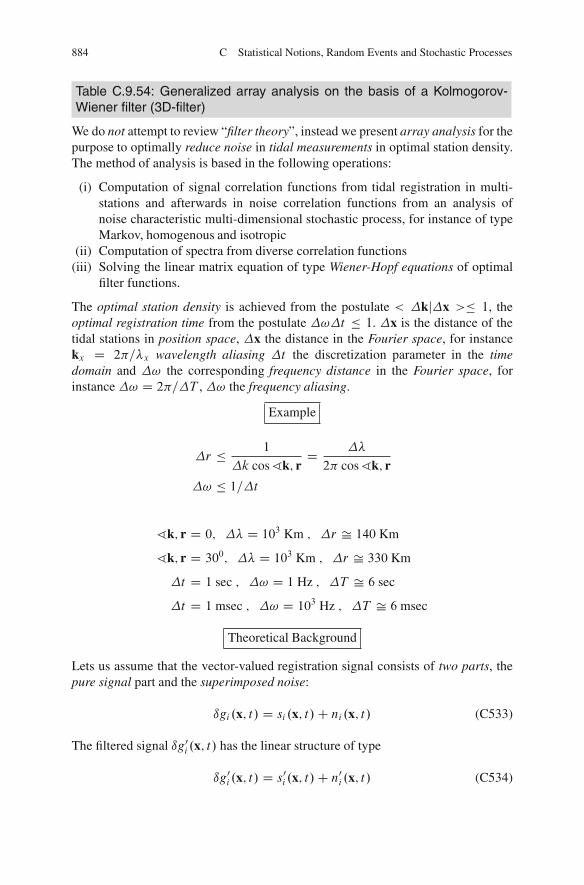
884 C Statistical Notions, Random Events and Stochastic Processes
Table C.9.54: Generalized array analysis on the basis of a Kolmogorov-Wiener filter (3D-filter)
We do not attempt to review “filter theory”, instead we present array analysis for thepurpose to optimally reduce noise in tidal measurements in optimal station density.The method of analysis is based in the following operations:
(i) Computation of signal correlation functions from tidal registration in multi-stations and afterwards in noise correlation functions from an analysis ofnoise characteristic multi-dimensional stochastic process, for instance of typeMarkov, homogenous and isotropic
(ii) Computation of spectra from diverse correlation functions(iii) Solving the linear matrix equation of type Wiener-Hopf equations of optimal
filter functions.
The optimal station density is achieved from the postulate < �kj�x >� 1, theoptimal registration time from the postulate �!�t � 1. �x is the distance of thetidal stations in position space, �x the distance in the Fourier space, for instancekx D 2=�x wavelength aliasing �t the discretization parameter in the timedomain and �! the corresponding frequency distance in the Fourier space, forinstance �! D 2=�T , �! the frequency aliasing.
Example
�r � 1
�k cos ^k; rD ��
2 cos ^k; r
�! � 1=�t
^k; r D 0; �� D 103 Km ; �r Š 140 Km
^k; r D 300; �� D 103 Km ; �r Š 330 Km
�t D 1 sec ; �! D 1 Hz ; �T Š 6 sec
�t D 1 msec ; �! D 103 Hz ; �T Š 6 msec
Theoretical Background
Lets us assume that the vector-valued registration signal consists of two parts, thepure signal part and the superimposed noise:
ıgi .x; t/ D si .x; t/C ni .x; t/ (C533)
The filtered signal ıg0i .x; t/ has the linear structure of type
ıg0i .x; t/ D s0
i .x; t/C n0i .x; t/ (C534)

C-9 Scalar-, Vector-, and Tensor Valued Stochastic Processes 885
The filter error "i .x; t/ D s0i .x; t/ � si .x; t/ C n0
i .x; t/ � ni .x; t/ is designedby I1t r�ij .x; t/ D min or I1 det�ij .x; t/ D min subject to the error tensor�ij .x; t/ WD Ef"i .x; t/"j .x; t/g D min. The filter fij .x; t/ is defined by the linearVolterra setup
n0i .x; t/ WD
C1Z
�1dnx1
Zd�1fij .x1; �1/nj .x � x1; t � �1/ (C535)
J Œ�ij .fkl .x; t//� D min lead the “necessary” generalized Wiener-Hopf equations.
˚si sj .r; r0; t; t 0/ D
C1Z
�1dnr00
C1Z
�1dt 00fik.r; r00/˚jk.r; r00/ (C536)
ef ij D esi sj .k1; !1/Œesi sk C enink �C (C537)
Œ�C identifies the generalized inverse of type minimum norm least squares.
eF Œi�i � D essŒi�i �ŒessŒi�i � C ennŒi�i �� (C538)
The result of 3D or linearized multi-channel leads to an easy solution. If we wouldcare for a nonlinear filter subject to the multi-index J WD .j1; j2; � � � ; j˛/ andK WD.k1; k2; � � � ; kˇ/ we will receive the solution
˚ij D .fik; ˚jk/ (C539)
with respect to the scalar product .:; :/ of the corresponding Hilbert space.Numericals examples you can find in C. B. Archambeau et. al. (1965), J. W. Britilland F. E. Whiteway (1965), H. W. Briscoe and P. L. Fleck (1965), J. P. Burg(1964), J. F. Claerbout (1964), P. Embree et. al. (1963), E. Grafarend (1972),A. N. Kolmogorov (1941), N. Wiener (1949, 1964, 1968).
Comments
In experimental sciences, namely geosciences like geophysics, geodesy, environ-mental sciences, namely, weather, air pollution, rainfall, oceanography, temperatureaffected sciences take action on a spatially and temporally large scale to very largescales. For this reason, they never can be considered stationary or homogenous-isotropic, but
non-stationary inhomogeneous or anisotropic
in the statistical sense Spock and Pilz (2008) if not Guttorp and Sampson (1994) asone of the attempts to model non-stationary, other examples are geodetic networks

886 C Statistical Notions, Random Events and Stochastic Processes
in two- and three-dimensional Euclidean space and on two-, three- and four-dimensional manifolds including the sphere, the ellipsoid or General Relativity as anexcellent example for inhomogeneity and anisotropy presented here. C. Calder andN. Cressie (2007) review different directions in spectral and convolution based onGaussian non-stationary random modeling. Speck and Pilz (2008) present a spectraldecomposition without any restriction to the Gaussian approach. They advice thereader to apply a special Generalized Linear Mixed Model (GLMM), the topic of ourbook, namely derived from the spectral decomposition of non-stationary randomfields.
Topics
(i) Stationary and isotropic random field
versus
(ii) Non-stationary, locally isotropic random field(iii) Interpretation in the context of linear mixed models (LMMs)
Y D Fˇ C Ab C "0
a. Fˇ: design matrix of the first kind, result: regression function, trendbehaviour F fixed design matrix
b. Ab: non-deterministic random fluctuations around the trend functions, Afixed design matrix.
c. "0: independent, homoscedastic error term centered at zero
(iv) Relation to non-stationary, locally isotropic random fields(v) Generalized linear mixed models (GLMMs)
(vi) Extending generalized linear mixed models (DHGLMMs)(vii) Limear and mixed models and Hermitic polynomials
(viii) Anisotropic stochastic process axisymmetric, Chandrasekhar (1950),Grafarend (1972)

Appendix DBasics of Groebner Basis Algebra
D-1 Definitions
To enhance the understanding of the theory of Groebner bases presented inChap. 15, the following definitions supplemented with examples are presented.Three commonly used monomial ordering systems are; lexicographic ordering,graded lexicographic ordering and graded reverse lexicographic ordering. First wedefine the monomial ordering before considering the three types.
Definition D.1. (Monomial ordering):
A monomial ordering on k Œx1; : : : ; xn� is any relation> on Zn0 or equivalently any
relation on the set x˛; ˛ 2 Zn0 satisfying the following conditions:
(a) Is total (or linear) ordering on Zn0
(b) If ˛ > ˇ and � 2 Zn0, then ˛ C � > ˇ C �
(c) < is a well ordering on Zn0.
This condition is satisfied if and only if every strictly decreasing sequence in Zn0
eventually terminates.
Definition D.2. (Lexicographic ordering):
This is akin to the ordering of words used in dictionaries. If we define a polynomialin three variables as P D kŒx; y; z� and specify an ordering x > y > z, i.e., x comesbefore y and y comes before z, then any term with x will supersede that of y whichin tern supersedes that of z. If the powers of the variables for respective monomialsare given as ˛ D .˛1; : : :; ˛n/ and ˇ D .ˇ1; : : :; ˇn/; ˛; ˇ 2 Z
n0; then ˛ >lex ˇ ifin the vector difference ˛ �ˇ 2 Z
n; the most left non-zero entry is positive. For thesame variable (e.g., x) this subsequently means x˛ >lex xˇ:
E. Grafarend and J. Awange, Applications of Linear and Nonlinear Models,Springer Geophysics, DOI 10.1007/978-3-642-22241-2,
887
© Springer-Verlag Berlin Heidelberg 2012

888 D Basics of Groebner Basis Algebra
Example D.1.
x > y5z9 is an example of lexicographic ordering. As a second example, considerthe polynomial f D 2x2y8 � 3x5yz4 C xyz3 � xy4, we have the lexicographicorder; f D �3x5yz4 C 2x2y8 � xy4 C xyz3 jx > y > z .
Definition D.3. (Graded lexicographic ordering):
In this case, the total degree of the monomials is taken into account. First, oneconsiders which monomial has the highest total degree before looking at thelexicographic ordering. This ordering looks at the left most (or largest) variableof a monomial and favours the largest power. Let ˛; ˇ 2 Z
n0; then ˛ >grlex ˇ if
j˛j DnP
iD1˛i > jˇj D
nP
iD1ˇi or j˛j D jˇj, and ˛ >lex ˇ; in ˛ � ˇ 2 Z
n; the most
left non zero entry is positive.
Example D.2.
x8y3z2 >grlex x6y2z3 j.8; 3; 2/ >grlex .6; 2; 3/, since j.8; 3; 2/j D 13 > j.6; 2; 3/j D
11 and˛ � ˇ D .2; 1;�1/. Since the left most term of the difference (2) is positive,the ordering is graded lexicographic. As a second example, consider the polynomialf D 2x2y8 � 3x5yz4 C xyz3 � xy4; we have the graded lexicographic order;f D �3x5yz4 C 2x2y8 � xy4 C xyz3 jx > y > z:
Definition D.4. (Graded reverse lexicographic ordering):
In this case, the total degree of the monomials is taken into account as in the caseof graded lexicographic ordering. First, one considers which monomial has thehighest total degree before looking at the lexicographic ordering. In contrast to thegraded lexicographic ordering, one looks at the right most (or largest) variable ofa monomial and favours the smallest power. Let ˛; ˇ 2 Z
n0; then ˛ >grevlex ˇ if
j˛j DnP
iD1˛i > jˇj D
nP
iD1ˇi or j˛j D jˇj, and ˛ >grevlex ˇ, and in ˛ � ˇ 2 Z
n the
right most non zero entry is negative.
Example D.3.
x8y3z2 >grevlex x6y2z3 j.8; 3; 2/ >grevlex .6; 2; 3/ since j.8; 3; 2/j D 13 >
j.6; 2; 3/j D 11 and ˛ � ˇ D .2; 1;�1/. Since the right most term of the difference(-1) is negative, the ordering is graded reverse lexicographic. As a second example,

D-2 Buchberger Algorithm 889
consider the polynomial f D 2x2y8 � 3x5yz4 C xyz3 � xy4 , we have the gradedreverse lexicographic order: f D 2x2y8 � 3x5yz4 � xy4 C xyz3 jx > y > z .
If we consider a non-zero polynomial f D P˛ a˛x
˛ in k Œx1; : : : :; xn� and fix themonomial order, the following additional terms can be defined:
Definition D.5.
Multidegree of f : Multideg (f / D max.˛ 2 Zn0 ja˛ ¤ 0/ Leading Coefficient
of f : LC (f / D amultideg.f / 2 k Leading Monomial of f : LM (f / D xmultideg.f /
(with coefficient 1) Leading Term of f : LT .f / D LC.f / LM .f /.
Example D.4.
Consider the polynomial f D 2x2y8 � 3x5yz4 C xyz3 � xy4 with respect tolexicographic order fx > y > zg , we haveMultideg (f )=(5,1,4)LC (f )= �3LM (f )= x5yz4
LT (f )= �3x5yz4
The definitions of polynomial ordering above have been adopted from Cox et al.(1997), pp. 52–58.
D-2 Buchberger Algorithm
computes the Groebner basis using the computer algebraic systems ((CAS) ofMathematica and Maple. With Groebner basis, most nonlinear equations that areencountered in geodesy and geoinformatics can be solved. All that is required of theuser is to write algorithms that can easily run in Mathematica or Maple using stepsthat are discussed in Sects. D-21 and D-22 below.
D-21 Mathematica Computation of Groebner Basis
Groebner basis can be computed using algebraic softwares of Mathematica (e.g.,version 7 onwards). In Mathematica, Groebner basis command is executed bywriting
InŒ1� WD GroebnerBasisŒfpolynomialsg; fvariablesg�; (D.1)

890 D Basics of Groebner Basis Algebra
where In[1]:= is the Mathematica prompt which computes the Groebner basis forthe Ideal generated by the polynomials with respect to the monomial order specifiedby monomial order options.
Example D.5. (Mathematica computation of Groebner basis):
In Example 15.3 on p. 536, the systems of polynomial equations were given as
�f1 D xy � 2yf2 D 2y2 � x2:
Groebner basis of this system would be computed by
InŒ1� WD GroebnerBasisŒff1; f2g; fx; yg�; (D.2)
leading to the same values as in (15.10) on p. 536. With this approach, however, oneobtains too many elements of Groebner basis which may not be relevant to the taskat hand. In a case where the solution of a specific variable is desired, one can avoidcomputing the undesired variables, and alleviate the need for back-substitution bysimply computing the reduced Groebner basis. In this case (D.1) modifies to
InŒ1� WD GroebnerBasisŒfpolynomialsg; fvariablesg; felimsg�; (D.3)
where elims is for elimination order. Whereas the term reduced Groebner basis iswidely used in many Groebner basis literature, we point out that within Mathematicasoftware, the concept of a reduced basis has a different technical meaning. In thisbook, as in its predecessor, and to keep with the tradition, we maintain the use ofthe term reduced Groebner basis.
Example D.6. (Mathematica computation of reduced Groebner basis):
In Example D.2.1, one would compute the reduced Groebner basis using (D.3) as
InŒ1� WD GroebnerBasisŒff1; f2g; fx; yg; fyg�; (D.4)
which will return only �2x2 C x3. Note that this form is correct only when theretained and eliminated variables are disjoint. If they are not, there is absolutely noguarantee as to which category a variable will be put in! As an example, considerthe solution of three polynomials x2 C y2 C z2 � 1, xy � zC 2, and z2 � 2x C 3y.In the approach presented in (D.4), the solution would be
InŒ1� WD GroebnerBasisŒfx2Cy2Cz2�1; xy�zC2; z2�2xC3yg; fx; y; zg; fx; yg�;(D.5)
leading to

D-2 Buchberger Algorithm 891
f1024� 832z� 215z2 C 156z3 � 25z4 C 24z5 C 13z6 C z8g:
Lichtblau (Priv. Comm.) however suggests that the retained variable, in this case .z/and the eliminated variables .x; y/ be separated, i.e.,
InŒ1� WD GroebnerBasisŒfx2C y2C z2� 1; xy � zC 2; z2 � 2xC 3yg; fzg; fx; yg�:(D.6)
The results of (D.6) are the same as those of (D.5), but with the advantage ofa vastly better speed if one uses an ordering better suited for the task at hand,e.g., elimination of variables in this example. For the problems that are solved inour books, the condition of the retained and eliminated variables being disjoint istrue, and hence the approach in (D.5) has been adopted. The univariate polynomial�2x2 C x3 is then solved for x using the roots command in Matlab (see e.g.,Hanselman and Littlefield (1997), p. 146) by
roots. Œ1 �2 0 0� /: (D.7)
The values of the row vector in (D.7) are the coefficients of the cubic polynomialx3�2x2C0xC0 D 0 obtained from (D.4). The values of y from Example (15.3) onp. 536 can equally be computed from (D.4) by replacing y in the option part withx and thus removing the need for back substitution. We leave it for the reader tocompute the values of y from Example (15.3) and also those of z in Example (15.3)using reduced Groebner basis (D.3) as an exercise. The reader should confirm thatthe solution of y leads to y3 � 2y with the roots y D 0 or y D ˙1:4142. Fromexperience, we recommend the use of reduced Groebner basis for applications ingeodesy and geoinformatics. This will; fasten the computations, save on computerspace, and alleviates the need for back-substitution.
D-22 Maple Computation of Groebner Basis
In Maple Version 10 the command is accessed by typing > with (Grobner); Basis(WL; T ) is for Groebner, gbasis (WL; T ) is for reduced Groebner basis. WL listor set of polynomials, T monomial order description, e.g. “plex” (variables) –pure lexicographic order and > is the Maple prompt and the semicolon ends theMaple command). Once the Groebner basis package has been loaded, the executioncommand then becomes > gbasis (polynomials, variables) which computes theGroebner basis for the ideal generated by the polynomials with respect to themonomial ordering specified by variables in the executable command. We shouldpoint out that at the time of writing this book, May 2012, version 16 of Maple hasbeen released.
892 D Basics of Groebner Basis Algebra
D.3 Gauss Combinatorial Formulation

D.3 Gauss Combinatorial Formulation 893

References
Aarts, E.H. and Korst, J. (1989): Simulated Annealing and Boltzman Machines, Wiley, New YorkAbbe, E. (1906): Uber die Gesetzmaßigkeit in der Verteilung der Fehler bei Beobachtungsreihen,
Gesammelte Abhandlungen, Vol. II, Jena 1863 (1906)Abdous, B. and R. Theodorescu (1998): Mean, median, mode IV, Statistica Neerlandica 52 (1998),
356-359Abel, J.S. and Chaffee, J.W. (1991): Existence and uniqueness of GPS solutions, IEEE Transac-
tions on Aerospace and ElectronicSystems 27 (1991) 952-956.I. Abhandlung Monatsberichte der Akademie der Wissenschafte 1853, Werke 4 (1929) 1-11Absil, P.A., Mahony, R., Sepulehre, R. and Van Dooren, P. (2002): A Grassmann-Rayleigh quotient
iteration for computing invariant subspaces, SIAM Review 44 (2002), 57-73Abramowitz, M. and J.A. Stegun (1965): Handbook of mathematical functions, Dover Publication,
New York 1965Adams, M. and V. Guillemin (1996): Measure theory and probability, 2nd edition, Birkhauser-
Verlag, Basel Boston Berlin 1996Adelmalek, N.N. (1974): On the discrete linear L1 approximation and L1 solutions of overdeter-
mined linear equations, J. Approximation Theory 11 (1974), 38-53Adler, R. and Pelzer, H. (1994): Development of a Long Term Geodetic Monitoring System of
Recent Crustal Activity Along the Dead Sea Rift. Final scientific report for the Gennan-IsraelFoundation GIF
Aduol, F.W.O. (1989): Intergrierte geodatische Netzanalyse mit stochastischer Vorinformation uberSchwerefeld und Referenzellipsoid, DGK, Reihe C, Heft Nr. 351
Afifi, A.A. and V. Clark (1996): Computer-aided multivariate analysis, Chapman and Hall, BocaRaton 1996
Agnew, D.C. (1992): The time-domain behaviour of power-law noises. Geophysical researchletters, 19(4):333-336, 1992
Agostinelli, C. and M. Markatou (1998): A one-step robust estimator for regression based on theweighted likelihood reweighting scheme, Stat. & Prob. Letters 37 (1998), 341-350
Agreo, G. (1995): Maximum likelihood estimation for the exponential power function parameters,Comm. Statist. Simul. Comput. 24 (1995), 523-536
Aickin, M. and C. Ritenbaugh (1996): Analysis of multivariate reliability structures and theinduced bias in linear model estimation, Statistics in Medicine 15 (1996), 1647-1661
Aitchinson, J. and I.R. Dunsmore (1975): Statistical prediction analysis, Cambridge UniversityPress, Cambridge 1975
Aitken, A.C. (1935): On least squares and linear combinations of observations, Proc. Roy. Soc.Edinburgh 55 (1935), 42-48
E. Grafarend and J. Awange, Applications of Linear and Nonlinear Models,Springer Geophysics, DOI 10.1007/978-3-642-22241-2,
895
© Springer-Verlag Berlin Heidelberg 2012

896 References
Airy, G.B. (1861): On the algebraical and numerical theory of errors of observations and thecombination of observations, Macmillan Publ., London 1861
Aki, K. and Richards P.G. (1980): Quantitative seismology, W.H. Freeman, San FranciscoAlbert, A. (1969): Conditions for positive and nonnegative definiteness in terms of pseudo inverses,
SIAM J. Appl. Math. 17 (1969), 434-440Alberda, J.E. (1974): Planning and optimization of networks: some general considerations, Boll.
di Geodesicl, e Scienze, Aff. 33 (1974) 209-240Albertella, A. and F. Sacerdote (1995): Spectral analysis of block averaged data in geopotential
global model determination, Journal of Geodesy 70 (1995), 166-175Alcala, J.T., Cristobal, J.A. and W. Gonzalez-Manteiga (1999): Goodness-of-fit test for linear
models based on local polynomials, Statistics & Probability Letters 42 (1999), 39-46Aldrich, J. (1999): Determinacy in the linear model: Gauss to Bose and Koopmans, International
Statistical Review 67 (1999), 211-219Alefeld, G. and J. Herzberger (1974): Einfhrung in die Intervallrechung, Bibliographisches Inst.
Mannheim 1974Alefeld, G. and J. Herzberger (1983): Introduction to interval computation. Computer science and
applied mathematics, Academic Press, New York London 1983Ali, A.K.A., Lin, C.Y. and E.B. Burnside (1997): Detection of outliers in mixed model analysis,
The Egyptian Statistical Journal 41 (1997), 182-194Allende, S., Bouza, C. and I. Romero (1995): Fitting a linear regression model by combining least
squares and least absolute value estimation, Questiio 19 (1995), 107-121Allmer, F. Louis Krger (1857-1923), 25 pages, Technical University of Graz, Graz 2001 Alzaid,
A.A. and L. Benkherouf (1995): First-order integer-valued autoregressive process with Eulermarginal distributions, J. Statist. Res. 29 (1995), 89-92
Amiri-Simkooei, A.R. (2004): A new method for second order design of geodetic networks: aimingat high reliability, survey Review, 37 (2004), pp. 552-560
Amiri-Simkooei, A.R. (2007): Least-squares estimation of variance components, Theory and EPSapplications, Ph.D. Thesis, Delft Univ. of Tech., delft, The Netherlands 2007
An, H.-Z., F.J. Hickernell and L.-X. Zhu (1997): A new class of consistent estimators for stochasticlinear regressive models, J. Multivar. Anal. 63 (1997), 242-258
Andel, J. (1984): Statistische Analyse von Zeitreihen, Akademie Verlag, Stuttgart 1984Anderson, P.L. and M.M. Meerscaert (1997): Periodic moving averages of random variables with
regularly varying tails, Ann. Statist. 25 (1997), 771-785Anderson, R.D., Henderson H.V., Pukelsheim F. and Searle S.R. (1984): Best estimation of
variance components from balanced data, with arbitrary kurtosis, Mathematische Operations-forschung und Statistik, Series Statistics 15, pp. 163-176
Anderson, T.W. (1945): Non-central Wishart Distribution and Its Application to Statistics, doctoraldissertation, Princeton University
Anderson, T.W. (1946): The non-central Wishart distribution and certain problems of multivariatestatistics, Ann. Math. Stat., 17, 409-431
Anderson, T.W. (1948): The asymptotic distributions of the roots of certain determinantalequations, J. Roy. Stat. Soc., B, 10, 132-139
Anderson, T.W. (1951): Classification by multivariate analysis, psychometrika, 16, 31-50Anderson, T.W. (1973): Asymptotically efficient estimation of covariance matrices with linear
structure, The Annals of Statistics 1 (1973), 135-141Anderson, T.W. (1984): An introduction to multivariate statistical analysis, 2nd ed., J. Wiley,
New York 1982Anderson, T.W. (2003): An introduction to multivariate statistical analysis, J. Wiley, Stanford CA,
2003Anderson, T.W. and M.A. Stephens (1972): Tests for randomness of directions against equatorial
and bimodal alternatives, Biometrika 59 (1972), 613-621Anderson, W.N. and R.J. Duffin (1969): Series and parallel addition of matrices, J. Math. Anal.
Appl. 26 (1969), 576-594Ando, T. (1979): Generalized Schur complements, Linear Algebra Appl. 27 (1979), 173-186

References 897
Andrews, D.F. (1971): Transformations of multivariate data, Biometrics 27 (1971), 825-840Andrews, D.F. (1974): Technometrics 16 (1974), 523-531Andrews, D.F., Bickel, P.J. and F.R. Hampel (1972): Robust estimates of location, Princeton
University Press, Princeton 1972Angelier, J., Tarantola, A., Vallete, B. and S. Manoussis (1982): Inversion of field data in fault
tectonics to obtain the regional stress - I, Single phase fault populations: a new method ofcomputing the stress tensor, Geophys. J. R. astr. Soc., 69, 607-621
Angulo, J.M. and Bueso, M.C. (2001): Random perturbation methods applied to multivariateSpatial Sampling design, Environmetrics, 12, 631-646.
Anh, V.V. and T. Chelliah (1999): Estimated generalized least squares for random coefficientregression models, Scandinavian J. Statist. 26 (1999), 31-46
Anido, C. and T. Valdees (2000): Censored regression models with double exponential errordistributions: an iterative estimation procedure based on medians for correcting bias, RevistaMatemeatica Complutense 13 (2000), 137-159
Anscoube, F.J. (1960): Rejection of outliers, Technometrics, 2 (1960), pp. 123-147Ansley, C.F. (1985): Quick proofs of some regression theorems via the QR Algorithm, The
American Statistician 39 (1985), 55-59Anton, H. (1994): Elementary linear algebra, J. Wiley, New York 1994Arcadis (1997): Ingenieurgeologischer Situationsbericht fur 1997, Bericht des Pumpspeicherwerks
Hohenwarthe, VEAG, 1997Archambeau, C.B. and Bradford, J.C. and Broome, P.W. and Dean, W.C. and Flinn, E.A. (1965):
Data processing techniques for the detection and interpretation of teleseismic signals, Proc.IEEE 53 (1965), 1860-1865
Arellano-Valle, R. and Bolfarine, H. and Lachos, V (2005): Skew-normal linear mixed models.In Journal of Data Science vol 3, pp.415-438
Arnold, B.C. and R.M. Shavelle (1998): Joint confidence sets for the mean and variance of a normaldistribution, J. Am. Statist. Ass. 52 (1998), 133-140
Arnold, B.F. and P. Stahlecker (1998): Prediction in linear regression combining crisp data andfuzzy prior information, Statistics & Decisions 16 (1998), 19-33
Arnold, B.F. and P. Stahlecker (1999): A note on the robustness of the generalized least squaresestimator in linear regression, Allg. Statistisches Archiv 83 (1999), 224-229
Arnold, K.J. (1941): On spherical probability distributions, P.H. Thesis, M.I.T., Boston 1941Arnold, S.F. (1981): The theory of linear models and multivariate analysis, J. Wiley, New York
1981Arrowsmith, D.K. and C.M. Place (1995): Differential equations, maps and chaotic behavior,
Champman and Hall, London 1995Arun, K.S. (1992): A unitarily constrained total least squares problem in signal processing, SIAM
J. Matrix Anal. Appl. 13 (1992), 729-745Ashkenazi V. and Grist, S. (1982): Inter-comparison of 3-D geodetic network adjustment models,
International sypmosium on geodetic networks and computations of the I.A.G. Munich, August31 to September 5, 1981.
Atiyah, M.F., Hitchin, N.J. and Singer, J.M.: Self-duality in four-dimensional Riemanniangeometry. Proc. Royal Soc. London A362 (1978) 425-461
Austen, G. and Grafarend, E.W. and Reubelt, T. (2001): Anal: Earth’s gravitational field from semicontinuous ephe low earth orbiting GPS-tracked satellite of type CRA or Goce, in: Vistas forGeodesy in the New Millenn Adam and Schwarz, International Association of Geo posia 125,309-315, 2001
Aven, T. (1993): Reliability and risk analysis, Chapman and Hall, Boca Raton 1993Awange, L.J. (1999): Partial procrustes solution of the three dimensional orientation problem from
GPS/LPS observations, Quo vadis geodesia...? Festschrift to E.W. Grafarend on the occasion ofhis 60th birthday, Eds. F. Krumm and V.S. Schwarze, Report Nr. 1999.6-1
Awange, J.L. (2002): Grobner bases, multi polynomial resultants and the Gauss-Jacobi combina-torial algorithms - adjustment of nonlinear GPS/LPS observations, Schriftenreihe der Institutedes Studiengangs Geodasie und Geoinformatik, Report 2002.1

898 References
Awange, J. and E.W. Grafarend (2002): Linearized Least Squares and nonlinear Gauss-Jacobicombinatorial algorithm applied to the 7-parameter datum transformation C7(3) problem,Zeitschrift fur Vermessungswesen 127 (2002), 109-116
Awange, J.L. (2012): Environmental Monitoring using GNSS. Global Navigation Satellite Sys-tems, Springer, Berlin-New York.
Azzalini, A. (1996): Statistical inference, Chapman and Hall, Boca Raton 1996Azzam, A.M.H. (1996): Inference in linear models with non stochastic biased factors, Egyptian
Statistical Journal, ISSR - Cairo University 40 (1996), 172-181Azzam, A., Birkes, D. and J. Seely (1988): Admissibility in linear models with polyhedral
covariance structure, Probability and Statistics, essays in honor of Franklin A. Graybill, J.N.Srivastava, Ed. Elsevier Science Publishers, B.V. (North-Holland), 1988
Baarda, W. (1967): Statistical Concepts in Geodesy. Netherlands Geodetic Commission, Publica-tions on Geodesy, New Series, Vol. 2, No.4, Delft.
Baarda, W. (1967): A generalization of the concept strength of the figure, Publications on Geodesy,New Series 2, Delft 1967
Baarda, W. (1968): A testing procedure for use in geodetic networks, Netherlands GeodeticCommission, New Series, Delft, Netherlands, 2 (5), 1968
Baarda, W. (1973): S-transformations and criterion matrices, Netherlands Geodetic Commission,Vol. 5, No. 1, Delft 1973
Baarda, W. (1977): Optimization of design and computations of control networks, F. Halmos andJ. Somogyi (eds.), Akademiai Kiado, Budapest 1977, 419-436
Babai, L. (1986): On Lovasz’ lattice reduction and the nearest lattice point problem, Combinatorica6 (1986), 1-13
Babu, G.J. and E.D. Feigelson (1996): Astrostatistics, Chapman and Hall, Boca Raton 1996Bai, J. (1994): Least squares estimation of a shift in linear processes, Journal of Time Series
Analysis 15 (1994), 453-472Bognarova, M., Kubacek, L. and Volaufova J. (1996): Comparison of MINQUE and LMVQUIE
by simulation. Acta Univ. Palacki. Olomuc., Fac. Rerum Nat., Math. 35 (1996), 25-38.Bachelier, L. (1900): Theorie de le speculation, Ann, Sci. EC. Norm. Super. 17 (1900) 21-26Bahr, H.G. (1988): A quadratic approach to the non-linear treatment of non-redundant observations
Manuscripta Geodaetica, 13 (1988) 191-197.Bahr, H.G. (1991): Einfach uberbestimmtes ebenes Einschneiden, differentialgeometrisch
analysiert, Zeitschrift fur Vermessungswesen 116 (1991) 545-552.Bai, W.M., Vigny, C., Ricard, Y. and Froidevaus, C. (1992): On the origin of deviatoric stresses in
the lithosphere, J. geophys. Res., B97, 11728-11737Bai, Z.D., Chan, X.R., Krishnaiah, P.R. and L.C. Zhao (1987): Asymptotic properties of the
EVLP estimation for superimposed exponential signals in noise, Technical Report 87-19, CMA,University of Pittsburgh, Pittsburgh 1987
Bai, Z.D. and Y. Wu (1997): General M-estimation, J. Multivar. Anal. 63 (1997), 119-135Bajaj, C.L. (1989): Geometric Modelling with Algebraic Surfaces. In: The Mathematics of
Surfaces III, Ed.: D.C. Handscomb, Clarendon Press, Oxford.Bajaj, C., Garity, T. and Waren, J. (1988): On the applications of multi-equational resultants,
Department of Computer Science, Purdue University, Technical Report CSD-TR-826, pp. 1-22,1988.
Baksalary, J.K. and Kala, R. (1981): Linear transformations preserving best linear unbiasedestimators in a general Gauss-Markoff model. Ann. Stat. 9 (1981), 913-916.
Baksalary, J.K. and A. Markiewicz (1988): Admissible linear estimators in the general Gauss-Markov model, J. Statist. Planning and Inference 19 (1988), 349-359
Baksalary, J.K. and Puntanen, S. (1989): Weighted-Least-squares estimation in the general Gauss-Markov model. In: Statistical Data Analysis and Inference, Pap. Int. Conf., Neuchatel/Switzerl.(Y. Dodge, ed.), North-Holland, Amsterdam, pp. 355-368.
Baksalary, J.K. and Liski, E.P. and G. Trenkler (1989): Mean square error matrix improvementsand admissibility of linear estimators, J. Statist. Planning and Inference 23 (1989), 313-325

References 899
Baksalary, J.K. and F. Pukelsheim (1989): Some properties of matrix partial ordering, LinearAlgebra and it Appl., 119 (1989), pp. 57-85
Baksalary, J.K. and F. Pukelsheim (1991): On the Lowner, Minus and Star partial orderings ofnonnegative definite matrices and their squares, Linear Algebra and its Applications 151 (1991),135-141
Baksalary, J.K. and Rao, C.R., Markiewicz, A. (1992): A study of the influence of the “naturalrestrictions” on estimation problems in the singular Gauss-Markov model. J. Stat. Plann.Inference 31, 3 (1992), 335-351.
Balakrishnan, N. and Basu, A.P. (eds.) (1995): The exponential distribution, Gordon and BreachPublishers, Amsterdam 1995
Balakrishnan, N. and R.A. Sandhu (1996): Best linear unbiased and maximum likelihoodestimation for exponential distributions under general progressive type-II censored samples,Sankhya 58 (1996), 1-9
Bamler, R. and P. Hartl (1998): Synthetic aperture radar interferometry, Inverse Problems 14(1998), R1-R54
Banachiewicz, T. (1937): Zur Berechnung der Determinanten, wie auch der Inversen und zur daraufbasierten Au osung der Systeme linearen Gleichungen, Acta Astronom. Ser. C3 (1937), 41-67
Bancroft, S. (1985): An algebraic solution of the GPS equations, IEEE Transaction on Aerospaceand Electronic Systems AES-21 (1985) 56-59.
Bandemer, H. (2005): Mathematik und Ungewissheit: Drei Essais zu Problemen der Anwendung,Edition avn Gutenberg platz, Leipzig 2005
Bandemer, H. et al. (1976): Optimale Versuchsplanning, Z. Auflage Akademic Verlag, Berlin 1976Bandemer, H. et al. (1977): Theorie und Anwendung der optimalen Versuchsplanung I. Akademie-
Verlag, BerlinBandemer, H. and W. Nather (1980): Theorie and Anwendung der optimalen Versuchsplanung II,
akademic Verlag, Berlin 1980Bandemer, H. and S. Gottwald (1993): Einfhrung in die Fuzzy-Methoden, Akademic-Verlag,
Berlin 1993Bahndorf, J. (1991): Zur Systematisierung der Seilnetzberechnung und zur Optimierung von
Seilnetzen. Deutsche Geodatische Kommission, Reihe C, Nr. 373, Miinchen.Bansal, N.K., Hamedani, G.G. and H. Zhang (1999): Non-linear regression with multidimensional
indices, Statistics & Probability Letters 45 (1999), 175-186Barankin, E.W. (1949): Locally best unbiased estimates, Ann. Math. Statist. 20 (1949), 477-501Barber, B.C. (1993): The non-isotropic two-dimensional random walk, Waves in Random Media,
3 (1993) 243-256Barham, R.H. and W. Drane (1972): An algorithm for least squares estimation of nonlinear
parameters when some of the parameters are linear, Technometrics 14 (1972), 757-766Barlett, M. (1933): On the theory of statistical regression, Proc. Roy. Soc .. Edinb., 53, 260-283.Barlett, M. (1937): Property od sufficiency and statistical tests, Proc. Roy. Soc., A 160, 268-282Barlett, M. (1947): Multivariate analysis, J. Roy. Stat. Soc., Supple., 9, 176-197.Barlow, R.E., Clarotti, C.A. and F. Spizzichino (eds.) (1993): Reliability and decision making,
Chapman and Hall, Boca Raton 1993Barlow, R.E. and F. Proschan (1966): Tolerance and confidence limits for classes of distributions
based on failure rate, Ann. Math. Statist 37 (1966), 1593-1601Barnard, J., McCulloch, R. and X.-L. Meng (2000): Modeling covariance matrices in terms of
standard deviations and correlations, with application to shrinkage, Statistica Sinica 10 (2000),1281-1311
Barnard, M.M. (1935): The scalar variations of skull parameters in four series of Egyptian skulls,Ann. Eugen. 6 (1935), 352-371
Barndorff-Nielsen, O. (1978): Information and exponential families in statistical theory, J. Wiley,New York, 238 pp.
Barndorff-Nielsen, O.E., Cox, D.R. and C. Kluppelberg (2001): Complex stochastic systems,Chapman and Hall, Boca Raton, Florida 2001
Barnett, V. and Lewis, T. (1994): Outliers in Statistical Data. John Wiley, New York, 1994.

900 References
Barnett, V. (1999): Comparative statistical inference, 3rd ed., J. Wiley, New York 1999Barone, J. and A. Novikoff (1978): A history of the axiomatic formulation of probability from
Borel to Kolmogorov, Part I, Archive for History of Exact Sciences 18 (1978), 123-190Barrlund, A. (1998): Efficient solution of constrained least squares problems with Kronecker
product structure, SIAM J. Matrix Anal. Appl. 19 (1998), 154-160Barrodale, I. and D.D. Oleski (1981): Exponential approximation using Prony’s method, The
Numerical Solution of Nonlinear Problems, eds. Baker, C.T.H. and C. Phillips, 258-269Bartelme, N. and Meissl, P. (1975): Ein einfaches, rasches und numerisch stabiles Verfahren zur
Bestimmung des kurzesten Abstandes eines Punktes von einem spharoidischen Rotationsellip-soid, Allgemeine Vermessungs-Nachrichten 82 (1975) 436-439.
Bartlett, M.S. (1980): An introduction to stochastic processes with special reference to methodsand applications, paperback edition, University press, Cambridge 1980
Bartlett, M.S. and D.G. Kendall (1946): The statistical analysis of variance-heterogeneity andthe logarithmic transformation, Queen’s College Cambridge, Magdalen College Oxford,Cambridge/Oxford 1946
Bartoszynski, R. and M. Niewiadomska-Bugaj (1996): Probability and statistical inference,J. Wiley, New York 1996
Barut, A.O. and R.B. Haugen (1972): Theory of the conformally invariant mass, Annals of Physics71 (1972), 519-541
Basset JR., G. and R. Koenker (1978): Asymptotic theory of least absolute error 73 (1978),618-622
Basawa, I.V. (2001): Inference in stochastic processes in: D.N. Shanbhag and C.R. Rao. Handbookof statistics, pp. 55-77, Vol 19, Elsevier Science 2001
Basch, A. (1913): Uber eine Anwendung der graphostatischen Methode auf den Ausgleich vonBeobachtungsergebnissen. OZfV 11, 11-18, 42-46.
Baselga, S. (2007): Global Optimization Solution of Robust Estimation. J Surv. Eng. 2007, 133,123-128.
Basu, S. and Mukhopadhyay, S. (2000): Binary response regression with normal scale mixturelinks. Dey, D.K., Ghosh S.K.-and Mallick, B.K. eds., Generalized linear models: A Bayesianperspective, Marcel Dekker, New York
Batchelor, G.K. (1946): Theory of axisymmetric turbulenz, Proc. Royal Soc. A186 (1946) 480Batchelor, G.K. and A.A. Townsend (1950): The nature of turbulent motion at large wave numbers,
Fluid Mech. (1952) 238-255Batchelor, G.K. (1953): The theory of homogeneous turbulence, Cambridge University Press,
Cambridge, 1953.Batchelor, G.K. (1967): The theory of homogenous turbulence, Cambridge (1967)Baselga, S. (2007): Critical Limitation in Use of’t Test for Gross Error Detection. J Surv. Eng.
2007, 133,52-55.Bateman, H. (1910): The transformation of the electrodynamical equations, Proc. London Math.
Soc. 8 (1910), 223-264, 469-488Bateman, H. (1910): The transformation of coordinates which can be used to transform one
physical problem into another, Proc. London Math. Soc. 8 (1910), 469-488Bates, D.M. and D.G. Watts (1980): Relative curvature measures of nonlinearity (with discussion),
J. Roy. Statist. Soc. B42 (1980), 1-25Bates, D.M. and M.J. Lindstorm (1986): Nonlinear least squares with conditionally linear param-
eters, Proceedings of the Statistical Computation Section, American Statistical Association,Washington 1986
Bates, D.M. and D.G. Watts (1988a): Nonlinear regression analysis and its applications, J. Wiley,New York 1988
Bates, D.M. and D.G. Watts (1988b): Applied nonlinear regression, J. Wiley, New York 1988Bates, R.A., Riccomagno, E., Schwabe, R. and H.P. Wynn (1998): Lattices and dual lattices in
optimal experimental design for Fourier models, Computational Statistics & Data Analysis 28(1998), 283-296

References 901
Batschelet, E. (1965): Statistical methods for the analysis of problems in animal orientation andcertain biological rhythms, Amer. Inst. Biol. Sciences, Washington
Batschelet, E. (1971): Recent statistical methods for orientation, (Animal Orientation Symposium1970 on Wallops Island), Amer. Inst. Biol. Sciences, Washington, D.C., 1971
Batschelet, E. (1981): Circular statistics in biology, Academic Press, New York London 1981Bauer, H. (1992): Maß- und Integrationstheorie, 2. Au age, Walter de Gruyter, Berlin New York
1992Bauer, H. (1996): Probability theory, de Gruyter Verlag, Berlin New York 1996Bayen, F. (1976): Conformal invariance in physics, in: Cahen, C. and M. Flato (eds.), Differential
geometry and relativity, Reidel Publ., 171-195, Dordrecht 1976Beale, E.M. (1960): Confidence regions in non-linear estimation, J. Roy. Statist. Soc. B22 (1960),
41-89Beaton, A.E. and J.W. Tukey (1974): Technometrics 16 (1974), 147-185Becker, T. and Weispfenning, V. (1993): Grobner bases. A computational approach to commutative
algebra. Graduate Text in Mathematics 141, Springer-Verlag, New York 1993.Becker, T., Weispfennig, V. and H. Kredel (1998): Grobner bases: a computational approach to
commutative algebra, Corr. 2. print., Springer-Verlag, Heidelberg Berlin New York 1998Beckermann, B. and E.B. Saff (1999): The sensitivity of least squares polynomial approximation,
Int. Series of Numerical Mathematics, Vol. 131: Applications and computation of orthogonalpolynomials (eds. W. Gautschi, G.H. Golub, G. Opfer), 1-19, Birkhauser-Verlag, Basel BostonBerlin 1999
Beckers, J., Harnad, J., Perroud, M. and P. Winternitz (1978): Tensor fields invariant undersubgroups of the conformal group of space-time, J. Math. Phys. 19 (1978), 2126-2153
Beder, C. and Forstner, W, (2006): Direct Solutions for Computing Cylinders from Minima/ Setsof 3D Points. European Conference on Computer Vision ECCV 2006. Graz, Austria 2006,S. 135-146.
Behnken, D.W. and N.R. Draper (1972): Residuals and their variance, Technometrics 11 (1972),101-111
Behrens, W.A. (1929): Ein Beitrag zur Fehlerberechnung bei wenigen Beobachtungen, Land-wirtschaftliche Jahrbucher 68 (1929), 807-837
Belikov, M.V. (1991): Spherical harmonic analysis and synthesis with the use of column-wiserecurrence relations, manuscripta geodaetica 16 (1991), 384-410
Belikov, M.V. and K.A. Taybatorov (1992): An efficient algorithm for computing the Earth’sgravitational potential and its derivatives at satellite altitudes, manuscripta geodaetica 17 (1992),104-116
Ben-Menahem, A. and Singh, S.J. (1981): Seismic waves and sources. Springer-Verlag New York1981
Ben-Israel, A. and T. Greville (1974): Generalized inverses: Theory and applications, J. Wiley,New York 1974
Benbow, S.J. (1999): Solving generalized least-squares problems with LSQR, SIAM J. MatrixAnal. Appl. 21 (1999), 166-177
Benciolini. B. (1984): Continuous networks II. Erice Lecture Notes, this volume. Heidelberg.Benda, N. and R. Schwabe (1998): Designing experiments for adaptively fitted models, in: MODA
5 - Advances in model-oriented data analysis and experimental design, Proceedings of the5th International Workshop in Marseilles, eds. Atkinson, A.C., Pronzato, L. and H.P. Wynn,Physica-Verlag, Heidelberg 1998
Bennett, B. M. (1951): Note on a solution of the generalized Behrens-Fisher problem,Ann.Insr:Srat:XIath., 2, 87-90.
Bennett, R.J. (1979): Spatial time series, Pion Limited, London 1979Benning, W. (1974): Der kurzeste Abstand eines in rechtwinkligen Koordinaten gegebenen
Außenpunktes vom Ellipsoid, Allgemeine Vermessungs-Nachrichten 81 (1974) 429-433.Benning, W. (1987): Iterative ellipsoidische Lotfußpunktberechung, Allgemeine Vermessungs-
Nachrichten 94 (1987) 256-260.

902 References
Benning, W. and Ahrens, B. (1979): Konzept und Realisierung eines Systems zur automatischenFehlerlokalisierung und automatischen Berechnung von Naherungskoordinaten. N achrichtenaus dem 6ffentlichen Vermessungsdienst N ordrhein-Westfalen, Heft 2, 107-124.
Beran, R.J. (1968): Testing for uniformity on a compact homogeneous space, J. App. Prob.5 (1968), 177-195
Beran, R.J. (1979): Exponential models for directional data, Ann. Statist. 7 (1979), 1162-1178Beran, J. (1994): Statistical methods for long memory processes, Chapman and Hall, Boca Raton
1994Berberan, A. (1992): Outlier detection and heterogeneous observations - a simulation case study,
Australian Journal of Geodesy, Photogrammetry and Surveying 56 (1992), 49-61Berberan, A. (1995): Multiple Outlier Detection-A Real Case Study. Surv. Rev. 1995, 33, 41-49.Bergbauer, K. and Lechner, W. and Schuchert, M. and Walk, R. (1979): Anlage, Beobachtung und
Ausgleichung eines dreidimensionalen Testnetzes. Diplomarbeit Hochschule der bundeswehr.Nunchen 1979.
Berger, M.P.F. and F.E.S. Tan (1998): Optimal designs for repeated measures experiments,Kwantitatieve Methoden 59 (1998), 45-67
Berman, A. and R.J. Plemmons (1979): Nonnegative matrices in the mathematical sciences,Academic Press, New York London 1979
Bertsekas, D.P. (1996): Incremental least squares methods and the extended Kalman filter, SiamJ. Opt. 6 (1996), 807-822
Berry, J.C. (1994): Improving the James-Stein estimator using the Stein variance estimator, Statist.Probab. Lett. 20 (1994), 241-245
Bertuzzi, A., Gandolfi, A. and C. Sinisgalli (1998): Preference regions of ridge regression andOLS according to Pitman’s criterion, Sankhya: The Indian Journal of Statistics 60 (1998),437-447
Bessel, F.W. (1838): Untersuchungen uber die Wahrscheinlichkeit der Beobachtungsfehler,Astronomische Nachrichten 15 (1838), 368-404
Betensky, R.A. (1997): Local estimation of smooth curves for longitudinal data, Statistics inMedicine 16 (1997), 2429-2445
Betti, B. and Crespi, M. and Sanso, F. (1993): A geometric illustration of ambiguity resolution inGPS theory and a Bayesian approach. Manuscr Geod 18:317-330
Beylkin, G. and N. Saito (1993): Wavelets, their autocorrelation function and multidimensionalrepresentation of signals, in: Proceedings of SPIE - The international society of opticalengineering, Vol. LB26, Int. Soc. for Optical Engineering, Bellingham 1993
Bezdek, J.C. (1973): Fuzzy Mathematics in Pattern Classification, Ph.D. Thesis, Cornell Univer-sity, Ithaca, NY
Bhatia, R. (1996): Matrix analysis, Springer-Verlag, Heidelberg Berlin New York 1996Bhattacharyya, D.P. and R.D. Narayan (1939): Moments of the D2-statistic for population with
unequal dispresions, Sankhya, 5,401-412.Bhattacharya, R.N. and R. Ranga Rao (1976): Normal approximation and asymptotic expansions,
J. Wiley, New York 1976Bhimasankaram, P. and Sengupta, D. (1996): The linear zero functions approach to linear models.
Sankhya, Ser. B 58, 3 (1996), 338-351.Bhimasankaram, P. and SahaRay, R. (1997): On a partitioned linear model and some associated
reduced models. Linear Algebra Appl. 264 (1997), 329-339.Bhimasankaram, P. and Sengupta, D., and Ramanathan, S. (1995): Recursive inference in a general
linear model. Sankhya, Ser. A 57, 2 (1995), 227-255.Biacs, Z.F., Krakiwsky, E.J. and Lapucha, D. (1990): Reliability Analysis of Phase Observations
in GPS Baseline Estimation. J Surv. Eng. 1990, 116, 204-224.Biancale, R., Balmino, G., Lemoine, J.-M., Marty, J.-M., Moynot, B., Barlier, F., Exertier, P.,
Laurain, O., Gegout, P., Schwintzer, P., Reigber Ch., Bode A., Konig, R., Massmann, F.-H.,Raimondo, J.C., Schmidt, R. and Zhu, S.Y., (2000): A new global Earth’s gravity field modelfrom satellite orbit perturbations: GRlMS-Sl. Geophys. Res. Lett., 27,3611-3614.

References 903
Bibby, J. (1974): Minimum mean square error estimation, ridge regression, and some unansweredquestions, colloquia mathematica societatis Janos Bolyai, Progress in statistics, ed. J. Gani,K. Sarkadi, I. Vincze, Vol. I, Budapest 1972, North Holland Publication Comp., Amsterdam1974
Bickel, P.J., Doksum, K. and J.L. Hodges (1982): A Festschrift for Erich L. Lehmann, Chapmanand Hall, Boca Raton 1982
Bickel, P.J. and K.A. Doksum (1981): An analysis of transformations revisited, J. Am. Statist. Ass.76 (1981), 296-311
Bierman, G.J. (1977): Factorization Methods for discrete sequential estimation, Academic Press,New York London 1997
Bill, R. (1985): Kriteriummatrizen ebener geodatischer Netze, Ph.D. Thesis, Akademic d. Wis-senschafien, Deutsche Geodatische Kommission, Munchen,
Bill, R. (1985b): Kriteriummatrizen ebener geodatischer Netze, Deutsche Geodatische Kommis-sion, Munchen, Reihe A, No. 102
Bill, R. and Kaltenbach H. (1986): Kriteriummatrizen ebener geodatischer Netze - Zur Schutzungvon Korrelations funktionen uvittels Polynomen and Splines, Acl. Vermessungsnaeir AVN 96(1986) 148-156
Bilodeau, M. and D. Brenner (1999): Theory of multivariate statistics, Springer-Verlag, HeidelbergBerlin New York 1999
Bingham, C. (1964): Distributions on the sphere and projective plane, Ph. D. Thesis, YaleUniversity 1964
Bingham, C. (1974): An antipodally symmetric distribution on the sphere, Ann. Statist. 2 (1974),1201-1225
Bingham, C., Chang, T. and D. Richards (1992): Approximating the matrix Fisher and Binghamdistributions: Applications to spherical regression and Procrustes analysis, Journal of Multivari-ate Analysis 41 (1992), 314-337
Bini, D. and V. Pan (1994): Polynomial and matrix computations, Vol. 1: Fundamental Algorithms,Birkhauser-Verlag, Basel Boston Berlin 1994
Bill, R. (1984): Eine Strategie zur Ausgleichung und Analyse von Verdichtungsnetzen, DeutscheGeodatische Kommission, Bayerische Akademie der Wissenschaften, Report C295, 91 pages,Munchen 1984
Bill, R. (1985): Kriterium matrizen chener geodatischer Netze, Deutsche Geodatische Kommis-sion, Series A, report 102, Munich 1985
Bill, R. and H. Kaltenbach (1985): Kriterium matrizen ebener geodesticher Netze, zur Schutzungvon Korrelations functionen mittels Polynomen and Spline, All. Vermessungswesen 96 (1986),pp. 148-156
Birtill, J.W. and Whiteway, F.E. (1965): The application of phased arrays to the analysis of seismicbody waves, Phil.Trans.Roy.Soc. London, A 258 (1965), 421-493
Bischof, C.H. and G. Quintana-Orti (1998): Computing rank-revealing QR factorizations of densematrices, ACM Transactions on Mathematical Software 24 (1998), 226-253
Bischoff, W. (1992): On exact D-optimal designs for regression models with correlated observa-tions, Ann. Inst. Statist. Math. 44 (1992), 229-238
Bischoff, W. and Heck, B., Howind, J. and Teusch, A. (2005): A procedure for testing theassumption of homoscedasticity in least squares residuals: a case study of GPS carrier-phaseobservations, Journal of Geodesy, 78:397-404, 2005.
Bischoff, W. and Heck, B. and Howind, J. and Teusch, A. (2006): A procedure for estimating thevariance function of linear models and for checking the appropriateness of estimated variances:a case study of GPS carrier-phase observations. J Geod 79(12):694-704
Bradley, J.V. (1968): Distribution-free statistical tests, Englewood Cliffs, Prentice-Hall 1968Briscoe, H.W. and Fleck, P.L (1965): Data recording and processing for the experimental large
aperture seismic array, Proc. IEEE 53 (1965), 1852-1859Bjerhammar, A. (1951): Rectangular reciprocal matrices with special reference to calculation, Bull.
Geeodeesique 20 (1951), 188-210

904 References
Bjerhammar, A. (1951): Application of calculus of matrices to the method of least-squares withspecial reference to geodetic calculations, Trans. RIT, No. 49, Stockholm 1951
Bjerhammar, A. (1955): En ny matrisalgebra, SLT 211-288, Stockholm 1955Bjerhammar, A. (1958): A generalized matrix algebra, Trans. RIT, No. 124, Stockholm 1958Bjerhammar, A. (1969): Linear Prediction and Filtering, Royal Inst. Techn. Div. Geodesy,
Stockholm 1969.Bjerhammar, A. (1973): Theory of errors and generalized matrix inverses, Elsevier, Amsterdam
1973Bjorck, A. (1967): Solving linear least squares problems by Gram-Schmidt orthogonalization,
Nordisk Tidskr. Informationsbehandling (BIT) 7 (1967), 1-21Bjorck, A. (1990): Least Squares Methods. In: Handbook of Numerical Analysis, Eds.: P.G.
Ciarlet, J.L. Lions, North Holland, AmsterdamBjorck, A. (1996): Numerical methods for least squares problems, SIAM, Philadelphia 1996Bjorck, A. and G.H. Golub (1973): Numerical methods for computing angles between linear
subspaces, Mathematics of Computation 27 (1973), 579-594Bjorkstrom, A. and R. Sundberg (1999): A generalized view on continuum regression, Scandina-
vian Journal of Statistics 26 (1999), 17-30Blackman, R.B. (1965): Linear data - smoothing and prediction in theory and practice, Reading
1965Blaha, G. (1987): Nonlinear Parametric Least-Squares Adjustment. AFGL Technical Report 87-
0204, Air Force Geophysics Laboratory, Bedford, Mass.Blaha, G. (1991): Non-Iterative Geometric Approach to Nonlinear Parametric Least-Squares
Adjustment with or without Constraints. Report No. PL-TR-91-2136, Phillips Laboratory, AirForce Systems Command, Hanscom Air Force Base Massachusetts.
Blaha, G. and Besette, R.P. (1989): Nonlinear least squares method via an isomorphic geometricalsetup, Bulletin Geodesique 63 (1989) 115-138.
Blaker, H. (1999): Shrinkage and orthogonal decomposition, Scandinavian Journal of Statistics 26(1999), 1-15
Blaschke, W.; Leichtweiss, K. (1973): Elementare Differentialgeometrie. Springer-Verlag, BerlinHeidelberg.
Blewitt, G. (2000): Geodetic network optimization for geophysical parameters, GeophysicalResearch Letters 27 (2000), 2615-3618
Bloomfield, P. and W.L. Steiger (1983): Least absolute deviations - theory, applications andalgorithms, Birkhauser-Verlag, Basel Boston Berlin 1983
Bobrow, J.E. (1989): A direct minimization approach for obtaining the distance between convexpolyhedra, Int. J. Robotics Research 8 (1989), 65-76
Boedecker, G. (1977): The development of an observation scheme for the variance-covariancematrix of the unknowns, Proceedings International Symposium on Optimization of Design andComputation of Control Networks, Sopron 1977.
Boggs, P.T., Byrd, R.H. and R.B. Schnabel (1987): A stable and efficient algorithm for nonlinearorthogonal distance regression, SIAM J. Sci. Stat. Comput. 8 (1987), 1052-1078
Boik, R.J. (1986): Testing the rank of a matrix with applications to the analysis of interaction inANOVA. J. Am. Stat. Assoc. 81 (1986), 243-248.
Bollerslev, T. (1986): Generalized autoregressive conditional heteroskedasticity, J. Econometrics31 (1986), 307-327
Boogaart, K.G. and van den A. Brenning (2001): Why is universal kriging better than IRFkkriging:estimation of variograms in the presence of trend, Proceedings of 2001 Annual Conferenceof the International Association for Mathematical Geology, September 6-12, 2001, Cancun,Mexico
Boogaart, K.G. and van den H. Schaeben (2002a): Kriging of regionalized directions, axes, andorientations 1. Directions and axes, Mathematical Geology, to appear
Boogaart, K.G. and van den H. Schaeben (2002b): Krigging of normalised directions, axes, Month.Geology 34 (2002) 479

References 905
Boon, F. and Ambrosius, B. (1997): Results of real-time applications of the LAMBDA method inGPS based aircraft landings. In: Proceedings KIS97, pp 339-345
Boon, F., de Jonge, P.J. and Tiberius, C.C.J.M. (1997): Precise aircraft positioning by fastambiguity resolution using improved troposphere modelling. In: Proceedings ION GPS-97.vol. 2, pp 1877-1884
Booth, J.G. and J.P. Hobert (1996): Standard errors of prediction in generalized linear mixedmodels, J. Am. Statist. Ass. 93 (1996), 262-272
Bopp, H.; Krauss, H. (1978): Strenge oder herk6mmliche bedingte Ausgleichung mit Unbekan-nten bei nichtlinearen Bedingungsgleichungen? Allgemeine Vermessungsnachrichten, 85. Jg.,Heft 1, 27-3l.
Bordes L., Nikulin, M. and V. Voinov (1997): Unbiased estimation for a multivariate exponentialwhose components have a common shift, J. Multivar. Anal. 63 (1997), 199-221
Borg, I. and P. Groenen (1997): Modern multidimensional scaling, Springer Verlag, Berlin NewYork 1997
Borkowski, K.M. (1987): Transformation of geocentric to geodetic coordinates without approxi-mation, Astrophys. Space. Sci. 139 (1987) 1-4.
Borkowski, K.M. (1989): Accurate algorithm to transform geocentric to geodetic coordinates, Bull.Geod. 63 (1989) 50-56.
Borovkov, A.A. (1998): Mathematical statistics, Gordon and Breach Science Publishers, Amster-dam 1998
Borre, K. (1977): Geodetic elasticity theory. Bulletin Geodesique, 63-71.Borre, K. (1978): Error propagation in absolute geodetic networks - a continuous approach -. Studia
geophysica et geodaetica, 213-223.Borre, K. (1979a): Covariance functions for random error propagation in large geodetic networks.
Scientific Bulletin of the Stanislaw I Staszic University of Mining and Metallurgy, Krakow,23-33.
Borre, K. (1979b): On discrete networks versus continua. 2. Int. Symp. wei tgespannte Flachentra.gwerke. Beri chtsheft 2. p. 79-85. Stuttgart.
Borre, K. (1980): Elasticity and stress-strain relations in geodetic networks, in: Proceedings ofthe International School of Advanced Geodesy, ed. E. Grafarend and A. Marussi, p. 335-374,Florence.
Borre, K. (2001): Plane networks and their applications, Birkhauser-Verlag, Basel Boston Berlin2001
Borre, K. and Meissl, P. (1974): Strength analysis of leveling type networks, an application ofrandom walk theory, Geodaetisk Institute Meddelelse No. 50, Copenhagen.
Borre, K. and T. Krarup (1974): Foundation of a Theory of Elasticity, for Geodetic Networks.7. nordiske geodaetm0de i K0benhavn.
Borre, K. and S.L. Lauritzen (1983): Some geometric aspects of adjustment, In. Festschrift toTorben Krarup, Eds. E. Kejlso et al., Geod. Inst., No. 58, pp. 70-90.
Bos, M.S., Fernandes, R.M., Williams, S.D.P. and L. Bastos (2008): Fast error analysis ofcontinuous GPS observations, J. Geodesy 82 (2008) 157-166
Bose, R.C. (1944): The fundamental theorem of linear estimation, Proc. 31st Indian ScientificCongress (1944), 2-3
Bose, R.C. (1947): The design of experiments, Presidential Address to Statistics Section, 34thsession of the Indian Science Congress Assoc. 1947
Bossler, J. (1973): A note on the meaning of generalized inverse solutions in geodesy, J. Geophys.Res. 78 (1973), 2616
Bossler, J., Grafarend, E. and R. Kelm (1973): Optimal design of geodetic nets II, J. Geophys. Res.78 (1973), 5887-5897
Bossler, J., Grafarend, E. and R. Kelm (1973) : Optimal Design of Geodetic Nets II, J. GeophysicalResearch 78 (1973) 5837-5898
Boulware, D.G., Brown, L.S. and R.D. Peccei (1970): Deep inelastic electroproduction andconformal symmetry, Physical Review D2 (1970), 293-298

906 References
Bowring, B.R. (1976): Transformation from spatial to geographical coordinates, Survey Review 23(1976) 323-327.
Bowring, B.R. (1985): The accuracy of geodetic latitude and height equations, Survey Review 28(1985) 202-206.
Box, G.E.P. and D.R. Cox (1964): Ana analysis of transformations, J. Roy. Statist. Soc. B26 (1964),211-252
Box, G.E.P. and G. Tiao (1973): Bayesian inference in statistical analysis, Addison-Wesley,Reading 1973
Box, G.E.P. and N.R. Draper (1987): Empirical model-building and response surfaces, J. Wiley,New York 1987
Box, M.J. (1971): Bias in nonlinear estimation, J. Roy. Statist. Soc. B33 (1971), 171-201Branco, M.D. (2001): A general class of multivariate skew-elliptical distributions, J. Multivar.
Anal. 79 (2001), 99-113Brandt, S. (1992): Datenanalyse. Mit statistischen Methoden und Computerprogrammen, 3. Au.,
BI Wissenschaftsverlag, Mannheim 1992Brandt, S. (1999): Data analysis: statistical and computational methods for scientists and engineers,
3rd ed., Springer-Verlag, Heidelberg Berlin New York 1999Brandstatter, G. (1974): Notiz zur analytischen Losung des ebenen Ruckwartsschnittes,
Osterreichische Zeitschrift fur Vermessungswesen 61 (1974) 134-136.Braess, D. (1986): Nonlinear approximation theory, Springer-Verlag, Heidelberg Berlin New York
1986Branham, R.L. (1990): Scientific Data Analysis. An Introduction to Overdetermined Systems,
Springer-Verlag, New YorkBrauner, H. (1981): Differentialgeometrie. Vieweg, Wiesbaden.Breckling, J. (1989): Analysis of directional time series: application to wind speed and direction,
Springer-Verlag, Heidelberg Berlin New York 1989Bremand, P. (1999): Markov chains, Gibbs fields, Monte Carlo simulation and queues, Spring
Verlag, New York 1999Breslow, N.E. and D.G. Clayton (1993): Approximate inference in generalized linear mixed
models, J. Am. Statist. Ass. 88 (1993), 9-25Brill, M. and E. Schock (1987): Iterative solution of ill-posed problems - a survey, in: Model
optimization in exploration geophysics, ed. A. Vogel, Vieweg, Braunschweig 1987Brillinger, E.D. (1964): An introduction to polyspectra, Economic Research Program Memoran-
dum no 67, Princeton 1964Bro, R. (1997): A fast non-negativity-constrained least squares algorithm, J. Chemometrics 11
(1997), 393-401Bro, R. and S. de Jong (1997): A fast non-negativity-constrained least squares algorithm, Journal
of Chemometrics 11 (1997), 393-401Brock, J.E. (1968), Optimal matrices describing linear systems, AIAA J. 6 (1968), 1292-1296Brockwell, P. and Davies, R. (2003). Time Series: Theorie and Methods. Springer, New YorkBrokken, F.B. (1983): Orthogonal Procrustes rotation maximizing congruence, Psychometrika 48
(1983) 343-352.Brovelli, M.A., Sanso, F. and G. Venuti (2003): A discussion on the Wiener-Kolmogorov prediction
principle with easy-to-compute and robust variants, Journal of Geodesy 76 (2003), 673-683Brown, B. and R. Mariano (1989): Measures of deterministic prediction bias in nonlinear models,
Int. Econ. Rev. 30 (1989), 667-684Brown, B.M., P. Hall, and G.A. Young (1997): On the effect of inliers on the spatial median,
J. Multivar. Anal. 63 (1997), 88-104Brown, H. and R. Prescott (1999): Applied mixed models in medicine, J. Wiley, New York 1999Brown, K.G. (1976): Asymptotic behavior of Minque-type estimators of variance components, The
Annals of Statistics 4 (1976), 746-754Brown, P.J., Le, N.D. and J.V. Zidek (1994): Multivariate spatial interpolation and exposure to air
pollutants. Can J Stat 2:489-509

References 907
Brown, W.S. (1971): On Euclid’s Algorithm and the Computation of Polynomial Greatest CommonDivisors. Journal of the ACM, 18(4), 478-504.
Brualdi, R.A. and H. Schneider (1983): Determinantal identities: Gauss, Schur, Cauchy, Sylvester,Kronecker, Jacobi, Binet, Laplace, Muir and Cayley, Linear Algebra Appl. 52/53 (1983),765-791
Brunk, H.D. (1958): On the estimation of parameters restricted by inequalities, Ann. Math. Statist.29 (1958), 437-454
Brunner, F.K. (1979): On the analysis of geodetic networks for the determination of the incrementalstrain tensor, Survey Review 25 (1979) 146-162.
Brunner, F.K. (1999): Zur Prazision von GPS Messungen, Geowiss. Mitteilungen, TU Wien, Heft50:1-10, 1999.
Brunner, F.K., Hartinger, H. and L. Troyer (1999): GPS signal diffraction modelling: the stochasticsigma-model, Journal of Geodesy 73 (1999), 259-267
Brunner, F.K. (2009): Ranm-veit analyse von GPs messengun mittels Turbulenz theorie, Firstholloquium E. Grafarend, Stuttgart 2009
Bruno, A.D. (2000): Power geometry in algebraic and differential equations, Elsevier, AmsterdamLausanne New York Oxford Shannon Singapore Tokyo 2000
Brus, D.J. and de Gruijter, J.J. (1997): Random sampling or geostatistical modeling? Chosingbetween design-based and model-based sampling strategies for soil (with discussion). Geo-derma 80:1-44
Brus, D.J. and Heuvelink, G.B.M. (2007): Optimization of sample patterns for universal kriging ofenvironmental variables. Geoderma 138: 86-95
Brzeezniak, Z. and T. Zastawniak (1959): Basic stochastic processes, Springer-Verlag, HeidelbergBerlin New York 1959
Buchberger, B. (1965a): Ein Algorithmus zum Auffinden der Basiselemente des Restklassenringesnach einem nulldimensionalen PolynomideaL Dissertation der Universitat Innsbruck.
Buchberger, B. (1965b): An algorithm for finding a basis for the residue class ring of a zerodimensional polynomial ideal (German), Ph.D. thesis, University of Innsbruck, Institute ofMathematics.
Buchberger, B. (1970): Ein algorithmisches Kriterium fur die Losbarkeit eines algebraischenGleichungsystems, Aequationes Mathematicae 4 (1970) 374-383.
Buchberger, B. (1979): A criterion for detecting unnecessary reductions in the construction ofGroebner bases. Proceedings of the 1979 European Symposium on Symbolic and Algebraiccomputation, Springer lecture notes in Computer Science 72, Springer-Verlag, pp. 3-21, Berlin-Heidelberg-New York 1979.
Buchberger, B. (1985): Groebner Bases: An Algorithmic Method in Polynomial Ideal Theory. In:Multidimensional Systems Theory, Ed.: N.K. Bose, D. Reidel Publishing Company, Dordrecht-Boston-Lancaster.
Buchberger, B. and Kutzler, B. (1986): Computer-Algebra fiir den Ingenieur. In: MathematischeMethoden in der Technik, Hrsg.: J. Lehn, H. Neunzert, H. Wacker, Band 4, RechnerorientierteVerfahren, B.G. Teubner, Stuttgart
Buchberger, B. (1999): Personal communication.Buchberger, B. and Winkler, F. (1998): Groebner bases and applications. London mathematical
society lecture note series 251, Cambridge university press, 1998.Buell, C.E. (1972): Correlation functions for wind and geopotential on isobaric surfaces, Journal
of Applied Meteorology, 1972.Bueso, M.C., Angulo, J.M., Qian, G. and Alonso, F.J. (1999): Spatial sampling design based on
stochastic complexity. J. Multivar. Anal. 71: 94-110Buhmann, M.D. (2001): Approximatipn and interpolation with radial functions, In: Multivariate
Approximation and Applications, Cambridge University Press, Cambridge 2001, 25-43Bunday, B.D., S.M.H. Bokhari, and K.H. Khan (1997): A new algorithm for the normal distribution
function, Sociedad de Estadistica e Investigacion Operativa 6 (1997), 369-377Bunke, H. and O. Bunke (1974): Identifiability and estimability, Math. Operationsforschg. Statist.
5 (1974), 223-233

908 References
Bunke, H. and O. Bunke (1986): Statistical inference in linear models, J. Wiley, New York 1986Bunke, H. and O. Bunke (1989): Nonlinear regression, functional relations and robust methods,
Vol 2, Wiley 1989Bunke, O. (1977): Mixed models, empirical Bayes and Stein estimators, Math. Operationsforschg.
Ser. Statistics 8 (1977), 55-68Buonaccorsi, J., Demidenko, E. and T. Tosteson (2000): Estimation in longitudinal random effects
models with measurement error, Statistica Sinica 10 (2000), 885-903Burg, J.P (1964): Three-dimensional filtering with an array of seismometers, Geophysics 29
(1964), 693-713Burns, F., Carlson, D., Haynsworth, E., and T. Markham (1974): Generalized inverse formulas
using the Schur complement, SIAM J. Appl. Math. 26 (1974), 254-259Businger, P. and G.H. Golub (1965): Linear least squares solutions by Householder transforma-
tions, Numer. Math., 7 (1965), 269-276Butler, N.A. (1999): The efficiency of ordinary least squares in designed experiments subject to
spatial or temporal variation, Statistics & Probability Letters 41 (1999), 73-81Caboara, M. and E. Riccomagno (1998): An algebraic computational approach to the identifiability
of Fourier models, J. Symbolic Computation 26 (1998), 245-260Cadet, A. (1996): Polar coordinates in Rnp, application to the computation of the Wishart and Beta
laws, Sankhya: The Indian Journal of Statistics 58 (1996), 101-114Cai, J. (2004): Statistical inference of the eigenspace components of a symmetric random
deformation tensor, Dissertation, Deutsche Geodatische Kommission (DGK) Reihe C, Heft Nr.577, 138 Seiten, Munchen, 2004
Cai, J. and Grafarend, E. and Schaffrin, B. (2004): The A-optimal regularization parameter inuniform Tykhonov-Phillips regularization - ˛-weighted BLE, IAG Symposia 127 “Hotine-Marussi Symposium on Mathematical Geodesy”, Matera, Italy, 17-21 June 2002, edited byF. Sanso, Springer, 309-324
Cai, J. and Grafarend, E. and Schaffrin B. (2005): Statistical inference of the eigenspacecomponents of a two-dimensional, symmetric rank two random tensor, J. of Geodesy, Vo1. 78,426-437
Cai, J. and Grafarend, E. (2007): Statistical analysis of the eigenspace components of thetwodimensicnial, symmetric rank-two strain rate tensor derived from the space geodeticmeasurements (ITRF92-ITRF2000 data sets) in central Mediterranean and Western Europe,Geophysical Journal International, Vol. 168, 449-472
Cai, J. and Koivula, H. and Poutanen, M. (2008): The statistical analysis of the eigenspace com-ponents of the strain rate tensor derived from FinnRef GPS measurements (1997-2004), IAGSymposia 132 “VI Hotine-Marussi Symposium on Theoretical and Computational Geodesy”,Wuhan, China, 29 May-2 June, 2006, eds. P. Xu, J. Liu and A. Dermanis, pp. 79-87, Springer,Berlin, Heidelberg
Cai, J. and Hu, C. and Grafarend, E. and Wang, J. (2008): The uniform Tykhonov-Phillipsregularization (a weighted S-homBLE) and its application in GPS rapid static positioning,in Fennoscandia, IAG Symposia 132 “VI Hotine-Marussi Symposium on Theoretical andComputational Geodesy”, Wuhan, China, 29 May-2 June, 2006, eds. P. Xu, J. Liu and A.Dermanis, pp. 221-229, Springer, Berlin, Heidelberg
Cai, J. and Wang, J. and Wu, J. and Hu, C. and Grafarend, E. and Chen, J. (2008): Horizontaldeformation rate analysis based on multi-epoch GPS measurements in Shanghai, Journal ofSurveying Engineenng, Vol. 134(4), 132-137
Cai, J. and Grafarend, E. and Hu, C. (2009): The total optimal criterion in solving the mixed integerlinear model with GNSS carrier phase observations, Journal of GPS Solutions, Vol. 13, 221-230,doi: 10.1007 Is 10291-008-0 115-y
Calder, C. and Cressie, N. (2007): Some topics in convolution-based modeling. In Proceedings ofthe 56th session of the International Statistics Institute, Lisbon.
Cambanis, S. and I. Fakhre-Zakeri (1996): Forward and reversed time prediction of autoregressivesequences, J. Appl. Prob. 33 (1996), 1053-1060

References 909
Campbell, H.G. (1977): An introduction to matrices, vectors and linear programming, 2nd ed.,Printice Hall, Englewood Cliffs 1977
Candy, J.V. (1988): Signal processing, McGrow Hill, New York 1988Canny, J.F. (1988): The complexity of robot motion planning, ACM doctoral dissertation award,
MIT Press, 1988.Canny, J.F., Kaltofen, E. and Yagati, L. (1989): Solving systems of nonlinear polynomial equations
faster, Proceedings of the International Symposium on Symbolic and Algebraic ComputationsISSAC, July 17-19, Portland, Oregon 1989. pp. 121-128.
Carlin, B.P. and T.A. Louis (1996): Bayes and empirical Bayes methods, Chapman and Hall, BocaRaton 1996
Carlitz, L. (1963): The inverse of the error function, Pacific J. Math. 13 (1963), 459-470Carlson, D., Haynsworth, E. and T. Markham (1974): A generalization of the Schur complement
by means of the Moore-Penrose inverse, SIAM J. Appl. Math. 26 (1974), 169-179Carlson, D. (1986): What are Schur complements, anyway? Linear Algebra and its Applications
74 (1986), 257-275Carmo Do, M. (1983): Diiferentialgeometrie von Kurven und Flachen. Vieweg-Studium, Braun-
schweig.Carroll, J.D., Green, P.E. and A. Chaturvedi (1999): Mathematical tools for applied multivariate
analysis, Academic Press, San Diego 1999Carroll, J.D. and P.E. Green (1997): Mathematical tools for applied multivariate analysis,
Academic Press, San Diego 1997Carroll, R.J. and D. Ruppert (1982a): A comparison between maximum likelihood and generalized
least squares in a heteroscedastic linear model, J. Am. Statist. Ass. 77 (1982), 878-882Carroll, R.J. and D. Ruppert (1982b): Robust estimation in heteroscedastic linear models, Ann.
Statist., 10 (1982), pp. 429-441Carroll, R.J., Ruppert, D. and L. Stefanski (1995): Measurement error in nonlinear models,
Chapman and Hall, Boca Raton 1995Carruthers, P. (1971): Broken scale invariance in particle physics, Phys. Lett. Rep. 1 (1971), 1-30Caspary, W. (1987): Concepts of Network and Deformation Analysis, Monograph 11, The
University of New South Wales, School of Surveying, N.S.W., Australia, 1987Caspary, W.; Borutta, H. (1986): Geometrische Deformationsanalysemit robusten Schatzverfahren,
Allgemeine Vermessungsnachrichten 8-9/1986, S.315-326Caspary, W. and Lohse, P. and Van Mierlo, J. (1991): SSG 4.120: Non-linear Adjustment. In:
National Report of the Federal Republic of Germany on the Geodetic Activities in the Years1987-1991, Eds.: E.W. Grafarend, K. Schnadelbach Deutsche Geodatische Kommission, ReiheB, Nr.294.
Caspary, W. and K. Wichmann (1994): Lineare Modelle. Algebraische Grundlagen und statistischeAnwendungen, Oldenbourg Verlag, Munchen/Wien 1994
Castillo, J. (1994): The singly truncated normal distribution, a non-steep exponential family, Ann.Inst. Statist. Math 46 (1994), 57-66
Castillo, J. and P. Puig (1997): Testing departures from gamma, Rayleigh and truncated normaldistributions, Ann. Inst. Statist. Math. 49 (1997), 255-269
Cattani, E., Dickenstein, A. and Sturmfels, B. (1998): Residues and resultants, J. Math. Sci.University of Tokyo 5 (1998) 119-148.
Cayley, A. (1843): On the application os Quaternions to the theory of rotation, Phil. May. 33,(1848), pp. 196-200
Cayley, A. (1845): On Jacobi’s elliptic functions, in reply to the Rev. B. Bronwix and onquaternions, Philos, May. 261 (1845), pp. 208-211
Cayley, A. (1855): Sept differents memoires d’analyse, No. 3, Remarque sur la notation desfonctions algebriques, Journal fur die reine und angewandte Mathematik 50 (1855), 282-285
Cayley, A. (1857): A memoir on the theory of matrices, Phil. Trans. Roy. Soc. London, 148(1857), pp. 17-37 (collected works, vol. 2, 475-496)
Cayley, A. (1858): A memoir on the theory of matrices, Phil. Transactions, Royal Society ofLondon 148 (1858), 17-37

910 References
Cayley, A. (1863): On Jacobi’s elliptic functions, in reply to the Rev. B. Bronwin, and onquaternions (appendix only), in: The collected mathematical Papers, Johnson reprint Co.,p. 127, New York, 1963
Cayley, A. (1885): On the Quaternion equation qQ � Qq’ D 0, Messenger, 14 (1885), pp. 108-112Cenkov, N.N. (1972): Statistical decision rule and optimal inference, Nauka 1972Champagne, F.H. (1978): The fine scale structure of the turbulent velocity field, J. Fluid. Mech.
86 (1978) 67-108Chaffee, J. and Abel, J. (1994): On the exact solutions of the pseudorange equations, IEEE
Transactions on Aerospace and Electronic Systems 30 (1994) 1021-1030.Chan, K.-S. and H. Tong (2001): Chaos, a statistical perspective, Springer-Verlag, Heidelberg
Berlin New York 2001Chan, K.-S. and H. Tong (2002): A note on the equivalence of two approaches for specifying a
Markov process, Bernoulli 8 (2002), 117-122Chan, T.F. and P.C. Hansen (1991): Some applications of the rank revealing QR factorizations,
Numer. Linear Algebra Appl., 1 (1991), 33-44Chan, T.F. and P.C. Hansen (1992): Some applications of the rank revealing QR factorization,
SIAM J. Sci. Statist. Comput., 13 (1992), 727-741Chandrasekar, S. (1950): The theory of axisymmetric turbulence, Proc. Royal Soc. a2242 (1950)
557Chandrasekar, S. and I.C.F. Ipsen (1995): Analysis of a QR algorithm for computing singular
values, SIAM J. Matrix Anal. Appl. 16 (1995), 520-535Chandrasekar, S., Gu, M. and A.H. Sayed (1998): A stable and efficient algorithm for the indefinite
linear least-squares problem, SIAM J. Matrix Anal. Appl. 20 (1998), 354-362Chandrasekar, S., Golub, G.H., Gu, M. and A.H. Sayed (1998): Parameter estimation in the
presence of bounded data uncertainties, SIAM J. Matrix Anal. Appl. 19 (1998), 235-252Chang, F.-C. and Y.-R. Yeh (1998): Exact A-optimal designs for quadratic regression, Statistica
Sinica 8 (1998), 527-533Chang, H. and Fu, A.Q. and Le, N.D. and Zidek J.V. (2005): Designing environmental monitoring
networks for measuring extremes. http://www.samsi.info/TR/tr2005-04.pdfChang, T. (1986): Spherical regression, Annals of Statistics 14 (1986), 907-924Chang, T. (1988): Estimating the relative rotations of two tectonic plates from boundary crossings,
J. Am. Statist. Ass. 83 (1988), 1178-1183Chang, T. (1993): Spherical regression and the statistics of tectonic plate reconstructions,
International Statis. Rev. 51 (1993), 299-316Chang, X.W., Yang, X., Zhou, T. (2005): MLAMBDA: a modified LAMBDA method for integer
ambiguity determination, Proceedings ION GNSS2005, Long BeachChapman, D.G. and H. Robbins (1951): Minimum variance estimation without regularity
assumptions, Ann. Math. Statist. 22 (1951), 581-586Char, B.W. et al. (1990): MAPLE Reference Manual. Fifth Edition. Waterloo Maple PublishingChartres, B.A. (1963): A geometrical proof of a theorem due to Slepian, SIAM Review 5 (1963),
335-341Chatfield, C. and A.J. Collins (1981): Introduction to multivariate analysis, Chapman and Hall,
Boca Raton 1981Chatterjee, S. and A.S. Hadi (1986): Influential observations, high leverage points, and outliers in
linear regression, Stat. Sci. 1 (1986), pp. 379-416Chatterjee, S. and A.S. Hadi (1988): Sensitivity analysis in linear regression, J. Wiley, New York
1988Chatterjee, S. and M. Machler (1997): Robust regression: a weighted least-squares approach,
Commun. Statist. Theor. Meth. 26 (1997), 1381-1394Chaturvedi, A. and A.T.K. Wan (1998): Stein-rule estimation in a dynamic linear model, J. Appl.
Stat. Science 7 (1998), 17-25Chaturvedi, A. and A.T.K. Wan (1999): Estimation of regression coefficients subject to interval
constraints in models with non-spherical errors, Indian Journal of Statistics 61 (1999), 433-442Chaturvedi, A. and A.T.K. Wan (2001): Stein-rule restricted regression estimator in a linear regres-
sion model with nonspherical disturbances, Commun. Statist.-Theory Meth. 30 (2001), 55-68
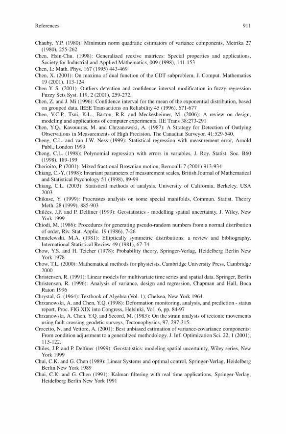
References 911
Chauby, Y.P. (1980): Minimum norm quadratic estimators of variance components, Metrika 27(1980), 255-262
Chen, Hsin-Chu. (1998): Generalized reexive matrices: Special properties and applications,Society for Industrial and Applied Mathematics, 009 (1998), 141-153
Chen, L: Math. Phys. 167 (1995) 443-469Chen, X. (2001): On maxima of dual function of the CDT subproblem, J. Comput. Mathematics
19 (2001), 113-124Chen Y.-S. (2001): Outliers detection and confidence interval modification in fuzzy regression
Fuzzy Sets Syst. 119, 2 (2001), 259-272.Chen, Z. and J. Mi (1996): Confidence interval for the mean of the exponential distribution, based
on grouped data, IEEE Transactions on Reliability 45 (1996), 671-677Chen, V.C.P., Tsui, K.L., Barton, R.R. and Meckesheimer, M. (2006): A review on design,
modeling and applications of computer experiments. IIE Trans 38:273-291Chen, Y.Q., Kavouuras, M. and Chrzanowski, A. (1987): A Strategy for Detection of Outlying
Observations in Measurements of High Precision. The Canadian Surveyor. 41:529-540.Cheng, C.L. and van J.W. Ness (1999): Statistical regression with measurement error, Arnold
Publ., London 1999Cheng, C.L. (1998): Polynomial regression with errors in variables, J. Roy. Statist. Soc. B60
(1998), 189-199Cherioito, P. (2001): Mixed fractional Brownian motion, Bernoulli 7 (2001) 913-934Chiang, C.-Y. (1998): Invariant parameters of measurement scales, British Journal of Mathematical
and Statistical Psychology 51 (1998), 89-99Chiang, C.L. (2003): Statistical methods of analysis, University of California, Berkeley, USA
2003Chikuse, Y. (1999): Procrustes analysis on some special manifolds, Commun. Statist. Theory
Meth. 28 (1999), 885-903Chilees, J.P. and P. Delfiner (1999): Geostatistics - modelling spatial uncertainty, J. Wiley, New
York 1999Chiodi, M. (1986): Procedures for generating pseudo-random numbers from a normal distribution
of order, Riv. Stat. Applic. 19 (1986), 7-26Chmielewski, M.A. (1981): Elliptically symmetric distributions: a review and bibliography,
International Statistical Review 49 (1981), 67-74Chow, Y.S. and H. Teicher (1978): Probability theory, Springer-Verlag, Heidelberg Berlin New
York 1978Chow, T.L. (2000): Mathematical methods for physicists, Cambridge University Press, Cambridge
2000Christensen, R. (1991): Linear models for multivariate time series and spatial data. Springer, BerlinChristensen, R. (1996): Analysis of variance, design and regression, Chapman and Hall, Boca
Raton 1996Chrystal, G. (1964): Textbook of Algebra (Vol. 1), Chelsea, New York 1964.Chrzanowski, A. and Chen, Y.Q. (1998): Deformation monitoring, analysis, and prediction - status
report, Proc. FIG XIX into Congress, Helsinki, Vo1. 6, pp. 84-97Chrzanowski, A. Chen, Y.Q. and Secord, M. (1983): On the strain analysis of tectonic movements
using fault crossing geodetic surveys, Tectonophysics, 97, 297-315:Crocetto, N. and Vettore, A. (2001): Best unbiased estimation of variance-covariance components:
From condition adjustment to a generalized methodology. J. Inf. Optimization Sci. 22, 1 (2001),113-122.
Chiles, J.P. and P. Delfiner (1999): Geostatistics: modeling spatial uncertainty, Wiley series, NewYork 1999
Chui, C.K. and G. Chen (1989): Linear Systems and optimal control, Springer-Verlag, HeidelbergBerlin New York 1989
Chui, C.K. and G. Chen (1991): Kalman filtering with real time applications, Springer-Verlag,Heidelberg Berlin New York 1991

912 References
Ciarlet, P.G. (1988): Mathematical elasticity, Vol. 1: three-dimensional elasticity, North HollandPubl. Comp., Amsterdam
Claerbout, J.F. (1964): Detection of p - waves from weak sources at great distances, Geophysics29 (1964), 197-211
Clark, G.P.Y. (1980): Moments of the least squares estimators in a nonlinear regression model, JR.Statist. Soc. B42 (1980), 227-237
Clerc-Beerod, A. and S. Morgenthaler (1997): A close look at the hat matrix, Student 2 (1997), 1-12Cobb, L., Koppstein, P. and N.H. Chen (1983): Estimation and moment recursions relations for
multimodal distributions of the exponential family, J. Am. Statist. Ass. 78 (1983), 124-130Cobb, G.W. (1997): Introduction to design and analysis of experiments, Springer-Verlag,
Heidelberg Berlin New York 1997Cochran, W. (1972): Some effects of errors of measurement on linear regression, in: Proceedings
of the Sixth Berkeley Symposium on Mathematical Statistics and Probability, 527-539, UCP,Berkeley 1972
Cochran, W. (1972): Stichprobenverfahren, de Gruyter, Berlin 1972Cohen, A. (1966): All admissible linear estimates of the mean vector, Ann. Math. Statist. 37
(1966), 458-463Cohen, C. and A. Ben-Israel (1969): On the computation of canonical correlations, Cahiers Centre
eEtudes Recherche Opeer 11 (1969), 121-132Cohen J., Kesten M., and Newman C. (eds.) (1985): Random matrices and their applications,
Amer. Math. Soc., ProvidenceCollett, D. (1992): Modelling binary data, Chapman and Hall, Boca Raton 1992Collet, D. and T. Lewis (1981): Discriminating between the von Mises and wrapped normal
distributions, Austr. J. Statist. 23 (1981), 73-79Colton, D., Coyle, J. and P. Monk (2000): Recent developments in inverse acoustic scattering
theory, SIAM Review 42 (2000), 369-414Comte, F. and Rozenholc, Y. (2002): Adaptive estimation of volatility functions in (auto-)
regressive models, Stoel cesses and their Applications 97, 111-145, 2002.Cook, R.D., Tsai, C.L. and B.C. Wei (1986): Bias in nonlinear regression, Biometrika 73 (1986),
615-623Cook, R.D. and S. Weisberg (1982): Residuals and influence in regression, Chapman and Hall,
London 1982Cook, R.D. and Goldberg, M.L. (1986): Curvatures for parameter subsets in nonlinear regression.
Annals of Statistics, 14.Corbeil, R.R. and S.R. Searle (1976): restricted maximum likelihood (REML) estimation of
variance components in the mixed model, Technometrics, 18 (1976), pp. 31-38Cottle, R.W. (1974): Manifestations of the Schur complement, Linear Algebra Appl. 8 (1974),
189-211Coulman, C.E. and J. Vernin (1991): Significance of anisotropy and the outer scale of turbulence
for optical and radio seeing, Applied Optics 30 (1991) 118-126Cox, L.B. and J.S.Y. Wang (1993): Fractal surfaces: measurement and applications in the earth
Sciences. Fractals 1 1 (1993), pp. 87-115Cox, A.J. and N.J. Higham (1999): Row-wise backward stable elimination methods for the
equality constrained least squares problem, SIAM J. Matrix Anal. Appl. 21 (1999), 313-326Cox, D., Little, J. and O’Shea, D. (1997): Ideals, Varieties, and Algorithms, An introduction to
computational algebraic geometry and commutative algebra, Springer-Verlag, New York 1997.Cox, D., Little, J. and O’Shea, D. (1998): Using algebraic geometry. Graduate Text in Mathematics
185, Springer-Verlag, New York 1998.Cox, D.A. (1998): Introduction to Grobner bases, Proceedings of Symposia in Applied
Mathematics 53 (1998) 1-24.Cox, D.B. Brading, J.D.W. (1999): Integration of LAMBDA ambiguity resolution with Kalman
filter for relative navigation of spacecraft. In: Proceedings ION NTM 99, pp 739-745Cox, D.R. and D.V. Hinkley (1979): Theoretical statistics, Chapman and Hall, Boca Raton 1979Cox, D.R. and V. Isham (1980): Point processes, Chapman and Hall, Boca Raton (1980)
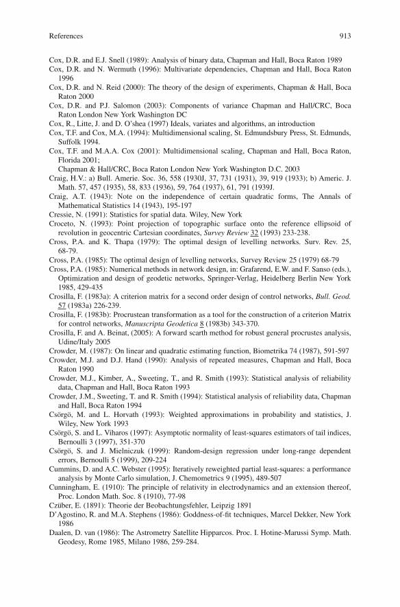
References 913
Cox, D.R. and E.J. Snell (1989): Analysis of binary data, Chapman and Hall, Boca Raton 1989Cox, D.R. and N. Wermuth (1996): Multivariate dependencies, Chapman and Hall, Boca Raton
1996Cox, D.R. and N. Reid (2000): The theory of the design of experiments, Chapman & Hall, Boca
Raton 2000Cox, D.R. and P.J. Salomon (2003): Components of variance Chapman and Hall/CRC, Boca
Raton London New York Washington DCCox, R., Litte, J. and D. O’shea (1997) Ideals, variates and algorithms, an introductionCox, T.F. and Cox, M.A. (1994): Multidimensional scaling, St. Edmundsbury Press, St. Edmunds,
Suffolk 1994.Cox, T.F. and M.A.A. Cox (2001): Multidimensional scaling, Chapman and Hall, Boca Raton,
Florida 2001;Chapman & Hall/CRC, Boca Raton London New York Washington D.C. 2003
Craig, H.V.: a) Bull. Amerie. Soc. 36, 558 (1930J, 37, 731 (1931), 39, 919 (1933); b) Americ. J.Math. 57, 457 (1935), 58, 833 (1936), 59, 764 (1937), 61, 791 (1939J.
Craig, A.T. (1943): Note on the independence of certain quadratic forms, The Annals ofMathematical Statistics 14 (1943), 195-197
Cressie, N. (1991): Statistics for spatial data. Wiley, New YorkCroceto, N. (1993): Point projection of topographic surface onto the reference ellipsoid of
revolution in geocentric Cartesian coordinates, Survey Review 32 (1993) 233-238.Cross, P.A. and K. Thapa (1979): The optimal design of levelling networks. Surv. Rev. 25,
68-79.Cross, P.A. (1985): The optimal design of levelling networks, Survey Review 25 (1979) 68-79Cross, P.A. (1985): Numerical methods in network design, in: Grafarend, E.W. and F. Sanso (eds.),
Optimization and design of geodetic networks, Springer-Verlag, Heidelberg Berlin New York1985, 429-435
Crosilla, F. (1983a): A criterion matrix for a second order design of control networks, Bull. Geod.57 (1983a) 226-239.
Crosilla, F. (1983b): Procrustean transformation as a tool for the construction of a criterion Matrixfor control networks, Manuscripta Geodetica 8 (1983b) 343-370.
Crosilla, F. and A. Beinat, (2005): A forward scarth method for robust general procrustes analysis,Udine/Italy 2005
Crowder, M. (1987): On linear and quadratic estimating function, Biometrika 74 (1987), 591-597Crowder, M.J. and D.J. Hand (1990): Analysis of repeated measures, Chapman and Hall, Boca
Raton 1990Crowder, M.J., Kimber, A., Sweeting, T., and R. Smith (1993): Statistical analysis of reliability
data, Chapman and Hall, Boca Raton 1993Crowder, J.M., Sweeting, T. and R. Smith (1994): Statistical analysis of reliability data, Chapman
and Hall, Boca Raton 1994Csorgo, M. and L. Horvath (1993): Weighted approximations in probability and statistics, J.
Wiley, New York 1993Csorgo, S. and L. Viharos (1997): Asymptotic normality of least-squares estimators of tail indices,
Bernoulli 3 (1997), 351-370Csorgo, S. and J. Mielniczuk (1999): Random-design regression under long-range dependent
errors, Bernoulli 5 (1999), 209-224Cummins, D. and A.C. Webster (1995): Iteratively reweighted partial least-squares: a performance
analysis by Monte Carlo simulation, J. Chemometrics 9 (1995), 489-507Cunningham, E. (1910): The principle of relativity in electrodynamics and an extension thereof,
Proc. London Math. Soc. 8 (1910), 77-98Czuber, E. (1891): Theorie der Beobachtungsfehler, Leipzig 1891D’Agostino, R. and M.A. Stephens (1986): Goddness-of-fit techniques, Marcel Dekker, New York
1986Daalen, D. van (1986): The Astrometry Satellite Hipparcos. Proc. I. Hotine-Marussi Symp. Math.
Geodesy, Rome 1985, Milano 1986, 259-284.

914 References
Dach, R. (2000): Einfluß von Auflasteffekten auf Prazise GPS-Messungen, DGK, Reihe C, HeftNr. 519.
Dai, L., Nagarajan, N., Hu, G. and Ling, K. (2005): Real-time attitude determination for microsatellites by LAMBDA method combined with Kalman filtering. In: AIAA proceedings 22ndICSSC, Monterey
Daniel, J.W. (1967): The conjugate gradient method for linear and nonlinear operator equations,SIAM J. Numer. Anal. 4 (1967), 10-26
Dantzig, G.B. (1940): On the nonexistence of tests of Student’s hypothesis having power functionsindependent of 2, Ann. Math. Statist. 11 (1949), 186-192
Das, I. (1996): Normal-boundary intersection: A new method for generating the Pareto surface innonlinear multicriteria optimization problems, SIAM J. Optim. 3 (1998), 631ff.
Das, R. and B.K. Sinha (1987): Robust optimum invariant unbiased tests for variance components.In Proc. of the Second International Tampere Conference in Statistics. T. Pukkila andS. Puntanen (eds.), University of Tampere/Finland (1987), 317-342
Das Gupta, S., Mitra, S.K., Rao, P.S., Ghosh, J.K., Mukhopadhyay, A.C. and Y.R. Sarma (1994):Selected papers of C.R. Rao, Vol. 1, J. Wiley, New York 1994
Das Gupta, S., Mitra, S.K., Rao, P.S., Ghosh, J.K., Mukhopadhyay, A.C. and Y.R. Sarma (1994):Selected papers of C.R. Rao, Vol. 2, J. Wiley, New York 1994
Davenport, J.H., Siret, Y. and Tournier, E. (1988): Computer algebra. Systems and algorithms foralgebraic computation, Academic Press Ltd., St. Edmundsbury, London 1988.
David, F.N. (1937): A note on unbiased limits for the correlation coefficient, Biometrika,29, 157-160
David, F.N. (1938): Tables of the Ordinates and Probability Integral o/the Distribution of theCorrelation Coefficient in Small Samples, London, Biometrika.
David, F.N. (1953): A note on the evaluation of the multivariate normal integral, Biometrika,40, 458-459
David, F.N. (1954): Tables of the ordinates and probability integral of the distribution of thecorrelation coefficient in small samples, Cambridge University Press, London 1954
David, F.N. and N.L. Johnson (1948): The probability integral transformation when parametersare estimated from the sample, Biometrika 35 (1948), 182-190
David, H.A. (1957): Some notes on the statistical papers of Friedrich Robert Helmert (1943-1917),Bull. Stat. Soc. NSW 19 (1957), 25-28
David, H.A. (1970): Order Statistics, J. Wiley, New York 1970David, H.A., Hartley, H.O. and E.S. Pearson (1954): The distribution of the ratio in a single
normal sample, of range to standard deviation, Biometrika 41 (1954), 482-293Davidian, M. and A.R. Gallant (1993): The nonlinear mixed effects model with a smooth random
effects density, Biometrika 80 (1993), 475-488Davidian, M., and D.M. Giltinan (1995): Nonlinear models for repeated measurement data,
Chapman and Hall, Boca Raton 1995Davis, R.A. (1997): M-estimation for linear regression with infinite variance, Probability and
Mathematical Statistics 17 (1997), 1-20Davis, R.A. and W.T.M. Dunsmuir (1997): Least absolute deviation estimation for regression with
ARMA errors, J. Theor. Prob. 10 (1997), 481-497Davis, J.H. (2002): Foundations of deterministic and stochastic control, Birkhauser-Verlag, Basel
Boston Berlin 2002Davison, A.C. and D.V. Hinkley (1997): Bootstrap methods and their application, Cambridge
University Press, Cambridge 1997Dawe, D.J. (1984): Matrix and finite element displacement analysis of structures, Clarendon
Press, OxfordDecreusefond, L. and A.S. Ustunel (1999): Stochastic analysis of the fractional Brownian motion,
Potential Anal. 10 (1999), 177-214Dedekind, R. (1901): Gauß in seiner Vorlesung uber die Methode der kleinsten Quadrate, Berlin
1901

References 915
Defant, A. and K. Floret (1993): Tensor norms and operator ideals, North Holland, Amsterdam1993
Deitmar, A. (2002): A first course in harmonic analysis, Springer-Verlag, Heidelberg Berlin NewYork 2002
Demidenko, E. (2000): Is this the least squares estimate?, Biometrika 87 (2000), 437-452Denham, M.C. (1997): Prediction intervals in partial least-squares, J. Chemometrics 11 (1997),
39-52Denham, W. and S. Pines (1966): Sequential estimation when measurement function nonlinearity
is comparable to measurement error, AIAA J4 (1966), 1071-1076Denis, J.-B. and A. Pazman (1999): Bias of LS estimators in nonlinear regression models with
constraints. Part II: Bi additive models, Applications of Mathematics 44 (1999), 375-403Dermanis, A. (1977): Geodetic linear estimation techniques and the norm choice problem,
Manuscripta geodetica 2 (1977), 15-97Dermanis, A. (1978): Adjustment of geodetic observations in the presence of signals, International
School of Anvanced Geodesy, Erice, Sicily, May-June 1978, Bollettino di Geodesia e ScienzeAffini 38 (1979), 513-539
Dermanis, A. (1980): Adjustment of geodetic observations in the presence of signals. In:Proceedings of the international school of advanced geodesy. Bollettino di Geodesia e ScienzeAffini. Vol. 38, pp. 419-445
Dermanis, A. (1998): Generalized inverses of nonlinear mappings and the nonlinear geodeticdatum problem, Journal of Geodesy 72 (1998), 71-100
Dermanis, A. and E. Grafarend (1981): Estimability analysis of geodetic, astrometric andgeodynamical quantities in Very Long Baseline Interferometry, Geophys. J. R. Astronom. Soc.64 (1981), 31-56
Dermanis, A. and F. Sanso (1995): Nonlinear estimation problems for nonlinear models,manuscripta geodaetica 20 (1995), 110-122
Dermanis, A. and R. Rummel (2000): Data analysis methods in geodesy, Lecture Notes in EarthSciences 95, Springer-Verlag, Heidelberg Berlin New York 2000
Dette, H. (1993): A note on E-optimal designs for weighted polynomial regression, Ann. Stat.21 (1993), 767-771
Dette, H. (1997): Designing experiments with respect to ’standardized’ optimality criteria, J. R.Statist. Soc. B59 (1997), 97-110
Dette, H. (1997): E-optimal designs for regression models with quantitative factors - a reasonablechoice?, The Canadian Journal of Statistics 25 (1997), 531-543
Dette, H. and W.J. Studden (1993): Geometry of E-optimality, Ann. Stat. 21 (1993), 416-433Dette, H. and W.J. Studden (1997): The theory of canonical moments with applications in
statistics, probability, and analysis, J. Wiley, New York 1997Dette, H. and T.E. O’Brien (1999): Optimality criteria for regression models based on predicted
variance, Biometrika 86 (1999), 93-106Deutsch, F. (2001): Best approximation in inner product spaces, Springer-Verlag, Heidelberg
Berlin New York 2001Dewess, G. (1973): Zur Anwendung der Schatzmethode MINQUE auf Probleme der Prozeß-
Bilanzierung, Math. Operationsforschg. Statistik 4 (1973), 299-313Dey, D. and Ghosh, S. and Mallick, B. (2000): Generalized linear models: A Bayesian perspective.
Marcel Dekker, New YorkDiCiccio, T.J. and B. Efron (1996): Bootstrap confidence intervals, Statistical Science 11 (1996),
189-228Diebolt, J. and J. Zuber (1999): Goodness-of-fit tests for nonlinear heteroscedastic regression
models, Statistics & Probability Letters 42 (1999), 53-60Dieck, T. (1987): Transformation groups, W de Gruyter, Berlin/New York 1987Diggle, P.J., Liang, K.Y. and S.L. Zeger (1994): Analysis of longitudinal data, Clarendon Press,
Oxford 1994Diggle, P., Lophaven S. (2006): Bayesian geostatistical design. Scand. J. Stat. 33:53-64

916 References
Ding, C.G. (1999): An efficient algorithm for computing quantiles of the noncentral chi-squareddistribution, Computational Statistics & Data Analysis 29 (1999), 253-259
Dixon, A.L. (1908): The elimination of three quantics in two independent variables, Proc. LondonMathematical Society series 2 6 (1908) 468-478.
Dixon, G.M. (1994): Division Algebras: Octonions, Quaternions, Complex Numbers and theAlgebraic Design of Physics, Kluwer Aca. Publ., Dordrecht-Boston-London 1994
Dixon, W.J. (1951): Ratio involving extreme values, Ann. Math. Statistics 22 (1951), 68-78Dobbie, M.J. and Henderson, B.L. and Stevens, D.L. Jr. (2008): Sparse sampling: spatial design
for monitoring stream networks. Stat. Surv. 2: 113-153Dobson, A.J. (1990): An introduction to generalized linear models, Chapman and Hall, Boca
Raton 1990Dobson, A.J. (2002): An introduction to generalized linear models, 2nd ed., Chapman/Hall/CRC,
Boca Raton 2002Dodge, Y. (1987): Statistical data analysis based on the L1-norm and related methods, Elsevier,
Amsterdam 1987Dodge, Y. (1997): LAD Regression for Detecting Outliers in Response and Explanatory Variables,
J. Multivar. Anal. 61 (1997), 144-158Dodge, Y. and D. Majumdar (1979): An algorithm for finding least square generalized inverses for
classification models with arbitrary patterns, J. Statist. Comput. Simul. 9 (1979), 1-17Dodge, Y. and J. Jureckovea (1997): Adaptive choice of trimming proportion in trimmed
least-squares estimation, Statistics & Probability Letters 33 (1997), 167-176Donoho, D.L. and P.J. Huber (1983): The notion of breakdown point, Festschrift fur Erich
L. Lehmann, eds. P.J. Bickel, K.A. Doksum and J.L. Hodges, Wadsworth, Belmont, Calif.157-184, 1983
Dorea, C.C.Y. (1997): L1-convergence of a class of algorithms for global optimization, Student 2(1997)
Dorrie, H. (1948): Kubische und biquadratische Gleichungen. Leibniz-Verlag, MiinchenDowns, T.D. and A.L. Gould (1967): Some relationships between the normal and von Mises
distributions, Biometrika 54 (1967), 684-687Draper, N.R. and R. Craig van Nostrand (1979): Ridge regression and James-Stein estimation:
review and comments, Technometrics 21 (1979), 451-466Draper, N.R. and J.A. John (1981): Influential observations and outliers in regression,
Technometrics 23 (1981), 21-26Draper, N.R. and F. Pukelsheim (1996): An overview of design of experiments, Statistical Papers
37 (1996), 1-32Draper, N.R. and F. Pukelsheim (1998): Mixture models based on homogenous polynomials,
J. Stat., Planning and Inference, 71 (1998), pp. 303-311Draper, N.R. and F. Pukelsheim (2002): Generalized Ridge Analysis Under Linear Restrictions,
With Particular Applications to Mixture Experiments Problems, Technometrics, 44, 250-259.Draper, N.R. and F. Pukelsheim (2003): Canonical reduction of second order fitted models subject
to linear restrictions, Statistics and Probability Letters, 63 (2003), pp. 401-410Drauschke, M., Forstner, W. and Brunn, A. (2009): Multidodging: Ein effizienter Algorithmus
zur automatischen Verbesserung von digitalisierten Luftbildern. Seyfert, Eckhardt (Hg.):Publikationen der DGPF, Band 18: Zukunft mit Tradition. Jena 2009, S. 61-68.
Drauschke, M. and Roscher, R. and Labe, T. and Forstner, W. (2009): Improving Image Segmen-tation using Multiple View Analysis. Object Extraction for 3D City Models, Road Databasesand Traffic Monitoring - Concepts, Algorithms and Evaluatin (CMRT09). 2009, S. 211-216.
Driscoll, M.F. (1999): An improved result relating quadratic forms and Chi-Square Distributions,The American Statistician 53 (1999), 273-275
Driscoll, M.F. and B. Krasnicka (1995): An accessible proof of Craig’s theorem in the generalcase, The American Statistician 49 (1995), 59-62
Droge, B. (1998): Minimax regret analysis of orthogonal series regression estimation: selectionversus shrinkage, Biometrika 85 (1998), 631-643

References 917
Dryden, I.L. (1998): General registration and shape analysis. STAT 96/03. Stochastic Geometry:Likelihood and Computation, by W.S. Kendell, O. Barndoff-Nielsen and M.N.N. van Lieshout,Chapman and Hall/CRC Press, 333-364, Boca Raton 1998.
Drygas, H. (1970): The coordinate-free approach to Gauss-Markov estimation. SpringerVerlag,Berlin-Heidelberg-New York, 1970.
Drygas, H. (1972): The estimation of residual variance in regression analysis, Math. OperationsForsch. Atatist., 3 (1972), pp. 373-388
Drygas, H. (1975a): Weak and strong consistency of the least squares estimators in regressionmodels. Z. Wahrscheinlichkeitstheor. Verw. Geb. 34 (1975), 119-127.
Drygas, H. (1975b): Estimation and prediction for linear models in general spaces, Math.Operationsforsch. Statistik 6 (1975), 301-324
Drygas, H. (1977): Best quadratic unbiased estimation in variance-covariance component models,Math. Operationsforsch. Statistik, 8 (1977), pp. 211-231
Drygas, H. (1983): Sufficiency and completeness in the general Gauss-Markov model, SankhyaSer. A45 (1983), 88-98
Duan, J.C. (1997): Augmented GARCH (p,q) process and its diffusion limit, J. Econometrics 79(1997), 97-127
Duda, R.O., Hart, P.E. and Stork, D.G. (2000): Pattern classification, 2ed., Wiley, New York, 2000Duncan, W.J. (1944): Some devices for the solution of large sets of simultaneous linear equations,
London, Edinburgh and Dublin Philosophical Magazine and Journal of Science (7th series) 35(1944), 660-670
Dunfour, J.M. (1986): Bias of s2 in linear regression with dependent errors, The AmericanStatistician 40 (1986), 284-285
Dunnett, C.W. and M. Sobel (1954): A bivariate generalization of Student’s t-distribution, withtables for certain special cases, Biometrika 41 (1954), 153-69
Dupuis, D.J., Hamilton, D.C. (2000): Regression residuals and test statistics: Assessing naiveoutlier deletion. Can. J. Stat. 28, 2 (2000), 259-275
Durand, D. and J.A. Greenwood (1957): Random unit vectors II : usefulness of Gram-Charlierand related series in approximating distributions, Ann. Math. Statist. 28 (1957), 978-986
Durbin, J. and G.S. Watson (1950): Testing for serial correlation in least squares regression,Biometrika 37 (1950), 409-428
Durbin, J. and G.S. Watson (1951): Testing for serial correlation in least squares regression II,Biometrika 38 (1951), 159-177
Dvorak, G. and Benveniste, Y. (1992): On transformation strains and uniform fields in multiphaseelastic media, Proc. R. Soc. Lond., A437, 291-310
Ecker, E. (1977): Ausgleichung nach der Methode der kleinsten Quadrate, Ost. Z.Vermessungswesen 64 (1977), 41-53
Eckert, M (1935): Eine neue achentrene (azimutale) Erdkarte, Petermann’s Mitteilungen 81(1935), 190-192
Eckhart, C. and G. Young (1939): A principal axis transformation for non-Hermitean matrices,Bull. Amer. Math. Soc. 45 (1939), 188-121
Eckl, M.C., Snay, R.A., Solder, T., Cline, M.W. and G.L. Mader (2001): Accuracy of GPS-derivedpositions as a function of interstation distance and observing-session duration, Journal ofGeodesy 75 (2001), 633-640
Edelman, A. (1989): Eigenvalues and condition numbers of random matrices, PhD dissertation,Massachussetts Institute of Technology 1989
Edelman, A. (1998): The geometry of algorithms with orthogonality constraints, SIAM J. MatrixAnal. Appl. 20 (1998), 303-353
Edelman, A., Elmroth, E. and B. Kagstrom (1997): A geometric approach to perturbation theoryof matrices and matrix pencils. Part I: Versal deformations, SIAM J. Matrix Anal. Appl. 18(1997), 653-692
Edelman, A., Arias, T.A. and Smith, S.T. (1998): The geometry of algorithms with orthogonalityconstraints, SIAM J. Matrix Anal. Appl. 20 (1998), 303-353

918 References
Edgar, G.A. (1998): Integral, probability, and fractal measures, Springer-Verlag, Heidelberg BerlinNew York 1998
Edgeworth, F.Y. (1883): The law of error, Philosophical Magazine 16 (1883), 300-309Eeg, J. and T. Krarup (1973): Integrated geodesy, Danish Geodetic Institute, Report No.
7, Copenhagen 1973Effros, E.G. (1997): Dimensions and C* algebras, Regional Conference Series in Mathematics 46,
Rhode Island 1997Efron, B. and R.J. Tibshirani (1994): An introduction to the bootstrap, Chapman and Hall, Boca
Raton 1994Eibassiouni, M.Y. and J. Seely (1980): Optimal tests for certain functions of the parameters in a
covariance matrix with linear structure, Sankya 42 (1980), 64-77Eichhorn, A. (2005): Ein Beitrag zur parametrischen Identifikation von dynamischen
Strukturmodellen mit Methoden der adaptiven Kalman Filterung, Deutsche GeodatischeKommission, Bayerische Akademic der Wissenschaften, Reihe C 585, Munchen 2005
Einstein, A. (1905): Ueber die von der molekularkinetische Theorie der Waerme geforderteBerechnung von in Fluessigkeiten suspendierten Teilchen, Ann. Phys. 17 (1905) 549-560
Ekblom, S. and S. Henriksson (1969): Lp-criteria for the estimation of location parameters, SIAMJ. Appl. Math. 17 (1969), 1130-1141
Elden, L. (1977): Algorithms for the regularization of ill-conditioned least squares problems, 17(1977), 134-145
Elhay, S., Golub, G.H. and J. Kautsky (1991): Updating and downdating of orthogonal polynomialswith data fitting applications, SIAM J. Matrix Anal. Appl. 12 (1991), 327-353
Elian, S.N. (2000): Simple forms of the best linear unbiased predictor in the general linearregression model, American Statistician 54 (2000), 25-28
Ellis, R.L. and I. Gohberg (2003): Orthogonal systems and convolution operators, Birkhauser-Verlag, Basel Boston Berlin 2003
Ellis, S.P. (1998): Instability of least squares, least absolute correlation and least median ofsquared linear regression, Stst. Sci., 13 (1998), pp. 337-350
Ellis, S.P. (2000): Singularity and outliers in linear regression with application to least squares,least absolute deviation, and least median of squares linear regression. Metron 58, 1-2 (2000),121-129.
Ellenberg, J.H. (1973): The joint distribution of the standardized least squares residuals from ageneral linear regression, J. Am. Statist. Ass. 68 (1973), 941-943
Elpelt, B. (1989): On linear statistical models of commutative quadratic type, Commun.Statist.-Theory Method 18 (1989), 3407-3450
El-Basssiouni, M.Y. and Seely, J. (1980): Optimal tests for certain functions of the parameters ina covariance matrix with linear structure, Sankya A42 (1980), 64-77
Elfving, G. (1952): Optimum allocation in linear regression theory, Ann. Math. Stat. 23 (1952),255-263
El-Sayed, S.M. (1996): The sampling distribution of ridge parameter estimator, EgyptianStatistical Journal, ISSR - Cairo University 40 (1996), 211-219
Embree, P.J., Burg, P. and Backus, M.M. (1963): Wide band velocity filtering - the pie slid process,Geophysics 28 (1963), 948-974
Engeln-Mullges, G. and Reutter, F. (1990): Formelsammlung zur numerischen Mathematik mitC-Programmen. Bibliographisches Institut Mannheim & F. A. Brockhaus AG
Engl, H.W., Hanke, M. and A. Neubauer (1996): Regularization of inverse problems, KluwerAcademic Publishers, Dordrecht 1996
Engl, H.W., A.K. Louis, and W. Rundell (1997): Inverse problems in geophysical applications,SIAM, Philadelphia 1997
Engler, K., Grafarend, E.W., Teunissen, P. and J. Zaiser (1982): Test computations of three-dimensional geodetic networks with observables in geometry and gravity space, Proceedingsof the International Symposium on Geodetic Networks and Computations. Vol. VII,119-141 Report B258/VII. Deutsche Geodatische Kommission, Bayerische Akademie derWissenschaften, Munchen 1982.

References 919
Eringen, A.C. (1962): Non linear theory of continuous media, McGraw Hill Book Comp., NewYork
Ernst, M.D. (1998): A multivariate generalized Laplace distribution, Computational Statistics 13(1998), 227-232
Eshagh, M. and Sjoberg (2008): The modified best quadratic unbiased non-negative estimator(MBQUNE) of variance components. Stud. Geophysics Geod. 52 (2008) 305-320
Ethro, U. (1991): Statistical Test of Significance for Testing Outlying Observations. SurveyReview. 31:62-70.
Euler, N. and W.H. Steeb (1992): Continuous symmetry, Lie algebras and differential equations,B.I. Wissenschaftsverlag, Mannheim 1992
Even Tzur, G. (2004): Variance Factor Estimation for Two-Step Analysis of Deformation Net-works. Journal of surveying engineering. Journal of Surveying Engineering, 130(3): 113-118.
Even Tzur, G. (2006): Datuln Definition and its Influence on the Reliability of Geodetic Networks.ZN, 131: 87-95.
Even Tzur, G. (2009): Two-Steps Analysis of Movement of the Kfar-Hanassi Network. FIGWorking week 2009, Eilat, Israel.
Everitt, B.S. (1987): Introduction to optimization methods and their application in statistics,Chapman and Hall, London 1987
Fahrmeir, L. and G. Tutz (2001): Multivariate statistical modelling based on generalized linearmodels, Springer-Verlag, Heidelberg Berlin New York 2001
Fakeev, A.G. (1981): A class of iterative processes for solving degenerate systems of linearalgebraic equations, USSR. Comp. Maths. Math. Phys. 21 (1981), 15-22
Falk, M., Husler, J. and R.D. Reiss (1994): Law of small numbers, extremes and rare events,Birkhauser-Verlag, Basel Boston Berlin 1994
Fan, J. and I. Gijbels (1996): Local polynomial modelling and its applications, Chapman and Hall,Boca Raton 1996
Fang, K.-T. and Y. Wang (1993): Number-theoretic methods in statistics, Chapman and Hall, BocaRaton 1993
Fang, K.-T. and Y.-T. Zhang (1990): Generalized multivariate analysis, Science Press Beijing,Springer Verlag, Bejing, Berlin New York 1990
Fang, K.-T., Kotz, S. and K.W. Ng (1990): Symmetric multivariate and related distributions,Chapman and Hall, London 1990
Farahmand, K. (1996): Random polynomials with complex coefficients, Statistics & ProbabilityLetters 27 (1996), 347-355
Farahmand, K. (1999): On random algebraic polynomials, Proceedings of the American Math.Soc. 127 (1999), 3339-3344
Faraway, J. (2006). Extending the linear model with R. Chapman and Hall, CRE.Farebrother, R.W. (1988): Linear least squares computations, Dekker, New York 1988Farebrother, R.W. (1999): Fitting linear relationships, Springer-Verlag, Heidelberg Berlin New
York 1999Farrel, R.H. (1964): Estimators of a location parameter in the absolutely continuous case, Ann.
Math. Statist. 35 (1964), 949-998Fasseo, A. (1997): On a rank test for autoregressive conditional heteroscedasticity, Student 2
(1997), 85-94Faulkenberry, G.D. (1973): A method of obtaining prediction intervals, J. Am. Statist. Ass. 68
(1973), 433-435Fausett, D.W. and C.T. Fulton (1994): Large least squares problems involving Kronecker products,
SIAM J. Matrix Anal. Appl. 15 (1994), 219-227Fazekas, I. and Kukush, A. S. Zwanzig (2004): Correction of nonlinear orthogonal regression
estimator. Ukr. Math. J. 56, 1101-1118Fedorov, V.V. (1972): Theory of Optimal Experiments. Academic PressFedorov, V.V. and Hackl, P. (1994): Optimal experimental design: spatial sampling. Calcutta Stat
Assoc Bull 44:173-194

920 References
Federov, V.V. and Muller, W.G. (1988): Two approaches in optimization of observing networks,in Optimal Design and Analysis of Experiments, Y. Dodge, V.V. Federov & H.P. Wynn, eds,North-Holland, Amsterdam, pp. 239-256
Fedorov, V.V. and Flagnagan, D. (1997): Optimal monitoring on Merer‘s expansion of covariancekernel, J. Comb. Inf. Syst. Sci. 23(1997) 237-250
Fedorov, V.V. and P. Hackl (1997): Model-oriented design of experiments, Springer-Verlag,Heidelberg Berlin New York 1997
Fedorov, V.V., Montepiedra, G. and C.J. Nachtsheim (1999): Design of experiments for locallyweighted regression, J. Statist. Planning and Inference 81 (1999), 363-382
Fedorov, V.V. and Muller, W.C. (2007): Optimum desighn of correlated fields via covariance kernelexpansion, in: Lopez Fidalgo, Rodriguez, J. and Forney, B. (eds) Physica Verlag Heidelberg
Feinstein, A.R. (1996): Multivariate analysis, Yale University Press, New Haven 1996Feldmann, R.V. (1962): Matrix theory I: Arthur Cayley - founder of matrix theory, Mathematics
teacher, 57, (1962), pp. 482-484Felus, Y.A. and R.C. Burtch (2005): A new procrustes algorithm for three dimensional datum
conversion, Ferris State University 2005Fengler, M., Freeden, W. and V. Michel (2003): The Kaiserslautern multiscale geopotential model
SWITCH-03 from orbit pertubations of the satellite CHAMP and its comparison to the modelsEGM96, UCPH2002-02-0.5, EIGEN-1s, and EIGEN-2, Geophysical Journal International(submitted) 2003
Fenyo, S. and H.W. Stolle (1984): Theorie und Praxis der linearen Integralgleichungen 4. BerlinFeuerverger, A. and P. Hall (1998): On statistical inference based on record values, Extremes 1:2
(1998), 169-190Fiebig, D.G., Bartels, R. and W.Kramer (1996): The Frisch-Waugh theorem and generalized least
squares, Econometric Reviews 15 (1996), 431-443Fierro, R.D. (1996): Pertubation analysis for twp-sided (or complete) orthogonal decompositions,
SIAM J. Matrix Anal. Appl. 17 (1996), 383-400Fierro, R.D. and J.R. Bunch (1995): Bounding the subspaces from rank revealing two-sided
orthogonal decompositions, SIAM J. Matrix Anal. Appl. 16 (1995), 743-759Fierro, R.D. and P.C. Hansen (1995): Accuracy of TSVD solutions computed from rank-revealing
decompositions, Numer. Math. 70 (1995), 453-471Fierro, R.D. and P.C. Hansen (1997): Low-rank revealing UTV decompositions, Numer.
Algorithms 15 (1997), 37-55Fill, J.A. and D.E. Fishkind (1999): The Moore-Penrose generalized inverse for sums of matrices,
SIAM J. Matrix Anal. Appl. 21 (1999), 629-635Finsterwalder, S. and Scheufele, W. (1937): Das Ruckwartseinschneiden im Raum, Sebastian
Finsterwalder zum 75 Geburtstage, pp. 86-100, Verlag Hebert Wichmann, Berlin 1937.Fischer, F.A. (1969): Einfuhrung in die Statische Ubertragungstheorie, Bib. Institute, Maurheim,
Zurigh 1969Fischler, M.A. and Bolles, R.C. (1981): Random Sample Consensus: A Paradigm for Medell
Fitting with Application to Image Analysis and Automated Cartography, Communications ofthe ACM 24 (1981) 381-395
Fiserova, E. (2004): Estimation in universal models with restrictions. Discuss. Math., Probab. Stat.24, 2 (2004), 233-253.
Fiserova, E. (2006): Testing hypotheses in universal models. Discuss. Math., Probab. Stat. 26(2006), 127-149
Fiserova, E. and Kubacek, L. (2003) Sensitivity analysis in singular mixed linear models withconstraints. Kybernetika 39, 3 (2003), 317-332
Fiserova, E. and Kubacek, L. (2004): Statistical problems of measurement in triangle. Folia Fac.Sci. Nat. Univ. Masarykianae Brunensis, Math. 15 (2004), 77-94
Fiserova, E. and Kubacek, L. (2003): Insensitivity regions and outliers in mixed models withconstraints. Austrian Journal of Statistic 35, 2-3 (2003), 245-252
Fisher, N.I. (1993): Statistical Analysis of Circular Data, Cambridge University Press, Cambridge1993

References 921
Fisher, N.I. and Hall, P. (1989): Bootstrap confidence regions for directional data, J. Am. Statist.Ass. 84 (1989), 996-1002
Fisher, N.J. (1985): Spherical medians, J. Roy. Statist. Soc. B47 (1985), 342-348Fisher, N.J. and A.J. Lee (1983): A correlation coefficient for circular data, Biometrika 70 (1983),
327-332Fisher, N.J. and A.J. Lee (1986): Correlation coefficients for random variables on a sphere or
hypersphere, Biometrika 73 (1986), 159-164Fisher, R.A. (1915): Frequency distribution of the values of the correlation coefficient in samples
from an indefinitely large population, Biometrika 10 (1915), 507-521Fisher, R.A. (1935): The fiducial argument in statistical inference, Annals of Eugenics 6 (1935),
391-398Fisher, R.A. (1939): The sampling distribution of some statistics obtained from nonlinear
equations, Ann. Eugen. 9 (1939), 238-249Fisher, R.A. (1953): Dispersion on a sphere, Pro. Roy. Soc. Lond. A217 (1953), 295-305Fisher, R.A. (1956): Statistical Methods and Scientific Inference, Edinburg: Oliver and Boyd, 1956Fisher, R.A. and F. Yates (1942): Statistical tables for biological, agricultural and medical research,
2nd edition, Oliver and Boyd, Edinburgh 1942Fisz, M. (1971): Wahrscheinlichkeitsrechnung und mathematische Statistik, Berlin (Ost) 1971Fitzgerald, W.J., Smith, R.L., Walden, A.T. and P.C. Young (2001): Non-linear and nonstationary
signal processing, Cambridge University Press, Cambridge 2001Fitzgibbon, A., Pilu, M. and Fisher, R.B. (1999): Direct least squares fitting of ellipses, IEEE
Transactions on Pattern Analysis and Machine Intelligence 21 (1999) 476-480.Fletcher, R. and C.M. Reeves (1964): Function minimization by conjugate gradients, Comput. J.
7 (1964) 149-154Fletcher, R. (1987): Practical Methods of Optimization. Second Edition, John Wiley & Sons,
Chicester.Fletling, R. (2007): Fuzzy clusterung zur Analyse von Uberwachungsmessungen, in: F.K. Brunner
(ed.) Ingenienr vermessung, pp. 311-316, Wichmann Verlag, Heidelberg 2007Flury, B. (1997): A first course in multivariate statistics, Springer-Verlag, Heidelberg Berlin New
York 1997Focke, J. and G. Dewess (1972): Uber die Schatzmethode MINQUE von C.R. Rao und ihre
Verallgemeinerung, Math. Operationsforschg. Statistik 3 (1972), 129-143Forstner, W. (1976): Statistical Test Methods for Blunder Detection in Planimetric Block
Triangulation. Presented paper to Comm. III, ISP Helsinki 1976Forstner, W. (1978a): PrOfung auf grobe Bildkoordinatenfehler bei der relativen Orientierung?
BuL, 1978, 205-212Forstner, W. (1978b): Die Suche nach groben Fehlern in photogrammetrischen Lageblocken,
Dissertation der Universitat Stuttgart .Forstner, W. (1979a): Ein Verfahren zur Schatzung von Varianz- und Kovarianzkomponenten,
Ally. Vermess. Nachrichten 86 (1979), pp. 446-453Forstner, W. (1979b): On Internal and External Reliability of Photogrammetric Coordinates.
Proceedings of the Annual Convention of the ASP-ACSM, Washington 1979Forstner, W. (1979c): Konvergenzbeschleunigung bei der a posteriori Varianzschatzung, Zeitschrift
fur Vermessungswesen 104 (1979), 149-156Forstner, W. (1979d): Ein Verfahren zur Schatzung von Varianz- und Kovarianz-Komponenten,
Allgemeine Vermessungsnachrichten 86 (1979), 446-453Forstner, W. (1980a): The Theoretical Reliability of Photogrammetric Coordinates. Archives of
the ISPRS. XIV Congress of the Int. Society for Photogrammetry Comm. 111, Hamburg, 1980Forstner, W. (1980b): Zur PrOfung zusatzlicher Parameter in Ausgleichungen. ZN, 1980, 105,
510-519Forstner, W. (1983): Reliability and Discernability of Extended Gauss-Markov Models.
Ackermann, F. (ed.) Deutsche Geodatische Kommission, A98, 1983, 79-103

922 References
Forstner, W. (1985): Determination of the Additive Noise Variance in Observed AutoregressiveProcesses using Variance Component Estimation Technique. Statistics and Decision,Supplement Issue No. 2. Munchen 1985, S. 263-274.
Forstner, W. (1987): Reliability Analysis of Parameter Estimation in Linear Models withApplications to Mensuration Problems in Computer Vision. CVGIP - Computer Vision,Graphics, and Image Processing. 1987, S. 273-310.
Forstner, W. (1990): Modelle intelligenter Bildsensoren und ihre Qualitat. Grol1 Kopf, R.E. (ed.)Springer, 1990, 254, 1-21
Forstner, W. (1993a): Image Matching. In: Haralick, R.M. I Shapiro, L.G. (Hg.): Computer and-RObot Vision. Addison-Wesley, S. 289-379
Forstner, W. (1993c): Uncertain Spatial Relationships and their Use for Object location inDigital/mages. Forstner, W.; Haralick, R.M. Radig, B. (ed.)lnstitut fur Photogrammetrie,Universitat Bonn, 1992 (Buchbeitrag)
Forstner, W. (1994a): Diagnostics and Performance Evaluation in Computer Vision. Performanceversus Methodology in Computer Vision, NSF/ARPA Workshop. Seattle 1994, S. 11-25.
Forstner, W. (1994b): Generic Estimation Procedures for Orientation with Minimum andRedundant Information Technical Report. Institute for Photogrammetry, University Bonn.
Forstner, W. (1995a): A 2D-data Model for Representing Buildings. Technical Report, Institut furPhotogrammetrie, Universitat Bonn
Forstner, W. (1995b): The Role of Robustness in Computer Vision. Proc. Workshop “Milestonesin CCfmi5uier Vision”. Vorau 1995.
Forstner, W. (1997a):Evaluation of Restoration Filters. Technical Report, Institut furPhotogrammetrie, Universitat Bonn
Forstner, W. (1997b): Parameter free information Preserving filter and Noise VarianceEqualization, Technical Report, Institut fur Photogrammetrie, Universitat Bonn
Forstner, W. (1998): On the Theoretical Accuracy of Multi Image Matching, Restoration andTriangulation. Festschrift zum 65. Geburtstag von Prof. Dr.-Ing. mult. G. Konecny. Institut furPhotogrammetrie, Universitat Hannover 1998
Forstner, W. (1999a): On Estimating Rotations. Heipke, C. / Mayer, H. (Hg.): Festschrift furProf. Dr.-Ing. Heinrich Ebner zum 60. Geburtstag. Lehrstuhl fur Photogrammetrie undFernerkundung, TU Munchen 1999.
Forstner, W. (1999b): Uncertain Neighborhood Relations of Point Sets and Fuzzy DelaunayTriangulation. Proceedings of DAGM Symposium Mustererkennung. Bonn, Germany 1999.
Forstner, W. (1999c): Choosing Constraints for Points and Lines in Image Triplets 1999. TechnicalReport, Institut fur Photogrammetrie, University Bonn.
Forstner, W. (1999d): Interior Orientation from Three Vanishing Points, Technical Report, Institutfur Photogrammetrie, Universitat Bonn
Forstner, W. (1999e): Tensor-based Distance Transform. Technical Report, Institut furPhotogrammetrie, Universitat Bonn.
Forstner, W. (2000): Optimally Reconstructing the Geometry of Image Triplets. Vernon, David(Hg.): Appeared in: Computer Vision - ECCV 2000. 2000, S. 669-684.
Forstner, W. (2001a): Algebraic Projective Geometry and Direct Optimal Estimation of GeometricEntities. Appeared at the Annual OeAGM 2001 Workshop.
Forstner, W. (2001b): Direct optimal estimation of geometric entities using algebraic projectivegeometry. Festschrift anlasslich des 60. Geburtstages von Prof. Dr.-Ing. Bernhard Wrobel.Technische Universitat Darmstadt 2001, S. 69-87.
Forstner, W. (2002): Computer Vision and Photogrammetry – Mutual Questions: Geometry,Statistics and Cognition. Bildteknik/lmage Science, Swedish Society for Photogrammetry andRemote Sensing. 2002, S. 151-164.
Forstner, W. (2003): Notions of Scale in Geosciences. Neugebauer, Horst J. I Simmer, Clemens(Hg.): Dynamics of Multi-Scale Earth Systems. 2003, S. 17-39.
Forstner, W. (2005): Uncertainty and Projective Geometry. Bayro Corrochano, Eduardo (Hg.):Handbook of Geometric Computing. 2005, S. 493-535.
References 923
Forstner, W. (2009): Computer Vision and Remote Sensing - Lessons Learned. Fritsch, Dieter(Hg.): Photogrammetric Week 2009. Heidelberg 2009, S. 241-249.
Forstner, W. and Schroth, R. (1981): On the estimation of covariance matrices for photogrammetricimage coordinates. VI: Adjustment procedures of geodetic networks, 43-70.
Forstner, W. and Wrobel, B. (1986): Digitale Photogrammetrie, Springer (Buch)Forstner, W. and Gulch, E. (1987): A Fast Operator for Detection and Precise Location of Distinct
Points, Corners and Centres of Circular Features. Proceedings of the ISPRS IntercommissionWorkshop, 1987. Jg. 1987.
Forstner, W. and Vosselmann, G. (1988): The Precision of a Digital Camera. ISPRS 16th Congress.Kyoto 1988, S. 148-157.
Forstner, W. and Braun, C. (1993): Direkte Schatzung von Richtungen und Rotationen. Institut furPhotogrammetrie, Bonn
Forstner, W. and Shao, J. (1994): Gabor Wavelets for Texture Edge Extraction. ISPRS CommissionIII Symposium on Spatial Information from Digital Photogrammetry and Computer Vision.Munich, Germany
Forstner, W. and Brugelmann, R. (1994): ENOVA - Estimation of Signal Dependent NoiseVariance. 3rd ECCV, Stockholm
Forstner, W. and Moonen, B. (1999): A Metric for Covariance Matrices. Krumm, F. Schwarze,V.S. (Hg.): Quo vadis geodesia . . . ?, Festschrift for Erik W. Grafarend on the occasion of his60th birthday. TR Dept. of Geodesy and Geoinformatics, Stuttgart University 1999.
Forstner, W. and B. Moonen (2003): A metric for covariance matrices, in: E. Grafarend, F. Krummand V. Schwarze: Geodesy - the Challenge of the 3rd Millenium, 299-309, Springer-Verlag,Heidelberg Berlin New York 2003
Forstner, W. and Dickscheid, T. and Schindler, F. (2009): Detecting Interpretable and AccurateScale-Invariant Keypoint. 12th IEEE International Conference on Computer Vision (ICCV’09).Kyoto, Japan 2009, S. 2256-2263.
Forsgren, A. and W. Murray (1997): Newton methods for large-scale linear inequality-constrainedminimization, Siam J. Optim. to appear
Forsythe, A.R. (1960): Calculus of Variations. New YorkForsythe, A.B. (1972): Robust estimation of straight line regression coefficients by minimizing
p-th power deviations, Technometrics 14 (1972), 159-166Foster, L.V. (2003): Solving rank-deficient and ill-posed problems using UTV and QR
factorizations, SIAM J. Matrix Anal. Appl. 25 (2003), 582-600Fotiou, A. and D. Rossikopoulos (1993): Adjustment, variance component estimation and testing
with the affine and similarity transformations, Zeitschrift fur Vermessungswesen 118 (1993),494-503
Fotiou, A.(1998): A pair of closed expressions to transform geocentric to geodetic coordinates,Zeitschrift fur Vermessungswesen 123 (1998) 133-135.
Fotopoulos, G. (2003): An Analysis on the Optimal Combination of Geoid, Orthometric andEllipsoidal Height Data. Report No. 20185, Department of Geomatics Engineering, Universityof Calgary, Calgary, Canada.
Fotopoulos, G., (2005): Calibration of geoid error models via a combined adjustment of ellipsoidal,orthometric and gravimetrical geoid height data. 1. Geodesy, 79, 111-123.
Forstner, W., (1979): Ein Verfahren zur Achatzung von varianz und kovarianzkomponenten.Allgemeine Vermessungs-Nachrichten, 86, 446-453.
Foucart, T. (1999): Stability of the inverse correlation matrix. Partial ridge regression, J. Statist.Planning and Inference 77 (1999), 141-154
Fox, A.J. (1972): Outliers in time series. J. Royal Stat. Soc., Series B, 43, (1972), 350-363Fox, M. and H. Rubin (1964): Admissibility of quantile estimates of a single location parameter,
Ann. Math. Statist. 35 (1964), 1019-1031Franses, P.H. (1998): Time series models for business and economic forecasting, Cambridge
University Press, Cambridge 1998Fraser, D.A.S. (1963): On sufficiency and the exponential family, J. Roy. Statist. Soc. 25 (1963),
115-123

924 References
Fraser, D.A.S. (1968): The structure of inference, J. Wiley, New York 1968Fraser, D.A.S. and I. Guttman (1963): Tolerance regions, Ann. Math. Statist. 27 (1957), 162-179Freeman, R.A. and P.V. Kokotovic (1996): Robust nonlinear control design, Birkhauser-Verlag,
Basel Boston Berlin 1996Freund, P.G.O. (1974): Local scale invariance and gravitation, Annals of Physics 84 (1974),
440-454Frey, M. and J.C. Kern (1997): The Pitman Closeness of a Class of Scaled Estimators, The
American Statistician, May 1997, Vol. 51 (1997), 151-154Frisch, U. (1995): Turbulence, the legacy of A.N. Kolmogorov, Cambridge University Press,
Cambridge 1995Fristedt, B. and L. Gray (1995): A modern approach to probability theory, Birkhauser-Verlag,
Basel Boston Berlin 1997Frobenius, F.G. (1893): Gedachtnisrede auf Leopold Kronecker (1893), Ferdinand Georg
Frobenius, Gesammelte Abhandlungen, ed. J.S. Serre, Band III, 705-724, Springer-Verlag,Heidelberg Berlin New York 1968
Frobenius, G. (1908): Uber Matrizen aus positiven Elementen, Sitzungsberichte der KoniglichPreussischen Akademie der Wissenschaften von Berlin, 471-476, Berlin 1908
Frohlich, H. and Hansen, H.H. (1976): Zur Lotfußpunktrechnung bei rotationsellipsoidischerBezugsflache, Allgemeine Vermessungs-Nachrichten 83 (1976) 175-179.
Fuentes, M. (2002): lnterpolation of non stationary air pollution processes: a spatial spectralapproach. In statistical Modeling, vol. 2, pp. 281-298.
Fuentes, M. and Smith, R. (2001): A new class of non stationary models. In Tech. report at NorthCarolina State University, Institute of Statistics
Fuentes, M., Chaudhuri, A. and Holland, D.M. (2007): Bayesian entropy for spatial samplingdesign of environmental data. J. Environ. Ecol. Stat. 14:323-340
Fujikoshi, Y. (1980): Asymptotic expansions for the distributions of sample roots undernon-normality, Biometrika 67 (1980), 45-51
Fukushima, T. (1999): Fast transform from geocentric to geodetic coordinates, Journal of Geodesy73 (1999) 603-610.
Fuller, W.A. (1987): Measurement error models, Wiley, New York 1987Fulton, T., Rohrlich, F. and L. Witten (1962): Conformal invariance in physics, Reviews of
Modern Physics 34 (1962), 442-457Furno, M. (1997): A robust heteroskedasticity consistent covariance matrix estimator, Statistics
30 (1997), 201-219Galil, Z. (1985): Computing d-optimum weighing designs: Where statistics, combinatorics, and
computation meet, in: Proceedings of the Berkeley Conference in Honor of Jerzy Neyman andJack Kiefer, Vol. II, eds. L.M. LeCam and R.A. Olshen, Wadsworth 1985
Gallant, A.R. (1987): Nonlinear statistical models, J. Wiley, New York 1987Gallavotti, G. (1999): Statistical mechanics: A short treatise, Springer-Verlag, Heidelberg Berlin
New York 1999Gander, W. (1981): Least squares with a quadratic constraint, Numer. Math. 36 (1981),
291-307Gander, W., Golub, G.H. and Strebel, R. (1994): Least-Squares fitting of circles and ellipses, BIT
No. 43 (1994) 558-578.Gandin, L.S. (1963): Objective analysis of meteorological fields. Gidrometeorologicheskoe
Izdatel’stvo (GIMIZ), LeningradGao, X.S. and Chou, S.C. (1990): Implicitization of rational parametric equations. Technical
report, Department of Computer Science TR-90-34, University of Texas, Austin 1990.Gao, S. and T.M.F. Smith (1995): On the nonexistence of a global nonengative minimum bias
invariant quadratic estimator of variance components, Statistics and Probability letters 25(1995), 117-120
Gao, S. and T.M.F. Smith (1998): A constrained MINQU estimator of correlated response variancefrom unbalanced dara in complex surveys, Statistica Sinica 8 (1998), 1175-1188

References 925
Gao, Y., Lahaye, F., Heroux, P., Liao, X., Beck, N. and M. Olynik (2001): Modeling and estimationof C1-P1 bias in GPS receivers, Journal of Geodesy 74 (2001), 621-626
Garceıa-Escudero, L.A., Gordaliza, A. and C. Matrean (1997): k-medians and trimmed k-medians,Student 2 (1997), 139-148
Garcia-Ligero, M.J., Hermoso, A. and J. Linares (1998): Least squared estimation for distributedparameter systems with uncertain observations: Part 1: Linear prediction and filtering, AppliedStochastic Models and Data Analysis 14 (1998), 11-18
Garderen K.J. van, (1999): Exact geometry of autoregressive models, Journal of Time SeriesAnalysis 20 (1999), 1-21
Gaspari, G. and Cohn, S.E. (1999): Construction of correlation I in two and three dimensions,Q. 1. R. Meteorol. Soc., 757, 1999.
Gastwirth, J.L. and H. Rubin (1975): The behaviour of robust estimators on dependent data, Ann.Stat., 3 (1975), pp. 1070-1100
Gatti, M. (2004): An empirical method of estimation of the variance-covariance matrix in GPSnetwork design, Survey Review 37, (2004), pp. 531-541
Gauss, C.F. (1809): Theoria Motus, Corporum Coelesium, Lib. 2, Sec. III, Perthes u. Besser Publ.,205-224, Hamburg 1809
Gauss, C.F. (1816): Bestimmung der Genauigkeit der Beobachtungen, Z. Astronomi 1 (1816),185-197
Gauss, C.F. (1923): Anwendung der Wahrscheinlichkeitsrechnung auf eine Aufgabe derpraktischen Geometrie, Gauss Works IV: 1923
Gautschi, W. (1982): On generating orthogonal polynomials, SIAM Journal on Scientific andStatistical Computing 3 (1982), 289-317
Gautschi, W. (1985): Orthogonal polynomials - constructive theory and applications, J. Comput.Appl. Math. 12/13 (1985), 61-76
Gautschi, W. (1997): Numerical analysis - an introduction, Birkhauser-Verlag, Basel BostonBerlin 1997
Gauss, C.F. (1809): Theoria motus corporum coelestium. GattingenGeisser, S. (1975): The predictive sample reuse method with applications. J. Math. Statist. 28:
385-394Gelb, A. (1974): Applied optimal estimation, Ed., MIT Press, Cambridge/Mass and LondonGelfand, A.E. and D.K. Dey (1988): Improved estimation of the disturbance variance in a linear
regression model, J. Econometrics 39 (1988), 387-395Gelfand, I.M., Kapranov, M.M. and Zelevinsky, A.V. (1990): Generalized Euler Integrals and
A-Hypergeometry Functions, Advances in Mathematics 84 (1990) 255-271.Gelfand, I.M., Kapranov, M.M. and Zelevinsky, A.V. (1994): Discriminants, resultants and
multidimensional determinants, Birkhauser, Boston 1994.Gelderen, M. van and R. Rummel (2001): The solution of the general geodetic boundary value
problem by least squares, Journal of Geodesy 75 (2001), 1-11Gelman, A., Carlin, J.B., Stern, H.S. and D.B. Rubin (1995): Bayesian data analysis, Chapman
and Hall, London 1995Genton, M.G. (1998): Asymptotic variance of M-estimators for dependent Gaussian random
variables, Statistics and Probability Lett. 38 (1998), 255-261Genton, M.G. and Y. Ma (1999): Robustness properties of dispersion estimators, Statistics &
Probability Letters 44 (1999), 343-350Genugten, B. and Van Der, B. (1997): Testing in the restricted linear model using canonical
partitions. Linear Algebra Appl. 264 (1997), 349-353.Gephart, J. and Forsyth D. (1984): An improved method for determining the regional stress
tensor - using earthquake focal mechanism data: application to the San Fernando earthquakesequence, J. geophys. Res., B89, 9305-9320
Gere, G.M. and W. Weaver (1965): Matrix algebra for engineers, Van Nostrand Co., New York1956
Ghosh, M., Mukhopadhyay, N. and P.K. Sen (1997): Sequential estimation, J. Wiley, New York1997

926 References
Ghosh, S. (1996): Wishart distribution via induction, The American Statistician 50 (1996), 243-246Ghosh, S. (1999): Multivariate analysis, design of experiments, and survey sampling, Marcel
Dekker, Basel 1999Ghosh, S., Beran, J. and J. Innes (1997): Nonparametric conditional quantile estimation in the
presence of long memory, Student 2 (1997), 109-117Ghosh, S. (ed.) (1999): Multivariate analysis, design of experiments, and survey sampling, Marcel
Dekker, New York 1999Giacolone, M. (1997): Lp-norm estimation for nonlinear regression models, Student 2 (1997),
119-130Giering, O. (1984): Bemerkungen zum ebenen Trilaterationsproblem. Deutsche Geodatische
Kommission, Reihe A, Nr. 101.Giering, O. (1986): Analytische Behandlung des raumlichen Trilaterationsproblems 4, 6, 0, o.
Deutsche Geodatische Kommission, Reihe A, Nr. 104Gil, A. and J. Segura (1998): A code to evaluate prolate and oblate spheroidal harmonics,
Computer Physics Communications 108 (1998), 267-278Gilbert, E.G. and C.P. Foo (1990): Computing the distance between general convex objects in
three-dimensional space, JEEE Transactions on Robotics and Automation 6 (1990), 53-61Gilchrist, W. (1976): Statistical forecasting, Wiley, London 1976Gill, P.E., Murray, W. and Wright, M.H. (1981): Practical Optimization. Academic Press, London.Gill, P.E., Murray, W. and Saunders, M.A. (2002): Snopt: An SQP algorithm for large scale
constrained optimization, Siam J. Optim. 12 (2002), 979-1006Gillard, D., Wyss, M. and J. Nakata (1992): A seismotectonic model for Western Hawaii based on
stress tensor inversion from fault plane solutions, J. Geophys., Res., B97, 6629-6641Giri, N. (1977): Multivariate statistical inference, Academic Press, New York London 1977Giri, N. (1993): Introduction to probability and statistics, 2nd edition, Marcel Dekker, New York
1993Giri, N. (1996a): Multivariate statistical analysis, Marcel Dekker, New York 1996Giri, N. (1996b): Group invariance in statistical inference, World Scientific, Singapore 1996Girko, V.L. (1979): Distribution of eigenvalues and eigenvectors of hermitian stochastic matrices,
Ukrain. Math. J., 31, 421-424Girko, V.L. (1985): Spectral theory of random matrices, Russian Math. Surveys, 40, 77-120Girko, V.L. (1988): Spectral theory of random matrices, Nauka, Moscow 1988Girko, V.L. (1990): Theory of random determinants, Kluwer Academic Publishers, Dordrecht
1990Girko, V.L. and A.K. Gupta (1996): Multivariate elliptically contoured linear models and some
aspects of the theory of random matrices, in: Multidimensional statistical analysis and theoryof random matrices, Proceedings of the Sixth Lukacs Symposium, eds. Gupta, A.K. and V.L.Girko, 327-386, VSP, Utrecht 1996
Glatzer, E. (1999): uber Versuchsplanungsalgorithmen bei korrelierten Beobachtungen, Master’sthesis, Wirtschaftsuniversitat Wien
Gleick, J. (1987): Chaos, viking, New York 1987Gleser, L.J. and I. Olkin (1972): Estimation for a regression model with an unknown covariance
matrix, in: Proceedings of the sixth Berkeley symposium on mathematical statistics andprobability, Vol. 1, 541-568, University of California Press, Berkeley 1972
Glimm, J. (1960): On a certain class of operator algebras, Trans. American Mathematical Society95 (1960), 318-340
Gnedenko, B.V. and A.N. Kolmogorov (1968): Limit distributions for sums of independentrandom variables, Addison-Wesley Publ., Reading, Mass. 1968
Gnedin, A.V. (1993): On multivariate extremal processes, J. Multivar. Anal. 46 (1993), 207-213Gnedin, A.V. (1994): On a best choice problem with dependent criteria, J. Applied Probability 31
(1994), 221-234Gneiting, T. (1999): Correlation functions for atmospheric data analysis, Q. J. R. Meteorol. Soc.
125 (1999), 2449-2464

References 927
Gneiting, T. and Savati, Z. (1999): The characterization problem for isotropic covariance functions,Analy. Royal Met. Society 115 (1999) 2449-2450
Gnot, S. and Michalski, A. (1994): Tests based on admissible estimators in two variancecomponents models, Statistics 25 (1994), 213-223
Gnot, S. and Trenkler, G. (1996): Nonnegative quadratic estimation of the mean squared errors ofminimax estimators in the linear regression model, Acta Applicandae Mathematicae 43 (1996),71-80
Godambe, V.P. (1991): Estimating Functions, Oxford University Press 1991Godambe, V.P. (1995): A unified theory of sampling from finite populations, J. Roy. Statist. Soc.
B17 (1955), 268-278Gobel, M. (1998): A constructive description of SAGBI bases for polynomial invariants of
permutation groups, J. Symbolic Computation 26 (1998), 261-272Goldberger, A.S. (1962): Best linear unbiased prediction in the generalized linear regression
model, J. Am. Statist. Ass. 57 (1962), 369-375Goldberger, A.S. (1964): Economic theory, Wiley, New York, 1964Goldberg, M.L., Bates, D.M. and Watts, D.G. (1983): Simplified methods for assessing
nonlinearity. American Statistical Association/Business and Economic Statistics Section, 67-74.Goldie, C.M. and S. Resnick (1989): Records in a partially ordered set, Annals Probability 17
(1989), 678-689Goldie, C.M. and S. Resnick (1995): Many multivariate records, Stochastic Processes Appl. 59
(1995), 185-216Goldie, C.M. and S. Resnick (1996): Ordered independent scattering, Commun. Statist. Stochastic
Models 12 (1996), 523-528Goldman, A.J. and Zelen, M. (2003): Weak generalized inverses and minimum variance linear
unbiased estimation. J. Res. Natl. Bur. Stand., Sect. B 68 (1964), 151-172.Goldstine, H. (1977): A history of numerical analysis from the 16th through the 19th century,
Springer-Verlag, Heidelberg Berlin New York 1977Golshstein, E.G. and N.V. Tretyakov (1996): Modified Lagrangian and monotone maps in
optimization, J. Wiley, New York 1996Golub, G.H. (1968): Least squares, singular values and matrix approximations, Aplikace
Matematiky 13 (1968), 44-51Golub, G.H. (1973): Some modified matrix eigenvalue problems, SIAM Review 15 (1973),
318-334Golub, G.H. and C.F. van Loan (1983): Matrix Computations. North Oxford Academic, Oxford.Golub, G.H. and C.F. van Loan (1996): Matrix computations, 3rd edition, John Hopkins University
Press, Baltimore 1996Golub, G.H. and W. Kahan (1965): Calculating the singular values and pseudo-inverse of a matrix,
SIAM J Numer. Anal. 2 (1965), 205-224Golub, G.H. and U. von Matt (1991): Quadratically constrained least squares and quadratic
problems, Numer. Math. 59 (1991), 561-580Golub, G.H., Hansen, P.C. and O’Leary, D.P. (1999): Tikhonov regularization and total least
squares, SIAM J. Matrix Anal. Appl. 21 (1999), 185-194Geomez, E., Geomez-Villegas, M.A. and Mareın, J.M. (1998): A multivariate generalization of the
power exponential family of distributions, Commun. Statist. - Theory Meth. 27 (1998), 589-600Gonin, R. and A.H. Money (1987): A review of computational methods for solving the nonlinear
L 1 norm estimation problem, in: Statistical data analysis based on the L1 norm and relatedmethods, Ed. Y. Dodge, North Holland 1987
Gonin, R. and A.H. Money (1989): Nonlinear Lp-norm estimation, Marcel Dekker, New York 1989Goodall, C. (1991): Procrustes methods in the statistical analysis of shape, J. Roy. Stat. Soc. B53
(1991), 285-339Goodman, J.W. (1985): Statistical optics, J. Wiley, New York 1985Gordon, A.D. (1997): L1-norm and L2-norm methodology in cluster analysis, Student 2 (1997),
181-193Gordon, A.D. (1999): Classification, 2nd edition, Chapman and Hall, Yew York 1999

928 References
Gordon, L. and M. Hudson (1977): A characterization of the Von Mises Distribution, Ann. Statist.5 (1977), 813-814
Gordon, R. and Stein, S. (1992): Global tectonics and space geodesy, Science, 256, 333-342Gordonova, V.I. (1973): The validation of algorithms for choosing the regularization parameter,
Zh. vychisl. Mat. mat. Fiz. 13 (1973), 1328-1332Gorman, O.T.W. (2001): Adaptive estimation using weighted least squares, Aust. N. Z. J. Stat. 43
(2001), 287-297Gosset, W.S. (1908): The probable error of a mean, Biometrika, 6, 1-25.Gotthardt, E. (1940): Zur Unbestimmtheit des raumlichen Ruckwartseinschnittes, Mitteilungen
der Ges. f. Photogrammetry e.V., Janner 1940, Heft 5.Gotthardt, E. (1971): Grundsutzliches zur Fehlertheorie and Ausgleichung von Polygonzugen and
Polygonnetzen, Wichmann Verlag, Karlsruhe 1971Gotthardt, E. (1974): Ein neuer gefahrlicher Ort zum raumlichen Ruckwartseinschneiden, Bildm.
u. Luftbildw., 1974.Gotthardt E. (1978): Einfuhrung in die Ausgleichungsrechnung, 2nd ed., Wichmann, Karlsruhe
1978Gould, A.L. (1969): A regression technique for angular varietes, Biometrica 25 (1969), 683-700Gower, J.C. (1974): The median center, Applied Statistics 2, (1974), pp. 466-470Grabisch, M. (1998): Fuzzy Integral as a Flexible and Interpretable Tool of Aggregation, In
(Ed. B. Bouchon-Meunier, Aggregation and Fusion of Imperfect Information, pp. 51-72,Physica Verlag, Heidelberg, 1998
Grafarend, E.W.: a) DGK C 153, Munchen 1970; b) AVN 77, 17 (1970); c) Vermessungstechnik19, 66 (1971); d) ZfV 96, 41 (1971); e) ZAMM. imDruck.
Grafarend, E.W. (1967a): Bergbaubedingte Deformation und ihr Deformationstensor,Bergbauwissenschaften 14 (1967), 125-132
Grafarend, E.W. (1967b): Allgemeiner Fehlertensor bei a priori und a posteriori-Korrelationen,Zeitschrift fur Vermessungswesen 92 (1967), 157-165
Grafarend, E.W. (1969): Helmertsche Fußpunktkurve oder Mohrscher Kreis? AllgemeineVermessungsnachrichten 76 (1969), 239-240
Grafarend, E.W. (1970a): Praeidiktion und Punktamasse, AVN (1970), S. 17Grafarend, E.W. (1970b): Verallgemeinerte Methode der kleinsten Quadrate fur zyklische
Variable, Zeitschrift fur Vermessungswesen 4 (1970), 117-121Grafarend, E.W. (1970c): Die Genauigkeit eines Punktes im mehrdimensionalen Euklidischen
Raum, Deutsche Geodatische Kommission bei der Bayerischen Akademie der WissenschaftenC 153, Munchen 1970
Grafarend, E.W. (1970d): Fehlertheoretische Unscharferelation, Festschrift Professor Dr.-Ing.Helmut Wolf, 60. Geburtstag, Bonn 1970
Grafarend, E.W. (1971a): Mittlere Punktfehler und Vorwartseinschneiden, Zeitschrift furVermessungswesen 96 (1971), 41-54
Grafarend, E.W. (1971b): Isotropietests von Lotabweichungen Westdeutschlands, Z. Geophysik37 (1971), 719-733
Grafarend, E.W. (1972a): Nichtlineare Pradiktion, Zeitschrift fur Vermessungswesen 97 (1972),245-255
Grafarend, E.W. (1972b): Isotropietests von Lotabweichungsverteilungen Westdeutschlands II, Z.Geophysik 38 (1972), 243-255
Grafarend, E.W. (1972c): Genauigkeitsmaße geodatischer Netze, Deutsche GeodatischeKommission bei der Bayerischen Akademie der Wissenschaften A73, Munchen 1972
Grafarend, E.W. (1973a): Nichtlokale Gezeitenanalyse, Mitt. Institut fur Theoretische GeodasieNo. 13, Bonn 1973
Grafarend, E.W. (1973b): Optimales Design geodatische Netze 1 (zus. P. Harland), DeutscheGeodatische Kommission bei der Bayerischen Akademie der Wissenschaften A74, Munchen1973

References 929
Grafarend, E.W. (1973c): Eine Lotabweichungskarte Westdeutschlands nach einem geodatischkonsistenten Kolmogorov-Wiener Modell , Deutsche Geodatische Kommission, BayerischeAkademie der Wissenschaften, Report A 82, Munchen 1975
Grafarend, E.W. (1974): Optimization of geodetic networks, Bollettino di Geodesia e ScienzeAffini 33 (1974), 351-406
Grafarend, E.W. (1975a): Three dimensional Geodesy 1. The holonomity problem, Zeitschrift furVermessungswesen 100 (1975) 269-280.
Grafarend, E.W. (1975b): Second order design of geodetic nets, Zeitschrift fur Vermessungswesen100 (1975), 158-168
Grafarend, E.W. (1976): Geodetic applications of stochastic processes, Physics of the Earth andPlanetory Interiors 12 (1976), 151-179
Grafarend, E.W. (1977a): Geodasie - Gaufische oder Cartansche Flachengeometrie. AllgemeineVermessungs-Nachrichten, 84. Jg., Heft 4, 139-150.
Grafarend, E.W. (1977b): Stress-strain relations in geodetic networks Report 16, GeodeticInstitute, University of Uppsala.
Grafarend, E.W. (1978): Operational geodesy, in: Approximation Methods in Geodesy, eds.H. Moritz and H. Sunkel, 235-284, H. Wichmann Verlag, Karlsruhe 1978
Grafarend, E.W. (1981): Die Beobachtungsgleichungen der dreidimensionalen Geodasie imGeometrie- und Schwereraum. Ein Beitrag zur operationellen Geodasie, Zeitschrift furVermessungswesen 106 (1981) 411-429.
Grafarend, E.W. (1982): Six lectures on geodesy and global geodynamics, In: H. Moritz andH. Snkel (Ed.), Lecture Notes, Mitt. Geod .. lnst. Techn. UnL Graz, 41, 531-685
Grafarend, E.W. (1983): Stochastic models for point manifolds, in: Mathematical models ofgeodetic/photogrammetric point determination with regard to outliers and systematic errors,ed. F.E. Ackermann, Report A98, 29-52, Deutsche Geodatische Kommission, BayerischeAkademie der Wissenschaften, Munchen 1983
Grafarend, E.W. (1984): Variance-covariance component estimation of Helmert type in theGauss-Helmert model, Zeitschrift fur Vermessungswesen 109 (1984), 34-44
Grafarend, E.W. (1985a): Variance-covariance component estimation, theoretical results andgeodetic applications, Statistics and Decision, Supplement Issue No. 2 (1985), 407-447
Grafarend, E.W. (1985b): Criterion matrices of heterogeneously observed three-dimensionalnetworks, manuscripta geodaetica 10 (1985), 3-22
Grafarend, E.W. (1985c): Criterion matrices for deforming networks, in: Optimization and Designof Geodetic Networks, E. Grafarend and F. Sanso (eds.), 363-428, Springer-Verlag, HeidelbergBerlin New York 1985
Grafarend, E.W. (1986a): Generating classes of equivalent linear models by nuisance parameterelimination - applications to GPS observations, manuscripta geodaetica 11 (1986) 262-271
Grafarend, E.W. (1986b): Three dimensional deformation analysis: global vector sphericalharmonic and local element representation, Tectonophysics, 130, 337-359
Grafarend, E.W. (1988): Azimuth transport and the problem of orientation within geodetic traversesand geodetic networks, Vermessung, Photogrammetrie, Kulturtechnik 86 (1988) 132-150.
Grafarend, E.W. (1989a): Four lectures on special and general relativity, Lecture Notes in EarthSciences, F. Sanso and R. Rummel (eds.), Theory of Satellite Geodesy and Gravity FieldDetermination, Nr. 25, 115-151, Springer-Verlag Berlin New York 1989
Grafarend, E.W. (1989b): Photogrammetrische Positionierung, Festschrift Prof. Dr.-Ing. Dr. H.C.Friedrich Ackermann zum 60. Geburtstag, Institut fur Photogrammetrie, Universitat Stuttgart,Report 14, 45-55, Suttgart
Grafarend, E.W. (1990): Dreidimensionaler Vorwartsschnitt. Zeitschrift fiir Vermessungswesen,10, 414-419.
Grafarend, E.W. (1991a): Relativistic effects in geodesy, Report Special Study Group 4.119,International Association of Geodesy, Contribution to Geodetic Theory and Methodology ed.F. Sanso, 163-175, Politecnico di Milano, Milano/Italy 1991

930 References
Grafarend, E.W. (1991b): The Frontiers of Statistical Scientific Theory and Industrial Applications(Volume II of the Proceedings of ICOSCO-I), American Sciences Press, 405-427, New York1991
Grafarend, E.W. (1991c): Application of Geodesy to Engineering. IAG-Symposium No. 108, Eds.K. Linkwitz, V. Eisele, H. J. Monicke, Springer-Verlag, Berlin-Heidelberg-New York 1991.
E. Grafarend, T. Krarup, R. Syffus: Journal of Geodesy 70 (1996) 276-286Grafarend, E.W. (1998): Helmut Wolf - das wissenschaftliche Werk/the scientific work , Heft
A115, Deutsche Geodatische Kommission, Bayerische Akademie der Wissenschaften, C.H.Beck’sche Verlagsbuchhandlung, 97 Seiten, Munchen 1998
Grafarend, E.W. (2000): Mixed integer-real valued adjustment (IRA) problems, GPS Solutions 4(2000), 31-45
Grafarend, E.W. and Kunz, J. (1965): Der Ruckwartseinschnitt mit dem Vermessungskreisel,Bergbauwissenschaften 12 (1965) 285-297.
Grafarend, E. and E. Livieratos (1978): Rand defect analysis of satellite geodetic networks I :geometric and semi-dynamic mode, manuscipta geodaetica 3 (1978) 107-134
Grafarend, E. and K. Heinz (1978): Rank defect analysis of satellite geodetic networks II :dynamic mode, manuscipta geodaetica 3 (1978) 135-156
Grafarend, E.W. and P. Harland (1973) : Optimales Design geodaetischer Netze I, DeutscheGeodaetische Kommission, Bayerische Akademie der Wissenschaften, Series A, C.H. BeckVerlag, Munich 1973
Grafarend, E.W. and B. Schaffrin (1974): Unbiased free net adjustment, Surv. Rev. XXII, 171(1974), 200-218
Grafarend, E.W., Heister, H., Kelm, R., Kropff, H. and B. Schaffrin (1979): Optimierunggeodatischer Messoperationen , 499 pages, H. Wichmann Verlag, Karlsruhe 1979
Grafarend, E.W. and G. Offermanns (1975): Eine Lotabweichungskarte Westdeutschlandsnach einem geodatisch konsistenten Kolmogorov-Wiener Modell, Deutsche GeodatischeKommission bei der Bayerischen Akademie der Wissenschaften A82, Munchen 1975
Grafarend, E.W. and B. Schaffrin (1976): Equivalence of estimable quantities and invariants ingeodetic networks, Z. Vermessungswesen 191 (1976), 485-491
Grafarend, E.W., Schmitt, G. and B. Schaffrin (1976): Uber die Optimierung lokaler geodatischerNetze (Optimal design of local geodetic networks), 7th course, High precision SurveyingEngineering (7. Int. Kurs fur Ingenieurvermessung hoher Prazision) 29 Sept - 8 Oct 1976,Darmstadt 1976
Grafarend, E.W. and Richter, B. (1977): Generalized Laplace condition, Bull. Geod. 51 (1977)287-293.
Grafarend, E.W. and B. Richter (1978): Threedimensional geodesy II - the datum problem -,Zeitschrift fur Vermessungswesen 103 (1978), 44-59
Grafarend, E.W. and A. d’Hone (1978): Gewichtsschatzung in geodatischen Netzen, DeutscheGeodatische Kommission bei der Bayerischen Akademie der Wissenschaften A88, Munchen1978
Grafarend, E.W. and B. Schaffrin (1979): Kriterion-Matrizen I - zweidimensional homogene undisotope geodatische Netze - ZfV 104 (1979), 133-149
Grafarend, E.W., J.J. Mueller, H.B. Papo, and B. Richter (1979): Concepts for reference frames ingeodesy and geodynamics: the reference directions, Bull. Geeodeesique 53 (1979), 195-213
Grafarend, E.W., Heister, H., Kelm, R., Knopff, H. and Schaffrin, B. (1979): OptimierungGeodatischer Messoperationen, Herbat Wichmann Verlag, Karlsruhe 1979.
Grafarend, E.W. and R.H. Rapp (1980): Advances in geodesy. Selected papers from Rev. Geophys.Space Phys., Richmond, Virg., Am Geophys Union,Washington
Grafarend, E.W. and A. Kleusberg (1980): Expectation and variance component estimation ofmultivariate gyrotheodolite observations, I. Allgemeine Vermessungs-Nachrichten 87 (1980),129-137
Grafarend, E.W., Kleusberg, A. and B. Schaffrin (1980): An introduction to the variance-covariance component estimation of Helmert type, Zeitschrift fur Vermessungswesen 105(1980), 161-180

References 931
Grafarend, E.W. and B. Schaffrin (1982): Kriterion Matrizen II: Zweidimensionale homogeneund isotrope geodatische Netze, Teil II a: Relative cartesische Koordinaten, Zeitschrift furVermessungswesen 107 (1982), 183-194, Teil IIb: Absolute cartesische Koordinaten, Zeitschriftfur Vermessungswesen 107 (1982), 485-493
Grafarend, E.W., Knickemeyer, E.H. and B. Schaffrin (1982): Geodatische Datumtransformatio-nen, Zeitschrift fur Vermessungswesen 107 (1982), 15-25
Grafarend, E.W., Krumm, F. and B. Schaffrin (1985): Criterion matrices of heterogeneouslyobserved threedimensional networks, manuscripta geodaetica 10 (1985), 3-22
Grafarend, E.W. and F. Sanso (1985): Optimization and design of geodetic networks, Springer-Verlag, Heidelberg Berlin New York 1985
Grafarend, E.W. and V. Muller (1985): The critical configuration of satellite networks, especially ofLaser and Doppler type, for planar configurations of terrestrial points, manuscripta geodaetica10 (1985), 131-152
Grafarend, E.W. and F. Krumm (1985): Continuous networks I, in: Optimization and Design ofGeodetic Networks. E. Grafarend and F. Sanso (eds.), 301-341, Springer-Verlag, HeidelbergBerlin New York 1985
Grafarend, E.W., Krumm, F. and B. Schaffrin (1985): Criterion matrices of heterogenouslyobserved three dimensional networks, manuscripta geodetica 10 (1985) 3-22
Grafarend, E.W., Krumm, F. and B. Schaffrin (1986): Kriterion-Matrizen III: Zweidimensionalehomogene und isotrope geodatische Netze, Zeitschrift fur Vermessungswesen 111 (1986),197-207
Grafarend, E.W., Krumm, F. and B. Schaffrin (1986): Kriterion-Matrizen III: Zweidimensionalhomogene und isotrope geodatische Netze, Zeitschrift fur Vermessungswesen 111 (1986),197-207
Grafarend, E.W. and B. Schaffrin (1988): Von der statistischen zur dynamischen Auffasunggeodatischer Netze, Zeitschrift fur Vermessungswesen 113 (1988), 79-103
Grafarend, E.W. and B. Schaffrin (1989a): The Planar Trisection Problem. Festschrift to TorbenKrarup, Eds.: E. Kejlso, K. Poder, C.C. Tscherning, Geodaetisk Institute, No. 58, Kobenhavn,149-172.
Grafarend, E.W. and B. Schaffrin (1989b): The geometry of nonlinear adjustment - the planartrisection problem, Festschrift to Torben Krarup eds. E. Kejlso, K. Poder and C.C. Tscherning,Geodaetisk Institut, Meddelelse No. 58, 149-172, Kobenhavn 1989
Grafarend, E.W. and A. Mader (1989): A graph-theoretical algorithm for detecting configurationdefects in triangular geodetic networks, Bull. Geeodeesique 63 (1989), 387-394
Grafarend, E.W., Lohse, P. and Schaffrin, B. (1989): Dreidimensionaler Ruckwartsschnitt,Zeitschrift fur Vermessungswesen 114 (1989) 61-67, 127-137, 172-175, 225-234, 278-287.
Grafarend, E.W. and B. Schaffrin (1991): The planar trisection problem and the impact ofcurvature on non-linear least-squares estimation, Comput. Stat. Data Anal. 12 (1991), 187-199
Grafarend, E.W. and Lohse, P. (1991): The minimal distance mapping of the topographic surfaceonto the (reference) ellipsoid of revolution, Manuscripta Geodaetica 16 (1991) 92-110.
Grafarend, E.W. and B.Schaffrin (1993): Ausgleichungsrechnung in linearen Modellen,Brockhaus, Mannheim 1993
Grafarend, E.W. and Xu, P. (1994): Observability analysis of integrated INS/GPS system,Bollettino di Geodesia e Scienze Affini 103 (1994), 266-284
Grafarend, E.W., Krumm, F. and F. Okeke (1995): Curvilinear geodetic datum transformations,Zeitschrift fur Vermessungswesen 120 (1995), 334-350
Grafarend, E.W. and P. Xu (1995): A multi-objective second-order optimal design for deformingnetworks, Geophys. Journal Int. 120 (1995), 577-589
Grafarend, E.W. and Keller, W. (1995): Setup of observational functionals in gravity space as wellas in geometry space, Manuscripta Geodetica 20 (1995) 301-325.
Grafarend, E.W., Krumm, F. and Okeke, F. (1995): Curvilinear geodetic datum transformation,Zeitschrift fur Vermessungswesen 120 (1995) 334-350.
Grafarend, E.W., Syffus, R. and You, R.J. (1995): Projective heights in geometry and gravityspace, Allgemeine Vermessungs-Nachrichten 102 (1995) 382-402.

932 References
Grafarend, E.W., Krarup, T. and R. Syffus (1996): An algorithm for the inverse of a multivariatehomogeneous polynomial of degree n, Journal of Geodesy 70 (1996), 276-286
Grafarend, E.W. and G. Kampmann (1996): C10(3): The ten parameter conformal group as adatum transformation in three dimensional Euclidean space, Zeitschrift fur Vermessungswesen121 (1996), 68-77
Grafarend, E.W. and Shan, J. (1996): Closed-form solution of the nonlinear pseudo-ranging equa-tions (GPS), Artificial Satellites, Planetary Geodesy No. 28, Special issue on the 30th anniver-sary of the Department of Planetary Geodesy, Vol. 31, No. 3, pp. 133-147, Warszawa 1996.
Grafarend, E.W. and Shan, J. (1997a): Closed-form solution of P4P or the three-dimensionalresection problem in terms of Mobius barycentric coordinates, Journal of Geodesy 71 (1997)217-231.
Grafarend, E.W., and Shan, J. (1997b): Closed form solution of the twin P4P or the combinedthree dimensional resection-intersection problem in terms of Mobius barycentric coordinates,Journal of Geodesy 71 (1997) 232-239.
Grafarend, E.W. and Shan J. (1997c): Estimable quantities in projective networks, Zeitschrift furVermessungswesen, Part I, 122 (1997), 218-226, Part II, 122 (1997), 323-333
Grafarend, E.W. and Okeke, F. (1998): Transformation of conformal coordinates of type Mercatorfrom global datum (WGS 84) to local datum (regional, national), Marine Geodesy 21 (1998)169-180.
Grafarend, E.W. and Syfuss, R. (1998): Transformation of conformal coordinates of typeGauss-Kruger or UTM from local datum (regional, national, European) to global datum (WGS84) part 1: The transformation equations, Allgemeine Vermessungs-Nachrichten 105 (1998)134-141.
Grafarend, E.W. and Ardalan, A. (1999): World geodetic datum 2000, Journal of Geodesy 73(1999) 611-623.
Grafarend, E.W. and Awange, J.L. (2000): Determination of vertical deflections by GPS/LPSmeasurements, Zeitschrift fur Vermessungswesen 125 (2000) 279-288.
Grafarend, E.W. and J. Shan (2002): GPS Solutions: closed forms, critical and specialconfigurations of P4P, GPS Solutions 5 (2002), 29-42
Grafarend, E.W. and J. Awange (2002): Algebraic solution of GPS pseudo-ranging equations,GPS Solutions 5 (2002), 20-32
Grafarend, E.W. and J. Awange (2002): Nonlinear adjustment of GPS observations of typepseudo-ranges, GPS Solutions 5 (2002), 80-93
Graham, A. (1981): Kronecker products and matrix calculus, J. Wiley, New York 1981Gram, J.P. (1883): Uber die Entwicklung reeller Functionen in Reihen mittelst der Methode der
kleinsten Quadrate, J. Reine Angew. Math. 94 (1883), 41-73Granger, C.W.J. and Hatanka, M. (1964): Spectral analysis of economic time series, Princeton 1964Granger, C.W.J. and P. Newbold (1986): Forecasting economic time series, 2nd ed., Academic
Press, New York London 1986Granger, C.W.J. and T. Terasvirta (1993): Modelling nonlinear economic relations, Oxford
University Press, New York 1993J.T. Graves: Transactions of the Irish Academy 21 (1848) 338Graybill, F.A. (1954): On quadratic estimates of variance components, The Annals of
Mathematical Statistics 25 (1954), 267-372Graybill, F.A. (1961): An intorduction to linear statistical models, Mc Graw-Hill, New York, 1961Graybill, F.A. (1983): Matrices with applications in statistics, 2nd ed., Wadsworth, Beltmont 1983Graybill, F.A. and R.A. Hultquist (1961): Theorems concerning Eisenhart’s model II, The Annals
of Mathematical Statistics 32 (1961), 261-269Green, B. (1952): The orthogonal approximation of an oblique structure in factor analysis,
Psychometrika 17 (1952), 429-440Green, P.J. and B.W. Silverman (1993): Nonparametric regression and generalized linear models,
Chapman and Hall, Boca Raton 1993Green, P.E., Frosch, R.A. and Romney, C.F. (1965): Principles of an experimental large aperture
seismic array, Proc. IEEE 53 (1965) 1821-1833

References 933
Green, P.E., Kelly, E.J. and Levin, M.J. (1966): A comparison of seismic array processingmethods, Geophys. J. R. astr. Soc. 11 (1966) 67-84
Greenbaum, A. (1997): Iterative methods for solving linear systems, SIAM, Philadelphia 1997Greenwood, J.A. and D. Durand (1955): The distribution of length and components of the sum of
n random unit vectors, Ann. Math. Statist. 26 (1955), 233-246Greenwood, P.E. and G. Hooghiemstra (1991): On the domain of an operator between supremum
and sum, Probability Theory Related Fields 89 (1991), 201-210Gregersen, S. (1992): Crustal stress regime in Fennoscandia from focal mechanisms, J. geophys.
Res., B97, 11821-11827Grenander, U. (1981): Abstract inference, J. Wiley, New York 1981Greub, W.H. (1967): Multilinear algebra, Springer Verlag, Berlin 1967Grewal, M.S., Weill, L.R. and Andrews, A.P. (2001): Global Positioning Systems, Inertial
Navigation and Integration, John Wiley & Sons, New York 2001.Griffith, D.F. and D.J. Higham (1997): Learning LaTeX, SIAM, Philadelphia 1997Grigoriu, M. (2002): Stochastic calculus, Birkhanser, Boston-Basel-Baein 2002Grimstad, A. and T.Mannseth (2000): Nonlinearity, sale and sensitivity for parameter estimation
problems, SIAM J. Sci. Comput. 21 (2000), 2096-2113Grodecki, J. (1999): Generalized maximum-likelihood estimation of variance components with
inverted gamma prior, Journal of Geodesy 73 (1999), 367-374Grobner, W. (1968): Algebraische Geometrie I. Bibliographisches Institut, Mannheim.Grobner, W. (1970): Algebraische Geometrie II. Bibliographisches Institut, MannheimGrobner, W. and N. Hofreiter (eds., 1973): Integraltafel, zweiter Teil, bestimmte Integrale. 5.
’verbesserte Auflage, Wien.Grochenig, K. (2001): Foundations of time-frequency analysis, Birkauser Verlag, Boston Basel
Berlin 2001Groenigen, van J.W. and Siderius, W. and Stein, A. (1999): Constrained optimisation of soil
sampling for minimisation of the kriging variance. Geoderma 87:239-259Groß, J. (1996): On a class of estimators in the general Gauss-Markov model, Commun. Statist. -
Theory Meth. 25 (1996), 381-388Groß, J. (1996): Estimation using the linear regression model with incomplete ellipsoidal
restrictions, Acta Applicandae Mathematicae 43 (1996), 81-85Groß, J. (1998): Statistical estimation by a linear combination of two given statistics, Statistics
and Probability Lett. 39 (1998), 379-384Groß, J. (2003): Linear regression. Springer, Berlin, 2003.Groß, J. and G. Trenkler (1997): When do linear transforms of ordinary least squares and
Gauss-Markov estimator coincide?, Sankhya 59 (1997), 175-178Groß, J., Trenkler, G. and E.P. Liski (1998): Necessary and sufficient conditions for superiority of
misspecified restricted least squares regression estimator, J. Statist. Planning and Inference 71(1998), 109-116
Groß, J., Puntanen, S. (2000): Estimation under a general partitioned linear model. Linear AlgebraAppl. 321, 1-3 (2000), 131-144.
Groß, J., Trenkler, G. and H.J. Werner (2001): The equality of linear transforms of the ordinaryleast squares estimator and the best linear unbiased estimator, Sankhya: The Indian Journal ofStatistics 63 (2001), 118-127
Großmann, W. (1973): Grundzuge der Ausgleichungsrechnung, Springer-Verlag, HeidelbergBerlin New York 1973
Großman, N. (1980): Four Lectures on Geometry for-Geodesists. In: Proceedings of theInternational School of Advanced Geodesy, Erice (Italy), May 18.-June 2.1978, Eds.: E. W.Grafarend, A. Marussi, published by the University FAF, Munich.
Groten, E. (1964): Symposium “Extension of the Gravity Anomalies to Unsurveyed Areas”,Columbus (Ohio) 1964
Groten, E. (1964): lnst. f. Astr. Phys. Geod., Publ. No. 39, Miinchen 1967.Grubbs, F.E. (1973): Errors of measurement, precision, accuracy and the statistical comparison of
measuring instruments, Technometrics 15 (1973), 53-66

934 References
Grubbs, F.E. and G. Beck (1972): Extension of sample sizes and precentage points for significancetests of outlying observations, Technometrics 14 (1972), 847-854
Gruen, A. and Kahmen, H. (Eds.) (1989): Optical 3-D Measurement Techniques. Wichmann,Karlsruhe.
Grundig, L. (1975): Die Berechnung vorgespannter Seil- und Hangenetze unter der Beriicksich-tigung ihrer topologischen und physikalischen Eigenschaften und der Ausgleichungsrechnung.Sonderforschungsbereich 64, Universitat Stuttgart, Mitteilungen 34/1975.
Grundig, L. (1976): Ausgleichung grofier geodatischer Netze, Bestimmung vonNaherungskoordinaten, Ausgleichungstechniken und Fehlersuche. VII. InternationalerKurs fiir Ingenieurvermessungen, Darmstadt, 41-51.
Grunert, J.A. (1841): Das Pothenotsche Problem in erweiterter Gestalt; nebst Bemerkungenuber seine Anwendungen in der Geodasie, Grunerts Archiv fur Mathematik und Phsyik 1pp. 238-241, 1841.
Guckenheimer, J., Myers, M. and Sturmfels, B. (1997): Computing Hopf birfucations, SIAM J.Numerical Analysis 34 (1997) 1-21.
Guenther, W.C. (1964): Another derivation of the non-central Chi-Square distribution, J. Am.Statist. Ass. 59 (1964), 957-960
Gui, Q. and J. Zhang (1998): Robust biased estimation and its applications in geodetic adjustments,Journal of Geodesy 72 (1998), 430-435
Gui, Q.M. and J.S. Liu (2000): Biased estimation in the Gauss-Markov model, AllgemeineVermessungsnachrichten 107 (2000), 104-108
Gulliksen, H. and S.S. Wilks (1950), Regression tests for several samples Psychometrica, 15,91-114
Gullikson, M. (1995a): The partial Procrustes problem - A first look, Department of ComputingScience, Umea University, Report UMINF-95.11, Sweden 1995.
Gullikson, M. (1995b): Algorithms for the partial Procrustes problem, Department of IndustrialTechnology, Mid Sweden University s-891 18, Report 1995:27, Ornskoldsvik, Sweden 1995.
Gullikson, M. and Soderkvist, I. (1995): Surface fitting and parameter estimation with nonlinearleast squares, Zeitschrift fur Vermessungswesen 25 (1989) 611-636.
Gullikson, M., Soederkvist, I. and P.A. Wedin (1997): Algorithms for constrained and weightednonlinear least-squares, Siam J. Optim. 7 (1997), 208-224
Gullikson, M. and P.A. Wedin (2000): The use and properties of Tikhonov filter matrices, SIAMJ. Matrix Anal. Appl. 22 (2000), 276-281
Gumbel, E.J., Greenwood, J.A. and D. Durand (1953): The circular normal distribution: theoryand tables, J. Am. Statist. Ass. 48 (1953), 131-152
Gundlich, B. and Koch, K.R. (2002): Confidence regions for GPS baselines by Bayesian statistics.J Geod 76:55-62
Guolin, L. (2000): Nonlinear curvature measures of strength and nonlinear diagnosis, AllgemeineVermessungsnachrichten 107 (2000), 109-111
Gupta, A.K. and D.G. Kabe (1997): Linear restrictions and two step multivariate least squareswith aplications, Statistics & Probability Letters 32 (1997), 413-416
Gupta, A.K. and D.K. Nagar (1998): Quadratic forms in disguised matrix T-variate, Statistics 30(1998), 357-374
Gupta, S.S. (1963): Probability integrals of multivariate normal and multivariate t1, Annals ofMathematical Statistics 34 (1963), 792-828
Gurtin, M.E. (1981): An introduction to continuum mechanics, Academic Press, New YorkGuttman, I. (1970): Statistical tolerance regions, Griffin, London 1970Guttman, L. (1946): Enlargement methods for computing the inverse matrix, Ann. Math. Statist.
17 (1946), 336-343Guttorp, P. and Sampson, P. (1994). Methods for estimating heterogeneous spatial covariance. In
Patil, G. and Rao, C. eds., Handbook of Statistics, vol. 12, pp. 661-689.Guu, S.M., Lur, Y.Y. and C.T. Pang (2001): On infinite products of fuzzy matrices, SIAM J.
Matrix Anal. Appl. 22 (2001), 1190-1203

References 935
Haantjes, J. (1937): Conformal representations of an n-dimensional Euclidean space with a non-definite fundamental form on itself, in: Nederl. Akademie van Wetenschappen, Proc. Sectionof Sciences, Vol. 40, 700-705, Noord-Hollandsche Uitgeversmaatschappij, Amsterdam 1937
Haantjes, J. (1940): Die Gleichberechtigung gleichformig beschleunigter Beobachter fur dieelektromagnetischen Erscheinungen, in: Nederl. Akademie van Wetenschappen, Proc. Sectionof Sciences, Vol. 43, 1288-1299, Noord-Hollandsche Uitgeversmaatschappij, Amsterdam 1940
Habermann, S.J. (1996): Advanced statistics, volmue I: description of populations, Springer-Verlag, Heidelberg Berlin New York 1996
Hadamard, J. (1893): Leson sur la propagation des ondes et les quations de l’hydrodynamique,Paris 1893, reprint Chelsea Publ., New York 1949
Hadamard, J. (1899): Theorem sur les series entieres, Acta Math. 22 (1899), 1-28Hadamard, J. Lecons sur la propagation des ondes et les equations de l’hydrodynamique, Paris
1893, reprint Chelsea Publ., New York 1949Hardle, W., Liang, H. and J. Gao (2000): Partially linear models, Physica-Verlag, Heidelberg 2000Hager, W.W. (1989): Updating the inverse of a matrix, SIAM Rev. 31 (1989), 221-239Hager, W.W. (2000): Iterative methods for nearly singular linear systems, SIAM J. Sci. Comput.
22 (2000), 747-766Hahn, M. and R. Bill (1984): Ein Vergleich der L1- und L2-Norm am Beispiel. Helmerttransfor-
mation, AVN 11-12, pp. 440, 1984Hahn, W. and P. Weibel (1996): Evolutionare Symmetrietheorie, Wiss. Verlagsgesellschaft,
Stuttgart 1996Hajos G. (1970): Einfiihrung in die Geometrie. BSB B. G. Teubner, Leipzig.Hald, A. (1998): A history of mathematical statistics from 1750 to 1930, J. Wiley, New York 1998Hald, A. (2000): The early history of the cumulants and the Gram-Charlier series, International
Statistical Review 68 (2000), 137-153Halmos, P.R. (1946): The theory of unbiased estimation, Ann. Math. Statist. 17 (1946), 34-43Hamilton, W.C. (1964): Statistics in Physical Science. The Ronald Press Company, New-YorkHammer, E. (1896): Zur graphischen Ausgleichung beim trigonometrischen Einschneiden von
Punkten, Optimization methods and softwares 5 (1995) 247-269.Hammersley, J.M. (1950): On estimating restricted parameters, J. R. Statist. Soc. B12 (1950), 192Hampel, F.R. (1971) A general qualitative definition of robustness, Ann. Math. Phys. Statist. 42
(1971) DOI 10.1214/aoms/1177693054Hampel, F.R. (1973): Robust estimation: a condensed partial survey, Zeitschrift fur
Wahrscheinlichkeitstheorie und verwandte Gebiete 27 (1973), 87-104Hampel, F.R. (1974): The influence curve and its role in robust estimation, J. Ann. Stat. Assoc.,
69 (1974), pp. 383-393Hampel, F.R., Ronchetti, E.M., Rousseeuw, P.J. and W.A. Stahel (1986): Robust statistics, J.
Wiley, New York 1986Han, S. (1995): Ambiguity resolution techniques using integer least squares estimation for rapid
static or kinematic positioning. In: Symposium Satellite Navigation Technology: 1995 andbeyond, Brisbane, Australia, 10 p
Han, S. C., Kwon, J. H. and Jekeli, C. (2001): Accurate absolute GPS positioning through satelliteclock error estimation, Journal of Geodesy 75 (2001) 33-43.
Han, Y.Y. (1992): Geometric analysis of finite strain tensors in tectonodeformation mechanics, Se.China, B35, 102-116
Hanagal, D.D. (1996): UMPU tests for testing symmetry and stress-passing in some bivariateexponential models, Statistics 28 (1996), 227-239
Hand, D.J. and M.J. Crowder (1996): Practical longitudinal data analysis, Chapman and Hall,Boca Raton 1996
Hand, D.J., Daly, F., McConway, K., Lunn, D. and E. Ostrowski (1993): Handbook of small datasets, Chapman and Hall, Boca Raton 1993
Hand, D.J. and C.C. Taylor (1987): Multivariate analysis of variance and repeated measures,Chapman and Hall, Boca Raton 1987

936 References
Handl, A. (2010): Multivariate Analysemethoden. Theorie und Praxis multivariater Verfahrenunter besonderer Berucksichtigung von S-PLUS, Springer-Verlag, Heidelberg Berlin New York
Hanke, M. (1991): Accelerated Landweber iterations for the solution of ill-posed equations,Numer. Math. 60 (1991), 341-375
Hanke, M. and P.C. Hansen (1993): Regularization methods for large-scale problems, SurveysMath. Indust. 3 (1993), 253-315
Hanselman, D. and Littlefield, B. (1997): The student edition of Matlab, Prentice-Hall, New Jersey1997.
Hansen, E. (1992): Global Optimization Using Interval Analysis, Marcel Dekker, New YorkHansen, P.C. (1987): The truncated SVD as a method for regularization, BIT 27 (1987), 534-553Hansen, P.C. (1990): The discrete Picard condition for discrete ill-posed problems, BIT 30 (1990),
658-672Hansen, P.C. (1990): Truncated singular value decomposition solutions to discrete ill-posed
problems with ill-determined numerical rank, SIAM J. Sci. Statist. Comput. 11 (1990), 503-518Hansen, P.C. (1994): Regularization tools: a Matlab package for analysis and solution of discrete
ill-posed problems, Numer. Algorithms 6 (1994), 1-35Hansen, P.C. (1995): Test matrices for regularization methods, SIAM J. Sci. Comput. 16 (1995),
506-512Hansen, P.C. (1998): Rank-deficient and discrete ill-posed problems, SIAM, Philadelphia 1998Hanssen, R.F. (2001): Radar infriometry, Kluwer Academic Pule, Dordecht-Boston-London 2001Hanssen, R.F., Teunissen, P.J.G. and Joosten, P. (2001): Phase ambiguity resolution for stacked
radar interferometric data. In: Proc KIS2001, international symposium on kinematic systems ingeodesy, Geomatics and Navigation, Banff, pp 317-320
Haralick, R.M., Lee, C., Ottenberg, K., and Nolle, M. (1991): Analysis and Solution of the ThreePoint Perspective Pose Estimation Problem, Proc. IEEE Org. on Computer Vision and PatternRecognition, pp. 592-598, 1991.
Haralick, R.M., Lee, C., Ottenberg, K., and Nolle, M. (1994): Review and Analysis of Solutionof the Three Point Perspective Pose Estimation Problem, International Journal of ComputerVision 13 3 (1994) 331-356.
Hardtwig, E. (1968): Fehler- und Ausgleichsrechung, Bibliographisches Institut, Mannheim 1968Harley, B.I. (1954): A note on the probability integral of the correlation coefficient, Biometrika,
41, 278-280Harley, B.I. (1956): Some properties of an angular transformation for the correlation coefficient,
Biometrika 43 (1956), 219-223Harris, B. (1967): Spectral analysis of time series, New York 1967Harter, H.L. (1964): Criteria for best substitute interval estimators with an application to the
normal distribution, J. Am. Statist. Ass. 59 (1964), 1133-1140Harter, H.L. (1974/75): The method of least squares and some alternatives (five parts) International
Statistics Review 42 (1974), 147-174, 235-264, 43 (1975), 1-44, 125-190, 269-278Harter, H.L. (1977): The non-uniqueness of absolute values regression, Commun. Statist. Simul.
Comput. 6 (1977), 829-838Hartley, H.O. and J.N.K. Rao (1967): Maximum likelihood estimation for the mixed analysis of
variance model, Biometrika 54 (1967), 93-108Hartinger, H. and Brunner, F.K. (1999): Variances of GPS Phase Observations: The SIGMA-
Model. GPS Solution 2/4: 35-43, 1999Hartman, P. and G.S. Watson (1974): Normal distribution functions on spheres and the modified
Bessel function, Ann.Prob. 2 (1974), 593-607Hartmann, C., Van Keer Berghen, P., Smeyersverbeke, J. and D.L. Massart (1997): Robust
orthogonal regression for the outlier detection when comparing two series of measurementresults, Analytica Chimica Acta 344 (1997), 17-28
Hartung, J. (1978): Zur Verwendung von Vorinformation in der Regressionsanalyse, Tech. report,Inst. fur Angew. Statistik, Universitat Bonn, Germany 1978
Hartung, J. (1981): Non-negative minimum biased invariant estimation in variance componetmodels, Annals of Statistics 9(1981), 278-292

References 937
Hartung, J. (1982): Statistik, pp. 611-613, Oldenburg Verlag, MiinchenHartung, J. (1999): Ordnungserhaltende positive Varianzschatzer bei gepaarten Messungen ohne
Wiederholungen, Allg. Statistisches Archiv 83 (1999), 230-247Hartung, J. and B. Voet (1986): Best invariant unbiased estimators for the mean squared error of
variance component estimators, J. Am. Statist. Ass. 81 (1986), 689-691Hartung, J. and Elpelt, B. (1989): Multivariate Statistik, Oldenbourg Verlag, Munchen 1989Hartung, J., Elpelt, B. and K.H. Klosener (1995): Statistik, Oldenbourg Verlag, Munchen 1995Hartung, J. and K.H. Jockel (1982): Zuverlassigkeits- und Wirtschaftlichkeitsuberlegungen bei
Straßenverkehrssignalanlagen, Qualitat und Zuverlassigkeit 27 (1982), 65-68Hartung, J. and D. Kalin (1980): Zur Zuverlassigkeit von Straßenverkehrssignalanlagen, Qualitat
und Zuverlassigkeit 25 (1980), 305-308Hartung, J. and H.J. Werner (1980): Zur Verwendung der restringierten Moore-Penrose-Inversen
beim Testen von linearen Hypothesen, Z. Angew. Math. Mechanik 60 (1980), T344-T346Harvey, A.C. (1993): Time series models, 2nd ed., Harvester Wheatsheaf, New York 1993Harville, D.A. (1976): Extension of the Gauss-Markov theorem to include the estimation of
random effects, Annals of Statistics 4 (1976), 384-395Harville, D.A. (1977): Maximum likelihood approaches to variance component estimation and to
related problems, J. Am. Statist. Ass. 72 (1977), 320-339Harville, D.A. (1997): Matrix algebra from a statistician’s perspective, Springer-Verlag, Heidelberg
Berlin New York 1997Harville, D.A. (2001): Matrix algebra: exercises and solutions, Springer-Verlag, Heidelberg Berlin
New York 2001Haselett, J. (1989): Space time modeling in meterology- a review, Bul. Int. Statist. 53 (1989)
229-246Hasselman, K., Munk, W. and MacDonald, G. (1963): Bispectrum of ocean waves in:
M. Rosenblatt: Timeseries analysis, New York 1963Hassibi, A. and S. Boyd (1998): Integer parameter estimation in linear models with applications
to GPS, JEEE Trans. on Signal Processing 46 (1998), 2938-2952Haslett, J. (1989): Space time modeling in meteorology - a review, Bull. lnt. Stat. lnst., 53,
229-246, 1989Haslett, J. and K. Hayes (1998): Residuals for the linear model with general covariance structure,
J. Roy. Statist. Soc. B60 (1998), 201-215Hastie, T.J. and R.J. Tibshirani (1990): Generalized additive models, Chapman and Hall, Boca
Raton 1990Hauser, M.A., Potscher, B.M. and E. Reschenhofer (1999): Measuring persistence in aggregate
output: ARMA models, fractionally integrated ARMA models and nonparametric procedures,Empirical Economics 24 (1999), 243-269
Haussdorff, F. (1901): Beitrage zur Wahrscheinlichkeitsrechnung, Koniglich SachsischeGesellschaft der Wissenschaften zu Leipzig, berichte Math. Phys. Chasse 53 (1901), 152-178
Hawkins, D.M. (1993): The accuracy of elemental set approximation for regression, J. Am. Statist.Ass. 88 (1993), 580-589
Hayakawa, T. and Puri, M.L. (1985): Asymptotic distributions of likelihood ratio criterion fortesting latent roots and latent vectors of a covariance matrix under an elliptical population,Biometrica, 72, 331-338
Hayes, K. and J. Haslett (1999): Simplifying general least squares, American Statistician 53(1999), 376-381
O. Hazlett: On the theory of associative division algebras, Trans. American Math. Soc. 18 (1917)167-176
He, K. (1995): The robustness of bootstrap estimator of variance, J. Ital. Statist. Soc. 2 (1995),183-193
He, X. (1991): A local breakdown property of robust tests in linear regression, J. Multivar. Anal.38, 294-305, 1991
He, X., Simpson, D.G. and Portnoy, S.L. (1990): Breakdown robustness of tests, J. Am. Statist.Ass. 85, 446-452, 1990

938 References
Healy, D.M. (1998): Spherical Deconvolution, J. Multivar. Anal. 67 (1998), 1-22Heck, B. (1981): Der Ein uß einzelner Beobachtungen auf das Ergebnis einer Ausgleichung und
die Suche nach Ausreißern in den Beobachtungen, Allgemeine Vermessungsnachrichten 88(1981), 17-34
Heck, B.(1987): Rechenverfahren und Auswertemodelle der Landesvermessung, WichmannVerlag, Karlsruhe 1987.
Heideman, M.T., Johnson, D.H. and C.S. Burrus (1984): Gauss and the history of the fast Fouriertransform, JEEE ASSP Magazine 1 (1984), 14-21
Heiligers, B. (1994): E-optimal designs in weighted polynomial regression, Ann. Stat. 22 (1994),917-929
Hein, G. (1986): Integrated geodesy. In: Suenkel H (ed), Mathematical and numerical techniquesin physical geodesy. Lecture Notes in Earth Sciences vol. 7. Springer, Heidelberg, pp. 505-548
Hein, G. and Landau, H. (1983): A contribution to 3D - operational geodesy, Part 3: Opera - amulti-purpose program for operational adjustment of geodetic observations of terrestrial type.Deutsche Geodatische Kommission, 8ayerische Akademie der Wissenschaften, Report B 264,Munchen
Heine, V. (1955): Models for two-dimensional stationary stochastic processes, Biometrika 42(1955), 170-178
Heinrich, L. (1985): Nonuniform estimates, moderate and large derivations in the central limittheorem for m-dependent random variable, Math. Nachr. 121 (1985), 107-121
Heitz, S. (1967): Habilitationsschrift, Bonn 1967Hekimoglu, S. (1998): Application of equiredundancy design to M-estimation, Journal of
Surveying Engineering 124 (1998), 103-124Hekimoglu, S. and M. Berber (2003): Effectiveness of robust methods in heterogeneous linear
models, Journal of Geodesy 76 (2003), 706-713Helmert, F.R. (1875): Uber die Berechnung des wahrscheinlichen Fehlers aus einer endlichen
Anzahl wahrer Beobachtungsfehler, Z. Math. U. Physik 20 (1875), 300-303Helmert, F.R. (1876): Diskussion der Beobachtungsfehler in Koppes Vermessung fur die
Gotthardtunnelachse, Z. Vermessungswesen 5 (1876), 129-155Helmert, F.R. (1876): Die Genauigkeit der Formel von Peters zur Berechnung der
wahrscheinlichen Beobachtungsfehler direkter Beobachtungen gleicher Genauigkeit,Astronomische Nachrichten 88 (1876), 113-120
Helmert, F.R. (1876): Die Genauigkeit der Formel von Peters zur Berechnung deswahrscheinlichen Fehlers direkter Beobachtungen gleicher Genauigkeit, Astron. Nachrichten88 (1976), 113-132
Helmert, F.R. (1876a): Uber die Wahrscheinlichkeit der Potenzsummen der Beobachtungsfehler,Z. Math. U. Phys. 21 (1876), 192-218
Helmert, F.R. (1907): Die Ausgleichungsrechnung nach der Methode der kleinsten Quadrate,mit Anwendungen auf die Geodasie, die Physik und die Theorie der Messinstrumente, B.G.Teubner, Leipzig Berlin 1907
Helmert, F.R. (1924): Die Ausgleichungsrechnung nach der. Methode der Kleinsten Quadrate. 3.Auflage. Teubner. Leipzig. 1924
Henderson, H.V. (1981): The vec-permutation matrix, the vec operator and Kronecker products: areview, Linear and Multilinear Algebra 9 (1981), 271-288
Henderson, H.V. and S.R. Searle (1981): Vec and vech operators for matrices, with some uses inJacobians and multivariate statistics
Henderson, H.V. and S.R. Searle (1981): On deriving the inverse of a sum of matrices, SIAMReview 23 (1981), 53-60
Henderson, H.V., Pukelsheim, F. and S.R. Searle (1983): On the history of the Kronecker product,Linear and Multilinear Algebra 14 (1983), 113-120
Hendriks, H. and Z. Landsman (1998): Mean location and sample mean location on manifolds:Asymptotics, tests, confidence regions, J. Multivar. Anal. 67 (1998), 227-243
Hengst, M. (1967): Einfuehrung in die Mathematische Statistik und ihre Anwendung,Bibliographisches Institut, Mannheim 1967

References 939
Henrici, P. (1962): Bounds for iterates, inverses, spectral variation and fields of values ofnon-normal matrices, Numer. Math. 4 (1962), 24-40
Hensel, K. (1968): Leopold Kronecker’s Werke, Chelsea Publ. Comp., New York 1968Herzberg, A.M. and A.V. Tsukanov (1999): A note on the choice of the best selection criterion for
the optimal regression model, Utilitas Mathematica 55 (1999), 243-254Hesse, K. (2003): Domain decomposition methods in multiscale geopotential determination from
SST and SGG, Berichte aus der Mathematik, Shaker Verlag, Aachen 2003Hetherington, T.J. (1981): Analysis of directional data by exponential models, Ph.D. Thesis,
University of California, Berkeley 1981Heuel, S. and Forstner, W. (2001): Matching, Reconstructing and Grouping 30 Lines From Multi-
ple Views Using Uncertain Projective Geometry. CVPR 2001, Posters Session 4.2001, S. 721.Heyde, C.C. (1997): Quasi-likelihood and its application. A general approach to optimal parameter
estimation, Springer-Verlag, Heidelberg Berlin New York 1997Hickernell, F.J. (1999): Goodness-of-fit statistics, discrepancies and robust designs, Statistics and
Probability Letters 44 (1999), 73-78Hida, T. and Si, S. (2004): An innovation approach to random fields: application of white noice
theory, World Scientific 2004Higham, N.J. and F. Tisseur (2000): A block algorithm for matrix 1-norm estimation, with an
application to 1-norm pseudospectra, SIAM J. Matrix Anal. Appl. 21 (2000), 1185-1201Hinze, J.O. (1975): Turbulence, Mc Graw Hill, New York 1975Heikkinen, M. (1982): Geschlossene Formeln zur Berechnung raumlicher geodatischer Koordi-
naten aus rechtwinkligen Koordinaten, Zeitschrift fur Vermessungswesen 107 (1982) 207-211.Hein, G. (1982a): A contribution to 3D-operational Geodesy (Principles and observation equations
of terrestrial type), DGK Reihe B, Heft Nr. 258/VII pp. 31-64.Hein, G. (1982b): A contribution to 3D-operational Geodesy part 2, DGK Reihe B, Heft Nr.
258/VII pp. 65-85.Heiskanen, W. A. and Moritz, H. (1976): Physical Geodesy, Freeman and Company, London 1976.Hemmleb, G. (1986): Vor hundert Fahren wurde Friedvich Robert Helmert Direkto des
Pvenssischen Geodetischen Institutes, Vermessungstechnik 34, (1986), pp. 178Hide, R. (2010): A path od discovery in geophysical fluid dynamics, Royal Astron. Soc.,
Astronomy and Geophysics, 51 (2010) 4.16-4.23Hinde, J. (1998): Overdispersion: models and estimation, Comput. Stat. & Data Anal. 27 (1998),
151-170Hinkley, D. (1979): Predictive likelihood, Ann. Statist. 7 (1979), 718-728Hinkley, D., Reid, N. and E.J. Snell (1990): Statistical theory and modelling, Chapman and Hall,
Boca Raton 1990Hiroven, R.A.: a) Publ. Inst. Geod. Photogr. Cart., Ohio State University Report No.4, 1956; b)
Ann. Acad. Scient. 1962.Hirvonen, R.A. (1971): Adjustment by least squares in geodesy and photogrammetry, Frederick
Ungar Publ. Co., New YorkHirvonen, R.A. and Moritz, H. (1963): Practical computation of gravity at high altitudes, Institute
of Geodesy, Photogrammetry and Cartography, Ohio State University, Report No. 27, Ohio1963.
Hjorth, J.S.U. (1993): Computer intensive statistical methods, Chapman and Hall, Boca Raton1993
Ho, L.L. (1997): Regression models for bivariate counts, Brazilian J. Probability and Statistics 11(1997), 175-197
Hoaglin, D.C. and R.E. Welsh (1978): The Hat Matrix in regression and ANOVA, The AmericanStatistician 32 (1978), 17-22
Hodge, W.V.D. (1941): Theory and applications of harmonic integrals, Cambridge UniversityPress, Cambridge 1941
Hodge, W.V.D. and D. Pedoe (1968): Methods of algebraic geometry, I, Cambridge UniversityPress, Cambridge 1968

940 References
Hoel, P.G. (1965): Minimax distance designs in two dimensional regression, Ann. Math. Statist.36 (1965), 1097-1106
Hoel, P.G., S.C. Port and C.J. Stone (1972): Introduction to stochastic processes, Houghton MifflinPubl., Boston 1972
Hoerl, A.E. and Kennard, R.W. (1970): Ridge regression: biased estimation for nonorthogonalproblems, Technometrics 12 (1970), 55-67
Hoerl, A.E. and R.W. Kennard (2000): Ridge regression: biased estimation for nonorthogonalproblems, Technometrics 42 (2000), 80-86
Hopke, W. (1980): Fehlerlehre und Ausgleichungsrechnung, De Gruyter, Berlin 1980Hoffmann, K. (1992): Improved estimation of distribution parameters: Stein-type estimators,
Teubner-Texte zur Mathematik, Stuttgart/Leipzig 1992Hofmann, B. (1986): Regularization for applied inverse and ill-posed problems, Teubner Texte
zur Mathematik 85, Leipzig 1986Hofman-Wellenhof, B., Lichtenegger, H. and Collins, J. (1994): Global Positioning System:
Theory and practice, Springer-Verlag, Wien 1994.Hofmann-Wellenhof, B., Moritz, H. (2005): Physical Geodesy, Springer Wien, New YorkHogg, R.V. (1972): Adaptive robust procedures: a partial review and some suggestions for future
applications and theory, J. Am. Statist. Ass. 43 (1972), 1041-1067Hogg, R.V. and R.H. Randles (1975): Adaptive distribution free regression methods and their
applications, Technometrics 17 (1975), 399-407Hong, C.S. and H.J. Choi (1997): On L1 regression coefficients, Commun. Statist. Simul. Comp.
26 (1997), 531-537Hora, R.B. and R.J. Buehler (1965): Fiducial theory and invariant estimation, Ann. Math. Statist.
37 (1965), 643-656Horaud, R., Conio, B. and Leboulleux, O. (1989): An Analytical Solution for the Perspective
4-Point Problem, Computer Vision, Graphics and Image Processing 47 (1989) 33-44.Horn, R.A. (1989): The Hadamard product, in Matrix Theory and Applications, C.R. Johnson,
ed., Proc. Sympos. Appl. Math. 40 (1989), 87-169Horn, R.A. and C.R. Johnson (1990): Matrix analysis, Cambridge University Press, Cambridge
1990Horn, R.A. and C.R. Johnson (1991): Topics on Matrix analysis, Cambridge University Press,
Cambridge 1991Horn, S.D. and R.A. Horn (1975): Comparison of estimators of heteroscedastic variances in linear
models, Am. Stat. Assoc., 70, 872-879.Hornoch, A.T. (1950): uber die Zuruckfuhrung der Methode der kleinsten Quadrate auf das
Prinzip des arithmetischen Mittels, Osterr. Zeitschrift fur Vermessungswesen 38 (1950), 13-18Hoschek, J. and Lasser, D. (1992): Grundlagen der geometrischen Datenverarbeitung.
B.G. Teubner, Stuttgart.Hosking, J.R.M. and J.R. Wallis (1997): Regional frequency analysis. An approach based on
L-moments, Cambridge University Press 1997Hosoda, Y. (1999): Truncated least-squares least norm solutions by applying the QR decomposition
twice, trans. Inform. Process. Soc. Japan 40 (1999), 1051-1055Hotelling, H. (1931): The generalization of Student’s ratio, Ann. Math. Stat., 2, 360-378.Hotelling, H. (1933): analysis of a complex of statistical variables into principal components,
J. Educ. Psych., 24, 417-441, 498-520.Hotelling, H. (1951): A generalized T test and measure of multivariate dispersion, Proceedings
of the Second Berkeley Symposium on Mathematical Statistics and Probability, University ofCalifornia Press, Berkeley and Los Angeles, 23-41.
Hotelling, H. (1953): New light on the correlation coefficient and its transform, J. Roy. Statist.Soc. B15 (1953), 225-232
Householder, A.S. (1958): Unitary Triangulation of a Nonsymmetric Matrix. J. Assoc. CompoMach., Vol. 5, 339.
Howind, J., Bohringer, M., Mayer, M., Kutterer, H., Lindner, K.v. and Heck, B (2000):Korrelationsstudien bei GPS-Phasenbeobachtungen. In: Dietrich, R. (ed): Deutsche Beitrage

References 941
zu GPS-Kampagnen des Scientific Committee on Antartic Research (SCAR) 1995-1998,Deutsche Geodatische Kommission B310: 201-205, Munich, 2000.
Hoyle, M.H. (1973), Transformations - an introduction and a bibliography, Int. Statist. Review 41(1973), 203-223
Hsu, J.C. (1996): Multiple comparisons, Chapman and Hall, Boca Raton 1996Hsu, P.L. (1938a): Notes on Hotelling’s, generalized T, Ann. Math. Stat., 9, 231-243Hsu, P.L. (1938b): On the best unbiassed quadratic estimate of the variance, Statist. Res. Mem.,
Univ. London 2 (1938), 91-104.Hsu, P.L. (1940a): On generalized analysis of variance (1), Biometrika, 31, 221-237Hsu, P.L. (1940s): An algebraic derivation of the distribution of rectangular coordinates, Proc.
Edinburgh Math. Soc. 6 (1940), 185-189Hsu, R. (1999): An alternative expression for the variance factors in using Iterated Almost
Unbiased Estimation, Journal of Geodesy 73 (1999), 173-179Hsu, Y.S., Metry, M.H. and Y.L. Tong (1999): Hypotheses testing for means of dependent and
heterogeneous normal random variables, J. Statist. Planning and Inference 78 (1999), 89-99Huang, J.S. (1999): Third-order expansion of mean squared error of medians, Statistics &
Probability Letters 42 (1999), 185-192Huber, P.J. (1964): Robust estimation of a location parameter, Annals Mathematical Statistics 35
(1964), 73-101Huber, P.J. (1972): Robust statistics: a review, Annals Mathematical Statistics 43 (1972),
1041-1067Huber, P.J. (1981): Robust Statistics, J. Wiley, New York 1981Huber, P.J. (1984): Finite sample breakdown of M- and P- estimators, Ann. Stat., 12 (1984),
pp. 119-126Huber, P.J. (1985): Projection persuit, Annals of Statistics 13, (1984), pp. 435-475Huckeman, S., Hotz, T. and A. Munk (2007): Intrinsic shape analysis: geodesic PCA for
Riemannian manifolds modulo isometric Lie group actions, Statistica Sinicia 2007Huckeman, S. (2009): On the meaning of the mean slope, Digital Signal Processing 16 (2009)
468-478Huckeman, S. (2010): On the meaning of mean slope, arXiv. (1002.07950.) (stat. ME), preprint
2010Huet, S., A. Bouvier, M.A. Gruet and E. Jolivet (1996): Statistical tools for nonlinear regression,
Springer-Verlag, Heidelberg Berlin New York 1996Huffel, van S. and H. Zha (1991a): The restricted total least squares problem: Formulation,
algorithm, and properties, SIAM J. Matrix Anal. Appl. 12 (1991), 292-309Huffel, van S. and H. Zha (1991b): The total least squares problem, SIAM J. Matrix Anal. Appl.
12 (1991), 377-407Huffel, van S. and H. Zha (1993): The total least square problem, in: C.R. Rao (ed.), Handbook of
Statistics, Vol. 2, pp. 337-408, North Holland, Amsterdam-London-New York-Tokyo 1993Hugentobler, U. and Dach, R. and Fridez, P. (2004): Bernese GPS Software Version 5.0. University
of Bern, 2004.Humak K M. S. (1977): Statistische Methoden der Modellbildung Band I. Statistische Inferenz
fur lineare Parameter. Akademie-Verlag, Berlin, 1977.Hunter, D.B. (1995): The evaluation of Legendre functions of the second kind, Numerical
Algorithms 10 (1995), 41-49Huwang, L. and Y.H.S. Huang (2000): On errors-in-variables in polynomical regression-Berkson
case, Statistica Sinica 10 (2000), 923-936Hwang, C. (1993): Fast algorithm for the formation of normal equations in a least-squares
spherical harmonic analysis by FFT, manuscripta geodaetica 18 (1993), 46-52Ibragimov, F.A. and R.Z. Kasminskii (1981): Statistical estimation, asymptotic theory, Springer-
Verlag, Heidelberg Berlin New York 1981ICD (2000): Interface Control Document, Navstar GPS Space Segment/Navigation User
Interfaces, ICDGPS-200C

942 References
Ihorst, G. and G. Trenkler (1996): A general investigation of mean square error matrix superiorityin linear regression, Statistica 56 (1996), 15-23
Imhof, L. (2000): Exact designs minimizing the integrated variance in quadratic regression,Statistics 34 (2000), 103-115
Imhof, J.P. (1961): Computing the distribution of quadratic forms in normal variables, Biometrika48 (1961), 419-426
Imon, A.H.M.R. (2002): On deletion residuals. Calcutta Stat. Assoc. Bull. 53, 209-210 (2002),65-79.
Inda, de M.A. et al. (1999): Parallel fast Legendre transform, proceedings of the ECMWFWorkshop Towards TeraComputing - the Use of Parallel Processors in Meteorology”, WorlsScientific Publishing Co 1999
Ireland, K. and Rosen, M. (1990): A classical introduction to modern number theory, Springer-Verlag, New York 1990.
Irle, A. (1990): Sequentialanalyse: Optimale sequentielle Tests, Teubner Skripten zurMathematischen Stochastik. Stuttgart 1990
Irwin, J.O. (1937): On the frequency distribution of the means of samples from a populationhaving any law of frequency with finite moments with special reference to Pearson’s Type II,Biometrika 19 (1937), 225-239
Isham, V. (1993): Statistical aspects of chaos, in: Networks and Chaos, Statistical and ProbabilisticAspects (ed. D.E. Barndorff-Nielsen et al.), 124-200, Chapman and Hall, London 1993
Ishibuchi, H., Nozaki, K. and Tanaka H. (1992): Distributed representation of fuzzy rules and itsapplication to pattern classification, Fuzzy Sets and Systems 52 (1992), 21-32
Ishibuchi, H., Nozaki, K., Yamamoto, N. and Tanaka, H. (1995): Selecting fuzzy if-then rulesfor classification problems using genetic algorithms, IEEE Transactions on Fuzzy Systems 3(1995), 260-270
Ishibuchi, H. and Murata, T. (1997): Minimizing the fuzzy rule base and maximizing itsperformance by a multi-objective genetic algorithm, in: Sixth FUZZ-IEEE Conference,Barcelona 1997, 259-264
Ishimaru, A. (1978): Wave Propagation and Scattering in Random Media, Vol.2. Academic Press,New York, 1978.
Ivanov, A.V., S. Zwanzig, (1981): An asymptotic expansion for the distribution of the least squaresestimator of a vector parameter in nonlinear regression. Soviet Math. Dokl. Vol. 23 (1981),No.1, 118-121.
Ivanov, A.V., S. Zwanzig, (1996): Saddlepoint approximation in nonlinear regression. Theory ofStochastic Processes, 2, (18),1996,156-162.
Ivanov, A.V., S. Zwanzig, (1983): An asymptotic expansion of the distribution of the least squaresestimator in the nonlinear regression model. Statistics, VoL 14 (1983), No. 1, 7-27.
Izenman, A.J. (1975): Reduced-rank regression for the multivariate linear model, J. Multivar.Anal. 5 (1975), 248-264
Jacob, N. (1996): Pseudo-differential operators and Markov processes, Akademie Verlag, Berlin1996
Jacobi, C.G.J. (1841): Deformatione et proprietatibus determinatum, Crelle’s J. reine angewandteMathematik, Bd.22
Jacod, J., Protter, P. (2000): Probability essentials, Springer-Verlag, Heidelberg Berlin New York2000
Jaeckel, L.A. (1972): Estimating regression coefficients by minimizing the dispersion of theresiduals, Annals Mathematical Statistics 43 (1972), 1449-1458
Jajuga, K. (1995): On the principal components of time series, Statistics in Transition 2 (1995),201-205
James, A.T. (1954): Normal multivariate analysis and the orthogonal group, Ann. Math. Statist.25 (1954), 40-75
Jammalamadaka S. R., Sengupta D. (1999): Changes in the general linear model: A unifiedapproach. Linear Algebra Appl. 289, 1-3 (1999), 225-242.
References 943
Jammalamadaka, S.R., SenGupta, A. (2001): Topics in circular statistics, World Scientific,Singapore 2001
Janacek, G. (2001): Practical time series, Arnold, London 2001Jara, A., Quintana, E. and E. Sammertin (2008): Linear effects mixed models with skew-elliptical
distributions: A Bayesian approach. In Computational Statist. Data Analysis 52 (2008)5033-5045
Jeffery, H. (1961): Cartesian tensors, Cambridge University PressJekeli, C. (2001): Inertial Navigation Systems with Geodetic Applications. Walter deGruyter,
Berlin-New York, 352pJennison, C. and B.W. Turnbull (1997): Distribution theory of group sequential t, x2 and F-Tests
for general linear models, Sequential Analysis 16 (1997), 295-317Jennrich, R.I. (1969): Asymptotic properties of nonlinear least squares estimation, Ann. Math.
Statist. 40 (1969), 633-643Jensen, J.L. (1981): On the hyperboloid distribution, Scand. J. Statist. 8 (1981), 193-206Jiang, J. (1997): A derivation of BLUP - Best linear unbiased predictor, Statistics & Probability
Letters 32 (1997), 321-324Jiang, J. (1999): On unbiasedness of the empirical BLUE and BLUP, Statistics & Probability 41
(1999), 19-24Jiang, J., Jia, H. and H. Chen (2001): Maximum posterior estimation of random effects in
generalized linear mixed models, Statistica Sinica 11 (2001), 97-120Joe, H. (1997): Multivariate models and dependence concepts, Chapman and Hall, Boca Raton
1997Jorgensen, B. (1984): The delta algorithm and GLIM, Int. Statist. Review 52 (1984), 283-300Jorgensen, B. (1997): The theory of dispersion models, Chapman and Hall, Boca Raton 1997Jorgensen, B., Lundbye-Christensen, S., Song, P.X.-K. and L. Sun (1996b): State space models
for multivariate longitudinal data of mixed types, Canad. J. Statist. 24 (1996b), 385-402Jorgensen, P.C., Kubik, K., Frederiksen, P. and W. Weng (1985): Ah, robust estimation! Australian
Journal of Geodesy, Photogrammetry and Surveying 42 (1985), 19-32John, S. (1962): A tolerance region for multivariate normal distributions, Sankya A24 (1962),
363-368Johnson, N.L. and S. Kotz (1972): Distributions in statistics: continuous multivariate distributions,
J. Wiley, New York 1972Johnson, N.L., Kotz, S. and X. Wu (1991): Inspection errors for attributes in quality control,
Chapman and Hall, Boca Raton 1991Johnson, N.L. and S. Kotz and Balakrishnan, N. (1994): Continuous Univariate Distributions,
vol 1. 2nd ed, John Wiley & Sons, New York, 784pJohnson, N.L. and S. Kotz and Balakrishnan, N. (1995): Continuous Univariate Distributions,
vol 2. 2nd ed, John Wiley & Sons, New York, 752pJonge de, P.J., Tiberius, C.C.J.M. (1996a): The LAMBDA method for integer ambiguity estima-
tion: implementation aspects. Publications of the Delft Computing Centre, LGR-Series No. 12Jonge de, P.J., Tiberius, C.C.J.M. (1996b): Integer estimation with the LAMBDA method. In:
Beutler, G et al. (eds) Proceedings IAG symposium No. 115, GPS trends in terrestrial, airborneand spaceborne applications. Springer, Heidelberg, pp 280-284
Jonge de, P.J., Tiberius, C.C.J.M., Teunissen, P.J.G. (1996): Computational aspects of theLAMBDA method for GPS ambiguity resolution. In: Proceedings ION GPS-96, pp 935-944
Jordan, W., Eggert, O. and Kneissl, M. (1956): Handbuch der Vermessungskunde, Vol. III,Hohenmessung. Metzlersche Verlagsbuchhandlung, 10th edition, Stuttgart.
Jorgenson, B. (1999): Multivariate dispersion models, J. multivariate Analysis, 74, (1999),pp. 267-281
Joshi, V.M. (1966): Admissibility of confidence intervals, Ann. Math. Statist. 37 (1966),629-638
Judge, G.G. and M.E. Bock (1978): The statistical implications of pre-test and Stein-ruleestimators in econometrics, Amsterdam 1978

944 References
Judge, G.G., W.E. Griffiths, R.C. Hill, and T.C. Lee (1980): The Theory and Practice ofEconometrics, New York: John Wiley & Sons, 793 pages
Judge, G.G. and T.A. Yancey (1981): Sampling properties of an inequality restricted estimator,Economics Lett. 7 (1981), 327-333
Judge, G.G. and T.A. Yancey (1986): Improved methods of inference in econometrics, Amsterdam1986
Jukiec, D. and R. Scitovski (1997): Existence of optimal solution for exponential model by leastsquares, J. Comput. Appl. Math. 78 (1997), 317-328
Jupp, P.E. and K.V. Mardia (1980): A general correlation coefficient for directional data andrelated regression problems, Biometrika 67 (1980), 163-173
Jupp, P.E. and K.V. Mardia (1989): A unified view of the theory of directional statistics,1975-1988, International Statist. Rev. 57 (1989), 261-294
Jureckova, J. (1995): Affine- and scale-equivariant M-estimators in linear model, Probability andMathematical Statistics 15 (1995), 397-407
Jureckova, J.; Sen, P.K. (1996): In Robust Statistical Procedures Asymptotics and Interrelation,John Wiley & Sons: New York, USA, 1996.
Jurisch, R. and G. Kampmann (1997): Eine Verallgemeinerung des arithmetischen Mittels fureinen Freiheitsgrad bei der Ausgleichung nach vermittelnden Beobachtungen, Zeitschrift furVermessungswesen 122 (1997), 509-521
Jurisch, R. and G. Kampmann (1998): Vermittelnde Ausgleichungsrechnung mit balanciertenBeobachtungen - erste Schritte zu einem neuen Ansatz, Zeitschrift fur Vermessungswesen 123(1998), 87-92
Jurisch, R. and G. Kampmann (2001): Plucker-Koordinaten - ein neues Hilfsmittel zur Geometrie-Analyse und Ausreissersuche, Vermessung, Photogrammetrie und Kulturtechnik 3 (2001),146-150
Jurisch, R. and G. Kampmann (2002): Teilredundanzen und ihre naturlichen Verallgemeinerungen,Zeitschrift fur Vermessungswesen 127 (2002), 117-123
Jurisch, R., Kampmann, G. and B. Krause (1997): uber eine Eigenschaft der Methode derkleinsten Quadrate unter Verwendung von balancierten Beobachtungen, Zeitschrift furVermessungswesen 122 (1997), 159-166
Jurisch, R., Kampmann, G. and J. Linke (1999a): uber die Analyse von Beobachtungen inder Ausgleichungsrechnung - Außere und innere Restriktionen, In “Qua Vadis Geodesia”,Festschrift fur Erik W. Grafarend, Schriftenreihe der Institute des Studienganges Geodasie undGeoinformatik 1999, 207-230
Jurisch, R., Kampmann, G. and J. Linke (1999b): uber die Analyse von Beobachtungen in derAusgleichungsrechnung - Teil I, Zeitschrift fur Vermessungswesen 124 (1999), 350-357
Jurisch, R., Kampmann, G. and J. Linke: uber die Analyse von Beobachtungen in derAusgleichungsrechnung - Teil II, Zeitschrift fur Vermessungswesen 124 (1999), 350-357
Kagan, A.M., Linnik, J.V. and C.R. Rao (1965): Characterization problems of the normal lawbased on a property of the sample average, Sankya A27 (1965), 405-406
Kagan, A. and L.A. Shepp (1998): Why the variance?, Statist. Prob. Letters 38 (1998), 329-333Kagan, A. and Z. Landsman (1999): Relation between the covariance and Fisher information
matrices, Statistics & Probability Letters 42 (1999), 7-13Kagan, Y.Y. (1992): Correlations of earthquake focal mechanisms, Geophys. J. Int., 110,
305-320Kagan, Y.Y. (1990): Random stress and earthquake statistics: spatial dependence, Geophys. J. Int.,
102, 573-583Kagan, Y.Y. (1991): Likelihood analysis of earthquake catalogues, Geophys. J. Int., 106, 135-148Kagan, Y.Y. and L. Knopoff (1985):Lorder statistical moment of the seismic moment tensor,
Geophys. J. R. astr. Soc., 81,429-444Kahmen, H. and Faig, W. (1988): Surveying, Walter de Gruyter, Berlin 1988.Kahn, M., Mackisack, M.S., Osborne, M.R. and G.K. Smyth (1992): On the consistency of
Prony’s method and related algorithms, Jour. Comp. and Graph. Statist. 1 (1992), 329-349

References 945
Kahng, M.W. (1995): Testing outliers in nonlinear regression, Journal of the Korean Stat. Soc. 24(1995), 419-437
Kakkuri, J. and Chen, R. (1992): On horizontal crustal strain in Finland, Bull. Geod., 66, 12-20Kakwani, N.C. (1968): Note on the unbiasedness of mixed regression estimation, Econometrica
36 (1968), pp. 610-611Kalkbrener, M. (1990a): Primitive Polynomial Remainder Sequences. Technical Report RISCLinz
Series no. 90-01.0, Research Institute for Symbolic Computation, Univ. of Linz.Kalkbrener, M. (1990b): Solving Systems of Bivariate Algebraic Equations by using Primitive
Polynomial Remainder Sequences. Technical Report RISC-Linz Series no. 90-21.0, ResearchInstitute for Symbolic Computation, Univ. of Linz.
Kalkbrener, M. (1990c): Schreiben von M. Kalkbrener, Research Institute for SymbolicComputation, Johannes Kepler Universitat Linz an P. Lohse, Geodatisches Institut derUniversitat Stuttgart vom 30. Mai 1990. nicht veroffentlicht.
Kalkbrener, M. (1991): Three Contributions to Elimination Theory. Dissertation, Institut fiirMathematik, Technisch-Naturwissenschaftliche Fakultat, Johannes Kepler Universit.at Linz.
Kallianpur, G. (1963): von Mises functionals and maximum likelihood estimation, Sankya A25(1963), 149-158
Kallianpur, G. and Y.-T. Kim (1996): A curious example from statistical differential geometry,Theory Probab. Appl. 43 (1996), 42-62
Kallenberg, O. (1986): Random measures, Academic Press, London 1984Kallenberg, O. (1997): Foundations of modern probability, Springer-Verlag, Heidelberg Berlin
New York 1997Kaleva, O. (1994): Interpolation of fuzzy data, Fuzzy Sets Sys, 61, 63-70.Kalman, R.: A New Approach to Linear Filtering and Prediction Problems, Trans. ASME Ser.
D, J. Basic Eng. 82, 35 (1960J.Kaminsky, K.S. and P.I. Nelson (1975): Best linear unbiased prediction of order statistics in
location and scale families, J. Am. Statist. Ass. 70 (1975), 145-150Kaminsky, K.S. and L.S. Rhodin (1985): Maximum likelihood prediction, Ann. Inst. Statist. Math.
A37 (1985), 507-517Kampmann, G. (1988): Zur kombinativen Norm-Schatzung mit Hilfe der L1-, der L2- und der
Boskovic-Laplace-Methode mit den Mittlen der linearen Programmierung, Ph.D. Thesis, BonnUniversity, Bonn 1988
Kampmann, G. (1992): Zur numerischen uberfuhrung verschiedener linearer Modelle derAusgleichungsrechnung, Zeitschrift fur Vermessungswesen 117 (1992), 278-287
Kampmann, G. (1994): Robuste Deformationsanalyse mittels balancierter Ausgleichung,Allgemeine Vermessungs-Nachrichten 1 (1994), 8-17
Kampmann, G. (1997): Eine Beschreibung der Geometrie von Beobachtungen in derAusgleichungsrechnung, Zeitschrift fur Vermessungswesen 122 (1997), 369-377
Kampmann, G. and B. Krause (1996): Balanced observations with a straight line fit, Bolletino diGeodesia e Scienze Affini 2 (1996), 134-141
Kampmann, G. and B. Krause (1997): A breakdown point analysis for the straight line fit basedon balanced observations, Bolletino di Geodesia e Scienze Affini 3 (1997), 294-303
Kampmann, G. and B. Renner (1999): uber Modelluberfuhrungen bei der linearenAusgleichungsrechnung, Allgemeine Vermessungs-Nachrichten 2 (1999), 42-52
Kampmann, G. and B. Renner (2000): Numerische Beispiele zur Bearbeitunglatenter Bedingungen und zur Interpretation von Mehrfachbeobachtungen in derAusgleichungsrechnung, Zeitschrift fur Vermessungswesen 125 (2000), 190-197
Kampmann, G. and B. Krause (2004): Zur statistischen Begrundung des Regressionsmodells derbalanzierten Ausgleichungsrechnung, Z. Vermessungswesen 129 (2004), 176-183
Kannan, N. and D. Kundu (1994): On modified EVLP and ML methods for estimatingsuperimposed exponential signals, Signal Processing 39 (1994), 223-233
Kantz, H. and Scheiber, T. (1997): Nonlinear rime series analysis, Cambridge University Press,Cambridge 1997

946 References
Kanwal, R.P. (1971): Linear integral equations, theory and techniques. Academic Press, New York,London 1971
Kaplan, E.D. and Hegarty, C.J. (eds) (2006): Understanding GPS: Principles and Applications.2nd ed, Artech
Karatzas, I. and S.E. Shreve (1991): Brownian motion and stochastic calculus, Springer-Verlag,Heidelberg Berlin New York 1991
Karcz, I., Forrai, J. and Steinberg, G. (1992): Geodetic Network for Study of Crustal Moven1entsAcross the Jordan-Deas Sea Rift. Journal of Geodynamics. 16:123-133.
Kariya, T. (1989): Equivariant estimation in a model with an ancillary statistic, Ann. Statist 17(1989), 920-928
Karlin, S. and W.J. Studden (1966): Tchebychev systems, Interscience, New York (1966)Karlin, S. and W.J. Studden (1966): Optimal experimental designs, Ann. Math. Statist. 57 (1966),
783-815Karman, T. (1937): Proc. Nat. Acad. Sci. Volume 23, Washington 1937Karman, T. and L. Howarth: Proc. Roy. Soc. A 164 (1938).Karman, T. (1937): On the statistical theory of turbulence, Proc. Nat. Acad. Sci. 23 (1937) DS-1U5.Karman, T. and L. Howrath (1938): On the statistical theory of isotropic turbulence, Proc. Royal
Soc. London A 164 (1938) 192-215Karr, A.F. (1986): Pointe process and their statistical interference, Marcel Dekker, New York, 1986Kaula, W.M.: a) J. Geoph. Res. 64, 2401 (1959); b, Rev. Geoph. 507 (1963).Kasala, S. and T. Mathew (1997): Exact confidence regions and tests in some linear functional
relationships, Statistics & Probability Letters 32 (1997), 325-328Kasietczuk, B. (2000): Geodetic network adjustment by the maximum likelihood method with
application of local variance, asymmetry and excess coefficients, Anno LIX - Bollettino diGeodesia e Scienze Affini 3 (2000), 221-235
Kass, R.E. and P.W. Vos (1997): Geometrical foundations of asymptotic inference, J. Wiley,New York 1997
Kastrup, H.A. (1962): Zur physikalischen Deutung und darstellungstheoretischen Analyse derkonformen Transformationen von Raum und Zeit, Annalen der Physik 9 (1962), 388-428
Kastrup, H.A. (1966): Gauge properties of the Minkowski space, Physical Review 150 (1966),1183-1193
Kay, S.M. (1988): Sinusoidal parameter estimation, Prentice Hall, Englewood Cliffs, N.J. 1988Keller, J.B. (1975): Closest unitary, orthogonal and Hermitian operators to a given operator, Math.
Mag. 46 (1975), 192-197Kelly, R.J. and T. Mathew (1993): Improved estimators of variance components having smaller
probability of negativity, J. Roy. Stat. Soc. B55 (1993), 897-911Kelm R, (1978): Ist die Variantzshatzung nach Helmert MINQUE? Allgemeine
VermessungsNachrichten, 85, 49-54.Kemperman, J.H.B. (1956): Generalized tolerance limits, Ann. Math. Statist. 27 (1956), 180-186Kendall, D.G. (1974): Pole seeking Brownian motion and bird navigation, J. Roy. Statist. Soc.
B36 (1974), 365-417Kendall, D.G. (1984): Shape manifolds, Procrustean metrics, and complex projective space,
Bulletin of the London Mathematical Society 16 (1984), 81-121Kendall, M.G. (1960): The evergreen correlation coefficient, 274-277, in: Essays on Honor of
Harold Hotelling, ed. I. Olkin, Stanford University Press, Stanford 1960Kendall, M.G. and Stuart, A. (1958): The advanced theory of statistics, Vol. 1, distribution theory,
Charles Griffin and Company Ltd, LondonKendall, M.G. and Stuart, A. (1977): The advanced theory of statistics. Vol. 1: Distribution theory.
Charles Griffin & Company Lt., London-High Wycombe, 1977 (4th ed.)Kendall, M.G. and Stuart, A. (1979): The advanced theory of statistics. Vol. 2: Inference and
relationship. Charles Griffin & Company Lt., London-High Wycombe, 1979 (4th ed.).Kenney, C.S., Laub, A.J. and M.S. Reese (1998): Statistical condition estimation for linear
systems, SIAM J. Scientific Computing 19 (1998), 566-584

References 947
Kent, J. (1976): Distributions, processes and statistics on spheres, Ph. D. Thesis, University ofCambridge
Kent, J.T. (1983): Information gain and a general measure of correlation, Biometrika 70 (1983),163-173
Kent, J.T. (1997): Consistency of Procrustes estimators, J. R. Statist. Soc. B59 (1997), 281-290Kerr, R.M. (1985): Higher order derivative correlations and alignment of small scale structures in
isotropic numerical turbulence, J. Fluid Mech. 153 (1985) 31-58Kertz, W. (1969): Einfuehrung in die Geophysik, BI - Taschenbuch, Mannheim 1969/71Keshin, M. (2004): Directional statistics of satellite-satellite single-difference widelane phase
biases, Artificial satellites, 39 (2004), pp. 305-324Khan, R.A. (1998): Fixed-width confidence sequences for the normal mean and the binomial
probability, Sequential Analysis 17 (1998), 205-217Khan, R.A. (2000): A note on Hammersley’s estimator of an integer mean, J. Statist. Planning and
Inference 88 (2000), 37-45Khatri, C.G. and C.R. Rao (1968): Solutions to some fundamental equations and their applications
to characterization of probability distributions, Sankya A30 (1968), 167-180Khatri, C.G. and S.K. Mitra (1976): Hermitian and nonnegative definite solutions of linear matrix
equations, SIAM J. Appl. Math. 31 (1976), 597-585Khuri, A.I., Mathew, T. and B.K. Sinha (1998): Statistical tests for mixed linear models, J. Wiley,
New York 1998Khuri, A.I. (1999): A necessary condition for a quadratic form to have a chi-squared distribution:
an accessible proof, Int. J. Math. Educ. Sci. Technol. 30 (1999), 335-339Kiamehr R., (2006): Precise Gravimetric Geoid Model for Iran Based o’n GRACE and SRTM Data
and the Least-Squares Modification of Stokes’ Formula with Some Geodynamic Interpretations.Ph.D. Thesjs, Division of Geodesy, Royal Institute of Technology, Stockholm, Sweden
Kiamehr, R. and Eshagh, M. (2008): Estimating variance components of ellipsoidal, orthometricand geoidal heights through the GPS/levelling network in Iran, J. Earth and Space Physics 34(2008) 1-13
Kianifard F., Swallow W. H. (1996): A review of the development and application of recursiveresiduals in linear models. J. Am. Stat. Assoc. 91, 433 (1996), 391-400.
Kida, S. (1989): Statistics of velocity gradients in turbulence at moderate Reynolts number, Fluiddynamics research 4 (1989) 347-370
Kidd, M. and N.F. Laubscher (1995): Robust confidence intervals for scale and its application tothe Rayleigh distribution, South African Statist. J. 29 (1995), 199-217
Kiefer, J. (1974): General equivalence theory for optimal designs (approximate theory), Ann. Stat.2 (1974), 849-879
Kiefer, J. (1959): Optimum experimental design. J Royal Stat Soc Ser B 21:272-319Kiefer, J.C. and J. Wolfowitz (1959): Optimum design in regression problem, Ann. Math. Statist.
30 (1959), 271-294Killian, K. (1990): Der gefahrliche Ort des uberbestimmten raumlichen Ruckwartseinschneidens,
Ost.Zeitschrift fur Vermessungs wesen und Photogrammetry 78 (1990) 1-12.King, J.T. and D. Chillingworth (1979): Approximation of generalized inverses by iterated
regularization, Numer. Funct. Anal. Optim. 1 (1979), 499-513King, M.L. (1980): Robust tests for spherical symmetry and their application to least squares
regression, Ann. Statist. 8 (1980), 1265-1271Kirkwood, B.H., Royer, J.Y., Chang, T.C. and R.G. Gordon (1999): Statistical tools for estimating
and combining finite rotations and their uncertainties, Geophys. J. Int. 137 (1999), 408-428Kirsch, A. (1996): An introduction to the mathematical theory of inverse problems, Springer-
Verlag, Heidelberg Berlin New York 1996Kitagawa, G. and W. Gersch (1996): Smoothness priors analysis of time series, Springer-Verlag,
Heidelberg Berlin New York 1996Klebanov, L.B. (1976): A general definition of unbiasedness, Theory of Probability and Appl. 21
(1976), 571-585

948 References
Klees, R., Ditmar, P. and P. Broersen (2003): How to handle colored observation noise in largeleast-squares problems, Journal of Geodesy 76 (2003), 629-640
Kleffe, J. (1976): A note on MINQUE for normal models, Math. Operationsforschg. Statist. 7(1976), 707-714
Kleffe, J. (1977): Invariant methods for estimating variance components in mixed linear models,Math. Operations forsch. Statistic. Series Ststist., 8 (1977), pp. 233-250
Kleffe, J. and R. Pincus (1974): Bayes and the best quadratic unbiased estimators for parametersof the covariance matrix in a normal linear model, Math. Operationsforschg. Statistik 5 (1974),43-76
Kleffe, J. and R. Pincus (1974): Bayes and the best quadratic unbiased estimators for variancecomponents and heteroscedastic variances in linear models, Math. Operationsforschg. Statistik5 (1974), 147-159
Kleffe, J. and J.N.K. Rao (1986): The existence of asymptotically unbiased nonnegative quadraticestimates of variance components in ANOVA models, J. Am. Statist. Ass. 81 (1986),692-698
Kleijnen, J.P.C. and Beers, van W.C.M. (2004): Application driven sequential design for simulationexperiments: Kriging metamodeling. J Oper Res Soc 55:876-893
Kleijnen, J.P.C. (2004): An overview of the design and analysis of simulation experiments forsensitivity analysis. Eur J Oper Res 164:287-300
Klein, U. (1997): Analyse und Vergleich unterschiedlicher Modelle der dreidimensionale, DGK,Reihe C, Heft Nr. 479.
Kleusberg, A. and E.W. Grafarend (1981): Expectation and variance component estimation ofmultivariate gyrotheodolite observation II , Allgemeine Vermessungsnachrichten 88 (1981),104-108
Kleusberg, A. (1994): Die direkte Losung des raumlichen Hyperbelschnitts, Zeitschrift furVermessungswesen 119 (1994) 188-192.
Kleusberg, A. (1999): Analytical GPS navigation solution, Quo vadis geodesia...? Festschrift forE.W. Grafarend on the occasion of his 60th birthday, Eds. F. Krumm and V.S. Schwarze, ReportNr. 1999.6-1.
Klingbeil, E. (1977): Variationsrechnung. Bibliographisches Institut. B.I. Wissenschaftsverlag,Mannheim.
Klingenberg, W. (1973): Eine Vorlesung iiber Differentialgeometrie. Springer-Verlag, BerlinHeidelberg.
Klingenberg, W. (1982): Riemannian Geometry. Walter de Gruyter, Berlin.Klonecki, W. and S. Zontek (1996): Improved estimators for simultaneous estimation of variance
components, Statistics & Probability Letters 29 (1996), 33-43Kmenta, J. (1971): Elements of econometrics, Macmillan, New York, 1971Knautz, H. (1996): Linear plus quadratic (LPQ) quasiminimax estimation in the linear regression
model, Acta Applicandae Mathematicae 43 (1996), 97-111Knautz, H. (1999): Nonlinear unbiased estimation in the linear regression model with nonnormal
disturbances, J. Statist. Planning and Inference 81 (1999), 293-309Knickmeyer, E.H. (1984): Eine approximative Losung der allgemeinen linearen Geodatischen
Randwertaufgabe durch Reihenentwicklungen nach Kugelfunktionen, Deutsche GeodatischeKommission bei der Bayerischen Akademie der Wissenschaften, Munchen 1984
Knuth D. E. (1973): The Art of Computer Programming. Vol. I, Fundamental Algorithms, 2ndEdn., Addison-Wesley
Koch, G.G. (1968): Some futher remarks on A general approach to the estimation of variancecomponents, Technometrics 10 (1968), 551-558
Koch, K.R. (1991): Moment tensor inversion of local earthquake data - I. investigation of themethod and its numerical stability with model calculations, Geophys. J. Int., 106, 305-319
Koch, K.R. (1969): Solution of the Geodetic Boundary Value Problem for a Reference Ellipsoid.Journal of Geophysical Research, 74, 3796-3803; 1969
Koch, K.R. (1970a): Lunar Shape and Gravity Field. Photogrammetric Engineering, 36, 375-380,1970

References 949
Koch, K.R. (1970b): Darstellung’des Erdschwerefeldes in der Satellitengeodasie durchdasPotential einer einfachen Schicht Zeitschrift fur Vermessungswesen, 95, 173-179, 1970
Koch, K.R. (1970c): Reformulation of the Geodetic Boundary Value Problem in View ofthe Results of Geometric Satellite Geodesy. Advances in Dynamic Gravimetry, edited byW.T. Kattner, 111-114, Instrument Society of America, Pittsburgh 1970
Koch, K.R. (1970d): Uber die Bestimmung des Gravitationsfeldes eines Himmelskorpers mit Hilfeder Saterliten photogrammetrie. Bildmessung und Luftbildwesen, 38, 331-338, Karlsruhe 1970
Koch, K.R. (1970e): Surface Density Values for the Earthfrom Satellite and Gravity Observations.Geophysical Journal of the Royal Astronomical. Society, 21, 1-12 1970
Koch, K.R. (1971a): Die geodatische Randwertaufgabe bei bekannter ErdoberfHiche. ZeitschriftfiiI Vermessungswesen, 96, 218-224, 1971
Koch, K.R. (1971b): Simple Layer Potential of a Level. Ellipsoid. Bollettino di Geofisica teoricaed applicata, 13, 264-270, 1971
Koch, K.R. (1971c): Geophysikalische Interpretation von mittleren D’ichtewerten der Erdober-flache aus Satelitenbeobachtungen und Schwerem,essungen. Das Unternehmen Erdmantel,herausgegeben von W; Kertz u.a., 244-246, Deutsche Forschungsgemeinschaft, Bonn 1971
Koch, K.R. (1972a): Geophysical Interpretation of Density Anomalies of the Earth Computed fromSatellite Observations and Gravity Measurements. Zeitschrift fur Geophysik, 38, 75-84, 1972
Koch, K.R. (1972b): Method of Integral Equations for the Geodetic Boundary Value Problem.Mitteilungen aus dem Institut fur Theoretische Geodasie der Universitat Bonn, Nr, 4, 38-49,Bonn 1972 .
Koch, K.R. (1973): Kontinentalverschiebung und Erdschwerefeld. Zeitschrift fur Vermessungswe-sen, 98, 8-12, 1973
Koch, K.R. (1974): Earth’s Gravity Field and Station Coordinates From Doppler Data, SatelliteTriangulation, and Gravity Anomalies. NOAA Technical Report NOS 62, U.S. Department ofCommerce, Rockville, Md 1974
Koch, K.R. (1975): Rekursive numerische Filter. Zeitschrift fiir Vermessungswesen,. 100,281-292, 1975
Koch, K.R. (1976): Schatzung. einer Kovarianzmatrix und Test ihrer Identitat mit einer gegebenenMatrix. Allgemeine Vermessungs-’-Nachrichten, 83, 328-333, 1976
Koch, K.R. (1978a): Hypothesentests bei singulren Ausgleichungsproblemen, ZfV, Vol. 103,pp. 1-10
Koch, K.R. (1978b): Schatzung von Varianzkomponenten. Allgemeine Vermessungs-Nachrichten,85, 264-269, 1978
Koch, K.R. (1979a): Parameter Estimation in Mixed Models. Correlation Analysis andSystematical Errors with Special Reference, to Geodetic Problems, Report No.6, 1-10,Geodetic Institute, Uppsala University, Uppsala 1979
Koch, K.R. (1979b): Parameter Estimation in the Gauss-Helmert Model. Bollettino di Geodesia eScienze Affini, 38, 553-563, 1979
Koch, K.R. (1980): Parameterschatzung und Hypothesentests in linearep. Modellen. Dummler,Bonn, 1980, pp. 308
Koch, K.R. (1981): Varianz- und Kovarianzkomponentenschatzung fur Streckenmessungen aufEichlinien Allgemeine Vermessungs-Nachrichten, 88, 135-132; 1981
Koch, K.R. (1982): S-transformations and projections for obtaining estimable parameters, in:Blotwijk, M.J. et al. (eds.): 40 Years of Thought, Anniversary volume for Prof. Baarda’s 65thBirthday Vol. 1, Technische Hogeschool Delft, Delft (1982), 136-144
Koch, K.R. (1983): Estimation of Variances and Covariances in the Multivariate and in theIncomplete Multivariate Model. Deutsche Geodatische Kommission, Reihe A, Nr. 98, 53-59,Munchen 1983
Koch, K.R. (1985): Ein Statistisches Auswerteverfahren fur Deformationsmessungen, AVN,Vol. 92, pp. 97-108
Koch, K.R. (1986): Maximum Likelihood Estimate of Variance Components; Ideas by A.J. Pope.Bulletin Geodesique 60 329-338 1986

950 References
Koch, K.R. (1987a): Zur Auswertung von Streckenmessungen auf Eichlinien mi’ttelsVarianzkomponentenschatzung. Allgemeine Vennessungs-Nachrichten, 94, 63-71, 1987
Koch, K.R. (1987b): Bayesian Inference for Variance Components. Manuscripta Geodaetica, 12,309-313 1987
Koch, K.R. (1987c): Parameterschaetzung und Hypothesentests in linearen Modellen, 2nd ed.,Duemmler, Bonn 1987
Koch, K.R. (1988a): Parameter estimation and hypothesis testing in linear models, Springer-Verlag, Heidelberg Berlin New York 1988
Koch, K.R. (1988b): Konfidenzinte:r:valle der Bayes-Statistik fur die Varianzen von Streckenmes-sungen ’auf Eichlinien. Vermessung Photogrammetrie, Kultur’technik, 86, 337-340, 1988
Koch, K.R. (1988c): Bayesian Statistics for Variance Components with Informative andNoninformative Priors. Manuscripta GeodaetIca, 13, 370-373; 1988
Koch, K.R. (1990): Bayesian Inference with Geodetic Applications. Springer-Verlag, BerlinHeidelberg NewYork 1990, pp. 208
Koch, K.R. (1999): Parameter estimation and hypothesis testing in linear models, 2nd ed.,Springer-Verlag, Heidelberg Berlin New York 1999
Koch, K.R. (2008): Determining uncertainties of correlated measurements by Monte Carlosimulations applied to laserscanning, Journal of Applied Geodesy, 2, 139-147 (2008).
Koch, K.R. and J. Kusche (2002): Regularization of geopotential determination from satellite databy variance components, Journal of Geodesy 76 (2002), 259-268
Koch, K.R. and A.J. Pope, (1969): Least Squares Adjustment with Zero Variances. Zeitschrift furVermessungswesen, 94, 390-393, 1969 (zusammen mit A.J. Pope)
Koch, K.R. and B.U. Witte, (1971): Earth’s’ Gravity Field Represented by a Simple-LayerPotential from Doppler Tracking of Satellites, Journal of Geophysical Research, 76, 8471-8479,1971
Koch, K.R. and A.J. Pope, (1972): Punktbestimmung durch die Vereinigung von geometrischerund dynamischer Satelllitengeodasie. Zeitschrift fur Vermessungswesen, 97, 1-6, 1972
Koch, K.R. and A.J. Pope, (1972): Uniqueness and Existence for the Geodetic Boundary ValueProblem Using the Known Surface of the Earth. Bulletin Geodesique, 106, 467-476, 1972
Koch, K.R. and H. Frohlich (1974): Integrationsfehler in den Variationsgleichungen fur das’Modell der einfachen Schicht in der Satellitengeodasie. Mitteilungen aU8 dem Institut furTheoretische Geodasie der Universitat Bonn, Nr. 25; Bonn 1974
Koch, K.R. and W. Bosch, (1980): The geopotential from Gravity Measurements, Levelling Dataand Satellite Results. Bulletin Geodesique, 54, 73-79, 1980
Koch, K.R. and M. Schmidt, (1994): Deterministiche and Stochastische signals, Dummler, Bonn1994, pp. 358
Koch, K.R. and Z. Ou, (1994): Analytical expressions for Bayes estimates of variance components.Manuscripta Geodetica 19 284-293, 1994
Konig, D. and V. Schmidt (1992): Zufallige Punktprozesse, Teubner Skripten zur MathematischenStochastik, Stuttgart 1992
Koenker, R. and G. Basset (1978): Regression quantiles, Econometrica 46 (1978), 33-50Kollo, T. and H. Neudecker (1993): Asymptotics of eigenvalues and unit-length eigenvectors of
sample variance and correlation matrices, J. Multivar. Anal. 47 (91993), 283-300Kollo, T. and D. von Rosen (1996): Formal density expansions via multivariate mixtures, in:
Multidimensional statistical analysis and theory of random matrices, Proceedings of the SixthLukacs Symposium, eds. Gupta, A.K. and V.L.Girko, 129-138, VSP, Utrecht 1996
Kolmogorov, A.N. (1941): Interpolation’ und Extrapolation von stationaeren zufaelligen Folgen,Bull. Acad. Sci. (USSR), Ser. Math. 5. (1941), 3-14
Kolmogorov, A.N. (1950): Foundations of the Theory of Probability, New York, Chelsea Pub. co.Kolmogorov, A.N. (1962): A refinement of previous hypothesis concerning the local structure
of turbulence in a viscous incompressible fluid at high Reynolds number, Fluid mechanics 13(1962) 82-85
Konoshi, S. and Rao, C.R. (1992): Principal component analysis for multivariate familial data,Biometrica, 79, 631-641

References 951
Koopman, R. (1982): Parameterschatzung ber a priori information, Vandenhoeck and Ruprecht,Gottingen 1982
Koopmans, T.C. and O. Reiersol (1950): The identification of structural characteristics, Ann.Math. Statistics 21 (1950), 165-181
Korc, F. and Forstner, W. (2008): Interpreting Terrestrial/mages of Urban Scenes UsingDiscriminative Random Fields. 21 st Congress of the International Society for Photogrammetryand Remote Sensing (ISPRS). Beijing, China 2008, S. 291-296 Part B3a.
Kosko, B. (1992): Networks and fuzzy systems, Prentice-Hall, Englewood Cliffs, N.J. 1992Kosmol, P. (1989): Methoden zur numerischen Behandlung nichtlinearer Gleichungen und
Optimierungsaufgaben, B. G. Teubner, Stuttgart.Kotecky, R. and J. Niederle (1975): Conformally covariant field equations: First order equations
with non-vanishing mass, Czech. J. Phys. B25 (1975), 123-149Kotsakis, C. (2005): A type of biased estimators for linear models with uniformly biased data,
Journal of Geodesy, vol. 79, no. 6/7, pp. 341-350Kott, P.S. (1998): A model-based evaluation of several well-known variance estimators for the
combined ratio estimator, Statistica Sinica 8 (1998), 1165-1173Koukouvinos, C. and J. Seberry (1996): New weighing matrices, Sankhya: The Indian Journal of
Statistics B, 58 (1996), 221-230Kourouklis S., Paige C. C. (1996): A constrained least squares approach to the general
GaussMarkov linear model. J. Am. Stat. Assoc. 76, 375 (1981), 620-625.Kowalewski, G. (1995): Robust estimators in regression, Statistics in Transition 2 (1995),
123-135Kraichnan R.H. (1974): On Kolmogorov’s inertial-range theories, J . Fluid Mech. (1974), vol. 62,
part 2, pp. 305-330Kraemer, J. and B. Eisfeller (2009): A-GNSS, a different approach, Inside GNSS, Sep/Oct issue,
(2009), 52-61Kramer, W., Bartels, R. and D.G. Fiebig (1996): Another twist on the equality of OLS and GLS,
Statistical Papers 37 (1996), 277-281Krantz, S.G. and H.R. Parks (2002): The implicit function theorem - history, theory and
applications, Birkhauser-Verlag, Basel Boston Berlin 2002Krarup, T. (1969): A Contribution to the mathematical foundation of physical geodesy, Publ.
Danish Geod. Inst. 44, CopenhagenKrarup, T. (1979): S-transformations or how to live without the generalized inverse-almost, Danish
Geodetic Institute, Copenhagen 1979Krarup, T. (1980): Integrated geodesy. In: Proceedings of the international school of advanced
geodesy. Bollettino di Geodesia e Scienze Affini 38:480-496Krarup, T. (1982): Nonlinear adjustment and curvature, In. Forty years of thought, Delft,
pp. 145-159, 1982.Krarup, T., Juhl, J. and K. Kubik (1980): Gotterdammerung over least squares adjustment, in:
Proc. 14th Congress of the International Society of Photogrammetry, Vol. B3, Hamburg 1980,369-378
Krause, L.O. (1987): A direct solution of GPS-Type Navigation equations, IEEE Transactions onAerospace and Electronic Systems 23 (1987) 225-232.
Krauss, K.: a) ZfV 95,387 (1970); b) ZfV 96, 233 (1971).Krengel, U. (1985): Ergodic theorems, de Gruyter, Berlin New York 1985Kres, H. (1983): Statistical tables for multivariate analysis, Springer-Verlag, Heidelberg Berlin
New York 1985Krige, D. (1951): A statistical approach to some basic mine valuation problems on the
Witwatersrand. J Chem Metall Mining Soc South Afr 52:119-139Krishna, S. and Manocha, D. (1995): Numerical algorithms for evaluating one-dimensional
algebraic sets, Proceedings of the International Symposium on Symbolic and AlgebraicComputation ISSAC, July 10-12, pp. 59-67, Montreal, Canada, 1995.
Kronecker, L. (1903): Vorlesungen uber die Theorie der Determinanten, Erster Band, Bearbeitetund fortgefuhrt von K.Hensch, B.G.Teubner, Leipzig 1903

952 References
Krumbein, W.C. (1939): Preferred orientation of pebbles in sedimentary deposits, J. Geol. 47(1939), 673-706
Krumm, F. (1982): Criterion matrices for estimable quantities. Proceedings Survey ControlNetworks, ed. Borre, K., Welsch, W.M., Vol. 7, pp. 245-257, Schriftenreih Wiss. StudiengangVermessungswesen, Hochschule der Bundeswehr Munchen.
Krumm, F., Grafarend, E. and B. Schaffrin (1986): Continuous networks, Fourier analysis andcriterion matrices, manuscripta geodaetica 11 (1986), 57-78
Krumm, F. (1987): Geodatische Netze im Kontinuum: Inversionsfreie Ausgleichung undKonstruktion von Kriterionmatrizen, Deutsche Geodatische Kommission, BayerischeAkademie der Wissenschaften, Ph. D. Thesis, Report C334, Munchen 1987
Krumm, F. and F. Okeke (1998): Graph, graph spectra, and partitioning algorithms in a geodeticnetwork structural analysis and adjustment, Bolletino di Geodesia e Science Affini 57 (1998),1-24
Kruskal, W. (1946): Helmert’s distribution, American Math. Monthly 53 (1946), 435-438Kruskal, W. (1968): When are Gauß-Markov and least squares estimators identical? A coordinate-
free approach, Ann. Statistics 39 (1968), 70-75Kryanev, A.V. (1974): An iterative method for solving incorrectly posed problem, USSR. Comp.
Math. Math. Phys. 14 (1974), 24-33Krzanowski, W.J. and F.H.C. Marriott (1994): Multivariate analysis: part I - distribution, ordination
and inference, Arnold Publ., London 1994Krzanowski, W.J. and F.H.C. Marriott (1995): Multivariate analysis: part II - classification,
covariance structures and repeated measurements, Arnold Publ., London 1995Kuang, S.L. (1991): Optimization and design of deformations monitoring schemes, PhD
dissertation, Department of Surveying Engineering, University of New Brunswick, Tech. Rep.91, Fredericton 1991
Kuang, S. (1996): Geodetic network analysis and optimal design, Ann Arbor Press, Chelsea,Michigan 1996
Kubacek, L. (1988): Foundations of the Estimation Theory. Elsevier, Amsterdam-Oxford,New York-Tokyo, 1988.
Kubacek, L. (1995): Linear statistical models with constraints revisited. Math. Slovaca 45, 3(1995), 287-307.
Kubacek, L. (1995): On a linearization of regression models. Appl. Math., Praha, 40, 1 (1995),61-78.
Kubacek, L. (1996a): Linear model with inaccurate variance components, Applications ofMathematics 41 (1996), 433-445
Kubacek, L. (1996b): Nonlinear error propagation law, Applications of Mathematics 41 (1996),329-345
Kubacek, L. (1996c): Models with a low nonlinearity. Tatra Mt. Math. Publ. 7 (1996),149-155.
Kubacek, L. (1997): Notice on the Chipman generalization of the matrix inverse. Acta Univ.Palacki. Olomuc., Fac. Rerum Nat., Math. 36 (1997), 95-98.
Kubacek, L. (2002): On an accuracy of change points. Math. Slovaca 52,4 (2002), 469-484.Kubacek, L. (2005): Underparametrization in a regression model with constraints II. Math.
Slovaca 66 (2005), 579-596.Kubacek, L. and Kubackova, L. (1978): The present approach to the study of the least-squares
method. Studia geoph. et geod. 22 (1978), 140-147.Kubacek, L., Kubackova, L. and J. Kukaca (1987): Probability and statistics in geodesy and
geophysics, Elsevier, Amsterdam 1987Kubacek, L., Kubackova, L. and Volaufova, J. (1995): Statistical Models with Linear Structures.
Veda, Bratislava, 1995.Kubacek, L. and Kubackova, L. and J. Kukaca (1995): Statistical models with linear structures,
slovak Academy of Sciences, Bratislava 1995Kubacek, L. and Kubackova, L. (1997): One of the calibration problems. Acta Univ. Palacki. 010-
muc., Fac. Rerum Nat., Math. 36 (1997), 117-130.

References 953
Kubacek, L. and Kubackova, L. (1998): Testing statistical hypotheses in deformation measurement;one generalization of the Scheffe theorem. Acta Univ. Palacki. Olomu., Fac. Rerum Nat., Math.37 (1998), 81-88.
Kubacek, L. and Kubackova, L. (2000): Nonsensitiveness r:egions in universal models. Math.810- vaca 50, 2 (2000), 219-240.
Kubacek, L., Kubackova L., SevCik J. (2002): Linear conform transformation: errors in bothcoordinate systems. Appl. Math., Praha 47, 4 (2002), 361-380.
Kubacek, L., Fiserova, E. (2003): Problems of sensitiveness and linearization in a determinationof isobestic points. Math. Slovaca 53, 4 (2003), 407-426.
Kubackova, L. (1996): Joint confidence and threshold ellipsoids in regression models. Tatra Mt.Math. Publ. 7 (1996), 157-160.
Kubik, K.K. (1967): Iterative Methoden zur Losunge des nichtlinearen Ausgleichungsproblemes,Zeitschrift fur Vermessungswesen 91 (1967) 145-159.
Kubik, K. (1970): The estimation of the weights of measured quantities within the method of leastsquares. Bulletin Geodesique, 44, 21-40.
Kubik, K. (1982): Kleinste Quadrate und andere Ausgleichsverfahren, VermessungPhotogrammetrie Kulturtechnik 80 (1982), 369-371
Kubik, K., and Y. Wang (1991): Comparison of different principles for outlier detection, AustralianJournal of Geodesy, Photogrammetry and Surveying 54 (1991), 67-80
Kuechler, U. and M. Soerensen (1997): Exponential families of stochastic processes, Springer-Verlag, Heidelberg Berlin New York 1997
Kukush, A. and S. Zwanzig (2002): On consistent estimatiors in nonlinear functional errors-in-variables models. p. 145-154. In Total Least squares and Erros-in-Variables Modeling ed.Sabine Huffel, Philippe Lemmerling, Kluwer
Kullback, S. (1934): An application of characteristic functions to the distribution problem ofstatistics, Annals Math. Statistics 4 (1934), 263-305
Kullback, S. (1935): On samples from a multivariate normal population, Ann. Math. Stat. 6,202-213
Kullback, S.(1952): An application of information theory to multivariate analysis, Ann. Math.Stat., 23, 88-102
Kullback, S. (1956): An application of information theory to multivariate analysis II, Ann. Math.Stat., 27, 122-146
Kumaresan, R. (1982): Estimating the parameters of exponentially damped or undampedsinusoidal signals in noise, PhD thesis, The University of Rhode Island, Rhode Island 1982
Kunderova, P. (2000): Linear models with nuisance parameters and deformation measurement.Acta Univ. Palacki. Olomuc., Fac. Rerum Nat., Math. 39 (2000), 95-105.
Kunderova, P. (2001): Locally best and uniformly best estimators in linear models with nuisanceparameters. Tatra Mt. Math. Publ. 22 (2001), 27-36.
Kunderova, P. (2001): Regular linear model with the nuisance parameters with constraints of thetype I. Acta Univ. Palacki. Olomuc., Fac. Rerum Nat., Math. 40 (2001), 151-159.
Kunderova, P. (2002): Regular linear model with nuisance parameters with constraints of the typeII. Folia Fac. Sci. Nat. Univ. Masarykianae Brunensis, Math. 11 (2002), 151-162.
Kunderova, P. (2003): Eliminating transformations for nuisance parameters in linear model. ActaUniv. Palacki. Olomuc., Fac. Rerum Nat., Math. 42 (2003), 59-68.
Kunderova, P. (2005): One singular multivariate linear model with nuisance parameters. ActaUniv. Palacki. Olomuc., Fac. Rerum Nat., Math. 44 (2005), 57-69.
Kundu, D. (1993a): Estimating the parameters of undamped exponential signals, Technometrics35 (1993), 215-218
Kundu, D. (1993b): Asymptotic theory of least squares estimator of a particular nonlinearregression model, Statistics and Probability Letters 18 (1993), 13-17
Kundu, D. (1994a): Estimating the parameters of complex valued exponential signals,Computational Statistics and Data Analysis 18 (1994), 525-534
Kundu, D. (1994b): A modified Prony algorithm for sum of damped or undamped exponentialsignals, Sankhya A56 (1994), 525-544
954 References
Kundu, D. (1997): Asymptotic theory of the least squares estimators of sinusoidal signal, Statistics30 (1997), 221-238
Kundu, D. and A. Mitra (1998): Fitting a sum of exponentials to equispaced data, Sankhya: TheIndian Journal of Statistics 60 (1998), 448-463
Kundu, D. and R.D. Gupta (1998): Asymptotic properties of the least squares estimators of a twodimensional model, Metrika 48 (1998), 83-97
Kunst, R.M. (1997): Fourth order moments of augmented ARCH processes, Commun. Statist.Theor. Meth. 26 (1997), 1425-1441
Kurz, S. (1996): Positionierung mittels Ruckwartsschnitt in drei Dimensionen. Studienarbeit,Geodatisches Institut, University of Stuttgart, Stuttgart 1996.
Kuo, W., Prasad, V.R., Tillman, F.A. and C.-L. Hwang (2001): Optimal reliability design,Cambridge University Press, Cambridge 2001
Kuo, Y. (1976): An extended Kronecker product of matrices, J. Math. Anal. Appl. 56 (1976),346-350
Kupper, L.L. (1972): Fourier series and spherical harmonic regression, J. Roy. Statist. Soc. C21(1972), 121-130
Kupper, L.L. (1973): Minimax designs of Fourier series and spherical harmonic regressions: acharacterization of rotatable arrangements, J. Roy. Statist. Soc. B35 (1973), 493-500
Kurata, H. (1998): A generalization of Rao’s covariance structure with applications to severallinear models, J. Multivar. Anal. 67 (1998), 297-305
Kurz, L. and M.H. Benteftifa (1997): Analysis of variance in statistical image processing,Cambridge University Press, Cambridge 1997
Kusche, J. (2001): Implementation of multigrid solvers for satellite gravity anomaly recovery,Journal of Geodesy 74 (2001), 773-782
Kusche, J. (2002): Inverse Probleme bei der Gravitationsfeldbestimmung mittels SST- undSGG-Satellitenmissionen , Deutsche Geodatische Kommission, Report C548, Munchen 2002
Kusche, J. (2003): A Monte-Carlo technique for weight estimation in satellite geodesy, Journal ofGeodesy 76 (2003), 641-652
Kushner, H. (1967): Dynamical equations for optimal nonlinear filtering, J. Diff. Eq. 3 (1967),179-190
Kushner, H. (1967): Approximations to optimal nonlinear filters, IEEE Trans. Auto. Contr. AC-12(1967), 546-556
Kutoyants, Y.A. (1984): Parameter estimation for stochastic processes, Heldermann, Berlin 1984Kutterer, H. (1994): Intervallmathematische Behandlung endlicher Unscharfen linearer Ausgle-
ichsmodelle, PhD Thesis, Deutsche Geodatische Kommission DGK C423, Munchen 1994Kutterer, H. (1999): On the sensitivity of the results of least-squares adjustments concerning the
stochastic model, Journal of Geodesy 73 (1999), 350-361Kutterer, H. (2002): Zum Umgang mit Ungewissheit in der Geodasie - Bausteine fur eine neue
Fehlertheorie - , Deutsche Geodatische Kommission, Report C553, Munchen 2002Kutterer, H. and S.Schon (1999): Statistische Analyse quadratischer Formen - der
Determinantenansatz, Allg. Vermessungsnachrichten 10 (1999), 322-330Lagrange, J. L. (1877): Lecons eIementaires sur les mathematiques donnees a l’Ecole Normale en
1795. In: Oeuvres de Lagrange, Ed.: M. J. A. Serret, Tome 7, Section IV, Paris.Laha, R.G. (1956): On the stochastic independence of two second-degree polynomial
statistics in normally distributed variates, The Annals of Mathematical Statistics 27 (1956),790-796
Laha R.G. and E. Lukacs (1960): On a problem connected with quadratic regression, Biometrika47 (1960), 335-343
Lai, T.L. and C.Z. Wie (1982): Least squares estimates in stochastic regression model with applica-tions to stochastic regression in linear dynamic systems, Anals of Statistics 10 (1982), 154-166
Lai, T.L. and C.P. Lee (1997): Information and prediction criteria for model selection in stochasticregression and ARMA models, Statistical Sinica 7 (1997) 285-309
Laird, N.M. and J.H. Ware (1982): Random-effects models for longitudinal data, Biometrics 38(1982), 963-974

References 955
Lame, M. G. (1818): Examen des differentes methodes employees pour resoudre les problemes degeometrie. Paris
LaMotte, L.R. (1973a): Quadratic estimation of variance components, Biometrics 29 (1973),311-330
LaMotte, L.R. (1973b): On non-negative quadratic unbiased estimation of variance components,J. Am. Statist. Ass. 68(343): 728-730.
LaMotte, L.R. (1976): Invariant quadratic estimators in the random, one-way ANOVA model,Biometrics 32 (1976), 793-804
LaMotte, L.R. (1996): Some procedures for testing linear hypotheses and computing RLSestimates in multiple regression. Tatra Mt. Math. Publ. 7 (1996), 113-126.
LaMotte, L.R., McWhorter, A. and R.A. Prasad (1988): Confidence intervals and tests on thevariance ratio in random models with two variance components, Com. Stat. - Theory Meth. 17(1988), 1135-1164
Lamperti, J. (1966): Probility: a survey of the mathematical theory, WA Benjamin Inc., New York1966
Lancaster, H.O. (1965): The helmert matrices, American Math. Monthly 72 (1965), 4-11Lancaster, H.O. (1966): Forerunners of the Pearson Chi2 , Australian Journal of Statistics 8
(1966), 117-126Langevin, P. (1905): Magnetisme et theorie des electrons, Ann. De Chim. et de Phys. 5 (1905),
70-127Lanzinger, H. and U. Stadtmuller (2000): Weighted sums for i.i.d. random variables with relatively
thin tails, Bernoulli 6 (2000), 45-61Lapaine, M. (1990): “A new direct solution of the transformation problem of Cartesian into
ellipsoidal coordinates”. Determination of the geoid: Present and future. Eds. R.H. Rapp and F.Sanso, pp. 395-404. Springer-Verlag, New York 1990.
Laplace, P.S. (1793): Sur quelques points du Systeme du monde, Memoire de I’Academie royaledes Sciences de Paris, in Oeuvres Completes, 11 (1793), pp. 477-558
Laplace, P.S. (1811): Memoiresur les integrales definies et leur application aux probabilites etspecialement a la recherche du milieu qu’il faut choisir entre les resultats des observations,Euvres completes XII, Paris, 1811, 357-412.
Lardy, L.J. (1975): A series representation for the generalized inverse of a closed linear operator,Atti Accad. Naz. Lincei Rend. Cl. Sci. Fis. Mat. Natur. 58 (1975), 152-157
Lauer, S.: Dissertation, Bonn 1971Lauritzen, S. (1973): The probabilistic background of some statistical methods in Physical
Geodesy, Danish Geodetic Institute, Maddelelse 48, Copenhagen 1973Lauritzen, S. (1974): Sufficiency, prediction and extreme models, Scand. J. Statist. 1 (1974),
128-134Lauter, H. (1970): Optimale Vorhersage und Schatzung in regularen und singularen
Regressionsmodellen, Math. Operationsforschg. Statistik 1 (1970), 229-243Lauter, H. (1971): Vorhersage bei stochastischen Prozessen mit linearem Regressionsanteil, Math.
Operationsforschg. Statistik 2 (1971), 69-85, 147-166Lawless, J.F. (1982): Statistical models and lifetime data, Wiley, New York 1982Lawley, D.N. (1938): A generalization of Fisher’s z-test. Biometrika, 30, 180-187Lawson, C.L. and R.J. Hanson (1995): Solving least squares problems, SIAM, Philadelphia 1995
(reprinting with corrections and a new appendix of a 1974 Prentice Hall text)Lawson, C.L. and R.J. Hanson (1974): Solving least squares problems, Prentice-Hal, Englewod
Cliffs, NJ 1974Laycock, P.J. (1975): Optimal design: regression models for directions, Biometrika 62 (1975),
305-311LeCam, L. (1960): Locally asymptotically normal families of distributions, University of
California Publication 3, Los Angeles 1960, 37-98LeCam, L. (1970): On the assumptions used to prove asymptotic normality of maximum likelihood
estimators, Ann. Math. Statistics 41 (1970), 802-828

956 References
LeCam, L. (1986): Proceedings of the Berkeley conference in honor of Jerzy Neyman and JackKiefer, Chapman and Hall, Boca Raton 1986
Leichtweiss, K. (1962): -ober eine Art von Kriimmungsinvarianten beliebiger Untermannig-faltigkeiten des n-dimensionalen euklidischen Raums. Hbg. Math. Abh., Bd. XXVI, 156-190.
Leis, R. (1967): Vorlesung”en Uber partielle Differentialgleichungen zweiter Ordnung. MannheimLee, Y. W. (1960): Statistical theory of communication, New York 1960Lee, Y. W., in: Selected Papers of N. Wiener, MIT-Press 1964Lee, J.C. and S. Geisser (1996): On the Prediction of Growth Curves, in: Lee, C., Johnson, W.O.
and A. Zellner (eds.): Modelling and Prediction Honoring Seymour Geisser, Springer-Verlag,Heidelberg Berlin New York 1996, 77-103
Lee, J.C., Johnson, W.O. and A. Zellner (1996): Modeling and prediction, Springer-Verlag,Heidelberg Berlin New York 1996
Lee, M. (1996): Methods of moments and semiparametric econometrics for limited dependentvariable models, Springer-Verlag, Heidelberg Berlin New York 1996
Lee, P. (1992): Bayesian statistics, J. Wiley, New York 1992Lee, S.L. (1995): A practical upper bound for departure from normality, Siam J. Matrix Anal.
Appl. 16 (1995), 462-468Lee, S.L. (1996): Best available bounds for departure from normality, Siam J. Matrix Anal. Appl.
17 (1996), 984-991Lee, S.L. and J.-Q. Shi (1998): Analysis of covariance structures with independent and
non-identically distributed observations, Statistica Sinica 8 (1998), 543-557Lee, Y. and J.A. Nelder (1996): Hierarchical generalized linear models, J. Roy. Statist. Soc. B58
(1996), 619-678Lee, Y., Neider, J. and Pawitan, Y. (2006): Generalized linear models with random effects,
Chapman & Hall/CRC, New YorkLehmann, E.L. (1959): Testing statistical hypotheses, J. Wiley, New York 1959Lehmann, E.L. and H. Scheffee (1950): Completeness, similar regions and unbiased estimation,
Part I, Sankya 10 (1950), 305-340Lehmann, E.L. and G.Casella (1998): Theory of point estimation, Springer-Verlag, Heidelberg
Berlin New York 1998Leick, A. (1995): GPS satellite surveying, 2nd Edition, John Wiley & Sons, New York 1995.Leick, A. (2004): GPS Satellite Surveying, 3rd ed, John Wiley & Sons, New Jersey, 435pLemmerling H., Van Huffel S. (2002): Structured total least squares. Analysis, algorithms and
applications. In: Total least squares and errors-in-variables modelling. Analysis, algorithms andapplications (S. Van Huffel et al., ed), Kluwer Academic Publishers, Dordrecht, 2002, pp. 79-91.
Lenstra, H.W. (1983): Integer programming with a fixed number of variables, Math. OperationsRes. 8 (1983), 538-548
Lenth, R.V. (1981): Robust measures of location for directional data, Technometrics 23 (1981),77-81
Lenstra, A.K., Lenstra, H.W. and L. Lovacz (1982): Factoring polynomials with rationalcoefficients, Math. Ann. 261 (1982), 515-534
Lentner, M.N. (1969): Generalized least-squares estimation of a subvector of parameters inrandomized fractional factorial experiments, Ann. Math. Statist. 40 (1969), 1344-1352
Lenzmann, L. (2003): Strenge Auswertung des nichtlnearen Gauß-Helmert-Modells, AVN 2(2004), 68-73
Lesaffre, E. and G. Verbeke (1998): Local influence in linear mixed models, Biometrics 54 (1998),570-582
Lesanska E. (2001): Insensitivity regions for testing hypotheses in mixed models with constraint.Tatra Mt. Math. Publ. 22 (2001), 209-222.
Lesanska E. (2002): Effect of inaccurate variance components in mixed models with constraints.Folia Fac. Sci. Nat. Univ. Masarykianae Brunensis, Math. 11 (2002), 163-172.
Lesanska E. (2002): Insensitivity regions and their properties. J. Electr. Eng. 53 (2002), 68-71.Lesanska E. (2002): Nonsensitiveness regions for threshold ellipsoids. Appl. Math., Praha 47, 5
(2002), 411-426.

References 957
Lesanska E. (2002): Optimization of the size of nonsensitive regions. Appl. Math., Praha 47, 1(2002), 9-23.
Leslie, M. (1990): Turbulence in fluids, 2nd ed., Kluwer publ., Dordicht 1990Letac, G. and M. Mora (1990): Natural real exponential families with cubic variance functions,
Ann. Statist. 18 (1990), 1-37Lether, F.G. and P.R. Wentson (1995): Minimax approximations to the zeros of Pn (x) and
Gauss-Legendre quadrature, J. Comput. Appl. Math. 59 (1995), 245-252Levenberg, K. (1944): A method for the solution of certain non-linear problems in least-squares,
Quaterly Appl. Math. 2 (1944) 164-168Levin, J. (1976): A parametric algorithm for drawing pictures of solid objects composed of
quadratic surfaces, Communications of the ACM 19 (1976), 555-563Lewis, R.M. and V. Torczon (2000): Pattern search methods for linearly constrained minimization,
SIAM J. Optim. 10 (2000), 917-941Lewis, T.O. and T.G. Newman (1968): Pseudoinverses of positive semidefinite matrices, SIAM J.
Appl. Math. 16 (1968), 701-703Li, B.L. and C. Loehle (1995): Wavelet analysis of multiscale permeabilities in the subsurface,
Geophys. Res. Lett. 22 (1995), 3123-3126Li, C.K. and R. Mathias (2000): Extremal characterizations of the Schur complement and resulting
inequalities, SIAM Review 42 (2000), 233-246Liang, K. and K. Ryu (1996): Selecting the form of combining regressions based on recursive
prediction criteria, in: Lee, C., Johnson, W.O. and A. Zellner (eds.): Modelling and predictionhonoring Seymour Geisser, Springer-Verlag, Heidelberg Berlin New York 1996, 122-135
Liang, K.Y. and S.L. Zeger (1986): Longitudinal data analysis using generalized linear models,Biometrika 73 (1986), 13-22
Liang, K.Y. and S.L. Zeger (1995): Inference based on estimating functions in the presence ofnuisance parameters, Statist. Sci. 10 (1995), 158-199
Lichtenegger, H. (1995): Eine direkte Losung des raumlichen Bogenschnitts, OsterreichischeZeitschrift fur Vermessung und Geoinformation 83 (1995) 224-226.
Lilliefors, H.W. (1967): On the Kolmogorov-Smirnov test for normality with mean and varianceunknown, J. Am. Statist. Ass.. 62 (1967), 399-402
Lim, Y.B., Sacks, J. and Studden, W.J. (2002): Design and analysis of computer experiments whenthe output is highly correlated over the input space. Canad J Stat 30:109-126
Lin, K.C. and Wang, J. (1995): Transformation from geocentric to geodetic coordinates usingNewton’s iteration, Bulletin Geodesique 69 (1995) 300-303.
Lin, X. and N.E. Breslow (1996): Bias correction in generalized linear mixed models with multiplecomponents of dispersion, J. Am. Statist. Ass. 91 (1996), 1007-1016
Lin, X.H. (1997): Variance component testing in generalised linear models with random effects,Biometrika 84 (1997), 309-326
Lin, T. and Lee, J. (2007):.Estimation and prediction in linear mixed models with skew-normalrandom effects for longitudinal data. In Statistics in Medicine, published online
Lindley, D.V. and A.F.M. Smith (1972): Bayes estimates for the linear model, J. Roy. Stat. Soc. 34(1972), 1-41
Lindsey, J.K. (1997): Applying generalized linear models, Springer-Verlag, Heidelberg BerlinNew York 1997
Lindsey, J.K. (1999): Models for repeated measurements, 2nd edition, Oxford University Press,Oxford 1999
Linke, J., Jurisch, R., Kampmann, G. and H. Runne (2000): Numerisches Beispiel zurStrukturanalyse von geodatischen und mechanischen Netzen mit latenten Restriktionen,Allgemeine Vermessungsnachrichten 107 (2000), 364-368
Linkwitz, K. (1961): Fehlertheorie und Ausgleichung von Streckennetzen nach der Theorieelastischer Systeme. Deutsche Geodatische Kommission, Reihe C, Nr. 46.
Linkwitz, K. (1989): Bemerkungen zu Linearisierungen in der Ausgleichungsrechnung. In: Prof.Dr.Ing. Dr. h.c. Friedrich Ackermann zum 60. Geburtstag, Schriftenreihe des Institutes fiirPhotogrammetrie, Heft 14.

958 References
Linkwitz, K. and Schek, H.J. (1971): Einige Bemerkungen zur Berechnung von vorgespanntenSeilnetz-Konstruktionen. Ingenieur-Archiv, 40.
Linnainmaa, S., Harwood, D. and Davis, L.S. (1988): Pose Determination of a Three-DimensionalObject Using Triangle Pairs, IEEE transaction on pattern analysis and Machine intelligence105 (1988) 634-647.
Linnik, J.V. and I.V. Ostrovskii (1977): Decomposition of random variables and vectors, Transl.Math. Monographs Vol. 48, American Mathematical Society, Providence 1977
Lippitsch, A. (2007): A deformation analysis method for the metrological ATLAS cavern networkat CERN, Ph.D. thesis, Graz University of Technology, Graz/Austria/2007
Liptser, R.S. and A.N. Shiryayev (1977): Statistics of random processes, Vol. 1, Springer-Verlag,Heidelberg Berlin New York 1977
Liski, E.P. and S. Puntanen (1989): A further note on a theorem on the difference of the generalizedinverses of two nonnegative definite matrices, Commun. Statist.-Theory Meth. 18 (1989),1747-1751
Liski, E.P. and T. Nummi (1996): Prediction in repeated-measures models with engineeringapplications, Technometrics 38 (1996), 25-36
Liski, E.P., Luoma, A., Mandal, N.K. and B.K. Sinha (1998): Pitman nearness, distance criterionand optimal regression designs, Calcutta Statistical Ass. Bull. 48 (1998), 191-192
Liski, E.P., Mandal, N.K., Shah, K.R. and B.K. Sinha (2002): Topics in optimal design,Springer-Verlag, Heidelberg Berlin New York 2002
Lisle, R. (1992): New method of estimating regional stress orientations: application to focalmechanism of data of recent British earthquakes, Geophys. J. Int., 110,276.,282
Liu, J. (2000): MSEM dominance of estimators in two seemingly unrelated regressions, J. Statist.Planning and Inference 88 (2000), 255-266
Liu, S. (2000): Efficiency comparisons between the OLSE and the BLUE in a singular linearmodel, J. Statist. Planning and Inference 84 (2000), 191-200
Liu, X.-W. and Y.-X. Yuan (2000): A robust algorithm for optimization with general equality andinequality constraints, SIAM J. Sci. Comput. 22 (2000), 517-534
Ljung, L. (1979): Asymptotic behavior of the extended Kalman filter as a parameter estimator forlinear systems, IEEE Trans. Auto. Contr. AC-24 (1979), 36-50
Lloyd, E.H. (1952): Least squares estimation of location and scale parameters using orderstatistics, Biometrika 39 (1952), 88-95
Lohse, P. (1990): Dreidimensionaler Ruckwartsschnit. Ein Algorithmus zur Streckenberechnungohne Hauptachsentransformation, Zeitschrift fur Vermessungswesen 115 (1990) 162-167.
Lohse, P. (1994): Ausgleichungsrechnung in nichtlinearen Modellen, Deutsche Geod. KommissionC 429, Munchen 1994
Lohse, P., Grafarend, E.W. and Schaffriin, B. (1989a): Dreidimensionaler Riickwartsschnitt. TeilIV, V, Zeitschrift fiir Vermessungswesen, 5, 225-234; 6, 278-287.
Lohse, P., Grafarend, E.W. and Schaffriin, B. (1989b): Three-Dimensional Point Determinationby Means of Combined Resection and Intersection. Paper presented at the Conference on 3-DMeasurement Techniques, Vienna, Austria, September 18-20, 1989.
Longford, N.T. (1993): Random coefficient models, Clarendon Press, Oxford 1993Longford, N. (1995): Random coefficient models, Oxford University Press, 1995Longley, J.W. and R.D. Longley (1997): Accuracy of Gram-Schmidt orthogonalization and
Householder transformation for the solution of linear least squares problems, Numerical LinearAlgebra with Applications 4 (1997), 295-303
Lord, R.D. (1948): A problem with random vectors, Phil. Mag. 39 (1948), 66-71Lord, R.D. (1995): The use of the Hankel transform in statistics, I. General theory and examples,
Biometrika 41 (1954), 44-55Lorentz, G.G. (1966): Metric entropy and approximation, Bull. Amer. Math. Soc. 72 (1966),
903-937Loskowski, P. (1991): Is Newton’s iteration faster than simple iteration for transformation between
geocentric and geodetic coordinates? Bulletin Geodesique 65 (1991) 14-17.

References 959
Lu, S., Molz, F.J. and H.H. Liu (2003): An efficient three dimensional anisotropic, fractionalBrownian motion and truncated fractional LEVY motion simulation algorithm based onsuccessive random additions, Computers and Geoscience 29 (2003) 15-25
Ludlow, J. and W. Enders (2000): Estimating non-linear ARMA models using Fourier coefficients,International Journal of Forecasting 16 (2000), 333-347
Lumley, J.L. (1970): Stochastic tools in turbulence, Academic Press, New York 1970Lumley, J.L. (1978): Computational modelling of turbulence, Advances in applied mechanics 18
(1978) 123-176Lumley, J.L. (1983): Turbulence modelling, J. App. Mech. Trans. ASME 50 (1983) 1097-1103Lund, U. (1999): Least circular distance regression for directional data, Journal of Applied
Statistics 26 (1999), 723-733Lutkepol, H. (1996): Handbook of matrices, J. Wiley, New York 1996Lyubeznik, G. (1995): Minimal resultant system, Journal of Algebra 177 (1995) 612-616.Ma, X.Q. and Kusznir, N.J. (1992): 3-D subsurface displacement and strain fields for faults and
fault arrays in a layered elastic half-space, Geophys. J. Int., 111, 542-558Mac Duffee, C.C. (1946): The theory of matrices (1933), reprint Chelsea Publ., New York 1946Macaulay, F. (1902): On some formulae in elimination, Proceeding in London Mathematical
Society pp. 3-27, 1902.Macaulay, F. (1916): The algebraic theory of modular systems, Cambridge Tracts in Mathematics
19, Cambridge University Press, Cambridge 1916.Macaulay, F. (1921): Note on the resultant of a number of polynomials of the same degree,
Proceeding in London Mathematical Society 21 (1921) 14-21.Macinnes, C.S. (1999): The solution to a structured matrix approximation problem using
Grassmann coordinates, SIAM J. Matrix Analysis Appl. 21 (1999), 446-453Madansky, A. (1959): The fitting of straight lines when both variables are subject to error, J. Am.
Statist. Ass. 54 (1959), 173-205Madansky, A. (1962): More on length of confidence intervals, J. Am. Statist. Ass. 57 (1962),
586-589Mader, G.L. (2003): GPS Antenna Calibration at the National Geodetic Survey. http://www.
ngs.noaa.gov/ANTCAL/images/summary.pdfMaejima, M. (1978): Some Lp versions for the central limit theorem, Ann. Probability 6 (1978),
341-344Maekkinen, J. (2002): A bound for the Euclidean norm of the difference between the best linear
unbiased estimator and a linear unbiased estimator, Journal of Geodesy 76 (2002), 317-322Maess, G. (1988): Vorlesungen uber numerische Mathematik II. Analysis, Birkhauser-Verlag,
Basel Boston Berlin 1988Magder, L.S. and S.L. Zeger (1996): A smooth nonparametric estimate of a mixing distribution
using mixtures of Gaussians, J. Am. Statist. Ass. 91 (1996), 1141-1151Magee, L. (1998): Improving survey-weighted least squares regression, J. Roy. Statist. Soc. B60
(1998), 115-126Magness, T.A. and J.B. McGuire (1962): Comparison of least-squares and minimum variance
estimates of regression parameters, Ann. Math. Statist. 33 (1962), 462-470Magnus, J.R. and H. Neudecker (1988): Matrix differential calculus with applications in statistics
and econometrics, J. Wiley, New York 1988Mahalanobis, P. C. (1930): On tests and measures of group divergence, J. and Proc. Asiat. Soc.
Beng., 26, 341-5S8.Mahalanobis, P. C. (1936): On the generalized distance in statistics, Proc. Nat. Inst. Sci. India, 2,
49-55.Mahalanobis, A. and M. Farooq (1971): A second-order method for state estimation of nonlinear
dynamical systems, Int. J. Contr. 14 (1971), 631-639Mahalanobis, P.C., Bose, R.C. and S.N. Roy (1937): Normalisation of statistical variates and the
use of rectangular coordinates in the theory of sampling distributions, Sankhya 3 (1937), 1-40Mallet, A. (1986): A maximum likelihood estimation method for random coefficient regression
models, Biometrika 73 (1986), 645-656

960 References
Malliavin, P. (1997): Stochastic analysis, Springer-Verlag, Heidelberg Berlin New York 1997Mallick, B., Denison, D. and Smith, A. (2000): Semiparamefric generalized linear models. Dey,
D., Ghosh, S:ai1d MaJITck B.K. eds., Generalized linear models: A Bayesian perspective,Marcel Dekker, New York.
Mallows, C.L. (1959): Latent roots and vectors of random matrices, Tech. Report 35, StatisticalTech. Research Group, Section of Math. Stat., Dept. of Math., Princeton University, Princeton,1959
Mallows, C.L. (1961): Latent vectors of random symmetric matrices, Biometrika 48 (1961),133-149
Malyutov, M.B. and R.S. Protassov (1999): Functional approach to the asymptotic normality ofthe non-linear least squares estimator, Statistics & Probability Letters 44 (1999), 409-416
Mamontov, Y. and M.Willander (2001): High-dimensional nonlinear diffusion stochasticprocesses, World Scientific, Singapore 2001
Mandel, J. (1994): The analysis of two-way layouts, Chapman and Hall, Boca Raton 1994Mangoubi, R.S. (1998): Robust estimation and failure detection, Springer-Verlag, Heidelberg
Berlin New York 1998Manly, B.F. (1976): Exponential data transformation, The Statistican 25 (1976) 37-42Manocha, D. (1992): Algebraic and Numeric techniques for modeling and Robotics, Ph.D. thesis,
Computer Science Division, Department of Electrical Engineering and Computer Science,University of California, Berkeley 1992.
Manocha, D. (1993): Efficient algorithms for multipolynomial resultant, the Computer Journal 36(1993) 485-496.
Manocha, D. (1994a): Algorithms for computing selected solutions of polynomial equations,Extended abstract appearing in the proceedings of the ACM ISSAC 94.
Manocha, D. (1994b): Computing selected solutions of polynomial equations, Proceedings ofthe International Sypmosium on Symbolic and Algebraic Computations ISSAC, July 20-22,pp. 1-8, Oxford 1994.
Manocha, D. (1994c): Solving systems of polynomial equations, IEEE Computer Graphics andapplication, pp. 46-55, March 1994.
Manocha, D. (1998): Numerical methods for solving polynomial equations, Proceedings ofSymposia in Applied Mathematics 53 (1998) 41-66.
Manocha, D. and Canny, J. (1991): Efficient techniques for multipolynomial resultant algorithms,Proceedings of the International Symposium on Symbolic Computations, July 15-17, 1991,pp. 86-95, Bonn 1991.
Manocha, D. and Canny, J. (1992): Multipolynomial resultant and linear algebra, Proceedings ofthe International Symposium on Symbolic and Algebraic Computations ISSAC, July 27-29,1992, pp. 158-167, Berkeley 1992.
Manocha, D. and Canny, J. (1993): Multipolynomial resultant algorithms, Journal of SymbolicComputations 15 (1993) 99-122.
Mardia, K.V. (1962): Multivariate Pareto distributions, Ann. Math. Statistics 33 (1962), 1008-1015Mardia, K.V. (1970a): Families of bivariate distributions, Griffin, London 1970Mardia, K.V. (1970b): Measures of multivariate skewness and kurtosis with applications,
Biometrika 57 (1970), 519-530Mardia, K.V. (1972): Statistics of directional data, Academic Press, New York London 1972Mardia, K.V. (1975): Characterization of directional distributions, Statistical Distributions,
Scientific Work 3 (1975), G.P. Patil et al. (eds.), 365-385Mardia, K.V. (1975): Statistics of directional data, J. Roy. Statist. Soc. B37 (1975), 349-393Mardia, K.V. (1976): Linear-circular correlation coefficients and rhythmometry, Biometrika 63
(1976), 403-405Mardia, K.V. (1988): Directional data analysis: an overview, J. Applied Statistics 2 (1988),
115-122Mardia, K.V. and M.L. Puri (1978): A robust spherical correlation coefficient against scale,
Biometrika 65 (1978), 391-396

References 961
Mardia, K.V., Kent, J. and J.M. Bibby (1979): Multivariate analysis, Academic Press, New YorkLondon 1979
Mardia, K.V., Southworth, H.R. and C.C. Taylor (1999): On bias in maximum likelihoodestimators, J. Statist. Planning and Inference 76 (1999), 31-39
Mardia, K.V. and P.E. Jupp (1999): Directional statistics, J. Wiley, New York 1999Marinkovic, P, Grafarend, E. and T. Reubelt (2003): Space gravity spectroscopy: the benefits of
Taylor-Karman structured criterion matrices, Advances in Geosciences 1 (2003), 113-120Maritz, J. S. (1953): Estimation of the correlation coefficient in the case of a bivariate normal
population when one of the variables is dichotomized, Psychometrika, 18, 97-110.Mariwalla, K.H. (1971): Coordinate transformations that form groups in the large, in: De Sitter
and Conformal Groups and their Applications, A.O. Barut and W.E. Brittin (Hrsg.), Vol. 13,177-191, Colorado Associated University Press, Boulder 1971
Markatou, M. and X. He (1994): Bounded influence and high breakdown point testing proceduresin linear models, J. Am. Statist. Ass. 89, 543-49, 1994
Markiewicz, A. (1996): Characterization of general ridge estimators, Statistics & ProbabilityLetters 27 (1996), 145-148
Markov, A.A. (1912): Wahrscheinlichkeitsrechnung, 2nd edition, Teubner, Leipzig 1912Marosseviec, T. and D. Jukiec (1997): Least orthogonal absolute deviations problem for
exponential function, Student 2 (1997), 131-138Marquardt, D.W. (1963): An algorithm for least-squares estimation of nonlinear parameters, J.
Soc. Indust. Appl. Math. 11 (1963), 431-441Marquardt, D.W. (1970): Generalized inverses, ridge regression, biased linear estimation, and
nonlinear estimation, Technometrics 12 (1970), 591-612Marriott, J. and P. Newbold (1998): Bayesian comparison of ARIMA and stationary ARMA
models, Journal of Statistical Review 66 (1998), 323-336Marsaglia, G. and G.P.H. Styan (1972): When does rank (ACB) D rank A C rank B?, Canad.
Math. Bull. 15 (1972), 451-452Marsaglia G. and G.P.H. Styan (1974a): Equalities and inequalities for ranks of matrices. Linear
Multilinear Algebra 2 (1974), 269-292.Marsaglia G. and G.P.H. Styan (1974b): Rank conditions for generalized inverses of partitioned
matrices. Sankhya, Ser. A 36 (1974), 437-442.Marshall, J. (2002): L1-norm pre-analysis measures for geodetic networks, Journal of Geodesy 76
(2002), 334-344Martinec, Z. (2002): Lecture Notes 2002. Scalar surface spherical harmonics,
GeoForschungsZentrum Potsdam 2002Maruyama, Y. (1998): Minimax estimators of a normal variance, Metrika 48 (1998), 209-214Masry, E. (1997): Additive nonlinear ARX time series and projection estimates, Econometric
Theory 13 (1997), 214-252Mastronardi, N., Lemmerling, P. and S. van Huffel (2000): Fast structured total least squares
algorithm for solving the basic deconvolution problem, Siam J. Matrix Anal. Appl. 22 (2000),533-553
Masuyama, M. (1939): Correlation between tensor quantities, Proc. Phys.-Math. Soc. Japan, (3):21, 638-647
Masuyama, M. (1939b): Tensor characteristic of vector set,-Proc. Phys.-Math. Soc. Japan (3):21-648
Mathai, A.M. (1997): Jacobians of matrix transformations and functions of matrix arguments,World Scientific, Singapore 1997
Mathai, A.M. and Provost, S.B. (1992): Quadratic Forms in Random Variables. Marcel Dekker,New York, 367p
Mathar, R. (1997): Multidimensionale Skalierung, B. G. Teubner Verlag, Stuttgart 1997.Matheron, G. (1970): The theory of regionalized variables and its applications. Fascicule 5, Les
Cahiers du Centre de Morphologie Mathematique. Ecole des Mines de Paris, Fontainebleau,211 p

962 References
Matheron, G. (1993): The intrinsic random functions and their applications, Adv. App. Prob. 5(1973) 439-468
Mathes, A. (1998): GPS und GLONASS als Teil eines hybrid Meßsystems in der geodasie amBeispiel des Systems HIGGINS, Dissertationen, DGK, Reihe C, Nr. 500.
Mathew, T. (1989): Optimum invariant tests in mixed linear models with two variance components,Statistical Data Analysis and Inference, Y. Dodge (ed.), North-Holland 1989, 381-388
Mathew, T. (1997): Wishart and Chi-Square Distributions Associated with Matrix QuadraticForms, J. Multivar. Anal. 61 (1997), 129-143
Mathew, T. and B.K. Sinha (1988): Optimum tests in unbalanced two-way models withoutinteraction, Ann. Statist. 16 (1988), 1727-1740
Mathew, T. and S. Kasala (1994): An exact confidence region in multivariate calibration, TheAnnals of Statistics 22 (1994), 94-105
Mathew, T. and W. Zha (1996): Conservative confidence regions in multivariate calibration, TheAnnals of Statistics 24 (1996), 707-725
Mathew, T. and K. Nordstrom (1997): An inequality for a measure of deviation in linear models,The American Statistician 51 (1997), 344-349
Mathew, T. and W. Zha (1997): Multiple use confidence regions in multivariate calibration, J. Am.Statist. Ass. 92 (1997), 1141-1150
Mathew, T. and W. Zha (1998): Some single use confidence regions in a multivariate calibrationproblem, Applied Statist. Science III (1998), 351-363
Mathew, T., Sharma, M.K. and K. Nordstrom (1998): Tolerance regions and multiple-useconfidence regions in multivariate calibration, The Annals of Statistics 26 (1998), 1989-2013
Mathias, R. and G.W. Stewart (1993): A block QR algorithm and the singular value decomposition,Linear Algebra Appl. 182 (1993), 91-100
Matz, G., Hlawatsch, F. and Kozek, W. (1997): Generalized evolutionary spectral analysis andthe Weyl-spectrum of non stationary random processes. In IEEE Trans. Signal. Proc., vol. 45,no. 6, pp. 1520-1534.
Mauly, B.F.J. (1976): Exponential data transformations, Statistician 27 (1976), 37-42Mautz, R. (2001): Zur Losung nichtlinearer Ausgleichungsprobleme bei der Bestimmung von
Frequenzen in Zeitreihen, DGK, Reihe C, Nr. 532.Mautz, R. (2002): Solving nonlinear adjustment problems by global optimization, Boll. di
Geodesia e Scienze Affini 61 (2002), 123-134Maxwell, S.E. (2003): Designig experiments and analyzing data. A model comparison perspective,
Lawrence Erlbaum Associates, Publishers, London New Jersey 2003Maybeck, P. (1979): Stochastic models, estimation, and control, Vol. 1, Academic Press, New
York London 1979Maybeck, P. (1982): Stochastic models, estimation and control, Vol. 1 and 2, Academic Press,
Washington 1982Mayer, D.H. (1975): Vector and tensor fields on conformal space, J. Math. Physics 16 (1975),
884-893McComb, W.D. (1990): the physics of fluid turbulence, Clarendon Press, 572 pages, Oxford 1990McCullagh, P. (1983): Quasi-likelihood functions, The Annals of Statistics 11 (1983), 59-67McCullagh, P. (1987): Tensor methods in statistics, Chapman and Hall, London 1987McCullagh, P. and Nelder, J.A. (1989): Generalized linear models, Chapman and Hall, London
1989McCullagh, P. and Nelder, L. (2006): Generalized linear models. Chapman and Hall, CRC,
New YorkMcCulloch, C.E. (1997): Maximum likelihood algorithms for generalized linear mixed models,
J. Am. Statist. Ass. 92 (1997), 162-170McCulloch, C.E. and S.R. Searle (2001): Generalized, linear, and mixed models, J. Wiley,
New York 2001McElroy, F.W. (1967): A necessary and sufficient condition that ordinary least-squares estimators
be best linear unbiased, J. Am. Statist. Ass. 62 (1967), 1302-1304
References 963
McGaughey, D.R. and G.J.M Aitken (2000): Statistical analysis of successive random additionsfor generating fractional Brownian motion, Physics A 277 (2000) 25-34
McGilchrist, C.A. (1994): Estimation in generalized mixed models, J. Roy. Statist. Soc. B56(1994), 61-69
McGilchrist, C.A. and C.W. Aisbett (1991): Restricted BLUP for mixed linear models, BiometricalJournal 33 (1991), 131-141
McGilchrist, C.A. and K.K.W. Yau (1995): The derivation of BLUP, ML, REML estimation meth-ods for generalised linear mixed models, Commun. Statist.-Theor. Meth. 24 (1995), 2963-2980
McMorris, F.R. (1997): The median function on structured metric spaces, Student 2 (1997),195-201
Meditch, J.S. (1969): Stochastic optimal linear estimation and control, McGraw Hill, New York1969
Meetz, K. and W.L. Engl (1980): Electromagnetic field, SpringerMehta, M.L. (1967): Random/matrices and the statistical theory of energy levels, Academic Press,
New YorkMehta, M.L. (1991): Random matrices, Academic Press, New York London 1991Meidow, J., Beder, C. and Forstner, W. (2009): Reasoning with uncertain points, straight lines,
and straight line segments in 20. ISPRS Journal of Photogrammetry and Remote Sensing, 64.Jg. 2009, Heft: 2, S. 125-139.
Meidow, J., Forstner, W. and C. Beder (2009): Optimal parameter estimation with homogeneousentities and arbitrary constraints, pappers recognition, proc. 31st DAGM Sym. , Jena, Germany,pages 292-301, Springer Verlag, Berlin-Heidelberg 2010
Meier, S. (1967): Die Terrestriche Refraktion in Kongsfjord (West Spitzbergen), Geod. Geophys.Vertiff., Reihe 3, pp. 32-51, Berlin 1967
Meier, S. (1970): Beitrdge zur Refraktion in Kohen Breiten, Geod. Geophys. Veroff., Reihe, Berlin1970
Meier, S. (1975): Zur Geninigkert der Trigonometrischen Hohen messung uber Eis bei stabilerTemperatur and Refrektions schichtung, Vermessungstechnik 23 (1975) 382-385
Meier, S. (1976): Uber die Abhungigkeit der Refraktions schwankung von der Zeileite,vermessungstechnik 24 (1976) 378-382
Meier, S. (1977): Zur Refraktions schwankung in der turbulenten unterschicht der AtmosphereVermassungstechnik 25 (1977) 332-335
Meier, S. (1978): Stochastische Refreaktions modelle, Geod. Geophys. Reihe3, 40 (1978) 63-73Meier, S. (1978): Refraktions schwankung and Turbilenz, Geod. Geophy. Reihe3, 41, (1978) 26-27Meier, S. (1981): Planar geodetic covariance functions , Rev. of Geophysics and Space Physics 19
(1981) 673-686Meier, S. (1982): Stochastiche Refraktions modell fur Zielstrahlen in dreidimensionalen
Euklischen Raum Vermessungstechnik 30 (1982) 55-57Meier, S. (1982): Stochastiche Refraktions modell fur Zielstrahlen in eiven Vertikalchene der
Freien Atmosphere Vermessungstechnik 30 (1982) 55-57Meier, S. (1982): Varianz and Erhaltungs neiyung der lokalen Lichtstrahlkrummung in Bodennahe,
Vermessungstechnik 30 (1982) 420-423Meier, S. and W. Keller (1990): Geostatistik, Einfuhrung in der Theorie der Zufulls prozesse,
Springer Verley, Wein New York 1990Meinhold, P. und E. Wagner (1979): Partielle Differentialgleichungen. Frankfurt/Main.Meissl, P. (1965): uber die Innere Genauigkeit dreidimensionaler Punkthaufen, Z.
Vermessungswesen 90 (1965), 198-118Meissl, P. (1969): Zusammenfassung und Ausbau der inneren Fehlertheorie eines Punkthaufens,
Deutsche Geod. Kommission A61, Munchen 1994, 8-21Meissl, P. (1970): Ober die Fehlerfortpflanzung in gewissen regelmaBigen flachig ausgebreiteten
Nivellementnetzen. Zeitschrift fur Vermessungswesen 2i, 103-109.Meissl, P. (1976): Hilbert spaces and their application to geodetic least-squares problems,
Bolletino di Geodesia e Scienze Affini 35 (1976), 49-80

964 References
Meissl, P. (1982): Least squares adjustment. A modern approach, Mitteilungen der geodatischenInstitut der Technischen Universitat Craz, Folge 43.
Melas, V.B. (2006): Functional approach to optimal experimental design. Springer, BerlinMelbourne, W. (1985): The case of ranging in GPS-based geodetic systems, Proc.1st Int.Symp.
on Precise Positioning with GPS, Rockville, Maryland (1985), 373-386Menz, J. (2000): Forschungsergebnisse zur Geomodellierung und deren Bedeutung, Manuskript
2000Menz, J. and N. Kolesnikov (2000): Bestimmung der Parameter der Kovarianzfunktionen aus den
Differenzen zweier Vorhersageverfahren, Manuskript, 2000Merriman, M. (1877): On the history of the method of least squares, The Analyst 4 (1877)Merriman, M. (1884): A textbook on the method of least squares, J. Wiley, New York 1884Merrit, E. L. (1949): Explicit Three-point resection in space, Phot. Eng. 15 (1949) 649-665.Meyer, C.D. (1973): Generalized inverses and ranks of block matrices, SIAM J. Appl. Math. 25
(1973), 597-602Mhaskar, H.N., Narcowich, F.J and J.D. Ward (2001): Representing and analyzing scattered data
on spheres, In: Multivariate Approximations and Applications, Cambridge University Press,Cambridge 2001, 44-72
Mierlo van, J. (1980): Free network adjustment and S-transformations, Deutsche Geod.Kommission B252, Munchen 1980, 41-54
Mierlo van, J. (1982): Difficulties in defining the quality of geodetic networks. ProceedingsSurvey Control Networks, ed. Borre, K., Welsch, W.M., Vol. 7, pp. 259-274. SchriftenreiheWiss. Studiengang Vermessungswesen, Hochschule der Bundeswehr, Munchen.
Migon, H.S. and D. Gammermann (1999): Statistical inference, Arnold London 1999Milbert, D. (1979): Optimization of Horizontal Control Networks by nonlinear Programming.
NOAA, Technical Report NOS 79 NGS 12, RockvilleMillar, A.M. and Hamilton, D.C. (1999): Modern outlier detection methods and their effect on
subsequent inference. J. Stat. Comput. Simulation 64, 2 (1999), 125-150.Miller, R.G. (1966): Simultaneous statistical inference, Mc Graw-Hill Book Comp., New York
1966Mills, T.C. (1991): Time series techniques for economists, Cambridge University Press, Cambridge
1991Minzhong, J. and C. Xiru (1999): Strong consistency of least squares estimate in multiple
regression when the error variance is infinite, Statistica Sinica 9 (1999), 289-296Minkler, G. and J. Minkler (1993): Theory and application of Kalman filtering, Magellan Book
Company 1993Minoux, M. (1986): Mathematical Programming. John Wiley & Sons, Chicester.Mirsky, C. (1960): Symmetric gauge functions and unitarily invariant norms, Quarterly Journal of
Mathematics, 11 (1960), pp. 50-59Mises, von R. (1918): Ueber die Ganzzahligkeit der Atomgewichte und verwandte Fragen, Phys.Z.
19 (1918) 490-500Mises von, R. (1945): On the classification of observation data into distinct groups, Annals of
Mathematical Statistics, 16, 68-73.Misra, P. and Enge, P. (2001): Global Positioning System-Signals, Measurement, and Performance.
Ganga-Jamuna Press, Lincoln, Massachusetts, 2001Misra, R.K. (1996): A multivariate procedure for comparing mean vectors for populations with
unequal regression coefficient and residual covariance matrices, Biometrical Journal 38 (1996),415-424
Mitchell, T.J. and Morris, M.D. (1992): Bayesian design and analysis of computer experiments:two examples. Stat Sinica 2:359-379
Mitra, S.K. (1971): Another look at Rao’s MINQUE of variance components, Bull. Inst. Inernat.Stat. Assoc., 44 (1971), pp. 279-283
Mitra, S.K. (1982): Simultaneous diagonalization of rectangular matrices, Linear Algebra Appl.47 (1982), 139-150

References 965
Mitra, S.K. and Rao, C.R. (1968): Some results in estimation and tests of linear h-ypotheses underthe Gauss-Markov model. Sankhya, Ser. A, 30 (1968), 281-290.
Mittermayer, E. (1972): A generalization of least squares adjustment of free networks, Bull. Geod.No. 104 (1972) 139-155.
Moenikes, R., Wendel, J. and Trommer, G.F. (2005): A modified LAMBDA method for ambiguityresolution in the presence of position domain constraints. In: Proceedings ION GNSS2005.Long Beach
Mohan, S.R. and S.K. Neogy (1996): Algorithms for the generalized linear complementarityproblem with a vertical block Z-matrix, Siam J. Optimization 6 (1996), 994-1006
Moire, C. and J.A. Dawson (1992): Distribution, Chapman and Hall, Boca Raton 1996Molenaar, M. (1981): A further inquiry into the theory of S - transformations and criterion
matrices. Neth. Geod. Comm., Publ. on Geodesy. New Series, Vol. 6, Nr. 1, DelftMoller, H. M. (1998): Grobner bases and numerical analysis, In Groebner bases and applications.
Eds. B. Buchberger and F. Winkler, London mathematical society lecture note series 251.Cambridge university press, pp. 159-177, 1998.
Molz, F.J., Liu, H.H. and Szulga, J. (1987): Fractional Brownian motion and fractional Gaussiannoise in subsurface hydrology: A review, presentation of fundamental properties and extensions,Water Resour. Res., 33(10), 2273-2286z
Money, A.H. et al. (1982): The linear regression model: Lp-norm estimation and the choice ofp, Commun. Statist. Simul. Comput. 11 (1982), 89-109
Monin, A.S. and A.M. Yaglom (1981): Statistical fluid mechanics: mechanics of turbulence, Vol.2, The Mit Press, Cambridge 1981
Monin, A.S. and A.M. Yaglom (1971): Statistical fluid mechanics, Vol I, 769 pages, MIT Press,Cambridge/Mass 1971
Monin, A.S. and A.M. Yaglom (1975): Statistical fluid mechanics, Vol II, 874 pages, pages, MITPress, Cambridge/Mass 1975
Montfort van, K. (1989): Estimating in structural models with non-normal distributed variables:some alternative approaches, ’Reprodienst, Subfaculteit Psychologie’, Leiden 1989
Montgomery, D.C. (1996): Introduction to statistical quality control, 3rd edition, J. Wiley, NewYork 1996
Montgomery, D.C., Peck, E.A. and Vining, G.G. (2001): Introduction to linear regression analysis.John Wiley & Sons, Chichester, 2001 (3rd ed).
Mood, A.M., Graybill, F.A. and D.C. Boes (1974): Introduction to the theory of statistics, 3rd ed.,McGraw-Hill, New York 1974
Moon, M.S. and R.F. Gunst (1994): Estimation of the polynomial errors-in-variables model withdecreasing error variances, J. Korean Statist. Soc. 23 (1994), 115-134
Moon, M.S. and R.F. Gunst (1995): Polynomial measurement error modeling, Comput. Statist.Data Anal. 19 (1995), 1-21
Moore, E.H. (1900): A fundamental remark concerning determinantal notations with theevaluation of an important determinant of special form, Ann. Math. 2 (1900), 177-188
Moore, E.H. (1920): On the reciprocal of the general algebraic matrix, Bull. Amer. Math. Soc. 26(1920), 394-395
Moore, E.H. (1935): General Analysis, Memoirs American Philosophical Society, pp. 147-209,New York
Moore, E.H. and M.Z. Nashed (1974): A general approximation theory of generalized inverses oflinear operators in Banoch spaces, SIAM J. App. Math. 27 (1974)
Moors, J.J.A., and van Houwelingen, V.C. (1987): Estimation of linear models with inequalityrestrictions, Tilburg University Research report FEW 291, The Netherlands
Morgan, B.J.T. (1992): Analysis of quantal response data, Chapman and Hall, Boca Raton1992
Morgan, A.P. (1992): Polynomial continuation and its relationship to the symbolic reductionof polynomial systems, In Symbolic and Numerical Computations for Artificial Intelligence,pp. 23-45, 1992.

966 References
Morgenthaler, S. (1992): Least-absolute-deviations fits for generalized linear models, Biometrika79 (1992), 747-754
Morgera, S. (1992): The role of abstract algebra in structured estimation theory, IEEE Trans.Inform. Theory 38 (1992), 1053-1065
Moritz, H. (1972): Advanced least - squares estimation. The Ohio State University, Department ofGeodetic Science, Report No. 175, Columbus..
Moritz, H. (1973): Least-squares collocation. DGK, A 59, MuenchenMoritz, H. (1976): Covariance functions in least-squares collocation, Rep. Ohio State Uni. 240Moritz, H. (1978): The operational approach to physical geodesy. The Ohio State University,
Department of Geodetic Science, Report 277, ColumbusMoritz, H. (1980): Advanced physical geodesy. Herbert Wichmann Verlag KarlsruheMoritz, H. and Suenkel, H. (eds) (1978): Approximation methods in geodesy. Sammlung
Wichmann Neue Folge, Band 10, Herbert Wichmann VerlagMorris, C.N. (1982): Natural exponential families with quadratic variance functions, Ann. Statist.
10 (1982), 65-80Morris, M.D. and Mitchell, T.J. and Ylvisaker, D. (1993): Bayesian design and analysis of
computer experiments: use of derivatives in surface prediction. Technometrics 35:243-255Morrison, D.F. (1967): Multivariate statistical methods, Mc Graw-Hill Book Comp., New York
1967Morrison, T.P. (1997): The art of computerized measurement, Oxford University Press, Oxford
1997Morsing, T. and C. Ekman (1998): Comments on construction of confidence intervals in
connection with partial least-squares, J. Chemometrics 12 (1998), 295-299Moser, B.K. and J.K. Sawyer (1998): Algorithms for sums of squares and covariance matrices
using Kronecker Products, The American Statistician 52 (1998), 54-57Mount, V.S. and Suppe J. (1992): Present-day stress orientations adjacent to active strike-slip
faults: California and Sumatra, J. geophys. Res., B97, 11995-12013Moutard, T. (1894): Notes sur la propagation des ondes et les eequations de l’hydroudynamique,
Paris 1893, reprint Chelsea Publ., New York 1949Mudholkar, G.S. (1997): On the efficiencies of some common quick estimators, Commun.
Statist.-Theory Meth. 26 (1997), 1623-1647Mukhopadhyay, P. and R. Schwabe (1998): On the performance of the ordinary least squares
method under an error component model, Metrika 47 (1998), 215-226Mueller, C.H. (1997): Robust planning and analysis of experiments, Springer-Verlag, Heidelberg
Berlin New York 1997Mueller, C.H. (1998): Breakdown points of estimators for aspects of linear models, in: MODA
5 - Advances in model-oriented data analysis and experimental design, Proceedings of the5th International Workshop in Marseilles, eds. Atkinson, A.C., Pronzato, L. and H.P. Wynn,Physica-Verlag, Heidelberg 1998
Mueller, H. (1985): Second-order design of combined linear-angular geodetic networks, Bull.Geodeesique 59 (1985), 316-331
Muller, B., Zoback, M.L., Fuchs, K., Mastin, L., Geregersen, S., Pavoni, N., Stephansson, O. andLjunggren, C. (1992): Regional patterns of tectonic stress in Europe, J. geophys. Res., B97,11783-11803
Muller, D.E. (1956): A method for solving algebraic equations using an automatic computer.Mathematical Tables and other Aids to Computation, Vol. X, No. 56, 208-215.
Muller, F.J. (1925): Direkte (Exakte) Losungen des einfachen Ruckwarscnittseinschneidensim Raum. 1 Teil, Zeitschrift fur Vermessungswesen 37 (1925) 249-255, 265-272, 349-353,365-370, 569-580.
Muller, H. and M. Illner (1984): Gewichtsoptimierung geodatischer Netze. Zur Anpassung vonKriteriummatrizen bei der Gewichtsoptimierung, Allgemeine Vermessungsnachrichten (1984),253-269

References 967
Muller, H. and G. Schmitt (1985): SODES2 - Ein Programm-System zur Gewichtsoptimierungzweidimensionaler geodatischer Netze. Deutsche Geodatische Kommission, Munchen, ReiheB, 276 (1985)
Muller, W.G. (2005): A comparison of spatial design methods for correlated observations.Environmetrics 16:495-505
Muller, W.G. and Pazman, A. (1998): Design measures and approximate information matrices forexperiments without replications. J Stat Plan Inf 71:349-362
Muller, W.G. and Pazman, A. (1999): An algorithm for the computation of optimum designs undera given covariance structure. J Comput Stat 14:197-211
Muller, W.G. and Pazman, A. (2003): Measures for designs in experiments with correlated errors.Biometrika 90:423-434
Muller, P., Sanso, B. and De Iorio, M. (2004): Optimal Bayesian design by inhomogeneousMarkov Chain simulation. J Am Stat Assoc 99: 788-798
Mueller, J. (1987): Sufficiency and completeness in the linear model, J. Multivar. Anal. 21 (1987),312-323
Mueller, J., Rao, C.R. and B.K. Sinha (1984): Inference on parameters in a linear model: areview of recent results, in: Experimental design, statistical models and genetic statistics, K.Hinkelmann (ed.), Chap. 16, Marcel Dekker, New York 1984
Mueller, W. (1995): An example of optimal design for correlated observations, OsterreichischeZeitschrift fur Statistik 24 (1995), 9-15
Mueller, W. (1998): Spatial data collection, contributions to statistics, Physica Verlag, Heidelberg1998
Mueller, W. (1998): Collecting spatial data - optimum design of experiments for random fields,Physica-Verlag, Heidelberg 1998
Mueller, W. (2001): Collecting spatial data - optimum design of experiments for random fields,2nd ed., Physica-Verlag, Heidelberg 2001
Mueller, W. and A. Peazman (1998): Design measures and extended information matrices forexperiments without replications, J. Statist. Planning and Inference 71 (1998), 349-362
Mueller, W. and A.Peazman (1999): An algorithm for the computation of optimum designs undera given covariance structure, Computational Statistics 14 (1999), 197-211
Mueller-Gronbach, T. (1996): Optimal designs for approximating the path of a stochastic process,J. Statist. Planning and Inference 49 (1996), 371-385
Muir, T. (1911): The theory of determinants in the historical order of development, volumes 1-4,Dover, New York 1911, reprinted 1960
Muirhead, R.J. (1982): Aspects of multivariate statistical theory, J. Wiley, New York 1982Mukherjee, K. (1996): Robust estimation in nonlinear regression via minimum distance method,
Mathematical Methods of Statistics 5 (1996), 99-112Mukhopadhyay, N. (2000): Probability and statistical inference, Dekker, New York 2000Muller, C. (1966): Spherical harmonics - Lecture notes in mathematics 17 (1966), Springer-Verlag,
Heidelberg Berlin New York, 45 pp.Muller, D. and Wei, W.W.S. (1997): Iterative least squares estimation and identification of the
tranfer function model, J. Time Series Analysis 18 (1997), 579-592Mundt, W. (1969): Statistische Analyse geophysikalischer Potentialfelder hinsichtlich Aufbau und
Struktur der tieferen, Erdkruste, Deutsche Akademic der Wissen schaften, Berlin 1969Munoz-Pichardo, J.M., Munoz-Garceıa, J., Ferneandez-Ponce, J.M. and F. Leopez-Bleaquez
(1998): Local influence on the general linear model, Sankhya: The Indian Journal of Statistics60 (1998), 269-292
Musyoka, S. M. (1999): Ein Modell fur ein vierdimensionales integriertes regionales geodatischesNetz, Ph. D. thesis, Department of Geodesy, University of Karlsruhe (Internet Publication),1999.
Murray, F.J. and J. von Neumann (1936): On rings of operator I, Ann. Math. 37 (1936), 116-229Murray, J.K. and J.W. Rice (1993): Differential geometry and statistics, Chapman and Hall, Boca
Raton 1993Myers, J.L. (1979): Fundamentals of experimental designs, Allyn and Bacon, Boston 1979

968 References
Naes, T. and H. Martens (1985): Comparison of prediction methods for multicollinear data,Commun. Statist. Simulat. Computa. 14 (1985), 545-576
Nagaev, S.V. (1979): Large deviations of sums of independent random variables, Ann. Probability7 (1979), 745-789
Nagar, A.L. and N.C. Kakwani (1964): The bias and moment matrix of a mixed regressionestimator, Econometrica, 32 (1964), pp. 174-182
Nagar, A.L. and N.C. Kakwani (1969): Note on the use of prior information in statisticalestimation of econometrics relation, Sankhya series A 27, (1969), pp. 105-112
Nagar, D.K. and A.K. Gupta (1996): On a test statistic useful in Manova with structured covariancematrices, J. Appl. Stat. Science 4 (1996), 185-202
Nagaraja, H.N. (1982): Record values and extreme value distributions, J. Appl. Prob. 19 (1982),233-239
Nagarsenker, B.N. (1977): On the exact non-null distributions of the LR criterion in a generalMANOVA model, Sankya A39 (1977), 251-263
Nakamura, N. and S.Konishi (1998): Estimation of a number of components for multivariate nor-mal mixture models based on information criteria, Japanese J. Appl. Statist. 27 (1998), 165-180
Nakamura, T. (1990): Corrected score function for errors-invariables models: methodology andapplication to generalized linear models, Biometrika 77 (1990), 127-137
Namba, A. (2001): MSE performance of the 2SHI estimator in a regression model withmultivariate t error terms, Statistical Papers 42(2001), 82-96
Nashed, M.Z. (1970): Steepest descent for singular linear operator equations, SIAM J. Number.Anal. 7 (1970), pp. 358-362
Nashed, M.Z. (1971): Generalized inverses, normal solvability, and iteration for singular operatorequations pp. 311-359 in Nonlinear Functional Analysis and Applications (L. B. Rail, editor),Academic Press, New York, 1971
Nashed, M.Z. (1974): Generalized Inverses and Applications, Academic Press, New York 1974Nashed, M.Z. (1976): Generalized inverses and applications, Academic Press, New York London
1976Nather, W. (1985): Exact designs for regression models with correlated errors, Statistics 16 (1985),
479-484Nather, W. and Walder, K. (2003): Experimental design and statistical inference for cluster point
processeswith applications to the fruit dispersion of Anemochorous forest trees, Biometrical J45, pp. 1006-1022, 2003
Nather, W. and Walder, K. (2007): Applying fuzzy measures for considering interaction effects inroot dispersal models in Fuzzy Sets and Systems 158; S. 572-582, 2007
Nelder, J.A. and R.W.M. Wedderburn (1972): Generalized linear models, J. Roy. Stat. Soc., SeriesA 35, (1972), pp. 370-384
Nelson, C.R. (1973): Applied time series analysis for managerial forecasting, Holden Day, SanFrancisco, 1973
Nelson, R. (1995): Probability, stochastic processes, and queueing theory, Springer-Verlag,Heidelberg Berlin New York 1995
Nesterov, Y.E. and A.S. Nemirovskii (1992): Interior point polynomial methods in convexprogramming, Springer-Verlag, Heidelberg Berlin New York 1992
Nesterov, Y.E. and A.S. Nemirovskii (1994): Interior point polynomial algorithms in convexprogramming, SIAM Vol. 13, Pennsylvania 1994
Neudecker, H. (1968): The Kronecker matrix product and some of its applications in econometrics,Statistica Neerlandica 22 (1968), 69-82
Neudecker, H. (1969): Some theorems on matrix differentiation with special reference toKronecker matrix products, J. Am. Statist. Ass. 64 (1969), 953-963
Neudecker, H. (1978): Bounds for the bias of the least squares estimator of 2 in the case of a first-order autoregressive process (positive autocorrelation), Econometrica 45 (1977), 1257-1262
Neudecker, H. (1978): Bounds for the bias of the LS estimator of 2 in the case of a first-order(positive) autoregressive process when the regression contains a constant term, Econometrica46 (1978), 1223-1226

References 969
Neumaier, A. (1998): Solving ill-conditioned and singular systems: a tutorial on regularization,SIAM Rev. 40 (1998), 636-666
Neumann, J. (2009): Zur modellierung cines erweitertur unischerheits hanshaltes in ParameterSchetzung and hyphothesen test, Bayer, Akad. Wissen Schaften, Deutsche GeodeitischeKommission Reiche C634, Munchen 2009
Neumann, J. and H. Kutterer (2007): Adaptative Kalman Filtering mit imprazisen Daten, in:F. K. Brunner (ed.) Ingenienrvermessung, pages 420-424, Wickmann Verlag, Heidelberg 2007
Neuts, M.F. (1995): Algorithmic probability, Chapman and Hall, Boca Raton 195Neutsch, W. (1995): Koordinaten: Theorie und Anwendungen, Spektrum Akademischer Verlag,
Heidelberg 1995Neway, W.K. and J.K. Powell (1987): Asymmetric least squares estimation and testing,
Econometrica 55 (1987), 819-847Newman, D. (1939): The distribution of range in samples from a normal population, expressed in
terms of an independent estimate of standard deviation, Biometrika 31 (1939), 20-30Neykov, N.M. and C.H. Mueller (2003): Breakdown point and computation of trimmed likelihood
estimators in generalized linear models, in: R. Dutter, P. Filzmoser, U. Gather, P.J. Rousseeuw(eds.), Developments in Robust Statistics, 277-286, Physica Verlag, Heidelberg 2003
Neyman, J. (1934): On the two different aspects of the representative method, J. Roy. Statist. Soc.97 (1934), 558-606
Neyman, J. (1937): Outline of the theory of statistical estimation based on the classical theory ofprobability, Phil. Trans. Roy. Soc. London 236 (1937), 333-380
Neytchev P. N. (1995): SWEEP operator for least-squares subject to linear constraints. Comput.Stat. Data Anal. 20, 6 (1995), 599-609.
Nicholson, W.K. (1999): Introduction to abstract algebra, 2nd ed., J. Wiley, New York 1999Niemeier, W. (1985): Deformationsanalyse, in: Geodatische Netze in Landes- und
Ingenieurvermessung II, Kontaktstudium, ed. H. Pelzer, Wittwer, Stuttgart 1985Nobre, S. and M. Teixeiras (2000): Der Geodat Wilhelm Jordan und C.F. Gauss, Gauss-
Gesellschaft e.V. Goettingen, Mitt. 38, 49-54 Goettingen 2000Nyquist, H. (1988): Least orthogonal absolute deviations, Comput. Statist. Data Anal. 6 (1988),
361-367Nyquist, H., Rice, S.O. and J. Riordan ( l959): The distribution of random determinants, Quart.
Appl. Math., 12, 97-104.O’Neill, M., Sinclair, L.G. and F.J. Smith (1969): Polynomial curve fitting when abscissa and
ordinate are both subject of error, Comput. J. 12 (1969), 52-56O’Neill, M.E. and K. Mathews (2000): A weighted least squares approach to Levene’s test of
homogeneity of variance, Australia & New Zealand J. Statist. 42 (2000), 81-100Nicholson, W. K. (1999): Introduction to abstract algebra, Second Edition, John Wiley & Sons,
New York-Chichester-weinheim-Brisbane-Singapore 1999.Nkuite G. (1998): Adjustment with singular variance-covariance matrix for models of geometric
deformation analysis. Ph.D. thesis, Deutsche Geodatische Kommission bei der BayerischenAkademie der Wissenschaften Reihe C: Dissertationen, 501 Mlinchen: Verlag der BayerischenAkademie der Wissenschaften, 1998 (in German).
Nordstrom K. (1985): On a decomposition of the singular Gauss-Markov model. In: LinearStatistical Inference, Proc. Int. Conf., Poznan, Poland, 1984, Lect. Notes Stat. (Calh1ski T.,Klonecki W., eds.) Springer-Verlag, Berlin, 1985, pp. 231-245.
Nordstrom, K. and Fellman, J. (1990): Characterizations and dispersion matrix robustness ofefficiently estimable parametric functionals in linear models with nuisance parameters. LinearAlgebra Appl. 127 (1990), 341-36l.
Nurhonen, M. and Puntanen, S. (1992): A property of partitioned generalized regression.Commun. Stat., Theory Methods 21, 6 (1992), 1579-1583.
Nussbaum, M. and S. Zwanzig(1988): A minimax result in a model with infmitely many nuisanceparameters, Transaction of the Tenth Prague Conference on Information Theory, StatisticalDecisions, Random Processes, Prague 1988, 215-222.

970 References
Oberlack, M. (1997): Non-Isotropic Dissipation in Non-Homogeneous Turbulence, J. FluidMech., vol. 350, pp. 351-374, (1997)
Obuchow, A.M. (1958): Statistische Beschribung stetiger Felder, in: H. Goering (ed.) Sammelbandzur ststischen Theorie der Turbolenz, pp. 1-42, Akademic Verlag 1958.
Obuchow, A.M. (1962): Some specific features of atmospheric turbulence, Fluid mechanics 13(1962) 77-81
Obuchow, A.M. (1962): Some specific features of atmospheric turbulence, J. Geophys. Res. 67(1962) 3011-3014
Odijk, D. (2002): Fast precise GPS positioning in the presence of ionospheric delays. Publicationson Geodesy, vol. 52, Netherlands Geodetic Commission, Delft
Offlinger, R. (1998): Least-squares and minimum distance estimation in the three-parameterWeibull and Freechet models with applications to river drain data, in: Kahle, et al. (eds.),Advances in stochastic models for reliability, quality and safety, 81-97, Birkhauser-Verlag,Basel Boston Berlin 1998
Ogawa, J. (1950): On the independence of quadratic forms in a non-central normal system, OsakaMathematical Journal 2 (1950), 151-159
Ohtani, K. (1988): Optimal levels of significance of a pre-test in estimating the disturbancevariance after the pre-test for a linear hypothesis on coefficients in a linear regression, Econom.Lett. 28 (1988), 151-156
Ohtani, K. (1996): Further improving the Stein-rule estimator using the Stein variance estimatorin a misspecified linear regression model, Statist. Probab. Lett. 29 (1996), 191-199
Ohtani, K. (1998): On the sampling performance of an improved Stein inequality restrictedestimator, Austral. & New Zealand J. Statist. 40 (1998), 181-187
Ohtani, K. (1998): The exact risk of a weighted average estimator of the OLS and Stein-ruleestimators in regression under balanced loss, Statistics & Decisions 16 (1998), 35-45
Okamoto, M. (1973): Distinctness of the Eigenvalues of a quadratic form in a multivariate sample,Ann. Stat. 1 (1973), 763-765
Okeke, F.I. (1998): The curvilinear datum transformation model, DGK, Reihe C, Heft Nr. 481.Okeke, F. and F. Krumm (1998): Graph, graph spectra and partitioning algorithms in a geodetic net-
work structural analysis and adjustment, Bolletino di Geodesia e Scienze Affini 57 (1998), 1-24Oktaba, W. (1984): Tests of hypotheses for the general Gauss-Markov model. Biom. J. 26 (1984),
415-424.Olkin, I. (1998): The density of the inverse and pseudo-inverse of a random matrix, Statistics and
Probability Letters 38 (1998), 131-135Olkin, J. (2000): The 70th anniversary of the distribution of random matrices: a survey, Technical
Report No. 2000-06, Department of Statistics, Stanford University, Stanford 2000Olkin, I. and S.N. Roy (1954): On multivariate distribution theory, Ann. Math. Statist. 25 (1954),
329-339Olkin, I. and A.R. Sampson (1972): Jacobians of matrix transformations and induced functional
equations, Linear Algebra Appl. 5 (1972), 257-276Olkin, J. and J.W. Pratt (1958): Unbiased estimation of certain correlation coefficient, Annals
Mathematical Statistics 29 (1958), 201-211Olsen, A., Seely, J. and D. Birkes (1976): Invariant quadratic unbiased estimators for two variance
components, Annals of Statistics 4 (1976), 878-890Omre, H. (1987): Bayesian krigingmerging observations and qualified guess in kriging. Math
Geol 19:25-39Omre, H. and Halvorsen, K. (1989): The Bayesian bridge between simple and universal kriging.
Math Geol 21:767-786Ord, J.K. and S. Arnold (1997): Kendall’s advanced theory of statistics, volume IIA, classical
inference, Arnold Publ., 6th edition, London 1997Ortega, J. and Rheinboldt, W. (1970): Iterative Solution of Nonlinear Equations in Several
Variables. Academic Press, New York.Osborne, M.R. (1972): Some aspects of nonlinear least squares calculations, Numerical Methods
for Nonlinear Optimization, ed. F.A. Lootsma, Academic Press, New York London 1972

References 971
Osborne, M.R. (1976): Nonlinear least squares the Levenberg algorithm revisited, J. Aust. Math.Soc. B19 (1976), 343-357
Osborne, M.R. and G.K. Smyth (1986): An algorithm for exponential fitting revisited, J. App.Prob. (1986), 418-430
Osborne, M.R. and G.K. Smyth (1995): A modified Prony algorithm for fitting sums of exponentialfunctions, SIAM J. Sc. And Stat. Comp. 16 (1995), 119-138
Osiewalski, J. and M.F.J. Steel (1993): Robust Bayesian inference in elliptical regression models,J. Economatrics 57 (1993), 345-363
Ouellette, D.V. (1981): Schur complements and statistics, Linear Algebra Appl. 36 (1981), 187-295Owens, W.H. (1973): Strain modification of angular density distributions, Techtonophysics 16
(1973), 249-261Ozone, M.I. (1985): Non-iterative solution of the � equations, Surveying and Mapping 45 (1985)
169-171.Paciorek, C. (2007): Bayesian smoothing with Gaussian processes using Fourier basis functions
in the spectialGP package, J. Statist. Software 19 (2007) 1-38Padmawar, V.R. (1998): On estimating nonnegative definite quadratic forms, Metrika 48 (1998),
231-244Pagano, M. (1978): On periodic and multiple autoregressions, Annals of Statistics 6 (1978),
1310-1317Paige, C.C. and M.A. Saunders (1975): Solution of sparse indefinite systems of linear equations,
SIAM J. Numer. Anal. 12 (1975), 617-629Paige, C. and C. van Loan (1981): A Schur decomposition for Hamiltonian matrices, Linear
Algebra and its Applications 41 (1981), 11-32Pakes, A.G. (1999): On the convergence of moments of geometric and harmonic means, Statistica
Neerlandica 53 (1999), 96-110Pal, N. and W.K. Lim (2000): Estimation of a correlation coefficient: some second order decision
- theoretic results, Statistics and Decisions 18 (2000), 185-203Pal, S.K. and P.P. Wang (1996): Genetic algorithms for pattern recognition, CRC Press, Boca
Raton 1996Palancz, B. and J.L. Awange (2012): Application of Pareto optimality to linear models with
errors-in-all-variables. J. Geo. (2011), doi: 10.1007/s00190-011-0536-1Panazachos C. and Kiratzi A. (1992): A formulation for reliable estimation of active crustal
deformation and its application to central Greece, Geophys. J. Int., 111, 424-432Panda, R. et. al. (1989): Turbulenz in a randomly stirred fluid, Phys. Fluid, A1 (1989) 1045-1053Papo, H. (1985): Extended Free Net Adjustment Constraints. Bulletin Geodesique 59,
pp. 378-390.Papo, H. (1986): Extended Free Net Adjustment Constraints. NOAA Technical Report NOS 119
NGS 37, September 1986, 16 p.Papoulis, A. (1991): Probability, random variables and stochastic processes, McGraw Hill,
New York 1991Park, H. (1991): A parallel algorithm for the unbalanced orthogonal Procrustes problem, Parallel
Computing 17 (1991), 913-923Park, S.H., Kim Y.H. and H. Toutenberg (1992): Regression diagnostic for removing an
observation with animating graphics, Statistical papers, 33 (1992), pp. 227-240Parker, W.V. (1945): The characteristic roots of matrices, Duke Math. J. 12 (1945), 519-526Parkinson, B.W. and Spilker, J.J. (eds) (1996): Global Positioning System: Theory and
Applications. vol 1, American institute of Aeronautics and Astronautics, Washington, DC, 793pParthasaratky, K.R. (1967): Probability measures on metric spaces, Academic Press, New York
London 1967Parzen, E. (1962): On estimation of a probability density function and mode, Ann. Math. Statistics
33 (1962), 1065-1073Passer, W. (1933): Uber die Anwendung statischer Methoden auf den Ausgleich von Liniennetzen.
OZfV 31, 66-71.

972 References
Patel, J.K. and C.B. Read (1982): Handbook of the normal distribution, Marcel Dekker, New Yorkand Basel 1982
Patil, V.H. (1965): Approximation to the Behrens-Fisher distribution, Biometrika 52 (1965),267-271
Patterson, H.D. and Thompson, R. (1971): Recovery of the inter-block information when blocksizes are unequal. Biometrika, 58, 545-554 .
Paul, M.K. (1973): A note on computation of geodetic coordinates from geocentric (Cartesian)coordinates, Bull. Geod. No. 108 (1973)135-139.
Pazman, A. (1982): Geometry of Gaussian Nonlinear Regression - Parallel Curves and ConfidenceIntervals. Kybernetica, 18, 376-396.
Pazman, A. (1984): Nonlinear Least Squares - Uniqueness Versus Ambiguity. Math.Operationsforsch. u. Statist., ser. statist., 15, 323-336.
Pazman, A. and Muller, W.G. (2001): Optimal design of experiments subject to correlated errors.Stat Probab Lett 52:29-34
Peazman, A. (1986): Foundations of optimum experimental design, Mathematics and itsapplications, D. Reidel, Dordrecht 1986
Peazman, A. and J.-B. Denis (1999): Bias of LS estimators in nonlinear regression models withconstraints. Part I: General case, Applications of Mathematics 44 (1999), 359-374
Peazman, A. and W. Muller (1998): A new interpretation of design measures, in: MODA 5 -Advances in model-oriented data analysis and experimental design, Proceedings of the 5thInternational Workshop in Marseilles, eds. Atkinson, A.C., Pronzato, L. and H.P. Wynn,Physica-Verlag, Heidelberg 1998
Pearson, E.S. (1970): William Sealy Gosset, 1876-1937: Student as a statistician, Studies in theHistory of Statistics and Probalbility (E.S. Pearson and M.G. Kendall, eds.), Hafner Publ.,360-403, New York 1970
Pearson, E. S. and S. S. Wilks (1933): Methods of statistical analysis appropriate for k samples oftwo variables, Biometrika, 25, 353-378
Pearson, E.S. and H.O. Hartley (1958): Biometrika Tables for Statisticians Vol. 1, CambridgeUniversity Press, Cambridge 1958
Pearson, K. (1905): The problem of the random walk, Nature 72 (1905), 294Pearson, K. (1906): A mathematical theory of random migration, Mathematical Contributions
to the Theory of Evolution, XV Draper’s Company Research Memoirs, Biometrik Series III,London 1906
Pearson, K. (1931): Historical note on the distribution of the Standard Deviations of Samples ofany size from any indefinitely large Normal Parent Population, Biometrika 23 (1931), 416-418
Peddada, S.D. and T. Smith (1997): Consistency of a class of variance estimators in linear modelsunder heteroscedasticity, Sankhya 59 (1997), 1-10
Pleitgen, H and Saupe, D (1988): The science of fractal image, Springer Verlag, New York 1988Peitgen, H-O. and Jurgens, H. and Saupe, D. (1992): Chaos and fractals, springer Verlag, 1992Pelzer, H. (1971): Zur Analyse geodatischer Deformationsmessungen, Deutsche Geodatische
Kommission, Akademie der Wissenschaften, Reihe C (164), Munchen 1971Pelzer, H. (1974): Zur Behandlung singularer Ausgleichungsaufgaben, Z. Vermessungswesen 99
(1974), 181-194, 479-488Pelzer, H. (1985): Geodiitische Netze , in Landes- und Ingenieurvermessung II. Wittwer, Stuttgart,
847p (in German)Pena, D., Tiao, G.C., and R.S. Tsay (2001): A course in time series analysis, J. Wiley, New York
2001Penev, P. (1978): The transformation of rectangular coordinates into geographical by closed
formulas Geo. Map. Photo, 20 (1978) 175-177.Peng, H.M., Chang, F.R. and Wang, L.S. (1999): Attitude determination using GPS carrier phase
and compass data. In: Proceedings of ION NTM 99, pp 727-732Penrose, R. (1955): A generalised inverse for matrices, Proc. Cambridge Phil. Soc. 51 (1955),
406-413

References 973
Penrose, R. (1956): On best approximate solution of linear matrix equations, Proc. CambridgePhilos. Soc. 52 (1956) pp. 17-19
Penny, K.I. (1996): Appropriate critical values when testing for a single multivariate outlier byusing the Mahalanobis distance, in: Applied Statistics, ed. S.M. Lewis and D.A. Preece, J. Roy.Statist. Soc. 45 (1996), 73-81
Percival, D.B. and A.T. Walden (1993): Spectral analysis for physical applications, Cambridge,Cambridge University Press 1997
Percival, D.B. and A.T. Walden (1999): Wavelet methods for time series analysis, CambridgeUniversity Press, Cambridge 1999
Perelmuter, A. (1979): Adjustment of free networks, Bull. Geod. 53 (1979) 291-295.Perlman, M.D. (1972): Reduced mean square error estimation for several parameters, Sankhya
series, B 34 (1972), pp. 89-92Perrin, J. (1916): Atoms, Van Nostrand, New York 1916Perron, F. and N. Giri (1992): Best equivariant estimation in curved covariance models, J. Multivar.
Anal. 40 (1992), 46-55Perron, F. and N. Giri (1990): On the best equivariant estimator of mean of a multivariate normal
population, J. Multivar. Anal. 32 (1990), 1-16Persson, C.G., (1980): MINQUE and related estimators for variance components in linear models.
PhD thesis, Royal Institute of Technology, Stockholm, Sweden.Petrov, V.V. (1975): Sums of independent random variables, Springer Verlag, Berlin-Heidelberg-
New York 1975Pfeufer, A. (1990): Beitrag zur Identifikation und Modellierung dynamischer Deformation-
sprozesse, Vermessungstechnik 38 (1990), 19-22Pfeufer, A. (1993): Analyse und Interpretation von uberwachungsmessungen - Terminologie und
Klassifikation, Zeitschrift fur Vermessungswesen 118 (1993), 19-22Pick, M.(1985): Closed formulae for transformation of Cartesian coordinates into a system of
geodetic coordinates, Studia geoph. et geod. 29 (1985) 653-666.Pilz, J. (1983): Bayesian estimation and experimental design in linear regression models,
Teubner-Texte zur Mathematik 55, Teubner, Leipzig 1983Pilz, J. and Spock, G. (2008): Bayesian spatial sampling design. In: Proc. 18th Intl. Geostatics
World Congeress (J. M. Oritz and X. Emery, Eds.), Gecamin Ltd., Santiago de Chile 2008, 21-30Pilz, J.(1991): Bayesian estimation and experimental design in linear regression models. Wiley,
New YorkPilz, J. Schimek, M.G. and Spock, G. (1997): Taking account of uncertainty in spatial covariance
estimation. In: Baafi E, Schofield N (ed) Proceedings of the fifth international geostatisticscongress. Kluwer, Dordrecht, pp. 302-313
Pilz, J. and Spock, G. (2006): Spatial sampling design for prediction taking account of uncertaincovariance structure. In: Caetano M, PainhoM (ed) Proceedings of accuracy 2006. InstitutoGeografico Portugues, pp. 109-118
Pilz, J. and Spock, G. (2008): Why do we need and how should we implement Bayesian krigingmethods. Stoch Environ Res Risk Assess 22/5:621-632
Pincus, R. (1974): Estimability of parameters of the covariance matrix and variance components,Math. Operationsforschg. Statistik 5 (1974), 245-248
Pinheiro, J.C. and D.M. Bates (2000): Mixed-effects models in S and S-Plus, Statistics andComputing, Springer-Verlag, Heidelberg Berlin New York 2000
Piquet, J. (1999): Turbulent flows, models and physics, Springer Verlag, 761 pages, Berlin 1999Pistone, G. and Wynn, H. P. (1996): Generalized confounding with Grobner bases, Biometrika 83
(1996) 112-119.Pitman, E.J.G. (1979): Some basic theory for statistical inference, Chapman and Hall, Boca Raton
1979Pitmen, E.J.G. (1939): A note on normal correlation, Biometrika, 31, 9-12.Pitman, J. and M. Yor (1981): Bessel processes and infinitely divisible laws, unpublished report,
University of California, Berkeley

974 References
Plachky, D. (1993): An estimation-theoretical characterization of the Poisson distribution,Statistics and Decisions, Supplement Issue 3 (1993), 175-178
Plackett, R.L. (1949): A historical note on the method of least-squares, Biometrika 36 (1949),458-460
Plackett, R.L. (1972): The discovery of the method of least squares, Biometrika 59 (1972), 239-251Plato, R. (1990): Optimal algorithms for linear ill-posed problems yield regularization methods,
Numer. Funct. Anal. Optim. 11 (1990), 111-118Pohst, M. (1987): A modification of the LLL reduction algorithm, J. Symbolic Computation 4
(1987), 123-127Poirier, D.J. (1995): Intermediate statistics and econometrics, The MIT Press, Cambridge 1995Poisson, S.D. (1827): Connaissance des temps de l’annee 1827Polasek, W. and S. Liu (1997): On generalized inverses and Bayesian analysis in simple ANOVA
models, Student 2 (1997), 159-168Pollock, D.S.G. (1979): The algebra of econometrics, Wiley, Chichester 1979Pollock, D.S.G. (1999): A handbook of time series analysis, signal processing and dynamics,
Academic Press, San Diego 1999Polya, G. (1919): Zur Statistik der sphaerischen Verteilung der Fixsterne, Astr. Nachr. 208 (1919),
175-180Polya, G. (1930): Sur quelques points de la theeorie des probabilitees, Ann. Inst. H. Poincare 1
(1930), 117-161Polzehl, J. and S. Zwanzig (2004): On a symmetrized simulation extrapolation estimator in linear
errors-in-variables mddels, Journal of Computational Statistics and Data Analysis.47 (2004)675-688
Pope, A.J. (1972): Some pitfalls to be avoided in the iterative adjustment of nonlinear problems.Proceedings of the 38th Annual Meeting. American Society of Photogrammetry, WashingtonD. C., March 1972.
Pope, A.J. (1974): Two Approaches to Nonlinear Least Squares Adjustments. The CanadianSurveyor, Vol. 28, No.5, 663-669.
Pope, A.J. (1976): The statistics of residuals and the detection of outliers, NOAA TechnicalReport, NOW 65 NGS 1, U.S. Dept. of Commerce, Rockville, Md., 1976
Pope, A. (1982): Two approaches to non-linear least squares adjustments, The Canadian Surveyor28 (1982) 663-669.
Popinski, W. (1999): Least-squares trigonometric regression estimation, ApplicationesMathematicae 26 (1999), 121-131
Pordzik, P.R. and Trenkler, G. (1996): MSE comparisons of restricted least squares estimators inlinear regression model-revisited. Sankhya, Ser. B 58, 3 (1996), 352-359.
Portnoy, S.L. (1977): Robust estimation in dependent situations, Annals of Statistics, 5 (1977), pp.22-43
Portnoy, S. and Koenker, R. (1997): The Gaussian hare and the Laplacian tortoise: computabilityof squared error versus absolute-error estimators, Statistical Science 12 (1997), 279-300
Powell, J.L. (1984): Least absolute deviations estimating for the censored regression model, J. ofEconometrics, 25 (1984), pp. 303-325
Pratt, J.W. (1961): Length of confidence intervals, J. Am. Statist. Ass. 56 (1961), 549-567Pratt, J.W. (1963): Shorter confidence intervals for the mean of a normal distribution with known
variance, Ann. Math. Statist. 34 (1963), 574-586Prentice, R.L. and L.P. Zhao (1991): Estimating equations for parameters in means and covariances
of multivariate discrete and continuous responses, Biometrics, 47 (1991), pp. 825-839Prenter, P.M. (1975): Splines and Variational Methods. John Wiley & Sons. New York.Presnell, B. Morrison, S.P. and R.C. Littell (1998): Projected multivariate linear models for
directional data, J. Am. Statist. Ass. 93 (1998), 1068-1077Press, S.J. (1989): Bayesian statistics: Principles, models and applications, J. Wiley, New York
1989Press, W.H., Teukolsky, S.A., Vetterling, W.T. and B.P. Flannery (1992): Numerical Recipes in
FORTRAN (2nd edition), Cambridge University Press, Cambridge 1992

References 975
Priestley, M.B. (1981): Spectral analysis and time series, Vols. 1 and 2, Academic Press, NewYork London 1981
Priestley, M.B. (1988): Nonlinear and nonstationary time series analysis, Academic Press, NewYork London 1988
Prony, R. (1795): Essai experimentale et analytique, Journal of Ecole Polytechnique (Paris) 1(1795), 24-76
Pruscha, H. (1996): Angewandte Methoden der Mathematischen Statistik, Teubner Skripten zurMathematischen Stochastik, Stuttgart 1996
Pugachev, V.S. (1965): Theory of random functions, Oxford 1965Pugachev, V.S. and I.N. Sinitsyn (2002): Stochastic systems, Theory and applications, Russian
Academy of Sciences 2002Puntanen, S. (1986): Comments on “ on necessary and sufficient condition for ordinary least
estimators to be best linear unbiased estimators”, J. of American Statistical Association, 40(1986), p. 178
Puntanen, S. (1996): Some matrix results related to a partitioned singular linear model. Commun.Stat., Theory Methods 25, 2 (1996), 269-279.
Puntanen, S. (1997): Some further results related to reduced singular linear models. Commun.Stat., Theory Methods 26, 2 (1997), 375-385.
Puntanen, S. and Styan, G.P.H. (1989): The equality of the ordinary least squares estimator andthe best linear unbiased estimator. Amer. Statist. 43 (1989), 153-16l.
Puntanen, S. and Scott, A.J. (1996): Some further remarks on the singular linear model. LinearAlgebra Appl. 237/8 (1996), 313-327.
Puntanen, S., Styan, G.P.H. and H.J. Werner (2000): Two matrix-based proofs that the linearestimator Gy is the best linear unbiased estimator, J. Statist. Planning and Inference 88 (2000)173-179
Pukelsheim, F. (1976): Estimating variance components in linear models, J. Multivariate Anal. 6(1976), pp. 626-629
Pukelsheim, F. (1977): On Hsu’s model in regression analysis, Math. Operations forsch. Statist.Ser. Statistics, 8 (1977), pp. 323-331
Pukelsheim, F. (1979): Classes of linear models, in: van Vleck, L.D. and S.R. Searle (eds.),pp. 69-83, cornell University/Ithaca 1979
Pukelsheim, F. (1980): Multilinear estimation of skewness and curtosis in linear models, Metrika,27 (1980), pp. 103-113
Pukelsheim, F. (1981a): Linear models and convex geometry: Aspects of non-negative varianceestimation, Math. Operationsforsch. u. Stat. 12 (1981), 271-286
Pukelsheim, F. (1981b): On the existence of unbiased nonnegative estimates of variance covariancecomponents, Ann. Statist. 9 (1981), 293-299
Pukelsheim, F. (1990) : Optimal design of experiments , J. Wiley, New York 1990Pukelsheim, F. (1993): Optimal design of experiments, J. Wiley, New York 1993Pukelsheim, F. (1994): The three sigma rule, American Statistician 48 (1994), 88-91Pukelsheim, F. and G.P. Styan (1979): Nonnegative definiteness of the estimated dispersion matrix
in a multivariate linear model. Bull. Acad. Polonaise des Sci., Ser. Sci. Math., 27 (1979), pp.327-330
Pukelsheim, F. and B. Torsney (1991): Optimal weights for experimental designs on linearlyindependent support points, The Annals of Statistics 19 (1991), 1614-1625
Pukelsheim, F. and W.J. Studden (1993): E-optimal designs for polynomial regression, Ann. Stat.21 (1993), 402-415
Pynn, R. and Skjeltorp, A. (eds) Scaling Phenomena in Disordered Systems, Plenum PressNew york (1985).
Qingming, G. and L. Jinshan (2000): Biased estimation in Gauss-Markov model, AllgemeineVermessungsnachrichten 107 (2000), 104-108
Qingming, G., Yuanxi, Y. and G. Jianfeng (2001): Biased estimation in the Gauss-Markov modelwith constraints, Allgemeine Vermessungsnachrichten 108 (2001), 28-30

976 References
Qingming, G., Lifen, S., Yuanxi, Y. and G. Jianfeng (2001): Biased estimation in the Gauss-Markov model not full of rank, Allgemeine Vermessungsnachrichten 108 (2001), 390-393
Quintana-Orti, G., Sun, X. and C.H. Bischof (1998): A BLAS-3 version of the QR factorizationwith column pivoting, SIAM J. Sci. Comput. 19 (1998), 1486-1494
Raj, D. (1968): Sampling theory, Mc Graw-Hill Book Comp., Bombay 1968Ralston, A. and Wilf, H. W. (1979): Mathematische Methoden fiir Digitalrechner 2. R. Oldenbourg
Verlag, Miinchen.Ramsey, J.O. and B.W. Silverman (1997): Functional data analysis, Springer-Verlag, Heidelberg
Berlin New York 1997Rao, B.L.S.P. (1997a): Weighted least squares and nonlinear regression, J. Ind. Soc. Ag. Statistics
50 (1997), 182-191Rao, B.L.S.P. (1997b): Variance components, Chapman and Hall, Boca Raton 1997Rao, B.L.S.P. and B.R. Bhat (1996): Stochastic processes and statistical inference, New Age
International, New Delhi 1996Rao, C.R. (1945): Generalisation of Markoff’s Theorem and tests of linear hypotheses, Sankya 7
(1945), 9-16Rao, C.R. (1948a): Test of significance in multivariate analysis, Biometrika 35 (1948a) 58-79Rao, C.R. (1949): On the transformation useful in multivariate computations, Sankhya 9(1949)
251-253Rao, C.R. of (1951): An asymptotic expansion of the distribution of Wilks � criterion Bull.Inst.
Internat. Stat., 33, Part II, 177-180.Rao, C.R. (1952a): Some theorems on Minimum Variance Estimation, Sankhya 12, 27-42Rao, C.R. (1952b): Advanced statistical methods in biometric research, J. Wiley, New York 1952Rao. C.R. (1965a): Linear Statistical Interference and ist Applications, J. Wiley, New York 1965Rao, C.R. (1965b): The theory of least squares when the parameters are stochastic and its
application to the analysis of growth curves, Biometrika 52 (1965), 447-458Rao, C.R. (1965c): Linear Statistical Inference and Its Applications. John Wiley & Sons, New
York.Rao, C.R. (1967): Least squares theory using an estimated dispersion matrix and its application to
measurement of signals, Procedure of the Fifth Barkeley Symposium, Barkeley 1967.Rao, C.R. (1970): Estimation of heteroscedastic variances in linear models, J. Am. Stat. Ass.
65 (1970), 161-172Rao, C.R. (1971a): Estimation of variance and covariance components - MINQUE theory,
J. Multivar. Anal. 1 (1971), 257-275Rao, C.R., (1971b): Estimation of variance components and application, North-Holland Series in
statistics and probability, vol 3.Rao, C.R. (1971c): Unified theory of linear estimation, Sankhya A33 (1971), 371-394Rao, C.R. (1971d): Minimum variance quadratic unbiased estimation of variance components,
J. Multivar. Anal. 1 (1971), 445-456Rao, C.R. (1972): Estimation of variance and covariance components in linear models. J. Am.
Stat. Ass. 67 (1972), 112-115Rao, C.R. (1973a): Linear statistical inference and its applications, 2nd ed., J. Wiley, New York
1973Rao, C.R. (1973b): Representation of best linear unbiased estimators in the Gauss-Markoff model
with a singular dispersion matrix, J. Multivar. Anal. 3 (1973), 276-292Rao, C.R. (1973c): Unified theory of least squares, Comm. Statist., 1 (1977), pp. 1-8Rao, C.R. (1976): Estimation of parameters in a linear model, Ann. Statist. 4 (1976), 1023-1037Rao, C.R. (1977): Prediction of future observations with special reference to linear models. In.
Multivariate Analysis, Vol 4 (1977), pp. 193-208Rao, C.R. (1978): Choice of the best linear estimators in the Gauss-Markov model with singular
dispersion matrix, Comm. Stat. Theory Meth. A7 (13) (1978) 1199-1208.Rao, C.R. (1979): Separation theorems for singular values of matrices and their applications in
multivariate analysis, Journal of Multivariate Analysis 9, pp. 362-377.

References 977
Rao, C.R. (1984): Prediction of future observations in polynomial growth curve models, InProceedings of the Indian Statistical Institute Golden Jubilee Intl. Conf. on Stat.: applicationand future directions, Indian Stat. Ins., pp. 512-520, Calcutta 1984
Rao, C.R. (1985): The inefficiency of least squares: extensions of the Kantorovich inequality,Linear algebra and its applications 70 (1985), 249-255
Rao, C.R. (1988a): Methodology based on the L1-norm in statistical inference, Sankhya 50,289-313
Rao, C.R. (1988b): Prediction of future observations in growth curve models, J. of StatisticalScience, 2, 434-471
Rao, C.R. (1989): A lemma on optimization of a matrix function and a review of the unified theoryof linear estimation, ln: Y. Dodge (Ed.), Statistical Data Analysis and interference, pp. 337-418,Elsevier, Amsterdam 1989
Rao, C.R. and S.K. Mitra (1971): Generalized inverse of matrices and itsapplications, J. Wiley,New York 1971
Rao, C.R. and S.K. Mitra (1972): Generalized inverse of a matrix and its applications, in:Proceedings of the sixth Berkeley symposium on mathematical statistics and probability, Vol. 1,601-620, University of California Press, Berkeley 1972
Rao, C.R. and J. Kleffe (1979): Variance and covariance components estimation and applications,Technical Report No. 181, Ohio State University, Dept. of Statistics, Columbus, Ohio.
Rao, C.R. and J. Kleffe (1988): Estimation of variance components and applications, NorthHolland, Amsterdam 1988
Rao, C.R. and L.C. Zhao (1993): Asymptotic normality of LAD estimator in censored regressionmodels, Math. methods in Statistics, 2 (1993), pp. 228-239
Rao, C.R. and H. Toutenburg (1995): Linear models, least-squares and alternatives, Springer-Verlag, Heidelberg Berlin New York 1995
Rao, C.R. and R. Mukerjee (1997): Comparison of LR, score and Wald tests in a non-iiD setting,J. Multivar. Anal. 60 (1997), 99-110
Rao, C.R. and M.B. Rao (1998): Matrix algebra and its application to statistics and econometrics,World Scientific, Singapore 1998
Rao, C.R. and H. Toutenburg (1999): Linear models, Least squares and alternatives, 2nd ed.,Springer-Verlag, Heidelberg Berlin New York 1999
Rao, C.R. and G.J. Szekely (2000): Statistics for the 21st century - Methodologies for applicationsof the future, Marcel Dekker, Basel 2000
Rao, P.S.R.S. and Y.P. Chaubey (1978): Three modifications of the principle of the MINQUE,Commun. Statist. Theor. Methods A7 (1978), 767-778
Ratkowsky, D.A. (1983): Nonlinear regression modelling, Marcel Dekker, New YorkRavi, V. and H.-J. Zimmermann (2000): Fuzzy rule based classification with Feature Selector and
modified threshold accepting, European Journal of Operational Research 123 (2000), 16-28Ravi, V., Reddy, P.J. and H.-J. Zimmermann (2000): Pattern classification with principal
component analysis and fuzzy rule bases, European Journal of Operational Research 126(2000), 526-533
Ravishanker, N. and D.K. Dey (2002): A first course in linear model theory, CRC Press, BocaRaton 2002
Rayleigh, L. (1880): On the resultant of a large number of vibrations of the same pitch and ofarbitrary phase, Phil. Mag. 5 (1880), 73-78
Rayleigh, L. (1905): The problem of random walk, Nature 72 (1905), 318Rayleigh, L. (1919): On the problem of random vibrations, and of random flights in one, two or
three dimensions, Phil Mag. 37 (1919), 321-347Rebai, S. Philip, H. and Taboada, A. (1992): Modern tectonic stress field in the Mediterranean
region: evidence for variation instress directions at different scales, Geophys. J. Int., 110,106-140
Reeves, J. (1998): A bivariate regression model with serial correlation, The Statistician 47 (1998),607-615

978 References
Reich, K. (2000): Gauss’ Schuler. Studierten bei Gauss und machten Karriere. Gauss’ Erfolg alsHochschullehrer (Gauss’s students: studied with him and were successful. Gauss’s success as auniversity professor), Gauss Gesellschaft E.V.Gottingen, Mitteilungen Nr. 37, 33-62, Gottingen2000
Reilly, W., Fredrich, G., Hein, G., Landau, H., Almazan, J. and Caturla, J. (1992): Geodetic deter-mination of crustal defoemation across the Strait of Gibraltar, Geophys. J. Int., 111, 391-398
Relles, D.A. (1968): Robust regression by modified least squares, Ph.D. Thesis, Yale University,Yale 1968
Remmer, O. (1973): A Stability Investigation of Least Squares Adjustment by elements,Geodaetisk Institute Copenhagen, 1973
Remondi, B.W. (1984): Using the Global Positioning System (GPS) phase observable for relativegeodesy: modelling, processing and results. Ph.D.Thesis, Center for Space Research, TheUniversity of Texas, Austin 1984
Ren, H. (1996): On the eroor analysis and implementation of some eigenvalue decomposition andsingular value decomposition algorithms, UT-CS-96-336, LAPACK working note 115 (1996)
Rencher A.C. (2000): Linear models in statistics, J. Wiley, New York 2000Renfer, J.D. (1997): Contour lines of L1-norm regression, Student 2 (1997), 27-36Resnikoff, G.J. and G.J. Lieberman (1957): Tables of the noncentral t-distribution, Stanford
University Press, Stanford 1957Reubelt, T., Austen, G. and Grafarend, E.W. (2003): Harmonic analysis of the Earth’s gravitational
field by means of semi-continuous ephemeris of a low Earth orbiting (LEO) GPS-trackedsatellitecase study CHAMP, J. Geodesy, 77, 257-278
Rham De, G. (1984): Differentiable Manifolds. Springer-Verlag, Berlin HeidelbergRiccomagno, E., Schwabe, R. and H.P. Wynn (1997): Lattice-based optimum design for Fourier
regression, Ann. Statist. 25 (1997), 2313-2327Rice, J.R. (1969): The approximation of functions, Vol. II - Nonlinear and multivariate theory,
Addison-Wesley, Reading 1969Richards, F.S.G. (1961): A method of maximum likelihood estimation, J. Roy. Stat. Soc. B23
(1961), 469-475Richardson, R. (1992): Ridge forces, absolute plate motions, and the intraplate stress field,
J. geophys. Res., B97, 11739-11748Richter, H. and V. Mammitzsch (1973): Methode der kleinsten Quadrate, Stuttgart 1973Richter, B. (1986): Entwurf eines nichtrelativistischen geodatisch-astronomischen Bezugssystems,
DGK, Reihe C, Heft Nr. 322.Riedel, K.S. (1992): A Sherman-Morrison-Woodbury identity for rank augmenting matrices with
application to centering, SIAM J. Matrix Anal. Appl. 13 (1992), 659-662Riedwyl, H. (1997): Lineare Regression, Birkhauser-Verlag, Basel Boston Berlin 1997Richter, W.D. (1985): Laplace-Gauß integrals, Gaussian measure asymptotic behaviour and
probabilities of moderate deviations, Z.f. Analysis und ihre Anwendungen 4 (1985), 257-267Rinner, K. (1962): Uber die Genauigkeit des raumlichen Bogenschnittes, Zeitschrift fur
Vermessungswesen 87 (1962) 361-374.Rivest, L.P. (1982): Some statistical methods for bivariate circular data, J. Roy. Statist. Soc. B44
(1982), 81-90Ritt, J.F. (1950): Differential algebra, AMS colloquium publications.Rivest, L.P. (1988): A distribution for dependent unit vectors, Comm. Statistics A: Theory
Methods 17 (1988), 461-483Rivest, L. (1989): Spherical regression for concentrated Fisher-von Mises distributions, Annals of
Statistics 17 (1989), 307-317Roach, G.F. (1982): Green’s Functions. Cambridge University Press, Cambridge.Roberts, P.H. and H.D. Ursell (1960): Random walk on the sphere and on a Riemannan manifold,
Phil. Trans. Roy. Soc. A252 (1960), 317-356Robertson, H.P. (1940): The invariant theory of isotropic turbulence Proc. Cambridge Phil. Soc.
36 (1940) 209-223

References 979
Robinson, E.A. (1967): Multichannel time series analysis with digital programs, 298 pages,Holden Day, San Francisco 1967
Robinson, E.A. and Treitel, S. (1967): Principles of digital filtering, Geophysics 29 (1964),395-404
Robinson, G.K. (1982): Behrens-Fisher problem, Encyclopedia of the Statistical Sciences, Vol. 1,J. Wiley, New York 1982
Rodgers, J.L. and W.A. Nicewander (1988): Thirteen ways to look at the correlation coefficient,the Maerican Statistician 42 (1988), 59-66
Rohde C.A. (1965): Generalized inverses of partitioned matrices. J. Soc. Ind. Appl. Math. 13(1965), 1033-1035.
Rohde, C.A. (1966): Some results on generalized inverses, SIAM Rev. 8 (1966), 201-205Romano, J.P. and A.F. Siegel (1986): Counterexamples in probability and statistics, Chapman and
Hall, Boca Raton 1986Romanowski, M. (1979): Random errors in observations and the influence of modulation on their
distribution, K. Wittwer Verlag, Stuttgart 1979Rosen, F.: The algebra of Mohammed Ben Musa, London: Oriental Translation Fund 1831Rosen van, D. (1988): Moments for matrix normal variables, Statistics 19 (1988), 575-583Rosen, J.B., Park, H. and J. Glick (1996): Total least norm formulation and solution for structured
problems, SIAM J. Matrix Anal. Appl. 17 (1996), 110-126Roseen, K.D.P. (1948): Gauss’s mean error and other formulae for the precision of direct observa-
tions of equal weight, Tatigkeitsbereiche Balt. Geod. Komm. 1944-1947, 38-62, Helsinki 1948Rosenblatt, M. and Van Ness, J.W. (1965): Estimation of bispectrum, Ann. Math. Statist. 36
(1965), 1120-1136Rosenblatt, M. (1966): Remarks on higher order spectra, in : Multivariate Analysis, P.R.
Krishnaiah (ed.) Academic Press, New York 1966Rosenblatt, M. (1971): Curve estimates, Ann. Math. Statistics 42 (1971), 1815-1842Rosenblatt, M. (1997): Some simple remarks on an autoregressive scheme and an implied
problem, J. Theor. Prob. 10 (1997), 295-305Ross, G.J.S. (1982): Non-linear models, Math. Operationsforschung Statistik 13 (1982), 445-453Rosenborck, H.H. (1960): An Automatic Method for finding the Greatest or Least Value of a
Function. Computer Journal, 3, 175-184.Ross, S.M. (1983): Stochastic processes, J. Wiley, New York 1983Rotta, J.C. (1972): Turbulente Stromuugen, Teubner Verlag, 267 pages, Stuttgart 1972Rousseeuw, P.J. (1984): Least Median of Squares Regression, Journal of the American Statistical
Association, 79, pp. 871-880Rousseeuw, P.J. and A.M. Leroy (1987): Robust regression and outlier detection, J. Wiley,
New York 1987Roy, T. (1995): Robust non-linear regression analysis, J. Chemometrics 9 (1995), 451-457Rozanski, I.P. and R. Velez (1998): On the estimation of the mean and covariance parameter for
Gaussian random fields, Statistics 31 (1998), 1-20Rubin, D.B. (1976): Inference and missing data, Biometrica 63 (1976), pp. 581-590Rueda, C., Salvador, B. and M.A. Ferneandez (1997): Simultaneous estimation in a restricted
linear model, J. Multivar. Anal. 61 (1997), 61-66Rueschendorf, L. (1988): Asymptotische Statistik, Teubner, Stuttgart 1988Rummel, R. (1975): Zur Behandlung von Zufallsfunktionen und -folgen in der physikalischen
Geodasie, Deutsche Geodatische Kommission bei der Bayerischen Akademie derWissenschaften, Report No. C 208, Munchen 1975
Rummel, R. (1976): A model comparison in least-squares collocation. Bull Geod 50:181-192Rummel, R. and K. P.Schwarz (1977): On the nonhomogenity of the global covariance function,
Bull. Geeodeesique 51 (1977), 93-103Rummel, R. and Teunissen, P. (1982): A connection between geometric and gravimetric geodesy
- some remarks on the role of the gravity field. Feestbundel ter gelegenheid van de 65steverjaardag van Professor Baarda, Deel II, pp. 603-623, Department of GeodeticScience, DelftUniversity

980 References
Runge, C. (1900): Graphische Ausgleichung beim Ruckwatseinchneiden, Zeitschrift furVermessungswesen 29 (1900) 581-588.
Ruppert, D. and R.J. Carroll (1980): Trimmed least squares estimation in the linear model, J. Am.Statist. Ass. 75 (1980), 828-838
Rutherford, D.E. (1933): On the condition that two Zehfuss matrices be equal, Bull. Amer. Math.Soc. 39 (1933), 801-808
Rutherford, A. (2001): Introducing Anova and Ancova - a GLM approach, Sage, London 2001Rysavy, J. (1947): Higher geodesy. Jeska matice technicka, Praha, 1947 (in Czech).Saalfeld, A. (1999): Generating basis sets of double differences, Journal of Geodesy 73 (1999),
291-297Saastamoinen, J. (1973a): Contributions to the theory of atmospheric refraction. J. of Geodesy 46:
279-298Saastamoinen, J. (1973b):Contribution to the theory of atmospheric refraction. Part II refraction
corrections in satellite geodesy. Bulletin Godsique 107:13-34, 1973.Sacks, J. and D. Ylvisaker (1966): Design for regression problems with correlated errors, Annals
of Mathematical Statistics 37 (1966), 66-89Sahai, H. (2000): The analysis of variance: fixed, random and mixed models, 778 pages,
Birkhauser-Verlag, Basel Boston Berlin 2000Sahin, M., Cross, P.A. and P.C. Sellers. (1992): Variance components estimation applied to
satellite laser ranging, Bulletin Geodesique, vol. 66, no. 3, p. 284-295.Saichev, A.I. and W.A. Woyczynski (1996): Distributions in the physical and engineering sciences,
Vol. 1, Birkauser Verlag, Basel 1996Saito, T. (1973): The non-linear least squares of condition equations, Bull. Geod. 110 (1973)
367-395.Salmon, G. (1876): Lessons Introductory to modern higher algebra, Hodges, Foster and Co.,
Dublin 1876.Samorodnitsky, G. and M.S. Taqqu (1994): Stable non-Gaussian random processes, Chapman and
Hall, Boca Raton 1994Sampson, P.D. and P. Guttorp (1992): Nonparametric estimation of nonstationary spatial
covariance structure, J. Am. Statist. Ass. 87 (1992), 108-119Sander, B. (1930): Gefugekunde und Gesteine, J. Springer, Vienna 1930Sanseo, F. (1990): On the aliasing problem in the spherical harmonic analysis, Bull. Geeodesique
64 (1990), 313-330Sanseo, F. and G. Sona (1995): The theory of optimal linear estimation for continuous fields of
measurements, Manuscripta Geodetica 20 (1995), 204-230Sanso, F. (1973): An Exact Solution of the Roto-Translation Problem. Photogrammetria, Vol. 29,
203-216.Sanso, F. (1986): Statistical methods in physical geodesy. In: Suenkel H (ed), Mathematical and
numerical techniques in physical geodesy, Lecture Notes in Earth Sciences, vol. 7 Springer,pp 49-156
Sanso, F. and Tscherning, C.C. (2003): Fast spherical collocation: theory and examples. J Geod77(1-2):101-112
Sastry, K. and Krishna, V. (1948) On a Bessel function of the second kind and Wilks Z-distribution.Proc Indian Acad Sci Series A 28:532-536
Sastry, S. (1999): Nonlinear systems: Analysis, stability and control, Springer-Verlag, HeidelbergBerlin New York 1999
Sathe, S.T. and H.D. Vinod (1974): Bound on the variance of regression coefficients due toheteroscedastic or autoregressive errors, Econometrica 42 (1974), 333-340
Saw, J.G. (1978): A family of distributions on the m-sphere and some hypothesis tests, Biometrika65 (1978), 69-73
Saw, J.G. (1981): On solving the likelihood equations which derive from the Von Misesdistribution, Technical Report, University of Florida, 1981
References 981
Sayed, A.H., Hassibi, B. and T. Kailath (1996), Fundamental inertia conditions for theminimization of quadratic forms in indefinite metric spaces, Oper. Theory: Adv. Appl.,Birkhauser-Verlag, Basel Boston Berlin 1996
Schach, S. and T. Schafer (1978): Regressions- und Varianzanalyse, Springer-Verlag, HeidelbergBerlin New York 1978
Schafer, J.L. (1997): Analysis of incomplete multivariate data, Chapman and Hall, London 1997Schaffrin, B. (1979): Einige erganzende Bemerkungen zum empirischen mittleren Fehler bei
kleinen Freiheitsgraden, Z. Vermessungsesen 104 (1979), 236-247Schaffrin, B. (1981a): Some proposals concerning the diagonal second order design of geodetic
networks, manuscripta geodetica 6 (1981) 303-326Schaffrin, B. (1981b): Varianz-Kovarianz-Komponenten-Schatzung bei def Ausgleichung
heterogener, Wiederhungsmessungen. Ph.D. Thesis, University of Bonn, Bonn, Germany.Schaffrin, B. (1983a): Varianz-Kovarianz Komponentenschatzung bei der Ausgleichung
heterogener Wiederholungsmessungen, Deutsche Geodatische Kommission, Report C 282,Munchen, 1983
Schaffrin, B. (1983b): Model choice and adjustment techniques in the presence of priorinformation, Ohio State University Department of Geodetic Science and Surveying, Report351, Columbus 1983
Schaffrin, B. (1983c): A note on linear prediction within a Gauˇ - Markov model linearizedwith respect to a random approximation. 1st Int. Tampere Seminar on Linear Models and theirApplications. Tampere/ Finland.
Schaffrin, B. (1984): Das geodatische Datum mit stochastischer Vorinformation. Habilitationss-chrift Stuttgart.
Schaffrin, B. (1985a): The geodetic datum with stochastic prior information, Publ. C313, GermanGeodetic Commission, Munchen 1985
Schaffrin, B. (1985b): On Design Problems in Geodesy using Models with Prior Information.Statistics & Decisions, Supplement Issue 2 443-453.
Schaffrin, B. (1985c): A note on linear prediction within a Gauss-Markov model linearized withrespect to a random approximation. In: Proc. First Tampere Sem. Linear Models (1983), Eds.:T. Pukkila, S. Puntanen, Dept. of Math. Science/Statistics, Univ. of Tamp ere/Finland, ReportNo. A-138, 285-300.
Schaffrin, B. (1986): New estimation/prediction techniques for the determination of crustaldeformations in the presence of geophysical prior information, Technometrics 130 (1986),pp. 361-367
Schaffrin, B. (1991): Generalized robustified Kalman filters for the integration of GPS and INS,Tech. Rep. 15, Geodetic Institute, Stuttgart Unversity 1991
Schaffrin, B. (1997): Reliability measures for correlated observations, Journal of SurveyingEngineering 123 (1997), 126-137
Schaffrin, B. (1999): Softly unbiased estimation part1: The Gauss-Markov model, Linear Algebraand its Applications 289 (1999), 285-296
Schaffrin, B. (2001): Equivalent systems for various forms of kriging, including least-squarescollocation, Zeitschrift fur Vermessungswesen 126 (2001), 87-94
Schaffrin, B. (2005): On total least squares adjustment with constraints, in: A window on the futureof Geodesy, F. Sanso (ed.), pp. 417-421., Springer Verlag, Berlin-Heidelberg-New York 2005
Schaffrin, B. (2007): Connecting the dots: The straight line case revisited, Deutscher Verein furVermessungswesen (zfv2007), 132.Jg., 2007, pp. 385-394
Schaffrin, B. (2008): Minimum mean squared error (MSE) adjustment and the optimal Tykhonov-Phillips regularization parameter via reproducing best invariant quadratic uniformly unbiasedestimates (repro-BIQUUE), J. Geodesy, 92 (2008) 113-121
Schaffrin, B., Grafarend, E. and Schmitt G. (1977): Kanonisches Design geodatischer Netze I.Manuscripta geodaetica 2, pp. 263-306.
Schaffrin, B., Grafarend, E. and G. Schmitt (1977): Kanonisches Design Geodatischer Netze I,Manuscripta Geodaetica 2 (1977), 263-306

982 References
Schaffrin, B., Grafarend, E. and G. Schmitt (1978): Kanonisches Design Geodatischer Netze II,Manuscripta Geodaetica 2 (1978), 1-22
Schaffrin, B., Krumm, F. and Fritsch, D. (1980): Positiv diagonale Genauigkeit 0p.timierun vonRealnetzen Uber den Komplementarltats-Algorlthmus In: Ingenieurvermessung 80, ed. ConzettR, Schmitt M,Schmitt H. Beitrage zum VIII. Internat. Kurs fur Ingenieurvermessung, Zurich.
Schaffrin, B. and E.W. Grafarend (1982a): Kriterion-Matrizen II: Zweidimensionale homogeneund isotrope geodatische Netze, Teil II a: Relative cartesische Koordinaten, Zeitschrift furVermessungswesen 107 (1982), 183-194
Schaffrin, B. and E.W. Grafarend (1982b): Kriterion-Matrizen II: Zweidimensionale homogeneund isotrope geodatische Netze. Teil II b: Absolute cartesische Koordinaten, Zeitschrift furVermessungswesen 107 (1982), 485-493
Schaffrin, B. and E. Grafarend (1986): Generating classes of equivalent linear models by nuissanceparameter elimination, manuscripta geodaetica 11 (1986), 262-271
Schaffrin, B. and E.W. Grafarend (1991): A unified computational scheme for traditional androbust prediction of random effects with some applications in geodesy, The Frontiers ofStatistical Scientific Theory & Industrial Applications 2 (1991), 405-427
Schaffrin, B. and J.H. Kwon (2002): A Bayes filter in Friendland form for INS/GPS vectorgravimetry, Geophys. J. Int. 149 (2002), 64-75
Schaffrin, B. and A. Wieser (2008): On weighted total least squares adjustment for linearregression, J. Geodesy, 82, (2008) 415-421
Schall, R., Dunne, T.T. (1988): A unified approach to outliers in the general linear model. Sankhya,Ser. B 50, 2 (1988), 157-167.
Scheffe, H. (1959): The analysis of variance, Wiley, New York 1959Scheidegger, A.E. (1965): On the statistics of the orientation of bedding planes, grain axes and
similar sedimentological data, U.S. Geol. Survey Prof. Paper 525-C (1965), 164-167Schleider, D. (1982): Complex crustal strain approximation, Ph.D. dissertation, Reports of
Department of Surveying Engineering of UNB No.91, CanadaScheffe, H. (1943): On solutions of the Behrens-Fisher problem based on the t-distribution, Ann.
Math. Stat., 14, 35-44Scheffe, H. (1999): The analysis of variance. John Wiley & Sons, New York, 1999 (repr. of the
1959 orig.).Schek, H.J. (1974): The Force Densities Method for Form Finding and Computation of General
Networks. Computer Methods in Applied Mechanics and Engineering, 3, 115-134.Schek, H.J. (1975): Least-Squares-Losungen und optimale Dampfung bei nichtlinearen
Gleichungssystemen im Zusammenhang mit der bedingten Ausgleichung. Zeitschrift fiirVermessungswesen, 2, 67-77.
Schek, H.J. and Maier, P. (1976): Nichtlineare Normalgleichungen zur Bestimmung der Unbekan-nten und deren Kovarianzmatrix, Zeitschrift fur Vermessungswesen 101 (1976) 140-159.
Schetzen, M. (1980): The Volterra and Wiener theories of nonlinear systems, J. Wiley, New York1980
Schick, A. (1999): Improving weighted least-squares estimates in heteroscedastic linear regressionwhen the variance is a function of the mean response, J. Statist. Planning and Inference 76(1999), 127-144
Schiebler, R. (1988): Giorgio de Chirico and the theory of relativity, Lecture given at StanfordUniversity, Wuppertal 1988
Schmetterer, L. (1956): Einfuhrung in die mathematische Statistik, Wien 1956Schmidt, E. (1907): Entwicklung willkurlicher Funktionen, Math. Annalen 63 (1907), 433-476Schmidt, K. (1996): A comparison of minimax and least squares estimators in linear regression
with polyhedral prior information, Acta Applicandae Mathematicae 43 (1996), 127-138Schmidt, K.D. (1996): Lectures on risk theory, Teubner Skripten zur Mathematischen Stochastik,
Stuttgart 1996Schmidt, P. (1976): Econometrics, Marcel Dekker, New York 1976

References 983
Schmidt-Koenig, K. (1972): New experiments on the effect of clock shifts on homing pigeons inanimal orientation and navigation, Eds.: S.R. Galler, K. Schmidt-Koenig, G.J. Jacobs and R.E.Belleville, NASA SP-262, Washington D:C. 1972
Schmidt, V. (1999): Begrundung einer Meˇanweisung fur die Uberwachungsmessungen amMaschinenhaus des Pumpspeicherwerkes Hohenwarthe, Diplomarbeit, TU BergakademieFrieberg Inst. fur Markscheidewesen und Geodasie, 1999
Schmidt, W.H. and S. Zwanzig (1984): Testing hypothesis in nonlinear regression for nonnormaldistributions, Proceedings of the Conference on Robustness of Statistical Methods andNonparametric Statistics, VEBDeutscher Verlag der Wissenschaften Berlin, 1984, 134 138.
Schmidt, W.H. and S. Zwanzig (1986):, Second order asymptotics in nonlinear regression.J. Multiv. Anal., VoL 18, No. 2, 187-215.
Schmidt, W.H. and S. Zwanzig (1986): Testing hypothesis in nonlinear regression for nonnormaldistributions. Statistics, VoL 17, No.4, 483-503.
Schmitt, G. (1975): Optimaler Schnittwinkel der Bestimmungsstrecken beim einfachenBogenschnitt, Allg. Vermessungsnachrichten 6 (1975), 226-230
Schmitt, G. (1977): Experiences with the second-order design problem in theoretical and practicalgeodetic networks, Proceedings International Symposium on Optimization of Design andComputation of Control Networks, Sporon 1977
Schmitt, G. (1977): Experiences with the second-order design problem in theoretical and practicalgeodetic networks, Optimization of design and computation of control networks. F. Halmosand J. Somogyi eds, Akadeemiai Kiadeo, Budapest (1979), 179-206
Schmitt, G. (1978): Gewichtsoptimierung bei Mehrpunkteinschaltung mit Streckenmessung, Allg.Vermessungsnachrichten 85 (1978), 1-15
Schmitt, G., Grafarend, E. and B. Schaffrin, (1978): Kanonisches Design Geodatischer Netze II.Manuscr. Geod. 1, 1-22.
Schmitt, G. (1979): Zur Numerik der Gewichtsoptimierung in geodatischen Netzen, DeutscheGeodatische Kommission, Bayerische Akademie der Wissenschaften, Report 256, Munchen1979
Schmitt, G. (1980): Second order design of a free distance network considering different types ofcriterion matrices, Bull. Geodetique 54 (1980), 531-543
Schmitt, G. (1985): Second Order Design, Third Order Design, Optimization and design ofgeodetic networks, Springer-Verlag, Heidelberg Berlin New York 1985, 74-121
Schmitt, G., Grafarend, E.W. and B. Schaffrin.(1977): Kanonisches Design geodatischer Netze I,manus-cripta geodaetica 2 (1977), 263-306
Schmitt, G., Grafarend, E.W. and B. Schaffrin (1978): Kanonisches Design geodatischer Netze II,manuscripta geodaetica 3 (1978), 1-22
Schmutzer, E. (1989): Grundlagen der Theoretischen Physik, Teil I, BI Wissenschaftsverlag,Mannheim
Schneeweiß, H. and H.J. Mittag (1986): Lineare Modelle mit fehlerbehafteten Daten, Physica-Verlag, Heidelberg 1986
Schock, E. (1987): Implicite iterative methods for the approximate solution of ill-posed problems,Bolletino U.M.I., Series 1-B, 7 (1987), 1171-1184
Schoenberg, I.J. (1938): Metric spaces and completely monotone functions, Ann. Math. 39 (1938),811-841
Schon, S. (2003): Analyse und Optimierung geodatischer Messanordnungen unter besondererBerucksichtigung des Intervallansatzes, DGK, Reihe C, Nr. 567, Munchen, 2003
Schon, S. and Kutterer, H. (2006): Uncertainty in GPS networks due to remaining systematicerrors: the interval approach, in: Journal of Geodesy, Vol. 80 no. 3, pp. 150-162, 2006.
Schonemann, P.H. (1996): Generalized solution of the orthogonal Procrustes problem,Psychometrika 31 (1996) 1-10.
Schonemann, S.D. (1969): Methoden der Oknometrie, Bd. 1, Vuhlen, Berlin 1969Schonfeld P., Werner H.J. (1994): A note on C.R. Rao’s wider definition BLUE in the general
Gauss-Markov model. Sankhya, Ser. B 49, 1 (1987), 1-8.Schott, J.R. (1997): Matrix analysis for statistics, J. Wiley, New York 1997

984 References
Schott, J.R. (1998): Estimating correlation matrices that have common eigenvectors, Comput.Stat. & Data Anal. 27 (1998), 445-459
Schouten, J.A. and J. Haantjes (1936): uber die konforminvariante Gestalt der relativistischenBewegungsgleichungen, in: Koningl. Ned. Akademie van Wetenschappen, Proc. Section ofSciences, Vol. 39, Noord-Hollandsche Uitgeversmaatschappij, Amsterdam 1936
Schouten, J.A. and Struik, D.J. (1938): Einfiihrung in die neueren Methoden derDifferentialgeometrie. I/Il, Noordhoff, Groningen-Batavia.
Schreiber, O. (1882): Anordnung der Winkelbeobachtungen im GHttinger Basisnetz. lfV I,129-161
Schroeder, M. (1991): Fractals, chaos, power laws, Freeman, New York 1991Schultz, C. and G. Malay (1998): Orthogonal projections and the geometry of estimating functions,
J. Statist. Planning and Inference 67 (1998), 227-245Schultze, J. and J. Steinebach (1996): On least squares estimates of an exponential tail coefficient,
Statistics & Decisions 14 (1996), 353-372Schupler, B.R., Allshouse, R.L. and Clark, T.A. (1994): Signal Characteristics of GPS User
Antennas. Navigation 4113: 177-295Schuster, H.-F. and Forstner, W. (2003): Segmentierung, Rekonstruktion undDatenfusion bei der
Objekterfassung mit Entfernungsdaten - ein Oberb/ick. Proceedings 2. Oldenburger 3DTage.Oldenburg
Schur, J. (1911): Bemerkungen zur Theorie der verschrankten Bilinearformen mit unendlichvielen Veranderlichen, J. Reine und Angew. Math. 140 (1911), 1-28
Schur, J. (1917): uber Potenzreihen, die im Innern des Einheitskreises beschrankt sind, J. ReineAngew. Math. 147 (1917), 205-232
Schwarz, G. (1978): Estimating the dimension of a model, The Annals Of Statistics 6 (1978),461-464
Schwarz, H. (1960): Stichprobentheorie, Oldenbourg, Munchen 1960Schwarz, K. P. (1976): Least-squares collocation for large systems, Boll. Geodesia e Scienze
Affini 35 (1976), 309-324Schwarz, C.R. and Kok, J.J. (1993) Blunder detection and Data Snooping in LS and Robust
Adjustments. J Surv Eng 119:127-136Schwarze, V.S. (1995): Satellitengeodatische Positionierung in der relativistischen Raum-Zeit,
DGK, Reihe C, Heft Nr.449.Schwieger, W. (1996): An approach to determine correlations between GPS monitored deformation
epochs, In: Proc. of the 8th International Symposium on Deformation Measurements, HongKong, 17-26, 1996.
Scitovski, R. and D. Jukiec (1996): Total least squares problem for exponential function, InverseProblems 12 (1996), 341-349
Sckarosfsky, I.P. (1968): Generalized turbulence and space correlation and wave numberspectrumfunction pairs, Canadian J. of Physics 46 (1968) 2133-2153
Seal, H.L. (1967): The historical development of the Gauss linear model, Biometrika 54 (1967),1-24
Searle, S.R. (1971a). Linear Models, J. Wiley, New York 1971Searle, S.R. (1971b): Topics in variance components estimation, Biometrics 27 (1971), 1-76Searle, S.R. (1974): Prediction, mixed models, and variance components, Reliability and Biometry
(1974), 229-266Searle, S.R. (1982): Matrix algebra useful for statistics, Wiley, New York 1982Searle, S.R. (1994): Extending some results and proofs for the singular model. Linear Algebra
Appl. 210 (1994), 139-15l.Searle, S.R. and C.R. Henderson (1961): Computing procedures for estimating components of
variance in the two-way classification, mixed model, Biometrics 17 (1961), 607-616Searle, S.R., Casella, G. and C.E. McCulloch (1992): Variance components, J. Wiley, New York
1992Seber, G.A.F. (1977): Linear regression analysis, J. Wiley, New York 1977Seber, G.A.F. and Wild, C.J. (1989): Nonlinear Regression. John Wiley & Sons, New York.

References 985
Seeber, G. (1989): Satellitengeodiisie: - Grundlagen, Methoden und Anwendungen. WalterdeGruyter, Berlin- New York, 489p
Seely, J. (1970): Linear spaces and unbiased estimation, Ann. Math. Statist. 41 (1970),1725-1734
Seely, J. (1970): Linear spaces and unbiased estimation - Application to the mixed linear model,Ann. Math. Statist. 41 (1970), 1725-1734
Seely, J. (1971): Quadratic subspaces and completeness, Ann. Math. Statist. 42 (1971), 710-721Seely, J. (1975): An example of an inquadmissible analysis of variance estimator for a variance
component, Biometrika 62 (1975), 689Seely, J. (1977): Minimal sufficient statistics and completeness, Sankhya, Series A, Part 2, 39
(1977), 170-185Seely, J. (1980): Some remarks on exact confidence intervals for positive linear combinations of
variance components, J. Am. Statist. Ass. 75 (1980), 372-374Seely, J. and R.V. Hogg (1982): Unbiased estimation in linear models, Communication in Statistics
11 (1982), 721-729Seely, J. and Y. El-Bassiouni (1983): Applying Wald’s variance components test, Ann. Statist. 11
(1983), 197-201Seely, J. and E.-H. Rady (1988): When can random effects be treated as fixed effects for computing
a test statistics for a linear hypothesis?, Communications in Statistics 17 (1988), 1089-1109Seely, J. and Y. Lee (1994): A note on the Satterthwaite confidence interval for a variance,
Communications in Statistics 23 (1994), 859-869Seely, J., Birkes, D. and Y. Lee (1997): Characterizing sums of squares by their distribution,
American Statistician 51 (1997), 55-58Seemkooei, A.A. (2001): Comparison of reliability and geometrical strength criteria in geodetic
networks, Journal of Geodesy 75 (2001), 227-233Segura, J. and A. Gil (1999): Evaluation of associated Legendre functions off the cut and parabolic
cylinder functions, Electronic Transactions on Numerical Analysis 9 (1999), 137-146Seidelmann, P.K. (ed) (1992): Explanatory Supplement to the Astronomical Almanac. University
Science Books, Mill Valley, 752pSelby, B. (1964): Girdle distributions on the sphere, Biometrika 51 (1964), 381-392Sengupta D. (1995): Optimal choice of a new observation in a linear model. Sankhya, Ser. A 57,
1 (1995), 137-153.Sengupta, A. and R. Maitra (1998): On best equivariance and admissibility of simultaneous MLE
for mean direction vectors of several Langevin distributions, Ann. Inst. Statist. Math. 50 (1998),715-727
Sengupta, D. and S.R. Jammalamadaka (2003): Linear models, an integrated approach, In seriesof Multivariate analysis 6 (2003)
Sering, R.J. (1980): Approximation theorems of mathematical statistics, J. Wiley, New York 1980Shaban, A.M.M. (1994): ANOVA, MINQUE, PSD-MIQMBE, CANOVA and CMINQUE in
estimating variance components, Statistica 54 (1994), 481-489Shah, B.V. (1959): On a generalisation of the Kronecker product designs, Ann. Math. Statistics 30
(1959), 48-54Shalabh (1998): Improved estimation in measurement error models through Stein rule procedure,
J. Multivar. Anal. 67 (1998), 35-48Shamir, G. and Zoback, M.D. (1992): Stress orientation profile to 3.5 km depth near the San
Andreas fault at Cajon Pass, California, J. geophys. Res., B97, 5059-5080Shao, Q.-M. (1996): p-variation of Gaussian processes with stationary increments, Studia
Scientiarum Mathematicarum Hungarica 31 (1996), 237-247Shapiro, S.S. and M.B. Wilk (1965): An analysis of variance for normality (complete samples),
Biometrika 52 (1965), 591-611Shapiro, S.S., Wilk, M.B. and M.J. Chen (1968): A comparative study of various tests for
normality, J. Am. Statist. Ass. 63 (1968), 1343-1372Shapiro, L.S. and Brady, M. (1995): Rejecting outliers and estimating errors in an orthogonal
regression framework. Philos. Trans. R. Soc. Lond., Ser. A 350, 1694 (1995), 407-439.

986 References
Sheppard, W.F. (1912): Reduction of errors by means of negligible differences, Proc. 5th Int.Congress Mathematicians (Cambridge) 2 (1912), 348-384
Sheynin, O.B. (1966): Origin of the theory of errors, Nature 211 (1966), 1003-1004Sheynin, O.B. (1979): Gauß and the theory of errors, Archive for History of Exact Sciences 20
(1979)Sheynin, O. (1995): Helmert’s work in the theory of errors, Arch. Hist. Exact Sci. 49 (1995), 73-104Shiryayev, A.N. (1973): Statistical sequential analysis, Transl. Mathematical Monographs 8,
American Mathematical Society, Providence/R.I. 1973Shkarofsky, I.P. (1968): Generalized turbulence space-correlation and wave-number spectrum-
function pairs, Canadian Journal of Physics 46 (1968), 2133-2153Shorack, G.R. (1969): Testing and estimating ratios of scale parameters, J. Am. Statist. Ass. 64,
999-1013, 1969Shrivastava, M.P. (1941): Bivariate correlation surfaces. Sci Cult 6:615-616Shumway, R.H. and D.S. Stoffer (2000): Time series analysis and its applications, Springer-Verlag,
Heidelberg Berlin New York 2000Shut, G.H. (1958/59): Construction of orthogonal matrices and their application in analytical
Photogrammetrie, Photogrammetria XV (1958/59) 149-162Shwartz, A. and Weiss, A. (1995): Large deviations for performance analysis. Chapman and Hall,
Boca RatonSibuya, M. (1960): Bivariate extreme statistics, Ann. Inst. Statist. Math. 11 (1960), 195-210Sibuya, M. (1962): A method of generating uniformly distributed points on n-dimensional spheres,
Ann. Inst. Statist. Math. 14 (1962), 81-85Siegel, A.F. (1982): Robust Regression Using Repeated Medians Biometrika 69, pp. 242-244Siegel, C.L. (1937): Uber die analytische Theorie der quadratischen Formen, Ann. of Math. vol.
38, (1937), pp. 212-291Sillard, P., Altamimi, Z. and C. Boucher (1998): The ITRF96 realization and its associated velocity
field, Geophysical Research Letters 25 (1998), 3223-3226Silvey, S.D. (1969): Multicollilinearlity and imprecise estimation, J. Roy. Stat. Soc., Series B 35
(1969), pp 67-75Silvey, S.D. (1975): Statistical inference, Chapman and Hall, Boca Raton 1975Silvey, S.D. (1980): Optimal design, Chapman and Hall, 1980Sima, V. (1996): Algorithms for linear-quadratic optimization, Dekker, New York 1996Simmonet, M. (1996): Measures and probabilities, Springer-Verlag, Heidelberg Berlin New York
1996Simoncini, V. and F. Perotti (2002): On the numerical solution of and application to structural
dynamics, SIAM J. Sci. Comput. 23 (2002), 1875-1897Simonoff. J.S. (1996): Smoothing methods in statistics. Springer, Heidelberg Berlin New YorkSinai, Y.G. (1963): On properties of spectra of ergodic dynamical systems, Dokl. Akad. Nauk.
SSSR 150 (1963)Sinai, Y.G. (1963): On higher order spectral measures of ergodic stationary processes Theory
Probability Appl. (USSR) (1963) 429-436Singer, P., Strobel, D,. Hordt, R., Bahndorf, J. and Linkwitz, K. (1993): Direkte Losung des
raumlichen Bogenschnitts, Zeitschrift fur Vermessungswesen 118 (1993) 20-24Singh, R. (1963): Existence of bounded length confidence intervals, Ann. Math. Statist. 34 (1963),
1474-1485Sion, M. (1958): On general minimax theorems. Pac. J. Math. 8:171-176Sirkova, L. and V. Witkovsky (2001): On testing variance components in unbalanced mixed linear
model, Applications in Mathematics 46(2001), 191-213Sjoberg, L.E. (1983a): Unbiased estimation of variance-covariance components in condition
adjustment. Univ. of Uppsala, Institute of Geophysics, Dept. of Geodesy, Report No. 19,223-237.
Sjoberg, L.E. (1983b): Unbiased estimation of variance-components in condition adjustment withunknowns-a MINQUE approach. Zeitschriftfur Vennessungen, 108(9), 382-387.

References 987
Sjoberg, L.E. (1984a): Non-negative variance component estimation in the Gauss-Helmertadjustment model. Manuscripta Geodaetica, 9, 247-280.
Sjoberg, L.E. (1984b): Least-Squares modification of Stokes’ and Venin g-Meinez , formula byaccounting for truncation and potential coefficients errors. Manuscripta Geodaetica, 9, 209-229.
Sjoberg, L.E. (1985): Adjustment and. variance components estimation with a singular covariance. matrix. Zeitschriftfur Vermessungen, 110(4),145-151.
Sjoberg, L.E. (1993): General Matrix calculus, adjustment, variance covariance componentsestimation. Lecture note, Royal Institute of Technology, Stockholm, Sweden.
Sjoberg, L.E. (1994): The Best quadratic minimum biased non-negative definite estimator for anadditive two variance components model. Royal Institute of Technology, Stockholm, Sweden.
Sjoberg, L.E. (1995): The best quadratic minimum bias non-negative estimator for an additive twovariance component model. Manuscripta Geodaetica (1995) 20:139-144.
Sjoberg, L.E. (1999): An efficient iterative solution to transform rectangular geocentric coordinatesto geodetic coordinates, Zeitschrift fur Vermessungswesen 124 (1999) 295-297.
Sjoberg, L.E. (2008): A computational scheme to model the geoid by the modified Stokes formulawithout gravity reductions, J. Geod., 74, 255-268.
Sjoberg, L.E. (2011): On the best quadratic minimum bias non-negative estimator of a two-variancecomponent model, J. Geodetic Science 1(2011) 280-285
Skolnikoff, I.S. (1956): Mathematical Theory of Elasticity, McGraw-Hill, New York 1956Slakter, M.J. (1965): A comparison of the Pearson chi-square and Kolmogorov goodness-of-fit-
tests with respect to validity, J. Am. Statist. Ass. 60 (1965), 854-858Small, C.G. (1996): The statistical theory of shape, Springer-Verlag, Heidelberg Berlin New York
1996Smith, A.F.M. (1973): A general Bayesian linear model, J. Roy. Statist. Soc. B35 (1973), 67-75Smith, P.J. (1995): A recursive formulation of the old problem of obtaining moments from
cumulants and vice versa, J. Am. Statist. Ass. 49 (1995), 217-218Smith, T. and S.D. Peddada (1998): Analysis of fixed effects linear models under heteroscedastic
errors, Statistics & Probability Letters 37 (1998), 399-408Smyth, G.K. (1989): Generalized linear models with varying dispersion, J. Roy. Statist. Soc. B51
(1989), 47-60Snedecor, G.W. and W.G. Cochran (1967): Statistical methods, 6th ed., Ames lowa State
University Press 1967Sneeuw, N. and R. Bun (1996): Global spherical harmonic computation by two-dimensional
Fourier methods, Journal of Geodesy 70 (1996), 224-232Solari, H.G., Natiello, M.A. and G.B. Mindlin (1996): Nonlinear dynamics, IOP, Bristol 1996Soler, T. and Hothem, L.D. (1989): Important parameters used in geodetic transformations,
Journal of Surveying Engineering 115 (1989) 414-417.Soler, T. and van Gelder, B. (1991): On covariances of eigenvalues and eigenvectors of second
rank symmetric tensors, Geophys. J. Int., 105, 537-546Solm, B.Y. and Kim, G.B. (1997): Detection of outliers in weighted least squares regression.
Korean J. Comput. Appl. Math. 4, 2 (1997), 441-452.Solomon, P.J. (1985): Transformations for components of variance and covariance, Biometrica 72
(1985), 233-239Somogyi, J. (1998): The robust estimation of the 2D-projective transformation, Acta Geod. Geoph.
Hung. 33 (1998), 279-288Song, S.H. (1999): A note on S2 in a linear regression model based on two-stage sampling data,
Statistics & Probability Letters 43 (1999), 131-135Soper, H.E. (1916): On the distributions of the correlation coefficient in small samples, Biometrika
11 (1916), 328-413Soper, H.E., Young, A.W., Cave, B.M., Lee, A. and Pearsom, K. (1955) Biometrika 11 (1955)
328–415Spanos, A. (1999): Probability theory and statistical inference, Cambridge University Press,
Cambridge 1999

988 References
Spath, H. and G.A. Watson (1987): On orthogonal linear l1 approximation, NumerischeMathematik 51 (1987), 531-543
Spilker, J.J. (1996): Tropospheric Effects on GPS. In: Parkinson, B.W., Spilker, J.J. (eds) GlobalPositioning System: Theory and Applications, Volume 1, American Institute of Aeronauticsand Astronautics, Washington DC, pp 517-546
Spivak, M. (1979): Differential Geometry I-V. Publish or Perish Inc., Berkeley.Spock, G. (1997): Die geostatistische Berucksichtigung von a-priori Kenntnissen uber die
Trendfunktion und die Kovarianzfunktion aus Bayesscher, Minimax und Spektraler Sicht,master thesis, University of Klagenfurt
Spock, G. (2008): Non-stationary spatial modeling using harmonic analysis. In: Ortiz, J.M.,Emery, X. (ed) Proceedings of the eighth international geostatistics congress. Gecamin, Chile,pp. 389-398
Spock, G. and J. Pilz (2008): Non-spatial modeling using harmonic analysis, VIII Int. Geostatisticscongress, pp. 1-10, Santiago, 2008
Spock, G. and J. Pilz (2009): Spatial modelling and design covariance- robust minimax predictionbased on convex design ideas, Stoch. Environ. Res. Risk Assess (2009) 1-21
Sposito, V.A. (1982): On unbiased Lp regression. J. Am. Statist. Ass. 77 (1982), 652-653Sprent, P. and N.C. Smeeton (1989): Applied nonparametric statistical methods, Chapman and
Hall, Boca Raton, Florida 1989Sprinsky, W.H. (1974): The design of special purpose horizontal geodetic control networks. Ph.D.
thesis, Tha Ohio State Univ., Columbus.Sprott, D.A. (1978): Gauss’s contributions to statistics, Historia Mathematica 5 (1978), 183-203Srivastava, A.K., Dube, M. and V. Singh (1996): Ordinary least squares and Stein-rule predictions
in regression models under inclusion of some superuous variables, Statistical Papers 37 (1996),253-265
Srivastava, A.K. and Shalabh, S. (1996): Efficiency properties of least squares and Stein-Rulepredictions in linear regression models, J. Appl. Stat. Science 4 (1996), 141-145
Srivastava, A.K. and Shalabh, S. (1997): A new property of Stein procedure in measurement errormodel, Statistics & Probability Letters 32 (1997), 231-234
Srivastava, M.S. and D. von Rosen (1998): Outliers in multivariate regression models, J. Multivar.Anal. 65 (1998), 195-208
Srivastava, M.S., Rosen von, D. (2002): Regression models with unknown singular covariancematrix. Linear Algebra Appl. 354, 1-3 (2002), 255-273.
Srivastava, V.K. and Upadhyaha, S. (1975): Small-disturbance and large sample approximationsin mixed regression estimation, Eastern Economic Journal, 2 (1975), pp. 261-265
Srivastava, V.K. and B. Rah (1979): The Existence of the Mean of the Estimator in Seemingly,Communication in Statistics-Theory and Methods, A8(7)(1979), pp. 713-717
Srivastava, V.K. and Maekawa, K. (1995): Efficiency properties of feasible generalized leastsquares estimators in SURE models under non-normal disturbances, J. Econometrics66, pp. 99-121 (1995)
Stahlecker, P. and K. Schmidt (1996): Biased estimation and hypothesis testing in linear regression,Acta Applicandae Mathematicae 43 (1996), 145-151
Stahlecker, P., Knautz, H. and G. Trenkler (1996): Minimax adjustment technique in a parameterrestricted linear model, Acta Applicandae Mathematicae 43 (1996), 139-144
Stam, A.J. (1982): Limit theorems for uniform distributions on spheres in high dimensionalEuclidean spaces, J. Appl. Prob. 19 (1982), 221-229
Stark, E. and Mikhail, E. (1973): Least Squares and Non-Linear Functions. PhotogrammetricEngineering, Vol. XXXIX, No.4, 405-412.
Stark, H. (ed) (1987): Image recovery: theory and application. Academic, New YorkStaudte, R.G. and Sheather, S.J. (1990): In Robust Estimation and Testing. John Wiley & Sons:
USA, 1990.Steeb, W.H. (1991): Kronecker product of matrices and applications, B.J. Wissenschaftsverlag
1991Steele, B.M.: A modified EM algorithm for estimation in generalized mixed models

References 989
Stefanski, L.A. (1989): Unbiased estimation of a nonlinear function of a normal mean withapplication to measurement error models, Communications Statist. Theory Method. 18 (1989),4335-4358
Stefansky, W. (1971): Rejecting outliers by maximum normal residual, Ann. Math. Statistics42 (1971), 35-45
Stein, C. (1945): A two-sample test for a linear hypothesis whose power is independent of thevariance, Ann. Math. Statistics 16 (1945), 243-258
Stein, C. (1950): Unbiased estimates with minimum variance, Ann. Math. Statist. 21 (1950),406-415
Stein, C. (1959): An example of wide discrepancy between fiducial and confidence intervals, Ann.Math. Statist. 30 (1959), 877-880
Stein, C. (1964): Inadmissibility of the usual estimator for the variance of a normal distributionwith unknown mean, Ann. Inst. Statist. Math. 16 (1964), 155-160
Stein, C. and A. Wald (1947): Sequential confidence intervals for the mean of a normal distributionwith known variance, Ann. Math. Statist. 18 (1947), 427-433
Stein, M.L. (1999): Interpolation of spatial data: some theory for kriging. Springer, New YorkSteinberg, G. (1994): A Kinematic Approach in the Analysis of Kfar Hnassi Network. Perelmuter
Workshop on Dynamic Deformation Models, Haifa, Israel.Steiner, F. and B. Hajagos (1999): A more sophisticated definition of the sample median, Acta
Geod. Geoph. Hung. 34 (1999), 59-64Steiner, F. and B. Hajagos (1999): Insufficiency of asymptotic results demonstrated on statistical
efficiencies of the L1Norm calculated for some types of the supermodel fp(x), Acta Geod.Geoph.Hung. 34 (1999), 65-69
Steiner, F. and B. Hajagos (1999): Error characteristics of MAD-S (of sample medians) in case ofsmall samples for some parent distribution types chosen from the supermodels fp(x) and fa(x),Acta Geod. Geoph. Hung. 34 (1999), 87-100
Steinmetz, V. (1973): Regressionsmodelle mit stochastischen Koeffizienten, Proc. Oper. Res. 2,DGOR Ann. Meet., Hamburg 1973, 95-104
Stenger, H. (1971): Stichprobentheorie, Physica-Verlag, Wurzburg 1971Stephens, M.A. (1963): Random walk on a circle, Biometrika 50 (1963), 385-390Stephens, M.A. (1964): The testing of unit vectors for randomness, J. Amer. Statist. Soc. 59
(1964), 160-167Stephens, M.A. (1969): Tests for randomness of directions against two circular alternatives, J. Am.
Statist. Ass. 64 (1969), 280-289Stephens, M.A. (1969): Test for the von Mises distribution, Biometrika 56 (1969), 149-160Stephens, M.A. (1979): Vector correlations, Biometrika 66 (1979), 41-88Stepniak, C. (1985): Ordering of nonnegative definite matrices with application to comparison of
linear models, Linear Algebra And Its Applications 70 (1985), 67-71Stewart, G.W. (1995): Gauss, statistics, and Gaussian elimination, Journal of Computational and
Graphical Statistics 4 (1995), 1-11Stewart, G.W. (1995): Afterword, in Translation: Theoria Combinationis Observationum Erroribus
Minimis Obnoxiae, pars prior-pars posterior-supplementum by Carl Friedrich Gauss Theoryof the Combination of Observations Least Subject to Errors, Classics in Applied Mathematics,SIAM edition, 205-236, Philadelphia 1995
Stewart, G.W. (1977): On the perturbation of pseudo-inverses, projections and linear least squares,SIAM Review 19 (1977), 634-663
Stewart, G.W. (1992): An updating algorithm for subspace tracking, IEEE Trans. Signal Proc.40 (1992), 1535-1541
Stewart, G.W. (1998): Matrix algorithms, Vol. 1: Basic decompositions, SIAM, Philadelphia 1998Stewart, G.W. (1999): The QLP approximation to the singular value decomposition, SIAM J. Sci.
Comput. 20 (1999), 1136-1348Stewart, G.W. (2001): Matrix algorithms, Vol. 2: Eigen systems, SIAM, Philadelphia 2001Stewart, G.W. and Sun Ji-Guang (1990): Matrix perturbation theory, Academic Press, New York
London 1990

990 References
Stewart, K.G. (1997): Exact testing in multivariate regression, Econometric reviews 16 (1997),321-352
Steyn, H.S. (1951): The Wishart distribution derived by solving simultaneous linear differentialequations, Biometrika, 38, 470-472
Stigler, S.M. (1973): Laplace, Fisher, and the discovery of the concept of sufficiency, Biometrika60 (1973), 439-445
Stigler, S.M. (1973): Simon Newcomb, Percy Daniell, and the history of robust estimation1885-1920, J. Am. Statist. Ass. 68 (1973), 872-879
Stigler, S.M. (1977): An attack on Gauss, published by Legendre in 1820, Historia Mathematica4 (1977), 31-35
Stigler, S.M. (1986): The history of statistics, the measurement of uncertainty before 1900,Belknap Press, Harvard University Press, Cambridge/Mass. 1986
Stigler, S.M. (1999): Statistics on the table, the history of statistical concepts and methods,Harvard University Press, Cambridge London 1999
Stigler, S.M. (2000): International statistics at the millennium: progressing or regressing,International Statistical Review 68 (2000), 2, 111-121
Stone, M. (1974): Cross-validatory choice and assessment of statistical predictions. J R Statist SocB 36:111-133
Stopar, B. (1999): Design of horizontal GPS net regarding non-uniform precision of GPS baselinevector components, Bollettino di Geodesia e Scienze Affini 58 (1999), 255-272
Stopar, B. (2001): Second order design of horizontal GPS net, Survey Review 36 (2001), 44-53Storm, R. (1967): Wahrscheinlichkeitsrechnung, mathematische Statistik und statistische
Qualitatskontrolle, Leipzig 1967Stotskii, A.A. and Elgerad, K.G., Stoskaya, J.M. (1998): Structure analysis of path delay variations
in the neutral atmosphere, Astr. Astrophys. Transact. 17 (1998) 59-68Stoyan, D. and Stoyan, H. (1994): Fractals, Random Shapes and Point Fields, Chichester: John
Wiley & Sons, 1994Stoyanov, J. (1997): Regularly perturbed stochastic differential systems with an internal random
noise, Nonlinear Analysis, Theory, Methods & Applications 30 (1997), 4105-4111Stoyanov, J. (1998): Global dependency measure for sets of random elements: The Italian problem
and some consequences, in: Ioannis Karatzas et al. (eds.), Stochastic process and related topicsin memory of Stamatis Cambanis 1943-1995, Birkhauser-Verlag, Basel Boston Berlin 1998
Strang, G. and Borre, K. (1997): Linear Algebra, Geodesy and GPS, Wellesley Cambridge Press,Wellesley 1997.
Strubecker, K. (1964): Differentialgeometrie I-III. Sammlung Goschen, Berlin.Stuelpnagel, J. (1964): On the parametrization of the three-dimensional rotation group. SIAM
Review, Vol. 6, No.4, 422-430.Sturmfels, B. (1994): Multigraded resultant of Sylvester type, Journal of Algebra 163 (1994)
115-127.Sturmfels, B. (1996): Grobner bases and convex polytopes, American Mathematical Society,
Providence 1996.Sturmfels, B. (1998): Introduction to resultants, Proceedings of Symposia in Applied Mathematics
53 (1998) 25-39.Stoyanov, J. (1999): Inverse Gaussian distribution and the moment problem, J. Appl. Statist.
Science 9 (1999), 61-71Stoyanov, J. (2000): Krein condition inprobabilistic moment problems, Bernoulli 6 (2000),
939-949Srecok, A.J. (1968): On the calculation of the inverse of the error function, Math. Computation 22
(1968), 144-158Strobel, D. (1997): Die Anwendung der Ausgleichungsrechnung auf elastomechanische Systeme,
Deutsche Geodatische Kommission, Bayerische Akademie der Wissenschaften, Report C478,Munchen 1997
Stroud, A.H. (1966): Gaussian quadrature formulas, Prentice Hall, Englewood Cliffs, N.J.1966

References 991
Stuart, A. and J.K. Ord (1994): Kendall’s advanced theory of statistics: volume I, distributiontheory, Arnold Publ., 6th edition, London 1997
Student: The probable error of a mean, Biometrika 6 (1908), 1-25Stulajter, F. (1978): Nonlinear estimators of polynomials in mean values of a Gaussian stochastic
process, Kybernetika 14 (1978), 206-220Styan, G.P.H. (1973): Hadamard products and multivariate statistical analysis, Linear Algebra
Appl., 6 (1973), pp. 217-240Styan, G.P.H. (1983): Generalised inverses in: Encyclopedia of statistical sciences, Vol. 3, S. Kotz,
N.L. Johnson and C.B. Read (eds.), pp. 334-337, wiley, New York, 1983Styan, G.P.H. (1985): Schur complements and statistics, in: Proc. First International Tampere
Seminar on Linear Statistical Models, T. Pukkila and S. Puntaten (eds.), pp. 37-75, Dept, ofMath. Sciences, Univ. of Tampere, Finland, 1985
Subrahamanyan, M. (1972): A property of simple least squares estimates, Sankhya B34 (1972),355-356
Sugaria, N. and Y. Fujikoshi (1969): Asymptotic expansions of the non-null distributions of thelikelihood ratio criteria for multivariate linear hypothesis and independence, Ann. Math. Stat.40 (1969), 942-952
Sun, J.-G. (2000): Condition number and backward error for the generalized singular valuedecomposition, Siam J. Matrix Anal. Appl. 22 (2000), 323-341
Sun, W. (1994): A New Method for Localization of Gross Errors. Surv. Rev. 1994, 32,344-358.
Sun, Z. and Zhao, W. (1995): An algorithm on solving least squares solution of rank-defectivelinear regression equations with constraints. Numer. Math., Nanjing 17, 3 (1995), 252-257.
Sunkel, H. (1984): Fourier analysis of geodetic networks. Erice Lecture Notes, this volume,Heidelberg.
Sunkel, H. (1999): Ein nicht-iteratives Verfahren zur Transformation geodatischer Koordinaten,Oster. Zeitschrift fur Vermessungswesen 64 (1999) 29-33.
Svendsen, J.G.G. (2005): Some properties of decorrelation techniques in the ambiguity space.GPS Solutions. doi:10.1007/s10291-005-0004-6
Swallow, W.H. and S.R. Searle (1978): Minimum variance quadratic unbiased estimation(MIVQUE) of variance components, Technometrics 20 (1978), 265-272
Swamy, P.A.V.B. (1971): Statistical inference in random coefficient regression models, Springer-Verlag, Heidelberg Berlin New York 1971
Swamy, P.A.V.B. and J.A. Mehta (1969): On Theil’s mixed regression estimators, J. Americ. Stst.Assoc., 64 (1969), pp. 273-276
Swamy, P.A.V.B. and J.A. Mehta (1977): A note on minimum average risks estimators forcoefficients in linear models, Communications in Stat., Part A -Theory and Methods, 6 (1977),pp. 1181-1186
Sylvester, J.J. (1850): Additions to the articles, On a new class of theorems, and On Pascal’stheorem, Phil. Mag. 37 (1850), 363-370
Sylvester, J.J. (1851): On the relation between the minor determinants of linearly equivalentquadratic functions, Phil. Mag. 14 (1851), 295-305
Szabados, T. (1996): An elementary introduction to the Wiener process and stochastic integrals,Studia Scientiarum Mathematicarum Hungarica 31 (1996), 249-297
Szasz, D. (1996): Boltzmann’s ergodic hypothesis, a conjecture for centuries?, Studia ScientiarumMathematicarum Hungarica 31 (1996), 299-322
Takos, I. (1999): Adjustment of observation equations without full rank, Bolletino di Geodesia eScienze Affini 58 (1999), 195-208
Tanana, V.P. (1997): Methods for solving operator equations, VSP, Utrecht, Netherlands1997
Tanizaki, H. (1993): Nonlinear filters - estimation and applications, Springer-Verlag, HeidelbergBerlin New York 1993
Tanner, A. (1996): Tools for statistical inference, 3rd ed., Springer-Verlag, Heidelberg Berlin NewYork 1996

992 References
Tarpey, T. (2000): A note on the prediction sum of squares statistic for restricted least squares,The American Statistician 54 (2000), 116-118
Tarpey, T. and B. Flury (1996): Self-consistency, a fundamental concept in statistics, StatisticalScience 11 (1996), 229-243
Tasche, D. (2003): Unbiasedness in least quantile regression, in: R. Dutter, P. Filzmoser, U.Gather, P.J. Rousseeuw (eds.), Developments in Robust Statistics, 377-386, Physica Verlag,Heidelberg 2003
Tashiro, Y. (1977): On methods for generating uniform random points on the surface of a sphere,Ann. Inst. Statist. Math. 29 (1977), 295-300
Tatarski, V.J. (1961): Wave propagation in a turbulent medium Mc Graw Hill book Comp., NewYork 1961
Tate, R.F. (1959): Unbiased estimation functions of location and scale parameters, Ann. Math.Statist. 30 (1959), 341-366
Tate, R.F. and G.W. Klett (1959): Optimal confidence intervals for the variance of a normaldistribution, J. Am. Statist. Ass.. 16 (1959), 243-258
Tatom, F.B. (1995): The relationship between fractional calculus and fractals. Fractals, 1995, 3,217-229
Teicher, H. (1961): Maximum likelihood characterization of distribution, Ann. Math. Statist. 32(1961), 1214-1222
Tennekes, H. and J.L. Lumley (1972): A First Course in Turbulence, MIT Press, 300 pages,Cambridge, MA
Terasvirta, T. (1981): Some results on improving the least squares estimation of linear models bymixed estimators, Scandinavian Journal of Statistics 8 (1981), pp. 33-38
Terasvirta, T. (1982): Superiority comparisons of homogeneous linear estimators. Communicationsin Statistics, All, pp. 1595-1601
Taylor, J.R. (1982): An introduction to error analysis, University Science Books, Sausalito1982
Taylor, G.I. (1935): Statistical theory of turbulence. Proc. Roy. Soc. A 151, pp. 421-478.Taylor, G.I. (1938): The spectrum of turbulence. Proceedings Royal Society of London A 164,
pp. 476-490.Taylor, G.I. (1938): Production and dissipation of vorticity in a turbulent fluid. Proceedings Royal
Society of London A164, pp. 15-23.Tesafikova, E. and Kubacek, L. (2003): Estimators of dispersion in models with constraints
(demoprogram). Department of Algebra and Geometry, Faculty of Science, Palacky University,Olomouc, 2003.
Tesafikova, E. and Kubacek, L. (2004): A test in nonlinear regression models. Demo program.Department of Algebra and Geometry, Faculty of Science, Palacky University, Olomouc, 2004(in Czech).
Tesafikova, E. and Kubacek, L. (2005): Variance components and nonlinearity. Demoprogram.Department of Algebra and Geometry, Faculty of Science, Palacky University, Olomouc, 2005.
Teunissen, P.J.G. (1985a): The geometry of geodetic inverse linear mapping and non-linearadjustment, Netherlands Geodetic Commission, Publications on Geodesy, New Series, Vol.8/1, Delft 1985
Teunissen, P.J.G. (1985b): Zero order design: generalized inverses, adjustment, the datum problemand S-transformations, In: Optimization and design of geodetic networks, Grafarend, E.W. andF. Sanso eds., Springer-Verlag, Heidelberg Berlin New York 1985
Teunissen, P.J.G. (1987): The 1 and 2D Symmetric Helmert Transformation: Exact Non-linearLeast-Squares Solutions. Reports of the Department of Geodesy, Section Mathematical andPhysical Geodesy, No. 87.1, Delft
Teunissen, P.J.G. (1989a): Nonlinear inversion of geodetic and geophysical data: diagnosingnonlinearity, In: Brunner, F.K. and C. Rizos (eds.): Developments in four-dimensional geodesy,Lecture Notes in Earth Sciences 29 (1989), 241-264
Teunissen, P.J.G. (1989b): First and second moments of non-linear least-squares estimators, Bull.Geod. 63 (1989), 253-262
References 993
Teunissen, P.J.G. (1990): Non-linear least-squares estimators, Manuscripta Geodaetica 15 (1990),137-150
Teunissen, P.J.G. (1991): Circular Letter to all Special Study Group 4.120 Members, 24.01.1991,nicht ver6:ffentlicht.
Teunissen, P.J.G. (1993): Least-squares estimation of the integer GPS ambiguities, LGR series,No. 6, Delft Geodetic Computing Centre, Delft 1993
Teunissen, P.J.G. (1995a): The invertible GPS ambiguity transformation, Manuscripta Geodaetica20 (1995), 489-497
Teunissen, P.J.G. (1995b): The least-squares ambiguity decorrelation adjustment: a method forfast GPS integer ambiguity estimation, Journal of Geodesy 70 (1995), 65-82
Teunissen, P.J.G. (1997): A canonical theory for short GPS baselines. Part I: The baselineprecision, Journal of Geodesy 71 (1997), 320-336
Teunissen, P.J.G. (1997): On the sensitivity of the location, size and shape of the GPS ambiguitysearch space to certain changes in the stochastic model, Journal of Geodesy 71 (1997),541-551
Teunissen, P.J.G. (1997): On the GPS widelane and its decorrelating property, Journal of Geodesy71 (1997), 577-587
Teunissen, P.J.G. (1997): The least-squares ambiguity decorrelation adjustment: its performanceon short GPS baselines and short observation spans, Journal of Geodesy 71 (1997), 589-602
Teunissen, P.J.G. (1998): Quality Control and GPS. In: Teunissen PJG, KIeusberg A(eds) GPSforGeodesy, 2nd ed, Springer Verlag, Berlin, Hedilberg, pp. 271-318
Teunissen, P. (1998b): First and second moments of non-linear least-quares estimations, Bull.Geod. 63 (1989) 253-262
Teunissen, P.J.G. (1999a): The probability distribution of the GPS baseline for a class of integerambiguity estimators. J Geod 73: 275-284
Teunissen, P.J.G. (1999b): An optimality property of the integer leastsquares estimator. J. Geod.73:587-593
Teunissen, P.J.G. (2003): Theory of integer equivariant estimation with application to GNSS.J. Geod. 77:402-410
Teunissen, P.J.G. and Knickmeyer, E.H. (1988): Non-linearity and least squares, CISM JournalASCGC 42 (1988) 321-330.
Teunissen, P.J.G. and Kleusberg, A. (1998): GPS for geodesy, 2nd enlarged edition. Springer,Heidelberg
Teunissen, P.J.G., Simons, D.G., and Tiberius, C.C.J.M. (2005): Probability and observationtheory. Lecture Notes Delft University of Technology, 364 p
Teunissen, P.J.G. and A.R. Amiri-Simkooei (2008): Least-squares variance component estimation,Journal of Geodesy, 82 (2008): 65-82.
Teunissen, P.J.G. (2008):On a stronger-than-best property for best prediction, J. Geodesy 82(2008) 165-175
Theil, H. (1963): On the use of incomplete prior information in regression analysis, J,. Amer. Stat.Assoc., 58 (1963), pp. 401-414
Theil, H. (1965): The analysis of disturbances in regression analysis, J. Am. Statist. Ass. 60(1965), 1067-1079
Theil, H. (1971): Principles of econometrics, Wiley, New York 1971Theil, H. and A.S. Goldberger (1961): On Pure and Mixed Statistical Estimation in Economics,
International Economic Review, Vol. 2, 1961, p. 65Theobald, C.M. (1974): Generalizations of Mean Square Error Applied to Ridge Regression,
Journal of the Royal Statistical Society 36 (series B): 103-106.Thompson, R. (1969). Iterative estimation of variance components for non-orthogonal data,
Biometrics 25 (1969), 767-773Thompson, W.A. (1955): The ratio of variances in variance components model, Ann. Math. Statist.
26 (1955), 325-329Thompson, E. H. (1959a): A method for the construction of orthogonal matrices, Photogrammetria
III (1959) 55-59.

994 References
Thompson, E. H. (1959b): An exact linear solution of the absolute orientation. PhotogrammetriaXV (1959) 163-179.
Thomson, D.J. (1982): Spectrum estimation and harmonic analysis, Proceedings Of The IEEE 70(1982), 1055-1096
Thorand, V. (1990): Algorithmen zur automatischen Berechnung von Naherungskoordinaten ingeodatischen Lagenetzen. Vermessungstechnik, 4, 120-124.
Thorpe, J.A. (1979): Elementary Topics in Differential Geometry. Springer-Verlag, New York.Tychonoff, A.N. (1963): Solution of incorrectly formulated problems and regularization method,
Dokl. Akad. Nauk. SSSR, 151 (1963), pp. 501-504Tiberius, C.C.J.M., de Jonge, P.J. (1995): Fast positioning using the LAMBDA method. In:
Proceedings DSNS-95, paper 30, 8 pTiberius, C.C.J.M., Teunissen, P.J.G. and de Jonge, P.J. (1997): Kinematic GPS: performance and
quality control. In: Proceedings KIS97, pp. 289-299Tiberius, C.C.J.M., Jonkman, N. and F. Kenselaar (1999): The Stochastics of GPS Observables.
GPS World 10: 49-54Tiberius, C.C.J.M. and F. Kenselaar (2000): Estimation of the stochastic model for GPS code and
phase observables, Survey Review 35 (2000), 441-455Tiberius, C.C.J.M. and F. Kenselaar (2003): Variance Component Estimation and Precise GPS
Positioning: Case study, Journal of surveying engineering, 129(1): 11-18, 2003.Tikhonov, A.N. (1963): Solution of incorrectly formulated problems arid regularization method.
Dokl. Akad. Nauk. SSSR, 1 51, 501-504.Tikhonov, A.N. and V.Y. Arsenin (1977): Solutions of ill-posed problems, J. Wiley, New York 1977Tikhonov, A.N., Leonov, A.S. and A.G. Yagola (1998): Nonlinear ill-posed problems, Vol. 1,
Appl. Math. and Math. Comput. 14, Chapman & Hall, London 1998Tjostheim, D. (1990): Non-linear time series and Markov chains, Adv. Appl. Prob. 22 (1990),
587-611Tjur, T. (1998): Nonlinear regression, quasi likelihood, and overdispersion in generalized linear
models, American Statistician 52 (1998), 222-227Tobias, P.A. and D.C. Trinidade (1995): Applied reliability, Chapman and Hall, Boca Raton 1995Tominaga, Y. and I. Fujiwara (1997): Prediction-weighted partial least-squares regression
(PWPLS), Chemometrics and Intelligent Lab Systems 38 (1997), 139-144Tong, H. (1990): Non-linear time series, Oxford University Press, Oxford 1990Toranzos F.I. (1952): An asymmetric bell-shaped frequency curve, Ann. Math. Statist. 23 (1952),
467-469Torge, W. and Wenzel, H.G. (1978): Dreidimensionale Ausgleichung des Testnetzes
Westharz.Deutsche Geodattsche Kommission, Bayerische Akademie der WissenschaftenReport B234, Munchen.
Torge, W. (2001): Geodesy, 3rd edn. Walter de Gruyter, BerlinToro-Vizearrondo, C. and T.D. Wallace (1969): A Test of the Mean Square Error Criterion
for Restrictions in Linear Regression, Journal of the American Stst. Assoc., 63 (1969),pp. 558-572
Toutenburg, H. (1968): Vorhersage im allgemeinen linearen Regressionsmodell mitZusatzinformation uber die Koeffzienten, Operationsforschung Maths Statistik, Vol. 1,pp. 107-120, Akademic Verlag, Berlin 1968
Toutenburg, H. (1970a): Vorhersage im allgemeinen linearen Regressionsmodell mitstochastischen Regressoren, Math. Operationsforschg. Statistik 2 (1970), 105-116
Toutenburg, H. (1970b): Probleme linearer Vorhersagen im allgemeinen linearenRegressionsmodell, Biometrische Zeitschrift, 12: pp. 242-252
Toutenburg, H. (1970c): Uber die Wahl zwischen erwartungstreuen und nichterwartungstreuenVorhersagen, Operationsforschung Mathematische Statistik, vol. 2, pp. 107-118, AkademicVerlag, Berlin 1970
Toutenburg, H. (1973): Lineare Restriktionen und Modellwahl im allgemeinen linearenRegressionsmodell, Biometrische Zeitschrift, 15 (1973), pp. 325-342
Toutenburg, H. (1975): Vorhersage in linearen Modellen, Akademie Verlag, Berlin 1975

References 995
Toutenburg, H. (1976): Minimax-linear and MSE-linear estimators in generalized regression,Biometr. J. 18 (1976), pp. 91-104
Toutenburg, H. (1982): Prior Information in Linear Models, Wiley, New York.Toutenburg, H. (1989a): Investigations on the MSE-superiority of several estimators of filter
type in the dynamic linear model (i.e. Kalman model), Technical Report 89-26, Center forMultivariate Analysis, The Pennsylvania State University, State College
Toutenburg, H. (1989b): Mean-square-error-comparisons between restricted least squares, mixedand weighted mixed estimators, Forschungsbericht 89/12, Fachbereich Statistik, UniversitatDortmund, Germany
Toutenburg, H. (1996): Estimation of regression coefficients subject to interval constraints,Sankhya: The Indian Journal of Statistics A, 58 (1996), 273-282
Toutenburg, H. and Schaffrin, B. (1989): Biased mixed estimation and related problems, TechnicalReport, Universitat Stuttgart, Germany
Toutenburg, H. and Trenkler, G. (1990): Mean square error matrix comparisons of optimal andclassical predictors and estimators in linear regression, Computational Statistics and DataAnalysis 10: 297-305
Toutenburg, H., Trenkler, G. and Liski, E.P. (1992): Optimal estimation methods under weakenedlinear restrictions, Computational Statistics and Data Analysis 14: 527-536.
Toutenburg, H. and Shalabh (1996): Predictive performance of the methods of restricted andmixed regression estimators, Biometrical Journal 38: 951-959.
Toutenburg, H., Fieger, A. and Heumann, C. (1999): Regression modelling with fixed effects-missing values and other problems, in C. R. Rao and G. Szekely (eds.), Statistics of the 21stCentury, Dekker, New York.
Townsend, A.A. (1976): The Structure of Turbulent Shear Flow, Second Edition, CambridgeUniversity Press, 429 pages 1976
Townsend, E.C. and S.R. Searle (1971): Best quadratic unbiased estimation of variancecomponents from unbalanced data in the l-way classification, Biometrics 27 (1971), 643-657
Trefethen, L.N. and D. Bau (1997): Numerical linear algebra, Society for Industrial and AppliedMathematics (SIAM), Philadelphia 1997
Trenkler, G. (1985): Mean square error matrix comparisons of estimators in linear regression,Communications in Statistics, Part A-Theory and Methods 14: 2495-2509
Trenkler, G. (1987): Mean square error matrix comparisons among restricted least squaresestimators, Sankhya, Series A 49: 96-104
Trenkler, G. and Trenkler, D. (1983): A note on superiority comparisons of linear estimators,Communications in Statistics, Part A-Theory and Methods 17: 799-808
Trenkler, G. and Toutenburg, H. (1990): Mean-square error matrix comparisons between biasedestimators an overview of recent results, Statistical Papers 31: 165-179
Troskie, C.G. and D.O. Chalton (1996): Detection of outliers in the presence of multicollinearity,in: Multidimensional statistical analysis and theory of random matrices, Proceedings of theSixth Lukacs Symposium, eds. Gupta, A.K. and V.L. Girko, 273-292, VSP, Utrecht 1996
Troskie, C.G., Chalton, D.O. and M. Jacobs (1999): Testing for outliers and influential observationsin multiple regression using restricted least squares, South African Statist. J. 33 (1999), 1-40
Trujillo-Ventura, A. and Ellis, J.H. (1991): Multiobjective air pollution monitoring networkdesign. Atmos Environ 25:469-479
Tscherning, C.C. (1978): Collocation and least-squares methods as a tool for handling gravityfield dependent data obtained through space research techniques. Bull Geod 52:199-212
Tseng, Y.Y. (1936): The characterisitic value problem of Hermitian functional operators in anon-Hilbert space, Ph.D. Thesis, Univeristy of Chicago, Chicago 1936
Tseng, Y.Y. (1949a): Sur les solutions des equations operatrices fonctionnelles entre les espacesenitaires, C.R. Acad. Sci. Paris, 228 (1949), pp. 640-641
Tseng, Y.Y. (1949b): Generalized inverses of unbounded operators between two arbitrary spaces,Dokl. Acas. Nauk SSSR (new series) 67 (1949), pp. 431-434
Tseng, Y.Y. (1949c): Properties and classification of generalized inverses of closed operators,Dokl. Acad. Nauk SSSR (new series) 67 (1949), pp. 607-610

996 References
Tseng, Y.Y. (1956): Virtual solutions and general inversions, Uspehi. Mat. Nauk (new series)11, (1956), pp. 213-215
Tsimikas, J.V. and J. Ledolter (1997): Mixed model representation of state space models: Newsmoothing results and their application to REML estimation, Statistica Sinica 7 (1997),973-991
Tu, R. (1996): Comparison between confidence intervals of linear regression models with andwithout restriction. Commun. Stat., Theory Methods 28, 12 (1999), 2879-2898.
Tufts, D.W. and R. Kumaresan (1982): Estimation of frequencies of multiple sinusoids: makinglinear prediction perform like maximum likelihood, Proc. of IEEE Special issue on Spectralestimation 70 (1982), 975-989
Tukey, J.W. (9159): An introduction to the measurement of spectra, in: Grenander U.: Probabilityand statistics, New York
Turkington, D. (2000): Generalised vec operators and the seemingly unrelated regression equationsmodel with vector correlated disturbances, Journal of Econometrics 99 (2000), 225-253
Ulrych, T.J. and R.W. Clayton (1976): Time series modelling and maximum entropy, Phys. Earthand Planetary Interiors 12 (1976), 188-200
Vainikko, G.M. (1982): The discrepancy principle for a class of regularization methods, USSR.Comp. Math. Math. Phys. 22 (1982), 1-19
Vainikko, G.M. (1983): The critical level of discrepancy in regularization methods, USSR. Comp.Math. Math. Phys. 23 (1983), 1-9
Van Der Waerden, B.L. (1950): Modern Algebra, 3rd Edition, F. Ungar Publishing Co., New York1950.
Van Huffle, S. (1990): Solution and properties of the restricted total least squares problem,Proceedings of the International Mathematical Theory of Networks and Systems Symposium(MTNS 1989), 521-528
Vanicek, P. and E.W. Grafarend (1980): On the weight estimation in leveling, National Oceanicand Atmospheric Administration, Report NOS 86, NGS 17, Rockville 1980
Vanicek, P. and Krakiwsky, E.J. (1982): Geodesy: The concepts. North-Holland PublishingCompany, Amsterdam-New York-Oxford 1982.
Van Loa, C.F. (1978): Computing integrals involving the matrix exponential. IEEE Trans. Autom.Control AC- 23: 395-404
Van Mierlo, J. (1988): Ruckwartschnitt mit Streckenverhaltnissen, Algemain VermessungsNachrichten 95 (1988) 310-314.
Van Montfort, K. (1988): Estimating in structural models with non-normal distributed variables:some alternative approaches, Leiden 1988
Van Ness, J.W. (1965): Asymptotic normality of bispectral estimates, Technical report No 14,Dept. Statistics, Stanford University 1965
Vasconcellos, K.L.P. and M.C. Gauss (1997): Approximate bias for multivariate nonlinearheteroscedastic regressions, Brazilian J. Probability and Statistics 11 (1997), 141-159
Vasconcelos, W.V. (1998): Computational methods in commutative algebra and algebraicgeometry, Springer-Verlag, Berlin-Heidelberg 1998.
Ventsel, A.D. and M.I. Freidlin (1969): On small random perturbations of dynamical systems,Report delivered at the meeting of the Moscow Mathematical Society on March 25, 1969,Moscow 1969
Ventzell, A.D. and M.I. Freidlin (1970): On small random perturbations of dynamical systems,Russian Math. Surveys 25 (1970), 1-55
Verbeke, G. and G. Molenberghs (2000): Linear mixed models for longitudinal data, Springer-Verlag, Heidelberg Berlin New York 2000
Vernik, L. and Zoback, M.D. (1992): Estimation of ma.xjmum horizontal principal stressmagnitude from stress-induced well bore breakouts in the Cajon Pass scientific researchborehole, J. geophys. Res., B97, 5109-5119
Vernizzi, A., Goller, R. and P. Sais (1995): On the use of shrinkage estimators in filteringextraneous information, Giorn. Econ. Annal. Economia 54 (1995), 453-480

References 997
Veroren, L.R. (1980): On estimation of variance components, Statistica Neerlandica 34 (1980),83-106
Vetter, M. (1992): Automatische Berechnung zweidimensionaler Naherungskoordinaten -Konzeption und Realisierung im Programm AURA (Automatische Berechnung und Revisionapproximativer Koordinaten). Allgemeine Vermessungs-N achrichten, 99. Jg., Heft 6, 245-255.
Vichi, M. (1997): Fitting L2 norm classification models to complex data sets, Student 2 (1997),203-213
Viertl, R. (1996): Statistical Methods for Non-Precise DATA. CRC Press, Boca Raton, New York,London and Tokyo, 1996
Vigneau, E., Devaux, M.F., Qannari, E.M. and P. Robert (1997): Principal component regression,ridge regression and ridge principal component regression in spectroscopy calibration,J. Chemometrics 11 (1997), 239-249
Vincenty, T. (1978): Vergleich zweier Verfahren zur Berechnung der geodatischen Breite undHohe aus rechtwinkligen koorninaten, Allgemeine Vermessungs-Nachrichten 85 (1978)269-270.
Vincenty, T. (1980): Zur raumlich-ellipsoidischen Koordinaten-Transformation, Zeitschrift furVermessungswesen, 105 (1980) 519-521.
Vinod, H.D. and L.R. Shenton (1996): Exact moments for autoregressive and random walk modelsfor a zero or stationary initial value, Econometric Theory 12 (1996), 481-499
Vinograde, B. (1950): Canonical positive definite matrices underinternal linear transformations,Proc. Amer. Math. Soc.1 (1950), 159-161
Vogel, M. and Van Mierlo, J. (1994): Deformation Analysis of the Kfar-Hanassi Network.Perelmuter Workshop on Dynamic Deformation Models, Haifa, Israel.
Vogler, C.A. (1904): Zeitschrift fur Vermessungswesen 23 (1904), pp. 394-402Voinov, V.G. and M.S. Nikulin (1993): Unbiased estimators and their applications, volume 1:
univariate case, Kluwer, Academic Publishers, Dordrecht 1993Voinov, V.G. and M.S. Nikulin (1993): Unbiased estimators and their applications, volume 2:
multivariate case, Kluwer, Academic Publishers, Dordrecht 1993Volaufova, J. (1980): On the confidence region of a vector parameter. Math. Slovaca 30 (1980),
113-120.Volterra, V. (1930): Theory of functionals, Blackie, London 1930Von Mises, R. (1981): uber die Ganzzahligkeit der Atomgewichte und verwandte Fragen, Phys. Z.
19 (1918), 490-500Wackernagel, H. (1995): Multivariate geostatistics. Springer, HeidelbergWackernagel, H. (2003): Multivariate geostatistics. Springer-Verlag, Berlin, 3rd edition.Waerden Van Der, B.L. (1967): Algebra II. Springer-Verlag, Berlin.Wagner, H. (1959): Linear programming techniques for regression analysis, J. Am. Statist. Ass.
56 (1959), 206-212Wahba, G. (1975): Smoothing noisy data with spline functions, Numer. Math. 24 (1975), 282-292Wald, A. (1939): Contributions to the theory of statistical estimation and testing hypotheses, Ann.
Math. Statistics 10 (1939), 299-326Wald, A. (1945): Sequential tests for statistical hypothesis, Ann. Math. Statistics 16 (1945),
117-186Walder, O. (2006): Forpflanzung der Un scharfe von Messdaten auf abgeleitete differential
geometrische Grossen, PFG 6 (2006), 491-499Walder, O. (2007a): An application of the fuzzy theory in surface interpolation and surface
deformation analysis, Fuzzy sets and systems 158 (2007), 1535-1545Walder, O. (2007b): On analysis and forecasting of surface movement and deformation: Some AR
models and their application, Ace. Verm, Nachr., 3 (2007), 96-100Walder, O. and M. Buchroithner (2004): A method for sequential thinning of digital raster terrain
models, PF G 3, (2004), 215-221Walk, H. (1967a): Randeigenschaften zufalliger P otenzreihen und eine damit zusamnlenhangende
Verrillgemeirierung des Satzes von Fatou und Nevanlinna (mit K. Hinderer). Math. Ann. 172,94-104 (1967).
998 References
Walk, H. (1967b): Symmetrisierte und zentrierte Folgen von Zufallsvariablen. Math. Z. 102, 44-55(1967).
Walk, H. (1968): Uber das Randverhalten zufalliger Potenzreihen. 1. reine angew. Math. 230,66-103 (1968).
Walk, H. (1969a): Approximation durch Folgen linearer positiver Operatoren. Arch. Math. 20,398-404 (1969).
Walk, H. (1969b): Wachsumsverhalten zufalliger Potenzreihen. Z. Wahrscheinlichkeitstheorieverw. Gebiete 12, 293-306 (1969)
Walk, H. (1970a): Bemerkungen tiber multiplikative Systeme. Math. Ann. 186, 36-44 (1970)Walk, H. (1970b): Approximation unbeschrankter Funktionen durch lineare positive Operatoren.
Habilitationsschrift, Dniv. Stuttgart, Juni 1970.Walk, H. (1972): Konvergenz- und Guteaussagen fur die Approximation durch Folgen linearer
positiver - Operatoren (mit M. W. Muller). Proceedings of the International Conference onConstructive Function Theory, Varna, May 1970, 221-233 (1972).
Walk, H. (1973): Zufallige Potenzreihen mit multiplikativ abhangigen Koeffizienten. BuletinulInstitutului Politehnic din Jasi 19 (23), 107-114 (1973).
Walk, H. (1974): A generalization of renewal processes (mit K. Hinderer). European Meetingof Statisticians, Budapest 1972. Colloquia Mathematica Societatis Janos Bolyai 9, 315-318(1974).
Walk, H. (1977a): Approximation von Ableitungen unbeschrankter Funktionen durch line areOperatoren. Mathematica - Revue d’Analyse Numerique et de Theorie de l’Approximation 6,99-105 (1977).
Walk, H. (1977b): An invariance principle in stochastic approximation. Recent Developments inStatistics (eds. J. R. Barra et al.), 623-625 (1977). North Holland, Amsterdam
Walk, H. (1979): Sequential estimation of the solution of an integral equation in filtering theory.In: Stochastic Control Theory and Stochastic Differential Systems (eds. M. Kohlmann,W. Vogel), 598-605. Springer-Verlag, Berlin, 1979
Walk, H. (1980): A functional central limit theorem for martingales in C(K) and its application tosequential - estimates.J. reine angew. Math. 314 (1980), 117-135
Walk, H. (1983): Stochastic iteration for a constrained optimization problem. Commun. Statist. -Sequential Analysis 2 (1983-84), 369-385
Walk, H. (1985): On recursive estimation of the mode, Statistics and Decisions 3 (1985), 337-350.Walk, H. (1988): Limit behavior of stochastic approximation processes. Statistics and Decisions
6 (1988), 109-128.Walk, H. (1992a): Stochastic Approximation and Optimization of Random Systems (mit L. Ljung
und G. Pflug) (113 S.). Birkhauser, Basel, 1992Walk, H. (1992b): Stochastic Approximation and Optimization of Random Systems (mit L. Ljung
und G. Pflug) (113 S.). Birkhauser, Basel, 1992.Walk, H. (1998): Weak and strong universal consistency of semi-recursive partitioning and kernel
regression estimates (mit Gyorfi L, Kohler M). Stat. Decis. 16 (1998) 1-18Walk, H. (2001): Strong universal point wise consistency of recursive regression estimates. Ann.
Inst. Statist. Math. 53 (2001), 691-707.Walk, H. (2002): Almost sure convergence properties of Nadaraya-Watson regression estimates. In:
Modeling Uncertainty: An Examination of its Theory, Methods and Applications (eds. M. Dror,P. L’Ecuyer, F. Szidarovszky), 201-223 (2002). Kluwer Academic Publishers, Dordrecht.
Walk, H. (2003): The estimation problem of minimum mean’ squared error (mit L. Devroye,L. Gyorfi und D. Scnafer). Statistics and Decisions 21 (2003), 15-28
Walk, H. (2005): Strong laws of large numbers by elementary Tauberian arguments. Monatsh.Math. 144 (2005), 329-346.
Walk, H. (2006): Rates of convergence for partitioning and nearest neighbor regression estimateswith unbounded data (mit M. Kohler und A. Krzyzak). 1. Multivariate Anal. 97 (2006), 311-323
Walk, H. (2008a): A universal strong law of large numbers for conditional expectations via nearestneighbors. J. Multivariate Anal. 99 (2008), 1035-1050.

References 999
Walk, H. (2008b): Non parametric nearest neighbor based empirical portfolio selection strategies(mit L. Gyorfi und F. Udina). Statistics and Decisions 26 (2008), 145-157 .
Walk, H. (2009a): Optimal global rates of convergence for nonparametric regression withunbounded data (mit M. Kohler und A. Krzyzak). 1. Statist. Planning Inference 139 (2009),1286-1296.
Walk, H. (2009b): Strong laws of large numbers and nonparametric estimation. UniversitatStuttgart, Fachbereich Mathematik, Preprint 2009-003. In: Recent Developments in AppliedProbability and Statistics (eds. L. Devroye, B. Karasozen, M. Kohler, R. Korn), 183-214(2010). Physica-Verlag, Heidelberg
Walk, H. (2010): Strong consistency of kernel estimates of regression function under dependence.Statist. Probab. Letters 80 (2010), 1147-1156 .
Walker, J.S. (1996): Fast Fourier transforms, 2nd edition, CRC Press, Boca Raton 1996Walker, P.L. (1996): Elliptic functions, J. Wiley, New York 1996Walker, S. (1996): An EM algorithm for nonlinear random effect models, Biometrics 52 (1996),
934-944Wallace, D.L. (1980): The Behrens-Fisher and Fieller-Creasy problems, in: R.A. Fisher: an appre-
ciation, Fienberg and Hinkley, eds, Springer-Verlag, Heidelberg Berlin New York 1980, 117-147Wan, A.T.K. (1994): The sampling performance of inequality restricted and pre-test estimators in
a misspecified linear model, Austral. J. Statist. 36 (1994), 313-325Wan, A.T.K. (1994): Risk comparison of the inequality constrained least squares and other related
estimators under balanced loss, Econom. Lett. 46 (1994), 203-210Wan, A.T.K. (1994): The non-optimality of interval restricted and pre-test estimators under
squared error loss, Comm. Statist. A - Theory Methods 23 (1994), 2231-2252Wan, A.T. (1999): A note on almost unbiased generalized ridge regression estimator under
asymmetric loss, J. Statist. Comput. Simul. 62 (1999), 411-421Wan, A.T.K. and K. Ohtani (2000): Minimum mean-squared error estimation in linear regression
with an inequality constraint, J. Statist. Planning and Inference 86 (2000), 157-173Wang, C.C. (1970): A new representation theorem for isotropic functions: an answer to Professor
G.F. Smith’s criticism of my papers on representations for isotropic functions. Arch. Rat. Mech.Anal 36.
Wang, C.C. (1971): Corrigendum to my recent papers on “Representations for isotropic functions”,Arch. Rational Mech. Anal. 43 (1971) 392-395
Wang H. and D. Suter (2003): Using Symmetry in Robust Model Fitting, Pattern RecognitionLetters (PRL), Vol. 24, No.16, pp. 2953-2966
Wang, J. (1996): Asymptotics of least-squares estimators for constrained nonlinear regression,Annals of Statistics 24 (1996), 1316-1326
Wang, J. (1999): Stochastic Modeling for Real-Time Kinematic GPS/GLONASS Positioning.Journal of The Institute of Navigation 46: 297-305
Wang, J. (2000): An approach to GLONASS ambiguity resolution, Journal of Geodesy 74 (2000),421-430
Wang, J. and Satirapod, C. and Rizos, C.(2002): Stochastic assessment of GPS carrier phasemeasurements for precise static relative positioning, Journal of Geodesy, 76:95-104,2002.
Wang, M. C. and G.E. Uhlenbeck (1945): On the theory of the Brownian motion II, Review ofModern Physics 17 (1945), 323-342
Wang, N., Lin, X. and R.G. Guttierrez (1998): Bias analysis and SIMEX approach in generalizedlinear mixed measurement error models, J. Amer. Statist. Ass., 93, (1998), 249-261
Wang, N., Lin, X. and R.G. Guttierrez (1999): A bias correction regression calibration approach ingeneralized linear mixed measurement error models, Commun.Statist. Theory Meth. 28 (1999),217-232
Wang, Q-H. and B-Y. Jing (1999): Empirical likelihood for partial linear models with fixeddesigns, Statistics & Probability Letters 41 (1999), 425-433
Wang, S. and Uhlenbeck, G.I. (1945): On the theory of the Brownian motion II, Rev. ModernPhys. 17 (1945), 323-342

1000 References
Wang, S.G. and Chow, S.C. (1993): Advanced linear models. Theory and applications. MarcelDekker, Inc., New York, 1993.
Wang, S.G. and Ma, W.Q. (2002): On exact tests of linear hypothesis in linear models with nestederror structure. J. Stat. Plann. Inference 106, 1-2 (2002), 225-233.
Wang, T. (1996): Cochran Theorems for multivariate components of variance models, Sankhya:The Indian Journal of Statistics A, 58 (1996), 238-342
Ward, P. (1996): GPS Satellite Signal Characteristics. In: Kaplan, E.D. (ed.): UnderstandingGPS-Principles and Applications. Artech House Publishers, BostonILondon, 1996
Wassel, S.R. (2002): Rediscovering a family of means, Mathematical Intelligencer 24 (2002),58-65
Waterhouse, W.C. (1990): Gauss’s first argument for least squares, Archive for the History ofExact Sciences 41 (1990), 41-52
Watson, G.S. (1983): Statistics on spheres, J. Wiley, New York 1983Watson, G.S. (1956): Analysis of dispersion on a sphere, Monthly Notices of the Royal
Astronomical Society, Geophysical Supplement 7 (1956), 153-159Watson, G.S. (1956): A test for randomness of directions, Monthly Notices of the Royal
Astronomical Society Geophysical Supplement 7 (1956), 160-161Watson, G.S. (1960): More significance tests on the sphere, Biometrika 47 (1960), 87-91Watson, G.S. (1961): Goodness-of-fit tests on a circle, Biometrika 48 (1961), 109-114Watson, G.S. (1962): Goodness-of-fit tests on a circle-II, Biometrika 49 (1962), 57-63Watson, G.S. (1964): Smooth regression analysis, Sankhya: The Indian Journal of Statistics:
Series A (1964), 359-372Watson, G.S. (1965): Equatorial distributions on a sphere, Biometrika 52 (1965), 193-201Watson, G.S. (1966): Statistics of orientation data, Jour. of Geology 74 (1966), 786-797Watson, G.S. (1967): Another test for the uniformity of a circular distribution, Biometrika 54
(1967), 675-677Watson, G.S. (1967): Some problems in the statistics of directions, Bull. of I.S.I. 42 (1967),
374-385Watson, G.S. (1968): Orientation statistic in the earth sciences, Bull of the Geological Institutions
of the Univ. of Uppsala 2 (1968), 73-89Watson, G.S. (1969): Density estimation by orthogonal series, Ann. Math. Stat. 40 (1969): Density
estimation by orthogonal series, Ann. Math. Stat. 40 (1969), 1469-1498Watson, G.S. (1970): The statistical treatment of orientation data, Geostatistics - a colloquium
(ed. D.F. Merriam), Plenum Press, New York 1970, 1-10Watson, G.S. (1974): Optimal invariant tests for uniformity, Studies in Probability and Statistics,
Jerusalem Academic Press (1974), 121-128Watson, G.S. (1981) : The Langevin distribution on high -dimensional spheres, J. Appl. Statis. 15
(1981) 123-130Watson, G.S. (1982) : Asymptotic spectral analysis of cross - product matrices, Tech. Report
Dep.Statist., Princeton University 1982Watson, G.S: (1982): The estimation of palaeomagnetic pole positions, Statistics in Probability:
Essay in hohor of C.R. Rao, North-Holland, Amsterdam and New YorkWatson, G.S. (1982): Distributions on the circle and sphere, in: Gani, J. and E.J. Hannan (eds.):
Essays in Statistical Science, Sheffield, Applied Probability Trust, 265-280 (J. of AppliedProbability, special volume 19A)
Watson, G.S. (1983) : Large sample theory for distributions on the hypersphere with rotationalsymmetry, Ann. Inst.Statist. Math. 35 (1983) 303-319
Watson, G.S. (1983): Statistics on Spheres. Wiley, New YorkWatson, G.S. (1984) : The theory of concentrated Langevin distributions, J. Multivariate Analysis
14 (1984) 74-82Watson, G.S. (1986): Some estimation theory on the sphere, Ann. Inst. Statist. Math. 38 (1986),
263-275Watson, G.S. (1987): The total approximation problem, in: Approximation theory IV, eds. Chui,
C.K. et al., 723-728, Academic Press New York London 1987
References 1001
Watson, G.S. (1988): The Langevin distribution on high dimensional spheres, J. Applied Statistics15 (1988), 123-130
Watson, G. (1998): On the role of statistics in polomagnetic proof of continental drift, CanadianJ. Statistics 26 (1998), 383-392
Watson, G.S. and E.J. Williams (1956): On the construction of significance tests on the circle andthe sphere, Biometrika 43 (1956), 344-352
Watson, G.S. and E. Irving (1957): Statistical methods in rock magnetism, Monthly Notices Roy.Astro. Soc. 7 (1957), 290-300
Watson, G.S. and M.R. Leadbetter (1963): On the estimation of the probability density-I, Ann.Math. Stat 34 (1963), 480-491
Watson, G.S. and S. Wheeler (1964): A distribution-free two-sample test on a circle, Biometrika51 (1964), 256
Watson, G.S. and R.J. Beran (1967): Testing a sequence of unit vectors for serial correlation, Jour.of Geophysical Research 72 (1967), 5655-5659
Watson, G.S., Epp, R. and J.W. Tukey (1971): Testing unit vectors for correlation, J. ofGeophysical Research 76 (1971), 8480-8483
Webster, R., Atteia, O. and Dubois, J-P. (1994): Coregionalization of trace metals in the soil in theSwiss Jura. Eur J Soil Sci 45:205-218
Wedderburn, R. (1974): Quasi-likelihood functions, generalized linear models, and the Gauß-Newton method, Biometrica 61 (1974), 439-447
Wedderburn, R. (1976): On the existence and uniqueness of the maximum likelihood estimates forcertain generalized linear models, Biometrika 63: 27-32
Wei, B.C. (1998): Exponential family: nonlinear models, Springer-Verlag, Heidelberg BerlinNew York 1998
Wei, B.-C. (1998): Testing for varying dispersion in exponential family nonlinear models, Ann.Inst. Statist. Math. 50 (1998), 277-294
Wei, M. (1997): Equivalent formulae for the supremum and stability of weighted pseudoinverses,Mathematics of Computation 66 (1997), 1487-1508
Wei, M. (2000): Supremum and stability of weighted pseudoinverses and weighted least squaresproblems: analysis and computations, Nova Science Publisher, New York 2000
Wei, M. (2001): Supremum and stability of weighted pseudoinverses and weighted least squaresproblems analysis and computations, Nova Science Publishers, New York 2001
Wei, M. and A.R. De Pierro (2000): Upper perturbation bounds of weighted projections,weighted and constrained least squares problems, SIAM J. Matrix Anal. Appl. 21 (2000),931-951
Wei, M. and A.R. De Pierro (2000): Some new properties of the equality constrained and weightedleast squares problem, Linear Algebra and its Applications 320 (2000), 145-165
Weibull, M. (1953): The distribution of t- and F-statistics and of correlation and regressioncoefficients in stratified samples from normal populations with different means, Skand.Aktuarietidskr., 36, Supple., 1-106.
Weisberg, S. (1985): Applied Linear Regression, 2nd ed., Wiley, New YorkWeiss, J. (1993): Resultant methods for the inverse kinematics problem, Computational Kinematics
(Eds.) J. Angeles et al., Kluwer Academic Publishers, Netherlands 1993.Weiss, G. and R. Rebarber (2000): Optimizability and estimability for infinite-dimensional linear
systems, Siam J. Control Optim. 39 (2000), 1204-1232Weisstein, E.W. (1999): Legendre Polynomial, CRC Press LLC, Wolfram Research Inc. 1999Wellisch, S. (1910): Theorie und Praxis der Ausgleichungsrechnung Band 2: Probleme der
Ausgleichungsrechnung, 46-49, Kaiserliche und konigliche Hof-Buchdruckerei und Hof-Verlags-Buchhandlung, Carl Fromme, Wien und Leipzig 1910
Wellner, J. (1979): Permutation tests for directional data, Ann. Statist. 7 (1979), 924-943Wells, D.E., Lindlohr, W., Schaffrin, B. and E. Grafarend (1987): GPS design: Undifferenced
carrier beat phase observations and the fundamental difference theorem, University of NewBrunswick, Surveying Engineering, Technical Report Nr. 116, 141 pages, Fredericton/Canada1987
1002 References
Welsch, W. (1982): Zur Beschreibung des homogenen Strains oder Einige Betrachtungen zuraffinen Transformation, Zeitschrijt fur Vermessungswesen 107(1982), Heft 5, 8.173-182
Welsch, W., Schlemmer, H. and Lang, M., (Hrsg.) (1992): Geodatische Me:Bverfahren imMaschinenbau. Schriftenreihe des Deutschen Vereins fiir Vermessungswesen, Verlag KonradWittwer, Stuttgart.
Welsh, A.H. (1987): The trimmed mean in the linear model, Ann. Statist. 15 (1987), pp. 20-36Welsh, A.H. (1996): Aspects of statistical inference, J. Wiley, New York 1996Wenzel, H.G. (1977): Zur Optimierung von Schwerenetzen, Z. Vermessungswesen 102 (1977),
452-457Werkmeister, P. (1916): Graphische Ausgleichung bei trigonometrischer Punktbestimmung durch
Einschneiden, Zeitschrift fur Vermessungswesen 45 (1916), 113-126Werkmeister, P. (1916): Trigonometrische Punktbestimmung durch einfaches Einschneiden mit
Hilfe von Vertikalwinkeln, Zeitschrift fur Vermessungswesen 45 (1916) 248-251.Werkmeister, P. (1920): Uber die Genauigkeit trigonometrischer Punktbestimmungen, Zeitschrift
fur Vermessungswesen 49 (1920) 401-412, 433-456.Werner, D. (1913): Punktbestimmung durch Vertikalwinkelmessung, Zeitschrift fur
Vermessungswesen 42 (1913) 241-253.Werner, H.J. (1985): More on BL U estimation in regression models with possibly singular
covariances. Linear Algebra Appl. 67 (1985), 207-214.Werner, H.J. and Yapar, C. (1995): More on partitioned possibly restricted linear regression.
In: New trends in probability and statistics. Multivariate statistics and matrices in statistics.(Proceed. 5th Conf. Tartu - Plihajarve, Estonia, May 23-28, 1994, E.-M. Tiit et al., ed.), Vol. 3,1995, Utrecht, pp. 57-66.
Werner, H.J. and Yapar, C. (1996): A BLUE decomposition in the general linear regression model.Linear Algebra Appl. 237/238 (1996), 395-404.
Wernstedt, J. (1989): Experimentelle Prozeßanalyse, Oldenbourg Verlag, Munchen 1989Wess, J. (1960): The conformal invariance in quantum field theory, in: Il Nuovo Cimento, Nicola
Zanichelli (Hrsg.), Vol. 18, Bologna 1960Wetzel, W., Johnk, M.D. and P. Naeve (1967): Statistische Tabellen, de Gruyter, Berlin 1977Winkler, F. (1996): A polynomial algorithm in computer algebra, Springer-Verlag, Wien 1996.Whittaker, E.T. and G. Robinson (1924): The calculus of observations, Blackie, London 1924Whittle, P. (1952): On principal components and least square methods of factor analysis, Skand.
Aktuarietidskr., 35, 223-239.Whittle, P. (1954): On Stationary Processes in the Plane. Biometrika 41, 434-449.Whittle, P. (1963): Prediction and regulation, D. van Nostrand Co., Inc., Princeton 1963Whittle, P. (1963): Stochastic processes in several dimensions, Bull. Inst. Int. Statist. 40 (1963),
974-994Whittle, P. (1973): Some general points in the theory of optimal experimental design, J. Roy.
Statist.-Soc. B35 (1973), 123-130Wickerhauser, M.V. (1996): Adaptive Wavelet-Analysis, Theorie und Software, Vieweg & Sohn
Verlag, Braunschweig/Wiesbaden 1996Wiener, N. (1923): Differential Space, J. Math. and Phys. 2 (1923) 131-174Wiener, N. (1949): Extrapolation, interpolation and smoothing of stationary time series, New York
1949Wiener, N. (1958): Non linear problems in random theory, MIT - Press 1958Wiener, N. (1964): Selected papers of N. Wiener, MIT - Press 1964Wiener, N. (1968): Kybernetik, rororo-Taschenbuch, Hamburg 1968Wieser, A.; Brunner, F.K. (2001): An Extended Weight Model for GPS Phase Observations. Earth,
Planets and Spac 52:777-782Wieser, A.; Brunner, F.K. (2001): Robust estimation applied to correlated GPS phase observations.
Presented at First International Symposium on Robust Statistics and Fuzzy Techniques inGeodesy and GIS, Zurich, Switzerland, 2001
Wieser, A. (2002): Robust and fuzzy techniques for parameter estimation and quality assessmentin GPS. Reihe ‘Ingenieurgeodasie - TV Graz’, J- Shaker Verlag, Aachen (English)

References 1003
Wieser, A. and Gaggl, M. and Hartinger, H. (2005): Improved positioning accuracy with highsensitivity GNSS receivers and SNR aided integrity monitoring of pseudo-range observations.In: Proc ION GNSS 2005, September 13-16, Long Beach, CA: 1545-1554
Wigner, E.P. (1958): On the distribution of the roots of certain symmetric matrices, Ann. Math. 67(1958)
Wilcox, R.R. (1997): Introduction to robust estimation and hypothesis testing, Academic Press,San Diego 1997
Wilcox, R.R. (2001): Fundamentals of modern statistical methods, Springer-Verlag, HeidelbergBerlin New York 2001
Wilders, P. and E. Brakkee (1999): Schwarz and Schur: an algebraical note on equivalenceproperties, SIAM J. Sci. Comput. 20 (1999), 2297-2303
Wilkinson, J. (1965): The algebraic eigenvalue problem, Clarendon Press, Oxford 1965Wilks, S.S. (1932a): Certain generalizations in the analysis of variance, Biometrika 24, 471-494Wilks, S.S. (1932b): On the sampling distribution of the multiple correlation coefficient, Ann.
Math. Stat., 3, 196-203Wilks, S.S. (1932c): Moments and distributions of estimates of population parameters from
fragmentary samples, Annals of Mathematical Statistics 3: 163-195Wilks, S.S. (1934): Moment-generating operators for determinants of product moments in samples
from a normal system, Ann. of Math 35, 312-340Wilks, S.S. (1962): Mathematical statistics, J. Wiley, New York 1962Williams, E.J. (1963): A comparison of the direct and fiducial arguments in the estimation of a
parameter, J. Roy. Statist. Soc. B25 (1963), 95-99Wimmer, G. (1995): Properly recorded estimate and confidence regions obtained by an
approximate covariance operator in a special nonlinear model, Applications of Mathematics 40(1995), 411-431
Wimmer, H. (1981a): Ein Beitrag zur Gewichtsoptimierung geodatischer Netze, DeutscheGeodatische Kommission, Munchen, Reihe C (1981), 269
Wimmer, H. (1981b): Second-order design of geodetic networks by an iterative approximationof a given criterion matrix, in: Proc. of the IAG Symposium on geodetic networks andcomputations, R. Sigle ed., Deutsche Geodatische Kommission, Munchen, Reihe B, Nr. 258(1981), Heft Nr. III, 112-127
Wimmer, H. (1982): Ein Beitrag zur gewitchs optimierung geodetischer Netu Report C 269,Deutsche Geodestiche Kommission, Bayerische Akademic der Wissenschaften, Munchen 1982
Wishart, J. (1928): The generalized product moment distribution in samples from a normalmultivariate population, Biometrika 20 (1928), 32-52
Wishart, J. (1931): The mean, and second moment coefficient of the multiple correlationcoefficient in samples from a normal population, Biometrika, 22, 353-361.
Wishart, J. (1933): The generalized product moment distribution in a normal system, Proc. Camb.Phil. Soc., 29, 260-270
Wishart, J. (1948a): Proofs of the distribution law of the second order moment statistics,Biometrika, 35, 55-57.
Wishart, J. (1948b): Test of homogeneity of regression coefficients, and its application in theanalysis of covariance, presented to the Colloque International de Calcul des Probabilites et deStatistique Mathematique, Lyon.
Wishart, J. (1955): Multivariate analysis, App. Stat., 4, 103-116Wishart, J. and M.S. Bartlett (1932): The distribution of second order moment statistics in a
normal system, Proc. Camb. Phil. Soc., 28, 455-459.Wishner, R., Tabaczynski, J. and M. Athans (1969): A comparison of three non-linear filters,
Automatica 5 (1969), 487-496Witkovsky, V. (1996): On variance-covariance components estimation in linear models with AR(1)
disturbances. Acta Math. Univ. Comen., New Ser. 65, 1 (1996), 129-139.Witkovsky, V. (1998): Modified minimax quadratic estimation of variance components,
Kybernetika 34 (1998), 535-543

1004 References
Witting, H. and G. Nolle (1970): Angewandte Mathematische Statistik, Teubner Verlag, Stuttgart1970
Wold, S., Wold, H.O., Dunn, W.J. and Ruhe, A. (1984): The collinearity problem in linearregression. The partial least squares (PLS) approach to generalized inverses, SIAM Journal onScientific and Statistical Computing 5: 735-743
Wolf, H. (1961): Das Fehlerfortpflanzungsgesetz mit Guedern II, ZfVWolf, H. (1968): Ausgleichungsrechnung nach der Methode der kleinsten Quadrate, Ferdinand
Dummlers Verlag, Bonn 1968Wolf, H. (1973): Die Helmert-Inverse bei freien geodatischen Netzen, Z. Vermessungswesen 98
(1973), 396-398Wolf, H. (1975): Ausgleichungsrechnung I, Formeln zur praktischen Anwendung, Duemmler,
Bonn 1975Wolf, H. (1976): The Helmert block method, its origin and development, Proc. 2nd Int. Symp.
on problems related to the Redefinition of North American Geodetic Networks, 319-326,Arlington 1976
Wolf, H. (1977): Eindeutige und mehrdeutige Geodatische Netze. Adh. Braunschw. Wiss. Ges.,Band 28, G6ttingen, FRG, 1977.
Wolf, H. (1980a): Ausgleichungsrechnung II, Aufgaben und Beispiel zur praktischen Anwendung,Duemmler, Bonn 1980
Wolf, H. (1980b): Hypothesentests im Gauß-Helmert-Modell, Allg. Vermessungsnachrichten 87(1980), 277-284
Wolf, H. (1997): Ausgleichungsrechnung I und II, 3. Au age, Ferdinand Dummler Verlag, Bonn1997
Wolkowicz, H. and G.P.H. Styan (1980): More bounds for eigenvalues using traces, LinearAlgebra Appl. 31 (1980), 1-17
Wolter, K.H. and Fuller, W.A. (1982), Estimation of the quadratic errors-in-variables model,Biometrika 69 (1982), 175-182
Wong, C.S. (1993): Linear models in a general parametric form, Sankhya 55 (1993), 130-149Wong, W.K. (1992): A unified approach to the construction of minimax designs, Biometrika 79
(1992), 611-620Wood, A. (1982): A bimodal distribution for the sphere, Applied Statistics 31 (1982), 52-58Woolson, R.F. and W.R. Clarke (1984): Analysis of categorical incomplete data, J. Roy. Statist.
Soc. A147 (1984), 87-99Worbs, E. (1955): Carl Friedrich Gauß, ein Lebensbild, Leipzig 1955Wu, C.F. (1986): Jackknife, bootstrap and other resampling methods in regression analysis, Annals
of Statistics 14: 1261-1350Wu, C.F. (1980): On some ordering properties of the generalized inverses of non negative definite
matrices, Linear Algebra Appl., 32 (1980), pp. 49-60Wu, C.F.J. (1981): Asymptotic theory of nonlinear least squares estimation, Ann. Stat. 9 (1981),
501-513Wu, I.T., Wu, S.C., Hajj, G.A., Bertiger, W.I. and Lichten, S.M. (1993): Effects of antenna
orientation on GPS carrier phase. Manuscripta Geodaetica 18: 91-98Wu, Q. and Z. Jiang (1997): The existence of the uniformly minimum risk equivariant estimator
in Sure model, Commun. Statist. - Theory Meth. 26 (1997), 113-128Wu, W. (1984): On the decision problem and mechanization of the theorem proving elementary
geometry, Scientia Sinica 21 (1984) 150-172.Wu, Y. (1988): Strong consistency and exponential rate of the “minimum L1-norm” estimates in
linear regression models, Computational Statistics and Data Analysis 6: 285-295Wunsch, G. (1986): Handbuch der Systemtheorie, Oldenbourg Verlag, Munchen 1986Wyss, M., Liang, B.Y., Tanagawa, W. and Wu, X. (1992): Comparison of orientations of stress
and strain tensors based on fault plane solutions in Kaoiki, Hawaii, J. geophys. Res., 97,4769-4790
Xi, Z. (1993): Iterated Tikhonov regularization for linear ill-posed problems, Ph.D. Thesis,Universitat Kaiserslautern, Kaiserslautern 1993

References 1005
Xu, C., Ding, K., Cai, J. and Grafarend, E. (2009): Method for determining weight scale factorparameter in joint inverse problem of geodesy, Journal of Geodynamics, Vol. 47, 39-46.doi:10.1016/j.jog.2008.06.005
Xu, P. and Rummel, R. (1994): Generalized ridge regression with applications in determination ofpotential fields, Manuscripta. Geodetica, 20, pp. 8-20
Xu, P.L. (1986): Variance-covariance propagation for a nonlinear function, J. Wuhan Techn. UnLSurv. Mapping, 11, No. 2, 92-99
Xu, P.L. (1989a): On the combined adjustment of gravity and levelling data, Ph.D. diss., WuhanTech. Univ. Surv. Mapping
Xu, P.L. (1989b): On robust estimation with correlated observations, Bull. Geeodesique 63 (1989),237-252
Xu, P.L. (1989c): Statistical criteria for robust methods, ITC Journal, 1 (1989), pp. 37-40Xu, P.L. (1991): Least squares collocation with incorrect prior information, Z. Vermessungswesen
116 (1991), 266-273Xu, P.L. (1992): The value of minimum norm estimation of geopotential fields, Geophys. J. Int.
111 (1992), 170-178Xu, P.L. (1993): Consequences of Constant Parameters and Confidence Intervals of Robust
Estimation, Boll. Geod. Sci. Affini, 52, pp. 231-249Xu, P.L. (1995): Testing the hypotheses of non-estimable functions in free net adjustment models,
manuscripta geodaetica 20 (1995), 73-81Xu, P.L. (1996): Statistical aspects of 2-D symmetric random tensors, Proc. FIG int. Symp.Xu, P.L. (1999a): Biases and accuracy of, and an alternative to, discrete nonlinear filters, Journal
of Geodesy 73 (1999), 35-46Xu, P.L. (1999b): Spectral theory of constrained second-rank symmetric random tensors, Geophys.
J. Int. 138 (1999), 1-24Xu, P.L. (2001): Random simulation and GPS decorrelation, Journal of Geodesy 75 (2001),
408-423Xu, P.L. (2002a): Isotropic probabilistic models for directions, planes and referential systems,
Proc. Royal Soc. London A458 (2002), 2017-2038Xu, P.L. (2002b): A Hybrid Global Optimization Method: One-dimensional Case , J. comput.
appl. Math., 147, pp. 301-314.Xu, P.L. (2003): A Hybrid Global Optimization Method: The Multi-dimensional Case, J. comput.
appl. Math., 155, pp. 423-446Xu, P.L. (2005): Sign-constrained Robust Least Squares, Subjective Breakdown Point and the
Effect of Weights of Observations, J. of Geodesy, 79 (2005), pp. 146-159Xu, P.L. (2006) : Voronoi cells, probabilistic bounds and hypothesis testing in mixed integer linear
models, IEEE Transactions on Information Theory 52 (2006) 3122-3138Xu, P.L. and E.W. Grafarend (1996a): Statistics and geometry of the eigenspectra of three-
dimensional second-rank symmetric random tensors, Geophysical Journal International 127(1996), 744-756
Xu, P.L. and E.W. Grafarend (1996b): Probability distribution of eigenspectra and eigendirectionsof a twodimensional, symmetric rank two random tensor, Journal of Geodesy 70 (1996),419-430
Xu, P.L., Shen, Y., Fukuda, Y. and Liu, Y. (2006): Variance component estimation in linear inverseellipsoid models, J. Geodesy 80 (2006) 69-81
Xu, P.L., Liu, Y., Shen, Y. and Fukuda, Y. (2007): Estimability analysis of variance ad covariancecomponents. J. Geodesy 81 (2007) 593-602
Xu, Z.H., Wang, S.Y., Huang, Y.R. and Gao, A. (1992): Tectonic stress field of China inferredfrom a large number of small earthquakes, J. geophys. Res., B97, 11867-11877
Yadrenko, M.I. (1987): Correlation theory of stationary and related random functions, Vol I, Basicresults, Springer Verlag, New York 1987
Yaglom, A.M. (1961): Second-order homogeneous random fields in: Proceedings of the FourthBerkeley Symposium on Mathematical Statistics and Probability, 593-622, University ofCalifornia Press, Berkeley 1961

1006 References
Yaglom, A.M. (1962): An introduction to the theory of stationary random functions. DoverNew York, 1962.
Yaglom, A.M. (1987): Correlation theory of stationary and related random functions. Springer,New York
Yakhot, V. et. al (1989): Space-time correlations in turbulence: kinematical versus dynamicaleffects, Phys. Fluids A1 (1989) 184-186
Yancey, T.A., Judge, G.G., and Bock, M.E. (1974): A mean square error test when stochasticrestrictions are used in regression, Communications in Statistics, Part A-Theory and Methods3: 755-768
Yang, H. (1996): Efficiency matrix and the partial ordering of estimate, Commun. Statist. - TheoryMeth. 25(2) (1996), 457-468
Yang, Y. (1994): Robust estimation for dependent observations, Manuscripta geodaetica 19(1994), 10-17
Yang, Y. (1999): Robust estimation of geodetic datum transformation, Journal of Geodesy 73(1999), 268-274
Yang, Y. (1999): Robust estimation of systematic errors of satellite laser range, Journal of Geodesy73 (1999), 345-349
Yang, Y., Song, L. and Xu, T. (2001): Robust Estimator for the Adjustment of CorrelatedGPS Networks. Presented at First International Symposium on Robust Statistics and FuzzyTechniques in Geodesy and GIS, Zurich, Switzerland, 2001.
Yang, Y., Song, L. and Xu, T. (2002): Robust parameter estimation for geodetic correlatedobservations. Acta Geodaetica et Cartographica Sinica, 31(2), pp. 95-99
Yazji, S. (1998): The effect of the characteristic distance of the correlation function on the optimaldesign of geodetic networks, Acta Geod. Geoph. Hung. 33 (2-4) (1998), 215-234
Ye, Y. (1997): Interior point algorithms: Theory and analysis, J. Wiley, New York 1997Yeh, A.B. (1998): A bootstrap procedure in linear regression with nonstationary errors, The
Canadian J. Stat. 26 (1998), 149-160Yeung, M.-C. and T.F. Chan (1997): Probabilistic analysis of Gaussian elimination without
pivoting, SIAM J. Matrix Anal. Appl. 18 (1997), 499-517Ylvisaker, D. (1977): Test resistance, J. Am. Statist. Ass. 72, 551-557, 1977Yohai, V.J. (1987): High breakdown point and high efficiency robust estimates for regression,
Ann. Stat., 15 (1987), pp. 642-656Yohai, V.J. and R.H. Zamar (1997): Optimal locally robust M-estimates of regression, J. Statist.
Planning and Inference 64 (1997), 309-323Yor, M. (1992): Some aspects of Brownian motion, Part I: Some special functionals, Birkhauser-
Verlag, Basel Boston Berlin 1992Yor, M. (1992): Some aspects of Brownian motion, Part II: Some recent martingale problems,
Birkhauser-Verlag, Basel Boston Berlin 1997You, R.J.(2000): Transformation of Cartesian to geodetic coordinates without iterations, Journal
of Surveying Engineering 126 (2000) 1-7.Youssef, A.H.A. (1998): Coefficient of determination for random regression model, Egypt. Statist.
J. 42 (1998), 188-196Yu, Z.C. (1992): A generalization theory of estimation of variance-covariance components,
Manusc. Geodetica, 17, 295-301Yu, Z.C. (1996): A universal formula of maximum likelihood estimation of variance-covariance
components, Journal of Geodesy 70 (1996), 233-240Yu. Z. and M. Li (1996): Simultaneous location and evaluation of multi-dimensional gross
errors, Wuhan Tech. University of Surveying and mapping, Science reports, 1, (1996),pp. 94-103
Yuan, K.H. and P.M. Bentler (1997): Mean and covariance structure analysis - theoretical andpractical improvements, J. Am. Statist. Ass. 92 (1997), 767-774
Yuan, K.H. and P.M. Bentler (1998): Robust mean and covariance structure analysis, BritishJournal of Mathematical and Statistical Psychology (1998), 63-88

References 1007
Yuan, Y. (1999): On the truncated conjugate gradient method, Springer-Verlag, Heidelberg BerlinNew York
Yuan, Y. (2000): On the truncated conjugate gradient method, Math. Prog. 87 (2000), 561-571Yunck, T.P. (1993): Coping with the Atmosphere and Ionosphere in Precise Satellite and Ground
Positioning In: Environmental Effects on Spacecraft Positioning and Trajectories, GeophysicalMonograph 73, WGG, Vol l3, pp 1-16
Yusuf, S., Peto, R., Lewis, J., Collins, R. and P. Sleight (1985): Beta blockade during and aftermyocardial infarction: An overview of the randomized trials, Progress in CardiovascularDiseases 27 (1985), 335-371
Zabell, S. (1992): R.A. Fisher and the fiducial argument, Statistical Science 7 (1992), 369-387Zackin, R., de Gruttola, V. and N. Laird (1996): Nonparametric mixed-effects for repeated binary
data arising in serial dilution assays: Application to estimating viral burden in AIDS, J. Am.Statist. Ass. 91 (1996), 52-61
Zacks, S. (1971): The theory of statistical inference, J. Wiley, New York 1971Zadeh, L. (1965): Fuzzy sets, Information and Control 8 (1965), 338-353Zaiser, J. (1986): Begrundung Beobachtungsgleichungen und Ergebnisse fur dreidimensionales
geometrisch-physikalishes Modell der Geodasie, Zeitschrift fur Vermessungswesen 111 (1986)190-196.
Zavoti J. and T. Jansco (2006): The solution of the 7 parameter Datum transformation problemwith and withour the Grobner basis, Acta. Geod. Geophy. Hung. 41 (2006) 87-100
Zeavoti, J. (1999): Modified versions of estimates based on least squares and minimum norm,Acta Geod. Geoph. Hung. 34 (1999), 79-86
Zehfuss, G. (1858): Uber eine gewisse Determinante, Zeitschrift fur Mathematik und Physik 3(1858), 298-301
Zellner, A. (1962): An efficient method of estimating seemingly unrelated regressions and testsfor aggregation bias, Journal of the American Statistical Association 57: 348-368
Zellner, A. (1971): An introduction to Bayesian inference in econometrics, J. Wiley, New York1971
Zha, H. (1995): Comments on large least squares problems involving Kronecker products, SIAMJ. Matrix Anal. Appl. 16 (1995), 1172
Zhan, X. (2000): Singular values of differences of positive semi-definite matrices, Siam J. MatrixAnal. Appl. 22 (2000), 819-823
Zhang, B.X., Liu, B.S. and Lu, C.Y. (2004): A study of the equivalence of the BLUEs between apartitioned singular linear model and its reduced singular linear models. Acta Math. Sin., Engl.Ser. 20, 3 (2004), 557-568.
Zhang, Y. (1985): The exact distribution of the Moore-Penrose inverse of X with a density, in:Multivariate Analysis VI, Krishnaiah, P.R. (ed), 633-635, Elsevier, New York 1985
Zhang, S. (1994): Anwendung der Drehmatrix in Hamilton normierten Quaternionenen bei derBundelblock Ausgleichung, Zeitschrift fur Vermessungswesen 119 (1994) 203-211.
Zhang, J., Zhang, K. and Grenfell, R. (2004a): On the relativistic Doppler Effects and highaccuracy velocity estimation using GPS. In Proc The 2004 International Symposium onGNSSIGPS, December 6-8, Sydney, Australia
Zhang, J., Zhang, K., Grenfell, R., Li, Y. and Deakin, R. (2004b): Real-Time DopplerlDopplerRate Derivation for Dynamic Applications. In Proc The 2004 International Symposium onGNSSIGPS, December 6-8, Sydney, Australia
Zhang, J., Zhang, K., Grenfell, R. and Deakin, R. (2006a): GPS satellite velocity and accelerationDetermination using the Broadcast Ephemeris. The Journal of Navigation 59: 293-305
Zhang, J., Zhang, K., Grenfell, R. and Deakin, R. (2006b): Short note: On the relativistic Dopplereffect for precise velocity determination using GPS. Journal of Geodesy 80: 104-110
Zhang, J.Z., Chen, L.H. and N.Y. Deng (2000): A family of scaled factorized Broyden-likemethods for nonlinear least squares problems, SIAM J. Optim. 10 (2000), 1163-1179
Zhang, Z. and Y. Huang (2003): A projection method for least squares problems with a quadraticequality constraint, SIAM J. Matrix Anal. Appl. 25 (2003), 188-212

1008 References
Zhao, L.P., and Prentice, R.L. (1990): Correlated binary regression using a generalized quadraticmodel, Biometrika 77: 642-648
Zhao, L.P., Prentice, R.L., and Self, S.G. (1992): Multivariate mean parameter estimation by usinga partly exponential model, Journal of the Royal Statistical Society, Series B 54: 805-811
Zhao, Y. and S. Konishi (1997): Limit distributions of multivariate kurtosis and moments underWatson rotational symmetric distributions, Statistics & Probability Letters 32 (1997), 291-299
Zhdanov, M.S. (2002): Geophysical inverse theory and regularization problems, Methods inGeochemistry and Geophysics 36, Elsevier, Amsterdam Boston London 2002
Zhenhua, X. (1993): Iterated Tikhonov regularization for linear ill-posed problem, Ph.D.ThesisUniversity of Kaiserslautern, Kaiserslautern 1993
Zhen-Su, S., Jackson, E. and Orszag, S. (1990): Intermittency of turbulence, in: The Legacy ofJohn von Neumann (J. Glimm, J. Impagliazzo, I. Singer eds.) Proc. Symp. Pure Mathematics,Vol. 50, 197-211, American Mathematical Society, Providence, Rhode Island 1990
Zhou, J. (2001): Two robust design approaches for linear models with correlated errors, StatisticaSinica 11 (2001), 261-272
Zhou, K.Q. and S.L. Portnoy (1998): Statistical inference on hetero-skedastic models based onregression quantiles, J. Nonparametric Statistics 9 (1998), 239-260
Zhou, L.P. and Mathew, T. (1993): Combining independent tests in linear models. J. Am. Stat.Assoc. 88, 422 (1993), 650-655.
Zhu, J. (1996): Robustness and the robust estimate, Journal of Geodesy 70 (1996), 586-590Zhu, Z. and Stein, M.L. (2006): Spatial sampling design for prediction with estimated parameters.
J Agricult Biol Environ Stat 11:24-49Ziegler, A., Kastner, C. and M. Blettner (1998): The generalised estimating equations: an
annotated bibliography, Biometrical Journal 40 (1998), 115-139Zimmermann, H.-J. (1991): Fuzzy set theory and its applications, 2nd ed., Kluwer Academic
Publishers, Dordrecht 1991Zippel, R. (1993): Effective polynomial computation, Kluwer Academic Publications, Boston
1993.Zolotarev, V.M. (1997): Modern theory of summation of random variables, VSP, Utrecht 1997Zmyslony R. (1980): A characterization of best linear unbiased estimators in the general linear
model. In: Mathematical statistics and probability theory. (Proceed. 6th Int. Conf., Wisla,Poland, 1978, Lect. Notes Stat. 2), 1980, pp. 365-373.
Zoback, M.D. (1992a): Introduction to special section on the Cajon Pass scientific drilling project,J. geophys. Res., B97, 4991-4994
Zoback, M.D. (1992b): First and second-order patterns of stress in the lithosphere: the WorldStress Map Project, J. geophys. Res., B97, 11703-11728
Zoback, M.D. (1992c): Stress field constraints on intraplate seismicityin eastern North America,J. geophys. Res., B97, 11761-11782
Zoback, M.D. and Healy, J. (1992): In-situ stress measurements to 3.5 km depth in the CajonPass scientific research borehole: Implications for the mechanics of crustal faulting, J. geophys.Res., B97, 5039-5057
Zumberge, J.F. and Bertiger, W.I. (1996): Ephemeris and Clock Navigation Message Accuracy.In: Parkinson B.W., Spilker J.J. (eds) Global Positioning System: Theory and Applications,Volume 1, American Institute of Aeronautics and Astronautics, Washington DC, pp. 585-599
Zurmuhl, R. and S. Falk (1984): Matrizen und ihre Anwendungen, Teil 1: Grundlagen, 5.ed.,Springer-Verlag, Heidelberg Berlin New York 1984
Zurmuhl, R. and S. Falk (1986): Matrizen und ihre Anwendungen, Teil 2: Numerische Methoden,5.ed., Springer-Verlag, Heidelberg Berlin New York 1986
Zvara, K. (1989): Regression Analysis. Academia, Praha, 1989 (in Czech).Zwanzig, S. (1980): The choice of approximative models in nonlinear regression, Statistics, Vol.
11, No. 1, 23-47.Zwanzig, S. (1983): A note to the paper of Ivanov and Zwanzig on the asymptotic expansion of
the least squares estimator. Statistics, Vol. 14, No. 1, 29-32.

References 1009
Zwanzig, S. (1985): A third order comparison of least squares, jacknifing and cross validation forerror variance estimation in nonlinear regression. Statistics, VoL 16, No. 1, 47-54.
Zwanzig, S. (1987): On the consistency of the least squares estimator in nonlinear errors-in-variables models, Folia Oeconomia, Acta Universitatis Lodziensis. 8 poo
Zwanzig, S. (1989): On an asymptotic minimax result in nonlinear errors-in-variables models,Proceedings of the Fourth Prague Symposium on Asymptotic Statistics, Prague 1989, 549-558.
Zwanzig, S. (1990): Discussion to A. Pazman: Small-sample distributional properties of nonlinearregression estimator (a geometric approach). Statistics Vol. 21, No. 3, 361-363.
Zwanzig, S. (1991): Least squares estimation in nonlinear functional relations. ProceedingsProbastat 91, Bratislava, 171-177.
Zwanzig, S. (1994): On adaptive estimation in nonlinear regression. Kybemetika, Vol. 30, No. 3,359-367.
Zwanzig, S. (1997): On L1-norm estimators in nonlinear regression and in nonlinearerror-in-variables models, in L1-Statistical Procedures and Related Topics IMS LectureNotes-Monographs Series. Vol 31, 1997, 101-118.
Zwanzig, S. (1998a): Application of Hipparcos dates: A new statistical method for star reduction.Proceedings of Journees 1997, Academy of Sciences of the Czech Republic, AstronomicalInstitute, 142-144.
Zwanzig, S. (1998b): Experimental design for nonlinear error-in-variables models,Proceedings ofthe Third St.-Petersburg Workshop on Simulation, 225-230.
Zwanzig, S. (1999): How to adjust nonparametric regression estimators to models with errors inthe variables, Theory of Stochastic Processes. 5 (21) 272-277.
Zwanzig, S. (2000): Experimental design for nonlinear error-in-variables models, in Advanced inStochastc Simulation Methods Ed. Balakrishan, Melas, Ermakov
Zwanzig, S. (2007): Local linear estimation in nonparametric errors-in-variables models. Theoryof Stochastic Processes, VoL 13, 316-327
Zwet van, W.R. and J. Osterhoff (1967): On the combination of independent test statistics, Ann.Math. Statist. 38 (1967), 659-680
Zwinck, E. (ed) (1988): Christian Doppler- Leben und Werk; Der Doppler effekt. Schriftenreihedes Landespressebiiros / Presse- und Informationszentrum des Bundeslandes Salzburg,Sonderpublikationen 76, 140p (in German)
Zyskind, G. (1967): On canonical forms, non-negative covariance matrices and best and simpleleast squares linear estimators in linear models. Ann. Math. Stat. 38 (1967), 1092-1109.
Zyskind, G. (1969): On best linear estimation and a general Gauss-Markov theorem in linear mod-els with arbitrary nonnegative covariance structure, SIAM J. Appl. Math. 17 (1969), 1190-1202
Zyskind, G. (1975): Error structures. Projections and conditional inverses in linear model theory.In A survey of statistical design and linear models, J.W. Srivastava (ed.), pp. 647-663, NorthHolland, Amsterdam 1975

Index
A. Bjerhammar’s left inverse, 121Additive rank partitioning, 268, 289Adjoint form, 151Algebraic partitioning, 69Algorithms
Buchberger, 534, 536Euclidean, 534
ANOVA, 240Antisymmetry operator, 152Arithmetic mean, 146, 187, 192, 379Arnoldi method, 135Associativity, 595
Balancing variance, 335Basis, 168Bessel function, 371Best Linear Uniformly Unbiased Estimation,
207Bias matrix, 308, 332, 386Bias norms, 309Bias vector, 308, 332, 340, 386, 387, 392, 394,
395Bias weight matrix, 340, 342, 394, 395BIQUUE, 426Bounded parameters, 3Break points, 142Buchberger algorithm, 592
Canonical base, 136Canonical form, 673, 696Canonical LESS, 134Canonical MINOLESS, 297, 299, 300Canonical observation vector, 132Canonical unknown vector, 136Cartesian coordinates, 117, 642, 675
Cauchy–Green tensor, 128Cayley calculus, 236Cayley inverse, 342, 395Centering matrix, 465, 468Central point, 362Central statistical moment of second order,
189Centralized Lagrangean, 465Choleski decomposition, 617Choleski factorization, 136Circular normal distribution, 363, 374, 375Clifford algebra, 593Columns space, 141Commutativity, 595Complex algebra, 593Composition algebra, 592, 622Condition equation, 194Condition equations, 122Conformal, 380Constrained Lagrangean, 108, 196, 237, 238,
284, 311Constraint Lagrangean, 208Coordinate mapping, 265Coordinates, 152
Cartesian, 557Correlated observations, 185Covariance, 754Covariance components, 231Covariance factor, 227Covariance factorization, 215Covariances, 215Criterion matrix, 118Cross product, 150, 153, 155, 158Cumulative pdf, 679, 738Cumulative probability, 723–725Curved surfaces, 102Cyclic ordering, 152
E. Grafarend and J. Awange, Applications of Linear and Nonlinear Models,Springer Geophysics, DOI 10.1007/978-3-642-22241-2,
1011
© Springer-Verlag Berlin Heidelberg 2012

1012 Index
D. Hilbert, 538Datum defect, 265Datum problem, 495Dedekind, 538Degrees of freedom, 94, 228, 267, 682, 729Diagonal matrix, 467Differentiable manifold, 16, 102, 104Differential Geometry, 102Dilatation, 473, 674, 683Dilatation factor, 650Direct equations, 374Direct map, 641Dispersion matrix, 205, 207, 309, 394, 424,
754Dispersion vector, 217Distances, 557Division algebra, 593, 602, 622Division algorithm, 539
E. Noether, 538EIGEN, 728Eigencolumn, 300Eigenspace, 302Eigenspace analysis, 111, 130Eigenspace synthesis, 130, 142Eigensystems, 135, 301Eigenvalue, 300, 302Eigenvalue Analysis, 728Eigenvalue decomposition, 130, 132, 136Eigenvalues, 558
positive eigenvalues, 113zero eigenvalues, 113
Eigenvectors, 302Elliptic curve, 375Equations
polynomial, 538Error propagation, 470Error propagation law, 210, 402, 403, 407, 758Error vector, 210Error-in-variables, 384Euclidean, 113Euclidean length, 95Euclidean metric forms, 375Euclidean space, 112, 118Euclidian observation space, 642Euler circles, 104Euler–Lagrange strain, 128Euler–Lagrange tensor, 128Expectation operator, 757
Fibering, 95, 104, 263, 268Finite matrices, 602First central moment, 754
First derivatives, 96, 106, 191, 284, 303, 366,413, 450
First moment, 194, 754First moments, 422First order moments, 2051st Grassmann relation, 150Fisher normal distributed, 378Fisher sphere, 361Fisher-von Mises, 362Fixed effects, 187, 307, 317, 326, 329, 333,
334, 339, 384Fourier, 381Fourier–Legendre linear model, 59Fourier–Legendre space, 51Fourier-Legendre series, 381Fourth central moment, 755Fourth order moment, 196Free parameters, 3Frobenius, 311Frobenius error matrix, 462Frobenius matrix, 468Frobenius norm, 116, 311, 332, 387Frobenius norms, 334, 387Frobenius theorem, 593Fuzzy sets and systems, 128
G-inverse, 103Gain matrix, 520Gamma function, 645Gauss elimination, 110, 209, 414, 451, 534,
535, 545Gauss normal distribution, 362Gauss–Jacobi Combinatorial Algorithm, 172,
176, 178Gauss–Markov model, 208Gauss-Lapace normal distribution, 688Gauss-Laplace pdf, 677Gauß trapezoidal, 402General bases, 130General Gauss–Markov model
with mixed effects, 426General inverse Helmert transformation, 673General reciprocal, 602General Relativity, 113Generalized inverse, 103, 105, 129, 194, 315,
317Geodesic, 362Geodesy, 529Grassmann column vector, 166Grassmann coordinates, 141, 150, 152, 154,
158, 159, 166, 169direct, 170inverse, 170, 171

Index 1013
Grassmann manifold, 102Grassmann space, 141, 152, 154, 158, 164,
168, 169Grassmann vector, 159Grassmann–Plucker coordinates, 122Greatest common divisors (gcd), 534Groebner basis, 527, 539, 592
definition, 540Maple computation, 891Mathematica computation, 889
Hankel matrix, 606, 610Hat matrix, 114, 122, 146, 149, 150Helmert equation, 231Helmert matrix, 231, 609
augmented, 678extended, 678quadratic, 678
Helmert random variable, 694Helmert traces, 231Helmert transformation, 679
quadratic , 677rectangular , 677
Helmert’s ansatz, 229, 230Helmert’s distribution, 681Helmert’s polar coordinates, 733Helmert’s random variable, 708Hesse matrix, 114, 204, 403, 474, 759High leverage points, 172Hilbert basis invariants, 128Hilbert Basis Theorem, 538, 539Hilbert space, 108Hodge dualizer, 151Hodge star operator, 141, 150, 587, 640Hodge star symbol, 158Holonomity condition, 120, 122Homogeneous equations, 223Homogeneous inconsistent equations, 411Homogeneous linear prediction, 438Horizontal rank partitioning, 122, 132Hurwitz theorem, 593Hypothesis testing, 339, 394
Ideal, 536, 537Ideal membership, 540Idempotent, 113, 213Implicit Function Theorem, 263Inconsistent linear equation, 506Independent random variables, 640Inhomogeneous inconsistent equations, 411Inhomogeneous linear equations, 100Injective, 265, 267
Injective mapping, 638Injectivity, 94Injectivity defect, 302Inner product, 111, 363Interval calculus, 122Invariant quadratic estimation, 187, 221, 237Inverse equations, 374Inverse Jacobian determinant, 372Inverse map, 102, 641Inverse partitioned matrices, 109Inverse spectrum, 149Inverse transformations, 132IQUUE, 190
Jacobi determinant, 666, 673Jacobi map, 102Jacobi matrix, 69, 102, 114, 403, 641, 700, 759Jacobian, 641Jacobian determinant, 551, 647, 684Join, 150Join and meet, 141
Kalman filter, 493, 517, 519, 520Kernel, 94Khatri–Rao product, 116Killing analysis, 598Kolmogorov–Wiener prediction, 440Krige’s prediction concept, 441Kronecker, 538Kronecker matrix, 116Kronecker–Zehfuss product, 116, 338, 391,
495Kummer, 538KW prediction, 441
Lagrange function, 204Lagrange multiplier, 105, 108, 110, 191, 238,
414Lagrange multipliers, 284, 310, 413, 415, 422,
423Lagrange parameter, 449Lagrange polynomial, 124Lagrangean, 72, 336, 366, 390, 556, 557
multiplier, 536Lanczos method, 136Langevin distribution, 362Langevin sphere, 361Latent condition equations, 142, 168Latent conditions, 164Latent restrictions, 141, 168Laurent polynomials, 599

1014 Index
Leading Monomial (LM), 539Least Common Multiple (LCM), 541Least squares, 95, 180, 185, 240, 563, 602
Historical background, 180Least squares solution, 98, 103, 108, 268, 272,
411, 414Left complementary index, 267Left eigenspace, 133Left Gauss metric, 128Left inverse, 129LESS, 98Leverage point, 157, 162Lexicographic ordering, 536, 545, 887
graded reverse, 888Lie algebra, 592, 598Likelihood normal equations, 204Linear estimation, 332Linear Gauss–Markov model, 421Linear model, 108, 121, 150Linear operator, 95, 265, 268, 757Linear space, 103, 265Loss function, 361, 366LUUE, 190
Maple, 536Mathematica, 536Matlab, 536
“roots” command, 536Matrix algebra, 265, 593, 602Maximal rank, 103Maximum, 536Maximum Likelihood Estimation, 187, 202Maximum norm solution, 113Mean, 198Mean matrix, 754Mean Square Estimation Error, 307, 339, 345,
386, 392–395, 399Measurement errors, 517Median, 187, 198Median absolute deviation, 187Meet, 150, 153Minimum, 536Minimum bias, 310Minimum distance mapping, 101, 102Minimum geodesic distance, 362, 366Minimum norm, 268, 272, 618, 619Minimum variance, 207, 422MINOLESS, 266Mixed models, 240Model manifold, 265Modified Bessel function, 363Monomial ordering, 887Moore–Penrose inverse, 274, 289
Moore-Penrose inverse, 602Multideg, 540Multilinear algebra, 150Multiplicative rank partitioning, 266, 272Multipolynomial resultant, 547, 592Multipolynomial resultants, 529, 549Multivariate Gauss–Markov model, 496Multivariate LESS, 495Multivariate polynomials, 539
Necessary condition, 557Necessary conditions, 96, 106, 109, 191, 204,
208, 238, 270, 284, 304, 312, 336,337, 367, 390, 413, 448, 451
Non-symmetric matrices, 135Non-vanishing eigenvalues, 111Nondegenerate bilinear form, 111Nonlinear error propagation, 758Nonlinear model, 102Nonlinear models, 104, 525Nonlinear prediction, 438Nonlinear problem, 461Normal equation, 367Normal equations, 110, 191, 310, 337, 390,
391, 412, 414–416, 511Normal models, 196Normal space, 101Normalized column vectors, 166Normalized Grassmann vector, 159Null space, 94, 265–267
Objective functions, 113, 114Oblique normal distribution, 374, 375Observation equation, 518Observation point, 102Observation space, 94, 102, 111, 113, 130,
187, 214, 265, 266, 268, 364Observational equations, 511Observed Fischer information, 204Octonian algebra, 593One variance component, 223, 226, 230, 236Optimality conditions, 206Optimization problem, 202Orthogonal, 51Orthogonal column space, 141Orthogonal complement, 101Orthogonal matrix, 606Orthogonal projection , 104Orthogonality condition, 157, 229Orthogonality conditions, 164Orthonormal, 51, 679Orthonormal base vectors, 130, 150

Index 1015
Orthonormal frame of reference, 154Orthonormal matrix, 467, 474, 608Orthonormality, 673Outlier, 188, 198Outliers, 172, 332Overdetermined, 95, 186Overdetermined system of linear equations,
136
Parameter space, 94, 102, 175, 187, 265, 266,268, 364, 450
Partial differential equations, 540Partial inverse, 602Partial redundancies, 164PCA, 728Permutation matrix, 198Permutation operator, 151Plucker coordinate, 153Plucker coordinates, 141, 150, 154, 158, 159,
166, 169Polar coordinates, 363, 642, 675Polar decompositions, 131Polynomial, 528Polynomial coefficients, 94Polynomial equations, 540Polynomial of degree one, 94Polynomials
equivalence, 540ordering
lexicographic, 535roots, 536univariate, 536, 559
Positive definite, 106, 109, 113, 116, 130, 207,208, 296, 308, 312, 314, 332, 338,391, 416, 427, 558, 617
Positive semidefinite, 106, 108, 112, 296, 617Prediction equations, 520Prediction error, 520Prediction stage, 519Principal Component Analysis, 728Probability density function, 363, 638Probability distribution, 194Procrustes Algorithm, 461, 464, 472Projection lines, 556Projection matrices, 213Pseudo-observations, 176Pseudoinvese, 602Pullback operation, 175
Quadratic bias, 342, 396Quadratic estimation, 193Quadratic estimator, 193
Quadratic form, 189Quadratic Lagrangean, 337, 390Quaternion algebra, 593Quotient set, 104
Random, 428Random effect, 329, 339, 384, 386, 392, 399,
426, 438Random regression model, 474Random variable, 519Range, 267Range space, 94, 103, 266, 267Rank factorization, 289, 617Rank identity, 284Rank partitioning, 12, 95, 132, 157, 164, 215,
263, 266, 298Reduced Groebner basis, 537, 890Reduced Lagrangean, 465Redundancy, 147Redundancy matrix, 146, 147, 157, 164Regularization parameter, 307Relative index, 111Residual vector, 192, 316Ricci calculus, 236Ridge estimator, 342, 395Riemann manifold, 380Right complementary index, 267Right eigenspace, 133Right eigenspace analysis, 146Right Gauss metric, 128Right strain component, 128Risk function, 449, 464Robust, 332Robust approximation, 122Root mean square error, 187, 198, 679Rotation, 131, 461, 674Rotation matrix, 684Rotational invariances, 439
Sample mean, 665, 667, 676Sample median, 188, 198Sample variance, 667, 676, 683Scale change, 674Scale factor, 461Schur complement, 615Second central moment, 339, 393Second central moments, 385Second derivative, 106, 109, 271, 304, 367,
413, 450Second moment, 194, 754Second order design, 114, 115Second order moment, 196

1016 Index
Second order moments, 205Selfdual, 155Semidefinite, 111Sequential optimization problem, 312Series inversion, 659Set-theoretical partitioning, 104Similarity transformation, 521, 522Simple linear model, 200Singular value decomposition, 467, 728Skew product symbol, 158Slices, 103Slicing, 95, 263Spatial redundancies, 157Special Gauss–Markov model, 189, 205, 206,
208, 220, 223, 225, 239, 315, 318,322, 326
Special linear Gauss–Markov model, 392with datum defect, 308
Special Relativity, 113Spherical coordinates, 361Standard deviation, 188, 681Standard multivariate model, 497State differential equation, 522State equations, 519Statistical moment of first order, 189Stochastic, 205Stochastic observations, 187, 517Student’s random variable, 699Subdeterminants, 157, 162, 169Sufficiency condition, 96, 106, 109, 192, 284,
413Sufficiency conditions, 204, 208, 304, 312,
337, 390, 391Sufficient condition, 558Sufficient conditions, 451Surjective, 94, 265, 267Surjectivity defect, 94, 228, 302SVD, 728Sylvester resultant, 548Symmetric matrix, 129, 189, 224System equations, 518
Tangent space, 102Taylor series, 399, 653, 655Taylor–Karman matrix, 404Taylor–Karman structure, 118, 402Theory of Turbulence, 118Third central moment, 754Three fundamental partitionings, 95
Total degree, 888Total least squares, 108, 448Trace, 390Transformation matrix, 521Translation, 461, 674Translation vector, 473Translational invariant, 190, 193, 195, 228Trend components, 441Tykhonov–Phillips regularization, 302, 307Tykhonov–Phillips regulator, 342, 395
Unbiased estimation, 677Unconstrained Lagrangean, 96, 106,
271, 464Uniformly unbiased, 191, 193Unity, 595Univariate polynomials, 539Unknown parameters, 115Updating equations, 520
Vandermonde matrix, 606, 611Variance, 215, 231, 754Variance factor, 227Variance factorization, 215Variance-covariance, 215, 240, 403, 754Vector derivative, 106Vector of curtosis, 755Venn diagram, 104Vertical rank partitioning, 95, 98Von Mises, 362Von Mises circle, 361Von Mises distribution, 755
Weak isotropy, 439Weight factor, 342, 395Weight matrix, 115, 199, 472Weighted arithmetic mean, 175Weighted arithmetic means, 178Weighted Frobenius matrix norm, 207Weighted left inverse, 129Weighted Moore–Penrose inverse, 293Witt algebra, 592, 599
Zehfuss product, 116Zero correlation, 385