AP Calculus AB – Made Simple

ABOUT THE AUTHORSKatherine is an AP calculus AB student. When she is not learning calculus she likes to read books. She currently lives in the New York Tristate area with her family. Her academic goals are to graduate high school and enter College.Randy is an AP Calculus AB student. When he is not vigorously studying Calculus, he likes to spend time at home with his fish . He currently lives in New York with his parents and his two sisters. His academic goal is to get a 5 on the AP Calculus AB exam.

Chapter One: Limits and Continuity

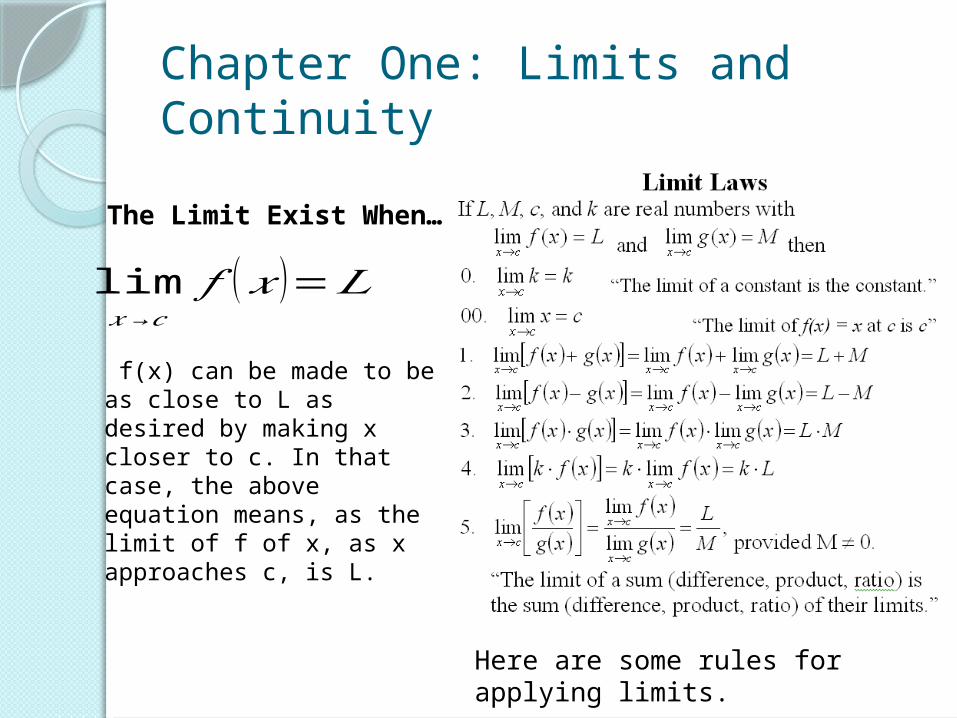
The Limit Exist When…

lim𝑥→𝑐

𝑓 (𝑥 )=𝐿

f(x) can be made to be as close to L as desired by making x closer to c. In that case, the above equation means, as the limit of f of x, as x approaches c, is L.

Here are some rules for applying limits.

Examples when the limit does not exist

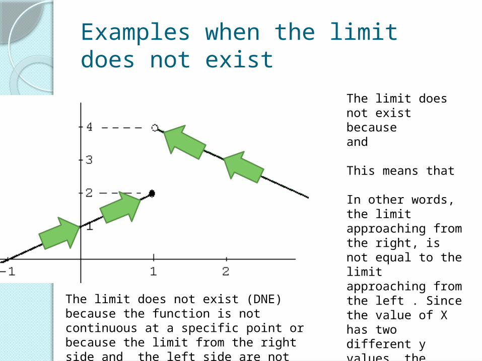
The limit does not exist because and

This means that

In other words, the limit approaching from the right, is not equal to the limit approaching from the left . Since the value of X has two different y values, the limit does not exist.

The limit does not exist (DNE) because the function is not continuous at a specific point or because the limit from the right side and the left side are not equal to each other.

Finding the Limit

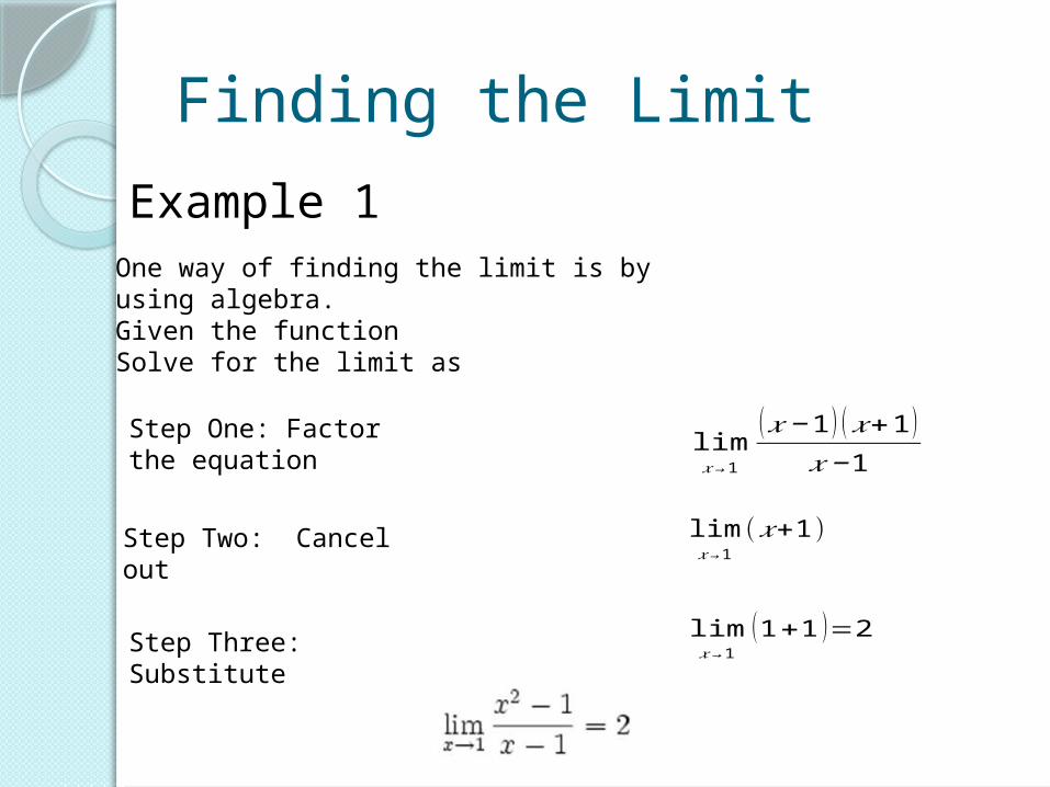
One way of finding the limit is by using algebra. Given the function Solve for the limit as

Example 1

Step One: Factor the equation

lim𝑥→ 1

(𝑥−1 ) (𝑥+1 )𝑥−1

Step Two: Cancel out

lim𝑥→ 1

(𝑥+1)

Step Three: Substitute

lim𝑥→ 1

(1+1 )=2

Example 2

0.5 1.50000

0.9 1.90000

0.99 1.99000

0.999 1.99900

0.9999 1.99990

0.99999 1.99999

... ...

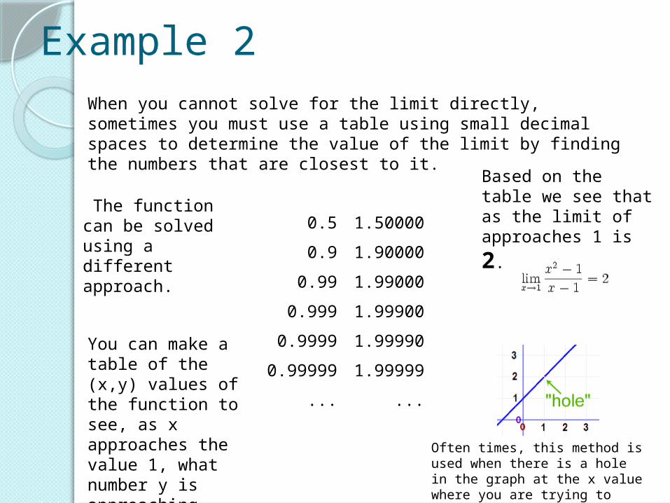
When you cannot solve for the limit directly, sometimes you must use a table using small decimal spaces to determine the value of the limit by finding the numbers that are closest to it.

The function can be solved using a different approach.

You can make a table of the (x,y) values of the function to see, as x approaches the value 1, what number y is approaching, but never reaching.

Based on the table we see that as the limit of approaches

1 is 2.

Often times, this method is used when there is a hole in the graph at the x value where you are trying to solve the limit.

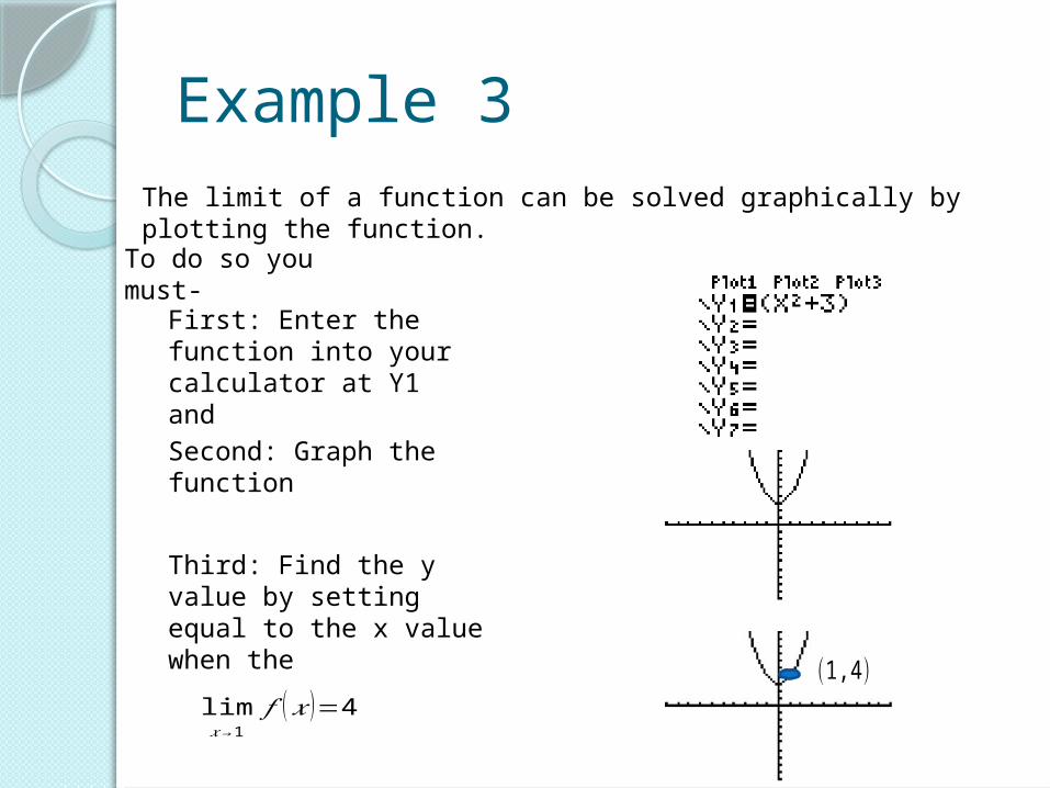
Example 3The limit of a function can be solved graphically by plotting the function.

To do so you must-

First: Enter the function into your calculator at Y1 and

Second: Graph the function

Third: Find the y value by setting equal to the x value when the

(1,4)lim𝑥→ 1

𝑓 (𝑥 )=4

Continuity

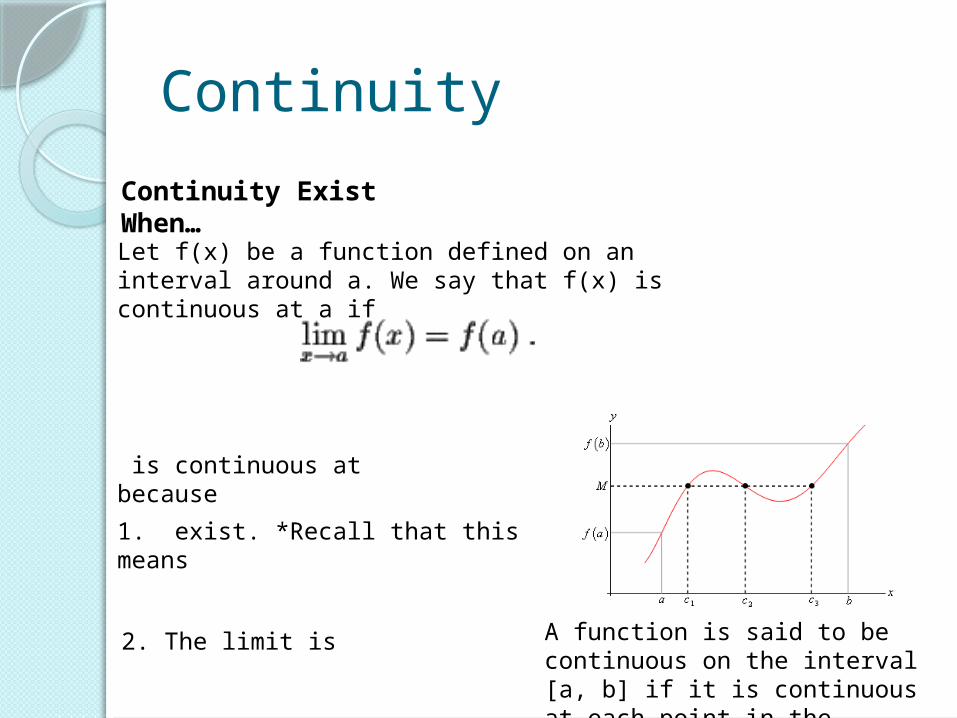
Continuity Exist When…

Let f(x) be a function defined on an interval around a. We say that f(x) is continuous at a if

is continuous at because

1. exist. *Recall that this means

2. The limit is A function is said to be continuous on the interval [a, b] if it is continuous at each point in the interval.

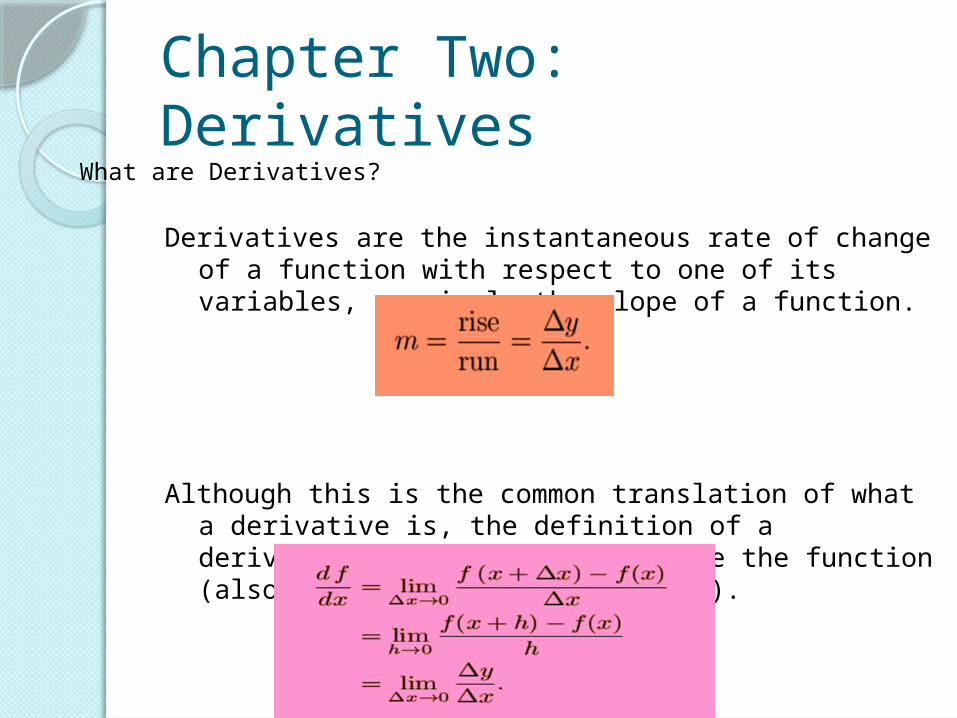
Chapter Two: DerivativesWhat are Derivatives?

Derivatives are the instantaneous rate of change of a function with respect to one of its variables, or simply the slope of a function.

Although this is the common translation of what a derivative is, the definition of a derivative is also defined by the the function (also known as the limit process).

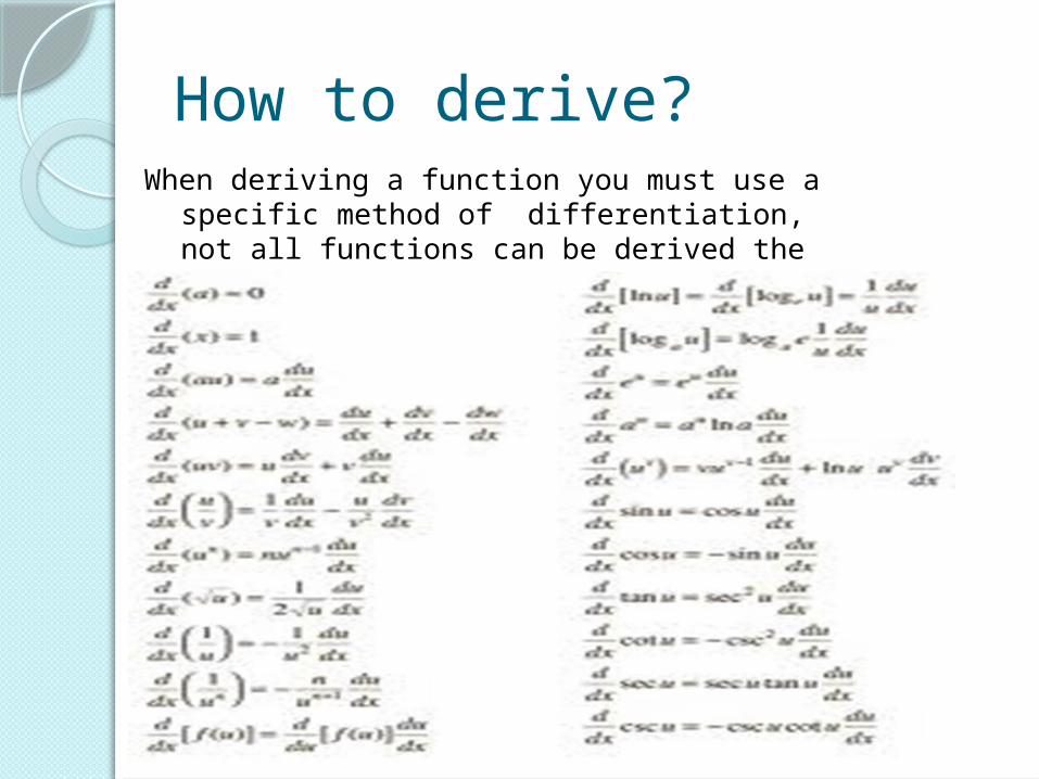
How to derive?When deriving a function you must use a specific method of

differentiation, not all functions can be derived the same way, so there are multiple methods of differentiation.

Analysis Of a Derivative Using a Graph

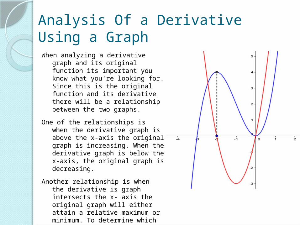
When analyzing a derivative graph and its original function its important you know what you're looking for. Since this is the original function and its derivative there will be a relationship between the two graphs.

One of the relationships is when the derivative graph is above the x-axis the original graph is increasing. When the derivative graph is below the x-axis, the original graph is decreasing.

Another relationship is when the derivative is graph intersects the x- axis the original graph will either attain a relative maximum or minimum. To determine which relative extrema may be attained you must see in which direction the graph goes. So if it goes from positive to negative its a maximum and when it goes from negative to positive it is a minimum.

Chapter Three: Antiderivatives

Definition of an Antiderivative

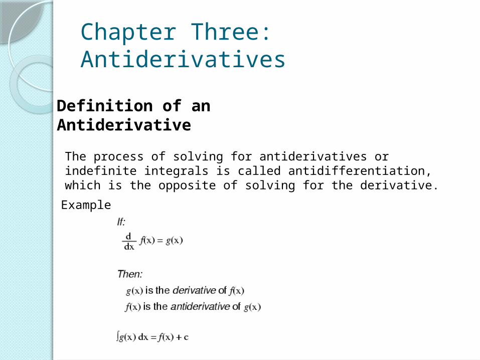
The process of solving for antiderivatives or indefinite integrals is called antidifferentiation, which is the opposite of solving for the derivative.

Example

Indefinite Integrals

𝐹=∫ 𝑓 (𝑥 ) 𝑑𝑥

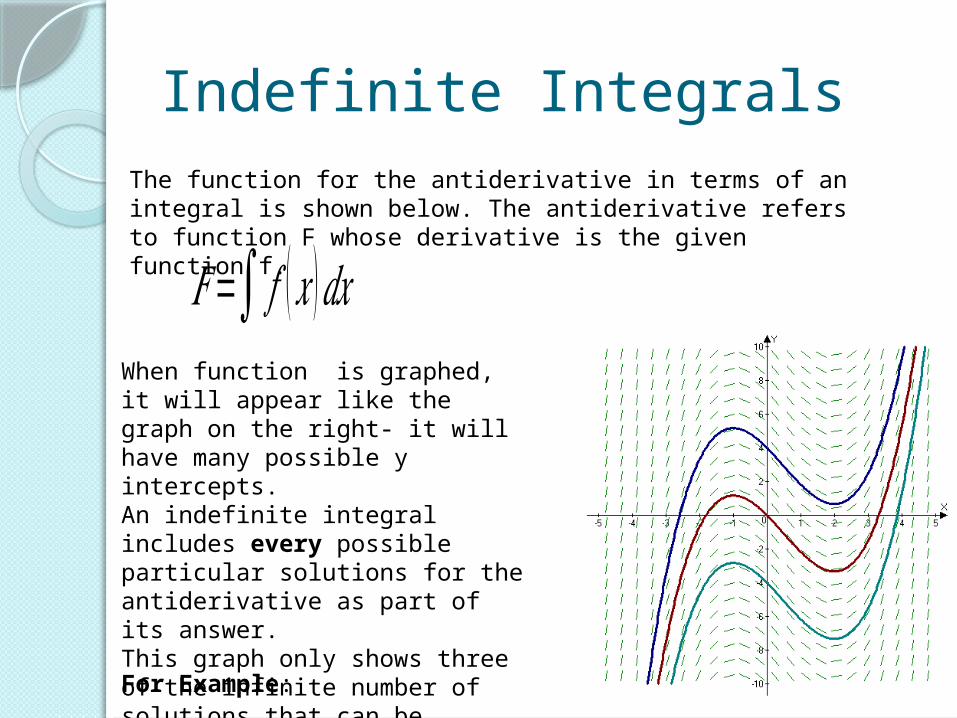
The function for the antiderivative in terms of an integral is shown below. The antiderivative refers to function F whose derivative is the given function f.

When function is graphed, it will appear like the graph on the right- it will have many possible y intercepts. An indefinite integral includes every possible particular solutions for the antiderivative as part of its answer.This graph only shows three of the infinite number of solutions that can be produced by varying the constant C that every indefinite integral has. For Example:

Definite Integrals

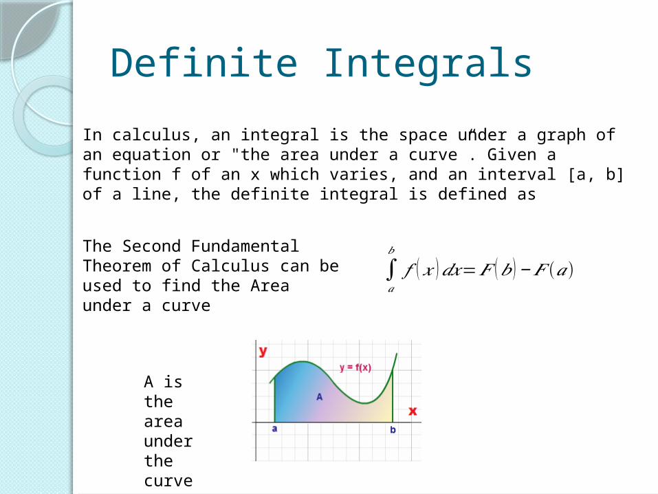
In calculus, an integral is the space under a graph of an equation or "the area under a curve”. Given a function f of an x which varies, and an interval [a, b] of a line, the definite integral is defined as

The Second Fundamental Theorem of Calculus can be used to find the Area under a curve

∫𝑎

𝑏

𝑓 (𝑥 )𝑑𝑥=𝐹 (𝑏)−𝐹 (𝑎)

A is the area under the curve

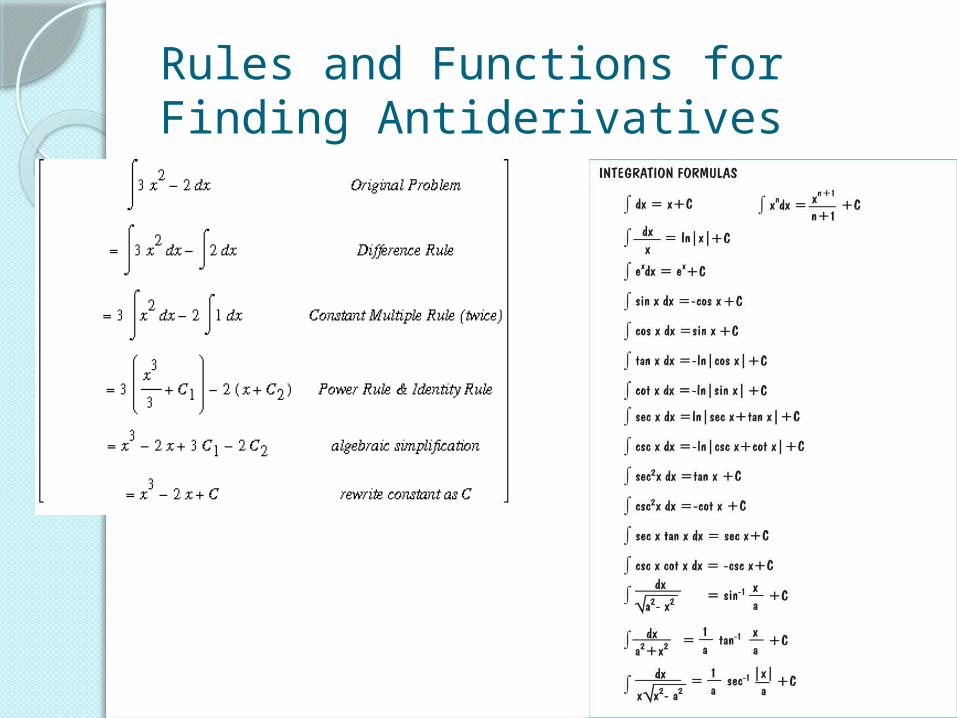
Rules and Functions for Finding Antiderivatives

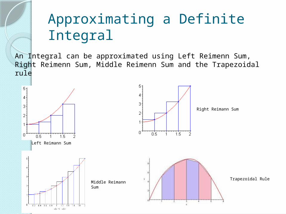
Approximating a Definite Integral

An Integral can be approximated using Left Reimenn Sum, Right Reimenn Sum, Middle Reimenn Sum and the Trapezoidal rule

Left Reimann Sum

Right Reimann Sum

Middle Reimann Sum

Trapezoidal Rule

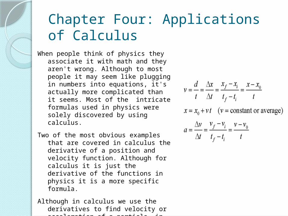
Chapter Four: Applications of Calculus

When people think of physics they associate it with math and they aren't wrong. Although to most people it may seem like plugging in numbers into equations, it's actually more complicated than it seems. Most of the intricate formulas used in physics were solely discovered by using calculus.

Two of the most obvious examples that are covered in calculus the derivative of a position and velocity function. Although for calculus it is just the derivative of the functions in physics it is a more specific formula.

Although in calculus we use the derivatives to find velocity or acceleration of a particle, in physics these specific functions are used to find the velocity and acceleration of a projectile (an object that is only influenced by gravity).

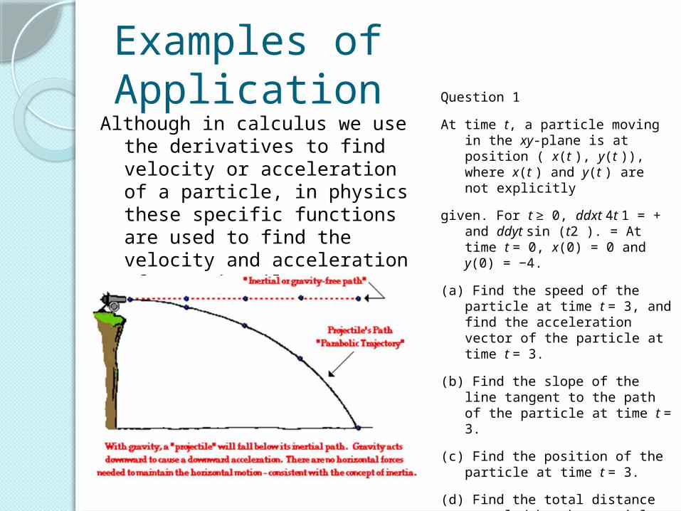
Examples of ApplicationAlthough in calculus we use the

derivatives to find velocity or acceleration of a particle, in physics these specific functions are used to find the velocity and acceleration of a projectile (an object that is only influenced by gravity).

Question 1

At time t, a particle moving in the xy-plane is at position ( x(t ), y(t )), where x(t ) and y(t ) are not explicitly

given. For t ≥ 0, ddxt 4t 1 = + and ddyt sin (t2 ). = At time t = 0, x(0) = 0 and y(0) = −4.

(a) Find the speed of the particle at time t = 3, and find the acceleration vector of the particle at time t = 3.

(b) Find the slope of the line tangent to the path of the particle at time t = 3.

(c) Find the position of the particle at time t = 3.

(d) Find the total distance traveled by the particle over the time interval 0 ≤ t ≤ 3.

This is an examples of a Free Response Question that you may come across

in Calculus.

Solution

Question 1

At time t, a particle moving in the xy-plane is at position ( x(t ), y(t )), where x(t ) and y(t) are not explicitly

given. For t ≥ 0, ddxt 4t 1 = + and ddyt sin (t2). = At time t = 0, x(0) = 0 and y(0) = −4.

(a) Find the speed of the particle at time t = 3, and find the acceleration vector of the particle at time t = 3.

(b) Find the slope of the line tangent to the path of the particle at time t = 3.

(c) Find the position of the particle at time t =3.

(d) Find the total distance traveled by the particle over the time interval 0 ≤ t ≤ 3

Citations• http://tutorial.math.lamar.edu/Classes/CalcI/DefnOfLimit.aspx• http://archives.math.utk.edu/visual.calculus/1/definition.6/• http://www.mathsisfun.com/calculus/limits-formal.html• http://

www.analyzemath.com/calculus/limits/find_limits_functions.html• http

://www.ehow.com/how_5023933_limit-function-analytically.html• http://www.calculus-help.com/continuity/• http://www.sosmath.com/calculus/limcon/limcon05/limcon05.ht

ml• http://www.snow.edu/jonathanb/Courses/Math1210/M1210.html • http://calculus2010.wikidot.com/solving-limits-graphically • http://www.murderati.com/blog/2012/2/9/the-end.html