Embed Size (px)
DESCRIPTION
ANSYS 14 CFX-Solver Theory Guide
Citation preview

7/16/2019 ANSYS CFX-Solver Theory Guide
http://slidepdf.com/reader/full/ansys-cfx-solver-theory-guide-5633873a6f5ee 1/417
ANSYS CFX-Solver Theory Guide
Release 14.0ANSYS, Inc.November 2011Southpointe
275 Technology DriveCanonsburg, PA 15317 ANSYS, Inc. iscertified to ISO9001:2008.
[email protected]://www.ansys.com(T ) 724-746-3304(F) 724-514-9494

7/16/2019 ANSYS CFX-Solver Theory Guide
http://slidepdf.com/reader/full/ansys-cfx-solver-theory-guide-5633873a6f5ee 2/417
Copyright and Trademark Information
© 2011 SAS IP, Inc. All rights reserved. Unauthorized use, distribution or duplication is prohibited.
ANSYS, ANSYS Workbench, Ansoft, AUTODYN, EKM, Engineering Knowledge Manager, CFX, FLUENT, HFSS and anyand all ANSYS, Inc. brand, product, service and feature names, logos and slogans are registered trademarks ortrademarks of ANSYS, Inc. or its subsidiaries in the United States or other countries. ICEM CFD is a trademark usedby ANSYS, Inc. under license. CFX is a trademark of Sony Corporation in Japan. All other brand, product, serviceand feature names or trademarks are the property of their respective owners.
Disclaimer Notice
THIS ANSYS SOFTWARE PRODUCT AND PROGRAM DOCUMENTATION INCLUDE TRADE SECRETS AND ARE CONFID-ENTIAL AND PROPRIETARY PRODUCTS OF ANSYS, INC., ITS SUBSIDIARIES, OR LICENSORS. The software productsand documentation are furnished by ANSYS, Inc., its subsidiaries, or affiliates under a software license agreementthat contains provisions concerning non-disclosure, copying, length and nature of use, compliance with exportinglaws, warranties, disclaimers, limitations of liability, and remedies, and other provisions. The software productsand documentation may be used, disclosed, transferred, or copied only in accordance with the terms and conditionsof that software license agreement.
ANSYS, Inc. is certified to ISO 9001:2008.
U.S. Government Rights
For U.S. Government users, except as specifically granted by the ANSYS, Inc. software license agreement, the use,duplication, or disclosure by the United States Government is subject to restrictions stated in the ANSYS, Inc.software license agreement and FAR 12.212 (for non-DOD licenses).
Third-Party Software
See the legal information in the product help files for the complete Legal Notice for ANSYS proprietary softwareand third-party software. If you are unable to access the Legal Notice, please contact ANSYS, Inc.
Published in the U.S.A.

7/16/2019 ANSYS CFX-Solver Theory Guide
http://slidepdf.com/reader/full/ansys-cfx-solver-theory-guide-5633873a6f5ee 3/417
Table of Contents
1. Basic Solver Capability Theory . . . . . . . . . . . . . . . . . . . . . . . . . . . . . . . . . . . . . . . . . . . . . . . . . . . . . . . . . . . . . . . . . . . . . . . . . . . . . . . . . . . . . . . . . . . . . . . . . . . . . . . . . . . . . . . . 11.1. Documentation Conventions ....... . . . . . . . . . . . . . . . . . . . . . . . . . . . . . . . . . . . . . . . . . . . . . . . . . . . . . . . . . . . . . . . . . . . . . . . . . . . . . . . . . . . . . . . . . . . . . . . . . . . . . 2
1.1.1. Dimensions ....... . . . . . . . . . . . . . . . . . . . . . . . . . . . . . . . . . . . . . . . . . . . . . . . . . . . . . . . . . . . . . . . . . . . . . . . . . . . . . . . . . . . . . . . . . . . . . . . . . . . . . . . . . . . . . . . . . . . . . . . 21.1.2. List of Symbols ....... . . . . . . . . . . . . . . . . . . . . . . . . . . . . . . . . . . . . . . . . . . . . . . . . . . . . . . . . . . . . . . . . . . . . . . . . . . . . . . . . . . . . . . . . . . . . . . . . . . . . . . . . . . . . . . . . . . 2
1.1.2.1. Subscripts ....... . . . . . . . . . . . . . . . . . . . . . . . . . . . . . . . . . . . . . . . . . . . . . . . . . . . . . . . . . . . . . . . . . . . . . . . . . . . . . . . . . . . . . . . . . . . . . . . . . . . . . . . . . . . . . . . . 7
1.1.3.Variable Definitions ....... . . . . . . . . . . . . . . . . . . . . . . . . . . . . . . . . . . . . . . . . . . . . . . . . . . . . . . . . . . . . . . . . . . . . . . . . . . . . . . . . . . . . . . . . . . . . . . . . . . . . . . . . . . . 71.1.3.1. Isothermal Compressibility ...... . . . . . . . . . . . . . . . . . . . . . . . . . . . . . . . . . . . . . . . . . . . . . . . . . . . . . . . . . . . . . . . . . . . . . . . . . . . . . . . . . . . . . . . . 71.1.3.2. Isentropic Compressibility ...... . . . . . . . . . . . . . . . . . . . . . . . . . . . . . . . . . . . . . . . . . . . . . . . . . . . . . . . . . . . . . . . . . . . . . . . . . . . . . . . . . . . . . . . . . 71.1.3.3. Reference Pressure ....... . . . . . . . . . . . . . . . . . . . . . . . . . . . . . . . . . . . . . . . . . . . . . . . . . . . . . . . . . . . . . . . . . . . . . . . . . . . . . . . . . . . . . . . . . . . . . . . . . . . 71.1.3.4. Static Pressure ....... . . . . . . . . . . . . . . . . . . . . . . . . . . . . . . . . . . . . . . . . . . . . . . . . . . . . . . . . . . . . . . . . . . . . . . . . . . . . . . . . . . . . . . . . . . . . . . . . . . . . . . . . . . 81.1.3.5. Modified Pressure ....... . . . . . . . . . . . . . . . . . . . . . . . . . . . . . . . . . . . . . . . . . . . . . . . . . . . . . . . . . . . . . . . . . . . . . . . . . . . . . . . . . . . . . . . . . . . . . . . . . . . . . 81.1.3.6. Static Enthalpy ....... . . . . . . . . . . . . . . . . . . . . . . . . . . . . . . . . . . . . . . . . . . . . . . . . . . . . . . . . . . . . . . . . . . . . . . . . . . . . . . . . . . . . . . . . . . . . . . . . . . . . . . . . . 8
1.1.3.6.1. Material with Variable Density and Specific Heat ....... . . . . . . . . . . . . . . . . . . . . . . . . . . . . . . . . . . . . . . . . . . . . . . . 91.1.3.7.Total Enthalpy ....... . . . . . . . . . . . . . . . . . . . . . . . . . . . . . . . . . . . . . . . . . . . . . . . . . . . . . . . . . . . . . . . . . . . . . . . . . . . . . . . . . . . . . . . . . . . . . . . . . . . . . . . . . 101.1.3.8. Domain Temperature ....... . . . . . . . . . . . . . . . . . . . . . . . . . . . . . . . . . . . . . . . . . . . . . . . . . . . . . . . . . . . . . . . . . . . . . . . . . . . . . . . . . . . . . . . . . . . . . . 101.1.3.9. Static Temperature ....... . . . . . . . . . . . . . . . . . . . . . . . . . . . . . . . . . . . . . . . . . . . . . . . . . . . . . . . . . . . . . . . . . . . . . . . . . . . . . . . . . . . . . . . . . . . . . . . . . 10
1.1.3.9.1. Material with Constant Density and Specific Heat ....... . . . . . . . . . . . . . . . . . . . . . . . . . . . . . . . . . . . . . . . . . . . 11
1.1.3.9.2. Ideal Gas or Solid with cp=f(T) ...... . . . . . . . . . . . . . . . . . . . . . . . . . . . . . . . . . . . . . . . . . . . . . . . . . . . . . . . . . . . . . . . . . . . . . . . . . 111.1.3.9.3. Material with Variable Density and Specific Heat ....... . . . . . . . . . . . . . . . . . . . . . . . . . . . . . . . . . . . . . . . . . . . . . 11
1.1.3.10.Total Temperature ....... . . . . . . . . . . . . . . . . . . . . . . . . . . . . . . . . . . . . . . . . . . . . . . . . . . . . . . . . . . . . . . . . . . . . . . . . . . . . . . . . . . . . . . . . . . . . . . . . . 111.1.3.10.1. Material with Constant Density and Specific Heat ....... . . . . . . . . . . . . . . . . . . . . . . . . . . . . . . . . . . . . . . . . . 121.1.3.10.2. Ideal Gas with constant cp . . . . . . . . . . . . . . . . . . . . . . . . . . . . . . . . . . . . . . . . . . . . . . . . . . . . . . . . . . . . . . . . . . . . . . . . . . . . . . . . . . . 121.1.3.10.3. Ideal Gas with cp = f(T) ...... . . . . . . . . . . . . . . . . . . . . . . . . . . . . . . . . . . . . . . . . . . . . . . . . . . . . . . . . . . . . . . . . . . . . . . . . . . . . . . . . . . 121.1.3.10.4. Material with Variable Density and Specific Heat ....... . . . . . . . . . . . . . . . . . . . . . . . . . . . . . . . . . . . . . . . . . . . 13
1.1.3.11. Entropy ....... . . . . . . . . . . . . . . . . . . . . . . . . . . . . . . . . . . . . . . . . . . . . . . . . . . . . . . . . . . . . . . . . . . . . . . . . . . . . . . . . . . . . . . . . . . . . . . . . . . . . . . . . . . . . . . . . 131.1.3.11.1. Material with Constant Density and Specific Heat ....... . . . . . . . . . . . . . . . . . . . . . . . . . . . . . . . . . . . . . . . . . 131.1.3.11.2. Ideal Gas with constant cp or cp = f(T) ...... . . . . . . . . . . . . . . . . . . . . . . . . . . . . . . . . . . . . . . . . . . . . . . . . . . . . . . . . . . . . 141.1.3.11.3. Material with Variable Density and Specific Heat ....... . . . . . . . . . . . . . . . . . . . . . . . . . . . . . . . . . . . . . . . . . . . 14
1.1.3.12. Total Pressure ....... . . . . . . . . . . . . . . . . . . . . . . . . . . . . . . . . . . . . . . . . . . . . . . . . . . . . . . . . . . . . . . . . . . . . . . . . . . . . . . . . . . . . . . . . . . . . . . . . . . . . . . . 161.1.3.12.1. Incompressible Fluids ....... . . . . . . . . . . . . . . . . . . . . . . . . . . . . . . . . . . . . . . . . . . . . . . . . . . . . . . . . . . . . . . . . . . . . . . . . . . . . . . . . . . . 161.1.3.12.2. Ideal Gases ....... . . . . . . . . . . . . . . . . . . . . . . . . . . . . . . . . . . . . . . . . . . . . . . . . . . . . . . . . . . . . . . . . . . . . . . . . . . . . . . . . . . . . . . . . . . . . . . . . . . . 171.1.3.12.3. Material with Variable Density and Specific Heat ....... . . . . . . . . . . . . . . . . . . . . . . . . . . . . . . . . . . . . . . . . . . . 17
1.1.3.13. Shear Strain Rate ....... . . . . . . . . . . . . . . . . . . . . . . . . . . . . . . . . . . . . . . . . . . . . . . . . . . . . . . . . . . . . . . . . . . . . . . . . . . . . . . . . . . . . . . . . . . . . . . . . . . 181.1.3.14. Rotating Frame Quantities ....... . . . . . . . . . . . . . . . . . . . . . . . . . . . . . . . . . . . . . . . . . . . . . . . . . . . . . . . . . . . . . . . . . . . . . . . . . . . . . . . . . . . . 18
1.1.3.14.1. Incompressible Fluids ....... . . . . . . . . . . . . . . . . . . . . . . . . . . . . . . . . . . . . . . . . . . . . . . . . . . . . . . . . . . . . . . . . . . . . . . . . . . . . . . . . . . . 191.1.3.14.2. Ideal Gases ....... . . . . . . . . . . . . . . . . . . . . . . . . . . . . . . . . . . . . . . . . . . . . . . . . . . . . . . . . . . . . . . . . . . . . . . . . . . . . . . . . . . . . . . . . . . . . . . . . . . . 191.1.3.14.3. Material with Variable Density and Specific Heat ....... . . . . . . . . . . . . . . . . . . . . . . . . . . . . . . . . . . . . . . . . . . . 21
1.1.3.15. Courant Number ....... . . . . . . . . . . . . . . . . . . . . . . . . . . . . . . . . . . . . . . . . . . . . . . . . . . . . . . . . . . . . . . . . . . . . . . . . . . . . . . . . . . . . . . . . . . . . . . . . . . . 211.1.4. Mathematical Notation ....... . . . . . . . . . . . . . . . . . . . . . . . . . . . . . . . . . . . . . . . . . . . . . . . . . . . . . . . . . . . . . . . . . . . . . . . . . . . . . . . . . . . . . . . . . . . . . . . . . . . . 22
1.1.4.1.The Vector Operators ....... . . . . . . . . . . . . . . . . . . . . . . . . . . . . . . . . . . . . . . . . . . . . . . . . . . . . . . . . . . . . . . . . . . . . . . . . . . . . . . . . . . . . . . . . . . . . . . 22
1.1.4.1.1. Gradient Operator ....... . . . . . . . . . . . . . . . . . . . . . . . . . . . . . . . . . . . . . . . . . . . . . . . . . . . . . . . . . . . . . . . . . . . . . . . . . . . . . . . . . . . . . . . . . . 221.1.4.1.2. Divergence Operator ....... . . . . . . . . . . . . . . . . . . . . . . . . . . . . . . . . . . . . . . . . . . . . . . . . . . . . . . . . . . . . . . . . . . . . . . . . . . . . . . . . . . . . . 231.1.4.1.3. Dyadic Operator ....... . . . . . . . . . . . . . . . . . . . . . . . . . . . . . . . . . . . . . . . . . . . . . . . . . . . . . . . . . . . . . . . . . . . . . . . . . . . . . . . . . . . . . . . . . . . . 23
1.1.4.2. Matrix Transposition ....... . . . . . . . . . . . . . . . . . . . . . . . . . . . . . . . . . . . . . . . . . . . . . . . . . . . . . . . . . . . . . . . . . . . . . . . . . . . . . . . . . . . . . . . . . . . . . . . 231.1.4.3.The Identity Matrix (Kronecker Delta function) ....... . . . . . . . . . . . . . . . . . . . . . . . . . . . . . . . . . . . . . . . . . . . . . . . . . . . . . . . . 241.1.4.4. Index Notation ....... . . . . . . . . . . . . . . . . . . . . . . . . . . . . . . . . . . . . . . . . . . . . . . . . . . . . . . . . . . . . . . . . . . . . . . . . . . . . . . . . . . . . . . . . . . . . . . . . . . . . . . . 24
1.2. Governing Equations ....... . . . . . . . . . . . . . . . . . . . . . . . . . . . . . . . . . . . . . . . . . . . . . . . . . . . . . . . . . . . . . . . . . . . . . . . . . . . . . . . . . . . . . . . . . . . . . . . . . . . . . . . . . . . . . . . 251.2.1. Transport Equations ....... . . . . . . . . . . . . . . . . . . . . . . . . . . . . . . . . . . . . . . . . . . . . . . . . . . . . . . . . . . . . . . . . . . . . . . . . . . . . . . . . . . . . . . . . . . . . . . . . . . . . . . . . 25
1.2.1.1. The Continuity Equation ....... . . . . . . . . . . . . . . . . . . . . . . . . . . . . . . . . . . . . . . . . . . . . . . . . . . . . . . . . . . . . . . . . . . . . . . . . . . . . . . . . . . . . . . . . . 251.2.1.2.The Momentum Equations ....... . . . . . . . . . . . . . . . . . . . . . . . . . . . . . . . . . . . . . . . . . . . . . . . . . . . . . . . . . . . . . . . . . . . . . . . . . . . . . . . . . . . . . . 25
iiRelease 14.0 - © SAS IP, Inc. All rights reserved. - Contains proprietary and confidential informationof ANSYS, Inc. and its subsidiaries and affiliates.

7/16/2019 ANSYS CFX-Solver Theory Guide
http://slidepdf.com/reader/full/ansys-cfx-solver-theory-guide-5633873a6f5ee 4/417
1.2.1.3.The Total Energy Equation ....... . . . . . . . . . . . . . . . . . . . . . . . . . . . . . . . . . . . . . . . . . . . . . . . . . . . . . . . . . . . . . . . . . . . . . . . . . . . . . . . . . . . . . . . 261.2.1.4. The Thermal Energy Equation ....... . . . . . . . . . . . . . . . . . . . . . . . . . . . . . . . . . . . . . . . . . . . . . . . . . . . . . . . . . . . . . . . . . . . . . . . . . . . . . . . . . 26
1.2.2. Equations of State ....... . . . . . . . . . . . . . . . . . . . . . . . . . . . . . . . . . . . . . . . . . . . . . . . . . . . . . . . . . . . . . . . . . . . . . . . . . . . . . . . . . . . . . . . . . . . . . . . . . . . . . . . . . . . 271.2.2.1. Incompressible Equation of State ....... . . . . . . . . . . . . . . . . . . . . . . . . . . . . . . . . . . . . . . . . . . . . . . . . . . . . . . . . . . . . . . . . . . . . . . . . . . . . 281.2.2.2. Ideal Gas Equation of State ....... . . . . . . . . . . . . . . . . . . . . . . . . . . . . . . . . . . . . . . . . . . . . . . . . . . . . . . . . . . . . . . . . . . . . . . . . . . . . . . . . . . . . . 281.2.2.3. Real Gas and Liquid Equations of State ....... . . . . . . . . . . . . . . . . . . . . . . . . . . . . . . . . . . . . . . . . . . . . . . . . . . . . . . . . . . . . . . . . . . . . 28
1.2.2.3.1. Real Gas Properties ....... . . . . . . . . . . . . . . . . . . . . . . . . . . . . . . . . . . . . . . . . . . . . . . . . . . . . . . . . . . . . . . . . . . . . . . . . . . . . . . . . . . . . . . . . 281.2.2.3.1.1. Redlich Kwong Models ....... . . . . . . . . . . . . . . . . . . . . . . . . . . . . . . . . . . . . . . . . . . . . . . . . . . . . . . . . . . . . . . . . . . . . . . . . . . 29
1.2.2.3.1.1.1.The Standard Redlich Kwong Model ...... . . . . . . . . . . . . . . . . . . . . . . . . . . . . . . . . . . . . . . . . . . . . . . . 291.2.2.3.1.1.2.The Aungier Redlich Kwong Model ...... . . . . . . . . . . . . . . . . . . . . . . . . . . . . . . . . . . . . . . . . . . . . . . . . . 291.2.2.3.1.1.3.The Soave Redlich Kwong Model ...... . . . . . . . . . . . . . . . . . . . . . . . . . . . . . . . . . . . . . . . . . . . . . . . . . . . . 30
1.2.2.3.1.2. Peng Robinson Model ...... . . . . . . . . . . . . . . . . . . . . . . . . . . . . . . . . . . . . . . . . . . . . . . . . . . . . . . . . . . . . . . . . . . . . . . . . . . . . 311.2.2.3.1.3. Real Gas Constitutive Relations ....... . . . . . . . . . . . . . . . . . . . . . . . . . . . . . . . . . . . . . . . . . . . . . . . . . . . . . . . . . . . . . . 31
1.2.2.3.2. Real Gas Saturated Vapor Properties ....... . . . . . . . . . . . . . . . . . . . . . . . . . . . . . . . . . . . . . . . . . . . . . . . . . . . . . . . . . . . . . . . 341.2.2.3.3. Real Gas Liquid Properties ....... . . . . . . . . . . . . . . . . . . . . . . . . . . . . . . . . . . . . . . . . . . . . . . . . . . . . . . . . . . . . . . . . . . . . . . . . . . . . . . 341.2.2.3.4. IAPWS Equation of State ....... . . . . . . . . . . . . . . . . . . . . . . . . . . . . . . . . . . . . . . . . . . . . . . . . . . . . . . . . . . . . . . . . . . . . . . . . . . . . . . . . . 351.2.2.3.5. Metastable Superheated Liquid/Supercooled Vapor States ....... . . . . . . . . . . . . . . . . . . . . . . . . . . . . . 371.2.2.3.6. Numerical Testing to Delineate Metastable Regions ....... . . . . . . . . . . . . . . . . . . . . . . . . . . . . . . . . . . . . . . . . 371.2.2.3.7. The Acentric Factor ....... . . . . . . . . . . . . . . . . . . . . . . . . . . . . . . . . . . . . . . . . . . . . . . . . . . . . . . . . . . . . . . . . . . . . . . . . . . . . . . . . . . . . . . . . 37
1.2.2.4. General Equation of State ....... . . . . . . . . . . . . . . . . . . . . . . . . . . . . . . . . . . . . . . . . . . . . . . . . . . . . . . . . . . . . . . . . . . . . . . . . . . . . . . . . . . . . . . . 381.2.3. Conjugate Heat Transfer ...... . . . . . . . . . . . . . . . . . . . . . . . . . . . . . . . . . . . . . . . . . . . . . . . . . . . . . . . . . . . . . . . . . . . . . . . . . . . . . . . . . . . . . . . . . . . . . . . . . . . 39
1.3. Buoyancy ....... . . . . . . . . . . . . . . . . . . . . . . . . . . . . . . . . . . . . . . . . . . . . . . . . . . . . . . . . . . . . . . . . . . . . . . . . . . . . . . . . . . . . . . . . . . . . . . . . . . . . . . . . . . . . . . . . . . . . . . . . . . . . . . . . 391.3.1. Full Buoyancy Model ...... . . . . . . . . . . . . . . . . . . . . . . . . . . . . . . . . . . . . . . . . . . . . . . . . . . . . . . . . . . . . . . . . . . . . . . . . . . . . . . . . . . . . . . . . . . . . . . . . . . . . . . . . 391.3.2. Boussinesq Model ...... . . . . . . . . . . . . . . . . . . . . . . . . . . . . . . . . . . . . . . . . . . . . . . . . . . . . . . . . . . . . . . . . . . . . . . . . . . . . . . . . . . . . . . . . . . . . . . . . . . . . . . . . . . . . 40
1.4. Immersed Solids ....... . . . . . . . . . . . . . . . . . . . . . . . . . . . . . . . . . . . . . . . . . . . . . . . . . . . . . . . . . . . . . . . . . . . . . . . . . . . . . . . . . . . . . . . . . . . . . . . . . . . . . . . . . . . . . . . . . . . . . . 401.4.1. Immersed Solid Boundary Details ...... . . . . . . . . . . . . . . . . . . . . . . . . . . . . . . . . . . . . . . . . . . . . . . . . . . . . . . . . . . . . . . . . . . . . . . . . . . . . . . . . . . . . . 401.4.2. Laminar Flow Treatment ....... . . . . . . . . . . . . . . . . . . . . . . . . . . . . . . . . . . . . . . . . . . . . . . . . . . . . . . . . . . . . . . . . . . . . . . . . . . . . . . . . . . . . . . . . . . . . . . . . . . 421.4.3.Turbulent Flow Treatment ....... . . . . . . . . . . . . . . . . . . . . . . . . . . . . . . . . . . . . . . . . . . . . . . . . . . . . . . . . . . . . . . . . . . . . . . . . . . . . . . . . . . . . . . . . . . . . . . . . 42
1.4.3.1.Wall Distance ....... . . . . . . . . . . . . . . . . . . . . . . . . . . . . . . . . . . . . . . . . . . . . . . . . . . . . . . . . . . . . . . . . . . . . . . . . . . . . . . . . . . . . . . . . . . . . . . . . . . . . . . . . . . 421.4.3.2. SST Model ...... . . . . . . . . . . . . . . . . . . . . . . . . . . . . . . . . . . . . . . . . . . . . . . . . . . . . . . . . . . . . . . . . . . . . . . . . . . . . . . . . . . . . . . . . . . . . . . . . . . . . . . . . . . . . . . . 431.4.3.3. Scalable Wall Function ....... . . . . . . . . . . . . . . . . . . . . . . . . . . . . . . . . . . . . . . . . . . . . . . . . . . . . . . . . . . . . . . . . . . . . . . . . . . . . . . . . . . . . . . . . . . . . 43
1.5. Multicomponent Flow ........ . . . . . . . . . . . . . . . . . . . . . . . . . . . . . . . . . . . . . . . . . . . . . . . . . . . . . . . . . . . . . . . . . . . . . . . . . . . . . . . . . . . . . . . . . . . . . . . . . . . . . . . . . . . . . 441.5.1. Multicomponent Notation ....... . . . . . . . . . . . . . . . . . . . . . . . . . . . . . . . . . . . . . . . . . . . . . . . . . . . . . . . . . . . . . . . . . . . . . . . . . . . . . . . . . . . . . . . . . . . . . . . 441.5.2. Scalar Transport Equation ....... . . . . . . . . . . . . . . . . . . . . . . . . . . . . . . . . . . . . . . . . . . . . . . . . . . . . . . . . . . . . . . . . . . . . . . . . . . . . . . . . . . . . . . . . . . . . . . . . 441.5.3. Algebraic Equation for Components ....... . . . . . . . . . . . . . . . . . . . . . . . . . . . . . . . . . . . . . . . . . . . . . . . . . . . . . . . . . . . . . . . . . . . . . . . . . . . . . . . . 461.5.4. Constraint Equation for Components ....... . . . . . . . . . . . . . . . . . . . . . . . . . . . . . . . . . . . . . . . . . . . . . . . . . . . . . . . . . . . . . . . . . . . . . . . . . . . . . . . 461.5.5. Multicomponent Fluid Properties ....... . . . . . . . . . . . . . . . . . . . . . . . . . . . . . . . . . . . . . . . . . . . . . . . . . . . . . . . . . . . . . . . . . . . . . . . . . . . . . . . . . . . . 471.5.6. Energy Equation ....... . . . . . . . . . . . . . . . . . . . . . . . . . . . . . . . . . . . . . . . . . . . . . . . . . . . . . . . . . . . . . . . . . . . . . . . . . . . . . . . . . . . . . . . . . . . . . . . . . . . . . . . . . . . . . . 481.5.7. Multicomponent Energy Diffusion ....... . . . . . . . . . . . . . . . . . . . . . . . . . . . . . . . . . . . . . . . . . . . . . . . . . . . . . . . . . . . . . . . . . . . . . . . . . . . . . . . . . . . 49
1.6. Additional Variables ....... . . . . . . . . . . . . . . . . . . . . . . . . . . . . . . . . . . . . . . . . . . . . . . . . . . . . . . . . . . . . . . . . . . . . . . . . . . . . . . . . . . . . . . . . . . . . . . . . . . . . . . . . . . . . . . . . . 511.6.1.Transport Equations for Additional Variables ....... . . . . . . . . . . . . . . . . . . . . . . . . . . . . . . . . . . . . . . . . . . . . . . . . . . . . . . . . . . . . . . . . . . . . 511.6.2. Diffusive Transport Equations for Additional Variables ....... . . . . . . . . . . . . . . . . . . . . . . . . . . . . . . . . . . . . . . . . . . . . . . . . . . . . . . 52
1.6.3. Poisson Equations for Additional Variables ....... . . . . . . . . . . . . . . . . . . . . . . . . . . . . . . . . . . . . . . . . . . . . . . . . . . . . . . . . . . . . . . . . . . . . . . . 521.6.4. Algebraic Equations for Additional Variables ....... . . . . . . . . . . . . . . . . . . . . . . . . . . . . . . . . . . . . . . . . . . . . . . . . . . . . . . . . . . . . . . . . . . . . 531.7. Rotational Forces ....... . . . . . . . . . . . . . . . . . . . . . . . . . . . . . . . . . . . . . . . . . . . . . . . . . . . . . . . . . . . . . . . . . . . . . . . . . . . . . . . . . . . . . . . . . . . . . . . . . . . . . . . . . . . . . . . . . . . . . 53
1.7.1. Alternate Rotation Model ...... . . . . . . . . . . . . . . . . . . . . . . . . . . . . . . . . . . . . . . . . . . . . . . . . . . . . . . . . . . . . . . . . . . . . . . . . . . . . . . . . . . . . . . . . . . . . . . . . . 531.8. Sources ....... . . . . . . . . . . . . . . . . . . . . . . . . . . . . . . . . . . . . . . . . . . . . . . . . . . . . . . . . . . . . . . . . . . . . . . . . . . . . . . . . . . . . . . . . . . . . . . . . . . . . . . . . . . . . . . . . . . . . . . . . . . . . . . . . . . . 54
1.8.1. Momentum Sources ....... . . . . . . . . . . . . . . . . . . . . . . . . . . . . . . . . . . . . . . . . . . . . . . . . . . . . . . . . . . . . . . . . . . . . . . . . . . . . . . . . . . . . . . . . . . . . . . . . . . . . . . . . 541.8.1.1. Isotropic Loss Model ...... . . . . . . . . . . . . . . . . . . . . . . . . . . . . . . . . . . . . . . . . . . . . . . . . . . . . . . . . . . . . . . . . . . . . . . . . . . . . . . . . . . . . . . . . . . . . . . . . 541.8.1.2. Directional Loss Model ...... . . . . . . . . . . . . . . . . . . . . . . . . . . . . . . . . . . . . . . . . . . . . . . . . . . . . . . . . . . . . . . . . . . . . . . . . . . . . . . . . . . . . . . . . . . . . 551.8.1.3. General Momentum Sources ....... . . . . . . . . . . . . . . . . . . . . . . . . . . . . . . . . . . . . . . . . . . . . . . . . . . . . . . . . . . . . . . . . . . . . . . . . . . . . . . . . . . . 561.8.1.4. Immersed Solid Sources ....... . . . . . . . . . . . . . . . . . . . . . . . . . . . . . . . . . . . . . . . . . . . . . . . . . . . . . . . . . . . . . . . . . . . . . . . . . . . . . . . . . . . . . . . . . . 57
Release 14.0 - © SAS IP, Inc. All rights reserved. - Contains proprietary and confidential informationof ANSYS, Inc. and its subsidiaries and affiliates.iv
ANSYS CFX-Solver Theory Guide

7/16/2019 ANSYS CFX-Solver Theory Guide
http://slidepdf.com/reader/full/ansys-cfx-solver-theory-guide-5633873a6f5ee 5/417
1.8.2. General Sources ....... . . . . . . . . . . . . . . . . . . . . . . . . . . . . . . . . . . . . . . . . . . . . . . . . . . . . . . . . . . . . . . . . . . . . . . . . . . . . . . . . . . . . . . . . . . . . . . . . . . . . . . . . . . . . . . 571.8.3. Mass (Continuity) Sources ....... . . . . . . . . . . . . . . . . . . . . . . . . . . . . . . . . . . . . . . . . . . . . . . . . . . . . . . . . . . . . . . . . . . . . . . . . . . . . . . . . . . . . . . . . . . . . . . . 571.8.4. Bulk Sources ....... . . . . . . . . . . . . . . . . . . . . . . . . . . . . . . . . . . . . . . . . . . . . . . . . . . . . . . . . . . . . . . . . . . . . . . . . . . . . . . . . . . . . . . . . . . . . . . . . . . . . . . . . . . . . . . . . . . . 571.8.5. Radiation Sources ....... . . . . . . . . . . . . . . . . . . . . . . . . . . . . . . . . . . . . . . . . . . . . . . . . . . . . . . . . . . . . . . . . . . . . . . . . . . . . . . . . . . . . . . . . . . . . . . . . . . . . . . . . . . . 571.8.6. Boundary Sources ....... . . . . . . . . . . . . . . . . . . . . . . . . . . . . . . . . . . . . . . . . . . . . . . . . . . . . . . . . . . . . . . . . . . . . . . . . . . . . . . . . . . . . . . . . . . . . . . . . . . . . . . . . . . . 58
1.9. Boundary Conditions ....... . . . . . . . . . . . . . . . . . . . . . . . . . . . . . . . . . . . . . . . . . . . . . . . . . . . . . . . . . . . . . . . . . . . . . . . . . . . . . . . . . . . . . . . . . . . . . . . . . . . . . . . . . . . . . . . 581.9.1. Inlet (Subsonic) ...... . . . . . . . . . . . . . . . . . . . . . . . . . . . . . . . . . . . . . . . . . . . . . . . . . . . . . . . . . . . . . . . . . . . . . . . . . . . . . . . . . . . . . . . . . . . . . . . . . . . . . . . . . . . . . . . . 58
1.9.1.1. Mass and Momentum ........ . . . . . . . . . . . . . . . . . . . . . . . . . . . . . . . . . . . . . . . . . . . . . . . . . . . . . . . . . . . . . . . . . . . . . . . . . . . . . . . . . . . . . . . . . . . . 581.9.1.1.1. Normal Speed in ....... . . . . . . . . . . . . . . . . . . . . . . . . . . . . . . . . . . . . . . . . . . . . . . . . . . . . . . . . . . . . . . . . . . . . . . . . . . . . . . . . . . . . . . . . . . . . 581.9.1.1.2. Cartesian Velocity Components ....... . . . . . . . . . . . . . . . . . . . . . . . . . . . . . . . . . . . . . . . . . . . . . . . . . . . . . . . . . . . . . . . . . . . . . . 581.9.1.1.3. Cylindrical Velocity Components ....... . . . . . . . . . . . . . . . . . . . . . . . . . . . . . . . . . . . . . . . . . . . . . . . . . . . . . . . . . . . . . . . . . . . . 581.9.1.1.4.Total Pressure ....... . . . . . . . . . . . . . . . . . . . . . . . . . . . . . . . . . . . . . . . . . . . . . . . . . . . . . . . . . . . . . . . . . . . . . . . . . . . . . . . . . . . . . . . . . . . . . . . . . 591.9.1.1.5. Mass Flow Rate ....... . . . . . . . . . . . . . . . . . . . . . . . . . . . . . . . . . . . . . . . . . . . . . . . . . . . . . . . . . . . . . . . . . . . . . . . . . . . . . . . . . . . . . . . . . . . . . . 59
1.9.1.2. Turbulence ....... . . . . . . . . . . . . . . . . . . . . . . . . . . . . . . . . . . . . . . . . . . . . . . . . . . . . . . . . . . . . . . . . . . . . . . . . . . . . . . . . . . . . . . . . . . . . . . . . . . . . . . . . . . . . . 591.9.1.2.1. Default Intensity and Autocompute Length Scale ....... . . . . . . . . . . . . . . . . . . . . . . . . . . . . . . . . . . . . . . . . . . . 601.9.1.2.2. Intensity and Autocompute Length Scale ....... . . . . . . . . . . . . . . . . . . . . . . . . . . . . . . . . . . . . . . . . . . . . . . . . . . . . . . . 601.9.1.2.3. Intensity and Length Scale ....... . . . . . . . . . . . . . . . . . . . . . . . . . . . . . . . . . . . . . . . . . . . . . . . . . . . . . . . . . . . . . . . . . . . . . . . . . . . . . 601.9.1.2.4. k and Epsilon ....... . . . . . . . . . . . . . . . . . . . . . . . . . . . . . . . . . . . . . . . . . . . . . . . . . . . . . . . . . . . . . . . . . . . . . . . . . . . . . . . . . . . . . . . . . . . . . . . . . 61
1.9.1.3. Heat Transfer ...... . . . . . . . . . . . . . . . . . . . . . . . . . . . . . . . . . . . . . . . . . . . . . . . . . . . . . . . . . . . . . . . . . . . . . . . . . . . . . . . . . . . . . . . . . . . . . . . . . . . . . . . . . . . 61
1.9.1.3.1. Static Temperature ....... . . . . . . . . . . . . . . . . . . . . . . . . . . . . . . . . . . . . . . . . . . . . . . . . . . . . . . . . . . . . . . . . . . . . . . . . . . . . . . . . . . . . . . . . . 611.9.1.3.2.Total Temperature ....... . . . . . . . . . . . . . . . . . . . . . . . . . . . . . . . . . . . . . . . . . . . . . . . . . . . . . . . . . . . . . . . . . . . . . . . . . . . . . . . . . . . . . . . . . . 62
1.9.1.4. Additional Variables ....... . . . . . . . . . . . . . . . . . . . . . . . . . . . . . . . . . . . . . . . . . . . . . . . . . . . . . . . . . . . . . . . . . . . . . . . . . . . . . . . . . . . . . . . . . . . . . . . . 621.9.2. Inlet (Supersonic) ...... . . . . . . . . . . . . . . . . . . . . . . . . . . . . . . . . . . . . . . . . . . . . . . . . . . . . . . . . . . . . . . . . . . . . . . . . . . . . . . . . . . . . . . . . . . . . . . . . . . . . . . . . . . . . . 63
1.9.2.1. Heat Transfer ...... . . . . . . . . . . . . . . . . . . . . . . . . . . . . . . . . . . . . . . . . . . . . . . . . . . . . . . . . . . . . . . . . . . . . . . . . . . . . . . . . . . . . . . . . . . . . . . . . . . . . . . . . . . . 631.9.2.1.1. Static Temperature ....... . . . . . . . . . . . . . . . . . . . . . . . . . . . . . . . . . . . . . . . . . . . . . . . . . . . . . . . . . . . . . . . . . . . . . . . . . . . . . . . . . . . . . . . . . 631.9.2.1.2.Total Temperature ....... . . . . . . . . . . . . . . . . . . . . . . . . . . . . . . . . . . . . . . . . . . . . . . . . . . . . . . . . . . . . . . . . . . . . . . . . . . . . . . . . . . . . . . . . . . 63
1.9.3. Outlet (Subsonic) ...... . . . . . . . . . . . . . . . . . . . . . . . . . . . . . . . . . . . . . . . . . . . . . . . . . . . . . . . . . . . . . . . . . . . . . . . . . . . . . . . . . . . . . . . . . . . . . . . . . . . . . . . . . . . . . 631.9.3.1. Mass and Momentum ........ . . . . . . . . . . . . . . . . . . . . . . . . . . . . . . . . . . . . . . . . . . . . . . . . . . . . . . . . . . . . . . . . . . . . . . . . . . . . . . . . . . . . . . . . . . . . 63
1.9.3.1.1. Static Pressure (Uniform) ....... . . . . . . . . . . . . . . . . . . . . . . . . . . . . . . . . . . . . . . . . . . . . . . . . . . . . . . . . . . . . . . . . . . . . . . . . . . . . . . . . 631.9.3.1.2. Normal Speed ....... . . . . . . . . . . . . . . . . . . . . . . . . . . . . . . . . . . . . . . . . . . . . . . . . . . . . . . . . . . . . . . . . . . . . . . . . . . . . . . . . . . . . . . . . . . . . . . . . 631.9.3.1.3. Cartesian Velocity Components ....... . . . . . . . . . . . . . . . . . . . . . . . . . . . . . . . . . . . . . . . . . . . . . . . . . . . . . . . . . . . . . . . . . . . . . . 63
1.9.3.1.4. Cylindrical Velocity Components ....... . . . . . . . . . . . . . . . . . . . . . . . . . . . . . . . . . . . . . . . . . . . . . . . . . . . . . . . . . . . . . . . . . . . . 631.9.3.1.5. Average Static Pressure: Over Whole Outlet ...... . . . . . . . . . . . . . . . . . . . . . . . . . . . . . . . . . . . . . . . . . . . . . . . . . . . . . . 641.9.3.1.6. Average Static Pressure: Above or Below Specified Radius ....... . . . . . . . . . . . . . . . . . . . . . . . . . . . . . . . 641.9.3.1.7. Average Static Pressure: Circumferential ...... . . . . . . . . . . . . . . . . . . . . . . . . . . . . . . . . . . . . . . . . . . . . . . . . . . . . . . . . . . 641.9.3.1.8. Mass Flow Rate: Scale Mass Flows ....... . . . . . . . . . . . . . . . . . . . . . . . . . . . . . . . . . . . . . . . . . . . . . . . . . . . . . . . . . . . . . . . . . . . 641.9.3.1.9. Mass Flow Rate: Shift Pressure with or without Pressure Profile ....... . . . . . . . . . . . . . . . . . . . . . . . . 651.9.3.1.10. Mass Flow Rate: Shift Pressure with Circumferential Pressure Averaging ....... . . . . . . . . . 661.9.3.1.11. Radial Equilibrium ........ . . . . . . . . . . . . . . . . . . . . . . . . . . . . . . . . . . . . . . . . . . . . . . . . . . . . . . . . . . . . . . . . . . . . . . . . . . . . . . . . . . . . . . . 66
1.9.3.2.Turbulence, Heat Transfer, Convected Additional Variables, and Other Scalars ...... . . . . . . . . . . . . 671.9.4. Outlet (Supersonic) ...... . . . . . . . . . . . . . . . . . . . . . . . . . . . . . . . . . . . . . . . . . . . . . . . . . . . . . . . . . . . . . . . . . . . . . . . . . . . . . . . . . . . . . . . . . . . . . . . . . . . . . . . . . . 671.9.5. Opening ....... . . . . . . . . . . . . . . . . . . . . . . . . . . . . . . . . . . . . . . . . . . . . . . . . . . . . . . . . . . . . . . . . . . . . . . . . . . . . . . . . . . . . . . . . . . . . . . . . . . . . . . . . . . . . . . . . . . . . . . . . . 67
1.9.5.1. Mass and Momentum ........ . . . . . . . . . . . . . . . . . . . . . . . . . . . . . . . . . . . . . . . . . . . . . . . . . . . . . . . . . . . . . . . . . . . . . . . . . . . . . . . . . . . . . . . . . . . . 671.9.5.1.1. Cartesian Velocity Components ....... . . . . . . . . . . . . . . . . . . . . . . . . . . . . . . . . . . . . . . . . . . . . . . . . . . . . . . . . . . . . . . . . . . . . . . 671.9.5.1.2. Cylindrical Velocity Components ....... . . . . . . . . . . . . . . . . . . . . . . . . . . . . . . . . . . . . . . . . . . . . . . . . . . . . . . . . . . . . . . . . . . . . 671.9.5.1.3. Pressure and Direction ....... . . . . . . . . . . . . . . . . . . . . . . . . . . . . . . . . . . . . . . . . . . . . . . . . . . . . . . . . . . . . . . . . . . . . . . . . . . . . . . . . . . . 68
1.9.5.1.3.1. Loss Coefficient ....... . . . . . . . . . . . . . . . . . . . . . . . . . . . . . . . . . . . . . . . . . . . . . . . . . . . . . . . . . . . . . . . . . . . . . . . . . . . . . . . . . . . . . 681.9.5.2. Heat Transfer ...... . . . . . . . . . . . . . . . . . . . . . . . . . . . . . . . . . . . . . . . . . . . . . . . . . . . . . . . . . . . . . . . . . . . . . . . . . . . . . . . . . . . . . . . . . . . . . . . . . . . . . . . . . . . 68
1.9.5.2.1. Static Temperature ....... . . . . . . . . . . . . . . . . . . . . . . . . . . . . . . . . . . . . . . . . . . . . . . . . . . . . . . . . . . . . . . . . . . . . . . . . . . . . . . . . . . . . . . . . . 681.9.5.3. Additional Variables ....... . . . . . . . . . . . . . . . . . . . . . . . . . . . . . . . . . . . . . . . . . . . . . . . . . . . . . . . . . . . . . . . . . . . . . . . . . . . . . . . . . . . . . . . . . . . . . . . . 68
1.9.6. Wall ...... . . . . . . . . . . . . . . . . . . . . . . . . . . . . . . . . . . . . . . . . . . . . . . . . . . . . . . . . . . . . . . . . . . . . . . . . . . . . . . . . . . . . . . . . . . . . . . . . . . . . . . . . . . . . . . . . . . . . . . . . . . . . . . . . . 691.9.6.1. Mass and Momentum ........ . . . . . . . . . . . . . . . . . . . . . . . . . . . . . . . . . . . . . . . . . . . . . . . . . . . . . . . . . . . . . . . . . . . . . . . . . . . . . . . . . . . . . . . . . . . . 69
vRelease 14.0 - © SAS IP, Inc. All rights reserved. - Contains proprietary and confidential informationof ANSYS, Inc. and its subsidiaries and affiliates.
ANSYS CFX-Solver Theory Guide

7/16/2019 ANSYS CFX-Solver Theory Guide
http://slidepdf.com/reader/full/ansys-cfx-solver-theory-guide-5633873a6f5ee 6/417
1.9.6.1.1. No Slip (Not Moving, No Wall Velocity) ...... . . . . . . . . . . . . . . . . . . . . . . . . . . . . . . . . . . . . . . . . . . . . . . . . . . . . . . . . . . . . . 691.9.6.1.2. Free Slip ....... . . . . . . . . . . . . . . . . . . . . . . . . . . . . . . . . . . . . . . . . . . . . . . . . . . . . . . . . . . . . . . . . . . . . . . . . . . . . . . . . . . . . . . . . . . . . . . . . . . . . . . . . . 691.9.6.1.3. Finite Slip ....... . . . . . . . . . . . . . . . . . . . . . . . . . . . . . . . . . . . . . . . . . . . . . . . . . . . . . . . . . . . . . . . . . . . . . . . . . . . . . . . . . . . . . . . . . . . . . . . . . . . . . . . 691.9.6.1.4. Specified Shear ....... . . . . . . . . . . . . . . . . . . . . . . . . . . . . . . . . . . . . . . . . . . . . . . . . . . . . . . . . . . . . . . . . . . . . . . . . . . . . . . . . . . . . . . . . . . . . . . 691.9.6.1.5. No Slip (Moving, with Wall Velocity) ...... . . . . . . . . . . . . . . . . . . . . . . . . . . . . . . . . . . . . . . . . . . . . . . . . . . . . . . . . . . . . . . . . . 69
1.9.6.2. Turbulence ....... . . . . . . . . . . . . . . . . . . . . . . . . . . . . . . . . . . . . . . . . . . . . . . . . . . . . . . . . . . . . . . . . . . . . . . . . . . . . . . . . . . . . . . . . . . . . . . . . . . . . . . . . . . . . . 701.9.6.3. Heat Transfer ...... . . . . . . . . . . . . . . . . . . . . . . . . . . . . . . . . . . . . . . . . . . . . . . . . . . . . . . . . . . . . . . . . . . . . . . . . . . . . . . . . . . . . . . . . . . . . . . . . . . . . . . . . . . . 70
1.9.6.3.1. Adiabatic ...... . . . . . . . . . . . . . . . . . . . . . . . . . . . . . . . . . . . . . . . . . . . . . . . . . . . . . . . . . . . . . . . . . . . . . . . . . . . . . . . . . . . . . . . . . . . . . . . . . . . . . . . . 701.9.6.3.2. Fixed Temperature ....... . . . . . . . . . . . . . . . . . . . . . . . . . . . . . . . . . . . . . . . . . . . . . . . . . . . . . . . . . . . . . . . . . . . . . . . . . . . . . . . . . . . . . . . . . 701.9.6.3.3. Heat Flux ....... . . . . . . . . . . . . . . . . . . . . . . . . . . . . . . . . . . . . . . . . . . . . . . . . . . . . . . . . . . . . . . . . . . . . . . . . . . . . . . . . . . . . . . . . . . . . . . . . . . . . . . . 701.9.6.3.4. Heat Transfer Coefficient ....... . . . . . . . . . . . . . . . . . . . . . . . . . . . . . . . . . . . . . . . . . . . . . . . . . . . . . . . . . . . . . . . . . . . . . . . . . . . . . . . . 71
1.9.6.4. Additional Variables ....... . . . . . . . . . . . . . . . . . . . . . . . . . . . . . . . . . . . . . . . . . . . . . . . . . . . . . . . . . . . . . . . . . . . . . . . . . . . . . . . . . . . . . . . . . . . . . . . . 711.9.7. Symmetry Plane ....... . . . . . . . . . . . . . . . . . . . . . . . . . . . . . . . . . . . . . . . . . . . . . . . . . . . . . . . . . . . . . . . . . . . . . . . . . . . . . . . . . . . . . . . . . . . . . . . . . . . . . . . . . . . . . . 71
1.10. Automatic Time Scale Calculation ....... . . . . . . . . . . . . . . . . . . . . . . . . . . . . . . . . . . . . . . . . . . . . . . . . . . . . . . . . . . . . . . . . . . . . . . . . . . . . . . . . . . . . . . . . . . . 711.10.1. Fluid Time Scale Estimate ....... . . . . . . . . . . . . . . . . . . . . . . . . . . . . . . . . . . . . . . . . . . . . . . . . . . . . . . . . . . . . . . . . . . . . . . . . . . . . . . . . . . . . . . . . . . . . . . 711.10.2. Solid Time Scale Estimate ....... . . . . . . . . . . . . . . . . . . . . . . . . . . . . . . . . . . . . . . . . . . . . . . . . . . . . . . . . . . . . . . . . . . . . . . . . . . . . . . . . . . . . . . . . . . . . . . 73
1.11. Mesh Adaption ....... . . . . . . . . . . . . . . . . . . . . . . . . . . . . . . . . . . . . . . . . . . . . . . . . . . . . . . . . . . . . . . . . . . . . . . . . . . . . . . . . . . . . . . . . . . . . . . . . . . . . . . . . . . . . . . . . . . . . . . 741.11.1. Adaption Criteria ....... . . . . . . . . . . . . . . . . . . . . . . . . . . . . . . . . . . . . . . . . . . . . . . . . . . . . . . . . . . . . . . . . . . . . . . . . . . . . . . . . . . . . . . . . . . . . . . . . . . . . . . . . . . . 741.11.2. Mesh Refinement Implementation in ANSYS CFX ....... . . . . . . . . . . . . . . . . . . . . . . . . . . . . . . . . . . . . . . . . . . . . . . . . . . . . . . . . . . . 75
1.11.2.1. Adaption in Inflated Regions of the Mesh ....... . . . . . . . . . . . . . . . . . . . . . . . . . . . . . . . . . . . . . . . . . . . . . . . . . . . . . . . . . . . . . . 761.11.2.2. Adaption to the Original Geometry ....... . . . . . . . . . . . . . . . . . . . . . . . . . . . . . . . . . . . . . . . . . . . . . . . . . . . . . . . . . . . . . . . . . . . . . . . 76
1.11.3. Mesh Adaption Limitations ....... . . . . . . . . . . . . . . . . . . . . . . . . . . . . . . . . . . . . . . . . . . . . . . . . . . . . . . . . . . . . . . . . . . . . . . . . . . . . . . . . . . . . . . . . . . . . 771.11.3.1. Mesh Adaption Tips ....... . . . . . . . . . . . . . . . . . . . . . . . . . . . . . . . . . . . . . . . . . . . . . . . . . . . . . . . . . . . . . . . . . . . . . . . . . . . . . . . . . . . . . . . . . . . . . . 77
1.12. Flow in Porous Media ....... . . . . . . . . . . . . . . . . . . . . . . . . . . . . . . . . . . . . . . . . . . . . . . . . . . . . . . . . . . . . . . . . . . . . . . . . . . . . . . . . . . . . . . . . . . . . . . . . . . . . . . . . . . . . . 781.12.1. Full Porous Model ...... . . . . . . . . . . . . . . . . . . . . . . . . . . . . . . . . . . . . . . . . . . . . . . . . . . . . . . . . . . . . . . . . . . . . . . . . . . . . . . . . . . . . . . . . . . . . . . . . . . . . . . . . . . . 78
1.12.1.1. Heat Transfer Through the Fluid Only ....... . . . . . . . . . . . . . . . . . . . . . . . . . . . . . . . . . . . . . . . . . . . . . . . . . . . . . . . . . . . . . . . . . . . . 801.12.1.2. Additional Variable Transfer Through the Fluid Only ....... . . . . . . . . . . . . . . . . . . . . . . . . . . . . . . . . . . . . . . . . . . . . . . . 801.12.1.3. Heat Transfer Through the Fluid and Solid ....... . . . . . . . . . . . . . . . . . . . . . . . . . . . . . . . . . . . . . . . . . . . . . . . . . . . . . . . . . . . . . 801.12.1.4. Additional Variable Transfer Through the Fluid and Solid ....... . . . . . . . . . . . . . . . . . . . . . . . . . . . . . . . . . . . . . . . . 811.12.1.5.Time-varying Porosity ....... . . . . . . . . . . . . . . . . . . . . . . . . . . . . . . . . . . . . . . . . . . . . . . . . . . . . . . . . . . . . . . . . . . . . . . . . . . . . . . . . . . . . . . . . . . . 81
1.12.2. Porous Momentum Loss Models ....... . . . . . . . . . . . . . . . . . . . . . . . . . . . . . . . . . . . . . . . . . . . . . . . . . . . . . . . . . . . . . . . . . . . . . . . . . . . . . . . . . . . . 81
1.13. Wall and Boundary Distance Formulation ....... . . . . . . . . . . . . . . . . . . . . . . . . . . . . . . . . . . . . . . . . . . . . . . . . . . . . . . . . . . . . . . . . . . . . . . . . . . . . . . . 821.13.1. 1D Illustration of Concept ....... . . . . . . . . . . . . . . . . . . . . . . . . . . . . . . . . . . . . . . . . . . . . . . . . . . . . . . . . . . . . . . . . . . . . . . . . . . . . . . . . . . . . . . . . . . . . . . 821.13.2. Concept Generalized to 3D ....... . . . . . . . . . . . . . . . . . . . . . . . . . . . . . . . . . . . . . . . . . . . . . . . . . . . . . . . . . . . . . . . . . . . . . . . . . . . . . . . . . . . . . . . . . . . . 83
1.14.Wall Condensation Theory ....... . . . . . . . . . . . . . . . . . . . . . . . . . . . . . . . . . . . . . . . . . . . . . . . . . . . . . . . . . . . . . . . . . . . . . . . . . . . . . . . . . . . . . . . . . . . . . . . . . . . . . . 831.14.1.Wall Condensation Model ...... . . . . . . . . . . . . . . . . . . . . . . . . . . . . . . . . . . . . . . . . . . . . . . . . . . . . . . . . . . . . . . . . . . . . . . . . . . . . . . . . . . . . . . . . . . . . . . . 84
1.14.1.1. Laminar Boundary Layer Model ...... . . . . . . . . . . . . . . . . . . . . . . . . . . . . . . . . . . . . . . . . . . . . . . . . . . . . . . . . . . . . . . . . . . . . . . . . . . . . . . 841.14.1.2.Turbulent Boundary Layer Model ...... . . . . . . . . . . . . . . . . . . . . . . . . . . . . . . . . . . . . . . . . . . . . . . . . . . . . . . . . . . . . . . . . . . . . . . . . . . . 86
1.14.2. Condensation Heat Transfer (CHT) ....... . . . . . . . . . . . . . . . . . . . . . . . . . . . . . . . . . . . . . . . . . . . . . . . . . . . . . . . . . . . . . . . . . . . . . . . . . . . . . . . . . 871.14.3. Specification of Secondary Fluxes ....... . . . . . . . . . . . . . . . . . . . . . . . . . . . . . . . . . . . . . . . . . . . . . . . . . . . . . . . . . . . . . . . . . . . . . . . . . . . . . . . . . . 87
2.Turbulence and Wall Function Theory . . . . . . . . . . . . . . . . . . . . . . . . . . . . . . . . . . . . . . . . . . . . . . . . . . . . . . . . . . . . . . . . . . . . . . . . . . . . . . . . . . . . . . . . . . . . . . . . . . . 892.1. Turbulence Models ....... . . . . . . . . . . . . . . . . . . . . . . . . . . . . . . . . . . . . . . . . . . . . . . . . . . . . . . . . . . . . . . . . . . . . . . . . . . . . . . . . . . . . . . . . . . . . . . . . . . . . . . . . . . . . . . . . . . 89
2.1.1. Statistical Turbulence Models and the Closure Problem ........ . . . . . . . . . . . . . . . . . . . . . . . . . . . . . . . . . . . . . . . . . . . . . . . . . . . 892.1.1.1. Reynolds Averaged Navier-Stokes (RANS) Equations ....... . . . . . . . . . . . . . . . . . . . . . . . . . . . . . . . . . . . . . . . . . . . . . . . . 902.2. Eddy Viscosity Turbulence Models ....... . . . . . . . . . . . . . . . . . . . . . . . . . . . . . . . . . . . . . . . . . . . . . . . . . . . . . . . . . . . . . . . . . . . . . . . . . . . . . . . . . . . . . . . . . . . . 92
2.2.1.The Zero Equation Model in ANSYS CFX ....... . . . . . . . . . . . . . . . . . . . . . . . . . . . . . . . . . . . . . . . . . . . . . . . . . . . . . . . . . . . . . . . . . . . . . . . . . . . 942.2.2. Two Equation Turbulence Models ....... . . . . . . . . . . . . . . . . . . . . . . . . . . . . . . . . . . . . . . . . . . . . . . . . . . . . . . . . . . . . . . . . . . . . . . . . . . . . . . . . . . . . 94
2.2.2.1.The k-epsilon Model in ANSYS CFX ....... . . . . . . . . . . . . . . . . . . . . . . . . . . . . . . . . . . . . . . . . . . . . . . . . . . . . . . . . . . . . . . . . . . . . . . . . . . 952.2.2.2. Buoyancy Turbulence ....... . . . . . . . . . . . . . . . . . . . . . . . . . . . . . . . . . . . . . . . . . . . . . . . . . . . . . . . . . . . . . . . . . . . . . . . . . . . . . . . . . . . . . . . . . . . . . 962.2.2.3.The RNG k-epsilon Model in ANSYS CFX ....... . . . . . . . . . . . . . . . . . . . . . . . . . . . . . . . . . . . . . . . . . . . . . . . . . . . . . . . . . . . . . . . . . . 972.2.2.4.The k-omega Model in ANSYS CFX ....... . . . . . . . . . . . . . . . . . . . . . . . . . . . . . . . . . . . . . . . . . . . . . . . . . . . . . . . . . . . . . . . . . . . . . . . . . . 98
2.2.2.4.1.The Wilcox k-omega Model ...... . . . . . . . . . . . . . . . . . . . . . . . . . . . . . . . . . . . . . . . . . . . . . . . . . . . . . . . . . . . . . . . . . . . . . . . . . . . . . 98
Release 14.0 - © SAS IP, Inc. All rights reserved. - Contains proprietary and confidential informationof ANSYS, Inc. and its subsidiaries and affiliates.vi
ANSYS CFX-Solver Theory Guide

7/16/2019 ANSYS CFX-Solver Theory Guide
http://slidepdf.com/reader/full/ansys-cfx-solver-theory-guide-5633873a6f5ee 7/417
2.2.2.5.The Baseline (BSL) k-Omega Model ...... . . . . . . . . . . . . . . . . . . . . . . . . . . . . . . . . . . . . . . . . . . . . . . . . . . . . . . . . . . . . . . . . . . . . . . . . . 1002.2.2.6.The Shear Stress Transport (SST) ...... . . . . . . . . . . . . . . . . . . . . . . . . . . . . . . . . . . . . . . . . . . . . . . . . . . . . . . . . . . . . . . . . . . . . . . . . . . . . . 102
2.2.2.6.1. Blending Functions ....... . . . . . . . . . . . . . . . . . . . . . . . . . . . . . . . . . . . . . . . . . . . . . . . . . . . . . . . . . . . . . . . . . . . . . . . . . . . . . . . . . . . . . . 1032.2.2.6.2.The Wall Scale Equation ....... . . . . . . . . . . . . . . . . . . . . . . . . . . . . . . . . . . . . . . . . . . . . . . . . . . . . . . . . . . . . . . . . . . . . . . . . . . . . . . . . 103
2.2.2.7. Production Limiters ....... . . . . . . . . . . . . . . . . . . . . . . . . . . . . . . . . . . . . . . . . . . . . . . . . . . . . . . . . . . . . . . . . . . . . . . . . . . . . . . . . . . . . . . . . . . . . . . 1032.2.2.8. Curvature Correction for Two-Equation Models ....... . . . . . . . . . . . . . . . . . . . . . . . . . . . . . . . . . . . . . . . . . . . . . . . . . . . . . 104
2.2.3.The Eddy Viscosity Transport Model ...... . . . . . . . . . . . . . . . . . . . . . . . . . . . . . . . . . . . . . . . . . . . . . . . . . . . . . . . . . . . . . . . . . . . . . . . . . . . . . . . . 1062.2.3.1. Low Reynolds Number Formulation ....... . . . . . . . . . . . . . . . . . . . . . . . . . . . . . . . . . . . . . . . . . . . . . . . . . . . . . . . . . . . . . . . . . . . . . . 107
2.3. Reynolds Stress Turbulence Models ....... . . . . . . . . . . . . . . . . . . . . . . . . . . . . . . . . . . . . . . . . . . . . . . . . . . . . . . . . . . . . . . . . . . . . . . . . . . . . . . . . . . . . . . . . 1082.3.1. The Reynolds Stress Model ...... . . . . . . . . . . . . . . . . . . . . . . . . . . . . . . . . . . . . . . . . . . . . . . . . . . . . . . . . . . . . . . . . . . . . . . . . . . . . . . . . . . . . . . . . . . . . . 109
2.3.1.1. Pressure-Strain Terms ....... . . . . . . . . . . . . . . . . . . . . . . . . . . . . . . . . . . . . . . . . . . . . . . . . . . . . . . . . . . . . . . . . . . . . . . . . . . . . . . . . . . . . . . . . . . . . 1112.3.2. Omega-Based Reynolds Stress Models ....... . . . . . . . . . . . . . . . . . . . . . . . . . . . . . . . . . . . . . . . . . . . . . . . . . . . . . . . . . . . . . . . . . . . . . . . . . . . 113
2.3.2.1.The Omega Reynolds Stress Model ...... . . . . . . . . . . . . . . . . . . . . . . . . . . . . . . . . . . . . . . . . . . . . . . . . . . . . . . . . . . . . . . . . . . . . . . . . . 1132.3.2.2.The BSL Reynolds Stress Model ...... . . . . . . . . . . . . . . . . . . . . . . . . . . . . . . . . . . . . . . . . . . . . . . . . . . . . . . . . . . . . . . . . . . . . . . . . . . . . . . 1142.3.2.3. Pressure-Strain Correlation ....... . . . . . . . . . . . . . . . . . . . . . . . . . . . . . . . . . . . . . . . . . . . . . . . . . . . . . . . . . . . . . . . . . . . . . . . . . . . . . . . . . . . . 1152.3.2.4. Wall Boundary Condition ....... . . . . . . . . . . . . . . . . . . . . . . . . . . . . . . . . . . . . . . . . . . . . . . . . . . . . . . . . . . . . . . . . . . . . . . . . . . . . . . . . . . . . . . 116
2.3.3. Rotating Frame of Reference for Reynolds Stress Models ....... . . . . . . . . . . . . . . . . . . . . . . . . . . . . . . . . . . . . . . . . . . . . . . . . 1162.3.4. Explicit Algebraic Reynolds Stress Model ...... . . . . . . . . . . . . . . . . . . . . . . . . . . . . . . . . . . . . . . . . . . . . . . . . . . . . . . . . . . . . . . . . . . . . . . . . . 117
2.3.4.1. Streamline Curvature and System Rotation ....... . . . . . . . . . . . . . . . . . . . . . . . . . . . . . . . . . . . . . . . . . . . . . . . . . . . . . . . . . . . . 120
2.4. ANSYS CFX Transition Model Formulation ....... . . . . . . . . . . . . . . . . . . . . . . . . . . . . . . . . . . . . . . . . . . . . . . . . . . . . . . . . . . . . . . . . . . . . . . . . . . . . . . . 1212.4.1.Transition and Rough Walls ...... . . . . . . . . . . . . . . . . . . . . . . . . . . . . . . . . . . . . . . . . . . . . . . . . . . . . . . . . . . . . . . . . . . . . . . . . . . . . . . . . . . . . . . . . . . . . . 126
2.5. Large Eddy Simulation Theory ....... . . . . . . . . . . . . . . . . . . . . . . . . . . . . . . . . . . . . . . . . . . . . . . . . . . . . . . . . . . . . . . . . . . . . . . . . . . . . . . . . . . . . . . . . . . . . . . . . 1262.5.1. Subgrid-Scale Models ....... . . . . . . . . . . . . . . . . . . . . . . . . . . . . . . . . . . . . . . . . . . . . . . . . . . . . . . . . . . . . . . . . . . . . . . . . . . . . . . . . . . . . . . . . . . . . . . . . . . . . 128
2.5.1.1. Smagorinsky Model ...... . . . . . . . . . . . . . . . . . . . . . . . . . . . . . . . . . . . . . . . . . . . . . . . . . . . . . . . . . . . . . . . . . . . . . . . . . . . . . . . . . . . . . . . . . . . . . . . 1282.5.1.1.1. Wall Damping ....... . . . . . . . . . . . . . . . . . . . . . . . . . . . . . . . . . . . . . . . . . . . . . . . . . . . . . . . . . . . . . . . . . . . . . . . . . . . . . . . . . . . . . . . . . . . . . . 128
2.5.1.2. WALE Model ...... . . . . . . . . . . . . . . . . . . . . . . . . . . . . . . . . . . . . . . . . . . . . . . . . . . . . . . . . . . . . . . . . . . . . . . . . . . . . . . . . . . . . . . . . . . . . . . . . . . . . . . . . . . 1292.5.1.3. Dynamic Smagorinsky-Lilly Model ...... . . . . . . . . . . . . . . . . . . . . . . . . . . . . . . . . . . . . . . . . . . . . . . . . . . . . . . . . . . . . . . . . . . . . . . . . . 130
2.6. Detached Eddy Simulation Theory ....... . . . . . . . . . . . . . . . . . . . . . . . . . . . . . . . . . . . . . . . . . . . . . . . . . . . . . . . . . . . . . . . . . . . . . . . . . . . . . . . . . . . . . . . . . . 1322.6.1. SST-DES Formulation Strelets et al. ..... . . . . . . . . . . . . . . . . . . . . . . . . . . . . . . . . . . . . . . . . . . . . . . . . . . . . . . . . . . . . . . . . . . . . . . . . . . . . . . . . . . . 1332.6.2. Zonal SST-DES Formulation in ANSYS CFX ....... . . . . . . . . . . . . . . . . . . . . . . . . . . . . . . . . . . . . . . . . . . . . . . . . . . . . . . . . . . . . . . . . . . . . . . 1332.6.3. Discretization of the Advection Terms ....... . . . . . . . . . . . . . . . . . . . . . . . . . . . . . . . . . . . . . . . . . . . . . . . . . . . . . . . . . . . . . . . . . . . . . . . . . . . . 134
2.6.4. Boundary Conditions ....... . . . . . . . . . . . . . . . . . . . . . . . . . . . . . . . . . . . . . . . . . . . . . . . . . . . . . . . . . . . . . . . . . . . . . . . . . . . . . . . . . . . . . . . . . . . . . . . . . . . . . 1352.7. Scale-Adaptive Simulation Theory ....... . . . . . . . . . . . . . . . . . . . . . . . . . . . . . . . . . . . . . . . . . . . . . . . . . . . . . . . . . . . . . . . . . . . . . . . . . . . . . . . . . . . . . . . . . . 135
2.7.1. Discretization of the Advection Terms ....... . . . . . . . . . . . . . . . . . . . . . . . . . . . . . . . . . . . . . . . . . . . . . . . . . . . . . . . . . . . . . . . . . . . . . . . . . . . . 1392.8. Modeling Flow Near the Wall ...... . . . . . . . . . . . . . . . . . . . . . . . . . . . . . . . . . . . . . . . . . . . . . . . . . . . . . . . . . . . . . . . . . . . . . . . . . . . . . . . . . . . . . . . . . . . . . . . . . . . 139
2.8.1. Mathematical Formulation ....... . . . . . . . . . . . . . . . . . . . . . . . . . . . . . . . . . . . . . . . . . . . . . . . . . . . . . . . . . . . . . . . . . . . . . . . . . . . . . . . . . . . . . . . . . . . . 1392.8.1.1. Scalable Wall Functions ....... . . . . . . . . . . . . . . . . . . . . . . . . . . . . . . . . . . . . . . . . . . . . . . . . . . . . . . . . . . . . . . . . . . . . . . . . . . . . . . . . . . . . . . . . . 1402.8.1.2. Solver Yplus and Yplus ....... . . . . . . . . . . . . . . . . . . . . . . . . . . . . . . . . . . . . . . . . . . . . . . . . . . . . . . . . . . . . . . . . . . . . . . . . . . . . . . . . . . . . . . . . . . 1422.8.1.3. Automatic Near-Wall Treatment for Omega-Based Models ....... . . . . . . . . . . . . . . . . . . . . . . . . . . . . . . . . . . . . . 1422.8.1.4.Treatment of Rough Walls ...... . . . . . . . . . . . . . . . . . . . . . . . . . . . . . . . . . . . . . . . . . . . . . . . . . . . . . . . . . . . . . . . . . . . . . . . . . . . . . . . . . . . . . . 144
2.8.1.4.1. Rough Wall Treatment for Turbulence Models Based on the Dissipation Equa-tion ....... . . . . . . . . . . . . . . . . . . . . . . . . . . . . . . . . . . . . . . . . . . . . . . . . . . . . . . . . . . . . . . . . . . . . . . . . . . . . . . . . . . . . . . . . . . . . . . . . . . . . . . . . . . . . . . . . . . . . . . . . . . . 146
2.8.1.4.2. Automatic Rough Wall Treatment for Turbulence Models Based on the OmegaEquation ....... . . . . . . . . . . . . . . . . . . . . . . . . . . . . . . . . . . . . . . . . . . . . . . . . . . . . . . . . . . . . . . . . . . . . . . . . . . . . . . . . . . . . . . . . . . . . . . . . . . . . . . . . . . . . . . . . . . . . 1462.8.1.4.3.Transition and Rough Walls ...... . . . . . . . . . . . . . . . . . . . . . . . . . . . . . . . . . . . . . . . . . . . . . . . . . . . . . . . . . . . . . . . . . . . . . . . . . . . . 1472.8.1.4.4.Wall Function Approach for Omega-Based Turbulence Models ....... . . . . . . . . . . . . . . . . . . . . . . 147
2.8.1.5. Heat Flux in the Near-Wall Region ....... . . . . . . . . . . . . . . . . . . . . . . . . . . . . . . . . . . . . . . . . . . . . . . . . . . . . . . . . . . . . . . . . . . . . . . . . . 1482.8.1.5.1. Scalable Wall Functions ....... . . . . . . . . . . . . . . . . . . . . . . . . . . . . . . . . . . . . . . . . . . . . . . . . . . . . . . . . . . . . . . . . . . . . . . . . . . . . . . . . 1482.8.1.5.2. Automatic Wall Treatment ....... . . . . . . . . . . . . . . . . . . . . . . . . . . . . . . . . . . . . . . . . . . . . . . . . . . . . . . . . . . . . . . . . . . . . . . . . . . . . 1482.8.1.5.3. Effect of Rough Walls ...... . . . . . . . . . . . . . . . . . . . . . . . . . . . . . . . . . . . . . . . . . . . . . . . . . . . . . . . . . . . . . . . . . . . . . . . . . . . . . . . . . . . . . 1492.8.1.5.4.Treatment of Compressibility Effects ....... . . . . . . . . . . . . . . . . . . . . . . . . . . . . . . . . . . . . . . . . . . . . . . . . . . . . . . . . . . . . . 150
2.8.1.6. Additional Variables in the Near Wall Region ....... . . . . . . . . . . . . . . . . . . . . . . . . . . . . . . . . . . . . . . . . . . . . . . . . . . . . . . . . . . 154
viRelease 14.0 - © SAS IP, Inc. All rights reserved. - Contains proprietary and confidential informationof ANSYS, Inc. and its subsidiaries and affiliates.
ANSYS CFX-Solver Theory Guide

7/16/2019 ANSYS CFX-Solver Theory Guide
http://slidepdf.com/reader/full/ansys-cfx-solver-theory-guide-5633873a6f5ee 8/417
3. GGI and MFR Theory . . . . . . . . . . . . . . . . . . . . . . . . . . . . . . . . . . . . . . . . . . . . . . . . . . . . . . . . . . . . . . . . . . . . . . . . . . . . . . . . . . . . . . . . . . . . . . . . . . . . . . . . . . . . . . . . . . . . . . . . . . . . 1553.1. Interface Characteristics ...... . . . . . . . . . . . . . . . . . . . . . . . . . . . . . . . . . . . . . . . . . . . . . . . . . . . . . . . . . . . . . . . . . . . . . . . . . . . . . . . . . . . . . . . . . . . . . . . . . . . . . . . . . . 1553.2. Numerics ....... . . . . . . . . . . . . . . . . . . . . . . . . . . . . . . . . . . . . . . . . . . . . . . . . . . . . . . . . . . . . . . . . . . . . . . . . . . . . . . . . . . . . . . . . . . . . . . . . . . . . . . . . . . . . . . . . . . . . . . . . . . . . . . . 156
4. Transient Blade Row Modeling Theory . . . . . . . . . . . . . . . . . . . . . . . . . . . . . . . . . . . . . . . . . . . . . . . . . . . . . . . . . . . . . . . . . . . . . . . . . . . . . . . . . . . . . . . . . . . . . . . 1594.1. Time Transformation Method ....... . . . . . . . . . . . . . . . . . . . . . . . . . . . . . . . . . . . . . . . . . . . . . . . . . . . . . . . . . . . . . . . . . . . . . . . . . . . . . . . . . . . . . . . . . . . . . . . . . 1604.2. Fourier Transformation Method ....... . . . . . . . . . . . . . . . . . . . . . . . . . . . . . . . . . . . . . . . . . . . . . . . . . . . . . . . . . . . . . . . . . . . . . . . . . . . . . . . . . . . . . . . . . . . . . . 162
5. Multiphase Flow Theory . . . . . . . . . . . . . . . . . . . . . . . . . . . . . . . . . . . . . . . . . . . . . . . . . . . . . . . . . . . . . . . . . . . . . . . . . . . . . . . . . . . . . . . . . . . . . . . . . . . . . . . . . . . . . . . . . . . . . . 1655.1. Multiphase Notation ....... . . . . . . . . . . . . . . . . . . . . . . . . . . . . . . . . . . . . . . . . . . . . . . . . . . . . . . . . . . . . . . . . . . . . . . . . . . . . . . . . . . . . . . . . . . . . . . . . . . . . . . . . . . . . . . 165
5.1.1. Multiphase Total Pressure ....... . . . . . . . . . . . . . . . . . . . . . . . . . . . . . . . . . . . . . . . . . . . . . . . . . . . . . . . . . . . . . . . . . . . . . . . . . . . . . . . . . . . . . . . . . . . . . . 1665.2.The Homogeneous and Inhomogeneous Models ....... . . . . . . . . . . . . . . . . . . . . . . . . . . . . . . . . . . . . . . . . . . . . . . . . . . . . . . . . . . . . . . . . . . . . 166
5.2.1.The Inhomogeneous Model ...... . . . . . . . . . . . . . . . . . . . . . . . . . . . . . . . . . . . . . . . . . . . . . . . . . . . . . . . . . . . . . . . . . . . . . . . . . . . . . . . . . . . . . . . . . . . . 1665.2.1.1. Interfacial Area Density ....... . . . . . . . . . . . . . . . . . . . . . . . . . . . . . . . . . . . . . . . . . . . . . . . . . . . . . . . . . . . . . . . . . . . . . . . . . . . . . . . . . . . . . . . . . 166
5.2.1.1.1. The Particle Model ...... . . . . . . . . . . . . . . . . . . . . . . . . . . . . . . . . . . . . . . . . . . . . . . . . . . . . . . . . . . . . . . . . . . . . . . . . . . . . . . . . . . . . . . . . 1665.2.1.1.2.The Mixture Model ...... . . . . . . . . . . . . . . . . . . . . . . . . . . . . . . . . . . . . . . . . . . . . . . . . . . . . . . . . . . . . . . . . . . . . . . . . . . . . . . . . . . . . . . . . 1685.2.1.1.3.The Free Surface Model ...... . . . . . . . . . . . . . . . . . . . . . . . . . . . . . . . . . . . . . . . . . . . . . . . . . . . . . . . . . . . . . . . . . . . . . . . . . . . . . . . . . 169
5.2.2. The Homogeneous Model ...... . . . . . . . . . . . . . . . . . . . . . . . . . . . . . . . . . . . . . . . . . . . . . . . . . . . . . . . . . . . . . . . . . . . . . . . . . . . . . . . . . . . . . . . . . . . . . . 1695.3. Hydrodynamic Equations ....... . . . . . . . . . . . . . . . . . . . . . . . . . . . . . . . . . . . . . . . . . . . . . . . . . . . . . . . . . . . . . . . . . . . . . . . . . . . . . . . . . . . . . . . . . . . . . . . . . . . . . . . 170
5.3.1. Inhomogeneous Hydrodynamic Equations ....... . . . . . . . . . . . . . . . . . . . . . . . . . . . . . . . . . . . . . . . . . . . . . . . . . . . . . . . . . . . . . . . . . . . . 1705.3.1.1. Momentum Equations ....... . . . . . . . . . . . . . . . . . . . . . . . . . . . . . . . . . . . . . . . . . . . . . . . . . . . . . . . . . . . . . . . . . . . . . . . . . . . . . . . . . . . . . . . . . . 170
5.3.1.2. Continuity Equations ....... . . . . . . . . . . . . . . . . . . . . . . . . . . . . . . . . . . . . . . . . . . . . . . . . . . . . . . . . . . . . . . . . . . . . . . . . . . . . . . . . . . . . . . . . . . . . 1715.3.1.3.Volume Conservation Equation ....... . . . . . . . . . . . . . . . . . . . . . . . . . . . . . . . . . . . . . . . . . . . . . . . . . . . . . . . . . . . . . . . . . . . . . . . . . . . . . 1715.3.1.4. Pressure Constraint ...... . . . . . . . . . . . . . . . . . . . . . . . . . . . . . . . . . . . . . . . . . . . . . . . . . . . . . . . . . . . . . . . . . . . . . . . . . . . . . . . . . . . . . . . . . . . . . . . . 172
5.3.2. Homogeneous Hydrodynamic Equations ....... . . . . . . . . . . . . . . . . . . . . . . . . . . . . . . . . . . . . . . . . . . . . . . . . . . . . . . . . . . . . . . . . . . . . . . . 1725.3.2.1. Momentum Equations ....... . . . . . . . . . . . . . . . . . . . . . . . . . . . . . . . . . . . . . . . . . . . . . . . . . . . . . . . . . . . . . . . . . . . . . . . . . . . . . . . . . . . . . . . . . . 1725.3.2.2. Continuity Equations ....... . . . . . . . . . . . . . . . . . . . . . . . . . . . . . . . . . . . . . . . . . . . . . . . . . . . . . . . . . . . . . . . . . . . . . . . . . . . . . . . . . . . . . . . . . . . . 1725.3.2.3.Volume Conservation Equations ....... . . . . . . . . . . . . . . . . . . . . . . . . . . . . . . . . . . . . . . . . . . . . . . . . . . . . . . . . . . . . . . . . . . . . . . . . . . . . 1725.3.2.4. Pressure Constraint ...... . . . . . . . . . . . . . . . . . . . . . . . . . . . . . . . . . . . . . . . . . . . . . . . . . . . . . . . . . . . . . . . . . . . . . . . . . . . . . . . . . . . . . . . . . . . . . . . . 173
5.4. Multicomponent Multiphase Flow ........ . . . . . . . . . . . . . . . . . . . . . . . . . . . . . . . . . . . . . . . . . . . . . . . . . . . . . . . . . . . . . . . . . . . . . . . . . . . . . . . . . . . . . . . . . 1735.5. Interphase Momentum Transfer Models ....... . . . . . . . . . . . . . . . . . . . . . . . . . . . . . . . . . . . . . . . . . . . . . . . . . . . . . . . . . . . . . . . . . . . . . . . . . . . . . . . . . 173
5.5.1. Interphase Drag ....... . . . . . . . . . . . . . . . . . . . . . . . . . . . . . . . . . . . . . . . . . . . . . . . . . . . . . . . . . . . . . . . . . . . . . . . . . . . . . . . . . . . . . . . . . . . . . . . . . . . . . . . . . . . . 1745.5.2. Interphase Drag for the Particle Model ...... . . . . . . . . . . . . . . . . . . . . . . . . . . . . . . . . . . . . . . . . . . . . . . . . . . . . . . . . . . . . . . . . . . . . . . . . . . . . 174
5.5.2.1. Sparsely Distributed Solid Particles ....... . . . . . . . . . . . . . . . . . . . . . . . . . . . . . . . . . . . . . . . . . . . . . . . . . . . . . . . . . . . . . . . . . . . . . . . . 1755.5.2.1.1. Schiller Naumann Drag Model ...... . . . . . . . . . . . . . . . . . . . . . . . . . . . . . . . . . . . . . . . . . . . . . . . . . . . . . . . . . . . . . . . . . . . . . . . 176
5.5.2.2. Densely Distributed Solid Particles ....... . . . . . . . . . . . . . . . . . . . . . . . . . . . . . . . . . . . . . . . . . . . . . . . . . . . . . . . . . . . . . . . . . . . . . . . . 1765.5.2.2.1. Densely Distributed Solid Particles:Wen Yu Drag Model ...... . . . . . . . . . . . . . . . . . . . . . . . . . . . . . . . . . 1765.5.2.2.2. Densely Distributed Solid Particles: Gidaspow Drag Model ...... . . . . . . . . . . . . . . . . . . . . . . . . . . . . . 177
5.5.2.3. Sparsely Distributed Fluid Particles (Drops and Bubbles) ...... . . . . . . . . . . . . . . . . . . . . . . . . . . . . . . . . . . . . . . . . . 1775.5.2.3.1. Sparsely Distributed Fluid Particles: Ishii-Zuber Drag Model ...... . . . . . . . . . . . . . . . . . . . . . . . . . . . . 1775.5.2.3.2. Sparsely Distributed Fluid Particles: Grace Drag Model ...... . . . . . . . . . . . . . . . . . . . . . . . . . . . . . . . . . . . 178
5.5.2.4. Densely Distributed Fluid Particles ....... . . . . . . . . . . . . . . . . . . . . . . . . . . . . . . . . . . . . . . . . . . . . . . . . . . . . . . . . . . . . . . . . . . . . . . . . 1795.5.2.4.1. Densely Distributed Fluid Particles: Ishii-Zuber Drag Model ...... . . . . . . . . . . . . . . . . . . . . . . . . . . . . 1795.5.2.4.2. Densely Distributed Fluid Particles: Dense Spherical Particle Regime
(Ishii Zuber) ...... . . . . . . . . . . . . . . . . . . . . . . . . . . . . . . . . . . . . . . . . . . . . . . . . . . . . . . . . . . . . . . . . . . . . . . . . . . . . . . . . . . . . . . . . . . . . . . . . . . . . . . . . . . . . . . . . 1795.5.2.4.3. Densely Distributed Fluid Particles: Dense Distorted Particle Regime (IshiiZuber) ...... . . . . . . . . . . . . . . . . . . . . . . . . . . . . . . . . . . . . . . . . . . . . . . . . . . . . . . . . . . . . . . . . . . . . . . . . . . . . . . . . . . . . . . . . . . . . . . . . . . . . . . . . . . . . . . . . . . . . . . . . 1805.5.2.4.4. Densely Distributed Fluid Particles: Dense Spherical Cap Regime (Ishii Zuber) ...... . 1805.5.2.4.5. Densely Distributed Fluid Particles: Automatic Regime Selection (Ishii Zuber) ...... . 1805.5.2.4.6. Densely Distributed Fluid Particles: Grace Drag Model ...... . . . . . . . . . . . . . . . . . . . . . . . . . . . . . . . . . . . . 180
5.5.3. Interphase Drag for the Mixture Model ...... . . . . . . . . . . . . . . . . . . . . . . . . . . . . . . . . . . . . . . . . . . . . . . . . . . . . . . . . . . . . . . . . . . . . . . . . . . . 1805.5.4. Interphase Drag for the Free Surface Model ...... . . . . . . . . . . . . . . . . . . . . . . . . . . . . . . . . . . . . . . . . . . . . . . . . . . . . . . . . . . . . . . . . . . . . 1815.5.5. Lift Force ....... . . . . . . . . . . . . . . . . . . . . . . . . . . . . . . . . . . . . . . . . . . . . . . . . . . . . . . . . . . . . . . . . . . . . . . . . . . . . . . . . . . . . . . . . . . . . . . . . . . . . . . . . . . . . . . . . . . . . . . . 181
5.5.5.1.The Saffman Mei Lift Force Model ...... . . . . . . . . . . . . . . . . . . . . . . . . . . . . . . . . . . . . . . . . . . . . . . . . . . . . . . . . . . . . . . . . . . . . . . . . . . . 182
Release 14.0 - © SAS IP, Inc. All rights reserved. - Contains proprietary and confidential informationof ANSYS, Inc. and its subsidiaries and affiliates.viii
ANSYS CFX-Solver Theory Guide

7/16/2019 ANSYS CFX-Solver Theory Guide
http://slidepdf.com/reader/full/ansys-cfx-solver-theory-guide-5633873a6f5ee 9/417
5.5.5.2.The Legendre and Magnaudet Lift Force Model ...... . . . . . . . . . . . . . . . . . . . . . . . . . . . . . . . . . . . . . . . . . . . . . . . . . . . . . . 1835.5.5.3.The Tomiyama Lift Force Model ...... . . . . . . . . . . . . . . . . . . . . . . . . . . . . . . . . . . . . . . . . . . . . . . . . . . . . . . . . . . . . . . . . . . . . . . . . . . . . . . 183
5.5.6. Virtual Mass Force ....... . . . . . . . . . . . . . . . . . . . . . . . . . . . . . . . . . . . . . . . . . . . . . . . . . . . . . . . . . . . . . . . . . . . . . . . . . . . . . . . . . . . . . . . . . . . . . . . . . . . . . . . . . 1845.5.7. Wall Lubrication Force ....... . . . . . . . . . . . . . . . . . . . . . . . . . . . . . . . . . . . . . . . . . . . . . . . . . . . . . . . . . . . . . . . . . . . . . . . . . . . . . . . . . . . . . . . . . . . . . . . . . . . 185
5.5.7.1.The Antal Wall Lubrication Force Model ...... . . . . . . . . . . . . . . . . . . . . . . . . . . . . . . . . . . . . . . . . . . . . . . . . . . . . . . . . . . . . . . . . . . 1855.5.7.2.The Tomiyama Wall Lubrication Force Model ...... . . . . . . . . . . . . . . . . . . . . . . . . . . . . . . . . . . . . . . . . . . . . . . . . . . . . . . . . . . 1865.5.7.3.The Frank Wall Lubrication Force Model ...... . . . . . . . . . . . . . . . . . . . . . . . . . . . . . . . . . . . . . . . . . . . . . . . . . . . . . . . . . . . . . . . . . . 186
5.5.8. Interphase Turbulent Dispersion Force ....... . . . . . . . . . . . . . . . . . . . . . . . . . . . . . . . . . . . . . . . . . . . . . . . . . . . . . . . . . . . . . . . . . . . . . . . . . . . 1875.5.8.1. Favre Averaged Drag Model ...... . . . . . . . . . . . . . . . . . . . . . . . . . . . . . . . . . . . . . . . . . . . . . . . . . . . . . . . . . . . . . . . . . . . . . . . . . . . . . . . . . . . 1875.5.8.2. Lopez de Bertodano Model ...... . . . . . . . . . . . . . . . . . . . . . . . . . . . . . . . . . . . . . . . . . . . . . . . . . . . . . . . . . . . . . . . . . . . . . . . . . . . . . . . . . . . . 187
5.6. Solid Particle Collision Models ....... . . . . . . . . . . . . . . . . . . . . . . . . . . . . . . . . . . . . . . . . . . . . . . . . . . . . . . . . . . . . . . . . . . . . . . . . . . . . . . . . . . . . . . . . . . . . . . . . 1885.6.1. Solids Stress Tensor ....... . . . . . . . . . . . . . . . . . . . . . . . . . . . . . . . . . . . . . . . . . . . . . . . . . . . . . . . . . . . . . . . . . . . . . . . . . . . . . . . . . . . . . . . . . . . . . . . . . . . . . . . 188
5.6.1.1. Empirical Constitutive Equations ....... . . . . . . . . . . . . . . . . . . . . . . . . . . . . . . . . . . . . . . . . . . . . . . . . . . . . . . . . . . . . . . . . . . . . . . . . . . . 1885.6.1.2. Kinetic Theory Models for the Solids Stress Tensor ....... . . . . . . . . . . . . . . . . . . . . . . . . . . . . . . . . . . . . . . . . . . . . . . . . . 188
5.6.2. Solids Pressure ....... . . . . . . . . . . . . . . . . . . . . . . . . . . . . . . . . . . . . . . . . . . . . . . . . . . . . . . . . . . . . . . . . . . . . . . . . . . . . . . . . . . . . . . . . . . . . . . . . . . . . . . . . . . . . . . 1895.6.2.1. Empirical Constitutive Equations ....... . . . . . . . . . . . . . . . . . . . . . . . . . . . . . . . . . . . . . . . . . . . . . . . . . . . . . . . . . . . . . . . . . . . . . . . . . . . 1895.6.2.2. Kinetic Theory Models for Solids Pressure ....... . . . . . . . . . . . . . . . . . . . . . . . . . . . . . . . . . . . . . . . . . . . . . . . . . . . . . . . . . . . . . . 189
5.6.3. Solids Bulk Viscosity ....... . . . . . . . . . . . . . . . . . . . . . . . . . . . . . . . . . . . . . . . . . . . . . . . . . . . . . . . . . . . . . . . . . . . . . . . . . . . . . . . . . . . . . . . . . . . . . . . . . . . . . . 1905.6.3.1. Constitutive Equation Models ....... . . . . . . . . . . . . . . . . . . . . . . . . . . . . . . . . . . . . . . . . . . . . . . . . . . . . . . . . . . . . . . . . . . . . . . . . . . . . . . . 190
5.6.3.2. Kinetic Theory Models for Solids Bulk Viscosity ....... . . . . . . . . . . . . . . . . . . . . . . . . . . . . . . . . . . . . . . . . . . . . . . . . . . . . . . 1905.6.4. Solids Shear Viscosity ....... . . . . . . . . . . . . . . . . . . . . . . . . . . . . . . . . . . . . . . . . . . . . . . . . . . . . . . . . . . . . . . . . . . . . . . . . . . . . . . . . . . . . . . . . . . . . . . . . . . . . 190
5.6.4.1. Constitutive Equation Models ....... . . . . . . . . . . . . . . . . . . . . . . . . . . . . . . . . . . . . . . . . . . . . . . . . . . . . . . . . . . . . . . . . . . . . . . . . . . . . . . . 1905.6.4.2. Kinetic Theory Models for Solids Shear Viscosity ....... . . . . . . . . . . . . . . . . . . . . . . . . . . . . . . . . . . . . . . . . . . . . . . . . . . . . 190
5.6.5. Granular Temperature ....... . . . . . . . . . . . . . . . . . . . . . . . . . . . . . . . . . . . . . . . . . . . . . . . . . . . . . . . . . . . . . . . . . . . . . . . . . . . . . . . . . . . . . . . . . . . . . . . . . . . 1915.6.5.1. Algebraic Equilibrium Model ....... . . . . . . . . . . . . . . . . . . . . . . . . . . . . . . . . . . . . . . . . . . . . . . . . . . . . . . . . . . . . . . . . . . . . . . . . . . . . . . . . . 1915.6.5.2. Zero Equation Model ...... . . . . . . . . . . . . . . . . . . . . . . . . . . . . . . . . . . . . . . . . . . . . . . . . . . . . . . . . . . . . . . . . . . . . . . . . . . . . . . . . . . . . . . . . . . . . . 193
5.7. Interphase Heat Transfer ...... . . . . . . . . . . . . . . . . . . . . . . . . . . . . . . . . . . . . . . . . . . . . . . . . . . . . . . . . . . . . . . . . . . . . . . . . . . . . . . . . . . . . . . . . . . . . . . . . . . . . . . . . . 1935.7.1. Phasic Equations ....... . . . . . . . . . . . . . . . . . . . . . . . . . . . . . . . . . . . . . . . . . . . . . . . . . . . . . . . . . . . . . . . . . . . . . . . . . . . . . . . . . . . . . . . . . . . . . . . . . . . . . . . . . . . 1935.7.2. Inhomogeneous Interphase Heat Transfer Models ....... . . . . . . . . . . . . . . . . . . . . . . . . . . . . . . . . . . . . . . . . . . . . . . . . . . . . . . . . . . 194
5.7.2.1. Overall Heat Transfer Coefficients ....... . . . . . . . . . . . . . . . . . . . . . . . . . . . . . . . . . . . . . . . . . . . . . . . . . . . . . . . . . . . . . . . . . . . . . . . . . . 1955.7.2.2. Particle Model Correlations ....... . . . . . . . . . . . . . . . . . . . . . . . . . . . . . . . . . . . . . . . . . . . . . . . . . . . . . . . . . . . . . . . . . . . . . . . . . . . . . . . . . . . 195
5.7.2.3. Mixture Model Correlations ....... . . . . . . . . . . . . . . . . . . . . . . . . . . . . . . . . . . . . . . . . . . . . . . . . . . . . . . . . . . . . . . . . . . . . . . . . . . . . . . . . . . . 1965.7.2.4. The Two Resistance Model ...... . . . . . . . . . . . . . . . . . . . . . . . . . . . . . . . . . . . . . . . . . . . . . . . . . . . . . . . . . . . . . . . . . . . . . . . . . . . . . . . . . . . . . 196
5.7.3. Homogeneous Heat Transfer in Multiphase Flow ........ . . . . . . . . . . . . . . . . . . . . . . . . . . . . . . . . . . . . . . . . . . . . . . . . . . . . . . . . . . . 1985.8. Multiple Size Group (MUSIG) Model ...... . . . . . . . . . . . . . . . . . . . . . . . . . . . . . . . . . . . . . . . . . . . . . . . . . . . . . . . . . . . . . . . . . . . . . . . . . . . . . . . . . . . . . . . . . 198
5.8.1. Model Derivation ....... . . . . . . . . . . . . . . . . . . . . . . . . . . . . . . . . . . . . . . . . . . . . . . . . . . . . . . . . . . . . . . . . . . . . . . . . . . . . . . . . . . . . . . . . . . . . . . . . . . . . . . . . . . 1985.8.1.1. Population Balance Equation ....... . . . . . . . . . . . . . . . . . . . . . . . . . . . . . . . . . . . . . . . . . . . . . . . . . . . . . . . . . . . . . . . . . . . . . . . . . . . . . . . . 1985.8.1.2. Size Fraction Equations ....... . . . . . . . . . . . . . . . . . . . . . . . . . . . . . . . . . . . . . . . . . . . . . . . . . . . . . . . . . . . . . . . . . . . . . . . . . . . . . . . . . . . . . . . . . 1995.8.1.3. Source Terms ....... . . . . . . . . . . . . . . . . . . . . . . . . . . . . . . . . . . . . . . . . . . . . . . . . . . . . . . . . . . . . . . . . . . . . . . . . . . . . . . . . . . . . . . . . . . . . . . . . . . . . . . . . 200
5.8.2. Size Group Discretization ....... . . . . . . . . . . . . . . . . . . . . . . . . . . . . . . . . . . . . . . . . . . . . . . . . . . . . . . . . . . . . . . . . . . . . . . . . . . . . . . . . . . . . . . . . . . . . . . . 2015.8.2.1. Equal Mass Discretization ....... . . . . . . . . . . . . . . . . . . . . . . . . . . . . . . . . . . . . . . . . . . . . . . . . . . . . . . . . . . . . . . . . . . . . . . . . . . . . . . . . . . . . . . 2025.8.2.2. Equal diameter discretization ....... . . . . . . . . . . . . . . . . . . . . . . . . . . . . . . . . . . . . . . . . . . . . . . . . . . . . . . . . . . . . . . . . . . . . . . . . . . . . . . . . 202
5.8.2.3. Geometric Mass Discretization ....... . . . . . . . . . . . . . . . . . . . . . . . . . . . . . . . . . . . . . . . . . . . . . . . . . . . . . . . . . . . . . . . . . . . . . . . . . . . . . . 2025.8.2.4. Comparison ....... . . . . . . . . . . . . . . . . . . . . . . . . . . . . . . . . . . . . . . . . . . . . . . . . . . . . . . . . . . . . . . . . . . . . . . . . . . . . . . . . . . . . . . . . . . . . . . . . . . . . . . . . . . 2025.8.3. Breakup Models ....... . . . . . . . . . . . . . . . . . . . . . . . . . . . . . . . . . . . . . . . . . . . . . . . . . . . . . . . . . . . . . . . . . . . . . . . . . . . . . . . . . . . . . . . . . . . . . . . . . . . . . . . . . . . . 203
5.8.3.1. Luo and Svendsen Model ...... . . . . . . . . . . . . . . . . . . . . . . . . . . . . . . . . . . . . . . . . . . . . . . . . . . . . . . . . . . . . . . . . . . . . . . . . . . . . . . . . . . . . . . . 2035.8.3.2. User-Defined Models ....... . . . . . . . . . . . . . . . . . . . . . . . . . . . . . . . . . . . . . . . . . . . . . . . . . . . . . . . . . . . . . . . . . . . . . . . . . . . . . . . . . . . . . . . . . . . . 204
5.8.4. Coalescence Models ....... . . . . . . . . . . . . . . . . . . . . . . . . . . . . . . . . . . . . . . . . . . . . . . . . . . . . . . . . . . . . . . . . . . . . . . . . . . . . . . . . . . . . . . . . . . . . . . . . . . . . . . 2045.8.4.1. Prince and Blanch Model ...... . . . . . . . . . . . . . . . . . . . . . . . . . . . . . . . . . . . . . . . . . . . . . . . . . . . . . . . . . . . . . . . . . . . . . . . . . . . . . . . . . . . . . . . . 2045.8.4.2. User-Defined Models ....... . . . . . . . . . . . . . . . . . . . . . . . . . . . . . . . . . . . . . . . . . . . . . . . . . . . . . . . . . . . . . . . . . . . . . . . . . . . . . . . . . . . . . . . . . . . . 206
5.9.The Algebraic Slip Model ...... . . . . . . . . . . . . . . . . . . . . . . . . . . . . . . . . . . . . . . . . . . . . . . . . . . . . . . . . . . . . . . . . . . . . . . . . . . . . . . . . . . . . . . . . . . . . . . . . . . . . . . . . . 2065.9.1. Phasic Equations ....... . . . . . . . . . . . . . . . . . . . . . . . . . . . . . . . . . . . . . . . . . . . . . . . . . . . . . . . . . . . . . . . . . . . . . . . . . . . . . . . . . . . . . . . . . . . . . . . . . . . . . . . . . . . 206
ixRelease 14.0 - © SAS IP, Inc. All rights reserved. - Contains proprietary and confidential informationof ANSYS, Inc. and its subsidiaries and affiliates.
ANSYS CFX-Solver Theory Guide

7/16/2019 ANSYS CFX-Solver Theory Guide
http://slidepdf.com/reader/full/ansys-cfx-solver-theory-guide-5633873a6f5ee 10/417
5.9.2. Bulk Equations ....... . . . . . . . . . . . . . . . . . . . . . . . . . . . . . . . . . . . . . . . . . . . . . . . . . . . . . . . . . . . . . . . . . . . . . . . . . . . . . . . . . . . . . . . . . . . . . . . . . . . . . . . . . . . . . . 2065.9.3. Drift and Slip Relations ....... . . . . . . . . . . . . . . . . . . . . . . . . . . . . . . . . . . . . . . . . . . . . . . . . . . . . . . . . . . . . . . . . . . . . . . . . . . . . . . . . . . . . . . . . . . . . . . . . . . 2075.9.4. Derivation of the Algebraic Slip Equation ....... . . . . . . . . . . . . . . . . . . . . . . . . . . . . . . . . . . . . . . . . . . . . . . . . . . . . . . . . . . . . . . . . . . . . . . . 2085.9.5. Turbulence Effects ....... . . . . . . . . . . . . . . . . . . . . . . . . . . . . . . . . . . . . . . . . . . . . . . . . . . . . . . . . . . . . . . . . . . . . . . . . . . . . . . . . . . . . . . . . . . . . . . . . . . . . . . . . . 2095.9.6. Energy Equation ....... . . . . . . . . . . . . . . . . . . . . . . . . . . . . . . . . . . . . . . . . . . . . . . . . . . . . . . . . . . . . . . . . . . . . . . . . . . . . . . . . . . . . . . . . . . . . . . . . . . . . . . . . . . . . 2095.9.7. Wall Deposition ....... . . . . . . . . . . . . . . . . . . . . . . . . . . . . . . . . . . . . . . . . . . . . . . . . . . . . . . . . . . . . . . . . . . . . . . . . . . . . . . . . . . . . . . . . . . . . . . . . . . . . . . . . . . . . . 210
5.10.Turbulence Modeling in Multiphase Flow ........ . . . . . . . . . . . . . . . . . . . . . . . . . . . . . . . . . . . . . . . . . . . . . . . . . . . . . . . . . . . . . . . . . . . . . . . . . . . . . 2105.10.1. Phase-Dependent Turbulence Models ....... . . . . . . . . . . . . . . . . . . . . . . . . . . . . . . . . . . . . . . . . . . . . . . . . . . . . . . . . . . . . . . . . . . . . . . . . . . 210
5.10.1.1.The Eddy Viscosity Hypothesis ...... . . . . . . . . . . . . . . . . . . . . . . . . . . . . . . . . . . . . . . . . . . . . . . . . . . . . . . . . . . . . . . . . . . . . . . . . . . . . . . 2105.10.1.2. Algebraic Models ....... . . . . . . . . . . . . . . . . . . . . . . . . . . . . . . . . . . . . . . . . . . . . . . . . . . . . . . . . . . . . . . . . . . . . . . . . . . . . . . . . . . . . . . . . . . . . . . . . 210
5.10.1.2.1. Zero Equation Model ...... . . . . . . . . . . . . . . . . . . . . . . . . . . . . . . . . . . . . . . . . . . . . . . . . . . . . . . . . . . . . . . . . . . . . . . . . . . . . . . . . . . . 2105.10.1.2.2. Dispersed Phase Zero Equation Model ...... . . . . . . . . . . . . . . . . . . . . . . . . . . . . . . . . . . . . . . . . . . . . . . . . . . . . . . . . . 211
5.10.1.3. Two-Equation Models ....... . . . . . . . . . . . . . . . . . . . . . . . . . . . . . . . . . . . . . . . . . . . . . . . . . . . . . . . . . . . . . . . . . . . . . . . . . . . . . . . . . . . . . . . . . 2115.10.1.4. Reynolds Stress Models ....... . . . . . . . . . . . . . . . . . . . . . . . . . . . . . . . . . . . . . . . . . . . . . . . . . . . . . . . . . . . . . . . . . . . . . . . . . . . . . . . . . . . . . . . 212
5.10.2.Turbulence Enhancement ....... . . . . . . . . . . . . . . . . . . . . . . . . . . . . . . . . . . . . . . . . . . . . . . . . . . . . . . . . . . . . . . . . . . . . . . . . . . . . . . . . . . . . . . . . . . . . 2125.10.3. Homogeneous Turbulence for Multiphase Flow ........ . . . . . . . . . . . . . . . . . . . . . . . . . . . . . . . . . . . . . . . . . . . . . . . . . . . . . . . . . . . 212
5.11. Additional Variables in Multiphase Flow ........ . . . . . . . . . . . . . . . . . . . . . . . . . . . . . . . . . . . . . . . . . . . . . . . . . . . . . . . . . . . . . . . . . . . . . . . . . . . . . . . 2125.11.1. Additional Variable Interphase Transfer Models ....... . . . . . . . . . . . . . . . . . . . . . . . . . . . . . . . . . . . . . . . . . . . . . . . . . . . . . . . . . . . . 213
5.11.1.1. Particle Model Correlations ....... . . . . . . . . . . . . . . . . . . . . . . . . . . . . . . . . . . . . . . . . . . . . . . . . . . . . . . . . . . . . . . . . . . . . . . . . . . . . . . . . . 214
5.11.1.2. Mixture Model Correlations ....... . . . . . . . . . . . . . . . . . . . . . . . . . . . . . . . . . . . . . . . . . . . . . . . . . . . . . . . . . . . . . . . . . . . . . . . . . . . . . . . . . 2155.11.2. Homogeneous Additional Variables in Multiphase Flow ........ . . . . . . . . . . . . . . . . . . . . . . . . . . . . . . . . . . . . . . . . . . . . . . . 215
5.12. Sources in Multiphase Flow ........ . . . . . . . . . . . . . . . . . . . . . . . . . . . . . . . . . . . . . . . . . . . . . . . . . . . . . . . . . . . . . . . . . . . . . . . . . . . . . . . . . . . . . . . . . . . . . . . . . 2165.12.1. Fluid-specific Sources ....... . . . . . . . . . . . . . . . . . . . . . . . . . . . . . . . . . . . . . . . . . . . . . . . . . . . . . . . . . . . . . . . . . . . . . . . . . . . . . . . . . . . . . . . . . . . . . . . . . . 2165.12.2. Bulk Sources ....... . . . . . . . . . . . . . . . . . . . . . . . . . . . . . . . . . . . . . . . . . . . . . . . . . . . . . . . . . . . . . . . . . . . . . . . . . . . . . . . . . . . . . . . . . . . . . . . . . . . . . . . . . . . . . . . . 216
5.13. Interphase Mass Transfer ...... . . . . . . . . . . . . . . . . . . . . . . . . . . . . . . . . . . . . . . . . . . . . . . . . . . . . . . . . . . . . . . . . . . . . . . . . . . . . . . . . . . . . . . . . . . . . . . . . . . . . . . . 2165.13.1. Secondary Fluxes ....... . . . . . . . . . . . . . . . . . . . . . . . . . . . . . . . . . . . . . . . . . . . . . . . . . . . . . . . . . . . . . . . . . . . . . . . . . . . . . . . . . . . . . . . . . . . . . . . . . . . . . . . . . 2175.13.2. User Defined Interphase Mass Transfer ...... . . . . . . . . . . . . . . . . . . . . . . . . . . . . . . . . . . . . . . . . . . . . . . . . . . . . . . . . . . . . . . . . . . . . . . . . . . 2185.13.3. General Species Mass Transfer ...... . . . . . . . . . . . . . . . . . . . . . . . . . . . . . . . . . . . . . . . . . . . . . . . . . . . . . . . . . . . . . . . . . . . . . . . . . . . . . . . . . . . . . . . 218
5.13.3.1. Equilibrium Models ....... . . . . . . . . . . . . . . . . . . . . . . . . . . . . . . . . . . . . . . . . . . . . . . . . . . . . . . . . . . . . . . . . . . . . . . . . . . . . . . . . . . . . . . . . . . . . . 2195.13.3.1.1. Raoult’s Law ........ . . . . . . . . . . . . . . . . . . . . . . . . . . . . . . . . . . . . . . . . . . . . . . . . . . . . . . . . . . . . . . . . . . . . . . . . . . . . . . . . . . . . . . . . . . . . . . 2195.13.3.1.2. Henry’s Law ........ . . . . . . . . . . . . . . . . . . . . . . . . . . . . . . . . . . . . . . . . . . . . . . . . . . . . . . . . . . . . . . . . . . . . . . . . . . . . . . . . . . . . . . . . . . . . . . 220
5.13.3.2.Two Resistance Model with Negligible Mass Transfer ...... . . . . . . . . . . . . . . . . . . . . . . . . . . . . . . . . . . . . . . . . . . . . . 2215.13.4.The Thermal Phase Change Model ...... . . . . . . . . . . . . . . . . . . . . . . . . . . . . . . . . . . . . . . . . . . . . . . . . . . . . . . . . . . . . . . . . . . . . . . . . . . . . . . . . 222
5.13.4.1.Wall Boiling Model ...... . . . . . . . . . . . . . . . . . . . . . . . . . . . . . . . . . . . . . . . . . . . . . . . . . . . . . . . . . . . . . . . . . . . . . . . . . . . . . . . . . . . . . . . . . . . . . . . 2245.13.4.1.1. Partitioning of the Wall Heat Flux ....... . . . . . . . . . . . . . . . . . . . . . . . . . . . . . . . . . . . . . . . . . . . . . . . . . . . . . . . . . . . . . . . . 2245.13.4.1.2. Sub-models for the Wall Boiling Model ...... . . . . . . . . . . . . . . . . . . . . . . . . . . . . . . . . . . . . . . . . . . . . . . . . . . . . . . . . 226
5.13.4.1.2.1.Wall Nucleation Site Density ....... . . . . . . . . . . . . . . . . . . . . . . . . . . . . . . . . . . . . . . . . . . . . . . . . . . . . . . . . . . . . . . 2265.13.4.1.2.2. Bubble Departure Diameter ....... . . . . . . . . . . . . . . . . . . . . . . . . . . . . . . . . . . . . . . . . . . . . . . . . . . . . . . . . . . . . . . . 2275.13.4.1.2.3. Bubble Detachment Frequency ....... . . . . . . . . . . . . . . . . . . . . . . . . . . . . . . . . . . . . . . . . . . . . . . . . . . . . . . . . . 2275.13.4.1.2.4. Bubble Waiting Time ....... . . . . . . . . . . . . . . . . . . . . . . . . . . . . . . . . . . . . . . . . . . . . . . . . . . . . . . . . . . . . . . . . . . . . . . . . . . 2285.13.4.1.2.5. Area Influence Factors ....... . . . . . . . . . . . . . . . . . . . . . . . . . . . . . . . . . . . . . . . . . . . . . . . . . . . . . . . . . . . . . . . . . . . . . . . 2285.13.4.1.2.6. Convective Heat Transfer ...... . . . . . . . . . . . . . . . . . . . . . . . . . . . . . . . . . . . . . . . . . . . . . . . . . . . . . . . . . . . . . . . . . . . . 228
5.13.4.1.2.7. Quenching Heat Transfer ...... . . . . . . . . . . . . . . . . . . . . . . . . . . . . . . . . . . . . . . . . . . . . . . . . . . . . . . . . . . . . . . . . . . . . 2285.13.4.1.2.8. Evaporation Rate ....... . . . . . . . . . . . . . . . . . . . . . . . . . . . . . . . . . . . . . . . . . . . . . . . . . . . . . . . . . . . . . . . . . . . . . . . . . . . . . . . 2295.13.4.1.3. Determination of the Wall Heat Flux Partition ....... . . . . . . . . . . . . . . . . . . . . . . . . . . . . . . . . . . . . . . . . . . . . . . 230
5.13.5. Cavitation Model ...... . . . . . . . . . . . . . . . . . . . . . . . . . . . . . . . . . . . . . . . . . . . . . . . . . . . . . . . . . . . . . . . . . . . . . . . . . . . . . . . . . . . . . . . . . . . . . . . . . . . . . . . . . . 2305.13.5.1.The Rayleigh Plesset Model ...... . . . . . . . . . . . . . . . . . . . . . . . . . . . . . . . . . . . . . . . . . . . . . . . . . . . . . . . . . . . . . . . . . . . . . . . . . . . . . . . . . . 2315.13.5.2. User Defined Cavitation Models ....... . . . . . . . . . . . . . . . . . . . . . . . . . . . . . . . . . . . . . . . . . . . . . . . . . . . . . . . . . . . . . . . . . . . . . . . . . . 232
5.13.6. The Droplet Condensation Model ...... . . . . . . . . . . . . . . . . . . . . . . . . . . . . . . . . . . . . . . . . . . . . . . . . . . . . . . . . . . . . . . . . . . . . . . . . . . . . . . . . . 2335.14. Free Surface Flow ........ . . . . . . . . . . . . . . . . . . . . . . . . . . . . . . . . . . . . . . . . . . . . . . . . . . . . . . . . . . . . . . . . . . . . . . . . . . . . . . . . . . . . . . . . . . . . . . . . . . . . . . . . . . . . . . . . 236
5.14.1. Implementation ....... . . . . . . . . . . . . . . . . . . . . . . . . . . . . . . . . . . . . . . . . . . . . . . . . . . . . . . . . . . . . . . . . . . . . . . . . . . . . . . . . . . . . . . . . . . . . . . . . . . . . . . . . . . 2365.14.2. Surface Tension ....... . . . . . . . . . . . . . . . . . . . . . . . . . . . . . . . . . . . . . . . . . . . . . . . . . . . . . . . . . . . . . . . . . . . . . . . . . . . . . . . . . . . . . . . . . . . . . . . . . . . . . . . . . . . 236
Release 14.0 - © SAS IP, Inc. All rights reserved. - Contains proprietary and confidential informationof ANSYS, Inc. and its subsidiaries and affiliates.x
ANSYS CFX-Solver Theory Guide

7/16/2019 ANSYS CFX-Solver Theory Guide
http://slidepdf.com/reader/full/ansys-cfx-solver-theory-guide-5633873a6f5ee 11/417
6. Particle Transport Theory . . . . . . . . . . . . . . . . . . . . . . . . . . . . . . . . . . . . . . . . . . . . . . . . . . . . . . . . . . . . . . . . . . . . . . . . . . . . . . . . . . . . . . . . . . . . . . . . . . . . . . . . . . . . . . . . . . . . 2396.1. Lagrangian Tracking Implementation ....... . . . . . . . . . . . . . . . . . . . . . . . . . . . . . . . . . . . . . . . . . . . . . . . . . . . . . . . . . . . . . . . . . . . . . . . . . . . . . . . . . . . . . 239
6.1.1. Calculation of Particle Variables ....... . . . . . . . . . . . . . . . . . . . . . . . . . . . . . . . . . . . . . . . . . . . . . . . . . . . . . . . . . . . . . . . . . . . . . . . . . . . . . . . . . . . . . 2396.1.2. Interphase Transfer Through Source Terms ....... . . . . . . . . . . . . . . . . . . . . . . . . . . . . . . . . . . . . . . . . . . . . . . . . . . . . . . . . . . . . . . . . . . . . . 240
6.2. Momentum Transfer ...... . . . . . . . . . . . . . . . . . . . . . . . . . . . . . . . . . . . . . . . . . . . . . . . . . . . . . . . . . . . . . . . . . . . . . . . . . . . . . . . . . . . . . . . . . . . . . . . . . . . . . . . . . . . . . . . . 2416.2.1. Drag Force on Particles ....... . . . . . . . . . . . . . . . . . . . . . . . . . . . . . . . . . . . . . . . . . . . . . . . . . . . . . . . . . . . . . . . . . . . . . . . . . . . . . . . . . . . . . . . . . . . . . . . . . . 2426.2.2. Buoyancy Force on Particles ....... . . . . . . . . . . . . . . . . . . . . . . . . . . . . . . . . . . . . . . . . . . . . . . . . . . . . . . . . . . . . . . . . . . . . . . . . . . . . . . . . . . . . . . . . . . 2436.2.3. Rotation Force ....... . . . . . . . . . . . . . . . . . . . . . . . . . . . . . . . . . . . . . . . . . . . . . . . . . . . . . . . . . . . . . . . . . . . . . . . . . . . . . . . . . . . . . . . . . . . . . . . . . . . . . . . . . . . . . . . 2446.2.4. Virtual or Added Mass Force ....... . . . . . . . . . . . . . . . . . . . . . . . . . . . . . . . . . . . . . . . . . . . . . . . . . . . . . . . . . . . . . . . . . . . . . . . . . . . . . . . . . . . . . . . . . . 2446.2.5. Pressure Gradient Force ....... . . . . . . . . . . . . . . . . . . . . . . . . . . . . . . . . . . . . . . . . . . . . . . . . . . . . . . . . . . . . . . . . . . . . . . . . . . . . . . . . . . . . . . . . . . . . . . . . . 2456.2.6. Turbulence in Particle Tracking ....... . . . . . . . . . . . . . . . . . . . . . . . . . . . . . . . . . . . . . . . . . . . . . . . . . . . . . . . . . . . . . . . . . . . . . . . . . . . . . . . . . . . . . . 2466.2.7. Turbulent Dispersion ....... . . . . . . . . . . . . . . . . . . . . . . . . . . . . . . . . . . . . . . . . . . . . . . . . . . . . . . . . . . . . . . . . . . . . . . . . . . . . . . . . . . . . . . . . . . . . . . . . . . . . . 247
6.3. Heat and Mass Transfer ...... . . . . . . . . . . . . . . . . . . . . . . . . . . . . . . . . . . . . . . . . . . . . . . . . . . . . . . . . . . . . . . . . . . . . . . . . . . . . . . . . . . . . . . . . . . . . . . . . . . . . . . . . . . . 2476.3.1. Heat Transfer ...... . . . . . . . . . . . . . . . . . . . . . . . . . . . . . . . . . . . . . . . . . . . . . . . . . . . . . . . . . . . . . . . . . . . . . . . . . . . . . . . . . . . . . . . . . . . . . . . . . . . . . . . . . . . . . . . . . . 2486.3.2. Simple Mass Transfer ...... . . . . . . . . . . . . . . . . . . . . . . . . . . . . . . . . . . . . . . . . . . . . . . . . . . . . . . . . . . . . . . . . . . . . . . . . . . . . . . . . . . . . . . . . . . . . . . . . . . . . . . 2496.3.3. Liquid Evaporation Model ...... . . . . . . . . . . . . . . . . . . . . . . . . . . . . . . . . . . . . . . . . . . . . . . . . . . . . . . . . . . . . . . . . . . . . . . . . . . . . . . . . . . . . . . . . . . . . . . . 250
6.3.3.1. Extension of the Liquid Evaporation Model ...... . . . . . . . . . . . . . . . . . . . . . . . . . . . . . . . . . . . . . . . . . . . . . . . . . . . . . . . . . . . . 2516.3.3.1.1. Examples of ideal mixtures ....... . . . . . . . . . . . . . . . . . . . . . . . . . . . . . . . . . . . . . . . . . . . . . . . . . . . . . . . . . . . . . . . . . . . . . . . . . . . 251
6.3.3.2. Determination of the Total Vapor Pressure of an Ideal Mixture ....... . . . . . . . . . . . . . . . . . . . . . . . . . . . . . . . . 251
6.3.3.3. Diffusion Regime (Non-Boiling Particles) ...... . . . . . . . . . . . . . . . . . . . . . . . . . . . . . . . . . . . . . . . . . . . . . . . . . . . . . . . . . . . . . . . . 2526.3.3.4. Boiling Particles ....... . . . . . . . . . . . . . . . . . . . . . . . . . . . . . . . . . . . . . . . . . . . . . . . . . . . . . . . . . . . . . . . . . . . . . . . . . . . . . . . . . . . . . . . . . . . . . . . . . . . . 253
6.3.4. Oil Evaporation/Combustion ....... . . . . . . . . . . . . . . . . . . . . . . . . . . . . . . . . . . . . . . . . . . . . . . . . . . . . . . . . . . . . . . . . . . . . . . . . . . . . . . . . . . . . . . . . . 2546.3.4.1. Light Oil Modification ....... . . . . . . . . . . . . . . . . . . . . . . . . . . . . . . . . . . . . . . . . . . . . . . . . . . . . . . . . . . . . . . . . . . . . . . . . . . . . . . . . . . . . . . . . . . . 254
6.3.5. Reactions ....... . . . . . . . . . . . . . . . . . . . . . . . . . . . . . . . . . . . . . . . . . . . . . . . . . . . . . . . . . . . . . . . . . . . . . . . . . . . . . . . . . . . . . . . . . . . . . . . . . . . . . . . . . . . . . . . . . . . . . . 2546.3.5.1. Arrhenius Reactions ....... . . . . . . . . . . . . . . . . . . . . . . . . . . . . . . . . . . . . . . . . . . . . . . . . . . . . . . . . . . . . . . . . . . . . . . . . . . . . . . . . . . . . . . . . . . . . . . 2546.3.5.2. Heat Release ....... . . . . . . . . . . . . . . . . . . . . . . . . . . . . . . . . . . . . . . . . . . . . . . . . . . . . . . . . . . . . . . . . . . . . . . . . . . . . . . . . . . . . . . . . . . . . . . . . . . . . . . . . . 2556.3.5.3. Char Oxidation ....... . . . . . . . . . . . . . . . . . . . . . . . . . . . . . . . . . . . . . . . . . . . . . . . . . . . . . . . . . . . . . . . . . . . . . . . . . . . . . . . . . . . . . . . . . . . . . . . . . . . . . 255
6.3.5.3.1. Field ....... . . . . . . . . . . . . . . . . . . . . . . . . . . . . . . . . . . . . . . . . . . . . . . . . . . . . . . . . . . . . . . . . . . . . . . . . . . . . . . . . . . . . . . . . . . . . . . . . . . . . . . . . . . . . 2556.3.5.3.2. Gibb ....... . . . . . . . . . . . . . . . . . . . . . . . . . . . . . . . . . . . . . . . . . . . . . . . . . . . . . . . . . . . . . . . . . . . . . . . . . . . . . . . . . . . . . . . . . . . . . . . . . . . . . . . . . . . . 256
6.3.5.4. Radiative Preheating ....... . . . . . . . . . . . . . . . . . . . . . . . . . . . . . . . . . . . . . . . . . . . . . . . . . . . . . . . . . . . . . . . . . . . . . . . . . . . . . . . . . . . . . . . . . . . . . 2586.3.5.5. Coal Combustion ....... . . . . . . . . . . . . . . . . . . . . . . . . . . . . . . . . . . . . . . . . . . . . . . . . . . . . . . . . . . . . . . . . . . . . . . . . . . . . . . . . . . . . . . . . . . . . . . . . . . 258
6.3.5.5.1. Coal Combustion - Gas Phase ....... . . . . . . . . . . . . . . . . . . . . . . . . . . . . . . . . . . . . . . . . . . . . . . . . . . . . . . . . . . . . . . . . . . . . . . . 2586.3.5.5.2. Coal Decomposition ....... . . . . . . . . . . . . . . . . . . . . . . . . . . . . . . . . . . . . . . . . . . . . . . . . . . . . . . . . . . . . . . . . . . . . . . . . . . . . . . . . . . . . . 2596.3.5.5.3. Devolatilization ....... . . . . . . . . . . . . . . . . . . . . . . . . . . . . . . . . . . . . . . . . . . . . . . . . . . . . . . . . . . . . . . . . . . . . . . . . . . . . . . . . . . . . . . . . . . . . 259
6.3.6. Hydrocarbon Fuel Analysis Model ...... . . . . . . . . . . . . . . . . . . . . . . . . . . . . . . . . . . . . . . . . . . . . . . . . . . . . . . . . . . . . . . . . . . . . . . . . . . . . . . . . . . . 2616.4. Basic Erosion Models ....... . . . . . . . . . . . . . . . . . . . . . . . . . . . . . . . . . . . . . . . . . . . . . . . . . . . . . . . . . . . . . . . . . . . . . . . . . . . . . . . . . . . . . . . . . . . . . . . . . . . . . . . . . . . . . . 262
6.4.1. Model of Finnie ....... . . . . . . . . . . . . . . . . . . . . . . . . . . . . . . . . . . . . . . . . . . . . . . . . . . . . . . . . . . . . . . . . . . . . . . . . . . . . . . . . . . . . . . . . . . . . . . . . . . . . . . . . . . . . . 2636.4.1.1. Implementation in CFX ....... . . . . . . . . . . . . . . . . . . . . . . . . . . . . . . . . . . . . . . . . . . . . . . . . . . . . . . . . . . . . . . . . . . . . . . . . . . . . . . . . . . . . . . . . . 263
6.4.2. Model of Tabakoff and Grant ....... . . . . . . . . . . . . . . . . . . . . . . . . . . . . . . . . . . . . . . . . . . . . . . . . . . . . . . . . . . . . . . . . . . . . . . . . . . . . . . . . . . . . . . . . . . 2636.4.2.1. Implementation in CFX ....... . . . . . . . . . . . . . . . . . . . . . . . . . . . . . . . . . . . . . . . . . . . . . . . . . . . . . . . . . . . . . . . . . . . . . . . . . . . . . . . . . . . . . . . . . 264
6.4.2.1.1. Mapping of CFX to Original Tabakoff Constants ....... . . . . . . . . . . . . . . . . . . . . . . . . . . . . . . . . . . . . . . . . . . . . 2656.4.2.1.2. Constants ....... . . . . . . . . . . . . . . . . . . . . . . . . . . . . . . . . . . . . . . . . . . . . . . . . . . . . . . . . . . . . . . . . . . . . . . . . . . . . . . . . . . . . . . . . . . . . . . . . . . . . 265
6.4.3. Overall Erosion Rate and Erosion Output ....... . . . . . . . . . . . . . . . . . . . . . . . . . . . . . . . . . . . . . . . . . . . . . . . . . . . . . . . . . . . . . . . . . . . . . . . . 2666.5. Spray Breakup Models ....... . . . . . . . . . . . . . . . . . . . . . . . . . . . . . . . . . . . . . . . . . . . . . . . . . . . . . . . . . . . . . . . . . . . . . . . . . . . . . . . . . . . . . . . . . . . . . . . . . . . . . . . . . . . . 2666.5.1. Primary Breakup/Atomization Models ....... . . . . . . . . . . . . . . . . . . . . . . . . . . . . . . . . . . . . . . . . . . . . . . . . . . . . . . . . . . . . . . . . . . . . . . . . . . . . 266
6.5.1.1. Blob Method ....... . . . . . . . . . . . . . . . . . . . . . . . . . . . . . . . . . . . . . . . . . . . . . . . . . . . . . . . . . . . . . . . . . . . . . . . . . . . . . . . . . . . . . . . . . . . . . . . . . . . . . . . . 2676.5.1.2. Enhanced Blob Method ....... . . . . . . . . . . . . . . . . . . . . . . . . . . . . . . . . . . . . . . . . . . . . . . . . . . . . . . . . . . . . . . . . . . . . . . . . . . . . . . . . . . . . . . . . 267
6.5.1.2.1. Input Parameters for the Enhanced Blob Method ....... . . . . . . . . . . . . . . . . . . . . . . . . . . . . . . . . . . . . . . . . . . 2696.5.1.3. LISA Model ...... . . . . . . . . . . . . . . . . . . . . . . . . . . . . . . . . . . . . . . . . . . . . . . . . . . . . . . . . . . . . . . . . . . . . . . . . . . . . . . . . . . . . . . . . . . . . . . . . . . . . . . . . . . . . 269
6.5.1.3.1. Film Formation ....... . . . . . . . . . . . . . . . . . . . . . . . . . . . . . . . . . . . . . . . . . . . . . . . . . . . . . . . . . . . . . . . . . . . . . . . . . . . . . . . . . . . . . . . . . . . . . 2706.5.1.3.2. Sheet Breakup and Atomization ....... . . . . . . . . . . . . . . . . . . . . . . . . . . . . . . . . . . . . . . . . . . . . . . . . . . . . . . . . . . . . . . . . . . . 2716.5.1.3.3. User Input Data for the LISA Model ...... . . . . . . . . . . . . . . . . . . . . . . . . . . . . . . . . . . . . . . . . . . . . . . . . . . . . . . . . . . . . . . . . 273
xRelease 14.0 - © SAS IP, Inc. All rights reserved. - Contains proprietary and confidential informationof ANSYS, Inc. and its subsidiaries and affiliates.
ANSYS CFX-Solver Theory Guide

7/16/2019 ANSYS CFX-Solver Theory Guide
http://slidepdf.com/reader/full/ansys-cfx-solver-theory-guide-5633873a6f5ee 12/417
6.5.1.4. Turbulence Induced Atomization ....... . . . . . . . . . . . . . . . . . . . . . . . . . . . . . . . . . . . . . . . . . . . . . . . . . . . . . . . . . . . . . . . . . . . . . . . . . . 2736.5.1.4.1. User Input Data for Turbulence Induced Atomization ....... . . . . . . . . . . . . . . . . . . . . . . . . . . . . . . . . . . . . 274
6.5.1.5. Usage and Restrictions for Primary Breakup Models ....... . . . . . . . . . . . . . . . . . . . . . . . . . . . . . . . . . . . . . . . . . . . . . . . 2746.5.2. Secondary Breakup Models ....... . . . . . . . . . . . . . . . . . . . . . . . . . . . . . . . . . . . . . . . . . . . . . . . . . . . . . . . . . . . . . . . . . . . . . . . . . . . . . . . . . . . . . . . . . . . 274
6.5.2.1. Breakup Regimes ....... . . . . . . . . . . . . . . . . . . . . . . . . . . . . . . . . . . . . . . . . . . . . . . . . . . . . . . . . . . . . . . . . . . . . . . . . . . . . . . . . . . . . . . . . . . . . . . . . . . 2746.5.2.2. Numerical Approach to Breakup Modeling ....... . . . . . . . . . . . . . . . . . . . . . . . . . . . . . . . . . . . . . . . . . . . . . . . . . . . . . . . . . . . . 2756.5.2.3. Reitz and Diwakar Breakup Model ...... . . . . . . . . . . . . . . . . . . . . . . . . . . . . . . . . . . . . . . . . . . . . . . . . . . . . . . . . . . . . . . . . . . . . . . . . . . 275
6.5.2.3.1. Bag Breakup ....... . . . . . . . . . . . . . . . . . . . . . . . . . . . . . . . . . . . . . . . . . . . . . . . . . . . . . . . . . . . . . . . . . . . . . . . . . . . . . . . . . . . . . . . . . . . . . . . . 2766.5.2.3.2. Stripping Breakup ....... . . . . . . . . . . . . . . . . . . . . . . . . . . . . . . . . . . . . . . . . . . . . . . . . . . . . . . . . . . . . . . . . . . . . . . . . . . . . . . . . . . . . . . . . 276
6.5.2.4. Schmehl Breakup Model [] ..... . . . . . . . . . . . . . . . . . . . . . . . . . . . . . . . . . . . . . . . . . . . . . . . . . . . . . . . . . . . . . . . . . . . . . . . . . . . . . . . . . . . . . . 2766.5.2.4.1. Breakup Process for Schmehl Breakup Model ...... . . . . . . . . . . . . . . . . . . . . . . . . . . . . . . . . . . . . . . . . . . . . . . . . . 277
6.5.2.5.Taylor Analogy Breakup (TAB) Model [] ..... . . . . . . . . . . . . . . . . . . . . . . . . . . . . . . . . . . . . . . . . . . . . . . . . . . . . . . . . . . . . . . . . . . . . 2796.5.2.6. ETAB [] ...... . . . . . . . . . . . . . . . . . . . . . . . . . . . . . . . . . . . . . . . . . . . . . . . . . . . . . . . . . . . . . . . . . . . . . . . . . . . . . . . . . . . . . . . . . . . . . . . . . . . . . . . . . . . . . . . . . . . 2816.5.2.7. Cascade Atomization and Breakup Model (CAB) ....... . . . . . . . . . . . . . . . . . . . . . . . . . . . . . . . . . . . . . . . . . . . . . . . . . . . . 283
6.5.3. Dynamic Drag Models ....... . . . . . . . . . . . . . . . . . . . . . . . . . . . . . . . . . . . . . . . . . . . . . . . . . . . . . . . . . . . . . . . . . . . . . . . . . . . . . . . . . . . . . . . . . . . . . . . . . . . 2846.5.3.1. Liu [] ..... . . . . . . . . . . . . . . . . . . . . . . . . . . . . . . . . . . . . . . . . . . . . . . . . . . . . . . . . . . . . . . . . . . . . . . . . . . . . . . . . . . . . . . . . . . . . . . . . . . . . . . . . . . . . . . . . . . . . . . . 2846.5.3.2. Schmehl [] ..... . . . . . . . . . . . . . . . . . . . . . . . . . . . . . . . . . . . . . . . . . . . . . . . . . . . . . . . . . . . . . . . . . . . . . . . . . . . . . . . . . . . . . . . . . . . . . . . . . . . . . . . . . . . . . . 284
6.6. Particle Collision Model ...... . . . . . . . . . . . . . . . . . . . . . . . . . . . . . . . . . . . . . . . . . . . . . . . . . . . . . . . . . . . . . . . . . . . . . . . . . . . . . . . . . . . . . . . . . . . . . . . . . . . . . . . . . . . 2856.6.1. Introduction to the Particle Collision Model ...... . . . . . . . . . . . . . . . . . . . . . . . . . . . . . . . . . . . . . . . . . . . . . . . . . . . . . . . . . . . . . . . . . . . . 285
6.6.1.1. Background Information ....... . . . . . . . . . . . . . . . . . . . . . . . . . . . . . . . . . . . . . . . . . . . . . . . . . . . . . . . . . . . . . . . . . . . . . . . . . . . . . . . . . . . . . . . 2856.6.2. Implementation of a Stochastic Particle-Particle Collision Model in ANSYS CFX ....... . . . . . . . . . . . . . . . 286
6.6.2.1. Implementation Theory ....... . . . . . . . . . . . . . . . . . . . . . . . . . . . . . . . . . . . . . . . . . . . . . . . . . . . . . . . . . . . . . . . . . . . . . . . . . . . . . . . . . . . . . . . . 2866.6.2.1.1. Particle Collision Coefficients Used for Particle-Particle Collision Model ...... . . . . . . . . . . 2886.6.2.1.2. Particle Variables Used for Particle-Particle Collision Model ...... . . . . . . . . . . . . . . . . . . . . . . . . . . . . . 288
6.6.2.1.2.1. Particle Number Density ....... . . . . . . . . . . . . . . . . . . . . . . . . . . . . . . . . . . . . . . . . . . . . . . . . . . . . . . . . . . . . . . . . . . . . . . 2896.6.2.1.2.2.Turbulent Stokes Number ....... . . . . . . . . . . . . . . . . . . . . . . . . . . . . . . . . . . . . . . . . . . . . . . . . . . . . . . . . . . . . . . . . . . . . 2896.6.2.1.2.3. Standard Deviation of Particle Quantities ....... . . . . . . . . . . . . . . . . . . . . . . . . . . . . . . . . . . . . . . . . . . . . . 2896.6.2.1.2.4. Integration Time Step Size (User Fortran Only) ...... . . . . . . . . . . . . . . . . . . . . . . . . . . . . . . . . . . . . . . . 290
6.6.3. Range of Applicability of Particle-Particle Collision Model ...... . . . . . . . . . . . . . . . . . . . . . . . . . . . . . . . . . . . . . . . . . . . . . . . . 2906.6.4. Limitations of Particle-Particle Collision Model in ANSYS CFX ....... . . . . . . . . . . . . . . . . . . . . . . . . . . . . . . . . . . . . . . . . . . 291
6.7. Particle-Wall Interaction ....... . . . . . . . . . . . . . . . . . . . . . . . . . . . . . . . . . . . . . . . . . . . . . . . . . . . . . . . . . . . . . . . . . . . . . . . . . . . . . . . . . . . . . . . . . . . . . . . . . . . . . . . . . 291
6.7.1. Introduction to Particle-Wall Interaction ....... . . . . . . . . . . . . . . . . . . . . . . . . . . . . . . . . . . . . . . . . . . . . . . . . . . . . . . . . . . . . . . . . . . . . . . . . . 2926.7.1.1. Background Information ....... . . . . . . . . . . . . . . . . . . . . . . . . . . . . . . . . . . . . . . . . . . . . . . . . . . . . . . . . . . . . . . . . . . . . . . . . . . . . . . . . . . . . . . . 292
6.7.2.The Elsaesser Particle-Wall Interaction Model ...... . . . . . . . . . . . . . . . . . . . . . . . . . . . . . . . . . . . . . . . . . . . . . . . . . . . . . . . . . . . . . . . . . . 2926.7.2.1. Classification of Impact Regimes ....... . . . . . . . . . . . . . . . . . . . . . . . . . . . . . . . . . . . . . . . . . . . . . . . . . . . . . . . . . . . . . . . . . . . . . . . . . . . 292
6.7.2.1.1. Cold Wall with Wall Film ( TWall < TPA) ..... . . . . . . . . . . . . . . . . . . . . . . . . . . . . . . . . . . . . . . . . . . . . . . . . . . . . . . . . . . . . . . . 2936.7.2.1.2. Hot Wall with Wall Film (TPA < TWall < TRA) ..... . . . . . . . . . . . . . . . . . . . . . . . . . . . . . . . . . . . . . . . . . . . . . . . . . . . . . . . . 2946.7.2.1.3. Hot Wall Without Wall Film (TWall > TRa) ..... . . . . . . . . . . . . . . . . . . . . . . . . . . . . . . . . . . . . . . . . . . . . . . . . . . . . . . . . . . . 295
6.7.2.2. Wall Roughness ....... . . . . . . . . . . . . . . . . . . . . . . . . . . . . . . . . . . . . . . . . . . . . . . . . . . . . . . . . . . . . . . . . . . . . . . . . . . . . . . . . . . . . . . . . . . . . . . . . . . . . 2966.7.2.3. Range of Applicability, Input Data and Restrictions ....... . . . . . . . . . . . . . . . . . . . . . . . . . . . . . . . . . . . . . . . . . . . . . . . . 297
6.7.3. Stick-to-Wall Model ...... . . . . . . . . . . . . . . . . . . . . . . . . . . . . . . . . . . . . . . . . . . . . . . . . . . . . . . . . . . . . . . . . . . . . . . . . . . . . . . . . . . . . . . . . . . . . . . . . . . . . . . . . 2976.7.4.The Sommerfeld-Frank Rough Wall Model (Particle Rough Wall Model) ...... . . . . . . . . . . . . . . . . . . . . . . . . . . . . 297
6.8. Quasi Static Wall Film Model ...... . . . . . . . . . . . . . . . . . . . . . . . . . . . . . . . . . . . . . . . . . . . . . . . . . . . . . . . . . . . . . . . . . . . . . . . . . . . . . . . . . . . . . . . . . . . . . . . . . . . . 2986.8.1. Assumptions ....... . . . . . . . . . . . . . . . . . . . . . . . . . . . . . . . . . . . . . . . . . . . . . . . . . . . . . . . . . . . . . . . . . . . . . . . . . . . . . . . . . . . . . . . . . . . . . . . . . . . . . . . . . . . . . . . . . 2996.8.2. Determination of Flooded Regime ....... . . . . . . . . . . . . . . . . . . . . . . . . . . . . . . . . . . . . . . . . . . . . . . . . . . . . . . . . . . . . . . . . . . . . . . . . . . . . . . . . . 2996.8.3. Energy Transfer to and from the Wall Film ....... . . . . . . . . . . . . . . . . . . . . . . . . . . . . . . . . . . . . . . . . . . . . . . . . . . . . . . . . . . . . . . . . . . . . . . . 299
6.8.3.1. Conductive Heat Transfer ...... . . . . . . . . . . . . . . . . . . . . . . . . . . . . . . . . . . . . . . . . . . . . . . . . . . . . . . . . . . . . . . . . . . . . . . . . . . . . . . . . . . . . . . . 2996.8.3.1.1. Non-flooded Regime ....... . . . . . . . . . . . . . . . . . . . . . . . . . . . . . . . . . . . . . . . . . . . . . . . . . . . . . . . . . . . . . . . . . . . . . . . . . . . . . . . . . . . . 3006.8.3.1.2. Flooded Regime ....... . . . . . . . . . . . . . . . . . . . . . . . . . . . . . . . . . . . . . . . . . . . . . . . . . . . . . . . . . . . . . . . . . . . . . . . . . . . . . . . . . . . . . . . . . . . 300
6.8.3.2. Convective Heat Transfer ...... . . . . . . . . . . . . . . . . . . . . . . . . . . . . . . . . . . . . . . . . . . . . . . . . . . . . . . . . . . . . . . . . . . . . . . . . . . . . . . . . . . . . . . . . 3006.8.3.2.1. Non-flooded Regime ....... . . . . . . . . . . . . . . . . . . . . . . . . . . . . . . . . . . . . . . . . . . . . . . . . . . . . . . . . . . . . . . . . . . . . . . . . . . . . . . . . . . . . 3006.8.3.2.2. Flooded Regime ....... . . . . . . . . . . . . . . . . . . . . . . . . . . . . . . . . . . . . . . . . . . . . . . . . . . . . . . . . . . . . . . . . . . . . . . . . . . . . . . . . . . . . . . . . . . . 300
Release 14.0 - © SAS IP, Inc. All rights reserved. - Contains proprietary and confidential informationof ANSYS, Inc. and its subsidiaries and affiliates.xii
ANSYS CFX-Solver Theory Guide

7/16/2019 ANSYS CFX-Solver Theory Guide
http://slidepdf.com/reader/full/ansys-cfx-solver-theory-guide-5633873a6f5ee 13/417
6.8.3.3. Calculation of the Average Wall Film Temperature ....... . . . . . . . . . . . . . . . . . . . . . . . . . . . . . . . . . . . . . . . . . . . . . . . . . . 3016.8.3.4. Evaporation from Film ....... . . . . . . . . . . . . . . . . . . . . . . . . . . . . . . . . . . . . . . . . . . . . . . . . . . . . . . . . . . . . . . . . . . . . . . . . . . . . . . . . . . . . . . . . . . 301
6.8.3.4.1. Non-flooded Regime (Non-boiling) ...... . . . . . . . . . . . . . . . . . . . . . . . . . . . . . . . . . . . . . . . . . . . . . . . . . . . . . . . . . . . . . . . 3016.8.3.4.2. Flooded Regime (Non-boiling) ...... . . . . . . . . . . . . . . . . . . . . . . . . . . . . . . . . . . . . . . . . . . . . . . . . . . . . . . . . . . . . . . . . . . . . . . 3016.8.3.4.3. Flooded and Non-flooded Regime (Boiling Particles) ...... . . . . . . . . . . . . . . . . . . . . . . . . . . . . . . . . . . . . . . 302
6.8.4. Mass Transfer to and from the Wall Film ....... . . . . . . . . . . . . . . . . . . . . . . . . . . . . . . . . . . . . . . . . . . . . . . . . . . . . . . . . . . . . . . . . . . . . . . . . . . 3026.8.5.Wall Film Thickness ....... . . . . . . . . . . . . . . . . . . . . . . . . . . . . . . . . . . . . . . . . . . . . . . . . . . . . . . . . . . . . . . . . . . . . . . . . . . . . . . . . . . . . . . . . . . . . . . . . . . . . . . . . 3026.8.6.Wall Film in Moving Mesh Applications ....... . . . . . . . . . . . . . . . . . . . . . . . . . . . . . . . . . . . . . . . . . . . . . . . . . . . . . . . . . . . . . . . . . . . . . . . . . . 302
6.8.6.1.Wall Film Moving with Mesh ....... . . . . . . . . . . . . . . . . . . . . . . . . . . . . . . . . . . . . . . . . . . . . . . . . . . . . . . . . . . . . . . . . . . . . . . . . . . . . . . . . . . 3036.8.6.2.Wall Film Moving Relative to Underlying Mesh ....... . . . . . . . . . . . . . . . . . . . . . . . . . . . . . . . . . . . . . . . . . . . . . . . . . . . . . . . 303
6.8.7. User Control for Heat and Mass Transfer Terms of Wall Particles ....... . . . . . . . . . . . . . . . . . . . . . . . . . . . . . . . . . . . . . . . 3037. Combustion Theory . . . . . . . . . . . . . . . . . . . . . . . . . . . . . . . . . . . . . . . . . . . . . . . . . . . . . . . . . . . . . . . . . . . . . . . . . . . . . . . . . . . . . . . . . . . . . . . . . . . . . . . . . . . . . . . . . . . . . . . . . . . . . 305
7.1.Transport Equations ....... . . . . . . . . . . . . . . . . . . . . . . . . . . . . . . . . . . . . . . . . . . . . . . . . . . . . . . . . . . . . . . . . . . . . . . . . . . . . . . . . . . . . . . . . . . . . . . . . . . . . . . . . . . . . . . . 3057.2. Chemical Reaction Rate ....... . . . . . . . . . . . . . . . . . . . . . . . . . . . . . . . . . . . . . . . . . . . . . . . . . . . . . . . . . . . . . . . . . . . . . . . . . . . . . . . . . . . . . . . . . . . . . . . . . . . . . . . . . . 3067.3. Fluid Time Scale for Extinction Model ...... . . . . . . . . . . . . . . . . . . . . . . . . . . . . . . . . . . . . . . . . . . . . . . . . . . . . . . . . . . . . . . . . . . . . . . . . . . . . . . . . . . . . . . 3067.4.The Eddy Dissipation Model ...... . . . . . . . . . . . . . . . . . . . . . . . . . . . . . . . . . . . . . . . . . . . . . . . . . . . . . . . . . . . . . . . . . . . . . . . . . . . . . . . . . . . . . . . . . . . . . . . . . . . . 306
7.4.1. Reactants Limiter ...... . . . . . . . . . . . . . . . . . . . . . . . . . . . . . . . . . . . . . . . . . . . . . . . . . . . . . . . . . . . . . . . . . . . . . . . . . . . . . . . . . . . . . . . . . . . . . . . . . . . . . . . . . . . 3077.4.2. Products Limiter ...... . . . . . . . . . . . . . . . . . . . . . . . . . . . . . . . . . . . . . . . . . . . . . . . . . . . . . . . . . . . . . . . . . . . . . . . . . . . . . . . . . . . . . . . . . . . . . . . . . . . . . . . . . . . . . 3077.4.3. Maximum Flame Temperature Limiter ...... . . . . . . . . . . . . . . . . . . . . . . . . . . . . . . . . . . . . . . . . . . . . . . . . . . . . . . . . . . . . . . . . . . . . . . . . . . . . . 307
7.5.The Finite Rate Chemistry Model ...... . . . . . . . . . . . . . . . . . . . . . . . . . . . . . . . . . . . . . . . . . . . . . . . . . . . . . . . . . . . . . . . . . . . . . . . . . . . . . . . . . . . . . . . . . . . . . 3087.5.1.Third Body Terms ....... . . . . . . . . . . . . . . . . . . . . . . . . . . . . . . . . . . . . . . . . . . . . . . . . . . . . . . . . . . . . . . . . . . . . . . . . . . . . . . . . . . . . . . . . . . . . . . . . . . . . . . . . . . . 309
7.6.The Combined Eddy Dissipation/Finite Rate Chemistry Model ...... . . . . . . . . . . . . . . . . . . . . . . . . . . . . . . . . . . . . . . . . . . . . . . . . . . 3097.7. Combustion Source Term Linearization ....... . . . . . . . . . . . . . . . . . . . . . . . . . . . . . . . . . . . . . . . . . . . . . . . . . . . . . . . . . . . . . . . . . . . . . . . . . . . . . . . . . . . 3097.8.The Flamelet Model ...... . . . . . . . . . . . . . . . . . . . . . . . . . . . . . . . . . . . . . . . . . . . . . . . . . . . . . . . . . . . . . . . . . . . . . . . . . . . . . . . . . . . . . . . . . . . . . . . . . . . . . . . . . . . . . . . . . 310
7.8.1. Laminar Flamelet Model for Non Premixed Combustion ....... . . . . . . . . . . . . . . . . . . . . . . . . . . . . . . . . . . . . . . . . . . . . . . . . . 3117.8.2. Coupling of Laminar Flamelet with the Turbulent Flow Field ....... . . . . . . . . . . . . . . . . . . . . . . . . . . . . . . . . . . . . . . . . . . . 3147.8.3. Flamelet Libraries ....... . . . . . . . . . . . . . . . . . . . . . . . . . . . . . . . . . . . . . . . . . . . . . . . . . . . . . . . . . . . . . . . . . . . . . . . . . . . . . . . . . . . . . . . . . . . . . . . . . . . . . . . . . . 315
7.9. Burning Velocity Model (Premixed or Partially Premixed) ....... . . . . . . . . . . . . . . . . . . . . . . . . . . . . . . . . . . . . . . . . . . . . . . . . . . . . . . . . . 3167.9.1. Reaction Progress ....... . . . . . . . . . . . . . . . . . . . . . . . . . . . . . . . . . . . . . . . . . . . . . . . . . . . . . . . . . . . . . . . . . . . . . . . . . . . . . . . . . . . . . . . . . . . . . . . . . . . . . . . . . . 3167.9.2. Weighted Reaction Progress ....... . . . . . . . . . . . . . . . . . . . . . . . . . . . . . . . . . . . . . . . . . . . . . . . . . . . . . . . . . . . . . . . . . . . . . . . . . . . . . . . . . . . . . . . . . . 318
7.10. Burning Velocity Model (BVM) ....... . . . . . . . . . . . . . . . . . . . . . . . . . . . . . . . . . . . . . . . . . . . . . . . . . . . . . . . . . . . . . . . . . . . . . . . . . . . . . . . . . . . . . . . . . . . . . . 319
7.10.1. Equivalence Ratio, Stoichiometric Mixture Fraction ....... . . . . . . . . . . . . . . . . . . . . . . . . . . . . . . . . . . . . . . . . . . . . . . . . . . . . . . . 3197.11. Laminar Burning Velocity ....... . . . . . . . . . . . . . . . . . . . . . . . . . . . . . . . . . . . . . . . . . . . . . . . . . . . . . . . . . . . . . . . . . . . . . . . . . . . . . . . . . . . . . . . . . . . . . . . . . . . . . 321
7.11.1.Value ....... . . . . . . . . . . . . . . . . . . . . . . . . . . . . . . . . . . . . . . . . . . . . . . . . . . . . . . . . . . . . . . . . . . . . . . . . . . . . . . . . . . . . . . . . . . . . . . . . . . . . . . . . . . . . . . . . . . . . . . . . . . . 3217.11.2. Equivalence Ratio Correlation ....... . . . . . . . . . . . . . . . . . . . . . . . . . . . . . . . . . . . . . . . . . . . . . . . . . . . . . . . . . . . . . . . . . . . . . . . . . . . . . . . . . . . . . . 321
7.11.2.1. Fifth Order Polynomial ...... . . . . . . . . . . . . . . . . . . . . . . . . . . . . . . . . . . . . . . . . . . . . . . . . . . . . . . . . . . . . . . . . . . . . . . . . . . . . . . . . . . . . . . . . . 3227.11.2.2. Quadratic Decay ....... . . . . . . . . . . . . . . . . . . . . . . . . . . . . . . . . . . . . . . . . . . . . . . . . . . . . . . . . . . . . . . . . . . . . . . . . . . . . . . . . . . . . . . . . . . . . . . . . . 3227.11.2.3. Beta Function ....... . . . . . . . . . . . . . . . . . . . . . . . . . . . . . . . . . . . . . . . . . . . . . . . . . . . . . . . . . . . . . . . . . . . . . . . . . . . . . . . . . . . . . . . . . . . . . . . . . . . . . 3227.11.2.4. Residual Material Dependency ....... . . . . . . . . . . . . . . . . . . . . . . . . . . . . . . . . . . . . . . . . . . . . . . . . . . . . . . . . . . . . . . . . . . . . . . . . . . . . 3237.11.2.5. Metghalchi and Keck ...... . . . . . . . . . . . . . . . . . . . . . . . . . . . . . . . . . . . . . . . . . . . . . . . . . . . . . . . . . . . . . . . . . . . . . . . . . . . . . . . . . . . . . . . . . . . 323
7.12. Turbulent Burning Velocity ....... . . . . . . . . . . . . . . . . . . . . . . . . . . . . . . . . . . . . . . . . . . . . . . . . . . . . . . . . . . . . . . . . . . . . . . . . . . . . . . . . . . . . . . . . . . . . . . . . . . . 3247.12.1.Value ....... . . . . . . . . . . . . . . . . . . . . . . . . . . . . . . . . . . . . . . . . . . . . . . . . . . . . . . . . . . . . . . . . . . . . . . . . . . . . . . . . . . . . . . . . . . . . . . . . . . . . . . . . . . . . . . . . . . . . . . . . . . . 324
7.12.2. Zimont Correlation ....... . . . . . . . . . . . . . . . . . . . . . . . . . . . . . . . . . . . . . . . . . . . . . . . . . . . . . . . . . . . . . . . . . . . . . . . . . . . . . . . . . . . . . . . . . . . . . . . . . . . . . . 3247.12.3. Peters Correlation ....... . . . . . . . . . . . . . . . . . . . . . . . . . . . . . . . . . . . . . . . . . . . . . . . . . . . . . . . . . . . . . . . . . . . . . . . . . . . . . . . . . . . . . . . . . . . . . . . . . . . . . . . . 3267.12.4. Mueller Correlation ....... . . . . . . . . . . . . . . . . . . . . . . . . . . . . . . . . . . . . . . . . . . . . . . . . . . . . . . . . . . . . . . . . . . . . . . . . . . . . . . . . . . . . . . . . . . . . . . . . . . . . . . 326
7.13. Extended Coherent Flame Model (ECFM) ....... . . . . . . . . . . . . . . . . . . . . . . . . . . . . . . . . . . . . . . . . . . . . . . . . . . . . . . . . . . . . . . . . . . . . . . . . . . . . . . 3277.13.1.Turbulent Flame Stretch ....... . . . . . . . . . . . . . . . . . . . . . . . . . . . . . . . . . . . . . . . . . . . . . . . . . . . . . . . . . . . . . . . . . . . . . . . . . . . . . . . . . . . . . . . . . . . . . . . 3297.13.2. Laminar Flame Thickness ....... . . . . . . . . . . . . . . . . . . . . . . . . . . . . . . . . . . . . . . . . . . . . . . . . . . . . . . . . . . . . . . . . . . . . . . . . . . . . . . . . . . . . . . . . . . . . . 3297.13.3. Wall Quenching Model ...... . . . . . . . . . . . . . . . . . . . . . . . . . . . . . . . . . . . . . . . . . . . . . . . . . . . . . . . . . . . . . . . . . . . . . . . . . . . . . . . . . . . . . . . . . . . . . . . . . 330
7.14. Residual Material Model ...... . . . . . . . . . . . . . . . . . . . . . . . . . . . . . . . . . . . . . . . . . . . . . . . . . . . . . . . . . . . . . . . . . . . . . . . . . . . . . . . . . . . . . . . . . . . . . . . . . . . . . . . . 3307.14.1. Exhaust Gas Recirculation ....... . . . . . . . . . . . . . . . . . . . . . . . . . . . . . . . . . . . . . . . . . . . . . . . . . . . . . . . . . . . . . . . . . . . . . . . . . . . . . . . . . . . . . . . . . . . . 3317.14.2. Principal Variables and Transport Equation ....... . . . . . . . . . . . . . . . . . . . . . . . . . . . . . . . . . . . . . . . . . . . . . . . . . . . . . . . . . . . . . . . . . . . 331
xiiRelease 14.0 - © SAS IP, Inc. All rights reserved. - Contains proprietary and confidential informationof ANSYS, Inc. and its subsidiaries and affiliates.
ANSYS CFX-Solver Theory Guide

7/16/2019 ANSYS CFX-Solver Theory Guide
http://slidepdf.com/reader/full/ansys-cfx-solver-theory-guide-5633873a6f5ee 14/417
7.14.3. Mixture Composition ....... . . . . . . . . . . . . . . . . . . . . . . . . . . . . . . . . . . . . . . . . . . . . . . . . . . . . . . . . . . . . . . . . . . . . . . . . . . . . . . . . . . . . . . . . . . . . . . . . . . . 3327.14.4. Reinitialization for Subsequent Engine Cycles ....... . . . . . . . . . . . . . . . . . . . . . . . . . . . . . . . . . . . . . . . . . . . . . . . . . . . . . . . . . . . . . . . 3337.14.5. Equivalence Ratio and Conditional Fresh/Residual Mixtures ....... . . . . . . . . . . . . . . . . . . . . . . . . . . . . . . . . . . . . . . . . . . 333
7.15. Spark Ignition Model ...... . . . . . . . . . . . . . . . . . . . . . . . . . . . . . . . . . . . . . . . . . . . . . . . . . . . . . . . . . . . . . . . . . . . . . . . . . . . . . . . . . . . . . . . . . . . . . . . . . . . . . . . . . . . . . 3357.16. Autoignition Model ...... . . . . . . . . . . . . . . . . . . . . . . . . . . . . . . . . . . . . . . . . . . . . . . . . . . . . . . . . . . . . . . . . . . . . . . . . . . . . . . . . . . . . . . . . . . . . . . . . . . . . . . . . . . . . . . . 336
7.16.1. Ignition Delay Model ...... . . . . . . . . . . . . . . . . . . . . . . . . . . . . . . . . . . . . . . . . . . . . . . . . . . . . . . . . . . . . . . . . . . . . . . . . . . . . . . . . . . . . . . . . . . . . . . . . . . . . 3367.16.2. Knock Model ...... . . . . . . . . . . . . . . . . . . . . . . . . . . . . . . . . . . . . . . . . . . . . . . . . . . . . . . . . . . . . . . . . . . . . . . . . . . . . . . . . . . . . . . . . . . . . . . . . . . . . . . . . . . . . . . . . 3377.16.3. Ignition Delay Time ....... . . . . . . . . . . . . . . . . . . . . . . . . . . . . . . . . . . . . . . . . . . . . . . . . . . . . . . . . . . . . . . . . . . . . . . . . . . . . . . . . . . . . . . . . . . . . . . . . . . . . . 337
7.16.3.1. Douaud and Eyzat ....... . . . . . . . . . . . . . . . . . . . . . . . . . . . . . . . . . . . . . . . . . . . . . . . . . . . . . . . . . . . . . . . . . . . . . . . . . . . . . . . . . . . . . . . . . . . . . . . 3387.16.3.2. Hardenberg and Hase ....... . . . . . . . . . . . . . . . . . . . . . . . . . . . . . . . . . . . . . . . . . . . . . . . . . . . . . . . . . . . . . . . . . . . . . . . . . . . . . . . . . . . . . . . . . 338
7.17. Phasic Combustion ....... . . . . . . . . . . . . . . . . . . . . . . . . . . . . . . . . . . . . . . . . . . . . . . . . . . . . . . . . . . . . . . . . . . . . . . . . . . . . . . . . . . . . . . . . . . . . . . . . . . . . . . . . . . . . . . 3387.18. NO Formation Model ...... . . . . . . . . . . . . . . . . . . . . . . . . . . . . . . . . . . . . . . . . . . . . . . . . . . . . . . . . . . . . . . . . . . . . . . . . . . . . . . . . . . . . . . . . . . . . . . . . . . . . . . . . . . . . . 338
7.18.1. Formation Mechanisms ....... . . . . . . . . . . . . . . . . . . . . . . . . . . . . . . . . . . . . . . . . . . . . . . . . . . . . . . . . . . . . . . . . . . . . . . . . . . . . . . . . . . . . . . . . . . . . . . . 3397.18.1.1. Thermal NO ........ . . . . . . . . . . . . . . . . . . . . . . . . . . . . . . . . . . . . . . . . . . . . . . . . . . . . . . . . . . . . . . . . . . . . . . . . . . . . . . . . . . . . . . . . . . . . . . . . . . . . . . . 3397.18.1.2. Prompt NO ........ . . . . . . . . . . . . . . . . . . . . . . . . . . . . . . . . . . . . . . . . . . . . . . . . . . . . . . . . . . . . . . . . . . . . . . . . . . . . . . . . . . . . . . . . . . . . . . . . . . . . . . . . 3417.18.1.3. Fuel Nitrogen ....... . . . . . . . . . . . . . . . . . . . . . . . . . . . . . . . . . . . . . . . . . . . . . . . . . . . . . . . . . . . . . . . . . . . . . . . . . . . . . . . . . . . . . . . . . . . . . . . . . . . . . . 3427.18.1.4. NO Reburn ....... . . . . . . . . . . . . . . . . . . . . . . . . . . . . . . . . . . . . . . . . . . . . . . . . . . . . . . . . . . . . . . . . . . . . . . . . . . . . . . . . . . . . . . . . . . . . . . . . . . . . . . . . . 3427.18.1.5. Turbulence Effects ....... . . . . . . . . . . . . . . . . . . . . . . . . . . . . . . . . . . . . . . . . . . . . . . . . . . . . . . . . . . . . . . . . . . . . . . . . . . . . . . . . . . . . . . . . . . . . . . 3437.18.1.6.Temperature Variance Equation ....... . . . . . . . . . . . . . . . . . . . . . . . . . . . . . . . . . . . . . . . . . . . . . . . . . . . . . . . . . . . . . . . . . . . . . . . . . . . 344
7.18.1.7. Model Control ...... . . . . . . . . . . . . . . . . . . . . . . . . . . . . . . . . . . . . . . . . . . . . . . . . . . . . . . . . . . . . . . . . . . . . . . . . . . . . . . . . . . . . . . . . . . . . . . . . . . . . . 3457.18.1.7.1. Adjusting Model Coefficients ....... . . . . . . . . . . . . . . . . . . . . . . . . . . . . . . . . . . . . . . . . . . . . . . . . . . . . . . . . . . . . . . . . . . . . . . 3457.18.1.7.2. User Defined NO Formation Mechanisms ....... . . . . . . . . . . . . . . . . . . . . . . . . . . . . . . . . . . . . . . . . . . . . . . . . . . . . 345
7.19. Chemistry Post-Processing ....... . . . . . . . . . . . . . . . . . . . . . . . . . . . . . . . . . . . . . . . . . . . . . . . . . . . . . . . . . . . . . . . . . . . . . . . . . . . . . . . . . . . . . . . . . . . . . . . . . . . 3457.20. Soot Model ...... . . . . . . . . . . . . . . . . . . . . . . . . . . . . . . . . . . . . . . . . . . . . . . . . . . . . . . . . . . . . . . . . . . . . . . . . . . . . . . . . . . . . . . . . . . . . . . . . . . . . . . . . . . . . . . . . . . . . . . . . . . . 346
7.20.1. Soot Formation ....... . . . . . . . . . . . . . . . . . . . . . . . . . . . . . . . . . . . . . . . . . . . . . . . . . . . . . . . . . . . . . . . . . . . . . . . . . . . . . . . . . . . . . . . . . . . . . . . . . . . . . . . . . . . 3467.20.2. Soot Combustion ....... . . . . . . . . . . . . . . . . . . . . . . . . . . . . . . . . . . . . . . . . . . . . . . . . . . . . . . . . . . . . . . . . . . . . . . . . . . . . . . . . . . . . . . . . . . . . . . . . . . . . . . . . 3487.20.3. Turbulence Effects ....... . . . . . . . . . . . . . . . . . . . . . . . . . . . . . . . . . . . . . . . . . . . . . . . . . . . . . . . . . . . . . . . . . . . . . . . . . . . . . . . . . . . . . . . . . . . . . . . . . . . . . . . 348
8. Radiation Theory . . . . . . . . . . . . . . . . . . . . . . . . . . . . . . . . . . . . . . . . . . . . . . . . . . . . . . . . . . . . . . . . . . . . . . . . . . . . . . . . . . . . . . . . . . . . . . . . . . . . . . . . . . . . . . . . . . . . . . . . . . . . . . . . . 3518.1. Radiation Transport ...... . . . . . . . . . . . . . . . . . . . . . . . . . . . . . . . . . . . . . . . . . . . . . . . . . . . . . . . . . . . . . . . . . . . . . . . . . . . . . . . . . . . . . . . . . . . . . . . . . . . . . . . . . . . . . . . . . 351
8.1.1. Blackbody Emission ....... . . . . . . . . . . . . . . . . . . . . . . . . . . . . . . . . . . . . . . . . . . . . . . . . . . . . . . . . . . . . . . . . . . . . . . . . . . . . . . . . . . . . . . . . . . . . . . . . . . . . . . . 3528.1.2. Quantities of Interest ...... . . . . . . . . . . . . . . . . . . . . . . . . . . . . . . . . . . . . . . . . . . . . . . . . . . . . . . . . . . . . . . . . . . . . . . . . . . . . . . . . . . . . . . . . . . . . . . . . . . . . . . 353
8.1.2.1. Optical Thickness ....... . . . . . . . . . . . . . . . . . . . . . . . . . . . . . . . . . . . . . . . . . . . . . . . . . . . . . . . . . . . . . . . . . . . . . . . . . . . . . . . . . . . . . . . . . . . . . . . . . . 3548.1.3. Radiation Through Domain Interfaces ....... . . . . . . . . . . . . . . . . . . . . . . . . . . . . . . . . . . . . . . . . . . . . . . . . . . . . . . . . . . . . . . . . . . . . . . . . . . . . 354
8.2. Rosseland Model ...... . . . . . . . . . . . . . . . . . . . . . . . . . . . . . . . . . . . . . . . . . . . . . . . . . . . . . . . . . . . . . . . . . . . . . . . . . . . . . . . . . . . . . . . . . . . . . . . . . . . . . . . . . . . . . . . . . . . . . 3568.2.1. Wall Treatment ....... . . . . . . . . . . . . . . . . . . . . . . . . . . . . . . . . . . . . . . . . . . . . . . . . . . . . . . . . . . . . . . . . . . . . . . . . . . . . . . . . . . . . . . . . . . . . . . . . . . . . . . . . . . . . . . 356
8.3.The P1 Model ...... . . . . . . . . . . . . . . . . . . . . . . . . . . . . . . . . . . . . . . . . . . . . . . . . . . . . . . . . . . . . . . . . . . . . . . . . . . . . . . . . . . . . . . . . . . . . . . . . . . . . . . . . . . . . . . . . . . . . . . . . . . 3578.3.1. Wall Treatment ....... . . . . . . . . . . . . . . . . . . . . . . . . . . . . . . . . . . . . . . . . . . . . . . . . . . . . . . . . . . . . . . . . . . . . . . . . . . . . . . . . . . . . . . . . . . . . . . . . . . . . . . . . . . . . . . 357
8.4. Discrete Transfer Model ...... . . . . . . . . . . . . . . . . . . . . . . . . . . . . . . . . . . . . . . . . . . . . . . . . . . . . . . . . . . . . . . . . . . . . . . . . . . . . . . . . . . . . . . . . . . . . . . . . . . . . . . . . . . . 3578.5. Monte Carlo Model ...... . . . . . . . . . . . . . . . . . . . . . . . . . . . . . . . . . . . . . . . . . . . . . . . . . . . . . . . . . . . . . . . . . . . . . . . . . . . . . . . . . . . . . . . . . . . . . . . . . . . . . . . . . . . . . . . . . 358
8.5.1. Monte Carlo Statistics ...... . . . . . . . . . . . . . . . . . . . . . . . . . . . . . . . . . . . . . . . . . . . . . . . . . . . . . . . . . . . . . . . . . . . . . . . . . . . . . . . . . . . . . . . . . . . . . . . . . . . . . 3598.6. Spectral Models ....... . . . . . . . . . . . . . . . . . . . . . . . . . . . . . . . . . . . . . . . . . . . . . . . . . . . . . . . . . . . . . . . . . . . . . . . . . . . . . . . . . . . . . . . . . . . . . . . . . . . . . . . . . . . . . . . . . . . . . 359
8.6.1. Gray ....... . . . . . . . . . . . . . . . . . . . . . . . . . . . . . . . . . . . . . . . . . . . . . . . . . . . . . . . . . . . . . . . . . . . . . . . . . . . . . . . . . . . . . . . . . . . . . . . . . . . . . . . . . . . . . . . . . . . . . . . . . . . . . . 359
8.6.2. Multiband Model ...... . . . . . . . . . . . . . . . . . . . . . . . . . . . . . . . . . . . . . . . . . . . . . . . . . . . . . . . . . . . . . . . . . . . . . . . . . . . . . . . . . . . . . . . . . . . . . . . . . . . . . . . . . . . 3598.6.3. Weighted Sum of Gray Gases ....... . . . . . . . . . . . . . . . . . . . . . . . . . . . . . . . . . . . . . . . . . . . . . . . . . . . . . . . . . . . . . . . . . . . . . . . . . . . . . . . . . . . . . . . . . 3608.6.3.1.Weighted Sum of Gray Gases Model Parameters ....... . . . . . . . . . . . . . . . . . . . . . . . . . . . . . . . . . . . . . . . . . . . . . . . . . . . . 361
9. Electromagnetic Hydrodynamic Theory . . . . . . . . . . . . . . . . . . . . . . . . . . . . . . . . . . . . . . . . . . . . . . . . . . . . . . . . . . . . . . . . . . . . . . . . . . . . . . . . . . . . . . . . . . . . . 3639.1. Electromagnetic Models ....... . . . . . . . . . . . . . . . . . . . . . . . . . . . . . . . . . . . . . . . . . . . . . . . . . . . . . . . . . . . . . . . . . . . . . . . . . . . . . . . . . . . . . . . . . . . . . . . . . . . . . . . . 363
9.1.1. Constitutive Relationships ....... . . . . . . . . . . . . . . . . . . . . . . . . . . . . . . . . . . . . . . . . . . . . . . . . . . . . . . . . . . . . . . . . . . . . . . . . . . . . . . . . . . . . . . . . . . . . . 3649.1.2. Magnetohydrodynamics (MHD) ....... . . . . . . . . . . . . . . . . . . . . . . . . . . . . . . . . . . . . . . . . . . . . . . . . . . . . . . . . . . . . . . . . . . . . . . . . . . . . . . . . . . . . . 3659.1.3. Electrohydrodynamics (EHD) ....... . . . . . . . . . . . . . . . . . . . . . . . . . . . . . . . . . . . . . . . . . . . . . . . . . . . . . . . . . . . . . . . . . . . . . . . . . . . . . . . . . . . . . . . . . 3659.1.4. Ferrohydrodynamics (FHD) ....... . . . . . . . . . . . . . . . . . . . . . . . . . . . . . . . . . . . . . . . . . . . . . . . . . . . . . . . . . . . . . . . . . . . . . . . . . . . . . . . . . . . . . . . . . . . . 3659.1.5. Electromagnetic Basics: Potential Formulation in ANSYS CFX ....... . . . . . . . . . . . . . . . . . . . . . . . . . . . . . . . . . . . . . . . . . . 365
Release 14.0 - © SAS IP, Inc. All rights reserved. - Contains proprietary and confidential informationof ANSYS, Inc. and its subsidiaries and affiliates.xiv
ANSYS CFX-Solver Theory Guide
7/16/2019 ANSYS CFX-Solver Theory Guide
http://slidepdf.com/reader/full/ansys-cfx-solver-theory-guide-5633873a6f5ee 15/417
9.1.6. Boundary Conditions ....... . . . . . . . . . . . . . . . . . . . . . . . . . . . . . . . . . . . . . . . . . . . . . . . . . . . . . . . . . . . . . . . . . . . . . . . . . . . . . . . . . . . . . . . . . . . . . . . . . . . . . 3669.1.7.Transformed Equations ....... . . . . . . . . . . . . . . . . . . . . . . . . . . . . . . . . . . . . . . . . . . . . . . . . . . . . . . . . . . . . . . . . . . . . . . . . . . . . . . . . . . . . . . . . . . . . . . . . . . 3669.1.8. Conductive Media Approximation ....... . . . . . . . . . . . . . . . . . . . . . . . . . . . . . . . . . . . . . . . . . . . . . . . . . . . . . . . . . . . . . . . . . . . . . . . . . . . . . . . . . 367
9.2. Fluid Dynamics Model ...... . . . . . . . . . . . . . . . . . . . . . . . . . . . . . . . . . . . . . . . . . . . . . . . . . . . . . . . . . . . . . . . . . . . . . . . . . . . . . . . . . . . . . . . . . . . . . . . . . . . . . . . . . . . . . 36810. Rigid Body Theory . . . . . . . . . . . . . . . . . . . . . . . . . . . . . . . . . . . . . . . . . . . . . . . . . . . . . . . . . . . . . . . . . . . . . . . . . . . . . . . . . . . . . . . . . . . . . . . . . . . . . . . . . . . . . . . . . . . . . . . . . . . . . 371
10.1. Equations of Motion of Rigid Body ....... . . . . . . . . . . . . . . . . . . . . . . . . . . . . . . . . . . . . . . . . . . . . . . . . . . . . . . . . . . . . . . . . . . . . . . . . . . . . . . . . . . . . . . . . 37110.2. Rigid Body Solution Algorithms ....... . . . . . . . . . . . . . . . . . . . . . . . . . . . . . . . . . . . . . . . . . . . . . . . . . . . . . . . . . . . . . . . . . . . . . . . . . . . . . . . . . . . . . . . . . . . . 371
10.2.1.Translational Equations of Motion ....... . . . . . . . . . . . . . . . . . . . . . . . . . . . . . . . . . . . . . . . . . . . . . . . . . . . . . . . . . . . . . . . . . . . . . . . . . . . . . . . . 37110.2.1.1. Newmark Integration ....... . . . . . . . . . . . . . . . . . . . . . . . . . . . . . . . . . . . . . . . . . . . . . . . . . . . . . . . . . . . . . . . . . . . . . . . . . . . . . . . . . . . . . . . . . . 372
10.2.2. Rotational Equations of Motion ....... . . . . . . . . . . . . . . . . . . . . . . . . . . . . . . . . . . . . . . . . . . . . . . . . . . . . . . . . . . . . . . . . . . . . . . . . . . . . . . . . . . . . 37310.2.2.1. First Order Backward Euler ...... . . . . . . . . . . . . . . . . . . . . . . . . . . . . . . . . . . . . . . . . . . . . . . . . . . . . . . . . . . . . . . . . . . . . . . . . . . . . . . . . . . . 37310.2.2.2. Simo Wong Algorithm ........ . . . . . . . . . . . . . . . . . . . . . . . . . . . . . . . . . . . . . . . . . . . . . . . . . . . . . . . . . . . . . . . . . . . . . . . . . . . . . . . . . . . . . . . . 374
11. Discretization and Solution Theory . . . . . . . . . . . . . . . . . . . . . . . . . . . . . . . . . . . . . . . . . . . . . . . . . . . . . . . . . . . . . . . . . . . . . . . . . . . . . . . . . . . . . . . . . . . . . . . . . . 37511.1. Numerical Discretization ....... . . . . . . . . . . . . . . . . . . . . . . . . . . . . . . . . . . . . . . . . . . . . . . . . . . . . . . . . . . . . . . . . . . . . . . . . . . . . . . . . . . . . . . . . . . . . . . . . . . . . . . 375
11.1.1. Discretization of the Governing Equations ....... . . . . . . . . . . . . . . . . . . . . . . . . . . . . . . . . . . . . . . . . . . . . . . . . . . . . . . . . . . . . . . . . . . . 37511.1.1.1. Order Accuracy ....... . . . . . . . . . . . . . . . . . . . . . . . . . . . . . . . . . . . . . . . . . . . . . . . . . . . . . . . . . . . . . . . . . . . . . . . . . . . . . . . . . . . . . . . . . . . . . . . . . . . 37811.1.1.2. Shape Functions ....... . . . . . . . . . . . . . . . . . . . . . . . . . . . . . . . . . . . . . . . . . . . . . . . . . . . . . . . . . . . . . . . . . . . . . . . . . . . . . . . . . . . . . . . . . . . . . . . . . 378
11.1.1.2.1. Hexahedral Element ....... . . . . . . . . . . . . . . . . . . . . . . . . . . . . . . . . . . . . . . . . . . . . . . . . . . . . . . . . . . . . . . . . . . . . . . . . . . . . . . . . . . . 37911.1.1.2.2.Tetrahedral Element ....... . . . . . . . . . . . . . . . . . . . . . . . . . . . . . . . . . . . . . . . . . . . . . . . . . . . . . . . . . . . . . . . . . . . . . . . . . . . . . . . . . . . 380
11.1.1.2.3.Wedge Element ....... . . . . . . . . . . . . . . . . . . . . . . . . . . . . . . . . . . . . . . . . . . . . . . . . . . . . . . . . . . . . . . . . . . . . . . . . . . . . . . . . . . . . . . . . . . 38111.1.1.2.4. Pyramid Element ....... . . . . . . . . . . . . . . . . . . . . . . . . . . . . . . . . . . . . . . . . . . . . . . . . . . . . . . . . . . . . . . . . . . . . . . . . . . . . . . . . . . . . . . . . 382
11.1.1.3. Control Volume Gradients ....... . . . . . . . . . . . . . . . . . . . . . . . . . . . . . . . . . . . . . . . . . . . . . . . . . . . . . . . . . . . . . . . . . . . . . . . . . . . . . . . . . . . 38211.1.1.4. Advection Term ........ . . . . . . . . . . . . . . . . . . . . . . . . . . . . . . . . . . . . . . . . . . . . . . . . . . . . . . . . . . . . . . . . . . . . . . . . . . . . . . . . . . . . . . . . . . . . . . . . . 383
11.1.1.4.1. 1st Order Upwind Differencing Scheme ........ . . . . . . . . . . . . . . . . . . . . . . . . . . . . . . . . . . . . . . . . . . . . . . . . . . . . . 38311.1.1.4.2. Specified Blend Factor ....... . . . . . . . . . . . . . . . . . . . . . . . . . . . . . . . . . . . . . . . . . . . . . . . . . . . . . . . . . . . . . . . . . . . . . . . . . . . . . . . . 38311.1.1.4.3. Central Difference Scheme ........ . . . . . . . . . . . . . . . . . . . . . . . . . . . . . . . . . . . . . . . . . . . . . . . . . . . . . . . . . . . . . . . . . . . . . . . . 38411.1.1.4.4. Bounded Central Difference Scheme ........ . . . . . . . . . . . . . . . . . . . . . . . . . . . . . . . . . . . . . . . . . . . . . . . . . . . . . . . . . 38411.1.1.4.5. High Resolution Scheme ........ . . . . . . . . . . . . . . . . . . . . . . . . . . . . . . . . . . . . . . . . . . . . . . . . . . . . . . . . . . . . . . . . . . . . . . . . . . . 384
11.1.1.5. Diffusion Terms ....... . . . . . . . . . . . . . . . . . . . . . . . . . . . . . . . . . . . . . . . . . . . . . . . . . . . . . . . . . . . . . . . . . . . . . . . . . . . . . . . . . . . . . . . . . . . . . . . . . . . 38511.1.1.6. Pressure Gradient Term ........ . . . . . . . . . . . . . . . . . . . . . . . . . . . . . . . . . . . . . . . . . . . . . . . . . . . . . . . . . . . . . . . . . . . . . . . . . . . . . . . . . . . . . . 38511.1.1.7. Mass Flows ....... . . . . . . . . . . . . . . . . . . . . . . . . . . . . . . . . . . . . . . . . . . . . . . . . . . . . . . . . . . . . . . . . . . . . . . . . . . . . . . . . . . . . . . . . . . . . . . . . . . . . . . . . . 386
11.1.1.7.1. Pressure-Velocity Coupling ....... . . . . . . . . . . . . . . . . . . . . . . . . . . . . . . . . . . . . . . . . . . . . . . . . . . . . . . . . . . . . . . . . . . . . . . . . . 38611.1.1.7.2. Compressibility ...... . . . . . . . . . . . . . . . . . . . . . . . . . . . . . . . . . . . . . . . . . . . . . . . . . . . . . . . . . . . . . . . . . . . . . . . . . . . . . . . . . . . . . . . . . . . 387
11.1.1.8. Transient Term ........ . . . . . . . . . . . . . . . . . . . . . . . . . . . . . . . . . . . . . . . . . . . . . . . . . . . . . . . . . . . . . . . . . . . . . . . . . . . . . . . . . . . . . . . . . . . . . . . . . . . 38711.1.1.9. Mesh Deformation ....... . . . . . . . . . . . . . . . . . . . . . . . . . . . . . . . . . . . . . . . . . . . . . . . . . . . . . . . . . . . . . . . . . . . . . . . . . . . . . . . . . . . . . . . . . . . . . . 388
11.1.2.The Coupled System of Equations ....... . . . . . . . . . . . . . . . . . . . . . . . . . . . . . . . . . . . . . . . . . . . . . . . . . . . . . . . . . . . . . . . . . . . . . . . . . . . . . . . . 38911.2. Solution Strategy - The Coupled Solver ....... . . . . . . . . . . . . . . . . . . . . . . . . . . . . . . . . . . . . . . . . . . . . . . . . . . . . . . . . . . . . . . . . . . . . . . . . . . . . . . . . . 390
11.2.1. General Solution ....... . . . . . . . . . . . . . . . . . . . . . . . . . . . . . . . . . . . . . . . . . . . . . . . . . . . . . . . . . . . . . . . . . . . . . . . . . . . . . . . . . . . . . . . . . . . . . . . . . . . . . . . . . 39011.2.2. Linear Equation Solution ....... . . . . . . . . . . . . . . . . . . . . . . . . . . . . . . . . . . . . . . . . . . . . . . . . . . . . . . . . . . . . . . . . . . . . . . . . . . . . . . . . . . . . . . . . . . . . . 392
11.2.2.1. Algebraic Multigrid ....... . . . . . . . . . . . . . . . . . . . . . . . . . . . . . . . . . . . . . . . . . . . . . . . . . . . . . . . . . . . . . . . . . . . . . . . . . . . . . . . . . . . . . . . . . . . . . 39211.2.3. Residual Normalization Procedure ....... . . . . . . . . . . . . . . . . . . . . . . . . . . . . . . . . . . . . . . . . . . . . . . . . . . . . . . . . . . . . . . . . . . . . . . . . . . . . . . . 394
11.3. Discretization Errors ....... . . . . . . . . . . . . . . . . . . . . . . . . . . . . . . . . . . . . . . . . . . . . . . . . . . . . . . . . . . . . . . . . . . . . . . . . . . . . . . . . . . . . . . . . . . . . . . . . . . . . . . . . . . . . . 394
11.3.1. Controlling Error Sources ....... . . . . . . . . . . . . . . . . . . . . . . . . . . . . . . . . . . . . . . . . . . . . . . . . . . . . . . . . . . . . . . . . . . . . . . . . . . . . . . . . . . . . . . . . . . . . . 39411.3.2. Controlling Error Propagation ....... . . . . . . . . . . . . . . . . . . . . . . . . . . . . . . . . . . . . . . . . . . . . . . . . . . . . . . . . . . . . . . . . . . . . . . . . . . . . . . . . . . . . . . 395Index ....... . . . . . . . . . . . . . . . . . . . . . . . . . . . . . . . . . . . . . . . . . . . . . . . . . . . . . . . . . . . . . . . . . . . . . . . . . . . . . . . . . . . . . . . . . . . . . . . . . . . . . . . . . . . . . . . . . . . . . . . . . . . . . . . . . . . . . . . . . . . . . . . . . 397
xvRelease 14.0 - © SAS IP, Inc. All rights reserved. - Contains proprietary and confidential informationof ANSYS, Inc. and its subsidiaries and affiliates.
ANSYS CFX-Solver Theory Guide

7/16/2019 ANSYS CFX-Solver Theory Guide
http://slidepdf.com/reader/full/ansys-cfx-solver-theory-guide-5633873a6f5ee 16/417
Release 14.0 - © SAS IP, Inc. All rights reserved. - Contains proprietary and confidential informationof ANSYS, Inc. and its subsidiaries and affiliates.xvi

7/16/2019 ANSYS CFX-Solver Theory Guide
http://slidepdf.com/reader/full/ansys-cfx-solver-theory-guide-5633873a6f5ee 17/417
Chapter 1: Basic Solver Capability Theory
This chapter describes the mathematical equations used to model fluid flow, heat, and mass transferin ANSYS CFX for single-phase, single and multi-component flow without combustion or radiation. It isdesigned to be a reference for those users who desire a more detailed understanding of the mathem-atics underpinning the CFX-Solver, and is therefore not essential reading. It is not an exhaustive texton CFD mathematics; a reference section is provided should you want to follow up this chapter in moredetail.
This chapter describes:1.1. Documentation Conventions1.2. Governing Equations1.3. Buoyancy1.4. Immersed Solids1.5. Multicomponent Flow1.6. Additional Variables1.7. Rotational Forces1.8. Sources1.9. Boundary Conditions1.10. Automatic Time Scale Calculation1.11. Mesh Adaption1.12. Flow in Porous Media1.13.Wall and Boundary Distance Formulation1.14.Wall Condensation Theory
For information on dealing with multiphase flow:• Multiphase Flow Theory (p. 165)
• Particle Transport Theory (p. 239)
For information on combustion and radiation theory:
• Combustion Theory (p. 305)
• Radiation Theory (p. 351)
Descriptions of the theory for other physical models are provided in:
• Turbulence and Wall Function Theory (p. 89)• GGI and MFR Theory (p. 155)
• Transient Blade Row Modeling Theory (p. 159)
• Electromagnetic Hydrodynamic Theory (p. 363)
• Rigid Body Theory (p. 371)
• Discretization and Solution Theory (p. 375)
• Wall Condensation Theory (p. 83)
1Release 14.0 - © SAS IP, Inc. All rights reserved. - Contains proprietary and confidential informationof ANSYS, Inc. and its subsidiaries and affiliates.
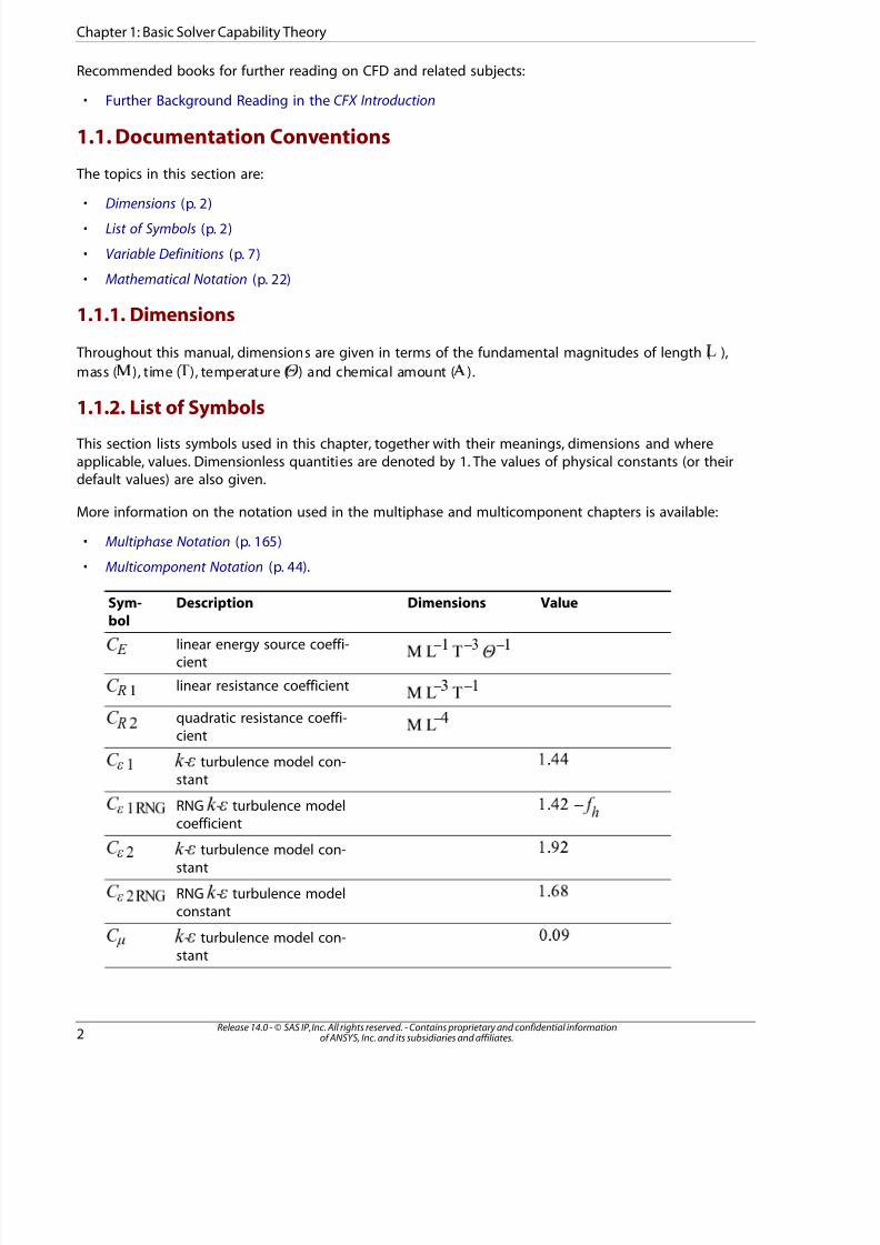
7/16/2019 ANSYS CFX-Solver Theory Guide
http://slidepdf.com/reader/full/ansys-cfx-solver-theory-guide-5633873a6f5ee 18/417
Recommended books for further reading on CFD and related subjects:
• Further Background Reading in the CFX Introduction
1.1. Documentation Conventions
The topics in this section are:
• Dimensions (p. 2)• List of Symbols (p. 2)
• Variable Definitions (p. 7)
• Mathematical Notation (p. 22)
1.1.1. Dimensions
Throughout this manual, dimensions are given in terms of the fundamental magnitudes of length ( ),
mass ( ), time ( ), temperature (
) and chemical amount ( ).
1.1.2. List of Symbols This section lists symbols used in this chapter, together with their meanings, dimensions and whereapplicable, values. Dimensionless quantities are denoted by 1. The values of physical constants (or theirdefault values) are also given.
More information on the notation used in the multiphase and multicomponent chapters is available:
• Multiphase Notation (p. 165)
• Multicomponent Notation (p. 44).
ValueDimensionsDescriptionSym-
bol
− − −¡
¢ £ ¢
linear energy source coeffi-cient
¤
¥
− − ¦ §
linear resistance coefficient ̈
©
−
quadratic resistance coeffi-cient
-
turbulence model con-stant
−
!
RNG"
-#
turbulence model
coefficient
$
% & ' ( )
0
-1
turbulence model con-stant
2
3 4
RNG5
-6
turbulence modelconstant
7
8 9 @ A B
C -D turbulence model con-stant
E
F
Release 14.0 - © SAS IP, Inc. All rights reserved. - Contains proprietary and confidential informationof ANSYS, Inc. and its subsidiaries and affiliates.2
Chapter 1: Basic Solver Capability Theory
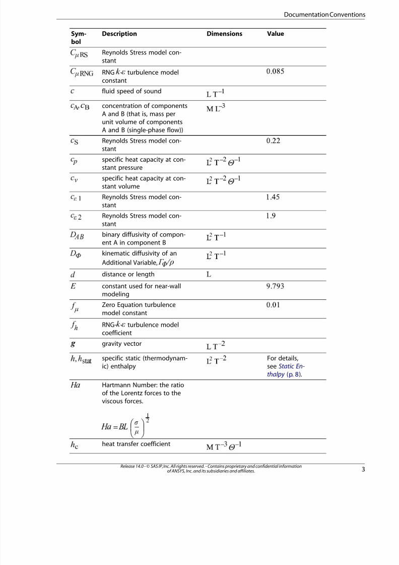
7/16/2019 ANSYS CFX-Solver Theory Guide
http://slidepdf.com/reader/full/ansys-cfx-solver-theory-guide-5633873a6f5ee 19/417
ValueDimensionsDescriptionSym-
bol
Reynolds Stress model con-stant
¡ ¢ £
RNG¤
-¥
turbulence modelconstant
¦
§ ¨ ©
−
fluid speed of sound
−
concentration of componentsA and B (that is, mass per
unit volume of componentsA and B (single-phase flow))
Reynolds Stress model con-stant
− −
! "
specific heat capacity at con-stant pressure
#
$
− −%
& ' (
specific heat capacity at con-
stant volume
)
0
Reynolds Stress model con-stant
1
2 3
Reynolds Stress model con-stant
4
5 6
− 7 8
binary diffusivity of compon-ent A in component B
9
@ A
− B C
kinematic diffusivity of an
Additional Variable, D E
F
G
H
distance or lengthI
constant used for near-wallmodeling
P
Zero Equation turbulencemodel constant
Q
R
RNG-S -T turbulence modelcoefficient
U
V
− W
gravity vector X
For details,see Static En-
thalpy (p. 8).
− Y ̀
specific static (thermodynam-ic) enthalpy
a a
b c d c
Hartmann Number: the ratioof the Lorentz forces to theviscous forces.
e f
=
g h i p
q
r
s
t
− −u
v w
heat transfer coefficientx
y
3Release 14.0 - © SAS IP, Inc. All rights reserved. - Contains proprietary and confidential informationof ANSYS, Inc. and its subsidiaries and affiliates.
Documentation Conventions

7/16/2019 ANSYS CFX-Solver Theory Guide
http://slidepdf.com/reader/full/ansys-cfx-solver-theory-guide-5633873a6f5ee 20/417
ValueDimensionsDescriptionSym-
bol
For details,see Total En-
thalpy (p. 10).
− ¡
specific total enthalpy¢
£ ¤ £
− ¥ ¦
turbulence kinetic energy perunit mass
§
local Mach number, ¨ ©
−
mass flow rate
− −
shear production of turbu-lence
For details,see Static
− −
static (thermodynamic) pres-sure
! " !
Pres-
sure (p. 8).
For details,
see Reference
− −# $
reference pressure %
& ' (
Pres-
sure (p. 7).
For details,see Total Pres-
sure (p. 16).
− −) 0
total pressure 1
2 3 2
For details,see Modified
− −4 5
modified pressure′ 6
Pres-
sure (p. 8).
− −7
8 9 @
universal gas constant A
B
Reynolds number, C D E F
G H
Magnetic Reynolds Number:the ratio between the mag-
I P
Q
netic advection and magneticdiffusion.
= R S
T
U V
W
location vectorX
volume fraction of phaseY ̀
a
− −b c
energy sourced
e
− − f f
momentum source g
h
− − i p
mass sourceq
r s
turbulent Schmidt number,
t u
v
v
w x
y
Release 14.0 - © SAS IP, Inc. All rights reserved. - Contains proprietary and confidential informationof ANSYS, Inc. and its subsidiaries and affiliates.4
Chapter 1: Basic Solver Capability Theory

7/16/2019 ANSYS CFX-Solver Theory Guide
http://slidepdf.com/reader/full/ansys-cfx-solver-theory-guide-5633873a6f5ee 21/417
ValueDimensionsDescriptionSym-
bol
Stanton number ¡
− ¢
mass flow rate from phase £
to phase .
¤
¥ ¦
For details,
see Static
§
static (thermodynamic) tem-
perature
¨ ̈
©
Temperat-
ure (p. 10).
For details,see Domain
domain temperature
Temperat-
ure (p. 10).
buoyancy reference temperat-ure used in the Boussinesqapproximation
!
"
saturation temperature#
$ % &
For details,see Total
'
total temperature(
) 0 )
Temperat-
ure (p. 11).
−1 vector of velocity 2
3 4 5 6 6
7
−8
velocity magnitude9
− @
fluctuating velocity compon-ent in turbulent flow
A
− −B C
fluid viscous and body forcework termD
E
molecular weight (Ideal Gasfluid model)
F
mass fraction of componentA in the fluid
G
H
used as a subscript to indic-ate that the quantity appliesto phase
I
P
used as a subscript to indic-ate that the quantity applies
to phase Q
R
−S
T
coefficient of thermal expan-sion (for the Boussinesq ap-proximation)
U
RNGV
-W
turbulence modelconstant
X
Y ` a
− −b b
diffusivity c
5Release 14.0 - © SAS IP, Inc. All rights reserved. - Contains proprietary and confidential informationof ANSYS, Inc. and its subsidiaries and affiliates.
Documentation Conventions

7/16/2019 ANSYS CFX-Solver Theory Guide
http://slidepdf.com/reader/full/ansys-cfx-solver-theory-guide-5633873a6f5ee 22/417
ValueDimensionsDescriptionSym-
bol
− −
molecular diffusion coeffi-
cient of component ¡
¢
£
− −¤ ¤
dynamic diffusivity of an Ad-ditional Variable
¥
¦
− −§ §
turbulent diffusivity ̈
©
identity matrix or KroneckerDelta function
−
turbulence dissipation rate
− −
bulk viscosity
Von Karman constant
− −
thermal conductivity
− −! !
molecular (dynamic) viscosity "
− −# #
turbulent viscosity $
%
− −& &
effective viscosity, + ' '
(
)
0 1 1
− 2
density 3
laminar Prandtl number,
4 5 6
7
8 9
turbulent Prandtl number,
@ A B
C
C D
E F
G
turbulence model constantfor the H equation
I
P
Q -R turbulence model con-stant
S
T
U -V turbulence model con-stant
W
X
Reynolds Stress model con-stant
Y
̀ a b
RNG c -d turbulence model
constant
e
f g h i
RNG p -q turbulence modelconstant
r
s t u v
− −w x
shear stress or sub-grid scalestress
y
molecular stress tensor
−
specific volume
Release 14.0 - © SAS IP, Inc. All rights reserved. - Contains proprietary and confidential informationof ANSYS, Inc. and its subsidiaries and affiliates.6
Chapter 1: Basic Solver Capability Theory

7/16/2019 ANSYS CFX-Solver Theory Guide
http://slidepdf.com/reader/full/ansys-cfx-solver-theory-guide-5633873a6f5ee 23/417
ValueDimensionsDescriptionSym-
bol
−
Additional Variable (non-react-ing scalar)
¡
general scalar variable¢
− £
angular velocity¤
1.1.2.1. Subscripts
Quantities that appear with subscripts ¥
, ¦
,§
refer to that quantity for component ̈
, ©
,
in a mul-ticomponent fluid.
Quantities that appear with subscripts
,
,
refer to that quantity for phase
,
,
in a multiphase
flow.
Such quantities are used only in the chapters describing multicomponent and multiphase flows.
• Multicomponent Flow (p. 44)
• Multiphase Flow Theory (p. 165)
1.1.3.Variable Definitions
1.1.3.1. Isothermal Compressibility
The isothermal compressibility defines the rate of change of the system volume with pressure. For details,see Variables Relevant for Compressible Flow in the CFX Reference Guide.
(1–1)
1.1.3.2. Isentropic Compressibility
Isentropic compressibility is the extent to which a material reduces its volume when it is subjected tocompressive stresses at a constant value of entropy. For details, see Variables Relevant for CompressibleFlow in the CFX Reference Guide.
(1–2)
!
" !
" #
$
1.1.3.3. Reference Pressure
The Reference Pressure Equation 1–3 (p. 8) is the absolute pressure datum from which all otherpressure values are taken. All relative pressure specifications in ANSYS CFX are relative to the Reference
Pressure. For details, see Setting a Reference Pressure in the CFX-Solver Modeling Guide.
7Release 14.0 - © SAS IP, Inc. All rights reserved. - Contains proprietary and confidential informationof ANSYS, Inc. and its subsidiaries and affiliates.
Documentation Conventions

7/16/2019 ANSYS CFX-Solver Theory Guide
http://slidepdf.com/reader/full/ansys-cfx-solver-theory-guide-5633873a6f5ee 24/417
(1–3)
¡ ¢ £
1.1.3.4. Static Pressure
CFX solves for the relative Static Pressure (thermodynamic pressure) Equation 1–4 (p. 8) in theflow field, and is related to Absolute Pressure Equation 1–5 (p. 8).
(1–4) ¤
¥ ¦ § ¦
(1–5)= + ̈ ¨ ̈
© ©
1.1.3.5. Modified Pressure
A modified pressure is used in the following circumstances:
• When certain turbulence models are used, (for example
-
,
-
, and Reynolds Stress), the modifiedpressure includes an additional term due to the turbulent normal stress. For details, see Equa-
tion 2–14 (p. 93).
• When buoyancy is activated, the modified pressure excludes the hydrostatic pressure field. For details,see Buoyancy and Pressure.
1.1.3.6. Static Enthalpy
Specific static enthalpy Equation 1–6 (p. 8) is a measure of the energy contained in a fluid per unitmass. Static enthalpy is defined in terms of the internal energy of a fluid and the fluid state:
(1–6)= + !
"
#
$ % & % $ % & %
$ % & %
$ % & %
When you use the thermal energy model, the CFX-Solver directly computes the static enthalpy. Generalchanges in enthalpy are also used by the solver to calculate thermodynamic properties such as temper-ature. To compute these quantities, you need to know how enthalpy varies with changes in both tem-perature and pressure. These changes are given by the general differential relationship Equa-
tion 1–7 (p. 8):
(1–7)=
∂∂
+
∂∂
' (
(
)
' )
(
0
' 0
1
2
which can be rewritten as Equation 1–8 (p. 9)
Release 14.0 - © SAS IP, Inc. All rights reserved. - Contains proprietary and confidential informationof ANSYS, Inc. and its subsidiaries and affiliates.8
Chapter 1: Basic Solver Capability Theory

7/16/2019 ANSYS CFX-Solver Theory Guide
http://slidepdf.com/reader/full/ansys-cfx-solver-theory-guide-5633873a6f5ee 25/417
(1–8)= +
+
∂∂
¡ ¢ £
¤
£
¤
¤
£
¥
¦
¦
where§
̈
is specific heat at constant pressure and ©
is density. For most materials the first term always
has an effect on enthalpy, and, in some cases, the second term drops out or is not included. For example,
the second term is zero for materials that use the Ideal Gas equation of state or materials in a solidthermodynamic state. In addition, the second term is also dropped for liquids or gases with constantspecific heat when you run the thermal energy equation model.
1.1.3.6.1. Material with Variable Density and Specific Heat
In order to support general properties, which are a function of both temperature and pressure, a table
for is generated by integrating Equation 1–8 (p. 9) using the functions supplied for and
. The enthalpy table is constructed between the upper and lower bounds of temperature and pressure
(using flow solver internal defaults or those supplied by the user). For any general change in conditions
from
to ! "
# $
%
, the change in enthalpy, & ' , is calculated in two steps: first at constant
pressure, and then at constant temperature using Equation 1–9 (p. 9).
(1–9)∫ ∫ − = +
+
∂∂
( ( ) 0 1
2
1
2
2
1
0 3
4
4
5
5
5
5
6 7
8
9
8
9
To successfully integrate Equation 1–9 (p. 9), the CFX-Solver must be provided thermodynamicallyconsistent values of the equation of state,
@
, and specific heat capacity,A
B
. “Thermodynamically consist-
ent” means that the coefficients of the differential terms of Equation 1–8 (p. 9) must satisfy the exact
differential property that:
(1–10)∂∂
∂∂
=
∂∂
∂∂
C
D
E E
D
C
F
G
G
F
or, in terms of the expressions given in Equation 1–9 (p. 9):
(1–11)
∂∂
=
∂
∂
−
+
∂∂
+
H
I
P
Q
P
Q
Q
P
P
Q
R
S
R
R
T
T
T
To satisfyU
V
in Equation 1–11 (p. 9), variables of the form '<Material Name>.Property Residual' are
computed and should resolve to zero.
The equation of state derivative within the second integral of Equation 1–9 (p. 9) is numerically evaluatedfrom the using a two point central difference formula. In addition, the CFX-Solver uses an adaptivenumber of interpolation points to construct the property table, and bases the number of points on anabsolute error tolerance estimated using the enthalpy and entropy derivatives.
9Release 14.0 - © SAS IP, Inc. All rights reserved. - Contains proprietary and confidential informationof ANSYS, Inc. and its subsidiaries and affiliates.
Documentation Conventions

7/16/2019 ANSYS CFX-Solver Theory Guide
http://slidepdf.com/reader/full/ansys-cfx-solver-theory-guide-5633873a6f5ee 26/417
1.1.3.7. Total Enthalpy
Total enthalpy is expressed in terms of a static enthalpy and the flow kinetic energy:
(1–12)= + ⋅ ¡ ¡
¢ £ ¢ ¤ ¢ ¥ ¢
where ¦ is the flow velocity. When you use the total energy model the CFX-Solver directly computestotal enthalpy, and static enthalpy is derived from this expression. In case of turbulence models for
which the kinetic turbulent energy § is available (such as k-epsilon, k-omega, SST, and so on), ̈ is includedin the total enthalpy. In rotating frames of reference, the total enthalpy includes the relative framekinetic energy. For details, see Rotating Frame Quantities (p. 18).
1.1.3.8. Domain Temperature
The domain temperature,©
, is the absolute temperature at which an isothermal simulation is per-
formed. For details, see Isothermal in the CFX-Solver Modeling Guide.
1.1.3.9. Static Temperature
The static temperature,
, is the thermodynamic temperature, and depends on the internal energy
of the fluid. In ANSYS CFX, depending on the heat transfer model you select, the flow solver calculateseither total or static enthalpy (corresponding to the total or thermal energy equations).
The static temperature is calculated using static enthalpy and the constitutive relationship for the ma-terial under consideration. The constitutive relation simply tells us how enthalpy varies with changesin both temperature and pressure.
Release 14.0 - © SAS IP, Inc. All rights reserved. - Contains proprietary and confidential informationof ANSYS, Inc. and its subsidiaries and affiliates.10
Chapter 1: Basic Solver Capability Theory

7/16/2019 ANSYS CFX-Solver Theory Guide
http://slidepdf.com/reader/full/ansys-cfx-solver-theory-guide-5633873a6f5ee 27/417
1.1.3.9.1. Material with Constant Density and Specific Heat
In the simplified case where a material has constant
and¡
¢
, temperatures can be calculated by integ-
rating a simplified form of the general differential relationship for enthalpy:
(1–13)− = −£ £ ¤ ¥ ¥
¦ § ¨ © ¨ § ¨ © ¨
which is derived from the full differential form for changes in static enthalpy. The default reference
state in the CFX-Solver is =
and = !
" # $
.
1.1.3.9.2. Ideal Gas or Solid with cp=f(T)
The enthalpy change for an ideal gas or CHT solid with specific heat as a function of temperature isdefined by:
(1–14)∫ − =% % & ' ( '
)
)
0 1 2 3 2 4 5 6
7 8 9
@ A B A
When the solver calculates static enthalpy, either directly or from total enthalpy, you can back statictemperature out of this relationship. When C
D
varies with temperature, the CFX-Solver builds an enthalpy
table and static temperature is backed out by inverting the table.
1.1.3.9.3. Material with Variable Density and Specific Heat
To properly handle materials with an equation of state and specific heat that vary as functions of tem-perature and pressure, the CFX-Solver needs to know enthalpy as a function of temperature and pressure,
E F G
.
H I P
can be provided as a table using, for example, an .rgp file. If a table is not pre-supplied,
and the equation of state and specific heat are given by CEL expressions or CEL user functions, the CFX-
Solver will calculate Q R S by integrating the full differential definition of enthalpy change.
Given the knowledge of T U V
and that the CFX-Solver calculates both static enthalpy and static
pressure from the flow solution, you can calculate static temperature by inverting the enthalpy table:
(1–15)− = −W W W X Y W X Y
̀ a b a c d e ` a b a
̀ a b a
c d e
c d e
In this case, you know f
g h i h
, p
q r s r
from solving the flow and you calculate t
u v w v
by table inversion.
1.1.3.10. Total Temperature
The total temperature is derived from the concept of total enthalpy and is computed exactly the sameway as static temperature, except that total enthalpy is used in the property relationships.
11Release 14.0 - © SAS IP, Inc. All rights reserved. - Contains proprietary and confidential informationof ANSYS, Inc. and its subsidiaries and affiliates.
Documentation Conventions

7/16/2019 ANSYS CFX-Solver Theory Guide
http://slidepdf.com/reader/full/ansys-cfx-solver-theory-guide-5633873a6f5ee 28/417
1.1.3.10.1. Material with Constant Density and Specific Heat
If
and¡
¢
are constant, then the total temperature and static temperature are equal because incom-
pressible fluids undergo no temperature change due to addition of kinetic energy. This can be illustratedby starting with the total enthalpy form of the constitutive relation:
(1–16)− = −£ £ ¤ ¥ ¥
¦ § ¨ § © § ¨ § ©
and substituting expressions for Static Enthalpy (p. 8) and Total Pressure (p. 16) for an incompressiblefluid:
(1–17)= + ⋅
(1–18)= + ⋅
! " ! # ! $ !
some rearrangement gives the result that:
(1–19)=% %
& ' & ( & ) &
for this case.
1.1.3.10.2. Ideal Gas with constant cp
For this case, enthalpy is only a function of temperature and the constitutive relation is:
(1–20)− = −0 0 1 2 2
3 4 5 6 4 5 6
which, if one substitutes the relation between static and total enthalpy, yields:
(1–21)= +⋅7 7
8 8
9
@
A B A C A D A
If the −E F
turbulence model is employed, turbulence kinetic energy,G
, is added to the total enthalpy,giving the modified total temperature for constant H
I
:
(1–22)= +⋅
+P P
Q Q
R
S
R
T T
U V U W U X U
1.1.3.10.3. Ideal Gas with cp = f(T)
The total temperature is evaluated with:
Release 14.0 - © SAS IP, Inc. All rights reserved. - Contains proprietary and confidential informationof ANSYS, Inc. and its subsidiaries and affiliates.12
Chapter 1: Basic Solver Capability Theory

7/16/2019 ANSYS CFX-Solver Theory Guide
http://slidepdf.com/reader/full/ansys-cfx-solver-theory-guide-5633873a6f5ee 29/417
(1–23)∫ − = ¡ ¢ £ ¢
¤
¤
¥ ¦ § ¦ ¨ ©
using table inversion to back out the total temperature.
1.1.3.10.4. Material with Variable Density and Specific Heat
In this case, total temperature is calculated in the exact same way as static temperature except thattotal enthalpy and total pressure are used as inputs into the enthalpy table:
(1–24)− = −
! " #
! " #
! " #
In this case you know $
% & %
, and you want to calculate '
( ) (
, but you do not know 0
1 2 1
. So, before calcu-
lating the total temperature, you need to compute total pressure. For details, see Total Pressure (p. 16).
For details, see Rotating Frame Quantities (p. 18).
1.1.3.11. Entropy
The concept of entropy arises from the second law of thermodynamics:
(1–25)= −3 4 5 4 6
4 7
8
which can be rearranged to give:
(1–26)= −9 @
9 A
B
9 C
D B
Depending on the equation of state and the constitutive relationship for the material, you can arriveat various forms for calculating the changes in entropy as a function of temperature and pressure.
1.1.3.11.1. Material with Constant Density and Specific Heat
In this case, changes in enthalpy as a function of temperature and pressure are given by:
(1–27)= +E F G E H
E I
P
Q
and when this is substituted into the second law gives the following expression for changes in entropyas a function of temperature only:
13Release 14.0 - © SAS IP, Inc. All rights reserved. - Contains proprietary and confidential informationof ANSYS, Inc. and its subsidiaries and affiliates.
Documentation Conventions

7/16/2019 ANSYS CFX-Solver Theory Guide
http://slidepdf.com/reader/full/ansys-cfx-solver-theory-guide-5633873a6f5ee 30/417
(1–28)= ¡ ¢
£
£
¤
which, when integrated, gives an analytic formula for changes in entropy:
(1–29)− =
¥ ¥ ¦
§
§
̈ ©
©
1.1.3.11.2. Ideal Gas with constant cp or cp = f(T)
For ideal gases changes in entropy are given by the following equation:
(1–30)∫ − = −
! "
! "
# $ %
which for general functions for&
'
the solver computes an entropy table as a function of both temper-
ature and pressure. In the simplified case when(
)
is a constant, then an analytic formula is used:
(1–31)− =
−
0 0 1
2
2
3
4
4
5 6 7 8
6 7 8
6 7 8
1.1.3.11.3. Material with Variable Density and Specific Heat
This is the most general case handled by the CFX-Solver. The entropy function,9 @ A
, is calculatedby integrating the full differential form for entropy as a function of temperature and pressure. Insteadof repetitively performing this integration the CFX-Solver computes a table of values at a number of temperature and pressure points. The points are chosen such that the approximation error for the entropyfunction is minimized.
The error is estimated using derivatives of entropy with respect to temperature and pressure. Expressionsfor the derivatives are found by substituting the formula for general enthalpy changes into the secondlaw to get the following expression for changes in entropy with temperature and pressure:
(1–32)= +
∂
∂
B C
D
E
B E
F
F
E
B G
H
H
I
which when compared with the following differential form for changes in entropy:
(1–33)=
∂∂
+
∂∂
P Q
Q
R
P R
Q
S
P S
T
U
gives that:
Release 14.0 - © SAS IP, Inc. All rights reserved. - Contains proprietary and confidential informationof ANSYS, Inc. and its subsidiaries and affiliates.14
Chapter 1: Basic Solver Capability Theory

7/16/2019 ANSYS CFX-Solver Theory Guide
http://slidepdf.com/reader/full/ansys-cfx-solver-theory-guide-5633873a6f5ee 31/417
(1–34)
∂∂
=
¡
¢
¡
£
£
(1–35)
∂∂
=
∂∂
¤
¥ ¦
¦
§
̈
©
The derivative of entropy with respect to temperature is exactly evaluated, while the derivative withrespect to pressure must be computed by numerically differentiating the equation of state. Note thatwhen properties are specified as a function of temperature and pressure using CEL expressions thedifferential terms in Equation 1–32 (p. 14) must also satisfy the exact differential relationship:
(1–36)∂∂
∂∂
=
∂∂
∂∂
or,
(1–37)∂∂
=
∂∂
∂∂
!
!
!
"
Also, see the previous section on Static Enthalpy (p. 8) for more details.
Unless an externally provided table is supplied, an entropy table is built by using the #
and$
%
functions
supplied by the user and integrating the general differential form:
(1–38)∫ ∫ − = +
∂∂
& &
'
(
) (
0
0
(
) 1
2
2
3
3
3
3
4 5
6
7
8
7
8
To calculate total pressure, you also need to evaluate entropy as a function of enthalpy and pressure,rather than temperature and pressure. For details, see Total Pressure (p. 16).
The recipe to do this is essentially the same as for the temperature and pressure recipe. First, you start
with differential form for9 @ A
:
(1–39)=
∂∂
+
∂∂
B C
C
D
B D
C
E
B E
F
G
and comparing this with a slightly rearranged form of the second law:
15Release 14.0 - © SAS IP, Inc. All rights reserved. - Contains proprietary and confidential informationof ANSYS, Inc. and its subsidiaries and affiliates.
Documentation Conventions

7/16/2019 ANSYS CFX-Solver Theory Guide
http://slidepdf.com/reader/full/ansys-cfx-solver-theory-guide-5633873a6f5ee 32/417
(1–40)= − ¡
¢
£
¤
¥ £
you get that:
(1–41)
∂
∂
=
¦
§ ̈
©
(1–42)
∂∂
= −
In this case, the entropy derivatives with respect to
and
can be evaluated from the constitutive re-
lationship
(getting
from!
and "
by table inversion) and the equation of state# $ %
.
Points in the& ' (
table are evaluated by performing the following integration:
(1–43)∫ ∫ − = −) )
0
1 2
3 0
1 4
5
5
6
6
7 8 9
@ A B
@ A B
over a range of C
and D
, which are determined to minimize the integration error.
1.1.3.12. Total Pressure
The total pressure, E
F G F
, is defined as the pressure that would exist at a point if the fluid was brought
instantaneously to rest such that the dynamic energy of the flow converted to pressure without losses. The following three sections describe how total pressure is computed for a pure component materialwith constant density, ideal gas equation of state and a general equation of state (CEL expression orRGP table). For details, see Multiphase Total Pressure (p. 166).
The terms Pressure and Total Pressure are absolute quantities and must be used to derive the TotalPressure when using an equation of state (compressible) formulation (particularly for Equa-
tion 1–48 (p. 17)).
The setting of the Total Pressure Option, described in Compressibility Control in the CFX-Pre User's
Guide, determines which equation is used to derive the total pressure.
1.1.3.12.1. Incompressible Fluids
For incompressible flows, such as those of liquids and low speed gas flows, the total pressure is givenby Bernoulli’s equation:
(1–44)= + ⋅H H I I P
Q R Q S Q T Q
which is the sum of the static and dynamic pressures.
Release 14.0 - © SAS IP, Inc. All rights reserved. - Contains proprietary and confidential informationof ANSYS, Inc. and its subsidiaries and affiliates.16
Chapter 1: Basic Solver Capability Theory

7/16/2019 ANSYS CFX-Solver Theory Guide
http://slidepdf.com/reader/full/ansys-cfx-solver-theory-guide-5633873a6f5ee 33/417
1.1.3.12.2. Ideal Gases
When the flow is compressible, total pressure is computed by starting with the second law of thermo-dynamics assuming that fluid state variations are locally isentropic so that you get:
(1–45)= ¡
¢
£
The left hand side of this expression is determined by the constitutive relation and the right hand sideby the equation of state. For an ideal gas, the constitutive relation and equation of state are:
(1–46)=¤ ¥ ¦ § ¤ §
̈
(1–47)= ©
which, when substituted into the second law and assuming no entropy variations, gives:
(1–48)∫ =
! " #
$ % & %
% ' %
where(
) 0 1 0
and2
3 4 3
are the static and total temperatures respectively (calculation of these quantities
was described in two previous sections, Static Temperature (p. 10) and Total Temperature (p. 11)). If 5
6
is a constant, then the integral can be exactly evaluated, but if 7
8
varies with temperature, then the
integral is numerically evaluated using quadrature. For details, see:
• Entropy (p. 13)
• Ideal Gas Equation of State (p. 28).
1.1.3.12.3. Material with Variable Density and Specific Heat
Total pressure calculations in this case are somewhat more involved. You need to calculate total pressuregiven the static enthalpy and static pressure, which the CFX-Solver solves for. You also want to assumethat the local state variations, within a control volume or on a boundary condition, are isentropic.
Given that you know9 @ A
(from integrating the differential form for enthalpy) andB C D
, youcan compute two entropy functions E F G and H I P . There are two options for generating these
functions:
• If Q R S and T U V are provided by a .rgp file then W X Y is evaluated by interpolation fro
` a b and c d e tables.
• If CEL expressions have been given for f
andg
h
only, theni p q
,r s t
andu v w
are all
evaluated by integrating their differential forms.
17Release 14.0 - © SAS IP, Inc. All rights reserved. - Contains proprietary and confidential informationof ANSYS, Inc. and its subsidiaries and affiliates.
Documentation Conventions

7/16/2019 ANSYS CFX-Solver Theory Guide
http://slidepdf.com/reader/full/ansys-cfx-solver-theory-guide-5633873a6f5ee 34/417
Once you have the ¡ ¢
table, calculated as described in Entropy (p. 13), computing total pressure
for a single pure component is a relatively trivial procedure:
1. The CFX-Solver solves for£
¤ ¥ ¤
and ¦
§ ¨ © ̈
2. Calculate
from
3. Calculate entropy =
! " ! ! " !
! " !
4. Using the isentropic assumption set =# #
$ % $ & $ ' $
5. Calculate total pressure by inverting =( ( ) 0
1 2 1 1 2 1
1 2 1
For details, see Rotating Frame Quantities (p. 18).
1.1.3.13. Shear Strain Rate
The strain rate tensor is defined by:
(1–49)= ∂
∂+ ∂
∂ 3
4
5
4
5
6 7
6
7
7
6
This tensor has three scalar invariants, one of which is often simply called the shear strain rate:
(1–50)=
∂∂
8
9
@
A
B
A B
C
D
with velocity components E
F
, G
H
, I
P
, this expands to:
(1–51)
=
∂∂
+
∂∂
+
∂∂
+
∂∂
+∂∂
+
∂∂
+∂∂
+
∂∂
+∂∂
Q
R
Q
S
Q
T
Q
S
Q
R
Q
T
Q
R
Q
T
Q
S
U
V
W
U
V
U W
V
W
X
Y
̀
̀
̀
̀
̀
̀
The viscosity of non-Newtonian fluids is often expressed as a function of this scalar shear strain rate.
1.1.3.14. Rotating Frame Quantities
The velocity in the rotating frame of reference is defined as:
Release 14.0 - © SAS IP, Inc. All rights reserved. - Contains proprietary and confidential informationof ANSYS, Inc. and its subsidiaries and affiliates.18
Chapter 1: Basic Solver Capability Theory

7/16/2019 ANSYS CFX-Solver Theory Guide
http://slidepdf.com/reader/full/ansys-cfx-solver-theory-guide-5633873a6f5ee 35/417
(1–52)= − × ¡ ¢
£ ¤ ¥ ¦ § ̈
where©
is the angular velocity,
is the local radius vector, and
is velocity in the stationary frame
of reference.
1.1.3.14.1. Incompressible Fluids
For incompressible flows, the total pressure is defined as:
(1–53)= + ⋅ − × ⋅ ×
! " #
$ % & $ % &
where '
( ) 0 )
is static pressure. The stationary frame total pressure is defined as:
(1–54)= + ⋅1 1 2 2 3
4 5 4 6 7 4 8 7 4 9 4
7 4 8 7 4 8
1.1.3.14.2. Ideal Gases
For compressible flows relative total pressure, rotating frame total pressure and stationary frame totalpressure are computed in the same manner as in Total Pressure (p. 16). First you start with the relativetotal enthalpy, rothalpy and stationary frame total enthalpy:
(1–55)= + ⋅@ @ A A
B C B D B E B F G H F G H
(1–56)= + ⋅ − × ⋅ ×I I P Q P Q R S
T U V U W X Y W X Y
(1–57)= + ⋅` ̀a a
b c b d e b f e b g b e b f e b f
whereh
i p q p
is the static enthalpy. In a rotating frame of reference, the CFX-Solver solves for the total
enthalpy,r
s t s
, which includes the relative kinetic energy.
Important
Rothalpy u
is not a positive definite quantity. If the rotation velocity is large, then the
last term can be significantly larger than the static enthalpy plus the rotating frame kineticenergy. In this case, it is possible that total temperature and rotating total pressure are un-defined and will be clipped at internal table limits or built in lower bounds. However, this isonly a problem for high angular velocity rotating systems.
If you again assume an ideal gas equation of state with variable specific heat capacity you can computerelative total temperature, total temperature and stationary frame total temperature using:
19Release 14.0 - © SAS IP, Inc. All rights reserved. - Contains proprietary and confidential informationof ANSYS, Inc. and its subsidiaries and affiliates.
Documentation Conventions

7/16/2019 ANSYS CFX-Solver Theory Guide
http://slidepdf.com/reader/full/ansys-cfx-solver-theory-guide-5633873a6f5ee 36/417
(1–58)∫ − = ¡ ¢ £ ¢
¤
¤
¥ ¦ § ¦ ¨ ©
and:
(1–59)∫ − = ! " !
#
#
$ % & '
( ) 0
1 2 1
and:
(1–60)∫ − =3 3 4 5 6 5
7
7
8 9 @ 9 A B 9 C D E F
G H I
P Q P R S P T
where all the total temperature quantities are obtained by inverting the enthalpy table. If U
V
is constant,
then these values are obtained directly from these definitions:
(1–61)= +⋅
W W
X X
Y
̀
a b a c d e f g a h a
d e f d e f
(1–62)= +⋅ − × ⋅ ×
i i p q p q
r r
s
t
u v u w u x u
y y
(1–63)= +⋅
At this point, given
,
,
j k
, l
m n o n
and
you can compute relative total pressure, total
pressure or stationary frame total pressure using the relationship given in the section describing totalpressure. For details, see Total Pressure (p. 16).
The names of the various total enthalpies, temperatures, and pressures when visualizing results in CFD-
Post or for use in CEL expressions is as follows.
Table 1.1 Variable naming: Total Enthalpies, Temperatures, and Pressures
Short Variable
Name
Long Variable
Name
Variable
htot Total Enthalpy
rothalpyRothalpy
Release 14.0 - © SAS IP, Inc. All rights reserved. - Contains proprietary and confidential informationof ANSYS, Inc. and its subsidiaries and affiliates.20
Chapter 1: Basic Solver Capability Theory

7/16/2019 ANSYS CFX-Solver Theory Guide
http://slidepdf.com/reader/full/ansys-cfx-solver-theory-guide-5633873a6f5ee 37/417
Short Variable
Name
Long Variable
Name
Variable
htotstn Total Enthalpy inStn Frame
¡ ¢ ¡ £ ¤ ¡ ¥
Ttotrel Total Temperat-ure in Rel Frame
¦
§ ¨ § ©
Ttot Total Temperat-ure
Ttotstn Total Temperat-ure in Stn Frame
!
ptotrel Total Pressure inRel Frame
"
# $ # % & ' (
ptot Total Pressure )
0 1 0
ptotstn Total Pressure inStn Frame
2
3 4 3 5 6 3 7
The Mach Number and stationary frame Mach numbers are defined as:
(1–64)=8
9
@
A B C
(1–65)=D
E
F
G H I
G H I
where P is the local speed of sound.
1.1.3.14.3. Material with Variable Density and Specific Heat
Rotating and stationary frame total temperature and pressure are calculated the same way as describedin Total Temperature (p. 11) and Total Pressure (p. 16). The only changes in the recipes are that rotating
frame total pressure and temperature require rothalpy, Q
, as the starting point and stationary frame
total pressure and temperature require stationary frame total enthalpy,R
S T S U V S W
.
1.1.3.15. Courant Number
The Courant number is of fundamental importance for transient flows. For a one-dimensional grid, it isdefined by:
(1–66)=X Y
̀
wherea
is the fluid speed,b
is the timestep and c
is the mesh size. The Courant number calculatedin ANSYS CFX is a multidimensional generalization of this expression where the velocity and lengthscale are based on the mass flow into the control volume and the dimension of the control volume.
For explicit CFD methods, the timestep must be chosen such that the Courant number is sufficientlysmall. The details depend on the particular scheme, but it is usually of order unity. As an implicit code,
21Release 14.0 - © SAS IP, Inc. All rights reserved. - Contains proprietary and confidential informationof ANSYS, Inc. and its subsidiaries and affiliates.
Documentation Conventions

7/16/2019 ANSYS CFX-Solver Theory Guide
http://slidepdf.com/reader/full/ansys-cfx-solver-theory-guide-5633873a6f5ee 38/417
ANSYS CFX does not require the Courant number to be small for stability. However, for some transientcalculations (for example, LES), one may need the Courant number to be small in order to accuratelyresolve transient details.
For certain compressible flow calculations, the acoustic Courant number is also calculated. For a one-dimensional grid, the acoustic Courant number is defined as:
(1–67)=++ ¡
(1–68)=−− ¢
(1–69)= + − £ ¤ ¥ ¦ § ¨ © ¤
where
is the local speed of sound.
CFX uses the Courant number in a number of ways:
1. The timestep may be chosen adaptively based on a Courant number condition (for example, to reachRMS or Courant number of 5). The acoustic Courant number is used for compressible flow calculationshaving the expert parameter setting ‘compressible timestepping = t’.
2. For transient runs using the Automatic timestep initialization option, the Courant number is used tocalculate the blend between the previous timestep and extrapolation options. The acoustic Courantnumber is used for compressible flow calculations.
3. For transient runs, the maximum and RMS Courant numbers are written to the output file everytimestep.
4. The Courant number field is written to the results file.
1.1.4. Mathematical Notation
This section describes the basic notation that is used throughout the CFX-Solver documentation.
1.1.4.1. The Vector Operators
Assume a Cartesian coordinate system in which
,
and
are unit vectors in the three coordinate dir-
ections. ∇ is defined such that:
(1–70)∇ = ∂
∂∂∂
∂∂
1.1.4.1.1. Gradient Operator
For a general scalar function , the gradient of ! is defined by:
Release 14.0 - © SAS IP, Inc. All rights reserved. - Contains proprietary and confidential informationof ANSYS, Inc. and its subsidiaries and affiliates.22
Chapter 1: Basic Solver Capability Theory

7/16/2019 ANSYS CFX-Solver Theory Guide
http://slidepdf.com/reader/full/ansys-cfx-solver-theory-guide-5633873a6f5ee 39/417
(1–71)∇ =∂∂
+∂∂
+∂∂
¡ ¢ £
£
¤
£
¥
£
¦
1.1.4.1.2. Divergence Operator
For a vector function§ ¨ ©
where:
(1–72)=
the divergence of
is defined by:
(1–73)∇ =∂∂
+∂∂
+∂∂
!
"
#
1.1.4.1.3. Dyadic Operator
The dyadic operator (or tensor product) of two vectors, $ and % , is defined as:
(1–74)⊗ =
& '
( ) ( ) ( )
( ) ( ) ( )
( ) ( ) ( )
0 0 0 1 0 2
1 0 1 1 1 2
2 0 2 1 2 2
By using specific tensor notation, the equations relating to each dimension can be combined into asingle equation. Thus, in the specific tensor notation:
(1–75)⊗∇ =
∂∂
+∂∂
+∂∂
∂∂
+∂∂
+∂∂
∂
∂ +
∂
∂ +
∂
∂
3 3
3 3 3 3 3 3
3 3 3 3 3 3
3 3 3 3 3 3
4
5
4
6
4
7
4
5
4
6
4
7
4
5
4
6
4
7
4
8 8 9 8 @ 8
8 9 9 9 @ 9
8 @ 9 @ @ @
1.1.4.2. Matrix Transposition
The transpose of a matrix is defined by the operatorA
. For example, if the matrix is defined by:
23Release 14.0 - © SAS IP, Inc. All rights reserved. - Contains proprietary and confidential informationof ANSYS, Inc. and its subsidiaries and affiliates.
Documentation Conventions

7/16/2019 ANSYS CFX-Solver Theory Guide
http://slidepdf.com/reader/full/ansys-cfx-solver-theory-guide-5633873a6f5ee 40/417
(1–76)∇ =
∂∂∂∂∂
∂
¡
¢
£
then:
(1–77) ∇
=
∂∂
∂∂
∂∂
¤
¤
¥
¤
¦
¤
§
̈
1.1.4.3. The Identity Matrix (Kronecker Delta function)
The Identity matrix is defined by:
(1–78)=
©
1.1.4.4. Index Notation
Although index notation is not generally used in this documentation, the following may help you if you are used to index notation.
In index notation, the divergence operator can be written:
(1–79)∇ =∂∂
where the summation convention is followed; that is, the index
is summed over the three components.
The quantity ⊗
can be represented by
(when!
and"
are vectors), or by# $
% & '
(when(
is a vector and)
is a matrix), and so on.
Hence, the quantity ⊗∇ 0 0 1 can be represented by:
(1–80)∂
∂ 2
3 4 4
5
5 6
Note the convention that the derivatives arising from the divergence operator are derivatives with respect
to the same coordinate as the first listed vector. That is, the quantity ⊗∇7 7 8
is represented
by:
Release 14.0 - © SAS IP, Inc. All rights reserved. - Contains proprietary and confidential informationof ANSYS, Inc. and its subsidiaries and affiliates.24
Chapter 1: Basic Solver Capability Theory

7/16/2019 ANSYS CFX-Solver Theory Guide
http://slidepdf.com/reader/full/ansys-cfx-solver-theory-guide-5633873a6f5ee 41/417
(1–81)∂
∂
¡ ¢ ¢
£
£ ¤
and not:
(1–82)
∂
∂ ¥
¦ § §
̈
© ̈
The quantity
(when
and
are matrices) can be written by
.
1.2. Governing Equations
The set of equations solved by ANSYS CFX are the unsteady Navier-Stokes equations in their conservationform.
If you are new to CFD, review Computational Fluid Dynamics in the CFX Introduction.
A list of recommended books on CFD and related subjects is available in Further Background Readingin the CFX Introduction.
For all the following equations, static (thermodynamic) quantities are given unless otherwise stated.
1.2.1.Transport Equations
In this section, the instantaneous equation of mass, momentum, and energy conservation are presented.For turbulent flows, the instantaneous equations are averaged leading to additional terms. These terms,together with models for them, are discussed in Turbulence and Wall Function Theory (p. 89).
The instantaneous equations of mass, momentum and energy conservation can be written as followsin a stationary frame:
1.2.1.1. The Continuity Equation
(1–83)∂∂
+ ∇ =
1.2.1.2. The Momentum Equations
(1–84)⊗∂ ∂ + ∇ = − ∇ + ∇ +!
! ! "
#
$
# % &
'
Where the stress tensor, ( , is related to the strain rate by
25Release 14.0 - © SAS IP, Inc. All rights reserved. - Contains proprietary and confidential informationof ANSYS, Inc. and its subsidiaries and affiliates.
Governing Equations

7/16/2019 ANSYS CFX-Solver Theory Guide
http://slidepdf.com/reader/full/ansys-cfx-solver-theory-guide-5633873a6f5ee 42/417
(1–85)= ∇ + ∇ − ∇
¡ ¢ £
¤
1.2.1.3. The Total Energy Equation
(1–86)∂ ∂ − ∂∂ + ∇ = ∇ ∇ + ∇ + +¥ ¥ ¥ ¦ ¦
§ ̈
©
©
§ ¨
Where
is the total enthalpy, related to the static enthalpy ! " # by:
(1–87)= +$ % %
& ' &
(
The term ∇) 0
represents the work due to viscous stresses and is called the viscous work term.
This models the internal heating by viscosity in the fluid, and is negligible in most flows.
The term 1 2
3
represents the work due to external momentum sources and is currently neglected.
1.2.1.4. The Thermal Energy Equation
An alternative form of the energy equation, which is suitable for low-speed flows, is also available. To
derive it, an equation is required for the mechanical energy 4 .
(1–88)=5 6
7
The mechanical energy equation is derived by taking the dot product of 8 with the momentum equation(Equation 1–84 (p. 25)):
(1–89)∂
∂+ ∇ = − ∇ + ∇ +
9 9 9 9 @
A B
C
A B D E
F
Subtracting this equation from the total energy equation (Equation 1–86 (p. 26)) yields the thermal energyequation:
(1–90)
∂∂ −
∂∂ + ∇ = ∇ ∇ + ∇ + ∇ +
G G G H
I P
Q
R
Q
I P S T R U
V
The term ∇W X
is always positive and is called the viscous dissipation. This models the internal heatingby viscosity in the fluid, and is negligible in most flows.
With further assumptions discussed in a moment, we obtain the thermal energy equation:
Release 14.0 - © SAS IP, Inc. All rights reserved. - Contains proprietary and confidential informationof ANSYS, Inc. and its subsidiaries and affiliates.26
Chapter 1: Basic Solver Capability Theory

7/16/2019 ANSYS CFX-Solver Theory Guide
http://slidepdf.com/reader/full/ansys-cfx-solver-theory-guide-5633873a6f5ee 43/417
(1–91)∂
∂+ ∇ = ∇ ∇ + ∇ +
¡
¢ £
¤
¢ £ ¥ ¦ §
̈
This equation can be derived from Equation 1–90 (p. 26) with two different sets of assumptions:
• If ©
is actually interpreted as internal energy,
(1–92)= −
then Equation 1–90 (p. 26)can be written as
(1–93)∂
∂+ ∇ = ∇ ∇ − ∇ + ∇ +
! "
#
which is equivalent to Equation 1–91 (p. 27) if we neglect − ∇$ %
and interpret&
as'
. This inter-
pretation is appropriate for liquids, where variable-density effects are negligible. Note that theprincipal variable is still called 'Static Enthalpy' in CFD-Post, although it actually represents internalenergy. Note also that, for liquids that have variable specific heats (for example, set as a CEL expres-
sion or using an RGP table or Redlich Kwong equation of state) the solver includes the ( )
contri-
bution in the enthalpy tables. This is inconsistent, because the variable is actually internal energy.For this reason, the thermal energy equation should not be used in this situation, particularly forsubcooled liquids.
• On the other hand if ∂∂
0
1
and ∇2 3
are neglected in Equation 1–90 (p. 26) then Equation 1–91 (p. 27)
follows directly. This interpretation is appropriate for low Mach number flows of compressible gases.
The thermal energy equation, despite being a simplification, can be useful for both liquids and gasesin avoiding potential stability issues with the total energy formulation. For example, the thermal energyequation is often preferred for transient liquid simulations. On the other hand, if proper acoustic beha-vior is required (for example, predicting sound speed), or for high speed flow, then the total energyequation is required.
1.2.2. Equations of State
The transport equations described above must be augmented with constitutive equations of state fordensity and for enthalpy in order to form a closed system. In the most general case, these state equationshave the form:
= 4 4 5 6
= +∂∂
∂∂
7 8 7 9 7 @
A
B
C
A
C
B
= + ∂∂
D E F E G
H
I
H
P
=Q Q R S
T T
27Release 14.0 - © SAS IP, Inc. All rights reserved. - Contains proprietary and confidential informationof ANSYS, Inc. and its subsidiaries and affiliates.
Governing Equations

7/16/2019 ANSYS CFX-Solver Theory Guide
http://slidepdf.com/reader/full/ansys-cfx-solver-theory-guide-5633873a6f5ee 44/417
Various special cases for particular material types are described below.
1.2.2.1. Incompressible Equation of State
This is the simplest case: density is constant and
¡
can be (at most) a function of temperature.
= ¢ ¢
£ ¤ ¥ ¦
= +§ ¨ © §
=
1.2.2.2. Ideal Gas Equation of State
For an ideal gas, density is calculated from the Ideal Gas law and
can be (at most) a function of
temperature:
=
!
" #
$ % &
'
=( ) 0 ( 1
2
=3 3 4
5 5
where 6 is the molecular weight, 7
8 9 @
is the absolute pressure, and A
B
is the universal gas constant.
1.2.2.3. Real Gas and Liquid Equations of State
In the current version of ANSYS CFX, the Redlich Kwong equation of state is available as a built-in optionfor simulating real gases. It is also available through several pre-supplied CFX-TASCflow RGP files. TheVukalovich Virial equation of state is also available but currently only by using CFX-TASCflow RGP tables.
Note
It is not possible to couple particles with gases that use the 'real gas' equations of state.
This limitation is caused by the way the particle tracker stores and accesses material propertiesfor coupled gas components and particle components. For performance reasons, the particletracker uses its own material database--which is limited to either constant properties or
temperature-dependent properties (specific heats, enthalpy). The property database of theparticle tracker does not support pressure-dependent properties.
1.2.2.3.1. Real Gas Properties
Cubic equations of state are a convenient means for predicting real fluid behavior. They are highlyuseful from an engineering standpoint because they generally only require that the user know the fluidcritical point properties, and for some versions, the acentric factor. These properties are well known formany pure substances or can be estimated if not available. They are called cubic equations of statebecause, when rearranged as a function volume they are cubic in volume. This means that cubic state
Release 14.0 - © SAS IP, Inc. All rights reserved. - Contains proprietary and confidential informationof ANSYS, Inc. and its subsidiaries and affiliates.28
Chapter 1: Basic Solver Capability Theory
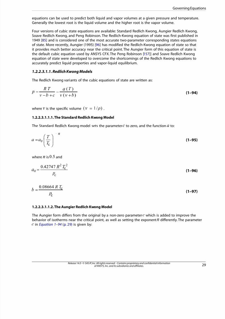
7/16/2019 ANSYS CFX-Solver Theory Guide
http://slidepdf.com/reader/full/ansys-cfx-solver-theory-guide-5633873a6f5ee 45/417
equations can be used to predict both liquid and vapor volumes at a given pressure and temperature.Generally the lowest root is the liquid volume and the higher root is the vapor volume.
Four versions of cubic state equations are available: Standard Redlich Kwong, Aungier Redlich Kwong,Soave Redlich Kwong, and Peng Robinson. The Redlich-Kwong equation of state was first published in1949 [85] and is considered one of the most accurate two-parameter corresponding states equationsof state. More recently, Aungier (1995) [96] has modified the Redlich-Kwong equation of state so thatit provides much better accuracy near the critical point. The Aungier form of this equation of state is
the default cubic equation used by ANSYS CFX. The Peng Robinson [157]] and Soave Redlich Kwongequation of state were developed to overcome the shortcomings of the Redlich Kwong equations toaccurately predict liquid properties and vapor-liquid equilibrium.
1.2.2.3.1.1. Redlich Kwong Models
The Redlich Kwong variants of the cubic equations of state are written as:
(1–94)=− +
−+
¡ ¢
£ ¤ ¥
¦ ¢
£ £ ¤
where§
is the specific volume =¨ ©
.
1.2.2.3.1.1.1. The Standard Redlich Kwong Model
The Standard Redlich Kwong model sets the parameter
to zero, and the function
to:
(1–95)=
−
where
is and
(1–96)=
!
"
"
#
$ $
(1–97)=%
& '
(
)
)
1.2.2.3.1.1.2. The Aungier Redlich Kwong Model
The Aungier form differs from the original by a non-zero parameter0
which is added to improve thebehavior of isotherms near the critical point, as well as setting the exponent 1 differently. The parameter2
in Equation 1–94 (p. 29) is given by:
29Release 14.0 - © SAS IP, Inc. All rights reserved. - Contains proprietary and confidential informationof ANSYS, Inc. and its subsidiaries and affiliates.
Governing Equations

7/16/2019 ANSYS CFX-Solver Theory Guide
http://slidepdf.com/reader/full/ansys-cfx-solver-theory-guide-5633873a6f5ee 46/417
(1–98)=
++ −
+
¡ ¢
£
¤ ¥
¦
§ § ̈
©
©
©
and the standard Redlich Kwong exponent of =
is replaced by a general exponent
. Optimumvalues of
depend on the pure substance. Aungier (1995) [96] presented values for twelve experimentaldata sets to which he provided a best fit polynomial for the temperature exponent
in terms of theacentric factor,
:
(1–99)= + +
1.2.2.3.1.1.3. The Soave Redlich Kwong Model
The Soave Redlich Kwong real gas model was originally published by Soave (1972). The model appliesto non-polar compounds and improves on the original Redlich Kwong model by generalizing the attrac-tion term to depend on the acentric factor, which accounts for molecules being non-spherical, and ac-counting for a range of vapor pressure data in the development of the temperature dependency of this
parameter. The Soave Redlich Kwong equation is explicit in pressure, and given by:
(1–100)=− +
−+
! "
# $ %
& "
# # $
where:
(1–101)='
( )
0
1
1
as in the original Redlich Kwong equation, and
(1–102)=
+
−
2 3 2 4
3
3
5
6
7
where:
(1–103)=8
9 @
A
B
B
C
D
D
and the parameter n is computed as a function of the acentric factor, ω:
Release 14.0 - © SAS IP, Inc. All rights reserved. - Contains proprietary and confidential informationof ANSYS, Inc. and its subsidiaries and affiliates.30
Chapter 1: Basic Solver Capability Theory

7/16/2019 ANSYS CFX-Solver Theory Guide
http://slidepdf.com/reader/full/ansys-cfx-solver-theory-guide-5633873a6f5ee 47/417
(1–104)= + − ¡ ¡
¢
1.2.2.3.1.2. Peng Robinson Model
The Peng Robinson model also gives pressure as a function of temperature and volume:
(1–105)= − − − + £
¤ ¥
¦ §
¨ ¥
¦ § ¦ §
© ©
where:
(1–106)=
as in the original Redlich Kwong equation, and
(1–107)=
+
−
where:
(1–108)=!
" #
$
%
%
&
'
'
and the parameter n is computed as a function of the acentric factor, ω:
(1–109)= + −( ) )
0
1.2.2.3.1.3. Real Gas Constitutive Relations
In order to provide a full description of the gas properties, the flow solver must also calculate enthalpyand entropy. These are evaluated using slight variations on the general relationships for enthalpy andentropy that were presented in the previous section on variable definitions. The variations depend onthe zero pressure, ideal gas, specific heat capacity and derivatives of the equation of state. The zero
pressure specific heat capacity must be supplied to ANSYS CFX while the derivatives are analyticallyevaluated from Equation 1–94 (p. 29)and Equation 1–105 (p. 31).
Internal energy is calculated as a function of temperature and volume (1
,2
) by integrating from the
reference state (3
4 5 6
,7
8 9 @
) along path 'amnc' (see diagram below) to the required state (A
,B
) using the
following differential relationship:
31Release 14.0 - © SAS IP, Inc. All rights reserved. - Contains proprietary and confidential informationof ANSYS, Inc. and its subsidiaries and affiliates.
Governing Equations

7/16/2019 ANSYS CFX-Solver Theory Guide
http://slidepdf.com/reader/full/ansys-cfx-solver-theory-guide-5633873a6f5ee 48/417
(1–110)= +
−
¡ ¢ £ £
¤
£
¤ ¥
¦
¦
First the energy change is calculated at constant temperature from the reference volume to infinitevolume (ideal gas state), then the energy change is evaluated at constant volume using the ideal gas§
̈
. The final integration, also at constant temperature, subtracts the energy change from infinite volume
to the required volume. In integral form, the energy change along this path is:
(1–111)∫ ∫ ∫
− =
−
+ −
−
∞ ∞
© ©
!
" # $
" # $
" # $
Once the internal energy is known, then enthalpy is evaluated from internal energy:
= +% & ' (
The entropy change is similarly evaluated:
Release 14.0 - © SAS IP, Inc. All rights reserved. - Contains proprietary and confidential informationof ANSYS, Inc. and its subsidiaries and affiliates.32
Chapter 1: Basic Solver Capability Theory

7/16/2019 ANSYS CFX-Solver Theory Guide
http://slidepdf.com/reader/full/ansys-cfx-solver-theory-guide-5633873a6f5ee 49/417
(1–112)∫ ∫ ∫
− =
+ −
−
∞ ∞
¡ ¢ ¡ ¢
£ ¤
£ ¡
£ ¢
¥
¡
£ ¡ ¦
¤
¤
£ ¤
£ ¡
£ ¢
§
̈
̈
̈
©
§
̈
where
is the zero pressure ideal gas specific heat capacity. By default, ANSYS CFX uses a 4th orderpolynomial for this and requires that coefficients of that polynomial are available. These coefficientsare tabulated in various references including Poling et al. [84].
In addition, a suitable reference state must be selected to carry out the integrations. The selection of this state is arbitrary, and can be set by the user, but by default, ANSYS CFX uses the normal boilingtemperature (which is provided) as the reference temperature and the reference pressure is set to thevalue of the vapor pressure evaluated using Equation 1–118 (p. 34) at the normal boiling point. Thereference enthalpy and entropy are set to zero at this point by default, but can also be overridden if desired.
Other properties, such as the specific heat capacity at constant volume, can be evaluated from the in-
ternal energy. For example, the Redlich Kwong model uses:
(1–113)=
∂∂
=
∂∂
−+
+
!
"
#
"
#
$ $ %
& #
&
'
(
(
)
where0
1
is the ideal gas portion of the internal energy:
(1–114)∫ = − = −2 2 2 3 4 5 6 4
7
7
8 9 @ A B C
D E F
specific heat capacity at constant pressure, G
H
, is calculated from I
P
using:
(1–115)= +Q Q R S
T
U
V W
X
where Y
and ̀
are the volume expansivity and isothermal compressibility, respectively. These two values
are functions of derivatives of the equation of state and are given by:
33Release 14.0 - © SAS IP, Inc. All rights reserved. - Contains proprietary and confidential informationof ANSYS, Inc. and its subsidiaries and affiliates.
Governing Equations

7/16/2019 ANSYS CFX-Solver Theory Guide
http://slidepdf.com/reader/full/ansys-cfx-solver-theory-guide-5633873a6f5ee 50/417
(1–116)= −
∂∂∂∂
¡
¢
£
¤
¢
¤
£
(1–117)
= −∂∂
¥
¦
§
̈
©
1.2.2.3.2. Real Gas Saturated Vapor Properties
When running calculations with liquid condensing out of the vapor (equilibrium phase change or Eu-lerian thermal phase change model) or dry calculations, the flow solver needs to know the form of thevapor pressure curve. Pressure and temperature are not independent in the saturation dome, so vaporsaturation properties are evaluated by first assuming an equation that gives the dependence of vaporpressure on temperature, and then substituting that into the equation of state.
For materials that use the cubic equations of state ANSYS CFX approximates the vapor pressure curveusing a form given by Poling et al. [84]:
(1–118)
= +
−
Vapor saturation properties are calculated by evaluating the equation of state and constitutive relationsalong the saturation curve.
1.2.2.3.3. Real Gas Liquid Properties
As previously mentioned, it is possible to derive liquid densities directly from the cubic state equations,however, this is not always desirable. For example, the Redlich Kwong models are very inaccurate, andsometimes completely wrong, in the compressed liquid regime.
Instead, when you select to use one of the Redlich Kwong variants for a liquid, the properties are assumedto vary along the vapor pressure curve as a function of saturation temperature. These properties areapproximate and should only be used when the amount of liquid in your calculation will be small. Forexample, they work well with the equilibrium condensation model or non-equilibrium small dropletphase change model.
To derive the liquid enthalpy and entropy, such that they are completely consistent with the gas phase,
requires all the same data as is provided for the gas phase: the critical point data, the acentric factorand the zero pressure specific heat coefficients.
To calculate saturated liquid densities, an alternative equation of state originally published by Yamadaand Gunn (1973), is used by CFX that gives liquid specific volume as a function of temperature:
Release 14.0 - © SAS IP, Inc. All rights reserved. - Contains proprietary and confidential informationof ANSYS, Inc. and its subsidiaries and affiliates.34
Chapter 1: Basic Solver Capability Theory

7/16/2019 ANSYS CFX-Solver Theory Guide
http://slidepdf.com/reader/full/ansys-cfx-solver-theory-guide-5633873a6f5ee 51/417
(1–119)= − − ¡
¢ ¢
£
¤ ¥
¦
§ ¨ ©
This equation is convenient because it only requires knowledge of the critical volume and temperature
as well as the acentric factor. The valid temperature range for the liquid equation of state is 0.4
<
< 0.99
. The solver will clip the temperature used in this equation to that range.
Saturated liquid enthalpy is calculated using knowledge of the gas saturation enthalpy and the followingequation:
(1–120)= −
where the enthalpy of vaporization,
! "
, is given by the following expression taken from Poling et al.
[84]:
(1–121)=
−
+
−
#
$ %
%
%
&
%
%
' (
) )
0 1 2 3 4
)
0 1 4 3 5
Saturated liquid entropy can easily be derived using the second law and the gas saturation entropy:
(1–122)= −6 6
7
8
9 @
9 @
Prediction of liquid specific heat capacity with the Redlich Kwong equation has a similar problem tothe liquid density, so ANSYS CFX uses an alternative form presented by Aungier (2000):
(1–123)= +
+
−
+
−
−
A A B
C
C
C
C
D D E
F F
G H
which requires knowledge of the zero pressure heat capacity coefficients, as well as the acentric factor.For the saturated liquid it is assumed that =I I
P Q
.
Note that the use either of the Redlich Kwong models for flows of almost entirely pure liquid is highlydiscouraged. If you want to use one of the cubic equations of state for this type of problem, then use
the Peng Robinson equation of state which, by default, will force the liquid phase properties to be de-pendent on temperature and pressure fully consistent with that equation of state.
1.2.2.3.4. IAPWS Equation of State
The IAPWS-IF97 database represents an accurate equation of state for water and steam properties. Thedatabase is fully described elsewhere [125], but a summary will be provided in this section. The IAPWSdatabase uses formulations for five distinct thermodynamic regions for water and steam, namely:
• subcooled water (1)
• supercritical water/steam (2)
35Release 14.0 - © SAS IP, Inc. All rights reserved. - Contains proprietary and confidential informationof ANSYS, Inc. and its subsidiaries and affiliates.
Governing Equations

7/16/2019 ANSYS CFX-Solver Theory Guide
http://slidepdf.com/reader/full/ansys-cfx-solver-theory-guide-5633873a6f5ee 52/417
• superheated steam (3)
• saturation data (4)
• high temperature steam (5)
Figure 1.1 Regions and Equations of IAPWS-IF97
Region 5 has not been implemented in ANSYS CFX because it represents a thermodynamic space atvery high temperatures (1073.15 - 2273.15 K) and reasonably low pressures (0-10 MPa) that can be ad-equately described using other property databases already in ANSYS CFX (that is, Ideal Gas EOS withNASA specific heat and enthalpy). Furthermore, because this region is not defined for pressures up to
100 MPa, as is the case for regions 1, 2 and 3, problems arise in filling out the pressure-temperaturespace in the tables when temperatures exceed 1073.15 K and pressures exceed 10 MPa. The databaseimplemented in CFX therefore covers temperatures ranging from 273.15 to 1073.15 K and pressuresranging from 611 Pa to 100 MPa.
The reference state for the IAPWS library is the triple point of water. Internal energy, entropy and enthalpyare all set to zero at this point.
Tref = 273.16 K, Pref = 611.657 Pa, uliquid = 0 J/kg, sliquid = 0 J/kg/K, hliquid = 0 J/kg
In ANSYS CFX, the analytical equation of state is used to transfer properties into tabular form, whichcan be evaluated efficiently in a CFD calculation. These IAPWS tables are defined in terms of pressure
and temperature, which are then inverted to evaluate states in terms of other property combinations(such as pressure/enthalpy or entropy/enthalpy). When developing the IAPWS database for ANSYS CFX,therefore, properties must be evaluated as functions of pressure and temperature. For the most part,this involves a straightforward implementation of the equations described in the IAPWS theory [ 125].Region 4 involves saturation data that uses only pressure or temperature information.
However, some difficulties are encountered when evaluating the properties around Region 3 (near thecritical point), where the EOS is defined explicitly in terms of density and temperature. In this region,the density must be evaluated using Newton-Raphson iteration. This algorithm is further complicatedin that the EOS is applicable on both the subcooled liquid and superheated vapor side leading up to
Release 14.0 - © SAS IP, Inc. All rights reserved. - Contains proprietary and confidential informationof ANSYS, Inc. and its subsidiaries and affiliates.36
Chapter 1: Basic Solver Capability Theory

7/16/2019 ANSYS CFX-Solver Theory Guide
http://slidepdf.com/reader/full/ansys-cfx-solver-theory-guide-5633873a6f5ee 53/417
critical conditions. Therefore, depending on the pressure-temperature state, one may be evaluating asubcooled liquid or a superheated vapor with the same EOS. To apply the Newton-Raphson scheme ina reliable way, one must detect on which side of the saturation dome the pressure-temperature stateapplies, and apply an appropriate initial guess. Such an iteration scheme, including logic for an initialguess, has been implemented in ANSYS CFX so that table generation around the critical region is possible.
1.2.2.3.5. Metastable Superheated Liquid/Supercooled Vapor States
The IAPWS library also extends to metastable states, so that this equation of state is available for non-equilibrium phase change models such as the Droplet Condensation Model. The EOS for regions 1 and3 in Figure 1.1 (p. 36) are stated to have reasonable accuracy for metastable states close to the saturationline d liquid states [125]. However, the term “reasonable” is not quantified, and therefore the degreeto which the extrapolation of the EOS can be applied is unknown.
In region 2, an additional set of equations have been developed for supercooled vapor conditions under10 MPa. These equations have been tuned to match the saturation data. Above 10 MPa, the EOS forthe superheated region can safely be extrapolated into supercooled conditions, but it does not matchsmoothly with the specialized supercooled equations below 10 MPa.
1.2.2.3.6. Numerical Testing to Delineate Metastable Regions
In order to make the IAPWS database as robust as possible, numerical testing has been done to determineapproximate metastable vapor/liquid spinodal lines. Figure 1.2 (p. 37) is given to demonstrate thesespinodal lines that are essentially boundaries up to which metastable conditions can exist. These wouldbe defined similar to saturation curves as functions of either temperature or pressure. The IAPWSdatabase tables are always generated up to these limits regardless of what flow models are specified(equilibrium or non-equilibrium) and thus allow non-equilibrium phase change models to be applied.
Figure 1.2 Spinodal Limits Built into Tables
1.2.2.3.7.The Acentric Factor
The acentric factor must be supplied when running the real gas models and is tabulated for manycommon fluids in Poling et al. [84]. If you do not know the acentric factor, or it is not printed in acommon reference, it can be estimated using knowledge of the critical point and the vapor pressurecurve with this formula:
37Release 14.0 - © SAS IP, Inc. All rights reserved. - Contains proprietary and confidential informationof ANSYS, Inc. and its subsidiaries and affiliates.
Governing Equations

7/16/2019 ANSYS CFX-Solver Theory Guide
http://slidepdf.com/reader/full/ansys-cfx-solver-theory-guide-5633873a6f5ee 54/417
(1–124)= −
−
¡
¡
¢ £
¤
¥
where the vapor pressure, ¦
§
, is calculated at =¨ ̈
©
. In addition to the critical point pressure, this
formula requires knowledge of the vapor pressure as a function of temperature.
1.2.2.4. General Equation of State
User-defined equations of state are also supported:
=
=
Noting that:
= −∂∂
∂∂
!
"
!
where =# $
,
the equation of state for enthalpy therefore follows as:
(1–125)= +
−∂∂
% & ' % ( ) (
)
(
% 0
1
1
2
Note, however, that user-defined expressions for 3
and4
5 must be thermodynamically consistent.Consistency requires that mathematical properties for exact differentials be satisfied. For example,
suppose6 7 8 9
is an exact differential defined as:
= +@ A B C D @ B E @ C
= ∂∂
F
G
H
I
= ∂∂
P
Q
R
S
Consistency then requires that:
=∂∂
∂∂
T
U
V
W
V
U
Applying this concept to Equation 1–125 (p. 38), it therefore follows that general equations of statemust obey:
Release 14.0 - © SAS IP, Inc. All rights reserved. - Contains proprietary and confidential informationof ANSYS, Inc. and its subsidiaries and affiliates.38
Chapter 1: Basic Solver Capability Theory

7/16/2019 ANSYS CFX-Solver Theory Guide
http://slidepdf.com/reader/full/ansys-cfx-solver-theory-guide-5633873a6f5ee 55/417
=
−
∂
∂∂
∂∂∂
¡
¢
£ ¤
¥
¤
£
¦
1.2.3. Conjugate Heat Transfer
CFX enables you to create solid regions in which the equations for heat transfer are solved, but withno flow. This is known as conjugate heat transfer , and the solid regions are known as solid domains.
Within solid domains, the conservation of energy equation can account for heat transport due to solidmotion, conduction, and volumetric heat sources:
(1–126)∂
∂+ ∇ ⋅ = ∇ ⋅ ∇ +§
̈ ©
̈ ©
where , , and are the enthalpy, density, and thermal conductivity of the solid, respectively.
is
the solid velocity, if specified, and
!
is an optional volumetric heat source. The solid motion advection
term (the term including"
#
) is optional and is added only when a solid motion velocity is set.
Additional information on plotting variables at a solid-fluid interface is available in Solid-Fluid InterfaceVariable Values in the CFX Reference Guide.
1.3. Buoyancy
For buoyancy calculations, a source term is added to the momentum equations as follows:
(1–127)= −$ % % &
' ( ) 0 1 2
3 4 5
The density difference − 6 6
7 8 9 is evaluated using either the Full Buoyancy model or the Boussinesqmodel, depending on the physics.
When buoyancy is activated, the pressure in the momentum equation excludes the hydrostatic gradientdue to
@
A B C
. This pressure is related to the absolute pressure as follows:
(1–128)= + + − D D D E F G G
H I P Q R S Q R S
Q R S
where T
U V W
is a reference location. The buoyancy reference location option is set under the Ref.
Location option in CFX-Pre and can be set to a particular location. For details, see Buoyancy and
Pressure.
Absolute pressure is used to evaluate fluid properties that are functions of pressure; it can be visualizedin CFD-Post.
1.3.1. Full Buoyancy Model
For buoyancy calculations involving variable density, − X X
Y ` a
is evaluated directly. This option is set
automatically when the simulation involves multicomponent flow, multiphase flow, or a fluid havingdensity set as a function of pressure, temperature, or other field variables.
39Release 14.0 - © SAS IP, Inc. All rights reserved. - Contains proprietary and confidential informationof ANSYS, Inc. and its subsidiaries and affiliates.
Buoyancy

7/16/2019 ANSYS CFX-Solver Theory Guide
http://slidepdf.com/reader/full/ansys-cfx-solver-theory-guide-5633873a6f5ee 56/417
1.3.2. Boussinesq Model
For buoyant flows where the density variation is driven only by small temperature variations, theBoussinesq model is used. In this model, a constant reference density
¡ ¢ £
is used for all terms other
than the buoyancy source term. The buoyancy source term is approximated as:
(1–129)− = − − ¤ ¤ ¤ ¥ ¦ ¦
§ ¨ © § ¨ ©
§ ¨ ©
where is the thermal expansivity:
(1–130)= −∂∂
and
is the buoyancy reference temperature.
1.4. Immersed Solids
The following topics are discussed:1.4.1. Immersed Solid Boundary Details1.4.2. Laminar Flow Treatment1.4.3.Turbulent Flow Treatment
1.4.1. Immersed Solid Boundary Details
This section describes notation used in the following sections pertaining to immersed solids.
Release 14.0 - © SAS IP, Inc. All rights reserved. - Contains proprietary and confidential informationof ANSYS, Inc. and its subsidiaries and affiliates.40
Chapter 1: Basic Solver Capability Theory

7/16/2019 ANSYS CFX-Solver Theory Guide
http://slidepdf.com/reader/full/ansys-cfx-solver-theory-guide-5633873a6f5ee 57/417
Figure 1.3 Notation for Nodes Near the Immersed Solid Boundary
Figure 1.3 (p. 41) shows a schematic diagram of an immersed solid boundary (shown as a red line). Thenodes and points near the boundary are labeled for reference in the following sections. The meaningof each label is tabulated below.
MeaningLabel
in-wall nodeIWin-wall pointIW′
near-wall nodeNW
point on the immersed solid boundaryIB
fluid nodeFL
fluid pointFL′
In the figure, the orange arrow represents the wall normal direction corresponding to the given NWnode.
Other notes about notation:
• “NIBG” elements are elements between corresponding NW and IW nodes. These are elements whichthe immersed solid surface cuts through, and are colored blue in the figure above.
• “NIBF” elements are elements between corresponding FL and NW nodes. These are elements which arimmediately adjacent to the “NIBG” elements and are colored white in the figure above.
•
is the wall distance between the NW node and the IB point along the wall normal direction.
• ¡
¢ £ ¤ ¥
is the wall distance between the NW node and the IW ′ point.
41Release 14.0 - © SAS IP, Inc. All rights reserved. - Contains proprietary and confidential informationof ANSYS, Inc. and its subsidiaries and affiliates.
Immersed Solids

7/16/2019 ANSYS CFX-Solver Theory Guide
http://slidepdf.com/reader/full/ansys-cfx-solver-theory-guide-5633873a6f5ee 58/417
•
¡ ¢ £ ¤
is the wall distance between the FL′ point and the NW node.
1.4.2. Laminar Flow Treatment
For laminar flows, no wall scale equation is solved. Instead, the velocity near the immersed boundaryis computed based on the wall distance, assuming constant wall shear in the boundary profile region.
The tangential fluid velocity at the near-wall fluid nodes is governed by:
(1–131)= +
+−
¥
¥
¦
¦
§
§ §
¥ ¥
̈ ©
̈ © ¨
where
! "
#
$ % & '
is the tangential component of the forcing velocity at the NW node, (
) 0
is
the dynamic viscosity at the NW node,1
2 3
and 4
5 6
are, respectively, the fluid velocity and dynamic
viscosity at the FL node, and 7
8 9 @ A
is the distance between the corresponding FL′ point and NW
node. Note that + B B
C D E F
is essentially the normal distance between this node and the
immersed boundary.
The normal component of the forcing velocity at the NW node is computed as the normal componentof the velocity at the IB point on the immersed boundary:
G
H I
H P Q
R S T U
The fluid velocity at the near-wall nodes is forced to be:
(1–132)= +V V V
W X
Y
̀ a
̀ b c
W d e f
W X
Y
g h i p
In this way, the velocity field is forced to flow around the immersed boundary to avoid (or alleviate)the problem of streamlines penetrating the immersed solid.
1.4.3.Turbulent Flow Treatment
For moving immersed solids or high Reynolds number turbulence cases, it is usually not possible togenerate a fine mesh that resolves the laminar sub-layer. Hence, wall functions are used for fluid elements
near the immersed boundary. The implementation of wall functions for immersed solids is more com-plicated than for wall functions near regular walls because of the non-uniform wall distance for elementsnext to the immersed boundary.
1.4.3.1. Wall Distance
For fluid nodes that are inside the immersed solid, the wall distance is set to zero. For fluid nodes nearthe immersed solid, the wall distance is computed as a function of the wall scales. The wall scales areset algebraically to zero for fluid nodes inside the immersed solid, but the shape of the immersedboundary is not properly taken into account for the wall scale equation.
Release 14.0 - © SAS IP, Inc. All rights reserved. - Contains proprietary and confidential informationof ANSYS, Inc. and its subsidiaries and affiliates.42
Chapter 1: Basic Solver Capability Theory

7/16/2019 ANSYS CFX-Solver Theory Guide
http://slidepdf.com/reader/full/ansys-cfx-solver-theory-guide-5633873a6f5ee 59/417
For the near-immersed-boundary nodes, the physical distance from the immersed boundary trackingmethod is used to implement the turbulent wall functions.
1.4.3.2. SST Model
The wall distance from the modified wall scale equation is used to compute the two blending factors. The production and dissipation terms inside the immersed solid are reset to zero for both the turbulentkinetic energy equation and turbulent frequency equation. This way, the turbulent kinetic energy andturbulent frequency will be solved without any source terms and solutions will serve as a natural con-dition for the fluid turbulence equations.
In the SST turbulence model, the turbulent eddy viscosity is computed from the turbulent kinetic energyand turbulent frequency:
(1–133)= ¡ ¢ £
¤
1.4.3.3. Scalable Wall Function
In general, it is impractical (if not impossible) to have a mesh which resolves the sublayer, and therefore,it is necessary to specify¥
¦ § ¨ ̈
taking account of the logarithmic region.
(1–134)=∗
∗©
!
(1–135)=∗" # $
%
& ' ( & ' )
(1–136)=∗ ∗ 0 1 0 2
(1–137)=+
=∗ +3
4
5 6 7
4
3
8
9 @ A
(1–138)= ∗B C D D
E F G H H
Here, I is the fluid tangential velocity relative to the immersed boundary, and P is computed as
the distance from the near-immersed-solid nodes to the immersed boundary. In the scalable wallfunction, the lower value of
∗ Q
is limited to 11.06 at the intersection between the logarithmic and the
linear near wall profile.
Further, the velocity at the NW nodes is forced according to the wall function:
43Release 14.0 - © SAS IP, Inc. All rights reserved. - Contains proprietary and confidential informationof ANSYS, Inc. and its subsidiaries and affiliates.
Immersed Solids

7/16/2019 ANSYS CFX-Solver Theory Guide
http://slidepdf.com/reader/full/ansys-cfx-solver-theory-guide-5633873a6f5ee 60/417
(1–139)= +
−
+
+
¡ ¡
¡ ¡
¢ £
¤
¥ ¦ § ̈
©
©
¥ ¦ § ̈
¤
¢ £
¤
¥ ¦ § ̈
©
©
¥ ¦ § ̈
Similar to the case of laminar flow, the tangential velocity on the NW nodes is enforced according to
equation Equation 1–139 (p. 44) and the momentum source term is computed taking into account boththe wall normal velocity and tangential forcing velocity:
(1–140)= +
!
" # $
% & ' (
In this way, the velocity field will be forced to flow around the immersed boundary to avoid (or alleviate)the problem of streamlines penetrating the immersed solid.
1.5. Multicomponent Flow
The following topics will be discussed:• Multicomponent Notation (p. 44)
• Scalar Transport Equation (p. 44)
• Algebraic Equation for Components (p. 46)
• Constraint Equation for Components (p. 46)
• Multicomponent Fluid Properties (p. 47)
• Energy Equation (p. 48)
• Multicomponent Energy Diffusion (p. 49)
1.5.1. Multicomponent Notation
Components are denoted using capital letters , , , etc. In general, a quantity subscribed with , ,
, and so on, refers to the value of the quantity corresponding to , , , etc. For example, the density
( )
) of component would be written 0
1
.
1.5.2. Scalar Transport Equation
For a multicomponent fluid, scalar transport equations are solved for velocity, pressure, temperatureand other quantities of the fluid. For details, see Governing Equations (p. 25). However, additionalequations must be solved to determine how the components of the fluid are transported within the
fluid.
The bulk motion of the fluid is modeled using single velocity, pressure, temperature and turbulencefields. The influence of the multiple components is felt only through property variation by virtue of differing properties for the various components. Each component has its' own equation for conservationof mass. After Reynolds-averaging (see Turbulence Models (p. 89)) this equation can be expressed intensor notation as:
Release 14.0 - © SAS IP, Inc. All rights reserved. - Contains proprietary and confidential informationof ANSYS, Inc. and its subsidiaries and affiliates.44
Chapter 1: Basic Solver Capability Theory

7/16/2019 ANSYS CFX-Solver Theory Guide
http://slidepdf.com/reader/full/ansys-cfx-solver-theory-guide-5633873a6f5ee 61/417
(1–141)
∂∂
+∂
∂
= −∂
∂− − ″ ″ +
∼ ∼ ∼
∼ ∼
¡
¢
¡
£
£
¡ ¡ ¤
¥
¥
¦
¦
¦
¥
¥ ¦ ¦
¥
¦ ¥
where:
∼ §
̈
is the mass-average density of fluid component©
in the mixture, that is, the mass of the component
per unit volume,
∑=∼ ∼ ∼
is the mass-average velocity field,
∼
is the mass-average velocity of fluid component
,
−∼ ∼
! ! is the relative mass flux,
"
#
is the source term for component$
which includes the effects of chemical reactions.
Note that if all the terms in the expanded form of Equation 1–141 (p. 45) are summed over all compon-ents, the result is the standard continuity equation,
(1–142)∂∂
+∂
∂=
∼%
&
'
&
(
)
)
because the reaction rates0
1
must sum to zero.
The relative mass flux term accounts for differential motion of the individual components. This termmay be modeled in a number of ways to include effects of concentration gradients, a pressure gradient,external forces or a temperature gradient. Of these possible sources of relative motion among themixture components, the primary effect is that of concentration gradient. The model for this effect givesrise to a diffusion-like term in Equation 1–141 (p. 45).
(1–143)− = −∂∂
∼ ∼∼
2 2 3
4
3
3
5
6
6 7 7
6
6
7
The molecular diffusion coefficient, 8
9
, is assumed to be equal to @ A
B
, where C
D
is the Kinematic
Diffusivity set on the Fluid Models tab for a domain in CFX-Pre. For details, see Fluid Models Tab inthe CFX-Pre User's Guide. A detailed description of the effects of the relative mass flux term and variousmodels for it may be found in reference [29].
Now, define the mass fraction of componentE
to be:
45Release 14.0 - © SAS IP, Inc. All rights reserved. - Contains proprietary and confidential informationof ANSYS, Inc. and its subsidiaries and affiliates.
Multicomponent Flow

7/16/2019 ANSYS CFX-Solver Theory Guide
http://slidepdf.com/reader/full/ansys-cfx-solver-theory-guide-5633873a6f5ee 62/417
(1–144)=∼
∼
¡
¡
¢
¢
Note that, by definition, the sum of component mass fractions over all components is 1. SubstitutingEquation 1–144 (p. 46) and Equation 1–143 (p. 45) into Equation 1–141 (p. 45), you have:
(1–145)
∂∂
+ ∂∂
=∂
∂
∂∂
−
∂∂
″ ″ +
∼ ∼ ∼
∼
£
£
¤ ¥
¦
¤ ¥
§
§
̈
¥
§ §
¤ ¥ ©
The turbulent scalar fluxes are modeled using the eddy dissipation assumption as:
(1–146)− ″ ″ =∂∂
∼
!
!
where " #
$
is the turbulent Schmidt number. Substituting Equation 1–146 (p. 46) into Equa-
tion 1–145 (p. 46) and assuming now that you have mass weighted averages of %
&
:
(1–147)∂
∂+
∂
∂=
∂∂
∂∂
+
∼ ∼ ∼'
( )
0
( )
1 1
2
)
1
3
4
5 4
5 5
4
4
5
4
6 7 7
where:
(1–148)= + 8 8
9
@ A
B B
C
C
D E E
Equation 1–147 (p. 46) is simply a general advection-diffusion equation of the form common to theequations solved for each of the other dependent variables in the fluid flow calculation. Thus, it is
convenient to solve for the F
G
in order to establish the composition of the fluid mixture.
1.5.3. Algebraic Equation for Components
The specified equation is used to calculate the component mass fraction throughout the solution domain.
1.5.4. Constraint Equation for Components
The CFX-Solver solves − H
I
mass fraction equations (either transport equations or algebraic equations)
for all but one of the components. The remaining component is known as the constraint componentbecause its mass fraction is determined by the constraint equation:
Release 14.0 - © SAS IP, Inc. All rights reserved. - Contains proprietary and confidential informationof ANSYS, Inc. and its subsidiaries and affiliates.46
Chapter 1: Basic Solver Capability Theory

7/16/2019 ANSYS CFX-Solver Theory Guide
http://slidepdf.com/reader/full/ansys-cfx-solver-theory-guide-5633873a6f5ee 63/417
(1–149)∑ == …
¡ ¢ £ ¤
¥
¡
¦ ¦ ¦
§
The performance of the CFX-Solver will not be affected by your choice of constraint component.
1.5.5. Multicomponent Fluid Properties The physical properties of general multicomponent mixtures are difficult to specify. The default treatmentin ANSYS CFX 14.0 makes the assumption that the components form an ideal mixture. For details, seeIdeal Mixture in the CFX-Solver Modeling Guide.
Now consider a given volume ̈
of the fluid mixture. Let ©
be the mass of component
present in
this volume, then =
.The partial volume of component
is defined to be the volume,
, that
would be occupied by the given mass of the component at the same (local) temperature and pressureas the mixture. The “thermodynamic density” of the component, which results from evaluating its
equation of state at the mixture temperature and pressure, may be expressed as = !
"
" "
. Because
the partial volumes of all components must sum to the total volume,#
, you have:
(1–150)
∑ ∑
∑ ∑
= =
= =
= … = …
= … = …
$
$
% &
% &
&
&
& '
&
( ) 0
1
(
( ) 0
1
(
(
(
(
( ) 0
1
(
(
( ) 0
1
(
(
2 2
2 2
3 3
3 3
or:
(1–151)∑== … 4
5
4
6 7 8
9
6
6
@
A
Thus, the mixture density may be calculated from the mass fractions B
C
and the thermodynamic density
of each component, which may require knowledge of the mixture temperature and pressure, as wellas an appropriate equation of state for each component.
Note carefully the distinction between D
E
and F
G
. The component mass density, H
I
, is a quantity
relating to the composition of the mixture, while the thermodynamic density, P
Q
, is a material
property of the component.
An arbitrary constitutive fluid property may be calculated from:
47Release 14.0 - © SAS IP, Inc. All rights reserved. - Contains proprietary and confidential informationof ANSYS, Inc. and its subsidiaries and affiliates.
Multicomponent Flow

7/16/2019 ANSYS CFX-Solver Theory Guide
http://slidepdf.com/reader/full/ansys-cfx-solver-theory-guide-5633873a6f5ee 64/417
(1–152)∑== …
¡
¢ £ ¤
¥
¢ ¢
¦
§
where ̈
©
is the property value for fluid component
. While it may appear anomalous at first sight that
density does not conform to this expression, thespecific volume
(volume per unit mass, that is,
)does indeed conform, as can be seen by considering Equation 1–152 (p. 48). Properties that may beevaluated for a multicomponent mixture using Equation 1–152 (p. 48) include the laminar viscosity
,
the specific heat at constant volume
, the specific heat at constant pressure
, and the laminar
thermal conductivity
.
1.5.6. Energy Equation
Recall that Equation 2–5 (p. 91) is the Reynolds-averaged conservation equation for energy of a singlecomponent fluid. Extending this equation for multicomponent fluids involves adding an additional dif-fusion term to the energy equation:
(1–153)∑∂∂
∂∂
!
"
#
$
%
$ $
$
#
&
For turbulent flow, this term is Reynolds-averaged (see Turbulence Models (p. 89)) giving:
(1–154)∑∂
∂
+ ″ + ″
∂ + ″
∂
∼ ∼∼
'
( ( ) )
0 0
'
1
2
3
2 2 2 2
2 2
1
4
This expression introduces several terms involving the fluctuations of diffusion coefficient, componententhalpy and species concentration. Under certain circumstances, the fluctuating components couldbe an important component of the diffusion process. However, adequate models are not availablewithin the existing turbulence model to account for these effects. Thus, only the mean component isretained in the current version of ANSYS CFX.
The implemented conservation of energy equation for multicomponent fluids involves only mean
scalar components and is expressed as:
Release 14.0 - © SAS IP, Inc. All rights reserved. - Contains proprietary and confidential informationof ANSYS, Inc. and its subsidiaries and affiliates.48
Chapter 1: Basic Solver Capability Theory

7/16/2019 ANSYS CFX-Solver Theory Guide
http://slidepdf.com/reader/full/ansys-cfx-solver-theory-guide-5633873a6f5ee 65/417
(1–155)
∑
∂∂
−∂∂
+∂
∂
=∂
∂
∂∂
+∂∂
+∂∂
+
¡
¢ £
¤
¡ ¥
¢ £
¥
¦
§
¥
̈ ©
¥
¤
©
¥
1.5.7. Multicomponent Energy Diffusion
The energy equation can be simplified in the special case that all species diffusivities are the same andequal to thermal conductivity divided by specific heat capacity,
(1–156)= =
!
"
#
$
Equation 1–156 (p. 49) holds when the Lewis number is unity for all components: = = % & ' ( )
0 1 0
.
For turbulent flow, assuming = 2 3
4
for all components is usually just as good as the common practice
of using the fluid viscosity for the default component diffusivity (unity Schmidt number, = =5 6 7 8
9 9
).
For = @ A
B
, the energy equation (Equation 1–155 (p. 49)) simplifies exactly to the following:
(1–157)∂∂
−∂∂
+∂
∂=
∂∂
+
∂∂
+C
D
E F
G
D H
E F
H
I
P
Q
R
H
S
T
T
T U T
V
W
W
Equation 1–157 (p. 49) has the advantage that only a single diffusion term needs to be assembled, ratherthan one for each component plus one for heat conduction. This can significantly reduce numericalcost, in particular when the fluid consists of a large number of components.
When component-dependent turbulent Schmidt numbers are specified, the turbulent energy flux needsto be generalized. This is achieved by splitting the turbulent fluctuation of enthalpy into the contributionsfrom temperature fluctuation, pressure fluctuation and fluctuations of component mass fractions:
(1–158)∑≈ +∂∂
+ ″=
X Y ̀
X
a
a X b
c c
d
c c c c
e
f
e e
g
h
Using this transformation, the turbulent energy flux can be modeled by applying the eddy diffusivitymodel with turbulent Prandtl number to the temperature fluctuations plus the sum of the secondaryenthalpy transport terms derived from the component mass fluxes:
49Release 14.0 - © SAS IP, Inc. All rights reserved. - Contains proprietary and confidential informationof ANSYS, Inc. and its subsidiaries and affiliates.
Multicomponent Flow

7/16/2019 ANSYS CFX-Solver Theory Guide
http://slidepdf.com/reader/full/ansys-cfx-solver-theory-guide-5633873a6f5ee 66/417
(1–159)∑− ≈ − ′′
′′ +∂∂
′′ + ′′
=
¡ ¢ ¡ £ ¤
¢
¥
¦ ¢ §
̈ ¨ ©
(1–160)∑− ≈ − ′′ ′′ − ∂∂
′′ ′′ − ′′ ′′=
!
" # " "
$
%
$ " $
&
'
(1–161)∑− ≈∂∂
+
∂∂
∂∂
−
′′ ′′
=
( ) 0 1
2
3 4
5
6
0
3
2
3 4
3
6
0 ( ) 7
8 9
@
@ 8
@
@ 8
A
B
A 8 A
C
D
Inserting the eddy diffusivity model for the turbulent component mass fluxes yields the followingmodel for the turbulent enthalpy flux:
(1–162)∑− ≈∂∂
+
∂∂
∂∂
+
∂∂
=
E F G H
I
P Q
R
S
G
P
I
P Q
P
S
G
I
T U
V
S
W X
Y
Y W
Y
Y W
̀
a
̀
Y
Y ̀
̀
W
b
c
d
The previous relation is equivalent to the eddy diffusivity model applied to enthalpy and generalized
for different e f
g
andh i
p q r
, as can be derived by expanding the enthalpy gradient term according to
the chain rule =s s t u v
w
:
(1–163)∑− ≈∂∂
=
∂∂
∂∂
+∂∂
∂∂
+∂∂
∂∂
=
x y
(1–164)∑− ≈
∂∂
+
∂∂
∂∂
+∂∂
=
j
k
j
j
l
m
(1–165)∑− ≈∂∂
+
∂∂
∂∂
+
∂∂
=
n o
z
z
z
z
{
|
{
z
z
{
}
~
Using the above relations, the energy equation for generalized turbulent component transport becomes:
Release 14.0 - © SAS IP, Inc. All rights reserved. - Contains proprietary and confidential informationof ANSYS, Inc. and its subsidiaries and affiliates.50
Chapter 1: Basic Solver Capability Theory

7/16/2019 ANSYS CFX-Solver Theory Guide
http://slidepdf.com/reader/full/ansys-cfx-solver-theory-guide-5633873a6f5ee 67/417
(1–166)∑
∂∂
−∂∂
+∂
∂
=∂
∂
+
∂∂
+
∂∂
∂∂
+
∂∂
− ′′ ′′
+=
¡ ¢
£
¤
¡ ¥ ¢
¤
¦ §
̈
£ ©
¤
£
̈
£ ©
£
¤
¤
¡
!
"
#
And for the special case that the eddy diffusivity assumption is used for modelling the turbulent massflux for each component:
(1–167)∑
∂∂
−∂∂
+∂
∂
=∂
∂
+
∂∂
+
∂∂
∂∂
+
+
∂∂
+=
$
% &
'
$ (
% ) &
(
0 1
2
' 3
4
(
5
'
2
' 3
'
(
5
2
6 7
8
(
6
9
@
@
A
B
B
@
B
B
@
C
D
C C
B
B C
C
@
E
F
G
H
For the Thermal Energy heat transfer model the pressure gradients are assumed to be small comparedto the other terms, and the corresponding terms are neglected from the equation.
1.6. Additional Variables
There are several types of Additional Variable equations supported by CFX-Solver:
• Transport Equations for Additional Variables (p. 51)
• Diffusive Transport Equations for Additional Variables (p. 52)• Poisson Equations for Additional Variables (p. 52)
• Algebraic Equations for Additional Variables (p. 53)
1.6.1.Transport Equations for Additional Variables
The general form of the transport equation for an Additional Variable is:
(1–168)∂
∂+ ∇ = ∇ ∇ +
I
P Q
R
P Q P S Q T
U V
where:
•W
is the fluid velocity in the case of a fluid or porous domain, or ≡X X
Y
in the case of a solid domain
with a specified solid motion velocity, where ̀
a
is the solid velocity.
• b
is the mixture density, mass per unit volume
• c is the conserved quantity per unit volume, or concentration
• =d e f
is the conserved quantity per unit mass
51Release 14.0 - © SAS IP, Inc. All rights reserved. - Contains proprietary and confidential informationof ANSYS, Inc. and its subsidiaries and affiliates.
Additional Variables
7/16/2019 ANSYS CFX-Solver Theory Guide
http://slidepdf.com/reader/full/ansys-cfx-solver-theory-guide-5633873a6f5ee 68/417
•
¡
is a volumetric source term, with units of conserved quantity per unit volume per unit time
• ¢
£
is the kinematic diffusivity for the scalar
For turbulent flow, this equation is Reynolds-averaged (see Turbulence Models (p. 89)) and becomes:
(1–169)∂
∂+ ∇ = ∇
+
∇
+¤
¥ ¦
§
¥ ¦ ¥ ̈
©
¦
where:
•
is the turbulence Schmidt number
•
is the turbulence viscosity
1.6.2. Diffusive Transport Equations for Additional Variables
The general form of the diffusive transport equation for an Additional Variable (non-reacting scalar) is:
(1–170)∂
∂= ∇ ∇ +
!
"
# ! $
% &
where:
• '
is the mixture density, mass per unit volume.
•(
is the conserved quantity per unit volume, or concentration.
• =) 0 1 is the conserved quantity per unit mass.
•2
3 is a volumetric source term, with units of conserved quantity per unit volume per unit time
• 4
5
is the kinematic diffusivity for the scalar.
1.6.3. Poisson Equations for Additional Variables
The general form of the Poisson equation for an Additional Variable (non-reacting scalar) is:
(1–171)∇ ∇ + = 6 7 8 9
@ A
where:
• B
is the mixture density, mass per unit volume.
• C is the conserved quantity per unit volume, or concentration.
• =D E F
is the conserved quantity per unit mass.
• G
H
is a volumetric source term, with units of conserved quantity per unit volume per unit time
• I
P
is the kinematic diffusivity for the scalar.
Release 14.0 - © SAS IP, Inc. All rights reserved. - Contains proprietary and confidential informationof ANSYS, Inc. and its subsidiaries and affiliates.52
Chapter 1: Basic Solver Capability Theory

7/16/2019 ANSYS CFX-Solver Theory Guide
http://slidepdf.com/reader/full/ansys-cfx-solver-theory-guide-5633873a6f5ee 69/417
1.6.4. Algebraic Equations for Additional Variables
Additional Variables may be set up as either algebraic equations or transport equations. For algebraicAdditional Variables, you must provide an expression for its value throughout the domain. An algebraicAdditional Variable definition can be as simple as a copy of an existing variable.
Important
Results obtained using an Additional Variable that references an existing variable may differfrom results obtained using the referenced variable directly. This is because the calculationrecipes used for such Additional Variables may differ from those used for the variable refer-enced. An example of this occurs when the referenced variable is a wall or boundary onlyvariable. In particular, a variable-specific recipe may exist to gather integration point valuesto nodes and this recipe may differ from the generic recipe applied for Additional Variables.
1.7. Rotational Forces
For flows in a rotating frame of reference, rotating at a constant angular velocity , additional sources
of momentum are required to account for the effects of the Coriolis force and the centrifugal force:
(1–172)= + ¡ ¡ ¡
¢ £ ¤ ¥ ¦ § ¥ ¤ ¨ ©
where:
(1–173)= − ×
(1–174)= − × × ! !
" # $
and where%
is the location vector and&
is the relative frame velocity (that is, the rotating frame velocityfor a rotating frame of reference).
In the energy equation, the advection and transient terms use the rothalpy, '
, defined by Equa-
tion 1–175 (p. 53), in place of the total enthalpy.
(1–175)= + − ( ) 0 1 2
3 4 5 4
6 7 7
1.7.1. Alternate Rotation ModelBy default, the advection term in the momentum equation models the relative frame velocity:
53Release 14.0 - © SAS IP, Inc. All rights reserved. - Contains proprietary and confidential informationof ANSYS, Inc. and its subsidiaries and affiliates.
Rotational Forces

7/16/2019 ANSYS CFX-Solver Theory Guide
http://slidepdf.com/reader/full/ansys-cfx-solver-theory-guide-5633873a6f5ee 70/417
(1–176)⊗∂
∂+ ∇
= ∇ − + ∇ + ∇ − × − × ×
¡
¢
£
¢
¤ ¥ ¦ ¢ § ¢ § §
̈
The alternate rotation model modifies the advection and transient terms so they involve the absolute
frame velocity, ©
, rather than the relative frame velocity, .
The change of variable in the advection term requires a modification of the original Coriolis sourceterm. The final form of the momentum equation becomes:
(1–177)⊗∂
∂+ ∇
= ∇ − + ∇ + ∇ − × − × ×
! ! !
" # $
%
Modeling details and recommendations on when this should be used are available in Alternate RotationModel in the CFX-Solver Modeling Guide.
1.8. Sources
Additional source terms can be applied either to a volume defined by a subdomain, or to a pointwithin a domain. A point source is actually implemented as a volumetric source within a single domainelement whose center is nearest to the specified point.
This section describes:1.8.1. Momentum Sources1.8.2. General Sources1.8.3. Mass (Continuity) Sources1.8.4. Bulk Sources1.8.5. Radiation Sources1.8.6. Boundary Sources
For additional details, see Sources in the CFX-Solver Modeling Guide.
1.8.1. Momentum Sources
A momentum source is implemented in ANSYS CFX as a force per unit volume acting on the fluid(s).Momentum sources can be used to model isotropic losses in porous regions, directional losses in porous
regions, or other processes. These situations are described further in the following sections. More in-formation on how to use the momentum source models is available in Momentum Sources in the CFX-
Solver Modeling Guide.
1.8.1.1. Isotropic Loss Model
The momentum loss through an isotropic porous region can be formulated using permeability and losscoefficients as follows:
Release 14.0 - © SAS IP, Inc. All rights reserved. - Contains proprietary and confidential informationof ANSYS, Inc. and its subsidiaries and affiliates.54
Chapter 1: Basic Solver Capability Theory

7/16/2019 ANSYS CFX-Solver Theory Guide
http://slidepdf.com/reader/full/ansys-cfx-solver-theory-guide-5633873a6f5ee 71/417
(1–178)
= − −
= − −
= − −
¡
¡
¡
¢
£
¤ £
¥
¤
¢
£
¤ £
¥
¤
¢
£
¤ £
¥
¤
¦ § § §
¦ ¨ ¨ ̈
¦ © © ©
where
! "
is the permeability and #
$ % & &
is the quadratic loss coefficient. The linear component of
this source represents viscous losses and the quadratic term represents inertial losses.
Note
'
( ) 0 0
may be thought of as a 'pressure gradient per dynamic head'. An engineering handbook
may provide data in the form of a 'pressure drop per unit head'. To calculate 1
2 3 4 4
, divide
by the distance over which the pressure drop occurs (which could be the thickness of a
perforated plate, for example).
The source may alternatively be formulated using linear and quadratic resistance coefficients, substituting
two coefficients 5
6 7
and 8
9 @
as follows:
(1–179)=A
B
C
D E
F G H I
(1–180)=P Q
R
S T U V W W
1.8.1.2. Directional Loss Model
The momentum source through an anisotropic porous region (such as a honeycomb or perforatedplate) may be modeled using the directional loss model. With this model, the streamwise direction(which is permitted to vary in space), must be specified. Consider a streamwise-oriented coordinate
system ( ′ ′ ′ X Y ̀ ) such that the ′ a -axis is aligned with the streamwise direction and the ′ ′ b c axes lie
on the transverse plane. The momentum losses in these directions are:
55Release 14.0 - © SAS IP, Inc. All rights reserved. - Contains proprietary and confidential informationof ANSYS, Inc. and its subsidiaries and affiliates.
Source

7/16/2019 ANSYS CFX-Solver Theory Guide
http://slidepdf.com/reader/full/ansys-cfx-solver-theory-guide-5633873a6f5ee 72/417
(1–181)
= − −
= − −
= − −
′ ′ ′
′ ′ ′
′ ′ ′
¡
¡
¡
¢
£
¤ £
¥
¤
¢
£
¤ £
¥
¤
¢
£
¤ £
¥
¤
¦ §
̈
§
̈
§
¦ ©
©
©
¦
where
! " # $
%
and &
' ( ) 0
1
are the streamwise and transverse permeabilities, and 2
3 4 5 5
6
and 7
8 9 @ @
A
are the
streamwise and transverse quadratic loss coefficients. These quantities may also be expressed in termsof linear and quadratic resistance coefficients.
In addition, the transverse loss may be modeled by multiplying the streamwise coefficients by somefactor. If this option is used together with a streamwise permeability, the implied transverse permeab-ility is equal to the streamwise permeability divided by this factor.
Note
Each of B
C D E E
F
and G
H I P P
Q
may be thought of as a 'pressure gradient per dynamic head'. An
engineering handbook may provide data in the form of a 'pressure drop per unit head'. To
calculate R
S T U U
V
or W
X Y ` ̀
a
, divide by the distance over which the pressure drop occurs (which
could be the thickness of a perforated plate, for example).
1.8.1.3. General Momentum Sources
The general momentum source is available for specifying momentum sources that are not covered by
the isotropic or directional loss models. A different source can be specified for each direction as follows:
(1–182)= b c d
e f f g h i p q g
(1–183)= r s t
u v v w x y w
(1–184)=
where the
quantities are the specified momentum components. In ANSYS CFX 14.0, a represent-ative scalar linearization coefficient based on the derivative:
(1–185)∂∂
may be specified to provide robust convergence when a general momentum source is present.
Release 14.0 - © SAS IP, Inc. All rights reserved. - Contains proprietary and confidential informationof ANSYS, Inc. and its subsidiaries and affiliates.56
Chapter 1: Basic Solver Capability Theory

7/16/2019 ANSYS CFX-Solver Theory Guide
http://slidepdf.com/reader/full/ansys-cfx-solver-theory-guide-5633873a6f5ee 73/417
1.8.1.4. Immersed Solid Sources
The presence of an immersed solid in the flow field is modeled through a body force similar to thegeneral momentum source. The solver automatically updates the mesh positions of the immersed solidat the beginning of each time step, and then sets up a list of fluid nodes that lie inside the given im-mersed solid. The solver applies the immersed solid sources to the fluid nodes which lie inside the im-mersed solid in order to drive the fluid velocity towards the immersed solid velocity. You can apply ascaling factor to the solver-calculated source coefficient to control how strongly the fluid velocity isforced to match the immersed solid velocity; this affects accuracy and robustness; for details, see Im-mersed Solid Control in the CFX-Pre User's Guide.
1.8.2. General Sources
Any scalar equation may have a source term
¡
. This covers the energy, Additional Variable, turbulence,
and mass fraction equations.
A linearization coefficient
(1–186)
∂∂
¢
£
¤
may also be specified to provide robust convergence when sources are present. For the energy equation,the derivative is actually taken with respect to temperature.
For details, see General Sources in the CFX-Solver Modeling Guide.
1.8.3. Mass (Continuity) Sources
The mass source contribution,¥
¦ §
, to the conservation equation for the fluid mass is specified exactly
as for a general source.
The mass source contributes an additional term to all other transported variables ̈
:
(1–187)= +© © ©
The exterior
must be specified in the case that
is positive, in which case, the source behaves
very much like an inlet boundary condition.
For details, see Mass (Continuity) Sources in the CFX-Solver Modeling Guide.
1.8.4. Bulk Sources
For details, see Sources in Multiphase Flow (p. 216).
1.8.5. Radiation Sources
For details, see Radiation Theory (p. 351).
57Release 14.0 - © SAS IP, Inc. All rights reserved. - Contains proprietary and confidential informationof ANSYS, Inc. and its subsidiaries and affiliates.
Source
7/16/2019 ANSYS CFX-Solver Theory Guide
http://slidepdf.com/reader/full/ansys-cfx-solver-theory-guide-5633873a6f5ee 74/417
1.8.6. Boundary Sources
For details, see Boundary Sources in the CFX-Solver Modeling Guide.
1.9. Boundary Conditions
The following topics will be discussed:
• Inlet (Subsonic) (p. 58)
• Inlet (Supersonic) (p. 63)
• Outlet (Subsonic) (p. 63)
• Outlet (Supersonic) (p. 67)
• Opening (p. 67)
• Wall (p. 69)
• Symmetry Plane (p. 71)
1.9.1. Inlet (Subsonic)
1.9.1.1. Mass and Momentum
1.9.1.1.1. Normal Speed in
The magnitude of the inlet velocity is specified and the direction is taken to be normal to the boundary.
The direction constraint requires that the flow direction,
¡
, is parallel to the boundary surface normal,
which is calculated at each element face on the inlet boundary.
1.9.1.1.2. Cartesian Velocity Components
The boundary velocity components are specified, with a non-zero resultant into the domain.
(1–188)= + +¢ £ ¤ ¥ ¦ § ̈
©
1.9.1.1.3. Cylindrical Velocity Components
In this case the velocity boundary condition is specified in a local cylindrical coordinate system. Onlythe axial direction of the local coordinate system needs to be given and the components of velocity inthe r, theta and z directions are automatically transformed by the CFX-Solver into Cartesian velocitycomponents. So, in this case you would specify:
(1–189)= + + !
" # $ % & ' ( ) 0 1 2 ( 3 0 1 2 ( 3 0 1 2 ( 3
‸ ‸
and the solver will compute the rotation matrix that transforms these components from the cylindricalcomponents to the Cartesian components such that the boundary condition is the same as if Cartesiancomponents were specified:
Release 14.0 - © SAS IP, Inc. All rights reserved. - Contains proprietary and confidential informationof ANSYS, Inc. and its subsidiaries and affiliates.58
Chapter 1: Basic Solver Capability Theory
7/16/2019 ANSYS CFX-Solver Theory Guide
http://slidepdf.com/reader/full/ansys-cfx-solver-theory-guide-5633873a6f5ee 75/417
(1–190)= + + ¡ ¢ £ ¤ ¥ ¦
§ ¨ ©
For details, see Cylindrical Velocity Components in the CFX-Solver Modeling Guide.
1.9.1.1.4.Total Pressure
The Total Pressure (p. 16),
, is specified at an inlet boundary condition and the CFX-Solver computes
the static pressure needed to properly close the boundary condition. For rotating frames of referenceone usually specifies the stationary frame total pressure instead.
The direction constraint for the Normal To Boundary option is the same as that for the Normal Speed
In option. Alternatively, the direction vector can be specified explicitly in terms of its three components.In both cases, the boundary mass flow is an implicit result of the flow simulation.
1.9.1.1.5. Mass Flow Rate
The boundary mass flow rate is specified along with a direction component. If the flow direction isspecified as normal to the boundary, a uniform mass influx is assumed to exist over the entire boundary.
Also, if the flow direction is set using Cartesian or cylindrical components, the component normal tothe boundary condition is ignored and, again, a uniform mass influx is assumed. The mass influx is cal-culated using:
(1–191)∫ =
! "
#
where
(1–192)∫ $ %
&
is the integrated boundary surface area at a given mesh resolution. The area varies with mesh resolution
because the resolution determines how well resolved the boundary surfaces are. The value of ' ( is
held constant over the entire boundary surface.
1.9.1.2. Turbulence
For the ) - 0 turbulence model and Reynolds stress models, the inlet turbulence quantities, 1 and 2 , are
either specified directly or calculated using expressions that scale the distribution at the inlet accordingto the turbulence intensity,
3
, where:
(1–193)= 4
5
6
The inlet flows of 7
and8
involve advection and diffusion.
59Release 14.0 - © SAS IP, Inc. All rights reserved. - Contains proprietary and confidential informationof ANSYS, Inc. and its subsidiaries and affiliates.
Boundary Conditions

7/16/2019 ANSYS CFX-Solver Theory Guide
http://slidepdf.com/reader/full/ansys-cfx-solver-theory-guide-5633873a6f5ee 76/417
(1–194)= +
¡ ¡ ¡
¢ £ ¤ ¥ ¦ § ¨ © ¥ ¦ ¨
(1–195)= +
! " # $ % ! # & ' ' ( )
The advection flows are evaluated using the computed inlet values of 0 and 1 :
(1–196)=2 3 4
5
6 7 8 9 @ A
B C 9 @
(1–197)=D E F
G
H I P Q R S
T U Q R
The diffusion flows are assumed to be negligible compared to advection, and are equated to zero.
1.9.1.2.1. Default Intensity and Autocompute Length Scale
When default inlet turbulence intensity is selected, the value is set to:
(1–198)= = V
W
X
which is an approximate value for internal pipe flow. The inlet turbulence energy is calculated using:
(1–199)=Y ` a
b c d e f
g g
and the turbulence dissipation calculated using:
(1–200)=h i p
q
r
s t u v w x
x
y
where:
(1–201)=
1.9.1.2.2. Intensity and Autocompute Length Scale
The turbulence intensity is specified directly and the distributions of and at the inlet calculated usingthe same relationships as the Default Intensity and Autocompute Length Scale option.
1.9.1.2.3. Intensity and Length Scale
The turbulence intensity and length scale are both specified. The turbulence kinetic energy and dissip-ation are calculated using:
Release 14.0 - © SAS IP, Inc. All rights reserved. - Contains proprietary and confidential informationof ANSYS, Inc. and its subsidiaries and affiliates.60
Chapter 1: Basic Solver Capability Theory

7/16/2019 ANSYS CFX-Solver Theory Guide
http://slidepdf.com/reader/full/ansys-cfx-solver-theory-guide-5633873a6f5ee 77/417
(1–202)= ¡ ¢
£ ¤ ¥ ¦ §
̈ ̈
and
(1–203)
=©
1.9.1.2.4. k and Epsilon
Both and are specified directly:
(1–204)=! !
" # $ % & ' ( % )
and
(1–205)=0 0
1 2 3 4 5 6 7 4 8
When the Reynolds stress model is employed, the Inlet boundary conditions are specified with the same
turbulence options as those for the9
-@
model. Additionally, the stress tensors are extracted using the
computed value of A . This is done by assuming the Inlet boundary to be isotropic with respect to theReynolds stresses, such that the normal stress components are:
(1–206)= = =B B B B B B C
D D E E F F
and the shear stress components are equal to zero:
(1–207)= = =G G G G G G
H I H P I P
1.9.1.3. Heat Transfer
1.9.1.3.1. Static Temperature
The inlet static temperature is specified:
(1–208)=Q Q
R S T S U V W X Y S R ` Y a
The inlet energy flow involves advection and diffusion.
(1–209)= +b b b
c d e f g h i p f q g i r s s t u
The energy flow by advection is a function of the specific total enthalpy,v
w x w
:
61Release 14.0 - © SAS IP, Inc. All rights reserved. - Contains proprietary and confidential informationof ANSYS, Inc. and its subsidiaries and affiliates.
Boundary Conditions

7/16/2019 ANSYS CFX-Solver Theory Guide
http://slidepdf.com/reader/full/ansys-cfx-solver-theory-guide-5633873a6f5ee 78/417
(1–210)= ¡ ¢
£ ¤ ¥ ¦ § ̈
̈ © ̈
where
is computed from the specific static enthalpy,
, and the inlet boundary velocity:
(1–211)= +
! "
#
The static enthalpy is computed using the specified value of $
% & ' (
, the boundary values of ) and 0 ,
and the thermodynamic relationship for =1 1 2 3
for the given fluid. The evaluation of 4
depends
upon the nature of the mass and momentum specification for the boundary condition.
The Inlet energy flow by diffusion is assumed to be negligible compared to advection, and equated tozero.
1.9.1.3.2.Total Temperature
The boundary advection and diffusion terms for specified total temperature are evaluated in exactlythe same way as specified static temperature, except that the static temperature is dynamically computedfrom the definition of total temperature:
(1–212)=5 5
6 7 6 8 9 @ A B 6 C D B E
which for a fluid with constant heat capacity is:
(1–213)= −F F
G
H
I
P Q R Q S T U V W Q Q X Q S T U V W Q
Y
Additional information on the treatment of variable specific heat is available in Ideal Gas Equation of
State (p. 28).
1.9.1.4. Additional Variables
The value of the Additional Variable is specified explicitly at an inlet:
(1–214)=` ̀
a b c d e f g d h
The inlet flow of i
involves advection and diffusion:
(1–215)= +p p p
q q q
r s t u v w x y u v x
and the advection quantity is evaluated using the specified value of
:
Release 14.0 - © SAS IP, Inc. All rights reserved. - Contains proprietary and confidential informationof ANSYS, Inc. and its subsidiaries and affiliates.62
Chapter 1: Basic Solver Capability Theory

7/16/2019 ANSYS CFX-Solver Theory Guide
http://slidepdf.com/reader/full/ansys-cfx-solver-theory-guide-5633873a6f5ee 79/417
(1–216)= ¡ ¢
£
¤ ¥ ¦ § ¨ ©
§ ̈
The inlet flow by diffusion is assumed to be negligible compared to advection, and set to zero.
1.9.2. Inlet (Supersonic)
1.9.2.1. Heat Transfer
1.9.2.1.1. Static Temperature
The static temperature is specified at the supersonic inlet boundary:
(1–217)=
! "
1.9.2.1.2.Total Temperature
Total temperature is specified at the supersonic inlet boundary:
(1–218)=# #
$ % $ & ' ( ) 0 $ 1 2 0 3
Static temperature is dynamically computed from the definition of total temperature.
1.9.3. Outlet (Subsonic)
1.9.3.1. Mass and Momentum
1.9.3.1.1. Static Pressure (Uniform)
Relative Static Pressure is specified over the outlet boundary:
(1–219)= 4 4
5 6 7 6 8 9 @ 6 A B 6 5 C B D
1.9.3.1.2. Normal Speed
The magnitude of the outlet velocity is specified and the direction is taken to be normal to theboundary at mesh resolution.
1.9.3.1.3. Cartesian Velocity Components
The boundary velocity components are specified, with a non-zero resultant out of the domain.
(1–220)= + +E F G H I P Q
R S T U V T W X V Y W X V Y W X V Y
1.9.3.1.4. Cylindrical Velocity Components
These are handled the same way as for an Inlet (Subsonic) (p. 58) boundary condition.
63Release 14.0 - © SAS IP, Inc. All rights reserved. - Contains proprietary and confidential informationof ANSYS, Inc. and its subsidiaries and affiliates.
Boundary Conditions

7/16/2019 ANSYS CFX-Solver Theory Guide
http://slidepdf.com/reader/full/ansys-cfx-solver-theory-guide-5633873a6f5ee 80/417
1.9.3.1.5. Average Static Pressure: Over Whole Outlet
The Outlet Relative Static Pressure allows the pressure profile at the outlet to vary based on upstreaminfluences while constraining the average pressure to a user-specified value
¡ ¢ £ ¤
, where:
(1–221)∫ = ¥
¦
¥ § ¦
̈
©
where
is the imposed pressure at each integration point and the integral is evaluated over the entire
outlet boundary surface. To enforce this condition, the pressure at each boundary integration point isset to:
(1–222)= + −
! " # $ % %
So, the integration point pressure in this case is set to the specified value plus the difference betweenthe local nodal value and the average outlet boundary pressure. In this way the outlet pressure profilecan vary, but the average value is constrained to the specified value.
1.9.3.1.6. Average Static Pressure: Above or Below Specified Radius
In this case, the average pressure is only constrained in the region above or below the specified radiusby shifting the calculated pressure profile by the difference between the specified average and thenodal average above or below the specified radius.
1.9.3.1.7. Average Static Pressure: Circumferential
The circumferential averaging option divides the exit boundary condition into circumferential bands
(oriented radially or axially depending on the geometry). The pressure within each band is constrainedto the specified average pressure value the same way as is done for the overall averaging:
(1–223)= + − & & ' & & '
( ) 0 1 1 0 2 3 4 5
where the specified value is applied within a band and the nodal average pressure is also calculatedwithin a band.
1.9.3.1.8. Mass Flow Rate: Scale Mass Flows
The mass flux distribution across the outlet is determined by starting with the local mass flow rate dis-
tribution calculated by the flow solver at each integration point:
(1–224)=6 7 8 9
@ A
@ A
@ A @ A
From that distribution, you calculate the estimated total mass flow rate through the outlet boundarycondition:
Release 14.0 - © SAS IP, Inc. All rights reserved. - Contains proprietary and confidential informationof ANSYS, Inc. and its subsidiaries and affiliates.64
Chapter 1: Basic Solver Capability Theory
7/16/2019 ANSYS CFX-Solver Theory Guide
http://slidepdf.com/reader/full/ansys-cfx-solver-theory-guide-5633873a6f5ee 81/417
(1–225)∑=
¡ ¢ £ ¤ £
¥ ¦ £
§ ¨ ̈
where the summation is over all boundary integration points. A scaling factor is computed at the endof each coefficient loop that is used to scale the local integration point mass flows such that they addup to the specified mass flow rate:
(1–226)= ©
Iteratively, during the computation, can be greater than or less than unity. The final integration pointmass flows are reset by multiplying the integration point mass flows by the scaling factor:
(1–227)= ! "
# $
# $
# $ # $
In this way, the mass flux profile is an implicit result of the solution and at the same time gives exactlythe specified mass flow rate.
1.9.3.1.9. Mass Flow Rate: Shift Pressure with or without Pressure Profile
This condition differs from the last one in that pressure is shifted in the continuity equation to get thespecified mass flow rate. Generally speaking, the mass flow rate at each boundary integration point isdependent upon both velocity and pressure:
(1–228)=% & ' ( ) 0
1 2
1 2
1 2 1 2
1 2
3 4 5 6
where the integration point velocity depends upon nodal velocity and integration point pressuresthrough the Rhie-Chow coupling. For this boundary condition, the integration point pressures are givenby an expression of the form:
(1–229)= + − − + 7 8 7 8 7 7 7
9 @ A B C D E C F G E C F G H I P D Q
where R
S T U V
is an optional specified pressure profile, W
X Y ` a
is the boundary node pressure, b
c d e f
is
the outlet boundary nodal average pressure, g
is the Pressure Profile Blend factor that sets how muchthe specified profile influences the boundary condition, and
h
i p q r s
is the level shift factor automatically
computed by the CFX-Solver each coefficient loop to enforce the specified mass flow rate, such that:
(1–230)∑= t u v w x y
where the sum, in this case, is over all the outlet boundary condition integration points.
65Release 14.0 - © SAS IP, Inc. All rights reserved. - Contains proprietary and confidential informationof ANSYS, Inc. and its subsidiaries and affiliates.
Boundary Conditions

7/16/2019 ANSYS CFX-Solver Theory Guide
http://slidepdf.com/reader/full/ansys-cfx-solver-theory-guide-5633873a6f5ee 82/417
1.9.3.1.10. Mass Flow Rate: Shift Pressure with Circumferential Pressure Averaging
A further extension of the shift pressure feature for outlet mass flow rate conditions (or outlet bound-aries using an Average Static Pressure specification) enforces the specified profile as an average pressureprofile (or average pressure) in circumferential bands (radial or axial), held at a particular value.
Starting with the original formula for the integration point pressure in Equation 1–229 (p. 65): insteadof imposing a particular profile distribution, an average pressure profile within bands is introduced:
(1–231)= + − + ¡ ¢ ¢
£ ¤ ¥ ¥ ¦ § ¨ © ¨ ¨ ©
where:
! " #
is the average pressure desired in band $
%
, and & '
( ) 0 1 2
is the current average
nodal value in band3
4
. 5
corresponds to the Pressure Profile Blend factor. When the specified profile
spatially varies, the flow solver will compute the average of that profile within each band and then use
those values for 6 7
8 9 @ A B
.
1.9.3.1.11. Radial Equilibrium
The radial equilibrium option divides the boundary condition into radially oriented circumferentialbands. The pressure within each band is constrained by the radial equilibrium condition:
=C D
C
E
F
G
E
H
I
H
P
This equation is used to calculate the pressure gradientQ R Q S
T
in each band,U
V
, based on the band
averaged tangential velocity, W
X
, and density, Y , as well as the band centre radius, ̀
a
. The band edge
pressures, b
c , are obtained by integrating this equation starting from the specified pressure at the ra-dial reference position. This pressure is used to constrain the solution pressure with the followingequation:
= + − + − d e d f g e d d g d g
h i p p q p p q p
where:
• r s
t u
is the area average nodal pressure, within a bandv
w
• x y
is linearly interpolated between the band edge values to the local face radius, r
• and
is the evaluated at the band mid-radius.
As for all average static-pressure options, the pressure profile blend factor, F , can be applied to thisboundary condition. If the factor F =,1 then the pressure at each face is fully constrained to the pressure
obtained from the radial equilibrium condition,
, so that a circumferential profile is not allowed
within the band. If the factor F =0, then a circumferential profile is allowed to develop with the averageof that profile equal to the radial equilibrium pressure.
Release 14.0 - © SAS IP, Inc. All rights reserved. - Contains proprietary and confidential informationof ANSYS, Inc. and its subsidiaries and affiliates.66
Chapter 1: Basic Solver Capability Theory

7/16/2019 ANSYS CFX-Solver Theory Guide
http://slidepdf.com/reader/full/ansys-cfx-solver-theory-guide-5633873a6f5ee 83/417
1.9.3.2. Turbulence, Heat Transfer, Convected Additional Variables, and Other Scalars
For scalar quantities, the CFX-Solver imposes a constant gradient constraint (generally non-zero) at theoutlet boundary.
1.9.4. Outlet (Supersonic)
The specification of a supersonic outlet boundary condition requires no accompanying values, exceptfor the radiation intensity if radiation is modeled.
1.9.5. OpeningAn opening boundary condition allows the fluid to cross the boundary surface in either direction. Forexample, all of the fluid might flow into the domain at the opening, or all of the fluid might flow outof the domain, or a mixture of the two might occur. An opening boundary condition might be usedwhere it is known that the fluid flows in both directions across the boundary.
1.9.5.1. Mass and Momentum
1.9.5.1.1. Cartesian Velocity Components
The Cartesian components of the flow velocity are specified at the opening boundary:
(1–232)= + + ¡ ¢ £ ¤ ¥ ¦
§ ¨ © ¨ © ¨ © ¨ ©
1.9.5.1.2. Cylindrical Velocity Components
These are handled the same way as for an Inlet (Subsonic) (p. 58) boundary condition.
67Release 14.0 - © SAS IP, Inc. All rights reserved. - Contains proprietary and confidential informationof ANSYS, Inc. and its subsidiaries and affiliates.
Boundary Conditions

7/16/2019 ANSYS CFX-Solver Theory Guide
http://slidepdf.com/reader/full/ansys-cfx-solver-theory-guide-5633873a6f5ee 84/417
1.9.5.1.3. Pressure and Direction
An opening boundary condition can also be specified with a Relative Pressure value:
(1–233)=
¡ ¢ £ ¤ ¥ ¤ ¦ § ¢ £ ̈
The value is interpreted as relative total pressure for inflow and relative static pressure for outflow.
The direction component, normal to boundary condition or direction components, must also be specified. The magnitude of the velocity at the opening boundary is then part of the solution.
1.9.5.1.3.1. Loss Coefficient
You can optionally specify a loss coefficient, © :
(1–234)=
with a velocity component specification at an opening boundary. The pressure drop is calculated using:
(1–235)=
! " "
#
where$
%
is the magnitude of the velocity component normal to the opening boundary. For inflows,
the constraint on pressure and velocity becomes:
(1–236)− = & ' ( ) &
0
1 2 3 4
5
1 6 7 6
and for outflows, the constraint becomes:
(1–237)+ = 8 9 @ A 8
B
C D E F
G
C H I H
The coefficient can be used to model the pressure drop across a screen or other planar resistance.
1.9.5.2. Heat Transfer
1.9.5.2.1. Static Temperature
Opening temperature or Static temperature can be specified at the opening boundary:
(1–238)=P P
Q R S R T U V W X Y X ` Q V W a
1.9.5.3. Additional Variables
For flow into the domain, the value of the Additional Variable at an opening boundary is that specifiedon the Additional Variable Details tab:
Release 14.0 - © SAS IP, Inc. All rights reserved. - Contains proprietary and confidential informationof ANSYS, Inc. and its subsidiaries and affiliates.68
Chapter 1: Basic Solver Capability Theory
7/16/2019 ANSYS CFX-Solver Theory Guide
http://slidepdf.com/reader/full/ansys-cfx-solver-theory-guide-5633873a6f5ee 85/417
(1–239)=
¡ ¢ £ ¤ ¥ ¤ ¦ § ¢ £ ̈
For flow out of the domain the specified value is not used. The value for flow out of the domain is cal-culated by the CFX-Solver and is the Additional Variable value taken from the solution field.
1.9.6.Wall
1.9.6.1. Mass and Momentum
1.9.6.1.1. No Slip (Not Moving, No Wall Velocity)
The velocity of the fluid at the wall boundary is set to zero, so the boundary condition for the velocitybecomes:
(1–240)=©
1.9.6.1.2. Free Slip
In this case, the velocity component parallel to the wall has a finite value (which is computed), but thevelocity normal to the wall, and the wall shear stress, are both set to zero:
(1–241)=
(1–242)=
1.9.6.1.3. Finite Slip
For details on finite slip wall, see Finite Slip Wall in the CFX-Solver Modeling Guide
1.9.6.1.4. Specified Shear
For details on specified shear wall, see Specified Shear in the CFX-Solver Modeling Guide
1.9.6.1.5. No Slip (Moving, with Wall Velocity)
In this case, the fluid at the wall boundary moves at the same velocity as the wall. There are three dif-ferent options for the wall velocity:
• Cartesian Components: You can directly specify Cartesian components in a local coordinate frame or
the global coordinate frame:
(1–243)= + +! " # $ % & '
( ) 0 0 1 2 3 4 1 2 3 4 1 2 3 4
• Cylindrical Components: You can directly specify cylindrical components in a local cylindrical coordinsystem:
69Release 14.0 - © SAS IP, Inc. All rights reserved. - Contains proprietary and confidential informationof ANSYS, Inc. and its subsidiaries and affiliates.
Boundary Conditions

7/16/2019 ANSYS CFX-Solver Theory Guide
http://slidepdf.com/reader/full/ansys-cfx-solver-theory-guide-5633873a6f5ee 86/417
(1–244)= + + ¡ ¢ ¡ £ ¡ ¤
¥ ¦ § ¨ ¨ ©
‸ ‸
and the solver automatically transforms the cylindrical velocity components into the global Cartesiancoordinate system.
• Counter-rotating Wall and Rotating Wall: A counter-rotating wall can be specified for walls in rotatingframes. In this case, the wall is stationary in the absolute frame; in the relative frame, it moves with a
velocity:
(1–245)= −
! !
where "
is the radial vector from the domain axis of rotation to the wall and#
is the domain an-gular velocity.
A rotating wall can be specified in both stationary and rotating frames. This option is useful to usein stationary domains when you would like to create a spinning wall. In this case, you enter a localrotation axis for the wall boundary and the wall velocity:
(1–246)=$ % &
' ( ) )
The solver automatically transforms the specified wall velocity into Cartesian components. This optioncould be used to duplicate the counter rotating wall option in rotating frames by explicitly setting theangular velocity equal to minus one times the domain angular velocity.
1.9.6.2. Turbulence
The treatment of wall boundary conditions for turbulent flow is the same as for laminar flow, exceptfor No Slip. For details, see Modeling Flow Near the Wall (p. 139).
1.9.6.3. Heat Transfer
1.9.6.3.1. Adiabatic
The Adiabatic Wall boundary condition allows no heat transfer across the Wall boundary:
(1–247)=0
1
1.9.6.3.2. Fixed Temperature
Static Temperature is specified at the wall boundary:
(1–248)=2 2
3 4 5 4 6 7 3 8 9 @
1.9.6.3.3. Heat Flux
Heat flux at the wall boundary is specified:
Release 14.0 - © SAS IP, Inc. All rights reserved. - Contains proprietary and confidential informationof ANSYS, Inc. and its subsidiaries and affiliates.70
Chapter 1: Basic Solver Capability Theory

7/16/2019 ANSYS CFX-Solver Theory Guide
http://slidepdf.com/reader/full/ansys-cfx-solver-theory-guide-5633873a6f5ee 87/417
(1–249)=
¡ ¢ £ ¤ ¥
1.9.6.3.4. Heat Transfer Coefficient
Heat flux at the wall boundary is calculated using:
(1–250)= −¦ § ¨ ¨
©
©
where
is a specified heat transfer coefficient,
is the specified boundary temperature, (that is,
outside the fluid domain) and
is the temperature at the internal near-wall boundary element center
node. For details, see Heat Transfer in the CFX-Solver Modeling Guide.
1.9.6.4. Additional Variables
The options for specifying Additional Variable quantities at wall boundaries are analogous to those forheat transfer.
1.9.7. Symmetry Plane
The symmetry plane boundary condition imposes constraints that ‘mirror’ the flow on either side of it.
For example, the normal velocity component at the symmetry plane boundary is set to zero:
(1–251)=
!
and the scalar variable gradients normal to the boundary are also set to zero:
(1–252)
∂∂ =
"
#
1.10. Automatic Time Scale Calculation
This section describes the way in which a timestep is calculated when using the Auto Timescaleor Auto Timescale with a Maximum Timescale option for setting the timestep used during thecalculation of a solution. For details, see Timestep Selection in the CFX-Solver Modeling Guide.
1.10.1. Fluid Time Scale Estimate
The following length scales are calculated by ANSYS CFX:
71Release 14.0 - © SAS IP, Inc. All rights reserved. - Contains proprietary and confidential informationof ANSYS, Inc. and its subsidiaries and affiliates.
Automatic Time Scale Calculation

7/16/2019 ANSYS CFX-Solver Theory Guide
http://slidepdf.com/reader/full/ansys-cfx-solver-theory-guide-5633873a6f5ee 88/417
(1–253)
=
=
=
¡
¢
£ ¤ ¥
¦ § ̈
©
where
is the domain volume (over all domains),
,
and
!
are the "
, #
and $
extents of the domain(over all domains) and
%
& '
is the area of an ‘open’ boundary (that is, inlets, outlets or openings).
Further length scales are then calculated depending on the Length Scale Option parameter, whichcan be Conservative, Aggressive or Specified Length Scale:
(1–254)=
(
( (
( (
(
) 0 1 2 3
4 5 2 3 6 7
4 5 2 3 6 7
8 ) 3 9
The velocity scales used to calculate a timestep are:
(1–255)
==
=−
@
@
A
A
A
B B
C
D
E F E F
G H I P G H I P
Q
E F R S T U E F R S V G
G H I P
where W
X Y
is the arithmetic average of the velocity on a boundary, ̀
a b c d
is the arithmetic average of
the nodal velocities, e
f g h i p q
and r
s t u v w x
are the maximum and minimum pressure values on an ‘open’
boundary and y
is the arithmetic average nodal density.
For compressible flows, a Mach number for the simulation is calculated as:
(1–256)
=
=
∂∂
−
where
is the arithmetic averaged speed of sound over all nodes.
For buoyant flows using the full buoyancy model:
(1–257)=
and for the Boussinesq model:
Release 14.0 - © SAS IP, Inc. All rights reserved. - Contains proprietary and confidential informationof ANSYS, Inc. and its subsidiaries and affiliates.72
Chapter 1: Basic Solver Capability Theory

7/16/2019 ANSYS CFX-Solver Theory Guide
http://slidepdf.com/reader/full/ansys-cfx-solver-theory-guide-5633873a6f5ee 89/417
(1–258)= − ¡ ¢ £ £
¤ ¥ ¦ ¤ § ̈
where ©
is the thermal expansivity and
and
are the maximum and minimum domain temper-
atures (over all domains).
The final fluid time scale used is calculated as:
(1–259)=
! " # $ % &
where:
=
'
(
) 0 1 2 2 2
3 (
4
)
)
5
6 7 8 9 @
A 7 B C D @ E
6 7 8 9 @
F B G
H
with the dynamic viscosity µ, the total mass m and the total mass flow into the systemI
P Q
.
For very small geometries, where the Reynolds number may be very small, including the diffusion scalein the automatic timescale calculation can lead to very small timesteps, which can unnecessarily slowdown convergence. For such cases it may be better to use a physical timescale based on advectionscales instead.
(1–260)= =R
S
T
R
U
V
W X Y ` a
b c d
If > e , then
(1–261)=f
g
h h h i
p
q
r s
r s t u v w x
1.10.2. Solid Time Scale Estimate
The solid time scale estimate will, in general, be much larger than the fluid time scale.
The length scale used to calculate a solid time scale, y
, is calculated in the same manner as for
fluid time scales. The default value is taken as the cube root of the volume of the solid domain.
A volume averaged diffusion is calculated as:
(1–262)=
where each quantity is volume averaged over the solid. The solid time scale is finally calculated as:
73Release 14.0 - © SAS IP, Inc. All rights reserved. - Contains proprietary and confidential informationof ANSYS, Inc. and its subsidiaries and affiliates.
Automatic Time Scale Calculation

7/16/2019 ANSYS CFX-Solver Theory Guide
http://slidepdf.com/reader/full/ansys-cfx-solver-theory-guide-5633873a6f5ee 90/417
(1–263)= ¡
¢
£
¤ ¥ ¦ § ̈
©
where
is the specified solid timescale factor, which has a default value of 1.
When a rotating motion is enabled in a solid domain, the advective time scale is then computed as
where is the angular velocity. The solid timestep is taken as the minimum between the diffusiveand this new advective (
) timescale.
The value of the computed timestep size is recorded in the .out file.
1.11. Mesh Adaption
Mesh adaption in ANSYS CFX is the process in which, once or more during a run, the mesh is selectivelyrefined in areas that depend on the adaption criteria specified. This means that as the solution is calcu-lated, the mesh can automatically be refined in locations where solution variables are changing mostrapidly, in order to resolve the features of the flow in these regions.
More information on the mesh adaption process and controls is available in Mesh Adaption in the CFX-
Pre User's Guide.
Within the mesh adaption step itself, three processes take place:
1. Adaption criteria are calculated for each mesh element.
2. The appropriate number of nodes are added to the existing mesh according to the adaption criteriacalculated.
3. The solution already calculated on the older mesh is linearly interpolated onto the new mesh.
This section describes the details of exactly which elements are refined and how the refinement takes
place.
1.11.1. Adaption Criteria
This section describes how the adaption criteria are calculated for each mesh edge.
• If the adaption criteria method is Solution Variation, then the adaption criteria,
, for a given mesh
edge of length
is calculated as:
(1–264)∑=
!
"
#
# "
$
#
%
where &
'
is the (
) 0
adaption variable (such as density, pressure, and so on), 1
2
is the global
range of the variable3
4
over all the nodes (excluding those on wall boundary conditions for turbu-
lent flow), 5
6 7
is the difference between 8
9
at one end of the edge and the other end, and @
A
B
is a scalar for adaption variable C
to scale all the D
E
to take values between 0 and 1.
Release 14.0 - © SAS IP, Inc. All rights reserved. - Contains proprietary and confidential informationof ANSYS, Inc. and its subsidiaries and affiliates.74
Chapter 1: Basic Solver Capability Theory

7/16/2019 ANSYS CFX-Solver Theory Guide
http://slidepdf.com/reader/full/ansys-cfx-solver-theory-guide-5633873a6f5ee 91/417
• If the adaption criteria method is Variation * Edge Length, then the adaption criteria
¡
for a
given mesh edge ¢ of length £
¤
is calculated as:
(1–265)∑= ¥
¦ §
̈ §
©
©
©
where:
is the global range of the
adaption variable
over all the nodes (excluding those
on wall boundary conditions for turbulent flow),
! "
is the difference between#
$
at one end of
the edge and the other end, and %
&
'
is a length chosen to scale all the (
)
to take values between
0 and 1.
• If you select more than one solution variable, then the adaption criteria are calculated for each variabat each edge, and the sum over all adaption variables is used.
• If you specify the adaption criteria to be an expression, then the expression is evaluated at each nodeand the calculation of the adaption criteria follows as if this were another solution variable.
The edges that have the largest adaption criteria are marked for refinement, providing that this wouldnot result in mesh edges that were shorter than the Minimum Edge Length, if this was specified.
1.11.2. Mesh Refinement Implementation in ANSYS CFX
There are two general methods for performing mesh adaption. Incremental adaption takes an existingmesh and modifies it to meet the adaption criteria. The alternative is remeshing, in which the wholegeometry is remeshed at every adaption step according to the adaption criteria. In ANSYS CFX, incre-mental adaption is used because this is much faster; however, this imposes the limitation that the res-ulting mesh quality is limited by the quality of the initial mesh.
The particular implementation of incremental adaption that is adopted in ANSYS CFX is known ashierarchical refinement or h-refinement. Each adaption step consists of a structured refinement of an existing mesh. A sequence of refinements form a set of hierarchical levels.
In each mesh adaption step, each mesh edge that is marked for adaption (see the previous section)has an extra node placed half-way along it. The mesh elements that share this edge are then dividedto use the new node, subject to the following:
• Neighboring elements must only differ by one refinement level. Hence, one mesh element cannot bedivided twice if its neighbor has not been divided at all.
• Where possible, regular refinement of an element takes place. Regular refinement means that all the
edges of an element are divided into two, and the element split accordingly. To make this possible,extra nodes may be added.
• No “hanging” nodes are allowed. This means that if an extra node is added to an edge, all the meshelements that share that edge must be refined.
• Only certain types of elements are allowed in the refined mesh: tetrahedron, prism, pyramid and hexahedron.
75Release 14.0 - © SAS IP, Inc. All rights reserved. - Contains proprietary and confidential informationof ANSYS, Inc. and its subsidiaries and affiliates.
Mesh Adaption

7/16/2019 ANSYS CFX-Solver Theory Guide
http://slidepdf.com/reader/full/ansys-cfx-solver-theory-guide-5633873a6f5ee 92/417
1.11.2.1. Adaption in Inflated Regions of the Mesh
In regions where inflation has taken place (so that there are prisms and some pyramid elements nearwall boundary conditions), the mesh adaption avoids refining these elements in the direction perpen-dicular to the wall. Only edges on the interface between the inflated elements and the rest of the tet-rahedral mesh are allowed to be marked for adaption. When the refinement of these edges takes place,the refinement propagates through the layers of prismatic elements to the wall boundary condition itself.
1.11.2.2. Adaption to the Original Geometry
Mesh adaption in ANSYS CFX does not have the capability of refining the surface mesh back to theoriginal geometry. This means that nodes that are added to the surface of the problem are added ontothe edges of the existing mesh rather than to the surfaces of the original geometry. An illustration of these two alternatives is shown below. Note that only the option shown on the left is available in ANSYSCFX.
Release 14.0 - © SAS IP, Inc. All rights reserved. - Contains proprietary and confidential informationof ANSYS, Inc. and its subsidiaries and affiliates.76
Chapter 1: Basic Solver Capability Theory

7/16/2019 ANSYS CFX-Solver Theory Guide
http://slidepdf.com/reader/full/ansys-cfx-solver-theory-guide-5633873a6f5ee 93/417
Note
Support for adaption of the mesh to the original surface geometry is expected in future re-
leases.
1.11.3. Mesh Adaption Limitations
Mesh Adaption in ANSYS CFX 14.0 is subject to the following limitations:
• Mesh adaptation is limited to allocate 2^31-1 words of 4 byte integer stack space; this limits the max-imum problem size for mesh adaptation to approximately 80 million elements (structured) and 200million elements (unstructured).
• Mesh adaption cannot be used in multi-domain simulations or in cases with external solver coupling.Mesh adaption also cannot be used for transient, mesh-motion, radiative-tracking, or particle-transport
cases.• The mesh may not be coarsened such that original mesh elements are combined. Mesh elements that
have been refined in earlier adaption steps may be coarsened, back to their original mesh elements,but not beyond.
• You must specify how much adaption takes place by specifying the maximum number of nodes in thfinal mesh. You cannot specify that mesh adaption should take place until the mesh stops changing ountil a particular solution criterion is satisfied.
• The method used is not well-suited to meshes with many high-aspect ratio elements, because it canonly refine elements in an isotropic manner.
• The method cannot improve the quality of the existing mesh.
1.11.3.1. Mesh Adaption Tips
• More than one adaption step applied to a surface mesh with no underlying geometry can lead to convergence problems with transonic problems.
• If you set Mesh Adaption Criteria Method to Solution Variation without specifying Minimum
Edge Length, then you may over-refine in regions where there are discontinuities. If you want to adapmeshes containing geometrically small features, you can exploit the adaption capability without limitaby not setting any minimum edge length.
77Release 14.0 - © SAS IP, Inc. All rights reserved. - Contains proprietary and confidential informationof ANSYS, Inc. and its subsidiaries and affiliates.
Mesh Adaption

7/16/2019 ANSYS CFX-Solver Theory Guide
http://slidepdf.com/reader/full/ansys-cfx-solver-theory-guide-5633873a6f5ee 94/417
• If you set Mesh Adaption Criteria Method to Variation * Edge Length, then you will not over-refine discontinuities. This method places an emphasis on adapting long edges with large variations of solution variable in preference to short edges with large variations of solution variable. This methodwill also refine long edges with a small variation of solution variable.
• Adaption criteria values for each node will be computed as the average value of all edges connectedto the node, and these values will be stored in the results file for visualization purposes.
• If you find that the mesh adaption appears to have missed a discontinuity in a solution by refining the
mesh in front of or behind the discontinuity, then your solution was not sufficiently converged beforemesh adaption took place. As a solution containing a discontinuity develops, the location of such adiscontinuity may move. If the solution is not sufficiently converged before mesh adaption takes place,then the mesh will be refined at the location of the discontinuity, which will move as convergencecontinues. A lower Target Residual can be set on the Mesh Adaption/Advanced Parameters tab tocorrect this problem.
1.12. Flow in Porous Media
Flow in porous media in ANSYS CFX can be calculated using either:
• A fluid domain together with a model for momentum loss. The effects of porosity are accounted foronly through this loss term; all other terms in the governing equations are not changed. As a result,this formulation can be called the “superficial velocity formulation”. For information on the momentumloss models available with this formulation, see Momentum Sources (p. 54).
• A porous domain that involves one or more fluids and an optional solid. Porosity modifies all terms inthe governing equations as well as the loss term. As a result, this formulation can be called the “truevelocity formulation” or the “full porous model”. This method supports solid models (for example, formodeling thermal conductivity of the solid), and models for the interaction between the fluid and solidparts of the domain.
1.12.1. Full Porous Model
The full porous model is at once both a generalization of the Navier-Stokes equations and of Darcy'slaw commonly used for flows in porous regions. It can be used to model flows where the geometry istoo complex to resolve with a grid. The model retains both advection and diffusion terms and cantherefore be used for flows in rod or tube bundles where such effects are important.
In deriving the continuum equations, it is assumed that ‘infinitesimal’ control volumes and surfaces arelarge relative to the interstitial spacing of the porous medium, but small relative to the scales that youwant to resolve. Thus, given control cells and control surfaces are assumed to contain both solid andfluid regions.
The volume porosity
at a point is the ratio of the volume ′¡
available to flow in an infinitesimal
control cell surrounding the point, and the physical volume¢
of the cell. Hence:
(1–266)′ =£ ¤ £
It is assumed that the vector area available to flow, ′ ¥
, through an infinitesimal planar control surface
of vector area ¦
is given by:
Release 14.0 - © SAS IP, Inc. All rights reserved. - Contains proprietary and confidential informationof ANSYS, Inc. and its subsidiaries and affiliates.78
Chapter 1: Basic Solver Capability Theory

7/16/2019 ANSYS CFX-Solver Theory Guide
http://slidepdf.com/reader/full/ansys-cfx-solver-theory-guide-5633873a6f5ee 95/417
(1–267)′ = ⋅ ¡
where: = ¢ £
¤ ¥
is a symmetric second rank tensor, called the area porosity tensor. Recall that the
dot product of a symmetric rank two tensor with a vector is the vector ⋅ = ¦ § ¨ ©
. ANSYS CFX
presently allows only
to be isotropic; that is, =
.
The general scalar advection-diffusion equation in a porous medium becomes:
(1–268)∂∂
+ ∇ ⋅ − ∇ ⋅ ∇ =
! " ! " # " $
In addition to the usual production and dissipation terms, the source term%
will contain transfer termsfrom the fluid to the solid parts of the porous medium.
In particular, the equations for conservation of mass and momentum are:
(1–269)∂∂
+ ∇ ⋅ = & '
(
) 0 0
and:
⊗∂∂
+ ∇ ⋅ − ∇ ⋅
∇ + ∇ − ∇
1 2 1 1 2 1 1 1
3
4 5 5 6 7
8
9
(1–270)= − ∇ @ A A B
C
where D is the true velocity, E
F
is the effective viscosity - either the laminar viscosity or a turbulent
quantity, and G
H
is a momentum source, which could be written as − ⋅ I P
(where = Q R
S T
and
represents a resistance to flow in the porous medium). This is in general a symmetric positive definitesecond rank tensor, in order to account for possible anisotropies in the resistance.
In the limit of large resistance, a large adverse pressure gradient must be set up to balance the resistance.In that limit, the two terms on the right-hand side of Equation 1–270 (p. 79) are both large and of op-posite sign, and the convective and diffusive terms on the left-hand side are negligible. Hence, Equa-
tion 1–270 (p. 79) reduces to:
= − ⋅ ∇−U V W
X
Hence, in the limit of large resistance, you obtain an anisotropic version of Darcy's law, with permeab-ility proportional to the inverse of the resistance tensor. However, unlike Darcy's law, you are working
with the actual fluid velocity componentsY
, which are discontinuous at discontinuity in porosity, rather
than the continuous averaged superficial velocity, = ⋅` a b
79Release 14.0 - © SAS IP, Inc. All rights reserved. - Contains proprietary and confidential informationof ANSYS, Inc. and its subsidiaries and affiliates.
Flow in Porous Media

7/16/2019 ANSYS CFX-Solver Theory Guide
http://slidepdf.com/reader/full/ansys-cfx-solver-theory-guide-5633873a6f5ee 96/417
1.12.1.1. Heat Transfer Through the Fluid Only
Heat transfer can be modeled with an equation of similar form:
(1–271)∂∂
+ ∇ ⋅ − ∇ ⋅ ∇ = ¡
¢
£ ¤ ¥ ¤ ¥ ¦ ¥ §
̈
©
where
is an effective thermal diffusivity and
contains a heat source or sink to or from the porous
medium.
1.12.1.2. Additional Variable Transfer Through the Fluid Only
For the fluid phases:
(1–272)∂
∂+ ∇ ⋅ − ∇ ⋅ ∇ =
!
"
#
where $
%
is an effective diffusivity.
1.12.1.3. Heat Transfer Through the Fluid and Solid
The current porous solid heat transfer formulation allows a finite temperature difference between thefluid phases and the solid phase. It is a non-thermal equilibrium model, therefore there are separateenergy equations for each phase within the domain (N fluid phases plus one solid phase). In addition,it makes no assumption on the solid material properties.
For the fluid phases:
(1–273)∂∂ + ∇ ⋅ − ∇ ⋅ ∇ = + & ' &
( ) 0
1
) 2 3 2 ( 4 5
6 7
8
9 @
For the solid phase:
(1–274)∂
∂+ ∇ ⋅ − ∇ ⋅ ∇ = +
A B A
C D E F
G
D E F F C H I
P
Q Q
Q Q
Q Q Q Q Q Q
Q
Q
Q R
where = −S S
T
, and the interfacial heat transfer between the fluid and the solid, U
V W
, is determined
using an overall heat transfer coefficient model using:
(1–275)= − = −X X Y ` a a
b c c b
b c c b
d
is the overall heat transfer coefficient between the fluid and the solid.
e
f g
is the interfacial area density between the fluids and the solid. For multiphase flows, this concept
can be split into a fluid-independent interfacial area density and a contact area fraction between thefluid and the solid:
Release 14.0 - © SAS IP, Inc. All rights reserved. - Contains proprietary and confidential informationof ANSYS, Inc. and its subsidiaries and affiliates.80
Chapter 1: Basic Solver Capability Theory

7/16/2019 ANSYS CFX-Solver Theory Guide
http://slidepdf.com/reader/full/ansys-cfx-solver-theory-guide-5633873a6f5ee 97/417
(1–276)=
¡
¢ £ ¤
where ¥
¦
represents the contact area fraction of fluid§
with the solid. For single-phase flows, = ̈
©
.
1.12.1.4. Additional Variable Transfer Through the Fluid and Solid
For the fluid phases:
(1–277)∂
∂+ ∇ ⋅ − ∇ ⋅ ∇ = +
! "
For the solid phase:
(1–278)∂
∂+ ∇ ⋅ − ∇ ⋅ ∇ = +
# $ #
% & '
(
& ' ' ) 0
1
2 2 2
2 2 2 2 2 3
where = −4 4
5
, and the interfacial transfer between the fluid and the solid,6
7 8
, is determined using
an overall transfer coefficient model using:
(1–279)= − = −9 9 @ A B B
C D D C E
D C
F is the overall additional variable transfer coefficient between the fluid and the solid.
G
H I
is described in Heat Transfer Through the Fluid and Solid (p. 80).
1.12.1.5. Time-varying Porosity For calculations without any heat or Additional Variable transfer through the solid, it is possible to usea porosity that varies with time. For calculations that do include heat or Additional Variable transferthrough the solid, this is inadvisable because the term proportional to the rate of change of porosityis omitted from the equations within the solid.
1.12.2. Porous Momentum Loss Models
The momentum loss models available for porous domains are identical to the loss models availablewith the superficial velocity formulation. In particular, two options are available:
• Isotropic Loss Model (p. 54)• Directional Loss Model (p. 55)
Note that, in these models, the velocity may refer to either true velocity or superficial velocity. Changingfrom one to the other leads to different coefficients. For fluid domains, the solver assumes that thecoefficients multiply the superficial velocity, while for porous domains, you may choose either true orsuperficial velocity.
81Release 14.0 - © SAS IP, Inc. All rights reserved. - Contains proprietary and confidential informationof ANSYS, Inc. and its subsidiaries and affiliates.
Flow in Porous Media

7/16/2019 ANSYS CFX-Solver Theory Guide
http://slidepdf.com/reader/full/ansys-cfx-solver-theory-guide-5633873a6f5ee 98/417
1.13.Wall and Boundary Distance Formulation
Wall and boundary distances are used in various functions that control the transition between near-walland freestream turbulence models, and in the mesh deformation model. These distances are derivedusing the same formulation, which is described here.
The following topics are discussed:
• 1D Illustration of Concept (p. 82)
• Concept Generalized to 3D (p. 83)
1.13.1. 1D Illustration of Concept
Consider the 1D case of a horizontal surface, with the y direction normal to the surface:
Consider the following Poisson equation for a variable :
(1–280)= −¡ ¢
¡
£
¤
¤
with a boundary condition of =¥
at the wall.
Integrate once:
(1–281)= − +¦ §
¦ ̈
̈ ©
Integrate again:
(1–282)= − + +
Because =
at =
, you can deduce that =
. You also know from Equation 1–280 (p. 82) that:
Release 14.0 - © SAS IP, Inc. All rights reserved. - Contains proprietary and confidential informationof ANSYS, Inc. and its subsidiaries and affiliates.82
Chapter 1: Basic Solver Capability Theory

7/16/2019 ANSYS CFX-Solver Theory Guide
http://slidepdf.com/reader/full/ansys-cfx-solver-theory-guide-5633873a6f5ee 99/417
(1–283)= +
¡ ¢
¡ £
£
¤
Substituting into Equation 1–282 (p. 82) for ¥
¦
and §
̈
, you are left with a quadratic equation for © in
terms of and :
(1–284)= +
Rearranging this gives:
(1–285)+ + = !
"
where =#
, =$
% &
% '
, and = −( )
Solving this quadratic and choosing the positive root gives:
(1–286)= − +
+
0
1 2
1 0
1 2
1 0
2
3
1.13.2. Concept Generalized to 3D
Equation 1–280 (p. 82) becomes a diffusion-only transport equation with a uniform source term of unity:
(1–287)∇ = −4
5
Dirichlet conditions of =6
are applied on boundaries of interest (such as walls), and Neumann (or
zero flux) conditions are applied on other boundaries. Equation 1–286 (p. 83) is then evaluated, replacing
7 8 7 9
with ∇@
(A B A C
is always positive) and D
is interpreted as the distance to the nearest
boundary where =E
was set. This gives the following expression for desired distance:
(1–288)= − ∇ + ∇ +F F F
G
BecauseH
is always positive, the wall distance is also always positive.
1.14.Wall Condensation Theory
The wall condensation model may be used to model condensation of a condensable component of avariable composition mixture, such as steam and air. Condensation may occur on walls or fluid solidboundaries that are sufficiently cold to permit condensation onto a thin liquid film. It assumes that theprimary resistance to heat transfer is caused by the boundary gradient of concentration of the condens-able component, and that the liquid film is sufficiently thin that its contribution to heat transfer resistance
83Release 14.0 - © SAS IP, Inc. All rights reserved. - Contains proprietary and confidential informationof ANSYS, Inc. and its subsidiaries and affiliates.
Wall Condensation Theory

7/16/2019 ANSYS CFX-Solver Theory Guide
http://slidepdf.com/reader/full/ansys-cfx-solver-theory-guide-5633873a6f5ee 100/417
is negligible. Condensation is modeled as a boundary mass sink of the condensable component, effect-ively removing the condensed mass of the condensable from the fluid domain. Flow in the liquid filmis not modeled.
This chapter describes the following:1.14.1.Wall Condensation Model1.14.2. Condensation Heat Transfer (CHT)1.14.3. Specification of Secondary Fluxes
1.14.1.Wall Condensation Model
A laminar boundary layer model (Equation 1–298 in the CFX-Solver Theory Guide) is employed for laminarflow. A turbulent boundary layer model (Equation 1–304 in the CFX-Solver Theory Guide) is employedfor turbulent flow. This makes use of the turbulent wall functions.
Although you see the Wall Condensation Model as a wall boundary condition for component massfractions, the internal solver implementation extends the boundary source machinery rather than theboundary condition machinery. Wall condensation mass sinks are implemented as internally codedboundary sources which use the same infrastructure as user-defined boundary sources. The implement-
ation is consistent with that of a user boundary mass source with:
(1–289)Sink Option = Specified Mass Fractions and Local Temperature
and with values of outgoing mass fractions to be assigned as follows:
(1–290)
Unique Condensable Component Mass Fraction = 1
Non-Condensable Component Mass Fractions = 0
The following topics are discussed:
1.14.1.1. Laminar Boundary Layer Model1.14.1.2.Turbulent Boundary Layer Model
1.14.1.1. Laminar Boundary Layer Model
In a laminar boundary layer, the molar fluxes
¡
, ¢
£
of a non-condensable component ¤
and a condens-
able component ¥
of a binary gaseous mixture through a plane parallel to, and at a distance ¦
from,
a wall, are given by:
(1–291)= −∂∂
= § § ¨ ©
̈
(1–292)= −∂∂
! " !
#
$ %
is the binary diffusion coefficient, &
'
is the molar convective flux of the mixture,(
)
is the molar
density of the mixture and 0
1
, 2
3
are the molar fractions of the non-condensable and condensable
components, respectively.
Release 14.0 - © SAS IP, Inc. All rights reserved. - Contains proprietary and confidential informationof ANSYS, Inc. and its subsidiaries and affiliates.84
Chapter 1: Basic Solver Capability Theory

7/16/2019 ANSYS CFX-Solver Theory Guide
http://slidepdf.com/reader/full/ansys-cfx-solver-theory-guide-5633873a6f5ee 101/417
Adding Equation 1–291 (p. 84) and Equation 1–292 (p. 84), using + =
¡ ¢
, gives = £ £
¤ ¥
. Hence,
substituting into (Equation 1–292 (p. 84)) and rearranging gives:
(1–293)= −−
∂∂
¦ §
̈
©
©
Hence, integrating from the wall ( =
) to the edge of the boundary layer ( =
) gives:
∫ =
−−
!
" #
"
$
% & % '
%
%
(
Finally, assuming )
0
= constant in the boundary layer gives:
(1–294)=
−−
1
2 3
4
5 4
5
6
7 6 8 6
6
It is convenient to express this result in terms of mass concentrations 9
@
, A
B
, C
D
, and mass fluxes E
F
,
G
H
, I
P
. Component mass concentrations are related to component molar concentrations and molecular
weightsQ
R
,S
T
as follows:
(1–295)= = U V W U V W
X X
Y
Y Y
̀
Also, mixture concentrations are related to component concentrations as follows:
(1–296)= + = + a a a b b b
c d
d e
f
g
From Equation 1–295 (p. 85) and Equation 1–296 (p. 85), we define a mixture molecular weight relatingmixture mass and molar concentrations as follows:
(1–297)= ⇒ =++
h i p i
i p i p
p p
q q q
r r s s
r s
t
Finally, we can substitute Equation 1–297 (p. 85) into Equation 1–294 (p. 85) to express the condensablecomponent mass flux as follows:
(1–298)= =
−−
u v w x
y
y
where the mass transfer coefficient for laminar flow,
, is given by:
85Release 14.0 - © SAS IP, Inc. All rights reserved. - Contains proprietary and confidential informationof ANSYS, Inc. and its subsidiaries and affiliates.
Wall Condensation Theory
7/16/2019 ANSYS CFX-Solver Theory Guide
http://slidepdf.com/reader/full/ansys-cfx-solver-theory-guide-5633873a6f5ee 102/417
(1–299)=
¡
¡
¢ £
¤
¥
¥
¦
§ ¥
¦
The condensable component molar fraction at the interface is determined by assuming that the vaporis in thermal equilibrium with the liquid film at the interface, and hence its partial pressure is equal toits saturation pressure at the interface temperature. In reality, the vapor at the edge of the boundary
layer may be a supersaturated wet vapor, or mist. Only the dry part of the vapor will form the concen-tration gradient which drives the condensation mass flux. Hence, only the molar fraction of dry vapormust be used to determine the mass flux. This is achieved by clipping the molar fraction at the edgeof the boundary layer as follows:
(1–300)= ̈ © ¨ © ¨ ©
where
denotes the saturated molar fraction.
It is assumed that the liquid droplets suspended in the vapor are not transported to the interface, butmerely act as a reservoir for the production of dry vapor to counter the depletion of the boundary layer
by condensation.
1.14.1.2. Turbulent Boundary Layer Model
For turbulent flows, the concentration boundary layer is modeled using turbulent wall functions. Con-sequently, we use discrete versions of Equation 1–291 (p. 84), Equation 1–292 (p. 84) employing turbulentwall functions to model the mass fluxes in the turbulent boundary layer. Thus:
(1–301)= − − = !
" # $ " # % " & " #
(1–302)= − − ' ' ( ) ( (
0 1 2 0 1 3 4 5 4 1
Here, w subscripts refer to wall quantities, P subscripts refer to near wall mesh points, and6
7
is the
wall multiplier determined by the form of the turbulent wall function ( =8 9 @ A
B C D E
for laminar flow).
Performing the same manipulations as in the previous section, we obtain:
(1–303)= −−
− F G
H H
H
I P Q
I R I S
I S
As the multi-component flow model solves for mass fractions rather than molar fractions, it is more
convenient to work with mass fluxes and mass fractions rather than molar fluxes and mole fractions. This gives the following formula for the condensation mass flux:
(1–304)= −−
− T U
V V
V
W X Y
W ` W X
W X
Note that the turbulent wall function array is only defined at no-slip walls. It is not defined at free slipwalls, specified stress walls, and non-overlap boundary conditions. Hence, for CFX Release 14, wallcondensation is disallowed on these types of walls in the case of turbulent flows.
Release 14.0 - © SAS IP, Inc. All rights reserved. - Contains proprietary and confidential informationof ANSYS, Inc. and its subsidiaries and affiliates.86
Chapter 1: Basic Solver Capability Theory

7/16/2019 ANSYS CFX-Solver Theory Guide
http://slidepdf.com/reader/full/ansys-cfx-solver-theory-guide-5633873a6f5ee 103/417
1.14.2. Condensation Heat Transfer (CHT)
At a fluid-solid boundary, the latent heat released by condensation to the liquid film is assumed to beabsorbed by the solid phase at the interface. This gives a heat source to the solid side:
(1–305)= − ¡ ¢
£ ¤
where ¥
is the latent heat of vaporization.
At an isothermal wall boundary, the wall is assumed to constitute an infinite reservoir on which theeffect of the condensation heat source is negligible, hence it is maintained at its constant temperature.
1.14.3. Specification of Secondary Fluxes
Strictly speaking, it is necessary for you to specify only secondary fluxes for incoming boundary masssources. For this model of wall condensation, the corresponding boundary mass sources are outgoing. The solver implementation of the wall condensation model exploits the boundary mass source machinery.All secondary fluxes are computed using the local solution values of variables, with the single exception
of component mass sources to the mass fraction equations. Consequently, for this model, all secondarysource information is automatically included.
It is possible in principal to define other boundary mass sources in addition to the condensation sinks,provided that they are consistent with the internal options used for the wall condensation term. However,in the current implementation, additional mass sources on wall condensation boundaries are disallowed.
87Release 14.0 - © SAS IP, Inc. All rights reserved. - Contains proprietary and confidential informationof ANSYS, Inc. and its subsidiaries and affiliates.
Wall Condensation Theory

7/16/2019 ANSYS CFX-Solver Theory Guide
http://slidepdf.com/reader/full/ansys-cfx-solver-theory-guide-5633873a6f5ee 104/417
Release 14.0 - © SAS IP, Inc. All rights reserved. - Contains proprietary and confidential informationof ANSYS, Inc. and its subsidiaries and affiliates.88

7/16/2019 ANSYS CFX-Solver Theory Guide
http://slidepdf.com/reader/full/ansys-cfx-solver-theory-guide-5633873a6f5ee 105/417
Chapter 2: Turbulence and Wall Function Theory
This chapter describes:2.1.Turbulence Models2.2. Eddy Viscosity Turbulence Models2.3. Reynolds Stress Turbulence Models2.4. ANSYS CFX Transition Model Formulation2.5. Large Eddy Simulation Theory2.6. Detached Eddy Simulation Theory2.7. Scale-Adaptive Simulation Theory2.8. Modeling Flow Near the Wall
2.1.Turbulence Models
Turbulence consists of fluctuations in the flow field in time and space. It is a complex process, mainlybecause it is three dimensional, unsteady and consists of many scales. It can have a significant effecton the characteristics of the flow. Turbulence occurs when the inertia forces in the fluid become signi-ficant compared to viscous forces, and is characterized by a high Reynolds Number.
In principle, the Navier-Stokes equations describe both laminar and turbulent flows without the needfor additional information. However, turbulent flows at realistic Reynolds numbers span a large rangeof turbulent length and time scales, and would generally involve length scales much smaller than thesmallest finite volume mesh, which can be practically used in a numerical analysis. The Direct NumericalSimulation (DNS) of these flows would require computing power which is many orders of magnitudehigher than available in the foreseeable future.
To enable the effects of turbulence to be predicted, a large amount of CFD research has concentratedon methods which make use of turbulence models. Turbulence models have been specifically developedto account for the effects of turbulence without recourse to a prohibitively fine mesh and direct numer-ical simulation. Most turbulence models are statistical turbulence model, as described below. The twoexceptions to this in ANSYS CFX are the Large Eddy Simulation model and the Detached Eddy Simulationmodel.
• Large Eddy Simulation Theory (p. 126)
• Detached Eddy Simulation Theory (p. 132)
2.1.1. Statistical Turbulence Models and the Closure Problem
When looking at time scales much larger than the time scales of turbulent fluctuations, turbulent flowcould be said to exhibit average characteristics, with an additional time-varying, fluctuating component.For example, a velocity component may be divided into an average component, and a time varyingcomponent.
In general, turbulence models seek to modify the original unsteady Navier-Stokes equations by the in-troduction of averaged and fluctuating quantities to produce the Reynolds Averaged Navier-Stokes(RANS) equations. These equations represent the mean flow quantities only, while modeling turbulenceeffects without a need for the resolution of the turbulent fluctuations. All scales of the turbulence field
89Release 14.0 - © SAS IP, Inc. All rights reserved. - Contains proprietary and confidential informationof ANSYS, Inc. and its subsidiaries and affiliates.

7/16/2019 ANSYS CFX-Solver Theory Guide
http://slidepdf.com/reader/full/ansys-cfx-solver-theory-guide-5633873a6f5ee 106/417
are being modeled. Turbulence models based on the RANS equations are known as Statistical TurbulenceModels due to the statistical averaging procedure employed to obtain the equations.
Simulation of the RANS equations greatly reduces the computational effort compared to a Direct Nu-merical Simulation and is generally adopted for practical engineering calculations. However, the averagingprocedure introduces additional unknown terms containing products of the fluctuating quantities, whichact like additional stresses in the fluid. These terms, called ‘turbulent’ or ‘Reynolds’ stresses, are difficultto determine directly and so become further unknowns.
The Reynolds (turbulent) stresses need to be modeled by additional equations of known quantities inorder to achieve “closure.” Closure implies that there is a sufficient number of equations for all the un-knowns, including the Reynolds-Stress tensor resulting from the averaging procedure. The equationsused to close the system define the type of turbulence model.
2.1.1.1. Reynolds Averaged Navier-Stokes (RANS) Equations
As described above, turbulence models seek to solve a modified set of transport equations by introducing
averaged and fluctuating components. For example, a velocity
¡
may be divided into an average
component,¢
£
, and a time varying component,¤
¥
.
(2–1)= +¦ ¦ §
̈ ¨ ̈
The averaged component is given by:
(2–2)∫ =
+
©
©
where
is a time scale that is large relative to the turbulent fluctuations, but small relative to the
time scale to which the equations are solved. For compressible flows, the averaging is actually weightedby density (Favre-averaging), but for simplicity, the following presentation assumes that density fluctu-ations are negligible.
For transient flows, the equations are ensemble-averaged. This allows the averaged equations to besolved for transient simulations as well. The resulting equations are sometimes called URANS (UnsteadyReynolds Averaged Navier-Stokes equations).
Substituting the averaged quantities into the original transport equations results in the Reynolds averagedequations given below. For details, see Transport Equations (p. 25). In the following equations, the baris dropped for averaged quantities, except for products of fluctuating quantities.
(2–3)∂∂
+ ∂∂
=
(2–4)∂
∂+
∂∂
= −∂∂
+∂
∂− +
! "
# $
! " "
%
$ $
& ! ' ' (
)
0
) 0
) 0
) 0 ) 0 1
where2
is the molecular stress tensor (including both normal and shear components of the stress).
Release 14.0 - © SAS IP, Inc. All rights reserved. - Contains proprietary and confidential informationof ANSYS, Inc. and its subsidiaries and affiliates.90
Chapter 2: Turbulence and Wall Function Theory

7/16/2019 ANSYS CFX-Solver Theory Guide
http://slidepdf.com/reader/full/ansys-cfx-solver-theory-guide-5633873a6f5ee 107/417
The continuity equation has not been altered but the momentum and scalar transport equations containturbulent flux terms additional to the molecular diffusive fluxes. These are the Reynolds stresses,
¡ ¡
¢ £
.
These terms arise from the nonlinear convective term in the un-averaged equations. They reflect thefact that convective transport due to turbulent velocity fluctuations will act to enhance mixing overand above that caused by thermal fluctuations at the molecular level. At high Reynolds numbers, tur-bulent velocity fluctuations occur over a length scale much larger than the mean free path of thermalfluctuations, so that the turbulent fluxes are much larger than the molecular fluxes.
The Reynolds averaged energy equation is:
(2–5)
∂∂
−∂∂
+∂
∂
=∂
∂
∂∂
−
+
∂∂
−
+
¤ ¥
¦
§
¦ ̈
¤ © ¥
̈
̈
¤ ¥
̈
© ¤
This equation contains an additional turbulence flux term, ! "
#
compared with the instantaneous
equation. For details on this, see Equation 1–86 (p. 26). The −
∂
∂$ % & ' '
(
) 0 ) 0 )
1
term in the
equation is the viscous work term that can be included by enabling Viscous Work in CFX-Pre.
The mean Total Enthalpy is given by:
(2–6)= + +2 2 3 3 4
5 6 5 7 7
Note that the Total Enthalpy contains a contribution from the turbulent kinetic energy, k , given by:
(2–7)=8 9
@
A
Similarly, the Additional Variable B may be divided into an average component, C , and a time varyingcomponent, D . After dropping the bar for averaged quantities, except for products of fluctuating
quantities, the Additional Variable equation becomes
(2–8)∂
∂
+∂
∂
=∂
∂
∂
∂
−
+ E F
G H
E I F
H
P
F
H
E Q R S
T
T
T T
T U
where V W X
Y
is the Reynolds flux.
Turbulence models close the Reynolds averaged equations by providing models for the computationof the Reynolds stresses and Reynolds fluxes. CFX models can be broadly divided into two classes: eddyviscosity models and Reynolds stress models.
91Release 14.0 - © SAS IP, Inc. All rights reserved. - Contains proprietary and confidential informationof ANSYS, Inc. and its subsidiaries and affiliates.
Turbulence Model

7/16/2019 ANSYS CFX-Solver Theory Guide
http://slidepdf.com/reader/full/ansys-cfx-solver-theory-guide-5633873a6f5ee 108/417
2.2. Eddy Viscosity Turbulence Models
One proposal suggests that turbulence consists of small eddies which are continuously forming anddissipating, and in which the Reynolds stresses are assumed to be proportional to mean velocitygradients. This defines an “eddy viscosity model”.
The eddy viscosity hypothesis assumes that the Reynolds stresses can be related to the mean velocity
gradients and eddy (turbulent) viscosity by the gradient diffusion hypothesis, in a manner analogousto the relationship between the stress and strain tensors in laminar Newtonian flow:
(2–9)− =
∂∂
+∂∂
−
+
∂∂
¡ ¡ ¢
£
¤
£
¤
¥ ¦ ¢
£
¤
§ ̈
©
§
̈
̈
§
§ ̈
©
where
is the eddy viscosity or turbulent viscosity, which must be modeled.
Analogous to the eddy viscosity hypothesis is the eddy diffusivity hypothesis, which states that theReynolds fluxes of a scalar are linearly related to the mean scalar gradient:
(2–10)− =∂∂
where !
"
is the eddy diffusivity, and this has to be prescribed. The eddy diffusivity can be written as:
(2–11)= #
$
% &
'
'
'
where ( )
0 is the turbulent Prandtl number. Eddy diffusivities are then prescribed using the turbulentPrandtl number.
The above equations can express turbulent fluctuations in terms of functions of the mean variables
only if the turbulent viscosity, 1
2
, is known. Both the3
-4
and5
-6
two-equation turbulence models use
this variable.
Subject to these hypotheses, the Reynolds averaged momentum and scalar transport equations become:
(2–12)∂
∂+
∂∂
= −∂ ′∂
+∂
∂
∂∂
+∂∂
+ 7 8
9 @
7 8 8
A
@ @
B
8
@
8
@
C
D
E
D E
D E
F G G
D
E
E
D
H
whereI
P
is the sum of the body forces, and Q
R S S
is the Effective Viscosity defined by:
(2–13)= + T T T
U V V W
and ′ X
is a modified pressure, defined by:
Release 14.0 - © SAS IP, Inc. All rights reserved. - Contains proprietary and confidential informationof ANSYS, Inc. and its subsidiaries and affiliates.92
Chapter 2: Turbulence and Wall Function Theory

7/16/2019 ANSYS CFX-Solver Theory Guide
http://slidepdf.com/reader/full/ansys-cfx-solver-theory-guide-5633873a6f5ee 109/417
(2–14)′ = + +∂∂
¡ ¢ £
¤
¥
¦ § §
̈
̈
The last term in Equation 2–14 (p. 93),
∂
∂
©
involves the divergence of velocity. It is neglected in ANSYS CFX, although this assumption is strictlycorrect only for incompressible fluids.
The treatment of the second term in the right-hand side of Equation 2–14 (p. 93) depends on the expertparameter pressure value option, which can take the following values:
DescriptionOption
When is required (for example, to calculate material properties), it is derived
from ′
using Equation 2–14 (p. 93).
1
When is required (for example, to calculate material properties), it is approx-imated as being equal to ′
.2
This is thedefault. Option 2 is an approximation which may be numerically better-behaved than
option 1.
′ !
is not computed using the term " #
. However, this term is incorpor-
ated directly in the momentum equation.
3
This option is mathematically equivalent to option 1, but may differ numerically.
The Reynolds averaged energy equation becomes:
(2–15)
∂∂
−∂∂
+∂
∂
=∂
∂
∂∂
+∂∂
+
∂∂
−
+
$ %
&
'
& (
$ ) %
(
0
1
(
2
%
( (
) 3 $ 4 4 5
6 7 6
8
8 6 7 6
8 8
6
6 8 8
9 9 8 9 8 @
Note that although the transformation of the molecular diffusion term may be inexact if enthalpy dependson variables other than temperature, the turbulent diffusion term is correct, subject to the eddy diffus-
ivity hypothesis. Moreover, as turbulent diffusion is usually much larger than molecular diffusion, smallerrors in the latter can be ignored.
Similarly, the Reynolds averaged transport equation for Additional Variables (non-reacting scalars) be-comes:
93Release 14.0 - © SAS IP, Inc. All rights reserved. - Contains proprietary and confidential informationof ANSYS, Inc. and its subsidiaries and affiliates.
Eddy Viscosity Turbulence Models

7/16/2019 ANSYS CFX-Solver Theory Guide
http://slidepdf.com/reader/full/ansys-cfx-solver-theory-guide-5633873a6f5ee 110/417
(2–16)∂∂
+∂
∂=
∂∂
+
∂∂
+ ¡
¢ £
¤ ¡
£
¥
¦
§
¡
£
̈
©
©
©
©
Eddy viscosity models are distinguished by the manner in which they prescribe the eddy viscosity andeddy diffusivity.
2.2.1.The Zero Equation Model in ANSYS CFX
Very simple eddy viscosity models compute a global value for
from the mean velocity and a geometric
length scale using an empirical formula. Because no additional transport equations are solved, thesemodels are termed ‘zero equation.’
The zero equation model in ANSYS CFX uses an algebraic equation to calculate the viscous contributionfrom turbulent eddies. A constant turbulent eddy viscosity is calculated for the entire flow domain.
The turbulence viscosity is modeled as the product of a turbulent velocity scale,
, and a turbulence
length scale,
, as proposed by Prandtl and Kolmogorov,
(2–17)= ! "
# $
$ $
where %
&
is a proportionality constant. The velocity scale is taken to be the maximum velocity in the
fluid domain. The length scale is derived using the formula:
(2–18)=
' (
)
0
1
2
where 3
4
is the fluid domain volume. This model has little physical foundation and is not recommended.
2.2.2.Two Equation Turbulence Models
Two-equation turbulence models are very widely used, as they offer a good compromise between nu-merical effort and computational accuracy. Two-equation models are much more sophisticated thanthe zero equation models. Both the velocity and length scale are solved using separate transportequations (hence the term ‘two-equation’).
The5
-6
and7
-8
two-equation models use the gradient diffusion hypothesis to relate the Reynolds
stresses to the mean velocity gradients and the turbulent viscosity. The turbulent viscosity is modeledas the product of a turbulent velocity and turbulent length scale.
In two-equation models, the turbulence velocity scale is computed from the turbulent kinetic energy,which is provided from the solution of its transport equation. The turbulent length scale is estimatedfrom two properties of the turbulence field, usually the turbulent kinetic energy and its dissipation rate. The dissipation rate of the turbulent kinetic energy is provided from the solution of its transport equation.
Release 14.0 - © SAS IP, Inc. All rights reserved. - Contains proprietary and confidential informationof ANSYS, Inc. and its subsidiaries and affiliates.94
Chapter 2: Turbulence and Wall Function Theory

7/16/2019 ANSYS CFX-Solver Theory Guide
http://slidepdf.com/reader/full/ansys-cfx-solver-theory-guide-5633873a6f5ee 111/417
2.2.2.1. The k-epsilon Model in ANSYS CFX
k is the turbulence kinetic energy and is defined as the variance of the fluctuations in velocity. It has
dimensions of (L2 T-2); for example, m2 /s2.
is the turbulence eddy dissipation (the rate at which the
velocity fluctuations dissipate), and has dimensions of ¡
per unit time (L2 T-3); for example, m2 /s3.
The ¢ -£ model introduces two new variables into the system of equations. The continuity equation is
then:
(2–19)∂∂
+∂
∂=
¤
¥ ¦
¤ §
̈
̈
and the momentum equation becomes:
(2–20)∂
∂+
∂∂
= −∂ ′∂
+∂
∂
∂∂
+∂∂
+ ©
©
where!
"
is the sum of body forces, #
$ % %
is the effective viscosity accounting for turbulence, and ′ &
is
the modified pressure as defined in Equation 2–14 (p. 93).
The'
-(
model, like the zero equation model, is based on the eddy viscosity concept, so that:
(2–21)= + ) ) )
0 1 1 2
where 3
4
is the turbulence viscosity. The 5 -6 model assumes that the turbulence viscosity is linked to
the turbulence kinetic energy and dissipation via the relation:
(2–22)= 7 8 9
@
A
B
C
D
whereE
F
is a constant. For details, see List of Symbols (p. 2).
The values of G
andH
come directly from the differential transport equations for the turbulence kineticenergy and turbulence dissipation rate:
95Release 14.0 - © SAS IP, Inc. All rights reserved. - Contains proprietary and confidential informationof ANSYS, Inc. and its subsidiaries and affiliates.
Eddy Viscosity Turbulence Models

7/16/2019 ANSYS CFX-Solver Theory Guide
http://slidepdf.com/reader/full/ansys-cfx-solver-theory-guide-5633873a6f5ee 112/417
(2–23)∂
∂+
∂∂
=∂
∂
+
∂∂
+ − + ¡
¢ £
¤ ¡
£
¥
¥
¦
¡
£
§ ¨ §
©
©
©
©
(2–24)∂
∂+
∂∂
=∂
∂
+
∂∂
+ − +
! " ! ! "
#
#
#
$
% #
% & % % % ' ( ) (
where0
1 2
,3
4 5
,6
7
and8
9
are constants. For details, see List of Symbols (p. 2).
@
A B
and C
D E
represent the influence of the buoyancy forces, which are described below. F
G
is the tur-
bulence production due to viscous forces, which is modeled using:
(2–25)=
∂∂
+∂∂
∂∂
−∂∂
∂∂
+
H I
P
Q
R
Q
R
Q
R
Q
I
R
Q
S T
U
V
W
X
X
W
W
X
U
U
V
U
U
For incompressible flow, ∂ ∂Y ̀
a a
is small and the second term on the right side of Equa-
tion 2–25 (p. 96) does not contribute significantly to the production. For compressible flow,
∂ ∂b c
d d
is only large in regions with high velocity divergence, such as at shocks.
The term e
f
in Equation 2–25 (p. 96) is based on the “frozen stress” assumption [54]. This prevents
the values of g
andh
becoming too large through shocks, a situation that becomes progressively worseas the mesh is refined at shocks. The parameter Compressible Production (accessible on the Advanced
Control part of the Turbulence section in CFX-Pre (see Turbulence in the CFX-Pre User's Guide)) can beused to set the value of the factor in front of
i
p
, the default value is 3, as shown. A value of 1 will
provide the same treatment as CFX-4.
In order to avoid the build-up of turbulent kinetic energy in stagnation regions, two production limitersare available. For details, see Production Limiters (p. 103).
2.2.2.2. Buoyancy Turbulence
If the full buoyancy model is being used, the buoyancy production term q
r s
is modeled as:
(2–26)= −∂∂
t
u
v w
x
v
y
and if the Boussinesq buoyancy model is being used, it is:
(2–27)=∂∂
This buoyancy production term is included in the equation if the Buoyancy Turbulence option inCFX-Pre is set to Production, or Production and Dissipation. It is also included in the
Release 14.0 - © SAS IP, Inc. All rights reserved. - Contains proprietary and confidential informationof ANSYS, Inc. and its subsidiaries and affiliates.96
Chapter 2: Turbulence and Wall Function Theory

7/16/2019 ANSYS CFX-Solver Theory Guide
http://slidepdf.com/reader/full/ansys-cfx-solver-theory-guide-5633873a6f5ee 113/417
equation if the option is set to Production and Dissipation.
¡ ¢
is assumed to be proportional
to £
¤ ¥
and must be positive, therefore it is modeled as:
(2–28)= ⋅ ¦ § ¦
̈ © ©
If the directional option is enabled, then
is modified by a factor accounting for the angle
between
velocity and gravity vectors:
(2–29)= ⋅ ⋅
! "
Default model constants are given by:
Turbulence Schmidt Number#
$
:
•%
&
= 0.9 for Boussinesq buoyancy
•'
(
= 1 for full buoyancy model
Dissipation Coefficient, C3 = 1
Directional Dissipation = Off
For omega based turbulence models, the buoyancy turbulence terms for the)
equation are derived
from 0
1 2
and 3
4 5
according to the transformation = ′6 7 8 9
.
2.2.2.3. The RNG k-epsilon Model in ANSYS CFX
The RNG −@ A
model is based on renormalization group analysis of the Navier-Stokes equations. Thetransport equations for turbulence generation and dissipation are the same as those for the standard
−B C
model, but the model constants differ, and the constantD
E F
is replaced by the functionG
H I P Q R
.
The transport equation for turbulence dissipation becomes:
(2–30)
∂∂
+∂
∂=
∂∂
+
∂∂
+ − +
S T
U V
S W T
V
X
X
Y
T
V
T
̀
a b a S T a b
c
c
c
d
e f g h c
e f g h i e f g h e f g h e p q r q
where:
(2–31)= −s t
u
v
w x y
and:
97Release 14.0 - © SAS IP, Inc. All rights reserved. - Contains proprietary and confidential informationof ANSYS, Inc. and its subsidiaries and affiliates.
Eddy Viscosity Turbulence Models

7/16/2019 ANSYS CFX-Solver Theory Guide
http://slidepdf.com/reader/full/ansys-cfx-solver-theory-guide-5633873a6f5ee 114/417
(2–32)
=−
+
=
¡
¢
£
¤
¤
¥ ¦ § ̈
©
©
For details, see List of Symbols (p. 2).
2.2.2.4. The k-omega Model in ANSYS CFX
One of the advantages of the
-
formulation is the near wall treatment for low-Reynolds numbercomputations. The model does not involve the complex nonlinear damping functions required for the
- model and is therefore more accurate and more robust. A low-Reynolds - model would typically
require a near wall resolution of <+
, while a low-Reynolds number!
-"
model would require at
least <+ #
. In industrial flows, even <+ $
cannot be guaranteed in most applications and for this
reason, a new near wall treatment was developed for the%
-&
models. It allows for smooth shift froma low-Reynolds number form to a wall function formulation.
The ' -( models assumes that the turbulence viscosity is linked to the turbulence kinetic energy andturbulent frequency via the relation:
(2–33)= ) 0
1
2
3
2.2.2.4.1.The Wilcox k-omega Model
The starting point of the present formulation is the4
-5
model developed by Wilcox [11]. It solves two
transport equations, one for the turbulent kinetic energy,6
, and one for the turbulent frequency,7
. The stress tensor is computed from the eddy-viscosity concept.
8 -equation:
(2–34)∂
∂+
∂∂
=∂
∂
+
∂∂
+ − ′ + 9 @
A B
9 C @
B
D
D
E
@
B
F G 9 @ H F
I
I
I
P
Q I
Q Q R
S
-equation:
Release 14.0 - © SAS IP, Inc. All rights reserved. - Contains proprietary and confidential informationof ANSYS, Inc. and its subsidiaries and affiliates.98
Chapter 2: Turbulence and Wall Function Theory

7/16/2019 ANSYS CFX-Solver Theory Guide
http://slidepdf.com/reader/full/ansys-cfx-solver-theory-guide-5633873a6f5ee 115/417
(2–35)∂
∂+
∂∂
=∂
∂
+
∂∂
+ − + ¡
¢ £
¤ ¡
£
¥
¥
¦
¡
£
§
¡
̈
© ¡ ©
In addition to the independent variables, the density, , and the velocity vector, , are treated as known
quantities from the Navier-Stokes method.
is the production rate of turbulence, which is calculated
as in the ! -" model Equation 2–25 (p. 96).
The model constants are given by:
(2–36)′ = #
(2–37)=$
(2–38)= %
(2–39)=&
'
(2–40)=(
)
The unknown Reynolds stress tensor, 0 1 1
2 3
, is calculated from:
(2–41)− =
∂∂
+∂∂
−
+
∂∂
4 5 5 6
7
8
7
8
9 4 @ 6
7
8
A B
C
A
B
B
A
A B
C
D
D
In order to avoid the build-up of turbulent kinetic energy in stagnation regions, two production limitersare available. For details, see Production Limiters (p. 103).
The buoyancy production term is included in theE
-equation if the Buoyancy Turbulence option inCFX-Pre is set to Production or Production and Dissipation. The formulation is the same is given inEquation 2–26 (p. 96) and Equation 2–27 (p. 96).
The buoyancy turbulence terms for theF
-equation are derived from G
H I
and P
Q R
according to the
transformation S
T U
.
The additional buoyancy term in theV
-equation reads:
(2–42)= + − W
X
Y
` a W W
b c d c d c e
Here the first term on the right hand side, which comes from thef
-equation, is included only if theBuoyancy Turbulence option is set to Production and Dissipation. The second term, originating from
theg
-equation, is included with both Production and Production and Dissipation options.
99Release 14.0 - © SAS IP, Inc. All rights reserved. - Contains proprietary and confidential informationof ANSYS, Inc. and its subsidiaries and affiliates.
Eddy Viscosity Turbulence Models

7/16/2019 ANSYS CFX-Solver Theory Guide
http://slidepdf.com/reader/full/ansys-cfx-solver-theory-guide-5633873a6f5ee 116/417
If the directional option is enabled, then the first term on the right hand side is modified according toEquation 2–29 (p. 97):
(2–43)= + ⋅ −
¡
¢
£ ¤ ¥
¦ § ¨ § ¨ § ©
2.2.2.5. The Baseline (BSL) k-Omega Model
The main problem with the Wilcox model is its well known strong sensitivity to freestream conditions(Menter [12]). Depending on the value specified for
at the inlet, a significant variation in the resultsof the model can be obtained. This is undesirable and in order to solve the problem, a blending between
the
-
model near the surface and the
-
model in the outer region was developed by Menter [9]. It
consists of a transformation of the
-
model to a
-
formulation and a subsequent addition of the
corresponding equations. The Wilcox model is thereby multiplied by a blending function
and the
transformed!
-"
model by a function − #
$
. %
&
is equal to one near the surface and decreases to a value
of zero outside the boundary layer (that is, a function of the wall distance). For details, see Wall and
Boundary Distance Formulation (p. 82). At the boundary layer edge and outside the boundary layer, the
standard'
-(
model is therefore recovered.Wilcox model:
(2–44)∂
∂+
∂∂
=∂
∂
+
∂∂
+ − ′ ) 0
1 2
) 3 0
2
4
4
5
0
2
6 7 ) 0 8
9
9
9
@
A 9
A
B
(2–45)∂
∂+
∂∂
=∂
∂
+
∂∂
+ − C D
E F
C G D
F
H
H
I
D
F
P
D
Q
R S C D
T
T
T
U
V T
W
X
X
X
Y
Transformed −` a
model:
(2–46)∂
∂+
∂∂
=∂
∂
+
∂∂
+ − ′ b c
d e
b f c
e
g
g
h
c
e
i p b c q
r
r
r
s
t r
t
u
(2–47)
∂∂
+∂
∂
=∂
∂
+
∂∂
+∂∂
∂∂
+ −
v w
x y
v w
y
w
y
v
w
y
w
y
w
v w
Now the equations of the Wilcox model are multiplied by function
, the transformed - equations
by a function −
and the corresponding - and - equations are added to give the BSL model. In-
cluding buoyancy effects the BSL model reads:
Release 14.0 - © SAS IP, Inc. All rights reserved. - Contains proprietary and confidential informationof ANSYS, Inc. and its subsidiaries and affiliates.100
Chapter 2: Turbulence and Wall Function Theory

7/16/2019 ANSYS CFX-Solver Theory Guide
http://slidepdf.com/reader/full/ansys-cfx-solver-theory-guide-5633873a6f5ee 117/417
(2–48)∂
∂+
∂∂
=∂
∂
+
∂∂
+ − ′ + ¡
¢ £
¤ ¡
£
¥
¥
¦
¡
£
§ ¨ ¡ © §
(2–49)
∂∂
+∂
∂=
∂∂
+
∂∂
+ −∂∂
∂∂
+ − +
!
"
!
#
$
#
% & %
'
'
'
(
) ' ) ' '
0 ) 1
2
3
4
2
2
4
The coefficient5
in the buoyancy production term 6
7 8
in Equation 2–42 (p. 99) and Equation 2–43 (p. 100)
is also replaced by the new coefficient9
@
.
The coefficients of the new model are a linear combination of the corresponding coefficients of theunderlying models:
(2–50)= + −A B A B A
C D D D E
All coefficients are listed again for completeness:
101Release 14.0 - © SAS IP, Inc. All rights reserved. - Contains proprietary and confidential informationof ANSYS, Inc. and its subsidiaries and affiliates.
Eddy Viscosity Turbulence Models

7/16/2019 ANSYS CFX-Solver Theory Guide
http://slidepdf.com/reader/full/ansys-cfx-solver-theory-guide-5633873a6f5ee 118/417
(2–51)′ =
(2–52)=¡
¢
(2–53)= £
¤
(2–54)=¥
¦ §
(2–55)= ̈
©
(2–56)=
(2–57)=
(2–58)=
(2–59)=
2.2.2.6. The Shear Stress Transport (SST)
The!
-"
based SST model accounts for the transport of the turbulent shear stress and gives highly ac-curate predictions of the onset and the amount of flow separation under adverse pressure gradients.
The BSL model combines the advantages of the Wilcox and the # -$ model, but still fails to properlypredict the onset and amount of flow separation from smooth surfaces. The reasons for this deficiencyare given in detail in Menter [9]. The main reason is that both models do not account for the transportof the turbulent shear stress. This results in an overprediction of the eddy-viscosity. The proper transportbehavior can be obtained by a limiter to the formulation of the eddy-viscosity:
(2–60)=%
& '
& ( ) 0
1
2
2 3
where
(2–61)=4 5 6
7
8
Again 9
@
is a blending function similar to A
B
, which restricts the limiter to the wall boundary layer, as
the underlying assumptions are not correct for free shear flows. C is an invariant measure of the strainrate.
Release 14.0 - © SAS IP, Inc. All rights reserved. - Contains proprietary and confidential informationof ANSYS, Inc. and its subsidiaries and affiliates.102
Chapter 2: Turbulence and Wall Function Theory

7/16/2019 ANSYS CFX-Solver Theory Guide
http://slidepdf.com/reader/full/ansys-cfx-solver-theory-guide-5633873a6f5ee 119/417
2.2.2.6.1. Blending Functions
The blending functions are critical to the success of the method. Their formulation is based on the dis-tance to the nearest surface and on the flow variables.
(2–62)= ¡ ¢ £
¤
¥
¦
with:
(2–63)=
′
§ ¨ ©
! "
#
$ $
where % is the distance to the nearest wall, & is the kinematic viscosity and:
(2–64)=
∂
∂
∂
∂
−' ( )
0 1
2
3
1
3
4 5
5 6 6 7
8 9
(2–65)= @ A B C
D
D
E
with:
(2–66)=
′
F G H
I
P Q R
S
R Q
T
T
2.2.2.6.2.The Wall Scale Equation
During the solution of a simulation using the SST or BSL model, you will see a plot in the CFX-SolverManager for Wall Scale. These models require the distance of a node to the nearest wall for performing
the blending between U - V and W -X . Detailed information on the wall scale equation is available in Wall
and Boundary Distance Formulation (p. 82).
2.2.2.7. Production Limiters
A disadvantage of standard two-equation turbulence models is the excessive generation of turbulence
energy, Y
̀
, in the vicinity of stagnation points. In order to avoid the build-up of turbulent kinetic energy
in stagnation regions, a formulation of limiters for the production term in the turbulence equations isavailable.
The formulation follows Menter [9] and reads:
103Release 14.0 - © SAS IP, Inc. All rights reserved. - Contains proprietary and confidential informationof ANSYS, Inc. and its subsidiaries and affiliates.
Eddy Viscosity Turbulence Models

7/16/2019 ANSYS CFX-Solver Theory Guide
http://slidepdf.com/reader/full/ansys-cfx-solver-theory-guide-5633873a6f5ee 120/417
(2–67)= ¡ ¢ £
¤ ¤ ¥ ¦ §
The coefficient ̈
©
is called Clip Factor and has a value of 10 for
based models. This limiter
does not affect the shear layer performance of the model, but has consistently avoided the stagnationpoint build-up in aerodynamic simulations.
Using the standard Boussinesq-approximation for the Reynolds stress tensor, the production term
can be expressed for incompressible flow as:
(2–68)
=
= =
∂∂
+∂∂
!
" # " # " #
"
#
#
"
$
where%
denotes the magnitude of the strain rate and&
' (
the strain rate tensor.
Kato and Launder [128] noticed that the very high levels of the shear strain rate)
in stagnation regionsare responsible for the excessive levels of the turbulence kinetic energy. Because the deformation near
a stagnation point is nearly irrotational, that is the vorticity rate0
is very small, they proposed the fol-lowing replacement of the production term:
(2–69)
=
= =
∂∂
−∂∂
1 2 3 4
4 4 4 4
5
6
5
6
7
8
9 @ 9 @ 9 @
9
@
@
9
whereA
denotes the magnitude of the vorticity rate andB
C D
the vorticity tensor. In a simple shear flow,
E
andF
are equal. Therefore, formulation recovers in such flows, as seen in the first parts of Equa-
tion 2–68 (p. 104) and Equation 2–69 (p. 104).
The production limiters described above are available for the two ε based turbulence models and forthe (k,
G
)-, BSL- and SST-turbulence models. They are available in the Advanced Control settings of theTurbulence Model section in CFX-Pre. For details, see Turbulence: Option in the CFX-Pre User's Guide. The allowed options of the production limiter are Clip Factor and Kato Launder.
2.2.2.8. Curvature Correction for Two-Equation Models
One weakness of the eddy-viscosity models is that these models are insensitive to streamline curvatureand system rotation. Based on the work of Spalart and Shur [191] a modification of the production termhas been derived which allows to sensitize the standard two-equation models to these effects [ 192]. The empirical function suggested by Spalart and Shur [191] to account for these effects is defined by
Release 14.0 - © SAS IP, Inc. All rights reserved. - Contains proprietary and confidential informationof ANSYS, Inc. and its subsidiaries and affiliates.104
Chapter 2: Turbulence and Wall Function Theory

7/16/2019 ANSYS CFX-Solver Theory Guide
http://slidepdf.com/reader/full/ansys-cfx-solver-theory-guide-5633873a6f5ee 121/417
(2–70)= ++
−
−− ¡
¢
¢
¡ ¡ ¢ ¡
£ ¤ ¥ ¦ ¥ § ¤ ̈
£ £ £ £ ©
©
©
It is used as a multiplier of the production term and has been limited in ANSYS CFX in the followingway:
(2–71)→ ⋅
where
= + −
! " #
and
= $ $
% % & ' ( ' ) & 0
The original function is limited in the range from 0.0 corresponding, for example, to a strong convexcurvature (stabilized flow, no turbulence production) up to 1.25 (for example, strong concave curvature,enhanced turbulence production). The lower limit is introduced for numerical stability reasons, whereasthe upper limit is needed to avoid overgeneration of the eddy viscosity in flows with a destabilizingcurvature/rotation. The specific limiter 1.25 provided a good compromise for different test cases whichhave been considered with the SST model (for example, flow through a U-turn, flow in hydro cyclone,
and flow over a NACA 0012 wing tip vortex [192]). The scaling coefficient1
2 3 4 5 6
has been introduced
to allow the user to influence the effect of the curvature correction if needed for a specific flow. Thedefault value of this scaling coefficient is 1.0 and can be changed on the Fluid Models tab of the Domain
details view in CFX-Pre.
Assuming that all the variables and their derivatives are defined with respect to the reference frame of
the calculation, which is rotating with a rate7
8 9 @
, the argumentsA
andB
of the function C
D E F G F H E I
are defined in the following way:
(2–72)=P
Q
R
(2–73)=
+ +
S T U
V U
V W
X U X U T
T V
Y ` a ̀
Y a
Y b c a c a b c Y c b
d e f
g
where the first term in brackets is equivalent to the 2nd velocity gradient (in this case the Lagrangianderivative of the strain rate tensor) and the 2nd term in the brackets is a measure of the system rotation. The strain rate and vorticity tensor are defined, respectively, using Einstein summation convention as
105Release 14.0 - © SAS IP, Inc. All rights reserved. - Contains proprietary and confidential informationof ANSYS, Inc. and its subsidiaries and affiliates.
Eddy Viscosity Turbulence Models

7/16/2019 ANSYS CFX-Solver Theory Guide
http://slidepdf.com/reader/full/ansys-cfx-solver-theory-guide-5633873a6f5ee 122/417
(2–74)=
∂∂
+∂∂
¡
¢
¡
¢
£ ¤
£
¤
¤
£
(2–75)=
∂∂
−∂∂
+¥
¦
§
¦
§
¨ ¥
©
©
©
©
where
=
=
! !
"
= # $ %
& & &
and, where
' (
' )
0 1
are the components of the Lagrangian derivative of the strain rate tensor.
Finally, based on the performed tests, the empirical constants 2
3 4
, 5
6 7
and 8
9 @
involved in Equa-
tion 2–70 (p. 105) are set equal to 1.0, 2.0, and 1.0, respectively.
This curvature correction is available forA
andB
-based eddy-viscosity turbulence models ( −C D
,
RNG −E F , G -H , BSL, SST) as well as the DES-SST and SAS-SST turbulence models.
2.2.3.The Eddy Viscosity Transport Model
A very simple one-equation model has been developed by Menter [32] [33]. It is derived directly from
the −I P
model and is therefore named the −Q R
S T
model:
(2–76)∂
∂+
∂∂
= −
+
+
∂∂
∼ ∼∼
∼ ∼ ∼ U
V W
X
V Y W
̀
a V W a V
W
b
c
V W
d
W
̀
e
f e
f
e
e
g h
e
f
i p
q
where∼
r
is the kinematic eddy viscosity,∼
s
t
is the turbulent kinematic eddy viscosity andu
is a model
constant.
The model contains a destruction term, which accounts for the structure of turbulence and is based onthe von Karman length scale:
Release 14.0 - © SAS IP, Inc. All rights reserved. - Contains proprietary and confidential informationof ANSYS, Inc. and its subsidiaries and affiliates.106
Chapter 2: Turbulence and Wall Function Theory

7/16/2019 ANSYS CFX-Solver Theory Guide
http://slidepdf.com/reader/full/ansys-cfx-solver-theory-guide-5633873a6f5ee 123/417
(2–77)= ∂
∂∂∂
¡
¢ ¢
£ ¤
¥ ¥
¦ ¦
§
§
where S is the shear strain rate tensor. The eddy viscosity is computed from:
(2–78)=∼
̈ ©
In order to prevent a singularity of the formulation as the von Karman length scale goes to zero, thedestruction term is reformulated as follows:
(2–79)
=
=∂∂
∂∂
=
−
∼
∼ ∼
−
!
" "
#
#
$ " "
" "
% &
&
'
(2–80)∂
∂+
∂∂
= − +
+
∂∂
∼ ∼∼
∼ ∼ (
) 0
1
) 2 0
3
4 5 ) 0 4 ) 6 7
) 0
8
0
3
9
@ 9
@
9 A
9 9
@
B C C D
The coefficients are:
ValueCoefficient
0.144c 1
1.86c 2
7.0c 3
13.5 A+
0.41E
1.0F
By default, the model is solved in combination with the scalable wall function. For details, see ScalableWall Functions (p. 140).
2.2.3.1. Low Reynolds Number Formulation
Low Reynolds formulation of the model is obtained by including damping functions. Near wall dampingfunctions have been developed to allow integration to the surface:
107Release 14.0 - © SAS IP, Inc. All rights reserved. - Contains proprietary and confidential informationof ANSYS, Inc. and its subsidiaries and affiliates.
Eddy Viscosity Turbulence Models

7/16/2019 ANSYS CFX-Solver Theory Guide
http://slidepdf.com/reader/full/ansys-cfx-solver-theory-guide-5633873a6f5ee 124/417
(2–81)
=++
= −
−
∼
∼
+
¡ ¡
¡ ¡
¡
¢ £ ¡
¤
¤
¤
¥
¦
§
where D2 is required to compute the eddy-viscosity which goes into the momentum equations:
(2–82)= ∼ ̈ ©
The low Reynolds formulation of the −
model requires a near wall mesh resolution of <+ .
2.3. Reynolds Stress Turbulence Models
These models are based on transport equations for all components of the Reynolds stress tensor and
the dissipation rate. These models do not use the eddy viscosity hypothesis, but solve an equation forthe transport of Reynolds stresses in the fluid. The Reynolds stress model transport equations are solvedfor the individual stress components.
Algebraic Reynolds stress models solve algebraic equations for the Reynolds stresses, whereas differentialReynolds stress models solve differential transport equations individually for each Reynolds stresscomponent.
The exact production term and the inherent modeling of stress anisotropies theoretically make ReynoldsStress models more suited to complex flows; however, practice shows that they are often not superiorto two-equation models.
The Reynolds averaged momentum equations for the mean velocity are:
(2–83)∂
∂+
∂∂
−∂
∂
∂∂
+∂∂
= −∂ ″∂
−∂
∂+
! "
"
#
"
"
$
" "
% % &
'
(
' (
(
'
(
(
' ' (
' ( )
'
where ″ 0 is a modified pressure, 1
2
3
is the sum of body forces and the fluctuating Reynolds stress
contribution is 4 5 5
6 7
. Unlike eddy viscosity models, the modified pressure has no turbulence contribution
and is related to the static (thermodynamic) pressure by:
(2–84)″ = + ∂∂ 8 8 9
@
A
B
B
In the differential stress model, C D D
E F
is made to satisfy a transport equation. A separate transport
equation must be solved for each of the six Reynolds stress components of G H H
I P
. The differential
equation Reynolds stress transport is:
Release 14.0 - © SAS IP, Inc. All rights reserved. - Contains proprietary and confidential informationof ANSYS, Inc. and its subsidiaries and affiliates.108
Chapter 2: Turbulence and Wall Function Theory

7/16/2019 ANSYS CFX-Solver Theory Guide
http://slidepdf.com/reader/full/ansys-cfx-solver-theory-guide-5633873a6f5ee 125/417
(2–85)
∂∂
+∂
∂−
∂∂
+
∂∂
= − + +
¡ ¡
¢ £
¤ ¡ ¡
£
¥ ¦ §
̈
©
¡ ¡
¡ ¡
£
¥ ©
where
! and "
# $ % & are shear and buoyancy turbulence production terms of the Reynolds stresses re-
spectively,'
( )
is the pressure-strain tensor, and C is a constant.
Buoyancy turbulence terms 0
1 2 3 4
also take the buoyancy contribution in the pressure strain term into
account and are controlled in the same way as for the −5 6
and −7 8
model. See the discussionbelow Equation 2–27 (p. 96).
2.3.1.The Reynolds Stress Model
The standard Reynolds Stress model in ANSYS CFX is based on the 9 -equation. The CFX-Solver solves
the following equations for the transport of the Reynolds stresses:
(2–86)
∂∂
+∂
∂−
∂∂
+
∂∂
= − + +
@ A A
B C
D @ A A
C
E F @
G
H
A A
C
I P @ H Q I
R S
T
T R S
T
U
R S
T
R S R S R S R S V
W
X
whereY
̀ a
is the pressure-strain correlation, and b
c d
, the exact production term, is given by:
(2–87)= −∂∂
−∂∂
e f g g
h
i
f g g
h
i
p q p r
q
r
q r
p
r
The production due to buoyancy is
(2–88)= − −
s t u t t v
w x y w x y w x w x
where the second term represents the buoyancy contribution from the pressure-strain term (Launder
[196]), and
is given by
(2–89)= +
If the Boussinesq buoyancy model is used, then
is modeled as
109Release 14.0 - © SAS IP, Inc. All rights reserved. - Contains proprietary and confidential informationof ANSYS, Inc. and its subsidiaries and affiliates.
Reynolds Stress Turbulence Models

7/16/2019 ANSYS CFX-Solver Theory Guide
http://slidepdf.com/reader/full/ansys-cfx-solver-theory-guide-5633873a6f5ee 126/417
(2–90)=∂∂
¡
¢
£
¤
¥
¦
§
̈ ¦
where © is the thermal expansion coefficient. Otherwise the term is modeled as (full buoyancy model
based on density differences)
(2–91)= − ∂∂
As the turbulence dissipation appears in the individual stress equations, an equation for
is still required. This now has the form:
(2–92)∂
∂+
∂∂
= − + +∂
∂
+
∂∂
! "
#
$
% & % % &
"
'
'
(
"
)
) 0 ) 0 0 0 1
)
2
0 )
3 4 3
5 6
In these equations, the anisotropic diffusion coefficients of the original models have been replaced byan isotropic formulation, which increases the robustness of the Reynolds stress model.
The Reynolds Stress model is also available with anisotropic diffusion coefficients. In this case, the CFX-Solver solves the following equations for the transport of the Reynolds stresses:
(2–93)
∂∂
+∂
∂−
∂∂
+
∂∂
= − + +
7 8 8
9 @
A 7 8 8
@
B C 7 D
E
F
8 8
8 8
@
G B 7 F H G
I P
Q
Q I P
Q
Q R S Q R
I P
R
I P I P I P I P T U
whereV
W X
is the pressure-strain correlation, and Y
̀ a
, the exact production term, is given by Equa-
tion 2–87 (p. 109).
In this case the production due to buoyancy is for the Boussinesq approximation modeled as:
(2–94)=∂∂
b c d e
f
g h
i i
p
q
r s
t
r u
u
Otherwise the term is modeled as (full buoyancy model based on density differences):
(2–95)= −∂
∂v w
x
y
The equation for
is:
Release 14.0 - © SAS IP, Inc. All rights reserved. - Contains proprietary and confidential informationof ANSYS, Inc. and its subsidiaries and affiliates.110
Chapter 2: Turbulence and Wall Function Theory

7/16/2019 ANSYS CFX-Solver Theory Guide
http://slidepdf.com/reader/full/ansys-cfx-solver-theory-guide-5633873a6f5ee 127/417
(2–96)
∂∂
+∂
∂
= − + +∂
∂
+
∂∂
¡
¢ £
¤ ¡
¡
¥
¦ § ¦ ¡ ¦ §
£
̈ ©
¥
¡
¡
£
The model constants are listed below for each model.
2.3.1.1. Pressure-Strain Terms
One of the most important terms in Reynolds stress models is the pressure-strain correlation,
. It acts
to drive turbulence towards an isotropic state by redistributing the Reynolds stresses.
The pressure strain term can be split into two parts:
(2–97)= +! ! !
" # " # " # $ % $ &
where'
( ) 0 1
is the ‘slow’ term, also known as the return-to-isotropy term, and2
3 4 5 6
is called the ‘rapid’
term.
There are three varieties of the standard Reynolds stress models based on the7
-equation available. These are known as LRR-IP, LRR-QI and SSG. The LRR-IP and LRR-QI models were developed by Launder,Reece and Rodi [4]. In both models, the pressure-strain correlation is linear.“IP” stands for Isotropizationof Production and is the simplest of the 3 models. The two terms read:
(2–98)= − −
8 9 @
A
B
C C D B
E F E F E F G H H
(2–99)= − −
I P Q Q R
S T S T S T U V V
The values of the two coefficients are =W
X
and =Y
̀
. a is given by b
c c
.
“QI” stands for Quasi-Isotropic and differs from the IP model in the formulation of the rapid term:
(2–100)= −
+
−
−
−
∂
∂ +
∂
∂
−−
−
d
e
f f g
e
h i
p
q
p
q
e
r g f
s t s t s t
s
t
t
s
s t s t
u v
v v
v
where w
x y
is given by:
111Release 14.0 - © SAS IP, Inc. All rights reserved. - Contains proprietary and confidential informationof ANSYS, Inc. and its subsidiaries and affiliates.
Reynolds Stress Turbulence Models

7/16/2019 ANSYS CFX-Solver Theory Guide
http://slidepdf.com/reader/full/ansys-cfx-solver-theory-guide-5633873a6f5ee 128/417
(2–101)= −∂∂
−∂∂
¡ ¢ ¢
£
¤
¡ ¢ ¢
£
¤
¥ ¦ ¥ §
§
¦
¦ §
§
¥
The SSG model was developed by Speziale, Sarkar and Gatski [5] and uses a quadratic relation for thepressure-strain correlation.
In order to compare the pressure-strain correlations for the three models, a general form can be derivedbased on the anisotropy tensor
̈
©
and the mean strain rate tensor and vorticity tensor,
and
respectively. The general form reads:
(2–102)= −
+ −
! ! ! ! ! "
# $ % # $ % # & & $ ' ( ' ( # $ ) 0 0 1
(2–103)
= − + −
+
+ −
+ +
2 3 4 5 3 6 7 8 3 6 7 8 5 5
3 6 7 5 8 5 8 5 8 9 3 6 7 5 @ 5 @
A B C A B C A B C A D E D E
B C F A F A F C F F G F G C A B C F A F A F C F
H I P Q P R
S T
where
(2–104)= −U
V V
W
X
Y ̀
Y ̀
Y ̀
(2–105)=
∂∂
+∂∂
a
b
c
b
c
d e
d
e
e
d
(2–106)=
∂∂
−∂∂
f
g
h
g
h
i p
i
p
p
i
This general form can be used to model linear and quadratic correlations by using appropriate valuesfor the constants. The constants are listed in the table below for each model.
q
r s
t
u v
w
x
y
Mod-
el1.91.450.180.221.100.1152LRR-IP
1.91.450.180.221.100.1152LRR-QI
1.831.450.180.221.360.1SSG
j
k
l m
Mod-
el
0.60.60.00.80.00.01.8LRR-IP
Release 14.0 - © SAS IP, Inc. All rights reserved. - Contains proprietary and confidential informationof ANSYS, Inc. and its subsidiaries and affiliates.112
Chapter 2: Turbulence and Wall Function Theory

7/16/2019 ANSYS CFX-Solver Theory Guide
http://slidepdf.com/reader/full/ansys-cfx-solver-theory-guide-5633873a6f5ee 129/417
¡ ¢
£
¤ ¥
¦
§ ̈
©
Mod-
el
0.6550.8730.00.80.00.01.8LRR-QI
0.20.6250.650.80.9-1.051.7SSG
Selection of the appropriate model is carried out on the Fluid Models panel of the Domains form inCFX-Pre. The following options correspond to the types of models listed above:
• Reynolds Stress Model - LRR-IP
• SSG Reynolds Stress Model - SSG
• QI Reynolds Stress Model - LRR-IQ
The coefficients of the pressure strain term can be specified in CFX-Pre in the general form for the LRR-QI and SSG models. The LRR-IP model has been added for completeness in the table above. In CFX-Prethe pressure strain coefficients of the LRR-IP are asked in the form as given in Equation 2–98 (p. 111) andEquation 2–99 (p. 111). For the Boussinesq buoyancy model the default value of !
"
is 0.9 for LRR-IP and
LRR-QI and 2/3 for SSG. In the full buoyancy model based on density differences the default value of #
$
is 1.0 or all models.
2.3.2. Omega-Based Reynolds Stress Models
CFX provides two Reynolds Stress-%
models: the Omega Reynolds Stress and Baseline (BSL) Reynolds
Stress models. The two models relate to each other in the same way as the two equation −& '
andBSL models. For details, see The Baseline (BSL) k-Omega Model (p. 100).
The Reynolds Stress-(
turbulence model, or SMC-)
model, is a Reynolds Stress model based on the0
-equation. The advantage of the1
-equation is that it allows for a more accurate near wall treatmentwith an automatic switch from a wall function to a low-Reynolds number formulation based on the gridspacing.
The modeled equations for the Reynolds stresses can be written as follows:
(2–107)
∂∂
+∂
∂
= − ′ + + +∂
∂
+
∂∂
2 3 3
4 5
6 2 3 3
7 8 2 9 @ A B 7
5
C
C
D
3 3
5
E F
G
G E F
E F E F E F E F H
G
I
G
E F
G
P
The production due to buoyancy is modeled in the same way as given in the Equation 2–90 (p. 110) andEquation 2–91 (p. 110). The default value of Q
R
is 0.9 for the Boussinesq buoyancy model and 1.0 in the
full buoyancy model based on density differences.
2.3.2.1. The Omega Reynolds Stress Model
The Omega Reynolds Stress Model uses the following equation for S :
113Release 14.0 - © SAS IP, Inc. All rights reserved. - Contains proprietary and confidential informationof ANSYS, Inc. and its subsidiaries and affiliates.
Reynolds Stress Turbulence Models

7/16/2019 ANSYS CFX-Solver Theory Guide
http://slidepdf.com/reader/full/ansys-cfx-solver-theory-guide-5633873a6f5ee 130/417
(2–108)∂
∂+
∂∂
= + − +∂
∂
+
∂∂
¡
¢
£ ¡
¤
¥
¡
¦
§ § ¨ ¡
¤
©
©
¡
¤
The following coefficients apply:
(2–109)
===
=′
−′
=
∗
! "
#
2.3.2.2. The BSL Reynolds Stress Model
The coefficients$
and %
of the&
-equation, as well as both the turbulent Prandtl numbers ∗'
and(
,
are blended between values from the two sets of constants, corresponding to the)
-based modelconstants and the0
-based model constants transformed to an1
-formulation:
(2–110)
∂∂
+ ∂
= + − +
∂∂
+
∂∂
+ −∂∂
∂∂
2 3
4
5 2 3 6
3
7
8 8 9 2 3
@
A
A
B
3
@
C 2
B 3
7
@
3
@
D D E F
D
G
E D
D D
H
I
I
P
Q
R
• Set 1 (SMC-S
zone):
(2–111)
===
=′
−′
=
∗T
T
U
V
U
U
W
T U
X
Y ` a
b
b
b
c
The value of d
here corresponds to the −e f
model. For details, see The Wilcox k-omega Mod-
el (p. 98). The von Karman constant g has a commonly used value of 0.41.
• Set 2 (SMC-h
zone):
Release 14.0 - © SAS IP, Inc. All rights reserved. - Contains proprietary and confidential informationof ANSYS, Inc. and its subsidiaries and affiliates.114
Chapter 2: Turbulence and Wall Function Theory

7/16/2019 ANSYS CFX-Solver Theory Guide
http://slidepdf.com/reader/full/ansys-cfx-solver-theory-guide-5633873a6f5ee 131/417
(2–112)
===
=′
−′
=
∗
¡
¢
¡
¡
£
¡
¤
¥ ¦ §
̈
̈
̈
©
The blending of coefficients is done by smooth linear interpolation with the same weight function F asthe one used in a cross-diffusion term of the -equation (Equation 2–110 (p. 114)):
(2–113)= ⋅ + −
where =
with:
(2–114)
=
′
−
!
"
!
#
$ % & !
' ( ' )
0 0
and
(2–115)=
∂∂
∂∂
−
−1 2 3
4 5
6
7
5
7
8 9
8 @ A A
B C
2.3.2.3. Pressure-Strain Correlation
The constitutive relation for the pressure-strain correlation is given by:
(2–116)
= ′ − +
−
−
− −
−
−
D E F G H I I P Q R S S Q
E T S Q U G P V V Q
W X W X W X W X W X
W X W X W X Y Y W X
̀
The production tensor of Reynolds stresses is given by:
(2–117)= −∂∂
−∂∂
= a b c c
d
e
b c c
d
e
a a
f g f h
g
h
g h
f
h
h h
The tensor Dij, participating in the pressure-strain model Equation 2–116 (p. 115), differs from the produc-
tion tensor in the dot-product indices:
115Release 14.0 - © SAS IP, Inc. All rights reserved. - Contains proprietary and confidential informationof ANSYS, Inc. and its subsidiaries and affiliates.
Reynolds Stress Turbulence Models

7/16/2019 ANSYS CFX-Solver Theory Guide
http://slidepdf.com/reader/full/ansys-cfx-solver-theory-guide-5633873a6f5ee 132/417
(2–118)= −∂∂
−∂∂
¡ ¢ ¢
£
¤
¡ ¢ ¢
£
¤
¥ ¦ ¥ §
§
¦
¦ §
§
¥
The turbulent viscosity in the diffusion terms of the balance equations (Equation 2–107 (p. 113) and
Equation 2–108 (p. 114)) is calculated in the same way as in the Wilcox −¨ ©
model. For details, see The
Wilcox k-omega Model (p. 98).
(2–119)=
The coefficients for the model are:
′ =
= +
= −
!
= −" #
$
=%
&
='
(
2.3.2.4. Wall Boundary Condition
The −) model is used in combination with the automatic wall treatment developed for the −
0 1
based models ( −2 3 , BSL and SST). The formulation has been recalibrated to ensure a constant wallshear stress and heat transfer coefficient under variable near wall resolution.
2.3.3. Rotating Frame of Reference for Reynolds Stress Models
One of the advantages of Reynolds stress transport models, when compared to −4 5 and −6 7 models,is their ability to simulate the additional anisotropy of the Reynolds stresses due to the Coriolis forcesappearing in the rotating frame of reference.
The necessary additional source terms to account for the Coriolis forces have been implemented intoANSYS CFX for use with any of the available Reynolds stress transport models. These terms are described
in a book by Wilcox [30], and in more detail in a paper by Launder, Tselepidakis and Younis [31].
If the flow equations are written in the frame of the coordinate system, which rotates relative to the
steady inertial frame with a rate 8
9 @ A
then one new source term Gij has to be added directly to the
right hand side of the transport equation for B C C
D E
, Equation 2–107 (p. 113):
Release 14.0 - © SAS IP, Inc. All rights reserved. - Contains proprietary and confidential informationof ANSYS, Inc. and its subsidiaries and affiliates.116
Chapter 2: Turbulence and Wall Function Theory

7/16/2019 ANSYS CFX-Solver Theory Guide
http://slidepdf.com/reader/full/ansys-cfx-solver-theory-guide-5633873a6f5ee 133/417
(2–120)= ⋅ ⋅ + ¡ ¢ £ ¤ £ ¤
¥ ¦ §
̈ ©
¦ ¥ § ¥ ¦ §
where
is a Levi-Chivita factor, equal to 1 if its indices { i , j ,k } form an even permutation of {1,2,3},
equal to -1 for an odd permutation of {1,2,3}, and equal to 0 if any two indices are equal.
Besides the absolute velocity gradient tensor, participating in the production tensor Equation 2–117 (p. 115
and in the model equation for the pressure-strain correlation Equation 2–116 (p. 115), is written in therotating frame as a sum of the strain rate tensor Sij:
(2–121)=
∂∂
+∂∂
and the vorticity tensor!
" #
, which has an additional term due to system rotation:
(2–122)=
∂∂ −
∂
∂
+ ⋅$
%
&
%
&
' $
( )
(
)
)
(
( ) 0 0
1 2 3
This representation of the velocity gradient results in an apparent additional source term Gij Equa-
tion 2–120 (p. 117), coming from the production term (− 4 5
). That is why in reference [31] the Coriolis
source term Gij differs from Equation 2–120 (p. 117) by an additional factor of 2.
2.3.4. Explicit Algebraic Reynolds Stress Model
Explicit Algebraic Reynolds Stress Models (EARSM) represent an extension of the standard two-equation
models. They are derived from the Reynolds stress transport equations and give a nonlinear relationbetween the Reynolds stresses and the mean strain-rate and vorticity tensors. Due to the higher orderterms, many flow phenomena are included in the model without the need to solve transport equations.
The EARSM allow an extension of the current ( −6 7
and BSL) turbulence models to capture the followingflow effects:
• Secondary flows
• Flows with streamline curvature and system rotation.
The implementation is based on the explicit algebraic Reynolds stress model of Wallin and Johansson[188]. Differences from the original formulation by Wallin and Johansson are explained in the following
text. The current EARSM formulation can be used in CFX together with either the BSL −8 9
or −@ A
model. It is recommended that the current EARSM formulation be used with the BSL model (BSL EARSM).
With EARSM, the Reynolds stresses are computed from the anisotropy tensor according to its definition(see Equation 2–104 (p. 112)):
= +
B B C D E
F G F G F G
117Release 14.0 - © SAS IP, Inc. All rights reserved. - Contains proprietary and confidential informationof ANSYS, Inc. and its subsidiaries and affiliates.
Reynolds Stress Turbulence Models

7/16/2019 ANSYS CFX-Solver Theory Guide
http://slidepdf.com/reader/full/ansys-cfx-solver-theory-guide-5633873a6f5ee 134/417
where the anisotropy tensor
¡ ¢
is searched as a solution of the following implicit algebraic matrix
equation:
(2–123)= − + − − − −
= +
£ ¤ ¤ ¥ ¦ £ ¤ ¤ § ̈
©
The coefficients
in this matrix equation depend on the
-coefficients of the pressure-strain term inthe underlying Reynolds stress transport model. Their values are selected here as
=1.245,
!
=0,
"
#
=1.8, $
%
=2.25.
The values of &
'
, (
)
, and 0
1
are the same as those used in the original model by Wallin and Johansson
[188 ]. As for the value of 2
3
, it is increased from 1.2 to 1.245 in the course of calibrating EARSM for its
use together with the BSL −4 5 model.
6
7 8
and 9
@ A
denote the non-dimensional strain-rate and vorticity tensors, respectively. They are defined
as:
(2–124)=
∂∂
+∂∂
B C
D
E
D
E
F G
F
G
G
F
(2–125)=
∂∂
−∂∂
H I
P
Q
P
Q
R S
R
S
S
R
where the time-scaleT
is given by:
(2–126)= = =U V W X Y X
̀ ̀
In order to arrive at an explicit solution of the Equation 2–123 (p. 118), the anisotropy tensor is expressedas a polynomial based on the strain rate and the vorticity tensors as follows:
(2–127)
= + −
+
−
+
+ − −
a b c b d d e e f b c d d c
b c d d d d c e g f e e c
h i h i h p p i q h i h p p i h p p i
h p p r r i h p p r r i h i q h i
s t u
v
The w
-coefficients are evaluated to:
= − x y
= − ⋅ ⋅ ⋅ −
Release 14.0 - © SAS IP, Inc. All rights reserved. - Contains proprietary and confidential informationof ANSYS, Inc. and its subsidiaries and affiliates.118
Chapter 2: Turbulence and Wall Function Theory

7/16/2019 ANSYS CFX-Solver Theory Guide
http://slidepdf.com/reader/full/ansys-cfx-solver-theory-guide-5633873a6f5ee 135/417
= − ¡
¢
= − ⋅ ⋅ − £ ¤ ¥ ¤ ¦ ¦
§
̈
©
where the denominator Q is:
= −
The invariants, which appear in the formulation of the anisotropy tensor and the coefficients, are definedby:
=
! !
= " " # #
$ % & & %
= ' ( ) 0 0
1 2 2 3 3 1
The model representation of the anisotropy tensor Equation 2–127 (p. 118) and its coefficients 4
5 followsthe original model by Wallin and Johansson [188] with two differences. First, the fourth order tensor
polynomial contribution (the − 6
7
8 8
term) is neglected in Equation 2–127 (p. 118). Second,
the tensor basis is slightly changed for convenience according to Apsley and Leschziner [219]. Althoughthe tensor basis is changed, the model remains algebraically equivalent to the original model of Wallinand Johansson. The latter change results in correspondingly changed expressions for the coefficients
9
@
.
In three-dimensional flows, the equation to be solved for the function A is of sixth order and no explicit
solution can be derived, whereas in two-dimensional mean flows the function B
can be derived from
a cubic equation, an analytic solution of which is recommended by Wallin and Johansson [188] also forthree-dimensional cases:
(2–128)=
+ + + −
− ≥
+ −
−
< C
D E E E E E E E
D E E
E
E E
E
F G H
F G H
F
I
F G P
F
I
Q R S R S R S S
Q S
R
S
S
where
=
+ −
⋅
T
U U U
V V V V U
W X Y
̀
a
Y b
̀
= −
+ +
c c
d d d
e e e e
f g h i
h
p
h
i q
p
119Release 14.0 - © SAS IP, Inc. All rights reserved. - Contains proprietary and confidential informationof ANSYS, Inc. and its subsidiaries and affiliates.
Reynolds Stress Turbulence Models

7/16/2019 ANSYS CFX-Solver Theory Guide
http://slidepdf.com/reader/full/ansys-cfx-solver-theory-guide-5633873a6f5ee 136/417
A diffusion correction, suggested by Wallin and Johansson [188], is also implemented in CFX as an option.
This correction consists in the replacement of
¡
in the above written formulas for ¢
, £
¤
and ¥
¦
,
through ′ §
̈
:
′ = + ⋅ + © © ©
!
where "
# $
% is the equilibrium value of &
' , that is a value of (
) achieved under the source term equilib-rium 0
1
=2 :
= −−
= + 3 4
5
5 6 6
5 4 4
7 8
7 8
7 8
9
7 8
@
A
B
C D
For the parameter E
F G H H
, which scales the degree of the diffusion correction, Wallin and Johansson
suggest a value of 2.2. In the current CFX implementation, it is set by default to zero, but this can beoverridden.
In the original model by Wallin and Johansson [188], the diffusion terms in the transport equations for
I and P (or Q ) were calculated using the effective eddy viscosity, = = ⋅ R S T U S S T V
W
X Y Y
̀
X Y Y
̀
X Y Y
̀
a
,
of EARSM, where = −b c
d
e f f
g
. The EARSM model, implemented in CFX, uses the standard eddy vis-
cosity = = h i p q p r
s
t
u
for the diffusion terms. This model change helps to avoid the problems with
the asymptotic behavior at the boundary layer edge, which were reported by Hellsten [ 190].
For the underlying −v w
or BSL −x y
model, the standard coefficients are used.
2.3.4.1. Streamline Curvature and System Rotation
In order to account for effects of streamline curvature, the non-dimensional vorticity tensor is extendedin the following way ([189], [190]):
(2–129)=
∂∂
+∂∂
− ⋅
where the contribution of the curvature correction based on the work of Wallin and Johansson [189]and Spalart and Shur [191] is given in the following way:
(2–130)= −−
where
=′−
j
k k
l m m n l n j
k
and
Release 14.0 - © SAS IP, Inc. All rights reserved. - Contains proprietary and confidential informationof ANSYS, Inc. and its subsidiaries and affiliates.120
Chapter 2: Turbulence and Wall Function Theory

7/16/2019 ANSYS CFX-Solver Theory Guide
http://slidepdf.com/reader/full/ansys-cfx-solver-theory-guide-5633873a6f5ee 137/417
′ = + +
¡
¡ ¢
£ £ ¤
¥ ¦
¥ § ¨ ¦ ¨ ¦ § ¨ ¥ ¨ §
©
In this formulation
represents the Levi-Chivita factor, which is equal to 0 if two or more indices are
equal, 1 if the indices {i,j,k} form an even permutation of {1,2,3} and –1 if they form an odd permutation.
are the components of the coordinate system rotation vector. The coefficient !
"
has to be calib-
rated. The scaling coefficient#
$ % & ' (
has been introduced similar to the ‘Curvature Correction of Two-Equation Models’ in order to allow the user to influence the effect of the curvature correction term
)
0
1
2 3
4 4
5
if needed for a specific flow. The default value of this coefficient is 1.
In a rotational frame of reference, where the coordinate system rotates relative to a steady inertial frame,the vorticity tensor reads:
(2–131)=
∂∂ +
∂
∂
+6
7
8
7
8
9 6
@ A
@
A
A
@
@ A B B
C D E
Because the anisotropy tensor is computed in terms of nondimensional strain-rate and vorticity tensors,the nondimensional form of this term becomes:
(2–132)=
∂∂
+∂∂
+
F G
H
I
H
I
G P F
Q R
Q
R
R
Q
Q R S S
T U V
It should be noted that there are significant robustness issues with the streamline curvature modeldescribed in Equation 2–130 (p. 120). This is because one has the second velocity derivative (that is, thegradient of the strain rate) divided by the first velocity derivative (that is, the strain rate). Consequently,numerical noise in the second velocity derivative is amplified when the strain rate is small (for example,in the free stream outside of a shear layer). Because the curvature corrected Reynolds stresses enterdirectly in the momentum equation, this can create a feedback loop that results in increasing spikes inthe Reynolds stresses which are unphysical and can even cause the solver to diverge. The solution tothis problem turned out to be to compute two sets of Reynolds stresses with the EARSM, those withand without the curvature term in Equation 2–129 (p. 120). The Reynolds stresses without the curvatureterm are used in the momentum equations, while the Reynolds stresses with the curvature term are
used in the assembly of the production term in the W and X (or Y ) equations. Consequently, the change
in turbulence production due to curvature is still captured, however the feedback loop that caused thespikes in the Reynolds stresses is avoided because the curvature term does not enter directly into themomentum equations. There is probably some loss in accuracy due to this treatment. However this is
preferable to a model, which is not robust and cannot be used in industrial applications. The ̀
a
constant
in Equation 2–129 (p. 120). has been calibrated to a value of -0.4.
2.4. ANSYS CFX Transition Model Formulation
The full transition model is based on two transport equations, one for the intermittency and one forthe transition onset criteria in terms of momentum thickness Reynolds number. It is called ‘Gamma
121Release 14.0 - © SAS IP, Inc. All rights reserved. - Contains proprietary and confidential informationof ANSYS, Inc. and its subsidiaries and affiliates.
ANSYS CFX Transition Model Formulation

7/16/2019 ANSYS CFX-Solver Theory Guide
http://slidepdf.com/reader/full/ansys-cfx-solver-theory-guide-5633873a6f5ee 138/417
Theta Model’ and is the recommended transition model for general-purpose applications. It uses a newempirical correlation (Langtry and Menter) which has been developed to cover standard bypass transitionas well as flows in low free-stream turbulence environments. This built-in correlation has been extensivelyvalidated together with the SST turbulence model ([101], [102], [103]) for a wide range of transitionalflows. The transition model can also be used with the BSL or SAS-SST turbulence models as well.
It should be noted that a few changes have been made to this model compared to original version(that is, the CFX-5.7 formulation, [101],[102]) in order to improve the transition predictions. These include:
1. An improved transition onset correlation that results in improved predictions for both natural andbypass transition.
2. A modification to the separation induced transition modification that prevents it from causing earlytransition near the separation point.
3. Some adjustments of the model coefficients in order to better account for flow history effects on thetransition onset location.
You should use the new formulation [103], although the original version of the transition model (thatis, the CFX-5.7 formulation) can be recovered by specifying the optional parameter “TransitionModel Revision = 0” in the CCL in the following way:
FLUID MODELS:
…
TURBULENCE MODEL:
Option = SST
TRANSITIONAL TURBULENCE:
Option = Gamma Theta Model
Transition Model Revision = 0
TRANSITION ONSET CORRELATION:
Option = Langtry Menter
END
END
END
…
END
The transport equation for the intermittency, , reads:
(2–133)∂
∂+
∂
∂= − + − +
∂∂
+
∂∂
¡ ¢
£
¡ ¤ ¢
¥
¦ § ¦ §
¥
̈
̈
©
¢
¥
The transition sources are defined as follows:
(2–134)= =
!
"
! ! # $ % & ' ( ) 0 & 1 % ( # #
2 3
where4
is the strain rate magnitude. 5
6 7 8 9 @ A
is an empirical correlation that controls the length of the
transition region. The destruction/relaminarization sources are defined as follows:
(2–135)= = B C D E F G H C B F
I I I I I P Q R S T U P P P
whereV
is the magnitude of vorticity rate. The transition onset is controlled by the following functions:
Release 14.0 - © SAS IP, Inc. All rights reserved. - Contains proprietary and confidential informationof ANSYS, Inc. and its subsidiaries and affiliates.122
Chapter 2: Turbulence and Wall Function Theory

7/16/2019 ANSYS CFX-Solver Theory Guide
http://slidepdf.com/reader/full/ansys-cfx-solver-theory-guide-5633873a6f5ee 139/417
(2–136)= = ¡
¢ £ ¤
¥
¢ ¦
¥ §
̈ ©
(2–137)
=⋅
=
! "
! # ! " ! "
$
(2–138)
=
−
= −
=−
%
&
% % %
% '
(
)
0 1 2 3 4 5
0 1 2 3 4 0 1 2 3 4 6 0 1 2 3 4 5
4 7 8 9
@
A
B
C
D E
F G
is the critical Reynolds number where the intermittency first starts to increase in the boundary
layer. This occurs upstream of the transition Reynolds number,∼
H I
P Q
, and the difference between the
two must be obtained from an empirical correlation. Both the R
S T U V W X
and Y ̀
a b
correlations are functions
of ∼
c d
e f
.
The constants for the intermittency equation are:
(2–139)
=
===
g
g
g
h
i
i
i
i
p
q
r
The modification for separation-induced transition is:
(2–140)
=
⋅
−
=
=
−
s
t u
t u
v v
v u
s s s
w
x y
x
The model constants in Equation 2–140 (p. 123) have been adjusted from those of Menter et al. [101] inorder to improve the predictions of separated flow transition. The main difference is that the constant
that controls the relation between
and
was changed from 2.193, its value for a Blasius
123Release 14.0 - © SAS IP, Inc. All rights reserved. - Contains proprietary and confidential informationof ANSYS, Inc. and its subsidiaries and affiliates.
ANSYS CFX Transition Model Formulation

7/16/2019 ANSYS CFX-Solver Theory Guide
http://slidepdf.com/reader/full/ansys-cfx-solver-theory-guide-5633873a6f5ee 140/417
boundary layer, to 3.235, the value at a separation point where the shape factor is 3.5 (see, for exampleFigure 2 in Menter et al. [101]). The boundary condition for
at a wall is zero normal flux while for an
inlet¡
is equal to 1.0.
The transport equation for the transition momentum thickness Reynolds number,∼
¢ £
¤ ¥
, reads:
(2–141)∂ ∂ +∂
∂ = + ∂∂
+ ∂∂
∼ ∼ ∼ ¦ § ̈
©
¦ § ̈
§ ̈
The source term is defined as follows:
(2–142)= − − =∼
!
" # " # $ !
%
&
' ( ' ( ' ( ' ( ' (
)
(2–143)=
⋅ − −−
−
0 0 1
2
3 4
5
6
7 8 9 @
A
B
(2–144)= = = ⋅∼
C
D E F
G H
I C I
P Q
H
I
R S
T U
R S R S R S
(2–145)= =−
×
V W
X Y ̀
a
b W
c
d e
f g h i
p p q
r
s
t
u
The model constants for the∼
v w
x y
equation are:
(2–146)= =
The boundary condition for∼
at a wall is zero flux. The boundary condition for∼
at an inlet
should be calculated from the empirical correlation based on the inlet turbulence intensity.
The model contains three empirical correlations.
is the transition onset as observed in experiments.
This has been modified from Menter et al. [101] in order to improve the predictions for natural transition.It is used in Equation 2–142 (p. 124).
is the length of the transition zone and goes into Equa-
tion 2–134 (p. 122).
j
is the point where the model is activated in order to match both k l
m n
and
o
; it goes into Equation 2–137 (p. 123). At present, these empirical correlations are proprietary and
are not given in this manual.
Release 14.0 - © SAS IP, Inc. All rights reserved. - Contains proprietary and confidential informationof ANSYS, Inc. and its subsidiaries and affiliates.124
Chapter 2: Turbulence and Wall Function Theory

7/16/2019 ANSYS CFX-Solver Theory Guide
http://slidepdf.com/reader/full/ansys-cfx-solver-theory-guide-5633873a6f5ee 141/417
(2–147)= = =∼ ∼
¡ ¢ £ ¤ ¥ ¦ ¢ ¡ ¡ ¢ ¡
§ ¨ § ¨ § © § ̈
The first empirical correlation is a function of the local turbulence intensity,
, and the Thwaites
pressure gradient coefficient
defined as:
(2–148)=
!
"
# $
# %
&
'
where( ) ( 0
is the acceleration in the streamwise direction.
The transition model interacts with the SST turbulence model, as follows:
(2–149)∂∂
+∂
∂= − +
∂∂
+
∂∂
∼ ∼
1
2 3
4
2 5 3 6 7
4
8 9 8
3
4
@
@ A A
@
A
B
@
(2–150)= =∼ ∼
C D C E D E
F
G H H
F F
G H H
F
(2–151)= = =−
I
P Q R
S
T U T V W X T T
Y
̀
a b c
a d e f g h
i
p h
q
where r
s
and t
u
are the original production and destruction terms for the SST model and v
w x y
is
the original SST blending function. Note that the production term in the -equation is not modified. The rationale behind the above model formulation is given in detail in Menter et al. [101].
In order to capture the laminar and transitional boundary layers correctly, the grid must have a+
of
approximately one. If the+
is too large (that is, > 5) then the transition onset location moves upstream
with increasing+
. You should use the High Resolution discretization scheme (which is a bounded
second-order upwind biased discretization) for the mean flow, turbulence and transition equations.
Note
The default production limiter for the turbulence equations is the ‘Kato-Launder’ formulationwhen the transition model is used.
As outlined in CFX Transition Model in the CFX-Solver Modeling Guide, two reduced variants of thetransition model are available beside the two-equation Gamma Theta transition model. A zero equationmodel, where the user can prescribe the intermittency directly as a CEL expression Specified Intermit-
tency, and a one equation model, which solves only the intermittency equation using a user specifiedvalue of the transition onset Reynolds number Gamma Model.
125Release 14.0 - © SAS IP, Inc. All rights reserved. - Contains proprietary and confidential informationof ANSYS, Inc. and its subsidiaries and affiliates.
ANSYS CFX Transition Model Formulation

7/16/2019 ANSYS CFX-Solver Theory Guide
http://slidepdf.com/reader/full/ansys-cfx-solver-theory-guide-5633873a6f5ee 142/417
2.4.1.Transition and Rough Walls
If the two-equation transition model is used together with rough walls, then an equivalent sand-grainroughness height must be specified at the wall and in addition the option Roughness Correlation
must be selected on the Fluid Models tab of the Domain details view. Further information on therough wall modifications can be found in Treatment of Rough Walls (p. 144).
2.5. Large Eddy Simulation Theory This section outlines the theoretical details of the LES model in ANSYS CFX. Additional information onsetting up an LES simulation is available, as well as modeling advice. For details, see The Large EddySimulation Model (LES) in the CFX-Solver Modeling Guide.
The rationale behind the large-eddy simulation technique is a separation between large and small scales. The governing equations for LES are obtained by filtering the time-dependent Navier-Stokes equationsin the physical space. The filtering process effectively filters out the eddies whose scales are smallerthan the filter width or grid spacing used in the computations. The resulting equations thus govern thedynamics of the large eddies.
A filtered variable is denoted in the following by an overbar and is defined by
(2–152)∫ =
¡
¡
¡
¢ ¢ £ ¤
¥
where ¦
is the fluid domain, and§
is the filter function that determines the scale of the resolved eddies.
The unresolved part of a quantity ̈
is defined by
(2–153)′ = −© © ©
It should be noted that the filtered fluctuations are not zero:
(2–154)′ ≠
The discretization of the spatial domain into finite control volumes implicitly provides the filtering op-eration:
∫ = ∈
where
is the control volume. The filter function ′
implied here is then
Release 14.0 - © SAS IP, Inc. All rights reserved. - Contains proprietary and confidential informationof ANSYS, Inc. and its subsidiaries and affiliates.126
Chapter 2: Turbulence and Wall Function Theory

7/16/2019 ANSYS CFX-Solver Theory Guide
http://slidepdf.com/reader/full/ansys-cfx-solver-theory-guide-5633873a6f5ee 143/417
(2–155)
=
∈
¡
¡
¢
£ £
Filtering the Navier-Stokes equations leads to additional unknown quantities. In the following the theorywill be outlined for the incompressible equations. The filtered incompressible momentum equation canbe written in the following way:
(2–156)∂∂
+∂
∂= −
∂∂
+∂
∂
∂∂
+∂∂
−∂∂
¤
¥ ¦
¤ ¤
§
̈
¦ ¦
©
¤
¦
¤
¦
¦
where
denotes the subgrid-scale stress. It includes the effect of the small scales and is defined by
(2–157)= −
The large scale turbulent flow is solved directly and the influence of the small scales is taken into accountby appropriate subgrid-scale (SGS) models. In ANSYS CFX an eddy viscosity approach is used which
relates the subgrid-scale stresses
! "
to the large-scale strain rate tensor#
$ %
in the following way:
(2–158)−
−
= =
∂∂
+∂∂
&
'
& ( ) )
0
1
0
1
2 3
2 3
4 4 5 6 5 2 3 2 3
2
3
3
2
Unlike in RANS modelling, where the eddy viscosity 7
8 9 8
represents all turbulent scales, the subgrid-
scale viscosity only represents the small scales.
It should be noted that the isotropic part of @
A A
is not modeled, but added to the filtered static pressure.
Three models are available to provide the subgrid-scale (SGS) viscosity B
C D C
. You should use the wall-
adapted local eddy-viscosity model by Nicoud and Ducros [200](LES WALE model) as a first choice. Thisis an algebraic model like the Smagorinsky model, but overcomes some known deficiencies of theSmagorinsky model: the WALE model produces almost no eddy-viscosity in wall-bounded laminar flowsand is therefore capable to reproduce the laminar to turbulent transition. Furthermore, the WALE
model has been designed to return the correct wall-asymptotic+
E
F
-variation of the SGS viscosity and
needs no damping functions.
In addition to the WALE model, the Smagorinsky model [34] and the Dynamic Smagorinsky-Lilly model(Germano et al. [198], Lilly [199]) are available. The Dynamic Smagorinsky-Lilly model is based on theGermano-identity and uses information contained in the resolved turbulent velocity field to evaluatethe model coefficient, in order to overcome the deficiencies of the Smagorinsky model. The modelcoefficient is no longer a constant value and adjusts automatically to the flow type. However thismethod needs explicit (secondary) filtering and is therefore more time consuming than an algebraicmodel.
127Release 14.0 - © SAS IP, Inc. All rights reserved. - Contains proprietary and confidential informationof ANSYS, Inc. and its subsidiaries and affiliates.
Large Eddy Simulation Theory

7/16/2019 ANSYS CFX-Solver Theory Guide
http://slidepdf.com/reader/full/ansys-cfx-solver-theory-guide-5633873a6f5ee 144/417
2.5.1. Subgrid-Scale Models
2.5.1.1. Smagorinsky Model
The Smagorinsky model [34] is an algebraic model for the SGS viscosity vSGS. Based on dimensional
analysis, the SGS viscosity can be expressed as:
(2–159)∝ ¡ ¢
£ ¤ £
£ ¤ £
where l is the length scale of the unresolved motion (usually the grid size = ¥ ¦ §
) and qSGS is
the velocity of the unresolved motion.
Based on an analogy to the Prandtl mixing length model, the velocity scale is related to the gradientsof the filtered velocity:
(2–160)= =¨ © © © ©
This yields the Smagorinsky model [34] for the subgrid-scale (SGS) viscosity:
(2–161)=
!
"
with C S the Smagorinsky constant. The value of the Smagorinsky constant for isotropic turbulence with
inertial range spectrum:
(2–162)= − # $ % & $
'
( ) 0 1 ) 0
is:
(2–163)=
=
2
3 2
4
5
6 7 8
For practical calculations, the value of C S is changed depending on the type of flow and mesh resolution.
Its value is found to vary between a value of 0.065 (channel flows) and 0.25. Often a value of 0.1 is usedand has been found to yield the best results for a wide range of flows. This is also the default value of
C S.
The coefficient C S is, therefore, not a universal constant and this is the most serious shortcoming of this
model. Furthermore, damping functions are needed close to walls.
2.5.1.1.1.Wall Damping
Close to walls, the turbulent viscosity can be damped using a combination of a mixing length minimum
function, and a viscosity damping function 9
@
:
Release 14.0 - © SAS IP, Inc. All rights reserved. - Contains proprietary and confidential informationof ANSYS, Inc. and its subsidiaries and affiliates.128
Chapter 2: Turbulence and Wall Function Theory

7/16/2019 ANSYS CFX-Solver Theory Guide
http://slidepdf.com/reader/full/ansys-cfx-solver-theory-guide-5633873a6f5ee 145/417
(2–164)= ¡ ¢ £ ¤ ¤
¥ ¦ ¥ § ¨ ©
¨ ¨
with:
(2–165)= ⋅
! " "
C S and # are constants which you can set; their default values are 0.1 and 0.4 respectively.
By default, the damping function $
%
is 1.0. A Van Driest and a Piomelli like damping can be specified
by the user. For the Van Driest case, the damping function is:
(2–166)= − − ∼ & ' (
)
with A = 25. For the Piomelli case it is:
(2–167)= − −
∼
0 1 2
3
4
with A = 25. The normalized wall distance:
(2–168)= ⋅∼ ∼5 6 6 7
is defined as a function of the calculated wall distance 8
, kinematic viscosity9
, and local velocity scale∼@ .
The Van Driest or Piomelli wall damping can be switched on when the LES turbulence model is selected. The damping factor A is defaulted to 25.0.
2.5.1.2. WALE Model
The wall-adapted local eddy-viscosity model (Nicoud and Ducros [200]) is formulated locally and usesthe following equation to compute the eddy-viscosity:
(2–169)=
+
A B
C C
C C C C
D E D F
G H
I
G H
I
G H G H G H
I
G H
I
P
Q R P
S R P
S R T
where U
V W
X
denotes the traceless symmetric part of the square of the velocity gradient tensor:
129Release 14.0 - © SAS IP, Inc. All rights reserved. - Contains proprietary and confidential informationof ANSYS, Inc. and its subsidiaries and affiliates.
Large Eddy Simulation Theory

7/16/2019 ANSYS CFX-Solver Theory Guide
http://slidepdf.com/reader/full/ansys-cfx-solver-theory-guide-5633873a6f5ee 146/417
(2–170)= + − ¡ ¡ ¢ ¡
£ ¤
¥
£ ¤ ¤ £
£ ¤
¦ ¦
§ § §
and where = ̈ ¨ ̈
© ©
, = ∂ ∂
and
is the Kronecker symbol. The tensor !
" #
$
can be re-
written in terms of the strain-rate and vorticity tensors in the following way:
(2–171)= + − −% % % & & ' % % & &
( )
0
( 1 1 ) ( 1 1 ) ( ) 2 3 2 3 2 3 2 3
where the vorticity tensor4
5 6
is given by:
(2–172)=
∂∂
−∂∂
7
8
9
8
9
@ A
@
A
A
@
The main advantages of the WALE model are the capability to reproduce the laminar to turbulent
transition and the design of the model to return the correct wall-asymptotic+
B
C
-variation of the SGS
viscosity. It offers therefore the same advantages as the Dynamic Smagorinsky-Lilly model, and at the
same time does not require an explicit (secondary) filtering. The constantD
E
has been calibrated using
freely decaying isotropic homogeneous turbulence: the default value is 0.5 and is available in CFX-Pre.
2.5.1.3. Dynamic Smagorinsky-Lilly Model
Germano et al. [198] and subsequently Lilly [199]introduced a method for evaluating subgrid scalemodel coefficients using information contained in the resolved turbulent velocity field, in order toovercome the deficiencies of the Smagorinsky model. The model coefficient is no longer a constant
value and adjusts automatically to the flow type. The basic idea behind the model is an algebraicidentity, which relates subgrid scale stresses at two different filter widths. The filtering on the smallerfilter width is given implicitly by the grid size, whereas the filtering on the larger filter width requiresthe use of an explicit filtering procedure. Because it is required that the filter works on unstructuredgrids, a volume-weighted averaging of the variables from neighboring element centers to the corres-ponding vertex is used.
The so-called Germano identity reads:
(2–173)= − F G H
I P I P I P
whereQ
R S
represents the subgrid-scale (SGS) stress at scale andT
U V
the SGS stress at scale { }:
Release 14.0 - © SAS IP, Inc. All rights reserved. - Contains proprietary and confidential informationof ANSYS, Inc. and its subsidiaries and affiliates.130
Chapter 2: Turbulence and Wall Function Theory

7/16/2019 ANSYS CFX-Solver Theory Guide
http://slidepdf.com/reader/full/ansys-cfx-solver-theory-guide-5633873a6f5ee 147/417
(2–174)= − ¡ ¡ ¡ ¡
¢ £ ¢ £ ¢ £
(2–175)= −¤ ¥ ¥ ¥ ¥
¦ § ¦ § ¦ §
and {…} denotes secondary filtering of a quantity with > . The stress formulated by turbulent
motions of scale intermediate between and { } reads:
(2–176)= − ̈ © © © ©
Although the Germano procedure can be applied with any SGS model, the Smagorinsky model hasbeen used to compute the SGS stresses at the different filtering levels:
(2–177)− = − =
! " !
#
(2–178)− = − =$
%
$ & ' ' & (
) 0
) 0
1 1 2 ) 0 ) 0 2 ) 0
3 4 5 3 6
Using the Germano identity one obtains:
(2–179)= − = − 7 7
8
7 9 @ 9 @
A B
C
A B
A B
D D E A B
F G H F
E
A B
H I H
The resulting system of Equation 2–179 (p. 131) is over-determined and the coefficientP
Q appears insidethe secondary filter operation. In order to solve this system of equations, the error
R
S T
associated with
the Smagorinsky model is defined in the following way:
(2–180)= − +U V W X W X
Y ` Y ̀
a
b Y ̀
c d e c
b
Y ̀
e f e
Lilly [199] applied a least square approach to minimize the error. The coefficientg
h
is taken out of the
filtering procedure. This leads to
(2–181)=i
p q
q q
r
s t
u
s t
s t s t
(2–182)= − v w w
x y x y
x y
Using the coefficient
, the eddy viscosity is obtained by:
131Release 14.0 - © SAS IP, Inc. All rights reserved. - Contains proprietary and confidential informationof ANSYS, Inc. and its subsidiaries and affiliates.
Large Eddy Simulation Theory

7/16/2019 ANSYS CFX-Solver Theory Guide
http://slidepdf.com/reader/full/ansys-cfx-solver-theory-guide-5633873a6f5ee 148/417
(2–183)= ¡ ¢
£ ¤ £ ¥ ¦ §
̈
The model coefficient©
obtained using the dynamic Smagorinsky-Lilly model varies in time and space
over a fairly wide range. To avoid numerical instability, a relaxation of
in time is applied and an upper
and lower limit on the coefficient is imposed in the following way:
1. Lower bound in order to avoid negative viscosity:
(2–184)= =
2. Upper bound:
(2–185)=
! "
3. Relaxation in time:
(2–186)= + − =−
# $ # $ # $
%
&
%
&
%
& '
Freely decaying isotropic homogeneous turbulence has again been used to calibrate(
)
0 1 2
. The value
of 3
4
5 6 7
should be in the range of 0.04 to 0.09. The default value is 0.04 and can be specified in CFX-
Pre.
2.6. Detached Eddy Simulation Theory
This section outlines the theoretical details of the DES model in ANSYS CFX. Details on setting up a DESsimulation and modeling advice are available. For details, see The Detached Eddy Simulation Model(DES) in the CFX-Solver Modeling Guide.
Experience has shown that the use of LES in boundary layer flows at high Re numbers is prohibitivelyexpensive [57] and therefore not useful for many industrial flow simulations. On the other hand, turbulentstructures can be resolved in massively separated regions, where the large turbulent scales are of thesame dimension as the geometrical structure generating them (airfoil flaps, buildings, blunt trailingedges on turbine blades). DES is an attempt to combine elements of RANS and LES formulations in orderto arrive at a hybrid formulation, where RANS is used inside attached and mildly separated boundarylayers. Additionally, LES is applied in massively separated regions. While this approach offers many ad-vantages, it is clearly not without problems, as the model has to identify the different regions automat-ically. DES models require a detailed understanding of the method and the grid generation requirementsand should not be used as “black-box.” You are advised to read the ANSYS CFX technical report [55]on the subject, which explains all details on grid generation requirements, zonal formulation andboundary conditions.
The ANSYS CFX version of the DES model is based on the SST formulation. The advantage of this com-bination is that the accurate prediction of turbulent boundary layers up to separation and in mildlyseparated regions carries over from the SST model. In addition, the SST model supports the formulation
Release 14.0 - © SAS IP, Inc. All rights reserved. - Contains proprietary and confidential informationof ANSYS, Inc. and its subsidiaries and affiliates.132
Chapter 2: Turbulence and Wall Function Theory

7/16/2019 ANSYS CFX-Solver Theory Guide
http://slidepdf.com/reader/full/ansys-cfx-solver-theory-guide-5633873a6f5ee 149/417
of a zonal DES formulation [56], which is less sensitive to grid resolution restrictions than the standardDES formulation, as proposed by Strelets [58]. Refer to the ANSYS CFX technical report [55] for details.
2.6.1. SST-DES Formulation Strelets et al.
The idea behind the DES model of Strelets [58] is to switch from the SST-RANS model to an LES modelin regions where the turbulent length, Lt, predicted by the RANS model is larger than the local grid
spacing. In this case, the length scale used in the computation of the dissipation rate in the equationfor the turbulent kinetic energy is replaced by the local grid spacing, .
(2–187)= = → <
= =
∗
∗ ¡ ¢ £ ¢ ¤ ¢ ¥ ¥ ¤
¢ ¡ £
¦ ¦
§
¦
̈
©
̈
©
The practical reason for choosing the maximum edge length in the DES formulation is that the modelshould return the RANS formulation in attached boundary layers. The maximum edge length is thereforethe safest estimate to ensure that demand.
The DES modification of Strelets can be formulated as a multiplier to the destruction term in the k-equation:
(2–188)= → ⋅ =
∗ ∗
with CDES equal to 0.61, as the limiter should only be active in the −! "
model region. The numerical
formulation is also switched between an upwind biased and a central difference scheme in the RANSand DES regions respectively.
2.6.2. Zonal SST-DES Formulation in ANSYS CFX
The main practical problem with the DES formulation (both for the Spalart Allmaras and the standardSST-DES model) is that there is no mechanism for preventing the limiter from becoming active in theattached portion of the boundary layer. This will happen in regions where the local surface grid spacing
is less than the boundary layer thickness <# $
%
with c of the order of one. In this case the flow can
separate as a result of the grid spacing (grid-induced separation), which is undesirable. In order to reducethis risk, ANSYS CFX offers a zonal formulation of the DES formulation, based on the blending functionsof the SST model [56]. The blending functions are functions of the wall distance. For details, see Wall
and Boundary Distance Formulation (p. 82).
(2–189)=
−
=− &
'
(
& & &
)
0 0 1 0 0 1 2 3 4 5 6 7
2 3 4
8 9
In case FSST is set to 0, the Strelets model is recovered. The default option is = @ @
A A B C
, which offers the
highest level of protection against grid-induced separation, but might also be less responsive in LESregions. For details, refer to the ANSYS CFX technical report [ 55].
133Release 14.0 - © SAS IP, Inc. All rights reserved. - Contains proprietary and confidential informationof ANSYS, Inc. and its subsidiaries and affiliates.
Detached Eddy Simulation Theory

7/16/2019 ANSYS CFX-Solver Theory Guide
http://slidepdf.com/reader/full/ansys-cfx-solver-theory-guide-5633873a6f5ee 150/417
2.6.3. Discretization of the Advection Terms
Following Strelets [58], the zonal DES model switches from a second-order upwind scheme in the RANSregion to a central difference scheme in the LES region. The finite volume method approximates the
advection term in the transport equation for a generic variable
as:
(2–190)∑∇ ⋅ ≈
¡ ¢ £
¤
¥ £
¦ §
¦ §
¦ §
̈ ©
where
is the control volume value, the index denotes the integration points on the control
volume faces,
and
are the mass flow and the transported variable value estimated at the integ-
ration point! "
. The value of #
$ %
is obtained by interpolating from the surrounding grid nodes according
to the selected discretization scheme. Blending between the upwind-biased scheme and the central
scheme is achieved by combining the corresponding interpolation values&
' ( ) 0
and1
2 3 4 5
using the
blending function6
:
(2–191)= ⋅ + − ⋅7 8 7 8 7
9 @ 9 @ A 9 @ B C C
A specific form of the blending function D is taken from Strelets [58] with only minor changes:
(2–192)= ⋅E E F
G H I
P
Q R
(2–193)
= ⋅
−
=
= −
S T
T
U V
U
W
X Y
V ̀
a
b c
d e f g h i
p q r s
p q r s
t u v
(2–194)= ⋅
+ − w x
y y
with
being the maximum neighboring grid edge, and the same constant values as in Strelets
[58]:
Release 14.0 - © SAS IP, Inc. All rights reserved. - Contains proprietary and confidential informationof ANSYS, Inc. and its subsidiaries and affiliates.134
Chapter 2: Turbulence and Wall Function Theory

7/16/2019 ANSYS CFX-Solver Theory Guide
http://slidepdf.com/reader/full/ansys-cfx-solver-theory-guide-5633873a6f5ee 151/417
(2–195)= = = = ¡ ¡
¢ £ ¤ ¥ ¦ ¥ § ¥ ̈
Note
For the SST-DES model, the blending function © is additionally limited in order to preventthe grid-induced separation:
(2–196)= ⋅ ⋅−
where F1 and F2 are the first and second SST blending function
and
([129]), respectively. BF1 and
BF2 are blend factors and are used in order to select one of the two blending functions. The defaultand the recommendation is to use the second SST blending function F2, therefore the correspondingdefault values are BF1 = 0 and BF2 = 1.
A limiter based on the Courant-number has been developed in order to avoid oscillations due to thecentral difference scheme, which can occur for medium and high Courant-numbers (this limiter is notgiven in the original formulation of Strelets [58]). The blending function
!
is limited in the followingway:
(2–197)=
−
" "
# $ %
# $ %
& ' (
( ) 0
1 2 3 4 5 6
The default values of 7 8 9
@ A B
and are 5.0 and 1.0, respectively.
2.6.4. Boundary Conditions
For LES simulations, unsteady fluctuations have to be specified in most cases at the inlet boundaries. This greatly complicates the use of LES in industrial flows, as the details of these fluctuations are generallynot known. In DES simulations, it is in most cases possible to specify the same boundary conditions asfor the SST model. This is particularly true if the default setting of the zonal model are used ([55]).
2.7. Scale-Adaptive Simulation Theory
The Scale-Adaptive Simulation (SAS) is an improved URANS formulation, which allows the resolution of the turbulent spectrum in unstable flow conditions. The SAS concept is based on the introduction of the von Karman length-scale into the turbulence scale equation. The information provided by the vonKarman length-scale allows SAS models to dynamically adjust to resolved structures in a URANS simu-
lation, which results in a LES-like behavior in unsteady regions of the flowfield. At the same time, themodel provides standard RANS capabilities in stable flow regions.
In recent years the turbulent length-scale equation has been revisited by Menter and Egorov [130]. Itwas shown that the exact transport equation for the turbulent length-scale, as derived by Rotta [134],
does actually introduce the second derivative of the velocity field and thereby C
D E
into the turbulent
scale equation. In Menter and Egorov [130], a two-equation turbulence model was presented using a
−F G
H
formulation, which can be operated in RANS and SAS mode. While the further development of
this model is still ongoing, it was considered desirable to investigate if the SAS term in the −I P
Q
135Release 14.0 - © SAS IP, Inc. All rights reserved. - Contains proprietary and confidential informationof ANSYS, Inc. and its subsidiaries and affiliates.
Scale-Adaptive Simulation Theory

7/16/2019 ANSYS CFX-Solver Theory Guide
http://slidepdf.com/reader/full/ansys-cfx-solver-theory-guide-5633873a6f5ee 152/417
model could be transformed to existing two-equation models. The target two-equation model is theSST model and this leads to the formulation of the SST-SAS model.
The original version of the SST-SAS model (Menter and Egorov [131]) has undergone certain evolutionand the latest model version has been presented in Egorov and Menter [197]. One model change is the
use of the quadratic length scale ratio
¡ ¢
£
in the Equation 2–200 (p. 136) below, rather than the
linear form of the original model version. The use of the quadratic length scale ratio is more consistent
with the derivation of the model and no major differences to the original model version are expected.Another new model aspect is the explicitly calibrated high wave number damping to satisfy the require-ment for an SAS model that a proper damping of the resolved turbulence at the high wave numberend of the spectrum (resolution limit of the grid) must be provided. In the following the latest modelversion of the SST-SAS model (Egorov and Menter [197]) will be discussed, which is also the defaultversion in ANSYS CFX.
The governing equations of the SST-SAS model differ from those of the SST RANS model [129] by the
additional SAS source term¤
¥ ¦ ¥
in the transport equation for the turbulence eddy frequency§
:
(2–198)
∂
∂ +
∂
∂ = − +
∂
∂
+
∂
∂
̈ ©
̈ © ¨ ©
©
!
(2–199)
∂∂
+∂
∂
= − + +∂
∂
+
∂∂
+ −∂∂
∂∂
" #
$ %
" & #
'
#
(
) " 0 # 1
%
2
2
3
#
%
4
"
3 #
(
%
#
%
5
5
6
7 8 7
5
9
@ 5 @ 5 5
A
B
A
where C
D E
is the F
G
value for the −H I regime of the SST model.
The additional source term P
Q R Q
reads for the latest model version Egorov and Menter [197]:
(2–200)=
− ⋅
∂∂
∂∂
∂∂
∂∂
S T U V W
X
X
Y
T ̀
a
b
b
c
b
c
̀
̀
c
̀
c
d e d
f g h i i i i
p
p
p
p p
This SAS source term originates from a term
∫ ″ ⋅ ′ ′ +− ∞
∞
q r s t u t r v r
w w w
in Rotta’s transport equation for the correlation-based length scale, see Menter and Egorov [ 130]. Becausethe integral is zero in homogeneous turbulence, it should in general be proportional to a measure related
to inhomogeneity. The second velocity derivative ″x
was selected as this measure to ensure that the
Release 14.0 - © SAS IP, Inc. All rights reserved. - Contains proprietary and confidential informationof ANSYS, Inc. and its subsidiaries and affiliates.136
Chapter 2: Turbulence and Wall Function Theory

7/16/2019 ANSYS CFX-Solver Theory Guide
http://slidepdf.com/reader/full/ansys-cfx-solver-theory-guide-5633873a6f5ee 153/417
integral alone is modeled to zero at a constant shear rate, thus leading to ″
¡
and ultimately to
¢ ¢
£ ¤
¥
in the SAS source term (Equation 2–200 (p. 136)).
This model version (Egorov and Menter [197], Model Version=2007 ) is used as default. In order torecover the original model formulation (Menter and Egorov [131]), the parameter Model Versionmust be set to 2005 directly in the CCL:
FLUID MODELS:...
TURBULENCE MODEL:
Model Version = 2005
Option = SAS SST
END
...
END
The model parameters in the SAS source term Equation 2–200 (p. 136) are
= = =¦ § ̈
©
Here
is the length scale of the modeled turbulence
(2–201)= ⋅
and the von Karman length scale
! "
given by
(2–202)=′′
#
$ %
&
' (
is a three-dimensional generalization of the classic boundary layer definition
= ′ ′′ ) 0 1 2 1 2
3 4
5 6
The first velocity derivative ′7 8
is represented in 9
@ A
byB
, which is a scalar invariant of the strain
rate tensorC
D E
:
(2–203)= =
∂∂
+∂∂
F F F F
G
H
G
H
I P I P I P
I
P
P
I
Note, that the sameQ
also directly participates inR
S T S
(Equation 2–200 (p. 136)) and in the turbulence
production term = U V W
X
Y
.
The second velocity derivative ′′` a is generalized to 3-D using the magnitude of the velocity
Laplacian:
137Release 14.0 - © SAS IP, Inc. All rights reserved. - Contains proprietary and confidential informationof ANSYS, Inc. and its subsidiaries and affiliates.
Scale-Adaptive Simulation Theory

7/16/2019 ANSYS CFX-Solver Theory Guide
http://slidepdf.com/reader/full/ansys-cfx-solver-theory-guide-5633873a6f5ee 154/417
(2–204)∑′′ =
∂∂ ∂
¡ ¡
¢
¢
£ £
¤ ¥
As a result, ¦
and §
̈ ©
are both equal to (
) in the logarithmic part of the boundary layer, where
=0.41
is the von Karman constant.
Beside the use of the quadratic length scale ratio
, the latest model version provides for the
direct control of the high wave number damping. Two formulations are available:
1. The first formulation is the default and is realized by a lower constraint on the
value in the following
way:
(2–205)=
′′ −
⋅
=
!
"
#
$
% & '
(
) 0 1
2
3 4
5 6 7
This limiter is proportional to the grid cell size , which is calculated as the cubic root of the
control volume size8
9 @
. The purpose of this limiter is to control damping of the finest resolved
turbulent fluctuations. The structure of the limiter is derived from analyzing the equilibrium eddyviscosity of the SST-SAS model. Assuming the source term equilibrium (balance between productionand destruction of the kinetic energy of turbulence) in both transport equations, one can derive
the following relation between the equilibrium eddy viscosity A
B
C D
, E
F G
andH
:
(2–206)= ⋅ − ⋅ ⋅ I P Q R S T U V W
X
Y ̀
a b c
This formula has a similar structure as the subgrid scale eddy viscosity in the LES model bySmagorinsky:
= ⋅ ⋅ ⋅ d e f g
h
i p q
q
Therefore it is natural to adopt the Smagorinsky LES model as a reference, when formulating the
high wave number damping limiter for the SST-SAS model. The limiter, imposed on the r
s t
value,
must prevent the SAS eddy viscosity from decreasing below the LES subgrid-scale eddy viscosity:
(2–207)≥ u u
v
w x
v
y
Substitution of
and
in condition above (Equation 2–207 (p. 138)) results in the
limiter value used in Equation 2–205 (p. 138). Similar to LES, the high wave number damping is acumulative effect of the numerical dissipation and the SGS eddy viscosity. The model parameter
has been calibrated using decaying isotropic turbulence. The default value of
is 0.11 which
provides nearly the same energy spectrum as the Smagorinsky LES model.
2. The second formulation limits the eddy viscosity directly:
Release 14.0 - © SAS IP, Inc. All rights reserved. - Contains proprietary and confidential informationof ANSYS, Inc. and its subsidiaries and affiliates.138
Chapter 2: Turbulence and Wall Function Theory

7/16/2019 ANSYS CFX-Solver Theory Guide
http://slidepdf.com/reader/full/ansys-cfx-solver-theory-guide-5633873a6f5ee 155/417
(2–208)=
¡ ¡
¢ £ ¢
¡
¤ ¥ ¢
The LES-WALE model is used for the calculation of the LES eddy viscosity ¦
§
̈ ©
because this
model is suitable for transitional flows and does not need wall damping functions. This limitercan be turned on by setting the expert parameter limit sas eddy viscosity = t.The
limiter (Equation 2–205 (p. 138) is then automatically turned off. The default value for the WALEmodel coefficient is 0.5 and can be specified by the expert parameter limit sas eddy vis-cosity coef=0.5.
Similar to the DES formulation, the SAS model also benefits from a switch in the numerical treatmentbetween the steady and the unsteady regions. In DES, this is achieved by a blending function as proposedby Strelets [58], which allows the use of a second order upwind scheme with the CFX-Solver in RANSregions and a second order central scheme in unsteady regions. The blending functions are based onseveral parameters, including the grid spacing and the ratio of vorticity and strain rate, as explainedbelow.
2.7.1. Discretization of the Advection Terms
The discretization of the advection is the same as that for the SST-DES model, beside the fact that noRANS-shielding is performed for the SAS-SST model. For details, see Discretization of the Advection
Terms (p. 134).
2.8. Modeling Flow Near the Wall
This section presents the mathematical details of how flow near to a no-slip wall is modeled in ANSYSCFX. An introduction to near-wall flow, modeling details and guidelines on using wall functions arepresented. For details, see Modeling Flow Near the Wall in the CFX-Solver Modeling Guide.
2.8.1. Mathematical Formulation The wall-function approach in ANSYS CFX is an extension of the method of Launder and Spalding [13].In the log-law region, the near wall tangential velocity is related to the wall-shear-stress,
, by means
of a logarithmic relation.
In the wall-function approach, the viscosity affected sublayer region is bridged by employing empiricalformulas to provide near-wall boundary conditions for the mean flow and turbulence transport equations. These formulas connect the wall conditions (for example, the wall-shear-stress) to the dependent variablesat the near-wall mesh node which is presumed to lie in the fully-turbulent region of the boundary layer.
The logarithmic relation for the near wall velocity is given by:
(2–209)= = ++ +
where:
139Release 14.0 - © SAS IP, Inc. All rights reserved. - Contains proprietary and confidential informationof ANSYS, Inc. and its subsidiaries and affiliates.
Modeling Flow Near the Wal

7/16/2019 ANSYS CFX-Solver Theory Guide
http://slidepdf.com/reader/full/ansys-cfx-solver-theory-guide-5633873a6f5ee 156/417
(2–210)=+
¡ ¢
£
¤
(2–211)=
¥
¦
§
̈
©
u+ is the near wall velocity,
is the friction velocity, U t is the known velocity tangent to the wall at a
distance of
from the wall, y + is the dimensionless distance from the wall,
is the wall shear stress,
is the von Karman constant and C is a log-layer constant depending on wall roughness (natural log-arithms are used).
A definition of
in the different wall formulations is available in Solver Yplus and Yplus (p. 142).
2.8.1.1. Scalable Wall Functions
Equation 2–209 (p. 139) has the problem that it becomes singular at separation points where the nearwall velocity, U t, approaches zero. In the logarithmic region, an alternative velocity scale, u* can be used
instead of
:
(2–212)=∗ ! "
#
$ % & $ %
This scale has the useful property that it does not go to zero if U t goes to zero. Based on this definition,
the following explicit equation for'
(
can be obtained:
(2–213)= +∗)
0
1 2
3
4
5
6
The absolute value of the wall shear stress7
8
, is then obtained from:
(2–214)= ∗9 @ A A
B C
where:
(2–215)=
∗ ∗ D E F D G
and u* is as defined earlier.
One of the major drawbacks of the wall-function approach is that the predictions depend on the locationof the point nearest to the wall and are sensitive to the near-wall meshing; refining the mesh does notnecessarily give a unique solution of increasing accuracy (Grotjans and Menter [10]). The problem of inconsistencies in the wall-function, in the case of fine meshes, can be overcome with the use of theScalable Wall Function formulation developed by ANSYS CFX. It can be applied on arbitrarily fine
Release 14.0 - © SAS IP, Inc. All rights reserved. - Contains proprietary and confidential informationof ANSYS, Inc. and its subsidiaries and affiliates.140
Chapter 2: Turbulence and Wall Function Theory

7/16/2019 ANSYS CFX-Solver Theory Guide
http://slidepdf.com/reader/full/ansys-cfx-solver-theory-guide-5633873a6f5ee 157/417
meshes and allows you to perform a consistent mesh refinement independent of the Reynolds numberof the application.
The basic idea behind the scalable wall-function approach is to limit the y * value used in the logarithmic
formulation by a lower value of =∼∗ ∗
where 11.06 is the value of y * at the intersection
between the logarithmic and the linear near wall profile. The computed ∼∗ ¡
is therefore not allowed to
fall below this limit. Therefore, all mesh points are outside the viscous sublayer and all fine mesh incon-sistencies are avoided.
The boundary condition for the dissipation rate, ¢ , is then given by the following relation which is validin the logarithmic region:
(2–216)=£
¤ ¥
¦ §
̈
©
It is important to note the following points:
• To fully resolve the boundary layer, you should put at least 10 nodes into the boundary layer.
• Do not use Standard Wall Functions unless required for backwards compatibility.
• The upper limit for y + is a function of the device Reynolds number. For example, a large ship may have
a Reynolds number of 109 and y + can safely go to values much greater than 1000. For lower Reynolds
numbers (for example, a small pump), the entire boundary layer might only extend to around y + = 30
In this case, a fine near wall spacing is required to ensure a sufficient number of nodes in the boundalayer.
If the results deviate greatly from these ranges, the mesh at the designated Wall boundaries will requiremodification, unless wall shear stress and heat transfer are not important in the simulation.
In most turbulent flows the turbulence kinetic energy is not completely zero and the definition for
given in Equation 2–212 (p. 140) will give proper results for most cases. In flows with low free streamturbulence intensity, however, the turbulence kinetic energy can be very small and lead to vanishing
and therefore also to vanishing wall shear stress, If this situation happens, a lower limiter can be
applied to
by setting the expert parameter ‘ustar limiter = t’.
will then be calculatedusing the following relation:
(2–217)= ⋅ ! " # $ % &
' (
) 0 1
The coefficient used in this relation can be changed by setting the expert parameter ‘ustar limitercoef ‘. The default value of this parameter is 0.01.
141Release 14.0 - © SAS IP, Inc. All rights reserved. - Contains proprietary and confidential informationof ANSYS, Inc. and its subsidiaries and affiliates.
Modeling Flow Near the Wal

7/16/2019 ANSYS CFX-Solver Theory Guide
http://slidepdf.com/reader/full/ansys-cfx-solver-theory-guide-5633873a6f5ee 158/417
2.8.1.2. Solver Yplus and Yplus
In the solver output, there are two arrays for the near wall+
spacing. The definition for the Yplus
variable that appears in the post processor is given by the standard definition of +
¡
generally used in
CFD:
(2–218)= ⋅+ ¢
£ ¤ ¥
¦
§
where ̈
is the distance between the first and second grid points off the wall.
In addition, a second variable, Solver Yplus, is available which contains the+
©
used in the logarithmic
profile by the solver. It depends on the type of wall treatment used, which can be one of three differenttreatments in ANSYS CFX. They are based on different distance definitions and velocity scales. This haspartly historic reasons, but is mainly motivated by the desire to achieve an optimum performance interms of accuracy and robustness:
• Standard wall function (based on = )
• Scalable wall function (based on =
)
• Automatic wall treatment (based on =
)
The scalable wall function y + is defined as:
(2–219)= =+ ∗ ∗∗
and is therefore based on 1 /4 of the near wall grid spacing.
Note that both the scalable wall function and the automatic wall treatment can be run on arbitrarilyfine meshes.
2.8.1.3. Automatic Near-Wall Treatment for Omega-Based Models
While the wall-functions presented above allow for a consistent mesh refinement, they are based on
physical assumptions which are problematic, especially in flows at lower Reynolds numbers (Re<105),
as the sublayer portion of the boundary layer is neglected in the mass and momentum balance. Forflows at low Reynolds numbers, this can cause an error in the displacement thickness of up to 25%. It
is therefore desirable to offer a formulation which will automatically switch from wall-functions to alow-Re near wall formulation as the mesh is refined. The − ! model of Wilcox has the advantage thatan analytical expression is known for
"
in the viscous sublayer, which can be exploited to achieve thisgoal. The main idea behind the present formulation is to blend the wall value for
#
between the logar-ithmic and the near wall formulation.
The automatic wall treatment allows a consistent y + insensitive mesh refinement from coarse grids,
which do not resolve the viscous sublayer, to fine grids placing mesh points inside the viscous sublayer.
Release 14.0 - © SAS IP, Inc. All rights reserved. - Contains proprietary and confidential informationof ANSYS, Inc. and its subsidiaries and affiliates.142
Chapter 2: Turbulence and Wall Function Theory

7/16/2019 ANSYS CFX-Solver Theory Guide
http://slidepdf.com/reader/full/ansys-cfx-solver-theory-guide-5633873a6f5ee 159/417
Note that for highly accurate simulations, like heat transfer predictions, a fine grid with y + around 1 is
recommended.
The flux for the k -equation is artificially kept to be zero and the flux in the momentum equation iscomputed from the velocity profile. The equations are as follows:
Flux for the momentum equation, F U:
(2–220)= − ∗ ¡ ¢ ¢
£ ¤
with:
(2–221)=
+
¥
¦
§
̈
©
(2–222)= +
! " #
$
where
=%
&
'
(
)
0
1 2 3
and
= ++4
5
6 7 8
9
@ A B
Flux for the k -equation:
(2–223)= C
D
In the E -equation, an algebraic expression is specified instead of an added flux. It is a blend betweenthe analytical expression for
F
in the logarithmic region:
(2–224)= =
∗ ∗
+G
H
I P Q I P R
H
Q
S
T T
and the corresponding expression in the sublayer:
143Release 14.0 - © SAS IP, Inc. All rights reserved. - Contains proprietary and confidential informationof ANSYS, Inc. and its subsidiaries and affiliates.
Modeling Flow Near the Wal

7/16/2019 ANSYS CFX-Solver Theory Guide
http://slidepdf.com/reader/full/ansys-cfx-solver-theory-guide-5633873a6f5ee 160/417
(2–225)=
¡
¢ £
¤
with ¥
being the distance between the first and the second mesh point. In order to achieve a smooth
blending and to avoid cyclic convergence behavior, the following formulation is selected:
(2–226)= +
¦ ¦
¦
¦
§ ̈
©
̈
While in the wall-function formulation, the first point is treated as being outside the edge of the viscoussublayer; in the low-Re mode, the location of the first mesh point is virtually moved down through theviscous sublayer as the mesh is refined. Note that the physical location of the first mesh point is always
at the wall ( y = 0). However, the first mesh point is treated as if it were y away from the wall. Theerror in the wall-function formulation results from this virtual shift, which amounts to a reduction indisplacement thickness. Also, at very low Reynolds numbers this shift becomes visible when the solutionis compared with a laminar calculation, because the shift is not needed in the laminar near wall treatment.
This error is always present in the wall-function model. The shift is based on the distance between thefirst and the second mesh point y = y 2 - y 1 with y being the wall normal distance.
2.8.1.4. Treatment of Rough Walls
The near wall treatment which has been discussed above (Scalable Wall Functions, Automatic Wall Treatment) is appropriate when walls can be considered as hydraulically smooth. Surface roughnesscan have a significant effect on flows of engineering interest. Surface roughness typically leads to anincrease in turbulence production near the wall. This in turn can result in significant increases in thewall shear stress and the wall heat transfer coefficients. For the accurate prediction of near wall flows,particularly with heat transfer, the proper modelling of surface roughness effects is essential for a good
agreement with experimental data.
Wall roughness increases the wall shear stress and breaks up the viscous sublayer in turbulent flows. The figure below (Figure 2.1 (p. 145)) shows the downward shift in the logarithmic velocity profile:
(2–227)= + −+ +
where B=5.2. The shift
is a function of the dimensionless roughness height,+
, defined as
=+
.
Release 14.0 - © SAS IP, Inc. All rights reserved. - Contains proprietary and confidential informationof ANSYS, Inc. and its subsidiaries and affiliates.144
Chapter 2: Turbulence and Wall Function Theory

7/16/2019 ANSYS CFX-Solver Theory Guide
http://slidepdf.com/reader/full/ansys-cfx-solver-theory-guide-5633873a6f5ee 161/417
Figure 2.1 Downward Shift of the Logarithmic Velocity Profile
For sand-grain roughness, the downward shift can be expressed as:
(2–228)= + +
¡
¢
£
It has been shown that a technical roughness, which has peaks and valleys of different shape and size,
can be described by an equivalent sand-grain roughness ([113], [77]). The corresponding picture is a
wall with a layer of closely packed spheres, which have an average roughness height¤
¥
(see Figure
2.2 (p. 145)):
Figure 2.2 Equivalent Sand-Grain Roughness
Guidance to determine the appropriate equivalent sand-grain roughness height can be obtained fromWhite [14], Schlichting [77] and Coleman et al. [193].
Depending on the dimensionless sand-grain roughness+
¦
§
, three roughness regimes can be distin-
guished:
145Release 14.0 - © SAS IP, Inc. All rights reserved. - Contains proprietary and confidential informationof ANSYS, Inc. and its subsidiaries and affiliates.
Modeling Flow Near the Wal

7/16/2019 ANSYS CFX-Solver Theory Guide
http://slidepdf.com/reader/full/ansys-cfx-solver-theory-guide-5633873a6f5ee 162/417
• hydraulically smooth wall : ≤ ≤+
¡
• transitional-roughness regime: ≤ ≤+¢
£
• fully rough flow: ≥+¤
¥
The viscous sublayer is fully established near hydraulically smooth walls. In the transitional roughnessregime the roughness elements are slightly thicker than the viscous sublayer and start to disturb it, sothat in fully rough flows the sublayer is destroyed and viscous effects become negligible.
From the picture of the sand-grain roughness (note that Figure 2.2 (p. 145) shows a two-dimensional cutof a three-dimensional arrangement), it can be assumed that the roughness has a blockage effect, whichis about 50% of its height. The idea is to place the wall physically at 50% height of the roughness ele-ments:
(2–229)= ¦ ¦ §
̈
This gives about the correct displacement caused by the surface roughness.
2.8.1.4.1. Rough Wall Treatment for Turbulence Models Based on the Dissipation Equation
The Scalable Wall Function approach neglects the viscous sublayer and limits the value used in the
logarithmic formulation by a lower value of =+ © ©
(Equation 2–219 (p. 142)). This
limiter must be combined with the formulation Equation 2–229 (p. 146) for the rough wall treatment andreads:
(2–230)=+ +
2.8.1.4.2. Automatic Rough Wall Treatment for Turbulence Models Based on the OmegaEquation
The automatic wall treatment works well for smooth walls and has been extended for rough walls.
However, any calibration of the model coefficients has to be performed for both+
and+
and is
therefore more complex than for smooth walls. As outlined above, the viscous sublayer gets more and
more disturbed with increasing values of +
until it is destroyed in fully rough flows. Therefore, a
blending between the viscous sublayer and the logarithmic region is not physical for large values of +
. This fact supports the idea of placing the wall physically at 50% height of the roughness elements.
Due to this shift, the viscous sublayer formulation has only an influence for small values of +
!
in the
automatic near wall treatment for rough walls. The blending between the viscous sublayer formulationand the wall function is described in detail in the report Lechner and Menter [ 194].
Because the automatic wall treatment works together with the transition model, it is the default roughwall treatment. This default Automatic setting for the Wall Function option can be set on the Fluid
Models tab of the Domain details view in CFX-Pre. The CFX-Solver checks internally if a roughnessheight has been specified for a wall and then uses the proper wall treatment: when a roughness heightexists, then the automatic rough wall treatment is used, otherwise the automatic smooth wall treatment.
Release 14.0 - © SAS IP, Inc. All rights reserved. - Contains proprietary and confidential informationof ANSYS, Inc. and its subsidiaries and affiliates.146
Chapter 2: Turbulence and Wall Function Theory

7/16/2019 ANSYS CFX-Solver Theory Guide
http://slidepdf.com/reader/full/ansys-cfx-solver-theory-guide-5633873a6f5ee 163/417
2.8.1.4.3.Transition and Rough Walls
If the two-equation transition model (Gamma Theta Model) is used together with rough walls, then theoption Roughness Correlation must be turned on in CFX-Pre on the Fluid Models tab in order to takethe roughness effects into account in the transition model. Setting the sand-grain roughness height ata wall alone is not sufficient. The roughness correlation requires the geometric roughness height asinput parameter because it turned out that for the transition process from laminar to turbulent flow,the geometric roughness height is more important than the equivalent sand-grain roughness height. The correlation is defined as
(2–231)= ⋅ ¡ ¢ £
¤ ¥ ¦ § ¨ © ¤ ¥
where the function
depends on the geometric roughness height
. This function is proprietary and
therefore not given in this documentation. !
is then used in the correlations for "
# $ % & ' (
and
) 0
in Equation 2–147 (p. 125) instead of the 1 2
3 4
which represents the transition momentum thickness
Reynolds number (for details, see ANSYS CFX Transition Model Formulation (p. 121)). In other words theroughness effect is taken into account by using a modified transition momentum thickness Reynolds
number in the correlations for 5
6 7 8 9 @ A and B C .
Consequently the shift in Equation 2–229 (p. 146) was redefined as the minimum of either the geometric
roughness heightD
or the sand grain roughness heightE
F
as follows:
(2–232)= ⋅ G G H H
I
2.8.1.4.4.Wall Function Approach for Omega-Based Turbulence Models
The fact that the viscous sublayer is lost very quickly with increasing+
P
Q
suggests to neglect the viscous
sublayer in the formulation of a near wall treatment for rough walls and leads to a second rough walltreatment for
R
-based turbulence models. It should only be used if the user knows that the influence
of the viscous sublayer can be neglected (+
S
T
> 70) and if the flow is fully turbulent. It can only be
enabled by extracting the CCL and changing the Wall Function from Automatic to Scalable.
Then scalable wall functions are used both for smooth and rough walls for theU
-based turbulence
models. The idea is comparable to the scalable wall function approach for the −V W model, where the
first grid point is shifted to the edge of the viscous sublayer and only the relations of the logarithmicregion are used to derive the boundary conditions. In order to avoid a negative logarithm in the logar-ithmic law of the wall, a lower value of 11.06 is defined in the following manner:
(2–233)=+ + X X Y
̀
where = a b c a d
.
It should be noted that this value is smaller than the lower limit in the scalable wall functions of the
−e f model because for rough walls, the log layer extends to smaller values of
+ g . Because the scalable
wall function approach neglects the viscous sublayer, the diffusion coefficients in the Navier-Stokes andturbulence transport equations must no longer be computed as the sum of the laminar and turbulent
147Release 14.0 - © SAS IP, Inc. All rights reserved. - Contains proprietary and confidential informationof ANSYS, Inc. and its subsidiaries and affiliates.
Modeling Flow Near the Wal

7/16/2019 ANSYS CFX-Solver Theory Guide
http://slidepdf.com/reader/full/ansys-cfx-solver-theory-guide-5633873a6f5ee 164/417
viscosity. Instead the maximum value of the both is used. In the momentum equation for example theeffective viscosity will be computed as
(2–234)=
¡ ¢ ¢ £
Note that the logarithmic layer formulation is only correct if the molecular viscosity is not included in
the equations. This is ensured by the above formulation.
2.8.1.5. Heat Flux in the Near-Wall Region
Heat flux at the wall can be modeled using the scalable wall function approach or the automatic walltreatment. Using similar assumptions as those above, the non-dimensional near-wall temperature profilefollows a universal profile through the viscous sublayer and the logarithmic region. The non-dimensional
temperature, T +, is defined as:
(2–235)=−
+∗
¤
¥ ¦ § ¤ ¤
̈
©
where T w is the temperature at the wall, T f the near-wall fluid temperature, c p the fluid heat capacity
and qw the heat flux at the wall. The above equation can be rearranged to get a simple form for the
wall heat flux model:
(2–236)= −∗
+
Turbulent fluid flow and heat transfer problems without conjugate heat transfer objects require thespecification of the wall heat flux, qw, or the wall temperature, T w. The energy balance for each
boundary control volume is completed by multiplying the wall heat flux by the surface area and addingto the corresponding boundary control volume energy equation. If the wall temperature is specified,the wall heat flux is computed from the equation above, multiplied by the surface area and added tothe boundary energy control volume equation.
2.8.1.5.1. Scalable Wall Functions
For scalable wall functions, the non-dimensional temperature profile follows the log-law relationship:
(2–237)= ++ ∗ ! "
where∗
#
is defined in Equation 2–219 (p. 142) and $
is computed from Equation 2–239 (p. 149).
2.8.1.5.2. Automatic Wall Treatment
For the automatic wall function, the thermal boundary layer is modeled using the thermal law-of-the-wall function of B.A. Kader [15]. Then, the non-dimensional temperature distribution is modeled byblending the viscous sublayer and the logarithmic law of the wall. This can be modeled as:
Release 14.0 - © SAS IP, Inc. All rights reserved. - Contains proprietary and confidential informationof ANSYS, Inc. and its subsidiaries and affiliates.148
Chapter 2: Turbulence and Wall Function Theory

7/16/2019 ANSYS CFX-Solver Theory Guide
http://slidepdf.com/reader/full/ansys-cfx-solver-theory-guide-5633873a6f5ee 165/417
(2–238)= + +
+ ∗ − ∗ −
¡ ¢ £ ¤ £ ¥ ¤
¦ ¦ § ¨ § © ̈
where:
(2–239)= − +
(2–240)=+
∗
∗
!
"
Pr is the fluid Prandtl number, given by:
(2–241)= # $
% &
'
(
where )
is the fluid thermal conductivity.
2.8.1.5.3. Effect of Rough Walls
It can be shown for a flat plate with heat transfer that the wall heat flux is under-predicted if the logar-ithmic law of the wall for the temperature is used in the form which has been derived for smooth walls.
Based on the idea that for = = 0 1 0 1
2
the velocity and temperature logarithmic laws of the wall
are the same for smooth walls, the logarithmic law of the wall for the temperature has been extendedin a similar way as the one for the velocity to account for the wall roughness effect. But instead of the
roughness height Reynolds number+
3
4
, the formulation is based on+
5 6 7
8
due to the influence of
the Prandtl number which has already been accounted for in the smooth wall formulation. A calibrationconstant has been introduced because the Kader logarithmic law of the wall is not strictly identical with
the velocity log law for = = 9 @ 9 @
A
. It should also be noted that roughness elements introduce
pressure-drag on the sides of the elements, which is not present in the thermal formulation. The coef-ficient by which the thermal layer has to be shifted is therefore expected to be smaller than one. Theshift has been introduced in the rough wall treatment of both
B
andC
-based turbulence models. Themodification of the logarithmic law of the wall for the temperature reads:
(2–242)= ⋅ + − −+D E F
G H I P Q
R S T
where
= + + U V W
X Y ̀
The coefficienta
has been calibrated using the experimental data of Pimenta et al. [195] for a flat platewith heat transfer. The experiment was performed with air as fluid and it has been shown, that a value
of 0.2 is a good choice in this case (Lechner and Menter [194]). Therefore the default value of b
is 0.2. This coefficient is called Energy Calibration Coefficient and can be changed in the CCL if necessaryin the following way:
149Release 14.0 - © SAS IP, Inc. All rights reserved. - Contains proprietary and confidential informationof ANSYS, Inc. and its subsidiaries and affiliates.
Modeling Flow Near the Wal

7/16/2019 ANSYS CFX-Solver Theory Guide
http://slidepdf.com/reader/full/ansys-cfx-solver-theory-guide-5633873a6f5ee 166/417
FLUID MODELS:
...
TURBULENCE MODEL:
Option = SST
END
TURBULENT WALL FUNCTIONS:
Option = Automatic
Energy Calibration Coefficient = 0.2
END
...
END
If the wall function approach for
-based turbulence models is used, two additional points have to beconsidered.
1. Similar to Equation 2–233 (p. 147) a lower limit for ⋅ ¡
, which appears in the equation of +
¢
, has
been introduced. A value of 11.06 was chosen as lower limit:
(2–243)⋅ = ⋅ £ £
2. Because the scalable wall function approach neglects the viscous sublayer, the following relation is
automatically used to compute the effective conductivity ¤
¥ ¦ ¦
:
(2–244)= § § §
̈ © ©
2.8.1.5.4.Treatment of Compressibility Effects
With increasing Mach number (Ma > 3), the accuracy of the wall-functions approach degrades, whichcan result in substantial errors in predicted shear stress, wall heat transfer and wall temperature for
supersonic flows.
It has been found that the incompressible law-of-the-wall is also applicable to compressible flows if thevelocity profile is transformed using a so-called "Van Driest transformation" [16]. The logarithmic velocityprofile is given by:
(2–245)=
+
∗
!
where =" # $
% &
&
' (
, =+
) 0 ) 1
2 3 ,4
= 0.41 and C = 5.2. The subscript w refers to wall conditions,and the subscript “comp” refers to a velocity defined by the following equation (transformation):
(2–246)∫ =5
6
6
7 5
8 9 @ A
B
Near a solid wall, the integrated near-wall momentum equation reduces to:
Release 14.0 - © SAS IP, Inc. All rights reserved. - Contains proprietary and confidential informationof ANSYS, Inc. and its subsidiaries and affiliates.150
Chapter 2: Turbulence and Wall Function Theory

7/16/2019 ANSYS CFX-Solver Theory Guide
http://slidepdf.com/reader/full/ansys-cfx-solver-theory-guide-5633873a6f5ee 167/417
(2–247)=
¡
while the energy equation reduces to:
(2–248)= +¢ ¢ £ ¤
¥
¥
Expressions for shear stress and heat flux applicable to the boundary layer region are:
(2–249)=∂∂
¦ §
̈
©
and
(2–250)= −
∂∂
If Equation 2–247 (p. 151), Equation 2–249 (p. 151) and Equation 2–250 (p. 151) are substituted into Equa-
tion 2–248 (p. 151) and integrated, the resulting equation is:
(2–251)= − −
! "
# $
"
#
%
&
%
' %
&
'
which provides a relationship between the temperature and velocity profiles. Using the perfect gas law,and the fact that the pressure is constant across a boundary layer, Equation 2–251 (p. 151) replaces thedensity ratio found in Equation 2–246 (p. 150). Performing the integration yields the following equation
for the “compressible” velocity:
(2–252)=
+ −
( )
0
(
1
0
1
2 3 4 5
where:
(2–253)= 6 7 8
9
9
(2–254)= @ A B C D
E F G
(2–255)= + H I P
The above derivation provides most of the equations necessary for the implementation of wall-functionswhich are applicable to compressible flows. These wall-functions are primarily implemented in twolocations in ANSYS CFX: hydrodynamics and energy. First, consider the implementation in the hydro-
151Release 14.0 - © SAS IP, Inc. All rights reserved. - Contains proprietary and confidential informationof ANSYS, Inc. and its subsidiaries and affiliates.
Modeling Flow Near the Wal

7/16/2019 ANSYS CFX-Solver Theory Guide
http://slidepdf.com/reader/full/ansys-cfx-solver-theory-guide-5633873a6f5ee 168/417
dynamics section. The equation for the wall-shear-stress is obtained after a slight rearrangement of Equation 2–245 (p. 150):
(2–256)=
+
∗
∗
¡
¢
£
¤
¥
¦
§ ̈
©
This is similar to the low speed wall-function, except that U comp now replaces U . The Van Driest trans-
formation given by Equation 2–252 (p. 151), must now be performed on the near wall velocity. In theimplementation, Equation 2–252 (p. 151) is re-written in the following form:
(2–257)=
+
−
∗
∗
∗
∗
!
!
"
#
$ % & '
( )
( )
where:
(2–258)
=
=
=
=
= +
=
==
= + +
0 1 2
0
3 4
5
4 6
7
8
4 6
5
9 7
@ A
6
6
3 4
5 4 6 3 4
1
@ A
6
6
@ A 7
@ A
3 4
B
C
B
C B
D
B
C
D
B
D
D
E
F G H F G
F G
I P Q R
I P Q R
F G
This completes the wall-function modifications for the hydrodynamics.
The relationship between wall heat transfer, near wall velocity and near wall temperature is given byEquation 2–251 (p. 151) (and also in rearranged form after Equation 2–257 (p. 152): the equation for T w / T ).
A dimensionless variable,+
S
, can be defined as:
Release 14.0 - © SAS IP, Inc. All rights reserved. - Contains proprietary and confidential informationof ANSYS, Inc. and its subsidiaries and affiliates.152
Chapter 2: Turbulence and Wall Function Theory

7/16/2019 ANSYS CFX-Solver Theory Guide
http://slidepdf.com/reader/full/ansys-cfx-solver-theory-guide-5633873a6f5ee 169/417
(2–259)=+∗ ¡ ¢
£
¤
¥
and hence:
(2–260)= =
− −
+
∗
∗¦ § ̈
©
§ ¨ ©
From Equation 2–260 (p. 153) it is clear that knowing+
, the near wall velocity, the near wall temperatureand the wall heat transfer, the wall temperature can be calculated (if instead the wall temperature isknown, then the wall heat transfer is calculated). Before proceeding, it is instructive to consider theequation that is used in ANSYS CFX for low Mach number heat transfer. The equation is subsequentlymodified for use at higher Mach numbers. This unmodified equation is given by:
(2–261)= ++ + − + − ! " # ! " #
$
%
$
&
& '
where:
(2–262)=+ +( )
0
(2–263)= ++ +1
2 3
4 5
6
(2–264)= + 7 8 9 @ A
B
(2–265)= C D E F
It can be seen that this equation blends between the linear and logarithmic near wall regions, andhence is more general than just using the logarithmic profile that is implied by Equation 2–259 (p. 153).Equation 2–261 (p. 153) has been extended for use in the compressible flow regime by interpreting thelinear and logarithmic velocity profiles given above as “compressible” or Van Driest transformed velocities:
(2–266)=+ +G H
I P Q R S
(2–267)= ++ +T
U V
W X
Y
̀ a b c
This change is consistent with Equation 2–245 (p. 150). The “untransformed” velocities required byEquation 2–261 (p. 153) can be obtained by applying the inverse Van Driest velocity transformation tothese “compressible” velocities. The inverse transformation is given by:
153Release 14.0 - © SAS IP, Inc. All rights reserved. - Contains proprietary and confidential informationof ANSYS, Inc. and its subsidiaries and affiliates.
Modeling Flow Near the Wal

7/16/2019 ANSYS CFX-Solver Theory Guide
http://slidepdf.com/reader/full/ansys-cfx-solver-theory-guide-5633873a6f5ee 170/417
(2–268)= − −+ + +
¡
¡ ¢ ¡
£ ¤ ¥ ¦ £ ¤ ¥ ¦
where:
(2–269)= ∗ § ¨ ©
(2–270)= ∗
and A and B are defined following Equation 2–252 (p. 151) above. The reverse transformed velocitiesobtained from Equation 2–268 (p. 154) are substituted into Equation 2–261 (p. 153) to obtain the value of
+
. Either the wall heat transfer or the wall temperature can then be obtained from Equation 2–260 (p. 153).
The Van Driest transformation described above is used when the High Speed (compressible)
Wall Heat Transfer Model is selected in CFX-Pre. This option is available only in combinationwith the Total Energy heat-transfer model.
2.8.1.6. Additional Variables in the Near Wall Region
The treatment of additional scalar variables in the near wall region is similar to that for heat flux.
Release 14.0 - © SAS IP, Inc. All rights reserved. - Contains proprietary and confidential informationof ANSYS, Inc. and its subsidiaries and affiliates.154
Chapter 2: Turbulence and Wall Function Theory

7/16/2019 ANSYS CFX-Solver Theory Guide
http://slidepdf.com/reader/full/ansys-cfx-solver-theory-guide-5633873a6f5ee 171/417
Chapter 3: GGI and MFR Theory
This chapter provides an overview of the numerical methods used for GGI (general grid interface) inCFX.
A control surface approach is used to perform the connection across a GGI attachment or periodiccondition. A physically based intersection algorithm is employed to provide the complete freedom tochange the grid topology and physical distribution across the interface.
A general intersection algorithm permits connections to be successfully made, even when the resultantsurfaces on either side of an interface do not physically “fit” together to form a well defined physicalconnection. In addition, an automatic surface trimming function is performed by the GGI algorithm, toaccount for mismatched surface extent. This means that a GGI attachment or periodic condition canbe successfully defined where the surface on one side of the interface is larger (in extent) than the
surface on the other side of the interface. The interface is constructed between the overlapping regionsof the two sides of the interface.
Multiple Frames of Reference (MFR) allows the analysis of situations involving domains that are rotatingrelative to one another. For CFX, this feature focuses on the investigation of rotor/stator interaction forrotating machinery. Because MFR is based on the GGI technology, the most appropriate meshing stylemay be used for each component in the analysis.
When using a Reynolds stress turbulence model (see Reynolds Stress Model in the CFX-Solver Manager
User's Guide) the contribution of the Reynolds stresses to the momentum equations at GGI interfacesis approximated by an eddy viscosity approach. This approximation influences only the discretizationof the control volumes along the interface and is expected to be justifiable compared to the other ap-
proximations at the interface.
This chapter describes:3.1. Interface Characteristics3.2. Numerics
3.1. Interface Characteristics
The numerical algorithms employed, as well as the control surface treatment of the numerical fluxesacross the interface, are designed and implemented in such a way as to provide for maximum robustnessand accuracy. The treatment of the interface fluxes is fully implicit and fully conservative in mass, mo-
mentum, energy, scalars, etc. This means that the multigrid solver can be applied directly, without anypenalty in terms of robustness or convergence rate, to problems involving GGI conditions. Each of thedifferent types of GGI interfaces have the following attributes:
1. Strict conservation is maintained across the interface, for all fluxes of all equations (after accountingfor changes in pitch).
2. The interface treatment is fully implicit, so that the presence of an interface does not adversely affecoverall solution convergence.
155Release 14.0 - © SAS IP, Inc. All rights reserved. - Contains proprietary and confidential informationof ANSYS, Inc. and its subsidiaries and affiliates.

7/16/2019 ANSYS CFX-Solver Theory Guide
http://slidepdf.com/reader/full/ansys-cfx-solver-theory-guide-5633873a6f5ee 172/417
3. The interface is applicable to incompressible, subsonic, transonic and supersonic flow conditions, andall model options within CFX (for example, turbulence models, multiphase models, mixture models,CHT, reaction, etc.).
4. The interface accounts internally for pitch change by scaling up or down (as required) the local flowsas they cross the interface, for the case of frame change interfaces.
5. Any number of GGI connection conditions are possible within a computational domain.
The surface fluxes along each side of the interface are discretized in terms of nodal dependent variables,and in terms of control surface equations and control surface variables.
3.2. Numerics
If the case is transient rotor-stator, then the current relative position of each side of a sliding interfaceis first computed at the start of each timestep. Each frame change model then proceeds by discretizingthe surface fluxes along each side of the interface in terms of nodal dependent variables, and in termsof control surface equations and control surface variables. Each interface surface flow is discretized usingthe standard flux discretization approach, but employs both the nodal dependent variables on thelocal side of the interface and control surface variables on the interface region. Balance equations
within the interface region are generated for the interface variables from the flux contributions fromboth sides of the interface. These equations are called control surface equations (different from controlvolume equations) because they enforce a balance of surface flows over a given surface area.
In detail, the GGI connection condition is implemented as follows:
1. Define regions within the interface where the fluxes must balance: control surfaces. Within each controlsurface, identify new dependent variables. These are called interface variables. For a Stage interface,the balance is across the entire interface in the direction of rotation, with as many control surfacesperpendicular to the direction of rotation as the grid permits. For all other interfaces, the control surfacebalance is at the resolution of the interface grid.
2. Evaluate the fluxes at each interface location, by visiting all control volumes with surfaces exposed to
the interface. Evaluate the surface flows using the `standard' approach taken for all interior flux evalu-ations for advection, diffusion, pressure in momentum, and mass flows. Use a combination of nodaldependent variables and the interface variables in these evaluations. For example consider advection;if the flow is into the interface control volume, the advected quantity is equated to the interface variable.If the flow is out of the interface control volume, the advected quantity is equated to the local nodalcontrol volume variable. Below is a summary of all common flux discretizations at the interface:
• Advection: Mass out is connected to the upstream (nodal) values, and mass in is connected toupstream (control surface) values.
• Diffusion: A diffusion gradient is estimated using the regular shape function based gradient coef-ficients, but all dependence of the gradient estimate on nodes on the interface are changed to adependence on interface variables.
• Pressure in momentum: Evaluated using local nodal and control surface pressures and shapefunction interpolations.
• Local pressure gradient in mass redistribution: This gradient is estimated using the regular shapefunction based gradient coefficients, but all dependence of the gradient estimate on nodal pressureon the interface is in terms of the interface pressure variable.
3. When a face is in contact with more than one control surface balance equation, discretize the fluxesat each integration point location in terms of generic interface unknowns, evaluate the flux N times(where N is the number of control surfaces in contact with the face), each time using a different control
Release 14.0 - © SAS IP, Inc. All rights reserved. - Contains proprietary and confidential informationof ANSYS, Inc. and its subsidiaries and affiliates.156
Chapter 3: GGI and MFR Theory

7/16/2019 ANSYS CFX-Solver Theory Guide
http://slidepdf.com/reader/full/ansys-cfx-solver-theory-guide-5633873a6f5ee 173/417
surface variable and applying a weighting factor to the flow based on an `exposed fraction' basis. Eapartial flow is accumulated in the control volume equation and in the relevant control surface equati
4. Include each surface flow evaluation in two places: once in the interface control volume equation, anonce in the adjacent control surface equation. Once all interface surfaces have been visited, the resuequation set is as follows:
• All interface control volume equations are complete. Each equation has coefficients to the usualneighboring nodal variables, as well as to interface variables.
• All control surface equations are now complete. Each equation has coefficients to local interfacevariables as well as to nodal variables.
5. Solve the linear equation set to yield values of all nodal variables (from the control volume equationand all interface variables (from the control surface equations).
157Release 14.0 - © SAS IP, Inc. All rights reserved. - Contains proprietary and confidential informationof ANSYS, Inc. and its subsidiaries and affiliates.
Numeric

7/16/2019 ANSYS CFX-Solver Theory Guide
http://slidepdf.com/reader/full/ansys-cfx-solver-theory-guide-5633873a6f5ee 174/417
Release 14.0 - © SAS IP, Inc. All rights reserved. - Contains proprietary and confidential informationof ANSYS, Inc. and its subsidiaries and affiliates.158
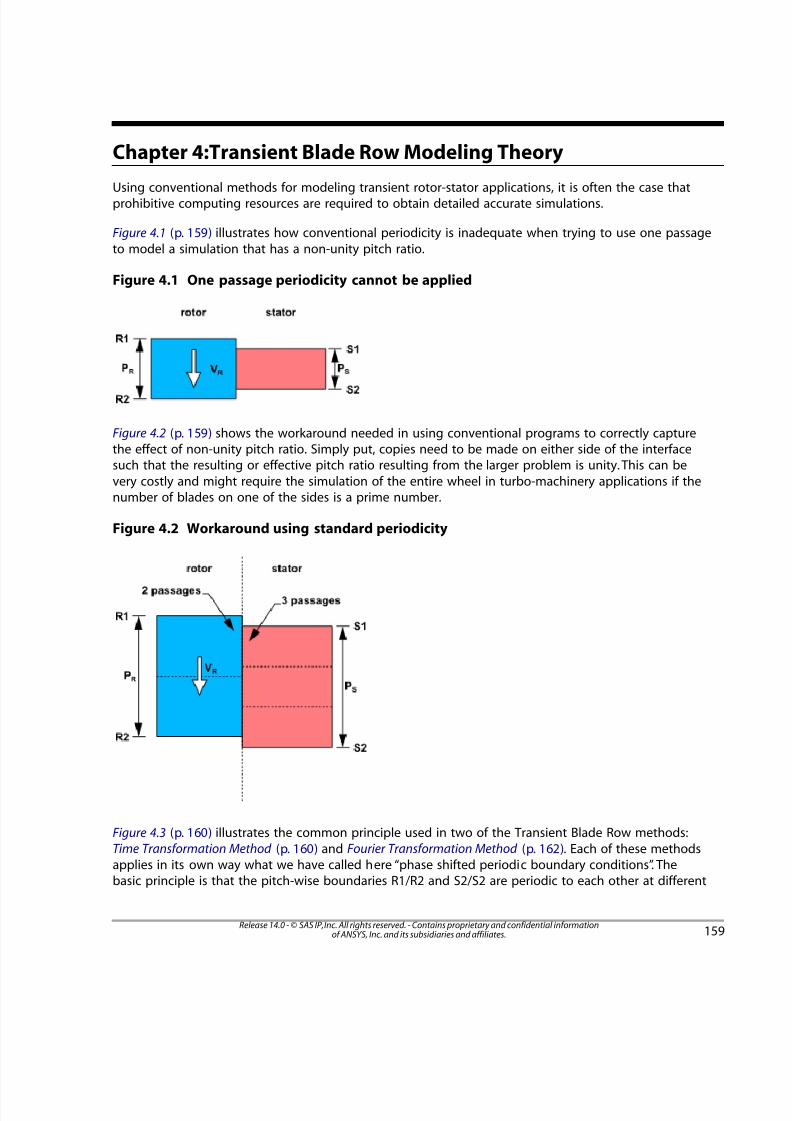
7/16/2019 ANSYS CFX-Solver Theory Guide
http://slidepdf.com/reader/full/ansys-cfx-solver-theory-guide-5633873a6f5ee 175/417
Chapter 4:Transient Blade Row Modeling Theory
Using conventional methods for modeling transient rotor-stator applications, it is often the case thatprohibitive computing resources are required to obtain detailed accurate simulations.
Figure 4.1 (p. 159) illustrates how conventional periodicity is inadequate when trying to use one passageto model a simulation that has a non-unity pitch ratio.
Figure 4.1 One passage periodicity cannot be applied
Figure 4.2 (p. 159) shows the workaround needed in using conventional programs to correctly capturethe effect of non-unity pitch ratio. Simply put, copies need to be made on either side of the interfacesuch that the resulting or effective pitch ratio resulting from the larger problem is unity. This can bevery costly and might require the simulation of the entire wheel in turbo-machinery applications if thenumber of blades on one of the sides is a prime number.
Figure 4.2 Workaround using standard periodicity
Figure 4.3 (p. 160) illustrates the common principle used in two of the Transient Blade Row methods:Time Transformation Method (p. 160) and Fourier Transformation Method (p. 162). Each of these methodsapplies in its own way what we have called here “phase shifted periodic boundary conditions”. Thebasic principle is that the pitch-wise boundaries R1/R2 and S2/S2 are periodic to each other at different
159Release 14.0 - © SAS IP, Inc. All rights reserved. - Contains proprietary and confidential informationof ANSYS, Inc. and its subsidiaries and affiliates.

7/16/2019 ANSYS CFX-Solver Theory Guide
http://slidepdf.com/reader/full/ansys-cfx-solver-theory-guide-5633873a6f5ee 176/417
instances in time. For example the relative position of R1 and S1 at
¡
is reproduced between sides R2
and S2 at an earlier time −¢ £
¤
where¥
is defined by − ¦ ¦ §
̈ © ̈
. Here
and
are the
rotor and stator pitches, respectively, and
is the velocity of the rotor.
Figure 4.3 Phase Shifted Periodic Boundary Conditions
4.1.Time Transformation Method
The Time Transformation method handles the problem of unequal pitch described above by transforming
the time coordinates of each rotor and stator passages. Let the
,
, and
coordinate axis representthe radial, tangential (pitchwise) and axial directions of the problem described in Figure 4.3 (p. 160).
Mathematically, the condition of enforcing the flow spatial periodic boundary conditions on both rotorand stator passages, respectively, is given by:
(4–1)= + − ! " # ! $ " #
% % % & '
(4–2)= + −( ) 0 1 2 ( ) 0 3 1 2
4 4 4 5 6
Alternatively, we can apply the following set of space-time transformations [217] to the problem aboveas:
(4–3)′ =7 7
(4–4)′ =8 8
(4–5)′ = 9 9
(4–6)′ = −@ @ A B
C D E
where = F G H
I P Q I P Q
.
Release 14.0 - © SAS IP, Inc. All rights reserved. - Contains proprietary and confidential informationof ANSYS, Inc. and its subsidiaries and affiliates.160
Chapter 4:Transient Blade Row Modeling Theory

7/16/2019 ANSYS CFX-Solver Theory Guide
http://slidepdf.com/reader/full/ansys-cfx-solver-theory-guide-5633873a6f5ee 177/417
The transformed set of equations now has regular spatial periodic boundary conditions as:
(4–7)′ ′ ′ ′ = ′ ′ + ′ ′ ¡ ¢ £ ¤ ¡ ¢ ¥ £ ¤
¦ ¦ ¦ § ̈
(4–8)′ ′ ′ ′ = ′ ′ + ′ ′© ©
And the periodicity is maintained at any instant in time in the computational domain.
There are two important implications of working with the transformed system above instead of theconventional system:
• The equations that are solved are in the computational ( ′
, ′
, ′
, ′!
) transformed space-time domain
and need to be transformed back to physical ("
,#
, $
,%
) domain before post-processing.
• The rotor and stator passages are marching at different time step sizes.
One way of understanding the difference in time step size stated in the second point is:
a) Each passage experiences a different period, i.e., the stator period is:
(4–9)=& ' (
) 0 0
whereas the rotor period is:
(4–10)=1 2 3
4 5 4
b) The period in each passage must be discretized using an identical number of timesteps 6 . We can
therefore write the rotor and stator periods as:
(4–11)=7 8 9
@ @
(4–12)=A B C
D D
whereE
F
andG
H
represent the time step size for the rotor and stator, respectively.
c) Combining the two definitions of rotor and stator periods in a) and b) we have the time step sizesin the rotor and stator related by their pitch ratio as:
(4–13)= I
I
P
P
Q
R
R
Q
The simulation time step size set for the run is used in the stator passage(s)S
T
and ANSYS CFX
computes the respective rotor passage time step sizeU
V
based on the rotor-stator interface pitch
ratio as described above.
161Release 14.0 - © SAS IP, Inc. All rights reserved. - Contains proprietary and confidential informationof ANSYS, Inc. and its subsidiaries and affiliates.
Time Transformation Method

7/16/2019 ANSYS CFX-Solver Theory Guide
http://slidepdf.com/reader/full/ansys-cfx-solver-theory-guide-5633873a6f5ee 178/417
When the solution is transformed back to physical time, the elapsed simulation time is considered thestator simulation time.
The flow interaction across the rotor-stator interfaces is handled by the pitch scaling machinery alreadypresent in the Profile Transformation method.
Another way of seeing the difference in time step sizes is to look at the time vs. pitchwise directionplot for both stator and rotor domains. In Figure 4.4 (p. 162) the rotor domain periodic boundaries are
plotted with reference to the stator domain. One can notice that, even though the rotor pitch is smallerthan the stator pitch in physical space, their boundaries match in the inclined computational space
after time + ¡
. Furthermore, if we look at the time step size of stator and rotor, we see that theyare different and related by the rotor-stator pitch ratio.
Figure 4.4 Rotor and stator periodic boundaries in space-time
For modeling information, see Transient Blade Row Modeling in the CFX-Solver Modeling Guide.
4.2. Fourier Transformation Method
The Fourier Transformation method applies the phase shifted boundary conditions illustrated in Figure4.3 (p. 160) in a more direct method than in the Time Transformation method.
It basically consists of attempting to directly "impose" a phase shift between the R1,R2 boundaries andthe S1,S2 boundaries for the primitive variables of the problem. A direct method of applying the phaseshift boundary method was proposed by Erdos [215] but his method requires storage of the signal fora compete period on all the R1/R2 S1/S2 boundaries including the interface shared by the rotor andstator sections. The Frequency Transformation method makes use of temporal Fourier series decompos-ition Equation 4–14 (p. 163) to avoid storing the signal on the S1/S2 and R1/R2 boundaries. This methodwas initially introduced by He [218].
Release 14.0 - © SAS IP, Inc. All rights reserved. - Contains proprietary and confidential informationof ANSYS, Inc. and its subsidiaries and affiliates.162
Chapter 4:Transient Blade Row Modeling Theory

7/16/2019 ANSYS CFX-Solver Theory Guide
http://slidepdf.com/reader/full/ansys-cfx-solver-theory-guide-5633873a6f5ee 179/417
(4–14)∑== −
−
¡ ¢
£ ¤
¤
£
¥ £ ¦ § ¨ ©
ɵ
In this method the signal is decomposed into harmonics of the fundamental frequency of
each passage. For example in typical TRS problems this fundamental frequency is the inverse of the
blade passing period
, where:
(4–15)=
The Fourier Transformation method in ANSYS CFX is implemented using a double passage method. Thedata is collected at the (implicit) interface (R2,S2) between the two passages, Figure 4.5 (p. 163). Whileperformance is case dependent, the double passage approach converges in fewer cycles than a singlepassage method, owing to the superior quality of the data update (Fourier data is collected at fullyimplicit flow variables, far from the actual periodic boundaries). The double passage Fourier Transform-ation approach converges very rapidly to a quasi-periodic state, requiring as few as 3-4 cycles in some
cases.
Figure 4.5 Double Passage Method
In Figure 4.5 (p. 163), the time shift is:
=−
!
" "
#
$ %
& ' ( ) 0 1
The signal 2 3
4 5
on S1 is equal to the signal on S2 phase shifted by
+
= + ≈ + 6 7 6 7 8 9 6 7 8 9
@ @ @ A B B
The signal C D
E F
on S3 is equal to the signal on S2 phase shifted by
163Release 14.0 - © SAS IP, Inc. All rights reserved. - Contains proprietary and confidential informationof ANSYS, Inc. and its subsidiaries and affiliates.
Fourier Transformation Method

7/16/2019 ANSYS CFX-Solver Theory Guide
http://slidepdf.com/reader/full/ansys-cfx-solver-theory-guide-5633873a6f5ee 180/417
−
:
= − ≈ − ¡ ¡ ¢ £ ¡ ¢ £
¤ ¤ ¤ ¥ ¦ ¦
Where § ̈
©
ɵ
is the reconstructed signal at S2 using the accumulated Fourier coefficients on thatsame boundary.
For modeling information, see Transient Blade Row Modeling in the CFX-Solver Modeling Guide.
Release 14.0 - © SAS IP, Inc. All rights reserved. - Contains proprietary and confidential informationof ANSYS, Inc. and its subsidiaries and affiliates.164
Chapter 4:Transient Blade Row Modeling Theory

7/16/2019 ANSYS CFX-Solver Theory Guide
http://slidepdf.com/reader/full/ansys-cfx-solver-theory-guide-5633873a6f5ee 181/417
Chapter 5: Multiphase Flow Theory
This chapter discusses:5.1. Multiphase Notation5.2.The Homogeneous and Inhomogeneous Models5.3. Hydrodynamic Equations5.4. Multicomponent Multiphase Flow5.5. Interphase Momentum Transfer Models5.6. Solid Particle Collision Models5.7. Interphase Heat Transfer5.8. Multiple Size Group (MUSIG) Model5.9.The Algebraic Slip Model5.10.Turbulence Modeling in Multiphase Flow
5.11. Additional Variables in Multiphase Flow5.12. Sources in Multiphase Flow5.13. Interphase Mass Transfer5.14. Free Surface Flow
Two distinct multiphase flow models are available in CFX, an Eulerian-Eulerian multiphase model anda Lagrangian Particle Tracking multiphase model. This section describes Eulerian-Eulerian multiphaseflow theory. For information about modeling Eulerian-Eulerian multiphase flow in ANSYS CFX, see"Multiphase Flow Modeling". Lagrangian Particle Tracking theory and modeling are described in Particle
Transport Theory (p. 239) and "Particle Transport Modeling", respectively.
You should be familiar with the mathematical implementation of single-phase flow before reading this
section. For details, see Basic Solver Capability Theory (p. 1).
5.1. Multiphase Notation
In addition to the notation given here, review the list of symbols. For details, see List of Symbols (p. 2).
Different phases of fluids are denoted using lowercase Greek letters
, ¡
,¢
, etc. In general, a quantity
subscribed with£ , ¤
,¥
, etc., refers to the value of the quantity for that particular phase. For example,
the volume fraction of ¦
is denoted§
̈
. Thus, the volume©
occupied by phase
in a small volume
around a point of volume fraction
is given by:
(5–1)=
The total number of phases is
. The volume fraction of each phase is denoted
!
, where = "
.
It is important to distinguish between the material density and the effective density of a fluid#
.Thematerial density,
$
%
, is the density of the fluid if it is the only phase present, that is, the mass of &
per
unit volume of '
. The effective density is then defined as:
165Release 14.0 - © SAS IP, Inc. All rights reserved. - Contains proprietary and confidential informationof ANSYS, Inc. and its subsidiaries and affiliates.

7/16/2019 ANSYS CFX-Solver Theory Guide
http://slidepdf.com/reader/full/ansys-cfx-solver-theory-guide-5633873a6f5ee 182/417
(5–2)=∼ ¡
¢
¢
¢
This is the actual mass per unit volume of phase£
, given that phase¤
only occupies a fraction of thevolume, that is, the mass of ¥ per unit volume of the bulk fluid.
The mixture density is given by:
(5–3)∑= ¦ ¦ §
̈
©
©
©
5.1.1. Multiphase Total Pressure
The total pressure in a multiphase simulation is defined as:
(5–4)∑= +
This definition is used for both incompressible and compressible flows, whereas single phase flows treattotal pressure differently depending on the simulation. For details, see Total Pressure (p. 16).
5.2.The Homogeneous and Inhomogeneous Models
Two different sub-models are available for Eulerian-Eulerian multiphase flow: the homogeneous modeland the inter-fluid transfer (inhomogeneous) model.
5.2.1.The Inhomogeneous Model
5.2.1.1. Interfacial Area Density
Interfacial transfer of momentum, heat and mass is directly dependent on the contact surface areabetween the two phases. This is characterized by the interfacial area per unit volume between phase
and phase !
, known as the interfacial area density, "
# $
. Note that it has dimensions of inverse length.
Interfacial transfer can be modeled using either the particle or mixture models. These essentially providedifferent algebraic prescriptions for the interfacial area density.
5.2.1.1.1.The Particle Model
The Particle model for interfacial transfer between two phases assumes that one of the phases is con-
tinuous (phase%
) and the other is dispersed (phase &
). The surface area per unit volume is then calculatedby assuming that phase
'
is present as spherical particles of Mean Diameter(
)
. Using this model, the
interphase contact area is:
(5–5)= 0
1
2
3 4
4
4
This simple model is modified for robustness purposes in two ways:
Release 14.0 - © SAS IP, Inc. All rights reserved. - Contains proprietary and confidential informationof ANSYS, Inc. and its subsidiaries and affiliates.166
Chapter 5: Multiphase Flow Theory

7/16/2019 ANSYS CFX-Solver Theory Guide
http://slidepdf.com/reader/full/ansys-cfx-solver-theory-guide-5633873a6f5ee 183/417
•
¡
is clipped to a minimum volume fraction to ensure the area density does not go exactly to zero.
• For large¢
£
(that is, when the assumption of ¤
being dispersed is invalid), the area density is decrease
to reflect the fact that it should lead to zero as ¥
¦
tends to 1.
With these modifications, the area density for the particle model is implemented as
(5–6)= §
̈
©
where
(5–7)=
<
−−
>
By default,
! "
and#
$ % &
take values of 0.8 and 10-7, respectively. In some cases, it may be appropriate
to use a different value for'
( ) 0
; for example, increasing it to 10-3 provides a very crude nucleation
model for boiling a subcooled liquid.1
2 3 4
is controlled by the parameter Minimum Volume Fraction
for Area Density.
For non-drag forces, the solver uses a slightly different formulation of area density called the Unclipped
Interfacial Area Density. In this formulation, the area density is permitted to go to zero, that is, =5
6 7 8
in Equation 5–7 (p. 167). In addition, the area density is reduced more aggressively as the dispersed phasevolume fraction becomes large:
(5–8)= 9 @ 9
A B
A B
C D E F G H H I P
where:
=
−−
′
Q
R
R
S
S
T
=U
=
≤
− < ≤′V
V V
V V
W
W W
W W
Non-dimensional interphase transfer coefficients may be correlated in terms of the particle Reynolds
number and the fluid Prandtl number. These are defined using the particle mean diameter, and thecontinuous phase properties, as follows:
167Release 14.0 - © SAS IP, Inc. All rights reserved. - Contains proprietary and confidential informationof ANSYS, Inc. and its subsidiaries and affiliates.
The Homogeneous and Inhomogeneous Model

7/16/2019 ANSYS CFX-Solver Theory Guide
http://slidepdf.com/reader/full/ansys-cfx-solver-theory-guide-5633873a6f5ee 184/417
(5–9)=− ¡ ¢
£
¤ ¥
¤
¥ ¤ ¥
¤
(5–10)= ¦ §
̈
©
©
©
©
where
,
and
are the viscosity, specific heat capacity and thermal conductivity of the continuous
phase .
5.2.1.1.2.The Mixture Model
This is a very simple model which treats both phases
, !
symmetrically. The surface area per unit
volume is calculated from
(5–11)= "
# #
$
% &
% &
% &
where'
( )
is an interfacial length scale, which you must specify.
By way of example, suppose you have oil-water flow in which you may have either water droplets in
continuous oil, or oil droplets in continuous water, in the limits →0
1
, →2
3
respectively. Then, a
simple model for interfacial area density that has the correct behavior in these two limits is given by:
(5–12)=+
⇒ =+
4
5 5
5 6 5 6
6
5 6 5 6
7 8
7 8
7 8 8 7
7 8
7 8 8 7
Non-dimensional interphase transfer coefficients may be correlated in terms of the mixture Reynolds
number and Prandtl number defined as follows:
(5–13)=−
9 9 @ A
B
C D
C D
D C C D
C D
(5–14)=E
F
G H
G H
G H
where I
P Q
, R
S T
, U
V W X
and Y
̀ a
are the density, viscosity, specific heat capacity and thermal conduct-
ivity of the mixture respectively, defined by:
Release 14.0 - © SAS IP, Inc. All rights reserved. - Contains proprietary and confidential informationof ANSYS, Inc. and its subsidiaries and affiliates.168
Chapter 5: Multiphase Flow Theory

7/16/2019 ANSYS CFX-Solver Theory Guide
http://slidepdf.com/reader/full/ansys-cfx-solver-theory-guide-5633873a6f5ee 185/417
(5–15)
= +
= +
¡ ¡
¢ ¡ ¢ ¡ ¢
£ ¤
£
£
¤
¤
£ ¤
£
£
¤
¤
5.2.1.1.3.The Free Surface Model
The free surface model attempts to resolve the interface between the fluids. If there are just two phasesin the simulation, the following equation is used for interfacial area density:
(5–16)= ∇ ¥ ¦
§ ¨ §
When more than two phases are present, this is generalized as follows:
(5–17)=∇ ∇
∇ + ∇ ©
5.2.2.The Homogeneous Model
In homogeneous multiphase flow, a common flow field is shared by all fluids, as well as other relevantfields such as temperature and turbulence. This allows some simplifications to be made to the multifluidmodel resulting in the homogeneous model.
For a given transport process, the homogeneous model assumes that the transported quantities (withthe exception of volume fraction) for that process are the same for all phases, that is,
(5–18)= ≤ ≤
Because transported quantities are shared in homogeneous multiphase flow, it is sufficient to solve forthe shared fields using bulk transport equations rather than solving individual phasic transport equations.
The bulk transport equations can be derived by summing the individual phasic transport equations(Equation 5–202 (p. 212)) over all phases to give a single transport equation for
:
(5–19)∂∂
+ ∇ − ∇ =
! " ! " # " $
where:
169Release 14.0 - © SAS IP, Inc. All rights reserved. - Contains proprietary and confidential informationof ANSYS, Inc. and its subsidiaries and affiliates.
The Homogeneous and Inhomogeneous Model

7/16/2019 ANSYS CFX-Solver Theory Guide
http://slidepdf.com/reader/full/ansys-cfx-solver-theory-guide-5633873a6f5ee 186/417
(5–20)
∑
∑
∑
=
=
=
=
=
=
¡ ¢ ¡
¡
¢ ¡
£ ¢ £
¤
¥
¤
¤
¤
¥
¤
¤
¤
¤
¥
¤ ¤
¦
¦
¦
§
§
§
The homogeneous model does not need to be applied consistently to all equations. For example, thevelocity field may be modeled as inhomogeneous, but coupled with a homogeneous turbulence model.Alternatively, a homogeneous velocity field may be coupled with inhomogeneous temperature fields.Homogeneous Additional Variables are also available in CFX.
5.3. Hydrodynamic Equations
The following is a summary of the equations of momentum and mass transfer for inhomogeneous andhomogeneous multiphase flow in CFX. The equivalent for single-phase flow is also available. For details,see Transport Equations (p. 25).
5.3.1. Inhomogeneous Hydrodynamic Equations
The inhomogeneous hydrodynamic equations are as follows:
• Momentum Equations (p. 170)
• Continuity Equations (p. 171)
• Volume Conservation Equation (p. 171)
• Pressure Constraint (p. 172)
5.3.1.1. Momentum Equations
(5–21)
⊗
∑
∂∂
+ ∇
= − ∇ + ∇ ∇ + ∇
+ − + +
=
+ +
¨ ¨ ̈
¨ ̈
¨ ¨ ©
!
"
#
• $
% &
describes momentum sources due to external body forces, and user defined momentum sources.
For details, see Sources (p. 54).
• '
(
describes the interfacial forces acting on phase ) due to the presence of other phases. Additional
information for the models available for interfacial forces is available in Interphase Momentum Transfer
Models (p. 173).
• The term:
Release 14.0 - © SAS IP, Inc. All rights reserved. - Contains proprietary and confidential informationof ANSYS, Inc. and its subsidiaries and affiliates.170
Chapter 5: Multiphase Flow Theory

7/16/2019 ANSYS CFX-Solver Theory Guide
http://slidepdf.com/reader/full/ansys-cfx-solver-theory-guide-5633873a6f5ee 187/417
(5–22)−+ + ¡ ¡
¢ £ £ £ ¢ ¢
represents momentum transfer induced by interphase mass transfer. For details, see Interphase
Mass Transfer (p. 216).
• The above momentum equations are valid for fluid phases only. For dispersed solid phases, additionalterms are present representing additional stresses due to particle collisions.
5.3.1.2. Continuity Equations
(5–23)∑∂∂
+ ∇ = +=
¤ ¥
¦
§ ¨ § ¨ ©
•
describes user specified mass sources. For details, see Sources (p. 54).
• !
" #
is the mass flow rate per unit volume from phase $
to phase%
. This term only occurs if interphas
mass transfer takes place. For details, see Interphase Mass Transfer (p. 216).
5.3.1.3. Volume Conservation Equation
This is simply the constraint that the volume fractions sum to unity:
(5–24)∑ ==
&
'
(
'
)
0
This equation may also be combined with the phasic continuity equations to obtain a transported
volume conservation equation. Take Equation 5–23 (p. 171), divide by phasic density, and sum over allphases. This yields:
(5–25)∑ ∑ ∑
∂∂
+ ∇ =
+
=
1 2
3 4
5 3 5 3
3
6
7
7
7
7
7
7
7
7
7
8 9 7
@
A
7 @
B
C
Interpreting this equation is simpler if you consider the special case of incompressible phases with nosources, in which it simplifies to:
(5–26)∑ ∇ =D E
F
F F
which requires the volume flows to have zero divergence. Equation 5–25 (p. 171) is the volume continuityequation solved by the CFX-Solver.
171Release 14.0 - © SAS IP, Inc. All rights reserved. - Contains proprietary and confidential informationof ANSYS, Inc. and its subsidiaries and affiliates.
Hydrodynamic Equations

7/16/2019 ANSYS CFX-Solver Theory Guide
http://slidepdf.com/reader/full/ansys-cfx-solver-theory-guide-5633873a6f5ee 188/417
5.3.1.4. Pressure Constraint
The complete set of hydrodynamic equations represent +
¡
equations in the ¢
£
unknowns ¤
¥
,
¦
§
, ̈
©
,
,
. You need −
more equations to close the system. These are given by constraints on
the pressure, namely that all phases share the same pressure field:
(5–27)= =
5.3.2. Homogeneous Hydrodynamic Equations
5.3.2.1. Momentum Equations
The homogeneous model for momentum transport assumes:
(5–28)= ≤ ≤ ! "
# $
and is given by Equation 5–23 (p. 171) and the momentum equation:
(5–29)⊗∂∂
+ ∇ − ∇ + ∇ = − ∇% % % % % &
'
( ( ) 0
1
2
where:
(5–30)
∑
∑
=
=
=
=
3 4 3
5 4 5
6
7
6
6
6
7
6
6
8
8
9
9
The following points should be noted:
• The interphase transfer terms have all canceled out.
• This is essentially a single phase transport equation, with variable density and viscosity.
5.3.2.2. Continuity Equations
The homogeneous continuity equation is the same as for full multiphase, Equation 5–23 (p. 171), exceptthat@
is not phase specific.
5.3.2.3. Volume Conservation Equations
The homogeneous volume conservation equation is the same as for full multiphase, Equation 5–24 (p. 171),
except thatA
is not phase specific.
Release 14.0 - © SAS IP, Inc. All rights reserved. - Contains proprietary and confidential informationof ANSYS, Inc. and its subsidiaries and affiliates.172
Chapter 5: Multiphase Flow Theory

7/16/2019 ANSYS CFX-Solver Theory Guide
http://slidepdf.com/reader/full/ansys-cfx-solver-theory-guide-5633873a6f5ee 189/417
5.3.2.4. Pressure Constraint
The pressure constraint given above for full multiphase flow is also used for homogeneous multiphaseflow.
5.4. Multicomponent Multiphase Flow
In multiphase multicomponent flows, transport equations for the mass fractions of components
¡ ¢
are assumed to take a similar form those used for single-phase multicomponent flow:
(5–31)∂∂
+ ∇ − ∇ =£
¤
¥ ¦ § ¥ ¦ § ¦ ¨ § ©
You should note that the molecular diffusion coefficients are given by
, where
is the Kin-
ematic Diffusivity.
Source terms in multicomponent multiphase flow behave the same as multicomponent mass sources,but on a per fluid basis. For details, see Sources (p. 54).
5.5. Interphase Momentum Transfer Models
The theory described in this section only applies to inhomogeneous multiphase flow. When using thehomogeneous model, momentum transfer between phases is assumed to be very large.
Interphase momentum transfer,
!
, occurs due to interfacial forces acting on each phase"
, due to
interaction with another phase #
. The total force on phase$
due to interaction with other phases is
denoted %
&
, and is given by:
(5–32)∑= ≠ ' '
(
) (
( )
Note that interfacial forces between two phases are equal and opposite, so the net interfacial forcessum to zero:
(5–33)∑= − ⇒ = 0 0 0
1 2 2 1
1
1
The total interfacial force acting between two phases may arise from several independent physical effects:
(5–34)= + + + + + + 3 3 3 3 3 3 3
4 5 4 5
6
4 5
7
4 5
7 8 9
4 5
@ A
4 5
B 6
C
The forces indicated above respectively represent the interphase drag force, lift force, wall lubricationforce, virtual mass force, turbulence dispersion force and solids pressure force (for dense solid particlephases only).
CFX provides a wide range of physical models for these forces. These models are described in the fol-lowing places:
173Release 14.0 - © SAS IP, Inc. All rights reserved. - Contains proprietary and confidential informationof ANSYS, Inc. and its subsidiaries and affiliates.
Interphase Momentum Transfer Models

7/16/2019 ANSYS CFX-Solver Theory Guide
http://slidepdf.com/reader/full/ansys-cfx-solver-theory-guide-5633873a6f5ee 190/417
• Interphase Drag (p. 174)
• Lift Force (p. 181)
• Wall Lubrication Force (p. 185)
• Virtual Mass Force (p. 184)
• Interphase Turbulent Dispersion Force (p. 187)
• Solid Particle Collision Models (p. 188)
For more information, see Multiphase Flow with Turbulence Dispersion Force in the CFX Reference Guide.
5.5.1. Interphase Drag
The following general form is used to model interphase drag force acting on phase
due to phase ¡
:
(5–35)= − ¢ £ £ ¤
¥
¥ ¦
§
¦ ¥
̈ ©
Note that =
and =
. Hence, the sum over all phases of all interphase transfer terms iszero.
In this section, you will learn how the coefficients
may be computed from a knowledge of dimen-
sionless drag coefficients. The range of models available for drag coefficients is also described.
The total drag force is most conveniently expressed in terms of the dimensionless drag coefficient:
(5–36)=
−!
"
# $ $ %
&
'
' (
)
0
1
where 2 is the fluid density, −3 3
4 5
is the relative speed, 6 is the magnitude of the drag force
and 7
is the projected area of the body in the direction of flow. The continuous phase is denoted by
8 and the dispersed phase is denoted by 9 .
5.5.2. Interphase Drag for the Particle Model
For spherical particles, the coefficients@
A B
C D E may be derived analytically. The area of a single particle
projected in the flow direction, F
G
, and the volume of a single particleH
I
are given by:
(5–37)
=
=
P
Q R
S
Q R
T
T
U
V
whereW
is the mean diameter. The number of particles per unit volume,X
Y
, is given by:
Release 14.0 - © SAS IP, Inc. All rights reserved. - Contains proprietary and confidential informationof ANSYS, Inc. and its subsidiaries and affiliates.174
Chapter 5: Multiphase Flow Theory

7/16/2019 ANSYS CFX-Solver Theory Guide
http://slidepdf.com/reader/full/ansys-cfx-solver-theory-guide-5633873a6f5ee 191/417
(5–38)= =
¡
¢
¡
£ ¤
¥
¦
¥
¦
§
The drag exerted by a single particle on the continuous phase is:
(5–39)= − − ̈ © © © ©
Hence, the total drag per unit volume on the continuous phase is:
(5–40)= = − −
!
" #
$ % & &
'
%
$
% $ % $
Comparing with the Momentum Equations (p. 170) for phase(
, where the drag force per unit volume is:
(5–41)= − ) 0 0 1
2 3
2 3
4
3 2
5 6
you get:
(5–42)= −7 7 8
9
@
A B
C D
E F
D
C
D C
G H
which can be written as:
(5–43)= −I I P
Q
R S
T U
V W
T U
T
U T
X Y
This is the form implemented in CFX.
The following section describes drag correlations specific to dispersed multiphase flow.
5.5.2.1. Sparsely Distributed Solid Particles
At low particle Reynolds numbers (the viscous regime), the drag coefficient for flow past sphericalparticles may be computed analytically. The result is Stokes’ law:
(5–44)= ̀
a
≪
For particle Reynolds numbers, such as Equation 5–9 (p. 168), that are sufficiently large for inertial effectsto dominate viscous effects (the inertial or Newton’s regime), the drag coefficient becomes independentof Reynolds number:
175Release 14.0 - © SAS IP, Inc. All rights reserved. - Contains proprietary and confidential informationof ANSYS, Inc. and its subsidiaries and affiliates.
Interphase Momentum Transfer Models

7/16/2019 ANSYS CFX-Solver Theory Guide
http://slidepdf.com/reader/full/ansys-cfx-solver-theory-guide-5633873a6f5ee 192/417
(5–45)= ≤ ≤ − ¡
¢
£
In the transitional region between the viscous and inertial regimes, < < for sphericalparticles, both viscous and inertial effects are important. Hence, the drag coefficient is a complex functionof Reynolds number, which must be determined from experiment.
This has been done in detail for spherical particles. Several empirical correlations are available. Theone available in CFX is due to Schiller and Naumann (1933) [6]. It can be written as follows:
5.5.2.1.1. Schiller Naumann Drag Model
(5–46)= +¤
¥
¦ § ¨ ©
CFX modifies this to ensure the correct limiting behavior in the inertial regime by taking:
(5–47)=
+
5.5.2.2. Densely Distributed Solid Particles
5.5.2.2.1. Densely Distributed Solid Particles: Wen Yu Drag Model
(5–48)=
′
+ ′
′ =
−
!
!
" # $ % & # $ ' (
Note that this has the same functional form as the Schiller Naumann correlation, with a modified particleReynolds number, and a power law correction, both functions of the continuous phase volume fraction
)
0
.
You may also change the Volume Fraction Correction Exponent from its default value of -1.65, if youwant.
Note
Although the Wen Yu drag law implemented in ANSYS CFX follows the implementation by
Gidaspow [18] and its subsequent wide use, this implementation of the drag law is, in fact,quite different from that given in the original Wen and Yu paper [181].
Release 14.0 - © SAS IP, Inc. All rights reserved. - Contains proprietary and confidential informationof ANSYS, Inc. and its subsidiaries and affiliates.176
Chapter 5: Multiphase Flow Theory

7/16/2019 ANSYS CFX-Solver Theory Guide
http://slidepdf.com/reader/full/ansys-cfx-solver-theory-guide-5633873a6f5ee 193/417
5.5.2.2.2. Densely Distributed Solid Particles: Gidaspow Drag Model
(5–49)
= >
=−
+− −
<
¡ ¡ ¢
£
¢ ¤
¢ ¥
¢ ¦
¥
¢
§ § ̈
©
̈
̈
̈
̈
̈
̈
̈
This uses the Wen Yu correlation for low solid volume fractions <
, and switches to Ergun’s law
for flow in a porous medium for larger solid volume fractions.
Note that this is discontinuous at the cross-over volume fraction. In order to avoid subsequent numer-ical difficulties, CFX modifies the original Gidaspow model by linearly interpolating between the Wen
Yu and Ergun correlations over the range < <
.
You may also change the Volume Fraction Correction Exponent of the Wen Yu part of the correlationfrom its default value of -1.65, if you want.
5.5.2.3. Sparsely Distributed Fluid Particles (Drops and Bubbles)At sufficiently small particle Reynolds numbers (the viscous regime), fluid particles behave in the samemanner as solid spherical particles. Hence, the drag coefficient is well approximated by the Schiller-Naumann correlation described above.
At larger particle Reynolds numbers, the inertial or distorted particle regime, surface tension effectsbecome important. The fluid particles become, at first, approximately ellipsoidal in shape, and finally,spherical cap shaped.
In the spherical cap regime, the drag coefficient is well approximated by:
(5–50)=!
"
Several correlations are available for the distorted particle regime. CFX uses the Ishii Zuber [19] andGrace [35] correlations.
5.5.2.3.1. Sparsely Distributed Fluid Particles: Ishii-Zuber Drag Model
In the distorted particle regime, the drag coefficient is approximately constant, independent of Reynoldsnumber, but dependent on particle shape through the dimensionless group known as the Eotvosnumber, which measures the ratio between gravitational and surface tension forces:
(5–51)= # $
% & '
(
)
0
Here, 1
is the density difference between the phases, 2
is the gravitational acceleration, and3
is the
surface tension coefficient.
The Ishii-Zuber correlation gives:
177Release 14.0 - © SAS IP, Inc. All rights reserved. - Contains proprietary and confidential informationof ANSYS, Inc. and its subsidiaries and affiliates.
Interphase Momentum Transfer Models

7/16/2019 ANSYS CFX-Solver Theory Guide
http://slidepdf.com/reader/full/ansys-cfx-solver-theory-guide-5633873a6f5ee 194/417
(5–52)= ¡ ¢
£
¤ ¥ ¦
In this case, CFX automatically takes into account the spherical particle and spherical cap limits by setting:
(5–53)=
=
§ § §
§ § §
̈ ¨ ̈
̈ ¨ ̈
The Ishii Zuber Model also automatically takes into account dense fluid particle effects. For details, seeDensely Distributed Fluid Particles (p. 179).
5.5.2.3.2. Sparsely Distributed Fluid Particles: Grace Drag Model
The Grace drag model is formulated for flow past a single bubble. Here the drag coefficient in the dis-torted particle regime is given by:
(5–54)=©
where the terminal velocity
is given by:
(5–55)= −−
!
" #
$ %
&
'
(
(
) 0 1 2 3
where:
(5–56)= = 4
5 6 7
7 8
9
@
A B
and:
(5–57)=
< ≤>
C
D D
D D
E F G H G
E F I I P
(5–58)=
−−
Q R S T
U
U
V
W X Y ` a
b c d
W X Y ̀
= − − e
f g h
i i
is the molecular viscosity of water at 25°C and 1 bar.
In this case, CFX automatically takes into account the spherical particle and spherical cap limits by setting:
Release 14.0 - © SAS IP, Inc. All rights reserved. - Contains proprietary and confidential informationof ANSYS, Inc. and its subsidiaries and affiliates.178
Chapter 5: Multiphase Flow Theory

7/16/2019 ANSYS CFX-Solver Theory Guide
http://slidepdf.com/reader/full/ansys-cfx-solver-theory-guide-5633873a6f5ee 195/417
(5–59)=
=
¡ ¡ ¡
¡ ¡ ¡
5.5.2.4. Densely Distributed Fluid Particles
5.5.2.4.1. Densely Distributed Fluid Particles: Ishii-Zuber Drag Model
The Ishii Zuber [19] drag laws automatically take into account dense particle effects. This is done indifferent ways for different flow regimes.
In the viscous regime, where fluid particles may be assumed to be approximately spherical, the SchillerNaumann correlation is modified using a mixture Reynolds number based on a mixture viscosity.
5.5.2.4.2. Densely Distributed Fluid Particles: Dense Spherical Particle Regime (Ishii Zuber
(5–60)
= +
= −
=
−
=+
+
−
∗
∗
¢ ¢
£
¤ ¥
¦
¦
¦
§
§
¦
¦ ¦
¦ ¦
̈
©
©
©
©
©
©
!
" #
Here, $
% & is the user defined Maximum Packing value. This is defaulted to unity for a dispersed fluidphase.
In the distorted particle regime, the Ishii Zuber modification takes the form of a multiplying factor tothe single particle drag coefficient.
179Release 14.0 - © SAS IP, Inc. All rights reserved. - Contains proprietary and confidential informationof ANSYS, Inc. and its subsidiaries and affiliates.
Interphase Momentum Transfer Models
7/16/2019 ANSYS CFX-Solver Theory Guide
http://slidepdf.com/reader/full/ansys-cfx-solver-theory-guide-5633873a6f5ee 196/417
5.5.2.4.3. Densely Distributed Fluid Particles: Dense Distorted Particle Regime (Ishii Zuber)
(5–61)
=
=
=
+
= −
∞
∞
¡ ¢
¡ £
¡ ¢
¤ ¢
¤ ¢
¤ ¢
¥
¥
¢
¦ § ¦
¦
§
§
§
§
̈
©
§
5.5.2.4.4. Densely Distributed Fluid Particles: Dense Spherical Cap Regime (Ishii Zuber)
(5–62)
= −
=
∞
∞
The Ishii Zuber correlation, as implemented in CFX, automatically selects flow regime as follows:
5.5.2.4.5. Densely Distributed Fluid Particles: Automatic Regime Selection (Ishii Zuber)
(5–63)= ≥= <
! ! ! !
! ! ! ! !
5.5.2.4.6. Densely Distributed Fluid Particles: Grace Drag Model
The Grace [35] drag model is formulated for flow past a single bubble. For details, see Sparsely Distributed
Fluid Particles (Drops and Bubbles) (p. 177).
For high bubble volume fractions, it may be modified using a simple power law correction:
(5–64)= ∞" # "
$ %
&
$
Here, ∞'
(
is the single bubble Grace drag coefficient. Advice on setting the exponent value for the
power law correction is available in Densely Distributed Fluid Particles: Grace Drag Model in the CFX-Solver Modeling Guide.
5.5.3. Interphase Drag for the Mixture Model
In the mixture model, a non-dimensional drag coefficient )
0
is defined as follows:
Release 14.0 - © SAS IP, Inc. All rights reserved. - Contains proprietary and confidential informationof ANSYS, Inc. and its subsidiaries and affiliates.180
Chapter 5: Multiphase Flow Theory

7/16/2019 ANSYS CFX-Solver Theory Guide
http://slidepdf.com/reader/full/ansys-cfx-solver-theory-guide-5633873a6f5ee 197/417
(5–65)= − − ¡ ¡ ¡ ¡ ¢ £ ¤
¥ ¦ §
¥ ¦
¥ ¦ ¦ ¥ ¦ ¥
where ̈
©
is the total drag exerted by phase
on phase
per unit volume.
The mixture density
is given by:
(5–66)= +
and the interfacial area per unit volume
! "
is given by:
(5–67)= #
$ $
%
& '
& '
& '
where(
) 0
is a user-specified mixture length scale.
5.5.4. Interphase Drag for the Free Surface Model
In the free surface model, interphase drag is calculated in the same way as for the mixture model (seeInterphase Drag for the Mixture Model (p. 180)), except that the interfacial area density is given by:
(5–68)= ∇ 1 2
3 4 3
When more than two phases are present, this is generalized as follows:
(5–69)= ∇ ∇∇ + ∇ 5
6 6
6 6
7 8
7 8
7 8
[The Free Surface Model (p. 169)]
5.5.5. Lift Force
The lift force acts perpendicular to the direction of relative motion of the two phases.
CFX contains a model for the shear-induced lift force acting on a dispersed phase in the presence of arotational continuous phase. This is given by:
(5–70)= − = − ×
=
9 9 @ @ A
A @
B C D
E
F
G
F
G
E
F G E E
E E
whereH
I
is a non-dimensional lift coefficient. In a rotating frame of reference with rotation vectorP
,
the lift force is given by:
181Release 14.0 - © SAS IP, Inc. All rights reserved. - Contains proprietary and confidential informationof ANSYS, Inc. and its subsidiaries and affiliates.
Interphase Momentum Transfer Models

7/16/2019 ANSYS CFX-Solver Theory Guide
http://slidepdf.com/reader/full/ansys-cfx-solver-theory-guide-5633873a6f5ee 198/417
(5–71)= − = − × +
=
∗ ∗ ∗
∗ ∗
¡ ¡ ¢ £
¢ ¡
¤ ¥ ¦
§
̈
©
̈
©
§
̈ © § §
§ §
Currently, ANSYS CFX has the following built-in lift models:
• The Saffman Mei Lift Force Model (p. 182)• The Legendre and Magnaudet Lift Force Model (p. 183)
• The Tomiyama Lift Force Model (p. 183)
5.5.5.1. The Saffman Mei Lift Force Model
This model is applicable mainly to the lift force on spherical solid particles, though it could be appliedto liquid drops that are not significantly distorted. It is a generalization of the older Saffman model,which was applicable to a lower range of particle Reynolds numbers than the Saffman Mei model.
The lift coefficient is correlated in terms of both particle Reynolds number and vorticity Reynolds
numbers:
(5–72)=−
= = ∇ ×
Saffman (1965, 1968) [86][170] correlated the lift force for low Reynolds number flow past a sphericalparticle as follows:
(5–73)= − =∇ ×
′ − × ∇ × +
!
! ! !
"
#
$
% & '
( )
(
0 (
1 )
(
) ( (
where ′ =2
3
, and ≤ ≤ ≤ 4 5
. By inspection, Saffman’s lift coefficient is related to the
one adopted in ANSYS CFX as follows:
(5–74)= ′6
7
6
8
9 9
Saffman’s correlation was generalized by Mei and Klausner (1994) [87] to a higher range of particleReynolds numbers, as follows:
(5–75)′ =
⋅ <
⋅ ⋅ < <@
A
B
C
D
E E
E
F G H
E
where = I
P Q
, and = − ⋅ +− R S T S
U V
W X Y ` a W b c W X Y
d .
Release 14.0 - © SAS IP, Inc. All rights reserved. - Contains proprietary and confidential informationof ANSYS, Inc. and its subsidiaries and affiliates.182
Chapter 5: Multiphase Flow Theory

7/16/2019 ANSYS CFX-Solver Theory Guide
http://slidepdf.com/reader/full/ansys-cfx-solver-theory-guide-5633873a6f5ee 199/417
5.5.5.2. The Legendre and Magnaudet Lift Force Model
This model, as developed by Legendre & Magnaudet (1998) [171], is applicable mainly to the lift forceof small diameter spherical fluid particles, though it could be applied to non-distorted liquid drops andbubbles. In contrast to the lift force model of Saffman-Mei for rigid solid particles, it accounts for themomentum transfer between the flow around the particle and the inner recirculation flow inside thefluid particle as caused by the fluid friction/stresses at the fluid interface. Therefore the predicted liftforce coefficients are about a factor of 2-5 smaller than for rigid solid particles.
The range of validity given by Legendre & Magnaudet (1998) is as follows:
(5–76)≤ ≤ = ≤ ¡ ¢
£
The lift force coefficient is then predicted by:
(5–77)= +¤ ¤ ¤
¥ ¥ ¦ § ¨ © ¥ ¦
where
= ′−
! " # $ % &
' ( )
0
(5–78)=+
+
−
−1
2 3 4 5 6 4 7 8
9
@
9
@
= A
B
′
=∞
+ − C
C
D
E F D
∞ = G
5.5.5.3. The Tomiyama Lift Force Model This is a model applicable to the lift force on larger-scale deformable bubbles in the ellipsoidal andspherical cap regimes. Like the Grace and Ishii-Zuber models for drag force, it depends on Eotvosnumber. Hence, it requires specification of the surface tension between the dispersed and continuousphases. Its main important feature is prediction of the cross-over point in bubble size at which particledistortion causes a reversal of the sign of the lift force to take place. The lift coefficient is given by(Tomiyama 1998) [172]:
183Release 14.0 - © SAS IP, Inc. All rights reserved. - Contains proprietary and confidential informationof ANSYS, Inc. and its subsidiaries and affiliates.
Interphase Momentum Transfer Models

7/16/2019 ANSYS CFX-Solver Theory Guide
http://slidepdf.com/reader/full/ansys-cfx-solver-theory-guide-5633873a6f5ee 200/417
(5–79)=
′
′ ≤
′ < ′ ≤− < ′
¡
¡
¢
£
where:
′ = ′ − ′ − ′ + ¤
¥ ¦
′ § ̈
is a modified Eotvos number, based on the long axis,©
, of the deformable bubble:
′ =−
= +
!
" # $ % $
& ' (
=−
) 0 0 1
2
3 4
5
6
The correlation has been slightly modified from Tomiyama’s original form, following Frank et al. (2004)
[173], whereby the value of 7
8
for ′ > has been changed to − to ensure a continuous de-
pendence on modified Eotvos number. Also, some publications omit the exponent of Eotvos number
in the formula for9
@
. The formula adopted here is taken from Wellek et al.[174].
5.5.6.Virtual Mass Force
The virtual mass force is proportional to relative phasic accelerations as follows:
(5–80)= − = −
A A
B B
C D E
F
F G
F
F G
H
I P
Q
I P
Q
H
I P
Q Q H H
In a rotating frame of reference with rotation vectorR
, the virtual mass force in terms of ∗
S
is modifiedby Coriolis theorem, and is given by:
(5–81)= − =
− + × −
∗ ∗ ∗ ∗∗ ∗
T T
U U
U U V W X
Y
Y ̀
Y
Y ̀
a
b
c d
e
c d
e
b
c d
e e b b
e b
The non-dimensional virtual mass coefficient =f
g h
for inviscid flow around an isolated sphere. In
general,i
p q
depends on shape and particle concentrationr
s t
may be specified by the user as a
constant or a CEL expression.
Release 14.0 - © SAS IP, Inc. All rights reserved. - Contains proprietary and confidential informationof ANSYS, Inc. and its subsidiaries and affiliates.184
Chapter 5: Multiphase Flow Theory

7/16/2019 ANSYS CFX-Solver Theory Guide
http://slidepdf.com/reader/full/ansys-cfx-solver-theory-guide-5633873a6f5ee 201/417
5.5.7.Wall Lubrication Force
Under certain circumstances, for example, bubbly upflow in a vertical pipe, the dispersed phase is ob-served to concentrate in a region close to the wall, but not immediately adjacent to the wall. This effectmay be modeled by the wall lubrication force, which tends to push the dispersed phase away from thewall.
Currently, ANSYS CFX has the following wall lubrication force models:
• The Antal Wall Lubrication Force Model (p. 185)
• The Tomiyama Wall Lubrication Force Model (p. 186)
• The Frank Wall Lubrication Force Model (p. 186)
5.5.7.1. The Antal Wall Lubrication Force Model
The Antal model, given by Antal et al. (1991) [88], computes the wall lubrication force as:
(5–82)= − − ¡ ¡ ¢ £ ¤ ¥
¦ § ¨ § ̈
̈
̈ © §
where
• =
+
The non-dimensional coefficients are defaulted to = −!
" #
and =$
% &
. You can change
these values.
•'
(
is the gas volume fraction.
• )
0
is the liquid density.
•1
2
is the unit normal pointing away from the wall.
• −3 3
4 5
is the relative velocity difference between phases, in the plane of the nearby wall surface (th
is, orthogonal to6
7
).
• 8
9
is the dispersed phase mean diameter.
• @
A
is the distance to the nearest wall.
Note that this force is only active in a thin layer adjacent to the wall; it is only active up to a cut-off distance of:
≤ − B C C D
E
F G F H I
where = P Q
R
S
with default values of T
U V
andW
X Y
.
Hence, this force will only be activated on a sufficiently fine mesh, and grid convergence can be expectedonly on extremely fine meshes.
185Release 14.0 - © SAS IP, Inc. All rights reserved. - Contains proprietary and confidential informationof ANSYS, Inc. and its subsidiaries and affiliates.
Interphase Momentum Transfer Models

7/16/2019 ANSYS CFX-Solver Theory Guide
http://slidepdf.com/reader/full/ansys-cfx-solver-theory-guide-5633873a6f5ee 202/417
5.5.7.2. The Tomiyama Wall Lubrication Force Model
Tomiyama (1998) [172] modified the wall lubrication force formulation of Antal, based on the resultsof experiments with the flow of air bubbles in glycerin in a pipe. The modification is as follows:
(5–83)=
−
−
¡ ¢
£
¤
¥ ¤
¦ § ¦
̈
¦
¦
© ©
Here,
is the pipe diameter. Hence, although the model was found to be superior to Antal's [88] (Frank
et al. 2004 [173]), it is restricted to flows in pipe geometries. As is the case for the Tomiyama lift force
correlation, the coefficient
is dependent on the Eotvos number, and hence on the surface
tension between the two phases. Frank et al (2004) modified this correlation slightly to ensure continuousdependence of the wall lubrication coefficient on Eotvos number:
(5–84)=
<≤ ≤− < ≤
<
− +
!
" # $ % % " # & ' $
5.5.7.3. The Frank Wall Lubrication Force Model
Frank et al. ([177], [173]) generalized the Tomiyama model to produce the Frank Wall Lubrication Forcemodel, which has no dependence on pipe diameter, and is given by:
(5–85)= ⋅
⋅−
⋅
−( (
(
)
0
1 2
0
1 2
3
4 5 6 6 7
7 8
7
9
@
@ A B
@
@ A B
Note:
•C D E
F
preserves the same dependence on Eotvos number as the Tomiyama model.
• The cut-off coefficient, G
H I
, determines the distance relative to the particle diameter over which the
force is active. =P
Q R
gives the same range as the Antal model with default constants.
• The damping coefficient,S
T U
, determines the relative magnitude of the force. =V
W X
gives the
same behavior as the Antal model with default constants. However, Frank et al. found that such high
Release 14.0 - © SAS IP, Inc. All rights reserved. - Contains proprietary and confidential informationof ANSYS, Inc. and its subsidiaries and affiliates.186
Chapter 5: Multiphase Flow Theory

7/16/2019 ANSYS CFX-Solver Theory Guide
http://slidepdf.com/reader/full/ansys-cfx-solver-theory-guide-5633873a6f5ee 203/417
damping of the wall lubrication force was not able to sufficiently counterbalance the Tomiyama liftforce in the near wall region.
• The power-law constant,
, makes the force fall off with a variable potential law relationship:
∼ ¡ ¢
£
¤ ¥
¤
. It is recommended that ¦
be in the range: 1.5 to 2.
• In extensive validation exercises by Frank et al. [177], the following model constants were determinedin order to produce the best possible agreement with experimental data for vertical bubbly flow in
pipes: =§
̈ ©
, =
, = .
5.5.8. Interphase Turbulent Dispersion Force
The topics in this section include:
• Favre Averaged Drag Model (p. 187)
• Lopez de Bertodano Model (p. 187)
5.5.8.1. Favre Averaged Drag Model
CFX implements a model for turbulent dispersion force, based on the Favre average of the interphasedrag force [90].
(5–86)= − =
∇−
∇
!
"
!
!
"
#
#
"
"
Here, $
% & is the momentum transfer coefficient for the interphase drag force. Hence, the model clearlydepends on the details of the drag correlation used
'
( )
is the turbulent Schmidt number for continuous
phase volume fraction, currently taken to be .
0
1 2
is a user-modifiable CEL multiplier. Its default value is unity.
5.5.8.2. Lopez de Bertodano Model
The model of Lopez de Bertodano (1991) [20] was one of the first models for the turbulent dispersionforce:
(5–87)= − = − ∇ 3 3 4 5 6 7
8
9 @
A
9 @
9 @
8
8 8
Unfortunately, it is not possible to recommend universal values of B
C D
for this model.E
F G
values of
0.1 to 0.5 have been used successfully for bubbly flow with bubble diameters of order a few millimeters.However, values up to 500 have been required for other situations. See Lopez de Bertodano [21] andMoraga et al. [91].
187Release 14.0 - © SAS IP, Inc. All rights reserved. - Contains proprietary and confidential informationof ANSYS, Inc. and its subsidiaries and affiliates.
Interphase Momentum Transfer Models

7/16/2019 ANSYS CFX-Solver Theory Guide
http://slidepdf.com/reader/full/ansys-cfx-solver-theory-guide-5633873a6f5ee 204/417
This model is included in CFX for historical back compatibility with CFX. However, the more universal
Favre Averaged Drag model is recommended for all situations where an appropriate value of
¡ ¢
is
unknown.
5.6. Solid Particle Collision Models
This section presents the theoretical background of the solid particle collision models implemented in
CFX.
The following topic(s) will be discussed:
• Solids Stress Tensor (p. 188)
• Solids Pressure (p. 189)
• Solids Bulk Viscosity (p. 190)
• Solids Shear Viscosity (p. 190)
• Granular Temperature (p. 191)
5.6.1. Solids Stress Tensor
Additional stresses due to inter-particle collisions are modeled using a collisional solids stress tensor inthe solid phase momentum equation only:
(5–88)= − +
∂∂
+∂∂
−∂∂
+
∂∂
£ ¤ ¥ ¦
§
̈
§
̈
§
̈
¥ ©
§
̈
¥
Here,
denotes solids pressure,
denotes solids shear viscosity, and
denotes solids bulk viscosity.
There are two important classes of models for these quantities:
5.6.1.1. Empirical Constitutive Equations
There exist wide classes of models where the constitutive elements of the solids stress are specifiedusing empirical constitutive relations. See, for example, (Enwald et al. [97]). In many of these, the solidspressure, shear and bulk viscosities are simple functions of the solid phase volume fraction.
5.6.1.2. Kinetic Theory Models for the Solids Stress Tensor
These are a class of models, based on the kinetic theory of gases, generalized to take into account in-elastic particle collisions. In these models, the constitutive elements of the solids stress are functionsof the solid phase granular temperature, defined to be proportional to the mean square of fluctuatingsolid phase velocity due to inter-particle collisions:
(5–89)= ′ !
" "
#
In the most general kinetic theory models, the granular temperature is determined from a transportequation. However, in many circumstances, it is possible to ignore the transport terms, and determinegranular temperature from the resulting algebraic equation.
Release 14.0 - © SAS IP, Inc. All rights reserved. - Contains proprietary and confidential informationof ANSYS, Inc. and its subsidiaries and affiliates.188
Chapter 5: Multiphase Flow Theory

7/16/2019 ANSYS CFX-Solver Theory Guide
http://slidepdf.com/reader/full/ansys-cfx-solver-theory-guide-5633873a6f5ee 205/417
5.6.2. Solids Pressure
5.6.2.1. Empirical Constitutive Equations
The most popular constitutive equations for solids pressure are due to (Gidaspow [18]). These actuallyspecify the solids pressure gradient, rather than solids pressure directly:
(5–90)= ⇒ ∇ = ∇ ¡ ¢ ¡ ¡
£ £ £ £ £ £
(5–91)= −¤ ¥ ¤ ¦
§
̈ © ©
Where
is the Elasticity Modulus,
is the Reference Elasticity Modulus,
is the Compaction
Modulus, and
!
is the Maximum Packing Parameter.
The Gidaspow model is implemented with an option for specifying the Reference Elasticity Modulus
and Compaction Modulus. There is also an option to specify the Elasticity Modulus" #
$
directly.
There is also an option to specify the solids pressure directly. This permits more general constitutiverelations than those where the solids pressure is a function of volume fraction only.
5.6.2.2. Kinetic Theory Models for Solids Pressure
The kinetic theory model for solids pressure is similar to the equation of state for ideal gases, modifiedto take account of inelastic collisions, and maximum solid packing.
(5–92)= + + % & ' ( ) 0 '
1
1
1 1 1
2
Here,3
denotes the coefficient of restitution for solid-solid collisions, and 4 5
6
7 denotes the radialdistribution function. Popular models for the radial distribution function are given by:
Gidaspow (1994) [18]:
(5–93)= −−
8 9 9 9
@ @ @ A
B C D
B
E
Lun and Savage (1986) [100]:
(5–94)= − − F G G G
H H H I
P Q R S
T
U V
Note that the radial distribution function tends to infinity as →W W
X X Y
. The singularity is removed in CFX
by setting:
(5–95)= + − + − + − ≥ ̀ a b b a a b a a b a a a a
c c d c d c d d
e
e f g
g
h
h
where = −i i
p q r
and:
189Release 14.0 - © SAS IP, Inc. All rights reserved. - Contains proprietary and confidential informationof ANSYS, Inc. and its subsidiaries and affiliates.
Solid Particle Collision Models
7/16/2019 ANSYS CFX-Solver Theory Guide
http://slidepdf.com/reader/full/ansys-cfx-solver-theory-guide-5633873a6f5ee 206/417
(5–96)
=
= ×
= ×
= ×
¡ ¢
£
¤
¥
¦
§
̈
5.6.3. Solids Bulk Viscosity
5.6.3.1. Constitutive Equation Models
Most simple constitutive equation models ignore the solids bulk viscosity. However, it is possible forthe user to specify a model for this, using a CEL expression, if required. Note that any solids volumefraction dependence must be included in the CEL expression.
5.6.3.2. Kinetic Theory Models for Solids Bulk Viscosity
There is general agreement on the correct kinetic theory form for the solids bulk viscosity (Lun et al.
1984 [99]).
(5–97)= +©
5.6.4. Solids Shear Viscosity
5.6.4.1. Constitutive Equation Models
The simplest constitutive equation model for solids shear viscosity was presented by Miller and Gidaspow
(1992) [106]. They successfully modeled gas-solid flow in a riser using a solids shear viscosity linearlyproportional to the solids phase volume fraction.
(5–98)= × ! "
#
#
Note that their constant of proportionality is dimensional, and is likely to require modification for differentfluid-solid material properties.
More complex models for solids shear stress allow the shear stress to become very large in the limit of maximum packing. A wide range of such models is discussed in the review article by Enwald et al [97].
It is possible for the user to implement any of these models, using a CEL expression for the solids shearviscosity. Note that any solids volume fraction dependence must be included in the CEL expression.
5.6.4.2. Kinetic Theory Models for Solids Shear Viscosity
Typically, the shear viscosity is expressed as a sum of at least two contributions: the kinetic and colli-sional contributions:
Release 14.0 - © SAS IP, Inc. All rights reserved. - Contains proprietary and confidential informationof ANSYS, Inc. and its subsidiaries and affiliates.190
Chapter 5: Multiphase Flow Theory

7/16/2019 ANSYS CFX-Solver Theory Guide
http://slidepdf.com/reader/full/ansys-cfx-solver-theory-guide-5633873a6f5ee 207/417
(5–99)= +
¡ ¡ ¢ £ ¤ ¡ ¥ ¦ § ¨ ̈
There is wide agreement on the correct form of the collisional contribution. As in the kinetic theory of gases, it is proportional to the square root of the granular temperature:
(5–100)= + ©
!
"
#
$
However, there are many proposals in the literature for the correct form of the kinetic contribution. Forexample:
Gidaspow (1994) [18]:
(5–101)=+
+ +
%
&
' (
) 0
) 0 1 2
3 4 5 6
3
7
3
8
9
9
@
Lun and Savage (1986) [100]:
(5–102)=
+
+ −
−
A
B
C D
E F
G
E E G F
E
H
I P Q R I
S I
I
T
U
V
W
W
Here, = +X Y
̀
a
.
Kinetic contributions are omitted from ANSYS CFX.
5.6.5. Granular Temperature
ANSYS CFX is restricted to models where the granular temperatureb
c
is determined algebraically.
5.6.5.1. Algebraic Equilibrium Model
d
e
may be specified directly by the user, or from the assumption of local equilibrium in a transport
equation model. The latter is based on:
(5–103)= ⇒∂∂ =
f
g
h
i
p q r
q
r
p
wheres
t u v
denotes the solids shear stress tensor Equation 5–88 (p. 188), and:
191Release 14.0 - © SAS IP, Inc. All rights reserved. - Contains proprietary and confidential informationof ANSYS, Inc. and its subsidiaries and affiliates.
Solid Particle Collision Models

7/16/2019 ANSYS CFX-Solver Theory Guide
http://slidepdf.com/reader/full/ansys-cfx-solver-theory-guide-5633873a6f5ee 208/417
(5–104)= −
−
∂∂
¡ ¢ £ ¤ ¥
¦
¥
§
̈
©
Expand the production term:
(5–105)∂∂
= − ∂∂
+ ∂
∂+ ∂
∂ ∂
∂+
−
∂
∂
! " #
"
#
!
$
$
!
"
#
#
"
"
#
!
!
$
$
%
(5–106)⇒ = − + + & ' ( ) 0 '
1
1
1
2 2
where:
(5–107)= − =∂
∂=
∂
∂+
∂
∂
3 4 5 6
7
8
9
7
8
7
8
@
@
@
A
A
B
C
C
B
D
D
In order to determineE
F
from Equation 5–103 (p. 191), it is useful to take into account the dependence
of solids pressure and shear bulk viscosities onG
H
. You have:
(5–108)∝ ∝ I P Q R P
S S
S
S
S
T U V
so you may write:
(5–109)= = W W X Y Y X
̀ ` ̀
̀ ̀
̀
a b c a b c d e f
(5–110)= =g g h i i h
p p
p p p p
q r s t u v q r s t u v
Hence, substituting into Equation 5–106 (p. 192), you may express the production term in terms of granular temperature as follows:
(5–111)
= + −
= −
w x y x
where:
(5–112)= + ≥ =
j j
Similarly, the dissipation term Equation 5–104 (p. 192) may be simplified as follows:
Release 14.0 - © SAS IP, Inc. All rights reserved. - Contains proprietary and confidential informationof ANSYS, Inc. and its subsidiaries and affiliates.192
Chapter 5: Multiphase Flow Theory

7/16/2019 ANSYS CFX-Solver Theory Guide
http://slidepdf.com/reader/full/ansys-cfx-solver-theory-guide-5633873a6f5ee 209/417
(5–113)= − ¡ ¢ ¡
£ ¤ £ ¤
¥ ¦ §
where:
(5–114)
= ≥
=
= − ≥
̈
©
!
"
Equating Equation 5–111 (p. 192) and Equation 5–113 (p. 193), and dividing by#
$
% & '
gives a quadratic
equation for(
)
:
(5–115)+ − − = 0 1 2 2 1 0
3 4 5 3 4 5
6 7 8
Note that 9
@
is strictly positive if, and only if, the coefficient of restitution is strictly less than unity. In
this case, in view of the fact that ≥ A
B
, Equation 5–115 (p. 193) has a unique positive solution:
(5–116)=− + − +
C
D D D D E E
E
F
G H G H G H
G
I P Q
R
The Algebraic Equilibrium model has the flaw that unphysically large granular temperatures can begenerated in regions of low solid particle volume fraction. To circumvent this, specify an upper boundfor the granular temperature. The square of the mean velocity scale is a reasonable estimate for this.
5.6.5.2. Zero Equation Model
The Zero Equation Model implements the simpler algebraic model of Ding and Gidaspow [98].
(5–117)=−
S
T
U V
W W
X X
5.7. Interphase Heat Transfer
In the multiphase model, there are separate enthalpy and temperature fields for each phase.
5.7.1. Phasic Equations
The multiphase version of the total energy equation generalizes Equation 1–86 (p. 26):
193Release 14.0 - © SAS IP, Inc. All rights reserved. - Contains proprietary and confidential informationof ANSYS, Inc. and its subsidiaries and affiliates.
Interphase Heat Transfe

7/16/2019 ANSYS CFX-Solver Theory Guide
http://slidepdf.com/reader/full/ansys-cfx-solver-theory-guide-5633873a6f5ee 210/417
(5–118)
∑
∂∂
−∂∂
+ ∇
= ∇ ∇ + ∇ + +
+ −=
+ +
¡
¢ £ ¢
¤
¡
¢ £
¢ ¥ ¦ ¢ § ¨ ©
£ £
The multiphase version of the thermal energy equation for static enthalpy (incompressible and lowspeed compressible flows only) generalizes Equation 1–93 (p. 27):
(5–119)
∂∂
+ ∇
= ∇ + ∇ + +
+ −=+ +
!
!
"
# $ % # $ %
# & ' # ( ) 0
1 % 1 %
2
2
2 2
2
2 2
2 2 2 2 2 2
3
2
2
4
5
2 4 4 6 4 7 2 6
8
9
where:
•@
A
,B
C
, D
E
, denote the static enthalpy, the temperature, and the thermal conductivity of phaseF
.
•G
H
represents the internal energy of phaseI
, although the variable is still called Static Enthalpy in CFD-
Post.
•P
Q R
describes external heat sources. For details, see Sources (p. 54).
•S
T
denotes interphase heat transfer to phaseU
across interfaces with other phases. For details, see In-
homogeneous Interphase Heat Transfer Models (p. 194).
• The term
(5–120)−+ + V W V W
X Y Y ` Y a X ̀
represents heat transfer induced by interphase mass transfer. For details, see Interphase Mass
Transfer (p. 216).
5.7.2. Inhomogeneous Interphase Heat Transfer Models
Interphase heat transfer occurs due to thermal non-equilibrium across phase interfaces. The total heat
per unit volume transferred to phase b due to interaction with other phases is denoted c
d
, and is given
by:
(5–121)∑=≠
e e
f
g f
f g
where:
Release 14.0 - © SAS IP, Inc. All rights reserved. - Contains proprietary and confidential informationof ANSYS, Inc. and its subsidiaries and affiliates.194
Chapter 5: Multiphase Flow Theory

7/16/2019 ANSYS CFX-Solver Theory Guide
http://slidepdf.com/reader/full/ansys-cfx-solver-theory-guide-5633873a6f5ee 211/417
(5–122)∑= − ⇒ =
¡ ¢ ¢ ¡
¡
¡
5.7.2.1. Overall Heat Transfer Coefficients
Heat transfer across a phase boundary is usually described in terms of an overall heat transfer coefficient
£
¤ ¥
, which is the amount of heat energy crossing a unit area per unit time per unit temperature differ-
ence between the phases. Thus, the rate of heat transfer, ¦
§ ̈
, per unit time across a phase boundary
of interfacial area per unit volume ©
, from phase
to phase
, is:
(5–123)= −
This may be written in a form analogous to momentum transfer:
(5–124)= − ! " "
# $
# $
%
$ #
& '
where the volumetric heat transfer coefficient,(
) 0
1 2 3 , is modeled using the correlations described below.
5.7.2.2. Particle Model Correlations
For particle model, the volumetric heat transfer coefficient is modeled as:
(5–125)=4 5 6
7 8
9
7 8 7 8
@ A
Hence, the interfacial area per unit volume and the heat transfer coefficientB
C D
are required.
More information on interfacial area density calculation is available.
It is often convenient to express the heat transfer coefficient in terms of a dimensionless Nusselt number:
(5–126)=E
F
G
In the particle model, the thermal conductivity scale H
is taken to be the thermal conductivity of the
continuous phase, and the length scale I is taken to be the mean diameter of the dispersed phase:
(5–127)=P
Q
R
S T
S S T
T
For laminar forced convection around a spherical particle, theoretical analysis shows that = . Fora particle in a moving incompressible Newtonian fluid, the Nusselt number is a function of the particle
Reynolds number and the surrounding fluid Prandtl number = U V W
X
Y X X
.
195Release 14.0 - © SAS IP, Inc. All rights reserved. - Contains proprietary and confidential informationof ANSYS, Inc. and its subsidiaries and affiliates.
Interphase Heat Transfe

7/16/2019 ANSYS CFX-Solver Theory Guide
http://slidepdf.com/reader/full/ansys-cfx-solver-theory-guide-5633873a6f5ee 212/417
Additional information on models in ANSYS CFX is available in Particle Model Correlations for OverallHeat Transfer Coefficient in the CFX-Solver Modeling Guide. Some additional details for the Interface Fluxmodel are provided below.
• Interface Flux
The heat flux coefficients for both fluids and the interfacial heat flux value, F 12, from Fluid 1 to
Fluid 2 (Fluid 1 is the fluid to appear on the left of the Fluid Pairs list) are specified. F 12 is the rate
of heat transfer per unit time per unit interfacial area from phase 1 to phase 2. Hence, the heattransferred to fluid 2 from fluid 1 per unit volume is given by:
(5–128)= − = ¡ ¢
£ ¤ ¤ £
¤ £ ¤ £
¥
¦ §
may be given as a constant or an expression.
Typically, ̈
©
will be a function of the fluid 1 and fluid 2 temperature fields, and possibly other
variables. In this case, the user may accelerate convergence of the coupled solver by also specifyingoptional fluid 1 and fluid 2 heat flux coefficients.
(5–129)≈∂∂
≥ ≈∂∂
≥
The solver takes the absolute value of these flux coefficients to ensure that they are positive. Thisis required for numerical stability. The partial derivatives need not be computed exactly; it is sufficientfor the specified coefficients to simply approximate the partial derivatives. Specification of heatflux coefficients only affects the convergence rate to the solution of the coupled heat transferequations, it does not affect the accuracy of the converged solution.
For example, the simple model using a heat transfer coefficient multiplied by a bulk temperature
difference my be recovered using:
= − = − = =
! " " ! # $ # $
5.7.2.3. Mixture Model Correlations
When using the mixture model, the Nusselt number is defined in terms of a mixture conductivity scaleand the mixture length scale:
(5–130)= = +%
&
'
& ( & ( &
) 0
) 0 ) 0
) 0
) 0 ) ) 0 0
For details, see Mixture Model Correlations for Overall Heat Transfer Coefficient in the CFX-Solver Mod-
eling Guide.
5.7.2.4. The Two Resistance Model
There are special situations where the use of an overall heat transfer coefficient is not sufficient tomodel the interphase heat transfer process. A more general class of models considers separate heat
Release 14.0 - © SAS IP, Inc. All rights reserved. - Contains proprietary and confidential informationof ANSYS, Inc. and its subsidiaries and affiliates.196
Chapter 5: Multiphase Flow Theory

7/16/2019 ANSYS CFX-Solver Theory Guide
http://slidepdf.com/reader/full/ansys-cfx-solver-theory-guide-5633873a6f5ee 213/417
transfer processes either side of the phase interface. This is achieved by using two heat transfer coeffi-cients defined on each side of the phase interface.
Defining the sensible heat flux to phase from the interface as:
(5–131)= −¡ ¢ £ £
¤
¤ ¥ ¤
and the sensible heat flux to phase ¦ from the interface as:
(5–132)= −§ ¨ © ©
where
and
are the phase
and phase
heat transfer coefficients respectively.
is interfacial
temperature, and it is assumed to be the same for both phases.
The fluid-specific Nusselt number is defined as:
(5–133)= !
"
#
# #
$
#
where %
&
is the thermal conductivity of fluid'
, and(
) 0
is the interfacial length scale (the mean particle
diameter for the Particle Model, and the mixture length scale for the Mixture Model).
In the absence of interphase mass transfer, you must have overall heat balance + =1 1
2 3
. This condition
determines the interfacial temperature:
(5–134)=
+
+4
5 4 5 4
5 5
6
7 7 8 8
7 8
It also determines the interphase heat fluxes in terns of an overall heat transfer coefficient:
(5–135)= − = − = +9 9 @ A A
@ @ @
B C
B C C B
B C B C
Hence, in the absence of interphase mass transfer, the two resistance model is somewhat superfluous,as it may be implemented using a user-specified overall heat transfer coefficient.
It is possible to specify a zero resistance condition on one side of the phase interface. This is equivalent
to an infinite fluid specific heat transfer coefficient → ∞D
E
. Its effect is to force the interfacial temper-
ature to be the same as the phase temperature, =F F
G H
.
Modeling advice is available in Two Resistance Model for Fluid Specific Heat Transfer Coefficients in theCFX-Solver Modeling Guide.
197Release 14.0 - © SAS IP, Inc. All rights reserved. - Contains proprietary and confidential informationof ANSYS, Inc. and its subsidiaries and affiliates.
Interphase Heat Transfe

7/16/2019 ANSYS CFX-Solver Theory Guide
http://slidepdf.com/reader/full/ansys-cfx-solver-theory-guide-5633873a6f5ee 214/417
5.7.3. Homogeneous Heat Transfer in Multiphase Flow
For all transport processes other than heat transfer, the shared field is the same as the transportedquantity in the equation. However, in the case of heat transfer, it is temperature which is shared butenthalpy which is transported. Hence, CFX does not solve a bulk enthalpy equation, but rather solvesa separate enthalpy equation for each fluid with a large interphase heat transfer term which forces thetemperature fields to be the same.
The equations solved are identical to the phasic equations for full multiphase described above. Forhomogeneous heat transfer model, the interphase heat transfer coefficient is not modeled by any of the correlations used in full multiphase. Instead it is chosen to be large relative to the other transportedprocesses in the equation, thereby ensuring the phasic temperatures are the same.
5.8. Multiple Size Group (MUSIG) Model
The MUSIG (Multiple Size Group) model has been developed to handle polydispersed multiphase flows.By polydispersed, it means that the dispersed phase has a large variation in size. One of the attributesof polydispersed multiphase flow is that the different sizes of the dispersed phases interact with eachother through the mechanisms of breakup and coalescence. Population balance is a well-established
method for calculating the size distribution of a polydispersed phase, including breakup and coalescenceeffects. MUSIG provides a framework in which the population balance method can be incorporated intothree-dimensional CFD calculations.
5.8.1. Model Derivation
5.8.1.1. Population Balance Equation
The starting point for the MUSIG model is the population balance equation. Let ¡ ¢
represent the
number density of particles of mass£
at time¤
. Then the population balance equation is:
(5–136)∂∂ + ∂∂ = − + −¥
¦ § ¥
̈
© § ¥ ¦ § ¥
where
,
,
, and !
"
respectively represent the birth rate due to breakup of larger particles, the
death rate due to breakup into smaller particles, the birth rate due to coalescence of smaller particles,and the death rate due to coalescence with other particles. These rates may further be expressed as:
Release 14.0 - © SAS IP, Inc. All rights reserved. - Contains proprietary and confidential informationof ANSYS, Inc. and its subsidiaries and affiliates.198
Chapter 5: Multiphase Flow Theory

7/16/2019 ANSYS CFX-Solver Theory Guide
http://slidepdf.com/reader/full/ansys-cfx-solver-theory-guide-5633873a6f5ee 215/417
(5–137)∫ =∞
¡ ¢ £ ¤ ¢ ¥ ¦ ¢
§
̈
(5–138)∫ = ©
(5–139)∫ = − − ! " " # ! " $ # ! $ % "
&
'
(
(5–140)∫ =∞
) 0 1 2 3 1 4 0 4 2 5 2
6
7
where 8 9 @
represents the specific breakup rate (the rate at which particles of massA
break into
particles of massB
and −C D
) andE F G
represents the specific coalescence rate (the rate at
which particles of mass H coalesce with particles of mass I to form particles of mass +P Q .
5.8.1.2. Size Fraction Equations
The next step of the MUSIG model is to discretize Equation 5–136 (p. 198) into size groups, or bins. Let
R
S
represent the number density of size group T :
(5–141)∫ = −
+
U V W X V Y X
̀
a
a
b
b
c d e
c d e
Also define the mass and volume fraction of size groupf
to beg
h
andi
p
, respectively, and recognize
that =q r s t
u u
u
u
. Now integrate Equation 5–136 (p. 198) over the bin size dimension and multiply by
v
w
to give:
(5–142)∂
∂+
∂∂
=x y
y
or:
(5–143)∂
∂+
∂∂
=
Defining the size fraction =
, this equation may also be written as:
199Release 14.0 - © SAS IP, Inc. All rights reserved. - Contains proprietary and confidential informationof ANSYS, Inc. and its subsidiaries and affiliates.
Multiple Size Group (MUSIG) Mode

7/16/2019 ANSYS CFX-Solver Theory Guide
http://slidepdf.com/reader/full/ansys-cfx-solver-theory-guide-5633873a6f5ee 216/417
(5–144)∂∂
+∂
∂=
¡ ¢ £
¤
¡ ¢ ¥ £ ¦
§
̈
§
§
§
̈ §
§
§
§
which is the size fraction equation used by the MUSIG model. A further simplification is to assume that
all size groups share the same density ©
and velocity
yielding the homogeneous MUSIG model:
(5–145)∂∂
+ ∂∂
=
!
!
"
"
!
! !
"
"
"
5.8.1.3. Source Terms
The contribution of the birth rate due to breakup of larger particles to the source term in Equa-
tion 5–145 (p. 200) is:
(5–146)∫ ∑
∑
=
=
=
>
>
−
+
# $ # % $
$ & $ $ '
( ) & $ $ 0
1 2 2
3
3
1
2
4 2
4 2 4
5
5
4 2
4 2
4
6
6
7 8 9
7 8 9
Similarly, the contribution of the death rate due to breakup into smaller particles is:
(5–147)∑=
<
@ A B C D E E
F G
H
H
G
I
G
I
P
Note that the total source due to breakup is zero when summed over all size groups:
(5–148)∑ − = Q R
S
T S T S
For the discretized coalescence sources, you must define the coalescence mass matrix U
V W X
as the
fraction of mass due to coalescence between groups Y
at ̀
which goes into groupa
:
Release 14.0 - © SAS IP, Inc. All rights reserved. - Contains proprietary and confidential informationof ANSYS, Inc. and its subsidiaries and affiliates.200
Chapter 5: Multiphase Flow Theory

7/16/2019 ANSYS CFX-Solver Theory Guide
http://slidepdf.com/reader/full/ansys-cfx-solver-theory-guide-5633873a6f5ee 217/417
(5–149)=
+ −
−< + <
− +
−< + <
−
−−
+
++
¡ ¡ ¡
¡ ¡
¡ ¡ ¡ ¡
¡ ¡ ¡
¡ ¡
¡ ¡ ¡ ¡
¢ £ ¤
¢ £ ¤
¤ ¤
¤ ¢ £ ¤
¤ ¢ £
¤ ¤
¤ ¢ £ ¤
¥
¥
¥
¥
¥
¥
The contribution of the birth rate due to coalescence of smaller particles to the source term in Equa-
tion 5–145 (p. 200) is:
(5–150)
∫
∑ ∑
∑ ∑
=
=
=
+
≤ ≤
≤ ≤
−
+
¦ § ¦ ¨ §
§ © § §
© § §
§ §
§ §
!
!
"
# $ %
# $ %
Similarly, the contribution of the death rate due to coalescence into larger groups is:
(5–151)∑=
& ' ( ) 0 0 1 1
0
2 3
4
4
5
3 5
3 5
5
6
Note that this formulation for the coalescence source terms guarantees that the total source to coales-cence is zero when summed over all size groups:
(5–152)∑ − = 7 8
9
@ 9 @ 9
This follows from the requirement that =A B B A B B
C D E C
together with the following
property of the mass matrix for all F G :
(5–153)∑ = H
I
P Q I
5.8.2. Size Group Discretization
We now consider how the size distribution is discretized into a predefined set of size groups. Note thatthe group sizes are represented by mass rather than diameter or volume, because this leads to simpler
201Release 14.0 - © SAS IP, Inc. All rights reserved. - Contains proprietary and confidential informationof ANSYS, Inc. and its subsidiaries and affiliates.
Multiple Size Group (MUSIG) Mode

7/16/2019 ANSYS CFX-Solver Theory Guide
http://slidepdf.com/reader/full/ansys-cfx-solver-theory-guide-5633873a6f5ee 218/417
equations for variable-density fluids. For setup convenience, however, the size group discretization iscontrolled by user-defined diameters; these diameters are converted to masses using the fluid density(for constant density fluids) or a user-specified reference density (for variable density fluids). The diameterand mass of a particular group are related by:
(5–154)= ¡
¢ £
¤
¥
There are three built-in recipes for creating size groups from a user-defined minimum and maximumdiameter: equal mass, equal diameter, and geometric.
5.8.2.1. Equal Mass Discretization
In this case, the minimum and maximum mass are calculated from the minimum and maximum diameter
using Equation 5–154 (p. 202). The mass of group ¦ is calculated using:
(5–155)= +
−
§ § § ¨
©
(5–156)=−
5.8.2.2. Equal diameter discretization
In this case, the diameter of group
is calculated from:
(5–157)= +
−
! ! ! "
# $ % &
(5–158)=−
'
' '
(
) 0 1 ) 2 3
and the group mass is calculated from Equation 5–154 (p. 202).
5.8.2.3. Geometric Mass Discretization
In this case, a geometrical progression for mass as follows:
(5–159)= +−
−4 4
4 4
5
6 5
7 8 9
7 @ A 7 8 9
5.8.2.4. Comparison
The following table compares diameters for the three discretization options for a polydispersed fluid
having =B
C D E
and =F
G H I
.
Release 14.0 - © SAS IP, Inc. All rights reserved. - Contains proprietary and confidential informationof ANSYS, Inc. and its subsidiaries and affiliates.202
Chapter 5: Multiphase Flow Theory

7/16/2019 ANSYS CFX-Solver Theory Guide
http://slidepdf.com/reader/full/ansys-cfx-solver-theory-guide-5633873a6f5ee 219/417
The equal mass distribution is weighted towards the largest bubbles the most, the geometric distributiontoward the smallest bubbles, and the equal diameter distribution is in between.
Geometric
Mass
Equal Dia-
meter
Equal
Mass
Group
22.5505851
28.41508432
35.825010003
45.135011184
56.845012165
71.555013006
90.165013757
11475014428
14385015039
180950156010
2271050161311
2861150166312
3601250171013
4541350175414
5721450179615
7211550183716
9081650187517
11441750191218
14421850194819
18171950198320
5.8.3. Breakup Models
Breakup kernels are often expressed as a function of the breakup fraction:
(5–160)=
¡
¡
¢ £
¤
¥
CFX-Solver supports two breakup models.
5.8.3.1. Luo and Svendsen Model
Luo and Svendsen [61] developed a theoretical model for the breakup of drops and bubbles in turbulentsuspensions. The model is based on the theory of isotropic turbulence and probability. The breakupkernel is modeled as:
203Release 14.0 - © SAS IP, Inc. All rights reserved. - Contains proprietary and confidential informationof ANSYS, Inc. and its subsidiaries and affiliates.
Multiple Size Group (MUSIG) Mode

7/16/2019 ANSYS CFX-Solver Theory Guide
http://slidepdf.com/reader/full/ansys-cfx-solver-theory-guide-5633873a6f5ee 220/417
(5–161)∫ = −
+ − ¡ ¢ ¡ £ ¤
¥
¦
§
§
¨ ¦ §
©
©
©
! " #
where:
(5–162)= + − −
$
% % &
' ( ) 0 1
2 3 2 3
4
4 5
6 7 8
6 7 8
6 7 8 9 7 8 @ @ 7 8
A
is the dimensionless size of eddies in the inertial subrange of isotropic turbulence. The lower limit of
the integration is given by:
(5–163)=B
C
D E
F
G
where
(5–164)=
H
I
P
Q
Q
R
S T U
In addition, V
W
is a calibration coefficient, = X , Y
̀
is the continuous-phase eddy dissipation rate, a
b
is
the continuous-phase kinematic viscosity, andc
is the surface tension coefficient.
5.8.3.2. User-Defined Models
A custom model for the breakup kernel d e e
f g
may also be provided. The model may be a CEL
expression or User Routine and may be a function of the diameter and/or mass of groupsh
and i
as
well as any fluid variable.
5.8.4. Coalescence Models
CFX-Solver supports two coalescence models.
5.8.4.1. Prince and Blanch Model
The model of Prince and Blanch [62] assumes that the coalescence of two bubbles occurs in three steps.First, the bubbles collide trapping a small amount of liquid between them. This liquid film then drainsuntil the liquid film separating the bubbles reaches a critical thickness. The film them ruptures and thebubbles join together.
The coalescence kernel is therefore modeled by a collision rate of two bubbles and a collision efficiencyrelating to the time required for coalescence:
Release 14.0 - © SAS IP, Inc. All rights reserved. - Contains proprietary and confidential informationof ANSYS, Inc. and its subsidiaries and affiliates.204
Chapter 5: Multiphase Flow Theory

7/16/2019 ANSYS CFX-Solver Theory Guide
http://slidepdf.com/reader/full/ansys-cfx-solver-theory-guide-5633873a6f5ee 221/417
(5–165)= + + ¡ ¡ ¢ ¢ ¢ £
¤ ¥ ¤ ¥
¦
¤ ¥
§
¤ ¥
̈
¤ ¥
The collision efficiency is modeled by comparing the time required for coalescence©
with the actual
contact time during the collision
:
(5–166)= −
!
" # " #
(5–167)=
$
% &
'
(
(
) 0
1
) 0
2
3
4 5 6
7
(5–168)=8
9
@
A B
A B
C
D E F
G E F
whereH
I
is the initial film thickness,P
Q
is the critical film thickness when rupture occurs, andR
S T
is the
equivalent radius:
(5–169)=
+
−
U
U U
V W
V W
X
The turbulent contributions to collision frequency are modeled as:
(5–170)= +Y ` a b b
c d
e
f e
c d
g c g d
h h
i p h
where the cross-sectional area of the colliding particles is defined by:
(5–171)= +q
r
s s
t u t u
v
the turbulent velocity is given by:
(5–172)=w x y
and
is a calibration factor. The buoyancy contribution to collision frequency is modeled as:
205Release 14.0 - © SAS IP, Inc. All rights reserved. - Contains proprietary and confidential informationof ANSYS, Inc. and its subsidiaries and affiliates.
Multiple Size Group (MUSIG) Mode

7/16/2019 ANSYS CFX-Solver Theory Guide
http://slidepdf.com/reader/full/ansys-cfx-solver-theory-guide-5633873a6f5ee 222/417
(5–173)= − ¡ ¢ £ £
¤ ¥
¦
§ ¦ ¤ ¥ ¨ ¥ ¨ ¤
where:
(5–174)= +©
and
is a calibration factor.
The shear contribution to collision frequency is currently neglected.
5.8.4.2. User-Defined Models
A custom model for the coalescence rate kernel ! !
" #
may also be provided. The model may
be a CEL expression or User Routine involving the diameter and/or mass of groups$
and %
as well as
any fluid variable. Note that the model must give symmetric coalescence rates( =
& ' ' & ' '
( ) ) (
).
5.9.The Algebraic Slip Model
Models for algebraic slip were first introduced by Ishii [59] Manninen and Taivassalo [60], provide amore general formulation which forms the basis for the implementation in CFX.
5.9.1. Phasic Equations
A starting point is to review the equations for multiphase flow. The continuity equation for phase 0 is:
(5–175)∂
∂+
∂
∂=
1 2
3
1 2 4
5
6
6
6
6 6
7
7
and the momentum equation is:
(5–176)∂
∂+
∂
∂= −
∂∂
+∂
∂+ +
8 9 @
A
8 9 @ @
B
9
C
B
9 D
B
9 8
E F
G
G G
H
G
G G
I
G
H
I
G
H
G G
I H
I
G
G
H
G
H
where P
Q
R
represents momentum transfer with other phases.
5.9.2. Bulk Equations
A bulk continuity equation is derived by summing Equation 5–175 (p. 206) over all phases:
Release 14.0 - © SAS IP, Inc. All rights reserved. - Contains proprietary and confidential informationof ANSYS, Inc. and its subsidiaries and affiliates.206
Chapter 5: Multiphase Flow Theory

7/16/2019 ANSYS CFX-Solver Theory Guide
http://slidepdf.com/reader/full/ansys-cfx-solver-theory-guide-5633873a6f5ee 223/417
(5–177)∂∂
+∂
∂=
¡
¢
£
¤
¤
¤
¥
¥
and a bulk momentum equation by summing Equation 5–176 (p. 206) over all phases:
(5–178)
∂
∂ +∂
∂ = − ∂∂ +∂ +
∂ + ¦ §
̈
¦ § §
©
©
©
¦
where:
(5–179)
∑
∑
∑
∑
=
=
=
= − −
!
"
"
"
!
!
#
"
"
"
"
#
!
"
" "
$
% #
"
"
"
"
#
!
#
"
%
5.9.3. Drift and Slip Relations
You now define the slip velocity to be the phasic velocity relative to the continuous phase:
(5–180)= −& & &
' (
)
(
)
0
)
and the drift velocity as:
(5–181)= −1 1 1
2 3
4
3
4
5
4
The slip and drift velocities are related by:
(5–182)∑= −6 6 7 6
8 9
@
A 9
@
9
9 A 9
@
With these relationships, the phasic continuity equation may be written in terms of mass fraction anddrift velocity as:
207Release 14.0 - © SAS IP, Inc. All rights reserved. - Contains proprietary and confidential informationof ANSYS, Inc. and its subsidiaries and affiliates.
The Algebraic Slip Mode

7/16/2019 ANSYS CFX-Solver Theory Guide
http://slidepdf.com/reader/full/ansys-cfx-solver-theory-guide-5633873a6f5ee 224/417
(5–183)∂
∂+
∂∂
+ = ¡
¢
£
¡ ¤ ¤
¥
¦
§
¥
¦ ¥
§
̈ ¦
§
5.9.4. Derivation of the Algebraic Slip Equation
The phasic and bulk momentum equations are first transformed to nonconservative form by combining
with the phasic and bulk continuity equations. The phasic momentum equation then becomes:
(5–184)∂∂
+∂∂
= −∂∂
+∂
∂+ + ©
©
©
and the bulk momentum equation becomes:
(5–185)∂∂
+∂∂
= −∂∂
+∂ +
∂+
!
"
#
! "
"
$
%
$
& &
$
! '
(
(
)
(
(
0
(
)
0 )
(
0 )
1
0 )
0
(
)
Equation 5–184 (p. 208) and Equation 5–185 (p. 208) are combined to eliminate the pressure gradient term,yielding:
(5–186)
=
∂∂
+ −∂∂
+
∂∂
−∂∂
− ∂∂
+ ∂ +∂
− −
2 3
4 4
5
3 4
4
6
4
4
6
3
6
3
6
3 7
8
9
8
@
A
A
8
B
8
B
A
A
B
A
8
B
B 8
B
A
B 8
9
B 8
B
A
8
C C
C
C
C
C
C
C
C
C C
C
C
C
Several assumptions are now made:
1. The dispersed phase is assumed to instantaneously reach its terminal velocity, so the transient termon the drift velocity is neglected.
2. The approximation is made that:
(5–187)∂∂
≈∂∂
D
D
E
D
D
E
F
G
F
H
G
I
G
I
H
G
3. The viscous stresses and apparent diffusion stresses are neglected.
With these approximations, Equation 5–186 (p. 208) simplifies to:
Release 14.0 - © SAS IP, Inc. All rights reserved. - Contains proprietary and confidential informationof ANSYS, Inc. and its subsidiaries and affiliates.208
Chapter 5: Multiphase Flow Theory

7/16/2019 ANSYS CFX-Solver Theory Guide
http://slidepdf.com/reader/full/ansys-cfx-solver-theory-guide-5633873a6f5ee 225/417
(5–188)= −
∂∂
+∂∂
−
¡ ¢ ¢
£
¤
£
£
¥
¦
§
̈
§
§ ©
©
̈
©
©
̈
̈
In addition, it is assumed that the interphase momentum transfer is due only to drag and that theparticles are spherical:
(5–189)= −
!
" "
which leads to the following closed relationship for the slip velocity:
(5–190)= − −
∂∂
+∂∂
−
# #
$
% &
% %
#
'
#
#
(
)
0 1 0 1
2
3
4
5
1 6
6
2
6
7
6
2
7
2
Note that, for rotating reference frames, the apparent accelerations are automatically included by takingthe derivative of the absolute frame velocity rather than relative frame velocity on the right-hand-side.
The effect of 8
9
@ A in the bulk momentum equation is neglected in the current implementation.
5.9.5.Turbulence Effects
In Eulerian-Eulerian multiphase, the averaging process used ensures that turbulence effects donot affect the continuity equation; instead, they appear as an apparent turbulent dispersion force inthe momentum equation.
In the ASM formulation outlined here, turbulent dispersion forces are not considered in the derivationof slip velocity. Instead, turbulent dispersion is modeled using the same turbulence model as for mul-ticomponent flows:
(5–191)″ ″ =∂∂
B C D
E
F G
C
H
I
I I
P
Q
Q
I
P
5.9.6. Energy Equation
For multicomponent fluids, the energy equation has an additional term corresponding to enthalpytransport by species velocities. For standard transported components, this velocity is modeled usingFick’s law. For ASM components, this term uses the drift velocity.
The following term is therefore added to the right-hand side of Equation 2–5 (p. 91):
209Release 14.0 - © SAS IP, Inc. All rights reserved. - Contains proprietary and confidential informationof ANSYS, Inc. and its subsidiaries and affiliates.
The Algebraic Slip Mode

7/16/2019 ANSYS CFX-Solver Theory Guide
http://slidepdf.com/reader/full/ansys-cfx-solver-theory-guide-5633873a6f5ee 226/417
(5–192)∑−∂
∂
¡ ¢ £ ¤
¥
¦
§
̈
¦ © ¦
¥
¦
5.9.7.Wall Deposition
If desired, the dispersed phase which accumulates on a boundary may be removed from the calculation.A sink for the ASM mass fraction is defined accordingly. The implicit assumption is that this mass is re-placed by an equal mass of the ballast (constraint) component. The energy equation also removes theenthalpy of the ASM species and adds the enthalpy of the ballast species.
5.10.Turbulence Modeling in Multiphase Flow
This section describes the extension of the single-phase turbulence models to multiphase simulations.Documentation that describes the theory of single-phase turbulence models should be read beforecontinuing with this section. For details, see Turbulence Models (p. 89).
5.10.1. Phase-Dependent Turbulence ModelsPhase dependent turbulence models can be used in conjunction with the inhomogeneous model(particle and mixture models) only.
5.10.1.1. The Eddy Viscosity Hypothesis
The eddy viscosity hypothesis is assumed to hold for each turbulent phase. Diffusion of momentum inphase
is governed by an effective viscosity:
(5–193)= +
5.10.1.2. Algebraic Models
5.10.1.2.1. Zero Equation Model
The default zero-equation model uses a formula based on geometric length scale and the mean solutionvelocity. It is correlated for single-phase turbulent pipe flow. The turbulence viscosity is modeled as the
product of a turbulent velocity scale,
, and a turbulence length scale,
! "
, as proposed by Prandtl
and Kolmogorov:
(5–194)= # $ % & '
( ) ) 0
( ) ( )
where 1
2
is a proportionality constant. The velocity scale is calculated to be the maximum velocity in
phase3
. If you specify a value for the velocity scale, it will be used for all phases. The length scale isderived using the formula:
Release 14.0 - © SAS IP, Inc. All rights reserved. - Contains proprietary and confidential informationof ANSYS, Inc. and its subsidiaries and affiliates.210
Chapter 5: Multiphase Flow Theory

7/16/2019 ANSYS CFX-Solver Theory Guide
http://slidepdf.com/reader/full/ansys-cfx-solver-theory-guide-5633873a6f5ee 227/417
(5–195)=
¡
¢ £
¤
¥ ¦ §
where ̈
©
is the fluid domain volume.
5.10.1.2.2. Dispersed Phase Zero Equation Model
(5–196)= ⇒ =
The parameter
is a turbulent Prandtl number relating the dispersed phase kinematic eddy viscosity
to the continuous phase kinematic eddy viscosity!
" #
.
In situations where the particle relaxation time is short compared to turbulence dissipation time scales,
you may safely use the default value =$
. If the particle relaxation time is long compared to turbulence
dissipation time scales, it may be better to use a value of >%
. This is highly model dependent. Several
models are available in the literature.
5.10.1.3. Two-Equation Models
For the&
-'
model, the turbulent viscosity is modeled as:
(5–197)=
( ) 0
1
2
3 4
5
4
4
4
6
The transport equations for7
and8
in a turbulent phase are assumed to take a similar form to the
single-phase transport equations:
(5–198)
∂∂
+ ∇
−
+
∇
= − +
9
@
A B C A B C D
D
E
C
A F B G H
I
I
I I
I
I I
P I
Q
I
I I
I
I
I R
Q S T
(5–199)
∂
∂+ ∇
−
+
∇
= − +
U
V V W
V
X
Y ` Y a
b
c
d
d
d d
d
d
d
e
d
d
d
d
e f d e g
d
d d h
e
Definitions of the terms are available. For details, see The k-epsilon Model in ANSYS CFX (p. 95).
The additional termsi
p q
r s t andu
v w
x y represent interphase transfer for
and
respectively. These are
omitted in CFX, though they may be added as user sources.
211Release 14.0 - © SAS IP, Inc. All rights reserved. - Contains proprietary and confidential informationof ANSYS, Inc. and its subsidiaries and affiliates.
Turbulence Modeling in Multiphase Flow

7/16/2019 ANSYS CFX-Solver Theory Guide
http://slidepdf.com/reader/full/ansys-cfx-solver-theory-guide-5633873a6f5ee 228/417
Other two equation turbulence models are treated in a similar way.
5.10.1.4. Reynolds Stress Models
The multiphase versions of Reynolds stress models are equivalent to the single phase version, with allflux and volumetric source terms multiplied by volume fractions. Single phase version information isavailable. For details, see Reynolds Stress Turbulence Models (p. 108).
By default, no additional exchange terms are added, though they may be added as user sources.
5.10.2.Turbulence Enhancement
Sato [22] successfully modeled Particle Induced Turbulence this for bubbly flow using an enhancedcontinuous phase eddy viscosity:
(5–200)= +
¡ ¢ ¡ £ ¡ ¤
where ¥
¦ §
is the usual Shear Induced Eddy Viscosity, and ̈
©
is an additional Particle Induced Eddy
Viscosity:
(5–201)= −
! !
The variable"
# $
has a value of 0.6.
5.10.3. Homogeneous Turbulence for Multiphase Flow
In homogeneous multiphase flow, bulk turbulence equations are solved which are the same as thesingle phase equations, except that the mixture density and the mixture viscosity are used. Single phase
turbulence model information is available in Turbulence Models (p. 89).
For inhomogeneous multiphase flow, it is possible to solve a single turbulence field in a similar way tohomogeneous flow. For details, see Homogeneous Turbulence in Inhomogeneous Flow in the CFX-
Solver Modeling Guide.
5.11. Additional Variables in Multiphase Flow
When%
exists in phase&
, the corresponding field variable is denoted'
(
. If it obeys a transport equation,
it is given by:
(5–202)
∂∂
+ ∇ − ∇
+
∇
= +
)
0
1 2 3 1 2 3 1 2 4
5
6 7
3
6 8
9
9 9
9
9
9
9
9
9
9
@
A 9
A 9
9
9
B
9
B
C D
C D C D
Note:
• E
F
is the conserved quantity per unit mass of phase G .
Release 14.0 - © SAS IP, Inc. All rights reserved. - Contains proprietary and confidential informationof ANSYS, Inc. and its subsidiaries and affiliates.212
Chapter 5: Multiphase Flow Theory

7/16/2019 ANSYS CFX-Solver Theory Guide
http://slidepdf.com/reader/full/ansys-cfx-solver-theory-guide-5633873a6f5ee 229/417
•
¡
is the conserved quantity per unit volume of phase ¢ , where =£ ¤ ¥
¦
¦
¦
• §
̈
©
is the Kinematic Diffusivity for the scalar in phase . This may be set for each Additional Variab
and each phase separately.
•
is the external volumetric source term in phase , with units of conserved quantity per unit
volume per unit time.
•
! " #
represents the total source to $
%
due to interphase transfer across interfaces with other phase
• Although the turbulent Schmidt number,& '
( )
, is shown to apply to phase0
only, it currently cannot
be specified on a phase-specific basis in CFX.
As in single phase, Diffusive Transport and Poisson equations are also available for multiphase AdditionalVariables). For details, see Additional Variables (p. 51). Diffusive transport equations exclude the advectionterm, turbulent diffusion term, and contributions due to interphase mass transfer from Equa-
tion 5–202 (p. 212). Poisson equations exclude these terms as well as the transient term.
5.11.1. Additional Variable Interphase Transfer Models
It is possible for an Additional Variable 1
2
to be coupled to a different Additional Variable 3
4
across a
phase interface between fluids5
and 6
.
The total source to 7
8
per unit volume due to interaction with other phases is given by:
(5–203)∑=≠
9 9
@
A
B @
@ B
A
C D
C D
where:
(5–204)∑= − ⇒ =E E E
F G
H
G F
H
F
F
H
I P I P
I P
The simplest models for interphase transfer between Q
R
and S
T
take the driving force to be proportional
to the difference in bulk Additional Variable values across the phase interface:
(5–205)= −U V W X
Y ̀
a
Y ̀
b
̀ Y
c d c d
(5–206)= −e f g h
i p
q
i p
q
p i
r s r s
The first of these is used if the Additional Variable is defined per unit mass. The latter is used if theAdditional Variable is defined per unit volume.
The coefficients t
u v
w x y are defined by analogy with heat transfer. For details, see Inhomogeneous In-
terphase Heat Transfer Models (p. 194).
213Release 14.0 - © SAS IP, Inc. All rights reserved. - Contains proprietary and confidential informationof ANSYS, Inc. and its subsidiaries and affiliates.
Additional Variables in Multiphase Flow

7/16/2019 ANSYS CFX-Solver Theory Guide
http://slidepdf.com/reader/full/ansys-cfx-solver-theory-guide-5633873a6f5ee 230/417
Transfer of an Additional Variable across a phase boundary is described by an additional variable
transfer coefficient
¡ ¢
. It is the amount of £
¤
crossing a unit area per unit time per unit difference
in¥
¦
across the phase boundary. Thus:
(5–207)= −§ ¨ ©
(5–208)= − !
" #
$
" # " # # "
% &
So, you have:
(5–209)=' ( )
0 1
2
0 1 0 1
3 4
It is often convenient to express the Additional Variable transfer coefficient in terms of a dimensionless
Sherwood number , analogous to the Nusselt number in heat transfer.
(5–210)=5
6
7
The diffusivity scale 8
is the kinematic diffusivity 9
for a volumetric variable, and the dynamic diffusivity
@ A
for a specific variable.
5.11.1.1. Particle Model Correlations
In the particle model, the diffusivity scale B
is that of the continuous phase, and the length scaleC
is
the mean diameter of the dispersed phase:
(5–211)=D
E
F
G H
G G H
H
For laminar forced convection around a spherical particle, theoretical analysis shows that = . For aparticle in a moving incompressible Newtonian fluid, the Sherwood number is a function of the particle
Reynolds number and the Additional Variable Prandtl number = I P Q
R R
.
Details on the models available in CFX for Additional Variable transfer are available. For details, see
Particle Model Correlations in the CFX-Solver Modeling Guide. Some additional details for the InterfaceFlux model are provided below.
• Interface Flux
The user specifies directly the interfacial flux S
T U
from Additional Variable V
W
in fluid 1 to Additional
VariableX
Y
in fluid 2 of a specified fluid pair. This is the rate of Additional Variable transfer per unit
time per unit interfacial area from phase 1 to phase 2. Hence, the amount of Additional Variabletransferred to fluid 2 from fluid 1 per unit volume is given by:
Release 14.0 - © SAS IP, Inc. All rights reserved. - Contains proprietary and confidential informationof ANSYS, Inc. and its subsidiaries and affiliates.214
Chapter 5: Multiphase Flow Theory

7/16/2019 ANSYS CFX-Solver Theory Guide
http://slidepdf.com/reader/full/ansys-cfx-solver-theory-guide-5633873a6f5ee 231/417
(5–212)= − = ¡ ¢
£ ¤ ¤ £ ¤ £ ¤ £
¥
¦ §
may be given as a constant or an expression.
Typically, ̈
©
will be a function of the fluid 1 and fluid 2 Additional Variable fields, and possibly
other variables. In this case, the user may accelerate convergence of the coupled solver by also
specifying optional fluid 1 and fluid 2 Additional Variable flux coefficients.
(5–213)
≈∂∂
≥ ≈∂∂
≥
≈∂∂
≥ ≈∂∂
≥
The solver takes the absolute value of these flux coefficients to ensure that they are positive. Thisis required for numerical stability. The partial derivatives need not be computed exactly; it is sufficientfor the specified coefficients to simply approximate the partial derivatives. Specification of AdditionalVariable flux coefficients affects only the convergence rate to the solution of the coupled transferequations; it does not affect the accuracy of the converged solution.
For example, the simple model using a transfer coefficient multiplied by bulk specific AdditionalVariable differences may be recovered using:
(5–214)= − = − = = ! ! " # $ " " "
% & & %
' (
' (
5.11.1.2. Mixture Model Correlations
If you are using the mixture model, the Sherwood number is defined in terms of a mixture diffusivityscale and the mixture length scale:
(5–215)= = +)
0
1
0 2 0 2 0
3 4
3 4 3 4
3 4
3 4 3 3 4 4
5.11.2. Homogeneous Additional Variables in Multiphase Flow
Homogeneous Additional Variables are assumed to have the same values for all phases, that is,
(5–216)= ≤ ≤5 5 6 7
8 9
and are described by the following bulk transport equation:
215Release 14.0 - © SAS IP, Inc. All rights reserved. - Contains proprietary and confidential informationof ANSYS, Inc. and its subsidiaries and affiliates.
Additional Variables in Multiphase Flow

7/16/2019 ANSYS CFX-Solver Theory Guide
http://slidepdf.com/reader/full/ansys-cfx-solver-theory-guide-5633873a6f5ee 232/417
(5–217)∂∂
+ ∇ − ∇ =
¡
¢ £ ¢ £ ¤ £ ¥
where:
(5–218)∑ ∑ ∑= = == = =¦ ¦ § ¨ §
§
¨ § © ¨ ©
Homogeneous diffusive transport equations exclude the advection term from Equation 5–217 (p. 216),while homogeneous Poisson equations exclude the advection and transient terms.
Homogeneous Additional Variables are available for both homogeneous and inhomogeneous flow.However, in most cases, the homogeneous assumption is inappropriate for volumetric Additional Vari-ables. For this reason, only specific Additional Variables are permitted to be homogeneous in ANSYSCFX.
5.12. Sources in Multiphase Flow The following topics will be discussed:
• Fluid-specific Sources (p. 216)
• Bulk Sources (p. 216)
5.12.1. Fluid-specific Sources
Fluid-specific sources are very similar to those in single phase, except that they are implemented on aphase basis. For details, see Sources (p. 54). You may need to multiply a multiphase source by thevolume fraction. For details, see Sources in Multiphase Flow in the CFX-Solver Modeling Guide.
5.12.2. Bulk Sources
Sources in multiphase flow often have the property that they scale with volume fraction, that is, as thevolume fraction source goes to 0, the source also goes to 0. Bulk sources satisfy this property. They areapplied at a fluid-independent level, and are therefore automatically added to the equations of all fluidsfor which they are relevant.
5.13. Interphase Mass Transfer
Interphase mass transfer occurs when mass is carried from one phase into another. It is applicable to
both the inhomogeneous and homogeneous multiphase models. For details, see Interphase Mass Transfer in the CFX-Solver Modeling Guide.
Mass transfer is represented by sources in the phasic continuity equations:
(5–219)∂∂
+ ∇ = +
• !
"
describes user specified mass sources. For details, see Sources (p. 54).
Release 14.0 - © SAS IP, Inc. All rights reserved. - Contains proprietary and confidential informationof ANSYS, Inc. and its subsidiaries and affiliates.216
Chapter 5: Multiphase Flow Theory

7/16/2019 ANSYS CFX-Solver Theory Guide
http://slidepdf.com/reader/full/ansys-cfx-solver-theory-guide-5633873a6f5ee 233/417
•
¡
is the mass source per unit volume into phase ¢ due to interphase mass transfer. This is expressed
as follows:
(5–220)∑==
£ £
¤
¥
¦
¤ ¥
§
̈
• ©
is the mass flow rate per unit volume from phase
to phase
. You must have:
(5–221)∑= − ⇒ ==
As it is important to keep track of the direction of mass transfer processes, it is convenient to express
! "
as follows:
(5–222)= −+ + # # #
$ % $ % % $
• The term: >+ &
' (
represents the positive mass flow rate per unit volume from phase )
to phase0
.
For mass transfer processes across a phase interphase, it is useful to express the volumetric mass sourcesin terms of mass fluxes:
(5–223)= 1 2 3
4 5 4 5 4 5
•6
7 8
is the mass flow rate per unit interfacial area from phase 9
to phase@
, and A
B C
is the interfacia
area density between the phases.
As interfacial area is commonly proportional to volume fraction, this permits automatic linearization of mass transfer terms relative to volume fraction.
By default, D
E F
is the clipped area density, which does not go to zero as volume fraction goes to zero.
Using a clipped area density is sometimes useful because it serves as a crude nucleation model forsome kinds of mass transfer. The droplet condensation model has an explicit nucleation model andtherefore does not use the clipped area density. In some other cases, using the clipped area density
can prevent obtaining a mass-conserving solution. If so, using the unclipped area density may givebetter results. This is possible by setting the expert parameter ipmt area density clip = f.
5.13.1. Secondary Fluxes
The mass source terms affecting the continuity equations, G
H I
are referred to as primary mass sources.
Clearly, if mass transfer occurs between phases, then this also induces additional sources and sinksbetween all other transport equations. These are referred to as secondary sources, or secondary fluxes,due to mass transfer.
217Release 14.0 - © SAS IP, Inc. All rights reserved. - Contains proprietary and confidential informationof ANSYS, Inc. and its subsidiaries and affiliates.
Interphase Mass Transfe
7/16/2019 ANSYS CFX-Solver Theory Guide
http://slidepdf.com/reader/full/ansys-cfx-solver-theory-guide-5633873a6f5ee 234/417
The default form of the secondary source terms for a transported variable
¡
is:
(5–224)∑= −=
+ +¢ £ ¤ £ ¤
¥ ¦
§
̈
¦ §
§
§ ¦
¦
©
That is, mass transfer from a phase
into a phase
carries the bulk conserved quantity
into phase
. This is referred to as an upwind formulation, as the upwinded value is carried out of the outgoingphase, and into the incoming phase.
This default formulation is modified in certain circumstances, in order to take account of discontinuitiesin the transported variable at the phase interface, for example, enthalpy in the case of phase change.For details, see The Thermal Phase Change Model (p. 222).
5.13.2. User Defined Interphase Mass Transfer
For advanced applications, it is possible to specify directly the interphase mass transfer sources.
If the interphase mass flux
between any pair of phases is specified, the volumetric mass source
is computed internally by multiplying by interfacial area density:
(5–225)= !
" # " # " #
• Alternatively, you may directly specify the volumetric mass source, or interphase mass flow, $
% &
.
In both cases, all transport equations are automatically assigned default secondary sources of the up-winded form:
(5–226)= −+ +' ( ) ( )
0 1 2 1 2
2
2 1
1
This default form of secondary sources may be overridden in CCL.
5.13.3. General Species Mass Transfer
Consider the interphase mass transfer of a component A which is present in two phases 3 and 4 . There
are several different but related variables for measuring the concentration of component A in a mixturethat contains it.
(5–227)
==
==
5 6
7 6
8 6
9 6
@ A
@ A
@ A
@ A
These are related at follows:
Release 14.0 - © SAS IP, Inc. All rights reserved. - Contains proprietary and confidential informationof ANSYS, Inc. and its subsidiaries and affiliates.218
Chapter 5: Multiphase Flow Theory

7/16/2019 ANSYS CFX-Solver Theory Guide
http://slidepdf.com/reader/full/ansys-cfx-solver-theory-guide-5633873a6f5ee 235/417
(5–228)
=
=
=
¡ ¢
£
¢
¢
¤
¥ ¦
¥ ¥ ¦
¥ ¦
¥ ¦
¦
¥ ¦
¥ ¦
¦
5.13.3.1. Equilibrium Models
Consider two phases § , ̈ , which contain a component A, and consider the situation where the component
A is in dynamic equilibrium between the phases. Typically, the concentrations of A in each phase arenot the same. However, there is a well defined equilibrium curve relating the two concentrations atequilibrium. This is often, though not always, expressed in terms of mole fractions:
(5–229)= © ©
For binary mixtures, the equilibrium curve depends on temperature and pressure. For multicomponentmixtures, it also depends on mixture composition. The equilibrium curve is in general monotonic andnonlinear. Nevertheless, it is convenient to quasi-linearize the equilibrium relationship as follows:
(5–230)= =
Other useful forms of the equilibrium relationship are:
(5–231)
= =
= == =
! !
" ! " !
# ! # !
$ %
$ % &
'
$ &
$ % &
'
$ % $ % &
(
$ & $ % &
(
$ % $ % &
)
$ & $ % &
)
The various equilibrium ratios are related as follows:
(5–232)= = =
0 0
1
1
0
2
2
0
3 4 5
6
3 4 5
7
4
5
3 4 5
8
4
5
3 4 5
9
5.13.3.1.1. Raoult’s Law
In gas-liquid systems, equilibrium relationships are most conveniently expressed in terms of the partialpressure of the solute in the gas phase.
It is well known that, for a pure liquid A in contact with a gas containing its vapor, dynamic equilibriumoccurs when the partial pressure of the vapor A is equal to its saturated vapor pressure at the sametemperature.
219Release 14.0 - © SAS IP, Inc. All rights reserved. - Contains proprietary and confidential informationof ANSYS, Inc. and its subsidiaries and affiliates.
Interphase Mass Transfe

7/16/2019 ANSYS CFX-Solver Theory Guide
http://slidepdf.com/reader/full/ansys-cfx-solver-theory-guide-5633873a6f5ee 236/417
Raoult’s law generalizes this statement for the case of an ideal liquid mixture in contact with a gas. It
states that the partial pressure
¡ ¢
of solute gas A is equal to the product of its saturated vapor pressure
£
¤ ¥ ¦ §
at the same temperature, and its mole fraction in the liquid solution ̈
©
.
(5–233)=
If the gas phase is ideal, then Dalton’s law of partial pressures gives:
(5–234)=
! ! !
and Raoult’s law in terms of a mole fraction equilibrium ratio:
(5–235)= " " #
$ % $ $ & ' ( )
5.13.3.1.2. Henry’s Law
In the case of a gaseous material A dissolved in a non-ideal liquid phase, Raoult’s law needs to begeneralized. Henry’s law states that a linear relationship exists between the mole fraction of A dissolvedin the liquid and the partial pressure of A in the gas phase. This is:
(5–236)= 0 1 2
3 4
5
3 6
7
8
is Henry’s constant for the component A in the liquid9
. It has units of pressure, and is known em-pirically for a wide range of material pairs, especially for common gases dissolved in water. It is stronglydependent on temperature.
Henry’s law may also be combined with Dalton’s law in order to express it in terms of a mole fractionequilibrium ratio:
(5–237)= = @ A @ A
B
C
D E
F
D G
F
D G
F
E
Unfortunately, there is no common convention on the definition of Henry’s constant. Another definitionin common use relates the partial pressure in the gas to the molar concentration in the liquid:
(5–238)= H I P
Q R
S
Q T
The two definitions of Henry’s constant are related by:
Release 14.0 - © SAS IP, Inc. All rights reserved. - Contains proprietary and confidential informationof ANSYS, Inc. and its subsidiaries and affiliates.220
Chapter 5: Multiphase Flow Theory
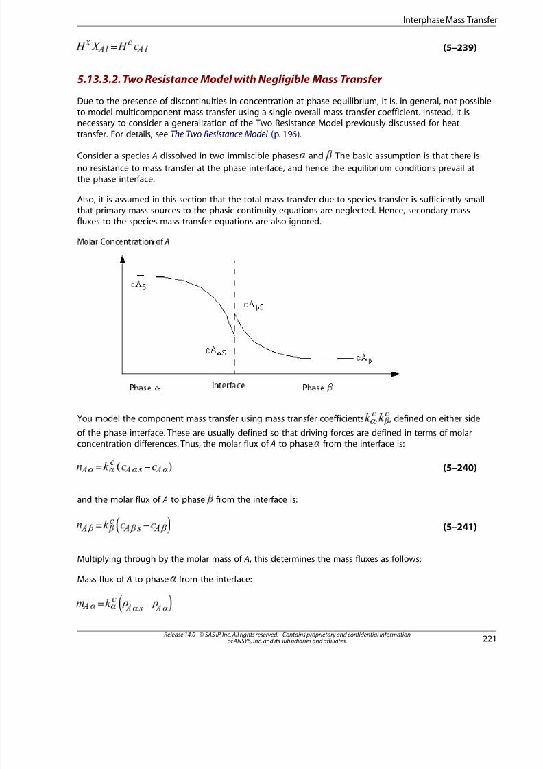
7/16/2019 ANSYS CFX-Solver Theory Guide
http://slidepdf.com/reader/full/ansys-cfx-solver-theory-guide-5633873a6f5ee 237/417
(5–239)= ¡ ¢
£
¤ ¥
¦
¤ ¥
5.13.3.2. Two Resistance Model with Negligible Mass Transfer
Due to the presence of discontinuities in concentration at phase equilibrium, it is, in general, not possibleto model multicomponent mass transfer using a single overall mass transfer coefficient. Instead, it is
necessary to consider a generalization of the Two Resistance Model previously discussed for heattransfer. For details, see The Two Resistance Model (p. 196).
Consider a species A dissolved in two immiscible phases§
and ̈
. The basic assumption is that there is
no resistance to mass transfer at the phase interface, and hence the equilibrium conditions prevail atthe phase interface.
Also, it is assumed in this section that the total mass transfer due to species transfer is sufficiently smallthat primary mass sources to the phasic continuity equations are neglected. Hence, secondary massfluxes to the species mass transfer equations are also ignored.
You model the component mass transfer using mass transfer coefficients©
,
, defined on either side
of the phase interface. These are usually defined so that driving forces are defined in terms of molarconcentration differences. Thus, the molar flux of A to phase
from the interface is:
(5–240)= −
!
"
and the molar flux of A to phase #
from the interface is:
(5–241)= −$ % & &
' ( (
)
' ( 0 ' (
Multiplying through by the molar mass of A, this determines the mass fluxes as follows:
Mass flux of A to phase 1 from the interface:
= −2 3 4 4
5 6 6
7
5 6 8 5 6
221Release 14.0 - © SAS IP, Inc. All rights reserved. - Contains proprietary and confidential informationof ANSYS, Inc. and its subsidiaries and affiliates.
Interphase Mass Transfe

7/16/2019 ANSYS CFX-Solver Theory Guide
http://slidepdf.com/reader/full/ansys-cfx-solver-theory-guide-5633873a6f5ee 238/417
Mass flux of A to phase
from the interface:
(5–242)= −¡ ¢ £ £
¤ ¥ ¥
¦
¤ ¥ § ¤ ¥
In order to eliminate the unknown interface values, Equation 5–241 (p. 221) and Equation 5–242 (p. 222)must be supplemented by the equilibrium relation between
̈
©
and
. This is most conveniently
expressed using the molar concentration equilibrium ratio:
(5–243)= ⇒ =
!
!
The mass balance condition:
(5–244)+ =" "
# $ # %
may now be combined with the quasi-linearized equilibrium relationship Equation 5–243 (p. 222) to de-
termine the interface mass concentrations:
(5–245)= =+
+ &
'
&
( & ( &
'
( (
) 0 1
2
) 3 1
0
2
) 0
3
2
) 3
2
0
2
3
2
These may be used to eliminate the interface values in Equation 5–241 (p. 221) and Equation 5–242 (p. 222)in order to express the interfacial mass fluxes in terms of the phasic mass concentrations:
(5–246)= − = − = +4 4 5 6 7 7
5 5
6
5
8 9 8 @ 9 @
A A
8 @ 8 9
9 @
A
9
A
A
@
A
5.13.4.The Thermal Phase Change Model
This model describes phase change induced by interphase heat transfer; it may be used to simulateboiling and condensation, or melting and solidification. For example, it may be used to model condens-ation of saturated vapor bubbles in sub-cooled liquid, or evaporation of saturated bubbles in superheatedliquid.
This section discusses the theory. For modeling information, see Thermal Phase Change Model.
It is essential to consider the heat transfer processes on each side of the phase interface. Hence, the Two Resistance model for interphase heat transfer must be used in conjunction with the Thermal PhaseChange model. For details, see The Two Resistance Model (p. 196).
Recall that, in this case, the sensible heat flux to phaseB
from the interface is:
(5–247)= −C D E E
F
F G F
and the sensible heat flux to phase H
from the interface is:
Release 14.0 - © SAS IP, Inc. All rights reserved. - Contains proprietary and confidential informationof ANSYS, Inc. and its subsidiaries and affiliates.222
Chapter 5: Multiphase Flow Theory

7/16/2019 ANSYS CFX-Solver Theory Guide
http://slidepdf.com/reader/full/ansys-cfx-solver-theory-guide-5633873a6f5ee 239/417
(5–248)= − ¡ ¢ ¢
£
£ ¤ £
•¥
¦
and§
̈
are the phase©
and phase
heat transfer coefficients respectively.
• The interfacial temperature is determined from considerations of thermodynamic equilibrium. Ignor
effects of surface tension on pressure, assume =
, the saturation temperature.
Note that this is in contrast to the case where there is no mass transfer. In that case, the interfacial
temperature is determined from the sensible heat balance + =
.
In the case of interphase mass transfer, the interphase mass transfer is determined from the total heatbalance, as follows.
Total heat flux to phase
from the interface:
(5–249)= + ! " #
$ $
$ % $ &
Total heat flux to phase '
from the interface:
(5–250)= −( ) 0 1
2 2
3 2 2 4
• 5
6 7
denotes mass flux into phase 8 from phase 9 .
• @
A B
and C
D E
represent interfacial values of enthalpy carried into and out of the phases due to phase
change, see below for details.
The total heat balance + =F F
G H now determines the interphase mass flux:
(5–251)=+
−I
P P
Q Q
R S
R S S R
S T R T
The secondary heat flux term must be modified in order to take account of the discontinuity in staticenthalpy due to latent heat between the two phases. This is achieved using a modification of the upwindformulation Equation 5–226 (p. 218), due to Prakash [53]. In this formulation, the bulk fluid enthalpy iscarried out of the outgoing phase, as in the default upwind formulation. However, the saturation enthalpyis carried into the incoming phase. Thus:
(5–252)> ⇒ = =
< ⇒ = =
U V V V V
U V V V V
W X W Y W X Y X
W X W Y W X Y X
̀ a b
̀ a b
This leads to a formulation which is stable both physically and numerically. It implies that the denom-inator of Equation 5–251 (p. 223) is non-zero, being greater than or equal to the latent heat:
= − c d d
e f g h i g h i
.
223Release 14.0 - © SAS IP, Inc. All rights reserved. - Contains proprietary and confidential informationof ANSYS, Inc. and its subsidiaries and affiliates.
Interphase Mass Transfe

7/16/2019 ANSYS CFX-Solver Theory Guide
http://slidepdf.com/reader/full/ansys-cfx-solver-theory-guide-5633873a6f5ee 240/417
5.13.4.1. Wall Boiling Model
Wall boiling starts when the wall temperature achieves a temperature which is sufficiently large to ini-tiate the activation of wall nucleation sites. This activation temperature is typically a few degrees abovethe saturation temperature. However, at this stage, the average temperature of the liquid in the vicinityof the heated wall is still well below the saturation temperature, hence in the sub-cooled boiling regime.
Evaporation starts in the microscopic cavities and crevices, which are always present on the solid surface.Liquid becomes supersaturated locally in these nucleation sites, leading to the growth of vapor bubblesat the sites. The bubbles become detached from the sites when they are sufficiently large that externalforces (inertial, gravitational, or turbulent) exceed the surface tension forces that keep them attachedto the wall. As the bubbles depart from the wall, they are displaced by superheated liquid in the vicinityof the nucleation sites, after which the nucleation site is free to create another bubble. In regions of the wall not affected by bubble growth, the wall heat transfer to the liquid may be described by singlephase convective heat transfer.
It is clear that detailed physics of bubble growth is very complex, and occurs on very small length scalesin the vicinity of the wall. It is unrealistic to model the detailed physics in a phase-averaged Eulerianmultiphase model. It is also unrealistic to resolve the small length scales with ultra-fine meshes. The
model described here is a so-called mechanistic model, which aims to model the important physicalsub-processes using engineering correlations. The model is a sub-grid scale model, in the sense thatthe complex physics is assumed to take place in a vicinity very close to the wall which is smaller thanthe mesh resolution at the wall.
The first and most well-known model of this kind was formulated by Kurul and Podowski (1991) [159],from the Rensselaer Polytechnic Institute. It is known as the RPI model. In this model, a number of thesub-models of the overall mechanistic model were taken from correlations originally developed for ex-ploitation in one-dimensional thermo-hydraulic simulation methods. This model was implemented inCFX-4, with the near-wall distance taking the place of the centerline wall distance in the one-dimensionalmodels. Unfortunately, this lead to results that were strongly mesh-dependent.
In the implementation in CFX-5.7.1, Egorov et al. formulated modifications of the one-dimensional cor-relations with the aim of restoring mesh independence to the results. This modification of the originalRPI model is described here.
The following topics are discussed in this section:
• Partitioning of the Wall Heat Flux (p. 224)
• Sub-models for the Wall Boiling Model (p. 226)
For more information about the wall boiling model and its usage, see Wall Boiling Model in the CFX-
Solver Modeling Guide.
5.13.4.1.1. Partitioning of the Wall Heat Flux
A fundamental feature of the mechanistic model of wall nucleation is the algorithm for deciding howthe wall heat flux is to be partitioned amongst the separated physical processes of evaporation andsensible heating of the liquid phase. In regions of the wall not influenced by nucleation sites, it is suffi-cient to consider the wall heat flux as contributing solely to single-phase liquid convective heat transfer.However, in the vicinity of the nucleation sites, some of the heat contributes to vapor production, andthe remainder to super heating of the liquid phase as it displaces the rising bubbles. This latter processis known as quenching.
Hence, the mechanistic heat partitioning model has the following general structure:
Release 14.0 - © SAS IP, Inc. All rights reserved. - Contains proprietary and confidential informationof ANSYS, Inc. and its subsidiaries and affiliates.224
Chapter 5: Multiphase Flow Theory

7/16/2019 ANSYS CFX-Solver Theory Guide
http://slidepdf.com/reader/full/ansys-cfx-solver-theory-guide-5633873a6f5ee 241/417
= +
¡ ¢ £
where¤
¥
is consumed for heating the sub-cooled liquid, and¦
§
is the evaporation heat flux. ̈
©
is further
assumed to be partitioned into two sub-processes:
= +
where
is the heat flux corresponding to convective heat transfer, and
is the heat flux correspond-
ing to quenching. Hence, in total, there is a three-way partition:
= + +
! "
In this model, vapor is assumed to be saturated everywhere, and no part of the wall heat flux is arrangedfor superheating of the vapor phase.
The heat partitioning model considers the whole wall surface as being separated into two fractions:
• Fraction #
$
is influenced by the vapor bubbles, formed on the wall.
• Fraction %
&
is the rest of the wall surface, with = − ' '
( )
.
The wall area fraction 0
1
represents the part of the wall surface that does not 'feel' the presence of the
vapor phase. The wall heat flux for this part of the surface is modeled in a similar way as for the single-phase flow of pure liquid, by using the turbulent wall function procedure in the case of the turbulent
flow. This part of 2
3
, called the convective heat flux4
5
, can be correlated for turbulent flow as:
= −6 7 8 9 9
@
@ A B C
where D
E
is the temperature of the solid wall, F
G
is the temperature of the liquid at the wall, and H
I
is
the turbulent heat transfer coefficient, which depends on the velocity field and on the near-wall gridcell size. Kurul and Podowski (1991) [159] modeled
P
Q
using a one-dimensional Stanton number correl-
ation. Egorov and Menter (2004) [163] modeledR
S
using the turbulent wall function.
The wall area fraction T
U
represents the remaining part of the wall surface, which exchanges heat with
both phases. The already mentioned heat fluxV
W
comes from this part of the surface and is consumed
for evaporation of the initially sub-cooled liquid:
(5–253)= −X Y ` `
a
b c d e f g
where h is the evaporation mass transfer rate per unit wall area, and i
p q r s t
and u
v
are the specific en-
thalpies of the saturated vapor and sub-cooled liquid, respectively.
A part of the heat flux to the liquid, coming from the wall area fraction w
x
, is transported between the
bubble departure and the next bubble formation at the same nucleation site. This additional mechanismof heating the liquid phase is called quenching, and is modeled as:
= −y
225Release 14.0 - © SAS IP, Inc. All rights reserved. - Contains proprietary and confidential informationof ANSYS, Inc. and its subsidiaries and affiliates.
Interphase Mass Transfe

7/16/2019 ANSYS CFX-Solver Theory Guide
http://slidepdf.com/reader/full/ansys-cfx-solver-theory-guide-5633873a6f5ee 242/417
The area fraction values
¡
and ¢
£
play an important role in the heat-partitioning model. They are related
to the nucleation site density per unit wall area ¤ and to the influence area of a single bubble formingat the wall nucleation site. The latter value is modeled by introducing the bubble departure diameter
value¥
¦
, which can generally serve as a length scale of the wall boiling mechanism. The RPI model
assumes that the diameter of the bubble influence zone is twice as large as §
̈
, therefore the non-di-
mensional area fraction of the bubble influence is:
(5–254)= ⋅ ©
Here the implicitly assumed factor of 2 for the diameter of the bubble influence can be user-specified.
It should be noted that, for the evaporation rate
and corresponding heat flux
(Equa-
tion 5–253 (p. 225)), the upper limit of Equation 5–254 (p. 226) for bubble influence area fraction does not
apply. Instead of using a factor of
as defined by Equation 5–254 (p. 226), the ! value is directly
modeled as being proportional to the nucleation site density"
.
5.13.4.1.2. Sub-models for the Wall Boiling Model
As mentioned in the previous section, the two most important parameters governing the heat partitioning
model are the nucleation site density#
and the bubble departure diameter$
%
. In the RPI wall-boiling
model they are correlated to the wall superheat = −& & &
' ( ) 0 1 2 2 ' 1 3
and to the near-wall liquid sub-
cooling = −4 4 4
5 6 7 5 8 9 @ A B
, respectively.
The following topics will be discussed:
• Wall Nucleation Site Density (p. 226)
• Bubble Departure Diameter (p. 227)
• Bubble Detachment Frequency (p. 227)
• Bubble Waiting Time (p. 228)
• Area Influence Factors (p. 228)
• Convective Heat Transfer (p. 228)
• Quenching Heat Transfer (p. 228)
• Evaporation Rate (p. 229)
5.13.4.1.2.1. Wall Nucleation Site Density
The model for wall nucleation site density adopted in the RPI model is that of Lemmert and Chawla(1977) [164]:
= = =−
C D D E F D G
H
I
P Q R
Note that the wall superheat in the above equation cannot be negative. Its negative value means thatthe wall temperature drops below the saturation temperature, where there is no boiling and the heatpartitioning model is not used.
Release 14.0 - © SAS IP, Inc. All rights reserved. - Contains proprietary and confidential informationof ANSYS, Inc. and its subsidiaries and affiliates.226
Chapter 5: Multiphase Flow Theory

7/16/2019 ANSYS CFX-Solver Theory Guide
http://slidepdf.com/reader/full/ansys-cfx-solver-theory-guide-5633873a6f5ee 243/417
This model was implemented in CFX-4 with parameter = , giving an overall correction factor of
. Egorov and Menter (2004) [163], conjecturing that this was a deliberate alteration by the RPI group,related to the corresponding factor in the bubble waiting time model. Egorov and Menter also reformu-lated the correlation as follows:
=¡ ¡ ¢ ¢
£
¤ ¥ ¦ § ¨ © ¤ ¥ ¦
where = × +
−
and =
. This formulation avoids fractional
powers of physical dimensions, hence is more amenable to the use of different unit systems.
Alternative correlations have been proposed for nucleation site density by Kocamustafaogullari andIshii (1983) [160].
5.13.4.1.2.2. Bubble Departure Diameter
Kurul and Podowski (1991) [159] adopted the correlation for bubble departure diameter due to Tolub-inski and Kostanchuk (1970) [165]:
(5–255)=
⋅
−
! " # $
% & '
" # $
( ) 0
The parameters of the model are dimensional ( =1
2 3 4
, =5
6 7 8
,
=9
@ A B
) and are chosen to fit pressurized water data. Hence the model is clearly not universal.
Negative liquid sub-cooling is possible here, where it means onset of the bulk boiling. Limiting the
bubble departure diameter applies to this situation and preventsC
D
from growing too high.
Note that the model is strongly dependent on a liquid temperature scale. In the original experimental
data, this was taken as the pipe center-line temperature. CFX-4 used the cell-center value in near wallcells, but this proved to give mesh-dependent results. Egorov and Menter restored mesh independence
by using the logarithmic form of the wall function to estimate the liquid temperature, E
F
, at a fixed value
of =+ G
. ANSYS CFX uses this method, with a user-modifiable value of +
H
.
5.13.4.1.2.3. Bubble Detachment Frequency
The computation of the evaporation rateI
requires an additional model parameter, namely the frequencyof the bubble detachment from the nucleation site. The model adopted by Kurul and Podowski is thatdue to Cole (1960) [166]:
=−
P
Q R R
S T R
U V
W X
U
Note that, due to its dependence on gravity, this correlation is taken from pool boiling. It is simply es-timated as the bubble rise velocity divided by the bubble departure diameter. The drag coefficient
factorY
̀
was taken to be unity by Ceumern-Lindenstjerna (1977) [169].
227Release 14.0 - © SAS IP, Inc. All rights reserved. - Contains proprietary and confidential informationof ANSYS, Inc. and its subsidiaries and affiliates.
Interphase Mass Transfe

7/16/2019 ANSYS CFX-Solver Theory Guide
http://slidepdf.com/reader/full/ansys-cfx-solver-theory-guide-5633873a6f5ee 244/417
5.13.4.1.2.4. Bubble Waiting Time
Kurul and Podowski (1991) [159] employed the model of Tolubinski and Kostanchuk (1970) [ 165]. Thisfixes the waiting time between departures of consecutive bubbles at 80% of the bubble detachmentperiod:
(5–256)=
¡
¢
The numerator in this equation is adjustable in ANSYS CFX.
5.13.4.1.2.5. Area Influence Factors
Recall from Partitioning of the Wall Heat Flux (p. 224) that Kurul and Podowski assumed a diameter of
influence of a nucleating bubble equal to twice the bubble departure diameter £
¤
. Encoding this as a
user-modifiable parameter ¥
¦
(default value = 2), the area fraction of the bubble influence is given by:
=
⋅
§
¨ ©
The area fraction
subjected to single phase liquid convective heat transfer is limited from below by
a small value, so its actual form is:
= −−
5.13.4.1.2.6. Convective Heat Transfer
As discussed in Partitioning of the Wall Heat Flux (p. 224), single phase convective heat transfer to the liquidphase is modeled using the turbulent wall function (Egorov and Menter 2004 [ 163]).
= −! " # $ $
%
% & ' (
This replaces the mesh dependent Stanton Number correlation originally employed by Kurul andPodowski (1991) [159].
5.13.4.1.2.7. Quenching Heat Transfer
As discussed in Partitioning of the Wall Heat Flux (p. 224), quenching heat transfer to the liquid phase inthe area of influence of the vapor phase is modeled using a quenching heat transfer coefficient:
= −) 0 1 2 2
3
3 4 5 6
In order to close the model, the quenching heat transfer coefficient7
8
, participating in the quenching
heat flux to liquid, must be defined. This value depends on the waiting time between the bubble de-parture and the next bubble formation.
With this value, the quenching heat transfer coefficient is correlated as:
Release 14.0 - © SAS IP, Inc. All rights reserved. - Contains proprietary and confidential informationof ANSYS, Inc. and its subsidiaries and affiliates.228
Chapter 5: Multiphase Flow Theory

7/16/2019 ANSYS CFX-Solver Theory Guide
http://slidepdf.com/reader/full/ansys-cfx-solver-theory-guide-5633873a6f5ee 245/417
= ¡ ¢
£
¤ ¥
¦ §
̈
§
where =©
is the liquid temperature conductivity coefficient. (Mikic and Rohsenow 1969
[167], Del Valle and Kenning 1985 [168]).
As for the case of bubble departure diameter, Egorov and Menter (2004) [163] used the logarithmicform of the wall function to estimate the liquid temperature
at a fixed+
value of 250.
5.13.4.1.2.8. Evaporation Rate
Knowing the bubble departure frequency, as well as the bubble size and the nucleation site density,one can obtain the evaporation rate as a product of the bubble mass, the detachment frequency andthe site density:
=
! " #
$
%
&
This was the form adopted by Kurul and Podowski (1991) [159].
Egorov and Menter expressed the evaporation rate in terms the non-limited area fraction′
'
(
:
= ⋅′ )
0 1 2
3
4
4
4
5
4
(unlike 6
7
,′
8
9
can exceed 1). In this case, the evaporation rate obtains the form:
= ⋅′@ A B C D
E F
G
In the final form of the evaporation rate, the area fraction factor′
H
I
is limited by:
(5–257)= ⋅ =′ ′ ′P Q Q R S T Q
U U V W X Y ̀
a
U V W X Y
The last limiting procedure is not used if the bubble departure diameter is below b . In this case
the non-limited form Equation 5–257 (p. 229) is used. The estimated value of for′
c
d e f g h
is the upper
limit for the nucleation sites area fraction, taking into account the effect of overlapping neighboringsites, operating out of phase. The functional form of this parameter is given in terms of the departurefrequency and waiting time:
=− ⋅
′ i
p q
r s t u v
w
which gives with the correlation Equation 5–256 (p. 228) forx
y
.
229Release 14.0 - © SAS IP, Inc. All rights reserved. - Contains proprietary and confidential informationof ANSYS, Inc. and its subsidiaries and affiliates.
Interphase Mass Transfe

7/16/2019 ANSYS CFX-Solver Theory Guide
http://slidepdf.com/reader/full/ansys-cfx-solver-theory-guide-5633873a6f5ee 246/417
5.13.4.1.3. Determination of the Wall Heat Flux Partition
The wall heat flux partition discussed in Partitioning of the Wall Heat Flux (p. 224), together with theuser’s choice of submodels described in Sub-models for the Wall Boiling Model (p. 226), gives the total
heat flux as a complex nonlinear function of the wall superheat = −
¡ ¢ £ ¤ ¥ ¦ §
= + +¨ © ¨ © ¨ © ¨ ©
In the case of an isothermal wall, the three components of the heat flux are computed explicitly asfunctions of the given wall superheat. However, in the case of a wall with specified total heat flux, or
specified wall heat transfer coefficient and outside temperature, the above equation determines
implicitly as a function of the total heat supplied to the wall. In this case,!
" # $
is computed by solving
the nonlinear equation =% % &
' ( ' ) 0 1
2 3 4
using the binary chop method. The resulting value of
5
6 7 8
is subsequently used to determine the three individual components of the wall heat partition.
Important
If you want to use the User Specified option for any of the sub-models described in Sub-
models for the Wall Boiling Model (p. 226), and if you want any of these to be functions of thewall superheat, then it is important to use the correct name for this variable. As the wallboiling model is described as a phase-pair model, this variable is a phase-pair based variablenamed Tsuperheat. For example:
9
@ A B
= water | steam.Tsuperheat
It is not appropriate to use a phase-specific temperature field at the wall, such as water.Tem-
perature, to determine C
D E F
as this variable does not participate in the binary chop algorithm
to determine the wall superheat.
5.13.5. Cavitation Model
The tendency for a flow to cavitate is characterized by the cavitation number, defined as:
(5–258)=
−G
H H
I P
Q
R
S
T
U
where V is a reference pressure for the flow (for example, inlet pressure), W
X
is the vapor pressure for
the liquid, and the denominator represents the dynamic pressure. Clearly, the tendency for a flow tocavitate increases as the cavitation number is decreased.
Cavitation is treated separately from thermal phase change, as the cavitation process is typically toorapid for the assumption of thermal equilibrium at the interface to be correct. In the simplest cavitationmodels, mass transfer is driven by purely mechanical effects, namely liquid-vapor pressure differences,rather than thermal effects. Current research is directed towards models which take both effects intoaccount.
Release 14.0 - © SAS IP, Inc. All rights reserved. - Contains proprietary and confidential informationof ANSYS, Inc. and its subsidiaries and affiliates.230
Chapter 5: Multiphase Flow Theory

7/16/2019 ANSYS CFX-Solver Theory Guide
http://slidepdf.com/reader/full/ansys-cfx-solver-theory-guide-5633873a6f5ee 247/417
In CFX, the Rayleigh Plesset model is implemented in the multiphase framework as an interphase masstransfer model. User defined models can also be implemented.
For cavitating flow, the homogeneous multiphase model is typically used.
5.13.5.1. The Rayleigh Plesset Model
The Rayleigh-Plesset equation provides the basis for the rate equation controlling vapor generation
and condensation. The Rayleigh-Plesset equation describing the growth of a gas bubble in a liquid isgiven by:
(5–259)+
+ =
−
¡
¡ ¢
¡
¡ ¢
£
¤
¥ ¥
¤
¦
¦ ¦
§
¦
̈
§
©
©
©
where
represents the bubble radius,
is the pressure in the bubble (assumed to be the vapor
pressure at the liquid temperature), is the pressure in the liquid surrounding the bubble,
is the liquid
density, and
is the surface tension coefficient between the liquid and vapor. Note that this is derivedfrom a mechanical balance, assuming no thermal barriers to bubble growth. Neglecting the secondorder terms (which is appropriate for low oscillation frequencies) and the surface tension, this equationreduces to:
(5–260)=−
! !
"
#
$
%
The rate of change of bubble volume follows as:
(5–261)= = −& '
& (
&
& (
) 0 ) 0
1 1
2
3
3 3
4
5
6 7
and the rate of change of bubble mass is:
(5–262)= =−
8 9
8
@
A
8 B
8
@
C D A
E E
A
F
G
F
F
G
H
I
P
If there are Q
R
bubbles per unit volume, the volume fractionS
T
may be expressed as:
(5–263)= =U V W X Y W
̀ a a a a
b
and the total interphase mass transfer rate per unit volume is:
231Release 14.0 - © SAS IP, Inc. All rights reserved. - Contains proprietary and confidential informationof ANSYS, Inc. and its subsidiaries and affiliates.
Interphase Mass Transfe

7/16/2019 ANSYS CFX-Solver Theory Guide
http://slidepdf.com/reader/full/ansys-cfx-solver-theory-guide-5633873a6f5ee 248/417
(5–264)= =−
¡
¢
¢ £
¤ ¥
¦
§ §
¥
̈ ©
©
©
̈
This expression has been derived assuming bubble growth (vaporization). It can be generalized to includecondensation as follows:
(5–265)=−
−
!
!
where " is an empirical factor which may differ for condensation and vaporization, designed to accountfor the fact that they may occur at different rates (condensation is usually much slower than vaporization).
For modeling purposes the bubble radius #
$
will be replaced by the nucleation site radius %
& ' (
.
Despite the fact that Equation 5–265 (p. 232) has been generalized for vaporization and condensation,it requires further modification in the case of vaporization.
Vaporization is initiated at nucleation sites (most commonly non-condensible gases). As the vaporvolume fraction increases, the nucleation site density must decrease accordingly, because there is less
liquid. For vaporization,)
0
in Equation 5–265 (p. 232) is replaced by −1 1
2 3 4 5
to give:
(5–266)=− −
−6 7
8 8 9
@
A A
9
A A
B C
D E F C
C
D E F
G
B
G
whereH
I P Q
is the volume fraction of the nucleation sites. Equation 5–265 (p. 232) is maintained in the
case of condensation.
To obtain an interphase mass transfer rate, further assumptions regarding the bubble concentrationand radius are required. The Rayleigh-Plesset cavitation model implemented in CFX uses the followingdefaults for the model parameters:
• = R S
T U V
• = −W
X Y ̀
• = a
b c d
• = e
f g h i
For an illustration and a validation of the Rayleigh-Plesset cavitation model see Bakir et al. [ 148]
5.13.5.2. User Defined Cavitation Models
Additional information on creating a user defined model is available. For details, see User DefinedCavitation Models in the CFX-Solver Modeling Guide.
Release 14.0 - © SAS IP, Inc. All rights reserved. - Contains proprietary and confidential informationof ANSYS, Inc. and its subsidiaries and affiliates.232
Chapter 5: Multiphase Flow Theory

7/16/2019 ANSYS CFX-Solver Theory Guide
http://slidepdf.com/reader/full/ansys-cfx-solver-theory-guide-5633873a6f5ee 249/417
When using a user defined cavitation model, the CFX-Solver will perform generic linearizations for thevolume fraction and volume continuity equations to help stability and convergence. The saturationpressure is used by the CFX-Solver in linearizing the cavitation rate against pressure.
5.13.6.The Droplet Condensation Model
The Droplet Condensation Model is useful for situations where a dry (or near-saturation) two-phaseflow undergoes rapid pressure reduction leading to nucleation and subsequent droplet condensation.It is also useful to model additional condensation when droplets are already present in significantquantities. Typical applications include low-pressure steam turbines, in which context this model is alsoreferred to as the Nonequilibrium Steam (NES) model. Such flows are typically transonic. The dropletphase can enter through the inlet or appear through various nucleation mechanisms, including homo-geneous (volumetric) and heterogeneous (surface) nucleation. Presently, only one homogeneous nucle-ation model is available for selection based on Classical theory. Heterogeneous and alternate homogen-eous nucleation models can be supplied using the available user defined option.
The Droplet Condensation Model differs from the Thermal Phase Change model (see The Thermal Phase
Change Model (p. 222)) in that the droplet diameter is calculated as part of the model rather than as auser input. This leads to improved accuracy. In order to do this a transport equation for droplet number
must also be solved, which has as its source term nucleation contributions. This model differs from theEquilibrium Phase Change model (see Equilibrium Phase Change Model in the CFX-Solver Modeling
Guide) in that it does not assume the flow to instantaneously reach equilibrium conditions, and thereforeimplicitly includes losses due to thermodynamic irreversibility.
In the following discussion, we consider a homogeneous multiphase system, in which the droplets movewith the same velocity as the continuous phase. However, the model has been generalized to inhomo-geneous systems as well.
The system of equations involves one continuous phase and any number of dispersed (condensed)phases. The condensed phases travel at the speed of the continuous phase. Any combination of con-densed phases can exist in the solution so that for the continuous phase, mass conservation becomes:
(5–267)∑∂∂
+∂
∂= − +
=
∗ ¡
¢ £
¤ ¡ ¥ ¦ ¡ §
̈ ©
where the mass sources are summed over the condensed phases. The condensed phases can changesize by condensation or evaporation.
For a condensed phase,
mass conservation is:
(5–268)
∂
∂ +
∂
∂ = +
∗
! " # $
%
%
%
%
&
& ' ( '
where each dispersed phase has a corresponding number equation of the form:
233Release 14.0 - © SAS IP, Inc. All rights reserved. - Contains proprietary and confidential informationof ANSYS, Inc. and its subsidiaries and affiliates.
Interphase Mass Transfe

7/16/2019 ANSYS CFX-Solver Theory Guide
http://slidepdf.com/reader/full/ansys-cfx-solver-theory-guide-5633873a6f5ee 250/417
(5–269)∂
∂+
∂∂
= ¡
¢ £
¤ ¡ ¥ ¦
§
§
§
§
§
̈
̈
©
and
is the nucleation model with units defined as the number of droplets generated per unit time
per unit volume of vapor and∗
is the nucleated droplet mass based on the critical radius∗
. Notethat the droplets are transported with the mixture velocity because no slip is assumed between thephases. The usual constraint applies for the volume fractions where:
(5–270)∑+ ==
In addition, global continuity and momentum equations are also solved as described in Homogeneous
Hydrodynamic Equations (p. 172). The continuous phase energy equation, in total enthalpy form, is
(5–271)∂
∂
+∂
∂
= −∂
∂
+∂
∂
∂
∂
+
! " #
$ %
! " & # "
'
$ %
( "
)
%
0
1
1 1
2
1
1 2 1 1
2
3 1
2
4
where a similar energy transport equation can be applied for the dispersed phases, either in the contextof small or large droplets as will be discussed subsequently. The Droplet Condensation model can beused for both small and large droplets. However, small and large droplets use different models for heattransfer and phase change. For large droplets, the heat transfer and phase change models describedby the Thermal Phase Change model should be used. For small droplets (less than 1
5 6
) the Small
Droplet heat transfer model is appropriate; it sets the droplet temperature to
(5–272)= −∗
7 7 8 7
9
9
@ A A B
@
@
where C
D
refers to the saturation temperature, E
F G
refers to the supercooling level in gas phase, H
I
is
the droplet radius, and∗
P
Q
is the critical radius at formation of the dispersed phase.
For small droplets, the interphase heat and mass transfer models are also modified to include the influ-
ence of the Knudsen ( R S
) number on the Nusselt number. The T U
dependence is required becausedroplet sizes vary significantly from the initial nucleated radius (in a non-continuum regime) in therange of angstroms. The droplet growth rate is:
(5–273)=+
−−
V W
V X
Y
W ` a b c
d d
e e
f g
f
f
f h
h i
which is subsequently used to compute the interphase mass transfer rate in conjunction with an inter-facial area density to be described later in this section.
The source of droplets into the domain is based on a nucleation model, which for classical nucleationmodels has the form of:
Release 14.0 - © SAS IP, Inc. All rights reserved. - Contains proprietary and confidential informationof ANSYS, Inc. and its subsidiaries and affiliates.234
Chapter 5: Multiphase Flow Theory
7/16/2019 ANSYS CFX-Solver Theory Guide
http://slidepdf.com/reader/full/ansys-cfx-solver-theory-guide-5633873a6f5ee 251/417
(5–274)=
−
∗ ¡
¢
£ ¤
¥
where ¦
is a constant determined by the particular nucleation model,∗
§
is the Gibbs free energy
change at the critical radius conditions, ̈
is Boltzmann's constant, and©
is the supercooled vapor
temperature. To compute the Gibbs free energy change a property database must be used that evaluatessupercooled state properties. This requires an equation of state for the vapor phase amenable to extra-polation into regions within the saturation zone. The IAPWS and Redlich Kwong equations of statesatisfy this requirement. A user defined nucleation model can also be applied, allowing for differenthomogeneous or heterogeneous nucleation models to be employed.
The interaction between the phases by mass transfer depends on calculating the droplet diameter,which, if a monodispersed distribution is assumed for droplets with a common origin, can be determined
from the droplet number,
. The relevant equation is then:
(5–275)=
with an interfacial area density defined as:
(5–276)=
!
"
#
#
#
The interfacial mass transfer term can then be computed with the known droplet growth rate and theinterfacial area density:
(5–277)=$ % &
' (
' )
0
0 0
0
which can be used to obtain the heat transfer term:
(5–278)= − +1 1 2 3 4
5 6 7
6 6
where 8
9
is an upwinded total enthalpy, its value either for the continuous or dispersed phase depending
on the direction of interphase mass transfer. In addition, @
A
is the heat transfer (per unit area) betweenthe dispersed and continuous phase based on:
(5–279)=+
−B
C
D E F G
H H
I
P
I
I Q
Since the droplets in condensing systems are generally quite small (less than 1 R S
), it is assumed that
the droplet temperature is uniform (a zero resistance model between the droplet surface and its internal
235Release 14.0 - © SAS IP, Inc. All rights reserved. - Contains proprietary and confidential informationof ANSYS, Inc. and its subsidiaries and affiliates.
Interphase Mass Transfe

7/16/2019 ANSYS CFX-Solver Theory Guide
http://slidepdf.com/reader/full/ansys-cfx-solver-theory-guide-5633873a6f5ee 252/417
temperature). This implies that almost all of the heat transfer either comes from the continuous phaseduring evaporation or goes into it during condensation.
The Nusselt ( ¡
) number underlying Equation 5–273 (p. 234) and Equation 5–279 (p. 235) is corrected to
account for droplet sizes that span a wide Knudsen number ( ¢ £
) range (from free-molecular to con-tinuum). The Nusselt number applied is:
(5–280)= + ¤ ¥
¦ § ̈
where©
is an empirical factor set to 3.18.
5.14. Free Surface Flow
This section describes free surface flow theory, which is the most common application of homogeneousmultiphase flow.
5.14.1. Implementation
The implementation of free surface flow in CFX is essentially the same as multiphase (homogeneousor inhomogeneous) along with some special discretization options to keep the interface sharp. Theseinclude:
• A compressive differencing scheme for the advection of volume fractions in the volume fraction equations.
• A compressive transient scheme for the volume fraction equations (if the problem is transient).
• Special treatment of the pressure gradient and gravity terms to ensure that the flow remain well behavedat the interface.
5.14.2. Surface Tension
The surface tension model used in CFX is based on the Continuum Surface Force model of Brackbill etal. [27]. This models the surface tension force as a volume force concentrated at the interface, ratherthan a surface force. Consider the free surface interface shown in the figure below:
Figure 5.1 Free Surface Interface
Release 14.0 - © SAS IP, Inc. All rights reserved. - Contains proprietary and confidential informationof ANSYS, Inc. and its subsidiaries and affiliates.236
Chapter 5: Multiphase Flow Theory

7/16/2019 ANSYS CFX-Solver Theory Guide
http://slidepdf.com/reader/full/ansys-cfx-solver-theory-guide-5633873a6f5ee 253/417
Define a Primary Fluid
(the liquid phase) and a Secondary Fluid ¡
(usually a gas phase). The surface
tension force given by the Continuum Surface Force model is:
(5–281)=¢ £ ¤
¥ ¦
¥ ¦
¥ ¦
where:
(5–282)= − + ∇ § ̈© ©
(5–283)= ∇
where is the surface tension coefficient,
!
is the interface normal vector pointing from the primary
fluid to the secondary fluid (calculated from the gradient of a smoothed volume fraction), ∇ "
is the
gradient operator on the interface and#
is the surface curvature defined by:
(5–284)= ∇$ %
& ' & '
The two terms summed on the right hand side of Equation 5–282 (p. 237) reflect the normal and tangentiacomponents of the surface tension force respectively. The normal component arises from the interfacecurvature and the tangential component from variations in the surface tension coefficient (the Marangonieffect).
The (
) 0
term is often called the interface delta function; it is zero away from the interface, thereby
ensuring that the surface tension force is active only near to the interface.
When the interface between the two fluids intersects a wall, it is possible to account for wall adhesion
by specifying the contact angle,1
, which the interface makes with the wall through the primary fluid. The interface normal vector used for the calculations of both curvature and the surface tension forcemust satisfy the wall contact angle.
237Release 14.0 - © SAS IP, Inc. All rights reserved. - Contains proprietary and confidential informationof ANSYS, Inc. and its subsidiaries and affiliates.
Free Surface Flow

7/16/2019 ANSYS CFX-Solver Theory Guide
http://slidepdf.com/reader/full/ansys-cfx-solver-theory-guide-5633873a6f5ee 254/417
Release 14.0 - © SAS IP, Inc. All rights reserved. - Contains proprietary and confidential informationof ANSYS, Inc. and its subsidiaries and affiliates.238

7/16/2019 ANSYS CFX-Solver Theory Guide
http://slidepdf.com/reader/full/ansys-cfx-solver-theory-guide-5633873a6f5ee 255/417
Chapter 6: Particle Transport Theory
Particle transport modeling is a type of multiphase model, where particulates are tracked through theflow in a Lagrangian way, rather than being modeled as an extra Eulerian phase. The full particulatephase is modeled by just a sample of individual particles. The tracking is carried out by forming a setof ordinary differential equations in time for each particle, consisting of equations for position, velocity,temperature, and masses of species. These equations are then integrated using a simple integrationmethod to calculate the behavior of the particles as they traverse the flow domain.
This chapter describes:6.1. Lagrangian Tracking Implementation6.2. Momentum Transfer6.3. Heat and Mass Transfer6.4. Basic Erosion Models6.5. Spray Breakup Models6.6. Particle Collision Model6.7. Particle-Wall Interaction6.8. Quasi Static Wall Film Model
The following section describes the methodology used to track the particles.
6.1. Lagrangian Tracking Implementation
Within the particle transport model, the total flow of the particle phase is modeled by tracking a smallnumber of particles through the continuum fluid. The particles could be solid particles, drops or bubbles.
The application of Lagrangian tracking in CFX involves the integration of particle paths through thediscretized domain. Individual particles are tracked from their injection point until they escape the domainor some integration limit criterion is met. Each particle is injected, in turn, to obtain an average of allparticle tracks and to generate source terms to the fluid mass, momentum and energy equations. Becauseeach particle is tracked from its injection point to final destination, the tracking procedure is applicableto steady state flow analysis.
The following sections describe the methodology used to track the particles.6.1.1. Calculation of Particle Variables6.1.2. Interphase Transfer Through Source Terms
6.1.1. Calculation of Particle Variables The particle displacement is calculated using forward Euler integration of the particle velocity over
timestep, ¡
.
As = ¢ £ ¤ ¤ ¥
¦ ¦
, the particle displacement is given as:
239Release 14.0 - © SAS IP, Inc. All rights reserved. - Contains proprietary and confidential informationof ANSYS, Inc. and its subsidiaries and affiliates.

7/16/2019 ANSYS CFX-Solver Theory Guide
http://slidepdf.com/reader/full/ansys-cfx-solver-theory-guide-5633873a6f5ee 256/417
(6–1)= + ¡ ¢ £
¤
¥
¤
¦
¤
¦
where the superscripts o and n refer to old and new values respectively, and§
̈
©
is the initial particle
velocity. In forward integration, the particle velocity calculated at the start of the timestep is assumedto prevail over the entire step. At the end of the timestep, the new particle velocity is calculated usingthe analytical solution to the particle momentum equation:
(6–2)=
is the sum of all forces acting on a particle. This equation is an example of the generic transport
equation:
(6–3)=−
+! "
! #
" "
$
%
&
' &
where(
is a generic transported variable, subscript )
indicates the value of the variable in the surround-
ing fluid,0
is a linearization coefficient and 1
is a general nonlinear source. The analytical solution of the generic transport equation above can be written as:
(6–4)= + − −
+
−
−
2 2 2 2 3 4 5
6 7
8
8 9 3 4 5
6 7
8
@ A @ A
B
The fluid properties are taken from the start of the timestep.
In the calculation of forces and values forC
and D
, many fluid variables, such as density, viscosity andvelocity are needed at the position of the particle. These variables are always obtained accurately bycalculating the element in which the particle is traveling, calculating the computational position withinthe element, and using the underlying shape functions of the discretization algorithm to interpolatefrom the vertices to the particle position.
6.1.2. Interphase Transfer Through Source Terms
Just as the fluid affects the particle behavior through forces and, for example, convective heat transfer,there is a counteracting influence of the particle on the fluid. This effect is termed as coupling betweenphases. If the fluid is allowed to influence trajectories but particles do not affect the fluid, then the in-
teraction is termed one-way coupling. If the particles also affect the fluid behavior, then the interactionis termed two-way coupling.
The flow prediction of the two phases in one-way coupled systems is relatively straightforward. Thefluid flow field may be calculated irrespective of the particle trajectories. One-way coupling may be anacceptable approximation in flows with low dispersed phase loadings where particles have a negligibleinfluence on the fluid flow.
Two-way coupling requires that the particle source terms are included in the fluid momentum equations. The momentum sources could be due to turbulent dispersion forces or drag. The particle source terms
Release 14.0 - © SAS IP, Inc. All rights reserved. - Contains proprietary and confidential informationof ANSYS, Inc. and its subsidiaries and affiliates.240
Chapter 6: Particle Transport Theory

7/16/2019 ANSYS CFX-Solver Theory Guide
http://slidepdf.com/reader/full/ansys-cfx-solver-theory-guide-5633873a6f5ee 257/417
are generated for each particle as they are tracked through the flow. Particle sources are applied in thecontrol volume that the particle is in during the timestep.
The particle sources to the fluid momentum equations are obtained by solving transport equations forthe sources. The generic equation for particle sources is:
(6–5)= + ¡
¢
£ ¤ ¥
¦
§
¦
§
Where¨ ©
are the contributions from the particles that are linear in the solution variable and
contains all other contributions, including when appropriate a mass transfer term −
.
This equation has the same form as the general particle transport and is solved in the same way asoutlined above.
The source, S, to be added to the continuous phase is then multiplied by the number flow rate for thatparticle, which is the mass flow rate divided by the mass of the particle.
In CFX, the particle source terms are recalculated each time particles are injected. The source terms arethen retained in memory in order that they may be applied each time the fluid coefficients are calculated. Thus, the particle sources may be applied even though particles have not been injected in the currentflow calculation.
6.2. Momentum Transfer
Consider a discrete particle traveling in a continuous fluid medium. The forces acting on the particlethat affect the particle acceleration are due to the difference in velocity between the particle and fluid,as well as to the displacement of the fluid by the particle. The equation of motion for such a particlewas derived by Basset, Boussinesq and Oseen for a rotating reference frame:
(6–6)= + + + + +
!
"
" #
$
$
$ % & ' ( ) & 0
which has the following forces on the right hand side:
•1
2
: drag force acting on the particle.
•3
4
: buoyancy force due to gravity.
•5
6
: forces due to domain rotation (centripetal and Coriolis forces).
• 7
8 9
: virtual (or added) mass force. This is the force to accelerate the virtual mass of the fluid in the
volume occupied by the particle. This term is important when the displaced fluid mass exceeds theparticle mass, such as in the motion of bubbles.
•@
A
: pressure gradient force. This is the force applied on the particle due to the pressure gradient in th
fluid surrounding the particle caused by fluid acceleration. It is only significant when the fluid densityis comparable to or greater than the particle density.
•B
C D
: Basset force or history term which accounts for the deviation in flow pattern from a steady state
This term is not implemented in CFX.
241Release 14.0 - © SAS IP, Inc. All rights reserved. - Contains proprietary and confidential informationof ANSYS, Inc. and its subsidiaries and affiliates.
Momentum Transfe

7/16/2019 ANSYS CFX-Solver Theory Guide
http://slidepdf.com/reader/full/ansys-cfx-solver-theory-guide-5633873a6f5ee 258/417
The left hand side of Equation 6–6 (p. 241) can be modified due to the special form of the virtual massterm (see Virtual or Added Mass Force (p. 244)) which leads to the following form of the particle velocity:
(6–7)=
++ + ′ + +
¡ ¡ ¡ ¡ ¡
¢
¢ £
¤ ¤
¤
¥
¥
¦
¥
¥
§
̈
©
Only a part of the virtual mass term, ′
, remains on the right hand side. The particle and fluid mass
values are given by:
(6–8)= =
! "
! "
# #
#
$ #
$
% %
with the particle diameter &
'
as well as the fluid and particle densities (
)
and 0
1
. The ratio of the ori-
ginal particle mass and the effective particle mass (due to the virtual mass term correction) is stored in
(6–9)
= + = +
− =+
2
3
3 3
4
4 4
2
4
4 4
5
5
6
5
5
6
6
5
6
7 8
9
@
9
@
7 8
9
@
9
@
A B A B
A B
A B
Using C
D E
, Equation 6–7 (p. 242) can be written as
(6–10)= + + ′ + +F
G G G G G
H
H I
P
Q Q
R
R
R
R
S T
U V
S T
W
Each term on the right hand side of Equation 6–10 (p. 242) can potentially be linearized with respect to
the particle velocity variableX
Y
, leading to the following equation for each term:
(6–11)= +` a b c
d e f g
The following sections show the contribution of all terms to the right hand side values h
and the lin-
earization coefficient i
p q r
.
6.2.1. Drag Force on Particles
The aerodynamic drag force on a particle is proportional to the slip velocity,s
t
, between the particle
and the fluid velocity:
Release 14.0 - © SAS IP, Inc. All rights reserved. - Contains proprietary and confidential informationof ANSYS, Inc. and its subsidiaries and affiliates.242
Chapter 6: Particle Transport Theory

7/16/2019 ANSYS CFX-Solver Theory Guide
http://slidepdf.com/reader/full/ansys-cfx-solver-theory-guide-5633873a6f5ee 259/417
(6–12)= = − − ¡ ¡ ¡ ¡ ¡ ¡ ¢ £ ¤ ¢ £ ¤
¥ ¥ ¦ ¦
§
§ ¨ ¨ ¦
§
§ § §
where©
is the drag coefficient and
is the effective particle cross section. The drag coefficient,
, is introduced to account for experimental results on the viscous drag of a solid sphere. The coefficient
is calculated in the same way as for Eulerian-Eulerian multiphase flow.
Using the new variable =
!
! "
, this leads to the following contribution to the right
hand side and linearization coefficient of Equation 6–7 (p. 242):
(6–13)=
+= # $ $
%
& &
'
&
%
(
)
(
0
1
1
2 3
1
4 5
(6–14)= −
+= −6
7
8 8
9
8
7
@
A
@
B C D
E
F
G H
I P
The particle momentum source due to drag is calculated from the following equation:
(6–15)= − = − Q
R S S
T
T U
V W X
Y Y
̀
̀ a a
The source, b
, added to the continuous phase is then multiplied with the number rate for that particle.
6.2.2. Buoyancy Force on Particles
The buoyancy force is the force on a particle immersed in a fluid. The buoyant force is equal to theweight of the displaced fluid and is given by
(6–16)= − =
−
= −
c d d d e e e
f
f
g
h f f
i i
i
i
i
p q
q
r
q
where s
is the gravity vector.
This leads to the following contribution to the right hand side of Equation 6–7 (p. 242):
(6–17)=−
+=
−
t u u
v v
v v
w
v
v
x
x
y
x
The buoyancy force has no contribution to the particle momentum source into the continuous phase.
243Release 14.0 - © SAS IP, Inc. All rights reserved. - Contains proprietary and confidential informationof ANSYS, Inc. and its subsidiaries and affiliates.
Momentum Transfe

7/16/2019 ANSYS CFX-Solver Theory Guide
http://slidepdf.com/reader/full/ansys-cfx-solver-theory-guide-5633873a6f5ee 260/417
6.2.3. Rotation Force
In a rotating frame of reference, the rotation term is an intrinsic part of the acceleration and is the sumof Coriolis and centripetal forces:
(6–18)= − × − × × ¡ ¢ ¡ ¡ £ ¤
¥ ¥ ¥ ¦
As described elsewhere (see Pressure Gradient Force (p. 245) and Virtual or Added Mass Force (p. 244)), theimplemented rotation term also contains contributions from the pressure gradient and the virtual massforce due to the domain rotation which leads to the following final contribution of the rotation termto the right hand side of Equation 6–7 (p. 242).
(6–19)
= − × − × ×− − − × − × ×
− − × − × ×
§ ¨ © ¨ ¨
¨ © ¨ ¨
¨ © ¨ ¨
Using the substitutions:
= − ×= − ×
= − × ×
!
!
" # $ % &
" # $ % ' '
" ( ) 0
Equation 6–19 (p. 244) can be written as:
(6–20)= + − + 1 1 1 1 2 2
3 4 5 6 7 3 4 5 6 8 3 9 @ A
where
• =B
if neither pressure gradient nor virtual mass force is taken into account
• =C D
E F
if only virtual mass force is taken into account
• = −G H H
I P
if only pressure gradient force is taken into account
• = −Q R S S
T
U V
W
if pressure gradient and virtual mass forces are taken into account
The rotation force has no contribution to the particle momentum source into the continuous phase.
6.2.4.Virtual or Added Mass Force
This force is caused by the fact that the particle has to accelerate some of the surrounding fluid, leadingto an additional drag of the following form:
Release 14.0 - © SAS IP, Inc. All rights reserved. - Contains proprietary and confidential informationof ANSYS, Inc. and its subsidiaries and affiliates.244
Chapter 6: Particle Transport Theory

7/16/2019 ANSYS CFX-Solver Theory Guide
http://slidepdf.com/reader/full/ansys-cfx-solver-theory-guide-5633873a6f5ee 261/417
(6–21)= −
¡ ¡ ¢
£
¤
¤ ¥
¤
¤ ¥
¦
§ ̈
§ ̈
©
©
If the virtual mass force is included, the coefficient
is normally set to 1. However, when the virtual
mass force is not included, then
effectively has the value zero, and
is equal to 1. The second
part of the right hand side contains the particle velocity deviation, hence, it can be brought to the left
hand side of the particle momentum equation (see Equation 6–7 (p. 242)), leading to a modified effectivemass. Considering only steady state flows, the remaining term can be written as
(6–22)′ = ∇ − !
"
#
$ %
$ %
& & & &
leading to the following contribution to the right hand side of Equation 6–7 (p. 242):
(6–23)= − ∇ − ' ( ( ' )
0 1 2 2 2
with
(6–24)= − × − × × 3 4 5 4 4 6
7 8 8
necessary if the particles are solved in a rotating system. The 9
@
term is shifted to the rotation term
(see Equation 6–19 (p. 244)), therefore, the implemented virtual mass term reduces to
(6–25)= − ∇ A B B C
D E F F
The particle momentum source due to the virtual mass force is computed from:
(6–26)= − G
H
I
I P
Q R
6.2.5. Pressure Gradient Force
The pressure gradient force results from the local fluid pressure gradient around the particle and isdefined as:
(6–27)
= − ∇S
T
U
V
W
X
X
This force is only important if large fluids pressure gradients exist and if the particle density is smallerthan or similar to the fluid density. Neglecting diffusive and source terms in the steady state momentumequation, the pressure gradient can be replaced by the velocity gradient. Assuming a constant fluidsdensity, the pressure gradient force can be written as
245Release 14.0 - © SAS IP, Inc. All rights reserved. - Contains proprietary and confidential informationof ANSYS, Inc. and its subsidiaries and affiliates.
Momentum Transfe

7/16/2019 ANSYS CFX-Solver Theory Guide
http://slidepdf.com/reader/full/ansys-cfx-solver-theory-guide-5633873a6f5ee 262/417
(6–28)= ∇ − = ∇ − ¡ ¡ ¢ ¡ ¡ ¢ £ £
¤
¤
¥ ¥
¥
¦ ¦ ¦ ¦
¦
¦ ¦ ¦
leading to the following contribution to the right hand side of Equation 6–7 (p. 242):
(6–29)
= ∇ − § ¨ ¨ § ©
with
(6–30)= − × − × ×
necessary if the particles are solved in a rotating system. The !
"
term is shifted to the rotation term
(see Equation 6–19 (p. 244)), therefore, the implemented pressure gradient term reduces to
(6–31)= ∇ # $ $ %
&
&
'
( )
0
0 0
The particle momentum source due to the pressure gradient force is computed from:
(6–32)= − 1
2
3
3 4
5
6.2.6.Turbulence in Particle Tracking
The calculation of the instantaneous fluid velocity, 6
7 in Equation 6–6 (p. 241), depends on the flow regimeand the type of particle tracking desired (mean or with turbulent dispersion). In laminar flows or inflows where mean particle tracking is calculated, 8
9
is equal to the mean local fluid velocity, @
A
, sur-
rounding the particle. The path of a particle is deterministic (that is, there is a unique path for a particleinjected at a given location in the flow).
In turbulent tracking, the instantaneous fluid velocity is decomposed into mean,B
C
, and fluctuating,
′D
E
, components. Now particle trajectories are not deterministic and two identical particles, injected
from a single point, at different times, may follow separate trajectories due to the random nature of the instantaneous fluid velocity. It is the fluctuating component of the fluid velocity which causes the
dispersion of particles in a turbulent flow.
The model of turbulent dispersion of particles that is used, which is due to Gosman and Ioannides [147],assumes that a particle is always within a single turbulent eddy. Each eddy has a characteristic fluctuating
velocity, ′F
G
, lifetime,H
I
, and length, l e. When a particle enters the eddy, the fluctuating velocity for that
eddy is added to the local mean fluid velocity to obtain the instantaneous fluid velocity used in Equa-
tion 6–19 (p. 244). The turbulent fluid velocity, ′P
Q
, is assumed to prevail as long as the particle/eddy in-
teraction time is less than the eddy lifetime and the displacement of the particle relative to the eddy
Release 14.0 - © SAS IP, Inc. All rights reserved. - Contains proprietary and confidential informationof ANSYS, Inc. and its subsidiaries and affiliates.246
Chapter 6: Particle Transport Theory

7/16/2019 ANSYS CFX-Solver Theory Guide
http://slidepdf.com/reader/full/ansys-cfx-solver-theory-guide-5633873a6f5ee 263/417
is less than the eddy length. If either of these conditions is exceeded, the particle is assumed to be
entering a new eddy with new characteristic ′
¡
,¢
£
, and l e.
The turbulent velocity, eddy and length and lifetime are calculated based on the local turbulenceproperties of the flow:
(6–33)
′ =
=
¤ ¥ ¦
§
¨ ¦
©
(6–34)= ! "
# #
$ % &
where k and'
are the local turbulent kinetic energy and dissipation, respectively, and(
)
is a turbulence
constant. The factor0
1
2 3 4
was chosen to relate the characteristic length scale to the eddy dissipation
length [39]. The variable 5
is a normally distributed random number which accounts for the randomnessof turbulence about a mean value. Because of this randomness, each component of the fluctuating
velocity ′ ′ ′6 7 8
may have a different value in each eddy.
6.2.7.Turbulent Dispersion
If turbulent particle dispersion is enabled, you will need to track a much larger number of particles(usually an order of magnitude higher) because a stochastic method is used. This will greatly increasecomputational time; therefore, this is most often performed as a post-process where there is only oneparticle iteration.
If turbulent dispersion is used in an iterative situation, it may not be possible to achieve completeconvergence because of the stochastic nature of the sources to the continuous phase, although therandom number generator used in determining the eddies is reset on each particle iteration.
6.3. Heat and Mass Transfer
The following topics will be discussed:
• Heat Transfer (p. 248)
• Simple Mass Transfer (p. 249)
• Liquid Evaporation Model (p. 250)
• Oil Evaporation/Combustion (p. 254)
• Reactions (p. 254)
• Coal Combustion (p. 258)
• Hydrocarbon Fuel Analysis Model (p. 261)
247Release 14.0 - © SAS IP, Inc. All rights reserved. - Contains proprietary and confidential informationof ANSYS, Inc. and its subsidiaries and affiliates.
Heat and Mass Transfe

7/16/2019 ANSYS CFX-Solver Theory Guide
http://slidepdf.com/reader/full/ansys-cfx-solver-theory-guide-5633873a6f5ee 264/417
6.3.1. Heat Transfer
The rate of change of temperature is governed by three physical processes: convective heat transfer,latent heat transfer associated with mass transfer, and radiative heat transfer.
The convective heat transfer
¡
is given by:
(6–35)= −¢ £ ¤ ¥ ¦ ¦
§
¨ ©
where is the thermal conductivity of the fluid,
and
are the temperatures of the fluid and of the
particle, and is the Nusselt number given by:
(6–36)= +
!
"
#
where $
% is the specific heat of the fluid, and & and ' are the fluid dynamic viscosity and thermalconductivity respectively.
For cases including multiphase reactions, the convective heat transfer has a blowing correction basedon the rate of mass transfer from the particle:
(6–37)=−
−
−( ( )
0
0
1 1
2
2
where3
is given by
(6–38)=4 5
6 7 8
9
@ A
@ B
and C D
C E
is the total mass transfer rate of the particle. This modification can be omitted by using the
expert parameter setting: pt heat transfer blowing correction = f.
The heat transfer associated with mass transferF
G
is given by the relation:
(6–39)∑=H
I P
I Q
R
S
T
where the sum is taken over all components of the particle for which heat transfer is taking place. The
latent heat of vaporizationU
is temperature dependent, and is obtained directly from the MATERIALSinformation for the liquid in the particle and its vapor.
Release 14.0 - © SAS IP, Inc. All rights reserved. - Contains proprietary and confidential informationof ANSYS, Inc. and its subsidiaries and affiliates.248
Chapter 6: Particle Transport Theory

7/16/2019 ANSYS CFX-Solver Theory Guide
http://slidepdf.com/reader/full/ansys-cfx-solver-theory-guide-5633873a6f5ee 265/417
The radiative heat transfer,
¡
, for a particle with diameter¢
£
, uniform temperature¤
¥
, and emissivity
¦
§
, is given by:
(6–40)= −¨ ©
where
is the Radiation Intensity on the particle surface at the location of the particle,!
is the RefractiveIndex of the fluid, and
"
is the Stefan-Boltzmann constant. An equivalent amount of heat can be removedfrom the radiation field.
The rate of change of temperature for the particle is then obtained from:
(6–41)∑ = + +# $
% &
% '
( ( (
) 0
) 1 2
where the sum in this equation is taken over all components of the particle including those not affectedby mass transfer.
The energy source to the continuous fluid is obtained from:
(6–42)= −3 4
3 5
6
7
6.3.2. Simple Mass Transfer
Each component of mass being transferred between the continuous and particle phases satisfies theequation:
(6–43)= − ⋅ −8 9
8 @
A 8 B C D E E
F
G
H
H G F H F I I
In this equation,P
Q
is the mass of the constituent in the particle,R
S T U
is the mass fraction of component
V
in the particle,W
X Y ̀
is the mass fraction of componenta
in the surrounding fluid, b
is the equilibrium
mass fraction ratio, c d
e
e
is the dynamic diffusivity of the mass fraction in the continuum, and is
the Sherwood number given by:
(6–44)= +
f
g h
i p q
r
s
If no value is set for the equilibrium mass fraction t
, a value of 1 is used.
The simple model assumes that the mass transfer is driven only by concentration differences. While thismay be appropriate in some situations, such as solids having a small moisture content, it does not ad-equately account for the vapor pressure dependence on particle temperature, which is imported forevaporating liquids. In these situations, the liquid evaporation model, presented below, is more appro-priate.
249Release 14.0 - © SAS IP, Inc. All rights reserved. - Contains proprietary and confidential informationof ANSYS, Inc. and its subsidiaries and affiliates.
Heat and Mass Transfe

7/16/2019 ANSYS CFX-Solver Theory Guide
http://slidepdf.com/reader/full/ansys-cfx-solver-theory-guide-5633873a6f5ee 266/417
The mass source to the continuous fluid is obtained from:
(6–45)= − ¡
¢
£
¢
¤
6.3.3. Liquid Evaporation Model
The liquid evaporation model is a model for particles with heat and mass transfer. The model uses twomass transfer correlations depending on whether the droplet is above or below the boiling point.
The boiling point is determined through an Antoine equation (vapor pressure equation that describesthe relation between vapor pressure and temperature for pure components, see Antoine Equation inthe CFX-Solver Modeling Guide) that is given by
(6–46)=
−
+
¥ ¥ ¦
§
¨ ©
where
,
and!
are user-supplied coefficients. The particle is boiling if the vapor pressure, "
# $ %
, is
greater than the ambient gas pressure, &
' ( ) 0 1 2 3
.
When the particle is above the boiling point, the mass transfer is determined by:
(6–47)= −+
4 5
4 6
7 7
8
9
@ A
where B is the latent heat of evaporation of the particle component and where C
D
and E
F
are the
convective and radiative heat transfers, respectively.
When the particle is below the boiling point, the mass transfer is given by:
(6–48)=
−−
G H
G I
P G Q R
S
S
T
T
U
U
V
W
X
Y
Y
̀ a b
where c
d
is the droplet diameter, e f is the dynamic diffusivity of the component in the continuum
and is the Sherwood number (see Equation 6–44 (p. 249)).g
h
andi
p
are the molecular weights of
the vapor and the mixture in the continuous phase, q
r
s
is the equilibrium vapor mole fraction of the
evaporating component at the droplet surface, and t
u
v w x
is the mole fraction of the evaporating com-
ponent in the gas phase.
The mass source to the continuous fluid is obtained from:
Release 14.0 - © SAS IP, Inc. All rights reserved. - Contains proprietary and confidential informationof ANSYS, Inc. and its subsidiaries and affiliates.250
Chapter 6: Particle Transport Theory

7/16/2019 ANSYS CFX-Solver Theory Guide
http://slidepdf.com/reader/full/ansys-cfx-solver-theory-guide-5633873a6f5ee 267/417
(6–49)= − ¡
¢
£
¢
¤
6.3.3.1. Extension of the Liquid Evaporation Model
The Liquid Evaporation model described in the previous section is limited to being applied to a single
component of a particle. Under the following assumptions, the Liquid Evaporation model can be extendedto multi-component evaporation:
1. Particle liquids are entirely miscible in all proportions
2. Intermolecular forces between different particle components are of equal strength
These assumptions imply that the liquids in a multi-component particle form an ideal mixture. Bydefinition an ideal mixture is one which obeys Raoult's law (where the vapor pressure of an ideal mixtureis dependent on the vapor pressure of each chemical component and the mole fraction of the componentpresent in the mixture).
6.3.3.1.1. Examples of ideal mixtures
There is actually no such thing as an ideal mixture. However, some liquid mixtures get fairly close tobeing ideal. These are mixtures of closely similar substances.
Commonly quoted examples include:
• hexane and heptane
• benzene and methylbenzene
The more dissimilar the nature of the substances, the more strongly the solution is expected to deviatefrom ideality.
6.3.3.2. Determination of the Total Vapor Pressure of an Ideal MixtureBased on the assumption of an ideal mixture, the total vapor pressure, ¥
¦ § ¦ ¨ ©
, can be calculated based
on the assumption of Raoult’s law
(6–50)∑= + + =
! " # ! " $ ! "
! % & '
where ( )
0
1
2 3 4 5
4 6 7 8
is the vapor pressure of a pure component9
and @
A
B
is the mole fraction of com-
ponentC
in the liquid phase. The vapor pressure of a pure component, D
E F G H I
H P Q R
is determined from an
Antoine equation. This equation has the following form:
(6–51)=
−
+
S T S U
V
T W
X
Y X
X
Y X
̀ a b c
b d e f
g h a i f
where p
q
, r
s
and t
u
are the Antoine coefficients of binary mixture i.
251Release 14.0 - © SAS IP, Inc. All rights reserved. - Contains proprietary and confidential informationof ANSYS, Inc. and its subsidiaries and affiliates.
Heat and Mass Transfe

7/16/2019 ANSYS CFX-Solver Theory Guide
http://slidepdf.com/reader/full/ansys-cfx-solver-theory-guide-5633873a6f5ee 268/417
Inserting Equation 6–51 (p. 251) into Equation 6–50 (p. 251) allows the calculation of the total vaporpressure of the mixture as follows:
(6–52)∑=
−
+
¡ ¢
£
¤ ¥
¦
¦
§
¦
¦
¦
̈ ¦
© ©
It can be seen that the total vapor pressure is a function of the material properties of the components,the particle temperature, as well as the instantaneous composition of the evaporating droplet.
A particle is assumed to be boiling if the total vapor pressure,
!
, of all evaporating components is
equal to or larger than the ambient gas pressure, "
# $ % & ' ( )
:
≥ 0 0
1 2 1 3 4 3 5 6 7 8 9 1
If the total vapor pressure is below the ambient gas pressure, the particle is assumed to not boil.
6.3.3.3. Diffusion Regime (Non-Boiling Particles)
The particle evaporates in the diffusion regime if the particle is below the boiling point.
The mass transfer of a single particle component can be derived from the mass conservation equationand can be written in the following form (see, for example, Abramzon and Sirignano [201] and Sazhin[202])
(6–53)=
−
−
@ A
@ B
C @ D E
F
F
G
G
H I
H I
P I
Q
R I
S
I
S
T T T
U V W T
where X
Y
is the droplet diameter, ̀ a
b
is the dynamic diffusivity of the component c in the continuum,
is the Sherwood number, and where d
e f g
and h
i
are the molecular weights of the vapor of com-
ponentp
and the mixture in the continuous phase. q
r
s
t u v w
is the mole fraction of the vapor of component
x
in the continuum, y
is the equilibrium vapor mole fraction of component
at the droplet surface.
For the calculation of the molar concentration of component
on the particle surface,
, again the
assumption of Raoult’s law is applied:
(6–54)= =
j
k l
j
The total mass flow rate is computed as the sum of the mass flow rates of all evaporating components:
Release 14.0 - © SAS IP, Inc. All rights reserved. - Contains proprietary and confidential informationof ANSYS, Inc. and its subsidiaries and affiliates.252
Chapter 6: Particle Transport Theory

7/16/2019 ANSYS CFX-Solver Theory Guide
http://slidepdf.com/reader/full/ansys-cfx-solver-theory-guide-5633873a6f5ee 269/417
(6–55)∑ ∑= =
−
−
¡
¢
¡
¢
£ ¤ ¥
¦
¦
§
§
̈
©
̈ ©
©
̈ ©
©
©
©
6.3.3.4. Boiling Particles
A particle is boiling if the total vapor pressure,
! " , is greater than or equal to the ambient gas pressure #
$ % & ' ( ) 0
.
When the particle reaches the boiling point, the mass transfer is determined by the convective and ra-diative heat transfer:
(6–56)∑
= − +
1 2
1 3
4 5 5
6
6
6
7 8
where9
@
is the latent heat of evaporation of component A
, and whereB
C
andD
E
are the convective
and radiative heat transfer, respectively.
In order to determine the evaporation rate of a particular particle component, an additional assumptionis required. It is assumed that the evaporation rate of each component is proportional to the ratio of the vapor pressure of this component to the total vapor pressure:
(6–57)∑=
F G F H
F G F H
I
I
P
Q
Q
R S T P
U V U S W
X
The component vapor pressure is computed from Raoult’s law:
(6–58)= = Y
Y
̀ Y
Y
̀
a b c d
e f e b g
d
h
a b c d
c i p q
e f e b g
r d
s
t t
t
Rearranging Equation 6–57 (p. 253):
(6–59)∑=u v
u w
x u v u w
y
y
and substituting it into Equation 6–56 (p. 253) gives the total mass transfer rate:
253Release 14.0 - © SAS IP, Inc. All rights reserved. - Contains proprietary and confidential informationof ANSYS, Inc. and its subsidiaries and affiliates.
Heat and Mass Transfe

7/16/2019 ANSYS CFX-Solver Theory Guide
http://slidepdf.com/reader/full/ansys-cfx-solver-theory-guide-5633873a6f5ee 270/417
(6–60)∑
∑= −
+ ¡ ¢
£ £
¤ ¥
¦
¦
§ ̈
¦
© ¦
¦
Using Equation 6–59 (p. 253) and Equation 6–60 (p. 254) the following equation for the mass transfer of
component can be derived:
(6–61)∑= − + = −
+
!
"
"
!
"
# $
# $
%
%
with the modified latent heat (averaged with the molar concentration):
(6–62)∑=&
'
' &
(
) (
0
1
) 1
0
1
2
2
Note that this modified latent heat is only used for the computation of the mass transfer rates inEquation 6–61 (p. 254).
6.3.4. Oil Evaporation/Combustion
The oil combustion model uses the particle transport model to track evaporating oil droplets, whichare modeled in a very similar way to the liquid evaporation model, and uses the eddy dissipationmodel for the combustion of the volatile gases in the gas phase.
• The Eddy Dissipation Model (p. 306)
• Liquid Evaporation Model (p. 250)
6.3.4.1. Light Oil Modification
The light oil modification bases the physical parameters used in the Reynolds number, the Nusseltnumber, and the Sherwood number on the gas assumed to be in the boundary layer of the droplet. This, in turn, depends upon the Antoine equation (that is, if the drop is boiling, the gas in the boundarylayer is all volatiles). In the other extreme, the gas in the boundary layer consists entirely of the localgas mixture.
6.3.5. Reactions
The only reactions allowed are generic Arrhenius reactions, and some specific char reactions for coalcombustion. The reactions determine the rate of change of species in the particle and the continuousphase, and the amount of heat released in the two phases.
6.3.5.1. Arrhenius Reactions
For the Arrhenius reactions, all reactants must be in the particle, but products can be in both the particleand the continuous phase. The rate of reaction is
Release 14.0 - © SAS IP, Inc. All rights reserved. - Contains proprietary and confidential informationof ANSYS, Inc. and its subsidiaries and affiliates.254
Chapter 6: Particle Transport Theory

7/16/2019 ANSYS CFX-Solver Theory Guide
http://slidepdf.com/reader/full/ansys-cfx-solver-theory-guide-5633873a6f5ee 271/417
∏= ⋅ ⋅
= ¡ ¢
£
¢
¤
¤
¥
¦ § ¨ © ¨
where
is the mass of reactant
, V is the particle volume,
is the order of reactant
, and
(6–63)= ⋅ ⋅ − ! " " "
#
$
% #
where A has units of
(6–64)∑=− − − −& ' ( ) 0 1 1
2 2 3
4
5 6 7 5 8 5
Note that the Arrhenius expression is evaluated at the particle temperature, 9
@
The rate of change of mass of a reactant A is then − ∗A B C
D
, and of a product B is + ∗E F G
H
, where
I P
is the mass coefficient of that species. The reaction ordersQ
R
and the temperature exponentS
may
be fractional numbers, and not necessarily integers.
6.3.5.2. Heat Release
For any reaction, the heat release depends upon the reference specific enthalpies of the various reactantsand products, if these are all provided. Alternatively, the heat release of a reaction can be specifieddirectly and is then given by
(6–65)= −
T
U V
U W
X
Y ̀ a
where b refers to the reference material, and c is the latent heat at the particle temperature.
6.3.5.3. Char Oxidation
6.3.5.3.1. Field
The char reaction is determined by both the rate of diffusion to the surface and the rate of chemicalreaction at the surface. The surface reaction is assumed to be first-order in the oxygen mole fraction.
The rate of diffusion of oxygen per unit area of particle surface is given by k d(Xg-XS), where Xg is the
mole fraction of oxygen in the furnace gases far from the particle boundary layer and X S is the mole
fraction of oxygen at the particle surface. The value of k d is given by:
(6–66)=
+
d
e
f
g g
g
h
h
i
p q r
s
s t
p q r
u
v
where:
• rp is the particle radius
255Release 14.0 - © SAS IP, Inc. All rights reserved. - Contains proprietary and confidential informationof ANSYS, Inc. and its subsidiaries and affiliates.
Heat and Mass Transfe

7/16/2019 ANSYS CFX-Solver Theory Guide
http://slidepdf.com/reader/full/ansys-cfx-solver-theory-guide-5633873a6f5ee 272/417
• TP is the particle temperature
• Tg is the far-field gas temperature
• P is the local pressure
• PA is atmospheric pressure
• Dref is the dynamic diffusivity (recommended value is 1.8e-5 [kg m^-1 s^-1])
• Tref is the reference temperature (recommended value is 293 [K])
•
is the exponent with value 0.75
The char oxidation rate per unit area of particle surface is given by k cXS. The chemical rate coefficient
k c is given by:
(6–67)=
−
¡ ¢ £
£
£
¤ ¤ ¥
¦
¤
¥
where:
• The parameters Ac and Tc depend on the type of coal, and are specified as input parameters.
• The default value of n is 0.0.
• For this model, k d and k c are in units of [kg m^-2 s^-1],
• Recommended values for Ac and Tc are 497 [kg m^-2 s^-1] and 8540 K [80].
By equating the diffusion rate and the chemical reaction rate to eliminate X S, the overall char reaction
rate of a particle is given by:
(6–68)= +− − −§ ̈
§ ©
!
and is controlled by the smaller of the rates k d and k c.
6.3.5.3.2. Gibb
The oxidation mechanism of carbon can be characterized by the parameter"
so that oxides are produced
according to the equation:
(6–69)+ → − + −# # #
$ $
The value of % is assumed to depend on the particle temperature TP:
Release 14.0 - © SAS IP, Inc. All rights reserved. - Contains proprietary and confidential informationof ANSYS, Inc. and its subsidiaries and affiliates.256
Chapter 6: Particle Transport Theory

7/16/2019 ANSYS CFX-Solver Theory Guide
http://slidepdf.com/reader/full/ansys-cfx-solver-theory-guide-5633873a6f5ee 273/417
(6–70)−−
=
−
¡
¢
¢
£
£
¤
where the constants are given by Gibb as AS = 2500 and TS = 6240 K.
By solving the oxygen diffusion equation analytically, the following equation is obtained for the rateof decrease in the char mass mc:
(6–71)= −−
+ +− − −¥ ¦
¥ §
¨ ©
©
¦
The far field oxygen concentration ρ ∞ is taken to be the time-averaged value obtained from the gas
phase calculation, and ρ c is the density of the char. Physically, k 1 is the rate of external diffusion, k 2 is
the surface reaction rate, and k 3 represents the rate of internal diffusion and surface reaction. These are
defined as follows:
(6–72)=
!
"
#
where D is the external diffusion coefficient of oxygen in the surrounding gas. The coefficient is calculatedin the same way as for the Field model, except in this model, kinematic diffusivity is used instead of dynamic diffusivity:
(6–73)=
+
$
$
%
& &
&
' ( ) 0 1
' ( )
2 3 4 5 6
7
where:
• Dref is the dynamic diffusivity (recommended value is 1.8e-5 [kg m^-1 s^-1])
• Tref is the reference temperature (recommended value is 293 [K])
•8
is the exponent with value 0.75.
(6–74)= −9 @
9
A
B
C
where k c is the carbon oxidation rate, defined by the modified Arrhenius equation
257Release 14.0 - © SAS IP, Inc. All rights reserved. - Contains proprietary and confidential informationof ANSYS, Inc. and its subsidiaries and affiliates.
Heat and Mass Transfe

7/16/2019 ANSYS CFX-Solver Theory Guide
http://slidepdf.com/reader/full/ansys-cfx-solver-theory-guide-5633873a6f5ee 274/417
(6–75)=
−
¡ ¢
¢
¢
£ £ ¤
£
¤
The default values of the model constants are Ac = 14 [m s^-1 K^-1] and Tc = 21580 K. Further:
(6–76)= −¥ ¥ ¦ ¦ ¦ §
̈ ©
where:
(6–77)=
!
The pore diffusivity, Dp, is computed from external diffusivity, D, according to:
(6–78)= × " "
#
Note that the units of k 1, k 2 and k 3 for this model are s-1, and the units for k c in Equation 6–75 (p. 258)
differ from those in Equation 6–67 (p. 256) in the Field model. "effic" is the so-called "internal diffusionefficiency" and describes the effective internal diffusion coefficient of oxygen within the particle pores.It is a user-accessible CCL parameter.
6.3.5.4. Radiative Preheating
The stability of a pulverized coal flame depends on the feedback of heat from the flame zone to the
raw coal as it emerges from the burner. In general, this preheating is supplied by a combination of convective heating by recirculating product gases, as well as by the absorption of radiation. CFX calculatesthe radiative heating using Equation 6–40 (p. 249).
The value of the particle emissivity$
%
is expected to change as pyrolysis proceeds (that is, it varies de-
pending upon the mass fractions of coal and char). The present model assumes a linear variation in &
'
from the raw coal value(
)
(coal) to the value for char0
1
(char). That is:
(6–79)= − +2 3 2 3 2
4
5
4
5
4
where f v is the fractional yield of volatiles. Typical values for 6
7
are 1 for coal and 0.6 for char.
6.3.5.5. Coal Combustion
6.3.5.5.1. Coal Combustion - Gas Phase
Coal combustion is calculated by combining a particle transport calculation of the coal particles withan eddy dissipation calculation for the combustion of the volatile gases in the gas phase. Two separate
Release 14.0 - © SAS IP, Inc. All rights reserved. - Contains proprietary and confidential informationof ANSYS, Inc. and its subsidiaries and affiliates.258
Chapter 6: Particle Transport Theory

7/16/2019 ANSYS CFX-Solver Theory Guide
http://slidepdf.com/reader/full/ansys-cfx-solver-theory-guide-5633873a6f5ee 275/417
gases are given off by the particles, the volatiles and the char products that come from the burning of carbon within the particle.
Gas phase combustion is modeled by means of regular single phase reactions. A transport equation issolved in the fluid for each material given off by the particles. The ‘volatiles’ may be either a pure sub-stance, a fixed composition mixture, or several independent materials.
6.3.5.5.2. Coal Decomposition
Pulverized coal particles are treated in CFX as non-interacting spheres with internal reactions, heattransfer and full coupling of mass, momentum and energy with the gaseous phase. The combustion of a coal particle is a two stage process: the devolatilization of the raw coal particle followed by the oxid-ation of the residual char to leave incombustible ash. The devolatilization is usually modeled as a singlestep or a two step process. The char oxidation is modeled either as a global reaction, or using an ana-lytical solution for the diffusion and reaction of oxygen within the pores of the char particle.
The devolatilization and char oxidation processes can occur on time scales of order milliseconds whichare several orders of magnitude less than the typical residence time of the particle in the furnace. Largevariations in time scales can result in numerically stiff equations, which can cause accuracy problemswith explicit integration algorithms. The CFX implementation of the particle transport model bases itstimestep on the reaction rate to ensure that the solution has the required accuracy.
6.3.5.5.3. Devolatilization
Devolatilization can be modeled by one or more reaction steps using the generic Arrhenius multiphasereactions capability, although normally the process is represented by one or two reaction steps. Thesimpler model is the single reaction model of Badzioch and Hawksley [78]. If, at time t, the coal particleconsists of mass fractions CO of raw (that is, unreacted) coal, Cch of residual char, and CA of ash, then
the rate of conversion of the raw coal is:
(6–80)= − ¡
¢
£ ¡
¤
¥ ¤
and the rate of production of volatiles in the gas phase is given by:
(6–81)=¦ §
¦ ̈
©
where Y is the actual yield of volatiles (that is, the proximate yield multiplied by a factor to correct forthe enhancement of yield due to rapid heating), so that the rate of char formation is:
(6–82)= −
! "
The rate constant k V is expressed in Arrhenius form as:
259Release 14.0 - © SAS IP, Inc. All rights reserved. - Contains proprietary and confidential informationof ANSYS, Inc. and its subsidiaries and affiliates.
Heat and Mass Transfe

7/16/2019 ANSYS CFX-Solver Theory Guide
http://slidepdf.com/reader/full/ansys-cfx-solver-theory-guide-5633873a6f5ee 276/417
(6–83)=
−
¡
¢
£ ¤
¥ ¥
¥
¦
where TP is the temperature of coal particles (assumed uniform), R is the gas constant, and AV and EV
are constants determined experimentally for the particular coal.
Often the volatiles yield of a particular type of coal is known only from laboratory proximate analysis,where the heating rate is low and the volatiles escaping from the coal may undergo secondary reactionsincluding cracking and carbon deposition on solid surfaces. It has been found experimentally thatvolatiles released from pulverized coal particles widely dispersed in a gas and heated quickly to typicalfurnace temperatures can produce a yield greater by as much as a factor of two than the proximatevalue. If the single reaction model is used, it is difficult to know which data to use because the coalparticles experience a wide range of temperatures as they disperse in the furnace.
Bituminous coals generally have a volatiles yield that depends strongly on temperature and heatingrates. In such cases, it is important to take account of this dependence, for example by using a multiplereaction model of devolatilization. As an alternative to the single reaction model, it is better to use themodel of Ubhayakar et al. [79] in which two reactions with different rate parameters and volatiles yieldscompete to pyrolyse the raw coal. The first reaction dominates at lower particle temperatures and hasa lower yield Y1 than the yield Y2 of the second reaction, which dominates at higher temperatures. As
a result, the final yield of volatiles will depend on the temperature history of the particle, will increasewith temperature, and will lie somewhere between Y1 and Y2. In this model, the mass fraction of com-
bustible material (the raw coal) is specified as the mass fraction of volatiles because all this materialcould be converted to volatiles.
Again it is assumed that a coal particle consists of mass fraction CO of raw coal, Cch of residual char
after devolatilization has occurred, and CA of ash. The rate constants k 1 and k 2 of the two reactions
determine the rate of conversion of the raw coal:
(6–84)= − +§ ̈
§ ©
̈
the rate of volatiles production is given by:
(6–85)= +
! ! " "
and so the rate of char formation is:
(6–86)= − + −# $
# %
& ' & ' $
( )
0 1
1
2
2
The initial value of CO is equal to (1-CA). The value of Y1, and parameters A1 and E1 which define k 1 in
the Arrhenius equation, analogous to Equation 6–83 (p. 260), are obtained from proximate analysis of the coal. Y2, A2 and E2 are obtained from high temperature pyrolysis. Note that the yields are defined
on a dry ash-free (DAF) basis.
Release 14.0 - © SAS IP, Inc. All rights reserved. - Contains proprietary and confidential informationof ANSYS, Inc. and its subsidiaries and affiliates.260
Chapter 6: Particle Transport Theory

7/16/2019 ANSYS CFX-Solver Theory Guide
http://slidepdf.com/reader/full/ansys-cfx-solver-theory-guide-5633873a6f5ee 277/417
Typically, the coal particle will swell due to the gas release during the devolatilization phase. Themodel assumes that the particle diameter changes in proportion to the volatiles released and the frac-tional increase in the mean diameter of the coal particle after complete devolatilization must be specifiedas input to the model. The particle diameter change due to swelling is calculated using the followingrelation:
(6–87)=
¡
¢
£
£
¤ ¥ ¤
¦ § ̈
¦ § ̈
©
©
where:
•
is the current particle diameter
•
is the swelling coefficient
•
is the particle diameter at the start of devolatilization
•
! "
is the rate of change of mass of the reference material
•#
$ % & ' (
is the mass of the reference material at the start of the devolatilization
When the swelling coefficient is equal to 0.0, the particle diameter stays constant during devolatilization.
6.3.6. Hydrocarbon Fuel Analysis Model
The ‘Hydrocarbon Fuel Analysis’ model enables you to define all the properties of a solid or liquid hy-drocarbon fuel in a user-friendly way. The solver uses the provided information to derive the parametersof related objects, such as the initial particle mass fractions, material properties of the volatiles released,and stoichiometric or mass coefficients of reactions.
The primary input data corresponds 1-to-1 to what, typically, is available from standard analysis of thesolid or liquid fuel:
• Heating value (higher or lower heating value)
• Proximate analysis (mass fractions of ash, moisture, fixed carbon, and volatiles)
– As Received: 1 = ash + moisture + fixed carbon + volatiles
– Dry Ash Free: 1 = fixed carbon + volatiles
• Ultimate analysis (mass fractions of carbon, hydrogen, oxygen, nitrogen, sulfur, and chlorine)
– As Received: 1 = ash + moisture + carbon + hydrogen + oxygen + nitrogen + sulfur + chlorine
– Dry Ash Free: 1 = carbon + hydrogen + oxygen + nitrogen + sulfur + chlorine.
Some additional input data is required by the solver, for which the default values should be appropriatein many cases:
• Volatiles yield enhancement: Ratio of actual yield under rapid heating to that determined at a slowheating rate in the proximate analysis.
• Average molar mass of volatiles released. Three options are available:
– Automatic: Computes average molar mass from volatiles elementary composition, assuming amixture of CH4, CO, H2 and H2O
261Release 14.0 - © SAS IP, Inc. All rights reserved. - Contains proprietary and confidential informationof ANSYS, Inc. and its subsidiaries and affiliates.
Heat and Mass Transfe

7/16/2019 ANSYS CFX-Solver Theory Guide
http://slidepdf.com/reader/full/ansys-cfx-solver-theory-guide-5633873a6f5ee 278/417
– Value: Use value specified in fuel analysis
– Use Material Definition: Use value defined in volatiles fuel material.
• Reference conditions for heating value (temperature and pressure)
• Moisture latent heat in case of higher heating value specified:
– Automatic: Standard value (2.4423 [MJ/kg])
–Value
: User value for given temperature and pressure. The above data are used to derive the following quantities:
• Initial mass fractions for particle (ash, char and raw combustible).
Note that initial char mass fraction will typically be zero, as char is produced from raw combustibleduring pyrolysis.
• Fuel volatiles material properties:
– Average molar mass
– Specific reference enthalpy (heating value)
– Carbon, hydrogen and oxygen content.• Stoichiometric coefficients for gas phase reactions:
– Fuel volatiles oxidation
– NO reburn by fuel.
• Mass coefficients for multiphase reactions:
– Devolatilization (decomposition of raw combustible into char and volatiles)
– Char oxidation.
These calculations are performed using a model fuel determined by the fuel analysis data. The model
fuel has all chlorine removed but accounts for the oxygen needed to oxidize sulfur to SO2. Nitrogen isincluded into the model fuel if the multiphase reactions are setup to release HCN to the gas phase,otherwise, the fuel nitrogen is removed.
The total amount of material released to the gas phase during devolatilization is the actual volatilesyield plus the moisture. Carbon, hydrogen and oxygen content of the volatiles are computed from ulti-mate analysis, which in turn defines the stoichiometric coefficients in the gas phase reactions involvingthe volatiles material. When the fuel nitrogen model is enabled, corrections are made in order to accountfor the carbon and hydrogen released as HCN.
6.4. Basic Erosion Models
The following topics will be discussed:
• Model of Finnie (p. 263)
• Model of Tabakoff and Grant (p. 263)
• Overall Erosion Rate and Erosion Output (p. 266)
Release 14.0 - © SAS IP, Inc. All rights reserved. - Contains proprietary and confidential informationof ANSYS, Inc. and its subsidiaries and affiliates.262
Chapter 6: Particle Transport Theory
7/16/2019 ANSYS CFX-Solver Theory Guide
http://slidepdf.com/reader/full/ansys-cfx-solver-theory-guide-5633873a6f5ee 279/417
6.4.1. Model of Finnie
The wear of a wall due to the erosive effect of particle impacts is a complex function of particle impact,particle and wall properties. For nearly all metals, erosion is found to vary with impact angle and velocityaccording to the relationship [63]:
(6–88)= ¡ ¢ £ ¤
¥
¦
where § is a dimensionless mass, ̈
©
is the particle impact velocity and is a dimensionless
function of the impact angle. The impact angle is the angle in radians between the approaching particletrack and the wall. The value of the exponent,
, is generally in the range 2.3 to 2.5 for metals.
Finnie’s model of erosive wear [64] relates the rate of wear to the rate of kinetic energy of impact of
particles on the surface, using =
:
(6–89)=
where:
(6–90)
= >
= − ≤
!
!
"
"
6.4.1.1. Implementation in CFX
In CFX, the need to adjust the dimension of # to obtain a non-dimensional erosion factor is overcomeby specifying:
(6–91)=
$
%
%
& '
(
)
0
where1
2
is equal to 3
4
5
and defaults to 1 [m/s] in CFX. Typical values for steel are 590 m/s.
6.4.2. Model of Tabakoff and Grant
In the erosion model of Tabakoff and Grant, the erosion rate 6
is determined from the following relation:
(6–92)= −
+ 7 8 9 @ A @ B 9 A
C D C E
F F
G
H
where:
263Release 14.0 - © SAS IP, Inc. All rights reserved. - Contains proprietary and confidential informationof ANSYS, Inc. and its subsidiaries and affiliates.
Basic Erosion Models

7/16/2019 ANSYS CFX-Solver Theory Guide
http://slidepdf.com/reader/full/ansys-cfx-solver-theory-guide-5633873a6f5ee 280/417
(6–93)=
+
¡ ¢ ¢ ¡
£
¡
¤ ¥ ¦
§
̈
(6–94)= − ©
(6–95)=
! "
#
(6–96)=
≤
>$
%
&
&
Here '
is the dimensionless mass (mass of eroded wall material divided by the mass of particle).(
)
is
the particle impact velocity.0
is the impact angle in radians between the approaching particle track
and the wall, 1
2
being the angle of maximum erosion. 3
4
to 5
6
, 7
8 9
and @
A
are model constants and
depend on the particle/wall material combination.
6.4.2.1. Implementation in CFX
The model constants in the original formulation of Tabakoff and Grant are only valid for particle velo-cities specified in feet per second [ft/s]. The Tabakoff formulation is modified in CFX as outlined below:
(6–97)=
− +
B C D
E
E
F G D E
H
I H P
Q
R
S
S
where:
Release 14.0 - © SAS IP, Inc. All rights reserved. - Contains proprietary and confidential informationof ANSYS, Inc. and its subsidiaries and affiliates.264
Chapter 6: Particle Transport Theory

7/16/2019 ANSYS CFX-Solver Theory Guide
http://slidepdf.com/reader/full/ansys-cfx-solver-theory-guide-5633873a6f5ee 281/417
(6–98)=
+
¡ ¢ ¢ ¡
£
¡
¤ ¥ ¦
§
̈
(6–99)= − ©
(6–100)=
!
(6–101)=
≤
>"
#
$
$
Note
In CFX, the erosive wear is calculated as grams of eroded material per gram of collidingparticles (not milligrams of eroded material per gram of colliding particles, as may be foundin literature).
6.4.2.1.1. Mapping of CFX to Original Tabakoff Constants
To make the model more general, the model is rewritten so that all model constants have a dimensionof velocity. The following list shows the link between the constants of the original model and those in
CFX:
6.4.2.1.2. Constants
CFX-Pre VariableDimensionsValue
K12 Constant(dimensionless)%
& '
(dimensionless)(
)
Reference Velocity1
[Velocity]0
1
Reference Velocity2
[Velocity]2
3
Reference Velocity3
[Velocity]4
5
Angle of MaximumErosion
[deg]6
7
where:
265Release 14.0 - © SAS IP, Inc. All rights reserved. - Contains proprietary and confidential informationof ANSYS, Inc. and its subsidiaries and affiliates.
Basic Erosion Models

7/16/2019 ANSYS CFX-Solver Theory Guide
http://slidepdf.com/reader/full/ansys-cfx-solver-theory-guide-5633873a6f5ee 282/417
(6–102)= ¡
¢ ¢
(6–103)=£ ¤
¥ ¦
§
(6–104)=¨ ©
6.4.3. Overall Erosion Rate and Erosion Output
The erosion of a wall due to a particle is computed from the following relation:
(6–105)= ∗ ∗
as an individual representative particle represents many actual particles. Here
is the mass of the
particle and is its number rate. The overall erosion of the wall is then the sum over all particles. Thisgives an erosion rate in kg/s, and an erosion rate density variable in the res file and post-processor in
kg/s/m2. Note that this erosion rate is only a qualitative guide to erosion, unless precise values for themodel constants are known.
6.5. Spray Breakup Models
Spray processes play an important role in many technical systems and industrial applications. Examplesare spray painting or fuel injection systems.
The following sections give an overview about the spray breakup models that are implemented in ANSYSCFX 14.0:
6.5.1. Primary Breakup/Atomization Models6.5.2. Secondary Breakup Models6.5.3. Dynamic Drag Models
6.5.1. Primary Breakup/Atomization Models
The main task of primary breakup (or atomizer) models is to determine starting conditions for thedroplets that leave the injection nozzle. These conditions are:
• Initial particle radius
• Initial particle velocity components
• Initial spray angle
The radius, velocity, and spray angle parameters are influenced by the internal nozzle flow (cavitationand turbulence induced disturbances), as well as by the instabilities on the liquid-gas interface.
The following primary breakup models are available in CFX:
• Blob Method (p. 267)
• Enhanced Blob Method (p. 267)
• LISA Model (p. 269)
Release 14.0 - © SAS IP, Inc. All rights reserved. - Contains proprietary and confidential informationof ANSYS, Inc. and its subsidiaries and affiliates.266
Chapter 6: Particle Transport Theory

7/16/2019 ANSYS CFX-Solver Theory Guide
http://slidepdf.com/reader/full/ansys-cfx-solver-theory-guide-5633873a6f5ee 283/417
• Turbulence Induced Atomization (p. 273)
For the Blob, Enhanced Blob, and the LISA model, the initial injection spray angle must be specifiedexplicitly, while for the Turbulence Induced Atomization model, the spray angle is computed within themodel.
A large variety of approaches of different complexities are documented in literature. For a comprehensivemodel overview, see Baumgarten et al. [120].
6.5.1.1. Blob Method
This is one of the simplest and most popular approaches to define the injection conditions of droplets.In this approach, it is assumed that a detailed description of the atomization and breakup processeswithin the primary breakup zone of the spray is not required. Spherical droplets with uniform size,
=
¡ ¢ £ ¤ ¤ ¥ ¦
, are injected that are subject to aerodynamic induced secondary breakup.
Assuming non-cavitating flow inside the nozzle, it is possible to compute the droplet injection velocityby conservation of mass:
(6–106)=§ ̈
© ̈
!
"
# $ % % & '
is the nozzle cross-section and(
) 0 1 1 2 3
the mass flow rate injected through the nozzle.
The spray angle is either known or can be determined from empirical correlations. The blob methoddoes not require any special settings and it is the default injection approach in CFX.
Figure 6.1 Blob Method
6.5.1.2. Enhanced Blob Method
Kuensberg et al. [110] have suggested an enhanced version of the blob-method. Similar to the blob-method, it is assumed that the atomization processes need not be resolved in detail. Contrary to thestandard blob-method, this method enables you to calculate an effective injection velocity and an ef-fective injection particle diameter taking into account the reduction of the nozzle cross section due tocavitation.
During the injection process, the model determines if the flow inside the nozzle is cavitating or not anddynamically changes the injection particle diameter and the particle injection velocity. The decision,whether the flow is cavitating or not, is based on the value of the static pressure at the vena contracta,
4
5 6 7 8
, that is compared to the vapor pressure, 9
@ A B C D
.
267Release 14.0 - © SAS IP, Inc. All rights reserved. - Contains proprietary and confidential informationof ANSYS, Inc. and its subsidiaries and affiliates.
Spray Breakup Models

7/16/2019 ANSYS CFX-Solver Theory Guide
http://slidepdf.com/reader/full/ansys-cfx-solver-theory-guide-5633873a6f5ee 284/417
(6–107)= − ¡
¢
£ ¡
¤
¥ ¦ § ¨ ¥ ¦ § ̈
©
with:
(6–108)=
!
is the coefficient of contraction that depends on nozzle geometry factor, such as nozzle length versus
nozzle diameter or the nozzle entrance sharpness [114].
If "
# $ % &
is higher than the vapor pressure, '
( ) 0 1 2
, the flow remains in the liquid phase and the injection
velocity is set equal to3
4 5 6 7
.
(6–109)=8 9
@ 9
A B
C
D E F G
G H I I P E
The initial droplet diameter is equal to the nozzle diameter, Q
R S T T U V
.
However, if W
X Y ` a
is lower than b
c d e f g
, it is assumed that the flow inside the nozzle is cavitating and
the new effective injection velocity,h
i p p
, and injection diameter, q
r s s
, are computed from a momentum
balance from the vena contracta to the nozzle exit (2):
(6–110)= − +t u
v
w u
x x t u
y
and:
(6–111)=
with:
Release 14.0 - © SAS IP, Inc. All rights reserved. - Contains proprietary and confidential informationof ANSYS, Inc. and its subsidiaries and affiliates.268
Chapter 6: Particle Transport Theory

7/16/2019 ANSYS CFX-Solver Theory Guide
http://slidepdf.com/reader/full/ansys-cfx-solver-theory-guide-5633873a6f5ee 285/417
(6–112)= ¡ ¢ £ ¡ ¤
¥ ¦ ¦ ¥ ¦ ¦
§
Figure 6.2 Enhanced-blob Method
6.5.1.2.1. Input Parameters for the Enhanced Blob Method
The following information is required for the enhanced blob method:
• Contraction coefficient due to cavitation inside the injection nozzle.
• Injection total pressure of the liquid - This information is required to compute the static pressure of thliquid at the vena contracta.
• Injection total temperature of the liquid - This information is required to compute the static temperatof the liquid at the vena contracta, which is required to determine the fluid vapor pressure from anAntoine equation (homogeneous binary mixture).
• Vapor pressure of the particle fluid
Two options are available to compute the material vapor pressure: Automatic and Particle
Material Vapor Pressure.
– To specify the material vapor pressure directly, use the Particle Material Vapor Pressuoption.
– To have CFX compute the particle material vapor pressure from a homogeneous binary mixture, uthe Automatic option.
• Normal distance of the pressure probe from the injection center - The fluid pressure at this position(marked as position 2 in Figure 6.2 (p. 269)) will be used to determine the acceleration of the liquid frothe vena contract to the injection nozzle outlet.
6.5.1.3. LISA Model
The LISA (Linearized Instability Sheet Atomization) model is able to simulate the effects of primarybreakup in pressure-swirl atomizers as described in this section and presented in detail by Senecal etal. [126].
In direct-injection spark ignition engines, pressure swirl atomizers are often used in order to establishhollow cone sprays. These sprays are typically characterized by high atomization efficiencies. Withpressure swirl injectors, the fuel is set into a rotational motion and the resulting centrifugal forces leadto a formation of a thin liquid film along the injector walls, surrounding an air core at the center of theinjector. Outside the injection nozzle, the tangential motion of the fuel is transformed into a radialcomponent and a liquid sheet is formed. This sheet is subject to aerodynamic instabilities that cause itto break up into ligaments.
269Release 14.0 - © SAS IP, Inc. All rights reserved. - Contains proprietary and confidential informationof ANSYS, Inc. and its subsidiaries and affiliates.
Spray Breakup Models

7/16/2019 ANSYS CFX-Solver Theory Guide
http://slidepdf.com/reader/full/ansys-cfx-solver-theory-guide-5633873a6f5ee 286/417
Figure 6.3 Pressure Swirl Atomizer
Within the LISA model, the injection process is divided into two stages:
• Film Formation (p. 270)
• Sheet Breakup and Atomization (p. 271)
6.5.1.3.1. Film Formation
Due to the centrifugal motion of the liquid inside the injector, a liquid film along the injector walls is
formed. The film thickness,
¡
, at the injector exit can be expressed by the following relation:
(6–113)= −¢ £ ¤ ¥ ¦ § ¦
̈
© © ©
where
is the mass flow rate through the injector,
is the particle density, and
is the injector exit
diameter. The quantity
is the axial velocity component of the film at the injector exit and dependson internal details of the injector. In CFX,
is calculated using the approach of Han et al. [ 127]. It is
assumed that the total velocity,
, is related to the injector pressure by the following relation:
(6–114)=
!
"
#
where $
is the pressure difference across the injector and%
&
is the discharge coefficient, which iscomputed from:
(6–115)=
'
(
) 0 1 2
1
3
4
4
5
6
7
Assuming that 8
is known, the total injection velocity can be computed from Equation 6–114 (p. 270).
The axial film velocity component, 9 , is then derived from:
Release 14.0 - © SAS IP, Inc. All rights reserved. - Contains proprietary and confidential informationof ANSYS, Inc. and its subsidiaries and affiliates.270
Chapter 6: Particle Transport Theory

7/16/2019 ANSYS CFX-Solver Theory Guide
http://slidepdf.com/reader/full/ansys-cfx-solver-theory-guide-5633873a6f5ee 287/417
(6–116)= ¡ ¢
where£
is the spray angle, which is assumed to be known. At this point, the thickness,¤
¥
, and axial
velocity component of the liquid film are known at the injector exit. Note that the computed film
thickness,¦
§
, will be equal to half the injector nozzle diameter if the discharge coefficient, ̈
©
, is larger
than 0.7. The tangential component of velocity ( =
) is assumed to be equal to the radial velocity
component of the liquid sheet downstream of the nozzle exit. The axial component of velocity is assumedto remain constant.
6.5.1.3.2. Sheet Breakup and Atomization
After the liquid film has left the injector nozzle, it is subject to aerodynamic instabilities that cause itto break up into ligaments. The theoretical development of the model is given in detail by Senecal etal. [126] and is only briefly repeated here.
The model assumes that a two-dimensional, viscous, incompressible liquid sheet of thickness
moves
with velocity
through a quiescent, inviscid, incompressible gas medium. A spectrum of infinitesimaldisturbances is imposed on the initially steady motion, and is given in terms of the wave amplitude,
,
as:
(6–117)= +
! "
#
where$
%
is the initial wave amplitude, =& ' (
is the wave number, = +) ) 0 )
1 2
is the complex
growth rate, 3
is the streamwise film coordinate, and4
is the time. The most unstable disturbance,5
,has the largest value of
6
7
and is assumed to be responsible for sheet breakup.
As derived by Senecal et al. [126], 8 can be computed by finding the maximum of the following equation:
(6–118)
= −+
+− − +
−
+
9 @ @ A
@ A B
9 @ @ A B C @ @ A B B C @
@ A B
D
D
E
F
G
H
I
P
Q
R Q Q Q Q Q Q
S
here =T U U
V W
, that is, the ratio of local gas density X
Y
to particle densities ̀
a
, andb
is the surface
tension coefficient. Once c is known, the breakup length, d , and the breakup time, e , are given by:
271Release 14.0 - © SAS IP, Inc. All rights reserved. - Contains proprietary and confidential informationof ANSYS, Inc. and its subsidiaries and affiliates.
Spray Breakup Models

7/16/2019 ANSYS CFX-Solver Theory Guide
http://slidepdf.com/reader/full/ansys-cfx-solver-theory-guide-5633873a6f5ee 288/417
(6–119)=
¡
¢
£
£
¤
¥
(6–120)=
¦
§
̈
̈
©
where
is the critical wave amplitude at breakup and
is an empirical sheet constant with
a default value of 12.
The unknown diameter,
, of the ligaments at the breakup point is obtained from a mass balance. For
wavelengths that are long compared to the sheet thickness ( <
; here the Weber Number,
, is based on half the film thickness and the gas density),
!
is given by:
(6–121)="
# $
%
&
'
(
using the long wave ligament factor, )
0
, of 8.0 (default) and 1
2
is the wave number corresponding to
the maximum growth rate,3
.
For wavelengths that are short compared to the sheet thickness, 4
5
is given by:
(6–122)=6
7 8
9
@
@
A
In this case, the short wave ligament factor, B
C
, of 16.0 (default) is used and D
E
is given by:
(6–123)= F
G H
I
P
Q
R
The most probable droplet diameter that is formed from the ligaments is determined from:
(6–124)= +S S
T
U V W
X
using the droplet diameter size factor of 1.88 (default) and is the particle Ohnesorge number thatis defined as:
Release 14.0 - © SAS IP, Inc. All rights reserved. - Contains proprietary and confidential informationof ANSYS, Inc. and its subsidiaries and affiliates.272
Chapter 6: Particle Transport Theory

7/16/2019 ANSYS CFX-Solver Theory Guide
http://slidepdf.com/reader/full/ansys-cfx-solver-theory-guide-5633873a6f5ee 289/417
(6–125)=
where ¡
is the Weber Number based on half the film thickness and the gas density. ¢
is the
Reynolds Number based on the slip velocity.
6.5.1.3.3. User Input Data for the LISA Model
Some of the settings for the simulation of primary breakup using the LISA model are:
• Injection pressure difference, £
• Nozzle geometry (outer nozzle diameter¤
¥
, injection half cone angle¦
)
• Normal distance of the density probe from the injection center:
The LISA model requires knowledge of downstream density . The solver finds this density by probingthe flow-field at a user-defined distance downstream of the injection location. This distance is a
user input given via Density Probe Normal Distance option in CFX-Pre.• Swirl Definition
To add swirl to the flow of particles that stream from the injection region, select the Swirl Definition
check box and then specify a non-dimensional value to impart a tangential velocity. The value thatyou specify is multiplied by the magnitude of the axial velocity (the axial velocity being directednormal to the injector inlet area, with a magnitude that satisfies mass continuity) in order to establishthe (single) value for tangential velocity, to be applied over the entire injector inlet area. The directionof swirl depends on whether you specify a positive or negative value; the positive swirl directionis established by using the right-hand rule and the injector axis.
• Particle mass flow rate, §
For a complete list of required and optional settings for the LISA model and primary breakup models ingeneral, see Settings for Particle Primary Breakup in the CFX-Pre User's Guide.
6.5.1.4. Turbulence Induced Atomization
This atomization model is based on the modification of the Huh and Gosman model as suggested byChryssakis (see [155, 156]). It accounts for turbulence induced atomization and can also be used topredict the initial spray angle. The model assumes that turbulent fluctuations within the injected liquidproduce initial surface perturbations, which grow exponentially by the aerodynamic induced Kelvin-Helmholtz mechanism and finally form new droplets. The initial turbulent fluctuations at the nozzle exitare estimated from simple overall mass, momentum and energy balances. Droplets are injected with
an initial diameter equal to the nozzle diameter, ̈
©
. It is assumed that unstable Kelvin-Helmholtz
waves grow on their surfaces, which finally break up the droplet. The effects of turbulence are introduced
by assuming, that the atomization length scale,
, is proportional to the turbulence length scale and
that the atomization time scale,
, can be written as a linear combination of the turbulence time scale
(from nozzle flow) and the wave growth time scale (external aerodynamic forces). At breakup, childdroplets also inherit a velocity component normal to their parents’ velocity direction. This is differentto the model suggested by Chryssakis, where child droplets did not get this velocity component.
The initial spray angle is computed from the following relation:
273Release 14.0 - © SAS IP, Inc. All rights reserved. - Contains proprietary and confidential informationof ANSYS, Inc. and its subsidiaries and affiliates.
Spray Breakup Models

7/16/2019 ANSYS CFX-Solver Theory Guide
http://slidepdf.com/reader/full/ansys-cfx-solver-theory-guide-5633873a6f5ee 290/417
(6–126)=
¡
¢
£
¤ ¥ ¦
§
§
The model does not take effects of cavitation into account, but assumes that the turbulence at thenozzle exit completely represents the influence of the nozzle characteristics on the atomization process.
6.5.1.4.1. User Input Data for Turbulence Induced Atomization
For the simulation of primary breakup using turbulence induced atomization, the following input datais needed:
• Particle mass flow rate, ̈
Injection pressure difference, ©
• Normal distance of the density probe from the injection center
• Nozzle length/diameter ratio - This is required for the calculation of the average turbulence kinetic energy
and dissipation rates.• Nozzle discharge coefficient - This is the ratio of mass flow through nozzle to theoretically possible mass
flow and can be specified optionally.
6.5.1.5. Usage and Restrictions for Primary Breakup Models
Primary breakup models are used to determine starting conditions for the droplets that leave the injectionnozzle. To accomplish this task, the models use averaged nozzle outlet quantities, such as liquid velocity,turbulent kinetic energy, location and distribution of liquid and gas zones, as input for the calculationof initial droplet diameters, breakup times and droplet injection velocities. Because all detailed inform-ation is replaced by quasi 1D data, the following restrictions will apply:
• Primary breakup model support will only be available for particle injection regions and not for boundarycondition.
• On particle injection regions, primary breakup will only be available for cone type injection, and onlyif the nozzle cross sectional area is larger than 0.
6.5.2. Secondary Breakup Models
The following sections give an overview about the currently available secondary breakup models inCFX. Further information about the breakup models can be found in the provided references.
6.5.2.1. Breakup Regimes
The breakup of a liquid jet into droplets is caused by a combination of different mechanisms: turbulencewithin the liquid phase, implosion of cavitation bubbles and external aerodynamic forces acting on theliquid jet. Depending on the injection parameters such as the relative velocity between liquid and gas,the liquid and gas densities and the liquid viscosity and surface tension the contribution of each of theabove mechanisms to the spray breakup varies.
Breakup regimes are typically classified in terms of the dimensionless numbers: Weber Number ( )
and Ohnesorge number ( ), as given by:
Release 14.0 - © SAS IP, Inc. All rights reserved. - Contains proprietary and confidential informationof ANSYS, Inc. and its subsidiaries and affiliates.274
Chapter 6: Particle Transport Theory

7/16/2019 ANSYS CFX-Solver Theory Guide
http://slidepdf.com/reader/full/ansys-cfx-solver-theory-guide-5633873a6f5ee 291/417
(6–127)= ¡ ¢
£
¤
¥ ¦ § ¨ ©
(6–128)=
where the subscript
refers to the droplet (particle) and the subscript
refers to the surrounding fluid.Sometimes, the Weber number is defined using the particle radius,
.
If a droplet is exposed to a gas flow, significant deformation starts at a Weber number of unity. Abovea certain value of the Weber number, the droplet deformation leads to breakup. Typically, the followingbreakup regimes are observed [117]:
< 12• Vibrational breakup:
12 < <
50
• Bag breakup:
50 < <100
• Bag-and-stamen breakup:
100 < <350
• Sheet stripping:
350 <• Catastrophic breakup:
6.5.2.2. Numerical Approach to Breakup Modeling
For the numerical simulation of droplet breakup, a so-called statistical breakup approached is used in
CFX. In this framework, it is assumed that if a droplet breaks up into child droplets, the particle diameteris decreased accordingly to the predictions of the used breakup model. The particle number rate is
adjusted so that the total particle mass remains constant (mass of parent droplet =
mass of childdroplets). Using this assumption, it is not required to generate and track new droplets after breakup,but to continue to track a single representative particle.
6.5.2.3. Reitz and Diwakar Breakup Model
This model ([115]) distinguishes between two breakup regimes: bag breakup and stripping breakup.Breakup occurs if a critical particle Weber number has been exceeded. Independent of the breakup re-gime, it is assumed that during breakup the following relation describes the reduction of the particle
radius:
(6–129)=− −
! "
! #
" "
#
$ $
% &
' ( ) 0 1 2
3
4
is the droplet radius prior to breakup, 5
6 7 8 9 @ A
is the new radius for the stable droplet and B
C D
is the
characteristic breakup time. Values forE
F G H I P Q
and t are calculated from the equations given in the fol-
lowing section:
275Release 14.0 - © SAS IP, Inc. All rights reserved. - Contains proprietary and confidential informationof ANSYS, Inc. and its subsidiaries and affiliates.
Spray Breakup Models

7/16/2019 ANSYS CFX-Solver Theory Guide
http://slidepdf.com/reader/full/ansys-cfx-solver-theory-guide-5633873a6f5ee 292/417
6.5.2.3.1. Bag Breakup
( > ¡ ¢ £
):
(6–130)=¤ ¥
¦ §
̈
©
and
(6–131)=
! " # $
# % &
'
6.5.2.3.2. Stripping Breakup
( > ( ) 0
1 2
):
(6–132)=3 4
5
6
7
7
8 9
@
A
B C D E
F
and
(6–133)=G
H
I P Q
R
S T U V W X
Y
S W ` a
b
c
The model constants d
e
, f
g
, h i p q
and r
s t
of the Reitz & Diwakar breakup model are accessible viaCCL. The standard values of the constants are given in Table 6.1: Reitz and Diwakar breakup model constants
and their default values (p. 276).
Table 6.1 Reitz and Diwakar breakup model constants and their default values
CCL NameValueCon-
stant
Time Factor for Bag Breakupu
v
w
Time Factor for Stripping20x
y
Critical Weber Number for Bag6.0
Weber Number Factor for Strip-ping
0.5
6.5.2.4. Schmehl Breakup Model [ 112 ]
In the Schmehl model, the droplet deformation and breakup times are based on experimental findingsof Hsiang et al. [109] and Pilch et al. [117]. It can be shown that irrespective of the breakup regime, thetime to deform a particle from a sphere into a disk shape is approximately constant, and is given by:
Release 14.0 - © SAS IP, Inc. All rights reserved. - Contains proprietary and confidential informationof ANSYS, Inc. and its subsidiaries and affiliates.276
Chapter 6: Particle Transport Theory
7/16/2019 ANSYS CFX-Solver Theory Guide
http://slidepdf.com/reader/full/ansys-cfx-solver-theory-guide-5633873a6f5ee 293/417
(6–134)= ∗ ∗
¡
with the characteristic time∗
¢
given as:
(6–135)=∗£
¤
¥
¦
¦
§
§
̈
©
The second phase of breakup, which is characterized by further distortion of the droplet to its finaldestruction, is modeled by the following correlations:
(6–136)=
− ≤ <
− ≤ <
− ≤ <
− ≤ <≤
∗
−
−
Note that the last two breakup regimes are an extension to the originally proposed model by Schmehland are based on experimental findings given by [117].
For large Ohnesorge numbers > , the following correlation is used:
(6–137)= +∗
! "
# $ % &
6.5.2.4.1. Breakup Process for Schmehl Breakup Model
The breakup process used by the Schmehl breakup model can be summarized as follows:
• Breakup can only occur if the droplet Weber number, , is larger than the critical Weber number,
' ( ) 0
, where:
(6–138)= + 1 2 3 4
5 6 7
• Depending on the Weber number regime at the beginning of the breakup process, the followingdroplet breakup scenarios are possible:
– Bag Breakup Regime - This is characterized by:
+ < < +8 9 @ 8 9 A
¡ In this regime, the breakup occurs in the second half of theB
C
toD
E F
time frame.
A random breakup time is computed.
277Release 14.0 - © SAS IP, Inc. All rights reserved. - Contains proprietary and confidential informationof ANSYS, Inc. and its subsidiaries and affiliates.
Spray Breakup Models

7/16/2019 ANSYS CFX-Solver Theory Guide
http://slidepdf.com/reader/full/ansys-cfx-solver-theory-guide-5633873a6f5ee 294/417
Child droplet sizes and normal velocity of children after breakup are computed.
If the particle life time exceeds the breakup time, then breakup occurs.
– Multimode Regime - This is characterized by + < < + ¡ ¢ ¡ £
.
¡ In this regime, the breakup occurs in the second half of the¤
¥
to¦
§ ̈
time frame.
A random breakup time is computed.
Child droplet sizes and normal velocity of children after breakup are computed.
If the particle life time exceeds the breakup time, then breakup occurs.
– Shear Breakup Regime - This is characterized by + <©
.
¡ In this regime, the breakup can occur any time between
and
time frame.
A random breakup time is computed.
Child droplet sizes and normal velocity of children after breakup are computed.
If the particle life time exceeds the breakup time, then breakup occurs.
Droplet size after breakup for the Bag Breakup and Multimode regimes is computed from the followingrelation:
(6–139)= −
! ! " #
$ % # $ % # &
with:
(6–140)= + ' ( ) )
0 1 2
In the Shear Breakup regime, the child droplet size,3
4 5 6 7 8 9
, is computed as:
(6–141)=−
@
@ @
@ @
A B C
D
D
E F G
E F
E F
where H
I
is the maximum stable diameter computed from the critical Weber number, P Q R S
,
with:
(6–142)=T
U
V W
X
X Y ` a
b
c d e f
g
Except for the Shear Breakup regime, all child droplets inherit their parent's velocity and an additional
velocity component,h
i
, which is given by:
Release 14.0 - © SAS IP, Inc. All rights reserved. - Contains proprietary and confidential informationof ANSYS, Inc. and its subsidiaries and affiliates.278
Chapter 6: Particle Transport Theory

7/16/2019 ANSYS CFX-Solver Theory Guide
http://slidepdf.com/reader/full/ansys-cfx-solver-theory-guide-5633873a6f5ee 295/417
(6–143)=−
−
¡ ¡
¢ ¢
£
¤
¥ ¦ §
¨ ©
with ∼
at =
! "
, and#
$
being the droplet diameter before breakup.
The velocity component %
&
is assumed to be in a plane normal to the parent droplet velocity direction.
Its circumferential orientation within this plane cannot be specified and is chosen randomly. The totalchild droplet velocity is then determined from:
(6–144)= +' ' '
( ( ) 0 1 2 3 0 4 5 6
6.5.2.5. Taylor Analogy Breakup (TAB) Model [ 116 ]
O'Rourke and Amsden proposed the so-called TAB model that is based on the Taylor analogy. Withinthe Taylor analogy, it is assumed that the droplet distortion can be described as a one-dimensional,forced, damped, harmonic oscillation similar to the one of a spring-mass system. In the TAB model, the
droplet deformation is expressed by the dimensionless deformation = 7 8 9 , where @ describes
the deviation of the droplet equator from its underformed position (see Figure 6.4 (p. 281)). Assumingthat the droplet viscosity acts as a damping force and the surface tension as a restoring force, it ispossible to write the equation of deformation motion as:
(6–145)= + = A
B
C D
A
E
C D
A
C F
C D
G
H H
I
I
P Q R S
T
U V W
Integration of this equation leads to the following time-dependent particle distortion equation:
(6–146)= +
− +
+
−
− X Y ` X a Y
X
a
X
a Y
a Y
b b
c
d
c
c
e
f
f f
g
with:
279Release 14.0 - © SAS IP, Inc. All rights reserved. - Contains proprietary and confidential informationof ANSYS, Inc. and its subsidiaries and affiliates.
Spray Breakup Models

7/16/2019 ANSYS CFX-Solver Theory Guide
http://slidepdf.com/reader/full/ansys-cfx-solver-theory-guide-5633873a6f5ee 296/417
(6–147)=
¡ ¢
£ ¤
¥
¥
¦
§
̈
(6–148)= −©
(6–149)=!
! !
"
#
$ %
&
'
and (
)
are the initial values of distortion and distortion rate of change. For the TAB model, 0
1
and
2
3
are typically taken as zero.
During particle tracking, Equation 6–107 (p. 268) is solved for the dimensionless particle distortion.Breakup only occurs if the particle distortion y exceeds unity, which means that the deviation of theparticle equator from its equilibrium position has become larger than half the droplet radius.
The Sauter mean radius of the child droplets after breakup is calculated from the following expression:
(6–150)=
+ +
−
4
4
5
6 4
7
8
5
9 @ 9 A B C D E
9 @ F G H I P
9
9 @ 9 A B C D E
Q
R
S
that is based on the conservation of surface energy and energy bound in the distortion and oscillationof the parent droplet and surface energy and kinetic energy of the child droplets.
The TAB model has been used to determine the normal velocity of the child droplets after breakup. At
the time of breakup, the equator of the parent droplet moves at a velocity of =T U U V W
X Y ̀
in a
direction normal to the parent droplet path. This velocity is taken as the normal velocity component
of the child droplets and the spray angle a can be determined from:
(6–151)=b c
c
d
e f g h
After breakup of the parent droplet, the deformation parameters of the child droplet are set to
= = i i .
The following user accessible model constants are available for the TAB breakup model.
Table 6.2 TAB Breakup Model Constants and their Default Values
CCL NameValueCon-
stant
Critical Amplitude Coefficient0.5p
q
Release 14.0 - © SAS IP, Inc. All rights reserved. - Contains proprietary and confidential informationof ANSYS, Inc. and its subsidiaries and affiliates.280
Chapter 6: Particle Transport Theory

7/16/2019 ANSYS CFX-Solver Theory Guide
http://slidepdf.com/reader/full/ansys-cfx-solver-theory-guide-5633873a6f5ee 297/417
Damping Coefficient5.0
¡
External Force Coefficient1/3¢
£
Restoring Force Coefficient8.0¤
¥
New Droplet Velocity Factor1.0¦
§
Energy Ratio Factor10/3 ̈
Figure 6.4 Particle distortion for the TAB model
6.5.2.6. ETAB [ 106 ]
The enhanced TAB model uses the same droplet deformation mechanism as the standard TAB model,but uses a different relation for the description of the breakup process. It is assumed that the rate of
child droplet generation,© ©
, is proportional to the number of child droplets:
(6–152)=
The constant
, depends on the breakup regime and is given as:
(6–153)=
≤
> !
"
"
# $
%
%
&
'
with (
being the Weber number that divides the bag breakup regime from the stripping breakup
regime. )
is set to default value of 80. Assuming a uniform droplet size distribution, the following
ratio of child to parent droplet radii can be derived:
281Release 14.0 - © SAS IP, Inc. All rights reserved. - Contains proprietary and confidential informationof ANSYS, Inc. and its subsidiaries and affiliates.
Spray Breakup Models

7/16/2019 ANSYS CFX-Solver Theory Guide
http://slidepdf.com/reader/full/ansys-cfx-solver-theory-guide-5633873a6f5ee 298/417
(6–154)= −
¡
¢
¢
£ ¤ ¥ ¦ § ¨ ©
¥
After breakup of the parent droplet, the deformation parameters of the child droplet are set to
= = . The child droplets inherit a velocity component normal to the path of the parent
droplet with a value:
(6–155)= ! "
#
where A is a constant that is determined from an energy balance consideration:
(6–156)=
− +
$
%
%
&
'
(
)
)
0
1 2 3 4 5 6 7
1 8 9 @ A B
C
D
D
with:
(6–157)=E
F G
H I
P
P
Q
R S T U V W X
Y
and ̀
a
being the parent droplet drag coefficient at breakup.
It has been observed that the TAB model often predicts a ratio of child to parent droplet that is too
small. This is mainly caused by the assumption, that the initial deformation parameters b and
c are zero upon injection, which may lead to far too short breakup times. The largely underestim-
ated breakup times in turn lead to an underprediction of global spray parameters such as the penetrationdepth, as well as of local parameters such as the cross-sectional droplet size distribution. To overcome
this limitation Tanner [107] proposed to set the initial value of the rate of droplet deformation, d
,
to the largest negative root of Equation 6–107 (p. 268):
(6–158)=
− −
e f g
f
f g
h i
h i
p
while keeping the initial value of the droplet deformation, = q
.r
s t
is determined from the fol-
lowing equation:
(6–159)=u v
w
w
x
y
with C = 5.5
The effect of setting to a negative number is to delay the first breakup of the large initial droplets
and to extend their life span, which results in a more accurate simulation of the jet breakup.
Release 14.0 - © SAS IP, Inc. All rights reserved. - Contains proprietary and confidential informationof ANSYS, Inc. and its subsidiaries and affiliates.282
Chapter 6: Particle Transport Theory

7/16/2019 ANSYS CFX-Solver Theory Guide
http://slidepdf.com/reader/full/ansys-cfx-solver-theory-guide-5633873a6f5ee 299/417
In addition to the TAB model constants, the following user accessible model constants are available forthe ETAB breakup model:
Table 6.3 ETAB Breakup Model Constants and Their Default Values
CCL NameValueCon-
stant
ETAB Bag Breakup Factor2/9
¡
Stripping Breakup Factor2/9 ¢
£
Critical Weber Number for StrippingBreakup
80 ¤
6.5.2.7. Cascade Atomization and Breakup Model (CAB)
A further development of the ETAB model, is the so-called Cascade Atomization and Breakup Model(CAB). Identical to the ETAB model, the following equation is used to determine the child droplet sizeafter breakup:
(6–160)= −¥
¥
¦
§
§
̈ ©
!
" #
the main difference being the definition of the breakup constant $
% &
:
(6–161)=
< <
< <
<
'
( )
( )
( )
0 1
2 3 4
5
6
7
where
(6–162)=−
−
8 8
9 9
9 @ A
9 9
9 @ A
B
C
D E
F G
H I
F G
H I
and
(6–163)=P P Q R
S T
U V W
X Y
The model constants ̀
a
,b
c
andd
e
have the same values as given for the TAB model. For details see
Table 6.2: TAB Breakup Model Constants and their Default Values (p. 280).
283Release 14.0 - © SAS IP, Inc. All rights reserved. - Contains proprietary and confidential informationof ANSYS, Inc. and its subsidiaries and affiliates.
Spray Breakup Models

7/16/2019 ANSYS CFX-Solver Theory Guide
http://slidepdf.com/reader/full/ansys-cfx-solver-theory-guide-5633873a6f5ee 300/417
In addition to the TAB model constants, the following user accessible model constants are available forthe CAB breakup model:
Table 6.4 CAB Breakup Model Constants and Their Default Values
CCL NameValueCon-
stant
CAB Bag Breakup Factor0.05
¡
Critical Weber Number for StrippingBreakup
80 ¢
Critical Weber Number for CatastrophicBreakup
350 £ ¤
6.5.3. Dynamic Drag Models
Many particle drag models assume that the droplet remains spherical throughout the domain. However,this is not always the case and the particle shape may be distorted significantly. In the extreme case,the particle shape will approach that of a disk. The drag coefficient is highly dependent on the particle
shape and it is therefore desirable to modify the standard drag laws to account for the effects of dropletdistortion.
In CFX, the following models are implemented that modify the drag coefficient depending on theparticle distortion:
6.5.3.1. Liu [ 108 ]
The drag coefficient is assumed to vary linearly between that of a sphere and that of a disk:
(6–164)= +¥ ¥ ¦
§ § ¨ © ¨
(6–165)< <
y is a measure of the particle distortion. If the droplet is not distorted =
, then the drag coefficient
of a sphere will be obtained. If the particle is maximally distorted =
, then the drag coefficient of a
disk will be obtained. This drag model is only available for the TAB, ETAB and CAB breakup models.
Note
The Liu drag coefficient modification is activated by default for the TAB, ETAB, and CAB
breakup models.
6.5.3.2. Schmehl [ 105 ]
The droplet deformation due to external aerodynamic forces leads to a change in the drag coefficientof the droplet that is assumed to vary between the two limiting geometries, a sphere and a disk. Thedrag coefficient of the droplet is given as:
Release 14.0 - © SAS IP, Inc. All rights reserved. - Contains proprietary and confidential informationof ANSYS, Inc. and its subsidiaries and affiliates.284
Chapter 6: Particle Transport Theory

7/16/2019 ANSYS CFX-Solver Theory Guide
http://slidepdf.com/reader/full/ansys-cfx-solver-theory-guide-5633873a6f5ee 301/417
(6–166)= + − ¡ ¡
¢ ¢ ¢ £ ¤ ¥ ¢ ¤ ¦ § ¨ © ̈
with:
(6–167)= + +−
! " # $ % $
& ' ( ) 0
(6–168)= +1
2
3 4 5 6 7 8
and:
(6–169)= − 9 @
A
The droplet aspect ratio, B
, and the particle distortion, C
, are related as follows:
(6–170)= D E
F
here G
is 1 for a sphere and 0 for the distorted particle (disc).
This drag model is available for the Schmehl breakup model only. It is activated by default.
6.6. Particle Collision Model
The following topics will be discussed:
6.6.1. Introduction to the Particle Collision Model6.6.2. Implementation of a Stochastic Particle-Particle Collision Model in ANSYS CFX6.6.3. Range of Applicability of Particle-Particle Collision Model6.6.4. Limitations of Particle-Particle Collision Model in ANSYS CFX
6.6.1. Introduction to the Particle Collision Model
Highly loaded gas-particle flows are commonly simulated by the two-fluid model where interactionsbetween particles are computed using the Kinetic Theory of Dense Gases. In classical Euler-Lagrangemodeling, the equations of motion of individual particles are solved without considering collisionsbetween particles because the presence of other particles is not taken into account.
The particle-particle collision model (PPCM) in ANSYS CFX takes inter-particle collisions and their effectson the particle and gas phase into consideration. The model implemented into ANSYS CFX is thestochastic particle-particle collision model by Oesterlé & Petitjean [151] that has been extended byFrank, Th. [149], Hussmann, B. et al. [150] and Sommerfeld [152].
6.6.1.1. Background Information
Standard Lagrange simulations are constrained to dilute gas-particle flows because particles are treatedas being independent of their neighbors. Activating the particle collision model facilitates the applicationof the Lagrange model to dense gas-solid flows with a high mass-loading while the particle volume
285Release 14.0 - © SAS IP, Inc. All rights reserved. - Contains proprietary and confidential informationof ANSYS, Inc. and its subsidiaries and affiliates.
Particle Collision Mode

7/16/2019 ANSYS CFX-Solver Theory Guide
http://slidepdf.com/reader/full/ansys-cfx-solver-theory-guide-5633873a6f5ee 302/417
fraction is still low. Hence, dense multiphase flows in which contact forces between particles prepon-derate over aerodynamic forces exerted by the fluid, such as in fluidized beds or hoppers, are excluded. This is because the model is limited to binary collisions which dominate, if the average distance betweentwo particles is much greater than their diameters.
Both the Euler-Euler multiphase model and the “classical” Euler-Lagrange model can approximate densegas-solid flows only roughly. The LPTM-PPCM (p. 285) model implemented in ANSYS CFX expands theEuler-Lagrange model by a stochastic inter-particle collision model by allowing the so-called four-way
coupling. Hereby, the mutual influence of gas and particles is accounted for as well as the mutual inter-action of (spherical) particles by means of binary collisions.
6.6.2. Implementation of a Stochastic Particle-Particle Collision Model in ANSYS
CFX
The main idea behind the stochastic collision model is the creation of a virtual collision partner , whichis done by using local size and velocity distributions of the droplet phase. Hence, the virtual droplet isa representative of the local droplet population. This approach avoids the need to know the locationsof neighboring droplets and the time consuming search for collision partners in order to decidewhether a collision takes place or not. Only the droplet size- and velocity-distribution functions must
be stored for each computational element, see Sommerfeld, M. (1996) [152]. The following illustrationshows a virtual collision partner, Particle P2, whose position is determined using the following consid-erations:
• Stochastic determination
• Probability equally distributed over cross section
Figure 6.5 Position of the Virtual Collision Partner
6.6.2.1. Implementation Theory
For the calculation of the instantaneous velocity of the virtual collision partner, a partial correlation of the turbulent fluctuation velocities between the real and the virtual particle is taken into account, asproposed by Sommerfeld, M. (2001) [154]. The correlation is a function of the turbulent Stokes number
¡
¢
, which is the ratio of the aerodynamic relaxation time and a characteristic eddy lifetime, the latter
provided by the turbulence model. Small particles being able to follow the gas flow easily have Stokesnumbers below unity; the Stokes numbers of large inertial particles exceed unity.
Sommerfeld’s correlation function,
Release 14.0 - © SAS IP, Inc. All rights reserved. - Contains proprietary and confidential informationof ANSYS, Inc. and its subsidiaries and affiliates.286
Chapter 6: Particle Transport Theory

7/16/2019 ANSYS CFX-Solver Theory Guide
http://slidepdf.com/reader/full/ansys-cfx-solver-theory-guide-5633873a6f5ee 303/417
(6–171)= −
¡ ¡
¢ £ ¤
which was adapted to LES-data of a homogeneous isotropic turbulence field by Lavieville, J., E. Deutsch,and O. Simonin (1995) [153], is used to determine the fluctuating velocity of the virtual collision partneras given below:
(6–172)′ = ′ + −¥ ¦ ¥ § ¦ ¨
© © ©
where the index 1 stands for the real particle and index 2 for the virtual particle, index represents the
three coordinate directions and the prime indicates a fluctuating part of the velocity.
is the -th
component of the mean fluctuation velocity in the control volume. ! is a Gaussian random number
with zero mean and a standard deviation of unity. It represents the uncorrelated part of the fluctuationvelocity of the virtual particle. Its instantaneous velocity is the sum of the fluctuating part describedabove and the local mean value. The collision frequency is then determined in analogy to the Kinetic Theory of Gases [151], by the following equation:
(6–173)= + − "
#
$ $ % % &
'
( ( ( ) 0
1
2 1
where3
4
and
5
6
represent the instantaneous velocities of the real particle 1 and its collision partner
2. The diameter of the latter is sampled from a Gaussian distribution around the local average value. The collision probability is a simple function of the collision frequency and the Lagrangian time stepand is calculated as follows:
(6–174)= − − 7 8 9
@
@
The time step can be altered in the collision subroutine to ensure accuracy and stability of the calculation
by limiting it to < A B C
D
. This allows for at most one binary collision per time step, as derived by
Sommerfeld, M. [152].
A uniformly distributed random number,E
, is then generated and compared to the collision probability
F
G
. If > H I
P
, the inter-particle collision is calculated deterministically. For < Q R
S
, no collision occurs
and the velocity components of the real particle remain unchanged. In case of a collision, the locationof the virtual particle is determined in a stochastic way. The calculation of the position of the collisionpartner relative to the real particle is done in a local coordinate system. The position is sampled randomlyfrom a uniform distribution on the collision cylinder cross section and a distance of the center pointaccording to the sum of the two particle radii. Subsequently, the position of the virtual particle istransformed back to the global system. A more detailed description is given by Frank, Th. (2002) [149].
At this stage, information on location, size and velocity of the virtual collision partner is known. Thenext step is to determine the change in the velocity components caused by the collision. To identifythe post-collision velocities, the momentum transferred between the particles has to be determined.For this purpose, it is again suitable to use a local coordinate system, different to the one mentioned
above and fixed to the real particle. To identify the post-collision velocities, the momentum T
transferred
between the particles has to be determined. Here a distinction is made between a sliding and a non-
sliding collision, if particle rotation is accounted for which affects the tangential components of U
.
287Release 14.0 - © SAS IP, Inc. All rights reserved. - Contains proprietary and confidential informationof ANSYS, Inc. and its subsidiaries and affiliates.
Particle Collision Mode

7/16/2019 ANSYS CFX-Solver Theory Guide
http://slidepdf.com/reader/full/ansys-cfx-solver-theory-guide-5633873a6f5ee 304/417
During a non-sliding collision, the relative movement at the point of contact ceases; whereas during asliding collision, relative motion of the contact surfaces is maintained under the influence of slidingfriction.
6.6.2.1.1. Particle Collision Coefficients Used for Particle-Particle Collision Model
Besides the coefficient of restitution considering the losses normal to the plane of contact, the coeffi-cients of sliding and static friction have to be supplied for the particle material, if particle rotation is
taken into account. Hence, in the case of rotating particles, a decision between the two collision modesis made based on the coefficient of static friction. The respective components of the transferred mo-mentum are determined and the post-collision velocity components are calculated in the local coordinatesystem. Finally these values are transformed back to the global coordinate system and passed to theLagrangian solver. Because the computational particles (parcel) represent a number of real particles, itis assumed that all the real particles inside the parcel collide with the same number of virtual particles.
The parameters used for the particle collision model are outlined below:
Sommerfeld Collision Model
• Coefficient of Restitution: Enter a numerical quantity or CEL based expression to specify
the value of coefficient of restitution for inter-particle collisions. A value of ‘1.0’ means a fully elasticcollision, while a value of ‘0.0’ would result in an inelastic collision.
• Static Friction Coefficient and Kinetic Friction Coefficient: Enter a numer-ical quantity or CEL based expression to specify values of coefficients of friction for inter-particlecollisions.
See Implementation Theory in the CFX-Solver Theory Guide for more information on setting upCoefficient of Restitution, Static Friction Coefficient, and Kinetic
Friction Coefficient.
User Defined This option is available only if you have created a particle user routine to set up the model. Specify the
name of Particle User Routine and select input arguments and type of particle variables returned tothe user routine from the Arguments and Variable List drop-down list, respectively. See Particle UserRoutines in the CFX-Pre User's Guide for information on setting up a particle user routine.
The friction coefficient values are dependent on particle material and should be obtained from experi-mental investigations. As another example, a suitable (static and kinetic) friction coefficient for the col-lision of steel particles can be assumed to be equal to 0.15, while a value of about 0.4 is mentioned inliterature for glass particles. Furthermore, these values are dependent on the surface roughness of theparticle material and the degree of sphericity of the particle material in the flow and are thereforesubject to uncertainty.
6.6.2.1.2. Particle Variables Used for Particle-Particle Collision Model
The calculation of particle collisions with the Sommerfeld collision model uses instantaneousand averaged fluid and particle quantities as well as the following additional quantities:
• Particle number density
• Turbulent Stokes number
• Standard deviation of particle diameter and particle velocity
• Size of the integration time step of the Lagrange particle solver (User Fortran only)
Release 14.0 - © SAS IP, Inc. All rights reserved. - Contains proprietary and confidential informationof ANSYS, Inc. and its subsidiaries and affiliates.288
Chapter 6: Particle Transport Theory

7/16/2019 ANSYS CFX-Solver Theory Guide
http://slidepdf.com/reader/full/ansys-cfx-solver-theory-guide-5633873a6f5ee 305/417
6.6.2.1.2.1. Particle Number Density
The particle number density,
¡
, describes the number of particles per unit volume and is calculated
as follows:
(6–175)∑
=¢
£ ¤
¥ ¦ §
̈
©
In this expression, the sum is taken over all particles and all time-steps taken in the control volume of
each vertex. Here is the particle integration time-step and is the number rate for the particle.
is the volume of the control volume associated with the vertex.
6.6.2.1.2.2. Turbulent Stokes Number
The turbulent Stoke number,
, is used for the calculation of the fluctuating velocity of the collision
partner of a droplet. The turbulent Stokes number is defined as the ratio of the aerodynamic relaxationtime,
!
, and a characteristic eddy lifetime, "
#
.
(6–176)=$
%
&
'
(
With
(6–177)=)
0 1
2
3
4
4
5
6
and
(6–178)=7
8
9
@
6.6.2.1.2.3. Standard Deviation of Particle Quantities
For the calculation of the collision partner, instantaneous, mean and the standard deviation of particlequantities are required. The standard deviations of the following variables are calculated and are availablefor solver internal use, as well as for Particle User Fortran and post-processing.
• Particle Velocity
• Particle Temperature
• Particle Diameter
• Particle Number Rate
The standard deviation of a particle variable,A
, is calculated within the “vertex variable” machinery and
uses the following definition:
289Release 14.0 - © SAS IP, Inc. All rights reserved. - Contains proprietary and confidential informationof ANSYS, Inc. and its subsidiaries and affiliates.
Particle Collision Mode

7/16/2019 ANSYS CFX-Solver Theory Guide
http://slidepdf.com/reader/full/ansys-cfx-solver-theory-guide-5633873a6f5ee 306/417
(6–179)= −
¡ ¢ £
¤
¤
For information on vertex and RMS particle variables, see Particle Field Variables in the CFX Reference
Guide.
6.6.2.1.2.4. Integration Time Step Size (User Fortran Only)
The particle integration time-step is passed to the collision model routine that is provided by the user. The time-step size is required to calculate the collision frequency for that particular integration.
Note
The particle integration time-step can be accessed by the user but it can not be changed. The only exception is made for the particle collision model when using Particle User Fortran.In this case, the solver allows users to overwrite the Particle Integration Timestepvariable. This extension is required, as the integration time-step computed from the particletracker is typically 2 to 4 orders of magnitude larger than the one computed (and usually
needed) by the collision model routine. This ensures an accurate calculation of the dropletcollision in regions with high particle concentration. For details, see Implementation of a
Stochastic Particle-Particle Collision Model in ANSYS CFX (p. 286).
Dimen-
sion
MeaningName
[Time]Size of the current integration time-stepParticle Integration Timestep
[ ] Turbulent Particle Stokes numberParticle Turbulent Stokes Number
[1/Length^3]Particle number densityParticle Number Density
[1/Time]Standard deviation of the particle number
rate
RMS Particle Number Rate
[Velo-city]
Standard deviation of particle velocityRMS Velocity
[Length]Standard deviation of particle diameterRMS Mean Particle Diameter
6.6.3. Range of Applicability of Particle-Particle Collision Model
The aim of the LPTM-PPCM (p. 285) is to raise one of the restrictions for a Lagrangian particle trackingmodel, namely to extend the range of applicability to higher concentrations of the dispersed particulatephase. A fluid particle flow can either be characterized by the ratio of the mean time between particle-particle collisions and the particle relaxation time:
(6–180)=¥
¥
¦
§
̈ ©
or by the inter-particle spacing defined as the ratio of the distance between two particles in the flowand the particle diameter:
Release 14.0 - © SAS IP, Inc. All rights reserved. - Contains proprietary and confidential informationof ANSYS, Inc. and its subsidiaries and affiliates.290
Chapter 6: Particle Transport Theory

7/16/2019 ANSYS CFX-Solver Theory Guide
http://slidepdf.com/reader/full/ansys-cfx-solver-theory-guide-5633873a6f5ee 307/417
(6–181)=
¡
¢
£
¤ ¤
¥
A fluid-particle flow is particle-particle collision dominated, if the ratio < ¦
¦
§
̈
, which means that the
time between adjacent particle-particle collisions is too small in order to allow the particle to get accel-erated by aerodynamic forces to its normal slip velocity with the carrier fluid until the next particle-particle collision occurs. This fairly well corresponds to an inter-particle spacing of less than 10 and thefluid-particle flow is called a dense flow.
In the case of dense fluid-particle flow, it is necessary to additionally account for the direct particle-to-particle momentum transfer. The PPCM model, in accordance with Oesterlé & Petitjean and Sommerfeld,accounts for this inter-particle momentum transfer by making the assumption that only binary particlecollisions occur in the intermediate regime between dilute fluid-particle flows and flow regimes inpacked and fluidized beds. For the latter conditions it is not sufficient to assume binary particle collisionsand therefore the PPCM model is not applicable to flow regimes, where multiple particles collide at thesame time or stay in direct frictional contact.
Also see Requirements for the Applicability of Particle-Particle Collision Model in the CFX-Solver ModelingGuide.
6.6.4. Limitations of Particle-Particle Collision Model in ANSYS CFX
General model limitations and underlying assumptions are mentioned in Range of Applicability of Particle-
Particle Collision Model (p. 290) and in [149], [150] and [152]. When using the particle-particle collisionmodel in ANSYS CFX, the following limitations apply:
• Particle collisions only take place between particles of the same type.
• Particle collisions are currently only supported for fully coupled particles.
• Collisions are taken into account in transient simulations only after the second time step, because thePPCM relies on volume-averaged particle properties, which are available only after the completed firsttime step. Thus, averaged particle properties used in the PPCM for the generation of the virtual collisio
partner in binary particle collisions lag behind by one time step. With →©
, the model converges tthe correct particle property representation for the virtual collision partner in the PPCM, but for largeintegration time steps the particle phase information seen by the tracked particle in the PPCM mightbe inaccurate.
Also see Requirements for the Applicability of Particle-Particle Collision Model in the CFX-Solver Modeling
Guide.
6.7. Particle-Wall Interaction
The following topics will be discussed:6.7.1. Introduction to Particle-Wall Interaction6.7.2.The Elsaesser Particle-Wall Interaction Model6.7.3. Stick-to-Wall Model6.7.4.The Sommerfeld-Frank Rough Wall Model (Particle Rough Wall Model)
291Release 14.0 - © SAS IP, Inc. All rights reserved. - Contains proprietary and confidential informationof ANSYS, Inc. and its subsidiaries and affiliates.
Particle-Wall Interaction

7/16/2019 ANSYS CFX-Solver Theory Guide
http://slidepdf.com/reader/full/ansys-cfx-solver-theory-guide-5633873a6f5ee 308/417
6.7.1. Introduction to Particle-Wall Interaction
Particle-wall interaction involves complex physics and not all aspects are well understood. Dimensionalanalysis shows that droplet-wall interaction depends on the wall temperature, wall material androughness, impact angle and impact velocity, the existence of a wall film, and various other parameters.
ANSYS CFX uses advanced particle-wall interaction and quasi-static wall film models to address someof the shortcomings found in ANSYS CFX 11.0 and previous releases (see the background information). The following advanced particle-wall interaction models are available in ANSYS CFX:
• Elsaesser particle-wall interaction model - This model accounts for all of the above listed influencingfactors during the particle droplet reflection.
• Stick-to-wall model - This model enforces all particles that hit a wall to become part of the wall film.
For details on the implementation of quasi-static wall film in ANSYS CFX, see Quasi Static Wall Film
Model (p. 298).
6.7.1.1. Background Information
In ANSYS CFX 11.0 and all previous releases, a very simplistic approach is used to describe the processof particles colliding with walls: It is assumed that during the collision process, particles exchange mo-mentum only with the wall. During such collisions, the momentum loss is controlled by constant ortime-dependent coefficients of restitution.
In the case of a fully inelastic collision, the particle is collected at a wall; however, the correspondingparticle mass or energy is no longer available for the simulation. It is also not possible to explicitly accountfor the effects of wall roughness or wall temperature during the particle-wall interaction.
6.7.2.The Elsaesser Particle-Wall Interaction Model
The Elsaesser model is used to describe the outcome of a drop impact on a wall. The model distinguishes
between three impact regimes, which are characterized by their wall temperature and the existence of a wall film.
This model is implemented in ANSYS CFX as per Elsässer [175], however, with one exception that the
double droplet reflection used in the original formulation of Elsässer is neglected. 1
This section uses the following notation for the remaining part of the model description:
• Incident parcel is designated with index “0”; whereas, “1” and consecutive integers are used for the re-flected parcels.
• Angles are always defined with respect to the wall tangent.
• The wall can be dry or wetted with the restriction that the wall film fluid is identical to the particle fluid.
6.7.2.1. Classification of Impact Regimes
The impact regime classification is based on the work of Bai and Gosman [176], who defined two limitingtemperature to distinguish between the following three temperature regimes:
• Cold wall with wall film (cold-wetting)
1 The governing equations used in the formulation of Elsaesser particle-wall interaction model in ANSYS CFX differ in some coefficientvalues from those presented in Elsässer [175].
Release 14.0 - © SAS IP, Inc. All rights reserved. - Contains proprietary and confidential informationof ANSYS, Inc. and its subsidiaries and affiliates.292
Chapter 6: Particle Transport Theory

7/16/2019 ANSYS CFX-Solver Theory Guide
http://slidepdf.com/reader/full/ansys-cfx-solver-theory-guide-5633873a6f5ee 309/417
• Hot wall with wall film (hot-wetting)
• Hot wall without wall film (hot-nonwetting)
The limiting temperatures are called pure adhesion temperature, TPA, and pure rebound temperature,
TPR. The pure adhesion and the pure rebound temperatures are functions of the wall and particle ma-
terial combination. Further dependencies (such as particle velocity, surface roughness, drop size andinitial temperature) probably play an important role for dynamic impact but are neglected (usually done
in most models), as the influences are not well known. Only the material properties and the ambientpressure are thus considered. The correlations used by Elsässer [175] to compute rebound and adhesiontemperatures are strictly valid only for a typical internal combustion engine application, which involvethe interaction of gasoline droplet on a wall material composed of aluminum.
Figure 6.6 Particle-wall interaction as a function of the incoming particle Weber number
(We) and the wall temperature (TWall)
6.7.2.1.1. Cold Wall with Wall Film (TWall < TPA)
In this temperature regime, also known as cold-wetting, the following three impingement options aremodeled (see Figure 6.7 (p. 294)):
• If the incoming particle Weber number (WeP) is below a critical Weber number (Wecrit) and a wall film
exists, then the impinging droplet is reflected.
• If the incoming particle Weber number is above a critical Weber number, then the incoming particlesticks to the wall and forms a wall film (in the particle solver, this means that the particle type is chang
from regular particle to wall particle).• If the incoming Weber number is increased further, then splashing occurs. In this case, part of the in-
coming droplet sticks to the wall and only part of it is reflected back into the gas phase. In the currenrelease of ANSYS CFX, mass removal from the wall film is neglected.
293Release 14.0 - © SAS IP, Inc. All rights reserved. - Contains proprietary and confidential informationof ANSYS, Inc. and its subsidiaries and affiliates.
Particle-Wall Interaction

7/16/2019 ANSYS CFX-Solver Theory Guide
http://slidepdf.com/reader/full/ansys-cfx-solver-theory-guide-5633873a6f5ee 310/417
Figure 6.7 Particle-wall interactions for cold-wet walls
6.7.2.1.2. Hot Wall with Wall Film (TPA < TWall < TRA)
In this temperature regime, also known as hot-wetting, the following impingement options are modeled(see Figure 6.8 (p. 295)):
• If the incoming particle Weber number is below a critical Weber number and a wall film exists, thenthe impinging droplet is reflected.
• If the incoming particle Weber number is above a critical Weber number and a wall film exists already,then the incoming particle sticks to the wall and its mass is transferred to the wall film.
• If the incoming particle Weber number is above a critical Weber number, then boiling and splashingare possible and are allowed to occur independently of each other. Also, a part of the impinging droplet
is transferred into the wall film.
• If the incoming Weber number is increased further, then splashing occurs. In this case, part of the in-coming droplet sticks to the wall and only part of it is reflected back into the gas phase. The mass re-moval from the wall film is neglected.
Release 14.0 - © SAS IP, Inc. All rights reserved. - Contains proprietary and confidential informationof ANSYS, Inc. and its subsidiaries and affiliates.294
Chapter 6: Particle Transport Theory

7/16/2019 ANSYS CFX-Solver Theory Guide
http://slidepdf.com/reader/full/ansys-cfx-solver-theory-guide-5633873a6f5ee 311/417
Figure 6.8 Particle-wall interactions for hot wall with wall film
6.7.2.1.3. Hot Wall Without Wall Film (TWall > TRa)
In this temperature regime, also known as hot-nonwetting, no wall film can exist and the followingimpingement options are modeled (see Figure 6.9 (p. 295)):
• If the incoming particle Weber number is below a critical Weber number, then the impinging dropletis reflected from the wall.
• If the incoming particle Weber number is above a critical Weber number, then part of the incomingdroplet is reflected from the wall. The other part of the droplet disintegrates and forms child dropletsthat are also reflected off the wall.
• If the incoming Weber number is increased further, then pure breakup occurs (that is, the incoming
droplets complete disintegrates and form child droplets that reflect from the wall).
Figure 6.9 Particle-wall interaction for hot walls without wall film
295Release 14.0 - © SAS IP, Inc. All rights reserved. - Contains proprietary and confidential informationof ANSYS, Inc. and its subsidiaries and affiliates.
Particle-Wall Interaction

7/16/2019 ANSYS CFX-Solver Theory Guide
http://slidepdf.com/reader/full/ansys-cfx-solver-theory-guide-5633873a6f5ee 312/417
6.7.2.2. Wall Roughness
Mean roughness values in internal combustion engine applications are of the same order as the dropdiameter. Therefore, a numerical consideration of the roughness cannot be neglected.
The Elsaesser model assumes an idealized 2D roughness profile in the impact plane of the drop. It is
presented as neighboring isosceles triangles with angle
and a height of ¡
¢
.
If a wall film exists, an effective film thickness, £
¤ ¥
, between roughness elements is calculated from:
(6–182)=¦ § ¦
̈ © ̈
is the local film thickness. A non-dimensional roughness height, , is computed as:
(6–183)=
with
being the droplet diameter.
The virtual roughness angle, ! , is determined based on "
# $
and % as follows:
= °& ≤
'
and >( )
0 1 2
= − ° + ° − °3 4 4
5 < ≤6
or ≤7 8
9 @ A
= °B >C and ≤D E
F G H
Particle with a non-dimensional size of larger than = I
P
are unaffected by wall roughness, while
for smaller droplets the reflection is computed based on the virtual roughness angle,Q
.
Note that contrary to the originally proposed model of Elsässer [175], multiple reflections within oneroughness element are not considered.
Release 14.0 - © SAS IP, Inc. All rights reserved. - Contains proprietary and confidential informationof ANSYS, Inc. and its subsidiaries and affiliates.296
Chapter 6: Particle Transport Theory

7/16/2019 ANSYS CFX-Solver Theory Guide
http://slidepdf.com/reader/full/ansys-cfx-solver-theory-guide-5633873a6f5ee 313/417
Figure 6.10 Treatment of rough walls
6.7.2.3. Range of Applicability, Input Data and Restrictions
The Elsaesser particle-wall interaction model is mainly targeted towards the application in internalcombustion engines, because most of the correlations used in the model are strictly only valid for gas-oline type of fuels and assume that the wall material is aluminum. The model uses over 50 differentmodel constants internally.
To run a simulation using the Elsaesser wall interaction model, the following input is required:
• Wall material density
• Wall material heat capacity
• Wall material thermal conductivity
The particle solver automatically uses any roughness information you provided to simulate the dropletreflection.
The Elsaesser model uses the child droplet generation capability of ANSYS CFX. This feature is turned onautomatically, if the Elsaesser (or any other) advanced particle-wall interaction model is selected. Particlesthat have hit the wall and have been changed into wall particles are reported separately in the particlefate section. The wall film is represented by wall particles and it is assumed that this film does not movedue to external forces. The wall film can exchange mass and energy with its surrounding, but no mo-mentum.
6.7.3. Stick-to-Wall Model
The model enforces all particles that hit a wall to become part of the wall film, regardless of their impactvelocity or impact angle. Also, particles that are collected on a wall are able to interact with their sur-roundings by exchanging mass and energy (for example, during the droplet evaporation).
6.7.4.The Sommerfeld-Frank Rough Wall Model (Particle Rough Wall Model)
The majority of industrially important disperse multiphase-flows are confined flows, such as flows incyclone separators or in pneumatic conveying pipe systems. The motion of large particles, which is
297Release 14.0 - © SAS IP, Inc. All rights reserved. - Contains proprietary and confidential informationof ANSYS, Inc. and its subsidiaries and affiliates.
Particle-Wall Interaction

7/16/2019 ANSYS CFX-Solver Theory Guide
http://slidepdf.com/reader/full/ansys-cfx-solver-theory-guide-5633873a6f5ee 314/417
dominated by inertia, is strongly influenced by the confinement. Studies of the wall-collision processhave shown that irregularities due to wall-roughness and deviation of particle shape from a sphere playimportant roles [208], [209], [210].
To account for the influence of wall roughness on the particle-wall collision, the irregular bouncingmodel of Frank [211] is used. This model is based on the virtual wall model that was proposed bySommerfeld [212].
Figure 6.11 Particle-Wall Interaction at a rough wall. Definition of ∆γ and characteristicroughness element length scales
In this model, it is assumed that the reflection of a particle at a rough wall can be modeled as the re-flection of the particle at a virtual wall that is inclined with an angle of
¡
relative to the real wall. The
inclination angle¢
£
is a function of the wall roughness scale and the particle diameter.
In the model of Frank [4] the inclination angle,¤
¥
, is sampled from a Gaussian distribution with a mean
value of 0° and a standard deviation of ¦
. The standard deviation depends on the particle diameter
§
̈
and the roughness parameters. It is estimated as:
(6–184)=
<
>
©
where:
• !
"
is the mean cycle of roughness (the average distance between peaks of wall material)
• #
$
is the mean roughness height
• % &
'
is the standard deviation of the roughness height
6.8. Quasi Static Wall Film Model
In ANSYS CFX, a so called quasi static wall film model is implemented that neglects the wall filmmovement due to external forces, such as shear stress, gravity, pressure forces, etc. In this model, wallparticles interact only with their surroundings via mass transfer (evaporation) or heat transfer (wallconduction, convection).
Release 14.0 - © SAS IP, Inc. All rights reserved. - Contains proprietary and confidential informationof ANSYS, Inc. and its subsidiaries and affiliates.298
Chapter 6: Particle Transport Theory

7/16/2019 ANSYS CFX-Solver Theory Guide
http://slidepdf.com/reader/full/ansys-cfx-solver-theory-guide-5633873a6f5ee 315/417
The following topics will be discussed:6.8.1. Assumptions6.8.2. Determination of Flooded Regime6.8.3. Energy Transfer to and from the Wall Film6.8.4. Mass Transfer to and from the Wall Film6.8.5.Wall Film Thickness6.8.6.Wall Film in Moving Mesh Applications6.8.7. User Control for Heat and Mass Transfer Terms of Wall Particles
6.8.1. Assumptions
The following main assumptions apply to the wall-film model:
• The wall film thickness is thin and the wall film does not alter the geometry.
• The existence of a wall film has no influence on the turbulence generation in the wall boundary layer.
• Film particles are in direct contact to the wall and heat transfer from wall to film takes place by condution.
• Film particles originating from different particle types do not mix (that is, fuel droplets that hit oil-
covered walls do not interact with each other). In ANSYS CFX, the particle solver checks that only oneparticle type can form a wall film on a domain boundary.
• In the non-flooded regime wall particles keep their spherical shape.
• The simulation is assumed to be turbulent.
• The wall film model can be used only in transient simulations.
• The wall film model cannot be used together with dispersed Eulerian particles.
6.8.2. Determination of Flooded Regime
By default, it is assumed that a wall face is covered by a wall film (flooded ) as soon as the first wall
particle is created on that particular face.
6.8.3. Energy Transfer to and from the Wall Film
The total heat transfer to a single wall film droplet is found from the following energy balance:
(6–185)= + + + ¡
¢ £
¢ ¤
¥ ¥ ¥ ¥
¦
§ ¨ © § ¨ © ¦
6.8.3.1. Conductive Heat Transfer
is the heat conducted from the wall, as given by:
(6–186)= − ! " # #
$ % & '
( ) 0
where =1 2
3
is the conductive heat transfer coefficient and 4
5
is the wall area covered by the
particle. This term is always included in the energy equation for wall particles.
299Release 14.0 - © SAS IP, Inc. All rights reserved. - Contains proprietary and confidential informationof ANSYS, Inc. and its subsidiaries and affiliates.
Quasi Static Wall Film Mode

7/16/2019 ANSYS CFX-Solver Theory Guide
http://slidepdf.com/reader/full/ansys-cfx-solver-theory-guide-5633873a6f5ee 316/417
6.8.3.1.1. Non-flooded Regime
In the non-flooded regime, is assumed to be equal to the drop diameter. The wall contact area is
computed from = ¡ ¢
£ £
¤
.
6.8.3.1.2. Flooded Regime
In the flooded regime, is set equal to the wall film thickness, ¥
¦
. The wall contact area is computed
from = § ¨ ©
, with
being the volume of the particle and
the wall film thickness that was
computed at the previous time step.
6.8.3.2. Convective Heat Transfer
The heat transferred from the gas to the film,
! " # $
, is given by:
(6–187)= −% & ' ( (
) 0 1 2
3 4 5
where 6
7
is the area covered by a wall particle,8
9
is the conservative gas temperature at the particle
position, and@
is the film heat transfer coefficient.
This term is always included in the energy equation for wall particles.
6.8.3.2.1. Non-flooded Regime
For the non-flooded regime, A
B
andC
are computed as:
(6–188)
=
=
D E F
G H I P F
Q Q
R S
T
The Nusselt number used for the calculation of U
is computed using the Ranz-Marshall correlation fora sphere:
(6–189)= + V W X Y ` a
b c d
6.8.3.2.2. Flooded Regime
In the flooded regime,e
is set equal to the transfer coefficient for energy computed by the flow solver.
Note
The energy transfer coefficient is only available for turbulent flows. A physics check is addedto the tracker setup phase to make sure that you set the flow type to turbulent .
Release 14.0 - © SAS IP, Inc. All rights reserved. - Contains proprietary and confidential informationof ANSYS, Inc. and its subsidiaries and affiliates.300
Chapter 6: Particle Transport Theory

7/16/2019 ANSYS CFX-Solver Theory Guide
http://slidepdf.com/reader/full/ansys-cfx-solver-theory-guide-5633873a6f5ee 317/417
6.8.3.3. Calculation of the Average Wall Film Temperature
The average wall film temperature (that is, the temperature of all wall particles associated to a boundaryvertex) is computed by using the particle vertex machinery, by adding up contributions of wall particles
(particles that already exist and new particles that turn into wall particles). This is done as a post-pro-cessing step after all particles have been tracked.
6.8.3.4. Evaporation from Film
¡ ¢ £ ¤
accounts for the energy that is removed from the wall film particle, as it evaporates into the
surrounding medium:
(6–190)=¥ ¦ §
̈ ©
is the latent heat of vaporization,
is the rate of evaporation.
6.8.3.4.1. Non-flooded Regime (Non-boiling)
The mass transfer rate for a single droplet is computed using the Liquid Evaporation Model . For particlesbelow the boiling point, the following relation is used:
(6–191)=
−−
! "
#
$
The transfer coefficient,%
&
, is defined as:
(6–192)=' ( ' ) 0 1
2
3
3 4
The Sherwood number is calculated using the Ranz-Marshall correlation for a sphere as:
= +5 6 7 8
9 9
@ A B
6.8.3.4.2. Flooded Regime (Non-boiling)
The mass transfer rate of a particle component, C , into the coupled Euler phase can be determined by
considering species mass balances on control surfaces on either side of the phase interface:
(6–193)= +D E D F
G H G G
I
P
is the mass fraction of the particle component at the film surface, and Q
R
is the surface diffusive
mass flux.
The surface mass flux can be expressed in terms of a mass transfer coefficient, S , as:
301Release 14.0 - © SAS IP, Inc. All rights reserved. - Contains proprietary and confidential informationof ANSYS, Inc. and its subsidiaries and affiliates.
Quasi Static Wall Film Mode

7/16/2019 ANSYS CFX-Solver Theory Guide
http://slidepdf.com/reader/full/ansys-cfx-solver-theory-guide-5633873a6f5ee 318/417
(6–194)= − ¡ ¢ ¢
£ ¤
¥
is the mass fraction of the volatile particle component as obtained from the flow field solution. The
transfer coefficient,¦
, is set equal to the transfer coefficient for scalars as computed by the flow solver.
Inserting Equation 6–194 (p. 302) into Equation 6–193 (p. 301) and solving for§
̈
, gives:
(6–195)=−
−©
6.8.3.4.3. Flooded and Non-flooded Regime (Boiling Particles)
For particles above the boiling point this relation is used:
(6–196)=− + +
! " # $ !
where%
& ' ( )
and0
1 2 3 4
is given by Equation 6–186 (p. 299) and Equation 6–187 (p. 300) respectively.
5
6 7 8
is computed in the same way as for regular particles.
6.8.4. Mass Transfer to and from the Wall Film
Mass transfer due to evaporation is computed from Equation 6–191 (p. 301), Equation 6–195 (p. 302) orEquation 6–196 (p. 302) depending on the regime (viz., flooded or non-flooded) and the state of theparticle (viz., boiling or non-boiling). Mass transfer from impinging droplets is computed by simplyadding the droplet mass to the film mass on a particular wall face.
6.8.5.Wall Film Thickness
The wall film thickness on a given (control volume) wall face is computed from the volume fraction,
9
@ A
, of all wall particles in a control volume, times the ‘control volume’ volume,B C D
E F
, divided by the
local control volume face area, G
H I P Q
:
(6–197)=R
S T U V
W
X
Y ` a b
̀ a b c
The generalization to control volume sectors or element faces is straightforward.
6.8.6.Wall Film in Moving Mesh Applications
Even though the wall film is assumed to be not moving due to external forces, there may be situations,where the wall film is either moving with the wall (for example, piston top) or moving relative to thegrid (for example, cylinder wall). The second situation occurs due to the moving mesh approach usedfor simulations with changing geometries.
Release 14.0 - © SAS IP, Inc. All rights reserved. - Contains proprietary and confidential informationof ANSYS, Inc. and its subsidiaries and affiliates.302
Chapter 6: Particle Transport Theory

7/16/2019 ANSYS CFX-Solver Theory Guide
http://slidepdf.com/reader/full/ansys-cfx-solver-theory-guide-5633873a6f5ee 319/417
Both situations are handled with the current approach without user interference. The distinctionwhether wall particles move with a wall or move relative to the underlying mesh is based on the valueof the so called Wall Velocity , which is given as:
For the moving wall:
Velocity of mesh (Vmesh) = Velocity of wall (Vwall) = Velocity of wall-particle (Vwall-particle)
For the stationary wall:
Velocity of mesh (Vmesh) ≠ 0, Velocity of wall (Vwall) = Velocity of wall-particle (Vwall-particle) = 0
6.8.6.1. Wall Film Moving with Mesh
The situation is identical to the case, where wall particles are located at a non-moving wall.
When a particle has hit a wall face, the topological data of the impact is known and is stored in theparticle database. Because the particle does not move, there is no need to update this data during thesimulation.
6.8.6.2. Wall Film Moving Relative to Underlying Mesh
This case requires the update of the wall particle topology data during the simulation, as wall particlesmay cross elements due to the specified mesh movement. The relocalization of wall particles is currentlydone after all particles have been tracked. Due to performance reasons the update is not done whiletracking wall particles. Relocalizing wall particles at the end of a fluid time step therefore puts an upperlimit onto the maximum allowed fluid time step, because for accurate simulations wall particle shouldnot cross more than one element per fluid time step. If a too large time step is used, wall particles willput their heat and mass sources into the last known element.
6.8.7. User Control for Heat and Mass Transfer Terms of Wall Particles
In ANSYS CFX, the coupling of heat and mass transfer terms of wall particles into the coupled Eulerianphase can be controlled, similar to the coupling control for regular particles. However, it is not possibleto control the coupling on a term-by-term basis, but the coupling is applicable on the global equationlevel. This means that if the particle energy equation is run in a fully coupled mode, then this will notonly apply to regular particles, but also to wall bounded particles (and the wall film they represent).Likewise, if the coupling of the energy equation is set to one-way coupled , then this also applies to thewall particles of that particular particle type. The coupling control for wall particles is essentiallyidentical to what is currently done for regular particles. The same applies to the particle mass transferequation.
303Release 14.0 - © SAS IP, Inc. All rights reserved. - Contains proprietary and confidential informationof ANSYS, Inc. and its subsidiaries and affiliates.
Quasi Static Wall Film Mode

7/16/2019 ANSYS CFX-Solver Theory Guide
http://slidepdf.com/reader/full/ansys-cfx-solver-theory-guide-5633873a6f5ee 320/417
Release 14.0 - © SAS IP, Inc. All rights reserved. - Contains proprietary and confidential informationof ANSYS, Inc. and its subsidiaries and affiliates.304

7/16/2019 ANSYS CFX-Solver Theory Guide
http://slidepdf.com/reader/full/ansys-cfx-solver-theory-guide-5633873a6f5ee 321/417
Chapter 7: Combustion Theory
This chapter covers the implementation of the combustion models in the CFX-Solver and extends theideas covered in Multicomponent Flow (p. 44). You should be familiar with the multicomponent flowchapter before reading this section.
This chapter describes:7.1.Transport Equations7.2. Chemical Reaction Rate7.3. Fluid Time Scale for Extinction Model7.4.The Eddy Dissipation Model7.5.The Finite Rate Chemistry Model7.6.The Combined Eddy Dissipation/Finite Rate Chemistry Model7.7. Combustion Source Term Linearization7.8.The Flamelet Model7.9. Burning Velocity Model (Premixed or Partially Premixed)7.10. Burning Velocity Model (BVM)7.11. Laminar Burning Velocity7.12.Turbulent Burning Velocity7.13. Extended Coherent Flame Model (ECFM)7.14. Residual Material Model7.15. Spark Ignition Model7.16. Autoignition Model7.17. Phasic Combustion7.18. NO Formation Model
7.19. Chemistry Post-Processing7.20. Soot Model
The following sections outline the basis of the implementation of combustion modeling in CFX. First,the transport equations for energy and the components are revisited, then the chemical reaction ratecomputation is described, and finally, the computation of the rate of progress of a chemical reactionis explained in the context of the Eddy Dissipation and Finite Rate Chemistry Models. Extinction ismodeled by setting the reaction rate locally to zero.
7.1.Transport Equations
Combustion models in CFX use the same algorithm used for Multicomponent Fluid with the addition
of a source/sink term due to chemical reactions. The equation of transport for component I with massfraction, Y I is then:
(7–1)∂
∂+
∂
∂=
∂∂
∂∂
+
¡
¢
£ ¡
¤ ¤
¥
¡
¤
¦
§
̈ §
̈ ̈
§
§
̈
§
©
where the source term SI is due to the chemical reaction rate involving component I .
305Release 14.0 - © SAS IP, Inc. All rights reserved. - Contains proprietary and confidential informationof ANSYS, Inc. and its subsidiaries and affiliates.

7/16/2019 ANSYS CFX-Solver Theory Guide
http://slidepdf.com/reader/full/ansys-cfx-solver-theory-guide-5633873a6f5ee 322/417
7.2. Chemical Reaction Rate
In general, chemical reactions can be described in terms of K elementary reactions involving N C com-
ponents that can be written as:
(7–2)∑ ∑
′ ⇔ ″
= … = … ¡ ¡
¢ £ ¤ ¥
¦
§ ¢
¢ £ ¤ ¥
¦
§ ¢
¨ ¨ ¨ ¨ ¨ ¨
© ©
where
is the stoichiometric coefficient for component
in the elementary reaction
. The stoichiomet-
ric coefficients for reactants are denoted by a single dash, ′
, and those for products by a double
dash, ″
.
The rate of production/consumption,!
"
, for component #
can be computed as the sum of the rate of
progress for all the elementary reactions in which component $
participates:
(7–3)∑= ″ − ′=
% & ' ' (
) )
0
1
0 ) 0 ) 0
2
where 3
4
is the elementary reaction rate of progress for reaction5
, which in CFX can be calculated
using the Eddy Dissipation Model or/and the Finite Rate Chemistry Model. 6
7
is the molar mass of
component 8
.
7.3. Fluid Time Scale for Extinction Model
When the model for flame extinction at high turbulence is activated, local extinction occurs when. <9 9
@ A
.
While B
C
is directly specified, the turbulence time scale is computed from the CFD solution fields. One
possibility is to apply the Kolmogorov time scale:
(7–4)=D
E
F
G H I P H Q H R H S
An alternative is to use the mixing time scale:
(7–5)=T
U
V
W X Y X ` a
7.4.The Eddy Dissipation Model
The eddy dissipation model is based on the concept that chemical reaction is fast relative to thetransport processes in the flow. When reactants mix at the molecular level, they instantaneously formproducts. The model assumes that the reaction rate may be related directly to the time required to mixreactants at the molecular level. In turbulent flows, this mixing time is dominated by the eddy properties
Release 14.0 - © SAS IP, Inc. All rights reserved. - Contains proprietary and confidential informationof ANSYS, Inc. and its subsidiaries and affiliates.306
Chapter 7: Combustion Theory

7/16/2019 ANSYS CFX-Solver Theory Guide
http://slidepdf.com/reader/full/ansys-cfx-solver-theory-guide-5633873a6f5ee 323/417
and, therefore, the rate is proportional to a mixing time defined by the turbulent kinetic energy, k, and
dissipation, .
(7–6)∝¡
¢
This concept of reaction control is applicable in many industrial combustion problems where reaction
rates are fast compared to reactant mixing rates.
In the Eddy Dissipation model, the rate of progress of elementary reaction k , is determined by thesmallest of the two following expressions:
7.4.1. Reactants Limiter
(7–7)=
′
£ ¤
¥
¦
§
̈
©
©
where [ I ] is the molar concentration of component I and I only includes the reactant components.
7.4.2. Products Limiter
(7–8)∑∑
=
″
!
! !
where P loops over all product components in the elementary reaction k.
The products limiter is disabled when the model coefficient B is set to a negative value. For both singlestep and multi-step reaction schemes, it is turned off by default, (set to -1), but may be turned on byexplicitly setting the model coefficient B to a positive value (although this is not recommended formultistep reaction schemes).
7.4.3. Maximum Flame Temperature Limiter
Optionally, a maximum flame temperature may be applied for the Eddy Dissipation model. The reactionrate is smoothly blended to zero when the specified upper temperature limit is approached. This isimplemented by an additional bound added to the minimum condition in the EDM reaction rate:
(7–9)=
" #
$
%
&
' ( ) 0 ( ) 0 1
where:
307Release 14.0 - © SAS IP, Inc. All rights reserved. - Contains proprietary and confidential informationof ANSYS, Inc. and its subsidiaries and affiliates.
The Eddy Dissipation Mode

7/16/2019 ANSYS CFX-Solver Theory Guide
http://slidepdf.com/reader/full/ansys-cfx-solver-theory-guide-5633873a6f5ee 324/417
(7–10)= − ¡ ¡ ¢
£
¤
¥ ¦ §
̈
©
may be interpreted as a virtual concentration, which vanishes if the temperature is equal to the
maximum flame temperature.
is the specific heat capacity of the fluid mixture at constant pressure
and
is the reaction heat release per mole.
7.5.The Finite Rate Chemistry Model
The Finite Rate Chemistry model, as implemented in CFX, assumes that the rate of progress of elementaryreaction k can be reversible only if a backward reaction is defined. Therefore, the rate of progress Rk , is
computed as:
(7–11)∏ ∏=
−
= …
′
= …
″ ! " # $ #
% %
& ' (
)
0
%
& ' (
)
0
1 1 1 1
2
3 4
2
3 4
where [ I ] is the molar concentration of component I and F k and Bk are the forward and backward rate
constants respectively.
r represent the reaction order of component I in the elementary reaction k . This reaction order is equalto the stoichiometric coefficient for elementary reactions, but it can be different for certain global reac-tions.
The only built-in formula for the forward and backward rate constants assumes an Arrhenius temperaturedependence as:
(7–12)= − 5 6 7
8
9 7
@ @
A
@
B
(7–13)= −
C D E
F
G E
H H
I
H
P
where:
• Ak is pre-exponential factor
• Q
R is the temperature exponent (dimensionless)
• E k is the activation energy
• T is the absolute temperature
S
T
can also be specified directly without using relations.
Separate sets of coefficients U
V
, W
X
and Y
̀
are applied to forward and backward rates.
Release 14.0 - © SAS IP, Inc. All rights reserved. - Contains proprietary and confidential informationof ANSYS, Inc. and its subsidiaries and affiliates.308
Chapter 7: Combustion Theory

7/16/2019 ANSYS CFX-Solver Theory Guide
http://slidepdf.com/reader/full/ansys-cfx-solver-theory-guide-5633873a6f5ee 325/417
7.5.1.Third Body Terms
In cases that a third body is needed for the reaction to occur, the rate of progress described earlier isscaled by:
(7–14)∑=
¡
¢
£
¤ ¢ ¢
¥
where¦
§ ̈
is the relative participation of component I i in reaction k .
For those components that have a high probability to participate in the reaction, the coefficient©
is
higher than those that rarely participate or do not participate at all ( =
). If the third body term is
present in a reaction, CFX assumes the default efficiency for all components (Option = Default). Effi-ciency factors can be specified for individual species by setting Option to Efficiency Factor
List and listing the components as well as their efficiency factors in the Materials List and Ef-
ficiency Factor List parameters, respectively. If the Efficiency Factor List option iseffective, the default still applies to those components that are not listed.
7.6.The Combined Eddy Dissipation/Finite Rate Chemistry Model
The effective reaction rate, for the combined model, is computed to be the minimum of the FiniteChemistry Rate and the Eddy Dissipation rate.
The Theory documentation for this model is the same as for others:
• The Eddy Dissipation Model (p. 306)
• The Finite Rate Chemistry Model (p. 308)
7.7. Combustion Source Term Linearization
The combustion source terms may have a dominant influence on the solution of the scalar and energyequations. Thus, it is important to treat the combustion source terms carefully in order to obtain robustconvergence of the fluid flow.
A property of multicomponent fluids is that the mass fraction of any given component is boundedbetween 0 and 1. Combustion tends to drive reactant concentrations towards the lower limit andproduct concentrations toward the upper limit. If the timestep is large, the combustion sources maycause scalars to exceed these bounds. Thus, the sources may need to be moderated to maintain phys-ically realistic mass fractions.
The combustion sources in CFX have been linearized to prevent the formation of negative mass fractions.Consider the solution of component I with the source term, R, which is calculated from Equa-
tion 7–15 (p. 309) in each control volume. To prevent the mass fraction of I from exceeding the boundsof 0 to 1, the source term is calculated according to:
(7–15)=
− +
+−
−∗ ∗ ∗
where =∗ and where − ∗∗ = −
!
309Release 14.0 - © SAS IP, Inc. All rights reserved. - Contains proprietary and confidential informationof ANSYS, Inc. and its subsidiaries and affiliates.
Combustion Source Term Linearization

7/16/2019 ANSYS CFX-Solver Theory Guide
http://slidepdf.com/reader/full/ansys-cfx-solver-theory-guide-5633873a6f5ee 326/417
and
is a small number (set to 10-6). The combustion reaction rate should approach 0 whenever anyof the reactant or product mass fractions approach 0. If the source is positive (for products), then thefirst term on the right hand side of Equation 7–15 (p. 309) is zero and the source is:
(7–16)= ≥ − ¡ ¢ £
¤
otherwise:
(7–17)=−
¥
¦
§
̈
Thus as → . →
If the source is negative (reactants), then the second term on the right hand side of Equation 7–15 (p. 309)is zero and the source is:
(7–18)= ≥ ©
otherwise:
(7–19)=
Thus as → . →
This treatment of combustion sources allows larger timesteps to be used in calculating a steady statesolution than would be possible without the linearization.
7.8.The Flamelet Model
The Flamelet concept [37] for non premixed combustion describes the interaction of chemistry withturbulence in the limit of fast reactions (large Damköhler number). The combustion is assumed to occurin thin sheets with inner structure called Flamelets. The turbulent flame itself is treated as an ensembleof laminar Flamelets which are embedded into the flow field.
The Flamelet model is a non equilibrium version of the classical “Burke-Schumann” limit. It adds newdetails to the simulation of combustion processes compared to other common combustion models forthe price of the solution of only two scalar equations in the case of turbulent flow. An arbitrary numberof intermediates may be specified as long as their laminar chemistry is known.
The main advantage of the Flamelet model is that even though detailed information of moleculartransport processes and elementary kinetic reactions are included, the numerical resolution of smalllength and time scales is not necessary. This avoids the well-known problems of solving highly nonlinearkinetics in fluctuating flow fields and makes the method very robust. Only two scalar equations haveto be solved independent of the number of chemical species involved in the simulation. Informationof laminar model flames are pre-calculated and stored in a library to reduce computational time. Onthe other hand, the model is still restricted by assumptions like fast chemistry or the neglecting of dif-ferent Lewis numbers of the chemical species.
Release 14.0 - © SAS IP, Inc. All rights reserved. - Contains proprietary and confidential informationof ANSYS, Inc. and its subsidiaries and affiliates.310
Chapter 7: Combustion Theory

7/16/2019 ANSYS CFX-Solver Theory Guide
http://slidepdf.com/reader/full/ansys-cfx-solver-theory-guide-5633873a6f5ee 327/417
The coupling of laminar chemistry with the fluctuating turbulent flow field is done by a statisticalmethod. The PDF used can in principle be calculated at every point in the flow field by solving a PDFtransport equation as shown by Pope and many others. The most often mentioned advantage of thismethod is that the nonlinear chemical source term needs no modeling. Even though the method avoidssome modeling which is necessary if using moment closure, it still requires modeling of some of themost important terms, in particular, the fluctuating pressure gradient term and the molecular diffusionterm. If combustion occurs in thin layers as assumed here, the molecular diffusion term is closely coupledto the reaction term and the problem of modeling the chemical source term is then shifted towardsmodeling the diffusion term.
However, there is no source term in the mixture fraction equation, which is the principal transportequation in the Flamelet model. Therefore, a presumed beta-PDF, which is a commonly accepted choice,is used here. Additionally, this avoids the extremely large computational efforts of calculating the PDFin 3D with a Monte Carlo method.
The following list outlines the assumptions made to derive the Flamelet model:
• Fast Chemistry
• Unity Lewis numbers for all species, = ¡
¢
• Combustion is in the Flamelet Regime
• Two feed system, that is, fluid composition at boundaries must be pure “fuel,” pure “oxidizer” or a lineablend of them.
• Diffusion flames. For premixed or partially premixed combustion, the Flamelet model can be combinewith a model for reaction progress. For details, see Burning Velocity Model (Premixed or Partially Pre-
mixed) (p. 316).
Fluid properties, including temperature and density, are computed from the mean composition of thefluid in the same way as for other combustion models, such as the Eddy Dissipation model.
The Flamelet model as implemented in CFX can be applied for non-adiabatic configurations. The only
limitation is that changes in the composition of the fluid due to different temperature and pressurelevels are not accounted for. However, the effect of heat loss and pressure on density and temperatureis taken into account. For heat losses occurring in many combustion devices, the influence of heat losseson composition is sufficiently small to be neglected.
In a large number of industrial combustion devices, pure non-premixed combustion is less present thanpremixed or partly premixed combustion. In CFX, a model for premixed and partially premixed combus-tion is available, which involves the Flamelet model as a sub-model. For details, see Burning Velocity
Model (Premixed or Partially Premixed) (p. 316).
7.8.1. Laminar Flamelet Model for Non Premixed Combustion
A diffusion flame is characterized by the diffusion of reactants into the flame front. While convectiveand diffusive time scales are of the same order of magnitude, the chemical time scales are much smallerfor typical combustion processes of interest. Several approaches to treat chemical reactions have beendeveloped and tested during the last decades.
The assumption of local chemical equilibrium has often been used in modeling the fast chemistry regime.For hydrocarbon flames, however, the assumption of local chemical equilibrium results in an over-pre-diction of intermediates like CO and H2. This suggests that non equilibrium effects are important in
modeling these flames. Further essential non equilibrium effects are flame extinction, lift-off and blow-out.
311Release 14.0 - © SAS IP, Inc. All rights reserved. - Contains proprietary and confidential informationof ANSYS, Inc. and its subsidiaries and affiliates.
The Flamelet Mode

7/16/2019 ANSYS CFX-Solver Theory Guide
http://slidepdf.com/reader/full/ansys-cfx-solver-theory-guide-5633873a6f5ee 328/417
Another well known approach is the flame sheet model of Burke and Schuman often characterized as'mixed is burned'. Here, only the mixture of the reactants is calculated and the chemistry is treated asinfinite fast and complete when mixing is complete. Therefore, combustion occurs in an infinitely thinsheet at the surface of stoichiometric mixture. Again non equilibrium effects are not taken into account,which are important if the strongly varying time scales of the turbulent flow fields approach those of the chemical reactions.
Linan [42] was the first who incorporated non equilibrium effects in diffusion flames. He analyzed the
inner structure of the thin laminar flame sheet, referred to here as a Flamelet using an asymptotic de-scription with a large Damköhler number as the expansion parameter. The Damköhler number is theratio of flow to chemical time scales:
(7–20)=
¡
¡
¢
£
¤
Linan’s method is similar to Prandtl's boundary layer theory. The inner layer of the thin reaction sheetwith well defined structure is called “Flamelet” from now on. A more simple description of flamelets ispossible by using the mixture fraction, which is the sum of all elementary mass fractions:
(7–21)∑==
¥
¦ §
§
̈
©
© ©
which have its origin in a system consisting of fuel inlet (labeled 1) and oxidizer inlet (labeled 2). Here
is the mass fraction of species i,
the mass fraction of a chemical element (such as C or H),
the molecular mass, and
!
the number of elements " in the molecule #
(7–22)= = −$
$
$
$
$
% & ' (
% & ' (
) 0
1 2 3 4 3 5 ' 6
1 2 3 4 3 5 ' 6
) 7
Assuming equal diffusivities and heat capacities for all chemical components a conservation equationfor the mixture fraction Z can be derived by summing all species conservation equations, and thechemical source terms therefore cancel exactly. The mixture fraction is not influenced by chemical reac-tions because it deals with elements rather than molecules, and elements are not affected by chemistry.
(7–23)∂
∂+
∂∂
=∂
∂
∂∂
8 9
@
8 9
A A
8 B
9
A
C C C
The isosurface =D D
E F
determines the location of stoichiometric mixture. To be able to describe the
location of the flamelets anywhere in the flow field, a new coordinate system is introduced here. Oneof its coordinates is locally perpendicular to the surface of stoichiometric mixture.
The transformation is shown for the temperature equation as an example. The 3 terms at the right handside represent chemical reactions, radiation and the transient pressure gradient, respectively. The lastis important for combustion involving fast changing pressure such as in closed burning chambers of apiston engine.
Release 14.0 - © SAS IP, Inc. All rights reserved. - Contains proprietary and confidential informationof ANSYS, Inc. and its subsidiaries and affiliates.312
Chapter 7: Combustion Theory

7/16/2019 ANSYS CFX-Solver Theory Guide
http://slidepdf.com/reader/full/ansys-cfx-solver-theory-guide-5633873a6f5ee 329/417
(7–24)∑∂∂
+∂∂
−∂
∂
∂∂
= + +
∂∂=
¡
¢
£
¡
¤ ¤
¥
¡
¤
¦
§
̈
©
§ §
¢
After applying the following transformation rules:
(7–25)
∂
∂ =
∂
∂ +
∂
∂
∂
∂
(7–26)∂
∂=
∂∂
+∂∂
∂∂
= !
!
!
"
# # #
(7–27)∂
∂=
∂∂
∂∂
$
%
$ %
& &
and using the assumption of a constant Lewis number:
(7–28)= ' (
)
0 1 2
3
you obtain the temperature equation in the form:
(7–29)
∑
∂∂
+∂∂
∂∂
−
∂∂
∂∂
−∂
∂∂∂
−
∂∂
∂∂
+∂∂
∂∂ ∂
+∂∂
∂∂ ∂
+∂∂
+∂∂
= + +∂∂=
4
5
4
6
5
4
6
7
8
4
6
7
8
4
6
7
6
8
4
6
6
8
4
6 6
6
8
4
6 6
4
6
4
6
9
@ A
B
9 9
C
D
E
F
G
F F
H
E E
I
P
P
Q
P
R
S
S
T
T S S T T
S
S
S
S
S
S T
S
T
S S
Because the Flamelet is assumed to be thin, only gradients normal to the surface of stoichiometricmixture are large, and all terms without a second derivative in respect to the mixture fraction Z can beneglected. When this is done formally by introducing a stretched coordinate, it turns out that the re-
maining equation is essentially one dimensional. The same arguments apply for all other equations aswell:
(7–30)∑∂∂
−∂∂
= + +∂∂=
U
V
W
U
X Y ̀
a b
c
` ̀
d
V
e f
g
h
i
h h
p
g g
q
r
r
Non equilibrium effects - the influence of the outer flow field on the inner reaction zone - are describedby the scalar dissipation rate s
t u
at stoichiometric mixture.
313Release 14.0 - © SAS IP, Inc. All rights reserved. - Contains proprietary and confidential informationof ANSYS, Inc. and its subsidiaries and affiliates.
The Flamelet Mode

7/16/2019 ANSYS CFX-Solver Theory Guide
http://slidepdf.com/reader/full/ansys-cfx-solver-theory-guide-5633873a6f5ee 330/417
(7–31)= ∇ ¡ ¢
£ ¤
£ ¤
£ ¤
¥
It represents a reciprocal residence time which is increased by stretch effects of the flow field and reducedby diffusion. At a critical value of =
¦ ¦
§
the flame shows a threshold behavior and extinguishes. The
stretch in physical space leads to a reaction zone which is so thin that the production of heat cannotbalance the heat loss caused by conduction. The temperature drops to unburnt values and the reactionsfreeze. `Freeze' means they are at lower temperatures and are much slower than the fluid time scales.
The important conclusion of this derivation is that flamelet structures in the presence of fast chemistrycan be described by one dimensional model flames. This will be used to model reacting turbulent flowfields.
7.8.2. Coupling of Laminar Flamelet with the Turbulent Flow Field
In the turbulent flow field, the Favre averaged (tilde superscript) mixture fraction equation is solved:
(7–32)
∂∂ +
∂
∂ =∂
∂
+
∂∂
∼ ∼ ∼ ̈ ©
̈ ©
©
The Favre averaging is extensively explained in the theory documentation of CFX. Statistical informationon the mixture fraction is obtained from the variance of Z.
(7–33)
∂ ″
∂+
∂ ″
∂=
∂∂
+
∂ ″∂
+
∂∂
−
∼ ∼ ∼
″
∼ ∼∼
!
" "
#
#
$
"
#
$
"
%
&
& &
'
(
&
'
( &
) )
)
)
0
The structure of this equation is similar to the mixture fraction equation itself except for last two termson the right hand side. The first source term is the production and the second source term models thedissipation of the variance. Here,
1
stands for the scalar dissipation rate and is modeled in turbulent
flow using the empirical relation:
(7–34)= ″∼∼∼ 2 3
4
5
6
7
8
It includes the effects of strain as well as mixture fraction fluctuations. The standard set of model coef-
ficients in CFX is =9
@
, =″A
B
C and =D
E
The mean composition of the fluid is computed as a function of mean mixture fraction, mixture fractionvariance and scalar dissipation rate by look-up in a flamelet library:
Release 14.0 - © SAS IP, Inc. All rights reserved. - Contains proprietary and confidential informationof ANSYS, Inc. and its subsidiaries and affiliates.314
Chapter 7: Combustion Theory

7/16/2019 ANSYS CFX-Solver Theory Guide
http://slidepdf.com/reader/full/ansys-cfx-solver-theory-guide-5633873a6f5ee 331/417
(7–35)∫ = ″
= ⋅ ∂
∼ ∼ ∼ ∼ ∼ ∼″
∼ ∼ ¡ ¡ ¡ ¢ ¡ ¡
£ £
¤ ¥
£
¤ ¥
¦ ¦
§
̈
©
The integration over the probability density function (PDF)
is not carried out during the CFD calculationbut is part of the generation process for the Flamelet library. For details, see Flamelet Libraries (p. 315).
The CFD solver looks up the preintegrated values from the library.
In principle, many types of PDF could be applied, but the most commonly agreed choice is the Beta-
PDF. The shape of
is presumed to be that of a beta function (
-function):
(7–36)∫
=−
−″
− −
− −
∼
!
!
"
# #
$
#
# #
%
(7–37)= −
″−
= −
−
″−
∼∼
∼∼
∼ ∼
∼& '
' '
'
( '
' '
'
) )
The Beta-PDF is used for the Flamelet libraries shipped with CFX, and for libraries created with CFX-RIF.For details, see CFX-RIF in the CFX-Solver Modeling Guide.
Note that for the table look-up, the solver is actually using 0 instead of 1
2 3
,i.e., the local value of the
scalar dissipation rate is applied instead of the value at stoichiometric mixture fraction. This is exactonly for stoichiometric mixture or for vanishing variance of mixture fraction (perfectly premixed case).However, many radicals of interest, for example, OH radicals, have significant concentrations only at
stoichiometry and in its surrounding, which makes this approximation acceptable. In principle, 4
5 6
couldbe derived from the solution fields, but this would introduce errors, too, because it would require eitheradditional modeling or averaging over the computational domain.
7.8.3. Flamelet Libraries
A flamelet library provides the mean species mass fractions as functions of mean mixture fraction,variance of mixture fraction and scalar dissipation rate:
(7–38)= ″
∼ ∼ ∼ ∼ ∼7 7 8 8
9 9
@ A
B
A separate Flamelet library is required for each fuel and each combination of fuel/oxidizer inlet temper-atures and pressure level. The libraries shipped with CFX are listed in Table 7.1: Flamelet libraries included
with CFX (p. 316). The files reside in the subdirectory: <CFXROOT>/etc/reactions-extra/flame-let/
315Release 14.0 - © SAS IP, Inc. All rights reserved. - Contains proprietary and confidential informationof ANSYS, Inc. and its subsidiaries and affiliates.
The Flamelet Mode

7/16/2019 ANSYS CFX-Solver Theory Guide
http://slidepdf.com/reader/full/ansys-cfx-solver-theory-guide-5633873a6f5ee 332/417
where <CFXROOT> is the location of your CFX installation.
Table 7.1 Flamelet libraries included with CFX
Pres-
sure
¡ ¢ £ ¤
¥
¦ § ¨ ©
Fuel/Ox-
idizer
Library file name
1[bar]
298[K]
298[K]
hydro-gen/air
H2_Air_Tf300K_Tox300K_p1bar.fll
1[bar]
300[K]
300[K]
Meth-ane/air
CH4_Air_Tf298K_Tox298K_p1bar.fll
If more libraries are needed, these can be created with CFX-RIF. For details, see CFX-RIF in the CFX-
Solver Modeling Guide.
Note
The flamelet libraries shipped with ANSYS CFX are provided to illustrate the flamelet modeland the partially premixed model capabilities. Flamelet libraries calculated using CFX-RIFmay consider a larger number of components and a more detailed reaction mechanism. Asa result, the calculated mixture composition based on flamelet libraries calculated using CFX-RIF may be more accurate.
7.9. Burning Velocity Model (Premixed or Partially Premixed)
The model for premixed or partially premixed combustion can be split into two independent parts:
• Model for the progress of the global reaction: Burning Velocity Model (BVM), also called Turbulent FlameClosure (TFC)
• Model for the composition of the reacted and non-reacted fractions of the fluid: Laminar Flamelet with
The mass fractions in the non-reacted fraction of the fluid,
, are obtained by linear blending of
fuel and oxidizer compositions. The species mass fractions in the burned fraction of the fluid,
! " # $ % &
,
are computed by applying the Flamelet model.
7.9.1. Reaction Progress
A single progress variable,'
, is used to describe the progress of the global reaction:
(7–39)+ →
The composition of the fluid is determined by blending the compositions of the non-reacted state (fresh
gases) and the reacted state (burned gases), where =( corresponds to fresh materials and =) cor-responds to fully reacted materials.
In turbulent flow, a bimodal distribution of 0
is assumed. At any given time and position in space thefluid is considered to be either fresh materials or fully reacted. This assumption is justified if the chem-ical reaction is fast compared to the integral turbulent time scales of the flow.
Release 14.0 - © SAS IP, Inc. All rights reserved. - Contains proprietary and confidential informationof ANSYS, Inc. and its subsidiaries and affiliates.316
Chapter 7: Combustion Theory

7/16/2019 ANSYS CFX-Solver Theory Guide
http://slidepdf.com/reader/full/ansys-cfx-solver-theory-guide-5633873a6f5ee 333/417
Then, the averaged reaction progress variable,∼
, is the probability for the instantaneous state of thefluid being reacted. The mean species composition of the fluid is computed according to:
(7–40)= − +∼ ∼ ∼ ∼ ∼
¡ ¢ ¡ ¢ ¡
£ £ £ ¤ ¥ ¦ § ¨ © ¤ ¦ §
For example, if =∼ , then the fluid at the given position will be fully reacted during 60% of time
and non-reacted and non-reacted during the remaining 40% of time.
The reaction progress variable is computed by solving a transport equation:
(7–41)∂
∂+
∂
∂=
∂∂
+
∂∂
+∼ ∼ ∼ ∼
!
"
#
$
$ $
%
& '
&
The default value of the turbulent Schmidt number(
)
for the reaction progress variable is =0
1
.
In the limits of pure fuel and pure oxidizer, the reaction progress is not well defined because burnt andunburnt conditions correspond to the same physical state:
(7–42)= = =∼ ∼ ∼ ∼
2 3 2 3
4 5 6 7 8 9 @ A 4 5 B 8 @ C D
(7–43)= = =∼ ∼ ∼ ∼
E F E F
G H I P Q R S T G H U Q S V W
This poses the issue of which boundary value to specify for∼
X when the mixture is either pure fuel or
pure oxidizer. Even though different values for∼
Y correspond to the same mixture composition, it is still
important to impose the proper value on the boundary, because it controls the combustion regime inthe domain after mixing has occurred:
• =∼ ̀
corresponds with premixed combustion
• =∼a corresponds with non-premixed combustion (diffusion flame)
In most cases, =∼b
is appropriate for fuel inlets (in fact, if =∼c
for fuel the Flamelet model could be
used and not solve for∼
d
at all). For oxidizer inlets, the appropriate boundary value depends on themixing process in the domain:
• =∼e
for oxidizer premixing with fuel (e.g., primary air)
• =∼f for oxidizer mixing with products (e.g., secondary air)
However, which case applies may not be known prior to the simulation. In case of a flow split, it mayeven be that both cases occur for the same oxidizer inlet. In this situation, the artificial distinction
between “burnt air” ( =∼g
) and “fresh air” ( =∼h
) may cause unphysical behavior such as even fuel
being generated by mixing of products with fresh air. For example, mixing “fresh air” ( =∼i
, =∼p
)
with products ( =∼q , =
∼r r
s t
) would result in a mixture that is only partially burnt ( =∼u v , = ⋅
∼w x w
y
).
The reaction progress of the resulting mixture equals the fraction of products < , equivalent to fuel
317Release 14.0 - © SAS IP, Inc. All rights reserved. - Contains proprietary and confidential informationof ANSYS, Inc. and its subsidiaries and affiliates.
Burning Velocity Model (Premixed or Partially Premixed

7/16/2019 ANSYS CFX-Solver Theory Guide
http://slidepdf.com/reader/full/ansys-cfx-solver-theory-guide-5633873a6f5ee 334/417
being re-established. This is unphysical. The correct behavior would be obtained by mixing products
with “burnt air” ( =∼
, =∼¡
).
7.9.2.Weighted Reaction Progress
In order to overcome the boundary value issue for reaction progress on oxidizer inlets, the weighted
reaction progress, ¢ , is introduced:
(7–44)= ⋅ −∼ ∼ ∼
£ ¤ ¥
Because =∼
¦
for pure oxidizer, the weighted reaction progress is well defined to be =∼
§
. Linear
combination of the transport equations for∼ ̈
and∼
©
yields the following transport equation for theweighted reaction progress:
(7–45)
∂∂
+∂
∂
=∂
∂
+
∂∂
+
+
∂∂
⋅∂∂
−
∼ ∼ ∼
∼ ∼ ∼ ∼
!
!
!
"
# !
"
# ! !
$
The turbulent Schmidt number for the weighted reaction progress by default is =%
&
. Because of
the formal derivation of the transport equation, its solution will be equivalent to solving for reactionprogress directly. In other words, introducing the weighted reaction progress overcomes the boundaryvalue issue for reaction progress without changing the model. Reaction progress can be restored frommixture fraction and the weighted reaction progress according to
(7–46)= −∼ ∼ ∼ ∼' ( ) (
The recipe for∼
0
is ill-posed for =∼1
. Therefore, numerical treatment is implemented in the limit of pure oxidizer to smoothly blend both the reaction progress and its gradient to zero:
→ →∼ ∂∂
∼
2
3
4
5
as →∼6
Default for ANSYS CFX 14.0 is to solve for weighted reaction progress. Expert control (CCL) is availablefor reverting to the standard reaction progress equation:
FLUID MODELS:
Option = Burning Velocity Model
REACTION PROGRESS VARIABLE:
Option = Reaction Progress
# default: Weighted Reaction Progress
END
END
Release 14.0 - © SAS IP, Inc. All rights reserved. - Contains proprietary and confidential informationof ANSYS, Inc. and its subsidiaries and affiliates.318
Chapter 7: Combustion Theory

7/16/2019 ANSYS CFX-Solver Theory Guide
http://slidepdf.com/reader/full/ansys-cfx-solver-theory-guide-5633873a6f5ee 335/417
7.10. Burning Velocity Model (BVM)
The burning velocity model (BVM), also known as turbulent flame closure (TFC), is used to close thecombustion source term for reaction progress.
(7–47)= −∂
∂
∂
∂
∼ ¡
¢
£ ¤
¥
¢
¦ ¦
§ §
(7–48)= ∇ ∼¨ © ¨
Where
is the density of the unburnt mixture. Note that the molecular diffusion term for the reaction
progress is removed from the transport equation. The diffusive exchange of species and energy, which
makes the flame proceed in space, is already accounted for by the source term
. However, turbulent
transport is a convective process and is modeled using the Eddy Diffusivity approximation.
The model is completed with a closure for the turbulent burning velocity
. Accordingly, this type of model is called Turbulent Burning Velocity Model (BVM). The concept has two significant advantagescompared to models based on molecular reaction rates:
1. In a given configuration,
!
typically varies by only 1 order of magnitude. In contrast, molecular react
rates occurring in combustion of hydro-carbonates typically vary in the computational domain byseveral orders of magnitude.
2."
#
can be measured directly in experiments, i.e., data is available for the quantity that is modeled.
Further, the burning velocity directly determines target quantities of a simulation, such as flame position. Thus, it is easier to derive and fine-tune accurate models for the burning velocity model than to do sofor approaches based on molecular reaction rates.
7.10.1. Equivalence Ratio, Stoichiometric Mixture Fraction
Referring to the unburnt mixture, the equivalence ratio $ describes the ratio of fuel relative to the
amount of fuel that potentially could be burnt with the available oxidizer. For stoichiometric mixture,
the equivalence ratio is defined to be =%
, i.e., the amount of fuel and oxidizer match such that they
could be burnt with neither fuel nor oxidizer left behind. >&
indicates fuel-rich mixtures (excess fuel),
and <'
indicates fuel-lean mixtures (excess oxidizer). The limits are =(
for pure oxidizer and = ∞)
(infinite) for pure fuel.
When the stoichiometric mixture fraction0
1 2
is known, the local equivalence ratio can be computed
from mixture fraction 3 according to
(7–49)=−
⋅−
4
5
5
5
5
6 7
6 7
The stoichiometric mixture fraction8
9 @
depends on the fuel and the oxygen content in the oxidizer and
is a property of the flamelet library.
319Release 14.0 - © SAS IP, Inc. All rights reserved. - Contains proprietary and confidential informationof ANSYS, Inc. and its subsidiaries and affiliates.
Burning Velocity Model (BVM

7/16/2019 ANSYS CFX-Solver Theory Guide
http://slidepdf.com/reader/full/ansys-cfx-solver-theory-guide-5633873a6f5ee 336/417
• Value
This option enables you to specify directly the stoichiometric mixture fraction used for calculatingthe equivalence ratio.
• Reactants
For this option, the reactants and their stoichiometric coefficients for a representative global reactionare specified. For example, for a single component fuel,
(7–50)+ →
¡ ¢ £ ¤
or for the generic form,
(7–51)∑ →¥ ¦
§
§ §
The stoichiometric mixture fraction is computed using the reactants stoichiometric coefficients andthe corresponding species mass fractions in the fuel and oxidizer streams, respectively. The species
mass fractions in the fuel and in the oxidizer are obtained from the flamelet library.
• Automatic
This option derives the stoichiometric mixture fraction from the flamelet library requiring no addi-tional information. The numerical procedure is described below.
Figure 1 shows the qualitative behavior of mass fractions for fuel and oxygen plotted over mixturefraction (hydrogen/air in the example).
Figure 7.1 Oxygen Mass Fraction Over Mixture Fraction
One can observe that the oxygen concentration is approximately linear below and above the stoichiomet-ric mixture fraction: linear decay on the lean side and constantly zero on the fuel side. Obviously, thecurvature of the curve is close to zero except near the sharp bend at stoichiometric mixture fraction. This observation is generalized to establish the following procedure
Release 14.0 - © SAS IP, Inc. All rights reserved. - Contains proprietary and confidential informationof ANSYS, Inc. and its subsidiaries and affiliates.320
Chapter 7: Combustion Theory

7/16/2019 ANSYS CFX-Solver Theory Guide
http://slidepdf.com/reader/full/ansys-cfx-solver-theory-guide-5633873a6f5ee 337/417
The stoichiometric mixture fraction approximated by the point of maximum curvature for oxygen mass
fraction, or
¡
, is
(7–52)≈∂
∂=
∂
∂
≤ ≤¢ ¢
£ ¢
¢
£ ¢
¢
¤ ¥
¦
¤
§ ¨ ©
This is a heuristic approach and only provides an approximation. It is recommended to check forplausibility of the calculated value, which is reported to the solver output file. For details, see CFX-Solver Output File (Combustion Runs) in the CFX-Solver Manager User's Guide.
7.11. Laminar Burning Velocity
The laminar burning velocity,
, is a property of the combustible mixture. It is defined as the speed
of the flame front relative to the fluid on the unburnt side of the flame. The burning velocity relative
to the burnt fluid will be higher by a factor equal to the expansion ratio, = ⋅
! " # $
!
.
Physically, the laminar burning velocity depends on the fuel, the equivalence ratio, the temperature of the unburnt mixture (preheating) and on pressure. Depending on the configuration in the simulation,it may be possible sometimes to neglect preheat and pressure dependencies. However, for partiallypremixed combustion, it is very important to account for the dependency on equivalence ratio. Specific-ally, the flammability limits have to be obeyed.
7.11.1.Value
User-defined laminar burning velocity,%
&
. It is recommended to account for dependency on fuel/oxidizer
ratio by making the expression depend on equivalence ratio or mixture fraction. Properties of the unburntmixture (temperature, density, specific heat capacity, thermal conductivity) may be used in the expressionin order to account for preheating or mixture dependency.
7.11.2. Equivalence Ratio Correlation
The equivalence ratio correlation follows the approach by Metghalchi and Keck [124], expressing thelaminar burning velocity as a base value at reference conditions,
'
( ) 0
, multiplied by correction factors
for preheat and pressure dependencies:
(7–53)= ⋅
⋅
1 1
2
2
3
3
4
5
6 6
7
8
9 @ A
9 @ A
The exponents for preheat dependency and for pressure dependency are quadratic polynomials inequivalence ratio:
321Release 14.0 - © SAS IP, Inc. All rights reserved. - Contains proprietary and confidential informationof ANSYS, Inc. and its subsidiaries and affiliates.
Laminar Burning Velocity

7/16/2019 ANSYS CFX-Solver Theory Guide
http://slidepdf.com/reader/full/ansys-cfx-solver-theory-guide-5633873a6f5ee 338/417
(7–54)= + + ¡ ¡ ¢ ¡ ¢
£ ¤ ¥
¥
(7–55)= + + ¦ § § ¨ § ̈
©
When all three coefficients are set to zero, then the preheat dependency or the pressure dependency
is disabled. For reference burning velocity, the following options are available:• Fifth Order Polynomial (p. 322)
• Quadratic Decay (p. 322)
• Beta Function (p. 322)
All three options specify the flammability limits for fuel-lean and for fuel-rich mixtures,
and
! " # $
.
The burning velocity is set to zero if the local equivalence ratio is out of these bounds.
7.11.2.1. Fifth Order Polynomial
The laminar burning velocity may be specified as a polynomial up to fifth order:
(7–56)= + + + + +% % & % & % & % & % & % &
'
(
) 0 1
1
2
2
3
3
4
4
This polynomial is evaluated on a specified fit range, ≤ ≤5 5 5
6 7 8 9 @ 6 7 8 9 A
. Outside this range, the burning
velocity is modeled to linearly decay to zero at the flammability limit.
7.11.2.2. Quadratic Decay
For quadratic decay the maximum laminar burning velocity at reference conditions,B
C D E
F
, and the cor-
responding equivalence ratio,G
H I P
, are given. For smaller or larger equivalence ratio the burning velocity
is modeled to decrease according to a quadratic decay coefficient, Q
R S T U V
:
(7–57)= − −W W X Y Y
̀
a
a
b c d
e f g c h
b c d
i
This quadratic function is evaluated on a specified fit range, ≤ ≤p p p
q r s t u q r s t v
. Outside this range, the
burning velocity is modeled to linearly decay to zero at the flammability limit.
7.11.2.3. Beta Function
The beta function correlation sets the maximum laminar burning velocity, w
x
y
, and the corresponding
equivalence ratio,
. A beta function is used to model the velocity decay to zero at the fuel-lean or
fuel-rich flammability limit:
= ⋅
⋅
−
−
−
−
Release 14.0 - © SAS IP, Inc. All rights reserved. - Contains proprietary and confidential informationof ANSYS, Inc. and its subsidiaries and affiliates.322
Chapter 7: Combustion Theory

7/16/2019 ANSYS CFX-Solver Theory Guide
http://slidepdf.com/reader/full/ansys-cfx-solver-theory-guide-5633873a6f5ee 339/417
where = ⋅−
−
¡ ¡
¡ ¡
¢ £ ¤ ¥ ¦ £ ¢ § ¦
¥ ¦ £ ¢ § ¨ ¥ ¦ £ ¢ § ¦
and = ⋅−
−©
.
7.11.2.4. Residual Material Dependency
In order to account for the residual material, an optional correction factor is multiplied to the laminarburning velocity:
(7–58)= ⋅
⋅
⋅ −
! "
# #
$
%
&
' ( )
0
1 2 3
1 2 3
where 4
5 6 7
denotes the molar fraction (volume fraction) of the residual material and8
is a coefficient
function of the equivalence ratio:
(7–59)= + +9 @ @ A @ A
B C D
D
In combination with the residual material model, the values of E
, F
andG
are calculated using the
equivalence ratioH
I P Q R S
conditioned to the ‘fresh’ mixture without residual material.
The residual material dependency in the laminar burning velocity correlation is optional. The defaultresidual material dependency coefficient
T
is constant zero, that is, no residual material dependency.
7.11.2.5. Metghalchi and Keck
The correlation by Metghalchi and Keck is based on the equivalence ratio correlation with quadraticdecay described above. Predefined sets of coefficients are provided for several hydrocarbon fuels. The
fuel type is characterized by the number of carbon atoms in the fuel molecule, here called the fuelcarbon index. Table 7.2: Fuel Dependent Coefficients for Metghalchi and Keck Laminar Burning Velocity
Correlation (p. 323) lists the coefficients for methane, propane and iso-octane (gasoline), respectively.
Table 7.2 Fuel Dependent Coefficients for Metghalchi and Keck Laminar Burning Velocity
Correlation
U
V W X Y ` a
b
c d e f g d
h
i p q
r
s t u v w
[m/s]
x
y
[m/s]
FuelCar-
bon
In-
dex
1.680.5331.061.3870.35Meth-ane1
2.500.5361.081.3870.342Pro-pane
3
3.800.6011.130.8470.263Iso-octane
8
323Release 14.0 - © SAS IP, Inc. All rights reserved. - Contains proprietary and confidential informationof ANSYS, Inc. and its subsidiaries and affiliates.
Laminar Burning Velocity

7/16/2019 ANSYS CFX-Solver Theory Guide
http://slidepdf.com/reader/full/ansys-cfx-solver-theory-guide-5633873a6f5ee 340/417
For fuels with other carbon indices the coefficients are obtained by linear interpolation of the providedvalues. Fit range, preheat dependency and pressure dependency are modeled independent of the fuel(Table 7.3: Common Coefficients for Metghalchi and Keck Laminar Burning Velocity Correlation (p. 324)).
Table 7.3 Common Coefficients for Metghalchi and Keck Laminar Burning Velocity
Correlation
¡
¢
£
¤
¥
¦
§
̈
©
! " #
00.22-0.380-0.82.981.40.7
7.12. Turbulent Burning Velocity
For turbulent flow, the effective or turbulent burning velocity$
%
will differ from the laminar burning
velocity,&
'
. Typically turbulence will increase the burning velocity, because wrinkling of the flame front
results in an increased effective flame surface. At very high turbulence, the opposite effect may occur,leading to a decrease in the effective burning velocity because of local extinction. A model is requiredto describe the turbulent burning velocity as a function of laminar burning velocity and turbulencequantities.
The burning velocity is defined relative to the unburnt fluid. Relative to the burnt fluid, it will be higher
by a factor equal to the fluid expansion ratio, = ⋅( ( ) )
0
1 2 3 4 5
0
2 1
.
7.12.1.Value
This option can be used to implement user models for turbulent burning velocity. Typically, this willinclude expressions using laminar burning velocity and turbulence quantities.
7.12.2. Zimont Correlation
The closure developed by Zimont et al. [38] [40] [41] is used for the turbulent burning velocity:
(7–60)= ′ −6 7 8 9 6 @ A
B C D E
F G H I G P I G H I G H
The leading factor, Q
, is a modeling coefficient that has the universal value = R
(default), with the
exception of H2/Air flames where = S
is recommended [41].
The stretching factor,T
, accounts for reduction of the flame velocity due to large strain rate (largedissipation rate of the turbulent kinetic energy). This effect is modeled in terms of the probability forturbulence eddy dissipation,
U
, being larger than a critical valueV
W X
. For >Y Y
̀ a
, flamelet extinction
takes place, while for <b b
c d , the stretching effect is ignored completely. Assuming a lognormal distri-bution for
e
, the stretching factor is given by:
(7–61)=
− +
∼f
g
h h
g
i p
where denotes the complimentary error function and =q r s t
u
v w x
is the standard deviation
of the distribution of y , with
being an empirical model coefficient (default =
).
Release 14.0 - © SAS IP, Inc. All rights reserved. - Contains proprietary and confidential informationof ANSYS, Inc. and its subsidiaries and affiliates.324
Chapter 7: Combustion Theory

7/16/2019 ANSYS CFX-Solver Theory Guide
http://slidepdf.com/reader/full/ansys-cfx-solver-theory-guide-5633873a6f5ee 341/417
¡
is the thermal conductivity of the unburned mixture. The turbulent flame speed closure model is
completed with the following models for integral velocity fluctuations level:
(7–62)′ =¢ £
integral turbulent length scale:
(7–63)=¤ ¥ ¦
§
̈ ©
and Kolmogorov length scale.
(7–64)=
The critical dissipation rate,
, is computed from a specified critical velocity gradient, !
" #
, and the
kinematic viscosity of the fluid,$
, according to:
(7–65)=% & '
( )
0 1
2
For steady laminar flow the critical velocity gradient for quenching, 3
4 5
, can be obtained numerically.
However, for turbulent flows, the critical value must be larger than in laminar cases because the smallestturbulent eddies, which are responsible for the largest strain rates, do not persist long enough to quencha flame front locally. Furthermore, different model problems may result in significant variation of thecritical values obtained. For these reasons, the quenching critical velocity gradient has to be tuned forindustrial simulations. In fact, it is the only significant parameter for tuning the model.
Theory or numerical modeling can suggest a range of physically plausible values of . 6
7 8
. For example,
the inverse of the chemical time scale of the reaction, 9
@ A
, scaled by a factor in the range 0.1 to 1.0 is
a reasonable starting point. For gas turbine combustion chambers (burning a lean methane/air mixture)values in the range:
=
− B C
D E
F
to
−G
H
depending on the configuration, have been used successfully [40] [41] It should be noted that theserecommended values are for atmospheric temperature and pressure.
Table 7.4 Default Model Coefficients for the Zimont Turbulent Burning Velocity Correlation
Default
Value
Paramet-
er
0.5 I
0.28 P
Q R S
10000−
T
U
V
W X
325Release 14.0 - © SAS IP, Inc. All rights reserved. - Contains proprietary and confidential informationof ANSYS, Inc. and its subsidiaries and affiliates.
Turbulent Burning Velocity

7/16/2019 ANSYS CFX-Solver Theory Guide
http://slidepdf.com/reader/full/ansys-cfx-solver-theory-guide-5633873a6f5ee 342/417
7.12.3. Peters Correlation
The Peters correlation for turbulent burning velocity was originally developed for the G-equation com-bustion model (N. Peters [37]). For CFX, it was adopted to be used with the burning velocity model.
(7–66)= + ¡
¢ £ ¤
where = − +
+ ′
¥ ¦ ¦ §
̈
̈
̈
̈
© ̈
̈
, ′ =
, =
!
! "
#
$
%
&
, and = ' ( )
0
1
2
.
Turbulence effects are modeled as a function of the ratio between the integral turbulence length scale,
3
, and the laminar flame thickness,4
5
.
(7–67)=′
6 7
8
9
@
A
(7–68)= =B
C
D
E F
G D
H
I
P
Q
Q
I
The diffusion coefficient for the flame is computed from molecular properties of the unburnt mixtureindicated by the subscript u. The default values for the model constants are listed in Table 7.5: Default
Model Coefficients for Peters Turbulent Burning Velocity Correlation (p. 326).
Table 7.5 Default Model Coefficients for Peters Turbulent Burning Velocity Correlation
DefaultValueCoeffi-cient
0.37R
S
0.78T
U
2.0V
W
1.0X
Y
7.12.4. Mueller Correlation
The correlation by Mueller et al. follows an approach similar to the Peters correlation. It accounts for
variation of the average laminar burning velocity due to turbulent fluctuations of mixture fraction andaccounts for extinction under high scalar dissipation rates. However, the Mueller correlation uses a dif-ferent correlation for turbulence dependency:
= ⋅ + ⋅
−
` ` a b
c
c
d e f
g
, = +′ ′h i i
p
q
p
q
r s t
u v w x u v w x
, ′ =y
Release 14.0 - © SAS IP, Inc. All rights reserved. - Contains proprietary and confidential informationof ANSYS, Inc. and its subsidiaries and affiliates.326
Chapter 7: Combustion Theory

7/16/2019 ANSYS CFX-Solver Theory Guide
http://slidepdf.com/reader/full/ansys-cfx-solver-theory-guide-5633873a6f5ee 343/417
Where = ¡
¢ £ ¤ ¥ ¢ ¤ ¥
is the laminar burning velocity at stoichiometric mixture fraction (equivalence
ratio =¦
). The laminar burning velocity is integrated over a presumed PDF accounting for fluctuations
of mixture fraction.
(7–69)∫ = ⋅§ ¨ © § © ©
The presumed PDF for mixture fraction is described in Coupling of Laminar Flamelet with the Turbulent
Flow Field (p. 314). Table 7.6: Default Model Coefficients for Mueller Turbulent Burning Velocity Correla-
tion (p. 327) lists the default values for the model coefficients.
Table 7.6 Default Model Coefficients for Mueller Turbulent Burning Velocity Correlation
Default
Value
Coeffi-
cient
1.5
0.8
1.0 [1/s]
1.0
7.13. Extended Coherent Flame Model (ECFM)
The Extended Coherent Flame Model (ECFM) shares the framework for premixed or partially premixedcombustion with the Burning Velocity Model (BVM). Transport equations are solved for mean mixturefraction (Equation 7–32 (p. 314)), variance of mixture fraction (Equation 7–33 (p. 314)) and for either reactionprogress (Equation 7–41 (p. 317)) or weighted reaction progress (Equation 7–45 (p. 318)).
In order to describe the intensity and the location of the reaction zone the flame surface density !
isintroduced, which is defined as the area of flame surface per unit volume. The physical units are thatof an inverse length (for example, [1/m]). The reaction source in Equation 7–41 (p. 317)or Equa-
tion 7–45 (p. 318) is defined in terms of flame surface density as:
(7–70)=" # $ %
&
'
(
The flame surface density is calculated by solving a transport equation:
(7–71)∂∂ + ∂∂ = ∂∂
+
∂ ∂
+ + + − )
0 1
2 )
1
3 4
5
6
) 3
1
7 7 7 ) 4
8
8
8
9
@ 8
A B C
The source terms and their physical meanings are as follows:
• Flame surface production by turbulent stretch
327Release 14.0 - © SAS IP, Inc. All rights reserved. - Contains proprietary and confidential informationof ANSYS, Inc. and its subsidiaries and affiliates.
Extended Coherent Flame Model (ECFM

7/16/2019 ANSYS CFX-Solver Theory Guide
http://slidepdf.com/reader/full/ansys-cfx-solver-theory-guide-5633873a6f5ee 344/417
(7–72)= ¡ ¢
£ ¤
• Flame surface production by mean flow dilatation
(7–73)=∂∂
¥
¦
§
̈
̈
©
• Thermal expansion and curvature
(7–74)=−
• Destruction due to consumption
(7–75)=−
!
"
#
$
%
where the typical (default) values for&
and '
are 1.6 and 1.0, respectively.
Note that the (
)
production term and the destruction term are formulated in terms of the volumetric
reaction progress0
, in contrast to the specific reaction progress1
(Favre-average):
(7–76)
= ⋅⋅ + −
2
3
3
2
2 2
4
5
6
6
7
8
The flame surface density 9
is a volumetric quantity, i.e. flame surface area per unit volume. In order
to be able to use the generic machinery for solving transport the specific flame surface density,@
, isintroduced as an auxiliary variable:
(7–77)= A B C
which can be rewritten as
(7–78)=D
E
F
The specific flame surface density is the flame surface area per unit mass. Rewriting Equation 7–71 (p. 327)in
terms of G
leads to:
Release 14.0 - © SAS IP, Inc. All rights reserved. - Contains proprietary and confidential informationof ANSYS, Inc. and its subsidiaries and affiliates.328
Chapter 7: Combustion Theory

7/16/2019 ANSYS CFX-Solver Theory Guide
http://slidepdf.com/reader/full/ansys-cfx-solver-theory-guide-5633873a6f5ee 345/417
(7–79)∂
∂+
∂∂
=∂
∂
+
∂∂
+ + + − ¡
¢ £
¤ ¡
£
¥
¦
§
¡
£
̈ ¨ ¨ © ¥
The volumetric transport Equation 7–71 (p. 327) and the specific transport Equation 7–79 (p. 329) areequivalent. The specific form has the advantage that it has the same structure as other transportequations, which are also in specific form, and therefore Equation 7–79 (p. 329) may be solved using the
same discretization schemes and numerical algorithms. The flame surface density
becomes a dependentvariable and is calculated according to Equation 7–77 (p. 328).
7.13.1.Turbulent Flame Stretch
The turbulent flame stretch accounts for the increase of flame surface area due to stretching andwrinkling of the flame front under turbulence. For the Extended Coherent Flame Model this effect isdescribed by the Intermittent Turbulent Net Flame Stretch (ITNFS) model proposed by Meneveau andPoinsot [186]:
(7–80)=
′
!
"
#
$
%
& '
(
&
(
)
) )
where0
1
2
is the laminar flame speed,3
4
5
is the laminar flame thickness, ′ =6 7 8 9 @ A B
is the mean tur-
bulent velocity fluctuation and =C D E
F
G H I
is the integral length scale of turbulence, and,
=P
Q
= − + ⋅ − + + − − +
′
−
R
S
S S T
U
S
S
V
W
X Y
X
Y
=
̀
a
b
c
d
e f f
′
=
−
−
′
g
h
i
h
i
p p
q
r r
q s t
7.13.2. Laminar Flame Thickness
The thickness of the laminar flame has to be provided in order to close the ITNFS model. For ideal gasesBlint’s correlation is a reasonable approximation:
329Release 14.0 - © SAS IP, Inc. All rights reserved. - Contains proprietary and confidential informationof ANSYS, Inc. and its subsidiaries and affiliates.
Extended Coherent Flame Model (ECFM

7/16/2019 ANSYS CFX-Solver Theory Guide
http://slidepdf.com/reader/full/ansys-cfx-solver-theory-guide-5633873a6f5ee 346/417
(7–81)= ⋅
= ⋅
¡
¢
¢
£
¤ ¡ ¥
¡
¢
¢
¦ §
̈
©
©
©
©
¦
§
̈
©
Where
is the Thickness Multiplier with a default value of 2.0,
is the Temperature Exponent with
a default value of 0.7 and
is the ‘diffusive’ flame thickness, which is scaled by a correction factor ac-
counting for the thermal expansion ratio in order to obtain the effective laminar flame thickness. Addi-tional information on laminar flame thickness calculation can be found in the literature, for example in[187].
7.13.3.Wall Quenching Model
Quenching of the flame at walls is modeled by a simple wall flux model [ 182]. The model assumes that
the boundary layer for the flame surface density
is thin such that the flame is unaffected by the walluntil it contacts it. When a flamelet is touching the wall it will be quenched, resulting in a destructionof flame surface density at the wall.
The probability of a flamelet touching the wall is proportional to the fluctuation of the velocity compon-ent normal to the wall, ′
, multiplied by a factor in order to account for a 50% chance for thefluctuation being directed towards the wall. This picture leads to a wall transfer coefficient equal to
′
, or the equivalent wall flux for flame surface density:
(7–82)= −′
!
"
# $ % & & ' $ (
where )
0 1
is the flame surface density at the internal near-wall boundary element center node. The
sign of the flux is defined to be positive for flux in, and negative for flux going out.
7.14. Residual Material Model
The standard mixture fraction/reaction progress model assumes a two-stream mixing process of fueland oxidizer. The residual material model extends this framework by mixing with a third stream, theresidual or ballast material. The global mixing and reaction scheme is:
(7–83)+ + → +
The residual material does not participate in the combustion directly, but it does interact with themixture and the propagation of the flame. The most significant effects are:
• Lower peak temperature (dilution)
• Slow down in laminar burning velocity
• Different mixture composition in chemical equilibrium because of lower temperature level and chemicalinteraction of residual with products
For the dependency of the laminar burning velocity on the residual material concentration see alsosection Equivalence Ratio Correlation (p. 321).
Release 14.0 - © SAS IP, Inc. All rights reserved. - Contains proprietary and confidential informationof ANSYS, Inc. and its subsidiaries and affiliates.330
Chapter 7: Combustion Theory

7/16/2019 ANSYS CFX-Solver Theory Guide
http://slidepdf.com/reader/full/ansys-cfx-solver-theory-guide-5633873a6f5ee 347/417
7.14.1. Exhaust Gas Recirculation
In principle the residual material could have an arbitrary composition. The Exhaust Gas model in ANSYSCFX restricts the residual material to be products originating from the same fuel and oxidizer as for thecombustion. Restricting the residual material to exhaust gas offers two advantages:
1. The interaction of the residual material with the products can be modeled using a single-mixturefraction chemistry library (that is, the same flamelet libraries can be used as without residual materia
2. Transformation of newly generated products into residual for simulation of subsequent engine cycle
For many practical applications it is appropriate to assume that the residuals are recirculated exhaustgas. Exhaust gas recirculation (EGR) may be either externally by guiding the exhaust gas through a ductor pipe into the fresh mixture, or internally by recirculation or incomplete load exchange.
It is still necessary to distinct between products and residuals, because a fresh mixture containing residualmaterial behaves differently than a partially-reacted mixture in the flamefront. The residual material willbe less reactive, due to lower temperature and lower radical concentrations, such that no flame developswhen merely mixing residuals with fuel and oxidizer.
7.14.2. Principal Variables and Transport Equation The mixture is described as a three-stream system of fuel, oxidizer and residual material. The correspond-
ing mass fractions neglecting any reaction sources (as for mixture fraction) are fuel tracer, ¡
¢
, oxidizer
tracer,£ ¤
¥ ¦
, and residual tracer or EGR tracer, §
. The tracer variables obey the following obvious con-
straints, here written for the turbulent means (the same relations apply for the laminar/instantaneousquantities):
(7–84)+ + =¨ © ¨ © ¨ ©
where
≤ ≤
! " #
The fuel tracer and mixture fraction are very closely related quantities. The difference is that the fueltracer refers to the mass of fresh fuel, while the mixture fraction does additionally include a contributionfrom the residual materials. The fuel tracer is equal to mixture fraction if, and only if, the residual massfraction is zero.
Without loss of generality the residual material is defined to be stoichiometric,
=$ $
% & '
( )
which establishes the following relation between the overall mixture fraction and the tracer variables:
331Release 14.0 - © SAS IP, Inc. All rights reserved. - Contains proprietary and confidential informationof ANSYS, Inc. and its subsidiaries and affiliates.
Residual Material Mode

7/16/2019 ANSYS CFX-Solver Theory Guide
http://slidepdf.com/reader/full/ansys-cfx-solver-theory-guide-5633873a6f5ee 348/417
(7–85)= + ⋅ ¡ ¢ ¡ ¢
£ ¤ ¥ ¦ § ̈
(7–86)=−
©
©
Using Equation 7–84 (p. 331) and Equation 7–85 (p. 332) it is sufficient to solve for two of the four variables
,
!
," #
$ %
and& '
( ) 0
. In addition to the mixture fraction equation discussed in section The Flamelet
Model (p. 310), a transport equation is solved for the Favre-averaged fuel tracer:
(7–87)∂∂
+∂
∂=
∂∂
+
∂∂
1 2 3
4
1 5 2 3
4
1 6
7
8
2 3
4
9
@
@ 9
@
A
B
9
@
The equation is identical to that for the mean mixture fraction, except for boundary and initial conditions.
When the residual material model is applied in combination with the weighted reaction progressmodel (for details, see Weighted Reaction Progress (p. 318)), the reaction progress is calculated based onthe fuel tracer instead of mixture fraction. The relation between weighted reaction progress and reactionprogress (Equation 7–44 (p. 318) and Equation 7–46 (p. 318)) then becomes the following:
(7–88)= −C D E F D E
G G
where
= ⋅ − H I P Q
R
7.14.3. Mixture Composition
The residual material corresponds to stoichiometric products and its composition can be obtained bylookup in the Flamelet library for stoichiometric conditions. The species mass fractions in the freshmixture with residual material are computed from mixture fraction and fuel tracer as follows:
(7–89)= − ⋅ + ⋅ ″ = =
S T U S V T U S V V W
X Y ` a b c d e f X
Y ` a b c
d e f X b g h
i p q
r s t i u s u v
w
where x
y
is the mixture fraction conditional to the combustible fraction of the mixture, that is, the
mixture without the residual material, see Equation 7–94 (p. 333).
The mass fraction in the total mixture is calculated by blending the fresh and burned fractions in thesame way as without the residual material model:
Release 14.0 - © SAS IP, Inc. All rights reserved. - Contains proprietary and confidential informationof ANSYS, Inc. and its subsidiaries and affiliates.332
Chapter 7: Combustion Theory

7/16/2019 ANSYS CFX-Solver Theory Guide
http://slidepdf.com/reader/full/ansys-cfx-solver-theory-guide-5633873a6f5ee 349/417
(7–90)= − ⋅ + ⋅ ″
¡ ¡ ¢ ¢ £
¤ ¤ ¥ ¦ § ¨ © ¤
The species mass fractions for the flamelet solution,
! " # $ ! $ %
, and for inert mixing,&
'
( ) 0
, are provided
by the flamelet library.
7.14.4. Reinitialization for Subsequent Engine Cycles
When running an Internal Combustion Engine simulation with multiple subsequent cycles, the combustionproducts will become the residual material in the following cycle. Therefore, the ‘new’ products mustbe transformed into residual material. This is achieved by reinitializing fuel tracer and reaction progressat specified times:
(7–91)= ⋅
−−
+ − ⋅
1 2 3
4 4
4
3 1 2
5
6 7 8 9 @ A
B C
B C
9 @ A
5
9 @ A
and
(7–92)=D
E F G
In case of the weighted reaction progress model, the second assignment is equivalent to:
(7–93)= H I
P Q R
In the expression for the new fuel tracer after reinitialization, S T
U
V W X
, the first term accounts for the excess
fuel in the burnt fraction of the mixture, and the second term accounts for the fuel in the fresh fraction.
Note that in the limit of zero scalar dissipation rate, = Y
, the reinitialization leaves the component
mass fractions effectively unchanged.
7.14.5. Equivalence Ratio and Conditional Fresh/Residual Mixtures
The Equivalence Ratio variable in the results file and in CEL is conditioned to the ‘fresh’ mixture.It is calculated for the fuel and oxidizer with the residual material removed from the mixture:
(7–94)=+
=−
̀
a b
a b a b
a b
a b
c d e f g
h
h i p
h
q r s
(7–95)=−
⋅−
t
u
u
u
u
v w x y
y
y
v w x y
v w x y
Without loss of generality the residual material is assumed to be stoichiometric. Mixture fraction andequivalence ratio conditional to the residual fraction are by definition
333Release 14.0 - © SAS IP, Inc. All rights reserved. - Contains proprietary and confidential informationof ANSYS, Inc. and its subsidiaries and affiliates.
Residual Material Mode

7/16/2019 ANSYS CFX-Solver Theory Guide
http://slidepdf.com/reader/full/ansys-cfx-solver-theory-guide-5633873a6f5ee 350/417
=
¡ ¢ £ ¤ ¥
£ ¦
and
=§
̈ ©
, respectively. Fuel-rich or fuel-lean residual material can be modeled as a combination of stoichiometric
residuals with either excess fuel or excess oxidizer in the fresh mixture. For the purpose of specifyingboundary conditions or initial values, the primitive variables can be calculated from the generalizedconditional mixture fractions, allowing
≠
according to:
(7–96)= − ⋅ + ⋅ ! !
" # $ % &
' " # $ (
" # $ % &
" # $ % &
(7–97)= − ⋅−
)
0
0
0
0
1 2 3 4 5
4 6
4 6
1 2 3 4 5
1 2 3 4 5
where7
8 9 @ A B
denotes the mass fraction of non-stoichiometric residual material, and
C
D E F G H
and
I
P Q R S T
are the conditional mixture fractions for the fresh and the residual mixture. Note that
=U V W
X Y ` a b c d e
if, and only if,
=f f
g h i p q
i r
. Conditional equivalence ratios can be transformed into conditional mixture fractions and vice versaaccording to:
Release 14.0 - © SAS IP, Inc. All rights reserved. - Contains proprietary and confidential informationof ANSYS, Inc. and its subsidiaries and affiliates.334
Chapter 7: Combustion Theory

7/16/2019 ANSYS CFX-Solver Theory Guide
http://slidepdf.com/reader/full/ansys-cfx-solver-theory-guide-5633873a6f5ee 351/417
(7–98)=⋅
⋅ + −
¡
¡
¢ £ ¤ ¥ ¦
¥ §
¢ £ ¤ ¥ ¦
¥ §
¢ £ ¤ ¥ ¦
¥ §
(7–99)=⋅
⋅ + − ̈
¨ ©
¨ © ̈
(7–100)=−
⋅−
! "
! #
! #
! "
! "
(7–101)=−
⋅−
$
%
%
%
%
& ' ( ) 0
( 1
( 1
& ' ( ) 0
& ' ( ) 0
7.15. Spark Ignition Model
The purpose of the spark ignition is two-fold: First, it is required in order to provide the appropriateconditions to start the combustion at time and location of the spark. Second, the initial size of the spark volume may be too small to be resolved by the mesh. Therefore, a model is needed in order to describethe initial growth of the spark kernel
The current model assumes that the burnt region around the spark initially grows as a ball. During thisphase the radius of the spark kernel,
2
3
, is computed solving a zero-dimensional initial value problem
(IVP). The radius at ignition,4
5 6 7 5 8 9
, is defined by the initial spark volume,@
A B A C A D E
:
(7–102)= ⋅F
F G
H G
I
I
P
Q
R
S
T U V
where =W X
Y
̀
a b c d b e f
g
h
i p i q i r s
t
The spark kernel radius is mapped onto the three-dimensional flow field by averaging the reactionprogress over the so-called phantom region. The phantom region is a ball of radius equal to the transition
radius,u
v w x y
, and center equal to the spark center,
. While solving for the kernel radius, the re-
action progress variable is algebraically set:
=
∼
for − ≤
=∼
for − > j j k
l m n o o n l
The initial value problem is solved until the kernel radius reaches the transition radius,
, specified
by the user. At this point, the IVP solver is stopped and transition to the principal combustion modelis made (i.e., switch to the burning velocity model).
335Release 14.0 - © SAS IP, Inc. All rights reserved. - Contains proprietary and confidential informationof ANSYS, Inc. and its subsidiaries and affiliates.
Spark Ignition Mode

7/16/2019 ANSYS CFX-Solver Theory Guide
http://slidepdf.com/reader/full/ansys-cfx-solver-theory-guide-5633873a6f5ee 352/417
The growth rate for the kernel radius is the turbulent burning velocity with a modification accountingfor high curvature while the kernel is small:
(7–103)=
−
¡ ¢ £
¤
¥
¦ § ¨ © ¦
̈
where = ⋅
The IVP solver uses quantities averaged over the phantom region for laminar and turbulent burning
velocities,
!
and"
#
, turbulence quantities,$
and%
, and densities of the burnt and the fresh mixture,
&
'
and (
)
.
7.16. Autoignition Model
A flammable mixture residing at sufficiently high temperature will ignite without further interactionafter some temporal delay. This phenomenon is called ‘autoignition’ or ‘selfignition’. The underlyingprocess is fuel reforming and buildup of intermediate species and radicals. In the initial stage of com-bustion this is accompanied by only a small fraction of the total heat release (‘low’ temperature com-bustion). When the radicals and intermediates have reached critical concentrations, the chemistrytransitions to the ‘high’ temperature regime with significant heat release.
The time expiring until the transition to the high temperature regime occurs, the ignition delay time,is determined by detailed chemistry with dozens of species and hundreds of reactions involved. ForCFD it is impractical to calculate this process in all details. Instead, the progress of fuel reforming and
radical buildup is correlated with the elapsed fraction of the delay time, 0 . A transport equation issolved in order to account for variations of the ignition delay time:
(7–104)∂∂
+ ∂∂
= ∂∂
+
∂
∂
+1
2 3
4
2 5 3
4
6
6
7
3
4
2
8
9
9
9
@
@ 9 A B C
The production term D E
F G H
is disabled when no fuel is available, such that there is no further growth
behind the flame front. The elapsed fraction of ignition delay time, I
, may also be interpreted as anormalized radical concentration.
Autoignition is modeled to occur when the scalar exceeds a threshold, ≥ P
. In other words, reactionoccurs if, and only if, the delay time has expired. This leads to a distinction in two kinds of autoignition
models: ‘Ignition Delay’ and ‘Knock’.
The physical information about ignition delay is provided by the ignition delay time,Q
R S T
, which is the
primary input parameter to the model.
7.16.1. Ignition Delay Model
The ignition delay model is applicable when the principal combustion models would burn too earlyotherwise. It is available for combustion models for non-premixed combustion:
Release 14.0 - © SAS IP, Inc. All rights reserved. - Contains proprietary and confidential informationof ANSYS, Inc. and its subsidiaries and affiliates.336
Chapter 7: Combustion Theory

7/16/2019 ANSYS CFX-Solver Theory Guide
http://slidepdf.com/reader/full/ansys-cfx-solver-theory-guide-5633873a6f5ee 353/417
• Eddy Dissipation (EDM)
• Laminar Flamelet with PDF
The ignition delay model suppresses the reaction locally until the delay time has expired. Prior to thatthe reaction rate is set to zero (Eddy Dissipation) or the reaction progress is set to ‘fresh’ material(Flamelet).
7.16.2. Knock Model The knock model is applicable when the principal combustion model would not ignite otherwise. Thisis the case for combustion models for premixed or partially-premixed combustion:
• Burning Velocity Model (BVM)
• Extended Coherent Flame Model (ECFM)
When autoignition (knock) occurs, a source term is added for reaction progress (BVM) or for flame surfacedensity (ECFM), respectively. The magnitude of the source is defined by the Knock Reaction Rate, whichby default is a first order Arrhenius reaction. For the BVM the following source is added locally to thereaction progress equation:
(7–105)= − ⋅ ⋅ − ⋅ − ¡ ¢ £ ¤ ¥ ¦ § ¥
̈ © ¨ © © ¨ ©
where − denotes a step function that is zero for < and one for > ,
! "
is the Pre
Exponential Factor with a default value of ⋅ −#
$ %
and &
' ( ) 0 1 ( 2
is the Activation Energy with
a default value of 15078 J/mol.
In order to improve the numerical robustness of the model, the knock reaction rate is limited to consumeonly a certain fraction 3 of the available fuel per timestep. The specified fraction is obeyed accurately
when using the first order time discretization scheme, and it is approximate for the second order scheme. The default limit is =4
, that is no more than 60% of the fuel locally available may burnt by knock per timestep.
For the ECFM, the flame surface density is locally pulled towards a value equivalent to the knock reactionrate by adding a corresponding ‘Dirichlet’ source term:
(7–106)= ⋅ − ⋅ −5 6 7 7 8 9
@ A B C D A A B C D A E
where
= F G H I
P Q R S P S P Q R S P
T
U V
and, whereW
is a large coefficient (for example, X
).
7.16.3. Ignition Delay Time
The ignition delay time,Y
̀ a b
, is a function of local conditions, namely the fuel, pressure and temperature.
The user may either specify a custom correlation by CEL or chose from the built-in empirical correlations.
337Release 14.0 - © SAS IP, Inc. All rights reserved. - Contains proprietary and confidential informationof ANSYS, Inc. and its subsidiaries and affiliates.
Autoignition Mode

7/16/2019 ANSYS CFX-Solver Theory Guide
http://slidepdf.com/reader/full/ansys-cfx-solver-theory-guide-5633873a6f5ee 354/417
7.16.3.1. Douaud and Eyzat
The ignition delay time of gasoline can be modeled using the empirical correlation by Douaud andEyzat [183]:
(7–107)= ⋅
−
¡ ¢ £ ¤
¥
¦ § ̈
§ © ¦ ¨
where the octane number, !
, is a user input parameter for the model. The correlation has been cal-
ibrated for the octane number range ≤ ≤" # .
7.16.3.2. Hardenberg and Hase
The ignition delay time of Diesel fuel can be modeled using the empirical correlation by Hardenbergand Hase [185]:
(7–108)
=
+ ⋅
⋅
⋅
−
+
−
$
% & '
( & %
)
( 0 1
2 3 4
5 2 6 7 6 8
9
@ A B C
where
=+
D
E F
G
The user input parameters are the mean piston speed, H I P
, the engine velocity in rounds per minute,
Q R S
, and the cetane number of the fuel,T U
. The apparent activation energy, V
W
, has been calibrated
for cetane number in the range ≤ ≤X Y
.
7.17. Phasic Combustion
For multiphase simulations, phasic combustion describes combustion within each individual phase. Thecombustion models are solved in exactly the same way as for a single phase simulation.
• The Eddy Dissipation Model (p. 306)
• The Finite Rate Chemistry Model (p. 308)• The Combined Eddy Dissipation/Finite Rate Chemistry Model (p. 309)
• The Flamelet Model (p. 310)
• Burning Velocity Model (Premixed or Partially Premixed) (p. 316)
7.18. NO Formation Model
The NO formation model is fully integrated into the CFX reaction and combustion module. This providescomplete control to the NO model by means of common interface (REACTION object) on one hand;
Release 14.0 - © SAS IP, Inc. All rights reserved. - Contains proprietary and confidential informationof ANSYS, Inc. and its subsidiaries and affiliates.338
Chapter 7: Combustion Theory

7/16/2019 ANSYS CFX-Solver Theory Guide
http://slidepdf.com/reader/full/ansys-cfx-solver-theory-guide-5633873a6f5ee 355/417
on the other hand the generic reaction system profits from the extensions implemented for the NOmodel (Arrhenius with Temperature PDF reaction rates, variable pre-exponential factor for Arrheniusrates).
7.18.1. Formation Mechanisms
The formation of NOx is a complicated process involving several different mechanisms which are termed:
• Thermal NO
• Prompt NO
• Fuel Nitrogen
• N2O
• Reburn (destruction of NO)
Reactions for the first three formation paths (thermal, prompt and fuel) and for NO reburn are predefinedin the REACTIONS database. It is possible to add reactions for other mechanisms, or modify the providedmechanisms, using the Reaction details view in CFX-Pre (or manually in the CCL commands file).
7.18.1.1. Thermal NO
The thermal NO mechanism is a predominant source of NOx in gas flames at temperatures above 1800K. The NO is formed from the combination of free radical O and N species, which are in abundance athigh temperatures. The two-step mechanism, referred to as the Zeldovich mechanism, is thought todominate the process:
(7–109)+ → +
(7–110)+ → + ¡
In sub or near stoichiometric conditions, a third reaction may be important:
(7–111)+ → +
When this step is included with the first two, it is referred to as the extended Zeldovich mechanism.
The rates of each of these three reactions (using the subscripts 1,2,3 to describe the three reactions)are expressed as [43]:
339Release 14.0 - © SAS IP, Inc. All rights reserved. - Contains proprietary and confidential informationof ANSYS, Inc. and its subsidiaries and affiliates.
NO Formation Mode

7/16/2019 ANSYS CFX-Solver Theory Guide
http://slidepdf.com/reader/full/ansys-cfx-solver-theory-guide-5633873a6f5ee 356/417
(7–112)= ⋅ −
¡
¢ ¢
£
(7–113)= ⋅ −
¤
¥
¦
§
(7–114)= ⋅ ̈
©
When multiplied by the concentrations of the reactants, they yield rates in terms of
,
which can be converted to a volumetric mass source term.
The first step tends to be rate limiting, producing both an NO and N radical species. The N radical isassumed to be oxidized by reaction Equation 7–110 (p. 339) in the Zeldovich mechanism and also byreaction Equation 7–111 (p. 339) in the extended Zeldovich mechanism. Either way, these second oxidationreactions are assumed to be fast and if Reaction Equation 7–109 (p. 339) occurs, then two NO molecules
will be formed. The thermal NO formation in
,
! " # $ % & ' ( ) 0
, is therefore related to the rate of
reaction Equation 7–109 (p. 339):
(7–115)= 1 2 3 4 5
6 7 8 9 @ A B C D E 6 7 9 @ A B C D E F
(7–116)=G G
H I P Q R S T U
Here,V
W X
denotes the molecular mass of NO. Thus, if the molar concentrations [O] and [N2] of O rad-
icals and N2 are known, the thermal NO mechanism can be calculated.
When using the Laminar Flamelet model, almost always the O radical concentration can be taken withoutfurther assumptions from the solution because the model predicts it directly. However, when using theEddy Dissipation model (EDM) and/or the Finite Rate Chemistry model (FRC), O radical concentrationsusually are not known directly but must be derived from other quantities. Here, the O radical concen-tration is estimated from the molecular oxygen dissociation,
(7–117)⇔ Y
(Westenberg, 1975):
(7–118)=
⋅ −− −
` a b c a d e d e
f g h i g h f g h f g h f g h
p
By substitution, the effective source term for NO then reads:
Release 14.0 - © SAS IP, Inc. All rights reserved. - Contains proprietary and confidential informationof ANSYS, Inc. and its subsidiaries and affiliates.340
Chapter 7: Combustion Theory

7/16/2019 ANSYS CFX-Solver Theory Guide
http://slidepdf.com/reader/full/ansys-cfx-solver-theory-guide-5633873a6f5ee 357/417
(7–119)=
¡ ¢
£ ¤ ¥ ¦ § ¨ © ¥ ¤ £ ¤ ¦ § ¨ ©
(7–120)= ⋅
⋅ ⋅− − −
! " # $
% & ' ( ) 0 1 2 3
4 5 6 7 8 4 7 8 4 7 8 4 4 7 8
9
7.18.1.2. Prompt NO
At temperatures lower than 1800 K, hydrocarbon flames tend to have an NO concentration that is toohigh to be explained with the Zeldovich mechanisms. Hydrocarbon radicals can react with molecularnitrogen to form HCN, which may be oxidized to NO under lean flame conditions.
(7–121)+ → + @
(7–122)+ → + A
The complete mechanism is very complicated. However, De Soete (see also Peters and Weber, 1991)proposed a single reaction rate to describe the NO source by the Fenimore mechanism,
B
C D E F G H I F P
(7–123)=
Q R S
R
T U V W X Y ` W a T U W X Y ` W a
b c d
e c d
f f
(7–124)= −g h i i
p q r s t q u q r s t q u v q r s t q u
w
x y
and
denote molar mass of NO and the mean molar mass of the mixture, respectively. The
Arrhenius coefficients depend on the fuel. (De Soete, 1974) proposed the following values:
Methane fuel
(7–125)
= ⋅
=
Acetylene fuel
341Release 14.0 - © SAS IP, Inc. All rights reserved. - Contains proprietary and confidential informationof ANSYS, Inc. and its subsidiaries and affiliates.
NO Formation Mode

7/16/2019 ANSYS CFX-Solver Theory Guide
http://slidepdf.com/reader/full/ansys-cfx-solver-theory-guide-5633873a6f5ee 358/417
(7–126)
= ⋅
=
¡
¢ £
¤
¥ ¦ § ¨ ¥ ©
¥ ¦ § ¨ ¥ ©
7.18.1.3. Fuel Nitrogen
The fuel nitrogen model assumes that nitrogen is present in the fuel by means of HCN. HCN is modeledto either form or destroy NO depending on the local conditions in the mixture, with HCO acting as anintermediate species. The mechanism consists of three reaction steps:
1. HCN-NO formation: + → +
2. HCN-NO destruction: + → +
3. HCO oxidation: + → +
The reaction rates in [mol/s] for the reactions are, respectively:
(7–127)= ⋅
⋅ ⋅ ⋅
−
− !
" # $ %
& ' %
(
) 0 )
1
2
3
4
where = +
5 6
7
8
9
(7–128)= ⋅ ⋅ ⋅ ⋅
−
−
@ A
B C D E F
G H F
@ I
P Q P
R
(7–129)= ⋅
⋅ ⋅ ⋅
−
− − S T
U V W X
Y ` X
S a
b c d e b d e
f
g
h
where i
p
q
denotes the molar fraction of r
and s denotes the mean molar mass of the mixture.
7.18.1.4. NO Reburn
Under fuel rich conditions, when the amount of oxygen available is not sufficient to oxidize all of thefuel, the excess fuel may lead to reduction of NO. This process can be described by a global reaction:
Release 14.0 - © SAS IP, Inc. All rights reserved. - Contains proprietary and confidential informationof ANSYS, Inc. and its subsidiaries and affiliates.342
Chapter 7: Combustion Theory

7/16/2019 ANSYS CFX-Solver Theory Guide
http://slidepdf.com/reader/full/ansys-cfx-solver-theory-guide-5633873a6f5ee 359/417
(7–130)+ → + +
¡ ¢ £ ¤ £ ¥ ¥ ¥
¦ ¦
One should keep in mind that this is only a global representation. The physical process actually occurringis much more complicated. The real process involves many intermediate components appearing duringcombustion of the fuel, e.g., CHx radicals, which attack the NO.
The stoichiometric coefficients for fuel, carbon dioxide and water vapor are fuel-dependent. For a givenfuel they can easily be derived from the element balance. For methane, the global NO reburn reactionis:
(7–131)+ → + + § ¨ ¨ ̈
The reaction rate will be fuel dependent. For coal volatiles, the reaction rate defaults to:
(7–132)= ⋅
⋅ ⋅ ⋅ −− ©
The same reaction rate is applied for the predefined NO reburn reaction for methane.
7.18.1.5. Turbulence Effects
The above reaction rates are applicable to laminar flow, premixed chemistry. In turbulence systems,fluctuations can have a dominant impact on the NO formation rate. For both the thermal and promptNO mechanisms, there is a strong dependence of the rates on the temperature due to their high activ-ation energy. Thus, temperature fluctuations, particularly positive fluctuations, can dramatically increasethe NO formed in flames. These temperature fluctuations are included in CFX using a statistical approach.
In order to determine the mean rate for NO formation, a presumed probability density function (presumedPDF) method is used to compute the weighted average of the reaction rate:
(7–133)∫ =−
∼!
" "
! " # " $ "
% & '
'
(
)
This integration is carried out separately for each reaction step. For simplicity, the subscripts (thermal
or prompt) have been omitted. The integration range for temperature,0 0
1 2
, is the range of
temperatures occurring. The default for NO reactions is the range [300 K; 2300 K], but this may bemodified by you on a per reaction scope.
The probability density function (PDF) 3
is computed from mean temperature,∼
4
, and the variance of
temperature, ″∼
5
6
. The shape of 7
is presumed to be that of a beta function ( 8
-function):
343Release 14.0 - © SAS IP, Inc. All rights reserved. - Contains proprietary and confidential informationof ANSYS, Inc. and its subsidiaries and affiliates.
NO Formation Mode

7/16/2019 ANSYS CFX-Solver Theory Guide
http://slidepdf.com/reader/full/ansys-cfx-solver-theory-guide-5633873a6f5ee 360/417
(7–134)∫
=−
−
− −
− −
¡
¢ ¢
£ £ ¤ £
¥ ¦
¥ ¦
§ ¨ © ̈
̈
¨ ̈
Where:
(7–135)=
−−
= −
−−
∼∼ ∼
∼∼ ∼
and:
(7–136)=−−
=−−
=″
−∼
∼ ∼
For vanishing temperature variance (vanishing temperature fluctuations), the beta function is approachingto a single Dirac peak (delta-function). In the limit, the integrated reaction rate is the same as for thatfor the standard Arrhenius rate. For very large fluctuation, the beta function goes towards a doubleDirac peak, and for small to medium temperature variance the shape of the PDF is similar to that of aGaussian distribution.
Arrhenius reaction rates integrated over a PDF for temperature is not limited to NO formation but maybe used for any reaction.
7.18.1.6. Temperature Variance Equation
For the temperature variance, ″∼!
"
, that is needed from constructing the probability density function(PDF) used for the temperature integration, the following transport equation is solved:
(7–137)
∂ ″∂
+∂ ″
∂
=∂
∂
+
∂ ″∂
+
∂∂
− ″
∼ ∼ ∼
∼ −∼
∼∼
#
$
% #
&
&
#
&
'
#
&
'
(
#
)
)
)
0
0 )
0
0 )
1 2 3 4 4 5 6 6
7
7
7
7
7
Default values for the model coefficients are =8
9 @ A B
and =C
D E F F
.
The above equation is missing some physical aspects namely the production of temperature fluctuationsdue to heat release by chemical reaction. Heat release is fluctuating, too, because of turbulent fluctuationsof the reactants. However, in the current model temperature variance is only needed as input to anothermodel: The construction of a probability density function with presumed shape. For this purpose, theabove equation provides sufficient accuracy.
Release 14.0 - © SAS IP, Inc. All rights reserved. - Contains proprietary and confidential informationof ANSYS, Inc. and its subsidiaries and affiliates.344
Chapter 7: Combustion Theory

7/16/2019 ANSYS CFX-Solver Theory Guide
http://slidepdf.com/reader/full/ansys-cfx-solver-theory-guide-5633873a6f5ee 361/417
For convenience of setting up a case, the temperature variance equation can be run without specifyingBC or IC data. In the first release, these are not offered by the user interface (CFX-Pre). If absent, zerofluctuations are assumed at inlets, openings and walls with specified temperature. At walls with specifiedheat flux or transfer coefficient, the default BC for temperature variance is zero flux.
7.18.1.7. Model Control
Because the model for NO formation is implemented by means of REACTION objects, you have fullcontrol of all aspects of the model. CFX provides the same flexibility for the NO model as for the genericcombustion and reaction system.
7.18.1.7.1. Adjusting Model Coefficients
It is possible for a user to modify any coefficient of the NO model. Because the NO formation reactionsare defined by means of REACTION objects, they may be edited either in CFX-Pre in the CCL Editor orin the CCL text file (commands file).
The model parameter that is most likely to need adjusting is the temperature integration range for thepresumed PDF. It is specified by the Lower Temperature and Upper Temperature parameters. These appear in the FORWARD REACTION RATE object when Option is set to Arrhenius with
Temperature PDF. The predefined reaction schemes come with the range set to the interval [300K, 2300 K]. It is recommended to adjust this to the maximum temperature range occurring. For manysystems, this temperature range is defined by the minimum inlet temperature and the adiabatic flametemperature.
7.18.1.7.2. User Defined NO Formation Mechanisms
The NO formation model can be extended to a user's specific needs by adding appropriate reactionsfor NO, for example, fuel nitrogen or the N2O reaction path. The procedure is the same as for any other
reaction. A user probably may want to chose the Arrhenius with Temperature PDF option forreactions rate in order to account for turbulent fluctuations of temperature.
It is also possible to select each NO formation path individually (thermal, prompt, fuel nitrogen, reburn,or possibly user defined). Simply add only those reactions to the mixture material that you want to ac-count for.
7.19. Chemistry Post-Processing
The components and reactions that are post-processed are one-way coupled to the main simulation. This means that there is no effect on mixture properties or heat release. The list of components andreactions for post-processing are specified by the user.
Post-processing components:
• No contribution to mixture properties (density, static enthalpy)
• No contribution to total mass
Post processing reactions:
• Generate sources for components that are also post-processed
• Generate no source for regular components (i.e., not post-processed ones)
• No heat release
345Release 14.0 - © SAS IP, Inc. All rights reserved. - Contains proprietary and confidential informationof ANSYS, Inc. and its subsidiaries and affiliates.
Chemistry Post-Processing

7/16/2019 ANSYS CFX-Solver Theory Guide
http://slidepdf.com/reader/full/ansys-cfx-solver-theory-guide-5633873a6f5ee 362/417
The above model assumptions are justified if the component mass fractions and reaction turnover aresmall relative to the bulk mixture. A typical application is the simulation of pollutants, e.g., NO formation. The transport equations for post-processing components are solved at the end of the flow analysis afterthe solving of the main equations. When the post-processing reactions require a temperature varianceequation (reaction rate option is Arrhenius with Temperature PDF) and the variance equationwas not solved during the analysis, then temperature variance will be post-processed as well. In thiscase, the temperature variance equation will be solved first to convergence or maximum number of it-erations and is then followed by the post-processing components group.
Note
For steady state cases, chemistry post-processing is not performed at the end of the flowanalysis if the termination of the flow analysis was due to a user-defined solver interruptcondition. For details, see Interrupt Control in the CFX-Pre User's Guide.
7.20. Soot Model
In the Magnussen soot model (Magnussen and Hjertager [46], it is assumed that soot is formed from a
gaseous fuel in two stages, where the first stage represents formation of radical nuclei, and the secondstage represents soot particle formation from these nuclei. Transport equations are solved for the spe-
cific concentration of radical nuclei,
¡
[mol/kg], and for the soot mass fraction,∼
¢
£
[kg/kg]:
(7–138)∂
∂+
∂
∂=
+
∂∂
+ +
∼ ∼ ∼ ∼∼ ∼
¤ ¥
¦
¤ § ¥
̈
©
©
¥
̈
! " # $ ! " # $
(7–139)∂
∂
+∂
∂
=
+
∂
∂
+ +∼ ∼ ∼ ∼
∼ ∼ % &
'
% ( &
)
0
0
1 2
&
)
3 3
4
5 4
5
6
6
4
5
7 8 9 @ @ A B 9 @ @ A B
The modeling procedure can be grouped into three independent parts:
1. Formation of nuclei and soot particles following the models of Tesner et al., [45]
2. Combustion of nuclei and soot particles
3. Magnussen’s Eddy Dissipation Concept (EDC) for modeling the effect of turbulence on mean reactionrates.
The soot model can be used in either single phase or multiphase flow (MPF) configurations. In multiphase
calculations, however, the soot variables cannot be a separate phase but must be assigned to one of the fluids.
7.20.1. Soot Formation
Formation of nuclei and soot particles is computed following the empirical models of Tesner et al. [ 45]. The source terms are formulated in terms of particle number concentrations for nuclei:
Release 14.0 - © SAS IP, Inc. All rights reserved. - Contains proprietary and confidential informationof ANSYS, Inc. and its subsidiaries and affiliates.346
Chapter 7: Combustion Theory

7/16/2019 ANSYS CFX-Solver Theory Guide
http://slidepdf.com/reader/full/ansys-cfx-solver-theory-guide-5633873a6f5ee 363/417
(7–140)= ⋅ ⋅ ¡ ¢ £ ¤ ¥ ¦ §
̈ ̈
©
and soot particles:
(7–141)= ⋅
Where = ⋅
! "
[part/mol] is Avogadro’s number and:
(7–142)=# $ % &
'
( ) ) 0
1
is the mass of a soot particle 2
3 4 4 5
and6
are the density and the mean diameter of the soot particles,
respectively. With the above definitions, the source terms for nuclei∼7
8 9 @ A B C D E
and soot formation∼F
G H I I P Q
can be modeled as (Tesner et al. [45]):
(7–143)= + − −∼R S T U V U V V
W X X Y ̀ a b c d e f g
g
(7–144)= −∼h i p q r r
s t u v w x x y
In the nuclei equation, the spontaneous formation of radical nuclei from the fuel,
, is modeled using
the Arrhenius approach,
(7–145)= −
where
is the mass fraction of carbon in the fuel material.
is a linear branching coefficient,
is a
linear termination coefficient, and
is a coefficient of linear termination or radical nuclei on soot
particles. In the soot equation, and are constants. The default values for all of the soot modelparameters are summarized in the following table:
Default value by [mol]Default Value by [part]Para-
meter
j k l
m
n o
⋅
− ⋅
−
⋅ z ⋅ { |
}
~
Fuel dependent (methane12/16, acetylene 24/26)
Fuel dependent (methane12/16, acetylene 24/26)
−
347Release 14.0 - © SAS IP, Inc. All rights reserved. - Contains proprietary and confidential informationof ANSYS, Inc. and its subsidiaries and affiliates.
Soot Mode

7/16/2019 ANSYS CFX-Solver Theory Guide
http://slidepdf.com/reader/full/ansys-cfx-solver-theory-guide-5633873a6f5ee 364/417
Default value by [mol]Default Value by [part]Para-
meter
⋅ ¡ ¢ £
¤ ¥ ⋅ −¦ § ¨ ©
⋅ ⋅
⋅ ! " #
$ % & ⋅ −' ( ) 0 1 2
3 4 5
6
Most references list the coefficients using the absolute particle number [part] in the physical dimensions.However, for numerical, reasons CFX is using [mol] instead. To convert from the [part] system into the
[mol] system, coefficients 7
8
and 9 have to be multiplied by Avogadro’s number
= ⋅ @
A B
[part/mol], and the coefficientC
D
needs to be divided by E
. All other coefficients
remain unchanged.
7.20.2. Soot Combustion
The mean rates of combustion of nuclei,∼F
G H I P Q R S T
, and soot particles,∼U
V W X X Y ̀
are calculated from the
fuel consumption reaction rate, ∼a
b c d e
in [kg/m3 /s], as:
(7–146)=∼ ∼
∼
∼f f
g
h
i
p
q r s t u v w x r u t
x r u t
(7–147)=∼ ∼
∼
∼y y
This is equivalent to posing the same assumptions to nuclei and soot particles combustion that weremade for fuel consumption. For example, when the Eddy Dissipation model is applied for the fuelconsumption reaction, combustion of nuclei and soot particles is assumed to operate at the fastchemistry limit. No special model for turbulence effects is required for the nuclei and soot combustionrates as this is already accounted for in the computation of the fuel reaction rate.
7.20.3.Turbulence Effects
The above reaction rates are applicable to laminar flow. In turbulent systems, fluctuations can have asignificant impact on nuclei and soot formation because of the nonlinearity of the respective sourceterms. To account for the effect of turbulence on soot formation, the Eddy Dissipation Concept (EDC)
developed by Magnussen [44] is applied.
The Eddy Dissipation Concept (EDC) is a reactor concept that identifies a reactor, where the combustionof fuel takes place, related to the fine structures in turbulence. This reactor is treated as a homogeneousreactor exchanging mass and energy with the surrounding fluid. The fraction of mass that is containedin the fine structures is determined from the turbulence quantities.
Local balance equations are solved to compute the temperature and the concentrations of nuclei andsoot particles in the fine structures and in the surrounding fluid, respectively. The mean source termsare then computed assuming a bimodal distribution of the fluid between the fine structures and thesurrounding. For a detailed explanation of the Eddy Dissipation Concept, see (Magnussen, 1989).
Release 14.0 - © SAS IP, Inc. All rights reserved. - Contains proprietary and confidential informationof ANSYS, Inc. and its subsidiaries and affiliates.348
Chapter 7: Combustion Theory

7/16/2019 ANSYS CFX-Solver Theory Guide
http://slidepdf.com/reader/full/ansys-cfx-solver-theory-guide-5633873a6f5ee 365/417
The EDC procedure need not be applied to the soot combustion terms, because turbulence is alreadyaccounted for in the computation of the fuel reaction rate. For details, see Soot Combustion (p. 348).
349Release 14.0 - © SAS IP, Inc. All rights reserved. - Contains proprietary and confidential informationof ANSYS, Inc. and its subsidiaries and affiliates.
Soot Mode

7/16/2019 ANSYS CFX-Solver Theory Guide
http://slidepdf.com/reader/full/ansys-cfx-solver-theory-guide-5633873a6f5ee 366/417
Release 14.0 - © SAS IP, Inc. All rights reserved. - Contains proprietary and confidential informationof ANSYS, Inc. and its subsidiaries and affiliates.350

7/16/2019 ANSYS CFX-Solver Theory Guide
http://slidepdf.com/reader/full/ansys-cfx-solver-theory-guide-5633873a6f5ee 367/417
Chapter 8: Radiation Theory
This chapter contains a simple summary of the theory of thermal radiation and the algorithms used inCFX:
• Radiation Transport (p. 351)
• Rosseland Model (p. 356)
• The P1 Model (p. 357)
• Discrete Transfer Model (p. 357)
• Monte Carlo Model (p. 358)
• Spectral Models (p. 359)
Details on modeling radiation in CFX are available in Radiation Modeling in the CFX-Solver ModelingGuide.
8.1. Radiation Transport
The goal of radiation modeling is to solve the radiation transport equation, obtain the source term, S,for the energy equation, and the radiative heat flux at walls, among others quantities of interest. Youshould restrict yourself to coherent time-independent radiation processes. This is normally a very goodapproximation of situations likely to be met in industrial applications because the time scale for radiationto come into local equilibrium is very short and the temperatures are relatively low.
The spectral radiative transfer equation (RTE) can be written as:
(8–1)
∫ =
− + + + ′ ′ ′ +
¡
¡ ¡ ¡ ¡
¢ £
¢ ¤
¥ ¥ £ ¥ £ ¦ §
¥
̈
¢ £ © ¢
where:
• v = frequency
• r = position vector
• s = direction vector
• s = path length
• K a = absorption coefficient
• K s = scattering coefficient
•
= Blackbody emission intensity
351Release 14.0 - © SAS IP, Inc. All rights reserved. - Contains proprietary and confidential informationof ANSYS, Inc. and its subsidiaries and affiliates.

7/16/2019 ANSYS CFX-Solver Theory Guide
http://slidepdf.com/reader/full/ansys-cfx-solver-theory-guide-5633873a6f5ee 368/417
•
¡
= Spectral radiation intensity which depends on position (r) and direction (s)
• T = local absolute temperature
•¢
= solid angle
•£
= in-scattering phase function
• S = radiation intensity source term
The RTE is a first order integro-differential equation for I v in a fixed direction, s. To solve this equation
within a domain, a boundary condition for I v is required. The following are the boundary conditions
currently supported in CFX:
• Diffusely emitting and reflecting opaque boundaries
(8–2)∫ = + ′ ′ ′′ <
¤ ¥
¤
¤ ¥ ¦ ¥ § ¨ © §
§
! "
where#
$ =spectral emissivity.
• Diffusely emitting and specularly reflecting boundaries
(8–3)∫ = + ′ ′ ′
+′ <
% & %
%
% & ' &
% % &
( ) ( 0 1
2
3
( 4 5
2 (
6
7 8 7 8 9
7
@
8
A
7 8
7
B
8 7 8 B
C D
where:
• E
F
G
=diffuse reflectivity= −H
I
*diffuse fraction
• P
Q
R
=specular reflectivity= −S
T
*(1-diffuse fraction)
• U
V
=spectral reflectivity= + W W
X
Y
X
̀
= −a
b
• c
d
=specular direction
• Semi-transparent walls (Monte Carlo only)
Due to the dependence on 3 spatial coordinates, 2 local direction coordinates, s, and frequency, theformal solution of the radiative transfer equation is very time consuming and usually accomplished bythe use of approximate models for the directional and spectral dependencies. For directional approxim-ations, CFX includes Rosseland, P-1, Discrete Transfer and Monte Carlo. For spectral ap-proximations, CFX includes: Gray, Multiband and Weighted Sum of Gray Gases.
8.1.1. Blackbody Emission
The energy spectrum for radiation emitted by a blackbody is represented by:
Release 14.0 - © SAS IP, Inc. All rights reserved. - Contains proprietary and confidential informationof ANSYS, Inc. and its subsidiaries and affiliates.352
Chapter 8: Radiation Theory

7/16/2019 ANSYS CFX-Solver Theory Guide
http://slidepdf.com/reader/full/ansys-cfx-solver-theory-guide-5633873a6f5ee 369/417
(8–4)=−
=− − ¡ ¢
£ ¤
¥
¦ § ¤
̈
© £ ¡ ¢
!
"
"
"
#
where:
•$
= refractive index
• % = Planck’s constant
•&
= speed of light in vacuum
•'
(
= Boltzmann’s constant
Writing = ) 0 1 2 3
4
, you have:
(8–5)=
−
5 6 7 8 9 7
@
A 7 B
6
C
D
E
F G
G
H
whereI
= Stefan-Boltzmann constant:
(8–6)≡P
Q R
S T
U V
The total blackbody emission is simply the integral of W
X
over all frequencies:
(8–7)∫ = =∞
Y ` Y a ` b a c d ̀
e e
f
g h
Note that the blackbody emission is proportional to the fourth power of the temperature and becauseof this strong dependence, radiation is usually unimportant or totally dominant for heat transfer.
The sun, for example, is approximately a blackbody at a temperature of 5700 K. The spectrum peaks inthe yellow part of the visible spectrum.
Combustion temperatures are typically 1000 - 2000 K, with spectrum peaks in the near infra-red range.Note that the peak of the spectrum as a function of wavelength is at:
(8–8)∼i p q r
s
8.1.2. Quantities of Interest
The spectral radiative heat flux,t
u
, passing through a surface at some location r with a unit vector
normal n is:
353Release 14.0 - © SAS IP, Inc. All rights reserved. - Contains proprietary and confidential informationof ANSYS, Inc. and its subsidiaries and affiliates.
Radiation Transpor

7/16/2019 ANSYS CFX-Solver Theory Guide
http://slidepdf.com/reader/full/ansys-cfx-solver-theory-guide-5633873a6f5ee 370/417
(8–9)∫ = ¡ ¢ ¡ ¢ £ ¤ ¥ ¦
§
̈
©
̈
Integrating the equation of transfer over solid angles, the divergence of the spectral radiative heat fluxis given by:
(8–10)− ∇ = −
where Gv is the spectral incident radiation, given by:
(8–11)∫ ≡
! ! "
The total radiative flux is obtained by integrating Equation 8–10 (p. 354) over the spectrum:
(8–12)∫ ∫ ∫ ∇ = = −
∞ ∞ ∞
# # $ % & ' $ ( & ) $ (
0
1
0
2 3 3 2 3 4 1
5 5 5
In the case of pure scattering, = 6
7
. Therefore ∇ =8
9
, as it should because in this case no energy
is lost from the radiation field; clearly this is also true in thermodynamic equilibrium.
8.1.2.1. Optical Thickness
Optical thickness is a dimensionless quantity that represents the ability of a given path length of gasto attenuate radiation of a given wavelength. Optical thickness is given by:
(8–13)∫ = ∗ ∗@ A B C B
D
E
F
whereG
is the optical thickness (or opacity) of the layer of thicknessH
and is a function of all the values
of I
P
between 0 andQ
. A large value of R
means large absorption of radiation. Note that this definition
of optical thickness is different from that traditionally found in the optics literature where the opticalthickness is a property of the material.
8.1.3. Radiation Through Domain InterfacesIf radiation is included through conducting solids, then usually the difference in refractive indicesbetween the fluid and solid determines the amount of reflection and refraction that occurs. The prob-ability of being reflected is given by Fresnels’ equation
Release 14.0 - © SAS IP, Inc. All rights reserved. - Contains proprietary and confidential informationof ANSYS, Inc. and its subsidiaries and affiliates.354
Chapter 8: Radiation Theory

7/16/2019 ANSYS CFX-Solver Theory Guide
http://slidepdf.com/reader/full/ansys-cfx-solver-theory-guide-5633873a6f5ee 371/417
(8–14)=
−+
+−+
¡ ¡
¡ ¡
¡ ¡
¡ ¡
¢
£ ¢
¢
£ ¢
¢
£ ¢
¢
£ ¢
The fraction of the electromagnetic wave that is reflected normally depends on the polarization of thephoton. CFX does not keep track of photon polarizations. Assuming that the photons are randomlypolarized, then it is sufficient to take the average result. The two extreme polarizations are termed
transverse electric (TE) and transverse magnetic (TM), and describe the orientations of the electric andmagnetic vectors relative to the interface.
For the TE mode, the ratio of reflected to incident wave amplitude (E E) is given by:
(8–15)=−
+ ¤
¥ ¦
¥ ¦
§
̈
̈
̈
̈
©
©
and for the TM mode the ratio of reflected to incident wave amplitude (
) is given by:
(8–16)=−
+
where
and!
are the incident and refracted angles, and"
#
and$
%
are the refractive indices of the two
media.
The probability of being reflected is determined by the energy flow at the interface which is proportionalto the square of the wave amplitude. Thus, the average reflection coefficient is given as:
(8–17)+ & &
' (
) )
and the probability of being transmitted is:
(8–18)− + 0 0
1 2
3 3
No absorption takes place at the interface, so the probability of transmission plus reflection is always
one. If the photon is transmitted, then the angle of refraction is determined by Snells’ law:
(8–19)=4
5
6
6
7
8
CFX performs these calculations at every radiation element boundary, although, in most cases, there isno change of refractive index.
355Release 14.0 - © SAS IP, Inc. All rights reserved. - Contains proprietary and confidential informationof ANSYS, Inc. and its subsidiaries and affiliates.
Radiation Transpor
7/16/2019 ANSYS CFX-Solver Theory Guide
http://slidepdf.com/reader/full/ansys-cfx-solver-theory-guide-5633873a6f5ee 372/417
8.2. Rosseland Model
The Rosseland approximation is a simplification of the Radiative Transport Equation (RTE) for the caseof optically thick media. It introduces a new diffusion term into the original energy transport equationwith a strongly temperature-dependent diffusion coefficient.
A good source for the simplification of the Radiation Transport Equation for the optically thick limit can
be seen in Siegel and Howe [23]. The total radiative heat flux in an optically thick, and linearly anisotropicscattering medium can be written as:
(8–20)∫ = −−
∇∞
¡ ¢ £
¤ ¥ ¦
§
̈
©
where
is the extinction coefficient (i.e., absorption plus scattering).
When the Rosseland Approximation is introduced into the energy transport equation, the conductionand radiative heat flux can be combined as:
(8–21)= +
(8–22)= − + ∇
(8–23)= −
! "
#
$
% &
where'
is the thermal conductivity and(
)
is the “total radiative conductivity.” Equation 8–21 (p. 356) iscalled upon to calculate the temperature field in the energy equation.
8.2.1.Wall Treatment
The Rosseland approximation is not valid near walls. Therefore, a special boundary condition must bespecified when heat conduction is comparable to radiation heat transfer. It has been proposed [24]that a temperature slip boundary condition should be in this region. From [ 24] the heat flux at the wall,0
1 2 3
is given by:
(8–24)=
− −4
5 6 6
7
8 9
9 @
A
B B
where C is the slip co-efficient, D
E
is the wall temperature and F
G
is the gas temperature at the wall. H
is computed as the solution of:
Release 14.0 - © SAS IP, Inc. All rights reserved. - Contains proprietary and confidential informationof ANSYS, Inc. and its subsidiaries and affiliates.356
Chapter 8: Radiation Theory

7/16/2019 ANSYS CFX-Solver Theory Guide
http://slidepdf.com/reader/full/ansys-cfx-solver-theory-guide-5633873a6f5ee 373/417
(8–25)∫ =
¡ ¢
£ ¢
¤
¥
¦
where§
̈
is given by:
(8–26)=
− − −+
©
©
©
©
©
8.3.The P1 Model
The Differential Approximation or P1 is also a simplification of the Radiation Transport Equation, whichassumes that the radiation intensity is isotropic or direction independent at a given location in space. The full form of the radiant energy equation and the derivation of the P1 model for radiation are givenin Modest [8]. Only a brief summary will be given here.
The spectral radiative heat flux in the diffusion limit for an emitting, absorbing, and linearly scatteringmedium, can be computed as:
(8–27)= −− −
∇
!
"
# $
% $ & $ & $
'
The equation for the spectral incident radiation that results from substituting the above terms into theradiation transport equation:
(8–28)− ∇
− − ∇
= − ( ( ) (
0 ( 1 0
2 3 4 3 4 3
3 2 3 5 3 3
where 6
is the linear anisotropy coefficient.
8.3.1.Wall Treatment
Assuming that the radiation intensity arriving at and leaving a wall are directionally independent, theboundary condition for Equation 8–28 (p. 357) at walls is:
(8–29)⋅ = −
− −
∂
∂=
−−
+7 8
9 9 @ 9
A
B
C
C
D A
E F
G F H F H F
F F
F
I F F
P
whereQ
is the unit vector outward normal to the wall,+
R
is a distance coordinate in the same direction,and S represents the value at the wall.
8.4. Discrete Transfer Model
The implementation of the Discrete Transfer model in CFX assumes that the scattering is isotropic;therefore, Equation 8–1 (p. 351) can be simplified as:
357Release 14.0 - © SAS IP, Inc. All rights reserved. - Contains proprietary and confidential informationof ANSYS, Inc. and its subsidiaries and affiliates.
Discrete Transfer Mode

7/16/2019 ANSYS CFX-Solver Theory Guide
http://slidepdf.com/reader/full/ansys-cfx-solver-theory-guide-5633873a6f5ee 374/417
(8–30)∫ = − + + + ′ ′ + ¡
¡ ¡
¢ £
¢ ¤
¥ ¥ £ ¥ £ ¦ §
¥
̈
£ ¢ ©
Assuming that the system is reasonably homogeneous, so that:
(8–31)∼ + ∼ +
! !
!
"
!
"
the approach is then to solve for the intensity, #
$
, along rays leaving from the boundaries using the
equation of transfer:
(8–32)= − + + − − +% & ' ' ( ( ) ' ( ) ( '
0 0 1 2 0 3 0 4 5 2 3 0 5
where:
6
7 8
= Radiation Intensity leaving the boundary
9
@
= Mean Radiation Intensity
Then, integrate A
over solid angle at discrete points to get the spectral incident radiation,B
and theradiative heat flux,
C
D
and use the homogeneity assumption to extend the solution to the entire domain.
Non-linearities in the system due to scattering, diffuse reflection, or temperature dependency of radiationquantities is overcome by iteration.
Because the objective of thermal radiation modeling is to obtain the total volumetric absorption andemission, additional calculations are still needed. For the Gray spectral model, the calculation is doneonce for a unique radiation intensity field. For the Multiband and Weighted Sum of Gray Gases, thesolution must be computed for each spectral band/ gray gas and a final integration to obtain the total
radiation quantities is required. Under the assumption of coherent radiation field, ie., the solution at agiven frequency is independent of that at all other frequencies.
8.5. Monte Carlo Model
The Monte Carlo model assumes that the intensity is proportional to the differential angular flux of
photons and you can think of the radiation field as a photon gas. For this gas, E
F
is the probability per
unit length that a photon is absorbed at a given frequency. Therefore, the mean radiation intensity, G
is proportional to the distance traveled by a photon in unit volume atH
, in unit time.
SimilarlyI
P
Q
is proportional to the rate of incidence of photons on the surface atR
, because volumetric
absorption is proportional to the rate of absorption of photons.
By following a typical selection of photons and tallying, in each volume element, the distance traveled,you can obtain the mean total intensity.
By following a typical selection of photons and tallying, in each volume element, the distance timesthe absorption coefficient, you can obtain the mean total absorbed intensity.
By following a typical selection of photons and tallying, in each volume element, the distance timesthe scattering coefficient, you can obtain the mean total scattered intensity.
Release 14.0 - © SAS IP, Inc. All rights reserved. - Contains proprietary and confidential informationof ANSYS, Inc. and its subsidiaries and affiliates.358
Chapter 8: Radiation Theory
7/16/2019 ANSYS CFX-Solver Theory Guide
http://slidepdf.com/reader/full/ansys-cfx-solver-theory-guide-5633873a6f5ee 375/417
By also tallying the number of photons incident on a surface and this number times the emissivity, youobtain the mean total radiative flux and the mean absorbed flux.
Note that no discretization of the spectrum is required because differential quantities are not usuallyimportant for heat transfer calculations. Providing that the spectral (Multiband or Weighted Sum of Gray Gases) selection is done properly, the Monte Carlo tallying automatically integrates over thespectrum.
8.5.1. Monte Carlo Statistics
The Monte Carlo radiation solver computes the standard deviation error based on Poisson statistics. The user-specified number of histories is divided into several groups. Histories are selected from eachgroup and their physical interactions (emission, absorption, reflection, and so on) are tracked throughthe domain. At the end of the calculation, each group provides values for the quantities of interest,such as irradiation heat flux or absorbed radiation. The mean value, and standard deviation, of eachquantity of interest are computed from the groups. A normalized standard deviation is computed bydividing the standard deviation by the mean value.
8.6. Spectral Models
The radiation intensity field is also a function of the spectrum as shown in Equation 8–1 (p. 351). In orderto make the spectral dependence tractable in conjunction with a flow calculation, CFX supports threedifferent models for the spectral dependency of the radiative transfer equation: Gray, Multiband andWeighted Sum of Gray Gases.
8.6.1. Gray
The Gray model assumes that all radiation quantities are nearly uniform throughout the spectrum,consequently the radiation intensity is the same for all frequencies. Then, the dependency of Equa-
tion 8–1 (p. 351) on frequency can be dropped.
This implies that only one radiative transfer equation must be solved and that all total radiationquantities and their spectral counterpart are the same.
8.6.2. Multiband Model
For this model, the spectrum is sub-divided into
spectral bands of finite width where radiativequantities are nearly uniform or can be averaged without losing accuracy. These bands should spanthe thermal radiation section of the spectrum. It is assumed that the value at a given spectral band isrepresented by the spectral band midpoint value in frequency domain.
CFX assumes that the main spectral variable is frequency because it is independent of the material re-fractive index and it will facilitate the setup of multidomain problems. Other spectral variables, suchwavelength and wavenumber would be available for vacuum only.
Then, the radiative transfer equation is integrated within is spectral band and a modified RTE is obtained:
359Release 14.0 - © SAS IP, Inc. All rights reserved. - Contains proprietary and confidential informationof ANSYS, Inc. and its subsidiaries and affiliates.
Spectral Models

7/16/2019 ANSYS CFX-Solver Theory Guide
http://slidepdf.com/reader/full/ansys-cfx-solver-theory-guide-5633873a6f5ee 376/417
(8–33)
∫
= − + +
+ ′ ′ ′ +
¡
¡
¡ ¡
¢ £ ¤
¢ ¥
¦ ¦ £ ¤ ¦ § ¤ ̈
¦
©
£ ¤ ¥ ¢
for !
" # , where the emission within the spectral band is weighted by:
(8–34)∫ ∫ ∫ = = − $ % & ' ( & % & ' ( & % & ' ( &
)
)
)
0
)
0
)
0 1
2 2
3
4 4 3
After solving one RTE per spectral band, total radiation intensity can be computed as:
(8–35)∑= 5 6 7 8 5 6 7
9
@
A
B
This immediately suggests that for an C
-band model, D
times as much work is required as for a gray,
E
-band model. In the case of the Discrete Transfer model, for small F
this turns out not to be true becausethe tracking of the rays through the geometry is a major one-off overhead.
This model can be used in conjunction with all available radiation models.
8.6.3.Weighted Sum of Gray Gases
The radiative absorption and emission from a gas can be characterized by the emissivity as a functionof temperature and pL, that is the product of the partial pressure and the path length. In the contextof typical combustion systems, the dominant emitters of radiation are carbon dioxide and water vapor(although hydrocarbons, CO and SO2 also make a minor contribution). Hottel and Sarofim [48] have
published emissivity charts for CO2 and H2O that have been obtained by a combination of measurement
and extrapolation. These plots show that emissivity is strongly dependent on G H
and also has a weaker
dependence on the gas temperature. This functional dependence can be accurately correlated by as-suming that the emissivity arises as the result of independent emission from a sufficient number of gray gases:
(8–36)∑= −
=
−I P Q
R
S
T
R S
U V W
X
Y
̀
Because emissivity must be proportional to absorptivity by Kirchoffs’ law, it follows that a
b
must approach
unity as →∞ c d . This imposes a constraint on the gray gas weights or amplitudes:
Release 14.0 - © SAS IP, Inc. All rights reserved. - Contains proprietary and confidential informationof ANSYS, Inc. and its subsidiaries and affiliates.360
Chapter 8: Radiation Theory

7/16/2019 ANSYS CFX-Solver Theory Guide
http://slidepdf.com/reader/full/ansys-cfx-solver-theory-guide-5633873a6f5ee 377/417
(8–37)∑ ==
¡
¢
£ ¡
¤
¥
Also the requirement that¦
§
is a monotonically increasing function of ̈ ©
is satisfied if all the
are
positive.
If the number of gray gases,
, is large, then
may be thought of as the fraction of the energy
spectrum, relative to the blackbody energy, for which the absorption coefficient is approximately
.
Then, the methodology described for the Multiband model can be used directly.
8.6.3.1. Weighted Sum of Gray Gases Model Parameters
Hadvig [49] has published charts of emissivity of combined CO2-H2O mixtures, for mixtures with different
relative proportions of CO2 and H2O. For the case of natural gas combustion, it can be shown that the
proportions of water vapor and carbon dioxide in the products of combustion is such that partialpressure ratio,
! "
#
/ $
% &
'
is approximately equal to 2. Similarly, this ratio is 1 for oils and other fuels
with the empirical formula, (CH2)x. Most other hydrocarbon fuels have combustion products with a
(
) 0
1
/ 2
3 4
5
ratio lying between 1 and 2. Starting from the charts of Hottel and Sarofim (1967) [48] for
CO2 and H2O and applying their correction factor for mixtures, Hadvig has evaluated the emissivity of
a gas mixture with 6
7 8
9
/ @
A B
C
= 1 and 2 and presented the results as a function of D
E
and F G
. Leckner
[50] has also published emissivity data, based on integrating the measured spectral data for CO2 and
H2O, which is in reasonable agreement with the Hottel charts where the charts are based on measured
data.
Taylor and Foster (1974) [51] have integrated the spectral data and constructed a multigray gas repres-entation:
(8–38)∑=
− =
− +H I P Q
R
S
R S R
T U U V
W
X
Y
̀ a b a
c c
where thed
e f
are represented as linear functions of g
h
:
(8–39)= + −i p p q
r s s s r t
u
v
As well as CO2 and H2O, the model developed by Beer, Foster and Siddall [52] takes into account thecontribution of CO and unburnt hydrocarbons, e.g., methane (CH4) which are also significant emitters
of radiation. These authors generalize the parameterization of the absorption coefficients as follows:
(8–40)+ → + + + w x x w x x x w x
y
y
y
where
is the partial pressure of CO and
is the total partial pressure of all hydrocarbon species.
361Release 14.0 - © SAS IP, Inc. All rights reserved. - Contains proprietary and confidential informationof ANSYS, Inc. and its subsidiaries and affiliates.
Spectral Models

7/16/2019 ANSYS CFX-Solver Theory Guide
http://slidepdf.com/reader/full/ansys-cfx-solver-theory-guide-5633873a6f5ee 378/417
The values of
¡ ¢
,£
¤ ¥
[K -1], ¦
§
[m-1 atm-1] and ̈
©
[m-1 atm-1] are given in Table 8.1: Gray gas emissivity
parameters for a carbon dioxide / water vapor / hydrocarbon mixture. (p. 362), together with a similar cor-
relation for
= 3, derived by Beer, Foster and Siddall [52], and suitable defaults for
= 2 or 1 (single
gray gas) representations.
Table 8.1 Gray gas emissivity parameters for a carbon dioxide / water vapor / hydrocarbon
mixture.
Oils pH2O/pCO2 = 1Gaseous Fuels pH2O/pCO2 = 2iNg
k HCik ib2ib1ik HCik ib2ib1i
0101010111
3.4108.970.4863.8507.130.43712
02.5-8.970.51401.88-7.130.5632
3.4108.970.4863.8507.130.43713
02.5-3.960.38101.88-0.520.3902
0109-5.010.133068.83-6.611.1733
3.4107.530.40923.8504.740.3641400.912.580.28400.697.190.2662
09.4-6.540.21107.4-7.410.2523
0130-3.570.0958080-4.520.1184
Note
To satisfy the requirement that the
factors sum to unity, the
factors must sum to 1.0
and the
!
factors must sum to 0.
Release 14.0 - © SAS IP, Inc. All rights reserved. - Contains proprietary and confidential informationof ANSYS, Inc. and its subsidiaries and affiliates.362
Chapter 8: Radiation Theory

7/16/2019 ANSYS CFX-Solver Theory Guide
http://slidepdf.com/reader/full/ansys-cfx-solver-theory-guide-5633873a6f5ee 379/417
Chapter 9: Electromagnetic Hydrodynamic Theory
Computational Fluid Dynamics is based on the conservation of mass, momentum, energy, and chemicalspecies. Computational Electromagnetics (CEM) is based on:
• Maxwell's equations and further relations
• Material relations for polarization (permittivity), conductivity, and magnetization (permeability).
The interaction of CEM and CFD is through body forces that result due to interactions between electro-magnetic fields and fluid motion.
Electromagnetic hydrodynamics is available to enable the modeling of:
• The electric potential for conducting materials (including magnetic induced currents)
• User-defined volumetric, point, and boundary sources
• Resistive heating in energy equations
• Conjugate transfer between fluid and solid domains
• Variable electrical conductivity (via CEL).
9.1. Electromagnetic Models
The solution of electromagnetic hydrodynamic problems at the continuum level requires the solutionof Maxwell’s equations. The fundamental equations are:
(9–1)∇ × = − ∂∂
(9–2)∇ × = +∂∂
¡
¢
(9–3)∇ ⋅ =
(9–4)∇ ⋅ = £
¤
The Continuity equation (conservation of electric charge), which is a combination of the equationsabove, is:
(9–5)∇ ⋅ =∂∂
¥
¦
§
In the equations above:
363Release 14.0 - © SAS IP, Inc. All rights reserved. - Contains proprietary and confidential informationof ANSYS, Inc. and its subsidiaries and affiliates.

7/16/2019 ANSYS CFX-Solver Theory Guide
http://slidepdf.com/reader/full/ansys-cfx-solver-theory-guide-5633873a6f5ee 380/417
• is the magnetic induction
• is the electric displacement
• is the electric field
• is the magnetic field
• is the current density
•
¡ is the electric charge density
To close this system of equations, constitutive relationships and a suitable set of boundary conditionsmust be included.
9.1.1. Constitutive Relationships
The electric field and the electric displacement are related through the polarization vector as:
(9–6)= +¢
£
where ¤
¥
is the permittivity of vacuum. For linear materials (typically diamagnetic or paramagnetic), the
polarization vector can be written as
(9–7)=¦ §
̈
©
where
is the electric susceptibility, which can be a function of the electric field .
A similar relationship is used to relate the magnetic induction to the magnetic field , and the
magnetization vector .
(9–8)= +
where
is the permeability of vacuum. For linear materials, the magnetization vector can written
as
(9–9)=
where
is the magnetic susceptibility.
Finally, for the current density can be written as
(9–10)= + ×
where ! is the electrical conductivity.
Release 14.0 - © SAS IP, Inc. All rights reserved. - Contains proprietary and confidential informationof ANSYS, Inc. and its subsidiaries and affiliates.364
Chapter 9: Electromagnetic Hydrodynamic Theory

7/16/2019 ANSYS CFX-Solver Theory Guide
http://slidepdf.com/reader/full/ansys-cfx-solver-theory-guide-5633873a6f5ee 381/417
9.1.2. Magnetohydrodynamics (MHD)
Magnetohydrodynamics (MHD) is the study of the interactions between magnetic fields and electrically
conducting fluids. The body (Lorentz) force acts on the fluid when electric current ( ) flows at an angle
to the imposed magnetic field ( ). The resistive heating is measured in Joules.
For a particle:
(9–11)= + ×
¡ ¢ £ ¤
where ¥ is the charge on the particle.
For a continuous fluid:
(9–12)= × ¦ § ¨ ©
where:
(9–13)= + ×
9.1.3. Electrohydrodynamics (EHD)
Electrohydrodynamics (EHD) is the study of the interactions between magnetic fields and electricallycharged fluids (species, particles). The body (Coulomb) force acts on the charged fluid along the imposed
electric field ( ).
(9–14)=
9.1.4. Ferrohydrodynamics (FHD)
Ferrohydrodynamics (FHD) is the study of interactions between magnetic fields and magnetically polar-izable fluids (that is, ferrofluids). The body (Kelvin) force acts on the fluid magnetic dipoles along to the
magnetic field ( ).
(9–15)= ⋅ ∇
!
9.1.5. Electromagnetic Basics: Potential Formulation in ANSYS CFX
The electric potential ("
) for electric field ( ) is:
365Release 14.0 - © SAS IP, Inc. All rights reserved. - Contains proprietary and confidential informationof ANSYS, Inc. and its subsidiaries and affiliates.
Electromagnetic Models

7/16/2019 ANSYS CFX-Solver Theory Guide
http://slidepdf.com/reader/full/ansys-cfx-solver-theory-guide-5633873a6f5ee 382/417
(9–16)= − ∇ −∂∂
¡
(9–17)∇ ⋅ = ∇ ⋅
− ∇ + × −∂∂
=¢ £ ¢ ¢
¤
The magnetic vector potential ( ) for magnetic induction ( ) is:
(9–18)= ∇ ×
(9–19)∇ × = ∇ ×
∇ ×
= − ∇ + × −
∂∂
¥
¦ § ¦ ¦
̈
9.1.6. Boundary Conditions
The boundary conditions are:
• × − =©
• ⋅ − =
• × − =
• ⋅ − =
9.1.7.Transformed Equations
In order to reduce the number of partial differential equations and transform them into somethingsimilar to the general transport equation within the ANSYS CFX solver, a formulation based on the
electric scalar potential
, and the magnetic vector potential is used. The following vector identities
are used:
(9–20)∇ ⋅ ∇ × =
(9–21)∇ × ∇ =
(9–22)∇ × ∇ × = ∇ ⋅ ∇ + ∇ ∇ ⋅
The electric and magnetic vector potentials are defined as:
Release 14.0 - © SAS IP, Inc. All rights reserved. - Contains proprietary and confidential informationof ANSYS, Inc. and its subsidiaries and affiliates.366
Chapter 9: Electromagnetic Hydrodynamic Theory

7/16/2019 ANSYS CFX-Solver Theory Guide
http://slidepdf.com/reader/full/ansys-cfx-solver-theory-guide-5633873a6f5ee 383/417
(9–23)= ∇ ×
(9–24)= − ∇ −∂∂
¡
Equation 9–1 (p. 363) and Equation 9–3 (p. 363) are automatically satisfied:
(9–25)∇ × = ∇ × − ∇ −
∂∂
= −
∂ ∇ ×∂
= −∂∂
¢
£ £ £
(9–26)∇ ⋅ ∇ × =
9.1.8. Conductive Media Approximation
Starting with Equation 9–5 (p. 363) and substituting the constitutive equations:
(9–27)
∇ ⋅ = ∇ ⋅ + × =
∇ ⋅
− ∇ −
∂∂
+ ×
=
∂∂
¤
¤
¥
¤
¦
¤
§
¦
̈
This can be rearranged as:
(9–28)∂∂
− ∇ ⋅ − ∇ = −∂∂
+ × ©
Assuming a quasi-steady model (that is, neglecting transient terms)
(9–29)∇ ⋅ − ∇ = − ×
Similarly for Equation 9–3 (p. 363):
(9–30)∇ × = + × +∂∂
Using the constitutive relation between the Magnetic Induction ( ) and the Magnetic Field ( ), in ad-dition to the quasi-steady approximation:
367Release 14.0 - © SAS IP, Inc. All rights reserved. - Contains proprietary and confidential informationof ANSYS, Inc. and its subsidiaries and affiliates.
Electromagnetic Models

7/16/2019 ANSYS CFX-Solver Theory Guide
http://slidepdf.com/reader/full/ansys-cfx-solver-theory-guide-5633873a6f5ee 384/417
(9–31)∇ ×
∇ ×
= + × ∇ ×
¡
Using vector identities (Equation 9–22 (p. 366)) assuming uniform magnetic permeability, and enforcing
the Coulomb gauge that ∇ ⋅ = , the transport equation for the magnetic vector potential becomes:
(9–32)∇ ⋅
∇
= + × ∇ ×
¢
£
Note that the left-hand side of the transport equation for the magnetic vector potential has onlytransport by diffusion, which is balanced by the sources on the right-hand side.
9.2. Fluid Dynamics Model
For reference, the transport equations for the fluid dynamics model expressed in vector notation (in-cluding electromagnetic sources) are presented below.
Conservation of Mass
(9–33)∂∂
+ ∇ ⋅ = ¤
¥
¤
Conservation of Linear Momentum
(9–34)⊗∂∂
+ ∇ ⋅ = − ∇ + ∇ ⋅ + + + ¦
§
¦ ¨ ¦ ©
where
denotes the sources of momentum arising from the electromagnetic forces and is given
by:
(9–35)= + × +
! " # $ # % %
Conservation of Energy
(9–36)∂
∂ −
∂
∂ + ∇ = ∇ ∇ + ∇ + +& & & ' '
( )
0
1
0
( ) 2 3 4
5
6
7 8 7
7 8 7
Where:
• 9
@ A @
is the total enthalpy, related to the static enthalpy B C D by:
Release 14.0 - © SAS IP, Inc. All rights reserved. - Contains proprietary and confidential informationof ANSYS, Inc. and its subsidiaries and affiliates.368
Chapter 9: Electromagnetic Hydrodynamic Theory

7/16/2019 ANSYS CFX-Solver Theory Guide
http://slidepdf.com/reader/full/ansys-cfx-solver-theory-guide-5633873a6f5ee 385/417
(9–37)= + ¡ ¡
¢ £ ¢
¤
• The term ∇¥ ¦
represents the work due to viscous stresses and is called the viscous work term
• The term § ̈
©
represents the work due to external momentum sources and is currently neglected.
• The term
represents the momentum source.
• The term
represents the energy source due to resistive heating and is given by ⋅
.
369Release 14.0 - © SAS IP, Inc. All rights reserved. - Contains proprietary and confidential informationof ANSYS, Inc. and its subsidiaries and affiliates.
Fluid Dynamics Mode

7/16/2019 ANSYS CFX-Solver Theory Guide
http://slidepdf.com/reader/full/ansys-cfx-solver-theory-guide-5633873a6f5ee 386/417
Release 14.0 - © SAS IP, Inc. All rights reserved. - Contains proprietary and confidential informationof ANSYS, Inc. and its subsidiaries and affiliates.370

7/16/2019 ANSYS CFX-Solver Theory Guide
http://slidepdf.com/reader/full/ansys-cfx-solver-theory-guide-5633873a6f5ee 387/417
Chapter 10: Rigid Body Theory
This chapter contains a summary of the theory of rigid body and the algorithms used in ANSYS CFX:10.1. Equations of Motion of Rigid Body10.2. Rigid Body Solution Algorithms
10.1. Equations of Motion of Rigid Body
The equations of motion of a rigid body can be written as:
(10–1)=
¡
(10–2)=¢
¢ £
These equations state that for a rigid body undergoing translation and rotation the rate of change of
linear and angular momentum, and , respectively, of the rigid body is equal to the applied force
and torque, and , respectively, acting on the body.
10.2. Rigid Body Solution Algorithms
The rigid body solution algorithm uses a linear momentum solver for the translation of the rigid bodyand a separate angular momentum solver for the rotation of the rigid body. There are two choices forthe angular momentum solver (a First Order Backward Euler solver and a Simo Wong solver).
The remainder of this section describes:10.2.1.Translational Equations of Motion10.2.2. Rotational Equations of Motion
10.2.1.Translational Equations of Motion
The equation of motion for a translating center of mass , Equation 10–1 (p. 371), can be expressed as:
(10–3)=¤
where ¥ is the mass and represents the sum of all forces which include aerodynamic, weight of rigidbody, spring and/or explicit external force.
Expanding the sum of all forces, Equation 10–3 (p. 371) may be written as:
371Release 14.0 - © SAS IP, Inc. All rights reserved. - Contains proprietary and confidential informationof ANSYS, Inc. and its subsidiaries and affiliates.

7/16/2019 ANSYS CFX-Solver Theory Guide
http://slidepdf.com/reader/full/ansys-cfx-solver-theory-guide-5633873a6f5ee 388/417
(10–4)= = + − − + ¡
¢ £ ¤ ¥ ¦ § ¤ ¨ © ¥
where
is the aerodynamic force, is the gravity,
! " # $ %
is the linear spring constant and & ' (
is
all other external forces acting on the body.
10.2.1.1. Newmark Integration
The linear momentum solver makes use of the Newmark integration scheme. The conventional Newmark integration scheme [203] can be expressed as:
(10–5)= + + − ++ +) ) 0 ) 0 1 ) 1 )
2 2 2 2 2 2 2 3
4
3
(10–6)= + − ++ +5 5 6 7 5 7 5
8 8 8 8 8 9 9
where@
is time,A
is representative of an entity such as spatial or angular position, and the subscripts
B
and +C
represent the known solution at timeD
and unknown solution at time +E E
, respectively.
The Newmark integration depends on two real parameters F
andG
. These parameters are directly linked
to accuracy and stability of the Newmark time integration scheme.
In typical applications of the Newmark method H
andI
are chosen to be ¼ and ½, respectively. This
choice of parameters corresponds to a trapezoidal rule which results in a second order accurate schemewhich is also unconditionally stable in linear analyses. The linear momentum equations are solved usingthese parameters.
For fixed values of the external forces, the linear momentum solver advances the solution over time
using the following procedure:
1. Expressing Equation 10–4 (p. 372) as
(10–7)= = + − − ++ +P P Q
R S T U V W X R T Y U R ` V a b c d d
and substituting for + e f
into Equation 10–5 (p. 372) where g is replaced by and rearranging,
+ h i
is determined from:
(10–8)=
+ + − + + + +
++
p p q
q
r
s
t u
r
s
t u
r
t
r v w x y r w x y u
s
t u
r w x
2. From Equation 10–5 (p. 372) where is replaced by and rearranging, +
is determined from:
Release 14.0 - © SAS IP, Inc. All rights reserved. - Contains proprietary and confidential informationof ANSYS, Inc. and its subsidiaries and affiliates.372
Chapter 10: Rigid Body Theory

7/16/2019 ANSYS CFX-Solver Theory Guide
http://slidepdf.com/reader/full/ansys-cfx-solver-theory-guide-5633873a6f5ee 389/417
(10–9)= − − − −+ + ¡
¡
¢ ¢ ¢ ¢ ¢ £
¤
£
3. From Equation 10–6 (p. 372) where¥
is replaced by and rearranging, + ¦ §
is determined from:
(10–10)= + − +
+ +¨ © ©
where is time.
Note that iteration of the above procedure is required to account for dependencies of the forces onthe position of the rigid body.
10.2.2. Rotational Equations of Motion
The equation of motion for a rotating rigid body can be rewritten in body-fixed coordinates (about thecenter of mass) as:
(10–11)× + =
where the mass moment of inertia matrix, , is defined as:
(10–12)
∫ ∫ ∫ ∫ ∫ ∫
∫ ∫ ∫
=
− + − − − − − − −
− − − − + − − − −
− − − − − − − + −
In the mass moment of inertia matrix shown in Equation 10–12 (p. 373), the center of mass is given by
!
"
"
"
, and# $
is a differential element of mass.
Equation 10–11 (p. 373) represents the spatial coordinate form for the classical Euler’s equation for therigid body in body-fixed coordinates.
Also, in Equation 10–11 (p. 373) is the total moment from all the separate contributions includingspring and other external moments:
(10–13)= − − +%
& ' ( ) 0 ) 1 2 1 ' 3 ) 4 5 1
where 6 7 8 9
is the aerodynamic torque,@
A B C D C E
is the rotational spring constant and F G H
is all other
external torques acting on the body.
10.2.2.1. First Order Backward Euler
From Equation 10–11 (p. 373) the first order backward Euler algorithm begins with:
373Release 14.0 - © SAS IP, Inc. All rights reserved. - Contains proprietary and confidential informationof ANSYS, Inc. and its subsidiaries and affiliates.
Rigid Body Solution Algorithms

7/16/2019 ANSYS CFX-Solver Theory Guide
http://slidepdf.com/reader/full/ansys-cfx-solver-theory-guide-5633873a6f5ee 390/417
(10–14)= − ×+−
+ ¡
¡
¡
Using the first order backward Euler algorithm, + ¢ £
is given by:
(10–15)= ++ + ¤
¥ ¥ ¥ ¦ ¦
where + § ̈
is determined from Equation 10–14 (p. 374)
Equation 10–15 (p. 374) can be expressed in terms of , angles in the global frame (see 206), as:
(10–16)=+−
+ ©
©
where
(10–17)=
−
and where
and
are Euler Angle Y and Euler Angle X, respectively. For details on Euler Angles see
Rigid Body Motion in the CFX-Solver Modeling Guide.
Integrating in global coordinates using the first order backward Euler algorithm:
(10–18)= ++ +
where +
is determined from Equation 10–16 (p. 374)
Note that in addition to providing only a first order integration of the rotational momentum the firstorder backward Euler method does not exactly conserve total angular momentum and is subject topotential of encountering Gimbal lock [205].
10.2.2.2. Simo Wong Algorithm
The Simo Wong (ALGO_C1 variant) algorithm is a second order time stepping algorithm that exactlyconserves energy and enforces conservation of total angular momentum. It uses a modified Newmark
integration scheme with constants of the Newmark method given by =
½ and =!
to realize the
second order accurate integration. A Quaternion representation is employed to avoid the potential of Gimbal lock and the use of convected incremental body fixed coordinates is adopted to ensure conser-vation of total angular momentum. For more information, see Simo Wong [204].
Release 14.0 - © SAS IP, Inc. All rights reserved. - Contains proprietary and confidential informationof ANSYS, Inc. and its subsidiaries and affiliates.374
Chapter 10: Rigid Body Theory

7/16/2019 ANSYS CFX-Solver Theory Guide
http://slidepdf.com/reader/full/ansys-cfx-solver-theory-guide-5633873a6f5ee 391/417
Chapter 11: Discretization and Solution Theory
This chapter describes:11.1. Numerical Discretization11.2. Solution Strategy - The Coupled Solver11.3. Discretization Errors
11.1. Numerical Discretization
Analytical solutions to the Navier-Stokes equations exist for only the simplest of flows under idealconditions. To obtain solutions for real flows, a numerical approach must be adopted whereby theequations are replaced by algebraic approximations that can be solved using a numerical method.
11.1.1. Discretization of the Governing EquationsANSYS CFX uses an element-based finite volume method, which first involves discretizing the spatialdomain using a mesh. The mesh is used to construct finite volumes, which are used to conserve relevantquantities such as mass, momentum, and energy. The mesh is three dimensional, but for simplicity wewill illustrate this process for two dimensions.
The figure below shows a typical two-dimensional mesh. All solution variables and fluid properties arestored at the nodes (mesh vertices). A control volume (the shaded area) is constructed around eachmesh node using the median dual (defined by lines joining the centers of the edges and element centerssurrounding the node).
375Release 14.0 - © SAS IP, Inc. All rights reserved. - Contains proprietary and confidential informationof ANSYS, Inc. and its subsidiaries and affiliates.

7/16/2019 ANSYS CFX-Solver Theory Guide
http://slidepdf.com/reader/full/ansys-cfx-solver-theory-guide-5633873a6f5ee 392/417
Figure 11.1 Control Volume Definition
To illustrate the finite volume methodology, consider the conservation equations for mass, momentum,and a passive scalar, expressed in Cartesian coordinates:
(11–1)
∂∂ +
∂∂ =
¡
¢
£
¢
¤
¤
(11–2)∂∂
+∂
∂= −
∂∂
+∂
∂
∂∂
+∂∂
¥
¦
¥ ¥
¦ ¦
¥
¦
¥
¦ §
̈ ̈
©
(11–3)∂∂
+∂
∂=
∂∂
∂∂
+
!
"
"
"
# $ $
"
%
These equations are integrated over each control volume, and Gauss’ Divergence Theorem is appliedto convert volume integrals involving divergence and gradient operators to surface integrals. If controlvolumes do not deform in time, then the time derivatives can be moved outside of the volume integralsand the integrated equations become:
Release 14.0 - © SAS IP, Inc. All rights reserved. - Contains proprietary and confidential informationof ANSYS, Inc. and its subsidiaries and affiliates.376
Chapter 11: Discretization and Solution Theory

7/16/2019 ANSYS CFX-Solver Theory Guide
http://slidepdf.com/reader/full/ansys-cfx-solver-theory-guide-5633873a6f5ee 393/417
(11–4)∫ ∫ + =
¡
¡ ¢
£ ¡ ¤ £ ¡ ¥
¦
§
̈ ̈
(11–5)∫ ∫ ∫ ∫ ∫ + = − +
∂∂
+∂∂
+
© © ©
©
©
!
"
# ! #
"
#
"
$ % %
!
#
#
!
#
&
(11–6)∫ ∫ ∫ ∫ + =
∂∂
+
'
(
)
) 0
1 2 ) 3 1 2 ) 4 5
2
) 4 6 ) 3
7
8
9 9
8
@ A A
9
9
7
B
where V and s respectively denote volume and surface regions of integration, and dn j are the differential
Cartesian components of the outward normal surface vector. The volume integrals represent source oraccumulation terms, and the surface integrals represent the summation of the fluxes. Note that changesto these equations need some generalization to account for mesh deformation. For details, see Mesh
Deformation(p. 388).
The next step in the numerical algorithm is to discretize the volume and surface integrals. To illustratethis step, consider a single element like the one shown below.
Figure 11.2 Mesh Element
Volume integrals are discretized within each element sector and accumulated to the control volume towhich the sector belongs. Surface integrals are discretized at the integration points (ipn) located at thecenter of each surface segment within an element and then distributed to the adjacent control volumes.Because the surface integrals are equal and opposite for control volumes adjacent to the integrationpoints, the surface integrals are guaranteed to be locally conservative.
After discretizing the volume and surface integrals, the integral equations become:
377Release 14.0 - © SAS IP, Inc. All rights reserved. - Contains proprietary and confidential informationof ANSYS, Inc. and its subsidiaries and affiliates.
Numerical Discretization

7/16/2019 ANSYS CFX-Solver Theory Guide
http://slidepdf.com/reader/full/ansys-cfx-solver-theory-guide-5633873a6f5ee 394/417
(11–7)∑
−
+ =
¡ ¡
¢
£
¤
¥ ¦
¥ ¦
(11–8)
∑ ∑
∑
−
+ = +
∂∂
+∂∂
+
§ §
§
§
̈
§
̈
©
©
! " "
#
#
#
$
(11–9)∑ ∑
−
+ =
∂∂
+
%
&
' ( ' (
)
0 ( 1
(
2 3 &
4
4
5 6
5 6
5 6
5 6
7 8 8
9
9
5 6
@
where =A B C D
E F G G
E F
, V is the control volume,H
is the time step,I
P
is the discrete outward
surface vector, the subscript ip denotes evaluation at an integration point, summations are over all the
integration points of the control volume, and the superscript o refers to the old time level. Note thatthe First Order Backward Euler scheme has been assumed in these equations, although a second orderscheme (discussed later) is usually preferable for transient accuracy.
11.1.1.1. Order Accuracy
Many discrete approximations developed for CFD are based on series expansion approximations of continuous functions (such as the Taylor series). The order accuracy of the approximation is determined
by the exponent on the mesh spacing or time step factor of the largest term in the truncated part of the series expansion, which is the first term excluded from the approximation. Increasing the order-ac-curacy of an approximation generally implies that errors are reduced more quickly with mesh or timestep size refinement. Unfortunately, in addition to increasing the computational load, high-order approx-imations are also generally less robust (that is, less numerically stable) than their low-order counterparts.ANSYS CFX uses second order accurate approximations as much as possible. The role of error is discussedfurther in Discretization Errors (p. 394).
11.1.1.2. Shape Functions
Solution fields and other properties are stored at the mesh nodes. However, to evaluate many of theterms, the solution field or solution gradients must be approximated at integration points. ANSYS CFXuses finite-element shape functions (unless otherwise noted) to perform these approximations. Finite-element shape functions describe the variation of a variable Q varies within an element as follows:
(11–10)∑==
R S R
T
U
T
T
V
W X Y ̀
where N i is the shape function for node i anda
b
is the value of c
at node i . The summation is over all
nodes of an element. Key properties of shape functions include:
Release 14.0 - © SAS IP, Inc. All rights reserved. - Contains proprietary and confidential informationof ANSYS, Inc. and its subsidiaries and affiliates.378
Chapter 11: Discretization and Solution Theory

7/16/2019 ANSYS CFX-Solver Theory Guide
http://slidepdf.com/reader/full/ansys-cfx-solver-theory-guide-5633873a6f5ee 395/417
(11–11)∑ ==
¡
¢
¡
£
¤ ¥ ¦ §
(11–12)
=
=≠
̈
©
©
The shape functions used in ANSYS CFX are linear in terms of parametric coordinates. They are used tocalculate various geometric quantities as well, including ip coordinates and surface area vectors. Thisis possible because Equation 11–10 (p. 378) also holds for the coordinates:
(11–13)∑==
The tri-linear shape functions for each supported mesh element are given below:
11.1.1.2.1. Hexahedral Element
Figure 11.3 Hexahedral Element
The tri-linear shape functions for the nodes are:
379Release 14.0 - © SAS IP, Inc. All rights reserved. - Contains proprietary and confidential informationof ANSYS, Inc. and its subsidiaries and affiliates.
Numerical Discretization

7/16/2019 ANSYS CFX-Solver Theory Guide
http://slidepdf.com/reader/full/ansys-cfx-solver-theory-guide-5633873a6f5ee 396/417
(11–14)
= − − −= − −= −= − −= − −
= −== −
¡ ¢ £ ¡ ¢ £
¡ ¢ £ ¡ ¢ £
¡ ¢ £ ¡ ¢ £
¡ ¢ £ ¡ ¢ £
¡ ¢ £ ¡ ¢ £
¡ ¢ £ ¡ ¢ £
¡ ¢ £ ¡ ¢ £
¡ ¢ £ ¡ ¢ £
¤
¥
¦
§
̈
©
11.1.1.2.2. Tetrahedral Element
Figure 11.4 Tetrahedral Element
The tri-linear shape functions for the nodes are:
Release 14.0 - © SAS IP, Inc. All rights reserved. - Contains proprietary and confidential informationof ANSYS, Inc. and its subsidiaries and affiliates.380
Chapter 11: Discretization and Solution Theory

7/16/2019 ANSYS CFX-Solver Theory Guide
http://slidepdf.com/reader/full/ansys-cfx-solver-theory-guide-5633873a6f5ee 397/417
(11–15)
= − − −===
¡ ¢ £ ¡ ¢ £
¡ ¢ £ ¡
¡ ¢ £ ¢
¡ ¢ £ £
¤
¥
¦
§
11.1.1.2.3.Wedge Element
Figure 11.5 Wedge Element
The tri-linear shape functions for the nodes are:
381Release 14.0 - © SAS IP, Inc. All rights reserved. - Contains proprietary and confidential informationof ANSYS, Inc. and its subsidiaries and affiliates.
Numerical Discretization

7/16/2019 ANSYS CFX-Solver Theory Guide
http://slidepdf.com/reader/full/ansys-cfx-solver-theory-guide-5633873a6f5ee 398/417
(11–16)
= − − −= −= −= − −=
=
¡ ¢ £ ¡ ¢ £
¡ ¢ £ ¡ £
¡ ¢ £ ¢ £
¡ ¢ £ ¡ ¢ £
¡ ¢ £ ¡ £
¡ ¢ £ ¢ £
¤
¥
¦
§
̈
©
11.1.1.2.4. Pyramid Element
Figure 11.6 Pyramid Element
The tri-linear shape functions for the nodes are:
(11–17)
= − − −= − −= −= − −
=
11.1.1.3. Control Volume Gradients
In a few situations, gradients are required at nodes. ANSYS CFX uses a form of the Gauss’ divergencetheorem to evaluate these control volume gradients:
Release 14.0 - © SAS IP, Inc. All rights reserved. - Contains proprietary and confidential informationof ANSYS, Inc. and its subsidiaries and affiliates.382
Chapter 11: Discretization and Solution Theory

7/16/2019 ANSYS CFX-Solver Theory Guide
http://slidepdf.com/reader/full/ansys-cfx-solver-theory-guide-5633873a6f5ee 399/417
(11–18)∑∇ =
¡
¢
£ ¤
£ ¤
where ¥
is the outward surface vector at ip.
This formula requires that¦
be evaluated at integration points using finite-element shape functions.
11.1.1.4. Advection Term
The advection term requires the integration point values of §
to be approximated in terms of the nodal
values of ̈
. The advection schemes implemented in ANSYS CFX can be cast in the form:
(11–19)= + ∇ ⋅© © ©
where
is the value at the upwind node, and
is the vector from the upwind node to the ip. Par-
ticular choices for and ∇ yield different schemes as described below.
11.1.1.4.1. 1st Order Upwind Differencing Scheme
A value of = !
yields a first order Upwind Difference Scheme (UDS). This scheme is very robust, but
it will introduce diffusive discretization errors that tend to smear steep spatial gradients as shown below:
11.1.1.4.2. Specified Blend Factor
By choosing a value for "
between 0 and 1, and by setting ∇#
equal to the average of the adjacent
nodal gradients, the discretization errors associated with the UDS are reduced. The quantity ∇ ⋅ $ % &
,
called the Numerical Advection Correction, may be viewed as an anti-diffusive correction applied tothe upwind scheme. The choice = ' is formally second-order-accurate in space, and the resulting
discretization will more accurately reproduce steep spatial gradients than first order UDS. However, itis unbounded, and may introduce dispersive discretization errors that tend to cause non-physical oscil-lations in regions of rapid solution variation as shown below.
383Release 14.0 - © SAS IP, Inc. All rights reserved. - Contains proprietary and confidential informationof ANSYS, Inc. and its subsidiaries and affiliates.
Numerical Discretization

7/16/2019 ANSYS CFX-Solver Theory Guide
http://slidepdf.com/reader/full/ansys-cfx-solver-theory-guide-5633873a6f5ee 400/417
11.1.1.4.3. Central Difference Scheme
With the central difference scheme (CDS),
is set to 1 and ∇¡
is set to the local element gradient. An
alternative interpretation is that¢
£ ¤
is evaluated using the tri-linear shape functions:
(11–20)∑=¥ ¦ § ¨ © ¥
The resulting scheme is also second-order-accurate, and shares the unbounded and dispersive propertiesof the Specified Blend Factor scheme. An additional undesirable attribute is that CDS may suffer fromserious decoupling issues. While use of this scheme is not generally recommended, it has proven bothuseful for LES-based turbulence models.
11.1.1.4.4. Bounded Central Difference Scheme
The central differencing scheme described above is an ideal choice in view of its low numerical diffusion.However, it often leads to unphysical oscillations in the solution fields. In order to avoid these oscillations,the bounded central difference (BCD) scheme can be used as the advection scheme.
The bounded central difference scheme is essentially based on the normalized variable diagram (NVD)approach [213] together with the convection boundedness criterion (CBC) [214]. It uses the central dif-ference scheme wherever possible, but blends to the first-order upwind scheme when the CBC is violated.
The bounded central difference scheme is suitable both for the LES and the SAS or DES turbulencemodels. For SAS and DES, the bounded central difference scheme then replaces the numerical blendingbetween the central differencing scheme and the specified differencing scheme. See Discretization of
the Advection Terms (p. 134) for more details regarding the numerical blending.
11.1.1.4.5. High Resolution Scheme
The High Resolution Scheme uses a special nonlinear recipe for at each node, computed to be as
close to 1 as possible without introducing new extrema. The advective flux is then evaluated using the
values of
and ∇
from the upwind node. The recipe for
is based on the boundedness principles
used by Barth and Jesperson [28]. This methodology involves first computing a
and!
" # $
at each
node using a stencil involving adjacent nodes (including the node itself). Next, for each integration
point around the node, the following equation is solved for % to ensure that it does not undershoot
&
' ( )
or overshoot0
1 2 3
:
Release 14.0 - © SAS IP, Inc. All rights reserved. - Contains proprietary and confidential informationof ANSYS, Inc. and its subsidiaries and affiliates.384
Chapter 11: Discretization and Solution Theory

7/16/2019 ANSYS CFX-Solver Theory Guide
http://slidepdf.com/reader/full/ansys-cfx-solver-theory-guide-5633873a6f5ee 401/417
(11–21)= + ∇ ⋅ ¡ ¢
£ ¤ ¥ ¤
The nodal value for ¦
is taken to be the minimum value of all integration point values surrounding the
node. The value of §
is also not permitted to exceed 1. This algorithm can be shown to be Total Variation
Diminishing (TVD) when applied to one-dimensional situations.
11.1.1.5. Diffusion Terms
Following the standard finite-element approach, shape functions are used to evaluate spatial derivativesfor all the diffusion terms. For example, for a derivative in the x direction at integration point ip:
(11–22)∂∂
= ∑∂∂
̈
©
©
̈
The summation is over all the shape functions for the element. The Cartesian derivatives of the shapefunctions can be expressed in terms of their local derivatives via the Jacobian transformation matrix:
(11–23)
∂∂∂∂∂∂
=
∂∂
∂∂
∂∂
∂∂
∂∂
∂∂
∂∂
∂∂
∂∂
∂∂∂∂∂∂
−
!
The shape function gradients can be evaluated at the actual location of each integration point (that is,true tri-linear interpolation), or at the location where each ip surface intersects the element edge (thatis, linear-linear interpolation). The latter formulation improves solution robustness at the expense of locally reducing the spatial order-accuracy of the discrete approximation.
11.1.1.6. Pressure Gradient Term
The surface integration of the pressure gradient in the momentum equations involves evaluation of the expression:
(11–24) " #
$ %
$ %
The value of P ip is evaluated using the shape functions:
(11–25)∑= & ' ( ) 0 &
1 2
3
3 1 2 1 2 1 2 3
As with the diffusion terms, the shape function used to interpolate 4
can be evaluated at the actuallocation of each integration point (that is, true tri-linear interpolation), or at the location where each ip
385Release 14.0 - © SAS IP, Inc. All rights reserved. - Contains proprietary and confidential informationof ANSYS, Inc. and its subsidiaries and affiliates.
Numerical Discretization

7/16/2019 ANSYS CFX-Solver Theory Guide
http://slidepdf.com/reader/full/ansys-cfx-solver-theory-guide-5633873a6f5ee 402/417
surface intersects the element edge (that is, linear-linear interpolation). By default, linear-linear interpol-ation is used unless the flow involves buoyancy, in which case tri-linear interpolation is used for improvedaccuracy.
11.1.1.7. Mass Flows
The discrete mass flow through a surface of the control volume, denoted by
¡ ¢
, is given by:
(11–26)=£ ¤ ¥ ¦
§ ¨ © ©
§ ̈
This expression must be discretized carefully to lead to proper pressure-velocity coupling and to accur-ately handle the effects of compressibility, as discussed below.
11.1.1.7.1. Pressure-Velocity Coupling
ANSYS CFX uses a co-located (non-staggered) grid layout such that the control volumes are identicalfor all transport equations. As discussed by Patankar [118], however, naïve co-located methods lead to
a decoupled (checkerboard) pressure field. Rhie and Chow [2] proposed an alternative discretizationfor the mass flows to avoid the decoupling, and this discretization was modified by Majumdar [119] toremove the dependence of the steady-state solution on the time step.
A similar strategy is adopted in ANSYS CFX. By applying a momentum-like equation to each integrationpoint, the following expression for the advecting (mass-carrying) velocity at each integration point isobtained:
(11–27)= +
∂∂
−∂∂
− −
(11–28)=−
!
" #
" #
" # " #
(11–29)= −$
%
&
' (
)
= approximation to the central coefficient of momentum equation, excluding the transient term
(11–30)=0
1
2
3 4
The overbars indicate averaging of adjacent vertex values to the integration point, while the o superscriptdenotes values at the previous time step.
The naïve discretization, given simply by averaging the adjacent vertex velocities to the integrationpoint, is augmented by a high-order pressure variation that scales with the mesh spacing. In particular,when substituted into the continuity equation, the expression
Release 14.0 - © SAS IP, Inc. All rights reserved. - Contains proprietary and confidential informationof ANSYS, Inc. and its subsidiaries and affiliates.386
Chapter 11: Discretization and Solution Theory

7/16/2019 ANSYS CFX-Solver Theory Guide
http://slidepdf.com/reader/full/ansys-cfx-solver-theory-guide-5633873a6f5ee 403/417
(11–31)
∂∂
−∂∂
¡
¢
¡
¢
£ ¤
£
£ ¤
£
£ ¤
becomes a fourth derivative of pressure that scales with ¥
¦
. This expression represents a spatially
third-order accurate term, and is sometimes also called the pressure-redistribution term. This term is
usually significantly smaller than the average of vertex velocities, especially as the mesh is refined toreasonable levels.
In some cases, the pressure-redistribution term can produce apparently significant spurious velocity
fields. This may occur when a strong pressure gradient is required to balance a body force, §
̈
, such as
buoyancy or porous drag. In these cases, the Rhie Chow discretization may lead to velocity wiggles atlocations where the body force is discontinuous (for example., at a free surface interface, or at theboundary of a porous region). The wiggles are greatly reduced or eliminated by redistributing the bodyforce as follows:
(11–32)
∂∂ −
−
∂∂ −
©
11.1.1.7.2. Compressibility
Mass flow terms in the mass conservation equation involve a product of the density and the advectingvelocity. For compressible flows, the discretization of this product is made as implicit as possible withthe use of the following Newton-Raphson linearization:
(11–33)≈ + −
Here, the superscripts
and!
respectively indicate the current and previous iterates. This results in anactive linearization involving both the new density and velocity terms for compressible flows at any
Mach number. The value of "
#
is linearized in terms of pressure as
(11–34)= +∂∂
− $ $
$
%
% %
& '
(
& '
11.1.1.8. Transient Term
For control volumes that do not deform in time, the general discrete approximation of the transient
term for the nth time step is:
(11–35)∫ ∂∂
≈−+ −
)
0 1 2 3 3
0 1 0 1
)
4
5 5
6
7
6
7
where values at the start and end of the time step are assigned the superscripts n+½ and n-½, respectively.
387Release 14.0 - © SAS IP, Inc. All rights reserved. - Contains proprietary and confidential informationof ANSYS, Inc. and its subsidiaries and affiliates.
Numerical Discretization

7/16/2019 ANSYS CFX-Solver Theory Guide
http://slidepdf.com/reader/full/ansys-cfx-solver-theory-guide-5633873a6f5ee 404/417
With the First Order Backward Euler scheme, the start and end of time step values are respectively ap-proximated using the old and current time level solution values. The resulting discretization is:
(11–36)∫ ∂∂
=
−
¡ ¢ £ ¤ ¤
¡ ¢ ¡ ¢
¥
¦ ¦
It is robust, fully implicit, bounded, conservative in time, and does not have a time step size limitation. This discretization is, however, only first-order accurate in time and will introduce discretization errorsthat tend to diffuse steep temporal gradients. This behavior is similar to the numerical diffusion exper-ienced with the Upwind Difference Scheme for discretizing the advection term.
With the Second Order Backward Euler scheme, the start and end of time step values are respectivelyapproximated as:
(11–37)= + −− § ¨ § ¨ § ¨ § ̈
©
(11–38)= + −+
When these values are substituted into the general discrete approximation, Equation 11–35 (p. 387), theresulting discretization is:
(11–39)∫ ∂∂
≈ − +
! " # #
! ! !
$
% % %
This scheme is also robust, implicit, conservative in time, and does not have a time step size limitation.It is second-order accurate in time, but is not bounded and may create some nonphysical solution os-cillations. For quantities such as volume fractions, where boundedness is important, a modified SecondOrder Backward Euler scheme is used instead.
11.1.1.9. Mesh Deformation
The integral conservation equations presented above in Equation 11–4 (p. 377) must be modified whenthe control volumes deform in time. These modifications follow from the application of the LeibnitzRule:
(11–40)∫ ∫ ∫ =∂∂ +
&
'
' (
) ' 0
)
(
' 0 ) ' 1
2 3 2
4
5 5
6 7
where8
9
is the velocity of the control volume boundary.
As before, the differential conservation equations are integrated over a given control volume. At this juncture, the Leibnitz Rule is applied, and the integral conservation equations become:
Release 14.0 - © SAS IP, Inc. All rights reserved. - Contains proprietary and confidential informationof ANSYS, Inc. and its subsidiaries and affiliates.388
Chapter 11: Discretization and Solution Theory

7/16/2019 ANSYS CFX-Solver Theory Guide
http://slidepdf.com/reader/full/ansys-cfx-solver-theory-guide-5633873a6f5ee 405/417
(11–41)∫ ∫ + − = ¡
¢
¢ £
¤ ¢ ¥ ¤ ¢ ¦
§ ̈
©
(11–42)
∫ ∫
∫ ∫ ∫
+ −
= − +
∂∂
+∂∂
+
! " #
$
% &
'
(
) ) ' )
(
)
(
0 1 1
'
)
)
'
)
%
2 3
4
(11–43)∫ ∫ ∫ ∫ + − =
∂∂
+
5 6
7
8
8 9
@ A 8 B @ A 8 C D
A
8 C E 8 B
F G
H
I I I
H
P Q Q
I
I
F
R
S T
The transient term accounts for the rate of change of storage in the deforming control volume, and
the advection term accounts for the net advective transport across the control volume's movingboundaries.
Erroneous sources of conserved quantities will result if the Geometric Conservation Law (GCL):
(11–44)∫ ∫ =U
V
V W
V X V Y
` a
b
c c
d e
is not satisfied by the discretized transient and advection terms. The GCL simply states that for eachcontrol volume, the rate of change of volume must exactly balance the net volume swept due to the
motion of its boundaries. The GCL is satisfied by using the same volume recipes for both the controlvolume and swept volume calculations, rather than by approximating the swept volumes using themesh velocities.
11.1.2.The Coupled System of Equations
The linear set of equations that arise by applying the finite volume method to all elements in the domainare discrete conservation equations. The system of equations can be written in the form:
(11–45)∑ =f g h
i p
q
i p
q
i p
q
r
wheres
is the solution, b the right hand side, a the coefficients of the equation, i is the identifying
number of the control volume or node in question, and nb means “neighbor”, but also includes thecentral coefficient multiplying the solution at the i th location. The node may have any number of suchneighbors, so that the method is equally applicable to both structured and unstructured meshes. Theset of these, for all control volumes constitutes the whole linear equation system. For a scalar equation
(for example, enthalpy or turbulent kinetic energy), t
u
v w
, x
y
and bi are each single numbers. For the
coupled, 3D mass-momentum equation set, they are a (4 x 4) matrix or a (4 x 1) vector, which can beexpressed as:
389Release 14.0 - © SAS IP, Inc. All rights reserved. - Contains proprietary and confidential informationof ANSYS, Inc. and its subsidiaries and affiliates.
Numerical Discretization

7/16/2019 ANSYS CFX-Solver Theory Guide
http://slidepdf.com/reader/full/ansys-cfx-solver-theory-guide-5633873a6f5ee 406/417
(11–46)=
¡
¢ £
¤ ¤ ¤ ¥ ¤ ¦ ¤ §
¥ ¤ ¥ ¥ ¥ ¦ ¥ §
¦ ¤ ¦ ¥ ¦ ¦ ¦ §
§ ¤ § ¥ § ¦ § §
¡
¢ £
and
(11–47)=
̈
©
(11–48)=
!
It is at the equation level that the coupling in question is retained and at no point are any of the rowsof the matrix treated any differently (for example, different solution algorithms for momentum versusmass). The advantages of such a coupled treatment over a non-coupled or segregated approach areseveral: robustness, efficiency, generality, and simplicity. These advantages all combine to make thecoupled solver an extremely powerful feature of any CFD code. The principal drawback is the highstorage needed for all the coefficients.
11.2. Solution Strategy - The Coupled Solver
Segregated solvers employ a solution strategy where the momentum equations are first solved, usinga guessed pressure, and an equation for a pressure correction is obtained. Because of the ‘guess-and-correct’ nature of the linear system, a large number of iterations are typically required in addition tothe need for judiciously selecting relaxation parameters for the variables.
ANSYS CFX uses a coupled solver, which solves the hydrodynamic equations (for u, v , w , p) as a singlesystem. This solution approach uses a fully implicit discretization of the equations at any given timestep. For steady state problems, the time-step behaves like an ‘acceleration parameter’, to guide theapproximate solutions in a physically based manner to a steady-state solution. This reduces the numberof iterations required for convergence to a steady state, or to calculate the solution for each time stepin a time-dependent analysis.
11.2.1. General Solution
The flow chart shown below illustrates the general field solution process used in the CFX-Solver.
The solution of each set of field equations shown in the flow chart consists of two numerically intensiveoperations. For each time step:
Release 14.0 - © SAS IP, Inc. All rights reserved. - Contains proprietary and confidential informationof ANSYS, Inc. and its subsidiaries and affiliates.390
Chapter 11: Discretization and Solution Theory

7/16/2019 ANSYS CFX-Solver Theory Guide
http://slidepdf.com/reader/full/ansys-cfx-solver-theory-guide-5633873a6f5ee 407/417
1. Coefficient Generation: The nonlinear equations are linearized and assembled into the solution matri
2. Equation Solution: The linear equations are solved using an Algebraic Multigrid method.
When solving fields in the CFX-Solver, the outer (or time step) iteration is controlled by the physicaltime scale or time step for steady and transient analyses, respectively. Only one inner (linearization) it-eration is performed per outer iteration in steady state analyses, whereas multiple inner iterations areperformed per time step in transient analyses.
391Release 14.0 - © SAS IP, Inc. All rights reserved. - Contains proprietary and confidential informationof ANSYS, Inc. and its subsidiaries and affiliates.
Solution Strategy - The Coupled Solve

7/16/2019 ANSYS CFX-Solver Theory Guide
http://slidepdf.com/reader/full/ansys-cfx-solver-theory-guide-5633873a6f5ee 408/417
11.2.2. Linear Equation Solution
ANSYS CFX uses a Multigrid (MG) accelerated Incomplete Lower Upper (ILU) factorization technique forsolving the discrete system of linearized equations. It is an iterative solver whereby the exact solutionof the equations is approached during the course of several iterations.
The linearized system of discrete equations described above can be written in the general matrix form:
(11–49)= ¡ ¢
where £
is the coefficient matrix,¤
the solution vector and¥
the right hand side.
The above equation can be solved iteratively by starting with an approximate solution,¦
§
, that is to
be improved by a correction, ′ ̈ , to yield a better solution,
+©
, that is,
(11–50)= + ′+
where ′
is a solution of:
(11–51)′ =
with
!
, the residual, obtained from:
(11–52)= −" # $ %
& &
Repeated application of this algorithm will yield a solution of the desired accuracy.
By themselves, iterative solvers such as ILU tend to rapidly decrease in performance as the number of computational mesh elements increases. Performance also tends to rapidly decrease if there are largeelement aspect ratios present.
11.2.2.1. Algebraic Multigrid
The convergence behavior of many matrix inversion techniques can be greatly enhanced by the use of a technique called ‘multigrid’. The multigrid process involves carrying out early iterations on a fine meshand later iterations on progressively coarser virtual ones. The results are then transferred back from thecoarsest mesh to the original fine mesh.
From a numerical standpoint, the multigrid approach offers a significant advantage. For a given meshsize, iterative solvers are efficient only at reducing errors that have a wavelength of the order of themesh spacing. So, while shorter wavelength errors disappear quite quickly, errors with longer wavelengths,of the order of the domain size, can take an extremely long time to disappear. The Multigrid Methodbypasses this problem by using a series of coarse meshes such that longer wavelength errors appearas shorter wavelength errors relative to the mesh spacing. To prevent the need to mesh the geometryusing a series of different mesh spacings, ANSYS CFX uses Algebraic Multigrid.
Release 14.0 - © SAS IP, Inc. All rights reserved. - Contains proprietary and confidential informationof ANSYS, Inc. and its subsidiaries and affiliates.392
Chapter 11: Discretization and Solution Theory

7/16/2019 ANSYS CFX-Solver Theory Guide
http://slidepdf.com/reader/full/ansys-cfx-solver-theory-guide-5633873a6f5ee 409/417
Algebraic Multigrid [25] forms a system of discrete equations for a coarse mesh by summing the finemesh equations. This results in virtual coarsening of the mesh spacing during the course of the iterations,and then re-refining the mesh to obtain an accurate solution. This technique significantly improves theconvergence rates. Algebraic Multigrid is less expensive than other multigrid methods because thediscretization of the nonlinear equations is performed only once for the finest mesh.
ANSYS CFX uses a particular implementation of Algebraic Multigrid called Additive Correction. This ap-proach is ideally suited to the CFX-Solver implementation because, it takes advantage of the fact that
the discrete equations are representative of the balance of conserved quantities over a control volume. The coarse mesh equations can be created by merging the original control volumes to create largerones as shown below. The diagram shows the merged coarse control volume meshes to be regular,but in general their shape becomes very irregular. The coarse mesh equations thus impose conservationrequirements over a larger volume and in so doing reduce the error components at longer wavelengths.
393Release 14.0 - © SAS IP, Inc. All rights reserved. - Contains proprietary and confidential informationof ANSYS, Inc. and its subsidiaries and affiliates.
Solution Strategy - The Coupled Solve

7/16/2019 ANSYS CFX-Solver Theory Guide
http://slidepdf.com/reader/full/ansys-cfx-solver-theory-guide-5633873a6f5ee 410/417
11.2.3. Residual Normalization Procedure
As described above, the raw residual, [r ], is calculated as the imbalance in the linearized system of discreteequations. The raw residuals are then normalized for the purpose of solution monitoring and to obtaina convergence criteria. An overview of the normalization procedure is given below.
For each solution variable, , the normalized residual is given in general by:
(11–53) = ∼
¡
¡
¢ £
¤
¤
¥
where¦
§
is the raw residual control volume imbalance, ap is representative of the control volume
coefficient, and ̈
is a representative range of the variable in the domain. The exact calculation of ap
and©
is not simple and is not presented here. However, some important notes are:
1. The normalized residuals are independent of the initial guess.
2. ap is the central coefficient of the discretized control volume equation and therefore includes relevantadvection, diffusion, source linearization, and other terms.
3. For steady state simulations, the time step is used only to underrelax the equations and is thereforeexcluded from the normalization procedure. This ensures that the normalized residuals are independentof the time step. The transient term is included in ap for transient simulations.
4. For multiphase, if equations are coupled through an interphase transfer process (such as interphasedrag or heat transfer), the residuals are normalized by the bulk ap.
11.3. Discretization Errors
There are often differences between the exact analytical solution of the modeled differential equations(see Equation 11–1 (p. 376)), and the fully converged solution of their discrete representations (seeEquation 11–4 (p. 377)). These differences are referred to as discretization errors.
Like the principal variables being solved for, errors in these values are both generated by localizedsources and propagated (that is, amplified, advected, diffused) throughout the solution domain. Localizedsources of error result from the high-order terms that are excluded from the discrete approximations of terms in the modeled equations. Conversely, error propagation results from the form of the terms thatare included in the discrete approximations. Both error sources and propagation are affected by thesolution and mesh distributions, as discussed in Controlling Error Sources (p. 394) and Controlling Error
Propagation (p. 395).
11.3.1. Controlling Error SourcesReducing the source of solution error (that is, the magnitude of terms excluded in the discrete approx-imations) is critical if accurate numerical solutions are desired. The two most effective strategies foraccomplishing this are to increase the order-accuracy of discrete approximations (for example, usingthe high resolution rather than the upwind difference advection scheme) and/or to reduce the meshspacing in regions of rapid solution variation. The former strategy is discussed above (see Advection
Term (p. 383)), and implications of the latter are now considered.
Release 14.0 - © SAS IP, Inc. All rights reserved. - Contains proprietary and confidential informationof ANSYS, Inc. and its subsidiaries and affiliates.394
Chapter 11: Discretization and Solution Theory

7/16/2019 ANSYS CFX-Solver Theory Guide
http://slidepdf.com/reader/full/ansys-cfx-solver-theory-guide-5633873a6f5ee 411/417
Finely spaced isotropic mesh distributions are ideal, but they are often not tractable. A more usefulstrategy for reducing sources of solution error is to generate anisotropic meshes with fine spacing indirections of most rapid solution variation and relatively coarse spacing in other directions. This is ex-emplified by typical boundary layer meshes that are compressed in the direction of most rapid solutionvariation (that is, normal to the wall).
It is important to realize, however, that sources of solution error are also affected by poor geometricalmesh quality (see Measures of Mesh Quality in the CFX-Solver Modeling Guide). In particular, the error
source contributions due to the discretization of transient/storage, diffusion, source and Rhie-Chow re-distribution terms increase with mesh anisotropy. This is why, for example, high orthogonality and lowexpansion factors are recommended in boundary layer meshes where diffusive transport dominates.
11.3.2. Controlling Error Propagation
Controlling the transport and, more importantly, the amplification of error, is also critical, given thatsources of solution error can often only be reduced and not eliminated. Little can be done to reduceerror transport because error is subject to the same physical processes (such as, advection or diffusion)as the conserved quantities. Fortunately, the amplification of error is more easily controlled.
Errors are amplified by strong unphysical influences in the discrete form of the modeled equations. These unphysical influences will lead to convergence difficulties, and in extreme cases, complete diver-gence. Similar to error sources, error amplification is controlled through the choice of discretizationand/or the mesh distribution.
As highlighted above, (unphysical) negative influences may be introduced into the discretization throughthe finite-element shape functions, and these influences may grow as geometrical mesh quality (seeMeasures of Mesh Quality in the CFX-Solver Modeling Guide) deteriorates. Tri-linear shape functions, forexample, are more susceptible to negative influences than linear-linear shape functions. Nevertheless,tri-linear shape functions are used as much as possible due to their improved accuracy, and linear-linearshape functions are used whenever solution robustness is critical.
Geometrical mesh quality is important regardless of the shape functions used. An excellent example of this occurs when mesh elements are folded. If the mesh is sufficiently folded, control volumes becomenegative and the balance between the transient/storage and flow terms is rendered physically invalid. The amount of a conserved quantity within a control volume will actually decrease given a net flowinto the control volume.
395Release 14.0 - © SAS IP, Inc. All rights reserved. - Contains proprietary and confidential informationof ANSYS, Inc. and its subsidiaries and affiliates.
Discretization Errors

7/16/2019 ANSYS CFX-Solver Theory Guide
http://slidepdf.com/reader/full/ansys-cfx-solver-theory-guide-5633873a6f5ee 412/417
Release 14.0 - © SAS IP, Inc. All rights reserved. - Contains proprietary and confidential informationof ANSYS, Inc. and its subsidiaries and affiliates.396

7/16/2019 ANSYS CFX-Solver Theory Guide
http://slidepdf.com/reader/full/ansys-cfx-solver-theory-guide-5633873a6f5ee 413/417
Index
Aadaption
criteria, 74to geometry, 76
Additional Variablesscalar transport equation Schmidt number, 52wall function model, 154
adiabatic boundary conditions, 70advection scheme, 383advection-diffusion equation, 79algebraic multigrid, 392Antoine equation, 250area influence factors, 228area porosity, 79Arrhenius reactions
in a particle calculation, 254atomization models, 266autoignition model, 336
ignition delay model, 336ignition delay time, 337knock model, 337
automatic wall treatmentflow at the wall - heat transfer, 148
Bbaseline (BSL) k-omega model, 100black body
energy spectrum, 352blending functions, 103blob method - primary breakup model, 267Boltzmann's constant, 353boundary conditions
adiabatic,70DES, 135mathematical models, 58mathematical models - inlet (subsonic), 58mathematical models - inlet (supersonic), 63mathematical models - opening, 67
mathematical models - outlet (subsonic), 63mathematical models - outlet (supersonic), 67mathematical models - symmetry plane, 71mathematical models - wall, 69
bounded central difference advection scheme, 384Boussinesq model, 40
buoyancy reference temperature, 40thermal expansivity, 40
bubble departure diameter, 227bubble detachment frequency, 227bubble waiting time, 228
buoyancy, 39Boussinesq model, 40full buoyancy model, 39
Ccavitation
theory, 230
central difference advection scheme,384char oxidation, 255chemistry post-processing , 345CHT
conjugate heat transfer, 39coal combustion, 258
char oxidation, 255decomposition,259devolatilization,259gas phase, 258radiative preheating, 258
coefficient of thermal expansion, 5
combustionautoignition model, 336combined eddy dissipation/finite rate chemistrymodel, 309ecfm, 327extended coherent flame model, 327finite rate chemistry model, 308laminar flamelet model, 310NOx model, 338phasic, 338premixed and partially premixed (Zimont) model,
316residual material model, 330soot model, 346spark ignition model, 335
compressibility, 387conducting solids, 354conjugate heat transfer
CHT, 39continuity equation, 25continuity source, 57control volume gradients, 382convective heat transfer, 228
counter-rotating,70coupling
four-way, 286Courant number, 21curvature correction, 104
DDarcy's law, 79density
effective density, 165
397Release 14.0 - © SAS IP, Inc. All rights reserved. - Contains proprietary and confidential informationof ANSYS, Inc. and its subsidiaries and affiliates.

7/16/2019 ANSYS CFX-Solver Theory Guide
http://slidepdf.com/reader/full/ansys-cfx-solver-theory-guide-5633873a6f5ee 414/417
fluid density, 165devolatilization,259diffusion and stress, 385dimensions, 2discrete transfer model, 357discretization,375domain
temperature, 10drag
interphase,174interphase (Gidaspow drag model), 177interphase (Grace drag model), 178, 180interphase (Ishii-Zuber drag model), 177, 179–180interphase (mixture model), 180interphase (particle), 174interphase (Schiller-Naumann drag model), 176interphase (Wen Yu drag model), 176
Dynamic Smagorinsky-Lilly model, 130
Eecfm, 327eddy viscosity
turbulence models, 92eddy viscosity transport model, 106effect of rough walls
flow at the wall - heat transfer, 149energy
equation, 26energy equation
multifluid model, 193
multiphase flow, 193enhanced blob method - primary breakup model, 267equation of state, 28
ideal gas, 28ideal gas - molecular weight, 28
erosion modelFinnie, 263 Tabakoff and Grant,263
erosion models, 262erosion rate, 266evaporation rate, 229explicit algebraic Reynolds Stress model, 117
extended coherent flame model, 327laminar flame thickness, 329turbulent flame stretch, 329wall quenching model, 330
Ffinite rate chemistry model, 308finite slip, 69finite volume method, 375Finnie erosion model, 263
four-way coupling, 286free slip, 69free surface
flow, 236full buoyancy model, 39
G
GGI, 155Gidaspow drag model, 177governing equations
continuity equation, 25energy equation, 26equation of state, 28momentum equation, 25multiphase flow, 171
Grace drag model, 178, 180
Hheat transfer
coefficient,195, 214particle transport, 248wall function model, 148
hierarchical refinement, 75high resolution advection scheme, 384homogeneous
hydrodynamic equations,172homogeneous multiphase, 169Hydrocarbon Fuel Analysis model, 261
Iidentity matrix, 6incremental adaption, 75inflation
and mesh adaption, 76inlet (subsonic)
mathematical model, 58inlet (supersonic)
mathematical model, 63Ishii-Zuber drag model, 177, 179–180
K
k-epsilon turbulence model, 95k-omega models
baseline (BSL), 100shear stress transport (SST), 102
k-omega turbulence model, 98Kronecker delta function, 6
LLagrangian tracking
integrates particle paths through the domain, 239
Release 14.0 - © SAS IP, Inc. All rights reserved. - Contains proprietary and confidential informationof ANSYS, Inc. and its subsidiaries and affiliates.398
Index

7/16/2019 ANSYS CFX-Solver Theory Guide
http://slidepdf.com/reader/full/ansys-cfx-solver-theory-guide-5633873a6f5ee 415/417
large eddy simulation , 126Dynamic Smagorinsky-Lilly model, 130Smagorinsky model, 128WALE model, 129
LES, 126lift force, 181linear equation solution, 392LISA model - primary breakup model, 269
Mmass flow, 386mass source, 57
multiphase,173mass transfer
particle transport, 249mathematical formulation of turbulence models,139mathematical notation, 22mesh adaption, 74
adapting to the geometry, 76
advice, 77advice - discontinuities,78and inflation, 76implementation,75limitations,77
mesh length scaleis the maximum edge length, 202
mesh refinementimplementation,75
MFR, 155mixture drag model, 180
modellingflow at the wall - Additional Variables, 154flow at the wall - heat transfer, 148flow near the wall, 139
modelsparticle collision, 285
modified pressure, 8isentropic compressibility, 7isothermal compressibility, 7
momentum equation, 25multifluid model, 170multiphase flow, 170
momentum sources, 54Monte Carlo radiation model, 358multicomponent flow
components - algebraic equation, 46components - constraint equation, 46components - transport equation, 44fluid properties, 47multiphase,173
multiphasefree surface, 236
multiphase flow, 165interphase drag models - Gidaspow drag model,177interphase drag models - Grace drag model, 178,180interphase drag models - Ishii-Zuber drag model,177, 179–180interphase drag models - mixture model, 180interphase drag models - Schiller-Naumann dragmodel, 176interphase drag models - Wen Yu drag model, 176lift force, 181mixture model - interfacial area equation, 168mixture model - Prandtl number, 168mixture model - Reynolds number, 168multicomponent multiphase flow, 173particle model - interfacial area equation, 166transport equations
multifluid model, 170turbulence, 210
NNavier-Stokes equations, 25no slip, 69normalized residual
procedure, 394NOx model, 338numerical advection correction scheme,383numerical discretization, 375Nusselt number, 195, 248
O
oil combustion model, 254light oil modification, 254
order accuracy, 378outlet (subsonic)
mathematical model, 63outlet (supersonic)
mathematical model, 67
PP1 radiation model, 357particle collision model, 285
particle integration timestep variable, 290particle number density variable,290particle Reynolds number, 167particle transport
boiling particles, 253heat transfer, 248liquid evaporation model, 250mass transfer, 249non-boiling particles, 252
particle transport theory, 239
399Release 14.0 - © SAS IP, Inc. All rights reserved. - Contains proprietary and confidential informationof ANSYS, Inc. and its subsidiaries and affiliates.

7/16/2019 ANSYS CFX-Solver Theory Guide
http://slidepdf.com/reader/full/ansys-cfx-solver-theory-guide-5633873a6f5ee 416/417
particle turbulent stokes number variable,290particle variables
particle integration Timestep, 290particle number density, 290particle turbulent Stokes number, 290RMS mean particle Diameter,290RMS particle number rate, 290RMS velocity, 290
phasic combustion, 338Planck's constant, 353porosity
area, 79volume, 78
porous regionsarea porosity definition, 78equations,78resistance definition, 78volume porosity definition, 78
PPCM
introduction to particle collision model, 285Prandtl number
multiphase,167pressure gradient, 385pressure-strain terms
Reynolds stress model, 111pressure-velocity coupling,386primary breakup/atomization models, 266proximate analysis of coal, 260
Q
quenching heat transfer, 228
Rradiation
discrete transfer model, 357Monte Carlo model, 358P1 model, 357radiative preheating, 258Rosseland model, 356Spectral models, 359theory, 351through conducting solids, 354
RANS equations, 90reference pressure, 7residual material model, 330
equivalence ratio and conditional fresh/refresh mix-tures, 333exhaust gas recirculation, 331mixture composition, 332principal variables in a transport equation, 331reinitialization for subsequent engine cycles, 333
resistance,79
Reynolds Averaged Navier Stokes (RANS) equations,90Reynolds number
particle, 167Reynolds stress model, 109Reynolds stress turbulence model, 108Rhie and Chow,386rigid body
theory, 371RMS mean particle diameter variable, 290RMS particle number rate variable,290RMS velocity variable, 290RNG k-epsilon model, 97Rosseland radiation models, 356rotating, 70rotating frame quantities, 18rough walls, 144
Sscalable wall functions
flow at the wall - heat transfer, 148scalable wall-functions, 140scalar
advection-diffusion equation, 79scalar dynamic diffusivity, 6Schiller-Naumann drag model, 176secondary breakup models, 274shape functions, 378shear strain rate, 18shear stress transport (SST) k-omega based model, 102size group discretization, 202
Smagorinsky model, 128solid domain, 39solid motion
additional variables, 51conjugate heat transfer, 39
solveryplus and yplus, 142
soot model, 346sources, 54
momentum,54spark ignition model, 335specified shear, 69
specify blend, 383Spectral radiation models, 359spray breakup models, 266
blob method, 267enhanced blob method, 267LISA model, 269primary breakup/atomization models, 266turbulence induced atomization, 273
SST k-omega based model, 102static pressure, 8
Release 14.0 - © SAS IP, Inc. All rights reserved. - Contains proprietary and confidential informationof ANSYS, Inc. and its subsidiaries and affiliates.400
Index

7/16/2019 ANSYS CFX-Solver Theory Guide
http://slidepdf.com/reader/full/ansys-cfx-solver-theory-guide-5633873a6f5ee 417/417
static temperature, 10statistical turbulence models, 89subdomain
sources, 54surface tension
in free surface flows, 236symbols
list of, 2symmetry plane
mathematical model, 71
T Tabakoff and Grant erosion model, 263thermal radiation
theory, 351total
enthalpy, 26total pressure, 16, 166total temperature, 11
transient, 387transient blade row
theory, 159transition model, 121transport equations, 25treatment of compressibility effects
flow at the wall - heat transfer, 150turbulence, 89
closure models, 89turbulence induced atomization - primary breakupmodel, 273
turbulence modelcurvature correction, 104eddy viscosity transport model, 106explicit algebraic Reynolds Stress model, 117k-epsilon turbulence model, 95k-omega turbulence model, 98large eddy simulation , 126LES, 126Reynolds stress 108
Vvariables
definitions of, 7vector
operators, 22volume
fraction, 165
volume porosity, 78Von Karman constant, 6
WWALE model, 129wall
counter-rotating, 70finite slip, 69free slip, 69mathematical model, 69no slip, 69rotating, 70specified shear, 69
wall boiling modelarea influence factors, 228bubble departure diameter, 227bubble detachment frequency, 227bubble waiting time, 228convective heat transfer, 228evaporation rate, 229partitioning wall heat flux, 224quenching, 225quenching heat transfer, 228
submodels,226theory, 224wall nucleation site density, 226
wall heat fluxpartitioning,224
wall nucleation site density, 226wall scale, 103Wen Yu drag model, 176

![Proceedings of the Second Middle East Turbomachinery ......the ANSYS-CFX solver, [ANSYS CFX-12.1, 2010]. The homogeneous two-phase mixture model is employed to model cavitation. The](https://img.dokumen.tips/doc/110x75/60b327ef9589750bfe1e3fd5/proceedings-of-the-second-middle-east-turbomachinery-the-ansys-cfx-solver.jpg)