Embed Size (px)
Citation preview
ANOVA TABLE
Factorial Experiment
Completely Randomized Design
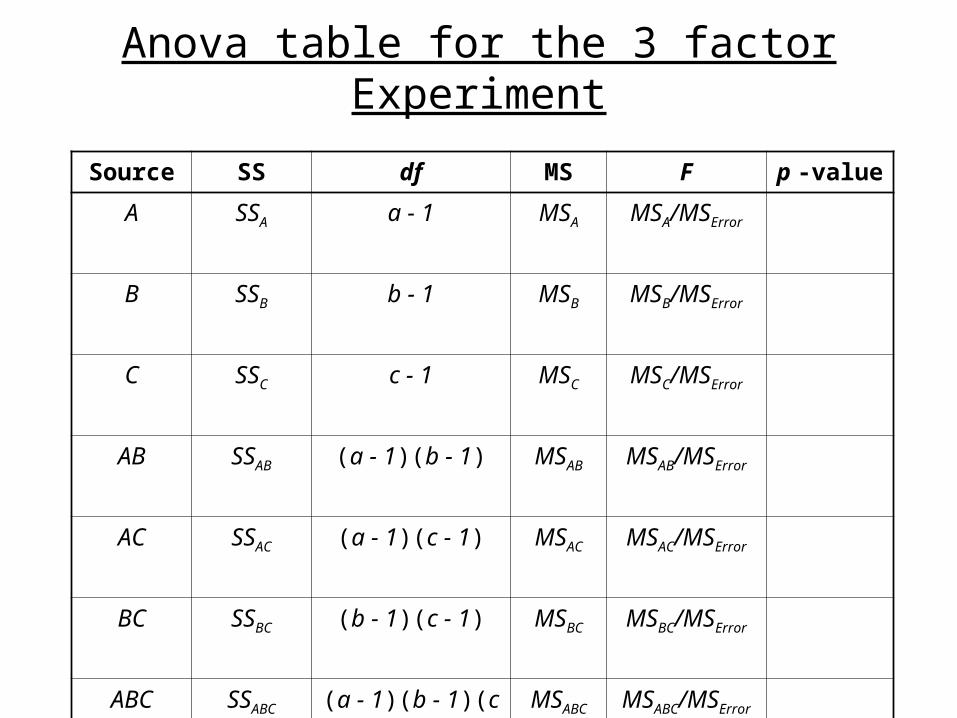
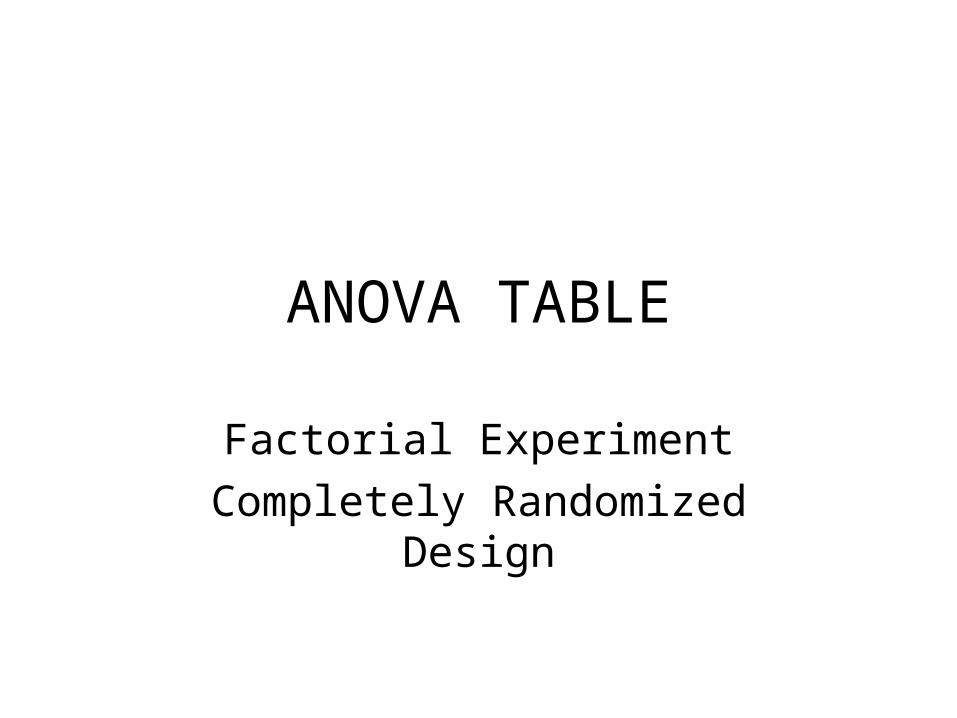
Anova table for the 3 factor Experiment
Source SS df MS F p -value
A SSA a - 1 MSA MSA/MSError
B SSB b - 1 MSB MSB/MSError
C SSC c - 1 MSC MSC/MSError
AB SSAB (a - 1)(b - 1) MSAB MSAB/MSError
AC SSAC (a - 1)(c - 1) MSAC MSAC/MSError
BC SSBC (b - 1)(c - 1) MSBC MSBC/MSError
ABC SSABC (a - 1)(b - 1)(c - 1) MSABC MSABC/MSError
Error SSError abc(n - 1) MSError
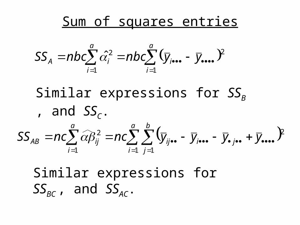
Sum of squares entries
a
ii
a
iiA yynbcnbcSS
1
2
1
2̂
Similar expressions for SSB , and SSC.
a
i
b
jjiij
a
iijAB yyyyncncSS
1 1
2
1
2
Similar expressions for SSBC , and SSAC.
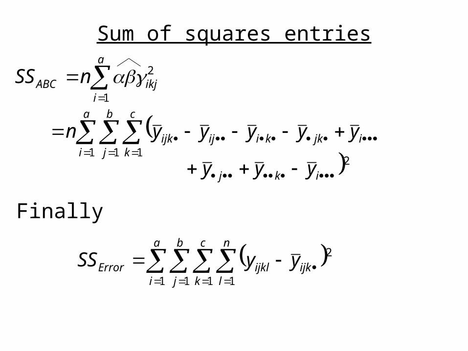
Sum of squares entries
Finally
a
iikjABC nSS
1
2
a
i
b
j
c
kijkkiijijk yyyyyn
1 1 1 2 ikj yyy
a
i
b
j
c
k
n
lijkijklError yySS
1 1 1 1
2
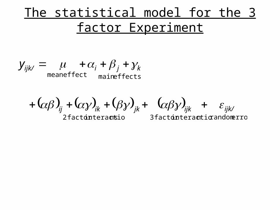
The statistical model for the 3 factor Experiment
effectsmain effectmean kjiijk/y
error randomninteractiofactor 3nsinteractiofactor 2
ijk/ijkjkikij

Anova table for the 3 factor Experiment
Source SS df MS F p -value
A SSA a - 1 MSA MSA/MSError
B SSB b - 1 MSB MSB/MSError
C SSC c - 1 MSC MSC/MSError
AB SSAB (a - 1)(b - 1) MSAB MSAB/MSError
AC SSAC (a - 1)(c - 1) MSAC MSAC/MSError
BC SSBC (b - 1)(c - 1) MSBC MSBC/MSError
ABC SSABC (a - 1)(b - 1)(c - 1) MSABC MSABC/MSError
Error SSError abc(n - 1) MSError
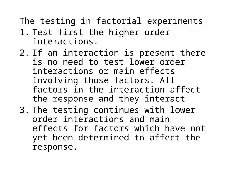
The testing in factorial experiments 1. Test first the higher order interactions.2. If an interaction is present there is no need
to test lower order interactions or main effects involving those factors. All factors in the interaction affect the response and they interact
3. The testing continues with lower order interactions and main effects for factors which have not yet been determined to affect the response.
Random Effects and Fixed Effects Factors
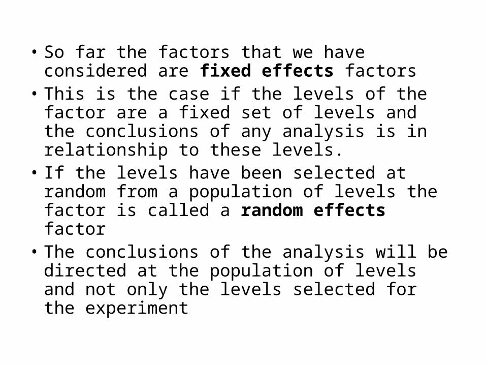
• So far the factors that we have considered are fixed effects factors
• This is the case if the levels of the factor are a fixed set of levels and the conclusions of any analysis is in relationship to these levels.
• If the levels have been selected at random from a population of levels the factor is called a random effects factor
• The conclusions of the analysis will be directed at the population of levels and not only the levels selected for the experiment
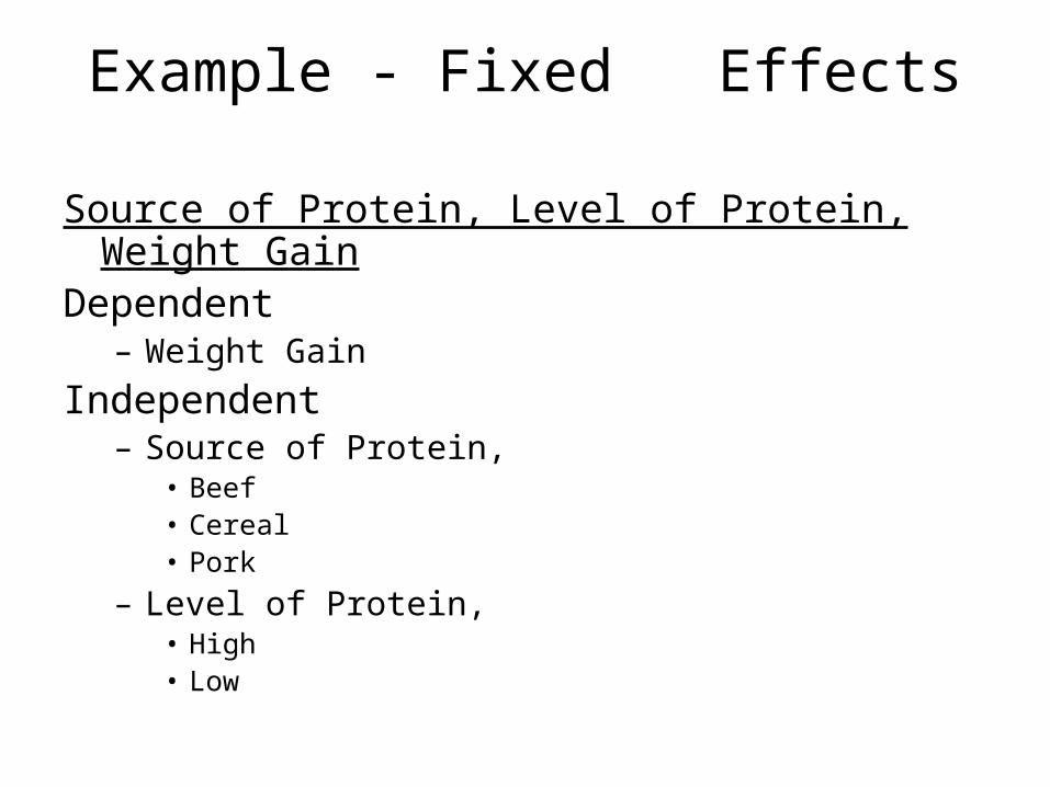
Example - Fixed Effects
Source of Protein, Level of Protein, Weight GainDependent
– Weight Gain
Independent– Source of Protein,
• Beef• Cereal• Pork
– Level of Protein,• High• Low
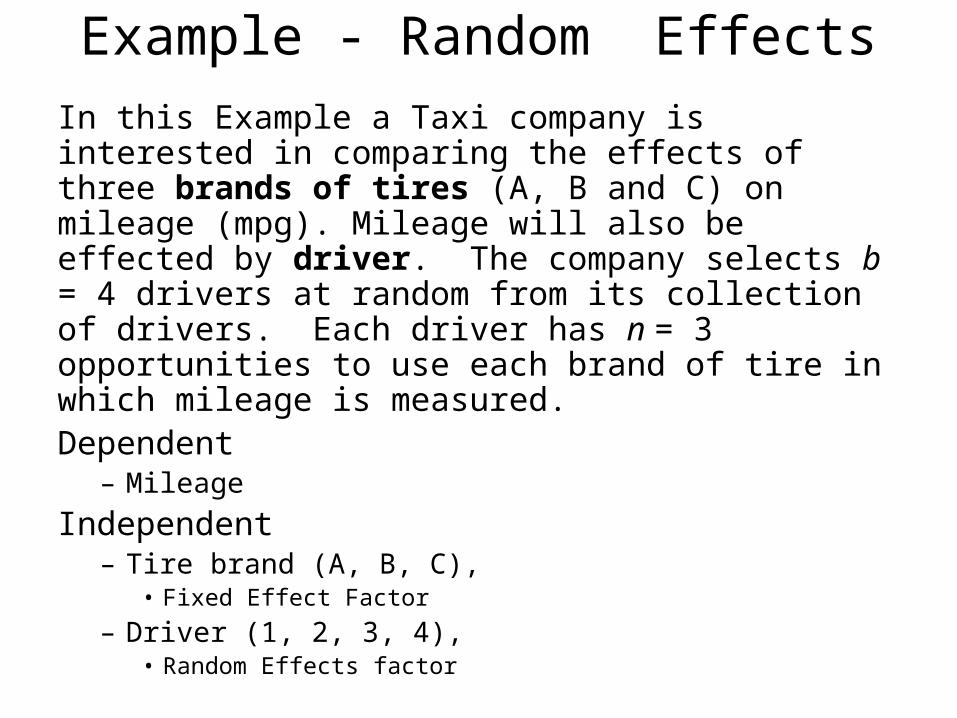
Example - Random Effects
In this Example a Taxi company is interested in comparing the effects of three brands of tires (A, B and C) on mileage (mpg). Mileage will also be effected by driver. The company selects b = 4 drivers at random from its collection of drivers. Each driver has n = 3 opportunities to use each brand of tire in which mileage is measured.Dependent
– Mileage
Independent– Tire brand (A, B, C),
• Fixed Effect Factor
– Driver (1, 2, 3, 4),• Random Effects factor
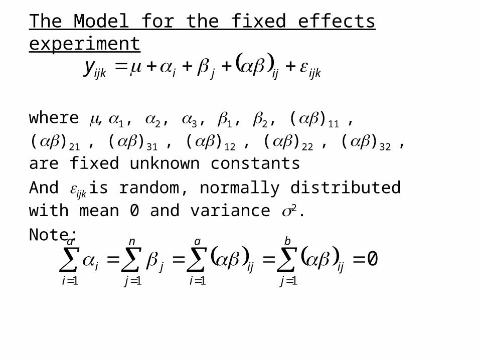
The Model for the fixed effects experiment
where , 1, 2, 3, 1, 2, ()11 , ()21 , ()31 , ()12 , ()22 , ()32 , are fixed unknown constants
And ijk is random, normally distributed with mean 0 and variance 2.
Note:
ijkijjiijky
01111
b
jij
a
iij
n
jj
a
ii
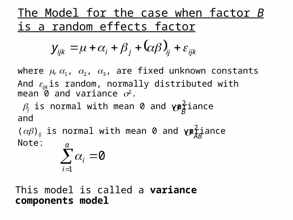
The Model for the case when factor B is a random effects factor
where , 1, 2, 3, are fixed unknown constants
And ijk is random, normally distributed with mean 0 and variance 2.
j is normal with mean 0 and varianceand
()ij is normal with mean 0 and varianceNote:
ijkijjiijky
01
a
ii
2B
2AB
This model is called a variance components model
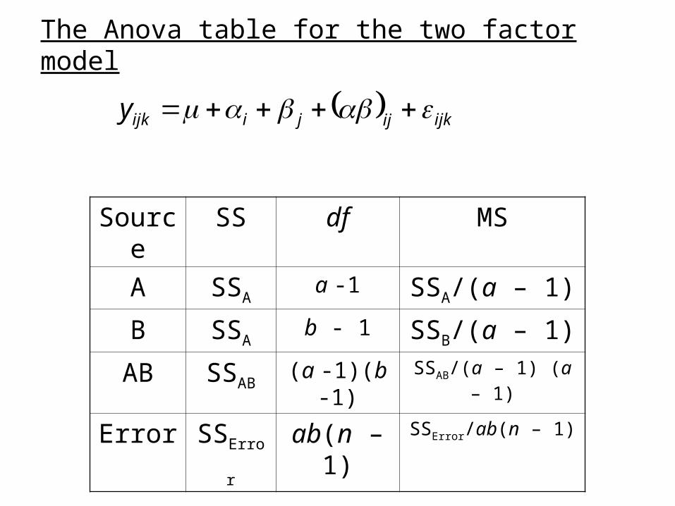
The Anova table for the two factor model
ijkijjiijky
Source SS df MS
A SSAa -1 SSA/(a – 1)
B SSAb - 1 SSB/(a – 1)
AB SSAB(a -1)(b -1) SSAB/(a – 1) (a – 1)
Error SSError ab(n – 1) SSError/ab(n – 1)
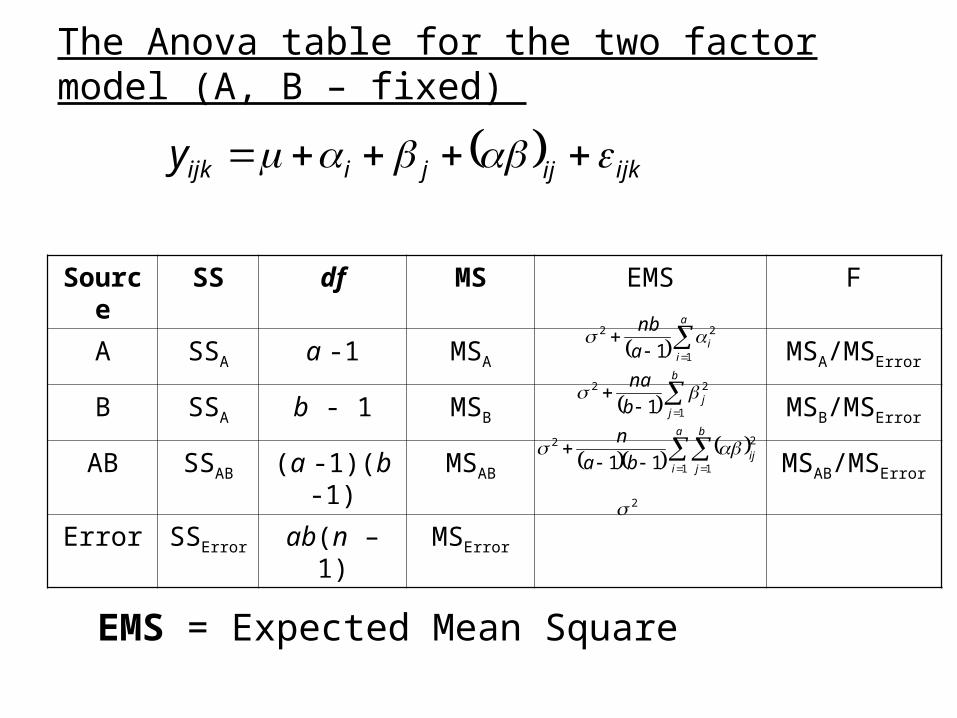
The Anova table for the two factor model (A, B – fixed)
ijkijjiijky
Source SS df MS EMS F
A SSA a -1 MSA MSA/MSError
B SSA b - 1 MSB MSB/MSError
AB SSAB (a -1)(b -1) MSAB MSAB/MSError
Error SSError ab(n – 1) MSError2
a
iia
nb
1
22
1
b
jjb
na
1
22
1
a
i
b
jijba
n
1 1
22
11
EMS = Expected Mean Square
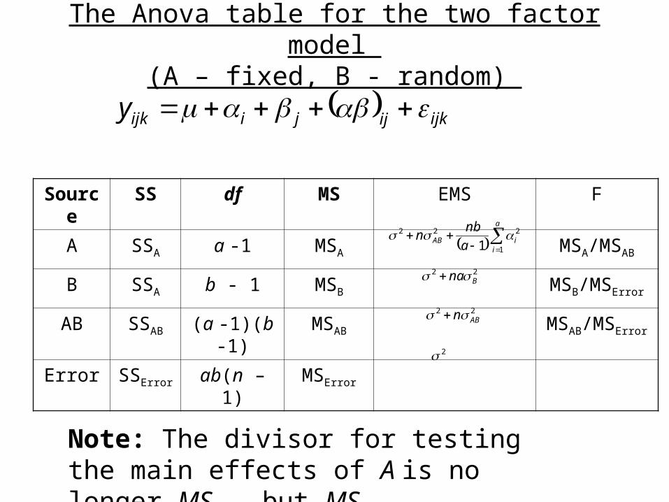
The Anova table for the two factor model (A – fixed, B - random)
ijkijjiijky
Source SS df MS EMS F
A SSA a -1 MSA MSA/MSAB
B SSA b - 1 MSB MSB/MSError
AB SSAB (a -1)(b -1) MSAB MSAB/MSError
Error SSError ab(n – 1) MSError2
a
iiAB a
nbn
1
222
1
22Bna
22ABn
Note: The divisor for testing the main effects of A is no longer MSError but MSAB.
Rules for determining Expected Mean Squares (EMS) in an Anova
Table
1. Schultz E. F., Jr. “Rules of Thumb for Determining Expectations of Mean Squares in Analysis of Variance,”Biometrics, Vol 11, 1955, 123-48.
Both fixed and random effects
Formulated by Schultz[1]
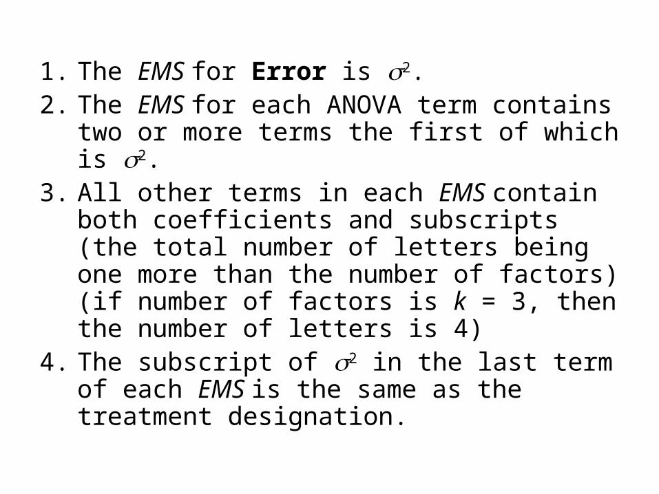
1. The EMS for Error is 2.2. The EMS for each ANOVA term contains
two or more terms the first of which is 2.3. All other terms in each EMS contain both
coefficients and subscripts (the total number of letters being one more than the number of factors) (if number of factors is k = 3, then the number of letters is 4)
4. The subscript of 2 in the last term of each EMS is the same as the treatment designation.
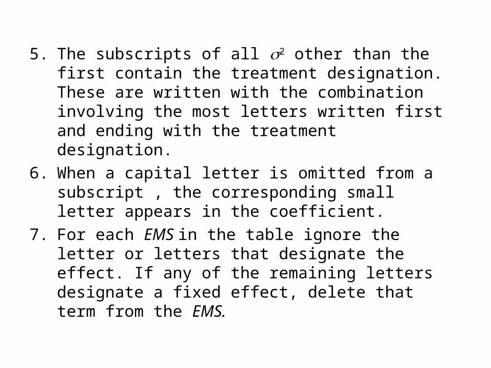
5. The subscripts of all 2 other than the first contain the treatment designation. These are written with the combination involving the most letters written first and ending with the treatment designation.
6. When a capital letter is omitted from a subscript , the corresponding small letter appears in the coefficient.
7. For each EMS in the table ignore the letter or letters that designate the effect. If any of the remaining letters designate a fixed effect, delete that term from the EMS.
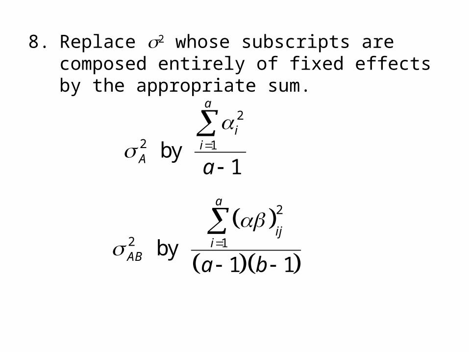
8. Replace 2 whose subscripts are composed entirely of fixed effects by the appropriate sum.
2
2 1 by 1
a
ii
A a
2
2 1 by 1 1
a
iji
AB a b
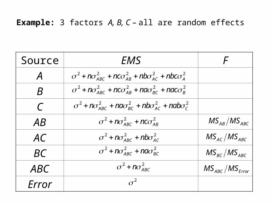
Example: 3 factors A, B, C – all are random effects
Source EMS F
A
B
C
AB
AC
BC
ABC
Error
2 2 2 2 2ABC AB AC An nc nb nbc
2 2 2 2 2ABC AB BC Bn nc na nac
2 2 2 2 2ABC BC AC Cn na nb nab
2 2 2ABC ABn nc
2 2 2ABC ACn nb
2 2 2ABC BCn na
2 2ABCn
2
AB ABCMS MS
AC ABCMS MS
BC ABCMS MS
ABC ErrorMS MS
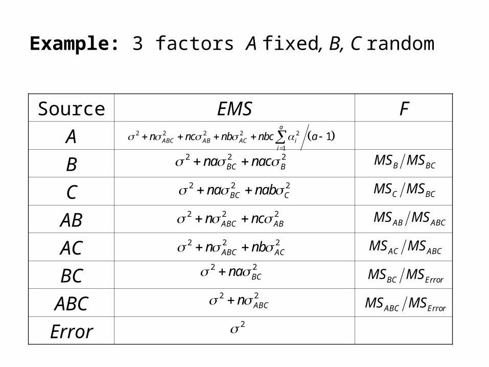
Example: 3 factors A fixed, B, C random
Source EMS F
A
B
C
AB
AC
BC
ABC
Error
2 2 2 2 2
1
1a
ABC AB AC ii
n nc nb nbc a
2 2 2
BC Bna nac
2 2 2BC Cna nab
2 2 2ABC ABn nc
2 2 2ABC ACn nb
2 2BCna
2 2ABCn
2
AB ABCMS MS
AC ABCMS MS
BC ErrorMS MS
ABC ErrorMS MS
C BCMS MS
B BCMS MS
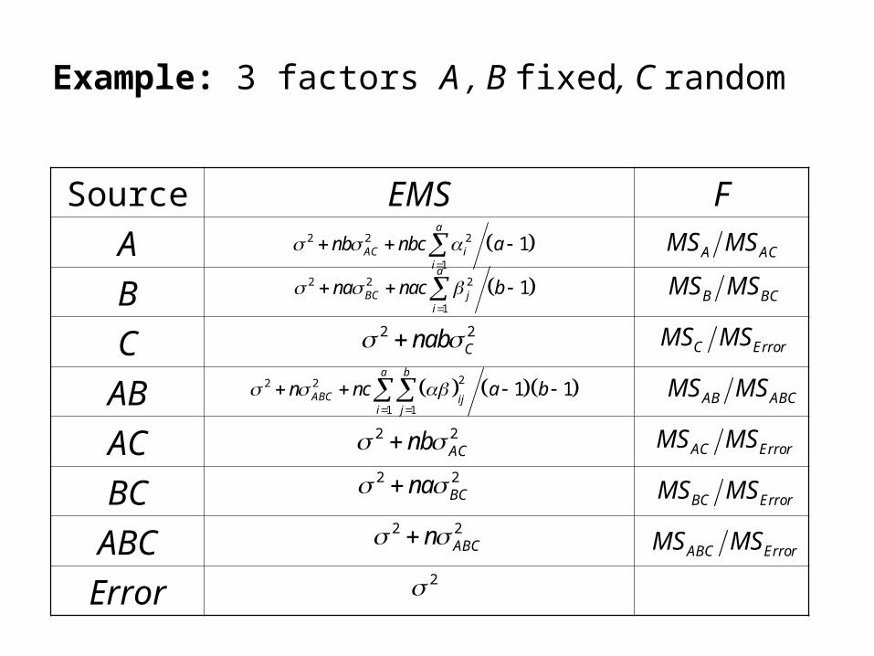
Example: 3 factors A , B fixed, C random
Source EMS F
A
B
C
AB
AC
BC
ABC
Error
2 2 2
1
1a
AC ii
nb nbc a
2 2Cnab
2 2ACnb
2 2BCna
2 2ABCn
2
AB ABCMS MS
AC ErrorMS MS
BC ErrorMS MS
ABC ErrorMS MS
C ErrorMS MS
B BCMS MS 2 2 2
1
1a
BC ji
na nac b
22 2
1 1
1 1a b
ABC iji j
n nc a b
A ACMS MS
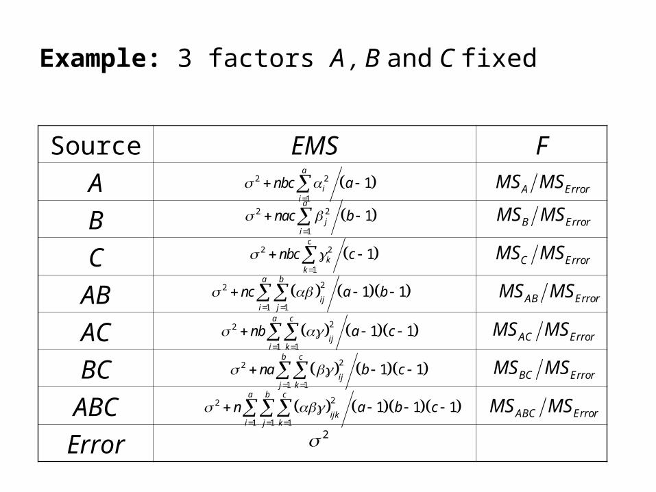
Example: 3 factors A , B and C fixed
Source EMS F
A
B
C
AB
AC
BC
ABC
Error
2 2
1
1a
ii
nbc a
2
AB ErrorMS MS
AC ErrorMS MS
BC ErrorMS MS
ABC ErrorMS MS
C ErrorMS MS
B ErrorMS MS 2 2
1
1a
ji
nac b
22
1 1
1 1a b
iji j
nc a b
A ErrorMS MS
2 2
1
1c
kk
nbc c
22
1 1
1 1a c
iji k
nb a c
22
1 1
1 1b c
ijj k
na b c
22
1 1 1
1 1 1a b c
ijki j k
n a b c
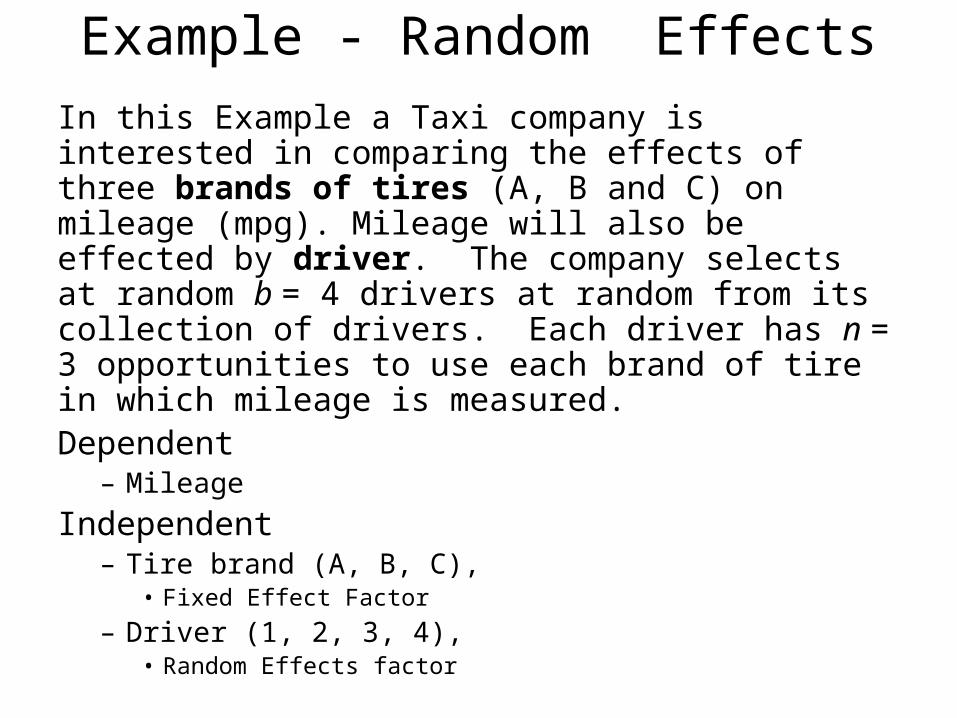
Example - Random Effects
In this Example a Taxi company is interested in comparing the effects of three brands of tires (A, B and C) on mileage (mpg). Mileage will also be effected by driver. The company selects at random b = 4 drivers at random from its collection of drivers. Each driver has n = 3 opportunities to use each brand of tire in which mileage is measured.Dependent
– Mileage
Independent– Tire brand (A, B, C),
• Fixed Effect Factor
– Driver (1, 2, 3, 4),• Random Effects factor
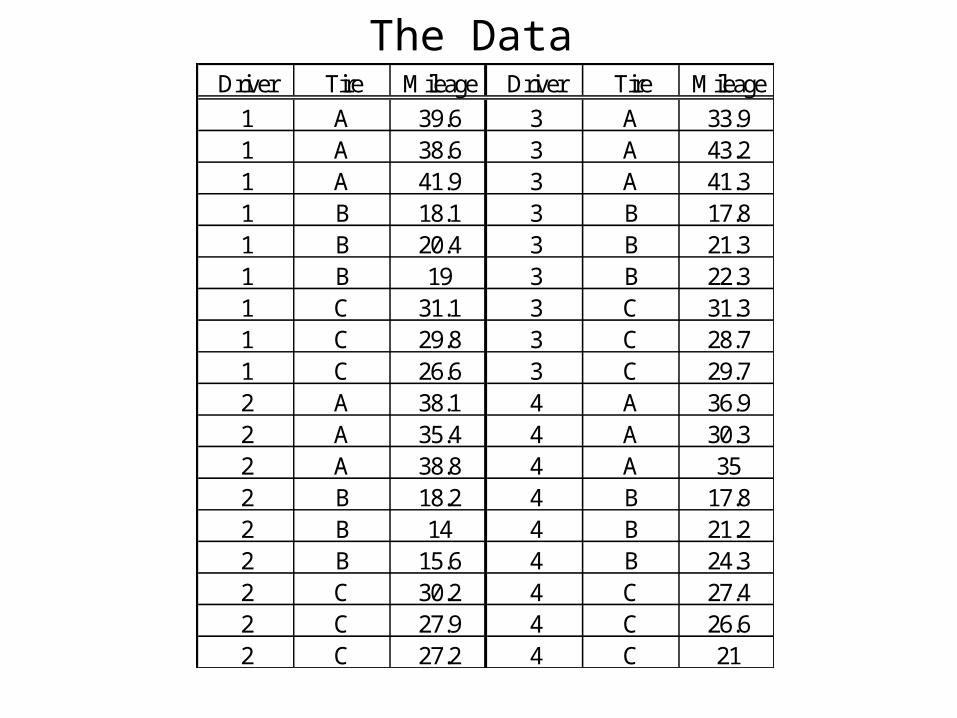
The DataDriver Tire Mileage Driver Tire Mileage
1 A 39.6 3 A 33.91 A 38.6 3 A 43.21 A 41.9 3 A 41.31 B 18.1 3 B 17.81 B 20.4 3 B 21.31 B 19 3 B 22.31 C 31.1 3 C 31.31 C 29.8 3 C 28.71 C 26.6 3 C 29.72 A 38.1 4 A 36.92 A 35.4 4 A 30.32 A 38.8 4 A 352 B 18.2 4 B 17.82 B 14 4 B 21.22 B 15.6 4 B 24.32 C 30.2 4 C 27.42 C 27.9 4 C 26.62 C 27.2 4 C 21
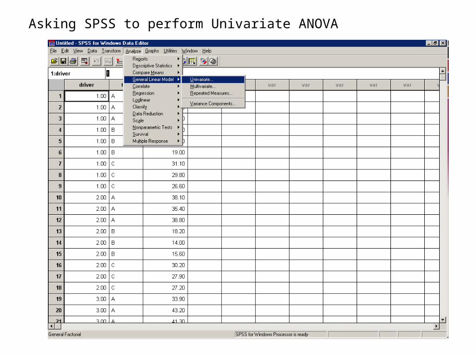
Asking SPSS to perform Univariate ANOVA
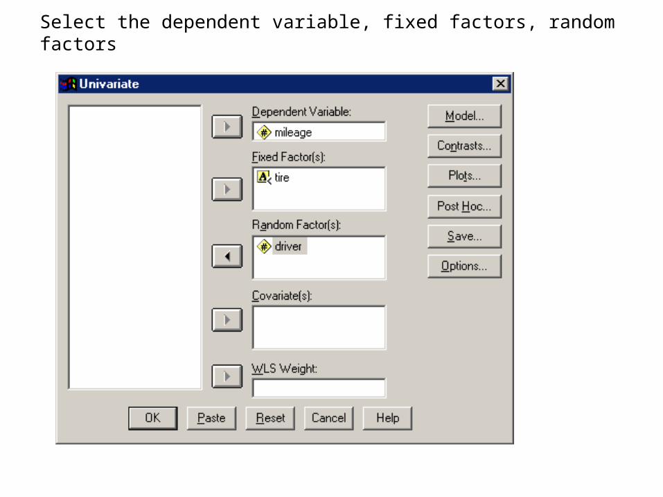
Select the dependent variable, fixed factors, random factors
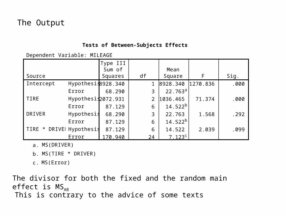
The Output
Tests of Between-Subjects Effects
Dependent Variable: MILEAGE
28928.340 1 28928.340 1270.836 .000
68.290 3 22.763a
2072.931 2 1036.465 71.374 .000
87.129 6 14.522b
68.290 3 22.763 1.568 .292
87.129 6 14.522b
87.129 6 14.522 2.039 .099
170.940 24 7.123c
SourceHypothesis
Error
Intercept
Hypothesis
Error
TIRE
Hypothesis
Error
DRIVER
Hypothesis
Error
TIRE * DRIVER
Type IIISum ofSquares df
MeanSquare F Sig.
MS(DRIVER)a.
MS(TIRE * DRIVER)b.
MS(Error)c.
The divisor for both the fixed and the random main effect is MSAB
This is contrary to the advice of some texts
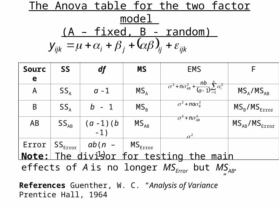
The Anova table for the two factor model (A – fixed, B - random)
ijkijjiijky
Source SS df MS EMS F
A SSA a -1 MSA MSA/MSAB
B SSA b - 1 MSB MSB/MSError
AB SSAB (a -1)(b -1) MSAB MSAB/MSError
Error SSError ab(n – 1) MSError2
a
iiAB a
nbn
1
222
1
22Bna
22ABn
Note: The divisor for testing the main effects of A is no longer MSError but MSAB.
References Guenther, W. C. “Analysis of Variance” Prentice Hall, 1964
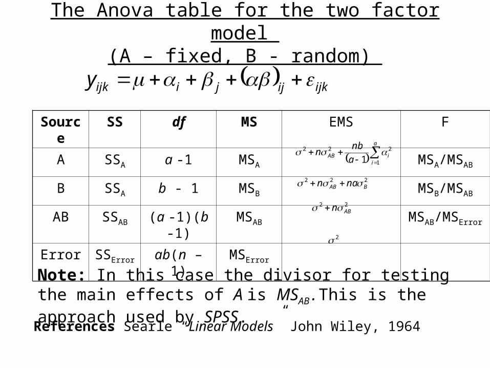
The Anova table for the two factor model (A – fixed, B - random)
ijkijjiijky
Source SS df MS EMS F
A SSA a -1 MSA MSA/MSAB
B SSA b - 1 MSB MSB/MSAB
AB SSAB (a -1)(b -1) MSAB MSAB/MSError
Error SSError ab(n – 1) MSError2
a
iiAB a
nbn
1
222
1
222BAB nan
22ABn
Note: In this case the divisor for testing the main effects of A is MSAB . This is the approach used by SPSS.
References Searle “Linear Models” John Wiley, 1964
Crossed and Nested Factors
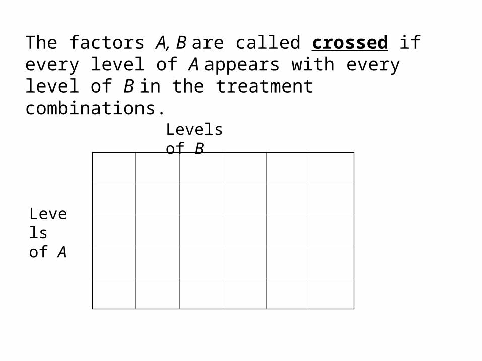
The factors A, B are called crossed if every level of A appears with every level of B in the treatment combinations.
Levels of B
Levels of A
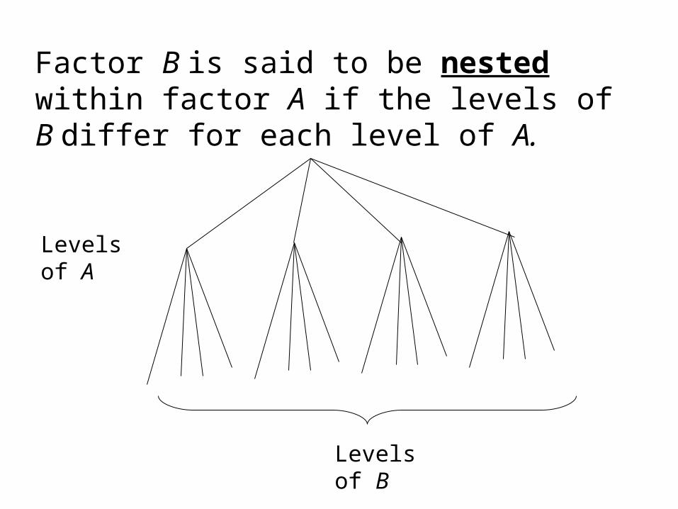
Factor B is said to be nested within factor A if the levels of B differ for each level of A.
Levels of B
Levels of A
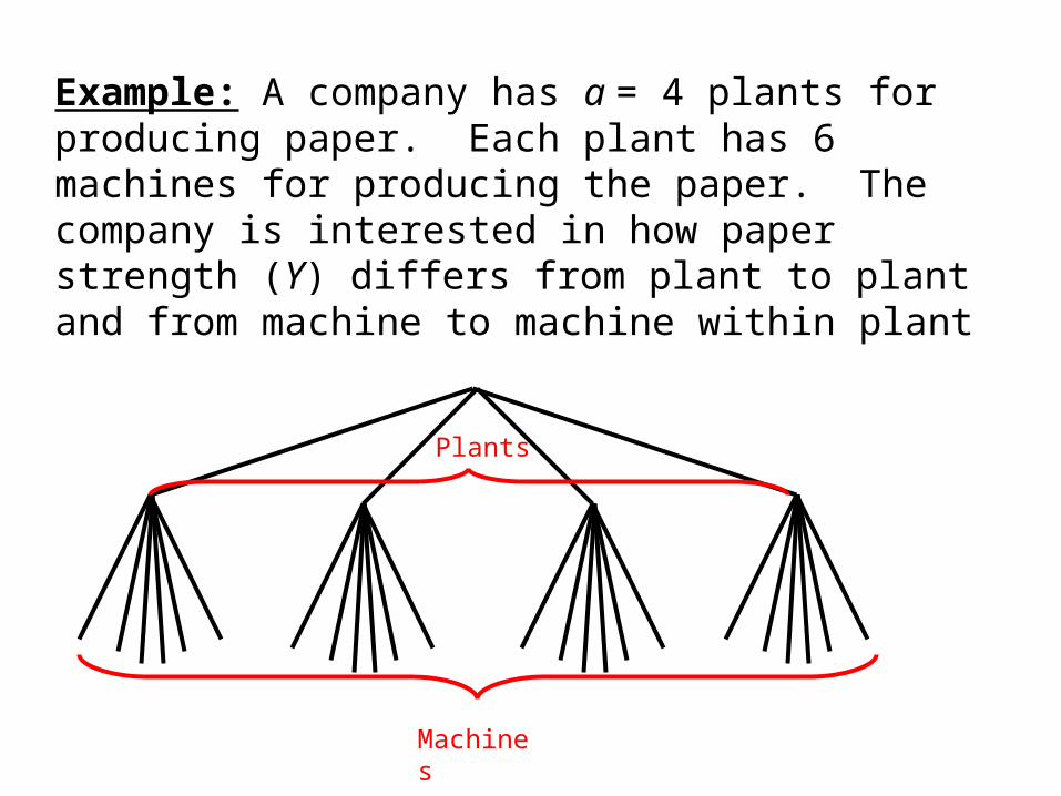
Example: A company has a = 4 plants for producing paper. Each plant has 6 machines for producing the paper. The company is interested in how paper strength (Y) differs from plant to plant and from machine to machine within plant
Plants
Machines
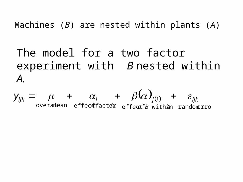
Machines (B) are nested within plants (A)
The model for a two factor experiment with B nested within A.
error random within ofeffect factor ofeffect mean overall
ijkAB
ijA
iijky
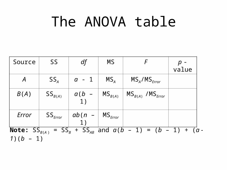
The ANOVA table
Source SS df MS F p - value
A SSA a - 1 MSA MSA/MSError
B(A) SSB(A) a(b – 1) MSB(A) MSB(A) /MSError
Error SSError ab(n – 1) MSError
Note: SSB(A ) = SSB + SSAB and a(b – 1) = (b – 1) + (a - 1)(b – 1)
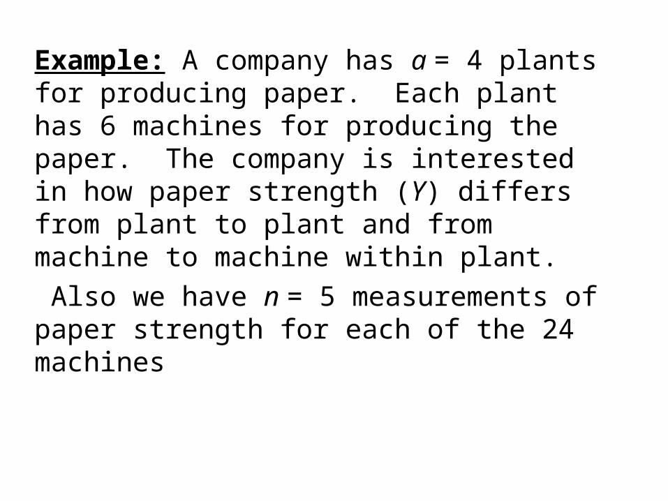
Example: A company has a = 4 plants for producing paper. Each plant has 6 machines for producing the paper. The company is interested in how paper strength (Y) differs from plant to plant and from machine to machine within plant.
Also we have n = 5 measurements of paper strength for each of the 24 machines
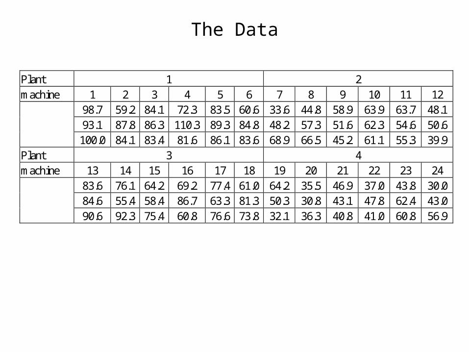
The Data
Plant 1 2 machine 1 2 3 4 5 6 7 8 9 10 11 12
98.7 59.2 84.1 72.3 83.5 60.6 33.6 44.8 58.9 63.9 63.7 48.1 93.1 87.8 86.3 110.3 89.3 84.8 48.2 57.3 51.6 62.3 54.6 50.6
100.0 84.1 83.4 81.6 86.1 83.6 68.9 66.5 45.2 61.1 55.3 39.9 Plant 3 4 machine 13 14 15 16 17 18 19 20 21 22 23 24
83.6 76.1 64.2 69.2 77.4 61.0 64.2 35.5 46.9 37.0 43.8 30.0 84.6 55.4 58.4 86.7 63.3 81.3 50.3 30.8 43.1 47.8 62.4 43.0
90.6 92.3 75.4 60.8 76.6 73.8 32.1 36.3 40.8 41.0 60.8 56.9
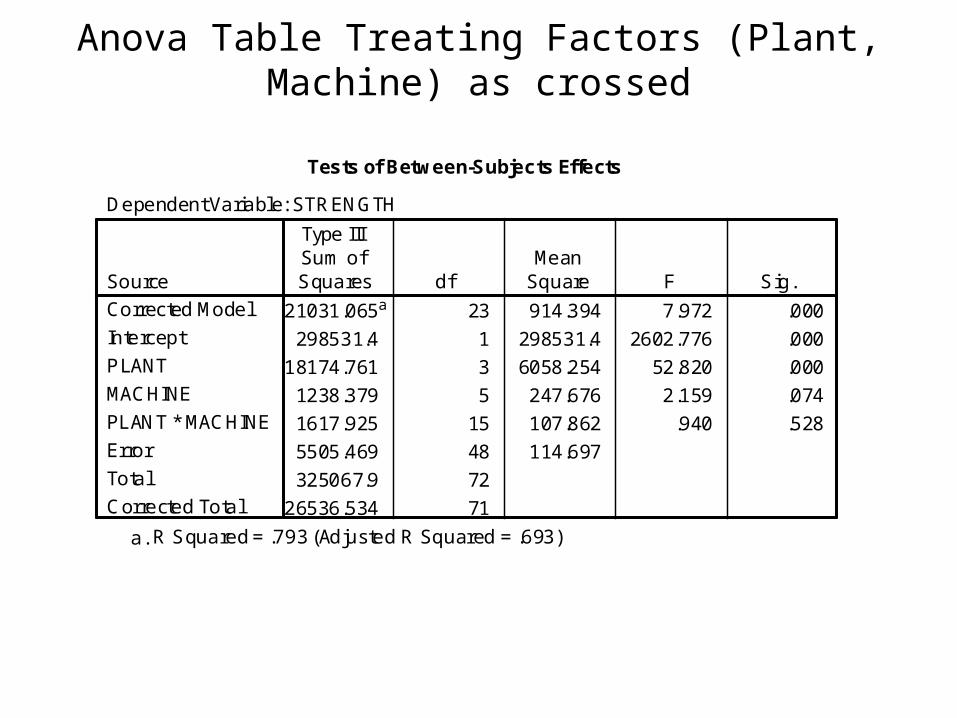
Anova Table Treating Factors (Plant, Machine) as crossed
Tests of Between-Subjects Effects
Dependent Variable: STRENGTH
21031.065a 23 914.394 7.972 .000
298531.4 1 298531.4 2602.776 .000
18174.761 3 6058.254 52.820 .000
1238.379 5 247.676 2.159 .074
1617.925 15 107.862 .940 .528
5505.469 48 114.697
325067.9 72
26536.534 71
SourceCorrected Model
Intercept
PLANT
MACHINE
PLANT * MACHINE
Error
Total
Corrected Total
Type IIISum of
Squares dfMean
Square F Sig.
R Squared = .793 (Adjusted R Squared = .693)a.
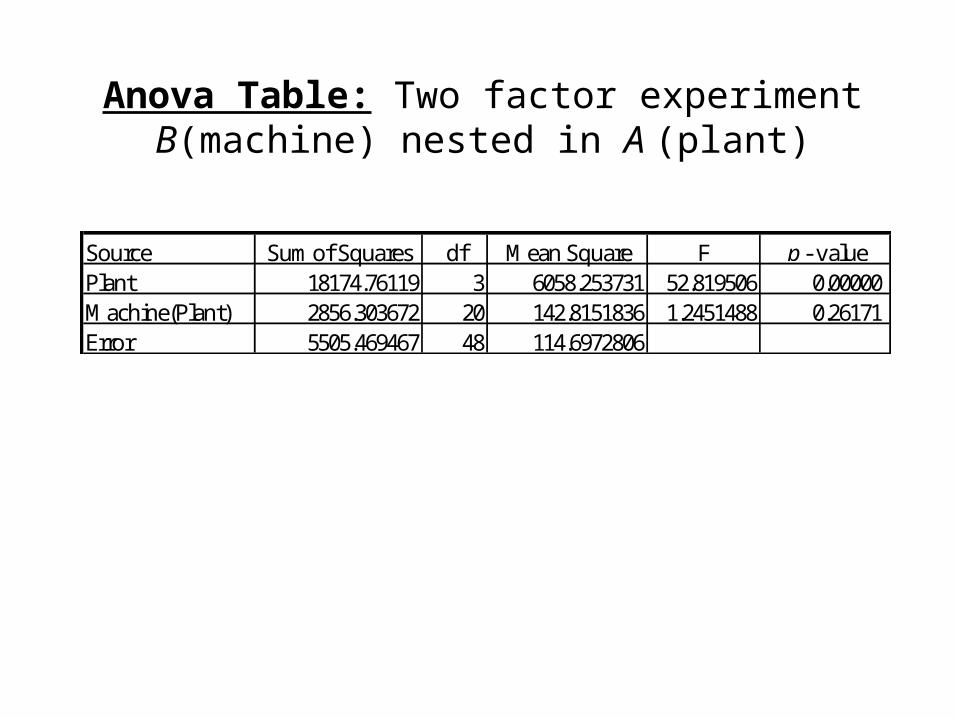
Anova Table: Two factor experiment B(machine) nested in A (plant)
Source Sum of Squares df Mean Square F p - valuePlant 18174.76119 3 6058.253731 52.819506 0.00000 Machine(Plant) 2856.303672 20 142.8151836 1.2451488 0.26171 Error 5505.469467 48 114.6972806
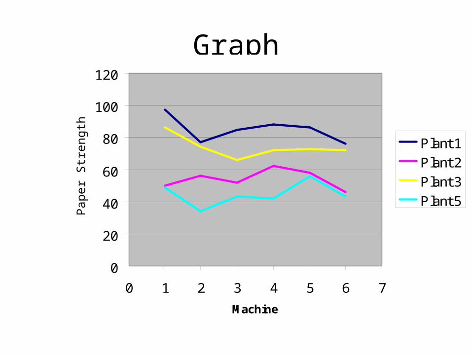
Graph
0
20
40
60
80
100
120
0 1 2 3 4 5 6 7
Machine
Plant 1
Plant 2
Plant 3
Plant 5
Pap
er S
tren
gth