Embed Size (px)
DESCRIPTION
spss
Citation preview

Advanced Techniques:ANOVA (SPSS 10.0)
SPSS Inc.233 S Wacker Drive, 11th FloorChicago, Illinois 60606312.651.3300
Training Department800.543.2185
v10.0 Revised 1/17/00 hc/ss

SPSS Neural Connection, SPSS QI Analyst, SPSS for Windows, SPSS DataEntry II, SPSS-X, SCSS, SPSS/PC, SPSS/PC+, SPSS Categories, SPSS Graphics,SPSS Professional Models, SPSS Advanced Models, SPSS Tables, SPSS Trendsand SPSS Exact Tests are the trademarks of SPSS Inc. for its proprietarycomputer software. CHAID for Windows is the trademark of SPSS Inc. andStatistical Innovations Inc. for its proprietary computer software. Excel forWindows and Word for Windows are trademarks of Microsoft; dBase is atrademark of Borland; Lotus 1-2-3 is a trademark of Lotus Development Corp. Nomaterial describing such software may be produced or distributed without thewritten permission of the owners of the trademark and license rights in thesoftware and the copyrights in the published materials.
General notice: Other product names mentioned herein are used foridentification purposes only and may be trademarks of their respectivecompanies.
Copyright(c) 2000 by SPSS Inc.
All rights reserved.
Printed in the United States of America.
No part of this publication may be reproduced or distributed in any form or byany means, or stored on a database or retrieval system, without the prior writtenpermission of the publisher, except as permitted under the United StatesCopyright Act of 1976.

Table of Contents - 1
ADVANCED TECHNIQUES:ANOVA (SPSS 10.0)
TABLE OF CONTENTS
Chapter 1 IntroductionWhy do Analysis of Variance 1-1Visualizing Analysis of Variance 1-1What is Analysis of Variance? 1-3Variance of Means 1-4Basic Principle of ANOVA 1-6A Formal Statement of ANOVA Assumptions 1-8
Examining Data and Testing AssumptionsWhy Examine the Data? 2-2Exploratory Data Analysis 2-3A Look at the Variable Cost 2-5A Look at the Subgroups 2-9Normality 2-11Comparing the Groups 2-17Homogeneity of Variance 2-17Effects of Violations of Assumptions in ANOVA 2-19
One-Factor ANOVALogic of Testing for Mean Differences 3-2Factors 3-2Running One-Factor ANOVA 3-3One Factor ANOVA Results 3-5Post Hoc Testing 3-7Why So Many Tests? 3-8Planned Comparisons 3-16How Planned Comparisons are Done 3-17Graphic the Results 3-19Appendix: Group Differences on Ranks 3-20
Multi-Way Univariate ANOVAThe Logic of Testing, and Assumptions 4-2How Many Factors? 4-2Interactions 4-3Exploring the Data 4-5Two-Factor ANOVA 4-13The ANOVA Table 4-18Predicted Means 4-19Ecological Significance 4-20Residual Analysis 4-21Post Hoc Tests of ANOVA Results 4-22
Chapter 2
Chapter 3
Chapter 4

2 - Table of Contents
Unequal Samples and Unbalanced Designs 4-24Sums of Squares 4-25Equivalence and Recommendations 4-26Empty Cells and Nested Designs 4-26
Multivariate Analysis of VarianceWhy Perform MANOVA? 5-2How MANOVA Differs from ANOVA 5-3Assumptions of MANOVA 5-3What to Look for in MANOVA 5-4Significance Testing 5-4Checking the Assumptions 5-5The Multivariate Analysis 5-11Examining Results 5-17What if Homogeneity Failed 5-19Multivariate Tests 5-19Checking the Residuals 5-23Conclusion 5-25Post Hoc Tests 5-26
Within-Subject Designs: Repeated MeasuresWhy Do a Repeated Measures Study? 6-2The Logic of Repeated Measures 6-2Assumptions 6-5Proposed Analysis 6-7Key Concept 6-7Comparing the Grade Levels 6-13Examining Results 6-19Planned Comparisons 6-26
Between and Within-Subject ANOVA: (Split-Plot)Assumptions of Mixed Model ANOVA 7-2Proposed Analysis 7-2A Look at the Data 7-2Summary of Explore 7-8Split-Plot Analysis 7-8Examining Results 7-12Tests of Assumptions 7-13Sphericity 7-14Multivariate Tests Involving Time 7-15Tests of Between-Subject Factors 7-15Averaged F Tests Involving Time 7-16Additional Within-Subject Factors and Sphericity 7-18Exploring the Interaction - Simple Effects 7-18Graphing the Interaction 7-25
Chapter 5
Chapter 6
Chapter 7

Table of Contents - 3
More Split-Plot DesignIntroduction: Ad Viewing with Pre-Post Brand Ratings 8-1Setting Up the Analysis 8-2Examining Results 8-7Tests of Assumptions 8-8ANOVA Results 8-11Profile Plots 8-13Summary of Results 8-15
Analysis of CovarianceHow is Analysis of Covariance Done? 9-2Assumptions of ANCOVA 9-2Checking the Assumptions 9-3Baseline ANOVA 9-3ANCOVA - Homogeneity of Slopes 9-5Standard ANCOVA 9-7Describing the Relationship 9-8Fitting Non-Parallel Slopes 9-9Repeated Measures ANCOVA with a Single Covariate 9-11Repeated Measures ANCOVA with a Varying Covariate 9-16Further Variations 9-18
Special TopicsLatin Square Designs 10-2An Example 10-2Complex Designs 10-6Random Effects Models 10-6
ReferencesReferences R-1
ExercisesExercises E-1
Chapter 8
Chapter 10
Chapter 9
References
Exercises

4 - Table of Contents

Introduction 1 - 1
SPSS Training
Introduction
Analysis of variance is performed in order to determine whetherthere are differences in the means between groups or acrossdifferent conditions. From a simple two-group experiment, to a
complex study involving many factors and covariates, the same coreprinciple applies. Why this technique is called analysis of variance(ANOVA) and not analysis of means, has to do with the methodology usedto determine if the means are far enough apart to be considered“significantly” different.
To examine the basic principle of ANOVA, image a simple experiment inwhich subjects are randomly assigned to one of three treatment groups,the treatments are applied, then subjects are tested on some performancemeasure. One possible outcome appears below. Performance scores areplotted along the vertical axis and each box represents the distribution ofscores within a treatment group.
Figure 1.1 Performance Scores: Distinct Populations
Chapter 1
WHY DOANALYSIS OF
VARIANCE?
VISUALIZINGANALYSIS OF
VARIANCE

Introduction 1 - 2
SPSS Training
Here a formal testing of the differences is almost unnecessary. Thegroups show no overlap in performance scores and the group means(medians are the dark bar at the center of each box) are well spacedrelative to the standard deviation of each group. Think of the variation,or distances going from group mean to group mean, and compare this tothe variation of the individual scores within each group.
Let us take another example. Suppose the same experiment describedabove results in the performance scores having little or no difference. Wepicture this below.
Figure 1.2 Performance Scores: Identical Populations
Here the group means are all but identical, so there is little variationor distance going from group mean to group mean compared to thevariation of performance scores within the groups. A formal ANOVAanalysis would merely confirm this.
A more realistic example involves groups with overlapping scores andgroup means that differ. This is shown in the plot below.

Introduction 1 - 3
SPSS Training
Figure 1.3 Performance Scores: Overlapping Groups
The formal ANOVA analysis needs to be done to determine if thegroup means do indeed differ in the population, that is, with whatconfidence can we claim that the group means are not the same. Onceagain, think of the variation of the group means (distances) between pairsof groups, or variation of the group means around the grand mean)relates to the variation of the performance scores within each group.
Stripped of technical adjustments and distributional assumptions, youare comparing the variation of group means to the variation of individualscores within the groups constitute the basis for analysis of variance. Tothe extent that the differences or variation between groups is largerelative to the variation of individual scores within the groups, we speakof the groups showing significant differences. Another way of reasoningabout the experiment we described is to say that if the treatmentsapplied to the three groups had no effect (no group differences), then thevariation in group means should be due to the same sources and be of thesame magnitude (after technical adjustments) as the variation amongindividuals within the groups.
WHAT ISANALYSIS OF
VARIANCE?

Introduction 1 - 4
SPSS Training
The technical adjustment just mentioned is required when comparingvariation in means scores to variation in individual scores. This isbecause the variance of means will be less than the variance of theindividual scores on which the mean is based. The basic mathematicalrelation is that the variance of the means based on a sample size of “n”will be equal to the variance of the individual scores in the sampledivided by “n”. The standard deviation of the mean is called the standarderror or the standard error of the mean. We will illustrate this law with alittle under 10,000 observations produced by a pseudo-random numbergenerator in SPSS, based on a normal distribution with a mean of zeroand a standard deviation of one. The results appear in Figure 1.4.
The first histogram shows the distribution of the original 9,600 datapoints. Notice almost all of the points fall between the values of –3 and+3.
The second histogram contains the mean scores of samples of size 4drawn from the original 9,600 data points. Each point is a mean score fora sample of size 4 for a total of 2,400 data points. The distribution ofmeans is narrower than that of the first histogram; almost all the pointsfall between –1.5 and +1.5.
In the final histogram each point is a mean of 16 observations fromthe original sample. The variation of these 600 points is less than that ofthe previous histograms with most points between -.9 and +.9. Despitethe decrease in variance, the means (or centers of the distributions)remain at zero.
This relation is relevant to analysis of variance. In ANOVA, whencomparing the variation between group mean scores to variation ofindividuals within groups, the sample sizes upon which the means arebased are explicitly taken into account.
VARIANCE OFMEANS

Introduction 1 - 5
SPSS Training
Figure 1.4 Variation in Means as a Function of Sample Size

Introduction 1 - 6
SPSS Training
While we will give a formal statement of the assumptions of ANOVA andproceed with complex variations, this basic principle comparing thevariation of group or treatment means to the variation of individualswithin groups (or some other grouping) will be the underlying theme.
The term “factor” denotes a categorical predictor variable. “DependentVariables” are interval level outcome variables, and “covariates” areinterval level predictor variables. ANOVA is considered a form of thegeneral linear model and most of the assumptions follow from that andare listed below:
• All variables must exhibit independent variance. In otherwords, a variable must vary, and it must not be a one-to-onefunction of any other variable. Though it is the dream of anydata analyst to have a dependent variable that is perfectlypredicted, if such were the case, the “F-ratio” for an analysisof variance could not be formed (Note: as a practical matter, ifyou find such a perfect prediction, lack of an “F-ratio” shouldnot result in any lost sleep).
• Dependent variables and covariates must be measured ininterval or ratio scale. Factors may be nominal or categorizedfrom ordinal or interval variables. However, ordinalhypothesis can only be tested in a pairwise fashion. Imposingthe desired metric through the appropriate set of contrastscan test interval hypothesis.
• For fixed effect models, all levels of predictor variables thatare of interest must be included in the analysis.
• The linear model specified is the correct one; it includes allthe relevant sources of variation, excludes all irrelevant ones,and is correct in its functional form (Note: in the words of theSgt. in Hill Street Blues “so, be careful out there”).
• Errors of measurement must be unbiased (have a zero mean).• Errors must be independent of each other and of the predictor
variables.• Error variances must be homogeneous.• Errors must be normally distributed. This final assumption is
not required for estimation, but must be met in order for an“F-ratio” to be accurately referred to as an “F-distribution”(Note: that is, it is required for testing, which is why you aredoing the analysis).
We will examine some of these assumptions in the data sets used inthe rest of this course.
We use an “analysis of variance” to test for differences betweenmeans for the following formal reason:
The formulation of the analysis of variance approach as a testof equality of means follows a deductive format. We can showthat if it is true that two (or more) means are equal, thencertain properties must hold for other functions of the data,such as between group and within group variation. The idea
BASICPRINCIPLE OF
ANOVA
A FORMALSTATEMENT OF
ANOVAASSUMPTIONS

Introduction 1 - 7
SPSS Training
behind the formulation of the familiar “F-ratio” is that if themeans being compared are equal, then the numerator anddenominator of the “F-ratio” represent independent estimatesof the same quantity (error variance) and their ratio mustthen follow a known distribution. This allows us to place adistinct probability on the occurrence of sample means asdifferent as those observed under the hypothesis of zerodifference among population means.
In this chapter we discussed the basic principle of analysis of varianceand gave a formal statement of the assumptions of the model. We turnnext to examining these assumptions and the implications if theassumptions are not met (Note: life as it really is).
SUMMARY

Introduction 1 - 8
SPSS Training

Examining Data and Testing Assumptions 2 - 1
SPSS Training
Examining Data and TestingAssumptions
The data set comes from Cox and Snell (1981). They obtained it from areport (Mooz, 1978) and reproduced it with the permission of the RandCorporation. Only a subset of the original variables is used in the data setwe will use.
The data set we will be using contains information for 32 light waternuclear power plants. Four variables are included: the capacity and costof the plant; time to completion from start of construction; and experienceof the architect-engineer who built the plant. These variables aredescribed in more detail below.
We will use only a subset of all the variables that were in the originaldata set, and have created categories from the variables capacity andexperience in order to use them as factors in an analysis of variance.
In order of the variables in the data file, they are:
Capacity Generating capacity1 Less than 800 MW’s (Mega Watts)2 800-10003 Greater than 1000
Experience Experience of the architect-engineerin building power plants
1 1-3 plants2 4-9 plants3 10 or more plants
Time time in months between issuing of construction permitand issuing of operating license.
Cost cost in millions of dollars adjusted to a 1976 base (In 1976dollars).
The analyst should choose the analysis that best conforms to the type ofinformation collected in the data and the research or analysis question(s)you wish to answer. We feel that in a short course there is an advantagein describing the various types of analyses that can be done. However, inpractice you would run only the most appropriate analysis. In otherwords if there were two factors in your study, you would run a two-factoranalysis and not begin with one factor analysis as we do here.
Chapter 2
DESCRIPTION OFTHE DATA
Note About theAnalyses That
Follow

SPSS Training
Examining Data and Testing Assumptions 2 - 2
The researcher should state the research questions clearly and concisely,and refer to these questions regularly as the design and implementationof the study progresses. Without this statement of questions, it is easy todeviate from them when engrossed in the details of planning or to makedecisions that are at variance with the questions when involved in acomplex study. Translating study objectives into questions serves as acheck on whether the study has met the objectives.
The next task is to analyze the researchable question(s). In doing thisone must
• Identify and define key terms• Identify sub questions, which must also be answered• Identify the scope and time frame imposed by the researchable
question
One of the most important decisions that should not be overlooked is toset down in terms of utmost clarity exactly what information is needed. Itis usually good procedure to verify that all the data are relevant to thepurposes of the study and that no essential data are omitted. Unless thisis specified, the reporting forms may yield information that is quitedifferent from what is needed, since there is a tendency to request toomuch data, some of which is subsequently never analyzed.
It is critical that the researcher be familiar with the data being analyzed,whether it is primary (data you collected) or secondary (someone elsecollected it) data. Not only is knowing your data important to definingyour population, but it can (1) help to spot trends on which to focus, and(2) provide assurance that you are measuring what you want to measure.
Visually review the data for several cases (or the entire data set if it isrelatively small). Be familiar with the meaning of every variable and withthe codes associated with the variables of interest.
Before applying formal tests (ANOVA for example in this course) to yourdata, it is important to first examine and check the data. This is done forseveral reasons:
• To identify data errors• To identify unusual points – outliers• To become aware of unexpected or interesting patterns• To check on or test the assumptions of the planned analysis• For ANOVA:• Homogeneity of variance• Normality of error
ResearchQuestion(s)
Data to beCollected
Know the Data
Scan the Data
WHY EXAMINETHE DATA?

Examining Data and Testing Assumptions 2 - 3
SPSS Training
Bar charts and histograms, as well as such summaries as means andstandard deviations have been used in statistical work for many years.Sometimes such summaries are ends in their own right; other times theyconstitute a preliminary look at the data before proceeding with moreformal methods. Seeing limitations in this standard set of procedures,John Tukey, a statistician at Princeton and Bell Labs, devised a collectionof statistics and plots designed to reveal data features that might not bereadily apparent from standard statistical summaries. In his bookdescribing these methods, entitled Exploratory Data Analysis (1977),Tukey described the work of a data analyst to be similar to that of adetective, the goal being to discover surprising, interesting, and unusualthings about the data. To further this effort Tukey developed both plotsand data summaries. These methods, called exploratory data analysisand abbreviated EDA, have become very popular in applied statistics anddata analysis. Exploratory data analysis can be viewed either as ananalysis in its own right, or as a set of data checks and investigationsperformed before applying inferential testing procedures.
These methods are best applied to variables that have at least ordinal(more commonly interval) scale properties and can take on manydifferent values. The plots and summaries would be less helpful for avariable that takes on only a few values (for example, on five point ratingscales)
We will use the SPSS EXPLORE procedure to examine the data and testsome of the ANOVA assumptions. In windows we first open the file.
All files for this class are located in the c:\Train\Anova folder on yourtraining machine. If you are not working in an SPSS Training center, thetraining files can be copied from the floppy disk that accompanies thiscourse guide. If you are running SPSS Server (click File..Switch Server tocheck), then you should copy these files to the server or a machine thatcan be accessed (mapped from) the computer running SPSS Server.
SPSS can display either variable names or variable labels in dialog boxes.In this course we display the variable names in alphabetical order. Inorder to match the dialog boxes shown here:
Click Edit..Options
Within the General tab of the Options dialog:
Click the Display names and Alphabetical option buttons inthe Display Variables area
Click OK.
Click File..Open..Data (move to the c:\Train\Anova directory)Select SPSS Portable file (.por) from Files of Type listDouble-click on Plant.por to open the file.Click on Analyze..Descriptive Statistics..ExploreMove the cost variable into the Dependent List box
EXPLORATORYDATA ANALYSIS
Plan of Analysis
A Note AboutVariable Names
and Labels inDialog Boxes
Note onCourse Data Files

SPSS Training
Examining Data and Testing Assumptions 2 - 4
Figure 2.1 Explore Dialog Box
The syntax for running the Explore procedure is given below:
EXAMINE VARIABLES=cost /PLOT BOXPLOT STEMLEAF /COMPARE GROUP /STATISTICS DESCRIPTIVES /CINTERVAL 95 /MISSING LISTWISE /NOTOTAL.
The variable to be summarized (here cost) appears in the DependentList box. The Factor list box can contain one or more categorical (forexample, in our data set capacity) variables, and if used would cause theprocedure to present summaries for each subgroup based on the factorvariable(s). We will use this feature later in this chapter when we want tosee differences between the groups. By default, both plots and statisticalsummaries will appear. We can request specific statistical summariesand plots using the Statistics and Plots pushbuttons. While not discussedhere, the Explore procedure can print robust mean estimates (M-estimators) and lists of extreme values, as well as normal probability andhomogeneity plots.
Click OK to run the Explore procedure.

Examining Data and Testing Assumptions 2 - 5
SPSS Training
The Explore procedure provides for us in this first run a summary of thevariable cost for all 32 plants.
Figure 2.2 Descriptives for the Variable Cost
A LOOK AT THEVARIABLE COST
Explore first displays information about missing data. The CaseProcess Summary pivot table (not shown) displays the number of validand missing observations; this information appears at the beginning ofthe statistical summary. Here we have data for the variable cost for all 32observations. (Typically an analyst does not have all the data.)
Next several measures of central tendency appear. Such statisticsattempt to describe, with a single number, where the data values aretypically found, or the center of the distribution. The mean is thearithmetic average. The median is the value at the center of thedistribution when it is ordered (either lowest to highest or highest tolowest), that is, half the data values are greater than, and half the datavalues are less than, the median. Medians are resistant to extremescores, and so are considered to be a robust measure of central tendency.The 5% trimmed mean is the mean calculated after the extreme upper 5%and the extreme lower 5% of the data values are dropped from thecalculation. Such a measure would be resistant to small numbers ofextreme or wild scores. In this case the three measures of centraltendency are similar (461.56, 448.11, and 455.67), and we can say thatthe typical plant costs about $450 million. If the mean were considerablyabove or below the median and the trimmed mean, it would suggest a
Measures ofCentral Tendency

SPSS Training
Examining Data and Testing Assumptions 2 - 6
skewed or asymmetric distribution. A perfectly symmetric distribution,for example, the normal, would produce identical expected means,medians, and trimmed means.
Explore provides several measures of the amount of variation across theplants. They indicate to what degree observations tend to cluster near thecenter of the distribution. Both the standard deviation and variance(standard deviation squared) appear. For example, if all the observationswere located at the mean then the standard deviation would be zero. Inthis case the standard deviation is $170.12 (million). Another way toexpress the variability is that the standard deviation is 36.86% of themean, which indicates that the data is moderately variable. The standarderror is an estimate of the standard deviation of the mean if repeatedsamples of the same size were taken from the same population ($30.07).It is used in calculating the 95% confidence interval for the sample meandiscussed below. Also appearing is the interquartile range, which isessentially the range between the 25th and 75th percentile values. Thusthe interquartile range represents the range including the middle 50percent of the sample (321.74). It is a variability measure more resistantto extreme scores than the standard deviation. We also see the minimumand maximum dollar amounts and the range. It is useful to check theminimum and maximum to make sure no impossible data values arerecorded (here a cost at zero or below).
The 95% confidence interval has a technical definition: if we were torepeatedly perform the study and computed the confidence intervals foreach sample drawn, on average, 95 out of each 100 such confidenceintervals would contain the true population mean. It is useful in that itcombines measures of both central tendency (mean) and variation(standard error) to provide information about where we should expect thepopulation mean to fall. Here, we can say that we estimate the cost of thelight water nuclear power plants to be $461.56 and we are 95-percentconfident that the true but unknown cost would be between $400.23 and$522.90.
The 95% confidence interval for the mean can be easily obtained fromthe sample mean, standard deviation, and sample size. The confidenceinterval is based on the sample mean, plus or minus 1.96 times thestandard error of the mean. (1.96 is used because 95% of the area under anormal curve is within 1.96 standard deviation of the mean [when doingin my head I cheat and use 2 since it is easier to multiply by]). Since thesample standard error of the mean is simply the sample standarddeviation divided by the square root of the sample size, the 95%confidence interval is equal to the sample mean plus or minus 1.96 times(sample standard deviation divided by {square root of the sample size}).Thus if you have the sample mean, sample standard deviation, and thesample size, you can easily compute the 95-percent confidence interval.
VariabilityMeasures
ConfidenceInterval for Mean

Examining Data and Testing Assumptions 2 - 7
SPSS Training
Skewness and Kurtosis provide numeric summaries about the shape ofthe distribution of the data. While many analysts are content to viewhistograms in order to make judgments regarding the distribution of avariable, these measures quantify the shape. Skewness is a measure ofthe symmetry of a distribution. It is normed so that a symmetricdistribution has zero skewness. Positive skewness indicates bunching ofthe data on the left and a longer tail on the right (for example, incomedistribution in the U.S.); negative skewness follows the reverse pattern(long tail on the left and bunching of the data on the right). The standarderror of skewness also appears, and we can use it to determine if the dataare significantly skewed. In our case, the skewness is .5 with a standarderror of .414. Thus, using the formula above the 95-percent confidenceinterval for skewness is between –0.311 and +1.311. Since the intervalcontains zero the data is not significantly skewed. (As a quick and dirtyrule of thumb, however, if the skewness is over 3 in either direction youmight want to consider a different approach in your study.)
Kurtosis also has to do with the shape of a distribution and is ameasure of how peaked the distribution is. It is normed to the normalcurve (kurtosis is zero). A curve that is more peaked than the normal hasa positive value and one that is flatter than the normal has negativekurtosis. Again our data is not significantly peaked. (Again the same ruleof thumb can be applied although some say that the value should belarger). The shape of the distribution can be of interest in its own right.Also, assumptions are made about the shape of the data distributionwithin each group when performing significance tests on meandifferences between groups. (As a quick rule of thumb, however, if thekurtosis is over 3 in either direction you might want to consider adifferent approach in your study.)
The stem & leaf plot is modeled after the histogram, but is designed toprovide more information. Instead of using a standard symbol (forexample, an asterisk “*” or block character) to display a case or group ofcases, the stem & leaf plot uses data values as the plot symbols. Thus theshape of the distribution is shown and the plot can be read to obtainspecific data values. The stem & leaf plot for the cost appears below:
Figure 2.3 Stem & Leaf Plot for Cost
Shape of theDistribution
Stem & Leaf Plot

SPSS Training
Examining Data and Testing Assumptions 2 - 8
In a stem & leaf plot the stem is the vertical axis and the leavesbranch horizontally from the stem (Tukey devised the stem & leaf). Thestem width indicates how to interpret the units in the stem; in this case astem unit represents one hundred dollars in the cost scale. The actualnumbers in the chart (leaves) provide an extra decimal place ofinformation about the data values. For example the stem of 5 and a leafof 6 would indicate a cost of $560 to $569. Thus besides viewing the shapeof the distribution we can pick out individual scores. Below the diagram anote indicates that each leaf represents one case. For large samples a leafmay represent two or more cases and in such situations an ampersand(&) represents two or more cases that have different data values.
The last line identifies outliers. These are data points far enoughfrom the center of the distribution (defined more exactly under Box &Whisker plots below) that they might merit more careful checking –extreme points might be data errors or possibly represent a separatesubgroup. If the stem & leaf plot were extended to include these outliersthe skewness would be apparent.
The stem & leaf plot attempts to describe data by showing everyobservation. In comparison, displaying only a few summaries, the box &whisker plot will identify outliers (data values far from the center of thedistribution). Below we see the box & whisker plot (also called a box plot)for cost.
Figure 2.4 Box & Whisker Plot for Cost
Box & WhiskerPlot
The vertical axis is the cost of the plants. In the plot, the solid lineinside the box represents the median. The “hinges” provide the top and

Examining Data and Testing Assumptions 2 - 9
SPSS Training
bottom borders to the box; they correspond to the 75th and 25th percentilevalues of cost, and thus define the interquartile range (IQR). In otherwords, the middle 50% of the data values fall within the box. The“whiskers” are the last data values that lie within 1.5 box lengths (orIQRs) of the respective hinge (edge of box). Tukey considers data pointsmore than 1.5 box lengths from the hinges to be far enough from thecenter to be noted as outliers. Such points are marked with a circle.Points more than 3 box lengths from the hinges are viewed by Tukey tobe “far out” points and are marked with an asterisk type symbol. Thisplot has no outliers or far-out points. If a single outlier appears at a givendata value, the case sequence number prints out beside it (an id variablecan be substituted), which aids data checking.
If the distribution were symmetric, then the median would becentered within the hinges and the whiskers. In the plot above, thedifferent lengths of the whiskers show the skewness. Such plots are alsouseful when comparing several groups, as we will see shortly.
We now produce the same summaries and plots for each subgroup (herebased on plant capacity).
Click on the Dialog Recall tool on the toolbar.
Click on the Explore procedureWhen the dialog box opens move the variable capacity to the
Factors List box.
Figure 2.5 Explore Dialog Box
A LOOK AT THESUBGROUPS
We also request normality plots and homogeneity tests.

SPSS Training
Examining Data and Testing Assumptions 2 - 10
Click Plots pushbuttonClick Normality plots with tests check boxClick Power estimation option button
Figure 2.6 Plots Sub-Dialog Box
Click ContinueClick OK
The command below will run the analysis
EXAMINE VARIABLES=cost BY capacity /PLOT BOXPLOT STEMLEAF NPPLOT SPREADLEVEL /COMPARE GROUP /STATISTICS DESCRIPTIVES /CINTERVAL 95 /MISSING LISTWISE /NOTOTAL.
The Npplot keyword on the /Plot subcommand requests the normalprobability plots, while the Spreadlevel keyword will produce the spread& level plots and the homogeneity of variance tests.
Below we see the statistics and the stem & leaf plot for the firstcapacity group (under 800 MW). Notice that relative to the group (not theentire set of plants as in the previous plots) there is an extreme score.

Examining Data and Testing Assumptions 2 - 11
SPSS Training
Figure 2.7 Descriptives for the First Group
Figure 2.8 Stem & leaf Plot for the First Group
NORMALITY The next pair of plots provides some specific information about thenormality of data points within the group. This is equivalent toexamining the normality of the residuals in ANOVA and is one of theassumptions made when the “F” tests of significance are made.

SPSS Training
Examining Data and Testing Assumptions 2 - 12
Figure 2.9 Q-Q Plot of the First Group
Figure 2.10 Detrended Q-Q Plot of the First Group
The first plot is called a normal probability plot. Each point is plottedwith its actual value on the horizontal axis and its expected normaldeviate value (based on the point’s rank-order within the group). If thedata follow a normal distribution, the points form a straight line.
The second plot is a detrended normal plot. Here the deviations ofeach point from a straight line (normal distribution) in the previous plotare plotted against the actual values. Ideally, they would distributerandomly around zero.
Next we look at the second group.

Examining Data and Testing Assumptions 2 - 13
SPSS Training
Figure 2.11 Descriptives for the Second Group
Figure 2.12 Stem & Leaf Plot for the Second Group
For the second group the stem & leaf plot shows a concentration ofcosts at the low end.
Figure 2.13 Q-Q Plot for the Second Group

SPSS Training
Examining Data and Testing Assumptions 2 - 14
Figure 2.14 Detrended Q-Q Plot for the Second Group
The pattern from the stem & leaf plot carries over to the normalprobability plot where the cluster of low cost values show in the lower leftcorner of the plot.
Let us examine the results for the third group.
Figure 2.15 Descriptives for the Third Group

Examining Data and Testing Assumptions 2 - 15
SPSS Training
Figure 2.16 Stem & Leaf Plot for the Third Group
Figure 2.17 Q-Q Plot for the Third Group

SPSS Training
Examining Data and Testing Assumptions 2 - 16
Figure 2.18 Detrended Q-Q Plot for the Third Group
In addition to a visual inspection, two tests of normality of the dataare provided. The test labeled Kolmogorov-Smirnov is a modification of itusing the Lilliefors Significance Correction (in which means andvariances must be estimated from the data) comparing the distribution ofthe data values within the group to the normal distribution. The Shapiro-Wilks test also compares the observed data to the normal distributionand has been found to have good power in many situations whencompared to other tests of normality (see Conover, 1980). For the firstgroup there seem to be no problems regarding normality, nor anystrikingly odd data values. Notice also that for the second group the testsof normality reject the null hypothesis that the data comes from a normaldistribution, while the third group the null hypothesis is not rejected.
Figure 2.19 Tests of Normality

Examining Data and Testing Assumptions 2 - 17
SPSS Training
The box and whisker allows visual comparison of the groups.
Figure 2.20 Box and Whiskers Plot
COMPARING THEGROUPS
The third group appears to contain higher cost plants than the firstand second groups. The variation within each group as gauged by thewhiskers seems fairly uniform. Notice the outlier in group one isidentified by its case sequence number. There does not seem to be anyincrease in variation or spread as the median cost rises from the first tothird group.
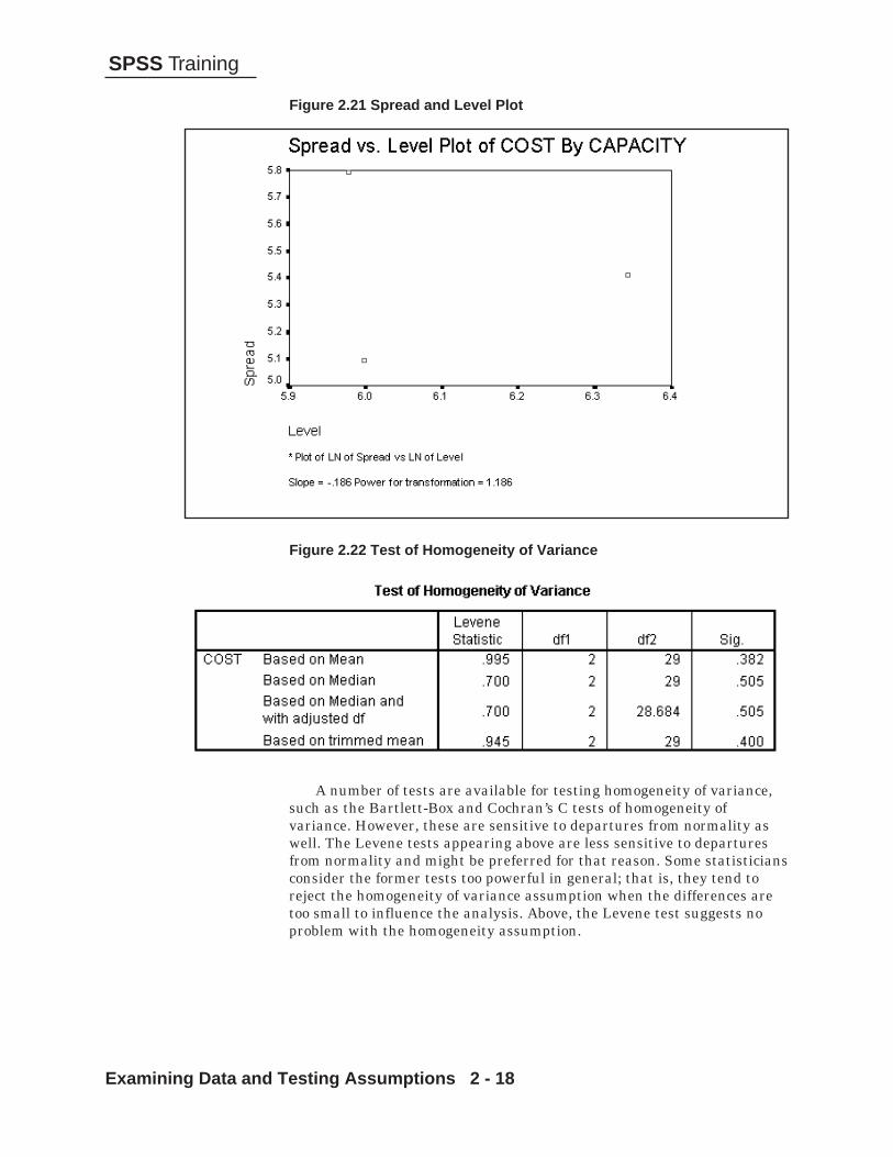
Homogeneity of variance within each population group is one of theassumptions in ANOVA. This can be tested by any of several statisticsand if the variance is systematically related to the level of the group(mean, median) data transformations can be performed to relieve this (wewill say more on this later in this chapter). The spread and level plotbelow provides a display of this by plotting the natural log of the spread(interquartile range) of the group against the natural log of the groupmedian. If you can overcome a seemingly inborn aversion to logs and viewthe plot, we desire relatively little variation in the log spread going acrossthe groups – which would suggest that the variances are stable acrossgroups. The reason for taking logs is technical. If there is a systematicrelation between the spread and the level (or variances and means), theslope of the best fitting line indicates what data transformation (withinthe class of power transformations) will best stabilize the variancesacross the different groups. We will say more about such transformationslater.
HOMOGENEITYOF VARIANCE
SPSS Training
Examining Data and Testing Assumptions 2 - 18
Figure 2.21 Spread and Level Plot
Figure 2.22 Test of Homogeneity of Variance
A number of tests are available for testing homogeneity of variance,such as the Bartlett-Box and Cochran’s C tests of homogeneity ofvariance. However, these are sensitive to departures from normality aswell. The Levene tests appearing above are less sensitive to departuresfrom normality and might be preferred for that reason. Some statisticiansconsider the former tests too powerful in general; that is, they tend toreject the homogeneity of variance assumption when the differences aretoo small to influence the analysis. Above, the Levene test suggests noproblem with the homogeneity assumption.

Examining Data and Testing Assumptions 2 - 19
SPSS Training
Overall the data fared fairly well in terms of the ANOVA assumptions.The only problem was normality of group 2. If inequality of variances wasa problem and a data transformation applied, that might relieve thedifficulty but no such transformation is called for. Since two of the threegroups seem fine we will proceed with the analysis.
Below we state in more detailed and formal terms the implications ofviolations of the assumptions and general conditions under which theyconstitute a serious problem.
In the fixed effects model this assumption is equivalent to assuming thatthe dependent variable is normally distributed in the population, since allother terms in the model are to be considered fixed effects. “F” and “t”tests used to test for differences among means in the analysis of varianceare unaffected by non-normality in large sample (this has led to thecommon practice of referring to the analysis of variance as robust withrespect to violations of the normality assumption). Less is known aboutsmall sample behavior, but the current belief among most statisticians isthat normality violations are generally not a cause for concern in fixedeffect models.
While inferences about means are generally not heavily affected bynon-normality, inferences about variances and about ratios of variancesare quite dependent on the normality assumption. Thus random effectsmodels are vulnerable to violations of normality where fixed effectsmodels are not. More important in the general case, since most analysesof variance involve fixed effects models, is the fact that many standardtests of the homogeneity of error variance depend on inferences aboutvariances, and are therefore vulnerable to violations of the normalityassumption.
Tests of the homogeneity of variance assumption such as the Bartlett-Box F, Cochran’s C and the F-max criterion all assume normality and areinaccurate in the presence of nonzero population kurtosis. If thepopulation kurtosis is positive (signifying a peaked or leptokurticdistribution), these tests will tend to reject the homogeneity assumptiontoo often, while a negative population kurtosis (indicative of a flat orplatykurtic distribution) will lead to too many failures to recognizeviolations of the homogeneity assumption. For this reason the Levene testfor homogeneity of variance (included in the Explore procedure) isstrongly recommended, as it is robust to violations of the normalityassumption.
Violations of the homogeneity of variance assumption are in general moretroublesome than violations of the normality assumption. In general, thesmaller the smaller the sample sizes of the groups and the moredissimilar the sizes of the groups, the more problematic violations of thisassumption become. Thus in a large sample with equal group sizes, even
Summary of thePlant Data
EFFECTS OFVIOLATIONS OF
ASSUMPTIONS INANOVA
Normality ofErrors in the
Population
Homogeneity ofPopulation Error
Variances AmongGroups

SPSS Training
Examining Data and Testing Assumptions 2 - 20
moderate to severe departures from homogeneity may not have largeeffects on inferences, while in small samples with unequal group sizes,even slight to moderate departures can be troublesome. This is onereason that statisticians recommend large samples and equal group sizeswhenever possible.
The magnitude of effects on actual Type I error level of violations ofthe homogeneity assumption depends on how dissimilar the variancesare, how large is the sample, and how dissimilar are the group sizes, asmentioned above. The direction of the distortion of actual Type I errorlevel depends on the relationship between variances and group sizes.Smaller sample from populations with larger variances lead to inflationof the actual Type I error level, while smaller samples from populationswith smaller variances result in actual Type I error levels smaller thanthe nominal test alpha levels.
Violations of the independence assumption can be serious even with largesamples and equal group sizes. Methods such as generalized leastsquares should be used with autocorrelated data.
Two further points should be considered here. First, our discussionhas centered on the impact of violations of assumptions on the actualType I (alpha) error level. When considerations such as the power of aparticular test are introduced, the situation can quickly become muchmore complicated. In addition, most of the work on the effects ofassumption violations has considered each assumption in isolation. Theeffects of violations of two or more assumptions simultaneously are lesswell known. For more detailed discussions of these topics, see Scheffe(1959) or Kirk (1982). Also, see Wilcox (1996, 1997) for who discusses theeffects of ANOVA assumption violation and presents robust alternatives.
Many researchers deal with violations of normality or homogeneity ofvariance assumptions by transforming their dependent variable in anonlinear manner. Such transformations include natural logarithms,square roots, etc. These types of transformations are also employed toachieve additivity of effects in factorial designs with non-crossoverinteractions. There are, however, serious potential problems with such anapproach.
While statistical procedures such as those employed by SPSS are notconcerned with the sources of the numbers they are used to analyze, andwill produce valid probabilities assuming only that distributionalassumptions are met. The interpretation of analyses of transformed datacan be quite problematic if the transformation employed is nonlinear.
If data are originally measured on an interval scale, which thecalculation of means assumes, then nonlinearly transforming thedependent variable and running a standard analysis results in a verydifferent set of questions being asked than with the dependent variable in
Population ErrorsUncorrelated with
Predictors andwith Each Other
A Note onTransformations

Examining Data and Testing Assumptions 2 - 21
SPSS Training
the original metric. Aside from the fact that a nonlinear transformation ofan interval scale destroys the interval properties assumed in thecalculation of means, the test of equality of a set of means of nonlinearlytransformed data does not test the hypothesis that the means of theoriginal data are equal, and there is no one to one relationship betweenthe two tests. Attempts to back-transform parameter estimates byapplying the inverse of the original transformation in order to apply theresults to the original research hypothesis do not work. The biasintroduced is a complicated one that actually increases with increasingsample size. For further information on this bias, see Kendall & Stuart(1968).
The practical implications of this point are that studies should bedesigned such that the variables which are of interest are measured, careshould be taken to see that they meet the assumptions required to makethe computation of basic descriptive statistics meaningful, and thatcommonly applied transformations in cases where ANOVA modelassumptions are violated may cause more trouble than they avert.Accurate probabilities attached to significance tests of the equality ofmeaningless quantities are of even less use than distorted probabilitiesattached to tests concerning meaningful variables, especially when thedirection and magnitude of distortions are of some degree estimable andcan be taken into account when interpreting research results.
In this chapter we discussed the implications of violation of some of theassumptions of ANOVA: homogeneity of variance, and normality of error.We used exploratory data analysis techniques on the data set prior toformal analysis in order to view the data and check on the assumptions.In the next chapter we will proceed with the actual one-factor ANOVAanalysis and consider planned and post-hoc comparisons.
SUMMARY

SPSS Training
Examining Data and Testing Assumptions 2 - 22

One-Factor Anova 3 - 1
SPSS Training
One-Factor ANOVA
Apply the principles of testing for population mean differences tosituations involving more than two comparison groups. Understand theconcept behind and the practical use of post-hoc tests applied to a set ofsample means.
We will run a one-factor (Oneway procedure) analysis of variancecomparing the different capacity groups on the cost of building a nuclearpower plant. Then, we will rerun the analysis requesting multiplecomparison (post hoc) tests to see specifically which population groupsdiffer. We will then plot the results using an error bar chart. Theappendix contains a nonparametric analysis of the same data.
We use the light water nuclear power plant data used in the last chapter.
We wish to investigate the relationship between the level of capacity ofthese plants and the cost associated with building the plants. One way toapproach this is to group the plants according to their generatingcapacity and compare these groups on their average cost. In our data setwe have the plants grouped into three capacity categories. Assuming weretain these categories we might first ask if there are any populationdifferences in cost among these groups. If there are significant meandifferences overall, we next want to know specifically which groups differfrom which others.
Analysis of variance (ANOVA) is a general method of drawingconclusions regarding differences in population means when twoor more comparison groups are involved. The independent-groups
t test applies only to the simplest instance (two groups), while ANOVAcan accommodate more complex situations. It is worth mentioning thatthe t test can be viewed as a special case of ANOVA and they yield thesame result in the two-group situation (same significance value, and the tstatistic squared is equal to the ANOVA’s F statistic).
We will compare three groups of plants based on their capacity anddetermine whether the populations they represent differ in the cost ofbeing built.
Chapter 3
Objective
Method
Data
Scenario
INTRODUCTION

One-Factor Anova 3 - 2
SPSS Training
The basic logic of significance testing is that we will assume that thepopulation groups have the same mean (null hypothesis), then determinethe probability of obtaining a sample with group mean differences aslarge (or larger) as what we find in our data. To make this assessmentthe amount of variation among the group means (between-groupvariation) is compared to the amount of variation among the observationswithin each group (within-group variation). Assuming that in thepopulation the group means are equal (null hypothesis), the only sourceof variation among the sample means would be the fact that the groupsare composed of different individual observations. Thus the ratio of thetwo sources of variation (between-group/within-group) should be aboutone when there are no population differences. When the distribution ofthe individual observations within each group follows the normal curve,the statistical distribution of this ratio is known (F distribution) and wecan make a probability statement about the consistency of our data withthe null hypothesis. The final result is the probability of obtaining sampledifferences as large (or larger) as what we found, if there were nopopulation differences. If this probability is sufficiently small (usuallyless than .05, i.e., less than 5 chances in 100) we conclude the populationgroups differ.
When performing a t test comparing two groups there is only onecomparison that can be made: group one versus group two. For thisreason the groups are constructed so their members systematically varyin only one aspect: for example, males versus females, or drug A versusdrug B. If the two groups differed on more than one characteristic (forexample, males given drug A versus females given drug B) it would beimpossible to differentiate between the two effects (gender and drug).
Why couldn’t a series of t tests be used to make comparisons amongthree groups? Couldn’t we simply use t tests to compare group one versusgroup two, group one versus group three, and group two versus groupthree? One problem with this approach is that when multiplecomparisons are made among a set of group means, the probability of atleast one test showing significance even when the null hypothesis istrue is higher than the significance level at which each test is performed(usually 0.05 or 0.01). In fact, if there is a large array of group means, theprobability of at least one test showing significance is close to one(certainty)! It is sometimes asserted that an unplanned multiplecomparison procedure can only be carried out if the ANOVA F test hasshown significance. This is not necessarily true as it depends on what theresearch question(s) are.
There remains a problem, however. If the null hypothesis is that allthe means are equal, the alternative hypothesis is that at least one of themeans is different. If the ANOVA F test gives significance, we know thereis a difference somewhere among the means, but that does not justify usin saying that any particular comparison is significant. The ANOVA Ftest, in fact, is an omnibus test, and further analysis is necessary tolocalize whatever differences there may be among the individual groupmeans.
LOGIC OFTESTING FOR
MEANDIFFERENCES
FACTORS

One-Factor Anova 3 - 3
SPSS Training
The question of exactly how one should proceed with further analysisafter making the omnibus F test in ANOVA is not a simple one. It isimportant to distinguish between those comparisons that were plannedbefore the data were actually gathered, and those that are made as partof the inevitable process of unplanned data-snooping that takes placeafter the results have been obtained. Planned comparisons are oftenknown as a-priori comparisons. Unplanned comparisons should betermed a-posteriori comparisons, but unfortunately the misnomer posthoc is more often used.
When the data can be partitioned into more than two groups,additional comparisons can be made. This might involve one aspect ordimension, for example four groups each representing a region of thecountry. Or the groups might vary along several dimensions, for exampleeight groups each composed of a gender (two categories) by region (fourcategories) combination. In this latter case, we can ask additionalquestions: (1) is there a gender difference? (2) is there a region difference?(3) do gender and region interact? Each aspect or dimension the groupsdiffer on is called a factor. Thus one might discuss a study or experimentinvolving one, two, even three or more factors. A factor is represented inthe data set as a categorical variable and would be considered anindependent variable. SPSS allows analysis of multiple factors, and hasdifferent procedures available based on how many factors are involvedand their degree of complexity. If only one factor is to be studied use theOneway (or One Factor ANOVA) procedure. When two or more factorsare involved simply shift to the general factorial procedure (GeneralLinear Model..General Factorial). In this chapter we consider a one-factorstudy (capacity relating to the cost of the plants), but we will discussmultiple factor ANOVA in later chapters.
First we need to open our data set.
Click File..Open..Data (move to the c:\Train\Anova directory)Select SPSS Portable (.por) from the Files of Type drop-down
listDouble-click on plant.por to open the file.
To run the analysis using SPSS for Windows:
Click Analyze..Compare Means ..One-Way ANOVA.Move cost into the Dependent List boxMove capacity into the Factor list box.
RUNNING ONE-FACTOR ANOVA

One-Factor Anova 3 - 4
SPSS Training
Figure 3.1 One-Way ANOVA Dialog Box
Enough information has been provided to run the basic analysis. TheContrasts pushbutton allows users to request statistical tests for plannedgroup comparisons of interest to them. The Post Hoc pushbutton willproduce multiple comparison tests that can test each group mean againstevery other one. Such tests facilitate determination of just which groupsdiffer from which others and are usually performed after the overallanalysis establishes that some significant differences exist. Finally, theOptions pushbutton controls such features as missing value inclusion andwhether descriptive statistics and homogeneity tests are desired.
Click on the Options pushbuttonClick to select both the Descriptive and Homogeneity-of-
varianceClick the Exclude cases analysis by analysis option button
Figure 3.2 One-way ANOVA Options Dialog Box

One-Factor Anova 3 - 5
SPSS Training
Click ContinueClick OK
The missing value choices deal with how missing data are to behandled when several dependent variables are given. By default caseswith missing values on a particular dependent variable are dropped onlyfor the specific analysis involving that variable. Since we are looking at asingle dependent variable, the choice has no relevance to our analysis.
The following syntax will run the analysis:
ONEWAY cost BY capacity /STATISTICS DESCRIPTIVES HOMOGENEITY /MISSING ANALYSIS .
The ONEWAY procedure performs a one-factor analysis of variance.Cost is the dependent measure and the keyword BY separates thedependent variable from the factor variable. We request descriptivestatistics and a homogeneity of variance test. We also told SPSS toexclude cases with missing data on an analysis by analysis basis.
Information about the groups appears in the figure below. We see thatcosts increase with the increase in capacity. 95-percent confidenceintervals for the capacity groups are presented in the table. One shouldnote that the standard deviations for the three groups appear to be fairlyclose.
Figure 3.3 Descriptive Statistics
ONE-FACTORANOVA RESULTS
DescriptiveStatistics

One-Factor Anova 3 - 6
SPSS Training
We also requested the Levene test of homogeneity of variance.
Figure 3.4 Levene Test of Homogeneity of Variance
Homogeneity ofVariance
This assumption of equality of variance for all groups was tested inChapter 2 using the EXPLORE (Examine) procedure. The Levene testalso shows that with this particular data set the assumption ofhomogeneity of variance is met, indicating that the variances do notdiffer across groups.
What do we do if the assumption of equal variances is not met? If thesample sizes are close to the same size and sufficiently large we couldcount on the robustness of the assumption to allow the process tocontinue. However, there is no general adjustment for the F test in thecase of unequal variances, as there was for the t test. A statisticallysophisticated analyst might attempt to apply transformations to thedependent variable in order to stabilize the within-group variances(variance stabilizing transforms). These are beyond the scope of thiscourse. Interested readers might turn to Emerson’s chapter in Hoaglin,Mosteller, and Tukey (1991) for a discussion from the perspective ofexploratory data analysis, and note that the spread & level plot inEXPLORE will suggest a variance stabilizing transform. A second andconservative approach would be to perform the analysis using astatistical method that does not assume homogeneity of variance. A one-factor analysis of group differences assuming that the dependent variableis only an ordinal (rank) variable is available as a nonparametricprocedure within SPSS. This analysis is provided in the appendix to thischapter. However, one should note that corresponding nonparametrictests are not available for all analysis of variance models.
Figure 3.5 ANOVA Summary TableThe ANOVA Table

One-Factor Anova 3 - 7
SPSS Training
The output includes the analysis of variance summary table and theprobability value we will use to judge statistical significance.
Most of the information in the ANOVA table is technical in natureand is not directly interpreted. Rather the summaries are used to obtainthe F statistic and, more importantly, the probability value we use inevaluating the population differences. Notice that in the first columnthere is a row for the between-group and a row for the within-groupvariation. The df column contains information about the degrees offreedom, related to the number of groups and the number of individualobservations within each group. The degrees of freedom are notinterpreted directly, but are used in estimating the between-group andwithin-group variation (variances). Similarly, the sums of squares areintermediate summary numbers used in calculating the between andwithin-group variances. Technically they represent the sum of thesquared deviations of the individual group means around the total grandmean (between) and the sum of the squared deviations of the individualobservations around their respective sample group mean (within). Thesenumbers are never interpreted and are reported because it is traditionalto do so. The mean squares are measures of between and within groupvariances. Recall in our discussion of the logic of testing that under thenull hypothesis both variances should have the same source and the ratioof between to within would be about one. This ratio, the sample Fstatistic, is 4.05 and we need to decide if it is far enough from one to saythat the group means are not equal. The significance (Sig.) columnindicates that under the null hypothesis of no group differences, theprobability of getting mean costs this far (or more) apart by chance isunder three percent (.028). If we were testing at the .05 level, we wouldconclude the capacity groups differ in average cost. In the language ofstatistical testing, the null hypothesis that power plants of these differentcapacities do not differ in cost is rejected at the 5% level.
From this analysis we conclude that the capacity groups differ in terms ofcost. In addition, we would like to know which groups differ from whichothers (Are they all different? Does the high capacity group differ fromeach of the other two?). This secondary examination of pairwisedifferences is done via procedures called multiple comparison testing(also called post hoc testing and multiple range testing). We turn to thisissue next.
The purpose of post hoc testing is to determine exactly which groupsdiffer from which others in terms of mean differences. This is usuallydone after the original ANOVA F test indicates that all groups are notidentical. Special methods are employed because of concern withexcessive Type I error.
In statistical testing, a Type I error is made if one falsely concludesthat differences exist when in fact the null hypothesis of no differences iscorrect (sometimes called a false positive). When we test at a given levelof significance say 5% (.05), we implicitly accept a five percent chance of aType I error occurring. The more tests we perform, the greater the overallchances of one or more Type I errors cropping up.
Conclusion
POST-HOCTESTING

One-Factor Anova 3 - 8
SPSS Training
This is of particular concern in our examination of which groupsdiffer from which others since the more groups we have the more tests wemake. If we consider pairwise tests (all pairings of groups, the number oftests for K groups is {[(K)*(K-1)]/2}. Thus for three groups, three tests aremade, but for 10 groups, 45 tests would apply. The purpose of the posthoc methodology is to allow such testing since we have interest inknowing which groups differ, yet apply some degree of control over theType I error.
There are different schemes of controlling for Type I error in post hoctesting. SPSS makes many of them available. We will briefly discuss thedifferent post hoc tests, and then apply some of them to the nuclear plantdata. We will apply several post hoc methods for comparison purposes, inpractice, usually only one would be run.
The ideal post hoc test would demonstrate tight control of Type I error,have good statistical power (probability of detecting true populationdifferences), and be robust over assumption violations (failure ofhomogeneity of variance, nonnormal error distributions). Unfortunately,there are implicit tradeoffs involving some of these desired features (TypeI error and power) and no one current post hoc procedure is best in allareas. Couple to this the facts that there are different statisticaldistributions on which pairwise tests can be based (t, F, studentizedrange, and others) and that there are different levels at which Type Ierror can be controlled (per individual test, per family of tests, variationsin between), and you have a huge collection of post hoc tests.
We will briefly compare post hoc tests from the perspective of beingliberal or conservative regarding the control of the false positive rate andapply several to our data. There is a full literature (including severalbooks) devoted to the study of post hoc (also called multiple comparison ormultiple range tests, although there is a technical distinction between thetwo) tests. More recent books (Toothaker, 1991) summarize simulationstudies that compare post hoc tests on their power (probability ofdetecting true population differences) as well as performance underdifferent scenarios of patterns of group means, and assumption violations(homogeneity of variance).
The existence of numerous post hoc tests suggests that there is nosingle approach that statisticians agree will be optimal in all situations.In some research areas, publication reviewers require a particular posthoc method, which simplifies the researcher’s decision.
Below we present some tests roughly ordered from the most liberal(greater statistical power and greater false positive rate) to the mostconservative (smaller false positive rate, less statistical power), andmention some designed to adjust for the lack of homogeneity of variance.
WHY SO MANYTESTS?
One-Factor Anova 3 - 9
SPSS Training
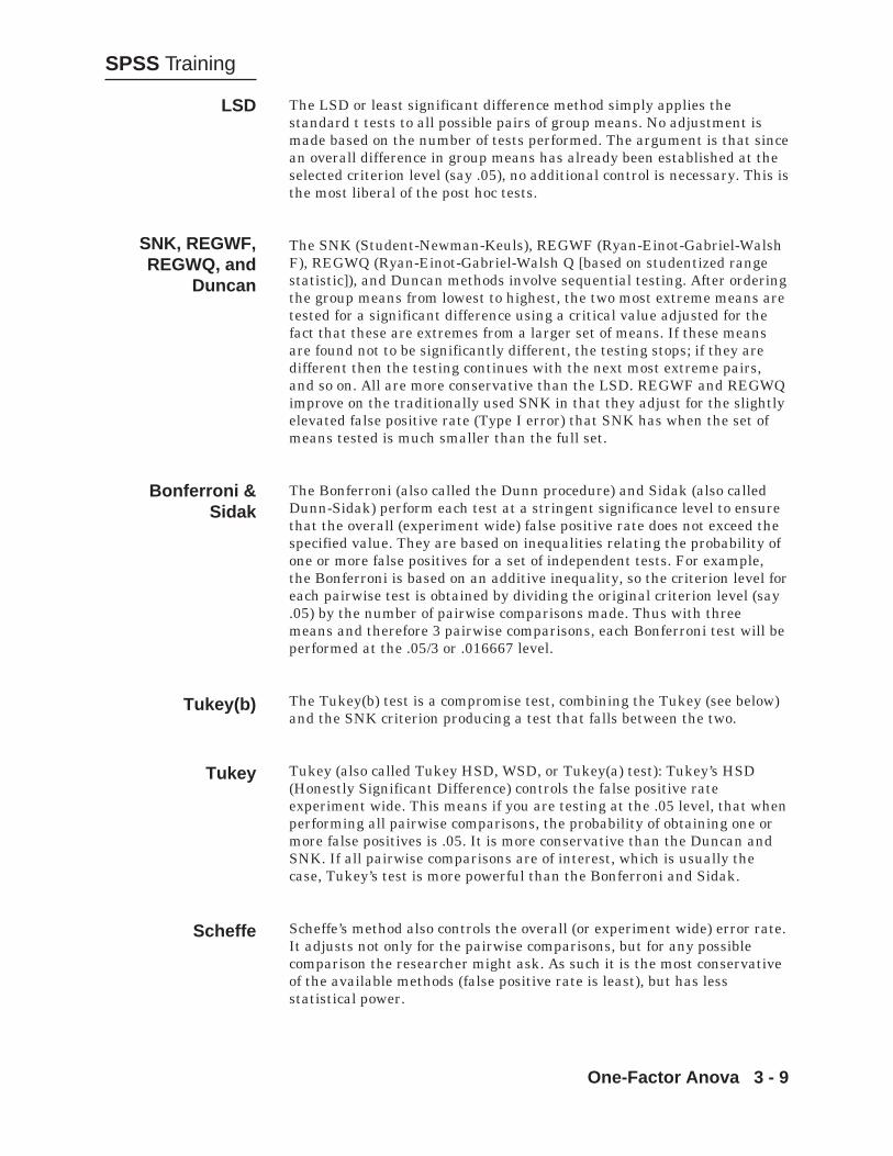
The LSD or least significant difference method simply applies thestandard t tests to all possible pairs of group means. No adjustment ismade based on the number of tests performed. The argument is that sincean overall difference in group means has already been established at theselected criterion level (say .05), no additional control is necessary. This isthe most liberal of the post hoc tests.
The SNK (Student-Newman-Keuls), REGWF (Ryan-Einot-Gabriel-WalshF), REGWQ (Ryan-Einot-Gabriel-Walsh Q [based on studentized rangestatistic]), and Duncan methods involve sequential testing. After orderingthe group means from lowest to highest, the two most extreme means aretested for a significant difference using a critical value adjusted for thefact that these are extremes from a larger set of means. If these meansare found not to be significantly different, the testing stops; if they aredifferent then the testing continues with the next most extreme pairs,and so on. All are more conservative than the LSD. REGWF and REGWQimprove on the traditionally used SNK in that they adjust for the slightlyelevated false positive rate (Type I error) that SNK has when the set ofmeans tested is much smaller than the full set.
The Bonferroni (also called the Dunn procedure) and Sidak (also calledDunn-Sidak) perform each test at a stringent significance level to ensurethat the overall (experiment wide) false positive rate does not exceed thespecified value. They are based on inequalities relating the probability ofone or more false positives for a set of independent tests. For example,the Bonferroni is based on an additive inequality, so the criterion level foreach pairwise test is obtained by dividing the original criterion level (say.05) by the number of pairwise comparisons made. Thus with threemeans and therefore 3 pairwise comparisons, each Bonferroni test will beperformed at the .05/3 or .016667 level.
The Tukey(b) test is a compromise test, combining the Tukey (see below)and the SNK criterion producing a test that falls between the two.
Tukey (also called Tukey HSD, WSD, or Tukey(a) test): Tukey’s HSD(Honestly Significant Difference) controls the false positive rateexperiment wide. This means if you are testing at the .05 level, that whenperforming all pairwise comparisons, the probability of obtaining one ormore false positives is .05. It is more conservative than the Duncan andSNK. If all pairwise comparisons are of interest, which is usually thecase, Tukey’s test is more powerful than the Bonferroni and Sidak.
Scheffe’s method also controls the overall (or experiment wide) error rate.It adjusts not only for the pairwise comparisons, but for any possiblecomparison the researcher might ask. As such it is the most conservativeof the available methods (false positive rate is least), but has lessstatistical power.
LSD
SNK, REGWF,REGWQ, and
Duncan
Bonferroni &Sidak
Tukey(b)
Tukey
Scheffe

One-Factor Anova 3 - 10
SPSS Training
Most post hoc procedures mentioned earlier (excepting LSD, Bonferroni,and Sidak) were derived assuming equal sample sizes in addition tohomogeneity of variance and normality of error. When subgroup samplesizes are unequal, SPSS substitutes a compromise value (the harmonicmean) for the sample sizes. Hochberg’s GT2 and Gabriel’s post hoc testexplicitly allow for unequal sample sizes.
The Waller-Duncan takes an interesting approach (Bayesian) thatadjusts the criterion value based on the size of the overall F statistic inorder to be sensitive to the types of group differences associated with theF (for example, large or small). Also, you can specify the ratio of Type I(false positive) to Type II (false negative) error in the test. This featureallows for adjustments if there are differential costs to the two types oferror.
Each of these post hoc tests adjusts for unequal variances and samplesizes in the groups. Simulation studies suggest that although Games-Howell can be too liberal when the group variances are equal and samplesizes are unequal, it is more powerful than the others.
An approach some analysts take is to run both a liberal (say LSD)and a conservative (Scheffe or Tukey HSD) post hoc test. Groupdifferences that show up under both criteria are considered solid findings,while those found different only under the liberal criterion are viewed astentative results.
To illustrate the differences among the post hoc tests we will requestsix different post hoc tests: (1) LSD, (2) Duncan, (3) SNK, (4) Tukey’sHSD, (5) Bonferroni, and (6) Scheffe.
Click Dialog Recall button
Select One-Way ANOVA
Within the One-Way ANOVA Dialog Box
Click on the Post Hoc pushbutton.Select the following types of post hoc tests: LSD, Duncan, SNK,
Tukey, Bonferroni, and Scheffe.
Specialized PostHocs Unequal
Ns:
Hochberg’s GT2& Gabriel
Waller-Duncan
UnequalVariances and
Unequal Ns:
Tamhane T2,Dunnett’s T3,
Games-Howell,Dunnett’s C

One-Factor Anova 3 - 11
SPSS Training
Figure 3.6 Post Hoc Dialog Box
By default, statistical tests will be done at the .05 level. For sometests you may supply your preferred criterion level. The command to runthe post hoc analysis appears below.
ONEWAY cost BY capacity /MISSING ANALYSIS /POSTHOC = SNK TUKEY DUNCAN SCHEFFE LSD
BONFERRONI ALPHA(.05).
Post hoc tests are requested using the POSTHOC subcommand. TheSTATSISTICS subcommand need not be included here since we havealready viewed the means and discussed the homogeneity test.
Click ContinueClick OK
The beginning part of the output contains the ANOVA table,descriptive statistics, and the homogeneity test, which we have alreadyreviewed. We will move directly to the post hoc test results.

One-Factor Anova 3 - 12
SPSS Training
Figure 3.7 LSD Post Hoc Results
All tests appear in one table. However, the Post Hoc Tests andHomogeneous Subsets pivot tables were edited in the Pivot Table Editorso that each test can be viewed and discussed separately. (To do so,double-click on the pivot table to invoke the Pivot Table Editor, then clickPivot..Pivot Trays so that the Pivot Trays option is checked and the PivotTrays window is visible. Next click and drag the pivot tray icon for Test(to see an icon's label, just click on the icon) from the Row dimension trayinto the Layer dimension tray. Now test results for any single post hoctest can be viewed by selecting the desired test from the Test drop-downlist located just above the table.)
The rows are constructed from every possible pairing of groups. Forexample, the less than 800 Mwe group is paired against the other twogroups, then the 800-1000 Mwe group is paired against the other twogroups, etc. The column label “Mean Difference (I-J)” contains the meandifference between each pairing of groups. We see that the <800 grouphas a mean cost difference of -$35.7866 with the 800-1000 group and adifference of -$193.5885 with the >1000 group. If a difference isstatistically significant at the specified level after applying any post hocadjustments (none for LSD), then an asterisk (*) appears beside the meandifference. Notice the actual significance value for the test appears in thecolumn labeled “Sig.”
The first LSD block indicates that in the population those plantshaving less than 800 Mwe’s differ significantly in cost from the plantshaving a capacity of greater than 1000 Mwe’s. In addition, the standarderrors and 95% confidence intervals for each mean difference aredisplayed. These provide information of the precision with which we haveestimated the mean differences. Note that, as you expect, if a meandifference is not significant, the confidence interval contains zero. UsingLSD, the high capacity group differs from each of the other two, but thelower capacity groups do not differ from each other.
Note

One-Factor Anova 3 - 13
SPSS Training
Figure 3.8 Duncan Results
SPSS does not present the Duncan results in the same format as wesaw for the LSD. This is because for some of the post hoc test methodsstandard errors and 95-percent confidence intervals are not defined (formultiple-range tests, recall testing stops once the remaining mostextreme means are not found different). Rather than display results withempty columns in such situations, a different format, homogeneoussubsets, is used. A homogeneous subset is a set of groups for which nopair of group means differs significantly. Depending on the post hoc testrequested SPSS will display a multiple comparison table, a homogeneoussubset table, or both. In this data set, it shows that the two lowercapacity groups do not differ in cost, but differ from the highest capacitygroup.
Figure 3.9 SNK Results

One-Factor Anova 3 - 14
SPSS Training
The SNK results display the same pattern as the Duncan tests.
Figure 3.10 Tukey Results for Multiple Comparisons
The Tukey multiple comparison tests show that the less than 800Mwe group is significantly different from the greater than 1000 Mwegroup, but this is the only pairwise difference.
Figure 3.11 Tukey Results for Homogeneous Subsets
The Tukey homogeneous subset table is consistent with the multiplecomparison table. The first homogeneous subset contains the two lower

One-Factor Anova 3 - 15
SPSS Training
capacity plants (they do not differ). The second homogeneous subset ismade up of the second and third groups (they do not differ). Thus the onlydifference is between the less than 800 Mwe group and the greater than1000 Mwe group. It should be pointed out that the second and thirdgroups are barely not significant (.07) and had the sample sizes beenlarger their difference might have been significant.
Figure 3.12 Bonferroni Results
The test shows that the less than 800 Mwe’s group has a significantlydifferent cost than the greater than 1000 Mwe’s group.
Figure 3.13 Scheffe Results for Multiple Comparisons

One-Factor Anova 3 - 16
SPSS Training
Figure 3.14 Scheffe Results for Homogeneous Subsets
From these results we can see that similar to the Bonferroni test,only the high and low capacity groups differ.
As discussed before, the different post hoc procedures offer differenttrade-offs between Type I error (falsely claiming a significant difference)and power (ability to detect a real difference). Your choice in the matterdepends on how you want to balance the two. In this analysis it appearsthat the high and low capacity groups do differ in cost, while the low andmiddle groups do not. The middle to high capacity difference might beusefully considered as a tentative finding.
Post hoc tests compare all pairs of groups and most of the methodsdiscussed apply a penalty function (adjusting the critical value) becauseso many tests are being made. In some experiments and studies, theresearcher has in mind some specific comparisons to be made betweengroup means. Compared to post hoc tests, planned comparisons are fewerin number and are to be formulated before viewing the data. Becausethey are limited in number (based on between-group degrees of freedom(the number of groups minus one)) and specified beforehand, theadjustments made for post hoc tests are not required.
A broad variety of planned comparisons (sometimes called a prioricomparisons) can be requested: all treatment groups might be comparedto a control group; a linear trend line could be fit; step comparisons couldbe made to detect a threshold.
To demonstrate this method, let us suppose that there is interest inmaking some specific comparisons between capacity groups. The idea isthat at some point the change in capacity would result in a large changein cost. To see if and where this occurs, we can compare the low to middlecapacity plants, then the middle to high capacity plants. If either of these
Conclusion
PLANNEDCOMPARISONS

One-Factor Anova 3 - 17
SPSS Training
comparisons is significant, we have an idea of where the big cost increasewill occur.
Planned comparisons between groups are done by applying a set ofcoefficients to the group means and testing whether the result is zero. Forexample, to compare the low and middle plant groups, multiply the meanof the low plants by one, the mean of the middle plants by negative one,the mean of the large plants by zero, and sum the result. Thus, wecompare the means, and if this difference is significantly different fromzero, then the low capacity plants differ from the middle capacity plants.In ONEWAY you can request planned comparisons by providing sets ofcoefficients.
To request tests of low versus middle, and the middle versus highcapacity groups we use the Contrasts pushbutton and apply thenecessary coefficients.
Click Dialog Recall tool
Select One-Way ANOVAClick the Contrasts pushbuttonType 1 in the Coefficients text box and click Add pushbuttonType –1 in the Coefficients text box and click Add pushbuttonType 0 in the Coefficients text box and click Add pushbuttonClick Next pushbuttonType 0 in the Coefficients text box and click Add pushbuttonType 1 in the Coefficients text box and click Add pushbuttonType -1 in the Coefficients text box and click Add pushbutton
Figure 3.15 Contrasts Dialog Box
HOW PLANNEDCOMPARISONS
ARE DONE
Each set of contrast coefficients is assigned a number (1,2, …) andappears as a column in the Coefficients list box.

One-Factor Anova 3 - 18
SPSS Training
Click Continue to process the ContrastsClick OK to run the analysis
This leads to the syntax below (note the PostHoc subcommand is notincluded although our previous post hoc requests are still stored in thePost Hoc dialog.
ONEWAY cost BY capacity /CONTRAST= 1 –1 0 /CONTRAST = 0 1 –1 /MISSING ANALYSIS.
The first contrast requests the difference between the low and middlegroups; the second compares the middle and high groups. We are limitedto two planned comparisons because with three groups we have but twobetween-group degrees of freedom.
Scroll to the Contrast Coefficients Pivot Table in the Viewerwindow.
Figure 3.16 Contrast Coefficients
The requested comparisons are first reproduced along with the grouplabels. We verify that the first compares the low to middle group, and thesecond compares the middle to high group.
Figure 3.17 Contrast Results
Notice that there are two sets of results, one labeled “assume equalvariances” and the other “does not assume equal variances”. Resultslabeled “does not assume equal variances” are adjusted results that canbe used if the homogeneity of variance assumption is not met. We

One-Factor Anova 3 - 19
SPSS Training
previously determined the variances are equal and will use the “assumeequal variances” statistics.
The column labeled "Value of Contrast" contains the values of thecontrast coefficients applied to the sample means, which here representthe mean difference between pairs of groups. This can be verified bychecking the group means appearing earlier. The first comparison(between the low and middle groups) is not significant, but the second one(comparing the middle and high capacity groups) is. This suggests thatthe big cost increase comes when shifting from the middle to highcapacity plants. A t test is used since each comparison involves onedegree of freedom; it is equivalent to using an F test (the t statisticsquared would equal the F).
Thus a limited number of planned comparisons between group meanscan be specified as part of the general analysis. Performing plannedcomparisons does not preclude running post hoc analyses later.
For presentations it is useful to display the sample group means alongwith their 95-percent confidence intervals. In SPSS for Windows
Click on Graphs..Error BarVerify that Simple is selected, then click Define pushbuttonMove cost into the Variable list boxMove capacity into the Category Axis list box.
Figure 3.18 Error Bar Dialog Box
GRAPHING THERESULTS
Click on OK
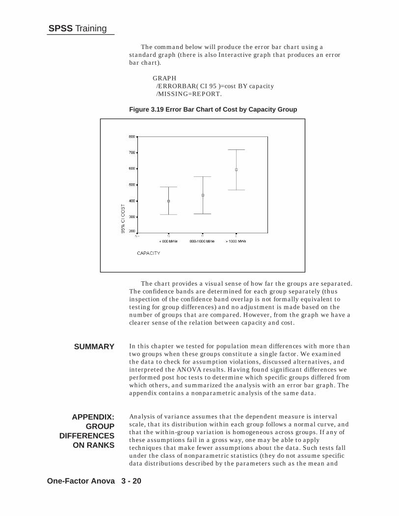
One-Factor Anova 3 - 20
SPSS Training
The command below will produce the error bar chart using astandard graph (there is also Interactive graph that produces an errorbar chart).
GRAPH /ERRORBAR( CI 95 )=cost BY capacity /MISSING=REPORT.
Figure 3.19 Error Bar Chart of Cost by Capacity Group
The chart provides a visual sense of how far the groups are separated.The confidence bands are determined for each group separately (thusinspection of the confidence band overlap is not formally equivalent totesting for group differences) and no adjustment is made based on thenumber of groups that are compared. However, from the graph we have aclearer sense of the relation between capacity and cost.
In this chapter we tested for population mean differences with more thantwo groups when these groups constitute a single factor. We examinedthe data to check for assumption violations, discussed alternatives, andinterpreted the ANOVA results. Having found significant differences weperformed post hoc tests to determine which specific groups differed fromwhich others, and summarized the analysis with an error bar graph. Theappendix contains a nonparametric analysis of the same data.
Analysis of variance assumes that the dependent measure is intervalscale, that its distribution within each group follows a normal curve, andthat the within-group variation is homogeneous across groups. If any ofthese assumptions fail in a gross way, one may be able to applytechniques that make fewer assumptions about the data. Such tests fallunder the class of nonparametric statistics (they do not assume specificdata distributions described by the parameters such as the mean and
SUMMARY
APPENDIX:GROUP
DIFFERENCESON RANKS

One-Factor Anova 3 - 21
SPSS Training
standard deviation). Since these methods make few if any distributionalassumptions, they can often be applied when the usual assumptions arenot met. If you are tempted to think that something is obtained fornothing, the downside of such methods is that if the stronger dataassumptions hold, the nonparametric tests are generally less powerful(probability of finding true differences) than the appropriate parametricmethod. Also, there are some parametric statistical analyses thatcurrently have no corresponding nonparametric method. It is fair to saythat the boundaries concerning when to use parametric versusnonparametric methods are in practice somewhat vague, and statisticianscan and often do disagree about which approach is optimal in a specificsituation.
For the purposes of this appendix let us assume that we needed torun the test using nonparametric methods. We will perform anonparametric procedure that only assumes that the dependent measurehas ordinal properties. The basic logic behind this test, the Kruskal-Wallis test, is as follows. If we rank order the dependent measurethroughout the entire sample, we would expect under the null hypothesis(of no population differences) that the average rank (technically the sumof the ranks adjusted for sample size) should be about the same for eachgroup. The Kruskal-Wallis test calculates the ranks, each sample group’smean rank, and the probability of obtaining group average ranks(weighted summed ranks) as far apart (or further) as what is observed inthe sample, if the population groups were identical.
To run the Kruskal-Wallis test in SPSS we would
Click Analyze..Nonparametric Tests..K IndependentSamples
Move cost into the Test Variable ListMove capacity into the Grouping Variable boxClick the Define Range button and enter a Minimum of 1 and
Maximum of 3.Click Continue
Figure 3.20 Analysis of Ranks Dialog Box

One-Factor Anova 3 - 22
SPSS Training
By default, the Kruskal-Wallis test will be performed. Theorganization of this dialog box closely resembles that of the One-WayANOVA. The command to run this analysis using SPSS follows.
NPAR TESTS /K-W=cost BY capacity(1 3)
The K-W subcommand instructs the nonparametric testing routine toperform the Kruskal-Wallis analysis of variance of ranks on thedependent variable cost with capacity as the independent or groupingvariable.
Click OK to run the analysis
Figure 3.21 Results of Kruskal-Wallis Nonparametric Analysis
We see the pattern of mean ranks (remember smaller ranks implylower cost) follows that of the original means of cost, increasing as thecapacity increases. The chi-square statistic is used in the Kruskal-Wallisindicates that it is very unlikely (fewer than 4 chances in 100) to obtainsamples with average ranks so far apart if the null hypothesis (no costdifferences between groups) were true. This is consistent with ourconclusion from the initial one-way ANOVA analysis.

Multi-Way Univariate ANOVA 4 - 1
SPSS Training
Multi-Way Univariate ANOVA
We will apply the principles of testing for differences in population meansto situations involving more than one factor. Also we will show how thetwo-factor ANOVA is a generalization of the one-factor design that wecovered in the last chapter. We will develop some understanding of thenew features of the analysis. We will then discuss the implications ofunequal sample sizes and empty cells.
We wish to test whether there are any differences in the cost of thenuclear power plants based on capacity or the experience of the architect/engineer. First we use the EXPLORE procedure to explore the subgroupsinvolved in the analysis. Next, we make use of the Univariate procedureto run the two-factor ANOVA, specifying cost as the dependent variablewith capacity and experience as factors. We display the results using anerror bar chart. In the appendix we perform post hoc tests based on theresults of our analysis.
We continue to use the nuclear plant data. The data set is an SPSSportable file (plant.por) containing information about 32 light waternuclear power plants. Four variables are included: the capacity and costof the plant; time to completion; and experience of the architect-engineerwho built the plant.
Analysis of variance (ANOVA) is a general method for drawingconclusions about differences in population means when two ormore comparison groups are involved. In an introductory statistics
class you have seen how a “t” test is used to contrast two groups, and inthe last chapter we saw how one-way ANOVA compares more than twogroups which differ along a single factor. In this chapter, we expand ourconsideration of ANOVA to allow multiple factors in a single analysis.Such an approach is efficient in that several questions are addressedwithin one study. The assumptions and issues considered in the lastchapter (normality of the dependent variable within each group,homogeneity of variance, and the importance of both) apply to generalANOVA and will not be repeated here.
We will investigate whether there are differences in the average costof a plant for the different plant capacities and levels of experience of thedesigner/engineer. Since two factors, capacity and experience, are underconsideration, we can ask three different questions: (1) Are there costdifferences based on capacity? (2) Are there differences based onexperience? (3) Do capacity and experience interact?
Chapter 4
Objective
Method
Data
INTRODUCTION
Multi-Way Univariate ANOVA 4 - 2
SPSS Training
A multi-factor analysis involves the same approach and principles, asdid a one-way ANOVA. The between-groups variation can now bepartitioned into pieces attributable to main effects and interactioncomponents, but the method is much the same. Some complications arisewith unequal cell sizes and empty cells that were not a problem when wetested a single factor. We will discuss these issues and illustrate theanalysis.
As in earlier chapters, we begin by running an exploratory dataanalysis, then proceed with more formal testing.
As before, we wish to draw conclusions about the populations from whichwe sample. The main difference in moving from a one-way ANOVA to thegeneral ANOVA is that more questions can be asked about thepopulations. However, the results will be stated in the same terms: howlikely is it that we would obtain means as far apart as what we observe inour sample, if there were no mean differences in the populations.Comparisons are again framed as a ratio of the variation among thegroup means (between-group variation) to the variation amongobservations within each group (within-group variation). When statisticaltests are performed, homogeneity of variance and normality of thedependent variable within each group are assumed. Comments madeearlier regarding robustness of the means analysis when theseassumptions are violated apply directly.
The new aspect we consider is how to include several factors, or askseveral different questions of the data, within a single analysis ofvariance. We will test whether there are differences in cost based oncapacity, whether there are differences based on the experience of theengineer, and finally, whether capacity and experience interactconcerning the cost of the plants. The interpretation of an interaction isdiscussed in the next section.
Although our example involves only two factors (capacity andexperience), ANOVA can accommodate more. Usually, the number offactors is limited by either the interests of the researcher, who mightwish to examine a few specific issues, or by sample size considerations.Sample size plays a role in that the greater the number of factors, thegreater the number of cell means that must be computed, and the smallerthe sample for each mean. For example, suppose we have a sample of 800plants and wish to look at cost differences due to whether the plant waslight water or heavy water (2 levels), capacity (3 levels), experience (3levels), region of the country (9 levels), and age of the plant (4 levels).There are 2*3*3*9*4 or 648 subgroup means involved. If the data weredistributed evenly across the levels, each subgroup mean would be basedon approximately two observations, and this would not produce a verypowerful analysis. Such analyses can be performed, and technically,questions involving single effects like capacity or experience would bebased on means involving fairly large samples. Also, some plannedexperiments permit many subgroups to be dropped (for example,incomplete designs). Yet the fact remains that with smaller samples,there are practical limitations in the number of questions you can ask ofthe data.
LOGIC OFTESTING, ANDASSUMPTIONS
HOW MANYFACTORS?

Multi-Way Univariate ANOVA 4 - 3
SPSS Training
When moving beyond one-factor ANOVA, the distinction between maineffects and interactions becomes relevant. A main effect is an effect (orgroup difference) attributable to a single factor (independent variable).For example, when we study cost differences across capacity groups andexperience groups, the effect of capacity alone, and the effect ofexperience alone, would be considered main effects. The two-wayinteraction would test whether the effect of one factor is the same at eachlevel of the other factor.
In our example, this can be phased in either of two ways. We couldsay the interaction tests whether the cost difference due to capacity(which could be zero) is the same for each level of experience.Alternatively, we can say that the two-way interaction tests whether theexperience difference in cost is the same for each capacity group. Whilethese two phrasings are mathematically equivalent, it can sometimes besimpler (based on the number of levels in each factor) for you to presentthe information from one perspective instead of the other. The presence ofa two-way interaction is important to report, since it qualifies ourinterpretation of a main effect. For example, a capacity by experienceinteraction implies that the magnitude of the capacity difference variesacross levels of experience. In fact, there may be no difference or areversal in the pattern of the capacity means for some experience levels.Thus statements about capacity differences must be qualified byexperience information.
Since we are studying two factors, there can be only one interaction.If we expand our analysis to three factors (say capacity, experience, andage of plant) we can ask both two-way (capacity by experience, capacityby age, experience by age) and three-way (capacity by experience by age)interaction questions. As the number of factors increases, so does thepossible complexity of the interactions. In practice, significant high-order(three, four, five-way, etc.) interactions are relatively rare compared tothe number of significant main effects.
Interpretation of an interaction can be done directly from a table ofrelevant subgroup means, but it is more convenient and common to viewa multiple-line chart of the means. We illustrate this below under severalscenarios.
Suppose that we have four levels of one independent variable (saylocation) and two levels for the second independent variable (say gender).In our scenario, suppose that women are more highly educated than men,there are regional differences in education, and that the genderdifferences are the same across regions. The line chart below plots a set ofmeans consistent with this pattern.
INTERACTIONS

Multi-Way Univariate ANOVA 4 - 4
SPSS Training
Illustration 4.1 Main Effects, No Interaction
In the illustration we see that the mean line for women is above thatof the men. In addition, there are differences among the four locations.However, note that the gender differences are nearly identical across thefour locations. This equal distance between the lines (parallelism of lines)indicates that there is no interaction present.
Illustration 4.2 No Main Effects, Strong Interaction
Here the overall means for men and women are about the same, asare the means for each location (pooling the two gender groups).

Multi-Way Univariate ANOVA 4 - 5
SPSS Training
However, the gender differences vary dramatically across the differentlocations: in location B women have higher education, in locations A andD there is no gender difference, and in location C males have highereducation. We cannot make a statement about gender differences withoutqualifying it with location information, nor can we make location claimswithout mentioning gender. Strong interactions are marked by thiscrossover pattern in a multiple-line chart.
Illustration 4.3 One Main Effect, Weak Interaction
We see a gender difference for each of the four locations, but themagnitude of this difference varies across locations (substantially greaterfor location D). This difference in magnitude of the gender effect wouldconstitute an interaction between gender and location. It would betermed a weak interaction because there is no crossover of the meanlines.
Additional scenarios can be charted, and we have not mentionedthree-way and higher interactions. Such topics are discussed inintroductory statistics and analysis of variance books (see the referencepage for suggestions). We will now proceed to analyze our data set.
We begin by applying exploratory data analysis to the cost of the plantswithin subgroups defined by combinations of capacity and experience. Inpractice, you would check each group’s summaries, look for patterns inthe data, and note any unusual points. Also, we will request that theExplore procedure perform a homogeneity of variance test.
Click on File..Open..Data (move to the c:\Train\Anova folder)Select SPSS Portable (*.por) from the Files of Type drop-
down listDouble-click on plant.por
EXPLORING THEDATA

Multi-Way Univariate ANOVA 4 - 6
SPSS Training
Click on Analyze..Descriptive Statistics..ExploreMove cost into the Dependent List boxMove the exper and capacity into the Factor List box.
Figure 4.1 Explore Dialog Box
Click on the Plots pushbuttonClick the Power estimation option button in the “Spread vs.
Level with Levene Test” area
Figure 4.2 Plots Dialog Box
By default, no homogeneity test is performed (“None” option button).Each of the remaining choices will lead to homogeneity being tested. The

Multi-Way Univariate ANOVA 4 - 7
SPSS Training
second (Power estimation) and third (Transformed) choices are used bymore technical analysts to investigate power transformations of thedependent measure that would yield greater homogeneity of variance.These issues are of interest to serious practitioners of ANOVA, but arebeyond the scope of this course (see Emerson in Hoaglin, Mosteller, andTukey (1991), also a brief discussion in Box, Hunter, and Hunter (1978),and the original (technical) paper by Box and Cox (1964)). TheUntransformed choice builds a plot without transforming the scale of thedependent measure.
Click on the Continue button to return to the Explore dialogbox
Since we are comparing capacity by experience subgroups, wedesignate exper (experience) and capacity as the factors (or nominalindependent variables). However, if we were to run this analysis, it wouldproduce a set of summaries for each capacity group, then a set for eachexperience group. In other words, each of the two factors would be treatedseparately, instead of being combined, which we desire. To instruct SPSSto treat each capacity by experience combination as a subgroup we mustuse SPSS syntax. The easiest way to accomplish this would be to click thePaste pushbutton that opens a syntax window and builds an Examinecommand that will perform an analysis for each factor.
Click on the Paste pushbutton to paste the syntax into a Syntaxwindow
Figure 4.3 Examine Command in Syntax Window
The Examine command requires only the Variables subcommand inorder to tun. We also include the Plot subcommand since we desire thehomogeneity test (controlled by the SPREADLEVEL keyword). The

Multi-Way Univariate ANOVA 4 - 8
SPSS Training
other subcommands specify default values and appear in order to make itsimple for the analyst to modify the command when necessary. Note thekeyword BY separates the dependent variable cost from the exper andcapacity factors. Currently, both exper and capacity follow the BYkeyword and thus have the same status: an analysis will be run for eachseparately. To indicate we wish a joint analysis, we insert an additionalBY keyword between exper and capacity on the VARIABLESsubcommand.
Figure 4.4 Examine Command Requesting Subgroup Analysis
SPSS now interprets the factor groupings to be based on eachcapacity by experience combination (exper BY capacity ).
Click Run..Current or click the Run button .
Looking at the descriptives for each of our subgroups we see thefollowing information.
All descriptive statistics appear in a single pivot table; the figures presentseparate sections of the table
Note

Multi-Way Univariate ANOVA 4 - 9
SPSS Training
Figure 4.5 Descriptives for 1-3 Plants and <800 MWe
We find in this subgroup that the mean cost is 404.0829 and otherdescriptive information is available to us.
Figure 4.6 Descriptives for 1-3 Plants and >1000 MWe
Figure 4.7 Descriptives for 4-9 Plants and <800 MWe

Multi-Way Univariate ANOVA 4 - 10
SPSS Training
Figure 4.8 Descriptives for 4-9 Plants and 800-1000 MWe
Figure 4.9 Descriptives for 4-9 Plants and > 1000 MWe
Figure 4.10 Descriptives for 10 or more Plants and <800 MWe

Multi-Way Univariate ANOVA 4 - 11
SPSS Training
Figure 4.11 Descriptives for 10 or more Plants and 800-1000 MWe
Figure 4.12 Descriptives for 10 or more Plants and >1000 MWe
In the Viewer window we find a warning message concerning thespread and level plot and the test for homogeneity of variance. Thismessage tells us that because we had a small number of cases in some ofour subgroups that the median and/or the interquartile range was notdefined. Thus the test and plot are not produced.
Figure 4.13 Test of Homogeneity of Variance

Multi-Way Univariate ANOVA 4 - 12
SPSS Training
Figure 4.14 Warning Messages
Now we move to view the Box and Whiskers Plot.
Figure 4.15 Box and Whisker Plot of Cost
We see variation in the lengths of the boxes that suggests that thevariation of cost within the subgroups is not homogeneous. We can seethat there are differences in the median cost across our subgroups, butwith the small sample sizes are they different enough to be statisticallysignificant? An outlier is visible at the high end. Does it seem so extremeas to suggest a data error?

Multi-Way Univariate ANOVA 4 - 13
SPSS Training
To run the analysis in SPSS we choose Analyze..General LinearModel menu. Please note that the General Linear Model menu choiceswill vary depending on your version of SPSS and whether you have theSPSS Advanced Models option installed. We will use the Univariateprocedure.
The Univariate choice permits the analyst to handle designs from thesimple to the more complex (incomplete block, Latin square, etc.) and alsoprovides the user with control over various aspects of the analyses. TheMultivariate menu choice performs multivariate (multiple dependentmeasures) analysis of variance, while the Repeated Measures menuchoice is used for studies in which an observation contributes to severalfactor levels (these are commonly called split-plot or repeated measuredesigns). Finally, the Variance Components menu choice performs ananalysis that estimates the variation in the dependent variableattributable to each random effect in a model (see discussion of randomand fixed effects below). Thus it assesses the relative influence of eachrandom effect in a model containing multiple random effects.
Click on Analyze..General Linear Model..UnivariateMove cost and to the Dependent Variable list boxMove exper and capacity to the Fixed Factor(s) list box.
Figure 4.16 Univariate Dialog Box
TWO-FACTORANOVA
Our analysis does not include random factors (other than the plant toplant variation that is already accounted for as the within-groupvariation. Briefly, fixed factors have a limited (finite) number of levelsand we wish to draw population conclusions about only those levels.
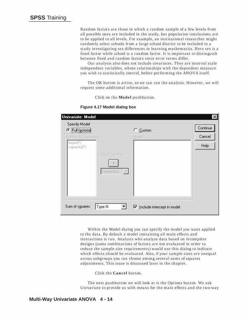
Multi-Way Univariate ANOVA 4 - 14
SPSS Training
Random factors are those in which a random sample of a few levels fromall possible ones are included in the study, but population conclusions areto be applied to all levels. For example, an institutional researcher mightrandomly select schools from a large school district to be included in astudy investigating sex differences in learning mathematics. Here sex is afixed factor while school is a random factor. It is important to distinguishbetween fixed and random factors since error terms differ.
Our analysis also does not include covariates. They are interval scaleindependent variables, whose relationships with the dependent measureyou wish to statistically control, before performing the ANOVA itself.
The OK button is active, so we can run the analysis. However, we willrequest some additional information.
Click on the Model pushbutton.
Figure 4.17 Model dialog box
Within the Model dialog you can specify the model you want appliedto the data. By default a model containing all main effects andinteractions is run. Analysts who analyze data based on incompletedesigns (some combinations of factors are not evaluated in order toreduce the sample size requirements) would use this dialog to indicatewhich effects should be evaluated. Also, if your sample sizes are unequalacross subgroups you can choose among several sums of squaresadjustments. This issue is discussed later in the chapter.
Click the Cancel button.
The next pushbutton we will look at is the Options button. We askUnivariate to provide us with means for the main effects and the two-way

Multi-Way Univariate ANOVA 4 - 15
SPSS Training
interaction. Also we will request a test of homogeneity of variance.
Click the Options pushbuttonMove (Overall), exper , capacity, and exper *capacity into
the Display Means for list boxClick the Homogeneity tests check box
Figure 4.18 Univariate: Options Dialog Box
Click on ContinueClick the Save pushbuttonClick the check boxes for Unstandardized Predicted Values
and both the Unstandardized and StandardizedResiduals.
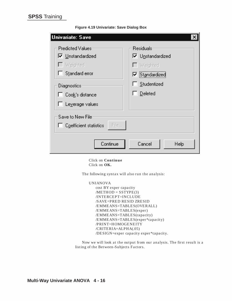
Multi-Way Univariate ANOVA 4 - 16
SPSS Training
Figure 4.19 Univariate: Save Dialog Box
Click on ContinueClick on OK.
The following syntax will also run the analysis:
UNIANOVAcost BY exper capacity/METHOD = SSTYPE(3)/INTERCEPT=INCLUDE/SAVE=PRED RESID ZRESID/EMMEANS=TABLES(OVERALL)/EMMEANS=TABLES(exper)/EMMEANS=TABLES(capacity)/EMMEANS=TABLES(exper*capacity)/PRINT=HOMOGENEITY/CRITERIA=ALPHA(.05)/DESIGN=exper capacity exper*capacity.
Now we will look at the output from our analysis. The first result is alisting of the Between-Subjects Factors.

Multi-Way Univariate ANOVA 4 - 17
SPSS Training
Figure 4.20 Between Subjects Factors
Next we see the result of the Levene’s test of equality of errorvariances (homogeneity of variance test).
Figure 4.21 Levene’s Test of Homogeneity of Variance
The significance level is .014 which means that if the error varianceswere equal in the population, we would get an “F” statistic this large only14 times in one thousand. Thus the homogeneity of variance assumptiondoes not hold. A technical analyst might move to the spread and levelplots to see if the dependent variable can transformed such thathomogeneity of variance holds. A nonparametric analysis could be done,although SPSS currently does not contain a two-factor nonparametricAnova procedure). We will proceed with the analysis, realizing that thetest results may not be completely accurate.

Multi-Way Univariate ANOVA 4 - 18
SPSS Training
The ANOVA table contains the information, much of it technical,necessary to evaluate whether there are significant differences in costacross capacity groups, across experience groups, and whether the twofactors interact.
Figure 4.22 The ANOVA Table
THE ANOVATABLE
The first column lists the different sources of variation. We areinterested in the capacity and experience main effects, as well as thecapacity by experience interaction. The source labeled “Error” containssummaries of the within-group variation (or Residual term) which will beused when calculating the “F” ratios (ratios of between-group to within-group variation). The remaining sources in the list are simply totalsinvolving the sources already described, and as such are generally not ofinterest. The Sum of Squares column contains a technical summary (sumof the squared deviations of group means around the overall mean, or ofindividual observations around their group mean) that is not interpreteddirectly, but is used in calculating the later column values. The “df”(degrees of freedom) column contains values that are functions of thenumber of levels of the factors (for capacity, experience, and capacity byexperience) or the number of observations (for residual). Although this isa gross oversimplification, you might think of degrees of freedom asmeasuring the number of independent values (whether means orobservations) that contribute to the sum of squares in the previouscolumn. As with sums of squares, degrees of freedom are technicalmeasures, not interpreted themselves, but used in later calculations.
Mean Square values are variance measures attributable to thevarious effects (capacity, experience, capacity by experience) and to thevariation of individuals within groups (error). The ratio of an effect meansquare to the mean square of the error provides the between-group towithin-group variance ratio, or “F” statistic. If there were no groupdifferences in the population, then the ratio of the between-group

Multi-Way Univariate ANOVA 4 - 19
SPSS Training
variation to the within-group variation should be about one. The column“Sig” contains the most interpretable numbers in the table: theprobabilities that one can obtain “F” ratios as large or larger (or groupmeans as far or farther apart) as what we find in our sample, if therewere no mean differences in the population.
The ANOVA table summarizes the statistical testing. Both experienceand capacity are marginally significant at the .046 and .050 respectively.The result for capacity is similar but not identical to its result in the onefactor ANOVA for several reasons. First, the within-groups error term isnow based on nine cells and not only three as before. Also, since thesample sizes are neither equal nor proportional, the effects of capacityand experience are not independent of each other and the test forcapacity adjusts for the experience factor. In the one factor analysis thesecond factor was ignored. The interaction is not significant indicatingthat the capacity differences do not change across different levels ofexperience.
Average cost shows significant differences across levels of plant capacityand levels of building experience. The two factors do not seem to interact.
In the Options dialog box we asked for the means to be displayed for eachmain effect and the interaction. The following figures provide thoserequested means.
Figure 4.23 Grand Mean and Means for Experience Levels
Conclusion
PREDICTEDMEANS
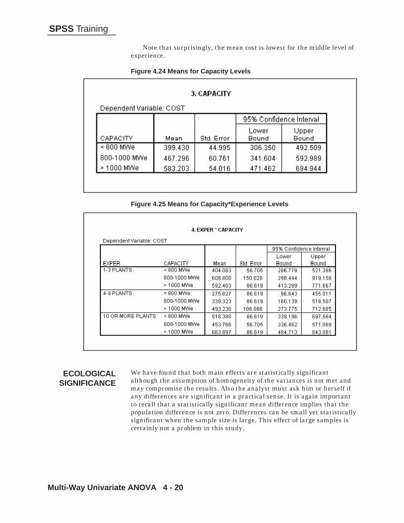
Multi-Way Univariate ANOVA 4 - 20
SPSS Training
Note that surprisingly, the mean cost is lowest for the middle level ofexperience.
Figure 4.24 Means for Capacity Levels
Figure 4.25 Means for Capacity*Experience Levels
We have found that both main effects are statistically significantalthough the assumption of homogeneity of the variances is not met andmay compromise the results. Also the analyst must ask him or herself ifany differences are significant in a practical sense. It is again importantto recall that a statistically significant mean difference implies that thepopulation difference is not zero. Differences can be small yet statisticallysignificant when the sample size is large. This effect of large samples iscertainly not a problem in this study.
ECOLOGICALSIGNIFICANCE

Multi-Way Univariate ANOVA 4 - 21
SPSS Training
To view the predicted values and residuals we turn to the case summaryprocedure, although we could simply examine them in the Data Editorwindow.
Click Analyze..Reports..Case SummariesMove cost, pre_1, res_1, and zre_1 to the Variables list boxClick on OK
The following syntax will also produce the case summary report.
SUMMARIZE/TABLES=cost pre_1 res_1 zre_1/FORMAT=VALIDLIST NOCASENUM TOTAL LIMIT=100/TITLE=’Case Summaries’ /FOOTNOTE ‘ ‘/MISSING=VARIABLE/CELLS=COUNT.
Figure 4.26 Case Summary Report
RESIDUALANALYSIS

Multi-Way Univariate ANOVA 4 - 22
SPSS Training
POST HOCTESTS OF
ANOVA RESULTS
Notice the predicted values are identical for all cases in the same cell,that is, group membership determines the predicted value. Thestandardized residuals are in standard deviation units; do you see anysurprisingly large residuals?
To run post hoc tests on our results we will need to re-open theUnivariatel dialog box.
Click the Dialog Recall Tool , then click Univariate
Click the Post Hoc pushbuttonMove exper and capacity into the Post Hoc Tests for boxSelect the LSD, Games-Howell, and Scheffe post hoc tests
(click their check boxes)
Figure 4.27 Post Hoc Test Dialog Box
Click ContinueClick OK.
As shown below, the Posthoc subcommand requests the post hoc tests.

Multi-Way Univariate ANOVA 4 - 23
SPSS Training
UNIANOVAcost BY exper capacity/METHOD = SSTYPE(3)/INTERCEPT=INCLUDE/SAVE=PRED RESID ZRESID/POSTHOC = capacity exper ( SCHEFFE LSD GH )/EMMEANS=TABLES(OVERALL)/EMMEANS=TABLES(exper)/EMMEANS=TABLES(capacity)/EMMEANS=TABLES(exper*capacity)/PRINT=HOMOGENEITY/CRITERIA=ALPHA(.05)/DESIGN=exper capacity exper*capacity.
We have selected the LSD, Games-Howell (because of the failure ofthe homogeneity of variance assumption), and Scheffe tests. We willexamine the post hoc tests only for capacity (since this chapter is lengthyas it is). In practice you would examine the results for both capacity andexperience if they were found to be significant. If time permits, review thepost hoc test results for experience. What do you find?
Figure 4.28 Post Hoc Tests For Capacity
We can see from the post hoc results with the LSD testing that boththe less than 800 MWe and 800-1000 MWe plants were different from theover 1000 MWe plants. This however is the most liberal test. The two

Multi-Way Univariate ANOVA 4 - 24
SPSS Training
other tests find only that the less than 800MWe plants are different fromthe over 1000MWe plants.
Figure 4.29 Homogenous Subsets for Capacity
As we would expect given the post hoc results, the homogeneoussubsets produced by the Scheffe test confirms that only the lowest andhighest capacity groups differ.
Up to now we have not discussed the implications of unequal samplesizes. The basic problem arises when the sample sizes are not equalacross groups (or not proportional if you are mainly interested in maineffects). When this occurs, or if cells are missing entirely, the effects inthe analysis become correlated, that is, they overlap. As the cell sizeimbalance increases, it becomes increasingly difficult to speak ofindependent effects. For example, if almost all high-capacity plants werebuilt by people with experience building 10 or more plants, how can wespeak of separate effects? The same problem, high correlation amongpredictor variables, is frequently discussed in the literature onregression. There are different methods for adjusting for such overlap ofeffects and we discuss some of these approaches and their implicationsbelow.
UNEQUALSAMPLES ANDUNBALANCED
DESIGNS

Multi-Way Univariate ANOVA 4 - 25
SPSS Training
From the Model dialog box you can choose a type of sums of squares. TypeIII is the most commonly used and is the default. Each type adjusts forunequal sample sizes in a different way. When all subgroup sample sizesare the same, the various sums of squares’ calculations yield the identicalresult.
• Type I. This method is also known as hierarchicaldecomposition of the sum-of-squares. Each term is adjustedfor only the terms that precedes it in the model. Type I sumsof squares are commonly used in situations in which theresearcher has a prior ordering of effects in mind. Forexample, if previous research has always found a factor to besignificant there might be interest in determining if a secondfactors makes a substantial contribution. In this situation,the known factor might be entered first in the model (notadjusting for the second factor), while the new factor followsin the model (so it is tested after adjusting for the first factor).
• Type II. This method calculates the sums of squares of aneffect in the model adjusted for all other “appropriate” effects.An appropriate effect is one that corresponds to all effectsthat do not contain the effect being examined. Thus a maineffect would adjust for all other main effects but interactions.A two-way interaction would adjust for all main effects andother two-way interactions, but ignore three-way and highereffects.
• Type III. This is the default. This method calculates the sumsof squares of an effect in the design as the sums of squaresadjusted for any other effects that do not contain it andorthogonal to any effects (if any) that contain it. Essentially,each effect is adjusted for all other effects (main effects, sameorder interactions, higher order interactions) in the model.Thus you can speak of an effect independent of all othereffects. The Type III sums of squares have a major advantagein that they are invariant with respect to the cell frequenciesas long as the general form of estimability remains constant.In practice, this means that Type III sums of squares is oftenconsidered useful for an unbalanced model with no missingcells. In a factorial design with no missing cells, this methodis equivalent to the Yates’ weighted-squares-of-meanstechnique. Type III is recommended on the strength of thefact that a statistical test for an effect adjusts for all othereffects in the model. However, if there are missing data cells,Type IV is preferred.
• Type IV. This method is designed for situations in whichthere are missing cells. The technical description of Type IVsums of squares follows. For any effect F in the design, if F isnot contained in any other effect, the Type IV = Type III =Type II. When F is contained in other effects, Type IVdistributes the contrasts being made among the parametersin F to all higher-level effects equitably. To give a practicalexample, suppose we were testing salary differences due to
SUMS OFSQUARES

Multi-Way Univariate ANOVA 4 - 26
SPSS Training
two factors: experience (in three categories) programming in acomputer language, and the computer language itself (twocategories). If there were no programmers with the highestexperience level for one of the languages (say Java), then thatexperience category would not be used when evaluating thecomputer language main effect. Thus the computer languageeffect would be evaluated from only those experiencecategories containing programmers of both languages. This isthe source of the equity mentioned above. The Type IV sum-of-squares method is commonly used for an unbalanced modelwith empty cells.
All of these types of sums of squares are equivalent when there is onlyone effect to be tested. Thus the one-way ANOVA procedure does not offerany options in terms of sums of squares. Also as mentioned above, theygive identical results for a balanced design. In practice today, the Type IIIsums of squares method is usually used if there are no missing cells. Ifcells are missing the Type IV method is generally chosen. When aresearcher wants to test effects after adjusting for certain effects, butignoring others, then the Type I or Type II methods are employed.
Any time that the between-subject portion of an analysis cannot be laidout in a full factorial setup with all cells filled (having at least oneobservation), matters can become quite complicated, and knowledge ofthe theory of estimable functions is required in order to determine justwhat hypotheses can be tested. The best advice that can be given here isto consult a statistician knowledgeable in experimental design in order todetermine the appropriate, testable hypotheses in a particular case
Virtually any testable hypothesis can be tested using the GeneralLinear Model - Univariate procedure with its flexible DESIGNsubcommand, but determining the appropriate hypothesis to test whenthere are missing cells can be extremely difficult. It should be noted inparticular that simply applying standard sets of commands to such datacan produce results that are uninterpretable, since the particularhypotheses tested have not been identified.
For further information on the analysis of such data, see Searle(1987) or Milliken and Johnson (1984). Of the two, Searle’s book is morecomplete but rather technical. Milliken and Johnson’s book is moreaccessible.
In this chapter we generalized ANOVA to the case with two or morefactors and discussed post hoc comparisons in the context. In addition,the effects of unequal sample size and missing cells were presented. Weturn next to another generalization: ANOVA with multiple dependentmeasures – multivariate analysis of variance.
EQUIVALENCEAND
RECOMMENDATIONS
EMPTY CELLSAND NESTED
DESIGNS
SUMMARY

Multivariate Analysis of Variance 5 - 1
SPSS Training
Multivariate Analysis OfVariance
The purpose of this chapter is to understand the properties ofmultivariate analysis of variance, drawing on our previous discussions ofunivariate ANOVA.
We run the EXPLORE procedure to check on some of the assumptions ofthe multivariate ANOVA. We will use the General Linear Model-Multivariate procedure to run a two-factor multivariate analysis ofvariance with two dependent variables.
We use the same data set as in the prior chapters, i.e., the nuclear powerplant data set (plant.por).
A two-factor two dependent variable multivariate analysis of variance –experience and plant capacity are the two fixed factors (3 levels each),cost and time (time before plant was licensed) are the dependentmeasures.
Multivariate analysis of variance (MANOVA) is a generalizationof analysis of variance that permits testing for mean differenceson several dependent measures simultaneously. In this chapter
we will explore the rationale and assumptions of multivariate analysis ofvariance, review the key summaries to examine in the results, and thenstep through an analysis looking at group differences on two measures inour data set.
Multivariate analysis of variance is used when there is an interest intesting for mean differences between groups on several dependentvariables simultaneously. ANOVA will test whether the mean of a singlevariable (scalar) differs across groups. MANOVA covers the broader caseof testing for mean differences in several variables (vector) across groups.
Chapter 5
Objective
Method
Data
Design
INTRODUCTION

Multivariate Analysis of Variance 5 - 2
SPSS Training
Multivariate analysis of variance (MANOVA) tests for population groupdifferences on several dependent measures simultaneously. Instead ofexamining differences for a single outcome variable (as analysis ofvariance does), MANOVA tests for differences on a set or vector of means.The outcome measures (dependent variables) are typically related; forexample, a set of ratings of employee performance, multiple physiologicalmeasures of stress, several scales assessing an attitude, a collection offitness measures, multiple scales measuring a product's appearance,several measures of the fiscal health of a company.
MANOVA is typically performed for two reasons: statistical powerand control of false positive results (also known as Type I error).
First, there can be greater statistical power, that is, the ability todetect true differences, in a multivariate analysis. The argument is that ifyou have several imperfect measures of an outcome, for example, severalphysiological measures of stress, the joint analysis will be more likely toshow a true difference in stress than any individual analysis. Amultivariate analysis compares mean differences across several variablesand takes formal account of their intercorrelations. In this way a smalldifference appearing in several related outcome variables may result in asignificant multivariate test, although no single outcome measure showsa significant difference. This is not to say there is a power advantage inthrowing 20 or so unrelated variables into a multivariate analysis ofvariance, since a true difference in a single outcome measure can bediluted in a joint test involving many variables that display no effect.However, if you are interested in studying group differences in outcomesfor which various measures exist (this occurs in marketing, social science,medical, ecological, and engineering studies), then MANOVA probablycarries greater statistical power.
The second argument for running MANOVA in place of separateunivariate (single outcome variable) analyses concerns controlling thefalse positive rate when multiple tests are done. If a separate ANOVA isrun for every outcome variable, each tested at the 0.05 level, then theoverall (or experiment-wise) false positive rate (chance of obtaining one ormore false positive test results) is well above 5 in 100 (0.05 or 5%)because of the multiple tests. A MANOVA applied to a study with sevenoutcome measures would result in a single test performed at the 0.05level. Although there are certainly alternative methods for controlling thefalse positive rate when multiple tests are performed (for example,Bonferroni adjustments), using a multivariate test accomplishes this aswell. Some researchers follow the procedure of first performing amultivariate test and only if the results are significant would theyexamine the individual univariate test results. This provides some controlover the false positive rate. It is not a perfect solution (it is similar to theargument for the LSD multiple comparison procedure) and has receivedsome criticism (see Huberty (1989)).
WHY PERFORMMANOVA?

Multivariate Analysis of Variance 5 - 3
SPSS Training
First, the good news, MANOVA is similar to ANOVA in that variationbetween group means is compared to variation of individuals withingroups. Since this variation is measured on several variables, MANOVAcomputes a matrix containing the variation and covariation (there areseveral variables!) of the vector of group means and a second matrixcontaining within-group variances and covariances. When testing inMANOVA, a ratio is taken not of the two variances (two numbers), but oftwo matrices. Instead of the usual “F” test, the multivariate form – calleda generalized “F” is used. The summary table will contain someunfamiliar statistics, but in the end will report the probability ofobtaining means as far (or farther) apart as you did by chance alone, justas ANOVA did.
In short, while the required matrix notation used while deriving ordescribing MANOVA is a bit intimidating, the same principles that haveguided us so far in analysis using ANOVA – variation between groupmeans compared to variation within groups – still holds true inMANOVA. The statistics change because we are now talking aboutvectors of means (a set of means) being tested jointly.
The assumptions made when performing multivariate analysis ofvariance are largely extensions of those made under ordinary analysis ofvariance. In addition to the usual assumptions for a linear model(additivity, independence between the error and model effects,independence of the errors), MANOVA testing assumes that the residualerrors follow a multivariate normal distribution in the population; this isa generalization of the normality assumption made in ANOVA. In SPSSyou can examine and test individual variables for normality within eachgroup. This is not equivalent to testing for multivariate normality, but isstill quite useful in evaluating the assumption. In addition, homogeneityof variance, familiar from ANOVA, has a multivariate extensionconcerning homogeneity of the within-group variance-covariancematrices. A multivariate test of homogeneity of variance (Box’s M test) isavailable to check this assumption.
For large samples, we expect departures from normality to makelittle difference. This is due to the central limit theorem argumentcombined with the fact that in MANOVA we are generally testing simplefunctions of group means. If the samples are small and multivariatenormality is violated, the results of the analysis may be effected. Datatransformations (for example, logs) on the dependent measure(s) mayalleviate the problem, but have potential problems of their own(interpretation, incomplete equivalence between tests in the transformedand untransformed scales). Unfortunately, a general class of multivariatenonparametric tests is not currently available; developments in this areawould help provide a solution.
Concerning homogeneity of variance, in practice if the sample size issimilar across groups then moderate departures from homogeneity of thewithin-group variance-covariance matrices do not effect the analysis. Ifhomogeneity does not hold and the sample size varies substantiallyacross groups, then test results can be effected. In the simplest scenarios,
HOW MANOVADIFFERS FROM
ANOVA
ASSUMPTIONSOF MANOVA

Multivariate Analysis of Variance 5 - 4
SPSS Training
CHECKING THEASSUMPTIONS
the direction of the effect depends on which sized group has the largervariances, but specific situations can be far more complex, in which caselittle is known.
After investigating whether the assumptions are met, primary interestwould be in the multivariate statistical tests. If significant effects arefound you might then examine univariate results. Additionally, you canperform post hoc comparisons to discover just where the differencesreside.
When testing for mean differences between groups on a single dependentvariable the test comes down to a ratio of between-group to within-groupvariation – a single number. In multivariate analysis, we are left withtwo matrices containing the between and within-group variation andcovariation. There are different test statistics that can apply. Most ofthem involve computing the latent roots of some function of the ratio ofthe two matrices. In depth discussion of these test measures is beyondthe scope of this course, but some comments about their characteristicswill be made when we review the results.
We will perform MANOVA with experience and plant capacity as thefactors with time to completion (licensing) and cost as dependentvariables. This pairing of dependent variables makes sense if you believethe adage that time is money. We expect that plants that require moretime to build should also be more costly. By using both variables we hopeto tap a more general measure of cost.
The analysis we conducted in Chapter 4 investigated the properties of thecost measure. There was some evidence for heterogeneity of variance,although the tests were not in complete agreement. The normal plot ofthe errors suggested some skewness. We will now proceed to look at someof the information from the EXPLORE procedure for the time variable.One caution, these plots look at each variable separately while theassumptions for MANOVA involve the joint distribution of the variables.As a practical matter, if the assumptions are met for the variables singly,things look good for the multivariate assumptions, but if the assumptionsfail for the single variables, they should fail for the multivariate situationas well.
Click File..Open..DataMove to the c:\Train\Anova directory (if necessary)Select SPSS Portable (*.por) from the Files of Type drop-down
listDouble-click on plant.por
WHAT TO LOOKFOR IN MANOVA
SIGNIFICANCETESTING
ProposedAnalysis

Multivariate Analysis of Variance 5 - 5
SPSS Training
Click on Analyze..Descriptive Statistics..ExploreMove time into the Dependent List boxMove capacity and exper into the Factor List box
Figure 5.1 Explore Dialog Box
Click the Plots pushbuttonClick the Normality plots with tests checkboxClick the Untransformed option button in the Spread vs.
Level with Levene Test area
Figure 5.2 Plots Dialog Box
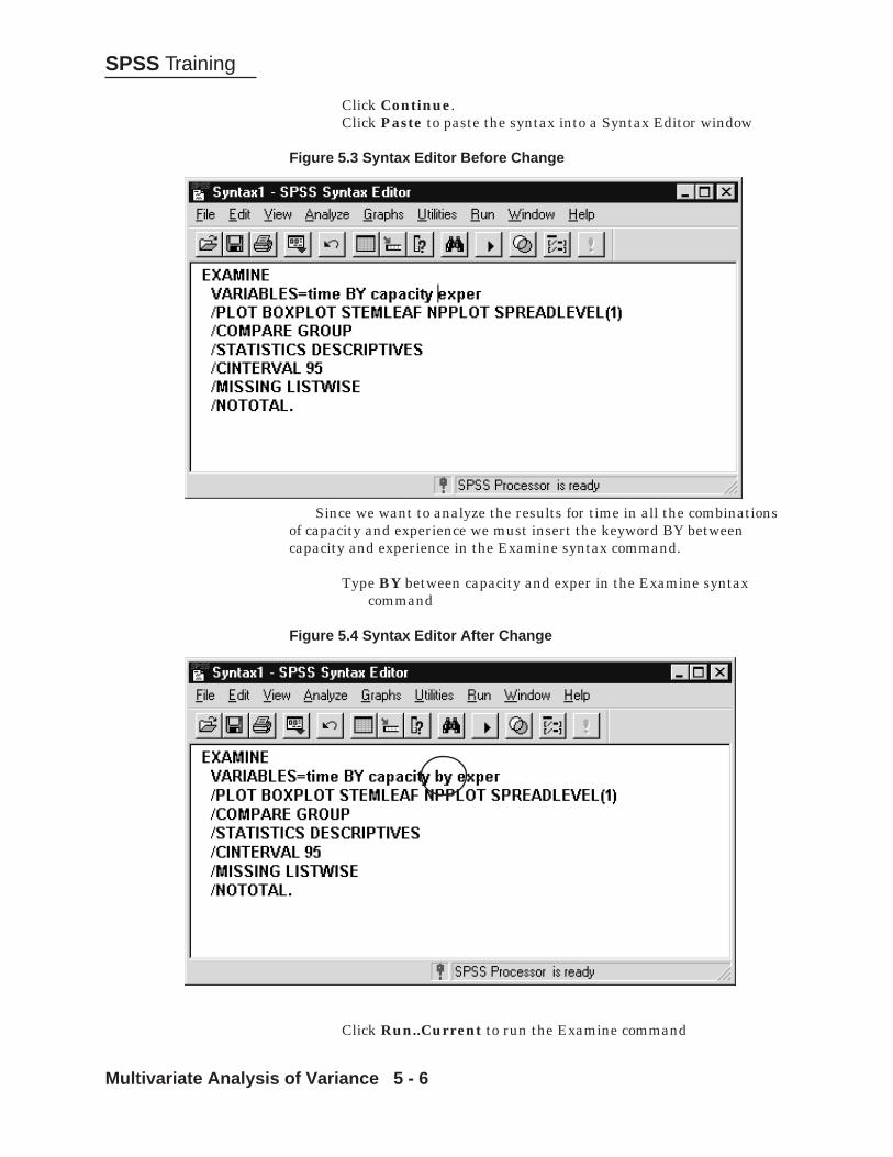
Multivariate Analysis of Variance 5 - 6
SPSS Training
Click Continue.Click Paste to paste the syntax into a Syntax Editor window
Figure 5.3 Syntax Editor Before Change
Since we want to analyze the results for time in all the combinationsof capacity and experience we must insert the keyword BY betweencapacity and experience in the Examine syntax command.
Type BY between capacity and exper in the Examine syntaxcommand
Figure 5.4 Syntax Editor After Change
Click Run..Current to run the Examine command

Multivariate Analysis of Variance 5 - 7
SPSS Training
We show the normal plots for the time variable below, noting that inmost groups there are too few observations to perform a normality test,but in the few cases that tests of normality could be made, the data wasconsistent with it.
Figure 5.4A Tests of Normality
Figure 5.5 Q-Q Plot of <800 MWe and 1-3 Plants

Multivariate Analysis of Variance 5 - 8
SPSS Training
Figure 5.6 Q-Q Plot of <800 MWe and 4-9 Plants
Figure 5.7 Q-Q Plot of <800 MWe and 10 or more Plants
Figure 5.8 Q-Q Plot of 800-1000 MWe and 4-9 Plants

Multivariate Analysis of Variance 5 - 9
SPSS Training
Figure 5.9 Q-Q Plot of 800-1000 MWe and 10 or more Plants
Figure 5.10 Q-Q Plot of >1000 MWe and 1-3 Plants
Figure 5.11 Q-Q Plot of >1000 MWe and 4-9 Plants

Multivariate Analysis of Variance 5 - 10
SPSS Training
Figure 5.12 Q-Q Plot of >1000 MWe and 10 or more Plants
Next we see the Box and Whisker plot for time.
Figure 5.13 Box and Whisker Plot for Time
There seems to be a fair amount of variation among the groups intime taken to license the plant. It looks as if there is more spread forgroups with less experience than there is for those with more experience.

Multivariate Analysis of Variance 5 - 11
SPSS Training
The Advanced Models module within SPSS adds several General LinearModel (GLM) procedures (multivariate (GLM) and repeated measures(GLM)) to Univariate within the SPSS Base system. These procedureshave several desirable features from the perspective of MANOVA: 1) Posthoc tests on marginal means (univariate only), 2) Type I through Type IVsums of squares available (greater flexibility in handling unbalanceddesigns/ missing cells), 3) Multiple Random Effect models can be easilyspecified, and 4) Residuals, predicted values and influence measures canbe saved as new variables to the data set. However, the MANOVAprocedure (which was the original procedure within SPSS performingMANOVA, and it is still available through syntax) contains several usefuladvanced functions. Within the MANOVA procedure are: 1) Roy-Bargmann step-down tests (testing for mean differences on a singledependent measure while controlling for the other dependent measures),and 2) Dimension reduction analysis and discriminant coefficients. Theselatter functions provide information as to how the dependent variablesinterrelate within the context of group differences (for a single main-effect analysis, this is equivalent to a discriminant analysis).
In short, while we expect the SPSS General Linear Model procedurewill be your first choice for multivariate analysis of variance, theMANOVA procedure can contribute additional information. (Please note,MANOVA can only be run from syntax.)
Click Analyze..General Linear Model..MultivariateMove cost and time into the Dependent Variables list boxMove capacity and exper into the Fixed Factors list box
Figure 5.14 Multivariate Dialog Box
THEMULTIVARIATE
ANALYSIS

Multivariate Analysis of Variance 5 - 12
SPSS Training
We must specify the dependent measure(s) and at least one factor.The dialog box for Multivariate contains list boxes for the dependentvariables, factors and covariates. The term “Fixed Factor(s)” in theMultivariate dialog box reminds us that the factors are assumed to befixed, that is, levels of the factor(s) used in the analysis were chosen bythe researcher (not randomly sampled) and cover the range to whichpopulation conclusions will be drawn. The Multivariate dialog box alsopermits a weight variable to be incorporated in the analysis (performsweighted least squares). Although rarely used in multivariate analyses(when used it is typically for univariate analysis), it adjusts the analysisbased on different levels of precision (or heterogeneity of variance) fordifferent individuals or groups.
The Multivariate dialog box contains several pushbuttons. The Plotspushbutton produces for each dependent measure a profile plotdisplaying group means. The Post Hoc pushbutton performs post hoctests on the marginal means (for multivariate analyses, each dependentvariable is analyzed separately). The Contrasts pushbutton performs anyplanned contrasts that the researcher wants to conduct; while theOptions pushbutton controls many options for the analysis. Finally theSave pushbutton permits you to save predicted values, residuals, andinfluence measures for later examination.
We could run the analysis at this point, but will examine the dialogboxes within Multivariate and request some additional options.
Click Model pushbutton
Figure 5.15 Multivariate: Model Dialog Box
For most analyses the Model dialog box is not used. This is becauseby default a full factorial model (all main effects, interactions, covariates)

Multivariate Analysis of Variance 5 - 13
SPSS Training
is fit and the various effects tested using Type III sums of squares (eacheffect is tested after statistically adjusting for all other effects in themodel). If there are any missing cells in your analysis, you might switchto Type IV sums of squares, which better adjusts for missing cells. If youare running specialized factorial designs that are incomplete (by planevery possible combination of factor levels is not present), or in whichthere are no replicates (interaction effects are used as error terms), youwould click the Custom option button in the Specify Model area andindicate which main effects and interactions to be included in the model.A custom model is sometimes used if there is no interest in testing highorder interaction effects. Since we are interested in both main effects andthe one interaction there is no need to modify this dialog box.
Click Cancel to exit the Model dialog boxClick Contrasts pushbutton
Figure 5.16 Multivariate: Contrasts Dialog Box
The Contrasts dialog box is identical for multivariate and univariateanalyses. You would use it to specify main effect group comparisons ofinterest, for which parameter estimates can be displayed and testsperformed. In statistical literature, these contrasts are sometimes calledplanned comparisons. For example, in an experiment in which there arethree treatment groups and a control group there is a very specificinterest in testing each experimental group against the control. One ofthe contrast choices (Simple) allows this. Several types of contrasts areavailable within the dialog box and using syntax you can specify yourown (Special). To request a set of contrasts, select the factor from theFactor(s) list box, select the desired contrast from the Contrast drop-downlist, and click the Change pushbutton. Since we have no specific plannedcontrasts that we wished to apply to the main effects, we will exit theContrast dialog box.
Click Cancel to exit the Contrasts dialog boxClick Post Hoc pushbutton

Multivariate Analysis of Variance 5 - 14
SPSS Training
Figure 5.17 Multivariate: Post Hoc Dialog Box
The Post Hoc dialog box is used to request post hoc comparisons onthe observed subgroup means. Post hocs test for significant differencesbetween every possible pairing of levels of a factor. Since many tests maybe involved, most post hocs adjust the significance criterion based on thenumber of tests in order to control the false positive error rate (Type Ierror). Usually post hocs are performed after a significant main effect isfound (in the initial analysis), and we will visit this dialog box later inthis chapter.
Click Cancel pushbutton to exit the Post Hoc dialog boxClick Save pushbutton
Click the Unstandardized Predicted Values,Unstandardized Residual, and Standardized Residualcheck boxes

Multivariate Analysis of Variance 5 - 15
SPSS Training
Figure 5.18 Multivariate: Save Dialog Box
The Save dialog box allows you to save predicted values, and varioustypes of residuals and influence measures as new variables in the datafile. Examining them might identify outliers and influential data points(data points whose exclusion substantially effects the analysis). Suchanalyses are standard for serious practitioners of regression and can beapplied in this context. In addition, the coefficient statistics (coefficientestimates, standard errors, etc.) can be saved to an SPSS data file (inmatrix format) and manipulated later (for example, apply the coefficientsto generate predictions for future cases). Although we stronglyrecommend an examination of the residuals, with the limited amount oftime available in this class, we will skip this step.
Click Continue to process the residual requestsClick Options pushbuttonSelect capacity, exper, and the capacity*exper interaction,
and move them into the Display Means for list boxClick the Homogeneity tests check box in the Display area.
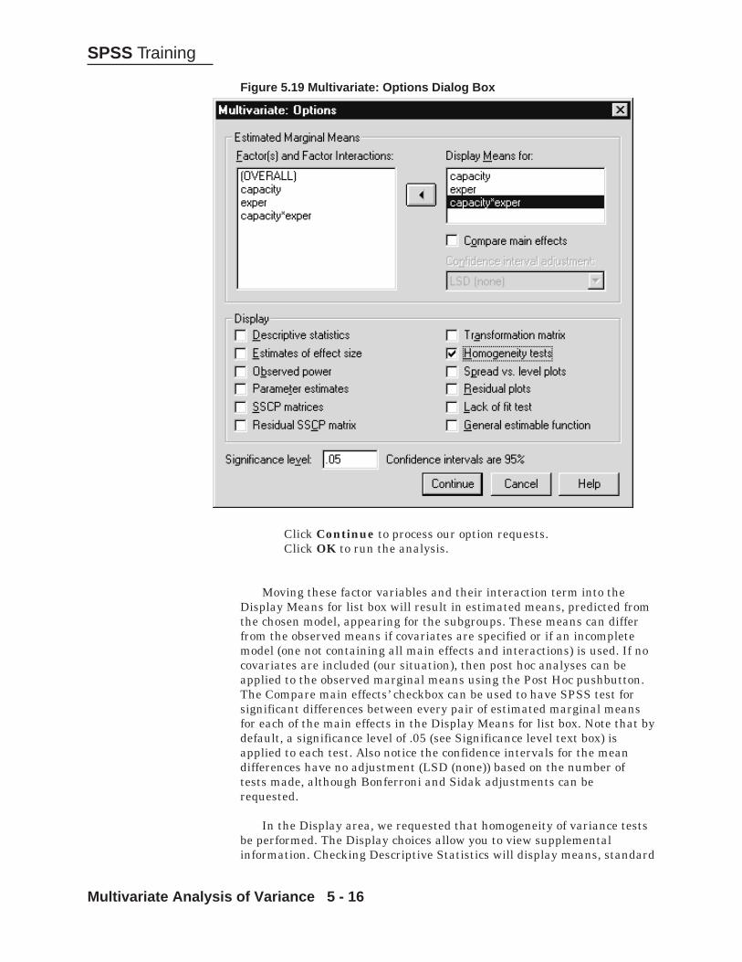
Multivariate Analysis of Variance 5 - 16
SPSS Training
Figure 5.19 Multivariate: Options Dialog Box
Click Continue to process our option requests.Click OK to run the analysis.
Moving these factor variables and their interaction term into theDisplay Means for list box will result in estimated means, predicted fromthe chosen model, appearing for the subgroups. These means can differfrom the observed means if covariates are specified or if an incompletemodel (one not containing all main effects and interactions) is used. If nocovariates are included (our situation), then post hoc analyses can beapplied to the observed marginal means using the Post Hoc pushbutton.The Compare main effects’ checkbox can be used to have SPSS test forsignificant differences between every pair of estimated marginal meansfor each of the main effects in the Display Means for list box. Note that bydefault, a significance level of .05 (see Significance level text box) isapplied to each test. Also notice the confidence intervals for the meandifferences have no adjustment (LSD (none)) based on the number oftests made, although Bonferroni and Sidak adjustments can berequested.
In the Display area, we requested that homogeneity of variance testsbe performed. The Display choices allow you to view supplementalinformation. Checking Descriptive Statistics will display means, standard

Multivariate Analysis of Variance 5 - 17
SPSS Training
deviations, and counts for each cell (subgroup) in the analysis. If effectsize is checked, then partial eta-square values will be presented for eacheffect (main effects, interactions). Eta-square is equivalent to the r-square in regression; the partial eta-square measures the proportion ofvariation in the dependent measure that can be attributed to each effectin the model after adjusting for the other effects. Parameter estimatesare the estimates for the coefficients in the model. Typically, they wouldbe requested if you wanted to construct a prediction equation. Thevarious sums of square matrices are computational summaries and notinterpreted directly.
The Significance level text box allows you to specify the significancelevel used to test for differences in the estimated marginal means (default.05), and the confidence intervals around parameter estimates (default.95).
We are now ready to proceed. The SPSS command below will run theanalysis.
GLMcost time BY capacity exper/METHOD = SSTYPE(3)/INTERCEPT = INCLUDE/SAVE = PRED RESID ZRESID/EMMEANS = TABLES(capacity)/EMMEANS = TABLES(exper)EMMEANS = TABLES(capacity*exper)/PRINT = HOMOGENEITY/CRITERIA = ALPHA(.05)/DESIGN = capacity exper capacity*exper.
In the GLM command the dependent variables (cost, time) precedethe BY keyword while the factor variables (capacity, exper) follow it. TypeIII (each effect is evaluated after adjusting for all other effects) sums ofsquares is requested (the default). The Emmeans subcommand will printa table of estimated marginal means for the factor variables.Homogeneity tests are obtained from the print subcommand and thealpha value (used for confidence intervals and significance tests of theestimated marginal means) is set to .05 (default). The Designsubcommand is used to specify the model to be applied to the data; ifnothing were specified, a full factorial model would be fit.
The first piece of Multivariate output describes the factors involved in theanalysis. They are labeled between-subject factors; this is appropriatebecause the three capacity groups and the three experience groups werecomposed of different plants. We will see within-subject analysis ofvariance (repeated measures) in a later chapter.
EXAMINING THERESULTS

Multivariate Analysis of Variance 5 - 18
SPSS Training
Figure 5.20 Between-Subject Factor Summary
The next two pivot tables provide information about the homogeneityof variance assumption. Box’s M tests for equality of covariance matrices(since there is more than a single dependent measure) across thedifferent subgroups. Levene’s homogeneity test is a univariate test and isapplied separately to each dependent variable.
Figure 5.21 Box’s Test of Equality of Covariance Matrices

Multivariate Analysis of Variance 5 - 19
SPSS Training
Figure 5.22 Levene’s Test of Equality of Error Variances
As mentioned above, Box’s M statistic can be used to test for equalityof variance-covariance matrices in the population. This generalizes thehomogeneity of variance test to a multivariate situation, testing forequality of group variances (as univariate homogeneity tests would) andcovariances (which univariate tests cannot) for all dependent measures inone test. Box’s test is not significant (.541) indicating no group differencesin the covariance matrices made up of the dependent measures. As aunivariate statistic, Levene’s test is applied to each dependent measure.The time measure is consistent with homogeneity assumption (sig. =.427), while cost measure does show group differences in variance (sig. =.014). Given that the Box’s test is not significant, we will proceed to viewthe multivariate test results.
As with ANOVA, MANOVA is robust under failure of homogeneity if thesample sizes in the cells are large and roughly equal. If the sample sizesare unequal, and larger variances are associated with larger cells, theMANOVA tests are conservative so you can be confident of significantfindings. If smaller cells have larger variances, the MANOVA tests areliberal so the Type I error is greater than it should be (see Hakstian,Roed, and Lind (1979)). If variance is related to the mean level of thegroup, a variance stabilizing transform is a possibility.
There are four multivariate test statistics commonly applied: Pillai’scriterion, Hotelling’s Trace criterion, Wilk’s Lambda, and Roy’s largestroot. The first three give identical results in a two-group analysis, andthen can differ. They all test the null hypothesis of no group meandifferences in the population. Results of Monte Carlo simulationsfocussing on robustness and statistical power, suggest that under generalcircumstances Pillai’s test is preferred. However, there are specifysituations, for example when the dependent measures are highly related(forming a strong core), that one of the others is the most powerful test.As a general rule, if different multivariate tests give you markedlydifferent results, it suggests something about the dimensionality and typeof group differences. For an accessible discussion of this see Olsen (1976).
WHAT IFHOMOGENEITY
FAILED?
MULTIVARIATETESTS

Multivariate Analysis of Variance 5 - 20
SPSS Training
The distribution of the first three multivariate statistics follows thegeneralized “F” distribution. While more complicated than the simple “F”,and having 3 sets of degrees of freedom it yields a probability value justas the regular “F” does. This generalized “F” test assumes a multivariatenormal distribution of the errors.
Figure 5.23 Multivariate Analysis of Variance Table
The upper part of the table tests whether the overall mean (Intercept)differs from zero in the population. It is not interesting since all it showsis that overall, cost and time were not both zero.
The Value column displays the sample value of each of the fourmultivariate test statistics. They are converted to “F” statistics (“F”column) and the associated hypothesis (Hypothesis df) and error (error df)degrees of freedom follow. These four columns are technical summaries;we are primarily interested in the significance values that appear underthe “Sig.” Heading. Here we see that for the capacity factor, three of thefour tests show that there are differences in the dependent measures(significance values of .055, .043, .034, .007). Notice the tests are not inagreement if you test at the .05 level. While Pillai’s is often therecommended test, it would be safe to conclude at least there is amarginal effect, perhaps something worth looking at with a largersample. We also see that for the experience factor, all four tests show thatthere are group differences in the means (significance values of .035, .028,.023, and .005). The test of an interaction between capacity andexperience was not significant (significance values of .307, .294, .286, and.073). Given these findings, we are next interested in looking at whetherboth cost and time show differences (univariate tests), and knowingwhich groups differ from which others (post hocs).

Multivariate Analysis of Variance 5 - 21
SPSS Training
Two additional columns can appear in the multivariate (orunivariate) analysis of variance table, but do not do so by default. Thenoncentrality parameter is a technical summary that describes themagnitude of the mean group differences in the form of a parameter forthe “F” distribution. It can be used to calculate the appropriate samplesize (statistical power analysis) if this study were to be repeated whileexpecting to find the same group differences. The Observed Powerindicates how likely you are to obtain a significant group difference(testing at the .05 level) if the population group means matched themeans in the sample. This can be useful in conducting postmortems ofyour analysis, that is, exploring why you failed to find significantdifferences.
We now examine the test results for each dependent measure.
Figure 5.24 Univariate Test Results
Although both dependent measures appear in this table the resultsare calculated independently, and are identical to what you would obtainif separate analyses were run on each dependent measure (univariateANOVA). Thus we find whether both of the dependent measures showedsignificant group differences. The sums of squares, df (degrees offreedom), mean square, and “F” columns are what we would expect in anordinary table. We described and disregarded the Intercept informationin the multivariate summary. Moving to the capacity section, we find costis right on the border of significance (.05) while time is not significant(.101). From the experience summary we find that again cost issignificant (.046) while time is not (.066). In the interaction area we findthat neither cost nor time are significant (.701 and .089). The Error

Multivariate Analysis of Variance 5 - 22
SPSS Training
section summarizes the within-group variation. The Corrected Modelsummary pools together all model effects (excluding the intercept), and isequal to the Corrected Total minus the Error Total. Some analysts turnto this overall test first to see if any effects are significant, and thenproceed to examine individual effects. However, most researchers movedirectly to the tests of specific main effects and interactions. The Totalsummary pools together everything in the analysis (including the error. Itshould be noted that if the sample sizes are not equal when multiplefactors are included in the analysis, then under Type III sums of squares(the default), the sums of squares for the totals will not generally beequal to the sums of their component sums of squares.
Finally, r-square values (based on the corrected model) for eachvariable appear as footnotes. Notice that the adjusted r-square for time(.320) is higher than that of cost (.222). This is consistent with timehaving a higher “F” statistic in the corrected model section.
Figure 5.25 Estimated Marginal Means for Capacity
Figure 5.26 Estimated Marginal Means for Experience

Multivariate Analysis of Variance 5 - 23
SPSS Training
Figure 5.27 Estimated Marginal Means for Capacity by ExperienceSubgroups
Estimated marginal means are means estimated for each level of afactor averaging across all levels of other factors (marginals), based onthe specified model (estimated). By default, SPSS fits a complete model(all main-effects and interactions), and in such cases these estimatedmeans are identical to the (unweighted) observed means. However, if apartial model were fit (for example, if all main effects were included buthigher order interactions were not) then the estimated means will differfrom the (unweighted) observed means. We see in the tables above thatthe average time and cost increase with the plant capacity. Interestingly,regarding experience, time and cost have their lowest means in themiddle experience group.
We first view the casewise listing of residuals for time. We will skip thelisting for cost since it is identical to that seen in Chapter 4, when we ranthe same model on cost alone.
Click Analyze..Reports..Case SummaryMove time, pre_2, res_2, and zre_2 into the Variables list box.
CHECKING THERESIDUALS

Multivariate Analysis of Variance 5 - 24
SPSS Training
Figure 5.28 Case Summary Dialog Box
Click on OK
The following syntax will also produce the case summary table.
SUMMARIZE/TABLE=time pre_2 res_2 zre_2/FORMAT=VALIDLIST NOCASENUM TOTAL LIMIT=100/TITLE=’Case Summaries’ /FOOTNOTE ‘ ‘/MISSING=VARIABLE/CELLS=COUNT.

Multivariate Analysis of Variance 5 - 25
SPSS Training
Figure 5.29 Casewise Listing of Residuals
There seem to be no especially large standardized residuals. Onceagain the predicted values are identical for all members of the samegroup.
From the multivariate analysis of variance we conclude that thedependent variables show significant mean differences across experiencegroups, although not in a strictly increasing fashion. There is a modesteffect across capacity groups and no sign of an interaction. Of the twomeasures, cost seems more sensitive to the group differences. What mightqualify the result? You could argue that the groupings of experience andcapacity levels are arbitrary and different groupings could yield differentresults. Also, with only 32 observations over a nine-cell design with twodependent measures, we expect very little power to detect differences.
CONCLUSION

Multivariate Analysis of Variance 5 - 26
SPSS Training
At this point of the analysis it is natural to ask just which groups differfrom which others. The GLM procedure in SPSS will perform separatepost hoc tests on each dependent variable in order to determine this. Posthoc tests are usually performed to investigate which pairs of levels withina factor differ after an overall (main effect) difference has beenestablished. SPSS offers many post hoc tests and characteristics of themwere reviewed in Chapter 3. Recall the basic idea behind post hoc testingis that some adjustment of the Type I (false positive or alpha) error ratemust be made due to the number of pairwise comparisons made. In ourexample, only three tests need to be performed within each factor (group1 vs. 2, 1 vs. 3, and 2 vs. 3). However, if there were ten levels ofexperience (or capacity or both), then there would be [10*9]/2 or 45pairwise tests, and the probability of one or more false positive resultswould be quite substantial. We asked for the following types of post hoctests to be performed: LSD (the most liberal), Scheffe (the mostconservative), and the Games-Howell (does not assume equal variances—recall the Levene test indicated there might be a homogeneity of varianceproblem with cost). Although both experience and capacity were foundsignificant, below we request post hocs only for experience. In practiceyou would view post hoc results for each significant main effect.
Click the Dialog Recall tool , then select Multivariate
Click Post Hoc pushbuttonMove exper into the Post Hoc Tests for list boxClick LSD, Scheffe, and Games-Howell checkboxes
Figure 5.30 Post Hoc Dialog Box
POST HOCTESTS

Multivariate Analysis of Variance 5 - 27
SPSS Training
Click Continue to process the post hoc requestsClick OK to run
The SPSS syntax below will produce the post hoc analysis.
GLMcost time BY capacity exper/METHOD = SSTYPE(3)/INTERCEPT = INCLUDE/SAVE = PRED RESID ZRESID/POSTHOC = exper ( SCHEFFE LSD GH/EMMEANS = TABLES(capacity)/EMMEANS = TABLES(exper)EMMEANS = TABLES(capacity*exper)/PRINT = HOMOGENEITY/CRITERIA = ALPHA(.05)/DESIGN = capacity exper capacity*exper.
The Posthoc subcommand instructs GLM to apply Scheffe, LSD andGames-Howell (GH) multiple comparison tests to the experience (exper)factor.
Although both multiple comparison and homogeneous subset tableswill be produced, we present only the former. Also note that for ease ofreading, the post hoc results, which appear in a single pivot table, aredisplayed below as three figures (within the pivot table editor, the pivottray window was opened and the post hoc test (Test) icon was moved intothe layer dimension).
Figure 5.31 LSD Post Hoc Test for Experience
Note The multiple comparison table was edited in the Pivot Table Editor andthe tests (TEST icon) were placed in the layer dimension (see Chapter 4for instructions) so we can separately view the results from each post hoc.

Multivariate Analysis of Variance 5 - 28
SPSS Training
Figure 5.32 Scheffe Post Hoc Test for Experience
Figure 5.33 Games-Howell Post Hoc Test for Experience
We can see that for both cost and time, every possible group pairingappears for the factor. The “Mean Difference” column contains thedifference in sample means between the two groups, and the “StandardError” column contains the standard error of the difference between themeans. The “Sig” column contains the significance value when theparticular test is applied to the group differences. These post hoc testresults provide detail concerning significant main effects.
Not surprisingly, the Scheffe results show fewer significant groupdifferences than LSD. Notice that there are no group differences on timeusing the Games-Howell tests, although both Scheffe and LSD showdifferences. This is probably due to the Games-Howell being less powerful

Multivariate Analysis of Variance 5 - 29
SPSS Training
SUMMARY
when homogeneity of variance holds, as it does for time.
In this chapter we discussed multivariate analysis of variance andapplied it to the plant data. We examined residuals from the analysis andperformed post hoc tests.

Multivariate Analysis of Variance 5 - 30
SPSS Training

Within-Subject Designs: Repeated Measures 6 - 1
SPSS Training
Within-Subject Designs:Repeated Measures
The objective of this chapter is to understand the distinguishingcharacteristics, assumptions, and methods of approaching within-subject(repeated measures) ANOVA, and to see how SPSS implements suchanalyses. We will discuss the univariate and multivariate approaches tothe repeated measures analysis.
We discuss the logic and assumptions of repeated measures and use theExplore procedure to examine the data. We then use the GLM RepeatedMeasures procedure to run a repeated-measures ANOVA with a singlewithin-subject factor. Pairwise comparisons are run and plannedcomparisons are set up.
The data set contains vocabulary test scores obtained from the samechildren over four years (grades 8 through 11). The sex of each child isalso recorded, but not used in this analysis.
In this chapter, we discuss yet another species of ANOVA, the specialcase where each subject (or unit of analysis) appears in severalconditions. We will see that this repeated measurement feature
requires some additional assumptions and a more complicated approachto computing error terms. The variation within each group, our constantcompanion to this point, must undergo some revision to accommodate thefact the same subject is tested in multiple conditions. We will discuss thegeneral features and assumptions of within-subject ANOVA, then anchorthe discussion with an actual analysis.
Chapter 6
Objectives
INTRODUCTION
Method
Data

Within-Subject Designs: Repeated Measures 6 - 2
SPSS Training
Repeated measures (also called within-subject) studies are used forseveral reasons. First, by using a subject as her own control a morepowerful (greater likelihood of finding a real difference) analysis ispossible. For example, consider testing me under two drug conditionscompared to testing two individuals, each under a single condition. Bytesting me twice instead of different people each time, the variability dueto person-to-person differences is reduced when comparing the twomeans, which should provide a more sensitive analysis. A second reasonin practice is cost reduction; recruitment costs are less if an individualcan contribute data to multiple conditions.
However, repeated measures analyses have potential problems. Sincean individual appears in multiple conditions there may be practice,fatigue, or carryover effects. Counterbalancing the order of conditionsaddresses the carryover problem, and the different trials or conditions areoften well spaced to reduce the practice and fatigue issues.
Examples of Repeated Measures Analysis:
1. Marketing – Compare customer’s rating on four differentbrands, or different products, for example four differentperfume fragrances.
2. Medicine – Compare test results before, immediately after,and six months after a procedure.
3. Education – Compare performance test scores before andafter an intervention program.
4. Engineering – Compare output from different machines afterrunning 1 hour, 8 hours, 16 hours, and 24 hours.
5. Agriculture – The original research area for which thesemethods were developed. Different chemical treatments areapplied to different areas within a plot of land (split plots).
6. Human Factors – Compare performance (reaction time,accuracy) under different environmental conditions. Forexample, examine pilot accuracy in reading different types ofdials under varying lighting conditions.
For an accessible introduction to repeated measures with a number ofworked examples, see Hand and Taylor (1987). For more technical andbroad (beyond ANOVA) discussions of repeated measures analysis seeLindsey (1993) or Crowder and Hand (1990).
In the simplest case of repeated measures analysis two values arecompared for each subject. For example, suppose that for each individualwe record a physiological measure under two conditions. We can obtainsample means for each drug and want to determine whether there aresignificant differences between the drugs in the larger population. Onedirect way to approach this would be to compute a difference or changescore for each individual, obtained by subtracting the two drug measures,and testing whether the mean difference score is different from zero. Weillustrate this in the spreadsheet below.
WHY DO AREPEATEDMEASURES
STUDY?
THE LOGIC OFREPEATEDMEASURES

Within-Subject Designs: Repeated Measures 6 - 3
SPSS Training
Table 6.1 Difference Scores with Two Conditions
We see a difference score is calculated for every individual and thesescores are averaged together. If there were no drug differences then wewould expect the average difference score to be about zero. To determineif the population mean difference score is different from zero, we needsome measure of the variability of sample mean difference scores. We canobtain such a variability measure by calculating the variation ofindividual difference scores around the sample mean difference score. Ifthe sample mean difference score is far enough from zero that it cannotbe accounted for by the variation of individual difference scores, we saythere is a significant population difference. This is what a paired t testdoes.
The analysis becomes a bit more complex when each subject (unit ofanalysis) appears in more than two levels (conditions) of a repeatedmeasure factor. Now no single difference score can summarize thedifferences. We illustrate this below.
Table 6.2 Difference Scores with Four Conditions
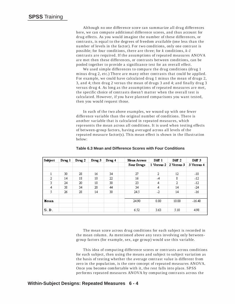
Within-Subject Designs: Repeated Measures 6 - 4
SPSS Training
Although no one difference score can summarize all drug differenceshere, we can compute additional difference scores, and thus account fordrug effects. As you would imagine the number of these differences, orcontrasts, is equal to the degrees of freedom available (one less than thenumber of levels in the factor). For two conditions, only one contrast ispossible; for four conditions, there are three; for k conditions, k-1contrasts are required. If the assumptions of repeated measures ANOVAare met then these differences, or contrasts between conditions, can bepooled together to provide a significance test for an overall effect.
We used simple differences to compare the drug conditions (drug 1minus drug 2, etc.) There are many other contrasts that could be applied.For example, we could have calculated drug 1 minus the mean of drugs 2,3, and 4; then drug 2 versus the mean of drugs 3 and 4; and finally drug 3versus drug 4. As long as the assumptions of repeated measures are met,the specific choice of contrasts doesn’t matter when the overall test iscalculated. However, if you have planned comparisons you want tested,then you would request those.
In each of the two above examples, we wound up with one fewerdifference variable than the original number of conditions. There isanother variable that is calculated in repeated measures, whichrepresents the mean across all conditions. It is used when testing effectsof between-group factors, having averaged across all levels of therepeated measure factor(s). This mean effect is shown in the illustrationbelow:
Table 6.3 Mean and Difference Scores with Four Conditions
The mean score across drug conditions for each subject is recorded inthe mean column. As mentioned above any tests involving only between-group factors (for example, sex, age group) would use this variable.
This idea of computing difference scores or contrasts across conditionsfor each subject, then using the means and subject to subject variation asthe basis of testing whether the average contrast value is different fromzero in the population, is the core concept of repeated measures ANOVA.Once you become comfortable with it, the rest falls into place. SPSSperforms repeated measures ANOVA by computing contrasts across the

Within-Subject Designs: Repeated Measures 6 - 5
SPSS Training
repeated measures factor levels for each subject, and then testingwhether the means of the contrasts are significantly different from zero.A matrix of coefficients detailing these contrasts can be displayed and iscalled the transformation matrix.
A repeated measure ANOVA has several assumptions common to allANOVA. First, that the model is correctly specified and additive.Secondly, that the errors follow a normal distribution and areindependent of the effects in the model. This latter assumption implieshomogeneity of variance when more than a single group is involved. Aswith general ANOVA, moderate departures from normality do not have asubstantial effect on the analysis, especially if the sample sizes are largeand the shape of the distribution is similar from group to group (ifmultiple groups are involved). In multi-group studies, failure ofhomogeneity of variance is a problem unless the sample sizes are aboutequal.
In addition to standard ANOVA assumptions, there is one specific torepeated measures when there are more than two levels to a repeatedmeasures factor. If a repeated measures factor contains only two levels,there is only one difference variable that can be calculated, and you neednot be concerned about the assumption. However, if a repeated measuresfactor has more than two levels, you generally want an overall test ofdifferences (main effect). Pooling the results of the contrasts (describedabove) between conditions creates the test statistic (F). The assumptioncalled sphericity deals with when such pooling is appropriate. The basicidea is that if the results of two or more contrasts (the sums of squares)are to be pooled, then they should be equally weighted and uncorrelated.To illustrate why this is important, view the spreadsheet below:
Table 6.4 Scale Differences and Redundancies in Contrasts
ASSUMPTIONS
The first contrast variable represents the difference between drug 1and drug 2 (Drug 1 – Drug 2). However, the second is 100 times thedifference between Drug 2 and Drug 3. It is clear from the mean andstandard deviation values of the second difference variable that thisvariable would dominate the other difference variables if the results werepooled. In order to protect against this, normalization is applied to thecoefficients used in creating the contrasts (each coefficient is divided bythe square root of the sum of the squared coefficients).

Within-Subject Designs: Repeated Measures 6 - 6
SPSS Training
Also, notice that the third contrast is a duplicate of the first.Admittedly, this is an extreme example, but it serves to make the pointthat since the results from each contrast are pooled (summed), then anycorrelation among the contrast variables will yield incorrect teststatistics. In order to provide the best chance of uncorrelated contrastsvariables, the contrasts or transformations are forced to be orthogonal(uncorrelated) before applying them to the data.
This combination of normalization and forcing the original contraststo be orthogonal (uncorrelated) is called orthonormalization. Again, whenactually applied to the data, these properties may not hold, and that iswhere the test of sphericity plays an important role.
This combination of assumptions, equal variances of the contrastvariables and zero correlation among them, is called the sphericityassumption. It is called sphericity because a sphere in multidimensionalspace would be defined by an equal radius value along eachperpendicular (uncorrelated) axis. Although contrasts are chosen so thatsphericity will be maintained, when applied to a particular data set,sphericity may be violated. The variance-covariance matrix of a group ofcontrast variables that maintain sphericity would exhibit the patternshown below.
Table 6.5 Covariance Matrix of Contrast Variables when SphericityHolds
The diagonal elements represent the variance of each contrast whenapplied to the data and the off-diagonal elements are the covariances. Ifthe sphericity assumption holds in the population, the variances willhave the same value (represented by the V) and the covariances will bezero.
A test of the sphericity assumption is available. If the sphericityassumption is met then the usual “F” test (pooling the results from eachcontrast) is the most powerful test. When sphericity does not hold, thereare several choices available. Technical corrections (Greenhouse-Geisser,Huynh-Feldt) can be made to the “F” tests (adjusting the number of thedegrees of freedom) that modify the results based on the degree ofsphericity violation. Another alternative is to take a multivariateapproach in which contrasts are tested simultaneously while takingexplicit account of the correlation and variance differences. The difficultyin choosing between these approaches is that no single method has been

Within-Subject Designs: Repeated Measures 6 - 7
SPSS Training
found (in Monte Carlo studies) to be best under all conditions examined.Also, the test for sphericity itself is not all that sensitive. For a summaryof the various approaches and a suggested strategy for testing, seeLooney and Stanley (1989).
The data are reported in Bock (1975, p.454) and consist of vocabularyscores obtained from a cohort of pupils at the eighth through eleventhgrade level. Alternative forms of the vocabulary section of theCooperative Reading Tests were administered and rescaled to anarbitrary origin. Interest is in the growth rate of vocabulary at a timewhen physical growth is slowing. Sixty-four subjects were studied.
We will perform a repeated measures analysis on the vocabulary growthdata. There is specific interest in the trend over time – is it linear? Thedata will be examined then repeated measures ANOVA applied withattention paid to the assumptions mentioned above.
The key concept to repeated measures analysis is that the contrasts(which are data transformations) will be applied across conditions of thewithin-subject factors, and if we conclude the contrasts are non-zero inthe population, there are significant differences between the conditions.
Click File..Open..Data (move to the c:\Train\Anova directory)Select SPSS Portable (.por) on the Files of Type drop-down listDouble-Click on VocabClick on Analyze..Descriptive Statistics..ExploreSelect the variables Grade8, Grade9, Grade 10, and Grade11
and move them to the Dependent List box.
Data Set
PROPOSEDANALYSIS
KEY CONCEPT

Within-Subject Designs: Repeated Measures 6 - 8
SPSS Training
Figure 6.1 Explore Dialog Box
Click on the Plots pushbuttonClick Dependents together option button in the Boxplots areaClick the Normality tests with plots check box
Figure 6.2 Plots Dialog Box
Placing the dependent variables together in a single boxplot, insteadof separate plots (Factor levels together), permits direct comparison of thevariables. Normal probability plots and tests are also requested.

Within-Subject Designs: Repeated Measures 6 - 9
SPSS Training
Click ContinueClick OK
The command below will run the analysis.
EXAMINE VARIABLES=grade8 grade9 grade10 grade11 /PLOT BOXPLOT STEMLEAF NPPLOT /COMPARE VARIABLES /STATISTICS DESCRIPTIVES /CINTERVAL 95 /MISSING LISTWISE /NOTOTAL.
We request summaries of the four variables, a normal probability plotwith normality test will appear (/Plot Npplot) for each variable. Also, thefour variables will appear in a single boxplot (/Compare Variables).
Figure 6.3 Descriptives for Grade 8

Within-Subject Designs: Repeated Measures 6 - 10
SPSS Training
Figure 6.4 Descriptives for Grade 9
Figure 6.5 Descriptives for Grade 10
Figure 6.6 Descriptives for Grade 11

Within-Subject Designs: Repeated Measures 6 - 11
SPSS Training
As we can see from the descriptive statistics, the mean score for thereading tests is going up in each year (from 1.1372 in Grade 8 to 3.4716in Grade 11), but the variances are fairly constant across the years (from3.568 to 4.704).
Figure 6.7 Normality Tests
The normality tests show that there is no problem with theassumption of normality for grades 8 and 10. However, grades 9 and 11show that there is some deviation from normality in those grade results.Although the assumption of normality is violated, the sample size is largeenough that we can probably ignore that violation.
Figure 6.8 Q-Q Plot for Grade 8

Within-Subject Designs: Repeated Measures 6 - 12
SPSS Training
Figure 6.9 Q-Q Plot for Grade 9
Figure 6.10 Q-Q Plot for Grade 10
Figure 6.11 Q-Q Plot for Grade 11

Within-Subject Designs: Repeated Measures 6 - 13
SPSS Training
These Q-Q plots also give us some indication of the degree to whichthe normality assumption is violated. Although the normality testsshowed that grades 9 and 11 had some deviation from the normal, the Q-Q plots are similar for all the grades. Again, we should note that thesample size is somewhat large and that we can probably not worry aboutthese violations of normality.
Figure 6.12 Box and Whiskers Plot
The Box plot indicates that the variation of scores within a test year isfairly constant. There are a few outliers; the case id information indicatesthat for the most part, the same few individuals stand out. From themedians we see that vocabulary scores grow over the several year period,and this growth seems to be slowing.
We have only one group of subjects. Each subject has a vocabularyscore under the four grade levels. Notice all four of the vocabulary scoresare attached to a single case (examine data in Data Editor window – notshown). If the four measures for a subject were spread throughout thefile, the analysis can still be run within SPSS, but only by using theGeneral Linear Model Univariate dialog box.
Click Analyze..General Linear Model..Repeated Measures
COMPARING THEGRADE LEVELS

Within-Subject Designs: Repeated Measures 6 - 14
SPSS Training
Here we provide names for any repeated measures factors andindicate the number of levels for each. Unlike a between-group factorwhich would be a variable (for example, region), a repeated measuresfactor is expressed as a set of variables.
Replace factor1 with Time in the Within-Subject Factor Nametext box
Press Tab key to move to the Number of Levels text boxType 4Click Add pushbutton
Figure 6.13 Define Repeated Measures (Within-Subject) Factor
We have defined one factor with four levels. In a more complex study(we will see one later in this chapter) additional repeated measures canbe added. The Measure pushbutton is used to provide two pieces ofinformation. First if there are multiple dependent measures involved inthe analysis (for example, suppose we also took four measures ofmathematical skills for each of our 64 subjects), this is declared in themeasure area. Secondly, you can use the Measure area to provide a labelfor the dependent measure in the results. Recall we named our fourvariables Time1 to Time4 so there would be no ambiguity about whichfactor level each represented. However, this choice on names does notindicate that these variables all measure vocabulary scores. You cansupply such labeling information in the Measures area.
Click Define pushbutton

Within-Subject Designs: Repeated Measures 6 - 15
SPSS Training
In this dialog box we link the repeated measures factor levels tovariable names, and declare any between-subject factors and covariates.Notice the Within-Subjects Variables box lists Time as the factor andprovides four lines labeled with level numbers 1 through 4. We mustmatch the proper variable to each of the factor levels. This step should bedone very carefully since incorrect matching of names and levels willgenerally produce an incorrect analysis (especially if more than onerepeated measure factor is involved). We can move the variables one byone, but since they are in the correct order we will move them as a group.
Move grade8, grade9, grade10, and grade11 into the Within-Subjects Variables box (maintain this variable order)
Click grade11 to select it.
Figure 6.14 Main Repeated Measures Dialog Box
The variable corresponding to each grade level is matched with theproper time level. Since grade11 is selected, the up arrow button is active.These up and down buttons will move variables up and down the list, soyou can easily make changes if the original ordering is incorrect. We haveneither between-subject factors nor covariates and can proceed with theanalysis, but first let us examine some of the available features.

Within-Subject Designs: Repeated Measures 6 - 16
SPSS Training
In the model dialog box (not shown) by default a complete model (allfactors and interactions) will be fit. As with procedures we saw earlier inthe course, a customized model can be fit for either between or within-subject factors. This is usually done when specialty designs (Latinsquares, incomplete designs) are run. The Contrasts pushbutton is usedto request that particular contrasts be applied to a factor (recall ourdiscussion of difference or contrast variables earlier).
Click Contrasts pushbutton
Figure 6.15 Contrasts Dialog Box
Check to see which contrast is selectedIf it is not polynomial then change it to PolynomialClick ContinueClick Plots pushbutton
The Plots pushbutton generates profile plots that graph means atfactor level combinations for up to three factors at a time. Such plots arepowerful tools in understanding interaction effects. We will only requesta plot for time, our repeated measure factor.

Within-Subject Designs: Repeated Measures 6 - 17
SPSS Training
Click on Time and move it to the Horizontal Axis list boxClick Add
Figure 6.16 Plots Dialog Box
Click Continue
The Post Hoc dialog box was discussed earlier in the class; it performspost hoc tests of means for between-subject factors. We will look at theavailable tests for repeated measures factors shortly. The Save dialog boxallows you to save predicted values, various residuals and influentialpoint measures. Also, you can save the estimated coefficients to a file forlater manipulation (perhaps in a prediction model, or to compare resultsfrom different data sets). We will look at the Option dialog box moreclosely.
Click Options pushbuttonMove Time into the Display Means for list boxClick to check the Compare Main Effects checkboxSelect Bonferroni on the Confidence interval adjustment
drop-down listClick on Descriptive statistics check boxClick Transformation Matrix check box

Within-Subject Designs: Repeated Measures 6 - 18
SPSS Training
Figure 6.17 Options Dialog Box
We request descriptive statistics. Estimated marginal means can beproduced for any factors in the model (here time). Since we are fitting acomplete model, the estimated marginal means are identical to theestimated means. We request pairwise comparisons for the time factorusing Bonferroni adjustments (the available adjustments for repeatedmeasure factors are LSD, Bonferroni and Sidak). In addition, we haveasked to see the transformation matrix. The transformation matrixcontains the contrast coefficients that are applied to the repeatedmeasures factor(s) to create the difference or contrast variables used inthe analysis. Here we display it only to reinforce our earlier discussion ofthis topic. Diagnostic residual plots are available and there is a control tomodify the confidence limits (default is 95%). The SSCP (sums of squaresand cross products) matrices are not ordinarily viewed. However, they docontain the sums of squares for each of the contrast variables. By viewingthem you can see that the overall test simply sums up the individualcontrast sums of squares, which is why sphericity is necessary.

Within-Subject Designs: Repeated Measures 6 - 19
SPSS Training
Click Continue to process the option requestsClick OK to run the analysis
The SPSS syntax below will run the repeated measures analysis.
GLM grade8 grade9 grade10 grade11 /WSFACTOR = time 4 Polynomial /METHOD = SSTYPE(3) /PLOT = PROFILE( time ) /EMMEANS = TABLES(time) COMPARE ADJ(BONFERRONI) /PRINT = DESCRIPTIVE TEST(MMATRIX) /CRITERIA = ALPHA(.05) /WSDESIGN = time .
First the variables that constitute the repeated measures factor arelisted. The WSFACTOR (within-subject factor) subcommand declarestime to be a within-subject factor with four levels. In addition, polynomialcontrasts will be applied when creating the contrast variables.Polynomial contrasts will perform linear, quadratic, and cubic contrastson the time factor. If there are significant changes in vocabulary overtime, as we expect, these contrasts will allow us to examine its specificform. The Print TEST (MMATRIX) specification will have thetransformation (called the M Matrix) display. Method declares the sumsof squares type.
The first summary displays information about the factors in the model.
Figure 6.18 Factor Summary
EXAMININGRESULTS
There is only a single within-subject (repeated measures) factor andno between-subject factors.

Within-Subject Designs: Repeated Measures 6 - 20
SPSS Training
Figure 6.19 Descriptive Statistics
Means, standard deviations, and sample sizes appear for each factorlevel. If you were unsure of your matching the variable names to factorlevels in the Define Repeated Measures Factors dialog box, you cancompare these means to those you would obtain from the Descriptives,Means, or Explore procedures to insure the proper variables are matchedwith the proper factor levels. Again, we see the increase in the meanscores as grade level increases.
Multivariate test results appear next. Since they would typically beused only if the sphericity assumption fails, we will skip these results fornow and examine the sphericity test.
Figure 6.20 Mauchly’s Sphericity Test
We see from the Significance (Sig.) information that the data areconsistent with the sphericity assumption. The significance value is above.05 (.277), indicating that the covariance matrix of orthonormalizedtransformation variables is consistent with sphericity (diagonal elementsidentical and off-diagonal elements zero in the population). Sincesphericity has been maintained we can use the standard (pooled) ANOVA

Within-Subject Designs: Repeated Measures 6 - 21
SPSS Training
results, and need not resort to alternative (multivariate) or adjusted(degree of freedom adjustment) tests. The Epsilon section of the pivottable provides the degree of freedom modification factor that should beapplied if the sphericity result were significant. Let us take a brief look atthe multivariate results.
Figure 6.21 Multivariate Tests
Remember these results need not be viewed since sphericity has beenmaintained. Here the test is whether all of the contrast variables(representing vocabulary score differences) are zero in the population,while explicitly taking into account any correlation and variancedifferences in the contrast variables. So if sphericity were violated theseresults could be used. Explanations about the various multivariate testswere given in Chapter 5. The multivariate tests indicate there arevocabulary score differences by grade.
Figure 6.22 Within-Subject Effects
This table contains the standard repeated measures output based onsumming the results from each contrast, as well as sphericity correctedresults. It shows the results for (1) sphericity assumed, and then (2)

Within-Subject Designs: Repeated Measures 6 - 22
SPSS Training
Greenhouse-Geisser, (3) Huynh-Feldt, and (4) Lower Bound adjustments.The test result (sphericity assumed) is highly significant, more so thanthe multivariate test, which is what we expect if sphericity holds: thepooled test is more powerful. Thus, we conclude there are significantdifferences in vocabulary across grade levels.
Figure 6.23 Test of Contrasts
Significant tests will be performed on each of the contrast variablesused to construct a repeated measure factor. Recall that by default,polynomial contrasts are used. Since the repeated measure factor is time,these contrasts test whether there are significant linear, quadratic andcubic trends in vocabulary growth over time. Note that linear andquadratic trends are significant (the linear contrast has a very large Fvalue), while cubic is not. This is consistent with the earlier commentthat vocabulary scores increase over time, but the growth seemed to beslowing down.
Figure 6.24 Test of Between-Subjects Effects
There were no between-subject factors in this study. If there were,the test results for them would appear in this section. There is a test ofthe intercept, or grand mean; this simply tests whether the average of allvocabulary scores is equal to zero in the population – not an interestinghypothesis to test.

Within-Subject Designs: Repeated Measures 6 - 23
SPSS Training
Figure 6.25 Transformation Matrix
The transformation variables are split into two groups: onecorresponding to the average across the repeated measures factor, theothers defining the repeated measures factor. The coefficients for theAverage variable are all .5, meaning each variable is weighted equally increating the Average transformation variable. If you wonder why theweights are not .25, recall that normalization requires the sum of thesquared weights to equal one. Turning to the transformed variables thatrepresent the time effect, the three sets of coefficients are orthogonalpolynomials corresponding to linear, quadratic, and cubic terms. Lookingat the first we see that there is a constant increase (of about .447) in thevalue of the coefficients across the four grade levels. In a similar way, thesecond transformation variable has two sign changes (negative topositive, then positive to negative) over the grade levels; this constitutesa quadratic effect. The SPSS Advanced Models manual has additionalinformation about the commonly used transformations.
Recall that the transformations are orthogonal; you can verify this forany pair by multiplying their coefficients at each level of the factor andsumming these products. The sum should be zero. For linear andquadratic we can calculate (-.671*.5 -.224*.5 +.224*.5 +.671*.5), which isindeed zero.

Within-Subject Designs: Repeated Measures 6 - 24
SPSS Training
Figure 6.26 Transformation Matrix (M Matrix)
Since we ask for analyses to compare main effects in the Optionsdialog box, a new transformation matrix is used to create four variablesequivalent to the four grade levels: the identity transformation. Noticethis is a separate analysis after the others have been completed using theoriginal transformation matrix.
Also, note the estimated marginal means match the observed means(this pivot table is not shown).
Figure 6.27 Pairwise Test Results

Within-Subject Designs: Repeated Measures 6 - 25
SPSS Training
Each grade level mean is tested against every other; essentially weare performing all pairwise tests with a Bonferroni correction. Thefootnotes indicate that each test is performed at an adjusted level ofsignificance using a Bonferroni correction. Thus the probability ofobtaining one or more false positive results is .05. We find in our studythat the grade 8 (time 1) scores are significantly different from all theothers; grade 9 (time 2) is different from grade 8 and grade 11 (time 4);grade 10 (time 3) is different from grade 8 and 11; while grade 11 issignificantly different from grades 8, 9, and 10. Substituting Bonferronicorrected paired t tests for post hoc comparisons provides a means toinvestigate differences within a repeated measures factor.
The program will also run a multivariate ANOVA attempting to testthe pairwise comparisons simultaneously; this is of no interest to us.
Figure 6.28 Profile Plot of Means
This plot (not really necessary since with one factor there can be nointeraction) shows us how the mean of the vocabulary scores is increasingwith grade level.

Within-Subject Designs: Repeated Measures 6 - 26
SPSS Training
Suppose we had some specific hypothesis about the grade levels that wewished to test. For example, if we thought that the grade to gradepromotion made a difference in the student’s vocabulary score, we mightwant to test grade 8 versus grade 9; grade 9 versus grade 10; and grade10 versus grade 11. The Contrast pushbutton provides a variety ofplanned comparisons and customized contrasts can be input usingsyntax.
Click the Dialog Recall tool , then click Repeated
MeasuresClick Define pushbuttonClick Contrasts pushbuttonClick Contrast drop-down arrow and select RepeatedClick Change pushbutton
Figure 6.29 Requesting Planned Comparisons
PLANNEDCOMPARISON
Repeated contrasts will compare each category to the one adjacent.Right click on any contrast on the list to obtain a brief description of it.The SPSS Advanced Models manual contains more details. Also be awarethat you can provide custom contrasts using the Special keyword insyntax.
Click Continue to process the contrastsClick OK to run the analysis
The command below will run the analysis.

Within-Subject Designs: Repeated Measures 6 - 27
SPSS Training
GLM grade8 grade9 grade10 grade11 /WSFACTOR = time 4 Repeated /METHOD = SSTYPE(3) /PLOT = PROFILE( time ) /EMMEANS = TABLES(time) COMPARE ADJ(BONFERRONI) /PRINT = DESCRIPTIVE TEST(MMATRIX) /CRITERIA = ALPHA(.05) /WSDESIGN = time .
The Wsfactor subcommand now requests that repeated contrasts beused in place of the default polynomials.
Again, most of the output is identical to the previous runs; we focuson the contrast tests and the transformation matrix.
Figure 6.30 Tests of Contrasts
We see that all three contrasts are significant at the .05 level. Thefirst contrast, comparing grade 8 to grade 9 has by far the greatest Fvalue. The second compares grade 9 to grade 10, and the third comparesgrade 10 to grade 11. These seem inconsistent with the pairwise tests wejust ran in which the grade 9 scores were not different from the grade 10scores. However, recall that we performed Bonferroni corrections on thosetests and the second contrast (here with significance level of .013) wouldnot be significant we testing at the adjusted Bonferroni level (about .008).If you return to the pairwise analysis you will see the results are quiteclose.
To confirm our understanding of the contrasts, we view thetransformation matrix.

Within-Subject Designs: Repeated Measures 6 - 28
SPSS Training
Figure 6.31 Transformation Matrix
We see the transformed variables do compare each grade level to theadjacent one. The transformed matrix is very useful in understandingand verifying which contrasts are being performed. These contrasts arenot orthogonal, and would not be used without modification(orthonormalization) in the sphericity and pooled significance testsappearing earlier.
In this chapter we reviewed how repeated measures ANOVA differs frombetween-group ANOVA and why it is used. Assumptions were discussedand an analysis was run based on student vocabulary scores measuredover time. A second analysis applied planned comparisons (a prioricontrasts) to a repeated measure analysis.
SUMMARY

Between and Within-Subject ANOVA: (Split-Plot) 7 - 1
SPSS Training
Between and Within-SubjectANOVA: (Split-Plot)
In this chapter we will expand upon the last chapter to include bothbetween and within-subject factors in one analysis. We will discuss theassumptions of this design and show an example. We will also explore theinteractions using simple effects.
We will first use the Explore command to examine the data and then runthe repeated measures ANOVA to do the basic mixed-model analysis(split-plot) and look at information regarding the assumptions.
The data set we will use is the same data as we used in Chapter 6,containing vocabulary test scores obtained from the same children overfour years (grades 8 through 11). However, in this analysis we will usethe sex of the subject as a between-subject factor.
The term “mixed model” technically refers to ANOVA models containingfixed and random factors. The designs we discuss, where subject is arandom effect, are a special case of the mixed model. The common usageof “mixed model” refers to designs with between and within-subjectfactors.
Many studies, especially experimental work, incorporate bothbetween and within-subject factors. Within-subject factors willhopefully lead to a more sensitive analysis, while between-
subject factors are necessary if any demographic characteristics areincluded or if there is reason to believe there would be strong carry-overeffects. Mixed model refers to a mixture of between and within factorsand is a direct generalization of the within-subjects analysis. Thesedesigns are also called split-plot designs, the term taken fromagricultural experiments in which a given plot of land would receivesingle level of one treatment factor, but would be split into subplots thatwould receive all treatment levels of a second factor. This would yieldbetween-plot and within-plot factors equivalent to the between andwithin-subject effects we have covered. We will discuss the features andassumptions of such analysis and run an example.
Chapter 7
Objective
Method
Data
Technical Note
INTRODUCTION

Between and Within-Subject ANOVA: (Split-Plot) 7 - 2
SPSS Training
If we take the assumptions of within-subject analyses as a starting point,normality of the variables and sphericity when there are more than twolevels of a within-subject factor, mixed model analyses involve little more.Since there are multiple groups, the normality of the variables nowapplies to the variation within each group. Also, homogeneity ofcovariance matrices is assumed (this can be applied to the originalvariables or the transformed variable – homogeneity of one implieshomogeneity of the other). This combination of assumptions, homogeneityand sphericity, is sometimes called compound symmetry.
We will fit a model with one between-subject factor (Sex) and one within-subject factor (Time) with four levels. Thus for this analysis thesphericity issue is relevant and will be approached just as it was inChapter 6. While we deal with a single between and a single within-subject factor, no additional assumptions are required to expand theanalysis to handle multiple factors of each type.
As before, we will use the Explore procedure to examine the distributionof vocabulary scores across grades and sex groups. Since we know fromChapter 6 that there are changes in vocabulary scores over time (grades),we will focus on the comparison of the two sex groups. This will providesome indication of normality and homogeneity of the vocabulary scores.
Click File..Open..DataMove to the c:\Train\Anova directorySelect SPSS Portable (.por) from the Files of Type drop-down
listDouble-click on vocab
Figure 7.1 Data from Vocabulary Study
ASSUMPTIONSOF MIXED
MODEL ANOVA
PROPOSEDANALYSIS
A LOOK AT THEDATA

Between and Within-Subject ANOVA: (Split-Plot) 7 - 3
SPSS Training
Click Analyze..Descriptive Statistics..ExploreMove Grade8, Grade9, Grade10, and Grade 11 into the
Dependent list box.Move Sex into the Factors box
Figure 7.2 Explore Dialog Box
Click on the Statistics pushbuttonMake sure that the Descriptives checkbox is the only one
selected
Figure 7.3 Explore Statistics Dialog Box
Click on Continue to process the Statistics choicesClick on the Plots pushbuttonVerify that the Factor levels together option is selected.Verify that the Stem-and-leaf checkbox is checkedClick Normality plots with tests checkboxSelect Power Estimation option button in Spread vs. Level with
Levene Test area

Between and Within-Subject ANOVA: (Split-Plot) 7 - 4
SPSS Training
Figure 7.4 Explore Plots Dialog Box
Click on Continue to process the Plots choicesClick on OK to run the EXPLORE procedure.
The syntax command below will run the analysis.
EXAMINE VARIABLES=grade8 grade9 grade10 grade11 BY sex /PLOT BOXPLOT STEMLEAF NPPLOT SPREADLEVEL /COMPARE GROUP /STATISTICS DESCRIPTIVES /CINTERVAL 95 /MISSING LISTWISE /NOTOTAL.
Normality tests and plots are generated by the Npplot keyword andhomogeneity tests are due to the Spreadlevel keyword on the Plotsubcommand.
Figure 7.5 Descriptives for Grade 8 Males

Between and Within-Subject ANOVA: (Split-Plot) 7 - 5
SPSS Training
Figure 7.6 Stem and Leaf for Grade 8 Males
Figure 7.7 Descriptives for Grade 8 Females
Figure 7.8 Stem and Leaf for Grade 8 Females

Between and Within-Subject ANOVA: (Split-Plot) 7 - 6
SPSS Training
Notice that the range for 8th grade males is about half the range forfemales, but the interquartile ranges are about the same. This is due inpart to an outlier among the females. While not shown, the vocabularyscores of the females were consistent with the normal distribution usingthe Shapiro-Wilks criterion, while the males showed a significantdeparture from normality.
Figure 7.9 Box Plots for Grade 8 Scores
The medians for the sex groups are very similar and the variation inthe female group seems greater. Despite appearances in the plot, the 8th
grade sex groups do not show significant differences in variation of testscores as evidenced by the Levene homogeneity test (not shown).
Figure 7.10 Descriptives for Grade 11 Males

Between and Within-Subject ANOVA: (Split-Plot) 7 - 7
SPSS Training
Figure 7.11 Stem and Leaf for Grade 11 Males
Figure 7.12 Descriptives for Grade 11 Females
Figure 7.13 Stem and Leaf for Grade 11 Females

Between and Within-Subject ANOVA: (Split-Plot) 7 - 8
SPSS Training
Most of the summary statistics are similar for males and females inthe grade 11th grade. The normality tests (not shown) indicate that thescores for males, but not females, are consistent with normal distribution.
Figure 7.14 Box Plots for Grade 11
Once again, the medians are very close and there are a few outliers.The Levene test (not shown) indicated that the sex populations do notdiffer in variance on 11th grade vocabulary scores.
The distribution of vocabulary scores within sex group was consistentwith the normal for 9th and 10th grade, the only exception being 10th gradefemales. Neither grade departed from homogeneity of variance betweensex groups. (These results are not shown.)
Overall, the data look good as far as homogeneity is concerned, and thedepartures from normality are not dramatic. If we had access to theoriginal test sheets, we might want to check the accuracy of the scores forthe outliers. We will proceed with the mixed-model ANOVA.
Click Analyze..General Linear Model..Repeated MeasuresReplace factor1 with Time in the Within-Subject Factor
Name text boxPress Tab and type 4 in the Number of Levels text boxClick Add pushbutton
9th and 10 th
Grades
SUMMARY OFEXPLORE
SPLIT-PLOTANALYSIS

Between and Within-Subject ANOVA: (Split-Plot) 7 - 9
SPSS Training
Figure 7.15 Define Factors Dialog Box
Click Define pushbuttonIn the Repeated Measures dialog box, click and drag Grade8,
Grade9, Grade10, and Grade 11 to the Within-SubjectVariables list box.
Move Sex into the Between-Subjects Factors list box
Figure 7.16 Between and Within-Subject Factors Defined
Click Contrasts pushbutton

Between and Within-Subject ANOVA: (Split-Plot) 7 - 10
SPSS Training
Select time in the Factors: list boxSelect Repeated from the Contrast drop-down listClick Change buttonVerify Sex is set to none for the contrast
Figure 7.17 Contrasts Dialog Box
Repeated contrasts will compare each factor level with the onefollowing it. Thus with four time level (8, 9, 10 and 11), the threerepeated contrasts compare 8th to 9th, 9th to 10th, and 10th to 11th grades,respectively.
Click Continue to process the Contrast changesClick Options pushbuttonIndividually move Sex and Time into the Display Means for
list boxClick the Compare Main Effects checkboxClick Descriptive statistics, Transformation matrix, and
Homogeneity tests option buttons

Between and Within-Subject ANOVA: (Split-Plot) 7 - 11
SPSS Training
Figure 7.18 Options Dialog Box
Click on Continue to process the Options requestsClick on OK to run the analysis
Besides descriptive statistics, we request estimated marginal means(which equal the observed means since we are fitting a full model) foreach of the factors. Since there are several groups involved in theanalysis, we ask for homogeneity of variance tests. We also requestpairwise comparisons for sex and time with no adjustement (LSD (none)).Since sex has only two levels, pairwise tests are not needed.
We will proceed with the analysis. The GLM command shown belowwill produce this analysis (obtained by clicking the Dialog Recall tool
, then Repeated Measures, and the Paste pushbutton)

Between and Within-Subject ANOVA: (Split-Plot) 7 - 12
SPSS Training
Figure 7.19 Syntax for This Analysis
The four vocabulary variables form the basis of the time factor.Estimated marginal means will be computed for the sex and time maineffects. The Print subcommand requests that descriptive statistics, thetransformation matrix (TEST(MMATRIX)) and homogeneity testsummaries appear. The Wsdesign subcommand declares time as the onlyrepeated measure factor in the model; similarly sex (see Designsubcommand) is the only between-subject factor.
Figure 7.20 Factors in the AnalysisEXAMININGRESULTS
The factors in the analysis are listed along with the sample sizes forthe between-subject factor.

Between and Within-Subject ANOVA: (Split-Plot) 7 - 13
SPSS Training
Figure 7.21 Descriptive Statistics
Subgroup means appear separately for each of the repeated measurevariables.
Although they do not appear together in the output, we will first examineresults pertaining to the assumptions of the analysis. Concerninghomogeneity of variance, the program provides Box’s M statistic andLevene’s test. Box’s M is a multivariate statistic testing whether thevariance-covariance matrices composed of the four repeated measuresvariables are equal across the between-subject factor subgrouppopulations (multivariate homogeneity). Levene’s test is univariate andtests homogeneity of variance for each of the four repeated measurevariables separately (univariate homogeneity).
Figure 7.22 Box’s M Test of Homogeneity
TESTS OFASSUMPTIONS

Between and Within-Subject ANOVA: (Split-Plot) 7 - 14
SPSS Training
Box’s M is not significant (significance value is .158), indicating thatthe data are consistent with the hypothesis of homogeneity of covariancematrices (based on the four repeated measures variables) across thepopulation subgroups.
Figure 7.23 Levene’s Test of Homogeneity
Not surprisingly, the results of Levene’s test are consistent with Box’sM. Box’s M test has the advantage of being a single multivariate test.However, Box’s M test is sensitive to both homogeneity and normalityviolations, while Levene’s is relatively insensitive to lack of normality.Since homogeneity of variance violations are generally more problematicfor ANOVA, Levene’s test is useful.
Since the within-subject factor (Time) has more than two levels, we willtest for the sphericity assumption. As discussed in Chapter 6, if theassumption is met the usual averaged F tests are correct and are the testof choice. If sphericity conditions are not met, several choices areavailable: multivariate tests may be used, corrections to the averaged Ftest can be made (Greenhouse-Geisser, Huynh-Feldt, etc.), or morecomplicated decision rules may be applied (Looney & Stanley, 1989). Wenow view the sphericity test results.
Figure 7.24 Mauchly’s Sphericity Test
SPHERICITY
The Mauchly test shows no evidence of sphericity violations and theGreenhouse-Geisser and Huynh-Feldt degree of freedom adjustments areclose to or equal to one. This result indicates we can proceed directly to

Between and Within-Subject ANOVA: (Split-Plot) 7 - 15
SPSS Training
the averaged F tests for effects involving Time. However for comparisonpurposes, we will also view the multivariate tests.
Figure 7.25 Multivariate TestsMULTIVARIATETESTS
INVOLVING TIME
As expected from the analysis in Chapter 6, there are significantdifferences in vocabulary scores over time. In addition, there is asignificant interaction between Sex and Time. This can be phrased in twoways; the population sex difference is not uniform across grades, or thetrend over time is not identical for the two sex populations.
Figure 7.26 Between-Subjects TestsTESTS OFBETWEEN-
SUBJECTFACTORS
The Repeated Measures procedure also presents the tests for thebetween-subject factors, in this case Sex. There is no significantdifference in overall vocabulary score between the females and males(significance value is .101).

Between and Within-Subject ANOVA: (Split-Plot) 7 - 16
SPSS Training
Figure 7.27 F Tests
AVERAGED FTESTS
INVOLVING TIME
The averaged F tests indicate a significant effect of time and a sex bytime interaction. Here we view only the test results labeled “sphericityassumed” since the sphericity assumption was met.
Figure 7.28 Repeated Measures Contrasts
As we saw in Chapter 6, the contrasts show that there are significantdifferences between each pair of grades on the vocabulary scores.However, the only significant sex by time interaction term involvesgrades 8 and 9. Thus the interaction between sex and time centers onthese two grades. The means involving both sex and time (see Figure7.21) can be examined for more detail.

Between and Within-Subject ANOVA: (Split-Plot) 7 - 17
SPSS Training
Figure 7.29 Transformation Matrix
This is shown only to verify that the repeated contrasts were used.
Figure 7.30 Pairwise Comparisons Involving Time
Pairwise comparisons appear for both sex and time. Since there areonly two sex groups, the pairwise comparisons tell us no more than theoverall main effect, and so are not of interest (not shown). The pairwise

Between and Within-Subject ANOVA: (Split-Plot) 7 - 18
SPSS Training
comparisons involving time (with no adjustment due to the number oftests performed) are all significant.
The sphericity assumption applies to all within-subject factors with morethan two levels. In such designs Repeated Measures will performsphericity tests for the appropriate within-subject factors and relevantinteractions (effects involving within-subject interactions). The approachtaken above applies to these situations as well.
A technique that can be used to explore interactions involves simpleeffects, that is, looking at the differences in one factor within a singlelevel of a second factor. For example, an interaction might be clarified bya factor showing a significant difference at one level of a second factorwhile showing no difference at a second level. Below we run simple effectsexamining sex differences within each grade and also examine timedifferences with each sex group. Typically, both analyses would not berun, but we wish to demonstrate how to set them up.
Within the SPSS Univariate (Unianova) or Repeated Measures(GLM) procedures, the method to obtain simple effects involvesrequesting the estimated marginal means table for the two factorsinvolved, and then obtaining tests on the factor of interest, applied to themeans table. For example, if we want tests performed on the time factorwithin each sex group, we need to request tests on the time factor, basedon the sex-by-time table of estimated marginal means. Currently, thisanalysis cannot be run directly from the Univariate and RepeatedMeasures dialog boxes, but involves only a minor change to syntax pastedfrom the dialogs. To demonstrate, we first return to the RepeatedMeasures dialog box.
Click the Dialog Recall tool , and then click Repeated
MeasuresClick the Define pushbuttonClick the Options pushbuttonMove sex*time into the Display Means for list box
ADDITIONALWITHIN-SUBJECT
FACTORS ANDSPHERICITY
EXPLORING THEINTERACTION -
SIMPLE EFFECTS

Between and Within-Subject ANOVA: (Split-Plot) 7 - 19
SPSS Training
Figure 7.31 Requesting the Sex by Time Table
We have requested estimated margin means for the sex*time tableand must later indicate the tests we want performed. We could havedropped the means display and main effects comparison for theindividual factors, sex and time, but will keep them to better illustratethe changes we must make concerning the sex*time table.
Click ContinueClick Paste pushbutton

Between and Within-Subject ANOVA: (Split-Plot) 7 - 20
SPSS Training
Figure 7.32 Syntax for Repeated Measures Analysis
There are three EMMEANS (estimated marginal means)subcommands. The first two, involving the sex, and time tables, containthe COMPARE keyword. It requests that main- or simple main-effecttests (depending on how many factors are specified under TABLES) andpairwise comparisons be performed. Pairwise tests can be adjusted usingBonferroni or Sidak adjustments, but, by default, no adjustment (LSD) ismade. Our task is to obtain these tests for time within the sex*time table.We must add the COMPARE keyword referencing one of the factors tothe /EMMEANS subcommand that contains the sex*time table.
Type COMPARE (SEX) at the end of the /EMMEANS =TABLES (sex*time) line
Copy and paste the modified /EMMEANS = TABLES (sex*time)line just below the original
Change COMPARE (SEX) to COMPARE (TIME) in the second/EMMEANS = TABLES (sex*time) subcommand

Between and Within-Subject ANOVA: (Split-Plot) 7 - 21
SPSS Training
Figure 7.33 Syntax Requesting Tests for Simple Effects
Now significance tests will be applied to the sex factor and then to thetime factor, each performed within every level of the other factor, basedon the sex-by-time table of estimated marginal means. Since the tableinvolves more than one factor, the tests will be run separately at eachlevel of the other factor(s). This logic can be extended to additionalfactors, so you can perform simple effect tests on one factor within a tableinvolving more than two factors.
Note that we do not need the estimated marginal means and tests forthe individual factors sex and time (/EMMEANS subcommandscontaining TABLES(SEX) and TABLES(TIME)) and these subcommandscould be removed. They were left in the “Display means for” list box inthe Repeated Measures Options dialog so we could see the syntax neededto request the tests.
Click Run..Current to run the analysis
Most of the results are identical to those viewed earlier. Here wefocus on the summaries involving simple effects.
Scroll down to the first Sex * Time section under EstimatedMarginal Means heading

Between and Within-Subject ANOVA: (Split-Plot) 7 - 22
SPSS Training
Figure 7.34 Estimated Marginal Means
The simple effects analysis will be based on this table. Even if a morecomplex model were being analyzed, say with three or four between-subject factors, then the simple effects analysis of a two-factorinteraction, would be based on the estimated means table involving thetwo factors of interest.
Figure 7.35 Pairwise Comparisons of Sex within Grade Levels (Time)
Recall that the COMPARE keyword on the /EMMEANS subcommandwill produce both overall tests and pairwise comparisons for the specifiedfactor. The Pairwise Comparisons table presents for each level of the timefactor (which represent grades 8, 9, 10 and 11), the female-male

Between and Within-Subject ANOVA: (Split-Plot) 7 - 23
SPSS Training
comparison. Because there are only two levels to sex, there is only oneunique comparison at each grade level. However, for factors with morethan two levels, all pairwise comparisons would appear.
Examining the comparisons, we see that only at time 2 (9th grade)was there a significant difference between males and females. Thus wecan describe the nature of the sex by time interaction: there are nosignificant differences between males and females in vocabulary scoresexcept in the 9th grade.
Figure 7.36 Univariate Tests (Simple Effects)
In addition to the simple pairwise comparisons, overall simple effecttests are presented. As the caption indicates, each F test represents a testof the simple effect of sex within a grade level (time). Since sex has onlytwo levels, these tests match the pairwise results viewed above, whichwere already discussed. However, for a factor with more than two levels,this summary would present an overall test of a factor within each levelof the second factor.
Now we examine the interaction question using simple effects of timewithin each sex group.
Scroll down to the second Sex * Time section under EstimatedMarginal Means heading

Between and Within-Subject ANOVA: (Split-Plot) 7 - 24
SPSS Training
Figure 7.37 Pairwise Comparisons for Time Performed Separately forMales and Females (Complete Table Not Shown)
Multiple comparisons of the grade levels are done separately forfemales and the males (levels of the sex factor). A caption appears at thebelow the table (not shown) indicating that the comparisons are based onthe estimated marginal means. All grade (time) comparisons aresignificant for the males, while all but two (9th versus 10th, and 10th versus11th) are significant for females. Thus males show a significantly increasein vocabulary scores at each grade level, while females didn’t showsignificant change from 9th to 10th or 10th to 11th grades. Females andmales thus show different patterns of vocabulary change over time, whichis the basis of the interaction.
In this way, understanding of a two-way interaction can be improvedby examining the simple effects of either factor. A plot is also helpful(shown later).

Between and Within-Subject ANOVA: (Split-Plot) 7 - 25
SPSS Training
Figure 7.38 Multivariate Tests (Simple Effects)
When examining the simple effects of sex within grade, overall Ftests were presented in the “Univariate Tests” table. This will be the casefor simple effects of any between-subject factor. Multivariate tests areused to perform overall tests of simple effects for within-subject factors.Multivariate tests are used to avoid complications that would occur ifBonferroni or Sidak corrections were requested and sphericity wereviolated. However, this means that when the sphericity assumptionholds, which is the case here, the simple effects test used (multivariatetest) is not the most powerful test. We find that there are significantoverall grade differences in vocabulary scores for both males and females.In this instance the overall test sheds less light on the nature of theinteraction than did the pairwise comparisons. For this reason, it isuseful to examine both results.
Profile plots, seen earlier in the course, provide a means of visualizing atwo- or three-factor interaction. We will request a plot of vocabularymeans for the grade and sex groups.
Click the Dialog Recall tool , and then click Repeated
MeasuresClick the Define pushbuttonClick Plots pushbuttonMove time into the Horizontal Axis boxMove sex into the Separate Lines boxClick Add pushbutton
GRAPHING THEINTERACTION

Between and Within-Subject ANOVA: (Split-Plot) 7 - 26
SPSS Training
Figure 7.39 Requesting a Profile Plot
Click Continue, and then OK
Figure 7.40 Profile Plot of Vocabulary Scores Across Grades for Malesand Females
The plot of the estimated marginal means (here identical to theobserved means) shows the steady increase in vocabulary score over timefor the males. In comparison, the females show a sharper increase fromgrade 8 to grade 9, and more gradual increases in the later grades. Thegreatest difference between males and females occurs in grade 9. Thesepatterns, as you would expect, are consistent with the simple effects testswe performed earlier.

More Split-Plot Design 8 - 1
SPSS Training
More Split-Plot Design
Understand the issues involved with more complex split-plot analyses.
Use GLM to run a between- and within-subject analysis (split-plot)involving multiple between- and multiple within-subject factors.
A marketing study in which different groups of subjects (groups based onsex and current brand used) rated different brands before and afterviewing a commercial. The aim of the analysis was to determine if ratingsimproved for a specific brand and whether this related to sex or brandused.
The example in this chapter will involve a more complex analysis,but will be done with fewer variations. A marketing experimentwas devised to evaluate whether viewing a commercial produces
improved ratings for a specific brand. Ratings on three brands (on a 1 to10 scale, where 10 is the highest rating) were obtained from subjectsbefore and after viewing the commercial. Since the hope was that thecommercial would improve ratings of only one brand (A), researchersexpected a significant brand by pre-post commercial interaction (onlybrand A ratings would change). In addition, there were two between-group factors: sex and brand used by subject. Thus the study had fourfactors overall: sex, brand used, brand rated, and pre-post commercial.We view the data below.
Chapter 8
Objective
Method
Data
INTRODUCTION:AD VIEWING
WITH PRE-POSTBRAND RATINGS

More Split-Plot Design 8 - 2
SPSS Training
Click File..Open..Data (move to the c:\Train\Anova directory ifnecessary)
Click SPSS Portable(*.por) in the Files of Type drop-down listDouble-click on brand
Figure 8.1 Data from the Brand Study
SETTING UP THEANALYSIS
Sex and user are the between-subject factors. The next six variablespre_a to post_c contain the three brand ratings before and after viewingthe commercial.
Click Analyze..General Linear Model..Repeated MeasuresReplace factor1 with prepost in the Within-Subject Factor
Name text boxPress Tab and type 2 in the Number of Levels text boxClick Add pushbuttonType brand in the Within-Subject Factor Name text boxPress Tab and type 3 in the Number of Levels text boxClick the Add pushbuttonClick the Measure pushbuttonType rating in the Measure Name text boxClick the Add pushbutton in the Measure Name area

More Split-Plot Design 8 - 3
SPSS Training
Figure 8.2 Two Within-Subject Factors Declared
SPSS now expects variables that comprise two within-subject factors.The order you name the factors only matters in that SPSS will order thefactor levels list in the next dialog so that the last factor named here hasits levels change most rapidly. Therefore depending on how yourvariables are ordered in the data, some factor orders make the laterdeclarations easier.
Click the Define pushbutton

More Split-Plot Design 8 - 4
SPSS Training
Figure 8.3 Repeated Measures Dialog with Two Factors
Both prepost and brand are listed as within-subject factors. There aresix rows, so every possible combination of levels between the two factorsis represented. Notice that the brand level changes first going down thelist. This was due to defining brand last in the Repeated Measures DefineFactor dialog. Defining the factors in an order consistent with the order ofvariables in your data file makes this step easier.
Move the following variables into the Within-SubjectsVariables list in the order given: pre_a pre_b pre_cpost_a post_b post_c
Move sex and user into the Between-Subjects Factors list box

More Split-Plot Design 8 - 5
SPSS Training
Figure 8.4 Between and Within-Subject Factors Defined
We can proceed with the analysis, but first let us request someoptions.
Click the Options pushbuttonClick the Descriptives checkboxIndividually move sex, user, prepost, and brand into the
Display Means for list boxClick the Homogeneity check box

More Split-Plot Design 8 - 6
SPSS Training
Figure 8.5 Options Dialog Box
Besides the descriptive statistics, we request estimated marginalmeans (which equal observed means since we are fitting a full model) foreach of the factors. Since there are several groups involved in theanalysis, we ask for homogeneity of variance tests.
We will proceed with the analysis. Contrasts can be applied to anyfactors in the same way as we have done earlier.
Click Continue to process the optionsClick OK to run the analysis
The command syntax below will produce this analysis.

More Split-Plot Design 8 - 7
SPSS Training
Figure 8.6 Syntax to Run Analysis
Variables which comprise the repeated-measures factors precede theBY keyword and the between-subject factors follow it. Notice the repeatedmeasure variables are ordered so that brand levels change first andbrand is mentioned last in the WSFACTOR subcommand. This order iscritical for the analysis, so care must be taken when running from syntax.The levels of each repeated measures factor are given and polynomialcontrasts (here uninteresting) are used. We requested estimatedmarginal means for each of the factors. The PRINT subcommand willdisplay the descriptive statistics and the homogeneity tests.
Figure 8.7 Factors in the AnalysisEXAMININGRESULTS

More Split-Plot Design 8 - 8
SPSS Training
The factors in the analysis are listed along with the sample sizes forthe between-subject factor groups.
Figure 8.8 Descriptive Statistics (Beginning)
Subgroup means appear separately for each repeated measurevariable. Means for the repeated measures factors can be seen in theestimated marginal means pivot tables, or viewed in profile plots.
Although they do not appear together in the output, we first examinesome assumptions of the analysis. Concerning homogeneity of variance,the program provides Box’s M statistic and Levene’ test. Box’s M is amultivariate statistic testing whether the variance-covariance matricescomposed of the six repeated measures variables are equal across thebetween-subject factor subgroup populations. Levene’s test is univariateand tests for homogeneity across subgroup populations for each of the sixrepeated measure variables separately.
TESTS OFASSUMPTIONS

More Split-Plot Design 8 - 9
SPSS Training
Figure 8.9 Box’s M Test of Homogeneity
Box’s M test is not significant, indicating that the data are consistentwith the assumption of homogeneity of covariance matrices (based on thesix repeated measures variables) across the population subgroups.
Figure 8.10 Levene’s Test of Homogeneity
Not surprisingly, the results of Levene’s test are consistent with Box’sM. Box’s test is sensitive to both homogeneity and normality violations,while Levene’s is relatively insensitive to lack of normality. Sincehomogeneity of variance violations are generally more problematic forANOVA, the Levene’s test is useful.

More Split-Plot Design 8 - 10
SPSS Training
Now let us examine the sphericity assumption since this determineswhether we simply view the pooled ANOVA results, or move tomultivariate or degree of freedom adjusted results.
Figure 8.11 Sphericity Tests
Notice no sphericity test is applied to the prepost factor. This isbecause it has only two levels, so only one difference variable is created,and there is no pooling of effects. The sphericity test for brand is notsignificant (Sig. = .832), nor is the sphericity test for the brand by prepostinteraction (Sig. = .975). Thus the data are consistent with sphericity. Asa result we will not view the multivariate test results or the adjustedpooled results (Huynh-Feldt, etc.), and instead focus on the standard(averaged) results.

More Split-Plot Design 8 - 11
SPSS Training
Figure 8.12 Within-Subject TestsANOVA RESULTS
Note that this table has been edited in Pivot Table Editor (epsiloncorrected results with sphericity assumed were placed in the top layer) todisplay only these results.
This table contains all tests that involve a within-subject factor; thoseinvolving only between-subject effects appear later. Looking at thesignificance (Sig.) column, we see a highly significant difference for pre-post commercial and a brand by user interaction. The brand by pre-postcommercial effect is not significant, indicating that although thecommercial may have shifted ratings (pre-post commercial is significant)it did not differentially improve the rating of brand A, which was the aimof the commercial. We will view the means and profile plots tounderstand the significant effects.
We will not view the multivariate results or the degree of freedomcorrected (appropriate if sphericity is violated) results. Nor will weexamine the tests of specific contrasts since we had no planned contrastsand the polynomial contrasts over brand categories make no conceptualsense.
Note

More Split-Plot Design 8 - 12
SPSS Training
Figure 8.13 Between-Subjects Tests
Of the between-subjects effects, only sex shows a significantdifference. Let us take a look at some of the means.
Figure 8.14 Means for Sex and Pre-Post Commercial
We see males give higher ratings than females and the post-commercial ratings are higher than the pre-commercial ratings. It seemsthat the commercial was a success, but a success for all brands, not justbrand A as hoped.

More Split-Plot Design 8 - 13
SPSS Training
To better view the interaction between user (brand used) and brand(brand rated) we request a profile plot
Click the Dialog Recall tool , then select Repeated
MeasuresClick Define pushbuttonClick Plots pushbuttonMove user into the Horizontal Axis list boxMove brand into the Separate Lines list boxClick Add pushbutton
Figure 8.15 Requesting a Profile Plot
PROFILE PLOTS
As many as three factors can be displayed in a profile plot, and so upto a three-way interaction can be examined. Note that multiple profileplots can be requested, which allows for many views of your data.
Click Continue to process the plot requestClick OK to run the analysis
The command below will produce the profile plot.

More Split-Plot Design 8 - 14
SPSS Training
GLMPre_a pre_b pre_c post_a post_b post_c BY sex user/WSFACTOR = prepost 2 Polynomial brand 3 Polynomial/MEASURE = rating/METHOD = SSTYPE(3)/PLOT = PROFILE(user*brand)/EMMEANS = TABLES(sex)/EMMEANS = TABLES(user)/EMMEANS = TABLES(prepost)/EMMEANS = TABLES(brand)/PRINT = DESCRIPTIVES HOMOGENEITY/CRITERIA = ALPHA(.05)/WSDESIGN/DESIGN .
The Plot subcommand requests a profile plot of user by brand.
Figure 8.16 Profile Plot of Brand Used by Brand Rating
In the plot, brand levels 1, 2, and 3 correspond to brands A, B, and C,respectively. The Brand used by Brand interaction shows (as we surelywould expect) that those who regularly use a particular brand rate ithigher than the other brands. Especially when there are many factorlevels, or several factors involved, profile plots can be very helpful inpractice.

More Split-Plot Design 8 - 15
SPSS Training
The homogeneity and sphericity assumptions were met. We did notexamine normality, but could do so by requesting residual plots in theOptions dialog box. We found that men gave higher brand ratings thanwomen, that the post-commercial ratings were higher than pre-commercial ratings, and that respondents rated their own brand highest.The expected brand by pre-post commercial interaction was not evident.
In this chapter we examined a more complex split-plot ANOVA involvingtwo between and two within-subject factors. We also used a profile plot todescribe an interaction effect.
SUMMARY OFRESULTS
SUMMARY
More Split-Plot Design 8 - 16
SPSS Training

Analysis of Covariance 9 - 1
SPSS Training
Analysis of Covariance
In this chapter we will discuss the purpose, assumptions, andinterpretation of analysis of covariance. In addition, we will demonstratean approach if the parallelism assumption is not met. We will thenextend the analysis to include within-subject designs while usingconstant and varying covariates.
We will use the General Linear Model Univariate and RepeatedMeasures procedures to perform the various runs to do the analyses andcheck the assumptions.
The data presented here are taken from page 806 of Winer(1971).However, we provide a different scenario that will influence theinterpretation of the results. It should be noted that the data file is verysmall and is only for illustrative purposes. Suppose a study was done toevaluate the effectiveness of three treatment drugs on pain-reduction ofankle injuries. There are three types of treatment drugs (variable Drugwith labels A, B, and C) and each patient is in one of the three druggroups (between-subjects factor). There is within-subject factor, whichinvolves measures taken during the early and later stages of the drugintervention (time periods 1 and 2). The dependent measure is a painrating scale. Also, physical therapy was performed throughout the study,and the amount of physical therapy varied from patient to patient. Sincephysical therapy may influence the level of pain reported, it is treated acovariate in the study. There are two measures of the hours of physicaltherapy a patient experienced, one taken from the period just after thedrug treatment was initiated (time period 1) and one taken later in thecourse of treatment (time period 2).
The main question concerns whether the drugs are effective in painreduction after controlling for the amount of physical therapy.
We will run various designs using the same data set. There will be a fixedbetween-subject factor Drug with 3 levels and a within-subject factor(time) with two levels. The dependent variable is reflected in PAIN1 andPAIN2. The covariate (hours of physical therapy) was measured at thesame time points as the dependent variable and is stored in PT1 andPT2.
We will run many different analyses on the same data set to demonstratethe flexibility of the technique and reduce possible confusion to constantlyswitching data. In practice, you would be interested in a specific set ofmodels.
Chapter 9
Objective
Method
Data andScenario
Design
Note

Analysis of Covariance 9 - 2
SPSS Training
Analysis of covariance can be viewed as an attempt to provide somestatistical control in place of lack of experimental control.Inclusion of a covariate allows the researcher to run the usual
ANOVAs while controlling for some other variable. This is not control inthe experimental sense, but control in the sense of making a statisticaladjustment to equate all groups on the covariate. Covariates are intervalscale variables; if they were categorical then they would be included asadditional factors in the design.
One purpose of analysis of covariance is to obtain a more sensitiveANOVA by reducing the within-group variability. If the covariate isrelated to the dependent variable the same way in each group, the withingroup variation can be reduced by removing the effect of the covariate.The classic case is an experiment in which subjects are randomlyassigned to groups, but vary on some background measure; analysis ofcovariance (ANCOVA) will control for this source of variation.
Analysis of covariance is often spoken of as a conditional analysis.Removing the effect of the covariate essentially equates all subjects onthe covariate, so instead of speaking of factor A having an effect we speakof factor A having an effect if subjects had identical values on thecovariate. A common example of analysis of covariance is the adjustingfor body weight in medical experiments. In this context, analysis ofcovariance adjusts the analysis as if each subject began at the sameweight.
ANCOVA is also used in non-experimental studies to substitutestatistical control for factors beyond the control of the researcher. Caremust be taken since if the covariate relates to factors in the study,controlling for covariate modifies the estimated effects of the factorsthemselves.
Basically, the dependent variable is regressed on the covariate, but therelevant variation of the dependent variable is not its variation aroundthe grand mean but instead is based on the pooled within-groupvariation. Thus a within-group regression with the covariate(s) is run andthe analysis of variance is performed on the residuals from theregression.
The major assumptions specific to ANCOVA are: 1) The relationshipbetween the covariate and the dependent variable (within groups) islinear; 2) The within-group distribution of the residuals is normal; and 3)The relationship between the covariate and the dependent variable (theslopes in the within-group regressions) is the same across all groups.
Assumption (1) need not hold, but the routines available in mostsoftware are based on a linear relationship. Assumption (2) is the usualnormality assumption, this time after the covariate has been applied. The
HOW ISANALYSIS OFCOVARIANCE
DONE?
ASSUMPTIONSOF ANCOVA
INTRODUCTION

Analysis of Covariance 9 - 3
SPSS Training
last assumption is important and can be tested. The degree of adjustmentmade is based on the pooled within-groups regression. If the sloperelating the covariate to the dependent variable varies across groups,then the common slope used to adjust each group does not reflect the truerelationship for that group. We will see that a different slope can be fit toeach group, but this requires rethinking just what we hope to accomplishwith the analysis.
Plots of the dependent variable and the covariate can be made separatelyfor each group (if there are relatively few cells in the analysis) to take aninformal look at the homogeneity of slopes. The residuals can bedisplayed in normal plots. The homogeneity of slopes assumption can beformally tested.
We first run a one-factor ANOVA to provide a baseline. We use theUnivariate procedure instead of a One-Way ANOVA in order to use thesame procedure throughout.
Click File..Open..DataMove to the c:\Train\Anova directory (if necessary)Select SPSS Portable (.por) from the Files of Type drop-down
listDouble-click on PainTreat.por
Figure 9.1 Data for Analysis of Covariance Example
CHECKING THEASSUMPTIONS
BASELINEANOVA
Click Analyze..General Linear Model..UnivariateMove PAIN1 into the Dependent Variable list boxMove Drug into the Fixed Factors list box

Analysis of Covariance 9 - 4
SPSS Training
Figure 9.2 Univariate Dialog Box
Click on OK to run the analysis.
PAIN1 (pain during period 1) is the dependent variable and there isone between-subjects factor (Drug) with three levels. The followingcommand will run this analysis.
UNIANOVA pain1 BY drug /METHOD = SSTYPE(3) /INTERCEPT = INCLUDE /CRITERIA = ALPHA(.05) /DESIGN = drug .

Analysis of Covariance 9 - 5
SPSS Training
Figure 9.3 ANOVA Table
This table shows no suggestion of a main effect of Drug in thisanalysis (significance level is .376). Thus during the early treatmentperiod, there were no differences attributable to drug found in the painmeasure.
In the second run we will include the covariate and the interaction termof the covariate and the between-subject factor. The assumption ofequality (homogeneity) of regression slopes can be tested by fitting amodel containing the main effects of Drug and PT1, as well as theDrug*PT1 interaction. The interaction term provides the test of the nullhypothesis of equal slopes. If the slopes relating the covariate to thedependent variable are identical (parallel) across the different groups,this interaction will not be significant.
Click the Dialog Recall tool , then click Univariate
(Verify that PAIN1 is in the Dependent variable box and Drug isin the Fixed Factor(s) list box)
Move PT1 into the Covariate(s) list boxClick the Model pushbuttonSelect Custom model option buttonClick Drug, then click the Build Term arrow to add Drug to the
modelClick PT1, and then click the Build Term arrow to add PT1 to
the modelSelect both Drug and PT1 in the Factors & Covariates list box
(use Ctrl-click), then click the Build Term arrow to add theDrug*PT1 interaction term to the model
ANCOVA –HOMOGENEITY
OF SLOPES

Analysis of Covariance 9 - 6
SPSS Training
Figure 9.4 Univariate Dialog Box
Click Continue to process the model requestsClick on OK to run the analysis
The following command will also run the analysis:
UNIANOVA pain1 BY drug WITH pt1 /METHOD = SSTYPE(3) /INTERCEPT = INCLUDE /CRITERIA = ALPHA(.05) /DESIGN = drug pt1 drug*pt1 .
The keyword WITH precedes covariates in UNIANOVA, just as BYprecedes factors. From the first command line alone, UNIANOVA wouldrun a standard analysis of covariance, not testing the interaction term. Inthe DESIGN subcommand we include the between-subjects factor (Drug),the covariate (PT1), and the factor by covariate interaction (Drug BYPT1). This interaction effect is the main focus of our interest.

Analysis of Covariance 9 - 7
SPSS Training
Figure 9.5 ANCOVA Table with Homogeneity of Slopes Test
The summary table indicates that the interaction is not significant(Sig. = .390), so the homogeneity of slopes assumption seems to be met.Thus the linear relationship between hours of physical therapy and painlevel does not differ across drug treatment groups. There is a suggestionof an effect of the covariate (Sig. = .067), but no effect due to Drug. Torepeat, with such a small sample there is little power to detectassumption violations, but we wish to demonstrate the method.
Having checked the parallelism of slopes assumption, we proceed withthe standard ANCOVA.
Click the Dialog Recall tool , then click Univariate
Click the Model pushbuttonSelect the Full factorial model option buttonClick Continue to process the changeClick Options pushbuttonClick Parameter Estimates checkboxClick ContinueClick OK to run the analysis.
The following command will run the analysis using syntax.
UNIANOVA pain1 BY drug WITH pt1 /METHOD = SSTYPE(3) /INTERCEPT = INCLUDE /PRINT = DESCRIPTIVE PARAMETER /CRITERIA = ALPHA(.05) /DESIGN = pt1 drug.
STANDARDANCOVA

Analysis of Covariance 9 - 8
SPSS Training
Figure 9.6 ANCOVA Summary Table
The results are similar to the previous analysis, no effect due to factorDrug, and a significant relationship between the covariate and dependentmeasure. The reason for the covariate now being significant probably hasto do with the extra degrees of freedom added to the error term – goingfrom 3 to 5 degrees of freedom is a big jump.
The Univariate procedure also presents some information to characterizethe relation between the covariate and dependent variable.
Figure 9.7 Parameter Estimates
In the GLM parameterization, the intercept parameter estimate givesthe estimated value of the last category of Drug (Drug = 3) when thecovariate is equal to 0. The Drug = 1 and Drug =2 coefficients subtractthe level 3 predicted value from the level 1 and level 2 predicted values,respectively. Adding one of these coefficients to the intercept estimategives the estimated value for that level of Drug when the covariate isequal to 0.
The B coefficient for PT1 is the regression coefficient used to predictthe dependent variable based on the covariate. Its positive coefficientindicates that higher levels of physical therapy are associated with
DESCRIBING THERELATIONSHIP

Analysis of Covariance 9 - 9
SPSS Training
greater pain levels. This is not the expected relationship and if this werereal data, it should be examined more carefully (perhaps patients withmore serious and painful injuries received more physical therapy). The95% confidence band for the regression coefficient is rather wide.
If an interaction between a covariate and a factor in the model issignificant, it indicates that the slopes relating the covariate to thedependent variable vary across groups. If there is interest in modelingthis, that is, fitting different slopes to each group, this can be specified inthe Univariate procedure. It is no longer the standard analysis ofcovariance since the degree of adjustment varies with the group, but theanalysis may be of interest in its own right.
Click the Dialog Recall tool , then click Univariate
Click the Model pushbuttonSelect the Custom Model option buttonIf Drug and Drug*PT1 are not already in the Model list box (from
our earlier analysis) then move Drug and Drug*PT1 (Ctrl-click to select both) into the Model box
Remove PT1 from the Model list box (if necessary)
Figure 9.8 Model for Separate Slope Analysis
FITTING NON-PARALLEL
SLOPES
Since PT1 is removed from the model, Univariate will assign threedegrees of freedom to the PT1 by Drug interaction. Thus it will fit aseparate slope (between PT1 and the dependent measure) for each levelof Drug. If we left PT1 in the model, as we did when testing slope

Analysis of Covariance 9 - 10
SPSS Training
homogeneity, then the PT1 effect would represent the overall slopebetween PT1 and the dependent measure, while the two degrees offreedom PT1 by Drug effect would test the interaction of PT1 and Drug.
Click Continue to process the changeClick OK to run the analysis
The following syntax will run the analysis.
UNIANOVA pain1 BY drug WITH pt1 /METHOD = SSTYPE(3) /INTERCEPT = INCLUDE /PRINT = PARAMETER /CRITERIA = ALPHA(.05) /DESIGN = drug drug*pt1 .
Figure 9.9 Between-Subject Tests
We notice that neither the main effect of Drug, nor the covariatemain effect or interaction of the factor and the covariate (bundledtogether in Drug*PT1) are significant (.577 and .109, respectively).

Analysis of Covariance 9 - 11
SPSS Training
Figure 9.10 Parameter Estimates
The values for the intercept and Drug = 1, Drug = 2, and Drug = 3 arethe same as explained earlier. Notice that there are 3 degrees of freedomfor Drug*PT1: one for each of the three slopes. The parameter estimatesfor Drug*PT1 provide the slope estimates, relating hours of physicaltherapy to reported pain level, for each of the three groups.
To illustrate analysis of covariance in the context of repeated measureswe will first run a split-plot analysis (between-subject factor Drug,within-subject factor time with two levels), using only the firstmeasurement of the covariate PT1 to illustrate the analysis. This is alsotermed repeated measures with a constant covariate since a singlecovariate value applies across levels of the repeated measure factors.
Click Analyze..General Linear Model..Repeated MeasuresReplace factor1 with timeEnter 2 in the number of levels boxClick the Add pushbutton
Click the Measure pushbuttonType pain in the Measure Name text boxClick the Add pushbutton in the Measure Name area
REPEATEDMEASURES
ANCOVA WITH ASINGLE
COVARIATE

Analysis of Covariance 9 - 12
SPSS Training
Figure 9.11 Repeated Measures Define Factors Dialog Box
Click the Define pushbuttonMove PAIN1 and PAIN2 into the Within-Subject Variables
list box in that orderMove Drug into the Between-subject Factor(s) list boxMove PT1 into the Covariates list box
Figure 9.12 Repeated Measures Dialog Box

Analysis of Covariance 9 - 13
SPSS Training
Click the Options pushbuttonSelect Descriptives, Parameter Estimates, Transformation
Matrix, and Homogeneity Tests
Figure 9.13 Options Dialog Box
Click Continue to process the requestClick OK to run the analysis
The following command will also run the analysis.
GLM pain1 pain2 BY drug WITH pt1 /WSFACTOR = time 2 Polynomial /MEASURE = pain /METHOD = SSTYPE(3) /PRINT = DESCRIPTIVE PARAMETER TEST(MMATRIX)
HOMOGENEITY /CRITERIA = ALPHA(.05) /WSDESIGN = time /DESIGN = pt1 drug .
Scroll down to Transformation section of results

Analysis of Covariance 9 - 14
SPSS Training
Figure 9.14 Transformation Matrix
The first transformation is the average of PAIN1 and PAIN2. Thusthe covariate will be applied to the effects that involve the average ofPAIN1 and PAIN2, that is, only between-subject effects.
Scroll up to the Tests of Between-Subjects Effects’ pivot table
Figure 9.15 Tests of Between-Subject Effects
The covariate is not quite significant (Sig. = .066). If it weresignificant, this would indicate that the amount of physical therapyduring the early phase of drug treatment is related to overall (period 1and period 2 measures, averaged together) pain ratings. The effect of theDrug factor, adjusted for the covariate, is not significant.

Analysis of Covariance 9 - 15
SPSS Training
Figure 9.16 Tests of Within-Subjects Effects (Sphericity Assumed)
Note: the pivot table above was edited in the Pivot Table Editor so onlythe sphericity assumed results appear. Since there are only two levels ofthe repeated measure factor, the sphericity test and corrections are notrelevant). We find no effects significant: main effect of time, interactionbetween time and factor Drug, interaction between the covariate andtime. This latter effect (Time by PT1) tests whether the slope relating thecovariate (physical therapy) to the dependent measure (pain) is the same(parallel) for each of the two time periods.
Figure 9.17 Parameter Estimates
This is the standard ANCOVA table of parameters under the generallinear model. Note a separate slope coefficient (for covariate PT1) iscalculated for PAIN1 and PAIN2; the model effects are adjusted for both.

Analysis of Covariance 9 - 16
SPSS Training
Since covariates are not always fixed measures at one time point,covariates that are measured under each condition can be used in theanalysis. We will analyze the same data using PT1 and PT2, measures ofthe covariates at the two time points. Note that GLM will adjust eachlevel of the repeated measure factor (PAIN1, PAIN2) for every covariate.Thus a covariate that varies over time is treated identically to thesituation in which multiple covariates are recorded at a single time point.
Click on the Dialog Recall tool , then click Repeated
MeasuresClick on the Define buttonAdd PT2 to the Covariates boxClick on OK
The following command will run this analysis.
GLM pain1 pain2 BY drug WITH pt1 pt2 /WSFACTOR = time 2 Polynomial /MEASURE = pain /METHOD = SSTYPE(3) /PRINT = PARAMETER TEST(MMATRIX) HOMOGENEITY /CRITERIA = ALPHA(.05) /WSDESIGN = time /DESIGN = pt1 pt2 drug .
Figure 9.18 Test of Within-Subjects Factors
REPEATEDMEASURES
ANCOVA WITH AVARYING
COVARIATE
As before, the pivot table has been edited so only the results thatassume sphericity appear.
As we can see Time, the interaction of Time and PT1, and theinteraction of Time and PT2 are both significant, but the Time by Druginteraction is not significant. This suggests that there is a change in painlevel over time and that this change is related to the amount of physicaltherapy in both the early and late stages of drug treatment. Although notsignificant, a Drug by Time interaction would suggest that the effect ofDrug is not uniform across the two time periods.

Analysis of Covariance 9 - 17
SPSS Training
Figure 9.19 Test of Between-Subjects Factors
The only significant effect is the covariate PT2 (the amount ofphysical therapy during the second time period). The results of the othereffects are consistent with the previous analysis.
Figure 9.20 Parameter Estimates
The interpretation of the parameter estimates is identical to ourearlier discussion (see Figure 9.17); each of the covariates is summarizedseparately. As we found earlier with PT1 (physical therapy during thefirst period), the estimates for the covariate coefficients of PT2 (physicaltherapy during the second period) indicate that pain level increases withmore physical therapy. Oddly, higher levels of physical therapy duringthe first period relate to lower pain levels during the second period.Notice a coefficient relates PT2 (amount of physical therapy during thesecond period) to the first period pain measure; it might be argued onlogical grounds that this coefficient should not be included in the model.
The fact that the intercept for the second period is greater (11.583)than that for the first period (7.342) indicates that pain levels increased

Analysis of Covariance 9 - 18
SPSS Training
over time! This could be shown more clearly by requesting the estimatedmarginal means for the Time factor using the Options dialog.
This process can be generalized to additional covariates and repeatedmeasures factors, and even more complicated variations. If you attemptthese analyses, make sure you display the transformation matrix thatwill inform you of the actual analysis that the General Linear Modelprocedures are performing.
FURTHERVARIATIONS

Special Topics 10 - 1
SPSS Training
Special Topics
We will discuss the setups for some specialty statistical models: LatinSquare Designs and Random Effects Designs. We will not discusssubstantive interpretation of the results.
In addition to the more or less standard analyses discussed in theprevious chapters, there are a number of more specialized ANOVAapplications. The family of incomplete designs, which includes Latin
Squares, allows experimenters to control for nuisance factors, or to studya number of factors without including all possible combinations of thefactor levels in the analysis. The price of this involves giving up theopportunity to test for interaction effects. In this chapter we demonstratethat the GLM procedure can perform such analyses with experimentaldata collected from a Latin Square design. A second application we willexplore involves ANOVA designs that contain more than a single randomfactor. Again, such models can be run using the GLM procedure.
Chapter 10
Objective
INTRODUCTION

Special Topics 10 - 2
SPSS Training
Latin Square designs are useful when there is interest in performing amultiple factor ANOVA, but it is impossible or undesirable to representall combinations of levels of factors in the analysis. For example, a three-factor design with each factor containing five levels implies 125 groups!Another common use of Latin Square designs involves controlling fornuisance factors, that is, controlling for the effects of factors that mayinfluence the outcome, but are not themselves of experimental interest.
The basic idea is that not all combinations of levels of levels of factorsare included, but those included are counterbalanced so that independentmain effects can be tested. The counterbalancing is designed to confoundmain effects with certain interaction terms, and an assumption is madethat the interaction terms are not significant. As a result of not includingall cells, at least some and possibly all interaction questions cannot betested. When there are no replicates within cells, the variation usuallyattributed to higher-order interactions is used as the error term in testingmain effects.
To illustrate a Latin Square design, Montgomery (1984) provides anexample of a dynamite manufacturer interested in evaluating the resultsof five chemical formulations on the explosive force of the resultingcompound. In addition, two other factors have been identified aspotentially influencing the compound, namely the quality of the rawmaterials and the person mixing the materials. These will be consideredto be systematic sources of error (nuisance factors) that need to beremoved from the analysis. Thus we consider three factors: formulation,batch of raw materials, and operator. Ideally, an experiment would beperformed so that each operator uses each batch of raw materials inpreparing each formulation (5 x 5 x 5, or 125 cells). Here we run into thepractical problem of there being not enough raw materials in a batch tosupply each operator for each formulation (25 combinations). For thisreason the researcher cannot perform the fully balanced experiment andinstead a Latin Square will be used.
Below we show the formulation assignments (A-E) with five operators(1-5) and five batches of material (1-5). The equal number of levels withineach factor is required for balancing and is a feature of such designs.
LATIN SQUAREDESIGNS
AN EXAMPLE
Notice that each formulation appears once in each row and column ofthe table – that is, once with each batch of materials and once with eachoperator. If interactions between batches, operators, and compounds arenegligible, then we can test for the effects of different formulations ofcompounds on explosive force without the noise introduced by raw
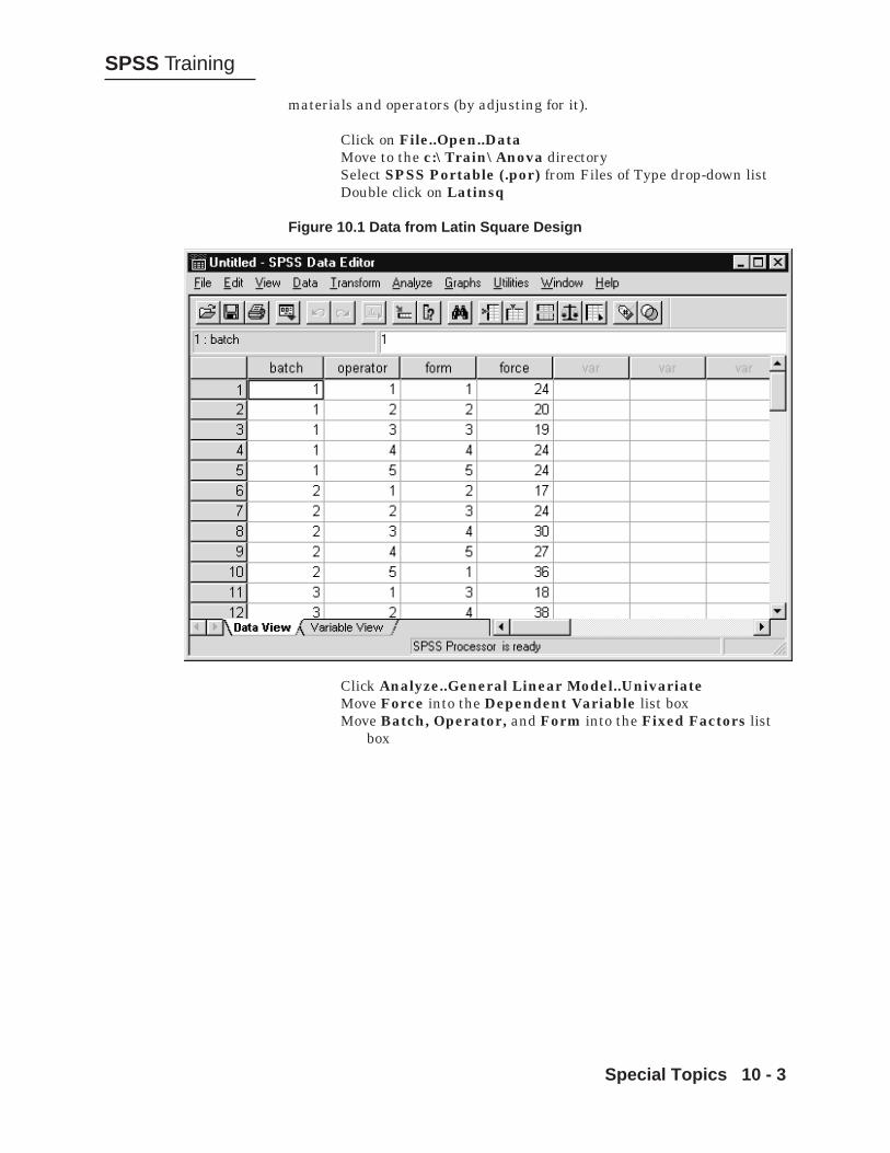
Special Topics 10 - 3
SPSS Training
materials and operators (by adjusting for it).
Click on File..Open..DataMove to the c:\Train\Anova directorySelect SPSS Portable (.por) from Files of Type drop-down listDouble click on Latinsq
Figure 10.1 Data from Latin Square Design
Click Analyze..General Linear Model..UnivariateMove Force into the Dependent Variable list boxMove Batch, Operator, and Form into the Fixed Factors list
box

Special Topics 10 - 4
SPSS Training
Figure 10.2 Univariate Dialog Box
Click the Model pushbuttonSelect Main Effects on the Build Term(s) drop-down listSeparately move Batch, Operator, and Form into the Model
list box
Figure 10.3 Univariate: Model Dialog Box

Special Topics 10 - 5
SPSS Training
Instead of the full model (all main effects and interactions), we will fita custom model consisting of only main effects. The residual variationfrom this model will be used as the error term.
Click on Continue to process ModelClick on OK to run the analysis.
The following syntax will also run the analysis.
UNIANOVA force BY batch operator form /METHOD = SSTYPE(3) /INTERCEPT = INCLUDE /CRITERIA = ALPHA(.05) /DESIGN = batch operator form .
The DESIGN subcommand indicates that only a main effects modelwill be tested. The remaining effects will be pooled together into aresidual term, which will be used as the error term in significancetesting. This is why the assumption of no interactions is so important.Since Unianova is the univariate version of the GLM procedure, the GLMcommand could have been used instead.
Figure 10.4 ANOVA Table
We see the tests of main effects performed using the residual as theerror term. The main effect of Form (formulation) is of greatest interestand is highly significant. For some designs, if there were replicationwithin each cell, the within-cell error term could be used for significancetesting.

Special Topics 10 - 6
SPSS Training
There are additional variants along this theme of Latin Square designs(Greco-Latin Square, etc.) as well as other classes of designs (for example,fractional factorial). They can be set up in GLM in much the same way asdemonstrated above. Such designs generally demand more knowledge ofthe user to plan the experiment, to understand which effects (maineffects, main effects and some two-way interactions, etc.) can be tested,and to interpret the results. For those who need to perform such studies,SPSS Trial Run is a design of experiments program that can generate avariety of complex designs. It can then analyze the results using the GLMprocedure, which is included in the program.
The preceding designs in this course contained only single randomfactors: plant variation within group, subject variation within group, andY variation within levels of A. In SPSS, by default GLM assumes there isa single random factor reflected in the case to case variation. GLM canaccommodate multiple random factors quite easily using dialog boxeswhen the random factors are crossed with the other factors, and can berun using syntax when the random factors are nested. This is because thenesting operation cannot be expressed currently in the GLM – GeneralFactorial Model dialog box. Most applied statistics books that discussexperimental design either cover the common designs or supply rules todetermine the correct error terms in the presence of multiple randomeffects (for example, Kirk (1982) or Milliken and Johnston (1984)).
To illustrate we will consider a simple two random-effect design. Anexperiment is performed in which subjects (5) inflate rubber rafts (6). Thetime it takes to inflate each raft is recorded. Rafts are sampled from aproduction line and each subject inflates each raft once. Here we have acompletely crossed (each subject inflates each raft) two-factor design withboth factors assumed random. In this case the interaction term is used totest each of the main effects, and if there had been replications (if eachsubject inflated each raft several times), the interaction itself would betested using the within-cells error term.
Click on File..Open..DataMove to the c:\Train\Anova directory (if necessary)Select SPSS Portable (.por) from the Files of Type drop-down
listDouble click raft.por to open the fileClick No when asked to save the Data Editor’s contents
COMPLEXDESIGNS
RANDOMEFFECTSMODELS

Special Topics 10 - 7
SPSS Training
Figure 10.5 Raft Data
Notice the data are arranged so each subject by raft combinationappears as a different case. If we structured the data as we ordinarilywould for repeated measures, each respondent on a single row of data, wewould not be able to declare raft as a random factor (there is no RandomFactor(s) list box in the General Linear Model – Repeated Measuresdialog box).
Click on Analyze..General Linear Model..UnivariateMove time into the Dependent Variable list boxMove subject and raft into the Random Factor(s) list box

Special Topics 10 - 8
SPSS Training
Figure 10.6 Univariate Dialog Box
Click OK to run the analysis
The following syntax will run the analysis
Figure 10.7 Syntax for Two Random Effects Analysis
The Random subcommand declares both subject and raft to berandom factors.

Special Topics 10 - 9
SPSS Training
Figure 10.8 Results
We have tests for both subject and raft main effects. Notice that theinteraction could not be tested (the error term for it has 0 degrees offreedom) because there were no replications.
A specific extension to the multiple random effects model is that in whichrandom effects are nested within random effects. A common example ofthis involves analyzing student test scores within schools when theschools are sampled from school districts. A variation of random effectmodels, named hierarchical linear analysis, can be applied to such data.SPSS will perform such analyses for a balanced design, but does notcurrently handle the general case. Specialized programs are available torun hierarchical linear analysis.
Armed with knowledge of experimental design and the appropriate errorterms, incomplete and random effects designs can be tested using SPSS.
SUMMARY
Extensions

Special Topics 10 - 10
SPSS Training

References R - 1
SPSS Training
References
Andrews, F. M., Klem, L., Davidson, T. N. O’Malley, P. M., and W. L.Rogers, A Guide fort Selecting Statistical Techniques for Analyzing SocialScience Data, Ann Arbor: Institute for Social Research, University ofMichigan, 1981.
Bock, R. D., Multivariate Statistical Methods in Behavioral Research,New York: McGraw-Hill, 1975.
Conover, W. J., Practical Nonparametric Statistics, 2nd edition, New York:Wiley, 1980.
Crowder, M. J. and D. J. Hand, Analysis of Repeated Measures, London:Chapman and Hall, 1990.
Finn, J. D., A General Model for Multivariate Analysis, New York: Holt,Rinehart and Winston, 1974.
Hand, D. J. and C. C. Taylor, Multivariate Analysis of Variance andRepeated Measures, London: Chapman and Hall, 1987.
Hakstain, A. R, J. C. Roed, and J. C. Lind, Two Sample T2 Procedure andthe Assumption of Homogeneous Covariance Matrices, PsychologicalBulletin, 86, Pgs. 1255-1263, 1979.
Huberty, C. J., Multivariate Analysis versus Multiple UnivariateAnalyses, Psychological Bulletin Volume 105, Pgs. 302-308, 1989.
Kendall, M. G., and A. Stuart, The Advanced Theory of Statistics, Volume3: Design and Analysis, and Time Series, New York: Hafner, 1968.
Kirk, R. E., Experimental Design: Procedures for the Behavioral Sciences,2nd edition, Belmont, CA: Brooks/Cole, 1982.
Klockars, Alan J. and Sax, G., Multiple Comparisons, SAGE QuantitativeApplications Series, Thousand Oaks CA: Sage, 1986.
Lindsey, J. K., Models for Repeated Measures, Oxford: Clarendon Press,1993.
Looney, S. W., and W. Stanley, Exploratory Repeated Measures Analysisfor Two or More Groups, The American Statistician, Volume 43, No. 4,Pgs 220-225, 1989.
McCullagh, P. and J. A. Nelder, Generalized Linear Models, 2nd edition,London: Chapman and Hall, 1989.

SPSS Training
References R - 2
Milliken, G. A., and D. E. Johnson, Analysis of Messy Data, Volume 1:Designed Experiments, New York: Van Nostrand Reinhold, 1984.
Montgomery, D. C., Design and Analysis of Experiments, 2nd edition, NewYork: Wiley, 1984.
Morrison, D. F., Multivariate Statistical Methods, 2nd edition, New York:McGraw-Hill, 1976.
Olson, C. L. On Choosing a Test Statistic in Multivariate Analysis ofVariance, Psychological Bulletin, Volume 83, No. 4 Pgs. 579-586, 1976.
Scheffe, H. The Analysis of Variance, New York: Wiley, 1959.
Searle, S. R., Linear Models for Unbalanced Data, New York: Wiley,1987.
Tukey, J. W., Exploratory Data Analysis, Reading MA.: Addison Wesley,1977.
Wilcox, Rand, R. Statistics for the Social Sciences, Academic Press, NewYork, 1996.
Wilcox, Rand R. Introduction to Robust Esimation and HypothesisTesting, Academic Press, New York, 1997.
Winer, B. J., Statistical Principles in Experimental Design, 2nd edition,New York: McGraw-Hill, 1971.

Exercises E - 1
SPSS Training
Exercises
The exercise file for this class (Workload.por) is located in thec:\Train\Anova folder on your training machine. If you are not workingin an SPSS Training center, the training files can be copied from thefloppy disk that accompanies this course guide. If you are running SPSSServer (click File..Switch Server to check), then you should copy thesefiles to the server or a machine that can be accessed (mapped from) thecomputer running SPSS Server.
These exercises are based on a single, rich data file. You will perform avariety of analyses (for example, a one-factor and a three-factor ANOVA)on the same data. Typically, if three factors were believed to be relevant,then a one-factor ANOVA would not be run. Thus analyses suggestedhere conform to the topical sequence in the training guide and are notnecessarily optimal to answer a specific research question. In fact, someanalyses that might be performed on this data (doubly-multivariateanalysis of variance) are not discussed in the course.
One-Factor ANOVAOpen the SPSS portable file Workload.por. This file contains data froman experimental investigation of the effects of a training workshop intostress and workload reduction techniques in airline pilots. The variablesare in four sets - descriptive grouping information, workload measurestaken before a flight, workload measures taken after a training course onstress and workload management, and a follow-up set of workloadmeasures taken three months after the training course. Each pilot wasmeasured once each (to avoid distraction) per flight and the twosubsequent flights were on the same route for comparative purposes. Inall two hundred pilots were measured over three time periods.
AGE Age in yearsHRSEXP Previous flying experience in flying hoursTYPE Type of aircraft cockpit (1=Automated, 2=Manual)ROUTE Designation of journey (1=Short Haul, 2=Medium Haul,
3=Long Haul)STAGE Stage of flight (1=Take Off, 2=Cruise, 3=Approach,
4=Landing)FLYTIME Length of flight (measured in seconds, presented in date/
time format)
(Before Stress and Workload Training Course)
HEART Heart Rate (Beats Per Minute)BLOOD Blood pressure (mmhg)TEMP Core Body Temperature (deg. f)
Note on ExerciseData
Note About theExercises
Chapter 3

SPSS Training
Exercises E - 2
STRESS Stress Rating (1=Low stress up to 7=High stress)CAPACITY Spare Mental Capacity Rating (1=All used up to 10 None
used up)ATTEN Percent of attention remaining (in percent)TIRED Tiredness Rating scale (1=Invigorated up to 10=Asleep)
(After Stress and Workload Training Course)
HEART2 Heart Rate (after training)BLOOD2 Blood pressure (after training)TEMP2 Core Body Temperature (after training)STRESS2 Stress rating (after training)CAPACIT2 Spare Mental Capacity (after training)ATTEN2 Percent of attention remaining (after training)TIRED2 Tiredness ratings (after training)
(Three Months After the Stress and Workload Training Course)
HEART3 Heart Rate (after 3 months)BLOOD3 Blood Pressure (after 3 months)TEMP3 Core Body Temperature (after 3 months)STRESS3 Stress Rating (after 3 months)CAPACIT3 Spare Mental Capacity (after 3 months)ATTEN3 Percent of attention remaining (after 3 months)TIRED3 Tiredness Rating (after 3 months)
Familiarize yourself with the variables and data within this dataset byusing the Frequencies, Descriptives and Explore procedures (with anyassociated graphical plots you choose).
Using the Means procedure and error bar graphs, compare the meanstress levels (use the stress variable, which measures stress before thetraining course) at different flight stages (use the variable type). Recallthat a pilot was tested at a single flight stage. Before performing a one-factor ANOVA, explore the data (asking for means, error bars etc.) andtry to predict the outcome of the analysis. Do you think there will be asignificant difference between the groups?
Perform a one-factor ANOVA, testing for stage differences in stress level.If differences are found, perform post hoc tests to explore thesedifferences in more detail. How would you summarize the results?
If the assumptions of ANOVA were not met, perform a nonparametrictest of group (stage) differences in stress. Are the results consistent withthe ANOVA analysis?

Exercises E - 3
SPSS Training
Multi-Way Univariate ANOVA
Open the SPSS portable file Workload.por. Now we are going to examinestress differences as a function of flight stage, route, and type of aircraft.Run an exploratory analysis examining stress (use the stress variable,which reports stress before taking the training course) within subgroupsbased on flight stage (stage), length of route (route) and aircraft type(type). Does the stress measure conform to the ANOVA assumptions?
Perform a three-factor ANOVA of stress with type, route, and stage asthe factors. Are there significant interactions among aircraft type, routelength, and flight stage as they relate to stress? If there are nointeractions, but there are significant main effects, then perform theappropriate post hoc tests to identify which subgroups differ from eachother.
Multivariate Analysis of VarianceOpen the SPSS portable file Workload.por. Perform a three-factor (route,type and stage) multivariate analysis of variance on several physiologicalmeasures of stress: blood pressure (blood), heart rate (heart), and bodytemperature (temp). Which effects and interactions are significant?Examine the univariate results. Are the effects consistent across thethree dependent measures?
Request a profile plot to examine the three-way interaction of route bystage by type as it relates to core body temperature (temp)? Describe thenature of the interaction.
For those with extra time: Perform a multivariate analysis using thesame factors, but on the subjective measures of workload (stress,capacity, atten, and tired)? Are the results similar to what you found forthe physiological measures?
Within-Subject Designs: Repeated MeasuresOpen the SPSS portable file Workload.por. Perform and exploratory dataanalysis on stress measured at the three time points (stress, stress2,stress3). Run a one-factor repeated-measures analysis examining thestress measure (stress, stress2, stress3) at the three time points of thestudy.
If there is a significant main effect of the time factor, explore the natureof it with post hoc tests and plots.
Chapter 4
Chapter 5
Chapter 6

SPSS Training
Exercises E - 4
Between- and Within-Subject ANOVA: Repeated MeasuresOpen the SPSS portable file Workload.por. Perform a repeated measuresanalysis with time (three levels) as a within-subject factor and type,route, and stage as between-subject factors. The dependent measure willbe stress (stress, stress2, stress3). Which effects are significant?
If there are significant interactions, explore then using simple effects andprofile plots.
For those with extra time: Run the same analysis using one of thephysiological measures.
Analysis of CovarianceOpen the SPSS portable file Workload.por. We will add a covariate to theanalysis run in Chapter 4. Run an analysis of covariance on stress withtype, route, and stage as between-subject factors and age as a covariate.The dependent measure will be stress.
Test for the parallelism of slope assumption (test for a four-wayinteraction among, age, type, route and stage).
If the parallelism of slopes assumption is met, then run the analysis ofcovariance and assess the relevance of the age covariate. Ask forparameter estimates and interpret the relationship between age andstress (even if nonsignificant).
Chapter 7
Chapter 9