Another description of the Mediterranean Sea outflow

Progress in Oceanography 82 (2009) 101–124

Contents lists available at ScienceDirect

Progress in Oceanography

journal homepage: www.elsevier .com/ locate /pocean

Another description of the Mediterranean Sea outflow

Claude MillotLaboratoire d’Océanographie Physique Biogéochimique, Antenne LOPB-COM-CNRS, BP 330, 83150 La Seyne/mer, France

a r t i c l e i n f o

Article history:Received 26 February 2008Received in revised form 13 April 2009Accepted 14 April 2009Available online 22 April 2009

Keywords:Mediterranean SeaStrait of GibraltarCirculationWater masses

0079-6611/$ - see front matter � 2009 Published bydoi:10.1016/j.pocean.2009.04.016

E-mail addresses: [email protected], cmillot@ifrem

a b s t r a c t

Papers about the outflow in the Strait of Gibraltar assume that (i) it is composed of only two Mediterra-nean Waters (MWs), the Levantine Intermediate Water (LIW) and the Western Mediterranean DeepWater (WMDW) from the eastern and western basins, respectively, (ii) both MWs are mixed near 6�W,hence producing a homogeneous outflow that is then split into veins, due to its cascading along differentpaths and to different mixing conditions with the Atlantic Water (AW).

A re-analysis of 1985–1986 CTD profiles (Gibraltar Experiment) indicates two other MWs, the WinterIntermediate Water (WIW) from the western basin and the Tyrrhenian Dense Water (TDW) basicallyoriginated from the eastern basin. In the central Alboran subbasin, these four MWs are clearly differen-tiated, roughly lying one above the other in proportions varying from north to south. Proportions alsovary with time, so that the outflow can be mostly of either eastern or western origin. While progressingwestward, the MWs can still be differentiated and associated isopycnals tilt up southward as much asbeing, in the sill surroundings, roughly parallel to the Moroccan continental slope where the densestMWs are. The MWs at the sill are thus juxtaposed and they all mix with AW, leading to an outflow thatis horizontally heterogeneous just after the sill (5�450W) before progressively becoming vertically heter-ogeneous as soon as 6�150W. There can be little LIW and/or no WMDW outflowing for a while.

An analysis of new 2003–2008 time series from two CTDs moored (CIESM Hydro-Changes Programme)at the sill (270 m) and on the Moroccan shelf (80 m) confirms the juxtaposition of the MWs, their indi-vidual and generally intense mixing with AW, as well as the large temporal variability of the outflowcomposition. Only LIW and TDW were indicated at the sill while, on the shelf, only LIW, TDW sometimesdenser there than �200 m below, and WMDW were indicated; but none of the MWs has been perma-nently outflowing at one or the other place.

The available data can be analyzed coherently. Intermediate and deep MWs are formed in both basinsin amounts that, although variable from year to year, allow their tracing up to the strait. Four major MWscirculate alongslope counterclockwise as density currents and as long as they are not trapped within abasin, which is necessarily the case for the deep MWs. In the Alboran, the intermediate MWs (WIW,LIW and upper-TDW) circulate in the north while the deep MWs (lower-TDW and WMDW) are uplifted,hence relatively motionless and mainly pushed away in the south. Since both the intermediate and deepMWs outflow at the sill, they are considered as light and dense MWs, the light–dense MWs interface pos-sibly intersecting the AW–MWs interface in the sill surroundings. Considering an outflow east of the sillcomposed of only two (light–dense) homogeneous layers gives significant results. Across the whole strait,the outflow has spatial and temporal variabilities much larger than previously assumed. The MWs aresuperposed in the sea and lead at the sill to juxtaposed and vertically stratified suboutflows that will cas-cade independently before forming superposed veins in the ocean. These veins can have similar densitiesand hydrographic characteristics even if associated with different MWs, which accounts for the featurespermanency assumed up to now. The outflow structure downstream of the sill depends on its composi-tion upstream and, more importantly, on that of AW in the sill surroundings where fortnightly and sea-sonal signals are imposed on the whole outflow.

� 2009 Published by Elsevier Ltd.

1. Introduction

Papers about the strait of Gibraltar in general, and about theMediterranean outflow in particular, are based on the same con-

Elsevier Ltd.

er.fr

cept. They assume that the outflow is composed of only two outof four major Mediterranean Waters (MWs), and that both aremixed near 6�W, hence producing a homogeneous outflow that isthen split into veins, due to its cascading along different pathsand to different mixing conditions with the Atlantic Water (AW).This concept is supported neither by the analyses we have been

mailto:[email protected]

mailto:[email protected]

http://www.sciencedirect.com/science/journal/00796611

http://www.elsevier.com/locate/pocean

102 C. Millot / Progress in Oceanography 82 (2009) 101–124

conducting for a while about the functioning of the MediterraneanSea nor by those we have recently undertaken about the Strait ofGibraltar itself. Current and personal thoughts are thus presentedseparately in Sections 1.1 and 1.2, respectively.

1.1. Current thoughts

Reliable information about the strait (Fig. 1) has been gatheredfrom some time, and Lacombe and Richez (1982) have first speci-fied its basic functioning, with a surface inflow of fresh AtlanticWater (salinity S � 36) and a deep outflow of salty MediterraneanWater (S � 38) that results from evaporation exceeding precipita-tion and rivers runoff in the sea. They have also emphasized thetremendous role of the internal tide in mixing the water massesand generating small-scale features.

Because they can easily be recognized on nearly all h–S (h: po-tential temperature) diagrams within the western basin of thesea and within the Alboran subbasin (Fig. 2) in particular, the saltyand relatively warm Levantine Intermediate Water (LIW), theintermediate water formed in the eastern basin, and the cool andrelatively fresh Western Mediterranean Deep Water (WMDW),the deep water formed in the western basin, have generally beenconsidered to be the sole components of the outflow. In a recent re-view paper, Baringer and Price (1999) consider the outflow to be90% LIW and 10% WMDW, as formerly proposed by Bryden andStommel (1984). Such proportions would mean the whole seaforms mainly intermediate water, mainly in the eastern basin,and there, only in the Levantine subbasin. The constancy of thesepercentages, still generally accepted nowadays, suggests that noattempt has been made to improve or reconsider them.

Assuming an outflow composed of only LIW and WMDW, it wassoon recognized (e.g. Bryden et al., 1978; Bryden and Stommel,1982) that these MWs are found mainly in the north and southof the Alboran, respectively, while pioneering observations (Allain,1964) mentioned the occurrence of WMDW at Camarinal Sill South(300 m; 5�450W). The only other MW reported (Gascard and Ri-

Fig. 1. The study area with the schematized GE transects (in blue) together with the HPC�300-m deepest part of Camarinal Sill South (CSS, green dashed line)), and the 80-m ocoast. (For interpretation of the references to colour in this figure legend, the reader is

chez, 1985) to intermittently occur in the western Alboran is theWinter Intermediate Water (WIW), the intermediate water formedin the western basin and that lies above LIW, but this observationhas not been considered in subsequent papers. In addition, the pos-sible occurrence, not only in the western Alboran but also in thewestern basin as a whole, of the deep waters formed in the easternbasin in both the Aegean and the Adriatic has never been men-tioned, even though attention has been paid to them through theEastern Mediterranean Transient (EMT; Roether et al., 1996).

After this series of general-oceanography papers, the develop-ment of two-layer hydraulic control simulations motivated newobservations during the 1985–1986 Gibraltar Experiment (GE)and turned general interest towards the dynamics of flows throughstraits, leading to significant progress in their understanding (Bry-den and Kinder, 1991). Of particular interest are the numerous andvery valuable sets of cross–strait/north–south CTD transects per-formed using relatively high resolution sampling (2–3 nauticalmiles (nm) in general, sometimes less), high frequency (few days)and during several campaigns such as LYNCH-702-86, GIB1 andGIB2. We present hereafter our analysis of the GIB1 and GIB2 datamainly and show some LYNCH data west of the sill.

Gascard and Richez (1985) and Kinder and Parrilla (1987) in-ferred that LIW was found at 200–600 m in the northern 2/3 ofthe Alboran while WMDW was found below 800 m in the centralregion (near 36�N) and below 400 m along the African slope. Parril-la et al. (1989) considered that LIW and WMDW have the same dis-tribution and characteristics until almost the sill as they had in theeastern Alboran. Pettigrew (1989) definitely demonstrated theoccurrence of WMDW at the sill while Kinder and Parrilla (1987)have shown its presence not only in the southern part of the sillbut also few nm west of it. Then, because of active mixing pro-cesses (e.g. Wesson and Gregg, 1994), these waters were consid-ered to become a single MW (Parrilla et al., 1989), which hasbeen generally accepted. To our knowledge, comparative analysesof successive north–south transects of h, S and r (the potentialdensity anomaly), from GE and other experiments as well, have

270-m site (red dot, 35�55.20N–5�45.00W, on a small plateau �1.1 km north of thene (orange dot, 35�52.80N–5�43.50W) that are at �10 and 5 km from the Moroccanreferred to the web version of this article.)

Fig. 2. Schematic diagram of the circulation of AW and all major MWs together with the major subbasins, islands and channels in the western basin of the Mediterranean Sea.All waters mainly flowing counterclockwise alongslope are represented by full lines in an on–offshore direction as seen from above. Dashed lines represent (i) for AW itsseaward spreading due to the mesoscale Algerian Eddies, (ii) for LIW and TDW their entrainment away from the Sardinian slope by these eddies, (iii) for WIW and WMDW inthe north of the basin their zone of formation, (iv) for WMDW in the Alboran its uplifting and relatively low circulation. More details are given in the text, as well as in Millot(1999) and Millot and Taupier-Letage (2005a).

C. Millot / Progress in Oceanography 82 (2009) 101–124 103

been published mainly for the Gulf of Cadiz (e.g. Ochoa and Bray,1991; Ambar et al., 2002) and the Alboran (see above). For thestrait itself, only Parrilla et al. (1989) inferred general features fromtransects collected during several campaigns.

Thereafter, and as done by Kinder and Parrilla (1987), authorsno longer analyzed cross–strait transects and either inferred orperformed along-strait ones. For instance, even thought Brayet al. (1995) considered most of the GE data and described the 3-D characteristics of the AW–MW interface within the strait, theyanalyzed changes in h–S diagrams only from west to east, not fromnorth to south. Baringer and Price (1997, 1999) concentrated onthe re-analysis of dedicated 1988 data and, considering that LIWand WMDW completely mix within the strait, relied on a uniquealong-strait CTD transect. The homogeneous outflow assumptionat the strait outlet is used in most of the recent simulations ofthe general circulation at ocean scale (e.g. Wu et al., 2007) and ofthe exchanges through the strait (e.g. Sannino et al., 2002), as wellas in most of the simulations (e.g. Serra and Ambar, 2002; Johnsonet al., 2002) and laboratory experiments (e.g. Davies et al., 2002)dedicated to the outflow.

Assuming a homogeneous outflow, it is widely accepted thatbasic features about its cascading from the sill are linked to its rel-atively high density and to the Coriolis effect while the gradualattenuation of its anomalously high thermohaline and densityproperties results from the mixing with the surrounding fresherand cooler AW. As a whole, the outflow then reaches quasi-equilib-rium as a density current and flows northward alongslope. At 100–200 km downstream from the strait, it is said to be subdivided intotwo main veins at 800 and 1200 m (e.g. Siedler, 1968; Madelain,1970) and a shallower one at 500 m (Howe et al., 1974; Zenk,1975; Ambar, 1983) while only the two deepest veins were some-times identified (e.g. Baringer and Price, 1997). At 6�050W wheremaximum depths are 400 m, the veins were generally hard to dis-tinguish (e.g. Baringer and Price, 1997; Ambar et al., 1999) whilethe two densest veins can be identified (400–700 m) at 6�300W(Borenäs et al., 2002). Following Madelain (1970), the veins havebeen generally attributed to the bottom topography, canyons hav-ing been expected to divert the original homogeneous outflow andcause it to mix differently with AW. Siedler (1968) hypothesizedthat the tidal mixing temporal variability within the strait couldlead to an outflow having alternatively different characteristics,hence mainly forming two veins, while Howe et al. (1974) sug-gested that the upper vein originates from shallow depth in thestrait.

According to north–south transects near 7�W (Ambar andHowe, 1979a,b), the saltiest and coolest water found in the southand the slightly fresher and warmer water found in the north

should form the two deepest veins. Most recent surveys (Ambaret al., 2002) have shown that the shallowest vein has relativelyhigh temperatures, while representative r values for the cores ofthe three veins at their equilibrium depths are 27.4, 27.5 and27.8 kg m�3. In their simulations of the outflow splitting, Borenäset al. (2002) consider that the two deepest veins at 6�300W differby Dr � 0.25 kg m�3.

Additionally, Bray et al. (1995) statistically analyzed the wholeGE data set. They considered a homogeneous MW and an AW com-posed of North Atlantic Central Water (NACW, h = 12–14 �C,S = 35.5–36.0), said to be found during all campaigns and overlaidby a modified form of NACW named Surface Atlantic Water (SAW,h = 16–22 �C, S = 36.0–36.5). They interpreted the h and S distribu-tions within the strait as a mixture of these three principal watertypes and inferred typical percentages for an upper, an interfaceand a lower layer, as well as seasonal and east–west variations.

1.2. Other thoughts

We already mentioned (Millot, 1999; Millot and Taupier-Letage,2005a) that significant WIW amounts occurred in the Alboran andcommented on the importance of the Tyrrhenian Dense Water(TDW) that results from the deep eastern waters cascading intothe western basin. The hydrographic characteristics in the sea ofAW and the four major MWs are synthesized in Section 1.2.1.

We also described in these papers the AW and MWs circulationin the whole sea and explained why, according to the Coriolis ef-fect, they circulate alongslope counterclockwise as density cur-rents looking like veins, except when they are trapped, as isnecessarily the case for the densest part of WMDW in the deepestpart of the western basin. A new schematization of the circulationin the western basin is proposed in Section 1.2.2.

Additionally, we specified some aspects of the outflow variabil-ity in both the long term (decades; Millot et al., 2006) and the shortterm (weeks; Millot, 2008). In this last paper we have also shownthat the outflow characteristics in the Atlantic depend more on thenature of AW in the sill surroundings than on the outflow compo-sition east of the sill. At medium scales (seasons-years), the role ofthe MWs–AW mixing in defining the outflow characteristics ismade more complex by the large seasonal variability and hugeinterannual increase of the AW salinity (Millot, 2007). Our own re-sults at Gibraltar are summarized in Section 1.2.3.

1.2.1. The waters hydrographic characteristicsDue to intense mixing in the sill surroundings, the h and S extre-

ma that characterize the various MWs markedly reduce from eastto west of the sill so that the numerical values given hereafter are


the extrema expected in the western Alboran. Some MWs arestructured like veins and these extrema are those associated withtheir cores. Therefore, they cannot be specified accurately eitherwith hydrographic sections, even when performed with a samplinginterval as small as 2–3 nm, or with time series at fixed locations.They could be accurately specified only with tow–yow devices,which cannot be envisaged in the long-term. Other MWsapproaching the sill are already mixed with AW so that actual ex-trema are markedly depth dependent. Note that, even though theSmin associated with NACW can be recognized in most of the sea,it markedly reduces from west to east.

WIW results from AW cooling in the Provençal and the Liguri-an (Fig. 2) and can represent relatively large amounts oftransformed AW. It was recognized in the strait (Gascard and Ri-chez, 1985) and it is said to occur intermittently in the Alboran(Vargas-Yanez et al., 2002), being characterized by hmin = 12.9–13.0 �C at 100–300 m. Even though never described in the GEpapers, it is clearly indicated on most GE CTD transects east ofthe sill (see Section 2).

LIW is the most known of all MWs, partly because it is clearlyindicated on h and S profiles in most of the sea by relative andabsolute maxima, respectively, hence forming a bump on a h–S dia-gram. However, it is generally forgotten that, along its route fromthe Levantine to Gibraltar, LIW is involved in the formation ofdense MWs in the Aegean, the Adriatic and the Provençal. There-fore, in addition to its own variability in both amount and charac-teristics when formed, and to its more or less continuous mixingwith surrounding MWs all along its route, a specific variability isimposed by these wintertime events. In the end, the variability isso complex that any type of seasonality can hardly be observedat Gibraltar. In the Alboran, hmax = 13.1–13.2 �C (200–400 m) andSmax = 38.50–38.52 (300–500 m). Since the waters above (WIW)and below (TDW) LIW have rarely, if not never, been considered,and as mixing prevents to any separation between them, all theseMWs were considered as being LIW, which led assuming that LIWrepresents up to 90% of the outflow.

TDW results from the mixing of the eastern basin deep MWs(EMDW, by analogy with WMDW) with the MWs resident in theTyrrhenian. In the Channel of Sicily (sills at 400 m, north–southoriented), EMDW is differentiated from LIW mainly by lower h(14.0 vs. 14.5 �C), the EMDW (respectively LIW) core being alongthe Tunisian/western (respectively Sicilian/eastern) slope. Un-mixed EMDW is denser than WMDW (29.15 vs. 29.10 kg m�3).When Sparnocchia et al. (1999) reported the cascading of the east-ern basin outflow down to �2000 m, we commented on the regu-lation of the WMDW amount such a cascading (of only EMDW)would lead to. If the WMDW amount is relatively low, only theWMDW uppermost part will mix with EMDW and TDW will bemainly of eastern origin, its upper part circulating like LIW. If theWMDW amount is relatively large, more of it will mix with EMDWand TDW will be more of western origin, its lower part behavinglike WMDW. Obviously, such a WMDW regulation and the TDWcharacteristics also depend on the EMDW amount and on the factthat not only WMDW but also old LIW and old TDW (see Section1.2.2) can be found at 400–2000 m in the Tyrrhenian. The relativelylarge r of the MWs resident there, compared to that of the cascad-ing EMDW, leads to a TDW outflow much thicker than the outflowfrom Gibraltar that is about twice as large. TDW lies in between thewell-known LIW and WMDW and more or less mixes with them,while, on a h–S diagram, it is located not far from a LIW–WMDWmixing line, which partly explains why it is currently ignored.TDW does not have a well-defined core in the ranges h = 13.0–13.1 �C and S = 38.48–38.51. We differentiate hereafter, for conve-nience, a lower-TDW from an upper-TDW that will behave morelike WMDW and LIW, respectively, but TDW has nothing to dowith LIW.

The fact that the cool (12.9–13.0 �C) and relatively fresh (38.44–38.48) WMDW, formed by deep convection mainly in the Provenç-al (�2000 m), can be the densest of the MWs in the western basinhas consequences for the outflow that have not been emphasizedenough. Indeed (see details in Section 1.2.2), first note that WMDWformed during a specific winter can be more or less dense. Thedensest WMDW cascades over the bottom at depths >2000 m only,circulates counterclockwise along the continental slope, and is firsttrapped in the Algerian and the Tyrrhenian before being upliftedmore and more by newly formed denser WMDW. The less denseWMDW never reaches depths of 2000 m, mixing and spreadingthere without circulating significantly. In most of the Alboran(<1500 m), the WMDW specificity is thus that it does not circulatesignificantly and is markedly mixed, although possibly relativelyyoung or very old. The linear trends (+0.03 �C/decade and +0.01/decade over four decades) in the deeper part of the Provençal(Béthoux et al., 1990) cannot be specified in the study area (Millotet al., 2006).

1.2.2. The circulation of the watersFig. 2 schematizes, for the western basin and in only one dia-

gram, the set of three diagrams we previously proposed for the cir-culation of AW and the major MWs in the whole sea. Basically, AWand the MWs circulate as density currents according to processesthat are exactly those currently admitted for the cascading and cir-culation of the Mediterranean outflow northward, due to rotation.Within such a relatively closed basin, all waters thus circulate ini-tially as veins (continuous lines in Fig. 2), alongslope and counter-clockwise. Peculiarities about the driving forces and equilibriumlevels are: (i) AW flows into the sea to compensate for its waterdeficit, hence for the sea level difference between the sea and theocean, (ii) WIW and WMDW formed in the north of the basin arefirst amassed locally in late winter, above LIW for WIW or on thebottom for WMDW, before spreading all year long, (iii) LIW contin-ues its route from the Levantine without being disturbed by itspassage through the Channel of Sicily, (iv) EMDW cascades fromthis channel and leads to TDW. Note that only the upper-TDW isidentified in Fig. 2 while the lower-TDW is not differentiated fromthe relatively motionless WMDW upper part (see below). Withinmost of the basin, we thus consider a set of intermediate MWs(WIW + LIW + upper-TDW) and a set of deep ones (lower-TDW + WMDW). Also note (i) the non-occurrence along the Africanslope of any intermediate vein, (ii) that intermediate MWs en-trained in the Algerian interior mix there until no longer associatedwith any horizontal density gradient, hence no longer circulatingand forming old LIW and old TDW somehow trapped in the basinand possibly entering the Tyrrhenian to be involved in the forma-tion of new TDW.

When newly formed WMDW is dense enough to reach the bot-tom in the Provençal (�2000 m), it amasses there before spreadingand circulating at greater depths that correspond to its equilibriumlevel. Such a WMDW surrounds the Balearic Islands (the channel is800 m deep) and skips most of the Alboran (depths <1500 m).Since the Channel of Sardinia is only 2000 m deep, WMDW circlesin the Algerian (2900 m) where huge yearly means of �10 cm s�1

were measured at �2700 m off Algeria (Millot and Taupier-Letage,2005b). This young WMDW is thus trapped there and it uplifts theolder but still relatively dense WMDW. Only the part of this olderWMDW lifted above 2000 m can outflow into the Tyrrhenian(3500 m), where it will circulate, mix and be trapped as long asnot uplifted by denser WMDW. In the Provençal, when newlyformed WMDW is not dense enough to reach the bottom, it sinksin a continuously stratified layer of old WMDW and mixes locallyat depths <2000 m, hence not circulating.

WMDW (and lower-TDW) found at depths much shallowerthan 2000 m (i.e. <1500 m) thus does not circulate significantly,

Table 1Beginning time of the GIB1 and GIB2 CTD profiles. Also specified are the dates of thefirst and last profiles for each transect, as well as the profile color (see text).


be it newly formed in the Provençal, uplifted in the Algerian andthe Tyrrhenian, or markedly mixed anywhere. Due to the Corioliseffect, both the intermediate MWs and AW that circulate alongs-lope depress the motionless deep MWs by several 100s m in boththe north and the south of the Alboran so that, when intermediateMWs do not spread far to the south, the deep MWs can reach shal-low levels in between. Since WMDW is formed nearly every win-ter, it has to outflow from the sea so that it must proceedtowards the strait and up to its sill depth. One reason leading tosuch a westward and upward motion that has never been envis-aged up to now could be the WMDW permanent occurrence upto very shallow depths (<100 m) in the Provençal, which could leadto WMDW pressed upward everywhere else. Whatever the case, inthe Alboran, (i) WMDW cannot be structured as a vein, so that itsaverage westward speed is necessary low, (ii) its age and charac-teristics cannot be specified, (iii) it is more or less mixed, (iv) itis mainly located in the south where the intermediate MWs hardlyspread.

Considering that both the ‘‘intermediate” and the ‘‘deep” sets ofMWs outflow at depths <300 m, we have found it more correct todeal thereafter with sets of ‘‘light” vs. ‘‘dense” MWs.

1.2.3. Recent results at GibraltarThe CIESM Hydro-Changes Programme (ciesm.org/marine/pro-

grams/hydrochanges.htm, HCP) initiated in the early 2000s main-tains moored CTDs (Sea-Bird SBE37-SMs) in the whole sea. TheCTD sensors are flushed before sampling, mainly to prevent sedi-mentation on the conductivity cell. Adequate nominal accuracies(0.002 �C, 0.0003 S/m), resolution (0.0001 �C, 0.00001 S/m) and sta-bility (0.0024 �C/yr, 0.0036 S/m/yr), as well as a multi-year auton-omy (1-h sampling), yield deployment duration limited mainly bythe mooring resistance. Among others, two CTDs are operatedsince January 2003 in the strait (Fig. 1), one at Camarinal Sill South(270 m) the other on the Moroccan shelf (80 m). They were ser-viced in April 2004, November 2005, March 2007 and October2008. Calibrations made by the manufacturer before January2003 and after November 2005 and March 2007 give drifts (in�C/yr and S/m/yr) at both 80 and 270 m much lower than the nom-inal values. Assuming linear drifts during these 33-month and 16-month periods allowed us to check the time series continuity. TheCTDs used from March 2007 to October 2008 are not post-cali-brated yet, so that data are not shown hereafter and just com-mented. Resulting from the short mooring length (10 m) and theGPS accuracy, positions/immersions are easily maintained (as con-firmed at the recovery). The data set is thus very reliable.

The 2003–2004 time series from the 270-m CTD and other onesfrom previous experiments indicate (Millot et al., 2006) that theoutflowing MWs have been temporarily warming and becomingmore saline since the mid 1990s, being in the early 2000s muchwarmer (�0.3 �C) and saltier (�0.06) than �20 years ago. OnlyLIW and upper-TDW, i.e. light MWs, were found at the sill withoutany dense MWs. As a probable consequence of the EMT, TDW wasmore of eastern origin than previously; but even more easternTDW has been encountered since then (see below). The 80-mCTD, set to monitor the inflow, in fact allows monitoring boththe inflow and part of the outflow, due to the large amplitude ofthe internal tide (Millot, 2007). The inflow shows a marked sea-sonal variability of S (amplitude �0.5, maximum in winter), dueto air–sea interactions, and a huge �0.05 yr�1 interannual salinifi-cation during the 2003–2007 period. Examples of the time seriesrecorded at both places are given in both papers and a schematicdiagram of the MWs distribution at the sill is proposed in Millotet al. (2006).

We already looked for comparisons with more standard hydro-graphic data and considered the very valuable GE transects. Eventhough the LYNCH campaign only focused on the strait itself, it is

interesting since transects were repeated several times withintwo weeks from 5�150W to 6�050W that were assumed to be thestrait entrance and outlet for the MWs. In addition, markedchanges occurred during the campaign in the composition of boththe set of MWs east of the sill and AW (NACW vs. SAW). Due tomixing, the outflow overall characteristics west of the sill dependless on the composition of the set of MWs than on that of AW (Mil-lot, 2008).

The marked differences between the current thoughts and ourpersonal ones led us to reconsider the former, and we deal hereaf-ter with a ‘‘MWs outflow” (not MW outflow) to emphasize its ex-pected heterogeneity. We describe the outflow characteristics firstwith a re-analysis of GE CTD profiles (mainly GIB1 and GIB2, Sec-tion 2) and then with an analysis of the full HCP CTD time series(Section 3). We discuss both analyses in Section 4 before conclud-ing in Section 5.

2. A re-analysis of Gibraltar experiment data

A series of north–south CTD transects across the Alboran subba-sin, the Strait of Gibraltar and the Gulf of Cadiz were repeated sev-eral times during several GE campaigns in1985–1986 (Fig. 1). TheLYNCH-702-86 (November 1985), GIB1 (March–April 1986) andGIB2 (September–October 1986) data available in the MEDATLASdatabase (MEDAR group, 2002) are of particular interest and weanalyzed all the profiles available between 4�300W and 6�150W.The interest of the LYNCH data was already specified (in Section1.2.3) and some data are shown hereafter. The GIB1 and GIB2 dataare interesting because, even though transects were not repeated,they covered the whole study area within one week. The featuresindicated in the GIB1 and GIB2 transects suggest relatively stabledynamical regimes during both campaigns, making them suitablefor a description of the outflow, and significant differences be-tween them illustrate some aspects of the variability. We thus


present hereafter mainly the GIB1 and GIB2 data (Fig. 1, Table 1).More accurate locations can be found in the literature. Dates andtimes in Table 1 define the profiles we considered.

The GIB1 and GIB2 transects are all of great value since theywere performed with relatively small sampling intervals, rangingfrom �2 nm (sometimes less) in the strait to �3 nm outside of it,generally down to a few metres above the bottom, and as rapidlyas possible. The longest deepest transects (4�300W, 5�000W,5�150W) were completed in 10–15 h and the shortest shallowestones (5�300W, 5�400W, 5�500W, 6�050W, 6�150W) in 4–6 h. Theseeight transects were not always performed successively, whichled to overall surveys lasting about a week while the required min-imum is about four days. As done by all previous authors, we con-sider that these transects are representative of a synoptic situationand do not depend on the relatively important tidal mixing vari-ability with time. As usually, we thus consider only the mixing var-iability with space.

When analyzing hydrographic transects so different in bothnorth–south extent (4–70 nm) and maximum depth (300–1400 m) with figures drawn with different y–z scales and focusingon the locations where data are available, one must keep in mindthe areas these transects actually represent as well as the conse-quences for both the MWs outflow and the AW inflow. For instance(Fig. 3), the transports of both the outflow and the inflow throughthe 4�300W section (90 nm, 1400 m) being similar to those throughthe sill/5�450W section (20 nm, 300 m), which has an area about 30times less, the distribution and speed of both flows markedly varyfrom one section to the other. Fig. 3 also allows an overview of theGIB1 and GIB2 data. East of the sill, the r = 28.75 kg m�3 isoline isassumed to represent the AW–MWs interface while, as argued la-ter on, separation of the light and dense MWs can be done withr = 29.08 kg m�3; west of the sill, other representative values werechosen. Fig. 3 helps understand the difficulty of the sampling sinceship drifts during a CTD profile can be relatively important due tolarge currents, not considering navigational constraints and com-mercial traffic. Even though the bathymetry can be relatively steep,the fact that most of the profiles were made down to a few metresabove the bottom helps ensure that, in general, no significantamount of the MWs was missed. Figures are drawn using all dataavailable in the MEDATLAS database with pressure intervals of2 dbar for GIB and 1 dbar for LYNCH.

Fig. 3. North–south bathymetric sections inferred from a navigation chart with a 5 nm in(in tens of degrees) and z-depth (in km) scales. Specific bathymetric features, such as Camand some transects are not exactly north–south or straight. Isopycnals rLD = 29.08 kg m�

(dashed) east of the sill; west of it, rAM = 27.0 kg m�3 (violet) while rLD = 29.0, 28.5 and 2reproduced in sections thereafter. The red and orange dots (5�450W) represent the CTDlegend, the reader is referred to the web version of this article.)

Data are analyzed from west to east and for GIB1 and GIB2simultaneously, first with h–S diagrams, then with y–z sectionsfor h, S and r. The h–S diagrams for all sections between 4�300Wand 5�500W are drawn with the same scales and with acronymsspecified at exactly the same positions to facilitate profiles com-parisons. Those from 5�500W to 6�150W are drawn with extendedscales to represent more data. Profiles that clearly indicate in theirupper part the WIW and/or LIW cores, hence light MWs, are plot-ted in red. Those indicating dense MWs only are plotted in bluewhile the ones indicative of both light and dense MWs are plottedin violet. As expected (Section 1.2), a general result will be that redprofiles are in the north, blue profiles in the south and violet pro-files in between. To simplify the analyses, the correspondence be-tween the shape of the profiles (i.e. the MWs they evidence) andtheir location (in a north–south direction) is not emphasized. Also,the measured extrema, in particular those associated with the lightMWs, do not regularly reduce westward up to the sill, which is dueto a still too large sampling interval for MWs structured as veins,not considering their own heterogeneity.

2.1. The 4�300W data

The h–S diagrams in Fig. 4 indicate all four major MWs duringboth GIB1 and GIB2. WIW was more clearly noticed during GIB2(12.9–13.0 �C, 38.25–38.35) than during GIB1 (�13.05 �C, �38.25)while LIW was less mixed during GIB1 (13.05–13.10 �C, 38.45–38.47) than during GIB2 (�13.05 �C, �38.45). Several GIB1 andtwo GIB2 red profiles indicate low WIW amount, hence a directAW–LIW mixing. The deepest among the red profiles also indicate,below LIW, both TDW and WMDW. Note that TDW is indicated bythe curved shape of the diagrams between LIW and WMDW, whichcannot result from a mixing between only LIW and WMDW.

During GIB1 (Fig. 4a), two violet profiles only indicate lower-TDW (not WMDW) in their deeper part, then heterogeneitiesclearly resulting mainly from LIW (not WIW), and finally mixingwith AW. During GIB2 (Fig. 4b), no violet profiles were observed.Instead, one relatively smooth blue profile tends to directly linkAW and WMDW, with some bending due to lower-TDW, thusclearly showing that dense MWs mix with AW far away fromthe sill, in the south and to depths of �400 m at least (seeFig. 5). The orange and brown plots allow estimating the GIB1–

terval aimed at comparing the transects areas, hence plotted with similar y-latitudearinal Sill centered at �5�450W but orientated NNW-SSE, are roughly represented,

3 and rAM = 28.75 kg m�3 are in blue and red, respectively, for GIB1 (full) and GIB28.0 kg m�3 (cyan) at 5�500W, 6�050W and 6�150W, respectively. Isopycnal coloring issites at 270 and 80 m. (For interpretation of the references to color in this figure

Fig. 4. h–S diagrams for the 4�300W transect: GIB1 (a), GIB2 (b), both (c). Till 5�500W, the h and S scales are the same and arbitrarily fixed acronyms (see text) are still at thesame place. In both (a) and (b), the red profiles indicate the WIW and/or LIW cores, the violet profiles indicate marked influence of the WIW and/or LIW veins while the blueprofiles indicate a direct mixing between AW and either lower-TDW or WMDW (no influence of either WIW or LIW). In (c), the GIB1 (respectively GIB2) profiles are orange(respectively brown). Isopycnals are plotted 0.05 kg m�3 apart. (For interpretation of the references to colour in this figure legend, the reader is referred to the web version ofthis article.)

Fig. 5. The 4�300W GIB1 and GIB2 transects in salinity (S1 and S2), potential temperature (T1 and T2) and potential density anomaly (D1 and D2). Profiles are colored asexplained in Fig. 4 and indicated in Table 1. For S1 and S2, S = 38.00 is thick, S = 38.45 is dashed, S > 38.435 are in grey. For T1 and T2, h = 13.05 �C is thick, h = 12.825 �C andh = 13.00 �C are dashed, h < 12.90 �C are in grey. For D1 and D2, r = 28.75 kg m�3 is red, r = 29.08 kg m�3 is blue (as in Fig. 3), r = 29.05 kg m�3 and r = 29.09 kg m�3 aredashed (see Section 4.4) and r > 29.085 kg m�3 are in grey. Most profiles were down to (thin line and light grey area) a few metres above the bottom (thick line and dark greyarea); in general, the maximum-depth and bottom-depth lines cannot be differentiated on the figures. The northern and southern limits of the transect (depth = 0) are notrealistic (see Fig. 3) and were arbitrarily fixed not too far the nearest profile, but information there is not reliable. Most of these values and comments apply till 6�150W. (Forinterpretation of the references to colour in this figure legend, the reader is referred to the web version of this article.)



GIB2 differences (Fig. 4c; references to h–S diagrams a, b, c are, ingeneral, not specified hereafter). Both LIW and TDW were moremixed during GIB2 than during GIB1, even though roughly thesame WMDW was sampled at the densest levels. Note thatr = 29.08 kg m�3 can be used to separate, for the red and violetprofiles, an upper irregular part associated with the light MWsfrom a lower smooth part associated with the dense MWs (thiswill be possible up to the sill).

The sections (Fig. 5) show that the northernmost profiles onlyindicate WIW. The WIW hmin is at 150–200 m (GIB1) and �200 m

Fig. 6. As in Fig. 4


(GIB2) while LIW is more clearly indicated by its Smax at �300 m(GIB1) and 400–500 m (GIB2) than by its hmax at �200 m (GIB1)and �300 m (GIB2). The WIW core is close to the upper slope, sothat red profiles indicating mixed WIW are more to the south. Eventhough the LIW core (actually between hmax and Smax) is also closeto the northern slope, the LIW influence can reach the wholesouthern slope (GIB1) or only part of it (GIB2). As usual, TDW isnever clearly indicated while WMDW is clearly indicated by itslow h, relatively low S and high r. Below 500 m and at givendepths, the TDW S and h values were higher during GIB1 than dur-

for 5�000W.

for 5�000W.


ing GIB2. Even though r was higher too, there was more TDW (vs.WMDW) during GIB1 than during GIB2. Also considering the rela-tive amounts of WIW vs. LIW allows concluding that both light anddense MWs were more from the eastern basin during GIB1 andmore from the western basin during GIB2.




The shallowest GIB1 and GIB2 red profiles (Fig. 6) indicate thatWIW is more mixed during GIB1, and some GIB1 (no GIB2) pro-files only indicate little of it. General features for LIW are re-

for 5�150W.

for 5�150W.


versed, with LIW more mixed during GIB2. However, similarnumbers of data representative of WIW and LIW during GIB1and GIB2 indicate similar amounts. All other GIB1 profiles wereviolet while only one violet profile was observed during GIB2 to-gether with three blue ones. Note that r > 29.09 kg m�3 was

Fig. 10. As in Fig.

Fig. 11. As in Fig.

found during GIB2 with some red, violet and blue profiles, butthe largest values were blue even though the blue profiles werenot the deepest ones (Fig. 7). S sections essentially show theLIW core at �400 m during GIB1 and GIB2 but the GIB1 LIWamount is larger than the GIB2 one. h sections show the WIW

4 for 5�300W.

5 for 5�300W.

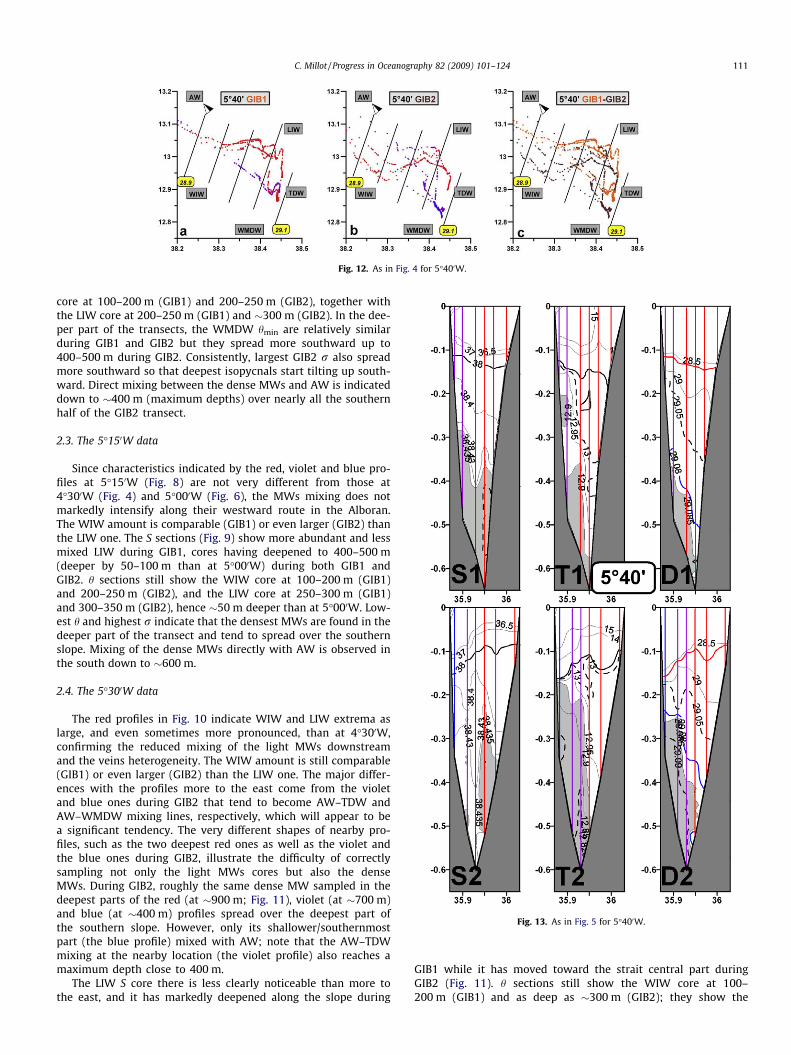
Fig. 12. As in Fig. 4 for 5�400W.

Fig. 13. As in Fig. 5 for 5�400W.


core at 100–200 m (GIB1) and 200–250 m (GIB2), together withthe LIW core at 200–250 m (GIB1) and �300 m (GIB2). In the dee-per part of the transects, the WMDW hmin are relatively similarduring GIB1 and GIB2 but they spread more southward up to400–500 m during GIB2. Consistently, largest GIB2 r also spreadmore southward so that deepest isopycnals start tilting up south-ward. Direct mixing between the dense MWs and AW is indicateddown to �400 m (maximum depths) over nearly all the southernhalf of the GIB2 transect.


Since characteristics indicated by the red, violet and blue pro-files at 5�150W (Fig. 8) are not very different from those at4�300W (Fig. 4) and 5�000W (Fig. 6), the MWs mixing does notmarkedly intensify along their westward route in the Alboran.The WIW amount is comparable (GIB1) or even larger (GIB2) thanthe LIW one. The S sections (Fig. 9) show more abundant and lessmixed LIW during GIB1, cores having deepened to 400–500 m(deeper by 50–100 m than at 5�000W) during both GIB1 andGIB2. h sections still show the WIW core at 100–200 m (GIB1)and 200–250 m (GIB2), and the LIW core at 250–300 m (GIB1)and 300–350 m (GIB2), hence �50 m deeper than at 5�000W. Low-est h and highest r indicate that the densest MWs are found in thedeeper part of the transect and tend to spread over the southernslope. Mixing of the dense MWs directly with AW is observed inthe south down to �600 m.


The red profiles in Fig. 10 indicate WIW and LIW extrema aslarge, and even sometimes more pronounced, than at 4�300W,confirming the reduced mixing of the light MWs downstreamand the veins heterogeneity. The WIW amount is still comparable(GIB1) or even larger (GIB2) than the LIW one. The major differ-ences with the profiles more to the east come from the violetand blue ones during GIB2 that tend to become AW–TDW andAW–WMDW mixing lines, respectively, which will appear to bea significant tendency. The very different shapes of nearby pro-files, such as the two deepest red ones as well as the violet andthe blue ones during GIB2, illustrate the difficulty of correctlysampling not only the light MWs cores but also the denseMWs. During GIB2, roughly the same dense MW sampled in thedeepest parts of the red (at �900 m; Fig. 11), violet (at �700 m)and blue (at �400 m) profiles spread over the deepest part ofthe southern slope. However, only its shallower/southernmostpart (the blue profile) mixed with AW; note that the AW–TDWmixing at the nearby location (the violet profile) also reaches amaximum depth close to 400 m.

The LIW S core there is less clearly noticeable than more tothe east, and it has markedly deepened along the slope during

GIB1 while it has moved toward the strait central part duringGIB2 (Fig. 11). h sections still show the WIW core at 100–200 m (GIB1) and as deep as �300 m (GIB2); they show the


LIW core at 200–300 m (GIB1) and �300 m (GIB2). Associatingboth the extrema amplitude and the relative areas occupiedby WIW and LIW with the relative amounts of the two waters,the GIB1 and GIB2 data clearly illustrate an interaction betweenthem along their westward route. During GIB1, the WIWamount is relatively low but WIW does not encounter majorchanges while the LIW amount is relatively large and LIWdeepens, probably due to increasing velocities. During GIB2,the WIW amount is relatively large and WIW deepens whilethe LIW is relatively low and LIW is found away from the slope.Clearly, the larger the light MW amount, the larger its west-ward velocity and its tendency to deepen, due to rotation,and to push away the MW below, but not modifying markedlythe MW above. During GIB1 and GIB2, lowest h and highest roccur in the south of this V-shaped passage where deep isolinestend to parallel the slope.


Approaching the sill (just �5 nm to the west), mixing intensifiesmarkedly and leads to a relatively complex situation (Fig. 12). Dur-ing GIB1, little amount of WIW is indicated on the available profilesdown to �100 m. Considering the amount and immersion of theWIW core more to the east, it might be that most WIW outflowsmore to the north. The four (out of six) red profiles show anAW–LIW mixing line while below, the LIW vein encountersmarked disturbances. During GIB2, three (out of six) red profilesindicate that the WIW amount is still relatively large and thatWIW hmin are still in the 12.90–12.95 �C range, so that WIW canclearly be an important component of the MWs outflow. DuringGIB1, two violet profiles were straighter than previously, indicatingan intensified AW–TDW mixing. During GIB2, none of the two vio-let profiles was as straight as at 5�300W while no violet profilessimilar to the 5�400W ones were observed at 5�300W. A similar re-mark concerns the blue GIB2 profile that is not as straight as (orstraighter than) at 5�300W; differentiating it from the violet pro-files was maintained as regard to continuity between the 5�300Wand 5�500W data. The S distribution (Fig. 13) shows during GIB1an LIW core still at 400–600 m, thus close to the deeper part ofthe strait there, and still along the slope while S values duringGIB2 are much lower and the core is still pushed away from theslope. The h distribution during GIB2 indicates a large data amountin the 12.95–13.00 �C range at 200–300 m close to the northernslope, so that WIW actually represented a significant part of theoutflow. The LIW hmax is more marked during GIB1. The lowest hvalues, associated with the largest r values, along the southernslope indicate both lower-TDW and WMDW, the latter duringGIB2 only.


Homogeneity of all profiles has increased, as expected 5 nmwest of the sill, but marked north–south differences are still indi-cated. To emphasize the continuity with those more to the east,h–S diagrams are first shown with the same scales (Fig. 14). Be-cause the diagrams there are mainly mixing lines between someMW and AW, they were no longer colored according to their shapebut according to the MW expected to be involved. Profiles involv-ing either WIW or LIW are red while those involving TDW andWMDW are violet and blue, respectively. We also found moreinteresting to display in 14c the LYNCH data instead of the GIB1–GIB2 comparison, all being compared later on. LYNCH transectswere performed twice, on both November 3 (LYNCH12) and 14(LYNCH34), at locations roughly similar to the #1 (south) to #5(north) GIB1 and GIB2 ones but the dramatic changes that occurredduring the campaign prevent from a priori coloring the profiles.

Among the seven GIB1 profiles (Fig. 14a), the most straight andmost southward one in the red group (#3) represents only AW–LIW mixing (rmax � 29.01 kg m�3) and does not indicate anyWIW. Other ones, in particular the northernmost #6–7, indicateAW–WIW mixing only. The WIW signature on #4–5 accounts forthe WIW importance even when in relatively low amount. The vio-let group (2 relatively close profiles, rmax � 29.03 kg m�3) indi-cates a similar AW–TDW mixing with few points near the #6–7lower part. Even though the AW–WIW and AW–TDW mixing linesare partly superimposed, it is clear that the outflow is separatedinto three juxtaposed ‘‘suboutflows” that have markedly differenth–S characteristics, maximum depth (see Fig. 17) and north–southlocation, the densest (respectively lightest) being the southern-most (respectively northernmost one). The rmax associated withTDW and LIW differ by only �0.02 kg m�3 and are larger by�0.1 kg m�3 than the WIW one.

During GIB2 (Fig. 14b), which was characterized upstream byrelatively large amounts of WIW vs. LIW and WMDW vs. TDW, aWMDW blue group (#1–2, rmax � 29.05 kg m�3) that is the south-ernmost one is differentiated from a TDW violet group (#3–4,rmax � 29.025 kg m�3). Profile #5/GIB2 is extremely interestingsince it shows a gap (28.911–28.945 kg m�3) and can thus be sep-arated in two. Extrema reached by its deeper part are just slightlylower than the #3/GIB1 ones and thus indicate LIW, which is con-sistent with LIW during GIB2 more mixed than during GIB1. Extre-ma reached by its lower part correspond to the #6/GIB1 ones,hence accounting for the WIW importance also during GIB2. TheGIB2 outflow was thus subdivided into four juxtaposed subout-flows, the interface between the WIW and LIW ones being inclinedand intersected by #5 (see comments below about #6/GIB2). Thermax associated with WMDW, TDW and LIW differ from each otherby only �0.03 kg m�3 and are larger by 0.1–0.15 kg m�3 than theWIW one.

The four LYNCH transects (Fig. 14c) illustrate the tremendouslylarge variability that can exist west of the sill just �10 days apart,mainly due to changes in the nature of AW (see Section 1.2.3). AllLYNCH12 green profiles were relatively similar, in terms of roughlocation and slope, while the LYNCH34 cyan ones can be separatedinto a southern group (#1–2–3) and a northern one (#3–4–5), #3belonging to one or the other group a few hours apart.

Comparing all diagrams in Fig. 14 allows two remarks. Withineach group, mixing lines can be similar with markedly differentrmax at markedly different depths (i.e. #1–2/GIB2; comparatively,#1–2/GIB1 reach less different depths). Since profiles nearlyreached the bottom, this information demonstrates that the subout-flows are continuously stratified, the actual overall rmax occurringat greatest depths. Differences in rmax between groups during onecampaign or for a group between the two campaigns can thus ap-pear unreliable. However, plotting all diagrams together supportsthe profiles characterization and grouping we made (Fig. 15a). Inparticular, note that (i) the WIW (pink) suboutflow is indicated by#6–7–(5)/GIB1 and #5–6/GIB2, (ii) the LIW (red) one by #3–4–(5)/GIB1 and #5/GIB2, (iii) the TDW (violet) one by four indiscern-ible points (#1–2/GIB1 and #3–4/GIB2), (iv) the WMDW (blue)one by #1–2/GIB2 only. Also note that associated rmax increasefrom north (WIW) to south (WMDW) while the associated h de-crease, and that the LYNCH grey dots concentrate around or tend to-ward GIB ones, which could allow coloring them accordingly.

The same h–S diagrams displayed over extended ranges(Fig. 16A for the MWs, Fig. 16B for AW) provide essential informa-tion and allow direct comparisons with the data downstream. First,all profiles in Fig. 16A are mixing lines between some AW andsome MW. During GIB1 (Fig. 16Aa), profiles #1–2 (violet) and#3–4 (red) indicate different MWs (TDW vs. LIW) in their densestpart and tend towards the same kind of AW while profiles #5–6–7(red, mainly associated with WIW) tend toward another kind of

Fig. 16. (A) Same as in Fig. 14 but for MWs wider ranges (same till 6�150W). Additional prTo better differentiate the profiles, dots are replaced by the profile #. Isopycnals are 0.1 kSame as in Fig. 16A but for wider ranges to represent both the MWs and AW (NACW an

Fig. 15. h–S diagrams at 5�500W (a, all plots in Fig. 14) and 6�050W (b, all plots inFig. 18) in reduced ranges to focus on the rmax values specified by dots that are pink(WIW), red (LIW), violet (TDW), blue (WMDW), grey (unspecified, LYNCH)) for GIB1(orange), GIB2 (brown), LYNCH12 (green) and LYNCH34 (cyan). (For interpretationof the references to colour in this figure legend, the reader is referred to the webversion of this article.)

Fig. 14. h–S diagrams at 5�500W for GIB1 (a), GIB2 (b) and LYNCH (c) with scales as in Fig. 4 (MWs acronyms are no more informative). Profiles numbers (GIB locations inFig. 17) from south to north are specified at the largest r value. Colors for (a) and (b) are as before (see Fig. 4). Color for (c) is green for transects 1,2 at the beginning (#2 onlyonce) and cyan for transects 3, 4 at the end (�10 days after, #1 only once). (For interpretation of the references to colour in this figure legend, the reader is referred to the webversion of this article.)


AW. Similarly, during GIB2 (Fig. 16Ab), profile #3 is different from#1–2 in their densest part (WMDW vs. TDW) and becomes similarto them in their less dense part. Profile #6/GIB2 is now indicatedand, due to both its similarities with the #5 upper part and itsnorthernmost location, it is red and associated with WIW, whichis consistent with the relatively large WIW–GIB2 amount up-stream. During LYNCH12, #1–2–3 and #4–5 form clearly differentgroups and the upper-part profiles tend to spread according totheir north–south location. During LYNCH34, the two groups ofprofiles due to the MWs (#1–2–3 vs. #4–5) tend to form onlyone group upward. Note the similarities between the two groupsof profiles during both GIB1 and GIB2 with either the LYNCH12or LYNCH34 ones.

Fig. 16B explains the upper-part profiles spreading indicated byFig. 16A. Both NACW and SAW occurred, the latter displaying sea-sonal variations between spring (GIB1) and fall (GIB2, LYNCH).However, nearly opposed situations were encountered since dur-

ofiles in the northern part of the GIB1 and GIB2 transects were out of range in Fig. 14.g m�3 apart. Profiles #2/LYNCH12 and #1/LYNCH34 were performed only once. (B)d SAW; see definitions in the text). Isopycnals are 1.0 kg m�3 apart.


ing GIB1, SAW was mainly in the south (#1–4) and NACW mainlyin the north (#5–7) while during GIB2, SAW was mainly in thenorth (#4–6) and NACW mainly in the south (#1–3). These varia-tions of the NACW vs. SAW distributions in both time and spacewere observed along the other transects during both GIB1 andGIB2, which guarantees their significance. Even though such spa-tial variations have never been mentioned and were unexpected,the temporal ones in the long-term (6 months apart for GIB) wereless dramatic than the LYNCH ones in the short-term (Fig. 16Bc).During LYNCH, only NACW was present at the beginning (green)while only SAW was present at the end (cyan) �10 days after. Asfor GIB1 and GIB2, the LYNCH variations were observed as far asin the eastern Alboran. The marked changes that occurred duringLYNCH in the composition of the MWs outflow east of the sill can-not be due to the changes in the distribution of NACW vs. SAW(Millot, 2008). Fig. 16Ac and Bc demonstrate that the wholeMWs outflow characteristics dramatically depend on the AW onesin the sill surroundings.

Fig. 17 shows that the two violet GIB1 profiles and the two blueGIB2 ones were roughly at the same place, as were (i) two red GIB1profiles and the two violet GIB2 ones, (ii) the red #5/GIB1 (mixtureof WIW and LIW) and #5/GIB2 (WIW above and LIW below).According to the available data, each of the four major MWs leadsto a suboutflow during GIB2 while no suboutflow can be associatedwith WMDW during GIB1, consistently will all data upstream. Thecharacteristics of the outflow can thus change dramatically at a gi-ven location/latitude, depending on the relative amounts of theMWs that, when present, are juxtaposed in the same way fromnorth to south and mix individually with AW. The outflow is sub-

Fig. 17. Same as in Fig. 5 for 5�500W. r = 27.0 kg m�3 is violet and r = 29.0 kg m�3 is cyareferred to the web version of this article.)

divided, as soon as 5�500W, into a series of suboutflows that areassociated with the MWs indicated upstream and are located sideby side, the densest being the southernmost one. The southern-most profiles indicate the densest MWs along the lower part ofthe slope during both GIB1 and GIB2 since r � 29.0 kg m�3 (repre-sentative of the MWs) tilts up southward while r � 28.0 kg m�3

(the AW–MWs interface there) tilts up northward.


The five profiles performed at 6�050W during each campaignthat were deep enough to possibly sample the MWs are displayedin both Figs. 18 and 15b, which allows comparisons with those at5�500W in Figs. 16A and 15a. During GIB1, profile #1 is colored inviolet and red since it is slightly but significantly different fromthe red group #2–3 that clearly indicates LIW while #4 indicatesWIW. As at 5�500W and further upstream, no profile can be associ-ated with WMDW. During GIB2, the associations #1-WMDW (notethe undulated shape), #2–3-TDW and #4-WIW are clear, especiallyfrom Fig. 15b. No profile indicates LIW, which is consistent withthe low amount of mixed LIW at 5�500W and further upstream;as suggested by data downstream, the small LIW suboutflow wasprobably missed there. Similarly, and as demonstrated by the dif-ferences between #2 and #3 that both sampled the TDW subout-flow with inaccuracies similar to those already noticed at 5�500Wfor #1–2/GIB2 (#3 is markedly deeper than #2), the WMDW sub-outflow was not accurately sampled by profile #1 and must clearlybe denser (in fact, the densest). Also note that #1/GIB1 did not cor-rectly sample the TDW suboutflow and that there is a relatively

n. (For interpretation of the references to colour in this figure legend, the reader is


large spacing between #1 and #2 during GIB2, which might indi-cate that the sampling interval there was not small enough. DuringLYNCH12, #2–3 indicate mixed LIW and #4 mixed WIW while dur-ing LYNCH34, consistent with the data at 5�500W, #2 (performed intriplicate) once indicates WMDW, all other profiles indicatingeither more mixed WMDW or LIW.

The large spatial variability during all campaigns and the largetemporal variability indicated by the LYNCH data illustrate the dif-ficulty of correctly sampling there. Additionally, separating AW–MWs mixing lines for two different MWs depends on the natureof AW. For instance, NACW–TDW and NACW–WMDW lines areseparated while the SAW–TDW and SAW–WMDW ones are super-posed (the reverse occurs for WIW and LIW). It is thus obvious thata suboutflow can be either missed or mistaken with another one,and that the extrema are clearly depth dependent (those indicatedby a unique-profile being unreliable). However, let us assume thatthe extrema associated with all the MWs during both GIB cam-paigns (except WMDW not correctly sampled during GIB2) arerepresentative of the actual ones. Even though the outflow compo-sition during GIB1 (WIW, LIW, TDW, no WMDW) and GIB2 (WIW,little LIW, TDW, WMDW) was markedly different, each of the MWswas characterized by extrema that were shifted from 5�500W to6�050W along the mixing lines with AW, which supports the color-ing. The rmax shift is �0.1 kg m�3 for TDW and LIW, �0.2 kg m�3

for WIW. Note that Drmax between the two densest suboutflows(TDW and LIW during GIB1, WMDW and TDW during GIB2) differby 0.1–0.2 kg m�3 while the range for all MWs is Dr = 0.2–0.3 kg m�3 (associated with Dh = 0.2–0.3 �C, DS = 0.2–0.3). Rangesat a given location for the densest suboutflows (between TDW–GIB1 and WMDW–GIB2 or between LIW–GIB1 and TDW–GIB2)are about half these values. Even though characterizing a priori agiven suboutflow by specific hydrographic values correspondingto a given MW is impossible, the southernmost (respectivelynorthernmost) suboutflow expected to be actually the denser(lighter) might always be relatively cool (warm), compared tothe neighboring ones, which would correspond to the observationsabout the veins downstream. Assuming a homogeneous outflowwas certainly hypothesized for convenience but has never beensupported by any data set, and no data sets is more detailed orcan be considered as more reliable than the GE one, even if stillnot accurate enough.

GIB1 and GIB2 are not very informative about the densest/southernmost suboutflow (Fig. 18) that is indicated by only one(#1) non-very representative profile. Overall largest densities werecertainly missed: during GIB1, they were due to TDW and thusprobably south of #1 since #1 is still relatively similar to #2–3 thatindicate LIW; during GIB2, they were due to WMDW and thusprobably between #1 and #2 since corresponding depth must begreater than at #1. During both LYNCH12 and LYNCH34, the dens-est/southernmost suboutflow is indicated by profiles #2 mainlysince #1 is either out of range or indicative or more mixed waterwhile #3–4 indicate either the same MW more mixed or anotherMW. We thus expect this suboutflow and other ones as well tohave moved toward the central part of the transect, which is some-how supported by the sections (Fig. 19). Apart from the NACWintrusion at 200–250 m during GIB2 (leading to the undulationson #1, Fig. 18), and even though overall maximum densities asso-ciated with the southernmost/densest suboutflow were certainlymissed, the deep isopycnals tend to flatten (GIB1) or even to tiltup northward (GIB2).


Among the four/eight GIB1/GIB2 profiles (Fig. 20), only two/three of the profiles sampled the outflow now found in the lowerpart of the northern/Iberian continental slope, which confirms

the displacement of the densest MWs from the southern slope(�5�500W) to the central part of the strait (�6�050W) and finallyto the northern slope (�6�150W). Such a limited number of profilesdoes not allow statistically significant results but they provide ex-tremely valuable information. Since the Smax found at 400–600 mnear 6�300W is S � 37 (Borenäs et al., 2002), we focus on larger val-ues. h–S diagrams (Fig. 21) are no longer straight mixing lines anddisplay marked undulations. These major changes prevent coloringthe profiles as done upstream but, more interestingly, several com-ments support coloration by undulation.

A mid-depth undulation such as the bump identified by a con-tinuous line on the #6/GIB2 h–S diagram (Fig. 21b) indicates h andS relative maxima. This bump’s general shape is similar to that ofany diagram displaying LIW in the sea or the whole outflow inthe ocean so that it characterizes an intermediate vein of relativelywarm salty water. Other mid-depth bumps that do not have rela-tive maxima depict a more mixed vein, or at least intrusions, ofMWs into AW. Successive bumps on a given diagram thus indicateoverlying veins or intrusions that are supposed contiguous. Thelowest parts of the #3/GIB1 and #5–6–7/GIB2 diagrams are mark-edly bended and represent the upper part of such bumps. Becauseprofiles covered nearly all the water column, these half-bumpsindicate actual veins still flowing over the bottom.

We assume that (i) the suboutflows upstream (at 5�500W(Fig. 16A) and 6�050W (Fig. 18)), which are consistent with theMWs amounts east of the sill, cascade individually and lead to spe-cific veins at 6�150W, (ii) all significant suboutflows upstream andveins at 6�150W were sampled so that each MW presence/absenceis consistent in the whole study area, (iii) the suboutflows andveins rmax are not accurately defined, in particular with only oneprofile, and the densest suboutflow (respectively vein) is thesouthernmost (respectively deepest) one, (iv) veins flow alongthe northern slope at 6�150W, as expected for any density current(Fig. 20), (v) when sampling a warm salty vein with profilesapproaching its core, all characteristics (h, S and r regularly in-crease, so that links exist between bumps on neighboring profiles(Fig. 21). The quite satisfying coloration we came with is: WIW(pink) during GIB1 and GIB2, LIW (red) mainly during GIB1 andboth mixed and in small amount during GIB2, TDW (violet) duringboth GIB2 and GIB1, WMDW (blue) during GIB2 only. When com-paring GIB1 and GIB2, a major remark concerns the TDW rmax.During GIB1, TDW is the densest vein and its rmax reduces onlyslightly (by �0.2 kg m�3) from 5�500W (where it is well defined)to 6�150W, roughly as much as the WMDW rmax during GIB2(reducing�0.25 kg m�3). During GIB2, TDW is no more the densestvein and its rmax reducing is larger (by �0.5 kg m�3). A similar re-mark concerns the LIW rmax that reduces only by �0.5 kg m�3

when unmixed and in large amount (GIB1) and by �0.7 kg m�3

when mixed and in small amount (GIB2). The WIW rmax reducedby larger amounts. Overall and as expected, the mixing of a veinwith AW is inversely proportional to its depth an amount: thegreater the depth and amount, the lower its rmax reducing.

The colored bars in Fig. 20 confirm these hypotheses since thepink, red, violet and blue layers have realistic thicknesses andmean depths on the various profiles during both GIB1 and GIB2.The non-occurrence of any red-LIW bump on #4/GIB1 that wouldbe expected from the #3 bump leads to a relatively thick pink layerthere, which might be due to small-scale heterogeneity. The #7/GIB2 red-LIW half-bump is not retrieved on #5–6, which is consis-tent with the LIW/GIB2 small amount. Quite surprisingly, bothWIW and TDW that were almost never mentioned in currentthoughts (Section 1.1) represented large percentages of the out-flow during both GIB1 and GIB2. Quite surprisingly too, LIW andWMDW that are currently thought as being the sole componentsof the outflow can represent a low percentage (LIW during GIB2)or be absent (WMDW during GIB1).

Fig. 19. As in Fig. 5 for 6�050W. Densities >r = 28.5 kg m�3 (cyan) are in grey, r = 28.75 kg m�3 is thick, r = 27.0 kg m�3 is violet. (For interpretation of the references to colourin this figure legend, the reader is referred to the web version of this article.)

Fig. 18. Same as in Fig. 16A for 6�050W.


Fig. 21 shows that the two densest veins rmax (GIB1: TDW andLIW, GIB2: WMDW and TDW) differ by a similarDrmax � 0.3 kg m�3 even though the GIB1-rmax are slightly largerthan the GIB2-rmax ones. Since this difference at 6�150W corre-

sponds to those reported 100–200 km downstream when the veinsno longer cascade and are characterized by rmax lower by�1.0 kg m�3, it might be that the densest veins similarly mixdownstream. Even though the densest veins correspond to differ-

Fig. 20. As in Fig. 5 for 6�150W and specific isolines. S = 36.0 (dashed) emphasizes the AW Smin, S = 37.0 (thick) represents the AW–MWs interface, S > 37.5 (grey) representsunmixed MWs, the largest isoline value is S = 38.0. In T1 and T2, h < 13.0 �C (dashed) are in lattice grey, h = 13.185 �C (thick) locates the vein on the bottom at #6/GIB2. In D1and D2, r = 27.0 kg m�3 (violet) represents the AW–MWs interface, r > 28.0 kg m�3 (cyan) are in grey, the largest isoline value is r = 28.5 kg m�3. (For interpretation of thereferences to colour in this figure legend, the reader is referred to the web version of this article.)

Fig. 21. h–S diagrams at 6�150W for GIB1 (a), GIB2 (b) and both (c) showing WIW (pink), LIW (red), TDW (violet) and WMDW (blue). Isopycnals are 0.1 kg m�3 apart. (Forinterpretation of the references to colour in this figure legend, the reader is referred to the web version of this article.)


ent MWs, the deep vein is �90-m thick and the intermediate one is50-m thick during both GIB1 and GIB2. Furthermore the two veinshave roughly similar h and S even though associated with differentMWs, this clearly explains the permanency of the veins character-istics currently assumed. The third upper vein described in the lit-erature is the WIW vein (possibly confused with the LIW one asduring GIB2), it is consistently the warmest, and Drmax are withinthe reported ranges.

During GIB1, the S section (Fig. 20) also shows the AW Smin

(<36.0) spreading over the whole transect. The low h values atthe base of the southern/Moroccan slope indicate NACW and somerelative maxima over the northern slope indicate heterogeneitiesdue to the AW–MWs interactions, while all densest isopycnalsare tilting up northward. During GIB2, the AW Smin is less spreadand the MWs Smax values are slightly lower. The h section still indi-cates NACW, which might be a frequent (if not permanent) feature,together with numerous heterogeneities.

3. The 80-m and 270-m time series analysis

The HCP data are presented in Section 1.2. Major results con-cerning the composition and spatio-temporal variability of theMWs outflow are displayed with a series of h–S diagrams allowingcomparisons between the data at both locations over time. Thenumber of diagrams/periods (six for the 2003–2007 time series)is a compromise allowing a relatively large number of diverse sit-uations to be differentiated (Fig. 22). The selection made from a vi-sual analysis only is validated by the large variability. As expectedfrom the GE transects analysis, only LIW, TDW and WMDW (notWIW) were found at the sill and/or on the Moroccan shelf, so thatonly the upper part (38.44–38.52) of the MWs S-range is of inter-est. Similarly, the MWs h-range is reduced to 12.92–13.25 �C since(i) the lowest h are generally located along the Moroccan slope, i.e.neither at the sill nor on the shelf, (ii) marked changes have oc-curred in the sea, and/or (iii) the oceanic trends are generally posi-

Fig. 22. h–S diagrams from the 2003–2007 (Julian days #12–1536) time series at 270 and 80 m and the six periods (a–f) specified in the text. The whole time series are plottedwith light grey dots (270 m) and dark grey ones (80 m), together with r = 29.05 and 29.10 kg m�3. The colors significance and the date intervals for each of the periods arespecified in both the text and the figure. Dashed lines connect consecutive data and provide information about mixing. (For interpretation of the references to colour in thisfigure legend, the reader is referred to the web version of this article.)


tive. Because TDW (i) cannot be clearly differentiated from LIWabove and WMDW below, (ii) is not characterized by any extre-mum and (iii) is often encountered at 270 m, terms such has lower,central and upper parts of a unique TDW-range (on such diagrams)are used to deal, as precisely as possible, with TDW being more orless dense (over time). Both NACW and SAW were measured at80 m (not shown). Days are Julian days from January 1st, 2003,and successive periods are separated by 20 days to avoid confusingsituations.

Days #12–450 (Fig. 22a). At 270 m, relatively high r (29.095–29.100 kg m�3) and S, associated with either TDW or LIW, occurredduring this period (blue points). This is particularly obvious whenTDW unmixed with either AW or any other MW was continuouslyobserved during the three first days (gold), so that more extreme

situations probably occurred before. Even though this was duringneaps (Section 4.1), this suggests a relatively intense TDW outflow.As shown by several dashed lines nearly parallel to isopycnals>29.08 kg m�3 for central-TDW (also for upper-TDW and LIW, un-clear in the figure), MWs unmixed with AW were often observedduring several consecutive records. However, mixing with AW(lines nearly perpendicular to the isopycnals) due to the internaltide was generally significant at the sill (even when the mosthomogeneous LIW outflowed), hence for the whole MWs outflow.No points indicative of either lower-TDW or WMDW were ob-served during this 440-day period. At 80 m, points (cyan) werevery rare (they were never so rare thereafter) and they all indicatedintense mixing with AW. Compared to points at 270 m, points at80 m were generally more shifted toward the lower left part of

Fig. 23. Density (r) data measured (grey dots) and selected with the sd criterion(cyan dots) for the MWs at 270 m from January 12 to July 27, 2003, together withthe daily moving averages of the measured density (blue curve) and speed (V)toward 225 �T (black curve); tidal amplitude at Tarifa (maxima �80 cm) is fromJulio Candela (personal communication). (For interpretation of the references tocolour in this figure legend, the reader is referred to the web version of this article.)


the diagram, which is a 80-m vs. 270-m difference often encoun-tered hereafter. Links exist between the MWs found at both loca-tions and between the facts that large densities occurred at thesill when few MWs occurred on the shelf.

Days #470–670 (Fig. 22b). At 270 m (green), either LIW orupper- and central-TDW were still encountered, sometimes notmixed with AW during several consecutive records but now withmarkedly lower S. Values at 80 m (yellow) were sometimes denserthan at 270 m, still associated with either LIW or TDW but in lessmixed conditions. Compared to those during the twice-longer per-iod #1, 80-m points were more numerous. But similarly, 80-mpoints were more shifted towards cooler and fresher waters than270-m ones. Points signed mainly TDW (upper, central and lower)at 80 m, and mainly LIW and upper + central (lower is rare) TDW at270 m. Links exist between relatively light MWs at the sill andmuch denser MWs on the shelf.

Days #690–790 (Fig. 22c). Only LIW, more or less mixed withAW, was found at 270 m (red) with h and S values significantlylower than during the two previous periods while only LIW (and/or upper-TDW) more mixed with AW was found at 80 m (pink).Since the densest waters (lower-TDW and WMDW), generally lo-cated along the Moroccan slope, were not sampled at any place,they were either absent or present in a limited amount. Such a sit-uation, with no (observed) or little (possibly outflowing) denseMWs from either the eastern basin (TDW) or the western one(WMDW), has never been encountered since.

Days #810–870 (Fig. 22d). Dramatic changes have now oc-curred at both 270 m (brown) and 80 m (violet). At 270 m, upper-to lower-TDW and rare WMDW were found in relatively unmixedconditions, as indicated by the low number of AW–TDW and AW–WMDW mixing lines as compared to the number of lines roughlyparallel to the isopycnals (clear at least for upper-TDW). At 80 m,mainly WMDW and lower- to central-TDW were found in moremixed (less salty at least) conditions. From the beginning of theexperiment, it is the first time that no LIW was recorded, that low-er-TDW was relatively frequent, and that WMDW was present atboth locations, which indicates an outflow mainly of western ori-gin. The mainly eastern origin has lasted for �800 days at least,probably more since the situation at the beginning of the experi-ment was relatively extreme. Changes about WMDW mainly,which were observed from this mid March to mid May 2005 periodand later on, could be due to the large amount of WMDW formedduring that winter in the Provençal subbasin (Fuda et al., 2007).

Days #890–1140 (Fig. 22e). The situation markedly changedagain since now all three MWs (LIW, TDW and WMDW) were mea-sured at both 270 m (dark green) and 80 m (light green). They weremixed either together (clear for lower-TDW and WMDW) or withAW at 270 m while there were mixed only with AW at 80 m. Char-acteristics of both LIW and upper-TDW at 270 m were less extreme(warm and salty) than during period #1 (and #6), but togetherwith the characteristics of the lower-TDW, they were more pro-nounced (saltier at least) than during periods #2–3–4. Most ofthe MWs at 80 m can be considered as a mixture of those at270 m. But as during period #4, the coolest values sign WMDWnever found at 270 m.

Days #1160–1536 (Fig. 22f). Period #6 at 270 m (brown) ischaracterized by upper-TDW similar to that encountered duringperiod #1, and by central- to lower-TDW more abundant and evendenser (<29.104 kg m�3) than during period #1, together with lessLIW and more WMDW. At 80 m (orange), mainly WMDW, central-and lower-TDW occurred. Note that, overall, the less mixed (i.e.densest) central- to lower-TDW (at 270 m) and WMDW (at 80 m)were observed simultaneously during this period.

Days #1536–1760 (not shown). Even though the CTDs usedfrom March 2007 to October 2008 are not post-calibrated yet,the continuity of the time series from before to after day #1556 ac-

counts for the accuracy of the data shown in Fig. 22f in particular.During this 220-day period, data at 270 m suggest the occurrenceof upper- to lower-TDW as in Fig. 22d and e while data at 80 min the displayed ranges are even more rare than in Fig. 22a. Assum-ing corrections similar to those previously made would not dra-matically change these features, which would illustrate anothersituation never encountered up to now.

4. Discussion

Complementary analyses provide a more detailed description ofthe MWs outflow. A current meter at 270 m allows specifyingsome aspects of its short-term variability (Section 4.1). Statisticson the 4-year long time series at 270 m provide significant infor-mation on its seasonal variability (Section 4.2). A synthesis of theresults obtained with the time series at both 80 m and 270 m al-lows specifying its long-term variability (Section 4.3). The low mix-ing of the light MWs up to the sill and the continuous evolution ofthe outflow structure meanwhile allow simple computations thatexplain some of the current thoughts and quantify the GIB1 vs.GIB2 differences (Section 4.4). Finally, a new concept of the MWsoutflow is proposed with the major aim to motivate as many aspossible further studies (Section 4.5).

4.1. Short-term variability

A RCM9 Aanderra current meter set at 270 m worked for�6.5 months in early 2003. One-hour velocities (V), all measuredin the 225-45 T direction, ranged from +190 cm s�1 (towards225 T) to �135 cm s�1 due to the large semi-diurnal variability.The daily (25-h) moving average of V (Fig. 23) displays a well-known (Candela et al., 1990) fortnightly signal locked on the tideat Tarifa with maximum deep-sill current during neaps, which isconsistent with the largest outflow at springs (Bryden et al.,1994; Vargas et al., 2006). The CTD data allow plotting r as greyand cyan dots, the latter resulting from a selection based on a cri-terion explained in Section 4.2. The S (38.32–38.51) and h (13.0–13.25 �C) curves are almost identical (S) or similar (h, descendingaxis) to the r one.


The r and V curves are in phase, the densest less-mixed MWsrapidly outflowing during neaps. During days #12–14, the largestr measured at the beginning of the experiment (Fig. 22a, goldpoints) lead to daily averages >29.096 kg m�3, and V was the larg-est ever measured too (�120 cm s�1 on day #13, 4-day average�100 cm s�1). Such a rapid outflow of dense MWs, even if maybeof limited vertical extent, probably represented a significant partof the whole outflow. Near day #80, the lowest r (�28.90 kg m�3)were associated with the lowest V (�25 cm s�1), such a slow out-flow of relatively light MWs probably not significantly modifyingthe whole outflow. Note that no r values were selected at this timeby the criterion. The huge fortnightly variability of the hydro-graphic parameters at the sill is obviously larger at shallowerdepths across the whole strait, which leads to a significant signalall along the outflow downstream that has never been looked for.

During this 6.5-month period, and even though variations in-duced on both r and V by the tide and other unknown or unre-solved forcings are relatively large, r data selected for the MWswere still in a relatively high range (29.05–29.10 kg m�3) whilethe overall mean V = 66 cm/s, which is a relatively large value ascompared to other published ones (e.g. Bryden et al., 1994). Thesefeatures are used to explain the differences we make thereafter be-tween an overflow and an outflow.

4.2. Seasonal variability

We do not expect any seasonal variability of the MWs outflowup to the sill (see Section 1.2), contrary to what occurs for theAW inflow (Millot, 2007). The 4-year long and 1-h time series(36,600 data) at 270 m, where points representative of the MWsare more numerous and less dependent on tidal mixing than at80 m, allows some objective and probably significant analysis.We address the seasonal variability first with a standard fittingof the 270-m time series, then with a method we are elaboratingand already applied to the 80-m one (Millot, 2007).

The curves in Fig. 24 represent the polynomial fits to sets of h, Sand r data selected in different ways for each of the four yearsstarting in January 2003. The polynomial degree (three) and 1-yearperiods are a priori able to detect any almost regular/sinusoidalsignal. The black curves are for all points in the MWs ranges usedfor Fig. 24 (38.44–38.52, 12.90–13.25 �C, 29.06–29.10 kg m�3),which selects numerous points indicative of AW–MWs mixing.The red curves are from points selected according to a tidal crite-rion, i.e. retaining only the hmin, Smax and rmax for each consecutivesemi-diurnal (12-h) period, which gives 3050 regularly distributedpoints that can still be influenced by AW–MWs mixing, particu-larly during springs. The blue curves are from the sets of 3050points selected according to a standard deviation (sd) criterion. Asd being computed over some (three) consecutive data and associ-

Fig. 24. Polynomial (degree 3) fits from the S (a), h (b), and r (c) data at 270 m during yealine). Black lines correspond to the whole set of data measured in the MWs displayed ran(Smax, hmin and rmax over 12-h successive intervals) while blue lines correspond to the saminterpretation of the references to colour in this figure legend, the reader is referred to

ated with the central one, only the data for which the sd is lowerthan some arbitrarily-fixed maximum value are retained, which al-lows selecting data representative of the most homogeneous MWsat one’s convenience.

For all three parameters, relatively similar ‘‘seasonal” variationsare observed during years #1–2 on one side, and during years #3–4on the other side. The former are very different, if not opposed, tothe latter. The corrected time series ending in March 2007, we didthe same analysis over four years with a 2-month shift, as well asover three years with a 6-month shift. We also conducted similaranalyses with the 80-m time series. All three time-intervals leadto the same conclusion at both 80 and 270 m, i.e. that S, h and rfor the MWs do not show any kind of seasonal variability.

Interesting information is provided by the distribution withtime of the data selected with the sd criterion. Relatively unmixedAW and MWs being defined by specific ranges (AW: S < 37,h > 13.5 �C; MWs: S > 38.4, h < 13.25 �C), frequencies of occurrencefor both waters are about 67% and 8% at 80 m, 0% and 92% at270 m. One can then consider, for both AW and the MWs, the dis-tribution with time (1-month averages) of the most homogeneousdata (i.e. having the lowest sd; we arbitrarily chose the 30% mosthomogeneous) in S, h and r, as well as of the so-called triplets thatcorrespond to the sets of data selected at the same time for allthree parameters. Considering other realistic ranges for eitherAW or the MWs, and/or computing the sd over two or four consec-utive values, and/or selecting slightly more (i.e. 40%) or less (i.e.20%) homogeneous data does not basically change the results dis-played in Fig. 25.

For the AW at 80 m (Fig. 25a), the distribution with time of the7320 data (30% of 67% of the 36,600 available data) selected for allthree parameters, and of the 4437 triplets that result from thisselection, displays a marked seasonal variability. Most homoge-neous data and numerous triplets occur during the second half ofFebruary (dashed lines). This is linked to the meteorological condi-tions in the study area and the wintertime mixing of any surfacelayer that leads to the S(AW) seasonal variability (Millot, 2007).As confirmed by a sharper selection (i.e. less than 30%) the interan-nual variability is significant too.

For the MWs at 80 m (Fig. 25b), the distribution of the 915 data(30% of 8%) and of the 695 triplets displays marked seasonal andinterannual variabilities. The seasonal variability appears as a peakoccurring well after the AW peak, i.e. when AW starts re-stratifyingand no longer mixes with the MWs as during the winter, allowingunmixed MWs to be often sampled. Then, seasonal stratificationreaches the MWs layer and lowers the number of homogeneousdata. The interannual variability mainly shows the non-occurrencein 2003 and the rare occurrence in early 2004 of the MWs(Fig. 22a). The similarity between the curves for the three param-eters yields to a relatively large number of triplets not related to

r #1 (full line), #2 (large dashed line), #3 (small dashed line) and #4 (dashed dottedges. Red lines correspond to regularly distributed data selected with a tidal criterion

e amount of data selected with the sd criterion (hence irregularly distributed). (Forthe web version of this article.)

Fig. 25. Monthly moving averages of the number of S (blue), h (red) and r (green) data selected with the sd criterion (30%) for AW at 80 m (a), the MWs at 80 m (b) and theMWs at 270 m (c); corresponding triplets are in black. The more homogeneous AW is encountered in the second half of February (dashed lines). See text and Millot (2007) fordetails. (For interpretation of the references to colour in this figure legend, the reader is referred to the web version of this article.)


some specific character of the MWs there. Rather, the scarcity ofunmixed MWs leads to select data influenced by mixing withAW, hence distributed, in a h–S diagram, along lines roughly per-pendicular to the isopycnals. Standard deviations for all threeparameters are thus proportional, leading data to be selected atthe same time. The large interannual variability prevents from evi-dencing the seasonal variability with a polynomial fit.

For the MWs at 270 m (Fig. 25c), the distribution of the 10980data (30% of 92%) and of the 5651 triplets displays a marked inter-annual variability (see Section 4.3) with no seasonal variability.This is obviously representative of most of the outflow approachingthe sill. However, tidal mixing with AW at the sill is intense (e.g.Figs. 22 and 23), characteristics of the outflow downstream fromthe sill markedly depend on AW in the sill surroundings (e.g.Fig. 18c) and AW displays a marked seasonal variability(Fig. 25a). Therefore, the MWs outflow in the ocean should displaya seasonal variability imposed, via mixing with AW in the sill sur-roundings, by the meteorological forcing.

4.3. Long-term variability

Fig. 25c also indicates that the three parameters at 270 m havenon-related variations and relatively similar and constant meanlevels in 2003–2004 while they have larger and sometimes moresimilar variations with different levels in 2005–2006. The MWsin 2003–2004 were more homogeneous in S and h than in r while,in 2005–2006, they were more homogeneous in r than in S and h,which is related to the general shape of the h–S diagrams (Fig. 22)that were more aligned with the isopycnals during the second halfof the experiment. The large number of homogeneous h at the endof 2004 corresponds to period #3 with only LIW (Fig. 22c). Thesimultaneity of some 270-m peaks in 2005 might be fortuitoussince they are not simultaneous in 2006.

Considering the LIW and upper-TDW vs. WIW amounts, as wellas the lower-TDW vs. WMDW ones, the GE data show that the out-flow can be more of eastern (GIB1) or western (GIB2) origin. Con-sistently, blue profiles (Table 1) were never observed during GIB1while observed on all transects during GIB2. Both campaigns alsoshow that, in the sill surroundings, the MWs are more juxtaposedthan superposed, the denser further south, and that all MWs mixmore with AW than together. Finally, the light–dense MWs inter-face (r = 29.08 kg m�3, Fig. 3) markedly tilts east of the sill, up tobeing nearly parallel to the southern continental slope, during bothGIB1 and GIB2. Such information about the outflow long-term vari-ations and cross–strait distribution currently inferred from CTDprofiles is fully consistent with that inferred from the less standardCTD time series.

Before comparing the six periods defined for the 2003–2007HCP experiment (Fig. 22), some points must be specified. Time ser-

ies at 80 m on the Moroccan shelf and at 270 m near Camarinal SillSouth do not generally indicate the densest MWs that are expected(from e.g. the GE data) to be at 200–300 m along the Moroccanslope. Such time series do not provide information about WIW thatalways outflows more to the north at shallower depths. The LIW Sand h overall maxima in 2003–2007 at 270 m and 5�450W (>38.51,>13.15 �C) were encountered �20 years ago in the western Alboranbut never expected to be measured at the sill (Millot et al., 2006). A1984 one-week time series at the sill (294 m; Pettigrew, 1989), i.e.close to our 270-m site, regularly indicated h < 12.9 �C, hence rela-tively unmixed WMDW, while we measured only �100 values outof �36600 in a higher range of 12.92–12.95 �C and only during thesecond half of the experiment.

Main characteristics during period #1 (�440 days, Fig. 22a) arethe occurrence of relatively large densities at 270 m associatedwith TDW (not WMDW) and the scarcity of points at 80 m mainlyshowing mixed TDW (not WMDW). This makes unlikely the out-flow of a significant amount of WMDW along the slope in between.When considering the large speeds at 270 m, we expect (withoutany proof) the isopycnals to have been either horizontal or tiltingup northward. Such a situation illustrates what we call anoverflow.

An almost opposite situation occurred during period #2(�200 days, Fig. 22b) with relatively low densities at 270 m, asso-ciated with either LIW or TDW, and relatively numerous points at80 m sometimes indicating either LIW or TDW denser than at270 m. There is little chance of finding a WMDW outflow in be-tween. However, denser TDW was certainly outflowing along theslope since AW–MWs mixing is lower there than on the shelf. Sucha situation indicating a relatively large tilting up of the MWs iso-pycnals southward is the most extreme we encountered.

Another extreme situation occurred during period #3(�100 days, Fig. 22c) with only relatively mixed LIW at both 270and 80 m, hence probably leaving no place in between for someTDW or WMDW outflow. One can think either that a core of lessmixed LIW is outflowing more to the north, making LIW the dom-inant component of the outflow, or that a relatively large amountof WIW is outflowing too, hence pushing the LIW core away fromthe northern slope, as during GIB2.

Dramatic changes then occurred since no LIW at all was ob-served at either 270 or 80 m during period #4 (�60 days,Fig. 22d). Instead, relatively unmixed, although relatively light,TDW was observed at 270 m while waters at 80 m were either sim-ilar, even if more mixed, to those at 270 m or markedly differentindicating for the first time the occurrence of mixed WMDW there,and hence the possible occurrence of less mixed WMDW along theslope in between. During period #5 (�250 days, Fig. 22e), similarcomments can be made about TDW and WMDW at both 270 and80 m. But LIW was also often encountered at both sites in more


or less mixed conditions. Denser WMDW might have outflownalong the southern slope. During period #6 (�380 days, Fig. 22f)the LIW occurrence markedly reduced at 270 m and completelydisappeared at 80 m. The overall densest TDW and maybesome WMDW were encountered at 270 m while the overallless-mixed WMDW was observed at 80 m, hence suggesting thatdenser WMDW were significantly outflowing in between.

The alternation of a MWs outflow mainly originated from eitherthe western basin or the eastern one as suggested by the GE pro-files is thus definitely demonstrated by the HCP time series that,additionally, document the large variability in all MWs amounts.Moored CTDs, possibly complemented by ship-handled CTDs oper-ated along transects as often as possible, are clearly efficient, reli-able and relatively simple instruments that are suitable formonitoring strategies and can provide significant informationabout such an outflow composition and variability in the long-term.

4.4. A two-layer approximation up to the sill

This subsection aims at checking, with relatively crude compu-tations from the GE data, if differentiating light vs. dense (insteadof intermediate vs. deep) MWs, can help explaining some of thecurrent thoughts (such as the 90% LIW and 10% WMDW). Anotheraim is to help us better describing how a MW such as WMDW canreach the sill depth, hence to try improving our own understandingof the whole sea functioning.

The GIB data set indicates that, from east to west in the Alboranup to the sill, the mixing of all MWs does not especially increasewhile all associated isopycnals more and more tilt up southward.Close to the sill, let’s say from �5�150W to �5�400W, it can be easilyassumed that both the light MWs (WIW, LIW, upper-TDW) and thedense MWs (lower-TDW, WMDW) circulate significantly all acrossthe strait, even if more or less homogeneously. More to the east, i.e.from �4�300W to �5�000W, this is expectedly not the case since,according to our personal thoughts, dense MWs are quite motion-less while, according to our data analysis, they can be found justbelow AW in the south. The thermal wind equations for two homo-geneous layers can thus be used to check if assuming an outflowcomposed of two (sets of) MWs as done by previous authors is sup-ported by the GE data or not. When characterizing the light vs.dense MWs by mean values of density (qL vs. qD), speed (VL vs.VD) and amount, i.e. section area (AL vs. AD), the slope of their inter-face is:

ILD ¼ f=g=ðqD � qLÞðqDVD � qLVLÞ

with f the Coriolis parameter (10�4 s�1) and g gravity (10 m s�2),ILD < 0 indicating a tilting up southward. These mean values mustalso satisfy the relationship:

Table 2The slope of the light–dense MWs interface ILD for the GIB1 and GIB2 transects east of thminimum immersion (Zmin), vertical range (DZ), width (Y) and numerical value. The AL andinterface identified with r = 28.75 kg m�3. VL, VD, QL and QD are computed as specified in

ILD (Zmin, DZ, Y) m/m/nm (10�3) AL 106 m2 AD 1

4�300 GIB1 360/60/66.0 (0.5) 35.5 71.0GIB2 380/180/66.0 (1.4) 40.0 62.2

5�000 GIB1 300/120/45.6 (1.4) 22.8 17.9GIB2 300/120/45.6 (1.4) 19.8 17.9

5�150 GIB1 300/200/15.0 (7) 12.9 6.3GIB2 320/120/15.0 (4) 11.8 7.0

5�300 GIB1 360/240/4.8 (27) 5.1 0.8GIB2 180/320/5.4 (32) 2.7 1.8

5�400 GIB1 320/180/3.0 (32) 3.2 0.4GIB2 220/160/5.4 (16) 2.3 1.3

VLAL þ VDAD ¼ Q

with Q the outflow transport. Specifying q values from the GE data(as displayed in particular by the h–S diagrams), A values from e.g.Fig. 3, and Q from the literature allows computing VL and VD values,hence checking the light vs. dense MWs transports (QL = VLAL vs.QD = VDAD).

We chose qL = 1 029.05 kg m�3 and qD = 1 029.09 kg m�3. Wespecified AL and AD from interfaces defined by qLD = 1029.08 kg m�3 for the light–dense MWs interface (slope = ILD) andqAM = 1 028.75 kg m�3 for the AW–MWs interface. We retainedfor Q the most recent and generally accepted estimate of0.7 � 106 m3 s�1 (Bryden et al. 1994). These assumptions and esti-mates are very crude but we checked what could be foreseen fromthe equations, i.e. that modifying realistically these values, hencechanging QL vs. QD, does not markedly change the inferred results.General distribution of qLD and qAM in Fig. 3 (as rLD and rAM) alsoprovides an overlook of both GIB1 and GIB2. Focusing on the tran-sects east of the sill, note that (i) qAM is generally, but not always,tilting up northward, (ii) qLD is always tilting up southward withmarked GIB1–GIB2 differences close to the sill, (iii) there, AD is rel-atively low during GIB1, (iv) qLD can parallel the southern slope.

Results (Table 2) first show that QL/Q is 40–65% at 4�300–5�000W(35–60% for QD/Q) and 70–95% closer to the sill (5–30% for QD/Q).Assuming the transports conservation through the various AL andAD sections, results away from the sill lead, close to the sill, tounacceptable features such as inflowing MWs. Furthermore per-centages of �50% are unexpected from the literature, this confirmsour thoughts that the 2-layer approximation is not valid away fromthe sill. Results close to the sill give % values that compare wellwith the currently assumed LIW to WMDW ratio of 9:1, which sup-ports our idea that LIW and WMDW have not been differentiatedup to now from the whole sets of light and dense MWs. It can benoted that relying on the VD and AD values close to the sill leadsto VD values in the central Alboran of a few 10�3 m s�1, which sup-ports our hypothesis that the dense MWs in the subbasin are quitemotionless. Results show marked differences between GIB1 andGIB2 since e.g. QL/Q is markedly larger during GIB1 (84–97%) thanduring GIB2 (70–80%), which supports our initial remark that thereare no reasons to assume a constant ratio between light and denseMWs, and that this ratio can markedly change. Particularly duringGIB2 when QD is relatively large, the interface found at more than300 m away from the sill can be found at less than 200 m near thesill (Zmin, Table 2). Also note that a relatively low QD east of the sill,as during GIB1 vs. GIB2, is consistent with relatively low r after thesill, due to the AW mixing at the sill. Finally, the maximum ILD val-ues (�3 � 10�2) are close to that of 5 � 10�2 inferred from Fig. 3 forthe Moroccan continental slope. At the sill, dense MWs can thuseasily flow along the southern slope and even over the shelf, hencepossibly leading to r values larger at 80 m than at 270 m.

e sill is inferred from a linear fit of r = 29.08 kg m�3; specified characteristics are itsAD sections areas are inferred from bathymetric profiles (Fig. 3) and from a AW–MWsthe text.

06 m2 VL 10�2 m s�1 VD 10�2 m s�1 QL/Q (%) QD/Q (%)

0.8 0.6 41 591.1 0.4 63 372.0 1.3 65 352.2 1.5 62 384.6 1.8 84 164.3 2.7 72 28

13 3 97 321 8 80 2021 8 95 522 15 71 29


4.5. Another concept of the outflow

Describing our understanding of the outflow is simplified byconsidering the sea as a unique basin transforming AW into lightand dense waters (LW, DW). Most of the DW formed in a shallow(2000 m) northern region reaches the bottom and amasses locallybefore spreading, cascading and circulating alongslope, as thewhole outflow itself along the Iberian slope. The key point is thatany cascading of dense DW uplifts less dense DW with the majorconsequence that, at depths <1500 m in the Alboran subbasin inparticular, the less dense uppermost DW does not circulatesignificantly.

Without any LW (in a simple idealistic case), or with DWformed in relatively large amount, the DW upper part is relativelyunmixed, it easily reaches the sill depth (�300 m) and outflowsthere, be rotation considered or not (rotation just shifting theDW outflow northward). Such a situation was observed at thebeginning of the first HCP period and we propose to consider itas an overflow (not outflow) of relatively homogeneous DW.

LW formed in relatively large amount amasses over DW beforespreading and circulating alongslope, hence easily outflowingthrough the strait. A large LW amount in the strait surroundingscan prevent any DW from outflowing in unmixed conditions (asduring the third HCP period).

In general, LW and DW are formed in significant amounts dur-ing several years so that both have to outflow at Gibraltar. In thesea, AW and LW flow together counterclockwise alongslope, lead-ing to a reduced mixing. Along its route in the northern Alboran,LW still does not strongly mix with AW, maybe because AW flowsin the south so that its amount in the north is reduced (see Figs. 2and 3), even though AW generally describes one or two anticy-clonic gyres there (Millot, 1999). On the contrary, uplifted DW isin direct contact with AW in the south of the basin and it tendsto move westward, i.e. against AW for a while. Furthermore theAW flow is very turbulent there (the Algerian Eddies), no doubtsthat DW in the southern Alboran is markedly mixed with AW.

Since LW outflows more easily than DW, VL >> VD and both thesmall (qD � qL) value and rotation lead to a marked tilting upsouthward of ILD in the strait surroundings. Assuming a constantQL, the larger VL the larger ILD and the easier the way in whichDW is brought up to the sill depth. In an extreme situation (largeQL, large |ILD|), DW is found on the southern slope and shelf whileLW is found at the sill (as during the second HCP period). Whateverthe case, LW and DW outflow side by side, being more juxtaposedthan superposed and then easily mix individually with AW.

Just west of the sill, this leads to a LW and a DW juxtaposedsuboutflows that are continuously stratified and that will then cas-cade separately alongslope. The LW suboutflow remains along thenorthern slope while the DW suboutflow first cascades from thesouthern slope towards the central part of the strait before cascad-ing along the northern slope too. The LW and DW suboutflows arethen identified as superposed LW and DW veins. The outflow char-acteristics downstream from the strait depend on its characteris-tics upstream and, more importantly, on the AW characteristicsin the sill surroundings.

5. Conclusion

Considering the major differences between the currentthoughts and our personal ones (Section 1), we have recentlyundertaken a series of analyses about the Strait of Gibraltar (Sec-tion 1.2.3). We first proposed herein (Section 2) a re-analysis ofCTD profiles collected in 1985–1986 during several campaigns(GIB1, GIB2, LYNCH-702-86) of the Gibraltar Experiment that weconsider as extremely valuable and reliable. We then proposed(Section 3) the analysis of two four-year CTD time series collected

in 2003–2007 close to Camarinal Sill South (270 m) and on thenearby Moroccan shelf (80 m) as part of the Hydro-Changes CIESMProgramme that we initiated in the early 2000s.

We showed that all four major MWs (WIW, LIW, TDW, WMDW)can be identified in the Alboran subbasin, hence indicating thateach of the two basins of the sea produces significant amounts ofboth intermediate and deep waters. In the sill surroundings, weprefer considering a set of light MWs (WIW, LIW, upper-TDW)and a set of dense MWs (lower-TDW, WMDW). The former circu-lates alongslope counterclockwise and is thus located along thenorthern slope. The latter is mainly uplifted and quite motionless,being possibly found just below AW along the southern slope. Wealso showed that any of the MWs, including LIW and WMDW, canbe more or less negligible components of the outflow. The MWsoutflow can mainly originate from either the eastern or the wes-tern basins, as indicated by the eastern (vs. western) dominanceencountered during GIB1 (vs. GIB2) and the first (vs. second) halfof the HCP experiment.

We identified situations (first HCP period) during which thedense MWs are relatively unmixed and flow mainly at the sill(not on the southern slope and shelf), which could be associatedwith what we have called an overflow. We also identified situa-tions (third period) during which the outflow is mainly composedof light MWs. More generally, both light and dense MWs outflowtogether, since the western and/or the eastern basin produce, onaverage, both of them in significant amounts. We have shown (Sec-tion 4.4) that a two-layer assumption and rotation can allow spec-ifying the light vs. dense outflow characteristics just east of the sill(�5�150W to 5�400W), hence supporting the GE data to demon-strate that the light–dense MWs interface can easily parallel thesouthern slope. Dense MWs can thus be found on the Moroccanshelf, being there eventually denser than at the sill (second HCPperiod). We have specified some aspects of the short-term, sea-sonal and long-term variabilities of the outflow characteristics(Sections 4.1–4.3).

In general, when all four MWs can be identified east of the sill,they come to be, near to the sill, less superposed than juxtaposed(the denser the more to the south) and they mix individually withAW. As demonstrated by the GIB and LYNCH data west of the sill,this leads to a series of juxtaposed suboutflows that will then cas-cade individually, hence regularly coming to be superposed asveins flowing northward along the Iberian slope. The outflow split-ting into veins is thus due mainly to the outflow composition eastof the sill, not to bathymetric features west of the sill. But the veinscharacteristics 100–200 km from the strait depend more on theAW composition (NACW vs. SAW) and distribution in the sill sur-roundings than on the MWs characteristics in the sea. It is thusillusory to characterize the veins by specific hydrographic values,furthermore fortnightly and seasonal signals are created in the sillsurroundings.

We hope that the hydrographic data analysis made herein onthe basis of personal thoughts will motivate further more sophisti-cated studies.

Acknowledgements

I thank (i) Frédéric Briand, general director of CIESM (The Med-iterranean Science Commission) for his initial and unflinching sup-port for the Hydro-Changes Programme on which data part of thispaper is based, (ii) Youssef Tber for his enthusiasm in initiating themonitoring of the study area from Morocco, (iii) the SHOMAR (Ser-vice Hydrographique et Océanographique de la Marine Royale duMaroc) for its efficient logistics, (iv) Jean-Luc Fuda and Gilles Rou-gier for their help during the servicing, (v) Julio Candela for provid-ing me with his data for the tide at Tarifa, (vi) Cathy and Rex Renofor their help in improving the English of a preliminary version of


the paper and Paul Robertson for providing valuable commentsabout the writing, (vii) the Université de la Méditerranée and Ber-nard Tramier from TOTAL-ELF for their financial support, (viii)AANDERAA for having lend me the currentmeter, (ix) the crew ofS/V Ailes et Iles.

References

Allain, C., 1964. L’hydrologie et les courants du Détroit de Gibraltar pendant l’été de1959. Revue des Travaux de l’Institut des Pêches Maritimes 28, 1–99.

Ambar, I., Howe, M.R., 1979a. Observations of the Mediterranean outflow – I. mixingin the Mediterranean outflow. Deep-Sea Research I 26A, 535–554.

Ambar, I., Howe, M.R., 1979b. Observations of the Mediterranean Outflow – II. Thedeep circulation in the vicinity of the Gulf of Cadiz. Deep-Sea Research I 26A,555–568.

Ambar, I., 1983. A shallow core of Mediterranean Water off Western Portugal. Deep-Sea Research I 30, 677–680.

Ambar, I., Armi, L., Bower, A., Ferreira, T., 1999. Some aspects of time variability ofthe Mediterranean Water off South Portugal. Deep-Sea Research I 46, 1109–1136.

Ambar, I., Serra, N., Brogueira, M.J., Cabeçadas, G., Abrantes, F., Freitas, P., Gonçalves,C., Gonzales, N., 2002. Physical, chemical and sedimentological aspects of theMediterranean outflow off Iberia. Deep-Sea Research II 49, 4163–4177.

Baringer, M., Price, J., 1997. Mixing and spreading of the Mediterranean outflow.Journal of Physical Oceanography 27, 1654–1677.

Baringer, M., Price, J., 1999. A review of the physical oceanography of theMediterranean outflow. Marine Geology 155, 63–82.

Béthoux, J.P., Gentili, B., Raunet, J., Tailliez, D., 1990. Warming trend in the WesternMediterranean Deep Water. Nature 347, 660–662.

Borenäs, K.M., Wahlin, A.K., Ambar, I., Serra, N., 2002. The Mediterranean outflowsplitting – a comparison between theoretical models and Canigo data. Deep-SeaResearch II 49, 4195–4205.

Bray, N.A., Ochoa, J., Kinder, T.H., 1995. The role of the interface in exchange throughthe Strait of Gibraltar. Journal of Geophysical Research 100 (C6), 10755–10776.

Bryden, H.L., Millard, R.C., Porter, D.L., 1978. CTD observations in the westernMediterranean sea during cruise 118, Leg 2 of R/V Chain, February 1975.Woodw Hole Oceanographic Institution Technical Report, 78–26, March, 38 pp.

Bryden, H.L., Stommel, H.M., 1982. Origin of the Mediterranean outflow. Journal ofMarine Research 40 (Suppl.), 55–71.

Bryden, H.L., Stommel, H.M., 1984. Limiting processes that determine basic featuresof the circulation in the Mediterranean Sea. Oceanologica Acta 7, 289–296.

Bryden, H.L., Kinder, T.H., 1991. Recent progress in strait dynamics. Reviews ofGeophysics (Supp.), 617–631.

Bryden, H.L., Candela, J., Kinder, T.H., 1994. Exchange through the Strait of Gibraltar.Progress in Oceanography 33, 201–248.

Candela, J., Winant, C., Ruiz, A., 1990. Tides in the Strait of Gibraltar. Journal ofGeophysical Research 95 (C5), 7313–7335.

Davies, P.A., Guo, Y., Rotenberg, E., 2002. Laboratory model studies of Mediterraneanoutflow adjustment in the Gulf fo Cadiz. Deep-Sea Research II 49, 4207–4223.

Fuda, J.-L., Font, J., Garcia-Lafuente, J., Gasparini, G.-P., Millot, C., and others, 2007.Hydrochanges: first results and perspectives. Rapports de la CommissionInternationale pour l’Exploration Scientifique de la mer Méditerranée. 38, 27.

Gascard, J.C., Richez, C., 1985. Water masses and circulation in the western AlboranSea and in the Straits of Gibraltar. Progress in Oceanography 15, 157–216.

Howe, M., Abdullah, M., Deetae, S., 1974. An interpretation of the double T–Smaxima in the Mediterranean outflow using chemical tracers. Journal of MarineResearch 32 (3), 377–386.

Johnson, J., Ambar, I., Serra, N., Stevens, I., 2002. Comparative studies of thespreading of Mediterranean water through the Gulf of Cadiz. Deep-Sea ResearchII 49, 4179–4193.

Kinder, T.H., Parrilla, G., 1987. Yes, some of the Mediterranean outflow does comefrom great depths. Journal of Geophysical Research 92 (C3), 2901–2906.

Lacombe, H., Richez, C., 1982. The regime of the Straits of Gibraltar. In: Nihoul, J.C.J.(Ed.), Hydrodynamics of Semi-Enclosed Seas. Elsevier, Amsterdam, pp. 13–74.

Madelain, F., 1970. Influence de la topographie du fond sur l’écoulementMediterranéen entre le Détroit de Gibraltar et le Cap Saint-Vincent. CahiersOcéanographiques 22, 43–61.

MEDAR Group, 2002. MEDATLAS/2002 database. Mediterranean and Black Seadatabase of temperature salinity and bio-chemical parameters. ClimatologicalAtlas. IFREMER Edition (4 CDroms).

Millot, C., 1999. Circulation in the Western Mediterranean sea. Journal of MarchSystems 20 (1–4), 423–442.

Millot, C., 2007. Interannual salinification of the Mediterranean inflow. GeophysicalResearch Letters, 34, L21069. doi: 10.1029/2007/GL031179. Available from:<www.ifremer.fr/lobtln>.

Millot, C., 2008. Short-term variability of the Mediterranean in- and out-flows.Geophysical Research Letters, 35, L15603. doi: 10.1029/2008/GL033762.Available from: <www.ifremer.fr/lobtln>.

Millot, C., Taupier-Letage, I., (2005a). Circulation in the Mediterranean Sea. In: TheHandbook of Environmental Chemistry, Water Pollution, Part K, vol.5, Springer-Verlag, Berlin-Heidelberg. . pp. 29–66. doi: 10.1007/b107143. Available from:<www.ifremer.fr/lobtln>.

Millot, C., Taupier-Letage, I., 2005b. Additional evidence of LIW entrainment acrossthe Algerian Basin by mesoscale eddies and not by a permanent westward-flowing vein. Progress in Oceanography 66, 231–250. Available from:<www.ifremer.fr/lobtln>.

Millot, C., Candela, J., Fuda, J.-L., Tber, Y., 2006. Large warming and salinification ofthe Mediterranean outflow due to changes in its composition. Deep-SeaResearch 53/4, 656–666. doi:10.1016/j.dsr.2005.12.017. Available from:<www.ifremer.fr/lobtln>.

Ochoa, J., Bray, N.A., 1991. Water mass exchange in the Gulf of Cadix. Deep-SeaResearch 38 (Suppl. 1), 465–503.

Parrilla, G., Kinder, T.H., Bray, N.A., 1989. Hidrologia del Agua Mediterranea en elEstrecho de Gibraltar durante el Experimento Gibraltar (Octubre, 1985–Octubre, 1986). In: Almazan, J.L., Bryden, H., Kinder, T., Parrilla, G. (Eds.),Seminario sobre la oceanografia fisica del Estrecho de Gibraltar, Madrid 24–28Octubre, 1988. pp. 95–121.

Pettigrew, N.R., 1989. Direct measurements of the flow of Western MediterraneanDeep Water over the Gibraltar sill. Journal of Geophysical Research 94 (C12),18089–18093.

Roether, W., Manca, B., Klein, B., Bregant, D., Georgopoulos, D., Beitzl, V., Kova, V.,Luchetta, A., 1996. Recent changes in Eastern Mediterranean Deep Waters.Science 271, 333–335.

Sannino, G., Bargagli, A., Artale, V., 2002. Numerical modeling of the mean exchangethrough the Strait of Gibraltar. Journal of Geophysical Research 107 (C8), 3094.doi:10.1029/2001JC000929.

Serra, N., Ambar, I., 2002. Eddy generation in the Mediterranean Undercurrent.Deep-Sea Research II 49 (19), 4225–4243.

Siedler, G., 1968. The frequency distribution of water types in the outflow region ofstraits. Kieler Meeresforschung 24, 59–65.

Sparnocchia, S., Gasparini, G.P., Astraldi, M., Borghini, M., Pistek, P., 1999. Dynamicsand mixing of the Eastern Mediterranean Outflow in the Tyrrhenian Basin.Journal of March Systems 20, 301–317.

Vargas-Yanez, M., Ramirez, T., Cortes, D., Sebastian, M., 2002. Warming trends in thecontinental shelf of Malaga Bay (Alboran Sea). Geophysical Research Letters 29(22), 2082. doi:10.1029/2002GL015306.

Vargas, J.M., García-Lafuente, J., Candela, J., Sánchez, A.J., 2006. Fortnightly andmonthly variability of the exchange through the Strait of Gibraltar. Progress inOceanography. doi:10.1016/j.pocean.2006.07.001.

Wesson, J.C., Gregg, M.C., 1994. Mixing at Camarinal Sill in the strait of Gibralter.Journal of Geophysical Research 99 (C3), 9847–9878.

Wu, W., Danabasoglu, G., Large, W.G., 2007. On the effects of parameterizedMediterranean overflow on North Atlantic ocean circulation and climate. OceanModelling 19 (1-2), 31–52.

Zenk, W., 1975. On the origin of the intermediate double maxima in T/S profilesfrom the North Atlantic. Meteor Forschungsergebnisse A 16, 35–43.

http://dx.doi.org/10.1029/2007/GL031179

http://www.ifremer.fr/lobtln

http://dx.doi.org/10.1029/2008/GL033762


http://dx.doi.org/10.1007/b107143



http://dx.doi.org/10.1016/j.dsr.2005.12.017


http://dx.doi.org/10.1029/2001JC000929

http://dx.doi.org/10.1029/2002GL015306

http://dx.doi.org/10.1016/j.pocean.2006.07.001

Documents

Another description of the Mediterranean Sea outflow