Embed Size (px)
Citation preview

Anomaly Subspace Detection Based
on a Multi-Scale Markov Random
Field Model
Research Thesis
Submitted in Partial Fulfillment of theRequirements for the Degree of
Master of Science in Electrical Engineering.
Arnon Goldman
Submitted to the Senate of the Technion - Israel Institute of Technology
Elul 5764 Haifa August 2004

ii
The Research Thesis Was Done Under The Supervision of Dr. Israel Cohen in
The Faculty of Electrical Engineering.
THE GENEROUS FINANCIAL HELP OF QUALCOMM IS GRATEFULLY
ACKNOWLEDGED.

Contents
1 Introduction 13
1.1 Motivation and Goals . . . . . . . . . . . . . . . . . . . . . . . . . 13
1.2 Overview of the Thesis . . . . . . . . . . . . . . . . . . . . . . . . 14
1.3 Organization . . . . . . . . . . . . . . . . . . . . . . . . . . . . . 16
1.4 Background . . . . . . . . . . . . . . . . . . . . . . . . . . . . . . 16
2 Modeling Natural Clutter Images 21
2.1 Introduction . . . . . . . . . . . . . . . . . . . . . . . . . . . . . . 21
2.2 The Simultaneous Auto-Regressive (SAR) Model . . . . . . . . . 23
2.3 The Gaussian Markov Random Field (GMRF) Model . . . . . . . 25
2.4 Generalized Long Correlation (GLC) Models . . . . . . . . . . . . 27
2.5 Summary . . . . . . . . . . . . . . . . . . . . . . . . . . . . . . . 28
3 Anomaly Detection 31
3.1 Introduction . . . . . . . . . . . . . . . . . . . . . . . . . . . . . . 31
iii

iv CONTENTS
3.2 Single Hypothesis Testing . . . . . . . . . . . . . . . . . . . . . . 34
3.3 The Matched Subspace Detector . . . . . . . . . . . . . . . . . . . 36
3.4 Summary . . . . . . . . . . . . . . . . . . . . . . . . . . . . . . . 38
4 Iterative Anomaly Detection 41
4.1 Introduction . . . . . . . . . . . . . . . . . . . . . . . . . . . . . . 41
4.2 Problem Formulation . . . . . . . . . . . . . . . . . . . . . . . . . 42
4.3 Mathematical Model . . . . . . . . . . . . . . . . . . . . . . . . . 43
4.4 Anomaly Detection Algorithm . . . . . . . . . . . . . . . . . . . . 45
4.5 Examples . . . . . . . . . . . . . . . . . . . . . . . . . . . . . . . 48
4.6 Summary . . . . . . . . . . . . . . . . . . . . . . . . . . . . . . . 49
5 Multi-Scale GMRF Models 53
5.1 Introduction . . . . . . . . . . . . . . . . . . . . . . . . . . . . . . 53
5.2 Statistical Models . . . . . . . . . . . . . . . . . . . . . . . . . . . 55
5.2.1 Pyramidal GMRF models . . . . . . . . . . . . . . . . . . 56
5.2.2 Multi-Layer GMRF model . . . . . . . . . . . . . . . . . . 59
5.3 Model Estimation . . . . . . . . . . . . . . . . . . . . . . . . . . . 62
5.4 Summary . . . . . . . . . . . . . . . . . . . . . . . . . . . . . . . 64
6 Anomaly Subspace Detection 67

CONTENTS v
6.1 Introduction . . . . . . . . . . . . . . . . . . . . . . . . . . . . . . 67
6.2 Model-Based Subspace Detection . . . . . . . . . . . . . . . . . . 68
6.3 Performance Analysis . . . . . . . . . . . . . . . . . . . . . . . . . 72
6.3.1 Receiver Operating Characteristics . . . . . . . . . . . . . 72
6.3.2 Performance Comparison . . . . . . . . . . . . . . . . . . . 74
6.4 Implementation . . . . . . . . . . . . . . . . . . . . . . . . . . . . 78
6.5 Summary . . . . . . . . . . . . . . . . . . . . . . . . . . . . . . . 82
7 Experimental Results 83
7.1 Introduction . . . . . . . . . . . . . . . . . . . . . . . . . . . . . . 83
7.2 Synthetic Imagery . . . . . . . . . . . . . . . . . . . . . . . . . . . 84
7.2.1 Generating Synthetic Images . . . . . . . . . . . . . . . . . 84
7.2.2 Target Detection . . . . . . . . . . . . . . . . . . . . . . . 87
7.3 Real Imagery . . . . . . . . . . . . . . . . . . . . . . . . . . . . . 91
7.3.1 Detection of Sea-Mines in Sonar Images . . . . . . . . . . 91
7.3.2 Detection of Wafer Defects . . . . . . . . . . . . . . . . . . 94
7.4 Summary . . . . . . . . . . . . . . . . . . . . . . . . . . . . . . . 96
8 Conclusion 99
8.1 Summary . . . . . . . . . . . . . . . . . . . . . . . . . . . . . . . 99

vi CONTENTS
8.2 Future Research . . . . . . . . . . . . . . . . . . . . . . . . . . . . 100

List of Figures
1.1 A comparison between detection methods. (a) A synthetic image
containing cloudy background and an airplane target in its center
; (b) Result of applying a single hypothesis test to the innovations
process of the image in (a), assuming a GMRFmodel ; (c) Result
of the proposed method applied to the image in (a), assuming a
multi-scale GMRFmodel. . . . . . . . . . . . . . . . . . . . . . . . 15
4.1 Block diagram of the iterative anomaly detection algorithm. . . . 46
4.2 (a) Original three sonar images containing sea-mines; (b) The cor-
responding images of first iteration anomalies, A1 (black pixels);
(c) The second iteration anomalies, A2; (d) The result of a mor-
phological filtering for coarse target detection . . . . . . . . . . . 51
5.1 The process of generating the Gaussian and Laplacian image pyra-
mids (Adopted from Elad [27]). . . . . . . . . . . . . . . . . . . . 55
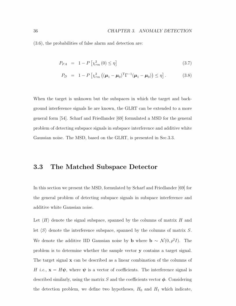
5.2 Modeling of an image according to pyramidal GMRFmodel I. . . 58
5.3 Modeling of an image according to pyramidal GMRFmodel II. . . 59
vii

viii LIST OF FIGURES
5.4 Multi-scale GMRFmodeling of an image using the multi-layer rep-
resentation. . . . . . . . . . . . . . . . . . . . . . . . . . . . . . . 61
6.1 An example of ROCcalculated for the proposed algorithm, using
3 principle component (p = 3) and various values of SNR . . . . . 73
6.2 An example of ROCcalculated for the proposed algorithm using
p independent components. Using larger number of independent
components, increases the SNRand improves the performance. . . 74
6.3 Flowcharts of the compared detection methods. . . . . . . . . . . 75
6.4 Synthetic images containing cloudy background and an airplane
target in their centers . . . . . . . . . . . . . . . . . . . . . . . . . 77
6.5 A comparison between detection methods. (a) Results of the Com-
peting Method applied to the images in Fig. 6.4 ; (b) Results of
Proposed Method I applied to the images in Fig. 6.4 ; (c) Results of
Proposed Method II applied to the images in Fig. 6.4 ; (d) Results
of Proposed Method III applied to the images in Fig. 6.4. The
images in (d) seems to have the lowest false alarm rate(FAR). . . 79
6.6 Performance of the anomaly detection based on Proposed Method
III (solid), Proposed Method II (dashed), and Proposed Method
I (dotted). (a)-(d) correspond to different parameter settings as
specified in Table 6.1. . . . . . . . . . . . . . . . . . . . . . . . . . 80
6.7 Flow chart of the proposed algorithm implementation. . . . . . . 81
7.1 Flow chart of the procedure for synthetic examples generation. . 86

LIST OF FIGURES ix
7.2 Synthetic images of cloudy sky with airplane images planted in
random places and orientations. . . . . . . . . . . . . . . . . . . . 88
7.3 Results of anomaly detection applied to the images in Fig.7.2. The
gray-scale represents the degree of local anomality around a given
pixel. The circles indicate regions where the local anomality is
above a predetermined threshold. . . . . . . . . . . . . . . . . . . 89
7.4 A synthetic image of cloudy sky with an airplane in its middle.
The airplane is unnoticeable by a human viewer due to its weak
signature. . . . . . . . . . . . . . . . . . . . . . . . . . . . . . . . 90
7.5 Anomaly detection applied to the image in Fig. 7.4. (a) First,
(b) second, and (c) third independent components. (d) Likelihood
ratio calculated by the proposed algorithm. . . . . . . . . . . . . . 90
7.6 Examples of sea-mine sonar images: Sea-mines appear in the sonar
images as a bar shaped object-highlight accompanied by a shadow
which represents the hiding of seabottom-reverberation by the sea-
mine [63]. . . . . . . . . . . . . . . . . . . . . . . . . . . . . . . . 92
7.7 Results of the anomaly detection applied to the images in Fig.7.6.
The sea-mines are detected by thresholding the gray-scale values
which represent the degree of local anomality around a given pixel. 93
7.8 Example of wafer images. The 128 × 128 images include small
round defects of about 3× 3 pixels. . . . . . . . . . . . . . . . . . 95
7.9 Results of the anomaly detection applied to the images in Fig.7.8. 96

x LIST OF FIGURES
8.1 A multi-resolution tree. Node sγ is the parent of node s in a
coarser scale. . . . . . . . . . . . . . . . . . . . . . . . . . . . . . 101

List of Tables
6.1 Properties of the different cases for which the ROCcurves in Fig. (6.6)
were drawn. The SNRcalculated for Proposed Method III is sig-
nificantly higher than the SNRcalculated for the other methods. . 78

LIST OF TABLES

Abstract
Automatic target detection in natural scenes, is a challenging problem due to the
large variability of background clutter and object appearance. When a typical
signature of the target is available, the detection can be carried out by using a
matched signal detector. Alternatively, anomaly detection methods are employed
when no a priori information about the targets is available. The detection process
is based on the anomalous nature of the targets with respect to the statistics of
the background data. The statistics of the background data in images, is often
described by random field models such as the Gaussian Markov random field
(GMRF), the simultaneous auto-regressive (SAR) model, and long correlation
(LC) models.
In many natural clutter images, scene elements often appear to have several
periodical patterns, of various period lengths. In such cases, conventional random
field models may not sufficiently describe the background clutter, and as a result,
the anomaly detection is unreliable. Furthermore, in real detection problems,
some partial information about the targets may be available in terms of a subspace
in which the target signals lie. In such cases, a matched subspace detector (MSD),
which considers the problem of detecting subspace signals in subspace interference
and additive noise, may be used as part of the detection process.
1

2 Glossary
In this work, we introduce multi-scale Gaussian markov random field (GMRF)
models and a corresponding anomaly subspace detection algorithm. We develop
the algorithm for target detection in cluttered images which follow one of the pro-
posed models. This model is based on a multi-scale representation of the image.
Using the Karhunen Loeve transform (KLT) we generate from the multi-scale
representation independent layers. We assume that these independent layers can
be modeled as GMRFs with different sets of parameters. The detection is subse-
quently carried out by using a modification of the MSD. The MSD was originally
developed for signal detection in subspace interference and white Gaussian noise.
Here we formulate a MSD for subspace signal detection in clutter, which follows
the multi-scale GMRF model.
A quantitative performance analysis with a comparison to competing methods
shows the advantages of the proposed method. The proposed model and algo-
rithm are applied to several target detection problems: detection of airplanes in
simulated cloudy backgrounds, detection of sea-mines in real sonar images, and
detection of defects in wafer images. The results demonstrate the robustness and
flexibility of the algorithm in adverse environments.

Glossary
Abbreviations
AR auto-regressive
DFT discrete Fourier transform
EM expectation maximization
FAR false alarm rate
GLC generalized long correlation
GLCP grey level co-occurrence probability
GLD grey level difference
GLRL grey level run length
GLRT generalized likelihood ratio test
GMRF Gaussian Markov random field
GMM Gaussian mixture model
HIP hierarchical image probability
HMT hidden Markov tree
3

4 Glossary
ICA independent components analysis
IDFT inverse discrete Fourier transform
IID independently and identically distributed
KLT Karhunen-Loeve transform
LC long correlation
LPF low pass filter
LS least squares
ML maximum likelihood
MLE maximum likelihood estimate
MPL maximum pseudo-likelihood
MRF Markov random field
MSD matched subspace detector
MSP multi-scale stochastic process
NCAR noncausal autoregressive
PCA principle components analysis
pdf probability density function
ROC receiver operating characteristics
ROI region of interest
SAR simultaneous autoregressive

Glossary 5
SNR signal-to-noise ratio
SVD singular value decomposition
Alphabetic Symbols
∗ Convolution.
A A subset of Ω which contain the anomalous pixels.
Aj A set of pixels which have been identified as anomalous in the
j-th iteration.
A(i)j A set of pixels which have been identified as anomalous in the
i-th internal iteration of the j-th external iteration.
b An additive IID Gaussian Noise. b ∼ N (0, ρ2I).
b` The `-th layer of the innovations process of the additive noise in
an image.
b`H0
The maximum likelihood estimate of the additive noise vector,
b`, under H0.
b`H1
The maximum likelihood estimate of the additive noise vector,
b`, under H1.
bH0 The maximum likelihood estimate of the additive noise vector,
b, under H0.
bH1 The maximum likelihood estimate of the additive noise vector,
b, under H1.
B A subset of Ω which contain the background pixels.
Bj A subset of B which contain pixels identified as anomalous in
the j-th iteration.

6 Glossary
B(i)j A subset of B which contain pixels identified as anomalous in
the i-th internal iteration of the j-th external iteration.
C(H1|H0) Cost of false detection.
C(H0|H1) Cost of miss detection.
d Differencing parameter of the LC model.
d(q(s)) Normalized distance of the feature vector q(s), from its expected
vector κ.
D Distance threshold (part of a decision rule).
Dp An operator which calculates the prediction error, ε(s), of the
multi-scale Gaussian Markov random field (GMRF) model with
p independent components.
f(q(s)|Hi) The conditional pdf of q(s) given Hi.
f(i1, i2) A 2-D separable low-pass filter.
f(i1) A 1-D low-pass filter: f(i1, i2) = f(i1)f(i2).
F The 2-D DFT operator.
g(s) The column stack ordering of the neighborhood of T (s).
G A set of multi-scale spatially invariant 2-D filters.
Gi A spatially invariant 2-D filter.
h A stabilization constant used in the LC model equation.
hj Image chips which span the signal subspace.
H The matrix whose columns span the signal subspace.
〈H〉 The signal subspace.
H` The matrix whose columns span the signal subspace (in the `-th
layer of the innovations process image).

Glossary 7
〈H`〉 The signal subspace (of the `-th layer of the innovations process
image).
H0 Hypothesis which indicate absence of target signal in the vector
n`.
H1 Hypothesis which indicate presence of target signal in the vector
n`.
〈H`S`〉 A subspace, spanned by the columns of the concatenated matrix
[H` S`
].
kj A set of N IID sample vectors having probability density func-
tion (pdf) p0 (·, θ0).
K A matrix whose columns are the top p eigen vectors of the co-
variance matrix of Y(s).
[·]` The `-th layer of 3-D data.
L(·) Generalized likelihood ratio test.
L`(s) The log-likelihood ratio, calculated for pixel s based on the `-th
layer of the innovations process.
L(s) The log-likelihood ratio, calculated for pixel s based on p layers
of the innovations process.
m The dimension of vector kj.
Mx ×My The size of image T .
nq The dimension of q(s).
n`(s) The column stack ordering of an Nx × Ny pixels image-chip of
ε` around s.
N Number of independently identically distributed (IID) sample
vectors.
Nf The length of filter f(i1) is (2Nf − 1).

8 Glossary
Nx ×Ny Size of the image chips hj and sj.
N (µ, Γ) Normal distribution with mean µ and covariance Γ.
p0(·, θ0) The probability density function (pdf) of y under H0.
p1(·, θ0) The probability density function (pdf) of y under H1.
pd2(ζ) The pdf of d2(q(s)) under H0.
PS The projection of a vector onto the subspace 〈S〉.
PHS The projection of a vector onto the subspace 〈HS〉.
Pr(·) Probability of an occurrence.
PS`The projection of a vector onto the subspace 〈S`〉.
PH`S`The projection of a vector onto the subspace 〈H`S`〉.
PD Probability of detection.
PFA Probability of false-alarm.
PG(`) A Gaussian image pyramid (` is the layers indices).
PL(`) A Laplacian image pyramid (` is the layers indices).
q(s) Feature vector related to pixel s.
Q The presumed maximum number of targets in the image.
Qj The number of potential targets in Aj.
r Relative indices of a neighbor in R.
r1 , r2 The horizontal and vertical components of the indices r.
RX(·) The Reed Xiaoli GLRT.
R A set of indices representing the neighborhood of a pixel.
Rh Half of the symmetric neighborhood R.
s = (s1, s2) Indices of a pixel in the image.
sj Image chips which span the interference subspace.
S The matrix whose columns span the interference subspace.

Glossary 9
〈S〉 The interference subspace.
S` The matrix whose columns span the interference subspace (in
the `-th layer of the innovations process image).
〈S`〉 The interference subspace (of the `-th layer of the innovations
process image).
T An image.
T(s) A multi-scale representation of image Y with independent lay-
ers.
T Transpose.
u Rank of the signal subspace.
vec(·) Column stack ordering of an image chip.
V (s) A matrix of coefficients (used by the multi-resolution Markov
model).
w = (w1, w2) The 2-D indices of data in the frequency domain.
x The target signal in the innovations process image.
x` The target signal in the `-th layer of the innovations process
image.
y A vector to be classified.
yo(s) An observation vector containing the values of the pixels in the
neighborhood of s.
y(s) A random process.
Y An image.
Y A multi-scale image generated from Y using G.
z Indices of the data in the z domain.
Z· The z-transform operator.
α, β Parameters of the Γ density function.

10 Glossary
γ(s) An operator which points to the parent of node s in a multi-
resolution tree.
Γ The sample covariance matrix of the reference data kj.
δ Threshold on the relative change ∆(n)j (a stopping rule).
∆(n)j The relative change between B(n)
j and B(n−1)j .
ε(s) Innovation process.
ε (s) Vector of innovations in pixel s.
ε` (s) The `-th component of ε (s).
ε (s) Estimate of the innovations process (prediction error) in pixel
s.
ε` (s) The `-th component of ε (s).
θ Column stack ordering of θ(r), r ∈ R.
θ Least-squares estimate of θ.
θ(r) Weight coefficient of a neighbor r ∈ R.
Θr A diagonal matrix with weight coefficients of neighbor r (in the
different layers of T).
κ Expected feature vector: κ = E[q(s)|H0].
ν(s) IID Gaussian random variables, with zero mean and unit vari-
ance.
ξ Decision of the GLRT (H0 or H1).
ρ2 The variance of the innovations process.
ρ2 Least-squares estimate of ρ2.
ρ2` The variance of b`.
Σ Covariance matrix of the feature vector q(s), under H0.
τ τ=1,2 if the data kj are real or complex valued, respectively.

Glossary 11
ϕ A confidence level - the probability of correctly deciding on H0
given H0 is true.
φ Coefficients vector of the interference signal in the interference
subspace.
φ` Coefficients vector of the interference signal in the interference
subspace.
Φ` The covariance matrix of b`
ρ`.
χ2q(c) The chi-square probability distribution function, with q degrees
of freedom and non-centrality parameter c.
ψ Coefficients vector of the target signal in the signal subspace:
x = Hψ .
ψ` Coefficients vector of the target signal in the signal subspace:
x` = H`ψ` .
Ω Support of an image.

12 Glossary

Chapter 1
Introduction
1.1 Motivation and Goals
During the last decade, there has been a remarkable progress in random field
models and their applications. Random field modeling has been applied exten-
sively to texture synthesis [16], [29], image segmentation [46], [68], [72], and tar-
get detection [36], [63]. Natural clutter models are able to describe a wide range
of image textures based on the interaction between neighboring pixels. Clut-
ter models as the GMRF, simultaneous autoregressive (SAR), and generalized
long correlation (GLC) model have proven to be effective in describing natural
textures with periodical as well as random elements [4], [29]. In many natural
clutter images, scene elements often appear to have several periodical patterns,
of various period lengths. In such cases, random field models as the GMRF and
the long correlation (LC) models may not sufficiently fit the clutter image. De-
viations of the clutter image from the random field model influence the detection
performance by increasing the false alarm rate. Furthermore, in real detection
problems, some a priori information about the targets is often available. The
information may include details about the exact nature of the target (the targets
13

14 CHAPTER 1. INTRODUCTION
signature) but may sometimes be more general - describing a subspace in which
the target’s signature may lie. Using this information in a flexible framework,
for rejecting anomalies which do not resemble targets, may improve the detection
performance, achieved by anomaly detection methods and matched filtering.
In this work, we introduce multi-scale Gaussian markov random field (GMRF)
models and a corresponding anomaly subspace detection algorithm. Figure 1.1
presents the improvement in the detection performance, achieved by modeling
an image using the multi-scale framework we propose. Figure 1.1(a) presents
the original synthetic image, containing an airplane in its center. The synthetic
background is a mixture of 3 different textures which contain periodic patterns
with different period lengths. This image is not expected to be well described
by the conventional GMRF model. Figure 1.1(b) presents the results of applying
a single hypothesis test to the innovations process of the image in Fig. 1.1(a),
assuming the image follows the GMRF model. The noisy results are caused by the
incorrect assumption regarding the statistical model which describes the image.
Figure 1.1(c) presents the likelihood ratios obtained by applying the proposed
method to the image in Fig. 1.1(a), assuming the multi-scale GMRF model we
propose. The results achieved by the proposed method seem to be less noisy and
therefore are expected to produce less false alarms.
1.2 Overview of the Thesis
In this thesis, we introduce multi-scale GMRF models and a corresponding anomaly
subspace detection algorithm. We develop the algorithm for target detection
in cluttered images which follow one of the proposed models. This model is

1.2. OVERVIEW OF THE THESIS 15
(a) (b) (c)
Figure 1.1: A comparison between detection methods. (a) A synthetic image
containing cloudy background and an airplane target in its center ; (b) Result
of applying a single hypothesis test to the innovations process of the image in
(a), assuming a GMRF model ; (c) Result of the proposed method applied to the
image in (a), assuming a multi-scale GMRF model.
based on a multi-scale representation of the image and the Karhunen-Loeve trans-
form (KLT). We generate from a given image, a multi-layer representation with
independent layers. We assume that these independent layers can be modeled as
GMRFs with different sets of parameters. The detection is subsequently carried
out by applying a modification of the matched subspace detector (MSD) to the
innovations process (prediction error) of the multi-scale GMRF. The MSD incor-
porates the available a priori information about the targets into the detection
process and thus improves the detection performance. The MSD was originally
developed for signal detection in subspace interference and white Gaussian noise
[69]. Here, we formulate a MSD for signal detection in subspace interference and
noise which follows the proposed multi-scale GMRF model. A quantitative per-
formance analysis with comparison to competing methods shows the advantages
of the proposed method. The proposed model and algorithm are applied to de-
tection of airplanes in simulated cloudy backgrounds; detection of sea-mines in
sonar images; and detection of defects in wafer images. The results demonstrate

16 CHAPTER 1. INTRODUCTION
the robustness and flexibility of the algorithm in adverse environments.
1.3 Organization
The structure of the thesis is as follows: In Chapter 2, we present statistical
models of natural clutter. We review the SAR, GMRF and GLC models. In
Chapter 3, we present anomaly detection approaches. We review the single hy-
pothesis testing approach and the MSD. In chapters 4-8 we propose novel clutter
models and detection methods. We analyze and demonstrate the method’s per-
formance using simulated and real images. In Chapter 4, we introduce an iterative
approach for anomaly detection based on a single hypothesis test. In Chapter 5,
we introduce multi-scale GMRF models. In section 6, we introduce an anomaly
subspace detector using a multi-scale GMRF model, we analyze the performance
of the proposed algorithm and compare the detection results to those obtained by
using competing methods. In Chapter 7, we demonstrate the application of the
proposed algorithm to automatic target detection in simulated and real imagery.
Finally, in Chapter 8, we propose subjects for future research and conclude.
1.4 Background
Most detection and segmentation methods rely on the statistical characterization
of the examined image. For some images, image segmentation could be easily
implemented using only the intensity of each pixel. In such cases, no high order
texture features are needed. But most of the time, the identification of class types
in the image can not be done so easily based only on the grey levels of the pixels.
Then the texture features become an helpful information in the segmentation

1.4. BACKGROUND 17
process. The simplest approach of texture analysis method in statistical category
is known as first order methods [37]. The statistics are based on individual pixel
values, rather then the relationship between pixels. Texture features such as
mean, variance, standard deviation, gradient, and skewness are usually extracted
from the image [37].
If an image shows regions with equal first order statistics, then second order
statistics should be used. In the second order approach the texture features are
extracted from an intermediate relationship matrix which is calculated using the
pixels within a pixels neighborhood. There are several commonly used methods in
this category [22]: grey level difference (GLD), grey level run length (GLRL), and
grey level co-occurrence probability (GLCP). The GLCP method can measure
textural characteristics such as homogeneity, grey level linear structure, contrast,
entropy, and image complexity [20],[18],[19].
Most random field models are based on the spatial interaction of pixels in local
neighborhoods. The noncausal autoregressive (NCAR) model represents each
pixel as a linear combination of pixels at nearby locations, and an additive white
noise variable. The Markov random field (MRF) replaces the white noise with
a spatially correlated random variable. A wider discussion on the properties of
these models and further details can be found in Chapter 5.2.
Model-based texture analysis is a mathematical process which can synthesize or
describe the texture image. The parameters of the model are used to establish the
distribution law of a pattern or simply used as features to classify the textures.
The fundamental difference between the model-based methods and the statistical
texture analysis methods is that the texture model has the capability to generate
the texture which matches the observed texture. Using a statistical method, the

18 CHAPTER 1. INTRODUCTION
texture features are measured without a representative texture in mind, and the
texture features extracted from the image, cannot be used in general to synthesize
a texture image.
Random field models were developed for describing natural clutter images. Man-
made objects therefore appear anomalous with respect to the random field model
which describes the clutter. Anomaly detection methods make use of the anoma-
lous appearance of such objects for their detection, but often make no a priori
assumptions about the nature of the targets. Statistical approaches of anomaly
detection, does not rely on an exhaustive statistical model of the targets, but
rather on the statistics of the background data. The detection is carried out by
estimating whether a test sample follows the same model as the background data.
Most methods assume that the data comes from a family of known models and
certain parameters are calculated to fit this model. These approaches are based
on modeling the the training data and rejecting test patterns that fall in regions
of low probability density. However, in order to achieve better performance, the
training data itself needs to be either free of outliers or the outliers to be known.
Hazel [36] has developed an anomaly detection technique, which is based on
GMRF modeling of the background in a multi-spectral image. A single hypothesis
scheme is used for the detection of regions, which appear unlikely with respect to
the probabilistic model of the background. A similar anomaly detection method
was presented by Bello [3] for the detection of anomalous complex image pix-
els, using the SAR model. A completely different approach for target detection is
based on a matched signal detector (matched filter). The matched signal detector
is employed when a typical signature of the target is available. In many detection
problems, the information about the targets is a subspace in which the targets lie.

1.4. BACKGROUND 19
In these applications, the matched signal detector is replaced by a MSD, a gener-
alization of the matched filter, which was formulated by Scharf and Friedlander
[69]. The MSD is used for detecting subspace signals in subspace interference and
additive noise, using the principle of the generalized likelihood ratio test (GLRT).
A state of the art review of anomaly detection methods can be found in Karkou
and Singh [57]. The survey includes different statistical approaches for image
modeling, hypothesis testing and clustering. Most of the presented methods are
driven by modeling data distributions and then calculating the likelihood of test
data with respect to the estimated statistical models.

20 CHAPTER 1. INTRODUCTION

Chapter 2
Modeling Natural Clutter Images
2.1 Introduction
Any analytical expression that explains the nature and extent of dependency of
a pixel intensity on intensities of its neighbors can be said to be a model [13].
An image processing or analysis technique only applies well for certain kinds
of images. Thus it is important to be able to model the image that is to be
processed. Once the model of the image is obtained, it will serve to explain the
statistical characteristics of the image and to efficiently process it. The awareness
of the importance of image models was enhanced at the end of the 1970s by a
workshop on image modelling held in Chicago in August, 1979 [66]. Since then,
the research activities in the image modelling area have increased considerably
[86].
During the last decade, there has been a remarkable progress in random field
models and their applications. Random field modeling has been applied exten-
sively to texture synthesis [16], [29], image segmentation [46], [68], [72], and
target detection [36], [63]. Most random field models are based on the spatial in-
21

22 CHAPTER 2. MODELING NATURAL CLUTTER IMAGES
teraction of pixels in local neighborhoods [5]. The NCAR model represents each
pixel as a linear combination of pixels at nearby locations, and an additive white
noise variable (innovations process). Chellappa and Kashyap [16], [41] proposed
an iterative estimation method and synthesis algorithm for the 2-dimensional
NCAR model. They illustrated the usefulness of the NCAR models for synthesis
of textures resembling several real texture images, possessing the local replica-
tion attribute. The local replication attribute is an essential ingredient of many
natural textures [16].
The MRF model was first introduced by Levi [49] in 1956. Woods [82] formulated
the two-dimensional discrete MRF based on the continuous case and the math-
ematical foundation given by Levi [49] and Wong [81]. The model was farther
developed and studied by Geman and Geman [34], Chellappa and Chatterjee [14],
and others. The discrete MRF model describes each pixel as a weighted sum of
its neighboring pixels and a random variable which represents the innovations
process. The difference between the MRF model and the NCAR model is that
the innovations process is spatially correlated. Yue [86] investigated the texture
distinguishing ability of the MRF models and the GLCP texture features. He
Compared the segmentation performance of the MRF and GLCP methods for
synthetic, Brodatz [9], and sea-ice images taken by a synthetic aperture radar.
A more general form of random field models is the LC model proposed by Kashyap
and Lapsa [44]. The LC models can be applied to images with a correlation
structure which extends over large regions using only a few model parameters.
Kashyap and Eom demonstrated the applicability of the LC model by presenting
a consistent estimation scheme [42] and a texture boundary detection method
[43], based on this models. Eom [29],[28] proposed a LC model with circular and

2.2. THE SIMULTANEOUS AUTO-REGRESSIVE (SAR) MODEL 23
elliptical correlation structure and a corresponding estimation algorithm. The
LC model, proposed by Eom, has the advantage of modeling diverse real textures
with less than five model parameters. Three parameters are used for defining
an isotropic LC model and the other two parameters are used for describing
the linear transformation (elongation and rotation) performed to the model’s
coordinate system. Bennett and Khotanzad [4] developed a random field model
and a corresponding estimation scheme, based on a generalization of the LC
model. They introduced the GLC model and showed that the NCAR and the
MRF models are special cases of this model.
In this chapter we present some known clutter image models. We provide the
SAR, GMRF and GLC models equations and present estimation and synthesis
approaches. The organization of this chapter is as follows: In Section 2.2, we
present the SAR model, in Section 2.3, we present the GMRF model, and in
section 2.4 we present the GLC model.
2.2 The Simultaneous Auto-Regressive (SAR)
Model
The SAR model [15], [16], [41] was one of the first random field models to be
developed. It represents each pixel as a linear combination of pixels at nearby
locations, and an additive white noise variable (innovations process).
Let Ω be the support of an image, and let s ∈ Ω denote the indices of a pixel
in the image. Let R be a given set of indices representing the neighborhood
of a pixel (A simple example is the 4-neighbors set where R=(-1,0),(1,0),(0,-
1),(0,1)). We denote the weight coefficient of a neighbor r ∈ R by θ(r) and the

24 CHAPTER 2. MODELING NATURAL CLUTTER IMAGES
innovations process by ε(s). The innovations process is a set of independently
and identically distributed (IID) Gaussian variables with zero mean and variance
ρ2. Assuming an image y follows the SAR model, a pixel y(s) in the image1 is
related to its neighboring pixels as follows:
y(s) =∑r∈R
θ(r)y (s + r) + ε (s) . (2.1)
Chellappa and Kashyap [15] presented a procedure for synthetic generation of
images which follow the SAR model. The procedure is based on the discrete
Fourier transform (DFT) of (2.1):
Fy(w1, w2) =ρFε(w1, w2)
λ(w1, w2)(2.2)
where
λ(w1, w2) = 1−∑
r=(r1,r2)∈Rθ(r)exp
[2πi
(r1w1
Mx
+r2w2
My
)](2.3)
and where Mx, My is the size of the image. This representation is obtained given
the toroidal lattice assumption, which comfortably determine the boundaries con-
dition:
y(Mx + s1,My + s2) = y(s1, s2) (2.4)
The synthetic images are obtained by inverse discrete Fourier transform (IDFT) of
(2.2). The SAR model is valid for all parameter values such that λ(w1, w2) 6= 0.
1For simplicity, we assume y(s) is not in the boundaries of the image, i.e. ∀r ∈ R, (s+r) ∈ Ω

2.3. THE GAUSSIAN MARKOV RANDOM FIELD (GMRF) MODEL 25
2.3 The Gaussian Markov Random Field (GMRF)
Model
The Markovian assumption is that the conditional probability of y(s), given all
the other values of y, depends only upon a finite group of neighboring pixels
y(s + r)|r ∈ R. The process is non-causal and is not driven by a white noise
source. y(s) is strict sense stationary and R is symmetric.
We assume that each image pixel can be represented as a weighted sum of its
neighboring pixels and an additive innovations process (as described by (2.1)).
The difference between the SAR model and the GMRF model is in the statistics
of the innovations process. In a GMRF, the white Gaussian innovations process
is replaced by a spatially correlated Gaussian noise. Woods [82] showed that
under the Markovian assumption, the innovations process of a GMRF is spatially
correlated with covariance given by:
E ε (s) ε (s + r) =
ρ2 , if r = (0, 0)−θ(r)ρ2 , if r ∈ R0 , otherwise.
(2.5)
Kashyap and Chellappa [41] showed that the correlation structure imposes sym-
metry on the neighborhood set. That is, r ∈ R implies −r ∈ R and θ(r) = θ(−r).
The GMRF model can also be written in terms of white noise sequence as follows
[41]:
Fy(w1, w2) =ρFε(w1, w2)√
λ(w1, w2)(2.6)
where
λ(w1, w2) = 1− 2∑
r=(r1,r2)∈Rh
θ(r)cos
[2π
(r1w1
Mx
+r2w2
My
)](2.7)

26 CHAPTER 2. MODELING NATURAL CLUTTER IMAGES
and where Rh is half of the symmetric neighborhood R. The difference between
(2.3) and (2.7) originates from the symmetry, imposed by the correlation struc-
ture. Using (2.2) and (2.7), the procedure of synthetic generation of images which
follow the GMRF model is evident.
In most detection problems, the background clutter model is unknown and there-
for should be estimated. Various methods for model estimation were developed
over the years, e.g., [36], [41], [70], [71], [87]. A computationally efficient method
for the GMRF model estimation is described in details in Kashyap and Chel-
lappa [41]. Let vec(·) denote the column stack ordering of an image chip. Let
the column stack ordering of the neighborhood of y(s) be denoted by g(s):
g(s) = vec[y(s + r), r ∈ R] (2.8)
and let
θ = vec[θ(r), r ∈ R]. (2.9)
Kashyap and Chellappa showed that the least squares estimates for θ and ρ2 are
given by [41]:
θ =
[∑s∈Ω
g(s)g(s)T
]−1 [∑s∈Ω
y(s)g(s)
](2.10)
ρ2 =1
|Ω|∑s∈Ω
(y(s)− θ
Tg(s)
)2
(2.11)
where T denotes transpose.

2.4. GENERALIZED LONG CORRELATION (GLC) MODELS 27
2.4 Generalized Long Correlation (GLC) Mod-
els
One of the main drawbacks of the SAR and GMRF models is their inability
to effectively model low frequency power in an image. The correlation function
of these models decays rapidly beyond the span of the defined neighbor set.
Bennett and Khotanzad [4] developed the GLC model and showed that it has
an autocorrelation function which decays much more slowly and thus, enables
effective modeling of clutter images with correlation of large spatial extent. They
showed that the SAR and the GMRF models are special cases of the GLC model.
Let y(s) be a random process which follows the one-dimensional LC model. We
denote the differencing parameter by d (where |d| < 0.5) and the innovations
process by ε. The innovations process is a white Gaussian noise sequence with
zero mean and variance ρ2. Then y(s) can be described in the frequency domain
by its z-transform as follows [4]:
(1− hz−1)dZy(z) = ρZε(z) (2.12)
where Z is the z-transform operator and h is a stabilization constant (which
moves the z = 1 pole into the unit circle). When h = 1, the model is unstable
(unrealizeable). Selecting h to be slightly less than one enables a stable approxi-
mation of the model. In order to obtain the two-dimensional GLC model, (2.12)
is generalized and extended as follows:
1−
∑
r=(r1,r2)∈Rθ(r)z−r1
1 z−r22
d
Zy(z1, z2) = ρZε(z1, z2) (2.13)
where the model parameters are the neighbor set R, the correlation coefficients

28 CHAPTER 2. MODELING NATURAL CLUTTER IMAGES
θ(r), the differencing parameter d, and the innovations standard-deviation ρ. Let
F be the DFT operator. Then the equivalent DFT representation of (2.13) is [4]:
Fy(w1, w2) =ρFε(w1, w2)
λ(w1, w2)d(2.14)
where λ(w1, w2) is given by (2.3). This representation is true under the toroidal
lattice assumption (y(Mx + 1, s2) = y(1, s2) and y(s1,My + 1) = y(s1, 1)).
For the special case of d = 1, (2.2) is identical to (2.14) and therefore the SAR
model is equivalent to this special case of the GLC model. Similarly, the GMRF
model is equivalent to the GLC model with d = 12.
2.5 Summary
Clutter image modeling is an active field of research. During the last decade,
there has been a remarkable progress in random field models and their applica-
tions. Most of the models are based on the spatial interaction of pixels in local
neighborhoods. The main challenge in clutter modeling is to represent a wide
range of textures using a small number of parameters and to efficiently estimate
these parameters. In this chapter we present some known clutter image models.
We provide the SAR, GMRF and GLC models equations and present estimation
and synthesis approaches.
The SAR model represents each pixel as a linear combination of pixels at nearby
locations, and an additive white noise variable (innovations process). This struc-
ture enables a simple procedure for image synthesis [4]. The more widely used
GMRF model describes each pixel as a weighted sum of its neighboring pixels

2.5. SUMMARY 29
and a spatially correlated innovations process. The GLC model, proposed by
Bennett and Khotanzad [4], is a more general form of random field models. This
model is based on a generalization of the LC model [29] and includes the SAR
and the GMRF models as its special cases. It better describes textures with long
correlation characteristics but lacks the simplicity which characterize the SAR
and the GMRF estimation and synthesis methods.
The statistical models, presented in this chapter, were developed for describing
clutter images. Regions in the image which are not part of the background clutter,
may appear anomalous with respect to its model. In chapter 3 we review anomaly
detection methods. These methods are used for detecting regions in the image
which appear improbable with respect to the background statistical model.

30 CHAPTER 2. MODELING NATURAL CLUTTER IMAGES

Chapter 3
Anomaly Detection
3.1 Introduction
In the previous chapter, we presented statistical models of background clutter
in images. The majority of work in the area of target detection has focused on
detection methods, which involve statistical characterization of both targets and
background [79]. Matched filters, for example, require a priori knowledge of a
typical signature of the target [77]. In a realistic situation, however, there is a
wide variety of potential targets which do not conform to a uniform model. Given
the fact that we can never train a machine learning system on all possible object
classes, it becomes important that it is able to distinguish between known and un-
known object information during testing. Anomaly detection is the identification
of new or unknown data that a learning system is not aware of during training
[57]. Anomaly detection techniques are useful in applications such as fault detec-
tion [52], radar target detection [12], detection of masses in mammograms [74],
e-commerce [52], and other signal processing and image analysis applications.
Statistical approaches of anomaly detection, does not rely on an exhaustive sta-
31

32 CHAPTER 3. ANOMALY DETECTION
tistical model of the targets, but rather on the statistics of the background data.
The detection is carried out by estimating whether a test sample comes from the
same distribution as the background data. Two main approaches exist to the
estimation of the pdf of the background data, parametric and non-parametric
methods [25]. The parametric methods assume that the data comes from a fam-
ily of known distributions (e.g. the normal distribution) and certain parameters
are calculated to fit this distribution. The simplest detection method can be
based on constructing a pdf for data of a known class. The detection is then
carried out by computing the probability of a test sample of belonging to that
class and thresholding these estimates. Another simple method is to threshold
the distance of a sample from a class mean (in terms of number of standard
deviations) [55], [56]. The distance measure can be Mahalanobis or some other
probabilistic distance [78].
Roberts and Tarassenko [64] developed a method for anomaly detection in Gaus-
sian mixture models (GMMs). Their method aims to minimize the number of
heuristically chosen thresholds in the novelty decision process. Their anomaly
detection method is similar to those presented by Barnett and Lewis [2], Bishop
[8], Brotherton et. al. [10], Desforges et. al. [25], Parra et. al. [60], Tarassenko
et. al. [75], Tarassenko [74], Tax et. al. [76], Yeung and Chow [85], and others.
The anomaly detection is based on the estimation of the density function of the
training data. The major contribution of this paper is that an automatic crite-
rion is used for determining the number of Gaussians. The growth decision is
based on measuring the smallest Mahalanobis distance between a training vector
and each Gaussian within the network. This method was tested on a medical
signal processing task to detect elpileptic seizures, exhibiting very high perfor-

3.1. INTRODUCTION 33
mance rates. Van Leemput et. al. [48] presented an outlier detection algorithm
for detection of multiple sclerosis lesions from multi-spectral magnetic resonance
images. The algorithm is based on the MRF model. Tissue specific intensity
models are estimated from the data itself and data which appear unlikely with
respect to the model is suspected to be part of a lesion.
In non-parametric methods the overall form of the density function is derived
from the data as well as the parameters of the model (e.g. histogram analysis).
As a result non-parametric methods give greater flexibility in general systems.
The parametric as well as the non-parametric approaches are based on modeling
the density of the training data and rejecting test patterns that fall in regions of
low density. However, in order to achieve better performance, the training data
itself needs to be either free of outliers or the outliers to be known.
A different approach for anomaly detection is based on clustering - partitioning
data into a number of clusters [61], [84]. Each data point can be assigned a degree
of membership to each of the clusters. Thresholding the degree of membership
can use for detecting data points which belong to none of the available classes.
The GLRT for unknown signals is the foundation for many anomaly detection al-
gorithms. Kelly [45] and Reed and Yu [62] developed GLRTs for multidimensional
image data assuming that the target signal and the covariance of the background
are unknown. Scharf and Friedlander [69] formulated the MSD - an extension
of the GLRT for unknown signals, to situations in which the target signature is
assumed to be in a known subspace. The matched filter and the single hypothesis
test are special cases of the MSD (generated for subspaces of rank 1 and of full
rank respectively).

34 CHAPTER 3. ANOMALY DETECTION
In Sec. 3.2 we describe the single hypothesis test, formulated based on the GLRT
for unknown signals, assuming Gaussian noise. Then, in Sec. 3.3 we present the
MSD, as formulated by Scharf and Friedlander [69].
3.2 Single Hypothesis Testing
Applying the GLRT to detection of unknown signals is the foundation for anomaly
detection algorithms. In this section we describe the single hypothesis test, for-
mulated based on the GLRT for unknown signals, assuming Gaussian noise.
Let y be a vector that is to be classified as arising from either pdf p0(·, θ0) or
p1(·, θ1), (hypothesis H0 or H1 respectively). Let kj ∈ Cm|1 ≤ j ≤ N be a set
of N IID sample vectors having pdf p0 (·, θ0). The GLRT is as follows [73]:
L (y) =max
θ1
[p1 (y, θ1) p0 (kj|1 ≤ j ≤ N , θ1)]
maxθ0
[p0 (y, θ0) p0 (kj|1 ≤ j ≤ N , θ0)]
H1
><H0
η (3.1)
where η is a threshold. Kelly [45] and Reed and Yu [62] developed a GLRT for
multidimensional image data assuming the the target signal and the covariance
of the background are unknown. Let N (µ, Γ) denote normal distribution with
mean µ and covariance Γ. Then the RX (Reed Xiaoli) GLRT between the target
absent hypothesis H0, and the target present hypothesis H1:
H0 : y ∼ N (µ0, Γ)
H1 : y ∼ N (µ1, Γ) (3.2)

3.2. SINGLE HYPOTHESIS TESTING 35
is as follows [62]:
RX(y) = (y − µ0)T
(N
N + 1Γ +
(y − µ0)(y − µ0)T
N + 1
)−1
(y − µ0)
H1
><H0
η (3.3)
where µ1 and Γ are unknown and:
Γ =1
N
N∑j=1
(kj − µ0) (kj − µ0)T (3.4)
is the sample covariance matrix of the reference data. As N →∞ the RX GLRT
converges to:
RXN→∞(y) = (y − µ0)T
(Γ)−1
(y − µ0)
H1
><H0
η (3.5)
which is the Mahalanobis distance [38] of vector y from µ0 [53]. It is evident
that the GLRT presented in (3.5) does not rely on any information about the
targets but rather on an estimated model of the background. The test is to decide
whether vector y belongs to the background and therefore is a single hypothesis
test. Let χ2m(λ) denote the non-central chi-square distribution with m degrees of
freedom and non-centrality parameter λ. Then the probability distributions of
the GLRT RX, under H0 and H1 are given in terms of chi-square and noncentral
chi-square densities as follows:
RX ∼
χ2τm (0) , under H0
χ2τm
((µ1 − µ0)
TΓ−1(µ1 − µ0))
, under H1.(3.6)
where τ=1,2 if the data are real or complex valued, respectively. Given (3.6) and
36 CHAPTER 3. ANOMALY DETECTION
(3.6), the probabilities of false alarm and detection are:
PFA = 1− P[χ2
τm (0) ≤ η]
(3.7)
PD = 1− P[χ2
τm
((µ1 − µ0)
TΓ−1(µ1 − µ0)) ≤ η
]. (3.8)
When the target is unknown but the subspaces in which the target and back-
ground interference signals lie are known, the GLRT can be extended to a more
general form [54]. Scharf and Friedlander [69] formulated a MSD for the general
problem of detecting subspace signals in subspace interference and additive white
Gaussian noise. The MSD, based on the GLRT, is presented in Sec.3.3.
3.3 The Matched Subspace Detector
In this section we present the MSD, formulated by Scharf and Friedlander [69] for
the general problem of detecting subspace signals in subspace interference and
additive white Gaussian noise.
Let 〈H〉 denote the signal subspace, spanned by the columns of matrix H and
let 〈S〉 denote the interference subspace, spanned by the columns of matrix S.
We denote the additive IID Gaussian noise by b where b ∼ N (0, ρ2I). The
problem is to determine whether the sample vector y contains a target signal.
The target signal x can be described as a linear combination of the columns of
H i.e., x = Hψ, where ψ is a vector of coefficients. The interference signal is
described similarly, using the matrix S and the coefficients vector φ. Considering
the detection problem, we define two hypotheses, H0 and H1 which indicate,

3.3. THE MATCHED SUBSPACE DETECTOR 37
respectively, absence and presence of target signal in the vector y:
H0 : y = Sφ + bH1 : y = Hψ + Sφ + b.
(3.9)
Let PS denote the projection of a vector onto the subspace 〈S〉:
PSy(s) = S(STS)−1STy(s) (3.10)
and let PHS denote the projection of a vector onto the subspace 〈HS〉, spanned
by the columns of the concatenated matrix[H S
]. The maximum likelihood
estimates of the additive noise vector, b, under H0 and under H1 are denoted by
bH0 and bH1 , respectively. These estimates are obtained by subtracting from y
the components which lie in the signal and interference subspaces as follows:
bH0 = (I − PS)y
bH1 = (I − PHS)y(3.11)
The detection problem can be formulated as a GLRT between H0 and H1. The
log-likelihood ratio, L, is given by:
L(s) = 2ln
[Pr(b(s)|H0)
Pr(b(s)|H1)
]= 2ln
exp
([bbH0
(s)]2
2ρ2
)
exp
([bbH1
(s)]2
2ρ2
)
=1
ρ2
[∥∥∥bH0(s)∥∥∥
2
2−
∥∥∥bH1(s)∥∥∥
2
2
]
=1
ρ2yT(PHS − PS)y. (3.12)
The signal-to-noise ratio (SNR) is the ratio between the signal and the noise in
terms of intensity. We define the SNR as the second power of the ratio between the

38 CHAPTER 3. ANOMALY DETECTION
signal, which do not lie in the interference subspace, and the standard deviation
of the noise, as follows:
SNR =1
ρ2xT[I − PeS]x. (3.13)
Let u denote the rank of the signal subspace. L is a sum of squared indepen-
dent normally distributed variables and therefore is chi-square distributed with
u degrees of freedom, as follows:
L ∼
χ2u (0) , under H0
χ2u (SNR) , under H1.
(3.14)
Under hypothesis H1, the non-centrality parameter of the chi-square distribution
of L is equal to the SNR [69]. The decision rule is based on thresholding the
log-likelihood ratio using the threshold η as follows:
ξ =
H0 if L ≤ ηH1 if L > η.
(3.15)
Given (3.14) and (3.15), the probabilities of false-alarm and detection are:
PFA = 1− P[χ2
u (0) ≤ η]
(3.16)
PD = 1− P[χ2
u (SNR) ≤ η]. (3.17)
3.4 Summary
We reviewed anomaly detectors for problems where no information about the
targets is known, and where some a priori information is available. We presented
the single hypothesis test, based on a statistical model of the background and no
information about the targets. We described the MSD as formulated by Scharf

3.4. SUMMARY 39
and Friedlander [69], and presented its performance with respect to the SNR of
the examined scene. We assume that using a priori information about the targets
in the detection process, may improve the detection performance. In chapter 4
we propose an iterative anomaly detection method which is based on a single
hypothesis test. Any information we have about the targets is used in the post-
processing in order to decide whether an anomalous region in the image is part
of a target. In chapter 6 we propose a novel detection method, based on the
MSD. Any a priori information about the targets is used for defining the targets
subspace used by this detector.

40 CHAPTER 3. ANOMALY DETECTION

Chapter 4
Iterative Anomaly Detection
4.1 Introduction
In this chapter, we propose an anomaly detection approach, which does not rely
on an exhaustive statistical model of the targets, but rather on the local statis-
tics of the data and possibly on some a priori information regarding the sizes and
shapes of targets. An iterative procedure of feature extraction, based on local
statistics and principle components analysis (PCA) is performed. The back-
ground is statistically characterized in a feature space of principle components.
A single hypothesis scheme is used for the detection of anomalous pixels in a given
region of interest (ROI). Subsequently, morphological operators are employed for
extracting the sizes and shapes of anomalous clusters in the image domain, and
identifying potential targets. We may compromise on the false alarm rate in order
to achieve a high probability of detection, since each iteration gradually reduces
the false alarm rate while maintaining the high probability of detection.
The chapter is organized as follows. In Sec. 4.2 we present a formulation of
the problem. In Sec. 4.3 we provide a mathematical model. In Sec. 4.4 we
41

42 CHAPTER 4. ITERATIVE ANOMALY DETECTION
describe the proposed iterative anomaly detection algorithm. Finally, in Sec. 4.5
we demonstrate the application of the algorithm to sea-mine detection in sonar
imagery.
4.2 Problem Formulation
Let Ω be the support of a gray scale image. The image may contain different
textures as background (i.e. grass, trees, soil, water) and some targets which
are anomalous with regards to the background. We would like to find a disjoint
partition of Ω, such that Ω = B⋃A, where B contains a few uniform subsets of
background pixel clusters: B =J⋃
j=1
Bj, and A contains anomalous pixels. The
subsets of the background pixels represent different textures of the background.
For example, in a typical terrain scene, B1 may contain pixels which constitute
grass, B2 may represent trees, and so on.
The proposed algorithm is based on an iterative two-category classification pro-
cedure. A set of pixels, Aj−1 , which have been identified as anomalous in the
(j − 1)’th iteration, is partitioned into background and anomalous subsets, Bj
and Aj respectively:
Aj−1 = Bj
⋃Aj (4.1)
where j ≥ 1 and A0 is initialized to the ROI in the image (possibly A0 = Ω).
The fundamental problem of the iterative anomaly detection procedure is to par-
tition the set of pixels, Aj−1, into two subsets: One, which is relatively uniform,
large and thus considered as the background subset (Bj), and a second subset

4.3. MATHEMATICAL MODEL 43
which contains anomalous pixels (Aj). Another problem is to determine a stop-
ping rule for the iterative procedure. The procedure should be iterated until the
number of targets pertaining to Aj does not exceed a given number. The maximal
number of detectable targets in a given ROI is closely related to the permissible
false alarm rate. A stopping rule based on such a criterion should incorporate
into the procedure a low complexity routine for coarse target detection.
4.3 Mathematical Model
Let s ∈ Ω be the coordinates of a pixel in the image. Let q(s) be a feature
vector related to the pixel s. Considering a two-category classification problem,
we define two possible hypotheses:
H0 : s ∈ B (background pixel)
H1 : s ∈ A (anomalous pixel)
A two-category classification problem is often worked out using the Bayes decision
rule for minimum cost [1]. Let C (H1|H0) and C (H0|H1) denote, respectively,
the costs of false detection and miss detection. Then the optimal minimum cost
decision rule is given by [33]:
f (q(s)|H0) P (H0) C (H1|H0)
H0
><H1
f (q(s)|H1) P (H1) C (H0|H1) (4.2)
where f (q(s)|Hi) is the conditional pdf of q(s) given Hi and P (Hi) is the a priori
probability of Hi.

44 CHAPTER 4. ITERATIVE ANOMALY DETECTION
In practice, the background can be well characterized (an empirical f (q(s)|H0)
can be generated) while the anomalies are of a wide variety and rare (a reliable
estimate of f (q(s)|H1) is unavailable). Therefore, the Bayes decision rule for
minimum cost is inapplicable. A suitable alternative to such problems is based on
a single hypothesis scheme [33]. Let κ = E [q(s)|H0] denote the expected feature
vector and Σ = E[(q(s)− κ) (q(s)− κ)T
∣∣∣ H0
]the covariance matrix under H0
hypothesis. Let the normalized distance of q(s) from its expected vector, κ, be
defined by:
d (q(s)) = (q(s)− κ)T Σ−1 (q(s)− κ) (4.3)
Then the decision rule is given by:
d (q(s))
H0
><H1
D (4.4)
where D is a threshold to determine whether a given pixel is anomalous or not.
This decision rule is based on the statistics of the background only. No knowledge
about the anomalies statistics is taken into consideration. The threshold, D, can
be determined according to a specified confidence level, ϕ, which is the probability
of correctly deciding on H0 given H0 is true. The threshold, D, and the confidence
level, ϕ, are related by:
ϕ ≡ Pr (H0|H0) = Pr (d (q(s)) ≤ D|H0) . (4.5)
In case the feature vector, q(s), is a Gaussian random vector of dimension nq,
the pdf of d2(q(s)) under the H0 hypothesis, denoted by pd2 (ζ), is the gamma
density function with parameters β = nq
2− 1 and α = 1/2 [33]. Accordingly, the

4.4. ANOMALY DETECTION ALGORITHM 45
relation between ϕ and D can be written as
ϕ =
D2∫
0
pd2 (ζ)dζ =
D2∫
0
1
2nq/2Γ (nq/2)ζ
nq−2
2 e−ζ/2dζ . (4.6)
The aforementioned decision rule is based on a one-dimensional measure, d(q(s)),
whereas the feature vector, q(s) is multi-dimensional (size nq). It is quite clear
that reducing the dimension of the feature space to a one dimensional distance
space eliminates valuable information. Accordingly the false detection rate is
likely to increase. However high false detection rate is acceptable, since we con-
sider an iterative procedure, and each iteration gradually reduces the false alarm
rate while maintaining a high probability of detection.
4.4 Anomaly Detection Algorithm
A block diagram of the proposed algorithm is presented in Fig. 4.1. The algorithm
consists of two iterative procedures. The basic procedure is an iterative disjoint
partition of Aj−1 into Aj and Bj. After the partitioning, the decision whether
to further partition Aj depends on the number of potential targets found in Aj.
This procedure iterates, reducing Aj’s population (Aj ⊂ Aj−1) until the number
of potential targets, found in Aj, is smaller than or equal to a given number, Q.
This procedure is an implementation of a rejection based classification approach.
This approach may be computationally efficient due to the rejection of most of
the pixels population in the early stages of the process (the first iterations). The
second procedure is implicit in the partition of Aj−1 into Aj and Bj. This step
itself is carried out in an iterative manner. A first guess of background subset,

46 CHAPTER 4. ITERATIVE ANOMALY DETECTION
Let ( )0
1j j−=B A
Feature extraction based on ( )1nj−
B
Transformation to the feature space:
Compute ( ) 1j−∈q s s A
Two-Category Classification: ( ) ( )
1n n
j j j− = ∪A B A
1
k
k
jj =
=
=∪
A A
B B
jQ Q≤ j=j+1
Choose a ROI in ˲:
0A
Let j=1
( )nj ˽˝ ≤
Yes
Yes
No
No
External Iteration
Internal Iteration
n=n+1
Let n=1
Find Targets in jA
jQ =Number of targets in jA
Let ( )n
j j=A A and ( )n
j j=B B
Figure 4.1: Block diagram of the iterative anomaly detection algorithm.
denoted by B(0)j is chosen in Aj−1. For each pixel in B(0)
j , an observation vector,
yo(s), is produced (containing the values of the pixels in the neighborhood of the
pixel s). The most dominant principle components of yo(s)|s ∈ B(0)j are chosen

4.4. ANOMALY DETECTION ALGORITHM 47
to be the features which span the feature space. A disjoint partition of Aj−1 into
A(1)j and B(1)
j is then carried out using the single hypothesis scheme, as described
in Section 3. The next step includes an update of the feature space using the first
most dominant principle components of yo(s)|s ∈ B(1)j and disjointly partition-
ing Aj−1 into A(2)j and B(2)
j in the new feature space. This procedure iterates,
with partitioning Aj−1 into A(n)j and B(n)
j where the feature space is obtained at
each iteration by PCA done on the background subset B(n−1)j . The stopping rule
for this iterative procedure relies on the relative change, ∆(n)j , between B(n−1)
j and
B(n)j . Specifically, we compute the relative change defined by:
∆(n)j =
∣∣∣(B(n)
j ∪ B(n−1)j
)\
(B(n)
j ∩ B(n−1)j
)∣∣∣∣∣∣B(n−1)
j
∣∣∣(4.7)
where |B(n)j | is the number of pixels in the subset B(n)
j . Then we compare the
relative change to a certain threshold, δ, and stop the iterations when ∆(n)j ≤ δ.
The relative change is defined here as the ratio between the number of pixels in
the exclusive-or set of B(n)j and B(n−1)
j , and the total number of pixels in B(n−1)j .
Small relative change indicates an insignificant difference between the present
background subset and the previous one.
The diagram in Fig. 4.1 shows also an external loop for partitioning the anomalous
subsets iteratively. Its stopping rule is based on the number of the potential
targets in the anomalous subset. Specifically, the number of potential targets in
Aj should be smaller than or equal to the presumed maximal number of possible
targets in the given ROI. The number of potential targets is determined without

48 CHAPTER 4. ITERATIVE ANOMALY DETECTION
much a priori knowledge about the targets, by clustering the pixels in the spatial
domain and identifying a cluster as target based on the size and shape of the
cluster. Morphological tools are used for finding connected sets with areas which
fit the presumed size. These are classified as potential targets and counted as
such. The number of potential targets, Qj, in the anomalous subset, is then
compared to the presumed maximum number of targets, Q. The external iterative
procedure proceeds until Qj ≤ Q.
4.5 Examples
Sea-mines detection in shallow water involves addressing the varying shape of
the ocean surface and vegetation [26] which yields large variability in background
clutter. Conventional methods using a preprocessing procedure and matched
filters [53] for detection of mine-size regions, that closely match a typical mine
signature, presume a priori knowledge of the mine’s size and shape. Normally,
mines in a sonar image include a highlight region, representing the mine’s body
and a dark region representing its shadow. The variability in the background
clutter and mine appearance in the sonar image, leads to a high false alarm rate
in conventional methods. Fig. 4.2(a) presents three sonar images with sea-mines
(one in each image). These images include different clutter patterns. The left
image in Fig. 4.2(a) contains a clutter pattern of highlights and shadows whereas
the particular mine in this image contains no highlight. The clutter in the central
image has a different pattern containing mine-like shaped blobs. The image on
the right has a large flat highlight region in its left side. Conventional methods fail
in detecting sea-mines in such varying environments. Furthermore, such clutters
may produce a large number of false alarms. An experienced human viewer would

4.6. SUMMARY 49
be able to detect the mines based on the difference from the background clutter.
The proposed algorithm mimics the detection mechanism of the human viewer
by detecting anomalies in the background clutter.
The application of the proposed algorithm to the three sonar images is demon-
strated in Fig. 4.2. The algorithm employs the 3 most dominant principle com-
ponents of 5 × 5 pixel neighborhoods. This neighborhood size characterizes the
information which differentiates between the background texture and mines. The
relative change threshold was set to 1%, the confidence level was set to 95%, the
presumed maximum number of targets was set to 2. The coarse target detec-
tion procedure was based on spatial morphologic detection of anomalous clusters
composed of 15 pixels or more. Fig. 4.2(b) show the result of the first external
iteration, containing several potential targets (connected pixel groups of at least
15 pixels). The second iteration, as shown in Fig. 4.2(c), significantly reduces the
number of potential targets. These potential targets are presented in Fig. 4.2(d)
after the morphological filtering.
4.6 Summary
The proposed algorithm includes an iterative procedure of feature extraction,
based on PCA of the spatial information around each pixel. The background is
statistically characterized in the feature space, and a single hypothesis scheme
is used for the detection of anomalous pixels. This method was successfully
employed on a large data-set of sea-mines sonar images.
The method proposed in this chapter can be extended to hyper-spectral imagery
[73] by incorporating the additional spectral information, related to each pixel,

50 CHAPTER 4. ITERATIVE ANOMALY DETECTION
into the feature vectors. Rather than considering each pixel spectra separately,
the spatial information is combined with the spectral data to improve the anomaly
detection performance. Multi-resolution representations [31] may as well improve
the detection performance, particularly in cases where the background textures
are nonuniform, and in cases where no a priori information regarding the sizes
and shapes of targets is available.

4.6. SUMMARY 51
(a)
(b)
(c)
(d)
Figure 4.2: (a) Original three sonar images containing sea-mines; (b) The cor-
responding images of first iteration anomalies, A1 (black pixels); (c) The second
iteration anomalies, A2; (d) The result of a morphological filtering for coarse
target detection

52 CHAPTER 4. ITERATIVE ANOMALY DETECTION

Chapter 5
Multi-Scale GMRF Models
5.1 Introduction
Clutter models as the GMRF, SAR, and GLC model have proven to be effective
in describing natural textures with periodical as well as random elements [4],
[29]. Many physical processes (e.g. atmospheric or oceanographic phenomena)
possess behavior over vast ranges of spatial or spatio-temporal scales [6], [30],
[47], [50], [83]. In many natural clutter images, scene elements often appear to
have several periodical patterns, of various period lengths. In such cases, random
field models as the GMRF and the LC models may not sufficiently fit the clutter
image. Deviations of the clutter image from the random field model influence the
detection performance by increasing the false alarm rate.
In this chapter we introduce multi-scale GMRF models. The multi-scale models
are based on a multi-scale representation of the image to be modelled. This
representation is composed of a set of images, arranged in a pyramidal or a multi-
layer structure, representing the original image in different scales. We assume
each layer of this structure can be modelled as a GMRF.
53

54 CHAPTER 5. MULTI-SCALE GMRF MODELS
A pyramidal representation of an image is based on a set of images, generated
from a single image by reducing its resolution. Burt and Adelson [11] presented
the Gaussian and Laplacian pyramidal representations and proposed a technique
for image encoding based on the Laplacian pyramid. Figure 5.1 presents the
process of generating a Gaussian pyramid PG(`) and a Laplacian pyramid PL(`).
The Gaussian pyramid is generated by repeatedly using a reduction operation
for reducing the resolution of the image. Each layer ` of the Gaussian pyramid is
generated from the previous layer by applying a Gaussian low pass filter (LPF)
and down-sampling the image by choosing every other pixel in each row and
every other row. The Laplacian pyramid is generated based on the Gaussian
pyramid and an expansion operation. The expansion operation enlarges the image
by doubling its size (in pixels) in each axis, using interpolation. Reducing and
then expanding an image preserve its size but eliminate up to half of the spatial
frequencies it contains.
The pyramidal representation is generated by repeatedly applying a LPF to the
original image and resampling the resulting image. Here, the multi-scale repre-
sentation is generated by filtering the original image with a certain set of filters.
The KLT is applied to the resulting multi-layer image for generating independent
layers. We assume that the independent layers can be modeled as GMRFs with
different sets of parameters.
This chapter is organized as follows: In section 5.2 we introduce the multi-scale
GMRF models. We propose three different models based on the pyramidal rep-
resentation and on a multi-layer representation generated using a set of scaling
filters. In section 5.3 we propose an estimation scheme for the multi-scale GMRF
models.

5.2. STATISTICAL MODELS 55
PG(1)
Reduce
PG(2)
PG(3)
PG(4)
PG(5)
Reduce
Reduce
Reduce
+
-
+
-
+
-
+
-
PL(1)
PL(2)
PL(3)
PL(4)
PL(5)
Expand
Expand
Expand
Expand
Figure 5.1: The process of generating the Gaussian and Laplacian image pyramids
(Adopted from Elad [27]).
5.2 Statistical Models
The statistical models proposed in this section, are based on modeling each layer
of the multi-scale representation of an image using a GMRF. We preferred it over
the more general GLC model due to its simplicity and suitability to a wide range
of natural textures. Another reason for using the GMRF model is its simple and
practical estimation methods.

56 CHAPTER 5. MULTI-SCALE GMRF MODELS
We propose 3 different models, two of which are based on the pyramidal repre-
sentation.
5.2.1 Pyramidal GMRF models
The pyramidal representation of an image can be used for modeling its multi-
scale characteristics. The different layers of the pyramidal representation contain
information in different spatial frequency bands. In the Laplacian pyramid, for
example, the spatial spectrum of the original image is divided into separate spec-
tral bands contained in separate layers of the pyramidal structure. We assume
each layer of the Laplacian pyramid can be modeled as a GMRF with a different
set of parameters. In this section we propose two possible multi-scale GMRF
models, based on the Laplacian pyramidal representation.
Pyramidal GMRF Model I
Figure 5.2 presents Pyramidal GMRF Model I. Each layer ` of the Laplacian
pyramid PL(`) is expanded (interpolated) to the size of the finest scale layer PL(1)
and then modeled as a GMRF with a different set of parameters. The innovations
process of each expanded layer is estimated. Eche pixel in the original image can
now be represented by a feature vector which contains the innovations, estimated
for the expanded versions of the different pyramid layers.
Let T(s) denote the multi-layer image generated by expanding each layer of the
pyramid PL(·) to the size of PL(1) and let T`(s) denote the `-th layer of T(s).
We denote the weight coefficient estimated for neighbor r ∈ R, and for the `-th
layer of T(s) by θ`(r), and the innovations process of the `-th layer by ε`(s). T(s)

5.2. STATISTICAL MODELS 57
is then given by the following equation:
T(s) =∑r∈R
ΘrT (s + r) + ε (s) (5.1)
where Θr is the following diagonal matrix:
Θr = diag(θ1 (r) , θ2 (r) , ..., θp (r)) (5.2)
and ε (s) is a vector of the innovations in pixel s in the different layers of T (s):
ε (s) = [ε1 (s) , ε2 (s) , ..., εp (s)]T. (5.3)
The estimation of the model parameters for each layer, is carried out using the
methods described in Sec. 5.3. Subsequently, we can estimate the innovations
process (prediction error), ε (s), by:
ε (s) = T(s)−∑r∈R
ΘrT (s + r). (5.4)
Pyramidal GMRF Model II
Figure 5.3 presents Pyramidal GMRF Model II. Each layer of the Laplacian pyra-
mid is modeled as a GMRF with a different set of parameters. The innovations
process of each layer is estimated and expanded (interpolated) to the size of the
finest scale layer. Eche pixel in the original image can now be represented by
a feature vector which contains the innovations ε (s), estimated for the different
pyramid layers.
The difference between the pyramidal models proposed here, is that in Pyramidal
GMRF model I, each layer ` of the Laplacian pyramid PL(`) is first expanded
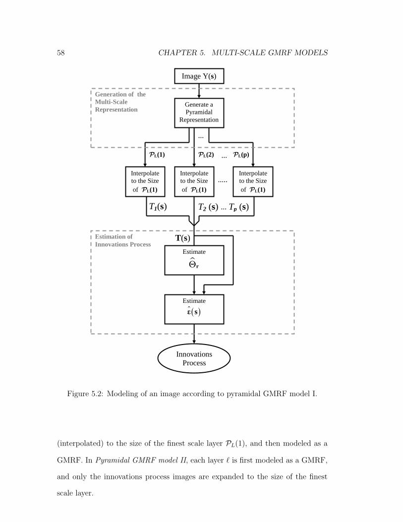
58 CHAPTER 5. MULTI-SCALE GMRF MODELS
Image Y(s)
Generate a Pyramidal
Representation
PL(1) PL(2)
PL(p)
Interpolate to the Size of PL(1)
Interpolate to the Size of PL(1)
Interpolate to the Size of PL(1)
T1(s) T2 (s) Tp (s)
Generation of the Multi-Scale Representation
T(s)
Estimate
ˡr
Estimate
( )˾ sɵ
Innovations Process
Estimation of Innovations Process
Figure 5.2: Modeling of an image according to pyramidal GMRF model I.
(interpolated) to the size of the finest scale layer PL(1), and then modeled as a
GMRF. In Pyramidal GMRF model II, each layer ` is first modeled as a GMRF,
and only the innovations process images are expanded to the size of the finest
scale layer.

5.2. STATISTICAL MODELS 59
Image Y(s)
Generate a Pyramidal
Representation
PL(1) PL(2)
PL(p)
Generation of the Multi-Scale Representation
Innovations Process
Estimation of Innovations Process
Estimate
ɵ1
Estimate ɵ ( )1˾ s
Estimate
ɵ2
Estimate ɵ ( )2˾ s
Estimate
ɵp
Estimate ɵ ( )p˾ s
Interpolate to the Size
of ɵ ( )1˾ s
Interpolate to the Size
of ɵ ( )1˾ s
Figure 5.3: Modeling of an image according to pyramidal GMRF model II.
5.2.2 Multi-Layer GMRF model
The pyramidal representation is generated by repeatedly applying a LPF to the
original image and resampling the resulting image. This approach dictates a con-
stant scaling factor (decreasing the resolution between each following layers by
2). In order to release this constraint, we propose an alternative method for gen-

60 CHAPTER 5. MULTI-SCALE GMRF MODELS
erating the multi-scale representation. This approach is based on a set of scaling
filters which extend over different support sizes. The multi-scale representation
is generated by filtering the original image using this set of filters. The KLT is
applied to the resulting multi-layer image for generating independent layers. We
assume that the independent layers can be modeled as GMRFs with different sets
of parameters.
Let Y (s) denote an image, and let G = G1, G2, ..., Gn denote a given set of
multi-scale spatially invariant filters (e.g. scaling and wavelet filters). We gener-
ate from the image a multi-scale image, Y, by applying the filters to the image
Y and concatenating the results in the third dimension:
Yi = Y ∗Gi , i = 1, ..., n (5.5)
Y(s) = [Y1 (s) , Y2 (s) , ..., Yn (s)] (5.6)
where ∗ denotes 2-dimensional convolution. The result Y is a 3-dimensional rep-
resentation of the image, thus each pixel is now transformed to a vector. The
KLT can be applied to Y(s), for generating a multi-scale image, T(s), with inde-
pendent layers. T(s) has p layers representing the top p independent components
of Y(s). Let K denote a matrix whose columns are the top p eigen vectors of the
covariance matrix of Y(s). T(s) is then given by:
T(s) = KTY(s). (5.7)
We assume that there is a set of filters, G, such that each image layer, T`(s), can
be modeled as a GMRF with a different set of parameters. We denote the weight
coefficient estimated for neighbor r ∈ R, and for the `-th layer of T(s) by θ`(r),
and the innovations process of the `-th layer by ε`(s). T(s) is then given by (5.1)
and (5.2). The innovations process ε (s) is estimated using (5.4).

5.2. STATISTICAL MODELS 61
Filtering
*G1
Image Y(s)
Filtering
*G2
Filtering
*Gn
Y1(s)
Y2(s)
Yn(s)
Y(s)
KLT
T(s)=KTY(s)
T(s)
Estimate l
r
Estimate
( )˾ sɵ
Innovations Process
Generation of Multi-Scale Representation
Estimation of Innovations Process
Figure 5.4: Multi-scale GMRF modeling of an image using the multi-layer repre-
sentation.
Figure 5.4 presents the multi-scale GMRF modeling of an image using the multi-
layer representation. The modeling process is divided to 3 stages: generation of
the multi-scale representation, KLT, and estimation of the innovations process.
The GMRF model is a special case of the multi-scale GMRF model, in which the
set of filters G, contain only the identity filter (a filter which causes no change
to the image). In this case, the ”multi-scale” representation contains the image

62 CHAPTER 5. MULTI-SCALE GMRF MODELS
in one scale only and the KLT doesn’t affect it. Finally, Θr becomes a matrix of
1 × 1 and thus, Θr = θr. For this special case, (5.1) reduces to the equation of
the known GMRF given in (2.1).
5.3 Model Estimation
The multi-scale GMRF models estimation is based on the estimation of the
GMRF models which describe each layer in the pyramidal structure or each inde-
pendent layer T`(s) of the multi-layer image representation T(s). The problem
of GMRF model estimation for image processing received some attention in im-
age processing literature. Various methods for the GMRF model estimation were
developed over the years, e.g. [7], [23], [35], [36], [41], [40], [59], [70], [71], [87].
Let T` denote the `-th layer of the multi-scale representation (pyramidal layer
or an independent layer from the multi-layer representation). A computationally
efficient method for the GMRF model estimation is the coding method, described
in details in Kashyap and Chellappa [41] and Besag [7]. Let the column stack
ordering of the neighborhood of T`(s) be denoted by g`(s):
g`(s) = vec[T`(s + r), r ∈ R] (5.8)
and let
θ` = vec[θ`(r), r ∈ R]. (5.9)
Based on Kashyap and Chellappa [41] and using (2.10), θ` and ρ2` are estimated

5.3. MODEL ESTIMATION 63
as follows:
θ` =
[∑s∈Ω0
g`(s)g`(s)T
]−1 [∑s∈Ω0
T`(s)g`(s)
](5.10)
ρ2` =
1
|Ω|∑s∈Ω
(T`(s)− θ
T
` g`(s))2
(5.11)
where Ω0 is a subset of the support Ω with every other site of Ω skipped. The
estimate of Θr is then:
Θr = diag(θ1 (r) , θ2 (r) , ..., θp (r)) (5.12)
One of the main disadvantages of the coding method is that the estimates are
not efficient [59] due to the partial use of the data. Another disadvantage is that
the estimate is not unique. Summing s in (5.10) over Ω− Ω0 instead of Ω0 may
produce considerably different estimates. Simple averaging of these dependent
estimates is not satisfactory.
The maximum likelihood (ML) estimate of θ` is consistent and efficient but does
not in general have a close form solution. The ML estimate can be obtained using
numerical optimization techniques on Mx × My equations of the form of (2.1)
(where Mx ×My is the size of the image), constrained by the requirement that
(2.7) be positive. This method is computationally inefficient, since it involves the
optimization of a nonlinear function with respect to a matrix valued parameter,
subject to nonlinear constraints.
Let ΩB, the boundary subset of Ω, be defined as follows:
ΩB = s|s ∈ Ω and (s + r) /∈ Ω for at least one r ∈ R (5.13)

64 CHAPTER 5. MULTI-SCALE GMRF MODELS
and let ΩI , the interior subset of Ω, be defined as follows:
ΩI = Ω− ΩB (5.14)
A computationally efficient and asymptotically consistent estimate of θ` for a
finite image can be obtained by summing s in (5.10) over ΩI . Equation (5.10)
can also be used for estimation in toroidal lattice representations by summing s
over Ω instead of ΩI .
The asymptotic consistency of this estimator has been shown in Kashyap and
Chellappa [41]. Since T`(s) is assumed to follow the GMRF model, we replace
T`(s) in 5.10 with the expression:
T`(s) =∑r∈R
θ(r)T`(s + r) + ε` (s). (5.15)
and summarize over ΩI instead of Ω0. After simplifying we receive the following
equation:
[∑s∈Ω0
g`(s)g`(s)T
](θ` − θ`
)=
∑s∈Ω0
g`(s)ε`(s) (5.16)
Since E (g`(s)ε`(s)) = 0 and∑
s∈Ω0
g`(s)g`(s)T is a positive definite matrix, the
estimate θ` is consistent.
5.4 Summary
Many physical processes possess behavior over vast ranges of spatial scales. Scene
elements often appear to have several periodical patterns, of various period
lengths. In such cases, random field models as the SAR, the GMRF and the

5.4. SUMMARY 65
LC models may not sufficiently fit the clutter image. In this chapter, we have
introduced multi-scale GMRF models. The models are based on multi-scale rep-
resentations of the image, ordered in a pyramidal or a multi-layer structure. We
assume each layer of the Laplacian pyramid or the multi-layer representation can
be modeled as a GMRF with a different set of parameters. The model estimation
scheme is based on estimating p GMRF parameters sets. We have presented the
concept of the computationally inefficient ML estimator and reviewed in more
details the inconsistent coding method and a consistent and computationally ef-
ficient extension of this method.
In Chapter 6, we introduce an anomaly subspace detector using the multi-scale
GMRF model. We analyze the performance of the proposed algorithm and com-
pare the detection results to those obtained by using competing methods.

66 CHAPTER 5. MULTI-SCALE GMRF MODELS
Chapter 6
Anomaly Subspace Detection
6.1 Introduction
Anomaly detection methods do not rely on an exhaustive statistical model of
the targets, but rather on a statistical model of the background. When a priori
information about the targets is available, incorporating it into the detection
process may improve detection performance. In most real detection problems, the
information about the targets is partial. Partial information about the targets
may help to define a subspace in which the targets lie. In this case the MSD may
be the natural detection method to be used.
The MSD was originally developed for signal detection in subspace interference
and white Gaussian noise [69]. However, noise and clutter patterns in images,
do not follow the white Gaussian noise model. Here, we formulate a MSD for
signal detection in subspace interference and noise which follow the multi-scale
GMRF model. A quantitative performance analysis with comparison to compet-
ing methods shows the advantages of the proposed method.
This chapter is organized as follows: In section 6.2 we introduce the MSD for the
67

68 CHAPTER 6. ANOMALY SUBSPACE DETECTION
multi-scale GMRF model. In section 6.3 we analize the methods performance and
compare it to competing methods. In section 6.4 we propose an implementation
of the method. Finally, in section 6.5 we conclude.
6.2 Model-Based Subspace Detection
In this section, we introduce an anomaly subspace detection method based on a
MSD and the multi-scale GMRF model introduced in the previous section.
Scharf and Friedlander [69] formulated a MSD for the general problem of detect-
ing subspace signals in subspace interference and additive white Gaussian noise.
However, anomaly detection in imagery, should be based on a statistical model
which better describes the background clutter and the noise. For this purpose,
we formulate a modified MSD for detection of subspace signals in subspace inter-
ference and additive noise which follows the multi-scale GMRF model, proposed
in the previous section.
Let hj|j = 1, . . . , u and sk|k = 1, . . . , v denote two sets of image chips, which
span the signal and interference subspaces of image Y , respectively. The image
chips are all of the same size:Nx × Ny pixels, which is usually much larger than
the size of the neighborhood R. It should be large enough for containing shapes
which span the signal and interference subspaces.
We assume that image Y contain mainly noise, which follows the multi-scale
GMRF model, and that the target and interference signals are rare. Let Dp
denote an operator which calculates the prediction error, ε(s), of the multi-scale
GMRF model with p independent components. Dp is defined by using (5.5), (5.7),

6.2. MODEL-BASED SUBSPACE DETECTION 69
and (5.4), as follows:
ε(s) = [ε1 (s) , ε2 (s) , ..., εp (s)]T = DpY (s) = KTY(s)−∑r∈R
ΘrKTY(s + r).
(6.1)
Let n`(s) denote the column stack ordering of an Nx × Ny pixels image-chip of
ε` around s:
n`(s) = vec(ε`(t)|t ∈ [Nx ×Ny image chip around s]). (6.2)
We define H` and S` as follows:
H` =[
vec ([Dph1]`) vec ([Dph2]`) . . . vec ([Dphu]`)]
S` =[
vec ([Dps1]`) vec ([Dps2]`) . . . vec ([Dpsv]`)]
(6.3)
where [·]` denotes the `-th layer of the 3-dimensional data.
Let 〈H`〉 denote the signal subspace, spanned by the columns of matrix H` and
let 〈S`〉 denote the interference subspace, spanned by the columns of matrix S`.
We denote the additive noise by b`. The problem is to determine whether the
sample vector n` contains a target signal. The target signal x` can be described as
a linear combination of the columns of H` i.e., x` = H`ψ`, where ψ` is a vector
of coefficients. The interference signal is described similarly, using the matrix
S` and the coefficients vector φ`. Considering the detection problem, we define
two hypotheses, H0 and H1 which indicate, respectively, absence and presence of
target signal in the vector n`:
H0 : n` = S`φ` + b`
H1 : n` = H`ψ` + S`φ` + b`.(6.4)

70 CHAPTER 6. ANOMALY SUBSPACE DETECTION
Let PS`denote the projection of a vector onto the subspace 〈S`〉:
PS`n`(s) = S`(S`
TS`)−1S`
Tn`(s) (6.5)
and let PH`S`denote the projection of a vector onto the subspace 〈H`S`〉, spanned
by the columns of the concatenated matrix[H` S`
]. The maximum likelihood
estimates of the additive noise vector, b`, under H0 and under H1 are denoted
by b`H0
and b`H1
, respectively. These estimates are obtained by subtracting from
n` the components which lie in the signal and interference subspaces as follows:
b`H0
= (I − PS`)n`
b`H1
= (I − PH`S`)n`
(6.6)
b` is the innovations process of a GMRF and therefore is normally distributed
with zero mean. We denote the covariance matrix of b` by ρ2`Φ`, where ρ2
` is the
variance of b`. ρ2`Φ` is obtained by using (2.5).
The detection problem can be formulated as a GLRT between H0 and H1. The
log-likelihood ratio, L`, calculated based on the `-th layer of the innovations
process is given by:
L`(s) = 2ln
[Pr(b`(s)|H0)
Pr(b`(s)|H1)
]= 2ln
exp
(hΦ−1/2`
bb`H0
(s)i2
2ρ2`
)
exp
(hΦ−1/2`
bb`H1
(s)i2
2ρ2`
)
=1
ρ2`
[∥∥∥Φ−1/2` b`
H0(s)
∥∥∥2
2−
∥∥∥Φ−1/2` b`
H1(s)
∥∥∥2
2
]. (6.7)
We assume the different layers of the innovations process b`(s) are normally and
independently distributed. Thus, the probability function of the p components of

6.2. MODEL-BASED SUBSPACE DETECTION 71
pixel s is the product of p Gaussian functions. Under the log function, the product
in the likelihood ratio expression is translated into a sum of p log-likelihood
ratios (separately calculated for each layer). The log-likelihood ratio, based on p
independent layers of the innovations process is then given by L(s) =p∑
`=1
L`(s)
as follows:
L(s) =
p∑
`=1
1
ρ2`
[∥∥∥Φ−1/2` b`
H0(s)
∥∥∥2
2−
∥∥∥Φ−1/2` b`
H1(s)
∥∥∥2
2
]=
=
p∑
`=1
1
ρ2`
[Φ−1/2` n`(s)]
T (PH`S`− PS`
) [Φ−1/2` n`(s)]. (6.8)
The SNR is the ratio between the signal and the noise in terms of intensity. We
define the SNR as the second power of the ratio between the signal, which do
not lie in the interference subspace, and the standard deviation of the noise, as
follows:
SNR =
p∑
l=1
1
ρ2`
x`T[I − PeS`
]x`. (6.9)
Let u denote the rank of the signal subspace and let q = up. L is a sum of
squared independent normally distributed variables and therefore is chi-square
distributed with q degrees of freedom, as follows:
L ∼
χ2q (0) , under H0
χ2q (SNR) , under H1.
(6.10)
Under hypothesis H1, the non-centrality parameter of the chi-square distribution
of L is equal to the SNR [69]. The decision rule is based on thresholding the
log-likelihood ratio using the threshold η as follows:
ξ =
H0 if L ≤ ηH1 if L > η.
(6.11)

72 CHAPTER 6. ANOMALY SUBSPACE DETECTION
Given (6.10) and (6.11), the probabilities of false-alarm and detection are:
PFA = 1− P[χ2
q (0) ≤ η]
(6.12)
PD = 1− P[χ2
q (SNR) ≤ η]. (6.13)
6.3 Performance Analysis
In this section we analyze the performance of the proposed algorithm. We present
the receiver operating characteristics (ROC) of the algorithm with respect to
different parameters and compare it to competing methods.
6.3.1 Receiver Operating Characteristics
The ROC of the proposed algorithm is calculated using (6.9), (6.12), and (6.13).
The SNR, given by (6.9), is a function of the target’s shape and intensity, the
variance of the background’s innovations process and the interference subspace
span. The SNR increases with the norm of x and the angle between x and 〈S〉.
For the synthetic example, used in these calculations, the SNR also increases
with the number p of independent layers we use for detection. Large background
variance results in a smaller SNR and therefore, performance degradation.
Figure. 6.1 presents the ROC of the proposed algorithm for various SNRs. This
example presents the performance of the proposed anomaly detection algorithm
using 3 independent component (p = 3). The probability of false alarm (PFA) and
the probability of detection (PD) are calculated using (6.12) and (6.13) respec-
tively. Figure 6.2 presents the ROC curves versus p given a constant target norm
and background variance. For the example we use, the SNR and the probability

6.3. PERFORMANCE ANALYSIS 73
10−15
10−10
10−5
100
10−2
10−1
100
PFA
PD
SN
R=
9.5
dB
SN
R=
14.3
dB
SN
R=17
.6dB
SN
R=16.1
dB
Figure 6.1: An example of ROC calculated for the proposed algorithm, using 3
principle component (p = 3) and various values of SNR
of detection (PD) improve with p. The use of more independent layers improves
the detection performance due to the additional information concealed in each
layer. It is theoretically possible that using an independent layer which contains
dim target signal (or no target signal at all) will reduce the effective SNR and
cause performance reduction. In practice, we checked the influence of this pa-
rameter on the detection performance using a large number of synthetic examples
and did not find any example for which the detection performance decreased with
p. Another factor which may influence the performance is the dimension of the
interference subspace. According to (6.9), when the dimension of S ′` decreases,
the SNR is lower and the performance is reduced.

74 CHAPTER 6. ANOMALY SUBSPACE DETECTION
10−15
10−10
10−5
100
10−2
10−1
100
PFA
PD
p=3
p=
2
p=
1
Figure 6.2: An example of ROC calculated for the proposed algorithm using
p independent components. Using larger number of independent components,
increases the SNR and improves the performance.
6.3.2 Performance Comparison
In order to analyze the detection performance of the proposed algorithm we
compared it with those of other methods. In this section we refer to the proposed
method as ”Proposed Method III ” and compare it to a competing method and to
other proposed methods which are similar to proposed method III except of one
element or step in the process. We applied the competing methods to synthetic
images of an airplane on cloudy background. The synthetic images are generated
by the process, described in Sec. 7.2. Figure 6.3 shows the flowcharts of the

6.3. PERFORMANCE ANALYSIS 75
Generate Multi-scale
Representation
Y(s)
Y1(s)
Estimate the innovations process of each layer
Y2 (s) Yp (s)
L(s) Likelihood Ratio
MSD
ɵ ( )1˾ s ɵ ( )2˾ s ɵ ( )p˾ s
Generate Multi-scale
Representation
Y(s)
Karhunen-Loeve Transform
T
T1(s)
Estimate the innovations process of each layer
Y(s)
T2 (s) Tp (s)
L(s) Likelihood Ratio
MSD
T (s)
ɵ ( )1˾ s ɵ ( )2˾ s ɵ ( )p˾ s
Y(s)
Y(s)
Estimate the innovations process of Y(s)
L(s) Likelihood Ratio
MSD
ɵ ( )˾ s
Y(s)
Estimate the innovations process of Y(s)
L(s) Likelihood
Single Hypothesis Test
ɵ ( )˾ s
Competing Method Proposed Method I Proposed Method II Proposed Method III
Figure 6.3: Flowcharts of the compared detection methods.
different method compared in this section:
A Competing Method: We assume the image follows the GMRF model. A
single hypothesis scheme is applied to the estimated innovations process of
the image for the detection of regions, which appear unlikely with respect
to its normal distribution [36].
Proposed Method I: We assume the image follows the conventional GMRF
model rather than the multi-scale GMRF model. The MSD, proposed in
Sec. 6.2, is applied to the estimated innovations process. By analyzing the
performance of this method and comparing it to Method III we examine
the contribution of the proposed multi-scale model to the detection perfor-
mance.

76 CHAPTER 6. ANOMALY SUBSPACE DETECTION
Proposed Method II: The multi-scale GMRF model is employed, skipping
the KLT step. We assume the layers of the multi-scale representation Y(s)
follow the GMRF model and estimate the innovations process of each of
these layers. The MSD, proposed in Sec. 6.2, is applied to the estimated
innovations process. By analyzing the performance of this method we ex-
amine the significance of the KLT in the modeling process.
Proposed Method III: This method includes all the elements of the multi-
scale model proposed in Sec. 5.2.2. We assume the image follows the pro-
posed multi-scale GMRF model. The MSD, proposed in sec. 6.2, is applied
to the estimated innovations process.
Figures 6.4 and 6.5 present examples in which the proposed and competing al-
gorithms are applied to the same synthetic images of airplanes on cloudy back-
ground. Figure 6.4 shows the synthetic images, generated using a mixture of three
images of different periodical patterns (generated by summing up 3 GMRFs with
3 different parameters sets). The airplane is planted in the center of each im-
age. Figure 6.5 (a) presents the results of the Competing Method, similar to the
method presented by Hazel [36], applied to the images in Fig 6.4. Figure 6.5 (b)
shows the resulting likelihood ratios generated by applying Proposed Method I to
the images in Fig. 6.4. Figure 6.5 (c) presents the resulting likelihood ratios gen-
erated by applying Proposed Method II to the images in Fig. 6.4. Figure 6.5 (d)
presents the resulting likelihood ratios generated by applying Proposed Method
III to the images in Fig. 6.4, assuming the proposed Multi-Scale GMRF model.
Figure 6.5 (d) shows the best detection results. The likelihood ratios are close to
0 everywhere except in the target’s region. The results of the Competing Method
contain high level of background noise which does not allow the targets detection

6.3. PERFORMANCE ANALYSIS 77
Figure 6.4: Synthetic images containing cloudy background and an airplane target
in their centers
by thresholding the likelihood image. The results of Proposed Method II contain
a noisy pattern which exceeds the likelihood level in the targets region (in the
center of the image). According to these examples, it seems that skipping the
KLT in the modelling process, significantly reduces the performance related to
Proposed Method III.
Figure 6.6 presents the ROC, analytically calculated for synthetic images of an
airplane on cloudy sky. The ROC curves reflect the performance of Proposed
Method II (solid) compared to the performance of Proposed Method I (dashed).
The images, for which the ROC’s where calculated, are similar to the right ex-
ample presented in Fig. 6.4. The only difference between the images is in the
SNR.
The SNRs for which the ROCs where drawn are summarized in Table 6.1. The
table specifies 4 different cases of background variances and target norms (L-
infinity norms of the targets image). The SNRs obtained by Proposed Method III,
which is based on the multi-scale GMRF model, are higher than those obtained by
Proposed Method I, which is based on a conventional GMRF model, and Proposed
Method II, which is based on a modification of the multi-scale GMRF model.

78 CHAPTER 6. ANOMALY SUBSPACE DETECTION
Table 6.1: Properties of the different cases for which the ROC curves in Fig. (6.6)
were drawn. The SNR calculated for Proposed Method III is significantly higher
than the SNR calculated for the other methods.
Case Background Target SNR[dB]Variance Norm Proposed Proposed Proposed
Method I Method II Method III(a) 188 1.3 2.8 -0.5 7.3(b) 188 1.4 3.2 0 7.7(c) 188 1.5 3.6 0.4 8.1(d) 188 1.7 4.0 0.8 8.5
6.4 Implementation
In this section, we describe an implementation of the proposed anomaly detection
algorithm and calculate its computational complexity. Figure 6.7 presents a flow
chart with the main steps of the algorithm:
1. Generation of a Multi-Scale Representation: The image Y is filtered
by a set of spatial filters, G, using (5.5), in order to create its multi-scale
representation, Y.
2. Independent Components Analysis: The Karhunen-Loeve transform
is applied to the vectors of the multi-scale representation, Y, using (5.7).
The result is a multi-scale representation, T, with independent layers.
3. Estimation of the Innovations Process: The GMRF parameters set is
separately estimated for each layer of T. The sample innovations, ε`(s), are
calculated for each layer, `, of T using (6.1) and the estimated parameters.
4. Matched Subspace Detector: S` and H` are calculated using (6.3). A
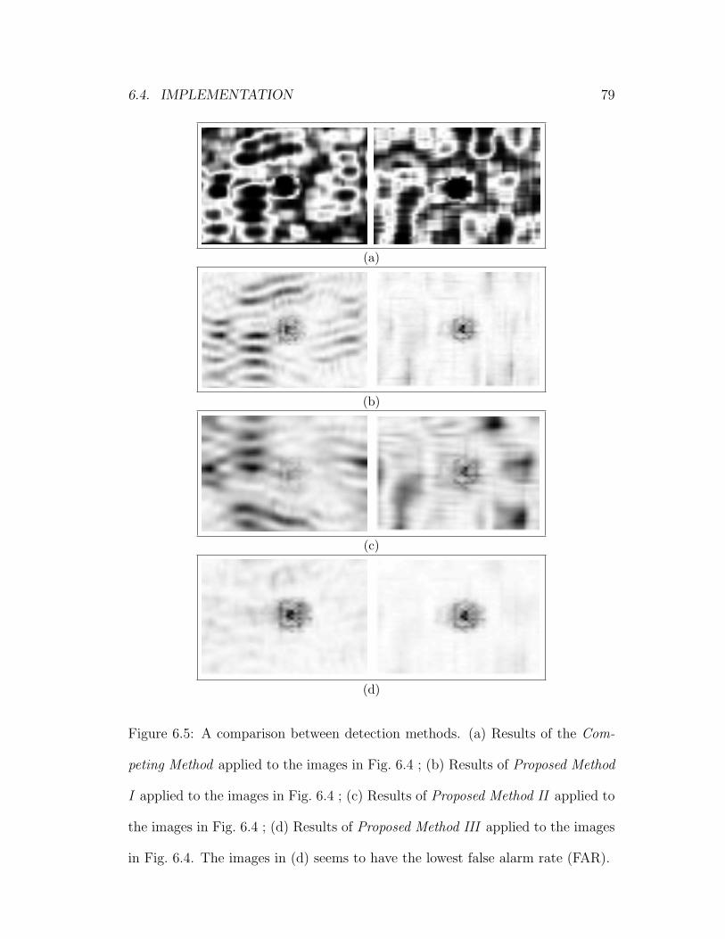
6.4. IMPLEMENTATION 79
(a)
(b)
(c)
(d)
Figure 6.5: A comparison between detection methods. (a) Results of the Com-
peting Method applied to the images in Fig. 6.4 ; (b) Results of Proposed Method
I applied to the images in Fig. 6.4 ; (c) Results of Proposed Method II applied to
the images in Fig. 6.4 ; (d) Results of Proposed Method III applied to the images
in Fig. 6.4. The images in (d) seems to have the lowest false alarm rate (FAR).

80 CHAPTER 6. ANOMALY SUBSPACE DETECTION
10−15
10−10
10−5
100
10−3
10−2
10−1
100
PFA
PD
10−15
10−10
10−5
100
10−3
10−2
10−1
100
PFA
PD
(a) (b)
10−15
10−10
10−5
100
10−3
10−2
10−1
100
PFA
PD
10−15
10−10
10−5
100
10−3
10−2
10−1
100
PFA
PD
(c) (d)
Figure 6.6: Performance of the anomaly detection based on Proposed Method III
(solid), Proposed Method II (dashed), and Proposed Method I (dotted). (a)-(d)
correspond to different parameter settings as specified in Table 6.1.
matched subspace detector is formed and the log-likelihood ratio, L, is
calculated for each pixel using (6.8).
5. Decision Rule (Thresholding): The decision rule given in (6.11) is ap-
plied to the log-likelihood ratio, L, in order to determine whether a pixel s
belongs to a target. The threshold, η, is determined by the admissible false
alarm rate (FAR) using (6.12).
The computational complexity of the proposed algorithm is a function of the
size of the image (Mx ×My), the rank of the space in which the signal and in-
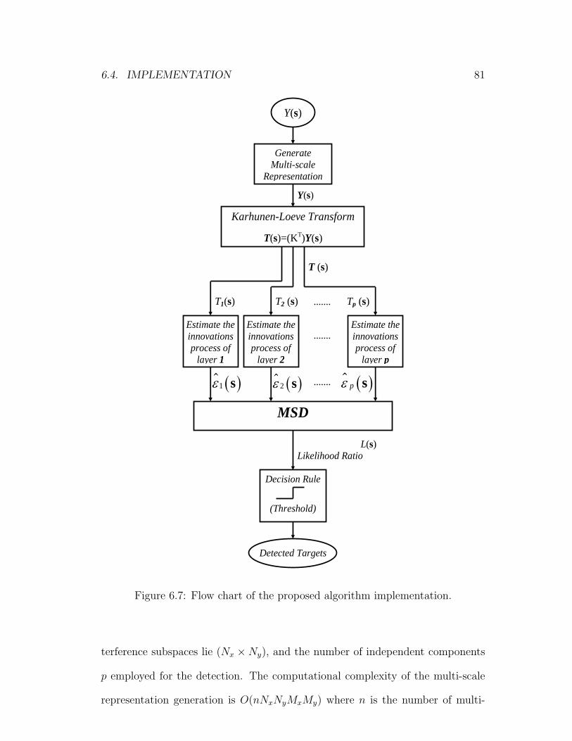
6.4. IMPLEMENTATION 81
Detected Targets
Generate Multi-scale
Representation
Y(s)
Karhunen-Loeve Transform
T(s)=(KT)Y(s)
T1(s)
Estimate the innovations process of
layer 1
Y(s)
T2 (s) Tp (s)
L(s) Likelihood Ratio
Decision Rule
(Threshold)
MSD
Estimate the innovations process of
layer 2
Estimate the innovations process of
layer p
T (s)
ɵ ( )1˾ s ɵ ( )2˾ s ɵ ( )p˾ s
Figure 6.7: Flow chart of the proposed algorithm implementation.
terference subspaces lie (Nx ×Ny), and the number of independent components
p employed for the detection. The computational complexity of the multi-scale
representation generation is O(nNxNyMxMy) where n is the number of multi-

82 CHAPTER 6. ANOMALY SUBSPACE DETECTION
scale filters. Applying the KLT to the multi-scale representation of the image
using the covariance matrix of the data is [32]: O(N2xN2
y MxMy + N3xN3
y ). Using
the singular value decomposition (SVD)-based approach, reduces the computa-
tional complexity of the KLT to O(N2xN2
y MxMy) [39]. The estimation of the
innovations process is O(|R|MxMy) and the MSD is O(MxMyNxNyp). Thus, the
total computational complexity of the proposed algorithm is O(N2xN2
y MxMy +
NxNyMxMyn + |R|MxMy).
6.5 Summary
We introduced an anomaly subspace detection method based on a multi-scale
GMRF model. The detection is carried out by applying a MSD to the innova-
tions process estimated assuming the image follows the multi-scale GMRF model.
The MSD incorporates available a priori information about the targets into the
detection process and thus potentially improves the detection performance. Per-
formance analysis was carried out by investigating the influence of different pa-
rameters on the detection performance, and comparing the performance of the
proposed method to those of competing methods. The analysis demonstrate the
advantages of the proposed method related to other methods which do not rely on
the multi-scale GMRF model. Finally, an implementation of the method was pro-
posed and its computational complexity was computed. In chapter 7 we present
some experimental results which support the analytical results presented in this
chapter. We demonstrate the proposed method using real images from different
sources.

Chapter 7
Experimental Results
7.1 Introduction
In the previous chapter we proposed an anomaly subspace detection method
and analyzed its performance. In this chapter, we present the results of apply-
ing the proposed model and algorithm to synthetic and real images from dif-
ferent sources. The algorithm is applied to: 1) simulated images of airplanes on
cloudy background; 2) Sonar images of sea-mines on sea-bottom background; and
3) Detection of defects in wafer images. The different examples and applications
demonstrate the robustness and flexibility of the algorithm.
The chapter is organized as follows: In section 7.2 we present the application
of the proposed model to synthetic images. We first describe the process of
generating synthetic clutter images and planting targets, then we present some
detection results. In section 7.3.1 we present the results of sea-mine detection in
sonar images. In section 7.3.2 we present the results of applying the proposed
method to defect detection in wafers production.
83

84 CHAPTER 7. EXPERIMENTAL RESULTS
7.2 Synthetic Imagery
In this section we present the application of the proposed method to target de-
tection in synthetic images of airplanes on cloudy background. We first present
a method for synthetic image generation, then we show some examples of like-
lihood ratio images, calculated using the proposed anomaly subspace detection
method.
7.2.1 Generating Synthetic Images
The synthetic examples presented in this subsection contain airplanes on cloudy
background. The synthetic cloudy background is created using random images
which follow the GMRF model. These random images, are generated based on
the expression of the GMRF model in terms of white noise. Let T (s) be an image
of Mx ×My pixels which follows the GMRF model, let F be the DFT operator,
and let w = (w1, w2) be the 2-dimensional indices of the data in the frequency
domain. Then the equivalent DFT representation of (2.1) for image T (s) is as
follows [41]:
FT(w) =ρFν(s)√
λ(w)(7.1)
where λ(w) is given by:
λ(w) = 1− 2∑r∈Rh
θ(r) cos
(2π
[r1w1
Mx
+r2w2
My
])(7.2)
ν(s)|s are IID Gaussian random variables, with zero mean and unit variance,
Rh is half of the symmetric neighborhood R, and r = (r1, r2). For the model

7.2. SYNTHETIC IMAGERY 85
to exist and be stable, the following expression must be true for every w in the
support of the image:
λ(w) > 0. (7.3)
From the expression in (7.1), the procedure for synthetic generation of random
fields obeying this model is evident. Further details can be found in [41].
Figure 7.1 presents a flow chart of the procedure used for generating synthetic
images of airplanes on cloudy background. The synthetic examples are generated
as follows:
1. Three random images are generated based on the GMRF model. Each
image is obtained by using (7.1) and (7.2)with different sets of parameters
(θ(1), θ(2), and θ(3)).
2. A weighted sum of the three images is calculated (using the weight coeffi-
cients ω1, ω2, and ω3). The result contains several periodical patterns with
different period lengths.
3. A small airplane image is planted in the background image in a random
position and orientation.
The results of this procedure contain mixtures of periodical patterns with different
period lengths. This procedure does not describe an accurate synthesis of images
which follow the multi-scale GMRF model. The process only claims to generate
images that may be better described by the multi-scale GMRF model rather than
the conventional GMRF model. The results presented in Sec. 6.3.2 demonstrate
the correctness of this argument. The effective SNR achieved by the MSD under
the multi-scale GMRF model assumption (Proposed Method II ) is higher than

86 CHAPTER 7. EXPERIMENTAL RESULTS
Generate a GMRF Image Using
Parameters set (1)
Generate a GMRF Image Using
Parameters set (2)
Generate a GMRF Image Using
Parameters set (3)
Multiply By The Weight
Coefficient 1
ˬ
Multiply By The Weight
Coefficient 2
Multiply By The Weight
Coefficient 3
A Small Airplane
Image
Synthetic Cloudy Background
Synthetic Image of an Airplane on
Cloudy Background
Plant The Airplane Image in the Synthetic Cloudy Background in Random Position and
Orientation.
Figure 7.1: Flow chart of the procedure for synthetic examples generation.
the SNR achieved under the conventional GMRF model assumption (Proposed
Method I ).

7.2. SYNTHETIC IMAGERY 87
7.2.2 Target Detection
Figure 7.2 presents examples of synthetic images generated as described above.
A multi-scale representation of each image is obtained by applying undecimated
wavelet transform with 2 scale levels to the image. Accordingly, the layers of
the multi-scale representation are the result of convolving the image with the
wavelet basis images. We employ a signal subspace that is constructed from the
span of 4 image chips of 11 × 11 pixels. The image chips contain bar shapes
in different orientations: 0, 45, 90, and 135 which resemble the fuselage of
airplane targets. Figure. 7.3 shows the likelihood ratio (in gray-scale), calculated
using (6.7). Black regions denote high likelihood ratio. The target detection is
carried out by thresholding the likelihood images. The threshold is determined
by the predefined admissible level of FAR. The detected targets are marked by
circles (in Fig. 7.3). This example demonstrates the robustness of the algorithm
in presence of different patterns of background. The image chips which span the
signal subspace (target subspace) are simple and generally do not require detailed
information about the targets.
Figures 7.4 and 7.5 show an example of target detection using the proposed al-
gorithm with 3 independent components (p = 3). Figure 7.4 shows a synthetic
image of cloudy sky with an airplane in its middle. The airplane is unnoticeable
by a human viewer due to its weak signature. Figures. 7.5(a)-(c) show the im-
ages of the 3 top independent components generated by the algorithm (as detailed
in Sec. 5.2). The target is clearly revealed in the 3rd independent component.
Figure 7.5(d) shows the likelihood ratio calculated by the proposed algorithm.
This image, unlike the images of the independent components, lacks the back-

88 CHAPTER 7. EXPERIMENTAL RESULTS
(a) (b)
(c) (d)
(e) (f)
Figure 7.2: Synthetic images of cloudy sky with airplane images planted in ran-
dom places and orientations.
ground patterns, which are rejected by the innovations noise and likelihood ratio
calculations. Thus, the target is more clearly revealed.

7.2. SYNTHETIC IMAGERY 89
(a) (b)
(c) (d)
(e) (f)
Figure 7.3: Results of anomaly detection applied to the images in Fig.7.2. The
gray-scale represents the degree of local anomality around a given pixel. The cir-
cles indicate regions where the local anomality is above a predetermined thresh-
old.

90 CHAPTER 7. EXPERIMENTAL RESULTS
Figure 7.4: A synthetic image of cloudy sky with an airplane in its middle. The
airplane is unnoticeable by a human viewer due to its weak signature.
(a) (b)
(c) (d)
Figure 7.5: Anomaly detection applied to the image in Fig. 7.4. (a) First, (b)
second, and (c) third independent components. (d) Likelihood ratio calculated
by the proposed algorithm.

7.3. REAL IMAGERY 91
7.3 Real Imagery
In this section we present the application of the proposed method to target detec-
tion in real imagery. We first show the results of applying the proposed method
to sea-mine detection in sonar images, then we present some examples of wafer
defects detection for quality assurance purpose. These two different examples
demonstrate the capability of the proposed model and algorithm to cope with
variety of background clutter patterns.
7.3.1 Detection of Sea-Mines in Sonar Images
The proposed method is demonstrated on real images from a database of sea-
mine sonar images. A sea-mine appears in the sonar images as a bar shaped
object-highlight accompanied by a shadow which represents the hiding of the
seabottom-reverberation by the sea-mine [63]. Mignotte and Collet [58] pre-
sented 3-class Markovian segmentation method for the detection of sea-mines in
sonar images. The sea-mine images were segmented to 3 kinds of regions: echo,
shadow, and sea-bottom reverberation areas, based on different MRF models,
estimated for the different classes. Dobeck et al. [26] implemented a matched
filter, K-nearest neighbor neural network classifier, and a discriminatory filter
classifier to detect such mine-like objects in sonar images. The classification pro-
cess employs up to 45 features for every possible mine-like object. The detection
in [26] is based on a large collection of mine-like objects signatures. In the ex-
ample presented here, no real signature examples are used for defining the signal
subspace. Figure 7.6 shows 6 sonar images. Each image contains one sea-mine on
highly cluttered seabottom background. The background patterns are diverse.

92 CHAPTER 7. EXPERIMENTAL RESULTS
(a) (b)
(c) (d)
(e) (f)
Figure 7.6: Examples of sea-mine sonar images: Sea-mines appear in the sonar
images as a bar shaped object-highlight accompanied by a shadow which repre-
sents the hiding of seabottom-reverberation by the sea-mine [63].
Figures 7.6(a)-(e) contain relatively slow changing backgrounds while Fig. 7.6(f)
contains background with a dominant periodical pattern. The sea-mine’s high-

7.3. REAL IMAGERY 93
(a) (b)
(c) (d)
(e) (f)
Figure 7.7: Results of the anomaly detection applied to the images in Fig.7.6.
The sea-mines are detected by thresholding the gray-scale values which represent
the degree of local anomality around a given pixel.
light in Fig. 7.6(f) is unnoticeable while its shadow clearly appears as a dark
region. The proposed method is applied to these images for detecting sea-mines.

94 CHAPTER 7. EXPERIMENTAL RESULTS
The multi-scale representations of the images are generated by applying undeci-
mated wavelet transform with 3 scale levels to the images. The signal subspace
is formed from the span of 4 image-chips of highlighted bars with dark shadows,
in different orientations. The result of the proposed anomaly detection, applied
to the sonar images, is shown in Fig. 7.7. The sea-mine in Fig. 7.6(f) is detected
despite the absence of sea-mine highlight, due to its dominant shadow. The lower
right circle in Fig. 7.7(c) marks a false alarm. This false alarm might result from
a mine-like highlight in the background pattern.
The detection results presented here, demonstrate the capability of the proposed
model and algorithm to cope with variety of background clutter patterns, using
the same filters set and signal subspace. All the sea-mines in these examples are
detected. The false alarm in Fig. 7.7(c) may be prevented by a more specific
definition of the signal subspace.
7.3.2 Detection of Wafer Defects
The proposed algorithm is applied to detection of defects in wafers images for
quality assurance. Figure 7.8 shows examples of wafer images. Each image
contains a defect whose diameter is smaller than 3 pixels. The MSD is set to
detect circles of 3 pixels diameter and linear shapes of 3 pixels length. The multi-
scale representation is generated in the same way as described in the synthetic
example. The likelihood images and the detected targets are presented in Fig. 7.9.
The results are less impressive than those obtained in the previous applications.
However, we are still able to detect the defects with a manageable rate of false
alarms. The cause of the performance degradation may be explained by the low
correlation of the background patterns. Images with weakly correlated patterns
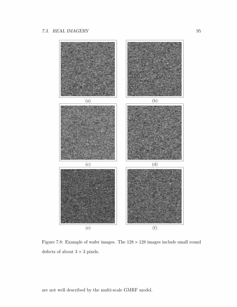
7.3. REAL IMAGERY 95
(a) (b)
(c) (d)
(e) (f)
Figure 7.8: Example of wafer images. The 128× 128 images include small round
defects of about 3× 3 pixels.
are not well described by the multi-scale GMRF model.

96 CHAPTER 7. EXPERIMENTAL RESULTS
(a) (b)
(c) (d)
(e) (f)
Figure 7.9: Results of the anomaly detection applied to the images in Fig.7.8.
7.4 Summary
We demonstrated the performance of the proposed algorithm with application to
automatic target detection. We proposed a procedure for generating synthetic

7.4. SUMMARY 97
images of airplanes on cloudy background, then we presented the results of ap-
plying the proposed algorithm to target detection in these synthetic images. The
proposed method was also applied to sea mine detection in real side-scan sonar
images, and to detection of defects in wafer images. The filter sets, as well as
the target and interference subspaces were intuitively chosen. We presented an
example in which targets, almost unnoticeable by a human viewer, were detected
by the proposed method. The results demonstrate the capability of the proposed
model and algorithm to cope with variety of targets and background clutter pat-
terns.

98 CHAPTER 7. EXPERIMENTAL RESULTS

Chapter 8
Conclusion
8.1 Summary
We have presented some models of natural clutter images and some known
anomaly detection methods. Then we introduced an iterative anomaly detection
method for feature extraction. The iterative method was applied to sea-mine
detection in sonar images. We have introduced multi-scale GMRF models and
a corresponding anomaly subspace detection algorithm. We developed the algo-
rithm for target detection in cluttered images which follow one of the proposed
models. The model was based on a multi-scale representation of the image and
the KLT.
We assumed that independent layers in the multi-scale representation can be
modeled as GMRFs with different sets of parameters. The detection is carried
out by applying a MSD to the innovations process (prediction error) of the multi-
scale GMRF. The MSD incorporates the available a priori information about the
targets into the detection process and thus improves the detection performance.
The MSD was originally developed for signal detection in subspace interference
99

100 CHAPTER 8. CONCLUSION
and white Gaussian noise [69]. Here, we have formulated a MSD for signal de-
tection in subspace interference and noise which follows the proposed multi-scale
GMRF model.
The performance of the algorithm was demonstrated with application to auto-
matic target detection in synthetic images, side-scan sonar data and wafer images.
The results show the capability of the proposed model and algorithm to cope with
variety of targets and background clutter patterns. Performance analysis was car-
ried out by investigating the influence of different parameters on the detection
performance, and comparing the performance of the proposed method to those
of similar methods. The analysis as well as the experimental results demonstrate
the advantages of the proposed method.
8.2 Future Research
The method we have proposed in this thesis opens a number of interesting topics
for future study:
1. Multi-scale stochastic processes modeling.
The detection method proposed in this thesis, is carried out using indepen-
dent image layers. Each independent layer is separately modeled. Models of
multi-scale stochastic processes (MSPs) use a pyramidal image structure for
modeling images in different scales [21], [24], [51], [65], [67], [80]. Figure 8.1
presents the pyramidal structure of a multi-resolution tree, presented by
Willsky [80]. The operator γ transforms node s to its parent sγ in a coarser
scale. The pyramid-based multi-scale stochastic process (MSP) models de-
scribe the Markovian relation between different levels of resolution. The
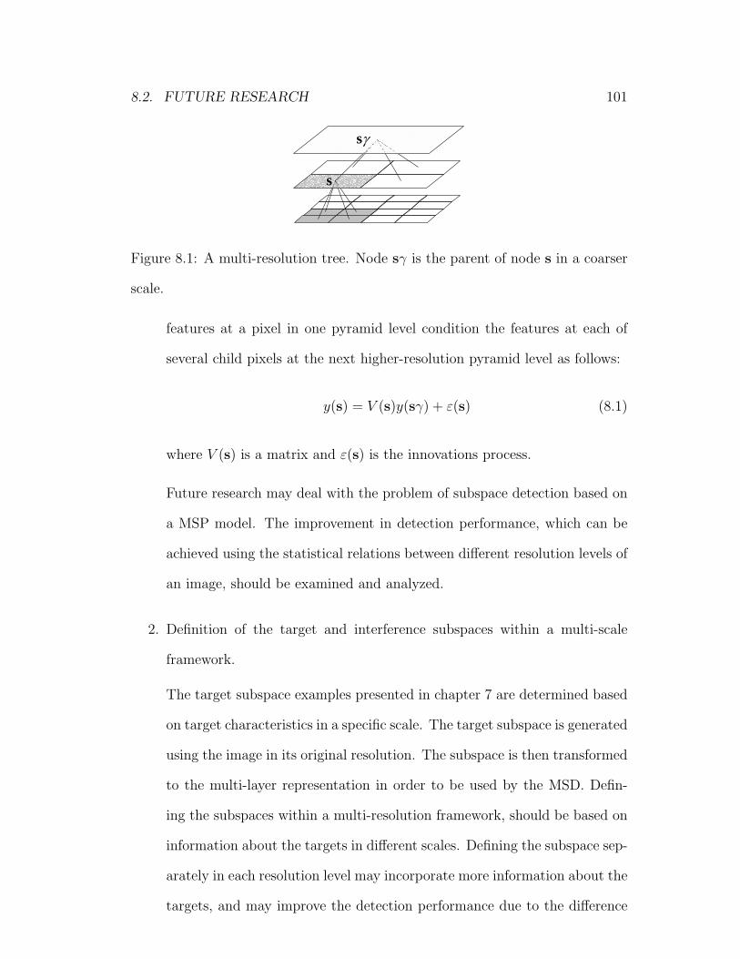
8.2. FUTURE RESEARCH 101
˼s
s
Figure 8.1: A multi-resolution tree. Node sγ is the parent of node s in a coarser
scale.
features at a pixel in one pyramid level condition the features at each of
several child pixels at the next higher-resolution pyramid level as follows:
y(s) = V (s)y(sγ) + ε(s) (8.1)
where V (s) is a matrix and ε(s) is the innovations process.
Future research may deal with the problem of subspace detection based on
a MSP model. The improvement in detection performance, which can be
achieved using the statistical relations between different resolution levels of
an image, should be examined and analyzed.
2. Definition of the target and interference subspaces within a multi-scale
framework.
The target subspace examples presented in chapter 7 are determined based
on target characteristics in a specific scale. The target subspace is generated
using the image in its original resolution. The subspace is then transformed
to the multi-layer representation in order to be used by the MSD. Defin-
ing the subspaces within a multi-resolution framework, should be based on
information about the targets in different scales. Defining the subspace sep-
arately in each resolution level may incorporate more information about the
targets, and may improve the detection performance due to the difference

102 CHAPTER 8. CONCLUSION
between the information about the targets, revealed by each resolution level.
Future research may deal with the performance improvement which can be
achieved by defining the subspaces within a multi-resolution framework.
3. Anomaly subspace detection in presence of non-stationary background.
When the background pattern changes in space, the stationarity assump-
tion of the proposed model may limit the detection performance. When the
change in the model parameters is slow, small areas may be well described
by a stationary approximation. Combining the background modeling and
the detection process with a segmentation procedure may help to better
describe the background patterns and improve the detection performance.
Future research may deal with non-stationary background patterns which
can be locally approximated by stationary pattern models. A comparative
performance analysis may demonstrate the possible advantages in segmen-
tation of the image and separately modeling each of its segments. Divid-
ing the image into smaller areas may justify the stationary approximation.
Smaller areas may also reduce the population of pixels, used for estimating
the statistical models for the different segments, and therefore may increase
the estimation error. This tradeoff should also be examined in future work.

Bibliography
[1] E. A. Ashton, “Detection of subpixel anomalies in multispectral infrared imagery
using an adaptive bayesian classifier,” IEEE Trans. Geoscience and Remote Sens-
ing, vol. 36, pp. 506–517, March 1998.
[2] V. Barnett and T. Lewis, Outliers in statistical data. NY, USA: Wiley, 1994.
[3] M. G. Bello, “A random-field model-based algorithm for anomalous complex image
pixel detection,” IEEE Transactions on Image Processing, vol. 1, no. 2, pp. 186–
196, April 1992.
[4] J. Bennet and A. Khotanzad, “Modeling textured images using generalized long
correlation models,” IEEE Transactions on Pattern Analysis and Machine Intel-
ligence, vol. 20, no. 12, pp. 1365–1370, December 1998.
[5] J. W. Bennett, “Modeling and analysis of gray tone, color, and multispectral tex-
ture images by random field models and their generalizations,” Ph.D. dissertation,
Electrical Engineering Department, Southern Methodist Univ., Methodist Univ.
Dallas, Tex, May 1997.
[6] L. M. Berliner, C. K. Wikle, and N. Cressie, “Long-lead prediction of pacific sst’s
via bayesian dynamic modeling,” J. Climate, vol. 13, pp. 3953–3968, 2000.
[7] I. E. Besag, “Spatial interaction and statistical analysis of lattice systems,” J.
Royal Stat. Sot., Ser. B, vol. B-36, pp. 192–236, 1974.
[8] C. Bishop, “Novelty detection and neural network validation,” in Proceedings of
the IEE Conference on Vision and Image Signal Processing. IEE, 1994, pp.
217–222.
[9] P. Brodatz, Textures : A Photographic Album for Artists and Designers. New-
York: Dover, 1966.
103

104 BIBLIOGRAPHY
[10] T. Brotherton, T. Johnson, and G. Chadderdon, “Classification and novelty de-
tection using linear models and class dependent elliptical basis function neural
network,” in Proceedings of the IJCNN Conference. Anchorage: IJCNN, May
1998.
[11] P. J. Burt and E. H. Adelson, “The laplacian pyramid as a compact image code,”
IEEE Transactions on communications, vol. COM-31, no. 4, pp. 532–540, April
1983.
[12] G. A. Carpenter, M. A. Rubin, and W. W. Streilein, “Artmap-fd: familiarity
discrimination applied to radar target recognition,” in Proceedings of the Interna-
tional Conference on Neural Networks, vol. 3, Houston, TX, 1997, pp. 1459–1464.
[13] R. Chellappa, “Two-dimensional discrete gaussian markov random field models
for image processing,” Progress in Pattern Recognition, vol. 2, pp. 79–112, 1985.
[14] R. Chellappa and S. Chatterjee, “Classification of textures using gaussian markov
random fields,” IEEE Trans. ASSP, vol. 33, pp. 959–963, 1985.
[15] R. Chellappa and R. L. Kashyap, “Synthetic generation and estimation in random
field models of images,” in Proc. IEEE CS Conf. Pattern Recognition and Image
Processing, Dallas Tex., August 1981, pp. 577–582.
[16] ——, “Texture synthesis using 2-d noncausal autoregressive models,” IEEE Trans-
actions on Acoustics, Speech and Signal Processing, vol. ASSP-33, no. 1, pp. 194–
203, Februaly 1985.
[17] H. Cheng and C. A. Bouman, “Multiscale bayesian segmentation using a trainable
context model,” IEEE Transactions on Image Processing, vol. 10, no. 4, pp. 511–
525, April 2001.
[18] D. A. Clausi, “Texture segmentation on sar ice imagery,” Ph.D. dissertation, Uni-
versity of Waterloo, Canada, 1996.
[19] ——, “An analysis of co-occurrence texture statistics as a function of grey level
quantization,” Canadian Journal of Remote Sensing, vol. 28, no. 1, pp. 45–62,
2002.
[20] D. A. Clausi and B. Yue, “Comparing cooccurrence probabilities and markov ran-
dom fields for texture analysis of sar sea ice imagery,” IEEE trans. on Geoscience
and Remote Sensing, vol. 42, no. 1, pp. 215–228, January 2004.

BIBLIOGRAPHY 105
[21] H. Coi and R. G. Baraniuk, “Multiscale image segmentation using waveletdomain
hidden markov models,” IEEE Transactions on Image Processing, vol. 10, no. 9,
pp. 1309–1321, 2001.
[22] C. A. H. R. W. Conners, “Theoretical comparison of texture algorithms,” IEEE
Transactions on Pattern Analysis and Machine Intelligence, vol. 2, no. 3, pp.
204–222, May 1980.
[23] G. R. Cross and A. K. Jain, “Markov random field texture models,” in Proceedings
of the IEEE Comput. Sot. Conf. Pattern Recog. Image Proc. Dallas, TX: IEEE,
August 1981, pp. 597–601.
[24] M. S. Crouse, R. D. Nowak, and R. G. Baraniuk, “Wavelet-based statistical signal
processing using hidden markov models,” IEEE Transactions on Signal Processing,
vol. 46, no. 4, pp. 886–902, 1998.
[25] M. Desforges, P. Jacob, and J. Cooper, Eds., Applications of probability density
estimation to the detection of abnormal conditions in engineering, vol. 212. In-
stitute of Mechanical Engineers, 1998.
[26] G. J. Dobeck, J. C. Hyland, and L. Smedley, “Automated detection/classification
of sea mines in sonar imagery,” in Proc. SPIE, vol. 3079, Orlando, Florida, April
1997, pp. 90–110.
[27] M. Elad, Image Processing and Analysis, Technion city, Haifa, Israel, 2003, text-
book of an image processing course Ch.11, pp. 235–256.
[28] K. Eom, “Long-correlation image models for textures with circular and elliptical
correlation structures,” in ICIP01, 2001, pp. I: 197–200.
[29] K. B. Eom, “Long-correlation image models for texture with circular and elliptical
correlation structures,” IEEE Transactions on Image Processing, vol. 10, no. 7,
pp. 1047–1055, July 2001.
[30] P. W. Fieguth, W. C. Karl, A. S.Willsky, and C.Wunsch, “Multiresolution optimal
interpolation and statistical analysis of topex/poseidon satellite altimetry,” IEEE
Trans. Geosci. Remote Sensing, vol. 33, pp. 280–292, March 1995.
[31] C. H. Fosgate, H. Krim, W. W. Irving, W. C. Karl, and A. S. Willsky, “Multiscale
segmentation and anomaly enhancement of sar imagery,” IEEE Transactions on
Image Processing, vol. 6, no. 1, pp. 7–20, January 1997.

106 BIBLIOGRAPHY
[32] D. Fradkin and D. Madigan, “Experiments with random projections for machine
learning,” in Proceedings of the ninth ACM SIGKDD international conference on
Knowledge discovery and data mining. ACM Press New York, NY, USA, 2003,
pp. 517–522.
[33] K. Fukunaga, Introduction to Statistical Pattern Recognition, 2nd ed. Academic
Press, 1990, ch. 3, pp. 66–77.
[34] S. Geman and D. Geman, “Stochastic relaxation, gibbs distributions, and the
bayesian restoration of images,” IEEE Trans. PAMI, vol. 6, no. 6, pp. 194–207,
November 1984.
[35] M. Hassner and J. Sklansky, “The use of markov random fields as models of
textures,” Comput. Graphics Image Proc., vol. 12, pp. 357–370, April 1980.
[36] G. G. Hazel, “Multivariate gaussian GMRF for multispectral scene segmantation
and anomaly detection,” IEEE Transactions on Geoscience and Remote Sensing,
vol. 38, no. 3, pp. 1199–1211, May 2000.
[37] J. R. Jensen, Introductory Digital Image Processing: A Remote Sensing Perspetive,
2nd ed. Prentice Hall, Inc., 1996.
[38] R. A. Johnson and D. W. Wichem, Applied Multi-variate Statistical Analysis.
Englewood Cliffs, NJ: Prentice Hall, 1998.
[39] K. V. R. Kanth, D. Agrawal, A. E. Abbadi, and A. Singh, “Dimensionality re-
duction for similarity searching in dynamic databases,” University of California,
Technical report 1998-10, May 1998.
[40] R. L. Kashyap, Image Modeling. New York: Academic, 1980, ch. Univariate and
multivariate random field models for images.
[41] R. L. Kashyap and R. Chellappa, “Estimation and choice of neighbors in spatial-
interaction models of images,” IEEE Transactions on Information Theory, vol.
IT-29, no. 1, pp. 60–72, January 1983.
[42] R. L. Kashyap and K. B. EOM, “A consistent estimation of parameters in the
long memory time series model,” Journal of Time Series Analysis, vol. 9, no. 1,
pp. 35–41, 1988.

BIBLIOGRAPHY 107
[43] ——, “Texture boundary detection based on long correlation model,” IEEE Trans.
on Pattern Anal. and Machine Intell., vol. 11, no. 1, pp. 58–67, 1989.
[44] R. L. Kashyap and P. M. Lapsa, “Sythesis and estimation of random fields using
long correlation models,” IEEE Trans. Pattern Analysis and Machine Intelligence,
vol. 6, no. 6, pp. 800–809, Nov. 1984.
[45] E. J. Kelly, “Adaptive detection and parameter estimation for multidimensional
signal models,” MIT Lincoln LAboratory, Lexington, MA, Tech. Rep. 848, April
1989.
[46] C. Kervrann and F. Heitz, “A Markov random field model-based approach to
unsupervised texture segmentation using local and global spatial statistics,” IEEE
Transactions on Image Processing, vol. 4, no. 6, pp. 856–862, June 1995.
[47] P. Kumar, “A multiple scale state-space model for characterizing subgrid scale
variability of near-surface soil moisture,” IEEE Trans. Geosci. Remote Sensing,
vol. 37, pp. 182–197, 1999.
[48] K. V. Leemput, F. Maes, D. Vandermeulen, A. Colchester, and P. Suetens, “Au-
tomated segmentation of multiple sclerosis lesions by model outlier detection,”
IEEE Trans. on Medical Imaging, vol. 20, no. 8, pp. 677–688, August 2001.
[49] P. Levi, “A special problem of brownian motion, and a general theory of gaussian
random functions,” in 3rd Berkeley Symp. Mathematical Statistics and Probability,
vol. 2, Berkeley California. California Press, 1956.
[50] S. Lovejoy and D. Schartzer, “Generalized scale invariance in the atmosphere and
fractal models of rain,” Water Resources Res., vol. 21, pp. 1233–1250, August
1985.
[51] M. R. Luettgen and A. S. Willsky, “Likelihood calculation for a class of multiscale
stochastic models, with application to texture discrimination,” IEEE Trans. Image
Proc., vol. 4, no. 2, pp. 194–207, 1995.
[52] C. Manikopoulos and S. Papavassiliou, “Network intrusion and fault detection:
a statistical anomaly approach,” IEEE Communications Magazine, vol. 40, pp.
76–82, October 2002.
[53] D. Manolakis and G. Shaw, “Detection algorithms for hyperspectral imaging ap-
plications,” IEEE Signal Processing Magazine, pp. 29–43, January 2002.

108 BIBLIOGRAPHY
[54] D. Manolakis, G. Shaw, and N. Keshava, “Comparative analysis of hyperspectral
adaptive matched filter detectors,” in SPIE, Algorithms for Multispectral, Hyper-
spectral, and Ultrasepctral Imagery VI, S. Shen and M. Descour, Eds., vol. 4049.
SPIE, April 2000, pp. 2–17.
[55] G. Manson, G. Pierce, and K. Worden, “On the long tern stability of normal
condition for damage detection in a composite panel,” in Proceedings of the 4th
international conference on damage assessment of Structures (DAMAS). Cardiff,
UK, June 2001, pp. 359–369.
[56] G. Manson, S. G. Pierce, K. Worden, T. Monnier, P. Guy, and K. Atherton,
“Long-term stability of normal condition data for novelty detection,” in Smart
Structures and Materials 2000: Smart Structures and Integrated Systems, N. M.
Wereley, Ed., vol. 3985. SPIE, June 2000, pp. 323–334.
[57] M. Markou and S. Singh, “Novelty detection: A review - part 1: Statistical ap-
proaches,” Signal Processing, vol. 83, no. 12, pp. 2481–2497, July 2003.
[58] M. Mignotte and C. Collet, “Three-class markovian segmentation of high-
resolution sonal images,” Computer Vision and Image Understanding, vol. 76,
no. 3, pp. 191–204, December 1999.
[59] P. A. P. Moran and J. E. Besag, “On the estimation and testing of spatial inter-
action in gaussian lattices,” Biometrika, vol. 62, no. 3, pp. 555–562, 1975.
[60] L. Parra, G. Deco, and S. Miesbach, “Statistical independence and novelty detec-
tion with information preserving non-linear maps,” Neural Comput., vol. 2, no. 8,
pp. 260–269, 1995.
[61] N. J. Pizzi, R. A. Vivanco, and R. L. Somorjai, “Evident: a functional magnetic
resonance image analysis system,” Artificial Intelligence in Medicine, vol. 21, no.
1-3, pp. 263–269, January-March 2001.
[62] I. S. Reed and X. Yu, “Adaptive multiple-band cfar detection of an optical pat-
tern with unknown spectral distribution,” IEEE Trans. Acoustics, Speech, Signal
Processing, vol. 38, pp. 1760–1770, October 1990.
[63] S. Reed, Y. Petillot, and J. Bell, “An automatic approach to the detection and ex-
traction of mine features in sidescan sonar,” IEEE Journal of Oceanic Engineering,
vol. 28, no. 1, pp. 90–105, January 2003.

BIBLIOGRAPHY 109
[64] S. Roberts and L. Tarassenko, “A probabilistic resource allocating network for
novelty detection,” Neural Comput., no. 6, pp. 270–284, 1994.
[65] J. K. Romberg, H. Coi, and R. G. Baraniuk, “Bayesian tree-stuctured image
modeling using wavelet domain hidden markov models,” IEEE Transactions on
Image Processing, vol. 10, no. 7, pp. 1056–1068, 2001.
[66] A. Rosenfeld, “Image modeling during the 1980’s: a brief overview. in markov
random fields: Theory and applications,” vol. 2, 1993.
[67] P. Sajda, C. Spence, and L. Parra, “A multi-scale probabilistic network model for
detection, synthesis and compression in mammographic image analysis,” Medical
Image Analysis, vol. 7, no. 2, pp. 187–204, June 2003.
[68] A. Sarkar, M. K. Biswas, and K. M. S. Sharma, “A simple unsupervised GMRF
model based image segmentation approach,” IEEE Transactions on Image Pro-
cessing, vol. 9, no. 5, pp. 801–811, May 2000.
[69] L. L. Scharf and B. Friedlander, “Matched subspace detectors,” IEEE Transactions
on Signal Processing, vol. 42, no. 8, pp. 2146–2156, August 1994.
[70] S. M. Schweizer and J. M. F. Moura, “Hyperspectral imagery: Clutter adaption
in anomaly detection,” IEEE Transactions on Information Theory, vol. 46, no. 5,
pp. 1855–1871, August 2000.
[71] ——, “Efficient detection in hyperspectral imagery,” IEEE Transactions on Image
Processing, vol. 10, no. 4, pp. 584–597, April 2001.
[72] A. Speis and G. Healey, “Feature extraction for texture discrimination via ran-
dom field models with random spatial interaction,” IEEE Transactions on Image
Processing, vol. 5, no. 4, pp. 635–645, April 1996.
[73] D. W. J. Stein, S. G. Beaven, L. E. Hoff, E. M. Winter, A. P. Schaum, and
A. D. Stocker, “Anomaly detection from hyperspectral imagery,” IEEE Signal
Processing Magazine, pp. 58–69, January 2002.
[74] L. Tarassenko, “Novelty detection for the identification of masses in mammo-
grams,” in Proceedings of the 4th IEE International Conference on Artificial Neu-
ral Networks, vol. 4. Cambridge, UK: IEE, 1995, pp. 442–447.

110 BIBLIOGRAPHY
[75] L. Tarassenko, A. Nairac, N. Townsend, and P. Cowley, “Novelty detection in jet
engines,” in IEE Colloquium on Condition Monitoring, Imagery, External Struc-
tures and Health, Birmingham, UK, 1999, pp. 41–45.
[76] D. M. J. Tax and R. P. W. Duin, “Outlier detection using classifier instability,”
in Advances in Pattern Recognition - The joint IAPR International Workshops.
Sydney, Australia: IAPR, 1998, pp. 593–601.
[77] L. van Kempen and H. Sahli, “Signal processing techniques for clutter parameters
estimation and clutter removal in GPR data for landmine detection,” in Proc.
11th IEEE Workshop on Statistical Signal Processing, Singapure, August 2001,
pp. 158–161.
[78] A. R. Webb, Statistical Pattern Recognition, 2nd ed. John Wiley and Sons, July
2002.
[79] R. A. Weisenseel, W. C. K. D. A. Castanon, and C. A. Dimarzio, “Statistical
approach to multi-channel spatial modeling for the detection of mine-like targets,”
in Proc. SPIE, Detection and Remediation Technologies for Mines and Mine-Like
Targets, vol. 3392, April 1998, pp. 1044–1053.
[80] A. S. Willsky, “Multiresolution markov models for signal and image processing,”
in Proceedings of the IEEE, vol. 90, no. 8, August 2002, pp. 1396–1458.
[81] E. Wong, “Two-dimensional random fields and representation of images,” SIAM
J. Appl. Math., vol. 16, pp. 756–770, 1968.
[82] J. W. Woods, “Two-dimensional discrete Markovian fields,” IEEE Transactions
on Information Theory, vol. IT-18, no. 2, pp. 101–109, March 1972.
[83] C. Wunsch and D. Stammer, “The global frequency-wavenumber spectrum of
oceanic variability estimated from topex/poseidon altimetric measurements,” J.
Geophys. Res., vol. 100, pp. 24,89524,910, 1995.
[84] Y. Yang and X. Liu, “A re-examination of text categorization methods,” in Pro-
ceedings of the 22nd annual international ACM SIGIR conference on Research and
development in information retrieval. ACM Press, 1999, pp. 42–49.
[85] D. Y. Yeung and C. Chow, “Parzen window network intrusion detectors,” in Pro-
ceedings of the International Conference on Pattern Recognition, Quebec, Canada,
2002.

BIBLIOGRAPHY 111
[86] B. Yue, “Sar sea ice recognition using texture methods,” Master’s thesis, Univer-
sity of Waterloo, Ontario, Canada, 2002.
[87] P. Zhao and J. Litva, “Consistency of modified LS estimation method for identi-
fying 2-D noncausal SAR model parameters,” IEEE Transactions on Automatic
Control, vol. 40, no. 2, pp. 316–320, February 1995.


![Beyond outliers and on to micro-clusters: Vision-guided ...For graph anomaly detection, [30,21] nd communities and suspicious clusters with spectral-subspace plots. SpokEn[30] considers](https://img.dokumen.tips/doc/110x75/5f47770af15dfb4e8b6989af/beyond-outliers-and-on-to-micro-clusters-vision-guided-for-graph-anomaly-detection.jpg)