Embed Size (px)
Citation preview
ANNALES DEL’INSTITUT FOURIER
Université Grenoble Alpes
Les Annales de l’institut Fourier sont membres duCentre Mersenne pour l’édition scientique ouvertewww.centre-mersenne.org
Dawei Chen & Qile ChenPrincipal boundary of moduli spaces of abelian and quadraticdierentialsTome 69, no 1 (2019), p. 81-118.<http://aif.centre-mersenne.org/item/AIF_2019__69_1_81_0>
© Association des Annales de l’institut Fourier, 2019,Certains droits réservés.
Cet article est mis à disposition selon les termes de la licenceCreative Commons attribution – pas de modification 3.0 France.http://creativecommons.org/licenses/by-nd/3.0/fr/
Ann. Inst. Fourier, Grenoble69, 1 (2019) 81-118
PRINCIPAL BOUNDARY OF MODULI SPACES OFABELIAN AND QUADRATIC DIFFERENTIALS
by Dawei CHEN & Qile CHEN (*)
Abstract. — The seminal work of Eskin–Masur–Zorich described the prin-cipal boundary of moduli spaces of abelian differentials that parameterizes flatsurfaces with a prescribed generic configuration of short parallel saddle connec-tions. In this paper we describe the principal boundary for each configuration interms of twisted differentials over Deligne–Mumford pointed stable curves. We alsodescribe similarly the principal boundary of moduli spaces of quadratic differentialsoriginally studied by Masur–Zorich. Our main technique is the flat geometric de-generation and smoothing developed by Bainbridge–Chen–Gendron–Grushevsky–Möller.Résumé. — Le travail fondateur d’Eskin–Masur–Zorich a décrit la limite prin-
cipale des espaces de modules des différentielles abéliennes qui paramètre les sur-faces plates possédant une configuration générique de petites connexions de sellesparallèles prescrite. Dans cet article, nous décrivons la limite principale pour chaqueconfiguration en terme de différentielles entrelacées sur les courbes stables pointéesde Deligne–Mumford. Nous décrivons également la limite principale des espaces demodules des différentielles quadratiques étudiée à l’origine par Masur–Zorich. Nosprincipaux outils sont la dégénérescence géométrique plate et le lissage développéspar Bainbridge–Chen–Gendron–Grushevsky–Möller.
1. Introduction
Many questions about Riemann surfaces are related to study their flatstructures induced from abelian differentials, where the zeros of differentialscorrespond to the saddle points of flat surfaces. Loci of abelian differentialswith prescribed type of zeros form a natural stratification of the modulispace of abelian differentials. These strata have fascinating geometry andcan be applied to study dynamics on flat surfaces.
Keywords: Abelian differential, principal boundary, moduli space of stable curves, spinand hyperelliptic structures.2010 Mathematics Subject Classification: 14H10, 14H15, 30F30, 32G15.(*) D. Chen is partially supported by the NSF CAREER grant DMS-1350396 andQ. Chen is partially supported by the NSF grant DMS-1560830.
82 Dawei CHEN & Qile CHEN
Given a configuration of saddle connections for a stratum of flat surfaces,Veech and Eskin–Masur ([11, 23]) showed that the number of collections ofsaddle connections with bounded lengths has quadratic asymptotic growth,whose leading coefficient is called the Siegel–Veech constant for this config-uration. Eskin–Masur–Zorich ([12]) gave a complete description of all pos-sible configurations of parallel saddle connections on a generic flat surface.They further provided a recursive method to calculate the correspondingSiegel–Veech constants. To perform this calculation, a key step is to de-scribe the principal boundary whose tubular neighborhood parameterizesflat surfaces with short parallel saddle connections for a given configuration.As remarked in [12], flat surfaces contained in the Eskin–Masur–Zorich
principal boundary can be disconnected and have total genus smaller thanthat of the original stratum. Therefore, as the underlying complex curvesdegenerate by shrinking the short saddle connections, the Eskin–Masur–Zorich principal boundary does not directly imply the limit objects fromthe viewpoint of algebraic geometry. In this paper we solve this problemby describing the principal boundary in the setting of the strata compact-ification [4] and consequently in the Deligne–Mumford compactification.
Main Result
For each configuration we give a complete description for the principalboundary in terms of twisted differentials over pointed stable curves.
This result is a combination of Theorems 2.1 and 3.4. Along the waywe deduce some interesting consequences about meromorphic differentialson P1 that admit the same configuration (see Propositions 2.3 and 3.8).Moreover, when a stratum contains connected components due to spin orhyperelliptic structures ([19]), Eskin–Masur–Zorich ([12]) described how todistinguish these structures nearby the principal boundary via an analyticapproach. Here we provide algebraic proofs for the distinction of spin andhyperelliptic structures in the principal boundary under our setting (seeSections 4.6 and 4.7 for related results).Masur–Zorich ([20]) described similarly the principal boundary of strata
of quadratic differentials. Our method can also give a description of theprincipal boundary in terms of twisted quadratic differentials in the senseof [3] (see Section 5 for details).
Twisted differentials play an important role in our description of theprincipal boundary, so we briefly recall their definition (see [4] for moredetails). Given a zero type µ = (m1, . . . ,mn), a twisted differential η of
ANNALES DE L’INSTITUT FOURIER
PRINCIPAL BOUNDARY OF DIFFERENTIALS 83
type µ on an n-pointed stable curve (C, σ1, . . . , σn) is a collection of (pos-sibly meromorphic) differentials ηi on each irreducible component Ci of C,satisfying the following conditions:
(0) η has no zeros or poles away from the nodes and markings of C andη has the prescribed zero order mi at each marking σi.
(1) If a node q joins two components C1 and C2, then ordq η1+ordq η2 =−2.
(2) If ordq η1 = ordq η2 = −1, then Resq η1 + Resq η2 = 0.(3) If C1 and C2 intersect at k nodes q1, . . . , qk, then ordqi η1−ordqi η2
are either all positive, or all negative, or all equal to zero for i =1, . . . , k.
Condition (3) provides a partial order between irreducible componentsthat are not disjoint. If one expands it to a full order between all irreduciblecomponents of C, then there is an extra global residue condition whichgoverns when such twisted differentials are limits of abelian differentials oftype µ. A construction of the moduli space of twisted differentials can befound in [2].By using η on all maximum components and forgetting its scales on
components of smaller order, [4] describes a strata compactification in theHodge bundle over the Deligne–Mumford moduli spaceMg,n. As remarkedin [4], if one forgets η and only keeps track of the underlying pointed stablecurve (C, σ1, . . . , σn), it thus gives the (projectivized) strata compactifica-tion inMg,n. Hence our description of the principal boundary in terms oftwisted differentials determines the corresponding boundary in the Deligne–Mumford compactification. To illustrate our results, we will often draw suchstable curves in the Deligne–Mumford boundary.For an introduction to flat surfaces and related topics, we refer to the
surveys [8, 24, 25]. Besides [4], there are several other strata compacti-fications, see [13] for an algebraic viewpoint, [9, 16] for a log geometricviewpoint and [21] for a flat geometric viewpoint. Algebraic distinctions ofspin and hyperelliptic structures in the boundary of strata compactifica-tions are also discussed in [7, 9, 14].
This paper is organized as follows. In Sections 2 and 3 we describe theprincipal boundary of type I and of type II, respectively, following theroadmap of [12]. In Section 4 we provide algebraic arguments for distin-guishing spin and hyperelliptic structures in the principal boundary. Fi-nally in Section 5 we explain how one can describe the principal boundaryof strata of quadratic differentials by using twisted quadratic differentials.
TOME 69 (2019), FASCICULE 1
84 Dawei CHEN & Qile CHEN
Throughout the paper we also provide a number of examples and figuresto help the reader quickly grasp the main ideas.
Notation
We denote by µ the singularity type of differentials, by H(µ) the stratumof abelian differentials of type µ and by Q(µ) the stratum of quadraticdifferentials of type µ. An n-pointed stable curve is generally denoted by(C, σ1, . . . , σn). We use (C, η) to denote a twisted differential on C. Theunderlying divisor of a differential η is denoted by (η). Configurations ofsaddle connections are denoted by C and all configurations considered inthis paper are admissible in the sense of [12].
Acknowledgements. We thank Matt Bainbridge, Alex Eskin, QuentinGendron, Sam Grushevsky, Martin Möller and Anton Zorich for inspiringdiscussions on related topics. We also thank the referee for carefully readingthe paper and many useful comments.
2. Principal boundary of type I
2.1. Configurations of type I: saddle connections joining distinctzeros
Let C be a flat surface in H(µ) with two chosen zeros σ1 and σ2 of orderm1 and m2, respectively. Suppose C has precisely p homologous saddleconnections γ1, . . . , γp joining σ1 and σ2 such that the following conditionshold:
• All saddle connections γi are oriented from σ1 to σ2 with identicalholonomy vectors.
• The cyclic order of γ1, . . . , γp at σ1 is clockwise.• The angle between γi and γi+1 is 2π(a′i + 1) at σ1 and 2π(a′′i + 1)at σ2, where a′i, a′′i > 0.
Then we say that C has a configuration of type C = (m1,m2, a′i, a′′i pi=1).
We emphasis here that this configuration C is defined with the two chosenzeros σ1 and σ2. If p = 1, we also denote the configuration by C = (m1,m2)for simplicity. Since the cone angle at σi is 2π(mi + 1) for i = 1, 2, wenecessarily have
(2.1)p∑i=1
(a′i + 1) = m1 + 1 andp∑i=1
(a′′i + 1) = m2 + 1.
ANNALES DE L’INSTITUT FOURIER
PRINCIPAL BOUNDARY OF DIFFERENTIALS 85
2.2. Graphs of configurations
Given two fixed zeros σ1 and σ2 and a configuration C = (m1,m2,
a′i, a′′i pi=1) as in the previous section, to describe the dual graphs of the
underlying nodal curves in the principal boundary of twisted differentials,we introduce the configuration graph G(C) as follows:
(1) The set of vertices is vR, v1, · · · , vp.(2) The set of edges is l1, · · · , lp, where each li joins vi and vR.(3) We associate to vR the subset of markings LR = σ1, σ2 and to
each vi a subset of markings Li ⊂ σj such that LRtL1t · · ·tLpis a partition of σ1, . . . , σn.
(4) We associate to each vi a positive integer g(vi) such thatp∑i=1
g(vi) = g and∑σj∈Li
mj + (a′i + a′′i ) = 2g(vi)− 2.
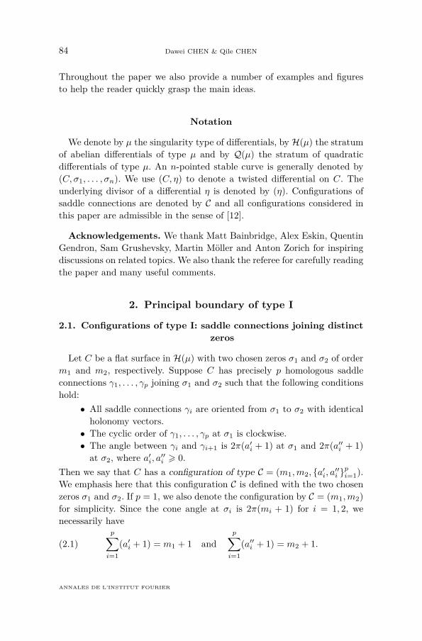
Figure 2.1 shows a pointed nodal curve whose dual graph is of type G(C):
R
C1
Cp
σ1
σ2
L1
Lp
Figure 2.1. A curve with dual graph of type C.
2.3. The principal boundary of type I
Denote by ∆(µ, C) the space of twisted differentials η satisfying the fol-lowing conditions:
• The underlying dual graph of η is given by G(C), with nodes qi andcomponents Ci corresponding to li and vi, respectively.
• The component R corresponding to the vertex vR is isomorphic toP1 and contains only σ1 and σ2 among all the markings.
• Each Ci has markings labeled by Li and has genus equal to g(vi).• For each i = 1, . . . , p, ordqi
ηCi= a′i+a′′i and ordqi
ηR = −a′i−a′′i −2.
TOME 69 (2019), FASCICULE 1
86 Dawei CHEN & Qile CHEN
• For each i = 1, . . . , p, ResqiηR = 0.
• ηR admits the configuration C of saddle connections from σ1 to σ2.
Recall that the twisted differential η defines a flat structure on R (up toscale). Thus it makes sense to talk about the configuration C on R. We saythat ∆(µ, C) is the principal boundary associated to the configuration C.
Suppose Cε ∈ H(µ) has the configuration C = (m1,m2, a′i, a′′i pi=1) such
that the p homologous saddle connections γ1, . . . , γp of C have length atmost ε. We want to determine the limit twisted differential as the lengthof all γi shrinks to zero. To avoid further degeneration, suppose that Cεdoes not have any other saddle connections shorter than 3ε (the locus ofsuch Cε is called the thick part of the configuration C in [12]). Take a smalldisk under the flat metric such that it contains σ1, σ2, all γi, and no otherzeros (see [12, Figure 5]). Within this disk, shrink γi to zero while keepingthe configuration C, such that all other periods become arbitrarily largecompared to γi.
Theorem 2.1. — The limit twisted differential of Cε as γi → 0 iscontained in ∆(µ, C). Conversely, twisted differentials in ∆(µ, C) can besmoothed to of type Cε.
Proof. — Since γi and γi+1 are homologous and next to each other, theybound a surface Cεi with γi and γi+1 as boundary (see the lower rightillustration of [12, Figure 5] where Cεi is denoted by Si). The inner anglebetween γi and γi+1 at σ1 is 2π(a′i + 1) and at σ2 is 2π(a′′i + 1). Shrinkingthe γj to zero under the flat metric, the limit of Cεi forms a flat surfaceCi, and denote by qi the limit position of σ1 and σ2 in Ci. This shrinkingoperation is the inverse of breaking up a zero, see [12, Figure 3], whichimplies that the cone angle at qi is 2π(a′i + a′′i + 1), hence Ci has a zero oforder a′i + a′′i at qi.On the other hand, instead of shrinking the γj , up to scale it amounts
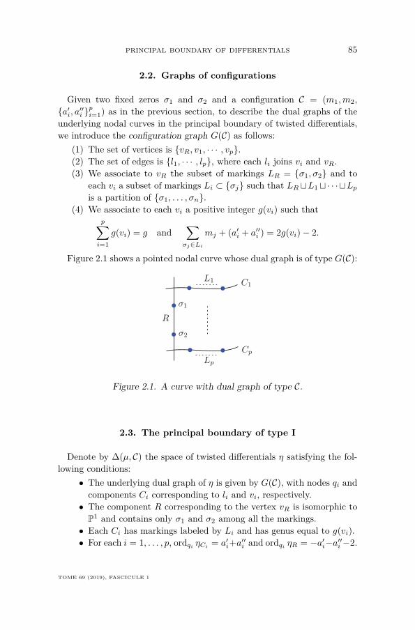
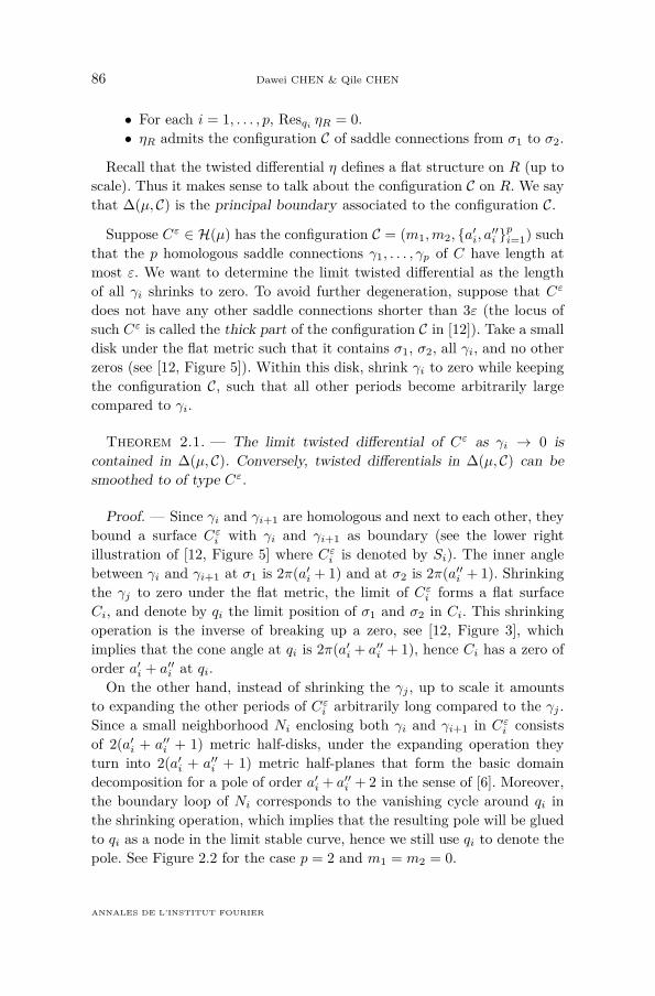
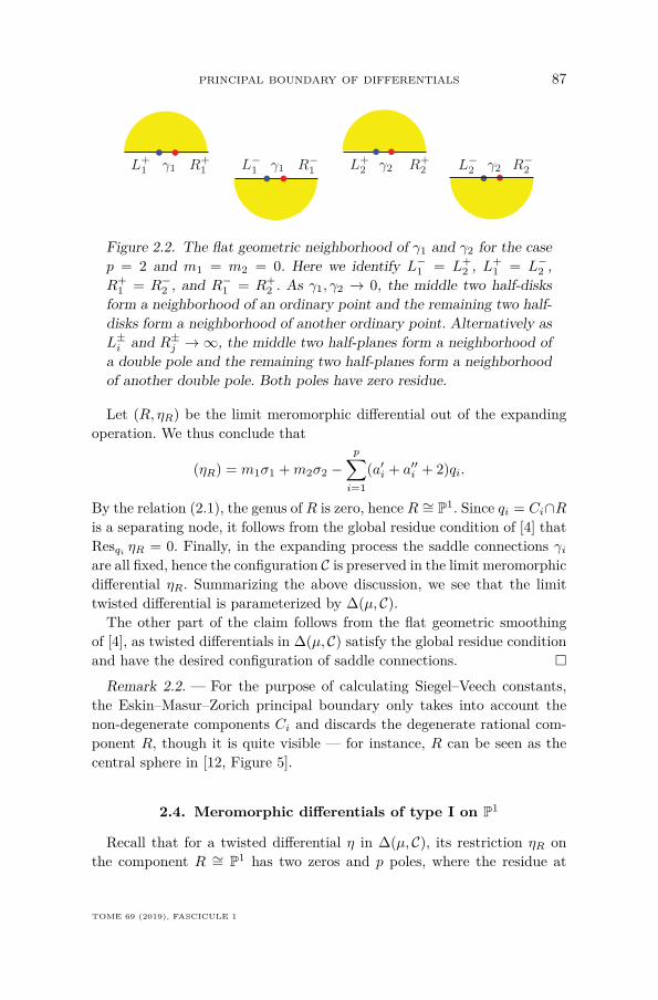
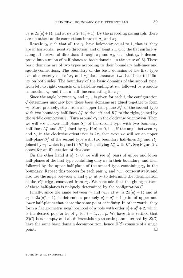
to expanding the other periods of Cεi arbitrarily long compared to the γj .Since a small neighborhood Ni enclosing both γi and γi+1 in Cεi consistsof 2(a′i + a′′i + 1) metric half-disks, under the expanding operation theyturn into 2(a′i + a′′i + 1) metric half-planes that form the basic domaindecomposition for a pole of order a′i + a′′i + 2 in the sense of [6]. Moreover,the boundary loop of Ni corresponds to the vanishing cycle around qi inthe shrinking operation, which implies that the resulting pole will be gluedto qi as a node in the limit stable curve, hence we still use qi to denote thepole. See Figure 2.2 for the case p = 2 and m1 = m2 = 0.
ANNALES DE L’INSTITUT FOURIER
PRINCIPAL BOUNDARY OF DIFFERENTIALS 87
γ1γ1 γ2γ2L+1 R+
1 L−1 R−
1 L+2 R+
2 L−2 R−
2
Figure 2.2. The flat geometric neighborhood of γ1 and γ2 for the casep = 2 and m1 = m2 = 0. Here we identify L−1 = L+
2 , L+1 = L−2 ,
R+1 = R−2 , and R−1 = R+
2 . As γ1, γ2 → 0, the middle two half-disksform a neighborhood of an ordinary point and the remaining two half-disks form a neighborhood of another ordinary point. Alternatively asL±i and R±j →∞, the middle two half-planes form a neighborhood ofa double pole and the remaining two half-planes form a neighborhoodof another double pole. Both poles have zero residue.
Let (R, ηR) be the limit meromorphic differential out of the expandingoperation. We thus conclude that
(ηR) = m1σ1 +m2σ2 −p∑i=1
(a′i + a′′i + 2)qi.
By the relation (2.1), the genus of R is zero, hence R ∼= P1. Since qi = Ci∩Ris a separating node, it follows from the global residue condition of [4] thatResqi
ηR = 0. Finally, in the expanding process the saddle connections γiare all fixed, hence the configuration C is preserved in the limit meromorphicdifferential ηR. Summarizing the above discussion, we see that the limittwisted differential is parameterized by ∆(µ, C).The other part of the claim follows from the flat geometric smoothing
of [4], as twisted differentials in ∆(µ, C) satisfy the global residue conditionand have the desired configuration of saddle connections.
Remark 2.2. — For the purpose of calculating Siegel–Veech constants,the Eskin–Masur–Zorich principal boundary only takes into account thenon-degenerate components Ci and discards the degenerate rational com-ponent R, though it is quite visible — for instance, R can be seen as thecentral sphere in [12, Figure 5].
2.4. Meromorphic differentials of type I on P1
Recall that for a twisted differential η in ∆(µ, C), its restriction ηR onthe component R ∼= P1 has two zeros and p poles, where the residue at
TOME 69 (2019), FASCICULE 1
88 Dawei CHEN & Qile CHEN
each pole is zero. Up to scale, ηR is uniquely determined by the zeros andpoles. In this section we study the locus of P1 marked at such zeros andpoles.Given integers m1,m2 > 1 and n1, . . . , np > 2 with m1 +m2−
∑pi=1 ni =
−2, let Z ⊂ M0,p+2 be the locus of pointed rational curves (P1, σ1, σ2, q1,
. . . , qp) such that there exists a differential η0 on P1 satisfying that
(η0) = m1σ1 +m2σ2 −p∑i=1
niqi and Resqi η0 = 0
for each i = 1, . . . , p.For a given (admissible) configuration C = (m1,m2, a′i, a′′i
pi=1), consider
the subset Z(C) ⊂ Z parameterizing differentials η0 on P1 (up to scale) thatadmit a configuration of type C.
Proposition 2.3. — Z is a union of Z(C) for all possible (admissible)configuration C and each Z(C) consists of a single point.
Proof. — We provide a constructive proof using the flat geometry ofmeromorphic differentials. Let us make some observation first. Suppose η0is a differential on P1 whose underlying divisor corresponds to a point inZ. Since η0 has zero residue at every pole, for any closed path γ that doesnot contain a pole of η0, the Residue Theorem says that∫
γ
η0 = 0.
In particular, if α and β are two saddle connections joining σ1 to σ2, thenα− β represents a closed path on P1, hence∫
α
η0 =∫β
η0,
and α and β necessarily have the same holonomy. It also implies that η0 hasno self saddle connections. Collect the saddle connections from σ1 to σ2,list them clockwise at σ1, and count the angles between two nearby ones.Since the saddle connections have the same holonomy, the angles betweenthem are multiples of 2π, and hence they give rise to a configuration C. Itimplies that the underlying divisor of η0 corresponds to a point in Z(C).Therefore, Z is a union of Z(C).Now suppose η0 admits a configuration of type C = (m1,m2, a′i, a′′i
pi=1),
i.e., up to scale it corresponds to a point in Z(C). Recall that σ1, σ2, andqi are the zeros and poles of order m1, m2, and a′i + a′′i + 2, respectively,where i = 1, . . . , p, and γ1, . . . , γp are the saddle connections joining σ1 toσ2 such that the angle between γi and γi+1 in the clockwise orientation at
ANNALES DE L’INSTITUT FOURIER
PRINCIPAL BOUNDARY OF DIFFERENTIALS 89
σ1 is 2π(a′i+1), and at σ2 is 2π(a′′i +1). By the preceding paragraph, thereare no other saddle connections between σ1 and σ2.Rescale η0 such that all the γi have holonomy equal to 1, that is, they
are in horizontal, positive direction, and of length 1. Cut the flat surface η0along all horizontal directions through σ1 and σ2, such that η0 is decom-posed into a union of half-planes as basic domains in the sense of [6]. Thesebasic domains are of two types according to their boundary half-lines andsaddle connections. The boundary of the basic domains of the first typecontains exactly one of σ1 and σ2 that emanates two half-lines to infin-ity on both sides. The boundary of the basic domains of the second type,from left to right, consists of a half-line ending at σ1, followed by a saddleconnection γi, and then a half-line emanating for σ2.Since the angle between γi and γi+1 is given for each i, the configuration
C determines uniquely how these basic domains are glued together to formη0. More precisely, start from an upper half-plane S+
1 of the second typewith two boundary half-lines L+
1 to the left and R+1 to the right, joined by
the saddle connection γ1. Turn around σ1 in the clockwise orientation. Thenwe will see a lower half-plane S−1 of the second type with two boundaryhalf-lines L−1 and R−1 joined by γ1. If a′1 = 0, i.e., if the angle between γ1and γ2 in the clockwise orientation is 2π, then next we will see an upperhalf-plane S+
2 of the second type with two boundary half-lines L+2 and R+
2joined by γ2, which is glued to S−1 by identifying L+
2 with L−1 . See Figure 2.2above for an illustration of this case.On the other hand if a′1 > 0, we will see a′1 pairs of upper and lower
half-planes of the first type containing only σ1 in their boundary, and thenfollowed by the upper half-plane of the second type containing γ2 in theboundary. Repeat this process for each pair γi and γi+1 consecutively, andalso use the angle between γi and γi+1 at σ2 to determine the identificationof the R±i -edges emanated from σ2. We conclude that the gluing patternof these half-planes is uniquely determined by the configuration C.Finally, since the angle between γi and γi+1 at σ1 is 2π(a′i + 1) and at
σ2 is 2π(a′′i + 1), it determines precisely a′i + a′′i + 1 pairs of upper andlower half-planes that share the same point at infinity. In other words, theyform a flat geometric neighborhood of a pole with order a′i + a′′i + 2, whichis the desired pole order of qi for i = 1, . . . , p. We have thus verified thatZ(C) is nonempty and all differentials up to scale parameterized by Z(C)have the same basic domain decomposition, hence Z(C) consists of a singlepoint.
TOME 69 (2019), FASCICULE 1
90 Dawei CHEN & Qile CHEN
Example 2.4. — Consider the case m1 = 1, m2 = 1, n1 = 2 and n2 = 2.The only admissible configuration is
a′1 = a′′1 = a′2 = a′′2 = 0,
hence Z consists of a single point. As a cross check, take σ1 = 1, q1 = 0,and q2 = ∞ in P1, and let z be the affine coordinate. Then up to scale η0can be written as
(z − 1)(z − σ2)z2 dz.
It is easy to see that Resqi η0 = 0 if and only if σ2 = −1.
Example 2.5. — Consider the case m1 = 1, m2 = 3 and n1 = n2 = n3 =2. There do not exist nonnegative integers a′1, a′2, a′3 satisfying that
(a′1 + 1) + (a′2 + 1) + (a′3 + 1) = m1 + 1 = 2,
because the left-hand side is at least 3. Since there is no admissible config-uration, we conclude that Z is empty. As a cross check, let q1 = 0, q2 = 1,and q3 =∞. Up to scale η0 can be written as
(z − σ1)(z − σ2)3
z2(z − 1)2 dz.
One can directly verify that there are no σ1, σ2 ∈ P1 \ 0, 1,∞ such thatResqi
η0 = 0.
3. Principal boundary of type II
3.1. Configurations of type II: saddle connections joining a zeroto itself
Let C be a flat surface in H(µ). Suppose C has precisely m homolo-gous closed saddle connections γ1, . . . , γm, each joining a zero to itself. LetL ⊂ 1, . . . ,m be an index subset such that the curves γl for l ∈ L boundq cylinders. After removing the cylinders along with all the γk, the remain-ing part in C splits into p = m− q disjoint surfaces C1, . . . , Cp, where theboundary of the closure Ck of each Ck consists of two closed saddle connec-tions αk and βk. These surfaces are glued together in a cyclic order to formC. More precisely, each Ck is connected to Ck+1 by either identifying αkwith βk+1 (as some γi in C) or inserting a metric cylinder with boundaryαk and βk+1. The sum of genera of the Ck is g−1, because the cyclic gluingprocedure creates a central handle, hence it adds an extra one to the totalgenus (see [12, Figure 7]).
ANNALES DE L’INSTITUT FOURIER
PRINCIPAL BOUNDARY OF DIFFERENTIALS 91
There are two types of the surfaces Ck according to their boundary com-ponents. If the boundary saddle connections αi and βi of Ci are disjoint,we say that Ci has a pair of holes boundary. In this case αi contains asingle zero zi with cone angle (2ai + 3)π inside Ci, and βi contains a singlezero wi with cone angle (2bi + 3)π inside Ci, where ai, bi > 0. We also takeinto account the special case m = 1, i.e., when we cut C along γ1, we getonly one surface C1 with two disjoint boundary components α1 and β1. Inthis case z1 is identified with w1 in C, and we still say that C1 has a pairof holes boundary.For the remaining case, if αj and βj form a connected component for the
boundary of Cj , we say that Cj has a figure eight boundary. In this caseαj and βj contain the same zero zj . Denote by 2(c′j + 1)π and 2(c′′j + 1)πthe two angles bounded by αj and βj inside Cj , where c′j , c′′j > 0, and letcj = c′j + c′′j .In summary, the configuration considered above consists of the data
(L, ai, bi, c′j , c′′j ).
Conversely, given the surfaces Ck along with some metric cylinders, lo-cal gluing patterns can create zeros of the following three types (see [12,Figure 12] and [5, Figures 6-8]):
(i) A cylinder, followed by k > 1 surfaces C1, . . . , Ck, each of genusgi > 1 with a figure eight boundary, followed by a cylinder. Thetotal angle at the newborn zero is
π +k∑i=1
(2c′i + 2c′′i + 4)π + π,
hence its zero order isk∑i=1
(ci + 2).
(ii) A cylinder, followed by k > 0 surfaces Ci, each of genus gi > 1with a figure eight boundary, followed by a surface Ck+1 of genusgk+1 > 1 with a pair of holes boundary. The total angle at thenewborn zero is
π +k∑i=1
(2c′i + 2c′′i + 4)π + (2bk+1 + 3)π,
hence its zero order isk∑i=1
(ci + 2) + (bk+1 + 1).
TOME 69 (2019), FASCICULE 1
92 Dawei CHEN & Qile CHEN
(iii) A surface C0 of genus g0 > 1 with a pair of holes boundary, followedby k > 0 surfaces Ci, each of genus gi > 1 with a figure eightboundary, followed by a surface Ck+1 of genus gk+1 > 1 with a pairof holes boundary. The total angle at the newborn zero is
(2a0 + 3)π +k∑i=1
(2c′i + 2c′′i + 4)π + (2bk+1 + 3)π,
hence its zero order isk∑i=1
(ci + 2) + (a0 + 1) + (bk+1 + 1).
For example, the flat surface in [12, Figure 7] is constructed as follows: S1with a pair of holes boundary, followed by S2 with a pair of holes boundary,then a cylinder, followed by S3 with a figure eight boundary, then anothercylinder, followed by S4 with a figure eight boundary, and finally back to S1.
3.2. The principal boundary of type II
Suppose Cε ∈ H(µ) has the configuration C = (L, ai, bi, c′j , c′′j ) withthem homologous saddle connections γ1, . . . , γm of length at most ε. More-over, suppose that Cε does not have any other saddle connections shorterthan 3ε. As before, we degenerate Cε by shrinking γi to zero while keepingthe configuration, such that the ratio of any other period to γi becomes ar-bitrarily large. Let ∆(µ, C) be the space of twisted differentials that arise aslimits of such a degeneration process. Recall the three types of gluing pat-terns and newborn zeros in the preceding section. We will analyze the typesof their degeneration as building blocks to describe twisted differentials in∆(µ, C).
For the convenience of describing the degeneration, we view a cylinderas a union of two half-cylinders by truncating it in the middle. Then asits height tends to be arbitrarily large compared to the width, each half-cylinder becomes a half-infinite cylinder, which represents a flat geometricneighborhood of a simple pole. Moreover, the two newborn simple poleshave opposite residues, because the two half-infinite cylinders have thesame width with opposite orientations.
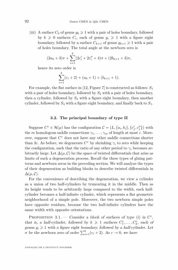
Proposition 3.1. — Consider a block of surfaces of type (i) in Cε,that is, a half-cylinder, followed by k > 1 surfaces Cε1 , . . . , Cεk, each ofgenus gi > 1 with a figure eight boundary, followed by a half-cylinder. Letσ be the newborn zero of order
∑ki=1(ci + 2). As ε→ 0, we have
ANNALES DE L’INSTITUT FOURIER
PRINCIPAL BOUNDARY OF DIFFERENTIALS 93
• The limit differential consists of k disjoint surfaces C1, . . . , Ck at-tached to a component R ∼= P1 at the nodes q1, . . . , qk, respectively.
• R contains only σ among all the markings.• For each i = 1, . . . , k, ordqi
ηCi= ci and ordqi
ηR = −ci − 2.• For each i = 1, . . . , k, Resqi ηR = 0.• ηR has two simple poles at q0 and qk+1 ∈ R \ σ, q1, . . . , qk with
opposite residues ±r.• ηR admits a configuration of type (i), i.e., it has precisely k + 1homologous self saddle connections with angles 2(c′i + 1)π and2(c′′i + 1)π in between consecutively for i = 1, . . . , k, and with ho-lonomy equal to r up to sign.
See Figure 3.1 for an illustration of the underlying curve of the limitdifferential.
R
C1 Ck
σq0 q1 qk qk+1
Figure 3.1. The underlying curve of the limit differential in Proposition 3.1.
Proof. — As ε → 0, the limit of each Cεi is a flat surface Ci, where thefigure eight boundary of Cεi shrinks to a single zero qi with cone angle(2ci + 2)π, i.e., qi is a zero of order ci. This shrinking operation is theinverse of the figure eight construction, see [12, Figure 10]. On the otherhand, instead of shrinking the boundary saddle connections αi, βi of the Cεi ,up to scale it amounts to expanding the other periods of the Cεi arbitrarilylong compared to the αi, βi. Since a small neighborhood Ni enclosing bothαi and βi in Cεi consists of 2(c′i + c′′i + 1) metric half-disks, under theexpanding operation they turn into 2(c′i + c′′i + 1) = 2(ci + 1) metric half-planes that form the basic domain decomposition for a pole of order ci+2 inthe sense of [6]. The boundary loop of Ni corresponds to the vanishing cyclearound qi in the shrinking operation, which implies that the resulting polewill be glued to qi as a node in the limit. In addition, the two half-cylindersexpand to two half-infinite cylinders, which create two simple poles q0 andqk+1 with opposite residues ±r, where r encodes the width of the cylinders.
TOME 69 (2019), FASCICULE 1
94 Dawei CHEN & Qile CHEN
Let (R, ηR) be the limit meromorphic differential out of the expandingoperation. We thus conclude that
(ηR) =(
k∑i=1
(ci + 2))σ −
k∑i=1
(ci + 2)qi − q0 − qk+1,
and hence the genus of R is zero. Since qi = Ci ∩ R is a separating node,it follows from the global residue condition of [4] that Resqi
ηR = 0. As across check,
k+1∑i=0
ResqiηR = Resq0 ηR + 0 + · · ·+ 0 + Resqk+1 ηR = 0,
hence ηR satisfies the Residue Theorem on R. Finally, the cylinders areglued to the figure eight boundary on both sides, hence the k + 1 homol-ogous self saddle connections have holonomy equal to r up to sign. Theirconfiguration (holonomy and angles in between) is preserved in the expand-ing process, hence the limit differential ηR possesses the desired configura-tion.
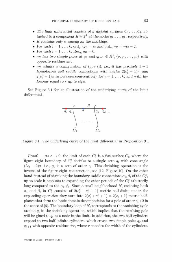
Proposition 3.2. — Consider a block of surfaces of type (ii) in Cε,that is, a half-cylinder, followed by k > 0 surfaces Cε1 , . . . , Cεk, each ofgenus gi > 1 with a figure eight boundary, followed by a surface Cεk+1 ofgenus gk+1 > 1 with a pair of holes boundary. Let σ be the newborn zeroof order
∑ki=1(ci + 2) + (bk+1 + 1). As ε→ 0, we have
• The limit differential consists of k+1 disjoint surfaces C1, . . . , Ck+1attached to a component R ∼= P1 at the nodes q1, . . . , qk+1, respec-tively.
• R contains only σ among all the markings.• For each i = 1, . . . , k, ordqi ηCi = ci and ordqi ηR = −ci − 2.• ordqk+1 ηCk+1 = bk+1 and ordqk+1 ηR = −bk+1 − 2.• For each i = 1, . . . , k, Resqi ηR = 0.• ηR has a simple pole at q0 ∈ R \ σ, q1, . . . , qk+1 with Resq0 ηR =−Resqk+1 ηR = ±r.
• ηR admits a configuration of type (ii), i.e., it has precisely k + 1homologous self saddle connections with angles 2(c′i + 1)π and2(c′′i + 1)π in between consecutively for i = 1, . . . , k, and with ho-lonomy equal to r up to sign.
See Figure 3.2 for an illustration of the underlying curve of the limitdifferential.
ANNALES DE L’INSTITUT FOURIER
PRINCIPAL BOUNDARY OF DIFFERENTIALS 95
R
C1 Ck
Ck+1
σq0 q1 qk qk+1
Figure 3.2. The underlying curve of the limit differential in Proposition 3.2.
Proof. — The proof is almost identical with the preceding one. The onlydifference occurs at the last surface. A small neighborhood Nk+1 enclosingβk+1 in Cεk+1 consists of 2(bk+1 + 1) half-disks, one of which is irregular asin [12, Figure 8], hence in the expanding process they turn into 2(bk+1 + 1)half-planes, giving a flat geometric neighborhood for a pole of order bk+1+2.Moreover, Nk+1 is homologous to the γi. The orientation of Nk+1 is theopposite to that of N0 enclosing the boundary α0 of the beginning halfcylinder, hence their homology classes add up to zero. We thus concludethat Resq0 ηR = −Resqk+1 ηR. Alternatively, it follows from the ResidueTheorem applied to R, since Resqi
ηR = 0 for all i = 1, . . . , k. The holonomyof the saddle connections and the angles between them are preserved in theexpanding process, hence ηR has the configuration as described.
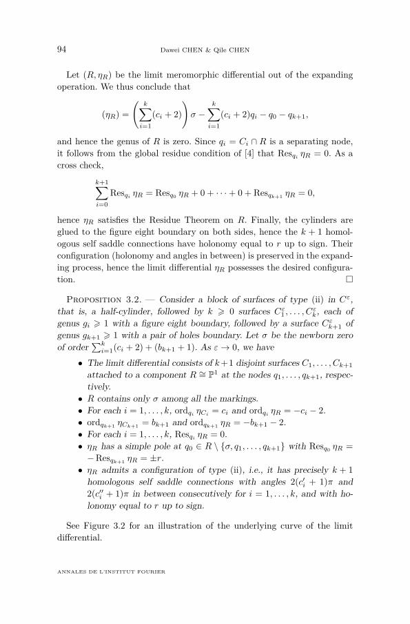
Proposition 3.3. — Consider a block of surfaces of type (iii) in Cε,that is, a surface Cε0 of genus gk+1 > 1 with a pair of holes boundary,followed by k > 0 surfaces Cε1 , . . . , Cεk, each of genus gi > 1 with a figureeight boundary, followed by a surface Cεk+1 of genus gk+1 > 1 with a pairof holes boundary. Let σ be the newborn zero of order
∑ki=1(ci + 2) +
(a0 + 1) + (bk+1 + 1). As ε→ 0, we have
• The limit differential consists of k+2 disjoint surfaces C0, . . . , Ck+1attached to a component R ∼= P1 at the nodes q0, . . . , qk+1, respec-tively.
• R contains only σ among all the markings.• For each i = 1, . . . , k, ordqi ηCi = ci and ordqi ηR = −ci − 2.• ordq0 ηC0 = a0 and ordq0 ηR = −a0 − 2.• ordqk+1 ηCk+1 = bk+1 and ordqk+1 ηR = −bk+1 − 2.• For each i = 1, . . . , k, Resqi
ηR = 0.• Resq0 ηR = −Resqk+1 ηR = ±r.• ηR admits a configuration of type (iii), i.e., it has precisely k + 1homologous self saddle connections with angles 2(c′i + 1)π and
TOME 69 (2019), FASCICULE 1
96 Dawei CHEN & Qile CHEN
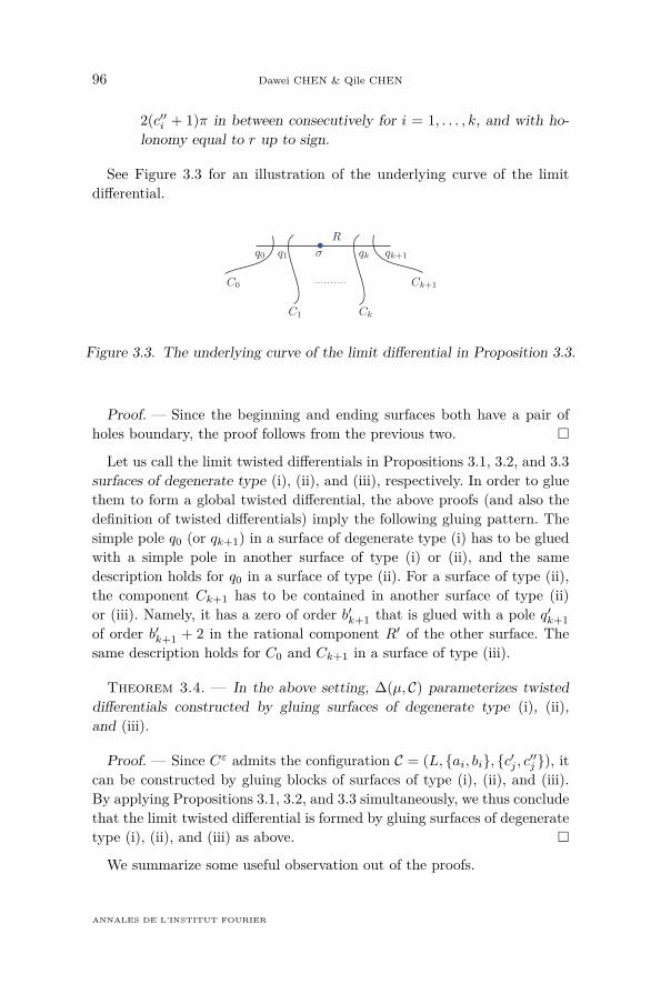
2(c′′i + 1)π in between consecutively for i = 1, . . . , k, and with ho-lonomy equal to r up to sign.
See Figure 3.3 for an illustration of the underlying curve of the limitdifferential.
R
C1 Ck
Ck+1C0
σq0 q1 qk qk+1
Figure 3.3. The underlying curve of the limit differential in Proposition 3.3.
Proof. — Since the beginning and ending surfaces both have a pair ofholes boundary, the proof follows from the previous two.
Let us call the limit twisted differentials in Propositions 3.1, 3.2, and 3.3surfaces of degenerate type (i), (ii), and (iii), respectively. In order to gluethem to form a global twisted differential, the above proofs (and also thedefinition of twisted differentials) imply the following gluing pattern. Thesimple pole q0 (or qk+1) in a surface of degenerate type (i) has to be gluedwith a simple pole in another surface of type (i) or (ii), and the samedescription holds for q0 in a surface of type (ii). For a surface of type (ii),the component Ck+1 has to be contained in another surface of type (ii)or (iii). Namely, it has a zero of order b′k+1 that is glued with a pole q′k+1of order b′k+1 + 2 in the rational component R′ of the other surface. Thesame description holds for C0 and Ck+1 in a surface of type (iii).
Theorem 3.4. — In the above setting, ∆(µ, C) parameterizes twisteddifferentials constructed by gluing surfaces of degenerate type (i), (ii),and (iii).
Proof. — Since Cε admits the configuration C = (L, ai, bi, c′j , c′′j ), itcan be constructed by gluing blocks of surfaces of type (i), (ii), and (iii).By applying Propositions 3.1, 3.2, and 3.3 simultaneously, we thus concludethat the limit twisted differential is formed by gluing surfaces of degeneratetype (i), (ii), and (iii) as above.
We summarize some useful observation out of the proofs.
ANNALES DE L’INSTITUT FOURIER
PRINCIPAL BOUNDARY OF DIFFERENTIALS 97
Remark 3.5. — If the homologous closed saddle connections in a con-figuration C of type II contains k distinct zeros, then a curve in ∆(µ, C)contains k rational components. Moreover, if two rational components in-tersect, then each of them has a simple pole at the node, and the residuesat the two branches of the node add up to zero. In general, at the polarnodes the residues are ±r for a fixed nonzero r ∈ C, such that their signsare alternating along the (unique) circle in the dual graph of the entirecurve, and that the holonomy of the saddle connections is equal to r up tosign.
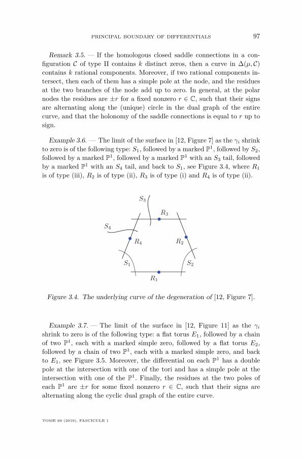
Example 3.6. — The limit of the surface in [12, Figure 7] as the γi shrinkto zero is of the following type: S1, followed by a marked P1, followed by S2,followed by a marked P1, followed by a marked P1 with an S3 tail, followedby a marked P1 with an S4 tail, and back to S1, see Figure 3.4, where R1is of type (iii), R2 is of type (ii), R3 is of type (i) and R4 is of type (ii).
S1
R1
S2
R2
R3
S3
S4
R4
Figure 3.4. The underlying curve of the degeneration of [12, Figure 7].
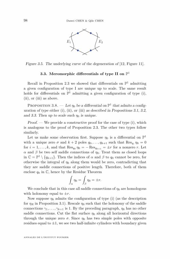
Example 3.7. — The limit of the surface in [12, Figure 11] as the γishrink to zero is of the following type: a flat torus E1, followed by a chainof two P1, each with a marked simple zero, followed by a flat torus E2,followed by a chain of two P1, each with a marked simple zero, and backto E1, see Figure 3.5. Moreover, the differential on each P1 has a doublepole at the intersection with one of the tori and has a simple pole at theintersection with one of the P1. Finally, the residues at the two poles ofeach P1 are ±r for some fixed nonzero r ∈ C, such that their signs arealternating along the cyclic dual graph of the entire curve.
TOME 69 (2019), FASCICULE 1
98 Dawei CHEN & Qile CHEN
E1 E2
Figure 3.5. The underlying curve of the degeneration of [12, Figure 11].
3.3. Meromorphic differentials of type II on P1
Recall in Proposition 2.3 we showed that differentials on P1 admittinga given configuration of type I are unique up to scale. The same resultholds for differentials on P1 admitting a given configuration of type (i),(ii), or (iii) as above.
Proposition 3.8. — Let η0 be a differential on P1 that admits a config-uration of type either (i), (ii), or (iii) as described in Propositions 3.1, 3.2,and 3.3. Then up to scale such η0 is unique.
Proof. — We provide a constructive proof for the case of type (i), whichis analogous to the proof of Proposition 2.3. The other two types followsimilarly.
Let us make some observation first. Suppose η0 is a differential on P1
with a unique zero σ and k + 2 poles q0, . . . , qk+1 such that Resqi η0 = 0for i = 1, . . . , k, and that Resq0 η0 = −Resqk+1 = ±r for a nonzero r. Letα and β be two self saddle connections of η0. Treat them as closed loopsin C = P1 \ qk+1. Then the indices of α and β to q0 cannot be zero, forotherwise the integral of η0 along them would be zero, contradicting thatthey are saddle connections of positive length. Therefore, both of themenclose q0 in C, hence by the Residue Theorem∫
α
η0 =∫β
η0 = ±r.
We conclude that in this case all saddle connections of η0 are homologouswith holonomy equal to ±r.Now suppose η0 admits the configuration of type (i) (as the description
for ηR in Proposition 3.1). Rescale η0 such that the holonomy of the saddleconnections γ1, . . . , γk+1 is 1. By the preceding paragraph, η0 has no othersaddle connections. Cut the flat surface η0 along all horizontal directionsthrough the unique zero σ. Since η0 has two simple poles with oppositeresidues equal to ±1, we see two half-infinite cylinders with boundary given
ANNALES DE L’INSTITUT FOURIER
PRINCIPAL BOUNDARY OF DIFFERENTIALS 99
by the first and the last saddle connections γ1 and γk+1, respectively. Therest part of η0 splits into half-planes as basic domains in the sense of [6],which are of two types according to their boundary. The boundary of thehalf-planes of the first type contains σ that emanates two half-lines toinfinity on both sides. The boundary of the half-planes of the second type,from left to right, consists of a half-line ending at σ, followed by a saddleconnection γi, and then a half-line emanated from σ.Since the angles between γi and γi+1 are given on both sides inside the
open surface (after removing the two half-infinite cylinders), this configu-ration determines how these half-planes are glued together. More precisely,say in the counterclockwise direction the angle between γi and γi+1 is2π(c′i + 1). Then starting from the upper half-plane S+
i of the second typecontaining γi in the boundary and turning counterclockwise, we will see c′ipairs of lower and upper half-planes of the first type, and then the lowerhalf-plane S−i+1 of the second type containing γi+1 in the boundary. Repeatthis process for each i on both sides. We conclude that the gluing pattern ofthese half-planes is uniquely determined by the configuration. After gluing,the resulting open surface has a single figure eight boundary formed by γ1and γk+1 at the beginning and at the end, which is then identified with theboundary of the two half-infinite cylinders to recover η0. Finally, since theangles between γi and γi+1 are 2π(c′i + 1) and 2π(c′′i + 1) on both sides, itdetermines precisely c′i+c′′i +1 = ci+1 paris of upper and lower half-planesthat share the same point at infinity. In other words, they give rise to aflat geometric representation of a pole of order ci + 2, which is the desiredpole order for i = 1, . . . , k.
4. Spin and hyperelliptic structures
For special µ, the stratum H(µ) can be disconnected. Kontsevich andZorich ([19]) classified connected components of H(µ) for all µ. Their resultsays thatH(µ) can have up to three connected components, where the extracomponents are caused by spin and hyperelliptic structures.
4.1. Spin structures
We first recall the definition of spin structures. Suppose µ= (2k1, . . . ,2kn)is a partition of 2g − 2 with even entries only. For an abelian differential(C,ω) ∈ H(µ), let
(ω) = 2k1σ1 + · · ·+ 2knσn
TOME 69 (2019), FASCICULE 1
100 Dawei CHEN & Qile CHEN
be the associated canonical divisor. Then the line bundle
L = O(k1σ1 + · · ·+ knσn)
is a square root of the canonical line bundle, hence L gives rise to a spinstructure (also called a theta characteristic). Denote by
h0(C,L) (mod 2)
the parity of ω. By Atiyah ([1]) and Mumford ([22]), parities of theta char-acteristics are deformation invariant. We also refer to ω along with its parityas a spin structure, which can be either even or odd, and denote the parityby φ(ω).Alternatively, there is a topological description for spin structures using
the Arf invariant, due to Johnson ([18]). For a smooth simple closed curveα on a flat surface, let Ind(α) be the degree of the Gauss map from α tothe unit circle. Namely, 2π · Ind(α) is the total change of the angle of theunit tangent vector to α under the flat metric as it moves along α one time.Let ai, bigi=1 be a symplectic basis of C, i.e., ai · aj = bi · bj = 0 and
ai · bj = δij for 1 6 i, j 6 g. When ω has only even zeros, the parity φ(ω)can be equivalently defined as
φ(ω) =g∑i=1
(Ind(ai) + 1)(Ind(bi) + 1) (mod 2).
In particular if ai crosses a zero σj from one side to the other, since thezero order of σj is even, Ind(ai) remains unchanged mod 2.
4.2. Hyperelliptic structures
Next we recall the definition of hyperelliptic structures. There are twocases: µ = (2g − 2) and µ = (g − 1, g − 1). For (C,ω) ∈ H(2g − 2), if C ishyperelliptic and the unique zero σ of ω is a Weierstrass point, i.e., σ is aramification point of the hyperelliptic double cover C → P1, then we saythat (C,ω) has a hyperelliptic structure. For (C,ω) ∈ H(g−1, g−1), if C ishyperelliptic and the two zeros σ1 and σ2 of ω are hyperelliptic conjugatesof each other, i.e., σ1 and σ2 have the same image under the hyperellip-tic double cover, then we say that (C,ω) has a hyperelliptic structure. Inparticular, the hyperelliptic involution exchanges them.
ANNALES DE L’INSTITUT FOURIER
PRINCIPAL BOUNDARY OF DIFFERENTIALS 101
4.3. Connected components of H(µ)
Now we can state precisely the classification of connected components ofH(µ) in [19]:
• Suppose g > 4. Then– H(2g − 2) has three connected components: the hyperelliptic
componentHhyp(2g−2), the odd spin componentHodd(2g−2),and the even spin component Heven(2g − 2).
– H(g−1, g−1), when g is odd, has three connected components:the hyperelliptic component Hhyp(g − 1, g − 1), the odd spincomponent Hodd(g − 1, g − 1), and the even spin componentHeven(g − 1, g − 1).
– H(g − 1, g − 1), when g is even, has two connected compo-nents: the hyperelliptic component Hhyp(g − 1, g − 1) and thenonhyperelliptic component Hnonhyp(g − 1, g − 1).
– All the other strata of the form H(2k1, . . . , 2kn) have twoconnected components: the odd spin component Hodd(2k1, . . .
, 2kn) and the even spin component Heven(2k1, . . . , 2kn).– All the remaining strata are connected.
• Suppose g = 3. Then– H(4) has two connected components: the hyperelliptic compo-
nent Hhyp(4) and the odd spin component Hodd(4), where theeven spin component coincides with the hyperelliptic compo-nent.
– H(2, 2) has two connected components: the hyperelliptic com-ponent Hhyp(2, 2) and the odd spin component Hodd(2, 2),where the even spin component coincides with the hyperel-liptic component.
– All the other strata are connected.• Suppose g = 2. Then both H(2) and H(1, 1) are connected. Each
of them coincides with its hyperelliptic component.
4.4. Degeneration of spin structures
Let Sg be the moduli space of spin structures on smooth genus g curves.The natural morphism Sg → Mg is an unramified cover of degree 22g.Moreover, Sg is a disjoint union of S+
g and S−g , parameterizing even andodd spin structures, respectively. Cornalba ([10]) constructed a compacti-fied moduli space of spin structures Sg = S+
g tS−g overMg, whose bound-
ary parameterizes degenerate spin structures on stable nodal curves and
TOME 69 (2019), FASCICULE 1
102 Dawei CHEN & Qile CHEN
distinguishes their parities. We first recall spin structures on nodal curvesof compact type. Suppose a nodal curve C consists of k irreducible compo-nents C1, . . . , Ck such that each of the nodes is separating, i.e., removing itdisconnects C. Let Li be a theta characteristic on Ci, i.e., L⊗2
i = KCi. At
each node of C, insert a P1-bridge, called an exceptional component, andtake the line bundle O(1) on it. Then the collection (Ci, Li)ki=1 along withO(1) on each exceptional component gives a spin structure on C, whoseparity is determined by
h0(C1, L1) + · · ·+ h0(Ck, Lk) (mod 2).
In particular, if Ci has genus gi, then g1 + · · ·+ gk = g. On each Ci thereare 22gi distinct theta characteristics, hence in total they glue to 22g spinstructures on C, which equals the number of theta characteristics on asmooth curve of genus g. One can think of the exceptional P1-componentintuitively as follows. For simplicity suppose C consists of two irreduciblecomponents C1 and C2 meeting at one node q by identifying q1 ∈ C1 withq2 ∈ C2. Then the dualizing line bundle ωC restricted to Ci is KCi
(qi),whose degree is odd, hence one cannot directly take its square root. Instead,we insert a P1-component between C1 and C2, and regardO(q1+q2) asO(2)on P1 so that its square root is O(1). Then an ordinary theta characteristicLi on Ci along with O(1) on P1 gives a Cornalba’s spin structure on C,where degL1 + degL2 + degO(1) = g − 1 is the same as the degree of anordinary theta characteristic on a smooth genus g curve.If C is not of compact type, the situation is more complicated, because
there are two types of spin structures. For example, consider the case whenC is an irreducible one-nodal curve, by identifying two points q1 and q2in its normalization C ′ as a node q. For the first type, one can take asquare root L of the dualizing line bundle ωC , which gives 22g−1 such spinstructures. Equivalently, pull back L to L′ on C ′. Then L′ is a squareroot of KC′(q1 + q2), and there are 22g−2 such L′ on C ′. By Riemann–Roch, h0(C ′, L′) − h0(C ′, L′(−q1 − q2)) = 1, hence neither q1 nor q2 is abase point of L′, and any section s of L′ that vanishes at one of the qimust also vanish at the other. Therefore, the space of sections H0(C ′, L′)has a decomposition V0 ⊕ 〈s〉, where V0 is the subspace of sections thatvanish at q1 and q2, and s is a section not vanishing at the qi. Note thatL⊗2 = ωC , whose fibers over q1 and q2 have a canonical identification byResq1 ω+ Resq2 ω = 0, where ω is a stable differential with at worst simplepoles at the qi, treated as a local section of ωC at q. In other words, there isa canonical way to glue the fibers of L′⊗2 over q1 and q2 to form ωC on C.Due to the sign ± when taking a square root, it follows that there are two
ANNALES DE L’INSTITUT FOURIER
PRINCIPAL BOUNDARY OF DIFFERENTIALS 103
choices to glue the fibers of L′ over q1 and q2 to form L on C, and exactlyone of the two choices preserves s as a section of L. One can intuitivelythink of s with an evaluation at qi such that s(q1)2 = s(q2)2 6= 0. Then thechoice of gluing the two fibers induced by s(q1) = s(q2) preserves s as asection of L, while the other choice induced by s(q1) = −s(q2) does not. Wethus conclude that this way gives 22g−1 spin structures on C, where halfof them are even and the other half are odd. For the second type, insertan exceptional P1-component connecting q1 and q2 in C ′. Take an ordinarytheta characteristic L′ on C ′ and the bundle O(1) on P1 as before. In thisway one obtains 22g−2 such L′. For a fixed L′, there is no extra choiceof gluing L′ to O(1) at q1 and q2, due to the automorphisms of O(1) onP1, and hence the parity of the resulting spin structure equals that of η′.Nevertheless, the morphism Sg → Mg is simply ramified along the locusof such η′ of the second type. Therefore, taking both types into accountalong with the multiplicity factor for the second type, we again obtain thenumber 22g, which is equal to the degree of Sg →Mg.
Below we describe a relation between degenerate spin structures andtwisted differentials. Suppose a twisted differential (C, η) is in the closureof a stratum H(µ) that contains a spin component, i.e., when µ has evenentries only. For a node q joining two components C1 and C2 of C, bydefinition ordq η1 + ordq η2 = −2. If both orders are odd, we do nothing atq. If both orders are even, we insert an exceptional P1 at q. In particular ifq is separating, in this case ordq η1 and ordq η2 are both even, because eachside of q contains even zeros only, and hence we insert a P1 at q, whichmatches the preceding discussion on curves of compact type. Now supposeηi on a component Ci of C satisfies that
(ηi) =∑j
2mjσj +∑k
2nkqk +∑l
(2hl − 1)ql,
where the σj are the zeros in the interior of Ci, the qk are the nodes ofeven order in Ci, and the ql are the nodes of odd order in Ci. Consider thebundle
(4.1) Li = O
∑j
mjσj +∑k
nkqk +∑l
hlql
on Ci. Then a spin structure L on C consists of the collection (Ci, Li) andthe exceptional components with O(1). However, if (C, η) has a node ofodd order, i.e., a node without inserting an exceptional component, thenthere are two gluing choices at such a node, as described above, hence Lis only determined by (C, η) up to finitely many choices, and its parity
TOME 69 (2019), FASCICULE 1
104 Dawei CHEN & Qile CHEN
may vary with different choices. From the viewpoint of smoothing twisteddifferentials, it means that different choices of opening up nodes of C maydeform (C, η) into different connected components of H(µ).
The idea behind the above description is as follows. For a node q joiningtwo components C1 and C2, if there is no twist at q, i.e., if ordq η1 =ordq η2 = −1, then locally at q one can directly take a square root ofωC . If ordq η1 and ordq η2 are both odd, i.e., if the twisting parameterordq ηi − (−1) is even, then its one-half gives the twisting parameter forthe limit spin bundle on C. On the other hand if ordq η1 and ordq η2 areeven, then the twisting parameter ordq ηi−(−1) is not divisible by 2, henceone has to insert an exceptional P1 at q, which is twisted once to make thetwisting parameters at the new nodes even. As a consequence, the resultingtwisted differential restricted to P1 is O(2), hence its one-half is the bundleO(1) encoded in the degenerate spin structure. The reader may refer to [13]for a detailed explanation.
4.5. Degeneration of hyperelliptic structures
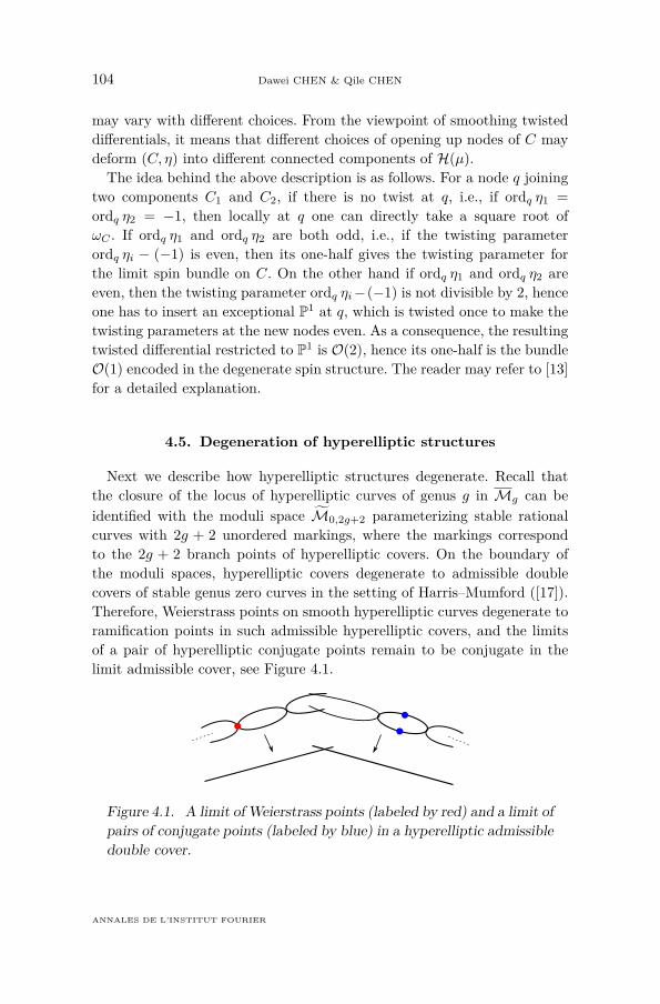
Next we describe how hyperelliptic structures degenerate. Recall thatthe closure of the locus of hyperelliptic curves of genus g in Mg can beidentified with the moduli space M0,2g+2 parameterizing stable rationalcurves with 2g + 2 unordered markings, where the markings correspondto the 2g + 2 branch points of hyperelliptic covers. On the boundary ofthe moduli spaces, hyperelliptic covers degenerate to admissible doublecovers of stable genus zero curves in the setting of Harris–Mumford ([17]).Therefore, Weierstrass points on smooth hyperelliptic curves degenerate toramification points in such admissible hyperelliptic covers, and the limitsof a pair of hyperelliptic conjugate points remain to be conjugate in thelimit admissible cover, see Figure 4.1.
Figure 4.1. A limit of Weierstrass points (labeled by red) and a limit ofpairs of conjugate points (labeled by blue) in a hyperelliptic admissibledouble cover.
ANNALES DE L’INSTITUT FOURIER
PRINCIPAL BOUNDARY OF DIFFERENTIALS 105
4.6. Spin and hyperelliptic structures for the principalboundary of type I
Let C = (m1,m2, a′i, a′′i pi=1) be an admissible configuration of type
I for a stratum H(µ). Suppose (C, η) is a twisted differential containedin ∆(µ, C). By the description of ∆(µ, C) in Section 2.3, C consists of pcomponents C1, . . . , Cp, each of genus gi > 1 with g1+· · ·+gp = g, attachedto a rational component R, and ηi is the differential of η restricted to Cisatisfying that (ηi) =
∑σj∈Ci
mjσj + (a′i + a′′i )qi, where qi is the nodejoining Ci with R.
Consider the case when µ has even entries only. Then H(µ) contains aneven spin component and an odd spin component (and possibly a hyperel-liptic component). This parity distinction can be extended to the principalboundary ∆(µ, C), see [12, Lemma 10.1] for a proof using the Arf invariant.For the reader’s convenience, below we recap the result and also providean algebraic proof.
Proposition 4.1. — Let (C, η) be a twisted differential in ∆(µ, C) de-scribed as above, with even zeros only. Then the parity of η is
φ(η) = φ(η1) + · · ·+ φ(ηp) (mod 2).
Proof. — Since (ηi) =∑σj∈Ci
mjσj+(a′i+a′′i )qi and themj are all even,it implies that a′i + a′′i is even for all i and the degenerate spin structureon Ci is given by O((ηi)/2) in the sense of Cornalba ([10]). Moreover, onthe rational component R, any theta characteristic has even parity (givenby zero). Since C is of compact type, the parity of η is equal to the sum ofthe parities of the ηi, as claimed.
Corollary 4.2. — Suppose C is of type I and µ contains only evenzeros. Then differentials in the thick part of H(µ) degenerate to twisteddifferentials in ∆(µ, C) with the same parity.
Note that for the parity discussion we only require that a′i + a′′i is evenfor each i, and there is no other requirement for the individual values of a′iand a′′i .
Next we consider hyperelliptic components. Since configurations of typeI require at least two distinct zeros, here we only need to treat the caseµ = (g−1, g−1), which contains a hyperelliptic componentHhyp(g−1, g−1)(and possibly spin components if g is odd).The following result is a reformulation of [12, Lemma 10.3]. Here we
again provide an algebraic proof.
TOME 69 (2019), FASCICULE 1
106 Dawei CHEN & Qile CHEN
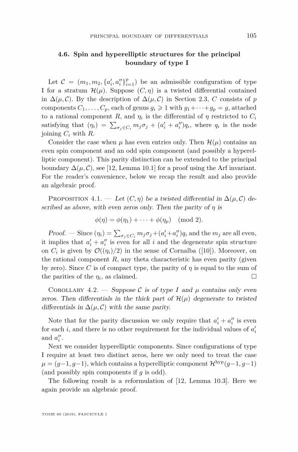
Proposition 4.3. — Suppose (C, η) is a twisted differential containedin ∆(g−1, g−1, C). Then differentials in the thick part of Hhyp(g−1, g−1)can degenerate to (C, η) if and only if either
• p = 1, (C1, η1) ∈ Hhyp(2g − 2), a′1 = a′′1 = g − 1, or• p = 2, (Ci, ηi) ∈ Hhyp(2gi − 2), a′i = a′′i = gi − 1 for i = 1, 2.
Proof. — Suppose (C, η) is a degeneration of differentials from Hhyp(g−1, g− 1). Then C admits an admissible hyperelliptic double cover π, wherethe two zeros σ1 and σ2 are conjugates under π. Since each Ci meets therational component R at a single node qi, and Ci is not rational, by thedefinition of admissible covers, qi has to be a ramified node under π. Bythe Riemann–Hurwitz formula, π restricted to R has only two ramificationpoints, which implies that p 6 2.For p = 1, C1 has genus g, and it admits a hyperelliptic double cover
with q1 being a ramification point, hence (C1, η1) ∈ Hhyp(2g−2). Moreover,there is only one saddle connection joining σ1 to σ2, so the angle conditionin the configuration C can only be a′1 = a′′1 = g − 1. See Figure 4.2 for thiscase and the corresponding hyperelliptic admissible cover.
σ1
σ2
q1q1
R
R
C1
C1
Figure 4.2. The case p = 1 in Proposition 4.3 and the correspondinghyperelliptic admissible cover.
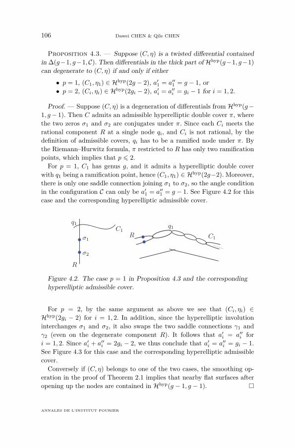
For p = 2, by the same argument as above we see that (Ci, ηi) ∈Hhyp(2gi − 2) for i = 1, 2. In addition, since the hyperelliptic involutioninterchanges σ1 and σ2, it also swaps the two saddle connections γ1 andγ2 (even on the degenerate component R). It follows that a′i = a′′i fori = 1, 2. Since a′i + a′′i = 2gi − 2, we thus conclude that a′i = a′′i = gi − 1.See Figure 4.3 for this case and the corresponding hyperelliptic admissiblecover.Conversely if (C, η) belongs to one of the two cases, the smoothing op-
eration in the proof of Theorem 2.1 implies that nearby flat surfaces afteropening up the nodes are contained in Hhyp(g − 1, g − 1).
ANNALES DE L’INSTITUT FOURIER
PRINCIPAL BOUNDARY OF DIFFERENTIALS 107
C1
C1
C2
C2
σ1
σ2
q1q1 q2
q2
R
R
Figure 4.3. The case p = 2 in Proposition 4.3 and the correspondinghyperelliptic admissible cover.
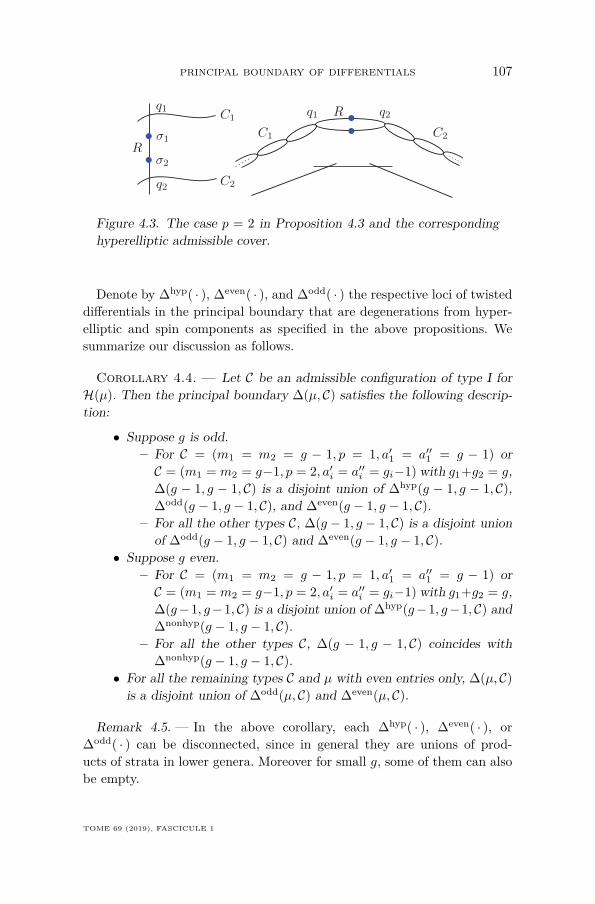
Denote by ∆hyp( · ), ∆even( · ), and ∆odd( · ) the respective loci of twisteddifferentials in the principal boundary that are degenerations from hyper-elliptic and spin components as specified in the above propositions. Wesummarize our discussion as follows.
Corollary 4.4. — Let C be an admissible configuration of type I forH(µ). Then the principal boundary ∆(µ, C) satisfies the following descrip-tion:
• Suppose g is odd.– For C = (m1 = m2 = g − 1, p = 1, a′1 = a′′1 = g − 1) orC = (m1 = m2 = g−1, p = 2, a′i = a′′i = gi−1) with g1+g2 = g,∆(g − 1, g − 1, C) is a disjoint union of ∆hyp(g − 1, g − 1, C),∆odd(g − 1, g − 1, C), and ∆even(g − 1, g − 1, C).
– For all the other types C, ∆(g − 1, g − 1, C) is a disjoint unionof ∆odd(g − 1, g − 1, C) and ∆even(g − 1, g − 1, C).
• Suppose g even.– For C = (m1 = m2 = g − 1, p = 1, a′1 = a′′1 = g − 1) orC = (m1 = m2 = g−1, p = 2, a′i = a′′i = gi−1) with g1+g2 = g,∆(g−1, g−1, C) is a disjoint union of ∆hyp(g−1, g−1, C) and∆nonhyp(g − 1, g − 1, C).
– For all the other types C, ∆(g − 1, g − 1, C) coincides with∆nonhyp(g − 1, g − 1, C).
• For all the remaining types C and µ with even entries only, ∆(µ, C)is a disjoint union of ∆odd(µ, C) and ∆even(µ, C).
Remark 4.5. — In the above corollary, each ∆hyp( · ), ∆even( · ), or∆odd( · ) can be disconnected, since in general they are unions of prod-ucts of strata in lower genera. Moreover for small g, some of them can alsobe empty.
TOME 69 (2019), FASCICULE 1
108 Dawei CHEN & Qile CHEN
4.7. Spin and hyperelliptic structures for the principalboundary of type II
Let C = (L, ai, bi, c′j , c′′j ) be a configuration of type II for a stratumH(µ). Consider the case when µ has even entries only, i.e., a differentialin H(µ) has odd or even parity. The parity distinction can be extended tothe principal boundary ∆(µ, C), see [12, Section 14.1]. Below we recap theresults and also provide alternative algebraic proofs.Recall the description for (C, η) in Theorem 3.4. Let us first simplify the
statement of [12, Lemma 14.1] in our setting.Lemma 4.6. — Let (C, η) be a twisted differential contained in ∆(µ, C).
Suppose µ has even zeros only. Then the following conditions hold:• η has even zero order at each marking of C.• η has even zero and pole order at a separating node of C.• For all non-separating nodes of C, the zero and pole orders of η are
either all even, or all odd.Proof. — Because µ has even zeros only, and those zeros are the markings
of C, the first condition holds by definition of twisted differentials.Suppose q is a separating node of C. By the description of C in Theo-
rem 3.4, q joins a component Ci with a rational component R. Since themarkings in the interior of Ci are even zeros, we conclude that ordq ηCi
has the same parity as 2gCi− 2, hence it is even, which implies the second
condition.Finally, recall that all non-separating nodes bound the (unique) cycle in
the dual graph of C. Since η has even order at all the other nodes and atall markings, going along the edges of the cycle one by one, the parity ofthe order of η at one vertex of the cycle determines that all the others havethe same parity, hence the last condition holds.
Remark 4.7. — If η has even order at all non-separating nodes, then thereis no rational component R in the central cycle of C that has a simple polarnode. In that case types (i) and (ii) do not appear in the description of C,which is exactly the way [12, Lemma 14.1] phrased.Next, we interpret [12, Lemmas 14.2, 14.3, and 14.4] in terms of Cor-
nalba’s spin structures.Lemma 4.8. — Suppose all rational components of (C, η) are of type (i).
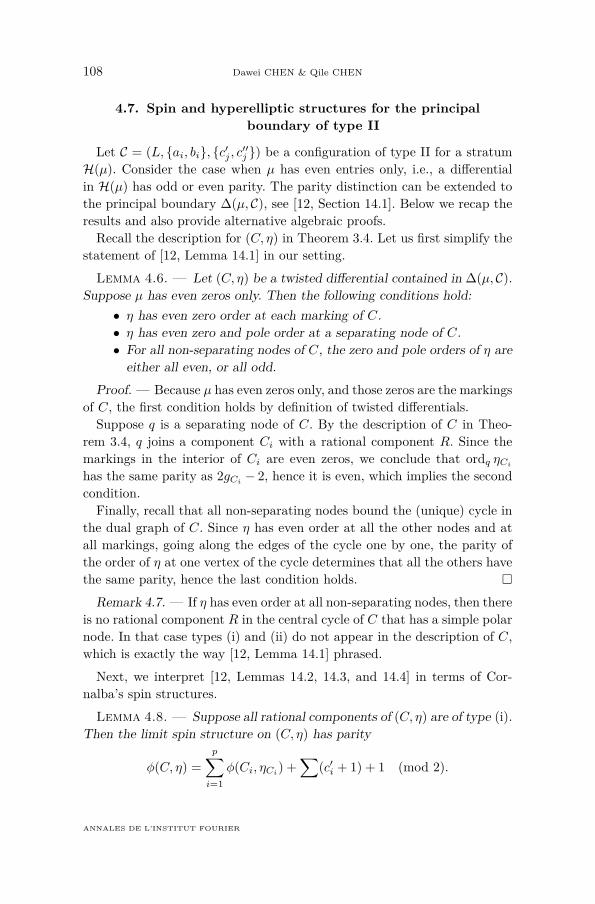
Then the limit spin structure on (C, η) has parity
φ(C, η) =p∑i=1
φ(Ci, ηCi) +∑
(c′i + 1) + 1 (mod 2).
ANNALES DE L’INSTITUT FOURIER
PRINCIPAL BOUNDARY OF DIFFERENTIALS 109
Proof. — We first remark that since η has even zeros only, c′i+c′′i is evenfor all i, hence using c′i or c′′i does not matter for the parity formula.Next, since only type (i) appears in the description of C, each Ci is a
tail of C, which is attached to C at a separating node, hence the limitspin structure on Ci is generated by one-half of (ηCi) (see (4.1)), and itcontributes φ(Ci, ηCi
) to the total parity.The central cycle S of C is a loop of rational components R1, . . . , Rk in
a cyclic order. At each node qi joining Ri to Ri+1, η has a simple pole onthe two branches of qi with opposite residues ±r, hence in the limit spinstructure we preserve qi and do not insert an exceptional P1 component.Therefore, the limit spin structure restricted to S is a square root L ofωS , where S has arithmetic genus one, and L|Ri = ORi . Starting from R1,identify the fibers of OR1 and OR2 at q1, then identify the fibers of OR2 andOR3 at q2, so on and so forth. The last identification between the fibersof ORk
and OR1 at qk has two choices, which makes h0(S,L) = 0 or 1.Hence the parity of the spin structure on S varies with the gluing choice,where the gluing choice is actually determined by the configuration datac′i, c′′i . By analyzing the Arf invariant, the parity contribution from S is∑
(c′i + 1) + 1, see the proof of [12, Lemma 14.2] for details.
Now we consider the last alternate conditions in Lemma 4.6.
Lemma 4.9. — Suppose η has even order at all non-separating nodes ofC. Then the parity of the limit spin structure on (C, η) is
φ(C, η) =p∑i=1
φ(Ci, ηCi),
where the Ci are the non-rational components of C.
Proof. — In this case on each Ci the limit spin structure is generated byone-half of (ηCi
), because ηCihas even zeros at the markings and nodes
(see (4.1)). The same analysis also holds for the rational components Ri,hence one-half of (ηRi
) gives the limit spin structure O(−1) on Ri whoseparity is even (equal to zero). Therefore, the total parity is given by thesum of the parities over all Ci.
Lemma 4.10. — Suppose η has odd order at every non-separating nodeof C. Let N be the total number of nearby flat surfaces under the previoussmoothing procedure. Then exactly N/2 of them have odd spin structureand N/2 have even spin structure.
Proof. — Let S be the central cycle of C. Then η has odd zeros andpoles at all the nodes of S. Hence in the limit spin structure we do not
TOME 69 (2019), FASCICULE 1
110 Dawei CHEN & Qile CHEN
insert an exceptional component at each node of S. Therefore, given thespin structure on each component of S, we have different gluing choices toform a global spin structure on C. When varying the gluing choice overone node of S while keeping the others, the parity of the resulting spinstructure differs by one, hence the desired claim follows. See also the proofof [12, Lemma 14.4] for an argument using the Arf invariant.
Next we consider the principal boundary of type II for hyperelliptic com-ponents. Below we recap [12, Lemmas 14.5 and 14.6] and provide algebraicproofs using hyperelliptic admissible covers.
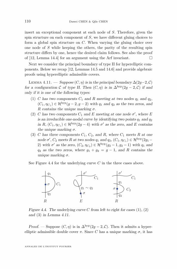
Lemma 4.11. — Suppose (C, η) is in the principal boundary ∆(2g−2, C)for a configuration C of type II. Then (C, η) is in ∆hyp(2g − 2, C) if andonly if it is one of the following types:
(1) C has two components C1 and R meeting at two nodes q1 and q2,(C1, ηC1) ∈ Hhyp(g − 2, g − 2) with q1 and q2 as the two zeros, andR contains the unique marking σ.
(2) C has two components C1 and E meeting at one node σ′, where Eis an irreducible one-nodal curve by identifying two points q1 and q2in R, (C1, ηC1) ∈ Hhyp(2g − 4) with σ′ as the zero, and E containsthe unique marking σ.
(3) C has three components C1, C2, and R, where C1 meets R at onenode σ′, C2 meets R at two nodes q1 and q2, (C1, ηC1) ∈ Hhyp(2g1−2) with σ′ as the zero, (C2, ηC2) ∈ Hhyp(g2 − 1, g2 − 1) with q1 andq2 as the two zeros, where g1 + g2 = g − 1, and R contains theunique marking σ.
See Figure 4.4 for the underlying curve C in the three cases above.
q1
q1
q2q2
q1 ∼ q2
σ′σ′
σσ
σ
C2
C1C1
C1
RR E
Figure 4.4. The underlying curve C from left to right for cases (1), (2)and (3) in Lemma 4.11.
Proof. — Suppose (C, η) is in ∆hyp(2g − 2, C). Then it admits a hyper-elliptic admissible double cover π. Since C has a unique marking σ, it has
ANNALES DE L’INSTITUT FOURIER
PRINCIPAL BOUNDARY OF DIFFERENTIALS 111
only one rational component R, and R has to contain σ. The cover π re-stricted to R has two ramification points, one of which is σ, and let σ′ bethe other. Denote by q1 and q2 the two polar nodes in R that arise in thedescription of degeneration types (i), (ii), or (iii). By definition of admis-sible cover, q1 and q2 are hyperelliptic conjugates under π. Moreover, anytail of C attached to R has to be attached at the ramification point σ′.
Based on the above constraints, there are three possibilities for π asfollows. First, q1 and q2 join R to a different component, and there is notail attached at σ′, which gives case (1). On the other hand if there is atail attached at σ′, it gives case (3). Finally one can identify q1 and q2 toform a self node of R, and attach a tail at σ′ to ensure that the genusof the total curve is at least two, which gives case (2). By analyzing thecorresponding admissible cover in each case, we see that the newly addedcomponents along with their differentials satisfy the desired claim.Conversely if (C, η) is one of the three cases, one can easily construct the
corresponding hyperelliptic admissible cover, and we omit the details.
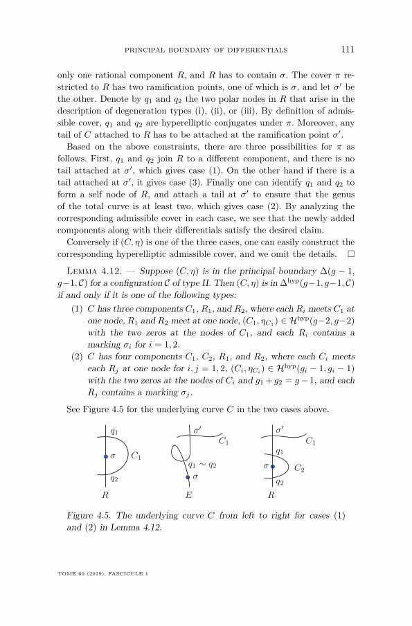
Lemma 4.12. — Suppose (C, η) is in the principal boundary ∆(g − 1,g−1, C) for a configuration C of type II. Then (C, η) is in ∆hyp(g−1, g−1, C)if and only if it is one of the following types:
(1) C has three components C1, R1, and R2, where each Ri meets C1 atone node, R1 and R2 meet at one node, (C1, ηC1) ∈ Hhyp(g−2, g−2)with the two zeros at the nodes of C1, and each Ri contains amarking σi for i = 1, 2.
(2) C has four components C1, C2, R1, and R2, where each Ci meetseach Rj at one node for i, j = 1, 2, (Ci, ηCi
) ∈ Hhyp(gi − 1, gi − 1)with the two zeros at the nodes of Ci and g1 + g2 = g− 1, and eachRj contains a marking σj .
See Figure 4.5 for the underlying curve C in the two cases above.
q1
q1
q2q2
q1 ∼ q2
σ′σ′
σσ
σ
C2
C1C1
C1
RR E
Figure 4.5. The underlying curve C from left to right for cases (1)and (2) in Lemma 4.12.
TOME 69 (2019), FASCICULE 1
112 Dawei CHEN & Qile CHEN
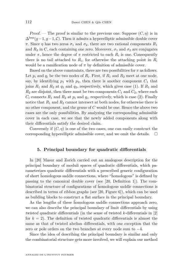
Proof. — The proof is similar to the previous one. Suppose (C, η) is in∆hyp(g−1, g−1, C). Then it admits a hyperelliptic admissible double coverπ. Since η has two zeros σ1 and σ2, there are two rational components R1and R2 in C, each containing one zero. Moreover, σ1 and σ2 are conjugatesunder π, hence the degree of π restricted to each Ri is one. Consequentlythere is no tail attached to Ri, for otherwise the attaching point in Riwould be a ramification node of π by definition of admissible cover.Based on the above constraints, there are two possibilities for π as follows.
Let pi and qi be the two nodes of Ri. First, if R1 and R2 meet at one node,say, by identifying p1 with p2, then there is another component C1 thatjoins R1 and R2 at q1 and q2, respectively, which gives case (1). If R1 andR2 are disjoint, then there must be two components C1 and C2, where eachCi connects R1 and R2 at pi and qi, respectively, which is case (2). Finallynotice that R1 and R2 cannot intersect at both nodes, for otherwise there isno other component, and the genus of C would be one. Hence the above twocases are the only possibilities. By analyzing the corresponding admissiblecover in each case, we see that the newly added components along withtheir differentials satisfy the desired claim.Conversely if (C, η) is one of the two cases, one can easily construct the
corresponding hyperelliptic admissible cover, and we omit the details.
5. Principal boundary for quadratic differentials
In [20] Masur and Zorich carried out an analogous description for theprincipal boundary of moduli spaces of quadratic differentials, which pa-rameterizes quadratic differentials with a prescribed generic configurationof short homologous saddle connections, where “homologous” is defined bypassing to the canonical double cover (see [20, Definition 1]). The com-binatorial structure of configurations of homologous saddle connections isdescribed in terms of ribbon graphs (see [20, Figure 6]), which can be usedas building blocks to construct a flat surface in the principal boundary.As the lengths of these homologous saddle connections approach zero,
we can also describe the principal boundary of limit differentials by usingtwisted quadratic differentials (in the sense of twisted k-differentials in [2]for k = 2). The definition of twisted quadratic differentials is almost thesame as that of twisted abelian differentials, with one exception that thezero or pole orders on the two branches at every node sum to −4.Since the idea of describing the principal boundary is similar and only
the combinatorial structure gets more involved, we will explain our method
ANNALES DE L’INSTITUT FOURIER
PRINCIPAL BOUNDARY OF DIFFERENTIALS 113
by going through a number of examples, in which almost all typical ribbongraphs appear. Consequently the method can be adapted to any givenconfiguration without further difficulties.
5.1. Ribbon graphs of configurations
We briefly recall the geometric meaning of the ribbon graphs (see [20,Section 1] and [15, Section 2]) for more details). A ribbon graph capturesthe information of boundary surfaces after removing the homologous saddleconnections in a given configuration and how these boundary surfaces areglued to form the original surface. A vertex labeled by , ⊕ or in thegraph represents a cylinder, a boundary surface of trivial holonomy or aboundary surface of non-trivial holonomy, respectively. Here whether ornot the holonomy is trivial corresponds to whether or not the quadraticdifferential is the square of an abelian differential. An edge joining twovertices represents a common saddle connection on the boundaries of thecorresponding two surfaces. The boundary of a ribbon graph is decoratedby integers that encode the information of cone angles between consecutivehomologous saddle connections. Each vertex is decorated by a set of integers(possibly empty) that encodes the type of singularities in the interior of thecorresponding boundary surface. Connected components of the boundaryof a ribbon graph correspond to newborn zeros after gluing the boundarysurfaces together.
5.2. Configurations in genus 2
In [20, Appendix B] Masur and Zorich described explicitly configurationsof homologous saddle connections for holomorphic quadratic differentialsin genus 2. Below we will describe the corresponding principal boundaryof limit twisted quadratic differentials for the three configurations of thestratum Q(2, 2) (see [20, Figure 22]).
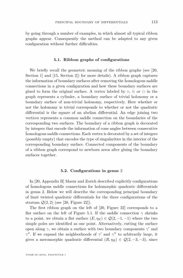
The first ribbon graph on the left of [20, Figure 22] corresponds to aflat surface on the left of Figure 5.1. If the saddle connection γ shrinksto a point, we obtain a flat surface (E, ηE) ∈ Q(2,−1,−1) where the twosimple poles are identified as one point. Alternatively, cutting the surfaceopen along γ, we obtain a surface with two boundary components γ′ andγ′′. If we expand the neighborhoods of γ′ and γ′′ to arbitrarily large, itgives a meromorphic quadratic differential (R, ηR) ∈ Q(2,−3,−3), since
TOME 69 (2019), FASCICULE 1
114 Dawei CHEN & Qile CHEN
the flat geometric neighborhood of a triple pole of a quadratic differen-tial corresponds to a (broken) half-plane. Combining them together, weconclude that the underlying pointed stable curve C of the limit differ-ential consists of E union R at two nodes, where both E and R containa marked double zero, see the right side of Figure 5.1. Conversely givensuch C and η = (ηE , ηR), since η is a twisted quadratic differential andsatisfies the global residue condition in [3], (C, η) can be smoothed into theMasur–Zorich principal boundary for this configuration.
γ RE
Figure 5.1. The surface corresponding to the first ribbon graph on theleft of [20, Figure 22] and the underlying curve of its degeneration asγ → 0.
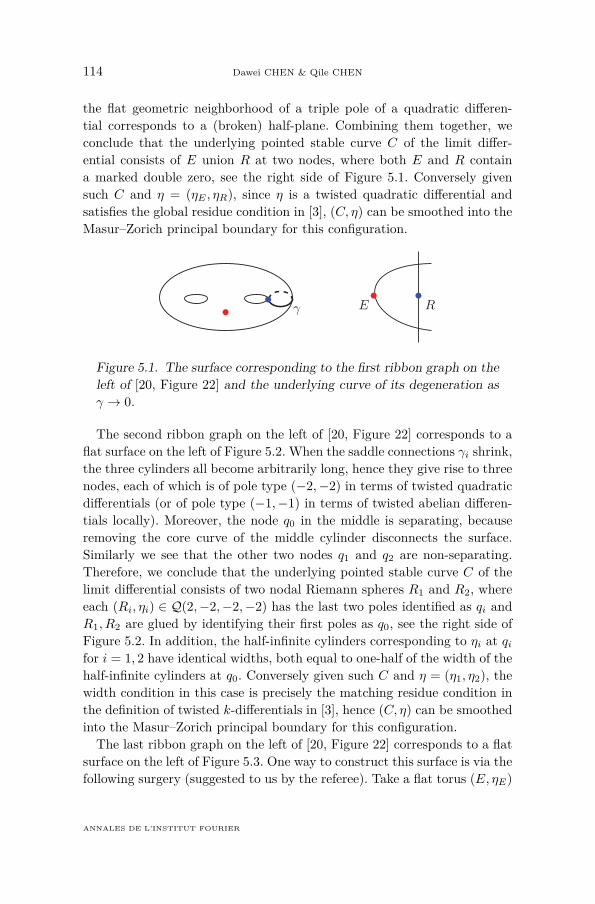
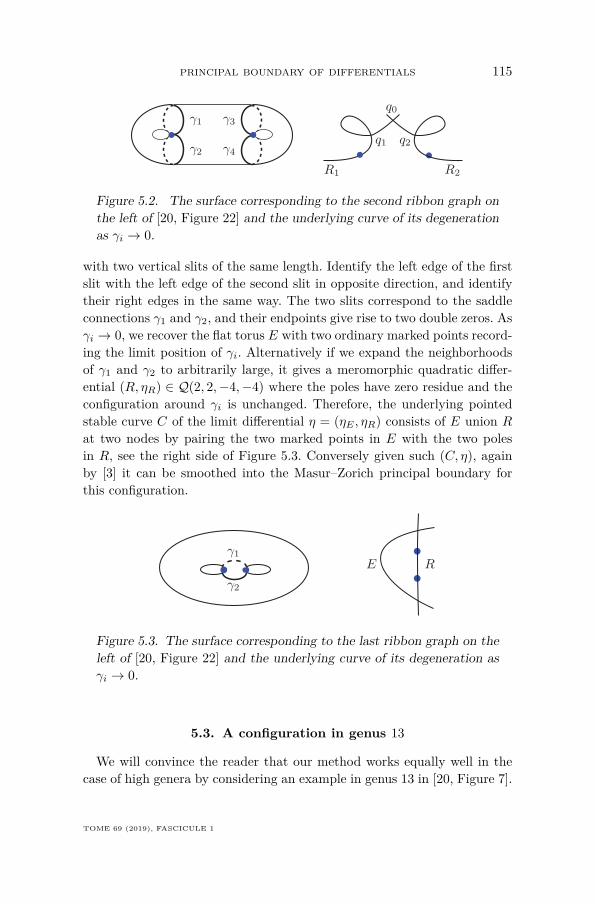
The second ribbon graph on the left of [20, Figure 22] corresponds to aflat surface on the left of Figure 5.2. When the saddle connections γi shrink,the three cylinders all become arbitrarily long, hence they give rise to threenodes, each of which is of pole type (−2,−2) in terms of twisted quadraticdifferentials (or of pole type (−1,−1) in terms of twisted abelian differen-tials locally). Moreover, the node q0 in the middle is separating, becauseremoving the core curve of the middle cylinder disconnects the surface.Similarly we see that the other two nodes q1 and q2 are non-separating.Therefore, we conclude that the underlying pointed stable curve C of thelimit differential consists of two nodal Riemann spheres R1 and R2, whereeach (Ri, ηi) ∈ Q(2,−2,−2,−2) has the last two poles identified as qi andR1, R2 are glued by identifying their first poles as q0, see the right side ofFigure 5.2. In addition, the half-infinite cylinders corresponding to ηi at qifor i = 1, 2 have identical widths, both equal to one-half of the width of thehalf-infinite cylinders at q0. Conversely given such C and η = (η1, η2), thewidth condition in this case is precisely the matching residue condition inthe definition of twisted k-differentials in [3], hence (C, η) can be smoothedinto the Masur–Zorich principal boundary for this configuration.The last ribbon graph on the left of [20, Figure 22] corresponds to a flat
surface on the left of Figure 5.3. One way to construct this surface is via thefollowing surgery (suggested to us by the referee). Take a flat torus (E, ηE)
ANNALES DE L’INSTITUT FOURIER
PRINCIPAL BOUNDARY OF DIFFERENTIALS 115
R1 R2
q1 q2
q0γ1
γ2
γ3
γ4
Figure 5.2. The surface corresponding to the second ribbon graph onthe left of [20, Figure 22] and the underlying curve of its degenerationas γi → 0.
with two vertical slits of the same length. Identify the left edge of the firstslit with the left edge of the second slit in opposite direction, and identifytheir right edges in the same way. The two slits correspond to the saddleconnections γ1 and γ2, and their endpoints give rise to two double zeros. Asγi → 0, we recover the flat torus E with two ordinary marked points record-ing the limit position of γi. Alternatively if we expand the neighborhoodsof γ1 and γ2 to arbitrarily large, it gives a meromorphic quadratic differ-ential (R, ηR) ∈ Q(2, 2,−4,−4) where the poles have zero residue and theconfiguration around γi is unchanged. Therefore, the underlying pointedstable curve C of the limit differential η = (ηE , ηR) consists of E union Rat two nodes by pairing the two marked points in E with the two polesin R, see the right side of Figure 5.3. Conversely given such (C, η), againby [3] it can be smoothed into the Masur–Zorich principal boundary forthis configuration.
γ1
γ2
E R
Figure 5.3. The surface corresponding to the last ribbon graph on theleft of [20, Figure 22] and the underlying curve of its degeneration asγi → 0.
5.3. A configuration in genus 13
We will convince the reader that our method works equally well in thecase of high genera by considering an example in genus 13 in [20, Figure 7].
TOME 69 (2019), FASCICULE 1
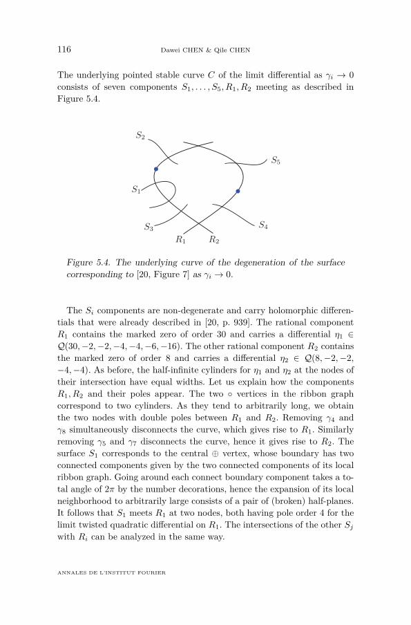
116 Dawei CHEN & Qile CHEN
The underlying pointed stable curve C of the limit differential as γi → 0consists of seven components S1, . . . , S5, R1, R2 meeting as described inFigure 5.4.
S1
S2
S3S4
S5
R1 R2
Figure 5.4. The underlying curve of the degeneration of the surfacecorresponding to [20, Figure 7] as γi → 0.
The Si components are non-degenerate and carry holomorphic differen-tials that were already described in [20, p. 939]. The rational componentR1 contains the marked zero of order 30 and carries a differential η1 ∈Q(30,−2,−2,−4,−4,−6,−16). The other rational component R2 containsthe marked zero of order 8 and carries a differential η2 ∈ Q(8,−2,−2,−4,−4). As before, the half-infinite cylinders for η1 and η2 at the nodes oftheir intersection have equal widths. Let us explain how the componentsR1, R2 and their poles appear. The two vertices in the ribbon graphcorrespond to two cylinders. As they tend to arbitrarily long, we obtainthe two nodes with double poles between R1 and R2. Removing γ4 andγ8 simultaneously disconnects the curve, which gives rise to R1. Similarlyremoving γ5 and γ7 disconnects the curve, hence it gives rise to R2. Thesurface S1 corresponds to the central ⊕ vertex, whose boundary has twoconnected components given by the two connected components of its localribbon graph. Going around each connect boundary component takes a to-tal angle of 2π by the number decorations, hence the expansion of its localneighborhood to arbitrarily large consists of a pair of (broken) half-planes.It follows that S1 meets R1 at two nodes, both having pole order 4 for thelimit twisted quadratic differential on R1. The intersections of the other Sjwith Ri can be analyzed in the same way.
ANNALES DE L’INSTITUT FOURIER
PRINCIPAL BOUNDARY OF DIFFERENTIALS 117
BIBLIOGRAPHY
[1] M. Atiyah, “Riemann surfaces and spin structures”, Ann. Sci. Éc. Norm. Supér. 4(1971), p. 47-62.
[2] M. Bainbridge, D. Chen, Q. Gendron, S. Grushevsky & M. Möller, “A smoothcompactification of strata of abelian differentials”, in preparation.
[3] ———, “Strata of k-differentials”, to appear in Algebr. Geom., https://arxiv.org/abs/1610.09238, 2016.
[4] ———, “Compactification of strata of abelian differentials”, Duke Math. J. 167(2018), no. 12, p. 2347-2416.
[5] M. Bauer & É. Goujard, “Geometry of periodic regions on flat surfaces andassociated Siegel-Veech constants”, Geom. Dedicata 174 (2015), p. 203-233.
[6] C. Boissy, “Connected components of the strata of the moduli space of meromor-phic differentials”, Comment. Math. Helv. 90 (2015), no. 2, p. 255-286.
[7] D. Chen, “Degenerations of Abelian differentials”, J. Differ. Geom. 107 (2017),no. 3, p. 395-453.
[8] ———, “Teichmüller dynamics in the eyes of an algebraic geometer”, in Surveyson recent developments in algebraic geometry, Proceedings of Symposia in PureMathematics, vol. 95, American Mathematical Society, 2017, p. 171-197.
[9] D. Chen & Q. Chen, “Spin and hyperelliptic structures of log twisted abeliandifferentials”, https://arxiv.org/abs/1610.05345, 2016.
[10] M. Cornalba, “Moduli of curves and theta-characteristics”, in Proceedings of theFirst College on Riemann Surfaces held in Trieste, November 9–December 18, 1987,World Scientific, 1989, p. 560-589.
[11] A. Eskin & H. Masur, “Asymptotic formulas on flat surfaces”, Ergodic TheoryDyn. Syst. 21 (2001), no. 2, p. 443-478.
[12] A. Eskin, H. Masur & A. Zorich, “Moduli spaces of Abelian differentials: the prin-cipal boundary, counting problems, and the Siegel–Veech constants”, Publ. Math.,Inst. Hautes Étud. Sci. 97 (2003), p. 61-179.
[13] G. Farkas & R. Pandharipande, “The moduli space of twisted canonical divisors,with an appendix by Felix Janda, Rahul Pandharipande, Aaron Pixton, and DimitriZvonkine”, J. Inst. Math. Jussieu 17 (2018), no. 3, p. 615-672.
[14] Q. Gendron, “The Deligne-Mumford and the incidence variety compactificationsof the strata of ΩMg”, Ann. Inst. Fourier 68 (2018), no. 3, p. 1169-1240.
[15] É. Goujard, “Siegel-Veech constants for strata of moduli spaces of quadratic dif-ferentials”, Geom. Funct. Anal. 25 (2015), no. 5, p. 1440-1492.
[16] J. Guéré, “A generalization of the double ramification cycle via log-geometry”,https://arxiv.org/abs/1603.09213, 2016.
[17] J. Harris & D. Mumford, “On the Kodaira dimension of the moduli space ofcurves”, Invent. Math. 67 (1982), no. 1, p. 23-88.
[18] D. Johnson, “Spin structures and quadratic forms on surfaces”, J. Lond. Math.Soc. 22 (1980), p. 365-373.
[19] M. Kontsevich & A. Zorich, “Connected components of the moduli spaces ofAbelian differentials with prescribed singularities”, Invent. Math. 153 (2003), no. 3,p. 631-678.
[20] H. Masur & A. Zorich, “Multiple saddle connections on flat surfaces and theprincipal boundary of the moduli spaces of quadratic differentials”, Geom. Funct.Anal. 18 (2008), no. 3, p. 919-987.
[21] M. Mirzakhani & A. Wright, “The boundary of an affine invariant submanifold”,Invent. Math. 209 (2017), no. 3, p. 927-984.
TOME 69 (2019), FASCICULE 1
118 Dawei CHEN & Qile CHEN
[22] D. Mumford, “Theta characteristics of an algebraic curve”, Ann. Sci. Éc. Norm.Supér. 4 (1971), p. 181-192.
[23] W. A. Veech, “Siegel measures”, Ann. Math. 148 (1998), no. 3, p. 895-944.[24] A. Wright, “Translation surfaces and their orbit closures: an introduction for a
broad audience”, EMS Surv. Math. Sci. 2 (2015), no. 1, p. 63-108.[25] A. Zorich, “Flat surfaces”, in Frontiers in number theory, physics, and geometry
I. On random matrices, zeta functions, and dynamical systems. Papers from themeeting, Les Houches, France, March 9–21, 2003, Springer, 2nd ed., 2006, p. 437-583.
Manuscrit reçu le 3 janvier 2017,révisé le 24 septembre 2017,accepté le 2 février 2018.
Dawei CHENDepartment of MathematicsBoston CollegeChestnut Hill, MA 02467 (USA)[email protected] CHENDepartment of MathematicsBoston CollegeChestnut Hill, MA 02467 (USA)[email protected]
ANNALES DE L’INSTITUT FOURIER


![Reminder Fourier Basis: t [0,1] nZnZ Fourier Series: Fourier Coefficient:](https://img.dokumen.tips/doc/110x75/56649d395503460f94a13929/reminder-fourier-basis-t-01-nznz-fourier-series-fourier-coefficient.jpg)


