Anisotropic and dynamic mesh adaptation for discontinuous ... · Anisotropic and dynamic mesh adaptation for discontinuous Galerkin methods applied to reactive transport Shuyu Sun,

Comput. Methods Appl. Mech. Engrg. 195 (2006) 3382–3405

www.elsevier.com/locate/cma

Anisotropic and dynamic mesh adaptation for discontinuousGalerkin methods applied to reactive transport

Shuyu Sun, Mary F. Wheeler *

The Institute for Computational Engineering and Sciences, ICES, The University of Texas at Austin,

Austin, TX 78712, USA

Accepted 17 June 2005

Abstract

Mesh adaptation strategies are proposed for discontinuous Galerkin methods applied to reactive transport prob-lems, with emphasis on dynamic and anisotropic adaptation. They include an anisotropic mesh adaptation schemeand two isotropic methods using an L2(L2) norm error estimator and a hierarchic error indicator. These dynamic meshadaptation approaches are investigated using benchmark cases. Numerical results demonstrate that the threeapproaches resolve time-dependent transport adequately without slope limiting for both long-term and short-term sim-ulations. It is shown that these results apply to problems where either diffusion or advection dominates in different sub-domains. Moreover, for these schemes, mass conservation is retained locally during dynamic mesh modification.Comparison studies indicate that the anisotropic mesh adaptation provides the most efficient meshes and has the leastnumerical diffusion among the three adaptation approaches.� 2005 Elsevier B.V. All rights reserved.

Keywords: Discontinuous Galerkin methods; A posteriori error estimators; Anisotropic mesh adaptation; Dynamic mesh adaptation;Reactive transport

1. Introduction

Discontinuous Galerkin (DG) methods employ non-conforming piecewise polynomial spaces to approx-imate the solutions of differential equations. The concept of discontinuous space approximations first ap-peared in the early 1970s (see, for example [49,25,22,6,7,4,16,24]) when discontinuous basis functions wereused to approximate second-order elliptic equations. But only recently have DG methods been investigated

0045-7825/$ - see front matter � 2005 Elsevier B.V. All rights reserved.doi:10.1016/j.cma.2005.06.019

* Corresponding author.E-mail address: [email protected] (M.F. Wheeler).

mailto:[email protected]

S. Sun, M.F. Wheeler / Comput. Methods Appl. Mech. Engrg. 195 (2006) 3382–3405 3383

intensively and applied to wide collections of problems. These schemes have many attractive properties[10,23,27,50,29,30,5]. The flexibility of DG allows for general non-conforming meshes with variable degreesof approximation. This makes the implementation of hp-adaptivity for DG substantially easier than con-ventional approaches. Moreover, DG methods are locally mass conservative at the element level. In addi-tion, they have less numerical diffusion than most conventional algorithms. They can treat rough coefficientproblems and can effectively capture discontinuities in solutions. DG can naturally handle inhomogeneousboundary conditions and curved boundaries. The average of the trace of fluxes from a DG solution alongan element interface is continuous and may be extended so that a continuous flux is defined over the entiredomain. Consequently, DG may be easily coupled with conforming methods. Furthermore, with appropri-ate meshing, DG with varying p can yield exponential convergence rates. For time-dependent problems inparticular, the mass matrices of DG are block diagonal, which is not true for conforming methods. Thisprovides a substantial computational advantage, especially if explicit time integrations are used.

Reactive transport is a fundamental process arising in many important engineering and scientific fieldssuch as petroleum, aerospace, environmental, chemical and biomedical engineering, and earth and life sci-ences. Realistic simulations for simultaneous transport and chemical reaction present significant computa-tional challenges [3,33,53,13,17,18,21,31,32,34,46,48,47,54,35,11,20,51,19,44,45,43]. DG has recently beenapplied to flow and transport problems in porous media [37,28,52,41,43], and an optimal convergence inL2(H1) was demonstrated for flow and transport problems [28,30,36,38]. The hp-convergence behaviorsin the L2(L2) and negative norms have been analyzed [36,38]. Explicit a posteriori error estimates of DGfor reactive transport have also been studied [39,42,40].

In this paper, we formulate and study three error indicator-guided dynamic mesh adaptation strategies;namely, the hierarchic anisotropic (HA), the L2(L2) isotropic (LI), and the hierarchic isotropic (HI) ap-proaches. In Section 2, we formulate the general scalar reactive transport equation and corresponding pri-mal DG schemes. In addition, we review properties and error estimators, both a priori and a posteriori, forthis model. In Section 3, we derive a new a posteriori error estimator, using hierarchic bases, that providesguidance on the anisotropic refinement of an element, and establish dynamic mesh adaptation strategies.Section 4 is devoted to numerical studies. It is demonstrated that effective mesh adaptations eliminatethe need of slope limiters for DG. Finally, in Section 5, our results are summarized, and future work isdescribed.

2. Governing equations and discontinuous Galerkin schemes

2.1. Governing equations

We consider reactive transport for a single flowing phase in porous media. We assume that a time-inde-pendent Darcy velocity field u is given and that it satisfies $ Æ u = q, where q is the imposed external totalflow rate.

For simplicity, only a single advection–diffusion-reaction equation is considered. However, results maybe extended to systems with kinetic reactions. In addition, for convenience, we assume that X is a boundedpolygonal domain in Rd (d = 1, 2 or 3) with boundary oX ¼ Cin [ Cout. Here, we denote by Cin the inflowboundary and by Cout the outflow/no-flow boundary, i.e.,

Cin ¼ fx 2 oX : u � n < 0g;Cout ¼ fx 2 oX : u � n P 0g;

where n denotes the unit outward normal vector to oX. The classical advection–diffusion-reaction equationfor a single flowing phase in porous media is given by

3384 S. Sun, M.F. Wheeler / Comput. Methods Appl. Mech. Engrg. 195 (2006) 3382–3405

o/cotþr � uc�DðuÞrcð Þ ¼ qc� þ rðcÞ; ðx; tÞ 2 X� ð0; T �; ð2:1Þ

where the unknown variable c is the concentration of a species (amount per volume). Here, T is the finalsimulation time. / denotes porosity and is assumed to be time-independent and uniformly bounded, aboveand below, by positive numbers. D(u) is a dispersion–diffusion tensor and is assumed to be uniformly sym-metric positive definite and bounded from above. r(c) is a reaction term, and qc� is a source term, where theimposed external total flow rate q is a sum of sources (injection) and sinks (extraction). c� is an injectedconcentration cw if q P 0 and is a resident concentration c if q < 0.

The following boundary conditions are imposed for this problem

uc�DðuÞrcð Þ � n ¼ cBu � n; ðx; tÞ 2 Cin � ð0; T �; ð2:2Þ�DðuÞrcð Þ � n ¼ 0; ðx; tÞ 2 Cout � ð0; T �; ð2:3Þ

where cB is the inflow concentration. The initial concentration is specified in the following way:

cðx; 0Þ ¼ c0ðxÞ; x 2 X. ð2:4Þ

2.2. Notation

Let Eh be a family of non-degenerate and possibly non-conforming partitions of X composed of trian-gles or quadrilaterals if d = 2, or tetrahedra, prisms or hexahedra if d = 3. Here h is the maximum elementdiameter for the mesh. The non-degeneracy requirement (also called regularity) is that the element is con-vex, and that there exists q > 0 such that if hj is the diameter of Ej 2 Eh, then each of the sub-triangles (ford = 2) or sub-tetrahedra (for d = 3) of element Ej contains a ball of radius qhj in its interior. We assumethat no element crosses the boundaries Cin and Cout. The set of all interior edges (for two-dimensionaldomain) or faces (for three-dimensional domain) for Eh is denoted by Ch. On each edge or face c 2 Ch,a unit normal vector nc is chosen. The sets of all edges or faces on Cout and on Cin for Eh are denotedby Ch,out and Ch,in, respectively, for which the normal vector nc coincides with the outward unit normalvector.

For s P 0, we define

H sðEhÞ :¼ / 2 L2ðXÞ : /jE 2 HsðEÞ;E 2 Eh

� �. ð2:5Þ

The discontinuous finite element space is taken to be

Dr Ehð Þ :¼ / 2 L2ðXÞ : /jE 2 PrðEÞ;E 2 Eh

� �; ð2:6Þ

where PrðEÞ denotes the space of polynomials of (total) degree less than or equal to r on E. Note that theresults in this paper are based on the local space Pr, but may be easily extended to the local space Qr.

We now define the average and jump for / 2 H sðEhÞ; s > 1=2. Let Ei;Ej 2 Eh and c = oEi \ oEj 2 Ch

with nc exterior to Ei. Denote

/f g :¼ 1

2/jEi

� ��cþ /jEj

� ��c

; ð2:7Þ

/½ � :¼ /jEi

� ��c� /jEj

� ��c. ð2:8Þ

Denote the upwind value of the concentration c�jc as follows:

c�jc :¼cjEi

if u � nc P 0;

cjEjif u � nc < 0.

(


The usual Sobolev norm on a domain R � X is denoted by k Æ km,R [1]. The broken norms are defined, form P 0, as

jjj/jjj2m :¼XE2Eh

/k k2m;E. ð2:9Þ

The inner product in (L2(R))d or L2(R) is indicated by (Æ , Æ)R, and the inner product in the boundary functionspace L2(c) is denoted by (Æ , Æ)c. The inner product over the entire domain (Æ , Æ)X is also written simply as (Æ , Æ).We define a cut-off operator M as

MðcÞðxÞ :¼ min cðxÞ;Mð Þ; ð2:10Þ
where M is a large positive constant.
2.3. Continuous-in-time schemes

We introduce the bilinear form B(c, w; u) defined as

Bðc;w; uÞ :¼XE2Eh

ZE

DðuÞrc� cuð Þ � rw�Z

Xcq�w�

Xc2Ch

Zc

DðuÞrc � nc

� �w½ �

� sform

Xc2Ch

Zc

DðuÞrw � nc

� �c½ � þ

Xc2Ch

Zc

c�u � nc w½ � þX

c2Ch;out

Zc

cu � ncwþ Jr0 c;wð Þ;

ð2:11Þ

where sform = �1 for NIPG (the nonsymmetric interior penalty Galerkin method [30]) or OBB-DG (theOden-Babuska-Baumann formulation of DG [23]), sform = 1 for SIPG (the symmetric interior penaltyGalerkin method [49,36,38]), and sform = 0 for IIPG (the incomplete interior penalty Galerkin method[36,14,38]). Here, q+ is the injection source term, and q� is the extraction source term, i.e.,

qþ :¼ max q; 0ð Þ; q� :¼ min q; 0ð Þ.

By definition, we have q = q+ + q�. In addition, we define the interior penalty term Jr0ðc;wÞ as

Jr0ðc;wÞ :¼

Xc2Ch

r2rc

hc

Zc

c½ � w½ �;

where r is a discrete positive function that takes the constant value rc on the edge or face c. We let rc � 0for OBB-DG and assume 0 < r0 6 rc 6 rm for SIPG, NIPG and IIPG.

The linear functional L(w; u, c) is defined as

Lðw; u; cÞ :¼Z

Xr MðcÞð Þwþ

ZX

cwqþw�X

c2Ch;in

Zc

cBu � ncw. ð2:12Þ

We state the weak formulation of the reactive transport problem, for which the proof may be found in[36,38].

Lemma 2.1 (Weak formulation). If c is a solution of (2.1)–(2.3) and c is essentially bounded, then c satisfies

o/cot

;w

þ Bðc;w; uÞ ¼ Lðw; u; cÞ; 8w 2 H s Ehð Þ; s >3

2; 8t 2 ð0; T �; ð2:13Þ

provided that the constant M for the cut-off operator is sufficiently large.


The continuous-in-time DG approximation CDGð�; tÞ 2 Dr Ehð Þ of (2.1)–(2.4) is defined by

o/CDG

ot;w

þ BðCDG;w; uÞ ¼ Lðw; u;CDGÞ; 8w 2 Dr Ehð Þ; t 2 ð0; T �; ð2:14Þ

/CDG;w� �

¼ /c0;wð Þ; 8w 2 Dr Ehð Þ; t ¼ 0. ð2:15Þ

A unique solution for the above DG scheme always exists [36].

Lemma 2.2 (Existence of a solution). Assume that the reaction rate is a locally Lipschitz continuous function

of the concentration. The discontinuous Galerkin scheme (2.14) and (2.15) has a unique solution for all t > 0.

The element-wise mass conservation of DG schemes is stated in the following Lemma [36]. We note thatthe concentration jump term, i.e., the fourth term in (2.16), is considered as part of the computed diffusiveflux for SIPG, NIPG and IIPG.

Lemma 2.3 (Local mass balance). The approximation of the concentration satisfies, on each element E, the

following local mass balance property:
ZE
o/CDG

ot�Z

oE=oXDðuÞrCDG � noE

� �þZ

oECDG�u � noE þ

Xc�oEnoX

r2rc

hc

Zc

CDG��E� CDG

��X=E

� �

¼Z

ECDGq� þ cwqþ� �

þZ

Er MðCDGÞ� �

. ð2:16Þ

2.4. Convergence results of DG

In [36,38], the following a priori error estimate was established for NIPG, SIPG and IIPG:

Theorem 2.4 (L2(H1) and L1(L2) error estimate for NIPG, SIPG and IIPG). Let c be the solution to (2.1)–(2.4), and assume c 2 L2 0; T ; H sðEhÞð Þ; oc=ot 2 L2 0; T ; H s�1ðEhÞ

� �and c0 2 H s�1ðEhÞ. We further assume

that c, u and q are essentially bounded and that the reaction rate is a locally Lipschitz continuous function of c.

If the constant M for the cut-off operator and the penalty parameter r0 are sufficiently large, then there exists

a constant K, independent of h and r, such that

CDG � c��

L1 0;T ;L2ð Þ þ jjjD12 uð Þr CDG � c

� �jjjL2 0;T ;L2ð Þ þ

Z T

0

Jr0 CDG � c;CDG � c� � 1

2

6 Khl�1

rs�1�d2

jjjcjjjL2 0;T ;Hsð Þ þ Khl�1

rs�1jjjoc=otjjjL2 0;T ;Hs�1ð Þ þ jjjc0jjjs�1

� �;

where l = min(r + 1, s), r P 1, s P 2, and d = 0 in the case of conforming meshes with triangles or tetrahedra.

In general cases, d = 1. h

The following a priori error estimate for OBB-DG was derived in [28,36].

Theorem 2.5 (L2(H1) and L1(L2) error estimate for OBB-DG). Let all assumptions in Theorem 2.4 hold

except sform = �1 and r � 0. If the constant M for the cut-off operator is sufficiently large, then there exists a

constant K, independent of h and r, such that

CDG � c��

L1 0;T ;L2ð Þ þ jjjD12 uð Þr CDG � c

� �jjjL2 0;T ;L2ð Þ

6 Khl�1

rs�52

jjjcjjjL2 0;T ;Hsð Þ þ jjjoc=otjjjL2 0;T ;Hs�1ð Þ þ jjjc0jjjs� �

;

where l = min(r + 1, s), r P 2, and s P 3. h


2.5. Residual-based explicit a posteriori error estimators

We introduce residual quantities that only depend on the approximate solution and data. The residualsconsist of the interior residual RI, the zeroth-order boundary residual RB0, and the first-order boundaryresidual RB1 as defined below:

RI ¼ q�CDG þ qþcw þ r MðCDGÞ� �

� /oCDG

ot�r � CDGu�DðuÞrCDG

� �; ð2:17Þ

RB0 ¼CDG�

; x 2 c; c 2 Ch;

0; x 2 oX;

(ð2:18Þ

RB1 ¼DðuÞrCDG � n�

; x 2 c; c 2 Ch;

cBu� CDGuþDðuÞrCDG� �

� n; x 2 Cin;

DðuÞrCDG � n; x 2 Cout.

8><>: ð2:19Þ

We recall two explicit a posteriori error estimators [42,39]. The L2(L2) norm error estimator will be used inSection 4.

Theorem 2.6 (Explicit a posteriori error estimator in L2(L2) for SIPG). Let the assumptions in Theorem 2.4hold. In addition, we assume / 2 W 2;1

1 ðð0; T Þ � XÞ;Dij 2 W 1;01 ðð0; T Þ � XÞ, u 2 L1(X) (u being independent of

time), u � njoX ¼ 0; and c0 2 Dr Ehð Þ. Then there exists a constant K, independent of h and r, such that

CDG � c��

L2 0;T ;L2ð Þ 6 KXE2Eh

g2E

!1=2

;

where

g2E ¼

h4E

r4RIk k2

L2 0;T ;L2ðEÞð Þ þ1

2

Xc�oEnoX

hc

rþ drhc

RB0k k2

L2 0;T ;L2ðcÞð Þ þ1

2

Xc�oEnoX

h3c

r3RB1k k2

L2 0;T ;L2ðcÞð Þ

þX

c�oE\oX

h3c

r3RB1k k2

L2 0;T ;L2ðcÞð Þ.

Here, hc ¼ maxðhE1; hE2Þ for c = oE1 \ oE2, r P 1, and d = 0 in the case of conforming meshes with triangles

or tetrahedra. In general cases, d = 1. h

Theorem 2.7 (Explicit a posteriori error estimator for OBB-DG, NIPG, SIPG or IIPG). Let the assump-

tions in Theorem 2.4 (for NIPG, SIPG or IIPG) or in Theorem 2.5 (for OBB-DG) hold . In addition, we assume

c0 2 Dr Ehð Þ. There exists a constant K, independent of h, such that

ffiffiffiffi/

pðCDG � cÞ

�� L1 0;T ;L2ðXÞð Þ

þ jjjD12 uð ÞrðCDG � cÞjjjL2 0;T ;L2ðXÞð Þ 6 K

XE2Eh

g2E

!1=2

;

where

g2E ¼ h2

E RIk k2L2 0;T ;L2ðEÞð Þ þ

Xc�oE\oX

hc RB1k k2L2 0;T ;L2ðcÞð Þ

þ 1

2

Xc�oEnoX

hc RB1k k2L2 0;T ;L2ðcÞð Þ þ h�1

c RB0k k2L2 0;T ;L2ðcÞð Þ

�þhc RB0k k2

L1 0;T ;L2ðcÞð Þ þ hc oRB0=otk k2L2 0;T ;L2ðcÞð Þ

�.

Here, hc ¼ maxðhE1; hE2Þ for c = oE1 \ oE2 and r P 1. h


We note that, in implementation, time derivative terms may be approximated by finite differences. Forexample, we may estimate the time derivative of the DG solution used in the interior residual RI by

oCDG

ot

CDG� �

tnþ1� CDG� �

tn

tnþ1 � tnfor t 2 tn; tnþ1ð Þ.

3. Anisotropic mesh adaptation

3.1. A hierarchic a posteriori error indicator

Residual-based explicit error estimators are efficient to compute and may be used to indicate a set ofelements that need to be refined, thus guiding adaptivity. However, these residual-based estimators yieldonly one piece of information for each element. Consequently, they do not provide guidance on aniso-tropic refinements. In this section, we derive error estimators using hierarchic bases. Unlike residual-basederror estimators, hierarchic error estimators give point-wise information on the error, and thus may beused to guide fully anisotropic hp-adaptation. Here, for simplicity, we consider only the anisotropic h-adaptation.

Hierarchic error estimators consist of solving the problem of interest by employing two discretizationschemes of different accuracy and using the difference between the approximations as an estimate for theerror. The advantages of this approach include their applicability to many classes of problems and thesimplicity and ease of their implementation. The reader is referred to [2,8,9,15,26] for furtherinformation.

For a given mesh Eh, we construct the mesh Eh=2 by isotropically refining each element of Eh. We denoteby CDG the DG solution in the coarse mesh Eh and by CDG,F the DG solution in the fine mesh Eh=2. Wemake the following saturation assumption:

CDG;F � c��

L2ðtÞ 6 b CDG � c��

L2ðtÞ; 0 6 b < 1. ð3:1Þ

Using Theorems 2.4 and 2.5, we observe, for all the four primal DGs, i.e., OBB-DG, SIPG, NIPG andIIPG, that b is less than or equal to the following value asymptotically:

b 61

2l�1¼ 1

2minðr;s�1Þ .

Theorem 3.1 (A posteriori error estimator for OBB-DG, SIPG, NIPG or IIPG). Let the saturationassumption (3.1) be satisfied. Then we have

1

1þ b

XE2Eh

g2E

!1=2

ðtÞ 6 CDG � c��

L2ðtÞ 61

1� b

XE2Eh

g2E

!1=2

ðtÞ;

where gEðtÞ ¼ kCDG;F � CDGkL2ðEÞðtÞ.


Proof. The theorem follows by the saturation assumption together with the triangle inequality:

XE2Eh

g2E

!1=2

ðtÞ ¼ CDG;F � CDG��

L2ðXÞðtÞ

6 CDG � c��

L2ðXÞðtÞ þ CDG;F � c��

L2ðXÞðtÞ

6 ð1þ bÞ CDG � c��

L2ðXÞðtÞ;

XE2Eh

g2E

!1=2

ðtÞ ¼ CDG;F � CDG��

L2ðXÞðtÞ

P CDG � c��

L2ðXÞðtÞ � CDG;F � c��

L2ðXÞðtÞ

P ð1� bÞ CDG � c��

L2ðXÞðtÞ. �

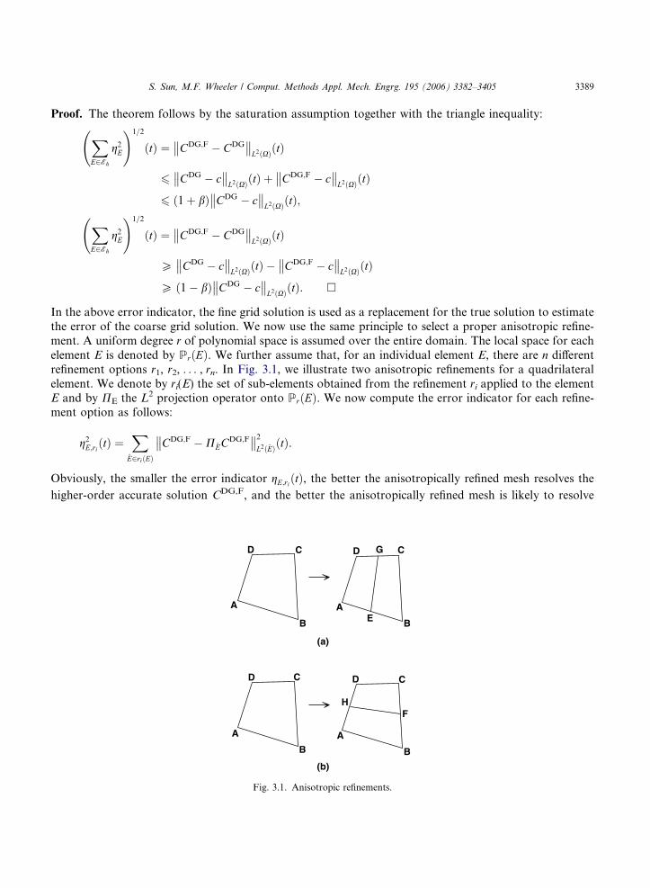
In the above error indicator, the fine grid solution is used as a replacement for the true solution to estimatethe error of the coarse grid solution. We now use the same principle to select a proper anisotropic refine-ment. A uniform degree r of polynomial space is assumed over the entire domain. The local space for eachelement E is denoted by PrðEÞ. We further assume that, for an individual element E, there are n differentrefinement options r1, r2, . . . , rn. In Fig. 3.1, we illustrate two anisotropic refinements for a quadrilateralelement. We denote by ri(E) the set of sub-elements obtained from the refinement ri applied to the elementE and by PE the L2 projection operator onto PrðEÞ. We now compute the error indicator for each refine-ment option as follows:

g2E;riðtÞ ¼

XE2riðEÞ

CDG;F �PECDG;F�� 2

L2ðEÞðtÞ.

Obviously, the smaller the error indicator gE;riðtÞ, the better the anisotropically refined mesh resolves the

higher-order accurate solution CDG,F, and the better the anisotropically refined mesh is likely to resolve

A

B

CD

A

B

CD

E

G

(a)

A

B

CD

A

B

CD

FH

(b)

Fig. 3.1. Anisotropic refinements.


the true solution c. Therefore, we choose the refinement ri at the time t such that gE;riðtÞ is minimized among

all available options.

3.2. Dynamic and anisotropic mesh adaptation

For transient problems involving a long period of simulation time, the location of biogeochemical phe-nomena generally moves with time. Most error indicators for transient problems, including the L2(L2) andL2(H1) error indicators reviewed in the previous section, provide global spatial and temporal estimates. It isdesirable that error indicators account for local physics only at the current time, and thus it is preferable tocompute error indicators only for a short time interval. The hierarchic error indicator presented in this sec-tion is point-wise in time and provides guidance on time-dependent mesh modifications. Because it is expen-sive to change the mesh at each time step, we divide the entire simulation period into a collection of timeslices, each of which may in turn contain a certain number of time steps. We adopt a non-growing dynamicadaptive strategy [40], where the mesh is adaptively adjusted while the number of elements remains con-stant. The maintenance of a constant number of elements prevents the computational workload fromincreasing with time steps. The initial mesh is chosen to be a uniform fine grid. We first present the dynamicand isotropic mesh adaptation strategy. We denote by #(S) the number of elements in a set S.

Algorithm 3.2 (Dynamic and isotropic mesh adaptation). Given an initial mesh E0, a modification factora 2 (0, 1), time slices {(T0,T1), (T1,T2), . . . , (TN � 1,TN)}, and iteration numbers {M1,M2, . . . , MN}:

1. Let n = 1.2. Let m = 1.3. Compute the initial concentration for the time slice (Tn � 1,Tn) using either the initial condition (if

n = 1) or the concentration at the end of last time slice (if n > 1) by local projections.4. Let Em;n ¼ E0 if n = 1 and m = 1; or Em;n ¼ EMn�1þ1;n�1 if n > 1 and m = 1.5. Compute the DG approximation of the PDE for the time slice (Tn � 1, Tn) based on the mesh Em;n,

and compute the error indicator gE for each element E 2 Em;n.6. Select Er 2 Em;n such that #ðErÞ ¼ a#ðEm;nÞd e and minfgE : E 2 ErgP maxfgE : E 2 Em;n n Erg.7. Select Ec 2 Em;n to minimize maxfgE : E 2 Ecg subject to that #ðEcÞ ¼ a#ðEm;nÞd e and that Ec satis-

fies the coarsening-compatible condition with regard to Em;n and Er.8. Refine all E 2 Er and coarsen all E 2 Ec to form a new mesh Emþ1;n.9. Let m = m + 1. If m 6Mn, go to step 3.

10. Let n = n + 1. If n 6 N, go to step 2.11. Report the solution and stop.

We have used a coarsening-compatible condition in the above algorithm. We note that, because DG al-lows for an arbitrary degree of nonconformity, each element may be refined. However, not every element isavailable for coarsening; for instance, the element without a father cannot be further coarsened. The coars-ening-compatible condition is defined as below.

Definition 3.3 (Coarsening-compatible condition). A coarsening element set Ec is said to satisfy thecoarsening-compatible condition with regard to a mesh E and a refinement element set Er if and only if:

1. Each element in Ec has a father.2. Brothers of an element in Ec are active, that is, they sit in E.3. None of the elements in Ec and their brothers are in Er.4. Brothers of an element in Ec are not in Ec.


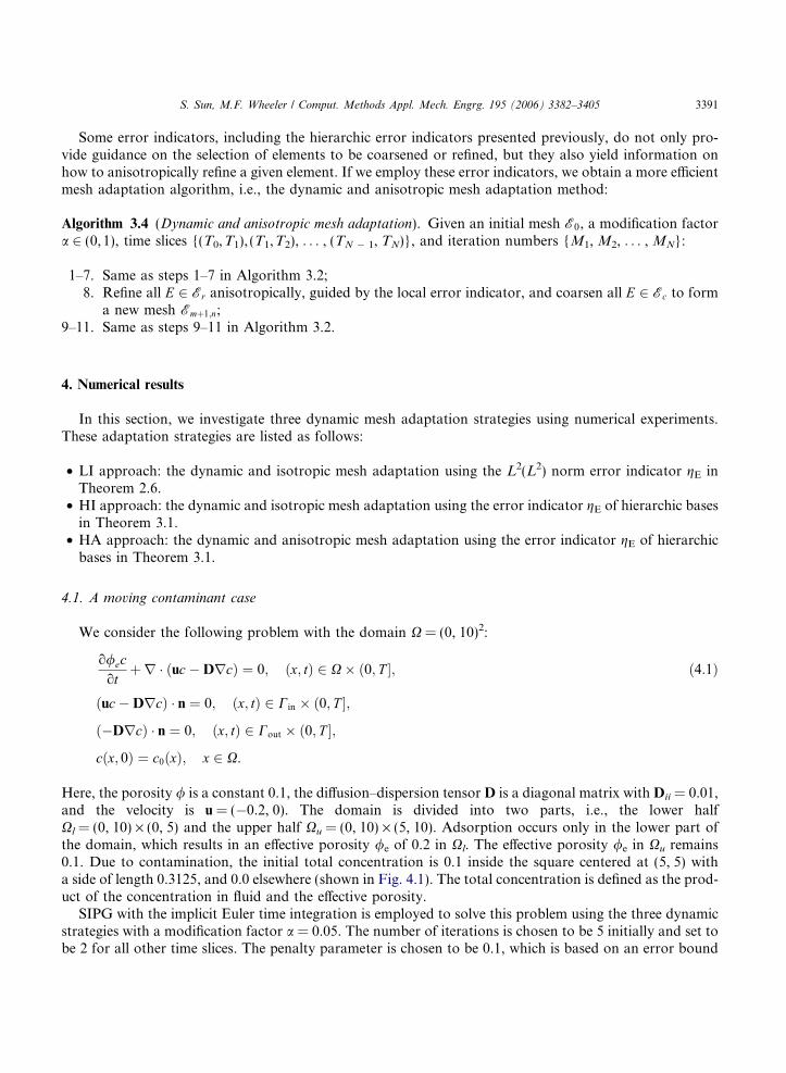
Some error indicators, including the hierarchic error indicators presented previously, do not only pro-vide guidance on the selection of elements to be coarsened or refined, but they also yield information onhow to anisotropically refine a given element. If we employ these error indicators, we obtain a more efficientmesh adaptation algorithm, i.e., the dynamic and anisotropic mesh adaptation method:

Algorithm 3.4 (Dynamic and anisotropic mesh adaptation). Given an initial mesh E0, a modification factora 2 (0, 1), time slices {(T0,T1), (T1,T2), . . . , (TN � 1, TN)}, and iteration numbers {M1, M2, . . . , MN}:

1–7. Same as steps 1–7 in Algorithm 3.2;8. Refine all E 2 Er anisotropically, guided by the local error indicator, and coarsen all E 2 Ec to form

a new mesh Emþ1;n;9–11. Same as steps 9–11 in Algorithm 3.2.

4. Numerical results

In this section, we investigate three dynamic mesh adaptation strategies using numerical experiments.These adaptation strategies are listed as follows:

• LI approach: the dynamic and isotropic mesh adaptation using the L2(L2) norm error indicator gE inTheorem 2.6.

• HI approach: the dynamic and isotropic mesh adaptation using the error indicator gE of hierarchic basesin Theorem 3.1.

• HA approach: the dynamic and anisotropic mesh adaptation using the error indicator gE of hierarchicbases in Theorem 3.1.

4.1. A moving contaminant case

We consider the following problem with the domain X = (0, 10)2:

o/ecotþr � uc�Drcð Þ ¼ 0; ðx; tÞ 2 X� ð0; T �; ð4:1Þ

uc�Drcð Þ � n ¼ 0; ðx; tÞ 2 Cin � ð0; T �;

�Drcð Þ � n ¼ 0; ðx; tÞ 2 Cout � ð0; T �;

cðx; 0Þ ¼ c0ðxÞ; x 2 X.

Here, the porosity / is a constant 0.1, the diffusion–dispersion tensor D is a diagonal matrix with Dii = 0.01,and the velocity is u = (�0.2, 0). The domain is divided into two parts, i.e., the lower halfXl = (0, 10) · (0, 5) and the upper half Xu = (0, 10) · (5, 10). Adsorption occurs only in the lower part ofthe domain, which results in an effective porosity /e of 0.2 in Xl. The effective porosity /e in Xu remains0.1. Due to contamination, the initial total concentration is 0.1 inside the square centered at (5, 5) witha side of length 0.3125, and 0.0 elsewhere (shown in Fig. 4.1). The total concentration is defined as the prod-uct of the concentration in fluid and the effective porosity.

SIPG with the implicit Euler time integration is employed to solve this problem using the three dynamicstrategies with a modification factor a = 0.05. The number of iterations is chosen to be 5 initially and set tobe 2 for all other time slices. The penalty parameter is chosen to be 0.1, which is based on an error bound

X

Y

0 1 2 3 4 5 6 7 8 9 100

1

2

3

4

5

6

7

8

9

10CONC1.000.900.800.700.600.500.400.300.200.100.00

Fig. 4.1. The initial fluid concentration and velocity for the moving contaminant case.


established in [38]. The simulation time interval is (0, 2) with a uniform time step Dt = 0.01. Each time slicecontains 10 time steps. The complete quadratic basis function is used for each element. The initial mesh is a16 · 16 uniform rectangular grid.

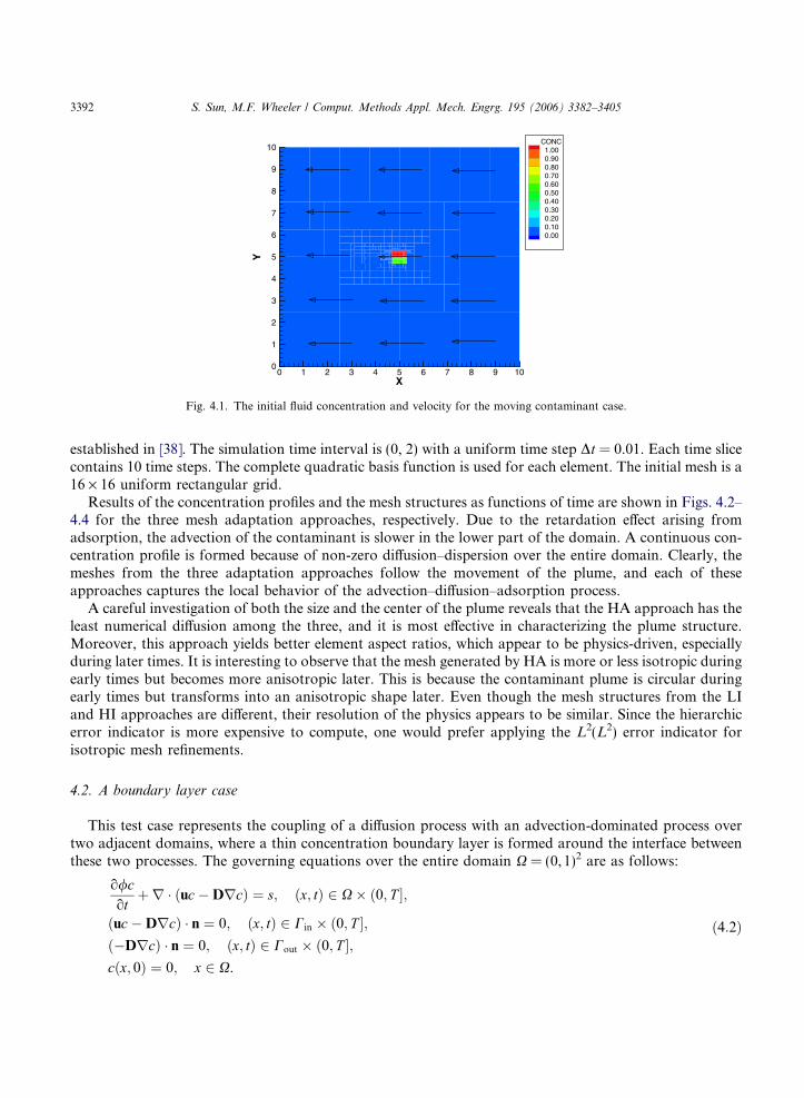
Results of the concentration profiles and the mesh structures as functions of time are shown in Figs. 4.2–4.4 for the three mesh adaptation approaches, respectively. Due to the retardation effect arising fromadsorption, the advection of the contaminant is slower in the lower part of the domain. A continuous con-centration profile is formed because of non-zero diffusion–dispersion over the entire domain. Clearly, themeshes from the three adaptation approaches follow the movement of the plume, and each of theseapproaches captures the local behavior of the advection–diffusion–adsorption process.

A careful investigation of both the size and the center of the plume reveals that the HA approach has theleast numerical diffusion among the three, and it is most effective in characterizing the plume structure.Moreover, this approach yields better element aspect ratios, which appear to be physics-driven, especiallyduring later times. It is interesting to observe that the mesh generated by HA is more or less isotropic duringearly times but becomes more anisotropic later. This is because the contaminant plume is circular duringearly times but transforms into an anisotropic shape later. Even though the mesh structures from the LIand HI approaches are different, their resolution of the physics appears to be similar. Since the hierarchicerror indicator is more expensive to compute, one would prefer applying the L2(L2) error indicator forisotropic mesh refinements.

4.2. A boundary layer case

This test case represents the coupling of a diffusion process with an advection-dominated process overtwo adjacent domains, where a thin concentration boundary layer is formed around the interface betweenthese two processes. The governing equations over the entire domain X = (0, 1)2 are as follows:

o/cotþr � uc�Drcð Þ ¼ s; ðx; tÞ 2 X� ð0; T �;

uc�Drcð Þ � n ¼ 0; ðx; tÞ 2 Cin � ð0; T �;�Drcð Þ � n ¼ 0; ðx; tÞ 2 Cout � ð0; T �;

cðx; 0Þ ¼ 0; x 2 X.

ð4:2Þ

Fig. 4.2. DG with the LI mesh adaptation applied to the moving contaminant case (left column: the concentration in fluid; rightcolumn: the mesh structure; from top row to bottom: t = 0.5, 1, 1.5 and 2, respectively).


Fig. 4.3. DG with the HI mesh adaptation applied to the moving contaminant case (left column: the concentration in fluid; rightcolumn: the mesh structure; from top row to bottom: t = 0.5, 1, 1.5 and 2, respectively).


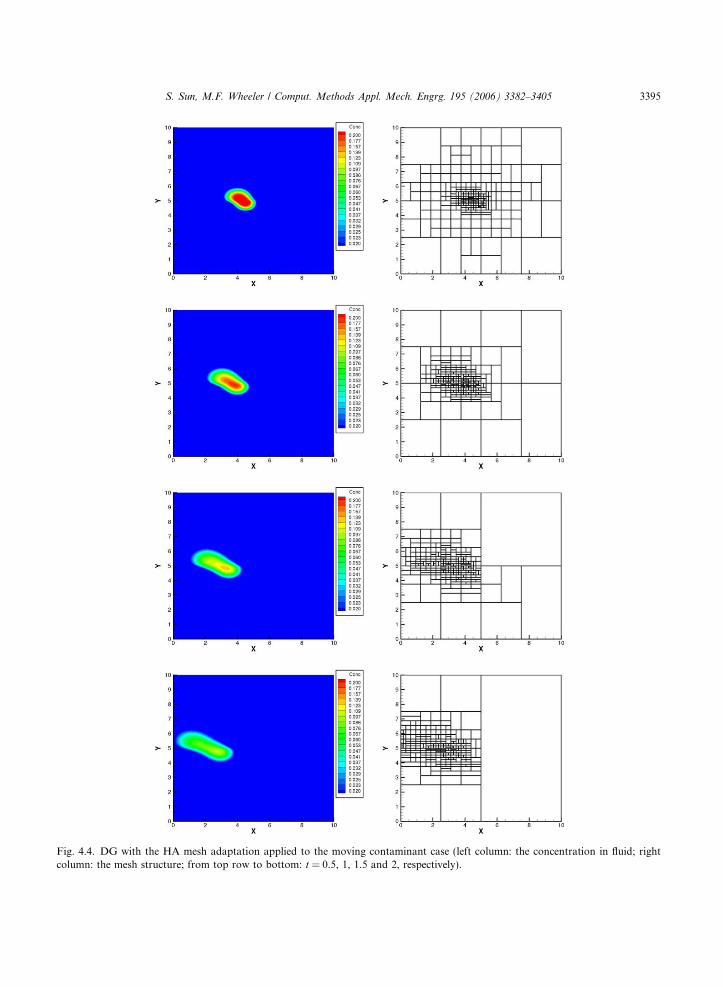
Fig. 4.4. DG with the HA mesh adaptation applied to the moving contaminant case (left column: the concentration in fluid; rightcolumn: the mesh structure; from top row to bottom: t = 0.5, 1, 1.5 and 2, respectively).


X

Y

0 0.25 0.5 0.75 10

0.1

0.2

0.3

0.4

0.5

0.6

0.7

0.8

0.9

1

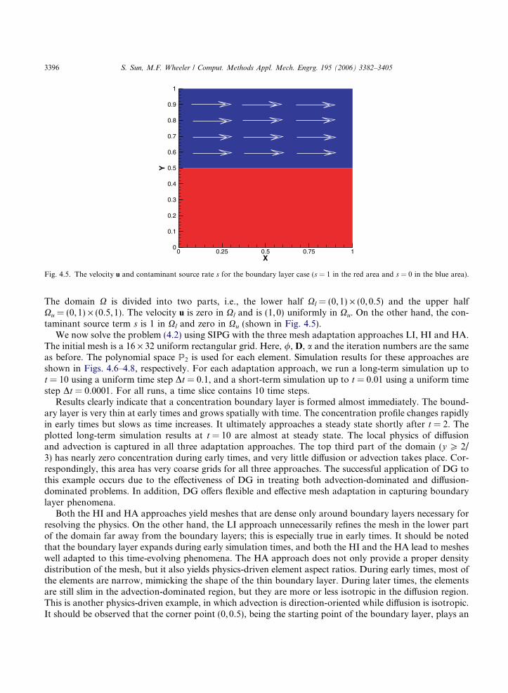
Fig. 4.5. The velocity u and contaminant source rate s for the boundary layer case (s = 1 in the red area and s = 0 in the blue area).


The domain X is divided into two parts, i.e., the lower half Xl = (0,1) · (0, 0.5) and the upper halfXu = (0,1) · (0.5,1). The velocity u is zero in Xl and is (1, 0) uniformly in Xu. On the other hand, the con-taminant source term s is 1 in Xl and zero in Xu (shown in Fig. 4.5).

We now solve the problem (4.2) using SIPG with the three mesh adaptation approaches LI, HI and HA.The initial mesh is a 16 · 32 uniform rectangular grid. Here, /, D, a and the iteration numbers are the sameas before. The polynomial space P2 is used for each element. Simulation results for these approaches areshown in Figs. 4.6–4.8, respectively. For each adaptation approach, we run a long-term simulation up tot = 10 using a uniform time step Dt = 0.1, and a short-term simulation up to t = 0.01 using a uniform timestep Dt = 0.0001. For all runs, a time slice contains 10 time steps.

Results clearly indicate that a concentration boundary layer is formed almost immediately. The bound-ary layer is very thin at early times and grows spatially with time. The concentration profile changes rapidlyin early times but slows as time increases. It ultimately approaches a steady state shortly after t = 2. Theplotted long-term simulation results at t = 10 are almost at steady state. The local physics of diffusionand advection is captured in all three adaptation approaches. The top third part of the domain (y P 2/3) has nearly zero concentration during early times, and very little diffusion or advection takes place. Cor-respondingly, this area has very coarse grids for all three approaches. The successful application of DG tothis example occurs due to the effectiveness of DG in treating both advection-dominated and diffusion-dominated problems. In addition, DG offers flexible and effective mesh adaptation in capturing boundarylayer phenomena.

Both the HI and HA approaches yield meshes that are dense only around boundary layers necessary forresolving the physics. On the other hand, the LI approach unnecessarily refines the mesh in the lower partof the domain far away from the boundary layers; this is especially true in early times. It should be notedthat the boundary layer expands during early simulation times, and both the HI and the HA lead to mesheswell adapted to this time-evolving phenomena. The HA approach does not only provide a proper densitydistribution of the mesh, but it also yields physics-driven element aspect ratios. During early times, most ofthe elements are narrow, mimicking the shape of the thin boundary layer. During later times, the elementsare still slim in the advection-dominated region, but they are more or less isotropic in the diffusion region.This is another physics-driven example, in which advection is direction-oriented while diffusion is isotropic.It should be observed that the corner point (0,0.5), being the starting point of the boundary layer, plays an

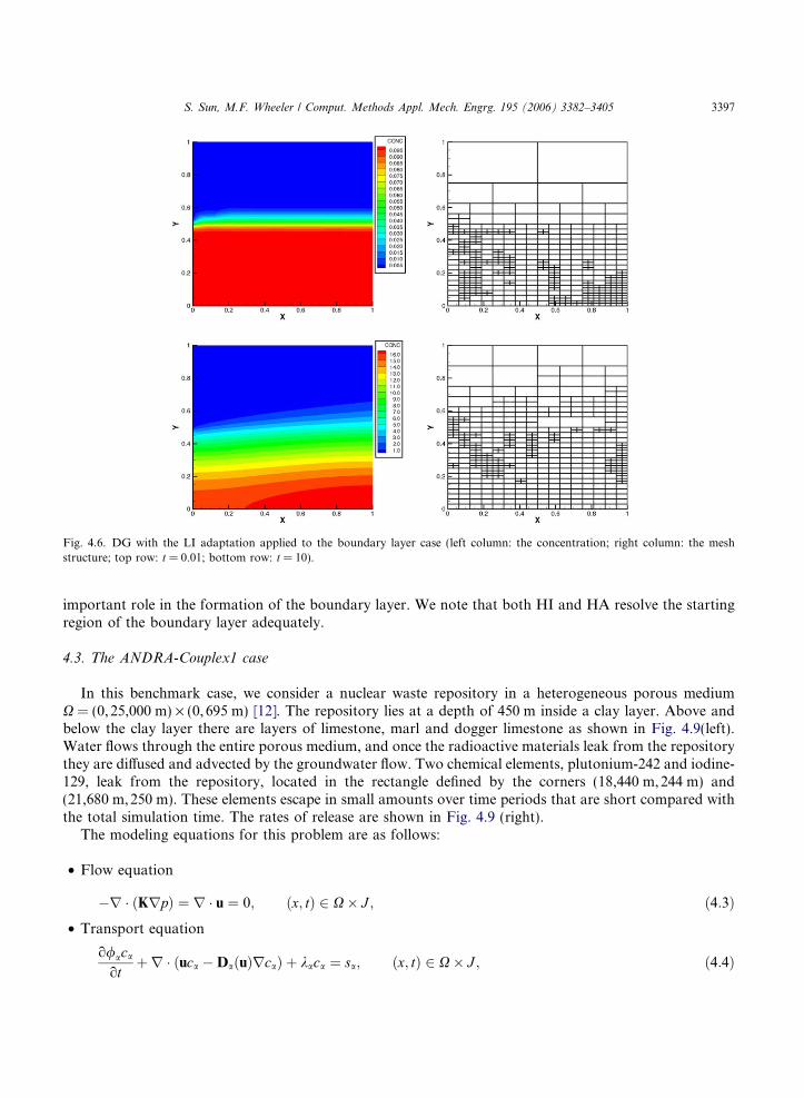
Fig. 4.6. DG with the LI adaptation applied to the boundary layer case (left column: the concentration; right column: the meshstructure; top row: t = 0.01; bottom row: t = 10).


important role in the formation of the boundary layer. We note that both HI and HA resolve the startingregion of the boundary layer adequately.

4.3. The ANDRA-Couplex1 case

In this benchmark case, we consider a nuclear waste repository in a heterogeneous porous mediumX = (0, 25,000 m) · (0, 695 m) [12]. The repository lies at a depth of 450 m inside a clay layer. Above andbelow the clay layer there are layers of limestone, marl and dogger limestone as shown in Fig. 4.9(left).Water flows through the entire porous medium, and once the radioactive materials leak from the repositorythey are diffused and advected by the groundwater flow. Two chemical elements, plutonium-242 and iodine-129, leak from the repository, located in the rectangle defined by the corners (18,440 m, 244 m) and(21,680 m, 250 m). These elements escape in small amounts over time periods that are short compared withthe total simulation time. The rates of release are shown in Fig. 4.9 (right).

The modeling equations for this problem are as follows:

• Flow equation

�r � Krpð Þ ¼ r � u ¼ 0; ðx; tÞ 2 X� J ; ð4:3Þ
• Transport equation
o/aca

otþr � uca �DaðuÞrcað Þ þ kaca ¼ sa; ðx; tÞ 2 X� J ; ð4:4Þ

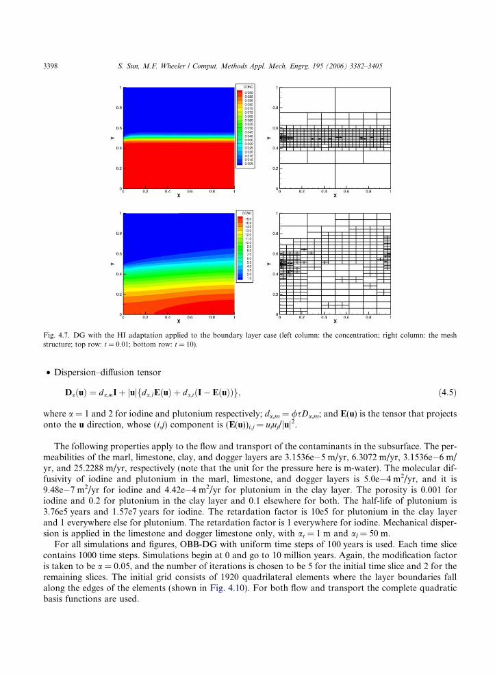
Fig. 4.7. DG with the HI adaptation applied to the boundary layer case (left column: the concentration; right column: the meshstructure; top row: t = 0.01; bottom row: t = 10).


• Dispersion–diffusion tensor

DaðuÞ ¼ da;mIþ uj j da;lEðuÞ þ da;t I� EðuÞð Þf g; ð4:5Þ

where a = 1 and 2 for iodine and plutonium respectively; da,m = /sDa,m; and E(u) is the tensor that projectsonto the u direction, whose (i,j) component is (E(u))i.j = uiuj/juj2.

The following properties apply to the flow and transport of the contaminants in the subsurface. The per-meabilities of the marl, limestone, clay, and dogger layers are 3.1536e�5 m/yr, 6.3072 m/yr, 3.1536e�6 m/yr, and 25.2288 m/yr, respectively (note that the unit for the pressure here is m-water). The molecular dif-fusivity of iodine and plutonium in the marl, limestone, and dogger layers is 5.0e�4 m2/yr, and it is9.48e�7 m2/yr for iodine and 4.42e�4 m2/yr for plutonium in the clay layer. The porosity is 0.001 foriodine and 0.2 for plutonium in the clay layer and 0.1 elsewhere for both. The half-life of plutonium is3.76e5 years and 1.57e7 years for iodine. The retardation factor is 10e5 for plutonium in the clay layerand 1 everywhere else for plutonium. The retardation factor is 1 everywhere for iodine. Mechanical disper-sion is applied in the limestone and dogger limestone only, with at = 1 m and al = 50 m.

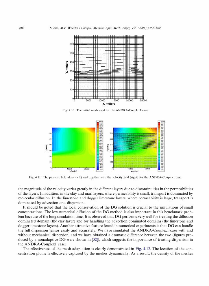
For all simulations and figures, OBB-DG with uniform time steps of 100 years is used. Each time slicecontains 1000 time steps. Simulations begin at 0 and go to 10 million years. Again, the modification factoris taken to be a = 0.05, and the number of iterations is chosen to be 5 for the initial time slice and 2 for theremaining slices. The initial grid consists of 1920 quadrilateral elements where the layer boundaries fallalong the edges of the elements (shown in Fig. 4.10). For both flow and transport the complete quadraticbasis functions are used.

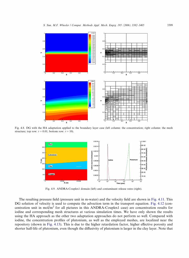
Fig. 4.8. DG with the HA adaptation applied to the boundary layer case (left column: the concentration; right column: the meshstructure; top row: t = 0.01; bottom row: t = 10).

Fig. 4.9. ANDRA-Couplex1 domain (left) and contaminant release rates (right).


The resulting pressure field (pressure unit in m-water) and the velocity field are shown in Fig. 4.11. ThisDG solution of velocity is used to compute the advection term in the transport equation. Fig. 4.12 (con-centration unit in mol/m2 for all pictures in this ANDRA-Couplex1 case) are concentration results foriodine and corresponding mesh structures at various simulation times. We have only shown the resultsusing the HA approach as the other two adaptation approaches do not perform so well. Compared withiodine, the concentration profiles of plutonium, as well as the employed meshes, are localized near therepository (shown in Fig. 4.13). This is due to the higher retardation factor, higher effective porosity andshorter half-life of plutonium, even though the diffusivity of plutonium is larger in the clay layer. Note that

x, meters

Y, m

eter

s

0 10000 15000 20000 250000

100

200

300

400

500

600

5000

Fig. 4.10. The initial mesh used for the ANDRA-Couplex1 case.

Fig. 4.11. The pressure field alone (left) and together with the velocity field (right) for the ANDRA-Couplex1 case.


the magnitude of the velocity varies greatly in the different layers due to discontinuities in the permeabilitiesof the layers. In addition, in the clay and marl layers, where permeability is small, transport is dominated bymolecular diffusion. In the limestone and dogger limestone layers, where permeability is large, transport isdominated by advection and dispersion.

It should be noted that the local conservation of the DG solution is crucial to the simulations of smallconcentrations. The low numerical diffusion of the DG method is also important in this benchmark prob-lem because of the long simulation time. It is observed that DG performs very well for treating the diffusiondominated domain (the clay layer) and for handling the advection dominated domains (the limestone anddogger limestone layers). Another attractive feature found in numerical experiments is that DG can handlethe full dispersion tensor easily and accurately. We have simulated the ANDRA-Couplex1 case with andwithout mechanical dispersion, and we have obtained a dramatic difference between the two (figures pro-duced by a nonadaptive DG were shown in [52]), which suggests the importance of treating dispersion inthe ANDRA-Couplex1 case.

The effectiveness of the mesh adaptation is clearly demonstrated in Fig. 4.12. The location of the con-centration plume is effectively captured by the meshes dynamically. As a result, the density of the meshes

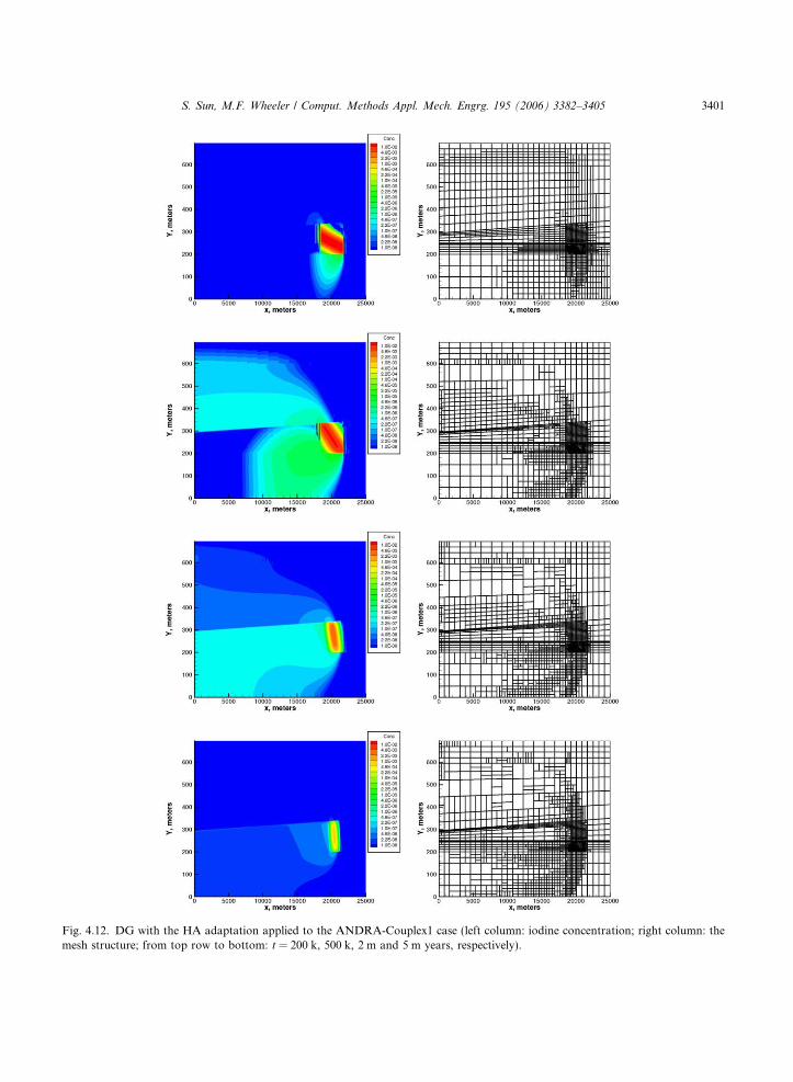
Fig. 4.12. DG with the HA adaptation applied to the ANDRA-Couplex1 case (left column: iodine concentration; right column: themesh structure; from top row to bottom: t = 200 k, 500 k, 2 m and 5 m years, respectively).


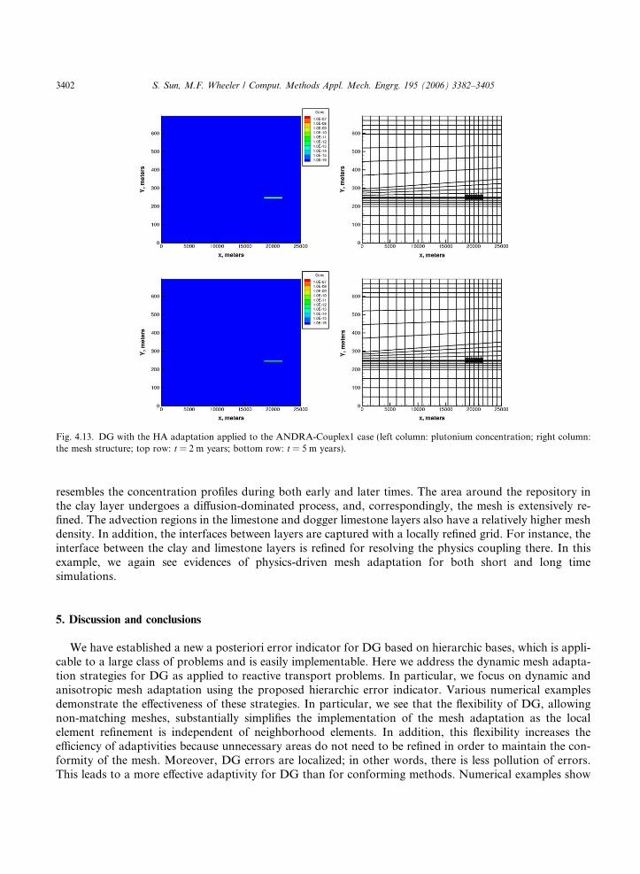
Fig. 4.13. DG with the HA adaptation applied to the ANDRA-Couplex1 case (left column: plutonium concentration; right column:the mesh structure; top row: t = 2 m years; bottom row: t = 5 m years).


resembles the concentration profiles during both early and later times. The area around the repository inthe clay layer undergoes a diffusion-dominated process, and, correspondingly, the mesh is extensively re-fined. The advection regions in the limestone and dogger limestone layers also have a relatively higher meshdensity. In addition, the interfaces between layers are captured with a locally refined grid. For instance, theinterface between the clay and limestone layers is refined for resolving the physics coupling there. In thisexample, we again see evidences of physics-driven mesh adaptation for both short and long timesimulations.

5. Discussion and conclusions

We have established a new a posteriori error indicator for DG based on hierarchic bases, which is appli-cable to a large class of problems and is easily implementable. Here we address the dynamic mesh adapta-tion strategies for DG as applied to reactive transport problems. In particular, we focus on dynamic andanisotropic mesh adaptation using the proposed hierarchic error indicator. Various numerical examplesdemonstrate the effectiveness of these strategies. In particular, we see that the flexibility of DG, allowingnon-matching meshes, substantially simplifies the implementation of the mesh adaptation as the localelement refinement is independent of neighborhood elements. In addition, this flexibility increases theefficiency of adaptivities because unnecessary areas do not need to be refined in order to maintain the con-formity of the mesh. Moreover, DG errors are localized; in other words, there is less pollution of errors.This leads to a more effective adaptivity for DG than for conforming methods. Numerical examples show


that local physical phenomena can be sharply captured by DG with dynamic mesh adaptations. The aniso-tropic mesh adaptation allows the flexible aspect ratios of individual elements to locally and dynamicallyaccommodate simulated phenomena, and this accommodation can lead to further computational savings.

We have numerically investigated three dynamic adaptation strategies, namely, HA, LI, and HI. Resultsindicate that all approaches resolve time-dependent transport processes for both long- and short-term sim-ulations and eliminate the need of slope limiters. The boundary layer case and the ANDRA-Couplex1 casedemonstrate that DG can treat both advection-dominated and diffusion-dominated problems, and theyshow that anisotropic mesh adaptations are flexible and effective in capturing boundary layer phenomena.Our numerical results further show that the number of iterations in each time slice may be as small as 1 or 2while obtaining an accurate mesh. We emphasize that, due to the discontinuous spaces employed in DG,the projections of concentration during mesh modifications only involve local computations and are locallymass conservative. These features ensure both the efficiency and the accuracy of DG during dynamic meshmodifications.

Comparisons of the three dynamic adaptation approaches clearly demonstrate the superior effectivenessof HA, which results in the most efficient physics-driven meshes and has the least numerical diffusion. TheHI approach performs similarly to the LI method for standard reactive transport problems, but it performsbetter for transport problems involving sharp boundary layers. However, the L2(L2) norm error indicatorcan be computed more efficiently than the hierarchic error indicator, which makes the choice between LIand HI problem-dependent.

The hierarchic error indicator has superior numerical performance to guide effective anisotropic and dy-namic mesh modification, but it is computationally expensive. Our future direction is to approximate thehierarchic error indicator by solutions of local problems on a fine grid. The goal of this approach is to re-duce the computational cost while maintaining its superior numerical performance, which is a topic we arecurrently pursuing.

References

[1] R.A. Adams, Sobolev Spaces, Academic Press, New York, 1975.[2] M. Ainsworth, J.T. Oden, A Posteriori Error Estimation in Finite Element Analysis, John Wiley and Sons, Inc., New York, 2000.[3] T. Arbogast, S. Bryant, C. Dawson, F. Saaf, C. Wang, M. Wheeler, Computational methods for multiphase flow and reactive

transport problems arising in subsurface contaminant remediation, J. Comput. Appl. Math. 74 (1–2) (1996) 19–32.[4] D.N. Arnold, An interior penalty finite element method with discontinuous elements, PhD thesis, The University of Chicage,

Chicago, IL (1979).[5] D.N. Arnold, An interior penalty finite element method with discontinuous elements, SIAM J. Numer. Anal. 19 (1982) 742–760.[6] I. Babuska, M. Zlamal, Nonconforming elements in the finite element method with penalty, SIAM J. Numer. Anal. 10 (1973) 863–

875.[7] G. Baker, Finite element methods for elliptic equations using nonconforming elements, Math. Comp. 31 (1977) 45–59.[8] R.E. Bank, R.K. Smith, A posteriori error-estimaters based on hierarchical bases, SIAM J. Numer. Anal. 30 (4) (1993) 921–935.[9] R.E. Bank, A. Weiser, Some a posteriori error estimators for elliptic partial differential equations, Math. Comp. 44 (1985) 283–

301.[10] C.E. Baumann, J.T. Oden, A discontinuous hp finite element method for convection–diffusion problems, Comput. Method. Appl.

Mech. Engrg. 175 (3–4) (1999) 311–341.[11] R.C. Borden, P.B. Bedient, Transport of dissolved hydrocarbons influenced by oxygen-limited biodegradation 1. Theoretical

development, Water Resour. Res. 22 (1986) 1973–1982.[12] A. Bourgeat, M. Kern, S. Schumacher, J. Talandier, The COUPLEX test cases: nuclear waste disposal simulation, Comput.

Geosci. 8 (2) (2004) 83–98.[13] C.Y. Chiang, C.N. Dawson, M.F. Wheeler, Modeling of in situ biorestoration of organic compounds in groundwater, Transport

Porous Med. 6 (1991) 667–702.[14] C. Dawson, S. Sun, M.F. Wheeler, Compatible algorithms for coupled flow and transport, Comput. Meth. Appl. Mech. Engrg.

193 (2004) 2565–2580.[15] L. Demkowicz, W. Rachowicz, Ph. Devloo, A fully automatic hp-adaptivity, J. Sci. Comput. 17 (1–3) (2002) 127–155.


[16] J. Douglas, T. Dupont, Interior penalty procedures for elliptic and parabolic Galerkin methods, Lect. Notes Phys. 58 (1976) 207–216.

[17] P. Engesgaard, K.L. Kipp, A geochemical transport model for redox-controlled movement of mineral fronts in groundwater flowsystems: a case of nitrate removal by oxidation of pyrite, Water Resour. Res. 28 (10) (1992) 2829–2843.

[18] A.K. Gupta, P.R. Bishnoi, N. Kalogerakis, A method for the simultaneous phase equilibria and stability calculations formultiphase reacting and non-reacting systmes, Fluid Phase Equilibr. 63 (8) (1991) 65–89.

[19] J.F. Kanney, C.T. Miller, C.T. Kelley, Convergence of iterative split-operator approaches for approximating nonlinear reactivetransport problems, Adv. Water Res. 26 (3) (2003) 247–261.

[20] J.S. Kindred, M.A. Celia, Contaminant transport and biodegradation 2. Conceptual model and test simulations, Water Resour.Res. 25 (1989) 1149–1159.

[21] F.M. Morel, J.G. Hering, Principles and Applications of Aquatic Chemistry, John Wiley and Sons, New York, 1993.[22] J.A. Nitsche, Uber ein Variationsprinzip zur Losung von Dirichlet-Problemen bei Verwendung von Teilraumen, die keinen

Randbedingungen unteworfen sind, Abh. Math. Sem. Univ. Hamburg 36 (1971) 9–15.[23] J.T. Oden, I. Babuska, C.E. Baumann, A discontinuous hp finite element method for diffusion problems, J. Comput. Phys. 146

(1998) 491–516.[24] J.T. Oden, L.C. Wellford Jr., Discontinuous finite element approximations for the analysis of shock waves in nonlinearly elastic

materials, J. Comput. Phys. 19 (2) (1975) 179–210.[25] H. Rachford, M.F. Wheeler, An h1-Galerkin procedure for the two-point boundary value problem, in: Carl deBoor (Ed.),

Mathematical Aspects of Finite Elements in Partial Differential Equations, Academic Press, Inc., 1974, pp. 353–382.[26] W. Rachowicz, D. Pardo, L. Demkowicz, Fully automatic hp-adaptivity in three dimensions, ICES report 04-22, University of

Texas at Austin, Austin, Texas (2004).[27] B. Riviere, Discontinuous Galerkin finite element methods for solving the miscible displacement problem in porous media. PhD

thesis, The University of Texas at Austin (2000).[28] B. Riviere, M.F. Wheeler, Non conforming methods for transport with nonlinear reaction, Contemp. Math. 295 (2002) 421–432.[29] B. Riviere, M.F. Wheeler, V. Girault, Part I: Improved energy estimates for interior penalty, constrained and discontinuous

Galerkin methods for elliptic problems, Comput. Geosci. 3 (1999) 337–360.[30] B. Riviere, M.F. Wheeler, V. Girault, A priori error estimates for finite element methods based on discontinuous approximation

spaces for elliptic problems, SIAM J. Numer. Anal. 39 (3) (2001) 902–931.[31] J. Rubin, Transport of reacting solutes in porous media: relation between mathematical nature of problem formulation and

chemical nature of reactions, Water Resour. Res. 19 (5) (1983) 1231–1252.[32] J. Rubin, R.V. James, Dispersion-affected transport of reacting solutes in saturated porous media: Galerkin method applied to

equilibrium-controlled exchange in unidirectional steady water flow, Water Resour. Res. 9 (5) (1973) 1332–1356.[33] F. Saaf, A study of reactive transport phenomena in porous media, PhD thesis, Rice University (1996).[34] J.V. Smith, R.W. Missen, W.R. Smith, General optimality criteria for multiphase multireaction chemical equilibrium, AIChE J. 39

(4) (1993) 707–710.[35] C.I. Steefel, P. Van Cappellen, Special issue: reactive transport modeling of natural systems, J. Hydrol. 209 (1–4) (1998) 1–388.[36] S. Sun, Discontinuous Galerkin methods for reactive transport in porous media, PhD thesis, The University of Texas at Austin

(2003).[37] S. Sun, B. Riviere, M.F. Wheeler, A combined mixed finite element and discontinuous Galerkin method for miscible displacement

problems in porous media, in: Recent Progress in Computational and Applied PDEs, Conference Proceedings for theInternational Conference, Zhangjiaje, July (2001), 321–348.

[38] S. Sun, M.F. Wheeler, Symmetric and non-symmetric discontinuous Galerkin methods for reactive transport in porous media,SIAM J. Numer. Anal. 43 (1) (2005) 195–219.

[39] S. Sun, M.F. Wheeler, A posteriori error estimation and dynamic adaptivity for symmetric discontinuous Galerkinapproximations of reactive transport problems, Comput. Meth. Appl. Mech. Engrg., in press, doi: 10.1016/j.cma.2005.02.021.

[40] S. Sun, M.F. Wheeler, Mesh adaptation strategies for discontinuous Galerkin methods applied to reactive transport problems, in:H.-W. Chu, M. Savoie, B. Sanchez, (Eds.), Proceedings of International Conference on Computing, Communications and ControlTechnologies (CCCT 2004), vol. I, (2004) pp. 223–228.

[41] S. Sun, M.F. Wheeler, Discontinuous Galerkin methods for coupled flow and reactive transport problems, Appl. Numer. Math.52 (2–3) (2005) 273–298.

[42] S. Sun, M.F. Wheeler, L2(H1) norm a posteriori error estimation for discontinuous Galerkin approximations of reactive transportproblems, J. Sci. Comput. 22 (2005) 501–530.

[43] S. Sun, M.F. Wheeler, A dynamic, adaptive, locally conservative and nonconforming solution strategy for transport phenomenain chemical engineering, in: Proceedings of American Institute of Chemical Engineers 2004 Annual Meeting, Austin, Texas,November 7–12 (2004).

[44] S. Sun, M.F. Wheeler, M. Obeyesekere, C.W. Patrick Jr., A deterministic model of growth factor-induced angiogenesis, Bull.Math. Biol. 67 (2) (2005) 313–337.


[45] S. Sun, M.F. Wheeler, M. Obeyesekere, C.W. Patrick Jr., Nonlinear behavior of capillary formation in a deterministicangiogenesis model, in: Proceedings of the Fourth World Congress of Nonlinear Analysts, Orlando, Florida, June 30–July 7(2004).

[46] A.J. Valocchi, M. Malmstead, Accuracy of operator splitting for advection–dispersion-reaction problems, Water Resour. Res.28 (5) (1992) 1471–1476.

[47] J. van der Lee, L. De Windt, Present state and future directions of modeling of geochemistry in hydrogeological systems,J. Contam. Hydrol. 47/2 (4) (2000) 265–282.

[48] M.Th. van Genuchten, Analytical soultions for chemical transport with simultaneous adsorption, zero-order production and first-order decay, J. Hydrol. 49 (1981) 213–233.

[49] M.F. Wheeler, An elliptic collocation-finite element method with interior penalties, SIAM J. Numer. Anal. 15 (1978) 152–161.[50] M.F. Wheeler, B.L. Darlow, Interior penalty Galerkin procedures for miscible displacement problems in porous media, in:

Computational Methods in Nonlinear Mechanics (Proc. Second Internat. Conf., Univ. Texas, Austin, Tex., 1979), North-Holland, Amsterdam, 1980, pp. 485–506.

[51] M.F. Wheeler, C.N. Dawson, P.B. Bedient, C.Y. Chiang, R.C. Bordern, H.S. Rifai, Numerical simulation of microbialbiodegradation of hydrocarbons in groundwater, in: Proceedings of AGWSE/IGWMCH Conference on Solving Ground WaterProblems with Models, National Water Wells Association, (1987) pp. 92–108.

[52] M.F. Wheeler, S. Sun, O. Eslinger, B. Riviere, Discontinuous Galerkin method for modeling flow and reactive transport in porousmedia, in: W. Wendland (Ed.), Analysis and Simulation of Multifield Problem, Springer Verlag, Berlin, 2003, pp. 37–58.

[53] G.T. Yeh, V.S. Tripathi, A critical evaluation of recent developments in hydrogeochemical transport models of reactivemultichemical components, Water Resour. Res. 25 (1) (1989) 93–108.

[54] G.T. Yeh, V.S. Tripathi, A model for simulating transport of reactive multispecies components: model development anddemonstration, Water Resour. Res. 27 (12) (1991) 3075–3094.

Documents

Anisotropic and dynamic mesh adaptation for discontinuous ... · Anisotropic and dynamic mesh adaptation for discontinuous Galerkin methods applied to reactive transport Shuyu Sun,