An Introduction and Survey of Estimation of Distribution Algorithms

Mark Hauschild and Martin Pelikan

MEDAL Report No. 2011004 (revision 1)

August 2011

Abstract

Estimation of distribution algorithms (EDAs) are stochastic optimization techniques that explore the space of

potential solutions by building and sampling explicit probabilistic models of promising candidate solutions. This

explicit use of probablistic models in optimization offers some significant advantages over other types of meta-

heuristics. This paper discusses these advantages and outlines many of the different types of EDAs. In addition,

some of the most powerful efficiency enhancement techniques applied to EDAs are discussed and some of the key

theoretical results relevant to EDAs are outlined.

Keywords

stochastic optimization, estimation of distribution algorithms, probabilistic models, model building, decomposable

problems, evolutionary computation, problem solving

Missouri Estimation of Distribution Algorithms Laboratory (MEDAL)

Department of Mathematics and Computer Science

University of Missouri–St. Louis

One University Blvd., St. Louis, MO 63121

E-mail: medal@cs.umsl.edu

WWW: http://medal.cs.umsl.edu/

An Introduction and Survey of Estimation of Distribution

Algorithms

Mark Hauschild

Missouri Estimation of Distribution Algorithms Laboratory (MEDAL)Dept. of Math and Computer Science, 320 CCB

University of Missouri at St. LouisOne University Blvd., St. Louis, MO 63121

mwh308@umsl.edu

Martin Pelikan

Missouri Estimation of Distribution Algorithms Laboratory (MEDAL)Dept. of Math and Computer Science, 320 CCB

University of Missouri at St. LouisOne University Blvd., St. Louis, MO 63121

pelikan@cs.umsl.edu

Abstract

Estimation of distribution algorithms (EDAs) are stochastic optimization techniques thatexplore the space of potential solutions by building and sampling explicit probabilistic modelsof promising candidate solutions. This explicit use of probablistic models in optimization offerssome significant advantages over other types of metaheuristics. This paper discusses theseadvantages and outlines many of the different types of EDAs. In addition, some of the mostpowerful efficiency enhancement techniques applied to EDAs are discussed and some of the keytheoretical results relevant to EDAs are outlined.

Keywords: stochastic optimization, estimation of distribution algorithms, probabilistic models,model building, decomposable problems, evolutionary computation, problem solving

1 Introduction

Estimation of distribution algorithmss (Baluja, 1994; Muhlenbein & Paaß, 1996a; Larranaga &Lozano, 2002; Pelikan, Goldberg, & Lobo, 2002) are stochastic optimization techniques that explorethe space of potential solutions by building and sampling explicit probabilistic models of promisingcandidate solutions. This model-based approach to optimization has allowed EDAs to solve manylarge and complex problems. EDAs were successfully applied to optimization of large spin glassinstances in two-dimensional and three-dimensional lattices (Pelikan & Hartmann, 2006), militaryantenna design (Yu, Santarelli, & Goldberg, 2006), multiobjective knapsack (Shah & Reed, 2010),groundwater remediation design (Arst, Minsker, & Goldberg, 2002; Hayes & Minsker, 2005), amino-acid alphabet reduction for protein structure prediction (Bacardit, Stout, Hirst, Sastry, Llora, &Krasnogor, 2007), identification of clusters of genes with similar expression profiles (Pena, Lozano,& Larranaga, 2004), economic dispatch (Chen & p. Chen, 2007), forest management (Ducheyne,De Baets, & De Wulf, 2004), portfolio management (Lipinski, 2007), cancer chemotherapy opti-mization (Petrovski, Shakya, & Mccall, 2006), environmental monitoring network design (Kollat,

1

Reed, & Kasprzyk, 2008), and others. It is important to stress that in most of these applica-tions no other technique was shown to be capable of achieving better performance than EDAs orsolving problems of comparable size and complexity. This paper will review the basic principleof EDAs, and point out some of the features of EDAs that distinguish these methods from othermetaheuristics and allow them to achieve these impressive results in such a broad array of problemdomains.

This survey aims to provide the reader with enough information to not only understand what anEDA is, but also to implement a basic EDA. Compared to the past surveys on this topic (Pelikan,Goldberg, & Lobo, 2002; Sastry, Pelikan, & Goldberg, 2006), this survey targets a broader audience,including readers who are not familiar with genetic algorithms or evolutionary computation. Inaddition, this survey covers many algorithms and methods that have not been covered in previouslypublished surveys on this topic (Pelikan, Goldberg, & Lobo, 2002; Sastry, Pelikan, & Goldberg,2006).

The paper is organized as follows. Section 2 describes the basic EDA procedure. Section 3 givesa broad overview of many example EDAs, divided into four broad categories. Section 4 discussessimilarities of EDAs and some of the most closely related stochastic optimization techniques. Sec-tion 5 reviews advantages and disadvantages of EDAs compared to other metaheuristics. Section 6discusses the most common efficiency enhancements that may be incorporated into EDAs to speedup their operation. Section 7 gives a broad overview of some of the most important theoreticalresults in the field of EDAs. Section 8 contains pointers to additional information on EDAs for theinterested reader, such as the important journals and conferences in the field, as well free softwareimplementations. Lastly, section 9 summarizes and concludes the paper.

2 Estimation of Distribution Algorithms

Suppose a researcher was presented with a large number of possible solutions to a problem andwished to generate new and (hopefully) better solutions. One way that he or she might approach thisproblem is to attempt to determine the probability distribution that would give higher probabilitiesto solutions in the regions with the best solutions available. Once this was completed, one couldsample this distribution to find new candidate solutions to the problem. Ideally, the repeatedrefinement of the probabilistic model based on representative samples of high quality solutionswould keep increasing the probability of generating the global optimum and, after a reasonablenumber of iterations, the procedure would locate the global optimum or its accurate approximation.In the rest of this section we discuss how EDAs do this automatically.

2.1 General EDA Procedure

Estimation of distribution algorithms (EDAs) (Baluja, 1994; Muhlenbein & Paaß, 1996a; Larranaga& Lozano, 2002; Pelikan, Goldberg, & Lobo, 2002) are stochastic optimization algorithms thatexplore the space of candidate solutions by sampling an explicit probabilistic model constructedfrom promising solutions found so far. EDAs typically work with a population of candidate solutionsto the problem, starting with the population generated according to the uniform distribution overall admissible solutions. The population is then scored using a fitness function. This fitness functiongives a numerical ranking for each string, with the higher the number the better the string. Fromthis ranked population, a subset of the most promising solutions are selected by the selectionoperator. An example selection operator is truncation selection with threshold τ = 50%, whichselects the 50% best solutions. The algorithm then constructs a probabilistic model which attempts

2

to estimate the probability distribution of the selected solutions. Once the model is constructed,new solutions are generated by sampling the distribution encoded by this model. These newsolutions are then incorporated back into the old population, possibly replacing it entirely. Theprocess is repeated until some termination criteria is met (usually when a solution of sufficientquality is reached or when the number of iterations reaches some threshold), with each iterationof this procedure usually referred to as one generation of the EDA. The basic EDA procedure isoutlined in Algorithm 1.

Algorithm 1 EDA pseudocodeg ← 0generate initial population P (0)while (not done) do

select population of promising solutions S(g) from P (g)build probabilistic model M(g) from S(g)sample M(g) to generate new candidate solutions O(g)incorporate O(g) into P (g)g ← g + 1

end while

The important step that differentiates EDAs from many other metaheuristics is the constructionof the model that attempts to capture the probability distribution of the promising solutions. Thisis not a trivial task as the goal is not to perfectly represent the population of promising solutions,but instead to represent a more general distribution that captures the features of the selectedsolutions that make these solutions better than other candidate solutions. In addition, we have toensure that the model can be built and sampled in an efficient manner.

2.2 Solving Onemax with a Simple EDA

Let us illustrate the basic EDA procedure with an example of a simple EDA solving the onemaxproblem. In onemax, candidate solutions are represented by vectors of n binary variables and thefitness is computed by

onemax(X1,X2, . . . ,Xn) =n∑

i=1

Xi , (1)

where n is the number of variables and Xi is the ith variable in the problem (ith position in theinput binary string). This function has one global optimum in the string of all 1s.

In this example our population size is set to N = 6, with n = 5 binary variables per solution.Truncation selection with threshold τ = 50% is used to select the subset of the most promisingsolutions (the 50% best solutions are selected). To estimate the probability distribution of thesepromising solutions, a probability vector is used that stores the probability of a 1 in each positionof the solution strings. The probability vector provides a fast and efficient model for solving theonemax problem and many other optimization problems, mainly due to the fact that it is basedon the assumption that all problem variables are independent. To learn a probability vector, theprobability pi of a 1 in each position i is set to the proportion of selected solutions containing a1 in this position. To generate a new binary string from the probability vector, for each positioni, a 1 is generated in this position with probability pi. For example, if p3 = 0.6, we generate a 1in the third position of a new candidate solution with the probability of 60%. In each generation

3

11011 (4)01010 (2)

10010 (2)

10111 (4)

01011 (3)

10000 (1)

11011 (4)

Figure 1: Two generations of a simple EDA using a probability vector to solve onemax.

(iteration of the algorithm), N = 6 candidate solutions are generated from the current model tocreate a new population of size N = 6. The simulation is outlined in Figure 1.

It is clear from the first generation that the procedure is having positive effects. The offspringpopulation already contains significantly more 1s than the original population and also includesseveral copies of the global optimum 11111. In addition, the probability of a 1 in any particular po-sition has increased; consequently, the probability of generating the global optimum has increased.The second generation leads to a probability vector that is even more strongly biased towards theglobal optimum and if the simulation was continued for one more generation, the probability vectorwould generate only the global optimum.

Even though the previous example was rather small, this procedure works on larger problems.To show this in practice, the probabilities of ones in each in different positions of solution stringsfrom an example run of an EDA on a bigger onemax problem are shown in Figure 2. In this casen = 50 and the population size is N = 100. We see that the proportions of 1s in different positionsincrease over time even in this experiment. While the probabilities of 1s in some positions dofluctuate in value in the initial iterations, eventually all the probability vector entries become 1.

Assuming that the population size is large enough to ensure reliable convergence (Harik, Cantu-Paz, Goldberg, & Miller, 1997; Goldberg, 2002), the EDA based on the probability vector modelprovides an efficient and reliable approach to solving onemax and many other optimization prob-lems. Nonetheless, is it always the case that the probability vector is sufficient for solving theproblem?

2.3 Linkage Learning EDAs: Using an EDA to Solve Trap-5

To illustrate some of the limitations of EDAs based on the probability vector, let us consider amore complex problem such as the concatenated trap of order 5 (trap-5) (Ackley, 1987; Deb &

4

0 10 20 30 40 500

0.1

0.2

0.3

0.4

0.5

0.6

0.7

0.8

0.9

1

Generation

Pro

babi

lity

vect

or e

ntrie

s

Figure 2: Proportions of 1s in a probability vector of a simple EDA on the onemax problem ofn = 50 using a population of N = 100 candidate solutions.

Goldberg, 1991). In trap-5, the input string is first partitioned into independent groups of 5 bitseach. The contribution of each group of 5 bits (trap partition) is computed as

trap5(u) =

{

5 if u = 54− u otherwise

, (2)

where u is the number of 1s in the input string of 5 bits. While the trap-5 function has only oneglobal optimum, the string of all 1s, it also has (2n/5 − 1) other local optima, namely those stringswhere all bits in at least one trap partition are 0 and all bits in each of the remaining partitions areeither 0 or 1. Trap-5 necessitates that all bits in each group be treated together, because statisticsof lower order are misleading (Thierens & Goldberg, 1993); that is why trap-5 provides an excellentexample to illustrate the limitations of the probability vector as a model.

The simple EDA shown in the previous simulation was run on trap-5. The first few generationsare shown in Figure 3. Almost immediately we see a problem: The fitness function ranks solutionswith many 0s higher than solutions with many 1s. By emphasizing solutions with many 0s, theprobability vector entries get lower over the two generations. In other words, in each generation,while our average population fitness is increasing, the strings are actually getting farther and fartheraway from the global optimum.

To see if the same behavior can be observed on a larger problem, an EDA with a probabilityvector was used to solve a trap-5 problem of 50 bits with a population of size N = 100. Figure 4ashows the proportions of 1s in each position of the solution strings. This example confirms thatthe proportions of 1s in different positions of solution strings decrease over time. Some entriesincrease for several iterations but the bias towards 0s at any individual position is too strong tobe overcome. Indeed, by generation 27 the entire population has converged to all 0s. One mayhypothesize that the situation would change if our population was larger but, unfortunately, largerpopulations would only make the continuous decrease in the proportion of 0s more stable.

To understand the reason for the failure of the EDA based on the probability vector on trap-5,let us return to the onemax example. For onemax, the average fitness of candidate solutions witha 1 in any position is better than the average fitness of solutions with a 0 in that position. Theselection is thus expected to give preference to 1s and the learning and sampling of the probabilityvector will ensure that these increased probabilities of 1s are reflected in the new populations of

5

11011 (0)00101 (2)

10010 (2)

10111 (0)

01011 (1)

01000 (3)

Figure 3: Two generations of a simple EDA using a probability vector to solve trap-5.

candidate solutions. However this situation is reversed for trap-5, for which the average fitness ofsolutions with a 0 in any position is greater than the average fitness of solutions with a 1 in thatposition (Deb & Goldberg, 1991), even though the optimum is still located in the string consistingof all 1s. This leads to the probability vector being strongly biased towards solutions with 0s in allpositions.

All is not lost, however. What if we can change the model to respect the linkages betweenthe bits in the same trap partition? If it was possible for the algorithm to learn the structure oftrap-5, it could then treat all the bits in the same trap partition as a single variable. That is, themodel would store the probability of each combination of 5 bits in any particular trap partition,and new solutions would be sampled by generating 5 bits at a time according to these probabilities.Since from the definition of trap-5 the average fitness of candidate solutions with all bits in a trappartition set to 1 is expected to be higher than the average fitness of solutions with one or more 0s inthat partition, we would expect the proportions of trap partitions with all 1s to increase over time.By merging the variables in each trap partition together, the extended compact genetic algorithm(ECGA) (Harik, 1999) explained further in section 3.1.3 does just that. Probabilistic models thatcombine groups of variables or bits into linkage groups and assume independence between thedifferent linkage groups are often referred to as marginal product models (Harik, 1999).

To show the difference that the marginal product model for trap-5 can make in practice, anEDA that uses this model was applied to solve a 50-bit trap-5 problem. Figure 4b shows theproportions of blocks of five 1s in different trap partitions in the population. These results showthat with an appropriate marginal product model the EDA performs similarly as it did on onemax,with the entire population converging to the global optimum in a little over 20 generations. Thisexample illustrates that, in terms of probability distributions, the main reason for the failure ofthe probability vector based EDA on trap-5 is the assumption that the problem variables areindependent.

6

0 10 20 30 40 500

0.1

0.2

0.3

0.4

0.5

0.6

0.7

0.8

0.9

1

Generation

Pro

babi

lity

vect

or e

ntrie

s

(a) EDA based on the probability vector

0 10 20 30 40 500

0.1

0.2

0.3

0.4

0.5

0.6

0.7

0.8

0.9

1

Generation

Pro

babi

litie

s of

111

11

(b) EDA based on a marginal product model withlinkage groups corresponding to trap partitions.

Figure 4: Statistics from two runs of an EDA on trap-5 of n = 50 bits using probabilistic modelsof different structure.

These examples make it clear that the class of allowable models and the methods for learningand sampling these models are key elements in EDA design. If the model built in each generationcaptures the important features of selected solutions and generates new solutions with these fea-tures, then the EDA should be able to quickly converge to the optimum (Muhlenbein & Mahnig,1999). However, as we will see later on, there is a tradeoff between the expressiveness of proba-bilistic models and the complexity of learning and sampling these models. Due to the importanceof the class of models used in an EDA, the type of probability models used in an EDA is often howone EDA is differentiated from another.

3 EDA Overview

Because of the key impact that the probabilistic models used have on EDA efficiency and appli-cability, EDAs are usually categorized by the types of distributions they are able to encode. Thissection covers four broad categories of EDAs. Note that this is not an exhaustive survey and onlya few representative algorithms are discussed for each category. For further information, please seemany of the individual papers for other examples.

In this section we assume the general structure of an EDA as outlined in Algorithm 1. Ratherthan go over all the details of every algorithm, instead we will point out what distinguishes aparticular algorithm from the others. Since in most cases the primary differences between EDAsare found in the class of probabilistic models used and the methods used for learning and samplingthese models, in the majority of this section we focus on these EDA components and omit lessimportant technical details.

Section 3.1 covers EDAs that can be used for problems using discrete variables. Section 3.2discusses EDAs for solving problems where candidate solutions are represented by permutations.Section 3.3 describes EDAs that address problems where candidate solutions are represented byreal-valued vectors. Section 3.4 covers EDAs for problems in genetic programming.

7

3.1 Discrete Variables

This section covers the first broad category of EDAs, those that work on fixed-length strings of afinite cardinality (usually binary). We start by describing EDAs that ignore all interactions betweenvariables and end with algorithms that are able to capture a broad variety of possible interactions.

3.1.1 Univariate Models

One of the simplest approaches is to assume that the problem variables are independent. Underthis assumption, the probability distribution of any individual variable should not depend on thevalues of any other variables. EDAs of this type are usually called univariate EDAs. Figure 5ashows an illustration of this type of model.

Mathematically, a univariate model decomposes the probability of a candidate solution(X1,X2, ...,Xn) into the product of probabilities of individual variables as

p(X1,X2, ...,Xn) = p(X1)p(X2), ..., p(Xn)

where p(Xi) is the probability of variable Xi, and p(X1,X2, ...,Xn) is the probability of the candi-date solution (X1,X2, ...,Xn). The univariate model for n variables thus consists of n probabilitytables and each of these tables defines probabilities of different values of the corresponding variable.Since the probabilities of different values of a variable must sum to 1, one of the probabilities maybe omitted for each variable. The probability vector discussed earlier in section 2.2 is an exampleunivariate model applicable to candidate solutions represented by fixed-length binary strings.

One example of a univariate EDA is the univariate marginal distribution algorithm (UMDA)(Muhlenbein & Paaß, 1996b), which is the algorithm we used to solve the onemax problem insection 2. UMDA works on binary strings and uses the probability vector p = (p1, p2, ..., pn) asthe probabilistic model, where pi denotes the probability of a 1 in position i of solution strings.To learn the probability vector, each pi is set to the proportion of 1s in the population of selectedsolutions. To create new solutions, each variable is generated independently based on the entriesin the probability vector. Specifically, a 1 is generated in position i with probability pi.

While most EDAs work by keeping a population of candidate solutions, incremental EDAsfully replace the population with the probabilistic model. The model is first set to give a uniformdistribution over the solution space. Each generation, several solutions are created and the mostfit solution or several most fit solutions are selected. The model is then slightly biased towardssolutions of this type. In this way the model is incrementally improved over time, without theexpense of storing large populations each generation.

One incremental univariate EDA is the population-based incremental learning (PBIL) (Baluja,1994) algorithm, which works on binary strings. Like UMDA, PBIL uses the probabilistic modelin the form of a probability vector. The initial probability vector encodes the uniform distributionover all binary strings by setting the probability of a 1 in each position to 0.5. In each generationof PBIL, the probability vector is sampled to generate a a small set of solutions using the samesampling procedure as in UMDA. The best solutions in this set are selected and for each variablein each selected solution, the corresponding entry in the probability vector is shifted by:

pi = (pi ∗ (1.0 − LR)) + (LR ∗ vi)

where pi is the probability of generating a 1 in bit position i, vi is the ith position in the solutionstring and LR is the learning rate specified by the user. To prevent premature convergence, eachprobability vector entry is also slightly varied each generation based on a mutation rate parameter.

8

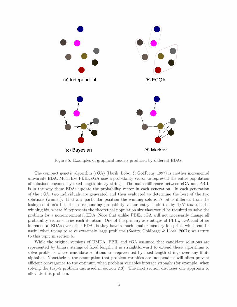
Figure 5: Examples of graphical models produced by different EDAs.

The compact genetic algorithm (cGA) (Harik, Lobo, & Goldberg, 1997) is another incrementalunivariate EDA. Much like PBIL, cGA uses a probability vector to represent the entire populationof solutions encoded by fixed-length binary strings. The main difference between cGA and PBILis in the way these EDAs update the probability vector in each generation. In each generationof the cGA, two individuals are generated and then evaluated to determine the best of the twosolutions (winner). If at any particular position the winning solution’s bit is different from thelosing solution’s bit, the corresponding probability vector entry is shifted by 1/N towards thewinning bit, where N represents the theoretical population size that would be required to solve theproblem for a non-incremental EDA. Note that unlike PBIL, cGA will not necessarily change allprobability vector entries each iteration. One of the primary advantages of PBIL, cGA and otherincremental EDAs over other EDAs is they have a much smaller memory footprint, which can beuseful when trying to solve extremely large problems (Sastry, Goldberg, & Llora, 2007); we returnto this topic in section 5.

While the original versions of UMDA, PBIL and cGA assumed that candidate solutions arerepresented by binary strings of fixed length, it is straightforward to extend these algorithms tosolve problems where candidate solutions are represented by fixed-length strings over any finitealphabet. Nonetheless, the assumption that problem variables are independent will often preventefficient convergence to the optimum when problem variables interact strongly (for example, whensolving the trap-5 problem discussed in section 2.3). The next section discusses one approach toalleviate this problem.

9

3.1.2 Tree-based models

The algorithms in the previous section assumed independence between problem variables. However,often the variables in a problem are related in some way. This section discusses EDAs capable ofcapturing some pair-wise interactions between variables by using tree-based models. In tree-basedmodels, the conditional probability of a variable may only depend on at most one other variable,its parent in a tree structure.

The mutual-information-maximizing input clustering (MIMIC) (De Bonet, Isbell, & Viola, 1997)uses a chain distribution to model interactions between variables. MIMIC works by using thepopulation of promising solutions to calculate the mutual information between all pairs of variables.Then, starting with the variable with the minimum conditional entropy, a chain dependency is addedto the variable with the maximum mutual information with the variable that was added last. Thisprocess is repeated until all the variables are selected. The resulting tree model consists of a singlechain of dependencies, with each parent having exactly one child. Once the structure of the modelhas been completed, the conditional probability of each variable based on its parent is calculatedfrom the promising solutions. Given a permutation of the n variables in a problem, π = i1, i2 . . . in,MIMIC decomposes the probability distribution of p(X1,X2, . . . ,Xn) as:

pπ(X) = p(Xi1 |Xi2)p(Xi2 |Xi3) . . . p(Xin−1|Xin)p(Xin)

where p(Xij |Xij+1) denotes the conditional probability of Xij given Xij+1

. New candidate solutionsare then generated by sampling the probability distribution encoded by the model. The samplingproceeds by generating the variables in the reverse order with respect to the permutation π, startingwith Xin and ending with Xi1 .

Baluja and Davies (1997) use dependency trees to model promising solutions, improving theexpressiveness of the probabilistic models compared to the chain models of MIMIC. In dependencytrees, each parent can have multiple children. This incremental EDA works by using a probabilitymatrix that contains all pairwise probabilities. The model is the tree that maximizes the mutualinformation between connected variables, which is the provably best tree model in terms of theKullback-Leibler divergence with respect to the true distribution (Chow & Liu, 1968). The prob-ability matrix is initialized so that it corresponds to the uniform distribution over all candidatesolutions. In each iteration of the algorithm, a tree model is built and sampled to generate severalnew candidate solutions. The best of these solutions are then used to update the probability matrix.

The bivariate marginal distribution algorithm (BMDA) (Pelikan & Muhlenbein, 1999) uses amodel based on a set of mutually independent trees (a forest). Each generation a dependencymodel is created by using Pearson’s chi-square statistics (Marascuilo & McSweeney, 1977) as themain measure of dependence. The model built is then sampled to generate new solutions based onthe conditional probabilities learned from the population.

3.1.3 Multivariate Interactions

While the tree-based models in section 3.1.2 provide EDAs with the ability to identify and exploitinteractions between problem variables, using tree models is often not enough to solve problemswith multivariate or highly-overlapping interactions between variables (Bosman & Thierens, 1999;Pelikan & Muhlenbein, 1999). This section describes several EDAs that are based on probabilisticmodels capable of capturing multivariate interactions between problem variables.

The extended compact genetic algorithm (ECGA) (Harik, 1999) uses a model that dividesthe variables into independent clusters and each of these clusters is treated as a single variable.The model building starts by assuming that all the problem variables are independent. In each

10

iteration of the model building, two clusters are merged together that improve the quality of themodel the most. The quality of a model is measured by the minimum description length (MDL)metric (Mitchell, 1997). The model building terminates when no merging of two clusters improvesthe MDL score of the model. Once the learning of the structure of the model is complete, aprobability table is computed for each cluster based on the population of selected solutions andthe new solutions are generated by sampling each linkage group based on these probabilities. Themodel building procedure is repeated in each generation of ECGA, so the model created in eachgeneration of ECGA may contain different clusters of variables. An example of an ECGA model isshown in Figure 5b.

Many problems contain highly overlapping subproblems that cannot be accurately modeled bydividing the problem into independent clusters. The Bayesian optimization algorithm (BOA) (Pe-likan, Goldberg, & Cantu-Paz, 2000) uses Bayesian networks to model candidate solutions, whichallow it to solve the large class of nearly decomposable problems, many of which cannot be decom-posed into independent subproblems of bounded order. A Bayesian network is an acyclic directedgraph with one node per variable, where an edge between nodes represents a conditional depen-dency. A Bayesian network with n nodes encodes a joint probability distribution of n randomvariables X1,X2, . . . ,Xn:

p(X1,X2, . . . ,Xn) =n∏

i=1

p(Xi|Πi), (3)

where Πi is the set of variables from which there exists an edge into Xi (members of Πi are calledparents of Xi), and p(Xi|Πi) is the conditional probability of Xi given Πi. Figure 5c shows anexample Bayesian network. The difference between Bayesian networks and tree models is that inBayesian networks, each variable may depend on more than one variable. The main differencebetween the marginal product models of ECGA and Bayesian networks is that Bayesian networksare capable of capturing more complex problem decompositions in which subproblems interact.

The model building in BOA starts with a network with no edges. A greedy algorithm is thenused to add edges to the network, adding the edge that gives the most improvement accordingto the Bayesian-Dirichlet (BD) metric (Heckerman, Geiger, & Chickering, 1995). Since the BDmetric has a tendency to favor overly complex models, usually an upper bound on the numberof allowable parents is set or a prior bias on the network structure is introduced to prefer sim-pler models (Heckerman, Geiger, & Chickering, 1994). New candidate solutions are generatedby sampling the probability distribution encoded by the built network using probabilistic logicsampling (Henrion, 1988).

The estimation of Bayesian network algorithm (EBNA) (Etxeberria & Larranaga, 1999) and thelearning factorized distribution algorithm (LFDA) (Muhlenbein & Mahnig, 1999) also use Bayesiannetworks to model the promising solutions. EBNA and LFDA use the Bayesian information cri-terion (BIC) (Schwarz, 1978a) to evaluate Bayesian network structures in the greedy networkconstruction algorithm. One advantage of the BIC metric over the BD metric is that it contains astrong implicit bias towards simple models and it thus does not require a limit on the number ofallowable parents or any prior bias towards simpler models. However, the BD metric allows a moreprincipled way to incorporate prior information into problem solving, as discussed in section 6.6.

Many complex problems in the real world are hierarchical in nature (Simon, 1968). A hierar-chical problem is a problem composed of subproblems, with each subproblem being a hierarchicalproblem itself until the bottom level is reached (Simon, 1968). On each level, the interactions withineach subproblem are often of much higher magnitude than the interactions between the subprob-lems. Due to the rich interaction between subproblems and the lack of feedback for discriminatingalternative solutions to the different subproblems, these problems cannot simply be decomposed

11

into tractable problems on a single level. Therefore, solving these hierarchical problems presentsnew challenges for EDAs. First, on each level of problem solving, the hierarchical problem solvermust be capable of decomposing the problem. Secondly, the problem solver must be capable ofrepresenting solutions from lower levels in a compact way so these solutions can be treated as asingle variable when trying to solve the next level. Lastly, since the solution at any given level maydepend on interactions at a higher level, it is necessary that alternate solutions to each subproblembe stored over time.

The hierarchical Bayesian Optimization Algorithm (hBOA) (Pelikan, 2005) is able to solvemany difficult hierarchically decomposable problems by extending BOA in two key areas. In orderto ensure that interactions of high order can be represented in a feasible manner, a more com-pact version of Bayesian networks is used. Specifically, hBOA uses Bayesian networks with localstructures (Chickering, Heckerman, & Meek, 1997; Friedman & Goldszmidt, 1999) to allow fea-sible learning and sampling of more complex networks than would be possible with conventionalBayesian networks. In addition, the preservation of alternative solutions over time is ensured byusing a niching technique called restricted tournament replacement (RTR) (Harik, 1995) whichencourages competition among similar solutions rather than dissimilar ones. Combined togetherthese changes allow hBOA to solve a broad class of nearly decomposable and hierarchical problemsin a robust and scalable manner (Pelikan & Goldberg, 2006).

Another type of model that can encode multivariate interactions is Markov networks. Thestructure of Markov networks is similar to Bayesian networks except that the connections betweenvariables are undirected. For a given decomposable function, a Markov network that ensuresconvergence to the global optimum may sometimes be considerably less complex than an adequateBayesian network, at least with respect to the number of edges (Muhlenbein, 2008). Nonetheless,sampling Markov networks is more difficult than sampling Bayesian networks. In other words, someof the difficulty moves from learning to sampling the probabilistic model compared to EDAs basedon Bayesian networks. Shakya and Santana (2008) uses Gibbs sampling to generate new solutionsfrom its model in the Markovianity based optimisation algorithm (MOA). MOA was shown to havecomparable performance to some Bayesian network based EDAs on deceptive test problems. Anexample of a Markov network model is shown in Figure 5d.

The affinity propagation EDA (AffEDA) designed by Santana, Larranaga, and Lozano (2010)starts by first generating a mutual information matrix between all variables. An affinity propagationalgorithm is then used to obtain a partitioning of the variables into independent clusters. Affinitypropagation is a clustering algorithm that, given a set of points and a measure of their similarity,finds clusters of similar points and for each cluster gives a representative example. Unlike manyclustering algorithms, affinity propagation does not require specifying the total number of clustersbeforehand. Once this model of independent clusters is generated by affinity propagation, it canbe sampled similarly to ECGA. The resulting algorithm was shown to be much faster than ECGAon simplified protein folding problems and on deceptive non-binary problems (Santana, Larranaga,& Lozano, 2010).

Using a more expressive class of probabilistic models allows EDAs to solve broader classes ofproblems. From this perspective, one should prefer tree models to univariate ones, and multivariatemodels to tree models. At the same time, using a more expressive class of models almost alwaysimplies that the model building and model sampling will be more computationally expensive.Nonetheless, since it is often not clear how complex a problem is before solving it and using eventhe most complex models described above creates only a low-order polynomial overhead even onproblems that can be solved with simpler models, it is often preferable to use the more generalclass of models rather than the more restricted one.

12

The algorithms in this section are able to cover a broad variety of possible interactions betweendiscrete variables in a problem. However, none of these algorithms is directly applicable to problemswhere candidate solutions are represented by permutations, which are discussed in the next section.

3.2 Permutation EDAs

In many important real-world problems, candidate solutions are represented by permutations overa given set of elements. Two important classes of such problems are the quadratic assignmentproblem (Koopmans & Beckmann, 1957) and the traveling salesman problem. These types ofproblems often contain two specific types of features or constraints that EDAs need to capture. Thefirst is the absolute position of a symbol in a string and the second is the relative ordering of specificsymbols. In some problems, such as the traveling-salesman problem, relative ordering constraintsmatter the most. In others, such as the quadratic assignment problem, both the relative orderingand the absolute positions matter. It certainly is possible to use non-permutation based EDAsusing specific encodings to solve permutation problems. For example, one may use the randomkey encoding (Bean, 1994) to solve permutation-based problems using EDAs for optimization ofreal-valued vectors (Bosman & Thierens, 2001b; Robles, de Miguel, & Larranaga, 2002). Randomkey encoding represents a permutation as a vector of real numbers. The permutation is definedby the reordering of the values in the vector that sorts the values in ascending order. The mainadvantage of using random keys is that any real-valued vector defines a valid permutation andany EDA capable of solving problems defined on vectors of real numbers can thus be used to solvepermutation problems. However, since EDAs do not process the aforementioned types of regularitiesin permutation problems directly their performance can often be poor (Bosman & Thierens, 2001b).The following EDAs attempt to encode both of these types of features or contraints for permutationproblems explicitly.

To solve problems where candidate solutions are permutations of a string, Bengoetxea, Larranaga,Bloch, Perchant, and Boeres (2000) starts with a Bayesian network model built using the sameapproach as in EBNA. However, the sampling method is changed to ensure that only valid per-mutations are generated. This approach was shown to have promise in solving the inexact graphmatching problem. In much the same way, the dependency-tree EDA (dtEDA) of Pelikan, Tsut-sui, and Kalapala (2007) starts with a dependency-tree model and modifies the sampling to ensurethat only valid permutations are generated. dtEDA for permutation problems was used to solvestructured quadratic assignment problems with great success (Pelikan, Tsutsui, & Kalapala, 2007).Both Bayesian networks as well as tree models are capable of encoding both the absolute positionand the relative ordering constraints.

Bosman and Thierens (2001c) extended the real-valued EDA to the permutation domain bystoring the dependencies between different positions in a permutation in the induced chromosomeelements exchanger (ICE). ICE works by first using a real-valued EDA as discussed in section 3.3,which encodes permutations as real-valued vectors using the random keys encoding. ICE extendsthe real-valued EDA by using a specialized crossover operator. By applying the crossover directlyto permutations instead of simply sampling the model, relative ordering is taken into account. Theresulting algorithm was shown to outperform many real-valued EDAs that use the random keyencoding alone (Bosman & Thierens, 2001c).

The edge histogram based sampling algorithm (EHBSA) (Tsutsui, 2002) works by creating anedge histogram matrix (EHM). For each pair of symbols, EHM stores the probabilities that oneof these symbols will follow the other one in a permutation. To generate new solutions, EHBSAstarts with a randomly chosen symbol. The EHM is then sampled repeatedly to generate new

13

symbols in the solution, normalizing the probabilities based on what values have already beengenerated. The EHM by itself does not take into account absolute positional importance at all. Inorder to address problems in which absolute positions are important, a variation of EHBSA thatinvolved templates was proposed (Tsutsui, 2002). To generate new solutions, first a random stringfrom the population was picked as a template. New solutions were then generated by removingrandom parts of the template string and generating the missing parts with sampling from the EHM.The resulting algorithm was shown to be better than most other EDAs on the traveling salesmanproblem. In another study, the node histogram sampling algorithm (NHBSA) of Tsutsui, Pelikan,and Goldberg (2006) considers a model capable of storing node frequencies at each position andagain uses a template.

3.3 Real-Valued Vectors

EDAs discussed thus far were applicable to problems with candidate solutions represented byfixed-length strings over a finite alphabet. However, candidate solutions for many problems arerepresented using real-valued vectors. In these problems the variables cover an infinite domain so itis no longer possible to enumerate variables’ values and their probabilities. This section discussesEDAs that can solve problems in the real-valued domain. There are two primary approaches toapplying EDAs to the real-valued domain: (1) Map the real-valued variables into the discretedomain and use a discrete EDA on the resulting problem, and (2) use EDAs based on probabilisticmodels defined on real-valued variables.

3.3.1 Discretization

The most straightforward way to apply EDAs in the real-valued domain is to discretize the problemand use a discrete EDA on the resulting problem. In this way it is possible to directly use the discreteEDAs in the real-valued domain. However, a naive discretization can be impractical as some valuesclose to each other in the continuous domain may become more distant in the discrete domain.In addition, the possible range of values must be known before the optimization starts. Finally,some regions of the search space are more densely covered with high quality solutions whereasothers contain mostly solutions of low quality; this suggests that some regions require a moredense discretization than others. To deal with these difficulties, various approaches to adaptivediscretization were developed using EDAs (Tsutsui, Pelikan, & Goldberg, 2001; Pelikan, Goldberg,& Tsutsui, 2003; Chen, Liu, & Chen, 2006; Suganthan, Hansen, Liang, Deb, Chen, Auger, &Tiwari, 2005; Chen & Chen, 2010). We discuss some of these next.

Tsutsui, Pelikan, and Goldberg (2001) proposed to divide the search space of each variable intosubintervals using a histogram. Two different types of histogram models were used: fixed height andfixed width. The fixed-height histogram ensured that each discrete value would correspond to thesame number of candidate solutions in the population; this allows for a more balanced discretizationwhere the areas that contain more high quality solutions also get more discrete values. The fixed-width histogram ensured that each discrete value corresponded to the interval of the same size.The results showed strong performance on the two-peaks and Rastrigin functions, which are oftendifficult without effective crossover operators.

Three different methods of discretization were tried (fixed-height histograms, fixed-width his-tograms and k-Means clustering) and combined with BOA to solve real-valued problems by Pelikan,Goldberg, and Tsutsui (2003). Adaptive mutation was also used after mapping the discrete valuesto the continuous domain. The resulting algorithm was shown to be successful on the two-peaksand deceptive functions.

14

0 2 4 6 80

0.2

0.4

0.6

0.8

1

x

f(x)

Variable 1 Variable 2 Variable 3

Figure 6: Example model generated by SHCLVND

Another way to deal with discretization was proposed by Chen and Chen (2010). Their methoduses the ECGA model and a split-on-demand (SoD) discretization to adjust on the fly how the real-valued variables are coded as discrete values. Loosely said, if an interval of discretization contains alarge number of candidate solutions and these variables are biased towards one side of the interval,then that region is split into two to increase exploration. The resulting real-coded ECGA (rECGA)worked well on a set of benchmark test problems (Suganthan, Hansen, Liang, Deb, Chen, Auger, &Tiwari, 2005) designed to test real-valued optimization techniques. In addition, rECGA was ableto obtain better solutions than the previously best known solutions obtained by other algorithmson a 40-unit economic dispatch problem.

While the above EDAs solved problems with candidate solutions represented by real-valuedvectors, they manipulated these through discretization and variation operators based on a discreterepresentation. In the next section we cover EDAs that work directly with the real-valued variablesthemselves.

3.3.2 Direct Representation

The stochastic hill-climbing with learning by vectors of normal distributions (SHCLVND) (Rudlof& Koppen, 1996) works directly with a population of real-valued vectors. The model is representedas a vector of normal distributions, one for each variable. While the mean of each variable’sdistribution can be different, all the distributions share the same standard deviation. Over timethe means are shifted towards the best candidate solutions generated and the deviation is slowlyreduced by a multiplicative factor. Figure 6 shows an example of this type of a model.

One disadvantage of SHCLVND is that it assumes that each variable has the same standarddeviation. Also, since it uses only a single normal distribution for each variable, it is only ableto accurately capture distributions of samples that are all centered around a single point in thesearch space. In addition, SHCLVND assumes that all the variables are independent. The followingalgorithms all attempt to alleviate one or more of these problems.

Sebag and Ducoulombier (1998) extended the idea of using a single vector of normal distributions

15

by storing a different standard deviation for each variable. In this way it is able to perform betterin scenarios where certain variables have higher variance than others. As in SHCLVND, however,all variables are assumed to be independent.

The estimation of Gaussian networks algorithm (EGNA) (Larranaga, Etxeberria, Lozano, &Pena, 1999) works by creating a Gaussian network to model the interactions between variablesin the selected population of solutions in each generation. This network is similar to a Bayesiannetwork except that the variables are real-valued and locally each variable has its mean and variancecomputed by a linear function from its parents. The network structure is learned greedily using acontinuous version of the BDe metric (Geiger & Heckerman, 1994), with a penalty term to prefersimpler models.

In the IDEA framework, Bosman and Thierens (2000) proposed models capable of capturingmultiple basins of attraction or clusters of points by storing the joint normal and kernel distri-butions. IDEA was able to outperform SHCLVND and other EDAs that used a single vectorof Gaussian distributions on a set of six function optimization problems commonly used to testreal-valued optimization techniques.

Gallagher, Frean, and Downs (1999) extended PBIL to real-valued spaces by using an AdaptiveGaussian mixture model (Priebe, 1994). The Adaptive Gaussian mixture model used a mixture ofGaussian distributions that are gradually modified to improve the model as each new solution issampled. One of the strengths of this method is that the complexity of the model can change overtime, with additional components added if the current model does not correspond closely enoughto the data (Gallagher, 2000).

The mixed iterated density estimation evolutionary algorithm (mIDEA) (Bosman & Thierens,2001a) also used mixtures of normal distributions. The model building in mIDEA starts by clus-tering the variables and fitting a probability distribution over each cluster. The final distributionused is then a weighted sum over the individual distributions. To evaluate dependencies betweenvariables, the Bayesian information criterion (BIC) (Schwarz, 1978b) metric is used.

In EDAs described so far, the variables were treated either as all real-valued or as all discretequantities. The mixed Bayesian optimization algorithm (mBOA) (Ocenasek, Kern, Hansen, &Koumoutsakos, 2004) can deal with both types of variables. Much as in hBOA, the probabilitydistribution of each variable is represented as a decision tree. The internal nodes of each treeencode tests on variables that the corresponding variable depends on. For discrete variables, thebranch taken during sampling is determined by whether or not the variable in the node is equalto a constant. For continuous variables, the branch taken is determined by whether the variablecorresponding to that node is less than a constant. The leaves determine the values of the sampledvariables. For discrete variables, the leaves contain the conditional probabilities of particular valuesof these variables. On the other hand, normal kernel distributions are used for continuous variables.

The real-coded Bayesian optimization algorithm (rBOA) (Ahn, Ramakrishna, & Goldberg,2004) tries to bring the power of BOA to the real-valued domain. rBOA uses a Bayesian networkto describe the underlying structure of the problem and a mixture of Gaussians to describe thelocal distributions. The resulting algorithm was shown to outperform mIDEA on several real-valueddeceptive problems.

Recently a new approach to developing EDAs to solve real-valued optimization problem hasbeen developed that is based on copula theory (Nelsen, 1998). Copulas are a way to describethe dependence between random variables, and according to copula theory a joint probabilitydistribution can be decomposed into n marginal probability distributions and a copula function.Copula-based EDAs (Salinas-Gutierrez, Hernandez-Aguirre, & Villa-Diharce, 2009; Wang, Zeng, &Hong, 2009a; Wang, Zeng, & Hong, 2009b) use this to their advantage, as the marginal distributions

16

*

+ Exp

X 10 X

p(Exp)=0.25

p(x)=0.05

p(*)=0.20

p(+)=0.30

p(1..10)=0.20

PIPE ECGP

Figure 7: Example of two different models used in EDA-GP.

and the dependencies between variables can be studied separately. These EDAs start by calculatingthe marginal distribution of each variable separately. The algorithms then pick a particular copulato construct the joint distribution. Given the marginal distributions and a copula, it is then possibleto generate new candidate solutions.

3.4 EDA-GP

After numerous successes in the design of EDAs for discrete and real-valued representations, a num-ber of researchers have attempted to replicate these successes in the domain of genetic programming(GP) (Koza, 1992). In GP the task is to evolve a population of computer programs representedby labeled trees. In this domain, some additional challenges become evident. To start with, thelength of candidate programs is expected to vary. Also, small changes in parent-child relationshipscan lead to large changes in the performance of the program, and often the relationship betweenoperators is more important than their actual physical position in candidate programs. However,despite these additional challenges, even in this environment, EDAs have been successful. In theremainder of this section, we outline a few attempts to design EDAs for GP.

The probabilistic incremental program evolution (PIPE) (Salustowicz & Schmidhuber, 1997)uses a probabilistic prototype tree (PPT) to store the probability distribution of all functions andoperators at each node of program trees. Initially the probability of all the functions and operatorsis set to represent the uniform distribution and used to generate the initial population. In eachgeneration the values of the PPT are updated from the population of promising solutions. Togenerate new solutions, the distribution at each node is sampled to generate a new candidateprogram tree. Subtrees that are not valid due to invalid combination of operators or functionsat the lowest level in the tree are pruned. Figure 7 shows an example PPT for PIPE. WhilePIPE does force positional dependence by using specific probabilities at each node, it does nottake into account interactions between nodes. Nonetheless, due to the simplicity of the modelused, the learning and sampling procedure of PIPE remains relatively fast compared to many otherapproaches to EDA-based GP.

17

An extension of PIPE is the extended compact genetic programming (ECGP) (Sastry & Gold-berg, 2000). Motivated by ECGA, ECGP splits nodes in the program trees into independentclusters. The algorithm starts by assuming that all nodes are independent. Then it proceeds bymerging nodes into larger clusters based on the MDL metric similar to that used in ECGA. Theindividual clusters are treated as a single variable and the tree is used to generate new candidatesolutions. Figure 7 shows an example model generated by ECGP.

Due to the chaotic nature of program spaces, finding an accurate problem decomposition canbe difficult over the entire search space of candidate programs. The meta-optimizing semantic evo-lutionary search (MOSES) (Looks, 2006) deals with this problem by first dynamically splitting upthe search space into separate program subspaces called demes that are maintained simultaneously.hBOA is then applied to each individual deme to generate new programs within that deme, whichcan also lead to new demes being created.

Several EDAs were developed for GP using probabilistic models based on grammar rules. Onesuch EDA is the stochastic grammar-based GP (SG-GP) (Ratle & Sebag, 2006), which starts byusing a fixed context-free grammar and attaching default probabilities to each rule. Based on thepromising solutions sampled during each generation, the probabilities of rules that perform wellare gradually increased. While in the base algorithm, no positional information is stored, it is alsopossible to extend the algorithm to keep track of the level where each rule is used.

Further extending the idea of representing the probability distribution over candidate programsusing probabilistic grammars, the program evolution with explicit learning (PEEL) (Shan, Mckay,Abbass, & Essam, 2003) attaches a depth and location parameter to each production rule. It startswith a small grammar and expands it by transforming a general rule that works at all locationsinto a specific grammar rule that only works at a specific depth and location. A metric based onant colony optimization is used to ensure that rules are not excessively refined.

All the aforementioned algorithms based on grammatical evolution used a fixed context-freegrammar. Grammar model-based program evolution (GMPE) (Shan, Mckay, & Baxter, 2004) goesbeyond context-free grammars by allowing the algorithm itself to generate completely new grammarrules. GMPE starts by generating a random initial population of program trees. Then a minimalgrammar is generated that is only able to generate the initial set of promising solutions. Oncethis is done, using the work based on theoretical natural language analysis, operators are used tocreate new rules and merge old rules together. The minimum message length (MML) (Wallace &Boulton, 1968) metric is used to compare grammars. This algorithm is very adaptable, being ableto generate a broad variety of possible grammars. However, comparing competing grammars iscomputationally expensive.

3.5 Multi-Objective EDAs

Most EDAs discussed so far were designed to solve problems with one objective. However, manyreal-world problems contain competing objectives. For example, when optimizing a car engine,one may want to maximize power and, at the same time, minimize environmental impact and fuelconsumption. One way to solve multi-objective problems is to transform the multiple objectivesinto a single objective by weighing the objectives in some way. However, it is often more desirableto find an optimal tradeoff between the objectives in the form of a diverse set of Pareto optimalsolutions (Deb, 2001; Coello & Lamont, 2004). In short, a solution is Pareto optimal if it outper-forms any other solution in at least one objective. In this section, we review several EDAs thataim to find diverse sets of Pareto optimal solutions for multi-objective optimization problems.

For these types of problems, it is no longer possible to find one solution that maximizes all the

18

goals simultaneously. Instead, the ultimate goal is to find a broad distribution of Pareto-optimalsolutions.

The Bayesian multi-objective optimization algorithm (BMOA) (Laumanns & Ocenasek, 2002)uses a special selection operator, ǫ-archive (Laumanns, Thiele, Deb, & Zitzler, 2002), to both ensurethat Pareto-optimal solutions are maintained over time and that diversity is maintained so that anapproximation of the entire Pareto set is preserved. The selection operator works by maintaininga minimal set of solutions that ǫ-dominates all other solutions generated so far, with ǫ being aproblem specific parameter that stands for the relative tolerance allowed for different objectivevalues. Results showed that the resulting algorithm was able to find a good model of the Pareto setfor smaller instances of the 0/1 multi-objective knapsack problem. Essentially, BMOA combinesthe mixed BOA (Ocenasek, Kern, Hansen, & Koumoutsakos, 2004) and the improved strengthPareto evolutionary algorithm (SPEA2) (Zitzler, Laumanns, & Thiele, 2002).

The naive mixture-based multi-objective iterated density-estimation evolutionary algorithm(MIDEA) (Bosman & Thierens, 2006) extended the IDEA framework to multi-objective optimiza-tion. A special selection operator was used to ensure preservation of diversity along the Pareto front,guided by a single parameter δ. The population is then clustered using the leader algorithm (Har-tigan, 1975), with the leader algorithm selected due its speed and the lack of any requirement tospecify the number of clusters beforehand. A univariate model is built for each cluster and sampledto generate new candidate solutions.

The multi-objective Bayesian optimization algorithm (mBOA) (Khan, Goldberg, & Pelikan,2002) uses the selection operator from the non-dominated sorting algorithm-II (NSGA-II) (Deb,Pratap, Agarwal, & Meyarivan, 2002) to maintain a diverse set of solutions along the Pareto-optimalfront. This selection operator gives each solution in the population a rank and a crowding distance.The rank provides pressure to maximize all objectives whereas the crowding distance providespressure to maintain diversity and broad coverage of the Pareto front. Solutions compete in binarytournaments. If the ranks of the two competing solutions differ, the winner of a tournament is thesolution with a better rank; if the ranks are equal, the crowding distance is used to determine thewinner. A Bayesian network model is then built for the selected solutions and the resulting networkis sampled to generate new candidate solutions for the next generation. The multi-objective BOAoutperformed the NSGA-II on several interleaved deceptive problems.

The multi-objective hierarchical BOA (mohBOA) (Pelikan, Sastry, & Goldberg, 2005) extendedhBOA to the multi-objective domain by combining hBOA, NSGA-II (Deb, Pratap, Agarwal, &Meyarivan, 2002) and clustering. mohBOA uses the non-dominated crowding of NSGA-II to rankcandidate solutions and assign crowding distances. This information is then used to select promis-ing solutions using the same procedure as in NSGA-II and mBOA. After selecting the promisingcandidate solutions, k-means clustering is used to obtain a clustering of the promising solutions.hBOA creates a separate Bayesian network model for each cluster and each created Bayesian net-work is used to generate the same number of new candidate solutions. New candidate solutions areincorporated into the old population using RTR to form the next generation’s population. The re-sults showed that mohBOA was able to solve the onemax-zeromax and trap5-invtrap5 in low-orderpolynomial time. Similar modifications were also tested in combination with marginal productmodels of ECGA in ref. (Pelikan, Sastry, & Goldberg, 2006).

Shah and Reed (2011) compared three different multi-objective evolutionary algorithms whensolving the multi-objective d-dimensional knapsack problem. Their results showed that the ǫ-hBOA (Kollat, Reed, & Kasprzyk, 2008) was able to outperform both the strength pareto evo-lutionary algorithm (SPEA2) (Zitzler, Laumanns, & Thiele, 2002) and the ǫ-NSGA-II (Kollat &Reed, 2005). The ǫ-hBOA uses the selection operator in NSGA-II to select promising candidate

19

solutions each generation. hBOA is then used to generate a Bayesian network model and sampledto generate new candidate solutions. ǫ-nondominated archiving (Laumanns, Thiele, Deb, & Zitzler,2002) is then used to form a new population from the candidate solutions, with this archive used asthe population for subsequent generations. Essentially, ǫ-hBOA combines the operators of hBOA,NSGA-II and SPEA2

4 Related Algorithms

All stochastic optimization algorithms guide their search for the optimum using probabilistic mod-els. In most optimization algorithms, the models are defined implicitly by the current state of thesearch and the set of operators. On the other hand, in EDAs, explicit probabilistic models suchas probability vectors and Bayesian networks are built from samples of high quality solutions andthese models are then sampled to generate new candidate solutions. Nonetheless, EDAs and mostother stochastic optimization techniques share many similarities, and this section will review someoptimization methods that are most closely related to EDAs.

Evolutionary algorithms use operators of selection and variation to update a population of can-didate solutions or a single candidate solution. For example, in genetic algorithms (Holland, 1973),binary tournament selection may be used to select promising solutions from the current populationand the new population may be created by applying one-point crossover and bit-flip mutation tothe selected parents. Selection and variation operators together with the current population ofcandidate solutions define the probability distribution over the populations of candidate solutions,and the new population of candidate solutions can be seen as a sample from that distribution.The main difference between most evolutionary algorithms and EDAs is that in EDAs the prob-ability distribution used to generate new candidate solutions is defined explicitly whereas in mostevolutionary algorithms the distribution is defined implicitly.

In some evolutionary algorithms, the distribution used to generate new candidate solutions is infact defined explicitly, just like in EDAs. For example, in evolution strategies (Rechenberg, 1973),new candidate solutions are often generated from a single normal distribution centered aroundthe best-so-far candidate solution or from a mixture of normal distributions centered around apopulation of high-quality solutions found so far. Similarly, many ant colony optimization (ACO)methods (Dorigo, 1992) and particle swarm optimization methods (PSO) (Kennedy & Eberhart,1995) use models that explicitly define a probability distribution over candidate solutions. Fromthis perspective, many evolutionary algorithms may be viewed as ”true” EDAs.

Developed independently of EDAs, the cross-entropy method (CE) (Rubinstein, 1996) is prob-ably the most closely related approach to EDAs and sees search much in the same way as EDAs.Similarly to EDAs, CE generates a random data set and then creates a model based on this randomdata set. Each iteration CE updates the model to increase model quality and ensure that it willgenerate better candidate solutions over time. Ideally, after a reasonable number of iterations, themodel should generate the global optimum with high probability

5 Advantages and Disadvantages of Using EDAs

Viewing optimization as the process of updating a probabilistic model over candidate solutionsprovides EDAs with several important features that distinguish these algorithms from evolution-ary algorithms and other, more conventional metaheuristics. This section reviews some of theseimportant features. Section 5.1 covers some of the important advantages EDAs have over other

20

metaheuristics. Section 5.2 then discusses some of the disadvantages that EDAs have when com-pared to other metaheuristics.

5.1 Advantages of EDAs

Adaptive operators. One of the biggest advantages of EDAs over most other metaheuristics istheir ability to adapt their operators to the structure of the problem. Most metaheuristics usefixed operators to explore the space of potential solutions. While problem-specific operatorsmay be developed and are often used in practice, EDAs are able to do the tuning of theoperator to the problem on their own. This important difference allows EDAs to solve someproblems for which other algorithms scale poorly (Pelikan & Hartmann, 2006; Shah & Reed,2010; Goldberg, 2002; Zhang, Sun, & Tsang, 2005; Zhang, Zhou, & Jin, 2008). However,adaptation in EDAs is usually limited by the initial choice of the probabilistic model. Asa consequence, adaptive EDAs (Santana, Larranaga, & Lozano, 2008; Lobo & Lima, 2010)have been proposed that dynamically change the type of model used while solving a problem.

Problem structure. Besides just providing the solution to the problem, EDAs also provide op-timization practitioners with a roadmap of how the EDA solved the problem. This roadmapconsists of the models that are calculated in each generation of the EDA, which representsamples of solutions of increasing quality. Mining these probabilistic models for informationabout the problem can reveal many problem-specific features, which can in turn be used toidentify promising regions of the search space, dependency relationships between problemvariables, or other important properties of the problem landscape. While gaining a betterunderstanding of the problem domain is useful in its own right, the obtained informationcan be used to design problem-specific optimization techniques or speed up solution of newproblem instances of similar type (Hauschild & Pelikan, 2009; Hauschild, Pelikan, Sastry, &Goldberg, 2008; Baluja, 2006; Schwarz & Ocenasek, 2000).

Prior knowledge exploitation. Practical solutions of enormously complex optimization prob-lems often necessitates that the practitioners bias the optimization algorithm in some waybased on prior knowledge. This is possible even with standard evolutionary algorithms, forexample by injecting specific solutions into the population of candidate solutions or by biasingthe populations using a local search. However, many approaches to biasing the search forthe optimum tend to be ad-hoc and problem specific. EDAs provide the framework for moreprincipled techniques to incorporate prior knowledge. For example, Bayesian statistics canbe used to bias model building in EDAs towards instances that appear to more likely leadto the global optimum or towards probabilistic models that more closely correspond to thestructure of the problem being solved. This can be done in a statistically meaningful way aswill be demonstrated in section 6.6.

Reduced memory requirements. Incremental EDAs reduce memory requirements by replacingthe population of candidate solutions by a probabilistic model. This allows practitioners tosolve extremely large problems that cannot be solved with other techniques. For example,Sastry, Goldberg, and Llora (2007) shows that solving a 225 (over 33 million) bit onemaxproblem with a simple genetic algorithm takes about 700 gigabytes but the cGA described in3.1.1 requires only a little over 128 megabytes.

21

5.2 Disadvantages of EDAs

Building explicit probabilistic models is often more time consuming than using implicit modelsdefined with simple search operators, such as tournament selection and two-point crossover. Thatis why it may sometimes be advantageous to use implicit models of conventional evolutionaryalgorithms instead of explicit ones of EDAs. However, doing this is only practical when searchoperators are available that allow scalable solutions of the target problem class; otherwise, the timecomplexity of learning a model is a small price to pay. Furthermore, the discovery of such operatorsmay not be straightforward and it also comes at a cost.

It is important to note that sometimes it is difficult to learn an adequate probabilistic modeland in some cases it is possible to create problems that render some model building algorithmsineffective. For example, many EDAs (such as BOA and ECGA) use a greedy algorithm to buildprobabilistic models and it has been shown that there exist problems for which the greedy algorithmoften leads to an inadequate model. Specifically, Coffin and Smith (2007) proposed the concate-nated parity function (CPF) for which pairwise correlations between variables cannot be easilydetected using only marginal statistics. One can envision several ways to alleviate this problem,such as limited probing (Heckendorn & Wright, 2004) and linkage identification by non-motonicitydetection (Munetomo & Goldberg, 1999). However, it is questionable whether the ability to solvesuch a special class of problems will outweigh the disadvantages of giving up the use of Bayesianstatistics in learning the probabilistic models. Furthermore, it was shown (Chen & Yu, 2009) thatthe difficulties of EDAs when solving CPF are mainly due to spurious linkages; therefore, usingmethods to reduce spurious linkages may provide yet another solution to this problem.

6 Efficiency Enhancement Techniques for EDAs

While EDAs provide scalable solutions to many problems that are intractable with other techniques,solving enormously complex problems often necessitates that additional efficiency enhancement(EE) (Goldberg, 2002; Sastry, Pelikan, & Goldberg, 2006; Pelikan, 2005) techniques are used.There are two main computational bottlenecks that must be addressed by efficiency enhancementtechniques for EDAs: (1) fitness evaluation and (2) model building.

Efficiency enhancements for EDAs can be roughly divided into the following categories (Pelikan,2005):

1. Parallelization.

2. Evaluation relaxation.

3. Hybridization.

4. Time continuation.

5. Sporadic and incremental model building.

6. Incorporating problem-specific knowledge and learning from experience.

In the remainder of this section we will briefly review each of these approaches, with an emphasison efficiency enhancement techniques that are specific to EDAs.

22

6.1 Parallelization

To enhance efficiency of any optimization technique, one may often parallelize the computationin some way. The most common approach to parallelization in EDAs and other metaheuristics isto parallelize fitness evaluation (Cantu-Paz, 2000). However, in the case of EDAs it is often alsoadvantageous to parallelize model building. One of the most impressive results in parallelizationof EDAs is the efficient parallel implementation of the compact genetic algorithm, which wassuccessfully applied to a noisy optimization problem with over one billion decision variables (Sastry,Goldberg, & Llora, 2007). Several approaches to parallelizing model building in advanced EDAswith multivariate models have also been proposed (Ocenasek, 2002; Ocenasek, Cantu-Paz, Pelikan,& Schwarz, 2006; Mendiburu, Lozano, & Miguel-Alonso, 2005).

6.2 Evaluation Relaxation

As previously discussed, one method to help alleviate the fitness bottleneck is parallelization.Nonetheless, to further improve performance of algorithms with expensive fitness evaluation, itis sometimes possible to eliminate some of the fitness evaluations by using approximate models ofthe fitness function, which can be evaluated much faster than the actual fitness function. Efficiencyenhancement techniques based on this principle are called evaluation relaxation techniques (Gold-berg, 2002; Smith, Dike, & Stegmann, 1995; Sastry, Goldberg, & Pelikan, 2001a; Pelikan & Sastry,2004; Sastry, Pelikan, & Goldberg, 2004).

There are two basic approaches to evaluation relaxation: (1) endogenous models (Smith, Dike,& Stegmann, 1995; Sastry, Goldberg, & Pelikan, 2001a; Pelikan & Sastry, 2004; Sastry, Pelikan, &Goldberg, 2004) and (2) exogenous models (Sastry, 2001b; Albert, 2001). With endogenous models,the fitness values for some of the new candidate solutions are estimated based on the fitness valuesof the previously generated and evaluated solutions. With exogenous models, a faster but lessaccurate surrogate model is used for some of the evaluations, especially for those early in the run.Of course, the two approaches can be combined to maximize the benefits.

Sastry, Goldberg, and Pelikan (2001b) incorporated endogenous models in the UMDA algorithmdiscussed in section 3.1.1. To estimate fitness, the probability vector was extended to also storestatistics on the average fitness of all solutions with a 0 or a 1 in any string position. These data werethen used to estimate fitness of new solutions. However, EDAs provide interesting opportunitiesfor building extremely accurate yet computationally efficient fitness surrogate models that go waybeyond the simple approach based on UMDA, because they provide the practitioners with detailedinformation about the structure of the problem. The endogenous-model approach when used withECGA (Sastry, Pelikan, & Goldberg, 2004) and BOA (Pelikan & Sastry, 2004) can accuratelyapproximate even complex fitness functions due to the additional information about the problemstructure encoded in the EDA model, yielding speedups of several orders of magnitude even foronly moderately sized problems (Pelikan & Sastry, 2004). This type of information is not availableat all to other types of metaheuristics.

6.3 Hybridization

In many real-world applications, EDAs are combined with other optimization algorithms. Typically,simple and fast local search techniques—which can quickly locate the closest local optimum—areincorporated into an EDA, reducing the problem of finding the global optimum to that of findingonly the basin of attraction of the global optimum. As an example, consider the simple deterministichill climber (DHC), which takes a candidate solution represented by a binary string and keeps

23

performing single-bit flips on the solution that lead to the greatest improvement in fitness (Hart,1994).

While even incorporating simple local search techniques can lead to significant improvementsin time complexity of EDAs, sometimes more advanced optimization techniques are available thatare tailored to the problem being solved. As an example, consider cluster exact approximation(CEA) (Hartmann, 1996), which can be incorporated into hBOA (Pelikan & Hartmann, 2006)when solving the problem of finding ground states of Ising spin-glass instances arranged on finite-dimensional lattices. Unlike DHC, CEA can flip many bits at once, often yielding solutions closeto the global optimum after only a few iterations.

Incorporating local search is relatively straightforward in most metaheuristics. However, theuse of probabilistic models of EDAs in optimization opens the door to the design of more advancedand powerful model-directed hybrids. Specifically, by exploiting the problem structure encoded bythe probabilistic model, it is possible to design specialized local search techniques which can signif-icantly outperform more conventional approaches to local search by using neighborhood operatorsthat more closely correspond to the structure of the problem. For example, if two variables arestrongly correlated and the value of one of them is modified, then it would make sense to con-sider modifying the value of the other variable as well. This idea was the motivation behind thebuilding-block mutation operator used by Sastry and Goldberg (2004a) to speed up problem solv-ing in ECGA. This operator worked by taking the best individual from the population and tryingdifferent combinations of bits in one of the independent linkage groups discovered by the modelbuilding phase, while leaving all the other linkage groups fixed; this was then repeated for eachlinkage group. This type of structural local search is simply not available to other metaheuristics.

Local search was also used to speed up the performance of BOA and hBOA by using informationfrom Bayesian networks by Lima, Pelikan, Sastry, Butz, Goldberg, and Lobo (2006). In this work,substructural neighborhoods were defined as a variable and all its parents in the Bayesian networkmodel discovered by BOA. Hillclimbing in the substructural space was then used on a proportionof the population. However, this technique did not take into account the context of possibleoverlapping interactions. Lima, Pelikan, Sastry, Butz, Goldberg, and Lobo (2006) also discussedother possible neighborhood structures that could be extracted from Bayesian networks. In a similarapproach, Handa (2007) started with bit mutation in EBNA, but then resampled any variables thatdepended on mutated bits depending on the conditional probability of the new parent variable’svalue.

To perform advanced local search based on Bayesian networks, Mendiburu, Santana, Lozano,and Bengoetxea (2007) proposed the use of loopy belief propagation (Pearl, 1988) to generatethe most likely instance from the Bayesian network learned in each iteration of EBNA. A similarapproach has later been studied by (Lima, Pelikan, Lobo, & Goldberg, 2009), who also usedloopy belief propagation but instead of conditional probabilities, the loopy belief propagation wasdriven by fitness statistics incorporated into the model in hBOA. Related approaches have alsobeen studied in the context of other probabilistic models (Ochoa, Hons, Soto, & Muhlenbein,2003; Hons, 2006; Santana, 2006; Muhlenbein & Hons, 2006; Hons, Santana, Larranaga, & Lozano,2007).

6.4 Time continuation

In time continuation, the goal is to maximize performance of evolutionary algorithms by exploitingthe trade-off between making more runs with a small population size and making fewer runs (oreven only a single run) with a larger population size (Goldberg, 1999; Srivastava & Goldberg,

24

2001; Goldberg, 2002). For example, sometimes it is possible to solve a problem in one singlegeneration with a large enough population size, but it may also be possible to solve this problemin many generations with a smaller population. Which is the most effective method is not alwaysreadily apparent: The goal in time continuation is to pick the method most efficient for a particularproblem, either to maximize solution quality given a fixed computational budget or to minimizetime to achieve a solution of a given quality.

Problem information encoded in probabilistic models of EDAs creates opportunities for usingthis information to design more efficient optimization techniques by exploiting the time continuationtradeoffs. For example, Sastry and Goldberg (2004b) showed that for ECGA on separable problemsof bounded difficulty, if the population was large enough for an accurate model of the underlyingproblem structure, an ECGA hybrid was able to solve these problems in a single generation byusing a local searcher with the neighborhood structure based on the ECGA model. However, forproblems with substantial amounts of noise, running the ECGA hybrid for a number of generationswas preferable.

6.5 Sporadic and incremental model building

Model building in ECGA, hBOA and other similar EDAs usually consists of two parts: (1) learningthe structure and (2) learning the parameters of the identified structure. Typically, learning themodel structure is much more complex than learning the parameters (Ocenasek & Schwarz, 2000;Pelikan, 2005). However, since the model structure is expected to not change much betweenconsequent iterations, one way to speed up model building is to use sporadic model building, inwhich the structure is updated only once in a while (Pelikan, Sastry, & Goldberg, 2008b).

Since the model structure is expected to not change much over time and making incrementalchanges to model structure is usually much simpler than building the structure from scratch, it mayalso be advantageous to change the model structure only incrementally without rebuilding the modelfrom scratch in every iteration. This is the basic idea of incremental model building (Etxeberria &Larranaga, 1999).

6.6 Incorporating problem-specific knowledge and learning from experience

EDAs typically do not require any information about the problem being solved except for therepresentation of candidate solutions and the fitness function. Nonetheless, if problem-specificinformation is available, it may be possible to use this information to improve performance ofthese algorithms significantly. There are two basic approaches to speed up EDAs by incorporatingproblem-specific knowledge: (1) bias the procedure for generating the initial population (Schwarz &Ocenasek, 2000; Sastry, 2001a; Pelikan & Goldberg, 2003) and (2) bias or restrict the model buildingprocedure (Schwarz & Ocenasek, 2000; Muhlenbein & Mahnig, 2002; Baluja, 2006). For boththese approaches, we may either (1) hard code the modifications based on prior problem-specificknowledge (Hauschild, Pelikan, Sastry, & Goldberg, 2008; Baluja, 2006; Schwarz & Ocenasek, 2000)or (2) develop automated procedures to improve EDA performance by learning from previous EDAruns on problems of similar type (learning from experience) (Hauschild & Pelikan, 2009).

One technique used to bias the initial population towards good solutions (and, consequently, toalso improve model quality) is called seeding (Schwarz & Ocenasek, 2000; Pelikan & Goldberg, 2003;Sastry, 2001a). Seeding works by inserting high-quality solutions into the initial population. Thesehigh-quality solutions can be either obtained from previous runs on similar problems, provided bya specialized heuristic (Schwarz & Ocenasek, 2000; Pelikan & Goldberg, 2003), or created in someway from high-quality solutions of smaller instances of the same problem (Sastry, 2001a).

25

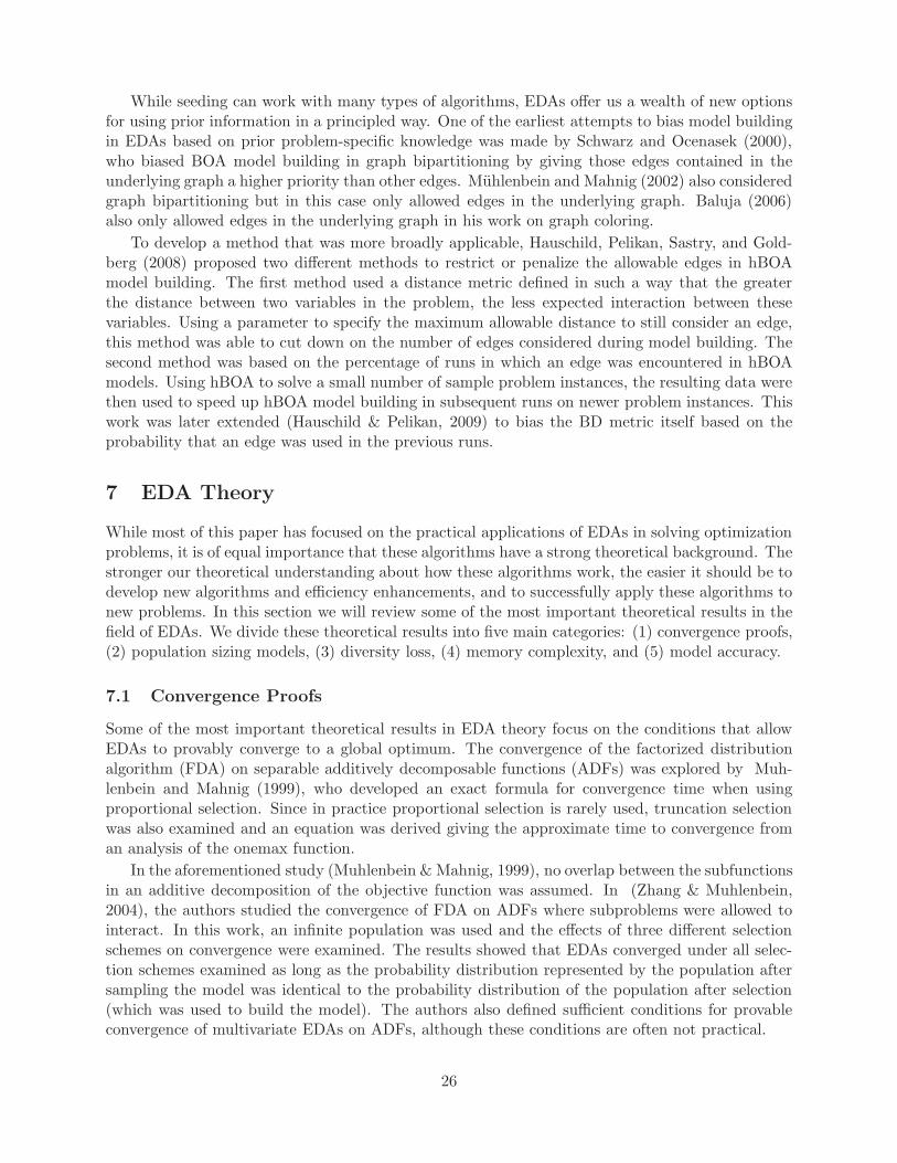
While seeding can work with many types of algorithms, EDAs offer us a wealth of new optionsfor using prior information in a principled way. One of the earliest attempts to bias model buildingin EDAs based on prior problem-specific knowledge was made by Schwarz and Ocenasek (2000),who biased BOA model building in graph bipartitioning by giving those edges contained in theunderlying graph a higher priority than other edges. Muhlenbein and Mahnig (2002) also consideredgraph bipartitioning but in this case only allowed edges in the underlying graph. Baluja (2006)also only allowed edges in the underlying graph in his work on graph coloring.

To develop a method that was more broadly applicable, Hauschild, Pelikan, Sastry, and Gold-berg (2008) proposed two different methods to restrict or penalize the allowable edges in hBOAmodel building. The first method used a distance metric defined in such a way that the greaterthe distance between two variables in the problem, the less expected interaction between thesevariables. Using a parameter to specify the maximum allowable distance to still consider an edge,this method was able to cut down on the number of edges considered during model building. Thesecond method was based on the percentage of runs in which an edge was encountered in hBOAmodels. Using hBOA to solve a small number of sample problem instances, the resulting data werethen used to speed up hBOA model building in subsequent runs on newer problem instances. Thiswork was later extended (Hauschild & Pelikan, 2009) to bias the BD metric itself based on theprobability that an edge was used in the previous runs.

7 EDA Theory

While most of this paper has focused on the practical applications of EDAs in solving optimizationproblems, it is of equal importance that these algorithms have a strong theoretical background. Thestronger our theoretical understanding about how these algorithms work, the easier it should be todevelop new algorithms and efficiency enhancements, and to successfully apply these algorithms tonew problems. In this section we will review some of the most important theoretical results in thefield of EDAs. We divide these theoretical results into five main categories: (1) convergence proofs,(2) population sizing models, (3) diversity loss, (4) memory complexity, and (5) model accuracy.

7.1 Convergence Proofs

Some of the most important theoretical results in EDA theory focus on the conditions that allowEDAs to provably converge to a global optimum. The convergence of the factorized distributionalgorithm (FDA) on separable additively decomposable functions (ADFs) was explored by Muh-lenbein and Mahnig (1999), who developed an exact formula for convergence time when usingproportional selection. Since in practice proportional selection is rarely used, truncation selectionwas also examined and an equation was derived giving the approximate time to convergence froman analysis of the onemax function.

In the aforementioned study (Muhlenbein & Mahnig, 1999), no overlap between the subfunctionsin an additive decomposition of the objective function was assumed. In (Zhang & Muhlenbein,2004), the authors studied the convergence of FDA on ADFs where subproblems were allowed tointeract. In this work, an infinite population was used and the effects of three different selectionschemes on convergence were examined. The results showed that EDAs converged under all selec-tion schemes examined as long as the probability distribution represented by the population aftersampling the model was identical to the probability distribution of the population after selection(which was used to build the model). The authors also defined sufficient conditions for provableconvergence of multivariate EDAs on ADFs, although these conditions are often not practical.

26

Zhang (2004) examined two different EDAs, the FDA which uses higher-order statistics, andthe UMDA using only first-order statistics. After developing limit models of UMDA and FDA,the authors show that in the case of a general objective function, the limit model of FDA has abetter chance of obtaining the global optimum than UMDA. The authors then proved this on anadditively decomposable objective function, showing that at least for some problems the chance ofconverging to the global optimum is indeed increased by using higher order statistics.

7.2 Population Sizing

The convergence proofs mentioned in the previous subsection assumed infinite populations in orderto simplify calculations. However, in practice using an infinite population is not possible. Thepopulation size in EDAs is closely related to the reliability and complexity of the search, similarlyas for other population-based evolutionary algorithms (Goldberg, Deb, & Clark, 1992; Goldberg,Sastry, & Latoza, 2001; Harik, Cantu-Paz, Goldberg, & Miller, 1997). Using a population thatis too small can lead to convergence to solutions of low quality and inability to reliably find theglobal optimum. On the other hand, using a population that is too large can lead to an increasedcomplexity of building and sampling probabilistic models, evaluating populations, and executingother EDA components. That is why choosing an adequate population size is crucial. Similarto GAs, EDAs must have a sufficient population size such that the initial supply of raw buildingblocks (Goldberg, Deb, & Clark, 1992) is sufficient and that good decisions are made betweencompeting partial solutions (Goldberg, Deb, & Clark, 1992). However, the population must belarge enough for EDAs to make good decisions on variable interactions.

To examine this topic, Pelikan, Sastry, and Goldberg (2002) explored the population size re-quired for BOA to solve decomposable problems of bounded difficulty with uniformly and nonuni-formly scaled subproblems. The results showed that the population sizes required grew nearly lin-early. The results also showed that the approximate number of evaluations grew subgradraticallyfor uniformly scaled subproblems but was quadratic on some nonuniformly scaled subproblems.

Yu, Sastry, Goldberg, and Pelikan (2007) refined the model of Pelikan, Sastry, and Goldberg(2002) to provide more accurate bounds for the adequate population size in multivariate EDAs andalso examined the effects of selection pressure on population size. The work focused on entropy-based EDAs and started by assuming an infinite population. Then, for a finite population size, thedistributions of the sampled entropy was investigated.

7.3 Diversity Loss

It is possible for stochastic errors in population sampling to lead to a loss of diversity. If this loss ofdiversity continues over time (by producing simplified models), it is possible for the population to nolonger contain enough information to solve the problem. Shapiro (2005) examined the susceptibilityof UMDA to diversity loss and discussed how it is necessary to set the learning parameters in sucha way that this does not happen.

Bosman, Grahl, and Thierens (2008) examined diversity loss in EDAs for solving real-valuedproblems and the approaches to alleviating this difficulty. The results showed that due to diversityloss some of the state-of-the-art EDAs for real-valued problems could still fail on slope-like regionsin the search space. The authors proposed using anticipated mean shift (AMS) to shift the meanof new solutions each generation in order to effectively maintain diversity.

27

7.4 Memory Complexity

Another factor of importance in EDA problem solving is the memory required to solve the problem.Gao and Culberson (2005) examined the space complexity of the FDA and BOA on additivelydecomposable functions where overlap was allowed between subfunctions. Gao and Culberson(2005) proved that the space complexity of FDA and BOA is exponential in the problem sizeeven with very sparse interaction between variables. While these results are somewhat negative,the authors point out that this only shows that EDAs have limitations and work best when theinteraction structure is of bounded size.

One way to reduce the memory complexity required in multivariate EDAs is to use incrementalEDAs. The incremental BOA (iBOA) (Pelikan, Sastry, & Goldberg, 2008a) starts with a simpleunivariate model that is gradually increased in complexity. Each generation, several solutions aregenerated and the best and worst fit individuals are used to determine whether to increase thecomplexity of the model by adding an edge between nodes, with the parameters of the model alsoslowly updated over time. To limit the required memory complexity, iBOA stores only the marginalprobabilities for the current model and any that would be required after adding an edge betweennodes. The resulting multivariate EDA has less memory complexity than BOA but was still ableto scalably solve deceptive trap problems.

7.5 Model Accuracy

Model accuracy studies examine the accuracy of the models in EDAs that successfully solve aproblem. By understanding the structure and complexity of the models and how they relate to theunderlying problem structure, researchers should be able to develop new theoretical models anddesign new efficiency enhancement techniques.

Hauschild, Pelikan, Sastry, and Lima (2009) analyzed the models generated by hBOA whensolving concatenated traps, random additively decomposable problems, hierarchical traps and 2DIsing spin glasses. The models generated were then compared to the underlying problem structureby comparing the number of spurious and correct edges added (given a perfect model). The resultsshowed that the models did closely correspond to the structure of the underlying problems andthat the models did not change significantly between consequent iterations of hBOA.

The relationship between the probabilistic models learned by BOA and the underlying problemstructure was also explored by Lima, Lobo, Pelikan, , and Goldberg (2010). The accuracy of themodels was defined as the ratio of the edges found in a perfect model over the total number ofedges in the network. One of the most important contributions of this study was to demonstratethe dramatic effect that selection has on spurious dependencies. The results showed that modelaccuracy was significantly improved when using truncation selection compared to tournament se-lection. Motivated by these results, the authors modified the complexity penalty of BOA modelbuilding to take into account tournament sizes when using binary tournament selection. This news-penalty was found to significantly improve the model structural accuracy of BOA even whentournament selection is used.

Echegoyen, Mendiburu, Santana, and Lozano (2011) also analyzed the structural accuracy ofthe models, this time using EBNA on concatenated traps, two variants of Ising spin glass and MAX-SAT. In this work two variations of EBNA were compared, one that was given the complete modelstructure based on the underlying problem and another that learned the approximate structure.The authors then examined the probability at any generation that the models would generate theoptimal solution. The results showed that it was not strictly necessary to have all the interactionsthat were in the complete model in order to solve the problems. It was also discovered that in order

28

for the algorithm to reach a solution, the probability of an optimal solution must always exceed acertain threshold.

Finally, the effects of spurious linkages on EDA performance were examined by Radetic andPelikan (2010). The authors started by proposing a theoretical model to describe the effects ofspurious (unnecessary) dependencies on the population sizing of EDAs. This model was thentested empirically on onemax and the results showed that while it would be expected that spuriousdependencies would have little effect on population size, when niching was included the effects weresubstantial.

8 Additional Information

This section provides pointers to additional sources of information on EDAs.

8.1 Software

The following list contains some free EDA implementations available online:

• Implementations of BOA, hBOA and dtEDA:

http://medal.cs.umsl.edu/software.php

• Implementation of ECGA in Matlab and C++:

http://illigal.org/category/source-code/

• Implementations of sequential and parallel mixed BOA and adaptive mixed BOA:

http://jiri.ocenasek.com/#Download

• Matlab toolbox for EDAs and several implementations:

http://www.sc.ehu.es/ccwbayes/members/rsantana/software/Software.html

• Implementation of the Adapted Maximum-Likelihood Gaussian Model Iterated Density Esti-mation Evolutionary Algorithm (AMaLGaM-IDEA):

http://homepages.cwi.nl/~bosman/source_code.php

• Source code for RM-MEDA and several other EDAs and test problems:

http://cswww.essex.ac.uk/staff/qzhang/mypublication.htm

• Implementations of Real-coded BOA and multi-objective Real-coded BOA:

http://www.evolution.re.kr/

8.2 Journals

The following journals are key venues for papers in EDAs and often contain papers on the cuttingedge of research in EDAs:

• Evolutionary Computation (MIT Press):

http://www.mitpressjournals.org/loi/evco

29

• IEEE Transactions on Evolutionary Computation (IEEE Press):

http://www.ieee-cis.org/pubs/tec/

• Swarm and Evolutionary Computation:

http://www.elsevier.com/wps/find/journaldescription.cws_home/724666/description#

description

• Genetic Programming and Evolvable Machines:

http://www.springer.com/computer/ai/journal/10710

8.3 Conferences

The following conferences are the primary ones that publish papers in the EDA field:

• ACM SIGEVO Genetic and Evolutionary Computation Conference (GECCO):

• Parallel Problem Solving in Nature (PPSN):

• IEEE Congress on Evolutionary Computation (CEC):

9 Summary and Conclusions

EDAs are among the most powerful evolutionary algorithms currently available, and there are nu-merous applications where EDAs have been shown to solve problems unsolvable with other existingtechniques. Nonetheless, EDAs are capable of not only solving many difficult problems, but theyalso provide practitioners with a great deal of information about how the problem was solved. Theability to provide practitioners with useful information about the problem landscape is a featurethat is highly desirable yet not offered by virtually any other general optimization technique. In ad-dition, most EDAs offer additional advantages over the more conventional evolutionary algorithmsand other metaheuristics, such as the ability to represent the population more efficiently using aprobabilistic model or include prior information of various forms in a rigorous manner.

EDAs use a large variety of probabilistic models, ranging from probability vectors to Bayesianand Markov networks. This diversity allows practitoners to solve a great variety of problems, fromthe simple to the complex, from the real-valued domain to the discrete one. Given almost anyproblem, it should be possible for practitioners to select an EDA that can solve it. The key is toensure that the class of probabilistic models used allows EDAs to effectively capture features ofhigh quality solutions that make these solutions better.

Acknowledgments

This project was sponsored by the National Science Foundation under CAREER grant ECS-0547013 and by

the University of Missouri in St. Louis through the High Performance Computing Collaboratory sponsored

by Information Technology Services. Any opinions, findings, and conclusions or recommendations expressed

in this material are those of the authors and do not necessarily reflect the views of the National Science

Foundation.

30

References

Ackley, D. H. (1987). An empirical study of bit vector function optimization. Genetic Algorithmsand Simulated Annealing , 170–204.

Ahn, C. W., Ramakrishna, R. S., & Goldberg, D. E. (2004). Real-Coded Bayesian OptimizationAlgorithm: Bringing the Strength of BOA into the Continuous World. In Deb, K. (Ed.),Proceedings of the Genetic and Evolutionary Computation Conference GECCO 2004 (pp.840–851). Springer-Verlag, Berlin.

Albert, L. A. (2001). Efficient genetic algorithms using discretization scheduling. Master’s thesis,University of Illinois at Urbana-Champaign, Department of General Engineering, Urbana,IL.

Arst, R., Minsker, B. S., & Goldberg, D. E. (2002). Comparing advanced genetic algorithms andsimple genetic algorithms for groundwater management. Proceedings of the American Societyof Civil Engineers (ASCE) Environmental & Water Resources Institute (EWRI) 2002 WaterResources Planning & Management Conference, Roanoke, VA.

Bacardit, J., Stout, M., Hirst, J. D., Sastry, K., Llora, X., & Krasnogor, N. (2007). Automatedalphabet reduction method with evolutionary algorithms for protein structure prediction.Genetic and Evolutionary Computation Conference (GECCO-2007), 346–353.

Baluja, S. (1994). Population-based incremental learning: A method for integrating genetic searchbased function optimization and competitive learning (Tech. Rep. No. CMU-CS-94-163). Pitts-burgh, PA: Carnegie Mellon University.

Baluja, S. (2006). Incorporating a priori knowledge in probabilistic-model based optimization.In Pelikan, M., Sastry, K., & Cantu-Paz, E. (Eds.), Scalable optimization via probabilisticmodeling: From algorithms to applications (pp. 205–219). Springer.

Baluja, S., & Davies, S. (1997). Using optimal dependency-trees for combinatorial optimization:Learning the structure of the search space. Proceedings of the International Conference onMachine Learning , 30–38.

Bean, J. C. (1994). Genetic algorithms and random keys for sequencing and optimization. ORSAJournal on Computing , 6 (2), 154–160.

Bengoetxea, E., Larranaga, P., Bloch, I., Perchant, A., & Boeres, C. (2000). Inexact graphmatching using learning and simulation of Bayesian networks. an empirical comparison be-tween different approaches with synthetic data. Berlin.

Bosman, P., & Thierens, D. (2006). Multi-objective optimization with the naive MIDEA. InLozano, J., Larraaga, P., Inza, I., & Bengoetxea, E. (Eds.), Towards a New EvolutionaryComputation, Volume 192 of Studies in Fuzziness and Soft Computing (pp. 123–157). SpringerBerlin / Heidelberg.

Bosman, P. A., Grahl, J., & Thierens, D. (2008). Enhancing the performance of maximum—likelihood Gaussian EDAs using anticipated mean shift. In Proceedings of the 10th interna-tional conference on Parallel Problem Solving from Nature: PPSN X (pp. 133–143). Berlin,Heidelberg: Springer-Verlag.

Bosman, P. A., & Thierens, D. (2001a). Advancing continuous IDEAs with mixture distributionsand factorization selection metrics. In Proceedings of the Optimization by Building and Us-ing Probabilistic Models OBUPM Workshop at the Genetic and Evolutionary ComputationConference GECCO2001 (pp. 208–212). Morgan Kaufmann.

31

Bosman, P. A., & Thierens, D. (2001b). Crossing the road to efficient ideas for permutationproblems. Genetic and Evolutionary Computation Conference (GECCO-2001), 219–226.

Bosman, P. A., & Thierens, D. (2001c). New IDEAs and more ICE by learning and using uncon-ditional permutation factorizations. Late-Breaking Papers of the Genetic and EvolutionaryComputation Conference (GECCO-2001), 16–23.

Bosman, P. A. N., & Thierens, D. (1999). Linkage information processing in distribution es-timation algorithms. Genetic and Evolutionary Computation Conference (GECCO-99), I ,60–67.

Bosman, P. A. N., & Thierens, D. (2000). Continuous iterated density estimation evolutionary al-gorithms within the IDEA framework. Workshop Proceedings of the Genetic and EvolutionaryComputation Conference (GECCO-2000), 197–200.

Cantu-Paz, E. (2000). Efficient and accurate parallel genetic algorithms. Boston, MA: Kluwer.

Chen, C., Liu, W., & Chen, Y. (2006). Adaptive discretization for probabilistic model buildinggenetic algorithms. In Proceedings of the 8th annual conference on Genetic and evolutionarycomputation, GECCO ’06 (pp. 1103–1110). New York, NY, USA: ACM.

Chen, C.-H., & p. Chen, Y. (2007). Real-coded ECGA for economic dispatch. Genetic andEvolutionary Computation Conference (GECCO-2007), 1920–1927.

Chen, S.-C., & Yu, T.-L. (2009). Difficulty of linkage learning in estimation of distributionalgorithms. In Proceedings of the 11th Annual conference on Genetic and evolutionary com-putation, GECCO ’09 (pp. 397–404). New York, NY, USA: ACM.

Chen, Y., & Chen, C. (2010). Enabling the extended compact genetic algorithm for real-parameter optimization by using adaptive discretization. Evolutionary Computation, 18 (2),199–228.

Chickering, D. M., Heckerman, D., & Meek, C. (1997). A Bayesian approach to learning Bayesiannetworks with local structure (Technical Report MSR-TR-97-07). Redmond, WA: MicrosoftResearch.

Chow, C., & Liu, C. (1968). Approximating discrete probability distributions with dependencetrees. IEEE Transactions on Information Theory , 14 , 462–467.

Coello, C., & Lamont, G. (2004). Applications of multi-objective evolutionary algorithms. Ad-vances in natural computation. World Scientific.

Coffin, D. J., & Smith, R. E. (2007). Why is parity hard for estimation of distribution algo-rithms? In Proceedings of the 9th annual conference on Genetic and evolutionary computa-tion, GECCO ’07 (pp. 624–624). New York, NY, USA: ACM.

De Bonet, J. S., Isbell, C. L., & Viola, P. (1997). MIMIC: Finding optima by estimating proba-bility densities. Advances in neural information processing systems (NIPS-97), 9 , 424–431.

Deb, K. (2001). Multi-objective optimization using evolutionary algorithms. Chichester, UK: JohnWiley & Sons.

Deb, K., & Goldberg, D. E. (1991). Analyzing deception in trap functions (IlliGAL Report No.91009). Urbana, IL: University of Illinois at Urbana-Champaign, Illinois Genetic AlgorithmsLaboratory.

Deb, K., Pratap, A., Agarwal, S., & Meyarivan, T. (2002, apr). A fast and elitist multiobjectivegenetic algorithm: Nsga-ii. Evolutionary Computation, IEEE Transactions on, 6 (2), 182 –197.

32

Dorigo, M. (1992). Optimization, learning and natural algorithms. Doctoral dissertation, Politec-nico di Milano, Italie.

Ducheyne, E., De Baets, B., & De Wulf, R. (2004). Probabilistic models for linkage learning inforest management. In Jin, Y. (Ed.), Knowledge incorporation in evolutionary computation(pp. 177–194). Springer.

Echegoyen, C., Mendiburu, A., Santana, R., & Lozano, J. A. (2011). Toward understandingEDAs based on Bayesian networks through a quantitative analysis. Evolutionary Computa-tion, IEEE Transactions on, PP(99), 1 –17.

Etxeberria, R., & Larranaga, P. (1999). Global optimization using Bayesian networks. In Ochoa,A., Soto, M. R., & Santana, R. (Eds.), Proceedings of the Second Symposium on ArtificialIntelligence (CIMAF-99) (pp. 151–173). Editorial Academia. Havana, Cuba.

Friedman, N., & Goldszmidt, M. (1999). Learning Bayesian networks with local structure. InJordan, M. I. (Ed.), Graphical models (pp. 421–459). MIT Press.

Gallagher, M. (2000). Multi-layer perceptron error surfaces: visualization, structure and mod-elling. Doctoral dissertation.

Gallagher, M., Frean, M., & Downs, T. (1999). Real-valued evolutionary optimization using aflexible probability density estimator. In Proceedings of the Genetic and Evolutionary Com-putation Conference (pp. 840–846). Citeseer.

Gao, Y., & Culberson, J. (2005). Space complexity of estimation of distribution algorithms.Evolutionary Computation, 13 (1), 125–143.

Geiger, D., & Heckerman, D. (1994). Learning Gaussian networks. In Proceedings of UAI’1994(pp. 235–243).

Goldberg, D. E. (1999). Using time efficiently: Genetic-evolutionary algorithms and the contin-uation problem. Genetic and Evolutionary Computation Conference (GECCO-99), 212–219.Also IlliGAL Report No. 99002.

Goldberg, D. E. (2002). The design of innovation: Lessons from and for competent geneticalgorithms. Kluwer.

Goldberg, D. E., Deb, K., & Clark, J. H. (1992). Genetic algorithms, noise, and the sizing ofpopulations. Complex Systems, 6 , 333–362.

Goldberg, D. E., Sastry, K., & Latoza, T. (2001). On the supply of building blocks. In Spector,L., et al. (Eds.), Genetic and Evolutionary Computation Conference (GECCO-2001) (pp.336–342). San Francisco, CA: Morgan Kaufmann. Also IlliGAL Report No. 2001015.

Handa, H. (2007). The effectiveness of mutation operation in the case of estimation of distribu-tion algorithms. Biosystems, 87 (2-3), 243 – 251. Papers presented at the Sixth InternationalWorkshop on Information Processing in Cells and Tissues, York, UK, 2005 - IPCAT 2005,Information Processing in Cells and Tissues.

Harik, G. (1999). Linkage learning via probabilistic modeling in the ECGA (IlliGAL Report No.99010). Urbana, IL: University of Illinois at Urbana-Champaign, Illinois Genetic AlgorithmsLaboratory.

Harik, G. R. (1995). Finding multimodal solutions using restricted tournament selection. Inter-national Conference on Genetic Algorithms (ICGA-95), 24–31.

33

Harik, G. R., Cantu-Paz, E., Goldberg, D. E., & Miller, B. L. (1997). The gambler’s ruin problem,genetic algorithms, and the sizing of populations. In International Conference on EvolutionaryComputation (ICEC-97) (pp. 7–12). Piscataway, NJ: IEEE Press.

Harik, G. R., Lobo, F. G., & Goldberg, D. E. (1997). The compact genetic algorithm (IlliGALReport No. 97006). Urbana, IL: University of Illinois at Urbana-Champaign, Illinois GeneticAlgorithms Laboratory.

Hart, W. E. (1994). Adaptive global optimization with local search. Doctoral dissertation, Uni-versity of California, San Diego, San Diego, CA.

Hartigan, J. A. (1975). Clustering algorithms. John Wiley and Sons, Inc.

Hartmann, A. K. (1996). Cluster-exact approximation of spin glass ground states. Physica A, 224 ,480.

Hauschild, M., Pelikan, M., Sastry, K., & Goldberg, D. E. (2008). Using previous models tobias structural learning in the hierarchical BOA. Genetic and Evolutionary ComputationConference (GECCO-2008), 415–422.

Hauschild, M., Pelikan, M., Sastry, K., & Lima, C. (2009, dec.). Analyzing probabilistic modelsin hierarchical BOA. Evolutionary Computation, IEEE Transactions on, 13 (6), 1199 –1217.

Hauschild, M. W., & Pelikan, M. (2009). Intelligent bias of network structures in the hierarchicalBOA. In Proceedings of the 11th Annual conference on Genetic and evolutionary computation,GECCO ’09 (pp. 413–420). New York, NY, USA: ACM.

Hayes, M. S., & Minsker, B. S. (2005). Evaluation of advanced genetic algorithms applied togroundwater remediation design. Proceedings of the American Society of Civil Engineers(ASCE) Environmental & Water Resources Institute (EWRI) World Water & EnvironmentalResources Congress 2005 & Related Symposia, Anchorage, AK.

Heckendorn, R. B., & Wright, A. H. (2004, December). Efficient linkage discovery by limitedprobing. Evol. Comput., 12 , 517–545.

Heckerman, D., Geiger, D., & Chickering, D. M. (1994). Learning Bayesian networks: Thecombination of knowledge and statistical data (Technical Report MSR-TR-94-09). Redmond,WA: Microsoft Research.

Heckerman, D., Geiger, D., & Chickering, D. M. (1995). Learning Bayesian networks:The combination of knowledge and statistical data. Machine Learning , 20 , 197–243.10.1007/BF00994016.

Henrion, M. (1988). Propagating uncertainty in Bayesian networks by probabilistic logic sam-pling. In Lemmer, J. F., & Kanal, L. N. (Eds.), Uncertainty in Artificial Intelligence (pp.149–163). Amsterdam, London, New York: Elsevier.

Holland, J. (1973). Genetic algorithms and the optimal allocation of trials. SIAM Journal ofComputing , 2 (2), 88–105.

Hons, R. (2006). Estimation of distribution algorithms and minimum relative entropy. Doctoraldissertation, University of Bonn, Germany.

Hons, R., Santana, R., Larranaga, P., & Lozano, J. A. (2007). Optimization by max-propagationusing kikuchi approximations. (Tech. Rep. EHUKAT-IK-2-07). Urbana, IL: Department ofComputer Science and Artificial Intelligence, University of the Basque Country.

Kennedy, J., & Eberhart, R. (1995, nov/dec). Particle swarm optimization. In Neural Networks,1995. Proceedings., IEEE International Conference on, Volume 4 (pp. 1942 –1948 vol.4).

34

Khan, N., Goldberg, D. E., & Pelikan, M. (2002). Multi-objective Bayesian optimization algo-rithm (IlliGAL Report No. 2002009). Urbana, IL: University of Illinois at Urbana-Champaign,Illinois Genetic Algorithms Laboratory.

Kollat, J. B., & Reed, P. M. (2005). The value of online adaptive search: a performance com-parison of NSGA-II, ǫ-NSGAII, and ǫ-MOEA. In The Third International Conference onEvolutionary Multi-Criterion Optimization (EMO 2005), Lecture Notes in Computer Science(pp. 386–398). Guanajuato, Mexico: Springer-Verlag.

Kollat, J. B., Reed, P. M., & Kasprzyk, J. R. (2008). A new epsilon-dominance hierarchicalBayesian optimization algorithm for large multi-objective monitoring network design prob-lems. Advances in Water Resources, 31 (5), 828–845.

Koopmans, T. C., & Beckmann, M. J. (1957). Assignment problems and the location of economicactivities. Econometrica, 25 , 53–76.

Koza, J. R. (1992). Genetic programming: On the programming of computers by means of naturalselection. Cambridge, MA: The MIT Press.

Larranaga, P., Etxeberria, R., Lozano, J. A., & Pena, J. M. (1999). Optimization by learning andsimulation of Bayesian and Gaussian networks (Technical Report). Department of ComputerScience and Artificial Intelligence, University of the Basque Country.

Larranaga, P., & Lozano, J. A. (Eds.) (2002). Estimation of distribution algorithms: A new toolfor evolutionary computation. Boston, MA: Kluwer.

Laumanns, M., & Ocenasek, J. (2002). Bayesian optimization algorithms for multi-objectiveoptimization. In Proceedings of the 7th International Conference on Parallel Problem Solvingfrom Nature, PPSN VII (pp. 298–307). London, UK, UK: Springer-Verlag.

Laumanns, M., Thiele, L., Deb, K., & Zitzler, E. (2002). Combining convergence and diversityin evolutionary multi-objective optimization. Evolutionary Computation, 10 , 263–282.

Lima, C. F., Lobo, F. G., Pelikan, M., , & Goldberg, D. (2010). Model accuracy in the Bayesianoptimization algorithm. Soft Computing .

Lima, C. F., Pelikan, M., Lobo, F. G., & Goldberg, D. E. (2009). Loopy substructural localsearch for the bayesian optimization algorithm. In Stutzle, T., Birattari, M., & Hoos, H. H.(Eds.), SLS, Volume 5752 of Lecture Notes in Computer Science (pp. 61–75). Springer.

Lima, C. F., Pelikan, M., Sastry, K., Butz, M. V., Goldberg, D. E., & Lobo, F. G. (2006).Substructural neighborhoods for local search in the Bayesian optimization algorithm. ParallelProblem Solving from Nature, 232–241.

Lipinski, P. (2007). ECGA vs. BOA in discovering stock market trading experts. Genetic andEvolutionary Computation Conference (GECCO-2007), 531–538.

Lobo, F. G., & Lima, C. F. (2010). Towards automated selection of estimation of distributionalgorithms. In Proceedings of the 12th annual conference companion on Genetic and evolu-tionary computation (GECCO-2010) (pp. 1945–1952). ACM.

Looks, M. (2006, 11 December). Competent program evolution. Doctor of science, WashingtonUniversity, St. Louis, USA.

Marascuilo, L. A., & McSweeney, M. (1977). Nonparametric and distribution-free methods forthe social sciences. CA: Brooks/Cole Publishing Company.

35

Mendiburu, A., Lozano, J., & Miguel-Alonso, J. (2005, aug.). Parallel implementation of EDAsbased on probabilistic graphical models. Evolutionary Computation, IEEE Transactionson, 9 (4), 406 – 423.

Mendiburu, A., Santana, R., Lozano, J. A., & Bengoetxea, E. (2007). A parallel frameworkfor loopy belief propagation. In Proceedings of the 2007 GECCO conference companion onGenetic and evolutionary computation, GECCO ’07 (pp. 2843–2850). New York, NY, USA:ACM.

Mitchell, T. M. (1997). Machine learning. McGraw-Hill.

Muhlenbein, H. (2008). Convergence of estimation of distribution algorithms for finite samples(Technical Report). Sankt Augustin, Germany: Fraunhofer Institut Autonomous intelligentSystems.

Muhlenbein, H., & Hons, R. (2006). The factorized distribution algorithm and the minimumrelative entropy principle. In Scalable Optimization via Probabilistic Modeling (pp. 11–37).

Muhlenbein, H., & Mahnig, T. (1999). Convergence theory and applications of the factorizeddistribution algorithm. Journal of Computing and Information Technology , 7 .

Muhlenbein, H., & Mahnig, T. (1999). FDA – A scalable evolutionary algorithm for the opti-mization of additively decomposed functions. Evolutionary Computation, 7 (4), 353–376.

Muhlenbein, H., & Mahnig, T. (2002). Evolutionary optimization and the estimation of searchdistributions with applications to graph bipartitioning. International Journal on ApproximateReasoning , 31 (3), 157–192.

Muhlenbein, H., & Paaß, G. (1996a). From recombination of genes to the estimation of distribu-tions I. Binary parameters. Parallel Problem Solving from Nature, 178–187.

Muhlenbein, H., & Paaß, G. (1996b). From recombination of genes to the estimation of distri-butions I. Binary parameters. In Eiben, A., Back, T., Shoenauer, M., & Schwefel, H. (Eds.),Parallel Problem Solving from Nature (pp. 178–187). Berlin: Springer Verlag.

Munetomo, M., & Goldberg, D. E. (1999). Linkage identification by non-monotonicity detectionfor overlapping functions. Evolutionary Computation, 7 (4), 377–398.

Nelsen, R. B. (1998). An introduction to copulas. Secaucus, NJ, USA: Springer-Verlag New York,Inc.

Ocenasek, J. (2002). Parallel estimation of distribution algorithms. Doctoral dissertation, Facultyof Information Technology, Brno University of Technology, Brno.

Ocenasek, J., Cantu-Paz, E., Pelikan, M., & Schwarz, J. (2006). Design of parallel estimation ofdistribution algorithms. In Pelikan, M., Sastry, K., & Cantu-Paz, E. (Eds.), Scalable Opti-mization via Probabilistic Modeling: From Algorithms to Applications (pp. 187–203). Springer.

Ocenasek, J., Kern, S., Hansen, N., & Koumoutsakos, P. (2004). A mixed Bayesian optimiza-tion algorithm with variance adaptation. In Yao, X., Burke, E., Lozano, J. A., Smith, J.,Merelo-Guervs, J. J., Bullinaria, J. A., Rowe, J., Tino, P., Kabn, A., & Schwefel, H.-P.(Eds.), Parallel Problem Solving from Nature - PPSN VIII, Volume 3242 of Lecture Notes inComputer Science (pp. 352–361). Springer Berlin / Heidelberg.

Ocenasek, J., & Schwarz, J. (2000). The parallel Bayesian optimization algorithm. In Proceedingsof the European Symposium on Computational Inteligence (pp. 61–67). Physica-Verlag.

Ochoa, A., Hons, R., Soto, M., & Muhlenbein, H. (2003). A Maximum Entropy Approach toSampling in EDA The Single Connected Case. Springer.

36

Pearl, J. (1988). Probabilistic reasoning in intelligent systems: Networks of plausible inference.San Mateo, CA: Morgan Kaufmann.

Pelikan, M. (2005). Hierarchical Bayesian optimization algorithm: Toward a new generation ofevolutionary algorithms. Springer-Verlag.

Pelikan, M., & Goldberg, D. E. (2003). Hierarchical BOA solves Ising spin glasses and MAXSAT.Genetic and Evolutionary Computation Conference (GECCO-2003), II , 1275–1286.

Pelikan, M., & Goldberg, D. E. (2006). Hierarchical Bayesian optimization algorithm. In Pelikan,M., Sastry, K., & Cantu-Paz, E. (Eds.), Scalable optimization via probabilistic modeling: Fromalgorithms to applications (pp. 63–90). Springer.

Pelikan, M., Goldberg, D. E., & Cantu-Paz, E. (2000). Linkage problem, distribution estimation,and Bayesian networks. Evolutionary Computation, 8 (3), 311–341. Also IlliGAL Report No.98013.

Pelikan, M., Goldberg, D. E., & Lobo, F. (2002). A survey of optimization by building and usingprobabilistic models. Computational Optimization and Applications, 21 (1), 5–20.

Pelikan, M., Goldberg, D. E., & Tsutsui, S. (2003). Getting the best of both worlds: Discrete andcontinuous genetic and evolutionary algorithms in concert. Information Sciences, 156 (3-4),147 – 171. Evolutionary Computation.

Pelikan, M., & Hartmann, A. K. (2006). Searching for ground states of Ising spin glasses withhierarchical BOA and cluster exact approximation. In Pelikan, M., Sastry, K., & Cantu-Paz,E. (Eds.), Scalable optimization via probabilistic modeling: From algorithms to applications(pp. 333–349). Springer.

Pelikan, M., & Muhlenbein, H. (1999). The bivariate marginal distribution algorithm. Advancesin Soft Computing—Engineering Design and Manufacturing , 521–535.

Pelikan, M., & Sastry, K. (2004). Fitness inheritance in the Bayesian optimization algorithm.Genetic and Evolutionary Computation Conference (GECCO-2004), 2 , 48–59.

Pelikan, M., Sastry, K., & Goldberg, D. E. (2002). Scalability of the Bayesian optimizationalgorithm. International Journal of Approximate Reasoning , 31 (3), 221–258.

Pelikan, M., Sastry, K., & Goldberg, D. E. (2005). Multiobjective hBOA, clustering, and scalabil-ity. In Proceedings of the 2005 conference on Genetic and evolutionary computation, GECCO’05 (pp. 663–670). New York, NY, USA: ACM.

Pelikan, M., Sastry, K., & Goldberg, D. E. (2006). Multiobjective estimation of distributionalgorithms. In Scalable Optimization via Probabilistic Modeling (pp. 223–248).

Pelikan, M., Sastry, K., & Goldberg, D. E. (2008a). iBOA: the incremental Bayesian optimiza-tion algorithm. In Proceedings of the 10th annual conference on Genetic and evolutionarycomputation, GECCO ’08 (pp. 455–462). New York, NY, USA: ACM.

Pelikan, M., Sastry, K., & Goldberg, D. E. (2008b). Sporadic model building for efficiency en-hancement of the hierarchical BOA. Genetic Programming and Evolvable Machines, 9 (1),53–84.

Pelikan, M., Tsutsui, S., & Kalapala, R. (2007). Dependency trees, permutations, and quadraticassignment problem. In Proceedings of the 9th annual conference on Genetic and evolutionarycomputation, GECCO ’07 (pp. 629–629). New York, NY, USA: ACM.

37

Pena, J., Lozano, J., & Larranaga, P. (2004). Unsupervised learning of Bayesian networks viaestimation of distribution algorithms: an application to gene expression data clustering. In-ternational Journal of Uncertainty, Fuzziness and Knowledge-Based Systems, 12 , 63–82.

Petrovski, A., Shakya, S., & Mccall, J. (2006). Optimising cancer chemotherapy using an estima-tion of distribution algorithm and genetic algorithms. Genetic and Evolutionary ComputationConference (GECCO-2006), 413–418.

Priebe, C. E. (1994). Adaptive mixtures. Journal of the American Statistical Associa-tion, 89 (427), 796–806.

Radetic, E., & Pelikan, M. (2010). Spurious dependencies and EDA scalability. In GECCO (pp.303–310).

Ratle, A., & Sebag, M. (2006). Avoiding the bloat with stochastic grammar-based genetic pro-gramming. CoRR, abs/cs/0602022 .

Rechenberg, I. (1973). Evolutionsstrategie: Optimierung technischer Systeme nach Prinzipiender biologischen Evolution. Stuttgart: Frommann-Holzboog.

Robles, V., de Miguel, P., & Larranaga, P. (2002). Solving the traveling salesman problem withEDAs. In Larranaga, P., & Lozano, J. A. (Eds.), Estimation of Distribution Algorithms. ANew Tool for Evolutionary Computation (pp. 227–238). Boston/Dordrecht/London: KluwerAcademic Publishers.

Rubinstein, R. Y. (1996). Optimization of computer simulation models with rare events. EuropeanJournal of Operations Research, 99 , 89–112.

Rudlof, S., & Koppen, M. (1996). Stochastic hill climbing with learning by vectors of normaldistributions. In First On-line Workshop on Soft Computing (pp. 60–70). Nagoya, Japan.

Salinas-Gutierrez, R., Hernandez-Aguirre, A., & Villa-Diharce, E. R. (2009). Using copulas inestimation of distribution algorithms. InMICAI 2009: Advances in Artificial Intelligence, Vol-ume 5845 of Lecture Notes in Computer Science (pp. 658–668). Guanajato, Mexico: Springer.

Salustowicz, R. P., & Schmidhuber, J. (1997). Probabilistic incremental program evolution:Stochastic search through program space. Proceedings of the European Conference of Ma-chine Learning (ECML-97), 1224 , 213–220.

Santana, R. (2006). Advances in graphical models for optimization and learning: Applicationsin protein modeling. Doctoral dissertation, University of the Basque Country, San Sebastian,Spain.

Santana, R., Larranaga, P., & Lozano, J. (2008). Adaptive estimation of distribution algorithms.In Cotta, C., Sevaux, M., & Srensen, K. (Eds.), Adaptive and Multilevel Metaheuristics, Vol-ume 136 of Studies in Computational Intelligence (pp. 177–197). Springer Berlin / Heidelberg.

Santana, R., Larranaga, P., & Lozano, J. A. (2010). Learning factorizations in estimation ofdistribution algorithms using affinity propagation. Evolutionary Computation, 18 (4), 515–546.

Sastry, K. (2001a). Efficient atomic cluster optimization using a hybrid extended compact geneticalgorithm with seeded population (IlliGAL Report No. 2001018). Urbana, IL: University ofIllinois at Urbana-Champaign, Illinois Genetic Algorithms Laboratory.

Sastry, K. (2001b). Evaluation-relaxation schemes for genetic and evolutionary algorithms. Mas-ter’s thesis, University of Illinois at Urbana-Champaign, Department of General Engineering,Urbana, IL.

38

Sastry, K., & Goldberg, D. E. (2000). On extended compact genetic algorithm (IlliGAL Report No.2000026). Urbana, IL: University of Illinois at Urbana-Champaign, Illinois Genetic AlgorithmsLaboratory.

Sastry, K., & Goldberg, D. E. (2004a, 26-30). Designing competent mutation operators via prob-abilistic model building of neighborhoods. Genetic and Evolutionary Computation Conference(GECCO-2004), 114–125.

Sastry, K., & Goldberg, D. E. (2004b). Let’s get ready to rumble: Crossover versus mutationhead to head. Genetic and Evolutionary Computation Conference (GECCO-2004), 126–137.

Sastry, K., Goldberg, D. E., & Llora, X. (2007). Towards billion bit optimization via paral-lel estimation of distribution algorithm. Genetic and Evolutionary Computation Conference(GECCO-2007), 577–584.

Sastry, K., Goldberg, D. E., & Pelikan, M. (2001a). Don’t evaluate, inherit. Genetic and Evolu-tionary Computation Conference (GECCO-2001), 551–558.

Sastry, K., Goldberg, D. E., & Pelikan, M. (2001b). Don’t evaluate, inherit. In Spector, L.,Goodman, E. D., Wu, A., Langdon, W. B., Voigt, H.-M., Gen, M., Sen, S., Dorigo, M.,Pezeshk, S., Garzon, M. H., & Burke, E. (Eds.), Genetic and Evolutionary ComputationConference (GECCO-2001) (pp. 551–558). San Francisco, CA: Morgan Kaufmann.

Sastry, K., Pelikan, M., & Goldberg, D. E. (2004). Efficiency enhancement of genetic algorithmsvia building-block-wise fitness estimation. Proceedings of the IEEE International Conferenceon Evolutionary Computation, 720–727.

Sastry, K., Pelikan, M., & Goldberg, D. E. (2006). Efficiency enhancement of estimation of distri-bution algorithms. In Pelikan, M., Sastry, K., & Cantu-Paz, E. (Eds.), Scalable Optimizationvia Probabilistic Modeling: From Algorithms to Applications (pp. 161–185). Springer.

Schwarz, G. (1978a). Estimating the dimension of a model. The Annals of Statistics, 6 , 461–464.

Schwarz, G. (1978b). Estimating the dimension of a model. Annals of Statistics, 6 , 461–464.

Schwarz, J., & Ocenasek, J. (2000). A problem-knowledge based evolutionary algorithm KBOAfor hypergraph partitioning. Personal communication.

Sebag, M., & Ducoulombier, A. (1998). Extending population-based incremental learning tocontinuous search spaces. In Parallel Problem Solving from Nature (pp. 418–427). BerlinHeidelberg: Springer Verlag.

Shah, R., & Reed, P. (2010). Comparative analysis of multiobjective evolutionary algorithms forrandom and correlated instances of multiobjective d-dimensional knapsack problems. Euro-pean Journal of Operations Research. In revision.

Shah, R., & Reed, P. (2011). Comparative analysis of multiobjective evolutionary algorithms forrandom and correlated instances of multiobjective d-dimensional knapsack problems. Euro-pean Journal of Operational Research, 211 (3), 466 – 479.

Shakya, S., & Santana, R. (2008). An EDA based on local markov property and gibbs sampling. InProceedings of the 10th annual conference on Genetic and evolutionary computation, GECCO’08 (pp. 475–476). New York, NY, USA: ACM.

Shan, Y., Mckay, R. I., Abbass, H. A., & Essam, D. (2003). Program evolution with explicitlearning: a new framework for program automatic synthesis. In University College, Universityof New South (pp. 1639–1646). IEEE Press.

39

Shan, Y., Mckay, R. I., & Baxter, R. (2004). Grammar model-based program evolution. In InProceedings of the 2004 IEEE Congress on Evolutionary Computation (pp. 478–485). IEEEPress.

Shapiro, J. L. (2005, January). Drift and scaling in estimation of distribution algorithms. Evol.Comput., 13 , 99–123.

Simon, H. A. (1968). The sciences of the artificial. Cambridge, MA: The MIT Press.

Smith, R. E., Dike, B. A., & Stegmann, S. A. (1995). Fitness inheritance in genetic algorithms.Proceedings of the ACM Symposium on Applied Computing , 345–350.

Srivastava, R., & Goldberg, D. E. (2001). Verification of the theory of genetic and evolutionarycontinuation. Genetic and Evolutionary Computation Conference (GECCO-2001), 551–558.Also IlliGAL Report No. 2001007.

Suganthan, P. N., Hansen, N., Liang, J. J., Deb, K., Chen, Y. P., Auger, A., & Tiwari, S.(2005). Problem definitions and evaluation criteria for the CEC 2005 Special Session on RealParameter Optimization (Technical Report). Nanyang Technological University.

Thierens, D., & Goldberg, D. E. (1993). Mixing in genetic algorithms. International Conferenceon Genetic Algorithms (ICGA-93), 38–45.

Tsutsui, S. (2002). Probabilistic model-building genetic algorithms in permutation representationdomain using edge histogram. In Proc. of the 7th Int. Conf. on Parallel Problem Solving fromNature (PPSN VII (pp. 224–233). Springer-Velag.

Tsutsui, S., Pelikan, M., & Goldberg, D. E. (2001). Evolutionary algorithm using marginal his-togram models in continuous domain. Workshop Proceedings of the Genetic and EvolutionaryComputation Conference (GECCO-2001), 230–233.

Tsutsui, S., Pelikan, M., & Goldberg, D. E. (2006). Node histogram vs. edge histogram: A compar-ison of pmbgas in permutation domains (MEDAL Report No. 2006009). Missouri Estimationof Distribution Algorithms Laboratory, University of Missour–St. Louis, St. Louis, MO.

Wallace, C. S., & Boulton, D. M. (1968). An information measure for classification. ComputerJournal , 11 (2), 185–194.

Wang, L.-F., Zeng, J.-C., & Hong, Y. (2009a). Estimation of distribution algorithm based onArchimedean copulas. In Proceedings of the International Conference GEC’2009 (pp. 993–996). Shangai, China: ACM.

Wang, L.-F., Zeng, J.-C., & Hong, Y. (2009b). Estimation of distribution algorithm based oncopula theory. In Proceedings of the 2009 Congress on Evolutionary Computation CEC-2009(pp. 1057–1063). Norway: IEEE Press.

Yu, T.-L., Santarelli, S., & Goldberg, D. E. (2006). Military antenna design using a simple geneticalgorithm and hBOA. In Pelikan, M., Sastry, K., & Cantu-Paz, E. (Eds.), Scalable optimiza-tion via probabilistic modeling: From algorithms to applications (pp. 275–289). Springer.

Yu, T.-L., Sastry, K., Goldberg, D. E., & Pelikan, M. (2007). Population sizing for entropy-based model building in discrete estimation of distribution algorithms. In Proceedings of the9th annual conference on Genetic and evolutionary computation, GECCO ’07 (pp. 601–608).New York, NY, USA: ACM.

Zhang, Q. (2004, feb.). On stability of fixed points of limit models of univariate marginal dis-tribution algorithm and factorized distribution algorithm. Evolutionary Computation, IEEETransactions on, 8 (1), 80 – 93.

40

Zhang, Q., & Muhlenbein, H. (2004, april). On the convergence of a class of estimation ofdistribution algorithms. Evolutionary Computation, IEEE Transactions on, 8 (2), 127 – 136.

Zhang, Q., Sun, J., & Tsang, E. (2005). Evolutionary algorithm with the guided mutation forthe maximum clique problem. IEEE Transactions on Evolutionary Computation, 9 , 2005.

Zhang, Q., Zhou, A., & Jin, Y. (2008). RM-MEDA: A Regularity Model-Based Multiobjec-tive Estimation of Distribution Algorithm. Evolutionary Computation, IEEE Transactionson, 12 (1), 41–63.

Zitzler, E., Laumanns, M., & Thiele, L. (2002). SPEA2: Improving the Strength Pareto Evo-lutionary Algorithm for Multiobjective Optimization. In Giannakoglou, K., et al. (Eds.),Evolutionary Methods for Design, Optimisation and Control with Application to IndustrialProblems (EUROGEN 2001) (pp. 95–100). International Center for Numerical Methods inEngineering (CIMNE).

41