ANALYTICAL METHOD FOR MICROMECHANICS OF TEXTILE …

ELSEVIER

Composites Science and Technology Sl(l997) 703-713

fQ 1997 Elsevier Science Limited

Printed in Northern Ireland. All rights reserved

PII: SO266.3538(97)00030-4 0266-3538/97/$17.00

ANALYTICAL METHOD FOR MICROMECHANICS OF TEXTILE COMPOSITES

Bhavani V. Sankar & Ramesh V. Marrey* Center for Studies of Advanced Structural Composites, Department of Aerospace Engineering,

Mechanics and Engineering Science, University of Florida, Gainesville, Florida 32611-6250, USA

(Received 4 March 1996; revised 3 October 1996; accepted 7 January 1997)

Abstract An analytical method called the selective averaging method (SAM) is proposed for prediction of the thermoelastic constants of textile composite materials. The unit cell of the composite is divided into slices (mesoscale), and the slices are subdivided into elements (microscale). The elastic constants of the homogenized medium are found by averaging the elastic constants of the elements selectively for both isostress and isostrain conditions. For thin textile composites where there are fewer unit cells in the thickness direction, SAM is used to compute directly the [A], [B] and [D] matrices of the composite plate. The results obtained by the SAM are compared with available finite-element-based micromechanical methods and analytical solutions. 0 1997 Elsevier Science Limited

Keywords: fiber composites, homogenization, micromechanics, stress averaging, strain averaging, textile composites, unit-cell analysis, woven composites

1 INTRODUCTION

The increasing demand for lightweight yet strong and stiff structures has led to the development of advanced fiber-reinforced composites. These materials are used not only in the aerospace industry but also in a variety of commercial applications in the automobile, marine and biomedical areas. Traditionally, fibrous composites are manufactured by laminating several layers of unidirectional fiber tapes pre-impregnated with matrix material. The effective properties of the composite can be controlled by changing several parameters like the fiber orientation in a layer, stacking sequence, fiber and matrix material properties and fiber volume fraction. However, the manufacture of fibrous laminated composites from prepregs is labor intensive. Laminated composites also lack through-thickness reinforcement, and hence have poor interlaminar strength and fracture toughness.

Recent developments in textile manufacturing

*Present address: Advance USA, Old Lyme, Connecticut, USA.

703

processes show some promise in overcoming the above limitations. Textile process such as weaving, braiding and knitting can turn large volumes of yarn into dry preforms at a faster rate, thus reducing costs and cycle times. The dry preforms are impregnated with an appropriate matrix material and cured in a mold by using processes such as resin-transfer molding (RTM). Two-dimensional woven and braided mats offer increased through-thickness properties as a consequence of yarn interlacing. The mats may be stitched with Kevlar or glass threads to provide additional reinforcement in the thickness direction.’ Three-dimensional woven and braided composites provide multidirectional reinforcement, thus directly enhancing the strength and stiffness in the thickness direction. Unlike laminated structures, three- dimensional composites do not possess weak planes of delamination, thus giving increased impact resistance and fracture toughness. Textile manufacturing processes in conjunction with resin-transfer molding are also suitable for the production of intricate structural forms with reduced cycle times. This allows complex-shaped structures to be fabricated as integral units, thus eliminating the use of joints and fasteners.

With the advancements in the aforementioned technologies there is a need to develop scientific methods of predicting the performance of the composites made by the above processes. There are numerous variables involved in textile processes besides the choice of the fiber and matrix materials. This, for example, includes (1) the number of filaments in the yarn specified by the yarn linear density and (2) the yarn architecture (description of the yarn geometry) determined by the type of weaving or braiding process. Thus, there is a need for analytical/numerical models to study the effect of these variables on the textile composite behavior. Ideally, a structural engineer would like to model textile composites as a homogeneous anisotropic material-preferably orthotropic-so that the structural computations can be simplified, and also the existing computer codes can be used in the design. This would require the prediction of the effective (macroscopic) properties of the composites from the

704 B. V. Sankar, R. V. Marrey

constituent material (microscopic) characteristics such as yarn and matrix properties, yarn/matrix interface characteristics and the yarn architecture. This is possible if we assume that there is a representative volume element (RVE) or a unit cell that repeats itself throughout the volume of the composite, which is true in the case of textile composites. The unit cell can be considered as the smallest possible building block for the textile composite, such that the composite can be created by assembling the unit cell in all three dimensions (Fig. 1). The prediction of the effective macroscopic properties from the constituent material characteristics is one of the aspects of the science known as micromechanics. The effective properties include thermomechanical properties like stiffness, strength and coefficients of thermal expansion as well as thermal conductivities, electromagnetic and other transport properties.

Numerical modeling of the unit cell is popular because of its ability to capture the effects of complicated yarn architectures. For instance, Yoshino and Ohtsuka* performed a two-dimensional finite- element analysis using plane strain elements to predict the stress distribution within a plain-weave fabric. Dasgupta et a1.3 used a homogenization scheme to predict the effective thermoelastic properties of woven-fabric composites. Whitcomb analyzed the unit cell of a plain-weave composite using three- dimensional finite elements to determine the effect of the yarn geometry and yarn volume fraction on the composite thermoelastic constants. Foye’ used in- homogeneous elements called replacement elements to model the unit cell. His model can be used to predict both composite stiffness and strength properties. Cox et aZ.6 presented a three-dimensional finite-element model using two types of element. The yarns are modeled as two-node line elements and the rest of the medium as eight-node solid elements. The model was used to predict failure mechanisms in angle- and orthogonal-interlock woven composites. Sankar and Marrey7 and Marrey and Sankar’ studied the stress-gradient effects in thin textile composite plates and beams by performing a finite-element analysis of the uniti cell. They computed the flexural rigidity and coefficients of thermal expansion (CTEs),

Y

b

Composite Unit cell

Fig. 1. Unit cell for a textile composite.

and showed that the beam/plate stiffness and thermal properties cannot be predicted from the equivalent thermoelastic constants of the material and beam/ plate thickness.

However, the computational memory and run-time requirements for a detailed finite-element analysis are enormous. There are several parameters that can be changed to alter the effective composite properties. These parameters may be the fiber material in the yarn, fiber volume fraction in the yarn (also called yarn packing density), overall fiber volume fraction, preform architecture or the matrix material properties. This emphasizes the need for simple analysis procedures to predict the trend in variation of composite properties when one of the parameters is changed. These procedures will be very useful in the preliminary selection of textile process and in generating performance maps of composites for various yarn architectures.” Ishikawa and Chou’@” developed the mosaic, fiber undulation and fiber bridging models to predict the thermomechanical behavior of woven composites. The basic principle in their model is to approximate the woven composite as a composite laminate and compute the properties by using lamination theory. Corrections are applied to account for the fiber continuity in the thickness direction and the fiber undulations that occur in the woven composite. These models were then extended by Yang et a1.13 in the fiber inclination model to predict the elastic properties of three-dimensional textile composites. The fiber inclination model was used to determine the elastic properties of, respectively, three-dimensional angle-interlock composites and braided composites by Whitney and Chou14 and Ma et al.‘” WhitneyI used a laminate analogy for predicting the elastic constants of unidirectional composites with elliptical fibers.

Analytical methods are approximate because they assume certain forms for the state of stress and strain in the unit cell. Averaging the stiffness or compliance of the matrix and the inclusion has long been used to estimate the bounds of effective elastic properties of the composite. Essentially, the stiffness averaging assumes a state of uniform strain in the composite (isostrain), and compliance averaging assumes a state of uniform stress (isostress) in the matrix and inclusion. In fact, the rule-of-mixtures expressions for estimating the effective properties of a unidirectional composite is based on such averaging schemes. Naik17 proposed an analytical method in which the yarns are discretized into segments. Knowing the direction of the yarn in each segment, the segment stiffness are computed by using appropriate transformations. Then, assuming a state of isostrain, the textile composite stiffness is obtained by volume averaging the yarn-segment stiffness and matrix stiffness in the unit cell. This method seems to work when there is multidirectional reinforcement in the composite.

Analytical method for micromechanics of textile composites 705

However, the method fails for composites with preferential yarn reinforcement. In this paper a scheme called the selective averaging method (SAM) is proposed-in which both stiffness and compliance coefficients can be averaged selectively depending on a more realistic assumption of either isostress or isostrain.

2 SELECTIVE AVERAGING METHOD (SAM) FOR 3D ELASTIC CONSTANTS

In this section, we demonstrate a micromechanical model to predict the effective three-dimensional elastic constants and effective coefficients of thermal expansion (CTEs) for a textile composite. The macroscale properties of the composite are determined at a scale much larger than the dimensions of the unit cell, but comparable to the dimensions of the structural component. The average stresses at a point at the structural scale will be called the macroscale stresses or macrostresses. The actual stresses at a point at the continuum level will be called the microscale stresses or microstresses.

Consider a rectangular hexahedron as the unit cell of the three-dimensional textile composite (Fig. 1). The edges of the unit cell are assumed to be parallel to the coordinate axes x, y and z, with unit cells repeating in all three directions. On the macroscale the composite is assumed to be homogeneous and orthotropic and the composite behavior is characterized by the following constitutive relationship:

(1)

where {a”} and {e”} are the macrostresses and macrostrains,? respectively; {a?} and [CM] are the macroscale CTEs and orthotropic elasticity matrix to be determined; AT is a uniform temperature difference throughout the unit cell. The temperature difference AT is computed from a reference state at which no stresses exist.

It is assumed that dimensions of the unit cell are a, b and c in the x, y and z directions respectively. The unit cell is discretized into slices on the mesoscale, and elements on the microscale as shown in Fig. 2. To distinguish between the macrolevel, mesolevel and microlevel properties, an over tilde is used to denote

t In the pseudo vector representation of stresses and strains, u1 = a,, ,..., u6 = z,,, and l 1 = E,, ,..., l s = yXv.

x’ (4 (b) (cl

Fig. 2. Hierarchy of discretization of a unit cell to determine first and fifth columns of the effective stiffness matrix: (a)

unit cell; (b) slice; (c) element.

the mesolevel properties, and a superscript M is used to denote the macrolevel properties. For example,

[CM], [cl and [Cl re P resent the macrolevel, mesolevel and microlevel stiffnesses, respectively.

The objective here is to determine the coefficients of the effective stiffness matrix [CM]. We will provide a detailed derivation for predicting the first column of the effective stiffness matrix. To find the first column of [CM], the unit cell is divided into slices (mesolevel) of thickness dx parallel to the yz plane (Fig. 2(a)). Each slice is further sub-divided into elements (microlevel) as shown in Fig. 2(b,c). The unit cell is subjected to a deformation such that all macrostrains except 6: are equal to zero and EE = 1. The uniform temperature difference AT is set to zero. It is assumed that the mesolevel and microlevel strains corresponding to the zero macrostrains are negligible. In other words,

E~=~~=E~=O i#l (2)

From eqn (2) and from the stress/strain relationships on the microlevel, mesolevel and macrolevel we can conclude that:

of isostrain within the slice the average stiffness of a slice

b

G,(x,Y,z) dy dz (4)

where C,,(x,y,z) is the element stiffness coefficient referred to the unit-cell coordinates. This is equivalent to performing stiffness averaging over the slice. Next, the stiffnesses of the slices are averaged on the macrolevel on the basis of the isostress assumption, i.e. g&x) = 0:. The average normal macrostrain in the x direction can be obtained as:

1 u ME_

E.Lx I PAX dx a x=~

(5)


Substituting for cXX from eqn (3) into eqn (5) and from the above isostress assumption we obtain:

(6)

Comparing the second part of eqn (6) with the macroscale stress/strain relationship in eqn (3) we obtain:

1 1 l-a 1

(7)

The macrostresses are found by volume averaging the corresponding microstress component over the unit cell. Then the macrostresses can be expressed as:

Cirer dx dy dz i = 1,...,6 (8)

Noting that e1 = c, (isostrain assumption within slice) and &r = gM1 (isostress assumption on the macroscale) and from eqn (3), the expressions for macrostresses in eqn (8) may be rewritten as follows:

(9 From eqn (9) it follows that the first column of the effective stiffness matrix can be expressed as:

Cil(x,y,Z) h dy dz

i = 2,...,6 (10)

A similar procedure can be implemented to determine the second and third columns of the macroscale stiffness matrix, [CM]. It should be noted that the mesoscale slices will be parallel to different planes. For example, for finding the second column of [CM], the mesoscale slices will be normal to the y axis and for the third column normal to the z axis.

A slightly different averaging scheme is used when the unit cell is subjected to shear strains on the macrolevel. Consider the case where the unit cell is

subjected to unit yYz at the macroscale. The unit cell is again discretized into slices and elements as shown in Fig. 2. It is assumed that all the other components of strain at the macrolevel, mesolevel and microlevel are zero. This can be expressed as:

E~=~~=E~=O i#4 (11)

where l q = yyr. We also assume that the shear stress is constant in a slice such that r,,(x,y,z) = ;tyz(x). The shear compliance of a slice can then be obtained by averaging the shear compliances of all the elements in the slice as:

dy dr

The fourth column of the stiffness matrix, CE, is obtained under the assumption that all the slices are under a state of constant shear strain:

i = 1,...,6 (13)

A similar procedure is used to determine the fifth and sixth columns of [CM].

To determine the macroscale CTEs, a uniform temperature difference, AT, is applied throughout the unit cell. The unit cell is constrained from expanding such that all the strain components on the macrolevel are zero. A state of isostrain is assumed in the unit cell, implying that the mechanical strain components on the mesolevel and microlevel are also zero. This can be expressed as:

eM=c_=~.=0 i=l I I I 1..., 6 (14)

Then, the thermoelastic constitutive relationships on the macrolevel and microlevel will reduce to:

{g”} = -[C”]{~X”}AT

{a} = - [C]{a}AT (15)

The macrostresses may be computed by volume averaging the corresponding microstress component as shown below:

Then, from eqns (15) and (16), we can compute the macroscale CTEs as:

{aI= & [c"l-'V~ (17)

where {I} is given by the expression:

{I} = I’ Ib r [C](a) dx dy dz 0 0 0

(18)

Analytical method for micromechanics of textile composites

3 SELECTIVE AVERAGING METHOD (SAM) FOR PLATE PROPERTIES

The method explained in the previous section assumes that the unit cells exist in all three dimensions. This will be true in the case of thick textile composites. However, there are many applications in which thin composites are used. In fact, in order to take advantage of the properties of composites, the structures have to be made of thin plate-like members with stiffeners for load transfer. In such cases there will be fewer unit cells in the thickness direction. Thus free-surface effects will be predominant. There will be severe stress gradients through the thickness, and they will have an influence on the apparent stiffness and strength of the structure.‘,s

The following simple example will illustrate the stress-gradient effects on the stiffness coefficients. Consider a layered medium consisting of alternating layers of materials of equal thickness with Young’s moduli El and E2 respectively (Fig. 3(a)). Any micromechanical model would predict that the medium can be considered as a homogeneous orthotropic material at the macroscale, and also that the effective Young’s modulus in the longitudinal direction is (E, + E,)/2, and there would not be any bending-stretching coupling in the principal material direction. However, if we consider a bimaterial beam consisting of the same two materials (Fig. 3(b)), we will find that there is a bending-stretching coupling, and also the flexural rigidity cannot be predicted from the Young’s modulus of the homogeneous orthotropic medium and the total beam thickness. The bimaterial beam has properties and behavior different from those of the corresponding infinite medium. This phenome- non is observed in the transverse shear behavior also.’ A similar behavior is also expected in thin textile composites where there are fewer unit cells in the thickness direction, and the unit cells are not subjected to a macroscopically homogeneous state of deformation as assumed in Section 2. One method of overcoming the above difficulties in thin textile composites is to model the composite as a plate, and compute the structural stiffness properties (e.g. [A], [B] and [D] of the plate) directly from the unit-cell analysis instead of from the continuum stiffness properties such as Young’s modulus, shear modulus, etc.

(8

Fig. 3.

(b)

Example to explain the stress-gradient effects. (a) Layered medium; (b) bimaterial beam.

Composite plate

.- b x

Unit cell

Fig. 4. Unit cell of a textile composite plate.

The textile composite plate is assumed to be in the xy plane with unit cells repeating in the x and y directions (Fig. 4). The lengths of the unit cell in the x and y directions are assumed to be a and b, respectively, and the unit-cell thickness is h. On the macroscale the plate is assumed to be homogeneous and the plate behavior is characterized by the plate constitutive relationship:

BM

DM

where &g, yz and KM are the midplane axial strain, shear strain and curvature; (YP and /?y are the plate thermal expansion and bending coefficients; Nj and Mi are the axial force and bending moment resultants, respectively, in the homogeneous plate. The plate stiffness matrix comprises the [AM], [B”] and [D”] sub-matrices, which are the plate extensional stiffness, coupling stiffness and bending stiffness matrices, respectively. The plate stiffness matrix can be expanded as:

(20)

The midplane strains and curvatures are related to the midplane displacements and rotations as:

W KM=-! a* KM= ---J WX W X Kx”, =-+---li

dx ’ y dy ’ dy ax

(22)


In this section, the SAM procedure to compute the plate stiffness coefficients and plate thermal coefficients (for a thin textile composite) is described. To distinguish between the macrolevel, mesolevel and microlevel [A], [B] and [D] matrices, an over tilde is used to denote the mesolevel stiffness, and a superscript M is used to denote the macrolevel plate stiffness. The complete plate stiffness matrix on the macroscale, as defined by eqn (20) will be denoted by [CM] such that:

[CM1 = [,“I ;:I (23)

The procedure to find the plate stiffness and thermal coefficients is analogous to that used to find the continuum thermoelastic constants. To find the first column of the effective plate stiffness matrix, the unit cell is discretized into slices (mesolevel) and elements (microlevel) as shown in Fig. 2. The unit cell is subject to the deformation given by E% = 1. The following assumptions are made regarding the midplane strains and curvatures on the macrolevel, mesolevel and microlevel:

eg = zio = $0 = 0, i =2,3

#$I= K; = Ki = 0, i = 1,2,3 (24)

It is also assumed that the non-zero strain component, E X0, and the force resultant, N,, are uniform within the mesoscale and macroscale, respectively. These two assumptions can be expressed as the following equations:

The mesolevel stiffness coefficient A,, can then be

(25)

obtained by averaging the corresponding element stiffness coefficients over the slice (consequence of the isostrain assumption) as:

where Qll is the plane stress stiffness coefficient in the classical lamination theory,” which has been trans- formed to the xyz coordinates of the unit cell (for an isotropic material, Qii = E/(1 - u”)). The macroscale force and moment resultants can be expressed in terms of the microscale stresses by the following relationships:

w=i[[[UidxdydZ i=1,2,3

(27)

z~i do dy dz i = 1,2,3

The assumption of uniform force resultants on the macroscale and eqn (27) yield the following

expressions for the first column of plate stiffness coefficients:

1 1” 1

A:: =I -CLX

a 0 AU(~) (28)

i = 1,2,3 (29)

AM

Z(X) Qil(X,Y,Z) h dY dz 11

i = 1,2,3, j =i +3 (30)

A similar procedure is followed to compute the second column of the effective plate stiffness matrix.

In the case of shear loading, y!J$ = 1, the unit cell is discretized into slices parallel to the xy plane. The assumptions of isostrain and uniform force resultants are reversed from the case of normal loading. The force resultant NXY is assumed to be uniform within a slice, such that

kY = Nx, (31)

It is also assumed that rXY is the only non-zero deformation component on the macrolevel, mesolevel and microlevel. Averaging the element compliance coefficients over the slice, we obtain:

1 lb” 1 -=_ Q&J) ab II o o Q&Y>z) dx dy

(32)

The mesolevel stiffnesses are then averaged over the volume of the unit cell to yield the third column of the plate stiffness matrix, as follows:

i = 1,2,3 (33)

i = 1,2,3, j=i +3 (34)

The expressions for the fourth, fifth and sixth columns of the plate stiffness matrix can be obtained in a similar fashion to that explained above, except that the one of the curvature components will be non-zero instead of a midplane strain component. For example, to determine the fourth column, K, will be the only non-zero deformation on the macroscale, mesoscale and microscale. Assuming that the curvature is uniform within a slice, we obtain K, = 17,. Then, by averaging the element stiffness coefficients over the slice, we obtain an expression analogous to eqn (26) as:

D,,(x) = i [lb z2Q&,y,z) dy dz (35)

The moment resultant M, is assumed to be uniform on


the mesoscale such that @=&lx. By averaging the slice compliance coefficients over the unit-cell volume, we get the following relationships for the fourth column of the plate stiffness matrix:

Qi~(x,y,z) dx dy dz

i = 1,2,3 (37)

0:: z2 &(x)

- Q~I(x,YJ> h 4 dz

i = 1,2,3, j =i +3 (38)

The fifth and sixth columns of the plate stiffness matrix can be found by using a similar procedure.

To find the plate thermal coefficients, EiO and Ki are assumed as zero in the macrolevel, mesolevel and microlevel. The thermal stresses developed in the microscale due to a uniform temperature difference of AT = To are given by:

The macroscale plate constitutive equation will reduce to

By averaging the microscale stresses given by eqn (39) over the unit-cell volume (using eqn (27)), and equating to the macroscale force and moment resultants in eqn (40), we obtain the following relationships for the plate CTEs:

(41)

where Z, and Z, are integrals given by the expressions:

1 i-c c-b 1-0

Zl =; JJJ o o o [Qlb>hdy dz (42)

z*=i z[Qlb> k dy dz (43)

4 RESULTS AND DISCUSSION

The SAM procedure was demonstrated for the following material systems.

l Example 1: bimaterial medium-both materials are assumed to be isotropic;

9 Example 2: unidirectional composite with identical Poisson’s ratios for fiber and matrix- fiber and matrix materials are isotropic;

l Example 3: unidirectional composite with different Poisson’s ratios for fiber and matrix- fiber and matrix materials are isotropic;

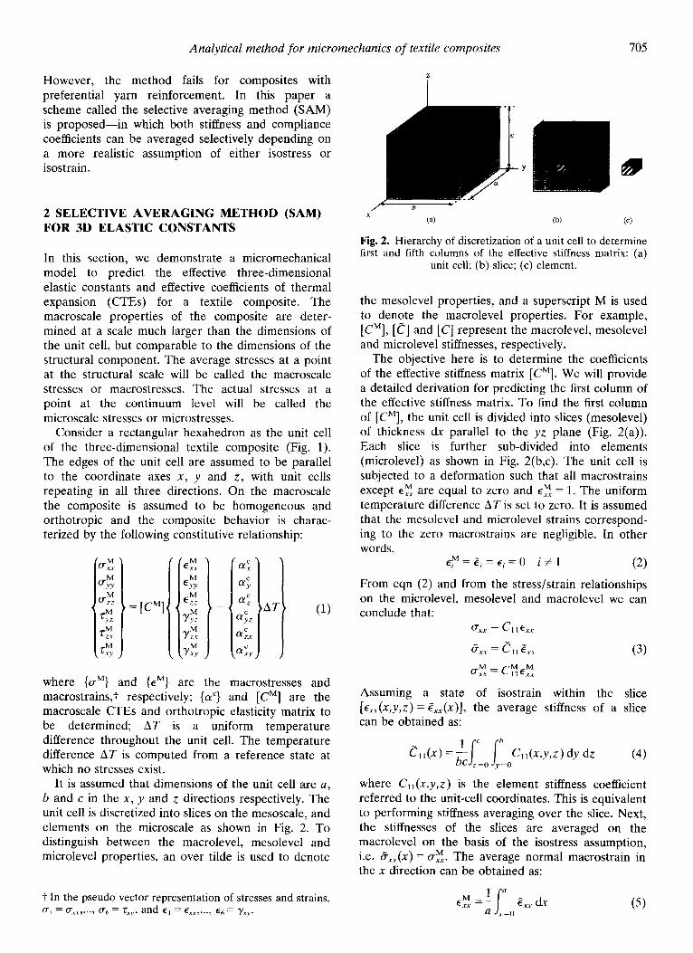
l Example 4: plain-weave textile composite (Fig. 5(a))-yarn geometry and properties obtained from Dasgupta et a1.;3

l Example 5: plain-weave textile composite-yarn geometry and properties obtained from Naik;17

l Example 6: 5harness satin weave (Fig. 5(b))- yarn geometry and properties obtained from Naik.17

For the textile composite examples (Examples 4-6), the yarn was assumed to be transversely isotropic and the matrix material as isotropic. The constituent material properties for the examples are listed in Table 1.

Before we discuss the numerical results, some finer points of the numerical computations and limitations of the present method will be discussed. The expressions for the elastic constants given in eqns (lo),

(13), (33), (34), (37) and (38) and other similar expressions are exact within the framework of assumptions made about the state of stress or strain at various levels. Thus the numerical method is only used to evaluate the integrals in the aforementioned expressions. For the purpose of numerical integration the unit cell is discretized into L x M x N hexahedral

(a>

(b>

Fig. 5. Yam pattern in textile preforms (unit-cell boundary in dotted lines): (a) plain weave; (b) 5-harness satin weave.


Table 1. Properties of constituent materials for Examples l-6

Example 1

Example 2

Example 3

Example 4

Examples 5, 6

Layer 1 (E-glass): Layer 2 (epoxy): Unit-cell size:

Fiber (E-glass): Matrix (epoxy): Unit-cell size:

Fiber (E-glass): Matrix (epoxy): Unit-cell size:

Yarn (glass/epoxy):

Matrix (epoxy): Unit-cell size:

Yarn (graphite/epoxy):

Matrix (epoxy): Unit-cell size:

E, = 70 GPa, y1 = 0.200, LYE = 5 X 1Om6 “Cl, VI = 0.5 E, = 3.50 GPa, yZ = 0.350, (Ye = 60 X 10mh ‘C’, V, = 0.5 0.500 mm X 0.500 X 0.256 mm

E, = 100 GPa, Ye = 0.3, aI = 10 x 10mh ‘C-l, V’ = 0.6 E, = 10 GPa, Y, = 0.3, (Y, = 100 x 10mh ‘C-’ 10~mX10~mX10~m

E, = 70 GPa, vf = 0.200, (Ye = 5 x 10mh ‘C’, V, = 0.6 E, = 3.50 GPa, v, = 0.350, (Y, = 60 X 10eh “C’ 10~mX10~mX10~m

E, = 58.61 GPa, E, = 14.49 GPa, GLT = 5.38 GPa, Y LT = 0.250, vTT = 0.247, (Y,_ = 6.15 x 1O-6 ‘C-l, (Ye = 22.64 x 10mh ‘C-l, v, = 0.26 E = 3.45 GPa, v = 0.37, (Y = 69 x 10mh ‘C-’ 1.680 mm X 1.680 mm X 0.228 mm

EL = 144.80 GPa, E, = 11.73 GPa, G, = 5.52 GPa, V ,_T = 0.23Ov, = 0.300, a,_ = -0.324 x lo-” VI, LYE = 14.00 x 10mh ‘C’, V, = 0.64 E = 3.45 GPa, v = 0.35, (Y = 40 X 10eh ‘C’ 2.822 mm X 2.822 mm X 0.2557 mm (Example 5); 7.055 mm X 7.055 mm X 0.2557 mm (Example 6)

y is the volume fraction of the constituent material.

elements. The integrands, which are various material stiffness coefficients C,, are assumed to be uniform over each element. The coordinates of the center of the hexahedron decide whether an element is a matrix element or a yarn element. Thus the information on the yarn architecture is used only to determine the material at a given integration point, and also to transform the yarn properties to the xyz coordinate system. In the numerical examples presented below, L, M and N were selected such that each element is a cube and the minimum of L, M and N was equal to 10. This number was arrived at after checking for convergence of results for a unidirectional fiber composite.

From the integral expressions (e.g. eqn (lo)), it can be seen that [CM], the stiffness matrix of the homogenized composite, is obtained by computing the weighted sum of the microscale [C] where the weights are positive numbers. For example, in eqn (lo), CE and c,, are both positive. Hence the positive definiteness of [C] is preserved even at the macroscale.

4.1 Results for continuum model A code called ~TEx-20 (pronounced as microtech) was written in FORTRAN 77 to implement SAM. The code was executed to estimate the thermoelastic constants for the six examples. Input to the code were the unit-cell dimensions, yarn geometry information, constituent material properties, and the number of divisions required to discretize the unit cell in the x, y and z directions. The user input to the code is presented in detail in ‘. The element stiffness matrix [C] was determined by computing the elasticity matrix

for the material point at the geometric center of the element, and transforming it to the unit-cell coordinate system. The predicted macroscale stiffness matrix, [CM17 and consequently the macroscale compliance matrix, will not be symmetric owing to the approximate nature of the analysis. Therefore, the macroscale compliance matrix was made symmetric by averaging the off-diagonal compliance coefficients. The macroscale elastic constants were computed by comparing the symmetricized compliance coefficients with that of a homogeneous, orthotropic medium. The thermoelastic constants for the examples were also computed with a three-dimensional finite-element analysis code called PTEx-10. In the finite-element procedure,’ exact periodic displacement and traction boundary conditions were imposed between opposite surfaces of the unit cell.

The results for a bimaterial medium (Example 1) are given in Table 2. The bimaterial medium is an infinite solid consisting of two different layers of equal thickness, stacked alternately in the z direction. The exact solution for the bimaterial medium was obtained by rule-of-mixtures type formulas, the details of which may be found in ‘. It can be observed that SAM marginally underpredicts the longitudinal and transverse Young’s moduli, while the in-plane and transverse shear moduli are exact. Table 3 presents the SAM results for two cases of unidirectional composite (Examples 2 and 3). The fiber and matrix have identical Poisson’s ratio in Example 2, and different Poisson’s ratio in Example 3. The SAM results were compared with the finite-element results and with analytical solutions for unidirectional composite properties. The analytical expressions used


Table 2. Continuum properties for Example 1

Example 1 SAM 36.02 8.72 2.48 15.23 0.599 0,183 3.88 52.20 (bimaterial FEA 36.79 9-79 2.48 15.23 0.312 0.208 8.19 59.60 medium) Exact 36.79 9.79 2.48 15.23 0.312 0.208 8.19 59.60

solution

Table 3. Continuum properties for Examples 2 and 3

(&a)

Example 2 SAM 64 (unidirectional FEA 63.55 composite) Rule of mixtures/ 64

Halpin-Tsai equations

Example 3 SAM 43.35 (unidirectional FEA 43.12 composite) Rule of mixtures/ 43.40

Halpin-Tsai equations

($a)

50.24 0.45 8.36 0.341 0.300 12.41 21.51 36.48 12.93 9.94 0.300 0.232 15.74 40.79 34.55 11.26 13.29 0.300 0.300 15.63 55.11

32.47 4.13 3.04 0.245 0.218 7.40 11.60 18.15 5.59 3.92 0.242 0.222 7.40 25.44 14.79 4.45 5.91 0.260 0.252 6.77 34.24

were the rule of mixtures and Halpin-Tsai equations for elastic constants, and Schapery’s expressions for CTEs.” All of the unidirectional composite thermoelastic constants but for the transverse modulus and transverse CTE (ET and czT) were found to match well with the compared data. Table 4 compares the SAM results for three textile composites (Examples 4, 5 and 6) with available analytical and experimental results. In all three cases the thermoelastic constants obtained by implementing SAM were in good agreement with the available results.

4.2 Results for plate model One of the objectives of this paper is to show that the plate stiffness properties of thin textile composites cannot be predicted from the continuum properties and plate thickness. This aspect was also highlighted by Marrey and Sankar,* where the authors performed a detailed finite-element analysis of the unit cell. The SAM procedure for the plate stiffness coefficients and plate CTEs was implemented in the code ~TEx-20. The computed plate thermoelastic coefficients for the examples are listed in Tables 5-7. The plate

Table 4. Continuum properties for Examples 4, 5 and 6

Gn G,, (Gpa)

Example 4 SAM 12.46 6.62 1.64 1.67 0.399 0.162 29.10 68.48 (plain weave) FEA 11.81 6.14 1.84 2.15 0.408 0.181 28.36 79.57

Dasgupta et a1.3 14.38 6.25 1.94 3.94 0.463 0.167 22.50 86.00

Example 5 SAM 63.41 11.13 3.79 4.24 0.402 0.027 1.36 21.53 (plain weave) FEA 53.61 10.88 4.41 4.72 0.365 0.128 1.56 22.71

Naik” 64.38 11.49 5.64 4.87 0.396 0.027 1.33 20.71 Test (Ref. 19) 61.92 - - - - 0.110 -

Example 6 SAM 69.30 11.62 4.06 4.73 0.355 0.031 1.21 20.25 (5-harness FEA 64.51 11.33 4.45 4.85 0.329 0.047 1.55 22.03 weave) Naik” 66.33 11.51 4.93 4.89 0.342 0.034 1.46 21.24

Test (Ref. 19) 69.43 - - 5.24 - 0.060 - -


Table 5. Non-zero [A], [B] and [D] coefficients for bimaterial plate

A,,,& A,, A66 B,,,&* B,, 46 D,,,&* 4, 46 opr, (Ypy (X106) (XIOh) (X106) (XIOS)

P”,. P”, (~10~) (x10-') (xIo~') (~10~~) (~10~‘) (xlOP”C’) (‘C’m~~‘)

SAM

FEA

Lamination theory

for two plies

Lamination theory

using continuum

elastic constants

9.844 2.045 3.899 -0.565 -0.108 -0.228 53.721 11.163 21,282 17,828 0.170 9.832 2.043 3.895 -0,563 - 0.108 -0.228 53.590 11.149 21,220 17.800 0.170 9.832 2.043 3.895 -0,563 -0.108 -0.228 53.573 11.131 21,220 17,814 0.170

9.844 2.048 3.899 OWMl 0~0000 0~0000 S3.762 11.183 21,293 8.190 0~0OOQ

Note: [A], [B] and [D] coefficients in SI units.

properties for the bimaterial case are presented in obtained with two-ply lamination theory. For the Table 5. In this case the bimaterial plate consisted unidirectional composite examples (Table 6), SAM only of two layers-one layer for each material. The was able to predict the [A] matrix coefficients (except bimaterial plate properties were also computed by for A& Dll, and the plate CTEs very well. However, using the lamination theory for two plies, from the SAM overpredicted D12 and OX2 and underpredicted continuum elastic constants presented in Table 2, and the coefficient DG6. For the textile composite examples a finite-element analysis.8 The SAM results for the (Table 7), SAM predicted all but Al2 and D12 with bimaterial plate were exact, i.e. identical to the results very good accuracy. It can be seen from Table 7 that

Table 6. Non-zero [A], [B] and [D] coefficients for single-ply unidirectional composite (Examples 2 and 3)

A,, (ok)

42 46 4, DE D Doh a” x (X106) (X106) (X106) (xlo-6) (X10_“) (Xl?) (XP) (X10_

Q “C ‘) (xlo~+‘)

Example 2 SAM 0.688 0.175 0.475 0.102 3.750 1,029 3.112 0,541 14.476 24.750 (unidirectional FEA 0,690 0.149 0.496 0.177 3.589 0,596 1.980 0,947 15,489 26.184 composite) Halpin-Tsai equations 0,673 0.109 0.363 0.113 5.606 0.908 3.026 0,939 15.625 55.112

and lamination

theory

Example 3 SAM 0443 0.074 0.261 0,040 2.308 0446 1.799 0,195 6.628 13,076 (unidirectional FEA 0.452 0,062 0.285 0,114 2.256 0.224 0.873 0.568 7,378 13,188 composite) Halpin-Tsai equations 0.444 0,039 0,151 0.045 3.702 0.328 1.262 0,371 6.774 34,239

and lamination

theory


Table 7. Non-zero [A], [B] and [D] coefficients for textile composite examples

Am+ 42 46 B,, 2 2 PP (X10) (X106) (X106)

(xlo3) Y;yo%; (x:2’) (x;;X) (x10~60.cy-L) (“C-l;-‘)

2.667 0446 0.379 oaooo 6,017 1,590 1,360 27.505 omlo

2.681 0.565 0.489 04000 5,687 1.518 1.577 21.465 oaKlo

2.783 0.503 0.490 04000 12,054 2.177 2.124 28.363 omoo

12.215 0.577 1.095 0~0000 44.782 2.133 4,398 1.994 04OiXl

12.090 3.470 1.223 0~0000 41.695 0.373 5.879 1.480 04000

13.938 1,787 1.208 oGiloo 75.942 9.734 6.582 1.556 omoo

16.039 0.631 1.209 0+90” 81,164 3.307 5.868 2.422

14.683 1.351 1.210 0.495” 90.072 1,123 6.149 2.910

16.531 0.770 1.239 oG?ilo 87.283 4.195 6.753 1.550

Example 4

(plain weave)

SAM

FEA

Lamination theory

using continuum

constants

Example 5

(plain weave)

SAM

FEA

Lamination theory

using continuum

constants

Example 6 SAM

(S-harness weave) FEA

Lamination theory

using continuum

constants


“In Example 6, B,, = -B,,, and p”, = -P’,.


the plate stiffness coefficients and plate CTEs

computed from the continuum elastic constants and CTEs are different from those computed using a direct

micromechanical procedure.

ACKNOWLEDGEMENTS

This research was supported by the NASA Langley Research Center grant NAG-l-1226 to the University

of Florida. The authors are thankful to C. C. Poe Jr and Wade C. Jackson of NASA/LaRC for their

constant encouragement.

REFERENCES

1.

2.

3.

4.

5.

6.

Sharma, S. K. and Sankar, B. V., Effects of through-the-thickness stitching on impact and interlaminar fracture properties of textile graphite/epoxy laminates. NASA CR-195042, National Aeronautics and Space Administration, Washington, DC, 1995. Yoshino, T. and Ohtsuka, T., Inner stress analysis of plane woven fiber reinforced plastic laminates. Bull. LYME, 1982,25,485-492. Dasgupta, A., Bhandarkar, S., Pecht, M. and Barkar, D., Tbermo-elastic properties of woven-fabric composites using homogenization techniques, In Proc. Ameri- can Society for Composites 5th Technical Conf: Lansing, MI. Technomic, Lancaster, PA, 1990, pp. 1001-1010. Whitcomb, J. D., Three-dimensional stress analysis of plain weave composites. In Composite Materials Fatigue and Fracture (Vol. 3), ASTM STP 1110. American Society for Testing and Materials, Philadelphia, PA, 1991, pp. 417-438. Foye, R. L., Approximating the stress field within the unit cell of a fabric reinforced composite using replacement elements. NASA CR-191422, National Aeronautics and Space Administration, Washington, DC, 1993. Cox, B. N., Carter, W. C. and Fleck, N. A., A binary model of textile composites-I. Formulation. Acta Metall. Mater., 1994, 42, 3463-3479.

7.

8.

9.

10.

11.

12.

13.

14.

15.

16.

17.

18.

19.

Sankar, B. V. and Marmy, R. V., A unit-cell model of textile composite beams for predicting stiffness properties. Compos. Sci. Technol., 1993, 49,61-69. Marrey, R. V. and Sankar, B. V., Micromechanical models for textile structural composites. NASA CR-198229, National Aeronautics and Space Admin- istration, Washington, DC, October 1995. Yang, J. M. and Chou, T. W., Performance maps of textile structural composites. In Proc. 6th Int. Conf on Composite Materials (ICCM VI), Vol. 5. 1987, pp. 579-588. Ishikawa, T. and Chou, T. W., Elastic behavior of woven hybrid composites. J. Compos. Mater., 1982, 16, 2-19. Ishikawa, T. and Chou, T. W., One-dimensional micromechanical analysis of woven fabric composites. AZAA J., 1983,21,1714-1721. Ishikawa, T. and Chou, T. W., In-plane thermal expansion and thermal bending coefficients of fabric composites. J. Compos. Mater., 1983, 17, 92-104. Yang, J. M., Ma, C. L. and Chou, T. W., Fiber inclination model of three-dimensional textile composite structures. J. Compos. Mater., 1986, 20, 472-484. Whitney, T. J. and Chou, T. W., Modeling of 3-D angle-interlock textile composite structures. J. Compos. Mater., 1989, 23, 890-911. Ma, C. L., Yang, J. M. and Chou, T. W., Elastic stiffness of three-dimensional braided textile structural composites. In Composite Materials: Testing and Design (7th Conference), ASTM STP 893. American Society for Testing and Materials, Philadelphia, PA, 1986, pp. 404-421. Whitney, J. M., A laminate analogy for micromechanics. In Proc. American Society for Composites 8th Technical Conference, Cleveland, OH. Technomic, Lancaster, PA, 1993, pp. 785-794. Nalk, R. A., Analysis of woven and braided fabric reinforced composites. NASA CR-194930, National Aeronautics and Space Administration, Washington, DC, 1994. Agarwal, D. A. and Broutman, L. J., Analysis and Performance of Fiber Composites. John Wiley, New York, 1990. Foye, R. L., Finite element analysis of the stiffness of fabric reinforced composites. NASA CR-189597, Na- tional Aeronautics and Space Administration, Washin- gton, DC, 1992.

Documents

ANALYTICAL METHOD FOR MICROMECHANICS OF TEXTILE …