Embed Size (px)
Citation preview

AD-AII6 508 MECHANICAL TECHNOLOGY INC LATHAM NY RESEARCH AND 0EV--ETC F/6 7/4ANALYTICAL FERROGRAPHY STANDARDIZATION. (U)JAN 82 P A SENHOLZI, A S MACIEJEWSKI N0001-81-C 0012
UNCLASSIFIED MTI-82TR56 NL1E hEEEEEEEEEEEIIEIIIEEEEIIEEIIEEIIEEEIIEEEEEEIIIEEIIEEEEIIEEEEEEEIIIIIIIIEEEEIIIIE

I g&-J-
I ii
Mwl jutio7 Unimte
SMechanical Technology Incorporated
Research and Development Division
ReerhadDvlpetDvso

I
FINAL REPORT
ANALYTICAL FERROGRAPHY STANDARDIZATION
Prepared For:
OFFICE OF NAVAL RESEARCH
ARLINGTON, VIRGINIA 22217
CONTRACT NOOO14-8 1-C-0012
JANUARY 1982I m
IN
Approvs-co pubh I

I j Final Report
MTI Technical Report No. 82TRS6
ANALYTICAL FERROGRAPHY STANDARDIZATION
P. B. Senholzi
A. S. Maciejewski
Applications EngineeringMechanical Technology Incorporated
Annapolis, Maryland
Contract N00014-81-C-0012
January 1982

Unclassified
'ECuP.ITY CLASSIFICATION OF THIS PAGE (When Data Entered)PAEREAD INSTRUCTIONS
REPORT DOCUMENTATION PAGE BEFORE COMPLETING FORM1. REPORT NUMBER 2. GOVT ACCESSION NO. 3. RECIPIENT'S CATALOG NUMBER
9 c,
4. TITLE (and Subtitle) S. TYPE OF REPORT & PERIOD COVERED
Analytical Ferrography Standardization Final Report
6. PERFORMING ORG. REPORT NUMBER
7. AUTHORte) I. CONTRACT OR GRANT NUMBER(*)
P. B. Senholzi ONRA. S. Maciejewski N00014-81-C-0012
9. PERPFORMING ORGANIZATION NAME AND ADDRESS 10. PROGRAM ELEMENT. PROJECT. TASK
Applications Engineering AREA & WORK UNIT NUMBERS
Mechanical Technology Incorporated1656 Homewood Landing RoadAnnapolis, Maryland 21401
II. CONTROLLING OFFICE NAME AND ADDRESS 12. REPORT DATE
Office of Naval Research January 1982
Code 431 is. NUMBER OF PAGES
Arlington, Virginia 2221714. MONITORING AGENCY NAME a AODREsS(iI different from Controlling Office) IS. SECURITY CLASS. (of this report)
Unclassified
15a. DECLASSIFICATION/DOWNGRAOINGSCHEDULE
16. DISTRIBUTION STATEMENT (of this Report)
Approved for public release; distribution unlimited
17. DISTRIBUTION STATEMENT (of the abetrect entered in Block 20, It different free, Report)
IS. SUPPLEMENTARY NOTES
19. KEY WORDS (Continue on Pewers* aide it noceceary and Identify by block number)
Ferrography Wear Debris Analysis Equipment Health MonitoringTribology LubricationDiagnostics Contamination
20. ABSTRACT (Continue an reerse old* t neceaeay and Identify by block trnueb)
> Wear particle technology is a recent development in the equipment wearfield. This technology is based on the analysis of wear debris as a nonde-structive reflection of the surface wear condition of the respective monitoredwear process. Such a monitoring approach can be applied to everything from
simple wear testing to sophisticated multicomponent wear systems. Wear particle
analysis technology is rapidly establishing itself as a valuable tool in both
the wear prevention and wear control arenas.e-
DD I JA N7 1473 EDITION OF I NOV65 IS OBSOLCT9 UnclassifiedSI, 0107.1 F.01A.AAA1

TABLE OF CONTENTS
Section Title Page
LIST OF FIGURES................................................... iv
LIST OF TABLES................................................... vii
FORWARD........................................................... viii
ABSTRACT.......................................................... ix
1.0 INTRODUCTION...................................................... 1
2.0 BACKGROUND........................................................ 2
3.0 TECHNICAL APPROACH................................................ 5
4.0 PROGRAM RESULTS.................................................. 32
5.0 PROGRAM STATISTICAL SUMMARY AND CONCLUSIONS..................... 94
6.0 NAVAL ANALYTICAL FERROGRAPHY STANDARDIZED PROCEDURE.............. 97
7.0 NAVAL FERROGRAPHY VERIFICATION PROGRAM RECOMMENDATIONS........... 98
8.0 REFERENCES........................................................ 99
APPENDIX A -INTERIM DRAFT. NAVAL ANALYTICAL FERROGRAPHY
STANDARDIZED PROCEDURE............................. A-1
2
I),"1.
iii -,2

LIST OF FIGURES
Figure No. Title Page
1. Phase I Stage I - Ferrography Verification Flow Chart ..... 7
2. Phase I Stage I - Analysis Summary ........................ 9
3. Phase I Stage II - Ferrography Verification Flow Chart .... 10
4. Phase I Stage II - Analyses Summary ....................... 11
5. Phase II Stage I - Ferrography Verification Flow Chart .... 13
6. Phase II Stage I Summary - Analyses Summary ............... 14
7. Phase II Stage II - Slide Distribution and Analysis ....... 15
8. Phase II Stage II Summary - Analyses Summary .............. 16
9. Data Plots ................................................ 20
10. Analysis of Variance Ferrography Data ..................... 21
11. Coefficients of Variation Analysis - Sample Distributions
and Laboratories .......................................... 23
12. Accuracy as a Function of Repeatability to a True Value ... 25
13. USR Standard .............................................. 26
14. Graphical Evaluation Analysis (Sample) .................... 27
15. Graphical Evaluation: MTU/Mineral/Light/X-Mitted/
New Method ................................................ 29
16. Graphical Evaluation: MTU/Mineral/Heavy/X-Mitted/
New Method ................................................ 30
17. Phase I Stage I - Data Plots: MTU Mineral/Light .......... 33
18. Phase I Stage I - Data Plots: NAEC Synthetic/Medium ...... 34
19. Phase I Stage I - Data Plots: OSU Hydraulic/Heavy ........ 35
20. Phase I Stage I - Sample Distributions: Lighting ......... 36
21. Phase I Stage I - Sample Distributions: Positioning
Method .................................................... 37
22. Phase I Stage I - Sample Distributions: Types of Oil ..... 39
23. Phase I Stage I - Sample Distributions: Laboratories ..... 40
24. Phase I Stage I - Coefficient of Variation: Intra-
Laboratory ................................................ 43
25. Phase I Stage I - Coefficient of Variation Sample
Distributions: Concentrations ............................ 44
26. Phase I Stage I - Coefficient of Variation Sample
Distributions: Lighting .................................. 45
iv

LIST OF FIGURES (Continued)
Figure No. Title Page
27. Phase I Stage I - Coefficient of Variation Sample
Distributions: Positioning Method ........................ 46
28. Phase I Stage I - Coefficient of Variation Sample
Distributions: Laboratories .............................. 47
29. Phase I Stage I - Graphical Regression Analysis Plots:
Light/Transmitted ......................................... 50
30. Phase I Stage I - Graphical Regression Analysis Plots:
Medium/Transmitted ........................................ 51
31. Phase I Stage I - Graphical Regression Analysis Plots:
Heavy/Transmitted ......................................... 52
32. Phase I Stage I - Distribution of Discriminations ......... 53
33. Phase I Stage II - Data Plots: MTU Mineral/Light ......... 54
34. Phase I Stage II - Data Plots: NAEC Synthetic/Medium ..... 55
35. Phase I Stage II - Data Plots: MTU Mineral/Heavy ......... 56
36. Phase I Stage II - Graphical Regression Analysis Plots:
Light/Reflected ........................................... 59
37. Phase I Stage II - Graphical Regression Analysis Plots:
Medium/Reflected .......................................... 60
38. Phase I Stage II - Graphical Regression Analysis Plots:
Heavy/Reflected ........................................... 61
39. Phase I Stage II - Distribution of Discriminations ........ 62
40. Phase II Stage I - Data Plots: NAEC Synthetic ............ 64
41. Phase II Stage I - Data Plots: NAEC Synthetic ............ 65
42. Phase II Stage I - Data Plots: NAEC Synthetic ............ 66
43. Phase II Stage I - Data Plots: NAEC Synthetic ............ 67
44. Phase II Stage I - Sample Distributions: Types of Oil .... 68
45. Phase II Stage I - Sample Distributions: Laboratories .... 69
46. Phase II Stage I - Sample Distributions: Laboratories -
Slide Position No. I ...................................... 70
47. Phase II Stage I - Sample Distributions: Laboratories -
Slide Position No. 5 ...................................... 71
v

LIST OF FIGURES (Continued)
Figure No. Title Page
48. Phase II Stage I - Sample Distributions: Laboratories -
Slide Position No. 10 ..................................... 72
49. Phase II Stage I - Coefficient of Variation Sample
Distributions: Types of Oil .............................. 74
50. Phase II Stage I - Coefficient of Variation Sample
Distributions: Laboratories .............................. 75
51. Phase II Stage I - Graphical Regression Analysis Plot ..... 77
52. Phase II Stage I - Graphical Regression Analysis Plot ..... 78
53. Phase II Stage I - Graphical Regression Analysis Plot ..... 79
54. Phase 11 Stage I - Distribution of Discriminations ........ 81
55. Phase II Stage II - Data Plots: MTU Mineral .............. 82
56. Phase II Stage II - Data Plots: OSU Hydraulic ............ 83
57. Phase II Stage II - Data Plots: NAEC Synthetic ........... 84
58. Phase II Stage II - Sample Distributions: Laboratories ... 85
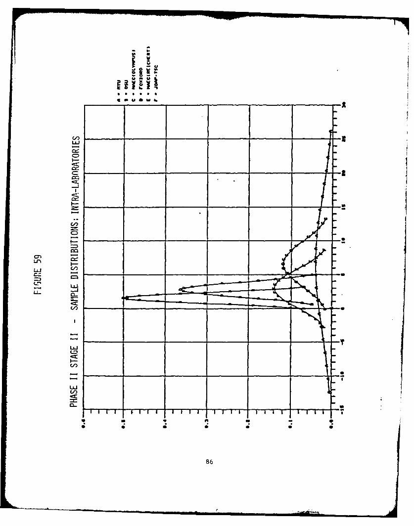
59. Phase 11 Stage II - Sample Distributions: Intra-
Laboratories .............................................. 86
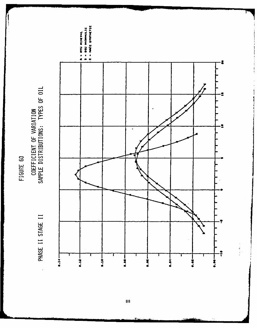
60. Phase II Stage II - Coefficient of Variation Sample
Distributions: Types of Oil .............................. 88
61. Phase II Stage II - Graphical Regression Analysis Plot .... 90
62. Phase II Stage II - Graphical Regression Analysis Plot .... 91
63. Phase II Stage II - Graphical Regression Analysis Plot .... 92
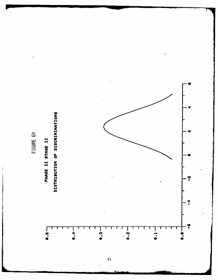
64. Phase II Stage II - Distribution of Discriminations ....... 93
vi

LIST OF TABLES
Table Title Page
1 Phase I Stage I - Analysis of Variance Ferrography Data ....... 41
2 Phase I Stage I - Coefficient of Variation Interlaboratory .. 48
3 Phase I Stage 11 Coefficient of Variation
Interlaboratory ............................................... 58
4 Phase II Stage I - Coefficient of Variation
Interlaboratory ............................................... 76
5 Phase 11 Stage 11 - Coefficient of Variation
Interlaboratory ............................................... 89
vii

FORWARD
This report presents the results of a study conducted by Mechanical Tech-
nology Incorporated (MTI) for the Office of Naval Research (ONR) under Con-
tract N00014-81-C-0012. This study was based on the standardization of Ana-
lytical Ferrography.
The work was performed under the direction of Lt. Cdmr. H. Martin and Mr.
M. K. Ellingsworth, Navy Program Managers. Mr. Peter Senholzi was the Program
Manager for the contract at MTI, with Mr. Alan Maciejewski serving as Project
Engineer.
The authors wish to acknowledge the program assistance provided by Mr. H.
Martin, Mr. R. Miller, and Mr. M. K. Ellingsworth of the Navy. Appreciation
is also extended to personnel from Oklahoma State University, Foxboro Analytical.
Michigan Technological University, National Bureau of Standards, Joint Oil
Analysis Program Technical Support Center, and the Naval Air Engineering Cen-
ter for their program participation and extensive contributions.
viii

ABSTRACT
Wear particle technology is a recent development in the equipment wear
field. This technology is based on the analysis of wear debris as a nonde-
structive reflection of the surface wear condition of the respective monitored
wear process. Such a monitoring approach can be applied to everything from
simple wear testing to sophisticated multicomponent wear systems. Wear particle
analysis technology is rapidly establishing itself as a valuable tool in both
the wear prevention and wear control arenas.
Analytical Ferrographic analysis is a relatively new approach to the analy-
sis of wear debris. Until recently, this technique has been utilized as a re-
search tool in a limited number of laboratory facilities. However, as a result
of initial successful utilization, Ferrographic technology is receiving ever
increasing interest. This increasing interest level has raised serious ques-
tions with respect to standardization and repeatability.
This report describes an effort to quantify and apportion Analytical Ferro-
graphy repeatability/nonrepeatability. Under a program sponsored by the Office
of Naval Research, six leading laboratories contributed controlled Analytical
Ferrographic analysis data. This data has been analyzed and the resulting re-
peatability/nonrepeatability assessed with respect to analysis variables.
ix

1.0 INTRODUCTION
Mechanical system availability, efficiency, and life are functions of both
structural integrity and wear integrity. Emphasis to date has been placed on
structural integrity, with a "throw away" philosophy accommodating the conse-
quences of low wear integrity. Recent resource limitations, however, have
prompted substantial interest into the area of wear integrity optimization.
This optimization process is approached through the interdisciplinary technology
of tribology. Tribological technology involves both the wear aspects of preven-
tion and control. Wear prevention occurs primarily in the equipment design
process, while wear control is primarily instituted in the operational arena.
Wear particle technology is a relatively recent development in the equip-
ment wear field. This technology is based on the analysis of wear debris as a
nondestructive reflection of the surface wear condition of the respective mon-
itored wear process. Such a monitoring approach can be applied to everything
from simple wear testing to sophisticated multicomponent wear systems. Wear
particle analysis technology is rapidly establishing itself as a valuable tool
in both the wear prevention and wear control arenas. In order to fully realize
the potential of wear particle analysis technology, additional research efforts
must be implemented in order to enhance and expand the technology.
Analytical Ferrographic analysis is a relatively new approach to the analy-
sis of wear debris. Until recently, this technique has been utilized as a re-
search tool in a limited number of laboratory facilities. However, as a result
of initial successful utilization, Ferrographic technology is receiving increas-
ing interest. This increasing interest level has raised serious questions with
respect to standardization and repeatability.
This program deals with the standardization of Analytical Ferrography.
Primary emphasis is directed at the quantification of Ferrographic repeatabil-
ity, variation apportionment between respective significant contributing fac-
tors, and the development of a standardized procedure.
II

2.0 BACKGROUND
Analytical Ferrography is based on the magnetic precipitation and subse-
quent analysis of wear debris from a lubricant sample. The approach utilized
involves passing a volume of lubricant over a glass substrate which is supported
over a magnetic field. Permanent magnets are arranged in such a way as to cre-
ate a varying field strength over the length of the substrate. This varying
strength results in the precipitation of wear debris (magnetic and ferromag-
netic) in a distribution with respect to size/mass over the substrate length
(approximately 55 mm). Once rinsed and fixed to the substrate, this deposit
serves as an excellent media for optical analysis of the composite wear partic-
ulates.
Ferrographic substrate deposit analysis involves the characterization of
debris quantity, distribution, elemental composition, and morphology. This
total analysis effort involves both quantitative and qualitative assessments.
Quantitative assessments are derived for quantity and size distribution
characterization utilizing a light reflected/light transmitted type densito-
meter. These assessments are registered by indicating the percentage of blocked
area in a particular microscopic field of view. Readings are taken over the
length of the substrate deposit in order to characterize debris size distribu-
tion.
Elemental composition and morphological debris assessments are very quali-
tative in nature. They involve the manual characterization of debris deposits
relying on observations conducted through an optical microscope.
This deposition and assessment process involves a multitude of variables.
Such aspects as sample preparation, sample dilution, sample volume, sample vis-
cosity, debris concentration, densitometer type, densitometer calibration, mea-
surement approach, measurement indexing, and debris distribution, all affect
Ferrographic assessment results. These aspects can be generally categorized in
three groups:
" technique/procedure,
" equipment, and
" operator.
2

In the initial stages of Ferrographic analysis, it was left up to each
individual laboratory to address the numerous analysis variables.
2.1 The Technical Cooperative Program
During the mid 1970's, an international committee was established under The
Technical Cooperative Program (TTCP) with the objective of fostering equipment
health monitoring. A prime emphasis area of this committee was wear particle
analysis and specifically Ferrographic Analysis. As part of this committee's
efforts, lubricant samples were distributed among participating laboratories,
for wear debris analysis. Upon comparing sample analyses, it became apparent
that slide variations existed between laboratory results. Further investiga-
tions revealed that at least a portion of this variation was due to individually
developed/tailored Ferrographic procedures. No variation apportionment could be
made, however, between procedure, operator, and equipment. Thus, a significant
standardization and repeatability problem was identified. This problem was
intensified by the fact that Ferrography was being applied by an ever increasing
number of organizations in a variety of applications.
2.2 Navy Standardized Procedures
As a first step in attacking the problems of Ferrographic standardization,
the Navy proceeded to generate a preliminary detailed Ferrographic Procedure.
Due to procedural controversies, dual procedural approaches were included for
density lighting technique and density reading indexing approaches.
In order to verify this procedure, clarify controversial dual approaches,
quantify repeatability, and identity respective significant contributing fac-
tors, a "round robi." sample analysis exercise was established between six major
wear particle analysis facilities.
2.2.1 Verification Program
In order to verify the Preliminary Navy Analytical Ferrography Standardization
Procedure, a joint program was developed and supported by six laboratories;
3

Michigan Technological University, Oklahoma State University, Foxboro Analy-
tical, the Naval Air Engineering Center, National Bureau of Standards, and the
Joint Oil Analysis Program Technical Support Center. Sets of identical lubri-
cant samples were distributed to each laboratory for analysis. Sample variables
consisted of lubricant type and debris concentration level. Laboratories were
directed to generate Ferrogram slides from each samples as per the preliminary
standardized procedure. Each slide was to be analyzed using all combinations of
suggested indexing and lighting techniques.
In conjunction with this effort, sample preparation variables were to be
eliminated by the circulation of sets of pre-made slides between each of the
laboratories. Each laboratory was to analyze the pre-made sets in the same
manner as outlined above.
Respective data has been generated by these six organizations and has been
subjected to an in-depth statistical treatment to be summarized in the following
discussions. This analysis was limited to Analytical Ferrography and did not
include either Direct Reading or In-Line Ferrographic Techniques.
4

3.0 TECHNICAL APPROACH
In order to adequately understand the statistical analysis of the verifi-
cation program, discussions of the pertinent variables, program organization,
and statistical tools will be presented.
3.1 Analysis Variables
As mentioned above, in order to verify the Preliminary Navy Analytical
Ferrography Standardized Procedure, a joint program was developed and supported
by several leading wear debris laboratories. A two phase "round robin" approach
was instituted. Each phase consisted of the analysis of fluid samples as well
as the analysis of pre-made Ferrograph slides.
Primary analysis variables addressed under this "round robin" exercise were
procedure, equipment, and operator/location. Secondary addressed variables
included; fluid type, debris concentration, debris size distribution, Ferrosco-
pic type, Ferrogram slide location, microscope lighting approach, and slide
indexing approach. Round robin test design incorporated both primary and sec-
ondary variable treatment.
3.2 Program Organization
The Naval Ferrography Verification Program was initiated in 1979. Under
the direction of the Office of Naval Research (ONR) Scientific Officer Lt. Cdmr.
H. Martin, the Naval Air Engineering Center (NAEC) was tasked to plan, organize,
and control a coordinated laboratory sample analysis effort, evaluating the
precision and repeatability of the Analytical Ferrographic equipment and respec-
tive procedure. Four facilities were initially selected to participate in this
effort. All were experienced in the Ferrography methodology and possessed the
desired technical expertise and professionalism to adequately perform in the
exercise. The four initial facilities and their representatives include:
I. Foxboro Analytical (FOX) - D. Anderson
2. Michigan Technological University (MTU) - Dr. J. Johnson
3. Naval Air Engineering Center (NAEC) - P. Senholzi
4. Oklahoma State University (OSU) - Dr. E. Fitch
5

After completion of Phase I of this program, a statistical analysis was
performed on the data generated. From this analysis certain preliminary con-
clusions were made. With the aid of these preliminary findings, ONR authorized
Mechanical Technology Incorporated (MTI) to plan, organize, and direct Phase II
of the verification program.
In addition to the four initial participants, two other organizations were
included in Phase II of the program. These organizations were:
1. Joint Oil Analysis Program Technical Support Center (JOAP-TSC) -
R. Lee
2. DOC National Bureau of Standards (NBS) - Dr. W. Ruff
At the conclusion of Phase II all data (including Phase I) were thoroughly
analyzed. In addition, a draft standardized procedure for Analytical Ferrogra-
phy was developed from this exercise in order to minimize error in technique
applications. As stated previously, the Naval Ferrography Verification Program
was performed in two separate phases. The following is a description of the
organization of each phase.
3.2.1 Phase I Organization
The initial phase of the program was directed and controlled by NAEC. This
phase was divided into a sample analysis stage and a slide analysis stage. Fig-
ure 1 illustrates the program organization during Stage I of this phase. The
three facilities responsible for providing fluid samples were selected on the
basis of their expertise. The three facilities, NAEC, MTU, and OSU, provided
three different types of fluids; synthetic lubricant, mineral lubricant, and
mineral-based hydraulic fluid, respecti,!ely. For each fluid type, the facility
provided sets of three samples containing wear debris of low, medium, and heavy
concentrations.
Each sample generating facility then distributed a complete set of their
respective fluid type samples to each of the participating analysis facilities,
while retaining a set for their analysis.
6

I z7"1
z0 -0
< 0 D
C):50 D cc <
LU 0~
LL_ /
0~ c3
CL 7

After receiving the three sets of fluid samples, each facility was to pre-
pare ferrograms of each sample type/concentration, according to a set of general
guidelines. Figure 2 illustrates the sample preparation and analysis activity
during Stage I. For each laboratory, three Ferrogram slides were made from each
sample bottle (nine total sample bottles). For each Ferrogram slide made, den-
sity reading sets were obtained four times. As a result, each laboratory pro-
duced 27 Ferrograms and 108 reading sets. When including all facilities, this
amounted to a total of 108 Ferrograms and 432 sets of readings.
After Stage I was completed, each facility was instructed to assemble a set
of four pre-made slides. The selected slide sets were first read by the gener-
ating laboratory and then packaged and distributed for analysis as indicated in
Figure 3. Each facility read each slide four times, as in Stage I, and for-
warded the set to the next facility. The slide sets were, at the conclusion of
the analysis sequence, returned to the respective generating facility in order
to verify that the slides did not degrade during transit. At the end of this
stage, a total of 320 reading sets were accomplished. The final breakdown by
fluid types for Stage II is summarized in Figure 4.
3.2.2 Phase II Organization
The second phase of the program was organized, directed, and controlled by
MTI. Based upon a detailed review of the data generated in the first phase,
certain portions of the initial program phase were revised or eliminated. With
the introduction of Phase II, a Ferrography procedure was provided for utiliza-
tion in the performance of the sample analysis as well as for solicitation
of critical comment.
As noted previously, two additional facilities were added to the study
during this second phase. As opposed to the first phase, sample distribution
was centrally coordinated by MTI. Three labs were solicited for bulk fluid
samples, as under Phase I, based on their experience with a particular fluid.
From MTU, NBS, and OSU, MTI received mineral lubricant, synthetic lubricant, and
mineral-based hydraulic fluid, respectively. Bulk fluid types were divided into
six sets of three bottles each, and subsequently distributed to the participating
8

ci,
-J< ci
-j
z 71 <M 0U
< D A
-r , C-4
U, C)
0n 0uj z
CD [CD
3z 0
0CC Z L cc0-r cocZ0 c O
olc'n C-4 co Zo
U)~ > < <C,,-
9 I- oJ~ g*u 0 -
0- Z0 C1 - U v 9
M cr cc

~c
S-J
() <a.
- -rr
-- LU
0D od UD U0
IL j 0-' U. 0 0 <:
I - >--C
U-10

M C,> >T T
U., ww
LL (0 0--
-5 2
-11 =ZU U) yU)U0 z
w) LU
Rip > -(0> >< cn z
-Ucc L c
0D CD
Cl)>>>< >
= 0 0

facilities, as illustrated in Figure 5. Upon receipt of the sample set, each
facility was instructed to prepare five Ferrogram slides from each sample bottle
for a total of fifteen Ferrograms per facility. For each of the fifteen Ferrograms,
five sequential reading sets were obtained, for a total of 75 reading sets per
facility. Figure 6 illustrates the output per facility as well as the final
tabulation by sample fluid type.
The data from Stage I of the second phase was then forwarded to MTI. This
data was statistically analyzed and presented at an interim review meeting of
the participants. At this meeting the participants also submitted their re-
spective Phase II, Stage I slides to MTI for distribution in Stage II of the
program. Participant comments and recommendations concerning the preliminary
standardized procedure were presented during this meeting.
Stage II of the second phase involved the distribution of a slide set,
assembled by MTI. This set consisted of two Ferrogram slides of each fluid type
for a total of six slides. The slides were marked with a code number so as to
avoid biasing the results of the participating laboratory. This slide set was
sent out by MTI to the first facility for analysis. Figure 7 indicates the
routing procedure for the slide set and corresponding results. For each slide,
five sequential reading sets were performed by each laboratory. This resulted
in 180 total reading sets or 60 reading sets per fluid type as summarized in
Figure 8.
Upon receipt of all data, MTI performed a statistical analysis and compared
the results to the previous program stages. In addition to the statistical
analysis, an interim draft of the Navy Analytical Ferrography Standardized Pro-
cedure was developed.
3.3 Statistical Approach
Respective Ferrographic analysis data were submitted to a central loca-
tion from each participating laboratory for each round robin phase. This data
consisted of sets of density readings for each sample/slide, indexed with
respect to Ferrogram slide location. Supporting information for each set was
12

z I I
z<0 11z ~ C/ 0-<I U -
0I I
o <cc cc I
LUCI
LL z
LL EE D
cLL
C/ c= c I a -Izc
<w j -I L
13

Ut
zCUC1
(D w
0 * - - 4C4C U, 4 Lf )
-z5
UD CD u Dw
P LLnu 0U
III NU Zr CCCNL ) .-40.I 0C L r
C/) cr c
-- (D Lc)L - zL -L)L)LnL nL ,-
< C,) zz
ccr
0 C0
< LU C4

U))
U) -
Lu 0
LU) _ __L Ln -n
Hz-0LL L
( wZ )-I o.c)10m
U) Cc :rw
<15

FIGURE 8
PHASE II - STAGE I SUMMARY
ANALYSES SUMMARY
* LABORATORY
JSALETIC HYDRAULIC]
2 SLIDES 2 SLIDES 2 SLIDES
5 5 READINGS 5 5 READINGS 5 5 READINGS
10 READINGS 10 READINGS 10 READINGS
30 READINGS PER FACILITY/LAB
6 LABS X 30 READINGS = 180 TOTAL
* SAMPLE FLUID TYPE
MIERLSYNTHETIC ] HYDRAULICl
10 10 10
10 10 10
10 6 LABS10 6 LABS 10 6 LABS
10 10 10)
10 10 10
10 10 10
60 READINGS 60 READINGS 60 READINGS
TOTAL - 180 READINGS
16
also submitted which included such items as volume of fluid analyzed, dilution
ratio, lighting approach, indexing approach, operator, and sample number.
Statistical analyses were performed on these data sets in order to determine
repeatability as well as apportion nonrepeatability among the competing sig-
nificant variables.
A four facet statistical format was applied to this data base. These
four facets included data plots (slide position versus normalized density),
analysis of variance, coefficient of variation analysis, and a graphical re-
gression analysis.
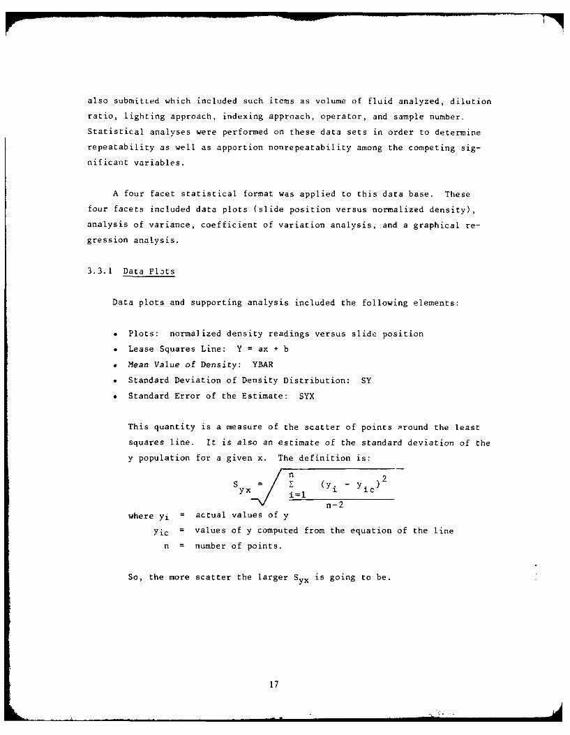
3.3.1 Data Pl3ts
Data plots and supporting analysis included the following elements:
" Plots: normalized density readings versus slide position
* Lease Squares Line: Y = ax + b
* Mean Value of Density: YBAR
* Standard Deviation of Density Distribution: SY
* Standard Error of the Estimate: SYX
This quantity is a measure of the scatter of points around the least
squares line. It is also an estimate of the standard deviation of the
y population for a given x. The definition is:
n-2where Yi = actual values of y
yic = values of y computed from the equation of the line
n = number of points.
So, the more scatter the larger Syx is going to be.
17

* Correlation Coefficient: r
This is a measure of the quantitative association between variables.
• Normal distribution graphs:
All the readings from each category (e.g. each lab) were treated, and
the mean and standard deviation were calculated. These numbers were
then substituted into the equation of a normal distribution:
1 (- 2f(x) = e 2S z
where x is the mean and Sx is the standard deviation.
Then the curves for all members of one category (e.g. all labs) were
superimposed. The axis of symmetry of each curve is at the mean
value, while the width of each curve is a function of the standard
deviation. The wider the curve, the more scatter there was in the
data.
A normal curve can also be interpreted like a histogram, e.g. fre-
quency as a funtion of value. Hence a short squat curve would result
from a wide range of values occurring at about the same frequency.
* Comparison Output:
The various factors in each category were compared as follows: the
mean and standard deviation for all readings from factor 1 (e.g. Lab 1)
were calculated, as were the same quantities from factor 2 (e.g. Lab 2).
There are standard statistical tests to determine, with a certain
degree of confidence, whether one can claim that the mean from factor
I readings is significantly different from the mean from the factor 2
readings, and likewise for standard deviation.
18

From these tests it was possible to claim with 95% confidence used
for example, that the mean of readings from Lab 1 is significantly
different from the mean of readings from Lab 2, and further, a range
of that diference can be calculated. We achieve an expression of the
form:
(XI, X2 are respective means; A, B are calculated.)
and this is what appears in the output.
For standard deviation, the expression involves a quotient:
SiA < - < B
- 2 -
(SI , S2 are respective s.d.; A, B are calculated), so the output indi-
cates that one standard deviation differs by a certain factor from
the other.
An example of the data plot is presented in Figure
3.3.2 Analysis of Variance
When several sources of variation are acting simultaneously on a set of
variations, the variance of the observations is the sum of the variance of the
independent sources. So, the total variance would be the sum of the variance
due to each independent factor, plus the remaining variance (called the resi-
dual) due to randomness. The variance of each factor, or group of factors, is
compared to the residual variance, and this quotient is compared with a table
value (F test) to tell whether a significant difference exists between factors.
Figure 10 represents an example of analysis of variance.
3.3.3 Coefficient of Variation Analysis
The coefficient of variation serves to reflect variability of a popula-
tion. This statistical treatment included the following elements:
19

z0
0
CIL
LUU
cr- C>J 0 ciii__ _ 0 (1)01= - 0 C/ LL
0 L
0 IILx <C,>-
CV) r- 0
20a

cn rn 6 z- nz z z z z z
zw w w i w w
z U. L Lo w w LU LU LU LU
z z z z z z
> 4 14 C4 C4 4
CL z
I.U 0 0 0 0 0 0
C= ai iuu w w w
zI.~m.LU
LL- *l LO q CV) m*J -
I L I ItU) 0LQ a/U 0' 00 (D CV LfU
0< aC1 0000
LL. ffO in~ u ) CV M0# (3 U 0 0 40 0 0(n 0 + + + + 4- +(1) 0)L
cr0 WI CF CV) U'ci) C 14 U) C b -: r-l.40 00 0 0
0 0cc00(n<
0L 0 0 0
U N 0 N F- M 0
C/) z0 0I
21

* Mean Value: YBAR
• Standard Deviation: SY
SY (Y7)2
n-i
Coefficient of Variation: COV
(Percent standard deviation)
COv = X 100
An example of coefficient of variation is presented in Figure 11.
3.3.4 Graphical Regression Analysis
The graphical regression analysis technique involves a comparison evalu-
ation utilizing an "x-y"/450 plot of all possible respective data combina-
tions. For example, in the case of the Ferrographic procedure verification
Phase I, the possible combinations would consist of five data sets (two for
NAEC) which results in ten possible combinations.
5] 5! =102 2!(5-2)! 1
Three types of lubricants will result in (10 x 3) or 30 combinations.
The three concentration levels of debris, two lighting techniques, and the two
indexing approaches, will produce 360 possible combinations and thus 360 "x-y"
comparison plots. Plots will also be made for circulated slide data.
Outputs from the resulting plots were a regression line fit, regression
and correlation coefficients, and intercept. Evaluation of this data provides
estimates of precision, accuracy, discrimination, and bias which are defined
as follows:
Precision is defined as the degree of repeatability of the measure-
ments of the results taken at each measuring laboratory. It is
affected by variables in instrumentation, personnel, handling, en-
vironments, etc. It can be designated as " AM": measurement
error variation.
22

0-D(/2 5>J)>
C~w-LflJ zl
I-. 0 <
C/, c- 1L.
< 0 L0
z ~
o
< , LC
0(
>2

" Accuracy is defined as a deviation, from the "true" value of a
random reading due to biases and precision variation.
* Discrimination can be defined as the ratio of " AP" to " AM" where
" AP" is sample-to-sample variation.
* Bias is defined as the average difference of measured values be-
tween laboratories.
These terms are graphically shown in Figure 12.
3.3.4.1 Example
The following example is provided in order to demonstrate the x-y tech-
nique.
Each of the pairs of standard alloys, 375 USR and 301 USR (U.S. Reduction),
have known concentrations of each element, shown by the two arrows on the
vertical axes on the following data plots.
Four to five samples were taken from the standard USR bar and analyzed by
the client's metallurgical lab equipment. Those results, which evaluate how
good or poor that equipment is, are shown on the horizontal axis labelled
"Sample", Figure 13.
The Zn and Cr charts show no bias, and good discriminating ability. But
Mn and Mg are biased; the lab equipment is reading too low. Fe and Si are
biased the other way; the equipment is reading too high. The discrimination
ratio for measuring Ti is inadequate, being close to a ratio of only 1/i.
3.3.4.2 Format
An example of the graphic evaluation format as applied to Ferrographic
data is presented in Figure 14.
24

1.1.1
LU
M010
LI.
m
LU mmml
cc ur
0. LU
0.j
25

: : T -.. . .. . .. . - - -
LLC4
---- ---- 2 ~~7-
-- I .zzrAz _

0 E
0 E CE
0 E 00
0 c:CDI
LA 0~0
iLL b.- c
LOl
AdISN~a
L IiaoinoS 5u i jn so a
27

3.3.4.3 Illustration
Figures 15 and 16 serve to illustrate the graphic technique as applied to
sample Ferrographic data. Discussions based on these trial data plots from
NAEC, MTI, and Foxboro are as follows:
" Figure 15 represents data from MTU/Mineral/Light; Transmitted/New 4
Method. The " AM" of the NAEC measurement is approximately 2.3
times greater than the " AM" of Foxboro. The poor precision of
the NAEC data, however, leads to no discrimination ability.
" Figure 16 represents data from MTU/Mineral/Heavy; Transmitted/New
Method. The millimeter (mm) positions from 15 to 50 have a AP"
to " AM" ratio of 1.8 to 0.6; or approximately 3/1. The desired
result for a reasonable ability to measure " AP" would have to
be much greater, from about 6/1 to i0/1. As indicated by the line
parallel to the X axis, Foxboro measurements are not correlated
to the NAEC measurements above values of (25) because of a possible
loss in discrimination capability. The results here are better than
Figure 15, but are still considered inadequate.
* The Foxboro data indicates higher levels than NAEC by four points
on the density scale, thus measuring the bias.
" For the positions from 0-10 mm, again the " AM" for the NAEC data
is approximately 2.3 times greater than the " AM" of Foxboro. These
are not considered useful measurements for heavy oil at these positions.
3.3.4 Statistical Analysis Summary
In order to summarize the above statistical discussion, outputs of the
multifaceted statistical approach are listed as follows:
* Data Plots
Trending Analysis
Scatter Comparison
Quantitative Comparisons
28

j7)
E E6~Eo
zz
cc w
-0 0 >b 0
00
mNVJUfS2~ o~O8
z2
0._ _

E ><% w
cc<0
E, Z 00 N 0 -J w
0 ~ 0
z0
31D7Az
LJ W WuJ
I CI
I I 1.crCYj
0 0 0 0 014 V) cu
LN3V43uflsV3V OUOSXOA
30

* Analysis of Variance
Variable Significants
* Coefficient of Variation Analysis
Repeatability Assessment
Repeatability Apportionment
* Graphical Regression Analysis
Bias
Discrimination
Quantitative Comparisons
Scatter
Trending Analysis
31

4.0 PROGRAM RESULTS
Verification program results will be presented with respect to phase and
stage. Due to the magnitude of the data generated under this program, only
representative analysis examples will be cited where necessary. A complete
volume of program data and analysis is on file both at the Office of Naval
Research and Mechanical Technology Incorporated.
4.1 Phase I - Stage I
Results from the initial verification program stage are presented in the
following summary. As described previously, this stage involved the analysis
of fluid samples.
4.1.1 Data Plots
Representative Phase I - Stage I data plots are presented in Figures 17,
18, and 19.
The following results can be drawn from the analysis of the total plot
population.
A. Trending agrees.
B. Quantitative variations exist.
C. Lighting Technique as presented in Figure 20
1) Mean of reflected higher than transmitted,
2) Trends and standard deviation very similar.
D. Indexing Technique as presented in Figure 21
I) Mean and standard deviation very similar.
32
' .... ... , ,, ,-- n . .. n n m mnm I ll I I - " .. . . -.-- .a' i'. ...

if..
xx
xx x 0Si
4. x . Lu
x x x-. x xx
x xuJx x x
x x
x x
at-~)i
I.X X
46
48 1
ON 4
33

LLC/ C"iMb 5A al1
00~
40 3. 3p W
0 @0
LC x
LU34

I.q
Bli
C C/) -L ,
'L - 0
LL.m
* e
x * xX - a ma
a ma
xxr
LL - erqnc
n 0
ex I I
xx x
C/x
xx35

S-4b
t.f
(-D
LU
03

-~ -- -ooF'
CN
LLI 4n
-
h37
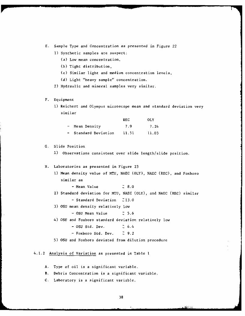
E. Sample Type and Concentration as presented in Figure 22
1) Synthetic samples are suspect:
(a) Low mean concentration,
(b) Tight distribution,
(c) Similar light and medium concentration levels,
(d) Light "heavy sample" concentration.
2) Hydraulic and mineral samples very similar.
F. Equipment
I) Reichert and Olympus microscope mean and standard deviation very
similar
REC OLY
- Mean Density 7.9 7.24
- Standard Deviation 11.51 11.03
G. Slide Position
1) Observations consistent over slide length/slide position.
H. Laboratories as presented in Figure 23
1) Mean density value of MTU, NAEC (OLY), NAEC (REC), and Foxboro
similar as
- Mean Value Z 8.0
2) Standard deviation for MTU, NAEC (OLY), and NAEC (REC) similar
- Standard Deviation Z13.0
3) OSU mean density relatively low
- OSU Mean Value Z 5.6
4) OSU and Foxboro standard deviation relatively low
- OSU Std. Dev. Z 6.4
- Foxboro Std. Dev. 9.2
5) OSU and Foxboro deviated from dilution procedure
4.1.2 Analysis of Variation as presented in Table 1
A. Type of oil is a significant variable.
B. Debris Concentration is a significant variable.
C. Laboratory is a significant variable.
38

gabg
IL
LU
Lii
C/ I -
* 0 00
39

.jow
Ll-u
* S S
F-
04

Z Z
1 0 a Z 0
o , uj wL wU wj z S
u U. 6L U . %
. 4J LL 4L :U- w- 5 I
2. I w ui w w w
Io 3a . . U. IL&-I
LI I .u U. . U. -
*~ ~ Li 'ai *. 0~
I %. W- - . %- %L &
up Z
LL- Or a I-.r W
I"' :Q1 u S US j A uS
4A 0. 4 W - 0
(X) .90 'a. '
u el xI go .1 0 C
4 -00I 4 F-: r - -=U iU, - a, 0 0
C/ X f %CI SZ, 0 - eU g,
-0 Z .0 .. 5 g ' S
_____ I-*-~J . I 8 s 5 g4AfI e 0 1 0 a 0
'aLL
2*j IW.
~~0 I
0 ~ ~ 0., -t 0 " 0
P: I S ' 5- "-. a% -0 0 .0
IL I Z-~ .0 '55 0" A
UA f 10 0 04 x0 0
1,
4A *- - 3
55.2 I *0 I- 5415

D. Lighting Technique is a significant variable.
E. Index Technique is not a significant variable.
F. Slide position is a significant variable.
4.1.3 Coefficient of Variation
A. Intra-Laboratory as presented in Figure 24
1) Range - 0 - 42%
Mean Z 19%
2) Sample Type
(a) Slight variation between types of fluid
- Mean COV Mineral 15%
- Mean COV Hydraulic 21%
- Mean COV Synthetic 17%
3) Sample Concentration as presented in Figure 25
(a) Light and heavy concentrations most significant
- Mean COV Light 22%
- Mean COV Medium 13%
- Mean COV Heavy ~ 19%
4) Lighting Technique as presented in Figure 26
(a) Very similar COV between lighting techniques.
5) Indexing Technique as presented in Figure 27
(a) Very similar COV between indexing techniques.
6) Equipment
(a) Very similar COV between microscopes.
7) Slide Position
(a) COV consistent with respect to slide position
8) Laboratory as presented in Figure 28
(a) MTU, OSU, Foxboro, and NAEC (OLY) similar
- Mean COV Z 17%
(b) NAEC (REC)
- Mean COV 14%
B. Interlaboratory as presented in Table 2
I) Range 1 10 - 74%
Mean 50%
2) Sample Type
(a) Slight variation between types of fluid.
42

LL.J
LD
0-r 7 - -- .--r r
C,43

C'14
LJ
LU-
LL. -
Ii ________44

F-3
-
LU -5

LL.1
A L&
_____E -
1 _ _ _ _6

I: IU
* S S 0 0
EmuOW
V
0Id
iI-aS3
0-
uJ
U-we
_________ _________ ________ _S
LzJCD
I-
LU
=0~
0
0 0 0 0 S
47

cr- 4 ccocoOCOOcoooooozoozoaooooo
'a 0 W, 0~
__ Li
0-
CN CD~
a - LLI 0
0 - -0~- -04 4 0 0 j -j w w w
2 i ~ W J U IU #L&40 iL
I.--
oL X- -=0 00 0
C:)-
- KE EZ1Z ZXZZ~z48

3) Sample Concentration
(a) Light and medium mean COV ~39%
(b) Heavy mean COV Z57%
4) Slide Position
(a) COV consistent over slide position
4.1.4 Graphical Regression Analysis
Representative Phase I - Stage I regression analysis plots are presented
in Figures 29, 30, and 31.
The following results can be drawn from the analysis of the total regres-
sion analysis plot population.
A. Poor quantitative interlaboratory correlation exists.
B. Inconsistent data bias exists.
C. Poor discrimination as presented in Figure 32
Mean Z.91
D. Substantial scatter exists.
4.2 Phase I - Stage II
Results from the second verification program stage is presented in the
following sunmmary. As described previously, this stage involved the analysis
of pre-made Ferrogram slides.
4.2.1 Data Plots
Representative Phase I - Stage II data plots are presented in Figures
33, 34, and 35.
The following results can be drawn from the analysis of the total plot
population.
A. Trending agrees
B. Quantitative variations exist
49

x A
%~ it
_________ %_: .b .,
% 4 %
C)
I~ I%
CD4
C)C
-L 'LI
F Xe
C/ - % . %
b -- .4
LL 44C/4 %4
-0xx
50

PS. 0 2 %
C/) %- V
-I x1! - %
C/-)cn x x
KL x x I.K
_% X%
- - * *Lus
LL 6. OK
. I .r..
x K
%c 0-oo %* ~
F,F,4
oeJ% "A
C~v %5%
0. 1

ILS'.0 S
0L
L% 0 7 1; %s
C) 31 %
*.. A: 12i
C/) %~
S - a
r-4 4::c
a 0. IL
*a
Lii
ul) 000 % '
S -S
%% xX 30 %
ti lo ' wt e.
hON USE
Lo52

1-4
I-
w I--
(12MtoK. ct
th4
0. ~ I
&A u
(153

'ac
40C/CieV
aLL (.DC/ *
S 0
.x
xx* a
ax
x
54

a at
<C W
LLLU
C--f~
-C7n
0 I
'BD
FT-T--v-l 1 '1B
55I.

(C 4
In CalC
x 0. C/)
x -n
xx
tnEo 7*.
*U = xci~o: x
AlIAS
IA f~Al K 48
0 3- JO'
* 0
Lii x v ~.x IWO to
K x
Al K
c~r +m
En.. - U56

C. Lighting Techniques
1) Mean of reflected higher than transmitted.
D. Indexing Technique
i) Mean and standard deviation very similar.
4.2.2 Coefficient of Variation
A. Interlaboratory as presented in Table 3
I) Range 16 - 93%
Mean 57%
2) Sample Type
(a) Slight variation between types of fluid.
3) Sample Concentration
(a) Light and heavy concentrations most significant.
- Heavy Mean COV - 60%
- Medium Mean COV 22%
- Light Mean COV 89%
4) Slide Position
(a) COV consistent over slide position.
4.2.3 Graphical Regression Analysis
Representative Phase I - Stage II regression analysis plots are presented
in Figures 36, 37, and 38.
The following results can be drawn from the analysis of the total regres-
sion analysis plot population.
A. Poor quantitative interlaboratory correlation exists.
B. Inconsistent data bias exists.
C. Poor discrimination as presented in Figure 39
Mean 1.52
D. Substantial scatter exists.
57

I7-
LUI
C) C14 CN. C4 C4- C~4 CN' C"J CNCC:) uLJ - )C) C:) C=) C: C C=
~- L- <c LU LUJ LUJ LU LU U LU LUJ LU- - N-. Z= - Ln Ln CT C, f
- L -= On = ~ CD C=) C14 N- =tLL-O £n O IV, C:) r- LA) 00 Lo N
S LU > C14 i-Il (NJ PeN 1 00 00 00 O7)' C) . . .
L LLC:) CD C:) C) C=) C:) c:) c; c:)LL. C:)
C:)
LL
LLLU '-- C=) .1- .9.9. .9- r-- .1 --
~ )CD CD C=) C) CD C=) C) C:) C) C)
LU - LLLUJ LLU LU LLUwLU-j I cmCzr =00 CD w-- N-- LALAU
F- N 00 00 Nl. -q 9 tn LO LAr- n C/14- N LO C) - = r-- N- rN-C0
-WL r- i r-i r- LO C14 CN pel
LUJ LA C) c; C:) C) C); c; C; C) C;DC) C4
- C:) C) C:) LL. C:) C:) C:) = CD C:) C:)
Ln ~LUJ LUI LUj LU >- LUJ LUJ LUJ - LU LUJ LUCTC I 'E UL C) L : r-I LA' (N -J CNJ C) r-I
--z v-Il 00 := <r a) CD LO "1 00 M Pf)a_ LU I -j .1- LO Lo U LA .9 (N -j CD v-I.!-
LUJ C:) C) C:) C:) C:) C:) LUJ C)CC
LUI
LUJ C) -
9=- v-LnC V- '-LnC) im r-q U)CD
C)O. LU LUJ LUJ
58

I-L
8 % %
as % as~
% %% if
C 02 10. S , a-
% 41
C-)
-JJ
LU C=
A J
-a-
0- 5 0 fA- S S u02*~u~~a~I '
2 _1 31 s=~ ~ * ..
C.% % '"
e--
Otho bI*XMSMO 00
- ,.59

.............. .
.A a
x
_j£
~~I,C/ %~-~r a a~
ob Uo %I I&
a. .A
% -
.4i q a S%
LLJ %
SSI
LD
-01
60

0. 0 0
ismu
3.m 40 0 a.FA oa
4; %0.. 'A
* 0.*
-0 a Z9 x
a6 x 3. 0 >4fEL *-
__ a3- X *jco c11
'4. 6
LD 'a % 4
LU z
9. 0
%
a.
.1L VX z XJ 0 V nL~b - ~%% .%*
* Z
A a P
~ asco-=
61

0
I-
w V)
NI.-
Lfl IA0
LU-
I-
0
to Ln D th Ytv) cu f
CID, C;
62

4.3 Phase II - Stage I
Results from the third verification program stage are presented in the
following summary. As described previously, this stage involved the analysis
of fluid samples.
4.3.1 Data Plots
Representative Phase II - Stage I data plots are presented in Figures
40, 41, 42, and 43.
The following results can be drawn from the analysis of the total plot
population.
A. Trending agrees.
B. Quantitative variations exist.
C. Sample Type as presented in Figure 44
1) Low Debris Concentration Levels
Mineral Mean Density 3.8
Hydraulic Mean Density Z 7.8
Synthetic Mean Density Z 4.3
D. Laboratories as presented in Figure 45
1) Mean density value and standard deviation of NAEC, MTU, and OSU
similar
Mean Density 4.4
Standard Deviation Z 2.4
2) Mean density value and standard deviation of Foxboro and JOAP/TSC
similar
Mean Density - 7.0
Standard Deviation 5.3
E. Slide Position as presented in Figures 46, 47, and 48
1) Observations consistent over slide position
63

fu 0
IL
#A I- > .
-to x K
nto m C,
x b!~ L I~
Ax L. to
x IA 0 x
p. v Sl 0 a
x xLiIJ X *
Is x iLiV. X
to x 5. x 0s a
In v
6* 64

CZC
x a ri.
VA La L. a
0 IA. I
a ma asw
'A S
x- x
*0
ma 'mow
Ls.. x'*mC' x m
0 0
0 cx L% IS
65 .

• LiJ d
* U
NC 4! r -0 0'A
am C/)of W
I~C IL In 'Ii
.: ao
a ft 11
ILI -
:I,
xl x -
- m :I- .UIa >>" f = iI I
mm a v xX wl
v , a
x 4!.. 1!
cox
66

rc P 0
I Ol
0 LLU hi
C/-r CK 4
o = I& U
- w
@1~6 Is ~* .hiI- ' . _ _ _ _ _
LL a0
an
x La c Eu x
- T
* -IV
LL... 67

LLI .J
LUU
CnC
~68

gom~i0 a i a I-0-
gn 0 c 0
C=)
-
__ __ __ _ __ __
C)
U)
.U- =LiJ
-J
-69

ClIC
S...70

I. ..... ..... ............
LJ
Cl)
71

* * S S S S
* * U * W
hi
5 4
I ____________ _____________ ____________
a
00
LU0~
CD- 0LJ.
-fLUjCD
-4 hia
- S.
C,,
=0~
na a a
* .* 0 0 S
72

4.3.2 Coefficient of Variation
A. Intra-Laboratory
1) Range 0 - 12%
Mean 5%
2) Sample Type as presented in Figure 49
(a) Mineral COV low with respect to synthetic and hydraulic type
samples.
Mineral Mean COV 3.64
Synthetic Mean COV Z 9.01
Hydraulic Mean COV 13.55
3) Slide Position
(a) COV consistent over slide positions.
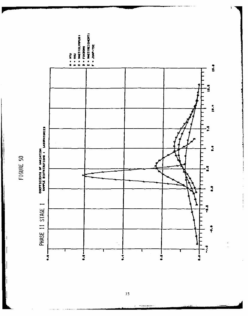
4) Laboratory as presented in Figure 50
(a) NAEC, Foxboro, and MTU similar
- Mean COV ~ 5%
(b) OSU and JOAP/TSC similar
- Mean COV ~ 2.5%
B. Interlaboratory as presented in Table 4
I) Range Z 22-60%
Mean 37%
2) Sample Type
(a) Mineral COV low with respect to synthetic and hydraulic type
samples.
Mineral Mean COV 26%
Hydraulic Mean COV 46%
Synthetic Mean COV Z 40%
3) Slide Position
(a) COV consistent over slide position
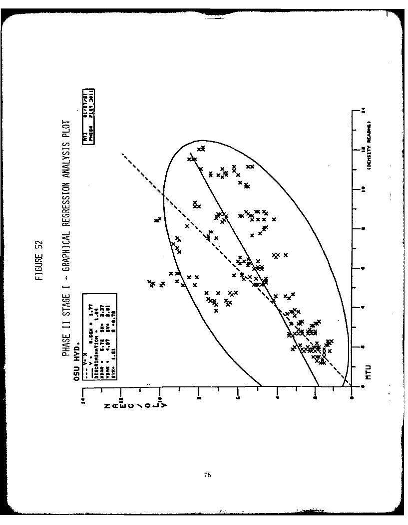
4.3.3 Graphical Regression Analysis
Representative Phase II - Stage I regression analysis plots are presented
in Figures 51, 52, and 53.
73

tr
LB..
LL-a
(474
L- m
LLSLDU
coo
b- _ _ _ __ _ _ _ __ _ _ _ __ _ _
Ijcn_ _
uJ _ _ _ _75

LU -I-
>000000000
IU. ++++++ ++0 wwwtwwwwwW
L: N oo * 0 fl 4 Sn 4_nN4rmMk 0 00000
L'-4
LLJL
<c LL -1- -- W 444nmmxxx
u... CL at- W 41W4 4 1
Il C)C
F. 7- ooozzz
-0 -4 0 -L
C/) w
C/,
76

xx,x
-% xx
C/) xLLI4
LU %*4
LU * %
*4%
C= %
I %4 xx-L *4I %
%4 K
% *4
f9%~ %4 X
Z %on %X'
Li-0
77
0%
I- V
C./) %LLJ % I
-J%
C'4
Ln
LUx xxx\ x
LUI
LD
s-i x
LUJ
% %51)
=-O O4>
* 78

IL
-LJ
. xxxC.,, x xx__j % x x
*xxx xLn xxx xx
If - XXX x XX4L : =Xxxx% x x
o~ x x~ xxx x
-n x x %.
xxx 4.
U) x%S %
V,) 1* . 4
V %.0S. %
Lii K%sqas %
= * .v~ %'Sc
I-I 4. T -
*~ 4.79

The following results can be drawn from the analysis of the total regres-
sion analysis population.
A. Poor quantitative and interlaboratory correlation exists.
B. Inconsistent data bias exists.
C. Poor discrimination as presented in Figure 54.
Mean .84
D. Substantial scatter exists.
4.4 Phase II - Stage II
Results from the final verification program stage are presented in the
following summary. As described previously, this stage involved the analysis
of pre-made Ferrogram slides.
4.4.1 Data Plots
Representative Phase II - Stage II data plots are presented in Figures
55, 56, and 57.
The following results can be drawn from the analysis of the total plot
population.
A. Trending agrees.
B. Quantitative variations exist.
C. Laboratories as presented in Figure 58.
i) Mean density value very similar for all laboratories
2) Standard deviation very similar for all laboratories.
4.4.2 Coefficient of Variation
A. Intra-Laboratory as presented in Figure 59
1) Range 0 - 12%
Mean - 4%
80

a0
z
X I
IL o
0 0u
'.4;
- w 81

FA L
M CL
A ;LU IX
L.S.x A
.Lac = KhwxC
mc
x 0.
CV-V
- q. 82

lo!
I - g-* I- 4w S
naU cc
O A
LnL
IL I I I h I
le x
K a S
4AAS
v V
- -x
83

PA _ _ _ _ _ _ _ _ _ __>_ _ __a
F- CLe j
"SC/) c
Xx, - W
LUrn
qall
a 31
v w
I xx A* X31,31
LUIC
= S.8 4

L-Eu
________ ________85

, AD-AL16 508 MECHANICAL TECHNOLOGY INC LATHAM NY RESEARCH AND DEV--ETC F/A 7/NANALYTICAL FERROGRAPHY STANDARDIZATION.(U)JAN 82 P B SENHOLZI, A S MACIEJEWSKI N0001 -81-C 0012
UNCLASSIFIED MTI-82TR56 NL
EonhhhhhhmmomhlEEIIIIIIII
ll11
4--R
C -g
c1 r,"
alJ
L7,,
C/)
'"6
- -
0u
I--
' I |I ! II-
- -m-
• L••
C,,6
.. . ..... " - ' . .= "- .. .i ' ' - , , , , , ,, ,

2) Sample Type as presented in Figure 60
(a) Slight variation between types of fluid.
3) Slide Position
(a) COV consistent with respect to slide position.
B. Interlaboratory as presented in Table 5
1) Range 1 10 - 98%
Mean ~ 41%
4.4.3 Graphical Regression Analysis
Representative Phase II - Stage II regression analysis plots are presented
in Figures 61, 62, and 63.
The following results can be drawn from the analysis of the total regres-
sion analysis plot population.
A. Poor quantitative interlaboratory correlation existsB. Inconsistent data bias exists.
C. Poor discrimination as presented in Figure 64
Mean Z 2.3
D. Substantial scatter exists.
87
I iu r ,m, j . .
fi
LLU-
-DC/)i
LL
PI I--
C=LO~
IL--LL L)-
(Uo - -
LLJ
LUU~
LU 88

LU w
000 40 0 w- r-- ----- U z d0- -a ty - . 0%- UNM M CP bMrM.00 c .0%rm V .00 0-1
4A rz~ C -- fmn -yr .44 4-4coCY drur%-dy r."~cy 0
cc %L~ww w Uu W J uJ ~ w w w~ W ~ -
00ON ~N . JN -a. .?u-df 0 4 - - W-A e
000000000000000000000 0000000000 u L.>i 0 , & t **04s,#+ 0&
4 LUJLU W WWWWWWUJUUJUWUJWWW WW wUWWWWWWW
'D. 5 -0 0 - 4 0.' %r ' P-P- r C4 WN j-d 0 %r F- M -
LLJ qcr 4 0 0 00 0000 00 0 000 00 0 0 0 0 S.-0000 ; C__4 4 4 * 0
g= . LULU WW W W ULIW U U W W WU W W W *
cI Z: " 0 - - 0 - d- ud - - -40.4 d . - C %O.N ?N-.? .Jx
- 00000 00000000000000 000000000 1.-l
I-- CfUWLJU w w w w w Gc
U..." -- -'00 4f 4C - A " 000 W "- -- 0~ r--N% -- 0L 4
LU 0000000000000000000000000000 OC 4-
- LU 0O~0 0 id N LU- z 0 3 60 0 0 0 0 0- 00 00 0060d 0 000090-4 4
LL. 000000000000000000000000000000LUJ1000***+4&** s I***# ,4-,***04
C)- w4w w ww w
I, 09960 4*000000 0 00000 OO**gO o estC0000000000 ,,0000
cn 0
89

I.%LAE
xU
C-c
Lii L
-I %
U9

ta-
CN ,
xD WLi.J V
C)
W
0x(. LmaJ
% %0
- %
l o fA 0 % #A
91

X x
'4 x~xx
0 xCb x
xn %__% x
L% %__j %
I-
(.0 db
-. 92
Ub 0
'ft
a4
393

5.0 PROGRAM STATISTICAL SUMMARY AND CONCLUSIONS
Based on the statistical results presented above for each program phase,
the following summary and conclusions have been generated. These results and
conclusions are presented with respect to the primary and secondary analysis
variables as covered in Section 3.1.
5.1 Lighting Technique
Both transmitted and reflected lighting approaches were considered with
respect to Analytical Ferrography density measurements.
A. Mean reflected density reading is higher than the transmitted
mean reading.
B. Trends the same.
C. Standard deviation the same.
D. Coefficient of variation the same.
E. Standardize on reflected approach.
5.2 Indexing Technique
Both a fixed density reading slide indexing approach (conventional) and a
floating slide indexing approach (new method) were considered.
A. Mean conventional density reading is the same as the new method
mean reading.
B. Trends the same.
C. Standard deviation the same.
D. Coefficient of variation the same.
E. Standardize on conventional approach.
5.3 Equipment
Both Reichert and Olympus Ferroscopes were considered under this round
robin effort.
94

A. Mean Reichert equipment density reading is the same as the Olympus
mean reading.
B. Trends the same.
C. Standard deviation the same.
D. Coefficient of variation the same.
E. Minimal Ferroscope type effect on variation.
5.4 Slide Position
Repeatability with respect to the indexed location on the Ferrogram was
considered. Debris size is a function of this slide location.
A. Minimal effect on variation which is somewhat of an unexpected
result.
5.5 Sample Type
Hydraulic fluid, mineral oil, and synthetic lubricant samples were considered.
A. Minimal effect on repeatability.
B. Hydraulic samples consistently higher variation.
5.6 Sample Debris Concentration
Light, medium, and heavy debris sample concentrations were considered.
A. Light and heavy concentrations have relatively the greatest effect
on variation.
5.7 Intra-Laboratory
Repeatability within each laboratory was considered.
A. Trends agree.
B. Good repeatability Phase I Phase 11 Phase II
within each laboratory. Stage I Stage I Stage II
- Mean COV 19% 5% 4%
95
- -- M- - --- - ?.A - --- ,_1

C. Procedure improved intra-laboratory variation.
5.8 Interlaboratory
Repeatability between all participating laboratories was considered.
A. Trends agree.
B. Poor repeatability Phase I Phase I Phase II Phase I!
between laboratories. Stage I Stage II Stage I Stage I]
- Mean COV 50% 57% 37% 41%
C. Poor Discrimination
between laboratories.
- Mean Discrimination .91 1.5 .84 2.3
D. Inconsistent interlaboratory bias.
E. Procedure has only limited effect on interlaboratory variation.
F. The prime source of interlaboratory variation appears to be the
Ferroscope densitometer as opposed to either the operator or
the Sample procedure variables.
5.9 Summary
The results of this analysis have served to indicate that the draft
Navy Analytical Ferrography Standardized Procedure has served to greatly im-
prove the repeatability of Analytical Ferrographic analysis within an indi-
vidual laboratory. However, repeatability between laboratories remains poor
due to what appears to be an equipment problem with the Ferroscope densi-
tometer. This problem could be addressed through the development of an ef-
fective densitometer calibration standard.
These results should not be construed as an effectiveness criticism of
either Ferrographic Analysis or wear debris analysis technology. Both of
these interrelated technical fields have proven their effectiveness in both
the maintenance and research communities. Care should be exercised however,
when comparing/correlating Ferrography results from different laboratories/
equipments.
96

6.0 NAVAL ANALYTICAL FERROGRAPHY STANDARDIZED PROCEDURE
Based on wear particle analysis research, Ferrography experience, statis-
tical analysis, and laboratory inputs, a draft Analytical Ferrography Standard-
ized Procedure has been developed under this program. The resultant draft
procedure is presented in Appendix A of this report.
As discussed earlier in this report, the standardized procedure will
result in analysis repeatability exhibiting a mean coefficient of variation
within a laboratory of approximately 5%. However, this procedure does not
guarantee adequate interlaboratory analysis repeatability due to overriding
equipment variations as presented in Section 5.9.
97

I7.0 NAVAL FERROGRAPHY VERIFICATION PROGRAM RECOMMENDATIONS
Verification program analysis and conclusions have identified several
areas warranting further attention. In light of these identified areas, the
following short term and long term recommendations are presented.
7.1 Short Term Recommendations
A. Publish Naval Analytical Ferrography Standardized Procedure.
B. Establish the procedure as a technical standard through an appropriate
standards organization.
C. Pursue Analytical Ferrography Densitometer calibration technique.
D. Verify Analytical Ferrography Densitometer calibration technique.
E. Develop a Direct Reading Ferrography standardized procedure.
F. Verify direct Reading Ferrography repeatability.
7.2 Long Term Recommendations
A. Develop a comprehensive, repeatable, precise wear particle character-
ization approach/technique/equipment. This new characterization approach
should assess lubricant borne debris concentration, size distribution, compo-
sition, and morphology for both metallic and nonmetallic particles.
98

8.0 REFERENCES
I. Wescott, V. C., et al, "Oil Analysis Program," U.S. Naval Air Engineering
Center, Final Report on Contract Number N00156-74-C-1682, Foxboro-Trans
Sonics Report, 1975.
2. Scott, D., and Seifert, W. W., "Ferrography - A New Tool For Analyzing
Wear Conditions," Fluid Power Testing Symposium, 1976.
3. Dalah, H., and Senholzi, P. B., "Characteristics of Wear Particles Generated
During Failure Progression of Roller Bearings," ASLE Paper presented at
ASLE Annual Meeting, 1976.
4. Senholzi, P. B., and Bowen, C. R., "Oil Analysis Research," National Confer-
ence on Fluid Power, October 1976.
5. Senholzi, P. B., "Oil Analysis/Wear Particle Analysis," Mechanical Failures
Prevention Group, 1977.
6. Senholzi, P. B., "Oil Analysis/Wear Particle Analysis 11," Institute of
Mechanical Engineers, 1978.
7. Maciejewski, A. S., "Oil Analysis Aspects of Tribology," Fluid Power
Research Conference, 1979.
8. Naval Air Engineering Center Report No. 92-0458, "Sample Preparation/
Ferrogram Procedure/Ferrogram Analysis," August 8, 1980.
9. Naval Air Engineering Center Tribology Laboratory Ferrogram Analysis
Report, November 7, 1977.
10. Bowen, E. R., and Westcott, V. C., "Wear Particle Atlas," Contract No.
N00156-74-C-1682, U.S. Naval Air Engineering Center, Controlling Office,
July 1976.
99

APPENIX A
A-i

INTERIM DRAFT
NAVALANALYTICAL FERROGRAPHY
STANDARDIZED PROCEDURE
MARCH 1982
Sponsor:
Office of Naval Research
Mechanical Technoogy Incorporated
1656 Homewood Landing Road
Annapolis, Maryland 21401
A
- -

1. SCOPE
1.1 This method covers the evaluation of liquid borne ferrous and ferro-
magnetic wear debris particulate by means of a magnetic separation technique.
It is applicable to mineral and synthetic lubricants as well as other viscous
fluids.
1.2 This method provides for the preparation and density determination
of the wear debris deposited on a glass substrate. A calculation procedure
for normalization of density data is provided.
NOTE 1: This method also has been applied to the analysis of wear debris
contained in grease. However, sufficient data is not available to include
this procedure here.
2. SUMMARY OF METHOD
2.1 A fluid sample is pumped over a prepared glass substrate located in
a high gradient magnetic field. The ferrous and ferromagnetic wear debris is
deposited on the glass substrate according to size and a determination of the
relative density of the particulate along the slide length is measure.
NOTE 2: Mechanical trapping and gravitational effects will influence
liquid borne non-ferrous metallic and hybrid wear debris. Although the de-
position of these particles will not be accurate with respect to size on the
substrate, their presence should be noted.
3. DEFINITIONS
3.1 Density - Percent light reduction which is a function of the parti-
cle concentration at various locations on the substrate.
3.2 Significant deposit - The concentration (density) of particles near-
est the entry point of the substrate, normally exhibiting the largest percent
of light reduction (approximately 55 mm up from the exit end of the slide).
Hi A-3

3.3 Percent Area Covered - Used in quantitative analysis, the percent of
the area covered by large ferrous particles (AL) and small ferrous particles
(AS), usually located at the entry area (55 mm) and 50 mm locations, respec-
tively.
4. SIGNIFICANCE AND USE
Ferrographic analysis provides an assessment of wear debris quantity,
size distribution, composition, and morphology. This analysis is useful in
assessing the wear condition of a lubricated component/system.
5. APPARATUS
5.1 Analytical Equipment
5.1.1 Fluid Analyzer, either Model 7058-3 (dual) or Model 7069-4 (duplex).
5.1.2 Ferroscope, Model 7507-7 or equivalent microscope, having both
transmitted and reflected light capability.
5.1.3 Density Reader, Model 7079-3 with optical measurement device and
digital readout.
5.1.4 Oven or equivalent heating device, capable of maintaining constant
temperature at 150OF (65.5 0 C) + 3.
NOTE 3: With the exception of 5.4, the only recognized and licensed
distributor of the equipment described is Foxboro Analytical, Burlington,
Massachusetts 01803.
5.2 Analytical Ferrograph Materials
5.2.1 Fixer/Solvent - Filtered tetrachloroethylene (Regent Grade)
A-4

I5.2.2 Delivery Tubing - Teflon, 1/16 in. (1.58 mm) I.D., cut to lengths
of 25 in. (635 mm).
5.2.3 Substrate - Microcover glass, 24 mm x 60 mm, thickness approxi-
mately .20 mm, with non-wetting barrier (Nyebar) applied.
5.2.4 Vials - Pre-cleaned, clear glass, 15 ml capacity, with caps.
5.2.5 Pipette Dispenser - 1 ml pre-calibrated, disposable pipettes.
NOTE 4: The Analytical Ferrograph materials can be obtained directly
from Foxboro Analytical, Burlington, Massachusetts 01803.
NOTE 5: The fixer (tetrachlorethylene) is a nonflammable chlorinated
hydrocarbon. Avoid skin contact and use only in well ventilated area.
NOTE 6: It is necessary that the evaluator fully understand the opera-
tion and general operating procedures of this equipment.
6. PREPARATION OF APPARATUS - ANALYZER
6.1 Remove delivery tubing from protective bag and cut one end at a 450
angle to the axis of the tubing. Use a sharp instrument (razor or scalpel
blade) as opposed to scissors.
NOTE 7: If only a qualitative analysis is desired, the tube should not
be cut on a 450 angle. This allows the particles to spread out, facilitating
morphological identification.
6.2 Position the delivery tube in the analyzer turret arm with the 450
end extending approximately 1/8 in. (3.17 mm) beyond the tip of arm. (See
Figure 1).
6.3 Thread the tubing through pump exit tubing clamp, pump delivery arms,
and pump entrance clamp and lightly secure delivery arms.
- IHAA
-

6.4 Remove glass substrate from protective bag and insert into substrate
fixture appropriately retracting and releasing positioning pin. Determine
that the substrate is properly positioned on the metal shelf, located at the
top of the slide bed. The "closed loop" end of the barrier on the substrate
should be located closest to the turret arm. A black dot on the slide should
be located at lower left hand corner of slide (plain view) (see Figure 2).
6.5 Position the turret arm so that the exit end of the supported tubing
is slightly above the surface of the slide. (Avoid dripping of sample on the
slide).
6.6 Rotate the drain tube holding fixture counterclockwise and lower the
notched end of tube until it resets on the exit edge of the slide.
7.0 SAMPLE PREPARATION
NOTE 8: Samples should be stored at 0°F (-17.8 0 C) if ferrographic analy-
sis is not performed within 24 hours of sampling. If stored under these con-
ditions, sample should be heated to 185 0 F (850C) for thirty (30) minutes prior
to step 7.1.2.
7.1 Undiluted Sample
7.1.1 Shake sample bottle by hand vigorously for approximately one (1)
minute. Loosen sample bottle cap (do not remove) and place in suitable heat-
ing apparatus. Raise temperature of the fluid to 150OF (65.5 0c) and maintain
such temperature for a period of ten (10) minutes.
7.1.2 Pipette 1 ml of fixer solution into a clean mixing vial.
7.1.3 Remove sample bottle from heating apparatus and tighten cap. Hand
shake sample fluid vigorously for sixty (60) seconds. Pipette 3 ml of sample
fluid into same mixing vial, cap, and hand shake for ten (10) seconds.
Ed A-6

8.6 Upon completion of the sample mixture pumping cycle reset pump timer
to 14 minutes and initiate a fixer pumping cycle. During this cycle, approx-
imately three (3) air bubbles should be intermittently introdured into the
delivery tube. These bubbles are created by removing and reinserting the
delivery tube into the fixer solution. Space air bubbles approximately five
(5) seconds apart.
8.7 Upon completion of the fixer pumping cycle lift the turret arm/de-
livery tubing from the glass substrate and allow the slide to drain off any
remaining fluid.
8.8 Allow the slide to drain off any remaining fluid.
8.8 Allow the slide to dry completely before removing from the analyzer
(approximately (20) twenty minutes). Institute measures to avoid air-borne
contaminants.
8.9 Remove glass substrate vertically from analyzer and affix identi-
fication tag. Place in protective cover until ready for analysis.
8.10 Discard all materials (pipette tips, vials, and tubing) used in
making slide. Reuse may introduce contaminants from previous samples, thereby
introducing error into the analysis.
9.0 PREPARATION OF APPARATUS - DENSITY READER
9.1 Prepare microscope and density reader according to the procedure
below. (Allow at least 30-45 minutes for initial warm-up of density reader.)
NOTE 12: Room temperature, in which equipment is operated, should be
750F (210C), to avoid overheating density reader, resulting in erratic be-
havior.
9.1.2 In order to adjust the reader for full scale, keep the light path
selector lever fully in and adjust thepotentiometer in the rear of the reader
to give a 100% area covered reading.
Ej A-7l g
..-

9.1.3 To zero the reader, the following procedures must be followed.
9.1.3.1 Using ordinary visual reflected light and the lOx objective,
locate an area outside the barrier on the ferrogram slide that is free of any
particles. Withdraw the light path selector lever and hold the reflected
light switch on read.
9.1.3.2 Attempt to zero the reader by adjusting the potentiometer on the
front of the reader. If this cannot be achieved, adjust the regulated voltage
supply to the reflected lamp by using the potentiometer at the rear of the
power supply. The light intensity may be further reduced by closing down the
aperture diaphragm.
9.1.3.3 By the adjustment of both potentiometers and the aperture dia-
phragm the reader should be able to be zeroed.
10.0 OPERATING PROCEDURE - DENSITY READINGS
10.0 Density readings are taken on the Ferrogram in order to assess the
relative quantity of debris at varous locations along the length of the sub-
strate. The percent area covered by debris (density) is determined from an
approximate 1 m diameter field of view. This relative measure of debris can
be normalized to a unit volume of actual used sample oil over the Ferrogram.
(trending of data over a series of oil samples) and for interlab comparisons.
Note that the percent area covered refers to the light reflected by the debris
on the Ferrogram in the field of view.
10.2 Place slide on microscope stage with the entry deposit of the slide
to the evaluator's left. Using a lOx objective, locate the significant de-
posit of particles in the following manner.
10.2.1 Locate the densest part of the significant deposit and center in
the field of view. (See Figure 3). With the reflected light switch held on
read, operate the x and y controls of the stage to obtain the maximum values.
m.
.- us~ A- 8
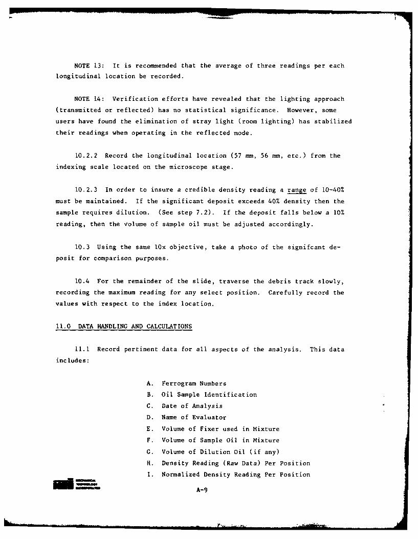
NOTE 13: It is recommended that the average of three readings per each
longitudinal location be recorded.
NOTE 14: Verification efforts have revealed that the lighting approach
(transmitted or reflected) has no statistical significance. However, some
users have found the elimination of stray light (room lighting) has stabilized
their readings when operating in the reflected mode.
10.2.2 Record the longitudinal location (57 mm, 56 mm, etc.) from the
indexing scale located on the microscope stage.
10.2.3 In order to insure a credible density reading a range of 10-40%
must be maintained. If the significant deposit exceeds 40% density then the
sample requires dilution. (See step 7.2). If the deposit falls below a 10%
reading, then the volume of sample oil must be adjusted accordingly.
10.3 Using the same lOx objective, take a photo of the signifcant de-
posit for comparison purposes.
10.4 For the remainder of the slide, traverse the debris track slowly,
recording the maximum reading for any select position. Carefully record the
values with respect to the index location.
11.0 DATA HANDLING AND CALCULATIONS
11.1 Record pertinent data for all aspects of the analysis. This data
includes:
A. Ferrogram Numbers
B. Oil Sample Identification
C. Date of Analysis
D. Name of Evaluator
E. Volume of Fixer used in Mixture
F. Volume of Sample Oil in Mixture
G. Volume of Dilution Oil (if any)
H. Density Reading (Raw Data) Per Position
1. Normalized Density Reading Per Position
Ed A-9ILLI-

11.2 Following completion of all density reading, the raw data generated
must be normalized (percent per ml) utilizing the following formula:
AN A
VT X
VO + VF
where:
AN = density reading normalized to I ml of sample (dirty) oil
A = raw density reading from ferrogram
VT = total volume fluid pumped over ferrogram (from mixer vial)
VO = volume oil in mixer vial
VF = volume fixer in mixer vial
11.3 If dilution procedures were performed, the following formula should
be used:
AAN-VO VSVT X X ____
VO + VF VS + VD
where:
VS = volume of sample oil used in dilution procedure
VD = volume of clean diluent oil used in the dilution procedure
NOTE 15: Normalized density data should be reported to one decimal place
(i.e. 3.9, 12.6, etc.).
A-10

450 CUT
900 CUT
DELIVERY TUBING
TURRET ARM -
GLASS SUBSTRATE
NOTE: (APPROXIMATELY 2 X I.D. OF TUBING)
DELIVERY TUBING PREPARATION AND POSITIONING
FIGURE I
A-i

FLUID ENTRYPOINT
DISTANCE FROM EXIT IN MM
BARRIER of
FLUID EXITPOINT
FERROGRAM SLIDE DIMENSION AND KEY FACTORS
FIGURE 2
- uec~aA-12

ENTRY 55mm__EXIT
SIGNFICAT DEOSITCENTRIN
SIGNIFICAN T OI CENTRIN
FIGURE 3
A-13

ACKNOWLEDGEMENTS
The following people have contributed to this document:
Mr. M. P. O'Donnell, Naval Air Engineering Center
Mr. D. P. Anderson, Foxboro Analytical
Mr. P. W. Centers, AFAPL/SFL, Wirght-Patterson Air Force Base
Dr. J. H. Johnson, Michigan Technological University
Mr. C. Hubert, Michigan Technological University
Mr. C. P. Merhib, Army Materials and Mechanics Research Center
Mr. T. Kelley, Naval Air Engineering Center
Mr. D. Norvelle, Oklahoma State University
Ms. J. Dobson, Oklahoma State University
Mr. B. L. Poppert, Assistant Technology Administrator, Naval Air
Systems Command (AIR-340E)
Mr. P. B. Senholzi, Mechanical Technology Incorporated
Dr. R. K. Tessmann, Gardner Denver
The Technical Cooperation Program, Sub Group P, Technical Panel 1,
Action Group 4
Mr. A. Maciejewski, Mechanical Technology Incorporated
Dr. W. Ruff, National Bureau of Standards
Mr. R. Lee, Joint Oil Analysis Program, Technical Support Center
LCDR H. P. Martin, Office of Naval Research
REFERENCES
1. Naval Air Engineering Center Report No. 92-0458, "Sample Preparation/
Ferrogram Procedure/Ferrogram Analysis," August 8, 1980.
2. Naval Air Engineering Center Tribology Laboratory Lubricant Sampling
Procedure, September 30, 1977.
3. Naval Air Engineering Center Tribology Laboratory Ferrogram Analysis
Report, November 7, 1977.
4. Bowen, E. Roderic, and Westcott, Vernon C., Wear Particle Atlas (Contract
No. N00156-74-C-1682, Controlling Office: Naval Air Engineering Center,
Lakehurst, NJ) July, 1976.
5. Naval Air Engineering Center Tribology Laboratory Contaminant Particle
Size Distribution Methodology - Sample Preparation and Analysis, June, 1977.
-A- 14


![Analytical Standardization of Ayurvedic Formulation- …...soluble extractive and water soluble extract values were determined.[ 3,4] Microbial screening Microbial screening carried](https://img.dokumen.tips/doc/110x75/5eaef11d6cb79344be2bc8d0/analytical-standardization-of-ayurvedic-formulation-soluble-extractive-and.jpg)