Embed Size (px)
Citation preview

P
PM
PX
M = X
ARTNeT
ANALYTICAL APPROACHES TO EVALUATINGPREFERENTIAL TRADE AGREEMENTS
JOHN GILBERT
This publication may be reproduced in whole or in part for educational or non-profit purposes
without special permission from the copyright holder, provided that the source is acknowledged.
The ESCAP Publications Office would appreciate receiving a copy of any publication that uses
this publication as a source.
No use may be made of this publication for resale or any other commercial purpose whatsoever
without prior permission. Applications for such permission, with a statement of the purpose and
extent of reproduction, should be addressed to the Secretary of the Publications Board, United
Nations, New York.
The shaded areas of the map indicate ESCAP members and associate members.
ESCAP is the regional development arm of the United Nations and serves as the main
economic and social development centre for the United Nations in Asia and the Pacific. Its
mandate is to foster cooperation between its 53 members and 9 associate members. ESCAP
provides the strategic link between global and country-level programmes and issues. It supports
Governments of countries in the region in consolidating regional positions and advocates
regional approaches to meeting the region’s unique socioeconomic challenges in a globalizing
world. The ESCAP office is located in Bangkok, Thailand. Please visit the ESCAP website at
www.unescap.org for further information.
i
Analytical Approaches to EvaluatingPreferential Trade Agreements
Prepared by
John Gilbert
2017
ARTNeT
ii
Analytical Approaches to Evaluating Preferential Trade Agreements
United Nations publicationCopyright © United Nations 2017All rights reservedPrinted in ThailandST/ESCAP/2788
For further information on this publication, please contact:Mia MikicDirectorTrade, Investment and Innovation DivisionUNESCAPRajadamnern Nok AvenueBangkok 10200, ThailandTel: (+66-2) 288-1902Fax: (+66-2) 288-1027, 288-3066e-mail: [email protected]
Reference to dollars ($) are to United States dollars unless otherwise stated.
The designations employed and the presentation of the material in this publication do not implythe expression of any opinion whatsoever on the part of the Secretariat of the United Nationsconcerning the legal status of any country, territory, city or area, or of its authorities, orconcerning the delimitation of its frontiers or boundaries.
Where the designation “country or area” appears, it covers countries, territories, cities or areas.
Bibliographical and other references have, wherever possible, been verified. The United Nationsbears no responsibility for the availability or functioning of URLs.
The views expressed in this publication are those of the authors or case study contributors anddo not necessarily reflect the views of the United Nations.
The opinions, figures and estimates set forth in this publication are the responsibility of theauthors and contributors, and should not necessarily be considered as reflecting the views orcarrying the endorsement of the United Nations. Any errors are the responsibility of the authors.
Mention of firm names and commercial products does not imply the endorsement of the UnitedNations, and any failure to mention a particular enterprise, commercial product or process is nota sign of disapproval.
The use of the publication for any commercial purposes is prohibited, unless permission is firstobtained from the Secretary of the Publication Board, United Nations, New York. Request forpermission should state the purpose and the extent of reproduction.
This publication has been issued without formal editing.
iii
ACKNOWLEDGEMENTS
This publication, “Analytical Approaches to Evaluating Preferential Trade Agreements”,
was prepared by Professor John Gilbert, Utah State University, the United States,
under the substantive direction and guidance of Dr. Mia Mikic, Director, Trade,
Investment and Innovation Division (TIID) of the United Nations Economic and Social
Commission for Asia and the Pacific (ESCAP).
The publication is the outcome of a project, “Enhancing the Capacity of the Lao PDR
and other ASEAN LDCs to Negotiate Trade and Investment and Engage in Regional
Economic Integration Processes”, implemented in partnership between the Deutsche
Gesellschaft für Internationale Zusammenarbeit (GIZ) GmbH and ESCAP’s Trade,
Investment and Innovation Division. The specific objective of the project was to
increase the capacity of Lao PDR government officials and other relevant parties to
prepare, negotiate and implement reciprocal preferential agreements in the area of
trade and investment.
The GIZ-ESCAP project also contributed to the “Regional Economic Integration of the
Lao PDR into ASEAN – Trade and Entrepreneurship Development (RELATED) Project”
that is part of Lao-German Development Cooperation, supervised by Dr. Hartmut
Janus, Project Director.
In addition to the preparation of this publication, the GIZ-ESCAP project included the
preparation of training material on “Enhancing Capacity for Trade Policymaking and
Negotiations of Preferential Trade Liberalization” as well as the implementation of
a capacity-building programme. These two components of the project were supervised
by Dr. Rajan S. Ratna from TIID, ESCAP.
The cover design was prepared by Ms. Chen Wen Chen, Consultant, TIID, ESCAP,
while the final checks were carried out by Ms. Pakkaporn Visetsilpanon, Research
Assistant, TIID, ESCAP. The publication was printed by Erawan Printing Limited
Partnership.

iv
v
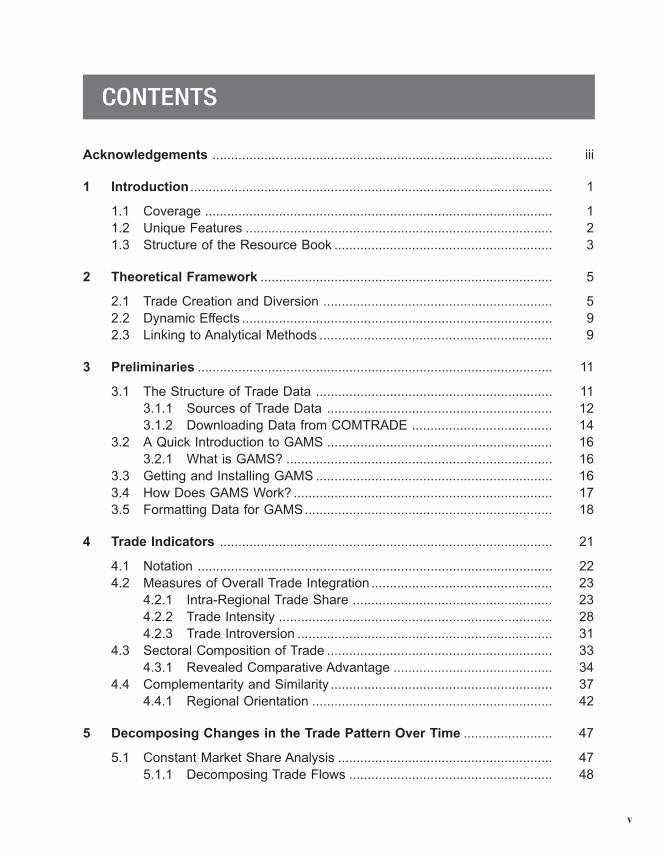
CONTENTS
Acknowledgements ............................................................................................ iii
1 Introduction .................................................................................................. 1
1.1 Coverage .............................................................................................. 1
1.2 Unique Features ................................................................................... 2
1.3 Structure of the Resource Book ........................................................... 3
2 Theoretical Framework ............................................................................... 5
2.1 Trade Creation and Diversion .............................................................. 5
2.2 Dynamic Effects .................................................................................... 9
2.3 Linking to Analytical Methods ............................................................... 9
3 Preliminaries ................................................................................................ 11
3.1 The Structure of Trade Data ................................................................ 11
3.1.1 Sources of Trade Data ............................................................. 12
3.1.2 Downloading Data from COMTRADE ...................................... 14
3.2 A Quick Introduction to GAMS ............................................................. 16
3.2.1 What is GAMS? ........................................................................ 16
3.3 Getting and Installing GAMS ................................................................ 16
3.4 How Does GAMS Work? ...................................................................... 17
3.5 Formatting Data for GAMS................................................................... 18
4 Trade Indicators .......................................................................................... 21
4.1 Notation ................................................................................................ 22
4.2 Measures of Overall Trade Integration ................................................. 23
4.2.1 Intra-Regional Trade Share ...................................................... 23
4.2.2 Trade Intensity .......................................................................... 28
4.2.3 Trade Introversion ..................................................................... 31
4.3 Sectoral Composition of Trade ............................................................. 33
4.3.1 Revealed Comparative Advantage ........................................... 34
4.4 Complementarity and Similarity ............................................................ 37
4.4.1 Regional Orientation ................................................................. 42
5 Decomposing Changes in the Trade Pattern Over Time ........................ 47
5.1 Constant Market Share Analysis .......................................................... 47
5.1.1 Decomposing Trade Flows ....................................................... 48
vi
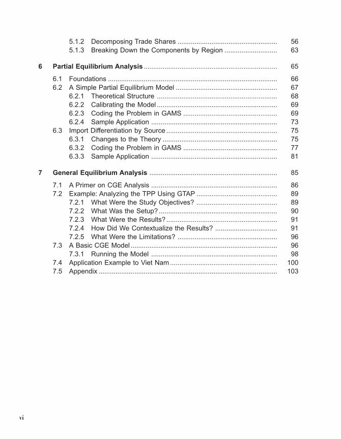
5.1.2 Decomposing Trade Shares ..................................................... 56
5.1.3 Breaking Down the Components by Region ............................ 63
6 Partial Equilibrium Analysis ....................................................................... 65
6.1 Foundations .......................................................................................... 66
6.2 A Simple Partial Equilibrium Model ...................................................... 67
6.2.1 Theoretical Structure ................................................................ 68
6.2.2 Calibrating the Model ................................................................ 69
6.2.3 Coding the Problem in GAMS .................................................. 69
6.2.4 Sample Application ................................................................... 73
6.3 Import Differentiation by Source ........................................................... 75
6.3.1 Changes to the Theory ............................................................. 75
6.3.2 Coding the Problem in GAMS .................................................. 77
6.3.3 Sample Application ................................................................... 81
7 General Equilibrium Analysis .................................................................... 85
7.1 A Primer on CGE Analysis ................................................................... 86
7.2 Example: Analyzing the TPP Using GTAP ........................................... 89
7.2.1 What Were the Study Objectives? ........................................... 89
7.2.2 What Was the Setup? ............................................................... 90
7.2.3 What Were the Results?........................................................... 91
7.2.4 How Did We Contextualize the Results? ................................. 91
7.2.5 What Were the Limitations? ..................................................... 96
7.3 A Basic CGE Model .............................................................................. 96
7.3.1 Running the Model ................................................................... 98
7.4 Application Example to Viet Nam ......................................................... 100
7.5 Appendix ............................................................................................... 103
vii
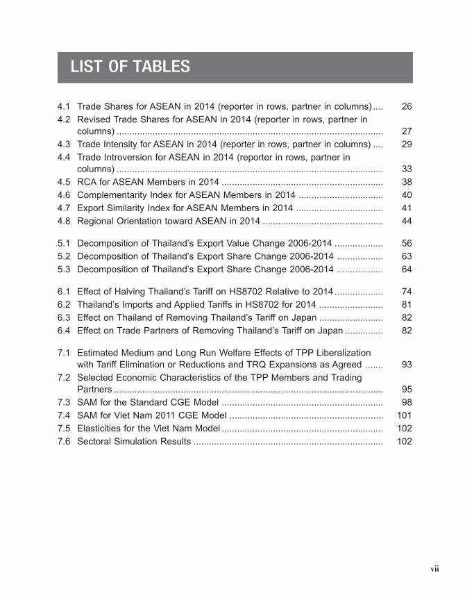
LIST OF TABLES
4.1 Trade Shares for ASEAN in 2014 (reporter in rows, partner in columns) .... 26
4.2 Revised Trade Shares for ASEAN in 2014 (reporter in rows, partner in
columns) ........................................................................................................ 27
4.3 Trade Intensity for ASEAN in 2014 (reporter in rows, partner in columns) .... 29
4.4 Trade Introversion for ASEAN in 2014 (reporter in rows, partner in
columns) ........................................................................................................ 33
4.5 RCA for ASEAN Members in 2014 ............................................................... 38
4.6 Complementarity Index for ASEAN Members in 2014 ................................. 40
4.7 Export Similarity Index for ASEAN Members in 2014 .................................. 41
4.8 Regional Orientation toward ASEAN in 2014 ............................................... 44
5.1 Decomposition of Thailand’s Export Value Change 2006-2014 ................... 56
5.2 Decomposition of Thailand’s Export Share Change 2006-2014 .................. 63
5.3 Decomposition of Thailand’s Export Share Change 2006-2014 .................. 64
6.1 Effect of Halving Thailand’s Tariff on HS8702 Relative to 2014................... 74
6.2 Thailand’s Imports and Applied Tariffs in HS8702 for 2014 ......................... 81
6.3 Effect on Thailand of Removing Thailand’s Tariff on Japan ......................... 82
6.4 Effect on Trade Partners of Removing Thailand’s Tariff on Japan ............... 82
7.1 Estimated Medium and Long Run Welfare Effects of TPP Liberalization
with Tariff Elimination or Reductions and TRQ Expansions as Agreed ....... 93
7.2 Selected Economic Characteristics of the TPP Members and Trading
Partners ......................................................................................................... 95
7.3 SAM for the Standard CGE Model ............................................................... 98
7.4 SAM for Viet Nam 2011 CGE Model ............................................................ 101
7.5 Elasticities for the Viet Nam Model ............................................................... 102
7.6 Sectoral Simulation Results .......................................................................... 102
viii
LIST OF FIGURES
2.1 Production, Consumption and Import Changes with a PTA ......................... 6
2.2 Economic Efficiency Changes with a PTA .................................................... 7
2.3 PTA with Terms of Trade Effects ................................................................... 8
3.1 The COMTRADE Interface ........................................................................... 15
3.2 A COMTRADE Data File ............................................................................... 18
5.1 Geometry of a Simple Share Decomposition ............................................... 58
6.1 Geometry of a Tariff ...................................................................................... 67
6.2 Lowering Tariffs and Economic Efficiency .................................................... 67
1
Chapter 1: Introduction
Chapter
1 INTRODUCTION
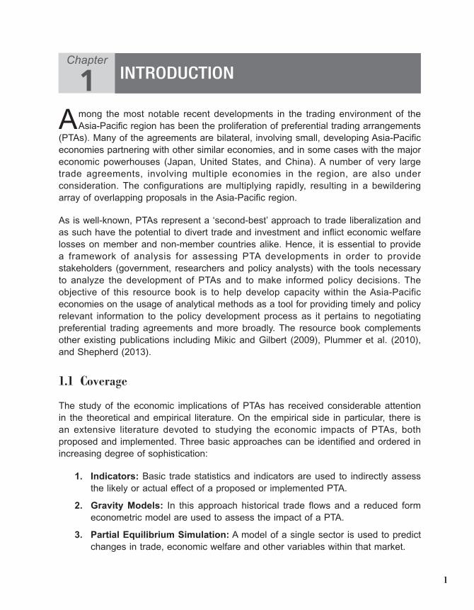
Among the most notable recent developments in the trading environment of the
Asia-Pacific region has been the proliferation of preferential trading arrangements
(PTAs). Many of the agreements are bilateral, involving small, developing Asia-Pacific
economies partnering with other similar economies, and in some cases with the major
economic powerhouses (Japan, United States, and China). A number of very large
trade agreements, involving multiple economies in the region, are also under
consideration. The configurations are multiplying rapidly, resulting in a bewildering
array of overlapping proposals in the Asia-Pacific region.
As is well-known, PTAs represent a ‘second-best’ approach to trade liberalization and
as such have the potential to divert trade and investment and inflict economic welfare
losses on member and non-member countries alike. Hence, it is essential to provide
a framework of analysis for assessing PTA developments in order to provide
stakeholders (government, researchers and policy analysts) with the tools necessary
to analyze the development of PTAs and to make informed policy decisions. The
objective of this resource book is to help develop capacity within the Asia-Pacific
economies on the usage of analytical methods as a tool for providing timely and policy
relevant information to the policy development process as it pertains to negotiating
preferential trading agreements and more broadly. The resource book complements
other existing publications including Mikic and Gilbert (2009), Plummer et al. (2010),
and Shepherd (2013).
1.1 Coverage
The study of the economic implications of PTAs has received considerable attention
in the theoretical and empirical literature. On the empirical side in particular, there is
an extensive literature devoted to studying the economic impacts of PTAs, both
proposed and implemented. Three basic approaches can be identified and ordered in
increasing degree of sophistication:
1. Indicators: Basic trade statistics and indicators are used to indirectly assess
the likely or actual effect of a proposed or implemented PTA.
2. Gravity Models: In this approach historical trade flows and a reduced form
econometric model are used to assess the impact of a PTA.
3. Partial Equilibrium Simulation: A model of a single sector is used to predict
changes in trade, economic welfare and other variables within that market.
2
Analytical Approaches to Evaluating Preferential Trade Agreements
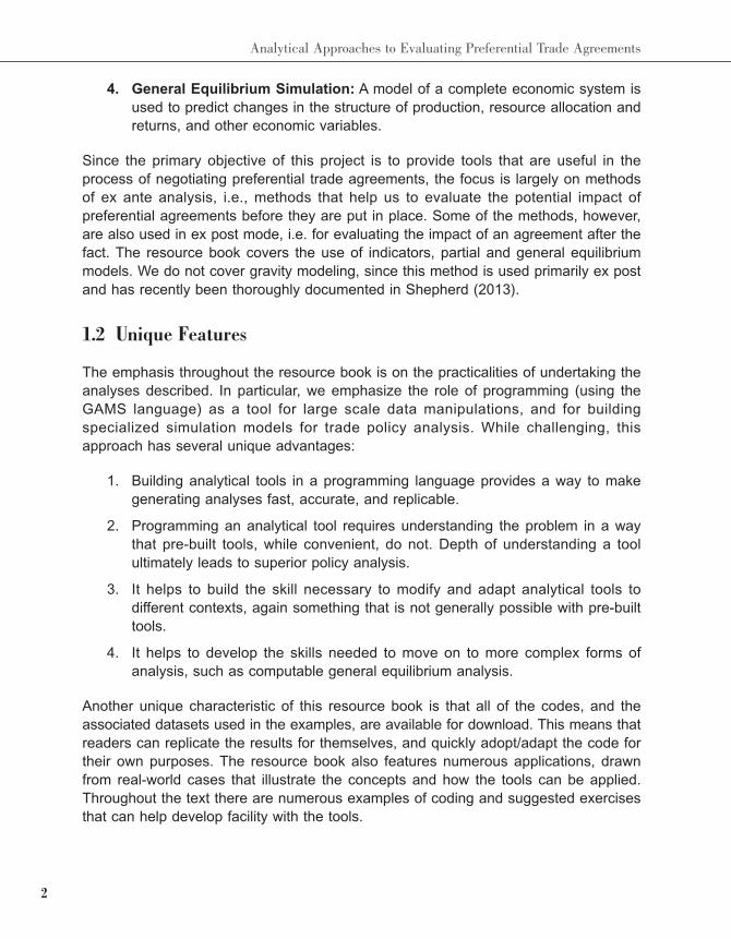
4. General Equilibrium Simulation: A model of a complete economic system is
used to predict changes in the structure of production, resource allocation and
returns, and other economic variables.
Since the primary objective of this project is to provide tools that are useful in the
process of negotiating preferential trade agreements, the focus is largely on methods
of ex ante analysis, i.e., methods that help us to evaluate the potential impact of
preferential agreements before they are put in place. Some of the methods, however,
are also used in ex post mode, i.e. for evaluating the impact of an agreement after the
fact. The resource book covers the use of indicators, partial and general equilibrium
models. We do not cover gravity modeling, since this method is used primarily ex post
and has recently been thoroughly documented in Shepherd (2013).
1.2 Unique Features
The emphasis throughout the resource book is on the practicalities of undertaking the
analyses described. In particular, we emphasize the role of programming (using the
GAMS language) as a tool for large scale data manipulations, and for building
specialized simulation models for trade policy analysis. While challenging, this
approach has several unique advantages:
1. Building analytical tools in a programming language provides a way to make
generating analyses fast, accurate, and replicable.
2. Programming an analytical tool requires understanding the problem in a way
that pre-built tools, while convenient, do not. Depth of understanding a tool
ultimately leads to superior policy analysis.
3. It helps to build the skill necessary to modify and adapt analytical tools to
different contexts, again something that is not generally possible with pre-built
tools.
4. It helps to develop the skills needed to move on to more complex forms of
analysis, such as computable general equilibrium analysis.
Another unique characteristic of this resource book is that all of the codes, and the
associated datasets used in the examples, are available for download. This means that
readers can replicate the results for themselves, and quickly adopt/adapt the code for
their own purposes. The resource book also features numerous applications, drawn
from real-world cases that illustrate the concepts and how the tools can be applied.
Throughout the text there are numerous examples of coding and suggested exercises
that can help develop facility with the tools.
3
Chapter 1: Introduction
1.3 Structure of the Resource Book
We begin (Chapter 2) with a general discussion of the economic theory behind the
formation of preferential trading agreements, and how it informs the analytical
approaches we take in assessing them. Next, we turn to some preliminary issues –
how to obtain trade data, and manipulate it for use in a programming environment like
GAMS (Chapter 3).
Preliminaries completed, we turn to the tools themselves, which are presented in
increasing order of complexity. Chapter 4 covers basic indicators that can be
constructed from trade flow data. This is followed in Chapter 5 by more complex
decompositions of trade indicators. Next we consider simulation methods, first partial
(Chapter 6) and then general equilibrium (Chapter 7) in nature.

4
Analytical Approaches to Evaluating Preferential Trade Agreements
5
Chapter 2: Theoretical Framework
Chapter
2 THEORETICAL FRAMEWORK
Here we briefly review the theoretical foundations underlying the economic analysis
of preferential trade agreements. Comprehensive reviews of the theory and the
debate surrounding the issue can be found in Panagariya (1999) and (2000), with the
latter concentrating almost exclusively on theoretical foundations.
2.1 Trade Creation and Diversion
The most common forms of PTA are the free trade area (FTA) and the customs union
(CU). The former is more widely observed in practice, while the latter is usually the
starting point for theoretical analysis (reflecting the simplifying benefit of the common
external tariff that distinguishes the two forms). Regardless of the form, the two most
basic concepts in the study of PTAs are trade creation and trade diversion, as
introduced in the work of Viner (1950) and Meade (1955). It is the conflicting signs of
these welfare terms that underlie the uncertainty and much of the controversy
surrounding PTA formation.
Trade creation is defined as the welfare gain associated with expansion of imports
from a relatively low cost source within the PTA. In essence, trade creation reflects
a partial reclamation of the deadweight (efficiency) loss associated with the initial
tariffs. It arises as resources formerly used in producing goods available at lower cost
through importation are released to more productive uses, and as consumers for whom
a tariff previously rendered consumption not beneficial expand their consumption
through imports.
Trade diversion is defined as the welfare loss associated with switching imports from
a relatively low cost supplier outside of the PTA to a relatively high cost supplier within
the PTA. The welfare loss occurs precisely because of the discriminatory tariffs applied
to members/non-members. As the source of imports switches, the tariff revenue initially
associated with imports is lost. Part of this is simply a transfer back to consumers on
whom the initial tariff was effectively imposed. But to the extent that post-PTA prices
exceed the tariff-exclusive initial prices, part of the loss is not transferred to consumers.
It is this part of revenue that constitutes trade diversion.
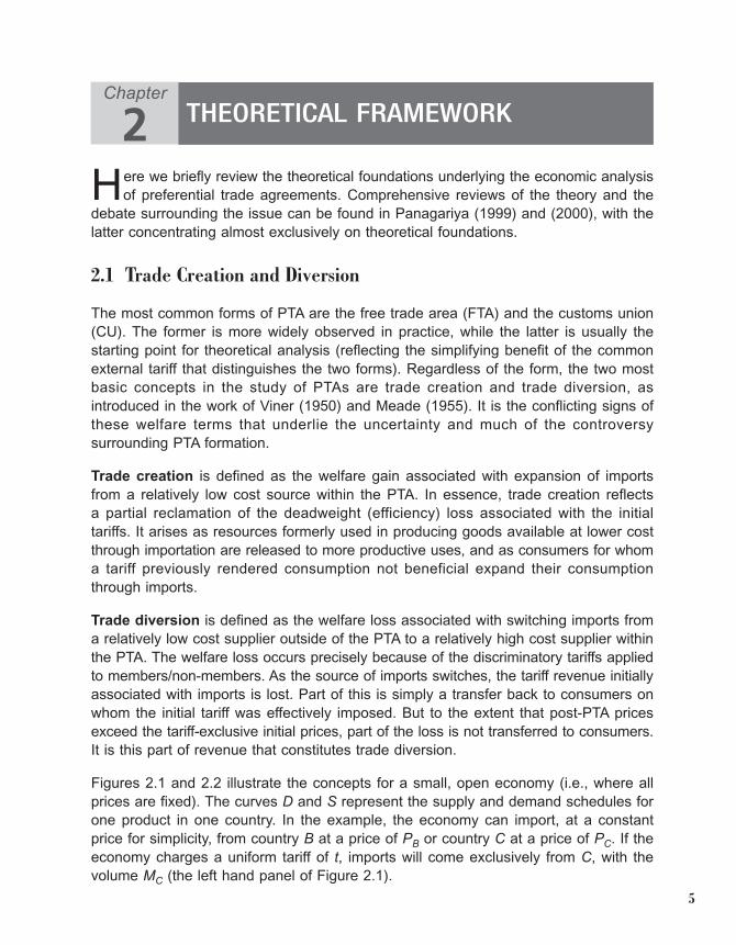
Figures 2.1 and 2.2 illustrate the concepts for a small, open economy (i.e., where all
prices are fixed). The curves D and S represent the supply and demand schedules for
one product in one country. In the example, the economy can import, at a constant
price for simplicity, from country B at a price of PB or country C at a price of PC. If the
economy charges a uniform tariff of t, imports will come exclusively from C, with the
volume MC (the left hand panel of Figure 2.1).
6
Analytical Approaches to Evaluating Preferential Trade Agreements
Figure 2.1: Production, Consumption and Import Changes with a PTA
(a) Pre-PTA (b) Post-PTA
Now suppose that the economy charges a zero tariff on imports from country B
while maintaining the tariff of t on country C. Imports will switch (be diverted) from
country C to country B. The new trade volume will be MB, in the right hand panel of
Figure 2.1. The volume of trade is larger (trade has been created).
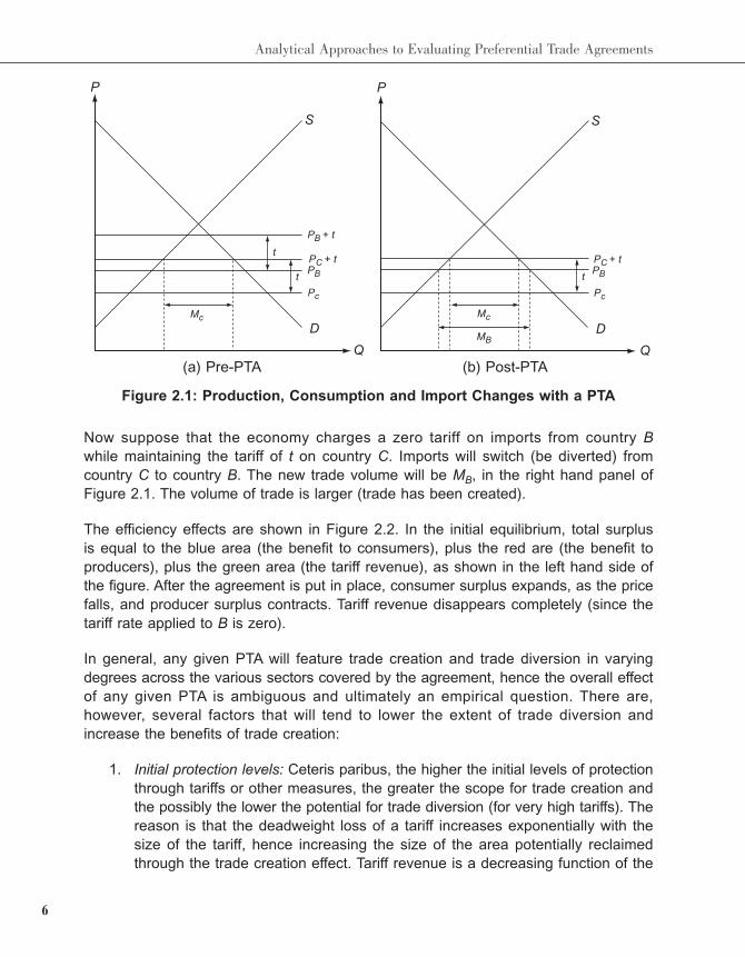
The efficiency effects are shown in Figure 2.2. In the initial equilibrium, total surplus
is equal to the blue area (the benefit to consumers), plus the red are (the benefit to
producers), plus the green area (the tariff revenue), as shown in the left hand side of
the figure. After the agreement is put in place, consumer surplus expands, as the price
falls, and producer surplus contracts. Tariff revenue disappears completely (since the
tariff rate applied to B is zero).
In general, any given PTA will feature trade creation and trade diversion in varying
degrees across the various sectors covered by the agreement, hence the overall effect
of any given PTA is ambiguous and ultimately an empirical question. There are,
however, several factors that will tend to lower the extent of trade diversion and
increase the benefits of trade creation:
1. Initial protection levels: Ceteris paribus, the higher the initial levels of protection
through tariffs or other measures, the greater the scope for trade creation and
the possibly the lower the potential for trade diversion (for very high tariffs). The
reason is that the deadweight loss of a tariff increases exponentially with the
size of the tariff, hence increasing the size of the area potentially reclaimed
through the trade creation effect. Tariff revenue is a decreasing function of the
P
D
Q
Mc
Pc
PB + t
PC + t PB
t
t
S
P
D
Q
S
PC + t PB
Mc
MB
Pc
t
7
Chapter 2: Theoretical Framework
size of the tariff when the tariff is sufficiently high (beyond the maximum
revenue tariff). In the limit, where tariff are prohibitive, only trade creation can
occur.
2. Competitiveness in member economies: The lower the prices at which member
economies are able to supply the needs of the PTA, the greater the scope for
trade creation and the lower the potential for trade diversion. In the limiting
case, if a member country is most efficient world supplier, and hence the initial
supplier pre-PTA, trade diversion is impossible and trade creation is
maximized.
3. Number of members: Related to the point above, the greater the number of
members of the agreement, the more likely it becomes to contain an efficient
producer of any given commodity. In the limit, a global PTA covering all goods
is equivalent to global free trade.
4. Sectoral coverage of the agreement: While broad sectoral coverage might
appear desirable (and is a requirement of Article XXIV of the WTO, which
governs preferential trading agreements), this is not necessarily the case.
Trade creation/diversion effects must be assessed at the sectoral level. In
general, it will be welfare superior to form an agreement covering sectors only
when trade creation effects in that sec-tor dominate trade diversion effects
(hence, for example, Scollay and Gilbert (2001) estimate that an agreement
between Japan and Republic of Korea that excludes agriculture is in fact
welfare superior to an agreement that includes agriculture).
Figure 2.2: Economic Efficiency Changes with a PTA
(a) Pre-PTA (b) Post-PTA
P
D
Q
Mc
Pc
PC + t PBt
S
P
D
Q
S
PC + t PB
Mc
MB
Pc
t
8
Analytical Approaches to Evaluating Preferential Trade Agreements
5. Barriers to non-members: As a general principle, the lower the barriers to trade
with non-members, the less the potential for diverting trade patterns.
The picture is complicated slightly by the introduction of terms-of-trade effects. These
are relevant when intra-PTA demand cannot be met by intra-PTA supply without
increasing prices, and/or when changes in the pattern of extra-PTA pattern of trade are
sufficiently large to alter the terms-of-trade with respect to non-members.
The first effect (intra-PTA) may create a gain for a partner country that is able to
expand into an export market through preferential treatment, but again initial tariff
levels play a critical role (in general, the higher the initial tariffs in the country that
exports post-PTA, the more likely a welfare gain becomes, see Panagariya (2000) for
further details). The overall effect remains ambiguous.
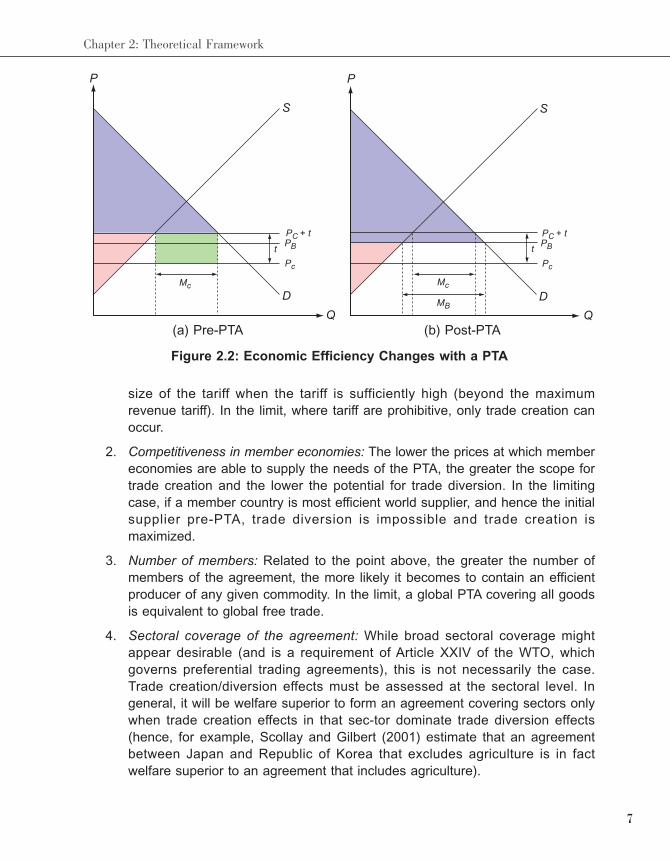
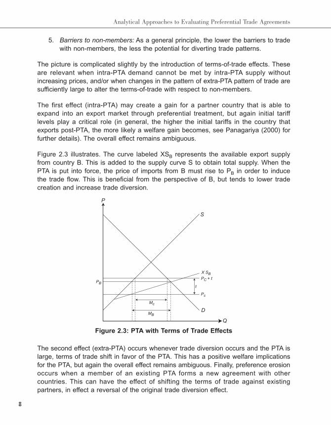
Figure 2.3 illustrates. The curve labeled XSB represents the available export supply
from country B. This is added to the supply curve S to obtain total supply. When the
PTA is put into force, the price of imports from B must rise to PB in order to induce
the trade flow. This is beneficial from the perspective of B, but tends to lower trade
creation and increase trade diversion.
P
D
Q
S
Mc
MB
PB
Pc
t
PC + t
X SB
Figure 2.3: PTA with Terms of Trade Effects
The second effect (extra-PTA) occurs whenever trade diversion occurs and the PTA is
large, terms of trade shift in favor of the PTA. This has a positive welfare implications
for the PTA, but again the overall effect remains ambiguous. Finally, preference erosion
occurs when a member of an existing PTA forms a new agreement with other
countries. This can have the effect of shifting the terms of trade against existing
partners, in effect a reversal of the original trade diversion effect.
9
Chapter 2: Theoretical Framework
A final theoretical point worth noting (and relating to point 5 above) is that it is always
possible to form a PTA that is welfare increasing (or at least not decreasing) for both
member and non-members. The theoretical result is due to Kemp and Wan (1976), as
applied to the CU, and Panagariya and Krishna (2002) in the case of FTAs. The
essence of these theorems is that the PTA can always adjust their external tariffs in
such a way that the extra-union trade flows are unchanged, while intra-union flows
expand. This is an important point with important policy prescriptions. It suggests that
multilateral reform accompanying PTA formation is likely to mitigate the potential for
trade diversion. It also suggests a mechanism by which welfare enhancing PTAs could
be designed and enforced, by checking the external trade pattern post-PTA (see
McMillan, 1993).
More recent literature has emphasized the role of differentiated products and imperfect
competition, and transportation costs. Differentiated products do not change the
conclusions markedly, except to the extent that, because each country has a degree
of monopoly power over its products, term-of-trade effects will definitely be present.
Where economies of scale are introduced, increased internal production leads to
a decrease in average cost which can magnify potential welfare gains, in addition to
allowing for increased variety, in particular if initial tariffs are high.
2.2 Dynamic Effects
While trade creation and diversion are the most fundamental concepts used in the
analysis of preferential trade agreements, they are static in nature. It is also
a sometimes argued that PTAs can have dynamic effects, both positive and negative.
Arguments for positive dynamic effects are based on the idea that a net trade-creating
PTA will generate higher incomes. Part of that income may be invested, which
generates still higher growth.
Another dynamic issue that has not been widely considered in the theoretical PTA
literature but is a component of the welfare cost of trade reform is adjustment costs.
It may be generally assumed that there is a cost involved in moving from one
equilibrium to another. This cost, while temporary, is nonetheless of policy interest.
2.3 Linking to Analytical Methods
Now consider the role of empirical investigation of PTAs. Most empirical studies of
PTAs seek to do one of two things. Either they attempt to determine whether or not
a proposed arrangement is likely to raise/lower welfare for the members/non-members
(ex-ante analysis), or they attempt to determine whether a given agreement did in fact
raise/lower welfare for the members/non-members (ex post analysis). Studies may
also, of course, attempt to address broader economic issues such as development,
income inequality, sectoral transformation, and so on.
10
Analytical Approaches to Evaluating Preferential Trade Agreements
The use of trade indices pre-PTA is in essence an attempt to indirectly gauge the
extent to which a given proposal is likely to have positive consequences by matching
real world data to theoretical characteristics that would promote such an outcome, as
outlined in Section 2.1. The use of trade indices post-PTA is in essence a search for
signs that trade diversion/creation (or some other economic outcome) did in fact occur,
and in what degree. Econometric modeling, including gravity model estimation is
a more sophisticated attempt do the same. For example, it might be argued that the
potential for trade creation is high if there is a strong overlap between the import and
export profiles of the trade partners. On the other hand, adjustment costs are likely to
be larger the greater the magnitude of production changes associated with PTA
formation, and lower if those changes involve shifts in intra-industry trade patterns than
inter-industry trade patterns (since intra-industry trade shifts may be reflecting changes
within a product category). Indices are a basic way of using data to assess possible
outcomes.
Simulation methods have the same objective, but increase the role of theory in
describing a wider range of possible outcomes. A partial equilibrium simulation model
will specify aspects of demand and supply in a market, fit to known data about that
market, and attempt to quantify the magnitude of the changes in trade, revenue,
economic surplus, and so on. Predictions may be used to infer other outcomes – large
predicted shifts in imports may suggest significant adjustment costs that may need to
be managed, and so on. Computable general equilibrium models up the degree of
sophistication considerably, by attempting to model an entire economic system and all
the interactions within, rather than a single market. Again though, the fundamental
objective is the same – utilize theory and data to attempt to quantify the magnitude
and direction of economic changes that are likely to occur with a PTA.
11
Chapter 3: Preliminaries
Chapter
3 PRELIMINARIES
This chapter has several objectives. First we will introduce the trade data and its
structure. We will then discuss the main sources of trade data, their pros and
cons. We will work through the process of obtaining data from one of these sources
– COMTRADE. Next we will discuss a programming language, called GAMS, which we
can use to manipulate trade data in various ways to obtain useful policy information.
By the end of the chapter you should be able understand the structure of trade data,
download a dataset from COMTRADE, and install a demonstration version of GAMS.
3.1 The Structure of Trade Data
International trade statistics record the flows of exports and imports from one country
to another over a defined time period. With a few exceptions, the data are recorded
as the value of the flow, not the volume. Generally, the countries between which trade
is measured are referred to as the ‘Reporter’ (i.e., the country that provided the data)
and the ‘Partner’. Flows from the reporter to the partner are exports, while flows from
the partner to the reporter are imports.
It is helpful to think about the trade data as a multi-dimensional array, the elements of
which are the values of exports or imports between a country pair in a particular
commodity. Because the export flows of one country are by definition the import flows
of another, each trade flow is, in principle, recorded twice, although in different terms.
Export data is recorded FOB, or free on board, and import data is recorded CIF, or
cost, insurance, freight, i.e., including costs of transportation.
Given data redundancy, a choice must be made as to which data should be used. As
a practical matter, the flows are reported by different agencies, and rarely match
exactly. The usual answer is that the import data is preferred to the export data, but
export data may be preferred in some cases if there is reason to suspect the import
data.
The fact that the data is recorded twice has another advantage: It allows for reporting
gaps to be filled using the ‘mirror’ data. In other words, if exports from a particular
reporter to a partner are not available, one can use the imports reported by the partner
instead. Filling the data this way is called mirroring. If both sides of a particular country
pair do not report, the data is missing, and mirroring cannot be done. Instead a model
must be created to predict the missing value. This process is called reconciling.
A reconciled trade flow array has no missing values. Further discussion of the structure
of trade data can be found in Mikic and Gilbert (2009).
12
Analytical Approaches to Evaluating Preferential Trade Agreements
3.1.1 Sources of Trade Data
We now turn to where to obtain international trade flow data. International trade data
can be obtained from national statistics or from one of several international databases.
We concentrate on the latter. Further discussion can be found in Plummer et al.
(2010).
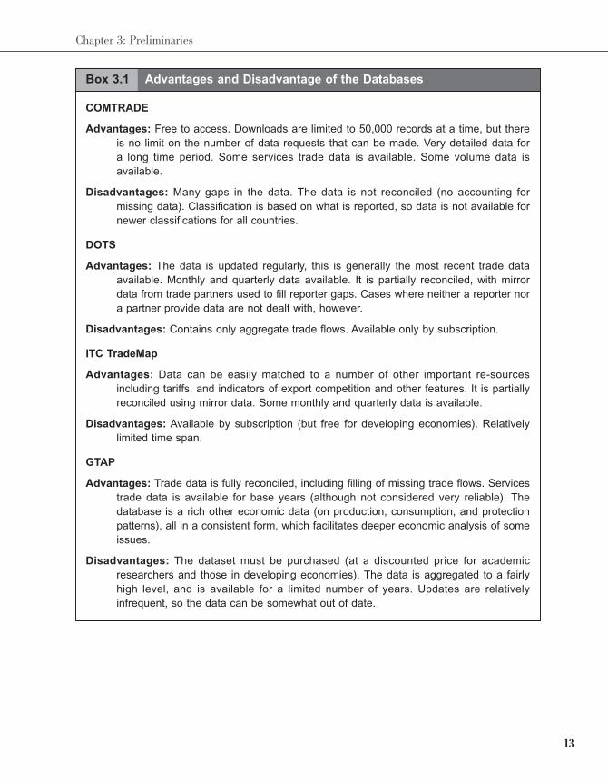
There are a number of potential databases to use, some of the advantages and
disadvantages of the various data sources are summarized in Box 3.1. The primary
data source for international trade flow data is the United Nations COMTRADE
database (comtrade.un.org). COMTRADE contains data on 248 economies, going
back as far as 1965 in some cases, although coverage varies. Data is available in
monthly and annual periods, although the latter series goes back further and has more
comprehensive coverage. The merchandise trade data available through this database
comes in several different classifications, including various versions of the Harmonized
System (HS), and the Standardized International Trade Classification (SITC). It is also
possible to obtain data classified using Broad Economic Classification (BEC). Data is
available at the 2, 4 and 6 digit levels. Data at the 6 digit level is available in both trade
values and trade volumes in some cases. The data is raw – it is just presented as
reported, and is not mirrored or reconciled.
Where only aggregate merchandise trade values are needed, an alternative to
COMTRADE is the Direction of Trade Statistics (DOTS) produced by the IMF
(www.imf.org). This dataset covers 190 economies, and flows are available at annual,
quarterly and even monthly time periods (for some economies) going as far back as
1980.
Another source of disaggregate trade data is the International Trade Center’s
TradeMap (www.trademap.org). This data is based on COMTRADE data,
supplemented with national trade sources. Data is available at up to the 6 digit level,
for the period 2001 on, for up to 220 countries (coverage varies). Some monthly and
quarterly data is available. The data has been partially reconciled, using the mirror
data.
Finally, the GTAP database (www.gtap.org) is a possible source. This database is
currently in its ninth iteration. It contains trade flow data for 140 regions and
57 sectors. The current version of the database has information on both merchandise
and service trade flows for the years 2011, 2007 and 2004. It also has time series data
on merchandise trade flows only from 1995 to 2013.
13
Chapter 3: Preliminaries
Box 3.1 Advantages and Disadvantage of the Databases
COMTRADE
Advantages: Free to access. Downloads are limited to 50,000 records at a time, but there
is no limit on the number of data requests that can be made. Very detailed data for
a long time period. Some services trade data is available. Some volume data is
available.
Disadvantages: Many gaps in the data. The data is not reconciled (no accounting for
missing data). Classification is based on what is reported, so data is not available for
newer classifications for all countries.
DOTS
Advantages: The data is updated regularly, this is generally the most recent trade data
available. Monthly and quarterly data available. It is partially reconciled, with mirror
data from trade partners used to fill reporter gaps. Cases where neither a reporter nor
a partner provide data are not dealt with, however.
Disadvantages: Contains only aggregate trade flows. Available only by subscription.
ITC TradeMap
Advantages: Data can be easily matched to a number of other important re-sources
including tariffs, and indicators of export competition and other features. It is partially
reconciled using mirror data. Some monthly and quarterly data is available.
Disadvantages: Available by subscription (but free for developing economies). Relatively
limited time span.
GTAP
Advantages: Trade data is fully reconciled, including filling of missing trade flows. Services
trade data is available for base years (although not considered very reliable). The
database is a rich other economic data (on production, consumption, and protection
patterns), all in a consistent form, which facilitates deeper economic analysis of some
issues.
Disadvantages: The dataset must be purchased (at a discounted price for academic
researchers and those in developing economies). The data is aggregated to a fairly
high level, and is available for a limited number of years. Updates are relatively
infrequent, so the data can be somewhat out of date.
14
Analytical Approaches to Evaluating Preferential Trade Agreements
3.1.2 Downloading Data from COMTRADE
In this resource book we will make use of data from the COMTRADE database, since
this is the most widely used source, especially for disaggregated data.1 The process
for downloading a dataset is quite straightforward.
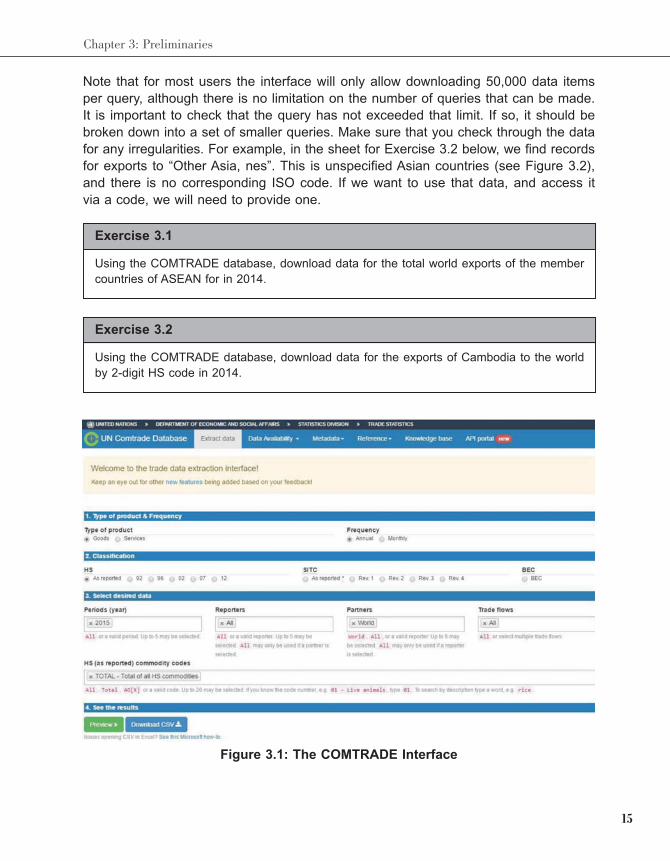
1. Go to the COMTRADE website (comtrade.un.org) click the get trade data
button. The interface to the database is shown in Figure 3.1.
2. Select the type of product (goods or services) and the frequency of the data
(annual or monthly).
3. Select the data classification (HS, SITC or BEC), then the revision if required.
4. Select the period (up to five separate years, or the group ‘all’ which will return
all available records). Selections are made by clicking in the box, and selecting
from the menu. Selections can be removed by clicking the ‘x’.2
5. Select the reporting country or countries in the same way. This is the country
that provided the data. Up to five can be selected at one time. Again, the
shortcut ‘all’ can be used if all reporting countries are desired.
6. Select the partner country or countries. Again, up to five can be selected at
a time. Special categories include ‘all’ and ‘world’ which select all partners and
the world total, respectively.
7. Select the trade flow, exports or imports, or re-exports and re-imports. The
latter refer to goods that are exported in the same state in which they were
imported (i.e., goods that did not undergo domestic processing), or imported in
the same state in which they were exported.
8. Select the commodity codes. Here there are a number of keys that can be
used. ‘Total’ returns total trade, ‘all’ returns all commodities. It is also possible
to specify various levels of aggregation, such as ‘AG02’, which will return all 2
digit classifications and so on. Note that the total trade does not necessarily
equal the sum of trade over all commodity groups. Up to twenty categories can
be chosen.
9. Click on the ‘Download CSV’ button to download the data in comma delimited
format, which can be opened in Excel or other programs for further
manipulation.
1 The World Bank Integrated Trade Solution (WITS – wits.worldbank.org) provides an alternative download
mechanism for COMTRADE data that is somewhat more flexible. It requires registration, but is free subject
to the same 50,000 item per query limit. Note that by default WITS reports values in thousands of dollars
rather than dollars.2 For more simultaneous selections, a legacy interface is also available. See the website for details.
15
Chapter 3: Preliminaries
Note that for most users the interface will only allow downloading 50,000 data items
per query, although there is no limitation on the number of queries that can be made.
It is important to check that the query has not exceeded that limit. If so, it should be
broken down into a set of smaller queries. Make sure that you check through the data
for any irregularities. For example, in the sheet for Exercise 3.2 below, we find records
for exports to “Other Asia, nes”. This is unspecified Asian countries (see Figure 3.2),
and there is no corresponding ISO code. If we want to use that data, and access it
via a code, we will need to provide one.
Exercise 3.1
Using the COMTRADE database, download data for the total world exports of the member
countries of ASEAN for in 2014.
Exercise 3.2
Using the COMTRADE database, download data for the exports of Cambodia to the world
by 2-digit HS code in 2014.
Figure 3.1: The COMTRADE Interface
16
Analytical Approaches to Evaluating Preferential Trade Agreements
3.2 A Quick Introduction to GAMS
Once we have trade data, we need a method for manipulating the data into a usable
form. Depending on what we want to do with the data there are many options. For
small problems, a simple program like Microsoft Excel is likely to be sufficient. For
problems involving more complex manipulations of larger datasets, more powerful
software is needed. Throughout this volume we will be developing a series of
programs using GAMS. GAMS has powerful data manipulation capabilities, and is also
a platform within which complex models can be developed. In this chapter we provide
some basic notes to get you started with the GAMS system. We’ll introduce more
complex features as we proceed.
3.2.1 What is GAMS?
GAMS is an acronym that stands for the General Algebraic Modeling System. It is
a high level programming language designed for building and solving mathematical
models numerically. GAMS provides a framework for model development that is
independent of the platform on which the model is to be run, and distinct from the
mathematical algorithms that are used to solve the model.3 This means that models
built in GAMS can be run on different machines, and solved using different techniques,
without any adjustment to the model itself. GAMS can solve a wide variety of
problems, and is capable of handling very large mathematical systems, and
manipulating very large datasets.
3.3 Getting and Installing GAMS
GAMS Corporation provides a student/demonstration version of GAMS free of charge.
This version of the software is limited in the dimensions of the models that can be built.
However all of the models developed in this book are small enough to be solved using
the student version of the software. The latest version can be downloaded from
www.gams.com/download/. Various flavors are available. For most users the 32 bit
Windows version will be appropriate. If you are using a 64 bit version of Windows you
can download the 64 bit Windows version. Versions are also available for users of
Linux (32 or 64 bit) and Mac OS X.
To install any Windows version of the software, right click the link on the GAMS site
and choose the Save Link As option from the context menu. Then save the installation
file in an appropriate location on your local computer (the file is approximately 60 mb).
Once the file has downloaded, double click on it to start the installation process. The
installer will prompt you for a directory in which to install the GAMS system (the default
3 GAMS is actually a front-end for numerous different commercial algorithms, all of which are packaged with
the GAMS system and may be licensed independently.
17
Chapter 3: Preliminaries
should be fine). It should also prompt you for a start menu location, and again the
default should be fine. A prompt will appear asking if you wish to copy a license file.
You can click no (without the license file GAMS will run in student/demonstration
mode). Once it has installed, GAMS will ask if you want to launch the IDE, or
integrated development environment. This is the main GAMS interface. Click ‘yes’ and
GAMS should appear.
There are a numerous packages that have been written to make using GAMS easier.
Thomas Rutherford developed some particularly useful packages while at
the University of Colorado. These include packages to automatic the process of
writing tables and reports, among other tasks. To install these packages go to
http://www.mpsge.org/ inclib/gams2tbl.htm, and download the package inclib.pck,
which should be placed in your GAMS directory, then run GAMSINST from the
command line, hitting enter at each prompt to select the defaults. Alternatively, you can
place a copy of the file GAMS2TBL.GMS in your project directory.
Exercise 3.3
Go to the GAMS website. Download and install a demonstration version of the GAMS
software. Download and install the inclib package.
Further details on the installation process are available for various platforms at the
GAMS website (www.gams.com/docs/document.htm). At the same location you can
also find the detailed GAMS User’s Guide, a GAMS Tutorial, and other useful
documentation in electronic form. Professor Rutherford’s notes at http://www.
mpsge.org/inclib/gams2tbl.htm provide further details on the usage of the add-on
packages.
3.4 How Does GAMS Work?
GAMS is a text based programming system that operates in a batch mode. A GAMS
program is a text file containing a set of instructions for pulling in data, manipulating
it, and writing results. The text file is usually given the suffix gms. To run the program,
the text file is submitted to the GAMS system. GAMS then checks for syntax errors,
works through the instructions reports the result back to GAMS. A list file (with the
suffix lst) is produced that contains on the program results, and, if something went
wrong in the process, information on where the problem lies. The best way to learn
about GAMS is to use it, so we’ll work through multiple examples in this book. Further
details on GAMS can be found in the GAMS User’s Guide. Zenios (1996) is another
useful reference on the capabilities of GAMS. Bruce McCarl also has an online
reference to GAMS that has very useful programming advice. Gilbert and Tower (2013)
contains further details on using GAMS for simulation modeling.
18
Analytical Approaches to Evaluating Preferential Trade Agreements
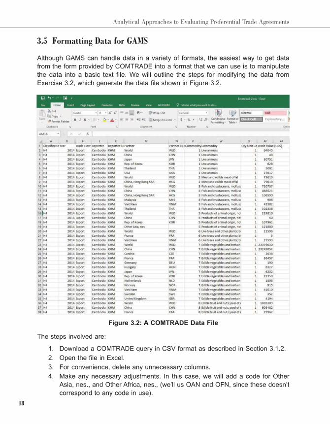
3.5 Formatting Data for GAMS
Although GAMS can handle data in a variety of formats, the easiest way to get data
from the form provided by COMTRADE into a format that we can use is to manipulate
the data into a basic text file. We will outline the steps for modifying the data from
Exercise 3.2, which generate the data file shown in Figure 3.2.
Figure 3.2: A COMTRADE Data File
The steps involved are:
1. Download a COMTRADE query in CSV format as described in Section 3.1.2.
2. Open the file in Excel.
3. For convenience, delete any unnecessary columns.
4. Make any necessary adjustments. In this case, we will add a code for Other
Asia, nes., and Other Africa, nes., (we’ll us OAN and OFN, since these doesn’t
correspond to any code in use).
19
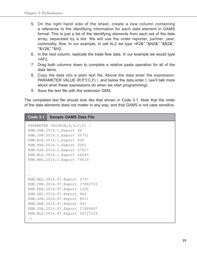
Chapter 3: Preliminaries
Code 3.1 Sample GAMS Data File
PARAMETER VALUE(R,P,Y,C,F) /
KHM.CHN.2014.1.Export 48
KHM.JPN.2014.1.Export 30751
KHM.KOR.2014.1.Export 628
KHM.THA.2014.1.Export 5001
KHM.USA.2014.1.Export 27617
KHM.WLD.2014.1.Export 64045
KHM.HKG.2014.2.Export 79619
.
.
.
KHM.BEL.2014.97.Export 2737
KHM.CHN.2014.97.Export 37882733
KHM.FRA.2014.97.Export 1200
KHM.DEU.2014.97.Export 449
KHM.JPN.2014.97.Export 8011
KHM.GBR.2014.97.Export 997
KHM.USA.2014.97.Export 17484847
KHM.WLD.2014.97.Export 58727229
/;
5. On the right hand side of the sheet, create a new column containing
a reference to the identifying information for each data element in GAMS
format. This is just a list of the identifying elements from each set of the data
array, separated by a dot. We will use the order reporter, partner, year,
commodity, flow. In our example, in cell AL2 we type =K2&″.″&N2&″.″&B2&″.″&V2&″.″&H2.
6. In the next column, replicate the trade flow data. In our example we would type
=AF2.
7. Drag both columns down to complete a relative paste operation for all of the
data items.
8. Copy the data into a plain text file. Above the data enter the expression:
PARAMETER VALUE (R,P,Y,C,F) /, and below the data enter /; (we’ll talk more
about what these expressions do when we start programming).
9. Save the text file with the extension GMS.
The completed text file should look like that shown in Code 3.1. Note that the order
of the data elements does not matter in any way, and that GAMS is not case sensitive.
20
Analytical Approaches to Evaluating Preferential Trade Agreements
Exercise 3.4
Using the COMTRADE data file from Exercise 3.1, construct the complete GAMS data file.
Exercise 3.5
Construct a GAMS data file for the total exports of all ASEAN economies to the world and
all ASEAN partner countries in 2014.
21
Chapter 4: Trade Indicators
Chapter
4 TRADE INDICATORS
As defined by Mikic and Gilbert (2009), a trade indicator is an index used to assess
the state of trade flows and the pattern of trade for an economy or group of
economies. A number of indicators can provide useful insights into the economic
effects of a preferential trade agreement both ex ante and ex post.
As Plummer et al. (2010) note, trade indicators are usually the first step in evaluating
potential regional trading agreements. They have a number of advantages and some
disadvantages, summarized in Box 4.1. In particular their relative simplicity means that
they can be calculated and used in the policy discussion very quickly. However, unlike
some econometric techniques (such as gravity modeling), indicators are not capable
of establishing causality. Moreover, because they are based on calibrations of the trade
data, any measurement error is passed through. Finally, indicators do just that –
indicate. They cannot directly predict economic impacts that may be of interest, such
as changes in economic welfare, trade volumes or tax revenues. For that, we need to
develop more sophisticated methods. Nonetheless, used ex ante indicators can
provide useful insights into such issues as the complementarity of trade profiles, and
used ex post they can provide useful information on the trade integration process, and
may highlight potential problems such as trade diversion.
In this chapter we introduce a variety of trade indicators that are useful for assessing
the impact of preferential trade agreements. The objectives of the chapter are to define
indices relating to the overall degree of trade integration, and pattern in sectoral trade,
to develop GAMS codes for calculating the indices, and to provide examples of the
calculation process and interpretation of the results. At the end of the chapter you
should be able to calculate and interpret all of the indices, and have an idea of how
the code could be modified to construct other indices describing different patterns in
the international trade data (see Mikic and Gilbert, 2009).
Box 4.1 Advantages and Disadvantage of Indicators
Advantages: Simple to construct. Based on data that is widely available for most countries.
Straightforward interpretation. Many indices are available to shed light on different
aspects of international trade patterns.
Disadvantages: Subject to measurement error. Do not indicate causality. Cannot directly
measure potential changes in economic variables of policy interest. Care must be
taken to apply indicators at an appropriate level of aggregation.
22
Analytical Approaches to Evaluating Preferential Trade Agreements
4.1 Notation
Before we start, it will be helpful develop a common notation. As noted in the previous
chapter, we can think of the trade statistics as a three dimensional array of value flows
evaluated in some common currency. Hence, let the trade flow array have dimensions
I × R × P, where I the set of traded commodities, with elements i, and R is the set of
reporting countries with elements r, and P is set of partner countries, with elements p.
Let xirp denote one element of the trade array, the exports of good i from reporter r to
partner p. Let mipr represent imports of good i from partner p to reporter r. Note that
we adopt the convention of putting the source of the flow (i.e., the exporting country)
before the destination (the importing country). Finally, let tirp = xirp + mipr indicate total
trade (imports plus exports) to and from a particular reporter. Where we are
considering changes across time periods with a superscript, which we drop for clarity
when considering a single time period.
We use summation notation to indicate various summary statistics. Hence, for
example, total exports of good i from reporter r is written Σp xirp, while total exports
from country r is written Σi, p xirp, and so on. Because we will use sums so often
though, it will be helpful to develop some compact notation. Let Xr represent total
exports of all goods from reporter r, and Xir represent total exports of good i from
reporter r, and Xrp represent total exports from reporter r to partner p. We can define
sums for trade and imports similarly.
Finally, let’s construct some special notation for cases where we want to sum either
over a subset of reporters or partners. Let W be a set containing all countries in the
world, and let B be a set of countries in a particular trade bloc. Define a subscript in
either the reporter or partner position to mean the sum over the elements in that set.
Hence, XrW is total exports of reporter r to the world, XrB denotes exports from reporter
r to the members of a defined trade bloc B, XWr is total exports from the world to
reporter r, XiW is total world exports of good i, and so on. Import and trade sums can
be defined similarly. Box 4.2 summarizes the notation for easy reference.
Box 4.2 Summary of Notation
xirp Exports of good i from reporter r to partner p.
mirp Imports of good i from partner p to reporter r.
tirp Total of exports and imports of good i from/to reporter r to/from partner p.
Xir Total exports of good i from reporter r.
Xrp Total exports from reporter r to partner p.
Xr Total exports of reporter r.
XiW Total world exports of good i.
XWr Total exports of the world to reporter r.
XW Total world exports.
23
Chapter 4: Trade Indicators
4.2 Measures of Overall Trade Integration
We begin with some statistics that can be used to evaluate the extent of regional
integration in overall trade.1
4.2.1 Intra-Regional Trade Share
A common statistic constructed to examine the regional trade pattern among members
of a given group or region is the intrabloc or intra-regional trade share. The aggregate
intra-regional trade share for a region B is defined simply as:
(4.1)
In words, it is the ratio of the total trade between economies in region B to the total
trade of B with the world as a whole, expressed as a percentage. Since in principle
the exports of region B to itself are equal to the imports from region B to itself, the ratio
can alternatively be calculated as
This index has several shortcomings. In particular we should note that the index is
increasing in the size of the members of the trade bloc in international trade. Hence,
the intra-regional trade share for NAFTA, for example, is likely to be higher than for
ASEAN in part purely because of the difference in size, and not necessarily because
of a higher degree of integration. Hence, we want to be very careful making
comparisons across different trade groups of divergent sizes. Frankel (1997) has
further discussion. Nonetheless, ex ante, high levels of intra-bloc trade is often
interpreted as reflecting a ‘natural’ trading bloc, in which trade diversion effects are
likely to be minimal, and ex post increases in intra-bloc trade over time are often
interpreted as reflecting the results of a PTA where one exists (assuming that the
membership is not also changing).
Coding the Problem in GAMS
So how can we write a GAMS program to calculate the intra-regional trade share?
First we need an appropriate dataset. In this case we need a data file containing total
exports of the economies of interest to each other and the world as a whole. The
dataset from Exercise 3.5, which is for the members of ASEAN is an example.
A sample code that accomplishes what we need is presented in Code 4.1. We’ll use
it to calculate the intra-ASEAN trade share.
1 In all the examples in this book we use the data as reported.
24
Analytical Approaches to Evaluating Preferential Trade Agreements
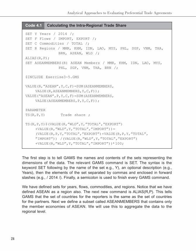
Code 4.1 Calculating the Intra-Regional Trade Share
SET Y Years / 2014 /;
SET F Flows / IMPORT, EXPORT /;
SET C Commodities / TOTAL /;
SET R Regions / MMR, KHM, IDN, LAO, MYS, PHL, SGP, VNM, THA,
BRN, ASEAN, WLD /;
ALIAS(R,P);
SET ASEANMEMBERS(R) ASEAN Members / MMR, KHM, IDN, LAO, MYS,
PHL, SGP, VNM, THA, BRN /;
$INCLUDE Exercise3-5.GMS
VALUE(R,”ASEAN”,Y,C,F)=SUM(ASEANMEMBERS,
VALUE(R,ASEANMEMBERS,Y,C,F));
VALUE(“ASEAN”,P,Y,C,F)=SUM(ASEANMEMBERS,
VALUE(ASEANMEMBERS,P,Y,C,F));
PARAMETER
TS(R,P,Y) Trade share ;
TS(R,P,Y)$(VALUE(R,”WLD”,Y,”TOTAL”,”EXPORT”)
+VALUE(R,”WLD”,Y,”TOTAL”,”IMPORT”))=
(VALUE(R,P,Y,”TOTAL”,”EXPORT”)+VALUE(R,P,Y,”TOTAL”,
”IMPORT”)) /(VALUE(R,”WLD”,Y,”TOTAL”,”EXPORT”)
+VALUE(R,”WLD”,Y,”TOTAL”,”IMPORT”))*100;
The first step is to tell GAMS the names and contents of the sets representing the
dimensions of the data. The relevant GAMS command is SET. The syntax is the
keyword SET following by the name of the set e.g., Y), an optional description (e.g.,
Years), then the elements of the set separated by commas and enclosed in forward
slashes (e.g., / 2014 /). Finally, a semicolon is used to finish every GAMS command.
We have defined sets for years, flows, commodities, and regions. Notice that we have
defined ASEAN as a region also. The next new command is ALIAS(R,P). This tells
GAMS that the set of countries for the reporters is the same as the set of countries
for the partners. Next we define a subset called ASEANMEMBERS that contains only
the member economies of ASEAN. We will use this to aggregate the data to the
regional level.
25
Chapter 4: Trade Indicators
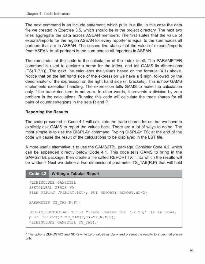
The next command is an include statement, which pulls in a file, in this case the data
file we created in Exercise 3.5, which should be in the project directory. The next two
lines aggregate the data across ASEAN members. The first states that the value of
exports/imports for the region ASEAN for every reporter is equal to the sum across all
partners that are in ASEAN. The second line states that the value of exports/imports
from ASEAN to all partners is the sum across all reporters in ASEAN.
The remainder of the code is the calculation of the index itself. The PARAMETER
command is used to declare a name for the index, and tell GAMS its dimensions
(TS(R,P,Y)). The next line calculates the values based on the formula (4.1) above.
Notice that on the left hand side of the expression we have a $ sign, followed by the
denominator of the expression on the right hand side (in brackets). This is how GAMS
implements exception handling. The expression tells GAMS to make the calculation
only if the bracketed term is not zero. In other words, it prevents a division by zero
problem in the calculations. Running this code will calculate the trade shares for all
pairs of countries/regions in the sets R and P.
Reporting the Results
The code presented in Code 4.1 will calculate the trade shares for us, but we have to
explicitly ask GAMS to report the values back. There are a lot of ways to do so. The
most simple is to use the DISPLAY command. Typing DISPLAY TS; at the end of the
code will cause the result of the calculations to be displayed in the LST file.
A more useful alternative is to use the GAMS2TBL package. Consider Code 4.2, which
can be appended directly below Code 4.1. This code tells GAMS to bring in the
GAMS2TBL package, then create a file called REPORT.TXT into which the results will
be written.2 Next we define a two dimensional parameter TS_TAB(R,P) that will hold
2 The options ZEROS NO and ND=2 write zero values as blank and present the results to 2 decimal places
only.
Code 4.2 Writing a Tabular Report
$LIBINCLUDE GAMS2TBL
$SETGLOBAL ZEROS NO
FILE REPORT /REPORT.TXT/; PUT REPORT; REPORT.ND=2;
PARAMETER TS_TAB(R,P);
LOOP(Y,$SETGLOBAL TITLE “Trade Shares for ‘,Y.TL,’ (r in rows,
p in columns)” TS_TAB(R,P)=TS(R,P,Y);
$LIBINCLUDE GAMS2TBL TS_TAB);
26
Analytical Approaches to Evaluating Preferential Trade Agreements
the value of the trade share for each year (since a table can only have two
dimensions). Finally, we set up a LOOP over each year (in this case there is only one),
and invoke GAMS2TBL to write the table. The resulting output, contained in the file
REPORT.TXT is given in Table 4.1.
Exercise 4.1
Run the code yourself to verify the results presented in Table 4.1.
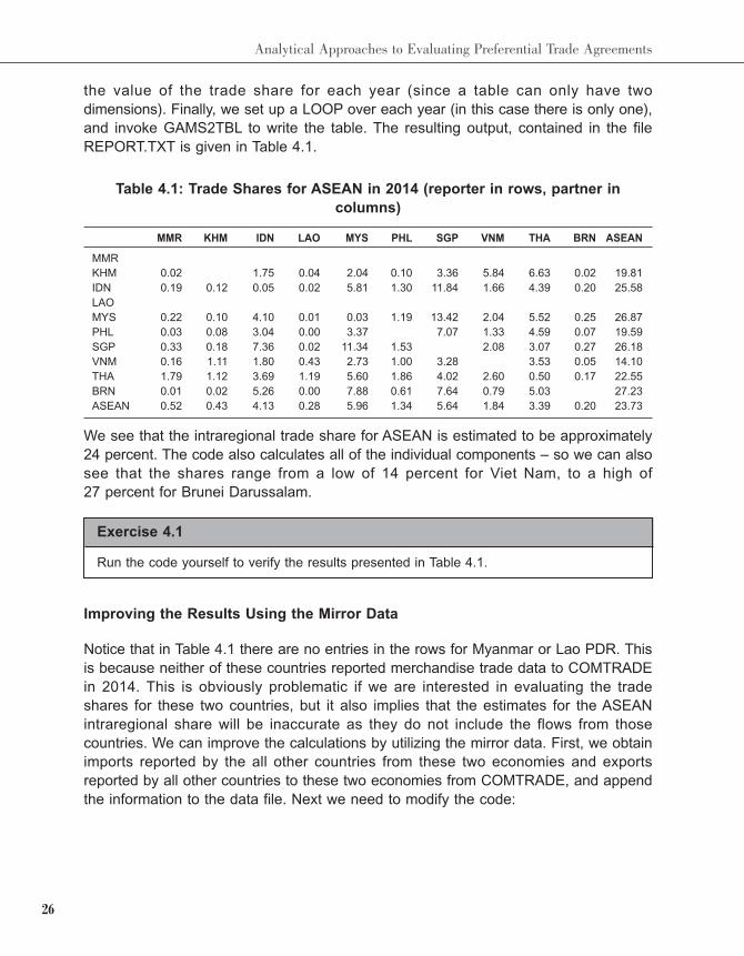
We see that the intraregional trade share for ASEAN is estimated to be approximately
24 percent. The code also calculates all of the individual components – so we can also
see that the shares range from a low of 14 percent for Viet Nam, to a high of
27 percent for Brunei Darussalam.
Table 4.1: Trade Shares for ASEAN in 2014 (reporter in rows, partner in
columns)
MMR KHM IDN LAO MYS PHL SGP VNM THA BRN ASEAN
MMR
KHM 0.02 1.75 0.04 2.04 0.10 3.36 5.84 6.63 0.02 19.81
IDN 0.19 0.12 0.05 0.02 5.81 1.30 11.84 1.66 4.39 0.20 25.58
LAO
MYS 0.22 0.10 4.10 0.01 0.03 1.19 13.42 2.04 5.52 0.25 26.87
PHL 0.03 0.08 3.04 0.00 3.37 7.07 1.33 4.59 0.07 19.59
SGP 0.33 0.18 7.36 0.02 11.34 1.53 2.08 3.07 0.27 26.18
VNM 0.16 1.11 1.80 0.43 2.73 1.00 3.28 3.53 0.05 14.10
THA 1.79 1.12 3.69 1.19 5.60 1.86 4.02 2.60 0.50 0.17 22.55
BRN 0.01 0.02 5.26 0.00 7.88 0.61 7.64 0.79 5.03 27.23
ASEAN 0.52 0.43 4.13 0.28 5.96 1.34 5.64 1.84 3.39 0.20 23.73
Improving the Results Using the Mirror Data
Notice that in Table 4.1 there are no entries in the rows for Myanmar or Lao PDR. This
is because neither of these countries reported merchandise trade data to COMTRADE
in 2014. This is obviously problematic if we are interested in evaluating the trade
shares for these two countries, but it also implies that the estimates for the ASEAN
intraregional share will be inaccurate as they do not include the flows from those
countries. We can improve the calculations by utilizing the mirror data. First, we obtain
imports reported by the all other countries from these two economies and exports
reported by all other countries to these two economies from COMTRADE, and append
the information to the data file. Next we need to modify the code:
27
Chapter 4: Trade Indicators
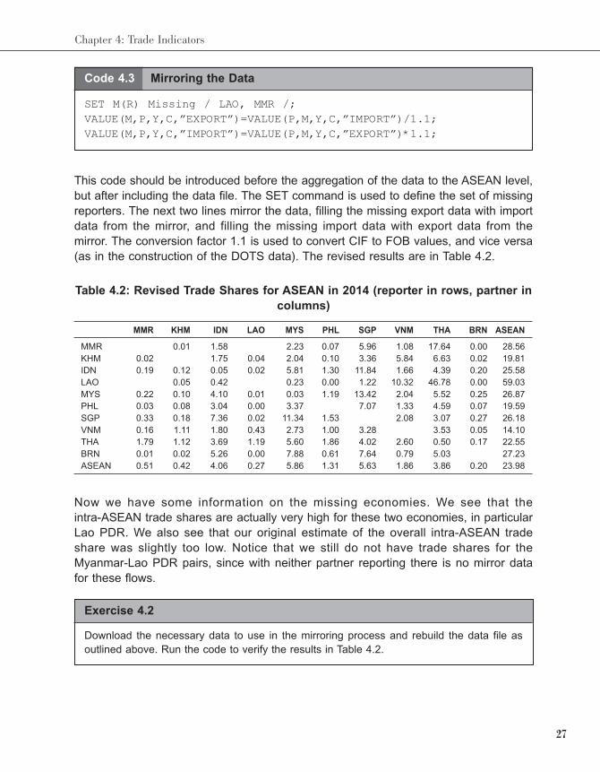
This code should be introduced before the aggregation of the data to the ASEAN level,
but after including the data file. The SET command is used to define the set of missing
reporters. The next two lines mirror the data, filling the missing export data with import
data from the mirror, and filling the missing import data with export data from the
mirror. The conversion factor 1.1 is used to convert CIF to FOB values, and vice versa
(as in the construction of the DOTS data). The revised results are in Table 4.2.
Now we have some information on the missing economies. We see that the
intra-ASEAN trade shares are actually very high for these two economies, in particular
Lao PDR. We also see that our original estimate of the overall intra-ASEAN trade
share was slightly too low. Notice that we still do not have trade shares for the
Myanmar-Lao PDR pairs, since with neither partner reporting there is no mirror data
for these flows.
Code 4.3 Mirroring the Data
SET M(R) Missing / LAO, MMR /;
VALUE(M,P,Y,C,”EXPORT”)=VALUE(P,M,Y,C,”IMPORT”)/1.1;
VALUE(M,P,Y,C,”IMPORT”)=VALUE(P,M,Y,C,”EXPORT”)*1.1;
Table 4.2: Revised Trade Shares for ASEAN in 2014 (reporter in rows, partner in
columns)
MMR KHM IDN LAO MYS PHL SGP VNM THA BRN ASEAN
MMR 0.01 1.58 2.23 0.07 5.96 1.08 17.64 0.00 28.56
KHM 0.02 1.75 0.04 2.04 0.10 3.36 5.84 6.63 0.02 19.81
IDN 0.19 0.12 0.05 0.02 5.81 1.30 11.84 1.66 4.39 0.20 25.58
LAO 0.05 0.42 0.23 0.00 1.22 10.32 46.78 0.00 59.03
MYS 0.22 0.10 4.10 0.01 0.03 1.19 13.42 2.04 5.52 0.25 26.87
PHL 0.03 0.08 3.04 0.00 3.37 7.07 1.33 4.59 0.07 19.59
SGP 0.33 0.18 7.36 0.02 11.34 1.53 2.08 3.07 0.27 26.18
VNM 0.16 1.11 1.80 0.43 2.73 1.00 3.28 3.53 0.05 14.10
THA 1.79 1.12 3.69 1.19 5.60 1.86 4.02 2.60 0.50 0.17 22.55
BRN 0.01 0.02 5.26 0.00 7.88 0.61 7.64 0.79 5.03 27.23
ASEAN 0.51 0.42 4.06 0.27 5.86 1.31 5.63 1.86 3.86 0.20 23.98
Exercise 4.2
Download the necessary data to use in the mirroring process and rebuild the data file as
outlined above. Run the code to verify the results in Table 4.2.
28
Analytical Approaches to Evaluating Preferential Trade Agreements
4.2.2 Trade Intensity
As we noted above, a problem with the trade share is that the measure will tend to
be larger the larger the size of the group considered, both in terms of the economic
size and number of members. If we want to compare the index across different
countries or groups, we need to normalize it in a way that makes the indices
comparable. A common correction is provided by constructing the trade intensity ratio,
also referred to as the concentration ratio. This is defined for region B as:
(4.2)
i.e., the simple intraregional trade share is divided by the share of world trade directed
to the region of interest. In other words, we normalize by considering the trade share
of the region relative to the world average for that region. This statistic is widely used
(see Ng and Yeats, 2003). In a sense, this statistic operates much like a rudimentary
gravity model. The statistic takes on a value of unity when the intraregional trade
pattern does not differ from the expected level given the pattern of world trade. The
interpretation is much like a trade share.
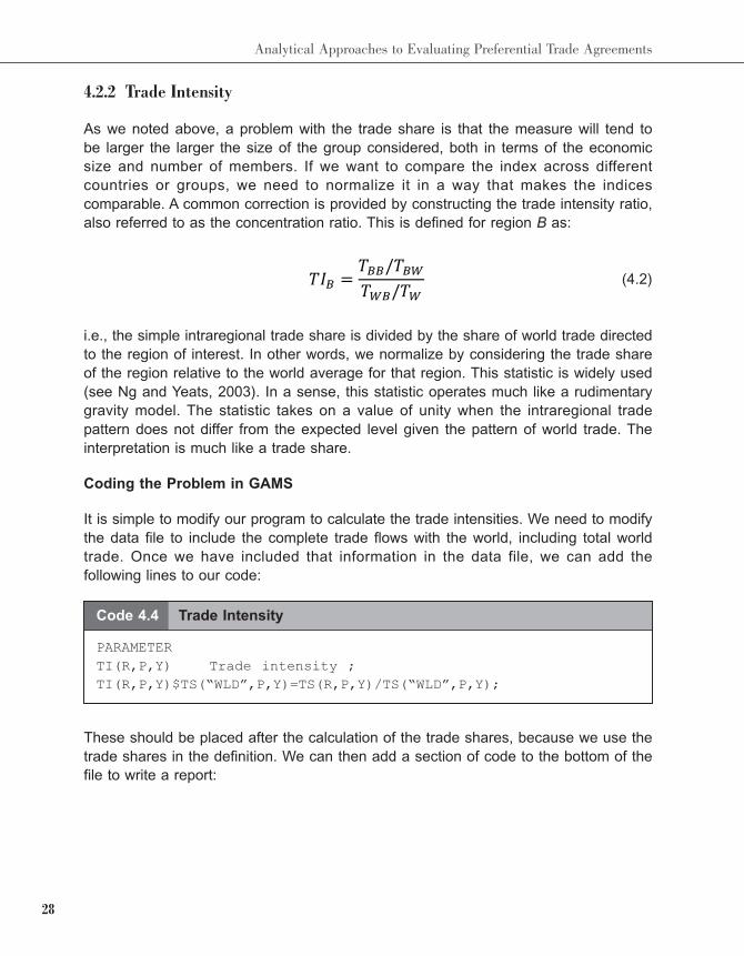
Coding the Problem in GAMS
It is simple to modify our program to calculate the trade intensities. We need to modify
the data file to include the complete trade flows with the world, including total world
trade. Once we have included that information in the data file, we can add the
following lines to our code:
Code 4.4 Trade Intensity
PARAMETER
TI(R,P,Y) Trade intensity ;
TI(R,P,Y)$TS(“WLD”,P,Y)=TS(R,P,Y)/TS(“WLD”,P,Y);
These should be placed after the calculation of the trade shares, because we use the
trade shares in the definition. We can then add a section of code to the bottom of the
file to write a report:
29
Chapter 4: Trade Indicators
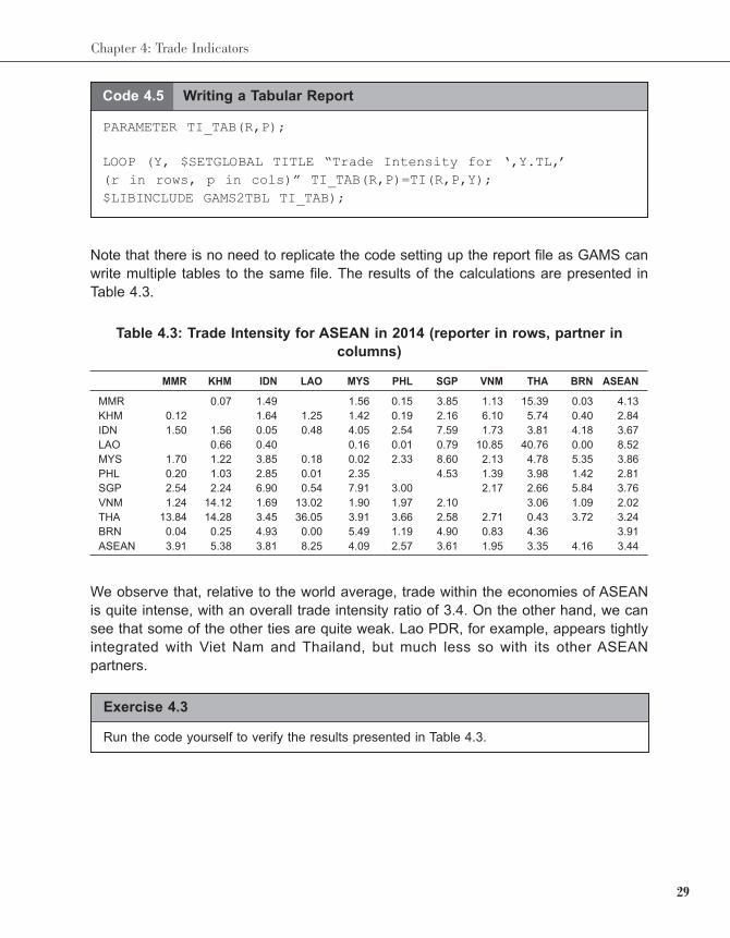
Note that there is no need to replicate the code setting up the report file as GAMS can
write multiple tables to the same file. The results of the calculations are presented in
Table 4.3.
Code 4.5 Writing a Tabular Report
PARAMETER TI_TAB(R,P);
LOOP (Y, $SETGLOBAL TITLE “Trade Intensity for ‘,Y.TL,’
(r in rows, p in cols)” TI_TAB(R,P)=TI(R,P,Y);
$LIBINCLUDE GAMS2TBL TI_TAB);
Table 4.3: Trade Intensity for ASEAN in 2014 (reporter in rows, partner in
columns)
MMR KHM IDN LAO MYS PHL SGP VNM THA BRN ASEAN
MMR 0.07 1.49 1.56 0.15 3.85 1.13 15.39 0.03 4.13
KHM 0.12 1.64 1.25 1.42 0.19 2.16 6.10 5.74 0.40 2.84
IDN 1.50 1.56 0.05 0.48 4.05 2.54 7.59 1.73 3.81 4.18 3.67
LAO 0.66 0.40 0.16 0.01 0.79 10.85 40.76 0.00 8.52
MYS 1.70 1.22 3.85 0.18 0.02 2.33 8.60 2.13 4.78 5.35 3.86
PHL 0.20 1.03 2.85 0.01 2.35 4.53 1.39 3.98 1.42 2.81
SGP 2.54 2.24 6.90 0.54 7.91 3.00 2.17 2.66 5.84 3.76
VNM 1.24 14.12 1.69 13.02 1.90 1.97 2.10 3.06 1.09 2.02
THA 13.84 14.28 3.45 36.05 3.91 3.66 2.58 2.71 0.43 3.72 3.24
BRN 0.04 0.25 4.93 0.00 5.49 1.19 4.90 0.83 4.36 3.91
ASEAN 3.91 5.38 3.81 8.25 4.09 2.57 3.61 1.95 3.35 4.16 3.44
We observe that, relative to the world average, trade within the economies of ASEAN
is quite intense, with an overall trade intensity ratio of 3.4. On the other hand, we can
see that some of the other ties are quite weak. Lao PDR, for example, appears tightly
integrated with Viet Nam and Thailand, but much less so with its other ASEAN
partners.
Exercise 4.3
Run the code yourself to verify the results presented in Table 4.3.
30
Analytical Approaches to Evaluating Preferential Trade Agreements
Some Improvements
Like the intraregional share, the trade intensity index does have some limitations.
There are two main concerns. The first is that the index is not symmetric around one.
Its lower bound is zero, while its upper bound is the inverse of the share of the region
of interest in total world trade. The latter also obviously varies by region, which
complicates making comparisons across regions and across time if a region’s share
of world trade is growing. The second potential concern is with the reference group
that provides the normalization. In the standard formula, the reference group is the
world as a whole, so we are comparing the region’s trade with its relative to the world’s
trade with the region. However, the region is by definition a subset of the world, so the
measure is biased for large regions in world trade. It can be argued that a better
normalization would be to compare with the rest of the world’s trade with the region
(i.e., to form the ratio of the share of intraregional trade to extraregional trade).
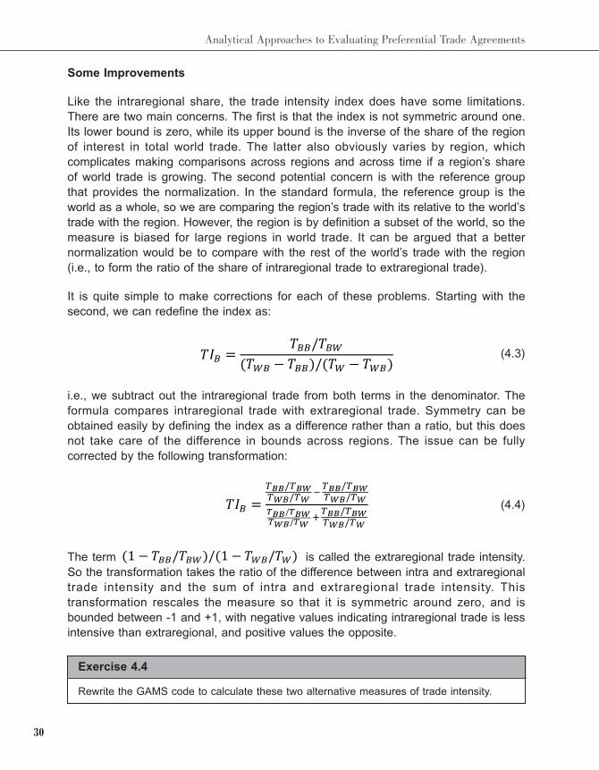
It is quite simple to make corrections for each of these problems. Starting with the
second, we can redefine the index as:
(4.3)
i.e., we subtract out the intraregional trade from both terms in the denominator. The
formula compares intraregional trade with extraregional trade. Symmetry can be
obtained easily by defining the index as a difference rather than a ratio, but this does
not take care of the difference in bounds across regions. The issue can be fully
corrected by the following transformation:
(4.4)
The term is called the extraregional trade intensity.
So the transformation takes the ratio of the difference between intra and extraregional
trade intensity and the sum of intra and extraregional trade intensity. This
transformation rescales the measure so that it is symmetric around zero, and is
bounded between -1 and +1, with negative values indicating intraregional trade is less
intensive than extraregional, and positive values the opposite.
Exercise 4.4
Rewrite the GAMS code to calculate these two alternative measures of trade intensity.
31
Chapter 4: Trade Indicators
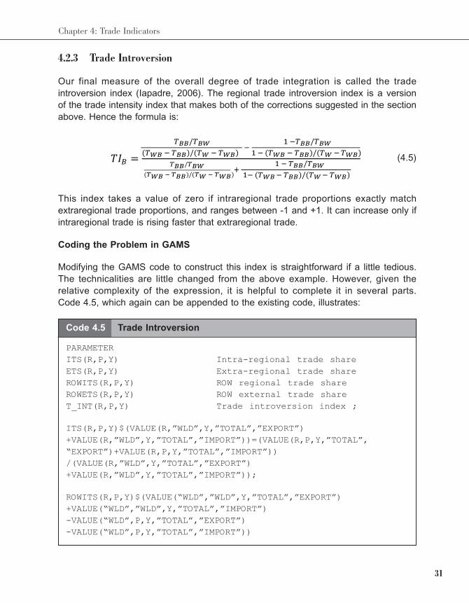
4.2.3 Trade Introversion
Our final measure of the overall degree of trade integration is called the trade
introversion index (Iapadre, 2006). The regional trade introversion index is a version
of the trade intensity index that makes both of the corrections suggested in the section
above. Hence the formula is:
(4.5)
This index takes a value of zero if intraregional trade proportions exactly match
extraregional trade proportions, and ranges between -1 and +1. It can increase only if
intraregional trade is rising faster that extraregional trade.
Coding the Problem in GAMS
Modifying the GAMS code to construct this index is straightforward if a little tedious.
The technicalities are little changed from the above example. However, given the
relative complexity of the expression, it is helpful to complete it in several parts.
Code 4.5, which again can be appended to the existing code, illustrates:
Code 4.5 Trade Introversion
PARAMETER
ITS(R,P,Y) Intra-regional trade share
ETS(R,P,Y) Extra-regional trade share
ROWITS(R,P,Y) ROW regional trade share
ROWETS(R,P,Y) ROW external trade share
T_INT(R,P,Y) Trade introversion index ;
ITS(R,P,Y)$(VALUE(R,”WLD”,Y,”TOTAL”,”EXPORT”)
+VALUE(R,”WLD”,Y,”TOTAL”,”IMPORT”))=(VALUE(R,P,Y,”TOTAL”,
“EXPORT”)+VALUE(R,P,Y,”TOTAL”,”IMPORT”))
/(VALUE(R,”WLD”,Y,”TOTAL”,”EXPORT”)
+VALUE(R,”WLD”,Y,”TOTAL”,”IMPORT”));
ROWITS(R,P,Y)$(VALUE(“WLD”,”WLD”,Y,”TOTAL”,”EXPORT”)
+VALUE(“WLD”,”WLD”,Y,”TOTAL”,”IMPORT”)
-VALUE(“WLD”,P,Y,”TOTAL”,”EXPORT”)
-VALUE(“WLD”,P,Y,”TOTAL”,”IMPORT”))
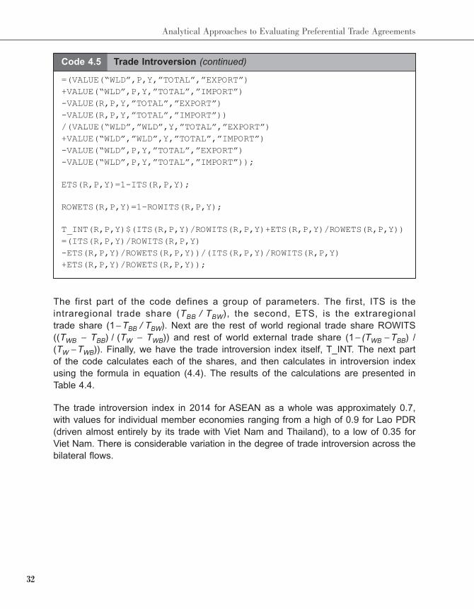
32
Analytical Approaches to Evaluating Preferential Trade Agreements
The first part of the code defines a group of parameters. The first, ITS is the
intraregional trade share (TBB / TBW), the second, ETS, is the extraregional
trade share (1 − TBB / TBW). Next are the rest of world regional trade share ROWITS
((TWB − TBB) / (TW − TWB)) and rest of world external trade share (1 − (TWB − TBB) /
(TW − TWB)). Finally, we have the trade introversion index itself, T_INT. The next part
of the code calculates each of the shares, and then calculates in introversion index
using the formula in equation (4.4). The results of the calculations are presented in
Table 4.4.
The trade introversion index in 2014 for ASEAN as a whole was approximately 0.7,
with values for individual member economies ranging from a high of 0.9 for Lao PDR
(driven almost entirely by its trade with Viet Nam and Thailand), to a low of 0.35 for
Viet Nam. There is considerable variation in the degree of trade introversion across the
bilateral flows.
=(VALUE(“WLD”,P,Y,”TOTAL”,”EXPORT”)
+VALUE(“WLD”,P,Y,”TOTAL”,”IMPORT”)
-VALUE(R,P,Y,”TOTAL”,”EXPORT”)
-VALUE(R,P,Y,”TOTAL”,”IMPORT”))
/(VALUE(“WLD”,”WLD”,Y,”TOTAL”,”EXPORT”)
+VALUE(“WLD”,”WLD”,Y,”TOTAL”,”IMPORT”)
-VALUE(“WLD”,P,Y,”TOTAL”,”EXPORT”)
-VALUE(“WLD”,P,Y,”TOTAL”,”IMPORT”));
ETS(R,P,Y)=1-ITS(R,P,Y);
ROWETS(R,P,Y)=1-ROWITS(R,P,Y);
T_INT(R,P,Y)$(ITS(R,P,Y)/ROWITS(R,P,Y)+ETS(R,P,Y)/ROWETS(R,P,Y))
=(ITS(R,P,Y)/ROWITS(R,P,Y)
-ETS(R,P,Y)/ROWETS(R,P,Y))/(ITS(R,P,Y)/ROWITS(R,P,Y)
+ETS(R,P,Y)/ROWETS(R,P,Y));
Code 4.5 Trade Introversion (continued)
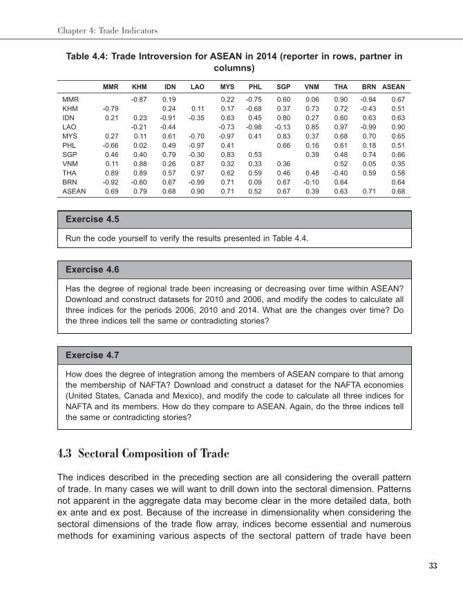
33
Chapter 4: Trade Indicators
4.3 Sectoral Composition of Trade
The indices described in the preceding section are all considering the overall pattern
of trade. In many cases we will want to drill down into the sectoral dimension. Patterns
not apparent in the aggregate data may become clear in the more detailed data, both
ex ante and ex post. Because of the increase in dimensionality when considering the
sectoral dimensions of the trade flow array, indices become essential and numerous
methods for examining various aspects of the sectoral pattern of trade have been
Table 4.4: Trade Introversion for ASEAN in 2014 (reporter in rows, partner in
columns)
MMR KHM IDN LAO MYS PHL SGP VNM THA BRN ASEAN
MMR -0.87 0.19 0.22 -0.75 0.60 0.06 0.90 -0.94 0.67
KHM -0.79 0.24 0.11 0.17 -0.68 0.37 0.73 0.72 -0.43 0.51
IDN 0.21 0.23 -0.91 -0.35 0.63 0.45 0.80 0.27 0.60 0.63 0.63
LAO -0.21 -0.44 -0.73 -0.98 -0.13 0.85 0.97 -0.99 0.90
MYS 0.27 0.11 0.61 -0.70 -0.97 0.41 0.83 0.37 0.68 0.70 0.65
PHL -0.66 0.02 0.49 -0.97 0.41 0.66 0.16 0.61 0.18 0.51
SGP 0.46 0.40 0.79 -0.30 0.83 0.53 0.39 0.48 0.74 0.66
VNM 0.11 0.88 0.26 0.87 0.32 0.33 0.36 0.52 0.05 0.35
THA 0.89 0.89 0.57 0.97 0.62 0.59 0.46 0.48 -0.40 0.59 0.58
BRN -0.92 -0.60 0.67 -0.99 0.71 0.09 0.67 -0.10 0.64 0.64
ASEAN 0.69 0.79 0.68 0.90 0.71 0.52 0.67 0.39 0.63 0.71 0.68
Exercise 4.5
Run the code yourself to verify the results presented in Table 4.4.
Exercise 4.6
Has the degree of regional trade been increasing or decreasing over time within ASEAN?
Download and construct datasets for 2010 and 2006, and modify the codes to calculate all
three indices for the periods 2006, 2010 and 2014. What are the changes over time? Do
the three indices tell the same or contradicting stories?
Exercise 4.7
How does the degree of integration among the members of ASEAN compare to that among
the membership of NAFTA? Download and construct a dataset for the NAFTA economies
(United States, Canada and Mexico), and modify the code to calculate all three indices for
NAFTA and its members. How do they compare to ASEAN. Again, do the three indices tell
the same or contradicting stories?
34
Analytical Approaches to Evaluating Preferential Trade Agreements
proposed. Many are discussed in Mikic and Gilbert (2009). In this section we
concentrate on a few indices that are particularly useful in the context of preferential
trading agreements.
4.3.1 Revealed Comparative Advantage
The theory of comparative advantage underlies economists’ explanations for the
observed pattern of inter-industry trade (trade in distinct products). In theoretical
models, comparative advantage is expressed in terms of differences in relative prices
evaluated in autarky, or the absence of trade. Since autarky prices are not observed,
other measures must be used. The revealed comparative advantage index (RCA) was
developed by Balassa (1965) and is widely used.3 The Balassa index is defined in
much the same way as the trade intensity index, but at the sectoral level. It is defined
as the ratio of the share of a given product in a country’s exports to its share in world
exports. Hence the revealed comparative advantage index in good i and country r is
written in our notation as:
(4.6)
where the numerator is the ratio of the value of trade in good i to total trade in
country r, and the denominator is the corresponding ratio for the world as a whole.
A country is said to have a revealed comparative advantage or disadvantage in
a product if the ratio exceeds or falls short of unity for that product.
As with the trade intensity index, there are several alternative ways of constructing an
RCA measure. Hoen and Oosterhaven (2004) suggest taking the difference of the
shares rather than the ratio, which generates an index symmetric around zero.
Alternatively, a transformation similar to that made in equation (4.4) and the
introversion index can be used to shift both the center and bounds. The normalization
can also be adjusted. In the Balassa index, the comparison is made to the world
average. An alternative is to use the rest of world average. Another is to compare to
the economy’s own pattern of imports (i.e., we can compare a country’s ratio of exports
of i in total exports to the ratio of its imports of i in total imports.) The latter is referred
to as the Michelaye index.
3 A recent paper by Fisher at al. (2016) uses input-output data to instead construct RCA indices based on
projected autarky unit costs. This has a much stronger theoretical grounding, but is computationally more
demanding.
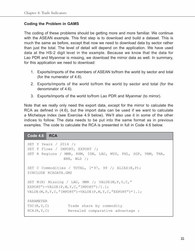
35
Chapter 4: Trade Indicators
Coding the Problem in GAMS
The coding of these problems should be getting more and more familiar. We continue
with the ASEAN example. This first step is to download and build a dataset. This is
much the same as before, except that now we need to download data by sector rather
than just the total. The level of detail will depend on the application. We have used
data at the HS-2 digit level in the example. Because we know that the data for
Lao PDR and Myanmar is missing, we download the mirror data as well. In summary,
for this application we need to download:
1. Exports/imports of the members of ASEAN to/from the world by sector and total
(for the numerator of 4.6).
2. Exports/imports of the world to/from the world by sector and total (for the
denominator of 4.6).
3. Exports/imports of the world to/from Lao PDR and Myanmar (to mirror).
Note that we really only need the export data, except for the mirror to calculate the
RCA as defined in (4.6), but the import data can be used if we want to calculate
a Michelaye index (see Exercise 4.9 below). We’ll also use it in some of the other
indices to follow. The data needs to be put into the same format as in previous
examples. The code to calculate the RCA is presented in full in Code 4.6 below.
Code 4.6 RCA
SET Y Years / 2014 /;
SET F Flows / IMPORT, EXPORT /;
SET R Regions / MMR, KHM, IDN, LAO, MYS, PHL, SGP, VNM, THA,
BRN, WLD /;
SET C Commodities / TOTAL, 1*97, 99 /; ALIAS(R,P);
$INCLUDE RCADATA.GMS
SET M(R) Missing / LAO, MMR /; VALUE(M,P,Y,C,”
EXPORT”)=VALUE(P,M,Y,C,”IMPORT”)/1.1;
VALUE(M,P,Y,C,”IMPORT”)=VALUE(P,M,Y,C,”EXPORT”)*1.1;
PARAMETER
TSC(R,Y,C) Trade share by commodity
RCA(R,Y,C) Revealed comparative advantage ;
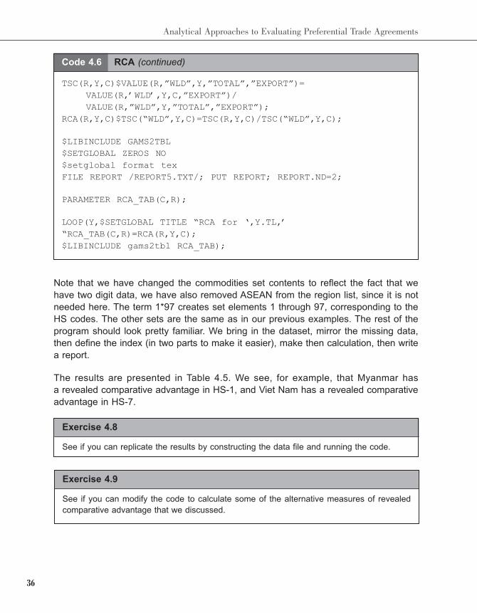
36
Analytical Approaches to Evaluating Preferential Trade Agreements
Note that we have changed the commodities set contents to reflect the fact that we
have two digit data, we have also removed ASEAN from the region list, since it is not
needed here. The term 1*97 creates set elements 1 through 97, corresponding to the
HS codes. The other sets are the same as in our previous examples. The rest of the
program should look pretty familiar. We bring in the dataset, mirror the missing data,
then define the index (in two parts to make it easier), make then calculation, then write
a report.
The results are presented in Table 4.5. We see, for example, that Myanmar has
a revealed comparative advantage in HS-1, and Viet Nam has a revealed comparative
advantage in HS-7.
Code 4.6 RCA (continued)
TSC(R,Y,C)$VALUE(R,”WLD”,Y,”TOTAL”,”EXPORT”)=
VALUE(R,’WLD’,Y,C,”EXPORT”)/
VALUE(R,”WLD”,Y,”TOTAL”,”EXPORT”);
RCA(R,Y,C)$TSC(“WLD”,Y,C)=TSC(R,Y,C)/TSC(“WLD”,Y,C);
$LIBINCLUDE GAMS2TBL
$SETGLOBAL ZEROS NO
$setglobal format tex
FILE REPORT /REPORT5.TXT/; PUT REPORT; REPORT.ND=2;
PARAMETER RCA_TAB(C,R);
LOOP(Y,$SETGLOBAL TITLE “RCA for ‘,Y.TL,’
“RCA_TAB(C,R)=RCA(R,Y,C);
$LIBINCLUDE gams2tbl RCA_TAB);
Exercise 4.8
See if you can replicate the results by constructing the data file and running the code.
Exercise 4.9
See if you can modify the code to calculate some of the alternative measures of revealed
comparative advantage that we discussed.
37
Chapter 4: Trade Indicators
4.4 Complementarity and Similarity
While the information that can be gleaned from the revealed comparative advantage
index and its variants provides a useful foundation for evaluating the potential for trade
complementarities on a good by good basis, Drysdale (1967) developed an aggregate
index that summarizes the degree of complementarity on a regional basis. This is
useful since it can sometimes be difficult to see broad patterns in the more detailed
data. The complementarity index is calculated between a given pair of countries, and
measures the degree to which one country’s import profile exports matches another’s
export profile. It is thus α useful summary measure of the sectoral trade profile. It is
defined as:
(4.7)
where Mip / Mp is the share of good i in the total imports of the partner, and Xir / Xr is
the share of exports of good i in the exports of the reporter. The index is zero when
no good exported by the reporter country is imported by the partner, and 1 when the
export-import shares exactly match.4 Ex ante, higher index values are assumed to
indicate more favorable prospects for a successful preferential trade arrangement
between the two countries.5 Ex post an increase in the degree of complementarity
indicates successful alignment of the trade structure.
An index of export similarity can be constructed in a very similar way, we just need to
replace the partner import share with their export share:
(4.8)
This metric can be used to identify competitors.6
4 The level of data disaggregation should be considered carefully. The more aggregated the data, the higher
the value of the index, in general.5 Ng and Yeats (2003) note several qualifications: An economy may not be able to expand production without
increasing costs (i.e., there may be internal terms-of-trade effects), high complementarity indices may be
misleading if the countries are geographically distant, and relative size differences can be very important.6 Note this type of index is one form of a general type called an ‘overlap’ index. Hence, there are a number
different formulas for complementarity and similarity in the literature. See Mikic and Gilbert (2009) for more
detail.
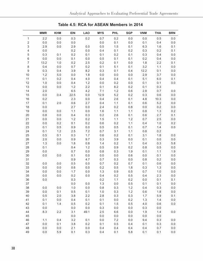
38
Analytical Approaches to Evaluating Preferential Trade Agreements
Table 4.5: RCA for ASEAN Members in 2014
MMR KHM IDN LAO MYS PHL SGP VNM THA BRN
1 2.2 0.0 0.3 0.2 0.7 0.2 0.0 0.0 0.5 0.0
2 0.0 0.0 0.0 0.0 0.1 0.0 0.1 0.4 0.0
3 2.9 0.0 2.9 0.0 0.5 1.5 0.1 6.3 1.6 0.1
4 0.0 0.2 0.0 0.4 0.1 0.2 0.3 0.2 0.1
5 0.3 0.1 0.2 0.1 0.1 0.2 0.1 0.3 0.4 0.0
6 0.0 0.0 0.1 0.0 0.5 0.1 0.1 0.2 0.4 0.0
7 13.2 1.0 0.2 2.5 0.2 0.1 0.0 1.8 2.2 0.1
8 0.4 0.0 0.7 0.2 0.1 5.1 0.1 3.2 1.1 0.0
9 0.3 0.4 3.9 8.2 0.3 0.1 0.4 12.2 0.1 0.0
10 1.2 5.0 0.0 1.8 0.0 0.0 0.0 2.9 3.7 0.0
11 0.1 0.2 0.4 4.0 0.4 0.4 0.1 5.1 6.0 0.1
12 1.0 0.0 0.4 1.2 0.0 0.2 0.0 0.1 0.1 0.0
13 0.0 0.0 1.2 2.2 0.1 8.2 0.2 0.1 0.3
14 2.0 6.5 4.2 7.1 1.2 0.6 2.8 0.7 0.0
15 0.0 0.4 22.5 0.0 12.9 5.2 0.2 0.3 0.6 0.0
16 0.2 2.3 0.0 0.4 2.6 0.1 4.8 10.3 0.0
17 0.1 2.0 0.6 2.7 0.4 1.1 0.1 0.6 5.2 0.0
18 0.0 2.7 0.0 2.4 0.2 0.8 0.0 0.2 0.0
19 0.0 0.0 1.1 0.0 1.6 1.1 1.1 0.8 1.3 0.2
20 0.8 0.0 0.4 0.3 0.2 2.6 0.1 0.6 2.7 0.1
21 0.0 0.0 1.2 0.2 1.5 1.1 1.2 0.7 2.5 0.0
22 0.0 0.2 0.1 0.2 0.6 0.2 1.1 0.4 1.0 0.2
23 0.1 0.5 0.9 0.0 0.5 0.5 0.1 0.7 1.4 0.0
24 0.1 1.2 2.5 7.2 0.7 3.1 1.1 0.8 0.2
25 0.5 0.1 0.3 1.7 0.6 0.2 0.1 3.1 1.8 0.0
26 2.0 0.0 0.9 9.7 0.3 3.9 0.0 0.1 0.0 0.0
27 1.3 0.0 1.8 0.8 1.4 0.2 1.1 0.4 0.3 5.8
28 0.1 0.4 1.2 0.5 0.9 0.2 0.8 0.5 0.0
29 0.0 0.7 0.0 0.8 0.3 1.9 0.1 1.1 1.9
30 0.0 0.0 0.1 0.0 0.0 0.0 0.6 0.0 0.1 0.0
31 0.9 4.7 0.7 0.3 0.0 0.8 0.2 0.0
32 0.0 0.0 0.5 0.0 0.7 0.2 0.7 0.1 0.6 0.0
33 0.0 0.0 0.6 0.0 0.2 0.5 1.8 0.3 1.3 0.0
34 0.0 0.0 1.7 0.0 1.3 0.9 0.5 0.7 1.0 0.0
35 0.0 0.0 0.2 0.0 0.4 0.2 0.5 0.4 2.3 0.0
36 0.0 0.3 0.2 1.1 0.2 0.0 0.1 0.1
37 0.0 0.0 1.3 0.0 0.5 0.1 0.1 0.0
38 0.0 0.0 1.0 0.0 0.8 0.3 1.2 0.4 0.3 0.0
39 0.0 0.1 0.5 0.1 1.0 0.3 1.2 0.6 1.8 0.0
40 0.5 2.0 3.8 2.2 2.8 0.3 0.3 1.7 5.9 0.1
41 0.1 0.0 0.4 0.1 0.1 0.0 0.2 1.3 1.4 0.0
42 0.1 1.4 0.5 0.2 0.1 1.5 0.5 4.0 0.6 0.0
43 0.0 0.0 0.0 0.3 0.0 0.0 0.3 0.0
44 8.3 2.2 3.1 49.1 2.5 6.6 0.0 1.9 1.4 0.0
45 0.0 0.0 0.0 0.0 0.0 0.0
46 1.1 0.4 3.2 0.1 0.0 7.2 0.0 9.4 0.3 0.0
47 0.0 0.1 3.8 0.2 0.1 0.5 0.4 0.1 0.3 0.0
48 0.0 0.0 2.1 0.0 0.4 0.4 0.4 0.4 0.7 0.0
49 0.0 5.9 0.1 0.3 0.4 0.1 5.8 0.1 0.1 0.0
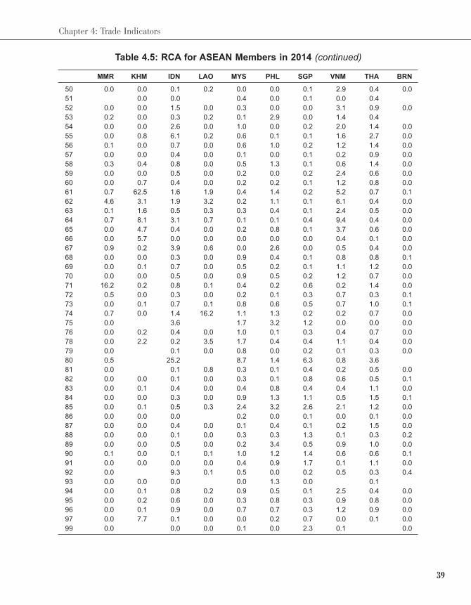
39
Chapter 4: Trade Indicators
50 0.0 0.0 0.1 0.2 0.0 0.0 0.1 2.9 0.4 0.0
51 0.0 0.0 0.4 0.0 0.1 0.0 0.4
52 0.0 0.0 1.5 0.0 0.3 0.0 0.0 3.1 0.9 0.0
53 0.2 0.0 0.3 0.2 0.1 2.9 0.0 1.4 0.4
54 0.0 0.0 2.6 0.0 1.0 0.0 0.2 2.0 1.4 0.0
55 0.0 0.8 6.1 0.2 0.6 0.1 0.1 1.6 2.7 0.0
56 0.1 0.0 0.7 0.0 0.6 1.0 0.2 1.2 1.4 0.0
57 0.0 0.0 0.4 0.0 0.1 0.0 0.1 0.2 0.9 0.0
58 0.3 0.4 0.8 0.0 0.5 1.3 0.1 0.6 1.4 0.0
59 0.0 0.0 0.5 0.0 0.2 0.0 0.2 2.4 0.6 0.0
60 0.0 0.7 0.4 0.0 0.2 0.2 0.1 1.2 0.8 0.0
61 0.7 62.5 1.6 1.9 0.4 1.4 0.2 5.2 0.7 0.1
62 4.6 3.1 1.9 3.2 0.2 1.1 0.1 6.1 0.4 0.0
63 0.1 1.6 0.5 0.3 0.3 0.4 0.1 2.4 0.5 0.0
64 0.7 8.1 3.1 0.7 0.1 0.1 0.4 9.4 0.4 0.0
65 0.0 4.7 0.4 0.0 0.2 0.8 0.1 3.7 0.6 0.0
66 0.0 5.7 0.0 0.0 0.0 0.0 0.0 0.4 0.1 0.0
67 0.9 0.2 3.9 0.6 0.0 2.6 0.0 0.5 0.4 0.0
68 0.0 0.0 0.3 0.0 0.9 0.4 0.1 0.8 0.8 0.1
69 0.0 0.1 0.7 0.0 0.5 0.2 0.1 1.1 1.2 0.0
70 0.0 0.0 0.5 0.0 0.9 0.5 0.2 1.2 0.7 0.0
71 16.2 0.2 0.8 0.1 0.4 0.2 0.6 0.2 1.4 0.0
72 0.5 0.0 0.3 0.0 0.2 0.1 0.3 0.7 0.3 0.1
73 0.0 0.1 0.7 0.1 0.8 0.6 0.5 0.7 1.0 0.1
74 0.7 0.0 1.4 16.2 1.1 1.3 0.2 0.2 0.7 0.0
75 0.0 3.6 1.7 3.2 1.2 0.0 0.0 0.0
76 0.0 0.2 0.4 0.0 1.0 0.1 0.3 0.4 0.7 0.0
78 0.0 2.2 0.2 3.5 1.7 0.4 0.4 1.1 0.4 0.0
79 0.0 0.1 0.0 0.8 0.0 0.2 0.1 0.3 0.0
80 0.5 25.2 8.7 1.4 6.3 0.8 3.6
81 0.0 0.1 0.8 0.3 0.1 0.4 0.2 0.5 0.0
82 0.0 0.0 0.1 0.0 0.3 0.1 0.8 0.6 0.5 0.1
83 0.0 0.1 0.4 0.0 0.4 0.8 0.4 0.4 1.1 0.0
84 0.0 0.0 0.3 0.0 0.9 1.3 1.1 0.5 1.5 0.1
85 0.0 0.1 0.5 0.3 2.4 3.2 2.6 2.1 1.2 0.0
86 0.0 0.0 0.0 0.2 0.0 0.1 0.0 0.1 0.0
87 0.0 0.0 0.4 0.0 0.1 0.4 0.1 0.2 1.5 0.0
88 0.0 0.0 0.1 0.0 0.3 0.3 1.3 0.1 0.3 0.2
89 0.0 0.0 0.5 0.0 0.2 3.4 0.5 0.9 1.0 0.0
90 0.1 0.0 0.1 0.1 1.0 1.2 1.4 0.6 0.6 0.1
91 0.0 0.0 0.0 0.0 0.4 0.9 1.7 0.1 1.1 0.0
92 0.0 9.3 0.1 0.5 0.0 0.2 0.5 0.3 0.4
93 0.0 0.0 0.0 0.0 1.3 0.0 0.1
94 0.0 0.1 0.8 0.2 0.9 0.5 0.1 2.5 0.4 0.0
95 0.0 0.2 0.6 0.0 0.3 0.8 0.3 0.9 0.8 0.0
96 0.0 0.1 0.9 0.0 0.7 0.7 0.3 1.2 0.9 0.0
97 0.0 7.7 0.1 0.0 0.0 0.2 0.7 0.0 0.1 0.0
99 0.0 0.0 0.0 0.1 0.0 2.3 0.1 0.0
Table 4.5: RCA for ASEAN Members in 2014 (continued)
MMR KHM IDN LAO MYS PHL SGP VNM THA BRN
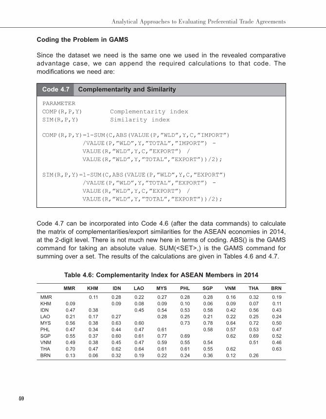
40
Analytical Approaches to Evaluating Preferential Trade Agreements
Coding the Problem in GAMS
Since the dataset we need is the same one we used in the revealed comparative
advantage case, we can append the required calculations to that code. The
modifications we need are:
Code 4.7 Complementarity and Similarity
PARAMETER
COMP(R,P,Y) Complementarity index
SIM(R,P,Y) Similarity index
COMP(R,P,Y)=1-SUM(C,ABS(VALUE(P,”WLD”,Y,C,”IMPORT”)
/VALUE(P,”WLD”,Y,”TOTAL”,”IMPORT”) -
VALUE(R,”WLD”,Y,C,”EXPORT”) /
VALUE(R,”WLD”,Y,”TOTAL”,”EXPORT”))/2);
SIM(R,P,Y)=1-SUM(C,ABS(VALUE(P,”WLD”,Y,C,”EXPORT”)
/VALUE(P,”WLD”,Y,”TOTAL”,”EXPORT”) -
VALUE(R,”WLD”,Y,C,”EXPORT”) /
VALUE(R,”WLD”,Y,”TOTAL”,”EXPORT”))/2);
Code 4.7 can be incorporated into Code 4.6 (after the data commands) to calculate
the matrix of complementarities/export similarities for the ASEAN economies in 2014,
at the 2-digit level. There is not much new here in terms of coding. ABS() is the GAMS
command for taking an absolute value. SUM(<SET>,) is the GAMS command for
summing over a set. The results of the calculations are given in Tables 4.6 and 4.7.
Table 4.6: Complementarity Index for ASEAN Members in 2014
MMR KHM IDN LAO MYS PHL SGP VNM THA BRN
MMR 0.11 0.28 0.22 0.27 0.28 0.28 0.16 0.32 0.19
KHM 0.09 0.09 0.08 0.09 0.10 0.06 0.09 0.07 0.11
IDN 0.47 0.38 0.45 0.54 0.53 0.58 0.42 0.56 0.43
LAO 0.21 0.17 0.27 0.28 0.25 0.21 0.22 0.25 0.24
MYS 0.56 0.38 0.63 0.60 0.73 0.78 0.64 0.72 0.50
PHL 0.47 0.34 0.44 0.47 0.61 0.58 0.57 0.53 0.47
SGP 0.55 0.37 0.60 0.61 0.77 0.69 0.62 0.69 0.52
VNM 0.49 0.38 0.45 0.47 0.59 0.55 0.54 0.51 0.46
THA 0.70 0.47 0.62 0.64 0.61 0.61 0.55 0.62 0.63
BRN 0.13 0.06 0.32 0.19 0.22 0.24 0.36 0.12 0.26
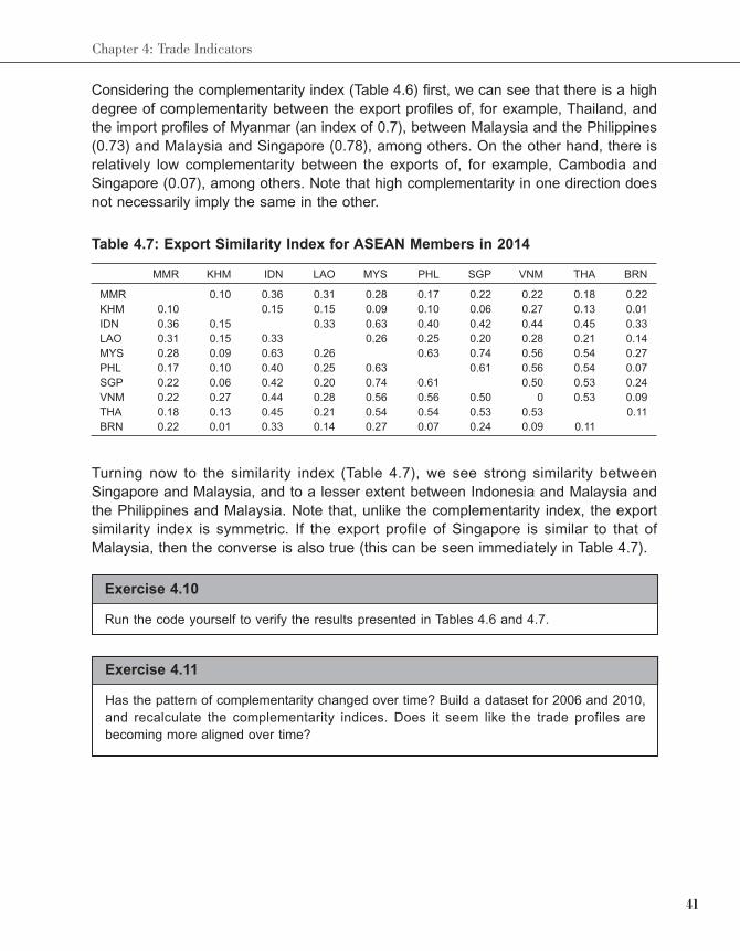
41
Chapter 4: Trade Indicators
Considering the complementarity index (Table 4.6) first, we can see that there is a high
degree of complementarity between the export profiles of, for example, Thailand, and
the import profiles of Myanmar (an index of 0.7), between Malaysia and the Philippines
(0.73) and Malaysia and Singapore (0.78), among others. On the other hand, there is
relatively low complementarity between the exports of, for example, Cambodia and
Singapore (0.07), among others. Note that high complementarity in one direction does
not necessarily imply the same in the other.
Table 4.7: Export Similarity Index for ASEAN Members in 2014
MMR KHM IDN LAO MYS PHL SGP VNM THA BRN
MMR 0.10 0.36 0.31 0.28 0.17 0.22 0.22 0.18 0.22
KHM 0.10 0.15 0.15 0.09 0.10 0.06 0.27 0.13 0.01
IDN 0.36 0.15 0.33 0.63 0.40 0.42 0.44 0.45 0.33
LAO 0.31 0.15 0.33 0.26 0.25 0.20 0.28 0.21 0.14
MYS 0.28 0.09 0.63 0.26 0.63 0.74 0.56 0.54 0.27
PHL 0.17 0.10 0.40 0.25 0.63 0.61 0.56 0.54 0.07
SGP 0.22 0.06 0.42 0.20 0.74 0.61 0.50 0.53 0.24
VNM 0.22 0.27 0.44 0.28 0.56 0.56 0.50 0 0.53 0.09
THA 0.18 0.13 0.45 0.21 0.54 0.54 0.53 0.53 0.11
BRN 0.22 0.01 0.33 0.14 0.27 0.07 0.24 0.09 0.11
Turning now to the similarity index (Table 4.7), we see strong similarity between
Singapore and Malaysia, and to a lesser extent between Indonesia and Malaysia and
the Philippines and Malaysia. Note that, unlike the complementarity index, the export
similarity index is symmetric. If the export profile of Singapore is similar to that of
Malaysia, then the converse is also true (this can be seen immediately in Table 4.7).
Exercise 4.10
Run the code yourself to verify the results presented in Tables 4.6 and 4.7.
Exercise 4.11
Has the pattern of complementarity changed over time? Build a dataset for 2006 and 2010,
and recalculate the complementarity indices. Does it seem like the trade profiles are
becoming more aligned over time?
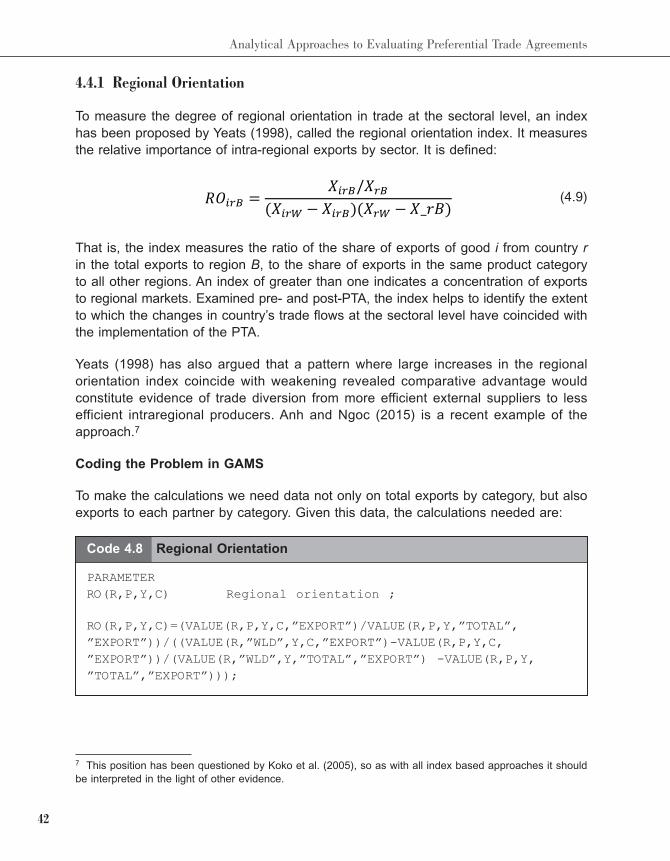
42
Analytical Approaches to Evaluating Preferential Trade Agreements
4.4.1 Regional Orientation
To measure the degree of regional orientation in trade at the sectoral level, an index
has been proposed by Yeats (1998), called the regional orientation index. It measures
the relative importance of intra-regional exports by sector. It is defined:
(4.9)
That is, the index measures the ratio of the share of exports of good i from country r
in the total exports to region B, to the share of exports in the same product category
to all other regions. An index of greater than one indicates a concentration of exports
to regional markets. Examined pre- and post-PTA, the index helps to identify the extent
to which the changes in country’s trade flows at the sectoral level have coincided with
the implementation of the PTA.
Yeats (1998) has also argued that a pattern where large increases in the regional
orientation index coincide with weakening revealed comparative advantage would
constitute evidence of trade diversion from more efficient external suppliers to less
efficient intraregional producers. Anh and Ngoc (2015) is a recent example of the
approach.7
Coding the Problem in GAMS
To make the calculations we need data not only on total exports by category, but also
exports to each partner by category. Given this data, the calculations needed are:
Code 4.8 Regional Orientation
PARAMETER
RO(R,P,Y,C) Regional orientation ;
RO(R,P,Y,C)=(VALUE(R,P,Y,C,”EXPORT”)/VALUE(R,P,Y,”TOTAL”,
”EXPORT”))/((VALUE(R,”WLD”,Y,C,”EXPORT”)-VALUE(R,P,Y,C,
”EXPORT”))/(VALUE(R,”WLD”,Y,”TOTAL”,”EXPORT”) -VALUE(R,P,Y,
”TOTAL”,”EXPORT”)));
7 This position has been questioned by Koko et al. (2005), so as with all index based approaches it should
be interpreted in the light of other evidence.
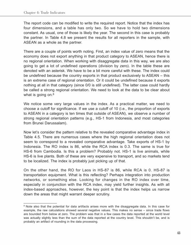
43
Chapter 4: Trade Indicators
The report code can be modified to write the required report. Notice that the index has
four dimensions, and a table has only two. So we have to hold two dimensions
constant. As usual, one of those is likely the year. The second in this case is probably
the partner. In Table 4.8 we present the results for all reporters in the sample, with
ASEAN as a whole as the partner.
There are a couple of points worth noting. First, an index value of zero means that the
economy does not export anything in that product category to ASEAN, hence there is
no regional orientation. When working with disaggregate data in this way, we are also
going to get a lot of undefined operations (division by zero). In the table these are
denoted with an asterisk. We have to be a bit more careful with these. The index could
be undefined because the country exports in that product exclusively to ASEAN – this
is an extreme case of regional orientation. Or it could be undefined because it exports
nothing at all in that category (since 0/0 is still undefined). The latter case could hardly
be called a strong regional orientation. We need to look at the data to be clear about
what is going on.8
We notice some very large values in the index. As a practical matter, we need to
choose a cutoff for significance. If we use a cutoff of 10 (i.e., the proportion of exports
to ASEAN in a category is ten times that outside of ASEAN), we observe a number of
strong regional orientation patterns (e.g., HS-1 from Indonesia, and most categories
from Brunei Darussalam).
Now let’s consider the pattern relative to the revealed comparative advantage index in
Table 4.5. There are numerous cases where the high regional orientation does not
seem to correspond to a revealed comparative advantage. Take exports of HS-1 by
Indonesia. The RO index is 86, while the RCA index is 0.3. The same is true for
HS-6 from Cambodia. Is this a problem? Probably not. HS-1 is live animals, while
HS-6 is live plants. Both of these are very expensive to transport, and so markets tend
to be localized. The index is probably just picking up of that.
On the other hand, the RO for Laos in HS-87 is 86, while RCA is 0. HS-87 is
transportation equipment. What is this reflecting? Perhaps integration into production
networks, or something else. Looking for changes in the RO index over time,
especially in conjunction with the RCA index, may yield further insights. As with all
index-based approaches, however, the key point is that the index helps us narrow
down the areas that might warrant deeper scrutiny.
8 Note also that the potential for data artifacts arises more with the disaggregate data. In this case for
example, the raw calculations showed several negative values. This makes no sense – since trade flows
are bounded from below at zero. The problem was that in a few cases the data reported at the world level
was actually slightly less than the sum of the data reported at the country level. This shouldn’t be, and is
probably an artifact of rounding in the data processing.
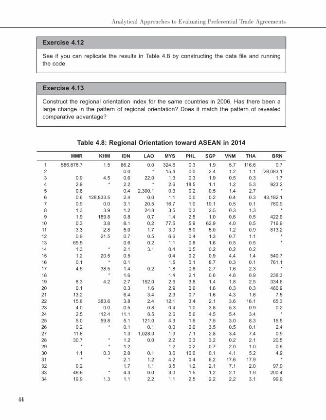
44
Analytical Approaches to Evaluating Preferential Trade Agreements
Exercise 4.12
See if you can replicate the results in Table 4.8 by constructing the data file and running
the code.
Exercise 4.13
Construct the regional orientation index for the same countries in 2006. Has there been a
large change in the pattern of regional orientation? Does it match the pattern of revealed
comparative advantage?
Table 4.8: Regional Orientation toward ASEAN in 2014
MMR KHM IDN LAO MYS PHL SGP VNM THA BRN
1 586,878.7 1.5 86.2 0.0 324.6 0.3 1.9 5.7 116.6 0.7
2 0.0 * 15.4 0.0 2.4 1.2 1.1 28,083.1
3 0.9 4.5 0.6 22.0 1.3 0.3 1.9 0.5 0.3 1.7
4 2.9 * 2.2 * 2.6 18.5 1.1 1.2 5.3 923.2
5 0.6 0.4 2,300.1 0.3 0.2 0.5 1.4 2.7 *
6 0.6 128,833.5 2.4 0.0 1.1 0.0 0.2 0.4 0.3 43,182.1
7 0.9 0.0 3.1 20.5 16.7 1.0 19.1 0.5 0.1 760.9
8 1.3 3.9 1.2 24.8 3.5 0.3 2.5 0.3 1.3 *
9 1.9 189.8 0.8 0.7 1.4 2.5 1.0 0.6 0.5 422.9
10 0.3 3.8 8.1 0.2 77.5 5.9 62.9 4.0 0.5 716.9
11 3.3 2.8 5.0 1.7 3.0 6.0 5.0 1.2 0.9 813.2
12 0.9 21.5 0.7 0.5 6.6 0.4 1.3 0.7 1.1 *
13 65.5 0.6 0.2 1.1 0.8 1.6 0.5 0.5 *
14 1.3 * 2.1 3.1 0.4 0.5 0.2 0.2 0.2
15 1.2 20.5 0.5 0.4 0.2 0.9 4.4 1.4 540.7
16 0.1 * 0.1 1.5 0.1 8.7 0.3 0.1 761.1
17 4.5 38.5 1.4 0.2 1.8 0.8 2.7 1.6 2.3 *
18 * 1.6 1.4 2.1 0.6 4.8 0.9 238.3
19 8.3 4.2 2.7 152.0 2.6 3.8 1.4 1.8 2.5 334.6
20 0.1 0.3 1.6 2.9 0.6 1.6 0.3 0.3 460.9
21 13.2 6.4 3.4 2.3 0.7 1.6 4.3 1.6 7.5
22 15.6 383.6 3.8 2.4 12.1 3.4 2.1 3.6 16.1 65.3
23 4.0 0.0 0.5 0.8 0.4 1.0 3.8 5.3 0.9 0.2
24 2.5 112.4 11.1 8.5 2.6 5.6 4.5 5.4 3.4 *
25 5.0 59.8 5.1 121.0 4.3 1.9 7.5 3.0 8.3 15.5
26 0.2 * 0.1 0.1 0.0 0.0 3.5 0.5 0.1 2.4
27 11.6 1.3 1,028.0 1.3 7.1 2.8 3.4 7.4 0.9
28 30.7 * 1.2 0.0 2.2 0.3 3.2 0.2 2.1 20.5
29 * * 1.2 1.2 0.2 0.7 2.0 1.0 0.9
30 1.1 0.3 2.0 0.1 3.6 16.0 0.1 4.1 5.2 4.9
31 * * 2.1 1.2 4.2 0.4 6.2 17.6 17.9 *
32 0.2 1.7 1.1 3.5 1.2 2.1 7.1 2.0 97.9
33 46.6 * 4.3 0.0 3.0 1.5 1.2 2.1 1.9 200.4
34 19.9 1.3 1.1 2.2 1.1 2.5 2.2 2.2 3.1 99.9
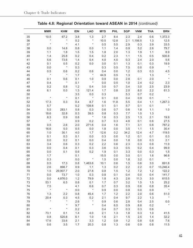
45
Chapter 4: Trade Indicators
35 10.5 67.2 3.8 1.3 2.7 8.4 2.3 2.4 0.6 1,372.3
36 * * 0.2 * 10.5 12.8 2.1 1,156.5 1.3 12.5
37 * * 4.1 * 0.5 5.5 2.9 0.3 3.9 33.5
38 0.0 14.8 0.8 0.0 1.1 1.4 0.9 5.2 2.6 79.7
39 1.1 1.8 1.5 1.5 1.8 2.0 1.3 1.9 1.1 8.9
40 1.4 25.8 0.2 0.4 0.2 2.3 1.1 1.5 0.5 500.8
41 5.6 73.6 1.4 0.4 4.0 4.0 0.3 2.4 2.0 5.6
42 0.1 0.5 0.2 0.0 3.0 0.1 1.3 0.1 0.3 19.9
43 0.0 * 0.3 0.3 0.5 7.5 0.0 0.9 *
44 0.5 0.6 0.2 0.6 0.4 0.0 1.2 0.3 0.3 4.5
45 * * 1.7 * 44.9 0.5 1.3 1.3 *
46 0.1 0.6 0.1 1.0 0.9 0.0 2.8 0.1 2.0 *
47 0.4 * 0.1 * 0.0 0.5 1.0 2.4 0.2 2.3
48 0.2 0.8 1.2 0.4 3.0 0.7 3.4 3.0 2.5 23.9
49 6.1 0.0 1.3 121.4 1.7 0.8 2.0 8.0 2.2 61.3
50 3.5 0.0 0.3 5.3 0.7 0.2
51 * * 0.1 * 0.1 0.0 0.4 0.9 0.1 *
52 17.3 0.3 0.4 8.7 1.6 11.8 5.5 0.4 1.1 1,267.3
53 5.7 0.2 109.8 0.1 0.1 5.7 0.1 0.1 *
54 5.5 283.1 0.8 0.3 0.6 0.7 0.6 1.8 1.1 1.0
55 18.6 32.8 0.3 39.5 0.8 0.3 7.7 1.5 1.3
56 8.3 0.9 0.8 * 1.6 0.3 2.5 1.3 2.1 19.9
57 * 0.9 0.2 0.7 0.3 4.8 0.1 0.6 27.5
58 0.5 2.6 2.0 271.6 0.4 1.6 7.1 3.1 0.8 787.2
59 16.6 5.0 0.5 0.0 1.8 0.0 3.5 1.1 1.5 30.4
60 1.0 30.1 4.0 1.7 12.6 0.2 34.2 12.4 4.7 119.5
61 0.1 0.3 0.1 0.0 0.3 0.0 1.2 0.1 0.1 0.3
62 0.0 0.2 0.1 0.0 0.4 0.0 1.8 0.0 0.3 2.1
63 3.4 0.6 0.3 0.2 2.2 0.6 2.3 0.3 0.8 11.9
64 0.0 0.4 0.1 0.3 3.6 0.3 0.5 0.2 0.4 99.9
65 0.0 0.1 0.6 0.2 1.9 0.1 3.3 0.0 0.3 1.5
66 1.7 0.1 15.5 0.0 3.0 0.1 1.6 96.8
67 0.3 0.0 * 1.5 0.0 1.8 3.2 0.1 *
68 0.5 17.3 0.8 1,463.6 10.1 0.6 1.5 0.6 3.0 691.8
69 2.6 898.7 0.9 1.1 1.3 0.2 2.2 2.2 0.7 13,246.4
70 1.5 29,907.7 2.0 27.8 0.8 1.5 1.2 7.2 1.2 122.2
71 0.0 73.7 1.0 0.3 0.8 0.1 0.4 0.0 0.4 141.7
72 0.0 4,876.0 1.2 79.9 1.8 4.3 2.6 11.3 3.0 615.5
73 53.1 6.5 0.8 0.1 1.7 0.7 3.2 1.5 1.5 25.2
74 7.5 4.1 6.6 0.7 0.3 0.9 0.6 0.8 35.4
75 * * 0.0 * 0.9 0.0 0.8 0.0 0.9 *
76 1.3 2.2 0.8 45.4 1.7 1.2 2.2 2.0 0.6 51.0
78 20.4 0.3 4.5 0.2 2.1 0.4 9.7 2.2 1.3 *
79 * * 2.6 * 0.9 0.6 2.8 0.4 2.5 0.0
80 * 9.7 * 0.4 6.5 0.9 8.8 0.2 *
81 * * 0.2 0.4 0.7 0.3 0.3 0.6
82 73.1 0.1 1.4 4.0 2.1 1.3 1.8 0.3 1.0 41.5
83 0.8 520.8 6.1 1.0 1.6 2.1 1.5 2.5 1.4 32.2
84 17.6 33.6 2.1 3.3 1.2 0.8 1.2 0.8 0.8 7.6
85 0.6 3.5 1.7 20.3 0.8 1.3 0.6 0.9 0.8 11.5
Table 4.8: Regional Orientation toward ASEAN in 2014 (continued)
MMR KHM IDN LAO MYS PHL SGP VNM THA BRN
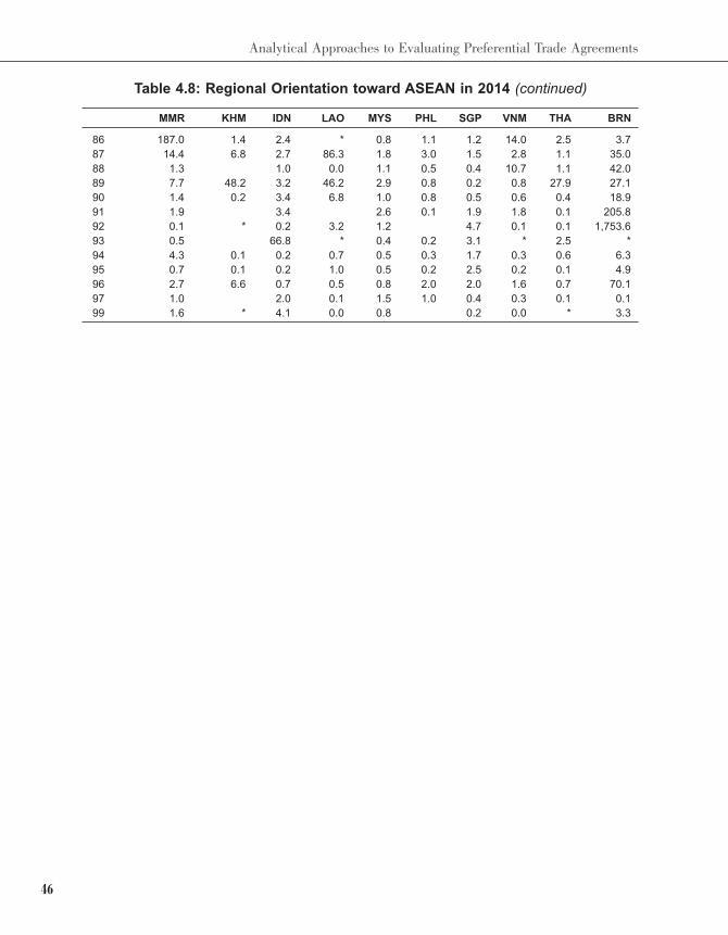
46
Analytical Approaches to Evaluating Preferential Trade Agreements
86 187.0 1.4 2.4 * 0.8 1.1 1.2 14.0 2.5 3.7
87 14.4 6.8 2.7 86.3 1.8 3.0 1.5 2.8 1.1 35.0
88 1.3 1.0 0.0 1.1 0.5 0.4 10.7 1.1 42.0
89 7.7 48.2 3.2 46.2 2.9 0.8 0.2 0.8 27.9 27.1
90 1.4 0.2 3.4 6.8 1.0 0.8 0.5 0.6 0.4 18.9
91 1.9 3.4 2.6 0.1 1.9 1.8 0.1 205.8
92 0.1 * 0.2 3.2 1.2 4.7 0.1 0.1 1,753.6
93 0.5 66.8 * 0.4 0.2 3.1 * 2.5 *
94 4.3 0.1 0.2 0.7 0.5 0.3 1.7 0.3 0.6 6.3
95 0.7 0.1 0.2 1.0 0.5 0.2 2.5 0.2 0.1 4.9
96 2.7 6.6 0.7 0.5 0.8 2.0 2.0 1.6 0.7 70.1
97 1.0 2.0 0.1 1.5 1.0 0.4 0.3 0.1 0.1
99 1.6 * 4.1 0.0 0.8 0.2 0.0 * 3.3
Table 4.8: Regional Orientation toward ASEAN in 2014 (continued)
MMR KHM IDN LAO MYS PHL SGP VNM THA BRN
47
Chapter 5: Decomposing Changes in the Trade Pattern Over Time
Chapter
5DECOMPOSING CHANGES IN THE TRADEPATTERN OVER TIME
In Chapter 4 we considered various indices that can be used to help evaluate the
impact that a preferential trade agreement has on patterns of trade. In many cases
we are interested in evaluating how the indices have changed over time. Clearly, one
way to do so is simply to construct the indices over a time period and look for patterns.
A more sophisticated method is to try and decompose the changes into component
parts that can help us to better understand the forces underlying the observed
changes. In this chapter we explore techniques for undertaking decompositions based
on the constant market shares approach.
5.1 Constant Market Share Analysis
Constant market share (CMS) analysis is a technique for decomposing the growth in
a country’s exports into components that correspond to holding its market shares
constant at various levels. In particular, a country’s trade may grow faster or slower
than the world average because its export profile is concentrated in commodities for
which demand is growing relatively quickly/slowly, or because its regional export profile
is dominated by countries that are growing relatively quickly/slowly, because the
economy is gradually becoming more or less competitive, or some combination
thereof. Obviously, preferential trading agreements have the potential to change these
effects. CMS analysis is designed to help us better understand the relative importance
of the various possible drivers of export growth.
The technique was introduced to the international trade context in Tyszynski (1951),
and was extended and popularized by Leamer and Stern (1970), with further
development by Richardson (1971) and Fagerberg and Sollie (1987), among others.1
CMS analysis has recently been applied to export growth of a number of broad
aggregate regions by Widodo (2010), and to US export growth in Gilbert (2010).
1 The theoretical foundations of the technique can be related to the two-stage (Armington) demand function
commonly adopted in the computable general equilibrium literature (see Merkies and van der Meer, 1988).
Ahmadi-Esfahani (2006) provides further discussion of the theoretical foundations and appropriate use and
diagnostic interpretation of the technique.
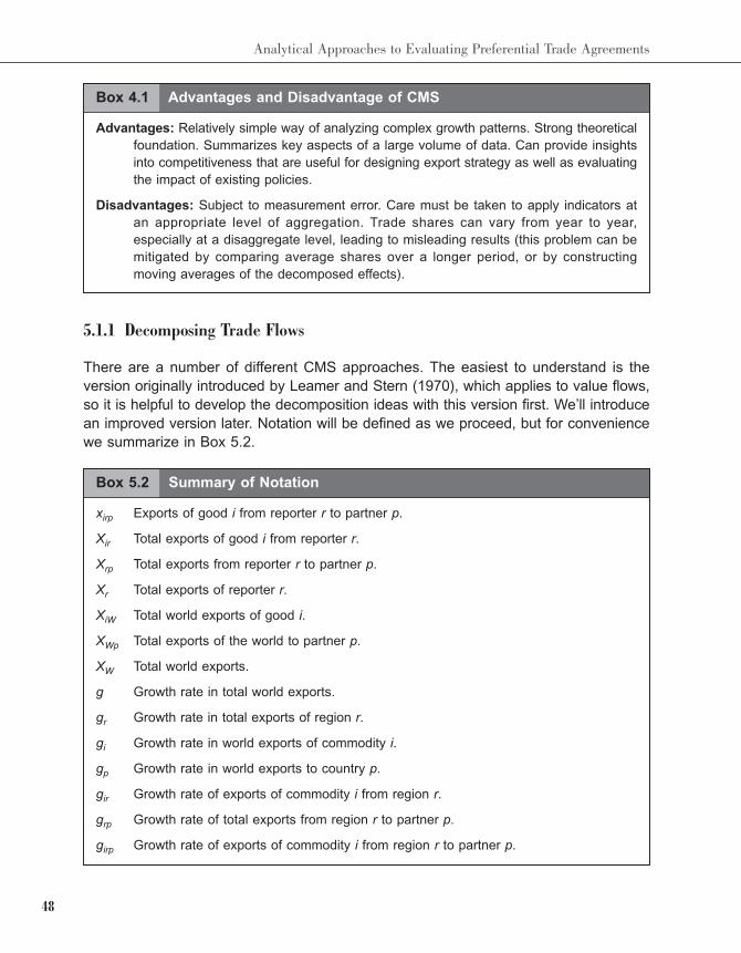
48
Analytical Approaches to Evaluating Preferential Trade Agreements
5.1.1 Decomposing Trade Flows
There are a number of different CMS approaches. The easiest to understand is the
version originally introduced by Leamer and Stern (1970), which applies to value flows,
so it is helpful to develop the decomposition ideas with this version first. We’ll introduce
an improved version later. Notation will be defined as we proceed, but for convenience
we summarize in Box 5.2.
Box 5.2 Summary of Notation
xirp Exports of good i from reporter r to partner p.
Xir Total exports of good i from reporter r.
Xrp Total exports from reporter r to partner p.
Xr Total exports of reporter r.
XiW Total world exports of good i.
XWp Total exports of the world to partner p.
XW Total world exports.
g Growth rate in total world exports.
gr Growth rate in total exports of region r.
gi Growth rate in world exports of commodity i.
gp Growth rate in world exports to country p.
gir Growth rate of exports of commodity i from region r.
grp Growth rate of total exports from region r to partner p.
girp Growth rate of exports of commodity i from region r to partner p.
Box 4.1 Advantages and Disadvantage of CMS
Advantages: Relatively simple way of analyzing complex growth patterns. Strong theoretical
foundation. Summarizes key aspects of a large volume of data. Can provide insights
into competitiveness that are useful for designing export strategy as well as evaluating
the impact of existing policies.
Disadvantages: Subject to measurement error. Care must be taken to apply indicators at
an appropriate level of aggregation. Trade shares can vary from year to year,
especially at a disaggregate level, leading to misleading results (this problem can be
mitigated by comparing average shares over a longer period, or by constructing
moving averages of the decomposed effects).
49
Chapter 5: Decomposing Changes in the Trade Pattern Over Time
A One Level Decomposition
Consider the change in a country’s export value between two periods. Using our
notation, the change in total exports from country r between period 1 and period 0 is
given by where a superscript denotes the time period. Let the rate of growth
in exports from country r be given by It is then clear that we can
write:
(5.1)
In words, the change in export value is equal to the initial export value multiplied
by the rate of growth between the two periods. Now, let be the
growth rate in the value of world exports over the same time period. Adding and
subtracting from the right hand side of equation (5.1) obviously leaves it
unchanged:
(5.2)
We can rearrange the terms in equation (5.2) to obtain:
(5.3)
This called a ‘one level’ CMS decomposition (in export values). It is the most basic
decomposition we can undertake.
What does (5.3) say? The first term on the right, is called the world growth effect.
It tells us how much the exports of economy r would have grown between period 0 and
period 1 if they were increasing at the same rate as the world average (in other words,
if its share of world exports was remaining constant). The second term, is
called the competitiveness effect. It represents the residual, or the amount that is not
explained by the growth of world trade, and must be attributable to something else. If
this term is negative the country’s exports have grown more slowly than the world
average, and thus the economy has lost market share. If the term is positive the
country’s exports have grown faster than the world average, and the economy has
instead gained market share.
A Two Level Decomposition
What if different commodities are growing at different rates in world trade, due to
changes in the structure of demand? Consider the residual effect in equation (5.3)
again. Total exports of region r are just the sum over all commodities of exports by
50
Analytical Approaches to Evaluating Preferential Trade Agreements
commodity (i.e., ). Let gir be the rate of growth in exports of i from r (i.e.,
). Then the residual term in (5.3) can be written as:
(5.4)
Once again, the right hand side is unchanged if we add and subtract the same term,
so letting gi be the rate of growth in world trade in commodity i (i.e.,
) we have:
(5.5)
Which can be rearranged to give us:
(5.6)
Substituting (5.6) into (5.3) we have:
(5.7)
This is called a two level CMS decomposition (in goods). The second term on the right
is called the commodity effect. It represents how much export growth can be attributed
to an export profile that is comprised of goods that are relatively slow/fast growing as
compared to the world average (or to put it in terms of shares, how much of the
change in the share of world exports is reflecting the changes in the shares of the
commodities exported by country r in world trade). This term will be positive if the
goods that are exported by country r are growing faster than the world average across
goods. The final term is again the residual, the unexplained portion after accounting
for overall world growth and the commodity composition of trade.
Another Two Level Decomposition
Different regional markets may also be growing at different rates, and we may want
to factor that into the normalization. Consider the residual effect in equation (5.3) once
more. Total exports of region r can also be written as the sum over all partners of
total exports by partner (i.e., ). Let grp be the rate of growth in total exports
from r to p (i.e., . Then the residual in (5.3) can alternatively be
written as:
51
Chapter 5: Decomposing Changes in the Trade Pattern Over Time
(5.8)
Let gp represent the growth in world exports to region p (i.e.,
Using the same trick as before, we can rewrite this as:
(5.9)
Substituting (5.9) into (5.3) we have:
(5.10)
This is also called a two level CMS decomposition, but this time across regional
markets. The second term on the right is called the regional market effect. It represents
how much export growth can be attributed to an export profile that is comprised of
regions that are relatively slow/fast growing as compared to the world average (or to
put it in terms of shares, how much of the change in the share of world exports is
reflecting the changes in the shares of the partners to which country r exports in world
trade). The final term is again the residual, or competitiveness effect.
A Three Level Decomposition
The final step is to allow for both sectoral and regional variations. Taking the residual
from (5.7) and recognizing that Xir = ∑p xirpXir, we can add a further term the same way
as before.2 The following expression is the complete CMS decomposition:
(World Growth Effect)
(Commodity Effect)
(Regional Market Effect)
(Competitiveness Effect)
(5.11)
2 Alternatively, we can use the residual in (5.10) to perform the market breakdown first. The terms will differ
in general. The technique is not invariant to the choice of order, an issue we discuss further below.
52
Analytical Approaches to Evaluating Preferential Trade Agreements
where is the rate of growth in exports of commodity i from
region r to partner p. The complete decomposition thus identifies four different
components of the growth in the exports of the country of interest:
1. World Growth Effect: The part of the growth attributed to the overall rise in
world exports.
2. Commodity Effect: The part of growth attributed to the commodity
composition of the country’s exports (positive if exports are concentrated in
commodities in which world demand is growing relatively quickly).
3. Regional Market Effect: The part of growth attributed to the regional
composition of the country’s exports (positive if exports are concentrated in
markets which are experiencing relatively rapid growth).
4. Competitiveness Effect: The residual effect, which captures the difference
between the actual export growth and the growth that would have occurred had
the export shares remained constant. A positive value is interpreted as an
increase in “competitiveness.”
Coding the Problem in GAMS
As usual, the first step is to download and build a dataset. For this application we need
data by both sector and destination for at least two periods. We will use Thailand’s
export data in 2006 and 2014 as an example. We have used data at the HS-2 digit
level. In summary, for this application we need to download:
1. Exports of all goods by HS-2 digit classification, and the total, from Thailand
to all trade partners in 2006.
2. Exports of all goods by HS-2 digit classification, and the total from the world
as a whole to all trade partners in 2006.
3. The same data for 2014.
The data needs to be put into the same format as in previous examples. The code to
calculate the decompositions given in equation (5.11) is presented in full in Code 5.1
below.
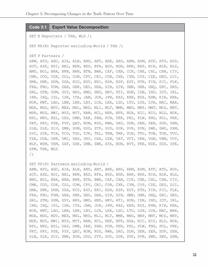
53
Chapter 5: Decomposing Changes in the Trade Pattern Over Time
Code 5.1 Export Value Decomposition
SET R Reporters / THA, WLD /;
SET RR(R) Reporter excluding World / THA /;
SET P Partners /
ABW, AFG, AGO, AIA, ALB, AND, ANT, ARE, ARG, ARM, ASM, ATF, ATG, AUS,
AUT, AZE, BDI, BEL, BEN, BES, BFA, BGD, BGR, BHR, BHS, BIH, BLR, BLZ,
BMU, BOL, BRA, BRB, BRN, BTN, BWA, CAF, CAN, CCK, CHE, CHL, CHN, CIV,
CMR, COG, COK, COL, COM, CPV, CRI, CUB, CXR, CYM, CYP, CZE, DEU, DJI,
DMA, DNK, DOM, DZA, ECU, EGY, ERI, ESH, ESP, EST, ETH, FIN, FJI, FLK,
FRA, FRO, FSM, GAB, GBR, GEO, GHA, GIB, GIN, GMB, GNB, GNQ, GRC, GRD,
GRL, GTM, GUM, GUY, HKG, HMD, HND, HRV, HTI, HUN, IDN, IND, IOT, IRL,
IRN, IRQ, ISL, ISR, ITA, JAM, JOR, JPN, KAZ, KEN, KGZ, KHM, KIR, KNA,
KOR, KWT, LAO, LBN, LBR, LBY, LCA, LKA, LSO, LTU, LUX, LVA, MAC, MAR,
MDA, MDG, MDV, MEX, MHL, MKD, MLI, MLT, MMR, MNG, MNP, MNT, MOZ, MRT,
MSR, MUS, MWI, MYS, MYT, NAM, NCL, NER, NFK, NGA, NIC, NIU, NLD, NOR,
NPL, NRU, NZL, OAS, OMN, PAK, PAN, PCN, PER, PHL, PLW, PNG, POL, PRK,
PRT, PRY, PSE, PYF, QAT, ROM, RUS, RWA, SAU, SDN, SEN, SER, SGP, SHN,
SLB, SLE, SLV, SMR, SOM, SSD, STP, SUD, SUR, SVK, SVN, SWE, SWZ, SXM,
SYC, SYR, TCA, TCD, TGO, TJK, TKL, TKM, TMP, TON, TTO, TUN, TUR, TUV,
TZA, UGA, UKR, UMI, UNS, URY, USA, UZB, VAT, VCT, VEN, VGB, VNM, VUT,
WLF, WSM, YEM, ZAF, ZAR, ZMB, ZWE, ATA, BUN, BVT, FRE, NZE, SGS, SPE,
SPM, THA, WLD
/;
SET PP(P) Partners excluding World /
ABW, AFG, AGO, AIA, ALB, AND, ANT, ARE, ARG, ARM, ASM, ATF, ATG, AUS,
AUT, AZE, BDI, BEL, BEN, BES, BFA, BGD, BGR, BHR, BHS, BIH, BLR, BLZ,
BMU, BOL, BRA, BRB, BRN, BTN, BWA, CAF, CAN, CCK, CHE, CHL, CHN, CIV,
CMR, COG, COK, COL, COM, CPV, CRI, CUB, CXR, CYM, CYP, CZE, DEU, DJI,
DMA, DNK, DOM, DZA, ECU, EGY, ERI, ESH, ESP, EST, ETH, FIN, FJI, FLK,
FRA, FRO, FSM, GAB, GBR, GEO, GHA, GIB, GIN, GMB, GNB, GNQ, GRC, GRD,
GRL, GTM, GUM, GUY, HKG, HMD, HND, HRV, HTI, HUN, IDN, IND, IOT, IRL,
IRN, IRQ, ISL, ISR, ITA, JAM, JOR, JPN, KAZ, KEN, KGZ, KHM, KIR, KNA,
KOR, KWT, LAO, LBN, LBR, LBY, LCA, LKA, LSO, LTU, LUX, LVA, MAC, MAR,
MDA, MDG, MDV, MEX, MHL, MKD, MLI, MLT, MMR, MNG, MNP, MNT, MOZ, MRT,
MSR, MUS, MWI, MYS, MYT, NAM, NCL, NER, NFK, NGA, NIC, NIU, NLD, NOR,
NPL, NRU, NZL, OAS, OMN, PAK, PAN, PCN, PER, PHL, PLW, PNG, POL, PRK,
PRT, PRY, PSE, PYF, QAT, ROM, RUS, RWA, SAU, SDN, SEN, SER, SGP, SHN,
SLB, SLE, SLV, SMR, SOM, SSD, STP, SUD, SUR, SVK, SVN, SWE, SWZ, SXM,
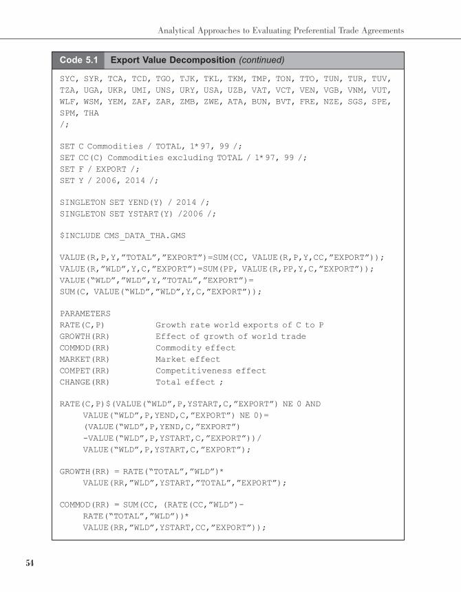
54
Analytical Approaches to Evaluating Preferential Trade Agreements
SYC, SYR, TCA, TCD, TGO, TJK, TKL, TKM, TMP, TON, TTO, TUN, TUR, TUV,
TZA, UGA, UKR, UMI, UNS, URY, USA, UZB, VAT, VCT, VEN, VGB, VNM, VUT,
WLF, WSM, YEM, ZAF, ZAR, ZMB, ZWE, ATA, BUN, BVT, FRE, NZE, SGS, SPE,
SPM, THA
/;
SET C Commodities / TOTAL, 1*97, 99 /;
SET CC(C) Commodities excluding TOTAL / 1*97, 99 /;
SET F / EXPORT /;
SET Y / 2006, 2014 /;
SINGLETON SET YEND(Y) / 2014 /;
SINGLETON SET YSTART(Y) /2006 /;
$INCLUDE CMS_DATA_THA.GMS
VALUE(R,P,Y,”TOTAL”,”EXPORT”)=SUM(CC, VALUE(R,P,Y,CC,”EXPORT”));
VALUE(R,”WLD”,Y,C,”EXPORT”)=SUM(PP, VALUE(R,PP,Y,C,”EXPORT”));
VALUE(“WLD”,”WLD”,Y,”TOTAL”,”EXPORT”)=
SUM(C, VALUE(“WLD”,”WLD”,Y,C,”EXPORT”));
PARAMETERS
RATE(C,P) Growth rate world exports of C to P
GROWTH(RR) Effect of growth of world trade
COMMOD(RR) Commodity effect
MARKET(RR) Market effect
COMPET(RR) Competitiveness effect
CHANGE(RR) Total effect ;
RATE(C,P)$(VALUE(“WLD”,P,YSTART,C,”EXPORT”) NE 0 AND
VALUE(“WLD”,P,YEND,C,”EXPORT”) NE 0)=
(VALUE(“WLD”,P,YEND,C,”EXPORT”)
-VALUE(“WLD”,P,YSTART,C,”EXPORT”))/
VALUE(“WLD”,P,YSTART,C,”EXPORT”);
GROWTH(RR) = RATE(“TOTAL”,”WLD”)*
VALUE(RR,”WLD”,YSTART,”TOTAL”,”EXPORT”);
COMMOD(RR) = SUM(CC, (RATE(CC,”WLD”)-
RATE(“TOTAL”,”WLD”))*
VALUE(RR,”WLD”,YSTART,CC,”EXPORT”));
Code 5.1 Export Value Decomposition (continued)
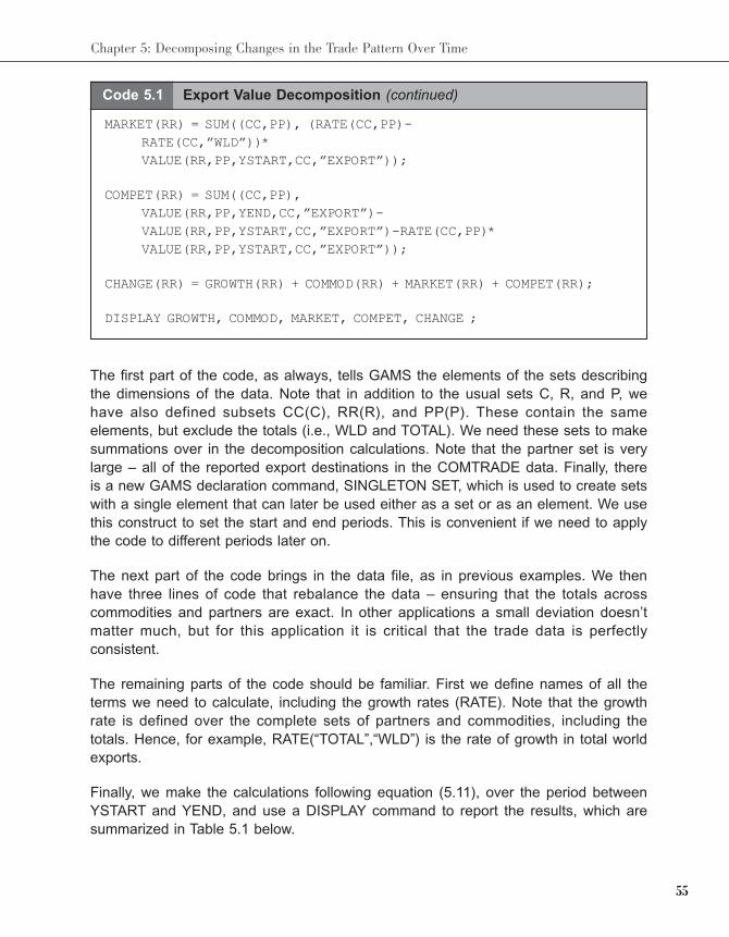
55
Chapter 5: Decomposing Changes in the Trade Pattern Over Time
MARKET(RR) = SUM((CC,PP), (RATE(CC,PP)-
RATE(CC,”WLD”))*
VALUE(RR,PP,YSTART,CC,”EXPORT”));
COMPET(RR) = SUM((CC,PP),
VALUE(RR,PP,YEND,CC,”EXPORT”)-
VALUE(RR,PP,YSTART,CC,”EXPORT”)-RATE(CC,PP)*
VALUE(RR,PP,YSTART,CC,”EXPORT”));
CHANGE(RR) = GROWTH(RR) + COMMOD(RR) + MARKET(RR) + COMPET(RR);
DISPLAY GROWTH, COMMOD, MARKET, COMPET, CHANGE ;
Code 5.1 Export Value Decomposition (continued)
The first part of the code, as always, tells GAMS the elements of the sets describing
the dimensions of the data. Note that in addition to the usual sets C, R, and P, we
have also defined subsets CC(C), RR(R), and PP(P). These contain the same
elements, but exclude the totals (i.e., WLD and TOTAL). We need these sets to make
summations over in the decomposition calculations. Note that the partner set is very
large – all of the reported export destinations in the COMTRADE data. Finally, there
is a new GAMS declaration command, SINGLETON SET, which is used to create sets
with a single element that can later be used either as a set or as an element. We use
this construct to set the start and end periods. This is convenient if we need to apply
the code to different periods later on.
The next part of the code brings in the data file, as in previous examples. We then
have three lines of code that rebalance the data – ensuring that the totals across
commodities and partners are exact. In other applications a small deviation doesn’t
matter much, but for this application it is critical that the trade data is perfectly
consistent.
The remaining parts of the code should be familiar. First we define names of all the
terms we need to calculate, including the growth rates (RATE). Note that the growth
rate is defined over the complete sets of partners and commodities, including the
totals. Hence, for example, RATE(“TOTAL”,“WLD”) is the rate of growth in total world
exports.
Finally, we make the calculations following equation (5.11), over the period between
YSTART and YEND, and use a DISPLAY command to report the results, which are
summarized in Table 5.1 below.
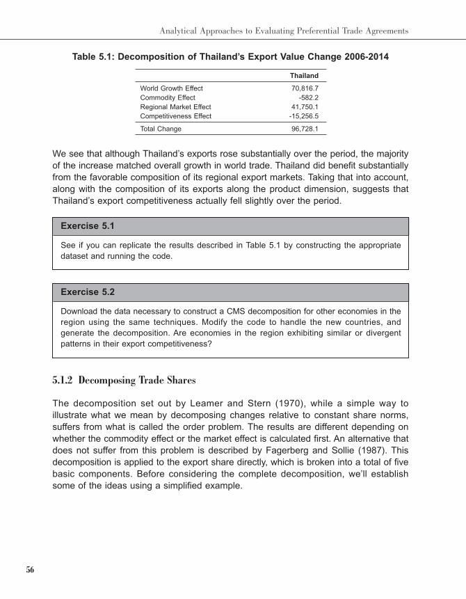
56
Analytical Approaches to Evaluating Preferential Trade Agreements
Table 5.1: Decomposition of Thailand’s Export Value Change 2006-2014
Thailand
World Growth Effect 70,816.7
Commodity Effect -582.2
Regional Market Effect 41,750.1
Competitiveness Effect -15,256.5
Total Change 96,728.1
Exercise 5.1
See if you can replicate the results described in Table 5.1 by constructing the appropriate
dataset and running the code.
Exercise 5.2
Download the data necessary to construct a CMS decomposition for other economies in the
region using the same techniques. Modify the code to handle the new countries, and
generate the decomposition. Are economies in the region exhibiting similar or divergent
patterns in their export competitiveness?
We see that although Thailand’s exports rose substantially over the period, the majority
of the increase matched overall growth in world trade. Thailand did benefit substantially
from the favorable composition of its regional export markets. Taking that into account,
along with the composition of its exports along the product dimension, suggests that
Thailand’s export competitiveness actually fell slightly over the period.
5.1.2 Decomposing Trade Shares
The decomposition set out by Leamer and Stern (1970), while a simple way to
illustrate what we mean by decomposing changes relative to constant share norms,
suffers from what is called the order problem. The results are different depending on
whether the commodity effect or the market effect is calculated first. An alternative that
does not suffer from this problem is described by Fagerberg and Sollie (1987). This
decomposition is applied to the export share directly, which is broken into a total of five
basic components. Before considering the complete decomposition, we’ll establish
some of the ideas using a simplified example.
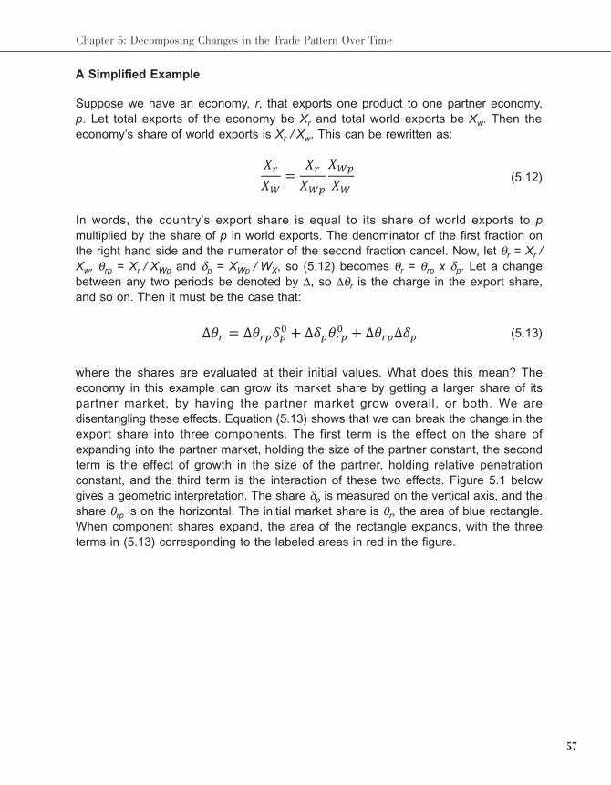
57
Chapter 5: Decomposing Changes in the Trade Pattern Over Time
A Simplified Example
Suppose we have an economy, r, that exports one product to one partner economy,
p. Let total exports of the economy be Xr and total world exports be Xw. Then the
economy’s share of world exports is Xr / Xw. This can be rewritten as:
(5.12)
In words, the country’s export share is equal to its share of world exports to p
multiplied by the share of p in world exports. The denominator of the first fraction on
the right hand side and the numerator of the second fraction cancel. Now, let θr = Xr /
Xw, θrp = Xr / XWp and δp = XWp / WX, so (5.12) becomes θr = θrp x δp. Let a change
between any two periods be denoted by Δ, so Δθr is the charge in the export share,
and so on. Then it must be the case that:
(5.13)
where the shares are evaluated at their initial values. What does this mean? The
economy in this example can grow its market share by getting a larger share of its
partner market, by having the partner market grow overall, or both. We are
disentangling these effects. Equation (5.13) shows that we can break the change in the
export share into three components. The first term is the effect on the share of
expanding into the partner market, holding the size of the partner constant, the second
term is the effect of growth in the size of the partner, holding relative penetration
constant, and the third term is the interaction of these two effects. Figure 5.1 below
gives a geometric interpretation. The share δp is measured on the vertical axis, and the
share θrp is on the horizontal. The initial market share is θr, the area of blue rectangle.
When component shares expand, the area of the rectangle expands, with the three
terms in (5.13) corresponding to the labeled areas in red in the figure.
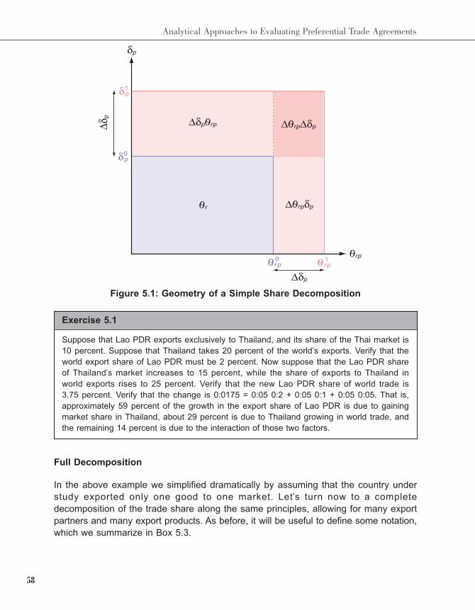
58
Analytical Approaches to Evaluating Preferential Trade Agreements
Figure 5.1: Geometry of a Simple Share Decomposition
Exercise 5.1
Suppose that Lao PDR exports exclusively to Thailand, and its share of the Thai market is
10 percent. Suppose that Thailand takes 20 percent of the world’s exports. Verify that the
world export share of Lao PDR must be 2 percent. Now suppose that the Lao PDR share
of Thailand’s market increases to 15 percent, while the share of exports to Thailand in
world exports rises to 25 percent. Verify that the new Lao PDR share of world trade is
3.75 percent. Verify that the change is 0:0175 = 0:05 0:2 + 0:05 0:1 + 0:05 0:05. That is,
approximately 59 percent of the growth in the export share of Lao PDR is due to gaining
market share in Thailand, about 29 percent is due to Thailand growing in world trade, and
the remaining 14 percent is due to the interaction of those two factors.
Full Decomposition
In the above example we simplified dramatically by assuming that the country under
study exported only one good to one market. Let’s turn now to a complete
decomposition of the trade share along the same principles, allowing for many export
partners and many export products. As before, it will be useful to define some notation,
which we summarize in Box 5.3.
59
Chapter 5: Decomposing Changes in the Trade Pattern Over Time
Consider first the regional pattern of exports of country r. The country’s share of total
world trade is defined as θr = Xr / XW. Similarly, θrp = Xrp / XWp is the share of the
country’s exports to region p in total world exports to region p. Finally, let δp = XWp /
XW be the share of total world exports that are destined for market p. Evidently, θr =
∑p θrpδp is an identity. As before, let a superscript 0 denote the first period, and
a superscript 1 the second period. To simplify the notation, let the change in any term
between period 1 and period zero be denoted using Δ. Hence, the change in the share
of country r in world trade between periods 0 and 1, is Δθr = .
(5.14)
This expression breaks down the change in the export share into its component parts
across the regional dimension. Now consider the commodity dimension. Let θir = Xir /
XiW represent the country’s share of the world market for commodity i, and βi = XiW /
XW represent the share of i in world trade. As above, θr = ∑i θirβi is an identity. Hence,
the change in the export share can also be described for all p by:
(5.15)
Expression (5.15) is breaking down the change in the export share into its component
parts across the commodity dimension. The final step is to integrate the regional and
commodity decompositions. We have defined xirp to be exports from country r good i
to region p. Evidently, Xrp = ∑ixirp and Xir = ∑p xirp Defining the share of exports from
country r of good i to country p in world exports of i to p as θirp = xirp / XiWp and the
share of world exports of i to p in world total exports to p as βip = xiWp / XWp, we can
Box 5.3 Summary of Notation
θr Share of region r in world exports.
θrp Share of region r exports to partner p in world exports to p.
δp Share of country p as a destination for total world exports.
θir Share of region r in world exports of commodity i.
θirp Share of region r in world exports of commodity i to region p.
βi Share of commodity i in world exports.
βip Share of commodity i in world exports to p.
θ r − θ r1 0
60
Analytical Approaches to Evaluating Preferential Trade Agreements
implement the commodity decomposition on a regional basis. It follows that (5.13) can
be written for each destination region:
(5.16)
Adding up (5.16) over p and substituting into (5.14) yields the complete decomposition
of the change in the country’s world market share:
(Market Share Effect)
(Commodity Composition Effect)
(Commodity Adaptation Effect) (5.17)
(Region Composition Effect)
(Region Adaptation Effect)
The left hand side of (5.17) is the change in export share. The right hand side breaks
that change down into components that represent:
1. Market Share Effect: Shows the impact of changes in the market shares by
commodity and destination, weighted by the commodity composition of each
destination and the regional composition of world trade in the base year. It can
be thought of as the increase in competitiveness having controlled for the initial
commodity and regional composition of the country’s exports.
2. Commodity Composition Effect: Shows to what extent the change in market
share can be explained by the initial commodity composition of the country’s
exports. It will be positive if the initial commodity composition of exports favors
those goods in which world trade is growing relatively rapidly.
3. Commodity Adaptation Effect: Shows to what extent the country has been
successful in adapting the commodity composition of its exports to meet
changes in the commodity composition of world demand.
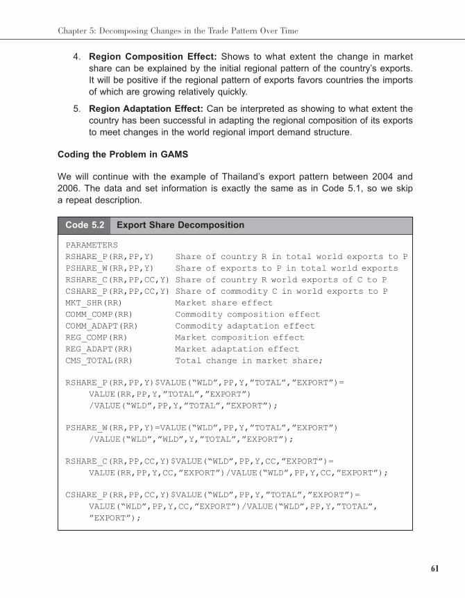
61
Chapter 5: Decomposing Changes in the Trade Pattern Over Time
4. Region Composition Effect: Shows to what extent the change in market
share can be explained by the initial regional pattern of the country’s exports.
It will be positive if the regional pattern of exports favors countries the imports
of which are growing relatively quickly.
5. Region Adaptation Effect: Can be interpreted as showing to what extent the
country has been successful in adapting the regional composition of its exports
to meet changes in the world regional import demand structure.
Coding the Problem in GAMS
We will continue with the example of Thailand’s export pattern between 2004 and
2006. The data and set information is exactly the same as in Code 5.1, so we skip
a repeat description.
Code 5.2 Export Share Decomposition
PARAMETERS
RSHARE_P(RR,PP,Y) Share of country R in total world exports to P
PSHARE_W(RR,PP,Y) Share of exports to P in total world exports
RSHARE_C(RR,PP,CC,Y) Share of country R world exports of C to P
CSHARE_P(RR,PP,CC,Y) Share of commodity C in world exports to P
MKT_SHR(RR) Market share effect
COMM_COMP(RR) Commodity composition effect
COMM_ADAPT(RR) Commodity adaptation effect
REG_COMP(RR) Market composition effect
REG_ADAPT(RR) Market adaptation effect
CMS_TOTAL(RR) Total change in market share;
RSHARE_P(RR,PP,Y)$VALUE(“WLD”,PP,Y,”TOTAL”,”EXPORT”)=
VALUE(RR,PP,Y,”TOTAL”,”EXPORT”)
/VALUE(“WLD”,PP,Y,”TOTAL”,”EXPORT”);
PSHARE_W(RR,PP,Y)=VALUE(“WLD”,PP,Y,”TOTAL”,”EXPORT”)
/VALUE(“WLD”,”WLD”,Y,”TOTAL”,”EXPORT”);
RSHARE_C(RR,PP,CC,Y)$VALUE(“WLD”,PP,Y,CC,”EXPORT”)=
VALUE(RR,PP,Y,CC,”EXPORT”)/VALUE(“WLD”,PP,Y,CC,”EXPORT”);
CSHARE_P(RR,PP,CC,Y)$VALUE(“WLD”,PP,Y,”TOTAL”,”EXPORT”)=
VALUE(“WLD”,PP,Y,CC,”EXPORT”)/VALUE(“WLD”,PP,Y,”TOTAL”,
”EXPORT”);
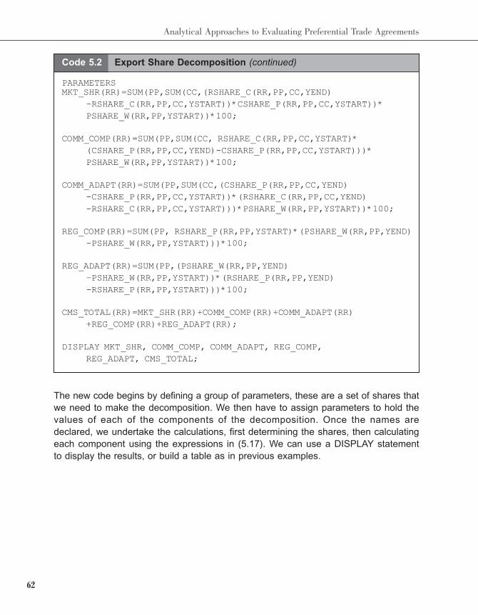
62
Analytical Approaches to Evaluating Preferential Trade Agreements
MKT_SHR(RR)=SUM(PP,SUM(CC,(RSHARE_C(RR,PP,CC,YEND)
-RSHARE_C(RR,PP,CC,YSTART))*CSHARE_P(RR,PP,CC,YSTART))*
PSHARE_W(RR,PP,YSTART))*100;
COMM_COMP(RR)=SUM(PP,SUM(CC, RSHARE_C(RR,PP,CC,YSTART)*
(CSHARE_P(RR,PP,CC,YEND)-CSHARE_P(RR,PP,CC,YSTART)))*
PSHARE_W(RR,PP,YSTART))*100;
COMM_ADAPT(RR)=SUM(PP,SUM(CC,(CSHARE_P(RR,PP,CC,YEND)
-CSHARE_P(RR,PP,CC,YSTART))*(RSHARE_C(RR,PP,CC,YEND)
-RSHARE_C(RR,PP,CC,YSTART)))*PSHARE_W(RR,PP,YSTART))*100;
REG_COMP(RR)=SUM(PP, RSHARE_P(RR,PP,YSTART)*(PSHARE_W(RR,PP,YEND)
-PSHARE_W(RR,PP,YSTART)))*100;
REG_ADAPT(RR)=SUM(PP,(PSHARE_W(RR,PP,YEND)
–PSHARE_W(RR,PP,YSTART))*(RSHARE_P(RR,PP,YEND)
-RSHARE_P(RR,PP,YSTART)))*100;
CMS_TOTAL(RR)=MKT_SHR(RR)+COMM_COMP(RR)+COMM_ADAPT(RR)
+REG_COMP(RR)+REG_ADAPT(RR);
DISPLAY MKT_SHR, COMM_COMP, COMM_ADAPT, REG_COMP,
REG_ADAPT, CMS_TOTAL;
Code 5.2 Export Share Decomposition (continued)
PARAMETERS
The new code begins by defining a group of parameters, these are a set of shares that
we need to make the decomposition. We then have to assign parameters to hold the
values of each of the components of the decomposition. Once the names are
declared, we undertake the calculations, first determining the shares, then calculating
each component using the expressions in (5.17). We can use a DISPLAY statement
to display the results, or build a table as in previous examples.
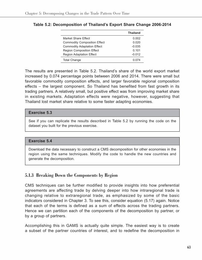
63
Chapter 5: Decomposing Changes in the Trade Pattern Over Time
The results are presented in Table 5.2. Thailand’s share of the world export market
increased by 0.074 percentage points between 2006 and 2014. There were small but
favorable commodity composition effects, and larger favorable regional composition
effects – the largest component. So Thailand has benefited from fast growth in its
trading partners. A relatively small, but positive effect was from improving market share
in existing markets. Adaptation effects were negative, however, suggesting that
Thailand lost market share relative to some faster adapting economies.
Table 5.2: Decomposition of Thailand’s Export Share Change 2006-2014
Thailand
Market Share Effect 0.002
Commodity Composition Effect 0.020
Commodity Adaptation Effect -0.035
Region Composition Effect 0.101
Region Adaptation Effect -0.012
Total Change 0.074
Exercise 5.3
See if you can replicate the results described in Table 5.2 by running the code on the
dataset you built for the previous exercise.
Exercise 5.4
Download the data necessary to construct a CMS decomposition for other economies in the
region using the same techniques. Modify the code to handle the new countries and
generate the decomposition.
5.1.3 Breaking Down the Components by Region
CMS techniques can be further modified to provide insights into how preferential
agreements are affecting trade by delving deeper into how intraregional trade is
changing relative to extraregional trade, as emphasized by some of the basic
indicators considered in Chapter 3. To see this, consider equation (5.17) again. Notice
that each of the terms is defined as a sum of effects across the trading partners.
Hence we can partition each of the components of the decomposition by partner, or
by a group of partners.
Accomplishing this in GAMS is actually quite simple. The easiest way is to create
a subset of the partner countries of interest, and to redefine the decomposition in
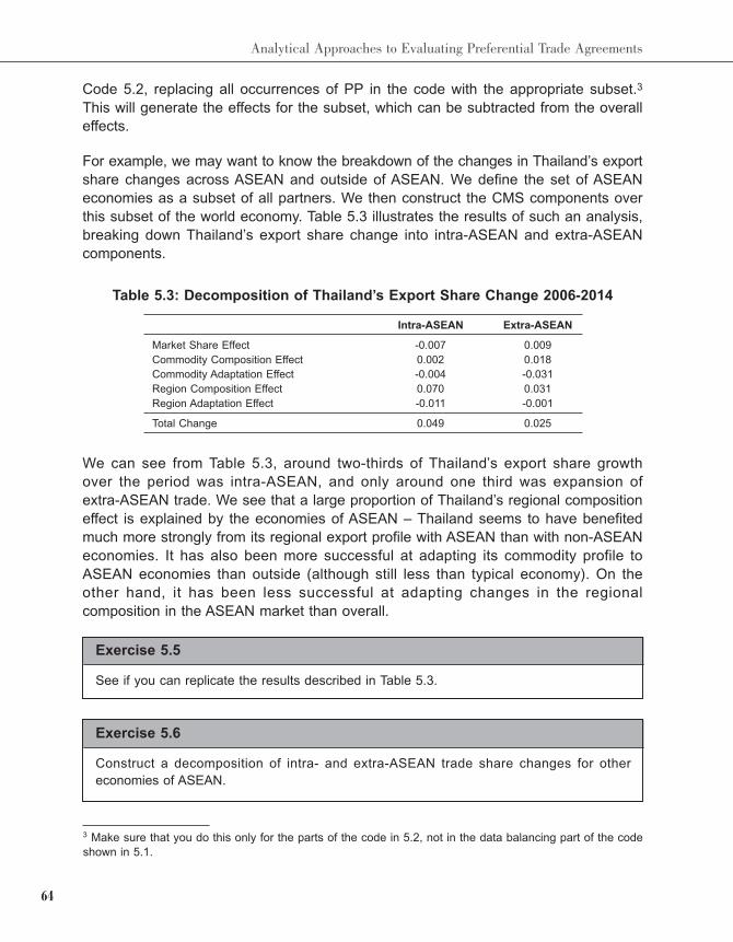
64
Analytical Approaches to Evaluating Preferential Trade Agreements
Code 5.2, replacing all occurrences of PP in the code with the appropriate subset.3
This will generate the effects for the subset, which can be subtracted from the overall
effects.
For example, we may want to know the breakdown of the changes in Thailand’s export
share changes across ASEAN and outside of ASEAN. We define the set of ASEAN
economies as a subset of all partners. We then construct the CMS components over
this subset of the world economy. Table 5.3 illustrates the results of such an analysis,
breaking down Thailand’s export share change into intra-ASEAN and extra-ASEAN
components.
3 Make sure that you do this only for the parts of the code in 5.2, not in the data balancing part of the code
shown in 5.1.
Table 5.3: Decomposition of Thailand’s Export Share Change 2006-2014
Intra-ASEAN Extra-ASEAN
Market Share Effect -0.007 0.009
Commodity Composition Effect 0.002 0.018
Commodity Adaptation Effect -0.004 -0.031
Region Composition Effect 0.070 0.031
Region Adaptation Effect -0.011 -0.001
Total Change 0.049 0.025
We can see from Table 5.3, around two-thirds of Thailand’s export share growth
over the period was intra-ASEAN, and only around one third was expansion of
extra-ASEAN trade. We see that a large proportion of Thailand’s regional composition
effect is explained by the economies of ASEAN – Thailand seems to have benefited
much more strongly from its regional export profile with ASEAN than with non-ASEAN
economies. It has also been more successful at adapting its commodity profile to
ASEAN economies than outside (although still less than typical economy). On the
other hand, it has been less successful at adapting changes in the regional
composition in the ASEAN market than overall.
Exercise 5.5
See if you can replicate the results described in Table 5.3.
Exercise 5.6
Construct a decomposition of intra- and extra-ASEAN trade share changes for other
economies of ASEAN.
65
Chapter 6: Partial Equilibrium Analysis
Chapter
6 PARTIAL EQUILIBRIUM ANALYSIS
While some of the indices that we have discussed are used ex ante, such as the
complementarity index, the primary purpose of most indices is ex post
evaluation. That is, they are used to help track how the trade pattern changes after
a policy intervention. When we are faced with evaluating a policy that has not yet been
implemented, we generally turn to simulation methods. The next two chapters deal with
two approaches that a widely used in the evaluation of preferential agreements –
partial and general equilibrium models. This type of approach places a much stronger
emphasis on the use of economic theory, alongside data, to generate policy information.
The distinction between partial and general equilibrium modeling, which we examine
in the next chapter, is that the former is considering only one market at a time, ignoring
potential interactions across markets. Partial equilibrium is just the technical terms for
demand and supply analysis. It is strictly valid only under some limited circumstances
(certain restrictions on demand and the assumption that the sector in question is small
relative to the economic system as a whole), which may not always hold in practice.
Nonetheless, the assumptions may be close enough that partial equilibrium modeling
generates important insights. Partial equilibrium models are a particularly useful
because they allow us to predict changes in key economic variables of interest,
including prices, the volume of trade, revenue and measures of economic efficiency.
Key advantages and disadvantages of partial equilibrium modeling are highlighted in
Box 6.1.
Box 6.1 Advantages and Disadvantage of Partial Equilibrium Models
Advantages: Theoretically sound (under certain assumptions). Very simple to implement
and apply to real data. Can be applied at a very disaggregate level (unlike CGE
models). Generate results on variables of policy interest directly (revenue, volume of
trade, etc.)
Disadvantages: Requires some knowledge of key parameters (elasticities), and results are
sensitive to those. Does not account for potential interaction among parts of the larger
economy. Assumptions underlying the partial equilibrium specification may not be
satisfied.
In this chapter we will review some basic demand and supply theory as it applies to
changes in trade policy. We will then develop the theory behind two basic partial
equilibrium models, build numerical versions of those models in GAMS, and
demonstrate how they can be applied to real world data. As with previous chapters,
all of the codes can be downloaded for use.
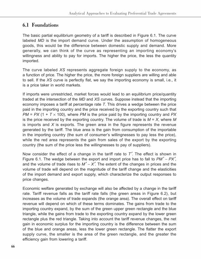
66
Analytical Approaches to Evaluating Preferential Trade Agreements
6.1 Foundations
The basic partial equilibrium geometry of a tariff is described in Figure 6.1. The curve
labeled MD is the import demand curve. Under the assumption of homogeneous
goods, this would be the difference between domestic supply and demand. More
generally, we can think of the curve as representing an importing economy’s
willingness and ability to pay for imports. The higher the price, the less the quantity
imported.
The curve labeled XS represents aggregate foreign supply to the economy, as
a function of price. The higher the price, the more foreign suppliers are willing and able
to sell. If the XS curve is perfectly flat, we say the importing economy is small, i.e., it
is a price taker in world markets.
If imports were unrestricted, market forces would lead to an equilibrium price/quantity
traded at the intersection of the MD and XS curves. Suppose instead that the importing
economy imposes a tariff at percentage rate T. This drives a wedge between the price
paid in the importing country and the price received by the exporting country such that
PM = PX (1 + T × 100), where PM is the price paid by the importing country and PX
is the price received by the exporting country. The volume of trade is M = X, where M
is imports and X is exports. The green area in the figure represents the revenue
generated by the tariff. The blue area is the gain from consumption of the importable
in the importing country (the sum of consumer’s willingnesses to pay less the price),
while the red area represents the gain from sales of the export by the exporting
country (the sum of the price less the willingnesses to pay of suppliers).
Now consider the effect of a change in the tariff rate to T′. The effect is shown in
Figure 6.1. The wedge between the export and import price has to fall to PM′ − PX′,and the volume of trade rises to M′ − X′. The extent of the changes in prices and the
volume of trade will depend on the magnitude of the tariff change and the elasticities
of the import demand and export supply, which characterize the output responses to
price changes.
Economic welfare generated by exchange will also be affected by a change in the tariff
rate. Tariff revenue falls as the tariff rate falls (the green areas in Figure 6.2), but
increases as the volume of trade expands (the orange area). The overall effect on tariff
revenue will depend on which of these terms dominates. The gains from trade to the
importing country expand, by the sum of the green upper green rectangle and the blue
triangle, while the gains from trade to the exporting country expand by the lower green
rectangle plus the red triangle. Taking into account the tariff revenue changes, the net
gain in economic surplus for the importing country is the difference between the sum
of the blue and orange areas, less the lower green rectangle. The flatter the export
supply curve, the smaller is the area of the green rectangle, and the greater the
efficiency gain from lowering a tariff.
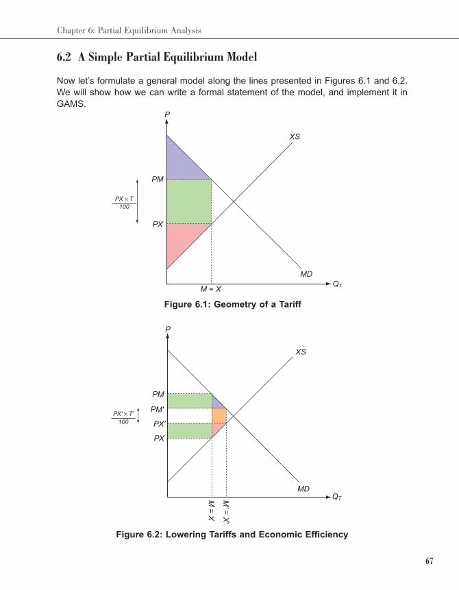
67
Chapter 6: Partial Equilibrium Analysis
6.2 A Simple Partial Equilibrium Model
Now let’s formulate a general model along the lines presented in Figures 6.1 and 6.2.
We will show how we can write a formal statement of the model, and implement it in
GAMS.
Figure 6.1: Geometry of a Tariff
Figure 6.2: Lowering Tariffs and Economic Efficiency
P
XS
MD
PM
PX
M = XQT
PX × T
100
P
XS
MD
PM
PM'
PX'
PX
PX' × T'
100
QTM =
X
M' =
X'
68
Analytical Approaches to Evaluating Preferential Trade Agreements
6.2.1 Theoretical Structure
To build the model, we need to describe each of the model relationships. Import
demand can be described by:
(6.1)
where and is the elasticity of import demand. The function is called
a constant elasticity of demand function. Similarly, we can describe export supply by:
(6.2)
where and is the elasticity of export supply. In the small country case,
The equilibrium condition requires that the volume of imports equals the volume
of exports, hence:
(6.3)
Finally, the tariff wedge between the import and export price is given by:
(6.4)
where T is the ad valorem tariff rate, expressed as a percentage. Given the parameter
values and, and the policy variable T, (6.1) to (6.4) are a system of four
equations in four unknowns, PM, PX, M and X.
Once we have determined the equilibrium prices and quantities, we can determine the
components of economic surplus. Tariff revenue is given by:
(6.5)
The changes in the gains from exchange to the importing and exporting countries are
a little bit trickier. Let PM0 be the initial import price, and let PM1 be the import price
after the tariff change. Then the change in the benefits of importing is:
(6.6)
69
Chapter 6: Partial Equilibrium Analysis
Similarly, the change in the benefits of exporting can be written as:
(6.7)
These expressions complete a basic partial equilibrium model that we can use to
simulate the economic impact of tariff changes in a single sector.
6.2.2 Calibrating the Model
Above we noted that if we know the parameter values and η, and the policy
variable T, we can solve for PM, PX, M and X. If T changes, we can work out the new
prices and quantities, along with the revenue and efficiency effects of the change.
When building a simulation model for policy analysis, the problem is actually slightly
different. In general we do not need to solve for the prices and quantities, since these
are observed. What we are interested in is how prices, trade, revenue, etc., are likely
to change when the policy variable changes. What we generally don’t know is the
values of the parameters.
If we have some idea (perhaps from previous literature) about the magnitudes of the
elasticity parameters and η, however, we can work back to find the other parameters
that are consistent with the data that we have observed. This process is called
calibration, and it amounts to fitting the theoretical model to the observed data.
In this particular case, calibration is quite simple. Suppose we know PM, M, and T.
Alternatively, we might know PM × M, i.e., the value of imports, in which case we can
normalize the import price to unity, and let the value equal the volume. From (6.3) we
know X, and from (6.5) we know PX. If we have an estimate of , then we can use
(6.1) to find αM = M / PM , and if we have an estimate of we can use (6.2) to find αx =
X / PXη. This is the calibration procedure for the model. Solving it will generate the data
that we observed.
6.2.3 Coding the Problem in GAMS
To build a model like this in GAMS is more complex than the examples we have seen
so far, since we actually require GAMS to solve the problem for us rather than simply
manipulate data. The required code is presented in Code 6.1 and Code 6.2.
The first part of the program (Code 6.1) is called the declarations. This is where we
tell GAMS the names of all of the pieces of the model. The first set of names we have
seen before, these are the PARAMETERS of the model, which means anything with
70
Analytical Approaches to Evaluating Preferential Trade Agreements
a fixed value. We provide a name for each of the parameters used in equations (6.1)
through (6.7). We also provide parameter names for the initial values of all of the
variables in the model. For example, MO represents the initial import volume (which
is fixed, since it is whatever we observe in the base year).
The next block of code declares the names of all of the VARIABLES in the model.
These are the values the will be determined by the solution of the model. Notice that
there are six variables corresponding to the terms in the equations set out above. For
convenience we have also added a term for the change in tariff revenue. Note the
distinction between variables and their initial values. For example, XO is the initial level
of exports, something that we have already observed. By contrast, X is the level of
exports that the model predicts will occur given the model and any tariff rate.
The final block in Code 6.1 is the declarations of EQUATIONS in the model. These are
just the names that were given to each of the relationships described by our theoretical
model. Hence M_DEM is the import demand equation (6.1), X_SUP is the export
supply equation (6.2), EQUIL is the equilibrium condition (6.3) and so on. Notice that
we have exactly the same number of equation declarations as we have variable
declarations, indicating that the model is identified.
The next part of the model (Code 6.2) is called the assignment. In this part of the code
we enter the data on the market under study, calibrate, and specify the structure of the
model equations.
The first block of code is the data, which in principle comes from real world source
(we present an example in the next subsection). The required data are estimates of
the elasticities of import demand and export supply, the initial volume of imports, the
initial import price, and the tariff rate (as a percentage). If volume and price data are
not available separately, then data on the value of imports can be used instead, with
a normalized price of one.
The second block of code is the calibration. This follows the procedure set out in
Section 6.2.2 to determine the initial values of the remaining variables in the model,
and the remaining parameters of the model.
The third block of the code does two things. The first is setting the initial values of the
variables to the corresponding values held in the associated parameters. Hence,
M.L=MO tells GAMS that it should start looking for a new value of M from the value
contained in MO, and similarly the other variables.1 The second is setting the lower
bounds on variables. The statement M.LO=0 means that the value of imports is not
1 By default GAMS will choose a starting value of zero. This is often not a good idea. In this model, for
example, equation (6.1) is not defined if PM = 0, since we can’t bring zero to a negative power.
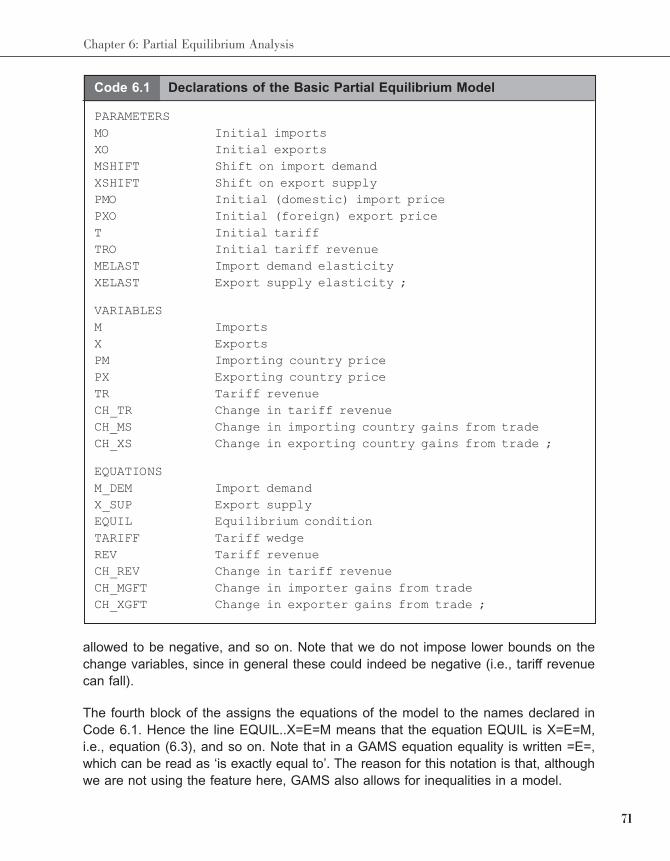
71
Chapter 6: Partial Equilibrium Analysis
Code 6.1 Declarations of the Basic Partial Equilibrium Model
PARAMETERS
MO Initial imports
XO Initial exports
MSHIFT Shift on import demand
XSHIFT Shift on export supply
PMO Initial (domestic) import price
PXO Initial (foreign) export price
T Initial tariff
TRO Initial tariff revenue
MELAST Import demand elasticity
XELAST Export supply elasticity ;
VARIABLES
M Imports
X Exports
PM Importing country price
PX Exporting country price
TR Tariff revenue
CH_TR Change in tariff revenue
CH_MS Change in importing country gains from trade
CH_XS Change in exporting country gains from trade ;
EQUATIONS
M_DEM Import demand
X_SUP Export supply
EQUIL Equilibrium condition
TARIFF Tariff wedge
REV Tariff revenue
CH_REV Change in tariff revenue
CH_MGFT Change in importer gains from trade
CH_XGFT Change in exporter gains from trade ;
allowed to be negative, and so on. Note that we do not impose lower bounds on the
change variables, since in general these could indeed be negative (i.e., tariff revenue
can fall).
The fourth block of the assigns the equations of the model to the names declared in
Code 6.1. Hence the line EQUIL..X=E=M means that the equation EQUIL is X=E=M,
i.e., equation (6.3), and so on. Note that in a GAMS equation equality is written =E=,
which can be read as ‘is exactly equal to’. The reason for this notation is that, although
we are not using the feature here, GAMS also allows for inequalities in a model.
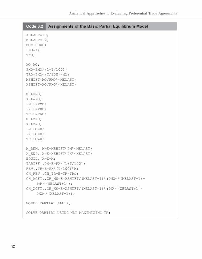
72
Analytical Approaches to Evaluating Preferential Trade Agreements
Code 6.2 Assignments of the Basic Partial Equilibrium Model
XELAST=10;
MELAST=-2;
MO=10000;
PMO=1;
T=0;
XO=MO;
PXO=PMO/(1+T/100);
TRO=PXO*(T/100)*MO;
MSHIFT=MO/PMO**MELAST;
XSHIFT=XO/PXO**XELAST;
M.L=MO;
X.L=XO;
PM.L=PMO;
PX.L=PXO;
TR.L=TRO;
M.LO=0;
X.LO=0;
PM.LO=0;
PX.LO=0;
TR.LO=0;
M_DEM..M=E=MSHIFT*PM**MELAST;
X_SUP..X=E=XSHIFT*PX**XELAST;
EQUIL..X=E=M;
TARIFF..PM=E=PX*(1+T/100);
REV..TR=E=PX*(T/100)*M;
CH_REV..CH_TR=E=TR-TRO;
CH_MGFT..CH_MS=E=MSHIFT/(MELAST+1)*(PMO**(MELAST+1)-
PM**(MELAST+1));
CH_XGFT..CH_XS=E=XSHIFT/(XELAST+1)*(PX**(XELAST+1)-
PXO**(XELAST+1));
MODEL PARTIAL /ALL/;
SOLVE PARTIAL USING NLP MAXIMIZING TR;
73
Chapter 6: Partial Equilibrium Analysis
The penultimate line of code tells GAMS that the model we want to solve contains all
of the declared equations. PARTIAL is the name that we have given the model. The
last line asks GAMS to solve the model. If the code is submitted to the GAMS system,
it will execute and find the solution. If the calibration is correct, the model solution
should be the same as the initial value. We can then add further SOLVE statements
to evaluate the effect of changes in policy. For example, appending Code 6.3 will
simulate the effect of raising the tariff from zero to 10 percent.
Code 6.3 A Scenario
T=10;
SOLVE PARTIAL USING NLP MAXIMIZING TR;
Exercise 6.1
By running the code above, verify that the model solves and calibrates correctly.
Exercise 6.2
Simulate the effect of a 10 percent tariff on the economic system.
Exercise 6.3
Suppose that you knew the volume of imports was 5,000 and the price was 2 (so the value
of imports is still 10,000). Change the data section of the model to reflect this, and verify
that this rescaling does not affect the estimates of the economic impact of the tariff change
in Exercise 6.2.
6.2.4 Sample Application
Consider HS category 8702 (motor vehicles for the transport of 10 or more people).
COMTRADE reports that Thailand’s imports in this category in 2014 were
$189,445,100 The UNCTAD TRAINS database reports the applied tariff rate to be
19 percent. The elasticities are harder to obtain. We assume a value of 20 for the
export supply elasticity, indicating that Thailand is very small in the world market.2 For
the import demand elasticity, we use information from the GTAP database, which
suggests an elasticity of approximately -4.3 What would happen if Thailand was to
2 The SMART model, available through WITS, which is structurally the same as that examined in the next
section, uses a default elasticity of 99, essentially the small country assumption.
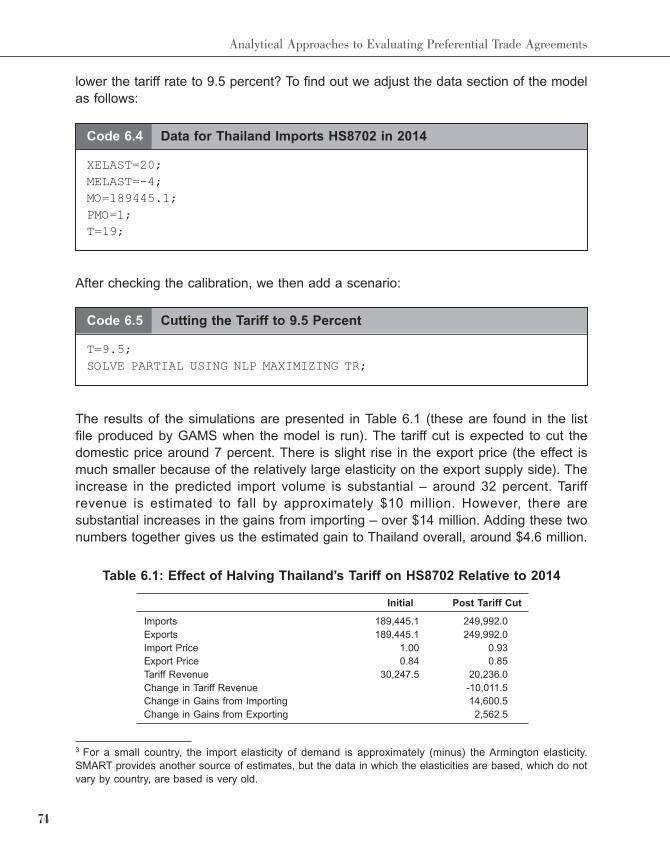
74
Analytical Approaches to Evaluating Preferential Trade Agreements
lower the tariff rate to 9.5 percent? To find out we adjust the data section of the model
as follows:
3 For a small country, the import elasticity of demand is approximately (minus) the Armington elasticity.
SMART provides another source of estimates, but the data in which the elasticities are based, which do not
vary by country, are based is very old.
Code 6.4 Data for Thailand Imports HS8702 in 2014
XELAST=20;
MELAST=-4;
MO=189445.1;
PMO=1;
T=19;
After checking the calibration, we then add a scenario:
Code 6.5 Cutting the Tariff to 9.5 Percent
T=9.5;
SOLVE PARTIAL USING NLP MAXIMIZING TR;
The results of the simulations are presented in Table 6.1 (these are found in the list
file produced by GAMS when the model is run). The tariff cut is expected to cut the
domestic price around 7 percent. There is slight rise in the export price (the effect is
much smaller because of the relatively large elasticity on the export supply side). The
increase in the predicted import volume is substantial – around 32 percent. Tariff
revenue is estimated to fall by approximately $10 million. However, there are
substantial increases in the gains from importing – over $14 million. Adding these two
numbers together gives us the estimated gain to Thailand overall, around $4.6 million.
Table 6.1: Effect of Halving Thailand’s Tariff on HS8702 Relative to 2014
Initial Post Tariff Cut
Imports 189,445.1 249,992.0
Exports 189,445.1 249,992.0
Import Price 1.00 0.93
Export Price 0.84 0.85
Tariff Revenue 30,247.5 20,236.0
Change in Tariff Revenue -10,011.5
Change in Gains from Importing 14,600.5
Change in Gains from Exporting 2,562.5
75
Chapter 6: Partial Equilibrium Analysis
6.3 Import Differentiation by Source
The model developed in the previous section is useful for understanding changes in
overall imports. It is thus useful for evaluating the overall impact of a general tariff
reform from the perspective of the importing country. It may also be useful for exporting
countries, when the objective is to determine how much overall trade might increase
in an export partner when they liberalize their trade. The model is limited, however, in
that it does not identify separate sources of imports, and does not allow for tariff
variation by source, both of which are important in evaluating preferential trade
agreements. The modifications required to allow the model to handle these cases are
not too difficult. In essence, we need to allow for differentiation of goods by source.
6.3.1 Changes to the Theory
The first step is to allow for different export sources. Suppose that the economy under
study imports from a set of partner countries indexed by p. Let the supply of each of
these countries be described by an export supply function of the same form as (6.2).
That is, we now have p export supply functions:
(6.8)
where Xp is exports from partner p, and PXp is the price received in partner p. Note
that we have allowed the elasticity of supply to vary by partner, along with the αXp
parameter. The equilibrium conditions also have to be adjusted, since there is now
a market with each partner, so (6.3) becomes:
Exercise 6.4
Verify the results yourself. What would be the effect of removing the tariff completely? What
if the tariff was to rise to 50 percent?
Exercise 6.5
One issue with this type of modeling is sensitivity of the results to the elasticities. Try varying
the elasticities slightly, do the results change significantly?
Exercise 6.6
See if you can calibrate the model to data from another sector/country to simulate the
effects of tariff reforms.
76
Analytical Approaches to Evaluating Preferential Trade Agreements
(6.9)
In other words, the exports of country p are equal to the imports from country p.
Similarly, equation (6.4) becomes:
(6.10)
Notice that the tariff can vary by source (as it generally would with a preferential trade
agreement in place). Tariff revenue (equation 6.5) can now be defined as:
(6.11)
Equation (6.1) remains the same, and we continue to interpret it as overall import
demand. What we need is a way to split the demand across the sources. We do so
via an assumption called the Armington specification.4 This means that imports are
differentiated by country of origin. This assumption allows us to add two more sets of
equations to the model. The first is called the Armington aggregator. This function
aggregate the individual country imports into aggregate imports. It takes the form:
(6.12)
where A is a shift parameter, δp represents the share of each country in the import
aggregate, and is a parameter reflecting the degree of substitutability between imports
from different sources. The latter is related to the elasticity of substitution (also called
the Armington elasticity) by p = -1/σ + 1. Hence a high degree of substitutability is
reflected in a value of close to 1, while a low degree is represented by a strongly
negative parameter value. Finally, we can derive demands for imports from each
country as:
(6.13)
4 The original reference is Armington (1969). A much more detailed discussion of the Armington assumption
and its implementation can be found in Gilbert and Tower (2013).
77
Chapter 6: Partial Equilibrium Analysis
where the set indexed by r has the same membership as the set indexed by p. The
interpretation of the expression is that at equilibrium, the importing country has to be
just indifferent between sources of the marginal unit (see Box 6.2 for further details).
Together, equations (6.8) through (6.13), along with equation (6.1), provide sufficient
theoretical structure to determine the values of all PMp, PXp, Xp, Mp, and the
aggregates, M, PM, and TR. As with the previous model, if we observe the initial trade
flows and policy instruments, and have estimates of the elasticities (import demand,
export supply and substitution across sources) we can calibrate the theory to the
observed data and simulate the effects of policy changes.
Box 6.1 More Details on Armington
The Armington assumption views demands as following a two stage optimization. In the first
stage the total amount the good to be imported is decided. The solution to this problem is
reflected in the import demand curve. In the second stage, a choice is made over the
alternative sources of imports. The constant elasticity of substitution function (6.12) is used
to describe the willingness to substitute over the sources, for any given level of total imports.
Buyers are assumed to minimize the cost of purchasing a consumption bundle. Hence they
solve the problem:
The first order conditions for a minimum are equations (6.13). Further details on the
mathematics, and some alternative interpretations, can be found in Gilbert and Tower
(2013).
6.3.2 Coding the Problem in GAMS
The code for the problem is presented in Code 6.3 and 6.4. Once again, we break the
code into the declarations (Code 6.3) and the assignments (Code 6.4). Since the code
is very similar to the example in Section 6.2, we keep our description brief and focused
on the new elements.
The first new element is the introduction of a SET containing the partner countries
(we will consider an example with real data later). The PARAMETER, VARIABLE and
EQUATION sections are much the same as in the previous example. We have
extended the relevant equations over the p dimension, added new terms for aggregate
imports and the aggregate import prices, and the associated equations and
parameters.
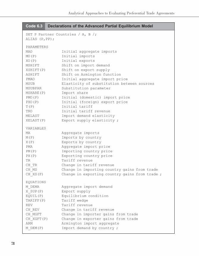
78
Analytical Approaches to Evaluating Preferential Trade Agreements
Code 6.3 Declarations of the Advanced Partial Equilibrium Model
SET P Partner Countries / A, B /;
ALIAS (P,PP);
PARAMETERS
MAO Initial aggregate imports
MO(P) Initial imports
XO(P) Initial exports
MSHIFT Shift on import demand
XSHIFT(P) Shift on export supply
ASHIFT Shift on Armington function
PMAO Initial aggregate import price
MSUB Elasticity of substitution between sources
MSUBPAR Substitution parameter
MSHARE(P) Import share
PMO(P) Initial (domestic) import price
PXO(P) Initial (foreign) export price
T(P) Initial tariff
TRO Initial tariff revenue
MELAST Import demand elasticity
XELAST(P) Export supply elasticity ;
VARIABLES
MA Aggregate imports
M(P) Imports by country
X(P) Exports by country
PMA Aggregate import price
PM(P) Importing country price
PX(P) Exporting country price
TR Tariff revenue
CH_TR Change in tariff revenue
CH_MS Change in importing country gains from trade
CH_XS(P) Change in exporting country gains from trade ;
EQUATIONS
M_DEMA Aggregate import demand
X_SUP(P) Export supply
EQUIL(P) Equilibrium condition
TARIFF(P) Tariff wedge
REV Tariff revenue
CH_REV Change in tariff revenue
CH_MGFT Change in importer gains from trade
CH_XGFT(P) Change in exporter gains from trade
ARM Armington import aggregate
M_DEM(P) Import demand by country ;
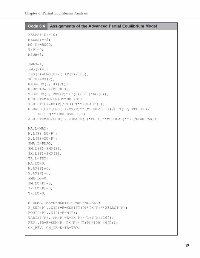
79
Chapter 6: Partial Equilibrium Analysis
Code 6.4 Assignments of the Advanced Partial Equilibrium Model
XELAST(P)=10;
MELAST=-2;
MO(P)=5000;
T(P)=0;
MSUB=3;
PMAO=1;
PMO(P)=1;
PXO(P)=PMO(P)/(1+T(P)/100);
XO(P)=MO(P);
MAO=SUM(P, MO(P));
MSUBPAR=-1/MSUB+1;
TRO=SUM(P, PXO(P)*(T(P)/100)*MO(P));
MSHIFT=MAO/PMAO**MELAST;
XSHIFT(P)=XO(P)/PXO(P)**XELAST(P);
MSHARE(P)=(PMO(P)/MO(P)**(MSUBPAR-1))/SUM(PP, PMO(PP)/
MO(PP)**(MSUBPAR-1));
ASHIFT=MAO/SUM(P, MSHARE(P)*MO(P)**MSUBPAR)**(1/MSUBPAR);
MA.L=MAO;
M.L(P)=MO(P);
X.L(P)=XO(P);
PMA.L=PMAO;
PM.L(P)=PMO(P);
PX.L(P)=PXO(P);
TR.L=TRO;
MA.LO=0;
M.LO(P)=0;
X.LO(P)=0;
PMA.LO=0;
PM.LO(P)=0;
PX.LO(P)=0;
TR.LO=0;
M_DEMA..MA=E=MSHIFT*PMA**MELAST;
X_SUP(P)..X(P)=E=XSHIFT(P)*PX(P)**XELAST(P);
EQUIL(P)..X(P)=E=M(P);
TARIFF(P)..PM(P)=E=PX(P)*(1+T(P)/100);
REV..TR=E=SUM(P, PX(P)*(T(P)/100)*M(P));
CH_REV..CH_TR=E=TR-TRO;
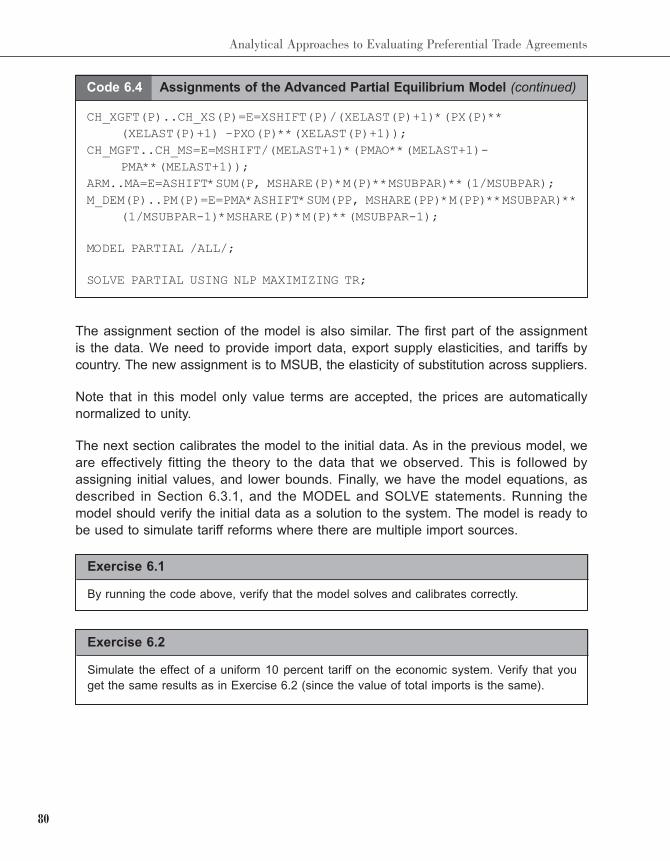
80
Analytical Approaches to Evaluating Preferential Trade Agreements
Code 6.4 Assignments of the Advanced Partial Equilibrium Model (continued)
CH_XGFT(P)..CH_XS(P)=E=XSHIFT(P)/(XELAST(P)+1)*(PX(P)**
(XELAST(P)+1) -PXO(P)**(XELAST(P)+1));
CH_MGFT..CH_MS=E=MSHIFT/(MELAST+1)*(PMAO**(MELAST+1)-
PMA**(MELAST+1));
ARM..MA=E=ASHIFT*SUM(P, MSHARE(P)*M(P)**MSUBPAR)**(1/MSUBPAR);
M_DEM(P)..PM(P)=E=PMA*ASHIFT*SUM(PP, MSHARE(PP)*M(PP)**MSUBPAR)**
(1/MSUBPAR-1)*MSHARE(P)*M(P)**(MSUBPAR-1);
MODEL PARTIAL /ALL/;
SOLVE PARTIAL USING NLP MAXIMIZING TR;
The assignment section of the model is also similar. The first part of the assignment
is the data. We need to provide import data, export supply elasticities, and tariffs by
country. The new assignment is to MSUB, the elasticity of substitution across suppliers.
Note that in this model only value terms are accepted, the prices are automatically
normalized to unity.
The next section calibrates the model to the initial data. As in the previous model, we
are effectively fitting the theory to the data that we observed. This is followed by
assigning initial values, and lower bounds. Finally, we have the model equations, as
described in Section 6.3.1, and the MODEL and SOLVE statements. Running the
model should verify the initial data as a solution to the system. The model is ready to
be used to simulate tariff reforms where there are multiple import sources.
Exercise 6.1
By running the code above, verify that the model solves and calibrates correctly.
Exercise 6.2
Simulate the effect of a uniform 10 percent tariff on the economic system. Verify that you
get the same results as in Exercise 6.2 (since the value of total imports is the same).
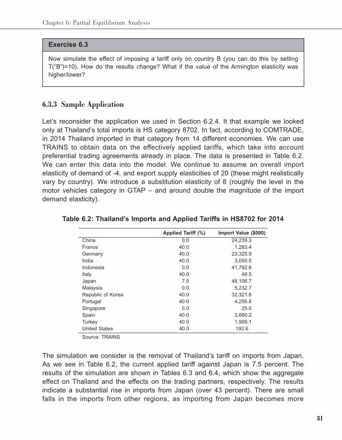
81
Chapter 6: Partial Equilibrium Analysis
6.3.3 Sample Application
Let’s reconsider the application we used in Section 6.2.4. It that example we looked
only at Thailand’s total imports is HS category 8702. In fact, according to COMTRADE,
in 2014 Thailand imported in that category from 14 different economies. We can use
TRAINS to obtain data on the effectively applied tariffs, which take into account
preferential trading agreements already in place. The data is presented in Table 6.2.
We can enter this data into the model. We continue to assume an overall import
elasticity of demand of -4, and export supply elasticities of 20 (these might realistically
vary by country). We introduce a substitution elasticity of 8 (roughly the level in the
motor vehicles category in GTAP – and around double the magnitude of the import
demand elasticity).
Exercise 6.3
Now simulate the effect of imposing a tariff only on country B (you can do this by setting
T(“B”)=10). How do the results change? What if the value of the Armington elasticity was
higher/lower?
Table 6.2: Thailand’s Imports and Applied Tariffs in HS8702 for 2014
Applied Tariff (%) Import Value ($000)
China 0.0 24,239.3
France 40.0 1,283.4
Germany 40.0 23,325.9
India 40.0 3,050.5
Indonesia 0.0 41,792.6
Italy 40.0 48.5
Japan 7.5 48,106.7
Malaysia 0.0 5,232.7
Republic of Korea 40.0 32,321.8
Portugal 40.0 4,256.8
Singapore 0.0 25.0
Spain 40.0 3,660.2
Turkey 40.0 1,909.1
United States 40.0 192.6
Source: TRAINS
The simulation we consider is the removal of Thailand’s tariff on imports from Japan.
As we see in Table 6.2, the current applied tariff against Japan is 7.5 percent. The
results of the simulation are shown in Tables 6.3 and 6.4, which show the aggregate
effect on Thailand and the effects on the trading partners, respectively. The results
indicate a substantial rise in imports from Japan (over 43 percent). There are small
falls in the imports from other regions, as importing from Japan becomes more
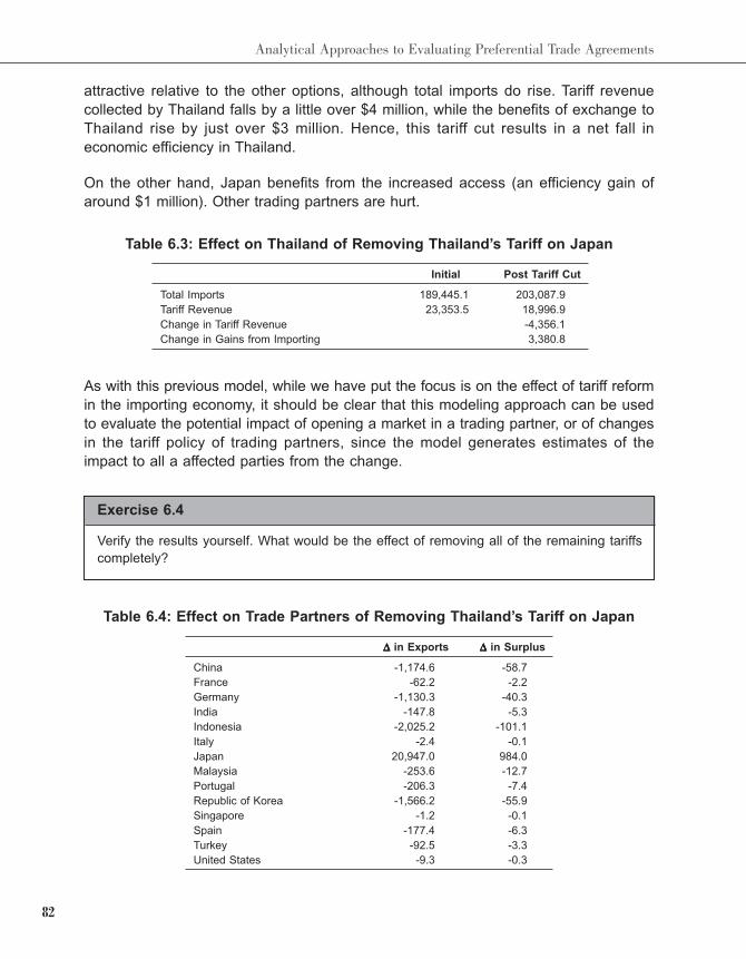
82
Analytical Approaches to Evaluating Preferential Trade Agreements
attractive relative to the other options, although total imports do rise. Tariff revenue
collected by Thailand falls by a little over $4 million, while the benefits of exchange to
Thailand rise by just over $3 million. Hence, this tariff cut results in a net fall in
economic efficiency in Thailand.
On the other hand, Japan benefits from the increased access (an efficiency gain of
around $1 million). Other trading partners are hurt.
Table 6.3: Effect on Thailand of Removing Thailand’s Tariff on Japan
Initial Post Tariff Cut
Total Imports 189,445.1 203,087.9
Tariff Revenue 23,353.5 18,996.9
Change in Tariff Revenue -4,356.1
Change in Gains from Importing 3,380.8
As with this previous model, while we have put the focus is on the effect of tariff reform
in the importing economy, it should be clear that this modeling approach can be used
to evaluate the potential impact of opening a market in a trading partner, or of changes
in the tariff policy of trading partners, since the model generates estimates of the
impact to all a affected parties from the change.
Exercise 6.4
Verify the results yourself. What would be the effect of removing all of the remaining tariffs
completely?
Table 6.4: Effect on Trade Partners of Removing Thailand’s Tariff on Japan
ΔΔΔΔΔ in Exports ΔΔΔΔΔ in Surplus
China -1,174.6 -58.7
France -62.2 -2.2
Germany -1,130.3 -40.3
India -147.8 -5.3
Indonesia -2,025.2 -101.1
Italy -2.4 -0.1
Japan 20,947.0 984.0
Malaysia -253.6 -12.7
Portugal -206.3 -7.4
Republic of Korea -1,566.2 -55.9
Singapore -1.2 -0.1
Spain -177.4 -6.3
Turkey -92.5 -3.3
United States -9.3 -0.3
83
Chapter 6: Partial Equilibrium Analysis
Exercise 6.5
Try varying the elasticities slightly, do the results change significantly? In particular the role
of the Armington elasticities.
Exercise 6.6
See if you can calibrate the model to data from another sector/country to simulate the
effects of tariff reforms. Try a case of own tariff reform, and a case of tariff reform in
a trading partner.

84
Analytical Approaches to Evaluating Preferential Trade Agreements
85
Chapter 7: General Equilibrium Analysis
Chapter
7 GENERAL EQUILIBRIUM ANALYSIS
Among the most sophisticated analytical tools for evaluating the economic impacts
of preferential trading agreements ex ante are computable general equilibrium or
CGE models. In contrast to partial equilibrium models, which consider only one sector,
these models attempt to predict the changes that will be observed across the entire
economic system. They can be a rich source of information in the policymaking process.
While the CGE approach has its strengths and weaknesses (see Box 7.1), it has
proven a very useful tool for analysis of trade policy. CGE models are multi-sectoral,
often multi-regional, flexible, and logically consistent. Because at their core they are
designed to track linkages across an economic system, they are well-suited to
examining the economy-wide implications of large changes in the economic
environment, and/or changes that affect multiple parts of the economic system at the
same time, as is generally the case with preferential trade agreements. Applications of
CGE models to understanding the economic implications of preferential trade
agreements are numerous. See, for example, Scollay and Gilbert (2000) for a survey
of models applied to APEC, Gilbert and Wahl (2012) for the case of Chinese trade
reform, Bekkers and Rojas-Romagosa (2016) for the TTIP, Gilbert et al. (2016) for the
TPP, and Robinson and Thierfelder (2002) and Lloyd and MacLaren (2004) for more
general overviews.
Box 7.1 Advantages and Disadvantage of CGE
Advantages: High degree of theoretical consistency, ability to highlight the importance of
linkages between sectors, can be adapted to incorporate unique features of an
economic system, able to predict values for many economic variables in the system,
such as economic welfare, in addition to sectoral shifts.
Disadvantages: The data requirements of CGE models are substantial, the human capital
investment required in building/using these models is also very high. There is often
uncertainty over parameters, specification, and experimental design. By covering all
sectors in an economy, a CGE model may miss key features of critical sectors. It can
be difficult to know what is driving the results.
Given the complexity of CGE methods, a thorough treatment is beyond the scope of
this book. We will provide some general discussion and examples of the application
of CGE techniques and the interpretation of CGE results. We will then demonstrate the
usage of a relatively small-scale CGE model. For readers interested in pursuing the
topic further, some useful introductions to the structure of typical CGE models include
86
Analytical Approaches to Evaluating Preferential Trade Agreements
Hosoe et al. (2010) and Gilbert and Tower (2013). An excellent overview of recent
developments in the area is Dixon and Jorgenson (2013). The aforementioned survey
papers are a good starting point for getting a feel for the scope of CGE applications
to preferential trade agreements.
7.1 A Primer on CGE Analysis
We begin with a basic introduction to some CGE concepts, based on the discussion
in Gilbert et al. (2016). General equilibrium is the branch of economics concerned with
the simultaneous determination of prices and quantities in multiple inter-connected
markets. CGE (sometimes also called applied general equilibrium or AGE) models are
numerical simulations built on general equilibrium principles, and are designed with the
objective of turning general equilibrium theory into a practical tool of policy analysis.
All CGE studies consist of three basic components (see Box 7.2): (i) a theoretical
description of an economic system, (ii) a set of data describing the basic
characteristics of the economic system at some point in time, and (iii) a set of shocks
describing the assumed changes in policy that will occur within the system. We
consider each of these aspects in turn.
Box 7.2 Components of a CGE Study
Theory: A description of how the economy works. In particular, a CGE model will describe
of the behavior of the economic agents in the model and the constraints that the face,
and connections between those agents.
Data: A complete description of all of the relevant flows of goods, resources and money in
an economic system at a point in time (flow data) and a set of values describing
aspects of the behavior of the agents in the model (behavioral data).
Shocks: A description of what external factors are going to change in the economic system
when the policy of interest is implemented.
The theory underlying CGE models is distinguished from other common approaches
to modeling the effect of trade policy changes by a number of features. In contrast to
partial equilibrium modeling, which we examined in Chapter 6, CGE is a multi-sectoral
approach. Hence, it provides information on an entire economic system and the
interactions among the markets within that system. In contrast to other multi-sectoral
approaches, such as input-output models, the behavior of agents or decision-makers
within CGE models (consumers, producers, governments and so on) is formulated in
terms of the constrained optimization problems that those agents face. CGE models
will describe the behavior of households as following utility maximization subject to
a budget constraint. Similarly, firms are profit maximizing, subject to the constraints
87
Chapter 7: General Equilibrium Analysis
imposed by technology and market structure. The CGE modeler must choose, and
explicitly set out, a description of the behavior of all agents in the model. In addition,
the modeler must explicitly choose where to draw the line between what is explained
by the logic inside the model and what lies outside of the model, called the closure,
and thereby the direction of economic causality. It is important to emphasize the
implication: CGE models are numerically implemented theoretical models.
A very important characteristic of the way in which constraints are defined in CGE
models is that accounting requirements are enforced across the economic system, in
terms of both quantity and value flows. This imposes an important logical consistency
on the overall model structure that is absent in partial equilibrium models (CGE models
adhere strictly to the basic economic maxim that there are no free lunches). Hence,
for example, the total labor supplied must equal the total labor used in an economic
activity (plus perhaps any unemployment). Similarly, the total quantity produced in an
industry in a period must equal the total consumed in the current period by some
economic agent (at home or abroad) plus any held as investment for future periods,
in both quantity and value terms. The modeler is free to choose (subject to the
observed data) the ways in which resources may be disposed, and the mechanisms
through which this occurs, but is not free to violate basic laws of physics or accounting.
In this respect CGE has a distinct advantage over other tools, which do not impose
the same logical requirements and may be misleading as a result.
Most CGE models are static. They are used to compare equilibria at two points, one
real and one hypothetical, without (directly) considering the path between the two.
Time is implicitly introduced through changes in the closure, representing different
adjustment time horizons. For example, a short-run simulation may treat capital as
sector-specific, a medium-run simulation may allow capital to be mobile across sectors
but available in a fixed total supply, and a long-run simulation may allow the capital
stock to adjust to maintain steady-state real returns to capital. Recursive dynamic
models add an adjustment path for endowments, populations and technology, with the
capital stock endogenously determined based on past investment. Agent behavior
remains essentially static, however. Truly dynamic models explicitly incorporate rational
inter-temporal behavior. These models are highly complex and relatively rarely used.
Finally in terms of the underlying theory, it is important to note that CGE models can
and often do have characteristics much more complex than those found in the textbook
general equilibrium models that lie at their core. Since the models are numerical, they
are not constrained by concerns of elegance and tractability in the same way as
theoretical models of international trade are. In addition to being larger and having
more agents, CGE models usually feature multiple distortions in the form of taxes and/
or quantitative restrictions. Almost all models incorporate the Armington assumption
which we examined in Chapter 6, or horizontal product differentiation by country, as
88
Analytical Approaches to Evaluating Preferential Trade Agreements
a mechanism for handling intra-industry trade in the data. This implies that even in
competitive models, all economies will have some degree of market power. Moreover,
although perfectly competitive models remain common, imperfect competition of
various forms is also frequently seen. Some recent models have also adopted
elements from the heterogeneous firm trade theory. The CGE method is in principle
quite flexible, and can be adapted to the characteristics of the problem at hand.
The data used in CGE modeling is of two basic types. The first is a description of the
value flows between all economic agents in the model. This data will describe the
pattern of consumption, production, factor and intermediate use, and international trade
at a point in time, the base year. Embedded within the value of data will be information
on the magnitudes of distortions to the economic system (in the form of tax wedges
on economic activities). Almost all CGE models will have a rich set of data on tariffs,
export support, domestic support, and consumption taxes. The data is typically
organized in a social accounting matrix. The most common source of this type of data
for multi-regional CGE models is a secondary one, the GTAP database, which has in
turn been constructed from a large set of primary sources (individual country input-
output tables, UN trade data, etc.) in a consistent way. The most recent release of this
data is GTAP9, which has a base year of 2011. In some cases the database may be
projected forward to a new base year. In this case, and also in recursive dynamic
models, data on the paths of key variables over time (projected productivity, capital and
labor growth) are also used. A common source of such data is the GTAPDyn project.
The second type of data used in CGE models is behavioral. This data will describe
how the agents respond to changes in their environment, and typically takes the form
of a set of elasticities, similar to partial equilibrium models. Because of the additional
detail in these models, there are many more parameters, including descriptions of
household demand (income and price elasticities), production (elasticities of
substitution across primary factors and intermediates), factor use (elasticities of
transformation across factor uses), and trade (Armington elasticities governing the
degree of substitutability between domestic and foreign goods in the same product
category). The main source of this type of data is again the GTAP database, which
contains parameter estimates compiled from the existing literature.
Finally, shocks are generally chosen by the modeler to replicate as closely as possible
the policy changes in question. In trade liberalization studies this will certainly include
changes to tariff levels and perhaps export support. They may also include changes
to other variables, such as transportation productivity, or output productivity, intended
to capture the impact of measures such as trade facilitation, or assumed technological
spillovers from trade. The shock structure is sometimes referred to as the simulation
or experimental design, the latter perhaps somewhat misleadingly given the
deterministic character of the CGE technique.
89
Chapter 7: General Equilibrium Analysis
The CGE model itself is a computer program in which the theory is used to first
replicate the original equilibrium data (calibration), and then to show how the
equilibrium data would change with the imposition of the shocks, given the theory.
It is important to note before continuing further that CGE is not always the best tool
of policy analysis. In particular, several conditions need to be met in order for the use
of CGE methods to be appropriate, summarized in Box 7.3. Many of these conditions
are met when analyzing preferential trade agreements. Nonetheless, CGE is
a complex technique, and should be used carefully and judiciously, in parallel with
other analytical approaches as required.
Box 7.3 When is CGE Appropriate?
1. The policy question involves large changes that are well outside of historical experiences.
This suggests the need to use simulation techniques of some kind.
2. The policy question involves multiple countries and/or multiple sectors. This suggests
that we need general equilibrium rather than partial equilibrium techniques.
3. Alternatively, the policy question involves only one sector directly, but that sector is large
enough to have an impact on the overall economy.
4. Answering the policy question requires detailed information on the economic system and
not just broad economic aggregates.
7.2 Example: Analyzing the TPP Using GTAP
In this section we describe an application of a multiregional CGE model called GTAP.
While most of the other sections of this resource book have been focused on the
practicalities of analysis, this section is a little different. The objective is to show how
a CGE study is designed and implemented, and what we can get out of the process.
The objective is not to discuss the mechanics of using this particular model. That topic
is far beyond the scope of this resource book, and is well-documented elsewhere.
Rather, we want to try and illustrate the thought process behind setting up a CGE
study and analyzing the results. The particular application we consider is drawn from
the recent paper by Gilbert et al. (2016), which looked at the potential economic impact
of the proposed the Trans-Pacific Partnership (TPP), which, if implemented, would link
together 12 economies in the Asia-Pacific.
7.2.1 What Were the Study Objectives?
The CGE simulations in this study formed a part of a major project to synthesize the
results of existing CGE simulations of the TPP. As part of the study, we wanted
estimates of the economic impact of the actual agreement that was negotiated, since
90
Analytical Approaches to Evaluating Preferential Trade Agreements
many of the earlier studies had been based on educated guesses or simple but likely
erroneous assumptions such as complete removal of all tariffs. Our primary interest
was in understanding the geographical dispersion of the aggregate economic benefits
of the agreement, and how they depended on the composition of the membership.
7.2.2 What Was the Setup?
Model: We used the GTAP model for this study. This is a comparative static model. It
assumes perfectly competitive markets, and makes the Armington assumption to
accommodate intra-industry trade flows. Because it is so widely used, it can be
considered a benchmark of sorts. Complete details of the basic model structure can
be found in Hertel (1997), but the basic structure of each economy is very similar to
the standard model we will describe later in this chapter. We made a couple of minor
adjustments to the theory of the basic model, allowing for different levels of
substitutability between regional versions of certain products by country, and different
levels of land mobility by country. This was considered important in dealing with some
issues relating to Japanese agriculture.
Closure: We chose a conservative macroeconomic closure – fixing the current
account as a proportion of GDP. We considered two different factor market closures
for capital. A ‘medium’ run scenario with capital mobile, and a ‘long run’ scenario with
capital growing to maintain steady state returns. This is a simple way of capturing
growth effects in a static model.
Data: The flow data we used was from GTAP, version 9. This data has a base year
of 2011. The data in GTAP is a complete description of production, consumption, factor
use, trade, and protection at the global level. Parameter data was also from GTAP, but
we made adjustments to the degree of substitutability of agricultural products in trade
(the Armington elasticities) for several agricultural products in Japan (notably rice). This
was to reflect the very high degree of preference in Japan for domestic rice over
foreign rice, and other agricultural products. We also adjusted land mobility down
slightly in Japan, to reflect the view that agricultural land use is not as flexible in Japan
as in other countries. The magnitudes of the adjustments were made based on
surveys of existing evidence.
Aggregation: The GTAP database contains a large number of regions and sectors,
and for computational reasons it generally needs to be aggregated. We chose an
aggregation with 27 regions. We individually identified the 12 TPP members, along with
some potential future members (identified through literature search). We also
separated out major trading partners. Remaining countries were grouped
geographically. On the commodity side, we aggregated to 32 sectors. Most of the
detail was put on agricultural/food products, reflecting the controversial role they were
playing in the negotiations.
91
Chapter 7: General Equilibrium Analysis
Shocks: We concentrated our analysis on the traditional trade policy aspects of the
TPP, in particular on changes in tariff rates and expansions of tariff rate quotas. The
magnitudes of the shocks were determined by carefully examining the schedules of
each TPP member when they were released. Because the schedules defined policy
changes at the tariff line level, care was taken to match these to the GTAP categories
and to weight the policy shocks appropriately.
7.2.3 What Were the Results?
CGE models generate information on possible changes in all aspects of an economic
system, but since our major interest in this particular study was on the magnitude and
distribution of aggregate economic gains, we focus on those (other results can be
found in the original study). The key results are presented in Table 7.1 which is
reproduced from Gilbert et al. (2016). In this table we describe the estimated
aggregate welfare effects of the tariff/TRQ reforms proposed in the final TPP
agreement, broken down by country/region in the model.
The table presents both the results in the medium run (assuming capital and labor are
fully mobile), and the long run (labor mobile, and capital accumulating to maintain long
run returns). The main welfare effects are in the columns labeled EV, which stands for
equivalent variation. This is the most frequently used aggregate welfare measure in
CGE models. The interpretation is this: If the proposed policy (i.e., the TPP) had been
in place in the base year, by how much would the value of household consumption
(in millions of dollars) have differed, evaluated at constant prices? In other words, EV is
a measure of the real increase in consumption capacity of aggregate households in the
model (in GTAP, the household includes both private and government consumption).
Note that EV is not same as the predicted change in GDP. The latter is a measure of
the change in the value of production. In a static model, the EV measure represents
the once and for all gains (i.e., the consumption is permanently larger).
The simulations suggest total economic benefits from the trade liberalization
component of the TPP of around $15 billion in the medium term and nearly $40 billion
in the long run. The results also indicate considerable variation in the regional
distribution, with the largest gains accruing to Japan, followed by Viet Nam and
Malaysia. Estimated gains to most other member economies were positive, but
modest. We also observed substantial drops in economic welfare for non-members, in
particular China and Thailand.
7.2.4 How Did We Contextualize the Results?
Reporting welfare effects is common and useful, but the primary purpose of CGE
modeling is to help us understand the consequences of proposed policy changes, and
why those consequences might arise. For that we need to contextualize the results,
92
Analytical Approaches to Evaluating Preferential Trade Agreements
and examine the driving forces underlying them carefully. For this study we tried to do
so in a number of different ways, including looking at the results from different angles
to tease out patterns, relating what we observed to economic theory and the
underlying data, comparing alternative scenarios, and comparing our results to other
studies undertaken using similar methods but different assumptions.
For example, to what extent are these welfare gains significant? To answer that we
need to normalize them. We therefore considered the EV of each region as
a proportion of its GDP. The results are also presented in Table 7.2. This normalization
helps us to understand the significance of the increase in economic welfare relative to
the size of the economy in which it occurs. We see for example, the while the raw
numbers tell us that Japan is likely to experience the largest welfare gains from the
TPP, relative to economic size the biggest effect by far is for Viet Nam (followed by
Brunei Darussalam and Malaysia).
To understand what was driving the results we utilized a particularly nice feature of
GTAP that allowed us to break down the sources of economic benefits/losses. The
breakdown is reported in Table 7.2 under the headings TOT (the terms of trade
component of the gain), and, in the long run, capital (the capital accumulation
component of the gain). The difference between the EV and the sum of these
components is called the allocative efficiency component. Broadly speaking, the
allocative efficiency component of EV reflects improvements in economic efficiency
inside the economy, while the terms of trade component represents the effects of
improvements in market access. Undertaking the breakdown allows us to see, for
example, that a large component of the gains accruing to Japan and Viet Nam are
from allocative efficiency, i.e., they come from improvements in the allocation of
resources/consumption within the economy. By contrast, the modest estimated gain to
New Zealand is associated almost exclusively with improvements in market access.
Because CGE models merge theory and data, understanding both can help us
understand the results we observe from CGE models more deeply. For example, why
is it that we see such large gains to Viet Nam? From economic theory we know that
distribution of benefits of a preferential trade agreement will depend critically on an
economy’s own initial protection structure (which affects the size of potential gains in
allocative efficiency, with more protected economies having more to gain); on the size
of trade in the economy’s GDP, with more trade dependent economies larger
beneficiaries of trade liberalization in relative terms; on the market access restrictions
they face in other partner economies (which will affect the scope of potential
expansions); and finally on the strength of their initial trade ties with other partner
economies, which will impact the ability of each economy to take advantage of
expanding market opportunities. These factors are economic characteristics largely
reflected in the base data of a CGE model. Hence, we went back to the base data for
clues as to the driving forces. Some of the key data drawn from GTAP that we
considered is presented in Table 7.2
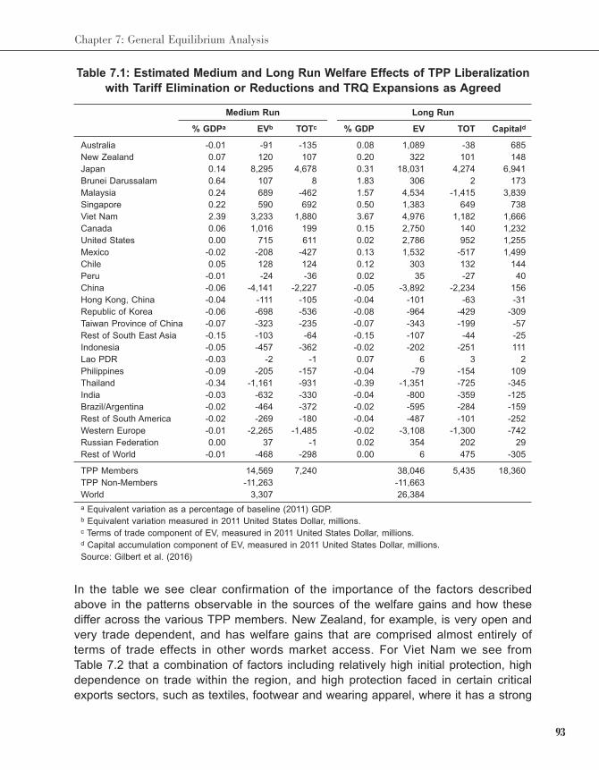
93
Chapter 7: General Equilibrium Analysis
Table 7.1: Estimated Medium and Long Run Welfare Effects of TPP Liberalization
with Tariff Elimination or Reductions and TRQ Expansions as Agreed
Medium Run Long Run
% GDPa EVb TOTc % GDP EV TOT Capitald
Australia -0.01 -91 -135 0.08 1,089 -38 685
New Zealand 0.07 120 107 0.20 322 101 148
Japan 0.14 8,295 4,678 0.31 18,031 4,274 6,941
Brunei Darussalam 0.64 107 8 1.83 306 2 173
Malaysia 0.24 689 -462 1.57 4,534 -1,415 3,839
Singapore 0.22 590 692 0.50 1,383 649 738
Viet Nam 2.39 3,233 1,880 3.67 4,976 1,182 1,666
Canada 0.06 1,016 199 0.15 2,750 140 1,232
United States 0.00 715 611 0.02 2,786 952 1,255
Mexico -0.02 -208 -427 0.13 1,532 -517 1,499
Chile 0.05 128 124 0.12 303 132 144
Peru -0.01 -24 -36 0.02 35 -27 40
China -0.06 -4,141 -2,227 -0.05 -3,892 -2,234 156
Hong Kong, China -0.04 -111 -105 -0.04 -101 -63 -31
Republic of Korea -0.06 -698 -536 -0.08 -964 -429 -309
Taiwan Province of China -0.07 -323 -235 -0.07 -343 -199 -57
Rest of South East Asia -0.15 -103 -64 -0.15 -107 -44 -25
Indonesia -0.05 -457 -362 -0.02 -202 -251 111
Lao PDR -0.03 -2 -1 0.07 6 3 2
Philippines -0.09 -205 -157 -0.04 -79 -154 109
Thailand -0.34 -1,161 -931 -0.39 -1,351 -725 -345
India -0.03 -632 -330 -0.04 -800 -359 -125
Brazil/Argentina -0.02 -464 -372 -0.02 -595 -284 -159
Rest of South America -0.02 -269 -180 -0.04 -487 -101 -252
Western Europe -0.01 -2,265 -1,485 -0.02 -3,108 -1,300 -742
Russian Federation 0.00 37 -1 0.02 354 202 29
Rest of World -0.01 -468 -298 0.00 6 475 -305
TPP Members 14,569 7,240 38,046 5,435 18,360
TPP Non-Members -11,263 -11,663
World 3,307 26,384
a Equivalent variation as a percentage of baseline (2011) GDP.b Equivalent variation measured in 2011 United States Dollar, millions.c Terms of trade component of EV, measured in 2011 United States Dollar, millions.d Capital accumulation component of EV, measured in 2011 United States Dollar, millions.
Source: Gilbert et al. (2016)
In the table we see clear confirmation of the importance of the factors described
above in the patterns observable in the sources of the welfare gains and how these
differ across the various TPP members. New Zealand, for example, is very open and
very trade dependent, and has welfare gains that are comprised almost entirely of
terms of trade effects in other words market access. For Viet Nam we see from
Table 7.2 that a combination of factors including relatively high initial protection, high
dependence on trade within the region, and high protection faced in certain critical
exports sectors, such as textiles, footwear and wearing apparel, where it has a strong
94
Analytical Approaches to Evaluating Preferential Trade Agreements
comparative advantage, explain the large relative gains in both efficiency and the terms
of trade.
Economic theory can help us nail down what is driving other patterns too. Why is it
that Thailand is estimated to lose so dramatically from the TPP? As a general matter,
effects of a preferential trade agreement on other countries manifest through two
closely related mechanisms. The first is termed the ‘trade diversion’ effect, the second
is the ‘preference erosion’ effect. Both operate through changes in the pattern of trade
in response to the differentials introduced to the protection pattern by preferential
liberalization. Trade diversion is where the newly introduced tariff preference causes
a switch in the source of imports from a non-member source to a member source.
From the perspective of the non-member economy, there will be a loss of market
share, reflected in welfare terms by a decline in the terms of trade.
Preference erosion is where a newly introduced tariff preference causes a shift in
imports away from a partner in a pre-existing agreement to a source in the new
(or expanded) agreement. A simple example may illustrate the distinction. When the
United States signs the TPP, we might anticipate trade diversion to impact India,
a current trading partner, but not a member of an existing agreement with the United
States, and preference erosion to impact Mexico, a current member of NAFTA. From
the perspective of the existing partner, preference erosion will again be reflected in
a decline in market share, and therefore the terms of trade.
So which particular countries are likely to be hurt most by the TPP? The above
discussion suggests we might want to look at two groups in particular. The first is
members of preferential trading agreements with TPP members that are not
themselves part of the TPP, and least developed economies, both of which would be
likely to be impacted by preference erosion. The second is large, efficient export
economies excluded from the agreement, which would be subject to diversion of trade.
Thailand fits both of these categories, and that largely explains the loss.
Another way of contextualizing the results is by comparing scenarios within the same
modeling framework. We have already seen one example of this – the medium vs long
run closure of the model helps us understand how the results change when we allow
for long run capital accumulation effects. In this study we ran a number of other
scenarios too, including some comparisons with other agreements, and some expansion
scenarios. The complete results are discussed in the paper, but as an example, we
considered a scenario where all tariffs were removed among the TPP members. The
objective was not to argue that this was a likely scenario, indeed we already knew
what the agreement contained. Rather, we wanted to know how much was being left
on the table. As it turns out, the answer is quite a lot. The gains from the actual
agreement are roughly 50 percent smaller than those available for the TPP members
as a whole. Most of the difference is borne by Japan. Information on the consequences
of the road not taken are often useful contributions to policy analysis.
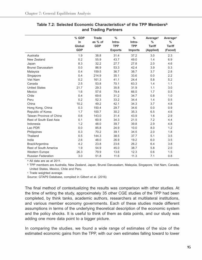
95
Chapter 7: General Equilibrium Analysis
Table 7.2: Selected Economic Characteristicsa of the TPP Membersb
and Trading Partners
% GDP Trade % % Averagec Averagec
in as % of Intra- Intra- % %
Global GDP TPP TPP Tariff Tariff
GDP Exports Imports (Applied) (Faced)
Australia 1.9 38.8 31.4 37.2 3.0 2.3
New Zealand 0.2 55.9 43.7 49.0 1.4 6.9
Japan 8.3 32.2 27.7 27.8 2.0 4.6
Brunei Darussalam 0.0 86.9 53.3 42.4 3.9 0.3
Malaysia 0.4 159.5 36.7 38.7 3.7 2.8
Singapore 0.4 214.9 35.1 33.6 0.0 2.2
Viet Nam 0.2 161.3 41.1 24.4 5.8 5.2
Canada 2.5 53.8 70.1 63.3 1.4 1.1
United States 21.7 29.3 35.8 31.9 1.1 3.0
Mexico 1.6 57.6 79.4 66.5 1.7 0.5
Chile 0.4 69.6 31.2 34.7 0.8 1.0
Peru 0.2 52.3 33.2 34.4 1.4 0.5
China 10.2 49.2 42.1 34.3 3.7 4.8
Hong Kong, China 0.3 150.4 29.7 34.6 0.0 0.9
Republic of Korea 1.7 100.7 30.2 35.3 6.5 4.6
Taiwan Province of China 0.6 143.0 31.4 43.9 1.6 2.9
Rest of South East Asia 0.1 60.9 34.3 21.5 7.2 4.4
Indonesia 1.2 48.0 39.7 39.8 2.9 4.8
Lao PDR 0.0 85.8 24.9 10.0 8.0 1.2
Philippines 0.3 70.2 39.1 34.5 2.0 1.8
Thailand 0.5 144.3 38.5 37.7 5.1 3.5
India 2.6 48.0 26.9 19.2 6.0 3.5
Brazil/Argentina 4.2 23.8 23.6 26.2 6.4 3.8
Rest of South America 1.9 54.9 45.0 38.7 5.8 2.0
Western Europe 26.3 79.9 13.6 12.3 0.6 1.5
Russian Federation 3.0 51.8 11.6 11.3 7.1 0.8
a All data are as at 2011.b TPP members are Australia, New Zealand, Japan, Brunei Darussalam, Malaysia, Singapore, Viet Nam, Canada,
United States, Mexico, Chile and Peru.c Trade weighted average.
Source: GTAP9 Database, compiled in Gilbert et al. (2016)
The final method of contextualizing the results was comparison with other studies. At
the time of writing the study, approximately 35 other CGE studies of the TPP had been
completed, by think tanks, academic authors, researchers at multilateral institutions,
and various member economy governments. Each of these studies made different
assumptions in terms of the underlying theoretical description of the economic system
and the policy shocks. It is useful to think of them as data points, and our study was
adding one more data point to a bigger picture.
In comparing the studies, we found a wide range of estimates of the size of the
estimated economic gains from the TPP, with our own estimates falling toward to lower

96
Analytical Approaches to Evaluating Preferential Trade Agreements
end of the range. Ultimately these differences could be related back to the
assumptions made in the modeling in a systematic way. Studies that considered
deeper cuts in protection, incorporated NTB estimates, allowed for capital accumulation
effects, or introduced imperfectly competitive markets generated systematically larger
welfare effects.
On the other hand, we also found considerable consistency in the pattern of the
distribution of gains across the member economies in the studies. While the
magnitudes of the gains varied, all the studies tended to predict the largest gains
accruing to Japan in an absolute sense, and to Viet Nam in a relative sense. This
consistency increased our confidence in the robustness of those patterns.
7.2.5 What Were the Limitations?
All studies, using all methods, have limitations, and this CGE study is no exception.
That is why contextualizing the results, and in particular placing them in context with
other studies is so crucial. The weaknesses of any one study can be mitigated by the
strengths of others. Probably the major limitation of this particular CGE analysis was
that it focused on tariff cuts and TRQ expansions, and ignored the possible impact of
other NTB cuts. Data on the impact of NTBs is less reliable than tariff and TRQ data,
hence adding them to the model makes the results more complete, but adds to the
uncertainty. Since a number of other studies had already been completed using
various NTB estimates, we decided to focus our attention on other aspects.
7.3 A Basic CGE Model
As we noted at the outset of the chapter, a complete description of how to build and
use CGE models is beyond the scope of this book. However, we do present a model
built in GAMS that can be used to simulate the economy-wide effect of trade reforms.
The GAMS code for implementing the model are presented in Codes 7.2 through 7.5
(at the end of the chapter), but we do not propose to discuss them in detail. It is based
on the model presented in Gilbert and Tower (2013), which contains the complete
details.1 As with all the programs discussed in this volume, the codes are available for
download should you want to work further with them. Here we provide an overview and
example.
Demand: The model features four distinct sources of final demand. There is a single
representative household, which has an objective function of the Cobb-Douglas form.
The household maximizes utility subject to it budget, which is determined by the value
of factor payments to the household, less taxes paid to the government. Government
1 This model is under continuous development. Please contact the author for the latest version of the code.
97
Chapter 7: General Equilibrium Analysis
consumption and investment are also sources of final demand, both in fixed quantities.
Finally, the rest of world (the external sector) is a source of demand for exports.
Foreign demand is modeled using the constant elasticity of demand function.
Supply: The basic model has consider two industries (1 and 2), operating under
competitive conditions. The underlying production technology assumes firms use two
primary factors (capital and labor) in variable proportions (modeled via CES), combined
with intermediate goods used in fixed proportions. Each industry produces a good
aimed at foreign markets and a good aimed at the domestic market (i.e., joint
production). The transformation function takes the CET form.
Trade: International trade is modeled via the Armington assumption. We use a single
Armington composite for household, intermediate, government and investment
demands. The Armington aggregator function is of the CES form. The economy is
assumed to be small with respect to import markets – i.e., the prices of importables
are given.
Distortions: For simplicity the only policy-based distortions in the model are tariffs,
which are applied to imports of all goods. Of course, adding other distortions to the
model would be possible.
Closure: The factor market closure is neoclassical – all factors of production are
available in fixed supply, are fully employed, and are fully mobile across sectors. This
can, or course, be adjusted. On the macroeconomic side, we use a Johansen-style
savings-investment closure. Investment at the commodity level is fixed, as are
government purchases. Government revenues are determined endogenously, with all
tax rates exogenous. Government saving is endogenous, financed by (implicit)
transfers from the household. Household savings varies to match the value of total
investment. The current account balance is fixed, and the foreign exchange rate is the
numeraire.
Flow Data: The data to which we will fit the model are described in the social
accounting matrix (SAM) presented in Table 7.3. The SAM describes value flows in the
economic system. Each entry represents a payment from the agent in the columns to
the agent in the rows. Hence the X column is exports, and the X row is imports. The
H, G, and I columns represent consumption by households, government, and
investment, and so on. For full details on the construction and interpretation of a SAM
see Gilbert and Tower (2013).
Parameters: We have used the CES form for value-added, and the Armington
functions. We have also used CED functions to represent foreign demand, and CET
functions to model the transformation between production for domestic markets and
production for export markets. We need to specify elasticities for each of these
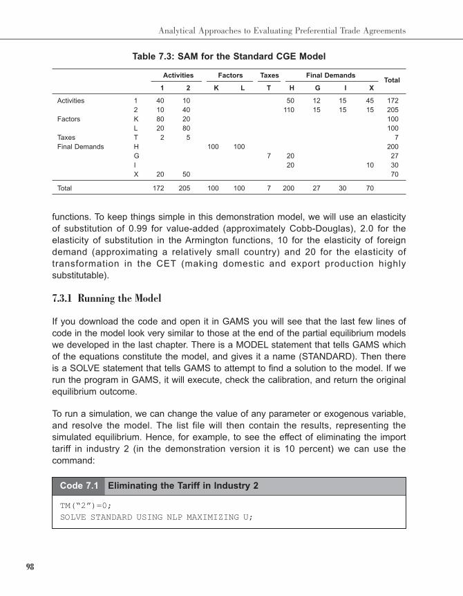
98
Analytical Approaches to Evaluating Preferential Trade Agreements
functions. To keep things simple in this demonstration model, we will use an elasticity
of substitution of 0.99 for value-added (approximately Cobb-Douglas), 2.0 for the
elasticity of substitution in the Armington functions, 10 for the elasticity of foreign
demand (approximating a relatively small country) and 20 for the elasticity of
transformation in the CET (making domestic and export production highly
substitutable).
7.3.1 Running the Model
If you download the code and open it in GAMS you will see that the last few lines of
code in the model look very similar to those at the end of the partial equilibrium models
we developed in the last chapter. There is a MODEL statement that tells GAMS which
of the equations constitute the model, and gives it a name (STANDARD). Then there
is a SOLVE statement that tells GAMS to attempt to find a solution to the model. If we
run the program in GAMS, it will execute, check the calibration, and return the original
equilibrium outcome.
To run a simulation, we can change the value of any parameter or exogenous variable,
and resolve the model. The list file will then contain the results, representing the
simulated equilibrium. Hence, for example, to see the effect of eliminating the import
tariff in industry 2 (in the demonstration version it is 10 percent) we can use the
command:
Table 7.3: SAM for the Standard CGE Model
Activities Factors Taxes Final DemandsTotal
1 2 K L T H G I X
Activities 1 40 10 50 12 15 45 172
2 10 40 110 15 15 15 205
Factors K 80 20 100
L 20 80 100
Taxes T 2 5 7
Final Demands H 100 100 200
G 7 20 27
I 20 10 30
X 20 50 70
Total 172 205 100 100 7 200 27 30 70
Code 7.1 Eliminating the Tariff in Industry 2
TM(“2”)=0;
SOLVE STANDARD USING NLP MAXIMIZING U;
99
Chapter 7: General Equilibrium Analysis
The results indicate that removing the tariff would have the effect of increasing imports
in the affected sector (by around 13 percent). We also observe increases in imports
in the other sector, by a smaller amount (around 6 percent). Why? The trade
liberalization increases household incomes, some of which is spent on increased
imports. This is the type of effect that general equilibrium models are designed to
capture. We can also see changes throughout the economic system of various
magnitudes. In this example, output levels in the simulation are left largely unchanged,
as are domestic consumption levels (although there is a slight tilt toward good 2).
As we can see, the simulation procedure is essentially the same as with the partial
equilibrium models. Now, however, because we are modeling an entire economic
system, there are a lot more questions we can potentially address. We can, for
example, consider changes in technology, changes in world demand or supply
conditions, immigration, foreign direct investment, and so on. In other words, CGE
models give us the ability to consider the possible economic impact of a much wider
range of economic changes that might be associated with preferential agreements than
just the removal of tariffs. We consider a few of the possibilities in the exercises below.
Exercise 7.1
Using the model, verify the results of the simulation yourself. Next consider the impact of
complete tariff reform (i.e., removal of the tariff in both sectors).
Exercise 7.2
Suppose that there was an increase in the international demand for good 2 (the relevant
parameter is XI). What would be the impact on the economic system?
Exercise 7.3
Suppose that as part of an agreement, an expansion of migration was also allowed. It is
expected that the supply of labor will expand by 10 percent. What is the economic impact?
(The relevant parameter is FBAR.)
100
Analytical Approaches to Evaluating Preferential Trade Agreements
7.4 Application Example to Viet Nam
While the demonstration of the CGE model above was based on small-scale and
artificial data, the CGE model and code presented is fully functional and can be used
as a foundation for real-world models. To apply the model to an actual country, we
need only to supply a real SAM and a set of parameters.2
A 5-sector, 3-factor SAM for Viet Nam in 2011 is shown in Table 7.4. This data was
drawn from the GTAP9 database. The GTAP database also contains estimates of key
model parameters. These are shown in Table 7.5. GTAP does not contain information
on transformation elasticities between domestic and export production, so we continue
to assume a high degree of substitutability (an elasticity of 20). We also assume
Viet Nam is relatively small in its export markets, and set the export demand elasticity
to a uniform value of -20.
To fit the model to this data, we need to change the sets in Code 7.4 to contain
all the industry and factor names, replace the tabular representation of the SAM in
Code 7.4 with the data in Table 7.4, and replace the parameter values in Code 7.4 with
those in Table 7.5. The remainder of the calibration procedure is automatic. You can
download the completed model for evaluation.
The scenario we will consider is complete removal of all tariffs. This is accomplished
by setting TM(I)=0 and solving the model. The model suggests a welfare gain of
approximately $50 million, or a modest 0.04 percent of baseline GDP. This is quite
small, reflecting relatively low initial tariffs.3 The predicted shifts at the sectoral level are
a bit more substantial – see Table 7.6. There is expansion of imports across the board,
but most notably in textiles. On the other hand, exports are predicted to contract in the
primary and tertiary sectors, while expanding strongly in the manufacturing. Production
reallocations follow the same basic pattern, with substantial reallocation expected
toward the textiles sector.
It is important not to take these results (or any model results) literally. There are
a multitude of assumptions that underlie them. However, CGE simulations of this type
can help us to get a handle on magnitudes and directions of economic changes, and
to assess the consequences of economic changes in a consistent manner.
2 The demonstration version of GAMS will only solve models of limited size. It should be possible to solve
a model with around 8-9 sectors and 2-3 factors. A licensed version of GAMS can solve models with very
large dimensions, and is essentially limited only by data availability.3 It is also biased downward because we do not have any secondary distortions and because the high level
of aggregation tends to smooth out tariff peaks.
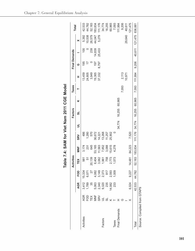
101
Chapter 7: General Equilibrium Analysis
Tab
le 7
.4:
SA
M f
or
Vie
t N
am
2011 C
GE
Mo
del
Acti
vit
ies
Facto
rsTaxes
Fin
al
Dem
an
ds
To
tal
AG
RF
OD
TE
XM
NF
SR
VU
LS
LK
TH
GI
X
Act
iviti
es
AG
R3
,41
21
5,3
34
98
13
,17
44
86
13
,45
91
95
10
05
,39
24
2,5
33
FO
D1
,78
96
,07
15
12
31
1,2
80
24
,80
51
70
10
,53
84
4,7
82
TE
X3
52
72
0,1
39
64
55
70
3,9
49
02
39
26
,57
95
2,1
83
MN
F5
,06
34
,08
26
,40
45
3,1
65
36
,67
21
9,3
65
19
71
4,8
39
44
,04
71
83
,83
4
SR
V2
,34
03
,14
93
,06
211
,56
31
4,2
21
37
,33
28
,79
72
5,4
33
5,2
79
111
,17
6
Fa
cto
rsU
L9
,32
02
,37
31
,96
17
,85
21
3,2
68
34
,77
4
SL
23
59
17
75
83
,08
811
,25
71
6,2
55
K1
4,0
82
2,5
93
2,7
73
15
,61
52
5,9
02
60
,96
5
Taxe
sT
23
31
,00
91
,57
34
,27
80
7,0
93
Fin
al D
em
ands
H34,7
74
16,2
55
60,9
65
111,9
94
G7
,09
32
,11
39
,20
6
I10,9
71
29,6
40
40,6
11
X6
,02
49
,22
71
4,4
81
84
,22
37
,52
0121,4
75
Tota
l42,5
33
44,7
82
52,1
83
183,8
34
111,1
76
34,7
74
16,2
55
60,9
65
7,0
93
111,9
94
9,2
06
40,6
11121,4
75
836,8
81
Sourc
e:
Com
pile
d f
rom
GTA
P9
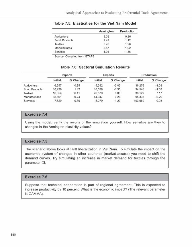
102
Analytical Approaches to Evaluating Preferential Trade Agreements
Table 7.5: Elasticities for the Viet Nam Model
Table 7.6: Sectoral Simulation Results
Imports Exports Production
Initial % Change Initial % Change Initial % Change
Agriculture 6,257 0.85 5,392 -3.02 36,276 -1.03
Food Products 10,236 1.82 10,538 -1.35 34,546 -1.03
Textiles 16,054 6.41 26,579 8.08 36,129 7.17
Manufactures 88,501 0.74 44,047 0.26 95,333 -0.29
Services 7,520 0.30 5,279 -1.29 103,660 -0.03
Armington Production
Agriculture 2.39 0.26
Food Products 2.49 1.12
Textiles 3.78 1.26
Manufactures 3.57 1.02
Services 1.94 1.36
Source: Compiled from GTAP9
Exercise 7.4
Using the model, verify the results of the simulation yourself. How sensitive are they to
changes in the Armington elasticity values?
Exercise 7.5
The scenario above looks at tariff liberalization in Viet Nam. To simulate the impact on the
economic system of changes in other countries (market access) you need to shift the
demand curves. Try simulating an increase in market demand for textiles through the
parameter XI.
Exercise 7.6
Suppose that technical cooperation is part of regional agreement. This is expected to
increase productivity by 10 percent. What is the economic impact? (The relevant parameter
is GAMMA).
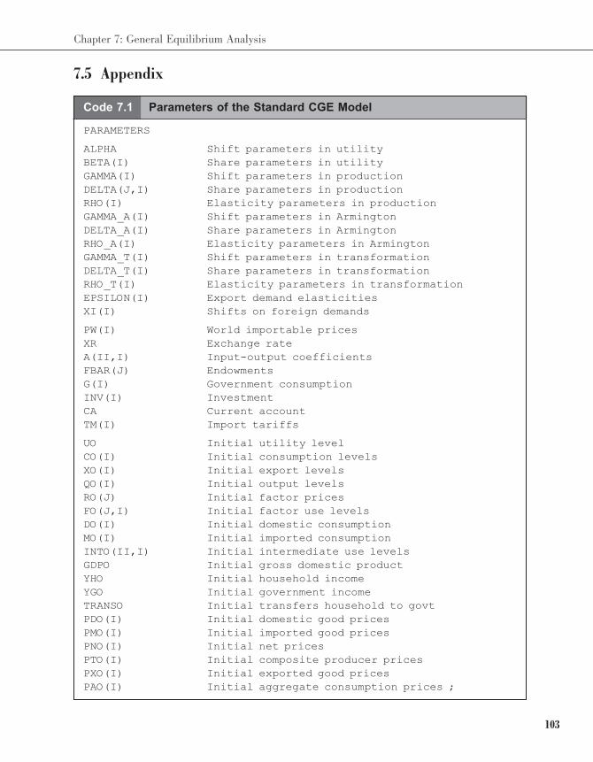
103
Chapter 7: General Equilibrium Analysis
7.5 Appendix
Code 7.1 Parameters of the Standard CGE Model
PARAMETERS
ALPHA Shift parameters in utility
BETA(I) Share parameters in utility
GAMMA(I) Shift parameters in production
DELTA(J,I) Share parameters in production
RHO(I) Elasticity parameters in production
GAMMA_A(I) Shift parameters in Armington
DELTA_A(I) Share parameters in Armington
RHO_A(I) Elasticity parameters in Armington
GAMMA_T(I) Shift parameters in transformation
DELTA_T(I) Share parameters in transformation
RHO_T(I) Elasticity parameters in transformation
EPSILON(I) Export demand elasticities
XI(I) Shifts on foreign demands
PW(I) World importable prices
XR Exchange rate
A(II,I) Input-output coefficients
FBAR(J) Endowments
G(I) Government consumption
INV(I) Investment
CA Current account
TM(I) Import tariffs
UO Initial utility level
CO(I) Initial consumption levels
XO(I) Initial export levels
QO(I) Initial output levels
RO(J) Initial factor prices
FO(J,I) Initial factor use levels
DO(I) Initial domestic consumption
MO(I) Initial imported consumption
INTO(II,I) Initial intermediate use levels
GDPO Initial gross domestic product
YHO Initial household income
YGO Initial government income
TRANSO Initial transfers household to govt
PDO(I) Initial domestic good prices
PMO(I) Initial imported good prices
PNO(I) Initial net prices
PTO(I) Initial composite producer prices
PXO(I) Initial exported good prices
PAO(I) Initial aggregate consumption prices ;
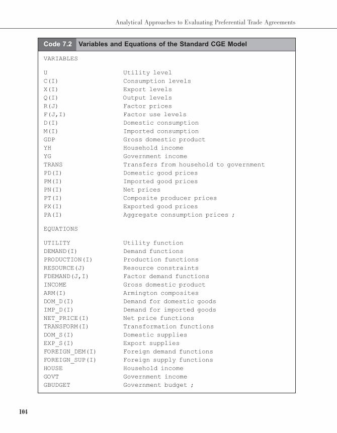
104
Analytical Approaches to Evaluating Preferential Trade Agreements
Code 7.2 Variables and Equations of the Standard CGE Model
VARIABLES
U Utility level
C(I) Consumption levels
X(I) Export levels
Q(I) Output levels
R(J) Factor prices
F(J,I) Factor use levels
D(I) Domestic consumption
M(I) Imported consumption
GDP Gross domestic product
YH Household income
YG Government income
TRANS Transfers from household to government
PD(I) Domestic good prices
PM(I) Imported good prices
PN(I) Net prices
PT(I) Composite producer prices
PX(I) Exported good prices
PA(I) Aggregate consumption prices ;
EQUATIONS
UTILITY Utility function
DEMAND(I) Demand functions
PRODUCTION(I) Production functions
RESOURCE(J) Resource constraints
FDEMAND(J,I) Factor demand functions
INCOME Gross domestic product
ARM(I) Armington composites
DOM_D(I) Demand for domestic goods
IMP_D(I) Demand for imported goods
NET_PRICE(I) Net price functions
TRANSFORM(I) Transformation functions
DOM_S(I) Domestic supplies
EXP_S(I) Export supplies
FOREIGN_DEM(I) Foreign demand functions
FOREIGN_SUP(I) Foreign supply functions
HOUSE Household income
GOVT Government income
GBUDGET Government budget ;
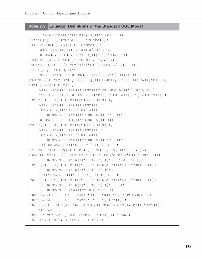
105
Chapter 7: General Equilibrium Analysis
Code 7.3 Equation Definitions of the Standard CGE Model
UTILITY..U=E=ALPHA*PROD(I, C(I)**BETA(I));
DEMAND(I)..C(I)=E=BETA(I)*YH/PA(I);
PRODUCTION(I)..Q(I)=E=(GAMMA(I)/(1-
SUM(II,A(II,I))))*SUM(J$FO(J,I),
DELTA(J,I)*F(J,I)**RHO(I))**(1/RHO(I));
RESOURCE(J)..FBAR(J)=E=SUM(I, F(J,I));
FDEMAND(J,I)..R(J)=E=PN(I)*Q(I)*SUM(JJ$FO(JJ,I),
DELTA(JJ,I)*F(JJ,I)**
RHO(I))**(-1)*DELTA(J,I)*F(J,I)**(RHO(I)-1);
INCOME..GDP=E=SUM(I, PN(I)*Q(I))+SUM(I, TM(I)*XR*PW(I)*M(I));
ARM(I)..C(I)+SUM(II,
A(I,II)*Q(II))+G(I)+INV(I)=E=GAMMA_A(I)*(DELTA_A(I)*
**RHO_A(I)+(1-DELTA_A(I))*M(I)**RHO_A(I))**(1/RHO_A(I));
DOM_D(I)..PD(I)=E=PA(I)*(C(I)+SUM(II,
A(I,II)*Q(II))+G(I)+INV(I))*
(DELTA_A(I)*D(I)**RHO_A(I)+
(1-DELTA_A(I))*M(I)**RHO_A(I))**(-1)*
DELTA_A(I)* (D(I)**(RHO_A(I)-1);
IMP_D(I)..PM(I)=E=PA(I)*(C(I)+SUM(II,
A(I,II)*Q(II))+G(I)+INV(I))*
(DELTA_A(I)*D(I)**RHO_A(I)+
(1-DELTA_A(I))*M(I)**RHO_A(I))**(-1)*
((1-DELTA_A(I))*M(I)**(RHO_A(I)-1);
NET_PRICE(I)..PN(I)=E=PT(I)-SUM(II, PA(II)*A(II,I));
TRANSFORM(I)..Q(I)=E=GAMMA_T(I)*(DELTA_T(I)*D(I)**RHO_T(I)+
(1-DELTA_T(I))* X(I)**RHO_T(I))**(1/RHO_T(I));
DOM_S(I)..PD(I)=E=PT(I)*Q(I)*(DELTA_T(I)*D(I)**RHO_T(I)+
(1-DELTA_T(I))* X(I)**RHO_T(I))**
(-1)*DELTA_T(I)*D(I)**(RHO_T(I)-1);
EXP_S(I)..PX(I)=E=PT(I)*Q(I)*(DELTA_T(I)*D(I)**RHO_T(I)+
(1-DELTA_T(I))* X(I)**RHO_T(I))**(-1)*
(1-DELTA_T(I))*X(I)**(RHO_T(I)-1);
FOREIGN_DEM(I)..PX(I)=E=XR*XI(I)*X(I)**(1/EPSILON(I));
FOREIGN_SUP(I)..PM(I)=E=XR*PW(I)*(1+TM(I));
HOUSE..YH=E=SUM(J, FBAR(J)*R(J))-TRANS-SUM(I, PA(I)*INV(I))-
XR*CA;
GOVT..YG=E=SUM(I, TM(I)*PW(I)*XR*M(I))+TRANS;
GBUDGET..SUM(I, G(I)*PA(I))=E=YG;
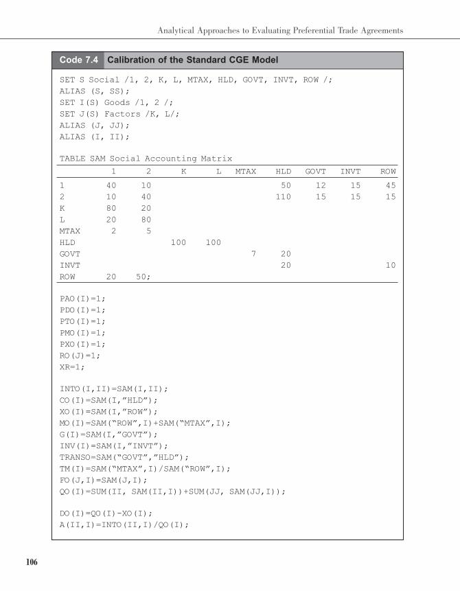
106
Analytical Approaches to Evaluating Preferential Trade Agreements
Code 7.4 Calibration of the Standard CGE Model
SET S Social /1, 2, K, L, MTAX, HLD, GOVT, INVT, ROW /;
ALIAS (S, SS);
SET I(S) Goods /1, 2 /;
SET J(S) Factors /K, L/;
ALIAS (J, JJ);
ALIAS (I, II);
TABLE SAM Social Accounting Matrix
1 2 K L MTAX HLD GOVT INVT ROW
1 40 10 50 12 15 45
2 10 40 110 15 15 15
K 80 20
L 20 80
MTAX 2 5
HLD 100 100
GOVT 7 20
INVT 20 10
ROW 20 50;
PAO(I)=1;
PDO(I)=1;
PTO(I)=1;
PMO(I)=1;
PXO(I)=1;
RO(J)=1;
XR=1;
INTO(I,II)=SAM(I,II);
CO(I)=SAM(I,”HLD”);
XO(I)=SAM(I,”ROW”);
MO(I)=SAM(“ROW”,I)+SAM(“MTAX”,I);
G(I)=SAM(I,”GOVT”);
INV(I)=SAM(I,”INVT”);
TRANSO=SAM(“GOVT”,”HLD”);
TM(I)=SAM(“MTAX”,I)/SAM(“ROW”,I);
FO(J,I)=SAM(J,I);
QO(I)=SUM(II, SAM(II,I))+SUM(JJ, SAM(JJ,I));
DO(I)=QO(I)-XO(I);
A(II,I)=INTO(II,I)/QO(I);
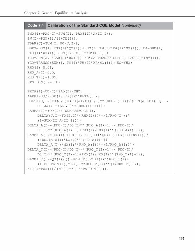
107
Chapter 7: General Equilibrium Analysis
PNO(I)=PAO(I)-SUM(II, PAO(II)*A(II,I));
PW(I)=PMO(I)/(1+TM(I));
FBAR(J)=SUM(I, FO(J,I));
GDPO=SUM(I, PNO(I)*QO(I))+SUM(I, TM(I)*PW(I)*MO(I)); CA=SUM(I,
PXO(I)*XO(I))-SUM(I, PW(I)*XR*MO(I));
YHO=SUM(J, FBAR(J)*RO(J))-XR*CA-TRANSO-SUM(I, PAO(I)*INV(I));
YGO=TRANSO+SUM(I, TM(I)*PW(I)*XR*MO(I)); UO=YHO;
RHO(I)=0.01;
RHO_A(I)=0.5;
RHO_T(I)=1.05;
EPSILON(I)=-10;
BETA(I)=CO(I)*PAO(I)/YHO;
ALPHA=UO/PROD(I, CO(I)**BETA(I));
DELTA(J,I)$FO(J,I)=(RO(J)/FO(J,I)**(RHO(I)-1))/(SUM(JJ$FO(JJ,I),
RO(JJ)/ FO(JJ,I)**(RHO(I)-1)));
GAMMA(I)=(QO(I)/(SUM(J$FO(J,I),
DELTA(J,I)*FO(J,I)**RHO(I)))**(1/RHO(I)))*
(1-SUM(II,A(II,I)));
DELTA_A(I)=(PDO(I)/DO(I)**(RHO_A(I)-1))/(PDO(I)/
DO(I)**(RHO_A(I)-1)+PMO(I)/ MO(I)**(RHO_A(I)-1));
GAMMA_A(I)=(CO(I)+SUM(II, A(I,II)*QO(II))+G(I)+INV(I))/
((DELTA_A(I)*DO(I)** RHO_A(I)+(1-
DELTA_A(I))*MO(I)**RHO_A(I))**(1/RHO_A(I)));
DELTA_T(I)=(PDO(I)/DO(I)**(RHO_T(I)-1))/(PDO(I)/
DO(I)**(RHO_T(I)-1)+PXO(I)/ XO(I)**(RHO_T(I)-1));
GAMMA_T(I)=QO(I)/((DELTA_T(I)*DO(I)**RHO_T(I)+
(1-DELTA_T(I))*XO(I)**RHO_T(I))**(1/RHO_T(I)));
XI(I)=PXO(I)/(XO(I)**(1/EPSILON(I)));
Code 7.4 Calibration of the Standard CGE Model (continued)

108
Analytical Approaches to Evaluating Preferential Trade Agreements
109
Bibliography
BIBLIOGRAPHY
Ahmadi-Esfahani, F.Z. (2006) “Constant Market Shares Analysis: Uses, Limitations and
Prospects” Australian Journal of Agricultural and Resource Economics 50: 510-26.
Anh, T.T. and L.M. Ngoc (2015) “Trade Creation or Trade Diversion in ASEAN and
ASEAN+6 FTAs: Trade Indicators Approach” Journal of Economics and Development
17(3): 25-41.
Armington, P.S. (1969) “A Theory of Demand for Products Distinguished by Place of
Production” International Monetary Fund Staff Papers 16: 159-76.
Balassa, B. (1965) “Trade Liberalisation and ‘Revealed’ Comparative Advantage”
Manchester School of Economic and Social Studies 33(2): 99-123.
Bekkers, E. and H. Rojas-Romagosa (2016) “Quantitative Trade Models and the Economic
Assessment of TTIP” (mimeo, CPB Netherlands Bureau for Economic Policy Analysis).
Bur sher, M.E. (2011) Introduction to Computable General Equilibrium Models, (Cambridge
University Press, Cambridge).
Dixon, P.B. and D. Jorgenson (2013) Handbook of Computable General Equilibrium
Modeling, Volume 1A (North Holland, Oxford).
Fagerberg, J. and G. Sollie (1987) “The Method of Constant Market Shares Analysis
Reconsidered” Applied Economics 19: 1571-83.
Fisher, E., J. Gilbert, K. Marshall and R. Oladi (2016) “A New Measure of Economic
Distance” CESifo Working Paper 5362.
Frankel, J.A. (1997) Regional Trading Blocs in the World Economic System (Institute for
International Economics, Washington DC).
Gilbert, J. (2010) “Notes on Constant Market Share Analysis of a Decade of US Export
Growth” Report prepared for the Peterson Institute for International Economics.
Gilbert, J., T. Furusawa and R. Scollay (2016) “The Economic Impact of the Trans-Pacific
Partnership: What Have We Learned from CGE Simulation?” ARTNeT Working
Paper 157.
Gilbert, J. and E. Tower (2013) Introduction to Numerical Simulation for Trade Theory and
Policy, (World Scientific, Singapore).
Gilbert, J. and T. Wahl (2002) “Applied General Equilibrium Assessments of Trade
Liberalization in China” World Economy 25: 697-731.
Hertel T.W., ed., (1997) Global Trade Analysis: Modeling and Applications, (Cambridge
University Press, Cambridge).
110
Analytical Approaches to Evaluating Preferential Trade Agreements
Hoen. A.R. and J. Oosterhaven (2006) “On the Measurement of Comparative Advantage”
Annals of Regional Science 40(3): 677-91.
Hosoe, N., K. Gasawa and H. Hashimoto (2010) Textbook of General Equilibrium
Modelling: Programming and Simulations, (Palgrave, New York).
Iapadre, L. (2006) “Regional Integration Agreements and the Geography of World Trade:
Statistical Indicators and Empirical Evidence” in P. De Lombaerde, ed. Assessment
and Measurement of Regional Integration, (Routledge, London).
Kemp, M.C. and H.Y. Wan (1976) “An Elementary Proposition Concerning the Formation
of Customs Unions” Journal of International Economics 6(1): 95-7.
Koko, A., T. Matha and P. Tingvall (2005) “European Integration and Trade Diversion: Yeats
Revisited” Swedish Institute for European Policy Studies Report 2005-7.
Leamer, E. and R. Stern (1970) Quantitative International Economics (Aldine, Chicago).
Lloyd, P.J. and D. MacLaren (2004) “Gains and Losses from Regional Trading Agreements:
A Survey” Economic Record 80: 445-97.
McMillan, J. (1993) “Does Regional Integration Foster Open Trade? Economic Theory and
GATT’s Article XXIV” in K. Anderson and R. Blackhurst (eds.) Regional Integration and
the Global Trading System, (St Martins, New York).
Meade, J.E. (1955) The Theory of Customs Unions, (North-Holland, Amsterdam).
Merkies, A.H.Q.M. and T. van der Meer (1988) “A Theoretical Foundation for Constant
Market Share Analysis” Empirical Economics 13: 65-80.
Mikic, M. and J. Gilbert (2009) Trade Statistics in Policymaking: A Handbook of Commonly
Used Trade Indices and Indicators, (United Nations ESCAP, Bangkok).
Ng, F. and A. Yeats (2003) “Major Trade Trends in East Asia: What are their Implications
for Regional Cooperation and Growth?” World Bank Policy Research Working Paper
3084.
Panagariya, A. (1999) “The Regionalism Debate: An Overview” World Economy 22(4):
477-511.
Panagariya, A. (2000) “Preferential Trade Liberalization: The Traditional Theory and New
Developments” Journal of Economic Literature 38: 287-331.
Panagariya, A. and K. Krishna (2002) “On Necessarily Welfare-Enhancing Free Trade
Areas” Journal of International Economics 57(2): 353-67.
Plummer, M.G., D. Cheong and S. Hamanaka (2010) Methodology for Impact Assessment
of Free Trade Agreements, (Asian Development Bank, Manila).
Richardson, J.D. (1971) “Constant Market Shares Analysis of Export Growth” Journal of
International Economics 1: 227-39.
111
Bibliography
Robinson, S. and K. Thierfelder (2002) “Trade Liberalisation and Regional Integration: The
Search for Large Numbers” Australian Journal of Agricultural and Resource Economics
46: 585-604.
Rutherford, T.F. (1998) “GAMS2TBL: A GAMS LIBINCLUDE Program for Producing
Formatted Tables” available at: http://www.mpsge.org/inclib/gams2tbl.htm.
Rutherford, T.F. (1999) “LIBINCLUDE Tools for Writing GAMS-Readable Data Files”
available at: http://www.mpsge.org/inclib/gams2txt.htm.
Scollay, R. and J. Gilbert (2000) “Measuring the Gains from APEC Trade Liberalisation:
An Overview of CGE Assessments” World Economy 23: 175-93.
Scollay, R. and J. Gilbert (2001) New Regional Trading Arrangements in the Asia-Pacific
(Institute for International Economics, Washington DC).
Shepherd, B. (2013) The Gravity Model of International Trade: A User Guide (United
Nations ESCAP, Bangkok)
Tyszynski, H. (1951) “World Trade in Manufactured Commodities, 1899-1950” Manchester
School 19: 272-304.
Viner, J. (1950) The Customs Union Issue (Carnegie Endowment for Inter-national Peace,
New York).
Widodo, T. (2010) “Market Dynamics in the EU, NAFTA, North East Asia and ASEAN: The
Method of Constant Market Shares (CMS) Analysis” Journal of Economic Integration
25: 480-500.
Yeats, A. (1998) “Does Mercosur’s Trade Performance Raise Concerns About the Effects
of Regional Trade Arrangements?” World Bank Economic Review 12(1): 1-28.
Zenios, S.A. (1996) “Modeling Languages in Computational Economics: GAMS” in
H. Amman and D.A. Kendrick, eds., Handbook of Computational Economics I, (North-
Holland, Amsterdam).
“As is well-known, preferential trade agreements (PTAs) represent a ‘second-best’
approach to trade liberalization and as such have the potential to divert trade and
investment and in inflict economic welfare losses on member and non-member countries
alike. Hence, it is essential to provide a framework of analysis for assessing PTA
developments in order to provide stakeholders (government, researchers and policy
analysts) with the tools necessary to analyze the development of PTAs and to make
informed policy decisions. The objective of this resource book is to help develop capacity
within the Asia-Pacific economies on the usage of analytical methods as a tool for
provide timely and policy relevant information to the policy development process as it
pertains to negotiating preferential trading agreements and more broadly.”
“Negotiating preferential trade agreements is a challenge for the least developed countries.
Research and analysis are important components of any evidence-based policymaking. This
publication presents our step-by-step approach that policymakers as well as researchers can
follow in order to evaluate preferential trade agreements. It will also be a very valuable guide
to negotiators as well as researchers associated with analytical work of preferential trade
agreements (PTAs).”
Dr. Hartmut Janus
Project Director, RELATED Project
GIZ Laos
“The Lao People’s Democratic Republic is currently facing several challenges in transforming its
PTAs into achieving meaningful market access and developmental goals. Policymakers need to
understand the complex mechanism for negotiating and successfully implementing PTAs in order
to reap their benefits. We recognize the fact that this publication will provide the knowledge
required by negotiators for undertaking important analytical studies of the impact of PTAs as well
as gaining a better understanding of trade negotiations.”
Mr. Saysana Sayakone
Deputy Director General
FTPD-MOIC, Lao PDR