Embed Size (px)
Citation preview
HAL Id: inria-00072528https://hal.inria.fr/inria-00072528
Submitted on 24 May 2006
HAL is a multi-disciplinary open accessarchive for the deposit and dissemination of sci-entific research documents, whether they are pub-lished or not. The documents may come fromteaching and research institutions in France orabroad, or from public or private research centers.
L’archive ouverte pluridisciplinaire HAL, estdestinée au dépôt et à la diffusion de documentsscientifiques de niveau recherche, publiés ou non,émanant des établissements d’enseignement et derecherche français ou étrangers, des laboratoirespublics ou privés.
Analytic combinatorics : functional equations, rationaland algebraic functions
Philippe Flajolet, Robert Sedgewick
To cite this version:Philippe Flajolet, Robert Sedgewick. Analytic combinatorics : functional equations, rational andalgebraic functions. [Research Report] RR-4103, INRIA. 2001. �inria-00072528�
4103
ISS
N 0
249-
6399
ISR
N IN
RIA
/RR
--41
03--
FR
+E
NG
appor t de r ech er ch e
��������������� ������� ��������������� ������� ��������� � � � !"������# �$���%�����& �'��!"������# �
Analytic Combinatorics: Functional Equations,Rational and Algebraic Functions
Philippe Flajolet, Robert Sedgewick
N ˚ 4103Janvier 2001
(�)+*,�-.,�/

Analytic Combinatorics: Functional Equations,Rational and Algebraic Functions
Philippe Flajolet, Robert Sedgewick
Theme 2 — Genie logicielet calcul symbolique
Projet Algo
Rapport de recherche n ˚ 4103 — Janvier 2001 — 100 pages
Abstract: This report is part of a series whose aim is to present in a synthetic way the major methodsand models in analytic combinatorics. Here, we detail the case of rational and algebraic functionsand discuss systematically closure properties, the location of singularities, and consequences regard-ing combinatorial enumeration. The theory is applied to regular and context-free languages, finitestate models, paths in graphs, locally constrained permutations, lattice paths and walks, trees, andplanar maps.
Key-words: Analytic combinatorics, functional equation, combinatorial enumeration, generatingfunction, asymptotic methods
(Resume : tsvp)
�������������� ���������������������������������! "� � ���# �� �$ �!%'& ��� �(��)*�#+, "�-��&. 0/"���1���2 �� � ���# �� � /�35476�829�/":<;"6�9#=?> ,A@ ) ,CB �D�FE @ �����GIHKJ"�L& � �-�NM
(O���+ ���P���� � �?QRHS=#=2MC8"6�=#TVU#=W9#9O6#6�X (O���+ ����-�!P � �?Q�HK=#=2M58�6=#T'U#=W9#=V=!8
Combinatoire analytique:Equations fonctionnelles, fonctions rationnelles et algebriques
Resume : Ce rappport fait partie d’une serie dediee a la presentation synthetique des principalesmethodes et des principaux modeles de la combinatoire analytique. On y discute en detail les fonc-tions rationnelles et algebriques, leurs proprietes de cloture, la localisation des singularites et lesconsequences qui en decoulent pour les denombrements combinatoires. La theorie est appliqueeaux langages reguliers et context-free, aux modeles d’etats finis, ainsi qu’aux cheminements dansles graphes, aux permutations localement contraintes, aux marches aleatoires, et aux cartes planaires.
Mots-cle : Combinatoire analytique, equation fonctionnelle, denombrement combinatoire, fonctiongeneratrice, methodes asymptotiques
i
ANALYTIC COMBINATORICS
Foreword
This report is part of a series whose aim is to present in a synthetic way the majormethods and models in analytic combinatorics. The whole series, after suitable editing, isdestined to be transformed into a book with the title
“Analytic Combinatorics”
The present report is
— Chapter 8, Functional Equations—Rational and Algebraic Functions.
It is part of the following collection of Research Reports from INRIA:
— Chapters 1–3, “Counting and Generating Functions”, RR 1888, 116 pages, 1993;— Chapters 4–5, “Complex Asymptotics and Generating Functions”, RR 2026, 100
pages, 1993;— Chapter 6, “Saddle Point Asymptotics”, RR 2376, 55 pages, 1994;— Chapter 7, “Mellin Transform Asymptotics”, RR 2956, 93 pages, 1996.— Chapter 9, “Multivariate Asymptotics and Limit Distributions”, RR 3162, 123
pages, May 1997.
For historical reasons, the headings of previous chapters in the series were “The AverageCase Analysis of Algorithms”.
Acknowledgements. This work was supported in part by the IST Programme of the European Unionunder contract number IST-1999-14186 (ALCOM-FT). Special thanks are due to Bruno Salvy forsharing his thoughts on the subject of algebraic asymptotics and to Pierre Nicod eme for a thoroughscan of an early version of the manuscript.

CHAPTER 8
Functional Equations—Rational and Algebraic Functions
Mathematics is infinitely wide, while the language that describes it is finite. It follows from thepigeonhole principle that there exist distinct concepts that are referred to by the same name.Mathematics is also infinitely deep and sometimes entirely different concepts turn out to be
intimately and profoundly related.
— Doron Zeilberger [101]
I wish to God these calculations had been executed by steam.
— Charles Babbage (1792-1871)
This part of the book deals with classes of generating functions implicitly defined bylinear, polynomial, or differential relations, globally referred to as functional equations.Functional equations arise in well defined combinatorial contexts and they lead system-atically to well-defined classes of functions. One then has available a whole arsenal ofmethods and algorithmic procedures in order to simplify equations, locate singularities,and eventually determine asymptotics of coefficients. The corresponding classes are asso-ciated with algebraic closure properties together with a strong form of analytic “regular-ity” that constrains the location and nature of singularities. We shall detail here the caseof rational functions (that arise from functional equations that are linear and from associ-ated finite-state models) and algebraic functions (that arise from polynomial systems and“context-free” decompositions). A companion chapter will treat holonomic functions (de-fined by linear differential equations with coefficients themselves polynomial or rationalfunctions that arise from a diversity of contexts including order statistics).
Rational functions come first in order of simplicity. Linear systems of equations occursystematically in all combinatorial problems that are associated with finite state models(themselves closely related to Markov chains), like paths in graphs, regular languages andfinite automata, patterns in strings, and transfer matrix models of statistical physics. Singu-larities are by nature always poles. Consequently, the asymptotic analysis of coefficients ofrational functions is normally achieved via localization of poles. Although difficulties mayarise either in noncombinatorial contexts (nonpositive problems) or when dealing simulta-neously with an infinite collection of functions (for instance, the generating functions oftrees of bounded height or width), the situation is however often tractable: for positive sys-tems, general theorems derived from the classical Perron-Frobenius theory of nonnegativematrices guarantee simplicity of the dominant positive pole.
Next in order of difficulty, there come the algebraic functions defined as solutionsto polynomial equations. Such functions occur in connection with the simplest nonlin-ear combinatorial models, namely the class of context-free models. Such models covermany types of combinatorial trees (that are related to the theory of branching processes inprobability theory) or walks (that are close to the probabilistic theory of random walks).
1
2 8. FUNCTIONAL EQUATIONS—RATIONAL AND ALGEBRAIC FUNCTIONS
Algebraic properties include the possibility of performing elimination by devices like re-sultants or Groebner basis: in this way, a system of equations can always be reduced to asingle equation. Singularities are in all cases of a simple form—they are branch points cor-responding locally to fractional power series, also known as Newton–Puiseux expansions.Accordingly, the asymptotic shape of the coefficients of any given algebraic function isthen entirely predictable by singularity analysis. However, nonlinear algebraic equationsadmit several solutions and a so-called “connection problem” has to be solved by consid-eration of the global geometry of the algebraic curve defined by a polynomial equation.Again, fortunately, the situation somewhat simplifies for positive algebraic systems thatcapture most of combinatorial applications.
Last but not least there come the holonomic functions that encompass rational andalgebraic functions. They are defined as solutions of linear differential equations with ra-tional function coefficients and they arise in a number of contexts, from order statistics toregular graphs. It has been realized over the last two decades, by Stanley, Lipshitz, andZeilberger most notably, that these functions enjoy an extremely rich set of nontrivial clo-sure properties. In particular, they encapsulate most of what is known to admit of closedform in combinatorial analysis. Algebraically, holonomic functions are objects that canbe specified by a finite amount of information so that the identities they satisfy is decid-able. For instance, even a restrictive consequence of this theory leads to an interestingfact summarized by Zeilberger’s aphorism “All binomial identities are trivial”. Analyt-ically, the nature of singularities is again governed by simple laws, a fact that derivesfrom turn-of-the-twentieth-century studies of singularities of linear differential equations(by Schwartz, Fuchs, Birkhoff, Poincare, and others). The classification involves a funda-mental dichotomy between what is known as regular singularity and irregular singularity.From there, like in the algebraic case, the asymptotic shape of the coefficients of any givenholonomic function is predictable by singularity analysis (regular singularity) or saddlepoint analysis (irregular singularity). However, unlike in the algebraic case, the connectionproblem is not known to be decidable and a priori quantitative bounds (based on combi-natorial reasoning) must sometimes be resorted to in order to prune singularities and com-pletely solve an asymptotic question that arises from a combinatorial problem expressedby a holonomic generating function.
Finally, we make a brief mention here of equations of the composition type. There,strong closure properties tend to fade away. However, a nice set of techniques that havebeen put to use successfully in the analysis of some important combinatorial problems.For instance, the counting of balanced trees [72] and the distributional analysis of heightin simple families of trees [41, 42] relate to analytic iteration theory. On another register,metric properties of general number representation systems and information sources [97]together with the corresponding analyses of digital trees [24] can be approached success-fully by means of functional analytic methods, especially transfer operators.
The rational, algebraic, and holonomic classes
Exact combinatorial enumeration is best expressed in terms of generating func-tions, the recurrent theme of this book. In this chapter and its companion (“FunctionalEquations—Holonomic Functions”), three major classes are identified: the rational class,the algebraic class, and the holonomic class. Each class is a world of its own with specificalgebraic properties and specific analytic properties.
At the level of algebra, everything is expressed in term of formal power series, sinceno consideration of convergence enters the discussion a priori. Given a domain � , what is
RATIONAL, ALGEBRAIC, HOLONOMIC CLASSES 3
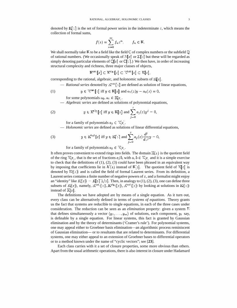
denoted by ��� � ��� � is the set of formal power series in the indeterminate � , which means thecollection of formal sums,
� H � M���� ���
� � � ��� � ��� ���We shall normally take � to be a field like the field � of complex numbers or the subfield �of rational numbers. (We occasionally speak of ��� � ��� � or ��� � ��� � but these will be regarded assimply denoting particular elements of ��� � ��� � or ��� � ��� � .) We then have, in order of increasingstructural complexity and richness, three major classes of objects,
��� �"!#� � � � �%$ �&�(' )�� � ��� �%$ �&*,+"'-� � ��� �.$ ��� � ��� � �corresponding to the rational, algebraic, and holonomic subsets of ��� � ��� � .
— Rational series denoted by � � �(! � � � � � are defined as solution of linear equations,
(1) / � �0� �(!#� � ��� � iff / � ��� � ��� � and 132 H � M /5461 � H � M7� 8 ,
for some polynomials 1 � � 132 � ��� ��� .— Algebraic series are defined as solutions of polynomial equations,
(2) / � � �"' ) � � � � � iff / � ��� � � � � and 89 �.� 1 9 H � M / 9 � 8 ,
for a family of polynomials 1 9 � �:� � � .— Holonomic series are defined as solutions of linear differential equations,
(3) / � ��*;+('-� � � � � iff / � ��� � ��� � and 89 ��� 1 9 H � M:< 9
< � 9 / � 8 ,
for a family of polynomials 1 9 � �:� � � .It often proves convenient to extend rings into fields. The domain � H � M is the quotient fieldof the ring �:� ��� , that is the set of fractions 1>=�? , with 1 � ? � ��� ��� and it is a simple exerciseto check that the definitions of (1), (2), (3) could have been phrased in an equivalent wayby imposing that coefficients lie in @ H � M instead of ��� � � . The quotient field of ��� � ��� � isdenoted by � H H � M M and is called the field of formal Laurent series. From its definition, aLaurent series contains a finite number of negative powers of � , and a formalist might enjoyan “identity” like � H H � M MA� �:� � � � �B� 6 =���� . Then, in analogy to (1), (2), (3), one can define threesubsets of � H H � M M , namely, � � �C! H H � M M � � �"' ) H H � M M � � *;+(' H H � M M by looking at solutions in � H H � M Minstead of �:� � ��� � .
The definitions we have adopted are by means of a single equation. As it turn out,every class can be alternatively defined in terms of systems of equations. Theory grantsus the fact that systems are reducible to single equations, in each of the three cases underconsideration. The reduction can be seen as an elimination property: given a system Dthat defines simultaneously a vector H />2 � �,�;� � /�E M of solutions, each component, />2 say,is definable by a single equation. For linear systems, this fact is granted by Gaussianelimination and by the theory of determinants (‘Cramer’s rule’). For polynomial systems,one may appeal either to Groebner basis elimination—an algorithmic process reminiscentof Gaussian elimination— or to resultants that are related to determinants. For differentialsystems, one may either appeal to an extension of Groebner bases to differential operatorsor to a method known under the name of “cyclic vectors”; see [23].
Each class carries with it a set of closure properties, some more obvious than others.Apart from the usual arithmetic operations, there is also interest in closure under Hadamard
4 8. FUNCTIONAL EQUATIONS—RATIONAL AND ALGEBRAIC FUNCTIONS
1. Basic objects.
Domain Notation Typical element ( � is a field)
Polynomials ��� ��� ������ � � � , with ��� � ��� ��� is a ring
Rational fractions ������� �� with ��� � � ��� ��� ������� is a field
Formal power series ��� � ��� � ����� � � � ��� � ��� � is a ring
Formal Laurent series ��� ����� � ������ � � � � ��� ����� � is a field
2. Special classes. (Coefficients � may be taken in either ��� ��� or in ������� .)Rational series �"!$#&%�� � ��� � solution of �'(�����*)�+, � �����.-0/Algebraic series � #21 3 � � ��� � solution of � �����*) � +54(464(+, � �����7-0/Holonomic series �"86921�� � ��� � solution of � �����*: � );+5464(4(+, � �����7-0/ ( :=<?>>�@ )
3. Closure properties.
Class Elimination (System A Eq.) B C D E : FRat Gaussian elim.; determinants Y Y Y Y Y N
Alg Groebner bases; resultants Y Y Y N Y N
Hol diff. Groebner bases; cyclic vector Y Y N Y Y Y
4. Singularities and coefficient asymptotics (simplified forms).
Singularity Coefficient form
Rat ���HGJI�� ��K ( L integer) M KN� ' I �POAlg ���HGJI�� �PQ ( RS-UTV �=W ) M QP� ' I ��OHol [regular sing.] ���HGSI�� �PX �ZY\[�]����HG^I��2�2_ ( ` algebraic) M Xa� ' �ZYb[�]cMd�2_�I �PO
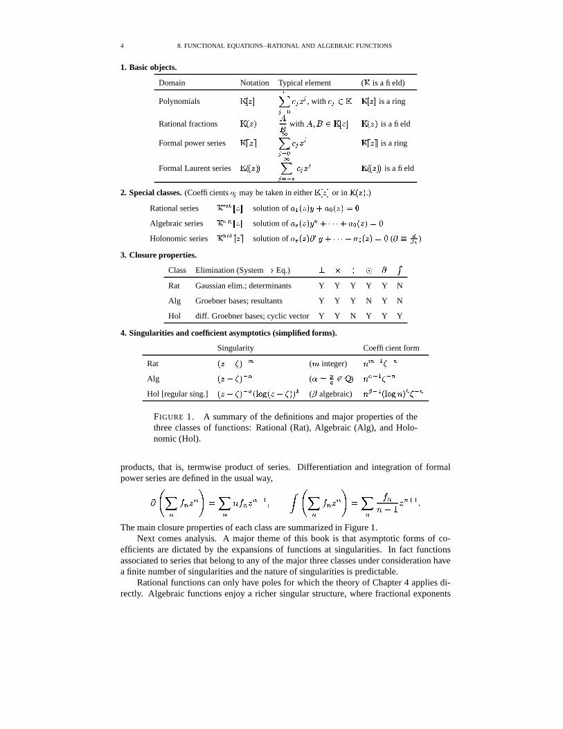
FIGURE 1. A summary of the definitions and major properties of thethree classes of functions: Rational (Rat), Algebraic (Alg), and Holo-nomic (Hol).
products, that is, termwise product of series. Differentiation and integration of formalpower series are defined in the usual way,e0f
�� � � �Pg �
�ih � � � ��j 2 � k f �
� � � �Pg � �
� �h 4 6 � �ml 2 �
The main closure properties of each class are summarized in Figure 1.Next comes analysis. A major theme of this book is that asymptotic forms of co-
efficients are dictated by the expansions of functions at singularities. In fact functionsassociated to series that belong to any of the major three classes under consideration havea finite number of singularities and the nature of singularities is predictable.
Rational functions can only have poles for which the theory of Chapter 4 applies di-rectly. Algebraic functions enjoy a richer singular structure, where fractional exponents
1. ALGEBRA OF RATIONAL FUNCTIONS 5
occur: the corresponding expansions known since Newton are called Newton–Puiseux ex-pansions and the conditions of singularity analysis are automatically satisfied. However,the inherently multivalued character of algebraic functions poses a specific “connectionproblem” as one needs to select the particular branch that is associated to any given combi-natorial problem. Holonomic functions have well-classified singularities that fall into twocategories called regular and irregular (also diversely known as first kind and second kind,or Fuchsian and non-Fuchsian). The simplest type, the regular type, introduces elementswith exponents that may be arbitrary algebraic numbers together with integral powers of alogarithm. Again, locally the conditions of singularity analysis are automatically satisfied,but again a connection problem arises—how do coefficients in the expansion at the singu-larity relate to the initial conditions given at the origin? Typical elements of coefficientsasymptotics that are encountered in this book are
H 6 4�� 9/
M � � � �� � h �
� h ��� 2� j �� ��� �and they reflect the nature of singularities present in each case. In effect, the first element istypical of rational asymptotics (here, a simple pole) and it arises in monomer-dimer tilingsof the interval. The second one corresponds to the asymptotic form of Catalan numbers andits origin is a singular element of an algebraic function with exponent 6 = / . The third onecorresponds to search cost in quadtrees and the algebraic number present in the exponentis indicative of a holonomic element.
Finally, positive functions, that is, solutions of positive systems, are the ones mostlikely to show up in elementary combinatorial applications. They are structurally moreconstrained and this fact is reflected to some extent by specific singularity and coefficientasymptotics. For instance, Perron-Frobenius theory says that, under certain natural condi-tions of “irreducibility”, a unique dominant pole (that is simple) occurs in rational asymp-totics. Similar conditions on positive algebraic systems constrain the singular exponent tobe equal to 2� , hence the characteristic factor h j ����� present in the asymptotic form of somany enumerative problems.
In this report, we consider the rational and algebraic classes in turn. First, at an alge-braic level, we state an elimination theorem and establish major closure properties. Nextcomes analysis, with its batch of singular asymptotics and matching coefficient forms. Ap-plications (including regular and context-free specifications) illustrate the general theoryin some important combinatorial situations.
1. Algebra of rational functions
Rational functions are the simplest of all objects considered in this chapter. They arenaturally defined as quotients of polynomials (Definition 8.1) or alternatively as compo-nents of solutions of linear systems (Theorem 8.1) a form that is especially convenientfor combinatorial enumeration. Coefficients of rational functions satisfy linear recurrenceswith constant coefficients and they also admit an explicit form, called “exponential poly-nomial” (Theorem 8.1) that is directly related to the location and multiplicity of poles andto the corresponding asymptotic behaviour of coefficients (Theorem 8.4). Closure proper-ties are stated as Theorem 8.2 while easy combinatorial forms for coefficients of rationalfunctions are given in Theorem 8.3 The asymptotic side of rational functions is the subjectof Section 2. An important class of positive systems has poles whose location and naturecan be predicted using an extension of the Perron-Frobenius theory of positive matrices(Theorems 8.5 and 8.6).
6 8. FUNCTIONAL EQUATIONS—RATIONAL AND ALGEBRAIC FUNCTIONS
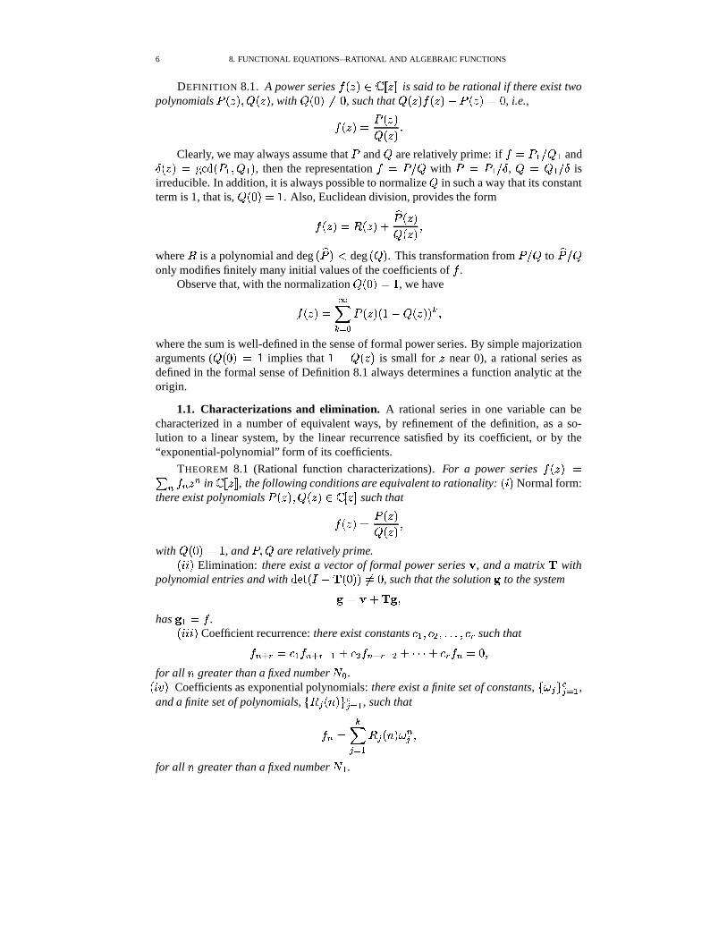
DEFINITION 8.1. A power series� H � M � ��� � ��� � is said to be rational if there exist two
polynomials � H � M ��� H � M , with� HK82M��� 8 , such that
� H � M � H � M�� � H � M7�A8 , i.e.,
� H � M � � H � M� H � M �Clearly, we may always assume that � and
�are relatively prime: if
� � ��2;= � 2 and� H � M ��2��0H � 2 ��� 2 M , then the representation� � �A= � with � � �72,= � ,
� � � 2 = � isirreducible. In addition, it is always possible to normalize
�in such a way that its constant
term is 1, that is,� HS8!M7� 6 . Also, Euclidean division, provides the form
� H � M���'H � M 4�� H � M� H � M
�
where is a polynomial and deg H�� M� deg H � M . This transformation from �A= � to
�� = �
only modifies finitely many initial values of the coefficients of�
.Observe that, with the normalization
� HS8!M7� 6 , we have
� H � M�� �� ��� �
H � M�H�6�� � H � M M � �
where the sum is well-defined in the sense of formal power series. By simple majorizationarguments (
� HK82M � 6 implies that 6�� � H � M is small for � near 0), a rational series asdefined in the formal sense of Definition 8.1 always determines a function analytic at theorigin.
1.1. Characterizations and elimination. A rational series in one variable can becharacterized in a number of equivalent ways, by refinement of the definition, as a so-lution to a linear system, by the linear recurrence satisfied by its coefficient, or by the“exponential-polynomial” form of its coefficients.
THEOREM 8.1 (Rational function characterizations). For a power series� H � M �� � � � � �
in ��� � � � � , the following conditions are equivalent to rationality: H���M Normal form:there exist polynomials � H � M ��� H � M � �0� ��� such that
� H � M � � H � M� H � M�
with� HK82M � 6 , and � ���
are relatively prime.H�����M Elimination: there exist a vector of formal power series � , and a matrix � withpolynomial entries and with �� � H���� � HS8!M M���A8 , such that the solution � to the system
� � � 4���� �has ��2 � �
.H�������M Coefficient recurrence: there exist constants � 2 � � � � �;�,� � � � such that� �ml � � �;2 � �ml � j 2�4!� � � �al � j � 4#"$"%"�4�� � � � � 8 �for all h greater than a fixed number & � .H���'1M Coefficients as exponential polynomials: there exist a finite set of constants, ($) 9+*-,9 � 2 ,and a finite set of polynomials, ( 9 H h M *+,9 � 2 , such that
� � ��
9 � 2 9 H h M ) �9 �
for all h greater than a fixed number & 2 .
1. ALGEBRA OF RATIONAL FUNCTIONS 7
The matrix � that defines a rational function via a linear system is often called a transitionmatrix or a transfer matrix. The form H���'�M for coefficients is called an exponential-polynomial. Naturally, one may always assume that the ) 9 are “sorted”, � )72������ ) � ����"$"%" ,which is the key to asymptotic approximations.Proof. H���M is equivalent to the definition of a rational power series, by the comments above.H���MA��� H�����M results from the fact that
�satisfies the 1-dimensional system
� � � 4H�6�� � M � . The converse property H���� M ��� H���M results from Cramer’s solution of linearsystems in terms of determinants. This provides a rational form for
�with denominator�� � H�� � � H � M M that is locally nonzero since, by assumption, �� � H � � � HS8!M M �� 8 . (Note
that this condition is in particular automatically satisfied inn the frequent case where � HK82Mis nilpotent.)H���M���� H���� ��M arises from the identity
8 � � H � M � H � M�� � H � M �upon extracting the coefficient of � �
. The converse implication H������ M���� H���M results fromtranslating the recurrence into an OGF equation in the standard way (multiply by � �
andsum).H���MA��� H���'1M is obtained by partial fraction expansion followed by coefficient extrac-tion by means of standard identity
6H�6�� )�� M � �
�� � h 4�� � 6� � 6� ) � � � �
where the binomial coefficient is a polynomial in h of exact degree � � 6 . The converseimplication H�� '�M���� H���M results from the same identity used in the opposite direction tosynthesize the function from its coefficients,
����
h 4�� � 6� � 6� ) � � � � 6H�6�� )�� M �
�
where the binomial coefficients � �ml � j 2� j 2�� ( ��� 6 ) form a basis of the set of polynomials��� h � . �
We have opted for the use of determinants as an approach to elimination in linear sys-tems. An alternative is Gaussian elimination. The principle is well known: the algorithmtakes a system of linear forms and combines them linearly, so as to eliminate all variablesin succession, until a normal form, ��� ��� � is attained. When we discuss elimination inpolynomial systems later in this chapter (Section 4), we shall encounter similarly two ap-proaches: one, based on resultants, makes extensive use of determinants while the other,relying on Groebner bases, is somewhat reminiscent of Gaussian elimination.
1.2. Closure properties and coefficients. Rational functions satisfy several closureproperties that derive rather directly from their definition or from the characterizationsgranted by Theorem 8.1.
THEOREM 8.2 (Rational series closure). The set � � �(! � � ��� � of rational series is closedunder the operations of sum H � 4�� M , product (
��� � ), quasi-inverse (defined by����
H�6 � � M j 2 , conditioned upon� � �A8 ), differentiation (
e� ), composition (
�"! � , conditionedupon � � �A8 ), and Hadamard (termwise) product,
� H � M�# � H � M7� f �
� � � � g # f � � � � � g �
�H � � "$� � M � � �
8 8. FUNCTIONAL EQUATIONS—RATIONAL AND ALGEBRAIC FUNCTIONS
Proof. Only the Hadamard closure deserves a comment: it results from the characterizationof coefficients of rational generating functions as exponential polynomials whose class isobviously closed under product. �
EXERCISE 1. Let ��� O�� - ��/ � � � � � � � � � � ��� � be the Fibonacci sequence. Ex-amine properties of the generating functions
�� K�� �����7- ��O��� ��� O � K � O EXERCISE 2. Develop a proof of closure under Hadamard products that is basedon the Hadamard integral formula of p. 55
Closed form for coefficients. A combinatorial sum expression for coefficients of rationalfunctions results from the expansion of 6 = � H � M as
� � H 6�� � H � M M � .
THEOREM 8.3 (Rational function coefficients). Let� H � M be a rational function with� H � M�� � H � M = � H � M and
�normalized by
� HK82M7��6 . Set
� H � M7� �9 ���
� 9 � 9 � 6�� � H � M7� � 2 �:4�� � � � 4#"$"%"�4�� E � E �and define the combinatorial sums:
� � Q � 2 ��� l � ��� l������ l E ��� �.�
�� 274#"$"%"�4 � E� 2 � �;�,� � � E H � � �2 � � �� "$"%" � ���E M �The coefficients of
�are expressible in finite terms from the
� � :
� � � � � H � M� H � M � �9 ���
� 9 � �Pj 9 �Proof. The multinomial expansion gives
6� H � M � 6
6�� H�6 � � H � M M� ����� ����������� � ���
�� 2 4 "%"%"�4 � E� 2 � �;�,� � � E H � ���2 � ���� "%"$" � � �E M � � � l � � � l������ l E � � �
and it suffices to multiply this expansion by the numerator � H � M . �As a consequence, the coefficients of �A= � are expressible as multinomial sums of
multiplicity at most � 6 (in fact only the number of nonzero monomials in � matters).(Multiplicity is also called “index” in Comtet’s book [26] that provides many interestingexamples of nontrivial expansions.) Note that, by “Fatou’s Lemma”, if all the coefficients� � � � � H � M are integers, then the � 9 and � 9 are themselves integers. (See the discussion in [87,p. 264].)
EXAMPLE 1. Fibonacci numbers and binomial coefficients. The generating function ofFibonacci numbers, when expanded according to Theorem 8.3 leads to
! �ml 2 � � � � � 66�� � � � � �
9 � h �#"
" �

2. ANALYSIS OF RATIONAL FUNCTIONS 9
so that Fibonacci numbers are sums of ascending diagonals of Pascal’s triangle. Naturally,infinitely many variants exist when expanding a rational function. For instance, one hasalso 6
6�� H �:4 � � M � 66�� �
66�� �
2 j � 66�� � �
66��
2 j � � 66�� � 2 j �2 j �
leading to a trivial variety of binomial forms. More generally, compositions with largestsummand � have an OGF that is
66�� H �:4 � � 4 "%"$"(� E M � 6
6�� � 2 j �2 j � 6 � �6�� / �:46� E l 2 �
and corresponding expansions lead to sums that are of index H �W6�M , 2, and 2, respectively.�
EXERCISE 3. The OGF of an ascending line in Pascal’s triangle, � O -� ��� Oa� > ���� , is a rational function.
It is a common but often fruitless exercise in combinatorial analysis to show “directly”equivalence between such combinatorial sums. In fact, as the example above illustrates,elementary combinatorial identities are often nothing but the image (in a world with littletransparent algebraic structure) of simple algebraic identities between generating functions(that live in a world with a strong structure).
2. Analysis of rational functions
In principle, the asymptotic analysis of coefficients of a rational function is “easy”given the exponential–polynomial form. However, in most applications of interest, rationalfunctions are only given implicitly as solutions to linear systems. This confers a great valueto criteria that ensure unicity and/or simplicity of the dominant pole. Accordingly, thebulk of this section is devoted to a brief exposition of Perron-Frobenius theory that coversadequately the case of positive linear systems.
2.1. General rational functions. The fact that coefficients of rational series are ex-pressible as exponential polynomials yields an asymptotic equivalent. The ) 9 satisfy) 9 � H � 9 M j 2 , where � 2 � � � � �;�,� are the poles of
� H � M , that is to say, the zeros of thedenominator of
�. The formula simplifies as soon as there is a unique number in (%) 9 * , say
)�2 , that dominates the other ones in absolute value.
THEOREM 8.4 (Rational function asymptotics). Let� � �A= � be a rational function
where �!��0H � ��� M�� 6 . Assume that�
has a unique dominant pole, that is, the zeros ( � 9+*of the denominator polynomial
� H � M satisfy � � 2 � � � � ��� � � � �� "%"%" , then ( �� 8 beingarbitrary)
� � � � � H � M��� 2 H h M � j �2 4� H H � � � � � M j�� �where 2 H h M is a polynomial.
If� H � M has several dominant poles, � � 2 � � � � � � � "%"$" � � � � � � � � l 2 ��� "%"$" , then
( �� 8 being arbitrary)
� � � �9 � 2
9 H h M � j �9 4� H H � � � l 2 � � M j�� M �
where the 9 H h M are polynomials. The degree of each 9 equals the order of the poleof
� H � M at � � minus one.
10 8. FUNCTIONAL EQUATIONS—RATIONAL AND ALGEBRAIC FUNCTIONS
Proof. Immediate from Theorem 8.1 �Observe that, if
� H � M has nonnegative coefficients,� H � M ��� �� � � � � � , then � 2 must at
least be real and positive by Pringsheim’s theorem. Unicity of a zero of smallest modulusfor
� H � M is equivalent to unicity of dominant singularity for� H � M and this is the simplest
case for analysis. The prototypical application is provided by the Fibonacci numbers! � �
8 ,! 2 ��6 , ! �ml � � ! �ml 274 ! � with OGF� H � M7� �
6�� � � � � �The poles are at 6 =�� and 6 = � , where� � 6 4 � 9
/� � � 6�� � 9
/�
and one has! ��� � � = � 9 .
EXAMPLE 2. Compositions into finite summands. The OGF of integer compositionshaving summands in the finite set
� � (�� 2 � �,�;� � � E * with �!��RH (�� 9-* M7��6 is H � M7� E9 � 2
66�� � 9 � ��� �
The characteristic polynomial H � M � � � � � has positive coefficients, so that there existsa unique positive � satisfying H � M�� 6 and additionally one has �� H � M � 8 . Also all otherroots of are of modulus strictly larger than � (by positivity of or Pringsheim’s theoremcombined with the gcd assumption). There results that
� � � � H � M7� � � � � 6 H � M � H � M � 6 � H � M�H � � � M � 6�� � H � M � j � �since the dominant pole at � is simple.
�The case where several dominant singularities are present can also be treated easily as
soon as one of them has a higher multiplicity, as this singles out a larger contribution in thecoefficients’ asymptotics.
EXAMPLE 3. Denumerants. The OGF of integer partitions with summands in the set� � (�� 2 � �;�,� � � E * where �!��0H (�� 9-* M7� 6 is� H � M7� E9 � 2
66�� � ��� �
This GF has poles at � � 6 and at roots of unity, but only the pole at � � 6 attainsmultiplicity , with � H � M � �� 2
6� 6H�6�� � M E
� � � E9 � 2 � 9 �
There results the estimate of the number of denumerants � � � � � H � M � � j 2 � �ml E j 2E j 2 � , thatis,
� � � � � H � M � �� E9 � 2 � 9���
j 2 h E j 2H � 6�M�� �
which is due to Schur.�
2. ANALYSIS OF RATIONAL FUNCTIONS 11
In the case when there exist several dominant singularities possessing the same multi-plicity, then fluctuations appear; refer to the discussion of Chapter 4. For a general linearrecurrence over � , equivalently for a GF in � H � M , it is for instance only known that the set��� � ( h �� � � � 8 * is a finite union of (finite or infinite) arithmetic progressions—thisconstitutes the Skolem-Mahler-Lech theorem. However,
���is not known to be computable
and it is not even known whether the property��� ��� is decidable. The function
66��� �:46� � ��6 4 6 � / 8 � 4 8 � � � � � � 8 � U2: � � � 6 � / � ��� � 8 � ; / � 4 8 � / 9 � � 4 "%"$" �
that is built on the Pythagorean triple = � � � 9�� illustrates some of the hardships. We have
� � ��� ��� H h 4 6NM��� �,� � � � � &.�����-� � = 9 �and, for instance, the way
� � approaches its extremes � � � � 2��� ��� depends on how wellmultiples of � approximate multiples of � , that is, on deep arithmetic properties of � = � .Such pathological situations, though possibly present amongst general rational functions,hardly ever occur in analytic combinatorics.
EXERCISE 4. Examine empirically the sign pattern of coefficients of the rationalfunctions��� �����7- �
� GJ� G � ���� �! � � �" � � GJ��� G$# ����� � i.e., ���&% O - � GSM � � �" G'# O �
2.2. Positive rational functions and Perron-Frobenius theory. For rational func-tions, positivity coupled with some ancillary conditions entails a host of important proper-ties, like unicity of the dominant singularity. Such facts result from the classical Perron-Frobenius theory of nonnegative matrices that we now summarize.
Consider first rational functions of the special form
� H � M7� 66�� � H � M
�for
� H � M a polynomial. It is assumed that�
has no constant term (� HS8!M�� 8 ), so that
� H � Mis properly defined as a formal power series. Assume next nonnegativity of the coefficientsof
�; this entails existence of a dominant real pole that is simple. If additionally
� H � M isnot a polynomial in �)( for some < � /
, then, as is easy to see, there is uniqueness (andsimplicity) of dominant singularity. As we show now, similar properties hold for systems:the conditions are those of properness and positivity coupled with a new combinatorialnotion of “irreducibility”. Granted these conditions, the analysis suitably extends what wejust saw of the scalar case.
2.2.1. Perron-Frobenius theory of nonnegative matrices. The properties of positiveand of nonnegative matrices have been superbly elicited by Perron [77] in 1907 and byFrobenius [43] in 1908–1912. The corresponding theory has far-reaching implications: itlies at the basis of the theory of finite Markov chains and it extends to positive operators ininfinite-dimensional spaces [60].
For a square matrix * ��� E,+>E , the spectrum is the set of its eigenvalues, that is,the set of - such that - � � * is not invertible (i.e., not of full rank), where � is the unitmatrix with the appropriate dimension. A dominant eigenvalue is one of largest modulus.
For * a scalar matrix of dimension � with nonnegative entries, a crucialrole is played by the dependency graph; this is the (directed) graph that has vertex set. � ( 6 �,� * and edge set containing the directed edge H 1 � ? M iff *0/ � 1 �� 8 . The
12 8. FUNCTIONAL EQUATIONS—RATIONAL AND ALGEBRAIC FUNCTIONS
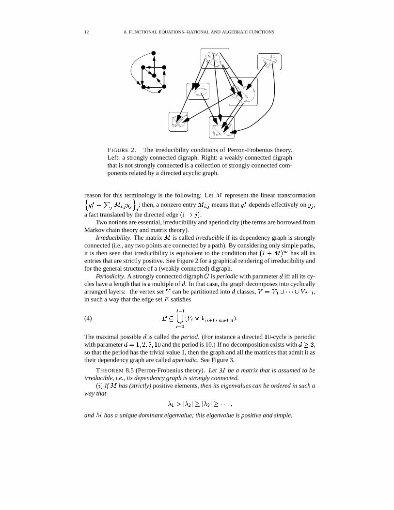
FIGURE 2. The irreducibility conditions of Perron-Frobenius theory.Left: a strongly connected digraph. Right: a weakly connected digraphthat is not strongly connected is a collection of strongly connected com-ponents related by a directed acyclic graph.
reason for this terminology is the following: Let * represent the linear transformation� /��� � � 9 * � � 9 / 9�� � ; then, a nonzero entry * � � 9 means that /��� depends effectively on / 9 ,
a fact translated by the directed edge H�� � "2M .Two notions are essential, irreducibility and aperiodicity (the terms are borrowed from
Markov chain theory and matrix theory).Irreducibility. The matrix * is called irreducible if its dependency graph is strongly
connected (i.e., any two points are connected by a path). By considering only simple paths,it is then seen that irreducibility is equivalent to the condition that H�� 4 * M E has all itsentries that are strictly positive. See Figure 2 for a graphical rendering of irreducibility andfor the general structure of a (weakly connected) digraph.
Periodicity. A strongly connected digraph � is periodic with parameter < iff all its cy-cles have a length that is a multiple of < . In that case, the graph decomposes into cyclicallyarranged layers: the vertex set
.can be partitioned into < classes,
. � . ��� "%"$" � . ( j 2 ,in such a way that the edge set � satisfies
(4) �� ( j 2� ���H . � � . � � l 2 �� + � ( M �
The maximal possible < is called the period. (For instance a directed 6�8 -cycle is periodicwith parameter < ��6 � / � 9 � 6�8 and the period is 10.) If no decomposition exists with < � /
,so that the period has the trivial value 1, then the graph and all the matrices that admit it astheir dependency graph are called aperiodic. See Figure 3.
THEOREM 8.5 (Perron-Frobenius theory). Let * be a matrix that is assumed to beirreducible, i.e., its dependency graph is strongly connected.H���M If * has (strictly) positive elements, then its eigenvalues can be ordered in such away that - 2 � � - � ��� � - � ��� "$"%" �and * has a unique dominant eigenvalue; this eigenvalue is positive and simple.
2. ANALYSIS OF RATIONAL FUNCTIONS 13
���
������������������
�������������������������������� ��������������������� ������������������������������������������ ����������������������������������������������� �������������������������������������������������������������������� ��������������������� ���������������������������������������������������������������
� �����������������
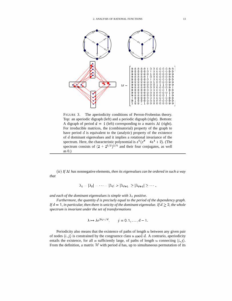
FIGURE 3. The aperiodicity conditions of Perron-Frobenius theory.Top: an aperiodic digraph (left) and a periodic digraph (right). Bottom:A digraph of period < � � (left) corresponding to a matrix * (right).For irreducible matrices, the (combinatorial) property of the graph tohave period < is equivalent to the (analytic) property of the existenceof < dominant eigenvalues and it implies a rotational invariance of thespectrum. Here, the characteristic polynomial is � � H ��� � � � ��4 / M . (Thespectrum consists of H / � / 2 ��� M 2 � � and their four conjugates, as wellas 0.)
H�����M If * has nonnegative elements, then its eigenvalues can be ordered in such a waythat
- 2 � � - � � � "$"%" � � - ( � � � - ( l 2 ��� � - ( l � ��� "%"$" �
and each of the dominant eigenvalues is simple with - 2 positive.Furthermore, the quantity < is precisely equal to the period of the dependency graph.
If < � 6 , in particular, then there is unicity of the dominant eigenvalue. If < � /, the whole
spectrum is invariant under the set of transformations
- �� -�� � � 9�� � ( � " �A8 � 6 � �,�;� � < � 6 �Periodicity also means that the existence of paths of length h between any given pair
of nodes � � " � is constrained by the congruence class h %'�� < . A contrario, aperiodicityentails the existence, for all h sufficiently large, of paths of length h connecting � � " � .From the definition, a matrix * with period < has, up to simultaneous permutation of its
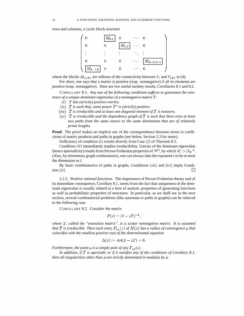
14 8. FUNCTIONAL EQUATIONS—RATIONAL AND ALGEBRAIC FUNCTIONS
rows and columns, a cyclic block structure������������8 * � � 2 8 "$"%" 88 8 * 2 � � "$"%" 8...
......
. . ....
8 8 8 "$"%" * ( j � � ( j 2* ( j 2 � � 8 8 "$"%" 8
�������������where the blocks * � � � l 2 are reflexes of the connectivity between
. � and. � l 2 in (4).
For short, one says that a matrix is positive (resp. nonnegative) if all its elements arepositive (resp. nonnegative). Here are two useful turnkey results, Corollaries 8.1 and 8.2.
COROLLARY 8.1. Any one of the following conditions suffices to guarantee the exis-tence of a unique dominant eigenvalue of a nonnegative matrix � :H���M � has (strictly) positive entries;H�� ��M � is such that, some power � � is (strictly) positive;H���� ��M � is irreducible and at least one diagonal element of � is nonzero;H�� '�M � is irreducible and the dependency graph of � is such that there exist at least
two paths from the same source to the same destination that are of relativelyprime lengths.
Proof. The proof makes an implicit use of the correspondence between terms in coeffi-cients of matrix products and paths in graphs (see below, Section 3.3 for more).
Sufficiency of condition H���M results directly from Case H���M of Theorem 8.5.Condition H�����M immediately implies irreducibility. Unicity of the dominant eigenvalue
(hence aperiodicity) results from Perron-Frobenius properties of * � , by which - � 2 � � - � � � .(Also, by elementary graph combinatorics, one can always take the exponent � to be at mostthe dimension .)
By basic combinatorics of paths in graphs, Conditions H���� ��M and H���'�M imply Condi-tion H�����M . �
2.2.2. Positive rational functions. The importance of Perron-Frobenius theory and ofits immediate consequence, Corollary 8.1, stems from the fact that uniqueness of the dom-inant eigenvalue is usually related to a host of analytic properties of generating functionsas well as probabilistic properties of structures. In particular, as we shall see in the nextsection, several combinatorial problems (like automata or paths in graphs) can be reducedto the following case.
COROLLARY 8.2. Consider the matrix! H � M7� H�� � � � M j 2 �
where � , called the “transition matrix”, is a scalar nonnegative matrix. It is assumedthat � is irreducible. Then each entry
! � � 9 H � M of * H � M has a radius of convergence � thatcoincides with the smallest positive root of the determinantal equation� H � M Q � �� � H���� � � M��A8 �Furthermore, the point � is a simple pole of any
! � � 9 H � M .In addition, if � is aperiodic or if it satisfies any of the conditions of Corollary 8.1,
then all singularities other than � are strictly dominated in modulus by � .
2. ANALYSIS OF RATIONAL FUNCTIONS 15
Proof. Define first (as in the statement) � � 6 = -�2 , where - 2 is the eigenvalue of � oflargest modulus that is guaranteed to be simple by assumption of irreducibility and byPerron-Frobenius properties. Next, the relations induced by
! ��� 4 ��� ! , namely,! � � 9 H � M7� � � � 9 4 �
� � � � � ! � � 9 H � M �together with positivity and irreducibility entail that the
! � � 9 H � M must all have the sameradius of convergence � . Indeed, each
! � 9 depends positively on all the other ones (byirreducibility) so that any infinite value of an entry in the system must propagate to all theother ones.
The characteristic polynomial� H � M7� �� � H���� � � M �has roots that are inverses of the eigenvalues of � and � � 6 = - 2 is smallest in modulus.Thus, since
�is the common denominator to all the
! � � 9 H � M , poles of any! � � 9 H � M can only
be included in the set of zeros of this determinant, so that the inequality � ��� holds.It remains to exclude the possibility � � � , which means that no “cancellations” with
the numerator can occur at � � � . The argument relies on finding a positive combinationof some of the
! � � 9 that must be singular at � . We offer two proofs, each of interest in itsown right: one H 1 M is conveniently based on the Jacobi trace formula, the other H ? M is basedon supplementary Perron–Frobenius properties.H 1 M Jacobi’s trace formula for matrices [48, p. 11],
(5) �� � ! �-G�P�� ��G�P ! Tr or +�� � ! �� � � Tr! +�� �
generalizes the scalar identities1 � / � 1 � � / l 1 and +�� � 1>? � +,� � 1 4 +�� � ? . Here we have(for � small enough)
Tr +,� � H�� � � � M j 2 � � �� 2 *�� � � � � � �
h� +�� � HS�� � H�� � � � M j 2 �where the first line results from expansion of the logarithm and the second line is an in-stance of the trace formula. Thus, by differentiation, the sum
� � *�� � � H � M is seen to besingular at � � 6 = - 2 and we have established that � � � .H ? M Alternatively, let ' 2 be the eigenvector of � corresponding to -.2 . Perron-Frobeniustheory also teaches us that, under the irreducibility and aperiodicity conditions, the vec-tor ' 2 has all its coordinates that are nonzero. Then the quantity
H 6 � � � M j 2 ' 2 � 66�� � - 2 ' 2
is certainly singular at 6 = -�2 . But it is also a linear combination of the! � � 9 ’s. Thus at least
one of the entries of!
(hence all of them by the discussion above) must be singular at� ��6 = - 2 . Therefore, we have again � � � .Finally, under the additional assumption that � is aperiodic, there follows from Perron-
Frobenius theory that � � 6 = - 2 is well-separated in modulus from all other singularities!. �
1The Jacobi trace formula is readily verified when the matrix is diagonizable, and from there, it can beextended to all matrices by an algebraic “density” argument.
16 8. FUNCTIONAL EQUATIONS—RATIONAL AND ALGEBRAIC FUNCTIONS
It is interesting to note that several of these arguments will be recycled when we dis-cuss the harder problem of analysing coefficients of positive algebraic functions in Sec-tion 5.2.
EXERCISE 5. The de Bruijn matrix � ������������ is essential in problems relatedto occurrences of patterns in random strings [39]. Its entries are given by
�� % � - ��.� �b� ��- ����� [�� ��� � or � ��- ��� + ��� [�� ��� � � �
Prove that it has a unique dominant eigenvalue. [Hint: consider a suitable graphwith vertices labelled by binary strings of length � .]
We next proceed to show that properties of the Perron-Frobenius type even extend toa large class of linear systems of equations that have nonnegative polynomial coefficients.Such a case is important because of its applicability to transfer matrices; see Section 3.3below.
Some definitions extending the ones of scalar matrices must first be set. A polynomial
� H � M7� 9 � 9 � 8 � � every � 9 ��A8 �
is said to be primitive if the quantity� � �2�� H ( � 9 * M is equal to 1; it is imprimitive
otherwise. Equivalently, � H � M is imprimitive iff � H � M � H ��� M for some bona fide poly-nomial and some
� � 6 . Thus, � � 6 4 � � � � 4 � � � � 4 � � 4 / � � are primitive while6 � 6 46� � � � � 4 � � � 6 4 / � � 4 9 � 2 � are not.
DEFINITION 8.2. A linear system with polynomial entries,
(6)� H � M7�#' H � M 4�� H � M � H � M
where � � � � ��� � + � , ' � � � ��� � , and� � � � ��� � the vector of unknowns is said to be:
H 1 M rationally proper (r–proper) if � HS8!M is nilpotent, meaning that � HK82M � is the nullmatrix;H ? M rationally nonnegative (r–nonnegative) if each component ' 9 H � M and each matrixentry � � � 9 H � M lies in � � � � � ;H � ) rationally irreducible (r–irreducible) if H � 4 � H � M M � has all its entries that arenonzero polynomials.H < M rationally aperiodic (r–periodic) if at least one diagonal entry of some power� H � M 8 is a primitive polynomial.
It is again possible to visualize these properties of matrices by drawing a directed graphwhose vertices are labelled 6 � / � �,�;� � � , with the edge connecting � to " that is weightedby the entry � � � 9 H � M of matrix � H � M . Properness means that all sufficiently long paths(and all cycles) must involve some positive power of � — it is a condition satisfied inwell-founded combinatorial problems; irreducibility means that the dependency graph isstrongly connected by paths involving edges with nonzero polynomials. Periodicity meansthat all closed paths involve weights that are polynomials in some � 8 for some � � 6 .
For instance, if � is a matrix with positive entries, then ��� is r–irreducible
and r–aperiodic, while � � � is r–periodic. The matrix � ����� � � �6 8
�� ! is r–
proper, r–irreducible, and r–aperiodic, since � � ����� � � 4 � � � �
� � �� ! . The matrix � �
2. ANALYSIS OF RATIONAL FUNCTIONS 17
��������
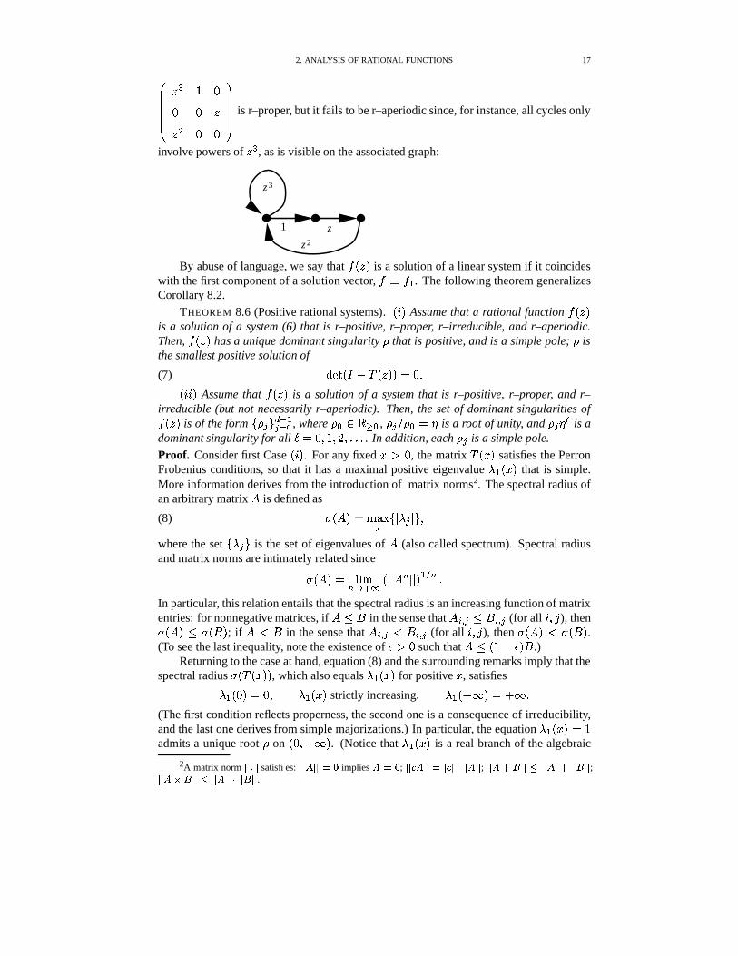
� � 6 88 8 �� � 8 8
� ! is r–proper, but it fails to be r–aperiodic since, for instance, all cycles only
involve powers of � � , as is visible on the associated graph:
2z
3
1 z
z
By abuse of language, we say that� H � M is a solution of a linear system if it coincides
with the first component of a solution vector,��� � 2 . The following theorem generalizes
Corollary 8.2.
THEOREM 8.6 (Positive rational systems). H���M Assume that a rational function� H � M
is a solution of a system (6) that is r–positive, r–proper, r–irreducible, and r–aperiodic.Then,
� H � M has a unique dominant singularity � that is positive, and is a simple pole; � isthe smallest positive solution of
(7) �� � H���� � H � M M��A8 �H�����M Assume that
� H � M is a solution of a system that is r–positive, r–proper, and r–irreducible (but not necessarily r–aperiodic). Then, the set of dominant singularities of� H � M is of the form ( � 9 * ( j 29 �.� , where � � � � �� , � 9 =�� � ��� is a root of unity, and � 9 ��� is adominant singularity for all � � 8 � 6 � / � �;�,� . In addition, each � 9 is a simple pole.
Proof. Consider first Case H���M . For any fixed ��� 8 , the matrix � H � M satisfies the PerronFrobenius conditions, so that it has a maximal positive eigenvalue -%2 H � M that is simple.More information derives from the introduction of matrix norms2. The spectral radius ofan arbitrary matrix � is defined as
(8) � H � M0� %W&.G9 (�� - 9 � * �where the set ( - 9 * is the set of eigenvalues of � (also called spectrum). Spectral radiusand matrix norms are intimately related since� H � M0� + � %� � l �
H � � � � � � M 2 � � �In particular, this relation entails that the spectral radius is an increasing function of matrixentries: for nonnegative matrices, if ���� in the sense that �"� � 9 �� � � 9 (for all � � " ), then� H � M � � H � M ; if � � in the sense that � � � 9 � � � 9 (for all � � " ), then � H � M� � H � M .(To see the last inequality, note the existence of � 8 such that � � H 6�� M � .)
Returning to the case at hand, equation (8) and the surrounding remarks imply that thespectral radius � H � H � M M , which also equals - 2 H � M for positive � , satisfies- 2 HK82M7�A8 � - 2 H � M strictly increasing
� - 2 H 4� M7� 4� �(The first condition reflects properness, the second one is a consequence of irreducibility,and the last one derives from simple majorizations.) In particular, the equation - 2 H � M�� 6admits a unique root � on HK8 � 4� M . (Notice that -.2 H � M is a real branch of the algebraic
2A matrix norm � � ��� � satisfies: � � ��� � � � implies � � � ; � � ����� � � � ������� � ��� � ; � � ������� ��� � � ���!�"� � �#� � ;� � �%$&�#� �'��� � ��� �(��� � �#� � .
18 8. FUNCTIONAL EQUATIONS—RATIONAL AND ALGEBRAIC FUNCTIONS
curve �� � H - ��� � H � M M&�78 that dominates all other branches in absolute value for � � 8 .There results from the general theory of algebraic functions, see Section 5, that - 2 H � M isanalytic at every point � � 8 .)
There remains to prove that: H 1 M � is at most a simple pole of� H � M ; H ? M � is actually a
pole; H � M there are no other singularities of modulus equal to � .Fact H 1 M amounts to the property that � is a simple root of the equation - H � M�� 6 ,
that is, - � H � M �� 8 . (To prove - � H � M �� 8 , we can argue a contrario. First derivatives- � H � M � - � � H � M , etc, cannot be zero till some odd order inclusively since this would contradictthe increasing character of - H � M around � along the real line. Next, if derivatives till someeven order � /
inclusively were zero, then we would have by the local analytic geometryof - H � M near � some complex value � 2 satisfying: � - H � 2 M � � 6 and � � 2 � � ; but for sucha value � 2 , by irreducibility and aperiodicity, for some exponent � , the entries of � H � 2 M 8would be all strictly dominated in absolute value by those of � H � M 8 , hence a contradiction.)Then, - � H � M���A8 holds and by virtue of
�� � H���� � H � M M�� H 6�� - 2 H � M M 9��� 2H�6�� - 9 H � M M7� H 6�� - 2 H � M M ��
� H ��� � H � M M6�� - 2 H � M
�
the quantity � is only a simple root of �� � H���� � H � M M .Fact H ? M means that no “cancellation” may occur at � � � between the numerator and
the denominator given by Cramer’s rule. It derives from an argument similar to the oneemployed for Corollary 8.2. Fact H � M derives from aperiodicity and the Perron-Frobeniusproperties. �
3. Combinatorial applications of rational functions
Rational functions occur as generating functions of well-recognized classes of enu-merative problems. We examine below the case of regular specifications and regular lan-guages (Subsections 3.1 and 3.2) that are closely related to transfer matrix methods andfinite state models or automata (Subsection 3.3). Local constraints in permutations repre-sent a direct application of transfer matrix methods (Subsection 3.4). Lattice paths lead toan extension of the regular framework to infinite alphabets and infinite grammars, reveal-ing interesting connections with the theory of continued fractions (Subsection 3.5). Forinstance, the classic continued fractions identity (originally due to Gauß),
�����
H 6 " = "%"%" H / h � 6�M M � � � 6
6�� 6 ";� �6�� / ",� �
. . .
�
expresses combinatorially a very “regular” decomposition of involutive permutations andhas implications on the physics of random interconnection networks.
3.1. Regular specifications. A combinatorial specification is said to be regular if itis nonrecursive (“iterative”, see Chapter 1) and it involves only the constructions of Atom,Union, Product, and Sequence. We consider here unlabelled structures. Since the operatorsassociated to these constructions are all rational, it follows that the corresponding OGFis rational. The OGF can be then systematically obtained from the specification by thesymbolic methods of Chapter 1.
3. APPLICATIONS OF RATIONAL FUNCTIONS 19
For instance, the OGF of the class ��� of general Catalan trees of height at most � isdefined by the recurrence
� � ����� ��� l 2 ��� � (���� * �Accordingly, the OGF’s are
� � H � M7� � � � 2 H � M7� �6�� �
� � � H � M7� �6�� �
6�� �� �;�,� �
and ��� H � M is none other than the � th convergent in the continued fraction expansion of theCatalan GF: 6
/ � 6�� � 6�� � � � � �6�� �
6�� �6�� �
. . .
�
The interesting connections with Chebyshev polynomials and Mellin transform techniques—the expected height of a tree of size h turns out to be asymptotic to � � h — are detailedin Chapter 7.
In a similar vein, the class �� ��� of integer compositions whose summands are at most� is
� ��� � ( � �� ( � �card � * * so that
� ��� H � M7� 66�� � � � � � "%"$" � � � �
The interesting asymptotics is again discussed in Chapter 7 in connection with Mellintransform asymptotics. The largest summand in a random composition of h turns out tohave expectation about +,� � � h ; see [49] for a general discussion.
EXERCISE 6. The OGF of integer compositions and of integer partitions withsummands constrained to be either in number at most L or of size at most � isrational.
3.2. Regular languages. The name “regular specification” has been chosen in orderto be in agreement with the notions of regular expression and regular language from formallanguage theory. These two concepts are now defined formally.
A language is a set of words over some fixed alphabet � . The structurally simplest (yetnontrivial) languages are the regular languages that can be defined in a variety of ways: byregular expressions and by finite automata, either deterministic or nondeterministic.
DEFINITION 8.3. The category RegExp of regular expressions is defined as the cat-egory of expressions that contains all the letters of the alphabet H 1 � � M as well as theempty symbol , and is such that, if 2 � � ������������� , then the formal expressions 2 � � , 2 " � and � 2 are regular expressions.
Regular expressions are meant to specify languages. The language H M denoted bya regular expression is defined inductively by the rules: H�� M H��M7� ( 1 * if is the letter1 � � and H��M&� ( * (with the empty word) if is the symbol ; H�� ��M H 2 � � M&� H 2 M � H � M (with � the set-theoretic union); H�������M H 2 " � M7� H 2 M "! H� � M (with" the concatenation of words extended to sets); H�� '�M H� � 2 M � ( * 4" H 2 M 4# H 2 M " H 2 M 4 "$"%" . A language is said to be a regular language if it is specified by a regularexpression.
A language is a set of words, but a word $ � H��M may be parsable in several waysaccording to . More precisely, one defines the ambiguity coefficient (or multiplicity) of $
20 8. FUNCTIONAL EQUATIONS—RATIONAL AND ALGEBRAIC FUNCTIONS
with respect to the regular expression as the number of parsings, written � H $ M�� ��� H $ M .In symbols, we have
��� ��� � � H $ M&� ��� � H $ M 4���� � H $ M � ��� � � � � H $ M&� � � -�� ��� �
H � M ��� � H�'1M �
with natural initial conditions ( � / H ? M � � / � 1 , ��� H $ M � � � � ), and with the definition of� ��� � taken as induced by the definition of � via unions and products, namely,
� ��� H $ M0� � � � 4 �9 � 2 � � � H $ M �As such, � H $ M lies in the completed set � � ( 4� * . We shall only consider here regularexpressions that are proper, in the sense that ��� H $ M 4� . It can be checked thatthis condition is equivalent to requiring that no
� � with � H � M enters in the inductivedefinition of the regular expression . (This condition is substantially equivalent to thenotion of well-founded specification in Chapter 1.) A regular expression is said to beunambiguous iff for all $ , we have ��� H $ M � ( 8 � 6 * ; it is said to be ambiguous, otherwise.
Given a language� � H �M , we are interested in two enumerating sequences� � � � �
� � �.� � �H $ M � � � �
� � �.�� ���� �
corresponding to the counting of words in the language, respectively, with and withoutmultiplicities. The corresponding OGF’s will be denoted by
� � H � M and� H � M . (Note that,
for a given language, the definition of�
is intrinsic, while that of� � is dependent on the
particular expression that describes the language.) We have the following.
PROPOSITION 8.1 (Regular expression counting). Given a regular expression as-sumed to be of finite ambiguity, the ordinary generating function
� � H � M of the language H �M , counting with multiplicity, is given by the inductive rules:
�� 6 � 1 �� � � � �� 4 � " �� � ��� �� H�6 � H � M M j 2 �In particular, if is unambiguous, then the ordinary generating function satisfies
� � H � M7�� H � M and is given directly by the rules above.
Proof. Formal rules associate to any proper regular expression a specification � :
�� 6 (the empty object)� 1 �� � / ( � / an atom)
�� �� 4 � " �� � ��� �� (#� *
It is easily recognized that this mapping is such that � generates exactly the collection ofall parsings of words according to . The translation rules of Chapter 1 then yield thefirst part of the statement. The second part follows since
� H � M � � � H � M whenever isunambiguous. �
The technique implied by Proposition 8.1 has already been employed silently in earlierchapters. For instance, the regular expression
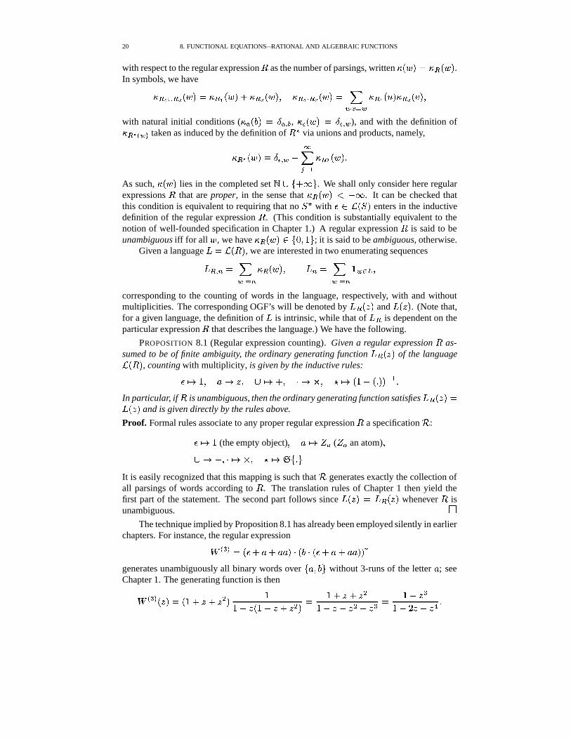
� � �� � H 4 1�4 1 1 M " H ? " H 4 15461 1 M M �generates unambiguously all binary words over ( 1 � ? * without 3-runs of the letter 1 ; seeChapter 1. The generating function is then
� � �� H � M7� H�6 4 �:46� � M 66�� � H�6 4 �A46� � M � 6 46��46� �
6�� � � � � � � � � 6�� � �6�� / �A4 � � �
3. APPLICATIONS OF RATIONAL FUNCTIONS 21
�������������������������������������������������
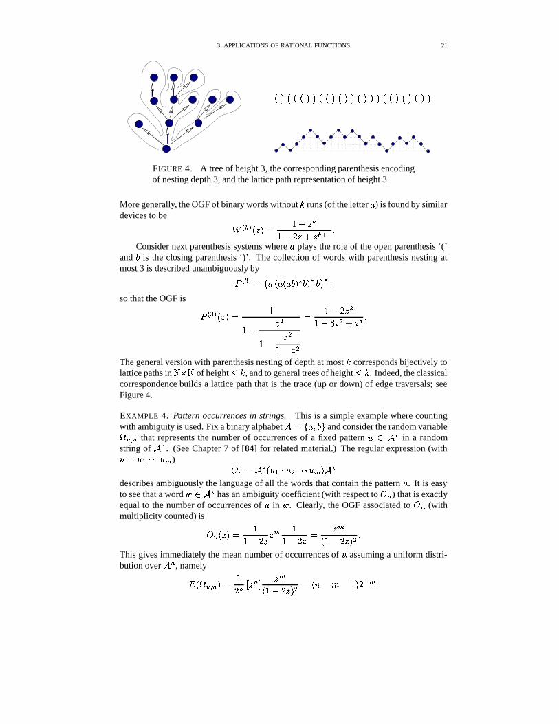
FIGURE 4. A tree of height 3, the corresponding parenthesis encodingof nesting depth 3, and the lattice path representation of height 3.
More generally, the OGF of binary words without�
runs (of the letter 1 ) is found by similardevices to be
� � � H � M7� 6�� � �6�� / �A4 � � l 2 �
Consider next parenthesis systems where 1 plays the role of the open parenthesis ‘(’and ? is the closing parenthesis ‘)’. The collection of words with parenthesis nesting atmost 3 is described unambiguously by
� � �� � � 1 H 1 H 1>? M � ? M � ? � � �so that the OGF is
� � �� H � M7� 6
6�� � �6�� � �
6�� � �
� 6�� / � �6�� = � � 46� � �
The general version with parenthesis nesting of depth at most�
corresponds bijectively tolattice paths in � � � of height � �
, and to general trees of height � �. Indeed, the classical
correspondence builds a lattice path that is the trace (up or down) of edge traversals; seeFigure 4.
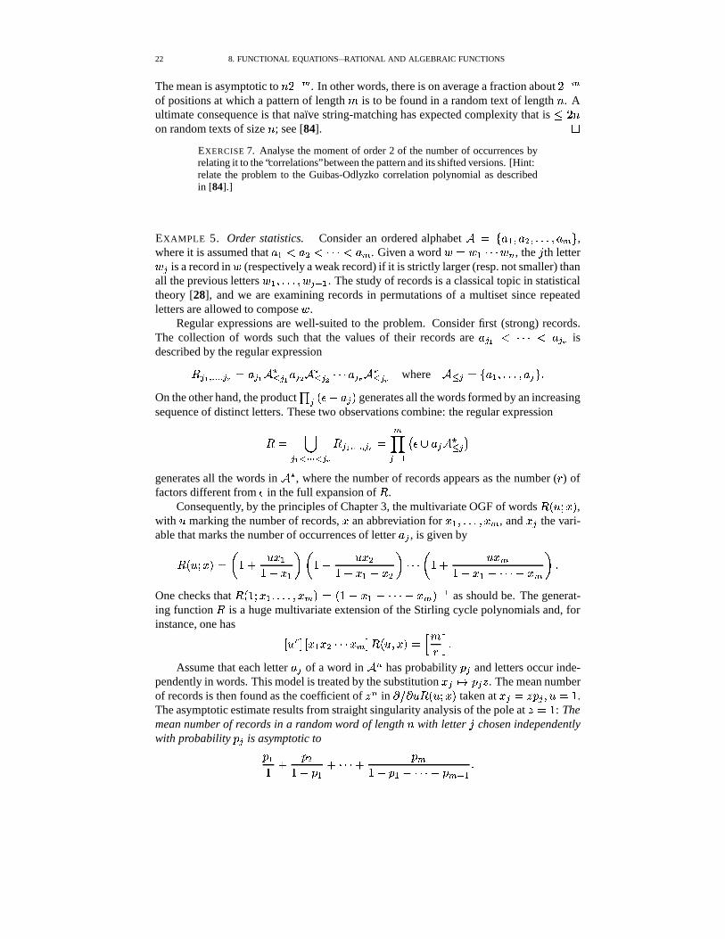
EXAMPLE 4. Pattern occurrences in strings. This is a simple example where countingwith ambiguity is used. Fix a binary alphabet � � ( 1 � ? * and consider the random variable� � � � that represents the number of occurrences of a fixed pattern � � � � in a randomstring of � �
. (See Chapter 7 of [84] for related material.) The regular expression (with� � � 2 "$"%" � E ) � � � � H � 2 " � � "%"$" � E M � �
describes ambiguously the language of all the words that contain the pattern � . It is easyto see that a word $ � � � has an ambiguity coefficient (with respect to � ) that is exactlyequal to the number of occurrences of � in $ . Clearly, the OGF associated to � (withmultiplicity counted) is
� H � M7� 66�� / � � E 6
6�� / � � � EH�6�� / � M � �
This gives immediately the mean number of occurrences of � assuming a uniform distri-bution over � �
, namely
� H � � � � M7� 6/ � � � � � � E
H�6�� / � M � � H h � 4 6NM / j E �
22 8. FUNCTIONAL EQUATIONS—RATIONAL AND ALGEBRAIC FUNCTIONS
The mean is asymptotic to h / j E . In other words, there is on average a fraction about/ j E
of positions at which a pattern of length is to be found in a random text of length h . Aultimate consequence is that naıve string-matching has expected complexity that is � / hon random texts of size h ; see [84].
�
EXERCISE 7. Analyse the moment of order 2 of the number of occurrences byrelating it to the “correlations” between the pattern and its shifted versions. [Hint:relate the problem to the Guibas-Odlyzko correlation polynomial as describedin [84].]
EXAMPLE 5. Order statistics. Consider an ordered alphabet � � ( 1 2 � 1 � � �;�,� � 1 E * ,where it is assumed that 1 2 1 � "$"%" 1 E . Given a word $ � $ 2 "%"$" $ � , the " th letter$ 9 is a record in $ (respectively a weak record) if it is strictly larger (resp. not smaller) thanall the previous letters $ 2 � �,�,� � $ 9 j 2 . The study of records is a classical topic in statisticaltheory [28], and we are examining records in permutations of a multiset since repeatedletters are allowed to compose $ .
Regular expressions are well-suited to the problem. Consider first (strong) records.The collection of words such that the values of their records are 1 9 � "%"$" 1 9�� isdescribed by the regular expression
9 ��������� � 9�� � 1 9 � � � � 9 � 1 9 � � � � 9 � "$"%"C1 9�� � � � 9�� where � � 9 � ( 132 � �;�,� � 1 9 * �On the other hand, the product � 9 H 4 1 9 M generates all the words formed by an increasingsequence of distinct letters. These two observations combine: the regular expression
� 9 ��� ����� � 9 � 9 � ������� � 9 � � E
9 � 2 � � 1 9 � � � 9 �generates all the words in � � , where the number of records appears as the number ( � ) offactors different from in the full expansion of .
Consequently, by the principles of Chapter 3, the multivariate OGF of words 'H � � � M ,with � marking the number of records, � an abbreviation for � 2 � �;�,� � � E , and � 9 the vari-able that marks the number of occurrences of letter 1 9 , is given by
'H � � � M7� 6 4 � � 2
6�� � 2 6 4 � � �6�� � 2 � � � "%"$"
6 4 � ��E
6�� � 2 � "%"%" � � E �One checks that 'H�6�� ��2 � �,�;� � � E M � H 6 � � 2 � "$"%" � � E M j 2 as should be. The generat-ing function is a huge multivariate extension of the Stirling cycle polynomials and, forinstance, one has
� � � � � � 2$� � "%"%" � EA� 'H � � � M7��� � �Assume that each letter 1 9 of a word in � �
has probability � 9 and letters occur inde-pendently in words. This model is treated by the substitution � 9 �� � 9 � . The mean numberof records is then found as the coefficient of � �
ine = e � VH � � � M taken at � 9 � � � 9 � � � 6 .
The asymptotic estimate results from straight singularity analysis of the pole at � � 6 : Themean number of records in a random word of length h with letter " chosen independentlywith probability � 9 is asymptotic to
� 26 4 � �
6�� � 2 4 "%"$" 4 � E6�� � 2 � "$"%" � � E j 2 �
3. APPLICATIONS OF RATIONAL FUNCTIONS 23
The analysis as � tends to 1, keeping � as a parameter, shows also that the limit of� � � � VH � � � M exists. By the continuity theorem for probability generating functions de-scribed in Chapter 9, this implies: The distribution of the number of records when h tendsto converges to the (finite) law with probability generating function
6 4 � � 26�� � 2 6 4 � � �
6�� � 2 � � � "$"%"6 4 � � E j 2
6�� � 2 � "%"$" � � E j 2 � � E��Similarly, the multivariate GF
�'H � � � M�� 6 4 � ��2
6�� � � 2 6 4 � � �6�� � 2 � � � � "%"%"
6 4 � � E
6 � � 2 � "$"%" � � � E �counts words by their number of weak records. This time, there is a double pole at � � 6 :The number of (weak) records has a mean asymptotic to � " h ( � a computable constant)and a limit Gaussian law.
�
Permutations and combinations of multisets are a classical topic in combinatorial anal-ysis; see for instance MacMahon’s book [68]. The corresponding statistics are of interest tocomputer scientists since they relate to searching in the context of sets and multisets obey-ing nonuniform data distributions. This last topic is for instance considered by Knuth [59,1.2.10.18] and developed by Burge [17] in a pre-symbolic context. Such techniques havebeen successfully employed to analyse data structures like the ternary search tries of Bent-ley and Sedgewick [9]; see [24]. Prodinger has also developed a collection of studiesconcerning words whose letter probabilities are geometrically distributed, � 9 � H�6 � M 9 :see for instance [55]. In the latter case, one may legitimately let the cardinality of the al-phabet become infinite. This approach then provides interesting -analogues of classicalcombinatorial quantities since they reduce to permutation statistics when � 6 .
EXERCISE 8. Analyse records in random permutations of a multiset, which cor-responds to extracting coefficients � � O �' 46464�� O �K � in
���� � � � ��� and����� � � � ��� . De-
rive in this way the fact that the mean number of records in a random permutationof M elements is the harmonic number � O . [Hint. See [59, 1.2.10.18] and [17].]
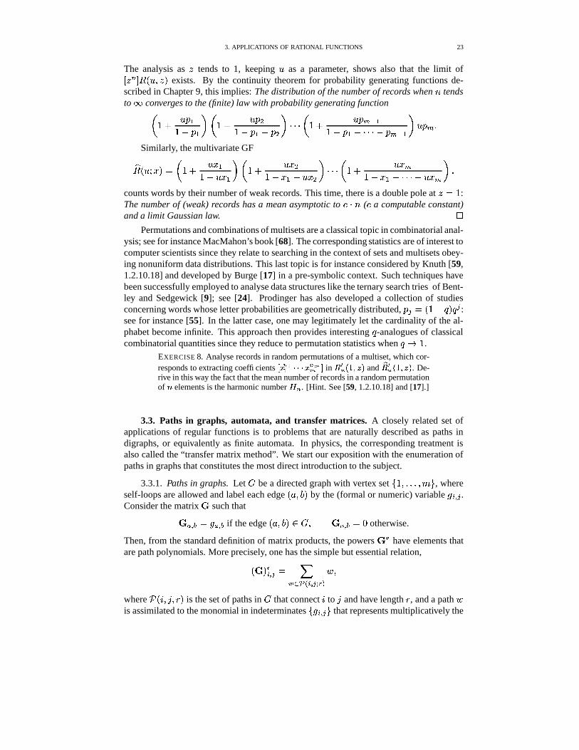
3.3. Paths in graphs, automata, and transfer matrices. A closely related set ofapplications of regular functions is to problems that are naturally described as paths indigraphs, or equivalently as finite automata. In physics, the corresponding treatment isalso called the “transfer matrix method”. We start our exposition with the enumeration ofpaths in graphs that constitutes the most direct introduction to the subject.
3.3.1. Paths in graphs. Let � be a directed graph with vertex set ( 6 � �,�;� � * , whereself-loops are allowed and label each edge H 1 � ? M by the (formal or numeric) variable ��� � 9 .Consider the matrix � such that
�'/ � 1 � ��/ � 1 if the edge H 1 � ? M � � � �'/ � 1 �A8 otherwise.
Then, from the standard definition of matrix products, the powers � � have elements thatare path polynomials. More precisely, one has the simple but essential relation,
H � M �� � 9 � �� � � � 9�� � $ �
where H�� � " � � M is the set of paths in � that connect � to " and have length � , and a path $is assimilated to the monomial in indeterminates ( � � � 9-* that represents multiplicatively the
24 8. FUNCTIONAL EQUATIONS—RATIONAL AND ALGEBRAIC FUNCTIONS
succession of its edges; for instance:
H � M �� � 9 � E � � � � E ��� E�� � E�� � 9 � E � � E � � E � � E � � E � � E � �
In other words, powers of the matrix associated to a graph “generate” all paths in a graph.One may then treat simultaneously all lengths of paths (and all powers of matrices) byintroducing the variable � to record length.
PROPOSITION 8.2. H���M Let � be a digraph and let � be the matrix associated to � .The OGF
!�� � � 9�� H � M of the set of all paths from � to " in a digraph � with � marking lengthand ��/ � 1 marking the occurrence of edge H 1 � ? M is the entry � � " of the matrix H ��� � � M j 2 ,namely
! � � � 9�� H � M7� H���� � � M j 2 �� � � 9 � � � � � 9�� H � M� H � M�
where� H � M0�7�� � H ��� � � M and
� � � � 9�� H � M is the determinant of the minor of index � � " of� � � � .H�����M The generating function of nonempty closed paths is given by � H ! � � � � � H � M � 6NM7� � �
� � H � M� H � M �Proof. Part H���M results from the discussion above which implies
! � � � 9�� H � M7� �� ��� � � H � � M � � 9 ��2H���� � � M j 2� � � 9 �
and from the cofactor formula of matrix inversion. Part H�� ��M results from Jacobi’s traceformula. Introduce the quantity known as the zeta function,� H � M Q � �-G�P f � �
� � 2! � � � � �� � �
hg � �-G�P f �
� � 2� �h Tr � ��g
� �-G�P � Tr +,� � H���� � � M j 2 � � �� � H�� � � � M j 2 �where the last line results from the Jacobi trace formula. Thus,
� H � M5� � H � M j 2 . On theother hand, differentiation combined with the definition of
� H � M yields
�� � H � M� H � M � � �
� � H � M� H � M� � �
� � 2! � � � � �� � ���
and Part H���� M follows. �EXERCISE 9. Can the coefficients of ����� be related to the polynomialsrepresenting self-loops, 2–loops, triangles, quadrangles, etc, in the graph � ?[See [19]]
EXERCISE 10. Observe that� I � �����I ����� - �O�� ' � O Tr � O - ��� � �� G � � �(the sum is over eigenvalues). Deduce an algorithm that determines the charac-teristic polynomial of a matrix of dimension L in � �ZL�� � arithmetic operations.
3. APPLICATIONS OF RATIONAL FUNCTIONS 25
[Hint: computing the quantities Tr � � for �J- � ����6� L requires precisely Lmatrix multiplications.]
In particular, the number of paths of length h is obtained by applying a substitution� Q � / � 1 �� 8 � 6 to H�� � � � M j 2 upon coefficient extraction by the � � � � operation. In asimilar vein, it is possible to consider weighted graphs, where the � / � 1 are assigned realweights; with the weight of a path being defined by the product of its edges weights, onefinds that � � � � H � � � � M j 2 equals the total weight of all paths of length h . If furthermorethe assignment is made in such a way that
� 1 ��/ � 1 ��6 , then the matrix � , which is calleda stochastic matrix, can be interpreted as the transition matrix of a Markov chain.
Let us assume that nonnegative weights are assigned to the edges of � . If the resultingmatrix is irreducible and aperiodic, then Perron-Frobenius theory applies. There exists� � 6 = -�2 , with - 2 � 8 the dominant eigenvalue of � , and the OGF of weighted pathsfrom � to " has a simple pole at � . In that case, it turns out that a random (weighted) pathof length h has, asymptotically as h � ,
— an average number of edges of type H�� � "1M that is ��� � � 9 h , for some nonzeroconstant � � � 9 � � ;
— an average number of encounters with vertex � that is ��� � h , for some nonzeroconstant � � � � .
In other words, a long random path tends to spend asymptotically a fixed (nonzero) frac-tion of its time at any given vertex or along any given edge. These observations are thecombinatorial counterpart of the elementary theory of finite Markov chains. The treatmentof such questions depends on the following lemma.
LEMMA 8.1 (Iteration of Perron-Frobenius matrices). Set * H � M7� H�� � � � M j 2 where� has nonnegative entries, is irreducible, and is aperiodic. Let -%2 be the dominant eigen-value of � . Then the “residue” matrix such that
(9) H���� � � M j 2 � 6�� � = -�2 4 H�6NM H � � - 2 M
has entries given by ( � � / � represents a scalar product)
� 9 � � � � 9 � � � � �where � and � are right and left eigenvectors of � corresponding to the eigenvalue - 2 .
Proof. Scaling � as � = - 2 reduces the situation to the case of a matrix with dominanteigenvalue equal to 1, so that we assume now - 2 ��6 . First observe that
� + � %� � �� � �
The limit exists for the following reason: geometrically, � decomposes as � � � 4 �where � is the projector on the eigenspace generated by the eigenvector � ; one has
� � �� � � 8 and � � � � , so that � � � � � 4 � �
; on the other hand,�
has spectral radius 6 ; thus + � % � �exists and it equals � (so that � � is a projector).
Now, for any vector $ , by properties of projections, one has $ � � H $ M � �
for some coefficient � H $ M . Application of this to each of the base vectors � 9 (i.e.,� 9 � H � 9 2 � �,�;� � � 9 ( M ) shows that the matrix has each of its columns proportional to theeigenvector � . A similar reasoning with the transpose ��� of � and the associated residue
26 8. FUNCTIONAL EQUATIONS—RATIONAL AND ALGEBRAIC FUNCTIONS
matrix � shows that the matrix has each of its rows proportional to the eigenvector � .In other words, for some constant � , one has
� � 9 � � � 9 � � �The normalization constant � is itself finally determined by applying to � and one findsthat � � 6 =) � � � � . �
EXERCISE 11. Relate explicitly the edge traversal and node encounter frequen-cies to the dominant eigenvectors of a graph assumed to be strongly connectedand not cyclically layered. Discuss the stationary probabilities of a Markov chainin this context.
EXERCISE 12. What happens when the matrix � is symmetric (i.e., the graph �is undirected)? Discuss formulæ for reversible Markov chains.
EXAMPLE 6. Locally constrained words. Consider a fixed alphabet � � ( 1 2 � �,�,� � 1 E *and a set � � �
�of forbidden transitions between consecutive letters. The set of words
over � with no forbidden transitions is denoted by and is called a locally constrainedlanguage. Clearly, the words of are in bijective correspondence with paths in a graphthat is constructed as follows. Set up the complete graph @ E,+3E , where the " vertex of thegraph represents the production of the letter 1 9 . Delete from the complete graph all edgesthat correspond to forbidden transitions. Then, a word of length h 4 6 has no forbiddentransition iff it corresponds to a path of length h in the modified graph. Consequently, theOGF of any locally constrained language is a rational function. Its OGF is given by
6 4 � H 6 � 6 � �;�,� � 6NM-H � � � � M j 2 H 6 � 6 � �;�,� � 6�M � �where � � 9 is 0 if H 1�� � 1 9 M � � and 1 otherwise. Various specializations, including multi-variate GF’s and nonuniform letter models are easily treated by this method.
The particular case where � consists of pairs of equal letters defines Smirnovwords [48, p. 69] and is amenable to a direct and explicit treatment. Let � H � 2 � �,�,� � � E Mbe the multivariate GF of words with the variable � 9 marking the number of occurrencesof letter 1 9 and
� H � 2 � �,�;� � � E M be the corresponding GF for Smirnov words. A simplesubstitution (already discussed in Chapter 3) shows that � and
�are related by
� H ��2 � �,�;� � ��E M7� � ��26�� � 2 � �,�;� � � E
6�� � E �
while � � H�6�� � 2 � "$"%" � � E M j 2 . There results that
(10)� H ��2 � �,�,� � � E M7� �
� 26 4�� 2
� �,�,� � ��E6 4�� E � f 6�� E � � 2
� 96 4�� 9 g
j 2�
In particular, setting � 9 � � , one gets the univariate OGF
� H � M7� 6 4 �6�� H � 6NM �
�
implying that the number of words of length h is H � 6�M �Pj 2 (as it should be).�
Locally constrained languages thus have rational generating functions. The processof proof can then be adapted to the enumeration of many types of objects provided theyhave a sufficiently “sequential” structure. Carlitz compositions defined below illustrate a
3. APPLICATIONS OF RATIONAL FUNCTIONS 27
recycling of the notion of regular expression to objects that are in fact defined over infinitealphabets.
EXAMPLE 7. Carlitz compositions. A Carlitz composition of the integer h is a composi-tion of h such that no two adjacent summands have equal values. Consider first composi-tions with a bound on the largest allowable summand. The OGF of Carlitz compositionsis directly derived from the GF of Smirnov words by substituting � 9 �� � 9
. In this way,the OGF of Carlitz compositions with maximum summand at most is found to be � E � H � M7�
��6�� E
9 � 2� 9
6 4 � 9 �� j 2 �
and the OGF of all Carlitz compositions is obtained by letting tend to infinity: thepreceding GF’s converge to
(11) � � � H � M7�
��6�� �9 � 2
� 96 4 � 9 �� j 2
�
In particular, we get Sequence A003242 of EIS3: � � � H � M7� 6 4 �:46� � 4 = � � 4 � � � 4 : � 4 6 � � � 4 / = � � 4 =#T � � 4 :�6 ���74#"$"%".�The asymptotic form of the number of Carlitz compositions is then easily found by
singularity analysis of meromorphic functions (see Chapter 4). We find � � �� � " � � � ��A8 � � 9.U!=#; � � �� 6 � :.9#8 / � �There, 6 = � is determined as the smallest positive root of the denominator in (11); see [57]for details. In this infinite alphabet example, the OGF is no longer rational but the essentialfeature of having a dominant polar singularity is preserved.
�
3.3.2. Finite automata. Finite automata are closely related to languages of paths ingraphs and to regular expressions.
DEFINITION 8.4 (Finite state automaton). A finite automaton � over a finite alphabet� and with vertex set
�, called the set of states, is a digraph whose edges are labelled by
letters of the alphabet, that is given together with a designated initial state � � �and a
designated set of final states� � � �
.
A word $ is said to be accepted by the automaton if there exists a path � in the graphconnecting the initial state � to one of the final states � � �
, so that the succession oflabels of the path � corresponds to the sequence of letters composing $ . (The path � isthen called an accepting path for $ .) The set of accepted words is denoted by H � M .
In all generality, a finite automaton is, by its definition, a nondeterministic device: if aword $ is accepted, one may not “know” a priori which choices of edges to select in orderto accept it. A finite automaton is said to be deterministic if given any state � �
and anyletter � � � , there is at most one edge from vertex that bears label � . In that case, onedecides easily (in linear time) whether a word is accepted by just following edges dictatedby the sequence of letters in $ .
3The EIS designates Sloane’s On-Line Encyclopedia of Integer Sequences [85]; see [86] for an earlierprinted version.
28 8. FUNCTIONAL EQUATIONS—RATIONAL AND ALGEBRAIC FUNCTIONS
The main structural result of the theory is that there is complete equivalence betweenthree descriptive models: regular expressions, deterministic finite automata, and nondeter-ministic finite automata. The corresponding theorems are due to Kleene (the equivalencebetween regular expression and nondeterministic finite automata) and to Rabin and Scott(the equivalence between nondeterministic and deterministic automata). Thus, finite au-tomata whether deterministic or not accept (“recognize”) the class of all regular languages.
EXERCISE 13. Any language definable by a regular expression is accepted by a(non-deterministic) finite automaton. [Hint: Perform an inductive constructionof an automaton based on separate constructions for unions, products, stars.]
EXERCISE 14. Kleene’s theorem: Any language accepted by a finite automatonis definable by a regular expression. [Hint: Construct (inductively on increasingvalues of
�) matrices of regular expressions where
� _ � % � is a regular expressionthat describes the set of paths from state
�to state � constrained never to pass
through a state of index � �.]
EXERCISE 15. Rabin and Scott’s theorem: Given any finite automaton � , thereexists an equivalent deterministic automation
�, i.e., ��� � �7-���� � � . [Hint: the
states of�
are all the subsets of the states of � and the transitions are determinedso that
�emulates all possible computations of � .]
EXERCISE 16. Regular languages are closed under intersection and complemen-tation.
PROPOSITION 8.3 (Finite state automata counting). Any language accepted by a finiteautomaton or described by a regular expression has a rational generating function. If thelanguage is specified by an automaton � � � ��� � � � � , that is deterministic, then thecorresponding ordinary generating function
� � H � M is defined as the component� � H � M of
the linear system of equations� 9 H � M7� � 9 46� / ��� ��� �� � � / H � M �
where � 9 equals 1 if 9 � � �and 0 otherwise, and where H 9 � 1 M is the state reachable
from state 9 when the letter 1 is read.
Proof. By the fundamental equivalence of models, one may freely assume the automatonto be deterministic. The quantity
� 9 is nothing but the OGF of the language obtained bychanging the initial state of the automaton to 9 . Each equation expresses the fact thata word accepted starting from 9 may be the empty word (if 9 is final) or, else, it mustconsist of a letter 1 followed by a continuation that is itself accepted when the automatonis started from the “next” state, that is, the state of index H 9 � 1 M .
Equivalently, one may reduce the proof to the enumeration of paths in graphs as de-tailed above. �
Given a problem that is described by a regular language, it is then a matter of choiceto enumerate it using a specification by a regular expression (provided it is unambiguous)or by a finite automaton (provided it is deterministic). Each problem usually has a morenatural presentation. From the structural standpoint, it should however be kept in mind thatthe conversion between a regular expression and an equivalent nondeterministic automatainvolves a moderate (at worst polynomial) blow-up in size, while the transformation of anondeterministic automaton to an equivalent deterministic one may involve an exponential
3. APPLICATIONS OF RATIONAL FUNCTIONS 29
increase in the number of states. (The construction underlying the equivalence theoremof Rabin and Scott involves the power-set of the set of states
�of the nondeterministic
automaton.) Note that the direct construction of the generating functions associated tofinite automata has been already encountered in Chapter 1 when discussing particular casesof languages containing or excluding a fixed pattern.
As the proof of the proposition shows, the OGF of the language defined by a deter-ministic finite automaton involves a quasi-inverse H�6�� ��� M j 2 where the transition ma-trix � is a direct encoding of the automaton’s transitions. Corollary 8.2 and Lemma 8.1were precisely custom-tailored for this situation. Consequently, quantifying probabilisticphenomena associated to finite automata is invariably reducible to finding eigenvectors ofmatrices.
EXAMPLE 8. Words with excluded patterns. Fix a pattern � � � 2 � � "%"$" � E . Let � �be the set of words that do not contain the word � as a factor, and
! � the set of wordsthat do not contain � as a subsequence. The language � � is defined by the (ambiguous)regular expression � ��� H � � � � � M . A deterministic finite automaton for � � � � � is readilyconstructed from � , from which a deterministic automaton results for the complement � � .(It suffices to exchange final and nonfinal states.) Thus, the generating function of � � isrational.
A similar argument, starting from the (ambiguous) regular expression that describes! � , namely
� � � 2 � � � � � � "$"%" � � � E � � �also shows (via the construction of the finite automaton) that the OGF of
! � is rational.�
EXERCISE 17. Extend the previous argument to prove the rationality of the OGFof words that do not contain any pattern from a finite set � , where pattern istaken either in the sense of a factor or a subsequence.
EXERCISE 18. Calculate explicitly the generating function of � � for an arbi-trary � in the case of a binary and of a ternary alphabet.
Determine the mean number of occurrences of � as subsequence in a ran-dom text of size M . Discuss the asymptotic form of the variance of the numberof such occurrences.
EXAMPLE 9. Variable-length codes. A finite set of words � $ � � is a (“variable-length”)code [11] if each word in � � admit at most one decomposition as a concatenation ofwords, each of which belonging to � . Obviously, such a code can be used for encodinginformations, adjusting formats of data to a particular transmission channel, etc.
It is not clear a priori how to decide whether any given set�
is a code. Let� H � M��� ���� � � � be the OGF of � (a polynomial). Then � is a code iff
66�� � H � M � � H � M �
where� H � M is the GF of all words that admit a decomposition as concatenations of words
in � . Now, Aho and Corasick have established in [3] that there exists a deterministicautomaton of size linear in the total size of
�(the total number of letters) that recognizes
� �(furthermore this automaton can be constructed in linear time). Thus, a system determining� H � M is found in linear time.
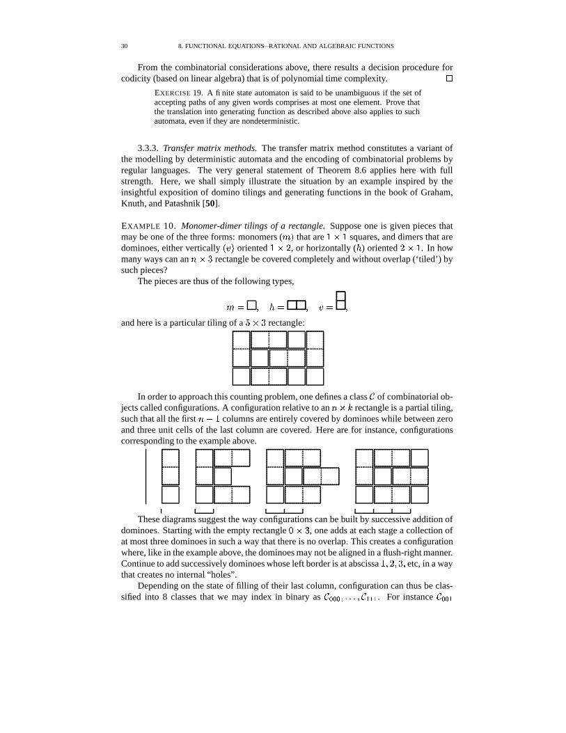
30 8. FUNCTIONAL EQUATIONS—RATIONAL AND ALGEBRAIC FUNCTIONS
From the combinatorial considerations above, there results a decision procedure forcodicity (based on linear algebra) that is of polynomial time complexity.
�
EXERCISE 19. A finite state automaton is said to be unambiguous if the set ofaccepting paths of any given words comprises at most one element. Prove thatthe translation into generating function as described above also applies to suchautomata, even if they are nondeterministic.
3.3.3. Transfer matrix methods. The transfer matrix method constitutes a variant ofthe modelling by deterministic automata and the encoding of combinatorial problems byregular languages. The very general statement of Theorem 8.6 applies here with fullstrength. Here, we shall simply illustrate the situation by an example inspired by theinsightful exposition of domino tilings and generating functions in the book of Graham,Knuth, and Patashnik [50].
EXAMPLE 10. Monomer-dimer tilings of a rectangle. Suppose one is given pieces thatmay be one of the three forms: monomers ( M that are 6 � 6 squares, and dimers that aredominoes, either vertically H�'�M oriented 6 � / , or horizontally ( � ) oriented
/ � 6 . In howmany ways can an h � = rectangle be covered completely and without overlap (‘tiled’) bysuch pieces?
The pieces are thus of the following types,
� � � � � ' � �and here is a particular tiling of a 9 � = rectangle:
In order to approach this counting problem, one defines a class of combinatorial ob-jects called configurations. A configuration relative to an h � �
rectangle is a partial tiling,such that all the first h � 6 columns are entirely covered by dominoes while between zeroand three unit cells of the last column are covered. Here are for instance, configurationscorresponding to the example above.
These diagrams suggest the way configurations can be built by successive addition ofdominoes. Starting with the empty rectangle 8 � = , one adds at each stage a collection ofat most three dominoes in such a way that there is no overlap. This creates a configurationwhere, like in the example above, the dominoes may not be aligned in a flush-right manner.Continue to add successively dominoes whose left border is at abscissa 6 � / � = �
etc, in a waythat creates no internal “holes”.
Depending on the state of filling of their last column, configuration can thus be clas-sified into 8 classes that we may index in binary as �(�"� � �,�;� � 2"2(2 . For instance �"� 2
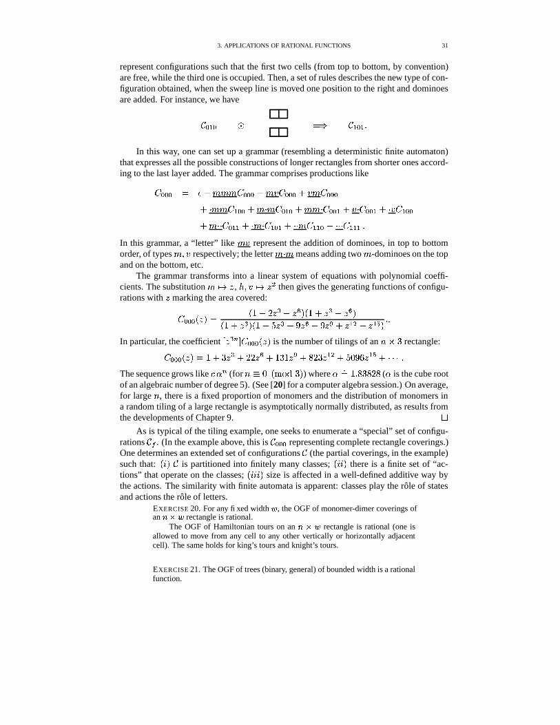
3. APPLICATIONS OF RATIONAL FUNCTIONS 31
represent configurations such that the first two cells (from top to bottom, by convention)are free, while the third one is occupied. Then, a set of rules describes the new type of con-figuration obtained, when the sweep line is moved one position to the right and dominoesare added. For instance, we have
� 2 � # � � 2 � 2 �In this way, one can set up a grammar (resembling a deterministic finite automaton)
that expresses all the possible constructions of longer rectangles from shorter ones accord-ing to the last layer added. The grammar comprises productions like �"�(� � 4 �(�"� 4 ' �(�"� 4 ' �(�"�
4#" 2 �(� 4 " � 2 � 4 " �"� 2�4 ' " �"� 274#" ' 2 �"�4 " " � 2(274 " " 2 � 274 " " 2"2 � 4#" " " 2"2(2��
In this grammar, a “letter” like ' represent the addition of dominoes, in top to bottomorder, of types � ' respectively; the letter " means adding two -dominoes on the topand on the bottom, etc.
The grammar transforms into a linear system of equations with polynomial coeffi-cients. The substitution �� � , � � ' �� � � then gives the generating functions of configu-rations with � marking the area covered: �"�(� H � M7� H�6�� / � � � � � M-H 6 46� � � � � M
H 6 46� � M�H�6�� 9 � � � T � � 4 T � � 46� 2 � � � 2 M � �In particular, the coefficient � � � � � �(�"� H � M is the number of tilings of an h � = rectangle: �"�"� H � M7� 6 4 = � � 4 /�/ � � 4 6�=�6 � � 4 ; / = � 2 � 4 9#8#T!U � 2 4#"$"%".�The sequence grows like � � �
(for h � 8 H %'�� =!M ) where � ���6 � ;#=!; / ; ( � is the cube rootof an algebraic number of degree 5). (See [20] for a computer algebra session.) On average,for large h , there is a fixed proportion of monomers and the distribution of monomers ina random tiling of a large rectangle is asymptotically normally distributed, as results fromthe developments of Chapter 9.
�As is typical of the tiling example, one seeks to enumerate a “special” set of configu-
rations � . (In the example above, this is �"�(� representing complete rectangle coverings.)One determines an extended set of configurations (the partial coverings, in the example)such that: H���M is partitioned into finitely many classes; H�� ��M there is a finite set of “ac-tions” that operate on the classes; H�� ����M size is affected in a well-defined additive way bythe actions. The similarity with finite automata is apparent: classes play the role of statesand actions the role of letters.
EXERCISE 20. For any fixed width � , the OGF of monomer-dimer coverings ofan M C�� rectangle is rational.
The OGF of Hamiltonian tours on an M5C�� rectangle is rational (one isallowed to move from any cell to any other vertically or horizontally adjacentcell). The same holds for king’s tours and knight’s tours.
EXERCISE 21. The OGF of trees (binary, general) of bounded width is a rationalfunction.
32 8. FUNCTIONAL EQUATIONS—RATIONAL AND ALGEBRAIC FUNCTIONS
EXERCISE 22. Find combinatorial interpretations of
� � ��� ������� - ��O��� ��� O � � � O �for any fixed integer � , where the numbers � O are the Fibonacci numbers. [Hint:see [50].]
EXERCISE 23. Given a fixed digraph � assumed to be strongly connected, anda designated start vertex, one travels at random, moving at each time to anyneighbour of the current vertex chosen with equal likelihood. Show that the ex-pectation of the time to visit all the vertices is a rational number that is effectively(though perhaps not efficiently!) computable.
Often, the method of transfer matrices is used to approximate a hard combinatorialproblem that is not known to decompose, the approximation being by means of a familyof models of increasing “widths”. For instance, the enumeration of the number � � oftilings of an h � h square by monomers and dimers remains a famous unsolved problem ofstatistical physics. Here, transfer matrix methods may be used to solve the h � $ version ofthe monomer–dimer coverings, in principle at least, for any fixed width $ . (The “diagonal”sequence of the h � $ rectangular models corresponds to the square model.) It has beenat least determined by computer search that the diagonal sequence � � starts as (this issequence A028420 in Sloane’s EIS [86]):
6 � : � 6�=�6 � 6�8!8�6 / � / ;"6�8#U!T � � / T#;!T�6 / U2: / : � 6#6�T � 9 / 92:<829 / = / 6 � �,�;� �From this and other numerical data, one estimates numerically that H � � M 2 � � � �6 � T � 8 / 6 �,�;� , but no expression for the constant is known to exist4. The difficulty of copingwith the finite-width models is that their complexity (as measured , e.g., by the numberof states) blows up exponentially with $ —such models are best treated by computer al-gebra; see [102]—and no law allowing to take a diagonal is visible. However, the finitewidth models have the merit of providing at least provable upper and lower bounds on theexponential growth rate of the hard “diagonal problem”.
3.4. Permutations and local constraints. In this subsection, we examine problemswhose origin lies in nineteenth century recreational mathematics. For instance, the menageproblem solved and popularized by Edouard Lucas in 1891, see [26], has the followingquaint formulation: What is the number of possible ways one can arrange h married cou-ples (‘menages’) around a table in such a way that men and women alternate, but nowoman sits next to her husband?
The menage problem is equivalent to a permutation enumeration problem. Sit firstconventionally the men at places numbered 8 � �,�;� � h � 6 , and let � � be the position at theright of which the � th wife is placed. Then, a menage placement imposes the condition� � �� � and � � �� � 4 6 for each � . We consider here a linearly arranged table (see remarksat the end for the other classical formulation that considers a round table), so that the
4In contrast, for coverings by dimers only, a strong algebraic structure is available and the number of covers�� O satisfies ��� O ��� �� �� � O�� '�� � O � � ����� ��� � ��O�����! #" O�%$'& � #" �)(
��*'+ �-, �� � ././0/1 ������2where 3 is Catalan’s constant; see [76] for context on this famous result.
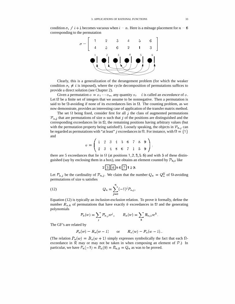
3. APPLICATIONS OF RATIONAL FUNCTIONS 33
condition � � �� � 4 6 becomes vacuous when � � h . Here is a menage placement for h �AUcorresponding to the permutation� ���� 6 / = � 9 U
� 9 U / 6 =
��61 2 3 4 5
Clearly, this is a generalization of the derangement problem (for which the weakercondition � � �� � is imposed), where the cycle decomposition of permutations suffices toprovide a direct solution (see Chapter 2).
Given a permutation � � � 2 "$"%" � � , any quantity � � � � is called an exceedance of � .Let
�be a finite set of integers that we assume to be nonnegative. Then a permutation is
said to be�
-avoiding if none of its exceedances lies in�
. The counting problem, as wenow demonstrate, provides an interesting case of application of the transfer matrix method.
The set�
being fixed, consider first for all " the class of augmented permutations � � 9 that are permutations of size h such that " of the positions are distinguished and thecorresponding exceedances lie in
�, the remaining positions having arbitrary values (but
with the permutation property being satisfied!). Loosely speaking, the objects in � � 9 canbe regarded as permutations with “at least” " exceedances in
�. For instance, with
� � ( 6 *and � �
�� 6 / = � 9 U : ; T/ = � ; U : 6 9 T
�� �
there are 5 exceedances that lie in�
(at positions 6 � / � = � 9 � U ) and with = of these distin-guished (say by enclosing them in a box), one obtains an element counted by � � � like
/3 4 ;DU 7 6 9DT �
Let � � � 9 be the cardinality of � � 9 . We claim that the number� � � ���� of
�-avoiding
permutations of size h satisfies
(12)� � � �
9 ���H ��6�M 9 � � � 9 �
Equation (12) is typically an inclusion-exclusion relation. To prove it formally, define thenumber � � � of permutations that have exactly
�exceedances in
�and the generating
polynomials
� � H $ M&� 9 � � � 9 $ 9 � � H $ M��
� � � � $ � �
The GF’s are related by
� � H $ M��� � H $ 4 6NM or � H $ M�� � � H $ � 6NM � �(The relation � � H $ M � � H $ 4 6NM simply expresses symbolically the fact that each
�-
exceedance in � may or may not be taken in when composing an element of .) Inparticular, we have � � H ��6�M7� � HS8!M�� � � � � � � as was to be proved.
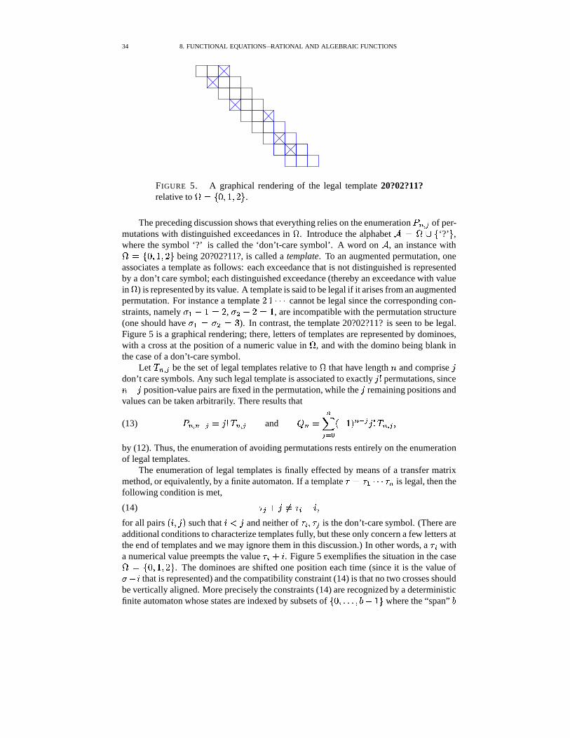
34 8. FUNCTIONAL EQUATIONS—RATIONAL AND ALGEBRAIC FUNCTIONS
FIGURE 5. A graphical rendering of the legal template 20?02?11?relative to
� � ( 8 � 6 � / * .
The preceding discussion shows that everything relies on the enumeration � � � 9 of per-mutations with distinguished exceedances in
�. Introduce the alphabet � � � � ( ‘?’ * ,
where the symbol ‘?’ is called the ‘don’t-care symbol’. A word on � , an instance with� � ( 8 � 6 � / * being 20?02?11?, is called a template. To an augmented permutation, oneassociates a template as follows: each exceedance that is not distinguished is representedby a don’t care symbol; each distinguished exceedance (thereby an exceedance with valuein�
) is represented by its value. A template is said to be legal if it arises from an augmentedpermutation. For instance a template
/ 6 "$"%" cannot be legal since the corresponding con-straints, namely � 2 � 65� /
, � � � / � 6 , are incompatible with the permutation structure(one should have � 2 � � � � = ). In contrast, the template 20?02?11? is seen to be legal.Figure 5 is a graphical rendering; there, letters of templates are represented by dominoes,with a cross at the position of a numeric value in
�, and with the domino being blank in
the case of a don’t-care symbol.Let � � � 9 be the set of legal templates relative to
�that have length h and comprise "
don’t care symbols. Any such legal template is associated to exactly " � permutations, sinceh � " position-value pairs are fixed in the permutation, while the " remaining positions andvalues can be taken arbitrarily. There results that
(13) � � � �Pj 9 � " � � � � 9 and� � � �
9 ���H ��6�M ��j 9 " � � � � 9 �
by (12). Thus, the enumeration of avoiding permutations rests entirely on the enumerationof legal templates.
The enumeration of legal templates is finally effected by means of a transfer matrixmethod, or equivalently, by a finite automaton. If a template � 2 "%"$" � is legal, then thefollowing condition is met,
(14) 9 4 " �� � 4 � �for all pairs H�� � "1M such that � " and neither of � � 9 is the don’t-care symbol. (There areadditional conditions to characterize templates fully, but these only concern a few letters atthe end of templates and we may ignore them in this discussion.) In other words, a � witha numerical value preempts the value � 4 � . Figure 5 exemplifies the situation in the case� � ( 8 � 6 � / * . The dominoes are shifted one position each time (since it is the value of� � � that is represented) and the compatibility constraint (14) is that no two crosses shouldbe vertically aligned. More precisely the constraints (14) are recognized by a deterministicfinite automaton whose states are indexed by subsets of ( 8 � �,�;� � ? � 6 * where the “span” ?
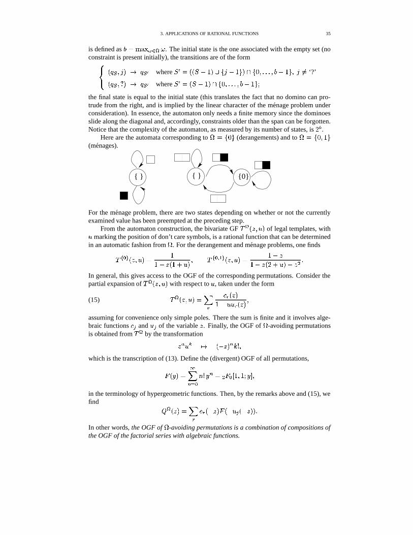
3. APPLICATIONS OF RATIONAL FUNCTIONS 35
is defined as ? � %W&<G�� � � ) . The initial state is the one associated with the empty set (noconstraint is present initially), the transitions are of the form�� � H �� � "1M �� ��� where
� � ��H H � � 6�M � ( "�� 6 * M� ( 8 � �,�;� � ? � 6 * � " �� ‘?’H �� � � M �� ��� where
� � ��H � � 6NM� ( 8 � �,�,� � ? � 6 * �the final state is equal to the initial state (this translates the fact that no domino can pro-trude from the right, and is implied by the linear character of the menage problem underconsideration). In essence, the automaton only needs a finite memory since the dominoesslide along the diagonal and, accordingly, constraints older than the span can be forgotten.Notice that the complexity of the automaton, as measured by its number of states, is
/ 1.
Here are the automata corresponding to� � ( 8 * (derangements) and to
� � ( 8 � 6 *(menages).
{0} { } { }
For the menage problem, there are two states depending on whether or not the currentlyexamined value has been preempted at the preceding step.
From the automaton construction, the bivariate GF � � H � � � M of legal templates, with� marking the position of don’t care symbols, is a rational function that can be determinedin an automatic fashion from
�. For the derangement and menage problems, one finds��� ��� H � � � M�� 6
6�� � H�6 4 � M� ��� � � 2 � H � � � M7� 6�� �
6�� � H / 4 � M 4 � � �In general, this gives access to the OGF of the corresponding permutations. Consider thepartial expansion of � � H � � � M with respect to � , taken under the form
(15) � � H � � � M�� �
�%� H � M6 � ��� � H � M
�
assuming for convenience only simple poles. There the sum is finite and it involves alge-braic functions � 9 and � 9 of the variable � . Finally, the OGF of
�-avoiding permutations
is obtained from � � by the transformation
� � � � �� H � � M � � � �which is the transcription of (13). Define the (divergent) OGF of all permutations,
! H / M7� �� ��� h � / � � � ! � � 6 � 6 � / � �
in the terminology of hypergeometric functions. Then, by the remarks above and (15), wefind � � H � M��
�� � H � � M ! H � � 9 H � � M M �
In other words, the OGF of�
-avoiding permutations is a combination of compositions ofthe OGF of the factorial series with algebraic functions.
36 8. FUNCTIONAL EQUATIONS—RATIONAL AND ALGEBRAIC FUNCTIONS
The expressions simplify much in the case of menages and derangements where thedenominators of � are of degree 1 in � . One has
� � � � H � M7� 66 4 �
! H �6 46� M�� 6 4 � � 4 / � � 4 T ����4 � � � 4 / U29 � � 4 6�;!9 � � � 4 "%"%" �
for derangements, whence a new derivation of the known formula,
� � ���� � �� ���
H ��6NM � h � H h � � M�� �
Similarly, for (linear) menage placements, one finds
� � � � 2 � H � M7� 66 4 �
! H �H 6 4 � M � M�� 6 4 � � 4 = � � 4 6�U � 4 T#U � � 4 U1:.9 � � 4#"$"%" �
which is EIS–A000271 and corresponds to the formula
� � � � 2 �� � �� ���
H ��6�M � / h � �
� H h � � M�� �Finally, the same techniques adapts to constraints that “wrap around”, that is, con-
straints taken modulo h . (This corresponds to a round table in the menage problem.) Inthat case, what should be considered is the loops in the automaton recognizing templates(see also the previous discussion of the zeta function of graphs). One finds in this way theOGF of the circular (i.e., classical) menage problem to be (EIS–A000179)�� � � � 2 � H � M�� 6�� �
6 4 �! H �
H�6 4 � M � M 4 / � ��6 4 ��4 � � 4 / � � 4 6�= � 4 ;!8 � � 4 9!:<T � � 4!"$"%" �which yields the classical solution of the (circular) menage problem,
�� � � � 2 �� � �� ���
H ��6�M � / h/ h � � / h � �
� H h � � M�� �a formula that is due to Touchard; see [26, p. 185] for pointers to the vast classical literatureon the subject. The algebraic part of the treatment above is close to the inspiring discussionoffered in Stanley’s book [87]. An application to robustness of interconnections in randomgraphs is presented in [38].
For asymptotic analysis purposes, the following general property proves useful: Let!
be the OGF of factorial numbers and assume that / H � M is analytic at the origin where itsatisfies / H � M�� � � - � � 4 H � � M ; then it is true that
(16) � � � � ! H / H � M M � � � � � ! H � H�6�� - � M M � h � � j � �(The proof results from simple manipulations of divergent series in the style of [8].) Thisgives at sight the estimates
� � ���� � h � j 2 � � � � � 2 �� � h � j � �More generally, for any set
�containing - elements, one has
� � � �� � h � j � �Furthermore, the number �� � � of permutations having exactly
�occurrences (
�fixed) of
an exceedance in�
is asymptotic to
� � � �� � h � j � - �� � �
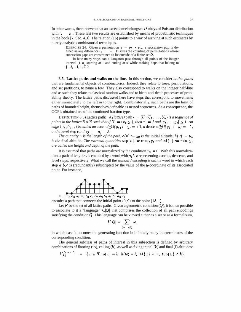
3. APPLICATIONS OF RATIONAL FUNCTIONS 37
In other words, the rare event that an exceedance belongs to�
obeys of Poisson distributionwith - � � � � . These last two results are established by means of probabilistic techniquesin the book [7, Sec. 4.3]. The relation (16) points to a way of arriving at such estimates bypurely analytic-combinatorial techniques.
EXERCISE 24. Given a permutation � -�� ' 46464�� O , a succession gap is de-fined as any difference � � 'cG��� . Discuss the counting of permutations whosesuccession gaps are constrained to lie outside of a finite set
�.
In how many ways can a kangaroo pass through all points of the integerinterval � � � M�� starting at
�and ending at M while making hops that belong to
��G � � G � � � � � � ?
3.5. Lattice paths and walks on the line. In this section, we consider lattice pathsthat are fundamental objects of combinatorics. Indeed, they relate to trees, permutations,and set partitions, to name a few. They also correspond to walks on the integer half-lineand as such they relate to classical random walks and to birth-and-death processes of prob-ability theory. The lattice paths discussed here have steps that correspond to movementseither immediately to the left or to the right. Combinatorially, such paths are the limit ofpaths of bounded height, themselves definable as nested sequences. As a consequence, theOGF’s obtained are of the continued fraction type.
DEFINITION 8.5 (Lattice path). A (lattice) path � � H�� � � � 2 � �,�;� � � � M is a sequence ofpoints in the lattice � � � such that if � 9 � H � 9 � / 9 M , then � 9 � " and � / 9 l 2 � / 9 � � 6 . Anedge � 9 � � 9 l 2 � is called an ascent ( 1 ) if / 9 l 2 � / 9 � 4 6 , a descent ( ? ) if / 9 l 2 � / 9 � ��6 ,and a level step ( � ) if / 9 l 2 � / 9 � 8 .
The quantity h is the length of the path, � H � MDQ � / � is the initial altitude, � H � MDQ � / �is the final altitude. The extremal quantities � "P (�� * Q � %W&<G 9 / 9 and
�,� (�� * Q � % ��� 9 / 9are called the height and depth of the path.
It is assumed that paths are normalized by the condition � � �A8 . With this normaliza-tion, a path of length h is encoded by a word with 1 � ? � � representing ascents, descents, andlevel steps, respectively. What we call the standard encoding is such a word in which eachstep 1 � ? � � is (redundantly) subscripted by the value of the / -coordinate of its associatedpoint. For instance,
$ � � � 1 � 1 2 1 � ? � � � � � 1 � ? � ? � ? 2 1 � � 2encodes a path that connects the initial point HK8 � 8!M to the point H�6�= � 6�M .
Let � be the set of all lattice paths. Given a geometric condition (�
), it is then possibleto associate to it a “language” � � � � that comprises the collection of all path encodingssatisfying the condition
�. This language can be viewed either as a set or as a formal sum,
� � � � � ��� � $
�
in which case it becomes the generating function in infinitely many indeterminates of thecorresponding condition.
The general subclass of paths of interest in this subsection is defined by arbitrarycombinations of flooring ( ), ceiling ( � ), as well as fixing initial H � ) and final ( � ) altitudes:
� E � � ���� � � � ( $ � Q � H $ M�� � � � H $ M�� � � �,� ( $ * � � � "P ( $ * � * �
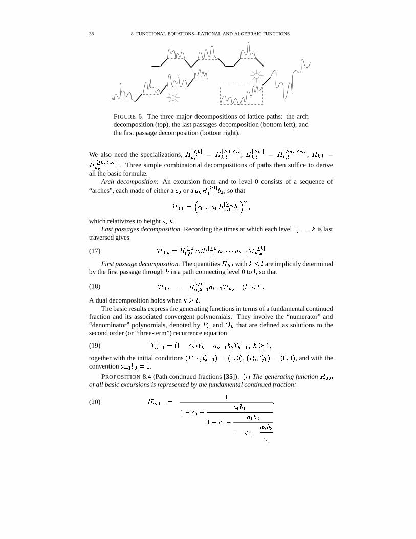
38 8. FUNCTIONAL EQUATIONS—RATIONAL AND ALGEBRAIC FUNCTIONS
FIGURE 6. The three major decompositions of lattice paths: the archdecomposition (top), the last passages decomposition (bottom left), andthe first passage decomposition (bottom right).
We also need the specializations, �� ���� � � � � �� � � ���� � � ,
� E �� � � � � E � �� �� � � ,
� � � � � � � � � �� � � . Three simple combinatorial decompositions of paths then suffice to deriveall the basic formulæ.
Arch decomposition: An excursion from and to level 0 consists of a sequence of“arches”, each made of either a � � or a 1 � � � 2 �2 � 2 ?,2 , so that
� � � � � � � � � 1 � � � 2 �2 � 2 ? 2 � �which relativizes to height � .
Last passages decomposition. Recording the times at which each level 8 � �;�,� � � is lasttraversed gives
(17) � � � � � � � � �� � � 1 � � � 2 �2 � 2 1 2 "$"%"(1 � j 2 � � � �� � �
First passage decomposition. The quantities � � � with
� � � are implicitly determinedby the first passage through
�in a path connecting level 0 to � , so that
(18) � � � � � � �� � �� � � j 2 1 � j 2 � � � � H � � � M �
A dual decomposition holds when� � � .
The basic results express the generating functions in terms of a fundamental continuedfraction and its associated convergent polynomials. They involve the “numerator” and“denominator” polynomials, denoted by � � and
� � that are defined as solutions to thesecond order (or “three-term”) recurrence equation
(19)� � l 2 � H�6�� ��� M � � � 1 � j 2,? � � � j 2 � � � 6 �
together with the initial conditions H � j 2 ��� j 2 M � H�6 � 8!M , H � � ��� � M � HK8 � 6�M , and with theconvention 1 j 2 ? � ��6 .
PROPOSITION 8.4 (Path continued fractions [35]). H���M The generating function � � �
of all basic excursions is represented by the fundamental continued fraction:
� � � � 6
6�� � � � 1 � ?,26�� �;2 � 1>2,? �
6�� � � � 1 � ? �. . .
�(20)
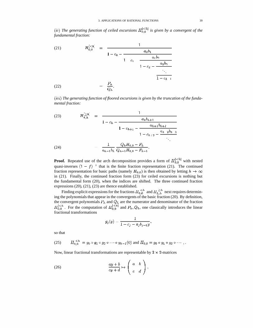
3. APPLICATIONS OF RATIONAL FUNCTIONS 39
H�����M The generating function of ceiled excursions �� ���� � � is given by a convergent of the
fundamental fraction:
�� ���� � � � 6
6�� � � � 1 � ?;26�� �;2 � 132 ? �
6�� � � � 1 � ? �. . .
6�� ��� j 2
(21)
� � �� � �(22)
H�������M The generating function of floored excursions is given by the truncation of the funda-mental fraction:
� ���� � � � 6
6�� ��� � 1 � ? � l 26�� � � l 2 � 1 � l 2,? � l �
6�� ��� l � � 1 � l � ? � l �. . .
(23)
� 61�� j 2 ? �
� � � � � � � �� � j 2 � � � � � � j 2�
(24)
Proof. Repeated use of the arch decomposition provides a form of �� ���� � � with nested
quasi-inverses H�6 � � M j 2 that is the finite fraction representation (21). The continuedfraction representation for basic paths (namely
� � � ) is then obtained by letting � � in (21). Finally, the continued fraction form (23) for ceiled excursions is nothing butthe fundamental form (20), when the indices are shifted. The three continued fractionexpressions (20), (21), (23) are thence established.
Finding explicit expressions for the fractions �� ���� � � and
� ���� � � next requires determin-ing the polynomials that appear in the convergents of the basic fraction (20). By definition,the convergent polynomials � � and
� � are the numerator and denominator of the fraction �� ���� � � . For the computation of
�� ���� � � and � � ��� � , one classically introduces the linear
fractional transformations � 9 H / M�� 66�� � 9 � 1 9 ? 9 l 2-/
�
so that
(25) �� � �� � � � � � ! � 2 ! � � ! "$"%" ! � � j 2 HK82M and
� � � � � � ! � 2 ! � � ! "$"%" � �Now, linear fractional transformations are representable by
/ � /-matrices
(26)1 /�4 ?�-/54 <
�� �� 1 ?� <
�� �
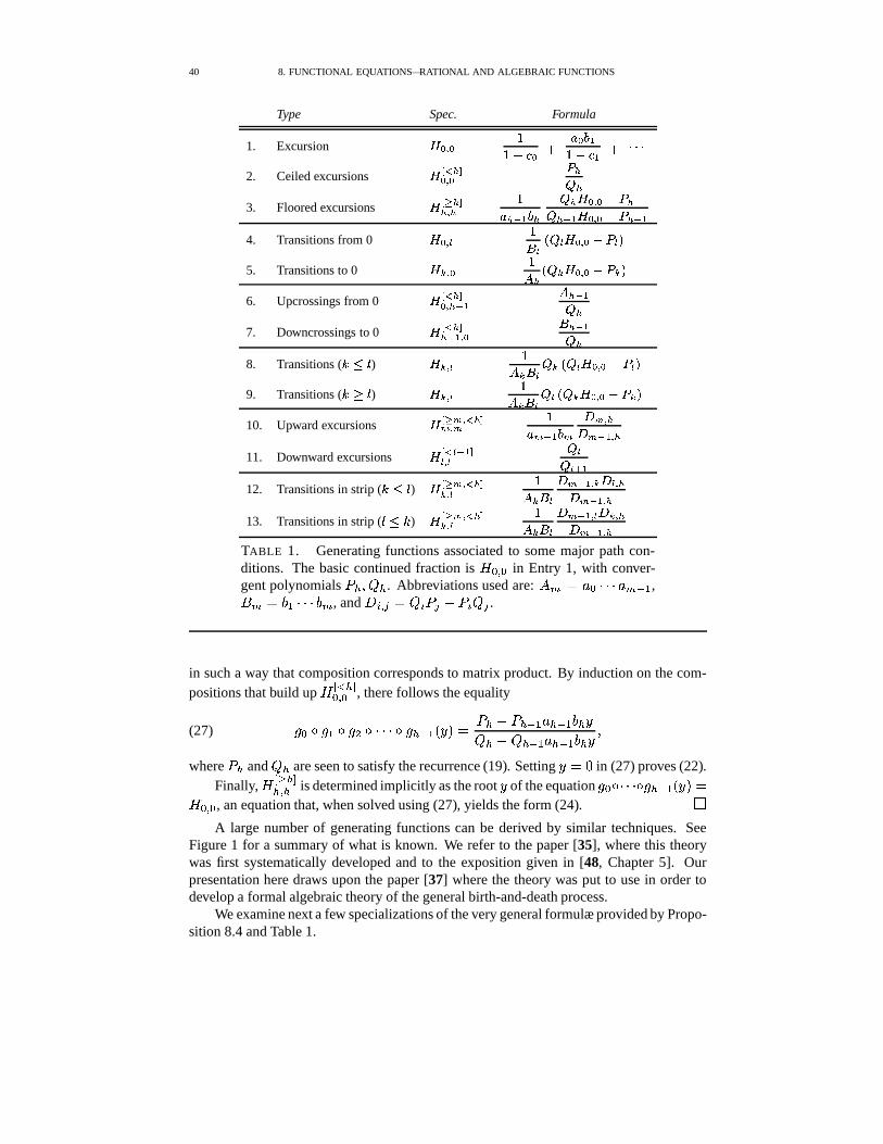
40 8. FUNCTIONAL EQUATIONS—RATIONAL AND ALGEBRAIC FUNCTIONS
Type Spec. Formula
1. Excursion � � % � �� G � + ��� '� G ' + 4464
2. Ceiled excursions � � ���'�� % � � �� �
3. Floored excursions � � � �'�� % � � � � ' � � � � � � % � G � �
� � � ' � � % � G � � � '4. Transitions from 0 � � % � �� � � � � � � % � G � � �5. Transitions to 0 � _ % � �
� _ � � _ � � % � G � _ �6. Upcrossings from 0 � � ���'�� % � � ' � � � '� �
7. Downcrossings to 0 � � ���'�� � ' % � � � � '
� �
8. Transitions (���
) � _ % � �� _ � � � _ � � � � � % � G � � �
9. Transitions (� � ) � _ % � �
� _ � � � � � � _ � � % � G � _ �10. Upward excursions � � ��K % ���'�K % K � K�� ' �K � K % �
� K�� ' % �11. Downward excursions � � � � � ' �� % � � �
� � � '12. Transitions in strip (
� ��) � � ��K % ���'�_ % � �
� _ � �� K�� ' % _ � � % �� K�� ' % �
13. Transitions in strip (�� �
) � � ��K % ���'�_ % � �� _ � �
� K�� ' % � � _ % �� K�� ' % �TABLE 1. Generating functions associated to some major path con-ditions. The basic continued fraction is
� � � in Entry 1, with conver-gent polynomials ��� ��� � . Abbreviations used are: ��E � 1 � "$"%"(1 E j 2 ,�:E � ?,2 "$"%" ?-E , and
� � � 9 � � � � 9 � � � � 9 .
in such a way that composition corresponds to matrix product. By induction on the com-positions that build up
�� ���� � � , there follows the equality
(27) � � ! � 2 ! � � ! "$"%" ! � � j 2 H / M7� � � � � � j 2 1 � j 2 ? � /� � � � � j 2 1 � j 2,? � /�
where � � and� � are seen to satisfy the recurrence (19). Setting / � 8 in (27) proves (22).
Finally, � ���� � � is determined implicitly as the root / of the equation � � ! "%"$" ! ��� j 2 H / M7�
� � � , an equation that, when solved using (27), yields the form (24). �A large number of generating functions can be derived by similar techniques. See
Figure 1 for a summary of what is known. We refer to the paper [35], where this theorywas first systematically developed and to the exposition given in [48, Chapter 5]. Ourpresentation here draws upon the paper [37] where the theory was put to use in order todevelop a formal algebraic theory of the general birth-and-death process.
We examine next a few specializations of the very general formulæ provided by Propo-sition 8.4 and Table 1.
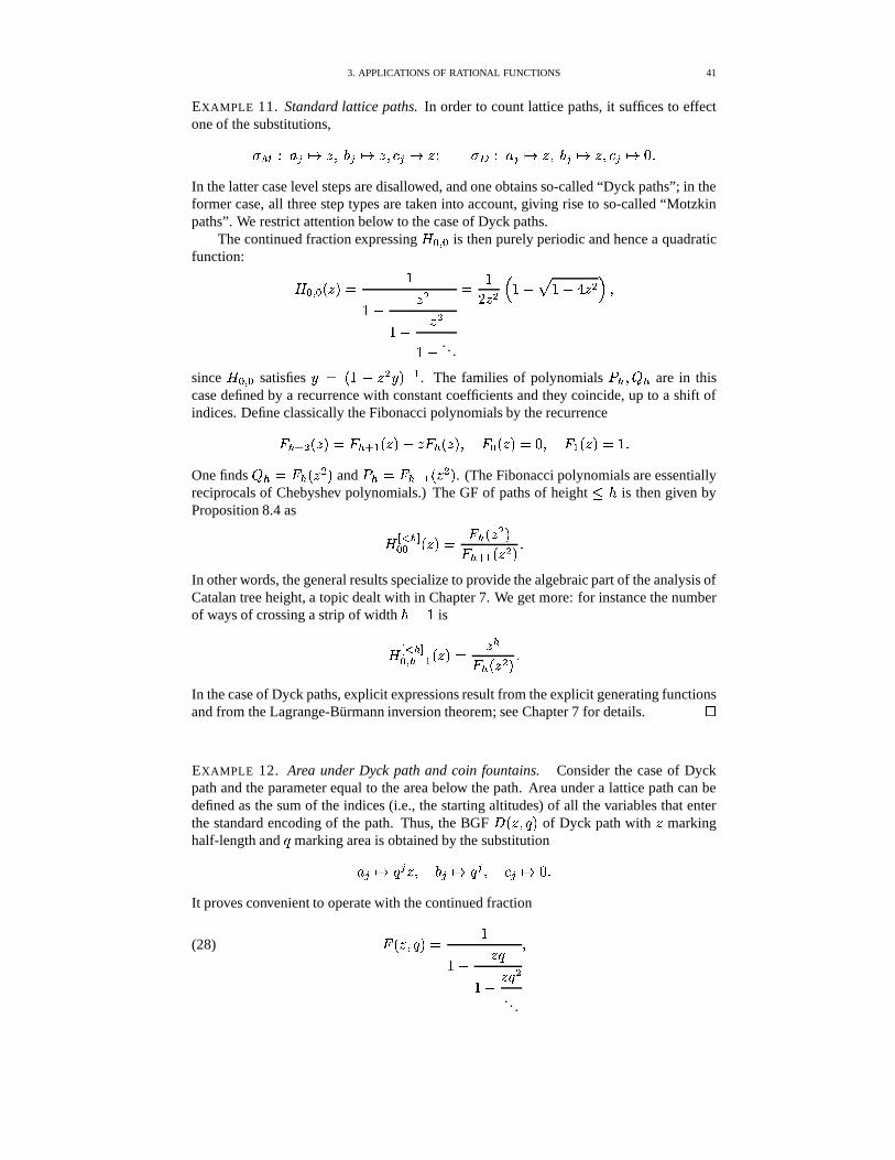
3. APPLICATIONS OF RATIONAL FUNCTIONS 41
EXAMPLE 11. Standard lattice paths. In order to count lattice paths, it suffices to effectone of the substitutions,��� Q 1 9 �� � � ? 9 �� � � � 9 �� � � ��� Q 1 9 �� � � ? 9 �� � � � 9 �� 8 �In the latter case level steps are disallowed, and one obtains so-called “Dyck paths”; in theformer case, all three step types are taken into account, giving rise to so-called “Motzkinpaths”. We restrict attention below to the case of Dyck paths.
The continued fraction expressing � � � is then purely periodic and hence a quadratic
function:
� � � H � M7� 6
6�� � �6�� � �
6�� . . .
� 6/ � � � 6���� 6�� � � � �
since � � � satisfies / � H�6 � � � / M j 2 . The families of polynomials � � ��� � are in this
case defined by a recurrence with constant coefficients and they coincide, up to a shift ofindices. Define classically the Fibonacci polynomials by the recurrence
! � l � H � M7� ! � l 2 H � M � � ! � H � M � ! � H � M7� 8 � ! 2 H � M7��6 �One finds
� � � ! � H � � M and � � � ! � j 2 H � � M . (The Fibonacci polynomials are essentiallyreciprocals of Chebyshev polynomials.) The GF of paths of height � � is then given byProposition 8.4 as
�� ����"� H � M7� ! � H � � M! � l 2 H � � M �
In other words, the general results specialize to provide the algebraic part of the analysis ofCatalan tree height, a topic dealt with in Chapter 7. We get more: for instance the numberof ways of crossing a strip of width � � 6 is
�� ���� � � j 2 H � M7� � �! � H � � M �
In the case of Dyck paths, explicit expressions result from the explicit generating functionsand from the Lagrange-Burmann inversion theorem; see Chapter 7 for details.
�
EXAMPLE 12. Area under Dyck path and coin fountains. Consider the case of Dyckpath and the parameter equal to the area below the path. Area under a lattice path can bedefined as the sum of the indices (i.e., the starting altitudes) of all the variables that enterthe standard encoding of the path. Thus, the BGF
� H � � M of Dyck path with � markinghalf-length and marking area is obtained by the substitution
1 9 �� 9 � � ? 9 �� 9 � � 9 �� 8 �It proves convenient to operate with the continued fraction
(28)! H � � M7� 6
6�� �� 6�� � �
. . .
�
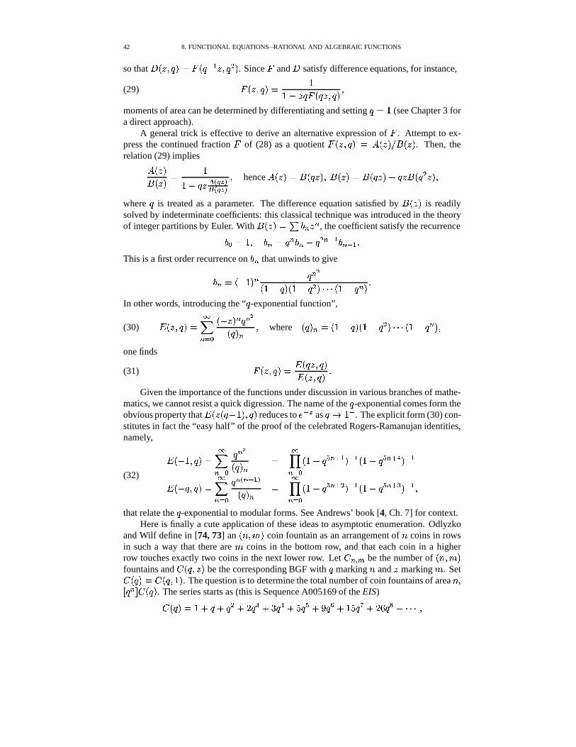
42 8. FUNCTIONAL EQUATIONS—RATIONAL AND ALGEBRAIC FUNCTIONS
so that� H � � M7� ! H j 2 � � � M . Since
!and
�satisfy difference equations, for instance,
(29)! H � � M7� 6
6�� �� ! H �� � M �moments of area can be determined by differentiating and setting � 6 (see Chapter 3 fora direct approach).
A general trick is effective to derive an alternative expression of!
. Attempt to ex-press the continued fraction
!of (28) as a quotient
! H � � M � � H � M =�� H � M . Then, therelation (29) implies
� H � M� H � M � 6
6�� ���� ��
� �� �hence � H � M7� � H �� M � � H � M7� � H �� M � ���� H � � M �
where is treated as a parameter. The difference equation satisfied by � H � M is readilysolved by indeterminate coefficients: this classical technique was introduced in the theoryof integer partitions by Euler. With � H � M7� � ? � � �
, the coefficient satisfy the recurrence
? � � 6 � ? � � � ? � � � �Pj 2 ? �Pj 2��This is a first order recurrence on ? � that unwinds to give
? � � H ��6�M � � �H 6�� M�H�6�� � M "%"%" H�6 � � M �
In other words, introducing the “ -exponential function”,
(30) � H � � M7� �� ���
H � � M � � �H M � �
where H M � � H 6�� M�H�6 � � M "%"%" H�6�� � M �one finds
(31)! H � � M7� � H �� � M� H � � M �
Given the importance of the functions under discussion in various branches of mathe-matics, we cannot resist a quick digression. The name of the -exponential comes form theobvious property that � H � H �'6�M � M reduces to � j as � 6 j . The explicit form (30) con-stitutes in fact the “easy half” of the proof of the celebrated Rogers-Ramanujan identities,namely,
(32)
� H ��6 � M7� �� ���
� �H M � � �
� ���H�6 � �al 2 M j 2 H�6�� �ml � M j 2
� H � � M7� ������
� � �ml 2 H M � � �
� ���H�6 � �al � M j 2 H�6�� �ml � M j 2 �
that relate the -exponential to modular forms. See Andrews’ book [4, Ch. 7] for context.Here is finally a cute application of these ideas to asymptotic enumeration. Odlyzko
and Wilf define in [74, 73] an H h � M coin fountain as an arrangement of h coins in rowsin such a way that there are coins in the bottom row, and that each coin in a higherrow touches exactly two coins in the next lower row. Let
� � E be the number of H h � Mfountains and
H � � M be the corresponding BGF with marking h and � marking . Set H M0� H � 6�M . The question is to determine the total number of coin fountains of area h ,� � � H M . The series starts as (this is Sequence A005169 of the EIS) H M���6 4 4 � 4 / � 4 = ���4 9 4 T � 4 6N9 � 4 / U ��4 "%"$" �
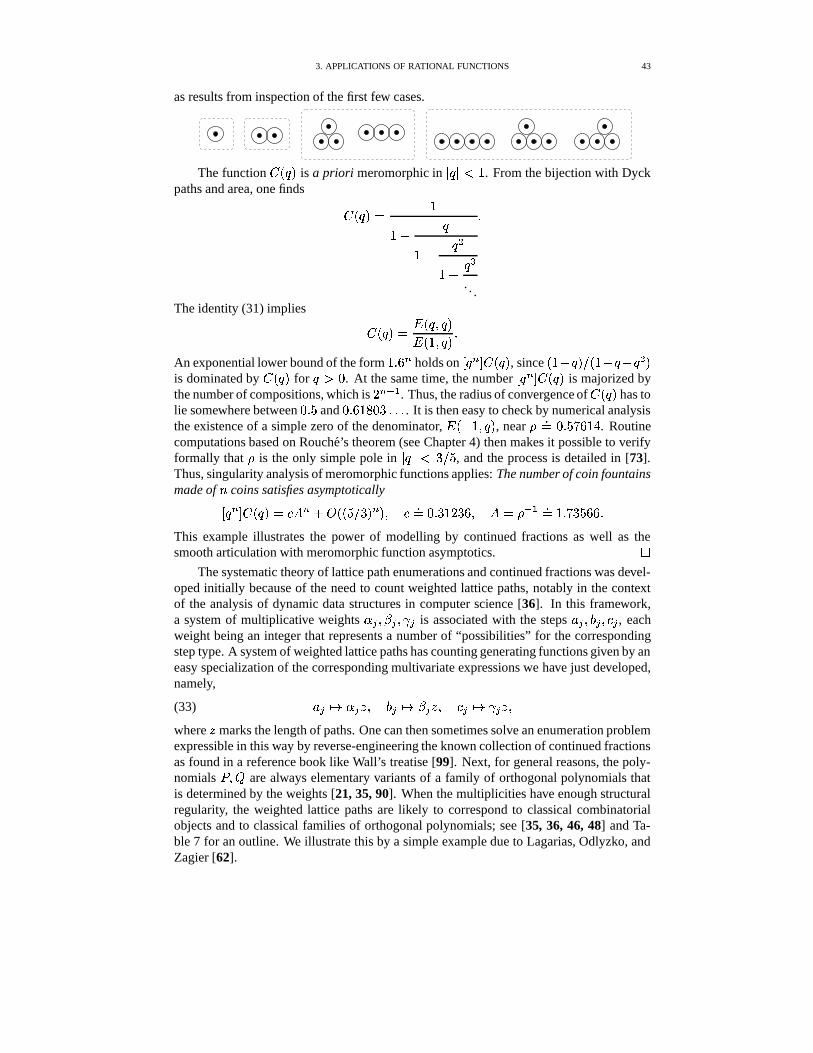
3. APPLICATIONS OF RATIONAL FUNCTIONS 43
as results from inspection of the first few cases.
The function H M is a priori meromorphic in � � 6 . From the bijection with Dyck
paths and area, one finds H M�� 6
6�� 6 � �
6�� �. . .
�
The identity (31) implies H M�� � H � M� H�6 � M �An exponential lower bound of the form 6 � U � holds on � � � H M , since H�6 � M = H�6 � � � Mis dominated by
H M for � 8 . At the same time, the number � � � H M is majorized bythe number of compositions, which is
/ �Pj 2 . Thus, the radius of convergence of H M has to
lie somewhere between 8 � 9 and 8 � U�6�;#8!= �,�;� . It is then easy to check by numerical analysisthe existence of a simple zero of the denominator, � H ��6 � M , near � �� 8 � 92:<U"6 � . Routinecomputations based on Rouche’s theorem (see Chapter 4) then makes it possible to verifyformally that � is the only simple pole in � � = = 9 , and the process is detailed in [73].Thus, singularity analysis of meromorphic functions applies: The number of coin fountainsmade of h coins satisfies asymptotically
� � � H M0� � � � 4� H HS9 = =!M � M � � ��A8 � ="6 / =#U � � � � j 2 ���6 � :<=29.U#U �This example illustrates the power of modelling by continued fractions as well as thesmooth articulation with meromorphic function asymptotics.
�The systematic theory of lattice path enumerations and continued fractions was devel-
oped initially because of the need to count weighted lattice paths, notably in the contextof the analysis of dynamic data structures in computer science [36]. In this framework,a system of multiplicative weights � 9 � � 9 � � 9 is associated with the steps 1 9 � ? 9 � � 9 , eachweight being an integer that represents a number of “possibilities” for the correspondingstep type. A system of weighted lattice paths has counting generating functions given by aneasy specialization of the corresponding multivariate expressions we have just developed,namely,
(33) 1 9 �� � 9 � � ? 9 �� � 9 � � � 9 �� � 9 � �where � marks the length of paths. One can then sometimes solve an enumeration problemexpressible in this way by reverse-engineering the known collection of continued fractionsas found in a reference book like Wall’s treatise [99]. Next, for general reasons, the poly-nomials � ���
are always elementary variants of a family of orthogonal polynomials thatis determined by the weights [21, 35, 90]. When the multiplicities have enough structuralregularity, the weighted lattice paths are likely to correspond to classical combinatorialobjects and to classical families of orthogonal polynomials; see [35, 36, 46, 48] and Ta-ble 7 for an outline. We illustrate this by a simple example due to Lagarias, Odlyzko, andZagier [62].
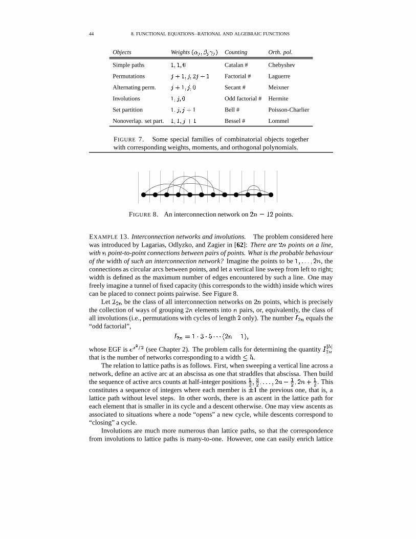
44 8. FUNCTIONAL EQUATIONS—RATIONAL AND ALGEBRAIC FUNCTIONS
Objects Weights �ZR � � ` ����� � Counting Orth. pol.
Simple paths� � � � / Catalan # Chebyshev
Permutations ��+ � � � � � ��+ �Factorial # Laguerre
Alternating perm. ��+ � � � � / Secant # Meixner
Involutions� � � � / Odd factorial # Hermite
Set partition� � � � ��+ �
Bell # Poisson-Charlier
Nonoverlap. set part.� � � � ��+ �
Bessel # Lommel
FIGURE 7. Some special families of combinatorial objects togetherwith corresponding weights, moments, and orthogonal polynomials.
FIGURE 8. An interconnection network on/ h � 6 / points.
EXAMPLE 13. Interconnection networks and involutions. The problem considered herewas introduced by Lagarias, Odlyzko, and Zagier in [62]: There are
/ h points on a line,with h point-to-point connections between pairs of points. What is the probable behaviourof the width of such an interconnection network? Imagine the points to be 6 � �,�;� � / h , theconnections as circular arcs between points, and let a vertical line sweep from left to right;width is defined as the maximum number of edges encountered by such a line. One mayfreely imagine a tunnel of fixed capacity (this corresponds to the width) inside which wirescan be placed to connect points pairwise. See Figure 8.
Let � � � be the class of all interconnection networks on/ h points, which is precisely
the collection of ways of grouping/ h elements into h pairs, or, equivalently, the class of
all involutions (i.e., permutations with cycles of length/
only). The number � � � equals the“odd factorial”,
� � � � 6 " = " 9 "%"$" H / h � 6NM �whose EGF is � � ��� (see Chapter 2). The problem calls for determining the quantity � � ���� �that is the number of networks corresponding to a width � � .
The relation to lattice paths is as follows. First, when sweeping a vertical line across anetwork, define an active arc at an abscissa as one that straddles that abscissa. Then buildthe sequence of active arcs counts at half-integer positions 2� � �� � �;�,� � / h � 2� � / h 4 2� . Thisconstitutes a sequence of integers where each member is � 6 the previous one, that is, alattice path without level steps. In other words, there is an ascent in the lattice path foreach element that is smaller in its cycle and a descent otherwise. One may view ascents asassociated to situations where a node “opens” a new cycle, while descents correspond to“closing” a cycle.
Involutions are much more numerous than lattice paths, so that the correspondencefrom involutions to lattice paths is many-to-one. However, one can easily enrich lattice
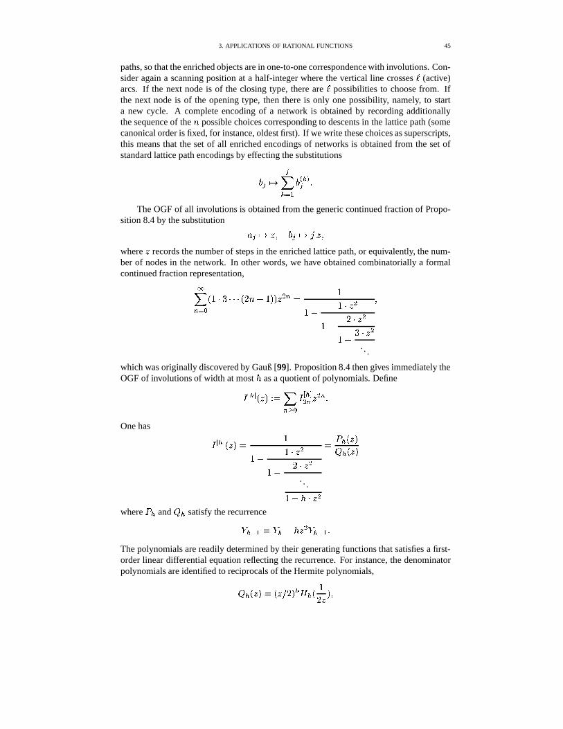
3. APPLICATIONS OF RATIONAL FUNCTIONS 45
paths, so that the enriched objects are in one-to-one correspondence with involutions. Con-sider again a scanning position at a half-integer where the vertical line crosses � (active)arcs. If the next node is of the closing type, there are � possibilities to choose from. Ifthe next node is of the opening type, then there is only one possibility, namely, to starta new cycle. A complete encoding of a network is obtained by recording additionallythe sequence of the h possible choices corresponding to descents in the lattice path (somecanonical order is fixed, for instance, oldest first). If we write these choices as superscripts,this means that the set of all enriched encodings of networks is obtained from the set ofstandard lattice path encodings by effecting the substitutions
? 9 �� 9� � 2 ? � � 9 �
The OGF of all involutions is obtained from the generic continued fraction of Propo-sition 8.4 by the substitution
1 9 �� � � ? 9 �� " � �where � records the number of steps in the enriched lattice path, or equivalently, the num-ber of nodes in the network. In other words, we have obtained combinatorially a formalcontinued fraction representation,
�� ���
H�6 " = "%"$" H / h � 6�M M � � � � 6
6�� 6 " � �6��
/ ",� �6�� = ";� �
. . .
�
which was originally discovered by Gauß [99]. Proposition 8.4 then gives immediately theOGF of involutions of width at most � as a quotient of polynomials. Define
� � ��� H � M Q � �� � � � ���� � � � � �
One has
� � ��� H � M7� 6
6�� 6 ",� �6�� / ";� �
. . .6 � � ",� �
� � � H � M� � H � M
where � � and� � satisfy the recurrence
� � l 2 � � � � � � � � � j 2��The polynomials are readily determined by their generating functions that satisfies a first-order linear differential equation reflecting the recurrence. For instance, the denominatorpolynomials are identified to reciprocals of the Hermite polynomials,
� � H � M7� H �>= / M � � H 6/ � M�
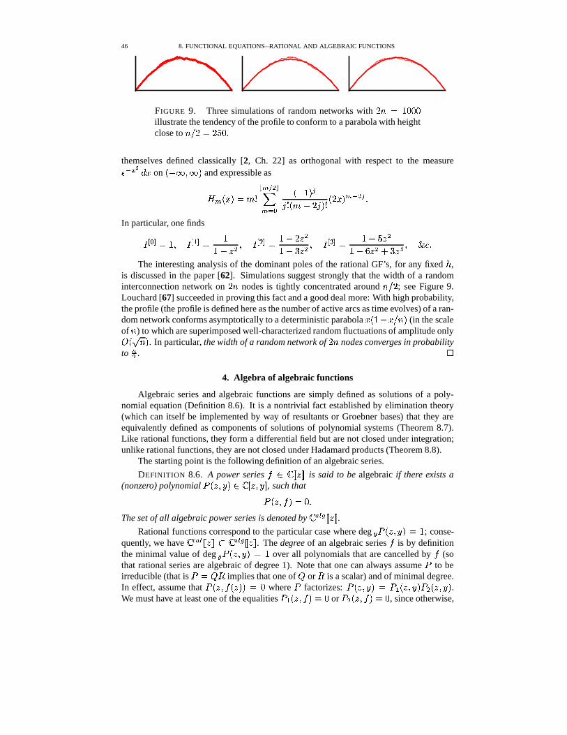
46 8. FUNCTIONAL EQUATIONS—RATIONAL AND ALGEBRAIC FUNCTIONS
0
20
40
60
80
100
120
140
160
180
200
220
240
260
200 400 600 800 1000
x
0
20
40
60
80
100
120
140
160
180
200
220
240
260
200 400 600 800 1000
x
0
20
40
60
80
100
120
140
160
180
200
220
240
200 400 600 800 1000
x
FIGURE 9. Three simulations of random networks with/ h � 6�8#8!8
illustrate the tendency of the profile to conform to a parabola with heightclose to h = / � / 9.8 .
themselves defined classically [2, Ch. 22] as orthogonal with respect to the measure� j�� � < � on H � � M and expressible as
E H � M�� � � E �����E �.�
H ��6�M 9" � H � / "2M�� H / � M E j � 9 �
In particular, one finds
� � � � ��6 � � � 2 � � 66�� � �
� � � � � � 6�� / � �6�� = � �
� � � � � � 6�� 9 � �6�� U � � 4 = � � ��� ���
The interesting analysis of the dominant poles of the rational GF’s, for any fixed � ,is discussed in the paper [62]. Simulations suggest strongly that the width of a randominterconnection network on
/ h nodes is tightly concentrated around h = / ; see Figure 9.Louchard [67] succeeded in proving this fact and a good deal more: With high probability,the profile (the profile is defined here as the number of active arcs as time evolves) of a ran-dom network conforms asymptotically to a deterministic parabola � H�6 � � = h M (in the scaleof h ) to which are superimposed well-characterized random fluctuations of amplitude only H � h M . In particular, the width of a random network of
/ h nodes converges in probabilityto
� � .�
4. Algebra of algebraic functions
Algebraic series and algebraic functions are simply defined as solutions of a poly-nomial equation (Definition 8.6). It is a nontrivial fact established by elimination theory(which can itself be implemented by way of resultants or Groebner bases) that they areequivalently defined as components of solutions of polynomial systems (Theorem 8.7).Like rational functions, they form a differential field but are not closed under integration;unlike rational functions, they are not closed under Hadamard products (Theorem 8.8).
The starting point is the following definition of an algebraic series.
DEFINITION 8.6. A power series� � ��� � ��� � is said to be algebraic if there exists a
(nonzero) polynomial � H � � / M � ��� � � / � , such that
� H � �"� M�� 8 �The set of all algebraic power series is denoted by � a
��� � � ��� � .Rational functions correspond to the particular case where deg -� H � � / MA� 6 ; conse-
quently, we have � r / � � � ��� ��$ � a��� � � ��� � . The degree of an algebraic series
�is by definition
the minimal value of deg � H � � / M � 6 over all polynomials that are cancelled by�
(sothat rational series are algebraic of degree 1). Note that one can always assume � to beirreducible (that is � � � implies that one of
�or is a scalar) and of minimal degree.
In effect, assume that � H � �"� H � M M � 8 where � factorizes: � H � � / M�� � 2 H � � / M � � H � � / M .We must have at least one of the equalities � 2 H � � � M � 8 or � � H � � � M��A8 , since otherwise,
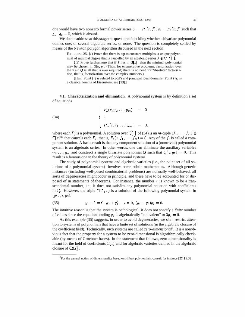
4. ALGEBRA OF ALGEBRAIC FUNCTIONS 47
one would have two nonzero formal power series �>2 � ��2 H � � � M , � � � � � H � �"� M such that� 2 " � � �A8 , which is absurd.We do not address at this stage the question of deciding whether a bivariate polynomial
defines one, or several algebraic series, or none. The question is completely settled bymeans of the Newton polygon algorithm discussed in the next section.
EXERCISE 25. � � � Prove that there is, up to constant multiples, a unique polyno-mial of minimal degree that is cancelled by an algebraic series # ��� #21 3 � � ��� � .� � � � Prove furthermore that if # lies in W � � ��� � , then the minimal polynomialmay be chosen in W � � � )�� . (Thus, for enumerative problems, factorization overthe field W is all that is ever required; there is no need for “absolute” factoriza-tion, that is, factorization over the complex numbers.)
[Hint. Point � � � is related to gcd’s and principal ideal domains. Point � � � � isa classical lemma of Eisenstein; see [13].]
4.1. Characterization and elimination. A polynomial system is by definition a setof equations
(34)
��������� ��2 H � � / 2 � �;�,� � /�E M � 8
...
� E H � � / 2 � �,�,� � /�E M � 8 �where each � 9 is a polynomial. A solution over ��� � ��� � of (34) is an -tuple H � 2 � �;�,� � � E M ���� � ��� � E that cancels each � 9 , that is, � 9 H � �"� 2 � �;�,� � � E M7�A8 . Any of the
� 9 is called a com-ponent solution. A basic result is that any component solution of a (nontrivial) polynomialsystem is an algebraic series. In other words, one can eliminate the auxiliary variables/ � � �,�;� � /#E and construct a single bivariate polynomial
�such that
� H � � /32 M � 8 . Thisresult is a famous one in the theory of polynomial systems.
The study of polynomial systems and algebraic varieties (i.e., the point set of all so-lutions of a polynomial system) involves some subtle mathematics. Although genericinstances (including well-posed combinatorial problems) are normally well-behaved, allsorts of degeneracies might occur in principle, and these have to be accounted for or dis-posed of in statements of theorems. For instance, the number � is known to be a tran-scendental number, i.e., it does not satisfies any polynomial equation with coefficientsin � . However, the triple H�6 � 6 � � M is a solution of the following polynomial system inH / 2 � / � � / � M :(35) / 2 � 6:� 8 � / � 46/ �2 � / �A8 � H / 2 � / � M / � �A8 �The intuitive reason is that the system is pathological: it does not specify a finite numberof values since the equation binding / � is algebraically “equivalent” to 8 / � � 8 .
As this example (35) suggests, in order to avoid degeneracies, we shall restrict atten-tion to systems of polynomials that have a finite set of solutions (in the algebraic closure ofthe coefficient field). Technically, such systems are called zero-dimensional5. It is a nonob-vious fact that the property for a system to be zero-dimensional is algorithmically check-able (by means of Groebner bases). In the statement that follows, zero-dimensionality ismeant for the field of coefficients � H � M and for algebraic varieties defined in the algebraicclosure of � H H � M M .
5For the general notion of dimensionality based on Hilbert polynomials, consult for instance [27, � 9.3].
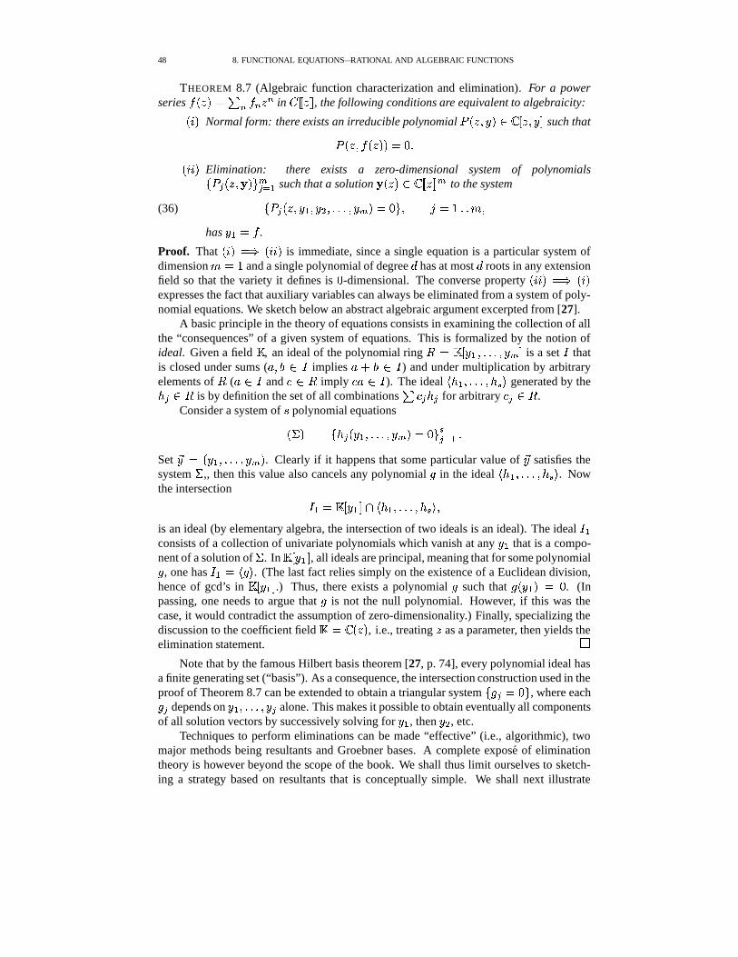
48 8. FUNCTIONAL EQUATIONS—RATIONAL AND ALGEBRAIC FUNCTIONS
THEOREM 8.7 (Algebraic function characterization and elimination). For a powerseries
� H � M7� � � � � � �in
� � � � � , the following conditions are equivalent to algebraicity:H���M Normal form: there exists an irreducible polynomial � H � � / M � ��� � � / � such that
� H � �"� H � M M � 8 �H�� ��M Elimination: there exists a zero-dimensional system of polynomials
( � 9 H � ��� M * E9 � 2 such that a solution� H � M � �&� � � � � E to the system
(36) ( � 9 H � � / 2 � / � � �;�,� � /�E M7�A8 * � " ��6 �,� �has / 2 � �
.
Proof. That H���M ��� H�����M is immediate, since a single equation is a particular system ofdimension ��6 and a single polynomial of degree < has at most < roots in any extensionfield so that the variety it defines is 8 -dimensional. The converse property H�����M ��� H���Mexpresses the fact that auxiliary variables can always be eliminated from a system of poly-nomial equations. We sketch below an abstract algebraic argument excerpted from [27].
A basic principle in the theory of equations consists in examining the collection of allthe “consequences” of a given system of equations. This is formalized by the notion ofideal. Given a field � , an ideal of the polynomial ring � ��� /32 � �,�,� � /�EA� is a set � thatis closed under sums ( 1 � ? � � implies 1 4 ? � � ) and under multiplication by arbitraryelements of ( 1 � � and � � imply � 1 � � ). The ideal ��2 � �,�,� � � �
� generated by the� 9 � is by definition the set of all combinations
� � 9 � 9 for arbitrary � 9 � .Consider a system of � polynomial equations
H D M (�� 9 H / 2 � �;�,� � /�E M7� 8 * �9 � 2 �Set �/ � H / 2 � �;�,� � /�E M . Clearly if it happens that some particular value of �/ satisfies thesystem D ,, then this value also cancels any polynomial � in the ideal � 2 � �,�;� � � �
� . Nowthe intersection
� 2 � ��� / 2 � � 2 � �;�,� � � �� �
is an ideal (by elementary algebra, the intersection of two ideals is an ideal). The ideal � 2consists of a collection of univariate polynomials which vanish at any /32 that is a compo-nent of a solution of D . In ��� />2 � , all ideals are principal, meaning that for some polynomial� , one has � 2 � � � . (The last fact relies simply on the existence of a Euclidean division,hence of gcd’s in ��� / 2 � .) Thus, there exists a polynomial � such that � H />2 M � 8 . (Inpassing, one needs to argue that � is not the null polynomial. However, if this was thecase, it would contradict the assumption of zero-dimensionality.) Finally, specializing thediscussion to the coefficient field � � � H � M , i.e., treating � as a parameter, then yields theelimination statement. �
Note that by the famous Hilbert basis theorem [27, p. 74], every polynomial ideal hasa finite generating set (“basis”). As a consequence, the intersection construction used in theproof of Theorem 8.7 can be extended to obtain a triangular system ( � 9 � 8 * , where each� 9 depends on / 2 � �,�;� � / 9 alone. This makes it possible to obtain eventually all componentsof all solution vectors by successively solving for / 2 , then / � , etc.
Techniques to perform eliminations can be made “effective” (i.e., algorithmic), twomajor methods being resultants and Groebner bases. A complete expose of eliminationtheory is however beyond the scope of the book. We shall thus limit ourselves to sketch-ing a strategy based on resultants that is conceptually simple. We shall next illustrate
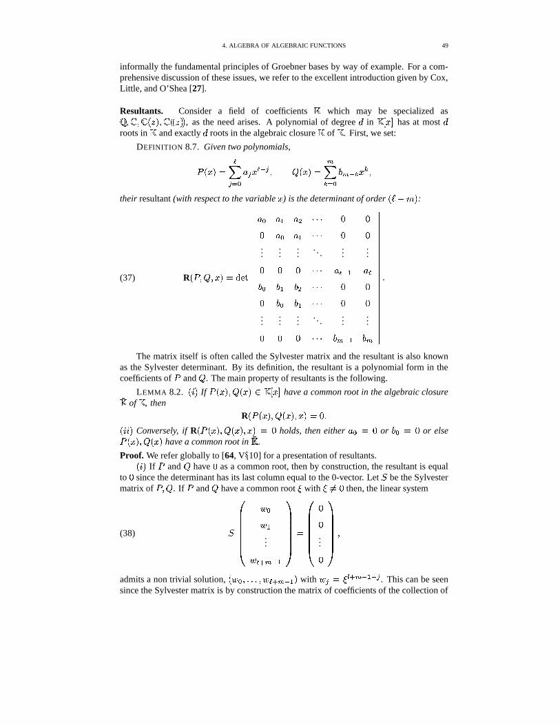
4. ALGEBRA OF ALGEBRAIC FUNCTIONS 49
informally the fundamental principles of Groebner bases by way of example. For a com-prehensive discussion of these issues, we refer to the excellent introduction given by Cox,Little, and O’Shea [27].
Resultants. Consider a field of coefficients � which may be specialized as� � � � � H � M � � H H � M M , as the need arises. A polynomial of degree < in �:� � � has at most <roots in � and exactly < roots in the algebraic closure
�� of � . First, we set:
DEFINITION 8.7. Given two polynomials,
� H � M�� �9 ��� 1 9 � � j 9 � � H � M�� E
� ��� ?-E j � � � �
their resultant (with respect to the variable � ) is the determinant of order H �74 M :
(37) R H � ��� � � M�� �� �
������������������������
1 � 1 2 1 � "$"%" 8 88 1 � 1 2 "$"%" 8 8...
......
. . ....
...8 8 8 "$"%" 1 � j 2 1 �? � ?;2 ? � "$"%" 8 88 ? � ?,2 "$"%" 8 8...
......
. . ....
...8 8 8 "$"%" ?-E j 2 ?-E
������������������������
�
The matrix itself is often called the Sylvester matrix and the resultant is also knownas the Sylvester determinant. By its definition, the resultant is a polynomial form in thecoefficients of � and
�. The main property of resultants is the following.
LEMMA 8.2. H���M If � H � M ��� H � M � ��� �3� have a common root in the algebraic closure�� of � , then
R H � H � M ��� H � M � � M�� 8 �H�����M Conversely, if R H � H � M ��� H � M � � M � 8 holds, then either 1 � � 8 or ? � � 8 or else� H � M ��� H � M have a common root in
�� .
Proof. We refer globally to [64, V�10] for a presentation of resultants.H���M If � and
�have 8 as a common root, then by construction, the resultant is equal
to 8 since the determinant has its last column equal to the 0-vector. Let�
be the Sylvestermatrix of � ���
. If � and�
have a common root � with � �� 8 then, the linear system
(38)�
�������� $ �$ 2...
$ � l E j 2
��������� �
��������88...8
��������� �
admits a non trivial solution, H $ � � �,�,� � $ � l E j 2 M with $ 9 � �� l E j 2 j 9
. This can be seensince the Sylvester matrix is by construction the matrix of coefficients of the collection of
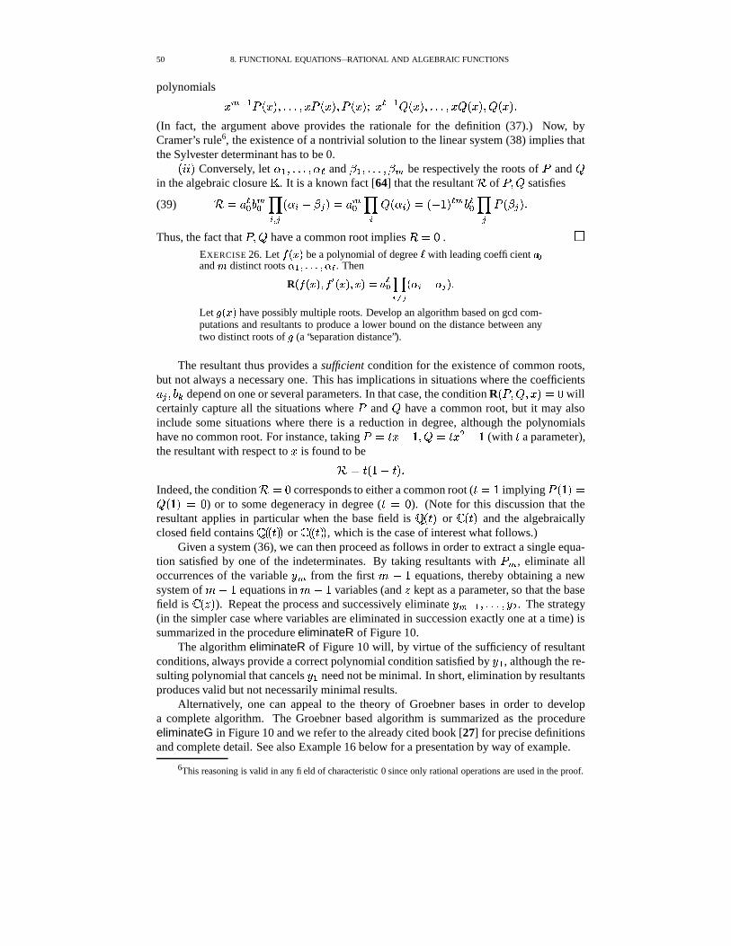
50 8. FUNCTIONAL EQUATIONS—RATIONAL AND ALGEBRAIC FUNCTIONS
polynomials � E j 2 � H � M � �;�,� � � � H � M � � H � M � � � j 2 � H � M � �,�;� � � � H � M ��� H � M �(In fact, the argument above provides the rationale for the definition (37).) Now, byCramer’s rule6, the existence of a nontrivial solution to the linear system (38) implies thatthe Sylvester determinant has to be 0.H�����M Conversely, let � 2 � �;�,� � � � and � 2 � �,�;� � � E be respectively the roots of � and
�in the algebraic closure
�� . It is a known fact [64] that the resultant � of � ���
satisfies
(39) � � 1 � � ? E� � � 9 H � � � � 9 M7� 1 E� � � H � � M�� H ��6NM � E ? � � 9 � H � 9 M �Thus, the fact that � ���
have a common root implies � 8 . �EXERCISE 26. Let # � ��� be a polynomial of degree � with leading coefficient �and L distinct roots R ' ����6� R � . Then
R � # � ��� � # � � ��� � ���.- � �����a� �ZR GJR � � Let � � ��� have possibly multiple roots. Develop an algorithm based on gcd com-putations and resultants to produce a lower bound on the distance between anytwo distinct roots of � (a “separation distance”).
The resultant thus provides a sufficient condition for the existence of common roots,but not always a necessary one. This has implications in situations where the coefficients1 9 � ? � depend on one or several parameters. In that case, the condition R H � ��� � � M�� 8 willcertainly capture all the situations where � and
�have a common root, but it may also
include some situations where there is a reduction in degree, although the polynomialshave no common root. For instance, taking � ��� � � 6 ��� ��� � � � 6 (with � a parameter),the resultant with respect to � is found to be
� ���-H�6 ��� M �Indeed, the condition � �A8 corresponds to either a common root ( ����6 implying � H 6�M7�� H 6�M � 8 ) or to some degeneracy in degree ( � � 8 ). (Note for this discussion that theresultant applies in particular when the base field is � H�� M or � H� M and the algebraicallyclosed field contains � H H� M M or � H H�� M M , which is the case of interest what follows.)
Given a system (36), we can then proceed as follows in order to extract a single equa-tion satisfied by one of the indeterminates. By taking resultants with ��E , eliminate alloccurrences of the variable / E from the first � 6 equations, thereby obtaining a newsystem of � 6 equations in � 6 variables (and � kept as a parameter, so that the basefield is � H � M ). Repeat the process and successively eliminate / E j 2 � �;�,� � / � . The strategy(in the simpler case where variables are eliminated in succession exactly one at a time) issummarized in the procedure eliminateR of Figure 10.
The algorithm eliminateR of Figure 10 will, by virtue of the sufficiency of resultantconditions, always provide a correct polynomial condition satisfied by / 2 , although the re-sulting polynomial that cancels />2 need not be minimal. In short, elimination by resultantsproduces valid but not necessarily minimal results.
Alternatively, one can appeal to the theory of Groebner bases in order to developa complete algorithm. The Groebner based algorithm is summarized as the procedureeliminateG in Figure 10 and we refer to the already cited book [27] for precise definitionsand complete detail. See also Example 16 below for a presentation by way of example.
6This reasoning is valid in any field of characteristic 0 since only rational operations are used in the proof.
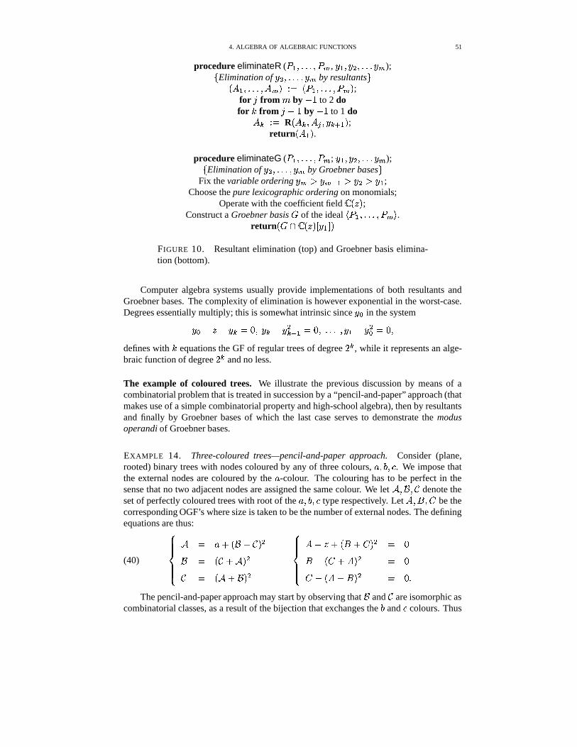
4. ALGEBRA OF ALGEBRAIC FUNCTIONS 51
procedure eliminateR ( � 2 � �;�,� � � E , / 2 � / � � �;�,� / E );( Elimination of / � � �,�,� � / E by resultants *H � 2 � �,�;� � � E M Q � H � 2 � �,�;� � � E M ;
for " from by ��6 to 2 dofor
�from " � 6 by ��6 to 1 do� � Q � R H � � � � 9 � / � l 2 M ;
return H ��2 M .procedure eliminateG ( �72 � �;�,� � � E ; / 2 � / � � �,�;�C/�E );
( Elimination of / � � �,�,� � / E by Groebner bases *Fix the variable ordering / E � / E j 2 � / � � / 2 ;
Choose the pure lexicographic ordering on monomials;Operate with the coefficient field � H � M ;
Construct a Groebner basis � of the ideal �� 2 � �;�,� � � E � .return H � � H � M � / 2 � M
FIGURE 10. Resultant elimination (top) and Groebner basis elimina-tion (bottom).
Computer algebra systems usually provide implementations of both resultants andGroebner bases. The complexity of elimination is however exponential in the worst-case.Degrees essentially multiply; this is somewhat intrinsic since / � in the system
/ � � � � / � �A8 � / � � / �� j 2 � 8 � �,�;� � / 2 � / �� � 8 �defines with
�equations the GF of regular trees of degree
/ �, while it represents an alge-
braic function of degree/ �
and no less.
The example of coloured trees. We illustrate the previous discussion by means of acombinatorial problem that is treated in succession by a “pencil-and-paper” approach (thatmakes use of a simple combinatorial property and high-school algebra), then by resultantsand finally by Groebner bases of which the last case serves to demonstrate the modusoperandi of Groebner bases.
EXAMPLE 14. Three-coloured trees—pencil-and-paper approach. Consider (plane,rooted) binary trees with nodes coloured by any of three colours, 1 � ? � � . We impose thatthe external nodes are coloured by the 1 -colour. The colouring has to be perfect in thesense that no two adjacent nodes are assigned the same colour. We let � ����� denote theset of perfectly coloured trees with root of the 1 � ? � � type respectively. Let � � � �
be thecorresponding OGF’s where size is taken to be the number of external nodes. The definingequations are thus:
(40)
��������� � � 1�4 H � 4 M �
� � H 4 � M�
� H � 4 � M �
��������� �
� �A4 H � 4 M � � 8
� � H 4 � M � � 8 � H � 4 � M � � 8 �The pencil-and-paper approach may start by observing that
�and are isomorphic as
combinatorial classes, as a result of the bijection that exchanges the ? and � colours. Thus
52 8. FUNCTIONAL EQUATIONS—RATIONAL AND ALGEBRAIC FUNCTIONS
� � . Then equation (40) simplifies into a system of 2 equations in 2 unknowns with �
a parameter:
(41)
�� � � � � � � � � � 8
� � � � � / � � � � � � 8 �Since � is to be eliminated, we may combine linearly the equations of (41) in order to getrid of � � (the highest power in � ),
(42)
�� � � � � � � � � � 8
� � � � � � 4 � � � 4 ; � � � 8
The second equation is linear in � and the value can then be plugged back into the firstequation, resulting in a fourth degree polynomial that cancels � ,
(43) 'H � � � M7��6�U � � � ; �� 4 H 6N: 4 ; � M � � � H � 4 6�; � M � 46� � 4 � ���
and the polynomial is easily checked to be irreducible.�
EXAMPLE 15. Three-coloured trees—resultant approach. Start again with the system (40)and take mechanically resultants with respect to
of the third equation together with the
first and second equations. This eliminates
and provides two polynomials cancelledby � and � :
(44)
� G � � G � � � G � � G " � � � G � � � � � G " � � � G " � � � G � � � � G � �� G^�HG � � G � � � � G � �"G " � � � G � � � � � G ".� � � G " � � � G � � � G � �
A further resultant with respect to � will then yield a polynomial involving � alone andcancelled by � :
� ��� � � + � ��� � � +0� � ��� �N+ � � � � � � G � � " �HG � / " � � �+ ��� � � � G � ��� �N+ �� � � � � G �� /.� � + � / �HG ��� � � � + � ��� � � G ��� � � G � � �HG� � � �G � ��� � � + � /.� � + � �N+ " � � + � � � + � � � + " ��+,� �This time, the polynomial of degree 8 in � . (From (43), we know it cannot be minimal.)
In fact it factors as
(45) H � � � 4 = � 4 6 46� M � H 6�U � � 4 "%"%" 4 � � M�� H � � � 4 = � 4 6 46� M � 'H � � � M �with 'H � � � M as in (43).
The series expansion for the combinatorial generating function � starts with
� H � M7� �:4 � � � 4 6�U � 4 9.U � � 4 / 9.U � � 4 6 / =!U � � 4 9.;!8#; � ��4#"$"%" �so that the first quadratic factor is disqualified as a candidate for minimal polynomial. Wehave thus found again the result of (43). Note that the complete factorization of (45) over� guarantees at the same time that 'H � � � M is the minimal polynomial so that � is of exactdegree 4. (See the exercise preceding Theorem 8.7.)
�
EXAMPLE 16. Three-coloured trees—Groebner basis approach. In accordance with theprocedure eliminateG we first fix an ordering on variables. For the case at hand, we choose �� �� �with the intent that variables should be eliminated in that order, first
, next � , then � .
Several orderings may be defined on monomials, but for our purposes, we chose the pure
4. ALGEBRA OF ALGEBRAIC FUNCTIONS 53
lexicographic ordering that is the usual alphabetic ordering of words in a dictionary (withpreceding � preceding � , though!). For instance, with this ordering, we have (think of � � , � � ' , � � $ and the lexicographic order in the Latin script) � � � � � � � � � �� � � � � ��� � � � �
The leading term of a polynomial with the chosen ordering is denoted by LTH � M . For
instance: LTH / � � 4 = � � 4 � � � 4 9 � � M7� 9 � � .
The basic operation of Groebner basis theory is the “division” operation of a polyno-mial
�by a sequence of polynomials � � H � 2 � �,�,� �"� �
M producing a remainder denoted
by���
. The idea is to “reduce” the polynomial�
by an operation that is reminiscent ofGaussian elimination (for multivariate linear polynomials) and of the Euclidean algorithm(for univariate nonlinear polynomials).
The principle of division is as follows. First transform each polynomial in� � of � into
a rewrite rule: H � � M5Q LTH � � M �� � � � 4 LT
H � � M �(a rule thus replaces a monomial by a combination of smaller monomials under the mono-mial order.) Use repeatedly � 2 � �,�,� � � � (in that order, say, for determinacy) to reducethe leading term of
�(that changes at each stage). When the leading term no longer re-
duces, then proceed similarly with the second leading term, the third one, and so on. Thealgorithm is specified in full in [27, p. 62]. On our example, the three rules are
H � 2 M � �� � ��4 � � � � � / � H � � M � �� / � 4 � �H � � M �� � � 4 / � � 4 � �
An instance of a reduction will be: � ��� � �� � � � � � / � � � � ��� � �� � 4 = � � � � � / � � 4 / �� 4 / � � ��� � �� "$"%"��
(In such a simple case, the effect of the rules is easy to describe: they eventually clear outall occurrences of
, with � 2 used a number of times and � � used once at the end to
dispose of the last linear term in
.)Next comes the notion of Groebner basis. The principle is to build a “good” set of
generators for the ideal defined by � , that is, the set of all polynomials� �
9 1 9 � 9 �
where the coefficients 1 9 are polynomials. (On the example, we would have 1 9 �� H � M � � � � � � .)
DEFINITION 8.8. A Groebner basis for an ideal � is a set � of polynomials such thatfor all
� � � , the division by � yields a complete reduction,��� �A8 �In particular, such a basis should “self-reduce” in the sense that for all � � � � � :
(46) ��� � � � � � � 8 �(Here � � and � represent arbitrary monomials, in accordance with standard multi-indexnotation.)
54 8. FUNCTIONAL EQUATIONS—RATIONAL AND ALGEBRAIC FUNCTIONS
Buchbergers’ algorithm constructs Groebner bases by enriching a given base � tillthe self-reduction property (46) is ensured. Define the
�-polynomial of two monic poly-
nomials � � as � � � � � , with � and � chosen to be the smallest monomials that achievecancellation of the leading terms of � and . (
�-polynomials are in a sense the simplest
nontrivial polynomials that should reduce.) One must have� H � � � M � � 8 , for all � � � � � .
Then, the construction of a Groebner basis from a sequence � proceeds incrementally:we start with � � � and successively add to � all pairs � � with � � � � such that� H � � M�� �� 8 . The process is stopped once saturation is reached. (The algorithm is speci-fied in full in [27, p. 97].)
For instance consider the system (40), that is, � � H � 2 � � � � � � M . Set initially � � � .The
�-polynomial of
� 2 � � � is obtained by taking 6 � 2 � 6 � � (the monomials �
disappear),giving
� � 4 � � 4 / � 46�:4 � � / � � � � �which reduces modulo � (by way of H � � M ) into� � � � � � � � � 4 � � 46� � / �
�� 4 / � �
� 4 / �� � � � �
Then, the two other pairs provide� � � � � � � �� 8 , and
� � � � � � 2 � �� 8 . At this stage,the new-comers
� � � � � � � are adjoined to � , giving the new value � � H � 2 � �,�,� �"� � M . Thecompletion process continues till � eventually stabilizes. We then take the Groebner basisto be � Q � � , after removing redundant polynomials [27, Sec. 2.9]. Here, a set of 4polynomials is obtained. In accordance with theory, the Groebner basis contains a singlepolynomial that depends on the variable � alone; this polynomial that is of degree 6 factorsas
H � � � 4 = � 4 �:4 6�M 'H � � � M �The minimal polynomial is once more recovered: Groebner elimination has faithfully ac-complished its task.
�
4.2. Closure properties and coefficients. By definition, algebraic functions satisfystrong algebraic closure properties. The proofs now fall as ripe fruits as a benefit of ourinvestment on elimination. From this point on, eliminate will designate either of the elim-inateR or eliminateG procedure.
THEOREM 8.8 (Algebraic function closure (1)). The set � alg � � � � � of algebraic seriesis closed under the operations of sum H � 4 � M , product (
� � � ), quasi-inverse (definedby
� �� H�6 � � M j 2 , conditioned upon� � � 8 ), differentiation (
e ), composition (
� ! � ,conditioned upon � � �A8 ).
Proof. Let ' and $ be defined by � H � � � M � 8 and� H � � '�M � 8 . For sum, product,
quasi-inverse, and composition, just appeal to
/ � � 4 ' Q ��� ��������� � H � / � � � ' � � H � � � M ��� H � � '�M � � / � � � '�M �/ � � ' Q ��� ��������� � H � / � � ' � � H � � � M ��� H � � '�M � � / � � � '�M �/ � H�6�� � M j 2 Q ��� ��������� � H � / � � / � 6 � � H � � � M � � / � � M �/ � � ! ' H � M Q ��� ��������� � H � � H�' � / M ��� H � � '1M � � / � '1M �
An immediate consequence is that if �WH � � / M is a rational function and � � � �"' ) � � � � � isalgebraic, then �'H � � � M is algebraic. Next, if � satisfies � H � � � M�� 8 , then the derivative
4. ALGEBRA OF ALGEBRAIC FUNCTIONS 55� � with respect to � satisfies
� � H � � �FM 4 � � � � H � � � M�� 8 or � � � � � � H � � � M� � H � � � M �
and is therefore a rational fraction in � . Thus, by the previous observation, � � is algebraic.�These results show that � �"' ) � � ��� � is a ring. They extend transparently to � �(' ) H H � M M which
is a field.Algebraic series are not closed under Hadamard product. To see it, consider
� H � M Q � 6� 6�� � # 6
� 6�� � � �� ���
66�U �
/ hh �� � �
The coefficient � � � � � H � M is asymptotic to 6 = H � h M . Consequently, by an Abelian theorem,
� H � M � 6�+�� � 6
6�� �� � � 6 j �
Such a singularity is incompatible with algebraicity, where only fractional power seriesmay occur; see the next section. On the positive side, we have the following.
THEOREM 8.9 (Algebraic function closure (2)). H���M If�
is rational and � is algebraic,then the Hadamard product
� # � is algebraic.H�����M Define the diagonal of a bivariate series! � ��� � � / � ,�
� � ! H � � / M7� �
! � � � � � �Then, the diagonal of a rational bivariate series is an algebraic series.
Proof. H���M Take� � � � �"! � � ��� � and � � � �"' ) � � � � � and consider the Hadamard product � � � #� . The Hadamard product distributes over sums, so that is is enough to show algebraicity
when�
is a simple fraction element,� � H�6�� 1 � M j E . This is settled by simple algebra,
sinceH 6�� 1 � M j E # � H � M7��H 6 � � M j E # � H 1 � M�� < E j 2
< � E j 2 � � E j 2 � H 1 � M � �An alternative, more analytic, derivation can be based on Hadamard’s formula for
Hadamard products. This important formula valid for all functions analytic at 0 is
(47)� # � H � M�� 6
/ � �k
�
� H� M � H � � M < �� �If
�and � are analytic in � ��� and � ��� �
respectively, then � can be any loop aroundzero whose elements � satisfy � � � and � �>= � � �
, that is,� � � � � � � �and the conditions are compatible provided � is of small enough modulus. (The verificationby direct series expansions is immediate.) For the original problem of � � �(! � � � � � # � �"' ) � � � � � ,an evaluation of (47) by residues then provides the result.H�����M Our proof will start from another of Hadamard’s formulæ,
(48)�� � ! H � � / M7� 6
/ � �k
�
! H� � � � M7< �� �that is proved by the same devices as (47). If
! H � � / M is analytic in � � � and � /�� �,
then � should be taken such that � ��� � � � � , and the domain of possible values is
56 8. FUNCTIONAL EQUATIONS—RATIONAL AND ALGEBRAIC FUNCTIONS
nonempty as long as � � � is small enough. (The verification is again by straight expansion.)This formula generalizes (47) since
� # � H � M7� �� � H � H � M � H / M M .
Now, for � ��� small, we can evaluate the integral by residues inside �>= � �. See [88]
for details. Assume � small enough and let! H � � / M0� � H � � / M = � H � � / M . Consider the roots� 2 H � M � �,�;� � � � H � M of the characteristic equation, � H � � �>= � M:� 8 that tend to 0 as � � 8 .
Then, for � small enough and � encircling the “small” roots � 2 H � M � �,�;� � � � H � M , a residuecomputation gives
�� � � �
9 � 2 Res � ! H� � � � M � � � � � �
Thus, the diagonal is a rational function of (some) branches of an algebraic function and itis therefore rational. �Closed form for coefficients. Coefficients of algebraic functions satisfy interesting re-lations, starting with recurrences of finite order. In addition, they can be presented ascombinatorial sums.
First, we show that algebraic functions satisfy differential equations. Take � �� �(' ) � � ��� � an algebraic series of degree < , with minimal polynomial � H � � / M ; and let �'H � � / Mbe a bivariate rational function. We have seen before that �WH � � � M is also algebraic. In fact,we are going to show that � can be rewritten as
�'H � � �FM7� ( j 29 ��� 9 H � M � 9 � 9 H � M � � H � M �
In other words, a quantity H � � � M with � algebraic is representable by a polynomial of� H � M � � � . The situation generalizes what is known about algebraic numbers and reduction
to polynomial form, for instance,6�� / 4 � =
� 6=�� / � � 6
U�� / � � = 4 6
U�� / � 6
U�� / � = 4 6
= �Write �'H � � / M � . H � � / M =�� H � � / M . Clearly, it suffices to prove that 6 =�� H � � � M re-
duces to polynomial form. We may freely assume that � is not a multiple of � , and since� is irreducible, we have �!��0H � � � M � 6 , where the gcd is taken in � H � M � / � . Then, byBezout’s theorem, there exists 1 H � � / M � ? H � � / M � � H � M � / � such that 1 � � ? � � 6 . In otherwords, 1 is the inverse of � modulo � . We thus have, at the expense of a single gcd andsimple polynomial reduction:
�WH � � � M � � 1 H � � / M . H � � / MF%V�� � H � � / M � � � �This gives the following basic result: Every rational fraction in � and � lives in the set��� ��� H � M � ( of polynomials with � -degree bounded from above by < .
Consider now H � M � / � � ( as a
H � M –vector space of dimension < . The H < 4 6�M firstderivatives � H � M � � � H � M � �,�;� � � � ( H � Mlie in that space and thus they must be bound. As a consequence, there exist coefficients � 9(in � H � M ) such that (
9 ��� � 9H � M < 9
< � 9 � H � M��A8 �
4. ALGEBRA OF ALGEBRAIC FUNCTIONS 57
This relation can be obtained constructively by cancelling a minor of maximal rank ofthe determinant expressing the linear dependency7 Extracting coefficients then produces arecurrence of the form
89 ��� < 9 H h M � �al 9 �A8 �
for a sequence of coefficients < 9 H h M � � H h M . (Denominators can always be eliminated sothat the coefficients can be taken to be polynomials of
� h � .)This discussion brings us to a general statement about coefficients of algebraic func-
tions.
THEOREM 8.10 (Algebraic coefficients). H���M The coefficients of any algebraic powerseries / H � M satisfy a linear recurrence with polynomial coefficients, namely,
89 �.� < 9 H h M / �al 9 �A8 �
where / � � � � � � / H � M and � 9 H h M � ��� h � .H�����M Let� H � � / M be a bivariate polynomial such that
� HS8 � 8!M�� 8 ,� � HK8 � 8!M � 8 and
� H � � 82M �� 8 . Consider the algebraic function implicitly defined by� H � M � � H � �"� H � M M .
Then, the Taylor coefficients of� H � M admit expressions as combinatorial sums,
(49) � � � � � H � M�� E 2
6 � � � / E j 2 � � E H � � / M �
Proof. Part H���M is established by the discussion above. Part H�����M is based on a yet unpub-lished memo of Flajolet and Soria, from which the discussion that follows is extracted.
First, a variant form of the coefficients is available, and Eq. (49) is elementarily equiv-alent to
(50) � � � � � H � M�� E � � � / E j 2 �
� E H � � / M � 6�� � � H � � / M �
as results from the observation that H 4 6NM � � H / M � E H / M7� (( � E l 2 H / M .The starting point of the analytic part of the proof is an integral formula giving the
root of an equation � H / M0� 8 inside a simple domain. Let � H / M be analytic and assume thatinside the domain defined by a closed curve � , the equation � H / M�� 8 has a unique root.Then, we have
(51) RootOf H � H / M�� 8 � � M�� 6�k
�
/ � � H / M� H / M < / �That formula can be seen as a modified form of the “principle of the argument” ([51]), butit can also be checked directly via a residue computation.
The algebraic function� H � M under consideration is a root of / � � H � � / M&�78 . There-
fore, if we proceed formally and apply formula (51) to � H / M � / � � H � � / M , we get
� H � M � 6/ � �
k�
/ 6 � � � H � � / M/ � � H � � / M < /
� 6�k
�
6�� � � H � � / M6�� 2
� H � � / M < / �(52)
7This result is often referred to in the combinatorics literature as “Comtet’s theorem”; see [25].
58 8. FUNCTIONAL EQUATIONS—RATIONAL AND ALGEBRAIC FUNCTIONS
Still proceeding formally, we expand the integrand using
(53)6
6�� � � 6 4 � 4 � � 4 � � 4 "%"%" �which leads to
(54)� H � M7�
E � k �
H�6�� � � H � � / M M � E H � � / M < /��/ E �
Now Cauchy’s coefficient formula,
� / E j 2 � � H / M7� 6�k��� � H / M < /
/ E �when applied to the integral in Eq. (54) provides
(55)� H � M �
E � � / E j 2 � H 6�� � � H � � / M M � E H � � / M �
which is the form given in (50).There only remains to complete the analytic part of the argument. First, by the as-
sumptions made regarding�
, the point HK8 � 82M is an ordinary point of the algebraic curve/ � � H � � / M � 8 . Thus all branches of the curve are “well separated” from the branchcorresponding to
� H � M . We can thus find � 2 � 8 and � 2 � 8 so that, when � lies in thedomain � � � � � 2 , we have � � H � M � ��� 2 while � � 9 H � M � � � 2 for all the conjugate branches� 9 H � M �� � H � M . In other words, the use of the integral formula (52) is justified providedwe take � ��� � 2 together with the contour � � (;/�= � /�� � � * for any � � � 2 . We shallhenceforth assume that such a choice has been made.
The next condition to be satisfied is the validity of expansion (53) used to derive (54).This requires the inequality � � � 6 when � � 2
� H � � / M . should have � � � 6 . But
the conditions on� H � � / M at HK8 � 8!M imply that in a sufficiently small neighbourhood of the
origin, i.e. � ��� � � and � /�� � � , the bound,� � H � � / M � � @ H � ���,4 � �#/�� 4 � / � � M �holds for some positive constant @ . Thus, for � ��� � � and � /�� � � , the condition� � H � � / M � � /�� is granted if
(56) � � � � / � 6�� � /��6 4 � /�� �
We can now conclude the argument. Choose as contour � a circle centered at the originwith radius � � % ��� H ��2 � � � M . To guarantee condition (56), impose that � be such that� � � � where � �A% ���
� 2 � � � � � 6 � �6 4�� �
Therefore, Equation (55) holds true. �Part H�����M of the theorem generalizes the Lagrange inversion formula that corresponds
to the “separable” case� H � � / M�� ��� H / M . As an example, the coefficients of� H � M7� �:4 � � � � H � M 4 � � � � H � M �
admit the “nice” form� � �
E 2 � 6
h � 4 6 � 9 � = h � / � / h � = 4 6 �In general, if
�comprises � monomials, the formula obtained is a H � � / M -fold summation.
5. ANALYSIS OF ALGEBRAIC FUNCTIONS 59
5. Analysis of algebraic functions
Algebraic functions can only have a type of singularity constrained to be a branchpoint. The local expansion at such a singularity is a fractional power series known as aNewton–Puiseux expansion. Singularity analysis is systematically applicable to algebraicfunctions—hence the characteristic form of asymptotic expansions that involve terms ofthe form ) � h � � �
(for some algebraic number ) and some rational exponent � = ). In thissection, we develop such basic structural results (Subsection 5.1). However, coming upwith effective solutions (i.e., decision procedures) is not obvious in the algebraic case.Hence, a number of nontrivial algorithms are also described (built on top of elimination byresultants or Groebner bases) in order to locate and analyse singularities (Newton’s poly-gon method), and eventually determine the asymptotic form of coefficients. In particular,the multivalued character of algebraic functions creates a need to solve “connection prob-lems”. Finally, like in the rational case, positive systems (Subsection 5.2) enjoy specialproperties that further constrain what can be observed as regards asymptotic behavioursand properties of random structures. Our presentation of positive systems is based on anessential result of the theory, the Drmota–Lalley–Woods theorem, that plays for algebraicfunctions a role quite similar to that of Perron-Frobenius theory for rational functions.
5.1. General algebraic functions. Let � H � � / M be an irreducible polynomial of��� � � / � ,� H � � / M7� � � H � M / ( 4 � 2 H � M / ( j 2 4 "%"$" 4 � ( H � M �
The solutions of the polynomial equation � H � � / M � 8 define a locus of points H � � / M in� � � that is known as a complex algebraic curve. Let < be the / -degree of � . Then, foreach � there are at most < possible values of / . In fact, there exist < values of / “almostalways”, that is except for a finite number of cases:
— If � � is such that � � H � � M � 8 , then there is a reduction in the degree in / andhence a reduction in the number of / -solutions for the particular value of � � � � .One can conveniently regard the points that disappear as “points at infinity”.
— If � � is such that � H � � � / M has a multiple root, then some of the values of / willcoalesce.
Define the exceptional set of � as the set (R is the resultant):� � ��� Q � ( � �� 'H � M7�A8 * � 'H � M Q � R H � H � � / M � e � H � � / M � / M �
(The quantity 'H � M is also known as the discriminant of � H � � / M taken as a function of / .)If � �� � � � � , then we have a guarantee that there exist < distinct solutions to � H � � / M ��8 ,since � � H � M �� 8 and
e � H � � / M �� 8 . Then, by the implicit function theorem, each of
the solutions / 9 lifts into a locally analytic function / 9 H � M . What we call a branch of thealgebraic curve � H � � / M�� 8 is the choice of such an / 9 H � M together with a connected
region of the complex plane throughout which this particular / 9 H � M is analytic.EXERCISE 27. Verify that, when � approaches � � with � ��� � �.-0/ , then a numberat least 1 of the values of ) satisfying
� ��� � ) ��-0/ tend to infinity.
Singularities of an algebraic function can thus only occur if � lies in the exceptionalset
� � ��� . At a point � � such that � � H � � M�� 8 , some of the branches escape to infinity,thereby ceasing to be analytic. At a point � � where the resultant polynomial VH � M vanishesbut � � H � M �� 8 , then two or more branches collide. This can be either a multiple point(two or more branches happen to assume the same value, but each one exists as an analyticfunction around � � ) or a branch point (some of the branches actually cease to be analytic).
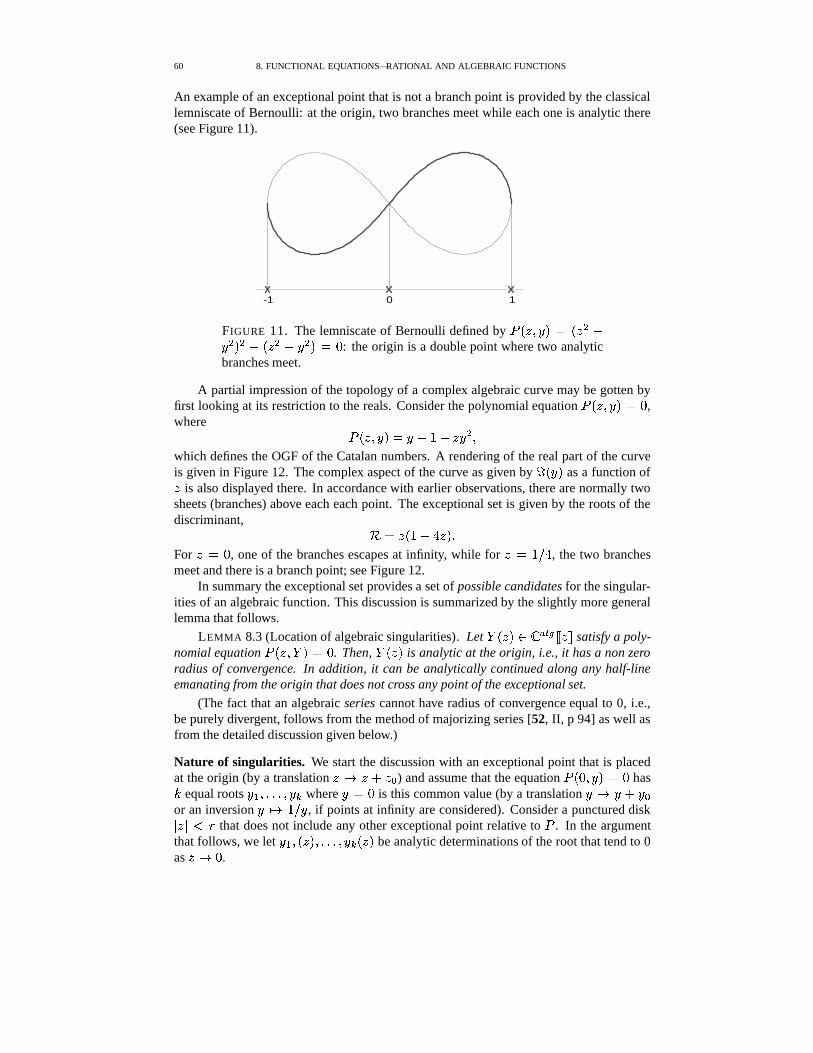
60 8. FUNCTIONAL EQUATIONS—RATIONAL AND ALGEBRAIC FUNCTIONS
An example of an exceptional point that is not a branch point is provided by the classicallemniscate of Bernoulli: at the origin, two branches meet while each one is analytic there(see Figure 11).
10-1
FIGURE 11. The lemniscate of Bernoulli defined by � H � � / M�� H � � 4/ � M � � H � � � / � M�� 8 : the origin is a double point where two analyticbranches meet.
A partial impression of the topology of a complex algebraic curve may be gotten byfirst looking at its restriction to the reals. Consider the polynomial equation � H � � / M�� 8 ,where
� H � � / M�� / � 6�� �#/ � �which defines the OGF of the Catalan numbers. A rendering of the real part of the curveis given in Figure 12. The complex aspect of the curve as given by � H / M as a function of� is also displayed there. In accordance with earlier observations, there are normally twosheets (branches) above each each point. The exceptional set is given by the roots of thediscriminant,
� � � H�6�� � � M �For � � 8 , one of the branches escapes at infinity, while for � � 6 = � , the two branchesmeet and there is a branch point; see Figure 12.
In summary the exceptional set provides a set of possible candidates for the singular-ities of an algebraic function. This discussion is summarized by the slightly more generallemma that follows.
LEMMA 8.3 (Location of algebraic singularities). Let� H � M � � / ��� � � ��� � satisfy a poly-
nomial equation � H � � � M ��8 . Then,� H � M is analytic at the origin, i.e., it has a non zero
radius of convergence. In addition, it can be analytically continued along any half-lineemanating from the origin that does not cross any point of the exceptional set.
(The fact that an algebraic series cannot have radius of convergence equal to 0, i.e.,be purely divergent, follows from the method of majorizing series [52, II, p 94] as well asfrom the detailed discussion given below.)
Nature of singularities. We start the discussion with an exceptional point that is placedat the origin (by a translation � �� ��4 � � ) and assume that the equation � HK8 � / M ��8 has�
equal roots / 2 � �,�;� � / � where / ��8 is this common value (by a translation / �� /�4 / �or an inversion / �� 6 = / , if points at infinity are considered). Consider a punctured disk� � � � that does not include any other exceptional point relative to � . In the argumentthat follows, we let / 2 � H � M � �,�;� � / � H � M be analytic determinations of the root that tend to 0as � � 8 .
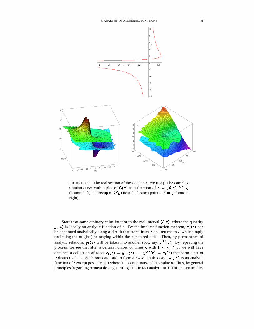
5. ANALYSIS OF ALGEBRAIC FUNCTIONS 61
–10
–8
–6
–4
–2
0
2
4
6
8
10
y
–1 –0.8 –0.6 –0.4 –0.2 0.2z
–1
0
1
Re(z)
–1 –0.8 –0.6 –0.4 –0.2 0 0.2 0.4 0.6 0.8 1
Im(z)
–2
0
2
4
y
0.15
0.2
0.25
0.3
0.35
Re(z)
–0.1
–0.05
0
0.05
0.1
Im(z)
–3
–2
–1
0
1
2
3
y
FIGURE 12. The real section of the Catalan curve (top). The complexCatalan curve with a plot of � H / M as a function of � � H��H � M � � H � M M(bottom left); a blowup of � H / M near the branch point at � � 2� (bottomright).
Start at at some arbitrary value interior to the real interval HK8 � � M , where the quantity/ 2 H � M is locally an analytic function of � . By the implicit function theorem, / 2 H � M canbe continued analytically along a circuit that starts from � and returns to � while simplyencircling the origin (and staying within the punctured disk). Then, by permanence ofanalytic relations, / 2 H � M will be taken into another root, say, / � 2 2 H � M . By repeating theprocess, we see that after a certain number of times � with 6 � � � �
, we will haveobtained a collection of roots / 2 H � M�� / � � 2 H � M � �;�,� � / ��� 2 H � M�� / 2 H � M that form a set of� distinct values. Such roots are said to form a cycle. In this case, / 2 H� � M is an analyticfunction of � except possibly at 0 where it is continuous and has value 0. Thus, by generalprinciples (regarding removable singularities), it is in fact analytic at 0. This in turn implies
62 8. FUNCTIONAL EQUATIONS—RATIONAL AND ALGEBRAIC FUNCTIONS
the existence of a convergent expansion near 0:
(57) / 2 H�� � M�� �� � 2 � �
� � �The parameter � is often called the local uniformizing parameter, as it reduces a mul-tivalued function to a single value one. This translates back into the world of � : eachdetermination of � 2 � � yields one of the branches of the multivalued analytic function as
(58) / 2 H � M7� �� � 2 � � � � � � �
Alternatively, with ) � � � � � � � a root of unity, the � determinations are obtained as
/ � 9 2 � �� � 2 � � )
� � � � � �
each being valid in a sector of opening / � . (The case � � 6 corresponds to an analyticbranch.)
If � � �, then the cycle accounts for all the roots which tend to 0. Otherwise, we
repeat the process with another root and, in this fashion, eventually exhaust all roots. Thus,all the
�roots that have value 8 at � �A8 are grouped into cycles of size � 2 � �,�;� � � � . Finally,
values of / at infinity are brought to zero by means of the change of variables / � 6 = � ,then leading to negative exponents in the expansion of / .
THEOREM 8.11 (Newton–Puiseux expansions at a singularity). Let� H � M be a branch
of an algebraic function � H � �"� H � M M � 8 . In a circular neighbourhood of a singularity�slit along a ray emanating from
�,
� H � M admits a fractional series expansion (Puiseuxexpansion) that is locally convergent and of the form� H � M7�
� ��� � � H � � � M � � � �
for a fixed determination of H � � � M 2 � � , where� � � � and � is an integer � /
, called the“branching type”.
Newton (1643-1727) discovered the algebraic form of Theorem 8.11, published it inhis famous treatise De Methodis Serierum et Fluxionum (completed in 1671). This methodwas subsequently developed by Victor Puiseux (1820–1883) so that the name of Puiseuxseries is customarily attached to fractional series expansions. The argument given aboveis taken from the neat exposition offered by Hille in [52, Ch. 12, vol. II]. It is known asa “monodromy argument”, meaning that it consists in following the course (–dromy) ofvalues of a multivalued analytic function along paths in the complex plane till it returns toits original (mono–) value.
Newton polygon. Newton also described a constructive approach to the determination ofbranching types near a point H � � � / � M , that by means of the previous discussion can alwaysbe taken to be HS8 � 8!M . In order to introduce the discussion, let us examine the Catalangenerating function near � � � 6 = � . Elementary algebra gives the explicit form of the twobranches
/ 2 H � M7� 6/ � � 6�� � 6�� � � � � / � H � M�� 6
/ � � 6 4 � 6�� � � � �whose forms are consistent with what Theorem 8.11 predicts. If however one starts directlywith the equation,
� H � � / M � / � 6�� �#/ � �A8
5. ANALYSIS OF ALGEBRAIC FUNCTIONS 63
then, the translation � � 6 = � � � (the minus sign is a mere notational convenience),/ � / 4 �yields
(59)� H � � � M � � 6
�� � 4 � � 4 � � � 4 � � � �
Look for solutions of the form� � � � � H�6 4 � H 6�M M with � �� 8 (the existence is granted
a priori by the Newton-Puiseux Theorem). Each of the monomials in (59) gives rise to aterm of a well determined asymptotic order. respectively �
��� � 2 � � � l 2 � � � � l 2 . If the
equation is to be identically satisfied, then the main asymptotic order of� H � � � M should
be 0. Since � �� 8 , this can only happen if two or more of the exponents in the sequenceH / � � 6 � � 4 6 � / � 4 6NM coincide and the coefficients of the corresponding monomial in� H � � � M is zero, a condition that is an algebraic constraint on the constant � . Furthermore,exponents of all the remaining monomials have to be larger since by assumption theyrepresent terms of lower asymptotic order.
Examination of all the possible combinations of exponents leads one to discover thatthe only possible combination arises from the cancellation of the first two terms of
�,
namely � 2� � � 4 � � , which corresponds to the set of constraints
/ � � 6 � � 6� �
� 4 � �A8 �with the supplementary conditions � 4 6 � 6 and
/ � 4 6 � 6 being satisfied by this choice� � 2� . We have thus discovered that� H � � � M��A8 is consistent asymptotically with
� � � � 2 ��� � � � � � � 2 ��� �The process can be iterated upon subtracting dominant terms. It invariably gives rise
to complete formal asymptotic expansions that satisfy� H � � � M � 8 (in the Catalan ex-
ample, these are series in � � 2 ��� ). Furthermore, elementary majorizations establish thatsuch formal asymptotic solutions represent indeed convergent series. Thus, local expan-sions of branches have indeed been determined. This is Newton’s algorithm for expandingalgebraic functions near a branch point.
An algorithmic refinement (also due to Newton) can be superimposed on the previousdiscussion and is known as the method of Newton polygons. Consider a general polynomial
� H � � � M7� 9 ���
� / � � 1 � �and associate to it the finite set of points H 1 9 � ? 9 M in � � � , which is called the Newtondiagram. It is easily verified that the only asymptotic solutions of the form
��� � �correspond to values of � that are inverse slopes (i.e.,
� � = � / ) of lines connecting two ormore points of the Newton diagram (this expresses the cancellation condition between twomonomials of
�) and such that all other points of the diagram are on this line or to the
right of it. In other words:
Newton’s polygon method. The possible exponents � such that� � � � � is a
solution to a polynomial equation correspond to the inverse slopes of the leftmostconvex envelope of the Newton diagram. For each viable � , a polynomial equa-tion constrains the possible values of the corresponding coefficient � . Completeexpansions are obtained by repeating the process, which means deflating
�from
its main term by way of the substitution� �� � � � � � .
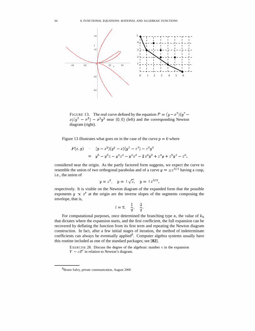
64 8. FUNCTIONAL EQUATIONS—RATIONAL AND ALGEBRAIC FUNCTIONS
–0.4
–0.2
0
0.2
0.4
y
–0.4 –0.2 0.2 0.4x
��
��
��
��
�
�
�
���������������
���������������
���������������
���������������
���������������
���������������
���������������
���������������
����������������������������������������������������������������������������������������
������������������������������������������������������������������������������������������
��
����������������������������������������������������������������������������������������
5
��������������������������������������������� � � � � � � � � � � � � � � � � � � � � �
!�!�!�!�!�!�!�!�!�!�!�!�!�!�!�!�!�!�!�!�!�!�!"�"�"�"�"�"�"�"�"�"�"�"�"�"�"�"�"�"�"�"�"�"�"
#�#�#�##�#�#�##�#�#�##�#�#�##�#�#�##�#�#�#
$�$�$�$$�$�$�$$�$�$�$$�$�$�$$�$�$�$$�$�$�$
%�%�%�%�%�%�%�%�%�%%�%�%�%�%�%�%�%�%�%%�%�%�%�%�%�%�%�%�%%�%�%�%�%�%�%�%�%�%%�%�%�%�%�%�%�%�%�%%�%�%�%�%�%�%�%�%�%%�%�%�%�%�%�%�%�%�%
&�&�&�&�&�&�&�&�&&�&�&�&�&�&�&�&�&&�&�&�&�&�&�&�&�&&�&�&�&�&�&�&�&�&&�&�&�&�&�&�&�&�&&�&�&�&�&�&�&�&�&&�&�&�&�&�&�&�&�&
'�'�'�'�'�'�'�''�'�'�'�'�'�'�''�'�'�'�'�'�'�'
(�(�(�(�(�(�((�(�(�(�(�(�((�(�(�(�(�(�(
0 1 2 3 4 5 6
1
2
3
4
FIGURE 13. The real curve defined by the equation � � H / � � � M�H / � �� M�H / � � � � M � � � / � near HK8 � 8!M (left) and the corresponding Newtondiagram (right).
Figure 13 illustrates what goes on in the case of the curve � � 8 where
� H � � / M � H / � � � M-H / � � � M-H / � � � � M � � � / �� / � / � � � / � � � 4 / � � � � / � � / � 4 � � /�4 � / � � � � �
considered near the origin. As the partly factored form suggests, we expect the curve toresemble the union of two orthogonal parabolas and of a curve / � ��� ����� having a cusp,i.e., the union of
/ � � � � / � � � � � / � ��� ����� �respectively. It is visible on the Newton diagram of the expanded form that the possibleexponents / � � � at the origin are the inverse slopes of the segments composing theenvelope, that is,
�7� / � 6/
� =/ �
For computational purposes, once determined the branching type � , the value of� �
that dictates where the expansion starts, and the first coefficient, the full expansion can berecovered by deflating the function from its first term and repeating the Newton diagramconstruction. In fact, after a few initial stages of iteration, the method of indeterminatecoefficients can always be eventually applied8. Computer algebra systems usually havethis routine included as one of the standard packages; see [82].
EXERCISE 28. Discuss the degree of the algebraic number in the expansion)+* ,.- in relation to Newton’s diagram.
8Bruno Salvy, private communication, August 2000
5. ANALYSIS OF ALGEBRAIC FUNCTIONS 65
Asymptotic form of coefficients. The Newton–Puiseux theorem describes precisely thelocal singular structure of an algebraic function. The expansions are valid around a singu-larity except for one direction. In particular they hold in indented disks of the type requiredin order to apply the formal translation mechanisms of singularity analysis (Chapter 5).
THEOREM 8.12 (Algebraic asymptotics). Let� H � M�� � � � � � �
be an algebraic se-ries. Assume that the branch defined by the series at the origin has a unique dominantsingularity at � � � 2 on its circle of convergence. Then, the coefficient
� � satisfies theasymptotic expansion,
� ��� � j��2�� � � � < � h j 2 j � � � �� �
where� � � � and � is an integer � /
.If
� H � M has several dominant singularities � � 2 � � � � � � � "%"$" � � � � � , then there existsan asymptotic decomposition (where is some small fixed number, � 8 )
� � � �9 � 2 � � 9 H h M 4� H H � � 2 �,4� M M j�� �
where � � 9 H h M � � j �9��� � ��� � �� <
� 9 � h j 2 j � � � � ���� �
each� � 9 � is in � , and each � 9 is an integer � /
.
Proof. The directional expansions granted by Theorem 8.11 are of the exact type requiredby singularity analysis; see Chapter 5. Composite contours should be used in the case ofmultiple singularities, where each � � 9 H h M is the contribution obtained by translation of thelocal singular element. �
In the case of multiple singularities, arithmetic cancellations may occur: consider forinstance the case of6
� 6�� � ��46� ���6 4 8 � U#8 � 4 8 � 8 � � � � 8 � =#U � � � 8 � � 8#; � � � "%"%" �
and refer to the corresponding discussion of rational coefficients, page 11. Fortunately,such delicate situations tend not to arise in combinatorial situations.
EXAMPLE 17. Unary-binary trees. the generating function of unary binary trees isdefined by � H � � � M � 8 where
� H � � / M7� / � � � ��/ � �#/ � �so that � H � M�� 6�� � � � 6�� / � � = � �
/ � � 6�� � � � H�6 4 � M�H�6 � = � M/ � �
There exist only two branches:�
and its conjugate��
that form a cycle of size 2 at 2� .The singularities of all branches are at 8 � ��6 � 2� as is apparent from the explicit form of�
or from the defining equation. The branch representing� H � M at the origin is analytic
there (by a general argument or by the combinatorial origin of the problem). Thus, thedominant singularity of
� H � M is at 2� and it is unique in its modulus class. The “easy” case ofTheorem 8.13 then applies once
� H � M has been expanded ear 2� . As a rule, the organization
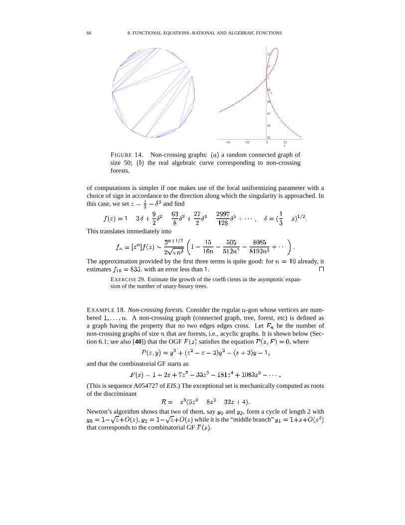
66 8. FUNCTIONAL EQUATIONS—RATIONAL AND ALGEBRAIC FUNCTIONS
0.5
0.6
0.7
0.8
0.9
1
1.1
1.2
y
–0.4 –0.2 0 0.2z
FIGURE 14. Non-crossing graphs: H 1 M a random connected graph ofsize 50; H ? M the real algebraic curve corresponding to non-crossingforests.
of computations is simpler if one makes use of the local uniformizing parameter with achoice of sign in accordance to the direction along which the singularity is approached. Inthis case, we set � � 2� � � �
and find
� H � M7� 6 � = � 4 T/� � � U#=
;� � 4
/ :/� � � / T#T2:
6 / ;� 4#"$"%" � � � H 6= � � M 2 ��� �
This translates immediately into
� � � � � � � � H � M � = �al 2 ���/ � � h �
6�� 6�9
6�U h 4 9.8!99�6 / h � � ;!8#;!9
;�6�T / h � 4#"$"%" �The approximation provided by the first three terms is quite good: for h � 6�8 already, itestimates
� 2 � � ;!=!9 . with an error less than 6 . �EXERCISE 29. Estimate the growth of the coefficients in the asymptotic expan-sion of the number of unary-binary trees.
EXAMPLE 18. Non-crossing forests. Consider the regular h -gon whose vertices are num-bered 6 � �;�,� � h . A non-crossing graph (connected graph, tree, forest, etc) is defined asa graph having the property that no two edges edges cross. Let
! � be the number ofnon-crossing graphs of size h that are forests, i.e., acyclic graphs. It is shown below (Sec-tion 6.1; see also [40]) that the OGF
! H � M satisfies the equation � H � � ! M��A8 , where
� H � � / M�� / � 4 H � � � � � =!M / � 4 H �:4 =!M / � 6 �and that the combinatorial GF starts as! H � M�� 6 4 / �A4 : � � 4 =#= � � 4 6�;�6 � � 4 6�8#;!= � 4 "%"$".�(This is sequence A054727 of EIS.) The exceptional set is mechanically computed as rootsof the discriminant � � � � HS9 � � � ; � � � = / �A4 � M �Newton’s algorithm shows that two of them, say / � and / � , form a cycle of length 2 with/ � ��6 � � �34 H � M , / � ��6 4 � �34 H � M while it is the “middle branch” / 2 � 6 45�34 H � � Mthat corresponds to the combinatorial GF
! H � M .
5. ANALYSIS OF ALGEBRAIC FUNCTIONS 67
The other exceptional points are the roots of the cubic factor of � , namely� � ( ��6 � T#=!8 / ; � 8 � 6 / 6�9.; � = � � 8!;#U#T * �Let � �� 8 � 6 / 9.; be the root in HK8 � 6�M . By Pringsheim’s theorem and the fact that the OGF ofan infinite combinatorial class must have a positive dominant singularity in � 8 � 6 � , the onlypossibility for the dominant singularity of />2 H � M is � . (For a more general argument, seebelow.)
For � near � , the three branches of the cubic give rise to one branch that is ana-lytic with value approximately 8 � U1:<;"6�U and a cycle of two conjugate branches with valuenear 6 � / 6 � / T at � � � . The expansion of the two conjugate branches is of the singulartype, � � � � 6�� �>= � �where� � � =
=2: 4 6�;=2: � � =!9
: � �� ���6 � / 6 � / T � � � 6
=2: � / / ; � T!;�6 � � 9 / T!8 � � ��A8 � 6 � T!=�6 �The determination with a minus sign must be adopted for representing the combinatorialGF when � � � j since otherwise one would get negative asymptotic estimates for thenonnegative coefficients. Alternatively, one may examine the way the three real branchesalong HK8 � � M match with one another at 0 and at � j , then conclude accordingly.
Collecting partial results, we finally get by singularity analysis the estimate
! � � �/ � � h � )
� 6 4 H 6h M � ) � 6�
��A; � /�/ � U#Twhere the cubic algebraic number � and the sextic � are as above.
�The example above illustrates several important points in the analysis of coefficients
of algebraic functions when there are no simple explicit radical forms. First of all a givencombinatorial problem determines a unique branch of an algebraic curve at the origin.Next, the dominant singularity has to be identified by “connecting” the combinatorialbranch with the branches at every possible singularity of the curve. Finally, computationstend to take place over algebraic numbers and not simply rational numbers.
So far, examples have illustrated the common situation where the exponent at thedominant singularity is 2� , which is reflected by a factor of h j � ��� in the asymptotic form ofcoefficients. Our last example shows a case where the exponent assumes a different value,namely 2� .
EXAMPLE 19. “Supertrees”. Consider the equation � H � �� M�� 8 where
� H � � / M7� �#/ � � / � 4 H / �A4 6�M / � � /�4 � �The general aspect of the curve is given in Figure 15 and the asymptotic expansion of
the branch with positive coefficients, / H � M�� ��46� � 4 = � � 4 ; � � 4 "%"$" , is sought.The discriminant is found to be
� � � H � �A4 =2M-H � � � 6�M � �so that the dominant singularity of the branch of combinatorial interest is � � 2� where itsvalue equals 1. The translation � � 2� � � � / ��6 4 �
transforms � into
�� H � � � M0��H 6�
���DM � � � � � � � � ; � � � � ; � � � � � �
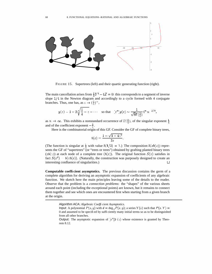
68 8. FUNCTIONAL EQUATIONS—RATIONAL AND ALGEBRAIC FUNCTIONS
–3
–2
–1
0
1
2
3
y
–0.6 –0.4 –0.2 0.2z
FIGURE 15. Supertrees (left) and their quartic generating function (right).
The main cancellation arises from 2� � � � � � �A8 : this corresponds to a segment of inverseslope 6 = � in the Newton diagram and accordingly to a cycle formed with 4 conjugatebranches. Thus, one has, as � � H 2� M j ,
/ H � M � 6�� / �� 6�
� �A4 "%"$" so that � � � � / H � M � 6� ;��CH �� M �
� h j � � �as h � . This exhibits a nonstandard occurrence of � H �� M , of the singular exponent 2�and of the coefficient exponent �
� .Here is the combinatorial origin of this GF. Consider the GF of complete binary trees,
? H � M7� 6�� � 6�� � � �/ � �
(The function is singular at 2� with value ? H 6 = / M5� 6 .) The composition ? H � ? H � M M repre-sents the GF of “supertrees” (or “trees or trees”) obtained by grafting planted binary trees( � ? H � M ) at each node of a complete tree H ? H � M ). The original function
� H � M satisfies infact
� H � � M � ? H � ? H � M M . (Naturally, the construction was purposely designed to create aninteresting confluence of singularities.)
�
Computable coefficient asymptotics. The previous discussion contains the germ of acomplete algorithm for deriving an asymptotic expansion of coefficients of any algebraicfunction. We sketch here the main principles leaving some of the details to the reader.Observe that the problem is a connection problems: the “shapes” of the various sheetsaround each point (including the exceptional points) are known, but it remains to connectthem together and see which ones are encountered first when starting from a given branchat the origin.
Algorithm ACA: Algebraic Coefficient Asymptotics.Input: A polynomial
� ��� � ) � with � - deg � � ��� � ) � ; a series) ����� such that
� ��� � ) �7-/ and assumed to be specified by sufficiently many initial terms so as to be distinguishedfrom all other branches.Output: The asymptotic expansion of � � O � ) ����� whose existence is granted by Theo-rem 8.12.
5. ANALYSIS OF ALGEBRAIC FUNCTIONS 69
The algorithm consists of three main steps: Preparation, Dominant singularities, and Transla-tion.
I. Preparation: Define the discriminant� �����7- R � � � � �� � ) � .� � '�� Compute the exceptional set � - ��� �� � ����� -i/ � and the points of infinity � � -
� � �� � � ����� - / � , where � � ����� is the leading coefficient of� ��� � ) � considered as a
function of ) .� � � � Determine the Puiseux expansions of all the � branches at each of the points of ��� � / �(by Newton diagrams and/or indeterminate coefficients). This includes the expansion ofanalytic branches as well. Let �() Q % � ����� � >� ' be the collection of all such expansions atsome R � ��� � / � .� � � � Identify the branch at 0 that corresponds to
) ����� .II. Dominant singularities (Controlled approximate matching of branches). Let � ' � � � ���� be a
partition of the elements of ��� � / � sorted according to the increasing values of their modulus: it isassumed that the numbering is such that if R � � and ` � � � , then � R���� `�� is equivalent to
� � � .Geometrically, the elements of � have been grouped in concentric circles. First, a preparation step isneeded.� � ' � Determine a nonzero lower bound � on the radius of convergence of any local Puiseux
expansion of any branch at any point of � . Such a bound can be constructed from theminimal distance between elements of � and from the degree � of the equation.
The sets � � are to be examined in sequence until it is detected that one of them contains a singu-larity. At step � , let � ' � � � ����6� �� be an arbitrary listing of the elements of � � . The problem is todetermine whether any � _ is a singularity and, in that event, to find the right branch to which it isassociated. This part of the algorithm proceeds by controlled numerical approximations of branchesand constructive bounds on the minimum separation distance between distinct branches.� � � � For each candidate singularity � _ , with
� � �, set I _ - � _ � � G���� � � . By assumption,
each I _ is in the domain of convergence of) ����� and of any )���� % � .� � � � Compute a nonzero lower bound � _ on the minimum distance between two roots of� ��I _ � ) ��-0/ . This separation bound can be obtained from resultant computations.� � � � Estimate
) ��I _ � and each ) � � % � ��I _ � to an accuracy better than � _ � " . If two elements,) ����� and )���� % � ����� are (numerically) found to be at a distance less than � _ for � - I _ , thenthey are matched: � _ is a singularity and the corresponding ) � � % � is the correspondingsingular element. Otherwise, � _ is declared to be a regular point for
) ����� and discardedas candidate singularity.
The main loop on � is repeated until a singularity has been detected., when ��- � � , say. The radius ofconvergence � is then equal to the common modulus of elements of � � � ; the corresponding singularelements are retained.
III. Coefficient expansion. Collect the singular elements at all the points � determined to be adominant singularity at Phase III. Translate termwise using the singularity analysis rule,
� �=GJ��� T ����� A � T ��� ��O�� �&G ������+ M �� �&G ������� � �ZM + � � �
and reorganize into descending powers of M , if needed.
This algorithm vindicates the following assertion:
PROPOSITION 8.5 (Decidability of algebraic connections.). The dominant singular-ities of a branch of an algebraic function can be determined by the algorithm ACA in afinite number of operations in the algebraic closure of the base field, � or � .
70 8. FUNCTIONAL EQUATIONS—RATIONAL AND ALGEBRAIC FUNCTIONS
5.2. Positive functions and positive systems. The discussion of algebraic singulari-ties specializes nicely to the case of positive functions. We first indicate a procedure thatdetermines the radius of convergence of any algebraic series with positive coefficients. Theprocedure takes advantage of Pringsheim’s theorem that allows us to restrict attention tocandidate singularities on the positive half-line. It represents a shortcut that is often suit-able for human calculation and, in fact, the it systematizes some of the techniques alreadyused implicitly in earlier examples.
Algorithm ROCPAF: Radius of Convergence of Positive Algebraic Functions.Input: A polynomial
� ��� � ) � with � - deg � � ��� � ) � ; a series) ����� such that
� ��� � ) �7-/ that is known to have only nonnegative coefficients ( � � O � ) ������� / ) and is assumed tobe specified by sufficiently many initial terms.Output: The radius of convergence � of
) ����� .Plane-sweep. Let � � be the subset of those elements of the exceptional set � which are positive
real. � � ' � Sort the subset of those branches �() � % � � at / � that have totally real coefficients. This isessentially a lexicographic sort that only needs the initial parts of each expansion. Setinitially � � -0/ and �������7- ) ����� .� � � � Sweep over all � � � � in increasing order. To detect whether a candidate � is the domi-nant positive singularity, proceed as follows:
— Sort the branches �()�� % � � at ��
that have totally real coefficients.— using the orders at �
�� and ��
, match the branch ������� with its corresponding branchat �
�, say � ����� ; this makes use of the total ordering between real branches at �
��and �
�. If the branch � ����� is singular, then return � -�� as the radius of conver-
gence of) ����� and use � ����� as the singular element of
) ����� at � - � ; otherwisecontinue with the next value of � � � � while replacing ������� by � ����� and � � by � .
This algorithm is a plane-sweep that takes advantage of the fact that the real branchesnear a point can be totally ordered; finding the ordering only requires inspection of a finitenumber of coefficients. The plane-sweep algorithm enables us to trace at each stage theoriginal branch and keep a record of its order amongst all branches. The method workssince no two real branches can cross at a point other than a multiple point, such a pointbeing covered as an element of
� l.
We now turn to positive systems. Most of the combinatorial classes known to admitalgebraic generating functions involve singular exponents that are multiples of 2� . Thisempirical observation is supported by the fact, to be proved below, that a wide class ofpositive systems have solutions with a square-root singularity. Interestingly enough, thecorresponding theorem is due to independent research by several authors: Drmota [31]developed a version of the theorem in the course of studies relative to limit laws in variousfamilies of trees defined by context-free grammars; Woods [100], motivated by questionsof Boolean complexity and finite model theory, gave a form expressed in terms of colouringrules for trees; finally, Lalley [63] came across a similarly general result when quantifyingreturn probabilities for random walks on groups. The statement that follows is a fundamen-tal result in the analysis of algebraic systems arising from combinatorics and is (rightly)called the “Drmota-Lalley-Woods” theorem. Notice that the authors of [31, 63, 100] provemore: Drmota and Lalley show how to pull out limit Gaussian laws for simple parameters(e.g., as in [31] by a perturbative analysis; see Chapter 9); Woods shows how to deduceestimates of coefficients even in some periodic or non-irreducible cases (see definitionsbelow).
5. ANALYSIS OF ALGEBRAIC FUNCTIONS 71
In the treatment that follows we start from a polynomial system of equations,
(;/ 9 � � 9 H � � / 2 � �,�;� � / E M * � " ��6 � �;�,� � �We shall discuss in the next section a class of combinatorial specifications, the “context-free” specifications, that leads systematically to such fixed-point systems. The case oflinear systems has been already dealt with, so that we limit ourselves here to nonlinearsystems defined by the fact that at least one polynomial
� 9 is nonlinear in some of theindeterminates / 2 � �,�;� � / E .
First, for combinatorial reasons, we define several possible attributes of a polynomialsystem.
— Algebraic positivity (or a-positivity). A polynomial system is said to be a-positive if all the component polynomials
� 9 have nonnegative coefficients.
Next, we want to restrict consideration to systems that determine a unique solution vectorH / 2 � �;�,� � / E M � H �&� � � � � M E . (This discussion is related to 0-dimensionality in the sensealluded to earlier.) Define the � -valuation v 1 � H �/ M of a vector �/ � ��� � ��� � E as the minimumover all " ’s of the individual valuations9 v 1 � H / 9 M . The distance between two vectors isdefined as usual by < H �/ �
�/ � M7� / j v / � ��� j � � . Then, one has:
— Algebraic properness (or a-properness). A polynomial system is said to be a-proper if it satisfies a Lipschitz condition
< H � H �/ M � � H �/ � M M @ < H �/ ��/ � M for some @ 6 .
In that case, the transformation�
is a contraction on the complete metric space of formalpower series and, by the general fixed point theorem, the equation / � � H / M admits aunique solution. In passing, this solution may be obtained by the iterative scheme,
�/ � � � HS8 � �,�,� � 8!M � � �/ � � l 2 � � H / � � M � / � + � %� � �
/ � � �The key notion is irreducibility. To a polynomial system, �/ � � H �/ M , associate its
dependency graph defined as a graph whose vertices are the numbers 6 � �;�,� � and theedges ending at a vertex " are
� � " , if / 9 figures in a monomial of� � H "2M . (This notion is
reminiscent of the one already introduced for linear system on page 8.5.)
— Algebraic irreducibility (or a-irreducibility). A polynomial system is said to bea-irreducible if its dependency graph is strongly connected.
Finally, one needs a technical notion of periodicity to dispose of cases like
/ H � M�� 6/ � � 6�� � 6�� � � � � �:4 � � 4 / � 4#"$"%" �
(the OGF of complete binary trees) where coefficients are only nonzero for certain residueclasses of their index.
— Algebraic aperiodicity (or a-aperiodicity). A power series is said to be aperiodicif it contains three monomials (with nonzero coefficients), � 8
� � � 8� � � 8
� , such that� � � � 2 and � � � � 2 are relatively prime. A proper polynomial system is said tobe aperiodic if each of its component solutions / 9 is aperiodic.
THEOREM 8.13 (Positive polynomial systems). Consider a nonlinear polynomial sys-tem �/ � � H �/ M that is a-proper, a-positive, and a-irreducible. In that case, all component
9Let� ��� �O �X � O�� O with
� X��� � ; the valuation of�
is by definition v � � � " � � .
72 8. FUNCTIONAL EQUATIONS—RATIONAL AND ALGEBRAIC FUNCTIONS
solutions / 9 have the same radius of convergence � . Then, there exist functions � 9analytic at the origin such that
(60) / 9 � � 9 � � 6�� �>=�� H � � � j M �In addition, all other dominant singularities are of the form � ) with ) a root of unity.
If furthermore the system is a-aperiodic, all / 9 have � as unique dominant singularity. Inthat case, the coefficients admit a complete asymptotic expansion of the form
(61) � � � � / 9 H � M � � j���� � 2 < � h j 2 j � ��� �� �
Proof. The proof consists in gathering by stages consequences of the assumptions. It isessentially based on close examination of “failures” of the implicit function theorem andthe way these lead to singularities.
H 1 M As a preliminary observation, we note that each component solution / 9 is analgebraic function that has a nonzero radius of convergence. In particular, singularitiesare constrained to be of the algebraic type with local expansions in accordance with theNewton-Puiseux theorem (Theorem 8.11).
H ? M Properness together with the positivity of the system implies that each / 9 H � M hasnonnegative coefficients in its expansion at 0, since it is a formal limit of approximants thathave nonnegative coefficients. In particular, each power series / 9 has a certain nonzeroradius of convergence � 9 . Also, by positivity, � 9 is a singularity of / 9 (by virtue of Pring-sheim’s theorem). From the nature of singularities of algebraic functions, there exists someorder � 8 such that each th derivative
e � / 9 H � M becomes infinite as � � � j9 .We establish now that �32 � "%"$" � � E . In effect, differentiation of the equations com-
posing the system implies that a derivative of arbitrary order � , e � / 9 H � M , is a linear form inother derivatives
e � / 9 H � M of the same order (and a polynomial form in lower order deriva-tives); also the linear combination and the polynomial form have nonnegative coefficients.Assume a contrario that the radii were not all equal, say � 2 � "$"%" � � � , with the other radii� � l 2 � �,�;� being strictly greater. Consider the system differentiated a sufficiently large num-ber of times, . Then, as � � � 2 , we must have
e � / 9 tending to infinity for " ��� . On theother hand, the quantities / � l 2 , etc., being analytic, their th derivatives that are analyticas well must tend to finite limits. In other words, because of the irreducibility assumption(and again positivity), infinity has to propagate and we have reached a contradiction. Thus,all the / 9 have the same radius of convergence and we let � denote this common value.
H �;2 M The key step consists in establishing the existence of a square-root singularity atthe common singularity � . Consider first the scalar case, that is
(62) / � � H � � / M7� 8 �where � is assumed to depend nonlinearly on / and have nonnegative coefficients. Therequirement of properness means that � is a factor of all monomials, except the constantterm � HS8 � 82M .
Let / H � M be the unique branch of the algebraic function that is analytic at 0. Compar-ison of the asymptotic orders in / inside the equality / � � H � � / M shows that (by nonlin-earity) we cannot have / � when � tends to a finite limit. Let now � be the radius ofconvergence of / H � M . This argument shows that / H � M is necessarily finite at its singularity � .We set � / H � M and note that, by continuity � � H � � M&�A8 .
5. ANALYSIS OF ALGEBRAIC FUNCTIONS 73
By the implicit function theorem, a solution H � � � / � M of (62) can be continued analyti-cally as H � � / � H � M M in the vicinity of � � as long as the derivative with respect to / ,� H � � � / � M Q ��6�� � � H � � � / � Mremains nonzero. The quantity � being a singularity, we must have
� H � � M � 8 . (Inpassing, the system
� � H � � M0�A8 � � H � � M&� 8 �determines only finitely many candidates for � .) On the other hand, the second derivative� � � � is nonzero at H � � M (by positivity, since no cancellation can occur); there results bythe classical argument on local failures of the implicit function theorem that / H � M has asingularity of the square-root type (see also Chapters 4 and 5). More precisely, the localexpansion of the defining equation (62) at H � � M binds H � � / M locally by
�(H � � � M � � H � � M � 6/H / � M � � � � H � � M 4#"$"%" � 8 �
where the subsequent terms are negligible by Newton’s polygon method. Thus, we have
/ � � �� � H � � M� � � H � � M H � � � M 2 ��� 4#"$"%" �
the negative determination of the square-root being chosen to comply with the fact that/ H � M increases as � � � j . This proves the first part of the assertion in the scalar case.H � � M In the multivariate case, we graft an ingenious argument [63] that is based on
a linearized version of the system to which Perron-Frobenius theory is applicable. First,irreducibility implies that any component solution / 9 depends nonlinearly on itself (bypossibly iterating
�), so that a discrepancy in asymptotic behaviours would result for the
implicitly defined / 9 in the event that some / 9 tends to infinity.Now, the multivariate version of the implicit function theorem grants locally the ana-
lytic continuation of any solution />2 � / � � �;�,� � /�E at � � provided there is no vanishing of theJacobian determinant� H � � � / 2 � �;�,� � /�E M Q � �� �
� � � 9 � ee / 9 � � H � � � / 2 � �,�,� � /�E M �where
� � � 9 is Kronecker’s symbol. Thus, we must have� H � � 2 � �,�;� � E M0� 8 where 9 Q � / 9 H � M �The next argument (we follow Lalley [63]) uses Perron-Frobenius theory and linear
algebra. Consider the modified Jacobian matrix
@ H � � � / 2 � �;�,� � /�E M Q � ee / 9 � � H � � � / 2 � �;�,� � /�E M �
which represents the “linear part” of�
. For � � />2 � �,�;� � /#E all nonnegative, the matrix @has positive entries (by positivity of
�) so that it is amenable to Perron-Frobenius theory.
In particular it has a positive eigenvalue - H � � />2 � �,�,� � /�E M that dominates all the other inmodulus. The quantity � - H � M7� - H / 2 H � M � �,�,� � / E H � M Mis increasing as it is an increasing function of the matrix entries that themselves increasewith � for � � 8 .
We propose to prove that� - H � M�� 6 , In effect,
� - H � M� 6 is excluded since otherwiseH�� � @ M would be invertible at � � � and this would imply� �� 8 , thereby contradicting
the singular character of the / 9 H � M at � . Assume a contrario� - H � M � 6 in order to exclude
74 8. FUNCTIONAL EQUATIONS—RATIONAL AND ALGEBRAIC FUNCTIONS
the other case. Then, by the increasing property, there would exists ��2 � such that� - H �32 M�� 6 . Let ' 2 be a left eigenvector of @ H � 2 � / 2 H �>2 M � �;�,� � /�E H �32 M M corresponding tothe eigenvalue
� - H �32 M . Perron-Frobenius theory grants that such a vector ' 2 has all itscoefficients that are positive. Then, upon multiplying on the left by ' 2 the column vectorscorresponding to / and
� H / M (which are equal), one gets an identity; this derived identityupon expanding near � 2 gives
(63) � H � � � 2 M7� � � � 9 � � � 9 H / � H � M � / � H � 2 M M�H / 9 H � M � / 9 H � 2 M M 4 "%"$" �
where "%"%" hides lower order terms and the coefficients � � � � � 9 are nonnegative with � � 8 .There is a contradiction in the orders of growth if each / � is assumed to be analytic at � 2since the left side of (63) is of exact order H � � � 2 M while the right side is at least as smallas to H � � �32 M � . Thus, we must have
� - H � M7��6 and� - H � M 76 for � � HK8 � � M .
A calculation similar to (63) but with � 2 replaced by � shows finally that, if
/ � H � M � /�� H � M � � � H � � � M � �then consistency of asymptotic expansions implies
/ � � 6 , that is � � 2� . (The argu-ment here is similar to the first stage of a Newton polygon construction.) We have thusproved that the component solutions / 9 H � M have a square-root singularity. (The existenceof a complete expansion in powers of H � � � M 2 ��� results from examination of the Newtondiagram.) The proof of the general case (60) is at last completed.H < M In the aperiodic case, we first observe that each / 9 H � M cannot assume an infinitevalue on its circle of convergence � � � � � , since this would contradict the boundedness of� / 9 H � M � in the open disk � ��� � (where / 9 H � M serves as an upperbound). Consequently, bysingularity analysis, the Taylor coefficients of any / 9 H � M are H h j 2 j�� M for some � � 6and the series representing / 9 at the origin converges on � � � � � .
For the rest of the argument, we observe that if / � � H � ��/ M , then / � � � E � H � �
�/ Mwhere the superscript denotes iteration of the transformation
�in the variables �/ �
H / 2 � �;�,� � / E M . By irreducibility,� � E � is such that each of its component polynomials in-
volves all the variables.Assume that there would exists a singularity � � of some / 9 H � M on � � � � � . The triangu-
lar inequality yields � / 9 H � � M � / 9 H � M where strictness is related to the general aperiodicityargument encountered at several other places in this book. But then, the modified Jaco-bian matrix @ � E � of
� � E � taken at the / 9 H � � M has entries dominated strictly by the entriesof @ � E � taken at the / 9 H � M . There results (see page 17) that the dominant eigenvalue of@ � E � H � �
�/ 9 H � � M M must be strictly less than 1. But this would imply that � � @ � E � H � ��/ 9 H � � M M
is intervertible so that the / 9 H � M would be analytic at � � . A contradiction has been reached:� is the sole dominant singularity of each / 9 and this concludes the argument. �We observe that the dominant singularity is obtained amongst the positive solutions of
the system� � � H � �
� M � � H � �� M7� 8 �
For the Catalan GF, this yields
� 6�� � � � 8 � 6�� / � � 8 �giving back (as expected) � � 2� , � 2� . For three coloured trees (with / 2 � / � � / � repre-senting � � � �
), the system is formed of the specialization of the defining equations (40),namely,
2 � � � H � 4 � M � � 8 � � � H � 4� 2 M � � 8 � � � H 2 4 � M � � 8 �
6. APPLICATIONS OF ALGEBRAIC FUNCTIONS 75
together with the Jacobian condition
�� �
����� 6 � / � � / � � / � � / �� / 2 � / � 6 � / � � / 2� / 2 � / � � / � � / 2 6
� ���� �A8 �
It is found (by elimination) that� � 6�� HK= � 4 6�M � where � � � 4 � � � 4 � � 6:� 8 �
with � �� 8 � = � U#;�6 and � �� 8 � 6<:#:.U#;�6 being the only feasible solution to the constraints.Thus, the number of 3-coloured trees grows roughly like 9 � U / � h j � ��� .
EXERCISE 30. Match the computation of the dominant singularity of 3-colouredtrees against the determination of the minimal polynomial
� ��� � � � of the previ-ous section.
6. Combinatorial applications of algebraic functions
In this section, we first present context-free specifications that admit a direct transla-tion into polynomial systems (Section 6.1). When particularized to formal languages, thisgives rise to context-free languages (Section 6.2) that, provided an unambiguity conditionis met, lead to algebraic generating functions. An important subclass, especially as regardscomputer science applications, is that of simple families of trees succinctly presented inSection 6.3.
The next two subsections introduce objects whose constructions still lead to algebraicfunctions, but in a non-obvious way. This includes: walks with a finite number of allowedbasic jumps (Section 6.4) and planar maps (Section 6.5). In that case, bivariate functionalequations are induced by the combinatorial decompositions. The common form is
(64)� H � � � � ! H � � � M � � 2 H � M � �,�;� � � � H � M M7�A8 �
where�
is a known polynomial and the unknowns are!
and �%2 � �,�;� � � � . Specific methodsare to be appealed to in order to attain solutions to such functional equations that wouldseem at first glance to be grossly underdetermined. Random walks lead to a linear versionof (64) that is treated by the so-called “kernel method”. Maps lead to nonlinear versionsthat are solved by means of Tutte’s “quadratic method”. In both cases, the strategy consistsin binding � and � by forcing them to lie on an algebraic curve (suitably chosen in order toeliminate the dependency on
! H � � � M ), and then pulling out the algebraic consequences ofsuch a specialization.
6.1. Context-free specifications. A context-free system is a collection of combinato-rial equations,
(65)
��������� 2 � � 2 H �1 � 2 � �;�,� � 3E M
......
3E � � E H �1 � 2 � �;�,� � 3E M �where �1 � H 1 2 � �,�;� M is a vector of atoms and each of the
� 9 only involves the combinatorialconstructions of disjoint union and cartesian product. A combinatorial class is said to
76 8. FUNCTIONAL EQUATIONS—RATIONAL AND ALGEBRAIC FUNCTIONS
be context-free if it is definable as the first component ( � 2 ) of a well-founded context-free system. The terminology comes from linguistics and it stresses the fact that objectscan be “freely” generated by the rules in (65), this without any constraints imposed by anoutside context10.
For instance the class of plane binary trees defined by� � �&4 H�� � ��� � M H � � � atoms M
is a context-free class. The class of general plane trees defined by
� � � ��������������� H � M ( � an atom)
is definable by the system
� � � � � � � � � 4 H � � � M �with � defining forests, and so it is also context-free. (This example shows more generallythat sequences can always be reduced to polynomial form.)
Context-free specifications may be used to describe all sorts of combinatorial objects.For instance, the class � of triangulations of convex polygons is specified symbolically by
(66) � � � 4 H�� � � M 4 H � � �'M 4 H � � � � � M �where � represents a generic triangle.
The general symbolic rules given in Chapter 1 apply in all such cases. Thereforethe Drmota-Lalley-Woods theorem (Theorem 8.13) provides the asymptotic solution to animportant category of problems.
PROPOSITION 8.6 (Context-free specifications). A context-free class admits anOGF that satisfies a polynomial system obtained from the specification by the translationrules:
� 4 � �� � 4 � � � � � �� � "'� �The OGF
H � M is an algebraic function to which algebraic asymptotics applies. In partic-ular, a context-free class that gives rise to an algebraically aperiodic irreducible systemhas an enumeration sequence satisfying � � �
� � h � )� �
where � � ) are computable algebraic numbers.
This last result explains the frequently encountered estimates involving a factor ofh j � ��� (corresponding to a square-root singularity of the OGF) that can be found through-out analytic combinatorics.
EXERCISE 31. If � � � are context-free specifications then: � � � the sequence class� -����������������P����� is context-free; � � � � the substitution class � -�� � � �A � � iscontext-free.
We detail below an example from combinatorial geometry.
10Formal language theory also defines context-sensitive grammars where each rule (called a production)is applied only if it is enabled by some external context. Context-sensitive grammars have greater expressivepower than context-free ones, but they depart significantly from decomposability since they are surrounded bystrong undecidability properties; accordingly context-sensitive grammars cannot be associated with any globalgenerating function formalism.
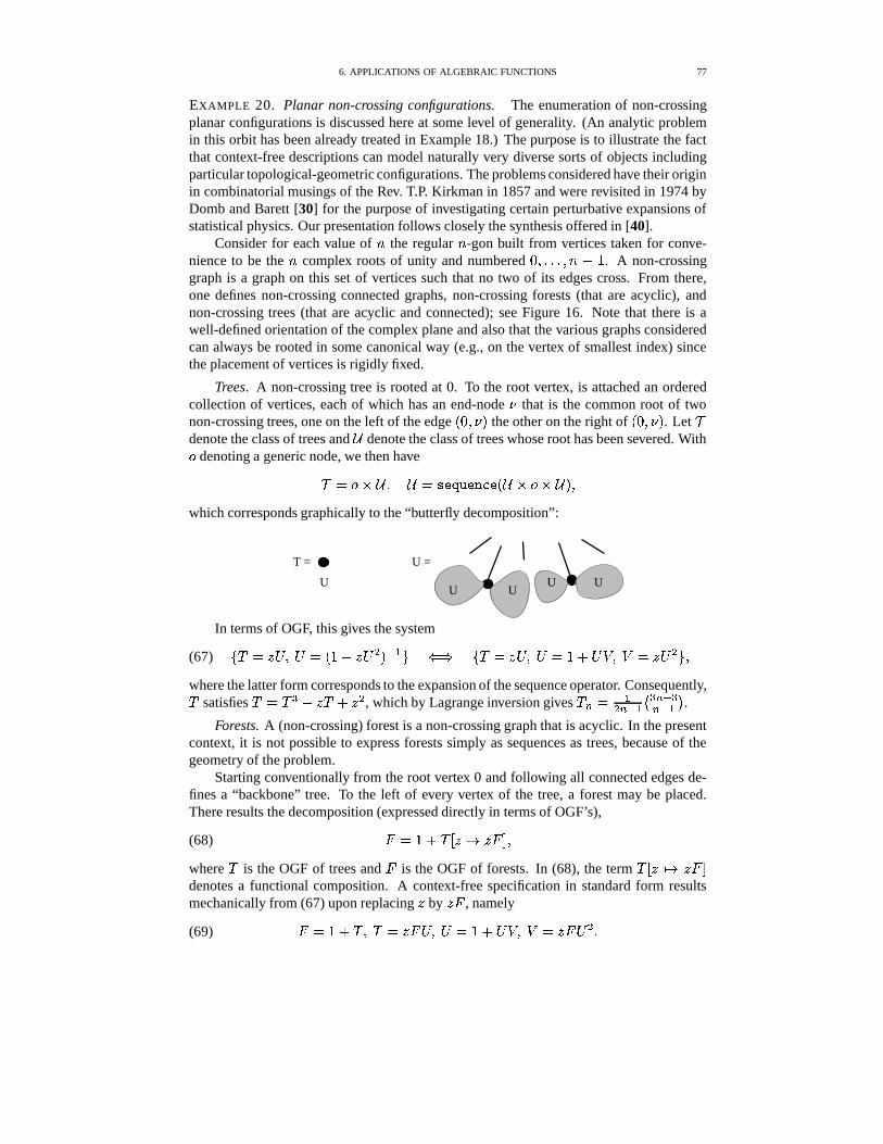
6. APPLICATIONS OF ALGEBRAIC FUNCTIONS 77
EXAMPLE 20. Planar non-crossing configurations. The enumeration of non-crossingplanar configurations is discussed here at some level of generality. (An analytic problemin this orbit has been already treated in Example 18.) The purpose is to illustrate the factthat context-free descriptions can model naturally very diverse sorts of objects includingparticular topological-geometric configurations. The problems considered have their originin combinatorial musings of the Rev. T.P. Kirkman in 1857 and were revisited in 1974 byDomb and Barett [30] for the purpose of investigating certain perturbative expansions ofstatistical physics. Our presentation follows closely the synthesis offered in [40].
Consider for each value of h the regular h -gon built from vertices taken for conve-nience to be the h complex roots of unity and numbered 8 � �,�;� � h � 6 . A non-crossinggraph is a graph on this set of vertices such that no two of its edges cross. From there,one defines non-crossing connected graphs, non-crossing forests (that are acyclic), andnon-crossing trees (that are acyclic and connected); see Figure 16. Note that there is awell-defined orientation of the complex plane and also that the various graphs consideredcan always be rooted in some canonical way (e.g., on the vertex of smallest index) sincethe placement of vertices is rigidly fixed.
Trees. A non-crossing tree is rooted at 0. To the root vertex, is attached an orderedcollection of vertices, each of which has an end-node � that is the common root of twonon-crossing trees, one on the left of the edge HK8 �
�M the other on the right of HK8 �
�M . Let �
denote the class of trees and�
denote the class of trees whose root has been severed. With� denoting a generic node, we then have
� � � � � � � � ��� � ������� H � � � � � M �which corresponds graphically to the “butterfly decomposition”:
UUU
U U
U = T =
In terms of OGF, this gives the system
(67) ( � � � � � � � H�6�� � � � M j 2 * � � ( � � � � � � � 6 4 � . � . � � � � * �where the latter form corresponds to the expansion of the sequence operator. Consequently,� satisfies � � � � � ���64 � � , which by Lagrange inversion gives � � � 2� �Pj 2 � � �Pj ��Pj 2�� .
Forests. A (non-crossing) forest is a non-crossing graph that is acyclic. In the presentcontext, it is not possible to express forests simply as sequences as trees, because of thegeometry of the problem.
Starting conventionally from the root vertex 0 and following all connected edges de-fines a “backbone” tree. To the left of every vertex of the tree, a forest may be placed.There results the decomposition (expressed directly in terms of OGF’s),
(68)! ��6 4���� � �� � ! � �
where � is the OGF of trees and!
is the OGF of forests. In (68), the term � � � �� � ! �denotes a functional composition. A context-free specification in standard form resultsmechanically from (67) upon replacing � by � ! , namely
(69)! � 6 4�� � � � � ! � � � ��6 4 � . � . � � ! � � �
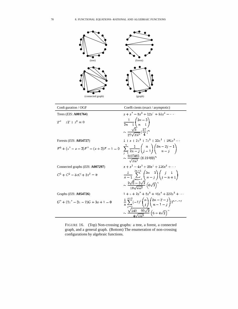
78 8. FUNCTIONAL EQUATIONS—RATIONAL AND ALGEBRAIC FUNCTIONS
(connected graph)
(tree) (forest)
(graph)
Configuration / OGF Coefficients (exact / asymptotic)
Trees (EIS: A001764) �N+,� � + � � � + ��� � � + � � � � +5464(4� � GJ� �^+ � � -0/ �
� M=G �� � M G �M G ���
* � �� � � M � � � " � OForests (EIS: A054727)
� +,�N+ � � � + �� � + � � � � + � � � � 464(4� � + ��� � GJ�HG � � � � +0���N+ � � � G � -0/ O�� ' �
� M G �� M�;G � � � � M G � � G �M G � �
* / / " � �� � M � � � � " � � � OConnected graphs (EIS: A007297) �N+,� � + " � � + ��� � � + ����� � � + 46464� � + � � G � � � + � � � - / �M G �
� Oa� ���� Om� '� � M G �M + � �
� � G �� GSM + � �
*� � � G � � �� � � M ��� � � �� O
Graphs (EIS: A054726)� +,�N+ � � � + � � + " � � + � � � � � +54(464
� � + � � � � G � �HG � � � + � ��+ � -0/ �MOa� '���� �&G � � �
� M � �� � M=G � G �M G � G � � � Oa� ' ���
*� � " /HG ��� � �" � � M � � � + " � � � OFIGURE 16. (Top) Non-crossing graphs: a tree, a forest, a connectedgraph, and a general graph. (Bottom) The enumeration of non-crossingconfigurations by algebraic functions.
6. APPLICATIONS OF ALGEBRAIC FUNCTIONS 79
This system is irreducible and aperiodic, so that the asymptotic shape of! � is of the
form � ) � h j � ��� , as predicted by Proposition 8.6. This agrees with the precise formuladetermined in Example 18.
Graphs. Similar constructions (see [40]) give the OGF’s of connected graphs andgeneral graphs. The results are summarized in Figure 16. Note the common shape of theasymptotic estimates and also the fact that binomial expressions are always available inaccordance with Theorem 8.10.
�
Note on “tree-like” structures. A context-free specification can always be regarded asdefining a class of trees. Indeed, if the " th term in the construction
� 9 is “coloured” withthe pair H�� � "2M , it is seen that a context-free system yields a class of trees whose nodes aretagged by pairs H�� � "1M in a way that is consistent with the system’s rules (65). However,despite this correspondence, it is often convenient to preserve the possibility of operatingdirectly with objects11 when the tree aspect is unnatural. By a terminology borrowed fromthe theory of syntax analysis in computer science, such trees are referred to as “parse trees”or “syntax trees”.
EXERCISE 32. The parse trees associated mechanically with the specification oftriangulations above are in bijective correspondence with binary (rooted plane)trees.
6.2. Context-free languages. Let � be a fixed finite alphabet whose elements arecalled letters. A grammar � is a collection of equations
(70) � Q
��������� �2 � � 2 H �1 � 2 � �;�,� � 0E M
......
0E � � E H �1 � 2 � �,�,� � 0E M �where each � 9 involves only the operations of union ( � ) and catenation product H " ) with�1 the vector of letters in � . For instance,
� 2 H �1 � 2 � � � � M�� 1 � " � " � � 1 � � � " 1 � " �2��A solution to (70) is an -tuple of languages over the alphabet � that satisfies the system.By convention, one declares that the grammar � defines the first component, :2 .
To each grammar (70), one can associate a context-free specification (65) by trans-forming unions into disjoint union, ‘ � ’
��‘ 4 ’, and catenation into cartesian products,
‘ " ’ �� ‘�
’. Let�� be the specification associated in this way to the grammar � . The
objects described by�� appear in this perspective to be trees (see the discussion above re-
garding parse trees). Let � be the transformation from trees of�� to languages of � that
lists letters in infix (i.e., left-to-right) order: we call such an � the erasing transforma-tion since it “forgets” all the structural information contained in the parse tree and onlypreserves the succession of letters. Clearly, application of � to the combinatorial specifica-tions determined by
�� yields languages that obey the grammar � . For a grammar � and aword $ � � � , the number of parse trees � � �� such that � H� M�� $ is called the ambiguitycoefficient of $ with respect to the grammar � ; this quantity is denoted by ��� H $ M .
A grammar � is unambiguous if all the corresponding ambiguity coefficients are ei-ther 0 or 1. This means that there is a bijection between parse trees of
�� and words of
11Some authors have even developed a notion of “object grammars”; see for instance [32] itself inspired bytechniques of polyomino surgery in [29].
80 8. FUNCTIONAL EQUATIONS—RATIONAL AND ALGEBRAIC FUNCTIONS
the language described by � : each word generated is uniquely “parsable” according to thegrammar. From Proposition 8.6, we have immediately:
PROPOSITION 8.7. Given a context-free grammar � , the ordinary generating functionof the language
��H � M , counting words with multiplicity, is an algebraic function. In
particular, a context-free language that admits an unambiguous grammar specificationhas an ordinary generating function
� H � M that is an algebraic function.
This theorem originates from early works of Chomsky and Schutzenberger [22] whichhave exerted a strong influence on the philosophy of the present book.
For example consider the Łukasiewicz language
� H 1�" �" �"� M � ? �This can be interpreted as the set of functional terms built from the ternary symbol 1 andthe nullary symbol ? :
� ( ? � 1>? ? ? � 1 1>? ?,? ? ? � 1>?-1>? ?,? ? � �;�,� *� ( ? � 1 H ? � ? � ? M � 1 H 1 H ? � ? � ? M � ? � ? M � 1 H ? � 1 H ? � ? � ? M � ? M � �,�,� * �
where � denotes combinatorial isomorphism. It is easily seen that the terms are in bijectivecorrespondence with their parse trees, themselves isomorphic to ternary trees. Thus thegrammar is unambiguous, so that the OGF equation translates directly from the grammar,
(71)� H � M7� � � H � M � 46� �
As another example, we revisit Dyck paths that are definable by the grammar,
(72)� ��6 � H 1�" � " ? " � M �
where 1 denotes ascents and ? denotes descents. Each word in the language must start witha letter 1 that has a unique matching letter ? and thus it is uniquely parsable according tothe grammar (72). Since the grammar is unambiguous, the OGF reads off:� H � M7� �:46� � � H � M � �
EXERCISE 33. Investigate the relations between parse trees of Łukasiewiczwords (71) and of non-crossing trees.
EXERCISE 34. Extend the discussion to trees where node degrees are constrainedto be multiples of some � � �
. Relate combinatorially this problem to � -arytrees.
6.3. Simple families of trees. Meir and Moon in a classic paper [69] were the first todiscover the possibility of general asymptotic results concerning simple families of trees.Recall that a simple family of trees is defined as the class of all rooted unlabelled planetrees such that the outdegrees of nodes are constrained to belong to a finite set
� � � . Thedegree polynomial is � H / M�Q � � � � � ��� � �where � � is a positive “multiplicity coefficient” (in the case of pure sets
�, one has � � � 6 ;
the situation � � � � covers trees with � � allowed colours for a node of degree ) ). Then,the OGF of all trees in the family satisfies� H � M � ��� H � H � M M �This is simply a scalar system to which the preceding theory applies.
6. APPLICATIONS OF ALGEBRAIC FUNCTIONS 81
Assume�
to be aperiodic, in the sense that the common gcd of the elements of�
equals 1. Then the pair H � � M (where � is the radius of convergence of � H � M and � � H � M )is a solution to
� ��� H M&�A8 � 6�� ��� � H M0�A8implying the “characteristic equation”,
(73) � H M � � � H M0� 8 �It can be seen that there is a unique positive solution to (73), which determines� � � H M � 6� � H M �Then, one finds in agreement with Theorems 8.12 and and 8.13,
� � � � � H � M � � � j��� � h �
� � ��H / � H M � � � H M M j 2 ��� �The result extends to finite weighted multisets of allowable node degrees (hence to thenonplanar labelled case). Periodicities are also easily reduced to the general case. See thelast chapter of this book for a summary.
EXERCISE 35. Examine the enumeration of “semi-simple” families of trees thatare binary trees defined by the fact that edges have size between two bounds � � , binary nodes have size 0, and end-nodes have size between two bounds � � . Such trees are relevant to the enumeration of secondary structures ofnucleic sequences in biology [89].
EXERCISE 36. Examine the enumeration of plane trees that are coloured in �different ways, where the colours at each node are constrained to satisfy a finiteset of compatibility rules [100].
EXERCISE 37. A branching process conditioned by fixing the size M of its totalprogeny leads to a simple family of trees.
EXERCISE 38. Show that non-plane trees with node degrees restricted tosome finite
�yield generating functions that are never algebraic but that the
type of the dominant singularity is still a square-root. [See P olya and Otter’sworks [75, 79].]
6.4. Walks and the kernel method. Start with a set�
that is a finite subset of � andis called the set of jumps. A walk (relative to
�) is a sequence $ � H $ � � $A2 � �,�;� � $ � M
such that $ � � 8 and $ � l 2 � $ � � � , for all � , 8 � � h . A nonnegative walk satisfies$ � � 8 and an excursion is a nonnegative walk such that, additionally, $ � � 8 . Thequantity h is called the length of the walk or the excursion. For instance, Dyck paths andMotzkin paths analysed in Section 3.5 are excursions that correspond to
� � ( ��6 � 4 6 *and
� � ( ��6 � 8 � 4 6 * respectively. (Walks and excursions can be viewed as particularcases of paths in a graph in the sense of Section 3.3, with the graph taken to be the infiniteset ��� � of integers.)
We propose to determine� � , the number of excursions of length h and type
�, via the
corresponding OGF
! H � M7� �� ���
� � � � �
82 8. FUNCTIONAL EQUATIONS—RATIONAL AND ALGEBRAIC FUNCTIONS
In fact, we shall determine the more general BGF
! H � � � MCQ � � � �
� � � � � � � � �
where� � � � is the number of walks of length h and final altitude
�(i.e., the value of $ � in
the definition of a walk is constrained to equal�
). In particular, one has! H � M7� ! H � � 82M .
We let � � denote the smallest (negative) value of a jump, and < denote the largest(positive) jump. A fundamental role is played in this discussion by the “characteristicpolynomial” of the walk,
� H / M Q � � � � / � � (9 �"j , � 9 / 9
that is a Laurent polynomial12. Observe that the bivariate generating function of general-ized walks where intermediate values are allowed to be negative, with � marking the lengthand � marking the final altitude, is rational:
(74) � H � � � M�� 66�� � � H � M �
Returning to nonnegative walks, the main result to be proved below is the follow-ing: For each finite set
� � � , the generating function of excursions is an algebraicfunction that is explicitly computable from
�. There are many ways to view this result.
The problem is usually treated within probability theory by means of Wiener-Hopf factor-izations [81]. In contrast, Labelle and Yeh [61] show that an unambiguous context-freespecification can be systematically constructed, a fact that is sufficient to ensure the al-gebraicity of the GF
! H � M . (Their approach is based implicitly on the construction of afinite pushdown automaton itself equivalent, by general principles, to a context-free gram-mar.) The Labelle-Yeh construction reduces the problem to a large, but somewhat “blind”,combinatorial preprocessing, and, for analysts it has the disadvantage of not extracting asimpler (and noncombinatorial) structure inherent in the problem. The method describedbelow is often known as the “kernel” method. It takes its inspiration from exercises in the1968 edition of Knuth’s book [58] (Ex. 2.2.1.4 and 2.2.1.11) where a new approach wasproposed to the enumeration of Catalan and Schroeder objects. The technique has sincebeen extended and systematized by several authors; see for instance [5, 6, 15, 33, 34].
Let� � H � M � � � � � ! H � � � M be the generating function of walks of length h with �
recording the final altitude. There is a simple recurrence relating� �ml 2 H � M to
� � H � M , namely,
(75)� �ml 2 H � M7� � H � M " � � H � M � � � H � M �
where � � H � M is a Laurent polynomial consisting of the sum of all the monomials of� H � M � � H � M that involve negative powers13 of � :
(76) � � H � M Q � j 29 �"j , � 9 H � � 9 � � H � M � � H � M M7� ( � � � * � H � M � � H � M �
12If � is a set, then the coefficients of � lie in � � 2 �� . The treatment above applies in all generality to caseswhere the coefficients are arbitrary positive real numbers. This accounts for probabilistic situations as well asmultisets of jump values.
13The convenient notation ��� � � � denotes the singular part of a Laurent expansion: ��� � � � � � � "�� �� � � ��� � �� � � � "�� ��� � .
6. APPLICATIONS OF ALGEBRAIC FUNCTIONS 83
The idea behind the formula is to subtract the effect of those steps that would take the walkbelow the horizontal axis. For instance, one has
� H � M7� � j 2� 4 H�6NM Q � � H � M7� � j 2
�� � HS8!M
� H � M7� � j �� � 4
� j 2� 4 H�6NM Q � � H � M7� � j �
� � 4� j 2� � � HK82M 4
� j ��
� �� HK8!Mand generally:
(77) - 9 H � M7� 6" � ( � � � * � 9 � H � M �
Thus, from (75) and (76) (multiply by � �ml 2 and sum), the generating function! H � � � M
satisfies the fundamental functional equation
(78)! H � � � M���6 4 � � H � M ! H � � � M � � ( � � � * H � H � M ! H � � � M M �
Explicitly, one has
(79)! H � � � M���6 4 � � H � M ! H � � � M�� � , j 2
9 �.� - 9 H � M��e 9e � 9 ! H � � � M��
� �.��
for Laurent polynomials - 9 H � M that depend on� H � M in an effective way by (77).
The main equations (78) and (79) involve one unknown bivariate GF,! H � � � M and �
univariate GF’s, the partial derivatives of!
specialized at � � 8 . It is true, but not atall obvious, that the single functional equation (79) fully determines the �&4 6 unknowns.The basic technique is known as “cancelling the kernel” and it relies on strong analyticityproperties; see the book by Fayolle et al. [34] for deep ramifications. The form of (79) tobe employed for this purpose starts by grouping on one side the terms involving
! H � � � M ,(80)
! H � � � M-H 6 � � � H � M M�� 6�� � , j 29 �.� - 9 H � M � 9 H � M � � 9 H � M Q ��� e 9e � 9 ! H � � � M�� �
If the right side was not present, then the solution would reduce to (74). In the case at hand,from the combinatorial origin of the problem and implied bounds, the quantity
! H � � � Mis bivariate analytic at H � � � M�� HS8 � 82M (by elementary exponential majorizations on thecoefficients). The main principle of the kernel method consists in coupling the values of �and � in such a way that 6 � � � H � M:� 8 , so that
! H � � � M disappears from the picture. Acondition is that both � and � should remain small (so that
!remains analytic). Relations
between the partial derivatives are then obtained from such a specializations, H � � � M ��H � � � H � M M , which happen to be just in the right quantity.
Consequently, we consider the “kernel equation”,
(81) 6�� � � H � M�� 8 �which is rewritten as
� , � ��" H � , � H � M M �Under this form, it is clear that the kernel equation (81) defines ��4 < branches of analgebraic function. A local analysis (Newton’s polygon method) shows that, amongst these� 4 < branches, there are � branches that tend to 0 as � � 8 while the other < tend to infinityas � � 8 . Let � � H � M � �,�;� � � , j 2 H � M be the � branches that tend to 0, that we call “small”branches. In addition, we single out � � H � M , the “principal” solution, by the reality condition
� � H � M � � � 2 � , � � Q � H � , M 2 � , � � � � H � � 8 l M �
84 8. FUNCTIONAL EQUATIONS—RATIONAL AND ALGEBRAIC FUNCTIONS
By local uniformization (57), the conjugate branches are given locally by
� � H � M7� � � H e � � � � � M H � � 8 l M �Coupling � and � by � � � � H � M produces interesting specializations of Equation (80).
In that case, H � � � M is close to HK8 � 8!M where!
is bivariate analytic so that the substitution isadmissible. By substitution, we get
(82) 6�� � , j 29 ��� - 9 H � � H � M M �
e 9e � 9 ! H � � � M �� ���
� � � 8 �;� � � 6 �This is now a linear system of � equation in � unknowns (the partial derivatives) withalgebraic coefficients that, in principle, determines
! H � � 8!M .A convenient approach to the solution of (82) is due to Mireille Bousquet-Melou. The
argument goes as follows. The quantity
(83) * H � M Q � � , � � � , ,j 2
9 ��� - 9 H � Me 9e � 9 ! H � � 8!M
can be regarded as a polynomial in � . It is monic while it vanishes by construction at the �small branches � � � �,�,� � � , j 2 . Consequently, one has the factorization,
(84) * H � M7� , j 2� ���
H � � � � H � M M �Now, the constant term of * H � M is otherwise known to equal � � � j , ! H � � 8!M , by the def-inition (83) of * H � M and by Equation (77) specialized to - � H � M . Thus, the comparisonof constant terms between (83) and (84) provides us with an explicit form of the OGF ofexcursions:
! H � � 8!M�� H ��6NM , j 2� j , � , j 2
� �.�� � H � M �
One can then finally return to the original functional equation and pull the BGF! H � � � M .
We can thus state:
PROPOSITION 8.8 (Kernel method for walks). Let�
be a finite step of jumps andlet
� H � M be the characteristic polynomial of�
. In terms of the � small branches of the“kernel” equation,
6�� � � H � M�� 8 �denoted by � � H � M � �;�,� � � , j 2 H � M , the generating function of excursions is expressible as
! H � M7� H ��6�M , j 2� � j , , j 2
� ���� � H � M where
� j , � � � j , � � H � Mis the multiplicity (or weight) of the smallest element � � � � .
More generally the bivariate generating function of nonnegative walks is bivariatealgebraic and given by
! H � � � M�� 6� , � � H � , � H � M M
, j 2� ���
H � � � � H � M M �
6. APPLICATIONS OF ALGEBRAIC FUNCTIONS 85
We give next a few examples illustrating this kernel technique.
Trees and Łukasiewicz codes. A particular class of walks is of special interest; it corre-sponds to cases where � � 6 , that is, the largest jump in the negative direction has ampli-tude 1. Consequently,
� 4 6�� ( 8 � � 2 � � � � �,�,� � � ( * . In that situation, combinatorial theoryteaches us the existence of fundamental isomorphisms between walks defined by steps
�and trees whose degrees are constrained to lie in 6 4 �
. The correspondence is by way ofŁukasiewicz codes14 (‘also known as ‘Polish” prefix codes, “Polish” prefix notation), andfrom it we expect to find tree GF’s in such cases.
As regards generating functions, there now exists only one small branch, namely thesolution � � H � M to � � H � M�� ��� H � � H � M M (where � H � M&� � � H � M ) that is analytic at the origin.One then has
! H � M7� ! H � � 8!M7� 2 � � H � M , so that the walk GF is determined by
! H � � 82M�� 6� � � H � M � � � H � M7� ��� H � � H � M M � � H � M Q � � � H � M �
This form is consistent with what is already known regarding the enumeration of simplefamilies of trees. In addition, one finds
! H � � � M�� 6�� � j 2 � � H � M6�� � � H � M � � � � � H � M
� � ��� H � M �Classical specializations are rederived in this way:
— the Catalan walk (Dyck path), defined by� � ( ��6 � 4 6 * and � H � M5� 6 4 � � ,
has� � H � M7� 6
/ � � 6���� 6�� � � � �— the Motzkin walk, defined by
� � ( ��6 � 8 � 4 6 * and � H � M0� 6 4 � 4 � � has
� � H � M�� 6/ � � 6�� � ��� 6�� / � � = � � �
— the modified Catalan walk, defined by� � ( ��6 � 8 � 8 4 6 * (with two steps of
type 8 ) and � H � M�� 6 4 / � 4 � � , has
� � H � M7� 6/ � � 6�� / � � � 6�� � � � �
— the < -ary tree walk (the excursions encode < -ary trees) defined by� � ( ��6 � < �
6 * , has � � H � M that is defined implicitly by� � H � M7� � H 6 4 � � H � M ( M �
Examples of the general case. Take now� � ( � / � ��6 � 6 � / * so that
� H � M7� � j � 4 � j 2 4 � 4 � � �Then, � � H � M � � 2 H � M are the two branches that vanish as � � 8 of the curve
/ � � � H 6 4 /54 / � 46/ � M �The linear system that determines
! H � � 82M and! � H � � 8!M is�
������ 6��
�� � H � M � 4 �
� � H � M ! H � � 8!M � �� � H � M
! � H � � 82M � 8
6�� �� 2 H � M � 4 �
� 2 H � M ! H � � 8!M � �� 2 H � M
! � H � � 82M � 814Such a code [66] is obtained by a preorder traversal of the tree, recording a jump of � when a node of
outdegree � is encountered. The sequence of jumps gives rise to an excursion followed by an extra jump.
86 8. FUNCTIONAL EQUATIONS—RATIONAL AND ALGEBRAIC FUNCTIONS
(derivatives are taken with respect to the second argument) and one finds
! H � � 8!M�� � 6� � � H � M � 2 H � M � ! � H � � 8!M�� 6
� H � � H � M 4 � 2 H � M 4 � � H � M � 2 H � M M �This gives the number of walks, through a combination of series expansions,
! H � M7� 6 4 / � � 4 / � � 4 6!6 � � 4 / � � 4 T#= � � 4 / : / � � 4 T2:16 � � 4 =�6�T � ����4#"$"%"��A single algebraic equation for
! H � M:� ! H � � 8!M is then obtained by elimination (e.g., viaGroebner bases) from the system:�
��������� �� � � H�6 4 � � 4 � �� 4 � �� M � 8� � 2 � � H�6 4 � 2�4 � � 2 4 � � 2 M � 8
� ! 4 � � � 2 � 8
Elimination shows that! H � M is a root of the equation
���,/ � � � � H�6 4 / � M / � 46� H / 4 = � M / � � H�6 4 / � M /�4 6A�A8 �For walks corresponding to
� � ( � / � ��6 � 8 � 6 � / * , we find similarly! H � M �
� 2 � � H � M � 2 H � M � where � � � � 2 are the small branches of / � � � H�6 4 / 4 / � 4 / � 4 / � M , theexpansion starts as
! H � M7� 6 4 �:4 = � � 4 T � � 4 = / � � 4 6 / 8 � 4 � :<= � � 4 6�T / 9 � � 4 ;#8!= � � � 4#"$"%" �and
! H � M is a root of the equation
� � / � � � � H 6 46� M / � 4 � H / 4 � M / � � H 6 4 � M /�4 6:� 8 �6.5. Maps and the quadratic method. A (planar) map is a connected planar graph
together with an embedding into the plane. In all, generality, loops and multiple edgesare allowed. A planar map therefore separates the plane into regions called faces (Fig-ure 17). The maps considered here are in addition rooted, meaning that a face, an incidentedge, and an incident vertex are distinguished. In this section, only rooted maps are con-sidered15. When representing rooted maps, we shall agree to draw the root edge with anarrow pointing away from the root node, and to take the root face as that face lying to theleft of the directed edge (represented in grey on Figure 17).
Tutte launched in the 1960’s a large census of planar maps, with the intention of attack-ing the four-colour problem by enumerative techniques16; see [16, 93, 94, 95, 96]. Thereexists in fact an entire zoo of maps defined by various degree or connectivity constraints.In this chapter, we shall limit ourselves to conveying a flavour of this vast theory, with thegoal of showing how algebraic functions arise. The presentation takes its inspiration fromthe book of Goulden and Jackson [48, Sec. 2.9]
Let�
be the class of all maps where size is taken to be the number of edges. Let* H � � � M be the BGF of maps with � marking the number of edges on the outside face.The basic surgery performed on maps distinguishes two cases based upon the nature of the
15Nothing is lost regarding asymptotic properties of random structures when a rooting is imposed. Thereason is that a map has, with probability exponentially close to 1, a trivial automorphism group; consequently,almost all maps of � edges can be rooted in $ � ways (by choosing an edge, and an orientation of this edge), andthere is an almost uniform $ � -to-1 correspondence between unrooted maps and rooted ones.
16The four-colour theorem to the effect that every planar graph can be coloured using only four colours waseventually proved by Appel and Haken in 1976, using structural graph theory methods supplemented by extensivecomputer search.
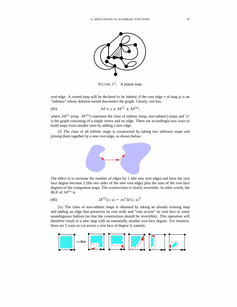
6. APPLICATIONS OF ALGEBRAIC FUNCTIONS 87
FIGURE 17. A planar map.
root edge. A rooted map will be declared to be isthmic if the root edge � of map � is an“isthmus” whose deletion would disconnect the graph. Clearly, one has,
(85)� � � 4 � � � 4 � � � �
where� � � (resp.
� � � ) represent the class of isthmic (resp. non-isthmic) maps and ‘ � ’
is the graph consisting of a single vertex and no edge. There are accordingly two ways tobuild maps from smaller ones by adding a new edge.
H���M The class of all isthmic maps is constructed by taking two arbitrary maps andjoining them together by a new root edge, as shown below:
The effect is to increase the number of edges by 1 (the new root edge) and have the rootface degree become 2 (the two sides of the new root edge) plus the sum of the root facedegrees of the component maps. The construction is clearly revertible. In other words, theBGF of
� � � is
(86) * � � H � � � M�� � � � * H � � � M � �H�����M The class of non-isthmic maps is obtained by taking an already existing map
and adding an edge that preserves its root node and “cuts across” its root face in someunambiguous fashion (so that the construction should be revertible). This operation willtherefore result in a new map with an essentially smaller root-face degree. For instance,there are 5 ways to cut across a root face of degree 4, namely,
�����������������������������������������������������������������������������
�����������������������������������������������������������������������������
������������������������������������������������������������������
������������������������������������������������������������������
������������������������������������������������������������������������������
������������������������������������������������������������������
������������������������������������������������������������������
������������������������������
������
������������������
��������������� � � � � � �
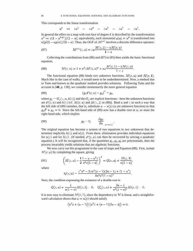
88 8. FUNCTIONAL EQUATIONS—RATIONAL AND ALGEBRAIC FUNCTIONS
This corresponds to the linear transformation� � �� � � 4 � � � 4 � � � 4 � � � 4 � � 2 �
In general the effect on a map with root face of degree�
is described by the transformation� � �� � H 6 � � � l 2 M = H 6 � � M ; equivalently, each monomial � H � M � � � is transformed into� H � H�6�M � � � H � M M = H�6 � � M . Thus, the OGF of� � �
involves a discrete difference operator:
(87) * � � H � � � M � � � * H � � 6�M � � * H � � � M6�� � �
Collecting the contributions from (86) and (87) in (85) then yields the basic functionalequation,
(88) * H � � � M�� 6 4 � � � * H � � � M � 4 � � * H � � 6�M � � * H � � � M6 � � �
The functional equation (88) binds two unknown functions, * H � � � M and * H � � 6�M .Much like in the case of walks, it would seem to be underdetermined. Now, a method dueto Tutte and known as the quadratic method provides solutions. Following Tutte and theaccount in [48, p. 138], we consider momentarily the more general equation
(89) H � 2 ! H � � � M 4�� � M � � � � �where � 9 � � 9 H � � � � � H � M M and the � 9 are explicit functions—here the unknown functionsare
! H � � � M and � H � M (cf. * H � � � M and * H � � 6NM in (88)). Bind � and � in such a way thatthe left side of (89) vanishes, that is, substitute � � �FH � M (a yet unknown function) so that� 2 ! 4 � � � 8 . Since the left-hand side of (89) now has a double root in � , so must theright-hand side, which implies
(90) � � �A8 � e � �e � ���� � ��� � �The original equation has become a system of two equations in two unknowns that de-termines implicitly � H � M and �FH � M . From there, elimination provides individual equationsfor � H � M and for � H � M . (If needed,
! H � � � M can then be recovered by solving a quadraticequation.) It will be recognized that, if the quantities 2 � � � � � � are polynomials, then theprocess invariably yields solutions that are algebraic functions.
We now carry out this programme in the case of maps and Equation (88). First, isolate* H � � � M by completing the square, giving
(91)
* H � � � M�� 6/
6�� � 4 � � �� � � H 6 � � M � � � H � � � M 4 * H � � 6�M
� H�6�� � M �where
� H � � � M�� � � � � � / � � � H � � 6NM-H / � � 6�M 4 H�6�� � � M� � � � � H�6�� � M � �
Next, the condition expressing the existence of a double root is
� H � � � M 4 6�FH 6�� � M * H � � 6�M�� 8 � � �� H � � � M 4
/ � � 6� � H�6�� � M � * H � � 6�M�� 8 �
It is now easy to eliminate * H � � 6NM , since the dependency in * is linear, and a straightfor-ward calculation shows that � � � H � M should satisfy� � � �A4 H � � 6�M � � � � �:4 H � � 6�M-H / � � =!M � � 8 �
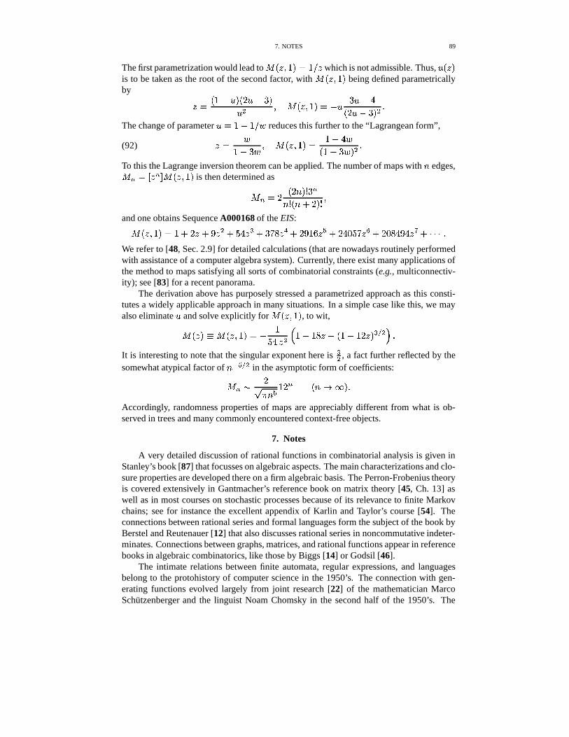
7. NOTES 89
The first parametrization would lead to * H � � 6NM���6 =�� which is not admissible. Thus, �FH � Mis to be taken as the root of the second factor, with * H � � 6�M being defined parametricallyby
� � H�6�� � M�H / � � =2M� � � * H � � 6NM � � � = � � �
H / � � =!M � �The change of parameter � � 6�� 6 =�$ reduces this further to the “Lagrangean form”,
(92) � � $6�� = $
� * H � � 6NM�� 6�� � $H 6�� = $ M � �
To this the Lagrange inversion theorem can be applied. The number of maps with h edges,* � � � � � ��* H � � 6NM is then determined as
* � � /H / h M�� = �h � H h 4 / M�� �
and one obtains Sequence A000168 of the EIS:* H � � 6NM�� 6 4 / �A4 T � � 4 9 � � � 4 =2:.; ����4 / T�6�U � 4 / � 829!: � � 4 / 8#; � T � � � 4#"$"%".�We refer to [48, Sec. 2.9] for detailed calculations (that are nowadays routinely performedwith assistance of a computer algebra system). Currently, there exist many applications ofthe method to maps satisfying all sorts of combinatorial constraints (e.g., multiconnectiv-ity); see [83] for a recent panorama.
The derivation above has purposely stressed a parametrized approach as this consti-tutes a widely applicable approach in many situations. In a simple case like this, we mayalso eliminate � and solve explicitly for * H � � 6NM , to wit,* H � M � * H � � 6�M�� � 6
9 � � � � 6�� 6�; � � H 6�� 6 / � M � ��� �It is interesting to note that the singular exponent here is
�� , a fact further reflected by thesomewhat atypical factor of h j ��� in the asymptotic form of coefficients:* � � /
� � h 6/ � H h � M �
Accordingly, randomness properties of maps are appreciably different from what is ob-served in trees and many commonly encountered context-free objects.
7. Notes
A very detailed discussion of rational functions in combinatorial analysis is given inStanley’s book [87] that focusses on algebraic aspects. The main characterizations and clo-sure properties are developed there on a firm algebraic basis. The Perron-Frobenius theoryis covered extensively in Gantmacher’s reference book on matrix theory [45, Ch. 13] aswell as in most courses on stochastic processes because of its relevance to finite Markovchains; see for instance the excellent appendix of Karlin and Taylor’s course [54]. Theconnections between rational series and formal languages form the subject of the book byBerstel and Reutenauer [12] that also discusses rational series in noncommutative indeter-minates. Connections between graphs, matrices, and rational functions appear in referencebooks in algebraic combinatorics, like those by Biggs [14] or Godsil [46].
The intimate relations between finite automata, regular expressions, and languagesbelong to the protohistory of computer science in the 1950’s. The connection with gen-erating functions evolved largely from joint research [22] of the mathematician MarcoSchutzenberger and the linguist Noam Chomsky in the second half of the 1950’s. The
90 8. FUNCTIONAL EQUATIONS—RATIONAL AND ALGEBRAIC FUNCTIONS
method of transfer matrices is closely related to finite automata and it belongs to the folk-lore of statistical physics; see Temperley’s monograph [91].
Lattice paths are fundamental objects of combinatorics and several books have beendevoted already to their enumerative aspects; see [71] for a treatment that offers insights onmotivations coming from neighbouring areas of classical statistics and probability theory.Historically, the connection between lattice paths and continued fractions has surfacedindependently in works of Touchard (topological configurations [92]), I.J. Good (randomwalks [47]), Lenard (one-dimensional statistical mechanics [65]), Szekeres (combinatoricsof some of Ramanujan’s identities), Flajolet (histories and dynamic data structures [35,36]), Jackson (combinatorics of Ising models [53]), and Read (chord diagrams [80]). Thebasic results are still rediscovered and published periodically. General syntheses appearin [35, 37, 48] and the relation to orthogonal polynomials is well developed in Godsil’sbook [46]. The presentation given here bases itself on reference [37], a study motivatedmore specifically by the formal theory of birth-and-death processes.
Algebraic functions are the modern counterpart of the study of curves by classicalGreek mathematicians. They are either approached by algebraic methods (this is the coreof algebraic geometry) or by transcendental methods. For our purposes, however, onlyrudiments of the theory of curves are needed. For this, there exist several excellent in-troductory books, of which we recommend the ones by Abhyankar [1], Fulton [44], andKirwan [56]. On the algebraic side, we have striven to provide an introduction to alge-braic functions that requires minimal apparatus. At the same time the emphasis has beenput somewhat on algorithmic aspects, since most algebraic models are nowadays likelyto be treated with the help of computer algebra. As regards symbolic computational as-pects, we recommend the treatise by von zur Gathen and Jurgen[98] for background, whilepolynomial systems are excellently reviewed in the book by Cox, Little, and O’Shea [27].
In the combinatorial domain, algebraic functions have been used early: in Euler andSegner’s enumeration of triangulations (1753) as well as in Schroder’s famous “vier com-binatorische Probleme” described in [88, p. 177]. A major advance was the realizationby Chomsky and Schutzenberger that algebraic functions are the “exact” counterpart ofcontext-free grammars and languages (see again the historic paper [22]). A masterful sum-mary of the early theory appears in the proceedings edited by Berstel [10] while a modernand precise exposition forms the subject of Chapter 6 of Stanley’s book [88]. On theanalytic-asymptotic side, many researchers have long been aware of the power of Puiseuxexpansions in conjunction with some version of singularity analysis (often in the form ofthe Darboux–Polya method: see [79] based on Polya’s classic paper [78] of 1937). How-ever, there appeared to be difficulties in coping with the fully general problem of algebraiccoefficient asymptotics [18, 70]. We believe that Section 5.1 sketches the first completetheory. In the case of positive systems, the “Drmota-Lalley-Woods” theorem is the key tomost problems encountered in practice—its importance should be clear from the develop-ments of Section 5.2.
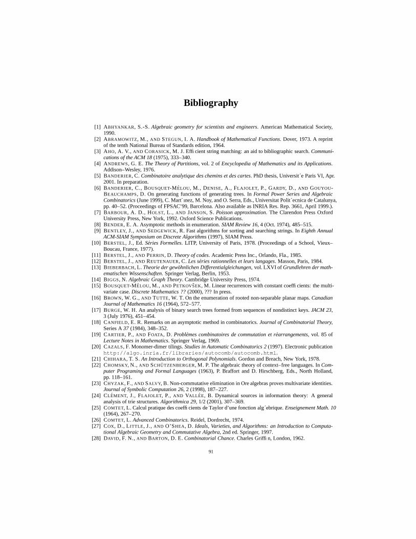
Bibliography
[1] ABHYANKAR, S.-S. Algebraic geometry for scientists and engineers. American Mathematical Society,1990.
[2] ABRAMOWITZ, M., AND STEGUN, I. A. Handbook of Mathematical Functions. Dover, 1973. A reprintof the tenth National Bureau of Standards edition, 1964.
[3] AHO, A. V., AND CORASICK, M. J. Efficient string matching: an aid to bibliographic search. Communi-cations of the ACM 18 (1975), 333–340.
[4] ANDREWS, G. E. The Theory of Partitions, vol. 2 of Encyclopedia of Mathematics and its Applications.Addison–Wesley, 1976.
[5] BANDERIER, C. Combinatoire analytique des chemins et des cartes. PhD thesis, Universit e Paris VI, Apr.2001. In preparation.
[6] BANDERIER, C., BOUSQUET-MELOU, M., DENISE, A., FLAJOLET, P., GARDY, D., AND GOUYOU-BEAUCHAMPS, D. On generating functions of generating trees. In Formal Power Series and AlgebraicCombinatorics (June 1999), C. Mart ınez, M. Noy, and O. Serra, Eds., Universitat Polit ecnica de Catalunya,pp. 40–52. (Proceedings of FPSAC’99, Barcelona. Also available as INRIA Res. Rep. 3661, April 1999.).
[7] BARBOUR, A. D., HOLST, L., AND JANSON, S. Poisson approximation. The Clarendon Press OxfordUniversity Press, New York, 1992. Oxford Science Publications.
[8] BENDER, E. A. Asymptotic methods in enumeration. SIAM Review 16, 4 (Oct. 1974), 485–515.[9] BENTLEY, J., AND SEDGEWICK, R. Fast algorithms for sorting and searching strings. In Eighth Annual
ACM-SIAM Symposium on Discrete Algorithms (1997), SIAM Press.[10] BERSTEL, J., Ed. Series Formelles. LITP, University of Paris, 1978. (Proceedings of a School, Vieux–
Boucau, France, 1977).[11] BERSTEL, J., AND PERRIN, D. Theory of codes. Academic Press Inc., Orlando, Fla., 1985.[12] BERSTEL, J., AND REUTENAUER, C. Les series rationnelles et leurs langages. Masson, Paris, 1984.[13] BIEBERBACH, L. Theorie der gewohnlichen Differentialgleichungen, vol. LXVI of Grundlehren der math-
ematischen Wissenschaften. Springer Verlag, Berlin, 1953.[14] BIGGS, N. Algebraic Graph Theory. Cambridge University Press, 1974.[15] BOUSQUET-MELOU, M., AND PETKOVSEK, M. Linear recurrences with constant coefficients: the multi-
variate case. Discrete Mathematics ?? (2000), ??? In press.[16] BROWN, W. G., AND TUTTE, W. T. On the enumeration of rooted non-separable planar maps. Canadian
Journal of Mathematics 16 (1964), 572–577.[17] BURGE, W. H. An analysis of binary search trees formed from sequences of nondistinct keys. JACM 23,
3 (July 1976), 451–454.[18] CANFIELD, E. R. Remarks on an asymptotic method in combinatorics. Journal of Combinatorial Theory,
Series A 37 (1984), 348–352.[19] CARTIER, P., AND FOATA, D. Problemes combinatoires de commutation et rearrangements, vol. 85 of
Lecture Notes in Mathematics. Springer Verlag, 1969.[20] CAZALS, F. Monomer-dimer tilings. Studies in Automatic Combinatorics 2 (1997). Electronic publication
http://algo.inria.fr/libraries/autocomb/autocomb.html.[21] CHIHARA, T. S. An Introduction to Orthogonal Polynomials. Gordon and Breach, New York, 1978.[22] CHOMSKY, N., AND SCHUTZENBERGER, M. P. The algebraic theory of context–free languages. In Com-
puter Programing and Formal Languages (1963), P. Braffort and D. Hirschberg, Eds., North Holland,pp. 118–161.
[23] CHYZAK, F., AND SALVY, B. Non-commutative elimination in Ore algebras proves multivariate identities.Journal of Symbolic Computation 26, 2 (1998), 187–227.
[24] CLEMENT, J., FLAJOLET, P., AND VALLEE, B. Dynamical sources in information theory: A generalanalysis of trie structures. Algorithmica 29, 1/2 (2001), 307–369.
[25] COMTET, L. Calcul pratique des coefficients de Taylor d’une fonction alg ebrique. Enseignement Math. 10(1964), 267–270.
[26] COMTET, L. Advanced Combinatorics. Reidel, Dordrecht, 1974.[27] COX, D., LITTLE, J., AND O’SHEA, D. Ideals, Varieties, and Algorithms: an Introduction to Computa-
tional Algebraic Geometry and Commutative Algebra, 2nd ed. Springer, 1997.[28] DAVID, F. N., AND BARTON, D. E. Combinatorial Chance. Charles Griffin, London, 1962.
91
92 BIBLIOGRAPHY
[29] DELEST, M.-P., AND VIENNOT, G. Algebraic languages and polyominoes enumeration. Theoretical Com-puter Science 34 (1984), 169–206.
[30] DOMB, C., AND BARRETT, A. Enumeration of ladder graphs. Discrete Mathematics 9 (1974), 341–358.[31] DRMOTA, M. Systems of functional equations. Random Structures & Algorithms 10, 1–2 (1997), 103–124.[32] DUTOUR, I., AND FEDOU, J.-M. Object grammars and random generation. Discrete Mathematics and
Theoretical Computer Science 2 (1998), 47–61.[33] FAYOLLE, G., AND IASNOGORODSKI, R. Two coupled processors: the reduction to a Riemann-Hilbert
problem. Zeitschrift fur Wahrscheinlichkeitstheorie und Verwandte Gebiete 47, 3 (1979), 325–351.[34] FAYOLLE, G., IASNOGORODSKI, R., AND MALYSHEV, V. Random walks in the quarter-plane. Springer-
Verlag, Berlin, 1999.[35] FLAJOLET, P. Combinatorial aspects of continued fractions. Discrete Mathematics 32 (1980), 125–161.[36] FLAJOLET, P., FRANCON, J., AND VUILLEMIN, J. Sequence of operations analysis for dynamic data
structures. Journal of Algorithms 1 (1980), 111–141.[37] FLAJOLET, P., AND GUILLEMIN, F. The formal theory of birth-and-death processes, lattice path combi-
natorics, and continued fractions. Advances in Applied Probability 32 (2000), 750–778.[38] FLAJOLET, P., HATZIS, K., NIKOLETSEAS, S., AND SPIRAKIS, P. On the robustness of interconnections
in random graphs: A symbolic approach. Theoretical Computer Science ?? (2001), ???–??? Accepted forpublication. A preliminary version appears as INRIA Research Report 4069, November 2000, 21 pages.
[39] FLAJOLET, P., KIRSCHENHOFER, P., AND TICHY, R. F. Deviations from uniformity in random strings.Probability Theory and Related Fields 80 (1988), 139–150.
[40] FLAJOLET, P., AND NOY, M. Analytic combinatorics of non-crossing configurations. Discrete Mathemat-ics 204, 1-3 (1999), 203–229. (Selected papers in honor of Henry W. Gould).
[41] FLAJOLET, P., AND ODLYZKO, A. The average height of binary trees and other simple trees. Journal ofComputer and System Sciences 25 (1982), 171–213.
[42] FLAJOLET, P., AND ODLYZKO, A. Limit distributions for coefficients of iterates of polynomials withapplications to combinatorial enumerations. Mathematical Proceedings of the Cambridge PhilosophicalSociety 96 (1984), 237–253.
[43] FROBENIUS, G. Uber Matrizen aus nicht negativen Elementen. Sitz.-Ber. Akad. Wiss., Phys-Math Klasse,Berlin (1912), 456–477.
[44] FULTON, W. Algebraic Curves. W.A. Benjamin, Inc., New York, Amsterdam, 1969.[45] GANTMACHER, F. R. Matrizentheorie. Deutscher Verlag der Wissenschaften, Berlin, 1986. A translation
of the Russian original Teoria Matriz, Nauka, Moscow, 1966.[46] GODSIL, C. D. Algebraic Combinatorics. Chapman and Hall, 1993.[47] GOOD, I. J. Random motion and analytic continued fractions. Proceedings of the Cambridge Philosophi-
cal Society 54 (1958), 43–47.[48] GOULDEN, I. P., AND JACKSON, D. M. Combinatorial Enumeration. John Wiley, New York, 1983.[49] GOURDON, X. Largest component in random combinatorial structures. Discrete Mathematics 180, 1-3
(1998), 185–209.[50] GRAHAM, R., KNUTH, D., AND PATASHNIK, O. Concrete Mathematics. Addison Wesley, 1989.[51] HENRICI, P. Applied and Computational Complex Analysis, vol. 2. John Wiley, New York, 1974.[52] HILLE, E. Analytic Function Theory. Blaisdell Publishing Company, Waltham, 1962. 2 Volumes.[53] JACKSON, D. Some results on product-weighted lead codes. Journal of Combinatorial Theory, Series A
25 (1978), 181–187.[54] KARLIN, S., AND TAYLOR, H. A First Course in Stochastic Processes, second ed. Academic Press, 1975.[55] KIRSCHENHOFER, P., AND PRODINGER, H. The number of winners in a discrete geometrically dis-
tributed sample. The Annals of Applied Probability 6, 2 (1996), 687–694.[56] KIRWAN, F. Complex Algebraic Curves. No. 23 in London Mathematical Society Student Texts. Cam-
bridge University Press, 1992.[57] KNOPFMACHER, A., AND PRODINGER, H. On Carlitz compositions. European Journal of Combinatorics
19, 5 (1998), 579–589.[58] KNUTH, D. E. The Art of Computer Programming, vol. 1: Fundamental Algorithms. Addison-Wesley,
1968. Second edition, 1973.[59] KNUTH, D. E. The Art of Computer Programming, 3rd ed., vol. 1: Fundamental Algorithms. Addison-
Wesley, 1997.[60] KRASNOSELSKII, M. Positive solutions of operator equations. P. Noordhoff, Groningen, 1964.[61] LABELLE, J., AND YEH, Y.-N. Generalized Dyck paths. Discrete Mathematics 82 (1990), 1–6.[62] LAGARIAS, J. C., ODLYZKO, A. M., AND ZAGIER, D. B. On the capacity of disjointly shared networks.
Computer Netwoks 10, 5 (1985), 275–285.[63] LALLEY, S. P. Finite range random walk on free groups and homogeneous trees. Ann. Probab. 21, 4
(1993), 2087–2130.[64] LANG, S. Linear Algebra. Addison-Wesley Publishing Co., Inc., Reading, Mass.-Don Mills, Ont., 1966.[65] LENARD, A. Exact statistical mechanics of a one–dimensional system with Coulomb forces. The Journal
of Mathematical Physics 2, 5 (Sept. 1961), 682–693.
BIBLIOGRAPHY 93
[66] LOTHAIRE, M. Combinatorics on Words, vol. 17 of Encyclopedia of Mathematics and its Applications.Addison–Wesley, 1983.
[67] LOUCHARD, G. Random walks, Gaussian processes and list structures. Theoretical Computer Science 53,1 (1987), 99–124.
[68] MACMAHON, P. A. Introduction to combinatory analysis. Chelsea Publishing Co., New York, 1955. Areprint of the first edition, Cambridge, 1920.
[69] MEIR, A., AND MOON, J. W. On the altitude of nodes in random trees. Canadian Journal of Mathematics30 (1978), 997–1015.
[70] MEIR, A., AND MOON, J. W. The asymptotic behaviour of coefficients of powers of certain generatingfunctions. European Journal of Combinatorics 11 (1990), 581–587.
[71] MOHANTY, S. G. Lattice path counting and applications. Academic Press [Harcourt Brace JovanovichPublishers], New York, 1979. Probability and Mathematical Statistics.
[72] ODLYZKO, A. M. Periodic oscillations of coefficients of power series that satisfy functional equations.Advances in Mathematics 44 (1982), 180–205.
[73] ODLYZKO, A. M. Asymptotic enumeration methods. In Handbook of Combinatorics, R. Graham,M. Gr otschel, and L. Lov asz, Eds., vol. II. Elsevier, Amsterdam, 1995, pp. 1063–1229.
[74] ODLYZKO, A. M., AND WILF, H. S. The editor’s corner: & coins in a fountain. American MatematicalMonthly 95 (1988), 840–843.
[75] OTTER, R. The number of trees. Annals of Mathematics 49, 3 (1948), 583–599.[76] PERCUS, J. K. Combinatorial Methods, vol. 4 of Applied Mathematical Sciences. Springer-Verlag, 1971.[77] PERRON, O. Uber Matrizen. Mathematische Annalen 64 (1907), 248–263.[78] POLYA, G. Kombinatorische Anzahlbestimmungen f ur Gruppen, Graphen und chemische Verbindungen.
Acta Mathematica 68 (1937), 145–254.[79] POLYA, G., AND READ, R. C. Combinatorial Enumeration of Groups, Graphs and Chemical Compounds.
Springer Verlag, New York, 1987.[80] READ, R. C. The chord intersection problem. Annals of the New York Academy of Sciences 319 (May
1979), 444–454.[81] ROBERT, P. Reseaux et files d’attente: methodes probabilistes, vol. 35 of Mathematiques & Applications.
Springer, Paris, 2000.[82] SALVY, B., AND ZIMMERMANN, P. GFUN: a Maple package for the manipulation of generating and
holonomic functions in one variable. ACM Trans. Math. Softw. 20, 2 (1994), 163–167.[83] SCHAEFFER, G. Conjugaison d’arbres et cartes combinatoires aleatoires. Ph.d. thesis, Universit e de Bor-
deaux I, Dec. 1998.[84] SEDGEWICK, R., AND FLAJOLET, P. An Introduction to the Analysis of Algorithms. Addison-Wesley
Publishing Company, 1996.[85] SLOANE, N. J. A. The On-Line Encyclopedia of Integer Sequences. 2000. Published electronically at
http://www.research.att.com/njas/sequences/.[86] SLOANE, N. J. A., AND PLOUFFE, S. The Encyclopedia of Integer Sequences. Academic Press, 1995.
Available electronically at http://www.research.att.com/njas/sequences/.[87] STANLEY, R. P. Enumerative Combinatorics, vol. I. Wadsworth & Brooks/Cole, 1986.[88] STANLEY, R. P. Enumerative Combinatorics, vol. II. Wadsworth & Brooks/Cole, 1998.[89] STEIN, P. R., AND WATERMAN, M. S. On some new sequences generalizing the Catalan and Motzkin
numbers. Discrete Mathematics 26, 3 (1979), 261–272.[90] SZEGO, G. Orthogonal Polynomials, vol. XXIII of Americam Mathematical Society Colloquium Publica-
tions. A.M.S, Providence, 1989.[91] TEMPERLEY, H. N. V. Graph theory and applications. Ellis Horwood Ltd., Chichester, 1981. Ellis Hor-
wood Series in Mathematics and its Applications.[92] TOUCHARD, J. Contribution a l’ etude du probl eme des timbres poste. Canadian Journal of Mathematics
2 (1950), 385–398.[93] TUTTE, W. T. A census of planar maps. Canadian Journal of Mathematics 15 (1963), 249–271.[94] TUTTE, W. T. On the enumeration of planar maps. Bull. Amer. Math. Soc. 74 (1968), 64–74.[95] TUTTE, W. T. On the enumeration of four-colored maps. SIAM Journal on Applied Mathematics 17
(1969), 454–460.[96] TUTTE, W. T. Planar enumeration. In Graph theory and combinatorics (Cambridge, 1983). Academic
Press, London, 1984, pp. 315–319.[97] VALLEE, B. Dynamical sources in information theory: Fundamental intervals and word prefixes. Algo-
rithmica 29, 1/2 (2001), 262–306.[98] VON ZUR GATHEN, J., AND GERHARD, J. Modern computer algebra. Cambridge University Press, New
York, 1999.[99] WALL, H. S. Analytic Theory of Continued Fractions. Chelsea Publishing Company, 1948.
[100] WOODS, A. R. Coloring rules for finite trees, and probabilities of monadic second order sentences. Ran-dom Structures Algorithms 10, 4 (1997), 453–485.
[101] ZEILBERGER, D. Closed form (pun intended!). Contemporary mathematics 143 (1988), 579–607.
94 BIBLIOGRAPHY
[102] ZEILBERGER, D. Symbol-crunching with the transfer-matrix method in order to count skinny phys-ical creatures. Integers 0 (2000), Paper A9. Published electronically at http://www.integers-ejcnt.org/vol0.html.
Contents
Chapter 8. Functional Equations—Rational and Algebraic Functions 1The rational, algebraic, and holonomic classes 21. Algebra of rational functions 51.1. Characterizations and elimination. 61.2. Closure properties and coefficients. 72. Analysis of rational functions 92.1. General rational functions. 92.2. Positive rational functions and Perron-Frobenius theory. 113. Combinatorial applications of rational functions 183.1. Regular specifications. 183.2. Regular languages. 193.3. Paths in graphs, automata, and transfer matrices. 233.4. Permutations and local constraints. 323.5. Lattice paths and walks on the line. 374. Algebra of algebraic functions 464.1. Characterization and elimination. 474.2. Closure properties and coefficients. 545. Analysis of algebraic functions 595.1. General algebraic functions. 595.2. Positive functions and positive systems. 706. Combinatorial applications of algebraic functions 756.1. Context-free specifications. 756.2. Context-free languages. 796.3. Simple families of trees. 806.4. Walks and the kernel method. 816.5. Maps and the quadratic method. 867. Notes 89
Bibliography 91
Index 97
95

Index
4-colour theorem, 86
algebraicclosure, 58curve, 59elimination, 47variety, 47
algebraic function, 46–90asymptotic, 59–75branch, 59closure, 54–58coefficient, 65–75Newton polygon, 62–64Puiseux expansion, 62–64singularities, 59–75
ambiguitycontext-free grammar, 79regular expression, 19
area (of Dyck path), 41asymptotic
algebraic, 59–75rational, 9–18
binomial sums, 8branch (of curve), 59Buchberger’s algorithm, see Groebner basis
Carlitz composition, 27coin fountain, 42composition (of an integer)
Carlitz, 27finite summands, 10largest summand, 19local constraints, 27
connection, 68context-free
language, 75, 79–80specification, 75–79
continued fraction, 37–46correlation polynomial, 22
denumerant, 10dependency graph, 11derangement, 33digital tree, 23digraph, see graphdiscriminant (of a polynomial), 59Drmota-Lalley-Woods Theorem, 70Dyck path, 41, 80, 85
eigenvalue, see matrixelimination, 3
algebraic, 47
rational, 6exceedances (in permutations), 33exponential polynomial, 7
Fibonacci number, 8, 10finite automaton, 27–30
deterministic, 27non-deterministic, 27
finite state model, 27, 30formal language, see languagefunctional equation
kernel method, 82quadratic method, 88
Gaussian elimination, 7generating function
algebraic, 46–89functional equations, 1–94rational, 5–46
graphaperiodic, 12colouring, 86map, 86–89non-crossing, 66–67, 77–79paths, 23–27periodic, 12strongly connected, 12zeta function, 24
Groebner basis, 50
Hadamard product, 8, 55Hermite polynomial, 45
ideal, 48, 53inclusion-exclusion, 33interconnection network, 44involution (permutation), 44
Jacobi trace formula, 15, 24
kernel method (functional equation), 82
language, 19context-free, 75, 79–80regular, 19–37
lattice path, 37–46decompositions, 38
Laurent seriesformal, 3
Łukasiewicz language, 85
map, 86–89Markov chain, 1, 25, 89matrix
97
98 INDEX
aperiodic, 12de Bruijn, 16eigenvalue, 11
dominant, 11irreducible, 12nonnegative, 14norm, 17Perron Frobenius theory, 11–14positive, 14spectral radius, 17spectrum, 11trace, 15, 24transfer, 7, 30
m enage problem, 32monodromy, 62Motzkin path, 41
network, 44Newton polygon, 62–64non-crossing configuration, 66–67, 77–79nucleic sequence, 81
order statistics, 22orthogonal polynomials, 43
parse tree, 79partition (of an integer)
denumerant, 10pattern
in words, 16word, 21
permutationderangement, 33exceedances, 33involution, 44multiset, 23records, 22
Perron Frobenius theory, 1, 11–14polynomial
primitive, 16polynomial system, 47, 70Puiseux expansion (algebraic function), 62–64
quadratic method (functional equation), 88
R (resultant notation), 49rational function, 5–46, 89
asymptotic, 9–18characterizations, 5–8coefficients, 8–9positive, 14
records, 22regular
expression, 19–37language, 19–37specification, 18
resultant, 47–52Rogers-Ramanujan identities, 42runs (in words), 20
seriesalgebraic, 3, 46–89formal power, 2holonomic, 3Laurent, 3rational, 3, 5, 46
simple family (of trees), 80Skolem-Mahler-Lech theorem, 11Smirnov words, 26spectral radius, 17spectrum, see matrixStirling number
cycle type, 22string, see wordsupertree, 67
transfer matrix, 7, 30transition matrix, see transfer matrixtree
3-coloured, 51–54height, 19, 21non-crossing, 66–67, 77–79parse tree, 79simple family, 80supertree, 67
triangulation (of polygon), 76trie, see digital tree
unambiguous, see ambiguityuniformization (algebraic function), 62
variety (algebraic), 47
wordexcluded patterns, 29language, 19local constraints, 26parenthesis system, 21pattern, 21records, 22regular expression, 19runs, 20Smirnov, 26
zeta functiongraphs, 24
��� ������ ��� ��� �� � ��������������������� � ��� � �! �"�"�/�$#� � �%� �����&� ')(�*+� �&,-� /. �102� � �"3 .�. �� � 4"5 3 ���6 1 � 3 ���"3879�&� � �:*+� � �&� /5 3 ���-*+; � � 1&< 6 � �>= ������?@��AB��C?2AD�E���F0@G
��� ������ ��� ��� �� � �����������H� ��"� � . �I��� /. � �I0�� � � 3 . 3"� J �� .� � � ���F� ��* �!�&3 � �3K� ./1 � < $ ��?+�E�E?2AD0 �� ����E� ������ ��� ��� �!���� ���������������$#��� �(L� � � � . � 6 1/1 �I� J ���3 �M� � �LN ?O3"� �/� ��� ./0/./. �>PRQ �E��* Q ��� Q �SA�� P ���T�����
��� ������ ��� ��� �� � �����������H���) 5 3 ��"��3"� � �VU�� � � � ��� � = � � 3 -�!�&3K�I���) 5 3 ��"��3"� � �V*+; � 1 �W 0 1/. �K?X02YE?+A �E�TGH0 �!� � ���� ������ ��� ��� ����� �����������ZA)�/�"� �[(��E� �� �1� �/. � $ � � < ����3 � ��� � . ��3 � � � . �I*+;]\ . � ��6 \ � $ A Q ;+Y����E(����E����; Q �K�^A
0 �� ���
�, ��� �� �����D�����(/ $ �!%'& ��� �(��)*�#+, "�-��&. 0/"���1���2 �� � ���# �� � /�35476�829�/ :<;"6�9#=?> ,A@ ) ,CB �D�FE @ �����G
HSJ���& � ����Mhttp://www.inria.fr� B�B ��8 / � T1_ U!=#T!T